Gender, Equality and Diversity Branch, WORKQUALITY Department Working Paper No. 6 / 2015 The gender and motherhood wage gap in the former Yugoslav Republic of Macedonia: An econometric analysis Marjan Petreski and Nikica Mojsoska Blazevski International Labour Organization ILO Decent Work Technical Support Team and Country Office for Central and Eastern Europe

The gender and motherhood wage gap in the former Yugoslav ... · Nikica Mojsoska Blazevski School of Business Economics and Management University American College Skopje [email protected]
Oct 10, 2019
Welcome message from author
This document is posted to help you gain knowledge. Please leave a comment to let me know what you think about it! Share it to your friends and learn new things together.
Transcript

Gender, Equality and Diversity Branch, Workquality Department
Working Paper No. 6 / 2015
Gender, Equality and Diversity Branch (GED)Conditions of Work and Equality Department
International Labour Office (ILO)4, route des Morillons1211 Geneva 22, Switzerlandtel. +41 22 799 [email protected]/ged
ILO DWT and Country Office for Central and Eastern Europe
Mozsár utca 14. BudapestHungary1066Tel : +36 1 301 4900 Fax : +36 1 353 3683 Email : [email protected] www.ilo.org/budapest
ISBN 9789221305170
The gender and motherhood wage gap in the former Yugoslav Republic of Macedonia:An econometric analysisMarjan Petreski and Nikica Mojsoska Blazevski
internationallabourorganization
ilo Decent Work technical Support team and Country office for Central and Eastern Europe
Marjan Petrevski
Nikica Mojsoska Blazevski
The gender and motherhood wage gap in the former Yugoslav Republic of Macedonia:
An econometric analysis
Copyright © International Labour Organization 2015
First published 2015
Publications of the International Labour Office enjoy copyright under Protocol 2 of the Universal Copyright Convention. Nev-ertheless, short excerpts from them may be reproduced without authorization, on condition that the source is indicated. For rights of reproduction or translation, application should be made to ILO Publications (Rights and Licensing), International Labour Office, CH-1211 Geneva 22, Switzerland, or by email: [email protected]. The International Labour Office welcomes such applications.
Libraries, institutions and other users registered with a reproduction rights organization may make copies in accordance with the licences issued to them for this purpose. Visit www.ifrro.org to find the reproduction rights organization in your country.
ILO Cataloguing in Publication Data
Petreski, Marjan; Mojsoska-Blazevski, Nikica
The gender and motherhood wage gap in the Former Yugoslav Republic of Macedonia : an econometric analysis / Marjan Petreski, Nikica Mojsoska Blazevski ; International Labour Office, ILO DWT and Country Office for Central and Eastern Europe. - Budapest: ILO, 2015 77 p.
ISBN: 9789221305170 (print); 9789221305187 (web pdf)
ILO DWT and Country Office for Central and Eastern Europe
wage differential / family responsibilities / women workers / sex discrimination / economic analysis / econometric model / Macedonia, former Yugoslav Republic
13.07
The designations employed in ILO publications, which are in conformity with United Nations practice, and the presentation of material therein do not imply the expression of any opinion whatsoever on the part of the International Labour Office concern-ing the legal status of any country, area or territory or of its authorities, or concerning the delimitation of its frontiers.
The responsibility for opinions expressed in signed articles, studies and other contributions rests solely with their authors, and publication does not constitute an endorsement by the International Labour Office of the opinions expressed in them.
Reference to names of firms and commercial products and processes does not imply their endorsement by the International Labour Office, and any failure to mention a particular firm, commercial product or process is not a sign of disapproval.
ILO publications and digital products can be obtained through major booksellers and digital distribution platforms, or ordered directly from [email protected]. For more information, visit our website: www.ilo.org/publns or contact [email protected].
1
Предговор
Овој извештај ги проценува и ги анализира родовиот и мајчинскиот јаз во платите во Македонија. Извештајот се заснова врз методологијата што беше развиена во работниот документ на МОТ – Мајчинскиот јаз во платите: Преглед на прашањата, теоријата и меѓународните докази (The motherhood pay gap: A review of the issues, theory and international evidence (Grimshaw and Rubery, 2015). Мајчинскиот јаз во платите го мери јазот во платите меѓу мајките и жените што не се мајки. Тој го мери, исто така, јазот во платите меѓу мајките и татковците. Ова е различно од родовиот јаз во платите, што го мери јазот во платите меѓу сите жени и мажи во работната сила (Grimshaw и Rubery, 2015).
Резултатите за Република Македонија сугерираат дека жените добиваат плати што помали за околу 18-19% од платата на мажите. Изненадувачки, студијата открива дека мајките (дефинирани како жени на возраст од 25 до 45 години, со дете на возраст до 6 години) биле еднакво платени како жените што не се мајки (или мајките со деца постари од шест години) во 2011 година, и дека тие заработувале 6% повеќе од жените што немаат деца на возраст под шест години во 2014 година. Резултатите сугерираат, исто така, дека мајките се платени 7,8% помалку од татковците. Во периодот меѓу 2011 и 2014 година, родовиот јаз во платите се намалил само кај најниско платените работни места на жените и мажите, што упатува на тоа дека воведувањето на минималната плата можеби придонело кон намалување на родовиот јаз во платите.
Преку компонентата „Промовирање на родовата еднаквост и зајакнување на положбата на жените во светот на работата“ на Спогодбата за партнерство меѓу МОТ и Норвешка, МОТ работи заедно со владите и социјалните партнери на развојот на база од знаења за родовата еднаквост на работното место, промовирање на претставувањето и застапувањето за работничките и градење на капацитетите на конституентите за промовирање на родовата еднаквост.
Во 2011 година, МОТ нарача студија за родовиот јаз во платите во Република Македонија1 што се фокусираше на факторите во основата на родовиот јаз во платите, неговите економски последици и постојните механизми и политики за неговото адресирање. Оттогаш наваму беше спроведена обука за подобрување на активностите за собирање податоци на националните заводи за статистика и за подобрување на пристапот до родово карактеристични податоци за пазарот на трудот. Земјата го посведочи и донесувањето на законот за минимална плата, што влезе во сила во 2012 година. Во текстилната и кожарската индустрија, каде што жените се прекумерно застапени, минималната плата беше утврдена на пониско ниво и се очекува дека ќе го достигне националното ниво во 2018 година.
Во јануари 2013 година, македонската Влада ја донесе својата прва „Национална стратегија за родова еднаквост“. Стратегијата се спроведува до 2020 година и, со оглед на обврските на Владата во согласност со Конвенцијата за еднаквост на платите, 1951 (бр. 100) и Конвенцијата за дискриминација (вработување и занимања), 1958 (бр. 111), ги приоретизира промовирањето на еднаквите плати за жените и мажите и борбата против дискриминацијата врз основа на полот.
Иако македонското законодавство предвидува еднаква плата за еднаква или иста работа, начелото за еднаква плата за работа со еднаква вредност што е вградено во Конвенцијата бр. 100 не е спроведено во целост во практиката. Еднаквата плата за работа со еднаква вредност би се применувала и за работниците што вршат работи што се со различна природа, но со
1 Милка Казанџиска, Марија Ристеска, Верена Шмит (2012): Родовиот јаз во платите во Поранешната Југо-словенска Република Македонија (МОТ).
Foreword
This report estimates and analyses the gender and motherhood wage gaps in the former Yugoslav Republic of Macedonia. It is based on the methodology developed in the ILO working paper The motherhood pay gap: A review of the issues, theory and international evidence (Grimshaw and Rubery, 2015). The motherhood pay gap measures the pay gap between mothers and non-mothers. It also measures the pay gap between mothers and fathers. This is different from the gender pay gap, which measures the pay gap between all women and men in the workforce (Grimshaw and Rubery, 2015).
The results for the former Yugoslav Republic in Macedonia suggest that women are paid about 18-19% of a men’s wages. Surprisingly, the study finds that mothers (defined as women aged 25-45, with a child aged up to 6 years) were paid equally to non-mothers (or mothers with children older than six) in 2011, and earned 6% more than women without children under the age of six in 2014. The results also suggest that mothers are paid 7.8% less than fathers. Between 2011 and 2014, the gender wage gap only decreased between the lowest-paid jobs held by women and men, suggesting that the introduction of the minimum wage may have contributed to reducing the gender wage gap.
Through the “Promoting Gender Equality and Women’s Empowerment in the World of Work” component of the ILO/Norway Partnership Agreement (PA), the ILO has been working with governments and social partners to develop a knowledge base on gender equality in the workplace, promote representation and advocacy for women workers, and to build the capacity of constituents to promote gender equality.
In 2011, the ILO commissioned a study on the gender pay gap in the former Yugoslav Republic of Macedonia1 that focused on its underlying factors, its economic consequences, and the existing mechanisms and policies in place to address it. Since then, training was conducted to improve the data collection efforts of the national statistical offices and to improve access to gender specific labour market data. The country also witnessed the adoption of a law on minimum wage, which came into force in 2012. For the textile and leather industry, where women are overrepresented, the minimum wage was set lower and is expected to reach the national level in 2018.
In January 2013, the Macedonian Government adopted its first ‘National Strategy for Gender Equality’. It runs until 2020 and, in view of the Government’s commitments under the Equal Remuneration Convention, 1951 (No. 100) and the Discrimination (Employment and Occupation) Convention, 1958 (No. 111), it prioritizes promoting equal pay between women and men and combating sex-based discrimination.
While the Macedonian legislation provides for equal remuneration for equal or identical work, the principle of equal remuneration for work of equal value, as enshrined in Convention No. 100, is not fully implemented in practice. Equal remuneration for work of equal value would also apply to workers performing work of a different nature which is, nevertheless, of equal value.
In this context, the ILO commissioned the present study to improve the understanding of the principle of equal remuneration for work of equal value, and to identify the gender pay gap and motherhood pay gap based on new available data. It is the first study based on the aforementioned ILO working paper on the motherhood pay gap.
1 Milka Kazandziska, Marija Risteska, Verena Schmidt (2012): The Gender Pay Gap in the Former Yugoslav Republic of Macedonia (ILO).

2
This report is authored by Marjan Petreski and Nikica Mojsoska-Blazevski from the University American College of Skopje.
The ILO implemented a workshop on equal pay and the gender/ motherhood pay gap in Skopje in September 2015, in which a draft of the paper was presented. The report was finalized after the workshop based on the comments received by government participants, employer organizations, and workers’ organizations.
This report has been prepared through the joint collaboration of Laura Addati and Edward Lawton, Gender, Equality and Diversity Branch; Kristen Sobeck and Rosalia Vazquez-Alvarez, Inclusive Labour Markets, Labour Relations and Working Conditions Branch; and Sofia Amaral de Oliveira, Decent Work Technical Support Team and Country Office for Central and Eastern Europe, Budapest. Verena Schmidt, Decent Work Technical Support Team and Country Office for Central and Eastern Europe, Budapest coordinated and edited the report. Emil Krstanovski, ILO National Coordinator in the former Yugoslav Republic of Macedonia provided important advice and coordination for the report.
We trust that this document will be a useful contribution to policy dialogue in the former Yugoslav Republic of Macedonia.
Shauna Olney Antonio GraziosiDirector, Gender, Equality and Diversity Branch Director, ILO Decent Work Technical Support
Team and Country Office for Central and Eastern Europe, Budapest

3
The gender and motherhood wage gap in the former Yugoslav Republic of Macedonia: An econometric analysis
Marjan Petreski
School of Business Economics and Management
University American College Skopje
Nikica Mojsoska Blazevski
School of Business Economics and Management
University American College Skopje
Abstract
The objective of this analysis is to estimate and analyze the gender and motherhood wage gaps in the former Yugoslav Republic of Macedonia for two years, 2011 and 2014. We are particularly interested in any meaningful shift in the gaps between 2011 and 2014, which may be ascribed to the effects of particular policies pursued after 2011. To that end, we rely on a standard Mincer earnings function, regressing the average log hourly wage onto indicators of gender and motherhood, respectively, and onto a set of personal and labour-market characteristics. We utilize OLS and the Heckman method to correct for the potential presence of selectivity bias into the labour market. We use data from the Labour Force Survey. In general, results suggest that females are paid less than males in the former Yugoslav Republic of Macedonia, with wages about 18-19 per cent less than male wages, while mothers (defined as women aged 25-45, with a child aged up to six years) were paid the same as non-mothers in 2011 and only slightly more than non-mothers – six per cent more – in 2014. Between these years, the gender wage gap reduced for the lowest-paid jobs only, suggesting that some policies – in particular the introduction of the minimum wage – may have worked to reduce the gender wage gap and hence mitigate the “floor stickiness” for females in the former Yugoslav Republic of Macedonia. In addition, there is limited evidence that a “glass ceiling” effect exists for highly paid (but not the highest-paid) jobs. Motherhood has been found insignificant throughout most of the wage distribution, including at its extremes, suggesting no sticky floor or glass ceiling for non-mothers. Our results suggest that mothers are less paid than fathers, receiving about 7.8 per cent lower wages, on average, than fathers. We conclude by suggesting some policy options which have the potential to reduce the gap and promote greater gender equality.
JEL classification: J16, J31, E24
Keywords: gender wage gap, motherhood wage gap, Blinder-Oaxaca decomposition, reweighting, RIF regressions
Acknowledgement: The authors express gratitude to the employees of the State Statistical Office for their high professionalism and hospitality while the authors accessed the LFS data in the protected room of the SSO, August 11-19, 2015.

4
5
CoNtENts
Foreword ....................................................................................................................................................... 1
Executive summary .......................................................................................................................................... 9
1. Introduction .............................................................................................................................................. 11
2. Theoretical foundations .......................................................................................................................... 12
2.1. Gender wage gap and labour market discrimination ................................................................... 12
2.2. Motherhood wage gap .................................................................................................................... 16
2.3. Previous studies and findings in the former Yugoslav Republic of Macedonia ........................... 15
3. Policy perspective .................................................................................................................................... 17
3.1. Equality of opportunity and antidiscrimination ........................................................................... 17
3.2. Institutional context for female employment and equality of opportunity ............................... 18
4. Gender aspects of the main labour market developments in the former Yugoslav Republic of Macedonia ................................................................................................ 21
5. Stylized facts about employment and wage differences ...................................................................... 25
5.1. Gender gaps in employment ........................................................................................................... 25
5.2. Gender wage differences ................................................................................................................ 27
5.3. Motherhood employment and wage differences .......................................................................... 30
6. Methodology and data ............................................................................................................................. 35
6.1. Economic models and estimation methods .................................................................................. 35
6.2. Gaps’ decomposition methods ....................................................................................................... 37
6.3. Data ................................................................................................................................................. 37
7. Results and discussion ............................................................................................................................. 38
7.1. Gender wage gap ............................................................................................................................. 38
7.1.1. Baseline findings ................................................................................................................... 38
7.1.2. Decompositions ..................................................................................................................... 42
7.2. Motherhood wage gap .................................................................................................................... 49
7.2.1. Baseline findings ................................................................................................................... 49
7.2.2. Decompositions ..................................................................................................................... 57
8. Conclusions and policy recommendations ............................................................................................. 62
8.1. Summary of findings ....................................................................................................................... 62
8.2. Policy implications .......................................................................................................................... 63
9. References ................................................................................................................................................ 65
10. Appendix: Additional tables .................................................................................................................... 68

6
List of tables
Table 1 – Employment and inactivity rates by education, 2014 .................................................................. 12
Table 2 – Gender gaps by level of education, 2014 ....................................................................................... 19
Table 3 - Main labour market indicators and gaps by age groups, 2014 ..................................................... 20
Table 4 – Structure of employment by professional status and gender, 2014 ........................................... 21
Table 5 – Labour market characteristics of genders, 2011 and 2014 .......................................................... 24
Table 6 – Occupational structure of employment (ISCO), by gender 2011 and 2014 ................................ 25
Table 7 – Gender wage difference by quintiles ............................................................................................. 27
Table 8 – Gender wage difference by occupation ......................................................................................... 28
Table 9 – Gender wage difference by education ........................................................................................... 29
Table 10 – Gender wage difference by sector of employment .................................................................... 30
Table 11 – Share of mothers in the 25-45 cohort under different definitions ............................................ 30
Table 12 – Employment characteristics of mothers and non-mothers, 2011 and 2014 ............................ 31
Table 13 – Occupational structure of employment, non-mothers vs. mothers .......................................... 31
Table 14 – Educational structure of employed mothers and non-mothers ................................................ 32
Table 15 – Motherhood wage difference by quintile wage distribution ...................................................... 33
Table 16 – Motherhood wage difference by occupation .............................................................................. 34
Table 17 – Motherhood wage difference by sector of employment ............................................................ 34
Table 18 – Gender wage gap, 2011 ................................................................................................................ 42
Table 19 – Gender wage gap, 2014 ................................................................................................................ 44
Table 20 – Blinder-Oaxaca decomposition of the gender wage gap ........................................................... 46
Table 21 – RIF regression decomposition of the gender wage gap, 2011 ................................................... 50
Table 22 – RIF regression decomposition of the gender wage gap, 2014 ................................................... 51
Table 23 – Gender and motherhood wage gap, 2011 ................................................................................... 55
Table 24 – Gender and motherhood wage gap, 2014 ................................................................................... 57
Table 25 – Motherhood wage gap, 2011 ........................................................................................................ 59
Table 26 – Motherhood wage gap, 2014 ........................................................................................................ 61
Table 27 – Blinder-Oaxaca decomposition of the motherhood wage gap .................................................. 63
Table 28 – RIF regression decomposition of the motherhood wage gap, 2011 .......................................... 66
Table 29 – RIF regression decomposition of the motherhood wage gap, 2014 .......................................... 66
7
List of figures
Figure 1 – Activity rates by gender ................................................................................................................ 19
Figure 2 – Occupational structure of employment by gender ..................................................................... 21
Figure 3 – Unemployment rate by gender ..................................................................................................... 22
Figure 4 – Educational structure of employment, by gender ...................................................................... 25
Figure 5 – Distribution of log hourly wages by gender, 2011 (left panel) and 2014 (right panel) .............. 26
Figure 6 – Distribution of log hourly wages by motherhood, 2011 (left panel) and 2014 (right panel) ..... 33
Figure 7 – Decomposition of the gender wage gap by reweighting, 2011 .................................................. 47
Figure 8 – Decomposition of the gender wage gap by reweighting, 2014 .................................................. 47
Figure 9 – Decomposition of the motherhood wage gap by reweighting, 2011......................................... 64
Figure 10 – Decomposition of the motherhood wage gap by reweighting, 2014 ...................................... 64
List of abbreviations
B-O Blinder-Oaxaca
EU European Union
ILO International Labour Organization
LFS Labour Force Survey
OLS Ordinary Least Squares
RIF Re-centred Influence Function
SSO State Statistical Office
US United States

8
9
Executive summary
The gender wage gap can be defined as the difference between the wages earned by women and by men. The gap has more than mere economic importance and reflects broader socio-economic relations within a society, indicating the access that women have to economic opportunities. The gender wage gap is part of the overall inequality of women in the labour market, which leads to their economic dependence, lack of decision-making power in the household (including what expenditures are made for the education and health of the children), and a greater tolerance for domestic violence. More recently, the public interest has focused on examining an issue related to the gender wage gap: the motherhood wage gap. The motherhood wage gap (sometimes also referred to as the family wage gap) shows the difference in the earnings between working mothers and childless women (and sometimes between mothers and fathers).
While there are some previous studies on the gender wage gap in the former Yugoslav Republic of Macedonia, the issue of the motherhood wage gap has not yet reached the research or policy agenda in the country (or in the Western Balkan region as a whole). This study intends to fill in the lack of evidence on the magnitude, developments, and specific elements of the gender and motherhood wage gaps in the former Yugoslav Republic of Macedonia. While it controls for the labour market characteristics of individual and selectivity bias in employment, it also disaggregates the gap across the wage distribution according to employment sector, education, and occupation. Moreover, the study is the first to examine whether mothers in the former Yugoslav Republic of Macedonia are penalized after returning to the labour market, reflecting the so-called motherhood wage gap. The study explores the possible factors affecting the wage gap between genders, and concludes by proposing policy actions. The study also involves a time dimension, as the analysis involves two years, 2011 and 2014. We were particularly interested to observe if there had been a significant shift in the gaps between the two years. Such a shift may be ascribed to the work of particular policies pursued after 2011, like the introduction of the minimum wage.
The study examines the unadjusted wage gap – the difference in the log hourly earnings of males and females (and mothers and non-mothers) – and then ascribes that difference to: i) differences in the labour market characteristics of men and women (such as different educational attainment, work experience, occupations and sectors of employment), known as the explained wage gap; and ii) the unexplained part of the gap (adjusted or true wage gap), which can be interpreted as discrimination. This discrimination can be a result of either a different rate of return (i.e. wage) for the same characteristics of men and women (for instance, men being paid more for each additional year of work experience), or different rates of return for certain unobservable characteristics between the workers (for example, employers valuing ability or motivation, which we cannot observe). The methodology is based on a standard Mincer earnings function, whereby we regress the log hourly wage onto indicators of gender and motherhood, respectively, and onto a set of personal and labour-market characteristics. We also utilized OLS and the Heckman method to correct for the potential presence of selectivity bias into the labour market. The Labour Force Survey data have been used when the analysis refers to the workers as “employees”, meaning wage or salaried workers.
The study finds a gender wage gap in the former Yugoslav Republic of Macedonia of about 18-19 per cent (the degree to which females’ wages are lower than males’ wages). This did not significantly change between 2011 and 2014. The adjusted gap (for the personal and labour market characteristics of both genders) is larger than the raw gap, and is mainly inflated by personal characteristics. This suggests that females who work likely have better personal characteristics than working males, although they still earn lower wages. Even when selectivity bias is taken into account, the gap continues to persist. The adjusted wage gap is largely unexplained, meaning that it warns of discrimination in the labour market against females (earning lower returns for the same characteristics), or that males have better unobservable characteristics that are valued by employers. The adjusted gender wage gap increases up the wage ladder: the higher the wage distribution, the more women face either discrimination or possess unobservable characteristics which the labour market translates into lower (than men’s) wages (in their particular decile). We also documented that the gap is higher in occupations and industries which pay higher wages. In any case, the slight increase in the gap at higher wage levels may suggest the presence of a “glass ceiling” effect for women in high-paid, but not the highest-paid, jobs. When women occupy the highest positions on the job ladder, discrimination declines. Between 2011 and 2014, the gap declined at the lowest wage levels, suggesting that some policies – in particular the introduction of the minimum wage – may have worked to reduce the gender wage gap and hence mitigate the “floor stickiness” for the lowest paid jobs.
10
Surprisingly, mothers in the former Yugoslav Republic of Macedonia were paid equally to non-mothers in 2011, and slightly more – by about six per cent – in 2014. The raw gap, which persists at about 13 per cent, is mainly explained by the observable characteristics of mothers. In other words, working mothers have better characteristics than non-mothers. The remaining unexplained part suggests that employers either commit positive discrimination against mothers (overpay them), or value some unobservable characteristics not present in non-mothers. This can be related to the traditional societal norms which expect women to marry and give birth to a child. Non-mothers are, however, not found to face sticky floors or glass ceilings. In both years, personal and labour market characteristics are found to explain significant portions of, if not all of, the motherhood wage gap along the wage ladder.
When compared to fathers, mothers are paid less, indicating a significant motherhood wage gap. The raw gap is calculated at 7.8 per cent, suggesting that mothers receive 7.8 per cent lower wages, on average, than fathers.

11
1. Introduction
The gender wage gap can be defined as the difference between the wages earned by women and men. The gap has more than mere economic importance and reflects broader socio-economic relations within a society, indicating what access women have to economic opportunities. The gender wage gap is one part of the overall inequality of women in the labour market, which can lead to their economic dependence and reduced bargaining power in the household, and puts them at greater risk for domestic violence (Blunch, 2012). Learning more about the factors explaining the wage gaps between men and women can help societies mitigate inequality, uncover the productivity potential of women, and boost growth. In developing countries, these types of studies may also play an important role in raising awareness of the existence of the gender wage gap.
The gender wage gap and the factors that cause it have been widely researched since the 1970s. This research has been focused on two particular issues: i) gender differences in labour market characteristics and human capital (for instance, women having lower education attainment or less work experience relative to men) that result in women earning less than men, and ii) discrimination in the labour market against women, such that women get lower returns (in other words, less pay) than men do for the same individual characteristics (such as education and work experience). While it is common that both elements contribute to the gender wage gap, they might also reinforce each other. For instance, if there is discrimination against females in the labour market that leads to lower returns on education, women may be less motivated to invest in their education, which may further increase the gender wage gap.
This issue has only recently gained traction within the research community in the Western Balkan countries. Most studies in the region focus on Serbia, though there are some studies on the former Yugoslav Republic of Macedonia. The issue has not been effectively dealt with by policymakers, partly due to a lack of evidence, but also because of the low awareness and poor understanding of the gender wage gap. The former Yugoslav Republic of Macedonia has ratified the ILO Equal Remuneration Convention, 1951 (No. 100), but it has not been translated into national legislation or implemented in its true nature. There have been some efforts to promote greater gender equality in all aspects of life (including the labour market), but with limited overall effect.
More recently, academic circles began to examine a related issue: the motherhood wage gap. This measures the wage gap between mothers and female non-mothers (and sometimes fathers). In general, findings show that the motherhood gap is larger in developing countries than in developed ones. However, this issue has not yet reached the research or policy agendas of the Western Balkan countries, including those of the former Yugoslav Republic of Macedonia.
This study intends to fill in the lack of evidence on the existence of the gender wage gap in the former Yugoslav Republic of Macedonia. It provides a detailed analysis of the gap and its evolution over time. While it controls for the labour market characteristics of individuals and for selection bias in employment, it also disaggregates the gap across the wage distribution according to employment sectors, occupations, company ownership and employment status (wage employment versus self-employment). Moreover, the study examines for the first time whether mothers in the former Yugoslav Republic of Macedonia are penalized for having children, evidenced by the so-called motherhood wage gap. The study explores the possible factors affecting the wage gap between genders, and proposes policy actions for them.
Section 2 lays out the study’s theoretical foundations and reviews the relevant literature. Section 3 highlights the issues from a policy perspective. Section 4 examines the major labour market developments in the former Yugoslav Republic of Macedonia in recent years. Section 5 provides facts and an initial discussion of the gender and motherhood wage gaps derived from the Labour Force Survey’s microdata. Section 6 presents the methodology and data used. Section 7 presents the results, and offers a discussion of them. Section 8 concludes the study, and offers lawmakers an array of policy recommendations.

12
2. theoretical foundations
2.1. Gender wage gap and labour market discrimination
The gender wage gap can be defined as the difference between the wages earned by women and men. The gap has more than mere economic importance; it reflects the broader socio-economic relations within a society by showing what access women have to economic opportunities. The gender wage gap is one part of the overall inequality of women in the labour market. This inequality can lead to economic dependence, reduced bargaining power in the household, and to greater risks for domestic violence (Blunch, 2012).
Eurostat measures the gender wage gap as the percentage difference between the average gross hourly wages of male and female employees, expressed as a percentage of male gross earnings. Most empirical studies measure the gap as the mean difference in the log wages of women and men, which is called the unadjusted or raw wage gap.
Commonly, one part of the unadjusted gender wage gap is associated with differences in the labour market characteristics of men and women, including differences in educational attainment, work experience, occupations and employment sectors. These arise from the historical constraints that limited women’s access to education and employment, as well as cultural stereotypes. This is the explained part of the gender wage gap. In other words, an average employed woman may not be identical to an average employed man in terms of education, work experience, occupation, or industry sector. This has to be taken into account when discussing and estimating the gender wage gap. However, discrimination will also be imbedded in the explained part. While in the past the wage gap was mainly associated with gender differences in education, women today are equally (or even more) educated than men in many countries. In addition, part of the gap is due to the differences in work experience between men and women, as women tend to work fewer hours and acquire less experience due to career interruptions over their lifetime, mainly related to childcare and housework. This may significantly reduce their earnings. What is important is whether the penalty for these career interruptions is proportionate to the loss of the human capital due to those interruptions (Manning, 2011). The segregation of women in lower-paying occupations may also explain part of the gender wage gap.
The explained gender wage gap may still be biased when there is a non-random selection of women and men in the labour force. If, for instance, employed women tend to have better educational characteristics than employed men, then controlling for workers’ individual characteristics and other characteristics might not reduce or can even inflate the wage gap. The literature has been extensive in correcting for the potential presence of selection bias, relying on the Heckman sample selection method. Some prominent articles about selection bias include those by Altonji and Blank (1999); Blau and Kahn (2003); Beblo et al. (2003); Albrecht et al. (2004); Neal (2004); Fortin (2005); Azmat et al. (2006); and Machado (2012).
The gap that persists after taking into account the selection bias and the differences in the labour market characteristics of men and women is called the adjusted or true wage gap. This is often interpreted in the literature as discrimination. However, discrimination can also manifest itself through the explained part of the gender wage gap, as shown above. This unexplained part of the gender wage gap can be the result of: i) different returns for the same characteristics of men and women (for instance, men being paid more for an additional year of work experience), or ii) returns for some unobservable characteristics between the workers (which we cannot observe and hence cannot be explicitly included in the studies). These unobservable characteristics refer to individual behavioural characteristics which affect a worker’s productivity but cannot be observed or adequately measured. These include workers’ attitudes towards risk-taking, overtime or unusual work hours, competition, ambition, and work effort. These characteristics are likely to differ between the two genders. Women may also prefer non-pecuniary rewards, such as more days off to balance work and personal life, or a workplace closer to home, which would also create an earnings gap between women and men. For instance, Felfe (2012a) shows that young mothers in Germany are prepared to trade a significant portion of their income for working in a family-friendly environment, like one with flexible working hours. This can result from a lack of partner support, or stem from the difficulties in accessing affordable child care.
It is also important to recall that the unexplained part of the gender wage gap can capture observable factors which are excluded from the dataset. For example, differences in pay can arise between men and women because they carry different levels of responsibility. If a dataset excludes information on the amount of responsibility held, any difference is also captured by the unexplained part of the gender wage gap.
13
While the effects of the explained part of the gender wage gap (related to factors like education and experience) have been well-estimated in the empirical literature, the empirical work on the unexplained part has had mixed results, partly because it is more difficult to observe, detect and model unobservable characteristics.
Discrimination can arise either as taste-based (see Becker’s 1971 taste-based discrimination theory) or as statistical discrimination (see Phelps’s 1972 statistical discrimination theory), both of which explain the gender wage gap on the labour demand side. Taste-based discrimination theory assumes that there are employers who discriminate against women (Sano, 2009). Those employers base the rewards they give to their workers on their subjective prejudice against women. For instance, employers may believe that women with children are less devoted to their work and put forward less effort, and thus are less productive. This might be reflected in their wages and in their opportunities for promotion. Statistical discrimination occurs when employers take into account the average difference between the expected productivity of the two groups when setting an individual’s wage. This may lead employers to discriminate based on that average (Blau and Kahn, 2007).
Besides wage discrimination against women (lower returns for characteristics that are otherwise the same as those of men), discrimination also arises in the form of occupational and industry-related segregation (referring to the prevalence of women in lower-paying occupations and sectors of the economy) and in opportunities for promotion. The overcrowding theory asserts that the discriminatory practices against women in certain “male” occupations lead to an excess supply of women in “women” occupations, decreasing wages in those occupations irrespective of the workers’ productivity (Blau and Kahn, 2007). Indeed, there is evidence that “women’s” occupations pay lower wages than “men’s” occupations, although they deliver work of equal value.
The “within-job” discrimination, where women are explicitly paid less than men with same job positions, has declined in recent decades due to the expansion of anti-discrimination and equal pay conventions and laws. Still, studies show that the adjusted wage gap prevails in developed economies, even within establishments (see, for instance, Heinze and Wolf, 2010).
One has to note that the empirical results of the gender wage gap should be treated with caution. In particular, the wage gap measured is static and only accounts for the gap at the mean of each distribution (that is, it compares the average woman with the average man). However, the incentives and preferences of individuals can change across their life span. So a study should also analyze the wage gap across the wage distribution, and take account of the preferences of women at different stages of their life cycle.
2.2. Motherhood wage gap
The motherhood wage gap (sometimes also referred as the family wage gap) shows the difference in the earnings between working mothers and childless women (and sometimes between mothers and fathers). The existence of this wage gap has been widely researched since the 1990s. The research has shown that the gap is larger in developing countries than in developed ones, and that there are differences in the factors that cause the gap in the two types of countries.
Grimshaw and Rubery (2015) group the factors causing the motherhood wage gap into three analytical frameworks: rationalist economic, sociological, and comparative institutionalist. The rationalist economic framework asserts that the gap exists due to the human capital reduction after women give birth, resulting in career interruption, a reduction in working time, and employment in family-friendly jobs or lower-paying jobs with better non-wage benefits (including part-time employment) (Beblo and Wolf, 2002; Amuendo-Dorantes and Kimmel, 2008; Ejrnaes and Kunze, 2013). If this explanation holds, then it suggests that females accommodate their labour market behaviour and preferences to better balance family and work, implying that there is no discrimination by employers. The sociological approach argues that the motherhood wage gap is the result of discrimination by employers who assume differences in the productivity and flexibility between mothers and non-mothers. This hypothesis was first advocated by Becker (1985). Discrimination means that employers treat mothers differently due to their own prejudice, and not as a result of the actual productivity of mothers. This is related to an undervaluation of the skills and experiences in “female” occupations. However, although discrimination explains part of the gap, a large part remains unexplained (Felfe, 2012b). The comparative institutionalist framework relates the motherhood wage gap with the tax and benefit system of the country, including maternal benefits in the legislative framework, policies towards childcare and elderly care, and cultural and family contexts. In this approach, the size and duration of the maternity benefit will influence the
14
motherhood wage gap by affecting the mother’s decision to participate in the labour market and how many hours she will work. Less work experience, then, will affect the size of the motherhood wage gap. Similarly, when there are fewer part-time jobs and jobs with flexible working schedules (like working from home), women with children will “shop” for jobs with better amenities that pay lower wages, giving a rise to higher motherhood pay gap.
Differences in the wages of mothers and non-mothers may also be related to the unobserved heterogeneity of women with respect to their abilities and preferences (Felfe, 2012b). Unobserved heterogeneity refers to the differences between women and men which cannot be observed (such as individual abilities, work preferences, and personal values) but are likely to influence the wage and wage gap. Models that account for this unobserved heterogeneity arrive at different results: while some authors do not find any significant wage gap between mothers and non-mothers (see Waldfogel, 1997, for the United States), others find a significant gap (Lundeberg and Rose, 2000; Anderson et al., 2003; Ejrnaes and Kunze, 2004).
The motherhood wage gap is influenced by several factors. First, it varies with the number of children a woman has, along with their their ages and sexes (although the last variable is found only in developing countries). Many studies find that the wage penalty for mothers increases with their number of children (Budig and England, 2001; Davies and Pierre, 2005). Moreover, mothers with younger children bear higher wage penalties. In developing countries, the presence of a daughter older than eleven years old actually reduces the wage gap, as it is expected that she can undertake some of the household tasks (see Agüero et al., 2011).
Penalties may also vary between types of mothers, related to the age at which the mother first gave birth. Davis and Pierre (2005) found a large penalty for mothers who had a child before the age of 25 in 11 EU countries. This can also be related to the mother’s marital status and household type. Studies also examine the effects of education (with different results), the length of maternity leave, and the sector of employment (public vs. private). One important question is whether the motherhood wage gap reflects a one-off penalty after mothers return to work, or if it has a long-term effect on a mother’s wage. These studies are scarcer, as they are based on longitudinal analysis. Some of them find that it is a one-off penalty (Zgang, 2010, using an unadjusted annual earnings pattern), while others find a persistent wage gap (Lundenberg and Rose, 2000, and Zgang, 2010, using fixed trends analysis).
On the other hand, men with children (fathers) are usually found to have higher wages than childless men (Budig, 2014), a phenomenon known as the fatherhood bonus. For example, Hodges and Budig (2010) find that, in the US between 1979 and 2006, fatherhood increased men’s wages by six per cent, and that the increase had been the largest for the most advantaged men in the labour market. Similar findings were reported by Glauber (2008), Lundberg and Rose (2000), Killewald (2013), and others. Men are found to spend more time in the office after becoming fathers, which explains the premium they get (Dey and Hill, 2007). However, the result is usually associated with fatherhood occurring during a marriage, and as attributed to residential and biological factors.

15
2.3. Previous studies and findings in the former Yugoslav Republic of Macedonia
The literature on the gender wage gap in the former Yugoslav Republic of Macedonia is rather scarce, and no study has yet been conducted on the motherhood wage gap. To our knowledge, there are two broader studies that inter alia analyze the gender wage gap (Angel-Urdinola, 2008 and Angel-Urdinola and Macias, 2008) and three that specifically focus on the gender wage gap (Kazandiska et al., 2012; Avlijaš et al., 2013; Petreski et al., 2014). In addition, the study of Blunch (2010) provides a comparative analysis of the gender wage gap in six countries of Eastern Europe and Central Asia, including the former Yugoslav Republic of Macedonia.
Avlijaš et al. (2013) find a gender wage gap in the former Yugoslav Republic of Macedonia of 17.9 per cent, meaning that a woman with the same labour market characteristics as a man earns 17.9 per cent less. The simple difference in the average female to male wage, or the raw (unadjusted) wage gap, is 13.4 per cent. This is lower than the adjusted wage gap, since employed women are better qualified on average than employed men. Similarly, Petreski et al. (2014) find an adjusted wage gap of 17.3 per cent. However, when they control for selection bias, the gap declines to 7.5 per cent, which could be ascribed to some unobservable factors or to discrimination. In particular, this selection bias arises when some women with specific characteristics (generally less educated women) decide to stay out of the labour market, meaning that employed women do not have the same characteristics as all working-age women but are self-selected to be active in the labour market. Because of this selection, results pertaining to the gap are likely to be biased, either upwards or downwards. For instance, if more educated females self-select into employment, the calculated gap will be lower than the actual one. We could assume that if less-educated females started to work, the gap would increase.
When considering the effect of education on the wage gap, Petreski et al. (2014) find that selection bias explains most of the gender wage gap in the primary-education group (75 per cent), and in much of the secondary-education group (55 per cent). In the tertiary group, once non-random selection is considered, the gender wage gap fades away.
Most studies find that the gap cannot be explained by the differences in the labour market characteristics of men and women, but instead posit that it is driven by self-selection into inactivity, discrimination (different returns for the same characteristics), and the effect of the unobservable characteristics of men and women which are rewarded by employers. All of these studies find that working women have better educational backgrounds than working men, mainly due to the low activity of less-educated females. Hence, controlling for workers’ characteristics actually inflates the wage gap so that the explained part of the gender wage gap is negative (Blunch, 2010; Avlijaš et al., 2013; Petreski et al., 2014). This implies that workers’ characteristics and job characteristics actually have a limited role in explaining the gender wage gap in the former Yugoslav Republic of Macedonia.
Some of the studies for the former Yugoslav Republic of Macedonia to date argue that the gender wage gap is due to discrimination against women (either based on observable or unobservable characteristics). Avlijaš et al. (2013) find that only one third of the adjusted gap can be explained by women being paid less while having the same labour market characteristics as men. Instead, the largest part of the adjusted gap (69 per cent) is due to differences between men and women which cannot be observed from the data, referred to as unobservable differences. Blunch (2010) also finds a large unexplained gender wage gap. Angel-Urdinola (2008) and Angel-Urdinola and Macias (2008) argue that the gender wage gap is not necessarily explained by labour market segmentation (where women enter mostly lower-paying sectors) but is more likely the result of labour market discrimination, where women with the same educations and in the same occupations and sectors are paid less than their male counterparts.
On the contrary, Petreski et al. (2014) find that the majority of the gender wage gap in the former Yugoslav Republic of Macedonia is due to the non-random selection of females into employment, not gender differences (i.e. discrimination). They find that it is not only the women with worst labour market characteristics that stay inactive, but also a relatively large proportion of females with better labour market characteristics, such as secondary education attainment. Their findings suggest that women who choose not to engage in the labour market include those with primary education levels and low skills, but also those with secondary education levels. This implies that women in the former Yugoslav Republic of Macedonia face high barriers to entry in the labour market, requiring them to be better qualified than men, on average, to access employment in the first place. While both low-skilled and highly-skilled men work, a disproportionate number of highly-skilled women work, since low-skilled women are often inactive (see Table 1).

16
table 1 – Employment and inactivity rates by education, 2014
EducationEmployment (%) Inactivity (%)
Males Females Males Females
Primary and less 24.5 20.2 46.8 62.7
secondary 57.5 50.5 47.6 33.0
tertiary 17.9 29.3 5.6 4.3
Source: Eurostat database.
17
3. Policy perspective
3.1. Equality of opportunity and antidiscrimination
The former Yugoslav Republic of Macedonia ratified the ILO Equal Remuneration Convention, 1951 (No. 100) in 1991. According to this Convention, men and women are entitled to equal remuneration for work of equal value. There are two types of work of equal value:
y equal or identical work in equal, identical or similar conditions; and
y different kinds of work that, based on objective criteria, are of equal value.
While the former is related to a more direct comparison and hence easier to implement, the latter involves the indirect comparison between otherwise different jobs. The key point here is in the “equal value” concept, which implies that jobs that appear to be very different can turn out to be of equal value when analyzed in terms of skill, effort, responsibility and working conditions (Kazandziska et al., 2012). Any two jobs compared do not need to be similar jobs, have the same employer, or be in the same sector.
The Labour Law (recent amendments in Official Gazette No. 74/2015) stipulates that employees are entitled to earnings in accordance with legislation, collective agreements and employment contracts. Wages are defined as basic wages, performance-based wages and bonuses, unless otherwise stipulated by relevant laws. The principle of equal remuneration for work of equal value is transposed into the Law in article 6, which stipulates that an employer is obliged to pay equal wages to employees for equal work. However, this formulation is much narrower and less effective than Convention No. 100, since it does not include equal remuneration for work of equal value. It thereby reduces the scope of its application, since women are often segregated into specific sectors and occupations. It is also unclear whether the full range of payments, including payments in kind, are included in the term “wages” as used in the provision. The Law also defines forms of direct and indirect discrimination, and article 9 prohibits any discrimination against women on the basis of pregnancy, birth and motherhood.
There is no specific institution responsible for tackling disputes relating to equal remuneration. Such cases are brought to the institutions dealing with broader discrimination issues and equal employment opportunities.
The Law on Equal Opportunities for Women (Official Gazette No. 6/2012) aims at ensuring equal opportunities for both genders. It delineates the jurisdictions, tasks and obligations of the parties responsible for ensuring equal opportunities, the procedure for identifying unequal treatment of women and men, and the rights and duties of the advocate/attorney for the equal opportunities for women and men. The advocate/attorney position for the equal opportunities for women and men has been set up in the Ministry of Labour and Social Policy in order to implement the Law.
The Law on the Prevention of and Protection against Discrimination lays the ground for the establishment of an independent, seven-member, non-professional Antidiscrimination Commission (Official Gazette No. 50/2010). The competencies of the Commission partly overlap with those of the Ombudsman, as well as with those of the advocate/attorney for equal opportunities (Kazandziska et al., 2012). If a person feels they are the victim of any form of discrimination, they can complain to the Antidiscrimination Commission, which then discusses and provides advice and recommendations on the available measures in the courts and other institutions. The opinions of the Commission are published on its website (http://www.kzd.mk/mk). The Commission also engages in some research activities related to gender discrimination. For instance, it has undertaken research on gender discrimination in job vacancies and found that about a quarter of the vacancies published in daily newspapers have an element of discrimination.1
The EU Progress Report 2014 asserts that there is a need to further improve the capacity of the main antidiscrimination bodies in the country. According to the Report, the female participation and employment rates remain very low compared with the EU average, and despite some improvement, the Department for Equal Opportunities within the Ministry of Labour and Social Policy still lacks appropriate resources. There are limited efforts and measures to improve the situation of Roma women, and women in rural areas are still subject to discriminatory customs, traditions and stereotypes.
1 The report is available only in Macedonian at http://www.kzd.mk/mk/dokumenti/2014.
18
3.2. Institutional context for female employment and equality of opportunity
Besides the antidiscrimination framework and policy, the overall situation of females in the labour market (including the gender wage gap) is also influenced by other policies and institutions, such as the maternity (and paternity) leave provisions, access to preschool childcare facilities, the flexibility of working arrangements, and by the social norms, culture and traditions.
Maternity leave provisions affect women’s decisions to supply their labour (participate in the labour market), and influence the number of hours that they devote to work. According to the Labour Law (articles 161-171, Official Gazette 167/15), female workers in Macedonia are entitled to nine months of paid maternity leave (up to 15 months for multiple births), with compulsory maternity leave starting at 28 days before birth (which can be extended to 45 days prior to birth). The country thus meets the ILO standards of a 14- to 18-week maternity leave laid down in the ILO Maternity Protection Convention, 2000 (No. 183) and the ILO Maternity Protection Recommendation, 2000 (No. 191), respectively. In 2014, changes were made to the legislation that allow mothers to have three additional months of unpaid leave, during which the state covers the health insurance. The benefit level that mothers receive while on maternity leave is 100 per cent of their base salary prior to leaving (laid down in the Law on Health Insurance). Labour Law article 166 provides financial incentives for mothers to get back to work before the end of the maternity leave period (in which case they receive their full wage from the employer and 50 per cent of the maternity leave benefit), but women very rarely utilize this option.
Recently, the law allowed for the possibility that replacement workers be substituted for female workers that are on maternity leave, meaning that the employers would be exempt from paying the social contributions for the replacement worker. The intention of this measure is to reduce the employers’ costs while their workers are on maternity leave. Employers are obligated to keep the returning mother’s job for at least the same time period for which the replacement worker was hired. This measure was introduced through changes in the Law on Employment and Insurance in Case of Unemployment (Official Gazette No. 154/2015), and the Law on Pension Insurance and Law on Health Insurance (both published in Official Gazette No. 154/2015). In addition, the law now allows for an additional unpaid leave of three months in total until a child reaches the age of three (Labour Law, article 170-a).
The Labour Law also provides specific protections for women during pregnancy, birth and parenting. Employers cannot dismiss female workers during pregnancy or maternity leave, and their work position is guaranteed at the expiry of their leave. Nevertheless, there have been cases of reported unlawful changes made to the work positions of women while on maternity leave handled by the Antidiscrimination Commission. Workers are also protected from overtime work and night work while pregnant and until their child turns one year old, and this can be extended until the child is three years old. Women in this context can work overtime and at night only if they provide written consent (Labour Law, article 64). In addition, mothers are entitled to a one-and-a-half hour break during working hours for breastfeeding until their child reaches the age of one.
Fathers have the right to a paid childbirth leave for up to seven days, although this article is more general and also includes a leave for other personal and family matters. Fathers are also entitled to use paternity leave in case the mother does not, but the use of paternity leave is very marginal, constituting about 0.1-0.2 per cent of the total number of maternity leaves.2 From a legislative perspective, the system of paid leave does not differentiate between maternity and parental leave, guaranteeing only maternity leave, which mothers can then transfer to fathers (Labour Law, article 167).
The above information shows that mothers are adequately protected during pregnancy, birth and parenting, and that the maternity leave legislation is quite flexible. However, the equality between genders is not apparent, since mothers are explicitly perceived as the primary caregivers. Given the relatively large size of the informal economy in the country (22 per cent of total employment in 2014, and 19 per cent of female employment), there are also many mothers excluded from these protections as mandated by law.
Data on time use indicate that there is no shared responsibility between the spouses in a household. The data from the time use survey of the SSO from 2009 show that, during a day, women spend three times more time on household activities than males. Women in a household with at least one small child (under six years) spend an average of 5.5 hours daily on household chores (including childcare) compared to only 1.3 hours spent by men. The difference is smaller in households with children aged seven to 17 (three hours of household activities for women and 0.5 hours by men). On the other hand, men spend more time pursuing leisure activities,
2 For a comparative study on maternity and paternity leave practices around the world, see ILO (2014).
19
in employment, and traveling. The gender differences in these activities are smaller when the children are older (seven to 17 years). This data also points out that women with smaller children (under six years) spend fewer hours in employment than those with children aged seven to 17.
Also important for a mother’s decision to enter or remain in the labour force is the access to childcare facilities. According to the Transmonee database of UNICEF, the enrolment in pre-primary education in Macedonia for children aged three to five years is very low, only 25 per cent in 2013-2014. Nurseries that provide care for children aged nine months to two years are scarce and not equally available across the country. According to the Transmonee data, the gross enrolment rate of children up to two years old in preschool facilities in 2013-2014 was nine per cent. The cost of childcare is not an important impediment to access, with monthly costs at 5.7 per cent of the average net wage, or 14 per cent of the minimum wage. These figures indicate a low availability of childcare facilities, especially in rural areas, which is a large constraint on female labour market participation. This is further exacerbated by a lack of facilities for elderly care. In recent years, the Government has made a large effort to expand access to childcare facilities. It has elaborated upon the provision for public childcare facilities, opened daily childcare centres in rural areas (with the assistance of UNICEF and the local authorities), and has promoted the opening of private childcare facilities (through simplifying the administrative procedures). As of February 2015, the legislation also allows for companies and private schools to open childcare facilities on their premises (changes in the Law on Child Protection, Official Gazette No. 25/2015).
The labour market decisions of mothers are also affected by the flexibility of working hours and work arrangements. There are few options for flexible work hours and schedules (such as working from home) available in the country. Flexibility is mainly understood as flexible start and end times in the workday. Moreover, the share of females working part-time is low, only five per cent in 2014 (the average for the EU-28 is 32 per cent). The low availability of part-time work and other forms of flexible work in Macedonia can be one of the reasons for the relatively low participation of women in the labour market, as the EU-28 data show a fairly large correlation between female employment rates and females’ share of part-time work (correlation coefficient of 0.5).
Eurostat data show that among females in Macedonia working part-time, 34 per cent report that they could not find full-time work, 19.5 per cent report that they work part-time due to family and personal responsibilities, 5.5 per cent report that they work part-time to take care of children or elderly family members, and 35 per cent state that they work part-time for other reasons. Interestingly, females in Macedonia are much less likely to report that they work-part time to balance their work life with childcare or elder care responsibilities (only 5.5 per cent) than women in EU-28 countries (27 per cent). Given the relatively low availability of childcare, this implies that the support of the extended family in taking care of young children is much more prevalent in Macedonia than in the EU. This stems from the social norms and traditions in the country, and the fact that it is common for two or more generations of a family to live together in one household. This family support is also important when school hours do not match working hours, which is mainly the case in schools where classes are organized in shifts. Otherwise, there are no specific family policies in the country to help mothers and promote shared responsibilities.
In terms of social norms and traditions, females in Macedonia are mainly perceived as secondary breadwinners, so their labour market decisions are to some extent conditional on those of their spouses or partners (see Mojsoska-Blazevski et al., 2015). This, along with the low availability of flexible working schedules, implies that even when women are active in the labour market and employed, their career preferences and aspirations are lower than those of men, as shown to be the case in developed economies as well (see, for instance, Felfe, 2012a, for Germany). In other words, they accommodate their labour market behaviour and preferences so as to balance their family life and work responsibilities. For example, women are more likely than men to dislike overtime work, long working hours, inflexible working schedules, greater responsibilities on the job, and business trips (these being unobservable characteristics of individuals). If this is true, then the gender wage gap will not reflect discrimination, but female choices (see section 2.1).
In conclusion, there are some important barriers to female participation in the labour market in Macedonia. These include non-flexible working arrangements and insufficient access to childcare and elderly facilities, However, these barriers are somewhat compensated by the support of the extended families. Women are usually considered to be the secondary breadwinners, resulting in lower career aspirations for women than for men on average, interruptions in women’s careers due to childbirth, and the likelihood that women accumulate less human capital and fewer networks during their career. All of these might lead to women’s lower human capital acquisition over their lifetime, and can give rise to the gender wage gap. But, in this case, the gender wage

20
gap does not originate in discrimination. It merely reflects the different human capitals of the genders. If the average female worker in Macedonia takes a longer maternity leave, is unwilling to take more responsibility on the job, and is not prepared to work overtime, then employers might have developed statistical prejudice against women, perceiving any woman as representative of the average, which in turn gives rise to lower pay for every woman relative to men (see section 2.1).
21
4. Gender aspects of the main labour market developments in the former Yugoslav Republic of Macedonia
The Macedonian labour market is characterized by high overall unemployment and low employment and participation rates. Within this generally difficult market context, females are still much more exposed to inactivity and low employment.
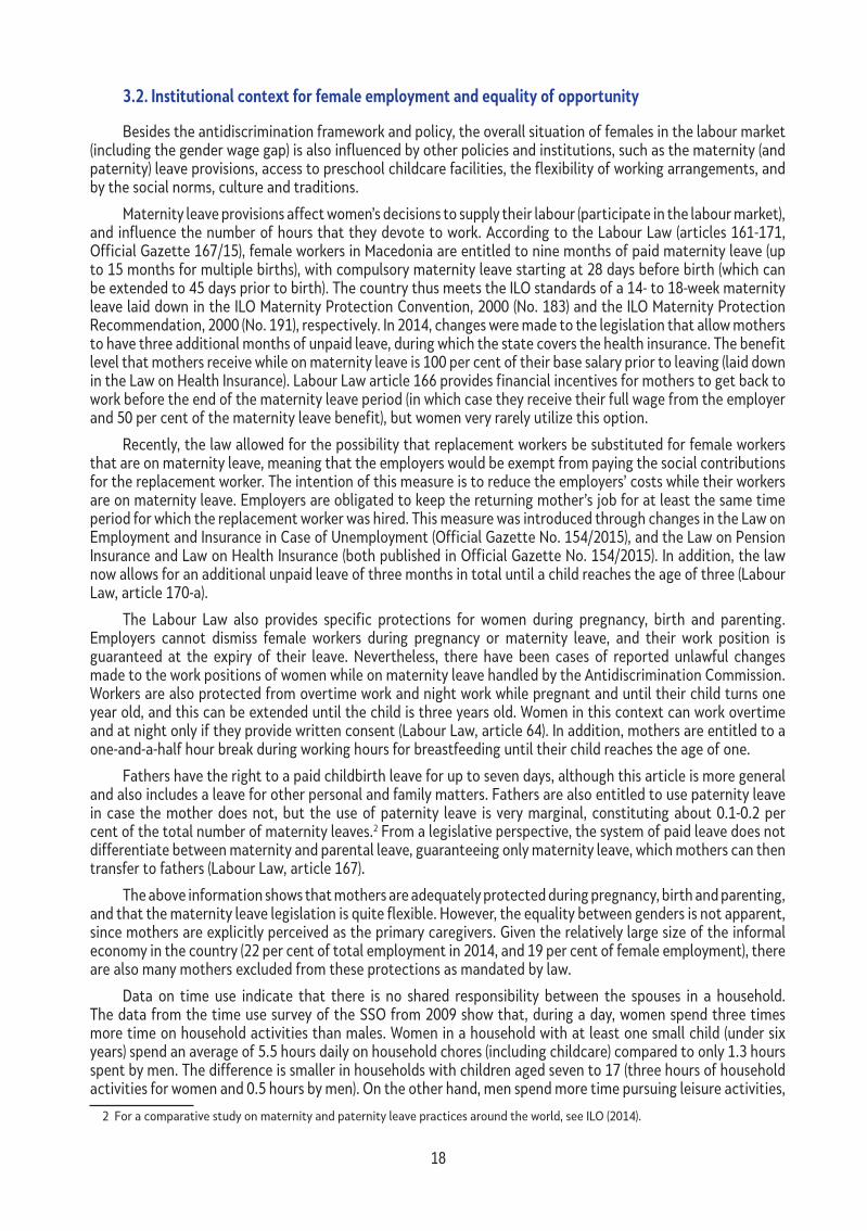
As Figure 1 shows, only half of the females of working age (15−64) were active in 2014, compared to about 78 per cent of males. Hence, the gender gap in activity is 25 percentage points (p.p.), which is more than twice the average EU-28 gender gap (11.6 per cent in 2014). Otherwise, the labour market activity of males in the former Yugoslav Republic of Macedonia is comparable to that of the EU-28 males (77.7 per cent compared to 78 per cent).
Figure 1 – Activity rates by gender
77,7
52,5
0,0
10,0
20,0
30,0
40,0
50,0
60,0
70,0
80,0
2010 2011 2012 2013 2014
All
Man
Woman
Source: Eurostat database.
The gender activity gap substantially declines as the level of education increases. At the primary education level or less, female activity is 40 p.p. lower than that of males, whereas the gap at the tertiary level is only 3.5 p.p. Apparently, the least educated women are the most likely to be excluded from the labour market (see Table 2), as their non-working opportunity costs seem to be very low, and they are more likely to come from traditional backgrounds which influence their decisions to further their education and work.
table 2 – Gender gaps by level of education, 2014
Primary education secondary education tertiary education
Female (%) Male (%) Gap (pp) Female
(%)Male (%) Gap (pp) Female
(%) Male (%) Gap (pp)
Activity rate 27.0 66.5 39.5 63.2 80.7 17.5 87.6 91.1 3.5
Employment rate 18.5 44.3 25.8 44.3 58.6 14.3 66.0 72.8 6.8
Unemployment rate 31.5 33.3 1.8 29.8 27.4 -2.4 24.6 20.1 -4.5
Source: Eurostat database.
When assessed by age, the gender activity gap is the lowest among young workers (14.2 p.p.), whose activity in general is very low (see Table 3). For the prime age group (25-54) the employment gap is about 26.8 p.p.,

22
with relatively high activity rates for both genders (93.2 per cent for males). The gap is the largest for older workers. This can be due to generational factors, since females were more traditionally housewives who were not extensively educated. This suggests that with time, as females are better educated and the traditional family structure changes, the gender activity gap will decline.
table 3 - Main labour market indicators and gaps by age group, 2014
15-24 25-54 55-64
Female (%)
Male (%)
Gap (pp)
Female (%)
Male (%)
Gap (pp)
Female (%)
Male (%)
Gap (pp)
Activity rate 25.1 39.3 14.2 66.4 93.2 26.8 33.5 66.8 33.3
Employment rate 11.3 18.9 7.6 48.5 69.8 21.3 27.1 50.3 23.2
Unemployment rate 55.0 52.0 -3.0 27.0 25.1 -1.9 19.0 29.2 10.2
Source: Eurostat database.
The female employment rate in the former Yugoslav Republic of Macedonia is significantly lower than that for males. The employment gap between the genders in 2014 was about 19 p.p., and has been rather stable over time. While, in general, employment in the country is low (47 per cent in 2014), the employment rate of females is very low, only 37.4 per cent in 2014. The gender employment gap substantially declines with the level of education attained. While at the primary education level females’ employment rate is on average 26 p.p. lower than that of males, the gap is less than seven p.p. at the tertiary level (see Table 2). The gender employment gap among individuals with tertiary educational attainment is mainly due to higher unemployment among women than among men (the gap amounts to 4.5 p.p.), and, to a lesser extent, to lower female activity (the gap amounts to 3.5 p.p.). This suggests that although educated females are much more likely to supply labour, they still face higher unemployment probabilities than males (compared to less educated individuals), which can indicate that women face discrimination by employers at the point of job entry, or that employers value the male unobservable characteristics more than those of females.
Females in the former Yugoslav Republic of Macedonia are less likely to work part-time than males (6.3 per cent of male employment as compared to 4.8 per cent). However, for those females that work part-time, family and childcare responsibilities are much more important factors than for males (see section 3.2 for greater elaboration on this issue).
When assessed by age (Table 3), the employment gap is highest among older workers aged 55−64, while it is relatively low for young workers (7.6 p.p.). Nevertheless, every young person irrespective of gender faces very low employment rates. The large gap in the higher age group suggests that older females face disproportionately greater difficulties in finding a job compared to younger women or males of the same age.
Females are much less likely to be self-employed than males (eight per cent of females compared to 24 per cent of males). This holds for self-employed individuals with employees (employers) and for self-employed workers without employees (own-account workers). On the other hand, women are overrepresented among contributing family workers. It is mainly women with primary education levels or less that are engaged as contributing family workers (Avlijaš et al., 2013).

23
table 4 – structure of employment by professional status and gender, 2014
All Males Females
Employees 73.8 70.7 78.7
self-employed persons 17.6 23.9 7.8
- Employers (self-employed persons with employees) 3.9 4.9 2.3
- self-employed persons without employees (own-account workers) 13.7 18.9 5.5
Contributing family workers 8.6 5.5 13.5
total 100.0 100.0 100.0
Source: Eurostat database.
Figure 2 shows the occupational structure of employment in the former Yugoslav Republic of Macedonia. While elementary occupations dominate in the employment of both genders, females are slightly overrepresented (as they are more likely to work in textiles and similar industries). The same holds for plant and machine operators. On the other hand, females are overrepresented among professionals and technicians, which are high-level occupations.
Figure 2 – occupational structure of employment by gender
0,0
5,0
10,0
15,0
20,0
25,0
Мажи
Жени
Source: Eurostat database.
Regarding unemployment trends, both genders are almost equally hurt by the difficulty of finding a job. From 2010 to 2014, the unemployment rate declined (see Figure 3), especially for females. However, since 2013, the unemployment rate for females has risen above the one for males.
In terms of education, females with primary education levels or less have a lower probability of being unemployed than do males. However, as the educational level increases, the gender gap reverses, and the male unemployment rate at the tertiary education level is 4.5 p.p. lower than that of tertiary-educated females (see Table 2).
23
Табела 4 – Структура на вработеноста според професионален статус и пол, 2014 г.
Сите Мажи Жени
Вработени 73,8 70,7 78,7
Самовработени лица 17,6 23,9 7,8
- Работодавачи (самовработени лица со вработени) 3,9 4,9 2,3
- Самовработени лица без вработени (работници за сопствена сметка)
13,7 18,9 5,5
Неплатени семејни работници 8,6 5,5 13,5
Вкупно 100,0 100,0 100,0
Извор: Базата на податоци на Евростат.
Слика 2 ја покажува структурата на вработеноста по занимања во Република Македонија. Иако елемен-тарните занимања преовладуваат во вработеноста за двата пола, жените се малку позастапени (бидејќи тие со поголема веројатност работат во текстилната и сличните индустрии). Истото важи за ракувачите на машини и постројки. Од друга страна, жените се позастапени меѓу стручњаците и техничарите, што претставуваат зани-мања на високо ниво.
Слика 2 – Структура на вработеноста според занимање и пол
22
Извор: Базата на податоци на Евростат.
Во однос на трендовите на невработеноста, и двата пола се речиси еднакво погодени од тешкотиите при наоѓањето работа. Во периодот од 2000 до 2014 година, стапката на невработеност се намалувала (видете Error! Reference source not found.), особено за жените. Меѓутоа, од 2013 година наваму, стапката на невработеност на жените станала поголема од таа за мажите.
Набљудувани според нивото на образованието, жените со завршено основно или пониско образование имаат помала веројатност да бидат невработени во споредба со мажите. Меѓутоа, како што се зголемува нивото на образованието, родовиот јаз станува обратен, така што стапката на невработеност на мажите со завршено терцијарно образование е 4,5 п.п. пониска од стапката на жените со завршено терцијарно образование (видете Error! Reference source not found.).
Слика 3 – Стапка на невработеност по пол
Извор: Базата на податоци на Евростат.
0,0
5,0
10,0
15,0
20,0
25,0
Males
Females
27,0
28,0
29,0
30,0
31,0
32,0
33,0
2010 2011 2012 2013 2014
All
Males
Females
Извор: Базата на податоци на Евростат.
Во однос на трендовите на невработеноста, и двата пола се речиси еднакво погодени од тешкотиите при наоѓањето работа. Во периодот од 2000 до 2014 година, стапката на невработеност се намалувала (видете Слика 3), особено за жените. Меѓутоа, од 2013 година наваму, стапката на невработеност на жените станала поголема од таа за мажите.
Набљудувани според нивото на образованието, жените со завршено основно или пониско образование имаат помала веројатност да бидат невработени во споредба со мажите. Меѓутоа, како што се зголемува нивото на образованието, родовиот јаз станува обратен, така што стапката на невработеност на мажите со завршено терцијарно образование е 4,5 п.п. пониска од стапката на жените со завршено терцијарно образование (видете Табела 2).

24
Figure 3 – Unemployment rate by gender
27,0
28,0
29,0
30,0
31,0
32,0
33,0
2010 2011 2012 2013 2014
Сите
Мажи
Жени
Source: Eurostat database.
The gender gap between unemployed persons decreases with age (see Table 3). Older females (55−64) have ten p.p. lower unemployment rates than males, but this is mainly related to the large inactivity of females in that age group. As we previously pointed out, females aged 55−64 have very low employment and activity rates, and the gender gaps are largest for this age group.
All
Males
Females

25
5. stylized facts about employment and wage differences
This section presents the main descriptive statistics derived from the microdata used in the study. At some points we reference the descriptive analyses presented based on the aggregate LFS data, to show the alignment and precision of the calculations.
5.1. Gender gaps in employment
The employment rate of females aged 15−64 was 35.3 in 2011 and 37.3 in 2014 (see Table 5).3 The same employment rate for females was reported by the SSO in 2014 (see section above). The gender employment gap was at 17 p.p. in 2011, increasing to 19 p.p. in 2014. The employment rate for females is the lowest in the young age bracket, given that the majority of females at this age are still involved in education. The gender employment gap is lowest at this point. The employment rate of the primary working age group (25−54) was 46.8 per cent in 2011 and 48.5 per cent in 2014. Females aged 55-64 experienced the largest increase in their employment rate between 2011 (24 per cent) and 2014 (27.1 per cent), by 3.1 p.p.
table 5 – Labour market characteristics of genders, 2011 and 2014
Employment rate
2011 2014
Males Females Males Females
All (15-64) 52.3 35.3 56.1 37.3
Age categories (employment rates)
15-24 17.7 10.8 18.9 11.3
25-54 65.7 46.8 69.8 48.5
55-64 47.3 24 50.3 27.1
Professional economic status (structure. in %)
Employee 69.8 76.4 70.7 78.6
Employer 7.1 3.6 4.9 2.4
self-employed 17.2 5.8 19 5.5
Contributing family worker 5.9 14.2 5.5 13.5
Source: Own calculations based on LFS.
Note: Weights used in the calculations.
As previously reported, the main professional status of females is that of “employee”, meaning a wage worker. About three quarters of females are working as employees (Table 5). Slightly more than 14 per cent are engaged as contributing family members, which is almost three times the proportion of males in the category. Only a small portion of females holds employer status. Compared to males, females are overrepresented among employees and contributing family workers.
3 The years assessed in this section do not necessarily show statistically significant differences. Interval estimation can show if these differences are statistically significant, but that is not the primary focus of this section.
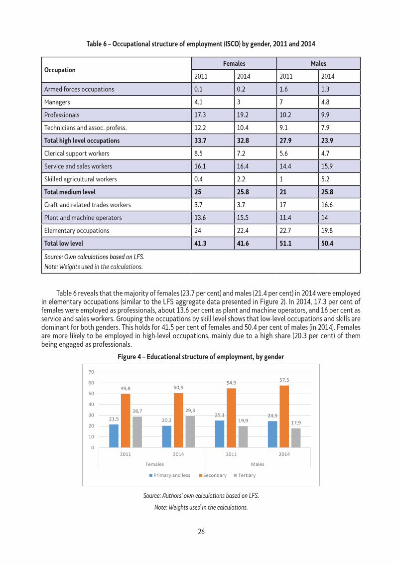
26
table 6 – occupational structure of employment (IsCo) by gender, 2011 and 2014
occupationFemales Males
2011 2014 2011 2014
Armed forces occupations 0.1 0.2 1.6 1.3
Managers 4.1 3 7 4.8
Professionals 17.3 19.2 10.2 9.9
Technicians and assoc. profess. 12.2 10.4 9.1 7.9
total high level occupations 33.7 32.8 27.9 23.9
Clerical support workers 8.5 7.2 5.6 4.7
Service and sales workers 16.1 16.4 14.4 15.9
Skilled agricultural workers 0.4 2.2 1 5.2
total medium level 25 25.8 21 25.8
Craft and related trades workers 3.7 3.7 17 16.6
Plant and machine operators 13.6 15.5 11.4 14
Elementary occupations 24 22.4 22.7 19.8
total low level 41.3 41.6 51.1 50.4
Source: Own calculations based on LFS.Note: Weights used in the calculations.
Table 6 reveals that the majority of females (23.7 per cent) and males (21.4 per cent) in 2014 were employed in elementary occupations (similar to the LFS aggregate data presented in Figure 2). In 2014, 17.3 per cent of females were employed as professionals, about 13.6 per cent as plant and machine operators, and 16 per cent as service and sales workers. Grouping the occupations by skill level shows that low-level occupations and skills are dominant for both genders. This holds for 41.5 per cent of females and 50.4 per cent of males (in 2014). Females are more likely to be employed in high-level occupations, mainly due to a high share (20.3 per cent) of them being engaged as professionals.
Figure 4 – Educational structure of employment, by gender
21,5 20,225,1 24,5
49,8 50,554,9 57,5
28,7 29,3
19,9 17,9
0
10
20
30
40
50
60
70
2011 2014 2011 2014
Females Males
Primary and less Secondary Tertiary
Source: Authors’ own calculations based on LFS.
Note: Weights used in the calculations.
21,5 20,225,1 24,5
49,8 50,554,9 57,5
28,7 29,3
19,9 17,9
0
10
20
30
40
50
60
70
2011 2014 2011 2014
Females Males
Primary and less Secondary Tertiary
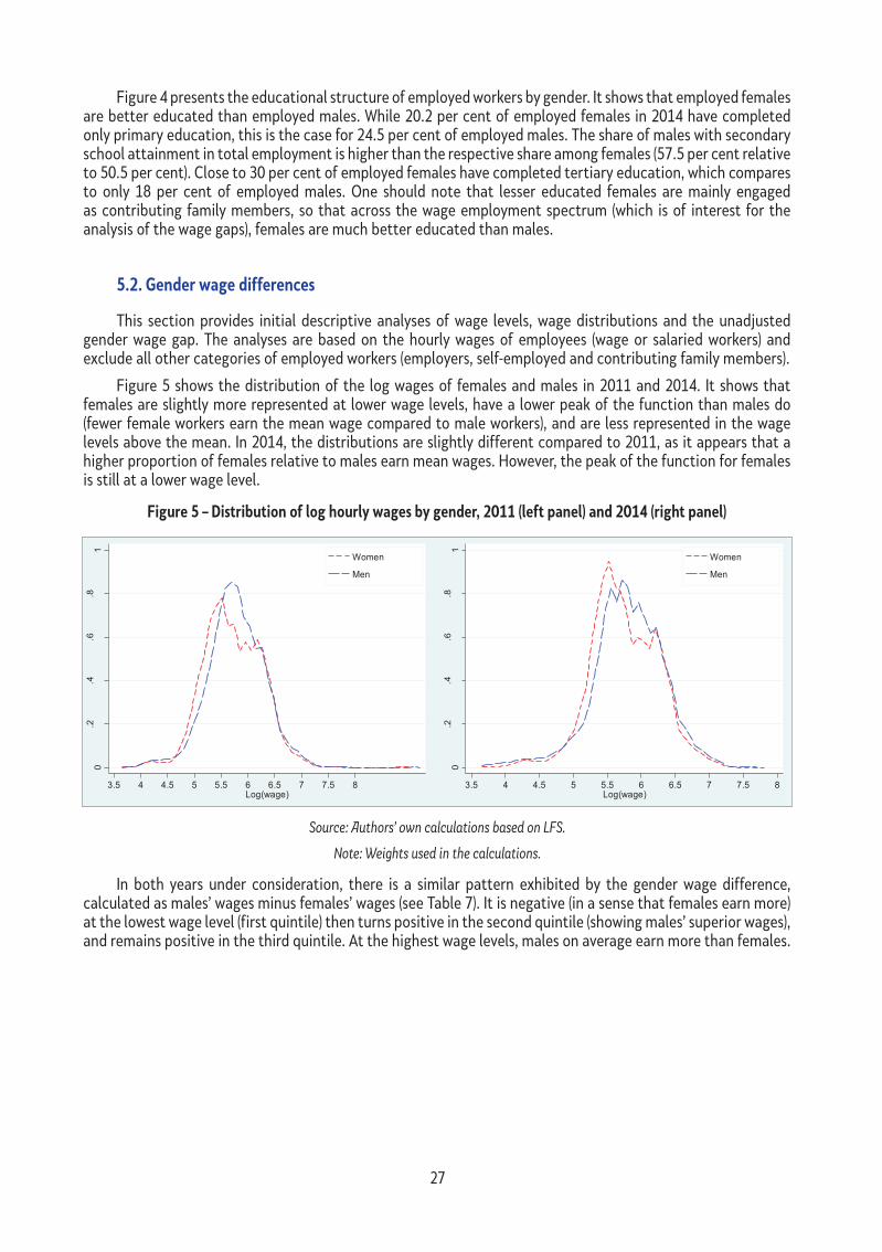
27
Figure 4 presents the educational structure of employed workers by gender. It shows that employed females are better educated than employed males. While 20.2 per cent of employed females in 2014 have completed only primary education, this is the case for 24.5 per cent of employed males. The share of males with secondary school attainment in total employment is higher than the respective share among females (57.5 per cent relative to 50.5 per cent). Close to 30 per cent of employed females have completed tertiary education, which compares to only 18 per cent of employed males. One should note that lesser educated females are mainly engaged as contributing family members, so that across the wage employment spectrum (which is of interest for the analysis of the wage gaps), females are much better educated than males.
5.2. Gender wage differences
This section provides initial descriptive analyses of wage levels, wage distributions and the unadjusted gender wage gap. The analyses are based on the hourly wages of employees (wage or salaried workers) and exclude all other categories of employed workers (employers, self-employed and contributing family members).
Figure 5 shows the distribution of the log wages of females and males in 2011 and 2014. It shows that females are slightly more represented at lower wage levels, have a lower peak of the function than males do (fewer female workers earn the mean wage compared to male workers), and are less represented in the wage levels above the mean. In 2014, the distributions are slightly different compared to 2011, as it appears that a higher proportion of females relative to males earn mean wages. However, the peak of the function for females is still at a lower wage level.
Figure 5 – Distribution of log hourly wages by gender, 2011 (left panel) and 2014 (right panel)
27
Извор: Сопствени пресметки врз основа на АРС. Забелешка: Во пресметките се користени пондери.
И во двете разгледувани години постои сличен модел на родовата разлика во платите што е пресметана како платата на мажите минус платата на жените (видете Error! Reference source not found.). Таа е негативна (во смисла на тоа дека жените заработуваат повеќе) на најниското ниво на платите (1-от квинтил), а потоа станува позитивна, покажувајќи ги повисоките плати на мажите, и е повторно позитивна во 3-от квинтил. На највисоките нивоа на платите, мажите во просек заработуваат повеќе од жените.
Табела 7 – Родови разлики во платите по квинтили
2011 2014
Жени Мажи
Разлика во
плата (%)
Жени Мажи
Разлика во
плата (%)
Прв квинтил 5,045 4,998 -4,7 5,191 5,079 -11,2 Втор квинтил 5,916 5,926 1 5,964 5,985 2,1 Трет квинтил 6,131 6,09 -4,1 6,122 6,109 -1,3 Четврти квинтил 6,285 6,27 -1,5 6,283 6,273 -1 Петти квинтил 6,455 6,471 1,6 6,468 6,501 3,3 Извор: Сопствени пресметки врз основа на АРС. Забелешка: Јазот е пресметан како логаритамските плати на мажите минус логаритамските плати на жените (помножени со 100), на аритметичката средина на платата за секој квинтил. Кога јазот е позитивен, мажите покажуваат повисоки плати од жените, на аритметичката средина, и обратно. Во пресметките се користени пондери.
0.2
.4.6
.81
Den
sity
3.5 4 4.5 5 5.5 6 6.5 7 7.5 8Log(wage)
Women
Men
0.2
.4.6
.81
Den
sity
3.5 4 4.5 5 5.5 6 6.5 7 7.5 8Log(wage)
Women
Men
Source: Authors’ own calculations based on LFS.
Note: Weights used in the calculations.
In both years under consideration, there is a similar pattern exhibited by the gender wage difference, calculated as males’ wages minus females’ wages (see Table 7). It is negative (in a sense that females earn more) at the lowest wage level (first quintile) then turns positive in the second quintile (showing males’ superior wages), and remains positive in the third quintile. At the highest wage levels, males on average earn more than females.

28
table 7 – Gender wage differences by quintiles
2011 2014
Females MalesWage diff.
(%)Females Males
Wage diff. (%)
1st quintile 5.045 4.998 -4.7 5.191 5.079 -11.2
2nd quintile 5.916 5.926 1 5.964 5.985 2.1
3rd quintile 6.131 6.09 -4.1 6.122 6.109 -1.3
4th quintile 6.285 6.27 -1.5 6.283 6.273 -1
5th quintile 6.455 6.471 1.6 6.468 6.501 3.3
Source: Authors’ own calculations based on LFS.
Note: The gap is calculated as males’ minus females’ log wages (multiplied by 100), at the mean wage for each quintile. Where positive, males are exhibiting higher wages than females, at the mean, and vice versa. Weights used in the calculations.
There are still some variations between the years regarding the magnitude and significance of the gender wage difference. For instance, while in 2011 females in the first quintile of the wage distribution were earning 3.4 per cent higher wages at the mean compared to males, this difference in 2014 was 11.5 per cent. Note, though, that we cannot confirm an increased wage difference in favour of females, as we are not reporting if the change in the gap is statistically significant (meaning that we are not performing interval estimation).4 In 2014, males were earning 2.7 per cent higher wages in the second quintile at the mean, whereas this difference was 2.5 per cent at the highest wage levels (fifth quintile).
The gender wage difference shows that across all occupations, females earn on average lower wages than males (see Table 8). However, this is the unadjusted gap and does not take into account the personal and labour market characteristics of the workers (such as education and work experience). Therefore, we cannot conclude at this stage that males are better off in terms of wages in the Macedonian labour market. It may simply mean that within each occupation, males have better personal or labour market characteristics compared to females, but not higher returns for those characteristics, which would point to discrimination.
4 Since the individuals that were sampled in 2011 and 2014 are not the same ones, the difference in the calculated wage gaps may only be a result of the different characteristics of the men and women involved in the two rounds of the survey, and not a systematic feature. In other words, this analysis does not tell us if we would find the same difference in the wage gaps if other individuals were part of the 2011 or 2014 sample.

29
table 8 – Gender wage differences by occupation
occupation
2011 2014
Females MalesWage diff.
(%)Females Males
Wage diff. (%)
Armed forces occupations 6.059 6.168 10.9 6.206 6.24 3.4
Managers 5.826 5.953 12.7 5.915 5.989 7.4
Professionals 6.25 6.237 -1.3 6.254 6.309 5.5
technicians and assoc. profess. 5.918 5.993 7.5 5.962 6.068 10.6
Clerical support workers 5.934 5.938 0.4 5.909 5.946 3.7
service and sales workers 5.467 5.702 23.5 5.525 5.754 22.9
skilled agricultural, forestry and fishery workers 5.306 5.682 37.6 5.303 5.445 14.2
Craft and related trades workers 5.477 5.7 22.3 5.439 5.76 32.1
Plant and machine operators and assemblers 5.301 5.695 39.4 5.45 5.77 32
Elementary occupations 5.358 5.417 5.9 5.462 5.432 -3
Source: Authors’ own calculations based on LFS.Note: Weights used in the calculations.
Data for 2014 show that the gender wage difference is largest for low-skilled occupations, such as craft and related trades workers and plant and machine operators, where males earn 29 per cent and 32 per cent higher wages than females, respectively (Table 8). The difference is also large for service and sales workers (at 23 per cent), skilled agricultural workers (17 per cent), and technicians and associate professions (12 per cent).
The gender wage difference (see Table 9) generally declines with the level of education. While the unadjusted gap for 2014 is 15.6 per cent at the primary education level, it declines to less than five per cent at the tertiary level and wanes at the post-tertiary level (masters and PhD).
table 9 – Gender wage difference by education
2011 2014
Females MalesUnadjusted
wage gap (%)Females Males
Unadjusted wage gap (%)
Primary 5.28 5.519 23.9 5.379 5.535 15.6
secondary 5.569 5.738 16.9 5.612 5.789 17.7
tertiary 6.097 6.139 4.2 6.113 6.16 4.7
Post-tertiary 5.752 5.752 0 5.784 5.784 0
Source: Authors’ own calculations based on LFS.Note: Weights used in the calculations.

30
As Table 10 shows, the pay difference is largest in the industrial sector (22.5 per cent) in 2014, followed by agriculture (about 14 per cent). The gap is lowest in the non-market service sector,5 where females, on average, earned about eight per cent lower hourly wages compared to males in 2014.
table 10 – Gender wage differences by sector of employment
2011 2014
Females MalesWage diff.
(%)Females Males
Wage diff. (%)
Agriculture 5.242 5.376 13.4 5.233 5.369 13.6
Industrial 5.477 5.755 27.8 5.584 5.809 22.5
service 5.69 5.766 7.6 5.709 5.802 9.3
Non-market services and activities 6.02 6.091 7.1 6.045 6.121 7.6
Source: Authors’ own calculations based on LFS.Note: Weights used in the calculations.
5.3. Motherhood employment and wage differences
Following the previous studies of the motherhood wage gap (see Grimshaw and Rubery, 2015), we define mothers as women aged 25−45 with at least one child below the age of six. The comparison group for the analysis of the motherhood wage gap consists of non-mothers: females aged 25−45 who are either childless or with children above the age of six (see the justification for the selection of the age span on p. 27). The age of six is chosen as the starting school age in the country, and is used in similar studies (for instance Agüero and Marks, 2011). However, we also provide estimations for three different definitions of mothers (as in Table 11).6 Following these definitions, the share of mothers in our sample is 24 per cent in 2014 (for mothers with a child up to three years of age). Of them, 34 per cent are mothers with a child aged up to six years, and 66 per cent are mothers with a child aged up to 18 years (see Table 11). Note that our main analysis below is based on mothers being defined as females aged 25−45 with at least one child aged up to six years, but some broader analyses are provided in the appendix.
table 11 – share of mothers between 25-45 years old, under different definitions
Mother with a child up to 3
Mother with a child up to 6
Mother with a child up to 18
2011 21.9 34.7 69.5
2014 24.1 34.2 65.9
Source: Own calculations based on LFS.Note: Weights used in the calculations.
Non-mothers in our sample exhibit higher employment rates than mothers (see Table 12). While 54 per cent of non-mothers were employed in 2014, only 37 per cent of mothers were employed. Regarding their professional status, we found no meaningful differences between employed mothers and non-mothers. Both categories of female workers are more likely to be employed as wage (salaried) workers (between 76−82 per cent
5 This category includes public administration and defense, education, health, compulsory social security, social work, arts, entertainment and recreation, other service activities, activities of households as employers, and undifferentiated goods- and service-producing activities of households for their own use. 6 Studies use different definitions of mothers in respect to the child’s age.
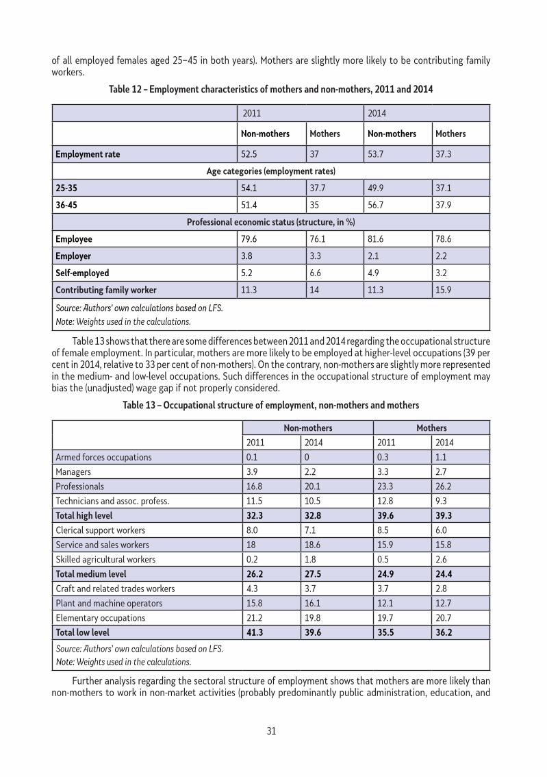
31
of all employed females aged 25−45 in both years). Mothers are slightly more likely to be contributing family workers.
table 12 – Employment characteristics of mothers and non-mothers, 2011 and 2014
2011 2014
Non-mothers Mothers Non-mothers Mothers
Employment rate 52.5 37 53.7 37.3
Age categories (employment rates)
25-35 54.1 37.7 49.9 37.1
36-45 51.4 35 56.7 37.9
Professional economic status (structure, in %)
Employee 79.6 76.1 81.6 78.6
Employer 3.8 3.3 2.1 2.2
self-employed 5.2 6.6 4.9 3.2
Contributing family worker 11.3 14 11.3 15.9
Source: Authors’ own calculations based on LFS.Note: Weights used in the calculations.
Table 13 shows that there are some differences between 2011 and 2014 regarding the occupational structure of female employment. In particular, mothers are more likely to be employed at higher-level occupations (39 per cent in 2014, relative to 33 per cent of non-mothers). On the contrary, non-mothers are slightly more represented in the medium- and low-level occupations. Such differences in the occupational structure of employment may bias the (unadjusted) wage gap if not properly considered.
table 13 – occupational structure of employment, non-mothers and mothers
Non-mothers Mothers
2011 2014 2011 2014
Armed forces occupations 0.1 0 0.3 1.1
Managers 3.9 2.2 3.3 2.7
Professionals 16.8 20.1 23.3 26.2
Technicians and assoc. profess. 11.5 10.5 12.8 9.3
total high level 32.3 32.8 39.6 39.3
Clerical support workers 8.0 7.1 8.5 6.0
Service and sales workers 18 18.6 15.9 15.8
Skilled agricultural workers 0.2 1.8 0.5 2.6
total medium level 26.2 27.5 24.9 24.4
Craft and related trades workers 4.3 3.7 3.7 2.8
Plant and machine operators 15.8 16.1 12.1 12.7
Elementary occupations 21.2 19.8 19.7 20.7
total low level 41.3 39.6 35.5 36.2
Source: Authors’ own calculations based on LFS.Note: Weights used in the calculations.
Further analysis regarding the sectoral structure of employment shows that mothers are more likely than non-mothers to work in non-market activities (probably predominantly public administration, education, and
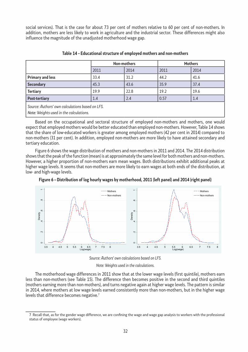
32
social services). That is the case for about 73 per cent of mothers relative to 60 per cent of non-mothers. In addition, mothers are less likely to work in agriculture and the industrial sector. These differences might also influence the magnitude of the unadjusted motherhood wage gap.
table 14 – Educational structure of employed mothers and non-mothers
Non-mothers Mothers
2011 2014 2011 2014
Primary and less 33.4 31.2 44.2 41.6
secondary 45.3 43.6 35.9 37.4
tertiary 19.9 22.8 19.2 19.6
Post-tertiary 1.4 2.4 0.57 1.4
Source: Authors’ own calculations based on LFS.Note: Weights used in the calculations.
Based on the occupational and sectoral structure of employed non-mothers and mothers, one would expect that employed mothers would be better educated than employed non-mothers. However, Table 14 shows that the share of low-educated workers is greater among employed mothers (42 per cent in 2014) compared to non-mothers (31 per cent). In addition, employed non-mothers are more likely to have attained secondary and tertiary education.
Figure 6 shows the wage distribution of mothers and non-mothers in 2011 and 2014. The 2014 distribution shows that the peak of the function (mean) is at approximately the same level for both mothers and non-mothers. However, a higher proportion of non-mothers earn mean wages. Both distributions exhibit additional peaks at higher wage levels. It seems that non-mothers are more likely to earn wages at both ends of the distribution, at low- and high-wage levels.
Figure 6 – Distribution of log hourly wages by motherhood, 2011 (left panel) and 2014 (right panel)
0.2
.4.6
.81
Den
sity
3.5 4 4.5 5 5.5 6 6.5 7 7.5 8Log(wage)
Mothers
Non-mothers
0.2
.4.6
.81
Den
sity
3.5 4 4.5 5 5.5 6 6.5 7 7.5 8Log(wage)
Mothers
Non-mothers
Source: Authors’ own calculations based on LFS.
Note: Weights used in the calculations.
The motherhood wage differences in 2011 show that at the lower wage levels (first quintile), mothers earn less than non-mothers (see Table 15). The difference then becomes positive in the second and third quintiles (mothers earning more than non-mothers), and turns negative again at higher wage levels. The pattern is similar in 2014, where mothers at low wage levels earned consistently more than non-mothers, but in the higher wage levels that difference becomes negative.7
7 Recall that, as for the gender wage difference, we are confining the wage and wage gap analysis to workers with the professional status of employee (wage workers).

33
table 15 – Motherhood wage difference by quintile of wage distribution
2011 2014
Non-mothers Mothers Wage diff. (%) Non-mothers Mothers Wage diff. (%)
1st quintile 5.007 5.024 1.7 5.091 5.15 5.9
2nd quintile 5.842 5.926 8.4 5.871 5.947 7.6
3rd quintile 5.985 6.025 4 6.012 6.047 3.5
4th quintile 6.181 6.173 -0.8 6.274 6.275 0.1
5th quintile 6.454 6.379 -7.5 6.403 6.413 1
Source: Authors’ own calculations based on LFS.
Note: The gap is calculated as mothers’ minus non-mothers’ log wages, at the mean wage for each quintile. Where positive, mothers are exhibiting higher wages than non-mothers, at the mean. Weights used in the calculations.
Table 16 shows that there is no particular pattern in the motherhood pay differences by occupation, and there is no consistency among years. In 2011, mothers with managerial positions were earning 31 per cent less compared to non-mothers. However, this difference halved by 2014. In 2014, mothers had higher wages than non-mothers in the following occupations: clerical support staff (by 15 per cent), elementary occupations (by 11 per cent), skilled agriculture workers (nine per cent), and professionals (eight per cent). On the contrary, mothers working as craftspeople and technicians/professionals had 8.5 per cent and seven per cent lower wages than non-mothers working at the same occupations, respectively.
table 16 – Motherhood wage differences by occupation
2011 2014
Non-mothers Mothers Wage diff.
(%) Non-mothers Mothers Wage diff. (%)
Armed forces occupations 6.041 6.109 6.8 6.163 6.216 5.3
Managers 5.823 5.511 -31.2 5.874 5.81 -6.4
Professionals 6.214 6.217 0.3 6.191 6.278 8.7
technicians and assoc. profess. 5.86 5.897 3.7 5.952 5.858 -9.4
Clerical support workers 5.853 6.024 17.1 5.774 5.963 18.9
service and sales workers 5.44 5.496 5.6 5.524 5.495 -2.9
skilled agricultural, forestry and fishery workers
5.672 5.492 -18 5.273 5.362 8.9
Craft and related trades workers 5.472 5.495 2.3 5.497 5.548 5.1
Plant and machine operators and assemblers
5.292 5.291 -0.1 5.467 5.473 0.6
Elementary occupations 5.301 5.28 -2.1 5.422 5.575 15.3
Source: Own calculations based on LFS.
Note: Weights used in the calculations.

34
The analysis reveals that there are no specific differences in the motherhood pay differences between educational levels. When categorized by employment sector, it appears that mothers are doing better than non-mothers in all sectors of employment, especially in non-market services and activities.
table 17 – Motherhood wage difference by sector of employment
sector
2011 2014
Non-mothers Mothers Wage diff. (%) Non-
mothers Mothers Wage diff. (%)
Agriculture 5.132 5.178 4.6 5.288 5.302 5.3
Industrial 5.452 5.441 -1.1 5.586 5.638 5.2
services 5.656 5.71 5.4 5.691 5.744 5.3
Non-market services and activities 5.962 6.086 12.4 5.979 6.135 15.6
Source: Authors’ own calculations based on LFS.
Note: Weights used in the calculations.

35
6. Methodology and data
6.1. Economic models and estimation methods
To estimate the gender and motherhood wage gaps, we rely on Mincer’s (1974) human capital earnings function, which relates the individual wage log to gender, motherhood, level of education, age, years of work experience and other labour-market characteristics, within a specification which is linear in education and quadratic in age8:
36
6. Методологија и податоци 6.1. Економски модели и методи за процена
За проценување на родовиот и мајчинскиот јаз во платите се потпираме врз Минцеровата (1974) функција на заработките од човечкиот капитал, што ја поврзува логаритамската функција на индивидуалната плата со родот, мајчинството, нивото на образование, возраста, годините работно искуство и другите карактеристики на пазарот на трудот, во рамките на спецификација што е линеарна за образованието и квадратна за возраста8:
ln(𝑦𝑦𝑖𝑖) = 𝛼𝛼 + 𝛽𝛽𝑔𝑔𝑔𝑔𝑔𝑔𝑔𝑔𝑔𝑔𝑔𝑔𝑖𝑖 + 𝛾𝛾1𝑔𝑔𝑔𝑔𝑒𝑒𝑖𝑖1 + 𝛾𝛾2𝑔𝑔𝑔𝑔𝑒𝑒𝑖𝑖2 + 𝛾𝛾3𝑔𝑔𝑔𝑔𝑒𝑒𝑖𝑖3 + 𝛾𝛾4𝑎𝑎𝑔𝑔𝑔𝑔𝑖𝑖 + 𝛾𝛾5𝑎𝑎𝑔𝑔𝑔𝑔𝑖𝑖2 + 𝛾𝛾6𝑡𝑡𝑔𝑔𝑔𝑔𝑒𝑒𝑔𝑔𝑔𝑔𝑖𝑖+𝑋𝑋𝑖𝑖′𝛿𝛿𝑘𝑘 +𝜀𝜀𝑖𝑖 (1)<}0{>
За процена на мајчинскиот јаз во платите користиме две равенки: ln(𝑦𝑦𝑖𝑖) = 𝛼𝛼 + 𝛽𝛽𝑔𝑔𝑔𝑔𝑔𝑔𝑔𝑔𝑔𝑔𝑔𝑔𝑖𝑖 + ∂1𝑚𝑚𝑚𝑚𝑡𝑡ℎ𝑔𝑔𝑔𝑔𝑖𝑖 + ∂2𝑐𝑐ℎ𝑖𝑖𝑖𝑖𝑔𝑔𝑖𝑖 + 𝛾𝛾1𝑔𝑔𝑔𝑔𝑒𝑒𝑖𝑖1 + 𝛾𝛾2𝑔𝑔𝑔𝑔𝑒𝑒𝑖𝑖2 + 𝛾𝛾3𝑔𝑔𝑔𝑔𝑒𝑒𝑖𝑖3 + 𝛾𝛾4𝑎𝑎𝑔𝑔𝑔𝑔𝑖𝑖 +𝛾𝛾5𝑎𝑎𝑔𝑔𝑔𝑔𝑖𝑖2 + 𝛾𝛾6𝑡𝑡𝑔𝑔𝑔𝑔𝑒𝑒𝑔𝑔𝑔𝑔𝑖𝑖+𝑋𝑋𝑖𝑖′𝛿𝛿𝑘𝑘 + 𝜀𝜀𝑖𝑖 (2)
ln(𝑦𝑦𝑖𝑖) = 𝛼𝛼 + ∂1𝑚𝑚𝑚𝑚𝑡𝑡ℎ𝑔𝑔𝑔𝑔𝑖𝑖 + 𝛾𝛾1𝑔𝑔𝑔𝑔𝑒𝑒𝑖𝑖1 + 𝛾𝛾2𝑔𝑔𝑔𝑔𝑒𝑒𝑖𝑖2 + 𝛾𝛾3𝑔𝑔𝑔𝑔𝑒𝑒𝑖𝑖3 + 𝛾𝛾4𝑎𝑎𝑔𝑔𝑔𝑔𝑖𝑖 + 𝛾𝛾5𝑎𝑎𝑔𝑔𝑔𝑔𝑖𝑖2 +𝛾𝛾6𝑡𝑡𝑔𝑔𝑔𝑔𝑒𝑒𝑔𝑔𝑔𝑔𝑖𝑖+𝑋𝑋𝑖𝑖′𝛿𝛿𝑘𝑘 + 𝜀𝜀𝑖𝑖 (3)
Ознаките се исти како порано, со тоа што 𝑚𝑚𝑚𝑚𝑡𝑡ℎ𝑔𝑔𝑔𝑔𝑖𝑖 е индикатор варијабила што добива вредност 1 за жените со најмалку едно дете на возраст под 6 години, така што ∂1 открива дали мајките се оштетуваат на пазарот на трудот и се очекува дека овој коефициент, слично како 𝛽𝛽, е негативен. Разликата меѓу (2) и (3) е во тоа што во (2) го користиме целиот примерок, така што таму се вклучени и мажите, додека, пак, во (3) се користи само примерок од жените. Оттаму, равенката (2), горе, има уште една варијабила, 𝑐𝑐ℎ𝑖𝑖𝑖𝑖𝑔𝑔𝑖𝑖 што добива вредност 1 ако лицето i има најмалку едно дете на возраст под 6 години. Ова е потребно за да може да се направат две споредби: мајки наспроти жени што не се мајки (т.е. жени што или немаат деца или имаат деца на возраст над 6 години), земајќи го збирот на коефициентите ∂1 и ∂2; мајки наспроти татковци, земајќи го збирот на коефициентите 𝛽𝛽 и ∂1. Меѓутоа, бидејќи овие пресметки може да бидат тешки за разбирање, равенката (3) го сведува примерокот само на жените, така што ∂1 директно го пресметува мајчинскиот јаз во платите (т.е. мајки наспроти жени што не се мајки).
Иако разгледуваме две години, 2011 и 2014 година, ги проценуваме (1), (2) и (3) за двете години посебно, бидејќи лицата што биле анкетирани во двете години се различни, со оглед на тоа што едно домаќинство може да остане во кохортата за анкетирање најмногу 18 месеци. Во рамките на една година, секое домаќинство се анкетира двапати. Како што сугерира литературата (на пр., Petrongolo и Olivetti, 2006), во процената на (1) нашата анализа е ограничена на лицата на возраст од 16 до 64 години, исклучувајќи ги невработените лица на возраст под 16 и над 64 години, студентите, пензионерите, лицата со попречености поради нефлексибилната понуда на трудот;
8 Студиите често ги вклучуваат или возраст или работното искуство и нивните квадратни изрази. Овде го користиме само квадратниот израз на возраста бидејќи тој веројатно ќе биде доволен за опфаќање на пресвртната точка на платата во текот на животниот циклус.
(1)
Here, ln(yi) is the log of the net hourly wage; genderi is a dummy variable taking a value of 1 for females and zero for males; edui1, edui2 and edui3 are dummy variables for completed education, categorized into four levels (primary or less, secondary, tertiary and post-graduate, and primary education is the omitted category); agei refers to years of age; tenurei to years of work experience in the current firm (as lifetime experience is not available); and
36
6. Методологија и податоци 6.1. Економски модели и методи за процена
За проценување на родовиот и мајчинскиот јаз во платите се потпираме врз Минцеровата (1974) функција на заработките од човечкиот капитал, што ја поврзува логаритамската функција на индивидуалната плата со родот, мајчинството, нивото на образование, возраста, годините работно искуство и другите карактеристики на пазарот на трудот, во рамките на спецификација што е линеарна за образованието и квадратна за возраста8:
ln(𝑦𝑦𝑖𝑖) = 𝛼𝛼 + 𝛽𝛽𝑔𝑔𝑔𝑔𝑔𝑔𝑔𝑔𝑔𝑔𝑔𝑔𝑖𝑖 + 𝛾𝛾1𝑔𝑔𝑔𝑔𝑒𝑒𝑖𝑖1 + 𝛾𝛾2𝑔𝑔𝑔𝑔𝑒𝑒𝑖𝑖2 + 𝛾𝛾3𝑔𝑔𝑔𝑔𝑒𝑒𝑖𝑖3 + 𝛾𝛾4𝑎𝑎𝑔𝑔𝑔𝑔𝑖𝑖 + 𝛾𝛾5𝑎𝑎𝑔𝑔𝑔𝑔𝑖𝑖2 + 𝛾𝛾6𝑡𝑡𝑔𝑔𝑔𝑔𝑒𝑒𝑔𝑔𝑔𝑔𝑖𝑖+𝑋𝑋𝑖𝑖′𝛿𝛿𝑘𝑘 +𝜀𝜀𝑖𝑖 (1)<}0{>
За процена на мајчинскиот јаз во платите користиме две равенки: ln(𝑦𝑦𝑖𝑖) = 𝛼𝛼 + 𝛽𝛽𝑔𝑔𝑔𝑔𝑔𝑔𝑔𝑔𝑔𝑔𝑔𝑔𝑖𝑖 + ∂1𝑚𝑚𝑚𝑚𝑡𝑡ℎ𝑔𝑔𝑔𝑔𝑖𝑖 + ∂2𝑐𝑐ℎ𝑖𝑖𝑖𝑖𝑔𝑔𝑖𝑖 + 𝛾𝛾1𝑔𝑔𝑔𝑔𝑒𝑒𝑖𝑖1 + 𝛾𝛾2𝑔𝑔𝑔𝑔𝑒𝑒𝑖𝑖2 + 𝛾𝛾3𝑔𝑔𝑔𝑔𝑒𝑒𝑖𝑖3 + 𝛾𝛾4𝑎𝑎𝑔𝑔𝑔𝑔𝑖𝑖 +𝛾𝛾5𝑎𝑎𝑔𝑔𝑔𝑔𝑖𝑖2 + 𝛾𝛾6𝑡𝑡𝑔𝑔𝑔𝑔𝑒𝑒𝑔𝑔𝑔𝑔𝑖𝑖+𝑋𝑋𝑖𝑖′𝛿𝛿𝑘𝑘 + 𝜀𝜀𝑖𝑖 (2)
ln(𝑦𝑦𝑖𝑖) = 𝛼𝛼 + ∂1𝑚𝑚𝑚𝑚𝑡𝑡ℎ𝑔𝑔𝑔𝑔𝑖𝑖 + 𝛾𝛾1𝑔𝑔𝑔𝑔𝑒𝑒𝑖𝑖1 + 𝛾𝛾2𝑔𝑔𝑔𝑔𝑒𝑒𝑖𝑖2 + 𝛾𝛾3𝑔𝑔𝑔𝑔𝑒𝑒𝑖𝑖3 + 𝛾𝛾4𝑎𝑎𝑔𝑔𝑔𝑔𝑖𝑖 + 𝛾𝛾5𝑎𝑎𝑔𝑔𝑔𝑔𝑖𝑖2 +𝛾𝛾6𝑡𝑡𝑔𝑔𝑔𝑔𝑒𝑒𝑔𝑔𝑔𝑔𝑖𝑖+𝑋𝑋𝑖𝑖′𝛿𝛿𝑘𝑘 + 𝜀𝜀𝑖𝑖 (3)
Ознаките се исти како порано, со тоа што 𝑚𝑚𝑚𝑚𝑡𝑡ℎ𝑔𝑔𝑔𝑔𝑖𝑖 е индикатор варијабила што добива вредност 1 за жените со најмалку едно дете на возраст под 6 години, така што ∂1 открива дали мајките се оштетуваат на пазарот на трудот и се очекува дека овој коефициент, слично како 𝛽𝛽, е негативен. Разликата меѓу (2) и (3) е во тоа што во (2) го користиме целиот примерок, така што таму се вклучени и мажите, додека, пак, во (3) се користи само примерок од жените. Оттаму, равенката (2), горе, има уште една варијабила, 𝑐𝑐ℎ𝑖𝑖𝑖𝑖𝑔𝑔𝑖𝑖 што добива вредност 1 ако лицето i има најмалку едно дете на возраст под 6 години. Ова е потребно за да може да се направат две споредби: мајки наспроти жени што не се мајки (т.е. жени што или немаат деца или имаат деца на возраст над 6 години), земајќи го збирот на коефициентите ∂1 и ∂2; мајки наспроти татковци, земајќи го збирот на коефициентите 𝛽𝛽 и ∂1. Меѓутоа, бидејќи овие пресметки може да бидат тешки за разбирање, равенката (3) го сведува примерокот само на жените, така што ∂1 директно го пресметува мајчинскиот јаз во платите (т.е. мајки наспроти жени што не се мајки).
Иако разгледуваме две години, 2011 и 2014 година, ги проценуваме (1), (2) и (3) за двете години посебно, бидејќи лицата што биле анкетирани во двете години се различни, со оглед на тоа што едно домаќинство може да остане во кохортата за анкетирање најмногу 18 месеци. Во рамките на една година, секое домаќинство се анкетира двапати. Како што сугерира литературата (на пр., Petrongolo и Olivetti, 2006), во процената на (1) нашата анализа е ограничена на лицата на возраст од 16 до 64 години, исклучувајќи ги невработените лица на возраст под 16 и над 64 години, студентите, пензионерите, лицата со попречености поради нефлексибилната понуда на трудот;
8 Студиите често ги вклучуваат или возраст или работното искуство и нивните квадратни изрази. Овде го користиме само квадратниот израз на возраста бидејќи тој веројатно ќе биде доволен за опфаќање на пресвртната точка на платата во текот на животниот циклус.
is a vector of other labour-market characteristics, such as type of contract, occupation, type of sector, and settlement (urban or rural) (Budig and England, 2001). The type of employment contract is either permanent or temporary, while the distinction “with written or without written contract” (i.e. informal employment) was not available. We consider ten occupational categories based on the two-digit codes of the International Standard Classification of Occupations (ISCO) (elementary occupations being the referent category) and four economic sectors grouped according to the National Classification of Activities NKD Rev.2 (2009): agriculture, industry, market services and non-market services, with industry being the reference category. Ethnicity, though very important for the Macedonian case, is not included as a variable is not available in LFS.
Our main interest is the coefficient β, which measures to what extent a female with the same labour-market characteristics as a male is paid less (or more). It is expected that β is negative.
To estimate the motherhood wage gap, we use two equations:
36
6. Методологија и податоци 6.1. Економски модели и методи за процена
За проценување на родовиот и мајчинскиот јаз во платите се потпираме врз Минцеровата (1974) функција на заработките од човечкиот капитал, што ја поврзува логаритамската функција на индивидуалната плата со родот, мајчинството, нивото на образование, возраста, годините работно искуство и другите карактеристики на пазарот на трудот, во рамките на спецификација што е линеарна за образованието и квадратна за возраста8:
ln(𝑦𝑦𝑖𝑖) = 𝛼𝛼 + 𝛽𝛽𝑔𝑔𝑔𝑔𝑔𝑔𝑔𝑔𝑔𝑔𝑔𝑔𝑖𝑖 + 𝛾𝛾1𝑔𝑔𝑔𝑔𝑒𝑒𝑖𝑖1 + 𝛾𝛾2𝑔𝑔𝑔𝑔𝑒𝑒𝑖𝑖2 + 𝛾𝛾3𝑔𝑔𝑔𝑔𝑒𝑒𝑖𝑖3 + 𝛾𝛾4𝑎𝑎𝑔𝑔𝑔𝑔𝑖𝑖 + 𝛾𝛾5𝑎𝑎𝑔𝑔𝑔𝑔𝑖𝑖2 + 𝛾𝛾6𝑡𝑡𝑔𝑔𝑔𝑔𝑒𝑒𝑔𝑔𝑔𝑔𝑖𝑖+𝑋𝑋𝑖𝑖′𝛿𝛿𝑘𝑘 +𝜀𝜀𝑖𝑖 (1)<}0{>
За процена на мајчинскиот јаз во платите користиме две равенки: ln(𝑦𝑦𝑖𝑖) = 𝛼𝛼 + 𝛽𝛽𝑔𝑔𝑔𝑔𝑔𝑔𝑔𝑔𝑔𝑔𝑔𝑔𝑖𝑖 + ∂1𝑚𝑚𝑚𝑚𝑡𝑡ℎ𝑔𝑔𝑔𝑔𝑖𝑖 + ∂2𝑐𝑐ℎ𝑖𝑖𝑖𝑖𝑔𝑔𝑖𝑖 + 𝛾𝛾1𝑔𝑔𝑔𝑔𝑒𝑒𝑖𝑖1 + 𝛾𝛾2𝑔𝑔𝑔𝑔𝑒𝑒𝑖𝑖2 + 𝛾𝛾3𝑔𝑔𝑔𝑔𝑒𝑒𝑖𝑖3 + 𝛾𝛾4𝑎𝑎𝑔𝑔𝑔𝑔𝑖𝑖 +𝛾𝛾5𝑎𝑎𝑔𝑔𝑔𝑔𝑖𝑖2 + 𝛾𝛾6𝑡𝑡𝑔𝑔𝑔𝑔𝑒𝑒𝑔𝑔𝑔𝑔𝑖𝑖+𝑋𝑋𝑖𝑖′𝛿𝛿𝑘𝑘 + 𝜀𝜀𝑖𝑖 (2)
ln(𝑦𝑦𝑖𝑖) = 𝛼𝛼 + ∂1𝑚𝑚𝑚𝑚𝑡𝑡ℎ𝑔𝑔𝑔𝑔𝑖𝑖 + 𝛾𝛾1𝑔𝑔𝑔𝑔𝑒𝑒𝑖𝑖1 + 𝛾𝛾2𝑔𝑔𝑔𝑔𝑒𝑒𝑖𝑖2 + 𝛾𝛾3𝑔𝑔𝑔𝑔𝑒𝑒𝑖𝑖3 + 𝛾𝛾4𝑎𝑎𝑔𝑔𝑔𝑔𝑖𝑖 + 𝛾𝛾5𝑎𝑎𝑔𝑔𝑔𝑔𝑖𝑖2 +𝛾𝛾6𝑡𝑡𝑔𝑔𝑔𝑔𝑒𝑒𝑔𝑔𝑔𝑔𝑖𝑖+𝑋𝑋𝑖𝑖′𝛿𝛿𝑘𝑘 + 𝜀𝜀𝑖𝑖 (3)
Ознаките се исти како порано, со тоа што 𝑚𝑚𝑚𝑚𝑡𝑡ℎ𝑔𝑔𝑔𝑔𝑖𝑖 е индикатор варијабила што добива вредност 1 за жените со најмалку едно дете на возраст под 6 години, така што ∂1 открива дали мајките се оштетуваат на пазарот на трудот и се очекува дека овој коефициент, слично како 𝛽𝛽, е негативен. Разликата меѓу (2) и (3) е во тоа што во (2) го користиме целиот примерок, така што таму се вклучени и мажите, додека, пак, во (3) се користи само примерок од жените. Оттаму, равенката (2), горе, има уште една варијабила, 𝑐𝑐ℎ𝑖𝑖𝑖𝑖𝑔𝑔𝑖𝑖 што добива вредност 1 ако лицето i има најмалку едно дете на возраст под 6 години. Ова е потребно за да може да се направат две споредби: мајки наспроти жени што не се мајки (т.е. жени што или немаат деца или имаат деца на возраст над 6 години), земајќи го збирот на коефициентите ∂1 и ∂2; мајки наспроти татковци, земајќи го збирот на коефициентите 𝛽𝛽 и ∂1. Меѓутоа, бидејќи овие пресметки може да бидат тешки за разбирање, равенката (3) го сведува примерокот само на жените, така што ∂1 директно го пресметува мајчинскиот јаз во платите (т.е. мајки наспроти жени што не се мајки).
Иако разгледуваме две години, 2011 и 2014 година, ги проценуваме (1), (2) и (3) за двете години посебно, бидејќи лицата што биле анкетирани во двете години се различни, со оглед на тоа што едно домаќинство може да остане во кохортата за анкетирање најмногу 18 месеци. Во рамките на една година, секое домаќинство се анкетира двапати. Како што сугерира литературата (на пр., Petrongolo и Olivetti, 2006), во процената на (1) нашата анализа е ограничена на лицата на возраст од 16 до 64 години, исклучувајќи ги невработените лица на возраст под 16 и над 64 години, студентите, пензионерите, лицата со попречености поради нефлексибилната понуда на трудот;
8 Студиите често ги вклучуваат или возраст или работното искуство и нивните квадратни изрази. Овде го користиме само квадратниот израз на возраста бидејќи тој веројатно ќе биде доволен за опфаќање на пресвртната точка на платата во текот на животниот циклус.
(3)
Notations are as before: mother1 is a dummy variable taking a value of one for females with at least one child below the age of six, so that ∂1 will reveal if mothers are penalized on the labour market. It is expected that the coefficient is, like β, negative. The distinction between (2) and (3) is that (2) uses the entire sample so that males feature there, while in (3) only the sample of females is used. Hence, equation (2), on top, has another variable childi only the sample of females is used. Hence, equation (2), on top, has another variable, childi which takes a value of one if person i has at least one child below the age of six. This is needed so that we can make two comparisons: mothers compared to non-mothers (i.e. females who are either childless or with children above the age of six), by taking the sum of the coefficients ∂1 and ∂2 ; and mothers compared to fathers, by taking the sum of the coefficients β and ∂1. However, as these calculations may be cumbersome to digest, equation (3) reduces the sample to females only, so that ∂ 1 directly computes the motherhood wage gap, comparing mothers to non-mothers.
Although we deal with both 2011 and 2014, we estimate (1), (2) and (3) for the two years separately. This is because the people who were interviewed in the two years differed, as a household may only stay in the interviewing cohort for 18 months. Within a year, each household is interviewed twice. As suggested in the literature (see Petrongolo and Olivetti, 2006), in estimating (1), we restrict our analysis to individuals aged 16−64, excluding non-employed persons under 16 and over 64 years of age; students; pensioners; persons with disability due to inflexible labour supply; persons employed with zero wages, as these are likely not the result of their human capital, but of a
8 Frequently, studies include either age or work experience and their quadratic term. Here, we use only the quadratic term of age, as it is likely to be sufficient in capturing the turning point of the wage over the life cycle.
(2)
36
specific situation in the labour market; and self-employed persons, due to the different factors affecting their wages. Our samples for the calculation of the gender wage gap consist of 35,335 individuals for 2011 and 26,597 individuals for 2014. To estimate (2) and (3), we further restrict the age span to 25−45, reflecting the usual childbearing period for women, as in Harkness and Waldfogel (2003), Gash (2009) and Pal and Waldfogel (2014), although other ages have been used in the literature (Felfe, 2012a; Zhang, 2010). In all cases, mothers with grown children over the age of 189 are excluded from the study. This is done to exclude potential outliers, such as unusually young or old mothers, as we believe motherhood in these ages is fairly unrelated to labour-market status or outcome10 . Our samples for the calculation of the motherhood wage gap consist of 27,370 individuals for 2011 and 20,977 for 2014 (including males), and 14,290 individuals for 2011 and 10,181 for 2014 (excluding males).
All regressions use the weights provided by the SSO, together with the surveys, to take into account the samples’ structures.
Our strategy begins with estimating all three regressions using only the variables of interest: equation (1) with genderi as the only explanatory variable; equation (2) with motheri and childi as the only explanatory variables; and equation (3) with motheri as the only explanatory variable. These will reveal the size and significance of the unadjusted (raw) gender and motherhood wage gaps. In the second step, we add the remaining explanatory variables, so as to estimate the adjusted gaps.
The main econometric challenge in estimating (1), (2) and (3) is that the wage offered for persons who are unemployed or inactive is not observed in the wage distribution. This would be irrelevant if the selection into the marketplace were fully random. However, some females may self-select and choose not to work or search for jobs, for various reasons: they may attach a large value to being a housewife, choose not to work because they receive remittances from their husband-migrant, do unpaid family work (especially in agriculture), or raise children. If this non-random selection is not considered in the estimation, then it may significantly bias the gender and motherhood wage gaps. This phenomenon is called incidental truncation, when the dependent variable (wage) is not observed because of the outcome of another variable (labour force participation or employment).
The Heckman selection model has been widely used in the literature to allow for non-random selection into the labour force, and to connect the unobservable factors determining one’s observed wage to the decision to work or not (Heckman, 1976; 1979). The model consists of two equations: the wage equation and the selection equation. The wage equation is our equation (1) whose coefficients could be estimated consistently if we include the inverse Mills ratio (λ(Z`iϕm), calculated using the first stage probit coefficient estimates, as an additional regressor in the wage equation. This would help us correct for any selectivity (endogeneity) in the sample of workers. In a more formal sense, the wage equation is as follows:
38
неопсервабилните карактеристики што ја определуваат опсервираната плата да не бидат независни од одлуката дали ќе се работи или не. Според тоа, моделот се состои од две равенки, равенката за платата и равенката за изборот. Равенката за платата е нашата равенка (1) (или, аналогно (2) или (3)) чиишто коефициенти може да се проценуваат конзистентно под услов ако го вклучиме обратниот Mилсов коефициент (𝜆𝜆(𝑍𝑍′𝑖𝑖𝜙𝜙𝑚𝑚), пресметан со пробит-процените на коефициентот од првата фаза како дополнителен регресор во равенката за платата, за да се коригира за каква било селективност (ендогеност) во примерокот на работниците. Во поформална смисла, равенката за платите е како што следува:
𝑦𝑦𝑖𝑖∗ = 𝑋𝑋𝑖𝑖
′Θ𝑘𝑘 + 𝜀𝜀𝑖𝑖 (4)
Каде што 𝑦𝑦𝑖𝑖∗ е логаритам од едночасовната заработка и не е опсервиран за луѓето што
не работат (оттаму доаѓа *); 𝑋𝑋𝑖𝑖′ ги опфаќа карактеристиките на пазарот на трудот (пол,
образование, претходно работно искуство, итн.) и претставува константен член во регресиската равенка; Θ𝑘𝑘 е вектор на коефициентите што се проценуваат; 𝜀𝜀𝑖𝑖 e стохастички член.
Равенката за изборот е пробит-модел за утврдување на учеството во работната сила (т.е. веројатноста некое лице да биде вработено). Таа го има следниов облик:
ℎ𝑖𝑖∗ = 𝑍𝑍𝑖𝑖
′ϕ𝑚𝑚 + 𝑢𝑢𝑖𝑖 (5)
Каде што ℎ𝑖𝑖∗ е бројот на работните часови и не е опсервиран за луѓето што не работат
(оттаму доаѓа *); ϕ𝑚𝑚 е вектор на коефициентите што се проценуваат; 𝑢𝑢𝑖𝑖 е стохастичкиот член. 𝑍𝑍𝑖𝑖
′ ги опфаќа варијабилите во 𝑋𝑋𝑖𝑖′ плус варијабилите што ја определуваат одлуката
за учествување, но не и платата директно. Тие се нарекуваат ограничувања на исклучувањето и условуваат дека бројот на експланаторните варијабили што се вклучени во регресијата на платата мора да биде вистинско подмножество на бројот на експланаторните варијабили што се вклучени во пробит-регресијата. Односно, секоја варијабила што се појавува како експланаторна варијабила во регресијата на платата треба, исто така, да биде експланаторна варијабила во равенката за изборот и во равенката за изборот мора да има најмалку еден елемент што не се појавува во равенката за платата (Wooldridge, 2009, Поглавје 17). Вообичаено користените варијабили за ограничување на исклучувањето во литературата вклучуваат: показател за тоа дали сопружникот има приходи или нивната големина; бројот на децата до некоја определена возраст; и показател за тоа дали мајката има барем една ќерка. Ние се потпираме само врз првите два показатели бидејќи сметаме дека третиот фактор може да биде важен за одлуката на мајката дали ќе работи или не во општества што се помалку развиени од македонското.
6.2. Методи за декомпозиција на јазовите Откако ги проценивме родовиот и мајчиниот јаз во платите, спроведуваме Blinder-Oaxaca декомпозиција (Blinder, 1973; Oaxaca, 1973). Како прилично стандардна процедура во литературата, таа овозможува декомпозиција на средните разлики во логаритамските плати врз основа на модели за линеарна регресија на контрафактички начин. Процедурата ја дели разликата во платите меѓу двете групи (во нашиот случај:
In this equation,
38
неопсервабилните карактеристики што ја определуваат опсервираната плата да не бидат независни од одлуката дали ќе се работи или не. Според тоа, моделот се состои од две равенки, равенката за платата и равенката за изборот. Равенката за платата е нашата равенка (1) (или, аналогно (2) или (3)) чиишто коефициенти може да се проценуваат конзистентно под услов ако го вклучиме обратниот Mилсов коефициент (𝜆𝜆(𝑍𝑍′𝑖𝑖𝜙𝜙𝑚𝑚), пресметан со пробит-процените на коефициентот од првата фаза како дополнителен регресор во равенката за платата, за да се коригира за каква било селективност (ендогеност) во примерокот на работниците. Во поформална смисла, равенката за платите е како што следува:
𝑦𝑦𝑖𝑖∗ = 𝑋𝑋𝑖𝑖
′Θ𝑘𝑘 + 𝜀𝜀𝑖𝑖 (4)
Каде што 𝑦𝑦𝑖𝑖∗ е логаритам од едночасовната заработка и не е опсервиран за луѓето што
не работат (оттаму доаѓа *); 𝑋𝑋𝑖𝑖′ ги опфаќа карактеристиките на пазарот на трудот (пол,
образование, претходно работно искуство, итн.) и претставува константен член во регресиската равенка; Θ𝑘𝑘 е вектор на коефициентите што се проценуваат; 𝜀𝜀𝑖𝑖 e стохастички член.
Равенката за изборот е пробит-модел за утврдување на учеството во работната сила (т.е. веројатноста некое лице да биде вработено). Таа го има следниов облик:
ℎ𝑖𝑖∗ = 𝑍𝑍𝑖𝑖
′ϕ𝑚𝑚 + 𝑢𝑢𝑖𝑖 (5)
Каде што ℎ𝑖𝑖∗ е бројот на работните часови и не е опсервиран за луѓето што не работат
(оттаму доаѓа *); ϕ𝑚𝑚 е вектор на коефициентите што се проценуваат; 𝑢𝑢𝑖𝑖 е стохастичкиот член. 𝑍𝑍𝑖𝑖
′ ги опфаќа варијабилите во 𝑋𝑋𝑖𝑖′ плус варијабилите што ја определуваат одлуката
за учествување, но не и платата директно. Тие се нарекуваат ограничувања на исклучувањето и условуваат дека бројот на експланаторните варијабили што се вклучени во регресијата на платата мора да биде вистинско подмножество на бројот на експланаторните варијабили што се вклучени во пробит-регресијата. Односно, секоја варијабила што се појавува како експланаторна варијабила во регресијата на платата треба, исто така, да биде експланаторна варијабила во равенката за изборот и во равенката за изборот мора да има најмалку еден елемент што не се појавува во равенката за платата (Wooldridge, 2009, Поглавје 17). Вообичаено користените варијабили за ограничување на исклучувањето во литературата вклучуваат: показател за тоа дали сопружникот има приходи или нивната големина; бројот на децата до некоја определена возраст; и показател за тоа дали мајката има барем една ќерка. Ние се потпираме само врз првите два показатели бидејќи сметаме дека третиот фактор може да биде важен за одлуката на мајката дали ќе работи или не во општества што се помалку развиени од македонското.
6.2. Методи за декомпозиција на јазовите Откако ги проценивме родовиот и мајчиниот јаз во платите, спроведуваме Blinder-Oaxaca декомпозиција (Blinder, 1973; Oaxaca, 1973). Како прилично стандардна процедура во литературата, таа овозможува декомпозиција на средните разлики во логаритамските плати врз основа на модели за линеарна регресија на контрафактички начин. Процедурата ја дели разликата во платите меѓу двете групи (во нашиот случај:
is the log hourly wage and is not observed for people who are not working (hence the *).
38
неопсервабилните карактеристики што ја определуваат опсервираната плата да не бидат независни од одлуката дали ќе се работи или не. Според тоа, моделот се состои од две равенки, равенката за платата и равенката за изборот. Равенката за платата е нашата равенка (1) (или, аналогно (2) или (3)) чиишто коефициенти може да се проценуваат конзистентно под услов ако го вклучиме обратниот Mилсов коефициент (𝜆𝜆(𝑍𝑍′𝑖𝑖𝜙𝜙𝑚𝑚), пресметан со пробит-процените на коефициентот од првата фаза како дополнителен регресор во равенката за платата, за да се коригира за каква било селективност (ендогеност) во примерокот на работниците. Во поформална смисла, равенката за платите е како што следува:
𝑦𝑦𝑖𝑖∗ = 𝑋𝑋𝑖𝑖
′Θ𝑘𝑘 + 𝜀𝜀𝑖𝑖 (4)
Каде што 𝑦𝑦𝑖𝑖∗ е логаритам од едночасовната заработка и не е опсервиран за луѓето што
не работат (оттаму доаѓа *); 𝑋𝑋𝑖𝑖′ ги опфаќа карактеристиките на пазарот на трудот (пол,
образование, претходно работно искуство, итн.) и претставува константен член во регресиската равенка; Θ𝑘𝑘 е вектор на коефициентите што се проценуваат; 𝜀𝜀𝑖𝑖 e стохастички член.
Равенката за изборот е пробит-модел за утврдување на учеството во работната сила (т.е. веројатноста некое лице да биде вработено). Таа го има следниов облик:
ℎ𝑖𝑖∗ = 𝑍𝑍𝑖𝑖
′ϕ𝑚𝑚 + 𝑢𝑢𝑖𝑖 (5)
Каде што ℎ𝑖𝑖∗ е бројот на работните часови и не е опсервиран за луѓето што не работат
(оттаму доаѓа *); ϕ𝑚𝑚 е вектор на коефициентите што се проценуваат; 𝑢𝑢𝑖𝑖 е стохастичкиот член. 𝑍𝑍𝑖𝑖
′ ги опфаќа варијабилите во 𝑋𝑋𝑖𝑖′ плус варијабилите што ја определуваат одлуката
за учествување, но не и платата директно. Тие се нарекуваат ограничувања на исклучувањето и условуваат дека бројот на експланаторните варијабили што се вклучени во регресијата на платата мора да биде вистинско подмножество на бројот на експланаторните варијабили што се вклучени во пробит-регресијата. Односно, секоја варијабила што се појавува како експланаторна варијабила во регресијата на платата треба, исто така, да биде експланаторна варијабила во равенката за изборот и во равенката за изборот мора да има најмалку еден елемент што не се појавува во равенката за платата (Wooldridge, 2009, Поглавје 17). Вообичаено користените варијабили за ограничување на исклучувањето во литературата вклучуваат: показател за тоа дали сопружникот има приходи или нивната големина; бројот на децата до некоја определена возраст; и показател за тоа дали мајката има барем една ќерка. Ние се потпираме само врз првите два показатели бидејќи сметаме дека третиот фактор може да биде важен за одлуката на мајката дали ќе работи или не во општества што се помалку развиени од македонското.
6.2. Методи за декомпозиција на јазовите Откако ги проценивме родовиот и мајчиниот јаз во платите, спроведуваме Blinder-Oaxaca декомпозиција (Blinder, 1973; Oaxaca, 1973). Како прилично стандардна процедура во литературата, таа овозможува декомпозиција на средните разлики во логаритамските плати врз основа на модели за линеарна регресија на контрафактички начин. Процедурата ја дели разликата во платите меѓу двете групи (во нашиот случај:
encompasses the labour market characteristics (gender, education, prior work experience) and an intercept.
38
неопсервабилните карактеристики што ја определуваат опсервираната плата да не бидат независни од одлуката дали ќе се работи или не. Според тоа, моделот се состои од две равенки, равенката за платата и равенката за изборот. Равенката за платата е нашата равенка (1) (или, аналогно (2) или (3)) чиишто коефициенти може да се проценуваат конзистентно под услов ако го вклучиме обратниот Mилсов коефициент (𝜆𝜆(𝑍𝑍′𝑖𝑖𝜙𝜙𝑚𝑚), пресметан со пробит-процените на коефициентот од првата фаза како дополнителен регресор во равенката за платата, за да се коригира за каква било селективност (ендогеност) во примерокот на работниците. Во поформална смисла, равенката за платите е како што следува:
𝑦𝑦𝑖𝑖∗ = 𝑋𝑋𝑖𝑖
′Θ𝑘𝑘 + 𝜀𝜀𝑖𝑖 (4)
Каде што 𝑦𝑦𝑖𝑖∗ е логаритам од едночасовната заработка и не е опсервиран за луѓето што
не работат (оттаму доаѓа *); 𝑋𝑋𝑖𝑖′ ги опфаќа карактеристиките на пазарот на трудот (пол,
образование, претходно работно искуство, итн.) и претставува константен член во регресиската равенка; Θ𝑘𝑘 е вектор на коефициентите што се проценуваат; 𝜀𝜀𝑖𝑖 e стохастички член.
Равенката за изборот е пробит-модел за утврдување на учеството во работната сила (т.е. веројатноста некое лице да биде вработено). Таа го има следниов облик:
ℎ𝑖𝑖∗ = 𝑍𝑍𝑖𝑖
′ϕ𝑚𝑚 + 𝑢𝑢𝑖𝑖 (5)
Каде што ℎ𝑖𝑖∗ е бројот на работните часови и не е опсервиран за луѓето што не работат
(оттаму доаѓа *); ϕ𝑚𝑚 е вектор на коефициентите што се проценуваат; 𝑢𝑢𝑖𝑖 е стохастичкиот член. 𝑍𝑍𝑖𝑖
′ ги опфаќа варијабилите во 𝑋𝑋𝑖𝑖′ плус варијабилите што ја определуваат одлуката
за учествување, но не и платата директно. Тие се нарекуваат ограничувања на исклучувањето и условуваат дека бројот на експланаторните варијабили што се вклучени во регресијата на платата мора да биде вистинско подмножество на бројот на експланаторните варијабили што се вклучени во пробит-регресијата. Односно, секоја варијабила што се појавува како експланаторна варијабила во регресијата на платата треба, исто така, да биде експланаторна варијабила во равенката за изборот и во равенката за изборот мора да има најмалку еден елемент што не се појавува во равенката за платата (Wooldridge, 2009, Поглавје 17). Вообичаено користените варијабили за ограничување на исклучувањето во литературата вклучуваат: показател за тоа дали сопружникот има приходи или нивната големина; бројот на децата до некоја определена возраст; и показател за тоа дали мајката има барем една ќерка. Ние се потпираме само врз првите два показатели бидејќи сметаме дека третиот фактор може да биде важен за одлуката на мајката дали ќе работи или не во општества што се помалку развиени од македонското.
6.2. Методи за декомпозиција на јазовите Откако ги проценивме родовиот и мајчиниот јаз во платите, спроведуваме Blinder-Oaxaca декомпозиција (Blinder, 1973; Oaxaca, 1973). Како прилично стандардна процедура во литературата, таа овозможува декомпозиција на средните разлики во логаритамските плати врз основа на модели за линеарна регресија на контрафактички начин. Процедурата ја дели разликата во платите меѓу двете групи (во нашиот случај:
is a vector of the coefficients to be estimated, and
38
неопсервабилните карактеристики што ја определуваат опсервираната плата да не бидат независни од одлуката дали ќе се работи или не. Според тоа, моделот се состои од две равенки, равенката за платата и равенката за изборот. Равенката за платата е нашата равенка (1) (или, аналогно (2) или (3)) чиишто коефициенти може да се проценуваат конзистентно под услов ако го вклучиме обратниот Mилсов коефициент (𝜆𝜆(𝑍𝑍′𝑖𝑖𝜙𝜙𝑚𝑚), пресметан со пробит-процените на коефициентот од првата фаза како дополнителен регресор во равенката за платата, за да се коригира за каква било селективност (ендогеност) во примерокот на работниците. Во поформална смисла, равенката за платите е како што следува:
𝑦𝑦𝑖𝑖∗ = 𝑋𝑋𝑖𝑖
′Θ𝑘𝑘 + 𝜀𝜀𝑖𝑖 (4)
Каде што 𝑦𝑦𝑖𝑖∗ е логаритам од едночасовната заработка и не е опсервиран за луѓето што
не работат (оттаму доаѓа *); 𝑋𝑋𝑖𝑖′ ги опфаќа карактеристиките на пазарот на трудот (пол,
образование, претходно работно искуство, итн.) и претставува константен член во регресиската равенка; Θ𝑘𝑘 е вектор на коефициентите што се проценуваат; 𝜀𝜀𝑖𝑖 e стохастички член.
Равенката за изборот е пробит-модел за утврдување на учеството во работната сила (т.е. веројатноста некое лице да биде вработено). Таа го има следниов облик:
ℎ𝑖𝑖∗ = 𝑍𝑍𝑖𝑖
′ϕ𝑚𝑚 + 𝑢𝑢𝑖𝑖 (5)
Каде што ℎ𝑖𝑖∗ е бројот на работните часови и не е опсервиран за луѓето што не работат
(оттаму доаѓа *); ϕ𝑚𝑚 е вектор на коефициентите што се проценуваат; 𝑢𝑢𝑖𝑖 е стохастичкиот член. 𝑍𝑍𝑖𝑖
′ ги опфаќа варијабилите во 𝑋𝑋𝑖𝑖′ плус варијабилите што ја определуваат одлуката
за учествување, но не и платата директно. Тие се нарекуваат ограничувања на исклучувањето и условуваат дека бројот на експланаторните варијабили што се вклучени во регресијата на платата мора да биде вистинско подмножество на бројот на експланаторните варијабили што се вклучени во пробит-регресијата. Односно, секоја варијабила што се појавува како експланаторна варијабила во регресијата на платата треба, исто така, да биде експланаторна варијабила во равенката за изборот и во равенката за изборот мора да има најмалку еден елемент што не се појавува во равенката за платата (Wooldridge, 2009, Поглавје 17). Вообичаено користените варијабили за ограничување на исклучувањето во литературата вклучуваат: показател за тоа дали сопружникот има приходи или нивната големина; бројот на децата до некоја определена возраст; и показател за тоа дали мајката има барем една ќерка. Ние се потпираме само врз првите два показатели бидејќи сметаме дека третиот фактор може да биде важен за одлуката на мајката дали ќе работи или не во општества што се помалку развиени од македонското.
6.2. Методи за декомпозиција на јазовите Откако ги проценивме родовиот и мајчиниот јаз во платите, спроведуваме Blinder-Oaxaca декомпозиција (Blinder, 1973; Oaxaca, 1973). Како прилично стандардна процедура во литературата, таа овозможува декомпозиција на средните разлики во логаритамските плати врз основа на модели за линеарна регресија на контрафактички начин. Процедурата ја дели разликата во платите меѓу двете групи (во нашиот случај:
is the error term.
The selection equation is a probit model determining labour force participation (the probability of being employed). It takes the following form:
38
неопсервабилните карактеристики што ја определуваат опсервираната плата да не бидат независни од одлуката дали ќе се работи или не. Според тоа, моделот се состои од две равенки, равенката за платата и равенката за изборот. Равенката за платата е нашата равенка (1) (или, аналогно (2) или (3)) чиишто коефициенти може да се проценуваат конзистентно под услов ако го вклучиме обратниот Mилсов коефициент (𝜆𝜆(𝑍𝑍′𝑖𝑖𝜙𝜙𝑚𝑚), пресметан со пробит-процените на коефициентот од првата фаза како дополнителен регресор во равенката за платата, за да се коригира за каква било селективност (ендогеност) во примерокот на работниците. Во поформална смисла, равенката за платите е како што следува:
𝑦𝑦𝑖𝑖∗ = 𝑋𝑋𝑖𝑖
′Θ𝑘𝑘 + 𝜀𝜀𝑖𝑖 (4)
Каде што 𝑦𝑦𝑖𝑖∗ е логаритам од едночасовната заработка и не е опсервиран за луѓето што
не работат (оттаму доаѓа *); 𝑋𝑋𝑖𝑖′ ги опфаќа карактеристиките на пазарот на трудот (пол,
образование, претходно работно искуство, итн.) и претставува константен член во регресиската равенка; Θ𝑘𝑘 е вектор на коефициентите што се проценуваат; 𝜀𝜀𝑖𝑖 e стохастички член.
Равенката за изборот е пробит-модел за утврдување на учеството во работната сила (т.е. веројатноста некое лице да биде вработено). Таа го има следниов облик:
ℎ𝑖𝑖∗ = 𝑍𝑍𝑖𝑖
′ϕ𝑚𝑚 + 𝑢𝑢𝑖𝑖 (5)
Каде што ℎ𝑖𝑖∗ е бројот на работните часови и не е опсервиран за луѓето што не работат
(оттаму доаѓа *); ϕ𝑚𝑚 е вектор на коефициентите што се проценуваат; 𝑢𝑢𝑖𝑖 е стохастичкиот член. 𝑍𝑍𝑖𝑖
′ ги опфаќа варијабилите во 𝑋𝑋𝑖𝑖′ плус варијабилите што ја определуваат одлуката
за учествување, но не и платата директно. Тие се нарекуваат ограничувања на исклучувањето и условуваат дека бројот на експланаторните варијабили што се вклучени во регресијата на платата мора да биде вистинско подмножество на бројот на експланаторните варијабили што се вклучени во пробит-регресијата. Односно, секоја варијабила што се појавува како експланаторна варијабила во регресијата на платата треба, исто така, да биде експланаторна варијабила во равенката за изборот и во равенката за изборот мора да има најмалку еден елемент што не се појавува во равенката за платата (Wooldridge, 2009, Поглавје 17). Вообичаено користените варијабили за ограничување на исклучувањето во литературата вклучуваат: показател за тоа дали сопружникот има приходи или нивната големина; бројот на децата до некоја определена возраст; и показател за тоа дали мајката има барем една ќерка. Ние се потпираме само врз првите два показатели бидејќи сметаме дека третиот фактор може да биде важен за одлуката на мајката дали ќе работи или не во општества што се помалку развиени од македонското.
6.2. Методи за декомпозиција на јазовите Откако ги проценивме родовиот и мајчиниот јаз во платите, спроведуваме Blinder-Oaxaca декомпозиција (Blinder, 1973; Oaxaca, 1973). Како прилично стандардна процедура во литературата, таа овозможува декомпозиција на средните разлики во логаритамските плати врз основа на модели за линеарна регресија на контрафактички начин. Процедурата ја дели разликата во платите меѓу двете групи (во нашиот случај:
Here,
38
неопсервабилните карактеристики што ја определуваат опсервираната плата да не бидат независни од одлуката дали ќе се работи или не. Според тоа, моделот се состои од две равенки, равенката за платата и равенката за изборот. Равенката за платата е нашата равенка (1) (или, аналогно (2) или (3)) чиишто коефициенти може да се проценуваат конзистентно под услов ако го вклучиме обратниот Mилсов коефициент (𝜆𝜆(𝑍𝑍′𝑖𝑖𝜙𝜙𝑚𝑚), пресметан со пробит-процените на коефициентот од првата фаза како дополнителен регресор во равенката за платата, за да се коригира за каква било селективност (ендогеност) во примерокот на работниците. Во поформална смисла, равенката за платите е како што следува:
𝑦𝑦𝑖𝑖∗ = 𝑋𝑋𝑖𝑖
′Θ𝑘𝑘 + 𝜀𝜀𝑖𝑖 (4)
Каде што 𝑦𝑦𝑖𝑖∗ е логаритам од едночасовната заработка и не е опсервиран за луѓето што
не работат (оттаму доаѓа *); 𝑋𝑋𝑖𝑖′ ги опфаќа карактеристиките на пазарот на трудот (пол,
образование, претходно работно искуство, итн.) и претставува константен член во регресиската равенка; Θ𝑘𝑘 е вектор на коефициентите што се проценуваат; 𝜀𝜀𝑖𝑖 e стохастички член.
Равенката за изборот е пробит-модел за утврдување на учеството во работната сила (т.е. веројатноста некое лице да биде вработено). Таа го има следниов облик:
ℎ𝑖𝑖∗ = 𝑍𝑍𝑖𝑖
′ϕ𝑚𝑚 + 𝑢𝑢𝑖𝑖 (5)
Каде што ℎ𝑖𝑖∗ е бројот на работните часови и не е опсервиран за луѓето што не работат
(оттаму доаѓа *); ϕ𝑚𝑚 е вектор на коефициентите што се проценуваат; 𝑢𝑢𝑖𝑖 е стохастичкиот член. 𝑍𝑍𝑖𝑖
′ ги опфаќа варијабилите во 𝑋𝑋𝑖𝑖′ плус варијабилите што ја определуваат одлуката
за учествување, но не и платата директно. Тие се нарекуваат ограничувања на исклучувањето и условуваат дека бројот на експланаторните варијабили што се вклучени во регресијата на платата мора да биде вистинско подмножество на бројот на експланаторните варијабили што се вклучени во пробит-регресијата. Односно, секоја варијабила што се појавува како експланаторна варијабила во регресијата на платата треба, исто така, да биде експланаторна варијабила во равенката за изборот и во равенката за изборот мора да има најмалку еден елемент што не се појавува во равенката за платата (Wooldridge, 2009, Поглавје 17). Вообичаено користените варијабили за ограничување на исклучувањето во литературата вклучуваат: показател за тоа дали сопружникот има приходи или нивната големина; бројот на децата до некоја определена возраст; и показател за тоа дали мајката има барем една ќерка. Ние се потпираме само врз првите два показатели бидејќи сметаме дека третиот фактор може да биде важен за одлуката на мајката дали ќе работи или не во општества што се помалку развиени од македонското.
6.2. Методи за декомпозиција на јазовите Откако ги проценивме родовиот и мајчиниот јаз во платите, спроведуваме Blinder-Oaxaca декомпозиција (Blinder, 1973; Oaxaca, 1973). Како прилично стандардна процедура во литературата, таа овозможува декомпозиција на средните разлики во логаритамските плати врз основа на модели за линеарна регресија на контрафактички начин. Процедурата ја дели разликата во платите меѓу двете групи (во нашиот случај:
is the number of working hours. It is not observed for people who are not working, hence the *.
38
неопсервабилните карактеристики што ја определуваат опсервираната плата да не бидат независни од одлуката дали ќе се работи или не. Според тоа, моделот се состои од две равенки, равенката за платата и равенката за изборот. Равенката за платата е нашата равенка (1) (или, аналогно (2) или (3)) чиишто коефициенти може да се проценуваат конзистентно под услов ако го вклучиме обратниот Mилсов коефициент (𝜆𝜆(𝑍𝑍′𝑖𝑖𝜙𝜙𝑚𝑚), пресметан со пробит-процените на коефициентот од првата фаза како дополнителен регресор во равенката за платата, за да се коригира за каква било селективност (ендогеност) во примерокот на работниците. Во поформална смисла, равенката за платите е како што следува:
𝑦𝑦𝑖𝑖∗ = 𝑋𝑋𝑖𝑖
′Θ𝑘𝑘 + 𝜀𝜀𝑖𝑖 (4)
Каде што 𝑦𝑦𝑖𝑖∗ е логаритам од едночасовната заработка и не е опсервиран за луѓето што
не работат (оттаму доаѓа *); 𝑋𝑋𝑖𝑖′ ги опфаќа карактеристиките на пазарот на трудот (пол,
образование, претходно работно искуство, итн.) и претставува константен член во регресиската равенка; Θ𝑘𝑘 е вектор на коефициентите што се проценуваат; 𝜀𝜀𝑖𝑖 e стохастички член.
Равенката за изборот е пробит-модел за утврдување на учеството во работната сила (т.е. веројатноста некое лице да биде вработено). Таа го има следниов облик:
ℎ𝑖𝑖∗ = 𝑍𝑍𝑖𝑖
′ϕ𝑚𝑚 + 𝑢𝑢𝑖𝑖 (5)
Каде што ℎ𝑖𝑖∗ е бројот на работните часови и не е опсервиран за луѓето што не работат
(оттаму доаѓа *); ϕ𝑚𝑚 е вектор на коефициентите што се проценуваат; 𝑢𝑢𝑖𝑖 е стохастичкиот член. 𝑍𝑍𝑖𝑖
′ ги опфаќа варијабилите во 𝑋𝑋𝑖𝑖′ плус варијабилите што ја определуваат одлуката
за учествување, но не и платата директно. Тие се нарекуваат ограничувања на исклучувањето и условуваат дека бројот на експланаторните варијабили што се вклучени во регресијата на платата мора да биде вистинско подмножество на бројот на експланаторните варијабили што се вклучени во пробит-регресијата. Односно, секоја варијабила што се појавува како експланаторна варијабила во регресијата на платата треба, исто така, да биде експланаторна варијабила во равенката за изборот и во равенката за изборот мора да има најмалку еден елемент што не се појавува во равенката за платата (Wooldridge, 2009, Поглавје 17). Вообичаено користените варијабили за ограничување на исклучувањето во литературата вклучуваат: показател за тоа дали сопружникот има приходи или нивната големина; бројот на децата до некоја определена возраст; и показател за тоа дали мајката има барем една ќерка. Ние се потпираме само врз првите два показатели бидејќи сметаме дека третиот фактор може да биде важен за одлуката на мајката дали ќе работи или не во општества што се помалку развиени од македонското.
6.2. Методи за декомпозиција на јазовите Откако ги проценивме родовиот и мајчиниот јаз во платите, спроведуваме Blinder-Oaxaca декомпозиција (Blinder, 1973; Oaxaca, 1973). Како прилично стандардна процедура во литературата, таа овозможува декомпозиција на средните разлики во логаритамските плати врз основа на модели за линеарна регресија на контрафактички начин. Процедурата ја дели разликата во платите меѓу двете групи (во нашиот случај:
is a vector of the coefficients to be estimated, and
38
неопсервабилните карактеристики што ја определуваат опсервираната плата да не бидат независни од одлуката дали ќе се работи или не. Според тоа, моделот се состои од две равенки, равенката за платата и равенката за изборот. Равенката за платата е нашата равенка (1) (или, аналогно (2) или (3)) чиишто коефициенти може да се проценуваат конзистентно под услов ако го вклучиме обратниот Mилсов коефициент (𝜆𝜆(𝑍𝑍′𝑖𝑖𝜙𝜙𝑚𝑚), пресметан со пробит-процените на коефициентот од првата фаза како дополнителен регресор во равенката за платата, за да се коригира за каква било селективност (ендогеност) во примерокот на работниците. Во поформална смисла, равенката за платите е како што следува:
𝑦𝑦𝑖𝑖∗ = 𝑋𝑋𝑖𝑖
′Θ𝑘𝑘 + 𝜀𝜀𝑖𝑖 (4)
Каде што 𝑦𝑦𝑖𝑖∗ е логаритам од едночасовната заработка и не е опсервиран за луѓето што
не работат (оттаму доаѓа *); 𝑋𝑋𝑖𝑖′ ги опфаќа карактеристиките на пазарот на трудот (пол,
образование, претходно работно искуство, итн.) и претставува константен член во регресиската равенка; Θ𝑘𝑘 е вектор на коефициентите што се проценуваат; 𝜀𝜀𝑖𝑖 e стохастички член.
Равенката за изборот е пробит-модел за утврдување на учеството во работната сила (т.е. веројатноста некое лице да биде вработено). Таа го има следниов облик:
ℎ𝑖𝑖∗ = 𝑍𝑍𝑖𝑖
′ϕ𝑚𝑚 + 𝑢𝑢𝑖𝑖 (5)
Каде што ℎ𝑖𝑖∗ е бројот на работните часови и не е опсервиран за луѓето што не работат
(оттаму доаѓа *); ϕ𝑚𝑚 е вектор на коефициентите што се проценуваат; 𝑢𝑢𝑖𝑖 е стохастичкиот член. 𝑍𝑍𝑖𝑖
′ ги опфаќа варијабилите во 𝑋𝑋𝑖𝑖′ плус варијабилите што ја определуваат одлуката
за учествување, но не и платата директно. Тие се нарекуваат ограничувања на исклучувањето и условуваат дека бројот на експланаторните варијабили што се вклучени во регресијата на платата мора да биде вистинско подмножество на бројот на експланаторните варијабили што се вклучени во пробит-регресијата. Односно, секоја варијабила што се појавува како експланаторна варијабила во регресијата на платата треба, исто така, да биде експланаторна варијабила во равенката за изборот и во равенката за изборот мора да има најмалку еден елемент што не се појавува во равенката за платата (Wooldridge, 2009, Поглавје 17). Вообичаено користените варијабили за ограничување на исклучувањето во литературата вклучуваат: показател за тоа дали сопружникот има приходи или нивната големина; бројот на децата до некоја определена возраст; и показател за тоа дали мајката има барем една ќерка. Ние се потпираме само врз првите два показатели бидејќи сметаме дека третиот фактор може да биде важен за одлуката на мајката дали ќе работи или не во општества што се помалку развиени од македонското.
6.2. Методи за декомпозиција на јазовите Откако ги проценивме родовиот и мајчиниот јаз во платите, спроведуваме Blinder-Oaxaca декомпозиција (Blinder, 1973; Oaxaca, 1973). Како прилично стандардна процедура во литературата, таа овозможува декомпозиција на средните разлики во логаритамските плати врз основа на модели за линеарна регресија на контрафактички начин. Процедурата ја дели разликата во платите меѓу двете групи (во нашиот случај:
is the error term.
38
неопсервабилните карактеристики што ја определуваат опсервираната плата да не бидат независни од одлуката дали ќе се работи или не. Според тоа, моделот се состои од две равенки, равенката за платата и равенката за изборот. Равенката за платата е нашата равенка (1) (или, аналогно (2) или (3)) чиишто коефициенти може да се проценуваат конзистентно под услов ако го вклучиме обратниот Mилсов коефициент (𝜆𝜆(𝑍𝑍′𝑖𝑖𝜙𝜙𝑚𝑚), пресметан со пробит-процените на коефициентот од првата фаза како дополнителен регресор во равенката за платата, за да се коригира за каква било селективност (ендогеност) во примерокот на работниците. Во поформална смисла, равенката за платите е како што следува:
𝑦𝑦𝑖𝑖∗ = 𝑋𝑋𝑖𝑖
′Θ𝑘𝑘 + 𝜀𝜀𝑖𝑖 (4)
Каде што 𝑦𝑦𝑖𝑖∗ е логаритам од едночасовната заработка и не е опсервиран за луѓето што
не работат (оттаму доаѓа *); 𝑋𝑋𝑖𝑖′ ги опфаќа карактеристиките на пазарот на трудот (пол,
образование, претходно работно искуство, итн.) и претставува константен член во регресиската равенка; Θ𝑘𝑘 е вектор на коефициентите што се проценуваат; 𝜀𝜀𝑖𝑖 e стохастички член.
Равенката за изборот е пробит-модел за утврдување на учеството во работната сила (т.е. веројатноста некое лице да биде вработено). Таа го има следниов облик:
ℎ𝑖𝑖∗ = 𝑍𝑍𝑖𝑖
′ϕ𝑚𝑚 + 𝑢𝑢𝑖𝑖 (5)
Каде што ℎ𝑖𝑖∗ е бројот на работните часови и не е опсервиран за луѓето што не работат
(оттаму доаѓа *); ϕ𝑚𝑚 е вектор на коефициентите што се проценуваат; 𝑢𝑢𝑖𝑖 е стохастичкиот член. 𝑍𝑍𝑖𝑖
′ ги опфаќа варијабилите во 𝑋𝑋𝑖𝑖′ плус варијабилите што ја определуваат одлуката
за учествување, но не и платата директно. Тие се нарекуваат ограничувања на исклучувањето и условуваат дека бројот на експланаторните варијабили што се вклучени во регресијата на платата мора да биде вистинско подмножество на бројот на експланаторните варијабили што се вклучени во пробит-регресијата. Односно, секоја варијабила што се појавува како експланаторна варијабила во регресијата на платата треба, исто така, да биде експланаторна варијабила во равенката за изборот и во равенката за изборот мора да има најмалку еден елемент што не се појавува во равенката за платата (Wooldridge, 2009, Поглавје 17). Вообичаено користените варијабили за ограничување на исклучувањето во литературата вклучуваат: показател за тоа дали сопружникот има приходи или нивната големина; бројот на децата до некоја определена возраст; и показател за тоа дали мајката има барем една ќерка. Ние се потпираме само врз првите два показатели бидејќи сметаме дека третиот фактор може да биде важен за одлуката на мајката дали ќе работи или не во општества што се помалку развиени од македонското.
6.2. Методи за декомпозиција на јазовите Откако ги проценивме родовиот и мајчиниот јаз во платите, спроведуваме Blinder-Oaxaca декомпозиција (Blinder, 1973; Oaxaca, 1973). Како прилично стандардна процедура во литературата, таа овозможува декомпозиција на средните разлики во логаритамските плати врз основа на модели за линеарна регресија на контрафактички начин. Процедурата ја дели разликата во платите меѓу двете групи (во нашиот случај:
encompasses the variables in
38
неопсервабилните карактеристики што ја определуваат опсервираната плата да не бидат независни од одлуката дали ќе се работи или не. Според тоа, моделот се состои од две равенки, равенката за платата и равенката за изборот. Равенката за платата е нашата равенка (1) (или, аналогно (2) или (3)) чиишто коефициенти може да се проценуваат конзистентно под услов ако го вклучиме обратниот Mилсов коефициент (𝜆𝜆(𝑍𝑍′𝑖𝑖𝜙𝜙𝑚𝑚), пресметан со пробит-процените на коефициентот од првата фаза како дополнителен регресор во равенката за платата, за да се коригира за каква било селективност (ендогеност) во примерокот на работниците. Во поформална смисла, равенката за платите е како што следува:
𝑦𝑦𝑖𝑖∗ = 𝑋𝑋𝑖𝑖
′Θ𝑘𝑘 + 𝜀𝜀𝑖𝑖 (4)
Каде што 𝑦𝑦𝑖𝑖∗ е логаритам од едночасовната заработка и не е опсервиран за луѓето што
не работат (оттаму доаѓа *); 𝑋𝑋𝑖𝑖′ ги опфаќа карактеристиките на пазарот на трудот (пол,
образование, претходно работно искуство, итн.) и претставува константен член во регресиската равенка; Θ𝑘𝑘 е вектор на коефициентите што се проценуваат; 𝜀𝜀𝑖𝑖 e стохастички член.
Равенката за изборот е пробит-модел за утврдување на учеството во работната сила (т.е. веројатноста некое лице да биде вработено). Таа го има следниов облик:
ℎ𝑖𝑖∗ = 𝑍𝑍𝑖𝑖
′ϕ𝑚𝑚 + 𝑢𝑢𝑖𝑖 (5)
Каде што ℎ𝑖𝑖∗ е бројот на работните часови и не е опсервиран за луѓето што не работат
(оттаму доаѓа *); ϕ𝑚𝑚 е вектор на коефициентите што се проценуваат; 𝑢𝑢𝑖𝑖 е стохастичкиот член. 𝑍𝑍𝑖𝑖
′ ги опфаќа варијабилите во 𝑋𝑋𝑖𝑖′ плус варијабилите што ја определуваат одлуката
за учествување, но не и платата директно. Тие се нарекуваат ограничувања на исклучувањето и условуваат дека бројот на експланаторните варијабили што се вклучени во регресијата на платата мора да биде вистинско подмножество на бројот на експланаторните варијабили што се вклучени во пробит-регресијата. Односно, секоја варијабила што се појавува како експланаторна варијабила во регресијата на платата треба, исто така, да биде експланаторна варијабила во равенката за изборот и во равенката за изборот мора да има најмалку еден елемент што не се појавува во равенката за платата (Wooldridge, 2009, Поглавје 17). Вообичаено користените варијабили за ограничување на исклучувањето во литературата вклучуваат: показател за тоа дали сопружникот има приходи или нивната големина; бројот на децата до некоја определена возраст; и показател за тоа дали мајката има барем една ќерка. Ние се потпираме само врз првите два показатели бидејќи сметаме дека третиот фактор може да биде важен за одлуката на мајката дали ќе работи или не во општества што се помалку развиени од македонското.
6.2. Методи за декомпозиција на јазовите Откако ги проценивме родовиот и мајчиниот јаз во платите, спроведуваме Blinder-Oaxaca декомпозиција (Blinder, 1973; Oaxaca, 1973). Како прилично стандардна процедура во литературата, таа овозможува декомпозиција на средните разлики во логаритамските плати врз основа на модели за линеарна регресија на контрафактички начин. Процедурата ја дели разликата во платите меѓу двете групи (во нашиот случај:
plus variables which determine the decision to participate in the market, but not the wage directly. These are called exclusion restrictions, and they require that the number of explanatory variables included in the wage regression is a strict subset of the number of explanatory variables included in the probit regression. That is, any variable that appears as an explanatory variable in the wage regression should also be an explanatory variable in the selection equation, and there must be at least one element in the selection equation that does not appear in the wage equation (Wooldridge, 2009). Commonly used exclusion-restriction variables in the literature include an indicator
9 In the results section, we conduct robustness checks by also defining mothers with at least one child up to the age of three,and with at least one child up to the age of 18. 10 For instance, unwanted pregnancies are more likely at an early age, and motherhood after a period of sterility is more likely at a later age.
38
неопсервабилните карактеристики што ја определуваат опсервираната плата да не бидат независни од одлуката дали ќе се работи или не. Според тоа, моделот се состои од две равенки, равенката за платата и равенката за изборот. Равенката за платата е нашата равенка (1) (или, аналогно (2) или (3)) чиишто коефициенти може да се проценуваат конзистентно под услов ако го вклучиме обратниот Mилсов коефициент (𝜆𝜆(𝑍𝑍′𝑖𝑖𝜙𝜙𝑚𝑚), пресметан со пробит-процените на коефициентот од првата фаза како дополнителен регресор во равенката за платата, за да се коригира за каква било селективност (ендогеност) во примерокот на работниците. Во поформална смисла, равенката за платите е како што следува:
𝑦𝑦𝑖𝑖∗ = 𝑋𝑋𝑖𝑖
′Θ𝑘𝑘 + 𝜀𝜀𝑖𝑖 (4)
Каде што 𝑦𝑦𝑖𝑖∗ е логаритам од едночасовната заработка и не е опсервиран за луѓето што
не работат (оттаму доаѓа *); 𝑋𝑋𝑖𝑖′ ги опфаќа карактеристиките на пазарот на трудот (пол,
образование, претходно работно искуство, итн.) и претставува константен член во регресиската равенка; Θ𝑘𝑘 е вектор на коефициентите што се проценуваат; 𝜀𝜀𝑖𝑖 e стохастички член.
Равенката за изборот е пробит-модел за утврдување на учеството во работната сила (т.е. веројатноста некое лице да биде вработено). Таа го има следниов облик:
ℎ𝑖𝑖∗ = 𝑍𝑍𝑖𝑖
′ϕ𝑚𝑚 + 𝑢𝑢𝑖𝑖 (5)
Каде што ℎ𝑖𝑖∗ е бројот на работните часови и не е опсервиран за луѓето што не работат
(оттаму доаѓа *); ϕ𝑚𝑚 е вектор на коефициентите што се проценуваат; 𝑢𝑢𝑖𝑖 е стохастичкиот член. 𝑍𝑍𝑖𝑖
′ ги опфаќа варијабилите во 𝑋𝑋𝑖𝑖′ плус варијабилите што ја определуваат одлуката
за учествување, но не и платата директно. Тие се нарекуваат ограничувања на исклучувањето и условуваат дека бројот на експланаторните варијабили што се вклучени во регресијата на платата мора да биде вистинско подмножество на бројот на експланаторните варијабили што се вклучени во пробит-регресијата. Односно, секоја варијабила што се појавува како експланаторна варијабила во регресијата на платата треба, исто така, да биде експланаторна варијабила во равенката за изборот и во равенката за изборот мора да има најмалку еден елемент што не се појавува во равенката за платата (Wooldridge, 2009, Поглавје 17). Вообичаено користените варијабили за ограничување на исклучувањето во литературата вклучуваат: показател за тоа дали сопружникот има приходи или нивната големина; бројот на децата до некоја определена возраст; и показател за тоа дали мајката има барем една ќерка. Ние се потпираме само врз првите два показатели бидејќи сметаме дека третиот фактор може да биде важен за одлуката на мајката дали ќе работи или не во општества што се помалку развиени од македонското.
6.2. Методи за декомпозиција на јазовите Откако ги проценивме родовиот и мајчиниот јаз во платите, спроведуваме Blinder-Oaxaca декомпозиција (Blinder, 1973; Oaxaca, 1973). Како прилично стандардна процедура во литературата, таа овозможува декомпозиција на средните разлики во логаритамските плати врз основа на модели за линеарна регресија на контрафактички начин. Процедурата ја дели разликата во платите меѓу двете групи (во нашиот случај: 38
неопсервабилните карактеристики што ја определуваат опсервираната плата да не бидат независни од одлуката дали ќе се работи или не. Според тоа, моделот се состои од две равенки, равенката за платата и равенката за изборот. Равенката за платата е нашата равенка (1) (или, аналогно (2) или (3)) чиишто коефициенти може да се проценуваат конзистентно под услов ако го вклучиме обратниот Mилсов коефициент (𝜆𝜆(𝑍𝑍′𝑖𝑖𝜙𝜙𝑚𝑚), пресметан со пробит-процените на коефициентот од првата фаза како дополнителен регресор во равенката за платата, за да се коригира за каква било селективност (ендогеност) во примерокот на работниците. Во поформална смисла, равенката за платите е како што следува:
𝑦𝑦𝑖𝑖∗ = 𝑋𝑋𝑖𝑖
′Θ𝑘𝑘 + 𝜀𝜀𝑖𝑖 (4)
Каде што 𝑦𝑦𝑖𝑖∗ е логаритам од едночасовната заработка и не е опсервиран за луѓето што
не работат (оттаму доаѓа *); 𝑋𝑋𝑖𝑖′ ги опфаќа карактеристиките на пазарот на трудот (пол,
образование, претходно работно искуство, итн.) и претставува константен член во регресиската равенка; Θ𝑘𝑘 е вектор на коефициентите што се проценуваат; 𝜀𝜀𝑖𝑖 e стохастички член.
Равенката за изборот е пробит-модел за утврдување на учеството во работната сила (т.е. веројатноста некое лице да биде вработено). Таа го има следниов облик:
ℎ𝑖𝑖∗ = 𝑍𝑍𝑖𝑖
′ϕ𝑚𝑚 + 𝑢𝑢𝑖𝑖 (5)
Каде што ℎ𝑖𝑖∗ е бројот на работните часови и не е опсервиран за луѓето што не работат
(оттаму доаѓа *); ϕ𝑚𝑚 е вектор на коефициентите што се проценуваат; 𝑢𝑢𝑖𝑖 е стохастичкиот член. 𝑍𝑍𝑖𝑖
′ ги опфаќа варијабилите во 𝑋𝑋𝑖𝑖′ плус варијабилите што ја определуваат одлуката
за учествување, но не и платата директно. Тие се нарекуваат ограничувања на исклучувањето и условуваат дека бројот на експланаторните варијабили што се вклучени во регресијата на платата мора да биде вистинско подмножество на бројот на експланаторните варијабили што се вклучени во пробит-регресијата. Односно, секоја варијабила што се појавува како експланаторна варијабила во регресијата на платата треба, исто така, да биде експланаторна варијабила во равенката за изборот и во равенката за изборот мора да има најмалку еден елемент што не се појавува во равенката за платата (Wooldridge, 2009, Поглавје 17). Вообичаено користените варијабили за ограничување на исклучувањето во литературата вклучуваат: показател за тоа дали сопружникот има приходи или нивната големина; бројот на децата до некоја определена возраст; и показател за тоа дали мајката има барем една ќерка. Ние се потпираме само врз првите два показатели бидејќи сметаме дека третиот фактор може да биде важен за одлуката на мајката дали ќе работи или не во општества што се помалку развиени од македонското.
6.2. Методи за декомпозиција на јазовите Откако ги проценивме родовиот и мајчиниот јаз во платите, спроведуваме Blinder-Oaxaca декомпозиција (Blinder, 1973; Oaxaca, 1973). Како прилично стандардна процедура во литературата, таа овозможува декомпозиција на средните разлики во логаритамските плати врз основа на модели за линеарна регресија на контрафактички начин. Процедурата ја дели разликата во платите меѓу двете групи (во нашиот случај:

37
if the spouse earns income, or the size of that income; the number of children aged up to a specific age; and an indicator if the mother has at least one daughter. We rely only on the first two, as we believe the third factor may be important for a mother’s decision to work in less-developed countries than Macedonia.
6.2. Gaps’ decomposition methods
After we estimate the gender and motherhood wage gaps, we will conduct a Blinder-Oaxaca decomposition (Blinder, 1973; Oaxaca, 1973). This fairly standard procedure enables us to decompose the mean differences in log wages based on linear regression models in a counterfactual manner. The procedure divides the wage differential between the two groups (in our case, males and females, mothers and non-mothers) into one part that is explained by group differences in productivity characteristics (such as education or work experience), and a residual part (the unexplained part) that cannot be accounted for by such differences in wage determinants. This unexplained part is often used as a measure for discrimination, but it also includes the effects of group differences in unobserved predictors (Jann, 2008) (see section 2.1). The two decompositions we are interested in could be written in the following manner:
Gender wage gap: (6)
Motherhood wage gap: (7)
The variables
39
мажи – жени; мајки – жени што не се мајки) на дел што е „објаснет“ од разликите на групите во карактеристиките на продуктивноста, како што се образованието или работното искуство, и преостанат дел („необјаснетиот“ дел) што не може да се објасни со таквите разлики во детерминантите на платата. Овој „необјаснет“ дел често се користи како мерка за дискриминацијата, но тој ги вклучува и ефектите на разликите на групите во однос на неопсервираните предиктори (Jann, 2008) (видете дел Error! Reference source not found.). Двете декомпозиции за коишто сме заинтересирани би можеле да се запишат на следниов начин:
Родов јаз во платите: �̅�𝑦𝑀𝑀 − �̅�𝑦𝐹𝐹 = (�̅�𝑋𝑀𝑀 − �̅�𝑋𝐹𝐹)′𝜃𝜃𝑘𝑘𝑀𝑀 + �̅�𝑋𝐹𝐹′(𝜃𝜃𝑘𝑘𝑀𝑀 − 𝜃𝜃𝑘𝑘𝐹𝐹) (6)
Мајчински јаз во платите: �̅�𝑦𝑁𝑁𝑁𝑁 − �̅�𝑦𝑀𝑀𝑀𝑀 = (�̅�𝑋𝑁𝑁𝑁𝑁 − �̅�𝑋𝑀𝑀𝑀𝑀)′𝜃𝜃𝑘𝑘𝑁𝑁𝑁𝑁 + �̅�𝑋𝑀𝑀𝑀𝑀′(𝜃𝜃𝑘𝑘𝑁𝑁𝑁𝑁 − 𝜃𝜃𝑘𝑘𝑀𝑀𝑀𝑀) (7)
Каде �̅�𝑦𝑀𝑀, �̅�𝑦𝐹𝐹, �̅�𝑦𝑁𝑁𝑁𝑁 и �̅�𝑦𝑀𝑀𝑀𝑀 се опсервираните просеци на логаритамските едночасовни заработки на мажите, жените, жените што не се мајки и на мајките, соодветно; �̅�𝑋𝑀𝑀, �̅�𝑋𝐹𝐹, �̅�𝑋𝑁𝑁𝑁𝑁 и �̅�𝑋𝑀𝑀𝑀𝑀 се просеците на индивидуалните карактеристики; 𝜃𝜃𝑘𝑘𝑀𝑀, 𝜃𝜃𝑘𝑘𝐹𝐹, 𝜃𝜃𝑘𝑘𝑁𝑁𝑁𝑁 и 𝜃𝜃𝑘𝑘𝑀𝑀𝑀𝑀 се регресиските коефициенти за моделот што ги објаснува едночасовните заработки, проценети посебно за мажите, жените, жените што не се мајки и за мајките. Изразите на левата страна во (6) и (7) се однесуваат на необработените јазови; првите членови на десната страна се однесуваат на објаснетиот дел, додека, пак, последните членови се однесуваат на необјаснетите делови.
Литературата за декомпозицијата доживеа еволуција: Fortin et al. (2011) ги ревидираат методите за декомпозиција што беа развиени по епохалниот труд на Oaxaca and Blinder11. Ние се потпираме врз две унапредувања на литературата за декомпозицијата. Како прво, истражувањето премина на процени на родовиот и мајчинскиот јаз во платите на различни перцентили на дистрибуцијата на платата. Важните прилози вклучуваат: Machado и Mata (2005), Firpo et al. (2007; 2009), Chernozhukov et al. (2013). Второ, се предлагаа полупараметарски и непараметарски методи, како што се впарувањето или пондерирањето, наспроти инхерентно параметарскиот карактер на Oaxaca-Blinder декомпозицијата. Репрезентативните трудови во оваа област вклучуваат: Barsky et al. (2002), Frölich (2007), Black et al. (2008), Ñopo (2008). Оттаму, покрај стандардната Blinder-Oaxaca декомпозиција, ние ги декомпонираме јазовите по децили, преку упатување на пристапот со пондерирање (Barsky et al. 2002); пристапот на рецентрирана функција на влијание (RIF) (Firpo et al. 2007); како и нивната комбинација.
6.3. Податоци Анализата се заснова врз Анкетата за работната сила (АРС) и се однесува на две години: 2011 и 2014 година. Идејата зад користењето две години е да се провери дали имало определени промени во родовиот и мајчинскиот јаз во платите што би можело да се припишат на определени промени на пазарот на трудот, особено на воведувањето
11 Ние одиме подалеку од вообичаената Oaxaca-Blinder декомпозиција бидејќи декомпозицијата на средната вредност може всушност да скрие многу информации за јазовите, особено во врска со ефектот на стаклен плафон.
,
39
мажи – жени; мајки – жени што не се мајки) на дел што е „објаснет“ од разликите на групите во карактеристиките на продуктивноста, како што се образованието или работното искуство, и преостанат дел („необјаснетиот“ дел) што не може да се објасни со таквите разлики во детерминантите на платата. Овој „необјаснет“ дел често се користи како мерка за дискриминацијата, но тој ги вклучува и ефектите на разликите на групите во однос на неопсервираните предиктори (Jann, 2008) (видете дел Error! Reference source not found.). Двете декомпозиции за коишто сме заинтересирани би можеле да се запишат на следниов начин:
Родов јаз во платите: �̅�𝑦𝑀𝑀 − �̅�𝑦𝐹𝐹 = (�̅�𝑋𝑀𝑀 − �̅�𝑋𝐹𝐹)′𝜃𝜃𝑘𝑘𝑀𝑀 + �̅�𝑋𝐹𝐹′(𝜃𝜃𝑘𝑘𝑀𝑀 − 𝜃𝜃𝑘𝑘𝐹𝐹) (6)
Мајчински јаз во платите: �̅�𝑦𝑁𝑁𝑁𝑁 − �̅�𝑦𝑀𝑀𝑀𝑀 = (�̅�𝑋𝑁𝑁𝑁𝑁 − �̅�𝑋𝑀𝑀𝑀𝑀)′𝜃𝜃𝑘𝑘𝑁𝑁𝑁𝑁 + �̅�𝑋𝑀𝑀𝑀𝑀′(𝜃𝜃𝑘𝑘𝑁𝑁𝑁𝑁 − 𝜃𝜃𝑘𝑘𝑀𝑀𝑀𝑀) (7)
Каде �̅�𝑦𝑀𝑀, �̅�𝑦𝐹𝐹, �̅�𝑦𝑁𝑁𝑁𝑁 и �̅�𝑦𝑀𝑀𝑀𝑀 се опсервираните просеци на логаритамските едночасовни заработки на мажите, жените, жените што не се мајки и на мајките, соодветно; �̅�𝑋𝑀𝑀, �̅�𝑋𝐹𝐹, �̅�𝑋𝑁𝑁𝑁𝑁 и �̅�𝑋𝑀𝑀𝑀𝑀 се просеците на индивидуалните карактеристики; 𝜃𝜃𝑘𝑘𝑀𝑀, 𝜃𝜃𝑘𝑘𝐹𝐹, 𝜃𝜃𝑘𝑘𝑁𝑁𝑁𝑁 и 𝜃𝜃𝑘𝑘𝑀𝑀𝑀𝑀 се регресиските коефициенти за моделот што ги објаснува едночасовните заработки, проценети посебно за мажите, жените, жените што не се мајки и за мајките. Изразите на левата страна во (6) и (7) се однесуваат на необработените јазови; првите членови на десната страна се однесуваат на објаснетиот дел, додека, пак, последните членови се однесуваат на необјаснетите делови.
Литературата за декомпозицијата доживеа еволуција: Fortin et al. (2011) ги ревидираат методите за декомпозиција што беа развиени по епохалниот труд на Oaxaca and Blinder11. Ние се потпираме врз две унапредувања на литературата за декомпозицијата. Како прво, истражувањето премина на процени на родовиот и мајчинскиот јаз во платите на различни перцентили на дистрибуцијата на платата. Важните прилози вклучуваат: Machado и Mata (2005), Firpo et al. (2007; 2009), Chernozhukov et al. (2013). Второ, се предлагаа полупараметарски и непараметарски методи, како што се впарувањето или пондерирањето, наспроти инхерентно параметарскиот карактер на Oaxaca-Blinder декомпозицијата. Репрезентативните трудови во оваа област вклучуваат: Barsky et al. (2002), Frölich (2007), Black et al. (2008), Ñopo (2008). Оттаму, покрај стандардната Blinder-Oaxaca декомпозиција, ние ги декомпонираме јазовите по децили, преку упатување на пристапот со пондерирање (Barsky et al. 2002); пристапот на рецентрирана функција на влијание (RIF) (Firpo et al. 2007); како и нивната комбинација.
6.3. Податоци Анализата се заснова врз Анкетата за работната сила (АРС) и се однесува на две години: 2011 и 2014 година. Идејата зад користењето две години е да се провери дали имало определени промени во родовиот и мајчинскиот јаз во платите што би можело да се припишат на определени промени на пазарот на трудот, особено на воведувањето
11 Ние одиме подалеку од вообичаената Oaxaca-Blinder декомпозиција бидејќи декомпозицијата на средната вредност може всушност да скрие многу информации за јазовите, особено во врска со ефектот на стаклен плафон.
and
39
мажи – жени; мајки – жени што не се мајки) на дел што е „објаснет“ од разликите на групите во карактеристиките на продуктивноста, како што се образованието или работното искуство, и преостанат дел („необјаснетиот“ дел) што не може да се објасни со таквите разлики во детерминантите на платата. Овој „необјаснет“ дел често се користи како мерка за дискриминацијата, но тој ги вклучува и ефектите на разликите на групите во однос на неопсервираните предиктори (Jann, 2008) (видете дел Error! Reference source not found.). Двете декомпозиции за коишто сме заинтересирани би можеле да се запишат на следниов начин:
Родов јаз во платите: �̅�𝑦𝑀𝑀 − �̅�𝑦𝐹𝐹 = (�̅�𝑋𝑀𝑀 − �̅�𝑋𝐹𝐹)′𝜃𝜃𝑘𝑘𝑀𝑀 + �̅�𝑋𝐹𝐹′(𝜃𝜃𝑘𝑘𝑀𝑀 − 𝜃𝜃𝑘𝑘𝐹𝐹) (6)
Мајчински јаз во платите: �̅�𝑦𝑁𝑁𝑁𝑁 − �̅�𝑦𝑀𝑀𝑀𝑀 = (�̅�𝑋𝑁𝑁𝑁𝑁 − �̅�𝑋𝑀𝑀𝑀𝑀)′𝜃𝜃𝑘𝑘𝑁𝑁𝑁𝑁 + �̅�𝑋𝑀𝑀𝑀𝑀′(𝜃𝜃𝑘𝑘𝑁𝑁𝑁𝑁 − 𝜃𝜃𝑘𝑘𝑀𝑀𝑀𝑀) (7)
Каде �̅�𝑦𝑀𝑀, �̅�𝑦𝐹𝐹, �̅�𝑦𝑁𝑁𝑁𝑁 и �̅�𝑦𝑀𝑀𝑀𝑀 се опсервираните просеци на логаритамските едночасовни заработки на мажите, жените, жените што не се мајки и на мајките, соодветно; �̅�𝑋𝑀𝑀, �̅�𝑋𝐹𝐹, �̅�𝑋𝑁𝑁𝑁𝑁 и �̅�𝑋𝑀𝑀𝑀𝑀 се просеците на индивидуалните карактеристики; 𝜃𝜃𝑘𝑘𝑀𝑀, 𝜃𝜃𝑘𝑘𝐹𝐹, 𝜃𝜃𝑘𝑘𝑁𝑁𝑁𝑁 и 𝜃𝜃𝑘𝑘𝑀𝑀𝑀𝑀 се регресиските коефициенти за моделот што ги објаснува едночасовните заработки, проценети посебно за мажите, жените, жените што не се мајки и за мајките. Изразите на левата страна во (6) и (7) се однесуваат на необработените јазови; првите членови на десната страна се однесуваат на објаснетиот дел, додека, пак, последните членови се однесуваат на необјаснетите делови.
Литературата за декомпозицијата доживеа еволуција: Fortin et al. (2011) ги ревидираат методите за декомпозиција што беа развиени по епохалниот труд на Oaxaca and Blinder11. Ние се потпираме врз две унапредувања на литературата за декомпозицијата. Како прво, истражувањето премина на процени на родовиот и мајчинскиот јаз во платите на различни перцентили на дистрибуцијата на платата. Важните прилози вклучуваат: Machado и Mata (2005), Firpo et al. (2007; 2009), Chernozhukov et al. (2013). Второ, се предлагаа полупараметарски и непараметарски методи, како што се впарувањето или пондерирањето, наспроти инхерентно параметарскиот карактер на Oaxaca-Blinder декомпозицијата. Репрезентативните трудови во оваа област вклучуваат: Barsky et al. (2002), Frölich (2007), Black et al. (2008), Ñopo (2008). Оттаму, покрај стандардната Blinder-Oaxaca декомпозиција, ние ги декомпонираме јазовите по децили, преку упатување на пристапот со пондерирање (Barsky et al. 2002); пристапот на рецентрирана функција на влијание (RIF) (Firpo et al. 2007); како и нивната комбинација.
6.3. Податоци Анализата се заснова врз Анкетата за работната сила (АРС) и се однесува на две години: 2011 и 2014 година. Идејата зад користењето две години е да се провери дали имало определени промени во родовиот и мајчинскиот јаз во платите што би можело да се припишат на определени промени на пазарот на трудот, особено на воведувањето
11 Ние одиме подалеку од вообичаената Oaxaca-Blinder декомпозиција бидејќи декомпозицијата на средната вредност може всушност да скрие многу информации за јазовите, особено во врска со ефектот на стаклен плафон.
are the observed averages of the log hourly wages of men, women, non-mothers and mothers, respectively;
39
мажи – жени; мајки – жени што не се мајки) на дел што е „објаснет“ од разликите на групите во карактеристиките на продуктивноста, како што се образованието или работното искуство, и преостанат дел („необјаснетиот“ дел) што не може да се објасни со таквите разлики во детерминантите на платата. Овој „необјаснет“ дел често се користи како мерка за дискриминацијата, но тој ги вклучува и ефектите на разликите на групите во однос на неопсервираните предиктори (Jann, 2008) (видете дел Error! Reference source not found.). Двете декомпозиции за коишто сме заинтересирани би можеле да се запишат на следниов начин:
Родов јаз во платите: �̅�𝑦𝑀𝑀 − �̅�𝑦𝐹𝐹 = (�̅�𝑋𝑀𝑀 − �̅�𝑋𝐹𝐹)′𝜃𝜃𝑘𝑘𝑀𝑀 + �̅�𝑋𝐹𝐹′(𝜃𝜃𝑘𝑘𝑀𝑀 − 𝜃𝜃𝑘𝑘𝐹𝐹) (6)
Мајчински јаз во платите: �̅�𝑦𝑁𝑁𝑁𝑁 − �̅�𝑦𝑀𝑀𝑀𝑀 = (�̅�𝑋𝑁𝑁𝑁𝑁 − �̅�𝑋𝑀𝑀𝑀𝑀)′𝜃𝜃𝑘𝑘𝑁𝑁𝑁𝑁 + �̅�𝑋𝑀𝑀𝑀𝑀′(𝜃𝜃𝑘𝑘𝑁𝑁𝑁𝑁 − 𝜃𝜃𝑘𝑘𝑀𝑀𝑀𝑀) (7)
Каде �̅�𝑦𝑀𝑀, �̅�𝑦𝐹𝐹, �̅�𝑦𝑁𝑁𝑁𝑁 и �̅�𝑦𝑀𝑀𝑀𝑀 се опсервираните просеци на логаритамските едночасовни заработки на мажите, жените, жените што не се мајки и на мајките, соодветно; �̅�𝑋𝑀𝑀, �̅�𝑋𝐹𝐹, �̅�𝑋𝑁𝑁𝑁𝑁 и �̅�𝑋𝑀𝑀𝑀𝑀 се просеците на индивидуалните карактеристики; 𝜃𝜃𝑘𝑘𝑀𝑀, 𝜃𝜃𝑘𝑘𝐹𝐹, 𝜃𝜃𝑘𝑘𝑁𝑁𝑁𝑁 и 𝜃𝜃𝑘𝑘𝑀𝑀𝑀𝑀 се регресиските коефициенти за моделот што ги објаснува едночасовните заработки, проценети посебно за мажите, жените, жените што не се мајки и за мајките. Изразите на левата страна во (6) и (7) се однесуваат на необработените јазови; првите членови на десната страна се однесуваат на објаснетиот дел, додека, пак, последните членови се однесуваат на необјаснетите делови.
Литературата за декомпозицијата доживеа еволуција: Fortin et al. (2011) ги ревидираат методите за декомпозиција што беа развиени по епохалниот труд на Oaxaca and Blinder11. Ние се потпираме врз две унапредувања на литературата за декомпозицијата. Како прво, истражувањето премина на процени на родовиот и мајчинскиот јаз во платите на различни перцентили на дистрибуцијата на платата. Важните прилози вклучуваат: Machado и Mata (2005), Firpo et al. (2007; 2009), Chernozhukov et al. (2013). Второ, се предлагаа полупараметарски и непараметарски методи, како што се впарувањето или пондерирањето, наспроти инхерентно параметарскиот карактер на Oaxaca-Blinder декомпозицијата. Репрезентативните трудови во оваа област вклучуваат: Barsky et al. (2002), Frölich (2007), Black et al. (2008), Ñopo (2008). Оттаму, покрај стандардната Blinder-Oaxaca декомпозиција, ние ги декомпонираме јазовите по децили, преку упатување на пристапот со пондерирање (Barsky et al. 2002); пристапот на рецентрирана функција на влијание (RIF) (Firpo et al. 2007); како и нивната комбинација.
6.3. Податоци Анализата се заснова врз Анкетата за работната сила (АРС) и се однесува на две години: 2011 и 2014 година. Идејата зад користењето две години е да се провери дали имало определени промени во родовиот и мајчинскиот јаз во платите што би можело да се припишат на определени промени на пазарот на трудот, особено на воведувањето
11 Ние одиме подалеку од вообичаената Oaxaca-Blinder декомпозиција бидејќи декомпозицијата на средната вредност може всушност да скрие многу информации за јазовите, особено во врска со ефектот на стаклен плафон.
,
39
мажи – жени; мајки – жени што не се мајки) на дел што е „објаснет“ од разликите на групите во карактеристиките на продуктивноста, како што се образованието или работното искуство, и преостанат дел („необјаснетиот“ дел) што не може да се објасни со таквите разлики во детерминантите на платата. Овој „необјаснет“ дел често се користи како мерка за дискриминацијата, но тој ги вклучува и ефектите на разликите на групите во однос на неопсервираните предиктори (Jann, 2008) (видете дел Error! Reference source not found.). Двете декомпозиции за коишто сме заинтересирани би можеле да се запишат на следниов начин:
Родов јаз во платите: �̅�𝑦𝑀𝑀 − �̅�𝑦𝐹𝐹 = (�̅�𝑋𝑀𝑀 − �̅�𝑋𝐹𝐹)′𝜃𝜃𝑘𝑘𝑀𝑀 + �̅�𝑋𝐹𝐹′(𝜃𝜃𝑘𝑘𝑀𝑀 − 𝜃𝜃𝑘𝑘𝐹𝐹) (6)
Мајчински јаз во платите: �̅�𝑦𝑁𝑁𝑁𝑁 − �̅�𝑦𝑀𝑀𝑀𝑀 = (�̅�𝑋𝑁𝑁𝑁𝑁 − �̅�𝑋𝑀𝑀𝑀𝑀)′𝜃𝜃𝑘𝑘𝑁𝑁𝑁𝑁 + �̅�𝑋𝑀𝑀𝑀𝑀′(𝜃𝜃𝑘𝑘𝑁𝑁𝑁𝑁 − 𝜃𝜃𝑘𝑘𝑀𝑀𝑀𝑀) (7)
Каде �̅�𝑦𝑀𝑀, �̅�𝑦𝐹𝐹, �̅�𝑦𝑁𝑁𝑁𝑁 и �̅�𝑦𝑀𝑀𝑀𝑀 се опсервираните просеци на логаритамските едночасовни заработки на мажите, жените, жените што не се мајки и на мајките, соодветно; �̅�𝑋𝑀𝑀, �̅�𝑋𝐹𝐹, �̅�𝑋𝑁𝑁𝑁𝑁 и �̅�𝑋𝑀𝑀𝑀𝑀 се просеците на индивидуалните карактеристики; 𝜃𝜃𝑘𝑘𝑀𝑀, 𝜃𝜃𝑘𝑘𝐹𝐹, 𝜃𝜃𝑘𝑘𝑁𝑁𝑁𝑁 и 𝜃𝜃𝑘𝑘𝑀𝑀𝑀𝑀 се регресиските коефициенти за моделот што ги објаснува едночасовните заработки, проценети посебно за мажите, жените, жените што не се мајки и за мајките. Изразите на левата страна во (6) и (7) се однесуваат на необработените јазови; првите членови на десната страна се однесуваат на објаснетиот дел, додека, пак, последните членови се однесуваат на необјаснетите делови.
Литературата за декомпозицијата доживеа еволуција: Fortin et al. (2011) ги ревидираат методите за декомпозиција што беа развиени по епохалниот труд на Oaxaca and Blinder11. Ние се потпираме врз две унапредувања на литературата за декомпозицијата. Како прво, истражувањето премина на процени на родовиот и мајчинскиот јаз во платите на различни перцентили на дистрибуцијата на платата. Важните прилози вклучуваат: Machado и Mata (2005), Firpo et al. (2007; 2009), Chernozhukov et al. (2013). Второ, се предлагаа полупараметарски и непараметарски методи, како што се впарувањето или пондерирањето, наспроти инхерентно параметарскиот карактер на Oaxaca-Blinder декомпозицијата. Репрезентативните трудови во оваа област вклучуваат: Barsky et al. (2002), Frölich (2007), Black et al. (2008), Ñopo (2008). Оттаму, покрај стандардната Blinder-Oaxaca декомпозиција, ние ги декомпонираме јазовите по децили, преку упатување на пристапот со пондерирање (Barsky et al. 2002); пристапот на рецентрирана функција на влијание (RIF) (Firpo et al. 2007); како и нивната комбинација.
6.3. Податоци Анализата се заснова врз Анкетата за работната сила (АРС) и се однесува на две години: 2011 и 2014 година. Идејата зад користењето две години е да се провери дали имало определени промени во родовиот и мајчинскиот јаз во платите што би можело да се припишат на определени промени на пазарот на трудот, особено на воведувањето
11 Ние одиме подалеку од вообичаената Oaxaca-Blinder декомпозиција бидејќи декомпозицијата на средната вредност може всушност да скрие многу информации за јазовите, особено во врска со ефектот на стаклен плафон.
and
39
мажи – жени; мајки – жени што не се мајки) на дел што е „објаснет“ од разликите на групите во карактеристиките на продуктивноста, како што се образованието или работното искуство, и преостанат дел („необјаснетиот“ дел) што не може да се објасни со таквите разлики во детерминантите на платата. Овој „необјаснет“ дел често се користи како мерка за дискриминацијата, но тој ги вклучува и ефектите на разликите на групите во однос на неопсервираните предиктори (Jann, 2008) (видете дел Error! Reference source not found.). Двете декомпозиции за коишто сме заинтересирани би можеле да се запишат на следниов начин:
Родов јаз во платите: �̅�𝑦𝑀𝑀 − �̅�𝑦𝐹𝐹 = (�̅�𝑋𝑀𝑀 − �̅�𝑋𝐹𝐹)′𝜃𝜃𝑘𝑘𝑀𝑀 + �̅�𝑋𝐹𝐹′(𝜃𝜃𝑘𝑘𝑀𝑀 − 𝜃𝜃𝑘𝑘𝐹𝐹) (6)
Мајчински јаз во платите: �̅�𝑦𝑁𝑁𝑁𝑁 − �̅�𝑦𝑀𝑀𝑀𝑀 = (�̅�𝑋𝑁𝑁𝑁𝑁 − �̅�𝑋𝑀𝑀𝑀𝑀)′𝜃𝜃𝑘𝑘𝑁𝑁𝑁𝑁 + �̅�𝑋𝑀𝑀𝑀𝑀′(𝜃𝜃𝑘𝑘𝑁𝑁𝑁𝑁 − 𝜃𝜃𝑘𝑘𝑀𝑀𝑀𝑀) (7)
Каде �̅�𝑦𝑀𝑀, �̅�𝑦𝐹𝐹, �̅�𝑦𝑁𝑁𝑁𝑁 и �̅�𝑦𝑀𝑀𝑀𝑀 се опсервираните просеци на логаритамските едночасовни заработки на мажите, жените, жените што не се мајки и на мајките, соодветно; �̅�𝑋𝑀𝑀, �̅�𝑋𝐹𝐹, �̅�𝑋𝑁𝑁𝑁𝑁 и �̅�𝑋𝑀𝑀𝑀𝑀 се просеците на индивидуалните карактеристики; 𝜃𝜃𝑘𝑘𝑀𝑀, 𝜃𝜃𝑘𝑘𝐹𝐹, 𝜃𝜃𝑘𝑘𝑁𝑁𝑁𝑁 и 𝜃𝜃𝑘𝑘𝑀𝑀𝑀𝑀 се регресиските коефициенти за моделот што ги објаснува едночасовните заработки, проценети посебно за мажите, жените, жените што не се мајки и за мајките. Изразите на левата страна во (6) и (7) се однесуваат на необработените јазови; првите членови на десната страна се однесуваат на објаснетиот дел, додека, пак, последните членови се однесуваат на необјаснетите делови.
Литературата за декомпозицијата доживеа еволуција: Fortin et al. (2011) ги ревидираат методите за декомпозиција што беа развиени по епохалниот труд на Oaxaca and Blinder11. Ние се потпираме врз две унапредувања на литературата за декомпозицијата. Како прво, истражувањето премина на процени на родовиот и мајчинскиот јаз во платите на различни перцентили на дистрибуцијата на платата. Важните прилози вклучуваат: Machado и Mata (2005), Firpo et al. (2007; 2009), Chernozhukov et al. (2013). Второ, се предлагаа полупараметарски и непараметарски методи, како што се впарувањето или пондерирањето, наспроти инхерентно параметарскиот карактер на Oaxaca-Blinder декомпозицијата. Репрезентативните трудови во оваа област вклучуваат: Barsky et al. (2002), Frölich (2007), Black et al. (2008), Ñopo (2008). Оттаму, покрај стандардната Blinder-Oaxaca декомпозиција, ние ги декомпонираме јазовите по децили, преку упатување на пристапот со пондерирање (Barsky et al. 2002); пристапот на рецентрирана функција на влијание (RIF) (Firpo et al. 2007); како и нивната комбинација.
6.3. Податоци Анализата се заснова врз Анкетата за работната сила (АРС) и се однесува на две години: 2011 и 2014 година. Идејата зад користењето две години е да се провери дали имало определени промени во родовиот и мајчинскиот јаз во платите што би можело да се припишат на определени промени на пазарот на трудот, особено на воведувањето
11 Ние одиме подалеку од вообичаената Oaxaca-Blinder декомпозиција бидејќи декомпозицијата на средната вредност може всушност да скрие многу информации за јазовите, особено во врска со ефектот на стаклен плафон.
are the averages of the individual characteristics; and
39
мажи – жени; мајки – жени што не се мајки) на дел што е „објаснет“ од разликите на групите во карактеристиките на продуктивноста, како што се образованието или работното искуство, и преостанат дел („необјаснетиот“ дел) што не може да се објасни со таквите разлики во детерминантите на платата. Овој „необјаснет“ дел често се користи како мерка за дискриминацијата, но тој ги вклучува и ефектите на разликите на групите во однос на неопсервираните предиктори (Jann, 2008) (видете дел Error! Reference source not found.). Двете декомпозиции за коишто сме заинтересирани би можеле да се запишат на следниов начин:
Родов јаз во платите: �̅�𝑦𝑀𝑀 − �̅�𝑦𝐹𝐹 = (�̅�𝑋𝑀𝑀 − �̅�𝑋𝐹𝐹)′𝜃𝜃𝑘𝑘𝑀𝑀 + �̅�𝑋𝐹𝐹′(𝜃𝜃𝑘𝑘𝑀𝑀 − 𝜃𝜃𝑘𝑘𝐹𝐹) (6)
Мајчински јаз во платите: �̅�𝑦𝑁𝑁𝑁𝑁 − �̅�𝑦𝑀𝑀𝑀𝑀 = (�̅�𝑋𝑁𝑁𝑁𝑁 − �̅�𝑋𝑀𝑀𝑀𝑀)′𝜃𝜃𝑘𝑘𝑁𝑁𝑁𝑁 + �̅�𝑋𝑀𝑀𝑀𝑀′(𝜃𝜃𝑘𝑘𝑁𝑁𝑁𝑁 − 𝜃𝜃𝑘𝑘𝑀𝑀𝑀𝑀) (7)
Каде �̅�𝑦𝑀𝑀, �̅�𝑦𝐹𝐹, �̅�𝑦𝑁𝑁𝑁𝑁 и �̅�𝑦𝑀𝑀𝑀𝑀 се опсервираните просеци на логаритамските едночасовни заработки на мажите, жените, жените што не се мајки и на мајките, соодветно; �̅�𝑋𝑀𝑀, �̅�𝑋𝐹𝐹, �̅�𝑋𝑁𝑁𝑁𝑁 и �̅�𝑋𝑀𝑀𝑀𝑀 се просеците на индивидуалните карактеристики; 𝜃𝜃𝑘𝑘𝑀𝑀, 𝜃𝜃𝑘𝑘𝐹𝐹, 𝜃𝜃𝑘𝑘𝑁𝑁𝑁𝑁 и 𝜃𝜃𝑘𝑘𝑀𝑀𝑀𝑀 се регресиските коефициенти за моделот што ги објаснува едночасовните заработки, проценети посебно за мажите, жените, жените што не се мајки и за мајките. Изразите на левата страна во (6) и (7) се однесуваат на необработените јазови; првите членови на десната страна се однесуваат на објаснетиот дел, додека, пак, последните членови се однесуваат на необјаснетите делови.
Литературата за декомпозицијата доживеа еволуција: Fortin et al. (2011) ги ревидираат методите за декомпозиција што беа развиени по епохалниот труд на Oaxaca and Blinder11. Ние се потпираме врз две унапредувања на литературата за декомпозицијата. Како прво, истражувањето премина на процени на родовиот и мајчинскиот јаз во платите на различни перцентили на дистрибуцијата на платата. Важните прилози вклучуваат: Machado и Mata (2005), Firpo et al. (2007; 2009), Chernozhukov et al. (2013). Второ, се предлагаа полупараметарски и непараметарски методи, како што се впарувањето или пондерирањето, наспроти инхерентно параметарскиот карактер на Oaxaca-Blinder декомпозицијата. Репрезентативните трудови во оваа област вклучуваат: Barsky et al. (2002), Frölich (2007), Black et al. (2008), Ñopo (2008). Оттаму, покрај стандардната Blinder-Oaxaca декомпозиција, ние ги декомпонираме јазовите по децили, преку упатување на пристапот со пондерирање (Barsky et al. 2002); пристапот на рецентрирана функција на влијание (RIF) (Firpo et al. 2007); како и нивната комбинација.
6.3. Податоци Анализата се заснова врз Анкетата за работната сила (АРС) и се однесува на две години: 2011 и 2014 година. Идејата зад користењето две години е да се провери дали имало определени промени во родовиот и мајчинскиот јаз во платите што би можело да се припишат на определени промени на пазарот на трудот, особено на воведувањето
11 Ние одиме подалеку од вообичаената Oaxaca-Blinder декомпозиција бидејќи декомпозицијата на средната вредност може всушност да скрие многу информации за јазовите, особено во врска со ефектот на стаклен плафон.
и
39
мажи – жени; мајки – жени што не се мајки) на дел што е „објаснет“ од разликите на групите во карактеристиките на продуктивноста, како што се образованието или работното искуство, и преостанат дел („необјаснетиот“ дел) што не може да се објасни со таквите разлики во детерминантите на платата. Овој „необјаснет“ дел често се користи како мерка за дискриминацијата, но тој ги вклучува и ефектите на разликите на групите во однос на неопсервираните предиктори (Jann, 2008) (видете дел Error! Reference source not found.). Двете декомпозиции за коишто сме заинтересирани би можеле да се запишат на следниов начин:
Родов јаз во платите: �̅�𝑦𝑀𝑀 − �̅�𝑦𝐹𝐹 = (�̅�𝑋𝑀𝑀 − �̅�𝑋𝐹𝐹)′𝜃𝜃𝑘𝑘𝑀𝑀 + �̅�𝑋𝐹𝐹′(𝜃𝜃𝑘𝑘𝑀𝑀 − 𝜃𝜃𝑘𝑘𝐹𝐹) (6)
Мајчински јаз во платите: �̅�𝑦𝑁𝑁𝑁𝑁 − �̅�𝑦𝑀𝑀𝑀𝑀 = (�̅�𝑋𝑁𝑁𝑁𝑁 − �̅�𝑋𝑀𝑀𝑀𝑀)′𝜃𝜃𝑘𝑘𝑁𝑁𝑁𝑁 + �̅�𝑋𝑀𝑀𝑀𝑀′(𝜃𝜃𝑘𝑘𝑁𝑁𝑁𝑁 − 𝜃𝜃𝑘𝑘𝑀𝑀𝑀𝑀) (7)
Каде �̅�𝑦𝑀𝑀, �̅�𝑦𝐹𝐹, �̅�𝑦𝑁𝑁𝑁𝑁 и �̅�𝑦𝑀𝑀𝑀𝑀 се опсервираните просеци на логаритамските едночасовни заработки на мажите, жените, жените што не се мајки и на мајките, соодветно; �̅�𝑋𝑀𝑀, �̅�𝑋𝐹𝐹, �̅�𝑋𝑁𝑁𝑁𝑁 и �̅�𝑋𝑀𝑀𝑀𝑀 се просеците на индивидуалните карактеристики; 𝜃𝜃𝑘𝑘𝑀𝑀, 𝜃𝜃𝑘𝑘𝐹𝐹, 𝜃𝜃𝑘𝑘𝑁𝑁𝑁𝑁 и 𝜃𝜃𝑘𝑘𝑀𝑀𝑀𝑀 се регресиските коефициенти за моделот што ги објаснува едночасовните заработки, проценети посебно за мажите, жените, жените што не се мајки и за мајките. Изразите на левата страна во (6) и (7) се однесуваат на необработените јазови; првите членови на десната страна се однесуваат на објаснетиот дел, додека, пак, последните членови се однесуваат на необјаснетите делови.
Литературата за декомпозицијата доживеа еволуција: Fortin et al. (2011) ги ревидираат методите за декомпозиција што беа развиени по епохалниот труд на Oaxaca and Blinder11. Ние се потпираме врз две унапредувања на литературата за декомпозицијата. Како прво, истражувањето премина на процени на родовиот и мајчинскиот јаз во платите на различни перцентили на дистрибуцијата на платата. Важните прилози вклучуваат: Machado и Mata (2005), Firpo et al. (2007; 2009), Chernozhukov et al. (2013). Второ, се предлагаа полупараметарски и непараметарски методи, како што се впарувањето или пондерирањето, наспроти инхерентно параметарскиот карактер на Oaxaca-Blinder декомпозицијата. Репрезентативните трудови во оваа област вклучуваат: Barsky et al. (2002), Frölich (2007), Black et al. (2008), Ñopo (2008). Оттаму, покрај стандардната Blinder-Oaxaca декомпозиција, ние ги декомпонираме јазовите по децили, преку упатување на пристапот со пондерирање (Barsky et al. 2002); пристапот на рецентрирана функција на влијание (RIF) (Firpo et al. 2007); како и нивната комбинација.
6.3. Податоци Анализата се заснова врз Анкетата за работната сила (АРС) и се однесува на две години: 2011 и 2014 година. Идејата зад користењето две години е да се провери дали имало определени промени во родовиот и мајчинскиот јаз во платите што би можело да се припишат на определени промени на пазарот на трудот, особено на воведувањето
11 Ние одиме подалеку од вообичаената Oaxaca-Blinder декомпозиција бидејќи декомпозицијата на средната вредност може всушност да скрие многу информации за јазовите, особено во врска со ефектот на стаклен плафон.
are the regression coefficients for the model explaining the separately-estimated hourly wages for men, women, non-mothers and mothers. The left sides of (6) and (7) refer to the raw gaps; the first terms on the right-hand sides refer to the explained part. The last terms refer to the unexplained parts.
The decomposition literature has seen an evolution, and Fortin et al. (2011) review the decomposition methods that have been developed since the seminal work of Oaxaca and Blinder11 . We rely on two advancements in the decomposition literature. First, we now estimate gender and motherhood wage gaps at different percentiles of the wage distribution. Important contributions to this advancement include Machado and Mata (2005), Firpo et al. (2007, 2009), and Chernozhukov et al. (2013). Second, we include semi- and non-parametric methods, such as matching or weighting, to balance out the inherently parametric character of the Oaxaca-Blinder decomposition. Representative papers in this field include Barsky et al. (2002), Frölich (2007), Black et al. (2008), and Ñopo (2008). Therefore, besides relying on the standard Blinder-Oaxaca decomposition, we decompose the gaps into deciles, referring to the weighting approach (Barsky et al., 2002), the recentred influence function (RIF) approach (Firpo et al., 2007), as well as to their combination.
6.3. Data
Our analysis is based on the Labour Force Survey (LFS), and refers to two years: 2011 and 2014. We use two years of data to check for changes in the gender and motherhood wage gaps, which could be attributed to some changes on the labour market, such as the introduction of the minimum wage. Each quarter, 5,000 households and all of their members aged 15-79 are sampled. According to the rotational model, the sample is divided into nine sub-samples with 1,250 households each, or a total of 11,250 households during the year, of which 8,750 are interviewed twice and the remaining 2,500 households are interviewed only once. The LFS is based on a stratified, rotational, two-stage random sample design. In the first stage, the enumeration districts are chosen, and in the second stage, eight households are selected in every enumeration district. Since the data is collected weekly but the processing is quarterly, the 52 weeks of the year have been divided into four quarters with 13 intervals.
11 We go beyond the usual Oaxaca-Blinder decomposition, as the decomposition at the mean may actually hide substantial information about the gaps, in particular about the glass ceiling effect.
39
мажи – жени; мајки – жени што не се мајки) на дел што е „објаснет“ од разликите на групите во карактеристиките на продуктивноста, како што се образованието или работното искуство, и преостанат дел („необјаснетиот“ дел) што не може да се објасни со таквите разлики во детерминантите на платата. Овој „необјаснет“ дел често се користи како мерка за дискриминацијата, но тој ги вклучува и ефектите на разликите на групите во однос на неопсервираните предиктори (Jann, 2008) (видете дел Error! Reference source not found.). Двете декомпозиции за коишто сме заинтересирани би можеле да се запишат на следниов начин:
Родов јаз во платите: �̅�𝑦𝑀𝑀 − �̅�𝑦𝐹𝐹 = (�̅�𝑋𝑀𝑀 − �̅�𝑋𝐹𝐹)′𝜃𝜃𝑘𝑘𝑀𝑀 + �̅�𝑋𝐹𝐹′(𝜃𝜃𝑘𝑘𝑀𝑀 − 𝜃𝜃𝑘𝑘𝐹𝐹) (6)
Мајчински јаз во платите: �̅�𝑦𝑁𝑁𝑁𝑁 − �̅�𝑦𝑀𝑀𝑀𝑀 = (�̅�𝑋𝑁𝑁𝑁𝑁 − �̅�𝑋𝑀𝑀𝑀𝑀)′𝜃𝜃𝑘𝑘𝑁𝑁𝑁𝑁 + �̅�𝑋𝑀𝑀𝑀𝑀′(𝜃𝜃𝑘𝑘𝑁𝑁𝑁𝑁 − 𝜃𝜃𝑘𝑘𝑀𝑀𝑀𝑀) (7)
Каде �̅�𝑦𝑀𝑀, �̅�𝑦𝐹𝐹, �̅�𝑦𝑁𝑁𝑁𝑁 и �̅�𝑦𝑀𝑀𝑀𝑀 се опсервираните просеци на логаритамските едночасовни заработки на мажите, жените, жените што не се мајки и на мајките, соодветно; �̅�𝑋𝑀𝑀, �̅�𝑋𝐹𝐹, �̅�𝑋𝑁𝑁𝑁𝑁 и �̅�𝑋𝑀𝑀𝑀𝑀 се просеците на индивидуалните карактеристики; 𝜃𝜃𝑘𝑘𝑀𝑀, 𝜃𝜃𝑘𝑘𝐹𝐹, 𝜃𝜃𝑘𝑘𝑁𝑁𝑁𝑁 и 𝜃𝜃𝑘𝑘𝑀𝑀𝑀𝑀 се регресиските коефициенти за моделот што ги објаснува едночасовните заработки, проценети посебно за мажите, жените, жените што не се мајки и за мајките. Изразите на левата страна во (6) и (7) се однесуваат на необработените јазови; првите членови на десната страна се однесуваат на објаснетиот дел, додека, пак, последните членови се однесуваат на необјаснетите делови.
Литературата за декомпозицијата доживеа еволуција: Fortin et al. (2011) ги ревидираат методите за декомпозиција што беа развиени по епохалниот труд на Oaxaca and Blinder11. Ние се потпираме врз две унапредувања на литературата за декомпозицијата. Како прво, истражувањето премина на процени на родовиот и мајчинскиот јаз во платите на различни перцентили на дистрибуцијата на платата. Важните прилози вклучуваат: Machado и Mata (2005), Firpo et al. (2007; 2009), Chernozhukov et al. (2013). Второ, се предлагаа полупараметарски и непараметарски методи, како што се впарувањето или пондерирањето, наспроти инхерентно параметарскиот карактер на Oaxaca-Blinder декомпозицијата. Репрезентативните трудови во оваа област вклучуваат: Barsky et al. (2002), Frölich (2007), Black et al. (2008), Ñopo (2008). Оттаму, покрај стандардната Blinder-Oaxaca декомпозиција, ние ги декомпонираме јазовите по децили, преку упатување на пристапот со пондерирање (Barsky et al. 2002); пристапот на рецентрирана функција на влијание (RIF) (Firpo et al. 2007); како и нивната комбинација.
6.3. Податоци Анализата се заснова врз Анкетата за работната сила (АРС) и се однесува на две години: 2011 и 2014 година. Идејата зад користењето две години е да се провери дали имало определени промени во родовиот и мајчинскиот јаз во платите што би можело да се припишат на определени промени на пазарот на трудот, особено на воведувањето
11 Ние одиме подалеку од вообичаената Oaxaca-Blinder декомпозиција бидејќи декомпозицијата на средната вредност може всушност да скрие многу информации за јазовите, особено во врска со ефектот на стаклен плафон.

38
7. Results and discussion
7.1. Gender wage gap
7.1.1. Baseline findings
We first present the results for 2011 and then for 2014.
Table 18 presents the results for the gender wage gap in 2011. As explained in the methodological section, the first three columns rely on an OLS estimation and report the results when only gender is used as explanatory variable (column 1), when personal characteristics are added (column 2), and when labour-market characteristics are added (column 3). Columns (4) and (5) present the results of the Heckman sample-selection correction by providing the results of the outcome (column 4) and the selection equation (column 5).
Results suggest that the raw gender wage gap in the former Yugoslav Republic of Macedonia is 11.6 per cent, implying that females are paid less than males, earning 11.6 per cent of a man’s wage on average. The gap is inflated to 17.4 per cent when personal characteristics are considered, suggesting that a female with the same personal characteristics of a male is paid 17.4 per cent less on average, all other factors remaining constant. This finding is not surprising: it has been documented previously (Avlijaš et al., 2013; Petreski et al., 2014) and suggests that females who work have, on average, better labour market characteristics than working males, i.e. are likely to be better educated. Low-skilled women, on the other hand, tend to stay outside the labour market for various reasons: childcare and elder care demands, housewife roles, because they receive remittances from a male migrant, or simply because they have high reservation wages. These women are non-randomly excluded from the labour market. This finding is further confirmed when the selection bias – the non-random exclusion of certain females from the labour market – is considered through the Heckman correction. The Inverse-Mills ratio here is negative and significant. This gender gap is also maintained when labour-market characteristics are added, suggesting that they neither reduce nor inflate the gap, and play no role in its change.
With regard to personal and labour-market characteristics, the findings are plausible and expected. A female’s wage increases with her age, a proxy for the work experience, in a sense that an additional year of age or experience results in a higher wage of about 1.8 per cent. However, the relationship is concave: a female’s wages grow until the age of 43, and then their growth declines. A year of additional experience within one’s current firm results in about 0.7 per cent higher wages. Education is found to pay off: those with secondary educations are paid about 8.8 per cent more; those with tertiary educations receive 26.2 per cent higher wages, while those with postgraduate degrees have wages nearly 50 per cent higher than those with primary educations or less. Generally, wages in urban areas are only two per cent higher than in rural areas.
Persons with a permanent contract have 6.8 per cent higher wages on average than those with temporary contracts. All occupations have distinct wage levels, meaning that all of them have significantly different wages than those for elementary occupations (the reference category), except machinists. Armed forces, managers and professionals have, on average, 50 per cent higher wages than persons with elementary occupations, while technicians and clerical workers are rewarded with 30 per cent higher wages. Wages in agriculture are about 14 per cent lower than industrial wages, service wages are is negligibly higher than those in the industrial sector, and non-market service jobs – mainly in the public sector – pay 13.3 per cent higher wages than industrial jobs.
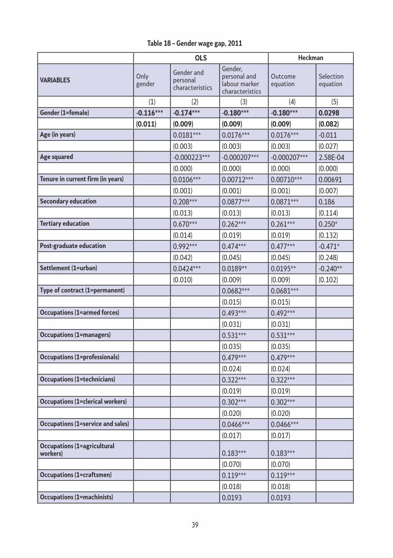
39
table 18 – Gender wage gap, 2011
oLs Heckman
VARIABLEs Only gender
Gender and personal characteristics
Gender, personal and labour marker characteristics
Outcome equation
Selection equation
(1) (2) (3) (4) (5)Gender (1=female) -0.116*** -0.174*** -0.180*** -0.180*** 0.0298
(0.011) (0.009) (0.009) (0.009) (0.082)Age (in years) 0.0181*** 0.0176*** 0.0176*** -0.011
(0.003) (0.003) (0.003) (0.027)Age squared -0.000223*** -0.000207*** -0.000207*** 2.58E-04
(0.000) (0.000) (0.000) (0.000)tenure in current firm (in years) 0.0106*** 0.00712*** 0.00710*** 0.00691
(0.001) (0.001) (0.001) (0.007)secondary education 0.208*** 0.0877*** 0.0871*** 0.186
(0.013) (0.013) (0.013) (0.114)tertiary education 0.670*** 0.262*** 0.261*** 0.250*
(0.014) (0.019) (0.019) (0.132)Post-graduate education 0.992*** 0.474*** 0.477*** -0.471*
(0.042) (0.045) (0.045) (0.248)settlement (1=urban) 0.0424*** 0.0189** 0.0195** -0.240**
(0.010) (0.009) (0.009) (0.102)type of contract (1=permanent) 0.0682*** 0.0681***
(0.015) (0.015)occupations (1=armed forces) 0.493*** 0.492***
(0.031) (0.031)occupations (1=managers) 0.531*** 0.531***
(0.035) (0.035)occupations (1=professionals) 0.479*** 0.479***
(0.024) (0.024)occupations (1=technicians) 0.322*** 0.322***
(0.019) (0.019)occupations (1=clerical workers) 0.302*** 0.302***
(0.020) (0.020)occupations (1=service and sales) 0.0466*** 0.0466***
(0.017) (0.017)occupations (1=agricultural workers) 0.183*** 0.183***
(0.070) (0.070)occupations (1=craftsmen) 0.119*** 0.119***
(0.018) (0.018)occupations (1=machinists) 0.0193 0.0193

40
(0.016) (0.016)sector (1=agriculture) -0.139*** -0.139***
(0.029) (0.029)sector (1=market services) 0.0382*** 0.0383***
(0.012) (0.012)sector (1=non-market services) 0.133*** 0.133***
(0.013) (0.013)Number of children 0.0168
(0.085)Employment status of spouse (1=employed) 0.00569
(0.089)Constant 5.848*** 5.086*** 5.016*** 5.018*** 2.227***
(0.007) (0.061) (0.059) (0.058) (0.521)
Inverse mills ratio (lambda -0.045*
(0.0269)observations 12435 12,435 12,435 12,575 12,575R-squared 0.013 0.307 0.408 Source: Authors’ calculations.
Note: *, ** and *** denote statistical significance at the 10, 5 and 1%, respectively. Standard errors given in parentheses. Results robust to heteroskedasticity. Weights used in the calculations.
Table 19 presents the results for the gender wage gap in 2014. These results, in general, are very similar as those from 2011, so our conclusions remain the same. The gender wage gap is of a very similar magnitude, 19.3 per cent, when personal and labour-market characteristics are considered. The small difference compared to the finding in 2011 is statistically insignificant12 , suggesting that the gap has persisted between 2011 and 2014. The conclusions for personal and labour-market characteristics remain the same.
12 The confidence interval of the coefficient on the gender variable (column 3) in 2011 is (-0.199; -0.166), while in 2014, (-0.214; -0.178). Since they overlap, the difference in the estimated coefficients in the both years is statistically insignificant.
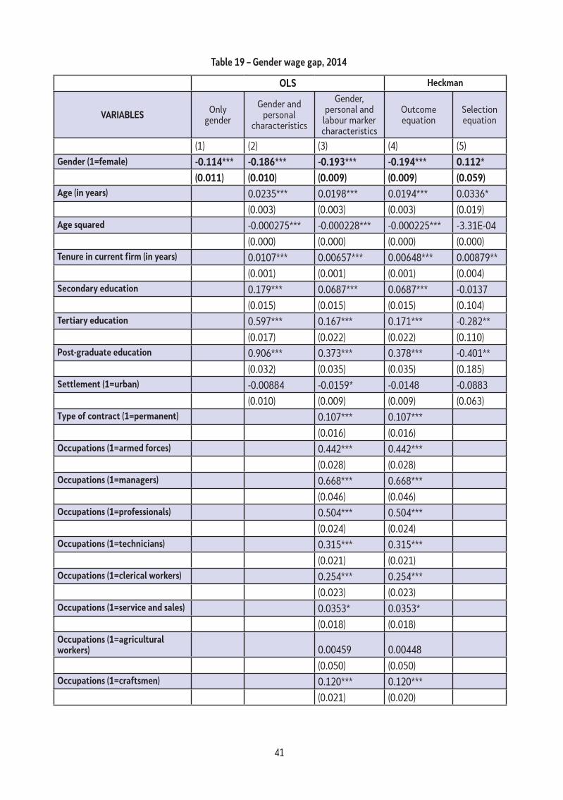
41
table 19 – Gender wage gap, 2014
oLs Heckman
VARIABLEs Only gender
Gender and personal
characteristics
Gender, personal and
labour marker characteristics
Outcome equation
Selection equation
(1) (2) (3) (4) (5)Gender (1=female) -0.114*** -0.186*** -0.193*** -0.194*** 0.112*
(0.011) (0.010) (0.009) (0.009) (0.059)Age (in years) 0.0235*** 0.0198*** 0.0194*** 0.0336*
(0.003) (0.003) (0.003) (0.019)Age squared -0.000275*** -0.000228*** -0.000225*** -3.31E-04
(0.000) (0.000) (0.000) (0.000)tenure in current firm (in years) 0.0107*** 0.00657*** 0.00648*** 0.00879**
(0.001) (0.001) (0.001) (0.004)secondary education 0.179*** 0.0687*** 0.0687*** -0.0137
(0.015) (0.015) (0.015) (0.104)tertiary education 0.597*** 0.167*** 0.171*** -0.282**
(0.017) (0.022) (0.022) (0.110)Post-graduate education 0.906*** 0.373*** 0.378*** -0.401**
(0.032) (0.035) (0.035) (0.185)settlement (1=urban) -0.00884 -0.0159* -0.0148 -0.0883
(0.010) (0.009) (0.009) (0.063)type of contract (1=permanent) 0.107*** 0.107***
(0.016) (0.016)occupations (1=armed forces) 0.442*** 0.442***
(0.028) (0.028)occupations (1=managers) 0.668*** 0.668***
(0.046) (0.046)occupations (1=professionals) 0.504*** 0.504***
(0.024) (0.024)occupations (1=technicians) 0.315*** 0.315***
(0.021) (0.021)occupations (1=clerical workers) 0.254*** 0.254***
(0.023) (0.023)occupations (1=service and sales) 0.0353* 0.0353*
(0.018) (0.018)occupations (1=agricultural workers) 0.00459 0.00448
(0.050) (0.050)occupations (1=craftsmen) 0.120*** 0.120***
(0.021) (0.020)

42
occupations (1=machinists) 0.0322* 0.0324*
(0.018) (0.018)sector (1=agriculture) -0.149*** -0.148***
(0.043) (0.043)sector (1=market services) 0.0045 0.00452
(0.013) (0.013)sector (1=non-market services) 0.0958*** 0.0956***
(0.015) (0.015)Number of children 0.043
(0.046)Employment status of spouse (1=employed) -0.046
(0.061)Constant 5.899*** 5.117*** 5.108*** 5.123*** 0.999***
(0.007) (0.064) (0.061) (0.061) (0.382)
Inverse Mills ratio (lambda) -0.073***
(0.0308)observations 9795 9,795 9,795 10,182 10,182R-squared 0.015 0.306 0.414Source: Authors’ calculations.
Note: *, ** and *** denote statistical significance at the 10, 5 and 1%, respectively. Standard errors given in parentheses. Results robust to heteroskedasticity. Weights used in the calculations.
7.1.2. Decompositions
In this section, we present the results of the decompositions of the gender wage gap. As explained in the methodological section, we first present the Blinder-Oaxaca decomposition. However, it decomposes the gap at its mean, and from that viewpoint is less informative. So we pursue decomposition at several deciles and hence rely on three methods: re-weighting, recentred influence function (RIF), as well as a combination of the two.
The estimates of the gender wage gap can be first summarized in the basic Blinder-Oaxaca decomposition (Table 20), where the gender gap is decomposed into the explained part (due to differences in workers’ personal and job characteristics) and the unexplained part (differences in returns for the same personal characteristics, and for unobservable differences in personal characteristics). The table presents our conclusions in section 6.1.1 for the two years: personal and labour-market characteristics widen the gap instead of reducing it, so that the entire adjusted gap remains unexplained, meaning that it is due to either unobservable characteristics or discrimination in the labour market against females.
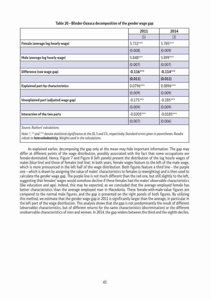
43
table 20 – Blinder-oaxaca decomposition of the gender wage gap
2011 2014
(1) (2)
Female (average log hourly wage) 5.732*** 5.785***
(0.008) (0.009)
Male (average log hourly wage) 5.848*** 5.899***
(0.007) (0.007)
Difference (raw wage gap) -0.116*** -0.114***
(0.011) (0.011)
Explained part by characteristics 0.0796*** 0.0896***
(0.009) (0.009)
Unexplained part (adjusted wage gap) -0.175*** -0.185***
(0.009) (0.009)
Interaction of the two parts -0.0205*** -0.0185***
(0.007) (0.006)
Source: Authors’ calculations.
Note: *, ** and *** denote statistical significance at the 10, 5 and 1%, respectively. Standard errors given in parentheses. Results robust to heteroskedasticity. Weights used in the calculations.
As explained earlier, decomposing the gap only at the mean may hide important information. The gap may differ at different points of the wage distribution, possibly associated with the fact that some occupations are female-dominated. Hence, Figure 7 and Figure 8 (left panels) present the distribution of the log hourly wages of males (blue line) and those of females (red line). In both years, female wages feature to the left of the male wage, which is more pronounced in the left half of the wage distribution. Both figures feature a third line – the purple one – which is drawn by assigning the value of males’ characteristics to females (a reweighting) and is then used to calculate the gender wage gap. The purple line is not much different than the red one, but still slightly to the left, suggesting that females’ wages would somehow decline if these females had the males’ observable characteristics (like education and age). Indeed, this may be expected, as we concluded that the average employed female has better characteristics than the average employed man in Macedonia. These female-with-male-value figures are compared to the normal male figures, and the gap is presented on the right panels of both figures. By utilizing this method, we estimate that the gender wage gap in 2011 is significantly larger than the average, in particular in the left part of the wage distribution. This analysis shows that the gap is not predominantly the result of different (observable) characteristics, but of different returns for the same characteristics (discrimination) or the different unobservable characteristics of men and women. In 2014, the gap widens between the third and the eighth deciles.

44
Figure 7 – Decomposition of the gender wage gap by reweighting, 2011
48
Извор: Пресметки на авторите Забелешка: Y оската на десната страна на графиконот е свртена обратно поради технички причини. Во пресметките се користени пондери.
Слика 8 – Декомпозиција на родовиот јаз во платите преку препондерирање, 2014 г.
Извор: Пресметки на авторите Забелешка: Y оската на десната страна на графиконот е свртена обратно поради технички причини. Во пресметките се користени пондери.
За добивање натамошни согледувања за тоа како еволуира родовиот јаз во платите по должината на дистрибуцијата на платите, ги претставуваме наодите од пристапот со RIF-регресијата. Оваа регресија директно го проценува влијанието на експланаторните варијабили врз дистрибуциската статистика од интерес (во нашиот случај тоа е платата) и потоа го пресметува јазот, поради неговиот објаснет и необјаснет дел. Во Error! Reference source not found. и Error! Reference source not found. е претставена декомпозицијата на родовиот јаз во платите врз основа на RIF-регресија по децили за двете разгледувани години. Необработениот јаз е сличен за сите различни групи децили во 2011 година, со исклучок на шестиот децил, каде што е понизок, и горниот децил, каде што јазот исчезнува. Веројатно е дека, откако жените ќе стигнат на врвот, не постои дискриминација во однос на платата и/или нивните неопсервабилни карактеристики се слични со оние на мажите. Меѓутоа, необјаснетиот дел се зголемува како што оди нагоре по скалата на платите: повисоко платените жени се соочуваат или со потешка дискриминација и/или поседуваат неопсервабилни карактеристики што на
0.2
.4.6
.81
Den
sity
3.5 4 4.5 5 5.5 6 6.5 7 7.5 8 8.5Log(wage)
WomenWomen as ManMen
0.1
.2.3
.4
Log
Wag
e D
iffer
entia
l Fem
ale
as M
en v
s. M
en
0 .2 .4 .6 .8 1Decile
0.2
.4.6
.81
Den
sity
3.5 4 4.5 5 5.5 6 6.5 7 7.5 8 8.5Log(wage)
WomenWomen as ManMen
0.1
.2.3
.4
Log
Wag
e D
iffer
entia
l Fem
ale
as M
en v
s. M
en
0 .2 .4 .6 .8 1Decile
Source: Authors’ calculations.
Note: The y-axis on the right-hand side is reversed due to technical limitations. Weights are used in the calculations.
Figure 8 – Decomposition of the gender wage gap by reweighting, 2014
48
Извор: Пресметки на авторите Забелешка: Y оската на десната страна на графиконот е свртена обратно поради технички причини. Во пресметките се користени пондери.
Слика 8 – Декомпозиција на родовиот јаз во платите преку препондерирање, 2014 г.
Извор: Пресметки на авторите Забелешка: Y оската на десната страна на графиконот е свртена обратно поради технички причини. Во пресметките се користени пондери.
За добивање натамошни согледувања за тоа како еволуира родовиот јаз во платите по должината на дистрибуцијата на платите, ги претставуваме наодите од пристапот со RIF-регресијата. Оваа регресија директно го проценува влијанието на експланаторните варијабили врз дистрибуциската статистика од интерес (во нашиот случај тоа е платата) и потоа го пресметува јазот, поради неговиот објаснет и необјаснет дел. Во Error! Reference source not found. и Error! Reference source not found. е претставена декомпозицијата на родовиот јаз во платите врз основа на RIF-регресија по децили за двете разгледувани години. Необработениот јаз е сличен за сите различни групи децили во 2011 година, со исклучок на шестиот децил, каде што е понизок, и горниот децил, каде што јазот исчезнува. Веројатно е дека, откако жените ќе стигнат на врвот, не постои дискриминација во однос на платата и/или нивните неопсервабилни карактеристики се слични со оние на мажите. Меѓутоа, необјаснетиот дел се зголемува како што оди нагоре по скалата на платите: повисоко платените жени се соочуваат или со потешка дискриминација и/или поседуваат неопсервабилни карактеристики што на
0.2
.4.6
.81
Den
sity
3.5 4 4.5 5 5.5 6 6.5 7 7.5 8 8.5Log(wage)
WomenWomen as ManMen
0.1
.2.3
.4
Log
Wag
e D
iffer
entia
l Fem
ale
as M
en v
s. M
en
0 .2 .4 .6 .8 1Decile
0.2
.4.6
.81
Den
sity
3.5 4 4.5 5 5.5 6 6.5 7 7.5 8 8.5Log(wage)
WomenWomen as ManMen
0.1
.2.3
.4
Log
Wag
e D
iffer
entia
l Fem
ale
as M
en v
s. M
en
0 .2 .4 .6 .8 1Decile
Source: Authors’ calculations.
Note: The y-axis on the right-hand side is reversed due to technical limitations. Weights are used in the calculations.
To gain further insight into how the gender wage gap evolves along the wage distribution, we present the findings of the RIF regression approach. This regression directly estimates the impact of the explanatory variables on the distributional statistic of interest (in our case, the wage), and then calculates the gap, including its explained and unexplained part. Table 21 and Table 22 present the decomposition of the gender wage gap based on the RIF regression by decile for both years of the investigation. The raw gap is similar across the decile groups in 2011, with the exception of the sixth decile, where it is lower, and of the top decile, where it vanishes completely. It is likely that, once females get to the top decile, there is no wage discrimination, or their unobservable characteristics are similar to those of males. However, the unexplained part increases up the wage ladder: higher-paid females appear to face tougher discrimination or possess unobservable characteristics which the labour market translates into lower wages than for males in their particular decile. It also could be that in the higher wage brackets, females who work have better personal characteristics than males. This could account for the growing explained part of the gender wage gap along the wage distribution. However, the slight increase in the adjusted gap in the seventh and eighth deciles should not be ignored, and may be considered a sign of a glass ceiling for the females in higher (but not the highest) paid jobs.
45
The second part of the tables further decomposes the explained and unexplained parts of the gender wage gap according to personal and labour-market characteristics13. It could be observed that the gender wage gap explained by personal characteristics is maintained over the wage distribution, while the gap explained by the labour market characteristics increases up the wage ladder. This suggests that occupations and industries which pay higher wages either commit larger discrimination against females, or employ females with worse unobservable characteristics than males. For the unexplained part, it is largely due to personal and not labour-market characteristics, especially in the right part of the wage distribution.
The findings for 2014 largely mimic those of 2011, although some higher variations in the gender gap could be observed among the wage deciles. A notable distinction is the reduction of the adjusted gender wage gap in the first and the second deciles of the wage distribution14, which may be considered an important development, given the introduction of the minimum wage in 2012.15 The first decile in 2011 referred to a wage below 6.400 MKD, while in 2014 it referred to a wage below 7.500 MKD. The second decile ranged from the first decile wage up to 7.500 MKD in 2011 and to 8.750 MKD in 2014. Hence, the introduction of the minimum wage has had an obvious effect on the wage distribution, shown as an upward shift in the wages for both men and women. This subsequently contributed to a reduction of the gender wage gap, since women are overrepresented among workers in the first and second deciles. It could be said that the floor stickiness for females in the former Yugoslav Republic of Macedonia reduced between 2011 and 2014.
Table A 1 and Table A 2 in the appendix present the same results as in Table 21 and Table 22, but in the RIF regression we applied a reweighting approach (which we also used for Figure 7 and Figure 8). The results remain largely the same, serving as a robustness check of our findings.
13 We decided to group the variables into two sets, because observing individual variables or less-aggregated sets would have resulted in very cumbersome tables. 14 The difference in the gaps between the two years in the first decile is statistically significant at five per cent, while the difference in the second decile is one per cent. 15 For a detailed analysis of the effects of the introduction of the minimum wage in Macedonia, including from a gender perspective, please consult Mojsoska-Blazevski and Kurtisi (2013).

46
tabl
e 21
– RI
F re
gres
sion
deco
mpo
sitio
n of
the
gend
er w
age
gap,
201
1
Deci
les
1020
3040
5060
7080
90
(1)
(2)
(3)
(4)
(5)
(6)
(7)
(8)
(9)
Fem
ale
(ave
rage
log
hour
ly w
age)
5.11
4***
5.30
9***
5.45
5***
5.55
3***
5.72
0***
5.92
2***
6.07
2***
6.15
2***
6.46
1***
(0
.008
)(0
.008
)(0
.008
)(0
.008
)(0
.010
)(0
.013
)(0
.011
)(0
.010
)(0
.011
)
Mal
e (a
vera
ge lo
g ho
urly
wag
e)5.
285*
**5.
470*
**5.
637*
**5.
712*
**5.
901*
**5.
973*
**6.
206*
**6.
333*
**6.
482*
**
(0
.008
)(0
.007
)(0
.007
)(0
.007
)(0
.008
)(0
.008
)(0
.010
)(0
.009
)(0
.009
)
Diff
eren
ce (r
aw w
age
gap)
-0.1
71**
*-0
.161
***
-0.1
82**
*-0
.159
***
-0.1
81**
*-0
.050
8***
-0.1
34**
*-0
.181
***
-0.0
214
(0
.012
)(0
.011
)(0
.011
)(0
.011
)(0
.013
)(0
.015
)(0
.015
)(0
.013
)(0
.014
)
Expl
aine
d pa
rt b
y ch
arac
teri
stic
s0.
0334
***
0.03
59**
*0.
0467
***
0.05
48**
*0.
0807
***
0.08
48**
*0.
104*
**0.
0841
***
0.04
04**
*
(0
.006
)(0
.005
)(0
.006
)(0
.006
)(0
.008
)(0
.008
)(0
.009
)(0
.008
)(0
.007
)
Une
xpla
ined
par
t (ad
j. w
age
gap)
-0.2
04**
*-0
.197
***
-0.2
29**
*-0
.214
***
-0.2
61**
*-0
.136
***
-0.2
37**
*-0
.265
***
-0.0
618*
**
(0
.012
)(0
.011
)(0
.010
)(0
.010
)(0
.011
)(0
.013
)(0
.013
)(0
.012
)(0
.014
)
Expl
aine
d by
cha
ract
eris
tics
(tot
al)
Gro
up o
f per
sona
l cha
ract
eris
tics
0.01
38**
*0.
0148
***
0.01
60**
*0.
0164
***
0.02
34**
*0.
0276
***
0.03
51**
*0.
0380
***
0.03
21**
*
(0
.004
)(0
.004
)(0
.004
)(0
.004
)(0
.004
)(0
.004
)(0
.005
)(0
.005
)(0
.005
)
Gro
up o
f lab
our m
arke
t cha
ract
eris
tics
0.01
95**
*0.
0211
***
0.03
06**
*0.
0384
***
0.05
73**
*0.
0572
***
0.06
84**
*0.
0461
***
0.00
827
(0
.005
)(0
.005
)(0
.005
)(0
.005
)(0
.006
)(0
.006
)(0
.007
)(0
.006
)(0
.006
)
tota
l wag
e st
ruct
ure
(une
xpla
ined
)
Gro
up o
f per
sona
l cha
ract
eris
tics
-0.5
25**
*-0
.559
***
-0.4
52**
*-0
.537
***
-0.6
30**
*-0
.529
***
-0.7
63**
*-0
.614
***
-0.5
81**
*
(0
.160
)(0
.142
)(0
.132
)(0
.129
)(0
.146
)(0
.164
)(0
.165
)(0
.162
)(0
.182
)
Gro
up o
f lab
our m
arke
t cha
ract
eris
tics
-0.1
62**
*-0
.146
***
-0.0
822*
-0.1
03**
-0.1
29**
*0.
185*
**0.
0824
0.11
6**
0.31
0***
(0
.051
)(0
.046
)(0
.042
)(0
.042
)(0
.047
)(0
.053
)(0
.053
)(0
.052
)(0
.059
)
Cons
tant
-0.4
83**
*-0
.507
***
-0.3
05**
-0.4
26**
*-0
.498
***
-0.2
09-0
.443
***
-0.2
34-0
.209
(0
.161
)(0
.142
)(0
.132
)(0
.130
)(0
.147
)(0
.165
)(0
.165
)(0
.163
)(0
.183
)
obs
erva
tion
s12
,575
12,5
7512
,575
12,5
7512
,575
12,5
7512
,575
12,5
7512
,575
Sour
ce: A
utho
rs’ c
alcu
latio
ns.
Note
: *, *
* and
*** d
enot
e st
atist
ical
sign
ifica
nce
at th
e 10
, 5 a
nd 1
%, r
espe
ctiv
ely.
Stan
dard
err
ors g
iven
in p
aren
thes
es. R
esul
ts ro
bust
to heteroske
dasticity
. Wei
ghts
use
d in
the
calc
ulat
ions
.

47
tabl
e 22
– RI
F re
gres
sion
deco
mpo
sitio
n of
the
gend
er w
age
gap,
201
4
Deci
les
1020
3040
5060
7080
90
(1)
(2)
(3)
(4)
(5)
(6)
(7)
(8)
(9)
Fem
ale
(ave
rage
log
hour
ly w
age)
5.28
9***
5.44
4***
5.47
4***
5.64
8***
5.70
4***
5.96
4***
6.10
5***
6.21
5***
6.50
6***
(0
.007
)(0
.006
)(0
.007
)(0
.009
)(0
.010
)(0
.013
)(0
.013
)(0
.011
)(0
.013
)
Mal
e (a
vera
ge lo
g ho
urly
wag
e)5.
443*
**5.
562*
**5.
712*
**5.
769*
**5.
969*
**6.
025*
**6.
255*
**6.
382*
**6.
518*
**
(0
.006
)(0
.006
)(0
.007
)(0
.007
)(0
.008
)(0
.008
)(0
.010
)(0
.010
)(0
.010
)
Diff
eren
ce (r
aw w
age
gap)
-0.1
53**
*-0
.118
***
-0.2
37**
*-0
.121
***
-0.2
64**
*-0
.061
3***
-0.1
49**
*-0
.167
***
-0.0
121
(0
.010
)(0
.009
)(0
.010
)(0
.011
)(0
.012
)(0
.016
)(0
.016
)(0
.014
)(0
.016
)
Expl
aine
d pa
rt b
y ch
arac
teri
stic
s0.
0238
***
0.03
66**
*0.
0450
***
0.06
05**
*0.
0762
***
0.08
54**
*0.
108*
**0.
107*
**0.
0578
***
(0
.005
)(0
.005
)(0
.006
)(0
.006
)(0
.007
)(0
.008
)(0
.010
)(0
.009
)(0
.008
)
Une
xpla
ined
par
t (ad
j. w
age
gap)
-0.1
77**
*-0
.155
***
-0.2
82**
*-0
.181
***
-0.3
40**
*-0
.147
***
-0.2
57**
*-0
.274
***
-0.0
699*
**
(0
.010
)(0
.009
)(0
.010
)(0
.010
)(0
.011
)(0
.013
)(0
.014
)(0
.013
)(0
.016
)
Expl
aine
d by
cha
ract
eris
tics
(tot
al)
Gro
up o
f per
sona
l cha
ract
eris
tics
0.00
674*
0.01
23**
*0.
0138
***
0.01
14**
*0.
0159
***
0.02
72**
*0.
0336
***
0.04
19**
*0.
0377
***
(0
.004
)(0
.004
)(0
.004
)(0
.004
)(0
.005
)(0
.005
)(0
.006
)(0
.006
)(0
.006
)
Gro
up o
f lab
our m
arke
t cha
ract
eris
tics
0.01
70**
*0.
0244
***
0.03
12**
*0.
0491
***
0.06
03**
*0.
0581
***
0.07
41**
*0.
0649
***
0.02
01**
*
(0
.005
)(0
.005
)(0
.005
)(0
.006
)(0
.007
)(0
.007
)(0
.008
)(0
.008
)(0
.007
)
tota
l wag
e st
ruct
ure
(une
xpla
ined
)
Gro
up o
f per
sona
l cha
ract
eris
tics
-0.0
847
-0.3
59**
*-0
.488
***
-0.3
96**
*-0
.521
***
-0.2
62-0
.205
-0.0
619
0.31
9
(0
.134
)(0
.120
)(0
.129
)(0
.138
)(0
.146
)(0
.173
)(0
.179
)(0
.170
)(0
.207
)
Gro
up o
f lab
our m
arke
t cha
ract
eris
tics
-0.0
685
-0.1
98**
*-0
.162
***
-0.1
43**
*-0
.059
90.
246*
**0.
190*
**0.
138*
*0.
270*
**
(0
.043
)(0
.039
)(0
.042
)(0
.045
)(0
.047
)(0
.056
)(0
.058
)(0
.055
)(0
.067
)
Cons
tant
0.02
36-0
.402
***
-0.3
68**
*-0
.359
***
-0.2
40.
131
0.24
20.
349*
*0.
659*
**
(0
.135
)(0
.120
)(0
.129
)(0
.139
)(0
.146
)(0
.174
)(0
.179
)(0
.170
)(0
.208
)
obs
erva
tion
s10
,182
10,1
8210
,182
10,1
8210
,182
10,1
8210
,182
10,1
8210
,182
Sour
ce: A
utho
rs’ c
alcu
latio
ns.
Note
: *, *
* and
*** d
enot
e st
atist
ical
sign
ifica
nce
at th
e 10
, 5 a
nd 1
%, r
espe
ctiv
ely.
Stan
dard
err
ors g
iven
in p
aren
thes
es. R
esul
ts ro
bust
to heteroske
dasticity
. Wei
ghts
use
d in
the
calc
ulat
ions
.

48
In conclusion, the gender wage gap in the former Yugoslav Republic of Macedonia is about 18-19 per cent of a male’s wage and has not changed significantly between 2011 and 2014. The adjusted gap is larger than the raw gap and is mainly inflated by personal characteristics, suggesting that females who work likely have better personal characteristics than working males. Even when selection bias is taken into account, the gap continues to persist. The adjusted wage gap is largely unexplained, meaning that it warns of discrimination in the labour market against females (through lower returns for the same characteristics) or indicates that males have better unobservable characteristics which are valued by employers. The adjusted gender wage gap increases up the wage ladder: the higher the wage distribution, the more females face either discrimination or possess unobservable characteristics which the labour market translates into lower wages than males in their particular decile. It also could be that at higher income levels, females who work have better personal characteristics than males, compared to females in the lower income brackets. We also noted that occupations and industries which pay higher wages either commit larger discrimination against females, or employ females with worse unobservable characteristics than males. In any case, a slight increase in the gap in the seventh and eighth deciles may suggest the presence of a glass ceiling effect for females in high (but not the highest) paid jobs. Between 2011 and 2014, the gap reduced in the first and second deciles, suggesting that some policies, in particular the introduction of the minimum wage, may have worked to reduce the gender wage gap and hence mitigate the floor stickiness for the lowest paid jobs.

49
7.2. Motherhood wage gap
7.2.3. Baseline findings
In this section, we turn to the motherhood wage gap. Recall that we define a mother as a female with at least one child up to the age of six. Since the motherhood wage gap is analyzed similarly to the gender wage gap, we provide several pairs of tables. First, we analyze the motherhood wage gap along the gender wage gap, so that we may compare mothers to non-mothers and to fathers. Then we explore whether the gender wage gap changes when we introduce the motherhood wage gap into the equation. Finally, we drop all males to analyze the motherhood gap only and make comparisons between mothers and non-mothers.
Table 23 presents the results of the gender and motherhood wage gaps together for 2011. The results for the gender wage gap are replicated, as in Table 18, suggesting that the introduction of the motherhood wage gap into the equation does not affect the size of the gender wage gap. This means that motherhood does not explain part of the (unexplained) gender wage gap in the former Yugoslav Republic of Macedonia. To be able to compare mothers with all non-mothers (including males) and mothers with fathers, we need to take into account the sum of two coefficients: [child+mother] for the former and [gender+mother] for the latter. We are also able to compare fathers with non-fathers. This is simply revealed by the coefficient in front of the child variable, because – in econometric terms – a father is defined when dgn=0, mother=0 and child=1. Hence, the coefficient in front of the child variable will reveal any fatherhood wage premium, bonus or penalty.
Apparently, mothers are paid more than non-mothers: the two coefficients equal about 14 per cent higher wages for mothers within the raw gap; 8.3 per cent when personal characteristics are considered; and six per cent higher wages when personal and labour-market characteristics are taken into account. This suggests that personal characteristics explain about 40 per cent of the raw gap, while labour-market characteristics explain 18 per cent of the gap. In total, these characteristics are powerful, explaining nearly 60 per cent of the raw motherhood wage gap. So, 60 per cent of the raw gap is explained by the better personal and labour market characteristics of working mothers compared to non-mothers. The unexplained part suggests that employers either commit positive discrimination against mothers (by overpaying them), or that mothers have unobservable characteristics that bring them higher rewards. Hence, the hypothesis that mothers may be paid less because they are less committed and devoted to their work, unable to to work overtime, or unwilling to travel is not confirmed in the former Yugoslav Republic of Macedonia. The selection-corrected estimates corroborate these findings but the Inverse-Mills ratio is insignificant, suggesting that selection is not present. Notice that the sum of the coefficients is statistically significant in all cases, although this is not directly shown in the tables.
On the contrary, mothers are less paid than fathers. The sum of the coefficients in front of the gender and mother variables amounts to a 7.8 per cent raw gap, suggesting that mothers receive 7.8 per cent lower wages, on average, than fathers. As with the gender wage gap, the motherhood wage gap (mothers compared to fathers) widens when characteristics are considered, suggesting that employed mothers on average have better characteristics than employed fathers but still receive lower wages.
As documented in other countries, fathers receive premiums on their wages when compared to non-fathers. The average premium is estimated to be between 4.9 per cent and 7.7 per cent, which is similar to what Hodges and Budig (2010) find, for example.

50
table 23 – Gender and motherhood wage gap, 2011
oLs Heckman
VARIABLEs Only gender
Gender and personal
characteristics
Gender, personal and
labour marker characteristics
Outcome equation
Selection equation
(1) (2) (3) (4) (5)Gender (1=female) -0.155*** -0.198*** -0.198*** -0.198*** -0.0325
(0.016) (0.014) (0.013) (0.013) (0.129)Children (1=if person has at least one child) 0.0632*** 0.0768*** 0.0486*** 0.0486*** 0.186
(0.018) (0.016) (0.015) (0.015) (0.241)Mother (1=if woman has at least one child) 0.0762** 0.00653 0.00963 0.00986 0.31
(0.031) (0.025) (0.022) (0.022) (0.289)Age (in years) 0.00686 0.00721 0.00724 0.0268
(0.013) (0.011) (0.011) (0.105)Age squared -6.68E-05 -5.12E-05 -5.17E-05 -0.00051
(0.000) (0.000) (0.000) (0.001)tenure in current firm (in years) 0.0151*** 0.00977*** 0.00978*** 0.0134
(0.001) (0.001) (0.001) (0.015)secondary education 0.179*** 0.0703*** 0.0704*** 0.186
(0.017) (0.017) (0.017) (0.140)tertiary education 0.634*** 0.252*** 0.252*** 0.155
(0.020) (0.025) (0.025) (0.169)Post-graduate education 0.983*** 0.499*** 0.498*** -0.591**
(0.045) (0.051) (0.051) (0.300)settlement (1=urban) 0.0333*** 0.0173 0.0172 -0.16
(0.013) (0.012) (0.012) (0.121)type of contract (1=permanent) 0.0552*** 0.0552***
(0.018) (0.018)occupations (1=armed forces) 0.425*** 0.425***
(0.035) (0.035)occupations (1=managers) 0.429*** 0.429***
(0.057) (0.057)occupations (1=professionals) 0.424*** 0.424***
(0.032) (0.032)occupations (1=technicians) 0.292*** 0.292***
(0.024) (0.024)occupations (1=clerical workers) 0.249*** 0.249***
(0.027) (0.027)occupations (1=service and sales) 0.0192 0.0193
(0.023) (0.023)

51
occupations (1=agricultural workers) 0.225* 0.225*
(0.127) (0.127)occupations (1=craftsmen) 0.101*** 0.101***
(0.024) (0.024)occupations (1=machinists) -0.00958 -0.00959
(0.021) (0.021)sector (1=agriculture) -0.174*** -0.174***
(0.047) (0.047)sector (1=market services) 0.0412** 0.0412**
(0.016) (0.016)sector (1=non-market services) 0.157*** 0.157***
(0.018) (0.018)Number of children -0.173
(0.112)Employment status of spouse (1=employed) 0.0118
(0.126)Constant 5.819*** 5.277*** 5.209*** 5.208*** 1.822
(0.011) (0.214) (0.196) (0.195) (1.817)
Inverse mills ratio (lambda) -0.029
(0.0611)observations 6,719 6,719 6,719 6,806 6,806R-squared 0.03 0.296 0.404Source: Authors’ calculations.
Note: *, ** and *** denote statistical significance at the 10, 5 and 1%, respectively. Standard errors given in parentheses. Results robust to heteroskedasticity. Weights used in the calculations.
Similar conclusions could be reached for 2014 (Table 24). The motherhood wage gap (compared to non-mothers) is maintained, and characteristics still explain about 60 per cent of the gap. However, mothers compared to fathers are paid less by only three per cent (raw gap) and by 15 per cent (adjusted gap). This reduction in the motherhood wage gap when compared to fathers from 2011 to 2014 may have been driven by the introduction of the minimum wage, assuming that mothers were more likely than fathers to receive wages below the statutory minimum wage introduced in 2012. However, this effect is difficult to prove. The perceptions of employers towards mothers may have also changed (not likely), the educational structure of employed mothers may have improved more than for employed fathers (more likely), or mothers on average may have also reduced the length of their maternity leave (career interruption). Interestingly, the fatherhood wage premium vanishes in 2014.
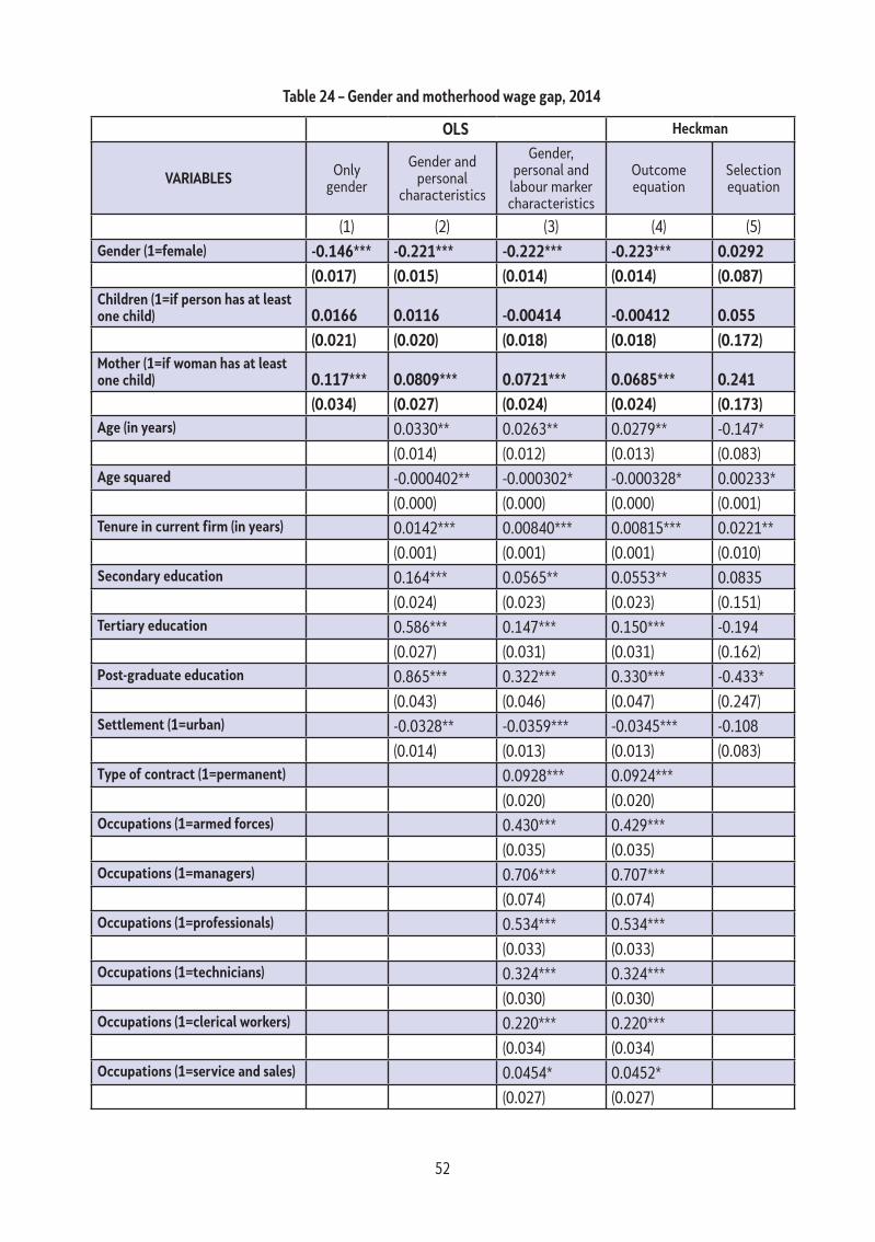
52
table 24 – Gender and motherhood wage gap, 2014
oLs Heckman
VARIABLEs Only gender
Gender and personal
characteristics
Gender, personal and
labour marker characteristics
Outcome equation
Selection equation
(1) (2) (3) (4) (5)Gender (1=female) -0.146*** -0.221*** -0.222*** -0.223*** 0.0292
(0.017) (0.015) (0.014) (0.014) (0.087)Children (1=if person has at least one child) 0.0166 0.0116 -0.00414 -0.00412 0.055
(0.021) (0.020) (0.018) (0.018) (0.172)Mother (1=if woman has at least one child) 0.117*** 0.0809*** 0.0721*** 0.0685*** 0.241
(0.034) (0.027) (0.024) (0.024) (0.173)Age (in years) 0.0330** 0.0263** 0.0279** -0.147*
(0.014) (0.012) (0.013) (0.083)Age squared -0.000402** -0.000302* -0.000328* 0.00233*
(0.000) (0.000) (0.000) (0.001)tenure in current firm (in years) 0.0142*** 0.00840*** 0.00815*** 0.0221**
(0.001) (0.001) (0.001) (0.010)secondary education 0.164*** 0.0565** 0.0553** 0.0835
(0.024) (0.023) (0.023) (0.151)tertiary education 0.586*** 0.147*** 0.150*** -0.194
(0.027) (0.031) (0.031) (0.162)Post-graduate education 0.865*** 0.322*** 0.330*** -0.433*
(0.043) (0.046) (0.047) (0.247)settlement (1=urban) -0.0328** -0.0359*** -0.0345*** -0.108
(0.014) (0.013) (0.013) (0.083)type of contract (1=permanent) 0.0928*** 0.0924***
(0.020) (0.020)occupations (1=armed forces) 0.430*** 0.429***
(0.035) (0.035)occupations (1=managers) 0.706*** 0.707***
(0.074) (0.074)occupations (1=professionals) 0.534*** 0.534***
(0.033) (0.033)occupations (1=technicians) 0.324*** 0.324***
(0.030) (0.030)occupations (1=clerical workers) 0.220*** 0.220***
(0.034) (0.034)occupations (1=service and sales) 0.0454* 0.0452*
(0.027) (0.027)
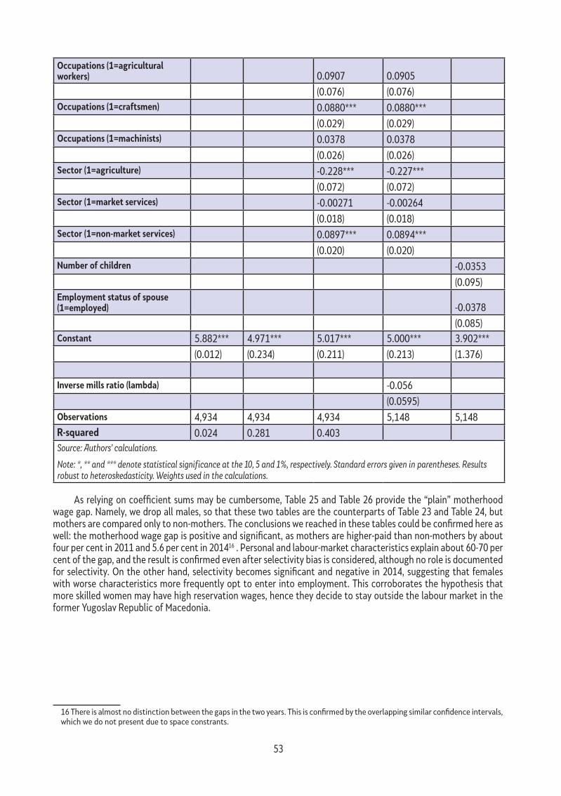
53
occupations (1=agricultural workers) 0.0907 0.0905
(0.076) (0.076)occupations (1=craftsmen) 0.0880*** 0.0880***
(0.029) (0.029)occupations (1=machinists) 0.0378 0.0378
(0.026) (0.026)sector (1=agriculture) -0.228*** -0.227***
(0.072) (0.072)sector (1=market services) -0.00271 -0.00264
(0.018) (0.018)sector (1=non-market services) 0.0897*** 0.0894***
(0.020) (0.020)Number of children -0.0353
(0.095)Employment status of spouse (1=employed) -0.0378
(0.085)Constant 5.882*** 4.971*** 5.017*** 5.000*** 3.902***
(0.012) (0.234) (0.211) (0.213) (1.376)
Inverse mills ratio (lambda) -0.056
(0.0595)observations 4,934 4,934 4,934 5,148 5,148R-squared 0.024 0.281 0.403Source: Authors’ calculations.
Note: *, ** and *** denote statistical significance at the 10, 5 and 1%, respectively. Standard errors given in parentheses. Results robust to heteroskedasticity. Weights used in the calculations.
As relying on coefficient sums may be cumbersome, Table 25 and Table 26 provide the “plain” motherhood wage gap. Namely, we drop all males, so that these two tables are the counterparts of Table 23 and Table 24, but mothers are compared only to non-mothers. The conclusions we reached in these tables could be confirmed here as well: the motherhood wage gap is positive and significant, as mothers are higher-paid than non-mothers by about four per cent in 2011 and 5.6 per cent in 201416 . Personal and labour-market characteristics explain about 60-70 per cent of the gap, and the result is confirmed even after selectivity bias is considered, although no role is documented for selectivity. On the other hand, selectivity becomes significant and negative in 2014, suggesting that females with worse characteristics more frequently opt to enter into employment. This corroborates the hypothesis that more skilled women may have high reservation wages, hence they decide to stay outside the labour market in the former Yugoslav Republic of Macedonia.
16 There is almost no distinction between the gaps in the two years. This is confirmed by the overlapping similar confidence intervals, which we do not present due to space constrants.

54
Next we consider the other explanatory variables. Additional years of tenure in a current firm increase a female’s average wage by 0.8 per cent, all other factors remaining constant. Education is rewarding for females: those with secondary education are typically paid seven per cent more, those with a tertiary education are paid 24 per cent more, and those with post-graduate degree receive 52 per cent more when compared to females with primary educations or less. Urban females are better paid by 5.3 per cent than rural females, and permanent contractors are better paid than their counterparts. Females in the army, manager positions and professional roles have wages more than 50 per cent higher than those in elementary occupations. Females in agriculture receive 22 per cent less than those in the industrial sector, while those working in public service earn eight per cent higher wages than women in the industrial sector.
table 25 – Motherhood wage gap, 2011
oLs Heckman
VARIABLEs Only gender
Gender and personal
characteristics
Gender, personal and
labour marker characteristics
Outcome equation
Selection equation
(1) (2) (3) (4) (5)Mother (1=if woman has at least one child) 0.137*** 0.0685*** 0.0396** 0.0400** 0.949***
(0.025) (0.021) (0.018) (0.017) (0.335)Age (in years) -0.0162 -0.0141 -0.0141 -0.0433
(0.019) (0.016) (0.016) (0.170)Age squared 2.50E-04 2.24E-04 2.24E-04 1.10E-03
(0.000) (0.000) (0.000) (0.002)tenure in current firm (in years) 0.0152*** 0.00842*** 0.00842*** -0.0083
(0.002) (0.001) (0.001) (0.020)secondary education 0.230*** 0.0714*** 0.0717*** 0.327
(0.022) (0.022) (0.022) (0.253)tertiary education 0.761*** 0.240*** 0.240*** 0.229
(0.026) (0.033) (0.033) (0.271)Post-graduate education 1.153*** 0.519*** 0.518*** -0.214
(0.049) (0.059) (0.059) (0.462)settlement (1=urban) 0.0734*** 0.0534*** 0.0532*** -0.198
(0.019) (0.015) (0.015) (0.181)type of contract (1=permanent) 0.0688** 0.0688**
(0.028) (0.028)occupations (1=armed for.) 0.562*** 0.562***
(0.060) (0.060)occupations (1=managers) 0.503*** 0.502***
(0.070) (0.070)occupations (1=professionals) 0.548*** 0.548***
(0.041) (0.041)occupations (1=technicians) 0.340*** 0.340***
(0.032) (0.032)occupations (1=clerical workers) 0.368*** 0.368***
(0.037) (0.036)
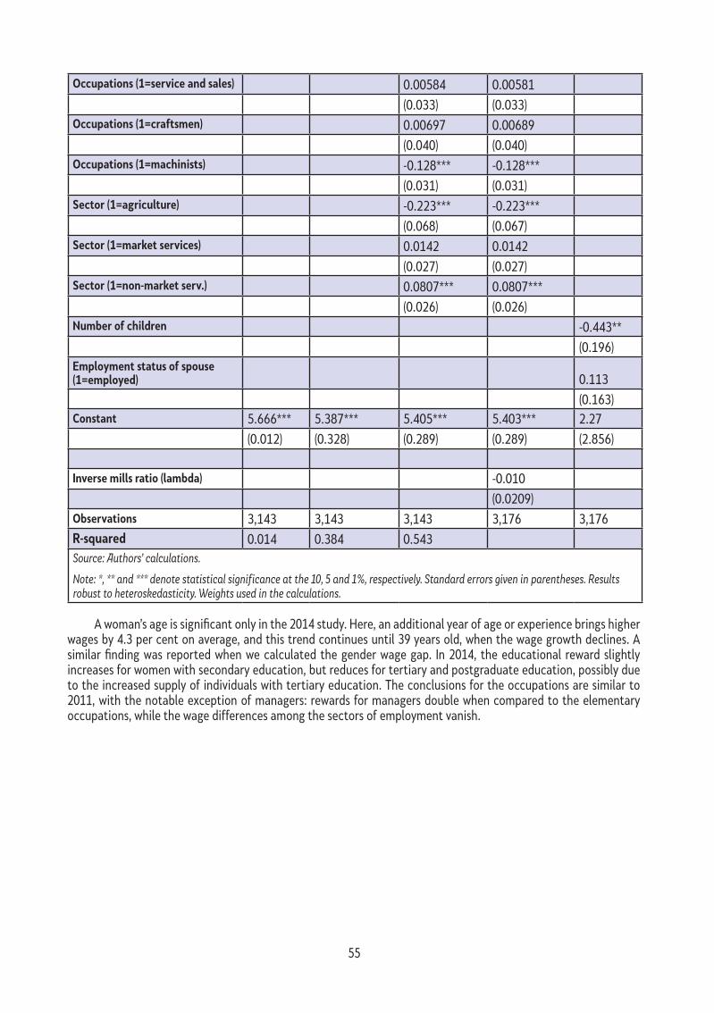
55
occupations (1=service and sales) 0.00584 0.00581
(0.033) (0.033)occupations (1=craftsmen) 0.00697 0.00689
(0.040) (0.040)occupations (1=machinists) -0.128*** -0.128***
(0.031) (0.031)sector (1=agriculture) -0.223*** -0.223***
(0.068) (0.067)sector (1=market services) 0.0142 0.0142
(0.027) (0.027)sector (1=non-market serv.) 0.0807*** 0.0807***
(0.026) (0.026)Number of children -0.443**
(0.196)Employment status of spouse (1=employed) 0.113
(0.163)Constant 5.666*** 5.387*** 5.405*** 5.403*** 2.27
(0.012) (0.328) (0.289) (0.289) (2.856)
Inverse mills ratio (lambda) -0.010
(0.0209)observations 3,143 3,143 3,143 3,176 3,176R-squared 0.014 0.384 0.543Source: Authors’ calculations.
Note: *, ** and *** denote statistical significance at the 10, 5 and 1%, respectively. Standard errors given in parentheses. Results robust to heteroskedasticity. Weights used in the calculations.
A woman’s age is significant only in the 2014 study. Here, an additional year of age or experience brings higher wages by 4.3 per cent on average, and this trend continues until 39 years old, when the wage growth declines. A similar finding was reported when we calculated the gender wage gap. In 2014, the educational reward slightly increases for women with secondary education, but reduces for tertiary and postgraduate education, possibly due to the increased supply of individuals with tertiary education. The conclusions for the occupations are similar to 2011, with the notable exception of managers: rewards for managers double when compared to the elementary occupations, while the wage differences among the sectors of employment vanish.

56
table 26 – Motherhood wage gap, 2014
oLs Heckman
VARIABLEs Only gender
Gender and personal
characteristics
Gender, personal and
labour marker characteristics
Outcome equation
Selection equation
(1) (2) (3) (4) (5)Mother (1=if woman has at least one child) 0.133*** 0.0862*** 0.0561*** 0.0490*** 0.157
(0.027) (0.021) (0.019) (0.019) (0.215)Age (in years) 0.0402** 0.0432*** 0.0508*** -0.313**
(0.018) (0.016) (0.017) (0.122)Age squared -0.000500* -0.000551** -0.000660*** 0.00444**
(0.000) (0.000) (0.000) (0.002)tenure in current firm (in years) 0.0135*** 0.00680*** 0.00622*** 0.0249*
(0.002) (0.002) (0.002) (0.015)secondary education 0.185*** 0.0873*** 0.0886*** -0.0374
(0.029) (0.029) (0.029) (0.233)tertiary education 0.669*** 0.187*** 0.197*** -0.351
(0.032) (0.039) (0.039) (0.246)Post-graduate education 0.917*** 0.350*** 0.369*** -0.57
(0.057) (0.062) (0.064) (0.351)settlement (1=urban) 0.00774 0.000685 0.00286 -0.0899
(0.020) (0.018) (0.018) (0.132)type of contract (1=permanent) 0.106*** 0.103***
(0.028) (0.028)occupations (1=armed forces) 0.564*** 0.560***
(0.088) (0.086)occupations (1=managers) 0.923*** 0.924***
(0.075) (0.074)occupations (1=professionals) 0.553*** 0.554***
(0.043) (0.043)occupations (1=technicians) 0.335*** 0.335***
(0.039) (0.038)occupations (1=clerical workers) 0.249*** 0.250***
(0.048) (0.047)occupations (1=service and sales) -0.0238 -0.0245
(0.035) (0.035)occupations (1=agricultural workers) -0.2 -0.197
(0.133) (0.133)occupations (1=craftsmen) 0.0448 0.0447
(0.047) (0.046)

57
occupations (1=machinists) -0.0468 -0.0462
(0.038) (0.037)sector (1=agriculture) 0.0172 0.0211
(0.079) (0.081)sector (1=market services) -0.00465 -0.00326
(0.030) (0.030)sector (1=non-market services) 0.0274 0.0271
(0.029) (0.029)Number of children 0.0413
(0.125)Employment status of spouse (1=employed) -0.00563
(0.117)Constant 5.736*** 4.556*** 4.498*** 4.381*** 7.168***
(0.013) (0.314) (0.279) (0.287) (2.081)
Inverse mills ratio (lambda) -0.164***
(0.0484)observations 2,196 2,196 2,196 2,286 2,286R-squared 0.016 0.379 0.527Source: Authors’ calculations.
Note: *, ** and *** denote statistical significance at the 10, 5 and 1%, respectively. Standard errors given in parentheses. Results robust to heteroskedasticity. Weights used in the calculations.
All of these calculations are based on our definition of a mother with at least one child up to the age of six. The literature, however, uses a variety of definitions, especially in regard to the age of the child. Hence, we use two alternative definitions: mothers with at least one child up to the age of three, and those with a child up to the age of 18. Hence, we produce Table A 3, Table A 4, Table A 5 and Table A 6, providing estimates for the motherhood wage gaps in 2011 and 2014 with the alternative definitions of mother. Findings remain largely robust, with one notable distinction: the motherhood wage gap vanishes in 2011, suggesting that the four per cent we have estimated above is unlikely to be stable. On the other hand, the adjusted motherhood wage gaps vary between three per cent and 6.8 per cent in 2014, which overlap with our central estimates above.
7.2.4. Decompositions
Finally, we decompose the motherhood wage gap in a similar fashion as the gender wage gap. We first provide the results of the standard Blinder-Oaxaca decomposition, then the results from the reweighting approach, assigning to the mothers the characteristics of non-mothers. Finally, we use the RIF regression. In the appendix, we provide the combined results of the latter two.
Table 27 presents the Blinder-Oaxaca decomposed motherhood wage gap. The bold lines present the raw gap, about 60 per cent of which is explained by characteristics, as concluded in section 6.2.1. The remaining part is still unexplained, and either suggests a positive discrimination for mothers, or that the unobservable characteristics of mothers are preferred to those of non-mothers. The hypothesis of the potential career-orientation of non-mothers is not supported in our results.
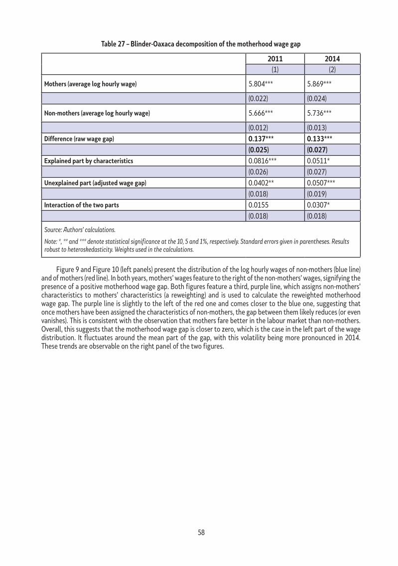
58
table 27 – Blinder-oaxaca decomposition of the motherhood wage gap
2011 2014(1) (2)
Mothers (average log hourly wage) 5.804*** 5.869***
(0.022) (0.024)
Non-mothers (average log hourly wage) 5.666*** 5.736***
(0.012) (0.013)Difference (raw wage gap) 0.137*** 0.133***
(0.025) (0.027)Explained part by characteristics 0.0816*** 0.0511*
(0.026) (0.027)Unexplained part (adjusted wage gap) 0.0402** 0.0507***
(0.018) (0.019)Interaction of the two parts 0.0155 0.0307*
(0.018) (0.018)
Source: Authors’ calculations.
Note: *, ** and *** denote statistical significance at the 10, 5 and 1%, respectively. Standard errors given in parentheses. Results robust to heteroskedasticity. Weights used in the calculations.
Figure 9 and Figure 10 (left panels) present the distribution of the log hourly wages of non-mothers (blue line) and of mothers (red line). In both years, mothers’ wages feature to the right of the non-mothers’ wages, signifying the presence of a positive motherhood wage gap. Both figures feature a third, purple line, which assigns non-mothers’ characteristics to mothers’ characteristics (a reweighting) and is used to calculate the reweighted motherhood wage gap. The purple line is slightly to the left of the red one and comes closer to the blue one, suggesting that once mothers have been assigned the characteristics of non-mothers, the gap between them likely reduces (or even vanishes). This is consistent with the observation that mothers fare better in the labour market than non-mothers. Overall, this suggests that the motherhood wage gap is closer to zero, which is the case in the left part of the wage distribution. It fluctuates around the mean part of the gap, with this volatility being more pronounced in 2014. These trends are observable on the right panel of the two figures.
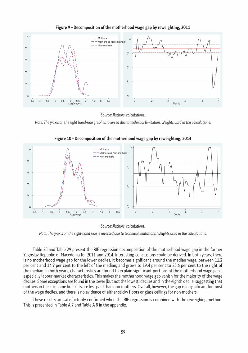
59
Figure 9 – Decomposition of the motherhood wage gap by reweighting, 2011
65
и што потоа се користи за пресметка на препондерираниот мајчински јаз во платите. Виолетовата линија е малку лево од црвената линија и се приближува до сината линија, што сугерира дека откако на мајките ќе им се назначат карактеристиките на жените што не се мајки, јазот веројатно се намалува (или дури и исчезнува). Ова е во согласност со опсервацијата дека мајките се подобро наградени во споредба со жените што не се мајки. Ова сугерира дека, севкупно, мајчинскиот јаз во платите е блиску до нулата, што е случајот барем на левата страна на дистрибуцијата на платите. Потоа, тој флуктуира околу средната вредност на јазот, при што непостојаноста е поистакната во 2014 година. Овие трендови може да се забележат на десната страна во двете слики.
Слика 9 – Декомпозиција на мајчинскиот јаз во платите преку препондерирање, 2011 г.
Извор: Пресметки на авторите Забелешка: Y оската на десната страна на графиконот е свртена обратно поради технички причини. Во пресметките се користени пондери.
Слика 10 – Декомпозиција на мајчинскиот јаз во платите преку препондерирање, 2014 г.
Извор: Пресметки на авторите Забелешка: Y оската на десната страна на графиконот е свртена обратно поради технички причини. Во пресметките се користени пондери.
-.8
-.6
-.4
-.2
0
Log
Wag
e D
iffer
entia
l Mot
hers
as
Non
-mot
hers
vs.
Non
-mot
hers
0 .2 .4 .6 .8 1Decile
0.2
.4.6
.81
Den
sity
3.5 4 4.5 5 5.5 6 6.5 7 7.5 8 8.5Log(wage)
MothersMothers as Non-mothersNon-mothers
-.3
-.2
-.1
0
Log
Wag
e D
iffer
entia
l Mot
hers
as
Non
-mot
hers
vs.
Non
-mot
hers
0 .2 .4 .6 .8 1Decile
0.2
.4.6
.81
Den
sity
3.5 4 4.5 5 5.5 6 6.5 7 7.5 8 8.5Log(wage)
MothersMothers as Non-mothersNon-mothers
Source: Authors’ calculations.
Note: The y-axis on the right hand-side graph is reversed due to technical limitation. Weights used in the calculations.
Figure 10 – Decomposition of the motherhood wage gap by reweighting, 2014
65
и што потоа се користи за пресметка на препондерираниот мајчински јаз во платите. Виолетовата линија е малку лево од црвената линија и се приближува до сината линија, што сугерира дека откако на мајките ќе им се назначат карактеристиките на жените што не се мајки, јазот веројатно се намалува (или дури и исчезнува). Ова е во согласност со опсервацијата дека мајките се подобро наградени во споредба со жените што не се мајки. Ова сугерира дека, севкупно, мајчинскиот јаз во платите е блиску до нулата, што е случајот барем на левата страна на дистрибуцијата на платите. Потоа, тој флуктуира околу средната вредност на јазот, при што непостојаноста е поистакната во 2014 година. Овие трендови може да се забележат на десната страна во двете слики.
Слика 9 – Декомпозиција на мајчинскиот јаз во платите преку препондерирање, 2011 г.
Извор: Пресметки на авторите Забелешка: Y оската на десната страна на графиконот е свртена обратно поради технички причини. Во пресметките се користени пондери.
Слика 10 – Декомпозиција на мајчинскиот јаз во платите преку препондерирање, 2014 г.
Извор: Пресметки на авторите Забелешка: Y оската на десната страна на графиконот е свртена обратно поради технички причини. Во пресметките се користени пондери.
-.8
-.6
-.4
-.2
0
Log
Wag
e D
iffer
entia
l Mot
hers
as
Non
-mot
hers
vs.
Non
-mot
hers
0 .2 .4 .6 .8 1Decile
0.2
.4.6
.81
Den
sity
3.5 4 4.5 5 5.5 6 6.5 7 7.5 8 8.5Log(wage)
MothersMothers as Non-mothersNon-mothers
-.3
-.2
-.1
0
Log
Wag
e D
iffer
entia
l Mot
hers
as
Non
-mot
hers
vs.
Non
-mot
hers
0 .2 .4 .6 .8 1Decile
0.2
.4.6
.81
Den
sity
3.5 4 4.5 5 5.5 6 6.5 7 7.5 8 8.5Log(wage)
MothersMothers as Non-mothersNon-mothers
Source: Authors’ calculations.
Note: The y-axis on the right-hand side is reversed due to technical limitations. Weights used in the calculations.
Table 28 and Table 29 present the RIF regression decomposition of the motherhood wage gap in the former Yugoslav Republic of Macedonia for 2011 and 2014. Interesting conclusions could be derived. In both years, there is no motherhood wage gap for the lower deciles. It becomes significant around the median wage, between 11.2 per cent and 14.9 per cent to the left of the median, and grows to 19.4 per cent to 25.6 per cent to the right of the median. In both years, characteristics are found to explain significant portions of the motherhood wage gaps, especially labour-market characteristics. This makes the motherhood wage gap vanish for the majority of the wage deciles. Some exceptions are found in the lower (but not the lowest) deciles and in the eighth decile, suggesting that mothers in these income brackets are less paid than non-mothers. Overall, however, the gap is insignificant for most of the wage deciles, and there is no evidence of either sticky floors or glass ceilings for non-mothers.
These results are satisfactorily confirmed when the RIF regression is combined with the reweighing method. This is presented in Table A 7 and Table A 8 in the appendix.

60
tabl
e 28
– RI
F re
gres
sion
deco
mpo
sitio
n of
the
mot
herh
ood
wag
e ga
p, 2
011
Deci
les
1020
3040
5060
7080
90
(1)
(2)
(3)
(4)
(5)
(6)
(7)
(8)
(9)
Mot
her (
aver
age
log
hour
ly w
age)
5.11
2***
5.31
2***
5.44
4***
5.63
6***
5.75
8***
5.93
5***
6.19
9***
6.24
6***
6.46
8***
(0
.023
)(0
.023
)(0
.026
)(0
.032
)(0
.031
)(0
.031
)(0
.027
)(0
.019
)(0
.024
)
Non
-mot
her (
aver
age
log
hour
ly w
age)
5.08
6***
5.28
5***
5.41
1***
5.48
7***
5.64
6***
5.73
7***
6.00
5***
6.21
9***
6.40
2***
(0
.012
)(0
.011
)(0
.011
)(0
.012
)(0
.014
)(0
.015
)(0
.019
)(0
.019
)(0
.018
)
Diff
eren
ce (r
aw w
age
gap)
0.02
670.
0265
0.03
290.
149*
**0.
112*
**0.
198*
**0.
194*
**0.
0272
0.06
62**
(0
.026
)(0
.026
)(0
.028
)(0
.034
)(0
.034
)(0
.034
)(0
.033
)(0
.027
)(0
.031
)
Expl
aine
d pa
rt b
y ch
arac
teri
stic
s0.
0216
*0.
0267
**0.
0442
***
0.05
22**
*0.
0913
***
0.11
7***
0.15
4***
0.15
2***
0.10
3***
(0
.012
)(0
.012
)(0
.014
)(0
.015
)(0
.020
)(0
.023
)(0
.031
)(0
.031
)(0
.024
)
Une
xpla
ined
par
t (ad
j. w
age
gap)
0.00
517
-0.0
0016
7-0
.011
4-0
.097
3***
0.02
020.
0809
***
0.04
-0.1
24**
*-0
.037
1
(0
.027
)(0
.025
)(0
.024
)(0
.028
)(0
.026
)(0
.027
)(0
.027
)(0
.028
)(0
.029
)
Expl
aine
d by
cha
ract
eris
tics
(tot
al)
Gro
up o
f per
sona
l cha
ract
eris
tics
-0.0
0818
-0.0
02-0
.001
20.
0015
30.
0195
**0.
0300
***
0.03
16**
0.03
76**
0.03
35**
(0
.011
)(0
.009
)(0
.009
)(0
.009
)(0
.010
)(0
.010
)(0
.014
)(0
.016
)(0
.016
)
Gro
up o
f lab
our m
arke
t cha
ract
.0.
0297
***
0.02
87**
*0.
0454
***
0.05
06**
*0.
0718
***
0.08
71**
*0.
123*
**0.
114*
**0.
0698
***
(0
.008
)(0
.008
)(0
.011
)(0
.012
)(0
.016
)(0
.018
)(0
.024
)(0
.022
)(0
.015
)
tota
l wag
e st
ruct
ure
(une
xpla
ined
)
Gro
up o
f per
sona
l cha
ract
eris
tics
-2.4
15**
1.34
61.
275
0.02
98-1
.107
0.61
50.
869
-0.1
83-0
.19
(1
.040
)(0
.987
)(0
.939
)(1
.019
)(1
.016
)(1
.038
)(0
.970
)(0
.847
)(1
.061
)
Gro
up o
f lab
our m
arke
t cha
ract
.0.
131
0.33
3**
0.23
7*-0
.223
0.36
9***
0.33
1**
-0.0
106
-0.1
110.
179
(0
.144
)(0
.136
)(0
.130
)(0
.141
)(0
.140
)(0
.143
)(0
.134
)(0
.117
)(0
.147
)
Cons
tant
-2.2
89**
1.67
9*1.
523
0.09
590.
758
0.86
60.
819
-0.1
70.
0265
(1
.042
)(0
.989
)(0
.941
)(1
.021
)(1
.018
)(1
.040
)(0
.970
)(0
.846
)(1
.061
)
obs
erva
tion
s3,
176
3,17
63,
176
3,17
63,
176
3,17
63,
176
3,17
63,
176
Sour
ce: A
utho
rs’ c
alcu
latio
ns.
Note
: *, *
* and
*** d
enot
e st
atist
ical
sign
ifica
nce
at th
e 10
, 5 a
nd 1
%, r
espe
ctiv
ely.
Stan
dard
err
ors g
iven
in p
aren
thes
es. R
esul
ts ro
bust
to h
eter
oske
dast
icity
. Wei
ghts
use
d in
the
calc
ulat
ions
.

61
tabl
e 29
– RI
F re
gres
sion
deco
mpo
sitio
n of
the
mot
herh
ood
wag
e ga
p, 2
014
Deci
les
1020
3040
5060
7080
90
(1)
(2)
(3)
(4)
(5)
(6)
(7)
(8)
(9)
Mot
her (
aver
age
log
hour
ly w
age)
5.30
7***
5.47
9***
5.56
9***
5.72
9***
5.84
3***
5.96
8***
6.23
6***
6.28
8***
6.51
9***
(0
.024
)(0
.022
)(0
.023
)(0
.025
)(0
.035
)(0
.037
)(0
.034
)(0
.026
)(0
.034
)
Non
-mot
her (
aver
age
log
hour
ly w
age)
5.27
9***
5.40
0***
5.45
1***
5.58
6***
5.72
8***
5.90
7***
5.98
0***
6.29
9***
6.48
7***
(0
.010
)(0
.010
)(0
.011
)(0
.011
)(0
.014
)(0
.020
)(0
.019
)(0
.023
)(0
.022
)
Diff
eren
ce (r
aw w
age
gap)
0.02
80.
0791
***
0.11
8***
0.14
3***
0.11
5***
0.06
070.
256*
**-0
.011
20.
0316
(0
.027
)(0
.024
)(0
.025
)(0
.028
)(0
.037
)(0
.042
)(0
.039
)(0
.034
)(0
.041
)
Expl
aine
d pa
rt b
y ch
arac
teri
stic
s0.
0216
**0.
0431
***
0.05
43**
*0.
0548
***
0.07
53**
*0.
109*
**0.
0944
***
0.11
9***
0.08
68**
*
(0
.011
)(0
.012
)(0
.014
)(0
.015
)(0
.020
)(0
.033
)(0
.033
)(0
.039
)(0
.031
)
Une
xpla
ined
par
t (ad
j. w
age
gap)
0.00
632
0.03
60.
0639
***
0.08
83**
*0.
0395
-0.0
486
0.16
2***
-0.1
30**
*-0
.055
2
(0
.027
)(0
.024
)(0
.023
)(0
.025
)(0
.031
)(0
.033
)(0
.031
)(0
.036
)(0
.040
)
Expl
aine
d by
cha
ract
eris
tics
(tot
al)
Gro
up o
f per
sona
l cha
ract
eris
tics
0.00
570.
0190
**0.
0213
**0.
0166
*0.
0232
**0.
0117
-0.0
126
-0.0
0964
0.01
37
(0
.009
)(0
.008
)(0
.009
)(0
.009
)(0
.010
)(0
.014
)(0
.014
)(0
.018
)(0
.019
)
Gro
up o
f lab
our m
arke
t cha
ract
.0.
0159
**0.
0240
***
0.03
30**
*0.
0382
***
0.05
22**
*0.
0976
***
0.10
7***
0.12
8***
0.07
30**
*
(0
.008
)(0
.009
)(0
.010
)(0
.012
)(0
.016
)(0
.027
)(0
.027
)(0
.031
)(0
.022
)
tota
l wag
e st
ruct
ure
(une
xpla
ined
)
Gro
up o
f per
sona
l cha
ract
eris
tics
-0.5
09-1
.032
0.02
-0.2
72-0
.723
-1.4
-0.8
28-2
.569
***
-2.7
08**
(0
.976
)(0
.833
)(0
.811
)(0
.878
)(1
.001
)(1
.118
)(1
.040
)(0
.986
)(1
.336
)
Gro
up o
f lab
our m
arke
t cha
ract
.-0
.081
2-0
.121
0.03
430.
166
0.62
1***
0.17
0.09
1-0
.292
**-0
.005
55
(0
.143
)(0
.122
)(0
.119
)(0
.129
)(0
.147
)(0
.165
)(0
.153
)(0
.147
)(0
.197
)
Cons
tant
-0.5
97-1
.189
-0.0
0961
-0.1
94-0
.142
-1.1
81-0
.898
-2.7
31**
*-2
.658
**
(0
.972
)(0
.830
)(0
.808
)(0
.874
)(0
.997
)(1
.115
)(1
.037
)(0
.984
)(1
.333
)
obs
erva
tion
s2,
286
2,28
62,
286
2,28
62,
286
2,28
62,
286
2,28
62,
286
Sour
ce: A
utho
rs’ c
alcu
latio
ns.
Note
: *, *
* and
*** d
enot
e st
atist
ical
sign
ifica
nce
at th
e 10
, 5 a
nd 1
%, r
espe
ctiv
ely.
Stan
dard
err
ors g
iven
in p
aren
thes
es. R
esul
ts ro
bust
to h
eter
oske
dast
icity
. Wei
ghts
use
d in
the
calc
ulat
ions
.
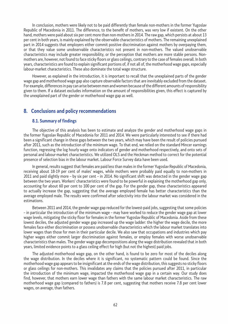
62
In conclusion, mothers were likely not to be paid differently than female non-mothers in the former Yugoslav Republic of Macedonia in 2011. The difference, to the benefit of mothers, was very low if existent. On the other hand, mothers were paid about six per cent more than non-mothers in 2014. The raw gap, which persists at about 13 per cent in both years, is mainly explained by the observable characteristics of mothers. The remaining unexplained part in 2014 suggests that employers either commit positive discrimination against mothers by overpaying them, or that they value some unobservable characteristics not present in non-mothers. The valued unobservable characteristics may include greater responsibility, or the perception that mothers are more stable persons. Non-mothers are, however, not found to face sticky floors or glass ceilings, contrary to the case of females overall. In both years, characteristics are found to explain significant portions of, if not all of, the motherhood wage gaps, especially labour-market characteristics. These also dominate the total wage structure.
However, as explained in the introduction, it is important to recall that the unexplained parts of the gender wage gap and motherhood wage gap also capture observable factors that are inevitably excluded from the dataset. For example, differences in pay can arise between men and women because of the different amounts of responsibility given to them. If a dataset excludes information on the amount of responsibilities given, this effect is captured by the unexplained part of the gender or motherhood wage gap as well.
8. Conclusions and policy recommendations
8.1. summary of findings
The objective of this analysis has been to estimate and analyze the gender and motherhood wage gaps in the former Yugoslav Republic of Macedonia for 2011 and 2014. We were particularly interested to see if there had been a significant change in these gaps between the two years, which may have been the result of policies pursued after 2011, such as the introduction of the minimum wage. To that end, we relied on the standard Mincer earnings function, regressing the log hourly wage onto indicators of gender and motherhood respectively, and onto sets of personal and labour-market characteristics. We utilized OLS and the Heckman method to correct for the potential presence of selection bias in the labour market. Labour Force Survey data have been used.
In general, results suggest that females are paid less than males in the former Yugoslav Republic of Macedonia, receiving about 18-19 per cent of males’ wages, while mothers were probably paid equally to non-mothers in 2011 and paid slightly more – by six per cent – in 2014. No significant shift was detected in the gender wage gap between the two years. Workers’ characteristics were found to be powerful in explaining the motherhood gap only, accounting for about 60 per cent to 100 per cent of the gap. For the gender gap, these characteristics appeared to actually increase the gap, suggesting that the average employed female has better characteristics than the average employed male. The results were confirmed after selectivity into the labour market was considered in the estimations.
Between 2011 and 2014, the gender wage gap reduced for the lowest-paid jobs, suggesting that some policies – in particular the introduction of the minimum wage – may have worked to reduce the gender wage gap at lower wage levels, mitigating the sticky floor for females in the former Yugoslav Republic of Macedonia. Aside from these lowest deciles, the adjusted gender wage gap increased up the wage ladder: the higher the wage decile, the more females face either discrimination or possess unobservable characteristics which the labour market translates into lower wages than those for men in their particular decile. We also saw that occupations and industries which pay higher wages either commit larger discrimination against females, or employ females with worse unobservable characteristics than males. The gender wage gap decompositions along the wage distribution revealed that in both years, limited evidence points to a glass ceiling effect for high (but not the highest) paid jobs.
The adjusted motherhood wage gap, on the other hand, is found to be zero for most of the deciles along the wage distribution. In the deciles where it is significant, no systematic pattern could be found. Since the motherhood wage gap appears to be insignificant at the ends of the wage distribution, this suggests no sticky floors or glass ceilings for non-mothers. This invalidates any claims that the policies pursued after 2011, in particular the introduction of the minimum wage, impacted the motherhood wage gap in a certain way. Our study does find, however, that mothers earn lower wage than fathers with the same labour market characteristics. The raw motherhood wage gap (compared to fathers) is 7.8 per cent, suggesting that mothers receive 7.8 per cent lower wages, on average, than fathers.
63
8.2. Policy implications
The study finds a relatively large and persistent gender wage gap in the former Yugoslav Republic of Macedonia of about 18-19 per cent. When the gap is adjusted for the personal and labour market characteristics of both genders, it further increases, as employed females have better labour market characteristics than employed males (such as education and work experience). This implies that if male employees in the former Yugoslav Republic of Macedonia had the same characteristics as females, the gap would further increase, meaning that they would earn even higher wages than females. The study finds that employers may discriminate against female employees, since men with the same characteristics as females receive higher pay for these characteristics (such as experience and education). We also show that there is a motherhood wage gap (mothers compared to fathers, but not when compared to non-mothers) of 7.8 per cent, meaning that mothers with the same labour market characteristics as fathers still earn about eight per cent lower wages than fathers on average.
Government efforts towards ensuring greater gender equality (including the ratification of the ILO Convention No. 100, national legislation, and institutional setups for gender equality and the prevention of discrimination) are proving ineffective. As documented, the gap persists into 2014. However, we find that the introduction of the minimum wage has likely reduced gender inequality for lower-paid and low-skilled women, which can be advocated for as a good policy measure (although gender wage equality was not considered as an argument for the introduction of the nation-wide minimum wage). A large part of this discrimination is unfortunately rooted in society’s norms, values and culture. In section 2 we delineated a theoretical basis of discrimination which can lead to taste-based or statistical discrimination. While these bases for discrimination are unlikely to change overnight, policy interventions can push things in the right direction over time.
What are the options for policymakers who aim to reduce the gender wage gap? Based on the main findings of the report and the institutional context of the country related to gender equality (section 3.2), we draw on some policies which may be effective in reducing the gender wage gap in Macedonia::
— Further invest in and expand the network of affordable, high-quality child care and early childhood education facilities. Improved access to early childcare facilities will positively affect female participation in the labour market, reduce the career interruptions of females, and can therefore improve the relative position of females in the labour market, including their wage prospects.
— Correctly transpose the ILO Equal Remuneration Convention, 1951 (No. 100) into the national labour legislation. This has the potential to reduce discrimination that is based on the segregation of women into “female” occupations, occupations which tend to pay lower wages that do not correspond to females’ productivity.
— Develop a clear procedural and institutional setting for disputes relating to equal remuneration. The real impact of the measures and the legislative provisions that promote gender equality (and the equality of remuneration) largely depends on their practical implementation, especially the issuance of sanctions when employers do not comply. Hence, the procedural and institutional settings in the country must be advanced so as to ensure the vigorous enforcement of the legislation.
— Support a family-friendly workplace culture in the public and private sectors. The inflexibility of working arrangements in Macedonia and a lack of family-friendly policies reduce a woman’s ability to balance work and family. Females can currently choose to not supply their labour at all, to work but accumulate less human capital during their career, or to choose a job with lower wages and higher non-pecuniary benefits.
— Support and develop the culture of gender equality in all aspects of society. As we argued in section 3.2, the culture and norms are not supportive of shared responsibilities between the genders. Extended families usually provide substantial support in the realm of childcare, but this does not promote greater gender equality in all aspects of work and life, or change the traditional role of females as secondary breadwinners.
— Promote the introduction of gender perspectives and equality in collective agreements, apart from the formal requirement of non-discrimination. The issue of anti-discrimination based on sex should be further developed within collective agreements, taking into account the specificities of each industry and branch.
— Fight against the stereotypes of what constitutes “female” and “male” occupations. This action requires a longer time frame, as it also demands interaction with cultural and social norms that are difficult to
64
change. Luckily, technology and technological advancements are also changing the skill and sex structures of occupations.
— Increase the minimum wage in the textile and leather industries, industries where women are overrepresented, to that of the national minimum wage, possibly progressively over time. This suggestion is based on the premise that wages in these female-dominated industries do not reflect the true productivity levels of the workers, and that their lower wages stem from the fact that they are female-dominated industries.
— Introduce gender provisions in the procurement rules. This measure has the potential to promote female employment by favouring companies that employ higher shares of female workers.
— Promote shared parental leave for both parents. The current system of paid leave does not differentiate between maternity and parental leave, guaranteeing only maternity leave which mothers can transfer to fathers. The legislation must be changed to equally promote paternal and maternal leave, and to promote shared leave for the two parents. .
We also note that cooperation among the social partners is crucial for the success of the above recommendations.

65
9. References
Agüero, J. M.; Marks, M. S. 2011. “Motherhood and female labour supply in the developing world: Evidence from infertility shocks”, in Journal of Human Resources, Vol. 46, No. 4, pp. 800−826.
Albrecht, J., van Vuuren, A.; Vroman, S. 2004. Decomposing the Gender Wage Gap in the Netherlands with Sam-ple Selection Adjustment, IZA Discussion Paper No. 1400 (Bonn, Institute for the Study of Labor).
Altonji, J.; Blank, R. 1999. “Race and Gender in the Labour Market”, in O. Ashenfelter, D. Card (eds.): Hand-book of Labour Economics, Vol. 3C (North-Holland), pp. 3141−3259.
Amuendo-Dorantes, C.; Kimmel, J. 2008. New Evidence on the Motherhood Wage Gap. IZA Discussion Paper No. 3662.
Anderson, D.; Binder, M.; Krause, K. 2003. “The Motherhood Wage Penalty Revisited: Experience, Heterogene-ity, Work Effort, and Work-Schedule Flexibility”, in Industrial and Labour Relations Review, Vol. 56, No. 2, pp. 273−294.
Angel-Urdinola, DF. 2008. Can the Introduction of a Minimum Wage in FYR the Former Yugoslav Republic of Macedonia Decrease the Gender Wage Gap?, Social Policy Discussion Paper No. 0837 (Washington DC, World Bank).
Angel-Urdinola DF; Macias, V. 2008. FYR The former Yugoslav Republic of Macedonia Labour Market Profile 2004–2007: A Policy Note (Washington, DC, World Bank).
Avlijaš, S.; Ivanovic, N.; Vladisavljevic, M.; Vujic, S. 2013. Gender wage gap in Western Balkans: Evidence from Serbia, the Former Yugoslav Republic of Macedonia and Montenegro (Belgrade, Foundation for Advance-ment of Economics).
Azmat, G.; Güell, M.; Manning, A. 2006. “Gender Gaps in Unemployment Rates in OECD Countries”, in Journal of Labour Economics, Vol. 24, No. 1, pp. 1−37.
Barsky, R.; Bound, J.; Charles, K.; Lupton, J. 2002. “Accounting for the Black-White Wealth Gap: A Nonpara-metric Approach”, in Journal of the American Statistical Association, Vol. 97, pp. 663−673.
Beblo, M.; Wolf, E. 2002. Wage Penalties for Career Interruptions, Zentrum für Europäische Wirtschaftsfor-schung Discussion Paper No. 02–45 (Mannheim, ZEW).
Beblo, M.; Beninger, D; Heinze, A; Laisney, F. 2003. Measuring Selectivity-corrected Gender Wage Gaps in the EU, Zentrum für Europäische Wirtschaftsforschung Discussion Paper No. 03−74 (Mannheim, ZEW).
Becker, G.S. 1971. The economics of discrimination (Chicago, University of Chicago Press).
Black, D.A.; Haviland, A; Sanders,S; and Taylor, L. 2008. “Gender Wage Disparities among the Highly Educat-ed”, in Journal of Human Resources, Vol. 43, No. 3, pp. 630−659.
Blau, F.; Kahn, L. 2003. “Understanding International Differences in the Gender Wage Gap”, in Journal of Labour Economics, Vol. 21, pp. 106−144.
Blau, F.; Kahn, L. 2007. “The gender wage gap: have women have got as far as they can?”, in Academy of Man-agement Perspective, Vol. 21, pp. 7−23.
Blinder, A. S. 1973. “Wage Discrimination: Reduced Form and Structural Estimates”, in The Journal of Human Resources, Vol. 8, No. 4, pp. 436−455.
Budig, M.J. 2014. The Fatherhood Bonus & The Motherhood Penalty: Parenthood and the Gender Gap in Pay (Washington, DC, Third Way).
Budig, M.J.; England, P. 2001. “The Wage Penalty for Motherhood”, in American Sociological Review, Vol. 66, No. 2, pp. 204−225.
Chernozhukov, V; Fernandez-Val, I; Melly, B. 2013. “Inference on Counterfactual Distributions”, in Econometri-ca, Vol. 81, No. 6, pp. 2205–2268.
66
Davies, R.; Pierre, G.. 2005. “The family gap in pay in Europe: A cross-country study”, in Labour Economics, Vol. 12, No. 4, pp. 469–486.
Dey, J.; Hill, C. 2007. Behind the Gender Gap (American Association of University Women Educational Founda-tion).
Ejrnæs, M.; Kunze, A. 2013. “Work and wage dynamics around childbirth” in The Scandinavian Journal of Eco-nomics, Vol. 115, No. 3, pp. 856–877.
Ejrnæs, M.; Kunze, A. 2004. Wage dips and drops around first birth, University of Copenhagen Working Paper No. 2004–01 (Copenhagen, University of Copenhagen).
Felfe, C. 2012a. “The motherhood wage gap: What about job amenities?”, in Labour Economics, Vol. 19, No. 1, pp. 59−67.
Felfe, C. 2012b. “The Willingness to Pay for Job Amenities: Evidence from Mothers’ Return to Work”, in Indus-trial & Labour Relations Review, Vol. 65, No. 2, pp. 427−454.
Firpo, Sergio; Fortin, N; Lemieux, T. 2007. Decomposing Wage Distributions using Recentered Influence Func-tions Regressions (University of British Columbia).
Firpo, Sergio; Fortin, N; Lemieux, T. 2009. “Unconditional Quantile Regressions”, in Econometrica, Vol. 77, No. 3, pp. 953−973.
Fortin, N. 2005. “Gender Role Attitudes and the Labour Market Outcomes of Women across OECD Coun-tries”, in Oxford Review of Economic Policy, Vol. 21, No. 3, pp. 416−438.
Fortin, N.; Lemieux, T; Firpo, S. 2011. Chapter 1 - Decomposition Methods in Economics, in O. Ashenfelter and D. Card (eds): Handbook of Labour Economics, Vol. 4, Pt. A, pp. 1−102.
Frölich, M. 2002. “Propensity score matching without conditional independence assumption−with an appli-cation to the gender wage gap in the United Kingdom”, in The Econometrics Journal, Vol. 10, No. 2, pp. 359−407.
Glauber, R. 2008. “Gender and race in families and at work: The fatherhood wage premium”, in Gender and Society, Vol. 22, pp. 8−30.
Grimshaw, D.; Rubery, J. 2015. The motherhood pay gap: A review of the issues, theory and international evi-dence (Geneva, ILO).
Harkness, S.; Waldfogel, G. 2003. “The Family Gap in Pay: Evidence from Seven Industrialized Countries”, in Research in Labour Economics, Vol. 22, pp. 369−413.
Heckman, J. 1976. “The Common Structure of Statistical Models of Truncation, Sample Selection and Limited Dependent Variables and a Simple Estimator for Such Models”, in Annals of Economic Social Measurement, Vol. 5, No. 4, pp. 475−492.
Heckman, J. 1979. “Sample Selection Bias as a Specification Error”, in Econometrica, Vol. 47, pp. 153−163.
Heinze, A.; Wolf, E. 2010. “The intra-firm gender wage gap: a new view on wage differentials based on linked employer–employee data”, in Journal of Population Economics, Vol. 23, No. 3, pp. 851−879.
Hodges, M.; Budig, M.J. 2010. “Who Gets the Daddy Bonus? Markers of Hegemonic Masculinity and the Im-pact of First-time Fatherhood on Men’s Earnings”, in Gender & Society, Vol. 24, No. 6, pp. 717−745.
International Labour Office (ILO). 2014. Maternity and paternity at work: law and practice across the world (Geneva).
Jann, B. 2008. “The Blinder-Oaxaca Decomposition for Linear Regression Models” in The Stata Journal, Vol. 8, No. 4, pp. 453−479.
Kazandiska, M.; Risteska, M.; Schmidt, V. 2012. The gender wage gap in the former Yugoslav Republic of The former Yugoslav Republic of Macedonia (Skopje, ILO Regional Office).
Killewald, A. 2013. “A Reconsideration of the Fatherhood Premium: Marriage, Coresidence, Biology, and Fathers’ Wages”, in American Sociological Review, Vol. 78, pp. 96−116.

67
Lundberg, S.; Rose, E. 2000. “Parenthood and the earnings of married men and women”, in Labour Economics, Vol. 7, No. 6, pp. 689−710.
Machado, C. 2012. Selection, Heterogeneity and the Gender Wage Gap, IZA Discussion Paper No. 7005 (Bonn, Institute for the Study of Labor).
Machado, J.A.F; Mata, J. 2005. “Counterfactual decomposition of changes in wage distributions using quan-tile regression”, in Journal of Applied Econometrics, Vol. 20, No. 4, pp. 445–465.
Manning, A. 2011. “Imperfect Competition in the Labour Market”, in O. Ashenfelter, D. Card (eds.): Handbook of Labour Economics, Vol. 4B (Amsterdam, Elsevier B.V.), pp. 973-1041)..
Mincer, J. 1974. Schooling, Experience and Earnings (New York, Columbia University Press).
Mojsoska-Blazevski, N.; Kurtisi, N. 2014. Initial Effects of the Introduction of a Minimum Wage in FYR Macedonia (Geneva, ILO).
Ñopo, H. 2008. “Matching as a Tool to Decompose Wage Gaps”, in Review of Economics and Statistics, Vol. 90, No. 2, pp. 290−299.
Oaxaca R. L. 1973. “Male-Female Wage Differentials in Urban Labour Markets”, in International Economic Review, Vol. 14, pp. 693−709.
Pal, I.; Waldfogel, J. 2014. Revisiting the Family Gap in Pay in the United States, Columbia Population Research Center Working Paper No. 14−02 (New York, CPRS).
Petreski, M.; Mojsoska-Blazevski, N.; Petreski, B. 2014. “Gender wage gap when women are highly inactive; Evidence with Macedonian data”, in Journal of Labour Research, Vol. 3, No. 4, pp. 393−411.
Mojsoska-Blazevski, N.; Petreski, M.; Petreska, D. 2015. “Increasing labour market activity of the poor, females and informal workers: Let’s make work pay in Macedonia”, in Eastern European Economics (publication forthcoming).
Petrongolo, B.; Olivetti, C. 2008. “Unequal Pay or Unequal Employment? A Cross-Country Analysis of Gender Gaps”, in Journal of Labour Economics, Vol. 26, No. 4, pp. 621−654.
Phelps, E.S. 1972. “The statistical theory of racism and women” in American Economic Review, Vol. 62, No. 4, pp. 414−445.
Sano, S. 2009. “Testing the Taste-Based Discrimination Hypothesis: Evidence from Data on Japanese Listed Firms”, in Japan Labour Review, Vol. 6, No. 1, pp. 36−50.
Waldfogel, J. 1997. “The Effect of Children on Women’s Wages”, in American Sociological Review, Vol. 62, pp. 209–217.
Wooldridge, J. M. 2009. Introductory Econometrics: A Modern Approach (Cincinnati, OH, South-Western, Thom-son Learning).
Zhang, X. 2010. “Can motherhood earnings losses be ever regained? Evidence from Canada”, in Journal of Family Issues, Vol. 31, No. 12, pp.1671–1688.
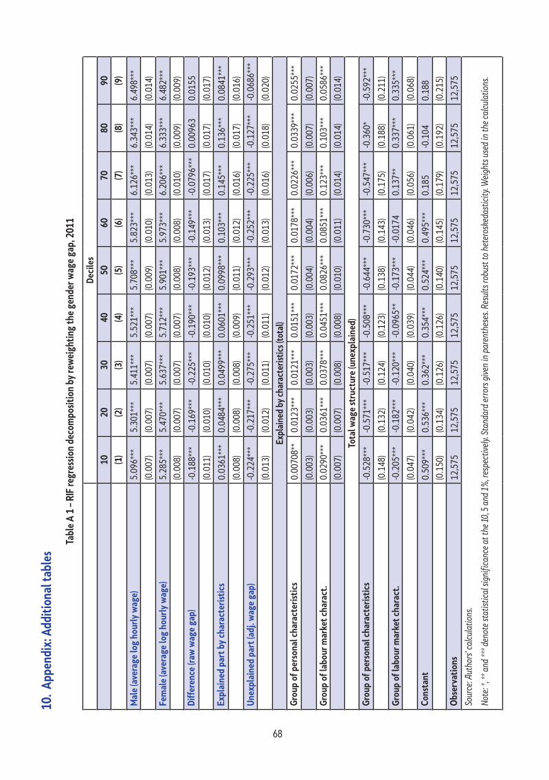
68
10.
Appe
ndix
: Add
ition
al ta
bles
tabl
e A
1 – R
IF re
gres
sion
deco
mpo
sitio
n by
rew
eigh
ting
the
gend
er w
age
gap,
201
1
Deci
les
1020
3040
5060
7080
90
(1)
(2)
(3)
(4)
(5)
(6)
(7)
(8)
(9)
Mal
e (a
vera
ge lo
g ho
urly
wag
e)5.
096*
**5.
301*
**5.
411*
**5.
521*
**5.
708*
**5.
823*
**6.
126*
**6.
343*
**6.
498*
**
(0
.007
)(0
.007
)(0
.007
)(0
.007
)(0
.009
)(0
.010
)(0
.013
)(0
.014
)(0
.014
)
Fem
ale
(ave
rage
log
hour
ly w
age)
5.28
5***
5.47
0***
5.63
7***
5.71
2***
5.90
1***
5.97
3***
6.20
6***
6.33
3***
6.48
2***
(0
.008
)(0
.007
)(0
.007
)(0
.007
)(0
.008
)(0
.008
)(0
.010
)(0
.009
)(0
.009
)
Diff
eren
ce (r
aw w
age
gap)
-0.1
88**
*-0
.169
***
-0.2
25**
*-0
.190
***
-0.1
93**
*-0
.149
***
-0.0
796*
**0.
0096
30.
0155
(0
.011
)(0
.010
)(0
.010
)(0
.010
)(0
.012
)(0
.013
)(0
.017
)(0
.017
)(0
.017
)
Expl
aine
d pa
rt b
y ch
arac
teri
stic
s0.
0361
***
0.04
84**
*0.
0499
***
0.06
01**
*0.
0998
***
0.10
3***
0.14
5***
0.13
6***
0.08
41**
*
(0
.008
)(0
.008
)(0
.008
)(0
.009
)(0
.011
)(0
.012
)(0
.016
)(0
.017
)(0
.016
)
Une
xpla
ined
par
t (ad
j. w
age
gap)
-0.2
24**
*-0
.217
***
-0.2
75**
*-0
.251
***
-0.2
93**
*-0
.252
***
-0.2
25**
*-0
.127
***
-0.0
686*
**
(0
.013
)(0
.012
)(0
.011
)(0
.011
)(0
.012
)(0
.013
)(0
.016
)(0
.018
)(0
.020
)
Expl
aine
d by
cha
ract
erist
ics (
tota
l)
Gro
up o
f per
sona
l cha
ract
eris
tics
0.00
708*
*0.
0123
***
0.01
21**
*0.
0151
***
0.01
72**
*0.
0178
***
0.02
26**
*0.
0339
***
0.02
55**
*
(0
.003
)(0
.003
)(0
.003
)(0
.003
)(0
.004
)(0
.004
)(0
.006
)(0
.007
)(0
.007
)
Gro
up o
f lab
our m
arke
t cha
ract
.0.
0290
***
0.03
61**
*0.
0378
***
0.04
51**
*0.
0826
***
0.08
51**
*0.
123*
**0.
103*
**0.
0586
***
(0
.007
)(0
.007
)(0
.008
)(0
.008
)(0
.010
)(0
.011
)(0
.014
)(0
.014
)(0
.014
)
tota
l wag
e st
ruct
ure
(une
xpla
ined
)
Gro
up o
f per
sona
l cha
ract
eris
tics
-0.5
28**
*-0
.571
***
-0.5
17**
*-0
.508
***
-0.6
44**
*-0
.730
***
-0.5
47**
*-0
.360
*-0
.592
***
(0
.148
)(0
.132
)(0
.124
)(0
.123
)(0
.138
)(0
.143
)(0
.175
)(0
.188
)(0
.211
)
Gro
up o
f lab
our m
arke
t cha
ract
.-0
.205
***
-0.1
82**
*-0
.120
***
-0.0
965*
*-0
.173
***
-0.0
174
0.13
7**
0.33
7***
0.33
5***
(0
.047
)(0
.042
)(0
.040
)(0
.039
)(0
.044
)(0
.046
)(0
.056
)(0
.061
)(0
.068
)
Cons
tant
0.50
9***
0.53
6***
0.36
2***
0.35
4***
0.52
4***
0.49
5***
0.18
5-0
.104
0.18
8
(0
.150
)(0
.134
)(0
.126
)(0
.126
)(0
.140
)(0
.145
)(0
.179
)(0
.192
)(0
.215
)
obs
erva
tion
s12
,575
12,5
7512
,575
12,5
7512
,575
12,5
7512
,575
12,5
7512
,575
Sour
ce: A
utho
rs’ c
alcu
latio
ns.
Note
: *, *
* and
*** d
enot
e st
atist
ical
sign
ifica
nce
at th
e 10
, 5 a
nd 1
%, r
espe
ctiv
ely.
Stan
dard
err
ors g
iven
in p
aren
thes
es. R
esul
ts ro
bust
to h
eter
oske
dast
icity
. Wei
ghts
use
d in
the
calc
ulat
ions
.

69
Тtab
le A
2 –
RIF
regr
essio
n de
com
posit
ion
by re
wei
ghtin
g th
e ge
nder
wag
e ga
p, 2
014
Deci
les
1020
3040
5060
7080
90
(1)
(2)
(3)
(4)
(5)
(6)
(7)
(8)
(9)
Mal
e (a
vera
ge lo
g ho
urly
wag
e)5.
281*
**5.
403*
**5.
536*
**5.
608*
**5.
752*
**5.
832*
**6.
131*
**6.
395*
**6.
567*
**
(0.0
06)
(0.0
06)
(0.0
06)
(0.0
06)
(0.0
08)
(0.0
09)
(0.0
13)
(0.0
16)
(0.0
17)
Fem
ale
(ave
rage
log
hour
ly w
age)
5.44
3***
5.56
2***
5.71
2***
5.76
9***
5.96
9***
6.02
5***
6.25
5***
6.38
2***
6.51
8***
(0
.006
)(0
.006
)(0
.007
)(0
.007
)(0
.008
)(0
.008
)(0
.010
)(0
.010
)(0
.010
)Di
ffer
ence
(raw
wag
e ga
p)-0
.162
***
-0.1
59**
*-0
.176
***
-0.1
61**
*-0
.216
***
-0.1
93**
*-0
.124
***
0.01
280.
0487
**
(0.0
09)
(0.0
08)
(0.0
09)
(0.0
09)
(0.0
11)
(0.0
12)
(0.0
16)
(0.0
19)
(0.0
20)
Expl
aine
d pa
rt b
y ch
arac
teri
stic
s0.
0203
***
0.02
98**
*0.
0315
***
0.05
33**
*0.
0717
***
0.09
03**
*0.
142*
**0.
193*
**0.
162*
**
(0.0
06)
(0.0
06)
(0.0
06)
(0.0
07)
(0.0
08)
(0.0
10)
(0.0
15)
(0.0
19)
(0.0
18)
Une
xpla
ined
par
t (ad
j. w
age
gap)
-0.1
82**
*-0
.189
***
-0.2
07**
*-0
.214
***
-0.2
88**
*-0
.284
***
-0.2
65**
*-0
.181
***
-0.1
13**
*
(0.0
10)
(0.0
10)
(0.0
10)
(0.0
10)
(0.0
12)
(0.0
11)
(0.0
16)
(0.0
19)
(0.0
22)
Expl
aine
d by
cha
ract
eris
tics
(tot
al)
Gro
up o
f per
sona
l cha
ract
eris
tics
0.00
706*
*0.
0102
***
0.00
832*
**0.
0079
9**
0.01
17**
*0.
0177
***
0.02
62**
*0.
0462
***
0.05
63**
*
(0.0
04)
(0.0
03)
(0.0
03)
(0.0
03)
(0.0
04)
(0.0
04)
(0.0
06)
(0.0
08)
(0.0
10)
Gro
up o
f lab
our m
arke
t cha
ract
eris
tics
0.01
33**
0.01
96**
*0.
0231
***
0.04
53**
*0.
0600
***
0.07
27**
*0.
116*
**0.
147*
**0.
105*
**
(0.0
06)
(0.0
06)
(0.0
05)
(0.0
06)
(0.0
08)
(0.0
09)
(0.0
13)
(0.0
16)
(0.0
16)
tota
l wag
e st
ruct
ure
(une
xpla
ined
)
Gro
up o
f per
sona
l cha
ract
eris
tics
-0.1
08-0
.363
***
-0.5
49**
*-0
.495
***
-0.5
37**
*-0
.511
***
-0.3
99**
0.25
20.
553*
*
(0.1
19)
(0.1
12)
(0.1
13)
(0.1
15)
(0.1
35)
(0.1
33)
(0.1
78)
(0.2
06)
(0.2
43)
Gro
up o
f lab
our m
arke
t cha
ract
eris
tics
-0.0
910*
*-0
.185
***
-0.2
49**
*-0
.208
***
-0.1
94**
*-0
.010
40.
147*
*0.
394*
**0.
325*
**
(0.0
39)
(0.0
36)
(0.0
37)
(0.0
37)
(0.0
44)
(0.0
43)
(0.0
58)
(0.0
68)
(0.0
81)
Cons
tant
0.01
660.
359*
**0.
590*
**0.
489*
**0.
443*
**0.
238*
-0.0
131
-0.8
27**
*-0
.991
***
(0
.121
)(0
.114
)(0
.115
)(0
.117
)(0
.137
)(0
.136
)(0
.182
)(0
.212
)(0
.251
)o
bser
vati
ons
10,1
8210
,182
10,1
8210
,182
10,1
8210
,182
10,1
8210
,182
10,1
82So
urce
: Aut
hors
’ cal
cula
tions
.
Note
: *, *
* and
*** d
enot
e st
atist
ical
sign
ifica
nce
at th
e 10
, 5 a
nd 1
%, r
espe
ctiv
ely.
Stan
dard
err
ors g
iven
in p
aren
thes
es. R
esul
ts ro
bust
to h
eter
oske
dast
icity
. Wei
ghts
use
d in
the
calc
ulat
ions
.

70
table A 3 – Motherhood wage gap, 2011 (mothers with at least one child aged up to 3)
oLs Heckman
VARIABLEs Only gender
Gender and personal
characteristics
Gender, personal and
labour marker characteristics
Outcome equation
Selection equation
(1) (2) (3) (4) (5)Mother (1=if woman has at least one child) 0.193*** 0.0709*** 0.0228 0.0229 -3.714***
(0.031) (0.025) (0.021) (0.021) (0.340)Age (in years) -0.00796 -0.00891 -0.00889 -0.0462
(0.019) (0.016) (0.016) (0.180)Age squared 0.000128 0.000143 1.43E-04 0.0011
(0.000) (0.000) (0.000) (0.003)tenure in current firm (in years) 0.0153*** 0.00847*** 0.00846*** -0.0102
(0.002) (0.001) (0.001) (0.021)secondary education 0.231*** 0.0721*** 0.0722*** 0.342
(0.022) (0.022) (0.022) (0.251)tertiary education 0.761*** 0.242*** 0.242*** 0.254
(0.026) (0.033) (0.033) (0.270)Post-graduate education 1.144*** 0.514*** 0.514*** -0.315
(0.049) (0.059) (0.059) (0.441)settlement (1=urban) 0.0730*** 0.0523*** 0.0522*** -0.213
(0.019) (0.015) (0.015) (0.178)type of contract (1=permanent) 0.0710** 0.0710**
(0.028) (0.028)occupations (1=armed forces) 0.559*** 0.559***
(0.061) (0.060)occupations (1=managers) 0.503*** 0.503***
(0.070) (0.070)occupations (1=professionals) 0.549*** 0.549***
(0.041) (0.041)occupations (1=technicians) 0.341*** 0.340***
(0.032) (0.032)occupations (1=clerical workers) 0.370*** 0.370***
(0.037) (0.037)occupations (1=service and sales) 0.00592 0.00592
(0.033) (0.033)occupations (1=craftsmen) 0.00868 0.00867
(0.040) (0.040)occupations (1=machinists) -0.127*** -0.127***
(0.031) (0.031)sector (1=agriculture) -0.226*** -0.226***

71
(0.068) (0.068)sector (1=market services) 0.014 0.014
(0.027) (0.027)sector (1=non-market services) 0.0815*** 0.0815***
(0.026) (0.026)Number of children 3.775***
(0.142)Employment status of spouse (1=employed) 0.23
(0.169)Constant 5.673*** 5.260*** 5.328*** 5.328*** 2.338
(0.012) (0.334) (0.292) (0.291) (3.018)
Inverse mills ratio (lambda) -0.171***
(0.0458)observations 3,143 3,143 3,143 3,176 3,176R-squared 0.019 0.384 0.542Source: Authors’ calculations.
Note: *, ** and *** denote statistical significance at the 10, 5 and 1%, respectively. Standard errors given in parentheses. Results robust to heteroskedasticity. Weights used in the calculations.
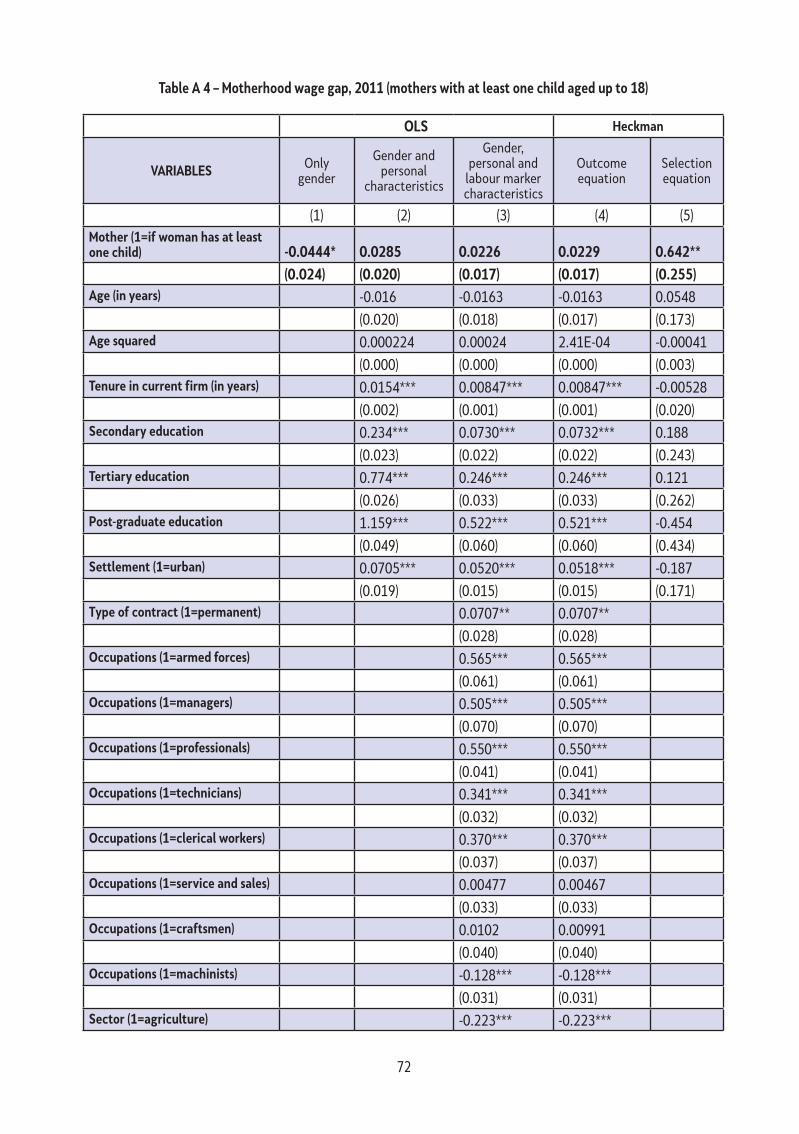
72
table A 4 – Motherhood wage gap, 2011 (mothers with at least one child aged up to 18)
oLs Heckman
VARIABLEs Only gender
Gender and personal
characteristics
Gender, personal and
labour marker characteristics
Outcome equation
Selection equation
(1) (2) (3) (4) (5)Mother (1=if woman has at least one child) -0.0444* 0.0285 0.0226 0.0229 0.642**
(0.024) (0.020) (0.017) (0.017) (0.255)Age (in years) -0.016 -0.0163 -0.0163 0.0548
(0.020) (0.018) (0.017) (0.173)Age squared 0.000224 0.00024 2.41E-04 -0.00041
(0.000) (0.000) (0.000) (0.003)tenure in current firm (in years) 0.0154*** 0.00847*** 0.00847*** -0.00528
(0.002) (0.001) (0.001) (0.020)secondary education 0.234*** 0.0730*** 0.0732*** 0.188
(0.023) (0.022) (0.022) (0.243)tertiary education 0.774*** 0.246*** 0.246*** 0.121
(0.026) (0.033) (0.033) (0.262)Post-graduate education 1.159*** 0.522*** 0.521*** -0.454
(0.049) (0.060) (0.060) (0.434)settlement (1=urban) 0.0705*** 0.0520*** 0.0518*** -0.187
(0.019) (0.015) (0.015) (0.171)type of contract (1=permanent) 0.0707** 0.0707**
(0.028) (0.028)occupations (1=armed forces) 0.565*** 0.565***
(0.061) (0.061)occupations (1=managers) 0.505*** 0.505***
(0.070) (0.070)occupations (1=professionals) 0.550*** 0.550***
(0.041) (0.041)occupations (1=technicians) 0.341*** 0.341***
(0.032) (0.032)occupations (1=clerical workers) 0.370*** 0.370***
(0.037) (0.037)occupations (1=service and sales) 0.00477 0.00467
(0.033) (0.033)occupations (1=craftsmen) 0.0102 0.00991
(0.040) (0.040)occupations (1=machinists) -0.128*** -0.128***
(0.031) (0.031)sector (1=agriculture) -0.223*** -0.223***

73
(0.068) (0.068)sector (1=market services) 0.0146 0.0146
(0.027) (0.027)sector (1=non-market services) 0.0820*** 0.0820***
(0.026) (0.026)Number of children -0.282**
(0.113)Employment status of spouse (1=employed) 0.0736
(0.170)Constant 5.732*** 5.409*** 5.452*** 5.451*** 0.868
(0.020) (0.343) (0.305) (0.304) (2.842)Inverse mills ratio (lambda) 0.0054
(0.0518)observations 3,143 3,143 3,143 3,176 3,176R-squared 0.002 0.382 0.542Source: Authors’ calculations.
Note: *, ** and *** denote statistical significance at the 10, 5 and 1%, respectively. Standard errors given in parentheses. Results robust to heteroskedasticity. Weights used in the calculations.

74
table A 5 – Motherhood wage gap, 2014 (mothers with at least one child aged up to 3)
oLs Heckman
VARIABLEs Only gender
Gender and personal
characteristics
Gender, personal and
labour marker characteristics
Outcome equation
Selection equation
(1) (2) (3) (4) (5)
Mother (1=if woman has at least one child) 0.150*** 0.121*** 0.0675*** 0.0585*** 0.175
(0.030) (0.024) (0.022) (0.022) (0.319)
Age (in years) 0.0466** 0.0477*** 0.0552*** -0.304**
(0.018) (0.016) (0.017) (0.123)
Age squared -0.000588** -0.000616*** -0.000722*** 0.00432**
(0.000) (0.000) (0.000) (0.002)
tenure in current firm (in years) 0.0135*** 0.00685*** 0.00623*** 0.0257*
(0.002) (0.002) (0.002) (0.015)
secondary education 0.189*** 0.0909*** 0.0920*** -0.0237
(0.029) (0.029) (0.029) (0.234)
tertiary education 0.671*** 0.191*** 0.202*** -0.341
(0.032) (0.039) (0.039) (0.247)
Post-graduate education 0.936*** 0.363*** 0.381*** -0.503
(0.057) (0.063) (0.064) (0.346)
settlement (1=urban) 0.00959 0.00161 0.00382 -0.0804
(0.020) (0.018) (0.018) (0.133)
type of contract (1=permanent) 0.107*** 0.104***
(0.028) (0.028)
occupations (1=armed forces) 0.561*** 0.557***
(0.091) (0.089)
occupations (1=managers) 0.917*** 0.918***
(0.075) (0.074)
occupations (1=professionals) 0.552*** 0.553***
(0.043) (0.043)
occupations (1=technicians) 0.332*** 0.333***
(0.039) (0.038)
occupations (1=clerical workers) 0.247*** 0.248***
(0.048) (0.047)
occupations (1=service and sales) -0.0237 -0.0247
(0.035) (0.035)
occupations (1=agricultural workers) -0.194 -0.192
(0.134) (0.133)
occupations (1=craftsmen)
0.0438 0.0439
(0.047) (0.046)
occupations (1=machinists) -0.0421 -0.0419
(0.038) (0.037)

75
sector (1=agriculture) 0.0164 0.0216
(0.079) (0.082)
sector (1=market services) -0.00514 -0.00382
(0.030) (0.030)
sector (1=non-market services) 0.0285 0.028
(0.029) (0.029)
Number of children 0.106
(0.220)
Employment status of spouse (1=employed) 0.0032
(0.117)
Constant 5.745*** 4.439*** 4.418*** 4.307*** 6.982***
(0.012) (0.312) (0.278) (0.287) (2.100)
Inverse mills ratio (lambda) -0.171***
(0.0458)
observations 2,196 2,196 2,196 2,286 2,286
R-squared 0.015 0.378 0.525
Source: Authors’ calculations.
Note: *, ** and *** denote statistical significance at the 10, 5 and 1%, respectively. Standard errors given in parentheses. Results robust to heteroskedasticity. Weights used in the calculations.

76
table A 6 – Motherhood wage gap, 2014 (mothers with at least one child aged up to 18)
oLs Heckman
VARIABLEs Only gender
Gender and personal
characteristics
Gender, personal and
labour marker characteristics
Outcome equation
Selection equation
(1) (2) (3) (4) (5)
Mother (1=if woman has at least one child) -0.0287 0.0379* 0.0298* 0.0189 0.502***
(0.023) (0.020) (0.017) (0.018) (0.172)
Age (in years) 0.0405** 0.0418** 0.0507*** -0.360***
(0.019) (0.017) (0.018) (0.129)
Age squared -0.000536* -0.000552** -0.000675*** 0.00499***
(0.000) (0.000) (0.000) (0.002)
tenure in current firm (in years) 0.0138*** 0.00693*** 0.00639*** 0.0280*
(0.002) (0.002) (0.002) (0.015)
secondary education 0.185*** 0.0858*** 0.0877*** -0.0457
(0.029) (0.029) (0.029) (0.235)
tertiary education 0.677*** 0.188*** 0.196*** -0.294
(0.032) (0.040) (0.040) (0.245)
Post-graduate education 0.928*** 0.353*** 0.367*** -0.503
(0.058) (0.064) (0.065) (0.352)
settlement (1=urban) 0.00396 -0.00161 -4.38E-05 -0.0749
(0.020) (0.018) (0.018) (0.131)
type of contract (1=permanent) 0.110*** 0.108***
(0.028) (0.028)
occupations (1=armed forces) 0.589*** 0.585***
(0.083) (0.081)
occupations (1=managers) 0.912*** 0.911***
(0.073) (0.072)
occupations (1=professionals) 0.558*** 0.559***
(0.043) (0.043)
occupations (1=technicians) 0.336*** 0.335***
(0.039) (0.038)
occupations (1=clerical workers) 0.251*** 0.251***
(0.048) (0.047)
occupations (1=service and sales) -0.0249 -0.0259
(0.035) (0.035)
occupations (1=agricultural workers) -0.201 -0.197
(0.133) (0.132)
occupations (1=craftsmen) 0.0442 0.0438
(0.047) (0.046)
occupations (1=machinists) -0.046 -0.0458
(0.038) (0.037)
sector (1=agriculture) 0.0239 0.0265
(0.078) (0.079)
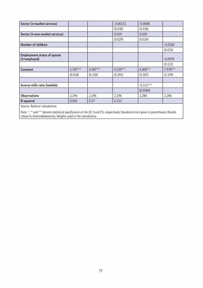
77
sector (1=market services) -0.00151 -0.0008
(0.030) (0.030)
sector (1=non-market services) 0.029 0.029
(0.029) (0.029)
Number of children -0.0568
(0.076)
Employment status of spouse (1=employed) -0.0978
(0.121)
Constant 5.787*** 4.587*** 4.539*** 4.400*** 7.978***
(0.018) (0.330) (0.291) (0.307) (2.199)
Inverse mills ratio (lambda) -0.151***
(0.0584)
observations 2,196 2,196 2,196 2,286 2,286
R-squared 0.001 0.37 0.523
Source: Authors’ calculations.
Note: *, ** and *** denote statistical significance at the 10, 5 and 1%, respectively. Standard errors given in parentheses. Results robust to heteroskedasticity. Weights used in the calculations.

78
tabl
e A
7 – R
IF re
gres
sion
deco
mpo
sitio
n by
rew
eigh
ting
the
mot
herh
ood
wag
e ga
p, 2
011
Deci
les
1020
3040
5060
7080
90
(1)
(2)
(3)
(4)
(5)
(6)
(7)
(8)
(9)
Mot
her (
aver
age
log
hour
ly w
age)
5.10
8***
5.30
6***
5.44
6***
5.59
8***
5.78
0***
5.93
2***
6.14
2***
6.19
5***
6.25
4***
(0
.022
)(0
.021
)(0
.031
)(0
.031
)(0
.025
)(0
.021
)(0
.023
)(0
.023
)(0
.040
)
Non
-mot
her (
aver
age
log
hour
ly w
age)
5.08
6***
5.28
5***
5.41
1***
5.48
7***
5.64
6***
5.73
7***
6.00
5***
6.21
9***
6.40
2***
(0
.012
)(0
.011
)(0
.011
)(0
.012
)(0
.014
)(0
.015
)(0
.019
)(0
.019
)(0
.018
)
Diff
eren
ce (r
aw w
age
gap)
0.02
230.
0202
0.03
480.
111*
**0.
134*
**0.
196*
**0.
137*
**-0
.023
7-0
.148
***
(0
.025
)(0
.024
)(0
.033
)(0
.033
)(0
.028
)(0
.026
)(0
.030
)(0
.030
)(0
.044
)
Expl
aine
d pa
rt b
y ch
arac
teri
stic
s-0
.014
20.
0281
0.04
430.
0215
0.02
650.
0490
*0.
0756
***
0.05
09*
-0.0
464
(0
.030
)(0
.028
)(0
.040
)(0
.039
)(0
.031
)(0
.027
)(0
.029
)(0
.030
)(0
.053
)
Une
xpla
ined
par
t (ad
just
ed w
age
gap)
0.03
65-0
.007
97-0
.009
430.
0893
**0.
107*
**0.
147*
**0.
0615
*-0
.074
6**
-0.1
02
(0
.036
)(0
.034
)(0
.042
)(0
.038
)(0
.031
)(0
.028
)(0
.031
)(0
.035
)(0
.064
)
Expl
aine
d by
cha
ract
eris
tics
(tot
al)
Gro
up o
f per
sona
l cha
ract
eris
tics
-0.0
667*
*-0
.026
4-0
.053
2-0
.087
6***
-0.0
615*
*-0
.029
-0.0
103
-0.0
197
-0.0
964*
(0
.028
)(0
.027
)(0
.034
)(0
.031
)(0
.024
)(0
.022
)(0
.023
)(0
.026
)(0
.052
)
Gro
up o
f lab
our m
arke
t cha
ract
.0.
0525
***
0.05
45**
*0.
0975
***
0.10
9***
0.08
81**
*0.
0779
***
0.08
59**
*0.
0706
***
0.05
00**
(0
.013
)(0
.013
)(0
.022
)(0
.024
)(0
.019
)(0
.015
)(0
.017
)(0
.015
)(0
.021
)
tota
l wag
e st
ruct
ure
(une
xpla
ined
)
Gro
up o
f per
sona
l cha
ract
eris
tics
-0.3
061.
294
1.46
2-0
.156
-0.2
510.
481
0.58
6-0
.211
1.33
6
(0
.969
)(0
.902
)(1
.087
)(0
.985
)(0
.818
)(0
.755
)(0
.852
)(0
.946
)(1
.668
)
Gro
up o
f lab
our m
arke
t cha
ract
.0.
171
0.26
4**
0.27
4*0.
296*
*0.
191*
0.12
6-0
.041
10.
0018
30.
028
(0
.129
)(0
.120
)(0
.145
)(0
.131
)(0
.109
)(0
.100
)(0
.113
)(0
.126
)(0
.222
)
Cons
tant
0.17
2-1
.566
*-1
.745
-0.0
509
0.16
7-0
.46
-0.4
830.
135
-1.4
66
(0
.987
)(0
.919
)(1
.109
)(1
.005
)(0
.834
)(0
.768
)(0
.865
)(0
.962
)(1
.702
)
obs
erva
tion
s3,
176
3,17
63,
176
3,17
63,
176
3,17
63,
176
3,17
63,
176
Sour
ce: A
utho
rs’ c
alcu
latio
ns.
Note
: *, *
* and
*** d
enot
e st
atist
ical
sign
ifica
nce
at th
e 10
, 5 a
nd 1
%, r
espe
ctiv
ely.
Stan
dard
err
ors g
iven
in p
aren
thes
es. R
esul
ts ro
bust
to h
eter
oske
dast
icity
. Wei
ghts
use
d in
the
calc
ulat
ions
.

79
tabl
e A
8 – R
IF re
gres
sion
deco
mpo
sitio
n by
rew
eigh
ting
the
mot
herh
ood
wag
e ga
p, 2
014
Deci
les
1020
3040
5060
7080
90
(1)
(2)
(3)
(4)
(5)
(6)
(7)
(8)
(9)
Mot
her (
aver
age
log
hour
ly w
age)
5.28
4***
5.47
1***
5.58
3***
5.74
0***
5.84
6***
6.02
7***
6.24
9***
6.33
0***
6.48
7***
(0
.022
)(0
.019
)(0
.022
)(0
.028
)(0
.038
)(0
.036
)(0
.037
)(0
.028
)(0
.028
)
Non
-mot
her (
aver
age
log
hour
ly w
age)
5.27
9***
5.40
0***
5.45
1***
5.58
6***
5.72
8***
5.90
7***
5.98
0***
6.29
9***
6.48
7***
(0
.010
)(0
.010
)(0
.011
)(0
.011
)(0
.014
)(0
.020
)(0
.019
)(0
.023
)(0
.022
)
Diff
eren
ce (r
aw w
age
gap)
0.00
509
0.07
11**
*0.
132*
**0.
154*
**0.
118*
**0.
120*
**0.
269*
**0.
0311
-0.0
0057
(0
.025
)(0
.022
)(0
.025
)(0
.030
)(0
.040
)(0
.042
)(0
.042
)(0
.036
)(0
.036
)
Expl
aine
d pa
rt b
y ch
arac
teri
stic
s-0
.031
1-0
.017
90.
0394
0.04
470.
0953
**0.
0693
0.10
5**
-0.0
0438
-0.0
0438
(0
.030
)(0
.025
)(0
.029
)(0
.036
)(0
.047
)(0
.045
)(0
.046
)(0
.037
)(0
.037
)
Une
xpla
ined
par
t (ad
j. w
age
gap)
0.03
620.
0891
***
0.09
22**
*0.
109*
**0.
0224
0.05
070.
164*
**0.
0355
0.00
381
(0
.035
)(0
.030
)(0
.033
)(0
.039
)(0
.044
)(0
.045
)(0
.045
)(0
.045
)(0
.045
)
Expl
aine
d by
cha
ract
eris
tics
(tot
al)
Gro
up o
f per
sona
l cha
ract
eris
tics
-0.0
425
-0.0
30.
0078
6-0
.003
8-0
.018
6-0
.030
10.
0049
4-0
.052
2-0
.052
2
(0
.028
)(0
.023
)(0
.025
)(0
.031
)(0
.035
)(0
.035
)(0
.036
)(0
.034
)(0
.034
)
Gro
up o
f lab
our m
arke
t cha
ract
.0.
0114
0.01
20.
0315
**0.
0485
***
0.11
4***
0.09
94**
*0.
100*
**0.
0479
***
0.04
79**
*
(0
.012
)(0
.010
)(0
.014
)(0
.018
)(0
.029
)(0
.023
)(0
.024
)(0
.015
)(0
.015
)
tota
l wag
e st
ruct
ure
(une
xpla
ined
)
Gro
up o
f per
sona
l cha
ract
eris
tics
-0.7
3-0
.948
-0.1
62-0
.167
-0.6
3-1
.995
*-0
.798
-2.6
59**
-2.6
00**
(0
.856
)(0
.732
)(0
.796
)(0
.934
)(1
.053
)(1
.101
)(1
.104
)(1
.102
)(1
.151
)
Gro
up o
f lab
our m
arke
t cha
ract
.-0
.121
-0.1
050.
0154
0.18
10.
630*
**0.
0509
0.15
8-0
.227
-0.0
527
(0
.123
)(0
.105
)(0
.115
)(0
.134
)(0
.152
)(0
.159
)(0
.159
)(0
.159
)(0
.166
)
Cons
tant
0.88
81.
142
0.23
90.
0954
0.02
281.
995*
0.80
42.
921*
**2.
656*
*
(0
.868
)(0
.742
)(0
.807
)(0
.948
)(1
.069
)(1
.117
)(1
.120
)(1
.117
)(1
.167
)
obs
erva
tion
s2,
286
2,28
62,
286
2,28
62,
286
2,28
62,
286
2,28
62,
286
Sour
ce: A
utho
rs’ c
alcu
latio
ns.
Note
: *, *
* and
*** d
enot
e st
atist
ical
sign
ifica
nce
at th
e 10
, 5 a
nd 1
%, r
espe
ctiv
ely.
Stan
dard
err
ors g
iven
in p
aren
thes
es. R
esul
ts ro
bust
to h
eter
oske
dast
icity
. Wei
ghts
use
d in
the
calc
ulat
ions
.

80

Gender, Equality and Diversity Branch, Workquality Department
Working Paper No. 6 / 2015
Gender, Equality and Diversity Branch (GED)Conditions of Work and Equality Department
International Labour Office (ILO)4, route des Morillons1211 Geneva 22, Switzerlandtel. +41 22 799 [email protected]/ged
ILO DWT and Country Office for Central and Eastern Europe
Mozsár utca 14. BudapestHungary1066Tel : +36 1 301 4900 Fax : +36 1 353 3683 Email : [email protected] www.ilo.org/budapest
The gender and motherhood wage gap in the former Yugoslav Republic of Macedonia:An econometric analysisMarjan Petreski and Nikica Mojsoska Blazevski
internationallabourorganization
ilo Decent Work technical Support team and Country office for Central and Eastern Europe
Related Documents