The finite difference method

Chapter 6

The finite di!erence method

”Read Euler: he is our master in everything.”Pierre-Simon Laplace (1749-1827)

”Euler: The unsurpassed master of analytic invention.”Richard Courant (1888-1972)

The finite di!erence approximations for derivatives are one of the simplest and of the oldest methodsto solve di!erential equations. It was already known by L. Euler (1707-1783) ca. 1768, in one dimensionof space and was probably extended to dimension two by C. Runge (1856-1927) ca. 1908. The advent offinite di!erence techniques in numerical applications began in the early 1950s and their development wasstimulated by the emergence of computers that o!ered a convenient framework for dealing with complexproblems of science and technology. Theoretical results have been obtained during the last five decadesregarding the accuracy, stability and convergence of the finite di!erence method for partial di!erentialequations.

Contents6.1 Finite di!erence approximations . . . . . . . . . . . . . . . . . . . . . . . . . . 796.2 Finite di!erence formulation for a one-dimensional problem . . . . . . . . . 816.3 Finite di!erence schemes for time-dependent problems . . . . . . . . . . . . 85

6.1 Finite di!erence approximations

6.1.1 General principle

The principle of finite di!erence methods is close to the numerical schemes used to solve ordinary dif-ferential equations (cf. Appendix C). It consists in approximating the di!erential operator by replacingthe derivatives in the equation using di!erential quotients. The domain is partitioned in space and intime and approximations of the solution are computed at the space or time points. The error betweenthe numerical solution and the exact solution is determined by the error that is commited by going froma di!erential operator to a di!erence operator. This error is called the discretization error or truncationerror. The term truncation error reflects the fact that a finite part of a Taylor series is used in theapproximation.

79

80 Chapter 6. The finite di!erence method

For the sake of simplicity, we shall consider the one-dimensional case only. The main concept behindany finite di!erence scheme is related to the definition of the derivative of a smooth function u at a pointx ! R:

u!(x) = limh"0

u(x + h)" u(x)h

,

and to the fact that when h tends to 0 (without vanishing), the quotient on the right-hand side providesa ”good” approximation of the derivative. In other words, h should be su"ciently small to get a goodapproximation. It remains to indicate what exactly is a good approximation, in what sense. Actually, theapproximation is good when the error commited in this approximation (i.e. when replacing the derivativeby the di!erential quotient) tends towards zero when h tends to zero. If the function u is su"cientlysmooth in the neighborhood of x, it is possible to quantify this error using a Taylor expansion.

6.1.2 Taylor series

Suppose the function u is C2 continuous in the neighborhood of x. For any h > 0 we have:

u(x + h) = u(x) + hu!(x) +h2

2u!!(x + h1) (6.1)

where h1 is a number between 0 and h (i.e. x + h1 is point of ]x, x + h[). For the treatment of problems,it is convenient to retain only the first two terms of the previous expression:

u(x + h) = u(x) + hu!(x) + O(h2)

where the term O(h2) indicates that the error of the approximation is proportional to h2. From theequation (6.1), we deduce that there exists a constant C > 0, such that for h > 0 su"cienty small wehave: !!!!

u(x + h)" u(x)h

" u!(x)!!!! # C h , C = sup

y#[x,x+h0]

|u!!(y)|2

,

for h # h0 (h0 > 0 given). The error commited by replacing the derivative u!(x) by the di!erentialquotient is of order h. The approximation of u! at point x is said to be consistant at the first order.This approximation is known as the forward di!erence approximant of u!. More generally, we define anapproximation at order p of the derivative.

Definition 6.1 The approximation of the derivative u! at point x is of order p (p > 0) if there existsa constant C > 0, independent of h, such that the error between the derivative and its approximation isbounded by Chp (i.e. is exactly O(hp)).

Likewise, we can define the first order backward di!erence approximation of u! at point x as:

u(x" h) = u(x)" hu!(x) + O(h2) .

Obviously, other approximations can be considered. In order to improve the accuracy of the approxi-mation, we define a consistant approximation, called the central di!erence approximation, by taking thepoints x " h and x + h into account. Suppose that the function u is three times di!erentiable in thevicinity of x:

u(x + h) = u(x) + hu!(x) +h2

2u!!(x) +

h3

6u(3)(!+)

u(x" h) = u(x)" hu!(x) +h2

2u!!(x)" h3

6u(3)(!$)

6.2. Finite di!erence formulation for a one-dimensional problem 81

where !+ !]x, x + h[ and !$ !]x" h, x[. By subtracting these two expressions we obtain, thanks to theintermediate value theorem:

u(x + h)" u(x" h)2h

= u!(x) +h2

6u(3)(!)

where ! is a point of ]x " h, x + h[. Hence, for every h !]0, h0[, we have the following bound on theapproximation error:

!!!!u(x + h)" u(x" h)

2h" u!(x)

!!!! # C h2 , C = supy#[x$h0,x+h0]

|u(3)(y)|6

.

This defines a second order consistant approximation to u!.

Remark 6.1 The order of the approximation is related to the regularity of the function u. If u is C2

continuous, then the approximation is consistant at the order one only.

6.1.3 Approximation of the second derivative

Lemma 6.1 Suppose u is a C4 continuous function on an interval [x" h0, x + h0], h0 > 0. Then, thereexists a constant C > 0 such that for every h !]0, h0[ we have:

!!!!u(x + h)" 2u(x) + u(x" h)

h2" u!!(x)

!!!! # C h2 . (6.2)

The di!erential quotient u(x+h)$2u(x)+u(x$h)h2 is a consistant second-order approximation of the second

derivative u!! of u at point x.

Proof. We use Taylor expansions up to the fourth order to achive the result:

u(x + h) = u(x) + hu!(x) +h2

2u!!(x) +

h3

6u(3)(x) +

h4

24u(4)(!+)

u(x" h) = u(x)" hu!(x) +h2

2u!!(x)" h3

6u(3)(x) +

h4

24u(4)(!")

where !+ !]x, x + h[ and !" !]x" h, x[. Like previously, the intermediate value theorem allows us to write:

u(x + h)" 2u(x) + u(x" h)h2

= u!!(x) +h2

12u(4)(!) ,

where ! !]x" h, x + h[. Hence, we deduce the relation (6.2) with the constant

C = supy#[x"h0,x+h0]

|u(4)(y)|12

.

!Remark 6.2 Likewise, the error estimate depends on the regularity of the function u. If u is C3 con-tinuous, then the error is of order h only.

6.2 Finite di!erence formulation for a one-dimensional problem

We consider a bounded domain # =]0, 1[$ R and u : # % R solving the non-homogeneous Dirichletproblem:

D""u!!(x) + c(x)u(x) = f(x) , x !]0, 1[ ,

u(0) = " , u(1) = # ,(6.3)

where c and f are two given functions, defined on #, c & 0.


6.2.1 Variational theory and approximation

Since Chapter 4, we know that if c ! L%(#) and f ! L2(#), then the solution u to this problem exists.Furthermore, if c = 0, we have the explicit formulation of u as:

u(x) =#

!G(x, y)f(y) dy + " + x(# " ") ,

where G(x, y) = x(1 " y) if y & x and G(x, y) = y(1 " x) if y < x. However, when c '= 0 there is noexplicit formula giving the solution u. Thus, we should resign to find an approximation of the solution.

The first step in deriving a finite di!erence approximation of the equation (6.3) is to partition theunit interval into a finite number of subintervals. Here, is a fundamental concept of the finite di!erenceapproximations: the numerical solution is not defined on the whole domain # but at a finite number ofpoints in # only.

We introduce the equidistributed grid points (xj)0&j&N+1 given by xj = jh, where N is an integerand the spacing h is given by h = 1/(N + 1). Typically, the spacing is aimed at becoming very small asthe number of grid points will become very large. At the boundary of #, we have x0 = 0 and xN+1 = 1.At each of these points, we are looking for numerical value of the solution, uj = u(xj). We imposeu(x0) = " and u(xN+1) = # and we use the di!erential quotient introduced in the previous section toapproximate the second order derivative of the equation (6.3).

The unknowns of the discrete problem are all the values u(x1), . . . , u(xN ) and we introduce the vectoruh ! RN of components uj , for j ! {1, . . . , N}.

6.2.2 A finite di!erence scheme

Suppose functions c and f are at least such that c ! C0(#) and f ! C0(#). The problem is then tofind uh ! RN , such that ui ( u(xi), for all i ! {1, . . . , N}, where u is the solution of problem (6.3).Introducing the approximation of the second order derivative by a di!erential quotient, we consider thefollowing discrete problem:

Dh

$%

&"uj+1 " 2uj + uj$1

h2+ c(xj)uj = f(xj) , j ! {1, . . . , N}

u0 = " , uN+1 = # ,(6.4)

The problem D has been discretized by a finite di!erence method based on a three-points centered schemefor the second-order derivative.

The problem (6.4) can be written in the matrix form as:

Ahuh = bh ,

where Ah is the tridiagonal matrix defined as:

Ah = A(0)h +

'

((((((()

c(x1) 0 . . . . . . 0

0 c(x2). . . ...

... . . . . . . . . . ...

... . . . c(xN$1) 00 . . . . . . 0 c(xN )

*

+++++++,

,

6.2. Finite di!erence formulation for a one-dimensional problem 83

with

A(0)h =

1h2

'

((((((()

2 "1 0 . . . 0

"1 2 "1 . . . ...... . . . . . . . . . ...... . . . "1 2 "10 . . . 0 "1 2

*

+++++++,

and bh =

'

((((((()

f(x1) +"

h2

f(x2)...

f(xN$1)

f(xN ) +#

h2

*

+++++++,

The question raised by this formulation is related to the existence of a solution. In other words, wehave to determine if the matrix Ah is invertible or not. The answer is given by the following proposition.

Proposition 6.1 Suppose c & 0. Then, the matrix Ah is symmetric positive definite.

Proof. We can observe that Ah is symmetric. Let consider a vector v = (vi)1$i$N ! RN . Since c & 0, we have:

vt Ah v = vt A(0)h v +

N-

i=1

c(xi)v2i & vt A(0)

h v ,

and the problem is reduced to show that A(0)h is positive definite. We notice that:

h2vt Ah v = x21 + (x2 " x1)2 + · · · + (xN"1 " xN )2 + x2

N ,

and thus vt Ah v & 0. Moreover, if vt Ah v = 0 then all terms xi+1 " xi = x1 = xN = 0. Hence, we conclude thatall xi = 0 and the result follows. !

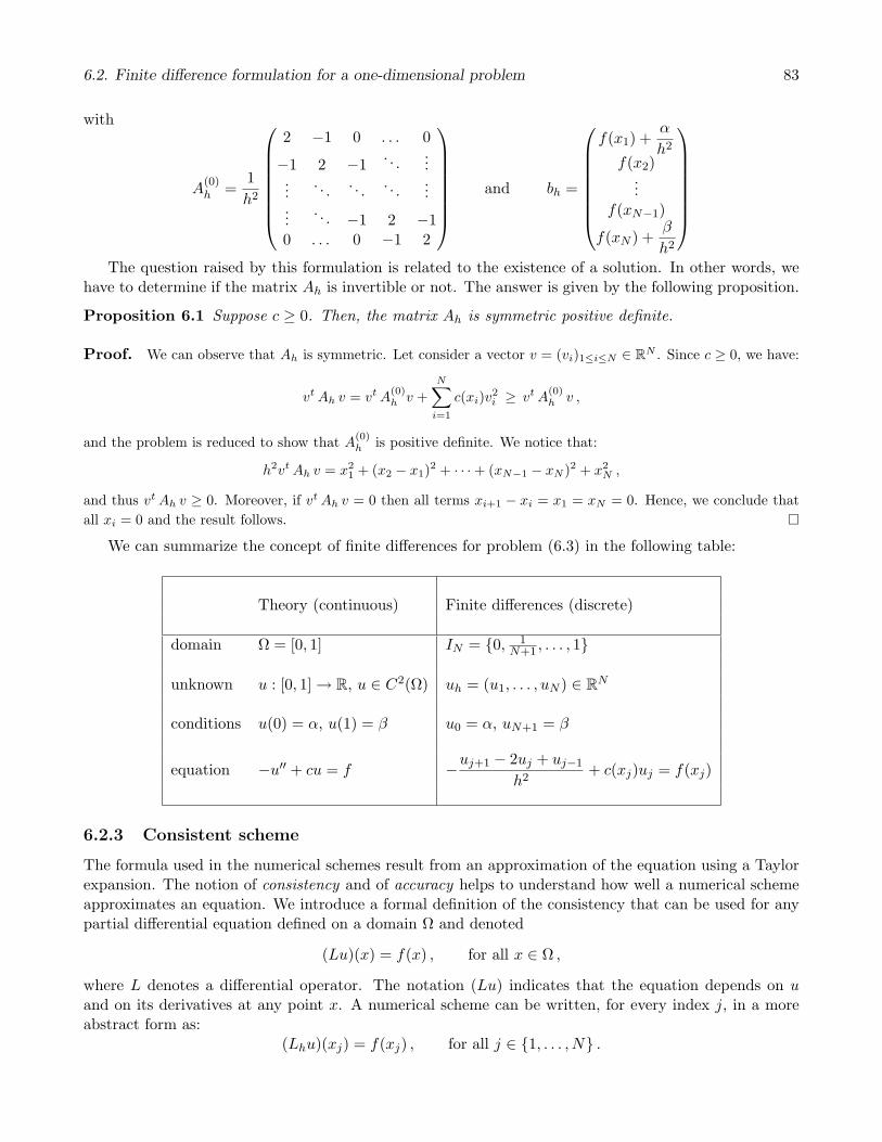
We can summarize the concept of finite di!erences for problem (6.3) in the following table:

Theory (continuous) Finite di!erences (discrete)

domain # = [0, 1] IN = {0, 1N+1 , . . . , 1}

unknown u : [0, 1] % R, u ! C2(#) uh = (u1, . . . , uN ) ! RN

conditions u(0) = ", u(1) = # u0 = ", uN+1 = #

equation "u!! + cu = f "uj+1 " 2uj + uj$1

h2+ c(xj)uj = f(xj)

6.2.3 Consistent scheme

The formula used in the numerical schemes result from an approximation of the equation using a Taylorexpansion. The notion of consistency and of accuracy helps to understand how well a numerical schemeapproximates an equation. We introduce a formal definition of the consistency that can be used for anypartial di!erential equation defined on a domain # and denoted

(Lu)(x) = f(x) , for all x ! # ,

where L denotes a di!erential operator. The notation (Lu) indicates that the equation depends on uand on its derivatives at any point x. A numerical scheme can be written, for every index j, in a moreabstract form as:

(Lhu)(xj) = f(xj) , for all j ! {1, . . . , N} .


For example, in the boundary value problem (6.3), the operator L is

(Lu)(x) = "u!!(x) + c(x)u(x) ,

and the problem can be written in the following form:find u ! C2(#) such that

(Lu)(x) = f(x) , for all x ! # . (6.5)

We define the operator Lh by:

(Lhu)(xj) = "u(xj+1)" 2u(xj) + u(xj$1)h2

+ c(xj)u(xj) , j ! {1, . . . , N}

and the discrete problem (6.4) can be formulated as follows:find u such that

(Lhu)(xj) = f(xj) , for all j ! {1, . . . , N} . (6.6)

Definition 6.2 A finite di!erence scheme is said to be consistent with the partial di!erential equation itrepresents, if for any su"ciently smooth solution u of this equation, the truncation error of the scheme,corresponding to the vector $h ! RN whose components are defined as:

($h)j = (Lhu)(xj)" f(xj) , for all j ! {1, . . . , N} (6.7)

tends uniformly towards zero with respect to x, when h tends to zero, i.e. if:

limh"0

)$h)% = 0 .

Moreover, if there exists a constant C > 0, independent of u and of its derivatives, such that, for allh !]0, h0] (h0 > 0 given) we have:

)$h) # C hp ,

with p > 0, then the scheme is said to be accurate at the order p for the norm ) · ).

The definition states that the truncation error is defined by applying the di!erence operator Lh to theexact solution u. This means that a consistent scheme implies that the exact solution almost solves thediscrete problem.

Lemma 6.2 Suppose u ! C4(#). Then, the numerical scheme (6.4) is consistent and second-orderaccurate in space for the norm ) · )%.

Proof. By using the fact that "u!! + cu = f and if we suppose u ! C4(#), we have

$h(xj) = "u(xj+1)" 2u(xj) + u(xj"1)h2

+ c(xj)u(xj) + f(xj)

= "u(xj) +h2

12u(4)(!j) + c(xj)u(xj) + f(xj)

=h2

12u(4)(!j) .

where each of the !j !]xj"1, xj+1[. Hence, we have:

)$h)% # h2

12supy#!

|u(4)(y)| ,

and the result follows. !

6.3. Finite di!erence schemes for time-dependent problems 85

Remark 6.3 Since the space dimension N is related to h by the relation h(N + 1) = 1, we have:

)$h)1 = O(h) , and )$h)2 = O(h3/2) .

The consistency error is a first step toward the analysis of the convergence error of the approximationmethod. However, it is not su"cient to analyze a numerical scheme.

Theorem 6.1 Suppose c & 0 and that the solution of the problem D is of class C4(#). Then, the finitedi!erence scheme Dh is second-order convergent for the norm ) · )%. Furthermore, if u and uh aresolutions of (6.5) and (6.6), we have the following estimate:

)u" uh)% # h2

96supx#!

|u(4)(x)| .

Proof. Admitted here. !

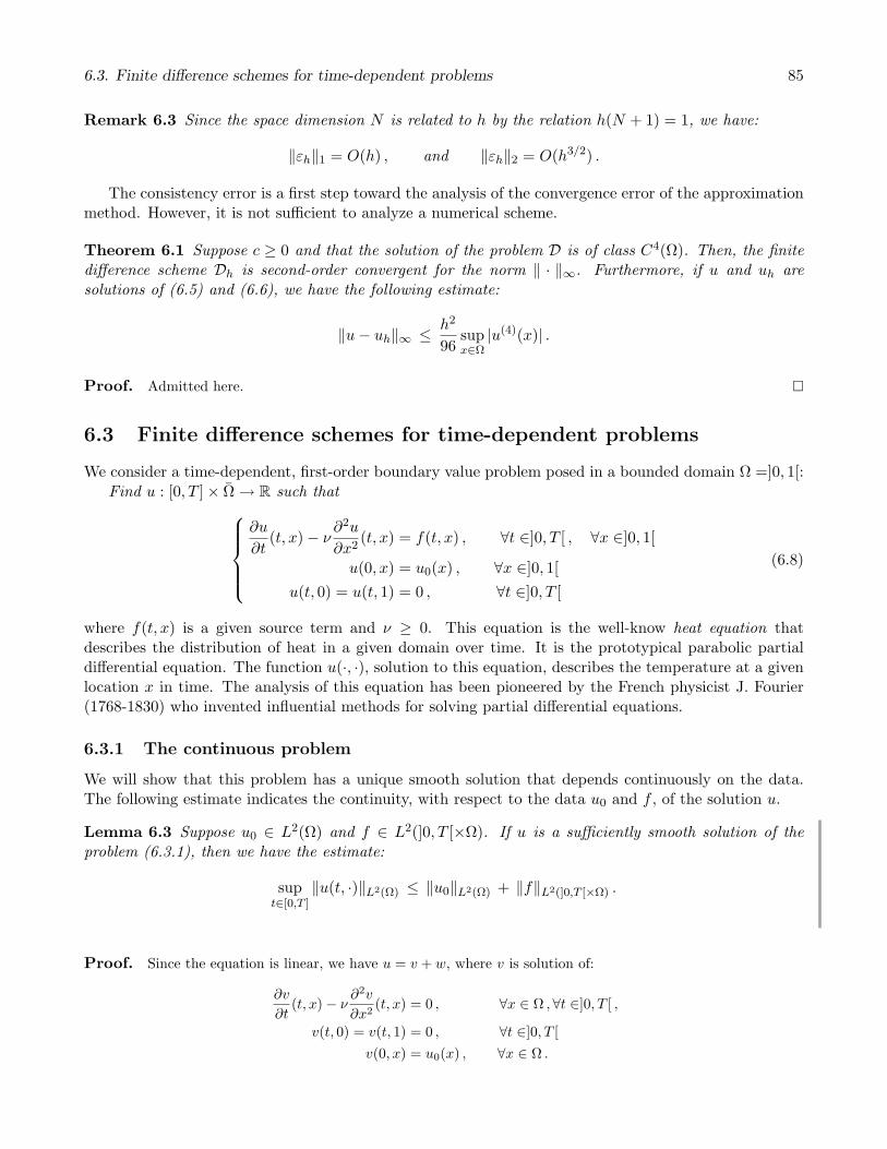
6.3 Finite di!erence schemes for time-dependent problems

We consider a time-dependent, first-order boundary value problem posed in a bounded domain # =]0, 1[:Find u : [0, T ]* # % R such that

$...%

...&

%u

%t(t, x)" &

%2u

%x2(t, x) = f(t, x) , +t !]0, T [ , +x !]0, 1[

u(0, x) = u0(x) , +x !]0, 1[u(t, 0) = u(t, 1) = 0 , +t !]0, T [

(6.8)

where f(t, x) is a given source term and & & 0. This equation is the well-know heat equation thatdescribes the distribution of heat in a given domain over time. It is the prototypical parabolic partialdi!erential equation. The function u(·, ·), solution to this equation, describes the temperature at a givenlocation x in time. The analysis of this equation has been pioneered by the French physicist J. Fourier(1768-1830) who invented influential methods for solving partial di!erential equations.

6.3.1 The continuous problem

We will show that this problem has a unique smooth solution that depends continuously on the data.The following estimate indicates the continuity, with respect to the data u0 and f , of the solution u.

Lemma 6.3 Suppose u0 ! L2(#) and f ! L2(]0, T [*#). If u is a su"ciently smooth solution of theproblem (6.3.1), then we have the estimate:

supt#[0,T ]

)u(t, ·))L2(!) # )u0)L2(!) + )f)L2(]0,T ['!) .

Proof. Since the equation is linear, we have u = v + w, where v is solution of:

%v

%t(t, x)" &

%2v

%x2(t, x) = 0 , +x ! # ,+t !]0, T [ ,

v(t, 0) = v(t, 1) = 0 , +t !]0, T [v(0, x) = u0(x) , +x ! # .


and similarly, w is solution of:

%w

%t(t, x)" &

%2w

%x2(t, x) = f(t, x) , +x ! # ,+t !]0, T [ ,

w(t, 0) = w(t, 1) = 0 , +t !]0, T [w(0, x) = 0 , +x ! # .

Hence, we can consider these two problems separately for v and w. Concerning the first problem, we multiply theequation by v(x, t) and integrate it with respect to x !]0, 1[. Applying the chain rule and the integration by parts,and taking into account the homogenous boundary conditions, yields the following result:

12

d

dt

/#

!v2(t, x) dx

0+ &

#

!

/%v

%x(t, x)

02

dx = 0 .

Since the second term is positive, we deduce:

+t !]0, T [ ,d

dt

/#

!v2(t, x) dx

0# 0 .

Now, we integrate with respect to the variable t !]0, s[, s ! [0, T ] and thus we obtain:

+s ! [0, T ] , )v(s, ·))2L2(!) # )u0)2L2(!) .

We proceed accordingly for the term w, to obtain:

12

d

dt

/#

!w2(t, x) dx

0+ &

#

!

/%w

%x(t, x)

02

dx =#

!(fw)(t, x) dx

# )f(t, ·))L2(!) )w(t, ·))L2(!) .

Poincare’s inequality leads to the estimate:

)w(t, ·))L2(!) # Cp

1111%w

%t(t, ·)

1111L2(!)

,

and thus we have (noticing that 2ab # (a2 + b2)):

12

d

dt)w(t, ·))2L2(!) + &

1111%w

%t(t, ·)

11112

L2(!)

# )f(t, ·))L2(!)

1111%w

%t(t, ·)

1111L2(!)

# 12

2)f(t, ·))2L2(!) +

1111%w

%x(t, ·)

11112

L2(!)

3.

Hence we can conclude that

d

dt)w(t, ·))2L2(!) #

d

dt)w(t, ·))2L2(!) + (2& " 1)

1111%w

%x(t, ·)

11112

L2(!)

# )f(t, ·))2L2(!) .

We integrate on ]0, s[ for s ! [0, T ] and taking into account the initial condition w(x, 0) = 0, we obtain:

+s ! [0, T ] , )w(s, ·))2L2(!) ##

!)f(s, ·))2L2(!) ds #

4)f)L2(!)

52,

and, by combining this estimate with the estimate on v, the results follows. !This results is important as it provides the uniqueness of a regular solution.

Corollary 6.1 Suppose u0 ! L2(#) and f ! L2(]0, T [*#). Then, if the problem (6.3.1) has a regularsolution, this solution is unique.


Proof. Suppose u1(t, x) and u2(t, x) are to regular solutions of the problem (6.3.1). Then, if we denote theirdi!erence by u = u1 " u2, we obtain a problem similar to the initial one but where both the initial data u0 andthe source term are zero: $

..%

..&

%u

%t(t, x)" &

%2u

%x2(t, x) = 0 , +(t, x) ! R&+ * #

u(0, x) = 0 , +x ! #u(t, x) = 0 , +(t, x) ! R&+ * %#

Then, using the previous estimate to this problem, we conclude that

supt#[0,T ]

)u(t, ·))L2(!) # 0 ,

and thus u = u1 " u2 = 0, the regular solutions are identical. !

Energy estimate

It is common to introduce the notion of energy of the solution u at time t as:

E(t) =12

#

!u2(t, x) dx =

12)u(t, ·))2L2(!) (6.9)

This is not the physical energy of the system but rather a mathematical tool used to analyze the behaviorof the solution. We shall see that using Lemma 6.3 and without the source term f , the energy is a non-increasing function of time. This result clearly indicates that this energy is controlled at any time t bythe energy at the initial time t = 0, which is given. This important property of the heat equation mustbe preserved in the numerical resolution of the problem.

We introduce a preliminary result before giving an energy estimate.

Lemma 6.4 (Gronwall) Let ",# be two real numbers and let u be a nonnegative real-valued functiondefined on R+ such that:

u(t) # " + #

# t

0u(s) ds , t ! R+ ,

then u(t) # " exp(#t).

Proof. Define v(t) = "+#

# t

0u(s) ds, t ! R+ so that v(t) & u(t) & 0. Taking the derivative and using the chain

rule leads to v!(t) = #v(t) # #v(t), and thus

v!(t)" #v(t) # 0 , t & 0 .

Multiplying by exp("#t) and integrating between 0 and t yields# t

0exp("#s)v!(s) ds" #v(s)) ds # 0 .

and after integrating by parts we have:#

!exp("#s)v!(s) ds = #

# t

0exp("#s)v(s) ds + exp("#t)v(t)" v(0) ,

and finally the result follows: v(t) # v(0) exp(#t) = " exp(#t). !

Lemma 6.5 (Energy estimate) Suppose u0 ! L2(#) and f ! L2(]0, T [*#). If u is a solution ofproblem (6.3.1) su"ciently smooth, then we have the following estimate:

#

!u2(t, x) dx # exp(t)

/#

!u2

0(x) dx +# t

0

#

!f2(t, s) dxds

0.


Proof. We proceed as previously, multiply the equation (6.3.1) by u and integrate with respect to the variablex and then t to obtain:

#

!u2(t, x) dx"

#

!u2

O(x) dx + 2&

# t

0

#

!

/%u

%x(s, x)

02

dxds

= 2#

!f(s, x)u(s, x) dxds

## t

0

#

!f2(s, x) dxds +

# t

0

#

!u2(s, x) dxds .

and we deduce: #

!u2(t, x) dx #

#

!u2

0(x) dx +# T

0

#

!f2(s, x) dxds +

# t

0

#

!u2(s, x) dxds .

Now, we invoke the Gronwall’s lemma with

" =#

!u2

0(x) dx +# T

0

#

!f2(, x) dxds and # = 1 ,

to obtain: #

!u2(s, x) dx # exp(t)

2#

!u2

0(x) dx +# T

0

#

!f2(s, x) dxds

3, +T > 0 ,

and the results follows. !The estimates given by Lemmas 6.3 and 6.5 are often referred to as a stability estimates, since they

express that the size of the solution can be bounded by the size of the initial data u0 and f . A consequenceof these results is that small perturbations of order $ of the initial data lead to small perturbations ofthe same order of the solution.

Corollary 6.2 Suppose the initial data u0 and f are slightly perturbated and replaced by new data u0,! !L2(#) and f! ! L2(]0, T [*#) such that:

)u0 " u0,!)L2(!) # $ , and )f " f!)L2(]0,T ['!) # $ .

Then, if u!(t, ·) denotes the new solution of the problem (6.3.1), we have the estimate:

supt#[0,T ]

)u(t, ·)" u!(t, ·))L2(!) # )u0 " u0,!)L2(!) + )f " f!)L2(]0,T ['!) # 2$ .

Proof. Since the problem (6.3.1) is linear, u " u! solves the problem for the source term f " f! and the initialdata u0 " u0,!. It is easy to see that for every t ! [0, T ] we have:

)u(t, ·)" u!(t, ·))L2(!) # )u0 " u0,!)L2(!) + )f " f!)L2(]0,T ['!) # 2$ .

and the results follows. !

6.3.2 Existence of a weak solution

In this section, we will briefly concentrate on the problem (6.3.1) with u0 ! L2(#) and f ! L2(]0, T [*#).Suppose the solution u(t, ·) ! H2(#) for almost every t !]0, T [. Let consider a test function v ! H1

0 (#)such that: #

!

%u

%t(t, x)v(x) dx" &

#

!

%2u

%x2(t, x)v(x) dx =

#

!f(t, x)v(x) dx .


Using the chain rule and integrating by parts, we obtain, for all v ! H10 (#):

#

!

%u

%t(t, x)v(x) dx + &

#

!

%u

%x(t, x)

dv

dx(x) dx =

#

!f(t, x)v(x) dx .

We introduce a bilinear continuous and elliptic form a(·, ·) defined as:

a(w, v) = ,w!, v!-L2(!) =#

!w!(x)v!(x) dx ,

that allows to write the previous problem (6.3.1) in a more compact form, for all v ! H10 (#):

$%

&

d

dt,u(t, ·), v-L2(!) + &a(u(t, ·), v) = ,f(t, ·), v-L2(!) ,

,u(0, ·), v-L2(!) = ,u0, v-L2(!) ,(6.10)

We give then the following result.

Theorem 6.2 Suppose u0 ! L2(#) and f ! L2(]0, T [*#). Then, the problem (6.10) has a uniquesolution u ! C0([0, T ];L2(#)) . L2({0, T};H1

0 (#)). Furthermore, we have the following energy estimate,for all t ! [0, T ]:

)u(t, ·))L2(!) # )u0)L2(!) exp("'2t) +# t

0)f(s, ·))L2(!) exp("'2(t" s)) ds .

Proof. We refer the reader to [Allaire, 2005, Lucquin, 2004] for a proof of this result. ! Thisenergy estimate shows that the solution of the problem (6.10) depends continuously on the data and thusthat the problem is well-posed. Moreover, the energy space C0([0, T ];L2(#)) . L2({0, T};H1

0 (#)) is theminimum regularity space in which the energy equalities are meaningfull.

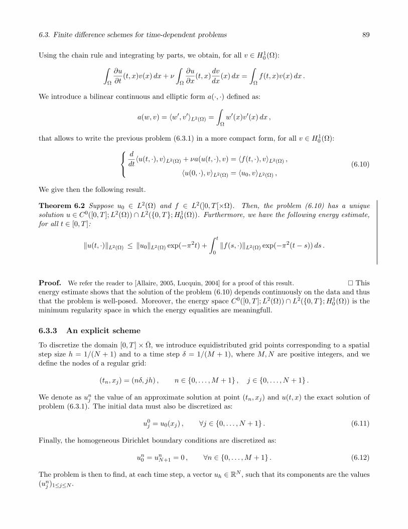
6.3.3 An explicit scheme

To discretize the domain [0, T ] * #, we introduce equidistributed grid points corresponding to a spatialstep size h = 1/(N + 1) and to a time step ( = 1/(M + 1), where M,N are positive integers, and wedefine the nodes of a regular grid:

(tn, xj) = (n(, jh) , n ! {0, . . . ,M + 1} , j ! {0, . . . , N + 1} .

We denote as unj the value of an approximate solution at point (tn, xj) and u(t, x) the exact solution of

problem (6.3.1). The initial data must also be discretized as:

u0j = u0(xj) , +j ! {0, . . . , N + 1} . (6.11)

Finally, the homogeneous Dirichlet boundary conditions are discretized as:

un0 = un

N+1 = 0 , +n ! {0, . . . ,M + 1} . (6.12)

The problem is then to find, at each time step, a vector uh ! RN , such that its components are the values(un

j )1&j&N .


Introducing the approximation of the second-order space derivative given by formula (6.2), and con-sidering a forward di!erence approximation for the time derivative:

%u

%t(tn, xj) /

un+1j " un

j

(,

we obtain the following scheme coupled with the initial (6.11) and boundary conditions (6.12), for n !{0, . . . ,M} and j = {1, . . . , N}:

un+1j " un

j

(" &

unj+1 " 2un

j + unj$1

h2= f(tn, xj) . (6.13)

This scheme is called explicit because the values (un+1j )1&j&N at time tn+1 are computed using the values

on the previous time level tn. Indeed, this system can be written in a vector form as:

Un+1 " Un

(+ AhUn = Cn , +n ! {0, . . . ,M} ,

where the matrix Ah and the vector Cn are defined as:

Ah =&

h2

'

((((((()

2 "1 0 . . . 0

"1 2 "1 . . . ...... . . . . . . . . . ...... . . . "1 2 "10 . . . 0 "1 2

*

+++++++,

and Cn =

'

(((()

f(t1, x1)......

f(tj , xN )

*

++++,. (6.14)

and with the initial data:

U0 =

'

()u0

1...

u0N

*

+, .

To analyze the numerical scheme, we introduce a norm on RN :

)u)p =

'

)N-

j=1

h|uj |p*

,1/p

, +1 # p # +0 (6.15)

where the limit case corresponds to )u)% = max1&j&N |uj |. Notice that this norm depends on the stepsize h = 1/N + 1. Through the weight parameter h, the norm )u)p is identical to the Lp(#) norm forpiecewise constant functions on each interval [xj , xj+1[ of the domain # = [0, 1].

Lemma 6.6 The numerical scheme (6.13) is consistent and first-order accurate in time for the norm) · )% and second-order accurate in space for the norm ) · )2.

Proof. Let consider a C2 continuous in time and C4 continuous in space function u(t, x). We write:

$h(u)nj =

u(tn+1, xj)" u(tn, xj)(

" &u(tn, xj+1)" 2u(tn, xj) + u(tn, xj"1)

h2" f(tn, xj) .

If u is solution of the heat equation then we have:

$h(u)nj = Aj " &Bj ,


where we posed

Aj =u(tn+1, xj)" u(tn, xj)

(" %u

%t(tn, xj) ,

Bj =u(tn, xj+1)" 2u(tn, xj) + u(tn, xj"1)

h2" %2u

%x2(tn, xj)

Using a Taylor expansion with respect to the time variable (xj being fixed) we obtain, for ) !]tn, tn+1[:

u(tn+1, xj) = u(tn, xj) + (%u

%t(tn, xj) +

(2

2%2u

%t2(), xj) ,

and thusAi =

(

2%2u

%t2(), xj) ,

and similarly for Bi we obtain for ! !]xj , xj+1[ (cf. Lemma (6.2)):

Bi =h2

12%4u

%x4(tn, !) ,

We obtain easily the consistency and the order of accuracy of the explicit scheme from this formulas. !

Corollary 6.3 If the ratio &(/h2 = 1/6 is kept constant when ( and h tend towards zero, then the explicitscheme (6.13) is second-order accurate in time and fourth-order accurate in space.

6.3.4 Other schemes

Changing the approximation of the time derivative for a backward di!erence would have resulted in thefollowing implicit scheme:

unj " un$1

j

(" &

unj+1 " 2un

j + unj$1

h2= f(tn, xj) . (6.16)

that requires solving a system of linear equations to compute the values (unj )1&j&N at time tn using the

values of the previous time level tn$1. The scheme can be written in vector form as:

Un " Un$1

(+ AhUn = Cn , +n ! {1, . . . ,M + 1} , (6.17)

where the matrix Ah and the vectors Cn and U0 are identical to the corresponding terms in the explicitscheme (6.13). However, computing the values un

j with respect to the values un$1j requires finding the

inverse of the tridiagonal matrix Ah.

Proposition 6.2 The matrix Ah is positive definite and thus is invertible.

Lemma 6.7 The numerical scheme (6.17) is consistent and first-order accurate in time for the norm) · )% and second-order accurate in space for the norm ) · )2.

Proof. Left as an exercise. !Using a convex combination of the explicit and implicit schemes, we define for 0 # * # 1, the so-called

*-scheme:

unj " un$1

j

("*&

unj+1 " 2un

j + unj$1

h2"(1"*)&

un$1j+1 " 2un$1

j + un$1j$1

h2= *f(tn, xj)+(1"*)f(tn$1, xj) , (6.18)

that gives the explicit (resp. implicit) scheme if * = 0 (resp. * = 1). Notice that this scheme is implicitfor * '= 0. For the value * = 1/2, the scheme is called the Crank-Nicholson scheme.


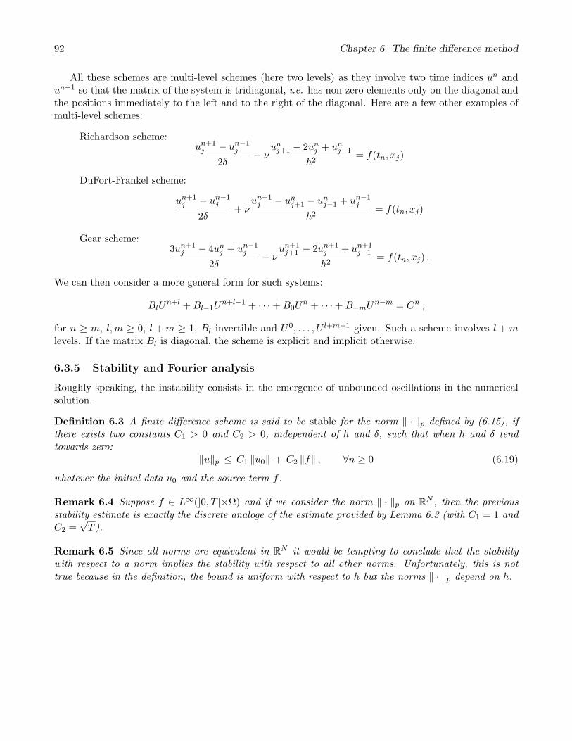
All these schemes are multi-level schemes (here two levels) as they involve two time indices un andun$1 so that the matrix of the system is tridiagonal, i.e. has non-zero elements only on the diagonal andthe positions immediately to the left and to the right of the diagonal. Here are a few other examples ofmulti-level schemes:

Richardson scheme:un+1

j " un$1j

2(" &

unj+1 " 2un

j + unj$1

h2= f(tn, xj)

DuFort-Frankel scheme:

un+1j " un$1

j

2(+ &

un+1j " un

j+1 " unj$1 + un$1

j

h2= f(tn, xj)

Gear scheme:3un+1

j " 4unj + un$1

j

2(" &

un+1j+1 " 2un+1

j + un+1j$1

h2= f(tn, xj) .

We can then consider a more general form for such systems:

BlUn+l + Bl$1U

n+l$1 + · · · + B0Un + · · · + B$mUn$m = Cn ,

for n & m, l,m & 0, l + m & 1, Bl invertible and U0, . . . , U l+m$1 given. Such a scheme involves l + mlevels. If the matrix Bl is diagonal, the scheme is explicit and implicit otherwise.

6.3.5 Stability and Fourier analysis

Roughly speaking, the instability consists in the emergence of unbounded oscillations in the numericalsolution.

Definition 6.3 A finite di!erence scheme is said to be stable for the norm ) · )p defined by (6.15), ifthere exists two constants C1 > 0 and C2 > 0, independent of h and (, such that when h and ( tendtowards zero:

)u)p # C1 )u0) + C2 )f) , +n & 0 (6.19)

whatever the initial data u0 and the source term f .

Remark 6.4 Suppose f ! L%(]0, T [*#) and if we consider the norm ) · )p on RN , then the previousstability estimate is exactly the discrete analoge of the estimate provided by Lemma 6.3 (with C1 = 1 andC2 =

1T ).

Remark 6.5 Since all norms are equivalent in RN it would be tempting to conclude that the stabilitywith respect to a norm implies the stability with respect to all other norms. Unfortunately, this is nottrue because in the definition, the bound is uniform with respect to h but the norms ) · )p depend on h.

The finite difference method

Documents