The FFT Via Matrix Factorizations

The FFT

Via Matrix Factorizations

A Key to Designing High Performance Implementations

Charles Van LoanDepartment of Computer Science

Cornell University

A High Level Perspective...

Blocking For Performance

A =

A11 A12 · · · A1q

A21 A22 · · · A2q... ... . . . ...

Ap1 Ap2 · · · Apq

n1

n2

nq

︸︷︷︸︸︷︷︸︸︷︷︸

n1 n2 nq

A well known strategy for high-performance Ax = b and Ax = λxsolvers.

Factoring for Performance

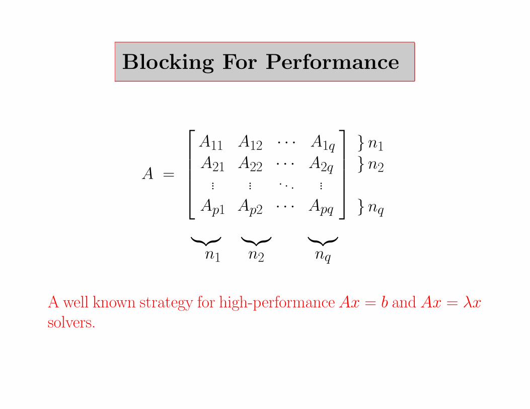
One way to execute a matrix-vector product

y = Fnx

when Fn = At · · ·A2A1 is as follows:

y = xfor k = 1:t

y = Akxend

A different factorization Fn = At · · · A1 would yield a differentalgorithm.

The Discrete Fourier Transform (n = 8)

y = F8x =

ω08 ω0

8 ω08 ω0

8 ω08 ω0

8 ω08 ω0

8

ω08 ω1

8 ω28 ω3

8 ω48 ω5

8 ω68 ω7

8

ω08 ω2

8 ω48 ω6

8 ω88 ω10

8 ω128 ω14

8

ω08 ω3

8 ω68 ω9

8 ω128 ω15

8 ω188 ω21

8

ω08 ω4

8 ω88 ω12

8 ω168 ω20

8 ω248 ω28

8

ω08 ω5

8 ω108 ω15

8 ω208 ω25

8 ω308 ω35

8

ω08 ω6

8 ω128 ω18

8 ω248 ω30

8 ω368 ω42

8

ω08 ω7

8 ω148 ω21

8 ω288 ω35

8 ω428 ω49

8

x

ω8 = cos(2π/8) − i · sin(2π/8)

The DFT Matrix In General...

If ωn = cos(2π/n)− i · sin(2π/n) then

[Fn]pq = ωpqn

= (cos(2π/n) − i · sin(2π/n))pq

= cos(2pqπ/n) − i · sin(2pqπ/n)

Fact:

FHn Fn = nIn

Thus, Fn/√

n is unitary.

Data Sparse Matrices

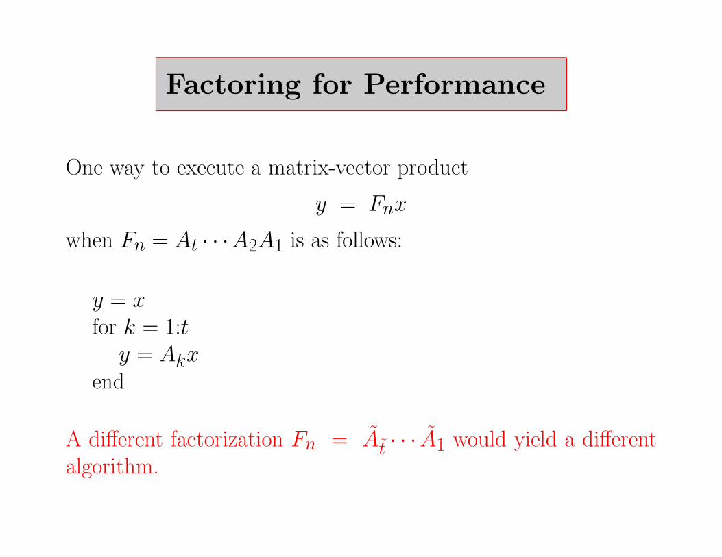
An n-by-n matrix A is data sparse if it can be represented withmany fewer than n2 numbers.

Example 1.A has lots of zeros. (“Traditional Sparse”)

Example 2.A is Toeplitz...

A =

a b c de a b cf e a bg f e a

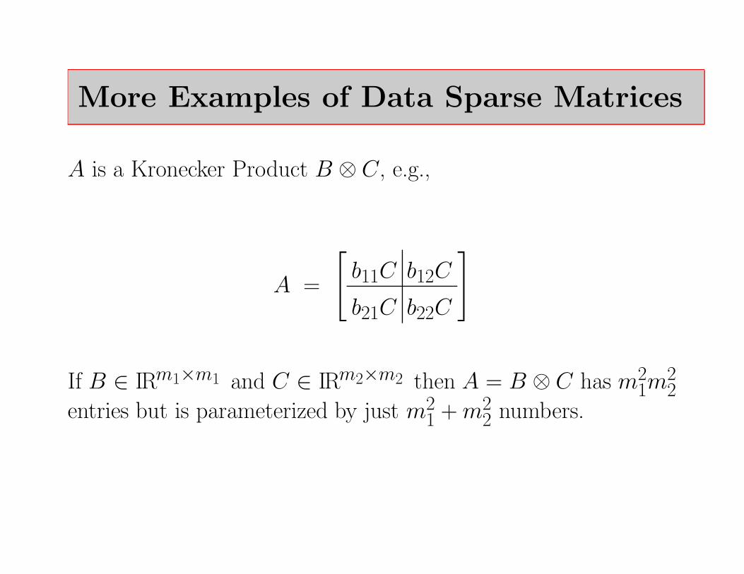
More Examples of Data Sparse Matrices

A is a Kronecker Product B ⊗ C, e.g.,

A =

[

b11C b12C

b21C b22C

]

If B ∈ IRm1×m1 and C ∈ IRm2×m2 then A = B ⊗ C has m21m

22

entries but is parameterized by just m21 + m2

2 numbers.

Extreme Data Sparsity

A =

n∑

i=1

n∑

j=1

n∑

k=1

n∑

`=1

S(i, j, k, `) · (2-by-2)⊗ · · · ⊗ (2-by-2)︸︷︷︸

d times

A is 2d -by-2d but is parameterized by O(dn4) numbers.

Factorization of Fn

The DFT matrix can be factored into a short product of sparsematrices, e.g.,

F1024 = A10 · · ·A2A1P1024

where each A-matrix has 2 nonzeros per row and P1024 is a per-mutation.

From Factorization to Algorithm

If n = 210 and

Fn = A10 · · ·A2A1Pn

then

y = Pnx

for k = 1:10

y = Akx ← 2n flops.

end

computes y = Fnx and requires O(n log n) flops.

Recursive Block Structure

F8(:, [ 0 2 4 6 1 3 5 7 ]) =

1 0 0 0 1 0 0 00 1 0 0 0 ω8 0 0

0 0 1 0 0 0 ω28 0

0 0 0 1 0 0 0 ω38

1 0 0 0 −1 0 0 00 1 0 0 0 −ω8 0 0

0 0 1 0 0 0 −ω28 0

0 0 0 1 0 0 0 −ω38

[F4 0

0 F4

]

Fn/2 “shows up” when you permute the columns of Fn so thatthe odd-indexed columns come first.

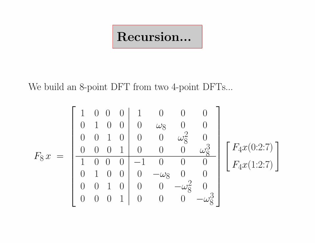
Recursion...

We build an 8-point DFT from two 4-point DFTs...

F8 x =

1 0 0 0 1 0 0 00 1 0 0 0 ω8 0 0

0 0 1 0 0 0 ω28 0

0 0 0 1 0 0 0 ω38

1 0 0 0 −1 0 0 00 1 0 0 0 −ω8 0 0

0 0 1 0 0 0 −ω28 0

0 0 0 1 0 0 0 −ω38

[F4x(0:2:7)

F4x(1:2:7)

]

Radix-2 FFT: Recursive Implementation

function y =fft(x, n)if n = 1

y = xelse

m = n/2; ω = exp(−2πi/n)

Ω = diag(1, ω, . . . , ωm−1)

zT = fft(x(0:2:n− 1),m)

zB = Ω· fft(x(1:2:n− 1),m)

y =

[Im Im

Im −Im

] [zT

zB

]

Overall: 5n log n flops.

end

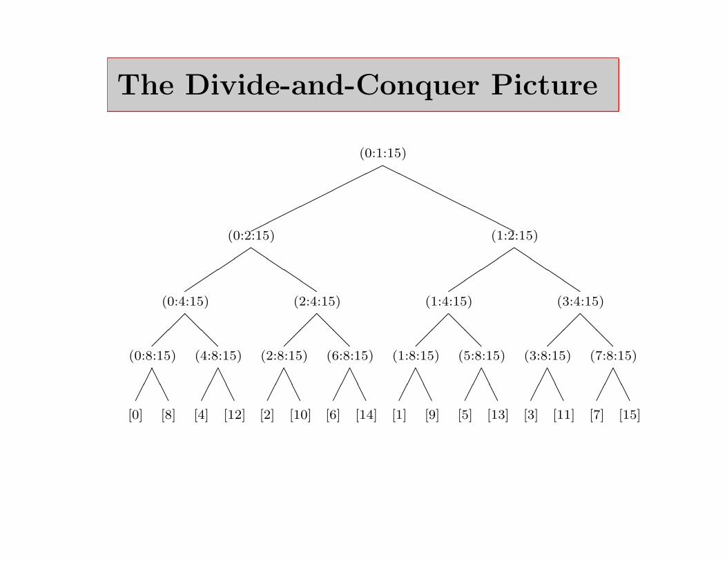
The Divide-and-Conquer Picture

(0:8:15)

[0] [8]

AA

(4:8:15)

[4] [12]

AA

(2:8:15)

[2] [10]

AA

(6:8:15)

[6] [14]

AA

(1:8:15)

[1] [9]

AA

(5:8:15)

[5] [13]

AA

(3:8:15)

[3] [11]

AA

(7:8:15)

[7] [15]

AA

(0:4:15)

@@

(2:4:15)

@@

(1:4:15)

@@

(3:4:15)

@@

(0:2:15)

QQ

QQ

(1:2:15)

QQ

QQ

(0:1:15)

HHHHHHHH

Towards a Nonrecursive Implementation

The Radix-2 Factorization...

If n = 2m and

Ωm = diag(1, ωn, . . . , ωm−1n ),

then

FnΠn =

[Fm ΩmFm

Fm −ΩmFm

]

=

[Im Ωm

Im −Ωm

]

(I2⊗ Fm).

where Πn = In(:, [0:2:n 1:2:n]).

Note: I2 ⊗ Fm =

[Fm 00 Fm

]

.

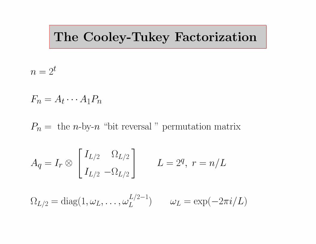
The Cooley-Tukey Factorization

n = 2t

Fn = At · · ·A1Pn

Pn = the n-by-n “bit reversal ” permutation matrix

Aq = Ir ⊗[

IL/2 ΩL/2

IL/2 −ΩL/2

]

L = 2q, r = n/L

ΩL/2 = diag(1, ωL, . . . , ωL/2−1L ) ωL = exp(−2πi/L)

The Bit Reversal Permutation

(0:8:15)

[0] [8]

AA

(4:8:15)

[4] [12]

AA

(2:8:15)

[2] [10]

AA

(6:8:15)

[6] [14]

AA

(1:8:15)

[1] [9]

AA

(5:8:15)

[5] [13]

AA

(3:8:15)

[3] [11]

AA

(7:8:15)

[7] [15]

AA

(0:4:15)

@@

(2:4:15)

@@

(1:4:15)

@@

(3:4:15)

@@

(0:2:15)

QQ

QQ

(1:2:15)

QQ

QQ

(0:1:15)

HHHHHHHH

Bit Reversal

x(0)x(1)x(2)x(3)x(4)x(5)x(6)x(7)x(8)x(9)x(10)x(11)x(12)x(13)x(14)x(15)

=


→


=


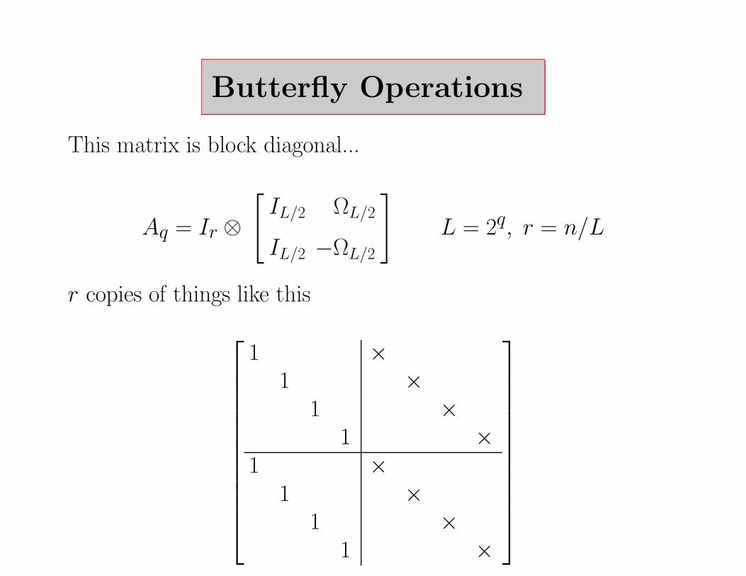
Butterfly Operations

This matrix is block diagonal...

Aq = Ir ⊗[

IL/2 ΩL/2

IL/2 −ΩL/2

]

L = 2q, r = n/L

r copies of things like this

1 ×1 ×

1 ×1 ×

1 ×1 ×

1 ×1 ×

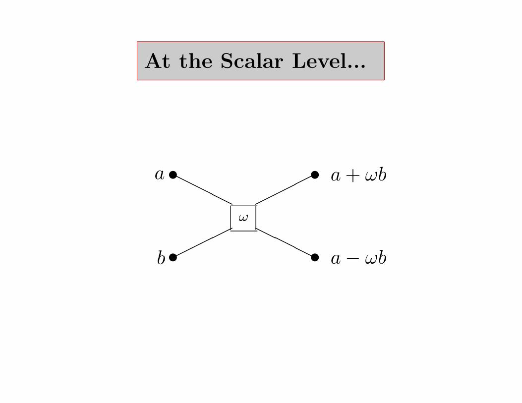
At the Scalar Level...

s

sHHHω

sHHH

s

b

a

a− ωb

a + ωb

Signal Flow Graph (n = 8)

x0

x4

x2

x6

x1

x5

x3

x7 s

s

s

s

s

s

s

s

HHH

HHH

HHH

HHH

HHH

HHH

HHH

HHH

ω08

ω08

ω08

ω08

s

s

s

s

s

s

s

s

@@

@@

@@

@@

@@

@@

@@

@@

@@

@@

@@

@@

@@

@@

@@

@@

ω28

ω08

ω28

ω08

s

s

s

s

s

s

s

s

AAAAAAAA

AAAAAAAA

AAAAAAAA

AAAAAAAA

AA

AA

AA

AA

AA

AA

AA

AA

AA

AA

AA

AA

AA

AA

AA

AA

ω38

ω28

ω18

ω08

s

s

s

s

s

s

s

s y0

y1

y2

y3

y4

y5

y6

y7

The Transposed Stockham Factorization

If n = 2t, then

Fn = St · · ·S2S1,

where for q = 1:t the factor Sq = AqΓq−1 is defined by

Aq = Ir ⊗BL, L = 2q, r = n/L,

Γq−1 = Πr∗ ⊗ IL∗, L∗ = L/2, r∗ = 2r,

BL =

[IL∗ ΩL∗IL∗ −ΩL∗

]

,

ΩL∗ = diag(1, ωL, . . . , ωL∗−1L ).

Perfect Shuffle

(Π4 ⊗ I2)

x0x1x2x3x4x5x6x7

=

x0x1x4x5x2x3x6x7

Cooley-Tukey Array Interpretation

Step q:

︸︷︷︸

r=n/L

k

L=2q−→

2k 2k+1

︸︷︷︸

r∗=n/L∗

L∗=2q−1

8

>

<

>

:

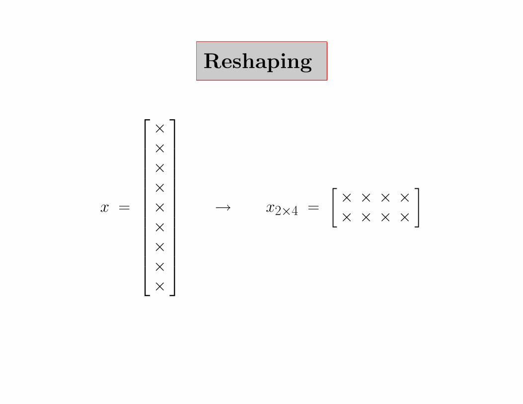
Reshaping

x =

×××××××××

→ x2×4 =

[× × × ×× × × ×

]

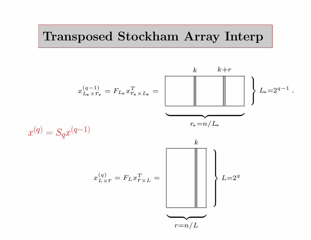
Transposed Stockham Array Interp

k k+r

x(q−1)L∗×r∗ = FL∗

xTr∗×L∗

=

︸︷︷︸

r∗=n/L∗

9

>

=

>

;

L∗=2q−1 .

x(q) = Sqx(q−1)

k

x(q)L×r = FLxT

r×L =

︸︷︷︸

r=n/L

9

>

>

>

>

>

>

>

>

=

>

>

>

>

>

>

>

>

;

L=2q

2× 2× 2 Basic Radix-2 Versions

Store intermediate DFTs by row or column

Intermediate DFTs adjacent or not.

How the two butterfly loops are ordered.

x =

(

Ir ⊗[

IL/2 ΩL/2

IL/2 −ΩL/2

])

x L = 2q, r = n/L

The Gentleman-Sande Idea

It can be shown that FTn = Fn and so if

Fn = At · · ·A1PTn

then

Fn = FTn = PnAT

1 · · ·ATt

and we can compute y = Fnx as follows...

y = xfor k = t:− 1:1

y = ATk x

endy = Pny

Convolution and Other Aps

From “problem space” to “DFT space” viafor k = t:− 1:1

x = ATk x

endx = Pnx

Do your thing in DFT space. Then inverse transform back toProblem space via

x = PTn x

for k = 1:tx = Akx

endx = x/n

Can avoid the Pn ops by working in “scrambled” DFT space.

Radix-4

Can combine four quarter-length DFTs to produce a single full-length DFT:

v =

I I I II−iI−I iII −I I −II iI−I−iI

abcd

=

(a + c)+ (b + d)(a− c)−i(b− d)(a + c)− (b + d)(a− c)+i(b− d)

,

The radix-4 butterfly.

Better re-use of data.

Fewer flops. Radix-4 FFT is 4.25n log n (instead of 5n log n).

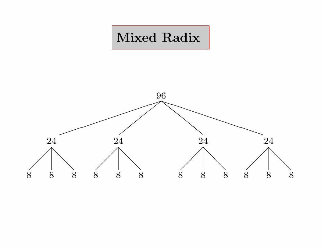
Mixed Radix

96

##

##

cc

cc

PPPPPPPPP24

@@

8 88

24

@@

8 88

24

@@

8 88

24

@@

8 88

Multiple DFTs

Given: n1-by-n2 matrix X .

Multicolumn DFT Problem...

X ← Fn1X

Multirow DFT Problem...

X ← XFn2

Blocked Multiple DFTs

X ← Fn1X becomes

[X1 | X2 | · · · | Xp

]←[Fn1X1 | Fn1X2 | · · · | Fn1Xp

]

The 4-Step Framework

A matrix reshaping of the x← Fnx operation when n = n1n2:

xn1×n2 ← xn1×n2Fn2 Multiple row DFT

xn1×n2 ← Fn(0:n1 − 1, 0:n2 − 1).∗ xn1×n2 Pointwise multiply

xn2×n1 ← xTn1×n2

Transpose

xn2×n1 ← xn2×n1Fn1 Multiple row DFT .

Can be arranged so communication is concentrated in the trans-pose step.

Distributed Transpose: Example

Initial:

X =

X00 X01 X02 X03X10 X11 X12 X13X20 X21 X22 X23X30 X31 X32 X33

.

Transpose each block:

X ←

XT00 XT

01 XT02 XT

03

XT10 XT

11 XT12 XT

13

XT20 XT

21 XT22 XT

23

XT30 XT

31 XT32 XT

33

.

Now regard as 2-by-2 and block transpose each block:

X ←

XT00 XT

10 XT02 XT

12

XT01 XT

11 XT03 XT

13

XT20 XT

30 XT22 XT

32

XT21 XT

31 XT23 XT

33

.

Now do a 2-by-2 block transpose:

X ←

XT00 XT

10 XT20 XT

30

XT01 XT

11 XT21 XT

31

XT02 XT

12 XT22 XT

32

XT03 XT

13 XT23 XT

33

.

Factorization and Transpose

xn×m ← xTm×n

corresponds to

x← P (m,n)x

where P (m,n) is a perfect shuffle permutation, e.g.,

P (3, 4) = I12(:, [0 3 6 9 1 4 7 10 2 5 8 11])

Different multi-pass transposition algorithms correspond to differ-ent factorizations of P (m,n).

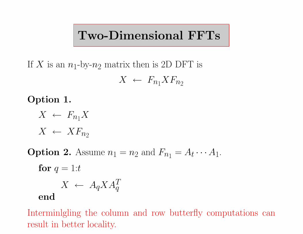
Two-Dimensional FFTs

If X is an n1-by-n2 matrix then is 2D DFT is

X ← Fn1XFn2

Option 1.

X ← Fn1X

X ← XFn2

Option 2. Assume n1 = n2 and Fn1 = At · · ·A1.

for q = 1:t

X ← AqXATq

end

Interminlgling the column and row butterfly computations canresult in better locality.

3-Dimensional DFTs

Given X(1:n1, 1:n2, 1:n3), apply DFT in each of the three dimen-sions.

If

x = reshape(X(1:n1, 1:n2, 1:n3), n1n2n3, 1)

then the problem is to compute

x ← (Fn3⊗ Fn2

⊗ Fn1)x

i.e.,x ← (In3

⊗ In2⊗ Fn1)x

x ← (In3⊗ Fn2

⊗ In1)xx ← (Fn3

⊗ In2⊗ In1)x

d-Dimensional DFTs

Sample for d = 5:

µ = 1X(α1, α2, α3, α4, α5)X(α2, α3, α4, α5, α1)

Fn1

ΠTn1,n

µ = 2X(α2, α3, α4, α5, α1)X(α3, α4, α5, α1, α2)

Fn2

ΠTn2,n

µ = 3X(α3, α4, α5, α1, α2)X(α4, α5, α1, α2, α3)

Fn3

ΠTn3,n

µ = 4X(α4, α5, α1, α2, α3)X(α5, α1, α2, α3, α4)

Fn4

ΠTn4,n

µ = 5X(α5, α1, α2, α3, α4)X(α1, α2, α3, α4, α5)

Fn5

ΠTn5,n

Intemingling of component DFTs and tensor transpositions.

References

FFTW: http:www.fftw.org

C. Van Loan (1992). Computational Frameworks for the Fast

Fourier Transform, SIAM Publications, Philadelphia, PA.

The FFT Via Matrix Factorizations

Documents