The Fast Fourier Transform and Applications to Multiplicationreif/courses/alglectures/reif.lectures/ALG3.2.pdf · Fast Fourier Transform • Viewed as Evaluation Problem: naïve algorithm

The Fast Fourier Transform and Applications to Multiplication

Prepared by

John Reif, Ph.D.

Analysis of Algorithms

Topics and Readings: - The Fast Fourier Transform Advanced Material : - Using FFT to solve other Multipoint Evaluation Problems - Applications to Multiplication

•  Reading Selection: •  CLR, Chapter 30

Nth Roots of Unity

•  Assume Commutative Ring (R,+,·, 0,1)

•  ω is principal nth root of unity if

–  ωk ≠ 1 for k = 1, …, n-1

–  ωn = 1, and

•  Example: for complex numbers

n-1jp

j=0

0 for 1 p nω = ≤ ≤∑

2 i/ne πω =

Example of nth Root of Unity for Complex Numbers

is the 8th root of unity 2 i/8e πω =

Fourier Matrix

1

2 2( 1)n

1 ( 1)( 1)

ijij

0

n-1

1 1 1

1

M ( ) = 1

1

so M( ) = for 0 i, j<n

agiven a =

a

n

n

n n n

ω ω

ω ω ω

ω ω

ω ω

−

−

− − −

# $% &% &% &% &% &% &% &' (

≤

# $% &% &% &' (

…

…

…

…

Discrete Fourier Transform

Input a column n-vector a = (a0, …, an-1)T

Output an n-vector which is the product of

the Fourier matrix times the input vector

n

0

n-1

n-1ik

i kk=0

DFT (a) = M( ) x a

f = where

f

f = a

ω

ω

" #$ %$ %$ %& '

∑

Inverse Fourier Transform -1 -1n

-1 -ijij

-1

n-1 n-1ik -kj k(i-j)

k=0 k=0

DFT (a) = M( ) x a1

M( ) = n

We must show M( ) M( ) = I

1 1 =

n n0 if i-j 0

= 1 if i-j = 0

using i

Theorem

proof

ω

ω ω

ω ω

ω ω ω

⋅

≠$%&

∑ ∑

n-1kp

k=0

dentity 0, for 1 p < nω = ≤∑

Fourier Transform is Polynomial Evaluation at the Roots of Unity

Input a column n-vector a = (a0, …, an-1)T

Output an n-vector (f0, …, fn-1)T which are the values polynomial f(x)at the n roots of unity

0

n

n-1

ii

n-1j

jj=0

fDFT (a) = where

f

f = f( ) and

f(x) = a x

ω

" #$ %$ %$ %& '

⋅∑

Fast Fourier Transform

•  Viewed as Evaluation Problem: naïve algorithm takes n2 ops

•  Divide and Conquer gives FFT with O(n log n) ops for n a power of 2

•  Key Idea: •  If ω is nth root of unity

then ω2 is n/2th root of unity •  So can reduce the problem to two

subproblems of size n/2

Algorithm FFTn

•  Input a = (a0, …, an-1)T, n a power of 2

T

' '0 n 0 2 21

2 2

T

" "0 n 1 3 11

2 2

' "i i i

[1] If n=1 then ouput

[2] f ,..., f (( , ,..., ) )

f ,..., f (( , ,..., ) )

n[3] For i=0, ..., 1 do f f f2

Tn n

Tn n

i

FFT a a a

FFT a a a

ω

−−

−−

⎛ ⎞←⎜ ⎟

⎝ ⎠

⎛ ⎞←⎜ ⎟

⎝ ⎠

− ← +

' "n i ii+2

0 1 n-1

f f f

[4] Output (f , f , ..., f )

iω← −

FFT Circuit (also known as Butterfly Network)

•  Total Recursion depth = log n •  Communication Distance 2d at depth d

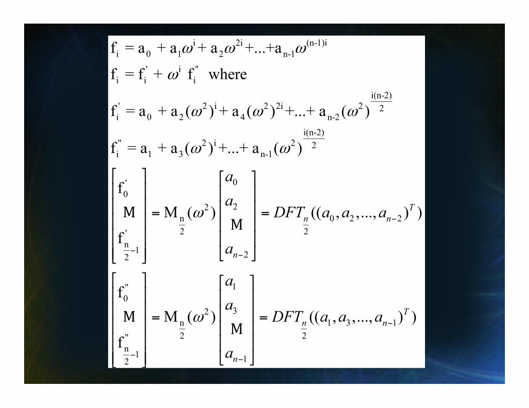
i 2i (n-1)ii 0 1 2 n-1

' i "i i i

i(n-2)' 2 i 2 2i 2 2i 0 2 4 n-2

i(n-2)" 2 i 2 2i 1 3 n-1

0'0

22n2'

n 1 22

f = a + a + a +...+a

f = f + f where

f = a + a ( ) + a ( ) +...+ a ( )

f = a + a ( ) +...+ a ( )

f M ( )

f

n

aa

a

ω ω ω

ω

ω ω ω

ω ω

ω

− −

⎡ ⎤ ⎡ ⎤⎢ ⎥ ⎢⎢ ⎥ ⎢=⎢ ⎥ ⎢⎢ ⎥ ⎢⎢ ⎥ ⎣ ⎦⎣ ⎦

MM 0 2 2

2

1"0

32n 1 3 12 2"

n 1 12

(( , ,..., ) )

f M ( ) (( , ,..., ) )

f

Tn n

Tn n

n

DFT a a a

aa

DFT a a a

a

ω

−

−

− −

⎥⎥ =⎥⎥

⎡ ⎤ ⎡ ⎤⎢ ⎥ ⎢ ⎥⎢ ⎥ ⎢ ⎥= =⎢ ⎥ ⎢ ⎥⎢ ⎥ ⎢ ⎥⎢ ⎥ ⎣ ⎦⎣ ⎦

MM

' ' " "n i n ii i2 2

n1n 2 n 2 i 2i2

' i "i i i

ni +' "2n i ii +2

nNote: f = f , f f , i=0, ..., 1

2

But =1, so ( ) = ( )n

for i=0, ..., 12

nThus, f = f + f for i=0, ..., 1

2

and f = f + f

ω ω ω ω ω

ω

ω

+ +

+

= −

⋅ =

−

−

⋅

' i "i i

n n2 n2 2

n = f - f for i=0, ..., 1

2

since ( ) 1, so = -1

ω

ω ω ω

−

= =

Operation Counts for FFT Algorithm

•  Assume n = 2k

•  # additions Add(n) = 2· Add(n/2) + n = n log n

•  # multiplications Mult(n) = 2· Mult(n/2) + n/2 = ½ n log n

•  Total Time O(n log n) •  Note in complex FFT,

# real ops is 5 n log n

Multipoint Polynomial Evaluation

•  Input polynomial

•  Problem evaluate f(x) at x0, x1, …, xn-1

•  Easy Cases: eval at roots of unity

FFT Case xk = ωk for k=0,…,n

1

0( )

ni

ii

f x a x−

=

=∑

Multipoint Polynomial Evaluation (cont’d)

2

Summary of FFT:( ) '( ) "( )

where '( ), "( ) both degree halved needed to only evaluate at half as many points

method f x f y x f yy x

f x f x

= +

=

⇒

Other Polynomial Evaluation Problems Solved by FFT

Each costs O(n log n) time

•  Evaluate at points Xi = bai + d for i=0,…, n-1(Chirp Transfom) –  Reduced to FFT

•  Single point evaluation of all derivatives of a polynomial –  Solve by reduction to above Chirp Transform of case 2)

•  Evaluate at points Xi = b(ai)2+ cai + d for i=0,…, n-1 –  Solve by divide and conquer similar to FFT

Single Point Evaluation of all Derivatives of Polynomial

•  Input and point x0

•  output

1

0( )

ni

ii

f x a x−

=

=∑

0( )

( ) for 0,..., 1k

k d f xf x x x k n

dx= = = −

Single Point Evaluation of all Derivatives of Polynomial (cont’d)

•  Taylor Series Representation of Then This reduces to case of evaluation at points

•  Solve this Chirp Transform problem by reduction FFT

1

00

( ) ( )n

ii

i

f x c x x−

=

= −∑

( )0( ) !k

kf x k c=

for 0,..., 1iix ab i n= = −

Advanced Material: Further Applications of FFT

1)  Convolution: Products and Powers of Polynomials •  Used for for Integer Multiplication

Algorithms •  Also used for Filtering on infinite

input streams 2)  Division and Inverse of Polynomials 3)  Multipoint Evaluation and

Interpolation

Advanced Material: Products and Powers of Polynomials

•  Input vectors a = (a0, a1, …, an-1)T b = (b0, b1, …, bn-1)T

•  Definition of Convolution c = a ⊗ b

Where for i=0, …, 2n-1 define ak = bk = 0 if k< 0 or k>n

n-1

i j i-jj=0

c = a b∑

Products and Powers of Polynomials (cont’d)

•  Convolution Theorem

•  Application to Polynomial Products: n-1

ii

i=0

n-1j

jj=0

2n-2 n-1i

i i j i-ji=0 j=0

p(x) = a x

q(x) = b x

p(x) q(x) = c x where c = a b⋅

∑

∑

∑ ∑

a⊗ b = FFT2n-1 FFT2n (a) ⋅FFT2n (b)( )

Products of m Polynomials

•  Generalized Convolution Theorem

k

n-1i

k k,ii=0

m(n-1)m mi

k i i k,jki=0k=1 k=1

j =1

for k=1, ..., m let P (x) = a x

P (x) = c x , where c = a

∑

∑

∑ ∑∏ ∏

( )1 2 m

-1n m n m 1 n m 2 n m m

a a ... a =

FFT FFT (a ) FFT (a ) ... FFT (a )

⊗ ⊗ ⊗

• • •

Wrapped Convolutions

•  a = (a0, a1, …, an-1)T , b = (b0, b1, …, bn-1)T •  Positive wrapped convolution is

c = (c0, c1, …, cn-1)T

•  Negative wrapped convolution is d = (d0, d1, …, dn-1)T

i n-1

i j i-j j n+i-jj=0 j=i+1

c = a b + a b∑ ∑

i n-1

i j i-j j n+i-jj=0 j=i+1

d = a b - a b∑ ∑

Application of Wrapped Convolution to Modular Polynomial Products

n-1i

ii=0

n-1j

jj=0

n

n-1i n n

ii=0

p(x) = a x

q(x) = b x

p(x) q(x) mod(x +1)

= d x since x = -1 mod(x +1)

⋅

∑

∑

∑

Computing Positive Wrapped Convolution

•  Let ω = principal nth root of unity •  Assume n has multiplicative inverse, Theorem

is the positive wrapped convolution of

n-vectors a and b.

( )-1n n nc = FFT FFT (a) FFT (b)⋅

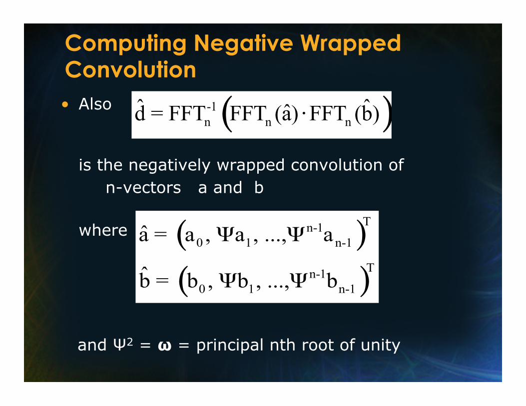
Computing Negative Wrapped Convolution •  Also

is the negatively wrapped convolution of

n-vectors a and b where

and Ψ2 = ω = principal nth root of unity

( )-1n n n

ˆ ˆˆd = FFT FFT (a) FFT (b)⋅

( )( )

Tn-10 1 n-1

Tn-10 1 n-1

a = a , a , ..., a

b = b , b , ..., b

Ψ Ψ

Ψ Ψ

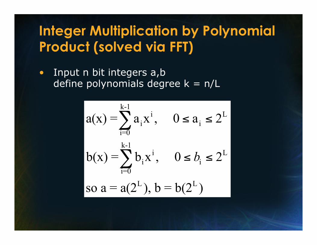
Integer Multiplication by Polynomial Product (solved via FFT)

•  Input n bit integers a,b define polynomials degree k = n/L

k-1i L

i ii=0

k-1i L

i ii=0

L L

a(x) = a x , 0 a 2

b(x) = b x , 0 2

so a = a(2 ), b = b(2 )

b

≤ ≤

≤ ≤

∑

∑

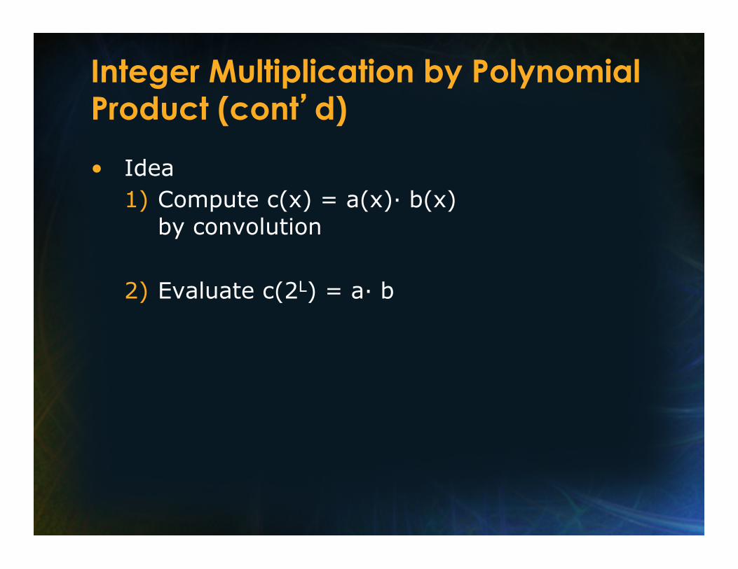
Integer Multiplication by Polynomial Product (cont’d)

•  Idea 1)  Compute c(x) = a(x)· b(x)

by convolution

2)  Evaluate c(2L) = a· b

Integer Multiplication Algorithms using Reduction to Polynomial Product

•  Pollard Mult Algorithm

•  Karp Mult Algorithm

•  Schönage-Strassen Mult Algorithm

2O(n(logn) )(loglogn) use L = logn∈

2O(n(logn) ) use L = n

O(n(logn)(loglogn)) use L = n and wrapped convolution

Pollard Multiplication Algorithm

•  n = kL, L = 1 + log k 1)  Choose primes P1, P2, P3 where

2)  Compute C(x) by convolution over finite field Zpi for i =1,2,3 (requires k mults on 2L bit integers)

31 2 3

Li i i

P P P 4 k

and P = á 2 + 1, á = O(1)

⋅ ⋅ ≥ ⋅

⋅

Pollard Multiplication Algorithm (cont’d)

3)  Evaluate C(2L)

•  Time Bounds

2

2

T(n) = 3kT(2L) + O(k logk) O(L) = 3kT (2(1 + logk)) + O(k(log k) ) O(n(log n) (log log n) ) for any > 0∈

⋅

≤ ∈

recursive mults FFT

Korp Multiplication Algorithm

1)  Compute C(x) modulo k by convolution

2)  Compute C(x) modulo (22L+1) by convolution

3)  Compute C(x) coefficients from C(x) mod k, C(x) mod (22L+1) by Chinese remaindering

s

s2

(s-1)2

n = 2 = kL

2 if s evenk =

2 else

!"#"$

Korp Multiplication Algorithm (cont’d)

4)  Compute C(2L)

•  Time

2

T(n) = 2kT(2L) + O(k logk)O(L)

= 2 nT (2 n ) + O(n log n) O(n(log n) )=

recursive mults FFT

Schönage-Strassen Multiplication Algorithm

(2’) Compute C(x) mod (xk+1) modulo (22L+1) by wrapped convolution

Requires only k recursive mults on 2L bit numbers

•  Time

T(n) = kT(2L) + O(k logk)O(L)

= nT (2 n ) + O(n log n) O(n log n)(log log n)=

recursive mults FFT

Still Open Problem: How Fast Can You Multiply Integers?

•  Can you mult n bit integers in O(n log n) time?

The Fast Fourier Transform and Applications to Multiplication

Prepared by

John Reif, Ph.D.

Analysis of Algorithms