The explicit Laplace transform for the Wishart process - arXiv

The explicit Laplace transform for the Wishart process∗

Alessandro Gnoatto† Martino Grasselli‡

October 31, 2018

Abstract

We derive the explicit formula for the joint Laplace transform of the Wishart process and its timeintegral which extends the original approach of [5]. We compare our methodology with the alternativeresults given by the variation of constants method, the linearization of the Matrix Riccati ODE’s andthe Runge-Kutta algorithm. The new formula turns out to be fast and accurate.

Keywords: Affine processes, Wishart process, ODE, Laplace Transform.

JEL codes: G13, C51.AMS Class 2010: 65C30, 60H35, 91B70.

1 Introduction

In this paper we propose an analytical approach for the computation of the moment generating functionfor the Wishart process which has been introduced by [5], as an extension of square Bessel processes([36], [38]) to the matrix case. Wishart processes belong to the class of affine processes and theygeneralise the notion of positive factor in so far as they are defined on the set of positive semidefinitereal d × d matrices, denoted by S+

d . Given a filtered probability space (Ω,F ,Ft,P) satisfying theusual assumptions and a d× d matrix Brownian motion B (i.e. a matrix whose entries are independentBrownian motions under P), a Wishart process on S+

d is governed by the SDE

dSt =√StdBtQ+Q>dB>t

√St +

(MSt + StM

> + b)dt, S0 ∈ S+

d , t ≥ 0 (1)

where Q ∈ GLd (the set of invertible real d × d matrices), M ∈ Md (the set of real d × d matrices)with all eigenvalues on the negative half plane in order to ensure stationarity, and where the matrix bsatisfies b (d − 1)Q>Q, that is b − (d − 1)Q>Q ∈ S+

d . In the literature, the constant drift term isoften of the more restrictive form b = αQ>Q, for α ≥ d − 1. In case the (Gindikin) real parameterα satisfies α ≥ d + 1, the process takes values in the interior of S+

d , denoted by S++d , in analogy with

the Feller condition for the scalar case. In the dynamics above√St denotes the square root in matrix

sense. Existence and uniqueness results for the solution of (1) may be found in [5] under parametric∗We are indebted to Jose Da Fonseca, Antoine Jacquier, Kyoung-Kuk Kim, Eberhard Mayerhofer, Eckhard Platen, Wolfgang

Runggaldier and an anonymous referee for helpful suggestions.†Dipartimento di Matematica - Universita degli Studi di Padova (Italy) and Mathematisches Institut, LMU Munchen (Ger-

many). Email: [email protected].‡Dipartimento di Matematica - Universita degli Studi di Padova (Italy), ESILV Ecole Superieure d’Ingenieurs Leonard de

Vinci, Departement Mathematiques et Ingenierie Financiere, Paris La Defense (France) and QUANTA FINANZA S.R.L., Venezia(Italy). Email: [email protected].

1

arX

iv:1

107.

2748

v5 [

q-fi

n.PR

] 2

0 A

ug 2

013

1 INTRODUCTION 2

restrictions and in [33] in full generality. We denote by WISd(S0, b,M,Q) the law of the Wishartprocess (St)t≥0. The starting point of the analysis was given by considering the square of a matrixBrownian motion St = B>t Bt, while the generalization to the particular dynamics (1) was introducedby looking at squares of matrix Ornstein-Uhlenbeck processes (see [5]).Bru proved many interesting properties of this process, like non-collision of the eigenvalues (whenα ≥ d + 1 under parametric restrictions) and the additivity property shared with square Bessel pro-cesses. Moreover, she computed the Laplace transform of the Wishart process and its integral (theMatrix Cameron-Martin formula using her terminology), which plays a central role in the applications:

EPS0

[exp

−Tr

[wSt +

∫ t

0

vSsds

]], (2)

where Tr denotes the trace operator and w, v are symmetric matrices for which the expression (2)is finite. Bru found an explicit formula for (2) (formula (4.7) in [5]) under the assumption that thesymmetric diffusion matrix Q and the mean reversion matrix M commute.Positive (semi)definite matrices arise in finance in a natural way and the nice analytical properties ofaffine processes on S+

d opened the door to new interesting affine models that allow for non trivialcorrelations among positive factors, a feature which is precluded in classic (linear) state space domainslike Rn≥0×Rm (see [18]). Not surprisingly, the last years have witnessed the birth of a whole branch ofliterature on applications of affine processes on S+

d . The first proposals were formulated in [21], [22],[23], [20] both in discrete and continuous time. Applications to multifactor volatility and stochasticcorrelation can be found in [15], [14], [12], [13], [16], [7], [4] and [6] both in option pricing andportfolio management. These contributions consider the case of continuous path Wishart processes. Asfar as jump processes on S+

d are concerned we recall the proposals by [3], [34] and [35]. [29] and[11] consider jump-diffusions models in this class, while [24] investigate processes lying in the moregeneral symmetric cones state space domain, including the interior of the cone S+

d (see also the recentdevelopements in [10]).The main contribution of this paper consists in relaxing the commutativity assumption made in [5]and proving that it is possibile to characterize explicitly the joint distribution of the Wishart processand its time integral for a general class of (even not symmetric) mean-reversion and diffusion matricessatisfying the assumptions above with a general constant drift term b. The proof of our general CameronMartin formula is in line with that of theorem 2” in Bru and we will provide a step-by-step derivation.The study of transform formulae for affine processes on S+

d is also the topic of [27], where resultsconcerning Wishart bridges are also provided.The paper is organized as follows: in section 2 we prove our main result, which extends the originalapproach by Bru. In section 3 we recall some other existing methods which have been employed in thepast literature for the computation of the Laplace transform: the variation of constant, the linearizationand the Runge-Kutta method. The first two methods provide analytical solutions, so they should beconsidered as competitors of our new methodology. We show that the variation of constants method isunfeasible for real-life computations, hence the truly analytic competitor is the linearization procedure.After that, we present some applications of our methodology to various settings: a multifactor stochasticvolatiliy model, a stochastic correlation model, a short rate model and finally we present a new approachfor the computation of a solution to the Algebraic Riccati equation.

2 THE MATRIX CAMERON-MARTIN FORMULA 3

2 The Matrix Cameron-Martin Formula

2.1 The Wishart process from the point of view of affine processes

Before we introduce our result, we would like to report some notations and terminology from [11]. Letus recall first the definition of an affine process.

Definition 1 A Markov process S on S+d is called affine if it is stochastically continuous and its Laplace

transform has exponential-affine dependence on the initial state, i.e. the following equation holds forall t ≥ 0 and u ∈ S+

d :

E[e−Tr[uSt]

]=

∫S+d

e−Tr[uξ] pt(x, dξ) = e−φ(t,u)−Tr[ψ(t,u)S0] , (3)

for some functions φ : R+ × S+d → R+ and ψ : R+ × S+

d → S+d .

In [11], a complete characterization of affine processes on S+d is provided in terms of the so-called

admissible parameter set (see Definition 2.3 in [11]), which constitutes the affine analogue of a Levytriplet. The Wishart process with dynamics (1) is a conservative pure diffusion affine process withadmissible parameter set (α, b,B(x), 0, 0, 0, 0), where B(x) = Mx+ xM> and α = Q>Q. Since theprocess is affine, it is possible to reduce the Kolmogorov PDE associated to the computation of (2) to anon linear (matrix Riccati) ODE.

Proposition 2 ([11]) Let St ∈WISd(S0, b,M,Q) be the Wishart process defined by (1), then

EPS0

[exp

−Tr

[wSt +

∫ t

0

vSsds

]]= exp −φ(t)− Tr [ψ(t)S0] ,

where the functions ψ and φ satisfy the following system of ODE’s.

dψ

dt= ψM +M>ψ − 2ψQ>Qψ + v ψ(0) = w, (4)

dφ

dt= Tr [bψ(t)] φ(0) = 0. (5)

2.2 Statement of the result

In this section we proceed to prove the main result of this paper. We report a formula completely in linewith the Matrix Cameron-Martin formula given by [5].

Theorem 3 Let S ∈WISd(S0, b,M,Q) be the Wishart process solving (1), assume

M>(Q>Q

)−1=(Q>Q

)−1M, (6)

let b (d+ 1)Q>Q and define the set of convergence of the Laplace transform

Dt =

w, v ∈ Sd : EP

S0

[exp

−Tr

[wSt +

∫ t

0

vSsds

]]< +∞

.

Then for all u, v ∈ Dt the joint moment generating function of the process and its integral is given by:

EPs0

[exp

−Tr

[wSt +

∫ t

0

vSsds

]]= exp −φ(t)− Tr [ψ(t)s0] ,


where the functions φ and ψ are given by:

ψ(t) =

(Q>Q

)−1M

2− Q−1

√vk(t)Q>

−1

2,

φ(t) = Tr

[b

(Q>Q

)−1M

2

]t

+1

2Tr[(Q>)−1

b (Q)−1

log(√

v−1(√

v cosh(√vt) + w sinh(

√vt)))]

,

with k(t) given by:

k(t) = −(√


√vt))−1 (√

v sinh(√vt) + w cosh(

√vt))

and v, w are defined as follows:

v = Q(

2v +M>Q−1Q>−1

M)Q>,

w = Q(

2w −(Q>Q

)−1M)Q>.

Moreover, the set where the Laplace transform is regular at least contains the area defined by

v −M>(2Q>Q)−1M, (7)

w (2Q>Q)−1M −Q−1√v(2Q>)−1. (8)

Remark 4 The derivation of Theorem 3 involves a change of probability measure that will be illustratedin the sequel. This change of measure introduces a lack of symmetry which does not allow to derive afully general formula. However, under the assumption (6) we are able to span a large class of processes.In fact, the equality (6) requires the symmetry of a matrix: this involves d(d− 1)/2 linear equalities ind2 variables, therefore if we fix the parameters of the matrix (QTQ)−1 and consider the constraints onthe parameters of M , we get d2− d(d− 1)/2 = d(d+ 1)/2 degrees of freedom for choosing the matrixM .In the two dimensional case, let:

(Q>Q

)−1=

(a b

b c

), M =

(x y

z t

),

then condition (6) can be expressed as:

bx+ cz = ay + tb,

meaning that we can span a large class of parameters, thus going far beyond the commutativity assump-tion QM = MQ for Q ∈ Sd,M ∈ S−d as in [5].

Remark 5 Conditions (7) - (8) give explicit parameter constraints in order to ensure the finiteness ofthe Laplace transform. If they are not satisfied, then the Laplace transform is regular only up to a(possibly finite) explosion time. Notice that conditions (7), (8) extend the usual assumptions v, w ∈ S+

d

as in [11].

2.3 Proof of Theorem 3

We will prove the theorem in several steps. We first consider a simple Wishart process with M = 0 andQ = Id, defined under a measure P equivalent to P. The second step will be given by the introduction


of the volatility matrix Q, using an invariance result. Finally, we will prove the extension for the fullprocess by relying on a measure change from P to P. Under this last measure, the Wishart process willbe defined by the dynamics (1).

As a starting point we fix a probability measure P such that P ≈ P. Under the measure P we consider amatrix Brownian motion B = (Bt)t≥0, which allows us to define the process Σt ∈WISd(S0, b, 0, Id),i.e. a process that solves the following matrix SDE:

dΣt =√

ΣtdBt + dB>t√

Σt + bdt, Σ0 ∈ S+d , (9)

where the drift term b satisfies the following condition:

b− (d+ 1) Id ∈ S+d .

For this process, relying on [36] and [5], we are able to calculate the Cameron-Martin formula. Forthe sake of completeness we report the result in [5], which constitutes an extension of the methodologyintroduced in [36]. The result was proved for the restrictive drift αId, but we will extend it to the generaldrift by looking to the system of Riccati ODEs.

Proposition 6 ([5] Proposition 5 p.742) If Φ : R+ → S+d is continuous, constant on [t,∞[ and such

that its right derivative (in the distribution sense) Φ′d : R+ → S−d is continuous, with Φd(0) = Id, andΦ′d(t) = 0, then for every Wishart process Σt ∈WISd(Σ0, α, 0, Id) we have:

E[exp

−1

2Tr

[∫ t

0

Φ′′d(s)Φ−1d (s)Σsds

]]= (detΦd(t))

α/2exp

1

2Tr[Σ0Φ

+d (0)

],

where

Φ+d (0) := lim

t0Φ′d(t).

We employ this result to prove the following claim, which establishes the Cameron Martin formula forthe more general drift b.

Proposition 7 Let Σ ∈WISd(Σ0, b, 0, Id), then

E[exp

−1

2Tr

[wΣt +

∫ t

0

vΣsds

]]= exp −φ(t)− Tr [ψ(t)Σ0] , (10)

where

ψ(t) = −√vk(t)

2

φ(t) =1

2Tr[b log

(√v−1 (√


√vt)))]

and k(t) is given by

k(t) = −(√v cosh(

√vt) + w sinh(

√vt))−1 (√


√vt)).

Proof. Let us first assume that b = αId. An application of Proposition 6 allows us to claim that

E[exp

−1

2Tr

[wΣt +

∫ t

0

vΣsds

]]= det

(cosh

(√vt)

+ sinh(√vt)k(t)

)α2

× exp

1

2Tr[Σ0

√vk(t)

], (11)


where k(t) is given by

k(t) = −(√v cosh(

√vt) + w sinh(

√vt))−1 (√


√vt)).

A direct inspection of (11), allows us to recognize the functions φ and ψ in this setting. For ψ we have

ψ(t) = −√vk(t)

2(12)

which is independent of b. The corresponding system of matrix Riccati ODE is

dψ

dt= −2ψψ + v ψ(0) = w, (13)

dφ

dt= Tr

[bψ(t)

]φ(0) = 0. (14)

Given the solution for ψ, we can determine an alternative formulation for φ upon integration. Thisalternative formulation encompasses the more general constant drift too. We show the calculation indetail:

dφ

dt= Tr

[bψ(t)

]= Tr

[b

(−√vk(t)

2

)].

Integrating the ODE yields

φ(t) = −1

2Tr

[b√v

∫ t

0

k(s)ds

].

We concentrate on the integral appearing in the second term:∫ t

0

k(s)ds =

∫ t

0

−(√v cosh(

√vs) + w sinh(

√vs))−1 (√

v sinh(√vs) + w cosh(

√vs))ds.

Define f(s) =√v cosh(

√vs) + w sinh(

√vs) and let us differentiate it:

df

ds=(√v sinh(

√vs) + w cosh(

√vs))√

v,

hence we can write

φ(t) =1

2Tr[b(log(√v cosh(

√vt) + w sinh(

√vt))− log

(√v))]

=1

2Tr[b log

(√v−1 (√


√vt)))]

.

Invariance under transformations. We define the transformation St = Q>ΣtQ, which is governedby the SDE:


√St + bdt, b = Q>bQ, (15)

where the process B = (Bt)t≥0 defined by dBt =√St−1Q>√

ΣdBt is easily proved to be a Brownianmotion under P.From [5], we know how to extend the Cameron Martin formula: the Laplace transform of the process Smay be computed as follows

EPS0

[e−Tr[wSt]

]= EP

(Q>)−1S0Q−1

[e−Tr[wQ

>ΣQ]]

= EPΣ0

[e−Tr[(QwQ

>)Σ]],

hence we can compute the Cameron Martin formula for the process S using the arguments QwQ> andQvQ>.


Inclusion of the drift - Girsanov transformation. The final step consists in introducing a measurechange from P, where the process has no mean reversion, to the measure P that will allow us to considerthe general process governed by the dynamics in equation (1). We now define a matrix Brownian motionunder the probability measure P as follows:

Bt = Bt −∫ t

0

√SsM

>Q−1ds = Bt −∫ t

0

Hsds,

for Hs =√SsM

>Q−1. The Girsanov transformation is given by the following stochastic exponential(see e.g. [17]):

∂P∂P

∣∣∣∣Ft

= exp

∫ t

0

Tr[H>dBs

]− 1

2

∫ t

0

Tr[HH>

]ds

= exp

∫ t

0

Tr[Q−1>M

√SsdBs

]− 1

2

∫ t

0

Tr[SsM

>Q−1Q−1>M]ds

.

We concentrate on the stochastic integral term, which under the parametric restriction (6), can be ex-pressed as

1

2

∫ t

0

Tr[(Q>Q

)−1M(√

SsdBsQ+Q>dB>s√Ss

)]=

1

2

∫ t

0

Tr[(Q>Q

)−1M (dSs − bds)

].

In summary, the stochastic exponential may be written as

∂P∂P

∣∣∣∣Ft

= exp

Tr

[(Q>Q

)−1M

2(St − S0 − bt)

]− 1

2

∫ t

0

Tr[SsM

>Q−1Q−1>M]ds

.

Under the assumption b (d + 1)Q>Q (which is a sufficient condition ensuring that the process doesnot hit the boundary of the cone S+

d , see Corollary 3.2 in [33]), using the same arguments as in [31]shows that the stochastic exponential is a true martingale.

Derivation of the Matrix Cameron-Martin formula. We consider the process under P:


√St +

(MSt + StM

> + b)dt.

Recall that under P, we have


√St + bdt,

then Σt = Q−1>StQ−1 solves

dΣt =√

ΣtdBt + dB>t√

Σt + bdt.

3 ALTERNATIVE EXISTING METHODS 8

We are now ready to apply the change of measure along the following steps:

EPS0

[exp

−1

2Tr

[wSt +

∫ t

0

vSsds

]]=EP

S0

[exp

−1

2Tr

[wSt +

∫ t

0

vSsds

]+ Tr

[(Q>Q

)−1M

2(St − S0 − bt)

]

−1

2

∫ t

0

Tr[SsM

>Q−1Q−1>M]ds

]= exp

−Tr

[(Q>Q

)−1M

2(S0 + bt)

]

× EPS0

[exp

−1

2Tr[(w −

(Q>Q

)−1M)St

+

∫ t

0

(v +M>Q−1Q−1>M

)Ssds

]].

But St = Q>ΣtQ, then:

EPS0

[exp

−1

2Tr

[wSt +

∫ t

0

vSsds

]]= exp

−Tr

[(Q>Q

)−1M

2(S0 + bt)

]

× EPQ>−1S0Q−1

[exp

−1

2Tr[Q(w −

(Q>Q

)−1M)Q>Σt

+

∫ t

0

Q(v +M>Q−1Q−1>M

)Q>Σsds

]].

The expectation may be computed via a direct application of formula (11) and after some standardalgebra we get the result of Theorem 3, with the obvious substitutions v → 2v and w → 2w.

Strip of regularity for Dt. Here we show that conditions (7) and (8) imply the boundedness of theLaplace transform for all t ≥ 0. By theorem (3.7) of [39] we know that the Laplace transform exists tillthe explosion time of the solution of the corresponding Riccati ODE. Knowing the explicit solution ofsuch ODE, a sufficient condition for non explosion is that for all t ≥ 0

h(t) =√v cosh(

√vt) + w sinh(

√vt) ∈ GLd.

As v appears in a square root, it must be that v 0. However, the inequality must be strict due toh(0) ∈ GLd, then v 0, i.e. condition (7). Now let us rewrite h(t) as follows:

h(t) =√ve√vt + e−

√vt

2+ w

e√vt − e−

√vt

2

=√ve−

√vt +

1

2(√v + w)

(e√vt − e−

√vt).

For v 0 we have that both e−√vt and e

√vt − e−

√vt belong to S+

d for all t ≥ 0, then h(t) ∈ GLd if√v + w 0 , which is condition (8).

3 Alternative existing methods

3.1 Variation of Constants Method

The variation of constants method represents the first solution provided in literature for the solution ofthe matrix ODE’s (4) - (5) (see e.g. [21], [22], [23]) and despite its theoretical simplicity, it turns out to

3 ALTERNATIVE EXISTING METHODS 9

be very time consuming, as we will show later in the numerical exercise. This is also equivalent to theprocedure followed by [1] and [32] who found the Laplace transform of the Wishart process alone (i.e.corresponding to v = 0 in (2)). The proof of the following proposition is standard and it is omitted.

Proposition 8 The solutions for ψ(t), φ(t) in Proposition 2 are given by:

ψ(t) = ψ′ + e(M>−2ψ′Q>Q)t

[(w − ψ′)−1

+ 2

∫ t

0

e(M−2Q>Qψ′)sQ>Qe(M>−2ψ′Q>Q)sds

]−1

e(M−2Q>Qψ′)t, (16)

φ(t) = Tr

[αQ>Q

∫ t

0

ψ(s)ds

], (17)

where ψ′ is a symmetric solution to the following algebraic Riccati equation

ψ′M +M>ψ′ − 2ψ′Q>Qψ′ + v = 0. (18)

3.2 Linearization of the Matrix Riccati ODE

The second approach we consider is the one proposed by [24], who used the Radon lemma in order tolinearize the matrix Riccati ODE (4) (see also [30], [26] and [2]).

Proposition 9 ([24]) The functions ψ(t), φ(t) in Proposition 2 are given by

ψ(t) = (wψ12(t) + ψ22(t))−1

(wψ11(t) + ψ21(t)) ,

φ(t) =α

2Tr[log (wψ12(t) + ψ22(t)) +M>t

],

where (ψ11(t) ψ12(t)

ψ21(t) ψ22(t)

)= exp

t

(M 2Q>Q

v −M>

).

3.3 Runge-Kutta Method

The Runge-Kutta method is a classical approach for the numerical solution of ODE’s. For a detailedtreatment, see e.g. [37]. If we want to solve numerically the system of equations (4) and (5), the mostcommonly used Runge-Kutta scheme is the fourth order one:

ψ(tn+1) = ψ(tn) +1

6h (k1 + 2k2 + 2k3 + k4) ,

tn+1 = tn + h,

k1 = g(tn, ψ(tn)),

k2 = g(tn +1

2h, ψ(tn) +

1

2hk1),

k3 = g(tn +1

2h, ψ(tn) +

1

2hk2),

k4 = g(tn + h, ψ(tn) + hk3),

where the function g is given by:

g(tn, ψ(tn)) = g(ψ(tn)) = ψ(tn)M +M>ψ(tn)− 2ψ(tn)Q>Qψ(tn) + v.

4 APPLICATIONS 10

3.4 Comparison of the methods

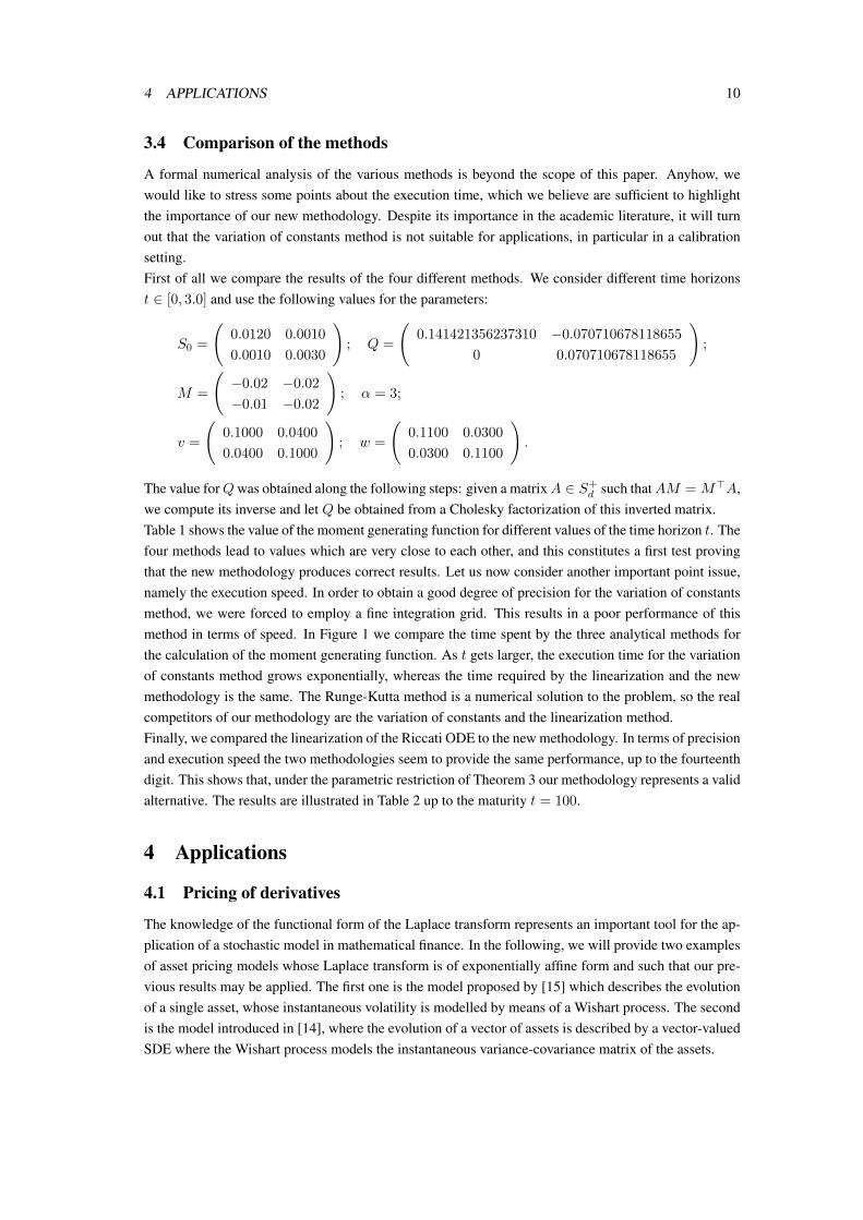
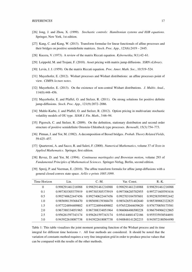
A formal numerical analysis of the various methods is beyond the scope of this paper. Anyhow, wewould like to stress some points about the execution time, which we believe are sufficient to highlightthe importance of our new methodology. Despite its importance in the academic literature, it will turnout that the variation of constants method is not suitable for applications, in particular in a calibrationsetting.First of all we compare the results of the four different methods. We consider different time horizonst ∈ [0, 3.0] and use the following values for the parameters:

S0 =

(0.0120 0.0010

0.0010 0.0030

); Q =

(0.141421356237310 −0.070710678118655

0 0.070710678118655

);

M =

(−0.02 −0.02

−0.01 −0.02

); α = 3;

v =

(0.1000 0.0400

0.0400 0.1000

); w =

(0.1100 0.0300

0.0300 0.1100

).

The value forQwas obtained along the following steps: given a matrixA ∈ S+d such thatAM = M>A,

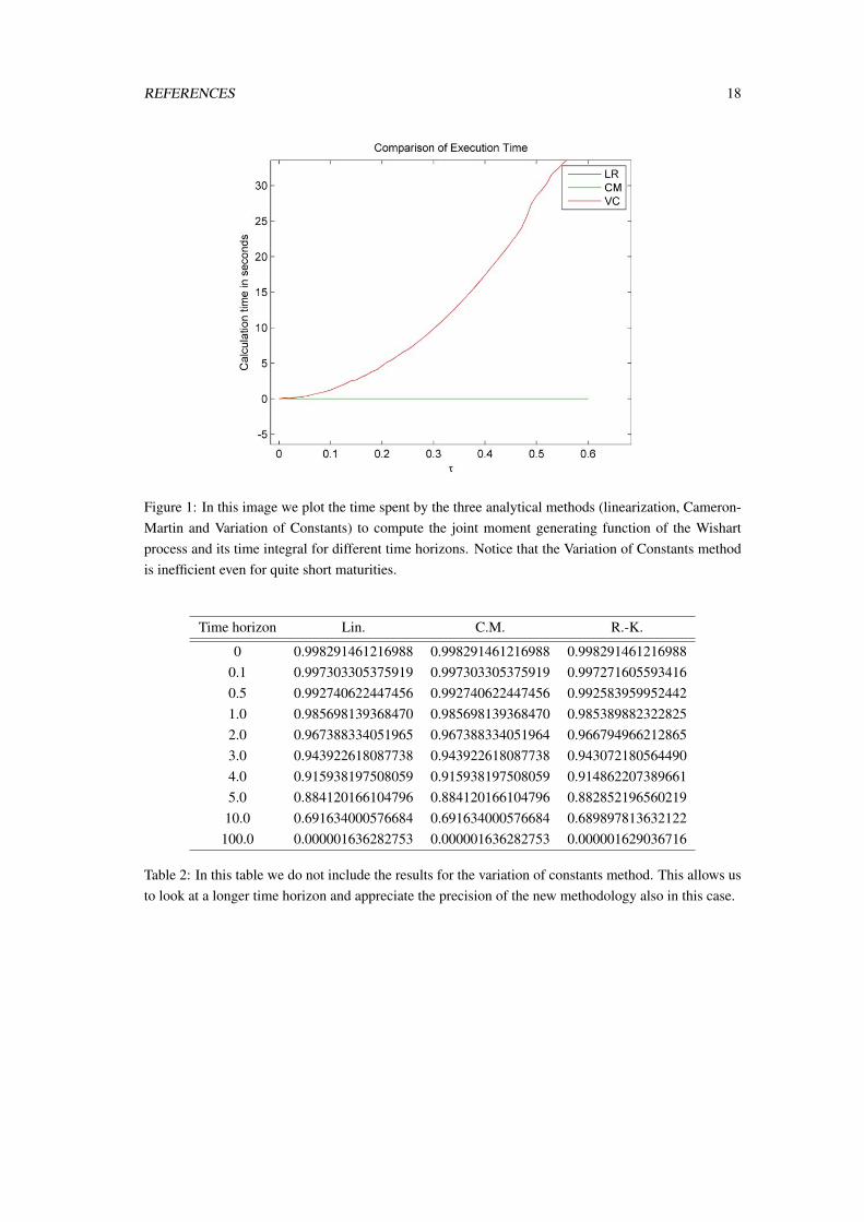
we compute its inverse and let Q be obtained from a Cholesky factorization of this inverted matrix.Table 1 shows the value of the moment generating function for different values of the time horizon t. Thefour methods lead to values which are very close to each other, and this constitutes a first test provingthat the new methodology produces correct results. Let us now consider another important point issue,namely the execution speed. In order to obtain a good degree of precision for the variation of constantsmethod, we were forced to employ a fine integration grid. This results in a poor performance of thismethod in terms of speed. In Figure 1 we compare the time spent by the three analytical methods forthe calculation of the moment generating function. As t gets larger, the execution time for the variationof constants method grows exponentially, whereas the time required by the linearization and the newmethodology is the same. The Runge-Kutta method is a numerical solution to the problem, so the realcompetitors of our methodology are the variation of constants and the linearization method.Finally, we compared the linearization of the Riccati ODE to the new methodology. In terms of precisionand execution speed the two methodologies seem to provide the same performance, up to the fourteenthdigit. This shows that, under the parametric restriction of Theorem 3 our methodology represents a validalternative. The results are illustrated in Table 2 up to the maturity t = 100.

4 Applications

4.1 Pricing of derivatives

The knowledge of the functional form of the Laplace transform represents an important tool for the ap-plication of a stochastic model in mathematical finance. In the following, we will provide two examplesof asset pricing models whose Laplace transform is of exponentially affine form and such that our pre-vious results may be applied. The first one is the model proposed by [15] which describes the evolutionof a single asset, whose instantaneous volatility is modelled by means of a Wishart process. The secondis the model introduced in [14], where the evolution of a vector of assets is described by a vector-valuedSDE where the Wishart process models the instantaneous variance-covariance matrix of the assets.

4 APPLICATIONS 11

4.1.1 A stochastic volatility model

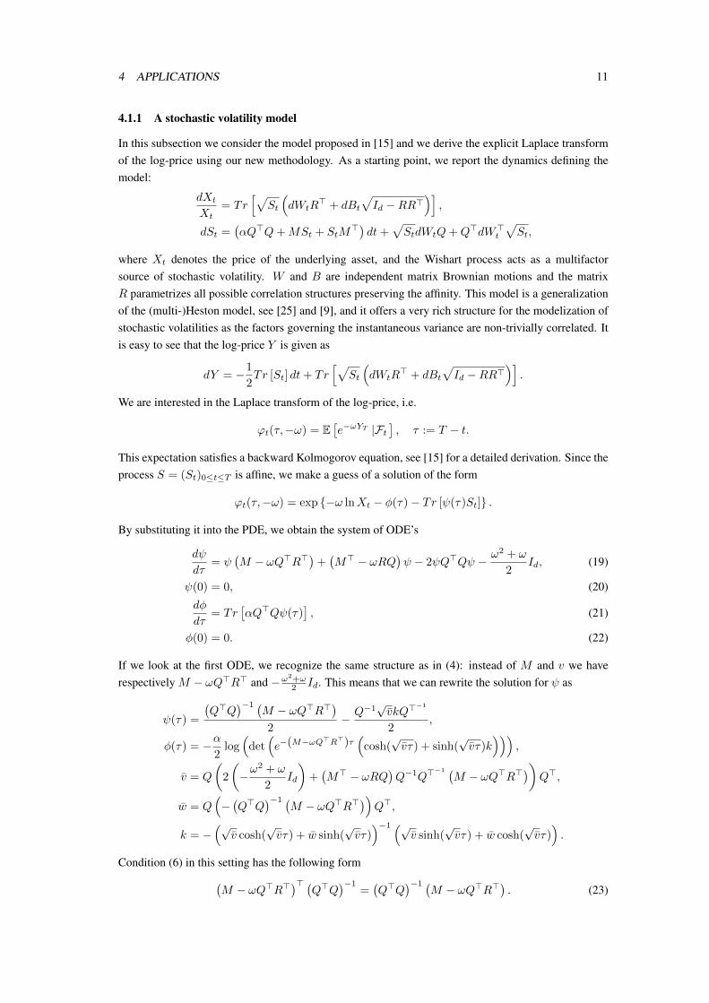
In this subsection we consider the model proposed in [15] and we derive the explicit Laplace transformof the log-price using our new methodology. As a starting point, we report the dynamics defining themodel:

dXt

Xt= Tr

[√St

(dWtR

> + dBt√Id −RR>

)],

dSt =(αQ>Q+MSt + StM

>) dt+√StdWtQ+Q>dW>t

√St,

where Xt denotes the price of the underlying asset, and the Wishart process acts as a multifactorsource of stochastic volatility. W and B are independent matrix Brownian motions and the matrixR parametrizes all possible correlation structures preserving the affinity. This model is a generalizationof the (multi-)Heston model, see [25] and [9], and it offers a very rich structure for the modelization ofstochastic volatilities as the factors governing the instantaneous variance are non-trivially correlated. Itis easy to see that the log-price Y is given as

dY = −1

2Tr [St] dt+ Tr

[√St

(dWtR

> + dBt√Id −RR>

)].

We are interested in the Laplace transform of the log-price, i.e.

ϕt(τ,−ω) = E[e−ωYT |Ft

], τ := T − t.

This expectation satisfies a backward Kolmogorov equation, see [15] for a detailed derivation. Since theprocess S = (St)0≤t≤T is affine, we make a guess of a solution of the form

ϕt(τ,−ω) = exp −ω lnXt − φ(τ)− Tr [ψ(τ)St] .

By substituting it into the PDE, we obtain the system of ODE’s

dψ

dτ= ψ

(M − ωQ>R>

)+(M> − ωRQ

)ψ − 2ψQ>Qψ − ω2 + ω

2Id, (19)

ψ(0) = 0, (20)

dφ

dτ= Tr

[αQ>Qψ(τ)

], (21)

φ(0) = 0. (22)

If we look at the first ODE, we recognize the same structure as in (4): instead of M and v we haverespectively M − ωQ>R> and −ω

2+ω2 Id. This means that we can rewrite the solution for ψ as

ψ(τ) =

(Q>Q

)−1 (M − ωQ>R>

)2

− Q−1√vkQ>

−1

2,

φ(τ) = −α2

log(

det(e−(M−ωQ>R>)τ

(cosh(

√vτ) + sinh(

√vτ)k

))),

v = Q

(2

(−ω

2 + ω

2Id

)+(M> − ωRQ

)Q−1Q>

−1 (M − ωQ>R>

))Q>,

w = Q(−(Q>Q

)−1 (M − ωQ>R>

))Q>,

k = −(√

v cosh(√vτ) + w sinh(

√vτ))−1 (√

v sinh(√vτ) + w cosh(

√vτ)).

Condition (6) in this setting has the following form(M − ωQ>R>

)> (Q>Q

)−1=(Q>Q

)−1 (M − ωQ>R>

). (23)

4 APPLICATIONS 12

For fixed ω we can express the condition above via the following systemM>

(Q>Q

)−1=(Q>Q

)−1M,

RQ(Q>Q

)−1=(Q>Q

)−1Q>R>.

(24)

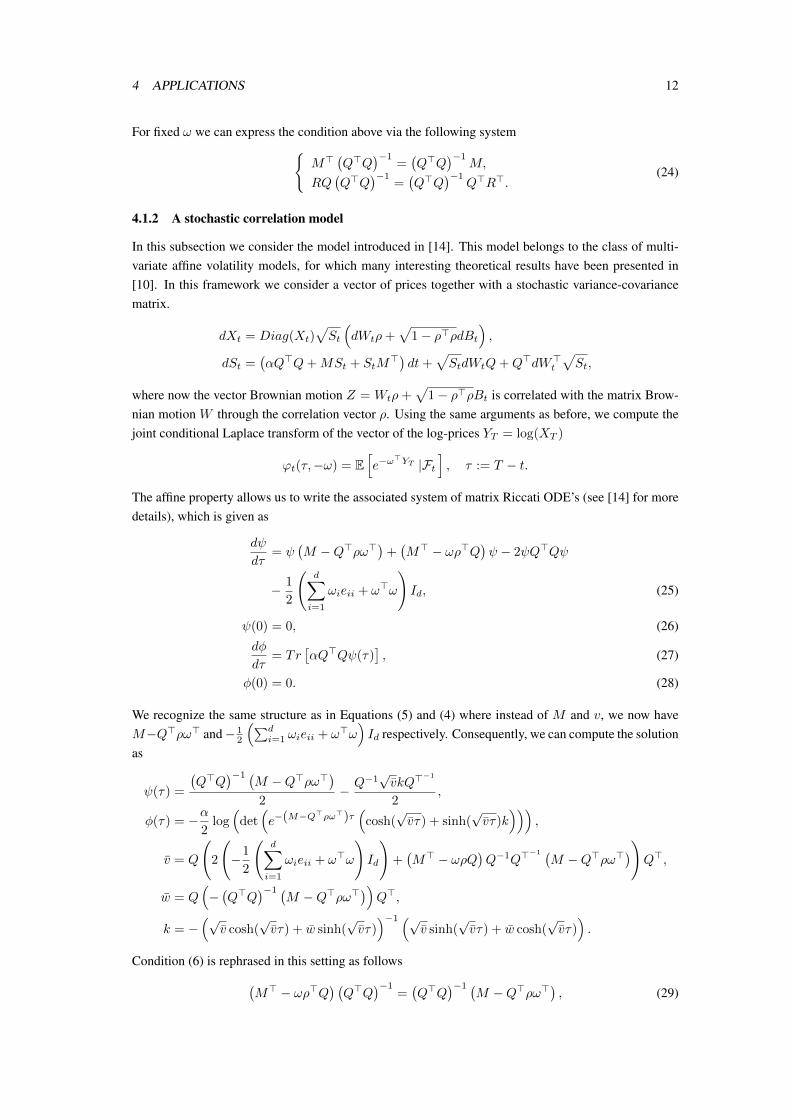
4.1.2 A stochastic correlation model

In this subsection we consider the model introduced in [14]. This model belongs to the class of multi-variate affine volatility models, for which many interesting theoretical results have been presented in[10]. In this framework we consider a vector of prices together with a stochastic variance-covariancematrix.

dXt = Diag(Xt)√St

(dWtρ+

√1− ρ>ρdBt

),

dSt =(αQ>Q+MSt + StM

>) dt+√StdWtQ+Q>dW>t

√St,

where now the vector Brownian motion Z = Wtρ+√

1− ρ>ρBt is correlated with the matrix Brow-nian motion W through the correlation vector ρ. Using the same arguments as before, we compute thejoint conditional Laplace transform of the vector of the log-prices YT = log(XT )

ϕt(τ,−ω) = E[e−ω

>YT |Ft], τ := T − t.

The affine property allows us to write the associated system of matrix Riccati ODE’s (see [14] for moredetails), which is given as

dψ

dτ= ψ

(M −Q>ρω>

)+(M> − ωρ>Q

)ψ − 2ψQ>Qψ

− 1

2

(d∑i=1

ωieii + ω>ω

)Id, (25)

ψ(0) = 0, (26)

dφ

dτ= Tr

[αQ>Qψ(τ)

], (27)

φ(0) = 0. (28)

We recognize the same structure as in Equations (5) and (4) where instead of M and v, we now haveM−Q>ρω> and− 1

2

(∑di=1 ωieii + ω>ω

)Id respectively. Consequently, we can compute the solution

as

ψ(τ) =

(Q>Q

)−1 (M −Q>ρω>

)2

− Q−1√vkQ>

−1

2,

φ(τ) = −α2

log(

det(e−(M−Q>ρω>)τ

(cosh(

√vτ) + sinh(

√vτ)k

))),

v = Q

(2

(−1

2

(d∑i=1

ωieii + ω>ω

)Id

)+(M> − ωρQ

)Q−1Q>

−1 (M −Q>ρω>

))Q>,

w = Q(−(Q>Q

)−1 (M −Q>ρω>

))Q>,

k = −(√


√vτ))−1 (√


√vτ)).

Condition (6) is rephrased in this setting as follows(M> − ωρ>Q

) (Q>Q

)−1=(Q>Q

)−1 (M −Q>ρω>

), (29)

4 APPLICATIONS 13

which may be expressed as M>

(Q>Q

)−1=(Q>Q

)−1M,

ωρ>Q>−1

= Q−1ρω>.(30)

This means that the two products have to be symmetric matrices.

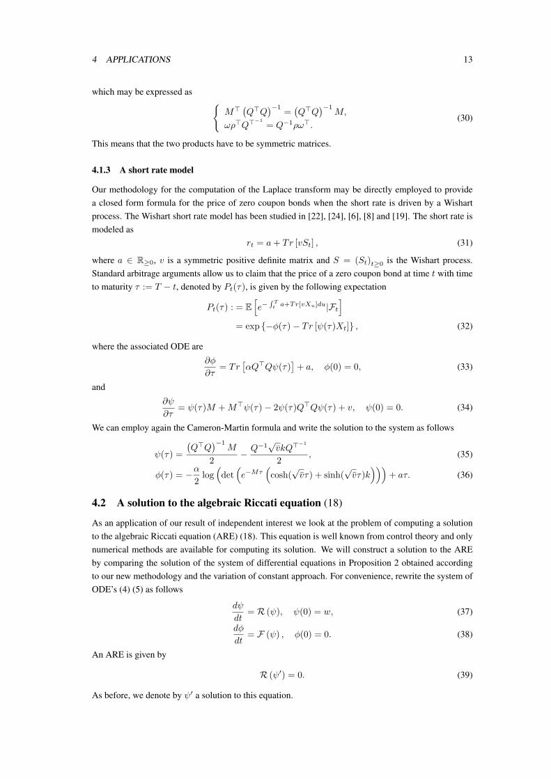
4.1.3 A short rate model

Our methodology for the computation of the Laplace transform may be directly employed to providea closed form formula for the price of zero coupon bonds when the short rate is driven by a Wishartprocess. The Wishart short rate model has been studied in [22], [24], [6], [8] and [19]. The short rate ismodeled as

rt = a+ Tr [vSt] , (31)

where a ∈ R≥0, v is a symmetric positive definite matrix and S = (St)t≥0 is the Wishart process.Standard arbitrage arguments allow us to claim that the price of a zero coupon bond at time t with timeto maturity τ := T − t, denoted by Pt(τ), is given by the following expectation

Pt(τ) : = E[e−

∫ Tta+Tr[vXu]du|Ft

]= exp −φ(τ)− Tr [ψ(τ)Xt] , (32)

where the associated ODE are

∂φ

∂τ= Tr

[αQ>Qψ(τ)

]+ a, φ(0) = 0, (33)

and

∂ψ

∂τ= ψ(τ)M +M>ψ(τ)− 2ψ(τ)Q>Qψ(τ) + v, ψ(0) = 0. (34)

We can employ again the Cameron-Martin formula and write the solution to the system as follows

ψ(τ) =

(Q>Q

)−1M

2− Q−1

√vkQ>

−1

2, (35)

φ(τ) = −α2

log(

det(e−Mτ

(cosh(

√vτ) + sinh(

√vτ)k

)))+ aτ. (36)

4.2 A solution to the algebraic Riccati equation (18)

As an application of our result of independent interest we look at the problem of computing a solutionto the algebraic Riccati equation (ARE) (18). This equation is well known from control theory and onlynumerical methods are available for computing its solution. We will construct a solution to the AREby comparing the solution of the system of differential equations in Proposition 2 obtained accordingto our new methodology and the variation of constant approach. For convenience, rewrite the system ofODE’s (4) (5) as follows

dψ

dt= R (ψ), ψ(0) = w, (37)

dφ

dt= F (ψ) , φ(0) = 0. (38)

An ARE is given by

R (ψ′) = 0. (39)

As before, we denote by ψ′ a solution to this equation.

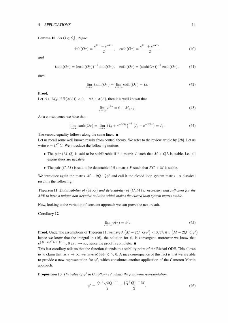
4 APPLICATIONS 14

Lemma 10 Let O ∈ S+d , define

sinh(Oτ) =eOτ − e−Oτ

2, cosh(Oτ) =

eOτ + e−Oτ

2(40)

and

tanh(Oτ) = (cosh(Oτ))−1

sinh(Oτ), coth(Oτ) = (sinh(Oτ))−1

cosh(Oτ), (41)

then

limτ→∞

tanh(Oτ) = limτ→∞

coth(Oτ) = Id. (42)

Proof.Let A ∈Md. If <(λ(A)) < 0, ∀λ ∈ σ(A), then it is well known that

limτ→∞

eAτ = 0 ∈Md×d. (43)

As a consequence we have that

limτ→∞

tanh(Oτ) = limτ→∞

(Id + e−2Oτ

)−1 (Id − e−2Oτ

)= Id. (44)

The second equality follows along the same lines.Let us recall some well known results from control theory. We refer to the review article by [28]. Let uswrite v = C>C. We introduce the following notions.

• The pair (M,Q) is said to be stabilizable if ∃ a matrix L such that M + QL is stable, i.e. alleigenvalues are negative.

• The pair (C,M) is said to be detectable if ∃ a matrix F stuch that FC +M is stable.

We introduce again the matrix M − 2Q>Qψ′ and call it the closed loop system matrix. A classicalresult is the following.

Theorem 11 Stabilizability of (M,Q) and detectability of (C,M) is necessary and sufficient for theARE to have a unique non-negative solution which makes the closed loop system matrix stable.

Now, looking at the variation of constant approach we can prove the next result.

Corollary 12

limτ→∞

ψ(τ) = ψ′. (45)

Proof. Under the assumptions of Theorem 11, we have λ(M − 2Q>Qψ′

)< 0, ∀λ ∈ σ

(M − 2Q>Qψ′

)hence we know that the integral in (16), the solution for ψ, is convergent, moreover we know thate(M−2Q>Qψ′)τ 0 as τ →∞, hence the proof is complete.This last corollary tells us that the function ψ tends to a stability point of the Riccati ODE. This allowsus to claim that, as τ →∞, we haveR (ψ(τ)) 0. A nice consequence of this fact is that we are ableto provide a new representation for ψ′, which constitutes another application of the Cameron-Martinapproach.

Proposition 13 The value of ψ′ in Corollary 12 admits the following representation

ψ′ =Q−1√vQ>

−1

2+

(Q>Q

)−1M

2. (46)

5 CONCLUSIONS 15

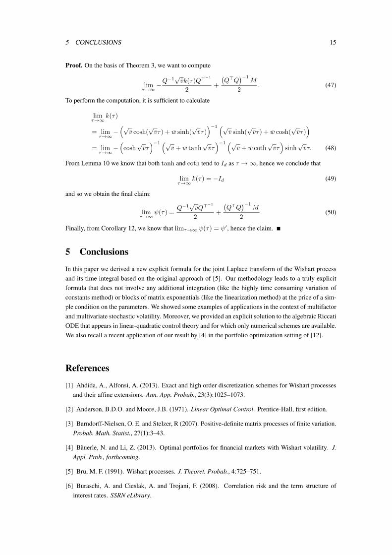
Proof. On the basis of Theorem 3, we want to compute

limτ→∞

−Q−1√vk(τ)Q>

−1

2+

(Q>Q

)−1M

2. (47)

To perform the computation, it is sufficient to calculate

limτ→∞

k(τ)

= limτ→∞

−(√


√vτ))−1 (√


√vτ))

= limτ→∞

−(

cosh√vτ)−1 (√

v + w tanh√vτ)−1 (√

v + w coth√vτ)

sinh√vτ. (48)

From Lemma 10 we know that both tanh and coth tend to Id as τ →∞, hence we conclude that

limτ→∞

k(τ) = −Id (49)

and so we obtain the final claim:

limτ→∞

ψ(τ) =Q−1√vQ>

−1

2+

(Q>Q

)−1M

2. (50)

Finally, from Corollary 12, we know that limτ→∞ ψ(τ) = ψ′, hence the claim.

5 Conclusions

In this paper we derived a new explicit formula for the joint Laplace transform of the Wishart processand its time integral based on the original approach of [5]. Our methodology leads to a truly explicitformula that does not involve any additional integration (like the highly time consuming variation ofconstants method) or blocks of matrix exponentials (like the linearization method) at the price of a sim-ple condition on the parameters. We showed some examples of applications in the context of multifactorand multivariate stochastic volatility. Moreover, we provided an explicit solution to the algebraic RiccatiODE that appears in linear-quadratic control theory and for which only numerical schemes are available.We also recall a recent application of our result by [4] in the portfolio optimization setting of [12].

References

[1] Ahdida, A., Alfonsi, A. (2013). Exact and high order discretization schemes for Wishart processesand their affine extensions. Ann. App. Probab., 23(3):1025–1073.

[2] Anderson, B.D.O. and Moore, J.B. (1971). Linear Optimal Control. Prentice-Hall, first edition.

[3] Barndorff-Nielsen, O. E. and Stelzer, R (2007). Positive-definite matrix processes of finite variation.Probab. Math. Statist., 27(1):3–43.

[4] Bauerle, N. and Li, Z. (2013). Optimal portfolios for financial markets with Wishart volatility. J.Appl. Prob., forthcoming.

[5] Bru, M. F. (1991). Wishart processes. J. Theoret. Probab., 4:725–751.

[6] Buraschi, A. and Cieslak, A. and Trojani, F. (2008). Correlation risk and the term structure ofinterest rates. SSRN eLibrary.

REFERENCES 16

[7] Buraschi, A. and Porchia, P. and Trojani, F. (2010). Correlation risk and optimal portfolio choice.The Journal of Finance, 65(1):393–420.

[8] Chiarella, C. and Hsiao, C. and To, T. (2010). Risk premia and Wishart term structure models.Working Paper, SSRN eLibrary.

[9] Christoffersen, P. and Heston, S. L. and Jacobs, K. (2009). The shape and term structure of theindex option smirk: why multifactor stochastic volatility models work so well. Management Science,72:1914–1932.

[10] Cuchiero, C. (2011). Affine and polynomial processes. PhD thesis, ETH Zurich.

[11] Cuchiero, C. and Filipovic, D. and Mayerhofer, E. and Teichmann, J. (2011). Affine processes onpositive semidefinite matrices. Ann. App. Prob., 21(2):397–463.

[12] Da Fonseca, J. and Grasselli, M. and Ielpo, F. (2011). Hedging (Co)Variance Risk with VarianceSwaps. Int. J. Theoretical Appl. Finance, 14:899–943.

[13] Da Fonseca, J. and Grasselli, M. and Ielpo, F. (2013). Estimating the Wishart Affine StochasticCorrelation Model Using the Empirical Characteristic Function. Stud. Nonlinear Dynam. Economet-rics, forthcoming.

[14] Da Fonseca, J. and Grasselli, M. and Tebaldi, C. (2007). Option pricing when correlations arestochastic: an analytical framework. Rev. Derivatives Res., 10(2):151–180.

[15] Da Fonseca, J. and Grasselli, M. and Tebaldi, C. (2008). A multifactor volatility Heston model.Quant. Finance, 8(6):591–604.

[16] Da Fonseca, J. and M. Grasselli (2011). Riding on the smiles. Quant. Finance, 11:1609–1632.

[17] Donati-Martin, C. and Doumerc, Y. and Matsumoto, H. and Yor, M. (2004). Some properties ofWishart process and a matrix extension of the Hartman–Watson law. Publ. Res. Inst. Math. Sci.,(40):1385–1412.

[18] Duffie, D. and Filipovic, D. and Schachermayer, W. (2003). Affine processes and applications infinance. Ann. App. Probab., 13:984–1053.

[19] Gnoatto, A. (2012). The Wishart short rate model. Int. J. Theoretical Appl. Finance, 15(8).

[20] Gourieroux, C. (2006). Continuous time Wishart process for stochastic risk. Econometric Rev.,25:177–217.

[21] Gourieroux, C. and Monfort, A. and Sufana, R. (2005). International money and stock marketcontingent claims. Working Papers 2005-41, Centre de Recherche en Economie et Statistique.

[22] Gourieroux, C. and Sufana, R. (2003). Wishart quadratic term structure models. SSRN eLibrary.

[23] Gourieroux, C. and Sufana, R. (2005). Derivative pricing with Wishart multivariate stochasticvolatility. J. Bus. Econ. Statist., 2004(October):1–44.

[24] Grasselli, M. and C. Tebaldi (2008). Solvable affine term structure models. Math. Finance,18:135–153.

[25] Heston, L. S. (1993). A closed-form solution for options with stochastic volatility with applicationsto bond and currency options. Rev. Finan. Stud., 6:327–343.

REFERENCES 17

[26] Jong, J. and Zhou, X. (1999). Stochastic controls: Hamiltonian systems and HJB equations.Springer, New York, 1st edition.

[27] Kang, C. and Kang, W. (2013). Transform formulae for linear functionals of affine processes andtheir bridges on positive semidefinite matrices. Stoch. Proc. App., 123(6):2419 – 2445.

[28] Kucera, V. (1973). A review of the matrix Riccati equation. Kybernetika, 9(1):42–61.

[29] Leippold, M. and Trojani, F. (2010). Asset pricing with matrix jump diffusions. SSRN eLibrary.

[30] Levin, J. J. (1959). On the matrix Riccati equation. Proc. Amer. Math. Soc., 10:519–524.

[31] Mayerhofer, E. (2012). Wishart processes and Wishart distributions: an affine processes point ofview. CIMPA lecture notes.

[32] Mayerhofer, E. (2013). On the existence of non-central Wishart distributions. J. Multiv. Anal.,114(0):448–456.

[33] Mayerhofer, E. and Pfaffel, O. and Stelzer, R. (2011). On strong solutions for positive definitejump-diffusions. Stoch. Proc. App., 121(9):2072–2086.

[34] Muhle-Karbe, J. and Pfaffel, O. and Stelzer, R. (2012). Option pricing in multivariate stochasticvolatility models of OU type. SIAM J. Fin. Math., 3:66–94.

[35] Pigorsch, C. and Stelzer, R. (2009). On the definition, stationary distribution and second orderstructure of positive semidefinite Ornstein-Uhlenbeck type processes. Bernoulli, 15(3):754–773.

[36] Pitman, J. and Yor, M. (1982). A decomposition of Bessel bridges. Probab. Theory Related Fields,59:425–457.

[37] Quarteroni, A. and Sacco, R. and Saleri, F. (2000). Numerical Mathematics, volume 37 of Texts inApplied Mathematics. Springer, first edition.

[38] Revuz, D. and Yor, M. (1994). Continuous martingales and Brownian motion, volume 293 ofFundamental Principles of Mathematical Sciences. Springer-Verlag, Berlin, second edition.

[39] Spreij, P. and Veerman, E. (2010). The affine transform formula for affine jump-diffusions with ageneral closed convex state space. ArXiv e-prints 1005.1099.

Time Horizon Lin. C.-M. Var. Const. R.-K.

0 0.998291461216988 0.998291461216988 0.998291461216988 0.9982914612169880.1 0.997303305375919 0.997303305375919 0.997306285702955 0.9972716055934160.5 0.992740622447456 0.992740622447456 0.992703104707601 0.9925839599524421.0 0.985698139368470 0.985698139368470 0.985426551402640 0.9853898823228251.5 0.977224894409802 0.977224894409802 0.976522044659620 0.9767708501755812.0 0.967388334051965 0.967388334051964 0.966066486500228 0.9667949662128652.5 0.956261597343174 0.956261597343174 0.954144681472186 0.9555359385446913.0 0.943922618087738 0.943922618087738 0.940848141282233 0.943072180564490

Table 1: This table visualizes the joint moment generating function of the Wishart process and its timeintegral for different time horizons τ . All four methods are considered. It should be noted that thevariation of constants method requires a very fine integration grid in order to produce precise values thatcan be compared with the results of the other methods.

REFERENCES 18

Figure 1: In this image we plot the time spent by the three analytical methods (linearization, Cameron-Martin and Variation of Constants) to compute the joint moment generating function of the Wishartprocess and its time integral for different time horizons. Notice that the Variation of Constants methodis inefficient even for quite short maturities.

Time horizon Lin. C.M. R.-K.

0 0.998291461216988 0.998291461216988 0.9982914612169880.1 0.997303305375919 0.997303305375919 0.9972716055934160.5 0.992740622447456 0.992740622447456 0.9925839599524421.0 0.985698139368470 0.985698139368470 0.9853898823228252.0 0.967388334051965 0.967388334051964 0.9667949662128653.0 0.943922618087738 0.943922618087738 0.9430721805644904.0 0.915938197508059 0.915938197508059 0.9148622073896615.0 0.884120166104796 0.884120166104796 0.88285219656021910.0 0.691634000576684 0.691634000576684 0.689897813632122

100.0 0.000001636282753 0.000001636282753 0.000001629036716

Table 2: In this table we do not include the results for the variation of constants method. This allows usto look at a longer time horizon and appreciate the precision of the new methodology also in this case.

The explicit Laplace transform for the Wishart process - arXiv

Documents