The Expected Value Premium

The Expected Value Premium

Long Chen∗

The Eli Broad College of Business

Michigan State University

Ralitsa Petkova†

Weatherhead School of Management

Case Western Reserve University

Lu Zhang‡

Stephen M. Ross School of Business

University of Michigan and NBER

September 2006§

Abstract

Fama and French (2002) estimate the equity premium using dividend growth rates to measureexpected rates of capital gain. We use a similar method to study the value premium. From1941 to 2005, the expected HML return is on average 6.0% per annum, consisting of an expecteddividend-growth component of 4.4% and an expected dividend-price-ratio component of 1.6%.The expected HML return is also countercyclical: a positive, one-standard-deviation shock toreal consumption growth lowers this premium by about 0.40%. Unlike the equity premium, thereis only mixed evidence suggesting that the expected value premium has declined over time.

∗Department of Finance, Eli Broad College of Business, Michigan State University, 321 Eppley Center, EastLansing, MI 48824. Tel: (517)353-2955, fax: (517)432-1080, and e-mail: [email protected].

†Department of Banking and Finance, Weatherhead School of Management, Case Western Reserve University,10900 Euclid Avenue, Cleveland OH 44106. Tel: (216)368-8553, and e-mail: [email protected].

‡Finance Department, Stephen M. Ross School of Business, University of Michigan, 701 Tappan Street, ER 7605Bus Ad, Ann Arbor MI 48109-1234. Tel: (734)615-4854, fax: (734)936-0282, and e-mail: [email protected].

§We thank George Constantinides, Bob Dittmar, Denitza Gintcheva, Bill Schwert, and seminar participants atKent State University and Case Western Reserve University for helpful comments. The first draft of this paper wascompleted while Lu Zhang was on the faculty of University of Rochester’s William E. Simon Graduate School ofBusiness Administration, whose support is gratefully acknowledged. We are responsible for all the remaining errors.

1 Introduction

Value stocks (stocks with high book-to-market ratios) earn higher average returns than growth

stocks (stocks with low book-to-market ratios). (See, for example, Rosenberg, Reid, and Lanstein

1985; Fama and French 1992; Lakonishok, Shleifer, and Vishny 1994). We study the value pre-

mium, defined as the difference between the expected returns of value stocks and growth stocks,

from a fresh angle by constructing an ex-ante measure of the value premium.

Our economic question is important. Following the seminal contributions of Fama and French

(1992, 1993, 1996), the value premium has become arguably as important as the equity premium in

investment management, capital budgeting, equity security analysis, risk management, and many

other applications. Moreover, most previous studies use average realized returns as proxies for

expected returns. But average returns are extremely noisy (e.g., Elton 1999; Fama and French

2002), and might not converge to expected returns in finite samples. As pointed out by Elton, there

are periods longer than ten years during which the stock market return is on average lower than the

risk free rate (1973–1984), and periods longer than 50 years during which risky bonds underperform

on average the risk free rate (1927–1981). Fama and French also argue forcefully that the estimates

of expected returns from fundamentals are more precise than the estimates from average returns.

Our estimation method follows Blanchard (1993) and Fama and French (2002). The basic idea

is simple. A rearrangement of the Gordon (1962) growth model says that:

R =D

P+ g (1)

where R is the equity return, DP

is the dividend price ratio, and g is the dividend growth rate. From

equation (1), the expected return can be decomposed into the expected dividend price ratio and the

expected dividend growth. To estimate these two components for value and growth portfolios, we

regress their future dividend price ratios and future dividend growth rates on a set of conditioning

variables. The expected value premium can then be calculated as the expected return of the value

2

portfolio minus the expected return of the growth portfolio.

Our fresh angle provides new insights into the magnitude of the value premium. First, a major

portion of the expected value premium comes from the dividend-growth component, which is often

larger in magnitude than the dividend-price-ratio component. The expected HML return is on

average 6.0% per annum from 1941 to 2005, consisting of an expected dividend-growth component

of 4.4% and an expected dividend-price-ratio component of 1.6%. And in the 1963–2005 subsam-

ple, the expected HML return is on average 6.2% per annum with an expected dividend-growth

component of 4.0% and an expected dividend-price-ratio component of 2.2%.

Crucially, our evidence that value portfolios have higher dividend growth rates than growth

portfolios does not contradict the conventional wisdom that growth firms have more growth op-

tions and grow faster than value firms.1 The crux is that our evidence is obtained from portfolios

rebalanced annually as in the Fama-French (1993) portfolio approach, but the conventional wis-

dom is based on the event-study approach using portfolios with fixed sets of firms. Because of

mean-reverting valuation ratios, value portfolios tend to experience above-average capital gains,

and growth portfolios tend to experience below-average capital gains. The portfolio approach with

annual refreshing accounts for these capital gains when calculating dividend growth rates from a

reinvestment perspective. But the event-study approach does not. Consequently, refreshed value

portfolios have higher dividend growth rates than refreshed growth portfolios, but unrefreshed value

portfolios have lower dividend growth rates than unrefreshed growth portfolios. We also provide

new evidence on the latter pattern using the Fama-French (1995) event-study framework.

And the expected value premium is countercyclical. From 1941 to 2005, the contemporaneous

correlation between the expected HML return and the default spread, a well-known countercyclical

variable, is 0.41 (p-value for testing zero correlation = 0.00). The correlation between the expected

HML return and the growth rate of real investment, a well-known procyclical variable, is −0.40

1For example, Bodie, Kane, and Marcus (2005, p. 127) write: “[G]rowth stocks have high ratios, suggesting thatinvestors in these firms must believe that the firm will experience rapid growth to justify the prices at which thestocks sell.”

3

(p-value = 0.00). However, the magnitude of the changes in the expected value premium in re-

sponse to macroeconomic shocks is too small relative to the magnitude of the premium itself. Using

a VAR framework, we document that a positive, one-standard-deviation shock to real investment

growth lowers the expected HML return by about 0.25% per annum. And a positive, one-standard-

deviation shock to real consumption growth reduces the expected HML return by about 0.40%.

Finally, purged from cyclical fluctuations, the expected value premium exhibits a weak down-

ward trend. But the evidence is mixed. Schwert (2003) shows that the value premium has declined

in the 1990s following the influential publications of Fama and French (1992, 1993), and argues

that academic research has made capital markets more efficient. Our evidence lends some support

to this argument. More generally, however, our evidence suggests that the poor profitability of

the value strategies in the 1990s is more likely to reflect cyclical movements in the value premium

rather than permanent downward shifts.

Our paper adds to the small but growing literature that uses valuation models to estimate

expected returns (e.g., Blanchard 1993; Claus and Thomas 2000; Jagannathan, McGrattan, and

Scherbina 2000; Gebhardt, Lee, and Swaminathan 2000; Constantinides 2002; Fama and French

2002). We use the methods of Blanchard and Fama and French, who study the equity premium.

But we focus on the value premium. Our analysis is also connected to Fama and French (2005),

who break average value-minus-growth returns into dividends and three sources of capital gain

including reinvestment of earnings, convergence in market-to-book ratios and general upward drift

in market-to-book. We instead use long-term dividend growth to measure the rates of capital gain.

Our story proceeds as follows. Section 2 delineates our estimation methods. Section 3 describes

our sample. The heart of the paper concerns the sources and the dynamics of the expected value

premium (Sections 4 and 5, respectively), and the predictability of the value premium (Section 6).

Finally, Section 7 interprets our results.

4

2 Experimental Design

Section 2.1 discusses the basic idea underlying our methods, and Section 2.2 presents the details.

2.1 The Basic Idea

We follow Blanchard (1993) and Fama and French (2002) to construct expected returns. The basic

idea is to estimate the expected rates of capital gain using dividend growth rates.

To be precise, let Rt+1 be the realized real stock return from time t to t + 1, 1+ Rt+1 =

(Dt+1+Pt+1)/Pt, where Pt is the stock price known at time t, and Dt+1 is the real dividend paid

over the period from t to t+1; Dt+1 is unknown until the beginning of time t+1. Following Blanchard

(1993), we divide both sides by Dt, take conditional expectations at time t, and linearize to obtain

the expected return at time t, denoted Et[Rt+1], as:

Et[Rt+1] = Et

[

Dt+1

Pt

]

+ Et[Agt+1], (2)

where Agt+1 is the long-run dividend growth rate defined as the annuity of future dividend growth:

Agt+1 ≡

[

r − g

1 + r

] ∞∑

i=0

[

1 + g

1 + r

]i

gt+i+1, (3)

with g and r being the average growth rate of real dividends and the average real stock return,

respectively. Finally, gt+1 denotes the realized growth rate of real dividends from time t to t+1.

Basically, equation (2) says that expected returns equal expected dividend price ratios plus ex-

pected long-run dividend growth rates. In our context, equation (2) implies that the expected value

premium equals the sum of the difference in the expected dividend price ratio and the difference

in the expected long-run dividend growth rate between value and growth portfolios.

2.2 Estimation Details

There are three basic steps in our estimation procedure.

5

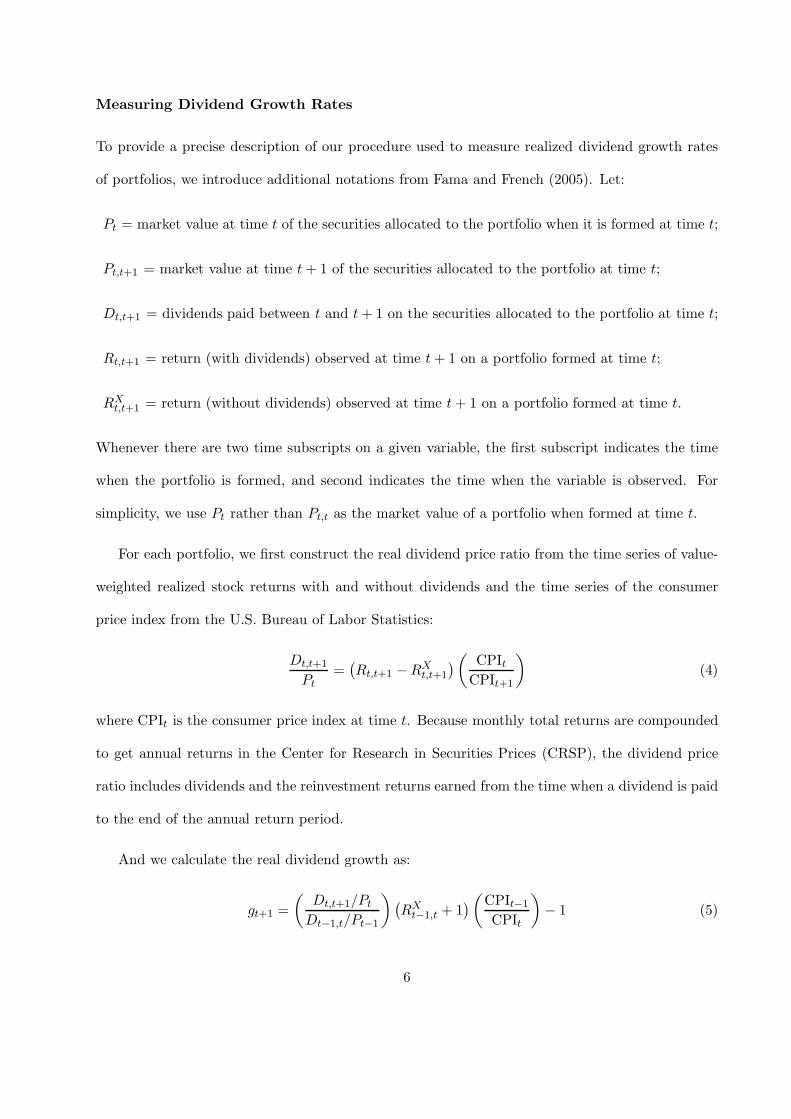
Measuring Dividend Growth Rates

To provide a precise description of our procedure used to measure realized dividend growth rates

of portfolios, we introduce additional notations from Fama and French (2005). Let:

Pt = market value at time t of the securities allocated to the portfolio when it is formed at time t;

Pt,t+1 = market value at time t + 1 of the securities allocated to the portfolio at time t;

Dt,t+1 = dividends paid between t and t + 1 on the securities allocated to the portfolio at time t;

Rt,t+1 = return (with dividends) observed at time t + 1 on a portfolio formed at time t;

RXt,t+1 = return (without dividends) observed at time t + 1 on a portfolio formed at time t.

Whenever there are two time subscripts on a given variable, the first subscript indicates the time

when the portfolio is formed, and second indicates the time when the variable is observed. For

simplicity, we use Pt rather than Pt,t as the market value of a portfolio when formed at time t.

For each portfolio, we first construct the real dividend price ratio from the time series of value-

weighted realized stock returns with and without dividends and the time series of the consumer

price index from the U.S. Bureau of Labor Statistics:

Dt,t+1

Pt

=(

Rt,t+1 − RXt,t+1

)

(

CPItCPIt+1

)

(4)

where CPIt is the consumer price index at time t. Because monthly total returns are compounded

to get annual returns in the Center for Research in Securities Prices (CRSP), the dividend price

ratio includes dividends and the reinvestment returns earned from the time when a dividend is paid

to the end of the annual return period.

And we calculate the real dividend growth as:

gt+1 =

(

Dt,t+1/Pt

Dt−1,t/Pt−1

)

(

RXt−1,t + 1

)

(

CPIt−1

CPIt

)

− 1 (5)

6

This definition of portfolio dividend growth needs further explanation. Using the definition of

return without dividends, RXt−1,t, we can rewrite equation (5) as:

gt+1 =

(

Dt,t+1/Pt

Dt−1,t/Pt−1

)(

Pt−1,t

Pt−1

)(

CPIt−1

CPIt

)

− 1 =

(

Dt,t+1

Dt−1,t

)(

Pt−1,t

Pt

)(

CPIt−1

CPIt

)

− 1 (6)

It appears that gt+1 does not collapse to (Dt,t+1/Dt−1,t)(CPIt−1/CPIt) − 1 because Pt and Pt−1,t

are values for different portfolios. Pt−1,t is the market value at time t of the portfolio formed at time

t−1 just before being refreshed at time t, while Pt is the market value at time t of the portfolio just

after being refreshed at time t. And the portfolio after refreshing (rebalancing) contains different

securities from those before refreshing.

From a reinvestment perspective, equation (5) is an economically meaningful measure of

portfolio dividend growth. Consider the following numerical example. Suppose at the end of June

of year t− 1, an investor invests $100 in the value portfolio that value weights a set of value stocks

(Pt−1 = $100). Suppose the value portfolio has a dividend price ratio of 5% (Dt−1,t/Pt−1 = 5%), so

at the end of June of year t the investor gets $5 as dividends. Also suppose, because of capital gains,

the market value of the value portfolio becomes $110 at the end of June of year t (Pt−1,t = $110).

At this time, the investor refreshes the portfolio, meaning that she cashes out $110 and reinvests

this same amount (Pt = $110) in the refreshed value portfolio that value weights a new set of value

stocks. Suppose that the new portfolio has a dividend price ratio of 6% (Dt,t+1/Pt = 6%). At the

end of June of year t+1, the investor will receive dividends of $110×6% = $6.6. The rate of dividend

growth from the end of June of year t to the end of June of year t+1 should thus be 6.6/5−1 = 0.32.

This dividend growth rate is precisely what equation (5) gets: (6%/5%)($110/$100)−1 = 0.32.

If, we do not reinvest the capital gain of $10 (Pt−1,t − Pt−1), the dividend growth rate is only

(6%/5%) − 1 = 0.20. However, it is important to capture this capital gain because it is a part of

the proceeds for the value strategy that investors can easily implement. In addition, our expected-

return construction builds on the idea of using dividend growth rates to measure the expected rates

of capital gain (e.g., Fama and French 2002).

7

The reinvestment logic thus sheds light on the apparent “inconsistency” in equation (6). The

crux is that, from the reinvestment perspective, after the investor cashes out $110 (Pt−1,t) at the

end of June of year t, she immediately reinvests the same amount of $110 (Pt) in the refreshed

portfolio that value weights a different set of stocks. In short, the reinvestment logic implies that

Pt−1,t = Pt. From equation (6), gt+1 does collapse to (Dt,t+1/Dt−1,t)(CPIt−1/CPIt) − 1.

Our definition of portfolio dividend growth is consistent with those in Campbell and Shiller

(1988), Cochrane (1992, 2006), and Bansal, Dittmar, and Lundblad (2005). For example, Cochrane

(2006, footnote 5) finds dividend yields by (expressed in the notations from Fama and French 2005):

Dt,t+1

Pt,t+1

=

(

Rt,t+1 + 1

RXt,t+1 + 1

)

− 1 =Pt,t+1 + Dt,t+1

Pt

Pt

Pt,t+1

− 1

and dividend growths by

Dt,t+1

Dt−1,t

=

(

Dt,t+1/Pt,t+1

Dt−1,t/Pt−1,t

)

(RXt,t+1 + 1) − 1 =

Dt,t+1

Pt,t+1

Pt−1,t

Dt−1,t

Pt,t+1

Pt

− 1 =Dt,t+1

Dt−1,t

Pt−1,t

Pt

− 1

Putting aside the CPI adjustment, the last equation is exactly our equation (6). Therefore, the rein-

vestment logic that gives rise to Pt−1,t = Pt is also implicitly embedded in Cochrane (1992, 2006).

Finally, the real dividend growth rates constructed from equation (5) are quite volatile even at

the portfolio level. To control for the effects of the outliers, we replace any annual observations of

dividend growth higher than 50% with 50% and those lower than −50% with −50%.

Measuring Long-run Dividend Growth Rates

To construct the long-run dividend growth, Agt+1, we follow Blanchard (1993) to estimate r as the

sample average of the realized real equity returns and g as the sample average of the real dividend

growth rates. From equation (3), Agt+1 is an infinite sum of future real dividend growth rates; in

practice we use a finite sum of 100 years of future growth. We assume that future real dividend

growth rates beyond 2005 equal the average dividend growth rate during the 1963–2005 period.2

2We also use the full-sample (1941–2005) average and the results are not materially affected (not reported).

8

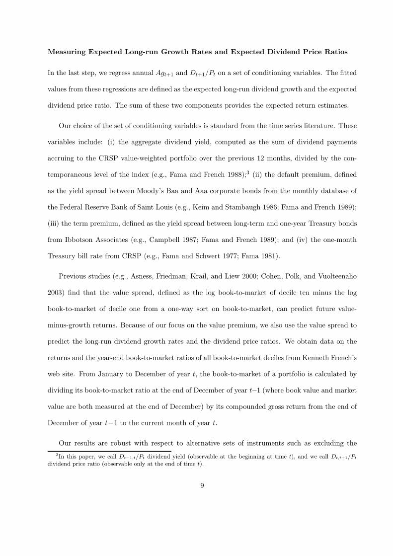
Measuring Expected Long-run Growth Rates and Expected Dividend Price Ratios

In the last step, we regress annual Agt+1 and Dt+1/Pt on a set of conditioning variables. The fitted

values from these regressions are defined as the expected long-run dividend growth and the expected

dividend price ratio. The sum of these two components provides the expected return estimates.

Our choice of the set of conditioning variables is standard from the time series literature. These

variables include: (i) the aggregate dividend yield, computed as the sum of dividend payments

accruing to the CRSP value-weighted portfolio over the previous 12 months, divided by the con-

temporaneous level of the index (e.g., Fama and French 1988);3 (ii) the default premium, defined

as the yield spread between Moody’s Baa and Aaa corporate bonds from the monthly database of

the Federal Reserve Bank of Saint Louis (e.g., Keim and Stambaugh 1986; Fama and French 1989);

(iii) the term premium, defined as the yield spread between long-term and one-year Treasury bonds

from Ibbotson Associates (e.g., Campbell 1987; Fama and French 1989); and (iv) the one-month

Treasury bill rate from CRSP (e.g., Fama and Schwert 1977; Fama 1981).

Previous studies (e.g., Asness, Friedman, Krail, and Liew 2000; Cohen, Polk, and Vuolteenaho

2003) find that the value spread, defined as the log book-to-market of decile ten minus the log

book-to-market of decile one from a one-way sort on book-to-market, can predict future value-

minus-growth returns. Because of our focus on the value premium, we also use the value spread to

predict the long-run dividend growth rates and the dividend price ratios. We obtain data on the

returns and the year-end book-to-market ratios of all book-to-market deciles from Kenneth French’s

web site. From January to December of year t, the book-to-market of a portfolio is calculated by

dividing its book-to-market ratio at the end of December of year t−1 (where book value and market

value are both measured at the end of December) by its compounded gross return from the end of

December of year t−1 to the current month of year t.

Our results are robust with respect to alternative sets of instruments such as excluding the

3In this paper, we call Dt−1,t/Pt dividend yield (observable at the beginning at time t), and we call Dt,t+1/Pt

dividend price ratio (observable only at the end of time t).

9

value spread or including Lettau and Ludvigson’s (2001a, 2005) cay and cdy variables in the set of

conditioning variables (not reported).

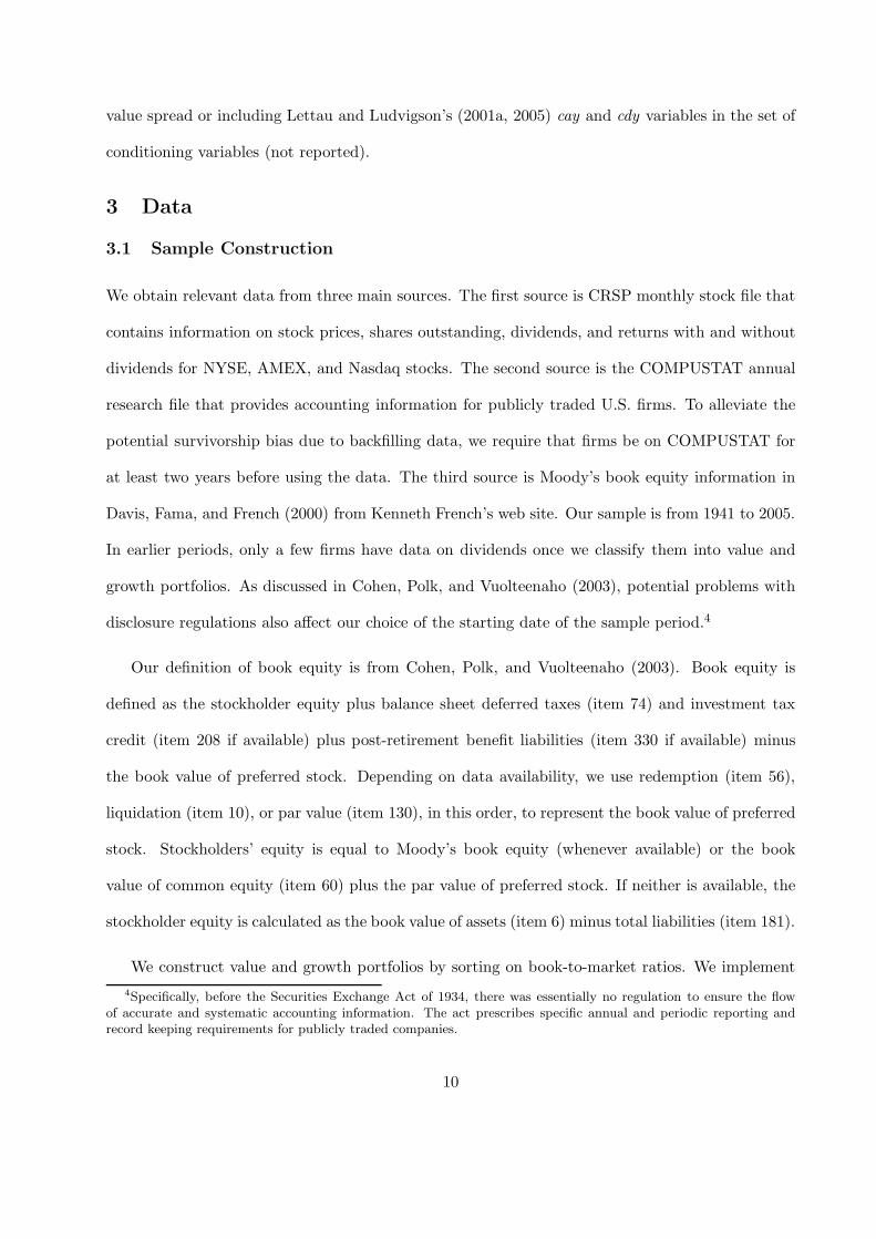
3 Data

3.1 Sample Construction

We obtain relevant data from three main sources. The first source is CRSP monthly stock file that

contains information on stock prices, shares outstanding, dividends, and returns with and without

dividends for NYSE, AMEX, and Nasdaq stocks. The second source is the COMPUSTAT annual

research file that provides accounting information for publicly traded U.S. firms. To alleviate the

potential survivorship bias due to backfilling data, we require that firms be on COMPUSTAT for

at least two years before using the data. The third source is Moody’s book equity information in

Davis, Fama, and French (2000) from Kenneth French’s web site. Our sample is from 1941 to 2005.

In earlier periods, only a few firms have data on dividends once we classify them into value and

growth portfolios. As discussed in Cohen, Polk, and Vuolteenaho (2003), potential problems with

disclosure regulations also affect our choice of the starting date of the sample period.4

Our definition of book equity is from Cohen, Polk, and Vuolteenaho (2003). Book equity is

defined as the stockholder equity plus balance sheet deferred taxes (item 74) and investment tax

credit (item 208 if available) plus post-retirement benefit liabilities (item 330 if available) minus

the book value of preferred stock. Depending on data availability, we use redemption (item 56),

liquidation (item 10), or par value (item 130), in this order, to represent the book value of preferred

stock. Stockholders’ equity is equal to Moody’s book equity (whenever available) or the book

value of common equity (item 60) plus the par value of preferred stock. If neither is available, the

stockholder equity is calculated as the book value of assets (item 6) minus total liabilities (item 181).

We construct value and growth portfolios by sorting on book-to-market ratios. We implement

4Specifically, before the Securities Exchange Act of 1934, there was essentially no regulation to ensure the flowof accurate and systematic accounting information. The act prescribes specific annual and periodic reporting andrecord keeping requirements for publicly traded companies.

10

both a one-way sort to obtain five book-to-market quintiles and a two-way, two-by-three sort on

size and book-to-market to obtain six portfolios a la Fama and French (1993). We denote the

one-way sorted quintiles as Low, 2, 3, 4, and High. The difference between quintiles High and Low,

denoted p5-1, represents the value-minus-growth strategy from the one-way sort. The six portfolios

from the two-way sort on size and book-to-market are denoted by S/L, B/L, S/M, B/M, S/H,

and B/H, and the value-minus-growth strategy from the two-way sort, denoted HML, is defined as

(S/H + B/H)/2 − (S/L + B/L)/2. Using the 25 portfolios from a two-way, five-by-five sort on size

and book-to-market yields similar results as the two-by-three sort (not reported).5

Our timing in portfolio construction differs slightly from that used in Fama and French (1993).

Instead of at the end of June, we form portfolios at the end of December for each year t. We use

book equity from the fiscal year ending in calendar year t−1 divided by market equity at the end of

December of year t. This method avoids any look-ahead bias that might arise because accounting

information from the current fiscal year is often not available at the end of the calendar year. Port-

folio ranking is effective from January of year t+1 to December of year t+1. We choose this timing of

portfolio formation to facilitate the interpretation of our test results. The reason is that this timing

is better in line with the timing of dividend growth, which goes from the beginning to the end of the

calendar year. Our different timing does not appear to be a source of concern, however. Using more

lagged information on book value makes it harder for us to find an ex-ante, positive value premium.

And using the more conventional timing yields quantitatively similar results (not reported).

3.2 The Equity Premium

Our method for estimating the expected value premium is basically a dynamic version of the Fama

and French (2002) method for estimating the equity premium. Before we report our value premium

estimates, it is important to ask whether the properties of the equity premium constructed in our

sample are comparable to those reported by Fama and French. The answer is affirmative.

5To be precise, the expected value premium from the finer sort is larger in magnitude than that from the two-by-three sort. The reason is that the finer sort generates more spread in book-to-market across portfolios.

11

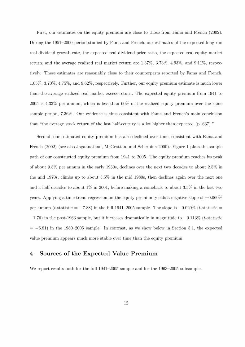
First, our estimates on the equity premium are close to those from Fama and French (2002).

During the 1951–2000 period studied by Fama and French, our estimates of the expected long-run

real dividend growth rate, the expected real dividend price ratio, the expected real equity market

return, and the average realized real market return are 1.37%, 3.73%, 4.93%, and 9.11%, respec-

tively. These estimates are reasonably close to their counterparts reported by Fama and French,

1.05%, 3.70%, 4.75%, and 9.62%, respectively. Further, our equity premium estimate is much lower

than the average realized real market excess return. The expected equity premium from 1941 to

2005 is 4.33% per annum, which is less than 60% of the realized equity premium over the same

sample period, 7.36%. Our evidence is thus consistent with Fama and French’s main conclusion

that “the average stock return of the last half-century is a lot higher than expected (p. 637).”

Second, our estimated equity premium has also declined over time, consistent with Fama and

French (2002) (see also Jagannathan, McGrattan, and Scherbina 2000). Figure 1 plots the sample

path of our constructed equity premium from 1941 to 2005. The equity premium reaches its peak

of about 9.5% per annum in the early 1950s, declines over the next two decades to about 2.5% in

the mid 1970s, climbs up to about 5.5% in the mid 1980s, then declines again over the next one

and a half decades to about 1% in 2001, before making a comeback to about 3.5% in the last two

years. Applying a time-trend regression on the equity premium yields a negative slope of −0.060%

per annum (t-statistic = −7.88) in the full 1941–2005 sample. The slope is −0.020% (t-statistic =

−1.76) in the post-1963 sample, but it increases dramatically in magnitude to −0.113% (t-statistic

= −6.81) in the 1980–2005 sample. In contrast, as we show below in Section 5.1, the expected

value premium appears much more stable over time than the equity premium.

4 Sources of the Expected Value Premium

We report results both for the full 1941–2005 sample and for the 1963–2005 subsample.

12

4.1 Estimates for the Value Premium, Ex-post and Ex-ante

Consistent with many previous studies, the first two rows of all panels in Table 1 show that the

ex-post average returns of the value-minus-growth strategies are reliably positive. Portfolio p5-1

has an average return of 6.2% per annum (t-statistic = 2.95) in the full sample, and 5.2% per annum

(t-statistic = 2.33) in the subsample. The t-statistics we report are adjusted for heteroscedasticity

and autocorrelations of up to six lags. Further, HML has an average return of 6.2% per annum

both in the full sample and in the subsample with t-statistics above four.

The expected value premium is reliably positive in our sample. From the seventh and eighth

rows in all panels of Table 1, the average expected dividend price ratio is higher for value firms than

for growth firms. Because the expected long-run dividend growth and the expected dividend price

ratio are both higher for value portfolios, their expected returns are higher than those of growth

portfolios. The last two rows of Panels A and B show that the expected return of p5-1 is 4.6% per

annum in the full sample and 4.2% in the subsample, and both are highly significant. From the

last two rows of Panels C and D, the expected HML return is 6.0% per annum in the full sample,

and 6.2% in the subsample, both of which are again highly significant.

Interestingly, Table 1 shows that expected returns for value and growth portfolios are generally

lower than their average realized returns. In particular, portfolio S/L has an expected return of

3.2% in the 1963–2005 sample, less than one half of its average realized return of 7.6% over the

same period. Fama and French (2002) find a similar discrepancy between expected returns and

average returns for the market portfolio and argue that average stock returns are a lot higher than

expected. We reinforce their conclusion by showing that it also holds in for size and book-to-market

portfolios. And the average expected returns for individual value and growth portfolios are also

more precisely estimated than their average realized returns.

However, the expected value-minus-growth returns from both sorting procedures are close to

their average returns. The expected HML return is on average 6% per annum, close to the aver-

13

age return of 6.2% in the 1941–2005 sample. This evidence suggests that the difference between

expected returns and average returns is similar in magnitude across value and growth portfolios.

From the middle two rows of all panels in Table 1, an important source of the expected value

premium is the expected long-run dividend growth, Et[Agt+1]. The average Et[Agt+1] for HML is

4.4% per annum in the full sample and 4.0% in the subsample, and both are highly significant.

The average long-run dividend growth rate contributes to more than 65% of the expected HML

return. From the one-way sort, the expected long-run dividend growth accounts for slightly above

one half of the average expected p5-1 return in the full sample, 4.6%, and about 35% of the average

expected p5-1 return in the 1963–2005 sample, 4.2%.

4.2 Dividend Growth Rates and the Importance of Rebalancing

Given the importance of dividend growth in driving the value premium, we present more detailed

results on dividend growth rates. Crucially, our evidence that value portfolios have higher divi-

dend growth rates than growth portfolios does not contradict the conventional wisdom that growth

stocks have more growth options and grow faster than value stocks. The crux is that our evidence

is obtained from portfolios refreshed annually, while the conventional wisdom is based on portfolios

with fixed sets of firms without refreshing.

Dividend Growth Rates for Refreshed Portfolios

From rows three and four in all panels of Table 1, the one-year ahead real dividend growth rate,

gt+1, for value portfolios is on average higher than that of growth portfolios, but the difference is

often insignificant. The real dividend growth rate of portfolio p5-1 is on average 4.7% per annum in

the full sample (t-statistic = 1.65). Controlling for size increases the average growth rate further to

5.9% for HML (t-statistic = 2.42). Figure 2 provides more information on the real dividend growth

rate by plotting its sample paths for the annually refreshed value and growth portfolios. The real

dividend growth rates for value portfolios are frequently higher than those for growth portfolios.

14

The Importance of Rebalancing

When the portfolios are refreshed annually, the firms in the growth portfolio next year are not the

same firms in the portfolio in the current year. Because dividend growth is measured using different

sets of firms, there is no particular reason to expect the dividend growth of growth portfolios to be

higher than the dividend growth of value portfolios.

More important, because of mean-reversion in valuation ratios (e.g., Figure 2 in Fama and

French 1995, more evidence in Figure 3 below), value investors are likely to experience above-

average capital gains, and growth investors are likely to experience below-average capital gains (or

even capital losses). The portfolio approach with rebalancing takes these capital gains and losses

into account when calculating dividend growth rates, but the event-study approach with fixed sets

of firms does not. Consequently, refreshed value portfolios have higher dividend growth rates (more

precisely, rates of capital gains) than refreshed growth portfolios, but unrefreshed value portfolios

have lower dividend growth rates than unrefreshed growth portfolios.

To illustrate this point further, consider again the numerical example in Section 2.2. The follow-

ing is the same setup but repeated here for convenience. At the end of June of year t−1, an investor

invests $100 in a value portfolio. Suppose the value portfolio has a dividend price ratio of 5%, im-

plying that at the end of June of year t, the investor gets $5 as dividends. Also suppose, because

of capital gains, the market value of the value portfolio becomes $110 at the end of June of year t.

At this time, however, suppose the investor does not refresh the portfolio. The market value of

the portfolio is $110, but she does not cash it out and reinvest it in a refreshed portfolio. And sup-

pose that the same firms in the value portfolio follow sticky dividend policies and continue to pay $5

of dividends. It follows that the new dividend price ratio for the portfolio is $5/110 = 4.55% < 5%.

Consistent with this reasoning, we show below in Figure 3 that, using the framework of Fama and

French (1995), dividend price ratios of unrefreshed value portfolios decline after portfolio formation.

Bottomline: the dividend growth rate for the unrefreshed value portfolio is zero ($5/$5 − 1 = 0%).

15

Alternatively, suppose the same firms in the unrefreshed value portfolio increase dividends from

$5 to $6. Its rate of dividend growth from the end of June of year t to the end of June of year t + 1

now becomes $6/$5 − 1 = 20%. This rate is lower than the 32% that we calculated earlier for the

refreshed portfolio when capital gains are reinvested. In general, as long as the firms in the value

portfolio do not increase dividends as fast as their rates of capital gain, then the dividend growth

for the unrefreshed value portfolio will likely be lower than that for the refreshed value portfolio.

Dividend Growth Rates for Unrefreshed Portfolios

To show that annual rebalancing is indeed the driving force behind our results that value portfolios

have higher dividend growth rates than growth portfolios, we report the real dividend growth for

unrefreshed value and growth portfolios for 21 years around the portfolio formation year.

Our test design follows closely the Fama and French (1995) event-study framework, in which

the stocks in the value and growth portfolios are held constant throughout the event years. To

complement the evidence on dividend growth, we also report the event-time evolution of dividend

price ratio (dividends over lagged stock price), profitability (earnings over lagged book equity), and

dividend on equity (dividends over lagged book equity).

We obtain data on dividend and earnings directly at the firm level. Monthly dividends for firm

j are calculated as: Djt+1 = (Rjt+1 − RXjt+1) × Pjt × Shroutjt, where Rjt+1 and RX

jt+1 are equity

returns from the beginning of month t to the beginning of month t+1 with and without dividends,

respectively, Pjt is stock price and Shroutjt is the number of shares outstanding at the beginning

of month t. We aggregate monthly dividends within the year to obtain annual dividends. And

because earnings data are not available in the pre-COMPUSTAT period, we follow Cohen, Polk,

and Vuolteenaho (2003) and use the clean-surplus relation to compute earnings from data on book

equity and dividends, i.e., earnings(t) = book value(t) − book value(t − 1) + dividends(t). To be

consistent, we use this relation to compute earnings throughout our 1941–2005 sample. Using direct

earnings data yields similar results in the post-COMPUSTAT sample (not reported).

16

Dividend growth for a unrefreshed portfolio is defined as the sum of dividends for all firms in the

portfolio divided by the sum of lagged dividends for the same firms. The dividend price ratio of a

portfolio is the sum of dividends for all firms in the portfolio divided by the sum of lagged stock prices

for the same firms. The profitability and the dividend on equity of a portfolio are the sum of earnings

and dividends, respectively, for all firms in the portfolio divided by the sum of lagged book equity.

All variables are subsequently adjusted for inflation using the consumer price index. Following Fama

and French (1995), for each portfolio formation year y, we calculate profitability, dividend on equity,

dividend price ratio, and dividend growth of value and growth portfolios for year y + △, where

△ = −10, . . . , 10. These variables for year y+△ are then averaged across portfolio formation years.

Panels A and C of Figure 3 report that the dividend growth rates for unrefreshed growth port-

folios are higher than those for unrefreshed value portfolios. For example, the spread in dividend

growth from the one-way sort is about 10% at the portfolio formation year, and remains positive

for almost ten years afterwards. For the two-way sort, the spread in dividend growth between the

small-growth portfolio, S/L, and the small-value portfolio, S/H, is about 15% at portfolio formation,

but the spread is much more short-lived and converges in about three years.

Panels B and D of Figure 3 help explain why the results on dividend growth for the unrefreshed

portfolios differ from those for the refreshed portfolios in Figure 2. The panels show that dividend

price ratios for unrefreshed value portfolios decline after portfolio formation. Because dividends

are much smoother than stock prices, the evidence suggests that value investors tend to experience

above-average capital gains. In contrast, dividend price ratios for unrefreshed portfolio Low and

portfolio B/L stay largely constant, suggesting below-average (or near zero) capital gains. An ex-

ception is portfolio S/L with declining dividend price ratios after portfolio formation. However, as

we show below in Panel D of Figure 4, portfolio S/L experiences a much more dramatic decline in

dividend on (book) equity than all the other portfolios. This evidence suggests that the decline in

dividend price ratio for portfolio S/L is also likely to result from declining dividends.

17

Complementing our dividend-growth evidence, Figure 4 confirms Fama and French’s (1995)

finding that there are size and book-to-market factors in earnings. High book-to-market signals

persistent poor earnings and low book-to-market signals strong earnings (Panels A and C). We add

to their evidence by showing that dividend on equity largely follows the same pattern as profitability

(Panels B and D). And the spread in dividend on equity between value and growth portfolios appears

even more persistent than the spread in profitability, especially for the two-way sort. This evidence

is perhaps not surprising because firms are likely to have more flexibility in adjusting earnings

through discretionary accruals than in adjusting dividends (e.g., Graham and Harvey 2001).

5 Dynamics of the Expected Value Premium

This section focuses on long-term and cyclical dynamics of the expected value premium.

Figure 5 plots the expected p5-1 return, the expected HML return, and their expected long-run

dividend growth rates and expected dividend price ratios. From Panels A and C, the expected p5-1

and HML returns are positive throughout the sample, suggesting these zero-investment strategies

are ex-ante profitable. And as an indication of the countercyclical properties of the value premium,

the expected p5-1 and HML returns also covary positively with the default premium, a well-known

countercyclical variable (e.g., Stock and Watson 1999).

From Panels B and D of Figure 5, the expected long-run dividend growth for value-minus-

growth strategies displays a noticeable decline from the early 1940s to the early 1980s, but an

increase thereafter. The expected dividend price ratios display opposite long-term movements.

This evidence is consistent with the present value logic which implies that a high dividend price

ratio means a low price, which in turn indicates lower future dividend growth.6 Because of the op-

posite movements between expected long-run dividend growth and expected dividend price ratios,

there is no noticeable long-term trend in the expected value premium. However, the expected p5-1

6This evidence concerns the predictability of long-run dividend growth, which differs from the weak evidence onpredictability of one-period ahead dividend growth (e.g., Lettau and Ludvigson 2005; Cochrane 2006).

18

return appears to have declined somewhat over time.

5.1 Trend Dynamics

Unlike the equity premium that displays a clear downward-sloping trend (Figure 1), there is only

mixed evidence suggesting that the expected value premium has declined over time.

We use two methods to isolate the cyclical component of the expected value premium from the

low-frequency trend component. First, we regress the expected value premium on a time trend:

The Expected Value Premium(t) = a + b t + εt, (7)

where the fitted component is defined as the trend component and the residual is defined as the

cyclical component. The second method is to pass the expected value premium through the Hodrick-

Prescott (HP, 1997) filter that separates the trend and the cyclical components.

From the time-trend regressions, the expected p5-1 return exhibits a downward trend in the

1941–2005 and the 1963–2005 samples, but the expected HML return does not. The expected HML

return exhibits a slight downward trend in the 1980–2005 sample, but the expected p5-1 return does

not. Specifically, the slope coefficient from regression (7) is −0.042% per annum for the expected

p5-1 return (t-statistic = −5.46) in the 1941–2005 sample, −0.023% (t-statistic = −1.86) in the

post-1963 sample, and −0.043% (t-statistic = −1.52) in the 1980–2005 sample. For the expected

HML return, the slope is 0.006% (t-statistic = 1.02) for in 1941–2005, −0.001% (t-statistic = −0.57)

in 1963–2005, and −0.076% (t-statistic = −3.90) in the 1980–2005 sample.

Panels A and B in Figure 6 plot the trend components for the expected p5-1 and HML returns,

respectively, estimated from time-trend regressions and the HP-filter based on the full sample. Panel

A shows a downward trend in expected returns for p5-1 but a slight upward trend for HML. Panel

B shows a downward movement in the HP-filtered trend component for HML, but not for p5-1.

Because the ex-ante and the ex-post average HML returns are close (Table 1), we also use the

ten-year moving averages of realized HML returns as a measure of the slow-moving trend compo-

19

nent of the value premium. It is clear from Panel C of Figure 6 that the expected value premium

has been quite stable with no visible downward trend. And Panel C largely confirms Schwert’s

(2003) observation that the magnitude of the value premium has declined over the 1990s following

the influential publications of Fama and French (1992, 1993). Schwert’s sample is from January

1982 to May 2002, however. And Panel C shows that the long-run value premium spikes afterwards.

Using the one-way sorted portfolio p5-1 instead of HML yields largely similar results.

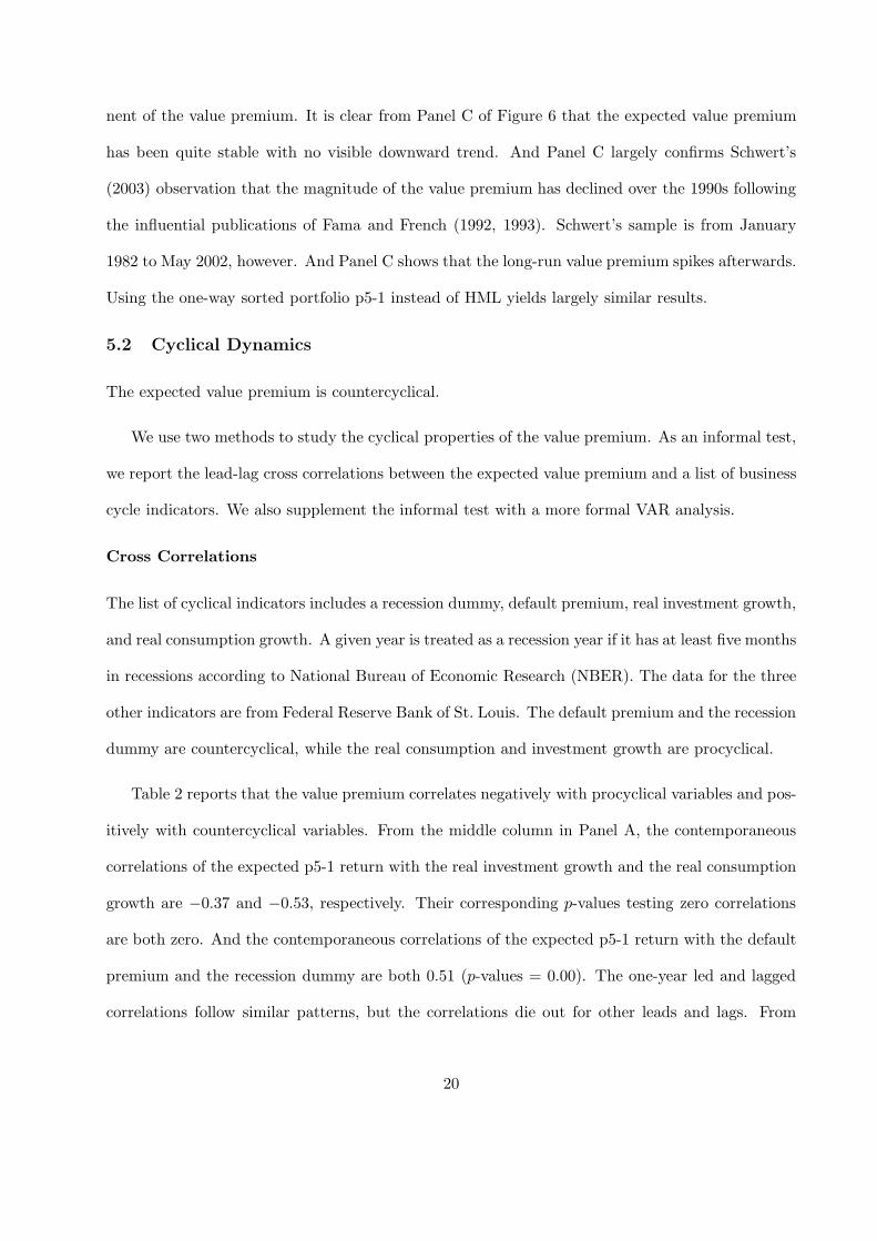
5.2 Cyclical Dynamics

The expected value premium is countercyclical.

We use two methods to study the cyclical properties of the value premium. As an informal test,

we report the lead-lag cross correlations between the expected value premium and a list of business

cycle indicators. We also supplement the informal test with a more formal VAR analysis.

Cross Correlations

The list of cyclical indicators includes a recession dummy, default premium, real investment growth,

and real consumption growth. A given year is treated as a recession year if it has at least five months

in recessions according to National Bureau of Economic Research (NBER). The data for the three

other indicators are from Federal Reserve Bank of St. Louis. The default premium and the recession

dummy are countercyclical, while the real consumption and investment growth are procyclical.

Table 2 reports that the value premium correlates negatively with procyclical variables and pos-

itively with countercyclical variables. From the middle column in Panel A, the contemporaneous

correlations of the expected p5-1 return with the real investment growth and the real consumption

growth are −0.37 and −0.53, respectively. Their corresponding p-values testing zero correlations

are both zero. And the contemporaneous correlations of the expected p5-1 return with the default

premium and the recession dummy are both 0.51 (p-values = 0.00). The one-year led and lagged

correlations follow similar patterns, but the correlations die out for other leads and lags. From

20

the middle column in Panel B, using the expected HML return yields largely similar results. The

evidence from the 1941–2005 sample is similar to that from the post-1963 sample.

Panels D and E of Figure 6 provide additional evidence on the cyclicality of the expected value

premium. The panels plot the cyclical components estimated using the time-trend regressions and

the HP-filter for the expected p5-1 and HML returns along with the NBER recession dummy. It is

clear from the panels that the expected value premiums peak in most of the recessions in the sample.

VAR Analysis

To study the degree of cyclicality in the expected value premium, we adopt a more formal VAR

framework. The VAR contains one cyclical indicator and either the expected p5-1 return or the ex-

pected HML return. We use two cyclical variables separately in the VAR, the real investment growth

and the real consumption growth. Using other cyclical variables yields largely similar results (not

reported). The lag in the VAR is one, which is based on the Akaike information criterion. In some

specifications, we also include the one-month T-bill rate to isolate the effects of monetary shocks.

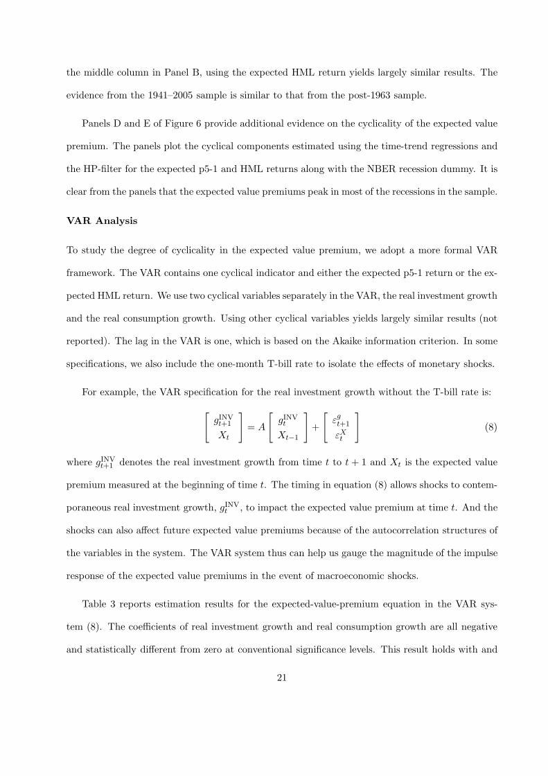
For example, the VAR specification for the real investment growth without the T-bill rate is:

[

gINVt+1

Xt

]

= A

[

gINVt

Xt−1

]

+

[

εgt+1

εXt

]

(8)

where gINVt+1 denotes the real investment growth from time t to t + 1 and Xt is the expected value

premium measured at the beginning of time t. The timing in equation (8) allows shocks to contem-

poraneous real investment growth, gINVt , to impact the expected value premium at time t. And the

shocks can also affect future expected value premiums because of the autocorrelation structures of

the variables in the system. The VAR system thus can help us gauge the magnitude of the impulse

response of the expected value premiums in the event of macroeconomic shocks.

Table 3 reports estimation results for the expected-value-premium equation in the VAR sys-

tem (8). The coefficients of real investment growth and real consumption growth are all negative

and statistically different from zero at conventional significance levels. This result holds with and

21

without controlling for the T-bill rate.

To help interpret the economic magnitudes of the VAR slopes, we plot the impulse response

functions from the estimated VARs. From Panels C and D, a positive, one-standard-deviation shock

to the real investment growth reduces the expected HML return by 0.30% per annum without con-

trolling for the T-bill rate and by about 0.26% with the T-bill rate. From Panels G and H, a positive,

one-standard-deviation shock to the real consumption growth reduces the expected HML return by

about 0.40% per annum with and without controlling for the T-bill rate. And Panels A, B, E, and

F report similar results using the expected p5-1 return, but the magnitudes are somewhat lower.

Our evidence on cyclical dynamics of the value premium lends support to the view that value

stocks are riskier than growth stocks in bad times (e.g., Jagannathan and Wang 1996, Lettau and

Ludvigson 2001b). Zhang (2005) provides an economic story for this view. He argues that value

firms want to disinvest more than growth firms because value firms are less profitable. However,

cutting capital is more costly than expanding capital, meaning that value firms do not have enough

flexibility in scaling down, and they are more adversely affected by economic downturns. Value firms

are thus riskier than growth firms in bad times. This countercyclical risk spread between value and

growth, combined with a countercyclical price of risk, gives rise to a countercyclical value premium.

More important, however, the magnitude of the negative response in the expected value pre-

mium to a positive one-standard-deviation shock to real consumption growth is only about 0.40%,

which is too small relative to the magnitude of the value premium, 6% per annum. And the re-

sponse of the value premium to a one-standard-deviation shock to real investment growth is even

smaller. This evidence lends support to the view articulated by Lewellen and Nagel (2006) that

the role of conditioning information in driving the value premium seems limited.

22

6 Predictability of the Value Premium

To complete our analysis, this section reports the predictive regressions used to construct the ex-

pected dividend growth and the expected dividend price ratio, the two components of the expected

value premium. As explain in Section 2.2, we run annual regressions of the long-run dividend

growth, Agt+1, and the dividend price ratio, Dt+1/Pt, on conditioning variables including the ag-

gregate dividend yield, the default premium, the term premium, the value spread, and the T-bill

rate. We also regress the value premium (the sum of Agt+1 and Dt+1/Pt, not the realized returns) on

the same set of conditioning variables. And we use the simulation method of Nelson and Kim (1993)

to adjust for the small-sample bias in the slopes and their standard errors (e.g., Stambaugh 1999).

These predictive regressions are of independent interest. Previous studies (e.g., Asness, Fried-

man, Krail, and Liew 2000; Cohen, Polk, and Vuolteenaho 2003) document that the realized value

premium is predictable using the value spread, suggesting that the expected value premium is

time-varying. In particular, Cohen et al. show that the expected return on value-minus-growth

strategies is atypically high at times when their spread in book-to-market ratio is wide. Our tests

provide additional insights into this issue of style timing using an alternative measure of the value

premium rather than realized returns.

The first three rows of all panels in Table 4 show that the value premium is predictable. The

adjusted R2 ranges from 15–24%. The null hypothesis that all the slopes are jointly zero is strongly

rejected in all cases (not tabulated). The aggregate dividend yield has some predictive power with

positive slopes. The term premium predicts the value premium with a negative sign, and the slopes

are mostly significant. Consistent with previous studies, the value spread predicts the value pre-

mium with a positive sign, but the slopes are insignificant at the five percent level. The aggregate

dividend yield and the term premium thus seem to have more predictive power than the value

spread. Finally, the default premium and the short-term interest rate do not have much predic-

tive power for the value premium. The rest of Table 4 reports predictive results for the long-run

23

dividend growth and the dividend price ratio, the two separate components of the value premium.

Overall , the conditioning variables do a better job in predicting these separate components than

the value premium itself, as reflected in much higher adjusted R2s.

7 Interpretation

Our results shed some light on the driving forces behind the value premium. Three competing

explanations coexist in the current literature. The first story says that the value premium results

from rational variations of expected returns (e.g., Fama and French 1993, 1996). The second story

says that investor sentiment causes the high premium for value stocks (e.g., De Bondt and Thaler

1985; Lakonishok, Shleifer, and Vishny 1994; Daniel, Hirshleifer, and Subrahmanyam 1998). And

the third story argues that the value premium results spuriously from sample-selection bias (e.g.,

Kothari, Shanken, and Sloan 1995; Schwert 2003) or data-snooping bias (e.g. MacKinlay 1995;

Conrad, Cooper, and Kaul 2003).

We show that more than one half of the expected value premium comes from the long-run

dividend growth. This evidence lends strong support to Fama and French (1998) and Davis, Fama,

and French (2000), who argue that the value premium is real and is unlikely to be driven purely

by statistical biases. This view is further buttressed by our large-sample evidence that there is no

noticeable downward trend in the value premium. While largely consistent with Schwert (2003),

our evidence suggests that value strategies’ low profitability in the 1990s is more likely to reflect

cyclical movements in the expected value premium rather than permanent downward shifts.

Our evidence that the expected dividend-growth component is larger in magnitude than the

expected dividend-price-ratio component in the value premium suggests that fundamentals are im-

portant driving forces behind the value premium. However, because our calculations of dividend

growth account for capital gains, our evidence is also consistent with the overreaction story of De

Bondt and Thaler (1985) and Lakonishok, Shleifer, and Vishny (1994). The reason is that correc-

tions of underpricing for value stocks and overpricing for growth stocks are captured in their capital

24

gains, which are in turn captured by dividend growth for annually refreshed portfolios.

And our evidence that the expected value premium is countercyclical lends support to the view

that value is riskier than growth in bad times when the price of risk is high (e.g., Jagannathan

and Wang 1996; Lettau and Ludvigson 2001b; Zhang 2005). However, the magnitude of the

negative response in the expected HML return to a positive, one-standard-deviation shock to real

consumption growth is only about 0.40% per annum, which is less than one-tenth of the total

magnitude of the value premium. This evidence lends support to the conclusion of Lewellen and

Nagel (2006) that the role of conditioning information in driving the value premium is limited and

that unconditional drivers are potentially more important (e.g., Fama and French 1993, 1996).

25

References

Asness, Clifford, Jacques Friedman, Robert Krail, and John Liew, 2000, Style timing: value versusgrowth, Journal of Portfolio Management 26, 50–60.

Bansal Ravi, Robert F. Dittmar, and Christian T. Lundblad, 2005, Consumption, dividends, andthe cross-section of equity returns, Journal of Finance 60 (4), 1639–1672.

Blanchard, Olivier J., 1993, Movements in the equity premium, Brookings Papers on Economic

Activity 2, 75–138.

Bodie, Zvi, Alex Kane, and Alan J. Marcus, 2005, Investments, 6th edition, McGraw-Hill/Irwin.

Campbell, John Y., 1987, Stock Returns and the term structure, Journal of Financial Economics

18, 373–399.

Campbell, John Y., and Robert J. Shiller, 1988, The dividend-price ratio and expectations offuture dividends and discount factors, Review of Financial Studies 1 (3), 195–228.

Claus, James, and Jacob Thomas, 2001, Equity premia as low as three percent? Evidence fromanalysts’ earnings forecasts for domestic and international stock markets, Journal of Finance

56, 1629–1666.

Cochrane, John H., 1992, Explaining the variance of price-dividend ratios, Review of Financial

Studies 5 (2), 243–280.

Cochrane, John H., 2006, The dog that did not bark: a defense of return predictability,forthcoming, Review of Financial Studies.

Cohen, Randolph B., Christopher Polk, and Tuomo Vuolteenaho, 2003, The value spread, Journal

of Finance 58, 609–641.

Conrad, Jennifer, Michael Cooper, and Gautam Kaul, 2003, Value versus glamour, Journal of

Finance 58 (5), 1969–1995.

Constantinides, George M., 2002, Rational asset pricing, Journal of Finance LVII (4), 1567–1591.

Daniel, Kent, David Hirshleifer, and Avanidhar Subrahmanyam, 1998, Investor psychology andcapital asset pricing, Journal of Finance 53, 1839–1885.

Davis, James L., Eugene F. Fama, and Kenneth R. French, 2000, Characteristics, covariances,and average returns: 1929 to 1997, Journal of Finance 55, 389–406.

De Bondt, Werner F. M., and Richard Thaler, 1985, Does the stock market overreact? Journal of

Finance 40, 793–805.

Elton, Edwin. J., 1999, Expected return, realized return, and asset pricing tests, Journal of

Finance 54, 1199-1220.

Fama, Eugene F., 1981, Stock returns, real activity, inflation, and money, American Economic

Review 71, 545–565.

Fama, Eugene F., and Kenneth R. French, 1988, Dividend yields and expected stock returns,Journal of Financial Economics 22, 3–25.

26

Fama, Eugene F., and Kenneth R. French, 1989, Business conditions and expected returns onstocks and bonds, Journal of Financial Economics 25, 23–49.

Fama, Eugene F., and Kenneth R. French, 1992, The cross-section of expected stock returns,Journal of Finance 47, 427–465.

Fama, Eugene F., and Kenneth R. French, 1993, Common risk factors in the returns on stocksand bonds, Journal of Financial Economics 33, 3–56.

Fama, Eugene F., and Kenneth R. French, 1995, Size and book-to-market factors in earnings andreturns, Journal of Finance 50, 131–155.

Fama, Eugene F., and Kenneth R. French, 1996, Multifactor explanations of asset pricinganomalies, Journal of Finance 51, 55–84.

Fama, Eugene F., and Kenneth R. French, 1998, Value versus growth: the international evidence,Journal of Finance LIII (6), 1975–1999.

Fama, Eugene F., and Kenneth R. French, 2002, The equity premium, Journal of Finance 57,637–659.

Fama, Eugene F., and Kenneth R. French, 2005, The anatomy of value and growth stock returns,working paper, Dartmouth College and University of Chicago.

Fama, Eugene F., and G. William Schwert, 1977, Asset returns and inflation, Journal of Financial

Economics 5, 115–146.

Gebhardt, William R., Charles M. C. Lee, and Bhaskaram Swaminathan, 2001, Toward an impliedcost of capital, Journal of Accounting Research 39, 135–176.

Gordon, Myron, 1962, The investment, financing, and valuation of the corporation, Burr Ridge,Richard D. Irwin, Illinois.

Graham, John R., and Campbell R. Harvey, 2001, The theory and practice of corporate finance:evidence from the field, Journal of Financial Economics 60, 187–243.

Hodrick, Robert J., and Edward C. Prescott, 1997, Postwar U.S. business cycles: An empiricalinvestigation, Journal of Money, Credit, and Banking 29, 1–16.

Jagannathan, Ravi, and Zhenyu Wang, 1996, The conditional CAPM and the cross-section ofexpected returns, Journal of Finance 51, 3–54.

Jagannathan, Ravi, Ellen R. McGrattan, and Anna Scherbina, 2000, The declining U.S. equitypremium, Federal Reserve Bank of Minneapolis Quarterly Review 24 (4), 3–19.

Keim, Donald B., and Robert F. Stambaugh, 1986, Predicting returns in the stock and bondmarkets, Journal of Financial Economics 17, 357–390.

Kothari, S. P., Jay Shanken, and Richard G. Sloan, 1995, Another look at the cross-section ofexpected stock returns, Journal of Finance 50, 185–224.

Lakonishok, Josef, Andrei Shleifer, and Robert W. Vishny, 1994, Contrarian investment,extrapolation, and risk, Journal of Finance 49, 1541–1578.

27

Lettau, Martin, and Sydney C. Ludvigson, 2001a, Consumption, aggregate wealth, and expectedstock returns, Journal of Finance 56, 815–849.

Lettau, Martin, and Sydney C. Ludvigson, 2001b, Resurrecting the (C)CAPM: A cross-sectionaltest when risk premia are time-varying, Journal of Political Economy 109, 1238–1287.

Lettau, Martin, and Sydney C. Ludvigson, 2005, Expected returns and expected dividend growth,Journal of Financial Economics 76, 583–626.

Lewellen, Jonathan, and Stefan Nagel, 2006, The conditional CAPM does not explain asset-pricinganomalies, forthcoming, Journal of Financial Economics.

MacKinlay, A. Craig, 1995, Multifactor models do not explain deviations from the CAPM, Journal

of Financial Economics 38, 3–28.

Nelson, Charles R., and Myung J. Kim, 1993, Predictable stock returns: the role of small samplebias, Journal of Finance 48, 641–661.

Rosenberg, Barr, Kenneth Reid, and Ronald Lanstein, 1985, Persuasive evidence of marketinefficiency, Journal of Portfolio Management 11, 9–11.

Schwert, G. William, 2003, Anomalies and market efficiency, in George Constantinides, MiltonHarris, and Rene Stulz, eds.: Handbook of the Economics of Finance (North-Holland,Amsterdam).

Stambaugh, Robert F., 1999, Predictive regressions, Journal of Financial Economics, 54, 375–421.

Stock, James H., and Mark W. Watson, 1999, Business cycle fluctuations in U.S. macroeconomictime series, in Handbook of Macroeconomics, edited by James B. Taylor and MichaelWoodford, 1, 3–64.

Zhang, Lu, 2005, The value premium, Journal of Finance 60, 67–103.

28

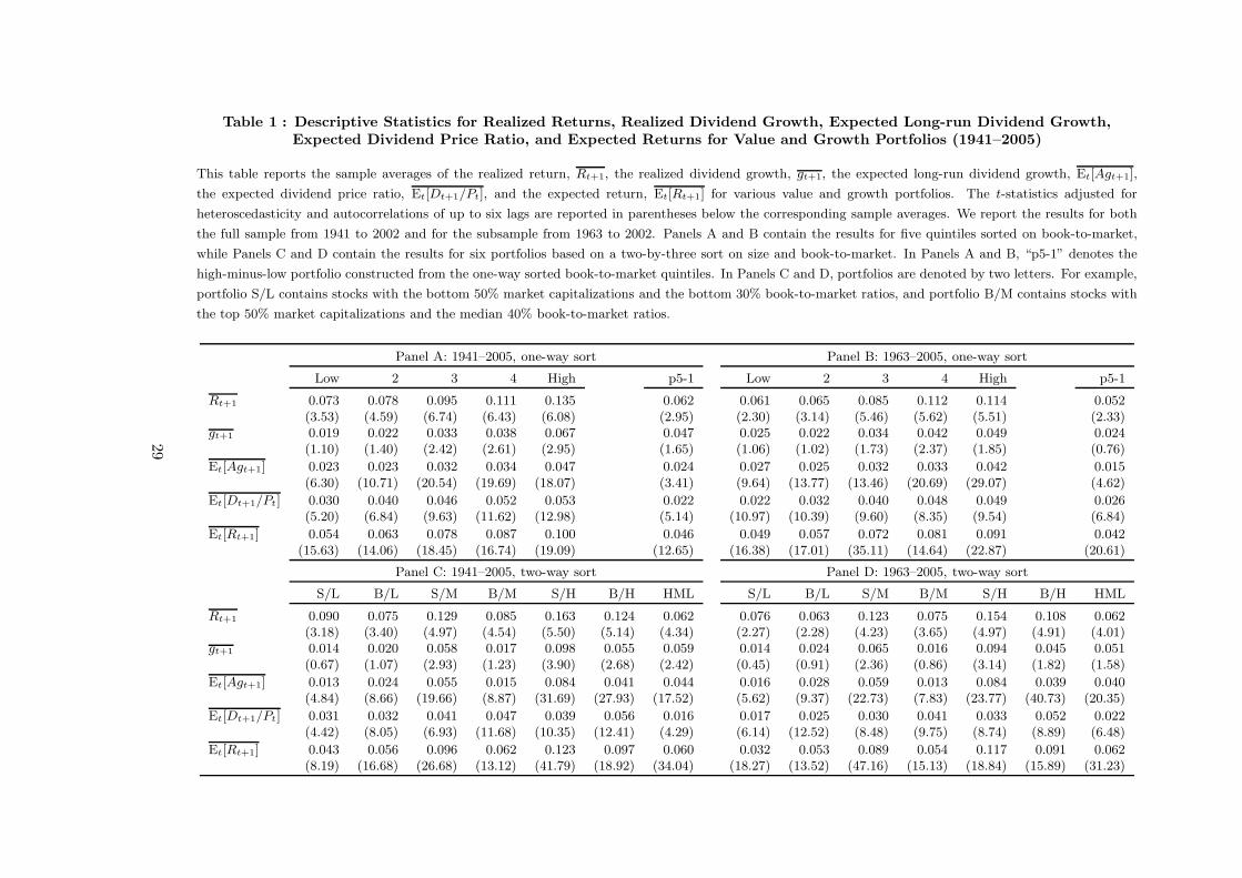
Table 1 : Descriptive Statistics for Realized Returns, Realized Dividend Growth, Expected Long-run Dividend Growth,Expected Dividend Price Ratio, and Expected Returns for Value and Growth Portfolios (1941–2005)

This table reports the sample averages of the realized return, Rt+1, the realized dividend growth, gt+1, the expected long-run dividend growth, Et[Agt+1],

the expected dividend price ratio, Et[Dt+1/Pt], and the expected return, Et[Rt+1] for various value and growth portfolios. The t-statistics adjusted for

heteroscedasticity and autocorrelations of up to six lags are reported in parentheses below the corresponding sample averages. We report the results for both

the full sample from 1941 to 2002 and for the subsample from 1963 to 2002. Panels A and B contain the results for five quintiles sorted on book-to-market,

while Panels C and D contain the results for six portfolios based on a two-by-three sort on size and book-to-market. In Panels A and B, “p5-1” denotes the

high-minus-low portfolio constructed from the one-way sorted book-to-market quintiles. In Panels C and D, portfolios are denoted by two letters. For example,

portfolio S/L contains stocks with the bottom 50% market capitalizations and the bottom 30% book-to-market ratios, and portfolio B/M contains stocks with

the top 50% market capitalizations and the median 40% book-to-market ratios.

Panel A: 1941–2005, one-way sort Panel B: 1963–2005, one-way sort

Low 2 3 4 High p5-1 Low 2 3 4 High p5-1

Rt+1 0.073 0.078 0.095 0.111 0.135 0.062 0.061 0.065 0.085 0.112 0.114 0.052(3.53) (4.59) (6.74) (6.43) (6.08) (2.95) (2.30) (3.14) (5.46) (5.62) (5.51) (2.33)

gt+1 0.019 0.022 0.033 0.038 0.067 0.047 0.025 0.022 0.034 0.042 0.049 0.024(1.10) (1.40) (2.42) (2.61) (2.95) (1.65) (1.06) (1.02) (1.73) (2.37) (1.85) (0.76)

Et[Agt+1] 0.023 0.023 0.032 0.034 0.047 0.024 0.027 0.025 0.032 0.033 0.042 0.015(6.30) (10.71) (20.54) (19.69) (18.07) (3.41) (9.64) (13.77) (13.46) (20.69) (29.07) (4.62)

Et[Dt+1/Pt] 0.030 0.040 0.046 0.052 0.053 0.022 0.022 0.032 0.040 0.048 0.049 0.026(5.20) (6.84) (9.63) (11.62) (12.98) (5.14) (10.97) (10.39) (9.60) (8.35) (9.54) (6.84)

Et[Rt+1] 0.054 0.063 0.078 0.087 0.100 0.046 0.049 0.057 0.072 0.081 0.091 0.042(15.63) (14.06) (18.45) (16.74) (19.09) (12.65) (16.38) (17.01) (35.11) (14.64) (22.87) (20.61)

Panel C: 1941–2005, two-way sort Panel D: 1963–2005, two-way sort

S/L B/L S/M B/M S/H B/H HML S/L B/L S/M B/M S/H B/H HML

Rt+1 0.090 0.075 0.129 0.085 0.163 0.124 0.062 0.076 0.063 0.123 0.075 0.154 0.108 0.062(3.18) (3.40) (4.97) (4.54) (5.50) (5.14) (4.34) (2.27) (2.28) (4.23) (3.65) (4.97) (4.91) (4.01)

gt+1 0.014 0.020 0.058 0.017 0.098 0.055 0.059 0.014 0.024 0.065 0.016 0.094 0.045 0.051(0.67) (1.07) (2.93) (1.23) (3.90) (2.68) (2.42) (0.45) (0.91) (2.36) (0.86) (3.14) (1.82) (1.58)

Et[Agt+1] 0.013 0.024 0.055 0.015 0.084 0.041 0.044 0.016 0.028 0.059 0.013 0.084 0.039 0.040(4.84) (8.66) (19.66) (8.87) (31.69) (27.93) (17.52) (5.62) (9.37) (22.73) (7.83) (23.77) (40.73) (20.35)

Et[Dt+1/Pt] 0.031 0.032 0.041 0.047 0.039 0.056 0.016 0.017 0.025 0.030 0.041 0.033 0.052 0.022(4.42) (8.05) (6.93) (11.68) (10.35) (12.41) (4.29) (6.14) (12.52) (8.48) (9.75) (8.74) (8.89) (6.48)

Et[Rt+1] 0.043 0.056 0.096 0.062 0.123 0.097 0.060 0.032 0.053 0.089 0.054 0.117 0.091 0.062(8.19) (16.68) (26.68) (13.12) (41.79) (18.92) (34.04) (18.27) (13.52) (47.16) (15.13) (18.84) (15.89) (31.23)

29

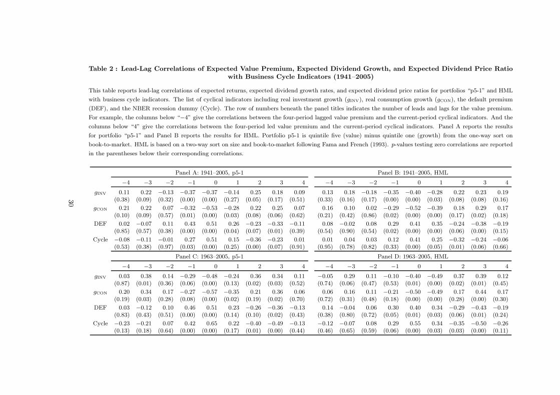
Table 2 : Lead-Lag Correlations of Expected Value Premium, Expected Dividend Growth, and Expected Dividend Price Ratiowith Business Cycle Indicators (1941–2005)

This table reports lead-lag correlations of expected returns, expected dividend growth rates, and expected dividend price ratios for portfolios “p5-1” and HML

with business cycle indicators. The list of cyclical indicators including real investment growth (gINV), real consumption growth (gCON), the default premium

(DEF), and the NBER recession dummy (Cycle). The row of numbers beneath the panel titles indicates the number of leads and lags for the value premium.

For example, the columns below “−4” give the correlations between the four-period lagged value premium and the current-period cyclical indicators. And the

columns below “4” give the correlations between the four-period led value premium and the current-period cyclical indicators. Panel A reports the results

for portfolio “p5-1” and Panel B reports the results for HML. Portfolio p5-1 is quintile five (value) minus quintile one (growth) from the one-way sort on

book-to-market. HML is based on a two-way sort on size and book-to-market following Fama and French (1993). p-values testing zero correlations are reported

in the parentheses below their corresponding correlations.

Panel A: 1941–2005, p5-1 Panel B: 1941–2005, HML

−4 −3 −2 −1 0 1 2 3 4 −4 −3 −2 −1 0 1 2 3 4

gINV 0.11 0.22 −0.13 −0.37 −0.37 −0.14 0.25 0.18 0.09 0.13 0.18 −0.18 −0.35 −0.40 −0.28 0.22 0.23 0.19(0.38) (0.09) (0.32) (0.00) (0.00) (0.27) (0.05) (0.17) (0.51) (0.33) (0.16) (0.17) (0.00) (0.00) (0.03) (0.08) (0.08) (0.16)

gCON 0.21 0.22 0.07 −0.32 −0.53 −0.28 0.22 0.25 0.07 0.16 0.10 0.02 −0.29 −0.52 −0.39 0.18 0.29 0.17(0.10) (0.09) (0.57) (0.01) (0.00) (0.03) (0.08) (0.06) (0.62) (0.21) (0.42) (0.86) (0.02) (0.00) (0.00) (0.17) (0.02) (0.18)

DEF 0.02 −0.07 0.11 0.43 0.51 0.26 −0.23 −0.33 −0.11 0.08 −0.02 0.08 0.29 0.41 0.35 −0.24 −0.38 −0.19(0.85) (0.57) (0.38) (0.00) (0.00) (0.04) (0.07) (0.01) (0.39) (0.54) (0.90) (0.54) (0.02) (0.00) (0.00) (0.06) (0.00) (0.15)

Cycle −0.08 −0.11 −0.01 0.27 0.51 0.15 −0.36 −0.23 0.01 0.01 0.04 0.03 0.12 0.41 0.25 −0.32 −0.24 −0.06(0.53) (0.38) (0.97) (0.03) (0.00) (0.25) (0.00) (0.07) (0.91) (0.95) (0.78) (0.82) (0.33) (0.00) (0.05) (0.01) (0.06) (0.66)

Panel C: 1963–2005, p5-1 Panel D: 1963–2005, HML

−4 −3 −2 −1 0 1 2 3 4 −4 −3 −2 −1 0 1 2 3 4

gINV 0.03 0.38 0.14 −0.29 −0.48 −0.24 0.36 0.34 0.11 −0.05 0.29 0.11 −0.10 −0.40 −0.49 0.37 0.39 0.12(0.87) (0.01) (0.36) (0.06) (0.00) (0.13) (0.02) (0.03) (0.52) (0.74) (0.06) (0.47) (0.53) (0.01) (0.00) (0.02) (0.01) (0.45)

gCON 0.20 0.34 0.17 −0.27 −0.57 −0.35 0.21 0.36 0.06 0.06 0.16 0.11 −0.21 −0.50 −0.49 0.17 0.44 0.17(0.19) (0.03) (0.28) (0.08) (0.00) (0.02) (0.19) (0.02) (0.70) (0.72) (0.31) (0.48) (0.18) (0.00) (0.00) (0.28) (0.00) (0.30)

DEF 0.03 −0.12 0.10 0.46 0.51 0.23 −0.26 −0.36 −0.13 0.14 −0.04 0.06 0.30 0.40 0.34 −0.29 −0.43 −0.19(0.83) (0.43) (0.51) (0.00) (0.00) (0.14) (0.10) (0.02) (0.43) (0.38) (0.80) (0.72) (0.05) (0.01) (0.03) (0.06) (0.01) (0.24)

Cycle −0.23 −0.21 0.07 0.42 0.65 0.22 −0.40 −0.49 −0.13 −0.12 −0.07 0.08 0.29 0.55 0.34 −0.35 −0.50 −0.26(0.13) (0.18) (0.64) (0.00) (0.00) (0.17) (0.01) (0.00) (0.44) (0.46) (0.65) (0.59) (0.06) (0.00) (0.03) (0.03) (0.00) (0.11)

30

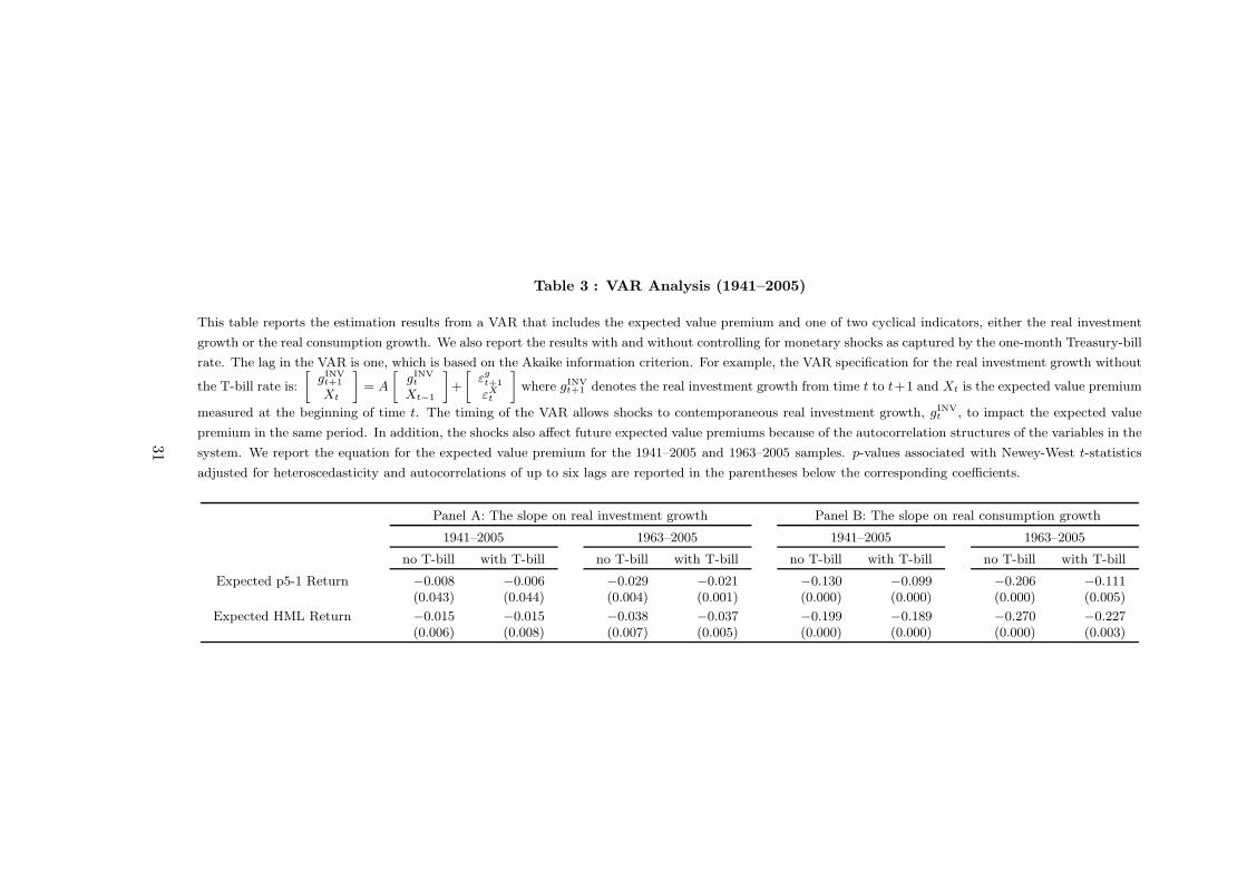
Table 3 : VAR Analysis (1941–2005)

This table reports the estimation results from a VAR that includes the expected value premium and one of two cyclical indicators, either the real investment

growth or the real consumption growth. We also report the results with and without controlling for monetary shocks as captured by the one-month Treasury-bill

rate. The lag in the VAR is one, which is based on the Akaike information criterion. For example, the VAR specification for the real investment growth without

the T-bill rate is:

»

gINVt+1

Xt

–

= A

»

gINVt

Xt−1

–

+

»

εgt+1

εXt

–

where gINVt+1 denotes the real investment growth from time t to t+1 and Xt is the expected value premium

measured at the beginning of time t. The timing of the VAR allows shocks to contemporaneous real investment growth, gINVt , to impact the expected value

premium in the same period. In addition, the shocks also affect future expected value premiums because of the autocorrelation structures of the variables in the

system. We report the equation for the expected value premium for the 1941–2005 and 1963–2005 samples. p-values associated with Newey-West t-statistics

adjusted for heteroscedasticity and autocorrelations of up to six lags are reported in the parentheses below the corresponding coefficients.

Panel A: The slope on real investment growth Panel B: The slope on real consumption growth

1941–2005 1963–2005 1941–2005 1963–2005

no T-bill with T-bill no T-bill with T-bill no T-bill with T-bill no T-bill with T-bill

Expected p5-1 Return −0.008 −0.006 −0.029 −0.021 −0.130 −0.099 −0.206 −0.111(0.043) (0.044) (0.004) (0.001) (0.000) (0.000) (0.000) (0.005)

Expected HML Return −0.015 −0.015 −0.038 −0.037 −0.199 −0.189 −0.270 −0.227(0.006) (0.008) (0.007) (0.005) (0.000) (0.000) (0.000) (0.003)

31

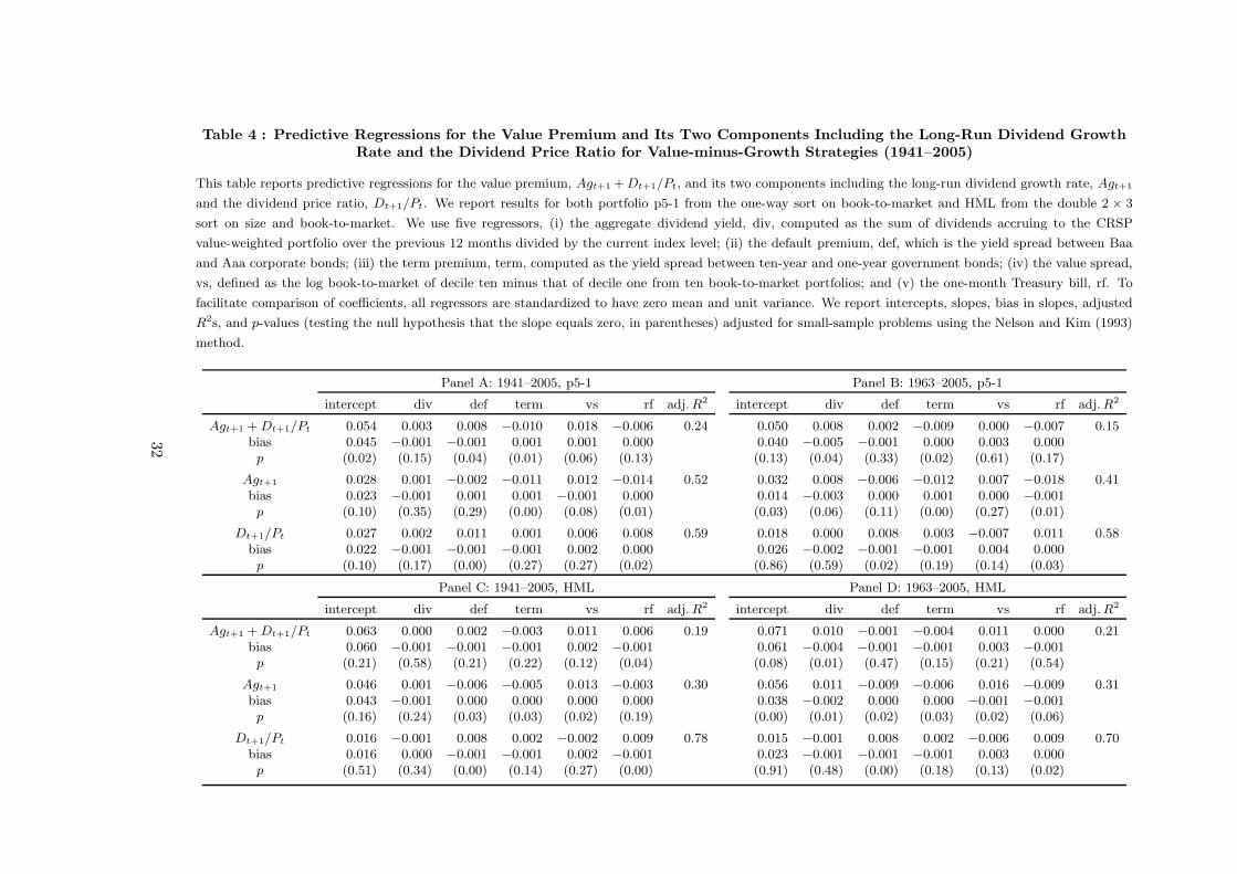
Table 4 : Predictive Regressions for the Value Premium and Its Two Components Including the Long-Run Dividend GrowthRate and the Dividend Price Ratio for Value-minus-Growth Strategies (1941–2005)

This table reports predictive regressions for the value premium, Agt+1 + Dt+1/Pt, and its two components including the long-run dividend growth rate, Agt+1

and the dividend price ratio, Dt+1/Pt. We report results for both portfolio p5-1 from the one-way sort on book-to-market and HML from the double 2 × 3

sort on size and book-to-market. We use five regressors, (i) the aggregate dividend yield, div, computed as the sum of dividends accruing to the CRSP

value-weighted portfolio over the previous 12 months divided by the current index level; (ii) the default premium, def, which is the yield spread between Baa

and Aaa corporate bonds; (iii) the term premium, term, computed as the yield spread between ten-year and one-year government bonds; (iv) the value spread,

vs, defined as the log book-to-market of decile ten minus that of decile one from ten book-to-market portfolios; and (v) the one-month Treasury bill, rf. To

facilitate comparison of coefficients, all regressors are standardized to have zero mean and unit variance. We report intercepts, slopes, bias in slopes, adjusted

R2s, and p-values (testing the null hypothesis that the slope equals zero, in parentheses) adjusted for small-sample problems using the Nelson and Kim (1993)

method.

Panel A: 1941–2005, p5-1 Panel B: 1963–2005, p5-1

intercept div def term vs rf adj. R2 intercept div def term vs rf adj. R2

Agt+1 + Dt+1/Pt 0.054 0.003 0.008 −0.010 0.018 −0.006 0.24 0.050 0.008 0.002 −0.009 0.000 −0.007 0.15bias 0.045 −0.001 −0.001 0.001 0.001 0.000 0.040 −0.005 −0.001 0.000 0.003 0.000p (0.02) (0.15) (0.04) (0.01) (0.06) (0.13) (0.13) (0.04) (0.33) (0.02) (0.61) (0.17)

Agt+1 0.028 0.001 −0.002 −0.011 0.012 −0.014 0.52 0.032 0.008 −0.006 −0.012 0.007 −0.018 0.41bias 0.023 −0.001 0.001 0.001 −0.001 0.000 0.014 −0.003 0.000 0.001 0.000 −0.001p (0.10) (0.35) (0.29) (0.00) (0.08) (0.01) (0.03) (0.06) (0.11) (0.00) (0.27) (0.01)

Dt+1/Pt 0.027 0.002 0.011 0.001 0.006 0.008 0.59 0.018 0.000 0.008 0.003 −0.007 0.011 0.58bias 0.022 −0.001 −0.001 −0.001 0.002 0.000 0.026 −0.002 −0.001 −0.001 0.004 0.000p (0.10) (0.17) (0.00) (0.27) (0.27) (0.02) (0.86) (0.59) (0.02) (0.19) (0.14) (0.03)

Panel C: 1941–2005, HML Panel D: 1963–2005, HML

intercept div def term vs rf adj. R2 intercept div def term vs rf adj. R2

Agt+1 + Dt+1/Pt 0.063 0.000 0.002 −0.003 0.011 0.006 0.19 0.071 0.010 −0.001 −0.004 0.011 0.000 0.21bias 0.060 −0.001 −0.001 −0.001 0.002 −0.001 0.061 −0.004 −0.001 −0.001 0.003 −0.001p (0.21) (0.58) (0.21) (0.22) (0.12) (0.04) (0.08) (0.01) (0.47) (0.15) (0.21) (0.54)

Agt+1 0.046 0.001 −0.006 −0.005 0.013 −0.003 0.30 0.056 0.011 −0.009 −0.006 0.016 −0.009 0.31bias 0.043 −0.001 0.000 0.000 0.000 0.000 0.038 −0.002 0.000 0.000 −0.001 −0.001p (0.16) (0.24) (0.03) (0.03) (0.02) (0.19) (0.00) (0.01) (0.02) (0.03) (0.02) (0.06)

Dt+1/Pt 0.016 −0.001 0.008 0.002 −0.002 0.009 0.78 0.015 −0.001 0.008 0.002 −0.006 0.009 0.70bias 0.016 0.000 −0.001 −0.001 0.002 −0.001 0.023 −0.001 −0.001 −0.001 0.003 0.000p (0.51) (0.34) (0.00) (0.14) (0.27) (0.00) (0.91) (0.48) (0.00) (0.18) (0.13) (0.02)

32

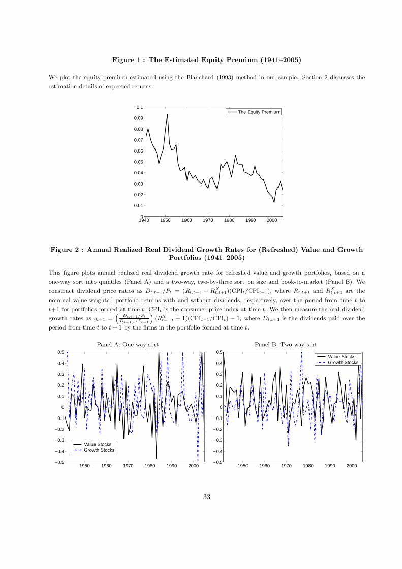
Figure 1 : The Estimated Equity Premium (1941–2005)

We plot the equity premium estimated using the Blanchard (1993) method in our sample. Section 2 discusses the

estimation details of expected returns.

1940 1950 1960 1970 1980 1990 20000

0.01

0.02

0.03

0.04

0.05

0.06

0.07

0.08

0.09

0.1

The Equity Premium

Figure 2 : Annual Realized Real Dividend Growth Rates for (Refreshed) Value and GrowthPortfolios (1941–2005)

This figure plots annual realized real dividend growth rate for refreshed value and growth portfolios, based on a

one-way sort into quintiles (Panel A) and a two-way, two-by-three sort on size and book-to-market (Panel B). We

construct dividend price ratios as Dt,t+1/Pt = (Rt,t+1 − RXt,t+1)(CPIt/CPIt+1), where Rt,t+1 and RX

t,t+1 are the

nominal value-weighted portfolio returns with and without dividends, respectively, over the period from time t to

t+1 for portfolios formed at time t. CPIt is the consumer price index at time t. We then measure the real dividend

growth rates as gt+1 =“

Dt,t+1/Pt

Dt−1,t/Pt−1

”

(RXt−1,t + 1)(CPIt−1/CPIt) − 1, where Dt,t+1 is the dividends paid over the

period from time t to t + 1 by the firms in the portfolio formed at time t.

Panel A: One-way sort Panel B: Two-way sort

1950 1960 1970 1980 1990 2000−0.5

−0.4

−0.3

−0.2

−0.1

0

0.1

0.2

0.3

0.4

0.5

Value StocksGrowth Stocks

1950 1960 1970 1980 1990 2000−0.5

−0.4

−0.3

−0.2

−0.1

0

0.1

0.2

0.3

0.4

0.5Value StocksGrowth Stocks

33

Figure 3 : Event-Time Evolution of Dividend Growth Rates and Dividend Price Ratios for(Unrefreshed) Value and Growth Portfolios (1941–2005))

This figure plots the event-time evolution of dividend growth rates and dividend price ratios for unrefreshed value

and growth portfolios. We construct value and growth portfolios using a one-way sort on book-to-market (to form

five quintiles) and a double, two-by-three sort on size and book-to-market (to form six portfolios as Fama and French

1993). Panel A plots dividend growth rates for portfolios High (value stocks) and Low (growth stocks) from the one-

way sort, and Panel C plots dividend growth rates for four portfolios including small-value (S/H), big-value (B/H),

small-growth (S/L), and big-growth (B/L) from the six double-sorted portfolios. Panel B plots the dividend price

ratios for portfolios High and Low, and Panel D does the same for portfolios S/H, B/H, S/L, and B/L. Dividend

growth for a unrefreshed portfolio is defined as the sum of dividends for all firms in the portfolio divided by the

sum of lagged dividends for the same set of firms. The dividend price ratio of a unrefreshed portfolio is the sum of

dividends for all firms in the portfolio divided by the sum of lagged stock prices for the same set of firms.

Panel A: Dividend growth, one-way sort Panel B: Dividend price ratio, one-way sort

−10 −5 0 5 100.95

1

1.05

1.1Value StocksGrowth Stocks

−10 −5 0 5 100.02

0.025

0.03

0.035

0.04

0.045

0.05

0.055

0.06Value StocksGrowth Stocks

Panel C: Dividend growth, two-way sort Panel D: Dividend price ratio, two-way sort

−10 −5 0 5 100.9

0.92

0.94

0.96

0.98

1

1.02

1.04

1.06

1.08

1.1

S/HB/HS/LB/L

−10 −5 0 5 100.01

0.015

0.02

0.025

0.03

0.035

0.04

0.045

0.05

0.055S/HB/HS/LB/L

34

Figure 4 : Event-Time Evolution of Profitability and Dividend on Equity for (Unrefreshed)Value and Growth Portfolios (1941–2005)

This figure plots the event time evolution of profitability and dividend on equity for unrefreshed value and growth

portfolios. We construct value and growth portfolios using a one-way sort on book-to-market (to form five quintiles)

and a double, two-by-three sort on size and book-to-market (to form six portfolios as Fama and French 1993). Panel

A plots the profitability for portfolios High (value stocks) and Low (growth stocks) from the one-way sort, and Panel

C plots the profitability for four portfolios including small-value (S/H), big-value (B/H), small-growth (S/L), and

big-growth (B/L) from the six double-sorted portfolios. Panel B plots the dividend on equity for portfolios High and

Low, and Panel D plots the dividend on equity for portfolios S/H, B/H, S/L, and B/L. Profitability for a unrefreshed

portfolio is defined as the sum of earnings for all firms in the portfolio divided by the sum of lagged book equity

for the same set of firms. Dividend on equity for a unrefreshed portfolio is the sum of dividends for all firms in the

portfolio divided by the sum of lagged stock price for the same set of firms.

Panel A: Profitability, one-way sort Panel B: Dividend on equity, one-way sort

−10 −5 0 5 10

0.06

0.08

0.1

0.12

0.14

0.16

0.18

0.2

0.22

0.24Value StocksGrowth Stocks

−10 −5 0 5 100.02

0.03

0.04

0.05

0.06

0.07

0.08

0.09

0.1Value StocksGrowth Stocks

Panel C: Profitability, two-way sort Panel D: Dividend on equity, two-way sort

−10 −5 0 5 10

0.04

0.06

0.08

0.1

0.12

0.14

0.16

0.18

0.2

0.22S/HB/HS/LB/L

−10 −5 0 5 100.01

0.02

0.03

0.04

0.05

0.06

0.07

0.08

0.09S/HB/HS/LB/L

35

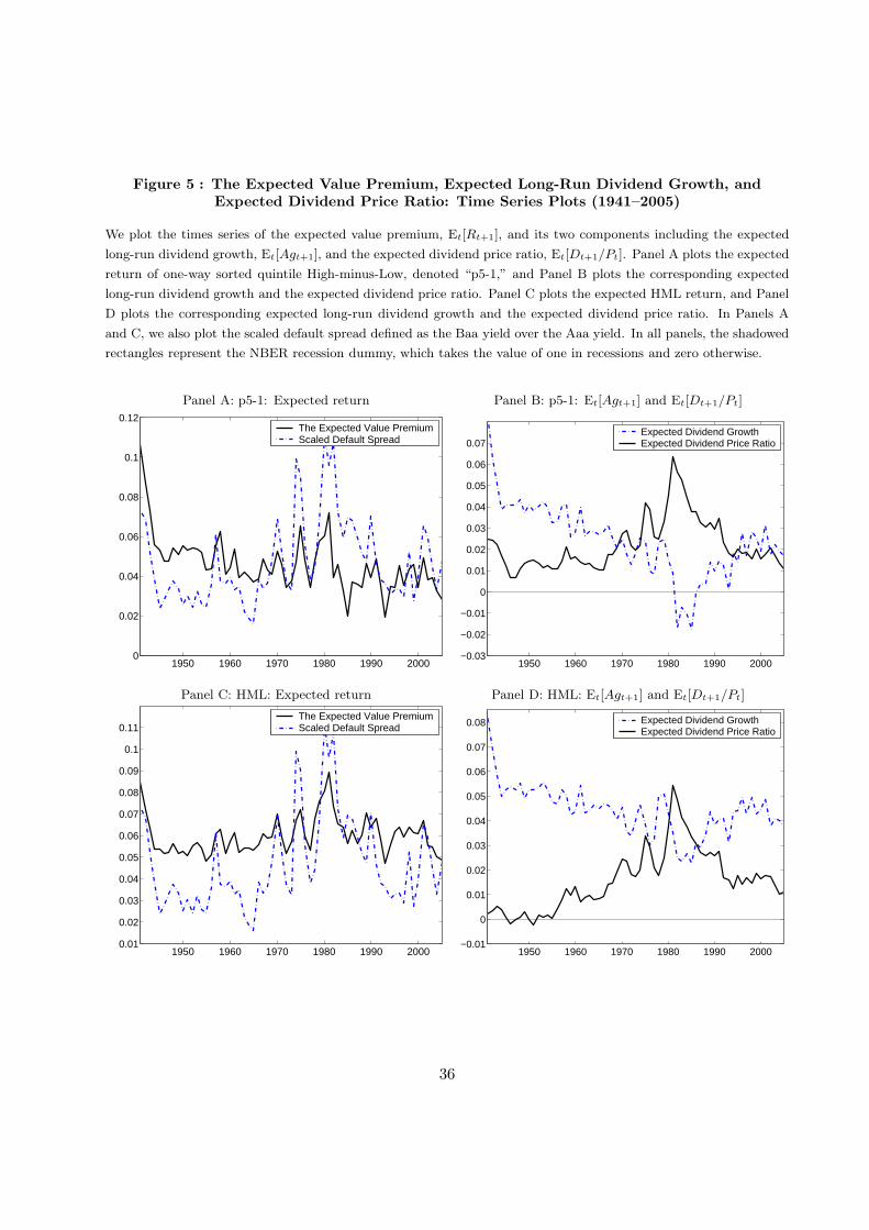
Figure 5 : The Expected Value Premium, Expected Long-Run Dividend Growth, andExpected Dividend Price Ratio: Time Series Plots (1941–2005)

We plot the times series of the expected value premium, Et[Rt+1], and its two components including the expected

long-run dividend growth, Et[Agt+1], and the expected dividend price ratio, Et[Dt+1/Pt]. Panel A plots the expected

return of one-way sorted quintile High-minus-Low, denoted “p5-1,” and Panel B plots the corresponding expected

long-run dividend growth and the expected dividend price ratio. Panel C plots the expected HML return, and Panel

D plots the corresponding expected long-run dividend growth and the expected dividend price ratio. In Panels A

and C, we also plot the scaled default spread defined as the Baa yield over the Aaa yield. In all panels, the shadowed

rectangles represent the NBER recession dummy, which takes the value of one in recessions and zero otherwise.

Panel A: p5-1: Expected return Panel B: p5-1: Et[Agt+1] and Et[Dt+1/Pt]

1950 1960 1970 1980 1990 20000

0.02

0.04

0.06

0.08

0.1

0.12The Expected Value PremiumScaled Default Spread

1950 1960 1970 1980 1990 2000−0.03

−0.02

−0.01

0

0.01

0.02

0.03

0.04

0.05

0.06

0.07Expected Dividend GrowthExpected Dividend Price Ratio

Panel C: HML: Expected return Panel D: HML: Et[Agt+1] and Et[Dt+1/Pt]

1950 1960 1970 1980 1990 20000.01

0.02

0.03

0.04

0.05

0.06

0.07

0.08

0.09

0.1

0.11The Expected Value PremiumScaled Default Spread

1950 1960 1970 1980 1990 2000−0.01

0

0.01

0.02

0.03

0.04

0.05

0.06

0.07

0.08 Expected Dividend GrowthExpected Dividend Price Ratio

36

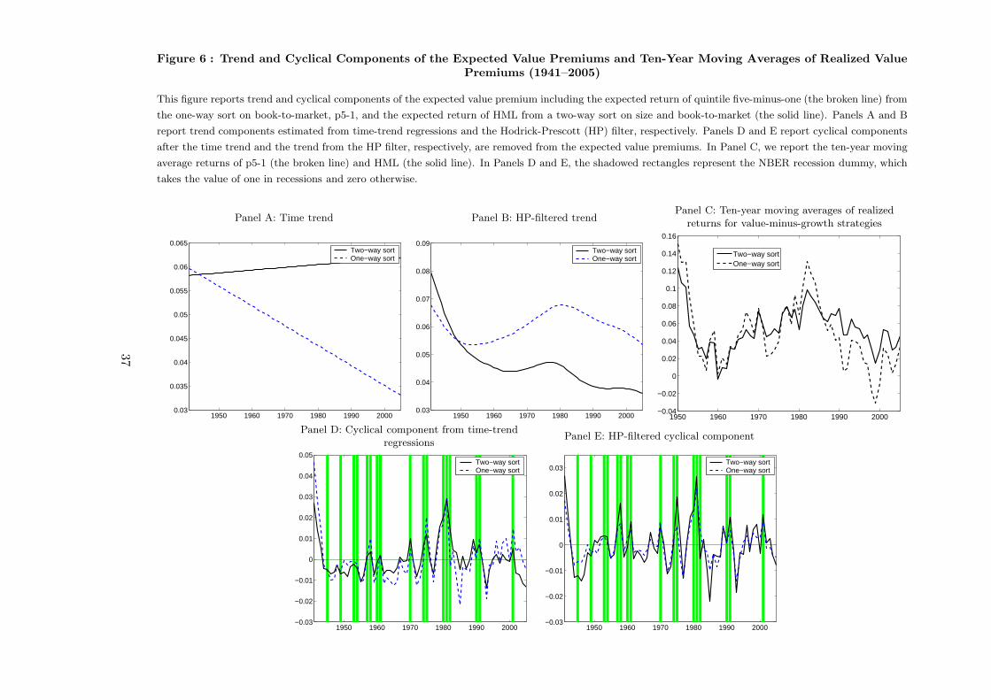
Figure 6 : Trend and Cyclical Components of the Expected Value Premiums and Ten-Year Moving Averages of Realized ValuePremiums (1941–2005)

This figure reports trend and cyclical components of the expected value premium including the expected return of quintile five-minus-one (the broken line) from

the one-way sort on book-to-market, p5-1, and the expected return of HML from a two-way sort on size and book-to-market (the solid line). Panels A and B

report trend components estimated from time-trend regressions and the Hodrick-Prescott (HP) filter, respectively. Panels D and E report cyclical components

after the time trend and the trend from the HP filter, respectively, are removed from the expected value premiums. In Panel C, we report the ten-year moving

average returns of p5-1 (the broken line) and HML (the solid line). In Panels D and E, the shadowed rectangles represent the NBER recession dummy, which

takes the value of one in recessions and zero otherwise.

Panel A: Time trend Panel B: HP-filtered trendPanel C: Ten-year moving averages of realized

returns for value-minus-growth strategies

1950 1960 1970 1980 1990 20000.03

0.035

0.04

0.045

0.05

0.055

0.06

0.065Two−way sortOne−way sort

1950 1960 1970 1980 1990 20000.03

0.04

0.05

0.06

0.07

0.08

0.09Two−way sortOne−way sort

1950 1960 1970 1980 1990 2000−0.04

−0.02

0

0.02

0.04

0.06

0.08

0.1

0.12

0.14

0.16

Two−way sortOne−way sort

Panel D: Cyclical component from time-trendregressions

Panel E: HP-filtered cyclical component

1950 1960 1970 1980 1990 2000−0.03

−0.02

−0.01

0

0.01

0.02

0.03

0.04

0.05Two−way sortOne−way sort

1950 1960 1970 1980 1990 2000−0.03

−0.02

−0.01

0

0.01

0.02

0.03Two−way sortOne−way sort

37

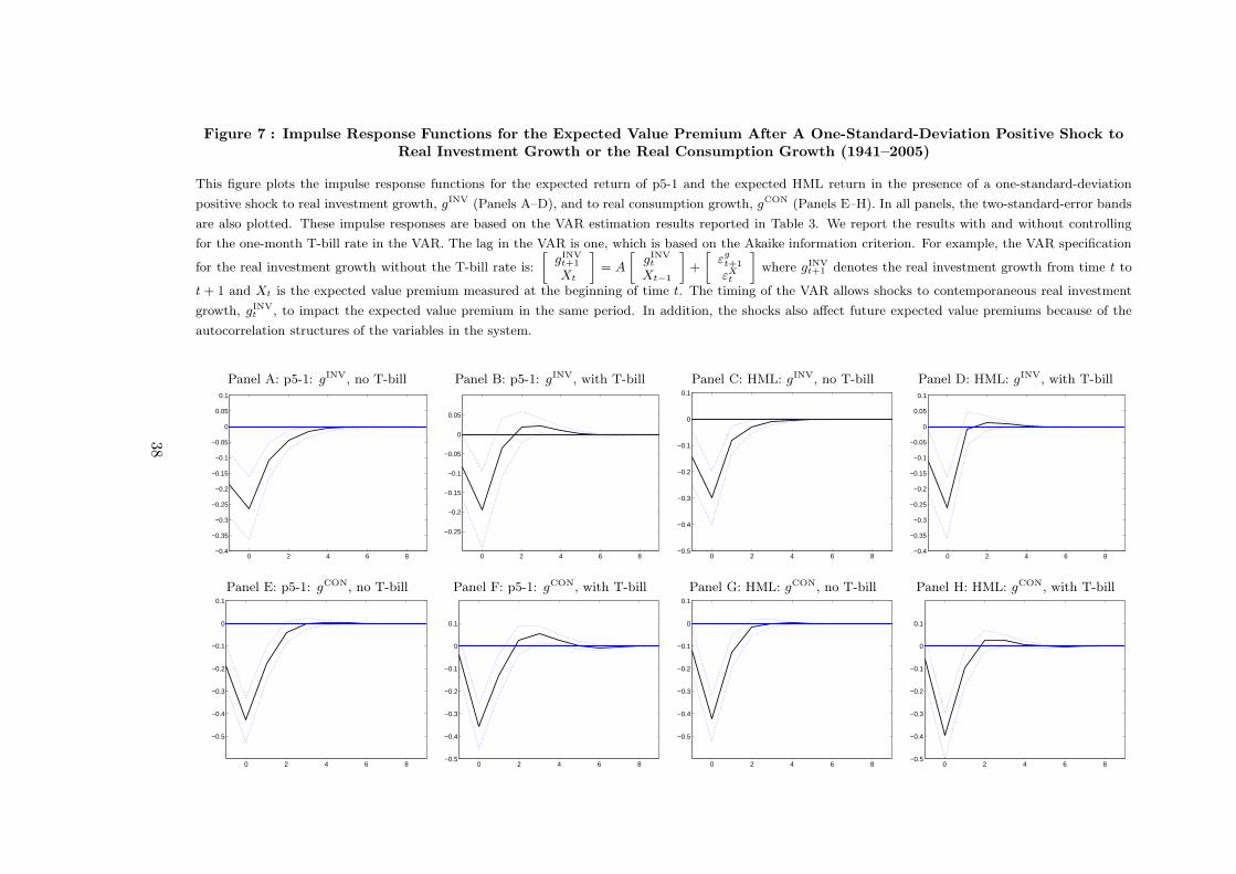
Figure 7 : Impulse Response Functions for the Expected Value Premium After A One-Standard-Deviation Positive Shock toReal Investment Growth or the Real Consumption Growth (1941–2005)

This figure plots the impulse response functions for the expected return of p5-1 and the expected HML return in the presence of a one-standard-deviation

positive shock to real investment growth, gINV (Panels A–D), and to real consumption growth, gCON (Panels E–H). In all panels, the two-standard-error bands

are also plotted. These impulse responses are based on the VAR estimation results reported in Table 3. We report the results with and without controlling

for the one-month T-bill rate in the VAR. The lag in the VAR is one, which is based on the Akaike information criterion. For example, the VAR specification

for the real investment growth without the T-bill rate is:

»

gINVt+1

Xt

–

= A

»

gINVt

Xt−1

–

+

»

εgt+1

εXt

–

where gINVt+1 denotes the real investment growth from time t to

t + 1 and Xt is the expected value premium measured at the beginning of time t. The timing of the VAR allows shocks to contemporaneous real investment

growth, gINVt , to impact the expected value premium in the same period. In addition, the shocks also affect future expected value premiums because of the

autocorrelation structures of the variables in the system.

Panel A: p5-1: gINV, no T-bill Panel B: p5-1: gINV, with T-bill Panel C: HML: gINV, no T-bill Panel D: HML: gINV, with T-bill

0 2 4 6 8−0.4

−0.35

−0.3

−0.25

−0.2

−0.15

−0.1

−0.05

0

0.05

0.1

0 2 4 6 8

−0.25

−0.2

−0.15

−0.1

−0.05

0

0.05

0 2 4 6 8−0.5

−0.4

−0.3

−0.2

−0.1

0

0.1

0 2 4 6 8−0.4

−0.35

−0.3

−0.25

−0.2

−0.15

−0.1

−0.05

0

0.05

0.1

Panel E: p5-1: gCON, no T-bill Panel F: p5-1: gCON, with T-bill Panel G: HML: gCON, no T-bill Panel H: HML: gCON, with T-bill

0 2 4 6 8

−0.5

−0.4

−0.3

−0.2

−0.1

0

0.1

0 2 4 6 8−0.5

−0.4

−0.3

−0.2

−0.1

0

0.1

0 2 4 6 8

−0.5

−0.4

−0.3

−0.2

−0.1

0

0.1

0 2 4 6 8−0.5

−0.4

−0.3

−0.2

−0.1

0

0.1

38