THE EXPECTED ROLES AND PROBLEMS FOR GPS CADASTRAL SURVEYS IN EGYPT

Proceedings of the 4th ICCAE Conf. 14-16 May, 2002

ICCAE Military Technical College 4rd International Conference

Kobry Elkobbah, On Civil & Architecture

Cairo, Egypt Engineering

THE EXPECTED ROLES AND PROBLEMS

FOR GPS CADASTRAL SURVEYS IN EGYPT

Mahmoud El-Mewafi *, Mohamed E.A. Amin **, Ahmed Shawkey

نتحذيذ مىاضع وقظ انشبكاث مه أكفأ انطزق انمساحيت انحذيثتاستخذاو األقمار انصىاعيتيعذ

وكان الستخذاو هذي انتكىىنىجيا األثز انفعال في انحصىل عهً بياواث . ط ئانجيىديسيت وانخزا

عانيت في أعمال انمساحت انطبىغزافيت و الكفاءة العمهيت سزيعت تفي بمتطهباث انذقت و

ويهذف هذا انبحث إنً إيجاد حهىل عمهيت مبسطت نبعض انمشاكم وانعقباث . انتفصيهيت

. انمصاحبت الستخذاو األقمار انصىاعيت في أعمال انمساحت انطبىغزافيت و انتفصيهيت في مصز

وأشارث وتائج دراست معايزة واختباراث دقت مستقبالث األقمار انصىاعيت وانتىصياث

انمقتزحت إنً تحسيه كفاءة ودقت تحذيذ مساحاث و حذود األرضي انمختارة مقاروت بانطزق

كما تضمه انبحث بعض انتىصياث انعمهيت انهامت انتي يجب أن تىضع في . انتقهيذيت األخزي

استخذاو األقمار انصىاعيت في أعمال انمساحت انطبىغزافيت و انتفصيهيت في داالعتبار عه

. مصز

Abstract

GPS has become the preferred positioning technology for geodetic control and

mapping surveys. The use of GPS technique in land surveying proved a great

efficiency and permitted to accelerate data acquisition and maintained the accuracy

needed for Cadastral and topographic surveys. The aim of this study is to introduce

outline recommended procedures for set up, automatically, topographic and cadastral

surveys in Egypt from survey data files obtained with GPS method with a high

accuracy. Results on the GPS equipment testing and calibrations following the

proposed recommended practices have been presented together with the GPS survey

results over the boundary markers of the selected cadastral lots.

* Associate Professor, Public Works Dept., Faculty of Engineering, Mansoura University, Egypt

** Head of Civil and Architecture Eng. Dept., Military Technical College Cairo, Egypt

*** Eng. Civil Engineering department, Military Technical college Cairo, Egypt

1. Introduction

The use of the Global Positioning System (GPS) is now being adopted and used by

the surveying profession. Traditionally, GPS has been used for high precision

geodetic survey, but increasingly it is being used for cadastral surveys. GPS has

recently become an important survey and mapping tool to supplement and, in many

cases, replace conventional techniques because of its advantage of accuracy,

efficiency and cost effectiveness[Barnes, G. and M. Eckl, 1996b].

A Cadastral survey is a survey conducted to obtain the data needed for the preparation

of a Cadastral map. A Cadastral map is simply a drawing that shows the natural and

artificial features of an area. This data consists of the horizontal and vertical locations

of the features to be shown on the map. The major trend over the last decade however,

has been to convert these cadastral maps to digital form and there by create digital

cadastral databases [Tommy Österberg, 1999].

The Egyptian Survey Authority (ESA) is now well advanced in creating digital

cadastral databases. A big issue however with regard to the digital cadastral databases

in urban and rural sectors concerns the problems associated with updating and

upgrading these digital cadastral databases, particularly from the point of view of the

authors. These problems are related to: planning a GPS cadastral survey and how the

coordinates are to be determined through appropriate connection to survey control;

testing/calibration of GPS equipment; field procedures for operating the equipment,

documentation, quality assurance and verification procedures, and; office procedures

for data reduction and result submission.

This paper concerned with test results on the GPS equipment calibration procedures,

GPS survey results over the boundary markers of the selected cadastral lots, which

has followed by the “recommended practices for field and office procedures”, are also

presented. Besides this some points of the building corners were observed by means

of a rapid static technique. These measurements are not subject of this paper.

2. GPS Equipment Calibration

GPS equipment, software and procedures should be tested before general usage. This

can be achieved by making measurements and processing data over known baselines

or a network of points [SES et al., 1999].

Unlike EDM equipment, GPS receivers cannot be calibrated for scale because the

definition of scale is inherent in the satellites and orbit data. However, antennas and

tribrachs can be calibrated for centering errors. Antenna centering errors are generally

not significant when geodetic quality equipment (e.g., with micro strip antennae) is

used for cadastral surveys. However, the Surveyor is entitled to request a calibration

test if there is reason to doubt the GPS results - particularly those on short lines [GPS

Guidelines, 1999].

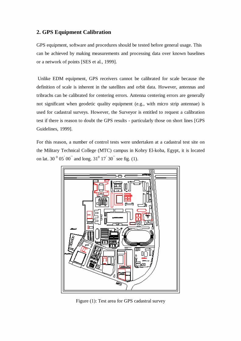
For this reason, a number of control tests were undertaken at a cadastral test site on

the Military Technical College (MTC) campus in Kobry El-koba, Egypt, it is located

on lat. 30 0 05

’ 00

’’ and long. 31

0 17

’ 30

’’ see fig. (1).

Figure (1): Test area for GPS cadastral survey

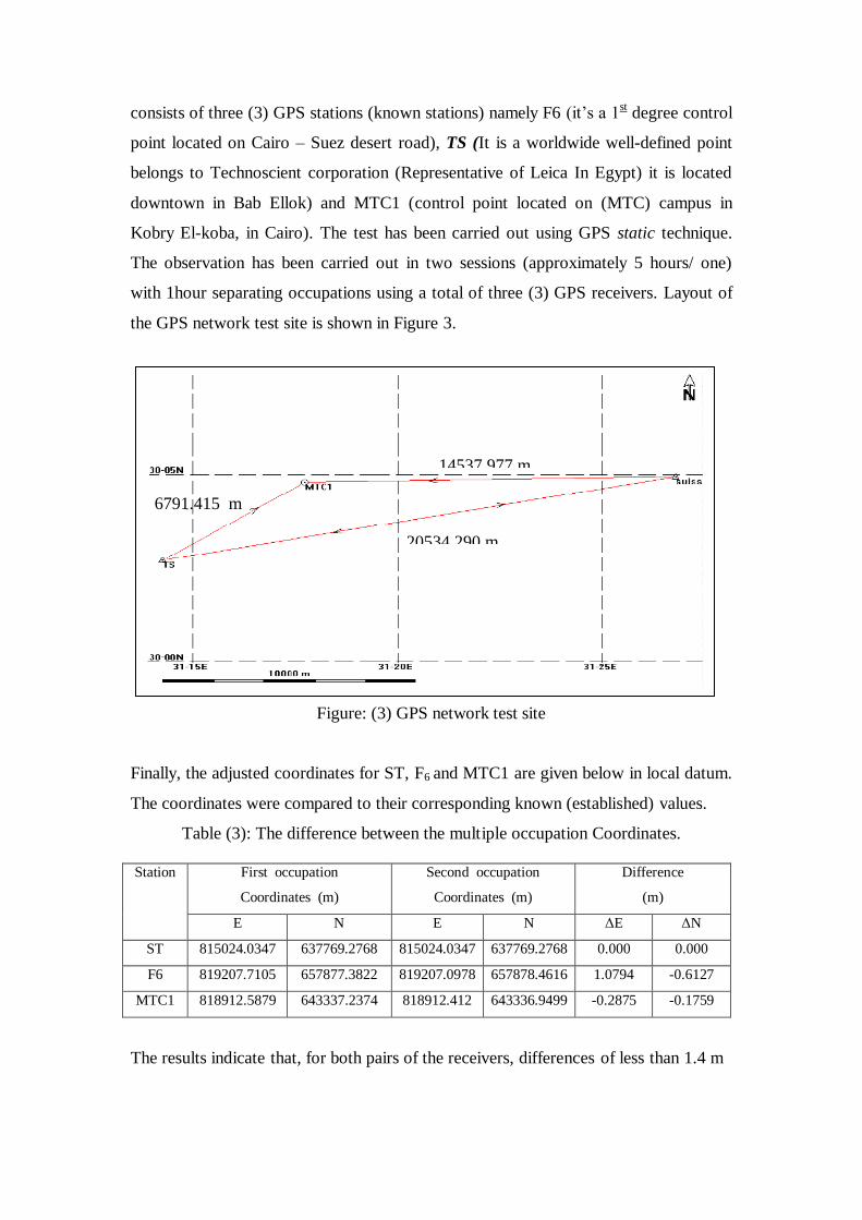
The list of Three Leica dual frequency GPS receivers being used in the test following

field criteria and processing requirements given in Table 1

Table (1): GPS equipments, field criteria and processing requirements

Used in the tests

GPS equipments

Type of receivers Leica System 300 (L1& L2)

Number of receivers tested 3 (R1, R2, R3)

Antenna with splitter 1 (for each test)

Processing software SKI version 2.11

Field test criteria

Observation length 10 minutes

Recording Interval 15 seconds

Number of satellites 5

GDOP 6

Sky Clearance 90 %

Processing requirements

Session length 10 minutes

Ambiguity Resolution Fixed

Used Cut Off Angle 15 o

Frequency used L1 and L2

2.1. EDM Baseline Test

An EDM baseline test is performed in order to ensure that the operation of a pair of

GPS receivers, associated antennas and cabling, and data processing software, give

distance results that can be compared with calibrated baseline data. GPS can be used

to measure the three components of a baseline, that is, expressed as either: (i) relative

latitude, longitude and height, or; (ii) relative Cartesian coordinates with respect to a

global geocentric reference frame, or; (iii) distance, azimuth and height difference

between the two antennas. However, EDM baseline testing only considers the

distance component. However, it is assumed that if the GPS equipment can verify the

known distances between the markers on the pillars of the EDM baseline, the

equipment is in good order and capable of delivering baseline solutions that are within

specification [BOO et al., 2000].

A series of EDM baseline test have been carried out at the existing EDM baseline

calibration test site in MTC on the May 2001. The site is being maintained by MTC

and their layout is shown in Figure 2.

Figure: (2) EDM baseline test site

The EDM test site comprises of six (6) pillars separated at specified interval. The

length between pillars has been routinely measured and documented as the published

true values. The test has been carried out using GPS rapid static technique. One

receiver (R1) was remained at the Pillar 1 during the entire observations while the

other one(R2) was roving. The differences between GPS computed distances and their

corresponding EDM values for each pair of pillars (receivers) are given in Table 2.

Table (2): Differences between EDM and GPS values for R1/R2 receivers

Baselines

(Pillars)

Distances (m)

Differences

(mm)

EDM

(m)

R1- R2

(m)

1-2 64.21372 64.21271 1.01

1-3 211.5805 211.5853 -4.8

1-4 469.1565 469.1687 -12.2

1-5 627.2452 627.2404 4.8

1-6 884.327 884.335 -8

The results indicate that, for both pairs of the receivers, differences of less than 13mm

has been given. This shows that the GPS equipment set being used are in good

condition.

2.2. GPS Network Test

A GPS network test is performed in order to ensure that the operation of GPS

receivers, associated antennas and cabling, and data processing software, give high

accuracy coordinate results. Such a test is the most realistic form of test as it ensures

that the results for all inter-antenna distances can be checked. The surveyor must

select a series of established control stations that satisfy the following conditions

[Barnes, G. and M. Eckl, 1996 a]:

• All coordinates of the test network are known in the local geodetic system.

• All stations have sky visibility of at least 90%.

• The test network should include a minimum of three (3) stations of GPS Network.

By holding the values of at least one of these sites fixed, coordinates for all other sites

are derived using the GPS observations. The difference between derived coordinates

and those provided is used to determine whether or not the validation is acceptable.

The comparison is made relative to the fixed site(s). Validation is acceptable if the

difference is less than 25 mm + 5 ppm for horizontal coordinates and 60 mm + 12

ppm for height [Carl Sumpter et al., 2001].

2.3. Multiple Occupation Test

The high correlation implicit in the dual baseline test (observations are taken at

exactly the same time so atmosphere and satellite configuration are the same) means

that additional, more independent tests need to be included in the cadastral survey

quality control. For this reason, all points are required to be occupied at least twice

with a minimum of 1 hour separating occupations. In the multiple occupation test the

difference in the position of each point from one occupation to the next is compared.

The differences should be within 1.4 meters. If all points pass the test, the mean

position for each point is computed. If any point fails the multiple occupation test (i.e.

differs by more than 1.4 meters in position), it should be reoccupied [Barnes, G. and

M. Eckl, 1996b].

A sample Multiple Occupation GPS network test has been carried out at study area for

the existing GPS geodetic network in Egypt on the 2nd

March 2001. The GPS network

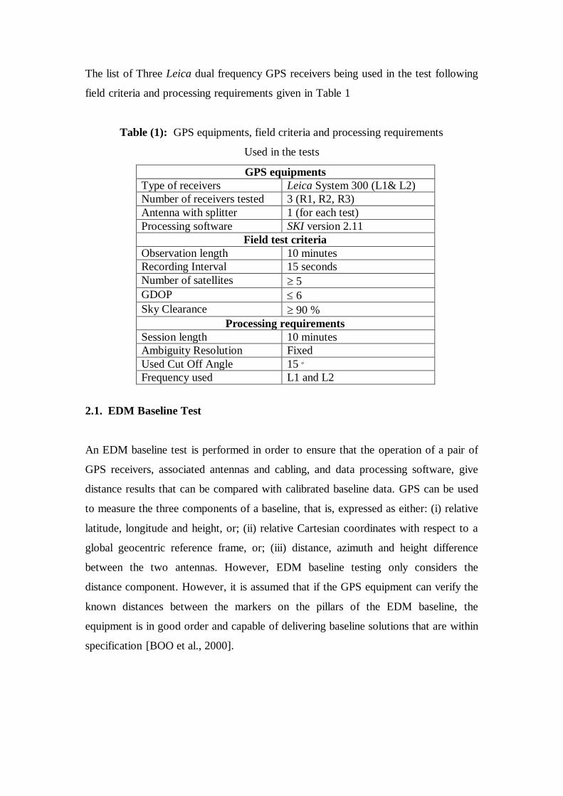
consists of three (3) GPS stations (known stations) namely F6 (it’s a 1st degree control

point located on Cairo – Suez desert road), TS (It is a worldwide well-defined point

belongs to Technoscient corporation (Representative of Leica In Egypt) it is located

downtown in Bab Ellok) and MTC1 (control point located on (MTC) campus in

Kobry El-koba, in Cairo). The test has been carried out using GPS static technique.

The observation has been carried out in two sessions (approximately 5 hours/ one)

with 1hour separating occupations using a total of three (3) GPS receivers. Layout of

the GPS network test site is shown in Figure 3.

Figure: (3) GPS network test site

Finally, the adjusted coordinates for ST, F6 and MTC1 are given below in local datum.

The coordinates were compared to their corresponding known (established) values.

Table (3): The difference between the multiple occupation Coordinates.

Station First occupation

Coordinates (m)

Second occupation

Coordinates (m)

Difference

(m)

E N E N ΔE ΔN

ST 815024.0347 637769.2768 815024.0347 637769.2768 0.000 0.000

F6 819207.7105 657877.3822 819207.0978 657878.4616 1.0794 -0.6127

MTC1 818912.5879 643337.2374 818912.412 643336.9499 -0.2875 -0.1759

The results indicate that, for both pairs of the receivers, differences of less than 1.4 m

6791.415 m

14537.977 m

20534.290 m

has been given. This shows that the GPS equipment set being used are in good

condition.

3. Transformation Parameters

A transformation of the GPS data to the local coordinate system of the origin marks

may be required. A set of transformation parameters can be defined from a selection

of primary control stations over the whole country. The most suitable transformation

would be a seven-parameter three-dimensional transformation and this is currently

available. The problem with this approach is that a national set of transformation

parameters is of insufficient accuracy for use throughout the country. In other words,

the coordinate of a point, which has been positioned using GPS and transformed from

WGS84 to local system, is only expected to be correct owing to distortions in the

underlying geodetic network. These distortions will affect a cadastral survey if the

origin is a long way from the parcel(s) to be surveyed [GPS Guidelines, 1999].

In this study the WGS84 positions were directly compared with the equivalent

Helmart 1906 positions to produce differences in latitude, longitude and ellipsoidal

height, which were subsequently converted to local east, north and height differences.

Nine (9) points (E7, A6, T2 , 01, G4 , G2 , G3 , G1, and G5) from the Egyptian

geodetic network at red Belt were entered in the SKI software and the program

generated a sets of transformation parameters based on Molodensky – Badekas,

parameters resulting from this process are shown in Table 4.

Table (4): Transformation parameters based on Molodensky – Badekas

Parameter Value Standard Deviation

x 118.279 m 1.0914 m

y -124.688 m 1.0914m

z 7.713 m 0.8626m

R x 5.195905 sec 2.2844sec

Rx -1.058113 sec 2.2058sec

Rx -6.814147 sec 2.7015sec

Scale 0.9896405 ppm 8.8086 ppm

When two points are taken as a check using SKI parameters program, the residuals of

these points are illustrated at table (5).

Table (5): The residuals in check points using above 7 –parameter

Point Residuals 1.0e-005 (m)

X Y Z

G7 0.03060560162473 0.04081888413049 -0.08874582784894

G8 0.04512533593285 0.02038421351455 -0.09116228303585

The results indicate that, the transformed results have different residuals, depending

on data distribution, their qualities, and sizes of test areas. In Egypt, more efforts

should be done to provide a standard for datum transformation and associated

procedures that will result in adequate and consistent accuracies over the country.

4. GPS Cadastral Survey

GPS Cadastral Survey, on the other hand, requires the coordinates to be determined of

the land parcel, in relation to a nearby GPS mark (established, for example, by the

(Control Survey). These coordinates may then be transformed to bearing and distance,

or otherwise used. This may be done using the Rapid Static GPS surveying technique.

4.1. Cadastral Control network

Cadastral Control network is the network of the GPS stations, tied to the state

geodetic network, which is surveyed to control all subsequent GPS Cadastral

Measurements. This network may be established at the same time the Cadastral

Measurements are made. However, the points and resulting baseline vectors used in

the Cadastral Control network shall be processed to derive the baseline solutions and

be adjusted by least squares independently of the observed Cadastral Measurements

[Standards and Guidelines, 2001].

A sample GPS cadastral control survey has been carried out on the 4 th

March 2001.

Layout of the GPS network test site is shown in Figure 3. The test site comprises of

Two (2) GPS stations (known stations) namely TS and, F6 which is separated about

20 km apart, and one (1) cadastral standard stations (MTC1). The test has been carried

out using GPS static technique. Three (3) Leica dual frequency GPS receivers are

being used in the measurements. A minimally constrained adjustment is also being

carried out using the SKI Adjustment Package. In the adjustment, the WGS84

coordinate for TS was held fixed. The adjusted coordinates for TS, F6, and MTC1

need to be transformed again into the local system ( Helmart 1906). Adjusted

coordinates for MTC1 are given in Table 6.

Table (6): Final Adjusted coordinates for MTC1

Cartesian Coordinates Geodetic coordinates

X 4720129.3992 m ± 0.0005 m

Y 2869394.6697 m ± 0.0004 m

Z 3178101.9134 m ± 0.0003 m

Lat 30 04 48.71337 N ± 0.0003 m

Lon 31 17 44.39828 E ± 0.0003 m

H= 64.1220 m ±0.0006 m

4.2. Field Procedures of GPS Cadastral Survey

Two ground control points are taken as basic points. By placing the basic points it has

been taken into consideration that the basic points shall be suitable for GPS reference

stations measurements. It means that obstructions must not disturb the receiving of

data from the satellites, and the location shall ensure a stable between the reference

station and the rover. GPS cadastral surveys on the selected lots (see Figure 5) were

carried out using rapid static technique. Surveys were done using three (3) receivers

with two (2) of them remained at the base stations (MTC1 and TS) and another one is

roving receiver.

Figure: (3) Test site for GPS cadastral survey using rapid static technique

Proceedings of the 4th ICCAE Conf. 14-16 May, 2002

Table (7): Differences between three sets of the grid coordinates (Base I values refer to EDM, Base II refer to MTC1 and Base III refer to TS)

Difference (II-III) mm

Difference (I-III) mm

Difference (I-II) mm T.S(III) MTC(II) EDM(I)

stn dy dx dy dx dy dx Y X Y X Y X

0 0.00 0 0 0 0.00 818847.4989 643337.685 818847.4989 643337.685 818847.4989 643337.685 1

-47.5 -37.80 -47.50 -37.80 -47.50 -37.80 818806.259 643356.6918 818806.259 643356.692 818806.2115 643356.654 2

9.1 -6.90 9.10 -6.90 9.10 -6.90 818644.2089 643483.3967 818644.2089 643483.3967 818644.218 643483.3898 4

21.40 35.70 21.60 35.60 21.40 35.70 818735.2053 643660.8636 818735.2055 643660.8635 818735.2269 643660.8992 5

-13.25 55.20 -13.25 55.30 -13.25 55.20 818787.8884 643685.5772 818787.8884 643685.5773 818787.8752 643685.6325 6

71.80 77.10 71.80 77.10 71.80 77.10 818774.8083 643636.8631 818774.8083 643636.8631 818774.8801 643636.9402 7

45.80 77.30 45.80 77.30 45.80 77.30 818811.0223 643424.1063 818811.0223 643424.1063 818811.0681 643424.1836 8

-15.20 6.50 -39.80 -13.80 -15.20 6.50 818855.0378 643548.378 818855.0132 643548.3577 818854.998 643548.3642 9

72.80 52.00 59.70 39.10 72.80 52.00 818951.1886 643592.697 818951.1755 643592.6841 818951.2483 643592.7361 11

-12.70 10.20 -26.20 -23.60 -12.70 10.20 818983.2896 643449.3998 818983.2761 643449.366 818983.2634 643449.3762 13

14.20 -14.70 -10.40 -4.80 14.20 -14.70 818888.3124 643375.6058 818888.2878 643375.6157 818888.302 643375.601 14

34.90 87.00 0.90 65.60 34.90 87.00 818937.0549 643246.2585 818937.0209 643246.2371 818937.0558 643246.3241 16

10.90 72.00 -24.40 49.50 10.90 72.00 819012.4234 643323.6426 819012.3881 643323.6201 819012.399 643323.6921 17

-23.42 39.60 -55.52 23.60 -23.42 39.60 819068.5985 643253.8714 819068.5664 643253.8554 819068.543 643253.895 18

43.40 29.00 10.30 8.30 43.40 29.00 819145.6214 643297.5006 819145.5883 643297.4799 819145.6317 643297.5089 19

66.20 69.00 21.50 40.90 66.20 69.00 819194.1893 643240.9819 819194.1446 643240.9538 819194.2108 643241.0228 20

40.20 19.20 -3.80 -8.50 40.20 19.20 819041.1436 643129.0638 819041.0996 643129.0361 819041.1398 643129.0553 21

-46.50 60.60 -78.70 40.40 -46.50 60.60 818987.5722 643191.9446 818987.54 643191.9244 818987.4935 643191.985 22

48.90 -6.20 48.80 -6.20 48.90 -6.20 819076.8862 643377.0804 819076.8861 643377.0804 819076.935 643377.0742 23

-48.80 5.00 -48.70 5.00 -48.80 5.00 819199.8737 643479.888 819199.8738 643479.888 819199.825 643479.893 25

70.50 9.10 70.40 9.10 70.50 9.10 819314.0207 643352.2773 819314.0206 643352.2773 819314.0911 643352.2864 28

-6.20 80.00 -6.50 80.10 -6.20 80.00 819124.954 643564.6709 819124.9537 643564.671 819124.9475 643564.751 29

0 0 0 0 0 0 min

44.70 33.80 78.70 80.10 72.80 87.00 max

1.79 1.65 1.89 1.59 1.79 1.65 R.M.S

Proceedings of the 4th ICCAE Conf. 14-16 May, 2002

Two sets of the resulting GPS grid coordinates and a set of EDM grid coordinates for

ten (10) boundary marks are given in Table 7. The GPS coordinates were first

computed in WGS 84, and then were transformed into their corresponding values in

local system (WGS 84 - Helmart 1906 –TM projection). The results in Table 7 shows

that the maximum coordinates difference referred to the tow basic reference points

were ∆E = 3.3 cm and ∆N = 4.4 cm and maximum coordinates difference referred to

the tow basic reference points and EDM measurements were ∆E = 8.7 cm and ∆N =

7.8 cm. RMS differences of 2mm is being achieved in both components (Easting and

Northing) which indicates the potential of GPS rapid static technique to be used for

GPS cadastral survey.

Further analysis has been done by calculating the area for individual lot and

comparing with their corresponding values shown on the Certified Plans (see Table

8). For the purposes of the examination, the differences were calculated between the

EDM- area and the area calculated from the GPS transformed coordinates.

Table 8: Area comparison between computed (GPS) and existing (EDM) values

Lot no.

EDM area

(m2)

Computed (GPS)

area (m2)

diff.

(m2)

Accuracy

(%)

area I 15467.95 15456.77 11.1767 0.072257

area II 19966.2 19975.3 -9.1015 0.045585

area III 16877.68 16886.21 -8.5258 0.050515

area IV 17484.05 17478.37 5.68335 0.032506

area V 22193.33 22202.91 -9.57664 0.043151

area VI 22528.47 22520.63 7.8363 0.034784

area VII 3889.484 3889.657 -0.1734 0.004458

area VIII 22903.51 22900.34 3.177 0.013871

area IX 33985.14 33971.37 13.774 0.040529

area X 10621.33 10617.77 3.563 0.033546

Σ 185923.2 185899.3 23.83301

Table 8 indicates that in general differences of less than 1m2 could be achieved for lot

area 1 Fadden (less than 0.10% difference). Again this shows the potential of using

rapid static technique in GPS cadastral survey.

14

4.3. Details Points And Corners

Unlike using total stations for surveying the use of GPS means that it is not possible

to measure all detailed points directly (e.g. corners of houses), because GPS requires

free sight to the satellites. It depends on the number and the kind of obstructions how

many detailed points it is necessary to measure by using off set functions. If there are

a lot of detailed points, where the use of off set functions is unavoidable, 3 - 4 points

are established by using GPS in the measure area [Yang. C.S., et al., 1999].

From these 3 - 4 points the rest of the detailed points are measured by use of a total

station. Also, it is remarkable that even in urban area intermingled with buildings,

over 95% of the observations on cadastral property boundary and corners surveyed

using a rapid static technique have good correspondences with the results obtained by

Total station technique. More details and associated procedures of some points of the

building corners were observed by means of a rapid static technique. These

measurements are not subject of this paper.

5. Lessons Learned and recommended procedures

This study shows that GPS can be applied directly to cadastral problems and can

produce high-quality coordinate values for property boundary and corners. The

following are recommended procedures when using GPS measurement techniques for

Cadastral Surveys.

1. A GPS system-testing program is considered a prerequisite for demonstrating that

GPS-derived coordinates are of a uniformly high quality. Recommendations were

made concerning three tests: (a) a zero-baseline test, (b) calibration of the GPS

equipment on an existing EDM baseline, and (c) connections to several existing

first order geodetic GPS control stations.

2. Field survey operations should be performed using the manufacturer’s

recommended receiver settings and observation times. Operations under adverse

conditions, such as in urban sectors concerns, may require longer observation

times than specified by the manufacturer.

15

3. Fixed height or adjustable height antenna tripods can be used for all rover GPS

observations. The elevation of an adjustable height antenna tripod/bipod should be

regularly checked to make sure slippage has not occurred.

4. A variety of GPS field data acquisition methods may be used for Cadastral

Measurements and Cadastral Control Network.

5. GPS observation procedures should be designed to detect and eliminate:

ambiguity initialization errors;

the effects of multipath;

interference from electrical interference such as substations, microwave

or other spurious radio signals;

poor satellite geometry due to satellite configuration and/or sky

coverage obstructions.

6. All Cadastral Control networks should be referenced to two or more Local

geodetic network or other published horizontal control stations, located in two

or more quadrants, relative to the cadastral project area.

7. The Cadastral Control network must be a geometrically closed figure.

Therefore, single radial (spur) lines or side shots to a point are not acceptable.

8. Before proceeding to the survey site, the surveyor should occupy two known

control points. This provides a general check that the GPS receiver as

configured is delivering the required accuracy (sub-meter). Once survey points

or monuments have been identified, they should be occupied for at least 60

seconds. All points should be reoccupied at least one hour after the first

occupation as an independent check on the coordinates.

9. The local accuracies of the corners coordinates are based upon the results of a

least squares adjustment of the survey observations used to establish their

positions. They can be computed from elements of a covariance matrix of the

adjusted parameters, where the known control coordinate values have been

weighted using their one-sigma network accuracies.

16

10. Finally, it is easy to use the GPS for cadastral surveys. You don’t need to

spent much time on education. But we still need qualified staff in the field to

make decisions about the cadastral problems.

Conclusion

Results from this study indicate that the proposed GPS Cadastral Survey

recommendations could be used as a guide in carrying out GPS cadastral surveys in

Egypt, and to verify the specified accuracy standard has been achieved. GPS

technology will not replace the existing survey techniques but it will provide another

means in carrying out cadastral surveys especially in the area where conventional

technique is not economical. To utilize GPS positioning, well-established control

networks and associated procedures are required. Then, coordinates of cadastral

points with sufficient accuracies can easily measured. To realize this, the derivation of

the consistent relationship between the existing national datum and WGS84 must be

one of the most important tasks.

Furthermore it has been proven that GPS technique provides an excellent way for

cadastral coordinates transfer purposes. Also, it is remarkable that even in urban area

intermingled with buildings, over 95% of the observations on cadastral property

boundary and corners surveyed using a rapid static technique have good

correspondences with the results obtained by Total station technique.

References

1. Barnes, G., M. Eckl and B. Chaplin (1996a). "A Medium Accuracy GPS

Methodology for Cadastral Surveying and Mapping." Surveying and Land

Information Systems Journal, 56 (1), pp. 3-12

2. Barnes, G. and M. Eckl (1996 b). "A GPS Methodology for Cadastral

Surveying in Albania: Phase II." Final Report submitted to Land Tenure

Center, University of Wisconsin, Madison, 26p.

17

3. BOO, T.C., KADIR, M., RIZOS, C., SES, S., & TONG, C.W., (2000). “GPS

for cadastral surveys in Malaysia.” Map & Measure, 10, 35-37.

4. Carl Sumpter, USFS, Mike Londe, BLM, Ken Chamberlain, USFS and Ken

Bays, BLM., 2001. “Standards And Guidelines For Cadastral Surveys Using

Global Positioning System Methods.” United States Department of

Agriculture- Forest Service and United States Department of the Interior-

Bureau of Land Management., March 21, 2001.

5. “GPS Guidelines for Cadastral Surveys” Office of the Surveyor-General OSG

Technical Report 11. Land Information New Zealand 1 July 1999, Crown

Copyright RGP/04/07/03/01.

6. SES, S., KADIR, M., CHIA, W.T., TENG, C.B., & RIZOS, C., (1999).

“Potential use of GPS for cadastral surveys in Malaysia.” 40th Aust. & 6th

S.E.Asian Surveyors Congress, Fermented, Australia, 30 October - 5

November 176-184.

7. “Standards and Guidelines for Cadastral Surveys Using Global Positioning

System Methods” United States Department Of The Interior Bureau Of Land

Management Washington, D.C. 20240 July 26, 2001

8. Tommy Österberg, 1999. “CADASTRAL SYSTEMS IN DEVELOPING

COUNTRIES.” Technical Director Swede survey SE-801 82 Gävle, Sweden.

Email: [email protected]

9. Yang. C.S., et al., 1999. “THE EXPECTED ROLES AND PROBLEMS OF

GPS FOR COORDINATED CADASTRAL SURVEYING.” Technical

Report of Cadastral Technology Research Institute, 11p, Korea Cadastral

Survey Corporation, Seoul, Korea.