The existence and stability of spike equilibria in the one-dimensional Gray–Scott model: The pulse-splitting regime

The Existence and Stability of Spike Equilibria in theOne-Dimensional Gray-Scott Model: The Pulse-Splitting RegimeTheodore Kolokolnikov�, Michael J. Wardy, Juncheng WeizAbstractThe existence, stability, and pulse-splitting behavior of spike patterns in the one-dimensionalGray-Scott model on a �nite domain is analyzed in the semi-strong spike-interaction regime. Thisregime is characterized by a localization of one of the components of the reaction near certain spikelocations, while the other component exhibits a more global spatial variation across the domain.The method of matched asymptotic expansions is used to construct k-spike equilibria in terms of acertain core problem. This core problem is studied numerically and qualitatively. For each integerk � 1, it is shown that there are two branches of k-spike equilibria that meet at a saddle-nodebifurcation value. For small values of the di�usivity D of the second component, these saddlenode bifurcation points occur at approximately the same value. A combination of asymptotic andnumerical methods is used to analyze the stability of these branches of k-spike equilibria withrespect to both drift instabilities associated with the small eigenvalues and oscillatory instabilitiesof the spike pro�le. In this way, the key bifurcation and spectral conditions of Ei, Nishiura, Ueda[Japan. J. Indus. Appl. Math., 18, (2001)] believed to be essential for pulse-splitting behavior ina reaction-di�usion system are veri�ed. A simple analytical criterion for the occurrence of pulse-splitting is formulated and veri�ed with full numerical simulations of the Gray-Scott model.1 IntroductionWe study the existence, stability, and pulse-splitting behavior of spike patterns in the one-dimensionalGray-Scott model. The Gray-Scott system, introduced in [15], models an irreversible reaction involvingtwo reactants in a gel reactor, where the reactor is maintained in contact with a reservoir of one of�Department of Mathematics, University of British Columbia, Vancouver, Canada V6T 1Z2yDepartment of Mathematics, University of British Columbia, Vancouver, Canada V6T 1Z2, (corresponding author)zDepartment of Mathematics, Chinese University of Hong Kong, New Territories, Hong Kong

1

the two species in the reaction. This system can be written in nondimensional form asVT = DvVXX � (F + k)V + UV 2 ; 0 < X < L ; T > 0 ; (1.1a)UT = DuUXX + F (1� U)� UV 2 ; 0 < X < L ; T > 0 ; (1.1b)UX = VX = 0 ; X = 0; L : (1.1c)Here Du > 0, Dv > 0 are the constant di�usivities, F > 0 is the feed rate, and k > 0 is a reaction-timeconstant. For various ranges of these parameters, (1.1) and its two-dimensional counterpart, are knownto posses a rich solution structure involving oscillating standing pulses, the propagation of travelingwaves, pulse-replication behavior, and chaotic phenomena (cf. [5]{[9] [22], [23], [26]{[28], [30], [32],[33], [34], [35], [36], [37], and [38]).We will analyze (1.1) in the singularly perturbed limit where Dv=Du is asymptotically small. Inour formulation, it is convenient to introduce the change of variablesv = V=pF ; x = �1 + 2X=L ; t = (F + k)T : (1.2)This leads to the dimensionless systemvt = "2vxx � v +Auv2 ; �1 < x < 1 ; t > 0 ; (1.3a)�ut = Duxx + (1� u)� uv2 � 1 < x < 1 ; t > 0 ; (1.3b)vx(�1; t) = ux(�1; t) = 0 ; v(x; 0) = v0(x) ; u(x; 0) = u0(x) : (1.3c)Here A > 0, D > 0, � > 1, and "� 1, are de�ned in terms of Du, Dv, L, F , and k, byD � 4DuFL2 ; "2 � 4DvL2(F + k) ; � � F + kF ; A � pFF + k : (1.4)The dimensionless system (1.3), �rst introduced in [28], is particularly convenient in that it showsthat, for "� 1, the construction of equilibrium solutions depends only on the two parameters A andD, while the reaction-time constant � > 1 only in uences the stability of these solutions. Since "� 1,for certain ranges of the parameters there are equilibrium solutions for v that consist of a sequence ofspikes. The parameter D measures the e�ect of the �nite domain and the strength of the inter-spikeinteractions. In this paper, we will assume that D � O("2) and " � 1. In this regime, called thesemi-strong spike interaction regime, spike patterns are such that v is localized near the spikes, whileu varies more globally across the domain. This is to be contrasted with the weak spike interactionregime studied in [32], [33], and [38], where D = O("2) and "� 1.2

There are three regimes for A where di�erent behaviors are found to occur. For the parameterrange A = O("1=2), referred to as the low feed-rate regime, there is a saddle-node bifurcation structureof equilibrium k-spike patterns, and the stability of these solutions depends intricately on A, D, and� . This regime has been analyzed in detail in the companion paper [19]. For the intermediate regime,where O("1=2)� A� O(1), there are certain scaling laws in terms of a universal nonlocal eigenvalueproblem that determine the stability of equilibrium spike patterns with respect to eigenvalues � = O(1)in the spectrum of the linearized problem. In this regime, studied in [7], [8], [9], [19], and [27], the�nite domain and inter-spike coupling do not play a central role. In addition, in this regime and when� is asymptotically large as "! 0, there can be drift instabilities associated with the small eigenvalues� = O("2) in the spectrum of the linearization. These instabilities signify the birth of traveling wavesolutions (see [26], [19]). In x2 we summarize the results of [19] for the intermediate regime thatare relevant to the analysis in this paper. Finally, in the regime where A = O(1), referred to hereas the pulse-splitting regime, the equilibrium spike patterns again exhibit a saddle-node bifurcationstructure, and this regime is intimately connected with a pulse-splitting behavior of spike patterns.For the in�nite-line problem this was observed in [28], and also in [7] in terms of a di�erent non-dimensionalization of the Gray-Scott model.The goal of this paper is to analyze the existence and stability of spike patterns for (1.3) in thepulse-splitting regime where A = O(1), " � 1, and D � O("2). In x3 we construct equilibrium k-spike patterns in terms of a certain core problem. For the in�nite-line problem, this core problem wasintroduced in [28]. We extend the analysis in [28] in two ways. Firstly, by allowing for a �nite domain,and by matching the core solution to appropriate outer expansions, we show formally in Proposition3.2 that when A = O(1) and "A=pD � 1, there are no k-spike equilibria to (1.3) that match smoothlyonto the intermediate regime solutions when A > Apk, whereApk � 1:347 coth� 1kpD� : (1.5)The value 1:347 arises from the saddle-node bifurcation value associated with the core problem(cf. [28]), while the other term in (1.5) arises from our analysis of (1.3) on the �nite domain. Secondly,in x4 we investigate qualitative properties of the solutions to the core problem. The results are givenin Propositions 4.1 and 4.2 below.In x5 we study the stability of k-spike equilibria for A = O(1) and "A=pD � 1 with respectto drift instabilities associated with the small eigenvalues of order � = O(") in the spectrum of thelinearization. In Proposition 5.2 we derive transcendental equations that the small eigenvalues satisfy.For � � O("�1), in Proposition 5.3 we show that these eigenvalues are in the stable left half-plane for3

the equilibrium solution branch that merges onto the intermediate regime solution. In Propositions5.4 and 5.5 we show that when � = O("�1), and exceeds some critical value, a drift instability occursas a result of a Hopf bifurcation. This leads to small-scale oscillations in the spike layer locations and abreathing-type instability (see Conjecture 5.6). A related type of Hopf bifurcation has been analyzed in[16] and [24] for hyperbolic tangent-type interfaces associated with a two-component reaction di�usionsystem with bistable nonlinearities. Related behavior for a three-component system has been shownnumerically in [31]. In x6 we numerically study the stability of k-spike equilibria with respect tothe large eigenvalues where � = O(1) as " ! 0. For � � O("�2), we show numerically that theequilibrium solution branch that merges onto the intermediate regime solutions is stable with respectto these eigenvalues, but that an instability due to a Hopf bifurcation in the spike pro�le can occurwhen � is on the range � = O("�2).0:01:02:03:04:0

0:0 0:5 1:0 1:5 2:0jvj2

A(a) jvj2 versus A 0255075100125150175200225

�1:0 �0:5 0:0 0:5 1:0t

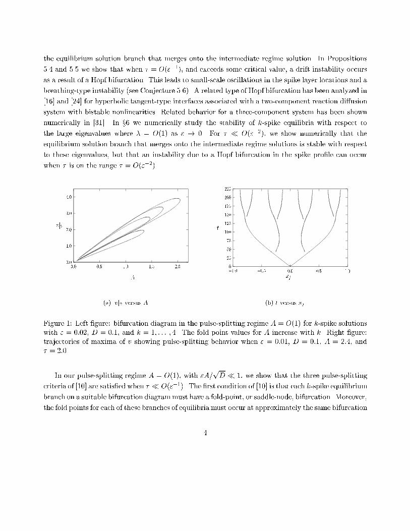
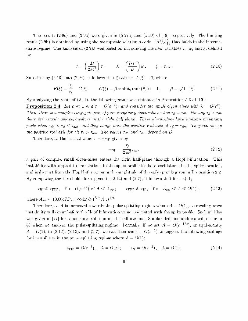
xj(b) t versus xjFigure 1: Left �gure: bifurcation diagram in the pulse-splitting regime A = O(1) for k-spike solutionswith " = 0:02, D = 0:1, and k = 1; : : : ; 4. The fold point values for A increase with k. Right �gure:trajectories of maxima of v showing pulse-splitting behavior when " = 0:01, D = 0:1, A = 2:4, and� = 2:0.In our pulse-splitting regime A = O(1), with "A=pD � 1, we show that the three pulse-splittingcriteria of [10] are satis�ed when � � O("�1). The �rst condition of [10] is that each k-spike equilibriumbranch on a suitable bifurcation diagrammust have a fold-point, or saddle-node, bifurcation. Moreover,the fold points for each of these branches of equilibria must occur at approximately the same bifurcation4

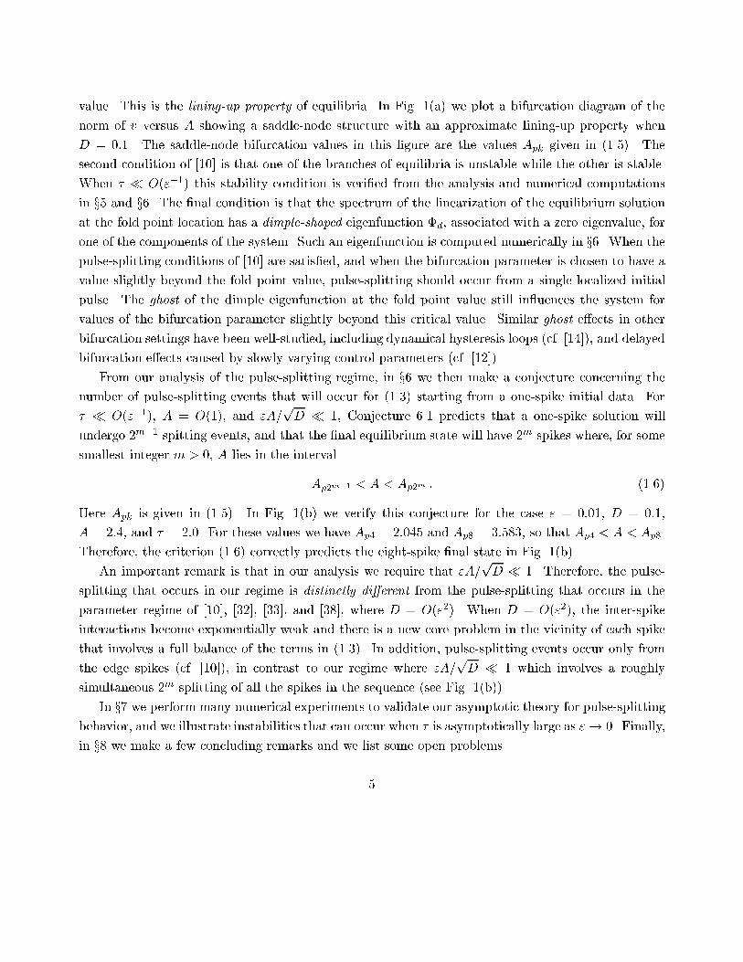
value. This is the lining-up property of equilibria. In Fig. 1(a) we plot a bifurcation diagram of thenorm of v versus A showing a saddle-node structure with an approximate lining-up property whenD = 0:1. The saddle-node bifurcation values in this �gure are the values Apk given in (1.5). Thesecond condition of [10] is that one of the branches of equilibria is unstable while the other is stable.When � � O("�1) this stability condition is veri�ed from the analysis and numerical computationsin x5 and x6. The �nal condition is that the spectrum of the linearization of the equilibrium solutionat the fold point location has a dimple-shaped eigenfunction �d, associated with a zero eigenvalue, forone of the components of the system. Such an eigenfunction is computed numerically in x6. When thepulse-splitting conditions of [10] are satis�ed, and when the bifurcation parameter is chosen to have avalue slightly beyond the fold point value, pulse-splitting should occur from a single localized initialpulse. The ghost of the dimple eigenfunction at the fold point value still in uences the system forvalues of the bifurcation parameter slightly beyond this critical value. Similar ghost e�ects in otherbifurcation settings have been well-studied, including dynamical hysteresis loops (cf. [14]), and delayedbifurcation e�ects caused by slowly varying control parameters (cf. [12]).From our analysis of the pulse-splitting regime, in x6 we then make a conjecture concerning thenumber of pulse-splitting events that will occur for (1.3) starting from a one-spike initial data. For� � O("�1), A = O(1), and "A=pD � 1, Conjecture 6.1 predicts that a one-spike solution willundergo 2m�1 spitting events, and that the �nal equilibrium state will have 2m spikes where, for somesmallest integer m > 0, A lies in the intervalAp2m�1 < A < Ap2m : (1.6)Here Apk is given in (1.5). In Fig. 1(b) we verify this conjecture for the case " = 0:01, D = 0:1,A = 2:4, and � = 2:0. For these values we have Ap4 = 2:045 and Ap8 = 3:583, so that Ap4 < A < Ap8.Therefore, the criterion (1.6) correctly predicts the eight-spike �nal state in Fig. 1(b).An important remark is that in our analysis we require that "A=pD � 1. Therefore, the pulse-splitting that occurs in our regime is distinctly di�erent from the pulse-splitting that occurs in theparameter regime of [10], [32], [33], and [38], where D = O("2). When D = O("2), the inter-spikeinteractions become exponentially weak and there is a new core problem in the vicinity of each spikethat involves a full balance of the terms in (1.3). In addition, pulse-splitting events occur only fromthe edge spikes (cf. [10]), in contrast to our regime where "A=pD � 1 which involves a roughlysimultaneous 2m splitting of all the spikes in the sequence (see Fig. 1(b)).In x7 we perform many numerical experiments to validate our asymptotic theory for pulse-splittingbehavior, and we illustrate instabilities that can occur when � is asymptotically large as "! 0. Finally,in x8 we make a few concluding remarks and we list some open problems.5

2 The Intermediate Regime: O("1=2)� A� O(1)In this section, we summarize the main results of [19] for the existence and stability of k-spike equi-librium solutions to (1.3) in the intermediate regime where O("1=2) � A � O(1). De�ning A byA = "1=2A, we begin with the equilibrium result of [19] in the low feed-rate regime where A = O(1).Proposition 2.1: For " ! 0, consider a k-spike equilibrium solution to (1.3) where the spikes haveequal height. Then, when A > Ake there are two such solutions; the small solution u�, v�, and thelarge solution u+, v+. The v-component for such a solution satis�esv� � 1p"AU� kXj=1�w �"�1(x� xj)�+O� "A2U2�D�� ; (2.1a)where w(y) satis�es (2.2) below and xj = �1 + (2j � 1)=k for j = 1; : : : ; k. In the jth inner region,where jx� xj j = O("), u is spatially constant to leading order, and satis�esu� � U� �1 +O� "A2U2�D�� : (2.1b)Here U� and the saddle-node bifurcation value Ake are given byU� = 12 241�s1� A2keA2 35 ; Ake �s 12�0tanh (�0=k) ; �0 � D�1=2 : (2.1c)The outer solution for u, valid for jx� xj j � O(") and j = 1; : : : ; k, is given byu� � 1� (1� U�)ag kXj=1G(x;xj) ; ag = h2pD tanh (�0=k)i�1 ; (2.1d)where G(x;xj) is the Green's function satisfying (2.3) below.This result was derived in Propositions 2.1 and 5.1 of [19]. In (2.1a), the pro�le w(y) satis�esw00 � w + w2 = 0 ; �1 < y <1 ; (2.2a)w ! 0 as jyj ! 1 ; w0(0) = 0 ; w(0) > 0 : (2.2b)The solution is w(y) = 32sech2(y=2). In contrast, the u-component in (2.1d), which is the globalvariable, is determined in terms of the Green's function G(x;xj) satisfyingDGxx �G = ��(x � xj) ; �1 < x < 1 ; Gx(�1;xj) = 0 : (2.3)6

In [19] the stability properties of (2.1) were examined in the low feed-rate regime A = O(1) (seex2{4 of [19]). Although the large solution v+, u+ was found to be unstable for any A > Ake, thestability properties of the small solution v�, u� were found to depend intricately on the parametersD, � , and k. Instabilities on an O(1) time-scale were of two types: oscillatory instabilities arising froma Hopf bifurcation that occur when A > AkL and � is su�ciently large, and competition instabilitiesarising from positive real eigenvalues that occur when Ake < A < AkL for any � > 0 (see x3 of [19]).For � = O(1), it was shown in x4 of [19] that there are also slow drift instabilities that occur on a longtime-scale of O("�2) when A satis�es Ake < A < AkS, where AkS > AkL. Precise formulae for thethresholds AkL and AkS were obtained in [19].The stability properties of the small solution are much simpler in the intermediate regime whereO(1)� A� O("�1=2), or equivalently when O("1=2)� A� O(1) (see x5 of [19]). For the remainderof this section we re-label the small solution as v, u. For A ! 1, we get from (2.1c) that U� �A2ke=4A2. Substituting this relation into (2.1a) we obtain that v satis�esv � ApD3p" coth (�0=k) kXj=1�w �"�1(x� xj)�+O� "A29 coth2 (�0=k)�� : (2.4a)In addition, the inner solution for u in (2.1b) becomesu � 3 coth (�0=k)A2pD �1 +O� "A29 coth2 (�0=k)�� : (2.4b)For A � 1, the corresponding outer solution from (2.1d) becomesu0(x) � 1� 1ag �1� A2ke4A2� kXj=1G(x;xj) : (2.4c)To plot a bifurcation diagram, it is convenient to de�ne a norm jvj2 byjvj2 � �Z 1�1 v2 dx�1=2 : (2.5)Then, in the intermediate regime, we obtain from (2.4a) thatjvj2 � p6DkA3 coth (�0=k) : (2.6)In the intermediate parameter regime it was shown in Proposition 5.4 of [19] that a k-spike equi-librium solution is stable with respect to the drift instabilities associated with the small eigenvalues of7

order � = O("2) when D = O(1) and � = O(1). Moreover, it was shown in [19] that there is a scalinglaw that determines the stability of the equilibrium solution with respect to the large O(1) eigenvaluesin the spectrum of the linearization. This latter result is summarized as follows:Proposition 2.2: Let " � 1, D = O(1), and O(1) � A � O("�1=2). Then, the k-spike equilibriumsmall solution u, v, is stable with respect to the large eigenvalues when � < �H , where�H � A4D9 tanh4 (�0=k) �0h�1� 6�0A2 tanh(�0=k)�2 + o(1) ; (2.7)and �0h = 1:748. As � increases past �H , this solution loses its stability to a Hopf bifurcation.This result was given in Proposition 5.3 of [19], and is based on spectral properties of the nonlocaleigenvalue problem�00 � �+ 2w�� 2w21 +p�0� R1�1w� dyR1�1w dy ! = �� ; �1 < y <1 ; (2.8)with �! 0 as jyj ! 1, where �0 is a bifurcation parameter.The scaling law for � given in (2.7) for a Hopf bifurcation of the spike pro�le shows that � =O(A4) � 1 when A � 1. Therefore, it is natural to seek drift instabilities of a k-spike equilibriumsolution that occur when � � 1. For a one-spike solution, this was done in x5.1 of [19], where thefollowing result was obtained:Proposition 2.3: Let "� 1 and � = O("�2). Then, an eigenvalue � = O("2) associated with a driftinstability of the one-spike small equilibrium solution satis�es the nonlinear algebraic equation� � 2"2sD [� tanh(�0�) tanh �0 � 1] ; s � 1� U�U� ; � � p1 + �� ; (2.9a)where �0 = 1=pD. In the intermediate parameter regime where O(1)� A� O("�1=2), (2.9a) reducesto � � 2"A23pD tanh �0 [� tanh(�0�) tanh �0 � 1] ; � � p1 + �� ; (2.9b)where A = "1=2A. For � � 1, any unstable mode associated with the one-spike solution has the formv � 1p"AU�w("�1 [x� x0(t)]) ; x0 � �"�e�t : (2.9c)8

The results (2.9c) and (2.9a) were given in (5.37b) and (5.39) of [19], respectively. The limitingresult (2.9b) is obtained by using the asymptotic relation s � 4"�1A2=A21e that holds in the interme-diate regime. The analysis of (2.9a) was based on introducing the new variables �d, !, and �, de�nedby � = � D2s"2� �d ; � = �2s"2D �! ; � = �d! : (2.10)Substituting (2.10) into (2.9a), it follows that � satis�es F (�) = 0, whereF (�) � ��d �G(�) ; G(�) � � tanh �0 tanh(�0�)� 1 ; � �p1 + � : (2.11)By analyzing the roots of (2.11), the following result was obtained in Proposition 5.6 of [19]:Proposition 2.4: Let " � 1 and � = O("�2), and consider the small eigenvalues with � = O("2).Then, there is a complex conjugate pair of pure imaginary eigenvalues when �d = �dh. For any �d > �dhthere are exactly two eigenvalues in the right half-plane. These eigenvalues have nonzero imaginaryparts when �dh < �d < �dm, and they merge onto the positive real axis at �d = �dm. They remain onthe positive real axis for all �d > �dm. The values �dh and �dm depend on D.Therefore, at the critical value � = �TW given by�TW = D2s"2 �dh ; (2.12)a pair of complex small eigenvalues enters the right half-plane through a Hopf bifurcation. Thisinstability with respect to translations in the spike pro�le leads to oscillations in the spike location,and is distinct from the Hopf bifurcation in the amplitude of the spike pro�le given in Proposition 2.2.By comparing the thresholds for � given in (2.12) and (2.7), it follows that for "� 1,�H � �TW ; for O("1=2)� A� Asw ; �TW � �H ; for Asw � A� O(1) ; (2.13)where Asw � �0:0047D�dh coth2 �0�1=6A1e"1=6.Therefore, as A is increased towards the pulse-splitting regime where A = O(1), a traveling waveinstability will occur before the Hopf bifurcation value associated with the spike pro�le. Such an ideawas given in [27] for a one-spike solution on the in�nite line. Similar drift instabilities will occur inx5 when we analyze the pulse-splitting regime. Formally, if we set A = O("�1=2), or equivalentlyA = O(1), in (2.12), (2.10), and (2.7), we can then use s = O("�1) to suggest the following scalingsfor instabilities in the pulse-splitting regime where A = O(1):�TW = O("�1) ; � = O(") ; �H = O("�2) ; � = O(1) : (2.14)9

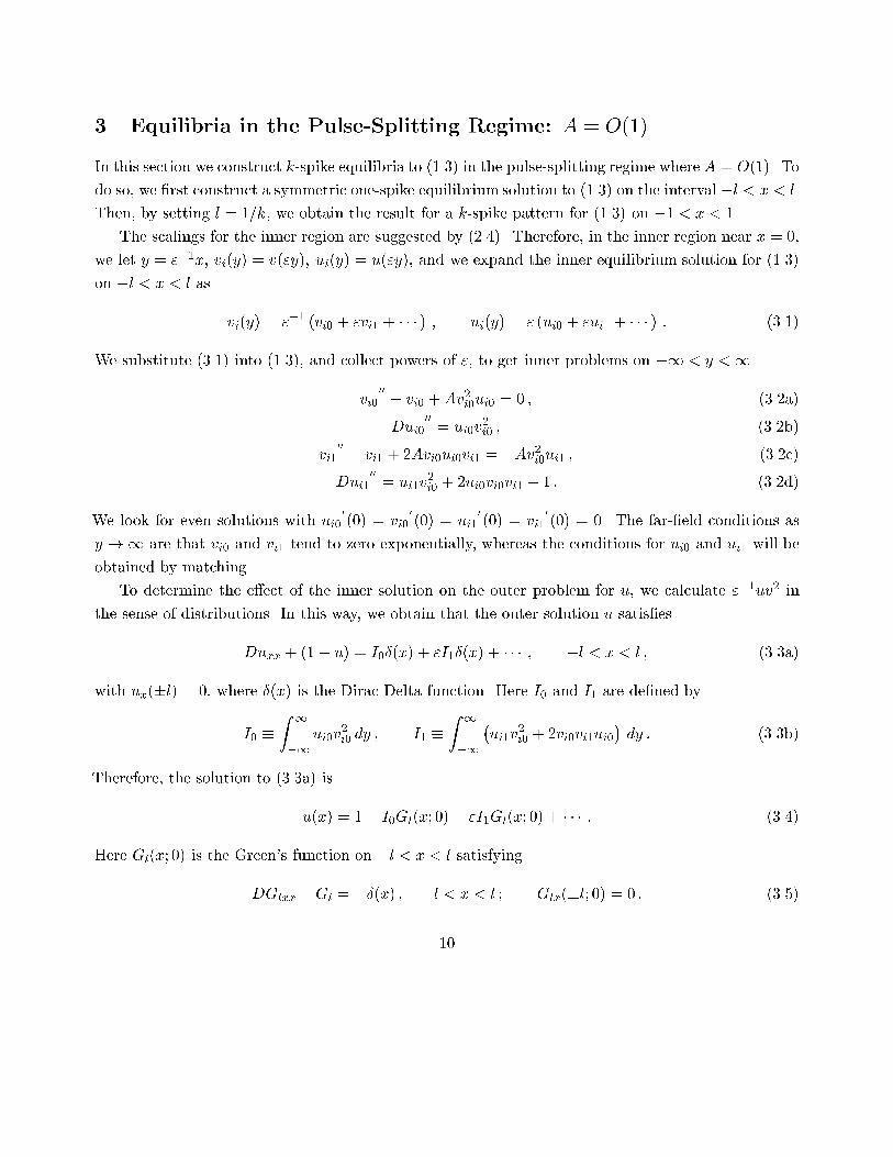
3 Equilibria in the Pulse-Splitting Regime: A = O(1)In this section we construct k-spike equilibria to (1.3) in the pulse-splitting regime where A = O(1). Todo so, we �rst construct a symmetric one-spike equilibrium solution to (1.3) on the interval �l < x < l.Then, by setting l = 1=k, we obtain the result for a k-spike pattern for (1.3) on �1 < x < 1.The scalings for the inner region are suggested by (2.4). Therefore, in the inner region near x = 0,we let y = "�1x, vi(y) = v("y), ui(y) = u("y), and we expand the inner equilibrium solution for (1.3)on �l < x < l as vi(y) = "�1 (vi0 + "vi1 + � � � ) ; ui(y) = " (ui0 + "ui1 + � � � ) : (3.1)We substitute (3.1) into (1.3), and collect powers of ", to get inner problems on �1 < y <1vi000 � vi0 +Av2i0ui0 = 0 ; (3.2a)Dui000 = ui0v2i0 ; (3.2b)vi100 � vi1 + 2Avi0ui0vi1 = �Av2i0ui1 ; (3.2c)Dui100 = ui1v2i0 + 2ui0vi0vi1 � 1 : (3.2d)We look for even solutions with ui00(0) = vi00(0) = ui10(0) = vi10(0) = 0. The far-�eld conditions asy !1 are that vi0 and vi1 tend to zero exponentially, whereas the conditions for ui0 and ui1 will beobtained by matching.To determine the e�ect of the inner solution on the outer problem for u, we calculate "�1uv2 inthe sense of distributions. In this way, we obtain that the outer solution u satis�esDuxx + (1� u) = I0�(x) + "I1�(x) + � � � ; �l < x < l ; (3.3a)with ux(�l) = 0, where �(x) is the Dirac Delta function. Here I0 and I1 are de�ned byI0 � Z 1�1 ui0v2i0 dy ; I1 � Z 1�1 �ui1v2i0 + 2vi0vi1ui0� dy : (3.3b)Therefore, the solution to (3.3a) isu(x) = 1� I0Gl(x; 0)� "I1Gl(x; 0) + � � � : (3.4)Here Gl(x; 0) is the Green's function on �l < x < l satisfyingDGlxx �Gl = ��(x) ; �l < x < l ; Glx(�l; 0) = 0 : (3.5)10

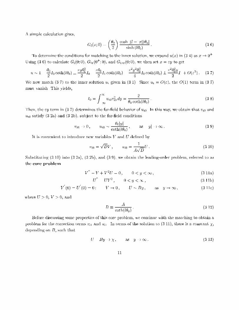
A simple calculation gives, Gl(x; 0) = ��02 � cosh [(l � jxj)�0]sinh (l�0) : (3.6)To determine the conditions for matching to the inner solution, we expand u(x) in (3.4) as x! 0�.Using (3.6) to calculate Gl(0; 0), Glx(0�; 0), and Glxx(0; 0), we then set x = "y to getu � 1� �02 I0 coth(l�0)� "y�202 I0 � "�02 I1 coth(l�0)� "2y2�304 I0 coth(l�0)� "2�20y2 I1 +O("3) : (3.7)We now match (3.7) to the inner solution ui given in (3.1). Since ui = O("), the O(1) term in (3.7)must vanish. This yields, I0 = Z 1�1 ui0v2i0 dy = 2�0 coth(l�0) : (3.8)Then, the "y term in (3.7) determines the far-�eld behavior of ui0. In this way, we obtain that vi0 andui0 satisfy (3.2a) and (3.2b), subject to the far-�eld conditionsvi0 ! 0 ; ui0 � �0jyjcoth(l�0) ; as jyj ! 1 : (3.9)It is convenient to introduce new variables V and U de�ned byvi0 = pDV ; ui0 = 1ApDU : (3.10)Substituting (3.10) into (3.2a), (3.2b), and (3.9), we obtain the leading-order problem, referred to asthe core problem V 00 � V + V 2U = 0 ; 0 < y <1 ; (3.11a)U 00 = UV 2 ; 0 < y <1 ; (3.11b)V 0(0) = U 0(0) = 0 ; V ! 0 ; U � By ; as y !1 ; (3.11c)where U > 0, V > 0, and B � Acoth(l�0) : (3.12)Before discussing some properties of this core problem, we continue with the matching to obtain aproblem for the correction terms vi1 and ui1. In terms of the solution to (3.11), there is a constant �,depending on B, such that U �By! � ; as y !1 : (3.13)11

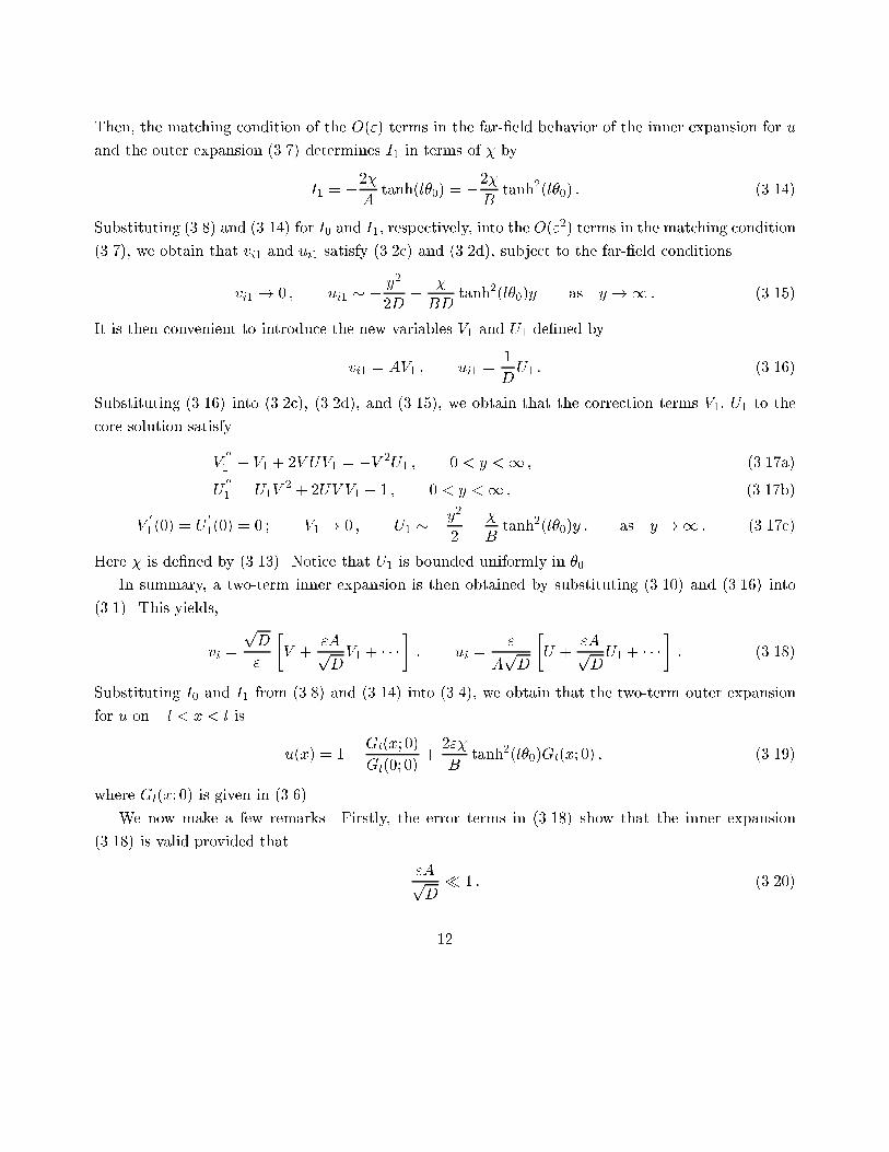
Then, the matching condition of the O(") terms in the far-�eld behavior of the inner expansion for uand the outer expansion (3.7) determines I1 in terms of � byI1 = �2�A tanh(l�0) = �2�B tanh2(l�0) : (3.14)Substituting (3.8) and (3.14) for I0 and I1, respectively, into the O("2) terms in the matching condition(3.7), we obtain that vi1 and ui1 satisfy (3.2c) and (3.2d), subject to the far-�eld conditionsvi1 ! 0 ; ui1 � � y22D � �BD tanh2(l�0)y as y !1 : (3.15)It is then convenient to introduce the new variables V1 and U1 de�ned byvi1 = AV1 ; ui1 = 1DU1 : (3.16)Substituting (3.16) into (3.2c), (3.2d), and (3.15), we obtain that the correction terms V1, U1 to thecore solution satisfyV 001 � V1 + 2V UV1 = �V 2U1 ; 0 < y <1 ; (3.17a)U 001 = U1V 2 + 2UV V1 � 1 ; 0 < y <1 ; (3.17b)V 01 (0) = U 01(0) = 0 ; V1 ! 0 ; U1 � �y22 � �B tanh2(l�0)y : as y !1 : (3.17c)Here � is de�ned by (3.13). Notice that U1 is bounded uniformly in �0.In summary, a two-term inner expansion is then obtained by substituting (3.10) and (3.16) into(3.1). This yields,vi = pD" �V + "ApDV1 + � � � � ; ui = "ApD �U + "ApDU1 + � � � � : (3.18)Substituting I0 and I1 from (3.8) and (3.14) into (3.4), we obtain that the two-term outer expansionfor u on �l < x < l is u(x) = 1� Gl(x; 0)Gl(0; 0) + 2"�B tanh2(l�0)Gl(x; 0) ; (3.19)where Gl(x; 0) is given in (3.6).We now make a few remarks. Firstly, the error terms in (3.18) show that the inner expansion(3.18) is valid provided that "ApD � 1 : (3.20)12

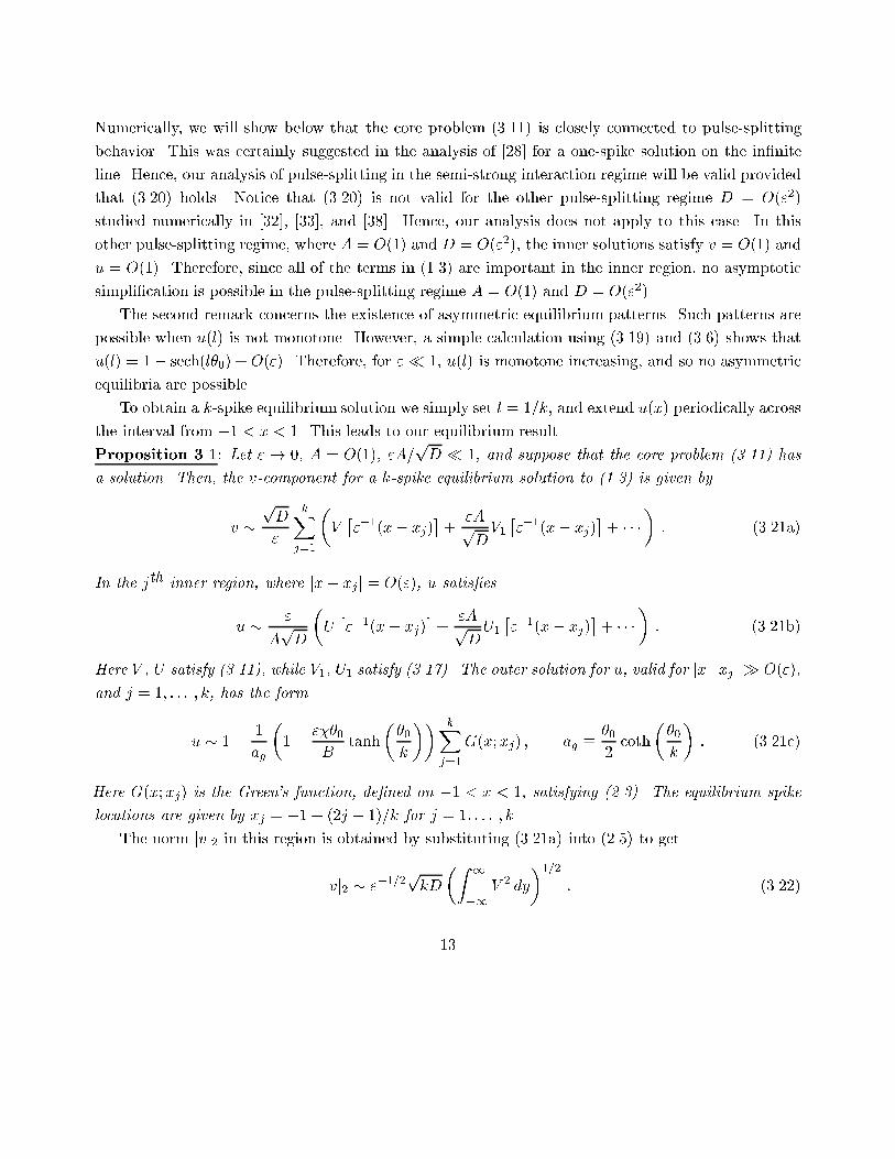
Numerically, we will show below that the core problem (3.11) is closely connected to pulse-splittingbehavior. This was certainly suggested in the analysis of [28] for a one-spike solution on the in�niteline. Hence, our analysis of pulse-splitting in the semi-strong interaction regime will be valid providedthat (3.20) holds. Notice that (3.20) is not valid for the other pulse-splitting regime D = O("2)studied numerically in [32], [33], and [38]. Hence, our analysis does not apply to this case. In thisother pulse-splitting regime, where A = O(1) and D = O("2), the inner solutions satisfy v = O(1) andu = O(1). Therefore, since all of the terms in (1.3) are important in the inner region, no asymptoticsimpli�cation is possible in the pulse-splitting regime A = O(1) and D = O("2).The second remark concerns the existence of asymmetric equilibrium patterns. Such patterns arepossible when u(l) is not monotone. However, a simple calculation using (3.19) and (3.6) shows thatu(l) = 1� sech(l�0) +O("). Therefore, for "� 1, u(l) is monotone increasing, and so no asymmetricequilibria are possible.To obtain a k-spike equilibrium solution we simply set l = 1=k, and extend u(x) periodically acrossthe interval from �1 < x < 1. This leads to our equilibrium result.Proposition 3.1: Let " ! 0, A = O(1), "A=pD � 1, and suppose that the core problem (3.11) hasa solution. Then, the v-component for a k-spike equilibrium solution to (1.3) is given byv � pD" kXj=1�V �"�1(x� xj)�+ "ApDV1 �"�1(x� xj)�+ � � �� : (3.21a)In the jth inner region, where jx� xjj = O("), u satis�esu � "ApD �U �"�1(x� xj)�+ "ApDU1 �"�1(x� xj)�+ � � �� : (3.21b)Here V , U satisfy (3.11), while V1, U1 satisfy (3.17). The outer solution for u, valid for jx�xj j � O("),and j = 1; : : : ; k, has the formu � 1� 1ag �1� "��0B tanh��0k �� kXj=1G(x;xj) ; ag � �02 coth��0k � : (3.21c)Here G(x;xj) is the Green's function, de�ned on �1 < x < 1, satisfying (2.3). The equilibrium spikelocations are given by xj = �1 + (2j � 1)=k for j = 1; : : : ; k.The norm jvj2 in this region is obtained by substituting (3.21a) into (2.5) to getjvj2 � "�1=2pkD�Z 1�1 V 2 dy�1=2 : (3.22)13

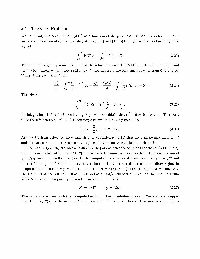
3.1 The Core ProblemWe now study the core problem (3.11) as a function of the parameter B. We �rst determine someanalytical properties of (3.11). By integrating (3.11a) and (3.11b) from 0 < y <1, and using (3.11c),we get Z 10 V 2U dy = Z 10 V dy = B : (3.23)To determine a good parameterization of the solution branch for (3.11), we de�ne U0 � U(0) andV0 � V (0). Then, we multiply (3.11a) by V 0 and integrate the resulting equation from 0 < y < 1.Using (3.11c), we then obtainV 202 + Z 10 U3 �V 3�0 dy = V 202 � U0V 303 � Z 10 13V 3U 0 dy = 0 : (3.24)This gives, Z 10 V 3U 0 dy = V 20 �32 � U0V0� : (3.25)By integrating (3.11b) for U , and using U 0(0) = 0, we obtain that U 0 > 0 on 0 < y <1. Therefore,since the left hand-side of (3.25) is non-negative, we obtain a key inequality0 < < 32 ; � U0V0 : (3.26)As ! 3=2 from below, we show that there is a solution to (3.11) that has a single maximum for Vand that matches onto the intermediate regime solution constructed in Proposition 2.1.The inequality (3.26) provides a natural way to parameterize the solution branches of (3.11). Usingthe boundary value solver COLSYS [2], we compute the numerical solution to (3.11) as a function of = U0V0 on the range 0 < < 3=2. In the computations we started from a value of near 3=2 andtook as initial guess for the nonlinear solver the solution constructed in the intermediate regime inProposition 2.1. In this way, we obtain a function B = B( ) from (3.11c). In Fig. 2(a) we show thatB( ) is multi-valued with B ! 0 as ! 0 and as ! 3=2. Numerically, we �nd that the maximumvalue Bc of B and the point c where this maximum occurs isBc = 1:347 ; c = 1:02 : (3.27)This value is consistent with that computed in [28] for the in�nite-line problem. We refer to the upperbranch in Fig. 2(a) as the primary branch, since it is this solution branch that merges smoothly as14

0:00:51:01:52:0

0:0 0:5 1:0 1:5

B(a) versus B0:02:55:07:5

0:0 0:5 1:0 1:5 2:0jvj2

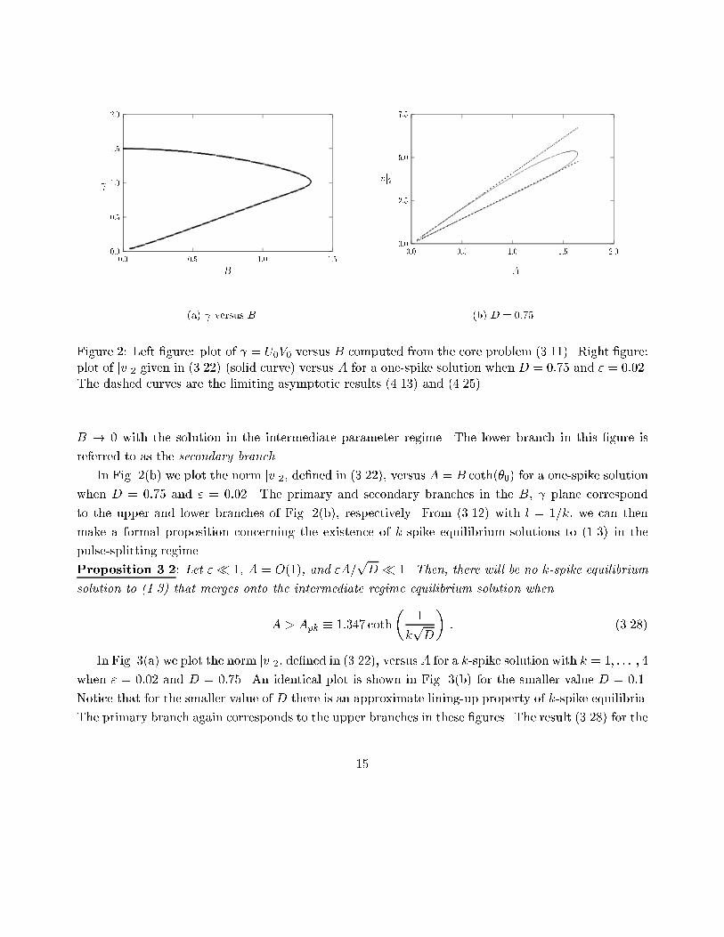
A(b) D = 0:75Figure 2: Left �gure: plot of = U0V0 versus B computed from the core problem (3.11). Right �gure:plot of jvj2 given in (3.22) (solid curve) versus A for a one-spike solution when D = 0:75 and " = 0:02.The dashed curves are the limiting asymptotic results (4.13) and (4.25).B ! 0 with the solution in the intermediate parameter regime. The lower branch in this �gure isreferred to as the secondary branch.In Fig. 2(b) we plot the norm jvj2, de�ned in (3.22), versus A = B coth(�0) for a one-spike solutionwhen D = 0:75 and " = 0:02. The primary and secondary branches in the B, plane correspondto the upper and lower branches of Fig. 2(b), respectively. From (3.12) with l = 1=k, we can thenmake a formal proposition concerning the existence of k-spike equilibrium solutions to (1.3) in thepulse-splitting regime.Proposition 3.2: Let "� 1, A = O(1), and "A=pD � 1. Then, there will be no k-spike equilibriumsolution to (1.3) that merges onto the intermediate regime equilibrium solution whenA > Apk � 1:347 coth� 1kpD� : (3.28)In Fig. 3(a) we plot the norm jvj2, de�ned in (3.22), versus A for a k-spike solution with k = 1; : : : ; 4when " = 0:02 and D = 0:75. An identical plot is shown in Fig. 3(b) for the smaller value D = 0:1.Notice that for the smaller value of D there is an approximate lining-up property of k-spike equilibria.The primary branch again corresponds to the upper branches in these �gures. The result (3.28) for the15

�nite domain is new, and below it will provide a criterion for predicting the number of pulse-splittingevents starting from initial data for (1.3).0:02:55:07:510:012:5

0:0 1:0 2:0 3:0 4:0 5:0jvj2

A(a) D = 0:750:01:02:03:04:0

0:0 0:5 1:0 1:5 2:0jvj2

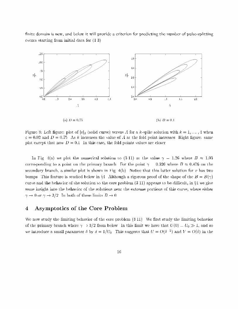
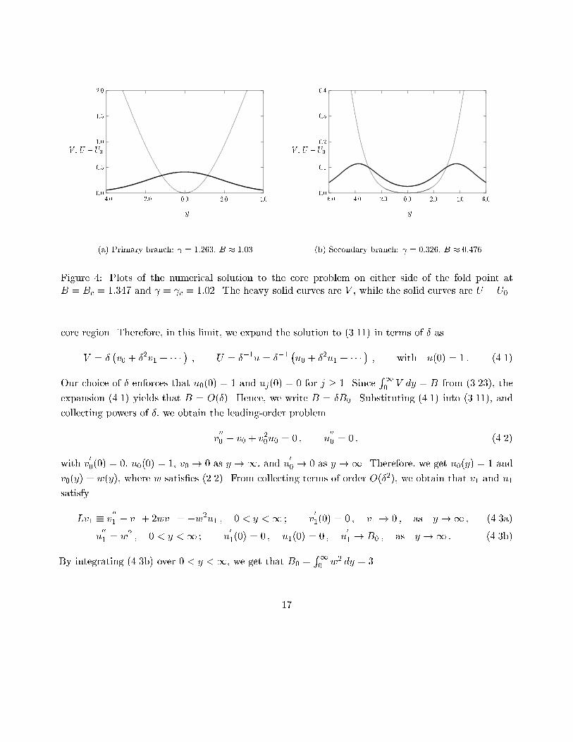
A(b) D = 0:1Figure 3: Left �gure: plot of jvj2 (solid curve) versus A for a k-spike solution with k = 1; : : : ; 4 when" = 0:02 and D = 0:75. As k increases the value of A at the fold point increases. Right �gure: sameplot except that now D = 0:1. In this case, the fold points values are closer.In Fig. 4(a) we plot the numerical solution to (3.11) at the value = 1:26 where B � 1:03corresponding to a point on the primary branch. For the point = 0:326 where B � 0:476 on thesecondary branch, a similar plot is shown in Fig. 4(b). Notice that this latter solution for v has twobumps. This feature is studied below in x4. Although a rigorous proof of the shape of the B = B( )curve and the behavior of the solution to the core problem (3.11) appears to be di�cult, in x4 we givesome insight into the behavior of the solutions near the extreme portions of this curve, where either ! 0 or ! 3=2. In both of these limits B ! 0.4 Asymptotics of the Core ProblemWe now study the limiting behavior of the core problem (3.11). We �rst study the limiting behaviorof the primary branch where ! 3=2 from below. In this limit we have that U(0) � U0 � 1, and sowe introduce a small parameter � by � = 1=U0. This suggests that U = O(��1) and V = O(�) in the16

0:00:51:01:52:0

�4:0 �2:0 0:0 2:0 4:0V , U � U0

y(a) Primary branch: = 1:263, B � 1:030:00:10:20:30:4

�6:0 �4:0 �2:0 0:0 2:0 4:0 6:0V , U � U0

y(b) Secondary branch: = 0:326, B � 0:476Figure 4: Plots of the numerical solution to the core problem on either side of the fold point atB = Bc = 1:347 and = c = 1:02. The heavy solid curves are V , while the solid curves are U � U0.core region. Therefore, in this limit, we expand the solution to (3.11) in terms of � asV = � �v0 + �2v1 + � � � � ; U = ��1u = ��1 �u0 + �2u1 + � � � � ; with u(0) = 1 : (4.1)Our choice of � enforces that u0(0) = 1 and uj(0) = 0 for j � 1. Since R10 V dy = B from (3.23), theexpansion (4.1) yields that B = O(�). Hence, we write B = �B0. Substituting (4.1) into (3.11), andcollecting powers of �, we obtain the leading-order problemv000 � v0 + v20u0 = 0 ; u000 = 0 ; (4.2)with v00(0) = 0, u0(0) = 1, v0 ! 0 as y !1, and u00 ! 0 as y !1. Therefore, we get u0(y) = 1 andv0(y) = w(y), where w satis�es (2.2). From collecting terms of order O(�2), we obtain that v1 and u1satisfyLv1 � v001 � v1 + 2wv1 = �w2u1 ; 0 < y <1 ; v01(0) = 0 ; v1 ! 0 ; as y !1 ; (4.3a)u001 = w2 ; 0 < y <1 ; u01(0) = 0 ; u1(0) = 0 ; u01 ! B0 ; as y !1 : (4.3b)By integrating (4.3b) over 0 < y <1, we get that B0 = R10 w2 dy = 3.17

Next, we multiply (4.3a) by w0 and integrate over 0 < y < 1. Then, using Lw0 = 0 andw0(0) = v01(0) = 0, we get Z 10 w0Lv1 dy = w00(0)v1(0) = �Z 10 w2w0u1 dy : (4.4)Integrating the last term in (4.4) by parts, and noting that u1(0) = 0, we getw00(0)v1(0) = 13 Z 10 w3u01 dy : (4.5)To calculate v1(0), we must determine u01(y). To do so, we substitute w(y) = 32sech2 (y=2) andw2 = w � w00 directly into (4.3b) to getu001 = w � w00 = 32sech2 (y=2)� w00 : (4.6)Integrating this equation twice, and using u01(0) = 0, u1(0) = 0, we readily obtainu1(y) = 6 ln hcosh�y2�i� 32sech2 �y2�+ 32 : (4.7)To determine v1(0), we integrate (4.6) once to getu01 = 3 tanh�y2�� w0 = �3w0w � w0 : (4.8)Finally, substituting (4.8) into (4.5), integrating the resulting expression by parts, and using theexplicit form of w, we obtainv1(0) = 13w00(0) Z 10 ��3w2w0 � w0w3� dy = 13w00(0) �w3(0) + w4(0)4 � = �3316 : (4.9)Since � U0V0, we use (4.1) to get = w(0) + �2v1(0). We summarize the result of this calculationin the following formal proposition:Proposition 4.1: Let � = 1=U0 � 1. Then, along the primary branch, the core problem (3.11) has asolution where ! 3=2 from below as � ! 0. This solution is given asymptotically byV � � �w(y) + �2v1(y) + � � � � ; U � ��1 �1 + �2u1(y) + � � � � ; (4.10a)where w(y) satis�es (2.2). Here u1(y) is given in (4.7), andB = 3� + � � � ; � U0V0 = 32 � 3316�2 + � � � : (4.10b)18

This gives the following local behavior for the B = B( ) curve: � U0V0 � 32 � 11B248 ; as B ! 0 : (4.10c)We now show that this limiting solution makes a smooth transition to the intermediate regime innersolution constructed in Proposition 2.1 of x2. To show this, we use B = 3� and (3.12) to calculate �in terms of A for a k-spike solution as A = 3� coth��0k � : (4.11)Substituting the leading terms of (4.10a) into the leading terms of (3.18), we obtain for � � 1, thatvi � ApDw3" coth (�0=k) ; ui � 3" coth(�0=k)A2pD : (4.12)This expression reproduces the leading-order terms in the intermediate regime inner expansion givenin Proposition 2.1. Moreover, for � � 1, we can use V � �w, to calculate the norm in (3.22) asjvj2 � "�1=2pkD�Z 1�1 V 2 dy�1=2 � A"�1=2p6kD3 coth (�0=k) : (4.13)This result agrees asymptotically with the intermediate regime norm given in (2.6). Therefore, thelimiting behavior of the primary branch where U0V0 ! 3=2 from below provides a smooth transitionto the expansions in the intermediate regime constructed in x5.For the secondary solution branch in the B, parameter plane, we now construct an asymptoticsolution to the core problem (3.11) where � U0V0 ! 0 from above. From (3.11a), we �rst observethat V 00(0) < 0 when > 1, and V 00(0) > 0 when 0 < < 1. Therefore, for values of justbelow = 1, the solution for V starts to have a dimple at the origin. As is decreased further,this dimple becomes more pronounced, and as ! 0 the solution to (3.11) begins to look like twospikes symmetrically placed about the origin. This was illustrated in Fig. 4(b) for = 0:326 whereB � 0:476. It is remarkable that the fold point value c = 1:02, given in (3.27), occurs at almost thesame value as where V �rst begins to exhibit a dimple. Therefore, as = U0V0 ! 0, we expect thatthe core solution splits into two disjoint spikes.To analyze this regime, we again label � = 1=U0, with U0 � U(0), except that now we make atwo-spike approximation for V with spikes located at y = y1 > 0 and y = �y1. As � ! 0, we will showthat y1 � � ln � � 1. Therefore, the separation between the spikes grows as � decreases. The analysis19

below to calculate y1 is similar in essence to the analytical construction of multi-bump solutions tothe Gierer-Meinhardt model (cf. [13]) given in [4].We look for a two-bump solution to (3.11) in the formV = � (w1 + w2 +R+ � � � ) ; U = ��1u = ��1 �1 + �2u1 + � � � � ; with u1(0) = 0 : (4.14)Here we have labelled w1(y) � w(y � y1) and w2(y) � w(y + y1). Substituting (4.14) into (3.11), andassuming that R� 1, we obtain that u1 and the residual R satisfyLR � R00 �R+ 2(w1 +w2)R = �2w1w2 � �2 �w21 + w22 + 2w1w2�u1 ; �1 < y <1 ; (4.15a)u001 = w21 + w22 + 2w1w2 ; �1 < y <1 ; (4.15b)with u01(0) = 0. Notice that R is small when the bumps are widely separated. In particular, wheny1 = O(� ln �), the two terms on the right hand-side of (4.15a) are both of order O(�2).To determine y1 we use a solvability condition. Assuming that the spikes are well-separated sothat y1 � 1, we multiply (4.15a) by w01, and then integrate by parts over �1 < y <1 to obtain thesolvability condition0 = Z 1�1w01LRdy � �2Z 1�1w1w01w2 dy � �2 Z 1�1w21w01u1 dy : (4.16)The dominant contribution to the �rst integral on the right hand-side of (4.16) arises from the regionwhere y = y1. In this region, we use w(y) � 6e�y to get w(y + 2y1) � 6e�y�2y1 . In this way, wecalculateI1 � 2Z 1�1w1w01w2 dy � 2Z 1�1w(y)w0 (y)w(y + 2y1) dy � 12e�2y1 Z 1�1 e�yw(y)w0(y) dy : (4.17)Integrating the last expression in (4.17) by parts, and then using w2 = w � w00 , we obtainI1 � 6e�2y1 Z 1�1 e�y �w � w00� dy = 6e�2y1 limy!�1 he�y �w + w0�i = 72e�2y1 : (4.18)To calculate the other integral on the right hand-side of (4.16) we integrate by parts once and useu1(0) = 0 to getI2 � �2 Z 1�1w21w01u1 dy = ��23 Z 1�1w31u01 dy = ��23 Z 1�1 [w(y)]3 u01(y + y1) dy : (4.19)Next, by integrating (4.15b) with u01(0) = 0, we getu01(y) � Z y0 [w(s� y1)]2 ds : (4.20)20

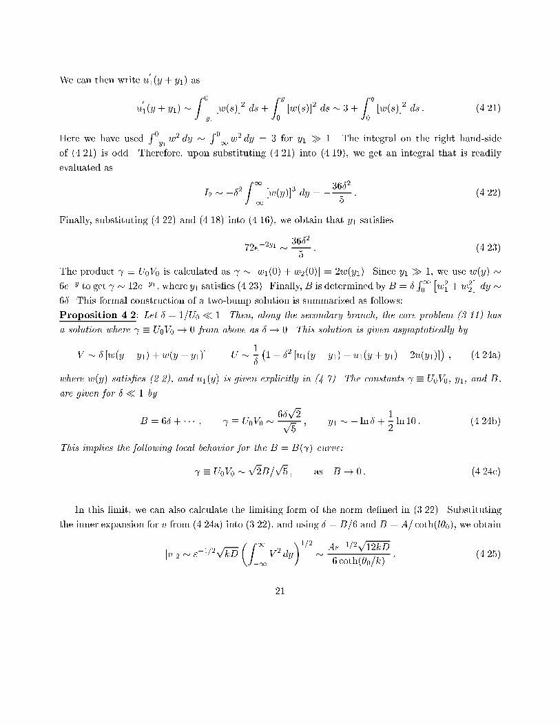
We can then write u01(y + y1) asu01(y + y1) � Z 0�y1 [w(s)]2 ds+ Z y0 [w(s)]2 ds � 3 + Z y0 [w(s)]2 ds : (4.21)Here we have used R 0�y1 w2 dy � R 0�1w2 dy = 3 for y1 � 1. The integral on the right hand-sideof (4.21) is odd. Therefore, upon substituting (4.21) into (4.19), we get an integral that is readilyevaluated as I2 � ��2 Z 1�1 [w(y)]3 dy = �36�25 : (4.22)Finally, substituting (4.22) and (4.18) into (4.16), we obtain that y1 satis�es72e�2y1 � 36�25 : (4.23)The product � U0V0 is calculated as � [w1(0) + w2(0)] = 2w(y1). Since y1 � 1, we use w(y) �6e�y to get � 12e�y1 , where y1 satis�es (4.23). Finally, B is determined by B = � R10 �w21 + w22� dy �6�. This formal construction of a two-bump solution is summarized as follows:Proposition 4.2: Let � = 1=U0 � 1. Then, along the secondary branch, the core problem (3.11) hasa solution where � U0V0 ! 0 from above as � ! 0. This solution is given asymptotically byV � � [w(y � y1) + w(y + y1)] U � 1� �1 + �2 [u1(y � y1) + u1(y + y1)� 2u(y1)]� ; (4.24a)where w(y) satis�es (2.2), and u1(y) is given explicitly in (4.7). The constants � U0V0, y1, and B,are given for � � 1 byB = 6� + � � � ; � U0V0 � 6�p2p5 ; y1 � � ln � + 12 ln 10 : (4.24b)This implies the following local behavior for the B = B( ) curve: � U0V0 � p2B=p5 ; as B ! 0 : (4.24c)In this limit, we can also calculate the limiting form of the norm de�ned in (3.22). Substitutingthe inner expansion for v from (4.24a) into (3.22), and using � = B=6 and B = A= coth(l�0), we obtainjvj2 � "�1=2pkD�Z 1�1 V 2 dy�1=2 � A"�1=2p12kD6 coth(�0=k) : (4.25)21

0:00:51:01:52:0

0:0 0:5 1:0 1:5

B(a) = U0V0 versus B05

101520

0:0 0:5 1:0 1:5U0

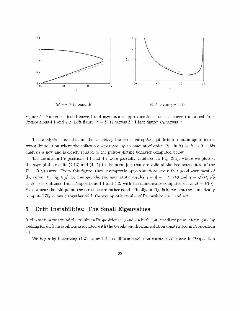
(b) U0 versus = U0V0Figure 5: Numerical (solid curves) and asymptotic approximations (dashed curves) obtained fromPropositions 4.1 and 4.2. Left �gure: = U0V0 versus B. Right �gure: U0 versus .This analysis shows that on the secondary branch a one-spike equilibrium solution splits into atwo-spike solution where the spikes are separated by an amount of order O(� lnB) as B ! 0. Thisanalysis is new and is closely related to the pulse-splitting behavior computed below.The results in Propositions 4.1 and 4.2 were partially validated in Fig. 2(b), where we plottedthe asymptotic results (4.13) and (4.25) to the norm jvj2 that are valid at the two extremities of theB = B( ) curve. From this �gure, these asymptotic approximations are rather good over most ofthe curve. In Fig. 5(a) we compare the two asymptotic results � 32 � 11B2=48 and � p2B=p5as B ! 0, obtained from Propositions 4.1 and 4.2, with the numerically computed curve B = B( ).Except near the fold point, these results are rather good. Finally, in Fig. 5(b) we plot the numericallycomputed U0 versus together with the asymptotic results of Propositions 4.1 and 4.2.5 Drift Instabilities: The Small EigenvaluesIn this section we extend the results in Propositions 2.3 and 2.4 in the intermediate parameter regime bylooking for drift instabilities associated with the k-spike equilibrium solution constructed in Proposition3.1.We begin by linearizing (1.3) around the equilibrium solution constructed above in Proposition22

3.1. Let ve and ue denote this equilibrium solution. We writev = ve + e�t� ; u = ue + e�t� : (5.1)Substituting (5.1) into (1.3) we obtain the eigenvalue problem"2�xx � �+ 2Aueve�+A�v2e = �� ; �1 < x < 1 ; (5.2a)D�xx � � � �v2e � 2ueve� = ��� ; �1 < x < 1 : (5.2b)We begin by examining (5.2) in the jth inner region where y = "�1(x�xj). Using (3.21a) and (3.21b),we calculate2Aueve � 2 �UV + "ApD (UV1 + U1V ) + � � � � ; v2e � D"2 �V 2 + 2"ApDV V1 + � � � � ; (5.3)where U , V satisfy (3.11), and U1, V1 satisfy (3.17). In this inner region we introduce � and N by�(x) = A" �(y; ") ; �(x) = "DN (y; ") : (5.4)Substituting (5.4) and (5.3) into (5.2), and with y = "�1(x�xj), we obtain the following inner problemon �1 < y <1:�yy � �+ 2 �UV + "ApD (UV1 + U1V ) + � � � ��+ �V 2 + 2"ApDV V1 + � � � �N = �� ; (5.5a)Nyy � �V 2 + 2"ApDV V1 + � � � �N � 2 �UV + "ApD (UV1 + U1V ) + � � � �� = "2D (1 + ��)N : (5.5b)As suggested by the intermediate regime result (2.14), we look for instabilities associated withsmall eigenvalues of order � = O("). Therefore, we seek an eigenfunction to (5.5) in the form�(y; ") = �0(y) + "ApD�1(y) + � � � ; N(y; ") = N0(y) + "ApDN1(y) + � � � ; � = "ApD�0 + � � � :(5.6)Substituting (5.6) into (5.5), we collect the leading-order terms to get�0yy � �0 + 2UV �0 + V 2N0 = 0 ; �1 < y <1 ; (5.7a)N0yy � V 2N0 � 2UV �0 = 0 ; �1 < y <1 : (5.7b)23

We look for an odd eigenfunction of (5.7) with �0 ! 0 and N0 bounded as jyj ! 1. From the O(")terms, we get the system for the next order correction�1yy + (�1 + 2UV )�1 + V 2N1 = �0�0 � 2(UV1 + U1V )�0 � 2V V1N0 ; �1 < y <1 ; (5.8a)N1yy � 2UV �1 � V 2N1 = 2(UV1 + U1V )�0 + 2V V1N0 ; �1 < y <1 : (5.8b)The boundary conditions are that �1 ! 0 and N1y is bounded as jyj ! 1.By di�erentiating (3.11), it is clear that a solution to (5.7) is�0 = cjVy ; N0 = cjUy : (5.9)This solution is odd, and we assume that this is the only solution to (5.7). The constant cj , associatedwith this jth inner region, will be determined below after matching to the outer solution. Substituting(5.9) into (5.8), we then express (5.8) in matrix form asL = cj � �0 00 0 �� VyUy �+ cj � �2(UV1 + U1V ) �2V V12(UV1 + U1V ) 2V V1 �� VyUy � ; (5.10a)where � (�1; N1)t, and the operator L is de�ned byL � � �1yyN1yy �+E� �1N1 � ; E � � �1 + 2UV V 2�2UV �V 2 � : (5.10b)To determine the solvability condition for (5.10), we let y denote the solution of the homogeneousadjoint equation Lyy � y1yyy2yy !+Et y1y2 ! = 0 ; (5.11)where t denotes transpose. We look for an odd solution to (5.11) where y1 ! 0 and y2y ! 0 asjyj ! 1.To determine the solvability condition for (5.10a), we multiply (5.10a) by yt and integrate byparts to get Z 1�1ytL dy = �yty �tyy� j1�1 = cj�0I2 + cjI1 ; (5.12a)where I1 and I2 are de�ned byI1 � Z 1�1 �yt2 �yt1 � �2(UV )yV1 + (V 2)yU1� dy ; I2 � Z 1�1y1Vy dy : (5.12b)24

Since and y are odd functions and yy ! 0 as y !1, (5.12a) can be reduced tocj�0I2 = �cjI1 +y2(1) (N1y(+1) +N1y(�1)) : (5.12c)The next step in the analysis is to calculate I1 explicitly. To do so, we introduce W by W =(V1y; U1y)t. Upon di�erentiating the system (3.17) for V1 and U1 with respect to y, it follows thatLW = � �2(UV )yV1 � (V 2)yU12(UV )yV1 + (V 2)yU1 � : (5.13)Therefore, I1 in (5.12b) can be written in terms of W . Integrating the resulting expression by parts,we get I1 = Z 1�1ytLW dy = �ytWy �yty W� j1�1 + Z 1�1W tLyy dy : (5.14)Using Lyy = 0, with y1 ! 0 and y2y ! 0 as jyj ! 1, (5.14) reduces toI1 = 2y2(1)U1yy(1) = �2y2(1) : (5.15)Here we have used U1yy(1) = �1 as seen from (3.17c). Finally, substituting (5.15) into (5.12c), weobtain a compact expression for �0cj�0 Z 1�1y1Vy dy = 2y2(1) �12 (N1y(+1) +N1y(�1)) + cj� ; j = 1; : : : ; k : (5.16)This completes the analysis of the jth inner region.Next, we match this jth inner solution constructed above to the outer solution for (5.2). Thiswill determine N1y(�1) and the constants cj , for j = 1; : : : ; k. In the outer region, away from O(")regions centered at the spike equilibrium locations, � in (5.2a) is exponentially small and � in (5.2b)is given by D�xx � (1 + ��)� = �v2e + 2ueve� : (5.17)Since the right hand-side of (5.17) is localized near each x = xj for j = 1; : : : ; k, its e�ect on the outersolution can be calculated in the sense of distributions. Recalling (5.4), (5.6), and (3.21), we get for xnear xj that the right hand-side of (5.17) is given by�v2e + 2ueve� � 1" �cj �UV 2�y + "ApD �N1V 2 + 2�1UV + 2cj (UyV V1 + UVyV1 + U1V Vy)�� : (5.18)25

Using (5.8b) we can write (5.18) as�v2e + 2ueve� � 1" �cj �UV 2�y + "ApDN1yy� : (5.19)Since UV 2 is even, we obtain in the the sense of distributions that1" �cj �UV 2�y + "ApDN1yy�! 2"Bcj�0(x� xj) + "ApD (N1y(+1)�N1y(�1)) �(x� xj) : (5.20)Here B � R10 UV 2 dy, given in (3.23), is the bifurcation parameter for the core problem (3.11). Inthis way, the following outer problem for �(x) is obtained from (5.17):D�xx � (1 + ��)� = kXi=1 �2"Bci�0(x� xi) + "ApD (N1y(+1)�N1y(�1)) �(x� xi)� ; �1 < x < 1 ;(5.21)with �x(�1) = 0.To determine N1y(�1) in (5.16) we use the matching condition that the far-�eld behavior ofthe jth inner solution as y ! +1 must agree with the behavior of �(x) as x ! x�j . De�ningy = "�1(x� xj), we obtain from (5.4) and (5.6), that this matching condition is"D �cjUy(�1) + "ApDN1� � �(x�j ) + "y�x(x�j ) + � � � : (5.22)To match the terms in (5.22), we require that�(x�j ) = �"cjBD ; (5.23a)N1y(�1) = D3=2"A �x(x�j ) : (5.23b)We now solve (5.21) on each subinterval and we use the condition (5.23a) for �(x�j ) and theboundary condition �x(�1) = 0. This yields,�(x) = 8>><>>: �"Bc1D cosh[��(1+x)]cosh[��(1+x1)] ; �1 < x < x1 ;"BcjD sinh[��(x�xj+1)]sinh[�(xj�xj+1)] � "Bcj+1D sinh[��(x�xj)]sinh[��(xj+1�xj)] ; xj < x < xj+1 ; j = 1; : : : ; k � 1 ;"BckD cosh[��(1�x)]cosh[��(1�xk)] ; xk < x < 1 : (5.24)26

Here �� is de�ned by �� � �0p1 + �� ; �0 � D�1=2 : (5.25)Next, we use (5.24) to calculate N1y(�1) in (5.23b). A simple calculation for j = 1 yields(N1y(+1) +N1y(�1))2 = Bp1 + ��2A ��c1�coth�2��k �+ tanh���k ��� c2csch�2��k �� :(5.26a)For j = 2; : : : ; k � 1, we get(N1y(+1) +N1y(�1))2 = Bp1 + ��2A ��cj�1csch�2��k �� 2cj coth�2��k �� cj+1csch�2��k �� :(5.26b)Similarly for j = k, we get(N1y(+1) +N1y(�1))2 = Bp1 + ��2A ��ck�1csch�2��k �� ck �coth�2��k �+ tanh���k ��� :(5.26c)Substituting (5.26) into (5.16), and using the the relation A = B coth (�0=k) from (3.12), we obtainthe following matrix problem for c = (c1; : : : ; ck)t and �0:�0c = � �p1 + ��2 tanh��0k �B � I� c : (5.27)Here � is de�ned by � � � y2(1)R10 y1Vy dy ; (5.28)and B is the tridiagonal matrixB � 0BBBBBBBBBBB@

d f 0 � � � 0 0 0f e f � � � 0 0 00 f e . . . 0 0 0... ... . . . . . . . . . ... ...0 0 0 . . . e f 00 0 0 � � � f e f0 0 0 � � � 0 f d1CCCCCCCCCCCA ; (5.29a)

27

with matrix entries d, e, and f de�ned byd � coth�2��k �+ tanh���k � ; e � 2 coth�2��k � ; f � csch�2��k � : (5.29b)The spectrum of B can be calculated explicitly as was done in Appendix D of [18]. This leads to thefollowing result:Proposition 5.1: The eigenvalues �j, ordered as 0 < �1 < : : : < �k, of B and the associated normalizedeigenvectors cj of B are�j = 2 coth�2��k �+ 2 csch�2��k � cos��jk � ; j = 1; : : : ; k ; (5.30a)ctk = 1pk �1;�1; 1; : : : ; (�1)k+1� ; cl;j =r2k sin��jk (l � 1=2)� ; j = 1; : : : ; k � 1 : (5.30b)Here ct denotes transpose and ctj = (c1;j ; : : : ; ck;j).By substituting (5.30) into (5.27), we obtain k transcendental equations for the eigenvalue �0. Theeigenvectors in (5.30) determine the constants cj , for j = 1; ::; k. In this way, we obtain the followingmain result for the small eigenvalues:Proposition 5.2: Let " � 1, and "A=pD � 1. Then, the small eigenvalues � associated with driftinstabilities of the k-spike equilibrium solution of Proposition 3.1 are of order O �"A=pD�, and satisfythe k transcendental equations,� � "�ApD �p1 + �� tanh��0k ��coth�2��k �+ csch�2��k � cos��jk ��� 1� ; j = 1; : : : ; k ;(5.31)where � and �� are de�ned in (5.28) and (5.25). The constant � depends on the bifurcation parameter associated with the core solution. In the inner region near the jth spike, the perturbation to thev-component of the equilibrium solution has the following form for some � � 1:v(x; t) � pD" �V ["�1(x� xj)] + �cjVy["�1(x� xj)]e�t� : (5.32)For a one-spike solution where k = 1, (5.31) can be reduced to� � "�ApD hp1 + �� tanh (�0) tanh (��)� 1i : (5.33)This expression is very similar in form to the result (2.9b) of Proposition 2.3 in the intermediateparameter regime. The only di�erence between (5.33) and (2.9b) is in a multiplicative factor. We nowshow that these two formulae do in fact agree if we let A! 0 in (5.33).28

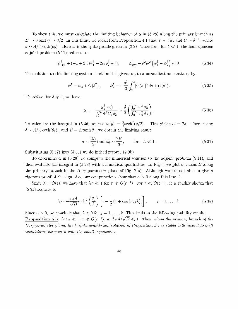
To show this, we must calculate the limiting behavior of � in (5.28) along the primary branch asB ! 0 and ! 3=2. In this limit, we recall from Proposition 4.1 that V � �w, and U � ��1, where� � A=[3 coth(�0)]. Here w is the spike pro�le given in (2.2). Therefore, for � � 1, the homogeneousadjoint problem (5.11) reduces to y1yy + (�1 + 2w) y1 � 2w y2 � 0 ; y2yy + �2w2 � y1 � y2� � 0 : (5.34)The solution to this limiting system is odd and is given, up to a normalization constant, by y1 = wy +O(�2) ; y2 = ��23 Z y0 [w(s)]3 ds+O(�4) : (5.35)Therefore, for � � 1, we have � � � y2(1)R10 y1Vy dy � �3 R10 w3 dyR10 w2y dy! : (5.36)To calculate the integral in (5.36) we use w(y) = 32sech2(y=2) . This yields � = 2�. Then, using� � A=[3 coth(�0)], and B = A tanh �0, we obtain the limiting result� � 2A3 tanh �0 � 2B3 ; for A� 1 : (5.37)Substituting (5.37) into (5.33) we do indeed recover (2.9b).To determine � in (5.28) we compute the numerical solution to the adjoint problem (5.11), andthen evaluate the integral in (5.28) with a numerical quadrature. In Fig. 6 we plot � versus B alongthe primary branch in the B, parameter plane of Fig. 2(a). Although we are not able to give arigorous proof of the sign of �, our computations show that � > 0 along this branch.Since � = O("), we have that �� � 1 for � � O("�1). For � � O("�1), it is readily shown that(5.31) reduces to � � �"�ApD sech2��0k ��1� 12 (1 + cos (�j=k))� ; j = 1; : : : ; k : (5.38)Since � > 0, we conclude that � < 0 for j = 1; : : : ; k. This leads to the following stability result:Proposition 5.3: Let "� 1, � � O("�1), and "A=pD � 1. Then, along the primary branch of theB, parameter plane, the k-spike equilibrium solution of Proposition 3.1 is stable with respect to driftinstabilities associated with the small eigenvalues.29

0:01:02:03:04:0

0:00 0:25 0:50 0:75 1:00 1:25 1:50�

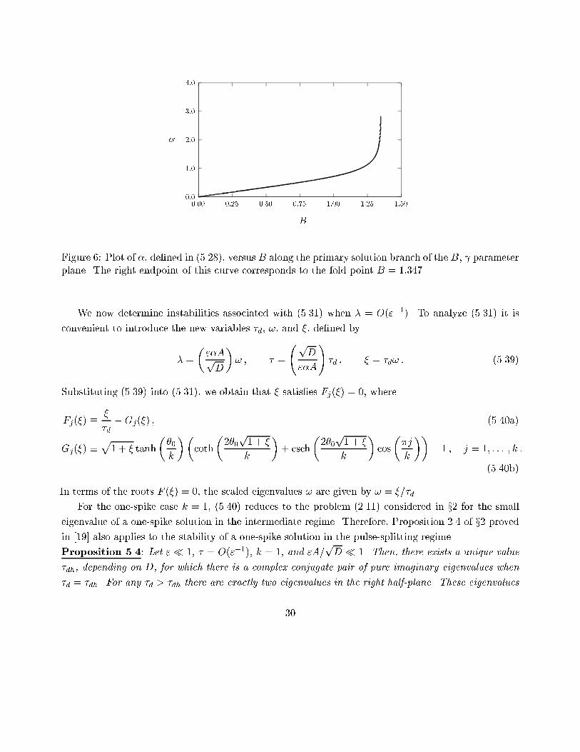
BFigure 6: Plot of �, de�ned in (5.28), versus B along the primary solution branch of the B, parameterplane. The right endpoint of this curve corresponds to the fold point B = 1:347.We now determine instabilities associated with (5.31) when � = O("�1). To analyze (5.31) it isconvenient to introduce the new variables �d, !, and �, de�ned by� = �"�ApD�! ; � = pD"�A! �d ; � = �d! : (5.39)Substituting (5.39) into (5.31), we obtain that � satis�es Fj(�) = 0, whereFj(�) � ��d �Gj(�) ; (5.40a)Gj(�) �p1 + � tanh��0k ��coth�2�0p1 + �k �+ csch�2�0p1 + �k � cos��jk ��� 1 ; j = 1; : : : ; k :(5.40b)In terms of the roots F (�) = 0, the scaled eigenvalues ! are given by ! = �=�d.For the one-spike case k = 1, (5.40) reduces to the problem (2.11) considered in x2 for the smalleigenvalue of a one-spike solution in the intermediate regime. Therefore, Proposition 2.4 of x2 provedin [19] also applies to the stability of a one-spike solution in the pulse-splitting regime.Proposition 5.4: Let "� 1, � = O("�1), k = 1, and "A=pD � 1. Then, there exists a unique value�dh, depending on D, for which there is a complex conjugate pair of pure imaginary eigenvalues when�d = �dh. For any �d > �dh there are exactly two eigenvalues in the right half-plane. These eigenvalues30

0:01:02:03:04:0

0:25 0:50 0:75 1:00 1:25 1:50�dh, !h

D(a) �dh and !h�1:0�0:50:00:51:0

0:00 0:25 0:50 0:75 1:00!I

!R(b) eigenvalues in right half-planeFigure 7: A one-spike solution. Left �gure: The Hopf bifurcation value �dh (heavy solid curve) andthe frequency !h (solid curve) versus D. Right �gure: The eigenvalues ! = !R + i!I in the righthalf-plane for �dh � � � �dm when D = 0:75 (heavy solid curve) and D = 0:1 (solid curve).merge onto the positive real axis when �d = �dm, and they remain there for all �d > �dm. In terms of� , the Hopf bifurcation in the spike location occurs when � = �TW , where�TW � pD"�A! �d : (5.41)To determine �dh for a one-spike solution where k = 1 we numerically determine the zeroes ofF1(�) = 0 on the imaginary axis. The zeroes occur when � = i�h and �d = �dh, which yields !h ��h=�dh. In Fig. 7(a) we plot �dh and !h versus D. To illustrate Proposition 5.4, we compute the rootsof F1(�) = 0 with � = �R + i�I on the range �dh � �d � �dm. In terms of ! = �=�d � !R + i!I , inFig. 7(b) we plot this path in the complex plane for D = 0:75 and D = 0:1.We now consider the multi-spike case where k > 1. We �rst look for roots of Fj(�) = 0 on thepositive imaginary axis � = i�I with �I � 0. By separating (5.40) into real and imaginary parts, weobtain FjR(�I) = �GjR(�I) ; FjI(�I) = �I�d �GjI(�I) ; j = 1; : : : ; k ; (5.42)where FjR(�I) = Re(Fj(i�I)), FjI(�I) = Im(Fj(i�I)), GjR(�I) = Re(Gj(i�I)), GjI(�I) = Re(Gj(i�I)).31

Using (5.40), it is readily seen that GjR(0) < 0 and that GjR(�I) is monotonically increasing withGjR(�I) ! +1 as �I ! 1. Therefore, FjR(�I) = 0 has a unique root, which we label by �Ij. Then,setting FjI(�Ij) = 0, we obtain the critical value �dj, de�ned by�dj � �IjGjI(�Ij) ; j = 1; : : : ; k : (5.43)In terms of �dj , we de�ne !j � �Ij=�dj . For each j, �dj denotes the unique value of �d where there is acomplex conjugate pair of small eigenvalues on the imaginary axis.By adapting the proof of Proposition 5.6 of [19], we can prove that, for each �xed j = 1; : : : ; k,there are exactly two roots of Fj(�) = 0 for any �d > �dj. In addition, these roots merge onto thepositive real axis when �d = ��dj > �dj, and they remain there for �d > ��dj . To show this, we �rstderive a formula for the number Mj of zeroes of Fj(�) = 0 in the right half-plane. To do so, wecalculate the winding number of Fj(�) over the counterclockwise contour composed of the imaginaryaxis �iR � Im(�) � iR and the semi-circle �R, given by j�j = R > 0, for Re(�) > 0. For any �d > 0,it is easy to see from (5.40) that the change in the argument of Fj(�) over �R as R !1 is �. SinceFj(�) is analytic in Re(�) � 0, and Fj(�) = Fj(�), the argument principle yields thatMj = 12 + 1� [argFj ]�I : (5.44)Here [argFj ]�I denotes the change in the argument of Fj(�) along the semi-in�nite imaginary axis�I = i�I , 0 � �I <1, traversed in the downwards direction.To calculate Mj, we note that FjI = O(�I) and FjR = O(p�I) as �I ! 1, and that FjI(0) = 0with FjR(0) > 0. This implies that argFj = �=2 as �I ! +1, and argFj = 0 at �I = 0. Since the rootto FjR(�I) = 0 is unique and independent of �d, the change in the argument [argFj ]�I is determinedby the sign of FjI(�I) at the unique root of FjR(�I) = 0. In this way, we get that [argFj ]�I is 3�=2when � > �dj and is ��=2 when 0 < �d < �dj. From (5.44) this yields that Mj = 2 when �d > �djand Mj = 0 when 0 < �d < �dj . Therefore, the roots of Fj(�) = 0 have a strict transversal crossinginto the right half-plane as � is increased past �dj . The fact that that the roots of Fj(�) = 0 mergeonto the real axis at some value ��dj follows from the simple observation that Gj(�) in (5.40b) is anincreasing, and concave, function when � > 0 is real, and that Gj(0) < 0. This proves that when �is real, Fj(�) = 0 will have exactly two roots for � � ��dj , where ��dj is determined from the conditionthat �=�d intersects Gj(�) tangentially at a unique point when � = ��dj . This leads to the followingstability result for a k-spike solution:Proposition 5.5: Let " � 1, � = O("�1), and "A=pD � 1. Then, along the primary branch of theB, parameter plane, the k-spike equilibrium solution of Proposition 3.1 is stable when 0 < � < �TW ,32

0:03:06:09:012:015:0

0:25 0:50 0:75 1:00 1:25 1:50�dj

D(a) Two spikes: �dj for j = 1; 2 051015202530

0:25 0:50 0:75 1:00 1:25 1:50�dj

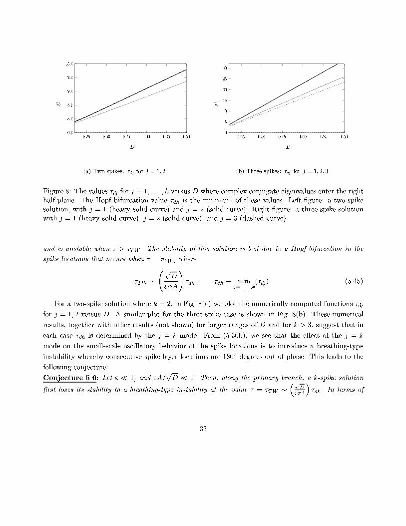
D(b) Three spikes: �dj for j = 1; 2; 3Figure 8: The values �dj for j = 1; : : : ; k versus D where complex conjugate eigenvalues enter the righthalf-plane. The Hopf bifurcation value �dh is the minimum of these values. Left �gure: a two-spikesolution, with j = 1 (heavy solid curve) and j = 2 (solid curve). Right �gure: a three-spike solutionwith j = 1 (heavy solid curve), j = 2 (solid curve), and j = 3 (dashed curve).and is unstable when � > �TW . The stability of this solution is lost due to a Hopf bifurcation in thespike locations that occurs when � = �TW , where�TW � pD"�A! �dh ; �dh � minj=1;::: ;k(�dj) : (5.45)For a two-spike solution where k = 2, in Fig. 8(a) we plot the numerically computed functions �djfor j = 1; 2 versus D. A similar plot for the three-spike case is shown in Fig. 8(b). These numericalresults, together with other results (not shown) for larger ranges of D and for k > 3, suggest that ineach case �dh is determined by the j = k mode. From (5.30b), we see that the e�ect of the j = kmode on the small-scale oscillatory behavior of the spike locations is to introduce a breathing-typeinstability whereby consecutive spike-layer locations are 180� degrees out of phase. This leads to thefollowing conjecture:Conjecture 5.6: Let " � 1, and "A=pD � 1. Then, along the primary branch, a k-spike solution�rst loses its stability to a breathing-type instability at the value � = �TW � �pD"�A� �dk. In terms of33

the v-component, this small-scale oscillatory instability takes the form,v(x; t) � pD" kXj=1 V �"�1[x� xj(t)]� ; xj(t) � xj(0) + �cj cos�"�A!ktpD � �� ; (5.46)where � � 1, and � is arbitrary. Here cj = (�1)j and xj(0) = �1 + (2j � 1)=k for j = 1; : : : ; k. Inaddition, !k = �Ik=�dk, where Fk(i�Ik) = 0.6 Stability of the Pro�le: The Large EigenvaluesWe now determine the stability of the k-spike equilibrium solution of Proposition 3.1 with respect toeigenvalues � with � = O(1) as " ! 0. Assuming that � � O("�2), we can repeat the calculationfrom (5.1)-(5.5) to derive the following leading order eigenvalue problem in the jth inner region:�0yy � �0 + 2UV �0 + V 2N0 = ��0 ; �1 < y <1 ; (6.1a)N0yy � V 2N0 � 2UV �0 = 0 ; �1 < y <1 : (6.1b)We seek an even eigenfunction of (6.1) for which �0 ! 0. Upon matching to the outer region below,the other boundary condition is that N0y ! 0 as jyj ! 1.To derive such an asymptotic boundary condition for N0, we consider the outer solution for � givenin (5.17). Since �0 and N0 are even, we obtain in place of (5.18) that near xj,�v2e + 2ueve� � 1" �2UV �0 + V 2N0� � 1"N0yy : (6.2)Therefore, since N0y is odd, we get in place of (5.21) thatD�xx � (1 + ��)� = 2 kXi=1 N0y(1)�(x � xi) ; �1 < x < 1 ; �x(�1) = 0 : (6.3)The solution to (6.3) can be written as�(x) = �2 kXi=1 N0y(1)G(x;xi) ; (6.4)where G(x;xi) is the Green's function satisfying (2.3). The leading order matching condition analogousto (5.22) is that "D�1N0 as jyj ! 1 agrees with �(x) as x ! xj. This enforces that N0y(1) = 0.Therefore, the leading order eigenvalue problem (6.1) is universal in that it does not involve a couplingof the eigenvalue problems associated with each inner region.34

�0:50�0:250:000:250:500:751:00

�10:0 �5:0 0:0 5:0 10:0�d

y(a) �d(y)�6:0�4:0�2:00:02:04:0

�10:0 �5:0 0:0 5:0 10:0Nd

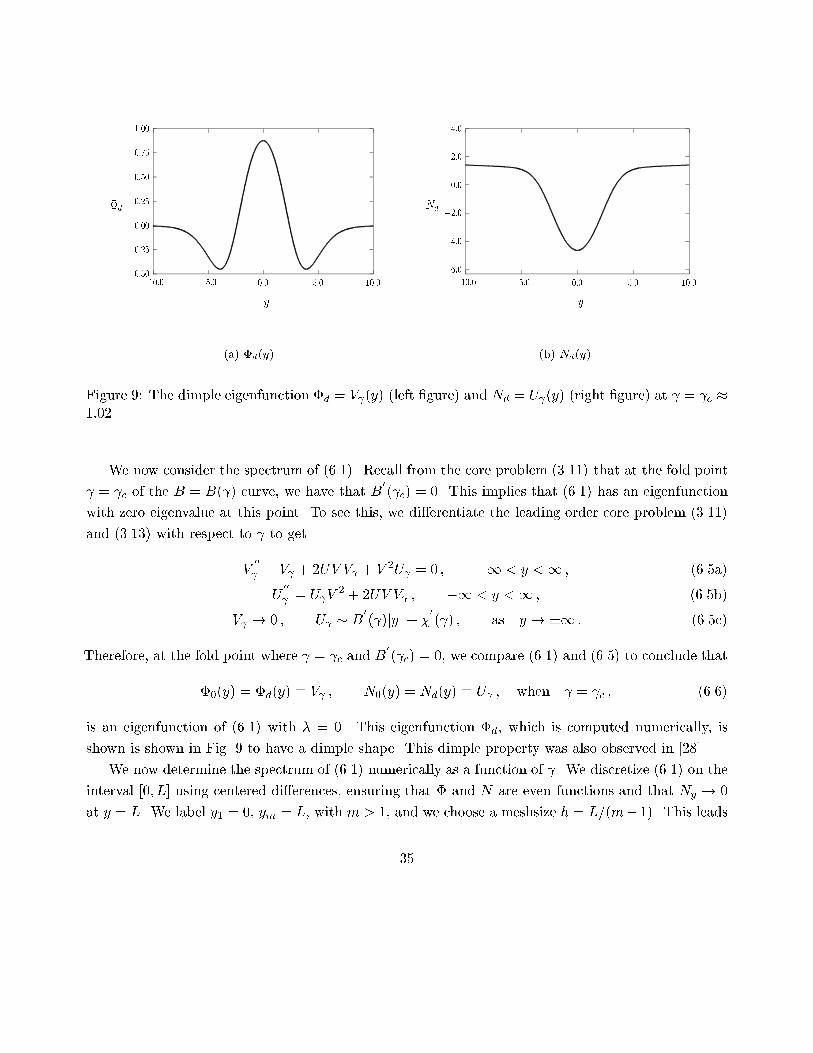
y(b) Nd(y)Figure 9: The dimple eigenfunction �d = V (y) (left �gure) and Nd = U (y) (right �gure) at = c �1:02.We now consider the spectrum of (6.1). Recall from the core problem (3.11) that at the fold point = c of the B = B( ) curve, we have that B0( c) = 0. This implies that (6.1) has an eigenfunctionwith zero eigenvalue at this point. To see this, we di�erentiate the leading order core problem (3.11)and (3.13) with respect to to getV 00 � V + 2UV V + V 2U = 0 ; �1 < y <1 ; (6.5a)U 00 = U V 2 + 2UV V ; �1 < y <1 ; (6.5b)V ! 0 ; U � B0( )jyj+ �0( ) ; as y ! �1 : (6.5c)Therefore, at the fold point where = c and B0( c) = 0, we compare (6.1) and (6.5) to conclude that�0(y) = �d(y) � V ; N0(y) = Nd(y) � U ; when = c ; (6.6)is an eigenfunction of (6.1) with � = 0. This eigenfunction �d, which is computed numerically, isshown is shown in Fig. 9 to have a dimple shape. This dimple property was also observed in [28].We now determine the spectrum of (6.1) numerically as a function of . We discretize (6.1) on theinterval [0; L] using centered di�erences, ensuring that � and N are even functions and that Ny ! 0at y = L. We label y1 = 0, ym = L, with m > 1, and we choose a meshsize h = L=(m� 1). This leads35

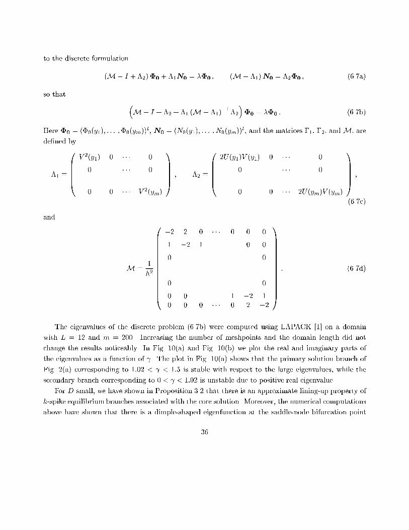
to the discrete formulation(M� I +�2)�0 +�1N0 = ��0 ; (M� �1)N0 = �2�0 ; (6.7a)so that �M� I +�2 +�1 (M� �1)�1 �2��0 = ��0 : (6.7b)Here �0 = (�0(y1); : : : ;�0(ym))t, N0 = (N0(y1); : : : ; N0(ym))t, and the matrices �1, �2, andM, arede�ned by�1 � 0BBBB@ V 2(y1) 0 � � � 00 . . . � � � 0... ... . . . ...0 0 � � � V 2(ym)1CCCCA ; �2 � 0BBBB@ 2U(y1)V (y1) 0 � � � 00 . . . � � � 0... ... . . . ...0 0 � � � 2U(ym)V (ym)

1CCCCA ;(6.7c)andM� 1h2

0BBBBBBBBBBBBB@�2 2 0 � � � 0 0 01 �2 1 . . . . . . 0 00 . . . . . . . . . . . . . . . 0... . . . . . . . . . . . . . . . ...0 . . . . . . . . . . . . . . . 00 0 . . . . . . 1 �2 10 0 0 � � � 0 2 �2

1CCCCCCCCCCCCCA : (6.7d)The eigenvalues of the discrete problem (6.7b) were computed using LAPACK [1] on a domainwith L = 12 and m = 200. Increasing the number of meshpoints and the domain length did notchange the results noticeably. In Fig. 10(a) and Fig. 10(b) we plot the real and imaginary parts ofthe eigenvalues as a function of . The plot in Fig. 10(a) shows that the primary solution branch ofFig. 2(a) corresponding to 1:02 < < 1:5 is stable with respect to the large eigenvalues, while thesecondary branch corresponding to 0 < < 1:02 is unstable due to positive real eigenvalue.For D small, we have shown in Proposition 3.2 that there is an approximate lining-up property ofk-spike equilibrium branches associated with the core solution. Moreover, the numerical computationsabove have shown that there is a dimple-shaped eigenfunction at the saddle-node bifurcation point36

�1:0�0:50:00:5

0:25 0:50 0:75 1:00 1:25 1:50Re(�)

(a) Re(�) versus �0:15�0:10�0:050:000:050:100:15

0:25 0:50 0:75 1:00 1:25 1:50Im(�)

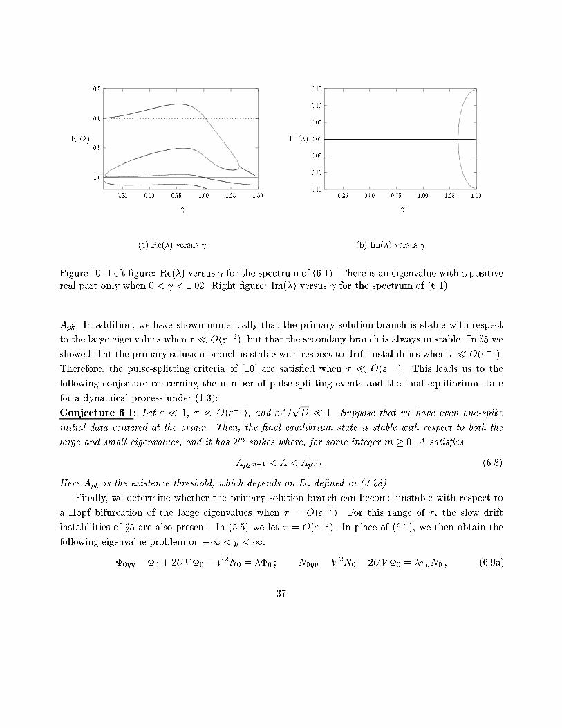
(b) Im(�) versus Figure 10: Left �gure: Re(�) versus for the spectrum of (6.1). There is an eigenvalue with a positivereal part only when 0 < < 1:02. Right �gure: Im(�) versus for the spectrum of (6.1).Apk. In addition, we have shown numerically that the primary solution branch is stable with respectto the large eigenvalues when � � O("�2), but that the secondary branch is always unstable. In x5 weshowed that the primary solution branch is stable with respect to drift instabilities when � � O("�1).Therefore, the pulse-splitting criteria of [10] are satis�ed when � � O("�1). This leads us to thefollowing conjecture concerning the number of pulse-splitting events and the �nal equilibrium statefor a dynamical process under (1.3):Conjecture 6.1: Let " � 1, � � O("�1), and "A=pD � 1. Suppose that we have even one-spikeinitial data centered at the origin. Then, the �nal equilibrium state is stable with respect to both thelarge and small eigenvalues, and it has 2m spikes where, for some integer m � 0, A satis�esAp2m�1 < A < Ap2m : (6.8)Here Apk is the existence threshold, which depends on D, de�ned in (3.28).Finally, we determine whether the primary solution branch can become unstable with respect toa Hopf bifurcation of the large eigenvalues when � = O("�2). For this range of � , the slow driftinstabilities of x5 are also present. In (5.5) we let � = O("�2). In place of (6.1), we then obtain thefollowing eigenvalue problem on �1 < y <1:�0yy � �0 + 2UV �0 + V 2N0 = ��0 ; N0yy � V 2N0 � 2UV �0 = ��LN0 ; (6.9a)37

where � = D�L"2 : (6.9b)

0:000:020:040:060:080:10

0:25 0:50 0:75 1:00 1:25 1:50�Lh

B(a) �Lh versus B 0:00:20:40:60:81:01:2

0:25 0:50 0:75 1:00 1:25 1:50�Ih

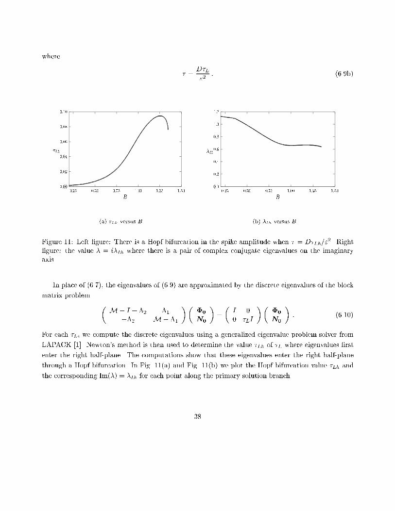
B(b) �Ih versus BFigure 11: Left �gure: There is a Hopf bifurcation in the spike amplitude when � = D�Lh="2. Right�gure: the value � = i�Ih where there is a pair of complex conjugate eigenvalues on the imaginaryaxis.In place of (6.7), the eigenvalues of (6.9) are approximated by the discrete eigenvalues of the blockmatrix problem � M� I +�2 �1��2 M� �1 �� �0N0 � = � I 00 �LI �� �0N0 � : (6.10)For each �L, we compute the discrete eigenvalues using a generalized eigenvalue problem solver fromLAPACK [1]. Newton's method is then used to determine the value �Lh of �L where eigenvalues �rstenter the right half-plane. The computations show that these eigenvalues enter the right half-planethrough a Hopf bifurcation. In Fig. 11(a) and Fig. 11(b) we plot the Hopf bifurcation value �Lh andthe corresponding Im(�) = �Ih for each point along the primary solution branch.38

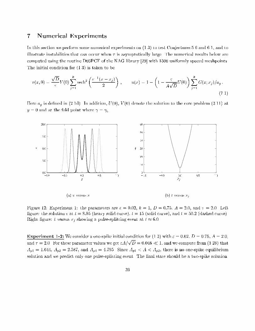
7 Numerical ExperimentsIn this section we perform some numerical experiments on (1.3) to test Conjectures 5.6 and 6.1, and toillustrate instabilities that can occur when � is asymptotically large. The numerical results below arecomputed using the routine D03PCF of the NAG library [29] with 1500 uniformly spaced meshpoints.The initial condition for (1.3) is taken to bev(x; 0) = pD" V (0) kXj=1 sech2�"�1(x� xj)2 � ; u(x) = 1��1� "ApDU(0)� kXj=1G(x;xj)=ag :(7.1)Here ag is de�ned in (2.1d). In addition, U(0), V (0) denote the solution to the core problem (3.11) aty = 0 and at the fold point where = c.0:05:010:015:020:0

�1:0 �0:5 0:0 0:5 1:0v

x(a) v versus x 0102030405060

�1:0 �0:5 0:0 0:5 1:0t

xj(b) t versus xjFigure 12: Experiment 1: the parameters are " = 0:02, k = 1, D = 0:75, A = 2:0, and � = 2:0. Left�gure: the solution v at t = 8:05 (heavy solid curve), t = 15 (solid curve), and t = 50:2 (dashed curve).Right �gure: t versus xj showing a pulse-splitting event at t � 6:0.Experiment 1-2:We consider a one-spike initial condition for (1.3) with " = 0:02, D = 0:75, A = 2:0,and � = 2:0. For these parameter values we get "A=pD = 0:046 � 1, and we compute from (3.28) thatAp1 = 1:644, Ap2 = 2:587, and Ap4 = 4:795. Since Ap1 < A < Ap2, there is no one-spike equilibriumsolution and we predict only one pulse-splitting event. The �nal state should be a two-spike solution.39

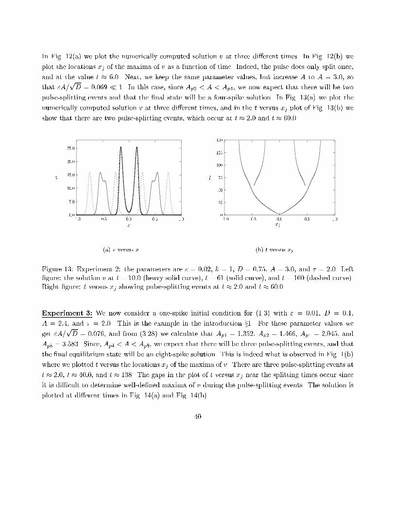
In Fig. 12(a) we plot the numerically computed solution v at three di�erent times. In Fig. 12(b) weplot the locations xj of the maxima of v as a function of time. Indeed, the pulse does only split once,and at the value t � 6:0. Next, we keep the same parameter values, but increase A to A = 3:0, sothat "A=pD = 0:069 � 1. In this case, since Ap2 < A < Ap4, we now expect that there will be twopulse-splitting events and that the �nal state will be a four-spike solution. In Fig. 13(a) we plot thenumerically computed solution v at three di�erent times, and in the t versus xj plot of Fig. 13(b) weshow that there are two pulse-splitting events, which occur at t � 2:0 and t � 60:0.0:05:010:015:020:025:0

�1:0 �0:5 0:0 0:5 1:0v

x(a) v versus x 0255075100125150

�1:0 �0:5 0:0 0:5 1:0t

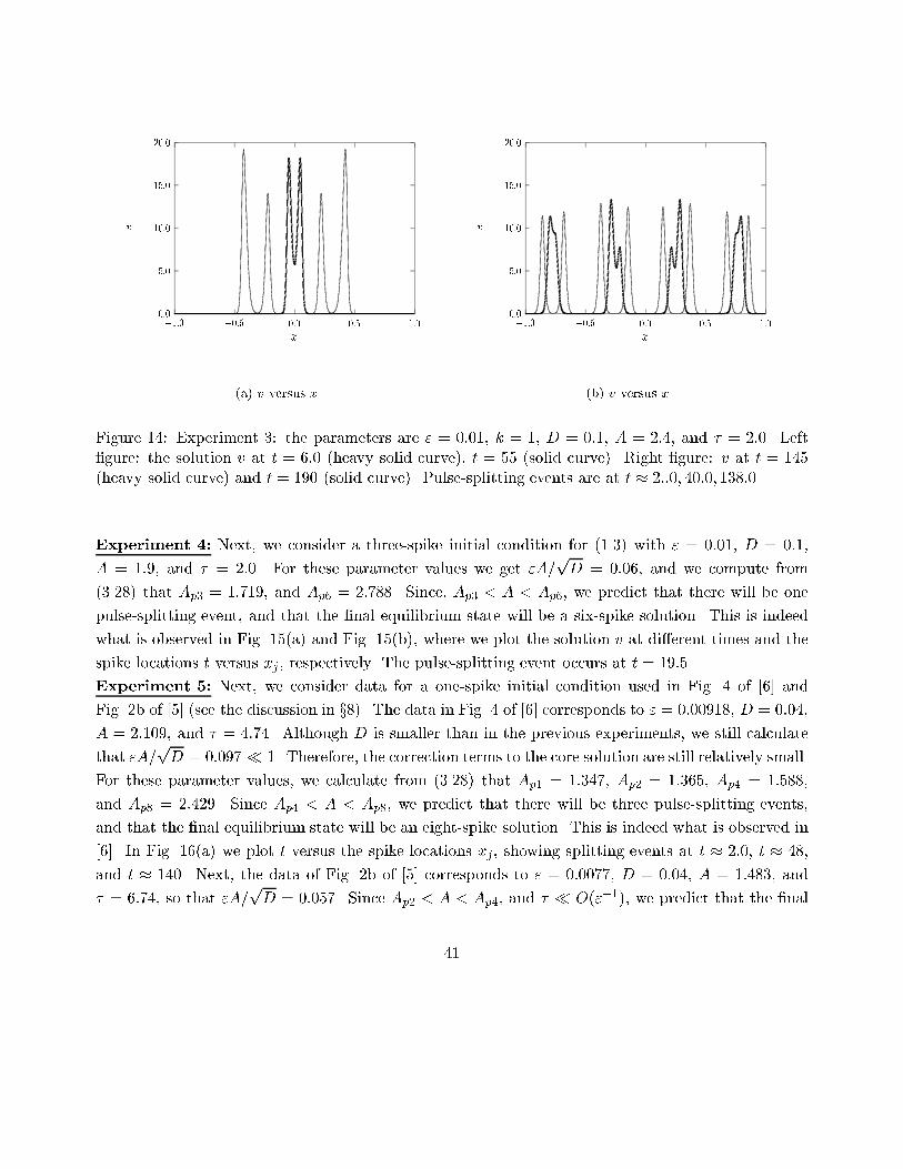
xj(b) t versus xjFigure 13: Experiment 2: the parameters are " = 0:02, k = 1, D = 0:75, A = 3:0, and � = 2:0. Left�gure: the solution v at t = 10:0 (heavy solid curve), t = 61 (solid curve), and t = 100 (dashed curve).Right �gure: t versus xj showing pulse-splitting events at t � 2:0 and t � 60:0.Experiment 3: We now consider a one-spike initial condition for (1.3) with " = 0:01, D = 0:1,A = 2:4, and � = 2:0. This is the example in the introduction x1. For these parameter values weget "A=pD = 0:076, and from (3.28) we calculate that Ap1 = 1:352, Ap2 = 1:466, Ap4 = 2:045, andAp8 = 3:583. Since, Ap4 < A < Ap8, we expect that there will be three pulse-splitting events, and thatthe �nal equilibrium state will be an eight-spike solution. This is indeed what is observed in Fig. 1(b)where we plotted t versus the locations xj of the maxima of v. There are three pulse-splitting events att � 2:0, t � 40:0, and t � 138. The gaps in the plot of t versus xj near the splitting times occur sinceit is di�cult to determine well-de�ned maxima of v during the pulse-splitting events. The solution isplotted at di�erent times in Fig. 14(a) and Fig. 14(b).40

0:05:010:015:020:0

�1:0 �0:5 0:0 0:5 1:0v

x(a) v versus x 0:05:010:015:020:0

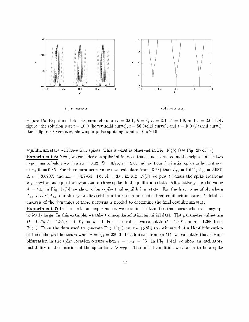
�1:0 �0:5 0:0 0:5 1:0v

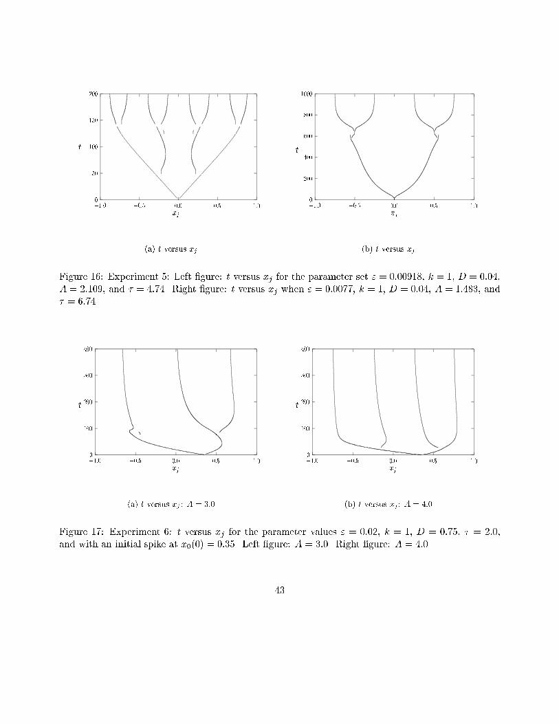
x(b) v versus xFigure 14: Experiment 3: the parameters are " = 0:01, k = 1, D = 0:1, A = 2:4, and � = 2:0. Left�gure: the solution v at t = 6:0 (heavy solid curve), t = 55 (solid curve). Right �gure: v at t = 145(heavy solid curve) and t = 190 (solid curve). Pulse-splitting events are at t � 2::0; 40:0; 138:0.Experiment 4: Next, we consider a three-spike initial condition for (1.3) with " = 0:01, D = 0:1,A = 1:9, and � = 2:0. For these parameter values we get "A=pD = 0:06, and we compute from(3.28) that Ap3 = 1:719, and Ap6 = 2:788. Since, Ap3 < A < Ap6, we predict that there will be onepulse-splitting event, and that the �nal equilibrium state will be a six-spike solution. This is indeedwhat is observed in Fig. 15(a) and Fig. 15(b), where we plot the solution v at di�erent times and thespike locations t versus xj, respectively. The pulse-splitting event occurs at t = 19:5.Experiment 5: Next, we consider data for a one-spike initial condition used in Fig. 4 of [6] andFig. 2b of [5] (see the discussion in x8). The data in Fig. 4 of [6] corresponds to " = 0:00918, D = 0:04,A = 2:109, and � = 4:74. Although D is smaller than in the previous experiments, we still calculatethat "A=pD = 0:097 � 1. Therefore, the correction terms to the core solution are still relatively small.For these parameter values, we calculate from (3.28) that Ap1 = 1:347, Ap2 = 1:365, Ap4 = 1:588,and Ap8 = 2:429. Since Ap4 < A < Ap8, we predict that there will be three pulse-splitting events,and that the �nal equilibrium state will be an eight-spike solution. This is indeed what is observed in[6]. In Fig. 16(a) we plot t versus the spike locations xj, showing splitting events at t � 2:0, t � 48,and t � 140. Next, the data of Fig. 2b of [5] corresponds to " = 0:0077, D = 0:04, A = 1:483, and� = 6:74, so that "A=pD = 0:057. Since Ap2 < A < Ap4, and � � O("�1), we predict that the �nal41

0:05:010:015:0

�1:0 �0:5 0:0 0:5 1:0v

x(a) v versus x 0255075100

�1:0 �0:5 0:0 0:5 1:0t

xj(b) t versus xjFigure 15: Experiment 4: the parameters are " = 0:01, k = 3, D = 0:1, A = 1:9, and � = 2:0. Left�gure: the solution v at t = 10:0 (heavy solid curve), t = 50 (solid curve), and t = 100 (dashed curve).Right �gure: t versus xj showing a pulse-splitting event at t � 20:0.equilibrium state will have four spikes. This is what is observed in Fig. 16(b) (see Fig. 2b of [5]).Experiment 6: Next, we consider one-spike initial data that is not centered at the origin. In the twoexperiments below we chose " = 0:02, D = 0:75, � = 2:0, and we take the initial spike to be centeredat x0(0) = 0:35. For these parameter values, we calculate from (3.28) that Ap1 = 1:644, Ap2 = 2:587,Ap3 = 3:6707, and Ap4 = 4:7950. For A = 3:0, in Fig. 17(a) we plot t versus the spike locationsxj, showing one splitting event and a three-spike �nal equilibrium state. Alternatively, for the valueA = 4:0, in Fig. 17(b) we show a four-spike �nal equilibrium state. For the �rst value of A, whereAp2 < A < Ap3, our theory predicts either a three or a four-spike �nal equilibrium state. A detailedanalysis of the dynamics of these patterns is needed to determine the �nal equilibrium state.Experiment 7: In the next four experiments, we examine instabilities that occur when � is asymp-totically large. In this example, we take a one-spike solution as initial data. The parameter values areD = 0:25, A = 1:35, " = 0:01, and k = 1. For these values, we calculate B = 1:301 and � = 1:366 fromFig. 6. From the data used to generate Fig. 11(a), we use (6.9b) to estimate that a Hopf bifurcationof the spike pro�le occurs when � = �H = 230:0. In addition, from (5.41), we calculate that a Hopfbifurcation in the spike location occurs when � = �TW = 55. In Fig. 18(a) we show an oscillatoryinstability in the location of the spike for � > �TW . The initial condition was taken to be a spike42

050100150200

�1:0 �0:5 0:0 0:5 1:0t

xj(a) t versus xj 02004006008001000

�1:0 �0:5 0:0 0:5 1:0t

xj(b) t versus xjFigure 16: Experiment 5: Left �gure: t versus xj for the parameter set " = 0:00918, k = 1, D = 0:04,A = 2:109, and � = 4:74. Right �gure: t versus xj when " = 0:0077, k = 1, D = 0:04, A = 1:483, and� = 6:74.

0100200300400

�1:0 �0:5 0:0 0:5 1:0t

xj(a) t versus xj : A = 3:0 0100200300400

�1:0 �0:5 0:0 0:5 1:0t

xj(b) t versus xj : A = 4:0Figure 17: Experiment 6: t versus xj for the parameter values " = 0:02, k = 1, D = 0:75, � = 2:0,and with an initial spike at x0(0) = 0:35. Left �gure: A = 3:0. Right �gure: A = 4:0.43

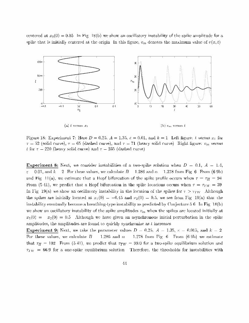
centered at x0(0) = 0:05. In Fig. 18(b) we show an oscillatory instability of the spike amplitude for aspike that is initially centered at the origin. In this �gure, vm denotes the maximum value of v(x; t).050010001500

�0:1 �0:1 0:0 0:1 0:1t

x1(a) t versus x1 10203040

0 10 20 30 40 50 60vm

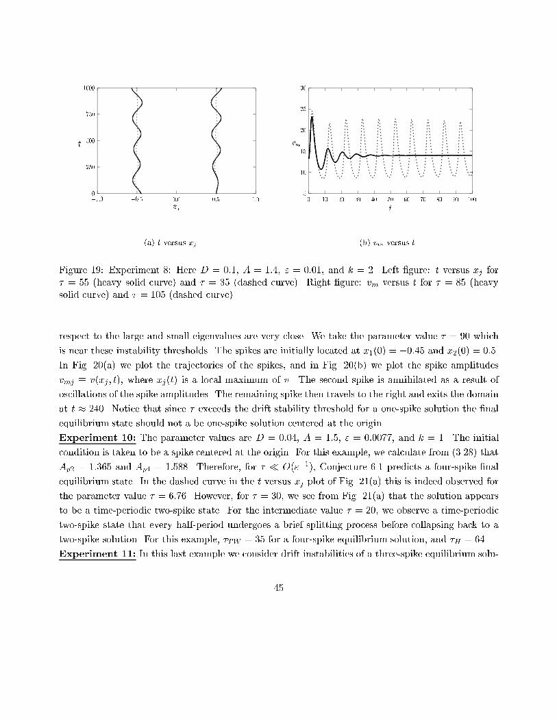
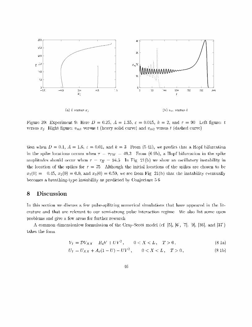
t(b) vm versus tFigure 18: Experiment 7: Here D = 0:25, A = 1:35, " = 0:01, and k = 1. Left �gure: t versus x1 for� = 52 (solid curve), � = 65 (dashed curve), and � = 71 (heavy solid curve). Right �gure: vm versust for � = 220 (heavy solid curve) and � = 235 (dashed curve).Experiment 8: Next, we consider instabilities of a two-spike solution when D = 0:1, A = 1:4," = 0:01, and k = 2. For these values, we calculate B = 1:286 and � = 1:278 from Fig. 6. From (6.9b)and Fig. 11(a), we estimate that a Hopf bifurcation of the spike pro�le occurs when � = �H = 94.From (5.41), we predict that a Hopf bifurcation in the spike locations occurs when � = �TW = 39.In Fig. 19(a) we show an oscillatory instability in the location of the spikes for � > �TW . Althoughthe spikes are initially located at x1(0) = �0:45 and x2(0) = 0:5, we see from Fig. 19(a) that theinstability eventually become a breathing-type instability as predicted by Conjecture 5.6. In Fig. 18(b)we show an oscillatory instability of the spike amplitudes vm when the spikes are located initially atx1(0) = �x2(0) = 0:5. Although we have given an asynchronous initial perturbation in the spikeamplitudes, the amplitudes are found to quickly synchronize as t increases.Experiment 9: Next, we take the parameter values D = 0:25, A = 1:35, " = 0:015, and k = 2.For these values, we calculate B = 1:286 and � = 1:278 from Fig. 6. From (6.9b) we estimatethat �H = 102. From (5.41), we predict that �TW = 99:0 for a two-spike equilibrium solution and�TW = 66:9 for a one-spike equilibrium solution. Therefore, the thresholds for instabilities with44

02505007501000

�1:0 �0:5 0:0 0:5 1:0t

xj(a) t versus xj 51015202530

0 10 20 30 40 50 60 70 80 90 100vm

t(b) vm versus tFigure 19: Experiment 8: Here D = 0:1, A = 1:4, " = 0:01, and k = 2. Left �gure: t versus xj for� = 55 (heavy solid curve) and � = 35 (dashed curve). Right �gure: vm versus t for � = 85 (heavysolid curve) and � = 105 (dashed curve).respect to the large and small eigenvalues are very close. We take the parameter value � = 90 whichis near these instability thresholds. The spikes are initially located at x1(0) = �0:45 and x2(0) = 0:5.In Fig. 20(a) we plot the trajectories of the spikes, and in Fig. 20(b) we plot the spike amplitudesvmj � v(xj ; t), where xj(t) is a local maximum of v. The second spike is annihilated as a result ofoscillations of the spike amplitudes. The remaining spike then travels to the right and exits the domainat t � 240. Notice that since � exceeds the drift stability threshold for a one-spike solution the �nalequilibrium state should not a be one-spike solution centered at the origin.Experiment 10: The parameter values are D = 0:04, A = 1:5, " = 0:0077, and k = 1. The initialcondition is taken to be a spike centered at the origin. For this example, we calculate from (3.28) thatAp2 = 1:365 and Ap4 = 1:588. Therefore, for � � O("�1), Conjecture 6.1 predicts a four-spike �nalequilibrium state. In the dashed curve in the t versus xj plot of Fig. 21(a) this is indeed observed forthe parameter value � = 6:76. However, for � = 30, we see from Fig. 21(a) that the solution appearsto be a time-periodic two-spike state. For the intermediate value � = 20, we observe a time-periodictwo-spike state that every half-period undergoes a brief splitting process before collapsing back to atwo-spike solution. For this example, �TW = 35 for a four-spike equilibrium solution, and �H = 64.Experiment 11: In this last example we consider drift instabilities of a three-spike equilibrium solu-45

050100150200250300

�1:0 �0:5 0:0 0:5 1:0t

xj(a) t versus xj 010203040

0 50 100 150 200 250 300vm

t(b) vm versus tFigure 20: Experiment 9: Here D = 0:25, A = 1:35, " = 0:015, k = 2, and � = 90. Left �gure: tversus xj. Right �gure: vm1 versus t (heavy solid curve) and vm2 versus t (dashed curve).tion when D = 0:1, A = 1:6, " = 0:01, and k = 3. From (5.41), we predict that a Hopf bifurcationin the spike locations occurs when � = �TW = 49:3. From (6.9b), a Hopf bifurcation in the spikeamplitudes should occur when � = �H = 94:5. In Fig. 21(b) we show an oscillatory instability inthe location of the spikes for � = 75. Although the initial locations of the spikes are chosen to bex1(0) = �0:45, x2(0) = 0:0, and x3(0) = 0:50, we see from Fig. 21(b) that the instability eventuallybecomes a breathing-type instability as predicted by Conjecture 5.6.8 DiscussionIn this section we discuss a few pulse-splitting numerical simulations that have appeared in the lit-erature and that are relevant to our semi-strong pulse interaction regime. We also list some openproblems and give a few areas for further research.A common dimensionless formulation of the Gray-Scott model (cf. [5], [6], [7], [9], [36], and [37])takes the form VT = DVXX �BdV + UV 2 ; 0 < X < L ; T > 0 ; (8.1a)UT = UXX +Ad(1� U)� UV 2 ; 0 < X < L ; T > 0 ; (8.1b)46

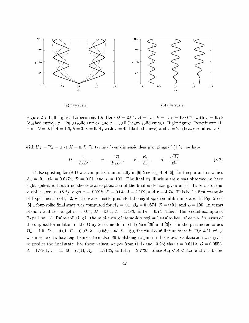
02505007501000

�1:0 �0:5 0:0 0:5 1:0t

xj(a) t versus xj 02505007501000

�1:0 �0:5 0:0 0:5 1:0t

xj(b) t versus xjFigure 21: Left �gure: Experiment 10: Here D = 0:04, A = 1:5, k = 1, " = 0:0077, with � = 6:76(dashed curve), � = 20:0 (solid curve), and � = 30:0 (heavy solid curve). Right �gure: Experiment 11:Here D = 0:1, A = 1:6, k = 3, " = 0:01, with � = 45 (dashed curve) and � = 75 (heavy solid curve).with UX = VX = 0 at X = 0; L. In terms of our dimensionless groupings of (1.3), we haveD � 4AdL2 ; "2 � 4DBdL2 ; � � BpAp ; A � pAdBd : (8.2)Pulse-splitting for (8.1) was computed numerically in [6] (see Fig. 4 of [6]) for the parameter valuesAd = :01, Bd = 0:0474, D = 0:01, and L = 100. The �nal equilibrium state was observed to haveeight spikes, although no theoretical explanation of the �nal state was given in [6]. In terms of ourvariables, we use (8.2) to get " = :00918, D = 0:04, A = 2:109, and � = 4:74. This is the �rst exampleof Experiment 5 of x6.2, where we correctly predicted the eight-spike equilibrium state. In Fig. 2b of[5] a four-spike �nal state was computed for Ad = :01, Bd = 0:0674, D = 0:01, and L = 100. In termsof our variables, we get " = :0077, D = 0:04, A = 1:483, and � = 6:74. This is the second example ofExperiment 5. Pulse-splitting in the semi-strong interaction regime has also been observed in terms ofthe original formulation of the Gray-Scott model in (1.1) (see [36] and [3]). For the parameter valuesDu = 1:0, Dv = 0:01, F = 0:02, k = 0:059, and L = 60, the �nal equilibrium state in Fig. 4.1b of [3]was observed to have eight spikes (see also [36]), although again no theoretical explanation was givento predict the �nal state. For these values, we get from (1.4) and (3.28) that " = 0:0119, D = 0:0555,A = 1:7901, � = 1:339 = O(1), Ap4 = 1:7135, and Ap8 = 2:7725. Since Ap4 < A < Ap8, and � is below47

the instability threshold, the Conjecture 6.1 correctly predicts an eight-spike �nal equilibrium state.There are many open problems related to pulse-splitting that await a rigorous proof. Two centralproblems are to prove rigorously the shape of the B = B( ) curve in Fig. 2(a), and to prove theformal results in Propositions 3.2, 4.1, and 4.2, that give the saddle-node bifurcation values Apk andthe qualitative properties of solutions along the two extremes of the B( ) curve. Another importantopen problem is to give a rigorous treatment of the stability of the primary and secondary solutionbranches with respect to both drift instabilities and instabilities associated with the large eigenvalues.Other areas where further research is needed is to characterize the dynamics of quasi-equilibriumspike patterns for (1.3) in the pulse-splitting regime, and to predict the times and locations wheresplitting events occur. In particular, a theoretical explanation of Experiments 6, 9 and 10 would be in-teresting. For semi-strong spike interactions, the dynamics of a two-spike evolution in the intermediateparameter regime were studied in [5] and [6]. Spike dynamics for the Gierer-Meinhardt model in thesemi-strong regime were studied in [17]. For the weak interaction regime of [32], where both di�usivi-ties are small and of the same order, spike dynamics was studied in [10] and [11]. Secondly, it wouldbe interesting to study the stability of stripe and ring patterns in the two dimensional Gray-Scottmodel with respect to both zig-zag instabilities associated with the small eigenvalues, and breakupinstabilities of stripes into spots, which result from large eigenvalue instabilities. Some work in thisdirection is given in [21], [25], and [20].AcknowledgementsT. K. was supported by a PGS-B graduate scholarship from NSERC (Canada). M. J. W. thanks thegrant support of NSERC, and the IMS of the Chinese University of Hong Kong where most of thispaper was written. J. W. thanks the support of RGC of Hong Kong and a direct grant from CUHK.M. J. W. is most grateful to the University of Washington Applied Math group for the generous useof their computer facilities.References[1] E. Anderson et al. LAPACK User's Guide: Third Edition, SIAM Publications (1999).[2] U. Ascher, R. Christiansen, R. Russell, Collocation Software for Boundary Value ODE's, Math.Comp., 33, (1979), pp. 659-679.48

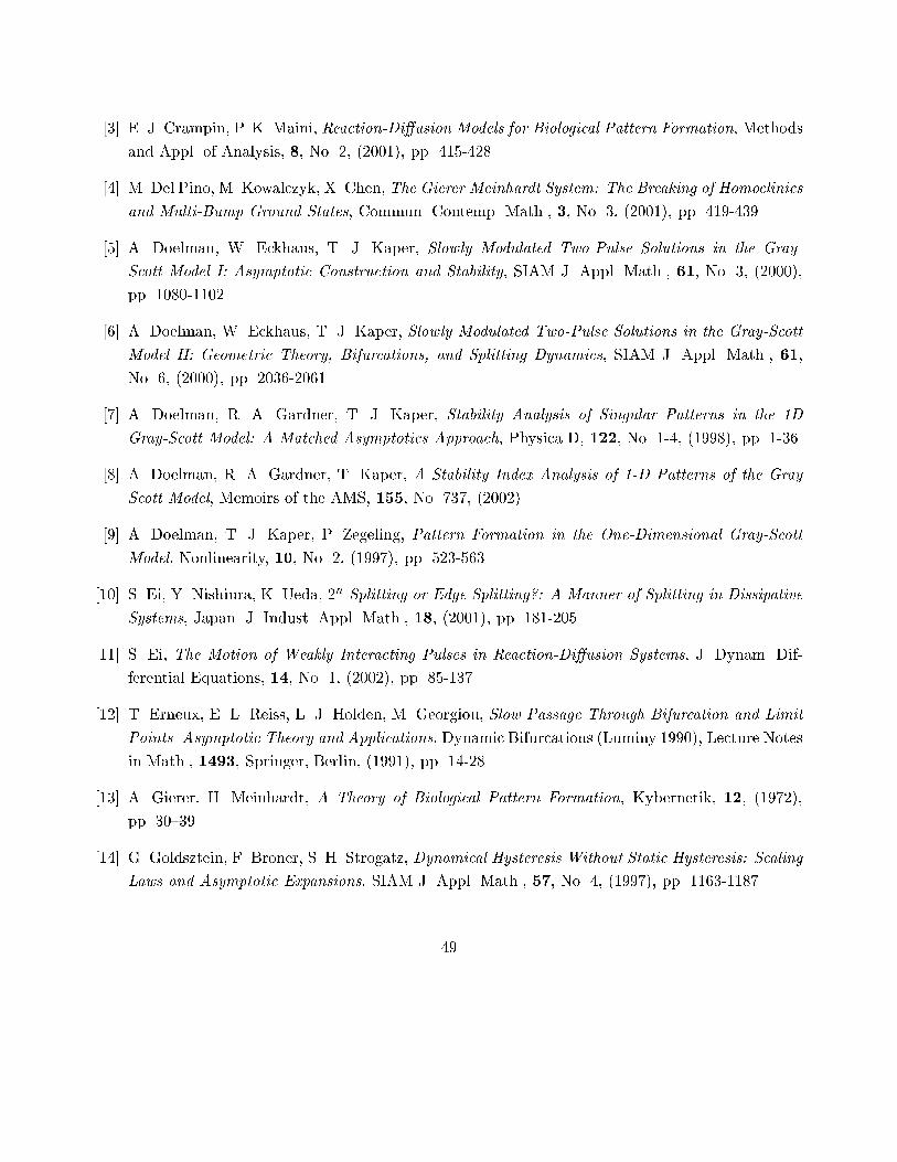
[3] E. J. Crampin, P. K. Maini, Reaction-Di�usion Models for Biological Pattern Formation, Methodsand Appl. of Analysis, 8, No. 2, (2001), pp. 415-428.[4] M. Del Pino, M. Kowalczyk, X. Chen, The Gierer Meinhardt System: The Breaking of Homoclinicsand Multi-Bump Ground States, Commun. Contemp. Math., 3, No. 3, (2001), pp. 419-439.[5] A. Doelman, W. Eckhaus, T. J. Kaper, Slowly Modulated Two-Pulse Solutions in the Gray-Scott Model I: Asymptotic Construction and Stability, SIAM J. Appl. Math., 61, No. 3, (2000),pp. 1080-1102.[6] A. Doelman, W. Eckhaus, T. J. Kaper, Slowly Modulated Two-Pulse Solutions in the Gray-ScottModel II: Geometric Theory, Bifurcations, and Splitting Dynamics, SIAM J. Appl. Math., 61,No. 6, (2000), pp. 2036-2061.[7] A. Doelman, R. A. Gardner, T. J. Kaper, Stability Analysis of Singular Patterns in the 1DGray-Scott Model: A Matched Asymptotics Approach, Physica D, 122, No. 1-4, (1998), pp. 1-36.[8] A. Doelman, R. A. Gardner, T. Kaper, A Stability Index Analysis of 1-D Patterns of the GrayScott Model, Memoirs of the AMS, 155, No. 737, (2002).[9] A. Doelman, T. J. Kaper, P. Zegeling, Pattern Formation in the One-Dimensional Gray-ScottModel, Nonlinearity, 10, No. 2, (1997), pp. 523-563.[10] S. Ei, Y. Nishiura, K. Ueda, 2n Splitting or Edge Splitting?: A Manner of Splitting in DissipativeSystems, Japan. J. Indust. Appl. Math., 18, (2001), pp. 181-205.[11] S. Ei, The Motion of Weakly Interacting Pulses in Reaction-Di�usion Systems, J. Dynam. Dif-ferential Equations, 14, No. 1, (2002), pp. 85-137.[12] T. Erneux, E. L. Reiss, L. J. Holden, M. Georgiou, Slow Passage Through Bifurcation and LimitPoints. Asymptotic Theory and Applications, Dynamic Bifurcations (Luminy 1990), Lecture Notesin Math., 1493, Springer, Berlin, (1991), pp. 14-28.[13] A. Gierer, H. Meinhardt, A Theory of Biological Pattern Formation, Kybernetik, 12, (1972),pp. 30{39.[14] G. Goldsztein, F. Broner, S. H. Strogatz, Dynamical Hysteresis Without Static Hysteresis: ScalingLaws and Asymptotic Expansions, SIAM J. Appl. Math., 57, No. 4, (1997), pp. 1163-1187.49

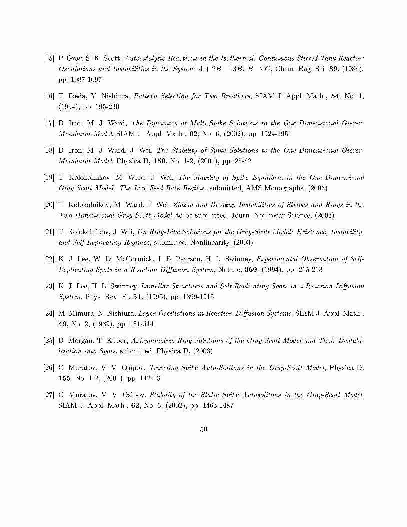
[15] P. Gray, S. K. Scott, Autocatalytic Reactions in the Isothermal, Continuous Stirred Tank Reactor:Oscillations and Instabilities in the System A+ 2B ! 3B, B ! C, Chem. Eng. Sci. 39, (1984),pp. 1087-1097.[16] T. Ikeda, Y. Nishiura, Pattern Selection for Two Breathers, SIAM J. Appl. Math., 54, No. 1,(1994), pp. 195-230.[17] D. Iron, M. J. Ward, The Dynamics of Multi-Spike Solutions to the One-Dimensional Gierer-Meinhardt Model, SIAM J. Appl. Math., 62, No. 6, (2002), pp. 1924-1951.[18] D. Iron, M. J. Ward, J. Wei, The Stability of Spike Solutions to the One-Dimensional Gierer-Meinhardt Model, Physica D, 150, No. 1-2, (2001), pp. 25-62.[19] T. Kolokolnikov, M. Ward, J. Wei, The Stability of Spike Equilibria in the One-DimensionalGray-Scott Model: The Low Feed-Rate Regime, submitted, AMS Monographs, (2003).[20] T. Kolokolnikov, M. Ward, J. Wei, Zigzag and Breakup Instabilities of Stripes and Rings in theTwo Dimensional Gray-Scott Model, to be submitted, Journ. Nonlinear Science, (2003).[21] T. Kolokolnikov, J. Wei, On Ring-Like Solutions for the Gray-Scott Model: Existence, Instability,and Self-Replicating Regimes, submitted, Nonlinearity, (2003).[22] K. J. Lee, W. D. McCormick, J. E. Pearson, H. L. Swinney, Experimental Observation of Self-Replicating Spots in a Reaction-Di�usion System, Nature, 369, (1994), pp. 215-218.[23] K. J. Lee, H. L. Swinney, Lamellar Structures and Self-Replicating Spots in a Reaction-Di�usionSystem, Phys. Rev. E., 51, (1995), pp. 1899-1915.[24] M. Mimura, N. Nishiura, Layer Oscillations in Reaction Di�usion Systems, SIAM J. Appl. Math.,49, No. 2, (1989), pp. 481-514.[25] D. Morgan, T. Kaper, Axisymmetric Ring Solutions of the Gray-Scott Model and Their Destabi-lization into Spots, submitted, Physica D, (2003).[26] C. Muratov, V. V. Osipov, Traveling Spike Auto-Solitons in the Gray-Scott Model, Physica D,155, No. 1-2, (2001), pp. 112-131.[27] C. Muratov, V. V. Osipov, Stability of the Static Spike Autosolitons in the Gray-Scott Model,SIAM J. Appl. Math., 62, No. 5, (2002), pp. 1463-1487.50

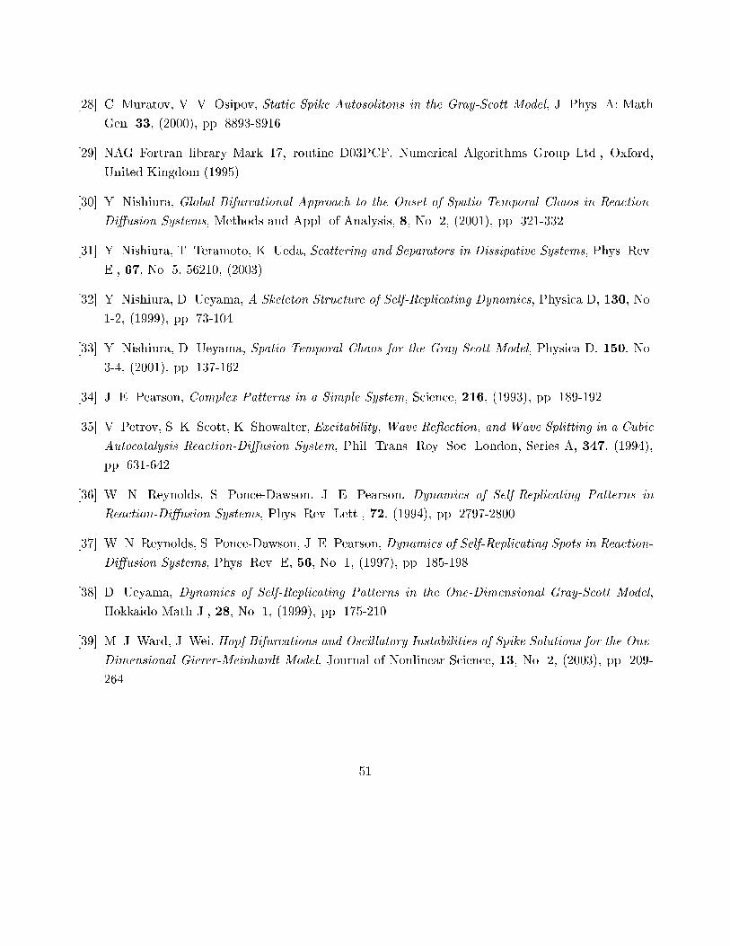
[28] C. Muratov, V. V. Osipov, Static Spike Autosolitons in the Gray-Scott Model, J. Phys. A: MathGen. 33, (2000), pp. 8893-8916.[29] NAG Fortran library Mark 17, routine D03PCF, Numerical Algorithms Group Ltd., Oxford,United Kingdom (1995).[30] Y. Nishiura, Global Bifurcational Approach to the Onset of Spatio-Temporal Chaos in Reaction-Di�usion Systems, Methods and Appl. of Analysis, 8, No. 2, (2001), pp. 321-332.[31] Y. Nishiura, T. Teramoto, K. Ueda, Scattering and Separators in Dissipative Systems, Phys. Rev.E., 67, No. 5, 56210, (2003).[32] Y. Nishiura, D. Ueyama, A Skeleton Structure of Self-Replicating Dynamics, Physica D, 130, No.1-2, (1999), pp. 73-104.[33] Y. Nishiura, D. Ueyama, Spatio-Temporal Chaos for the Gray-Scott Model, Physica D, 150, No.3-4, (2001), pp. 137-162.[34] J. E. Pearson, Complex Patterns in a Simple System, Science, 216, (1993), pp. 189-192.[35] V. Petrov, S. K. Scott, K. Showalter, Excitability, Wave Re ection, and Wave Splitting in a CubicAutocatalysis Reaction-Di�usion System, Phil. Trans. Roy. Soc. London, Series A, 347, (1994),pp. 631-642.[36] W. N. Reynolds, S. Ponce-Dawson, J. E. Pearson, Dynamics of Self-Replicating Patterns inReaction-Di�usion Systems, Phys. Rev. Lett., 72, (1994), pp. 2797-2800.[37] W. N. Reynolds, S. Ponce-Dawson, J. E. Pearson, Dynamics of Self-Replicating Spots in Reaction-Di�usion Systems, Phys. Rev. E, 56, No. 1, (1997), pp. 185-198.[38] D. Ueyama, Dynamics of Self-Replicating Patterns in the One-Dimensional Gray-Scott Model,Hokkaido Math J., 28, No. 1, (1999), pp. 175-210.[39] M. J. Ward, J. Wei, Hopf Bifurcations and Oscillatory Instabilities of Spike Solutions for the One-Dimensional Gierer-Meinhardt Model, Journal of Nonlinear Science, 13, No. 2, (2003), pp. 209-264.51