The Evolution of Market Power in the US Auto Industry

The Evolution of Market Power in the US AutoIndustry∗

Paul L. E. Grieco† Charles Murry‡ Ali Yurukoglu§

June 11, 2021

Abstract

We construct measures of industry performance and welfare in the U.S. car and light truckmarket from 1980-2018. We estimate a differentiated products demand model for this marketusing product level data on market shares, prices, and product characteristics, and consumerlevel data on demographics, purchases, and stated second choices. We estimate marginal costsunder the conduct assumption of Nash-Bertrand pricing. We relate trends in consumer welfareand markups to industry trends in market structure and the composition of products, like therise of import competition, the proliferation of SUV’s, and changes in vehicle characteristics. Wefind that although prices rose over time, concentration and market power decreased substantially.Consumer welfare increased over time due to improving product quality and falling marginalcosts. The fraction of total surplus accruing to consumers also increased.

JEL Codes: L11, L62, D43

1 Introduction

This paper analyzes the US automobile industry over forty years. During this period, the indus-try experienced numerous technological and regulatory changes and its market structure changeddramatically. Our goal is to examine whether these changes led to discernible changes in industryperformance. Our work complements a recent academic and policy literature analyzing long termtrends in market power and sales concentration from a macroeconomic perspective (De Loecker

∗We thank Naibin Chen, Andrew Hanna and Arnab Palit for excellent research assistance. We thank MatthewWeinberg for comments. Portions of our analysis use data derived from a confidential, proprietary syndicated productowned by MRI-Simmons

†The Pennsylvania State University.‡Boston College.§Graduate School of Business, Stanford University and NBER.

1

et al., 2020; Autor et al., 2020) with an industry-specific approach. Several papers and commen-tators point to a competition problem where price-cost margins and industry concentration haveincreased during this time period (Economist, 2016; Covarrubias et al., 2020). We find that, inthis industry, the situation for consumers has improved noticeably over time. Furthermore, ourestimates of price-cost margins for this industry differ from those computed using methods anddata from the recent macroeconomics literature.

To estimate trends in industry performance in the U.S. new car industry, we specify a het-erogeneous agent demand system and assume Nash-Bertrand pricing by multi-product automobilemanufacturers to consumers to estimate margins and consumer welfare over time. The key inputsinto the demand estimates are aggregate data on prices, market shares, and vehicle characteristicsover time, micro-data on the relationship between demographics and car characteristics over time,micro-data on consumers’ stated second choices, and the use of the real exchange rate between theUS and product origin countries as an instrumental variable for endogenous prices.

We find that median markups as defined by the Lerner index (L = p−mcp ) fell from 0.311 in 1980

to 0.196 by 2018. However, the industry model indicates that markups, although useful to proxy formarket efficiency when products are unchanging, is a conceptually unattractive measure of marketefficiency over long periods of time when products change. To quantify changes in welfare over time,we utilize a decomposition from Pakes et al. (1993a) to develop a measure of consumer surplus.Our approach leverages continuing products to capture changes in unobserved automobile qualityover time. However, it is not influenced by aggregate fluctuations in demand for automobiles e.g.,business cycle effects such as monetary policy or changes in alternative transportation options. Wefind that the fraction of total surplus going to consumers went from 0.63 in 1980 to 0.83 by 2018and that average consumer surplus per household increased by roughly $20,000 over our sampleperiod.

The increase in consumer surplus is predominantly due to the increasing quality of cars andfalling marginal costs. We confirm the patterns in Knittel (2011) that horsepower, size, and fuelefficiency have improved significantly over this time period. We use the estimated valuations ofcharacteristics to put a dollar amount on this improvement. Furthermore, we use market sharesof continuing products to estimate valuations of improvements in other characteristics such aselectronics, safety, or comfort features that are not readily available in common data sets (e.g.,audio and entertainment systems, rear-view cameras, driver assistance systems). Counterfactualswhich eliminate the observed increase in import competition or the increase in the number of vehiclemodels have moderate effects on consumer surplus. Counterfactuals which eliminate the increasein automobile quality and the fall in marginal costs lead to a reduction in most of the observedconsumer surplus increase.

A number of caveats are warranted for this analysis. First, our main results assume staticNash-Bertrand pricing each year and rule out changes in conduct, for example via the ability totacitly collude. Second, we do not model the complementary dealer, parts, or financing marketswhere the behavior of margins or product market efficiency over time may be different than the

2

automobile manufacturers.This paper is closely related to Hashmi and Biesebroeck (2016) who model dynamic competition

and innovation in the world automobile market over the period 1982 to 2006. We focus on analyzingthe evolution of consumer surplus and markups rather than modeling dynamic competition inquality. Furthermore, in addition to analyzing a longer time period, this paper uses microdata toestimate demand following Bordley (1993) and Berry et al. (2004), and uses a different instrumentalvariable. Other papers which analyze outcomes in other industries over long time periods includeBerndt and Rappaport (2001), Berry and Jia (2010), Borenstein (2011), and Brand (2020).

2 Data

We compiled a data set covering 1980 through 2018 consisting of automobile characteristics andmarket shares, individual consumer choices and demographic information, and consumer surveyresponses regarding alternate “second choice” products. This section describes the data sourcesand presents basic descriptive information.

2.1 Automobile Market Data

Our primary source of data is information on sales, manufacturer suggested retail prices (MSRP),and characteristics of all cars and light trucks sold in the US from 1980-2018 that we obtain fromWard’s Automotive. Ward’s keeps digital records of this information from 1988 through the present.To get information from before 1988, we hand collected data from Ward’s Automotive Yearbooks.The information in the yearbooks is non-standard across years and required multiple layers of digi-tization and re-checking. We supplemented the Ward’s data with additional information, includingvehicle country of production, company ownership information, missing and nonstandard productcharacteristics (e.g. electric vehicle eMPG and driving range, missing MPG, and missing prices),brand country affiliation (e.g. Volkswagen from Germany, Chrysler from USA), and model redesignyears. Prices in all years are deflated to 2015 USD using the core consumer price index.

Product aggregation Cars sold in the US are highly differentiated products. Each brand (or“make”) produces many models and each model can have multiple variants (more commonly called“trims”). Although we have specifications and pricing of individual trims, our sales data comesto us at the make-model level. Similar to other studies of this market, we make use of the salesdata by aggregating the trim information to the make-model level, see Berry et al. (1995) Berryet al. (2004), Goldberg (1995), and Petrin (2002). We aggregate price and product characteristicsby taking the median across trims.

In Table 1 we display summary statistics for our sample of vehicles at the make-model-yearlevel, so an example of an observation is a 1987 Honda Accord. There are 6,107 cars, 2,213 SUVs,676 trucks, and 618 vans in our sample.1 The average car has 52,247 sales in a year and the average

1We use Wards’ vehicle style designations to create our own vehicle designations. We aggregate CUV (crossover

3

Table 1: Summary Statistics

Mean Std. Dev. Min Max Mean Std. Dev. Min Max

Cars, N=6,130 SUVs, N=2,243

Sales 52,122.99 72,758.06 10 473,108 Sales 51,553.00 66,898.86 10 753,064Price 35.83 18.74 11.14 99.99 Price 40.44 14.99 12.75 96.94MPG 22.66 6.81 10.00 50.00 MPG 18.02 5.03 10.00 50.00HP 178.20 83.39 48.00 645.00 HP 232.30 74.98 63.00 510.00Height 55.77 4.22 43.50 107.50 Height 69.01 4.37 56.50 90.00Footprint 12,871.58 1,711.93 6,514.54 21,821.86 Width 13,789.91 1,791.43 8,127.00 18,136.00Weight 3,182.40 640.32 1,488.00 6,765.00 Weight 4,245.77 855.08 2,028.00 7,230.00US Brand 0.40 0.49 0.00 1.00 US Brand 0.40 0.49 0.00 1.00Import 0.59 0.49 0.00 1.00 Import 0.59 0.49 0.00 1.00Electric 0.02 0.14 0.00 1.00 Electric 0.02 0.12 0.00 1.00

Trucks, N=680 Vans, N=641

Sales 141,039.59 184,425.07 12 891,482 Sales 65,357.38 64,649.39 11.00 300,117Price 27.95 10.10 12.63 89.32 Price 31.43 5.54 17.79 47.65MPG 17.83 4.37 10.00 50.00 MPG 17.92 5.06 11.00 50.00HP 189.65 90.39 44.00 403.00 HP 188.18 63.79 48.00 329.00Height 68.42 6.34 51.80 83.40 Height 74.35 8.21 58.85 107.50Footprint 15,100.75 2,462.22 8,791.24 20,000.00 Length 15,173.34 1,882.28 11,169.30 21,821.86Weight 4,049.63 1,113.84 1,113.00 7,178.00 Weight 4,270.26 793.09 2,500.00 8,550.00US Brand 0.65 0.48 0.00 1.00 US Brand 0.71 0.45 0.00 1.00Import 0.35 0.48 0.00 1.00 Import 0.29 0.45 0.00 1.00Electric 0.00 0.00 0.00 0.00 Electric 0.00 0.06 0.00 1.00

Notes: An observation is a make-model-year, aggregated by taking the median across trims in a given year. Statistics are not sales weighted. Pricesare in 2015 000’s USD. Physical dimensions are in inches and curbweight is in pounds.

truck has 141,524 sales. Trucks and vans are more likely to be from US brands and less likely to beassembled outside of the US than cars and SUVs. Two percent of our sample has an electric motor(including hybrid gas-powered and electric only). We present a description of trends in vehiclecharacteristics in Section 3.

2.2 Price Instrument

To identify the price sensitivity of consumers, we rely on an instrumental variable that shifts pricewhile being plausibly uncorrelated with unobserved demand shocks. We employ a cost-shifterrelated to local production costs where a model is produced. For each automobile in each year, weuse the price level of expenditure in the country where the car was manufactured, obtained fromthe Penn World Tables variable plGDPe, lagged by one year to reflect planning horizons. Theprice level of expenditure is equal to the purchasing power parity (PPP) exchange rate relative tothe US divided by the nominal exchange rate relative to the US. As described in Feenstra et al.(2015), the ratio of price levels between a given country and the US is known as the “real exchangerate” (Real XR) between that country and the US. The real exchange rate varies with two sourcesthat are useful for identifying price sensitivities. First, if wages in the country of manufacturerise, the cost of making the car will rise, which will in turn raise the real exchange rate via thePPP rising. Therefore, the real exchange captures one source of input cost variation through locallabor costs. Another source of variation is through the nominal exchange rate. If the nominal

utility vehicles) and SUV to our SUV designation. Truck and van are native Wards designations. We designate allother styles (sedan, coupe, wagon, hatchback, convertible) as car. Many models are produced in multiple variants.For example the Chrysler LeBaron has been available as a sedan, coupe, and station wagon in various years. However,no model is produced as both a car and an SUV, or any other combination of our designations, in our sample.

4

exchange rate rises, so that the local currency depreciates relative to the dollar, a firm with marketpower will have an incentive to lower retail prices in the US, thereby providing another avenue ofpositive covariation between the real exchange rate and retail prices in the US. Exchange rates wereemployed as instrumental variables for car prices in Goldberg and Verboven (2001), which is focusedon the European car market. In Figure 1, we display the lagged Real XR for the most popularproduction countries, where the size of the marker is proportional to the number of products soldfrom each country and the black dashed line represents the U.S. price level.

Figure 1: Real Exchange Rates

Notes: Lagged real exchange rates from Penn World Table 9.2. Size of dots corresponds to number of sales byproduction country, except for USA.

We demonstrate the behavior of this instrumental variable in a simplified setup in Table 2.We estimate a logit model of demand, as in Berry (1994), first via OLS and then using two-stageleast squares with Real XR as an instrumental variable for price. We include make fixed effectsbecause brands assemble different models in different countries. For example, BMW assemblesvehicles for the US market in Germany and the US, General Motors has produced US sold vehiclesin Canada, Mexico, and South Korea (among other countries), and many of the Japanese andSouth Korean brands produce some of their models in the United States, Canada, and Mexico.The first column in Table 2 shows the first stage relevance of the instrumental variable. The signis positive as predicted by the theory with a first stage F-stat of 14.09. We cluster the standarderrors at the make level. The first stage implies a pass-through of Real XR to prices of 0.141, whichis consistent with estimates in the literature (Goldberg and Campa, 2010; Burstein and Gopinath,2014). The difference in the price coefficient in the last two columns demonstrates that employingthe IV moves the coefficient estimate on price in the negative direction, which is expected becausethe OLS coefficient should be biased in the positive direction if prices positively correlate withunobserved demand shocks conditional on observable characteristics. Comparing the mean ownprice elasticities between the OLS and IV estimates confirms the importance of controlling for

5

price endogeneity.

Table 2: Logit Demand

First Stage Reduced Form OLS IV

Real XR* 4.073 (1.085) -0.722 (0.232) – –Price -0.022 (0.005) -0.177 (0.063)Height -15.432 (3.559) -0.417 (0.465) -0.784 (0.488) -3.153 (1.245)Footprint -7.635 (4.543) 2.244 (0.535) 2.080 (0.521) 0.890 (1.012)Weight 31.866 (4.424) -1.855 (0.565) -0.965 (0.559) 3.795 (2.186)Horsepower 17.335 (2.615) -0.182 (0.153) 0.473 (0.146) 2.891 (1.114)Miles/$ 4.310 (1.325) -0.141 (0.197) 0.075 (0.211) 0.623 (0.418)No. Trims -1.280 (0.228) 1.235 (0.054) 1.197 (0.054) 1.008 (0.114)Yrs. Design 0.033 (0.048) -0.073 (0.013) -0.072 (0.014) -0.067 (0.015)Release Year -0.795 (0.442) -0.272 (0.072) -0.303 (0.078) -0.413 (0.124)Sport 4.737 (0.930) -0.696 (0.099) -0.557 (0.091) 0.144 (0.335)Electric 7.726 (1.762) -1.044 (0.256) -0.735 (0.246) 0.326 (0.579)Truck -3.953 (1.521) -0.553 (0.115) -0.652 (0.115) -1.254 (0.352)SUV -1.003 (1.188) 0.558 (0.105) 0.545 (0.112) 0.381 (0.229)Van -2.454 (1.569) -0.044 (0.143) -0.118 (0.155) -0.479 (0.327)Constant 390.230 (133.366) -21.062 (11.910) -16.934 (3.165) -42.639 (14.079)

Mean Own Price Elas. – – -0.808 -6.37Implied Pass-through 0.125 (0.026)First Stage F-Stat 14.09

Notes: Unit of observations: year make-model, from 1980 to 2018. Number of observations: 9,694.All specifications include year and make fixed effects. Standard errors clustered by make in paren-theses. Car characteristics in logs and price is in 2015 $10,000.* Real exchange rate from Penn Word Table 9.2, variable pl_gdp_con.

2.3 Consumer Choices and Demographics

We collect individual level data on car purchases and demographics from two data sources: theConsumer Expenditure Survey (CEX) and GfK MRI’s Survey of the American Consumer (MRI).These data sets provide observations on a sample of new car purchasers for each year, includingthe demographics of the purchaser and the car model purchased. CEX covers the years 1980-2005with an average of 1, 014 observations per year. MRI covers the years 1992-2018 with an averageof 2, 005 observations per year. We construct micro-moments from these data to use as targets forthe heterogeneous agent demand model, following Goldberg (1995), Petrin (2002), and Berry et al.(2004). There are some general patterns from these data that motivate specification choices forthe demand model. For example, that the average purchaser of a van having a larger family sizesuggests families value size more than non-families. That the average price of a car purchased bya high income versus low income buyer suggests higher income buyers are either less sensitive toprice or value characteristics that come in higher priced cars more. That rural households are morelikely to purchase a truck suggests different preferences for features of trucks by rural households.

In order to approximate the distribution of household demographics, we sample from the CPS,which contains the demographics information from 1980-2018 that we use from the CEX and MRIsamples. Average household income (in 2015 dollars) increases from $55,382 to $81,375 from 1980to 2018. Average household age increases from 46 to 51; average household size falls from 1.60 to

6

1.25; the percent of rural households decreases from 27.9 to 13.4.

2.4 Second Choices

We obtain data on consumers’ reported second choices from MartizCX, an automobile industryresearch and marketing firm. MaritzCX surveys recent car purchasers based on new vehicle regis-trations. The survey includes a question about cars that the respondents considered, but did notpurchase. We use the first listed car as the purchaser’s second choice. These data have previouslybeen used, such as in Leard et al. (2017) and Leard (2019), and are similar to the survey data usedin Berry et al. (2004).2 After we merge with our sales data, we use second choice data from 1991,1999, 2005 and 2015, representing 29,396, 20,413, 42,533, and 53,328 purchases, respectively.

In Table 3 we display information about second choices for many popular cars of different stylesand features to give a sense for how strong substitution appears in the data. For each year, wedisplay the modal second choice, the next most common second choice, and the share who reportthese two cars as second choices over the total responses for that car. For example, in 1991, thethe Dodge Ram Pickup is the modal second choice among the respondents who purchased a FordF Series. The Chevrolet CK Pickup is the second most popular second choice, and together, thesetwo second choices make up 69 percent of reported second choices for the Ford F Series. Fromthis sample of vehicles, second choices tend to be similar types of vehicles (i.e. trucks, cars, SUVs,vans). Also, there is substantial variation in the share that the two most frequent choices represent:for example, in 1991, the F Series and Dodge Ram represent 76 percent of reported second choicesfor the Chevrolet Silverado in 1999, but the Civic and Corolla only represent 22 percent of secondchoices for the Ford Focus in 2005. The generally strong substitution towards similar cars is crucialfor identifying unobserved heterogeneity in the demand model we present in Section 2.

3 Empirical Description of the New Car Industry, 1980-2018

In this section we describe trends in the U.S. automobile industry from 1980 to 2018 related tomarket power and market efficiency. We first discuss changes in prices and market structure.Second, we discuss trends in product characteristics.

3.1 Prices and Market Structure

Real prices in the automobile industry steadily rose from 1980 to 2018. At the same time, con-centration decreased. In Figure 2 we display these patterns. In panel (a), we document that theaverage manufacturer suggested retail price (MSRP) rose from around $17,000 in 1980 to around$36,000 in 2018 (in 2015 USD, deflated by the core consumer price index). The bulk of the change

2The MaritzCX survey asks respondents about vehicles that the respondents considered but did not purchase.One of the questions is whether the respondent considered any other cars or trucks when shopping for their vehicle.Respondents answer this question either yes or no. For those that answer yes, the survey asks respondents to providevehicle make-model and characteristics for the model most seriously considered.

7

Table 3: Second Choices, Selected Examples

Modal Second Next Second (Modal +Car Choice Choice Next)/n

1991, N=29,436

Ford F Series Dodge Ram Pickup Chevrolet CK Pickup 0.69Honda Accord Toyota Camry Nissan Maxima 0.32Dodge Caravan Ford Aerostar Plymouth Voyager 0.28Mercedes-Benz E Class BMW 5 Series Lexus LS 0.32Toyota 4Runner Ford Explorer Nissan Pathfinder 0.58Nissan 300ZX Alfa Romeo 164 Chevrolet Corvette 0.35

1999, N=20,413

Chevrolet Silverado Ford F Series Dodge Ram Pickup 0.76Toyota Camry Honda Accord Nissan Maxima 0.38Plymouth Voyager Ford Windstar Dodge Caravan 0.42Audi A6 BMW 5 Series Volvo 80 0.28Chevrolet Tahoe Ford Expedition Dodge Durango 0.36BMW Z3 Porsche Boxster Mazda MX-5 Miata 0.42

2005, N=42,977

Toyota Tacoma Nissan Frontier Ford F Series 0.35Ford Focus Toyota Corolla Honda Civic 0.22Honda Odyssey Toyota Sienna Chrysler Town & Country 0.71Lincoln Town Car Cadillac Deville Chrysler 300 Series 0.44Honda CR-V Toyota Rav4 Ford Escape 0.38Porsche Cayenne BMW X5 Land Rover Range Rover 0.43

2015, N=53,391

Ford F Series Chevrolet Silverado Ram Pickup 0.64Toyota Prius Honda Accord Hybrid Honda CR-V 0.11Toyota Sienna Honda Odyssey Chrysler Town & Country 0.64Volvo 60 BMW 3 Series Audi A4 0.16Nissan Frontier Toyota Tacoma Chevrolet Colorado 0.69Chevrolet Camaro Ford Mustang Dodge Challenger 0.46Toyota Prius PHEV Chevrolet Volt Nissan Leaf 0.32

Notes: Data from Maritz CX surveys in 1991, 1999, 2005, and 2015. Vehicles selected are high selling vehicles thatrepresent a range of styles and attributes.

8

in average price occurred before the year 2000, although the upper 25 percent of prices continuedto rise after 2000. At the same time, HHI measured at the parent company level fell from over 2500to around 1200, see panel (b). The C4 index saw a similar decrease over the same time period,from around 0.80 to 0.58. In Figure 2c we document the main source of decreasing concentration.While the total number of firms in this industry fell slightly from 1980 to 2018, there were abouttwice as many products in 2018 as there were in 1980. In 1980, the “Big 3” US manufacturersaccounted for a large portion of sales, whereas by 2018, sales were more evenly dispersed amongfirms.

Figure 2: Prices and Market Structure, 1980-2018

1980 1985 1990 1995 2000 2005 2010 2015

Year

$10,000

$20,000

$30,000

$40,000

$50,000Mean Price

IQR

(a) Prices

1980 1985 1990 1995 2000 2005 2010 2015

Year

0

0.05

0.1

0.15

0.2

0.25

0.3

HH

I0.5

0.6

0.7

0.8

0.9

1

C4

Sh

are

HHI

C4

(b) Measures of Concentration

1980 1985 1990 1995 2000 2005 2010 2015

Year

200

250

300

350

Count

of

Pro

duct

s O

ffer

ed

10

15

20

25

Count

of

Ult

imat

e O

wner

s

Count of Products

Count of Parent Companies

(c) Products and Manufacturers

1980 1985 1990 1995 2000 2005 2010 2015

Year

0

50

100

150

200

Nu

mb

er

of

Av

ail

ab

le M

od

els

Car

SUV

Truck

Van

(d) Count of Products by Styles

Notes: Panel (a): average price is not weighted by sales. Panel (b): HHI and C4 are defined at the parent companylevel, e.g. Honda is the parent company of the Honda and Acura brands. In Panel (c), the number of productscorresponds to a model available in a given year in our sample. The style definitions referred to in Panel (d) aredescribed in the text. Data is from Wards Automotive Yearbooks and the sample selection is described in the text.

3.2 Physical Characteristics of Vehicles

That prices rose while concentration fell might seem counterintuitive at first pass, however pricesare also a function of physical characteristics, quality, and production technology. There are twomain trends regarding the physical characteristics of cars. The first is the rise of the SUV, whichwas a nearly non-existent vehicle class in 1980 and by the end of our sample represented roughlyhalf of all sales. Second, cars and trucks have become larger and more powerful without sacrificingfuel efficiency (Knittel, 2011).

9

The number of products available to consumers increased from 1980 to 2018. A major contri-bution to this change is the rise of SUV production, particularly smaller SUVs that are designedto compete with sedans. Our SUV category aggregates SUVs (typically larger vehicles built onpickup truck frames, like the Toyota 4Runner) together with CUVs (smaller than SUVs and builton sedan frames, like the Honda CRV). In Figure 2(d) we display the number of products by vehiclestyle over time. In the early 1980’s less than 25 SUVs were available to consumers (typically largetruck-like vehicles) and after the year 2000 there were nearly 100 SUVs available in the market.Conversely, the count of available vehicles for other styles remained largely unchanged over theperiod of our sample.

Figure 3: Physical Vehicle Characteristics, 1980-2018

1980 1985 1990 1995 2000 2005 2010 2015

Year

50

100

150

200

250

300

350

Hors

epow

er

Car

SUV

Truck

Van

(a) Horsepower

1980 1985 1990 1995 2000 2005 2010 2015

Year

11

12

13

14

15

16

17

18

Sq

uar

e In

ches

(1

00

0s)

Car

SUV

Truck

Van

(b) Size (length × width)

1980 1985 1990 1995 2000 2005 2010 2015

Year

14

16

18

20

22

24

26

28

Mil

es p

er G

allo

n

Car

SUV

Truck

Van

(c) Fuel Economy

1980 1990 2000 2010 2014

Year

0

20

40

60

80

100

% F

acto

ry I

nst

alle

d

Air Cond.

Power Windows

Anit-lock Brake

Cassette

Side Airbag

Memory Seats

Rear Camera

(d) Additional Factory Installed Features

Notes: Panels (a)-(c) display average characteristics for available models in our sample. Panel (d) is the percent ofeach feature installed on total “cars” sold (i.e. not trucks, SUVs, or vans). Factory installed features were compiledfrom Wards Automotive Yearbooks from various years. For example, in 1980 61% of “cars” sold had air conditioning.

We display selected attributes over time in Figure 3. Average horsepower and car size (length bywidth) increased substantially from 1980 to 2018. Average horsepower more than doubled for carsand roughly tripled for trucks from 1980 to 2018, see Figure 3a. Cars became larger, SUVs and vansbecame smaller during the 1980s and then grew, and the average truck size grew substantially from1980 to 2018. At the same time as horsepower and size increased, average fuel economy remainedroughly constant, which largely reflects federal regulatory standards for fleet fuel economy, firstenacted in the Energy Policy and Conservation Act of 1975.

Additionally, attributes not related to size and power changed substantially from 1980 to 2018.

10

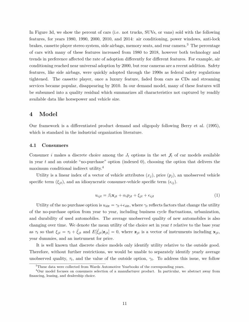
In Figure 3d, we show the percent of cars (i.e. not trucks, SUVs, or vans) sold with the followingfeatures, for years 1980, 1990, 2000, 2010, and 2014: air conditioning, power windows, anti-lockbrakes, cassette player stereo system, side airbags, memory seats, and rear camera.3 The percentageof cars with many of these features increased from 1980 to 2018, however both technology andtrends in preference affected the rate of adoption differently for different features. For example, airconditioning reached near universal adoption by 2000, but rear cameras are a recent addition. Safetyfeatures, like side airbags, were quickly adopted through the 1990s as federal safety regulationstightened. The cassette player, once a luxury feature, faded from cars as CDs and streamingservices became popular, disappearing by 2010. In our demand model, many of these features willbe subsumed into a quality residual which summarizes all characteristics not captured by readilyavailable data like horsepower and vehicle size.

4 Model

Our framework is a differentiated product demand and oligopoly following Berry et al. (1995),which is standard in the industrial organization literature.

4.1 Consumers

Consumer i makes a discrete choice among the Jt options in the set Jt of car models availablein year t and an outside “no-purchase” option (indexed 0), choosing the option that delivers themaximum conditional indirect utility.4

Utility is a linear index of a vector of vehicle attributes (xj), price (pj), an unobserved vehiclespecific term (ξjt), and an idiosyncratic consumer-vehicle specific term (εij).

uijt = βixjt + αipjt + ξjt + εijt (1)

Utility of the no purchase option is ui0t = γt+εi0t, where γt reflects factors that change the utilityof the no-purchase option from year to year, including business cycle fluctuations, urbanization,and durability of used automobiles. The average unobserved quality of new automobiles is alsochanging over time. We denote the mean utility of the choice set in year t relative to the base yearas τt so that ξjt = τt + ξjt and E[ξjt|zjt] = 0, where zjt is a vector of instruments including xjt,year dummies, and an instrument for price.

It is well known that discrete choice models only identify utility relative to the outside good.Therefore, without further restrictions, we would be unable to separately identify yearly averageunobserved quality, τt, and the value of the outside option, γt. To address this issue, we follow

3These data were collected from Wards Automotive Yearbooks of the corresponding years.4Our model focuses on consumers selection of a manufacturer product. In particular, we abstract away from

financing, leasing, and dealership choice.

11

Pakes et al. (1993b) and add the restriction that

∀j ∈ Ct : E[ξjt − ξjt−1] = E[(τt − τt−1) + (ξjt − ξjt−1)] = 0 (2)

where Ct is the set of vehicles offered in both year t and t − 1 that have not been redesignedby the manufacturer. Consider a model j as being the same nameplate and design generation.5

This restriction captures the fact that models within a model generation have substantively thesame design from year to year, although it allows for idiosyncratic changes in features, marketing,or consumer taste. It separately identifies average quality of the choice set from γt following atwo step argument: First, following the usual logic of discrete choice models, τt − γt is identified.Second, given that ξjt can be constructed from identified objects, the moment condition overcontinuing products (2) identifies τt (subject to the normalization that τ0 = 0). As this argumentfor identification is constructive, we will follow it closely when estimating the model below.

Separating average unobserved quality and the value of the outside option is important becausewe expect that unobserved product attributes change over time as in Figure 3d. It is important forus to incorporate this concept into consumer welfare. Second, the time effects capture aggregateeconomic conditions that influence the total sales of vehicles, but that are arguably not relevantfor assessing the functioning of competition in the industry.

We model consumer heterogeneity by interacting household characteristics and unobserved pref-erences with car attributes. Our specifications for preferences are the following:

αi = α +∑

h

αhDih (3)

βik = βk +∑

h

βkhDih + σkνik, (4)

where subscript k denotes the kth car characteristic (including a constant) and h indexes consumerdemographics. Allowing for observed heterogeneity allows substitution patterns to differ by de-mographics. The distribution of Dih is taken from the Current Population Survey. In practice,we do not interact every demographic with every car characteristic. See Table 4 for a completelisting of demographic - characteristic interactions and unobserved heterogeneity that we includein the model. Allowing for unobserved heterogeneity allows for more flexible substitution patterns.Unobserved taste for automobile characteristics, νik are assumed to be independent draws from thestandard normal distribution.6

For a given year, market shares in the model are given by integrating over the distribution ofconsumers who vary in their demographics, unobserved tastes for characteristics, and idiosyncraticerror terms,

5Vehicle models are periodically redesigned. Within a design generation and across years, models share the samestyling and the same (or very similar) attributes. A typical design generation is between five and seven years.

6While we include a large set of random coefficients, we do not include unobserved heterogeneity on price to avoidestimating consumers with positive taste for price.

12

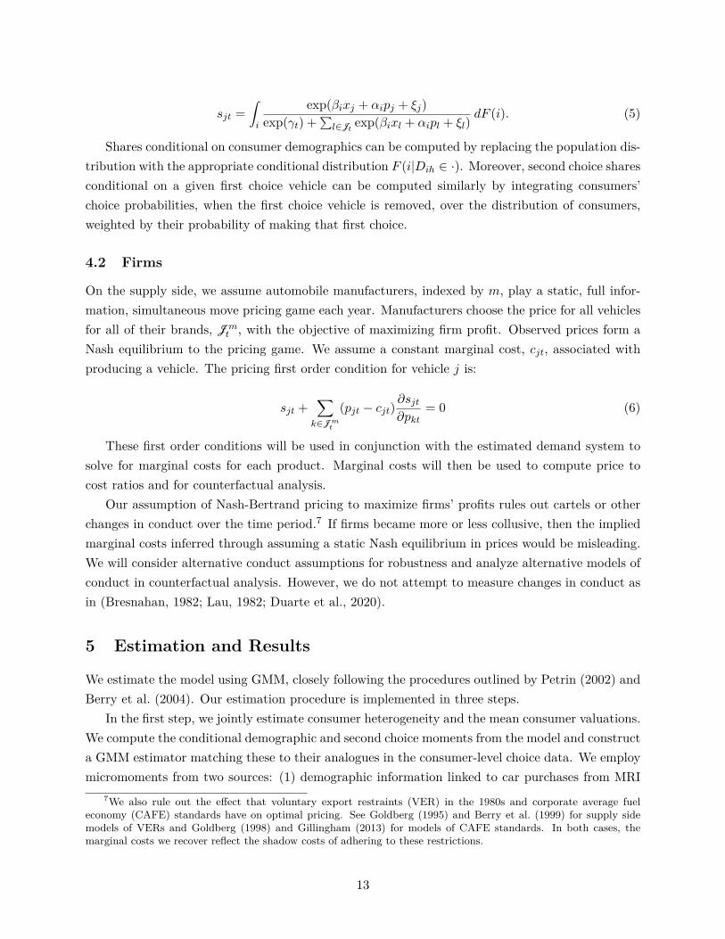
sjt =∫

i

exp(βixj + αipj + ξj)exp(γt) +

∑l∈Jt

exp(βixl + αipl + ξl)dF (i). (5)

Shares conditional on consumer demographics can be computed by replacing the population dis-tribution with the appropriate conditional distribution F (i|Dih ∈ ·). Moreover, second choice sharesconditional on a given first choice vehicle can be computed similarly by integrating consumers’choice probabilities, when the first choice vehicle is removed, over the distribution of consumers,weighted by their probability of making that first choice.

4.2 Firms

On the supply side, we assume automobile manufacturers, indexed by m, play a static, full infor-mation, simultaneous move pricing game each year. Manufacturers choose the price for all vehiclesfor all of their brands, Jm

t , with the objective of maximizing firm profit. Observed prices form aNash equilibrium to the pricing game. We assume a constant marginal cost, cjt, associated withproducing a vehicle. The pricing first order condition for vehicle j is:

sjt +∑

k∈Jmt

(pjt − cjt)∂sjt

∂pkt= 0 (6)

These first order conditions will be used in conjunction with the estimated demand system tosolve for marginal costs for each product. Marginal costs will then be used to compute price tocost ratios and for counterfactual analysis.

Our assumption of Nash-Bertrand pricing to maximize firms’ profits rules out cartels or otherchanges in conduct over the time period.7 If firms became more or less collusive, then the impliedmarginal costs inferred through assuming a static Nash equilibrium in prices would be misleading.We will consider alternative conduct assumptions for robustness and analyze alternative models ofconduct in counterfactual analysis. However, we do not attempt to measure changes in conduct asin (Bresnahan, 1982; Lau, 1982; Duarte et al., 2020).

5 Estimation and Results

We estimate the model using GMM, closely following the procedures outlined by Petrin (2002) andBerry et al. (2004). Our estimation procedure is implemented in three steps.

In the first step, we jointly estimate consumer heterogeneity and the mean consumer valuations.We compute the conditional demographic and second choice moments from the model and constructa GMM estimator matching these to their analogues in the consumer-level choice data. We employmicromoments from two sources: (1) demographic information linked to car purchases from MRI

7We also rule out the effect that voluntary export restraints (VER) in the 1980s and corporate average fueleconomy (CAFE) standards have on optimal pricing. See Goldberg (1995) and Berry et al. (1999) for supply sidemodels of VERs and Goldberg (1998) and Gillingham (2013) for models of CAFE standards. In both cases, themarginal costs we recover reflect the shadow costs of adhering to these restrictions.

13

and CEX and (2) second choice information from the MaritzCX survey. An example of a moment forthe first source is the difference between the observed and predicted average price for each quintileof the income distribution. For the second source, we match the correlations in car characteristicsbetween the purchased and second choice cars.8

In the second step, we estimate α and β and year fixed effects by regressing the estimatedconsumer mean valuations on product characteristics, prices, make dummies, and year dummies.Our assumption that xjt and the real exchange rate are uncorrelated with product-level demandshocks provides the classic moment conditions for 2SLS. The year fixed effects absorb the structuralparameters for annual variation in mean car quality, τt, and preference for outside good, γt.

In the third step we use the empirical analogue of the continuing product condition (2) toseparately estimate τt and γt from the estimated year effects.

The full estimation procedure is described in Appendix A. We compute standard errors using abootstrap procedure. We re-sample the micro data, including the sampled households in the CEXand MRI surveys as well as the MaritzCX survey, and re-estimate the model following the samethree step procedure.

5.1 Parameter Estimates

Table 4 presents parameter estimates for our demand system. In addition to the estimates pre-sented, we also include brand dummies, year dummies, and additional car characteristics that arenot interacted with unobserved or observed heterogeneity. The estimates imply that higher incomeindividuals are less price sensitive for the relevant range of incomes. Also, older households areestimated less price sensitive. Larger household have stronger preferences for vans and vehiclefootprint. Rural households have a stronger preference for trucks.

In general, we estimate large and economically meaningful coefficients representing unobservedheterogeneity, which rationalizes very strong substitution patterns observed in the second-choicedata. The largest random coefficients appear on vehicle style, suggesting consumers substitutemostly within vehicle style. Electric vehicles also have a large estimated random coefficient.

Table 5 summarizes the estimated own price elasticties based on the income of purchasersand how these change over time. In all years, higher income consumers tend to purchase moreprice-inelastic automobiles, consistent with the demographic interactions reported in Table 4. Au-tomobiles have become more elastic over time, despite rising incomes, due to changes in the productset. Our estimates of own-price elasticities for the earlier years in our sample are similar to BLP,Goldberg (1995), and Petrin (2002).

Decomposition of Time Effects

The restriction in equation 2 decomposes the time effects into average improvements in unobservablecar quality and relative movements in the utility of the outside good over time—potentially due to

8See Table 8 for a complete list of micromoments. See Berry et al. (2004) for details of the procedure.

14

Table 4: Coefficient Estimates

Demographic Interactions

β σ Income Inc.2 Age Rural Fam. Size 2 FS 3-4 FS 5+

Price -3.200 – 0.094 -0.464 2.068 – – – –(0.065) (0.009) (0.112) (0.104)

Van -7.292 5.348 – – – – 1.668 3.563 5.653(0.24) (0.102) (0.144) (0.151) (0.202)

SUV -0.083 3.646 – – – – – – –(0.072) (0.064)

Truck -7.533 6.309 – – – 3.009 – – –(0.284) (0.188) (0.313)

Footprint 0.517 1.884 – – – – 0.483 0.463 0.645(0.033) (0.044) (0.045) (0.048) (0.06)

Horsepower 1.094 1.249 – – – – – – –(0.029) (0.123)

Miles/Gal. -0.945 1.636 – – – – – – –(0.053) (0.071)

Luxury – 2.627 – – – – – – –(0.028)

Sport -3.066 2.62 – – – – – – –(0.062) (0.043)

Electric -5.342 3.835 – – – – – – –(0.168) (0.108)

EuroBrand – 1.923 – – – – – – –(0.03)

USBrand – 2.14 – – – – – – –(0.038)

Constant -3.164 – 0.362 – – – – – –(0.095) (0.032)

Height -1.819 – – – – – – – – –0.038

Curbweight 0.432 – – – – – – – – –0.033

No. Trims 1.122 – – – – – – – – –0.029

Yrs Redesign -0.118 – – – – – – – – –0.006

Release Yr. -0.417 – – – – – – – – –0.001

Notes: Brand and year dummies included. Footprint is log vehicle length times height in square inches. Weestimate separate βs for length, height, and width that are not displayed. The number of years since thevehicle has been redesigned, dummy for a new design, and the number of available trims are also included inthe regressions but not shown. Income is normalized to have zero mean and unit variance.

Table 5: Own Price Elasticities by Income Quintile Over Time

Income Quintile

Year 1 2 3 4 5

1980 -5.96 -5.78 -5.49 -5.13 -4.302000 -8.24 -7.83 -7.40 -6.88 -6.212018 -9.37 -8.56 -7.69 -6.90 -6.46

Notes: This table reports the mean own price elasticityacross products individuals conditional on income quintile ofindividuals in each reported year.

15

business cycle factors or changes in the utility of not purchasing a new car.

Figure 4: Quality and Aggregate Components of Time Effects

1980 1985 1990 1995 2000 2005 2010 2015

Year

$-10,000

$0

$10,000

$20,000

$30,000

$40,000Average Unobserved QualityValue of the Outside Good

Notes: Average unobserved quality, τt, and value of outside good, γt, in dollars. See text for estimation details.

Figure 4 displays the results of this decomposition. We find that unobservable vehicle qualityis steadily increasing roughly linearly. The value of the outside option generally increases over thetime period with noticeable deviations from trend during the 1990-1991 and 2007-2009 recessions.Car durability is likely an important aspect for both of these trends. We would expect increasedcar durability to increase the value of a car, and since this is an unobserved component of quality,this effect should appear in our quality adjustment, τ . Between 1980 and 2018, data from theNational Highway Traffic Safety Administration implies that the average time a consumer keeps anew car has risen from 3.9 to 5.9 years, consistent with increasing durability. This is part of theimprovement in unobserved quality captured by our quality adjustment along with improvementsin comfort and electronics. However, as cars become more durable, households will replace themless often, which has an effect of making the outside option appear more attractive. We expect thiseffect to be captured in the aggregate part of the time effect along with business cycle fluctuationsand the desirability of alternative transportation options. These series are broader than durability,however. Other unobserved features of cars include improved safety and electronic features such asrear view cameras and Bluetooth audio systems and improved comforts such as power or heatedseats. The outside option can also be influenced by alternative transportation options such aspublic transport or ride sharing, or changes in the commuting needs of the population.

5.2 Model Fit

We target correlations between the attributes of purchased cars and stated second choices for surveyyears 1991, 1999, 2005, and 2015. The first column of Table 6 presents the average correlationacross years for each attribute we target. These correlations exhibit strong substitution patternsby observable characteristic. As seen in the second column of Table 6, our estimated model is ableto match these moments well. We compare our fit to two models without unobserved heterogeneity.In column 3, we present the implied correlations from the logit model which assumes independence

16

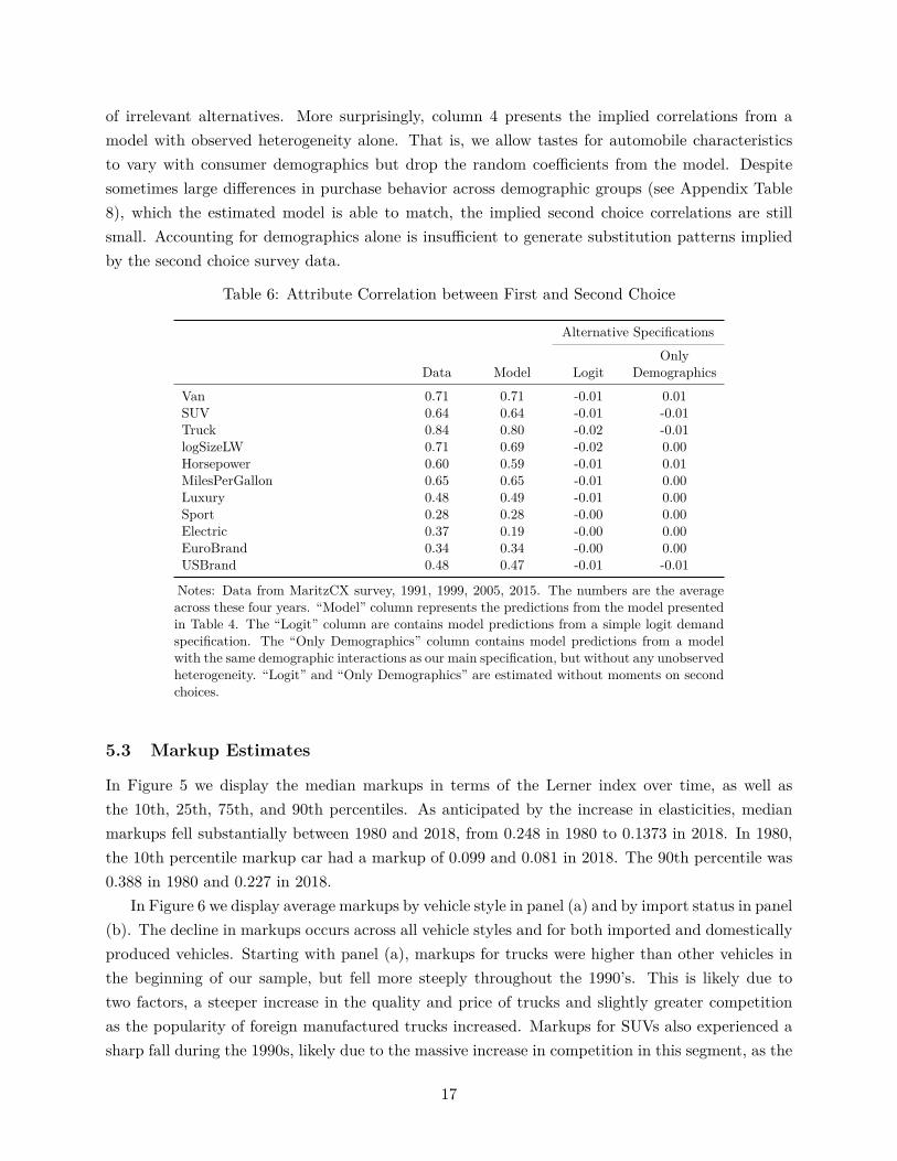
of irrelevant alternatives. More surprisingly, column 4 presents the implied correlations from amodel with observed heterogeneity alone. That is, we allow tastes for automobile characteristicsto vary with consumer demographics but drop the random coefficients from the model. Despitesometimes large differences in purchase behavior across demographic groups (see Appendix Table8), which the estimated model is able to match, the implied second choice correlations are stillsmall. Accounting for demographics alone is insufficient to generate substitution patterns impliedby the second choice survey data.

Table 6: Attribute Correlation between First and Second Choice

Alternative Specifications

OnlyData Model Logit Demographics

Van 0.71 0.71 -0.01 0.01SUV 0.64 0.64 -0.01 -0.01Truck 0.84 0.80 -0.02 -0.01logSizeLW 0.71 0.69 -0.02 0.00Horsepower 0.60 0.59 -0.01 0.01MilesPerGallon 0.65 0.65 -0.01 0.00Luxury 0.48 0.49 -0.01 0.00Sport 0.28 0.28 -0.00 0.00Electric 0.37 0.19 -0.00 0.00EuroBrand 0.34 0.34 -0.00 0.00USBrand 0.48 0.47 -0.01 -0.01

Notes: Data from MaritzCX survey, 1991, 1999, 2005, 2015. The numbers are the averageacross these four years. “Model” column represents the predictions from the model presentedin Table 4. The “Logit” column are contains model predictions from a simple logit demandspecification. The “Only Demographics” column contains model predictions from a modelwith the same demographic interactions as our main specification, but without any unobservedheterogeneity. “Logit” and “Only Demographics” are estimated without moments on secondchoices.

5.3 Markup Estimates

In Figure 5 we display the median markups in terms of the Lerner index over time, as well asthe 10th, 25th, 75th, and 90th percentiles. As anticipated by the increase in elasticities, medianmarkups fell substantially between 1980 and 2018, from 0.248 in 1980 to 0.1373 in 2018. In 1980,the 10th percentile markup car had a markup of 0.099 and 0.081 in 2018. The 90th percentile was0.388 in 1980 and 0.227 in 2018.

In Figure 6 we display average markups by vehicle style in panel (a) and by import status in panel(b). The decline in markups occurs across all vehicle styles and for both imported and domesticallyproduced vehicles. Starting with panel (a), markups for trucks were higher than other vehicles inthe beginning of our sample, but fell more steeply throughout the 1990’s. This is likely due totwo factors, a steeper increase in the quality and price of trucks and slightly greater competitionas the popularity of foreign manufactured trucks increased. Markups for SUVs also experienced asharp fall during the 1990s, likely due to the massive increase in competition in this segment, as the

17

Figure 5: Markups Over Time

1980 1985 1990 1995 2000 2005 2010 2015

Year

0.1

0.2

0.3

0.4

0.5Median

Quartiles

10-90 Deciles

Notes: Estimated markups for the U.S. automobile industry, 1980-2018. Markups expressed as the Lerner index,price-cost margin over price, p−mc

p.

number of SUVs available nearly tripled during this time and our demand estimates imply strongwithin category substitution. Turning to panel (b) in Figure 6, overall, imported vehicles havelower markups than domestically produced vehicles, where our classification is based on country ofproduction, not the headquarter country of the product. However, domestically produced vehiclesexperienced a much greater fall in markups over our sample period.

Figure 6: Markups over Time

1980 1985 1990 1995 2000 2005 2010 2015

Year

0.15

0.2

0.25

0.3

0.35

0.4Car

SUV

Truck

Van

(a) Markups by Vehicle Style

1980 1985 1990 1995 2000 2005 2010 2015

Year

0.15

0.2

0.25

0.3

0.35

0.4Domestic

Import

(b) Markups by Import Status

Note: Median markups across all vehicles. Vehicle style defined in the text. “Domestic” are those cars produced inthe U.S., regardless of brand headquarters.

5.3.1 Explaining the Evolution of Markups

What drives the decline in markups? A key observation to understand the estimated change inmarkups is that the trend is similar if we infer markups assuming single product firms as seen in

18

Figure 7: Markups and Prices

1980 1985 1990 1995 2000 2005 2010 2015

Year

0.15

0.2

0.25

0.3

0.35

0.25

0.3

0.35

0.4

0.45

0.5Baseline Markups

Single-product Markups

1/Price

Notes: Median markups for our baseline model and a model that assumes each product’s price is set independentlyof all other products. “1/Price” is the average price each year.

Figure 7 or assuming industry wide collusion in Figure 8. Therefore, decreases in concentration,although substantial, are not the primary driver in the estimated decrease of markups. In the singleproduct firm case, the Lerner index is equal to the inverse elasticity of the product:

p − mc

p= 1

elas = s

p× 1

dsdp

(7)

At our demand estimates, the only component of the elasticity which changes substantiallyover time are prices. Mechanically, prices are increasing while shares and the derivative of sharewith respect to price are roughly constant. This combination implies that markups decrease. Toillustrate this, we also plot 1/p in Figure 7. It mirrors the trend in both single and multi-productmarkups.

The economic reason why prices are increasing without shares decreasing and without changesin the derivative of share with respect to price is because car quality is increasing. The markup overtime is not a conceptually attractive proxy for welfare when the product set is changing.9 In ourestimates, the change in markups over time is fundamentally related to the change in car quality.We will thus focus on the model’s measures of welfare and surplus over time to assess industryperformance in Section 6.

5.4 Robustness to Conduct Assumption

In this section, we compare markup estimates under alternative assumptions of conduct. To sum-marize the results, while there is great disparity in the level of markups, these alternatives all pointtowards declining markups over the sample period as in the base case of Nash-Bertrand pricing. In

9For a simple example of when markups can be misleading, consider a logit monopolist with u = δ − αp + ε,whose market share is s = exp(δ−αp)

1+exp(δ−αp) . The pricing first order condition is p = c + 1α(1−s) = c + 1

α(1 + exp(δ − αp)).

Suppose the product improves in quality without changing its marginal cost. Totally differentiating the first ordercondition with respect to δ, we find dp

dδ= s

α> 0. Since marginal cost is constant, this implies markups rise. However,

since d(δ−αp)dδ

= 1 − s > 0 consumer surplus also increases.

19

the first case, we assume the Big Three US auto manufacturers (G.M., Ford, and Chrysler) colludeon prices for our entire sample.10 Markups are much higher than our baseline case in the 1980s,but then become closer to our baseline case throughout time. This is consistent with the decline inthe dominance of the Big-3 firms over time. Notably, markups at the end of the sample under theassumption that the Big-3 collude are lower than the Nash-Bertrand markups at the start of thesample. Therefore, under the assumption that the Big-3 were competing in 1980 and organized apricing cartel in response to import competition after 1980, we would still find a decline in markupsbetween 1980 and 2018. In the second case, we consider markups that are implied if all of the firmscolluded on prices. In this case, the level of markups are much higher, however there is still adecrease in markups over time.

Figure 8: Markups: Alternative Conduct Assumptions

1980 1985 1990 1995 2000 2005 2010 2015

Year

0.2

0.3

0.4

0.5

0.6

0.7

0.8

0.9 Baseline

Big 3 Collusion

Monopoly Collusion

Notes: Estimated median markups for Nash Bertrand pricing by parent companies (“Baseline”), the Big 3 U.S.automobile manufacturers colluding for every year in our sample (“Big 3 Collusion”), and joint price setting by everyparent company in our sample (“Monopoly Collusion”).

Figure 8 establishes that under a variety of constant conduct assumptions, markups decline overtime. However, it is possible that cartel could form during our sample period. We now ask howlarge such a cartel would need to be to have held markups constant over the period. To quantifythis, we consider different size cartels in 2018 to measure how many cartel members it would takefor a cartel in 2018 to achieve the baseline non-collusive level of markups found in 1980. Specifically,we form cartels with the largest-by-sales manufacturers, adding one manufacturer at a time. Theresults are in Table 7. One change in conduct from Nash-Bertrand that would produce estimatedincreases in markups would from 1980 would involve a cartel of the six largest parent companies.Overall, it seems that a price-fixing cartel on the scale needed to keep markups at their 1980 levelwould be unlikely to escape the notice of antitrust authorities.

10For Chrysler, we follow the ownership from Chrysler, to Daimler, to Cerebus private equity firm, then to Fiatand assume the owner of Chrysler colludes with all of the ultimate owner’s brands. For example, then the Fiat brandis part of the “cartel” after 2012.

20

Table 7: Average Markups with Different Cartel Assumptions

Average Markup

1980 Baseline 0.311

2018 Baseline 0.196

2018 Cartel MembershipGM + Ford + Toyota 0.222Top 3 + Fiat 0.264Top 4 + Honda 0.290Top 5 + Nissan 0.338

Notes: Computed average markups when we simulate collusion in2018 for various manufacturer cartels. In 2018, Fiat is the parentcompany of Chrysler.

5.5 Comparison to production-based approach

De Loecker et al. (2020) use financial and production data to estimate price to marginal cost ratiosfor a much of the US economy. They estimate a sizeable increase in the sales weighted averageprice to marginal cost ratio over the last several decades. Their approach uses a model of firmproduction and data on input expenditures and output revenue to estimate price over marginalcost ratios.11 De Loecker et al. (2020) report estimates for the US auto industry time series ofaverage price to marginal cost ratio which we compare to our measures in Figure 9a. Both the leveland trends in the price to marginal cost ratio differs from the estimates we derive, though bothseries are relatively flat from 1995 on-wards.

Figure 9: Comparison to De Loecker et al. (2020)

1980 1985 1990 1995 2000 2005 2010 2015

Year

0.8

1

1.2

1.4

1.6

1.8

Rat

io o

f P

rice

to

Mar

gin

al C

ost

(P

/MC

)

Mean Markups

DLEU (2020)

BLP (1995) Estimate

(a) Price over Marginal Cost

1980 1985 1990 1995 2000 2005 2010 2015

Year

$60

$70

$80

$90

$100

$110

$120

To

tal

Var

iab

le P

rofi

ts (

20

15

$ b

illi

on

s

(b) Total Variable Profits

Notes: Panel (a) displays our estimate, the estimate for the U.S. automobile industry from De Loecker et al. (2020),and the average estimate across 1971-1990 from Berry et al. (1995). Panel (b) displays our estimate of total variableprofits, sales multiplied by margins, summed across all products.

There are several possible explanations for the difference in estimates displayed in Figure 9a.The demand and conduct approach employed in this paper could be flawed because the exclusionrestriction for the instrumental variable we employ to estimate demand does not hold, or because

11A number of papers including Traina (2018); Basu (2019); Raval (2020); Demirer (2020) examine the specificassumptions and data requirements used to construct these estimates.

21

the conduct assumption of static Nash pricing does not hold.12 The production based estimatescould be off from the truth because the intermediate inputs observed in their data are not fullyflexible, because of the assumption that firms in their data produce single products, or because theclassification of accounting costs into costs of goods sold versus selling, general, and administrativecosts does not accurately capture the difference between marginal and average costs. Furthermore,the underlying data differ in that the Compustat based estimates in 9a do not capture some foreignbased firms, and production based estimates using Census data would miss models assembledoutside of the US and include commercial truck producers. Finally, the Compustat based estimatesinclude additional revenue streams outside of automobile manufacturing such as any verticallyintegrated parts manufacturing or consumer financing operations. The DLEU series does sharesome patterns with our estimates of total variable profits over time including a an increase in the1980’s, a dip and recovery in the 1990’s, and a dip and recovery around the Great Recession.

While the discrepancy between our estimates of markups is interesting, a full analysis of thedifferences between these approaches is beyond the scope of our study. De Loecker and Scott (2016)examine production and demand approaches for beer and find both approaches find plausibly similarmarkup estimates. Instead, an important advantage of our demand side approach is that it providesa direct measures of consumer surplus which are not available without an estimated demand system.For the remainder of the paper, we will use our approach to go beyond markups and analyze thewelfare trends of the US Auto industry.

6 The Evolution of Welfare

What are the implications of our estimates for assessing the performance of the industry overtime? It may seem natural to evaluate concentration and markups as proxies for welfare, and wedocumented that both concentration and markups have fallen. However, it is well known that therelationship between concentration and welfare is theoretically ambiguous (Demsetz, 1973). Abovewe show that the relationship between markups and welfare is ambiguous if the product set ischanging and that our markup estimates are largely driven by the changing cost and quality ofcars. Therefore, drawing conclusions about welfare by comparing markups or concentration overtime can be misleading because products are improving over time. Instead, this section directlyexamines welfare trends over time.

6.1 Consumer surplus, producer surplus, and deadweight loss over time.

We first define a consumer surplus measure appropriate for our context. Typically, studies usethe compensating variation of the product set relative to only the outside good being available toconsumers. While this approach is straightforward, it is sensitive to changes in the valuation ofthe outside good over time. For example, suppose consumers choose to delay buying cars during amacroeconomic downturn. Then in the down year the value of the outside good, γt will be high—as

12Although, as we note above, the downward trend in markups is robust to a variety of conduct assumptions.

22

more consumers choose not to purchase. Similarly, suppose there is a significant improvement inpublic transit over time, this again is reflected in an increase in γt which will cause a decline inconsumer surplus. It is easy to see that both of these cases will affect the standard consumersurplus measure, even when the quality of automobiles and their prices are held fixed. Since we areinterested in how the industry has served consumers over time, rather than evolution in the outsidegood, we propose an alternative measure of consumer surplus that removes outside good effects.

To make things concrete, consider the compensating variation of a consumer being offered theinside product bundle in year t with the outside good valued at γ relative to receiving only theoption to purchase this hypothetical outside good. Given our model assumptions, this is,

CSt(γ) =∫

i

1αi

log

exp(γ) +∑j∈Jt

exp(βixjt + αipγjt + ξjt)

− γ

dFt(i). (8)

In this calculation, pγt represents the equilibrium vector of prices when firms face an outside good

valued at γ.The traditional consumer surplus measure is simply CSt(γt)—the compensating variation that

would make consumers in year t indifferent between the product bundle they face and only theoutside good from that bundle. However we can also examine how the inside product bundlein year t would have been valued against the the outside good in other years, enabling a directcomparison of product sets across years. Our preferred surplus measure removes the influence ofchanges in the outside good over time by averaging over the outside good across all years in thesample,

CSt = 1T

T∑v=0

CSt(γv).

We can compute producer surplus and deadweight loss measures analogously.13

In Figure 10 we plot estimated consumer surplus (CSt), producer surplus, and deadweightloss over the sample period. Total surplus rises roughly $20, 000 per household, from $5, 000 to alittle over $25, 000. Overall, the market is very efficient, with deadweight loss representing a smallportion of total surplus. This finding is reminiscent of Bresnahan and Reiss (1991) who estimatethat most of the increase in competition comes with the entry of the second and third firms ontheir sample of retailers in multiple industries. The U.S. automobile market typically features fouror more parent companies producing each specific style of vehicle.14

Figure 11 contrasts our preferred welfare measure with the measure that fixes the value of theoutside good at the current year’s estimated value (e.g., CSt(γt)). Figure 11a displays consumersurplus, in 2015 dollars. Under the alternative measure, consumer surplus is relatively flat over theperiod with marked troughs in the early 1980s, early 1990s, and 2009, corresponding to the three

13Deadweight loss is computed by subtracting the sum of estimated consumer and producer surplus from theconsumer surplus calculated when products are priced at marginal cost.

14This can be seen directly from the diversion implied by our demand model. A vehicle’s highest diversion rivalsare typically products offered by other parent companies. On average, of a vehicles 5 closest substitutes, 3.8 areproduced by rival manufacturers, and 7.8 of top 10 substitutes are rivals.

23

Figure 10: Consumer Surplus, Producer Surplus, and Deadweight Loss

Notes: Consumer surplus, producer surplus and deadweight loss. Consumer surplus in the compensating variationprocedure detailed in the text. Deadweight loss is computed by netting consumer and producer surplus form efficientsurplus, defined as the surplus available when prices equal marginal costs. Surplus measured in 2015 dollars.

major economic downturns in our sample period. The difference between these panels is intuitivewhen we consider the significant changes in our estimates of the value of the outside good over time,as shown in Figure 4. Figure 11b plots the share of consumer surplus of total efficient surplus. Wedo this for our baseline measure of consumer surplus, as well as for a measure of consumer surpluswhere we compute the compensating variation to the current year’s outside option. We measuretotal efficient surplus by computing surplus when prices equal marginal costs. Consumers’ shareof available surplus is increasing from 1980 to 2018. For our baseline measure, consumers’ share ofsurplus rising dramatically, from 0.63 to 0.83.

Figure 11: Consumer Surplus Comparison

1980 1985 1990 1995 2000 2005 2010 2015

Year

$0

$5,000

$10,000

$15,000

$20,000

$25,000Baseline consumer surplusCS relative to current year outside good

(a) Consumer Surplus Comparison

1980 1985 1990 1995 2000 2005 2010 2015

Year

0.6

0.65

0.7

0.75

0.8

0.85

Rat

io o

f C

S t

o E

ffic

ien

t S

urp

lus Baseline

CS relative to current year outside good

(b) CS as a Share of Total Available Surplus

Notes: Panel (a) displays consumer surplus computed two ways: the baseline definition described in the text, andconsumer surplus computed as the compensating variation to the current year outside good. Panel (b) displays theratio of consumer surplus to total efficient surplus both way, where efficient surplus is computed as consumer surpluswhen prices equal estimated marginal costs of production, vehicle by vehicle.

24

6.2 Why does consumer surplus rise?

We now investigate the economic primitives driving the increase in consumer surplus over time.There are many plausible reasons for this increase. There has been a significant change in marketstructure; foreign brands now offer a larger proportion of products relative to the 1980s. Thenumber of products available has also increased dramatically which benefits consumers due toincreased variety and strong competition between models. Products have changed in terms ofcharacteristics in numerous ways: Today, SUVs are more popular than sedans, whereas they were anegligible part of the market in 1980. Automobiles are larger, more powerful, more efficient and offergreater comfort and reliability than in the past. Finally, production has become more efficient. Wepropose a series of counterfactuals where we isolate these industry trends and recompute equilibriumoutcomes to determine which are the main drivers of consumer surplus growth.

Figure 12: Consumer Welfare, Alternative Product Ownership

1980 1990 2000 2010 2018

Year

$0

$5,000

$10,000

$15,000

$20,000

$25,000

Consu

mer

Surp

lus

BaselineForeign Brands Owned by Big 3

1980 1990 2000 2010 2018

Year

$0

$5,000

$10,000

$15,000

$20,000

$25,000BaselineBig3 Collusion

1980 1990 2000 2010 2018

Year

$0

$5,000

$10,000

$15,000

$20,000

$25,000BaselineMonopoly Collusion

Notes: Vertical axis represents consumer surplus in 2015 dollars. In the first panel, we simulate the market equilibriumif all vehicles produced by foreign brands were owned by the Big 3 U.S. car manufacturers. In the second panel wesimulate market the equilibrium if the Big 3 jointly set prices. In the third panel we simulate market equilibrium ifall firms jointly set prices.

Mechanism 1: Increased competitive pressure form foreign brands. It is possible thatthe increase in foreign brands competing in the US led to downward pressure on prices that benefitedconsumers.15 To understand this mechanism, we simulate an alternative scenario where we assumeall vehicles sold by foreign brands in our data are, instead, owned by the Big 3 US car manufacturers(General Motors, Ford, and Chrysler), so that these manufacturers internalize the competitivepressure of the increase in foreign-owned products over our time period. To implement this, werandomly assign ownership of foreign brand vehicles to one of the Big 3 firms. We do this ten timesand take an average of the outcomes across the random assignments. Chrysler itself experiencesownership changes, so we track the ultimate owner of the Chrysler brand and treat that companyas a Big 3 firm.

15There is a distinction between foreign brands and imports. Foreign brands are brands owned by parent companiestraditionally headquartered outside of the U.S. Many foreign brands assemble vehicles in the U.S. (not imports) andmany U.S. brands assemble vehicles in other countries and import to the U.S.

25

The results, in terms of consumer surplus, are presented in the left panel of Figure 12. Through-out this section, the sold line in figures corresponds to our baseline consumer surplus, and the dashedline corresponds to a counterfactual. Our estimates indicate that, had foreign brands been ownedby domestic firms, consumer surplus would still have increased substantially. We conclude that thecompetitive pricing pressure from foreign brands did not contribute much to the rise in consumersurplus. Again, this is consistent with competition kicking in with only a few competitors withinclusters of similar products.

We benchmark the result against two alternatives to emphasize this point. In the middle panel,we plot a counterfactual where we assume the Big 3 coordinate pricing for the entire period with-out owning imports, and in the right panel we show a case where all firms enter into a cartel tomaximize joint profits. Only in the the full cartel case is the gain in consumer surplus dampenedsubstantially. In other words, by changing the ownership structure, the model is able to deliver out-comes where consumer surplus does not increase, but the ownership configuration which eliminatesglobal competition does not achieve this.

Figure 13: Consumer Welfare Product Set Counterfactuals

1980 1990 2000 2010 2018

Year

$0

$5,000

$10,000

$15,000

$20,000

$25,000Baseline

1980 Product Count

1980 1990 2000 2010 2018

Year

$0

$5,000

$10,000

$15,000

$20,000

$25,000Baseline

Eliminate SUV

1980 1990 2000 2010 2018

Year

$0

$5,000

$10,000

$15,000

$20,000

$25,000Baseline

1980 X Distribution

Notes: Vertical axis represents consumer surplus in 2015 dollars. In the first panel, we simulate the market equilibriumif we eliminate (randomly) products in every year so that in each year there are 165 products. In the second panel weeliminate all SUVs from our sample and simulate market the equilibrium. In the third panel we make the distributionof physical car attributes in the demand specification (horsepower, MPG, curbweight, footprint, and height) the sameas the 1980 distribution and simulate market equilibrium.

Mechanism 2: Product proliferation. Another reason for the increase in consumer surpluscould be the increase in the number of available products. Consumer welfare can increase with thenumber of products for two reasons. First, consumers like variety. Second, additional products inthe choice set crowds the characteristics space and adds to competitive pressure.

To quantify this mechanism, we simulate an alternate market where we restrict the number ofactive products to be at the 1980 level, 165 available products.16 The results are presented in theleft panel of Figure 13. There is not much gap between the counterfactual consumer surplus andthe estimated baseline path of consumer surplus. This is particularly striking considering that there

16In practice, we randomly select 165 products to be available each year. We do this procedure ten times and takean average of the outcome.

26

were over 314 products in 2018, so the choice set was reduced by more than half. This suggeststhat product proliferation was not a significant driver of the consumer surplus increase.

Mechanism 3: Changing product attributes. We now turn to changes in product charac-teristics. As can be seen in Figure 3, vehicles become more attractive between 1980 and 2018 inobservable characteristics such as efficiency and power, and harder-to-measure characteristics suchas safety, technology, durability, and aesthetic design improvements. Furthermore, the number ofSUV’s available to consumers increased noticeably. In our model, these features are captured inboth observed characteristics and an unobserved vertical quality term, ξ. In the middle and rightpanels of Figure 13, we examine the observable characteristics of vehicles. In the middle panel,we eliminate all SUV’s which enter into the market. SUVs represent a new and popular segmentof the automobile market that was essentially unavailable in 1980. While counterfactual consumersurplus is lower, like the other mechanisms discussed, this channel can only explain a small portionof the increase in consumer surplus.

Another notable trend in the industry has been the general growth in car characteristics suchas size and horsepower. In the right panel, we scale the distribution of horsepower, MPG, andfootprint year-by-year to match the mean and variance of these characteristics in the 1980 choiceset, holding marginal costs of production fixed. Consumers do prefer the choice set available tothem at the end of the period, but this channel as well can not explain much of the increase inconsumer surplus.

However, we do find a large effect due to the improvements in unobservable vehicle quality.In the left panel of Figure 14, we simulate a counterfactual where the unobservable mean vehiclequality is fixed at 1980 levels. Specifically, the rise in ξ is captured by the quality adjustmentterm τ in (2). We set τt = 0 ∀ t. In this case, the counterfactual delivers substantially lowerincreases in consumer surplus between 1980 and 2018. This comparison suggests that a largeportion of the increased surplus enjoyed by consumers is due to improvements to vehicles that areoutside our observed set of characteristics, such as safety features like rear view cameras, reliabilityimprovements, and improved electronics like Bluetooth audio systems.

Mechanism 4: Decreasing costs. We find that marginal costs of producing a car with fixedcharacteristics experiences a steady decline over time. Specifically, we regress the inferred marginalcost at the vehicle-year level on product characteristics and a time trend, and estimate a negativetrend. In the middle panel of Figure 14 we eliminate the downward trend in marginal costs andrecompute adjusted surplus measures. Since the trend is negative, this removes the benefits fromdecreasing marginal costs for a fixed set of product characteristics over time. We find that welfareincreases by about half as much as in the baseline. Thus falling marginal costs are also a significantdriver of the measured increase in consumer surplus.

Finally, in the right panel of Figure 14, we combine the left and middle panel counterfactualsand simulate a world where neither the unobservable product quality increases nor do marginal

27

Figure 14: Consumer Welfare Unobservable Quality and Marginal Cost Counterfactuals

1980 1990 2000 2010 2018

Year

$0

$5,000

$10,000

$15,000

$20,000

$25,000BaselineNo Change in Unobserved Quality

1980 1990 2000 2010 2018

Year

$0

$5,000

$10,000

$15,000

$20,000

$25,000BaselineNo MC Improvements

1980 1990 2000 2010 2018

Year

$0

$5,000

$10,000

$15,000

$20,000

$25,000BaselineNo Quality or MC Improvements

Notes: Vertical axis represents consumer surplus in 2015 dollars. In the first panel, we simulate the market equilibriumif we eliminate the adjustment to unobserved product quality, τ from equation X. In the second panel we eliminate alltrend in marginal cost efficiency improvements and simulate market the equilibrium. In the third panel we eliminateτ and the trend in marginal costs efficiency.

costs fall by the time trend. This combination almost entirely eliminates the measured increasedin consumer surplus.

7 Conclusion

Antitrust policy has come under scrutiny in the US in recent years. Critics argue that weak an-titrust enforcement from the 1980’s onward has led to an increasingly tight grip of large firms overproduct markets to the detriment of consumers. In this paper, we focus on the new automobilemarket over the last forty years. Employing a supply and demand industry oligopoly model withdetailed microdata, we find that concentration has decreased, markups have decreased (in con-trast to findings in studies estimating markups using accounting data), and consumer welfare hasincreased. The fraction of efficient surplus accruing to consumers has also increased.

We attribute the increase in consumer surplus primarily to increasing product quality anddecreasing marginal costs. Specifically, we find that unobservable attributes- those that are notmeasured by specifications such as size, horsepower, and fuel efficiency- have increased significantly.These attributes include characteristics like safety, reliability, comfort, and improved electronics.We find that competition was healthy enough that benefits from these improvements mostly accruedmostly to consumers. However, our simulations indicate that had competition been significantlyweaker, for example under a monopoly, then consumer benefits would have been offset throughhigher prices.

Our analysis makes a number of important assumptions. We assume a model of firm conductto infer marginal costs. Testing different models of firm conduct to detect changes over time wouldbe a useful direction for future research. We do not analyze adjacent markets such as the marketfor financing or the value chain between suppliers, manufacturers, and dealerships. Profits and firmbehavior in these markets are linked and could be offsetting the changes we measure here. Finally,

28

we largely abstract away from the used car market except as it appears in a time-varying outsideoption for consumers in our model. More detailed modelling of the joint dynamics of new and usedcars could lead to more precise measurements of consumer welfare.

Most importantly, to speak to the broader question of the performance of antitrust and industryregulation, more long term studies of specific industries are necessary. While broad based studiesusing accounting or production data are important and attractive due to their feasibility, specificindustry studies are useful to validate measurements. Furthermore, as proxies for welfare such asconcentration or markups can be misleading in an environment where products are improving overtime, specific industry studies often lend themselves to direct welfare calculations thereby avoidingthe use of proxy measurements.

29

References

Autor, D., D. Dorn, L. F. Katz, C. Patterson, and J. Van Reenen (2020, 02). The Fall of the LaborShare and the Rise of Superstar Firms*. The Quarterly Journal of Economics 135 (2), 645–709.

Basu, S. (2019). Are price-cost markups rising in the united states? a discussion of the evidence.Journal of Economic Perspectives 33 (3), 3–22.

Berndt, E. R. and N. J. Rappaport (2001). Price and quality of desktop and mobile personalcomputers: A quarter-century historical overview. American Economic Review 91 (2), 268–273.

Berry, S. and P. Jia (2010). Tracing the woes: An empirical analysis of the airline industry.American Economic Journal: Microeconomics 2 (3), 1–43.

Berry, S., J. Levinsohn, and A. Pakes (1995). Automobile prices in market equilibrium. Economet-rica: Journal of the Econometric Society, 841–890.

Berry, S., J. Levinsohn, and A. Pakes (1999). Voluntary export restraints on automobiles: Evalu-ating a trade policy. American Economic Review 89 (3), 400–430.

Berry, S., J. Levinsohn, and A. Pakes (2004). Differentiated products demand systems from acombination of micro and macro data: The new car market. Journal of Political Economy 112 (1),68–105.

Berry, S. T. (1994). Estimating discrete-choice models of product differentiation. The RANDJournal of Economics, 242–262.

Bordley, R. F. (1993). Estimating automotive elasticities from segment elasticities and firstchoice/second choice data. The Review of Economics and Statistics, 455–462.

Borenstein, S. (2011). What happened to airline market power? University of California BerkeleyHaas School of Business working paper .

Brand, J. (2020). Differences in differentiation: Rising variety and markups in retail food stores.Available at SSRN 3712513 .

Bresnahan, T. F. (1982). The oligopoly solution concept is identified. Economics Letters 10 (1-2),87–92.

Bresnahan, T. F. and P. C. Reiss (1991). Entry and competition in concentrated markets. Journalof political economy 99 (5), 977–1009.

Burstein, A. and G. Gopinath (2014). International prices and exchange rates. In Handbook ofinternational economics, Volume 4, pp. 391–451. Elsevier.

Covarrubias, M., G. Gutiérrez, and T. Philippon (2020). From good to bad concentration? usindustries over the past 30 years. NBER Macroeconomics Annual 34 (1), 1–46.

30

De Loecker, J., J. Eeckhout, and G. Unger (2020). The rise of market power and the macroeconomicimplications. The Quarterly Journal of Economics 135 (2), 561–644.

De Loecker, J. and P. T. Scott (2016). Estimating market power evidence from the us brewingindustry. Technical report, National Bureau of Economic Research.

Demirer, M. (2020). Production function estimation with factor-augmenting technology: An ap-plication to markups. Technical report, MIT working paper.

Demsetz, H. (1973). Industry Structure , Market Rivalry , and Public Policy. Journal of Law andEconomics 16 (1), 1–9.

Duarte, M., L. Magnolfi, and C. Sullivan (2020). Testing firm conduct.

Economist, T. (2016). Corporate concentration: the creep of consolidation across america’s corpo-rate landscape. Technical report.

Feenstra, R. C., R. Inklaar, and M. P. Timmer (2015). The next generation of the penn worldtable. American Economic Review 105 (10), 3150–82.

Gillingham, K. (2013). The economics of fuel economy standards versus feebates. Manuscript: YaleUniversity.

Goldberg, L. S. and J. M. Campa (2010). The sensitivity of the cpi to exchange rates: Distributionmargins, imported inputs, and trade exposure. The Review of Economics and Statistics 92 (2),392–407.

Goldberg, P. K. (1995). Product differentiation and oligopoly in international markets: The caseof the us automobile industry. Econometrica: Journal of the Econometric Society, 891–951.

Goldberg, P. K. (1998). The effects of the corporate average fuel economy standards in the us.Journal of Industrial Economics 46 (1), 1–33.

Goldberg, P. K. and F. Verboven (2001). The evolution of price dispersion in the european carmarket. The Review of Economic Studies 68 (4), 811–848.

Hashmi, A. R. and J. V. Biesebroeck (2016). The relationship between market structure andinnovation in industry equilibrium: a case study of the global automobile industry. Review ofEconomics and Statistics 98 (1), 192–208.

Knittel, C. R. (2011). Automobiles on steroids: Product attribute trade-offs and technologicalprogress in the automobile sector. American Economic Review 101 (7), 3368–99.

Lau, L. J. (1982). On identifying the degree of competitiveness from industry price and outputdata. Economics Letters 10 (1-2), 93–99.

Leard, B. (2019). Estimating consumer substitution between new and used passenger vehicles.

31

Leard, B., J. Linn, and Y. Zhou (2017). How much do consumers value fuel economy and perfor-mance. Evidence from technology adoption. Resources for the Future Report, 1–37.

Pakes, A., S. Berry, and J. A. Levinsohn (1993a). Applications and limitations of some recentadvances in empirical industrial organization: Price indexes and the analysis of environmentalchange. The American Economic Review 83 (2), 240–246.

Pakes, A., S. Berry, and J. A. Levinsohn (1993b). Applications and limitations of some recentadvances in empirical industrial organization: price indexes and the analysis of environmentalchange. The American Economic Review 83 (2), 240–246.

Pakes, A. and D. Pollard (1989). Simulation and the aymptotics of optimization estimators. Econo-metrica 57 (5), 1027–1057.

Petrin, A. (2002). Quantifying the benefits of new products: The case of the minivan. Journal ofPolitical Economy 110 (4), 705–729.

Raval, D. (2020). Testing the production approach to markup estimation. Available at SSRN3324849 .

Traina, J. (2018). Is aggregate market power increasing? production trends using financial state-ments. Production Trends Using Financial Statements (February 8, 2018).

32

A Demand Estimation Procedure

A.1 Unobserved Heterogeneity and Mean Valuation

Following Berry et al. (1995) we can decompose a consumer utility net of taste for the outside goodinto a vertical component δjt and horizontal components,17

uijt − γt = δjt + µijt(θ) + εijt.

Where the vertical component is

δjt = βxjt + αpjt + ξjt − γt (9)

and the heterogeneity term is

µijt(θ) =∑

k

∑h

βkhxkjtDih +

∑h

αhpjDih +∑

k

σkxkjtνik, (10)

where xkjt is the kth element of xjt and we collect the heterogeneity parameters into the vector

θ = ({βkh}, {αh}, σ).Our goal in this step is to estimate (θ, δ). For any consumer i, the conditional choice probability

as a function of parameters is

sij(θ, δ) = exp (δjt + µijt(θ))1 +

∑k∈Jt

exp (δkt + µikt(θ)) . (11)

Integrating these choice probabilities over the distribution of consumers gives us the market shares.Since there is a one-to-one mapping between δ and market shares, we can solve for mean valuationsas a function of θ by matching model predicted shares to the market share data,

sjt =∫

sij(θ, δ(θ))dFt(i).

We can now construct the moments for our estimator of θ. Let sij(θ) = sij(θ, δ(θ)). Forreadability, we drop t from the notation from the rest of this section and let yi be the observedpurchase of consumer i

Our first set of moments rely on micro-data where we observe consumers’ automobile choice aswell as their demographic characteristics, so we observe a random sample {yi, Di}. We use thisinformation to match product characteristics conditional on consumer demographics. Specifically,

17In this stage of estimation, it is convenient to re-normalize utility to be net of the outside good in year t, so thatγt is a term in δjt. We will show how to estimate γt below.

33

we construct moments of the form18

g1(θ) = E[xyi |i ∈ H] −∫ ∑

j

xjsij(θ) dF (i|i ∈ H), (12)

where H describes a set of consumers identifiable based on demographics and E[x(yi)|i ∈ H] isan estimate from the micro-data. In practice, we match differences and ratios of g1(θ) acrossalternative demographic sets. Table 8 lists the demographic moments we target and the associatedmodel fit.

Our second set of moments relies on micro-data for which we observe the consumers first andsecond choices of products. That is, the data is a random sample {yi, zi}, where zi is the statedsecond choice of consumer i. Conditional on purchasing an automobile, our model predicts the firstand second choices of consumer i,19

si(j,k)(θ) = exp (δj(θ) + µij(θ))∑`∈J exp (δ` + µi`(θ)) · exp (δk(θ) + µik(θ))∑

`∈J\j exp (δ` + µi`(θ)) . (13)

We construct moments based on the correlation of product characteristics of first and second choices,

g2(θ) = E[xyi ◦ xzi ] −∫ ∑

j,k

(xj ◦ xk)si(j,k)(θ)dF (i) (14)

where ◦ denotes element-wise multiplication and E[xyi ◦ xzi ] is an estimate based on the micro-data.Table 6 displays the second choice correlations we target and the model fit.

We stack these two sets of moments and estimate θ via simulated GMM. We use a weightmatrix based on the inverse variance matrix of the data moments. Simulation over the distributionof consumers follows Pakes and Pollard (1989). Given θ, our estimate of mean valuations is δ = δ(θ).

A.2 Mean Taste for Characteristics

With the estimates of mean valuations from the previous step, we can now estimate mean tastesfor product characteristics. We use the following regression equation,

δjt = βxjt + αpjt + ιt + ξjt, (15)

where ιt = τt − γt absorbs the effect of the average utility of the outside good and the averagecar quality in year t. We use our first stage estimate δ as a proxy for δ and employ a simple (IV)regression where the real exchange rate is our instrument for price.

18In practice, we condition this moment on purchasing an automobile, since the outside good does not havecharacteristics. An exception to this is that we do include one moment based on purchase probabilities in order toestimate a demographic coefficient on the constant.

19Our second choice data does not include information on outside good selection, so we again condition out theno purchase option when constructing second choice moments.

34

Table 8: Moments and Model Fit

CEX MRIData Model Data Model

x = Price ($10k)

E[x|Income Q5] − E[x|Income Q1] 0.60 0.40 0.22 0.38E[x|Income Q4] − E[x|Income Q1] 0.36 0.27 0.02 0.23E[x|Income Q3] − E[x|Income Q1] 0.19 0.15 -0.08 0.13E[x|Income Q2] − E[x|Income Q1] 0.07 0.08 -0.15 0.07E[x|Age > 60] − E[x|Age < 30] 0.26 0.34 0.52 0.37E[x|Age50 − 60] − E[x|Age < 30] 0.24 0.29 0.39 0.34E[x|Age40 − 50] − E[x|Age < 30] 0.27 0.24 0.33 0.29E[x|Age30 − 40] − E[x|Age < 30] 0.27 0.14 0.27 0.15

x = Van

E[x|Family = 2] − E[x|Family = 1] 0.02 0.02 0.03 0.02E[x|Family = 3/4] − E[x|Family = 1] 0.06 0.06 0.06 0.06E[x|Family = 5+] − E[x|Family = 1] 0.12 0.12 0.13 0.13

x = Car Size (length X width, log inches)

E[x|Family = 2] − E[x|Family = 1] 0.03 0.03 0.04 0.03E[x|Family = 3/4] − E[x|Family = 1] 0.03 0.02 0.02 0.02E[x|Family = 5+] − E[x|Family = 1] 0.04 0.04 0.03 0.03

x = Truck

E[x|Rural] − E[x|NotRural] – – -0.10 -0.10

x = Purchase Probability

E[x|Income Q2] /E[x|Income Q1] 2.27 1.66 – –E[x|Income Q3] /E[x|Income Q1] 3.64 2.71 – –E[x|Income Q4] /E[x|Income Q1] 5.47 5.08 – –E[x|Income Q5] /E[x|Income Q1] 7.81 9.24 – –

Notes: Moments from the consumer samples that we target in estimation, along with theanalog from our model at the estimated parameters. For the demographic moments, our datacomes from two surveys, the Consumer Expenditure Survey (CEX) covering years 1980-2005and MRI covering years 1992-2018.

A.3 Mean Quality over Time

Our final step estimates τ and γ separately using the continuing product condition (2). Theempirical analogue of this condition can be rewritten as an estimator of τt using the residuals fromour second step,

τt = τt−1 +∑

j∈Ct

( ˆξjt−1 − ˆξjt), (16)

with τ0 normalized to 0. Finally, we can estimate γt = ιt − τt.

35