The Evolution of Lead-lag ENSO-Indian Monsoon Relationship in GCM Experiments Center for Ocean-Land-Atmosphere studies George Mason University Emilia K.

The Evolution of Lead-lag ENSO-Indian Monsoon

Relationship in GCM Experiments

Center for Ocean-Land-Atmosphere studiesCenter for Ocean-Land-Atmosphere studiesGeorge Mason UniversityGeorge Mason University

Emilia K. Jin Emilia K. Jin andand James L. Kinter IIIJames L. Kinter III

4th International CLIVAR Climate of the 20th Century Workshop13-15th March 2007, Hadley Centre for Climate Change, Exeter, UK

International Climate of the Twentieth Century Project

Background and ObjectivesBackground and Objectives

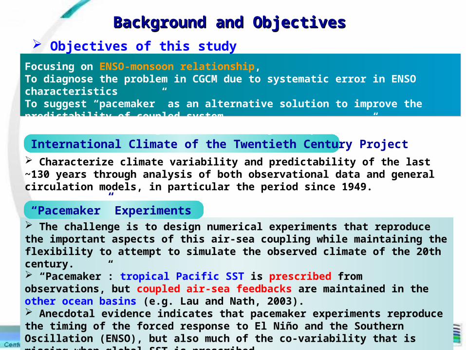
Characterize climate variability and predictability of the last ~130 years through analysis of both observational data and general circulation models, in particular the period since 1949.

The challenge is to design numerical experiments that reproduce the important aspects of this air-sea coupling while maintaining the flexibility to attempt to simulate the observed climate of the 20th century. “Pacemaker”: tropical Pacific SST is prescribed from observations, but coupled air-sea feedbacks are maintained in the other ocean basins (e.g. Lau and Nath, 2003). Anecdotal evidence indicates that pacemaker experiments reproduce the timing of the forced response to El Niño and the Southern Oscillation (ENSO), but also much of the co-variability that is missing when global SST is prescribed.

Objectives of this study

Focusing on ENSO-monsoon relationship,To diagnose the problem in CGCM due to systematic error in ENSO characteristicsTo suggest “pacemaker” as an alternative solution to improve the predictability of coupled systemTo assess the advantages and shortcomings in “pacemaker” results

“Pacemaker” Experiments

The Evolution of Lead-lag ENSO-Monsoon Relationship in GCM Experiments

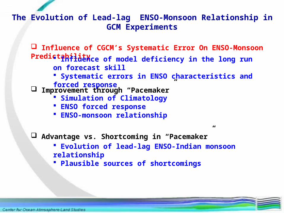
Influence of CGCM’s Systematic Error On ENSO-Monsoon Predictability

Improvement through “Pacemaker”

Advantage vs. Shortcoming in “Pacemaker”

Influence of model deficiency in the long run on forecast skill Systematic errors in ENSO characteristics and forced response

Simulation of Climatology ENSO forced response ENSO-monsoon relationship

Evolution of lead-lag ENSO-Indian monsoon relationship Plausible sources of shortcomings

Retrospective forecast

Model and Experimental DesignModel and Experimental Design

Leadmonth Run Period

Initial Condition

Atm Ocean

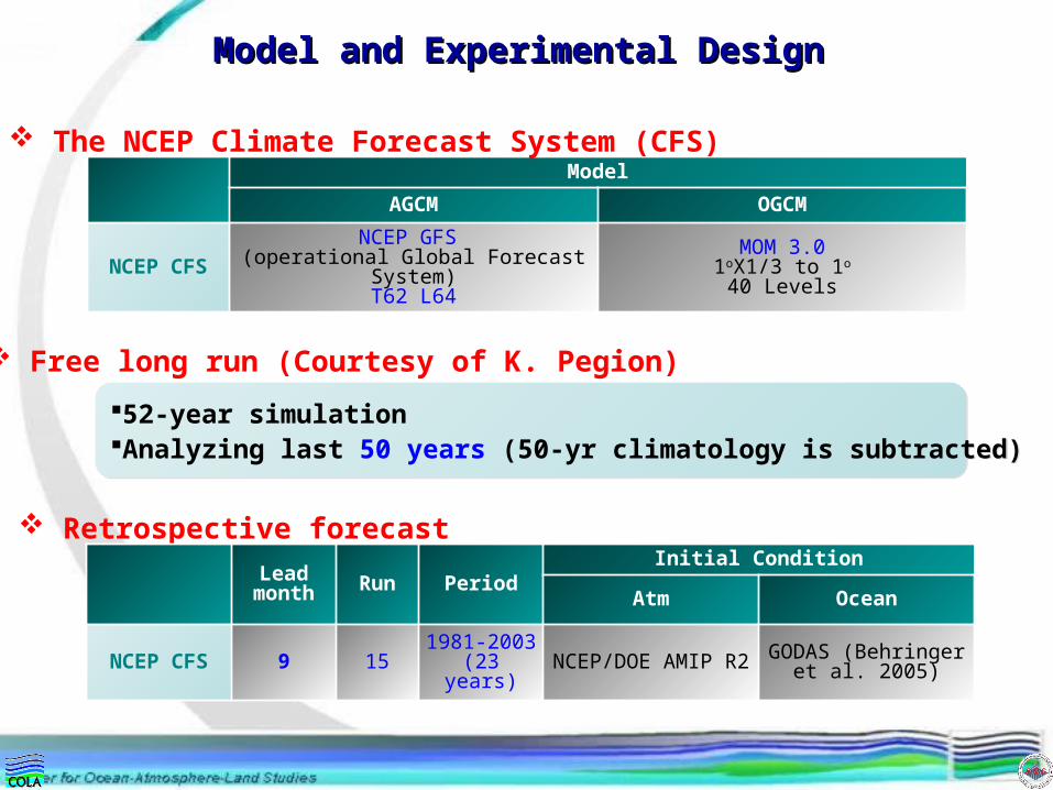
NCEP CFS 9 15 1981-2003(23 years) NCEP/DOE AMIP R2 GODAS (Behringer et

al. 2005)

Model

AGCM OGCM

NCEP CFSNCEP GFS

(operational Global Forecast System)T62 L64

MOM 3.01oX1/3 to 1o

40 Levels

The NCEP Climate Forecast System (CFS)

Free long run (Courtesy of K. Pegion)

52-year simulationAnalyzing last 50 years (50-yr climatology is subtracted)

52-year simulationAnalyzing last 50 years (50-yr climatology is subtracted)

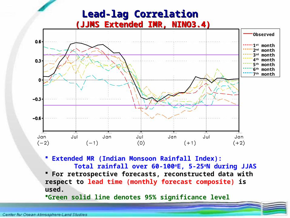
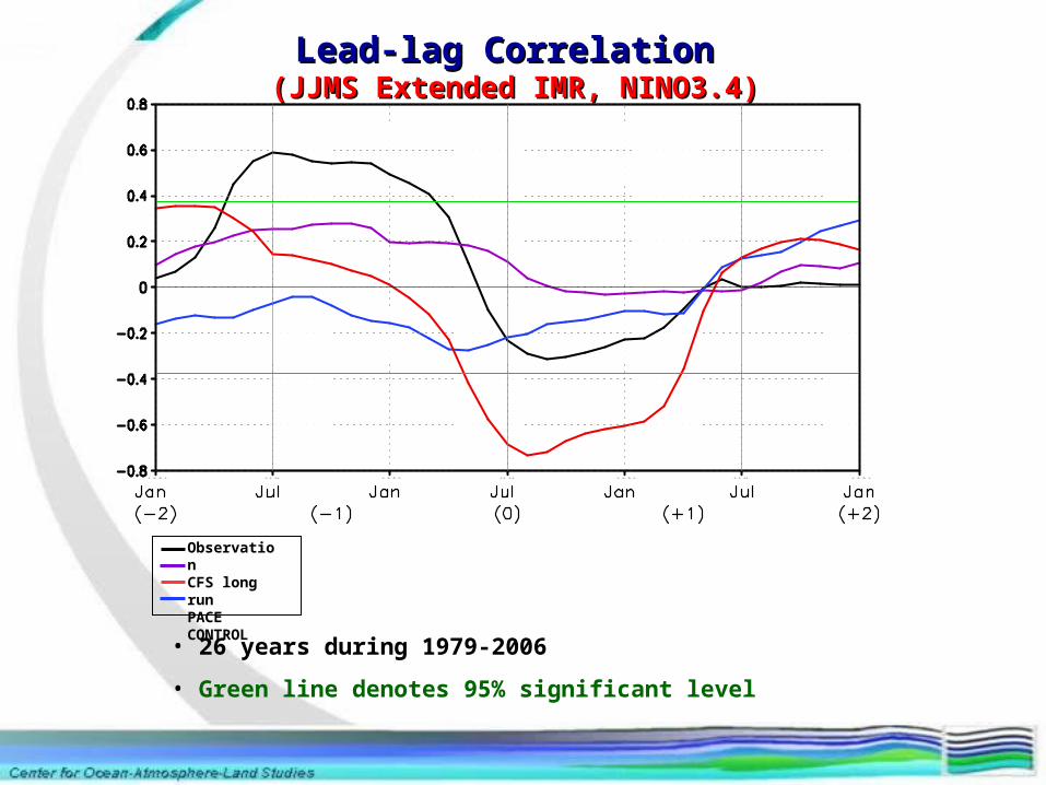
Lead-lag Correlation Lead-lag Correlation (JJMS Extended IMR, NINO3.4)(JJMS Extended IMR, NINO3.4)

Extended MR (Indian Monsoon Rainfall Index): Total rainfall over 60-100oE, 5-25oN during JJAS

For retrospective forecasts, reconstructed data with respect to lead time (monthly forecast composite) is used. Green solid line denotes 95% significance level

1st month2nd month3rd month4th month5th month6th month7th month

Observed

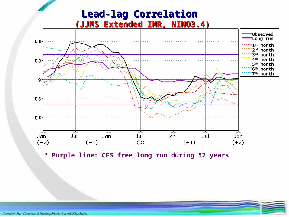
Lead-lag Correlation Lead-lag Correlation (JJMS Extended IMR, NINO3.4)(JJMS Extended IMR, NINO3.4)

Purple line: CFS free long run during 52 years

1st month2nd month3rd month4th month5th month6th month7th month

ObservedLong run

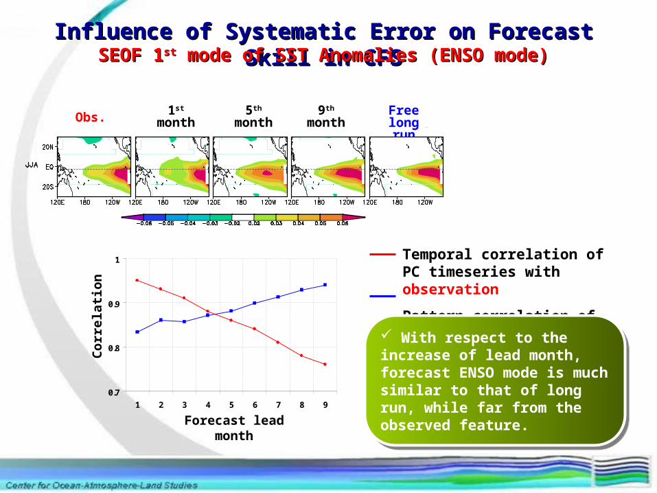
Temporal correlation of PC timeseries with observation

Pattern correlation of eigenvector with free long run

0.7

0.8

0.9

1

1 2 3 4 5 6 7 8 9

Forecast lead month

Co

rrel

atio

n

Influence of Systematic Error on Forecast Skill in CFSInfluence of Systematic Error on Forecast Skill in CFSSEOF 1SEOF 1stst mode of SST Anomalies (ENSO mode) mode of SST Anomalies (ENSO mode)

Obs. Free long run

1st month

9th

month5th

month

With respect to the increase of lead month, forecast ENSO mode is much similar to that of long run, while far from the observed feature.

With respect to the increase of lead month, forecast ENSO mode is much similar to that of long run, while far from the observed feature.

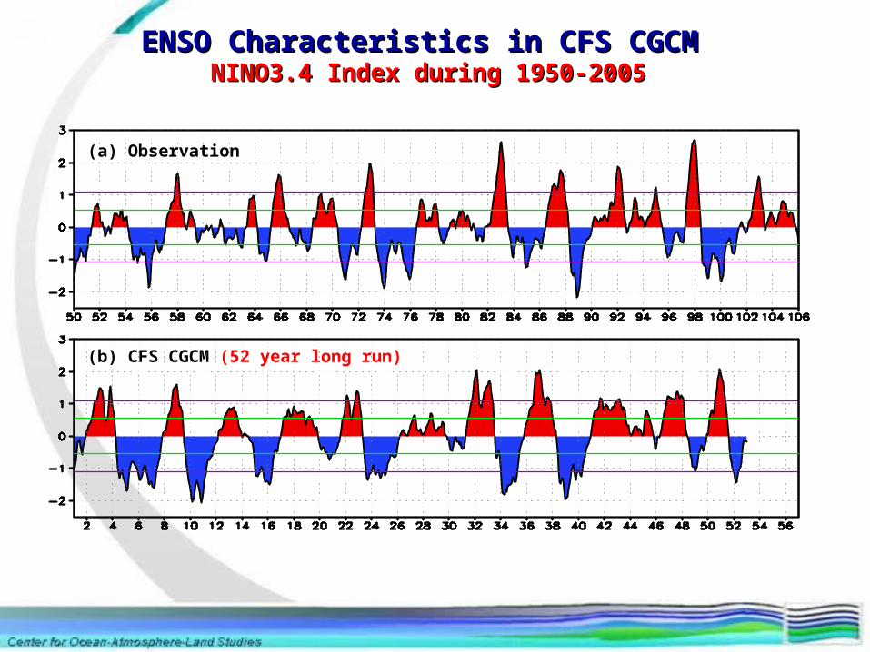
(a) Observation

(b) CFS CGCM (52 year long run)

ENSO Characteristics in CFS CGCM ENSO Characteristics in CFS CGCM NINO3.4 Index during 1950-2005NINO3.4 Index during 1950-2005

Calendar MonthS

ST

an

om

alie

s

Cal

en

dar

Mo

nth

Longitude

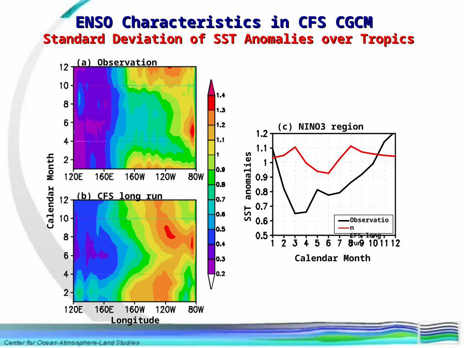
ObservationCFS long run

(a) Observation

(b) CFS long run

(c) NINO3 region

ENSO Characteristics in CFS CGCM ENSO Characteristics in CFS CGCM Standard Deviation of SST Anomalies over TropicsStandard Deviation of SST Anomalies over Tropics

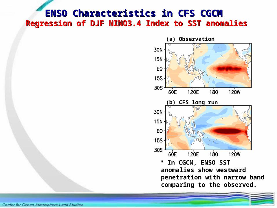
Regression of DJF NINO3.4 Index to SST anomaliesRegression of DJF NINO3.4 Index to SST anomalies

(a) Observation

(b) CFS long run

ENSO Characteristics in CFS CGCM ENSO Characteristics in CFS CGCM

In CGCM, ENSO SST anomalies show westward penetration with narrow band comparing to the observed.

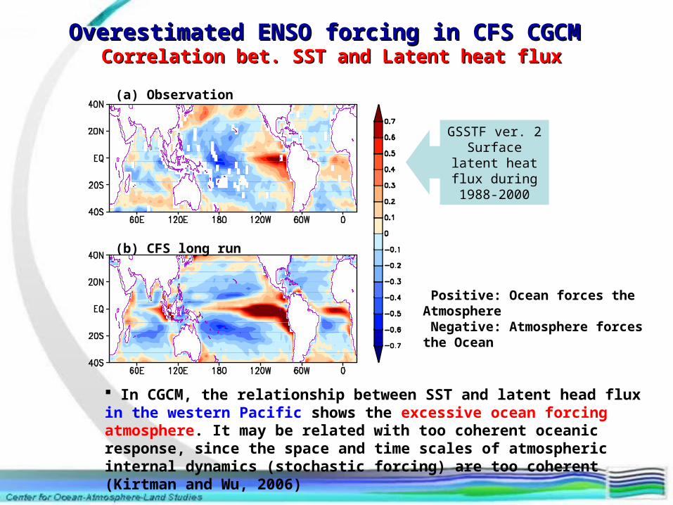
Overestimated ENSO forcing in CFS CGCM Overestimated ENSO forcing in CFS CGCM Correlation bet. SST and Latent heat fluxCorrelation bet. SST and Latent heat flux

GSSTF ver. 2 Surface latent

heat flux during 1988-2000

(a) Observation

(b) CFS long run

In CGCM, the relationship between SST and latent head flux in the western Pacific shows the excessive ocean forcing atmosphere. It may be related with too coherent oceanic response, since the space and time scales of atmospheric internal dynamics (stochastic forcing) are too coherent (Kirtman and Wu, 2006)

Positive: Ocean forces the Atmosphere Negative: Atmosphere forces the Ocean

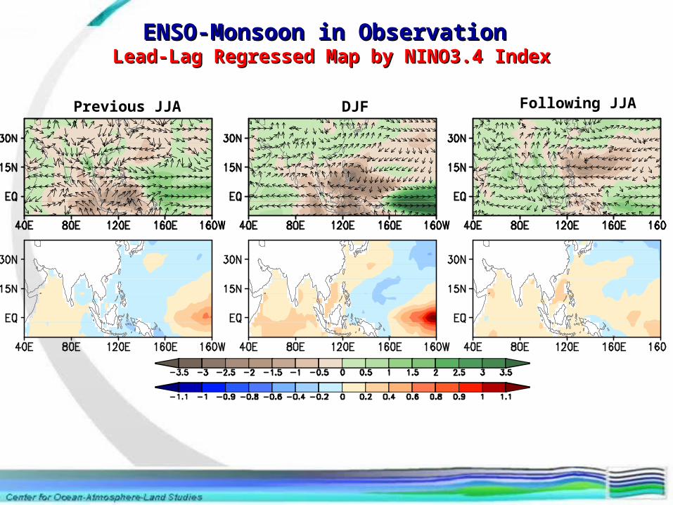
Previous JJA Following JJADJF

ENSO-Monsoon in Observation ENSO-Monsoon in Observation Lead-Lag Regressed Map by NINO3.4 IndexLead-Lag Regressed Map by NINO3.4 Index

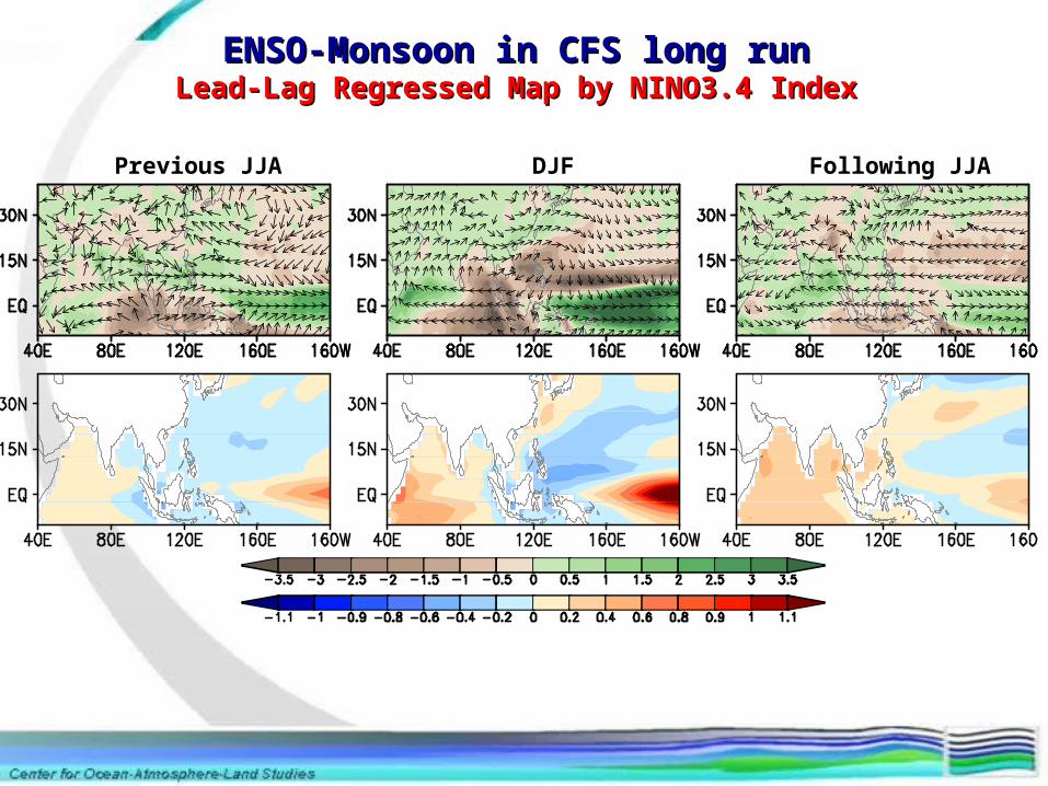
ENSO-Monsoon in CFS long runENSO-Monsoon in CFS long runLead-Lag Regressed Map by NINO3.4 IndexLead-Lag Regressed Map by NINO3.4 Index

Previous JJA Following JJADJF

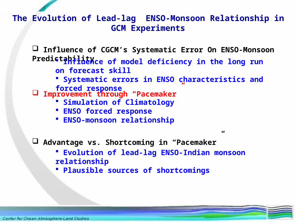
The Evolution of Lead-lag ENSO-Monsoon Relationship in GCM Experiments

Influence of CGCM’s Systematic Error On ENSO-Monsoon Predictability

Improvement through “Pacemaker”

Advantage vs. Shortcoming in “Pacemaker”

Influence of model deficiency in the long run on forecast skill Systematic errors in ENSO characteristics and forced response

Simulation of Climatology ENSO forced response ENSO-monsoon relationship

Evolution of lead-lag ENSO-Indian monsoon relationship Plausible sources of shortcomings

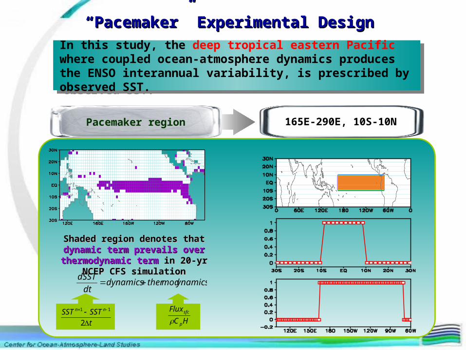
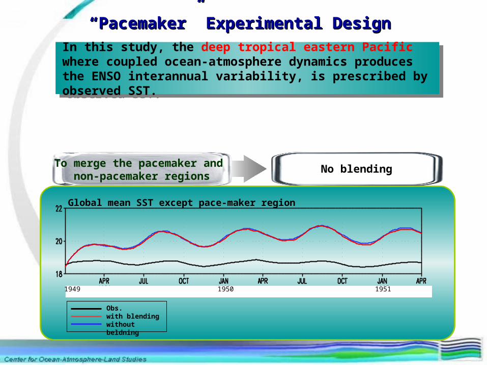
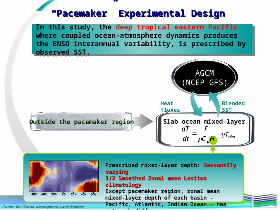
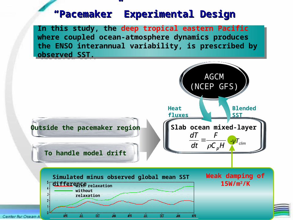
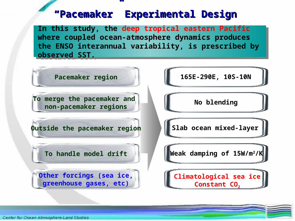
In this study, the deep tropical eastern Pacific where coupled ocean-atmosphere dynamics produces the ENSO interannual variability, is prescribed by observed SST.

In this study, the deep tropical eastern Pacific where coupled ocean-atmosphere dynamics produces the ENSO interannual variability, is prescribed by observed SST.

““Pacemaker” Experimental DesignPacemaker” Experimental Design

Pacemaker region

Outside the pacemaker region

To handle model drift

To merge the pacemaker and non-pacemaker regions

Other forcings (sea ice, greenhouse gases, etc)

In this study, the deep tropical eastern Pacific where coupled ocean-atmosphere dynamics produces the ENSO interannual variability, is prescribed by observed SST.

In this study, the deep tropical eastern Pacific where coupled ocean-atmosphere dynamics produces the ENSO interannual variability, is prescribed by observed SST.

““Pacemaker” Experimental DesignPacemaker” Experimental Design

Pacemaker region 165E-290E, 10S-10N

Shaded region denotes that Shaded region denotes that dynamic dynamic term prevails over thermodynamic term prevails over thermodynamic termterm in 20-yr NCEP CFS simulation in 20-yr NCEP CFS simulation

ynamicsmodtherdynamicsdt

dSST

HC

Flux

p

sfc

t

SSTSST nn

2

11

In this study, the deep tropical eastern Pacific where coupled ocean-atmosphere dynamics produces the ENSO interannual variability, is prescribed by observed SST.

In this study, the deep tropical eastern Pacific where coupled ocean-atmosphere dynamics produces the ENSO interannual variability, is prescribed by observed SST.

““Pacemaker” Experimental DesignPacemaker” Experimental Design

To merge the pacemaker and non-pacemaker regions

No blending

1949 1950 1951

Obs.with blending without beldning

Global mean SST except pace-maker region

In this study, the deep tropical eastern Pacific where coupled ocean-atmosphere dynamics produces the ENSO interannual variability, is prescribed by observed SST.

In this study, the deep tropical eastern Pacific where coupled ocean-atmosphere dynamics produces the ENSO interannual variability, is prescribed by observed SST.

““Pacemaker” Experimental DesignPacemaker” Experimental Design

Outside the pacemaker region Slab ocean mixed-layer

HC

F

dt

dT

p -γTclim

AGCMAGCM(NCEP GFS)(NCEP GFS)

Heat fluxes Blended SST

Prescribed mixed-layer depth: Prescribed mixed-layer depth: Seasonally varyingSeasonally varying1/3 Smoothed Zonal mean Levitus climatology1/3 Smoothed Zonal mean Levitus climatologyExcept pacemaker region, zonal mean mixed-layer Except pacemaker region, zonal mean mixed-layer depth of each basin - Pacific, Atlantic, Indian depth of each basin - Pacific, Atlantic, Indian Ocean - has not much differencesOcean - has not much differences

HC

F

dt

dT

p

In this study, the deep tropical eastern Pacific where coupled ocean-atmosphere dynamics produces the ENSO interannual variability, is prescribed by observed SST.

In this study, the deep tropical eastern Pacific where coupled ocean-atmosphere dynamics produces the ENSO interannual variability, is prescribed by observed SST.

““Pacemaker” Experimental DesignPacemaker” Experimental Design

Outside the pacemaker region Slab ocean mixed-layer

HC

F

dt

dT

p

AGCMAGCM(NCEP GFS)(NCEP GFS)

Heat fluxes Blended SST

HC

F

dt

dT

p

To handle model drift

Weak damping of 15W/m2/Kwith relaxation

without relaxation

Simulated minus observed global mean SST difference

-γTclim

In this study, the deep tropical eastern Pacific where coupled ocean-atmosphere dynamics produces the ENSO interannual variability, is prescribed by observed SST.

In this study, the deep tropical eastern Pacific where coupled ocean-atmosphere dynamics produces the ENSO interannual variability, is prescribed by observed SST.

““Pacemaker” Experimental DesignPacemaker” Experimental Design

Pacemaker region

Outside the pacemaker region

To handle model drift

To merge the pacemaker and non-pacemaker regions

165E-290E, 10S-10N

Weak damping of 15W/m2/K

No blending

Slab ocean mixed-layer

Other forcings (sea ice, greenhouse gases, etc)

Climatological sea iceConstant CO2

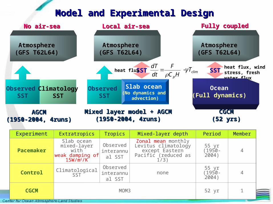
Experiment Extratropics Tropics Mixed-layer depth Period Member

PacemakerSlab ocean mixed-

layer withweak damping of

15W/m2/K

Observed interannual

SST

Zonal mean monthly Levitus climatology except Eastern

Pacific (reduced as 1/3)

55 yr(1950-2004) 4

Control Climatological SSTObserved

interannual SST

none 55 yr(1950-2004) 4

CGCM MOM3 52 yr 1

Model and Experimental DesignModel and Experimental DesignNo air-sea interactionNo air-sea interaction Local air-sea interactionLocal air-sea interaction Fully coupled systemFully coupled system

SSTSSTheat flux, wind stress, fresh water fluxheat flux

AGCMAGCM(1950-2004, 4runs)(1950-2004, 4runs)

Mixed layer model + AGCMMixed layer model + AGCM(1950-2004, 4runs)(1950-2004, 4runs)

CGCMCGCM(52 yrs)(52 yrs)

HC

F

dt

dT

p -γTclim

Atmosphere(GFS T62L64)

Atmosphere(GFS T62L64)

Atmosphere(GFS T62L64)

Ocean(Full dynamics)

Observed SST

Slab ocean (No dynamics and

advection)

Observed SST

ClimatologySST

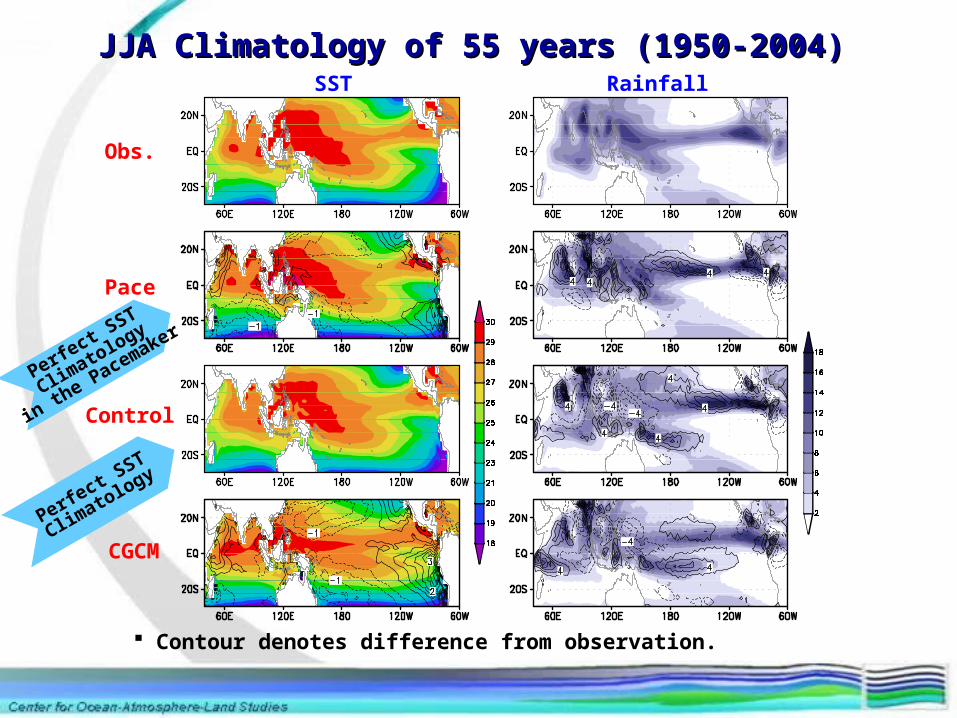
JJA Climatology of 55 years (1950-2004)JJA Climatology of 55 years (1950-2004)SST Rainfall

Obs.

Pace

Control

CGCM

Contour denotes difference from observation.

Perfect S

ST

Climatology

Perfect S

ST

Climatology

in the Pacemaker

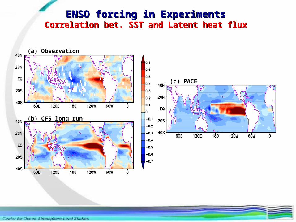
(a) Observation

(b) CFS long run

(c) PACE

ENSO forcing in ExperimentsENSO forcing in ExperimentsCorrelation bet. SST and Latent heat fluxCorrelation bet. SST and Latent heat flux

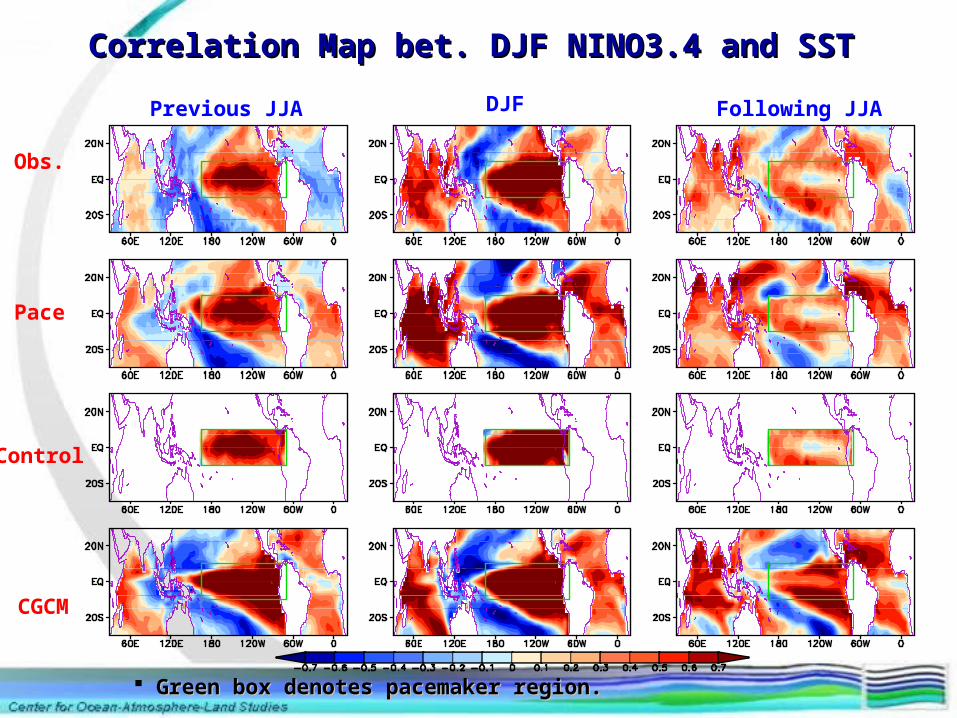
Correlation Map bet. DJF NINO3.4 and SSTCorrelation Map bet. DJF NINO3.4 and SST

Previous JJA Following JJADJF

Obs.

Pace

Control

CGCM

Green box denotes pacemaker region.Green box denotes pacemaker region.

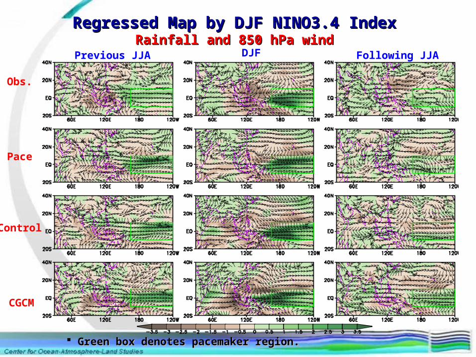
Regressed Map by DJF NINO3.4 IndexRegressed Map by DJF NINO3.4 Index

Previous JJA Following JJADJF

Obs.

Pace

Control

CGCM

Rainfall and 850 hPa windRainfall and 850 hPa wind

Green box denotes pacemaker region.Green box denotes pacemaker region.

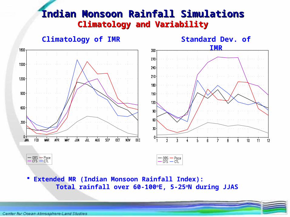
Climatology of IMR Standard Dev. of IMR

Indian Monsoon Rainfall SimulationsIndian Monsoon Rainfall SimulationsClimatology and VariabilityClimatology and Variability

Extended MR (Indian Monsoon Rainfall Index): Total rainfall over 60-100oE, 5-25oN during JJAS

Lead-lag Correlation Lead-lag Correlation (JJMS Extended IMR, NINO3.4)(JJMS Extended IMR, NINO3.4)

• 26 years during 1979-2006

• Green line denotes 95% significant level

ObservationCFS long runPACECONTROL

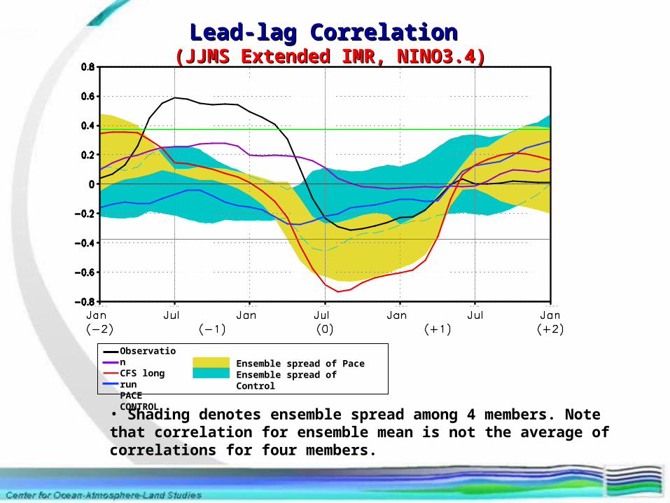
Lead-lag Correlation Lead-lag Correlation (JJMS Extended IMR, NINO3.4)(JJMS Extended IMR, NINO3.4)

Ensemble spread of PaceEnsemble spread of Control

• Shading denotes ensemble spread among 4 members. Note that correlation for ensemble mean is not the average of correlations for four members.

ObservationCFS long runPACECONTROL

The Evolution of Lead-lag ENSO-Monsoon Relationship in GCM Experiments

Influence of CGCM’s Systematic Error On ENSO-Monsoon Predictability

Improvement through “Pacemaker”

Advantage vs. Shortcoming in “Pacemaker”

Influence of model deficiency in the long run on forecast skill Systematic errors in ENSO characteristics and forced response

Simulation of Climatology ENSO forced response ENSO-monsoon relationship

Evolution of lead-lag ENSO-Indian monsoon relationship Plausible sources of shortcomings

Change of Lead-lag Correlation Change of Lead-lag Correlation 20-year Moving Window during 1950-200420-year Moving Window during 1950-2004

(HadSST and CMAP)

Lag correlation with respect to 20-yr moving window during 55 years

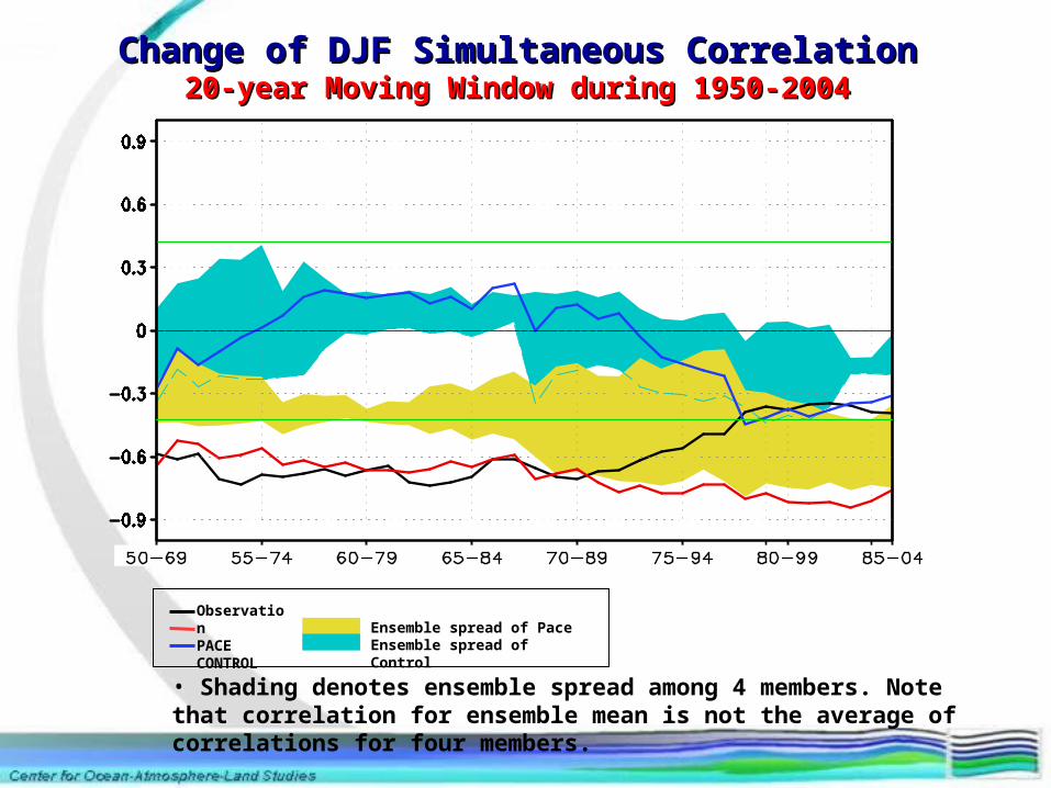
Change of DJF Simultaneous CorrelationChange of DJF Simultaneous Correlation20-year Moving Window during 1950-200420-year Moving Window during 1950-2004

Ensemble spread of PaceEnsemble spread of Control

ObservationPACECONTROL

• Shading denotes ensemble spread among 4 members. Note that correlation for ensemble mean is not the average of correlations for four members.

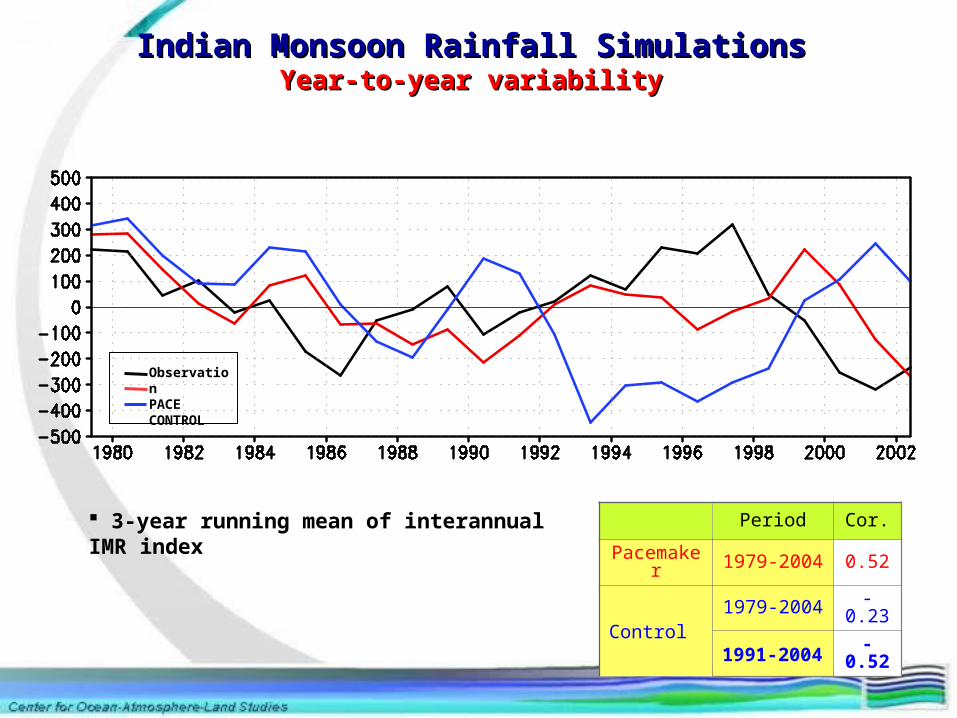
Indian Monsoon Rainfall SimulationsIndian Monsoon Rainfall SimulationsYear-to-year variabilityYear-to-year variability

3-year running mean of interannual IMR index

ObservationPACECONTROL

Period Cor.

Pacemaker 1979-2004 0.52

Control1979-2004 -0.23

1991-2004 -0.52

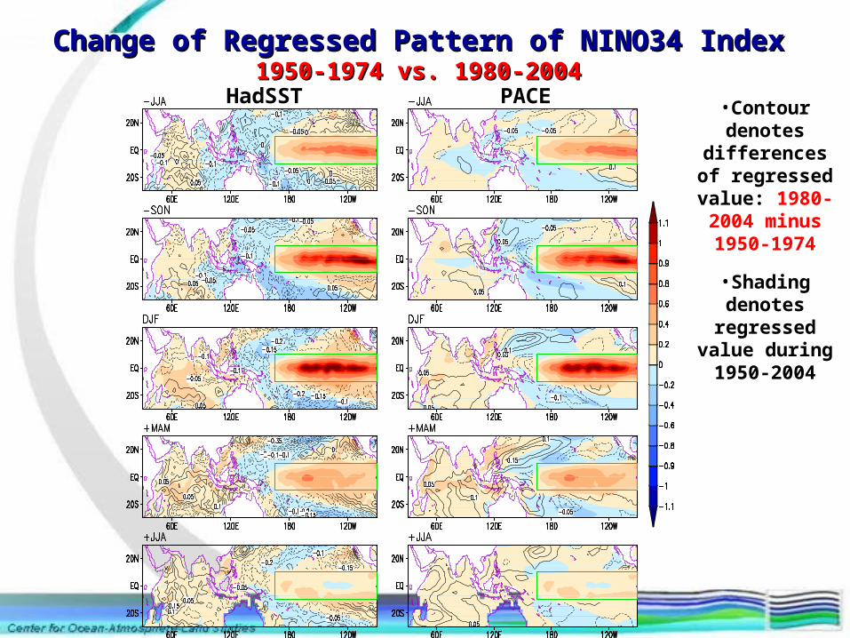
•Contour denotes differences of

regressed value: 1980-2004 minus

1950-1974

Change of Regressed Pattern of NINO34 IndexChange of Regressed Pattern of NINO34 Index1950-1974 vs. 1980-20041950-1974 vs. 1980-2004

•Shading denotes regressed value

during 1950-2004

HadSST PACE

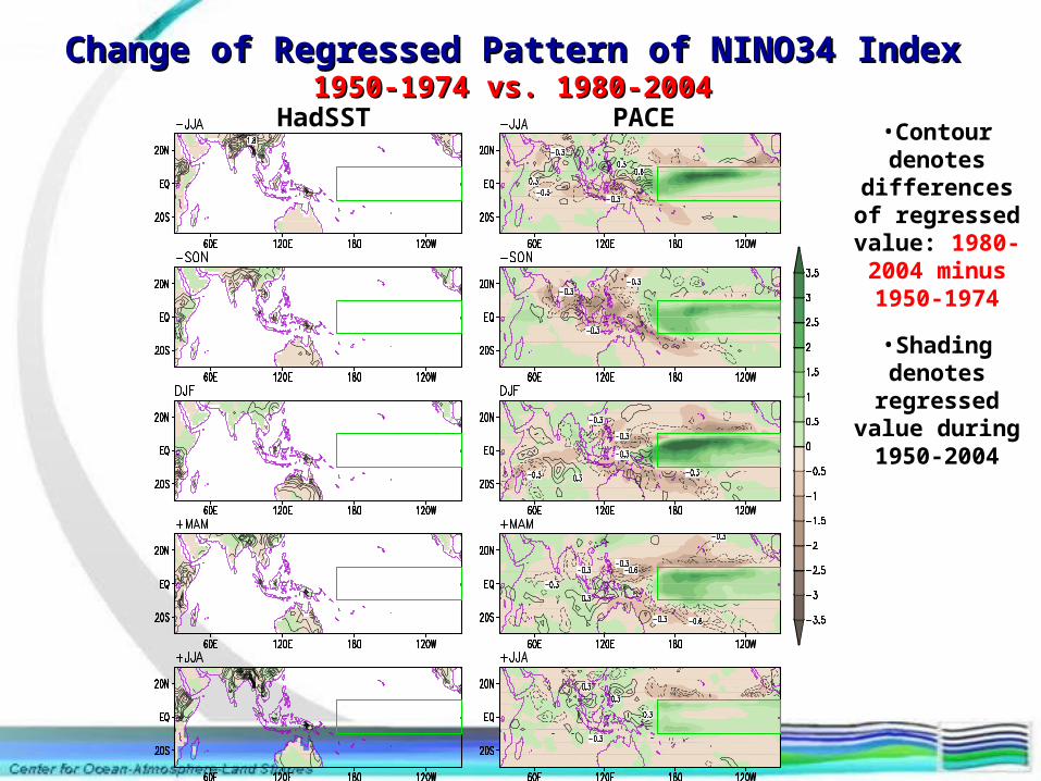
Change of Regressed Pattern of NINO34 IndexChange of Regressed Pattern of NINO34 Index1950-1974 vs. 1980-20041950-1974 vs. 1980-2004

•Contour denotes differences of

regressed value: 1980-2004 minus

1950-1974

•Shading denotes regressed value

during 1950-2004

HadSST PACE

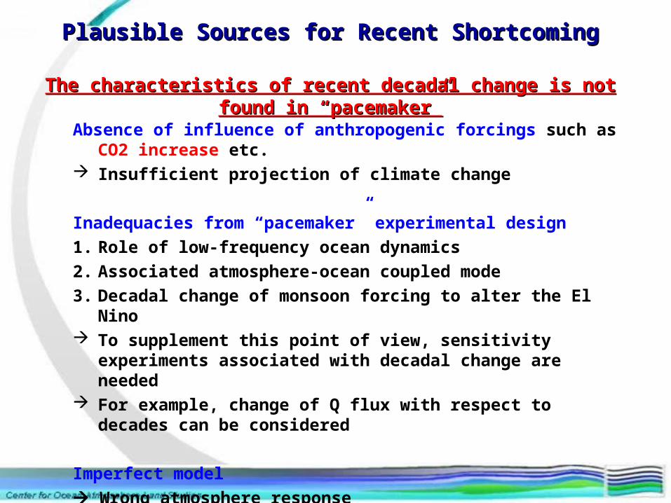
Plausible Sources for Recent ShortcomingPlausible Sources for Recent Shortcoming

Absence of influence of anthropogenic forcings such as CO2 increase etc. Insufficient projection of climate change

Inadequacies from “pacemaker” experimental design

1. Role of low-frequency ocean dynamics

2. Associated atmosphere-ocean coupled mode

3. Decadal change of monsoon forcing to alter the El Nino To supplement this point of view, sensitivity experiments associated with

decadal change are needed For example, change of Q flux with respect to decades can be considered

Imperfect model

Wrong atmosphere response

The characteristics of recent decadal change is not found in “pacemaker”The characteristics of recent decadal change is not found in “pacemaker”

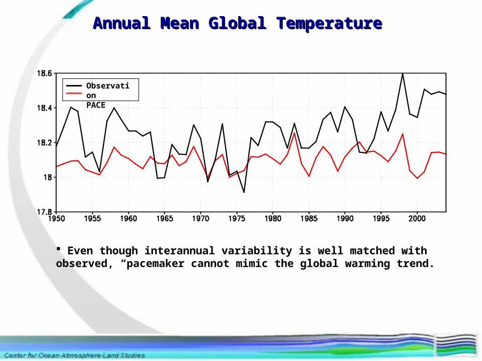
Annual Mean Global TemperatureAnnual Mean Global Temperature

ObservationPACE

Even though interannual variability is well matched with observed, “pacemaker cannot mimic the global warming trend.

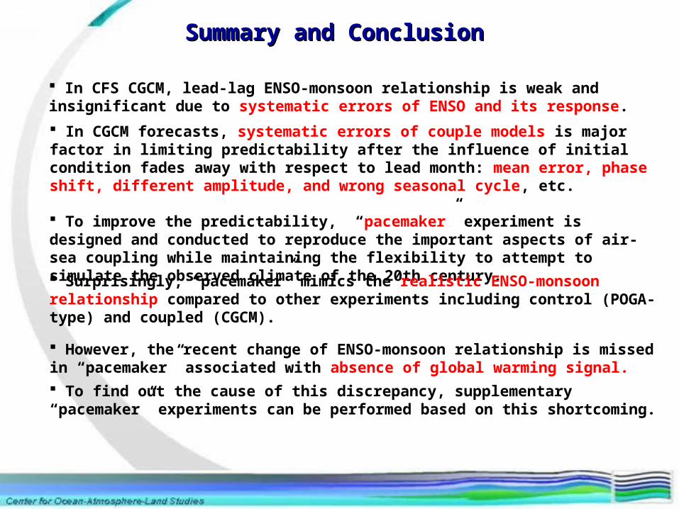
Summary and ConclusionSummary and Conclusion

In CFS CGCM, lead-lag ENSO-monsoon relationship is weak and insignificant due to systematic errors of ENSO and its response.

In CGCM forecasts, systematic errors of couple models is major factor in limiting predictability after the influence of initial condition fades away with respect to lead month: mean error, phase shift, different amplitude, and wrong seasonal cycle, etc.

To improve the predictability, “pacemaker” experiment is designed and conducted to reproduce the important aspects of air-sea coupling while maintaining the flexibility to attempt to simulate the observed climate of the 20th century.

Surprisingly, “pacemaker” mimics the realistic ENSO-monsoon relationship compared to other experiments including control (POGA-type) and coupled (CGCM).

However, the recent change of ENSO-monsoon relationship is missed in “pacemaker” associated with absence of global warming signal.

To find out the cause of this discrepancy, supplementary “pacemaker” experiments can be performed based on this shortcoming.

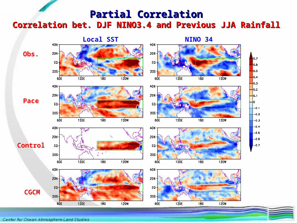
Local SST NINO 34

Obs.

Pace

Control

CGCM

Partial CorrelationPartial CorrelationCorrelation bet. DJF NINO3.4 and Previous JJA RainfallCorrelation bet. DJF NINO3.4 and Previous JJA Rainfall

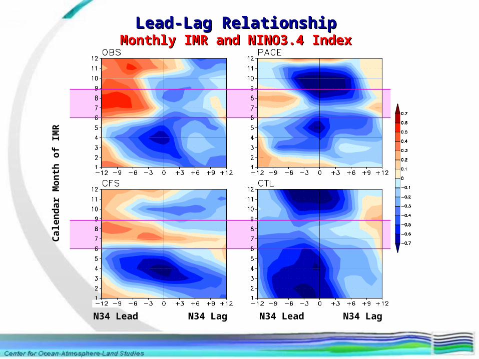
Cal

en

dar

Mo

nth

of

IMR

N34 Lead N34 Lag N34 Lead N34 Lag

Lead-Lag RelationshipLead-Lag RelationshipMonthly IMR and NINO3.4 IndexMonthly IMR and NINO3.4 Index

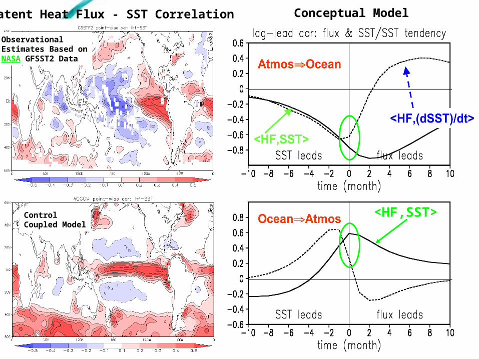
Latent Heat Flux - SST Correlation Conceptual Model

<HF,SST>

ObservationalEstimates Based onNASA GFSST2 Data

ControlCoupled Model

Western Pacific Problem

• Hypothesis: Atmospheric Internal Dynamics (Stochastic Forcing) is Occurring on Space and Time Scales that are Too Coherent

Too Coherent Oceanic Response Excessive Ocean Forcing Atmosphere Test: Add White Noise to Latent Heat

Flux

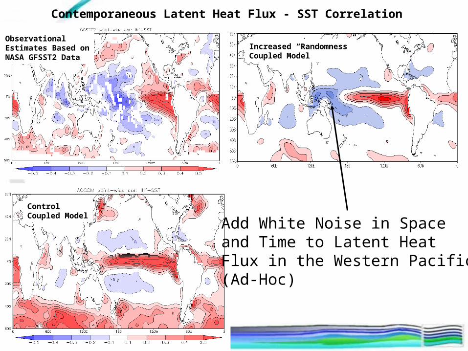
Contemporaneous Latent Heat Flux - SST Correlation

ControlCoupled Model

Increased “Randomness”Coupled Model

Add White Noise in Spaceand Time to Latent HeatFlux in the Western Pacific(Ad-Hoc)

ObservationalEstimates Based onNASA GFSST2 Data

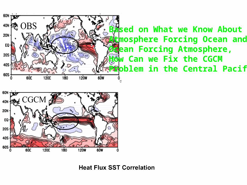
Based on What we Know AboutAtmosphere Forcing Ocean and Ocean Forcing Atmosphere,How Can we Fix the CGCM Problem in the Central Pacific?

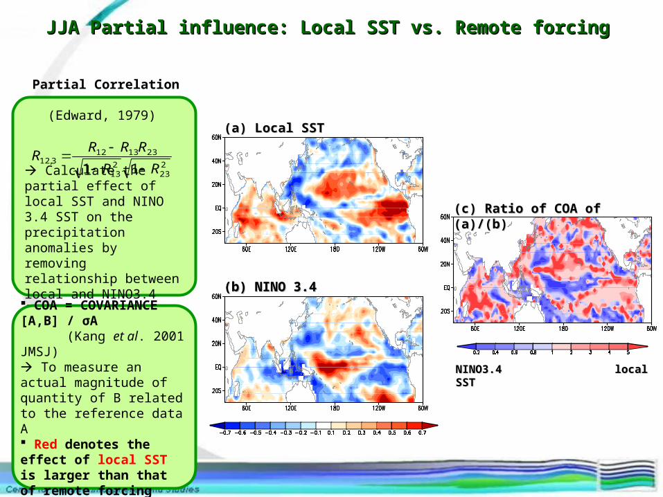
(a) Local SST(a) Local SST

(b) NINO 3.4(b) NINO 3.4

(c) Ratio of COA of (a)/(b)(c) Ratio of COA of (a)/(b)

(b) NINO 3.4(b) NINO 3.4

NINO3.4NINO3.4 local SST local SST

Partial Correlation (Edward, 1979)

Calculate the partial effect of local SST and NINO 3.4 SST on the precipitation anomalies by removing relationship between local and NINO3.4 SST

223

213

2313123,12

11 RR

RRRR

COA = COVARIANCE [A,B] / σA (Kang et al. 2001 JMSJ) To measure an actual magnitude of quantity of B related to the reference data A Red denotes the effect of local SST is larger than that of remote forcing

JJA Partial influence: Local SST vs. Remote forcingJJA Partial influence: Local SST vs. Remote forcing