THE EVALUATION OF DSI'S WATER QUALITY MONITORING NETWORK PERFORMANCE IN GEDIZ BASIN IN TERMS OF SAMPLING INTERVALS

THE EVALUATION OF DSI’S WATER QUALITY MONITORING NETWORK PERFORMANCE IN GEDIZ BASIN

IN TERMS OF SAMPLING INTERVALS

Cem Polat ÇETİNKAYA Sevinç ÖZKUL

Dokuz Eylül Üniversitesi Mühendislik Fakültesi İnşaat Mühendisliği Bölümü Tınaztepe-Buca/İZMİR

[email protected],[email protected]

ABSTRACT

The operational objective of DSI’s current water quality monitoring networks is “to preserve and improve the surface water quality”. In the scope of this objective, the monitoring goals of the nation-wide water quality network may be summarized as to assess the current water quality conditions and to detect the temporal changes (trends) in quality. Therefore, the prediction of the mean value and trends at a spe-cific level of statistical significance through systematic approaches is very important in order to define the monitoring goals in statistical terms.

The objectives of this study are to assess the necessary sampling interval to pre-dict long-term average value of water quality variables by the methodology pro-posed by Sanders and Adrian (1978), and to decide upon the required sampling interval to detect the on-going trends in water quality at a specific statistical signifi-cance level through the method applied by Lettenmaier (1976).

In this study, the results obtained within the project on “The Assessment of Effi-ciency in DSI’s Water Quality Monitoring Networks – Monitoring Network Optimization- II” (TUBITAK-YDABAG-100Y102) are discussed and evaluated. The project men-tioned is run by DEU Civil Engineering Department, Hydraulics Division with col-laboration of DSI General Directorate Domestic and Wastewater Division.

Keywords: Water quality monitoring network, monitoring objective, sampling interval, trend.

PRACTICES ON RIVER BASIN MANAGEMENT 317

ÖZET DSİ’nin halihazırdaki su kalitesi gözlem ağlarının hedefi “yüzeysel sularımızda su ka-

litesinin korunması ve iyileştirilmesi” şeklinde ifade edilmektedir. Bu hedef kapsamında DSİ tarafından Türkiye genelinde işletilen mevcut su kalitesi gözlem ağlarının gözlem amacı yüzeysel sularımızda su kalitesinin halihazır durumunun belirlenmesi ve su kalitesinde zamana göre değişim eğilimlerinin tayini olarak özetlenebilir. Bu bağlamda, sistematik bir yaklaşımla amaçların belirlenmesi ve ölçüm amacının istatistik tanımı için ortalama değerin ve eğilim-lerin belli bir anlamlılık seviyesinde tahmini önem kazanmaktadır.

Çalışmanın amacı, su kalitesi değişkenlerinin uzun süredeki gerçek ortalama değerlerinin belirlenmesi için gerekli veri miktarının, Sanders ve Adrian (1978) tarafından geliştirilen bir istatistik yaklaşımla tayin edilmesi, ve mevcut ölçüm sıklıklarının Lettenmaier’in (1976) öner-diği ve parametrik eğilim testlerinin uygulanmasına dayanan istatistik yaklaşımla irdelenmesidir.

Bu çalışmada, DEÜ İnşaat Mühendisliği Hidrolik ABD ve DSİ Genel Müdürlüğü İçmesuyu ve Kanalizasyon Dairesi Başk. tarafından ortaklaşa yürütülüp sonuçlandırılan ve TÜBİTAK tarafın-dan desteklenen YDABAG-100Y102 no.lu “DSI’nin Su Kalitesi İzleme Ağlarında Verimlilik Analizi- Ölçüm Ağı İyileştirilmesi – II” projesi kapsamında yapılan çalışmalar ile elde edilen sonuçlar irdelenmektedir.

Anahtar Kelimeler: Su kalitesi gözlem ağı, gözlem amacı, ölçüm sıklığı, eğilim.

1. INTRODUCTION

The design of water quality monitoring networks is realized in two steps: (a) definition of monitoring objectives and determination of boundary conditions, (b) selection of technical design criteria regarding the defined monitoring goals (selec-tion of sites, sampling intervals, variables and sampling period). On the other hand, regarding the current practices in Turkey, the monitoring objectives of the institu-tions such as DSI and EIE are defined as “the preservation and improvement of surface water quality conditions”, which, in reality, indicates a general description of monitor-ing purposes. However, regarding the present conditions in water and environ-mental pollution, more specific objectives should be defined in terms of water quality monitoring [Harmancıoğlu et al., 2003; Harmancıoğlu et al., 1998].

In view of the monitoring practices of DSI and EIE, two main monitoring goals may be defined: (a) assessment of the current surface water quality conditions and (b) assessment of temporal changes and trends in surface water quality conditions. Therefore, in order to determine the monitoring goals through a systematical ap-proach, the following steps should be applied in the design of water quality monitor-ing networks:

a) Water quality management: to preserve and improve water quality; b) Monitoring network objectives:

1) To assess the current condition of water quality; 2) To detect temporal changes in water quality variables;

c) Statistical definition of monitoring objectives: 1) The prediction of the mean value at a specific level of significance; 2) The prediction of trends at a specific level of significance.

318 INTERNATIONAL CONGRESS ON RIVER BASIN MANAGEMENT

The lack of a specific definition of monitoring objectives causes a deficiency in expected information production of a monitoring network, which directly affects its expected efficiency; hence, the description of monitoring goals indicated by those institutions should necessarily be specified with more details [Harmancıoğlu et al., 2003].

The presented study focuses on determination of the “sampling interval” and the “number of samples” required for the above statistical definitions indicated as “the prediction of the mean value at a specific level of significance” and “the prediction of trends at a specific level of significance” for the water quality sampling site 5005 Mu-radiye Köprüsü in Gediz Basin operated by DSI.

2. APPLIED METHODOLOGY

2.1. Assessment of Temporal Frequencies to Identify Water Quality Means

The monitoring design step on the “identification of the true mean value of wa-ter quality variables”, mentioned above is investigated by Sanders and Adrian (1978). The researchers have proposed a methodology towards the selection of temporal sampling intervals when the objective is to determine the true mean value of a water quality variable. The method is based on the expected half-width of the confidence interval of the mean value. Although this approach was intended for water quality variables, Sanders and Adrian (1978) applied it to streamflow data due to lack of sufficient water quality data and found it to be a reliable method [Sanders et al., 1983; Sanders, 1988].

For a series of random events, the confidence interval of the mean decreases as the number of samples increases. Thus, the accuracy of the estimate of the mean is a function of the number of sample observations. Therefore, a sampling frequency, as number of samples per year, can be determined for a specified confidence interval of the mean. Unfortunately, most hydrological time series are not random but signifi-cantly correlated and non-stationary, which makes standard statistical analyses diffi-cult. Thus, the method can be applied only after removing the serial correlation and non-stationarity from the series.

The Student t-statistic is selected to estimate the relationship between sampling frequency and the confidence interval of the mean of the random component. If the observations xi (i=1, ..., n) are stationary, independent and identically distributed, the variable t of Eq. (1) can be defined by a Student t-distribution:


n / - x =

St µ (1)

where, x : the calculated mean of the independent residuals, µ: the theoreti-cal population mean, S2: the sample variance of xi, and n: the number of inde-pendent observations [Sanders and Adrian, 1978].

For a specified level of significance, the variable t will lie in a confidence interval defined by known constants. This means that the probability that the random vari-able t is contained within the interval is equal to the level of significance (1-α), and the probability that the variable t is not contained within the interval is equal to α. This situation can be written by using the common statistical notation:

{ } αµαα - 1 =t

n / - x t = P /2-1 /2r ⟨⟨

S (2)

where, t1-α/2 and tα/2 are constants defined from the Student t-distribution for a specified level of significance and the number of samples.

By using the equality t1-α/2 = -tα/2, the confidence interval of the theoretical resid-ual mean can be written as:

nx

nx St + St - /2 /2 αα µ ⟨⟨ (3)

and the width of the confidence interval of this mean of the random sequence [xi] is:

nR S t2 = 2 /2α (4)

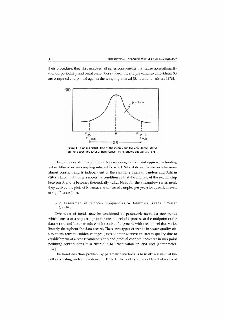
where R represents half the expected confidence interval of the mean [Sanders and Adrian, 1978]. Figure 1 shows the sampling distribution of the mean x together with the confidence interval bounded by µupper and µlower limits for a specified level of significance (1-α). 2R, then, is the confidence interval between the limits defined. Thus, R is a function of the standard deviation of the observed residuals, the square root of the number of the data, and the constant from the Student t-distribution. Consequently, to determine the temporal sampling criterion, a plot of half of the expected confidence interval of the residual mean versus the sampling frequency is sufficient since the confidence interval is symmetric about the mean.

Sanders and Adrian (1978) showed the application of the method for the case of streamflow due to the lack of sufficient water quality data for statistical analysis. In


their procedure, they first removed all series components that cause nonstationarity (trends, periodicity and serial correlations). Next, the sample variance of residuals Sa2 are computed and plotted against the sampling interval [Sanders and Adrian, 1978].

Figure 1. Sampling distribution of the mean x and the confidence interval 2R for a specified level of significance (1-α) [Sanders and Adrian,1978].

The Sa2 values stabilize after a certain sampling interval and approach a limiting

value. After a certain sampling interval for which Sa2 stabilizes, the variance becomes almost constant and is independent of the sampling interval. Sanders and Adrian (1978) stated that this is a necessary condition so that the analysis of the relationship between R and n becomes theoretically valid. Next, for the streamflow series used, they derived the plots of R versus n (number of samples per year) for specified levels of significance (1-α).

2.2. Assessment of Temporal Frequencies to Determine Trends in Water Quality

Two types of trends may be considered by parametric methods: step trends which consist of a step change in the mean level of a process at the midpoint of the data series; and linear trends which consist of a process with mean level that varies linearly throughout the data record. These two types of trends in water quality ob-servations refer to sudden changes (such as improvement in stream quality due to establishment of a new treatment plant) and gradual changes (increases in non-point polluting contributions to a river due to urbanization or land use) [Lettenmaier, 1976].

The trend detection problem by parametric methods is basically a statistical hy-pothesis testing problem as shown in Table 1. The null hypothesis H0 is that an event

low up


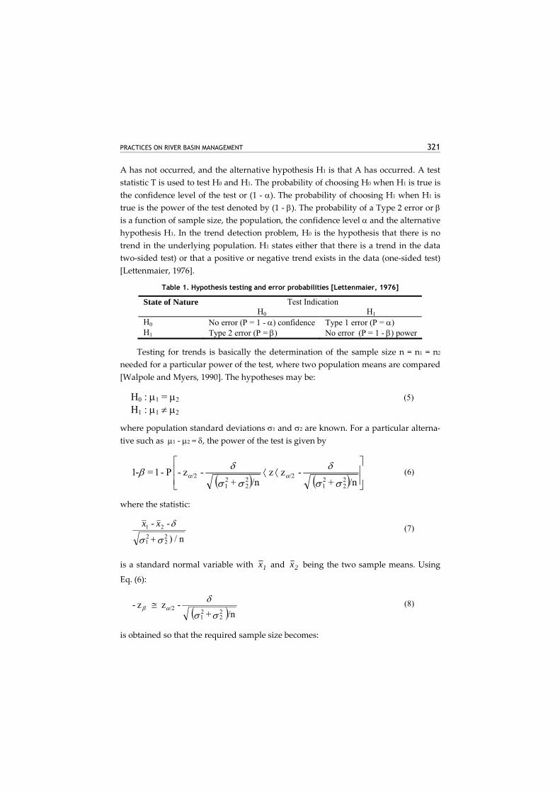
A has not occurred, and the alternative hypothesis H1 is that A has occurred. A test statistic T is used to test H0 and H1. The probability of choosing H0 when H1 is true is the confidence level of the test or (1 - α). The probability of choosing H1 when H1 is true is the power of the test denoted by (1 - β). The probability of a Type 2 error or β is a function of sample size, the population, the confidence level α and the alternative hypothesis H1. In the trend detection problem, H0 is the hypothesis that there is no trend in the underlying population. H1 states either that there is a trend in the data two-sided test) or that a positive or negative trend exists in the data (one-sided test) [Lettenmaier, 1976].

Table 1. Hypothesis testing and error probabilities [Lettenmaier, 1976]

State of Nature Test Indication H0 H1 H0 No error (P = 1 - α) confidence Type 1 error (P = α) H1 Type 2 error (P = β) No error (P = 1 - β) power

Testing for trends is basically the determination of the sample size n = n1 = n2 needed for a particular power of the test, where two population means are compared [Walpole and Myers, 1990]. The hypotheses may be:

H0 : µ1 = µ2 (5) H1 : µ1 ≠ µ2

where population standard deviations σ1 and σ2 are known. For a particular alterna-tive such as µ1 - µ2 = δ, the power of the test is given by

( ) ( )

⟨⟨

/n+ -z z

/n+ -z- P-1= 1

22

21

/222

21

/2σσ

δ

σσ

δβ αα- (6)

where the statistic:

n / ) - -

22

21

21

σσ

δ

+

xx (7)

is a standard normal variable with x1 and x2 being the two sample means. Using

Eq. (6):

( )/n + - z z-

22

21

/2σσ

δαβ ≅ (8)

is obtained so that the required sample size becomes:


( ) ( )n

z + z + / 2

2

≅α β σ σ

δ12

22

2 (9)

When the population variances are not known, the statistic of Eq. (7) is assumed to follow the Student t-distribution [Walpole and Myers, 1990].

The power of the test is important in the trend detection problem because it gives, at a fixed confidence level, the probability of the trend detection. The power of the test depends upon the sample size, trend magnitude and the marginal probability distribution of the dependent data series, which is assumed to be normal. For de-pendent series, it varies also with the form of the dependence of data.

To avoid an assumption of the distribution type, Lettenmaier (1976) proposes the use of nonparametric tests such as Spearman’s rho test for step trends and Mann-Whitney’s test for linear trends, which require the use of Monte Carlo simulated time series. Otherwise, Student t test is used, assuming that the independent data series are normally distributed.

The parametric test described above can be applied to detect step trends in the following way. The data set xi of size n, divided into two parts of equal size, has the means µ1 and µ2 so that the hypotheses are tested as given in Eq. (5).

For a confidence level (1 - α), the test statistic is defined as:

να/2,-121

21 t- 2S / n - =

xxt (10)

where t1-α/2, ν is the quantile of the Student t-distribution at probability level 1-α/2, the degrees of freedom ν are n-2, and S is the sample standard deviation of the data set:

( ) ( )

∑ ∑=

n/2

1

n

1+n/2=i

22

21

2 x - + x - 2 -n

1 = i

ii xxS (11)

Hypothesis H0 is accepted when t ≤ 0 or rejected when t > 0.

In parametric methods, a test criterion NT is defined as a population statistic as-suming that the population trend and standard deviation are known. With Tr = |µ1 -

µ2| representing the absolute value of the true difference between the two means, NT is defined as:

σ2 / n T = rTN (12)

The power of the test is then: ( )ναβ /2,-1T t - N F = - 1 (13)


where F is the cumulative distribution function of the standard Student t-distribution with ν = n-2 degrees of freedom [Lettenmaier, 1976].

In case of a linear trend, a similar approach is used to obtain the test criterion TN' as:

[ ]TN'

/

= n (n+1) (n -1)

n (12) r'

1/ 2T1 2

σε

(14)

for the well-known regression model:

i i + + x = εγτiy (15)

where εi is normally distributed with zero mean and variance σε2. τ is the trend magnitude and γ is the base level constant. In Eq. (14), σε represents the standard deviation of εi and Tr

′ = n τ. The test criterion NT′ for linear trends is similar to NT of

Eq. (12) for step trends except for the constants. The power of the test is again com-puted by Eq. (13).

The relationship between the detection power and the sampling interval ∆ for different specified values of Tr may also be identified. If the number of samples n is replaced by T/∆, where T is the total observation period and ∆ is the sampling fre-quency in Eqs. (12) and (14) by T/∆, a direct relation between the detection power and sampling frequency is obtained.

Lettenmaierʹs technique on trend detection has the advantage that it is an objec-tive-based approach to selection of sampling frequencies. Furthermore, it can be used for small sample sizes to determine what information the available data bring at particular levels of detection power. This technique is demonstrated on actual water quality data by Lettenmaier (1976) and Schilperoort et al.(1982). Their results show that the method works pretty well under the given assumptions.

3. APPLICATION TO GEDIZ BASIN

3.1 The General Status of Water Quality Monitoring Practices in Gediz Basin

Gediz Basin is located in Western Anatolia, and the river has a length of 276 km. With a 17800 km2 catchment area, Gediz Basin is the second largest basin in West Anatolia after Buyuk Menderes. The main tributaries of the river are Deliinis, Se-lendi, Demirci, Gordes, Medar, Alasehir and Nif streams. The long-term average water potential of the river is more than 1.3 billion m3, the average precipitation is 640 mm and runoff/precipitation ratio is around 26 %. In Gediz Basin, there is 521.000 ha of agricultural land from which 107.000 ha is irrigated [DSI, 1994].


Regarding the surface water quality in the Gediz, there are some important set-tlements (i.e. Akhisar, Saruhanlı, Salihli, Alaşehir, Turgutlu, Ahmetli, Manisa and Menemen) and industrial districts (Kemalpasa, Manisa and Menemen) contributing to the pollution in Gediz River. On the other hand, as mentioned above, there are 107.000 ha of irrigated agricultural land along the river banks, which are the main sources of non-point pollution [Coşak, 1999; DSİ, 1994].

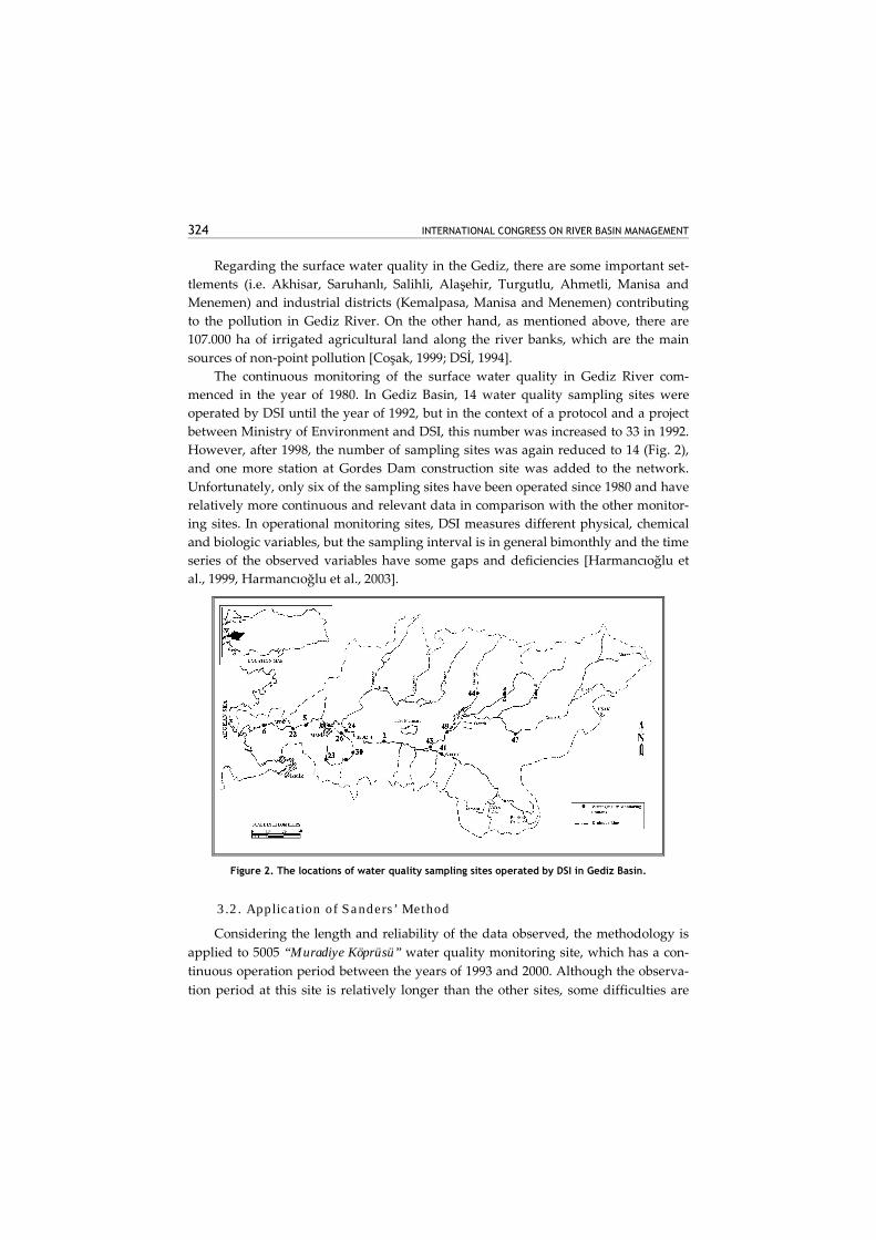
The continuous monitoring of the surface water quality in Gediz River com-menced in the year of 1980. In Gediz Basin, 14 water quality sampling sites were operated by DSI until the year of 1992, but in the context of a protocol and a project between Ministry of Environment and DSI, this number was increased to 33 in 1992. However, after 1998, the number of sampling sites was again reduced to 14 (Fig. 2), and one more station at Gordes Dam construction site was added to the network. Unfortunately, only six of the sampling sites have been operated since 1980 and have relatively more continuous and relevant data in comparison with the other monitor-ing sites. In operational monitoring sites, DSI measures different physical, chemical and biologic variables, but the sampling interval is in general bimonthly and the time series of the observed variables have some gaps and deficiencies [Harmancıoğlu et al., 1999, Harmancıoğlu et al., 2003].

Figure 2. The locations of water quality sampling sites operated by DSI in Gediz Basin.

3.2. Application of Sanders’ Method

Considering the length and reliability of the data observed, the methodology is applied to 5005 “Muradiye Köprüsü” water quality monitoring site, which has a con-tinuous operation period between the years of 1993 and 2000. Although the observa-tion period at this site is relatively longer than the other sites, some difficulties are


encountered during the application of the methodology. First of all, the discrete short-term monthly and bimonthly measurements at that site do not enable to consti-tute sub-sample sets for different sampling intervals. Therefore, the initial assump-tion of Sanders’ methodology, i.e., the stabilization of the sampling variances after a certain number of observations, has barely been validated by available data.

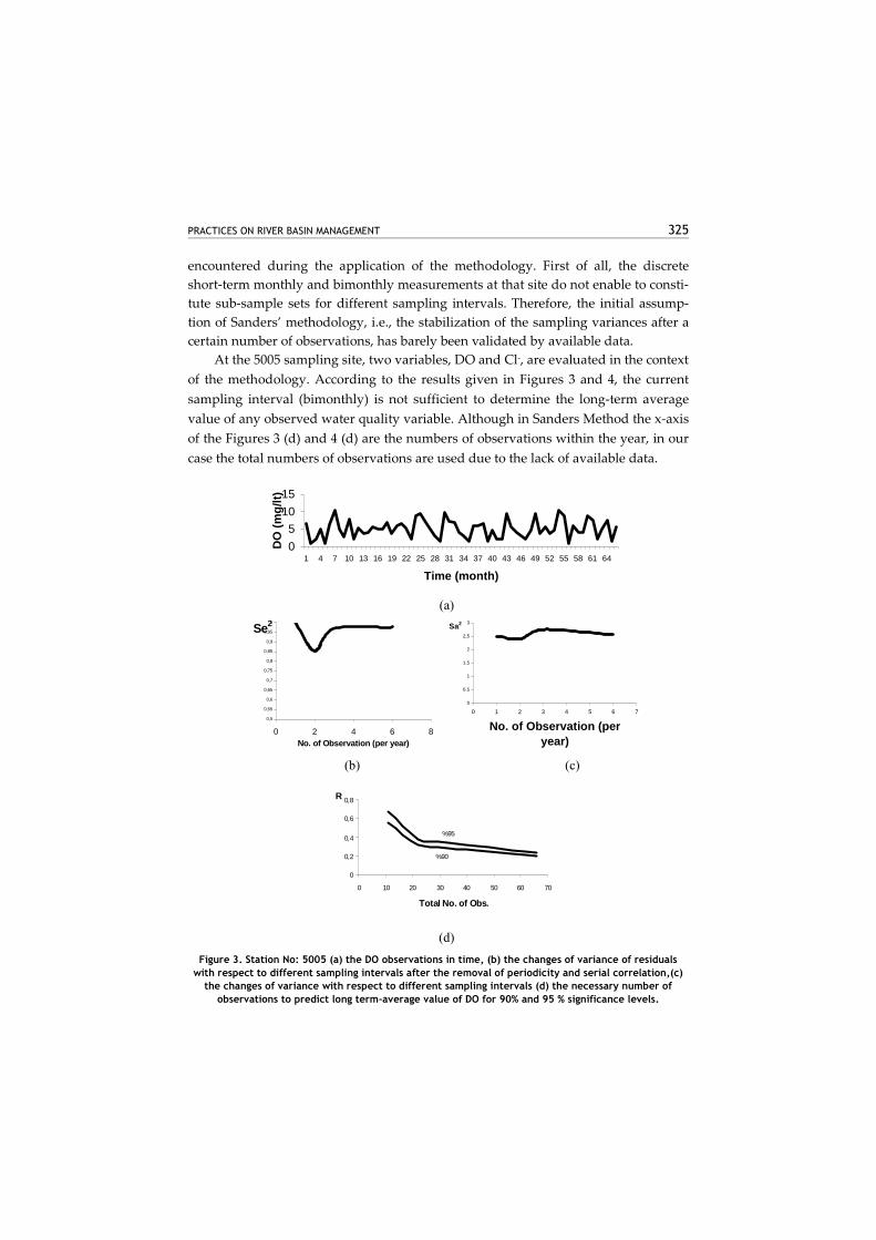
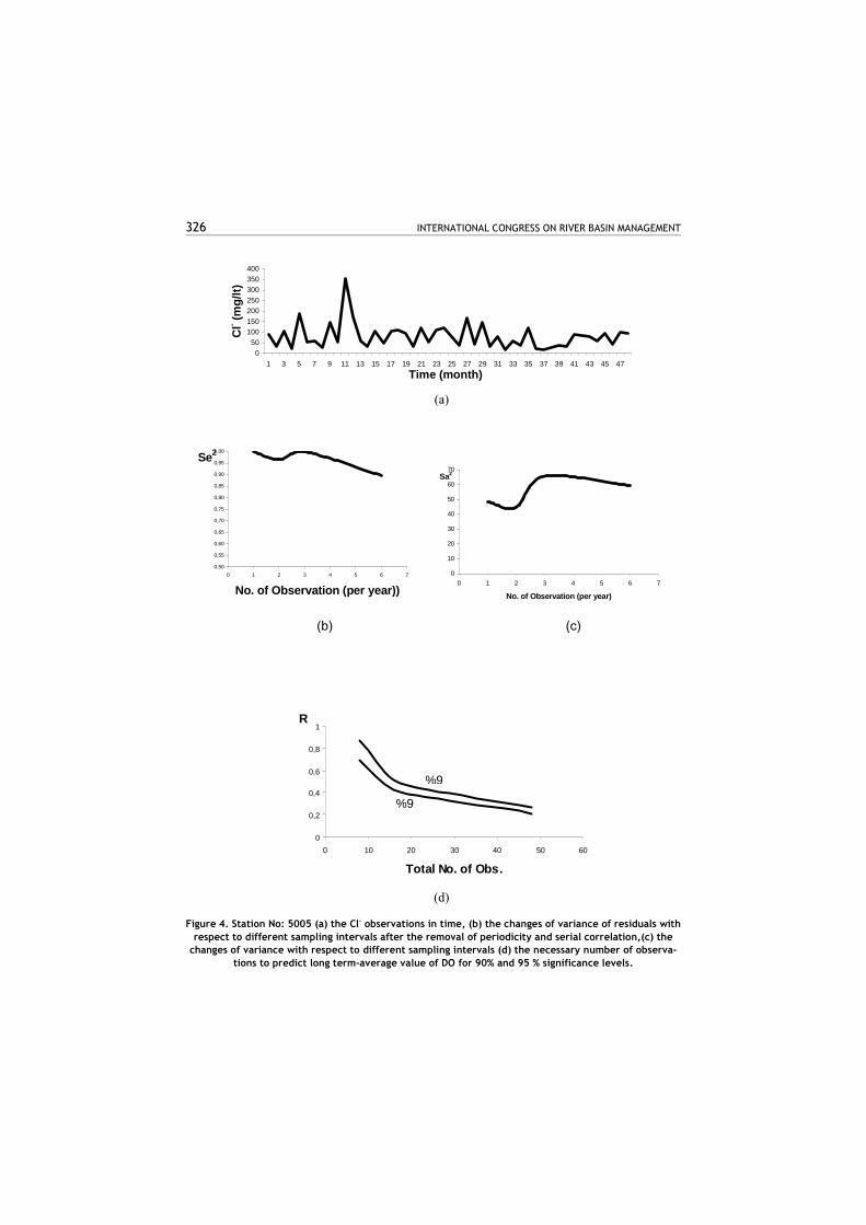
At the 5005 sampling site, two variables, DO and Cl-, are evaluated in the context of the methodology. According to the results given in Figures 3 and 4, the current sampling interval (bimonthly) is not sufficient to determine the long-term average value of any observed water quality variable. Although in Sanders Method the x-axis of the Figures 3 (d) and 4 (d) are the numbers of observations within the year, in our case the total numbers of observations are used due to the lack of available data.

05

1015

1 4 7 10 13 16 19 22 25 28 31 34 37 40 43 46 49 52 55 58 61 64

Time (month)

DO

(mg/

lt)

(a)

0,5

0,55

0,6

0,65

0,7

0,75

0,8

0,85

0,9

0,95

1

0 2 4 6 8No. of Observation (per year)

Se2

0

0,5

1

1,5

2

2,5

3

0 1 2 3 4 5 6 7

No. of Observation (per year)

Sa2

(b) (c)

0

0,2

0,4

0,6

0,8

0 10 20 30 40 50 60 70

Total No. of Obs.

R

%90

%95

(d)

Figure 3. Station No: 5005 (a) the DO observations in time, (b) the changes of variance of residuals with respect to different sampling intervals after the removal of periodicity and serial correlation,(c)

the changes of variance with respect to different sampling intervals (d) the necessary number of observations to predict long term-average value of DO for 90% and 95 % significance levels.


050

100150200250300350400

1 3 5 7 9 11 13 15 17 19 21 23 25 27 29 31 33 35 37 39 41 43 45 47Time (month)

Cl- (m

g/lt)

(a)

0,50

0,55

0,60

0,65

0,70

0,75

0,80

0,85

0,90

0,95

1,00

0 1 2 3 4 5 6 7

No. of Observation (per year))

Se2

0

10

20

30

40

50

60

70

0 1 2 3 4 5 6 7

No. of Observation (per year)

Sa2

(b) (c)

0

0,2

0,4

0,6

0,8

1

0 10 20 30 40 50 60

Total No. of Obs.

R

%9

%9

(d)

Figure 4. Station No: 5005 (a) the Cl- observations in time, (b) the changes of variance of residuals with

respect to different sampling intervals after the removal of periodicity and serial correlation,(c) the changes of variance with respect to different sampling intervals (d) the necessary number of observa-

tions to predict long term-average value of DO for 90% and 95 % significance levels.


3.3. Application of Lettenmaier Method

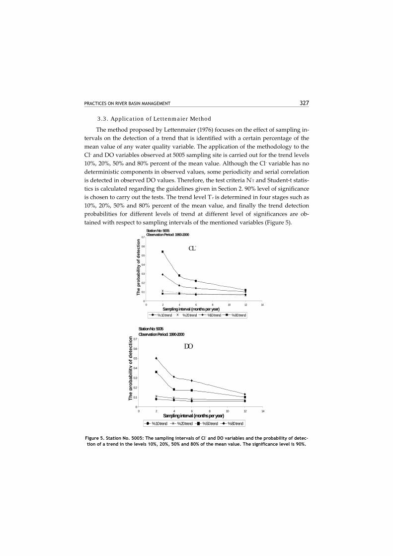
The method proposed by Lettenmaier (1976) focuses on the effect of sampling in-tervals on the detection of a trend that is identified with a certain percentage of the mean value of any water quality variable. The application of the methodology to the Cl- and DO variables observed at 5005 sampling site is carried out for the trend levels 10%, 20%, 50% and 80% percent of the mean value. Although the Cl- variable has no deterministic components in observed values, some periodicity and serial correlation is detected in observed DO values. Therefore, the test criteria NʹT and Student-t statis-tics is calculated regarding the guidelines given in Section 2. 90% level of significance is chosen to carry out the tests. The trend level Tʹr is determined in four stages such as 10%, 20%, 50% and 80% percent of the mean value, and finally the trend detection probabilities for different levels of trend at different level of significances are ob-tained with respect to sampling intervals of the mentioned variables (Figure 5).

CL-

Sampling interval (months per year)

0 0.1 0.2 0.3 0.4 0.5 0.6 0.7

0 2 4 6 8 10 12 14

The

prob

abili

ty o

f det

ectio

n

% 10 trend % 20 trend %50 trend % 80 trend

Station No: 5005 Observation Period: 1993-2000

Station No: 5005

Observation Period: 1990-2000

0 0.1 0.2 0.3 0.4 0.5 0.6 0.7

0 2 4 6 8 10 12 14

The

prob

abili

ty o

f det

ectio

n

% 10 trend % 20 trend % 50 trend % 80 trend

DO

Sampling interval (months per year)

Figure 5. Station No. 5005: The sampling intervals of Cl- and DO variables and the probability of detec-tion of a trend in the levels 10%, 20%, 50% and 80% of the mean value. The significance level is 90%.


The application of Lettenmaier’s methodology to the observed water quality variables is more convenient than the Sanders method, while the short series and missing values of observed data do not effect the application of the method. As it is shown in Fig. 5, this method enables to evaluate the information content of available data and sampling interval in terms of the probability of detection of any possible trends in the observations.

Unfortunately in Fig 5, it is indicated that the current sampling interval is insuf-ficient to detect any trends in surface water quality conditions; e.g. the bimonthly sampling interval of the Cl- variable enables the detection of a trend at the level of 80% of the mean value with the probability of 54%. For 50%, 20% and 10% of trend levels, the current sampling interval may detect the on-going trend with the prob-abilities of 27%, 11% and 8% respectively.

4. DISCUSSION OF THE OBTAINED RESULTS

In Fig. 5, it is indicated that the trend levels of 80% and 50% of the mean are more easily detected than the levels 20% and 10% of the mean. Therefore, the slight changes in surface water quality variables are not subject to detection by the current bimonthly sampling intervals. Furthermore, even the trend level of 80% of the mean may not be effectively detected with the current sampling interval. More generally, regarding Fig. 5, it can be assessed that the current sampling interval (bimonthly) is insufficient to detect any levels of trend in surface water quality conditions.

As it mentioned above, the method proposed by Lettenmaier is more applicable than Sanders method in terms of the current water quality monitoring practices in Turkey. If the monitoring objective is determined as the detection of trends in water quality conditions then Lettenmaier’s approach enables different types of evaluation of the current monitoring practices. The benefits of the application of the Letten-maier’s approach may be summarized as follows: (a) the method itself regards the monitoring objectives and evaluates the observed values with respect to the objec-tives, (b) the method is not affected by short-term observations, (c) during the evalua-tion, the serial correlation and periodicity of the observed values are taken into ac-count, (d) the information obtained by observed data may be evaluated at different statistical significance levels and therefore through the method one can decide that the observed data is suitable for monitoring objectives or not.

The only deficiency of Lettenmaier’s approach is that the method is data de-pendent; in other words, by Lettenmaier’s method, only the current and larger sam-pling intervals may be evaluated. Unfortunately, any extension to more frequent sampling than the current one may not be assessed through the method. In Fig. 5,


only the bimonthly and larger sampling intervals are considered, but it is difficult to decide whether more frequent sampling intervals such as daily, weekly etc. are nec-essary for more precise trend detection. Despite this deficiency in the method, Let-tenmaier’s approach is a suitable tool in the scope of the current water quality moni-toring practices in Turkey with respect to monitoring objectives if hey relate to the detection of surface water quality trends.

Another general result of the presented study is that statistical methods like Sanders and Lettenmaier, should be employed not at preliminary design of a moni-toring network but after a certain number of observations in the network has been obtained. The monitoring network design is an iterative procedure, therefore, statis-tical methods should also be applied regularly in order to assess whether the moni-toring objectives set at the preliminary phase are met, or any improvements are nec-essary for the sake of the objectives.

5. ACKNOWLEDGMENT

The study leading to this paper has been supported by TUBITAK (YDABAG-100Y102). This support is gratefully acknowledged.

6. REFERENCES

Coşak, C. (1999) Gediz Havzası Su Kalitesi Gözlem Ağında İstasyon Konumlarının İrdelenmesi, DEÜ Mühendislik Fakültesi İnşaat Mühendisliği Bölümü, Hidroloji ve Su Yapıları Diploma Projesi No: 193, Yön: Yrd Doç. Dr. Sevinç Özkul, İzmir, 76 s.

DSİ (1994) DSİ II. Bölge Müdürlüğü 1995 Yılı Program Bütçe Toplantısı Takdim Raporu, İzmir, 172 s, Nisan 1994.

Harmancioglu, N.B.; Singh, V.P.; Alpaslan, N. (eds.) (1998) Environmental Data Man-agement, Kluwer Academic Publishers, Water Science and Technology Library, Volume 27, 298 pp.

Harmancıoğlu, N.B.; Alpaslan, N.; Özkul, S.; İçağa, Y.; Fıstıkoğlu, O.; Onuşluel G.; Barbaros, F.; Akyar H.; Salihoğlu, I.; Alpaslan, A.; Aydınlıyım, F.; Onur, A.K.; Celtemen, S.P.; Baydere, A.R. ve Aklaf, G. (1999) DSİ'nin Su Kalitesi İzleme Ağlarında Verimlilik Analizi ve Ölçüm Ağı İyileştirilmesi İzmir, TÜBİTAK-YDABÇAG için yapılan YD-ABÇAG-489 no.lu uygulamalı araştırma projesi raporu, 208 s., Temmuz 1999.

Harmancıoğlu, N.B.; Özkul, S.; Fıstıkoğlu, O.; Onuşluel G.; Gül, A.; Çetinkaya C.P.; İçağa, Y.; Barbaros, F.; Akyar H.; Kahramanoğlu, N.; Seyrek, K.; Baltacı, F.; Onur, A.K.; Yıl-maz, N.; Celtemen, S.P.; Alpaslan, A. (2003) DSİ'nin Su Kalitesi İzleme Ağlarında Verimlilik Analizi ve Ölçüm Ağı İyileştirilmesi-II, İzmir, TÜBİTAK-YDABAG için yapı-lan YDABAG-100Y102 no.lu uygulamalı araştırma projesi raporu, 150 s., Nisan 2003.


Lettenmaier, D.P. (1976) “Detection of trends in water quality data from records with dependent observations”, Water Resources Research 12(5), 1037-1046.

Sanders, T.G. and Adrian, D.D. (1978) “Sampling frequency for river quality monitoring”, Water Resources Research 14(4), 569-576.

Sanders, T.G., Ward, R.C., Loftis, J.C., Steele, T.D., Adrian, D.D., Yevjevich, V. (1983) Design of Networks for Monitoring Water Quality, Water Resources Publications, Littleton, Colorado, 328p.

Sanders, T.G. (1988) “Water quality monitoring networks”, in D. Stephenson (ed.), Water and Wastewater System Analyses, Elsevier, Development in Water Science No.34, ch. 13, pp. 204-216.

Schilperoort, T., Groot, S., Watering, B.G.M., and Dijkman, F. (1982) “Optimization of the Sampling Frequency of Water Quality Monitoring Networks”, Waterloopkundig Laboratium Delft, Hydraulics Lab., Delft, the Netherlands.

Walpole, R.E. and Myers, R. H. (1990) Probability and Statistics for Engineers and Scientists, MacMillan Publishing Company, New York, 765 p..

THE EVALUATION OF DSI'S WATER QUALITY MONITORING NETWORK PERFORMANCE IN GEDIZ BASIN IN TERMS OF SAMPLING INTERVALS

Documents