QUANTITATIVE FINANCE RESEARCH CENTRE QUANTITATIVE F INANCE RESEARCH CENTRE QUANTITATIVE FINANCE RESEARCH CENTRE Research Paper 266 January 2010 The Evaluation Of Barrier Option Prices Under Stochastic Volatility Carl Chiarella, Boda Kang and Gunter H. Meyer ISSN 1441-8010 www.qfrc.uts.edu.au

Welcome message from author
This document is posted to help you gain knowledge. Please leave a comment to let me know what you think about it! Share it to your friends and learn new things together.
Transcript

QUANTITATIVE FINANCE RESEARCH CENTRE QUANTITATIVE F
INANCE RESEARCH CENTRE
QUANTITATIVE FINANCE RESEARCH CENTRE
Research Paper 266 January 2010
The Evaluation Of Barrier Option Prices Under Stochastic Volatility
Carl Chiarella, Boda Kang and Gunter H. Meyer
ISSN 1441-8010 www.qfrc.uts.edu.au

THE EVALUATION OF BARRIER OPTION PRICES UNDER
STOCHASTIC VOLATILITY
CARL CHIARELLA♯, BODA KANG† AND GUNTER H. MEYER⋆
Abstract. This paper considers the problem of numerically evaluating barrier
option prices when the dynamics of the underlying are driven by stochastic
volatility following the square root process of Heston (1993). We develop a
method of lines approach to evaluate the price as well as the delta and gamma of
the option. The method is able to efficiently handle both continuously monitored
and discretely monitored barrier options and can also handle barrier options
with early exercise features. In the latter case, we can calculate the early exercise
boundary of an American barrier option in both the continuously and discretely
monitored cases.
Keywords: barrier option, stochastic volatility, continuously monitored, dis-
cretely monitored, free boundary problem, method of lines, Monte Carlo simu-
lation.
JEL Classification: C61, D11.
1. Introduction
Barrier options are path-dependent options and are very popular in foreign ex-
change markets. They have a payoff that is dependent on the realized asset path
via its level; certain aspects of the contract are triggered if the asset price becomes
too high or too low during the option’s life. For example, an up-and-out call op-
tion pays off the usual max(S − K, 0) at expiry unless at any time during the
life of the option the underlying asset has traded at a value H or higher. In this
example, if the asset reaches this level (from below, obviously) then it is said to
“knock out” and become worthless. Apart from “out” options like this, there are
also “in” options which only receive a payoff if a certain level is reached, otherwise
they expire worthless. Barrier options are popular for a number of reasons. The
purchaser can use them to hedge very specific cash flows with similar properties.
Date: Current Version January 12, 2010.♯ [email protected]; School of Finance and Economics, University of Technology, Sydney,Australia.†Corresponding author: [email protected]; School of Finance and Economics, University ofTechnology, Sydney, PO Box 123, Broadway, NSW 2007, Australia.⋆ [email protected]; School of Mathematics, Georgia Institute of Technology, Atlanta.
1
2 CARL CHIARELLA, BODA KANG AND GUNTER H. MEYER
Usually, the purchaser has very precise views about the direction of the market.
If he or she wants the payoff from a call option but does not want to pay for all
the upside potential, believing that the upward movement of the underlying will
be limited prior to expiry, then he may choose to buy an up-and-out call. It will
be cheaper than a similar vanilla call, since the upside is severely limited. If he
is right and the barrier is not triggered he gets the payoff he wanted. The closer
that the barrier is to the current asset price then the greater the likelihood of the
option being knocked out, and thus the cheaper the contract.
Barrier options are common path-dependent options traded in the financial mar-
kets. The derivation of the pricing formula for barrier options was pioneered by
Merton (1973) in his seminal paper on option pricing. A list of pricing formulas
for one-asset barrier options and multi- asset barrier options both under the geo-
metric Brownian motion (GBM) framework can be found in the articles by Rich
(1994) and Wong & Kwok (2003), respectively. Gao, Huang & Subrahmanyam
(2000) analyzed option contracts with both knock-out barrier and American early
exercise features.
Derivative securities are commonly written on underlying assets with return dy-
namics that are not sufficiently well described by the GBM process proposed by
Black & Scholes (1973). There have been numerous efforts to develop alternative
asset return models that are capable of capturing the leptokurtic features found
in financial market data, and subsequently to use these models to develop option
prices that better reflect the volatility smiles and skews found in market traded
options. One of the classical ways to develop option pricing models that are capa-
ble of generating such behaviour is to allow the volatility to evolve stochastically,
for instance according to the square-root process introduced by Heston (1993).
The evaluation of barrier option prices under Heston stochastic volatility model
has been extensively discussed by Griebsch (2008) in her thesis.
There are certain drawbacks in the evaluation of the Barrier option prices under
SV using either tree or finite difference methods, for instance the convergence is
rather slow and it takes more effort to obtain accurate hedge ratios. It turns
out that another well known method, the method of lines is able to overcome
those disadvantages. In this paper, we introduce a unifying approach to price
both continuously and discretely monitored barrier options without or with early
exercise features. Specifically, except for American style knock-in options, we are
able to price all other kinds of European or American barrier options using the
framework developed here.

THE EVALUATION OF BARRIER OPTION PRICES 3
The remainder of the paper is structured as follows. Section 2 outlines the problem
of both continuously and discretely monitored barrier options where the underly-
ing asset follows stochastic volatility dynamics. In Section 3 we outline the basic
idea of the method of lines approach and implement it to find the price profile of
the barrier option. A number of numerical examples that demonstrate the com-
putational advantages of the method of lines approach are provided in Section 4.
Finally we discuss the impact of stochastic volatility on the prices of the barrier
option in Section 5 before we draw some conclusions in Section 6.
2. Problem Statement-Barrier Option with Stochastic Volatility
Let C(S, v, τ) denote the price of an up-and-out (UO) call option with time to
maturity τ 1 written on a stock of price S and variance v that pays a continuously
compounded dividend yield q. The option has strike price K and a barrier H .
Analogously to the setting in Heston (1993), the dynamics for the share price S
under the risk neutral measure are governed by the stochastic differential equation
(SDE) system 2
dS = (r − q)Sdt +√
vSdZ1, (1)
dv = κv(θv − v)dt + σ√
vdZ2, (2)
where Z1, Z2 are standard Wiener processes and E(dZ1dZ2) = ρdt with E the
expectation operator under the risk neutral measure. In (1), r is the risk free rate
of interest. In (2) the parameter σ is the so called vol-of-vol (in fact, σ2v is the
variance of the variance process v). The parameters κv and θv are respectively
the rate of mean reversion and long run variance of the process for the variance
v. These are under the risk-neutral measure and are relate to the corresponding
quantities by a parameter that appears in the market price of volatility risk.3
1Note that τ = T − t, where T is the maturity date of the option and t is the time.2Of course, since we are using a numerical technique we could in fact use more general processesfor S and v. The choice of the Heston processes is driven partly by the fact that this hasbecome a very traditional stochastic volatility model and partly because a companion paper onthe evaluation of European compound options under stochastic volatility uses techniques basedon a knowledge of the characteristic function for the stochastic volatility process, which is knownfor the Heston process (see Chiarella, Griebsch & Kang (2009)), and can be used for comparisonpurpose.3 In fact, if it is assumed that the market price of risk associated with the uncertainty drivingthe variance process has the form λ
√v, where λ is a constant (this was the assumption in
Heston (1993)) and κP
v, θP
v are the corresponding parameters under the physical measure, then
κv = κP
v + λσ, θv =κP
vθP
v
κPv+λσ
.

4 CARL CHIARELLA, BODA KANG AND GUNTER H. MEYER
We are also able to write down the above system (1)-(2) using independent Wiener
processes. Let W1 = Z2 and Z1 = ρW1 +√
1 − ρ2W2 where W1 and W2 are
independent Wiener processes under the risk neutral measure. Then, the dynamics
of S and v can be rewritten in terms of independent Wiener processes as
dS = (r − q)Sdt +√
vS(ρdW1 +√
1 − ρ2dW2), (3)
dv = κv(θv − v)dt + σ√
vdW1. (4)
The price of a barrier option under stochastic volatility at time t, C(S, v, τ), can
be formulated as the solution to a partial differential equation (PDE) problem.
We need to solve the PDE for the value of the barrier option C(S, v, τ) given by
∂C
∂τ= KC − rC, (5)
on the interval 0 ≤ τ ≤ T , where the Kolmogorov operator K is given by
K =vS2
2
∂2
∂S2+ ρσvS
∂2
∂S∂v+
σ2v
2
∂2
∂v2+ (r − q)S
∂
∂S+ (κv(θv − v) − λv)
∂
∂v,
(6)
where λ is the constant appearing in the equation for the market price of volatility
risk, which as stated in Footnote 3 is of the form λ√
v.
Both the terminal and boundary conditions need to be specified depending on the
detailed specifications of the barrier options:
• A continuously Monitored Barrier Option with or without early exercise
features, has the terminal condition
C(S, v, 0) = (S − K)+1{maxt S(t)<H}, (7)
• A discretely Monitored Barrier Option with or without early exercise fea-
tures, with N monitoring dates t ≤ t1 < t2 <, · · · , < tN ≤ T , has the
terminal condition
C(S, v, 0) = (S − K)+1{S(t1)<H,S(t2)<H,··· ,S(tN )<H}, (8)
• A continuously Monitored Barrier Option with early exercise features, has
the free (early exercise) boundary condition
C(b(v, τ), v, τ) = b(v, τ) − K, when b(v, τ) < H (9)
where S = b(v, τ) is the early exercise boundary for the barrier option at
time to maturity τ and variance v, and there also hold the smooth-pasting

THE EVALUATION OF BARRIER OPTION PRICES 5
conditions
limS→b(v,τ)
∂C
∂S= 1, lim
S→b(v,τ)
∂C
∂v= 0. (10)
• A discretely Monitored Barrier Option with early exercise features, has the
free (early exercise) boundary condition
C(b(v, τ), v, τ) = b(v, τ) − K, (11)
where b(v, τ) is the early exercise boundary for the barrier option at time
to maturity τ and variance v, and the smooth-pasting conditions
limS→b(v,τ)
∂C
∂S= 1, lim
S→b(v,τ)
∂C
∂v= 0. (12)
Before going into detail of the valuation, the following relations between the payoffs
of barrier options and vanilla options are pointed out. The in-out parity for
European barrier options, namely
knock-in + knock-out = vanilla;
allows us to consider only the family of knock-out options for the valuation using
the method of lines (MOL) since we are able to price vanilla option under Heston
model using the method of lines already. In next section, we are going to discuss
the detail of computing the up-and-out barrier option prices by implementing the
MOL.
3. Method of Lines (MOL) Approach
In this section,we will provide the details of the implementation of the Method of
Lines. The key idea behind the method of lines is to approximate a PDE with
a system of ordinary differential equations (ODEs), the solution of which can be
obtained with ODE techniques. When volatility is constant, the system of ODEs
is obtained by discretizing time. For the PDE (5), we must in addition discretize
the variance, v. S is retained as independent variable. We begin by setting
vm = m∆v, where m = 0, 1, 2, ..., M . Typically we will set the maximum variance
to be vM = 100%. Furthermore, we disctretise the time to expiry according to
τn = n∆τ , where n = 0, 1, 2, . . . , N and τN = T . We denote the option price along
the variance line vm and time line τn by C(S, vm, τn) = Cnm(S), and set
V (S, vm, τn) ≡ ∂C(S, vm, τn)
∂S= V n
m(S), (13)
which is of course the option delta at the particular grid point.
6 CARL CHIARELLA, BODA KANG AND GUNTER H. MEYER
We now select finite difference approximations for the derivative terms with respect
to v. For the second order term, at the grid point (S, vm, τn) we use the standard
central difference scheme
∂2C
∂v2=
Cnm+1 − 2Cn
m + Cnm−1
(∆v)2. (14)
Similarly for the cross-derivative term at the grid point (S, vm, τn), we use the
central difference approximation
∂2C
∂S∂v=
V nm+1 − V n
m−1
2∆v. (15)
Since the coefficients of the second order derivative terms go to zero as v → 0, we
use an upwinding finite difference scheme for the first order derivative term (see
Duffy (2006)), such that, at the grid point (S, vm, τn) we have
∂C
∂v=
Cn
m+1−Cnm
∆vif v ≤ α
β,
Cnm−Cn
m−1
∆vif v > α
β,
(16)
where α = κvθv and β = κv + λv. Since the second order derivative terms both
vanish as v → 0, upwinding helps to stabilise the finite difference scheme with
respect to v.
Next we must select a discretisation for the time derivative. Initially we use a
standard backward difference scheme, given at the grid point (S, vm, τn) by
∂C
∂τ=
Cnm − Cn−1
m
∆τ. (17)
This approximation is only first order accurate with respect to time. For the case
of the standard American put option, it is known from Meyer (2009) that the
accuracy of the method of lines increases considerably by using a second order
approximation for the time derivative, specifically
∂C
∂τ=
3
2
Cnm − Cn−1
m
∆τ− 1
2
Cn−1m − Cn−2
m
∆τ. (18)
Thus we initiate the method of lines solution by using (17) for the first several
time steps, and then switch to (18) for all subsequent time steps.
Applying (14)-(18) to the PDE (5), we now need to solve a system of second order
ODEs at each time step and variance grid point. For the first few time steps, the

THE EVALUATION OF BARRIER OPTION PRICES 7
ODE system at the grid point v = vm and τ = τn is
vmS2
2
d2Cnm
dS2+ ρσvmS
V nm+1 − V n
m−1
2∆v+
σ2vm
2
Cnm+1 − 2Cn
m + Cnm−1
(∆v)2
+α − βvm
2
Cnm+1 − Cn
m−1
∆v+
|α − βvm|2
Cnm+1 − 2Cn
m + Cnm−1
∆v
+ (r − q)SdCn
m
dS− rCn
m − Cnm − Cn−1
m
∆τ= 0, (19)
and for all subsequent time steps the ODE system has the form
vmS2
2
d2Cnm
dS2+ ρσvmS
V nm+1 − V n
m−1
2∆z+
σ2vm
2
Cnm+1 − 2Cn
m + Cnm−1
(∆v)2
+α − βvm
2
Cnm+1 − Cn
m−1
∆v+
|α − βvm|2
Cnm+1 − 2Cn
m + Cnm−1
∆v
+ (r − q)SdCn
m
dS− rCn
m − 3
2
Cnm − Cn−1
m
∆τ+
1
2
Cn−1m − Cn−2
m
∆τ= 0. (20)
We require two boundary conditions in the v direction, one at v0 and the other at
vM . For large values of v, the rate of change of the option price with respect to
v converges to zero. So for sufficiently large values of v, one can treat this rate of
change as zero without any impact on the accuracy of the solution at other values
of v. Thus we set ∂C/∂v = 0 along the variance boundary v = vM . To handle the
boundary condition at v is zero,we fit a quadratic polynomial through the option
prices at v1, v2 and v3, and then use this to extrapolate an approximation of the
price at v0. It turns out that this provides a satisfactory estimate of the price
along v0 for the purpose of generating a stable solution for small values of v4.
After taking the boundary conditions into consideration, at each grid point (τn, vm)
we must solve a system of M−1 second order ODEs along a line in the S direction.
We solve this system of ODEs iteratively for increasing values of v, using the latest
available estimates for Cnm+1, Cn
m−1, V nm+1 and V n
m−1. The initial estimates for Cnm
and V nm are simply Cn−1
m and V n−1m , then we use the latest estimates for Cn
m and
V nm found during the current iteration through the variance lines. At a grid value
of S we continue to iterate through the (v, τ) grid until the price profile converges
to a desired level of accuracy, and then proceed to the next value of S.
4See Chiarella, Kang, Meyer & Ziogas (2009) for more discussion and justification for this pro-cedure for handling the boundary conditions at v = 0 for stochastic volatility models.

8 CARL CHIARELLA, BODA KANG AND GUNTER H. MEYER
The system of ODEs (19) and (20), after rearrangement, maybe cast into the
generic first order system form
dCnm
dS= V n
m, (21)
dV nm
dS= Am(S)Cn
m + Bm(S)V nm + P n
m(S), (22)
where P nm(S) is a function of Cn
m+1, Cnm−1, V n
m+1, V nm−1, Cn−1
m and Cn−2m . We solve
the system (21)-(22) using the Riccati transform, full details of which are provided
by Meyer (2009). Note that we are only able to apply the Riccati transform to
the system (21)-(22) provided that both equations are treated as ODEs. We use
an iterative technique in which the price (Cnm) and the derivative (V n
m) terms are
updated until the price profile converges.
The Riccati transformation is given by
Cnm(S) = Rm(S)V n
m(S) + W nm(S), (23)
where R and W are solutions to the initial value problems
dRm
dS= 1 − Bm(S)Rm(S) − Am(S)(Rm(S))2, Rm(0) = 0, (24)
dW nm
dS= −Am(S)Rm(S)W n
m − Rm(S)P nm(S), W n
m(0) = 0, (25)
Since Rm is independent of τ , we begin by solving (24) and storing the solution.
The terminal condition of the final value ODE for V nm
dV nm
dS= Am(S)(Rm(S)V n
m + W nm(S)) + Bm(S)V n
m + P nm(S), (26)
will depend on the properties and the specifications of the barrier options:
• For continuously monitored barrier options without early exercise opportu-
nities, we solve (25) for increasing values of S, ranging from 0 < S < Smax.
Using the fact that Cnm(H) = 0 we obtain from (23) the terminal condition
V nm(H) = −W n
m(H)
Rm(H). (27)
• For continuously monitored barrier options with early exercise opportunity5, we solve (26) from the early exercise boundary point at which
V (bnm) = 1, (28)
5Technically, for the knock-out event and the exercise date to be well defined, the option contractis defined in a way such that when the asset price first touches the barrier, the option holder hasthe option to either exercise or let the option be knocked out.

THE EVALUATION OF BARRIER OPTION PRICES 9
where we denote the free boundary by S = b(vm, τn) which at grid point
(vm, τn) becomes b(vm, τn) = bnm. We solve (25) for increasing values of S,
ranging from 0 < S < Smax, where we select Smax sufficiently large such
that Smax > bnm will be guaranteed. We continue stepping forward in S,
solving (25), until we encounter the value S∗ such that
S∗ − K = Rm(S∗) + W nm(S∗), (29)
and thus bnm = min(S∗, H) is the value of the free boundary at grid point
(vm, τn)6. Once bnm has been determined we then solve (26) starting at
S = bnm and sweeping back to S = 0.
• For discretely monitored barrier options without early exercise features,
the procedures to solve the PDE are similar to those for the continuously
monitored counterpart, but we should change back to standard Euler back-
ward time difference for a number of steps after each monitoring time and
then switch to the second order scheme before the next monitoring time.
The time difference in the Riccati equation should be adjusted in a similar
manner as well.
• For discretely monitored options with early exercise features, we solve R
from the Riccati equation (24) and solve W from the forward sweep (25)
as usual. We find the free boundary point S∗ in the standard way as for
the continuously monitored option but let bnm = min {S∗, H} at each of the
monitoring dates and update the corresponding option value as well. At
the non-monitoring dates, we set bnm = S∗ as the early exercise boundary
value which is used as the terminal value from which to work backward
to solve equation (26) from S = bnm to S = 0. In this case, we need to
change back to the standard Euler backward time difference for a number
of steps after each monitoring time and then switch to the second order
scheme before the next monitoring time. The time difference in the Riccati
equation should be adjusted in a similar manner.
In Figure 1 we illustrate one sweep through the grid points on the v − τ plane. In
Figure 2 we show the stencil for the typical grid point in Figure 1, this essentially
shows the grid point values of C that enter the right-hand side of (22). Figure 3
then illustrates the solution of (25) along a line in the S direction from a typical
grid point in the v − τ plane.
6We remind the reader that at S∗ the first of the free boundary conditions (28) becomes V nm(S∗) =
1.

10 CARL CHIARELLA, BODA KANG AND GUNTER H. MEYER
Boundary condition ( )Mv v=
Initial Condition (Payoff)
Boundary condition 0v =
τ
v
Figure 1. One sweep of the solution scheme on the v−τ grid. Thestencil for the typical point o is displayed in Figure 2.
b
bCn−2
mCn−1
m
o Cnm
bCn
m+1
b
Cnm−1
Figure 2. Stencil for the typical grid point o of Figure 1. Thestencil for Cn
m depends on (Cnm−1, C
nm, Cn
m+1, Cn−1m , Cn−2
m ).
4. Numerical Examples
To demonstrate the performance of method of lines outlined in Section 3 we imple-
ment the method for a given set of parameter values shown in Table 1, chosen to be

THE EVALUATION OF BARRIER OPTION PRICES 11
S
maxS
*,( )m nS b v τ=
mv
v
nτ T τ
Early ex. condn. satisfied.
�
�
��
�
Figure 3. Solving for the option prices along a (vm, τn) line.
consistent with the stochastic volatility parameters being used by Heston (1993)
and which have been standard in many papers undertaking numerical studies of
stochastic volatility models 7.
Also in order to check and benchmark the results and to demonstrate the perfor-
mance of the MOL, we use several available methods, such as Finite Difference
(FD) method (see Kluge (2002)), Fourier Cosine Expansion (COS) method (see
Fang & Oosterlee (2009a) and Fang & Oosterlee (2009b)) together with the Monte
Carlo Simulation method (see Ibanez & Zapatero (2004)) to work out the prices
of different kinds of the Barrier options to compare the prices from the MOL.
From Tables 2 − 9 we can see that the MOL is very efficient in producing the
barrier option prices and it is also more important to note that the MOL produces
hedge ratios, such as deltas, gammas to the same level of accuracy as the prices
themselves. Figures 4 − 11 demonstrate that the MOL is able to produce both
smooth option prices and option deltas which is a part of the solution we have
after running the MOL.
7The source code for all methods was implemented using NAG Fortran with the IMSL libraryrunning on the UTS, Faculty of Business F&E HPC Linux Cluster which consists of 8 nodesrunning Red Hat Enterprise Linux 4.0 (64bit) with 2 × 3.33 GHz, 2 × 6 MB cache Quad CoreXeon X5470 Processors with 1333MHz FSB 8GB DDR2-667 RAM.

12 CARL CHIARELLA, BODA KANG AND GUNTER H. MEYER
Parameter Value SV Parameter Valuer 0.03 θ 0.1q 0.05 κv 2.00T 0.5 σ 0.1K 100 λv 0.00ρ ±0.50 H 130
Table 1. Parameter values used for the barrier option. The sto-chastic volatility (SV) parameters are those used in Heston’s originalpaper.
In fact, Tables 2 − 9 show that
• the prices of continuously monitored European up-and-call option pro-
duced from the MOL are close to those prices generated from the finite
difference method but the MOL provides better hedge ratios;
• the prices of discretely monitored European up-and-call option produced
from the MOL are close to those prices generated from the Fourier Cosine
Expansion method but the MOL is more efficient since the runtime of COS
method shown in Tables 6 and 8 are the time to produce only 5 prices while
the runtime of the MOL is the time to have prices of all grid points;
• the prices of both continuously and discretely monitored American up-and-
call option produced from the MOL are close to those prices generated from
the Monte Carlo simulation8 which ran considerably longer than the MOL.
ρ = −0.50, v = 0.1 S RuntimeMethod (N, M, Spts) 80 90 100 110 120 (sec)MOL (50,100,1140) 0.9045 1.8807 2.5978 2.4859 1.4858 9MOL (100,200,6400) 0.9044 1.8781 2.5908 2.4769 1.4782 268FD (200, 100, 200) 0.9029 1.8778 2.5903 2.4760 1.4775 162MC (400, 20, 1, 000, 000) 0.9355 1.9579 2.7407 2.6706 1.6773 485MC upper bound 0.9389 1.9628 2.7464 2.6762 1.6820MC lower bound 0.9321 1.9530 2.7351 2.6649 1.6726
Table 2. Prices of the continuously monitored barrier option with-out early exercise features computed using method of lines (MOL),finite difference (FD) and Monte Carlo simulation (MC). Parametervalues are given in Table 1, with ρ = −0.50 and v = 0.1.
8The specification of each Monte Carlo simulation in the tables are the numbers in the parenthesisafter MC which mean (No. of time steps, No. of volatility levels, No. of simulations) for theoptions without early exercise opportunities and (No. of time steps, No. of volatility levels,No. of early exercise opportunities, No. of simulations) for the options with early exerciseopportunities, respectively.

THE EVALUATION OF BARRIER OPTION PRICES 13
ρ = −0.50, v = 0.1 S RuntimeMethod (N, M, Spts) 80 90 100 110 120 (sec)MOL (50,150,1140) 1.4009 3.9350 8.2981 14.4015 21.8229 26MOL (100,200,2440) 1.4012 3.9364 8.3003 14.4033 21.8219 123MOL (100,200,6400) 1.4012 3.9363 8.3003 14.4032 21.8216 318MOL (200,400,9100) 1.4015 3.9371 8.3014 14.4037 21.8201 2668MC (100, 20, 50, 1, 000, 000) 1.3994 3.9238 8.2302 14.1086 20.9401 155600MC upper bound 1.4058 3.9347 8.2454 14.1261 20.9568MC lower bound 1.3930 3.9129 8.2151 14.0909 20.9234
Table 3. Prices of the continuously monitored barrier option withearly exercise features computed using method of lines (MOL) andMonte Carlo simulation (MC). Parameter values are given in Table1, with ρ = −0.50 and v = 0.1.
ρ = 0.50, v = 0.1 S RuntimeMethod (N, M, Spts) 80 90 100 110 120 (sec)MOL (50,100,1140) 0.8397 1.6226 2.2501 2.2539 1.4371 9MOL (100,200,6400) 0.8387 1.6200 2.2452 2.2472 1.4303 270FD (200, 100, 200) 0.8375 1.6200 2.2452 2.2472 1.4300 160MC (400, 20, 1, 000, 000) 0.8683 1.6958 2.3771 2.4225 1.6089 536MC upper bound 0.8729 1.7022 2.3846 2.4301 1.6154MC lower bound 0.8636 1.6894 2.3696 2.4149 1.6025
Table 4. Prices of the continuously monitored barrier option with-out early exercise features computed using method of lines (MOL),finite difference (FD) and Monte Carlo simulation (MC). Parametervalues are given in Table 1, with ρ = 0.50 and v = 0.1.
5. Impact of Stochastic Volatility on the prices of the barrier
option
In this section, we explore the impact of stochastic volatility on the price profiles of
Barrier options with various features. We consider two models for the underlying
asset price: (i) the geometric Brownian motion (GBM) model of Black & Scholes
(1973) and Merton (1973); (ii) the stochastic volatility (SV) model of Heston
(1993). Here we aim to observe the impact that stochastic volatility has on the
shape of the price profile, where the variance of S is consistent for both models.
Setting the spot variance to v = 0.1 (corresponding to a volatility - standard
deviation - of 33%) in the SV model, we determine the time-averaged variance
s2 for ln S over the life of the option by using the characteristic function for the
marginal density of x = ln S given in Cheang, Chiarella & Ziogas (2009).

14 CARL CHIARELLA, BODA KANG AND GUNTER H. MEYER
ρ = 0.50, v = 0.1 S RuntimeMethod (N, M, Spts) 80 90 100 110 120 (sec)MOL (50,150,1140) 1.6147 4.1178 8.3417 14.2937 21.6674 33MOL (100,200,2440) 1.6153 4.1193 8.3438 14.2954 21.6672 125MOL (100,200,6400) 1.6153 4.1192 8.3438 14.2953 21.6670 311MOL (200,300,8100) 1.6156 4.1199 8.3447 14.2959 21.6662 1252MC (100, 20, 50, 1, 000, 000) 1.6147 4.0763 8.2146 13.9252 20.8682 712578MC upper bound 1.6201 4.0844 8.2259 13.9378 20.8800MC lower bound 1.6093 4.0682 8.2033 13.9126 20.8563
Table 5. Prices of the continuously monitored barrier option withearly exercise features computed using method of lines (MOL) andMonte Carlo simulation (MC). Parameter values are given in Table1, with ρ = 0.50 and v = 0.1.
ρ = −0.50, v = 0.1 S RuntimeMethod (N, M, Spts) 80 90 100 110 120 (sec)MOL(50,100,1140) 1.0764 2.5173 4.0895 4.9894 4.8291 10MOL (100,200,6400) 1.0807 2.5289 4.1116 5.0235 4.8706 301COS (100, 200, 100) 1.0809 2.4871 4.0454 4.9779 4.8646 498MC (400, 20, 1, 000, 000) 1.0780 2.5257 4.1033 5.0166 4.8605 510MC upper bound 1.0834 2.5339 4.1135 5.0279 4.8718MC lower bound 1.0726 2.5175 4.0930 5.0054 4.8492
Table 6. Prices of the discretely monitored barrier option with-out early exercise features computed using method of lines (MOL),Fourier Cosine expansion (COS) and Monte Carlo simulation (MC).Parameter values are given in Table 1, with ρ = −0.50 and v = 0.1.
ρ = −0.50, v = 0.1 S RuntimeMethod (N, M, Spts) 80 90 100 110 120 (sec)MOL(50,100,1140) 1.4008 3.9339 8.3010 14.4446 22.0389 11MOL (100,250,2400) 1.4012 3.9364 8.3025 14.4182 21.8719 204MOL (150,250,6400) 1.4014 3.9368 8.3028 14.4157 21.8615 622MC (100, 20, 50, 1, 000, 000) 1.4002 3.9338 8.2967 14.4285 21.9274 155179MC upper bound 1.4066 3.9449 8.3123 14.4473 21.9459MC lower bound 1.3938 3.9228 8.2810 14.4097 21.9089
Table 7. Prices of the discretely monitored barrier option withearly exercise features computed using method of lines (MOL) andMonte Carlo simulation (MC). Parameter values are given in Table1, with ρ = −0.50 and v = 0.1.

THE EVALUATION OF BARRIER OPTION PRICES 15
ρ = 0.50, v = 0.1 S RuntimeMethod (N, M, Spts) 80 90 100 110 120 (sec)MOL(50,100,1140) 1.0889 2.3442 3.7654 4.7280 4.7939 10MOL (100,200,6400) 1.0935 2.3554 3.7867 4.7612 4.8355 305COS (100, 200, 100) 1.0881 2.3784 3.8342 4.8015 4.8380 511MC (400, 20, 1, 000, 000) 1.0995 2.3556 3.7860 4.7406 4.8087 513MC upper bound 1.1050 2.3636 3.7959 4.7515 4.8199MC lower bound 1.0919 2.3476 3.7760 4.7297 4.7976
Table 8. Prices of the discretely monitored barrier option with-out early exercise features computed using method of lines (MOL),Fourier Cosine expansion (COS) and Monte Carlo simulation (MC).Parameter values are given in Table 1, with ρ = 0.50 and v = 0.1.
ρ = 0.50, v = 0.1 S RuntimeMethod (N, M, Spts) 80 90 100 110 120 (sec)MOL(50,100,1140) 1.6157 4.1226 8.3647 14.3766 21.9039 12MOL (100,250,2400) 1.6162 4.1249 8.3688 14.3813 21.9079 217MOL (150,250,6400) 1.6164 4.1254 8.3696 14.3822 21.9086 598MC (100, 20, 50, 1, 000, 000) 1.6148 4.1250 8.3540 14.3172 21.7583 155311MC upper bound 1.6222 4.1371 8.3704 14.3653 21.7771MC lower bound 1.6073 4.1130 8.3376 14.2980 21.7395
Table 9. Prices of the discretely monitored barrier option withearly exercise features computed using method of lines (MOL) andMonte Carlo simulation (MC). Parameter values are given in Table1, with ρ = 0.50 and v = 0.1.
By requiring that s2 be equal for both the models, we then determine the necessary
parameter volatility σ for the BGM to ensure that they both have consistent
variance over the time period of interest. To match the time-averaged variance
for the GBM and SV models for a 6-month option, the global volatilities, s, are
31.48% for ρ = 0.50, and 31.80% for ρ = −0.50. The value of v in the SV model is
10%. Hence, the constant volatility σ in GBM is chosen to be 31.48% for ρ = 0.50,
and 31.80% for ρ = −0.50 in all the following comparisons.
Figures (12) and (13) demonstrate the difference between the continuously mon-
itored European up-and-out call option prices under Heston stochastic volatility
model and those option prices under the standard Geometric Brownian Motion.
Figures (14) and (15) demonstrate the difference between the discretely monitored
European up-and-out call option prices under Heston stochastic volatility model
and those option prices under the standard Geometric Brownian Motion.

16 CARL CHIARELLA, BODA KANG AND GUNTER H. MEYER
6080
100120
140160
180200
220
0
0.2
0.4
0.6
0.8
10
0.5
1
1.5
2
2.5
3
3.5
4
4.5
S
Price profile continuous Barrier without early exercise
v
C(S
,v,T
)
Figure 4. Price profile of a continuously monitored up-and-out calloption without early exercise opportunities.
6080
100120
140160
180200
220
0
0.2
0.4
0.6
0.8
10
1
2
3
4
5
6
7
8
9
10
S
Price profile discrete Barrier without early exercise
v
C(S
,v,T
)
Figure 5. Price profile of a discretely monitored up-and-out calloption without early exercise opportunities.
Figures (16) and (17) demonstrate the difference between the continuously mon-
itored American up-and-out call option prices under Heston stochastic volatility
model and those option prices under the standard Geometric Brownian Motion.
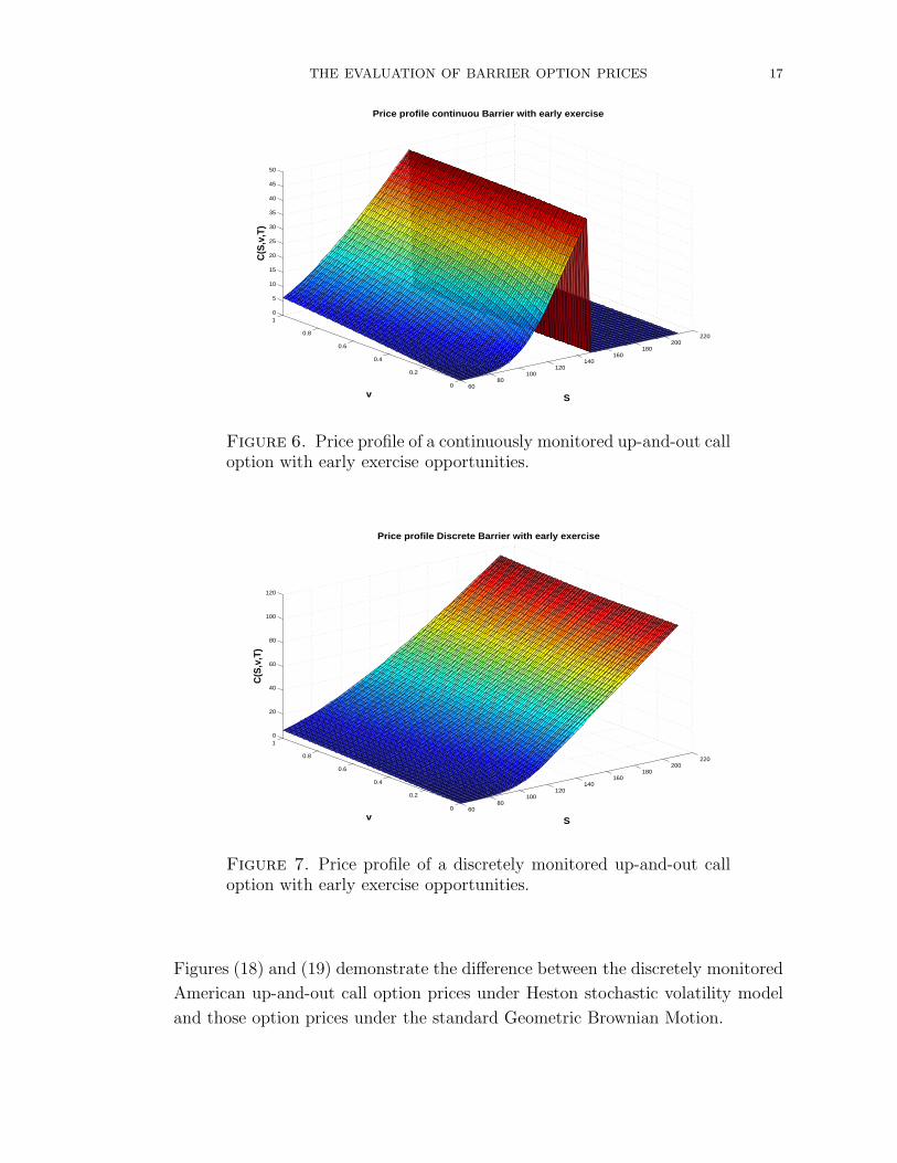
THE EVALUATION OF BARRIER OPTION PRICES 17
6080
100120
140160
180200
220
0
0.2
0.4
0.6
0.8
10
5
10
15
20
25
30
35
40
45
50
S
Price profile continuou Barrier with early exercise
v
C(S
,v,T
)
Figure 6. Price profile of a continuously monitored up-and-out calloption with early exercise opportunities.
6080
100120
140160
180200
220
0
0.2
0.4
0.6
0.8
10
20
40
60
80
100
120
S
Price profile Discrete Barrier with early exercise
v
C(S
,v,T
)
Figure 7. Price profile of a discretely monitored up-and-out calloption with early exercise opportunities.
Figures (18) and (19) demonstrate the difference between the discretely monitored
American up-and-out call option prices under Heston stochastic volatility model
and those option prices under the standard Geometric Brownian Motion.

18 CARL CHIARELLA, BODA KANG AND GUNTER H. MEYER
50
100
150
200
250
0
0.2
0.4
0.6
0.8
1−0.5
−0.4
−0.3
−0.2
−0.1
0
0.1
0.2
S
Delta profile continuous Barrier without early exercise
v
CS(S
,v)
Figure 8. Delta profile of a continuous monitoring up-and-out calloption without early exercise opportunities.
50
100
150
200
250
0
0.2
0.4
0.6
0.8
10
0.2
0.4
0.6
0.8
1
S
Delta profile Continuous Barrier with early exercise
v
CS(S
,v)
Figure 9. Delta profile of an up-and-out call option with earlyexercise opportunities.
6. Conclusion
We have studied the pricing of Barrier options under stochastic volatility using the
Method of Lines. We also provide the Barrier option pricing results from Finite
Difference method, Fourier Cosine Expansion method and Monte Carlo Simulation
approach as benchmarks to the MOL.

THE EVALUATION OF BARRIER OPTION PRICES 19
6080
100120
140160
180200
220
0
0.2
0.4
0.6
0.8
1−0.4
−0.3
−0.2
−0.1
0
0.1
0.2
0.3
S
Delta profile Discrete Barrier without early exercise
v
CS(S
,v)
Figure 10. Delta profile of a discrete monitoring up-and-out calloption without early exercise opportunities.
50
100
150
200
250
0
0.2
0.4
0.6
0.8
10
0.2
0.4
0.6
0.8
1
S
Delta profile Discrete Barrier with early exercise
v
CS(S
,v)
Figure 11. Delta profile of a discrete monitoring up-and-out calloption with early exercise opportunities.
It turns out that the MOL is able to handle both continuously and discretely mon-
itored options with or without early exercise opportunities. Hence we believe this
provides a unified framework to efficiently price various kinds of Barrier options
with different kinds of properties. One main advantage of the MOL is that it
produces the hedge ratios of the option, namely the deltas and gammas, to the
same accuracy as the prices themselves within the same time frame.

20 CARL CHIARELLA, BODA KANG AND GUNTER H. MEYER
0 20 40 60 80 100 120 140−0.05
0
0.05
0.1
0.15
0.2Price Difference (ρ=−0.5)
Share Price (S)
Pric
e D
iffer
ence
s
Stochastic VolatilityZero price difference
Figure 12. The effect of stochastic volatility on continuously mon-itored European up-and-out call (UOC) option. The correlation isρ = −0.5 and all other parameter values are as listed in Table 1.The at the money UOC price under GBM is 2.4197.
In future research, the knock-in option under stochastic volatility with early exer-
cise features should be further investigated.

THE EVALUATION OF BARRIER OPTION PRICES 21
0 20 40 60 80 100 120 140−0.2
−0.15
−0.1
−0.05
0
0.05Price Difference (ρ=0.5)
Share Price (S)
Pric
e D
iffer
ence
s
Stochastic VolatilityZero price difference
Figure 13. The effect of stochastic volatility on continuously mon-itored European up-and-out call option. The correlation is ρ = 0.5and all other parameter values are as listed in Table 1. The at themoney UOC price under GBM is 2.4197.
0 50 100 150 200 250−0.1
−0.05
0
0.05
0.1
0.15
0.2
0.25Price Difference (ρ=−0.5)
Share Price (S)
Pric
e D
iffer
ence
s
Stochastic Volatility
Zero price difference
Figure 14. The effect of stochastic volatility on discretely moni-tored European up-and-out call option. The correlation is ρ = −0.5and all other parameter values are as listed in Table 1. The at themoney UOC price under GBM is 3.9487.

22 CARL CHIARELLA, BODA KANG AND GUNTER H. MEYER
0 50 100 150 200 250−0.2
−0.15
−0.1
−0.05
0
0.05
0.1
0.15Price Difference (ρ=0.5)
Share Price (S)
Pric
e D
iffer
ence
s
Stochastic VolatilityZero price difference
Figure 15. The effect of stochastic volatility on discretely moni-tored European up-and-out call option. The correlation is ρ = 0.5and all other parameter values are as listed in Table 1. The at themoney UOC price under GBM is 3.9487.
0 20 40 60 80 100 120 140−0.1
−0.05
0
0.05
0.1
0.15Price Difference (ρ=−0.5)
Share Price (S)
Pric
e D
iffer
ence
s
Stochastic VolatilityZero price difference
Figure 16. The effect of stochastic volatility on the continuouslymonitored American up-and-out call option. The correlation is ρ =−0.5 and all other parameter values are as listed in Table 1. The atthe money UOC price under GBM is 8.2917.
THE EVALUATION OF BARRIER OPTION PRICES 23
0 20 40 60 80 100 120 140−0.04
−0.02
0
0.02
0.04
0.06
0.08
0.1
0.12
0.14Price Difference (ρ=0.5)
Share Price (S)
Pric
e D
iffer
ence
s
Stochastic VolatilityZero price difference
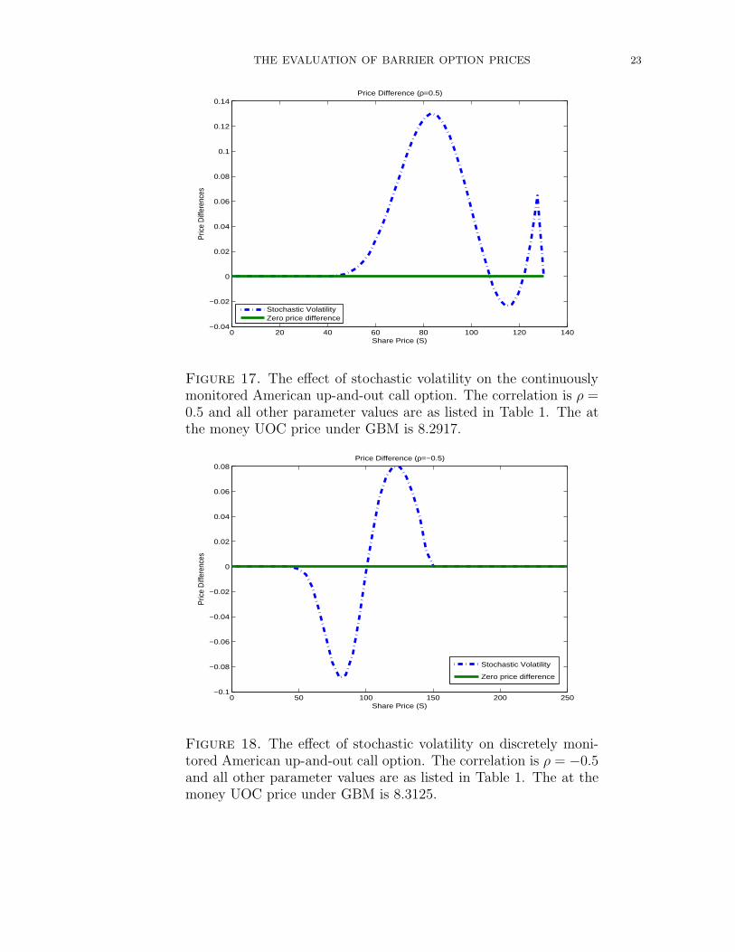
Figure 17. The effect of stochastic volatility on the continuouslymonitored American up-and-out call option. The correlation is ρ =0.5 and all other parameter values are as listed in Table 1. The atthe money UOC price under GBM is 8.2917.
0 50 100 150 200 250−0.1
−0.08
−0.06
−0.04
−0.02
0
0.02
0.04
0.06
0.08Price Difference (ρ=−0.5)
Share Price (S)
Pric
e D
iffer
ence
s
Stochastic Volatility
Zero price difference
Figure 18. The effect of stochastic volatility on discretely moni-tored American up-and-out call option. The correlation is ρ = −0.5and all other parameter values are as listed in Table 1. The at themoney UOC price under GBM is 8.3125.

24 CARL CHIARELLA, BODA KANG AND GUNTER H. MEYER
0 50 100 150 200 250−0.1
−0.05
0
0.05
0.1
0.15Price Difference (ρ=0.5)
Share Price (S)
Pric
e D
iffer
ence
s
Stochastic VolatilityZero price difference
Figure 19. The effect of stochastic volatility on discretely moni-tored American up-and-out call option. The correlation is ρ = 0.5and all other parameter values are as listed in Table 1. The at themoney UOC price under GBM is 8.3125.

THE EVALUATION OF BARRIER OPTION PRICES 25
References
Black, F. & Scholes, M. (1973), ‘The Pricing of Corporate Liabilites’, Journal of Political Econ-
omy 81, 637–659.
Cheang, G., Chiarella, C. & Ziogas, A. (2009), ‘The Representation of American Options Prices
under Stochastic Volatility and Jump Diffusion Dynamics’, Quantitative Finance Research
Centre, University of Technology Sydney . Research Paper No. 256.
Chiarella, C., Griebsch, S. & Kang, B. (2009), ‘The Evaluation of European Compound Option
Prices Under Stochastic Volatility’, Quantitative Finance Research Centre, University of
Technology Sydney . Working paper.
Chiarella, C., Kang, B., Meyer, G. H. & Ziogas, A. (2009), ‘The Evaluation of American Op-
tion Prices under Stochastic Volatility and Jump-Diffusion Dynamics Using the Method of
Lines’, International Journal of Theoretical and Applied Finance 12(3), 393–425.
Duffy, D. J. (2006), Finite Difference Methods in Financial Engineering: A Partial Differential
Equation Approach, Wiley; Har/Cdr edition.
Fang, F. & Oosterlee, C. W. (2009a), ‘A Novel Pricing Method for European Options Based on
Fourier-Cosine Series Expansions’, SIAM Journal on Scientific Computing 31(2), 826–848.
Fang, F. & Oosterlee, C. W. (2009b), ‘Pricing Early-Exercise and Discrete Barrier Options by
Fourier-Cosine Series Expansions’, Numerische Mathematik 114(1), 27–62.
Gao, B., Huang, J. Z. & Subrahmanyam, M. (2000), ‘The Valuation of American Barrier Options
Using the Decomposition Technique’, Journal of Economic Dynamics and Control 24, 1783–
1827.
Griebsch, S. (2008), Exotic Option Pricing in Heston’s Stochastic Volatility Model, PhD thesis,
Frankfurt School of Finance & Management.
Heston, S. (1993), ‘A Closed-Form Solution for Options with Stochastic Volatility with Appli-
cations to Bond and Currency Options’, Review of Financial Studies 6(2), 327–343.
Ibanez, A. & Zapatero, F. (2004), ‘Monte Carlo Valuation of American Options through Com-
putation of the Optimal Exercise Frontier’, Journal of Financial and Quantitative Analysis
39(2), 253–275.
Kluge, T. (2002), Pricing Derivatives in Stochastic Volatility Models Using the Finite Difference
Method, Diploma thesis, Chemnitz University of Technology.
Merton, R. C. (1973), ‘Theory of Rational Option Pricing’, Bell Journal of Economics and
Management Science 4, 141–183.
Meyer, G. (2009), Pricing Options and Bonds with the Method of Lines, Georgia Institute of
Technology, http://www.math.gatech.edu/ meyer/.
Rich, D. R. (1994), ‘The Mathematical Foundation of Barrier Option-Pricing Theory’, Advances
in Futures and Options Research 7, 267–311.
Wong, H. Y. & Kwok, Y. K. (2003), ‘Multi-asset Barrier Options and Occupation Time Deriva-
tives’, Applied Mathematical Finance 10(3), 245–266.
Related Documents


