T HE EU ETS AND F IRM F INANCIAL P ERFORMANCE :E VIDENCE FROM THE E UROPEAN E LECTRICITY S ECTOR Master Thesis Copenhagen Business School Master of Sciences in Applied Economics and Finance Authors: Magnus Poulsen (102115) and Pontus L¨ ofgren (124590) Supervisor: Lisbeth la Cour, PhD May 15, 2020 101 pages and 147,238 characters

Welcome message from author
This document is posted to help you gain knowledge. Please leave a comment to let me know what you think about it! Share it to your friends and learn new things together.
Transcript
THE EU ETS AND FIRM FINANCIAL
PERFORMANCE: EVIDENCE FROM THE
EUROPEAN ELECTRICITY SECTOR
Master Thesis
Copenhagen Business School
Master of Sciences in Applied Economics and Finance
Authors: Magnus Poulsen (102115) and Pontus Lofgren (124590)
Supervisor: Lisbeth la Cour, PhD
May 15, 2020
101 pages and 147,238 characters

Abstract
Prior studies on the economic consequences of the European Union Emissions
Trading System (EU ETS) on European electricity generating firms have so far re-
lied on data from the first phase of the scheme that ended in 2007. We address
this gap and find that EU ETS emission allowance price increases (decreases) have
a positive (negative) impact on stock return by employing multifactor models with
a balanced longitudinal dataset covering thirteen European electricity generating
firms during the third phase of the EU ETS. Moreover, we find that the positive re-
lationship is stronger for firms with carbon efficient electricity generation. Based
on the Arbitrage Pricing Theory and the Efficient Market Hypothesis, we argue
that price appreciations in EU ETS emission allowances positively affect firm per-
formance for European electricity generating firms in general and carbon efficient
generators in particular. A possible explanation is that inframarginal suppliers ob-
tain regulatory rent due to the pass-through of the marginal producer’s additional
emission compliance cost to consumers. This suggests that the EU ETS is success-
ful in financially incentivizing profit maximizing firms concerned with electricity
generation to decarbonize operations, which may be of interest to policymakers
considering more stringent emission compliance costs for other sectors.
2

Acknowledgements
First and foremost, we express our gratitude and appreciation to our supervisor
Lisbeth la Cour, Professor in Time Series Econometrics at the Department of Eco-
nomics, Copenhagen Business School, for excellent guidance throughout the pro-
cess of writing this thesis. We are also grateful to Claus Vorm, Deputy Head of
Multi Assets at Nordea Investment Management, for providing important insights
into how utility stocks perform in low interest environments. We were also for-
tunate to sit down with representatives from Ørsted to learn about the electricity
sector. Lastly, we thank Julian Karst, Information Service Officer at the European
Energy Exchange (EEX) for kindly providing the data required for our empirical
analysis.
3

Contents
1 Introduction 10
1.1 Background and Problem Discussion . . . . . . . . . . . . . . . . . 10
1.2 Purpose . . . . . . . . . . . . . . . . . . . . . . . . . . . . . . . . . 11
1.3 Research Question . . . . . . . . . . . . . . . . . . . . . . . . . . . 12
1.4 Thesis Structure . . . . . . . . . . . . . . . . . . . . . . . . . . . . . 12
2 Institutional Background and Literature Review 14
2.1 The European Electricity Market . . . . . . . . . . . . . . . . . . . 14
2.1.1 Infrastructure . . . . . . . . . . . . . . . . . . . . . . . . . . 14
2.1.2 Markets . . . . . . . . . . . . . . . . . . . . . . . . . . . . . 15
2.1.3 The European Electricity Mix . . . . . . . . . . . . . . . . . 17
2.1.4 Price-Setting and the Merit Order Curve . . . . . . . . . . . 20
2.2 The European Union Emissions Trading System . . . . . . . . . . . 21
2.2.1 Evolvement of the EU ETS . . . . . . . . . . . . . . . . . . . 22
2.2.2 Market Stability Reserve . . . . . . . . . . . . . . . . . . . . 28
2.3 Literature Review . . . . . . . . . . . . . . . . . . . . . . . . . . . . 29
2.3.1 European Union Allowances and Firm Financial Performancein the Electricity Sector . . . . . . . . . . . . . . . . . . . . 29
2.3.2 Pricing of European Union Allowances . . . . . . . . . . . . 33
3 Theory and Hypotheses 35
4

CONTENTS
3.1 Theory . . . . . . . . . . . . . . . . . . . . . . . . . . . . . . . . . . 35
3.1.1 Arbitrage Pricing Theory . . . . . . . . . . . . . . . . . . . . 35
3.1.2 Efficient Market Hypothesis . . . . . . . . . . . . . . . . . . 37
3.2 Hypotheses . . . . . . . . . . . . . . . . . . . . . . . . . . . . . . . 38
4 Methodology 41
4.1 Research Approach . . . . . . . . . . . . . . . . . . . . . . . . . . . 41
4.2 Data . . . . . . . . . . . . . . . . . . . . . . . . . . . . . . . . . . . 42
4.2.1 Firms . . . . . . . . . . . . . . . . . . . . . . . . . . . . . . 42
4.2.2 Carbon Intensity . . . . . . . . . . . . . . . . . . . . . . . . 44
4.2.3 European Union Allowance Prices . . . . . . . . . . . . . . . 45
4.2.4 Market Returns . . . . . . . . . . . . . . . . . . . . . . . . . 45
4.2.5 Control Variables: Oil and Natural Gas . . . . . . . . . . . . 46
4.2.6 Transformation of Data and Frequency . . . . . . . . . . . . 46
4.3 Econometric Theory . . . . . . . . . . . . . . . . . . . . . . . . . . 47
4.3.1 OLS Estimation . . . . . . . . . . . . . . . . . . . . . . . . . 47
4.3.2 Omitted Variable Bias . . . . . . . . . . . . . . . . . . . . . 49
4.3.3 Fixed Effects Regression . . . . . . . . . . . . . . . . . . . . 50
4.3.4 Random Effects Regression . . . . . . . . . . . . . . . . . . 52
4.3.5 OLS Diagnostics . . . . . . . . . . . . . . . . . . . . . . . . 52
4.3.6 Autocorrelation . . . . . . . . . . . . . . . . . . . . . . . . . 53
4.3.7 Stationarity . . . . . . . . . . . . . . . . . . . . . . . . . . . 54
4.3.8 Econometric Methodology . . . . . . . . . . . . . . . . . . . 56
5 Results 60
5.1 Overview of the Data . . . . . . . . . . . . . . . . . . . . . . . . . . 60
5.2 Autocorrelation and Stationarity . . . . . . . . . . . . . . . . . . . 67
5

CONTENTS
5.3 Regression Results . . . . . . . . . . . . . . . . . . . . . . . . . . . 70
5.3.1 Hypothesis I . . . . . . . . . . . . . . . . . . . . . . . . . . . 70
5.3.2 Hypothesis II . . . . . . . . . . . . . . . . . . . . . . . . . . 77
5.3.3 OLS Diagnostics . . . . . . . . . . . . . . . . . . . . . . . . 82
5.4 Summary of Findings . . . . . . . . . . . . . . . . . . . . . . . . . . 85
6 Discussion 87
6.1 EU Allowance Price Changes’ Impact on Financial Performance . . 87
6.2 Carbon Intensity and Financial Performance . . . . . . . . . . . . . 93
6.3 Practical Implications . . . . . . . . . . . . . . . . . . . . . . . . . . 95
6.4 Suggested Further Research . . . . . . . . . . . . . . . . . . . . . . 96
7 Conclusion 98
A Appendix 106
A.0.1 Autocorrelation and Stationarity . . . . . . . . . . . . . . . 106
A.0.2 OLS Diagnostic . . . . . . . . . . . . . . . . . . . . . . . . . 111
6

List of Figures
2.1 Illustration of Electricity Grid. . . . . . . . . . . . . . . . . . . . . . 15
2.2 Overview of Electricity Markets. . . . . . . . . . . . . . . . . . . . . 16
2.3 The European Electricity Mix . . . . . . . . . . . . . . . . . . . . . 18
2.4 Illustration of the European Carbon Intensity . . . . . . . . . . . . 19
2.5 Illustration of the Merit Order Curve . . . . . . . . . . . . . . . . . 20
3.1 Illustration of the Merit Order Curve with emission compliance costs 39
4.1 Carbon Intensity for sample firms . . . . . . . . . . . . . . . . . . . 44
5.1 Price Development of the variables under analysis . . . . . . . . . . 61
5.2 Price development of the Portfolio of Electricity Generating Firms,the Market Portfolio and Centrica plc . . . . . . . . . . . . . . . . . 65
5.3 Plots of the logarithmic weekly return and the corresponding ACFplot . . . . . . . . . . . . . . . . . . . . . . . . . . . . . . . . . . . 68
5.4 OLS Diagnostic - Pooled regression . . . . . . . . . . . . . . . . . . 82
5.5 OLS Diagnostic - Equally weighted portfolio . . . . . . . . . . . . . 83
5.6 OLS Diagnostic - Hypothesis II - Polluter . . . . . . . . . . . . . . . 85
6.1 Development for 10-year Government Yields for 2019 . . . . . . . 92
A.1 Plots of the logarithmic weekly return and the corresponding ACFplot . . . . . . . . . . . . . . . . . . . . . . . . . . . . . . . . . . . 110
A.2 OLS Diagnostic: One-year subperiod . . . . . . . . . . . . . . . . . 117
7

LIST OF FIGURES
A.3 OLS Diagnostic: Two-year subperiod . . . . . . . . . . . . . . . . . 120
A.4 OLS Diagnostic: Firm-specific . . . . . . . . . . . . . . . . . . . . . 133
8

List of Tables
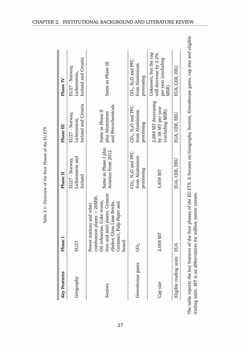
2.1 Overview of the Four Phases of the EU ETS . . . . . . . . . . . . . . 27
4.1 Overview of the companies under analysis . . . . . . . . . . . . . . 43
5.1 Descriptive statistics for variables under analysis . . . . . . . . . . . 63
5.2 Correlation matrix of returns . . . . . . . . . . . . . . . . . . . . . 64
5.3 Correlation matrix for Centrica plc . . . . . . . . . . . . . . . . . . 66
5.4 Summary of Augmented Dickey-Fuller test . . . . . . . . . . . . . . 69
5.5 Regression Results: Hypothesis I . . . . . . . . . . . . . . . . . . . 73
5.6 Regression Results: One-year subperiod . . . . . . . . . . . . . . . 75
5.7 Correlation matrix of returns for 2019 . . . . . . . . . . . . . . . . 76
5.8 Regression Results: Two-year subperiod . . . . . . . . . . . . . . . 77
5.9 Regression Results: Hypothesis II . . . . . . . . . . . . . . . . . . . 80
5.10 Regression Results: Firm-specific . . . . . . . . . . . . . . . . . . . 81
5.11 Extreme data points for Pooled regression . . . . . . . . . . . . . . 84
9

Chapter 1: Introduction
1.1 Background and Problem Discussion
The European Emission Trading System (EU ETS) was introduced in 2005 as a
policy instrument for the European Union to comply with the carbon emission re-
duction targets set out by the Kyoto protocol. Under the system, emitting entities
must surrender one European Union Allowance (EUA) per metric ton of green-
house gas emissions by year-end or face hefty fines. It is a cap-and-trade system
in which the annual number of allowances is decreasing, and firms can trade al-
lowances with one another (Chevallier, 2012). This sets a price on emissions that
serves to incentivize companies to invest in technologies that reduce emissions.
It is cost-efficient in the sense that firms with high abatement costs can purchase
emission rights from firms with cheaper ways to reduce emissions. Today, the EU
ETS is the world’s largest market for emissions and covers more than 13,500 instal-
lations, which are responsible for roughly half of the European Union’s emissions
(Hintermann et al., 2016).
The electricity sector is the largest polluter in the European Union. It is also
different from other sectors in a variety of interesting ways. Firstly, it is naturally
protected from foreign competition by means of infrastructure and regulation.
Secondly, it has a wide range of abatement options available that can substitute
10

CHAPTER 1. INTRODUCTION
carbon-intensive electricity generation. Lastly, it is currently the only sector that is
not allocated any emission allowances for free (Chevallier, 2012).
Perhaps surprising for the unversed reader, previous research has found that elec-
tricity generating firms profited from increased prices of emission allowances dur-
ing the first phase of the EU ETS that ran from 2005 to 2007, despite it constituting
an increased input cost. The phenomenon can be explained by the free allocation
method of emission allowances that was present in the first phase, combined with
a high pass-through rate of its opportunity cost to consumers (Sijm et al., 2006).
In effect, this resulted in windfall profits to the European electricity sector (Obern-
dorfer, 2009; Veith et al., 2009).
Much has changed in the last fifteen years. In terms of the regulatory nature of the
European Union Emissions Trading System, the electricity sector is now subject to
full auctioning of emission allowances, and the system itself has matured signif-
icantly (European Commission, 2015). In terms of the European electricity mix,
renewable energy production has penetrated the market, and carbon intensity has
roughly halved. As such, the results of the previous research may not hold today
and with this paper, we aim to address that gap.
1.2 Purpose
The purpose of the paper is to understand how price changes in European Union
Allowances affect financial performance for European electricity generating firms
during the third phase of the European Union Emissions Trading System. The
conclusions are relevant as it may provide important insights to European poli-
cymakers’ assessment of how to further develop the European Union Emissions
Trading System or for foreign policymakers considering implementing similar reg-
11

CHAPTER 1. INTRODUCTION
ulation. Further, it may be relevant to investors and electricity generating firms
seeking to maximize return on their investments.
1.3 Research Question
This paper seeks to deepen our understanding of how the European Union Emis-
sions Trading System’s greenhouse gas emission allowances affect firm financial
performance for European electricity generating firms during its third phase. We
define our overarching research question as follows:
How do price changes in European Union Allowances affect firm performance for
European electricity generating firms during the third phase of the EU ETS?
It will further nuance our understanding by investigating if and how these dynam-
ics change depending on the carbon intensity of the firm’s electricity production
by answering the following research question:
How does a potential impact of European Union Allowance price changes differ de-
pending on the carbon intensity of European electricity generating firms’ electricity
production during the third phase of EU ETS?
1.4 Thesis Structure
The remainder of the paper is structured as follows. Chapter II introduces the
reader to the electricity sector and the European Union Emissions Trading Sys-
tem to provide context for our overarching research question. To ensure sufficient
theoretical depth, it includes a literature review on the research of the interplay
between emission allowance price changes and firm performance for European
12

CHAPTER 1. INTRODUCTION
electricity generating firms and the price-setting forces on emission allowances.
Chapter III introduces the Arbitrage Pricing Theory and the Efficient Market Hy-
pothesis. Combined with previous research on the subject, these theories will lay
the foundation to our hypotheses. Chapter IV describes the data and the method-
ology. Chapter V will presents the empirical results discussed in Chapter VI, pre-
ceding the conclusion in Chapter VII.
13

Chapter 2: Institutional Background
and Literature Review
Chapter II begins by providing the reader with an introduction to the European
electricity sector including its infrastructure, markets, electricity mix, and price
setting mechanisms. Next, it presents an overview of the European Union Emis-
sions Trading System before providing a review of the literature covering its effect
the financial performance of European electricity generating firms as well as the
price setting forces on emission allowances.
2.1 The European Electricity Market
2.1.1 Infrastructure
The European Union has adopted a wide range of legislation aiming at achieving
the long-term goal of an integrated European energy market, in which electric-
ity is traded cross-borders competitively. Previously, each domestic energy market
was monopolistic or oligopolistic and consisted of one or a few vertically inte-
grated companies responsible for the generation, transportation, and distribution
of electricity. Today, regulation limiting the degree of vertical integration has
14

CHAPTER 2. INSTITUTIONAL BACKGROUND AND LITERATURE REVIEW
further divided the electrical sector into three participant groups: i) electricity
generators, ii) transmission system operators (TSO), and iii) distribution system
operators (DSO). The electricity grid is a network that connects electricity gen-
erators and consumers via transmission and distribution networks. Transmission
system operators are responsible for transporting electricity regionally over long
distances from power generators to distribution system operators that locally dis-
tribute electricity to households and industries. The European transmission grid
covers 300,000 km of power lines, including 355 cross-border lines. (Erbach,
2016).
Source: Erbach (2016)
Figure 2.1: Illustration of Electricity Grid.
2.1.2 Markets
Participants in the wholesale markets are electricity generators on the one side
and electricity suppliers and large industrial consumers on the other. They meet
on organized multilateral power exchanges such as Nordpool or over-the-counter.
Electricity is a unique commodity in the sense that it is essentially produced and
consumed simultaneously and that imbalances between production and consump-
tion in the grid can cause system collapse and blackouts. As such, the electricity
markets have been designed to accommodate this issue. The markets are ordered
15

CHAPTER 2. INSTITUTIONAL BACKGROUND AND LITERATURE REVIEW
sequentially starting years before the actual delivery and ending after the actual
delivery. This facilitates the balancing between supply and demand.
Source: Erbach (2016)
Figure 2.2: Overview of Electricity Markets.
In the forward and futures market, the two parties agree to the terms of the ex-
change years to weeks in advance of the transaction taking place. This allows gen-
erators to plan their output appropriately and for both parties to hedge against the
risk of fluctuating electricity prices. In the day-ahead market, electricity is traded
one day before delivery allowing electricity generators to adjust their capacity to
accommodate demand the following day. In the intra-day market, electricity is
traded on the day of delivery, and output can be fine-tuned. Lastly, in the balanc-
ing market, the Transmission System Operator will maintain system balance by
injections or take-offs of electricity (KU Leuven Energy Institute, 2015).
16

CHAPTER 2. INSTITUTIONAL BACKGROUND AND LITERATURE REVIEW
2.1.3 The European Electricity Mix
Electricity Generation Technologies
Electricity generation technologies are typically divided into three different cate-
gories: nuclear power, fossil-fueled power, and renewable electricity.
The process of generating electricity using nuclear power is thermal, in which
water is heated through nuclear fission to steam that drives a rotational turbine.
Nuclear power requires substantial initial investments, but the electricity is gener-
ated at low marginal cost and with no greenhouse gas emissions.
As with nuclear power generation, fossil-fuel power is generated through a ther-
mal process in which fuel is burned to create steam that drives a turbine. Fossil-
fuel generation can be divided into three subcategories, namely coal, natural gas,
and petroleum. Coal and natural gas fossil-fuel generation have efficiencies of
40% and 60%, respectively, meaning that a large portion of the energy is not being
transformed into electricity. These power plants are commonly operated using an
Integrated Gasification Combined Cycle procedure that allows for the use of both
fuel types as inputs. This allows the power plant to switch between fuel types de-
pending on the relative price of the input and the associated emission costs. Coal
emits, on average, approximately 2.5 times more carbon into the atmosphere than
natural gas for the same output of electricity.
Electricity generated from renewable energy sources are categorized into i) wind
power, ii) hydroelectric power, iii) biomass-based electricity, iv) photovoltaic elec-
tricity, and v) concentrating solar power.
Wind power generates electricity by exploiting wind to mechanically rotate a wind
turbine. Technological advancements have significantly increased efficiencies and
17

CHAPTER 2. INSTITUTIONAL BACKGROUND AND LITERATURE REVIEW
lowered the average cost of electricity output. Hydroelectric power exploits run-
ning water, typically from a reservoir, to drive a turbine that generates electricity.
It is a relatively stable source of electricity and can be constructed with very high
capacity. Hydroelectric power has been the primary source of renewable electric-
ity production in the European Union until recently when it ranks second to wind
power. Biomass-based electricity burns biomass, primarily wood, to create steam
that drives a turbine. Both photovoltaic and concentrating solar power use the
energy from the sun to create electricity (Rademaekers et al., 2011).
Development of the European Electricity Mix
Source: Jones (2020)
Figure 2.3: The European Electricity Mix
18

CHAPTER 2. INSTITUTIONAL BACKGROUND AND LITERATURE REVIEW
The European energy mix has undergone a significant shift towards less carbon-
intensive electricity generation. Since 2007, which was the last year of the first
phase of the EU ETS, electricity generation from coal has more than halved and
been entirely replaced by renewable energy sources, primarily wind power. In
2019, wind and solar power were responsible for a larger proportion of electric-
ity production than coal for the first time, and greenhouse gas emissions in the
electricity sector were 43% lower compared to the levels in 2007. Total electricity
generation has not changed considerably, with 3,312 TWh in 2005 and 3,227 TWh
in 2019.
Source: Jones (2020)
Figure 2.4: Illustration of the European Carbon Intensity
This transformation has been driven by multiple forces. An increased awareness
regarding global warming has increased demand for renewable energy sources,
with most electricity vendors offering “green energy” to its customers. Combined
with significant technological advancements in wind power that increase capacity
and efficiencies, investments in wind power increased substantially, often sup-
ported by government subsidies. In addition, the EU ETS’ price on emissions
has incentivized companies to invest in renewable energy production (Adabie and
19
CHAPTER 2. INSTITUTIONAL BACKGROUND AND LITERATURE REVIEW
Chamorro, 2008). Moreover, within the fossil-fuel generation, there has been a
large shift from coal to natural gas, driven by the increased cost of emissions. In
2019, for instance, a sharp increase in emission allowance prices partially drove
a significant fuel switch in thermal electricity generation from coal to natural gas
(Buck et al., 2020).
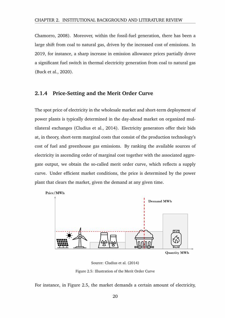
2.1.4 Price-Setting and the Merit Order Curve
The spot price of electricity in the wholesale market and short-term deployment of
power plants is typically determined in the day-ahead market on organized mul-
tilateral exchanges (Cludius et al., 2014). Electricity generators offer their bids
at, in theory, short-term marginal costs that consist of the production technology’s
cost of fuel and greenhouse gas emissions. By ranking the available sources of
electricity in ascending order of marginal cost together with the associated aggre-
gate output, we obtain the so-called merit order curve, which reflects a supply
curve. Under efficient market conditions, the price is determined by the power
plant that clears the market, given the demand at any given time.
Source: Cludius et al. (2014)
Figure 2.5: Illustration of the Merit Order Curve
For instance, in Figure 2.5, the market demands a certain amount of electricity,
20

CHAPTER 2. INSTITUTIONAL BACKGROUND AND LITERATURE REVIEW
which makes coal clear the market. Coal is then the price-setting technology and
the marginal producer. Because renewable energy sources and nuclear power
plants have lower marginal costs, they are infra-marginal producers with positive
contribution margins.
2.2 The European Union Emissions Trading System
The first indication of a European emission trading system appeared in 2000 when
the European Commission issued Green Paper on Greenhouse Gas Emissions Trading
within the European Union (Denny Ellerman et al., 2016). The EU ETS Directive
(Directive 2003/87/EC) was adopted in 2003 and subsequently launched in 2005
across all 27 member states as a policy instrument to ensure that the European
Union would meet its legally obligated emission reduction target of the 1997 Kyoto
protocol (Chevallier, 2012).
The EU ETS is a “cap and trade” system in which a cap is set on the total amount of
greenhouse gas emissions that can be emitted during a year. Each company must
surrender enough allowances to cover its installations’ emissions by year-end, or
hefty fines will be imposed (Chevallier, 2012). Because the cap is reduced over
time, the total emissions of the European Union are reduced.
Within the cap, companies can meet on the market and trade allowances. As
such, a price on greenhouse gas emissions is formed, which serves to incentivize
profit-maximizing companies to invest in green technologies that reduce emissions
(Hintermann et al., 2016). The companies that are able to reduce their greenhouse
emissions at a lower cost than the price of carbon will be financially incentivized
to do so. Under perfect market conditions in equilibrium, the marginal abatement
cost will equal the price of carbon and will be identical for all companies. As such,
21

CHAPTER 2. INSTITUTIONAL BACKGROUND AND LITERATURE REVIEW
investments will be concentrated at the most cost-effective abatement opportuni-
ties, which leads to a reduction in emissions at the lowest economic cost.
As of 2014, more than 13,500 energy-intensive installations responsible for ap-
proximately four percent of global greenhouse gas emissions are covered by the
system (Hintermann et al., 2016) making it the largest market for greenhouse gas
emissions (European Commission, 2015). Since its inception in 2005, the system
has been successfully implemented during three distinct phases, with the fourth
phase set to begin in 2021.
2.2.1 Evolvement of the EU ETS
Phase I: 2005 - 2007
The first phase of the EU ETS served as a “warm up phase” aimed at establishing
a price on carbon dioxide emissions, free trade in emission allowances, and the
infrastructure to monitor, report and verify emissions from installations covered
by the system (European Commission, 2013). In addition to power stations and
other combustion plants with an output above 20 MW, oil refineries, coke ovens,
iron and steel plants, cement clinkers, glass, lime, bricks, ceramics, pulp, as well as
the paper and board sectors were included in the system (European Commission,
2015). Together they covered 46% of the total CO2 emissions of EU countries with
the electricity sector being the largest emitter (Oberndorfer, 2009). Nine out of ten
allowances were allocated free-of-charge to limit the risk of adversely impacting
European competitiveness on international markets, which would result in carbon
spillover to countries outside the EU. A penalty charge to companies that failed
to sufficiently surrender allowances was set to e40 per ton of CO2. The price of
carbon dioxide reached e8 per ton in the first month (Chevallier, 2012).
22

CHAPTER 2. INSTITUTIONAL BACKGROUND AND LITERATURE REVIEW
Each covered country established its own “National Allocation Plan” that deter-
mined the amount of allowances that would be available for the country and how
they would be distributed between sectors (European Commission, 2015). The
National Allocation Plans had to comply with the criteria set out by the European
Commission in the ETS Directive to be approved. As such, the total EU cap con-
sisted of each member state’s respective national caps and would not be known
until all National Allocation Plans had been approved (Denny Ellerman et al.,
2016).
The EU had not yet gathered reliable emissions data, and the initial cap was set
based on estimates. In 2007, when the EU disclosed the emissions data compiled
from the monitoring activities, it became clear that the EU had vastly overallocated
allowances available in the market (Chevallier, 2012). At the time, an allowance
had limited temporal value as it could not be banked to the second phase that
would soon follow. This led to high volatility and spot prices plummeting dramat-
ically to a value of zero from e25-30 just months before (Aatola et al., 2013).
Phase II: 2008 - 2012
Phase II extended the EU ETS’ scope in sectors to include domestic aviation, in
geography to include Norway, Iceland, and Lichtenstein, and in emission types
by voluntary opt-in of nitrous oxide (N2O) (European Commission, 2015). The
system was linked to international carbon dioxide markets by accepting certain
Kyoto Protocol emission units under the Clean Development Mechanism (CDM)
and Joint Implementation (JI) alongside European Union Emission Allowances
(EUAs) (European Commission, 2015). These arrangements allow industrialized
countries to reduce their greenhouse gas emissions through international invest-
ments that reduce emissions in developing countries. The Kyoto credits that are
generated through CDM and JI projects are interchangeable with EUAs and can
23

CHAPTER 2. INSTITUTIONAL BACKGROUND AND LITERATURE REVIEW
thus be surrendered to offset greenhouse gas emissions subject to the regulation
(Denny Ellerman et al., 2016). The cap for these offsets during the second phase
was set to 1.3 billion (total cap in 2008 was 1.9 billion), but investments in large
hydroelectric power and forestry projects were not eligible. Although EU ETS was
the largest market for carbon dioxide and the primary driver for demand of Kyoto
credits, the use of offsets only constituted 10% of the cap despite being a perfect
substitute for EUAs (Denny Ellerman et al., 2016).
Trading volumes increased, and price volatility decreased during the second phase
due to a tighter emissions cap and because allowances were allowed to be banked
over the years (Aatola et al., 2013). Research finds that the more stringent emis-
sions cap significantly reduced emissions during the second phase (Martin & Wag-
ner, 2016).
Phase III: 2013 - 2020
The first commitment period of the Kyoto protocol ended in 2012, and it was
not followed by the Doha Amendment. In the absence of an international agree-
ment on greenhouse gas emission reduction, the third phase corresponds to the
objective of the EU’s Energy Climate Package introduced in 2008 with the goal of
reducing emissions by 20% by 2020 compared to 1990 (Chevallier, 2012).
The scope was extended in geography to include Croatia (that joined the EU in
2013), and in sectors by including the aluminium and petrochemical sectors and
in types by including N2O emissions from all installations and PFC from aluminium
production (European Commission, 2015).
A pan-EU cap for stationary installations declining by a linear factor of 1.74% com-
pared to the average total quantity of allowances issued annually in 2008 - 2012
was adopted. This corresponds to a decrease in absolute terms of 38,264,246 al-
24

CHAPTER 2. INSTITUTIONAL BACKGROUND AND LITERATURE REVIEW
lowances per year and would ensure a decrease in emissions from EU ETS covered
sectors by 21% compared to levels in 2005 (European Commission, 2015).
Although auctioning became the default allocation method in Phase III, a signif-
icant amount of allowances are still being issued for free. The power generation
sector, however, has been subject to full-auctioning since 2013 except for instal-
lations in certain countries covered by Article 10c of the EU ETS Directive. It
provided derogation from the default auctioning allocation method until 2019 to
support modernization investments that reduced the reliance on coal to generate
electricity. At the minimum, investments to diversify the energy mix and mod-
ernize their respective electricity sectors had to amount to the value of the free
allowances that were issued. Of ten eligible countries, eight states made use of the
exception: Bulgaria, Cyprus, Czech Republic, Estonia, Hungary, Lithuania, Poland
and Romania. (European Commission, 2015). The power generation sector was
considered suitable for full-auctioning due to its relatively low abatement costs to
reduce emissions and the weak exposure to international competition from firms
not covered by the EU ETS (Chevallier, 2012).
Phase IV: 2021 - 2030
The fourth phase of the EU ETS will begin from 2021 and run until 2030. To
increase the pace of the decrease in emissions, the EU will increase the annual
linear reduction rate of emissions to 2.2%, compared to 1.74% in phases III. The
purpose is to achieve a reduction in greenhouse gas emissions for sectors in the
EU ETS by 46% compared to the 2005 level. Also, the Market Stability Reserve
play a larger role in phase IV as the number of allowances put in the reserve
will temporarily double to 24% of the total number of allowances in circulation
from 2019 to 2023, after which the rate will return to 12% in 2024. The Market
Stability Reserve will be described in further detail in Section 2.2.2 but aims to
25

CHAPTER 2. INSTITUTIONAL BACKGROUND AND LITERATURE REVIEW
reduce the current overallocation of the total number of allowances in circulation.
The fourth phase will address the risk of carbon leakage by providing predictable,
robust, and a fair set of rules. The EU defines carbon leakage as an increase in
greenhouse gas emissions in one country as a product of strict climate policy in
another. The system of free allocation will be continue for another decade but will
focus on sectors at the highest risk of relocating their operations outside of the EU.
These sectors will continue receiving allowances for free, but free allocation will be
phased out to less exposed sectors by the end of phase IV. (European Commission,
2019b).
Additionally, as part of the fourth phase, there will be an increase in ”green” in-
vestments to modernize the system. The EU will set up several low-carbon fund-
ing mechanisms to help energy-intensive industrial sectors and the power sector
to meet the innovation and investment challenges facing the transition to a low
carbon economy. The two main new initiatives are an innovation fund and a mod-
ernization fund. The innovation fund will support the innovative technologies in
the industry and will be an extension of an existing fund and will correspond to a
market value of at least 450 million emission allowances. The modernization fund
will support investments in modernizing energy systems, energy efficiency, and fa-
cilitating the transition in carbon dependent regions in 10 lower-income member
states (European Commission, 2019b).
26
CHAPTER 2. INSTITUTIONAL BACKGROUND AND LITERATURE REVIEW
Tabl
e2.
1:O
verv
iew
ofth
eFo
urPh
ases
ofth
eEU
ETS
Key
Feat
ure
sPh
ase
IPh
ase
IIPh
ase
III
Phas
eIV
Geo
grap
hyEU
27EU
27-N
orw
ay,
Lich
tens
tein
and
Icel
and
EU27
-Nor
way
,Li
chte
nste
in,
Icel
and
and
Cro
atia
EU27
-Nor
way
,Li
chte
nste
in,
Icel
and
and
Cro
atia
Sect
ors
Pow
erst
atio
nsan
dot
her
com
bust
ion
plan
ts>
20M
W,
Oil
refin
erie
s,C
oke
oven
s,Ir
onan
dst
eelp
lant
s,C
emen
tcl
inke
r,G
lass
Lim
eB
rick
s,C
eram
ics,
Pulp
Pape
ran
dbo
ard.
Sam
eas
Phas
eI
plus
Avi
atio
nfr
om20
12
Sam
eas
Phas
eII
plus
Alu
min
ium
and
Petr
oche
mic
als
Sam
eas
Phas
eII
I
Gre
enho
use
gase
sC
O2
CO
2,N
2O
and
PFC
from
Alu
min
ium
proc
essi
ng
CO
2,N
2O
and
PFC
from
Alu
min
ium
proc
essi
ng
CO
2,N
2O
and
PFC
from
Alu
min
ium
proc
essi
ng
Cap
size
2,05
8M
T1,
858
MT
2,08
4M
Tde
crea
sing
by38
MT
per
year
(exc
ludi
ngM
SR)
Unk
now
n,bu
tth
eca
pw
illde
crea
seby
2.2%
per
year
(exc
ludi
ngM
SR)
Elig
ible
trad
ing
unit
sEU
AEU
A,C
ER,E
RU
EUA
,CER
,ER
UEU
A,C
ER,E
RU
The
tabl
ere
port
sth
eke
yfe
atur
esof
the
four
phas
esof
the
EUET
S.It
focu
ses
onG
eogr
aphy
,Sec
tors
,Gre
enho
use
gase
s,ca
psi
zean
del
igib
letr
adin
gun
its.
MT
isan
abbr
evia
tion
for
mill
ion
met
ric
tonn
es.
27
CHAPTER 2. INSTITUTIONAL BACKGROUND AND LITERATURE REVIEW
2.2.2 Market Stability Reserve
The EU ETS faced widespread criticism that the price of allowances was too low
to incentivize companies to reduce emissions (Perino & Willner, 2016). A sur-
plus of allowances, defined as the difference between the available amount of
allowances and the amount of allowances required for compliance in a given year,
had been built up during the second phase as a consequence of the financial crisis,
high imports of international credits and faster-than-expected transition towards
renewable electricity generation. The surplus was two billion allowances at the
start of phase III in 2013 and the cost of emitting a ton of CO2 was roughly equiv-
alent to a cup of coffee at e3. In the short-term, this risked undermining the
proper functioning of the emissions market and in the long-term, and it risked
adversely affecting the ability of the system to reduce emissions. As such, the EU
implemented a short-term and a long-term measure to mitigate these risks.
In 2015, the surplus was reduced to 1.78 billion allowances through what the
EU calls “back-loading”. Essentially, back-loading was the short-term measure of
postponing the auctioning of 900 million allowances to 2019 and 2020. It would
not change the overall amount of allowances available during the third phase but
served to redistribute the auctions in order to shift the short-term equilibrium to
achieve a higher price. 400 million, 300 million and 200 million allowances were
postponed during 2014, 2015, and 2016, respectively. As a result, the surplus was
reduced by an estimated 40% at the end of 2015.
As a long-term measure, the Market Stability Reserve took effect in January 2019.
It adjusts the number of allowances that are auctioned each year based on the
previous years’ surplus. In times of large surplus, allowances amounting to 12%
of the aggregate market surplus will be set aside, and their issuing shifted into
the future. As the surplus drops below 400 million, the allowances will be issued
28

CHAPTER 2. INSTITUTIONAL BACKGROUND AND LITERATURE REVIEW
to the market in intervals of 100 million per year (European Commission, 2013).
This process will continue until the surplus is depleted. The reserve operates com-
pletely based on a set of predefined rules and leaves no room for discretion to
the EU or member states. The aforementioned reintroduction of the back-loaded
allowances during 2014 to 2016 was cancelled and put in the reserve instead.
2.3 Literature Review
2.3.1 European Union Allowances and Firm Financial Perfor-
mance in the Electricity Sector
Even before the system was implemented in 2005, simulations suggested that the
EU ETS would benefit the electricity sector as a whole, as long as allowances were
distributed free of charge (Bode, 2006). A price on emissions constitutes an oppor-
tunity cost as an allowance can either be used as an input factor to cover emissions
or be sold to another firm that demands it, regardless of whether it was provided
for free or not. As such, the marginal production cost increases for companies
subject to the regulation, and profit-maximizing firms will attempt to transfer this
cost to its customers. In doing so, companies face the risk of losing market share to
competition not covered by the EU ETS. However, the electricity sector in the EU
has inherent entry barriers from foreign competition due to technical aspects that
limit the possible import penetration of electricity (Marin et al., 2018). As such,
electricity companies can transfer much of the opportunity cost that the price of
an allowance represents to its customers.
Sijm et al. (2006) combined spot and forward market prices of electricity in the
Netherlands and Germany with the price of EUA to investigate the pass-through
29
CHAPTER 2. INSTITUTIONAL BACKGROUND AND LITERATURE REVIEW
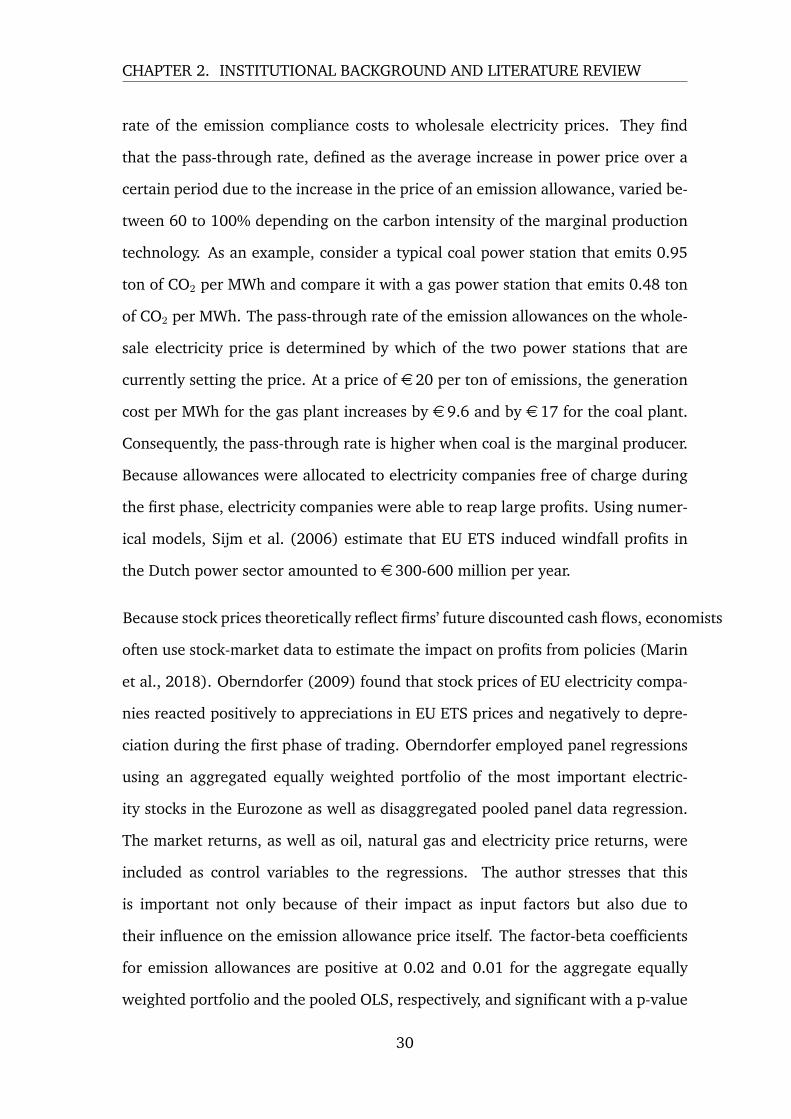
rate of the emission compliance costs to wholesale electricity prices. They find
that the pass-through rate, defined as the average increase in power price over a
certain period due to the increase in the price of an emission allowance, varied be-
tween 60 to 100% depending on the carbon intensity of the marginal production
technology. As an example, consider a typical coal power station that emits 0.95
ton of CO2 per MWh and compare it with a gas power station that emits 0.48 ton
of CO2 per MWh. The pass-through rate of the emission allowances on the whole-
sale electricity price is determined by which of the two power stations that are
currently setting the price. At a price of e20 per ton of emissions, the generation
cost per MWh for the gas plant increases by e9.6 and by e17 for the coal plant.
Consequently, the pass-through rate is higher when coal is the marginal producer.
Because allowances were allocated to electricity companies free of charge during
the first phase, electricity companies were able to reap large profits. Using numer-
ical models, Sijm et al. (2006) estimate that EU ETS induced windfall profits in
the Dutch power sector amounted to e300-600 million per year.
Because stock prices theoretically reflect firms’ future discounted cash flows, economists
often use stock-market data to estimate the impact on profits from policies (Marin
et al., 2018). Oberndorfer (2009) found that stock prices of EU electricity compa-
nies reacted positively to appreciations in EU ETS prices and negatively to depre-
ciation during the first phase of trading. Oberndorfer employed panel regressions
using an aggregated equally weighted portfolio of the most important electric-
ity stocks in the Eurozone as well as disaggregated pooled panel data regression.
The market returns, as well as oil, natural gas and electricity price returns, were
included as control variables to the regressions. The author stresses that this
is important not only because of their impact as input factors but also due to
their influence on the emission allowance price itself. The factor-beta coefficients
for emission allowances are positive at 0.02 and 0.01 for the aggregate equally
weighted portfolio and the pooled OLS, respectively, and significant with a p-value
30

CHAPTER 2. INSTITUTIONAL BACKGROUND AND LITERATURE REVIEW
below 1%. Oberndorfer argues that the positive influence is due to windfall prof-
its that occur as a result of the high pass-through rate of the opportunity cost of
the grandfathered emission allowances. Oberndorfer (2009) investigates the ef-
fect on a country-specific level and finds that the results hold true for all countries
investigated except Spain. Oberndorfer (2009) argues that Spain’s stringent price
regulation that limits the pass-through rate could be the reason for the inverse
effect. Zachmann and von Hirschhausen (2008) found that positive price shocks
in emission allowances disseminated more quickly to the final German wholesale
electricity price than negative price shocks and suggest that this price asymme-
try may be due to market power or ignorance amongst market agents due to the
immaturity of the market. This could result in increased profits but Oberndor-
fer (2009) did not find that such an asymmetry existed in stock price reactions,
indicating that market participants were either unaware of the asymmetric price
reactions in the wholesale electricity prices or that it was a German phenomenon.
Similar to Oberndorfer (2009), Veith et al. (2009) measure the EU ETS impact on
firm performance through investor expectations by employing a multifactor model
on a sample of 22 publicly traded electricity firms accounting for two-thirds of total
EU electricity generation. In line with Oberndorfer (2009), they find a positive re-
lationship between emission allowance futures prices and stock prices, indicating
financial market agents expect that electricity companies obtain higher earnings
by passing on the opportunity cost of the emission allowances to wholesale elec-
tricity prices. The authors fit the emission allowance return into their subperiod
pooled panel regressions and estimate that carbon prices positively yielded an es-
timated average stock market return by 0.8% during the first six months of the
trading system, suggesting that electricity generators may obtain regulatory rent.
As a robustness check, they again regress stock performance on overall stock per-
formance and emission allowance returns for companies that have carbon-neutral
electricity generation and thus fall outside of the system. Although these firms
31

CHAPTER 2. INSTITUTIONAL BACKGROUND AND LITERATURE REVIEW
sell the same common good as firms covered by the system, the empirical results
do not show a connection between emission allowance return and stock perfor-
mance. The authors present a lack of market power as a possible explanation, or
that investors in these entities do not consider emission price movements. In addi-
tion to regressing return on emission allowance returns and overall stock market
return, they control for commodity price impact by including the return on oil and
natural gas to a fixed effects regression model. The results regarding emission
allowance futures return remain robust with a factor-beta coefficient of 0.023 and
significant at 5%. Next, they further check for the robustness by controlling for
firm-specific characteristics in terms of fuel mix by including a dummy variable
equaling one if the company’s proportion of carbon-emitting electricity generation
is above the sample median. The binary variable is interacted with the return on
emission allowance prices to allow for both different intercept and slope. There is
no interaction effect when regressing emission allowance spot prices, but a slightly
negative coefficient when using emission allowance December 2008 futures. The
firms with a high share of fossil fuels in electricity generation lose approximately
half of the positive influence of emission allowance returns. According to the au-
thors, this indicates that investors did not consider the underlying fuel mix during
the first phase of the EU ETS that would end in December 2007 but that investors
expected future cash flows to be affected during the second phase. They argue
that investors likely anticipated and discounted adverse economic effects resulting
from a higher degree of auctioning that would be enforced during the subsequent
phase.
Bushnell et al. (2013) conducted an event study on how the large price decline in
emission allowances in April 2006 affected the stock prices of 552 European com-
panies subject to EU ETS in different sectors. They find that share prices within the
power sector decline, and that “clean” electricity companies’ share prices decline
further than their “dirty” counterparts. The authors argue that this implies that
32

CHAPTER 2. INSTITUTIONAL BACKGROUND AND LITERATURE REVIEW
the market understood that declining emission prices would reduce contribution
margins more severely for less carbon-intensive power generators. High emitting
electricity companies also experienced abnormal declines in share price, and the
authors suggest that this highlights a focus on revenue rather than costs among
investors.
To our knowledge, there has been no published research on the potential effects
of EUA price changes on firm performance among European electricity firms dur-
ing the second or third phase of the EU ETS. All the abovementioned studies lay
forward that their results may not hold true during later phases of the EU ETS,
primarily due to the end of grandfathering (Sijm et al., 2006; Oberndorfer, 2009;
Veith et al., 2009; Bushnell et al., 2013) and that the market becomes more effi-
cient as market agents become better informed (Oberndorfer, 2009; Bushnell et
al., 2013).
2.3.2 Pricing of European Union Allowances
The price of a ton of greenhouse gas emission in the EU ETS is determined by
the equilibrium between supply and demand in the market. Supply is primarily
determined by EU policy decision such as the size of the emissions cap, allocation
methods, linkages to international greenhouse gas emission markets and rules
about banking and borrowing of allowances. An example of the impact of supply
on EUA prices is the crash in 2006 when the markets realized that the EU had
oversupplied participants with allowances (Alberola et al., 2008). Hintermann
et al. (2016) review the literature of pricing during the second phase of the EU
ETS and find that demand is primarily determined by the amount of “business as
usual” emissions, which are mainly driven by the growth of the economy, its energy
efficiency and emission intensity. During times of economic growth, emissions
33

CHAPTER 2. INSTITUTIONAL BACKGROUND AND LITERATURE REVIEW
increase together with industrial production, which drives demand for allowances
resulting in price appreciations (Chevallier, 2012). Even unanticipated extreme
weather conditions drive demand for EUAs. For instance, during exceptionally
hot summer months or freezing winter months, households’ increased cooling and
heating have a short-term impact on business-as-usual emissions (Alberola et al.,
2008).
Moreover, in the Nordic region, low-marginal cost and renewable hydroelectric
power is responsible for baseload generation and constitutes more than half of
total electricity output in Sweden and Norway. As such, when water reservoir lev-
els are low, more carbon-intensive technologies must replace part of hydroelectric
power’s output leading to an increased demand for emission rights (Rickels et al.,
2012). Prices are also determined by the available abatement options and their
respective costs (Hintermann et al., 2016). As an example, coal and gas power
plants are commonly able to switch between the fuel types. Because natural gas
emits at least half as much as coal, a sector-wide switch between the two fuel types
can have an effect on the price of EUAs (Aatola et al., 2013).
34

Chapter 3: Theory and Hypotheses
The following chapter provides an explanation of the theory used to answer the
research question at hand. We will begin by explaining the Arbitrage Pricing The-
ory and then the Efficient Market Hypothesis and lastly turn to how these theories
are implemented to form testable hypotheses.
3.1 Theory
3.1.1 Arbitrage Pricing Theory
The Arbitrage Pricing Theory (APT) was developed by Ross (1976) as a multi-
factor asset pricing model that asserts a security’s expected return as a linear func-
tion of its relationship to various macroeconomic factors. The return of a risky
asset is determined by a set of common factors and an idiosyncratic risk compo-
nent:
E[ri] = α + βi,k · Fk + βi,k+1 · Fk+1 + εi (3.1)
where E[εi] = 0 by construction, whereas Cov[Fk, εi] = 0 and Cov[εi, εj] = 0 for
i 6= j by assumption. Multifactor models are tools that allow us to investigate the
ultimate source of risk and are useful to measure a risky asset’s exposure to certain
sources of uncertainty. As an example, Chen et al. (1986) identified the following
35

CHAPTER 3. THEORY AND HYPOTHESES
macroeconomic factors as significant in explaining security returns:
• Surprises in inflation
• Surprises in GDP as indicated by industrial production index
• Surprises in investor confidence due to changes in default premium in cor-
porate bonds
• Surprise shifts in the yield curve
The equation above forms a multidimensional security characteristic line (SCL)
that consists of a set of factors, whose beta-values are estimated using multivariate
regression analysis for a particular security (Bodie et al., 2011). Each beta-value
represents the security’s sensitivity to the respective factor’s systematic risk. As
such, an unexpected increase of one unit in a factor is associated with a change in
the expected return of the security equivalent to the beta-value (Berk & DeMarzo,
2017). The residual variance of the regression represents an idiosyncratic risk.
Although the arbitrage theory of capital asset pricing was developed as an alter-
native to the Capital Asset Pricing Model developed by Sharpe (1964), Lintner
(1965) and Treynor (1962), it does not assume that markets are perfectly effi-
cient Ross (1976). Hence, the market may occasionally misprice securities until
arbitrageurs exploit the anomaly, which adjusts the price to its fair value accord-
ing to the Law of One Price. As such, the APT does not assume that all investors
hold identical portfolios, namely the market portfolio identified through a mean-
variance model. Instead, investors hold highly diversified but different portfolios
that essentially have no idiosyncratic risk. In applications, however, it is assumed
that there is no idiosyncratic risk and that the equation above can explain the
expected return of a security.
36

CHAPTER 3. THEORY AND HYPOTHESES
3.1.2 Efficient Market Hypothesis
The Efficient Market Hypothesis was formalized by Fama (1970) and assumes
that security prices at any time fully reflect all available information. A market in
which prices always fully reflect all available information is efficient. There are
three levels of efficiency:
• The weak-form hypothesis states that security prices reflect all historical
trading data such as past returns, trading volumes and interest rates. This
implies that trend analysis is fruitless.
• The semi strong-form hypothesis asserts that all publicly available informa-
tion is reflected in the price of the security. Such information includes news
regarding product lines, management etc. in addition to historical trading
data.
• The strong-form version states that all information, including inside infor-
mation, is reflected in the stock price.
The dividend discount model states that the stock price is determined by the dis-
counted value of all future dividends (Berk & DeMarzo, 2017):
Pt =∞∑j=1
Dt+j
(1 + rt+j)(3.2)
Hence, any price change must be due to changes in expected future dividends or
the discount rate. Assuming markets are indeed efficient, firm performance can be
gauged through the stock price (Veith et al., 2009; Oberndorfer et al., 2012).
37
CHAPTER 3. THEORY AND HYPOTHESES
3.2 Hypotheses
This paper aims to find how changes in EUA prices affect firm performance of
European electricity generating firms. According to Arbitrage Pricing Theory, a
security’s expected return can be explained through its systematic exposure to
various macroeconomic factors, such as the return of EUA allowances. As such, a
positive effect should be revealed by a positive factor-beta coefficient on EUA price
changes through multivariate linear regression. A change in expected return, and
thereby stock price, reflects the expected future cash flows of the firm according
to the Efficient Market Hypothesis, and can, therefore, be used as a proxy for firm
financial performance.
Similar studies have already been conducted on the subject and argued for a pos-
itive effect on firm performance (Veith et al., 2009; Oberndorfer et al., 2012).
However, these studies were based on data from the first phase of the European
Union Emissions Trading System, and their results cannot be generalized to hold
during the currently active third phase of the system as there are several significant
differences. For instance, the emissions market has matured, and market agents
may have developed their understanding of the dynamics of the market. As such,
it is possible that the market has become more efficient and that participants have
changed their perceptions on how EUA price changes affect firm performance.
Moreover, multiple important policy changes may have changed the fundamental
functioning of the market. For the electricity sector, as an example, auctioning is
now the default method of emission allowance allocation and replaced free allo-
cation. Hence, one could suspect that the previously mentioned windfall profits
associated with grandfathering no longer occur. Additionally, renewable energy
sources have penetrated the European electricity market and are now responsible
for approximately one-third of electricity production output in the EU as compared
38

CHAPTER 3. THEORY AND HYPOTHESES
with a fifth just a decade ago (European Commission, 2019a). As such, the merit
curve may have been shifted in a way that changes the rent obtained by carbon
efficient inframarginal producers from its exposure to emission compliance costs.
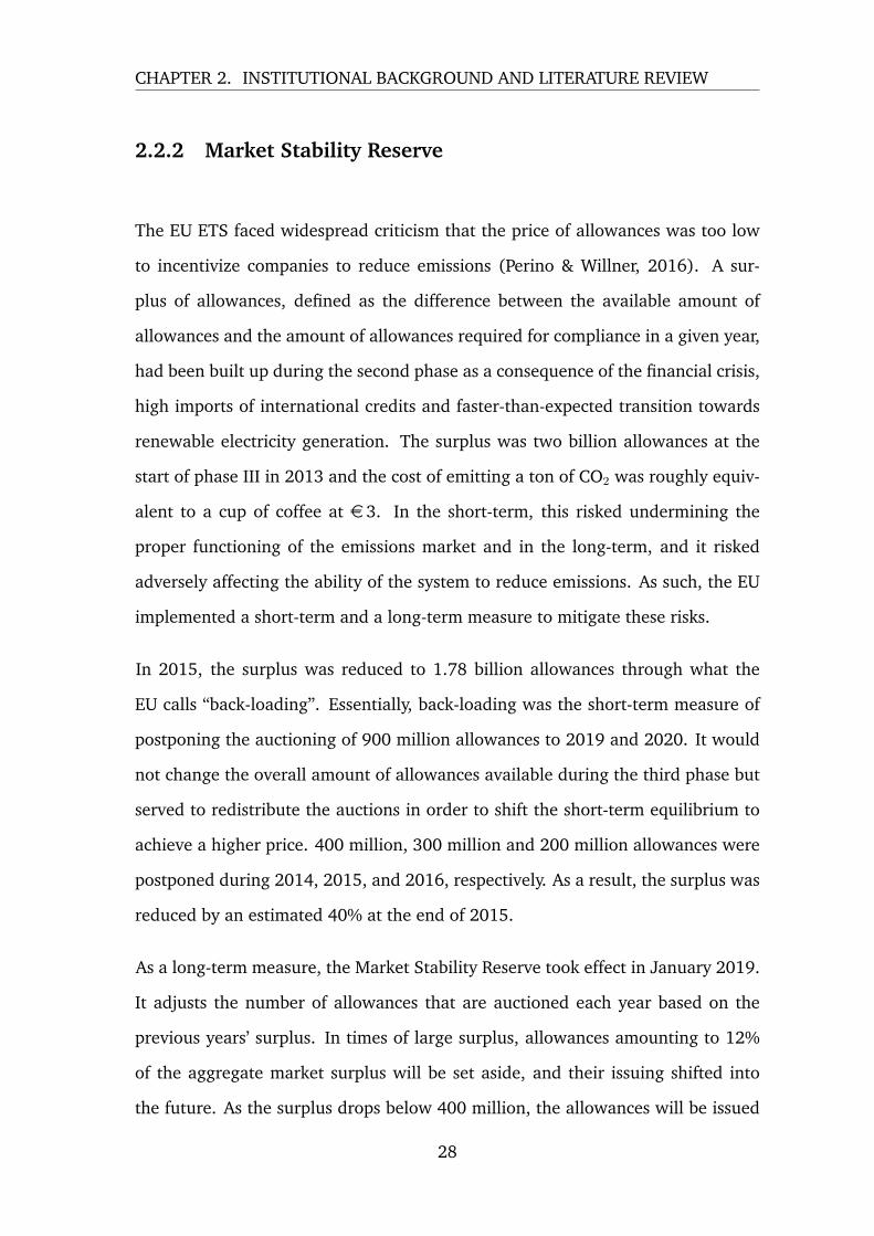
Electricity generating technologies from the left: solar and wind power, nuclear power, thermalcoal power, and thermal natural gas power. Source: Cludius et al. (2014)
Figure 3.1: Illustration of the Merit Order Curve with emission compliance costs
We suspect that the implications of these changes apply different forces on the
relationship between EUA price changes and firm performance among electricity
generating firms. As an example, the penetration of renewable energy sources
during the last decade should arguably increase the positive effect, whereas the
end of grandfathering should have an opposite effect. These conflicting forces
notwithstanding, research shows that EUA price increases are passed on to con-
sumers in the bids of the marginal producer. As such, emission allowances do not
represent a significant regulatory burden for the marginal producer. Moreover, the
contribution margin of inframarginal producers increases with increased emission
allowance prices resulting in an overall increase in profitability that will be re-
flected in the stock prices of the respective companies. As an example, consider
the chart above, in which the dark area represents the costs of emissions for the
coal generating marginal producer. The arrow illustrates the pass-through of the
allowance price to the consumer, assuming 100% pass-through rate, resulting in
39

CHAPTER 3. THEORY AND HYPOTHESES
regulatory rents for the inframarginal producers. This leads to the first hypothesis
of the paper:
Hypothesis I: Emission allowance price increases (decreases) positively (negatively)
affected electricity generating stock returns during the sample period.
By the same logic as above, we suspect that inframarginal companies with a higher
share of low-margin renewable electricity generation obtained even larger contri-
bution margins than their more carbon-intensive counterparts. This leads to the
second hypothesis of the paper:
Hypothesis II: EU Emission allowance price increases (decreases) had a larger pos-
itive (negative) effect on carbon efficient electricity generating stock returns during
the sample period.
40

Chapter 4: Methodology
In Chapter IV, we present the data and methodology used to empirically test our
hypotheses. First, we present our research approach. Next, we introduce the data
used in our econometric analysis. Last, we present the econometric methodology.
4.1 Research Approach
This thesis is based on a deductive research approach in which we formulate a
set of hypotheses built upon existing theory and previous research. Based on the
hypotheses, we design a methodology that aims to test whether the hypotheses
hold true. Our empirical research is primarily based on the methodology of Veith
et al. (2009) and Oberndorfer (2009) that investigated the relationship between
price changes in EU emission allowances and financial performance of electricity-
generating firms during the first phase of the EU ETS. To increase reliability, fi-
nancial data is primarily retrieved from organized financial databases. Data on
firm-specific carbon intensity was obtained from a report published by PwC or
from reports published by the respective company. Price data for stocks, market
index, oil and natural gas were used to calculate weekly returns that were used
in the subsequent econometric analysis. To strengthen validity, we employ multi-
ple diagnostic tests to the data and econometric models. Additionally, robustness
is increased by controlling for commodity price impact and employing regression
41

CHAPTER 4. METHODOLOGY
models using aggregate and disaggregate stock return data as well as controlling
for firm-specific fixed effects.
4.2 Data
4.2.1 Firms
The sample selection was conducted in a series of steps. First, we identified the
largest publicly traded companies in the utility sector by market capitalization via
the Dow Jones STOXX Europe 600 Utilities index. It is the largest index of listed
utility companies in Europe. Next, we excluded companies that were not listed
in the index during the whole sample period of January 2013 to December 2019,
which left 26 companies. We then excluded companies that fell under the Water
Utility classification based on their Global Industry Classification Standard. Lastly,
we assessed whether the firm was involved in electricity generation throughout
the sample period via the information provided in their respective annual reports
for 2013 and 2018 or 2019. In the end, thirteen firms remained in the sample.
These firms are presented in Table 4.1. The stock return data of the companies
was retreived from Bloomberg.
42

CHAPTER 4. METHODOLOGY
Tabl
e4.
1:O
verv
iew
ofth
eco
mpa
nies
unde
ran
alys
is
Nam
eA
bbre
viat
ion
Tick
er(I
SIN
)C
oun
try
ofhe
adqu
arte
rC
arbo
nin
ten
sity
for
2015
(gC
O2/k
Wh)
SSE
PLC
SSE
GB
0007
9087
33U
nite
dK
ingd
om39
7En
desa
SAEL
EES
0130
6701
12Sp
ain
460*
Iber
drol
aSA
IBE
ES01
4458
0Y14
Spai
n21
7Ve
rbun
dA
GV
ERAT
0000
7464
09A
ustr
ia55
Nat
urgy
Ener
gyG
roup
SAN
TGES
0116
8703
14Sp
ain
431
Cen
tric
apl
cC
NA
GB
00B
033F
229
Uni
ted
Kin
gdom
145*
Engi
eSA
ENG
FR00
1020
8488
Fran
ce37
7El
ectr
icit
ede
Fran
ceSA
EDF
FR00
1024
2511
Fran
ce81
EDP
-Ene
rgia
sde
Port
ugal
EDP
PTED
P0A
M00
09Po
rtug
al52
0A
2ASp
AA
2AIT
0001
2334
17It
aly
436
Fort
umO
yjFO
RFI
0009
0071
32Fi
nlan
d21
Enel
SpA
ENE
IT00
0312
8367
Ital
y40
9R
WE
AG
RW
ED
E000
7037
129
Ger
man
y72
1
The
firm
-spe
cific
info
rmat
ion
has
been
colle
cted
thro
ugh
annu
alre
port
san
dB
loom
berg
term
inal
.Th
eca
rbon
inte
nsit
yw
asob
tain
edfr
omPw
C’s
Clim
ate
Cha
nge
and
Elec
tric
ity
repo
rt.
*End
esa
SAan
dC
entr
ica
plc
wer
eno
tin
clud
edin
the
Clim
ate
Cha
nge
and
Elec
tric
ity
repo
rtfr
omPw
C.
How
ever
,th
eca
rbon
inte
nsit
yfo
rEn
desa
SAan
dC
entr
ica
plc
was
obta
ined
thro
ugh
Ende
saSA
’sSu
stai
nabi
lity
Rep
ort
from
2015
and
aC
arbo
nD
iscl
osur
ePr
ojec
tfo
rC
entr
ica
from
2015
.So
urce
:En
desa
(201
5),P
wC
(201
6),C
entr
ica
(201
7)
43

CHAPTER 4. METHODOLOGY
4.2.2 Carbon Intensity
Carbon intensity is defined as the emission per unit of electricity output generated
and is usually measured in gCO2/kWh. We are concerned with the carbon inten-
sity of the firms’ portfolio of power plants located in Europe. We obtained the
carbon intensity in 2015 for the electricity-generating firms from the report Cli-
mate Change and Electricity published by PwC in 2016. The report did not include
the carbon intensity for Endesa SA and Centrica plc. Instead, carbon intensity for
Endesa SA was retreived from its 2015 annual sustainability report and the carbon
intensity for Centrica plc was obtained from a questionnaire to the organization
Carbon Disclosure Project.
Source: Endesa (2015), PwC (2016), Centrica (2017)
Figure 4.1: Carbon Intensity for sample firms
We create a binary variable that equals 1 if the company’s carbon intensity is above
the sample median and 0 otherwise. This allows us to divide our sample firms into
44

CHAPTER 4. METHODOLOGY
a carbon efficient and carbon intensive group.
Figure 4.1 shows the carbon intensity for the firms under analysis and the Eu-
ropean Union carbon intensity average. Notice that there is a large dispersion
between the firms under analysis regarding carbon intensity.
4.2.3 European Union Allowance Prices
Companies with installations subject to the EU ETS must surrender allowances
to cover their emissions by year-end. We assume that market participants are
risk-averse and that they hedge their exposure to EUA price fluctuations by taking
positions in futures December contracts. EUA futures with expiration in Decem-
ber have significantly higher volumes than emission allowances traded in the spot
market and should, therefore, reflect prices better. Moreover, futures’ prices are
less affected by short run demand and supply fluctuations and thus less noisy
(Oberndorfer, 2009). Similar studies have also been based on futures (Oberndor-
fer, 2009; Veith et al., 2009).
The futures settlement prices were received by request from the European Energy
Exchange (EEX) that kindly provides its data for academic purposes. Although
there are multiple exchanges in which EUA futures contracts are traded, prices de-
velop identically across markets (Mansanet-Bataller et al., 2007), consistent with
the Law of One Price.
4.2.4 Market Returns
The Dow Jones STOXX Europe 600 covers large, mid and small capitalization
companies across 17 European countries: Austria, Belgium, Denmark, Finland,
France, Germany, Ireland, Italy, Luxembourg, the Netherlands, Norway, Poland,
45

CHAPTER 4. METHODOLOGY
Portugal, Spain, Sweden, Switzerland and the United Kingdom. It is weighted
based on free-float market capitalization, and its composition is reviewed on a
quarterly basis. The index represents a highly diversified portfolio and will be
used as a proxy for the overall market returns.
4.2.5 Control Variables: Oil and Natural Gas
In line with Arbitrage Pricing Theory and the idea of multifactor market models,
we add additional variables to the regression model that captures other potentially
influencing macroeconomic factors. We choose to follow Veith et al. (2009) and
Oberndorfer (2009) and include the price changes of oil and natural gas in our
regression equation. This will facilitate in comparing our results with their study.
Unlike Oberndorfer (2009), however, we choose not to include electricity prices,
which did not provide explanatory power in his study.
We use the price of one-month Brent crude oil contracts because it is extracted
from the North Sea and thus the primary source of oil in Europe. As for natural
gas prices, we use the one-month TTF Natural Gas contracts. The TTF Natural gas
is the largest market for natural gas in Europe. Both time series were retreived
from Bloomberg and Euro-denominated.
4.2.6 Transformation of Data and Frequency
Economic time series often exhibit growth that is approximately exponential, mean-
ing that in the long term the series grows by a certain rate per year on average.
This may have negative implications when performing linear regressions. To miti-
gate the risks associated with this, we calculate the natural logarithm of the time
series data to transform the series to exhibit linear growth (Stock & Watson, 2015).
46

CHAPTER 4. METHODOLOGY
This transformation also is often considered to stabilize the variance in the time
series data (Woolridge, 2013).
Using weekly data frequency, rather than daily, avoids issues with error-in-variables
problems with respect to irregularities (Scholes & Williams, 1977). Although
Oberndorfer (2009) used daily frequency, he argued that weekly observations are
preferable if the sample period is large enough because it reduces noise. We calcu-
late the weekly return using the closing price of the last trading day of the week.
Our sample period stretches from the first week of 2013 to the last week of 2020
with results in more than 360 observations for each series in the data set.
4.3 Econometric Theory
The following section provides an explanation of the econometric methods that
will be used to test the hypotheses presented in Section 3.2. First, the reader
is introduced to the Ordinary Least Squares (OLS) regression estimation. Next,
we discuss issues related to OLS estimation in terms of omitted variable bias and
present a Fixed Effects regression model to mitigate these issues. The inspiration
to this section is from Stock and Watson (2015), Woolridge (2013), and Enders
(2014).
4.3.1 OLS Estimation
Ordinary Least Squares (OLS) estimation a type of linear least squares method for
estimating the unknown parameters in a linear regression model. The multivariate
regression model can be expressed in matrix notation as follows, for consistency
47

CHAPTER 4. METHODOLOGY
vectors and matrices are denoted by bold type:
Y = Xβ + U (4.1)
Where:
• Y is the n× 1 dimensional matrix of n observations on the k + 1 regressors -
including the regressor for the intercept.
• X is the n×(k+1) dimensional matrix of n observations on the k+1 regressors
- including the regressor for the intercept.
• The k + 1 dimensional column vector Xi is the ith observation on the k + 1
regressors; that is, X′i = (1X1,i . . . Xk,i), where X′i denotes the transpose of
Xi.
• U is the n× 1 dimensional vector of the n error term.
• β is the (k + 1) × 1 dimensional vector of the k + 1 unknown regression
coefficients.
For the OLS estimation to provide the best linear unbiased estimators, the follow-
ing assumptions must hold.
1. E (ui|Xi) = 0, ui has conditional mean of zero.
2. (Xi, Yi) , i = 1, . . . , n, are independently and identically distributed (i.i.d)
draws from their joint distribution.
3. Large outliers are unlikely: Xi and ui have nonzero finite fourth moments.
4. X has full column rank i.e. there is no perfect multicollinearity.
48

CHAPTER 4. METHODOLOGY
The principle of OLS estimation is to minimize the sum of squared prediction
errors over all n observations. The sum of squared predicted errors can be written
as:n∑i=1
(Yi − b0 − b1X1,i − . . .− bkXk,i)2 (4.2)
Where Yi is the observed value, which the OLS estimation predicts, b0, b1, . . . , bk are
estimates of β0, β1, . . . , βk, which minimize the sum of squared prediction errors
and X1,i and Xk,i are the regressors included in the OLS estimation. The estimates
of the coefficients that minimize the sum of squared prediction errors are called
OLS estimators and are denoted as β in matrix notation. The difference between
Yi and the predicted Yi is the OLS residual and is denoted U in matrix notation.
The OLS estimators can be estimated by a closed form solution. These are ob-
tained by taking the derivative and setting the derivatives of the sum of squared
prediction errors with respect to each coefficient in the vector to zero and solving
for the estimator β. The solution to the equation system yields the OLS estimator
β. The closed form solution can be written as follows:
β = (X ′X)−1X ′Y (4.3)
A challenge in using multivariate linear regression models to explain a real-world
phenomena is to include all variables that have explanatory power on the depen-
dent variable. As such, there is typically an issue related to omitted variable bias.
4.3.2 Omitted Variable Bias
Omitted variable bias occurs when a regressor is correlated with a variable not in-
cluded in the analysis, and that variable influences the dependent variable. There
49
CHAPTER 4. METHODOLOGY
are two general conditions, which must hold true for an omitted variable bias to
arise: i) the omitted variable is a determinant of the dependent variable and ii)
the omitted variable is correlated with the regressors included in the analysis. If
there is an omitted variable bias in the model, the first least squares assumption
is is violated. The reason for this is that the error term ui is correlated with one
of the regressors and therefore, assumption one does not hold true. This leads to
the OLS estimators being biased and inconsistent. This can be explained mathe-
matically, let the correlation between Xi and ui be corr (Xi, ui) = ρXu. Assume
the second and third assumptions of the OLS holds true, but the first is violated,
because ρXu 6= 0. Then:
β1→β1 + ρXuσuσX
(4.4)
Even in large samples the omitted variable bias can an issue, because β does not
converge in probability to the true value β. The term ρXuσuσX
is the bias of β, which
is also present in large samples. The size of the bias depends on the correlation
between the regressor and error term, |ρXu| (Stock & Watson, 2015).
To mitigate the issues of omitted variable bias related to firm-specific character-
istics, we investigate the effect of a EUA price change by using the fixed effects
regression model. The fixed effects regression model is explained in the next sec-
tion.
4.3.3 Fixed Effects Regression
The fixed effects regression model is used to control for omitted variables in panel
data, when the omitted variables vary across entities but do not change over time.
The general panel regression model can be written as follows:
Yi,t = β0 + β1Xi,t + β2Zi + ui,t (4.5)
50

CHAPTER 4. METHODOLOGY
Where Zi is the unobserved variable that varies across entities i = 1, . . . , n, but
does not change over time. The goal is to estimate β1, i.e. to isolate the effect on
Yi given a change in Xi holding Zi constant. The model can be rewritten by letting
ai = β0 + β2Zi, and we obtain the generalized fixed effects regression model:
Yi,t = βXi,t + αi + Ui,t (4.6)
With i = 1, . . . , n and t = 1, . . . , T . This model allows the model to have specific
intercepts αi, where each αi can be understood as the fixed effect of entity i.
The fixed effects model’s entity-specific intercepts can be captured by using binary
variables, which in our case refers to the specific companies in our sample. Let
D1i be a binary variable which equals 1, when i = 1 and equals zero otherwise
and let D2i equal 1 when i = 2 and equal zero otherwise and so on. To avoid the
dummy variable trap, one of the binary variables should be excluded. The fixed
effects regression model can be written as:
Yi,t = β0 + β1Xi,t + γ2D2i + γ3D3i + . . .+ γnDni + ui,t (4.7)
This formula is equivalent to the generalized fixed effects regression model, but
explicitly shows the company-specific intercepts.
The first and second assumptions for the fixed effect regression model are slightly
different from the assumptions for the multivariate regression model, but the third
and the fourth are similar.
The assumptions for the fixed effects regression model are:
1. ui,t has conditional mean zero: E (uit|Xi,1, Xi,2, . . . , Xi,T , ai) = 0
2. (Xi,1, Xi,2, . . . , Xi,T , ui,1, ui,2, . . . , ui,T ) , i = 1, . . . , n are i.i.d. draws from
51

CHAPTER 4. METHODOLOGY
their joint distribution.
3. Large outliers are unlikely: Xi and ui have nonzero finite fourth moments.
4. There is no perfect multicollinearity.
4.3.4 Random Effects Regression
In contrast to fixed effects models, random effect models require that the unob-
served variables are uncorrelated with all the explanatory variables. If ai repre-
sents the unobserved variables, then Cov (xi,t,j, ai) = 0 must hold. In our case,
this his highly unlikely, as stock prices and EUA allowance prices are affected by
complex relationships between a magnitude of factors. Recall in Section 2.3.2,
the price of EU ETS allowances is determined by a variety of forces, for instance
weather conditions, which affects business-as-usual emissions that drive demand
for allowances. As such, we cannot plausibly argue that the unobserved variables
are uncorrelated with all explanatory variables, and we choose not to employ a
random effects model.
4.3.5 OLS Diagnostics
The first assumption for multivariate OLS estimation states that the error terms
should have a conditional mean of zero. This assumption implies that at any given
value of Xi, the errors should have a mean of zero. This can be investigated by
plotting the error terms over the fitted values of the model, which allows us to
visually assess if the estimated model’s residuals have a mean of zero indicating
white noise. Additionally, this plot can further provide indication if the error terms
are homo- or heteroscedastic. For homoscedasticity, the residuals should not show
indication of a pattern in the plot.
52

CHAPTER 4. METHODOLOGY
As stated earlier, the second assumption is that variables are independently and
identically distributed across entities for i = 1, . . . , n relating to how the sample is
drawn. We can use the Normal QQ plot to investigate the residuals to see if they
are normally distributed. If the residuals are normally distributed, they should
follow the diagonal line in the QQ-plot.
The third assumptions that large outliers are unlikely is important because the es-
timated coefficients are sensitive towards large outliers (Stock & Watson, 2015).
According to James et al. (2017) it is possible to identify outliers by examining
the Residuals vs leverage plot. To investigate the assumption for perfect multi-
collinearity, a correlation matrix for the variables is drawn.
The assumptions for fixed effects regression are quite similar to the multivariate
regression. The first assumption fixed effects is identical the first assumption in
multiple regression - the error term has to have a conditional mean of zero. This
can be violated if the errors are correlated with the values of the dependent vari-
ables. Further, for fixed effects Xi,t is allowed to be correlated over time within
the entity, i.e. Xi,t can be autocorrelated. If the error terms exhibit autocorrela-
tion, heteroscedasticity and autocorrelation consistent (HAC) standard errors can
be used to take this into account. The third and fourth assumptions are the same
as in the multivariate regression model. (Stock & Watson, 2015).
4.3.6 Autocorrelation
Time series data can exhibit autocorrelation, referring to that the value observed in
one period is correlated with the value in another. If present in the series, the least-
squares estimator might not be the best linear unbiased estimator. To examine if
the data exhibits autocorrelation, one can plot the autocorrelation function (ACF
plot) for the series. The plot displays the autocorrelation function’s correlation
53

CHAPTER 4. METHODOLOGY
coefficients between lags in time. Significant spikes indicate that autocorrelation
is present in the series (Stock & Watson, 2015).
A formal test for autocorrelation is the Durbin Watson test. It tests for the auto-
correlation in lag 1. If the residual is given by εt = ρεt−1 + ut, then the Durbin
Watson statistics tests the null hypothesis of ρ = 0, which means no first-order au-
tocorrelation and the alternative hypothesis ρ 6= 0 meaning first-order correlation
exists.
The Durbin Watson statistic is defined as:
DW =
∑Nt=2(εt − εt−1)2∑N
t=1 ε2t
(4.8)
Where ε is the residuals of our model, if the p-value reported by the Durbin Watson
test is significant it rejects the null hypothesis indicating that first order autocor-
relation among the residuals is present (Watson, 1951).
Again, if the ACF plot and/or the Durbin Watson test indicate that the errors are
autocorrelated, then the standard errors should be modelled using the heteroskedasticity-
and autocorrelation-consistent (HAC) standard errors (Stock & Watson, 2015).
4.3.7 Stationarity
Stock and Watson (2015) define time series data to be stationary if its probability
distribution does not change over time. This means that the joint distribution of
(Ys+1, Ys+2, . . . , Ys+T ) does not depend on s regardless of the value of T. If this is the
case Yt is said to be nonstationary. Stationarity requires that the future is like the
past in a probabilistic sense. If data is not stationary, it imposes several problems,
and the assumptions above might not hold true (Stock & Watson, 2015).
54

CHAPTER 4. METHODOLOGY
To test for stationarity, an informal and important method is to plot the time series
and the corresponding ACF plot for a visual interpretation. This allows us to see if
there is a stochastic trend present in the data. As stated in Section 4.2.6, the data
is transformed into its natural logarithmic return to stabilize the variance in the
data.
A formal process to detect stationarity is to conduct an augmented Dickey-Fuller
test to test for a unit root. The idea of the test is to test whether previous lags of
the Yt has an effect on Yt. Therefore the null hypothesis is H0 : γ = 0 versus the
one-sided alternative H1 : γ < 0 in the regression:
∆yt = β0 + γyt−1 +
p∑i=2
βi∆yt−i+1 + εt (4.9)
Where ∆yt is the change in the variable, β0, γ and βi are the estimated intercept,
the coefficient for the first lag and the coefficients for additionally lags running
from i = 0 to as many lags included in the model, respectively. By rejecting the
null hypothesis, the data is considered to be stationary. If a time trend element
tt is included in the regression, the alternative hypothesis changes to Yt being
stationary around a deterministic time trend, and the regression becomes:
∆yt = β0 + tt+ γyt−1 +
p∑i=2
βi∆yt−i+1 + εt (4.10)
The resulting t-statistic needs to be compared with the reported Dickey-Fuller crit-
ical values to determine whether to accept or reject the null hypothesis. The crit-
ical values vary depending on the equation under investigation (Stock & Watson,
2015). Enders (2014) argues that the selection of lag length can be difficult. If
an insufficient amount of lags is selected then the residuals do not behave like
white-noise processes while too many lags will reduce the power of the test in
order to reject the null of a unit root. When adding a lag, the number of pa-
55

CHAPTER 4. METHODOLOGY
rameters increases and the number of usable observations decreases. Stock and
Watson (2015) suggest that the lag length p can be estimated by using the Akaike
information criteria (AIC).
When testing our times series data, we will first investigate the visualization of
the data in order to determine whether or not to include a time trend in the Aug-
mented Dickey-Fuller test. When we are using real return data, the expectation
is that we should not find our data to be stationary around a deterministic trend
(Enders, 2014). A drift term will be included in the model because, on average,
the stock market is yielding a positive return (Martin & Wagner, 2016).
4.3.8 Econometric Methodology
The econometric analysis of this research will, to a large extent be based on Veith
et al. (2009) and Oberndorfer (2009) that studied how EUA prices affected firm
performance for electricity-generating companies during the first phase of the EU
ETS. This will allow us to compare our results in the subsequent discussion.
First, the returns of the electricity companies included in our sample will be re-
gressed on the return of the market portfolio and return on EU ETS allowances
during the whole sample period. The model to be estimated:
ri,t = β0 + β1rMkt,t + β2rEUA,t + εi,t (4.11)
Where ri,t represents the returns of each firm, i runs from from 1 to 13 over the
firms and t indicates the time, which runs from the first week in 2013 to the last
week in 2019. rMkt,t represents the returns of the market portfolio and rEUA,t
represents the returns of the emission allowances. β0, β1 and β2 are the estimated
coeffiecients and εi,t is the error term for each firm at each point in time.
56

CHAPTER 4. METHODOLOGY
A positive and significant β2 coefficient would indicate a positive relationship be-
tween price changes in EUA and firm performance. Next, we extend the model
to control for commodity price impact by including control variables for the re-
turns on one-month Euro-denominated futures contracts for Brent crude oil and
TTF natural gas. Oil and natural gas are frequently used as input factors among
conventional electricity producers and an change in price in these factors could
have an impact on expected future cash flows that could be reflected in the share
price. Moreover, recall Section 2.3.2 that explains that the price of fossil fuels
drive prices on emissions. For instance, a decrease in natural gas prices relative to
coal will lead to lower emissions and lower demand for allowances, resulting in a
lower equilibrium price for allowances. The model to be estimated:
ri,t = β0 + β1rMkt,t + β2rEUA,t + β3rOil,t + β4rGas,t + εi,t (4.12)
Where the variables from Equation 4.11 are the same, and the additional variables
rOil,t and rGas,t represents return for one-month Euro-denominated Brent crude oil
and TTF natural gas futures running from the first week in 2013 to the last week
in 2019.
Following Oberndorfer (2009), we will run these regressions both using pooled
panel data and the aggregate returns in an equally weighted portfolio. The model
is slightly different when running the regression with the equally weighted port-
folio, and the model becomes:
rPf,t = β0 + β1rMkt,t + β2rEUA,t + εt (4.13)
Where rPf,t is the return for the equally weighted portfolio, t runs from the first
week of 2013 to the last week of 2019. The rest of the variables are the same as
in the pooled regression model explained above.
57

CHAPTER 4. METHODOLOGY
Including the control variables oil and natural gas the model to be estimated is:
rPf,t = β0 + β1rMkt,t + β2rEUA,t + β3rOil,t + β4rGas,t + εt (4.14)
Next, we follow Veith et al. (2009) and control for fixed effects which allows us
to partial out firm-specific effects. For instance, firms are involved in electricity
generation to varying extents and subject to different local regulations that could
have an effect, for example, by limiting the pass-through rate. A dummy variable
equaling 1 for firm i, or 0 otherwise, will be added to the model. The model to be
estimated:
ri,t =∑i
ΘiDFIRMi + β1rMkt,t + β2rEUA,t + β3rGas,t + β4rOil,t + εi,t (4.15)
We then turn to investigating how the effect has changed over time. For instance,
policy actions such as the Market Stability Reserve that was announced in 2018
could possibly change the relationships that are observed. Potential differences
could provide additional insights that can contribute to the subsequence discus-
sion. We run the extended model that includes oil and natural gas rolling seven
times over subperiods of 12 months, using the pooled data in order to achieve a
sufficiently large set of observations.
Lastly, we will investigate if the carbon intensity of the underlying generation mix
has an effect on financial performance. Recall from Section 4.2.2 that we will
create a dummy variable representing whether the firm has a higher or lower
carbon intensity than the median. This dummy variable will be interacted with
the emission allowance return factor through the following equation:
ri,t = β0 + γ0Polluteri + β1rMkt,t + β2rEUA,t + γ1 (rEUA,t ∗ Polluteri) + εi,t (4.16)
58

CHAPTER 4. METHODOLOGY
This will allow for different intercepts and coefficients in terms of emission al-
lowance returns. Consider firm i that has a lower than median carbon intensity.
Its binary variable Polluter will equal 1 in the regression. γ0 + β0 will represent the
intercept for the firm and the interaction term γ1 (rEUA,t ∗ Polluteri) coefficient
represents the interaction effect. In the case that firm i has a higher than median
carbon intensity, then both γ0 and γ1 will fall out of the equation.
We consider heteroskedasticity and autocorrelation by consistently calculating and
reporting heteroscedasticity and autocorrelation consistent standard errors (HAC).
59

Chapter 5: Results
Chapter V will walk the reader through the empirical analysis of the paper. The
chapter is structured as follows. First, the reader is presented with an overview
of the data. Second, the data will be tested for autocorrelation and stationarity.
Third, the results from the regressions relating to the first and then the second
hypotheses will be presented. Lastly, diagnostics plots will be provided and dis-
cussed.
5.1 Overview of the Data
Figure 5.1 shows the indexed price development of the aggregate equally weighted
portfolio of the sample firms, the market portfolio, oil, and natural gas during the
third phase of the EU ETS. The aggregate price development of the sample stocks
appears to move in the same direction as the market portfolio that is proxied
through the Dow Jones STOXX Europe 600 index through most of the period.
However, during the period 2018 and 2019, the electricity-generating companies
outperform the market. Simultaneously, the price of European Union Allowances
exhibit a strong positive trend with a high degree of volatility. This could poten-
tially be a consequence of the Market Stability Reserve that was announced in
2018 and implemented in 2019. Recall from Chapter II, the Market Stability Re-
serve limited the supply of allowances available in the market in efforts to increase
60
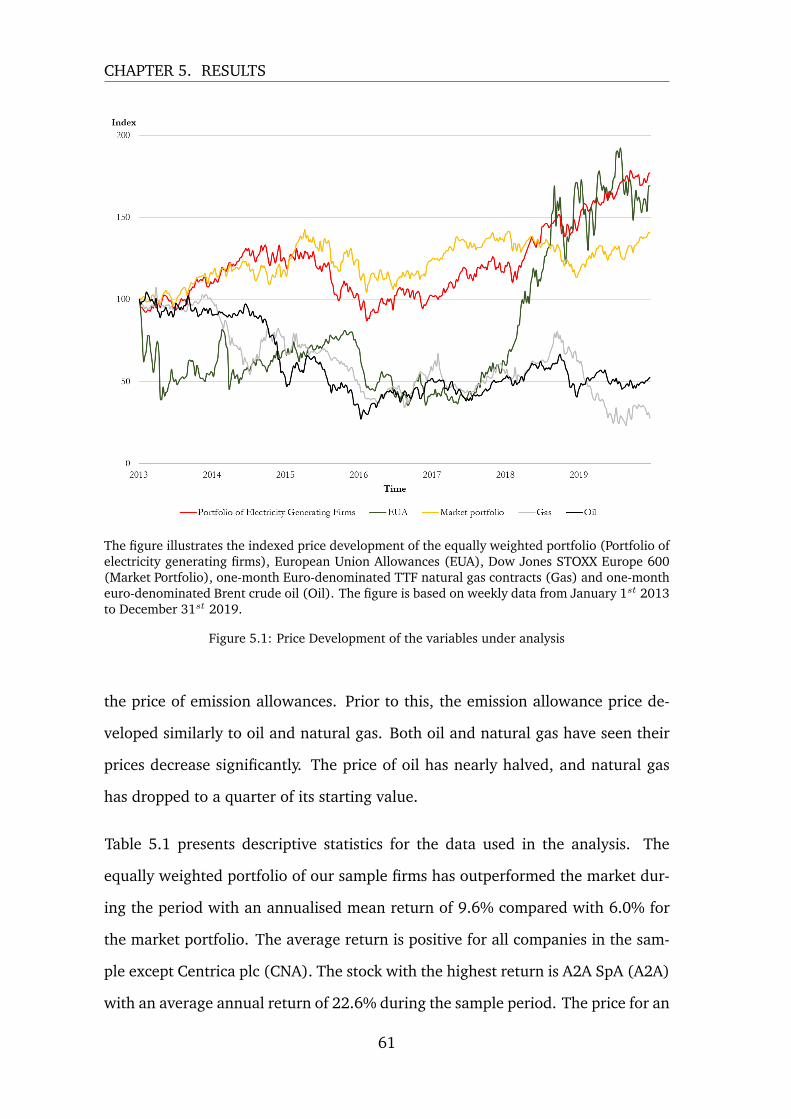
CHAPTER 5. RESULTS
The figure illustrates the indexed price development of the equally weighted portfolio (Portfolio ofelectricity generating firms), European Union Allowances (EUA), Dow Jones STOXX Europe 600(Market Portfolio), one-month Euro-denominated TTF natural gas contracts (Gas) and one-montheuro-denominated Brent crude oil (Oil). The figure is based on weekly data from January 1st 2013to December 31st 2019.
Figure 5.1: Price Development of the variables under analysis
the price of emission allowances. Prior to this, the emission allowance price de-
veloped similarly to oil and natural gas. Both oil and natural gas have seen their
prices decrease significantly. The price of oil has nearly halved, and natural gas
has dropped to a quarter of its starting value.
Table 5.1 presents descriptive statistics for the data used in the analysis. The
equally weighted portfolio of our sample firms has outperformed the market dur-
ing the period with an annualised mean return of 9.6% compared with 6.0% for
the market portfolio. The average return is positive for all companies in the sam-
ple except Centrica plc (CNA). The stock with the highest return is A2A SpA (A2A)
with an average annual return of 22.6% during the sample period. The price for an
61

CHAPTER 5. RESULTS
emission allowance has increased with an annualised mean of almost 20% over the
sample period. It has a high standard deviation of more than 40%. As illustrated
in Table 5.1, prices of an emission allowance varied significantly with a range
between approximately e3 to e30. The price of one-month Euro-denominated
futures contracts for Brent crude oil and TTF natural gas decreased on average by
5% and 10% per annum, respectively, during the sample period.
Next, calculate the Pearson’s correlation coefficients between the series to identify
possible multicollinearity issues between regressors and to potential irregularities.
The correlation matrix in Table 5.2 does not raise any concerns in terms of perfect
multicollinearity between the series. The variables with the highest correlation
coefficients have been colored - the correlation coefficients between 0.6 and 0.7
have been colored light gray and above 0.7 dark gray. The sample firms are all
positively correlated with the returns of emission allowances. The correlations
vary between 0.014 (Iberdrola SA) to 0.288 (Verbund AG). Moreover, as one can
expect, the electricity generating companies’ returns are positively correlated with
the return of the market portfolio. Once again, Centrica plc stands out with its
relatively low correlation to its peers with a correlation of 0.43 to the equally
weighted portfolio of sample firms.
Because of the low correlation and the abnormal negative average return for Cen-
trica plc, we suspect that the stock could potentially be different in some relevant
aspect from the rest of the population. In order to investigate Centrica plc, we plot
the price development of the equally weighted portfolio of electricity generating
firms, the market portfolio and Centrica plc for the total sample period.
62

CHAPTER 5. RESULTS
Table 5.1: Descriptive statistics for variables under analysis
Dependentvariables
Mean Median Max Min Std. Dev Obs
SSE 0.058 0.103 0.080 - 0.140 0.194 364ELE 0.197 0.262 0.139 - 0.083 0.196 364IBE 0.163 0.194 0.118 - 0.095 0.186 364VER 0.150 0.209 0.100 - 0.116 0.260 364NTG 0.125 0.123 0.139 - 0.093 0.210 364CNA - 0.132 - 0.122 0.124 - 0.194 0.271 364ENG 0.053 - 0.018 0.131 - 0.084 0.219 364EDF 0.015 0.022 0.140 - 0.141 0.305 364EDP 0.132 0.140 0.106 - 0.115 0.225 364A2A 0.226 0.248 0.113 - 0.117 0.252 364FOR 0.131 0.158 0.091 - 0.154 0.216 364ENE 0.156 0.300 0.099 - 0.102 0.216 364RWE 0.013 0.237 0.161 - 0.194 0.342 364Portfolio 0.096 0.209 0.091 - 0.074 0.172 364Independent variablesMarket return 0.060 0.144 0.054 - 0.071 0.150 364EUA price 10.18 6.850 29.58 3.230 7.429 365EUA return 0.198 0.224 0.196 - 0.428 0.481 364Oil price 58.94 55.81 89.03 26.43 15.00 365Oil return - 0.048 0.078 0.135 - 0.154 0.295 364Gas price 19.40 19.30 29.35 9.430 4.835 365Gas return - 0.108 - 0.201 0.281 - 0.232 0.392 364
This table reports the mean, median, maximum (Max), minimum (Min), the standarddeviation (Std. Dev.) and the number of observations (Obs) for each firm, the portfolioof electricity generating firms (Portfolio), European Union Allowances (EUA), Dow JonesSTOXX Europe 600 (Market), one-month Euro-denominated Brent crude oil (Oil) futurescontracts, and one-month Euro-denominated TTF natural gas futures contracts (Gas) fromJanuary 1st 2013 to December 31st 2019. The Mean, median and standard deviationhave been transformed into annualised figures. Maximum and minimum are presented inweekly values.
63

CHAPTER 5. RESULTS
Tabl
e5.
2:C
orre
lati
onm
atri
xof
retu
rns
Port
folio
SSE
ELE
IBE
VER
NTG
CN
AEN
GED
FED
PA
2AFO
REN
ER
WE
Oil
Gas
MK
TEU
A
Port
folio
1SS
E0.
538
1EL
E0.
687
0.35
91
IBE
0.75
30.
393
0.72
21
VER
0.70
40.
249
0.34
90.
416
1N
TG0.
746
0.33
60.
601
0.71
40.
393
1C
NA
0.43
20.
586
0.27
40.
269
0.17
10.
340
1EN
G0.
798
0.45
90.
530
0.62
40.
463
0.56
50.
371
1ED
F0.
668
0.32
10.
352
0.44
00.
395
0.42
20.
322
0.52
81
EDP
0.60
90.
367
0.51
50.
579
0.34
40.
545
0.25
50.
488
0.37
81
A2A
0.53
00.
260
0.46
00.
543
0.31
50.
496
0.23
00.
485
0.26
90.
420
1FO
R0.
690
0.36
30.
363
0.41
80.
469
0.44
30.
278
0.52
10.
428
0.35
30.
332
1EN
E0.
681
0.35
40.
620
0.70
80.
344
0.59
40.
283
0.65
00.
364
0.49
70.
631
0.38
01
RW
E0.
771
0.31
30.
421
0.48
30.
483
0.47
40.
257
0.57
20.
430
0.40
70.
319
0.47
40.
482
1O
il0.
322
0.28
00.
116
0.14
70.
219
0.28
40.
296
0.24
80.
246
0.22
00.
135
0.29
00.
173
0.19
31
Gas
0.10
30.
047
0.05
80.
027
0.09
90.
068
-0.0
010.
059
0.01
40.
044
0.08
20.
139
0.07
40.
075
0.10
91
MK
T0.
686
0.41
10.
513
0.62
20.
374
0.59
90.
411
0.65
40.
485
0.53
50.
484
0.49
60.
630
0.43
90.
347
0.07
21
EUA
0.18
90.
076
0.05
70.
014
0.28
80.
025
0.05
40.
094
0.16
10.
033
0.11
20.
243
0.04
40.
082
0.10
10.
184
0.05
71
This
tabl
ere
port
sPe
arso
n’s
corr
elat
ion
coef
ficie
nts
for
the
seri
esin
the
data
set.
The
vari
able
sar
e:Po
rtfo
lio:
the
aggr
egat
eeq
ually
wei
ghte
dre
turn
sof
the
sam
ple
ofel
ectr
icit
yge
nera
ting
firm
s;in
divi
dual
com
pani
es(s
eeTa
ble
5.1
for
full
nam
es);
MK
T:D
owJo
nes
STO
XX
Euro
pe60
0;EU
A:D
ecem
ber
futu
res
cont
ract
for
Euro
pean
Uni
onA
llow
ance
s;O
il:on
e-m
onth
Euro
-den
omin
ated
futu
res
cont
ract
for
Bre
ntcr
ude
oil;
and
gas:
one-
mon
thEu
ro-d
enom
inat
edfu
ture
sco
ntra
ctfo
rT
TFna
tura
lgas
.C
orre
lati
onco
effic
ient
sbe
twee
n0.
6an
d0.
7ar
eco
lore
din
light
gray
,cor
rela
tion
coef
ficie
nts
abov
e0.
7ar
eco
lore
din
dark
gray
.
64

CHAPTER 5. RESULTS
The figure illustrates the indexed price development of the equally weighted portfolio (Portfolioof Electricity Generating Firms), Dow Jones STOXX Europe 600 (Market portfolio) and Centricaplc. The figure is based on daily data from January 1st to December 31st 2019. In addition, it isindicated, when the United Kingdom voted for Brexit the 23rd of June 2016.
Figure 5.2: Price development of the Portfolio of Electricity Generating Firms, the Market Portfolioand Centrica plc
Figure 5.2 clearly shows the abnormal price development of Centrica plc during
the total period. Centrica plc yielded a negative return of -69.5% while the market
portfolio yielded a positive return of 40.6%. Centrica plc appears to have followed
similar price movements as its peers and the market portfolio until the middle of
2016, when it diverged and moved in the opposite direction to the average of the
sample firms. This coincides with the Brexit referendum vote on the 23rd of June
2016, which could potentially have an effect on how the market values Centrica
plc’s shares.
The market could discount certain risks associated with Brexit for Centrica plc, for
instance, the potential loss of cross-border electricity trading between the United
65

CHAPTER 5. RESULTS
Table 5.3: Correlation matrix for Centrica plc
Before Brexit After Brexit Total period
Portf. CNA EUA Portf. CNA EUA Portf. CNA EUA
Portfolio 1 1 1CNA 0.551 1 0.341 1 0.432 1EUA 0.192 0.132 1 0.18 -0.015 1 0.189 0.054 1
This table displays Pearson’s correlation coefficients for the equally weighted portfolio ofelectricity generating firms (Portf.), Centrica plc (CNA), and European Union Allowances(EUA) before Brexit, after Brexit and for the total period.
Kingdom and the European Union. It could also potentially affect the way that
market participants discount the effect of price changes in emission allowances if
they believe that Centrica plc’s British installations will no longer be subject to the
emission compliance cost after the United Kingdom has left the European Union.
The correlation matrix in Table 5.3 displays a large decrease in the correlation
between the returns of Centrica plc and emission allowances from 0.13 to -0.015
before and after Brexit. Whether this is a consequence of Brexit or merely a co-
incidence remains unclear and is outside the scope of this research. However, we
decide to perform a sensitivity analysis by performing the first sets of regressions
with and without Centrica plc in the sample. In the case of material differences
between the regressions, we must consider taking further steps to accommodate
this potential issue.
66

CHAPTER 5. RESULTS
5.2 Autocorrelation and Stationarity
As described in Section 4.3.6 a common method to investigate if times series are
stationary is to visualize the data. Figure 5.3 illustrates ten different plots. The
left hand side displays the natural logarithmic weekly return for the total sample
period for the aggregate equally weighted returns of the sample of electricity gen-
erating firms, the emission allowances, the market portfolio as well as one-month
Euro-denominated futures for Brent oil and TTF natural gas. Firm-specific plots
can be found in the appendix.
Overall, the plots on the left-hand side in Figure 5.3 indicate that the series are
stationary. The first plot on the left-hand side is the return for the equally weighted
portfolio of electricity generating firms and indicates a relatively constant mean
with a few spikes over the sample period. The emission allowances returns show
large spikes in the beginning of the sample period but seems to stabilize over time.
Natural gas stands out with a large variation at the end of the period. In general,
the plots indicate that the series are stationary.
We formally test for stationarity by testing for unit root in each series with the
Augmented Dickey-Fuller test. Because none of the plots of the returns indicate
that a trend is present we do not include a trend term. The test’s null hypothesis
is that the time series has a unit root. As such, the series is stationary according
to the test if it returns a γ t-statistic that is significant compared to the reported
Dickey-Fuller critical values.
Table 5.4 returns the results from the Augmented Dickey-Fuller test for each series.
One lag was selected by the Akaike Information Criterion and used in the test. The
Augmented Dickey-Fuller returns γ t-statistics that are significant when compared
to the reported critical values.
67

CHAPTER 5. RESULTS
Figure 5.3: Plots of the logarithmic weekly return and the corresponding ACF plot
68

CHAPTER 5. RESULTS
Table 5.4: Summary of Augmented Dickey-Fuller test
Dependent variables Intercept γ Lags Obs
SSE 0.31 -15.221*** 1 364ELE 0.002*** -15.385*** 1 364IBE 0.006*** -15.852*** 1 364VER 0.07* -13.884*** 1 364NTG 0.08* -14.937*** 1 364CNA 0.20 -13.923*** 1 364ENG 0.42 -14.833*** 1 364EDF 0.90 -14.063*** 1 364EDP 0.08* -15.489*** 1 364A2A 0.01** -14.304*** 1 364FOR 0.07* -14.746*** 1 364ENE 0.03** -14.732*** 1 364RWE 0.85 -13.255*** 1 364Portfolio 0.07* -15.419*** 1 364
Independent variables
Market 0.26 -14.618*** 1 364Oil 0.70 -13.321*** 1 364Gas 0.39 -16.162*** 1 364EUA 0.20 -14.249*** 1 364
Significance code: *p<0.1; **p<0.05; ***p<0.01
Critical values1% Level -3.445% Level -2.8710% Level -2.57
This table reports the p-values for the intercepts (Intercept), the t-statistic for the γ-coefficient (γ), number of lags selected (Lags) and number of observations (Obs). Theresults are a summary for each sample firm under analysis with the abbreviation from Ta-ble 4.1, the equally weighted portfolio (Portfolio), the market proxy - Dow Jones STOXXEurope 600 (Market), the one-month Brent crude oil (Oil), TTF natural gas contracts(Gas) and the European Union Allowances (EUA). The number of lags is selected by theinformation criteria AIC.
The autocorrelation function (ACF) plots on the right hand side of Figure 5.3
display the correlation coefficients between a time series and its lags. There are a
few significant spikes on the lags of the series for the natural logarithmic return of
the equally weighted portfolio, emission allowances, and natural gas. As such,
the autocorrelation function indicates that these series exhibit some degree of
autocorrelation. This will be taken into account by calculating heterscedastic and
69

CHAPTER 5. RESULTS
autocorrelation consistent standard errors.
5.3 Regression Results
The empirical analysis is structured as follows. First, we test Hypothesis I by
employing multivariate regression models on the data for the whole period using
disaggregate pooled data and aggregate data for the return of the stocks as well
as controlling for firm-specific fixed effects. Next, we control for commodity price
by including the returns of one-month Euro-denominated futures contracts for
Brent crude oil and TTF natural gas. To investigate if the empirical results are
consistent over time we run the pooled and aggregated regressions rolling over
twelve month subperiods. Last, we test for Hypothesis II by including a binary
variable representing the firms’ carbon intensities relative to the sample median. It
is interacted with the return on emission allowances to allow for different intercept
and slope in regard to emission price changes.
5.3.1 Hypothesis I
In this section, we present the empirical results related to the first hypothesis,
namely, if there is a positive effect from emission price increases on the stocks of
our sample firms. We begin by regressing the firms’ stock return with the returns
of the market portfolio and emission allowances as described with Equation 4.11
with the pooled panel data. The regression is run including and excluding Centrica
plc that appeared to behave differently to its peers to see if it affects the regression
results significantly. The results of the regressions are presented in Table 5.5.
The pooled regression that excludes Centrica plc (Excl. CNA) has a slightly higher
adjusted R2 and minor differences in the explanatory variables’ coefficients. Not
70

CHAPTER 5. RESULTS
surprisingly, the factor-beta for the market portfolio is positive but below one,
which is typical for defensive large utility stocks. In line with the first hypothesis,
the factor coefficients for the return on emission allowances are positive at 0.036
and 0.038 with and without Centrica plc, respectively, and significant at 1% level.
We extend the model to take into account a potential commodity price impact by
including control variables for the returns on oil and natural gas. The model that
is estimated is Equation 4.12. The addition of oil and natural gas returns in the
model has a minor positive contribution to the adjusted R2. The change in coeffi-
cients for the return on emission allowance prices and market portfolio is slightly
negative and inconsequential to the conclusions from the previous regression. Oil
is significant at 1% using the full sample and 5% excluding Centrica plc. Because
natural gas is not significant, we test whether natural gas is jointly significant to-
gether with oil by performing an F-test. It indicates that natural gas and oil are
jointly significant with a p-value of 0.04. As such, we decide to keep natural gas
in the equation. Moreover, since we cannot find any significant differences in the
results between the regressions that include the full sample or the sample that
excludes Centrica plc in the pooled regression we decide to proceed by using the
full sample of companies in the regressions that will follow.
Next, we run the same regressions but using the equally weighted portfolio. The
base model that includes the return on the market and the return on emission al-
lowances estimates a lower market factor-beta of 0.774 and a higher EUA factor-
beta of 0.054. As with the pooled regression, the addition of the control variables
for oil and natural gas produces very similar results with an emission allowance
coefficient of 0.050. Again, natural gas is not significant, and we perform an F-
test to test for joint significance with oil. Contrary to the pooled regression, it
fails to reject the null hypothesis. Recall from Table 5.2, the correlation between
the return on oil and natural gas is relatively low at approximately 0.1, indicating
71

CHAPTER 5. RESULTS
that we do not have an issue with suppression. A possible explanation to the loss
of significance is the reduction in sample size caused of the aggregation of the
firm-level observations. The regressions that use the equally weighted portfolio
have a substantially higher goodness-of-fit with an adjusted R2 of almost 0.5 com-
pared to approximately 0.25. This is likely due to the reduced noise caused by the
aggregation of the idiosyncratic movements of the individual stocks.
The fixed effect regressions generate identical coefficients as the pooled full-sample
regressions on three decimal points. This indicates that there are no fixed effects
in our sample, i.e. that there are no firm-specific effects to partial out. The aver-
age intercept is 0.001 and not significant at 5% for both fixed effects regressions,
which indeed is very close to the intercept of the corresponding pooled regres-
sions. The maximum absolute value of the individual intercepts is 0.004, but it is
not significant. To formally test if there are any individual fixed effects, we com-
pute F-tests on the effects based on the comparison between the fixed and pooled
models with the null hypothesis that there do not exist individual fixed effects. It
returns a p-value of 0.13, and we cannot reject the null hypothesis. We calculate
the cluster-robust variance-covariance matrix, which generates larger standard er-
rors for all estimated coefficients except natural gas.
72
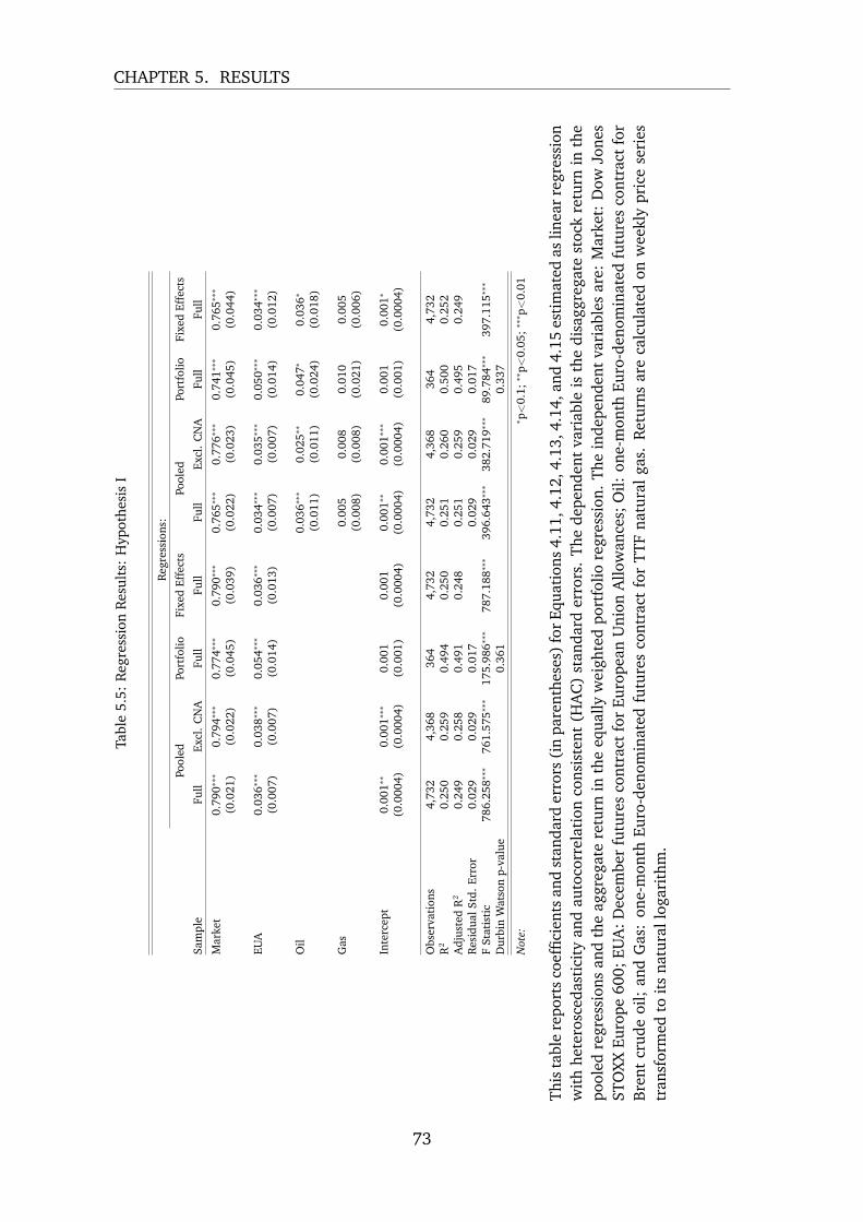
CHAPTER 5. RESULTS
Tabl
e5.
5:R
egre
ssio
nR
esul
ts:
Hyp
othe
sis
I
Reg
ress
ions
:
Pool
edPo
rtfo
lioFi
xed
Effe
cts
Pool
edPo
rtfo
lioFi
xed
Effe
cts
Sam
ple
Full
Excl
.C
NA
Full
Full
Full
Excl
.C
NA
Full
Full
Mar
ket
0.79
0∗∗∗
0.79
4∗∗∗
0.77
4∗∗∗
0.79
0∗∗∗
0.76
5∗∗∗
0.77
6∗∗∗
0.74
1∗∗∗
0.76
5∗∗∗
(0.0
21)
(0.0
22)
(0.0
45)
(0.0
39)
(0.0
22)
(0.0
23)
(0.0
45)
(0.0
44)
EUA
0.03
6∗∗∗
0.03
8∗∗∗
0.05
4∗∗∗
0.03
6∗∗∗
0.03
4∗∗∗
0.03
5∗∗∗
0.05
0∗∗∗
0.03
4∗∗∗
(0.0
07)
(0.0
07)
(0.0
14)
(0.0
13)
(0.0
07)
(0.0
07)
(0.0
14)
(0.0
12)
Oil
0.03
6∗∗∗
0.02
5∗∗
0.04
7∗0.
036∗
(0.0
11)
(0.0
11)
(0.0
24)
(0.0
18)
Gas
0.00
50.
008
0.01
00.
005
(0.0
08)
(0.0
08)
(0.0
21)
(0.0
06)
Inte
rcep
t0.
001∗∗
0.00
1∗∗∗
0.00
10.
001
0.00
1∗∗
0.00
1∗∗∗
0.00
10.
001∗
(0.0
004)
(0.0
004)
(0.0
01)
(0.0
004)
(0.0
004)
(0.0
004)
(0.0
01)
(0.0
004)
Obs
erva
tion
s4,
732
4,36
836
44,
732
4,73
24,
368
364
4,73
2R2
0.25
00.
259
0.49
40.
250
0.25
10.
260
0.50
00.
252
Adj
uste
dR2
0.24
90.
258
0.49
10.
248
0.25
10.
259
0.49
50.
249
Res
idua
lStd
.Er
ror
0.02
90.
029
0.01
70.
029
0.02
90.
017
FSt
atis
tic
786.
258∗∗∗
761.
575∗∗∗
175.
986∗∗∗
787.
188∗∗∗
396.
643∗∗∗
382.
719∗∗∗
89.7
84∗∗∗
397.
115∗∗∗
Dur
bin
Wat
son
p-va
lue
0.36
10.
337
Not
e:∗ p<
0.1;∗∗
p<0.
05;∗∗∗
p<0.
01
This
tabl
ere
port
sco
effic
ient
san
dst
anda
rder
rors
(in
pare
nthe
ses)
for
Equa
tion
s4.
11,4
.12,
4.13
,4.1
4,an
d4.
15es
tim
ated
aslin
ear
regr
essi
onw
ith
hete
rosc
edas
tici
tyan
dau
toco
rrel
atio
nco
nsis
tent
(HA
C)
stan
dard
erro
rs.
The
depe
nden
tva
riab
leis
the
disa
ggre
gate
stoc
kre
turn
inth
epo
oled
regr
essi
ons
and
the
aggr
egat
ere
turn
inth
eeq
ually
wei
ghte
dpo
rtfo
liore
gres
sion
.Th
ein
depe
nden
tva
riab
les
are:
Mar
ket:
Dow
Jone
sST
OX
XEu
rope
600;
EUA
:Dec
embe
rfu
ture
sco
ntra
ctfo
rEu
rope
anU
nion
Allo
wan
ces;
Oil:
one-
mon
thEu
ro-d
enom
inat
edfu
ture
sco
ntra
ctfo
rB
rent
crud
eoi
l;an
dG
as:
one-
mon
thEu
ro-d
enom
inat
edfu
ture
sco
ntra
ctfo
rT
TFna
tura
lga
s.R
etur
nsar
eca
lcul
ated
onw
eekl
ypr
ice
seri
estr
ansf
orm
edto
its
natu
rall
ogar
ithm
.
73
CHAPTER 5. RESULTS
Subperiod regressions
Next, we test if the regression results are consistent over time by dividing the sam-
ple into annual subperiods beginning with the first week in January and ending
with the last week in December
Table 5.6 presents the regression results for the one-year subperiods. Emission al-
lowance returns appear to have a positive and significant effect on the stock prices
during 2013, 2017 and 2018 at 0.048, 0.084, and 0.053, respectively. The re-
maining years do not produce significant factor coefficients for emission allowance
returns. 2019 stands out as a different year with a factor-beta for the market port-
folio that is exceptionally low at 0.281 compared with other years’ consistently
positive factor betas ranging between 0.766 to 0.843. Moreover, the 2019 regres-
sion’s R2 is considerably lower at 0.043 compared to the range 0.148 to 0.375.
The low explanatory power suggests that something that is not included in the
model is having a strong impact on the sample during the period.
74

CHAPTER 5. RESULTS
Tabl
e5.
6:R
egre
ssio
nR
esul
ts:
One
-yea
rsu
bper
iod
Dep
ende
ntva
riab
le:
Firm
stoc
kre
turn
2013
2014
2015
2016
2017
2018
2019
Mar
ket
0.84
3∗∗∗
0.80
2∗∗∗
0.76
6∗∗∗
0.84
2∗∗∗
0.82
7∗∗∗
0.82
3∗∗∗
0.28
1∗∗∗
(0.0
60)
(0.0
51)
(0.0
49)
(0.0
59)
(0.1
03)
(0.0
51)
(0.0
91)
EUA
0.04
8∗∗∗
0.01
2−
0.00
20.
024
0.08
4∗∗∗
0.05
3∗∗
−0.
010
(0.0
13)
(0.0
12)
(0.0
37)
(0.0
21)
(0.0
20)
(0.0
22)
(0.0
20)
Oil
−0.
041
0.10
9∗∗∗
0.00
30.
025
0.04
80.
062∗∗
0.06
7∗
(0.0
50)
(0.0
41)
(0.0
28)
(0.0
20)
(0.0
32)
(0.0
30)
(0.0
35)
Gas
−0.
152∗∗
0.03
8∗∗
0.07
5∗∗
−0.
025
−0.
037
0.07
0∗∗∗
−0.
004
(0.0
72)
(0.0
18)
(0.0
36)
(0.0
25)
(0.0
29)
(0.0
24)
(0.0
11)
Inte
rcep
t0.
001
0.00
4∗∗∗
−0.
002∗
0.00
01−
0.00
030.
004∗∗∗
0.00
2∗
(0.0
01)
(0.0
01)
(0.0
01)
(0.0
01)
(0.0
01)
(0.0
01)
(0.0
01)
Obs
erva
tion
s66
367
667
668
967
667
667
6R2
0.23
00.
375
0.33
80.
320
0.15
30.
325
0.04
9A
djus
ted
R2
0.22
60.
371
0.33
50.
316
0.14
80.
321
0.04
3R
esid
ualS
td.
Erro
r0.
029
0.02
50.
030
0.03
30.
029
0.02
80.
027
FSt
atis
tic
49.2
18∗∗∗
100.
613∗∗∗
85.8
20∗∗∗
80.4
12∗∗∗
30.3
10∗∗∗
80.8
34∗∗∗
8.60
0∗∗∗
Not
e:∗ p<
0.1;∗∗
p<0.
05;∗∗∗
p<0.
01
This
tabl
ere
port
sco
effic
ient
san
dst
anda
rder
rors
(in
pare
nthe
ses)
for
Equa
tion
s4.
11an
d4.
12es
tim
ated
aslin
ear
regr
essi
onw
ith
het-
eros
ceda
stic
ity
and
auto
corr
elat
ion
cons
iste
nt(H
AC
)st
anda
rder
rors
.Th
ede
pend
ent
vari
able
isth
edi
sagg
rega
test
ock
retu
rn.
The
inde
pen-
dent
vari
able
sar
e:M
arke
t:D
owJo
nes
STO
XX
Euro
pe60
0;EU
A:D
ecem
ber
futu
res
cont
ract
for
Euro
pean
Uni
onA
llow
ance
s;O
il:on
e-m
onth
Euro
-den
omin
ated
futu
res
cont
ract
for
Bre
ntcr
ude
oil;
and
gas:
one-
mon
thEu
ro-d
enom
inat
edfu
ture
sco
ntra
ctfo
rT
TFna
tura
lgas
.R
etur
nsar
eca
lcul
ated
onw
eekl
ypr
ice
seri
estr
ansf
orm
edto
its
natu
rall
ogar
ithm
.
75

CHAPTER 5. RESULTS
To get a better understanding of how 2019 is different from other years, we com-
pute the correlation matrix for the equally weighted portfolio, the Dow Jones
STOXX Europe 600 index, oil, natural gas, and emission allowance price changes
during 2019.
Table 5.7: Correlation matrix of returns for 2019
Portfolio Market Oil Gas EUA
Portfolio 1Market 0.208 1
Oil 0.232 0.501 1Gas -0.068 -0.027 -0.149 1EUA 0.150 0.188 0.061 0.169 1
This table reports the Pearson’s correlation coefficients for the subperiod 2019. The cor-relation coefficients are calculated based on the weekly natural logarithmic returns. Thevariables are the portfolio of electricity generating firms (Portfolio), the market proxy -Dow Jones STOXX Europe 600 (Market), the one-month Brent crude oil (Oil), TTF natu-ral gas contracts (Gas), and the European Union Allowances (EUA).
The correlation between the aggregate returns of the sample companies and Dow
Jones STOXX Europe 600 index is low at 0.208 during 2019 as compared with
0.686 during the full sample period. Figure 5.1 shows a relatively idle price de-
velopment for the market portfolio and a strong price increase for the equally
weighted portfolio. The correlation between the equally weighted portfolio and
oil is substantially stronger at 0.501 in 2019 compared with 0.322 during the full
sample period. However, it is not strong enough to raise concerns regarding sup-
pression.
To include more observations in the regressions, we extend the subperiods to cover
two years but leave 2013 by itself. The last subperiod (2018 - 2019) continues to
be notably different from the previous subperiods. The market coefficient for the
subperiod 2018 to 2019 is 0.609 and significant, which is lower than the other
subperiods that yield coefficients between 0.785 and 0.843. Moreover, the R2 is
once again lower than in the previous subperiods. As such, the reduced sample
76

CHAPTER 5. RESULTS
size of the subperiod 2019 regression does not explain the unexpected results.
Table 5.8: Regression Results: Two-year subperiod
Dependent variable:
Firm stock return2013 2014 - 2015 2016 - 2017 2018 - 2019
Market 0.843∗∗∗ 0.785∗∗∗ 0.826∗∗∗ 0.609∗∗∗
(0.060) (0.035) (0.047) (0.046)
EUA 0.048∗∗∗ 0.012 0.050∗∗∗ 0.028∗
(0.013) (0.012) (0.015) (0.015)
Oil −0.041 0.036 0.034∗ 0.054∗∗
(0.050) (0.022) (0.017) (0.022)
Gas −0.152∗∗ 0.046∗∗∗ −0.031∗ 0.016(0.072) (0.017) (0.018) (0.011)
Intercept 0.001 0.0004 0.0001 0.003∗∗∗
(0.001) (0.001) (0.001) (0.001)
Observations 663 1,352 1,365 1,352R2 0.230 0.347 0.254 0.169Adjusted R2 0.226 0.345 0.252 0.167Residual Std. Error 0.029 0.028 0.031 0.028F Statistic 49.218∗∗∗ 179.168∗∗∗ 116.015∗∗∗ 68.689∗∗∗
Note: ∗p<0.1; ∗∗p<0.05; ∗∗∗p<0.01
This table reports coefficients and standard errors (in parentheses) for Equations 4.11 and4.12 estimated as linear regression with heteroscedasticity and autocorrelation consistent(HAC) standard errors. The dependent variable is the disaggregate stock return. Theindependent variables are: Market: Dow Jones STOXX Europe 600; EUA: December fu-tures contract for European Union Allowances; Oil: one-month Euro-denominated futurescontract for Brent crude oil; and gas: one-month Euro-denominated futures contract forTTF natural gas. Returns are calculated on weekly price series transformed to its naturallogarithm.
5.3.2 Hypothesis II
In this section, we present the empirical results related to the second hypothesis,
namely, if a potential impact from price increases in European Union Allowances
77

CHAPTER 5. RESULTS
is stronger on firm stock return for firms with a lower carbon-intensive electricity
generation.
Recall that we create a binary variable “Polluter” that equals 1 if firm i’s carbon
intensity is above the sample median. To test the second hypothesis, we add the
binary variable to Equation 4.16 that controls for commodity price impact and
interact it with the return of emission allowances. This allows for carbon intensive
companies to have a different intercept and slope in regard to emission allowance
return. The results of this regression is presented in Table 5.9.
As hypothesized, the results indicate that there indeed is an interaction effect
between the degree of carbon intensity in electricity production and price changes
in emission allowances. While companies that have a lower than median carbon
intensity have a factor coefficient for emission allowance price changes of 0.051
while their carbon intensive counterparts have a lower 0.051 - 0.038 = 0.013
factor coefficient when taking the interaction effect into account. Interestingly, the
binary variable representing carbon insntive firms is positive, with a coefficient of
0.02, suggesting that carbon intensive companies, ceteris paribus, experienced a
higher average return during the sample period.
The addition of the binary variable for polluters and its interaction term with
emission allowance returns only slightly increases goodness-of-fit measured by the
adjusted R2. The factor betas for the market, emission allowances, natural gas, and
the interaction term Polluter * EUA are all individually significant at 1% level. The
binary variable polluter is significant at 5%, and oil is not significant at 10%. All
reported standard errors are heteroscedastic and autocorrelation consistent.
Next, we investigate the firm specific effects by running individual regressions
for each firm in the sample. Thirteen regressions are presented in Table 5.10.
Each regression has 364 observations, and the adjusted R2 varies between 0.189
78

CHAPTER 5. RESULTS
(CNA) to 0.425 (ENG). The Durbin Watson test for RWE indicates issues with
autocorrelation in its first lag. Three companies have a significant factor coefficient
for emission allowances: Verbund AG (0.138), Electricite de France SA (0.028),
and Fortum Oyj (0.089).
79

CHAPTER 5. RESULTS
Table 5.9: Regression Results: Hypothesis II
Dependent variable:
Firm stock return
(1) (2)
Market 0.765∗∗∗ 0.765∗∗∗
(0.022) (0.022)
EUA 0.034∗∗∗ 0.051∗∗∗
(0.007) (0.009)
Oil 0.005 0.005(0.008) (0.008)
Gas 0.036∗∗∗ 0.036∗∗∗
(0.011) (0.011)
Polluter 0.002∗∗
(0.001)
Polluter * EUA −0.038∗∗∗
(0.013)
Intercept 0.001∗∗ 0.0002(0.0004) (0.001)
Observations 4,732 4,732R2 0.251 0.253Adjusted R2 0.251 0.252Residual Std. Error 0.029 (df = 4727) 0.029 (df = 4725)F Statistic 396.643∗∗∗ (df = 4727) 267.038∗∗∗ (df = 4725)
Note: ∗p<0.1; ∗∗p<0.05; ∗∗∗p<0.01
This table reports coefficients and standard errors (in parentheses) for Equations 4.12 and4.16 estimated as linear regression with heteroscedasticity and autocorrelation consistent(HAC) standard errors. The dependent variable is the disaggregate stock return. Theindependent variables are: Market: Dow Jones STOXX Europe 600; EUA: December fu-tures contract for European Union Allowances; Oil: one-month Euro-denominated futurescontract for Brent crude oil; and gas: one-month Euro-denominated futures contract forTTF natural gas. Returns are calculated on weekly price series transformed to its naturallogarithm.
80

CHAPTER 5. RESULTS
Tabl
e5.
10:
Reg
ress
ion
Res
ults
:Fi
rm-s
peci
fic
Dep
ende
ntva
riab
le:
Firm
stoc
kre
turn
SSE
ELE
IBE
VER
NTG
CN
AEN
GED
FED
PA
2AFO
REN
ER
WE
Mar
ket
0.45
8∗∗∗
0.69
8∗∗∗
0.80
2∗∗∗
0.57
0∗∗∗
0.79
6∗∗∗
0.63
3∗∗∗
0.93
9∗∗∗
0.91
6∗∗∗
0.78
2∗∗∗
0.82
8∗∗∗
0.63
5∗∗∗
0.93
1∗∗∗
0.95
5∗∗∗
(0.0
63)
(0.0
72)
(0.0
59)
(0.0
79)
(0.0
70)
(0.0
90)
(0.0
61)
(0.0
85)
(0.0
68)
(0.0
77)
(0.0
80)
(0.0
68)
(0.1
24)
EUA
0.01
70.
009
−0.
007
0.13
8∗∗∗
−0.
011
0.01
40.
026
0.08
7∗∗∗
−0.
001
0.04
00.
089∗∗∗
0.00
10.
036
(0.0
23)
(0.0
18)
(0.0
18)
(0.0
26)
(0.0
22)
(0.0
25)
(0.0
20)
(0.0
28)
(0.0
22)
(0.0
29)
(0.0
22)
(0.0
23)
(0.0
32)
Oil
−0.
001
0.01
2−
0.00
40.
014
0.01
2−
0.03
40.
0001
−0.
040
0.00
10.
025
0.03
30.
019
0.02
8(0
.026
)(0
.019
)(0
.019
)(0
.031
)(0
.029
)(0
.046
)(0
.026
)(0
.034
)(0
.029
)(0
.025
)(0
.023
)(0
.022
)(0
.042
)
Gas
0.10
0∗∗∗
−0.
050
−0.
048∗
0.06
60.
062∗∗
0.16
3∗∗∗
0.01
40.
083∗
0.03
0−
0.04
20.
081∗∗
−0.
041
0.04
5(0
.032
)(0
.030
)(0
.026
)(0
.045
)(0
.029
)(0
.049
)(0
.034
)(0
.050
)(0
.035
)(0
.039
)(0
.039
)(0
.033
)(0
.055
)
Inte
rcep
t0.
001
0.00
3∗∗
0.00
2∗∗
0.00
20.
002
−0.
003∗
−0.
0001
−0.
001
0.00
20.
003∗∗
0.00
20.
002
−0.
001
(0.0
01)
(0.0
01)
(0.0
01)
(0.0
02)
(0.0
01)
(0.0
02)
(0.0
01)
(0.0
02)
(0.0
01)
(0.0
02)
(0.0
01)
(0.0
01)
(0.0
02)
Obs
erva
tion
s36
436
436
436
436
436
436
436
436
436
436
436
436
4R2
0.19
20.
268
0.39
20.
216
0.36
60.
198
0.43
10.
261
0.28
80.
244
0.30
80.
401
0.19
9A
djus
ted
R2
0.18
30.
260
0.38
50.
207
0.35
90.
189
0.42
50.
253
0.28
00.
235
0.30
00.
394
0.19
0R
esid
ualS
td.
Erro
r0.
024
0.02
30.
020
0.03
20.
023
0.03
40.
023
0.03
70.
026
0.03
10.
025
0.02
30.
043
FSt
atis
tic
21.3
17∗∗∗
32.9
02∗∗∗
57.9
04∗∗∗
24.7
20∗∗∗
51.8
99∗∗∗
22.2
07∗∗∗
67.9
86∗∗∗
31.6
79∗∗∗
36.3
03∗∗∗
28.9
53∗∗∗
39.9
78∗∗∗
59.9
60∗∗∗
22.2
43∗∗∗
Dur
bin
Wat
son
p-va
lue
0.88
40.
579
0.74
80.
986
0.32
50.
296
0.37
40.
781
0.46
60.
617
0.92
40.
866
0.04
1
Not
e:∗ p<
0.1;∗∗
p<0.
05;∗∗∗
p<0.
01
This
tabl
ere
port
sco
effic
ient
san
dst
anda
rder
rors
(in
pare
nthe
ses)
for
Equa
tion
4.12
esti
mat
edas
linea
rre
gres
sion
wit
hhe
tero
sced
asti
city
and
auto
corr
elat
ion
cons
iste
nt(H
AC
)st
anda
rder
rors
.Th
ede
pend
ent
vari
able
isth
est
ock
retu
rnfo
rth
esp
ecifi
cco
mpa
ny.
The
inde
pend
ent
vari
able
sar
e:M
arke
t:D
owJo
nes
STO
XX
Euro
pe60
0;EU
A:
Dec
embe
rfu
ture
sco
ntra
ctfo
rEu
rope
anU
nion
Allo
wan
ces;
Oil:
one-
mon
thEu
ro-d
enom
inat
edfu
ture
sco
ntra
ctfo
rB
rent
crud
eoi
l;an
dga
s:on
e-m
onth
Euro
-den
omin
ated
futu
res
cont
ract
for
TTF
natu
ralg
as.
Ret
urns
are
calc
ulat
edon
wee
kly
pric
ese
ries
tran
sfor
med
toit
sna
tura
llog
arit
hm.
81

CHAPTER 5. RESULTS
5.3.3 OLS Diagnostics
In this section, we will visually assess if the OLS assumptions hold true for the
models used to test hypotheses I and II.
Model Diagnostics for Hypothesis I
The figure illustrates four plots of the regressions’ residuals for the pooled regression residuals,and these are used to examine if the OLS assumptions hold.
Figure 5.4: OLS Diagnostic - Pooled regression
We plot the diagnostics plots of the extended models that include oil and natu-
ral gas as control variables for both the pooled and aggregated portfolio data to
investigate whether the OLS assumptions hold. The linearity assumption can be
checked by investigating the first plot Residuals vs Fitted. They do not display
any fitted pattern, suggesting that we can assume a linear relationship between
our predictors and the outcome variables. In the Normal Q-Q plot, the residuals
82

CHAPTER 5. RESULTS
The figure illustrates four plots for the regressions’ residuals for the equally weighted portfolio,and these are used to examine if the OLS assumptions hold.
Figure 5.5: OLS Diagnostic - Equally weighted portfolio
should follow the diagonal line to indicate normality of the residuals. In our case,
the residuals approximately follow this line with some divergence in both ends, in
particular for the pooled regression. The Scale-Location plot is used to visually
see if the variances in the residual errors are constant, in other words, it can be
used to identify a heteroscedasticity issue. The horizontal red line indicates that
the variability does not change depending on the size of the fitted values. This sug-
gests that we do not have an issue with heteroscedasticity. The last plot, Residuals
vs Leverage, helps us find influential outliers by plotting the standardized residu-
als and high leverage points. The plot also provides the three most extreme data
points that are particularly worth checking for validity. No observations lie outside
of Cook’s distance, and the plot does not raise concerns regarding outliers. How-
ever, we decide to investigate the extreme data points to confirm the validity of
the data.
83
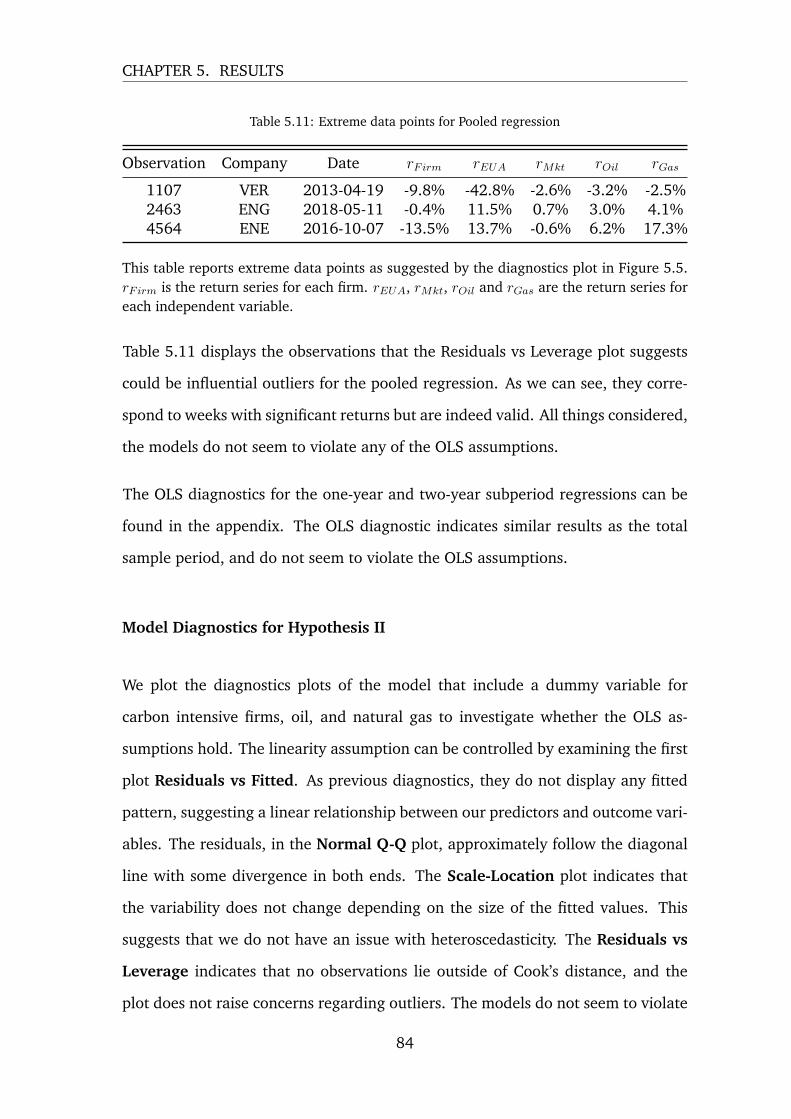
CHAPTER 5. RESULTS
Table 5.11: Extreme data points for Pooled regression
Observation Company Date rFirm rEUA rMkt rOil rGas
1107 VER 2013-04-19 -9.8% -42.8% -2.6% -3.2% -2.5%2463 ENG 2018-05-11 -0.4% 11.5% 0.7% 3.0% 4.1%4564 ENE 2016-10-07 -13.5% 13.7% -0.6% 6.2% 17.3%
This table reports extreme data points as suggested by the diagnostics plot in Figure 5.5.rFirm is the return series for each firm. rEUA, rMkt, rOil and rGas are the return series foreach independent variable.
Table 5.11 displays the observations that the Residuals vs Leverage plot suggests
could be influential outliers for the pooled regression. As we can see, they corre-
spond to weeks with significant returns but are indeed valid. All things considered,
the models do not seem to violate any of the OLS assumptions.
The OLS diagnostics for the one-year and two-year subperiod regressions can be
found in the appendix. The OLS diagnostic indicates similar results as the total
sample period, and do not seem to violate the OLS assumptions.
Model Diagnostics for Hypothesis II
We plot the diagnostics plots of the model that include a dummy variable for
carbon intensive firms, oil, and natural gas to investigate whether the OLS as-
sumptions hold. The linearity assumption can be controlled by examining the first
plot Residuals vs Fitted. As previous diagnostics, they do not display any fitted
pattern, suggesting a linear relationship between our predictors and outcome vari-
ables. The residuals, in the Normal Q-Q plot, approximately follow the diagonal
line with some divergence in both ends. The Scale-Location plot indicates that
the variability does not change depending on the size of the fitted values. This
suggests that we do not have an issue with heteroscedasticity. The Residuals vs
Leverage indicates that no observations lie outside of Cook’s distance, and the
plot does not raise concerns regarding outliers. The models do not seem to violate
84

CHAPTER 5. RESULTS
The figure illustrates four plots for the regressions’ residuals for the equally weighted portfolio,and these are used to examine if the OLS assumptions hold.
Figure 5.6: OLS Diagnostic - Hypothesis II - Polluter
any of the OLS assumptions. The OLS diagnostic for the firm-specific regression
results can be found in the appendix, and the diagnostic plots do not indicate a
violation of the OLS assumptions.
5.4 Summary of Findings
Our empirical results suggest that European Union Allowance price changes have
a positive impact on the return on the stocks of our sample of thirteen European
electricity-generating firms during the third phase of the EU ETS. In addition to
controlling for the overall return on the stock market, we have controlled for com-
modity price impact by including the return one-month Euro-denominated futures
85

CHAPTER 5. RESULTS
for Brent crude oil and TTF natural gas. The empirical results are consistent across
multiple regression models that use the pooled panel data, aggregated panel data
as well as controlling for firm-specific fixed effects. However, subperiod regres-
sions return ambiguous results with significant positive effects in 2013, 2017 and
2018 but not on 2014, 2015, 2016, and 2019.
Additionally, we have controlled for the relative degree of carbon intensity and
found that carbon intensive firms lose a large share of the positive effect that price
increases in emission allowances have on stock performance. On a firm-specific
level, three companies’ stock returns exhibit being positively influenced by price
increases in emission allowances. These are Verbund AG from Austria, Electricite
de France SA from France, and Fortum Oyj from Finland.
86

Chapter 6: Discussion
In Chapter VI, we interpret the empirical results and discuss and how the findings
relate to previous research, economic theory, and the deduced hypotheses. The
purpose of the chapter ultimately to provide answers to the research questions and
their implications as well to present our suggestions regarding further research.
6.1 EU Allowance Price Changes’ Impact on Finan-
cial Performance
We performed regressions with weekly frequency beginning with the first week of
2013 and ending with the last week of 2019. In addition to the overall stock mar-
ket, we controlled for potential commodity price impact by including price changes
in oil and natural gas futures, in line with the underlying concept of a multifac-
tor model. Moreover, three different econometric methods were employed. The
central finding of the econometric analysis is that the coefficients on the emission
allowances are consistently positive and significant when looking at the whole pe-
riod. In line with our first hypothesis, an increase in emission allowance price is
associated with an appreciation of the stock price of our sample of European elec-
tricity generating firms during the third phase of the EU ETS. As such, investors
appear to expect that future cash flows will increase when emissions are more
87

CHAPTER 6. DISCUSSION
expensive and decrease when they are less costly.
Specifically, if we consider the coefficient from the OLS regression using the pooled
panel data and controlling for oil and natural gas to gauge the magnitude of the
impact, a one percent increase in emission allowance price is associated with a
positive 0.034% return on the stock price. The price of an emission allowance
increased from approximately e6 to e26 during the third phase of the EU ETS,
which corresponds to a 333% increase. If we fit the return into the estimated
regression, the increase in emission prices yielded a positive impact on the stock
market return for the considered companies by an average of 11.3% from the
beginning of 2013 to the end of 2019.
Our methodology was designed based on the studies by Oberndorfer (2009) and
Veith et al. (2009) that investigated the impact of emission allowance prices on
stock performance for European electricity generating firms during the first phase
of the EU ETS that ran through 2005 - 2007. Recall from the literature review,
these studies found a positive relationship between the variables, in line with our
results, and argued that this is primarily due to windfall profits in the electricity
sector. Windfall profits occurred due to the combination of grandfathering, i.e.
free allocation of emission allowances, and a high pass-through rate of the oppor-
tunity cost of the allowances to consumers. The implementation of auctioning as
the default method of allocation for the electricity sector on the onset of the third
phase marked the end of these windfall profits. Consequently, we expected that
the extent of the positive relationship would be weaker than during the first phase
of the EU ETS. Nevertheless, our results indicate that the positive impact of emis-
sion allowances on the stock value of European electricity generating companies
has increased.
The average price of an emission allowance December futures contract during the
third phase of the EU ETS was lower than during the first phase. As such, we can
88

CHAPTER 6. DISCUSSION
exclude a stronger effect due to a larger nominal base as a reason. Instead, one
possible explanation is that the market has become more efficient as market par-
ticipants have had time to improve their understanding of the interplay between
emission allowance price changes and financial performance. The first phase of
the EU ETS was a pilot stage that, among other things, aimed to build the founda-
tion of the system by trial-and-error and pave the way for its future development.
As a result, there was much uncertainty regarding several components of the sys-
tem, perhaps most clearly illustrated by the plummet in emission allowance spot
price during the end of the first phase. For the investor, such uncertainty would
present challenges in discounting a conceivable effect into the stock price, which
in turn would be reflected in a weak connection.
During the third phase, however, the EU ETS was well-established, and several
mechanisms had been put in place to increase transparency and alignment be-
tween member states. For instance, the single EU-wide emissions cap that replaced
the National Allocation Plans and the implementation of the Market Stability Re-
serve have likely contributed to better aligned expectations and stability among
market participants. Moreover, conditions for the fourth phase that will begin in
2021 and end in 2030 have been disclosed with the most significant difference
likely being the larger linear rate at which the emissions cap decreases. These
things considered, investors are better able to discount the impact of emissions al-
lowance futures price changes to the stock price of European electricity-generating
companies.
Oberndorfer (2009) states that it would be interesting to investigate if his results
hold after auctioning has become the default method of allocation, and argues that
the effect will depend on the pass-through rate and the carbon intensity of the in-
framarginal producers relative to the intensity of the marginal producer. Over the
last decade, there has been a dramatic penetration of renewable energy sources
89

CHAPTER 6. DISCUSSION
into the European electricity mix, partially driven by technological advancements
in wind power, increased demand for “green energy”, and the increased marginal
generation cost for emitting power plants due to auctioning. This has pushed
the merit curve further to the right, with a larger cluster of carbon-neutral infra-
marginal producers. Because conventional thermal generation remains the typical
marginal producer, the emission allowance cost increases the wholesale electricity
price on the market. As such, when the price of an emission allowance increases,
the larger cluster of inframarginal producers gain higher contribution margins that
are reflected in the overall financial performance of the European electricity sector.
Another structural change to the European electricity sector that may explain part
of the stronger connection is the European Union’s efforts to reduce vertical in-
tegration by further dividing the electricity sector into its three core activities:
generation, transmission, and distribution. This split may have made our sample
of electricity generating companies less diversified and more focused towards elec-
tricity generation than the samples of Oberndorfer (2009) and Veith et al. (2009).
Because generation is the only activity that is subject to the emissions regulation,
the European electricity companies of today may be more exposed to the emission
allowance price changes than they were a decade ago.
Although emission allowance returns exhibit significant explanatory power dur-
ing the full observation period, the results for the subperiods do not consistently
display the corresponding correlation. There is a temporary lack of economic sig-
nificance during 2014 to 2016 and 2019. When we extend the periods to allow
for more observations, 2014 and 2015 as well 2018 and 2019 are not significant.
During 2014 to 2016, prices for emission allowances were considered too low to
have an impact on business-as-usual allowances, and the system faced widespread
criticism (Perino & Willner, 2016). With prices running as low as e3.2 for De-
cember futures contracts, it is possible that investors did not predict an economic
90

CHAPTER 6. DISCUSSION
impact on the cash flows of electricity-generating firms. In efforts to increase
the emission allowance prices, the European Commission took action to limit the
large oversupply of the total number of allowances in circulation. In 2014, 2015,
and 2016 the European Commission decided to back-load 400, 300 and 200 mil-
lion allowances, respectively, and in 2018 it decided on implementing the Market
Stability Reserve in the subsequent year to ensure that the price of emission al-
lowances would increase. The prices of emission allowance December futures be-
gan to increase dramatically in the second half of 2017, more than one and a half
year before the implementation of the system, indicating that investors expected
that such a system would succeed in increasing emission allowance prices. With
trust amongst market participants that prices would indeed stabilize at a higher
level, investors may have regained its expectations that price changes in emission
allowances would have an economic impact on European electricity-generating
firms.
Nevertheless, emission price returns lost its economic significance on firm stock
performance in 2019. However, the year stands out in the regressions in several
ways. For instance, the market beta from 2013 - 2018 is consistently between
0.766 and 0.843 as is expected by low-risk utility stocks that are less exposed to
economic cycles (Grout & Zalewska, 2006) while it is low at 0.281 during 2019.
Moreover, the adjusted R2 for 2019 is substantially lower at 0.043 compared with
an average of 0.296 during the previous subperiods regressions. Combined, this
indicates that the sample companies’ shareholder return was influenced by some-
thing that was not included in the model.
In 2019, central banks provided an increased stimulus to the financial markets
by increasing liquidity and lowering interest rates (Bell, 2020). Figure 6.1 dis-
plays the decrease in 10-year government bond interest rates in the United States,
Germany, the United Kingdom, Spain, and Italy during 2019. German interest
91

CHAPTER 6. DISCUSSION
rates are negative, and the remaining European countries’ interest rates reach be-
low 1% during the year. With such unfavourable interest rates, many investors
chose to seek returns from other securities. Investors regard utility stocks as a
relatively defensive investment in the stock market because of the stable nature of
cash flows and low exposure to the business cycle that allows utility companies to
consistently offer large dividends to shareholders. In low-interest environments,
investors may seek the return from utility companies rather than bonds (Huston,
2015). As such, the outperformance of the sample companies over the Dow Jones
Euro STOXX 600 index may be a result of this and obscure the economic impact of
EUA allowances and overall market performance on the stock return of electricity
generating companies.
The figure illustrates the development in interest rates for selected economies for 2019. The figureis based on daily observations for the United States (US), Germany (GR), the United Kingdom(UK), Spain (SP) and Italian (IT) 10 year government bonds. Source: Bloomberg
Figure 6.1: Development for 10-year Government Yields for 2019
During the year, the price of natural gas roughly halved driven by an exceptionally
mild winter that resulted in oversupplies in Europe. Recall from Chapter II that
92

CHAPTER 6. DISCUSSION
natural gas and coal are substitutes in thermal power generation and that coal is at
least roughly twice as carbon-intensive. The decrease in natural gas prices and the
simultaneous increase in emission prices led to a significant fuel switch from coal
to natural gas during the year (Qin, 2019). In turn, this contributed to a decrease
in power generation from coal by 25% and a fall in emissions from the electricity
sector by 12%, which is likely to be the largest annual fall ever (Buck et al., 2020).
The significant decrease in the carbon intensity of the generation mix during 2019
made the electricity sector much less exposed to emission price changes, possibly
resulting in the loss of economic significance in the regression during that year.
In conclusion, we confirm our first hypothesis, emission allowance price increases
have, on average, positively impacted stock return for our sample of thirteen Eu-
ropean electricity generating firms during the sample period. As such, emission
allowance returns served to expose the firms to systematic risk with an unexpected
increase in the factor resulting in an increase in the stock value. On the premise
of the Efficient Market Hypothesis, these empirical results indicate that investors
discount an expectation that price increases in emission allowances will, on aver-
age, positively impact the electricity generating firms’ future cash flows. As such,
financial performance for European electricity generating firms appear to be pos-
itively affected by price increases in European Union Allowances during the third
phase of the EU ETS.
6.2 Carbon Intensity and Financial Performance
We hypothesized that the return on the stocks of our sample of European electricity-
generating firms with a low carbon-intensive electricity generation was more pos-
itively (negatively) affected by price increases (decreases) of emission allowances
during the third phase of the EU ETS. We formed a binary variable representing
93

CHAPTER 6. DISCUSSION
firms with a higher than sample median carbon-intensive electricity generation in
Europe. It was interacted with the return on emission allowances to allow for
different intercept and slope regarding the emission allowance factor. The factor
coefficient for the interaction term was significantly negative, indicating that the
electricity generators’ portfolios of power plants affect the relationship between
price changes in emission allowances and stock return.
The empirical results suggest that investors predict that a less carbon-intensive
generation portfolio provides an increased positive effect on future cash flows from
price increases in emission allowances. Intuitively, the reason is that the contri-
bution margins for carbon efficient electricity generators increase when carbon-
intensive price-setting marginal producers must increase their bids to cover the
additional emission compliance costs. The results are consistent with the findings
of Vieth et al. (2009) that found that half of the positive effect from emission al-
lowance price increases were lost for companies with a higher than median share
of carbon emitting production. Verbund AG, Electricite de France SA and Fortum
Oyj are the three companies that individually exhibit a positive and significant
interaction effect between emission price changes and stock performance. Not
surprisingly, these companies are the least carbon-intensive firms in our sample of
thirteen European electricity-generating firms. Their primary sources of electricity
generation are hydroelectric, nuclear, and a combination of both for Verbund AG,
Electricite de France SA and Fortum Oyj, respectively. These technologies gener-
ate electricity without emissions and at relatively low marginal costs and should
benefit from increased costs of emission compliance.
Conclusively, the empirical results confirm the second hypothesis, emission al-
lowance price increases had a larger positive impact on stock return for our sam-
ple of electricity generating firms with a carbon efficient portfolio of power plants
relative to their carbon-intensive peers during the sample period. Hence, carbon
94
CHAPTER 6. DISCUSSION
efficient firms are more exposed to systematic risk in terms of emission allowance
return. An unexpected increase in the factor will lead to a larger increase in stock
return for the carbon efficient producer than for the carbon intensive generator.
On the premise of the Efficient Market Hypothesis, this indicates that investors
discount an expectation that price increases in emission allowances will have a
larger positive impact on carbon efficient firms’ future cash flows. As such, we
conclude that financial performance is more positively affected by price increases
in emission allowances for carbon efficient electricity generating firms, than their
carbon intensive counterparts. This suggests that the EU ETS is successful in finan-
cially incentivizing profit maximizing firms concerned with electricity generation
to decarbonize their portfolio of power plants.
6.3 Practical Implications
To our knowledge, this paper is the only empirical contribution to the question of
how emission pricing under the European Emission Trading System’s third phase
affects financial performance in the electricity sector. The results indicate that
financial market agents expect emission price changes to have consequences on
future cash flows, reflected in the valuation of the sample of electricity-generating
firms. On the premise of the Arbitrage Pricing Theory, emission allowance return
is a significant factor-beta that offers exposure to systematic risk. Investors can use
this empirical result to find an additional return on their investments and to hedge
positions given expectations of the price developments of emission allowances.
The electricity sector is currently the only sector that is subject to full auctioning,
whereas other sectors receive allowances for free to varying degrees. The results
may offer important insights to policymakers considering enforcing auctioning as
the default method of allocation to other sectors. The electricity sector is naturally
95

CHAPTER 6. DISCUSSION
protected from international competition by means of infrastructure, regulation,
and limitations in the distance that electricity can be efficiently transmitted. The
results may not apply to other sectors that are more significantly exposed to inter-
national competition, for instance, the manufacturing sector. Implementing full
auctioning on the European manufacturing sector may adversely affect its com-
petitiveness in an international context. Moreover, the ultimate goal of reducing
emissions would likely not be achieved as emissions would simply be transferred if
production is moved to countries that do not impose a cost on emissions. However,
the results may be interesting for other sectors, such as the cement and domestic
aviation sectors. In Europe, cement emits more greenhouse gases than the Belgian
economy and aviation is accountable for 3% of EU greenhouse gas emissions. Ce-
ment is typically produced close to its geographic end-market, and inter-European
aviation is for obvious reasons protected from international competition. As such,
full actioning may be viable for these sectors, and the evidence from the electricity
sector may provide useful insights to European policymakers in the development
of the European Emission Trading System.
6.4 Suggested Further Research
The empirical results of this paper are based on a sample of thirteen publicly
traded electricity companies. As such, the results are not necessarily generalizable
to all European electricity-generating companies, for instance, privately owned
firms. The sample firms have operations outside of Europe that are not subject
to the EU ETS, which has not been accounted for in the econometric analysis. If
researchers could obtain data directly from electricity-generating firms, it could
allow for more specific and in-depth analysis of the interplay between emission
pricing and profitability.
96

CHAPTER 6. DISCUSSION
On the same topic, a qualitative approach, for instance, using surveys and inter-
views, could provide important insights into how corporate managers in the Euro-
pean electricity sector consider emission allowance in their decision-making pro-
cess. As an example, it would be interesting to learn to what extent are electricity-
generating companies are actively hedging against price fluctuations in emission
allowances.
Next year, the fourth phase of the system will come into effect. The linear re-
duction rate will increase, leading to a more stringent cap. Combined with the
Market Stability Reserve continuing to limit oversupply, many expect that emis-
sion prices will continue to increase. A similar study that investigates the effects
of emission pricing’s impact on firm performance in the European electricity sector
during phase four would be interesting.
The electricity sector is currently the only sector that is subject to full auctioning.
This is due to the relatively low abatement costs and its natural protection from
foreign competition and emission spillover to regions outside of the European
Union. Sectors with higher abatement costs and exposure to international trade,
for instance, the steel sector, risk adversely losing international competitiveness
if they would have to fully compensate for their emissions. However, the cement
and inter-European air travel sectors are naturally protected in similar ways as
the electricity sector, and it would be particularly interesting with studies on how
price changes of emission allowance affect firm performance in these sectors.
97

Chapter 7: Conclusion
The European Union Emissions Trading System (EU ETS) is a policy instrument
that aims to incentivize firms to decarbonize operations by imposing emission
compliance costs through tradeable emission allowances. The electricity sector
is the largest emitter subject to the scheme, and the regulatory impact on the
sector plays a vital role in the overall success of the system.
This paper empirically investigates how price changes in EU ETS emission al-
lowances affect financial performance among European electricity generating firms
and compares the impact depending on the carbon intensity of the firm’s electricity
generation. Based on the Arbitrage Pricing Theory, we test if European electricity
stocks are exposed to systematic risk from unexpected emission price changes. We
utilize the financial stock markets to proxy financial performance on the premise
of the Efficient Market Hypothesis. Using a balanced longitudinal dataset with
weekly frequency on the stock performance of thirteen listed European electricity
generating firms from the beginning of 2013 to the end of 2019, the study empir-
ically tests for a potential impact of price changes on EU ETS emission allowance
December futures contracts on stock return. For robustness, multiple econometric
models are employed using disaggregated pooled returns and aggregated equally
weighted returns as well as controlling for firm-specific fixed effects. Further, we
control for the overall stock market performance by including the returns of the
Dow Jones Stoxx Europe 600 index and commodity price impact by including Euro
98

CHAPTER 7. CONCLUSION
denominated one-month futures contracts for Brent Oil and TTF Natural Gas. A
binary variable representing the firms’ relative carbon intensity to the median in
2015 is included and interacted to isolate its potential effect on the relationship
between firm stock return and EU ETS emission price return.
In line with Oberndorfer (2009) and Veith et al. (2009), the econometric models
find a positive and significant relationship between EU ETS emission price changes
and stock return for the sample of European electricity generating firms during the
sample period. However, the results are not consistent across subperiods. Further,
in line with Veith et al. (2009) the models find that the positive impact is larger
for firms with carbon efficient electricity generation. The empirical results indicate
that European electricity generating firms in general, and carbon efficient firms in
particular, are exposed to systematic risk from EU ETS emission allowances. Fi-
nancial market agents discount a positive impact of an increased EU ETS emission
allowance price on future cash flows of electricity generating firms. The impact
is expected to be larger for firms with carbon efficient operations. As such, we
conclude that there is a positive relationship between EU ETS emission allowance
prices on the financial performance of European electricity generating firms and
that the positive relationship is stronger for firms with carbon efficient operations.
The positive relationship may partially be explained by the high pass-through rate
of the additional emission compliance cost to the bids of the marginal power plant
(Sijm et al., 2006) that raises the wholesale electricity price in equilibrium. In
turn, this leads to increased regulatory rent for the inframarginal suppliers in the
market. Firms with carbon efficient portfolios of power plants have lower emission
compliance costs and therefore reap larger regulatory rents relative to their carbon
intensive peers.
This study contributes important findings to a limited and outdated set of aca-
demic studies and suggests that the EU ETS is indeed successful in financially
99

CHAPTER 7. CONCLUSION
incentivizing profit maximizing firms concerned with electricity generation to de-
carbonize operations. Although the results are not necessarily directly generaliz-
able to other sectors, the results may be of interest for policymakers considering
more stringent emission compliance in other sectors, primarily the cement and
domestic air travel sectors, that are naturally protected from foreign competition.
100
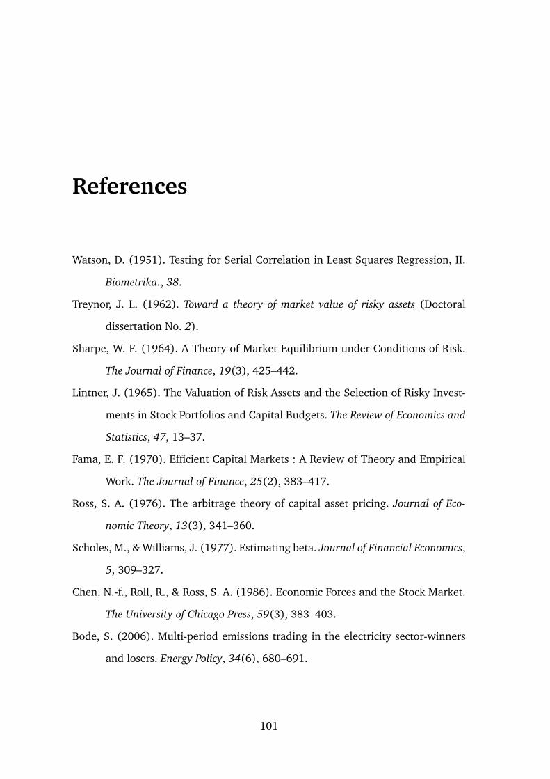
References
Watson, D. (1951). Testing for Serial Correlation in Least Squares Regression, II.
Biometrika., 38.
Treynor, J. L. (1962). Toward a theory of market value of risky assets (Doctoral
dissertation No. 2).
Sharpe, W. F. (1964). A Theory of Market Equilibrium under Conditions of Risk.
The Journal of Finance, 19(3), 425–442.
Lintner, J. (1965). The Valuation of Risk Assets and the Selection of Risky Invest-
ments in Stock Portfolios and Capital Budgets. The Review of Economics and
Statistics, 47, 13–37.
Fama, E. F. (1970). Efficient Capital Markets : A Review of Theory and Empirical
Work. The Journal of Finance, 25(2), 383–417.
Ross, S. A. (1976). The arbitrage theory of capital asset pricing. Journal of Eco-
nomic Theory, 13(3), 341–360.
Scholes, M., & Williams, J. (1977). Estimating beta. Journal of Financial Economics,
5, 309–327.
Chen, N.-f., Roll, R., & Ross, S. A. (1986). Economic Forces and the Stock Market.
The University of Chicago Press, 59(3), 383–403.
Bode, S. (2006). Multi-period emissions trading in the electricity sector-winners
and losers. Energy Policy, 34(6), 680–691.
101

REFERENCES
Grout, P., & Zalewska, A. (2006). The impact of regulation on market risk. Journal
of Financial Economics, 80(1), 149–184.
Sijm, J., Neuhoff, K., & Chen, Y. (2006). CO2 cost pass-through and windfall profits
in the power sector. Climate Policy, 6(1), 49–72.
Mansanet-Bataller, M., Pardo, A., & Valor, E. (2007). CO2 prices, energy and weather.
Energy Journal, 28(3), 73–92.
Alberola, E., Chevallier, J., & Cheze, B. (2008). Price drivers and structural breaks
in European carbon prices 2005-2007. Energy Policy, 36(2), 787–797.
Zachmann, G., & von Hirschhausen, C. (2008). First evidence of asymmetric cost
pass-through of EU emissions allowances: Examining wholesale electricity
prices in Germany. Economics Letters, 99(3), 465–469.
Oberndorfer, U. (2009). EU Emission Allowances and the stock market: Evidence
from the electricity industry. Ecological Economics, 68(4), 1116–1126.
Veith, S., Werner, J. R., & Zimmermann, J. (2009). Capital market response to
emission rights returns: Evidence from the European power sector. Energy
Economics, 31(4), 605–613.
Bodie, Z., Kane, A., & Marcus, A. J. (2011). Investments (9th ed.). New York, Mc-
Graw Hill.
Rademaekers, K., van de Laan, J., Boeve, S., Lise, W., & Kirchsteiger, C. (2011).
Investment needs for future adaptation measures in EU nuclear power plants
and other electricity generation technologies due to effects of climate change
(tech. rep. March). European Union.
Chevallier, J. (2012). Econometric analysis of carbon markets: The European Union
emissions trading scheme and the clean development mechanism (1st). Springer
Netherlands.
Oberndorfer, U., Alexeeva-Talebi, V., & Loschel, A. (2012). Understanding the
Competitiveness Implications of Future Phases of EU ETS on the Industrial
Sectors. SSRN Electronic Journal, (10).
102

REFERENCES
Rickels, W., Gorlich, D., Oberst, G., & Peterson, S. (2012). Carbon Price Dynamics –
Evidence from Phase II of the European Emission Trading Scheme, (1804).
Aatola, P., Ollikainen, M., & Toppinen, A. (2013). Price determination in the EU
ETS market: Theory and econometric analysis with market fundamentals.
Energy Economics, 36, 380–395.
Bushnell, J. B., Chong, H., & Mansur, E. T. (2013). Profiting from regulation: Evi-
dence from the European carbon market. American Economic Journal: Eco-
nomic Policy, 5(4), 78–106.
European Commission. (2013). COMMISSION DECISION of 5 September 2013
concerning national implementation measures for the transitional free al-
location of greenhouse gas emission allowances in accordance with Article
11(3) of Directive 2003/87/EC of the European Parliament and of the C.
Woolridge, J. (2013). Introductory Econometrics (5th). Mason, South Western.
Cludius, J., Hermann, H., Matthes, F. C., & Graichen, V. (2014). The merit order ef-
fect of wind and photovoltaic electricity generation in Germany 2008-2016
estimation and distributional implications. Energy Economics, 44(2014),
302–313.
Enders, W. (2014). Applied Econometric Time Series (4th). Alabama, John Wiley &
Sons Inc.
Endesa. (2015). 2015 Sustainability Report (tech. rep.).
European Commission. (2015). EU ETS Handbook (1st). European Union.
Huston, J. L. (2015). The Declaration of Dependence: Dividends in the Twenty-First
Century (1st). Archway Publishing.
KU Leuven Energy Institute. (2015). The current electricity market design in Europe
(tech. rep.). KU Leuven Energy Institute.
Stock, J. H., & Watson, M. W. (2015). Introduction to Econometrics (Third). Harlow,
United Kingdom, Pearson Education Limited.
103

REFERENCES
Denny Ellerman, A., Marcantonini, C., & Zaklan, A. (2016). The european union
emissions trading system: Ten years and counting. Review of Environmental
Economics and Policy, 10(1), 89–107.
Erbach, G. (2016). Understanding electricity markets in the EU. European Parli-
mentary Research Service, (November), 10.
Hintermann, B., Peterson, S., & Rickels, W. (2016). Price and market behavior in
phase II of the EU ETS: A review of the literature. Review of Environmental
Economics and Policy, 10(1), 108–128.
Martin, I., & Wagner, C. (2016). What is the Expected Return on a Stock. Retrieved
May 9, 2020, from https://www.aqr.com/About-Us/AQR-Insight-Award/
2017/What-is-the-Expected-Return-on-a-Stock
Perino, G., & Willner, M. (2016). Procrastinating reform: The impact of the market
stability reserve on the EU ETS. Journal of Environmental Economics and
Management, 80, 37–52.
PwC. (2016). Climate Change and Electricity (tech. rep.). PwC.
Berk, J., & DeMarzo, P. (2017). Corporate Finance (4th). Harlow, Pearson.
Centrica. (2017). Carbon Disclosure Project Centrica (tech. rep.).
James, G., Witten, D., Hastie, T., & Tibshirani, R. (2017). An Introduction to Sta-
tistical Learning: with Applications in R (7th). London, Springer.
Marin, G., Marino, M., & Pellegrin, C. (2018). The Impact of the European Emis-
sion Trading Scheme on Multiple Measures of Economic Performance. En-
vironmental and Resource Economics, 71(2), 551–582.
European Commission. (2019a). EU Energy in Figures (1st). Luxembourg.
European Commission. (2019b). Report on the functioning of the European carbon
market (tech. rep.). European Commission.
Qin, B. (2019). EU power: Year in Review (tech. rep.). BloombergNEF.
Bell, M. (2020). Review of markets over 2019 (tech. rep.). J.P.Morgan Asset Man-
agement.
104

REFERENCES
Buck, M., Redl, C., Hein, F., & Jones, D. (2020). The European Power Sector in 2019
(tech. rep.).
Jones, D. (2020). The Global Electricity Review 2020 (tech. rep.). Ember.
105

Appendix A: Appendix
A.0.1 Autocorrelation and Stationarity
106

APPENDIX A. APPENDIX
107

APPENDIX A. APPENDIX
108
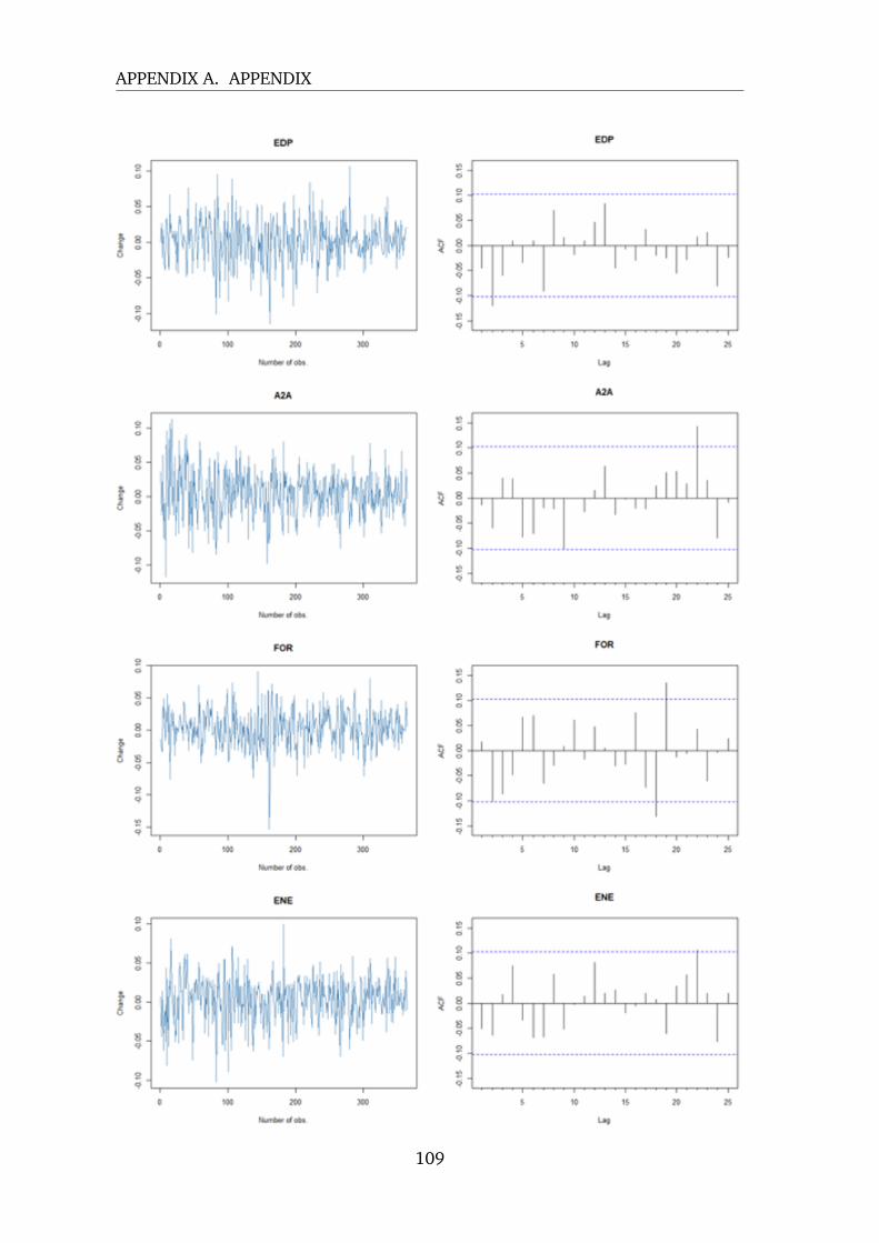
APPENDIX A. APPENDIX
109

APPENDIX A. APPENDIX
Figure A.1: Plots of the logarithmic weekly return and the corresponding ACF plot
110
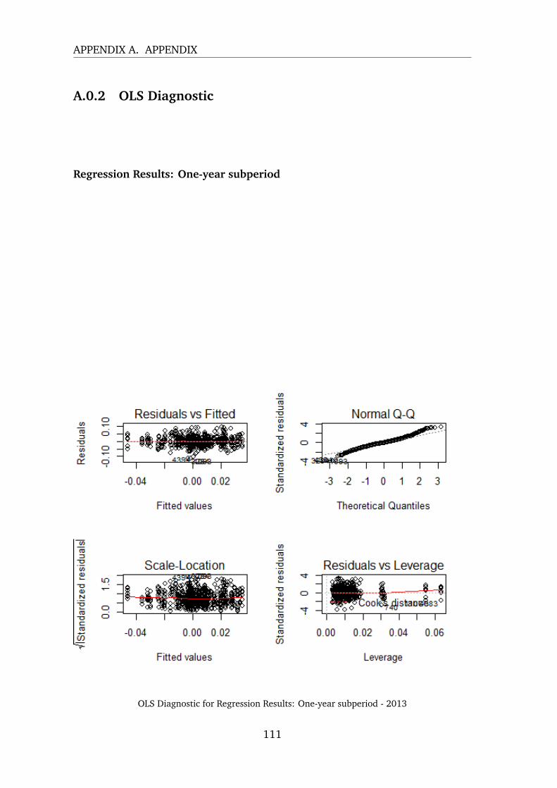
APPENDIX A. APPENDIX
A.0.2 OLS Diagnostic
Regression Results: One-year subperiod
OLS Diagnostic for Regression Results: One-year subperiod - 2013
111

APPENDIX A. APPENDIX
OLS Diagnostic for Regression Results: One-year subperiod - 2014
112

APPENDIX A. APPENDIX
OLS Diagnostic for Regression Results: One-year subperiod - 2015
113

APPENDIX A. APPENDIX
OLS Diagnostic for Regression Results: One-year subperiod - 2016
114

APPENDIX A. APPENDIX
OLS Diagnostic for Regression Results: One-year subperiod - 2017
115

APPENDIX A. APPENDIX
OLS Diagnostic for Regression Results: One-year subperiod - 2018
116

APPENDIX A. APPENDIX
OLS Diagnostic for Regression Results: One-year subperiod - 2019
Figure A.2: OLS Diagnostic: One-year subperiod
117

APPENDIX A. APPENDIX
Regression Results: Two-year subperiod
OLS Diagnostic for Regression Results: Two-year subperiod - 2014 - 2015
118

APPENDIX A. APPENDIX
OLS Diagnostic for Regression Results: Two-year subperiod - 2016 - 2017
119

APPENDIX A. APPENDIX
OLS Diagnostic for Regression Results: Two-year subperiod - 2018 - 2019
Figure A.3: OLS Diagnostic: Two-year subperiod
120

APPENDIX A. APPENDIX
Regression Results: Firm-Specific
OLS Diagnostic for Regression Results: Firm-specific - SSE
121

APPENDIX A. APPENDIX
OLS Diagnostic for Regression Results: Firm-specific - ELE
122

APPENDIX A. APPENDIX
OLS Diagnostic for Regression Results: Firm-specific - IBE
123
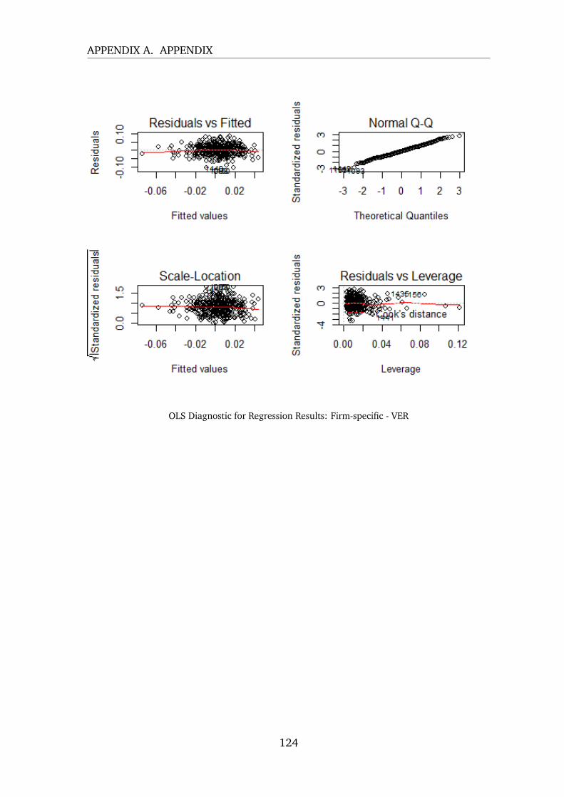
APPENDIX A. APPENDIX
OLS Diagnostic for Regression Results: Firm-specific - VER
124

APPENDIX A. APPENDIX
OLS Diagnostic for Regression Results: Firm-specific - NTG
125

APPENDIX A. APPENDIX
OLS Diagnostic for Regression Results: Firm-specific - CNA
126

APPENDIX A. APPENDIX
OLS Diagnostic for Regression Results: Firm-specific - ENG
127

APPENDIX A. APPENDIX
OLS Diagnostic for Regression Results: Firm-specific - EDF
128

APPENDIX A. APPENDIX
OLS Diagnostic for Regression Results: Firm-specific - EDP
129

APPENDIX A. APPENDIX
OLS Diagnostic for Regression Results: Firm-specific - A2A
130

APPENDIX A. APPENDIX
OLS Diagnostic for Regression Results: Firm-specific - FOR
131

APPENDIX A. APPENDIX
OLS Diagnostic for Regression Results: Firm-specific - ENE
132

APPENDIX A. APPENDIX
OLS Diagnostic for Regression Results: Firm-specific - RWE
Figure A.4: OLS Diagnostic: Firm-specific
133
Related Documents