The Environmental and Employment Effect of Australian ... · PDF filemacro-economy, different sectors, occupation groups, and household income deciles. II. ... Australian carbon tax

Abstract—The paper employs a computable general

equilibrium (CGE) model with an environmentally-extended

Social Accounting Matrix (SAM) to simulate the effects of a

carbon tax of $23 per tonne of carbon dioxide on different

economic agents, with and without a compensation policy.

According to the simulation results, the carbon tax can cut

emissions effectively, but will cause a mild economic contraction.

The proposed compensation plan has little impact on emission

cuts while significantly mitigating the negative effect of a

carbon tax on the economy. The effect on various employment

occupations is mildly negative, ranging from -0.6% to -1.7%,

with production and transport workers worst affected.

Index Terms—Carbon tax, CGE modelling, macro economy,

environmental effect, employment effect.

I. INTRODUCTION

Although Australia’ s greenhouse gas emissions are

relatively low – accounting for around 1.5% of global carbon

emissions, its emissions per capita are the highest in the

world (reference [1]). The high emissions per capita in

Australia are partly due to a small population and abundant

cheap energy resources, particularly brown and black coal,

which have very high emission intensity. The Gillard

government has committed to reducing carbon emissions by

80% below 2000 levels by 2050 and announced that it will

introduce a carbon tax from July 1st 2012.

The government’s proposal triggered strong resistance

from Opposition parties and various interest groups. They

claim that a carbon tax will cause a large economic

contraction, high unemployment, higher electricity prices

and the demise of the coal industry. Certainly, public opinion

about a carbon tax is divided. Amid anti- and pro- carbon tax

rallies and demonstrations, speculation about the effects of

the proposed tax varies widely.

To support the carbon tax proposal, the Australian

Treasury has undertaken comprehensive modelling. The

Treasury has employed a suite of different models, including

two CGE models, one input-output model and a number of

micro models for the electricity and road transport sectors.

The results from this modelling depend on the parameters

and assumptions used (as with all models), but given the

intricacy and complexity of the modelling, these are not easy

to articulate and evaluate. Similarly, the results will depend

on the degree of integration and compatibility of the different

Manuscript received March 6, 2014; revised May 9, 2014.

Xianming Meng and Mahinda Siriwardana are with the UNE Business

School, University of New England, Armidale, NSW 2351, Australia (e-mail:

[email protected]).

Judith McNeill is with the Institute for Rural Futures, School of

Behavioural, Cognitive and Social Sciences, University of New England.

models, again, matters not assessed easily. Perhaps as a result

of this, and certainly because of the way the politics has

played out, Australians are sceptical about the modelling

results, with the Opposition leader stating openly that the

carbon tax proposal is based on a lie.

In this paper we adopt a different approach. To single out

the effects of a carbon tax, we constructed a single country

static CGE model. In companion, an

environmentally-extended micro Social Accounting Matrices

(SAM) is developed. Based on the simulation results, this

paper purports to uncover the short run implications of a

carbon tax policy for carbon emission reduction, the

macro-economy, different sectors, occupation groups, and

household income deciles.

II. MODELLING FRAMEWORK

The effect of a carbon tax is a well researched topic

internationally. Notable research includes references [2]-[8].

A comprehensive review of international modelling literature

is given in reference [9].

Because the purpose of this study is to assess the effect of a

carbon tax policy, instead of forecasting the performance of

the whole economy overtime under the tax, the model

developed for this study is a static CGE model, based on

ORANI-G [5]. The comparative static nature of ORANI-G

helps to single out the effect of carbon tax policies while

keeping other factors being equal. The model employs

standard neoclassical economic assumptions: a perfectly

competitive economy with constant returns to scale, cost

minimisation for industries and utility maximisation for

households, and continuous market clearance. In addition,

zero profit conditions are assumed for all industries because

of perfect competition in the economy.

The Australian economy is represented by 35 sectors

which produce 35 goods and services, one representative

investor, ten household groups, one government and nine

occupation groups. The final demand includes household,

investment, government and exports. With the exception of

the production function, we adopted the functions in the

multi-households version of ORANI-G.

Overall, the production function is a five-layer nested

Leontief-CES function. As in the ORANI model, the top

level is a Leontief function describing the demand for

intermediate inputs and composite primary factors and the

The Environmental and Employment Effect of Australian

Carbon Tax

Xianming Meng, Mahinda Siriwardana, and Judith McNeill, Member, IEDRC

514

International Journal of Social Science and Humanity, Vol. 5, No. 6, June 2015

DOI: 10.7763/IJSSH.2015.V5.510

The balance of the paper is organised as follows. Section II

describes the model structure and database for the

simulations. Section III presents and discusses the simulation

results with special reference to different economic groups.

Section IV concludes the paper.

rest is various CES functions at lower levels. However, we

have two important modifications to demand functions for

electricity generation and energy use.

Carbon emissions in the model are treated as proportional

to the energy inputs used and/or to the level of activity. Based

on the carbon emissions accounting published by the

Department of Climate Change and Energy Efficiency, we

treat carbon emissions in three different ways. First, the

stationary fuel combustion emissions are tied with inputs (the

amount of fuel used). Based on the emissions data, the input

emission intensity – the amount of emissions per dollar of

inputs (fuels) – is calculated as a coefficient, and then the

model computes stationary emissions by multiplying the

amount of input used by the emission intensity. Second, the

industry activity emissions are tied with the output of the

industry. The output emission intensity coefficient is also

pre-calculated from the emission matrix and it is multiplied

by the industry output to obtain the activity emissions by the

industry. Third, the activity emissions by household sector

are tied with the total consumption of the household sector.

The total consumption emissions are obtained by the amount

of household consumption times the consumption emission

intensity coefficient pre-calculated from the emission matrix.

All three types of emission intensity are assumed fixed in the

model to reflect unchanged technology and household

preferences.

The main data used for the modelling include input-output

data, carbon emission data, and various behaviour parameters.

We briefly discuss each in turn.

The input-output data used in this study are from

Australian Input-output Tables 2004-2005, published by

ABS [10]. There are 109 sectors (and commodities) in the

original I-O tables. For the purpose of this study, we

disaggregate the energy sectors and aggregate other sectors

to form 35 sectors (and commodities). Specifically, the

disaggregation is as follows: the coal sector is split to black

coal and brown coal sectors; the oil and gas sector is

separated to the oil sector and gas sector; the petroleum and

coal products sector becomes four sectors – auto petrol,

kerosene, LPG and other petrol; the electricity supply sector

is split to five electricity generation sectors – black coal

electricity, brown coal electricity, oil electricity, gas

electricity and renewable electricity – and one electricity

distributor – the commercial electricity sector. This

disaggregation is based on the energy use data published by

ABARE. Utilizing the household expenditure survey data by

ABS [11], the household income and consumption data were

disaggregated to 10 household groups according to income

level and labour supply was disaggregated to 9 occupation

groups.

The carbon emissions data are based on the greenhouse gas

emission inventory 2005 published by the Department of

Climate Change and Energy Efficiency. There are two kinds

of emissions: energy emissions and the other emissions. The

former is mainly stationary energy emissions (emissions

from fuel combustion), for which the Australian Greenhouse

Emissions Information System provided emission data by

sector and by fuel type. We map these data into the 35 sectors

(and commodities) in our study. Based on this emission

matrix and the absorption (input demand) matrix for

industries, we can calculate the emission intensities by

industry and by commodity – input emission intensities. The

other emissions – the total emissions minus the stationary

emissions – are treated as activity emissions and they are

assumed directly related to the level of output in each

industry. Based on the total output for each industry in the

MAKE matrix of the I-O tables, we can calculate the output

emission intensities. We assume the activity emissions by

household are proportional to household consumption and,

using the data on household consumption by commodity in

I-O table, we can calculate the consumption emission

intensities.

Most of the behavioural parameters in the model are

adopted from ORANI-G, e.g. the Armington elasticities, the

primary factor substitution elasticity, export demand

elasticity, and the elasticity between different types of labour.

The changed or new elasticities include the household

expenditure elasticity, the substitution elasticities between

different electricity generations, between different energy

inputs and between composite energy and capital. Since we

included in the model 10 household groups and 35

commodities, we need the expenditure elasticities for each

household group and for each of the commodities. Reference

[12] estimated Australian household demand elasticities by

30 household groups and 14 commodities. We adopted these

estimates and mapping into the classification in our model.

Due to the aggregation and disaggregation as well as the

change of household consumption budget share, we found

the share weighted average elasticity (Engel aggregation)

was not unity. However, the Engel aggregation must be

satisfied in a CGE model in order to obtain consistent

simulation results. We adjusted (standardised) the elasticity

values to satisfy the Engel aggregation.

As stated earlier, the substitution effect between different

electricity generations is assumed perfect, so we assign a

large value of 50 to their substitution elasticity. The

substitution effects among energy inputs and between

composite energy and capital are considered very small, so

small elasticity values between 0.1 and 0.6 are commonly

used in the literature. In our model, we assume the cost of

energy-saving investment is very high given the current

technology situation and thus there is a very limited

substitution effect between capital and composite energy.

Consequently, we assign a value of 0.1 for this substitution

elasticity. There are two levels of substitution among energy

goods in our model. At the bottom level, the energy inputs

have a relatively high similarity, so we assign a value of 0.5

for substitution between black and brown coal, between oil

and gas and between various types of petroleum. At the top

level, we assume the substitution effect between various

types of composite energy inputs is very small, and assign a

value of 0.1.

III. SIMULATION ANALYSIS

The purpose of this study is to gauge the impact of an

Australian carbon tax policy on the environment, the

economy and various economic agents, so the level of carbon

tax is chosen to reflect the proposed government policy,

namely, $23 per tonne of carbon dioxide emissions with the

515

International Journal of Social Science and Humanity, Vol. 5, No. 6, June 2015

exemption of agriculture, road transport, and household

sectors. However, the government compensation plan is quite

complicated. There are various levels of compensation to a

number of industries such as manufactures and exporters. For

household, the government proposed reform of taxthresholds

and various family tax benefits like clean energy advance,

clean energy supplement and single income family

supplement. Not to complicate the study, we only impose a

simple revenue-neutral compensation for households: all

carbon tax revenue is transferred in lump sum equally to all

household deciles.

This study simulates and compares two scenarios: carbon

tax only and with compensation. This study is mainly

concerned with the short run effects, so a short-run

macroeconomic closure is assumed, e.g. fixed real wages and

capital stocks, free movement of labour but immobile capital

between sectors, and government expenditure to follow

household consumption. Unless specified, all projections

reported in this paper are shown in percentage changes.

Fig. 1. Emission reduction and carbon tax revenue.

A glance at Fig. 1 manifests that a $23 carbon tax is very

effective. The total carbon emissions decreased by about 70

mega tonnes. Given Australia’s emissions base of 587.1

mega tonnes in 2004-05, this indicates a 12% reduction rate.

In the mean time, the government can collect around $6.1

billion in tax revenue, which can improve the government

budget in the tax only scenario or relieve consumer’s burden

in the compensation scenario. A careful observation can

reveal more detailed feature.

First, the stationary emission cuts are the main contributor

to the effectiveness of the carbon tax policy. This looks odd

given the emission accounting data. Disaggregating total

Australian emissions into stationary emissions and other

emissions (or activity emissions), we find the size of activity

emissions is bigger: 275.3 mega tonnes for stationary

emissions and 311.8 mega tonnes for activity emission. Why

does the policy lead to more stationary emission cuts? The

features of policy design in our simulation matter much.

One is that, the designed carbon tax policy tried to mimic

the proposal of the government by exempting agriculture,

transport and household sectors. These three sectors are big

contributors to activity emissions – the agriculture sector

accounts for 149.4 mega tonnes, households for 54.6 mega

tonnes and road transport for 26.3 mega tonnes. The

exclusion of these three sectors makes the activity emission

reduction less effective.

The other is that the carbon price for both stationary

emissions and activity emissions is the same. Given the

smaller base of inputs (e.g. different types of fuels)

accounting for stationary emissions compared with

thetremendously larger output base for activity emissions, the

intensity for stationary emissions should be much bigger than

that for activity emissions. With the same carbon price, the

higher stationary emission intensity means higher production

cost and the industry will respond by reducing production

more and thus reducing emissions more. As a result, the

policy will work more efficiently on stationary emissions.

Second, in comparing both scenarios, the compensation

plan seems to have little impact on carbon emission reduction.

It is arguable that, while a carbon tax will reduce carbon

emissions by raising the prices of carbon intensive goods like

coal and electricity, a compensation policy will offset the

carbon reduction through increased demand for carbon

intensive goods. Countering this claim, the total emission

reduction decreases only very insignificantly from 70.40

mega tonnes in the carbon tax only scenario to 70.33 mega

tonnes in compensation scenario. This result may indicate

that, under a carbon tax (with or without a compensation

policy), consumers will shift their consumption from

emission-intensive goods towards more environmental

friendly goods. The change of consumers’ attitude is further

evident when we look into the stationary and activity

emissions under two scenarios. It is apparent that the

stationary emissions decrease under the compensation

scenario while the activity emissions increase. Since we

assume the activity emission intensity is fixed in the model,

activity emissions have to rise as total output increases in

response to the increased household demand under the

516

International Journal of Social Science and Humanity, Vol. 5, No. 6, June 2015

The simulation results are reported in terms of emission

reduction and carbon tax revenue, GDP and GNP, payment to

primary factors, government income and expenditure, real

household consumption and international trade, and

employment by occupation group and by sector, as shown in

Fig. 1- Fig. 3.

517

International Journal of Social Science and Humanity, Vol. 5, No. 6, June 2015

compensation plan. The decrease in stationary emissions

implies that fewer emission-intensive inputs are used and less

emission-intensive outputs are produced. These movements

of both emissions largely cancelled out each other, hence it is

understandable why the total emission reduction is almost the

same for both scenarios.

Third, the carbon tax revenue the government can collect

moves in the direction opposite to that of emission reduction.

As the carbon emission reduction decreases slightly in the

compensation scenario, carbon tax revenue increases slightly

from $6.101 billion to $6.108 billion. This opposite

movement can be easily understood. Given a fixed carbon tax

rate, the amount of carbon tax revenue is determined by the

base of a carbon tax (or emissions base). The higher emission

cuts means smaller carbon tax base and thus less tax revenue.

This result tells us that carbon tax revenue can be another

indicator of the effectiveness of carbon tax policy (from the

point of view of environment): the more carbon tax revenue

the government collects, the less efficient the carbon tax

policy will be.

Fig. 2. Percentage change in employment by occupation.

The employment effects are illustrated by change in

employment by occupation and by sector respectively.

Domestic employment is put into 9 occupations in our model.

The percentage changes of employment for each group are

shown in Fig. 2.

Understandably, the employment effects are negative for

all occupation groups under all scenarios due to the

contraction of the economy in the presence a carbon tax.

However, the employment impact on all occupation groups is

relatively small, ranging from -0.6% to -1.7% decrease.

Production and transport workers are the worst affected.

Apparently, this group is closely related to emission or

energy intensive sectors such as electricity, mining,

manufacturing and transportation. In the face of a carbon tax,

these sectors experience significant contraction and may lay

off large number of workers. Similarly, the close link with

emission intensive sectors explains the around 1% decrease

in employment for the second tier of most affected

occupation groups, e.g. managers & administrators, trade

persons & related workers, and labourers.

Interestingly, for those worst affected groups, the

compensation policy will deteriorate further their

employment prospects. This may be the result of consumers’

taste changing under a carbon tax. As consumers further

substitute away from carbon intensive goods to low carbon

commodities under the compensation policy, low carbon

sectors expand at the expense of emission intensive sectors.

As a result, occupations more closely associated with

emission intensive sectors would be worse off. For the same

reasoning, the rest of the groups are less affected and the

situation improves under the compensation scenario.

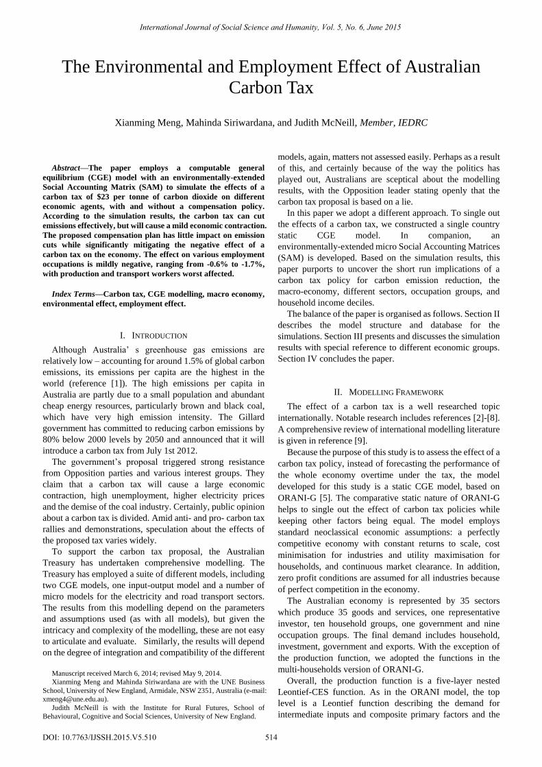
The employment by sector shown in Fig. 3 reveals a

different aspect of carbon tax impact. For some sectors, the

changes in employment are very large. It decreases by 53%

for the brown coal industry, increases by around 64% in the

renewable electricity industry and 23% in the gas electricity

sector. These changes are several times higher than the

corresponding changes in sectoral real output. The large

change in employment may be explained as follows. As the

real wage is rigid in the short run, firms will not incur too

much cost by employing more staff during an expansion and

have to lay off more workers in order to reduce production

costs during a contraction.

Since the large decrease in employment in the brown coal

sector will be largely cancelled out by the large employment

increase in the gas electricity and renewable electricity

sectors, the overall unemployment effect will not be large.

However, this is based on the assumption that workers can

move freely between sectors and between different regions.

In reality, workers may have difficulty doing so. In this case,

there would be large structural unemployment when the

economy is shifting from high carbon to low carbon

production. To reduce structural unemployment, government

assistance is much needed.

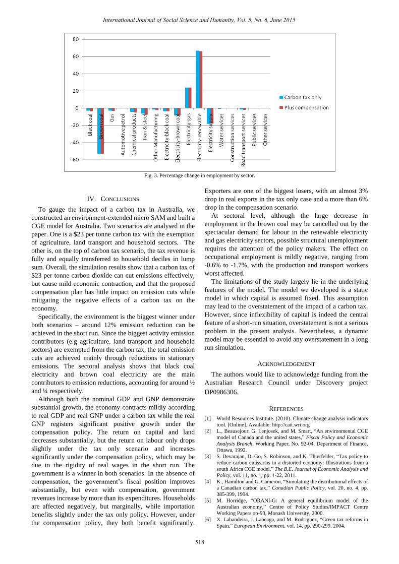
Fig. 3. Percentage change in employment by sector.

IV. CONCLUSIONS

To gauge the impact of a carbon tax in Australia, we

constructed an environment-extended micro SAM and built a

CGE model for Australia. Two scenarios are analysed in the

paper. One is a $23 per tonne carbon tax with the exemption

of agriculture, land transport and household sectors. The

other is, on the top of carbon tax scenario, the tax revenue is

fully and equally transferred to household deciles in lump

sum. Overall, the simulation results show that a carbon tax of

$23 per tonne carbon dioxide can cut emissions effectively,

but cause mild economic contraction, and that the proposed

compensation plan has little impact on emission cuts while

mitigating the negative effects of a carbon tax on the

economy.

Specifically, the environment is the biggest winner under

both scenarios – around 12% emission reduction can be

achieved in the short run. Since the biggest activity emission

contributors (e.g agriculture, land transport and household

sectors) are exempted from the carbon tax, the total emission

cuts are achieved mainly through reductions in stationary

emissions. The sectoral analysis shows that black coal

electricity and brown coal electricity are the main

contributors to emission reductions, accounting for around ½

and ¼ respectively.

Although both the nominal GDP and GNP demonstrate

substantial growth, the economy contracts mildly according

to real GDP and real GNP under a carbon tax while the real

GNP registers significant positive growth under the

compensation policy. The return on capital and land

decreases substantially, but the return on labour only drops

slightly under the tax only scenario and increases

significantly under the compensation policy, which may be

due to the rigidity of real wages in the short run. The

government is a winner in both scenarios. In the absence of

compensation, the government’s fiscal position improves

substantially, but even with compensation, government

revenues increase by more than its expenditures. Households

are affected negatively, but marginally, while importation

benefits slightly under the tax only policy. However, under

the compensation policy, they both benefit significantly.

Exporters are one of the biggest losers, with an almost 3%

drop in real exports in the tax only case and a more than 6%

drop in the compensation scenario.

At sectoral level, although the large decrease in

employment in the brown coal may be cancelled out by the

spectacular demand for labour in the renewable electricity

and gas electricity sectors, possible structural unemployment

requires the attention of the policy makers. The effect on

occupational employment is mildly negative, ranging from

-0.6% to -1.7%, with the production and transport workers

worst affected.

REFERENCES

[1] World Resources Institute. (2010). Climate change analysis indicators

tool. [Online]. Available: http://cait.wri.org

[2] L., Beausejour, G. Lenjosek, and M. Smart, “An environmental CGE

model of Canada and the united states,” Fiscal Policy and Economic

Analysis Branch, Working Paper, No. 92-04, Department of Finance,

Ottawa, 1992.

[3] S. Devarajan, D. Go, S. Robinson, and K. Thierfelder, “Tax policy to

reduce carbon emissions in a distorted economy: Illustrations from a

south Africa CGE model,” The B.E. Journal of Economic Analysis and

Policy, vol. 11, no. 1, pp. 1-22, 2011.

[4] K., Hamilton and G. Cameron, “Simulating the distributional effects of

a Canadian carbon tax,” Canadian Public Policy, vol. 20, no. 4, pp.

385-399, 1994.

518

International Journal of Social Science and Humanity, Vol. 5, No. 6, June 2015

The limitations of the study largely lie in the underlying

features of the model. The model we developed is a static

model in which capital is assumed fixed. This assumption

may lead to the overstatement of the impact of a carbon tax.

However, since inflexibility of capital is indeed the central

feature of a short-run situation, overstatement is not a serious

problem in the present analysis. Nevertheless, a dynamic

model may be essential to avoid any overstatement in a long

run simulation.

ACKNOWLEDGEMENT

The authors would like to acknowledge funding from the

Australian Research Council under Discovery project

DP0986306.

[5] M. Horridge, “ORANI-G: A general equilibrium model of the

Australian economy,” Centre of Policy Studies/IMPACT Centre

Working Papers op-93, Monash University, 2000.

[6] X. Labandeira, J. Labeaga, and M. Rodriguez, “Green tax reforms in

Spain,” European Environment, vol. 14, pp. 290-299, 2004.

Xianming Meng was born in China. He obtained his

BS in China, master and PhD degrees in economics in

Australia. He holds a research fellow position at the

institute for rural futures and a lectureship at the UNE

Business School, University of New England,

Armidale, NSW 2351, Australia. His research

interests include: environmental and resources

modelling, tourism modelling, computable general

equilibrium (CGE) modelling, time-series and panel

data analysis, economic growth and fluctuation, financial economics. In

recent years, he has published a number of papers in high quality academic

journals such as tourism management, tourism analysis, journal of

environmental and resource economics, natural resources research, and asia

pacific journal of economics and business. He currently works on a large

environmental project - Australian research council (ARC) linkage project:

“Adaptation to Carbon-tax-induced Changes in Energy Demand in Rural and

Regional Australia”.

Mahinda Siriwardana is a professor of economics

at UNE Business School, University of New

England, Armidale. He received his PhD from La

Trobe University in Melbourne. His main

research interests include CGE modelling, trade

policy analysis, and carbon price modelling. He has

published seven books, and numerous journal

articles in these fields. He is also a

recipient of several Australian research council

(ARC) grants.

Judith McNeill is a senior research fellow in the

institute for rural futures, school of Behavioural,

cognitive and social sciences, at the University of

New England. She is an economist with twenty years

university teaching and research experience, and was

formerly in the Australian public service in Canberra

and Darwin.

519

International Journal of Social Science and Humanity, Vol. 5, No. 6, June 2015

[7] The Treasury, Strong Growth, Low Pollution - Modelling a Carbon

Price, Commonwealth of Australia, Canberra, 2011.

[8] W. Wissema and R. Dellink, “AGE analysis of the impact of a carbon

energy tax on the Irish economy,” Ecological Economics, vol. 61, pp.

671-683, 2007.

[9] M. Siriwardana, S. Meng, and J. Mcneill, “The impact of a carbon tax

on the Australian economy: results from a CGE model,” Working

papers No. 2011-2, UNE Business School, University of New England,

2011.

[10] ABS (Australian Bureau of Statistics), Australian National Accounts:

input-output tables, 2004-2005. Catalogue No. 5209.0.55.001, ABS,

Canberra, 2008.

[11] ABS (Australian Bureau of Statistics), Household Expenditure Survey,

Catalogue No. 6530.0, Australian Bureau of Statistics, 2008.

[12] A. Cornwell and J. Creedy, “Measuring the welfare effects of tax

changes using the LES: An application to a carbon tax,” Empirical

Economics, vol. 22, pp. 589-613, 1997.