The Envelope Theorem, Euler and Bellman Equations, without Differentiability ∗ Ramon Marimon † Jan Werner ‡ April, 2017 Abstract We extend the envelope theorem, the Euler equation, and the Bellman equation to dy- namic constrained optimization problems where binding constraints can give rise to non- differentiable value functions and multiplicity of Lagrange multipliers. The envelope theo- rem – an extension of Milgrom and Segal’s (2002) theorem – establishes a relation between the Euler and the Bellman equation. We show that solutions and multipliers of the Bellman equation may fail to satisfy the respective Euler equations, in contrast with solutions and multipliers of the infinite-horizon problem. In standard dynamic optimisation problems the failure of Euler equations results in inconsistent multipliers, but not in non-optimal outcomes. However, in problems with forward-looking constraints this failure can result in inconsistent promises and non-optimal outcomes. We also show how the inconsistency problem can be resolved by an envelope selection condition and a minimal extension of the co-state. We extend the theory of recursive contracts of Marcet and Marimon (1998, 2017) to the case where the value function is non-differentiable, resolving a problem pointed out in Messner and Pavoni (2004). * This is a substantially revised version of previous drafts. We thank the participants in seminars and conferences where our work has been presented and, in particular Davide Debortoli and Daisuke Oyama, for their comments. † European University Institute, UPF-Barcelona GSE, CEPR and NBER ‡ University of Minnesota 1

Welcome message from author
This document is posted to help you gain knowledge. Please leave a comment to let me know what you think about it! Share it to your friends and learn new things together.
Transcript

The Envelope Theorem, Euler and Bellman Equations,
without Differentiability∗
Ramon Marimon† Jan Werner‡
April, 2017
Abstract
We extend the envelope theorem, the Euler equation, and the Bellman equation tody-
namic constrained optimization problems where binding constraints can give rise to non-
differentiable value functions and multiplicity of Lagrange multipliers. The envelope theo-
rem – an extension of Milgrom and Segal’s (2002) theorem – establishes arelation between
the Euler and the Bellman equation. We show that solutions and multipliers of the Bellman
equation may fail to satisfy the respective Euler equations, in contrast with solutions and
multipliers of the infinite-horizon problem. In standard dynamic optimisation problems the
failure of Euler equations results ininconsistent multipliers, but not in non-optimal outcomes.
However, in problems withforward-lookingconstraints this failure can result in inconsistent
promises and non-optimal outcomes. We also show how the inconsistency problem can be
resolved by an envelope selection condition and a minimal extension of the co-state. We
extend the theory of recursive contracts of Marcet and Marimon (1998, 2017) to the case
where the value function is non-differentiable, resolving a problem pointed out in Messner
and Pavoni (2004).
∗This is a substantially revised version of previous drafts.We thank the participants in seminars and conferenceswhere our work has been presented and, in particular Davide Debortoli and Daisuke Oyama, for their comments.
†European University Institute, UPF-Barcelona GSE, CEPR and NBER‡University of Minnesota
1

Keywords: limited enforcement, dynamic programming, Envelope Theorem, Euler equation,
Bellman equation, sub-differential calculus.
JEL Classification: C02, C61, D90, E00.
2

1 Introduction
The Euler equation and the Bellman equation are the two basic tools used to analyse dynamic
optimisation problems. Euler equations are the first-orderinter-temporalnecessary conditionsfor
optimal solutions and, under standard concavity-convexity assumptions, they are alsosufficient
conditions, provided that a transversality condition holds. Euler equations are usually second-
order difference equations. The Bellman equation allows thetransformation of an infinite-horizon
optimisation problem into a recursive problem, resulting in time-independent policy functions
determining the actions as functions of the states. The envelope theorem provides the bridge
between the Bellman equation and the Euler equations, confirming the necessity of the latter
for the former. The envelope theorem allows us to reduce the second-order difference equation
system of Euler equations to a first-order system, fully determined by the policy function of
the Bellman equation with corresponding initial conditions, provided that the value function is
differentiable.
Differentiability makes the bridge between the Bellman equation and the Euler equation tight.
If the value function is differentiable, the state providesunivocal information about the derivative
and, therefore, the inter-temporal change of values acrossstates (Bellman) is uniquely associated
with the change of marginal values (Euler) via the envelope theorem – as a result, the enve-
lope theorem allows for the passage of properties between the Euler and the Bellman equations.
That is, the necessity and sufficiency properties of the Euler equations on the one hand, and the
properties of Bellman policy functions on the other. However, the value function may not be
differentiable when constraints are binding and, in this case, knowing the state and its value does
not provide univocal information about the derivative. Sub-differential calculus (e.g. Rockafellar
(1970, 1981)) comes into play, but needs to be properly developed in order to characterise the
envelope bridge between the Euler and Bellman equations, without differentiability. This is the
objective of this paper.
Recursive methods have been widely applied in macroeconomics over the last 30 years since
the publication of Stokey et al. (1989), using the standard framework where assumptions, such
as interiority of optimal paths, imply the differentiability of the value function. However, the
differentiability issue cannot be ignored in a wide range ofcurrent applications. Models where
households, firms, or countries, may face binding constraints in equilibrium are, nowadays, more
3

the norm than the exception. Furthermore, contractual models often haveforward-looking con-
straints(i.e. involving future equilibrium outcomes). It is well known that optimization problems
with forward-looking constraints may have time-inconsistent solutions. That is, re-optimising in
an infinite-horizon problem at datet with initial value given asx∗t – wherex∗
t is the date-t state
of the optimal path from date0 – may lead to a solution which is not part of an optimal solu-
tion from date0. Standard dynamic programming fails, but as Marcet and Marimon (2017) have
shown, thesaddle-point Bellman equationwith an extended co-state can be used to recover re-
cursive structure of the problem. Nevertheless, the differentiability problem caused by binding
constraints remains and, as we show, it is more perverse whenconstraints areforward-looking.
Therefore, we focus our analysis on differentiability problems arising from binding constraints.
Our analysis covers the trilogy already mentioned. First, we study the envelope theorem for
static constrained optimisation problems without assuming differentiability of the value function
or interiority of the solutions. We extend the envelope theorem for directional derivatives of
Milgrom and Segal (2002, Corollary 5)1 by relaxing some of their assumptions, and provide
characterizations of the superdifferential of a concave value function and the subdifferential of
a convex value function. From the envelope theorem, we derive several sufficient conditions
for differentiability of the value function. For example, if there is a unique saddle-point, the
value function is differentiable and the standard form of the envelope theorem holds. A sufficient
condition for differentiability of concave value functionis that the saddle-point multiplier be
unique. For convex value function, a sufficient condition for differentiability is that the solution
be unique. We provide examples of applications of our results to static optimization problems.
This first part is covered in Sections 2 and 3.
Second, we turn tothe Euler equationsof the dynamic optimisation problem. Unless the so-
lution is interior, marginal values of the constraints (i.e. the Lagrange multipliers) are part of the
Euler equations. Applying the envelope theorem of Section 3, we show how the Euler equations
can be derived from the Bellman equation without assuming differentiability of the value func-
tion. If there are multiple multipliers of the Bellman equation, then some sequences of multipliers
may fail to satisfy the Euler equations and not be saddle-point multipliers of the infinite-horizon
1Earlier contributions include Dubeau and Govin (1982), Rockafellar (1984), Bonnisseau and Le Van (1996),
and references listed in Milgrom and Segal (2002). An extension to non-smooth optimisation problems has recently
been provided in Morand, Reffett and Tarafdar (2015).
4

problem. In particular, restarting the Bellman equation at apoint of non-differentiability of the
value function may result intime-inconsistent multipliers, which do not satisfy the Euler equa-
tions. We introduce an envelope selection condition that guarantees that multipliers generated
from the Bellman equation satisfy the Euler equations. The envelope selection is a consistency
condition on multipliers and does not affect solutions in standard dynamic optimization prob-
lems without forward-looking constraints. The recursive method of solving dynamic program-
ming problems can be extended to provide solutions with consistent multipliers by expanding
the co-state to include a subgradient of the value function.If the value function is differentiable,
this co-state is redundant, since the subgradient is unique. Extending the well-known result of
Benveniste and Scheinkman (1979), we show that the concave value function is differentiable if
the multiplier of the Bellman equation is unique.2 Section 4 contains this analysis for standard
dynamic optimization problems, and an example.
Third, in Section 5, we further develop Marcet and Marimon’s(1998, 2017)saddle-point
methodof solving dynamic optimisation problems with forward-looking constraints. The prob-
lem of inconsistent multipliers in the absence of forward-looking constraints becomes incon-
sistency of solutions and multipliers in the presence of such constraints. We show that the en-
velope selection condition guarantees that solutions and multipliers generated from the saddle-
point Bellman equation satisfy the Euler equations without assuming that the value function is
differentiable. Furthermore, we show that the envelope selection condition is equivalent to the
intertemporal consistency conditionintroduced by Marcet and Marimon, motivated by an ex-
ample of Messner and Pavoni (2004) showing that the saddle-point Bellman equation with a
non-differentiable value function can generate non-optimal outcomes in recursive contracts. Im-
posing the envelope selection condition in this example (see Example 4 in Section 5) results in a
recursive optimal solution satisfying the Euler equations.
Although the Euler equation is part of the standard ‘toolkit’ of dynamic optimization prob-
lems (e.g. Stokey et al. (1989)), we are not aware of any discussion of the consistency problem
presented in this paper. This is possibly due to the fact thatmost of the analyses, and compu-
tations, using Euler equations implicitly assume that the value function is differentiable.3 This
2Rincon-Zapatero and Santos (2009) study differentiability of concave value function in dynamic optimization
problems assuming that a constrained qualification condition holds.3Cole and Kubler (2012) identify the consistency problem of the saddle-point method with forward-looking
5
paper provides the the necessary ingredients for extendingthe existing computational methods
for solving this broader class of models. Section 6 providesfurther discussion and conclusions.
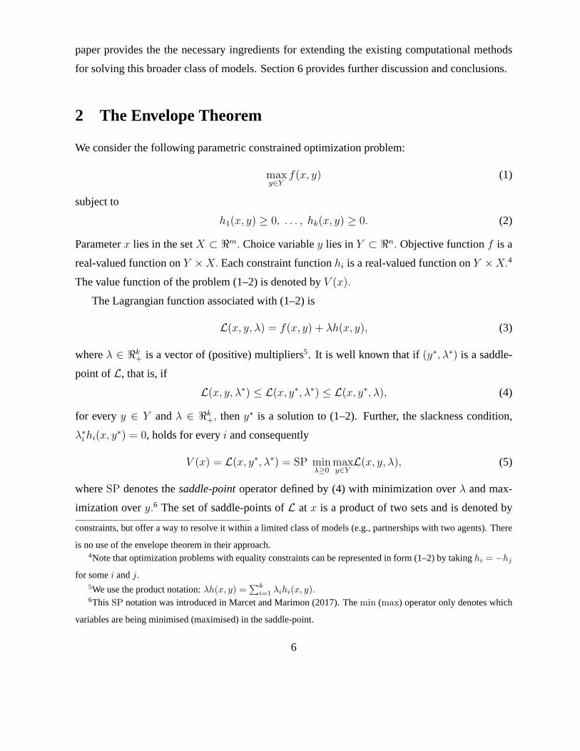
2 The Envelope Theorem
We consider the following parametric constrained optimization problem:
maxy∈Y
f(x, y) (1)
subject to
h1(x, y) ≥ 0, . . . , hk(x, y) ≥ 0. (2)
Parameterx lies in the setX ⊂ ℜm. Choice variabley lies inY ⊂ ℜn. Objective functionf is a
real-valued function onY ×X. Each constraint functionhi is a real-valued function onY ×X.4
The value function of the problem (1–2) is denoted byV (x).
The Lagrangian function associated with (1–2) is
L(x, y, λ) = f(x, y) + λh(x, y), (3)
whereλ ∈ ℜk+ is a vector of (positive) multipliers5. It is well known that if(y∗, λ∗) is a saddle-
point ofL, that is, if
L(x, y, λ∗) ≤ L(x, y∗, λ∗) ≤ L(x, y∗, λ), (4)
for everyy ∈ Y andλ ∈ ℜk+, theny∗ is a solution to (1–2). Further, the slackness condition,
λ∗i hi(x, y∗) = 0, holds for everyi and consequently
V (x) = L(x, y∗, λ∗) = SP minλ≥0
maxy∈Y
L(x, y, λ), (5)
whereSP denotes thesaddle-pointoperator defined by (4) with minimization overλ and max-
imization overy.6 The set of saddle-points ofL at x is a product of two sets and is denoted by
constraints, but offer a way to resolve it within a limited class of models (e.g., partnerships with two agents). There
is no use of the envelope theorem in their approach.4Note that optimization problems with equality constraintscan be represented in form (1–2) by takinghi = −hj
for somei andj.5We use the product notation:λh(x, y) =
∑k
i=1λihi(x, y).
6ThisSP notation was introduced in Marcet and Marimon (2017). Themin (max) operator only denotes which
variables are being minimised (maximised) in the saddle-point.
6
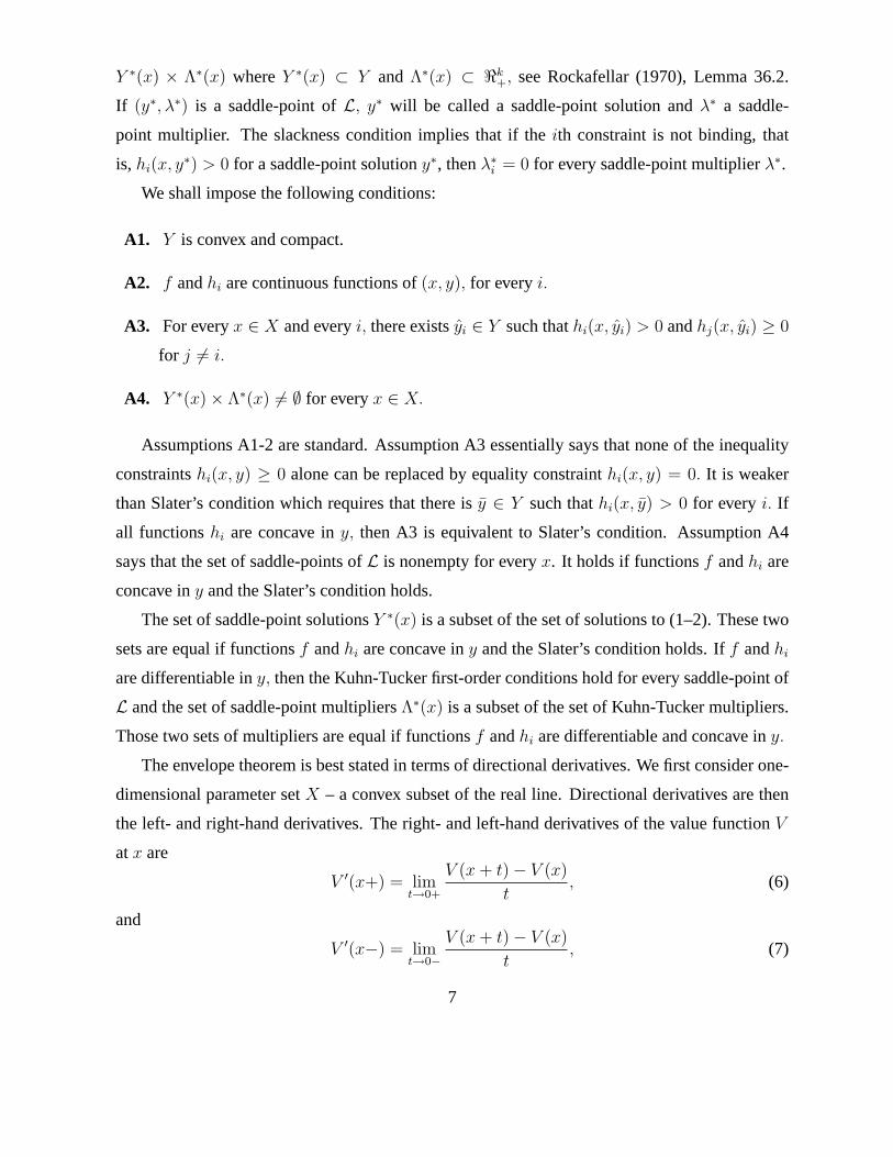
Y ∗(x) × Λ∗(x) whereY ∗(x) ⊂ Y and Λ∗(x) ⊂ ℜk+, see Rockafellar (1970), Lemma 36.2.
If (y∗, λ∗) is a saddle-point ofL, y∗ will be called a saddle-point solution andλ∗ a saddle-
point multiplier. The slackness condition implies that if the ith constraint is not binding, that
is, hi(x, y∗) > 0 for a saddle-point solutiony∗, thenλ∗i = 0 for every saddle-point multiplierλ∗.
We shall impose the following conditions:
A1. Y is convex and compact.
A2. f andhi are continuous functions of(x, y), for everyi.
A3. For everyx ∈ X and everyi, there existsyi ∈ Y such thathi(x, yi) > 0 andhj(x, yi) ≥ 0
for j 6= i.
A4. Y ∗(x) × Λ∗(x) 6= ∅ for everyx ∈ X.
Assumptions A1-2 are standard. Assumption A3 essentially says that none of the inequality
constraintshi(x, y) ≥ 0 alone can be replaced by equality constrainthi(x, y) = 0. It is weaker
than Slater’s condition which requires that there isy ∈ Y such thathi(x, y) > 0 for everyi. If
all functionshi are concave iny, then A3 is equivalent to Slater’s condition. Assumption A4
says that the set of saddle-points ofL is nonempty for everyx. It holds if functionsf andhi are
concave iny and the Slater’s condition holds.
The set of saddle-point solutionsY ∗(x) is a subset of the set of solutions to (1–2). These two
sets are equal if functionsf andhi are concave iny and the Slater’s condition holds. Iff andhi
are differentiable iny, then the Kuhn-Tucker first-order conditions hold for every saddle-point of
L and the set of saddle-point multipliersΛ∗(x) is a subset of the set of Kuhn-Tucker multipliers.
Those two sets of multipliers are equal if functionsf andhi are differentiable and concave iny.
The envelope theorem is best stated in terms of directional derivatives. We first consider one-
dimensional parameter setX – a convex subset of the real line. Directional derivatives are then
the left- and right-hand derivatives. The right- and left-hand derivatives of the value functionV
atx are
V ′(x+) = limt→0+
V (x + t) − V (x)
t, (6)
and
V ′(x−) = limt→0−
V (x + t) − V (x)
t, (7)
7
if the limits exist.
We have the following result:
Theorem 1: Suppose thatX ⊂ ℜ, conditions A1-A4 hold, and partial derivatives∂f
∂xand∂hi
∂xare
continuous functions of(x, y). Then the value functionV is right- and left-hand differen-
tiable at everyx ∈ intX and the directional derivatives are
V ′(x+) = maxy∗∈Y ∗(x)
minλ∗∈Λ∗(x)
[∂f
∂x(x, y∗) + λ∗∂h
∂x(x, y∗)
](8)
and
V ′(x−) = miny∗∈Y ∗(x)
maxλ∗∈Λ∗(x)
[∂f
∂x(x, y∗) + λ∗∂h
∂x(x, y∗)
], (9)
where the order of maximum and minimum does not matter.
Theorem 1 is an extension of Corollary 5 in Milgrom and Segal (2002). It is worth pointing
out that differentiability of functionsf andhi with respect to the variabley is not assumed in
Theorem 1.7 This will be important in applications to dynamic programming in Sections 4 and 5.
For a multi-dimensional parameter setX in ℜm, the directional derivative of the value func-
tion V atx ∈ X in the directionx ∈ ℜm such thatx + x ∈ X is defined as
V ′(x; x) = limt→0+
V (x + tx) − V (x)
t.
If partial derivatives ofV exist, then the directional derivativeV ′(x; x) is equal to the scalar
productDV (x)x, whereDV (x) is the vector of partial derivatives, i.e. the gradient vector.
Theorem 1 can be applied to the single-variable value function V (t) ≡ V (x + tx) for which
it holdsV ′(0+) = V ′(x; x). If Dxf(x, y) andDxhi(x, y) are continuous functions of(x, y), then
it follows that the directional derivative ofV is
V ′(x; x) = maxy∗∈Y ∗(x)
minλ∗∈Λ∗(x)
[Dxf(x, y∗) + λ∗Dxh(x, y∗)
]x, (10)
and the order of maximum and minimum does not matter.7Dubeau and Govin (1982) and Rockafellar (1984) assume differentiability of functionsf andhi and use Kuhn-
Tucker multipliers instead of saddle-point multipliers. Most of their results provide bounds on directional derivatives
of V.
8

3 Differentiability and Subdifferentials of the Value Function
3.1 Differentiability
The value functionV on X ⊂ ℜ is differentiable atx if the one-sided derivatives are equal to
each other. Sufficient conditions for differentiability can be obtained from Theorem 1.
Corollary 1: Under the assumptions of Theorem 1, each of the following conditions is sufficient
for differentiability of value functionV atx ∈ intX:
(i) there is a unique saddle-point,
(ii) there is a unique saddle-point solution andhi does not depend onx for everyi.
(iii) there is a saddle-point solution with non-binding constraints, and∂f
∂xdoes not depend
ony.8
(iv) there is a unique saddle-point multiplier and∂f
∂xand∂hi
∂xdo not depend ony, for every
i.
Condition (i) holds if there is a unique saddle-point solution with non-binding constraints so
that zero is the unique saddle-point multiplier. The condition of ∂f
∂xor ∂hi
∂xnot depending ony
in part (iv) is essentially the additive separability off andhi in x andy. Under the separability
condition, uniqueness of multiplier is necessary and sufficient for differentiability of the value
function. A result related to Corollary 1 (iii) can be found inKim (1993).
A sufficient condition for uniqueness of saddle-point solution to (1–2) is thatf be strictly
concave andhi be concave iny. A sufficient condition for uniqueness of saddle-point multiplier
is the following standard Constrained Qualification condition which implies uniqueness of the
Kuhn-Tucker multiplier:
CQ (1) f andhi are continuously differentiable functions ofy,
(2) vectorsDyhi(x, y∗) for i ∈ I(x, y∗) are linearly independent, where
I(x, y∗) = {i : hi(x, y∗) = 0} is the set of binding constraints.
8It is sufficient that the constraints withhi depending onx are non-binding. Other constraints may bind.
9

A weaker form of Constrained Qualification which is necessaryand sufficient for uniqueness
of Kuhn-Tucker multiplier can be found in Kyparisis (1985).Note thatCQ holds vacuously for
solutiony∗ with non-binding constraints.
Under condition (i) or (iv) of Corollary 1, the derivative of the value function is
V ′(x) =∂f
∂x(x, y∗) + λ∗∂h
∂x(x, y∗). (11)
Under condition (ii) or (iii), it holds
V ′(x) =∂f
∂x(x, y∗). (12)
For the multi-dimensional parameter setX in ℜm, the value function is differentiable if
V ′(x; x) = −V ′(x;−x) for every x ∈ ℜm. This holds under any of the sufficient conditions
of Corollary 1 withDxf andDxhi substituted for partial derivatives in (iv) and (v). IfV is differ-
entiable, then the gradientDV (x) is well defined, and the multi-dimensional counterpart of (11)
is
DV (x) = Dxf(x, y∗) + λ∗Dxh(x, y∗). (13)
Results of this section and Section 2 can be extended to minimization problems and saddle-
point problems. We present an extension to saddle-point problems in Appendix A.
3.2 Concave and Convex Value Functions
If the value function is concave or convex, the envelope theorem can be stated using the superdif-
ferential or the subdifferential, respectively, for a multi-dimensional parameter set. We consider
the concave case first.
Sufficient conditions forV to be concave are stated in the following well-known result,the
proof of which is omitted.
Proposition 1. If the objective functionf and all constraint functionshi are concave functions
of (x, y) onY × X, then the value functionV is concave.
The superdifferential∂V (x) of the concave value functionV is the set of all vectorsφ ∈ ℜm
such that
V (x′) + φ(x − x′) ≤ V (x) for everyx′ ∈ X.
We have the following:
10

Theorem 2: Suppose that conditions A1-A4 hold, derivativesDxf and Dxhi are continuous
functions of(x, y) for everyi, andV is concave. Then
∂V (x) =⋂
y∗∈Y ∗(x)
⋃
λ∗∈Λ∗(x)
{Dxf(x, y∗) + λ∗Dxh(x, y∗)} (14)
for everyx ∈ intX.
Sufficient conditions for differentiability of concave value function follow from Theorem 2.
Corollary 2: Under the assumptions of Theorem 2, the following hold forx ∈ intX:
(i) If the saddle-point multiplier is unique, then value function V is differentiable atx
and (13) holds for everyy∗ ∈ Y ∗(x).
(ii) If hi does not depend onx for everyi, then value functionV is differentiable atx and
(13) holds for everyy∗ ∈ Y ∗(x).
In Corollary 2 (i), it is sufficient that the multiplier is unique for the constraints withhi
depending onx. Corollary 2 (i) implies that the value function is differentiable if there is a
solution with non-binding constraints - those that depend on x - for then the unique saddle-point
multiplier is zero. A saddle-point multiplier may be uniqueeven if some constraints are binding.
Examples are given in Section 3.3. Corollary 2 (ii) extends Corollary 3 in Milgrom and Segal
(2002) to parametrized constraints.
We now provide a similar characterization for convex value functions. Sufficient conditions
for V to be convex are stated without proof in the following:
Proposition 2. If the objective functionf(y, ·) is convex inx for everyy ∈ Y and all constraint
functionshi are independent ofx, then the value functionV is convex.
If V is convex, then the subdifferential∂V (x) is the set of all vectorsφ ∈ ℜm such that9
V (x′) + φ(x − x′) ≥ V (x) for every x′ ∈ X.
We have the following:
9We use the same notation for the superdifferential and the subdifferential as is customary in the literature.
11
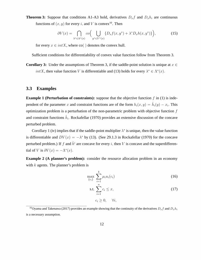
Theorem 3: Suppose that conditions A1-A3 hold, derivativesDxf and Dxhi are continuous
functions of(x, y) for everyi, andV is convex10. Then
∂V (x) =⋂
λ∗∈Λ∗(x)
co( ⋃
y∗∈Y ∗(x)
{Dxf(x, y∗) + λ∗Dxh(x, y∗)}), (15)
for everyx ∈ intX, where co( ) denotes the convex hull.
Sufficient conditions for differentiability of convex value function follow from Theorem 3.
Corollary 3: Under the assumptions of Theorem 3, if the saddle-point solution is unique atx ∈
intX, then value functionV is differentiable and (13) holds for everyλ∗ ∈ Λ∗(x).
3.3 Examples
Example 1 (Perturbation of constraints): suppose that the objective functionf in (1) is inde-
pendent of the parameterx and constraint functions are of the formhi(x, y) = hi(y) − xi. This
optimization problem is a perturbation of the non-parametric problem with objective functionf
and constraint functionshi. Rockafellar (1970) provides an extensive discussion of the concave
perturbed problem.
Corollary 1 (iv) implies that if the saddle-point multiplierλ∗ is unique, then the value function
is differentiable andDV (x) = −λ∗ by (13). (See 29.1.3 in Rockafellar (1970) for the concave
perturbed problem.) Iff andhi are concave for everyi, thenV is concave and the superdifferen-
tial of V is ∂V (x) = −Λ∗(x).
Example 2 (A planner’s problem): consider the resource allocation problem in an economy
with k agents. The planner’s problem is
max{ci}
k∑
i=1
µiui(ci) (16)
s.t.n∑
i=1
ci ≤ x, (17)
ci ≥ 0, ∀i,
10Oyama and Takenawa (2017) provides an example showing that the continuity of the derivativesDxf andDxhi
is a necessary assumption.
12

whereµ = (µ1, . . . , µk) ∈ ℜk++ is a vector of welfare weights andx ∈ ℜL
+ represents total
resources. Utility functionsui are continuous and increasing. LetV (x, µ) be the value of (16)
as function of weightsµ and total resourcesx. It follows from Corollary 1 (iv) thatV is differ-
entiable inx if the saddle-point multiplier of constraint (17) is unique. If utility functions ui are
differentiable, then the CQ condition holds, implying that the multiplier is unique. The derivative
is DxV = λ∗, whereλ∗ is the multiplier of the constraint (17).V is a convex function ofµ. The
subdifferential∂µV is (by Theorem 3) the convex hull of the set of vectors(u1(c∗1), . . . , uk(c
∗k))
over all saddle-point solutionsc∗ to (16). V is differentiable inµ if the saddle-point solution is
unique.
Consider an example withL = 1, k = 2, and ui(c) = c. Let the welfare weights be
parametrized by a single parameterµ so thatµ1 = µ andµ2 = 1 − µ with 0 < µ < 1. The
value function isV (x, µ) = max{µ, 1−µ}x. It is differentiable with respect toµ at everyµ 6= 12
and everyx. The solutionc∗ is unique for everyµ 6= 12. V is not differentiable with respect toµ
atµ = 12. The left-hand directional derivative atµ = 1
2is −x while the right-hand derivative isx
in accordance with Theorem 1.V is everywhere differentiable with respect tox.
4 Dynamic Optimization and Euler Equations
In this section we extend the standard results of dynamic programming to non-differentiable
value functions. Using the results of Sections 2 and 3, we show how to derive Euler equations
from the Bellman equation without differentiability of the value function. If the value function is
non-differentiable, then there may be sequences of solutions and multipliers generated from the
Bellman equation for which Euler equations do not hold because multipliers are inconsistent. We
develop a recursive method of selecting solutions with consistent multipliers.
We consider the following dynamic constrained maximization problem studied in Stokey et
al. (1989):
max{xt}∞t=1
∞∑
t=0
βtF (xt, xt+1) (18)
s.t. hi(xt, xt+1) ≥ 0, i = 1, ..., k, t ≥ 0,
for givenx0 ∈ X, where{xt}∞t=1 is a bounded sequence (i.e.,{xt} ∈ ℓn
∞) such thatxt ∈ X ⊂ ℜn
13

for everyt. FunctionsF andhi are real-valued functions onX × X. We impose the following
conditions:
D1. X is convex.
D2. There exists{xt} ∈ ℓn∞ such thathi(xt, xt+1) > 0 for everyt ≥ 0 and everyi.
D3. F andhi are bounded, andβ ∈ (0, 1).
D4. F andhi are concave functions of(x, y) onX × X,
D5. F andhi are increasing and differentiable onX.
The saddle-point problem associated with (18) is
SP max{xt}∞t=1
min{λt}
∞
t=1,λt≥0
∞∑
t=0
βt[F (xt, xt+1) + λt+1h(xt, xt+1)
], (19)
for given x0 ∈ X, whereλt ∈ ℜk are Lagrange multipliers and{xt} ∈ ℓn∞. It follows from
Dechert (1992) that if a sequence{x∗t} is a solution to (18), then under assumptions D1-D4 there
exists a summable sequence of multipliers{λ∗t} ∈ ℓk
1 such that{x∗t , λ
∗t} is a saddle-point of (19).
Conversely, if{x∗t , λ
∗t} is a saddle-point of (19), then{x∗
t} is a solution to (18).
By a standard variational argument, the first-ordernecessary conditionsfor saddle-point
{x∗t , λ
∗t}
∞t=1 of (19) are the followingintertemporal Euler equations:
DyF (x∗t , x
∗t+1) + λ∗
t+1Dyh(x∗t , x
∗t+1) + β
[DxF (x∗
t+1, x∗t+2) + λ∗
t+2Dxh(x∗t+1, x
∗t+2)
]= 0 (20)
for everyt ≥ 0. Equations (20) together with complementary slackness conditions and the given
constraints, define a system of second-order difference equations for{x∗t , λ
∗t} with x∗
0 = x0.
Complementary slackness conditions are
λ∗t+1h(x∗
t , x∗t+1) = 0, h(x∗
t , x∗t+1) ≥ 0. (21)
The sufficiency of the Euler equation and a transversality condition, see Stokeyet al. (1989),
continue to hold when a constraint is binding.
14

Proposition 3: Suppose that conditions D1-D5 hold. Let{x∗t , λ
∗t}, with {x∗
t} ∈ ℓn∞, x∗
0 =
x0, λ∗t ≥ 0, and h(x∗
t , x∗t+1) ≥ 0 for everyt, satisfy the Euler equations (20) and the
complementary slackness conditions (21). If the transversality condition
limt→∞
βt[DxF (x∗
t , x∗t+1) + λ∗
t+1Dxh(x∗t , x
∗t+1)
]= 0, (22)
holds, then{x∗t , λ
∗t} is a saddle-point of (19). In particular,{x∗
t} is a solution to (18).
Proof: see Appendix.
Let V (x0) be the value function of (18). The value function satisfies the Bellman equation
V (x) = maxy
{F (x, y) + βV (y)} (23)
s.t. hi(x, y) ≥ 0, i = 1, ..., k
The value functionV is concave and bounded under assumptions D1-4. IfDxF andDxhi are
continuous functions of(x, y) for everyi, then by envelope Theorem 2, the superdifferential of
V is
∂V (x) =⋂
y∗∈Y ∗(x)
⋃
λ∗∈Λ∗(x)
{DxF (x, y∗) + λ∗Dxh(x, y∗)} (24)
whereY ∗(x) is the set of saddle-point solutions andΛ∗(x) is the set of saddle-point multipliers
at x. Corollary 2 (i) implies thatV is differentiable if saddle-point multiplierλ∗ is unique. If
there is a solutiony∗ with non-binding constraints, then the unique multiplier is zero andV is
differentiable atx. This is the well-known result of Benveniste and Scheinkman (1979). Note
also that ifV is differentiable aty∗ and the Constraint Qualification condition holds, then the
saddle-point multiplier is unique andV is differentiable atx.
For every solution{x∗t} to (18),x∗
t+1 is a solution to the Bellman equation (23) atx∗t for every
t ≥ 0. The converse holds as well under assumptions D1- D3, see Stokey et al. (1989; Theorem
4.3). The latter result not only shows that it is sufficient tosequentially solve the Bellman equation
(23) to obtain a solution to (18) but also that solutions aretime-consistent. That is, if{x∗t}
∞t=1 is
a solution to (18) atx0 and the Bellman equation is restarted atx∗τ the resulting solution – say,
{x∗t}
τt=1, {xt}
∞t=τ+1 – is also a solution to (18) atx0.
It is well-known that if constraints are not binding and the value function is differentiable,
then the first-order conditions of the Bellman equation together with the envelope theorem imply
15

the Euler equations. Indeed, (24) simplifies then toDV (x) = DxF (x, y∗), the Euler equation
simplifies to
DyF (x∗t , x
∗t+1) + βDxF (x∗
t+1, x∗t+2) = 0,
and the latter obtains from the first-order conditions of (23). In general, it is convenient to intro-
duce thesaddle-point Bellman equationcorresponding to (23):
V (x) = SP minλ≥0
maxy
{F (x, y) + λh(x, y) + βV (y)} . (25)
The set of saddle-points of (25) is the product setY ∗(x) × Λ∗(x). The first-order condition for
saddle-point(y∗, λ∗) of (25) states that there exists a subgradient vectorφ∗ ∈ ∂V (y∗) such that
DyF (x, y∗) + λ∗Dyh(x, y∗) + βφ∗ = 0, (26)
see Rockafellar (1981, Ch.5).
If {x∗t , λ
∗t} is a saddle-point of (19), then(x∗
t+1, λ∗t+1) is a saddle-point of thesaddle-point
Bellman equation(25) atx∗t for every t ≥ 0. The converse implication requires a consistency
condition that involves subgradients{φ∗t} obtained from the first-order conditions for{x∗
t , λ∗t}.
Proposition 4: Suppose that conditions D1-D5 hold andDxF and Dxhi are continuous func-
tions for everyi. Let{x∗t , λ
∗t}
∞t=1, with {x∗
t} ∈ ℓn∞, be a sequence of saddle-points gener-
ated by the saddle-point Bellman equation (25), starting atx∗0 = x0, and let{φ∗
t}∞t=0 be the
corresponding sequence of subgradients satisfying (26), with φ∗t ∈ ∂V (x∗
t ) for all t. If the
following envelope selection condition
φ∗t = DxF (x∗
t , x∗t+1) + λ∗
t+1Dxh(x∗t , x
∗t+1) (27)
holds for everyt ≥ 0, then{x∗t , λ
∗t}
∞t=1 is a saddle-point of (19).
Proof: The first-order condition (26) for(x∗t+1, λ
∗t+1) atx∗
t , for t ≥ 1, is
DyF (x∗t , x
∗t+1) + λ∗
t+1Dyh(x∗t , x
∗t+1) + βφ∗
t+1 = 0. (28)
Eq. (28) together with the envelope selection condition (27) for φ∗t+1 imply that the Euler equation
(20) holds atx∗t . The transversality condition (22) can be written aslimt→∞ βtφ∗
t = 0. Since the
16

sequence{x∗t} is bounded, subgradients{φ∗
t} are bounded, too (see Rockafellar (1970), Theorem
24.7). This implies (22). The conclusion follows now from Proposition 3.2
Theenvelope selection condition(27) guaranteesconsistencyof multipliers generated by the
saddle-point Bellman equation. It can be dispensed with if the saddle-point multiplier is unique
(which is sufficient for value functionV to be differentiable) but not if there are multiple mul-
tipliers. Inconsistency of multipliers occurs if, given(x∗t , λ
∗t ) andφ∗
t ∈ ∂V (x∗t ) satisfying the
first-order condition (28) atx∗t−1, a multiplierλ∗
t+1 is chosen without satisfying the envelope se-
lection condition (27) when solving (28) atx∗t . Then the Euler equation (20) is not satisfied for
λ∗t andλ∗
t+1, and the sequence{x∗t , λ
∗t}
∞t=1 need not be a saddle-point of (19). This may happen if
V is not differentiable atx∗t and the saddle-point Bellman equation (25) is restarted atx∗
t without
recalling the selectionφ∗t ∈ ∂V (x∗
t ) previously made.
Proposition 4 does not provide a recursive method of generating consistent solutions from
the saddle-point Bellman equation, but it clearly suggests what that method should be: extend
the statex with a co-stateφ ∈ ∂V (x), and impose the envelope selection condition. To that
end, we define theselective value functionV s(x; φ) of statex andco-stateφ ∈ ∂V (x) as the
value function of the saddle-point Bellman equation (25) with the additional restriction that the
saddle-point satisfies the envelope selection condition. That is,
V s(x; φ) = SP minλ≥0
maxy
{F (x, y) + λh(x, y) + βV (y)} (29)
s.t. DxF (x, y) + λDxh(x, y) = φ.
Clearly,V s(x; φ) = V (x) but the solutions to (29) are a subset of those to (25). If(y∗, λ∗) is a
saddle-point of (29), then there isφ∗ ∈ ∂V (y∗) satisfying the first-order condition (26), that is,
φ∗ = −β−1 [DyF (x, y∗) + λ∗Dyh(x, y∗)] , (30)
and the recursive equationV s(x; φ) = F (x, y∗) + λ∗h(x, y∗) + βV s(y∗; φ∗) holds.
Using selective value functionV s we definepolicy functionsϕ : X × ℜn −→ X × ℜn and
ℓ : X × ℜn −→ ℜk+ as time-invariant selections from solution to saddle-point Bellman equation
(29) and the first-order condition (30). That is,ϕ(x, φ) = (y∗, λ∗) where(y∗, λ∗) is a saddle-point
of (29), andℓ(x, φ) = φ∗ whereφ∗ ∈ ∂V (y∗) satisfies (30).
Let{x∗t , λ
∗t , φ
∗t}
∞t=1 be a sequence generated by policy functions(ϕ, ℓ) – that is,(x∗
t+1, λ∗t+1) =
ϕ(x∗t , φ
∗t ) andφ∗
t+1 = ℓ(x∗t , φ
∗t ) for every t ≥ 0, with initial statex∗
0 = x0 and co-stateφ∗0 ∈
17

∂V (x0). It follows from Proposition 4 that{x∗t , λ
∗t} is a saddle-point of (19). Sequence{x∗
t , λ∗t , φ
∗t}
can be found by solving a system ofn + n + k first-order difference equations. Those equations
are (27), (28), and the complementary slackness conditions(21). The initial state and co-state are
x0 and an arbitraryφ0 ∈ ∂V (x0). Since the value functionV is concave, it is almost everywhere
differentiable implying that∂V (x0) = DV (x0) for almost everyx0.
Corollary 4 summarizes our results and reestablishes the link between the Bellman equation
and the Euler equations, as in the differentiable case.
Corollary 4: Suppose that conditions D1-D5 hold. If{x∗t , λ
∗t , φ
∗t}
∞t=1, with {x∗
t} ∈ ℓn∞, is a
sequence generated by policy functions(ϕ, ℓ), i.e. (x∗t+1, λ
∗t+1) = ϕ(x∗
t , φ∗t ) and φ∗
t+1 =
ℓ(x∗t , φ
∗t ), with x∗
0 = x0 and φ∗0 ∈ ∂V (x0), then{x∗
t , λ∗t}
∞t=1 is a saddle-point of (19)
at x0. Furthermore, if at dateτ + 1 a new sequence{x∗t , λ
∗t}
∞t=τ+1 is generated using
possibly different policy functions(ϕ, ℓ) starting from initial statex∗τ and co-stateφ∗
τ , then
({x∗t , λ
∗t}
τt=1, {x
∗t , λ
∗t}
∞t=τ+1) is a saddle-point of (19) atx0.
Example 3 illustrates the results of this section.
Example 3 (A dynastic problem): consider a dynasty of overlapping generations who live for
two periods. A household is formed by a young and an old member. In each period, the young
decides for the household consumption for the next period. The allocation problem of the dynasty
is to maximise the discounted utility of all future generations as follows:
max{xt}∞t=1
∞∑
t=0
βt [xt + 2xt+1] (31)
s.t.xt + xt+1 ≤ 4, xt+1 ≤ xt, xt ≥ 0, t ≥ 0,
for given x0 ∈ [0, 4]. Let V (x0) be the value function of (31). It is easy to see that the value
function is
V (x) =
3x(1 − β)−1 if x ≤ 2
8 − x + 3(4 − x)β(1 − β)−1 if x ≥ 2.
(32)
The unique solution to (31) forx0 = 2 is the constant sequencex∗t = 2.
The value functionV is concave. It is not differentiable atx = 2 where the super-differential
is
∂V (2) = [−(3β(1 − β)−1 + 1), 3(1 − β)−1]. (33)
18
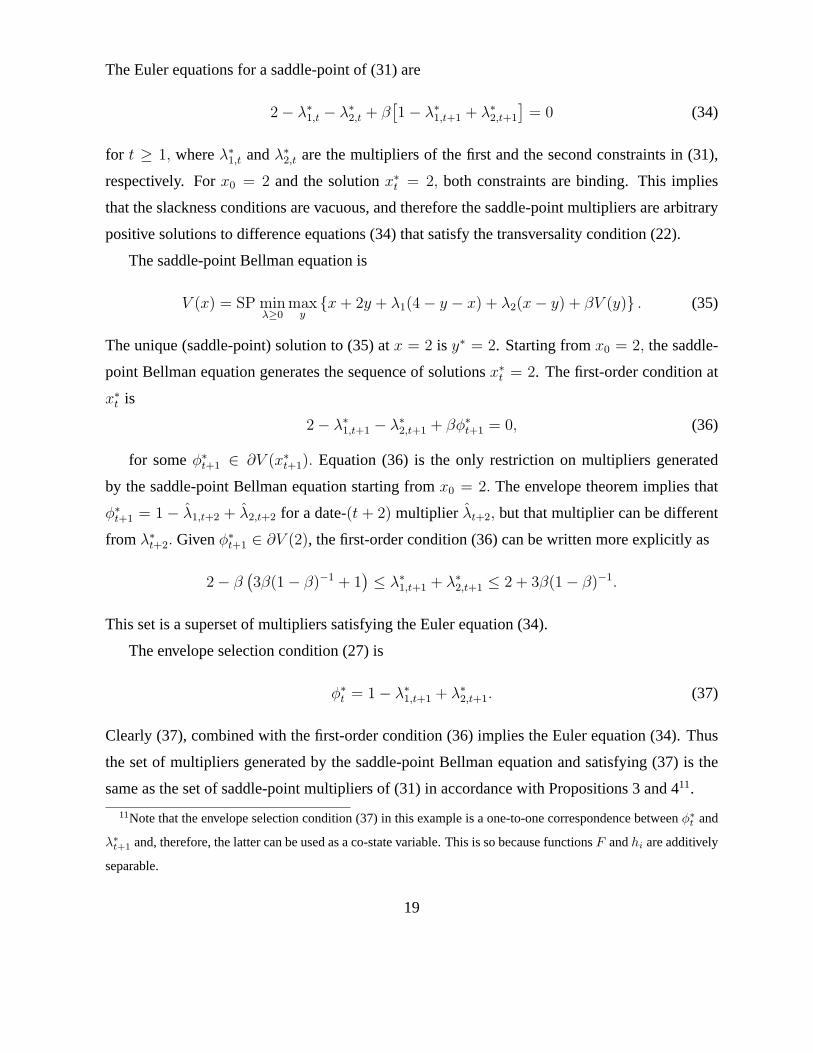
The Euler equations for a saddle-point of (31) are
2 − λ∗1,t − λ∗
2,t + β[1 − λ∗
1,t+1 + λ∗2,t+1
]= 0 (34)
for t ≥ 1, whereλ∗1,t andλ∗
2,t are the multipliers of the first and the second constraints in(31),
respectively. Forx0 = 2 and the solutionx∗t = 2, both constraints are binding. This implies
that the slackness conditions are vacuous, and therefore the saddle-point multipliers are arbitrary
positive solutions to difference equations (34) that satisfy the transversality condition (22).
The saddle-point Bellman equation is
V (x) = SP minλ≥0
maxy
{x + 2y + λ1(4 − y − x) + λ2(x − y) + βV (y)} . (35)
The unique (saddle-point) solution to (35) atx = 2 is y∗ = 2. Starting fromx0 = 2, the saddle-
point Bellman equation generates the sequence of solutionsx∗t = 2. The first-order condition at
x∗t is
2 − λ∗1,t+1 − λ∗
2,t+1 + βφ∗t+1 = 0, (36)
for someφ∗t+1 ∈ ∂V (x∗
t+1). Equation (36) is the only restriction on multipliers generated
by the saddle-point Bellman equation starting fromx0 = 2. The envelope theorem implies that
φ∗t+1 = 1 − λ1,t+2 + λ2,t+2 for a date-(t + 2) multiplier λt+2, but that multiplier can be different
from λ∗t+2. Givenφ∗
t+1 ∈ ∂V (2), the first-order condition (36) can be written more explicitly as
2 − β(3β(1 − β)−1 + 1
)≤ λ∗
1,t+1 + λ∗2,t+1 ≤ 2 + 3β(1 − β)−1.
This set is a superset of multipliers satisfying the Euler equation (34).
The envelope selection condition (27) is
φ∗t = 1 − λ∗
1,t+1 + λ∗2,t+1. (37)
Clearly (37), combined with the first-order condition (36) implies the Euler equation (34). Thus
the set of multipliers generated by the saddle-point Bellmanequation and satisfying (37) is the
same as the set of saddle-point multipliers of (31) in accordance with Propositions 3 and 411.
11Note that the envelope selection condition (37) in this example is a one-to-one correspondence betweenφ∗t and
λ∗t+1 and, therefore, the latter can be used as a co-state variable. This is so because functionsF andhi are additively
separable.
19

In sum, the intertemporal Euler equation (20) is anecessaryfirst-order condition for a solution
to (19) - and therefore to (18) - and by Proposition 3 it is alsosufficient. The same is true
for a sequence of saddle-points of the Bellman equation (23) if the saddle-point multiplier is
unique. If there are multiple multipliers, the system of Euler equations is asufficient but not
necessarycondition for a sequence of saddle-points of the Bellman equation. However, for every
sequence of solutions to a Bellman equation there exists a sequence of multipliers such that Euler
equation is satisfied. Such a sequence can be generated recursively using policy functions from
the selective value function and extending the statex∗t with a co-state subgradientφ∗
t ∈ ∂V (x∗t ).
The problem of time-inconsistency of multipliers discussed in this section can result in non-
optimal outcomes in the presence of forward-looking constraints. We address this problem now.
5 Recursive Contracts
In this section we extend the results of Section 4 to the recursive contracts of Marcet and Ma-
rimon (2017). Recursive contracts are dynamic optimizationproblems withforward-looking
constraints. The presence of forward-looking constraintsmakes the standard methods of dy-
namic programming inapplicable. Marcet and Marimon show that recursive contracts can be
solved by transforming optimization problems with forward-looking constraints into saddle-point
problems. Solutions to a saddle-point Bellman equation are solutions to the original contracting
problem provided that anintertemporal consistency conditionis satisfied. The necessity of this
consistency condition was motivated by an example given by Messner and Pavoni (2004), who
showed that non-unique solutions to the saddle-point Bellman equation can fail to be solutions to
the contracting problem. We show that imposing the envelopeselection condition and extending
the co-state generates time-consistent recursive saddle-point solutions. The envelope selection
condition is shown to be equivalent to Marcet and Marimon’sintertemporal consistency condi-
tion12.12Introduced in Marcet and Marimon (2015).
20

5.1 The partnership problem with limited enforcement
The deterministic partnership problem13 with limited enforcement takes the form
Vµ(y0) = max{ct}∞0
∞∑
t=0
βt
m∑
i=1
µi u(ci,t) (38)
s.t.m∑
i=1
ci,t ≤m∑
i=1
yi,t, (39)
∞∑
n=0
βn u(ci,t+n) ≥ vi(yi,t), (40)
ci,t ≥ 0, for all i, t ≥ 0,
where the sequence{ct} is bounded, i.e.{ct} ∈ ℓm∞. The sequence of incomes{yt} follows a law
of motionyt+1 = g(yt) for someg : ℜm+ → ℜm
+ for given initial income vectory0. We impose
the following conditions:
P1. The functionu : ℜ+ → ℜ+ is increasing, concave, and differentiable and the functions and
vi : ℜ+ → ℜ+, i = 1, ...,m, are increasing, concave and continuous.
P2. Sequence{yt} is bounded,µi > 0 for everyi, andβ ∈ (0, 1).
P3. There exists{ct} ∈ ℓm∞ with ci,t > 0 for everyi andt such that constraints (39) and (40)
hold with strict inequality.
A convenient way of analysing problem (38) is to consider thefollowing constrained saddle-
point problem resulting from adding forward-looking constraints (40) with multipliers to the
objective function (see Marcet and Marimon (2017) for details):
SP max{ct}∞t=0
min{µt}∞t=1
∞∑
t=0
βt
m∑
i=1
[µi,t+1 (u(ci,t) − vi(yi,t)) + µi,tvi(yi,t)] (41)
s.t.m∑
i=1
ci,t ≤m∑
i=1
yi,t
µi,t+1 ≥ µi,t
ci,t ≥ 0, for all i, t,
13Marcet and Marimon develop their theory in a more general dynamic stochastic formulation. The approach
presented in this section can be easily extended to their general setup.
21

whereµ0 = µ, and{ct} ∈ ℓm∞ and{µt} ∈ ℓm
∞. The unconstrained saddle-point problem for the
Lagrangian of (41) is
SP max{ct,λt+1}∞t=0
min{µt,γt}∞t=1
∞∑
t=0
βt
m∑
i=1
{µi,t+1 (u(ci,t) − vi(yi,t)) + µi,tvi(yi,t) (42)
− λi,t+1(µi,t+1 − µi,t) + γt+1 (yi,t − ci,t)}.
If {c∗t} ∈ ℓm∞ is a solution to (38), then there exists a bounded sequence14 of weights{µ∗
t} ∈ ℓm∞
and summable sequences of multipliers{λ∗t} ∈ ℓm
1 and{γ∗t } ∈ ℓ1 (see Dechert (1992)) such that
{c∗t , λ∗t , µ
∗t , γ
∗t } is a saddle-point of (42). Conversely, if{c∗t , λ
∗t , µ
∗t , γ
∗t } is a saddle-point of (42),
then{c∗t} is a solution to (38).
The first-order necessary conditions with respect toµi,t+1 for saddle-point{c∗t , λ∗t , µ
∗t , γ
∗t } of
(42) are
u(c∗i,t) −(vi(yi,t) + λ∗
i,t+1
)+ β
(vi(yi,t+1) + λ∗
i,t+2
)= 0 (43)
for everyi andt ≥ 0. The respective condition with respect toci,t is µ∗i,t+1u
′(c∗i,t) = γ∗t+1. Equa-
tion (43) is the intertemporal Euler equationfor the partnership problem. The Euler equation
together with first-order conditions forci,t, the constraints, and complementary slackness condi-
tions forγ∗t andλ∗
i,t, are a system of first-order difference equations.
As in Section 4 (see Proposition 3), Euler equations and a transversality condition are suffi-
cient conditions for a solution to (42).
Proposition 5: Let {c∗t , λ∗t , µ
∗t , γ
∗t }, with {c∗t}
∞t=0 ∈ ℓm
∞, {µ∗t}
∞t=0 ∈ ℓm
∞, µ∗0 = µ, λ∗
t ≥ 0 and
γ∗t ≥ 0 for everyt, satisfy the Euler equations (43), the first-order conditions w.r. toci,t,
and the constraints and complementary slackness conditions (21). If the transversality
condition
limt→∞
βt[vi(yi,t) + λ∗i,t+1] = 0 (44)
holds for everyi, then{c∗t , λ∗t , µ
∗t , γ
∗t } is a saddle-point of (42). In particular,{c∗t} is a
solution to the partnership problem (38).
Proof: see Appendix.
14In derivation of (41) weightsµ∗t obtain as partial sums of a summable sequence, and thereforeare a convergent
and hence bounded sequence.
22

Constrained saddle-point problem (41) has recursive structure that can be expressed by the
following saddle-point Bellman equation:
W ( y, µ) = SP minµ
maxc,λ
m∑
i=1
[µi(u(ci) − vi(yi)) + µivi(yi) − λi (µi − µi)] + βW (y, µ) (45)
s.t.m∑
i=1
ci ≤m∑
i=1
yi (46)
ci ≥ 0, λi ≥ 0, for all i,
where y = g(y). It follows from Theorem 3 in Marcet and Marimon (2017) that the value
functionVµ satisfies equation (45), that is,W (y0, µ) = Vµ(y0) for everyµ ∈ ℜm+ . By a solution to
the Bellman equation (45) we always mean a saddle-point(c∗, λ∗, µ∗, γ∗) whereγ∗ is a multiplier
of constraint (46). The set of saddle-points of (45) is a product of two setsM∗(y, µ) andN∗(y, µ)
so that(c∗, λ∗) ∈ M∗(y, µ) and(µ∗, γ∗) ∈ N∗(y, µ) for every saddle-point(c∗, λ∗, µ∗, γ∗).
The value functionW is homogeneous of degree one and convex inµ.15 The envelope theo-
rem for saddle-point problems, see (72) in the Appendix, when applied to the right-hand side of
(45) implies that
∂µW (y, µ) = v(y) + {λ∗| (c∗, λ∗) ∈ M∗(y, µ) for some c∗}. (47)
FunctionW is differentiable with respect toµ at(y, µ) if and only if there is unique multiplierλ∗
that is common to all solutionsc∗. SinceW is convex inµ, it is differentiable almost everywhere.
For every saddle-point(c∗, λ∗, µ∗, γ∗) of the Bellman equation (45) there exists subgradient
vectorφ∗ ∈ ∂µW (y, µ∗) such that the first-order conditions with respect toµi
u(c∗i ) − (vi(yi) + λ∗i ) + βφ∗
i = 0, (48)
hold for everyi.
For every sequence{c∗t , λ∗t , µ
∗t , γ
∗t } which is a saddle-point of (42),(c∗t , λ
∗t+1, µ
∗t+1, γ
∗t+1) is
a saddle-point of the Bellman equation at(yt, µ∗t ) for everyt. It follows that for every solution
{c∗t} to partnership problem (38), there exist weightsµ∗t+1 such that(c∗t , µ
∗t+1) is a solution to
the Bellman equation for everyt. As in Proposition 4, the converse result holds if the envelope
selection condition is satisfied.15See Marcet and Marimon (2017) for discussion of the homogeneity properties ofW with respect toµ.
23

Proposition 6: Suppose that conditions P1-P3 hold. Let{c∗t , λ∗t , µ
∗t , γ
∗t } be a sequence of saddle-
points generated by saddle-point Bellman equation (45) starting at (y0, µ), with {c∗t}∞t=0 ∈
ℓm∞ and{µ∗
t}∞t=0 ∈ ℓm
∞, and let{φ∗t}
∞t=0 be the corresponding sequence of subgradients sat-
isfying (48), withφ∗t ∈ ∂µW (yt, µ
∗t ) for all t. If the following envelope selection condition
φ∗i,t = vi(yi,t) + λ∗
i,t+1 (49)
holds for everyi and everyt ≥ 0, then{c∗t , λ∗t , µ
∗t , γ
∗t } is a saddle-point of (42)16.
Proof: The first-order conditions for saddle-point(c∗t , λ∗t+1, µ
∗t+1, γ
∗t+1) of Bellman equation (45)
at (yt, µ∗t ) are
u(c∗i,t) −(vi(yi,t) + λ∗
i,t+1
)+ βφ∗
i,t+1 = 0 (50)
andµ∗i,t+1u
′(c∗i,t) = γ∗t+1 for everyi. Eq. (50) together with the envelope selection condition (49)
imply the Euler equation (43). The complementary slacknessconditions follow from respective
conditions for (45). SinceW is convex inµ, and{yt} and{µ∗t} are bounded, the sequence{φ∗
t} is
bounded and hence the transversality conditionlimt→∞ βtφ∗t = 0 holds. The conclusion follows
now from Proposition 5.2
Proposition 6 corresponds to Theorem 4 in Marcet and Marimon(2017) where the envelope
selection condition (49) is replaced by theintertemporal consistency condition
φ∗i,t = u(c∗i,t) + βφ∗
i,t+1. (51)
Because of the first-order condition (50), those two conditions are equivalent. Note that condition
(51) and the transversality conditionlimt→∞ βtφ∗i,t = 0 imply that
φ∗i,t =
∞∑
n=0
βnu(c∗i,t+n).
Using (49) andλ∗i,t+1 ≥ 0, it follows that
∞∑
n=0
βnu(c∗i,t+n) ≥ vi(yi,t). (52)
16Note that recursive contracts are additively separable inµ∗t andµ∗
t+1 and, therefore,λ∗t+1 can be used as a
co-state variable (see footnote 11).
24

That is, the intertemporal consistency condition – equivalently, the envelope selection condition
– implies that the participation constraints (40) hold.
As in Section 4 (see Corollary 4), theenvelope selection condition(49) guaranteesconsis-
tencyof multipliers and solutions generated by the saddle-pointBellman equation. It can be
dispensed with if the saddle-point multiplier is unique, which is a necessary and sufficient con-
dition for value functionW to be differentiable inµ. Inconsistency of multipliers may occur if,
given(c∗t−1, λ∗t , µ
∗t , γ
∗t ) with the corresponding subgradientφ∗
t ∈ ∂µW (yt, µ∗t ) from the first-order
condition (50) att − 1, multiplier λ∗t+1 is chosen without satisfying envelope selection condition
(49) at t, which is likely to happen if the saddle-point Bellman equation is solved only know-
ing (yt, µ∗t ). Then the Euler equation (43) is not satisfied forλ∗
t andλ∗t+1, and the sequence
{c∗t , λ∗t , µ
∗t , γ
∗t } need not be a saddle-point of (42). Because the multiplierλ∗
t+1 has to be chosen
together with consumptionc∗t in the setM∗(yt, µ∗t ), inconsistent choice of the multiplier may lead
to consumption that is either suboptimal, or violates the participation constraints.
We define theselective value functionof statey and co-state(µ, φ) for φ ∈ ∂µW (y, µ) in a
similar way as in Section 4, that is:
W s( y, µ; φ) = SP minµ
maxc,λ
m∑
i=1
[µi(u(ci) − vi(yi)) + µivi(yi) − λi (µi − µi)] + βW (y, µ)
(53)
s.t. φi = v(yi) + λi, (54)m∑
i=1
ci ≤m∑
i=1
yi,
ci ≥ 0, λi ≥ 0, for all i,
wherey = g(y).17 It holds thatW s( y, µ; φ) = W ( y, µ), but the (saddle-point) solutions in (53)
and in (45) can be different. The first-order condition for saddle-point(c∗, λ∗, µ∗, γ∗) of (53) with
respect toµ is
u(c∗i ) − (vi(yi) + λ∗i ) + βφ∗
i = 0, (55)
whereφ∗ ∈ ∂µW (y, µ∗). It holds that
W s( y, µ; φ) =m∑
i=1
[µ∗i (u(c∗i ) − vi(yi)) + µivi(yi)] + βW s(y, µ∗; φ∗).
17Note that the multiplierλ is uniquely determined by constraint (54).
25

The policy functionsϕ : ℜ3m+ → ℜ2m
+ and ℓ : ℜ3m+ → ℜm+1
+ are defined byϕ(y, µ, φ) =
(c∗, µ∗, λ∗, γ∗) such that(c∗, µ∗, λ∗, γ∗) is a saddle-point of (53) andℓ(y, µ, φ) = φ∗ whereφ∗ ∈
∂µW (y, µ∗) satisfies (55).
Policy functions(ϕ, ℓ) can be used to generate sequences of saddle-points{c∗t , λ∗t , µ
∗t , γ
∗t } and
subgradients{φ∗t} such that(c∗t , λ
∗t+1, µ
∗t+1, γ
∗t+1) = ϕ(yt, µ
∗t , φ
∗t ) andφ∗
t+1 = ℓ(yt, µ∗t , φ
∗t ) for ev-
eryt ≥ 0, with initial statey0 and co-state(µ∗0, φ
∗0) whereµ∗
0 = µ andφ∗0 ∈ ∂µW (y0, µ). It follows
from Proposition 5 that{c∗t , λ∗t , µ
∗t , γ
∗t }
∞t=0 is a saddle-point of (42). Sequence{c∗t , λ
∗t , µ
∗t , γ
∗t , φ
∗t}
can be found by solving system equations (49) and (50) together with first-order conditions w.r.
ci,t and complementary slackness conditions. All these equations are first-order difference equa-
tions.
Corollary 5 which follows summarizes our results for recursive contracts. It generalizes the
main sufficiency result of Marcet and Marimon (2017; Theorem4 and its Corollary) to the case
where solutions may not be unique (the value functionW may not be differentiable).
Corollary 5: Suppose that conditions P1-P3 hold. If{c∗t , λ∗t , µ
∗t , γ
∗t } and{φ∗
t} are sequences of
saddle-points and subgradients generated by policy functions(ϕ, ℓ) starting fromµ∗0 = µ
and φ∗0 ∈ ∂µW (y0, µ), with {c∗t}
∞t=0 ∈ ℓm
∞ and {µ∗t}
∞t=0 ∈ ℓm
∞, then{c∗t , λ∗t , µ
∗t , γ
∗t } is a
saddle-point of (42) atµ. Furthermore, if at dateτ+1 a new sequence{c∗t , λ∗t , µ
∗t , γ
∗t }
∞t=τ+1
is generated using possibly different policy functions(ϕ, ℓ) starting from initial stateyτ and
co-state(µ∗τ , φ
∗τ ), then({c∗t , λ
∗t , µ
∗t , γ
∗t }
τt=1, {c
∗t , λ
∗t , µ
∗t , γ
∗t }
∞t=τ+1) is also a saddle-point of
(42) atµ.
Because the objective and the constraint functions are additively separable in the partnership
problem, the envelope selection condition (49) is a one-to-one relation between subgradientφ∗t
and multiplierλ∗t+1 and hence the multiplier can be used as co-state in the recursive method of
Corollary 5. More precisely, the co-state can be(µ∗t , λ
∗t+1) instead of(µ∗
t , φ∗t ).
In sum, when using an infinite-horizon approach, the intertemporal Euler equation (43) along
with other first-order conditions are necessary and sufficient for a solution to the partnership
problem (38). Using a dynamic programming approach, the envelope selection condition is a
necessary and sufficient condition for a sequence of saddle-points of the Bellman equation to be
a solution to the partnership problem. Such sequence can be generated recursively using a policy
26

function from the selective value function. As in Section 4,we provide an example that illustrates
the results of this section.
Example 4 (Messner and Pavoni (2004)):consider a partnership problem (38) with two agents
and linear utilities:
W (µ) = max{ct}∞0
∞∑
t=0
βt
2∑
i=1
µici,t (56)
s.t. c1,t + c2,t ≤ y,∞∑
j=0
βjc1,t+j ≥ 0,∞∑
j=0
βjc2,t+j ≥ b(1 − β)−1, (57)
ci,t ≥ 0, i = 1, 2, for all t ≥ 0,
where0 < b < y, µi > 0 for i = 1, 2, and0 < β < 1. Note that agent1’s participation constraint
is not binding.
The value function is
W (µ) =
(1 − β)−1[µ1(y − b) + µ2b] if µ1 ≥ µ2
(1 − β)−1µ2y if µ1 ≤ µ2.
(58)
If µ1 > µ2, the constant sequencec∗1,t = y − b andc∗2,t = b is a solution to (56), but we shall
see that there are many other solutions. The value functionW is convex and differentiable if
µ1 6= µ2, but it is not differentiable ifµ1 = µ2, where the sub-differential is
∂W (µ) = (1 − β)−1co{(y − b, b), (0, y)}. (59)
The saddle-point Bellman equation (45) is
W (µ) = SP minµ
maxc,λ
{2∑
i=1
[µici − λi (µi − µi)] − (µ2 − µ2)b(1 − β)−1 + βW (µ)
}(60)
s.t.c1 + c2 ≤ y,
ci ≥ 0, λi ≥ 0, i = 1, 2.
27

A sequence of saddle-points{µ∗t , c
∗t , λ
∗t , γ
∗t } of (60) generated by a policy function can be found
by recursively solving a system of equations consisting of the first-order conditions
µ∗i,t+1 − γ∗
t+1 = 0, (61)
c∗1,t − λ∗1,t+1 + βφ∗
1,t+1 = 0 (62)
c∗2,t − (b(1 − β)−1 + λ∗2,t+1) + βφ∗
2,t+1 = 0, (63)
with φ∗t+1 ∈ ∂W (µ∗
t+1), the complementary slackness conditions forλ∗t+1, and the envelope
selection conditions
φ∗1,t = λ∗
1,t+1 (64)
φ∗2,t = b(1 − β)−1 + λ∗
2,t+1. (65)
Suppose that the initial state isµ∗0 = µ such thatµ1 > µ2. SinceW is differentiable atµ∗
0, the
initial co-state isφ∗0 = DW (µ∗
0), that is,φ∗1,0 = (y − b)(1 − β)−1 andφ∗
2,0 = b(1 − β)−1. From
equations (64 - 65) we obtainλ∗1,1 = (y − b)(1 − β)−1 andλ∗
2,1 = 0, and using complementary
slacknessµ∗1,1 = µ1 andµ∗
2,1 = µ∗1,1. BecauseW is not differentiable atµ∗
1, φ∗1,1 andφ∗
2,1 can
be arbitrary satisfyingφ∗1,1 + φ∗
2,1 = y(1 − β)−1, φ∗1,1 ≥ 0 andφ∗
2,1 ≥ b(1 − β)−1 (see (59))
and consumption planc∗0 can be any selection satisfyingc∗1,0 = (y − b)(1 − β)−1 − βφ∗1,1 and
c∗2,0 = b(1 − β)−1 − βφ∗2,1. Selection ofc∗0 determinesφ∗
1. We have thus derivedφ∗1 = ℓ(µ∗
0, φ∗0),
and(c∗0, µ∗1, λ
∗1) = ϕ(µ∗
0, φ∗0) for a policy function(ϕ, ℓ).18
Next, iteration of equations (61 - 65) with given stateµ∗1 and co-stateφ∗
1 givesµ∗2 = µ∗
1, c∗1,1 =
φ∗1,1−βφ∗
1,2, c∗2,1 = φ∗2,1−βφ∗
2,2 whereφ∗1,2 +φ∗
2,2 = y(1−β)−1, φ∗1,2 ≥ 0 andφ∗
2,2 ≥ b(1−β)−1.
Again, a selection ofc∗1 determinesφ∗2. With this step, we have derivedφ∗
2 = ℓ(µ∗1, φ
∗1), and
(c∗1, µ∗2, λ
∗2) = ϕ(µ∗
1, φ∗1). All subsequent iterations follow the same pattern withµ∗
t = µ∗1 for
all t > 1, andµ∗t being the point of non-differentiability of value functionW. Time-invariant
policy function selects a stationary solution to the equations fort ≥ 2. Corollary 5 implies that
every sequence generated in this way is an optimal solution to (56). For example, consumption
sequencec∗1,t = y − b andc∗2,t = b is optimal and can be generated by a policy function with
λ∗1,t = (y − b)(1− β)−1, λ∗
2,t = 0, φ∗1,t = (y − b)(1− β)−1 andφ∗
2,t = b(1− β)−1 for t ≥ 1. One
can easily verify that a sequencec∗1,0 = y−b+∆, c∗2,0 = b−∆, c∗1,1 = y−b− 1β∆, c∗2,1 = b+ 1
β∆,
andc∗1,t = y − b andc∗2,t = b for t ≥ 2 is optimal, too, for any small positive∆.
18To simplify notation, we eliminated multipliersγ∗t (given by (61)) from consideration.
28

We show next that a sequence of saddle-points of the Bellman equation (60) may not be an
optimal solution to (56) if the envelope selection conditions (64, 65) are not satisfied. Consider
the same sequence of weights{µ∗t} as before and a sequence of consumptions, multipliers, and
subgradients given byc∗1,t = 0, c∗2,t = y for t ≥ 0, λ∗1,t = 0, λ∗
2,t = (y − b)(1 − β)−1 for
t ≥ 1, φ∗1,t = 0 andφ∗
2,t = y(1 − β)−1 for t ≥ 1, andφ∗0 = DW (µ∗
0). Note thatφ∗t ∈ ∂W (µ∗
t )
for all t. This sequence satisfies first-order conditions (61 - 63). However, envelope selection
conditions (64, 65) are violated fort = 1 implying that the Euler equation is violated at date 0.
This consumption sequence is not optimal since there is excessive consumption for agent 2.
Similarly, if βy ≥ b, then the sequence given byc∗1,t = y, c∗2,t = 0 for t ≥ 0, λ∗1,t =
(y − b)(1 − β)−1, λ∗2,t = 0 for t ≥ 1, φ∗
1,t = (βy − b)[β(1 − β)]−1, φ∗2,t = b[β(1 − β)]−1 for
t ≥ 1, andφ∗0 = DW (µ∗
0) satisfies equations (61 - 62) and alsoφ∗t ∈ ∂W (µ∗
t ). Here, envelope
selection conditions (64, 65) are violated at everyt ≥ 1. This consumption sequence does not
satisfy participation constraints (57).
6 Conclusions
This paper makes three contributions to constrained optimisation problems when the value func-
tion may be non-differentiable due to the presence of binding constraints. First, it extends the
envelope theorem by providing a novel characterization of the super- and sub-differentials for
concave and convex value functions. Second, it uncovers a previously unknown form of time-
inconsistency in standard dynamic constrained optimisation problems: restarting the Bellman
equation at a later state, sayx∗t , may result in time-inconsistent Lagrange multipliers forwhich
the Euler equations fail to hold and the continuation saddle-point is not part of a saddle-point of
the optimisation problem fromx0. Nevertheless, the solutions to the Bellman equation remain
time-consistent in the standard dynamic optimization problems. In the presence offorward-
looking constraints, the time-inconsistency of multipliers of the Bellman equation can turn into
time-inconsistent solutions. Our third contribution is a method of restoring time-consistency of
multipliers and/or solutions by imposing anenvelope consistency condition. The method extends
the co-state and introduces aselective value functionto recover the link between the solutions to
the Bellman and Euler equations. The method is superior to theexisting computational techniques
29

of solving dynamic models with binding constraints that often adopt relatively ad-hoc procedures
to account for non-linearities and possible time-inconsistencies caused by the presence of such
constraints19.
Appendix
A. Saddle-point problems
We extend results of Sections 2 and 3.1 to saddle-point problems.
Consider the following parametric saddle-point problem
SP maxy∈Y
minz∈Z
f(x, y, z) (66)
subject to
hi(x, y) ≥ 0, gi(x, z) ≤ 0, i = 1, . . . , k (67)
with parameterx ∈ ℜm. Let V (x) denote the value function of the problem (66–67). The La-
grangian function associated with (66–67) is
L(x, y, z, λ, γ) = f(x, y, z) + λh(x, y) + γg(x, z), (68)
whereλ ∈ ℜk+ andγ ∈ ℜk
+ are vectors of multipliers. A saddle-point ofL is vector(y∗, z∗, λ∗, γ∗)
whereL is maximized with respect toy ∈ Y and γ ∈ ℜk+, and minimized with respect to
z ∈ Z andλ ∈ ℜk+. The set of saddle-points ofL is a product of two setsM∗ andN∗ so that
(y∗, γ∗) ∈ M∗ and(z∗, λ∗) ∈ N∗ for every saddle-point(y∗, z∗, λ∗, γ∗). If (y∗, z∗, λ∗, γ∗) is a
saddle-point, then(y∗, z∗) is a solution to (66–67).
For single-dimensional parameterx, the directional derivatives of the value functionV at
x ∈ intX are
V ′(x+) = max(y∗,γ∗)∈M∗
min(z∗,λ∗)∈N∗
[∂f
∂x(x, y∗, z∗) + λ∗∂h
∂x(x, y∗) + γ∗ ∂g
∂x(x, z∗)
](69)
and
V ′(x−) = min(y∗,γ∗)∈M∗
max(z∗,λ∗)∈N∗
[∂f
∂x(x, y∗, z∗) + λ∗∂h
∂x(x, y∗) + γ∗ ∂g
∂x(x, z∗)
](70)
19For example, Guerrieri and Iacovello (2015) consider separate regimes where constraints are binding or not
binding.
30

where the order of maximum and minimum does not matter. Corollary 1 can be easily extended
to this case.
Suppose that multi-dimensional parameterx can be decomposed inx = (x1, x2) so that the
constraints in the saddle-point problem (66–67) can be written as
hi(x1, y) ≥ 0, gi(x
2, z) ≤ 0, i = 1, . . . , k. (71)
If function f is concave inx1 and convex inx2, while the functionshi are concave inx1andy
and the functionsgi are convex inx2 andz, thenV (x1, x2) is concave inx1 and convex inx2.
The super-sub-differential calculus of Section 3.2 can be extended to this class of saddle-point
problems. For instance, the subdifferential of value function V with respect tox2 is
∂Vx2(x) =⋂
(z∗,λ∗)∈N∗
co
⋃
(y∗,γ∗)∈M∗
{Dx2f(x, y∗, z∗) + λ∗Dx2h(x, y∗) + γ∗Dx2g(x, z∗)}
.
(72)
B. Proofs
We first prove the following Lemma:
Lemma 1. Under A1-A4, the setsY ∗(x) andΛ∗(x) are compact for everyx ∈ X. Further, the
correspondencesY ∗ andΛ∗ are upper hemi-continuous onX.
Proof:
Assumptions A1 and A2 imply that the valueV (x) of the optimization problem (1–2) is well
defined. Ifλ∗ is a saddle-point multiplier atx, then, by saddle-point property (4), it holds
f(x, yi) + λ∗h(x, yi) ≤ V (x). (73)
Using A3, it follows from (73) that
λ∗i ≤
V (x) − f(x, yi)
hi(x, yi). (74)
Usingλi(x) to denote the RHS of (74), we conclude that the domainℜk+ of multipliers in saddle-
point problem (4) can be replaced by the compact set×ki=1[0, λi(x)]. This implies that the set of
31

saddle-point multipliersΛ∗(x) is compact. The set of saddle-point solutionsY ∗(x) is compact,
too. The Maximum Theorem implies that correspondencesY ∗ andΛ∗ are upper hemi-continuous
onX. 2
Proof of Theorem 1:
We shall prove that equations (8) and (9) hold for arbitraryx0 ∈ intX. Let ∆f(t, y) denote
the difference quotient of functionf with respect tox atx0, that is
∆f(t, y) =f(x0 + t, y) − f(x0, y)
t
for t 6= 0. Fort = 0, we set∆f(0, y) = ∂f
∂x(x0, y). Assumptions of Theorem 1 imply that function
∆f(t, y) is continuous in(t, y) onY × {X − x0}.
Similar notation∆hi(t, y) is used for each functionhi, and∆L(t, y, λ) for the Lagrangian.
Functions∆hi(t, y) are continuous in(t, y). Note that∆L(t, y, λ) = ∆f(t, y)+λ∆h(t, y), where
we use the scalar-product notationλ∆h(t, y) =∑
i λi∆hi(t, y).
Saddle-point property (4) together with (5) imply that
V (x0 + t) ≥ L(x0 + t, y∗0, λ
∗t ) (75)
and
V (x0) ≤ L(x0, y∗0, λ
∗t ) (76)
for everyλ∗t ∈ Λ∗(x0 + t) andy∗
t ∈ Y ∗(x0 + t). Subtracting (76) from (75) and dividing the result
on both sides byt > 0, we obtain
V (x0 + t) − V (x0)
t≥ ∆L(t, y∗
0, λ∗t ) = ∆f(t, y∗
0) + λ∗t ∆h(t, y∗
0). (77)
Since (77) holds for everyy∗0 ∈ Y ∗(x0), we can take the maximum on the right-hand side and
obtainV (x0 + t) − V (x0)
t≥ max
y∗
0∈Y ∗(x0)
[∆f(t, y∗0) + λ∗
t ∆h(t, y∗0)]. (78)
Consider functionΨ defined as
Ψ(t, λ) = maxy∗
0∈Y ∗(x0)
[∆f(t, y∗0) + λ∆h(t, y∗
0)] (79)
so that the expression on the right-hand side of (78) isΨ(t, λ∗t ). SinceY ∗(x0) is compact by
Lemma 1, it follows from the Maximum Theorem thatΨ is a continuous function of(t, λ).
32

Further, sinceλ∗t ∈ Λ∗(x0 + t) andΛ∗ is an upper hemi-continuous correspondence by Lemma
1, we obtain
lim inft→0+
Ψ(t, λ∗t ) ≥ min
λ∗
0∈Λ∗(x0)
Ψ(0, λ∗0) = min
λ∗
0∈Λ∗(x0)
maxy∗
0∈Y ∗(x0)
[∂f
∂x(x0, y
∗0) + λ∗
0
∂h
∂x(x0, y
∗0)] (80)
where we used the scalar-product notationλ∗0
∂h∂x
=∑
i λ∗i0
∂hi
∂x. It follows from (80) and (78) that
lim inft→0+
V (x0 + t) − V (x0)
t≥ min
λ∗
0∈Λ∗(x0)
maxy∗
0∈Y ∗(x0)
[∂f
∂x(x0, y
∗0) + λ∗
0
∂h
∂x(x0, y
∗0)
]. (81)
We also have
V (x0 + t) ≤ L(x0 + t, y∗t , λ
∗0) (82)
and
V (x0) ≥ L(x0, y∗t , λ
∗0) (83)
which together imply
V (x0 + t) − V (x0)
t≤ ∆f(t, y∗
t ) + λ∗0∆h(t, y∗
t ) (84)
for t > 0. Taking the minimum overλ∗0 ∈ Λ∗(x0) on the right-hand side of (84) results in
V (x0 + t) − V (x0)
t≤ min
λ∗
0∈Λ∗(x0)
[∆f(t, y∗t ) + λ∗
0∆h(t, y∗t )]. (85)
Consider functionΦ defined as
Φ(t, y) = minλ∗
0∈Λ∗(x0)
[∆f(t, y) + λ∗0∆h(t, y)]
so that the expression on the right-hand side of (85) isΦ(t, y∗t ). It follows from the Maximum
Theorem thatΦ is a continuous function of(t, y). Using upper hemi-continuity of correspondence
Y ∗ (see Lemma 1), we obtain
lim supt→0+
Φ(t, y∗t ) ≤ max
y∗
0∈Y ∗(x0)
Φ(0, y∗0) = max
y∗
0∈Y ∗(x0)
minλ∗
0∈Λ∗(x0)
[∂f
∂x(x0, y
∗0) + λ∗
0
∂h
∂x(x0, y
∗0)]. (86)
It follows now from (86) and (85) that
lim supt→0+
V (x0 + t) − V (x0)
t≤ max
y∗
0∈Y ∗(x0)
minλ∗
0∈Λ∗(x0)
[∂f
∂x(x0, y
∗0) + λ∗
0
∂h
∂x(x0, y
∗0)
]. (87)
33

It holds (see Lemma 36.1 in Rockafellar (1970)) that
maxy∗
0∈Y ∗(x0)
minλ∗
0∈Λ∗(x0)
[∂f
∂x(x0, y
∗0)+λ∗
0
∂h
∂x(x0, y
∗0)
]≤ min
λ∗
0∈Λ∗(x0)
maxy∗
0∈Y ∗(x0)
[∂f
∂x(x0, y
∗0)+λ∗
0
∂h
∂x(x0, y
∗0)
].
(88)
It follows from (81), (87) and (88) that the right-hand side derivativeV ′(x0+) exists and is given
by
V ′(x0+) = maxy∗
0∈Y ∗(x0)
minλ∗
0∈Λ∗(x0)
[∂f
∂x(x0, y
∗0) + λ∗
0
∂h
∂x(x0, y
∗0)
]
where the order of maximum and minimum does not matter. This establishes eq. (8) of Theorem
1. The proof of (9) is similar.2
Proof of Theorem 2: By Theorem 23.2 in Rockafellar (1970),φ ∈ ∂V (x0) if and only if
V ′(x0; x)φ ≤ xφ for everyx such thatx0 + x ∈ X. Applying (10), we obtain thatφ ∈ ∂V (x0) if
and only if
minλ∗
0∈Λ∗(x0)
[Dxf(x0, y
∗0) +
k∑
i=1
λ∗i0Dxhi(x0, y
∗0)
]x ≤ φx for every x, (89)
for everyy∗0 ∈ Y ∗(x0), where we used the fact that inequality (89) holds for everyy∗
0 if and only
if it holds for the maximum overy∗0. The left-hand side of (89), as a function ofx, is the negative
of the support function of the set
⋃
λ∗
0∈Λ∗(x0)
{Dxf(x0, y∗0) +
k∑
i=1
λ∗i0Dxhi(x0, y
∗0)}. (90)
SinceΛ∗(x0) is convex and compact, the set (90) is compact and convex. Theorem 13.1 in
Rockafellar (1970) implies that (89) is equivalent to
φ ∈⋃
λ∗
0∈Λ∗(x0)
{Dxf(x0, y∗0) +
k∑
i=1
λ∗i0Dxhi(x0, y
∗0)}
for everyy∗0 ∈ Y ∗(x0). Consequently,φ ∈ ∂V (x0) if and only if
φ ∈⋂
y∗
0∈Y ∗(x0)
⋃
λ∗
0∈Λ∗(x0)
{Dxf(x0, y∗0) +
k∑
i=1
λ∗i0Dxhi(x0, y
∗0)}.
2
34

Proof of Corollary 2 : If Λ∗(x0) is a singleton set orhi does not depend onx for everyi, then
⋃
λ∗
0∈Λ∗(x0)
{Dxf(x0, y∗0) +
k∑
i=1
λ∗i0Dxhi(x0, y
∗0)}
is a singleton set for everyy∗0. The intersection of singleton sets in (14) can either be a singleton
set or an empty set. SinceV is concave, the subdifferential∂V (x0) is non-empty, and hence it
must be singleton. This proves thatV is differentiable atx0. 2
Proof of Theorem 3: The proof is similar to that of Theorem 2. Using (10) and Theorem 23.2 in
Rockafellar (1970), we obtain thatφ ∈ ∂V (x0) if and only if
maxy∗
0∈Y ∗(x0)
[Dxf(x0, y
∗0) +
k∑
i=1
λ∗i0Dxhi(x0, y
∗0)
]x ≥ φx for every x, (91)
for everyλ∗0 ∈ Λ∗(x0). The left-hand side of (91) is the support function of the compact (but not
necessarily convex) set
⋃
y∗
0∈Y ∗(x0)
{Dxf(x0, y∗0) +
k∑
i=1
λ∗i0Dxhi(x0, y
∗0)}.
Theorem 13.1 in Rockafellar (1970) implies thatφ ∈ ∂V (x0) if and only if
φ ∈⋂
λ∗
0∈Λ∗(x0)
co
(⋃
y∗
0∈Y ∗(x0)
{Dxf(x0, y∗0) +
k∑
i=1
λ∗i0Dxhi(x0, y
∗0)}
).
2
Proof of Corollary 3 : The proof is analogous to that of Corollary 2.
Proof of Proposition 3: We prove first that{x∗t} maximizes the Lagrangian in (19) when the
sequence of multipliers is fixed as{λ∗t}. Consider any sequence{xt} ∈ ℓn
∞ such thatxt ∈ X and
x∗0 = x0. Let
DT =T∑
t=0
βt{F (x∗
t , x∗t+1) + λ∗
t+1h(x∗t , x
∗t+1) −
[F (xt, xt+1) + λ∗
t+1h(xt, xt+1)]}
. (92)
Using the assumption of concavity ofF andhi, we obtain from (92) that
DT ≥T∑
t=0
βt{[
DxF (x∗t , x
∗t+1) + λ∗
t+1Dxh(x∗t , x
∗t+1)
](x∗
t − xt)
+[DyF (x∗
t , x∗t+1) + λ∗
t+1Dyh(x∗t , x
∗t+1)
] (x∗
t+1 − xt+1
)}.
35

Rearranging terms we have
DT ≥∑T−1
t=0 βt{[
DyF (x∗t , x
∗t+1) + λ∗
t+1Dyh(x∗t , x
∗t+1)
+β[DxF (x∗
t+1, x∗t+2) + λ∗
t+2Dxh(x∗t+1, x
∗t++2)
]] (x∗
t+1 − xt+1
)}
+βT[DyF (x∗
T , x∗T+1) + λ∗
T+1Dyh(x∗T , x∗
T+1)] (
x∗T+1 − xT+1
).
Using Euler equation (20), we obtain
DT ≥ −βT+1[DxF (x∗
T+1, x∗T+2) + λ∗
T+2Dxh(x∗T+1, x
∗T+2)
] (x∗
T+1 − xT+1
). (93)
Substituting (92) into (93), we obtain
T∑
t=0
βt[F (x∗
t , x∗t+1) + λ∗
t+1h(x∗t , x
∗t+1)
]−
T∑
t=0
βt[F (xt, xt+1) + λ∗
t+1h(xt, xt+1)]
≥ −βT+1[DxF (x∗
T+1, x∗T+2) + λ∗
T+2Dxh(x∗T+1, x
∗T+2)
] (x∗
T+1 − xT+1
)(94)
for everyT. Next, we take limits in (94) asT goes to infinity. Since sequences{xt} and{x∗t} are
bounded, the transversality condition (22) implies that the RHS is zero in the limit. Complemen-
tary slackness conditions imply that the first term on the LHSconverges to∑∞
t=0 βtF (x∗t , x
∗t+1).
This implies that the second term has a well defined limit and that{x∗t} maximizes the Lagrangian
at{λ∗t}.
The proof that{λ∗t} minimizes the Lagrangian in (19) when the sequence of choicevariables is
fixed as{x∗t} is straightforward and omitted.2
Proof of Proposition 5: The proof is similar to that of Proposition 3. We show first that {µ∗t , γ
∗t }
minimizes the Lagrangian in (42) when{c∗t , λ∗t} are fixed. Consider any sequence{µt, γt} such
that{µt} ∈ ℓm∞ andµt ≥ 0, γt ≥ 0 andµ0 = µ. Let DT be the difference between date-T partial
sums of the Lagrangians for{µ∗t , γ
∗t } and{µt, γt}. We have
DT =T∑
t=0
βt
{m∑
i=1
[∆µi,t+1
(u(c∗i,t) − vi(yi,t)
)+ ∆µi,tvi(yi,t)
−λ∗i,t+1(∆µi,t+1 − ∆µi,t) + (γ∗
t+1 − γt+1)(yi,t − c∗i,t)]}
,
where∆µt = µ∗t −µt. It follows from the Euler equation (43) and complementary slackness that
DT = βT+1
m∑
i=1
{−[µ∗
i,T+1 − µi,T+1][vi(yi,T+1) + λ∗i,T+2] − γt+1(yi,t − c∗i,t)
}. (95)
36
Sinceγt+1 ≥ 0 andc∗i,t ≤ yi,t, it follows from (95) that
DT ≤ −βT+1
m∑
i=1
[µ∗i,T+1 − µi,T+1][vi(yi,T+1) + λ∗
i,T+2]. (96)
Sinceµi,T andµ∗i,T are bounded, the transversality condition (44) implies that the limit on the
RHS of (96) is zero. ThereforelimT→∞ DT ≤ 0.
Next we prove that{c∗t , λ∗t} maximizes the Lagrangian in (42) when{µ∗
t , γ∗t } are fixed. Let
DT =T∑
t=0
βt
{m∑
i=1
[µ∗
i,t+1(u(c∗i,t) − u(ci,t)) + γ∗t+1(ci,t − c∗i,t)
]}
.
Using concavity ofu, we have
DT ≥T∑
t=0
βt
{m∑
i=1
[µ∗
i,t+1u′(c∗i,t)(c
∗i,t − ci,t) + γ∗
t+1(ci,t − c∗i,t)]}
. (97)
Using the first-order conditionγ∗t+1 = µ∗
i,t+1u′(c∗i,t), it follows from (97) thatDT ≥ 0 and conse-
quentlylimT→∞ DT ≥ 0. 2
37
References
L. Benveniste and J. Scheinkman (1979), “Differentiabilityof the Value Function in Dynamic
Models of Economics” Econometrica, 47, 727–732.
J.-M. Bonnisseau and C. Le Van (1996), “On the Subdifferentialof the Value Function in Eco-
nomic Optimization Problems,” Journal of Mathematical Economics, 25, 55–75.
H. Cole and F. Kubler (2012): “Recursive Contracts, Lotteries and Weakly Concave Pareto Sets”
Review of Economic Dynamics15(4), 475-500.
W. D. Dechert (1992): “Lagrange Multipliers in Infinite Horizon Discrete Time Optimal Control
Models” Journal of Mathematical Economics, 9, 285–302.
J. Gauvin and F. Dubeau (1982), “Differential Properties ofthe Marginal Function in Mathemat-
ical Programming,” Mathematical Programming Study, 19, 101–119.
L. Guerrieri and M. Iacoviello (2015), “OccBin: A toolkit forsolving dynamic models with
occasionally binding constraints easily,” Journal of Monetary Economics, 70, 22–38.
T. Kim (1993), “Differentiability of the Value Function,” Seoul Journal of Economics, 6, 257–
265.
J. Kyparisis (1985), “On Uniqueness of Kuhn-Tucker Multipliers in Nonlinear Programming,”
Mathematical Programming, 32, 242–246.
A. Marcet and R. Marimon (2017), ”Recursive Contracts,” EUI; first version (1998) EUI-ECO
WP #37; previous version (2015).
P. Milgrom and I. Segal (2002), “Envelope Theorems for Arbitrary Choice Sets” Econometrica,
70, 583–601.
M. Messner and N. Pavoni (2004), “On the Recursive saddle-point Method,” IGIER Working
paper 255, Universita Bocconi.
O. Morand, K. Reffett and S. Tarafdar (2015), “A Nonsmooth Approach to Envelope Theorems,”
Journal of Mathematical Economics, 61, 157–165.
D. Oyama and T. Takenawa (2017), “On the (Non-)Differentiability of the Optimal Value Func-
tion when the Optimal Solution is Unique,” University of Tokyo (mimeo).
J. P. Rincon-Zapatero and M. Santos (2009), “Differentiability of the Value Function without
Interiority Assumptions.” Journal of Economic Theory, 144, 1948-1964.
R.T. Rockafellar. Convex analysis. Princeton University Press, 1970.
38

R.T. Rockafellar, The Theory of Subgradients and its Applications to Problems of Optimization.
Convex and Nonconvex Functions. Heldermann Verlag, Berlin, 1981.
R.T. Rockafellar (1984), Directional Differentiability of the Optimal Value Function in a Nonlin-
ear Programming Problem. ” Mathematical Programming Study, 21, 213–226.
N.L. Stokey, R. E. Lucas and E. C. Prescott (1989), Recursive Methods in Economic Dynamics.
Cambridge, Ma.: Harvard University Press.
39
Related Documents


![Antony and Cleopatra [James F. Bellman, Kathryn Bellman]](https://static.cupdf.com/doc/110x72/55cf9761550346d03391502a/antony-and-cleopatra-james-f-bellman-kathryn-bellman.jpg)
![CPSC 490 – Problem Solving in Computer Sciencecs-490/2016W2/lectures/...Bellman-Ford Algorithm Calculatestheshortestpathfromstartnodestoeveryothernode. 1 initialize a vector dist[]](https://static.cupdf.com/doc/110x72/6099e0e9df0cf56c2c385ce7/cpsc-490-a-problem-solving-in-computer-science-cs-4902016w2lectures-bellman-ford.jpg)

