The Enduring Impact of the American Dust Bowl: Short and ...

The Enduring Impact of the American Dust Bowl:

Short and Long-run Adjustments to Environmental Catastrophe

Richard Hornbeck∗

Harvard University and NBER

December 2009

Abstract

The 1930’s American Dust Bowl was an environmental catastrophe that greatly

eroded sections of the Plains. Analyzing new data collected to identify low-, medium-,

and high-erosion counties, the Dust Bowl is estimated to have immediately, substan-

tially, and persistently reduced agricultural land values and revenues. During the

Depression and through at least the 1950’s, there was limited reallocation of farmland

from activities that became relatively less productive. Agricultural adjustments, such

as reallocating land from crops to livestock, recovered only 14% to 28% of the initial

agricultural cost. The economy adjusted predominately through migration, rather than

through capital inflows and increased industry.

JEL: N52, N32, Q54

∗I thank Daron Acemoglu, Esther Duflo, Claudia Goldin, Michael Greenstone, Peter Temin, and seminarparticipants at BU, Brussels, Chicago GSB, Federal Reserves, Harvard, HBS, LSE, Maryland, Michigan,MIT, Munich, NBER, Northwestern, Princeton, UCLA, Wharton, and Yale for their comments andsuggestions; as well as David Autor, Abhijit Banerjee, Nick Bloom, Geoff Cunfer, Joe Doyle, Greg Fischer,Price Fishback, Tim Guinnane, Raymond Guiteras, Eric Hilt, Larry Katz, Gary Libecap, Bob Margo,Ben Olken, Paul Rhode, Wolfram Schlenker, Tavneet Suri, Rob Townsend, and John Wallis. I thank LisaSweeney, Daniel Sheehan, and the GIS Lab at MIT; as well as Christopher Compean, Lillian Fine, PhoebeHoltzman, Paul Nikandrou, and Praveen Rathinavelu for their research assistance. For supporting researchexpenses, I thank the MIT Schultz Fund, MIT World Economy Lab, and MIT UROP program.

A recurrent theme in economics is that “short-run” impacts are mitigated in the “long-run”

by economic agents’ adjustments. The idea is central to the impact of global climate change

(Mendelsohn et al. 1994; Deschenes and Greenstone 2007; Dell et al. 2009; Fisher et al. 2009;

Guiteras 2009; Schlenker and Roberts 2009). Even small gradual changes in climate may trig-

ger large and permanent local environmental collapse (Scheffer et al. 2001; Diamond 2005).

Theoretical differences between short-run and long-run effects are well-known, but empiri-

cal evidence is needed to gauge the speed and magnitude of long-run adjustment in different

contexts (see, e.g., Blanchard and Katz 1992; Bresnahan and Ramey 1993; Foster and Rosen-

zweig 1995; Duflo 2004; Chetty et al. 2009). Historical settings provide a unique opportunity

to identify adjustments that may occur over long periods of time (Carrington 1996; Margo

1997; Davis and Weinstein 2002; Miguel and Roland 2006; Collins and Margo 2007; Redding

and Sturm 2008).

This paper analyzes the aftermath of large and permanent soil erosion during the 1930’s

that became widely known as the “American Dust Bowl.” The Dust Bowl substantially

reduced lands’ potential for agricultural production, and erosion varied across counties even

within a state. Detailed data allow for an examination of adjustment from 1940 to the

present. The analysis here focuses on the speed and magnitude of adjustment in the agri-

cultural sector, the resulting difference in short-run and long-run agricultural costs, and the

geographic reallocation of labor and capital.

The 1930’s Dust Bowl period was one of extreme soil erosion on the American Plains,

unexpectedly brought about by the combination of severe drought and intensive land-use.

Strong winds swept topsoil from the land in large dust storms, and occasional heavy rains

carved deep gullies in the land. By the 1940’s, many Plains areas had cumulatively lost more

than 75% of their original topsoil.

The effects of the Dust Bowl are interpreted here within a model of agricultural production,

in which land allocations are fixed in the short-run. Immediately following the Dust Bowl,

the true cost is capitalized into land values. In the long-run, profits partly recover as land

is reallocated toward activities less affected by erosion. Profits decrease by more than land

values in the short-run, as land values anticipate the partial recovery in profits. Further, in

a simple general equilibrium framework, adjustment may also occur through out-migration

and an expansion of local industry.

Crucial for the empirical analysis is the existence of local variation in erosion following

the Dust Bowl. In particular, the analysis is based on a comparison of areas that became

severely, moderately, or lightly eroded. Erosion levels are combined with census data to form

a balanced panel of counties from 1910 to the 1990’s. The regressions compare changes in

land values and other outcomes in more-eroded and less-eroded counties within the same

1

state, after adjusting for differences in pre-Dust Bowl characteristics.

The Dust Bowl is estimated to have imposed substantial long-run costs on Plains agricul-

ture. From 1930 to 1940, more-eroded counties experienced large and permanent declines

in agricultural land values. The per-acre value of farmland declined by 28% in high-erosion

counties and 17% in medium-erosion counties, relative to changes in low-erosion counties. If

low-erosion counties were not affected, either negatively by erosion or positively by general

equilibrium spillovers, the land value declines indicate a total capitalized agricultural loss

from the Dust Bowl of $153 million in 1930 dollars ($1.9 billion in 2007 dollars). Given aver-

age land values in 1930, the loss is represented by the value of farmland the size of Oklahoma.

Agricultural costs from the Dust Bowl appear to have been mostly persistent. More-

eroded counties experienced substantial immediate declines in agricultural revenues per-acre

of farmland, and lower revenues largely persisted. Two calculations, based on the persis-

tence of lower revenues and a comparison between revenues and land values, imply that

long-run adjustments recovered only 14% to 28% of the initial agricultural cost. Because the

Dust Bowl permanently reduced the productive potential of a fixed factor, it might not be

surprising that full recovery was not experienced in eroded areas.

Observed adjustments in agricultural land-use were limited and slow, consistent with the

estimated persistent short-run cost. Total farmland remained similar, reflecting an inelas-

tic demand for land in non-agricultural sectors. Within the agricultural sector, there were

potentially productive adjustments: the relative productivity of land decreased for crops

(compared to animals) and for wheat (compared to hay). Through the Great Depression

and at least the 1950’s, however, there was little adjustment of land from crops to pasture

or from wheat to hay.1

The Great Depression itself may have partly accounted for limited agricultural adjustment

and persistence in costs. In particular, credit constraints may have been important: more-

eroded areas experienced more bank failures during the 1930’s, and there was greater land-use

adjustment in more-eroded areas that had more banks prior to the 1930’s. In contrast, there

is little evidence that tenant farming slowed land-use adjustment. New Deal government pro-

grams do not appear to explain the lack of adjustment, at least not in more-eroded counties

relative to less-eroded counties, as payments were not targeted toward more-eroded counties.

Migration was the main margin of short-run and long-run economic adjustment. Pop-

ulation declined substantially from 1930 to 1940 in more-eroded counties relative to less-

eroded counties, along with out-migration from the entire region. The Depression may have

1Overall technological innovation may have responded to the Dust Bowl, e.g., hybrid corn (Griliches1957; Sutch 2008), but the within-region analysis is unable to identify aggregate shifts in the technologicalfrontier. Aggregate technological change does not appear to have been substantially erosion-biased.

2

limited outside employment opportunities and, by 1940, labor adjustment remained incom-

plete: unemployment was higher, a proxy for wages was lower, and the labor-capital ratio

in agriculture was higher. Equilibrium was reestablished by 1960 through further declines

in population rather than through capital inflows and an increase in local industry.

Overall, the Dust Bowl is estimated to have imposed substantial and persistent costs

on Plains agriculture. Adjustment took place mainly through decreased land values and

population, while agricultural and industrial adjustments were limited and slow. The analysis

helps in understanding a major episode in American economic history. The experience of the

American Dust Bowl highlights that agricultural costs from environmental destruction need

not be mostly mitigated by agricultural adjustments and that mass out-migration may result.

The paper is organized as follows. Section I provides historical background on the Dust

Bowl. Section II presents a model of agricultural production in the short-run and long-run,

and discusses in a simple general equilibrium framework how population, industry, and non-

eroded locations may also adjust to the Dust Bowl erosion. Section III describes the measure-

ment of erosion levels and presents baseline summary statistics by erosion level. Section IV

outlines the empirical methodology, Section V presents the results, and Section VI concludes.

I Historical Background

In the late nineteenth century, agricultural production began to expand substantially on

the American Plains. World War I temporarily increased demand for American agricul-

tural goods, and the Plains’ native grasslands became increasingly plowed up for crops.

Drought conditions during the 1930’s, and especially severe Plains droughts in 1934 and

1936, led to widespread crop failure. The loss of ground cover made farmland susceptible to

self-perpetuating dust storms (wind erosion) and substantial runoff during occasional heavy

rains (water erosion).

Dust storms blew enormous quantities of topsoil off Plains farmland. On “Black Sunday”

in 1935, one such storm blanketed East Coast cities in a haze. Due to repeated blowing soil on

the Plains, some residents were afflicted with dust pneumonia.2 The Dust Bowl period contin-

ued through 1938 and ended with the return of wetter weather and increased ground cover.3

The Dust Bowl was caused by a combination of prolonged severe drought and intensive

land-use. Unsustainable exploitation of land is emphasized by most historical accounts (SCS

2Cutler et al. 2007 do not detect late-life health effects among cohorts from regions more exposed inutero to the Dust Bowl and drought (measured by crop yields).

3Worster (1979, p.30) reports a substantial wind erosion area in 1940, which Geoff Cunfer (sincepublishing) discovered to be erroneous: based on a 1940 USDA document, which cites a December 8, 1939Washington Evening Star newspaper article, which in turn cites information provided by SCS technicians.The displayed 1940 wind erosion region was projected in 1939, and the 1940 USDA document states thatthe projections proved incorrect and that there turned out to be little blowing.

3

1955; Worster 1979; Hurt 1981) and contemporaries (SCS 1935 and 1939; Hoyt 1936; Wallace

1938).4 Some feared that the region would become the once-imagined “American Desert” if

private land-use practices were allowed to continue (Science 1934; News-week 1936). Hansen

and Libecap (2004) present evidence that externalities contributed to the Dust Bowl: while

farmers could discourage wind erosion by fallowing land or converting cropland to grasslands

and pasture, much of the benefit would be captured by neighboring farms.

New Deal government programs attempted to restrict agricultural production, though the

initial motivation was to raise prices, increase farm incomes, and stimulate the economy.

The 1933 Agricultural Adjustment Act paid farmers to reduce planted acreages, and the

government also purchased and destroyed livestock (Leuchtenburg 1963; Saloutos 1982).

When the Supreme Court declared aspects of New Deal policies unconstitutional, agri-

cultural policy shifted toward “conservation” (Rasmussen and Baker 1979; Phillips 2007).

Efforts to increase prices were combined with erosion control in the 1935 and 1936 Soil Con-

servation and Domestic Allotment Acts and the 1938 Agricultural Adjustment Act. The Soil

Conservation Service (SCS) was established to run soil erosion control projects that were

aimed at demonstrating the effectiveness of recommended soil conservation techniques (SCS

1937). The adjustments included converting cropland to grassland, planting alternate strips

of cash crops and drought-resistant crops, and fallowing land with productive cover.5 Soil

conservation districts and increased farm sizes may have lowered coordination problems and

helped prevent the Dust Bowl’s reoccurrence (Hansen and Libecap 2004).6

Figure 1 presents aggregate changes in agriculture and population on the Plains over

the twentieth century.7 Average farmland per-acre became less valuable from 1910 to 1940

(Panels A and B), partly due to an increase in total farmland (Panel C). Total farmland

stopped increasing in the 1940’s, and average land values and revenues began to rise.8 Dur-

ing the 1930’s, cropland per-acre of farmland decreased and fallow land per-acre of cropland

increased (Panels D and E). Farm sizes increased steadily after 1930 (Panel F). Total popula-

4Cunfer (2005) emphasizes the impact of severe weather and notes that broad land-use patterns haveremained similar on the Plains, though the data may obscure important adjustments in fallowing andcropland management (Hansen 2005).

5Two additional techniques were retaining crop residues to provide ground cover and plowing alongcontour lines. The SCS also took responsibility over the administration of some Civilian ConservationCorps work camps, which employed workers on public projects to reduce unemployment. Some of the workfocused on preventing erosion: terracing land, rehabilitating gullies, and planting trees as wind breaks.

6Historical accounts of government programs imply a substantial impact on land-use (e.g., Hurt 1985).7Aggregate numbers are calculated by summing over the same 769 Plains counties in every reported

period. The exception is Panel E: following Hansen and Libecap (2004), the sample is restricted to 587counties for which comparable fallow data is available from 1925 to 1964.

8The value of farmland is divided by the CPI, as land is an asset whose value will change with the priceof consumption. The value of revenue is divided by the PPI for all farm products, to focus on changes inproductivity rather than output prices.

4

tion grew at a roughly constant rate from 1910 to 2000, with slower growth from 1930 to 1950

(Panel G), and the fraction of people in rural areas declined (Panel H). From 1930 to 1940,

total population declined between 3% and 7% in the five central Plains states (Oklahoma,

Kansas, Nebraska, South Dakota, North Dakota).

The Dust Bowl was unexpected and likely increased farmers’ expectations of future drought

and erosion in all areas of the Plains, or at least created substantial uncertainty. All farmers

may have had incentives to adjust to the Dust Bowl, regardless of whether their land was

eroded. Conservation incentives may have contributed to aggregate decreases in cropland

and increases in fallowing.

By contrast, it was observable which particular lands were eroded after the Dust Bowl. The

subsequent analysis focuses on relative changes among differentially eroded counties, con-

trolling for state-wide changes that capture changing expectations about future drought or

erosion and other aggregate shocks (e.g., Great Depression, World War II, technology, prices).

Relative adjustments to the Dust Bowl should reflect the substantial decrease in produc-

tivity due to soil erosion. If crop production is sensitive to soil quality, then farmers may shift

more-eroded land into animal pasture. Similarly, farmers may shift land from soil-sensitive

crops (wheat) to erosion-resistant crops (hay). The Dust Bowl is also associated with sub-

stantial out-migration, famously described in Steinbeck’s The Grapes of Wrath. There is

little empirical evidence, however, that separates Dust Bowl migration and agricultural ad-

justment from aggregate changes in Plains’ population and agricultural production.9

II Theoretical Framework

II.A Agricultural Production: Short-run vs. Long-run

Agricultural production may be slow to adjust following the Dust Bowl, delaying the partial

recovery of profits. Decreased land values capitalize the true agricultural cost of the Dust

Bowl, anticipating the partial recovery of profits. In such a model, land values initially de-

crease by less than profits only to the extent that agricultural adjustments will mitigate the

initial cost (in present discounted value).10

In characterizing relative adjustment to the Dust Bowl, assume that a farmer chooses pro-

duction decisions in every period to maximize the present discounted value of profits. The

farmer produces one good in a competitive market and allocates a share � of land between

two production technologies, F1(�, V1) and F2(1− �, V2). Variable inputs V can be adjusted

9All migrants from the region may have been inappropriately (and derogatorily) lumped together as“Okies” fleeing the Dust Bowl. Worster (1979, p51) describes interviews with migrants registering atFederal Emergency Relief offices around the country: only 12% of families from Oklahoma attributed theirmigration to farm failure, 17% of families from Kansas, and 16% of families from Colorado.

10Future periods are discounted, so long-run mitigation is more effective when it occurs sooner. The trueagricultural cost includes both “short-run” and “long-run” costs, weighted appropriately.

5

quickly and are purchased in each period at a constant price (e.g., labor). The production

technologies reflect methods or fixed inputs that can only be adjusted slowly (e.g., cropland

vs. pasture or wheat vs. hay).

(i) Initial Equilibrium. For a given land allocation �, the farmer chooses variable in-

puts to obtain the maximal profit in technology 1 (Π1(�)) and technology 2 (Π2(1−�)). The

farmer chooses an optimal land allocation � such that Π′1(�) = Π

′2(1− �).11 The farmer ob-

tains an initial profit �I = Π1(�)+Π2(1−�). The value of land equals the present discounted

value of profits, �I

1−� , where � is a constant discount factor.12

(ii) Permanent Shock to Relative Profitability. At t = 0, the unexpected Dust

Bowl permanently decreases the relative profitability of the first technology: Π1(�) decreases

to �Π1(�), where � ∈ (0, 1). In the “short-run,” when t < T , variable inputs can ad-

just but the land allocation is constrained at its previous level (� = �). The land allo-

cation constraint binds because �Π′1(�) < Π

′2(1 − �). The farmer earns a short-run profit

�SR = �Π1(�) + Π2(1− �).In the “long-run,” when t = T , assume (for now) that the land allocation can adjust

costlessly. A new optimal �̂ is chosen such that �Π′1(�̂) = Π

′2(1 − �̂). The farmer earns a

long-run profit �LR = �Π1(�̂) + Π2(1− �̂).(iii) Long-run Changes in Profits. When the binding land allocation constraint is

lifted in the long-run, land is shifted from the first technology (�̂ < �) and profits increase

(�SR < �LR < �I). In particular, profit increases by∫ ��̂

Π′2(1 − x) − �Π′

1(x)dx; intuitively,

the difference in marginal profit is regained for each land unit adjusted. Taking a first-

order Taylor expansion of each marginal profit function around �, the term simplifies to12(� − �̂)(1 − �)Π′

1(�). The value of this “adjustment triangle” corresponds to one-half the

change in land allocation multiplied by the initial decrease in marginal return.13 Profits fall

in the short-run and partially recover in the long-run as the land allocation adjusts.14

(iv) Changes in Land Values. Land values in each period are the net present value

of profits, given a profit stream of �SR until period T and �LR thereafter. In each period

11The condition assumes that the profit functions are differentiable and concave, focusing on interiorsolutions and technological adjustment. If the initial equilibrium were a corner solution, later adoption ofthe other technology could be interpreted as technological change.

12The necessary assumptions are competition and free entry in land markets, with the marginal landbuyer having access to credit at a fixed interest rate. If the latter assumption were relaxed and the DustBowl temporarily lowered the discount factor, then land values would decline more in the short-run andincrease more in the long-run.

13The approximation is exact if Π′

2(1− �) and Π′

1(�) are linear.14Rearranging terms from the Taylor expansion, the change in land allocation (�̂ − �) equals the initial

decrease in marginal return ((1− �)Π′

1(�)), divided by the summed slopes of the two technologies’ marginalreturns at the initial equilibrium (Π

′′

2 (1 − �) + Π′′

1 (�)). The land allocation changes more when there is alarger decrease in marginal return, and when marginal returns are less sensitive to changes in land allocation.

6

0 ≤ t ≤ T − 1, the value of land is∑T−1i=t �

SR�i +∑∞i=T �

LR�i; for t ≥ T , land value is �LR

1−� .

The equations generate three main implications that are explored in the data. First, land

values initially fall by a smaller percentage than profits, due to the expected partial recovery

in profits.15 Second, land values increase if profits increase, though by a smaller percentage.16

Third, the value of land at t = 0 capitalizes the true PDV agricultural cost of the Dust Bowl.17

(v) Adjustment Costs. The sharp distinction between “short-run” and “long-run” is

of analytical convenience and can be interpreted as a simplified case of an unconstrained

model with convex or declining adjustment costs. Adjustment costs may be convex if capital

or other adjustment inputs have an upward sloping supply curve in each period. Adjust-

ment costs may decline over time due to learning-by-doing or other positive spillovers in

technological adoption (Griliches 1957, Foster and Rosenzweig 1995).18

The theoretical predictions are similar if land adjustment is costly: the land allocation is

adjusted less, leading to less long-run recovery in profits.19 Of particular empirical interest is

whether the adjustment cost is recoverable; if not, then land values increase when the sunk

cost is paid.20 Thus, observed changes in land values indicate whether adjustment takes

place on margins that require fixed or mobile investments.21

II.B General Equilibrium Effects of the Dust Bowl

The Dust Bowl was a major economic event and may have had general equilibrium effects

on non-agricultural sectors and non-Dust Bowl areas. Applying a Roback (1982) model to a

rural setting, this section outlines predicted long-run changes in population and production

15Rearranging terms, the value of land at t = 0 is �SR

1−� + (�LR − �SR)∑∞i=T �

i. Land value is greater

than the PDV of short-run profits (the first term) when the long-run increase in profits is larger and thelong-run is achieved sooner.

16Rearranging terms, the value of land in each period 0 ≤ t ≤ T − 1 is �LR

1−� − (�LR − �SR)∑Ti=t �

i. Landvalues increase as periods of short-run profits are past and periods of long-run profits become more immediate.

17Rearranging terms, the value of land at t = 0 is �T�LR+(1−�T )�SR

1−� . Intuitively, land value is a weightedaverage of long-run profits and short-run profits, where the weights are the relative value of each.

18Even with costless adjustment, the potential for learning to resolve uncertainty about optimal adjust-ments can delay investment (Dixit and Pindyck 1994; Bloom et al. 2007). Past crop-specific investmentsmay also depreciate over time, discouraging early adjustment (Chari and Hopenhayn 1991).

19In a stark example, assume shifting land L from technology 1 to 2 requires a one-time non-recoverable cost C12(L) to be paid in period T . If some land adjustment remains optimal, it satisfies:

(1 − �)Π′

1(�̂) = Π′

2(1 − �̂) − (1 − �)C′

12(� − �̂). Note that the first order condition assumes the farmerhas perfect access to credit, so effectively (1 − �) of the adjustment cost is paid in each period. Capitalconstraints would make full initial adjustment more costly.

20When considering the evolution of land values over time, there is a less-interesting additional termthat reflects the anticipated payment of the adjustment cost. For example, if a non-recoverable adjustmentcost is only � less than the PDV long-run recovery in profits: the value of land decreases at t = 0, remainsconstant, and then partially recovers at t = T when it increases by the full amount of the adjustment cost.

21Note, however, that the model assumes perfect foresight. Any systematic errors about the future costsof erosion, potential government subsidies, or other factors will also influence the evolution of land values.

7

in the agricultural and industrial sectors.

In the model, there are two locations (Dust Bowl and non-Dust Bowl).22 Two sectors

(agriculture and industry) produce freely tradeable goods using two homogeneous factors

(land and labor). The supply of land is fixed in each location. Labor is supplied by work-

ers who pay a cost to change location or sector. Workers must supply labor in the same

location that they live. Workers consume land (housing), agricultural goods, and industrial

goods. Assuming perfectly competitive markets, all prices (land values, wages, and prices

for agricultural and industrial goods) are set such that each market clears.

In the context of the model, assume that agricultural productivity declines in the Dust

Bowl area. The demand for agricultural land decreases. If the supply of land for agriculture

is inelastic, adjustment in the land market mainly occurs through decreased prices with little

change in total farmland.23

Further, assume that the productivity of agricultural labor declines in the Dust Bowl area.

Workers have an incentive to move to the non-Dust Bowl area and/or switch to the industrial

sector. Equilibrium wages remain relatively lower in the Dust Bowl area (agricultural sector)

to the extent that there are costs to moving (switching sectors). Note that workers consume

land that is now cheaper, so paid wages fall by more than local price-adjusted wages.

In the Dust Bowl area, lower wages encourage labor-intensive production in the agricultural

sector. Labor-capital ratios could increase and/or land allocations shift toward activities that

use more labor (and happen also to be less erosion resistant, such as crops vs. animals or

wheat vs. hay). Lower wages and land prices encourage the industrial sector to expand.24

Wages decrease in response to an in-migration of workers in the non-Dust Bowl area. Be-

cause the Dust Bowl area is less productive in agriculture, agricultural output prices increase

and the agricultural sector expands in the non-Dust Bowl area. In general, disadvantaged

production activities in the Dust Bowl area become advantaged in the non-Dust Bowl area,

so relative comparisons in production decisions (and population) will overstate adjustments

made in the Dust Bowl area. Land prices increase in the non-Dust Bowl area, so relative

comparisons with the Dust Bowl area will overstate the total cost of the Dust Bowl. Note,

however, if the Dust Bowl is small or the economy is open, spillovers to the non-Dust Bowl

area become negligible.

22The locations could be a more-eroded and less-eroded county within Oklahoma, or an eroded county inOklahoma and a non-eroded county in California.

23Supply is inelastic when workers and industrial firms (current or entering) have little use for additionalmarginal lands.

24If outputs were not traded freely, then the industrial sector could contract if it was supplied inputs by(or sold outputs to) the local agricultural sector.

8

III Data Construction and Baseline Characteristics by Erosion Level

County-level data on agriculture, population, and industry are drawn from the US census

(Gutmann 2005; Haines 2005). Variables of interest include the value and quantity of agricul-

tural land, agricultural revenue and capital, total cropland and pasture, revenue from crops

or animals, production and acreage for specific crops, number of farms, population, rural

population, farm population, retail sales, manufacturing workers and value added, and un-

employment (see Data Appendix). Other data sources include banking data from the FDIC;

New Deal expenditures from the Office of Government Reports (Fishback et al. 2005); and

drought data from the National Climatic Data Center (Boustan et al. 2008).

Core results focus on a balanced panel of 769 Plains counties from 1910 to 1997, for which

data on key variables are available in every period of analysis (see Data Appendix).25 To

account for county border changes, census data are adjusted in later periods to maintain the

1910 county definitions (Hornbeck 2009).

Figure 2 displays the 769 sample counties, overlaid with a map of cumulative erosion dam-

age after the Dust Bowl. The white area is low erosion (less than 25% of topsoil lost), light

gray is medium erosion (25% to 75% of topsoil lost), dark gray is high erosion (more than

75% of topsoil lost), and crossed out areas are not in the sample (mainly due to unavailable

data in 1910 and 1925). The map, prepared by the Soil Conservation Service (SCS), was

obtained from the National Archives and traced using GIS software.26

The main limitation of the erosion measure is that it does not just reflect erosion that oc-

curred during the Dust Bowl.27 Large-scale detailed erosion surveys only began in the 1930’s,

and were based on soil measurements by specialists sent to each county (SCS 1935).28 Thus,

25Data from 1935 are omitted due to ongoing erosion and severe drought; production data correspondingto 1934 was often not collected.

26Documentation is sparse, but the map is recorded as “based on the 1934 Reconnaissance Erosion Surveyand other surveys.” The National Archives have three copies of this same map with publishing dates in1948, 1951, and 1954 – prior to the next substantial period of erosion in the mid-1950’s. There are no othererosion maps from December 1937 until the 1948 map.

27An additional type of published map indicates periods when wind erosion occurred on the Plains:showing broad areas of blowing from 1935 to 1936 and in 1938, which correspond closely to areas withthe highest wind speeds (Chepil et al. 1962). The broad wind erosion region has less detailed variation,however, and it is not clear how the exact area was determined. There was substantial wind erosion in otherplaces and at other times during the Dust Bowl, as well as water erosion, and the maps give little sense ofthe cumulative effect on the soil.

28The Soil Erosion Service (SES) was established in 1933 (replaced in 1935 by the SCS) and publishedthe very detailed 1934 Reconnaissance Erosion Survey. In August 1936, the SCS published a map of whichgeneral areas had been affected to different degrees and a second more-detailed map in December 1937. Theerosion maps indicate whether areas experienced wind erosion or sheet (water) erosion, whether the erosiontype was slight, moderate, or severe, and whether there were many gullies (water erosion). A limitationis that there is no natural way to compare erosion across types to generate a single index for how muchan area was affected. Also, the maps do not directly measure erosion that occurred during the Dust Bowl,there is no baseline data, and the erosion categories vary over time. Hansen and Libecap (2004) assign

9

there is no baseline data on erosion and topsoil levels prior to the Dust Bowl. The empir-

ical analysis does not require a literal interpretation of the erosion measure (percentage of

original topsoil lost); rather, the categories are interpreted as proxies for differential erosion.

To focus on the change in erosion over the 1930’s, the empirical analysis controls for county

characteristics in 1930, 1925, 1920, and 1910 that might predict baseline erosion levels.

The Dust Bowl occurred only on the Plains, so the main sample is restricted to the 12

Plains states in Figure 2: Colorado, Iowa, Kansas, Minnesota, Montana, Nebraska, New

Mexico, North Dakota, Oklahoma, South Dakota, Texas, and Wyoming. The erosion map

was prepared for the entire country and many areas in non-Plains states were also classified

as moderately or severely eroded; presumably, based mainly on erosion in earlier periods.

More-eroded counties experienced a substantial relative drop in land values in Plains states

(and not in non-Plains states), which suggests that mapped erosion levels are an effective

proxy for the Dust Bowl erosion on the Plains in the 1930’s (see Results Appendix).

Table 1 presents baseline differences among sample counties in 1930, based on assigned

post-Dust Bowl erosion levels.29 Column 1 presents means for all counties in 1930. Columns

2 and 3 report coefficients from a single regression of each outcome variable on the fraction

of a county in medium-erosion and high-erosion, controlling for state fixed effects.30

Counties with more erosion after the Dust Bowl tended to have previously: higher land

values, denser population, more but smaller farms, a larger fraction of cropland in corn or

cotton (as opposed to wheat and hay), and more animals. Column 4 reports the average

difference between a high-erosion county and a medium-erosion county. High-erosion and

medium-erosion counties were more similar, though high-erosion counties had more cropland

allocated to corn.

Measured erosion levels are correlated with county characteristics for two reasons. First,

part of the erosion occurred prior to the Dust Bowl and could be caused by, reflected in, or

otherwise jointly determined with pre-Dust Bowl county characteristics. Second, the Dust

Bowl’s intensity was partly determined by the intensity of cultivation and other county land-

use practices. The main empirical challenge is that counties with different characteristics

may have changed differently after the 1930’s, even if the Dust Bowl had not occurred. For

example, an increase in the relative price of corn would differentially increase revenues in

areas growing more corn.

erosion categories based on the 1936 map, as they are focused specifically on causes of wind erosion.29Given the construction of the sample, there are no missing values for panels A, B, and C. For panels D

and E, missing values are assumed to be zero (generally in areas where the products are not produced).30The means and regressions are weighted by county farmland levels, as the empirical analysis is focused

on changes for an average acre of farmland. The variables will be included as controls in later weightedregressions, so their weighted difference is more relevant to interpreting their importance as control variables.

10

The empirical analysis focuses on specifications that control for differential changes over

time that are correlated with the reported county characteristics in 1930 and lagged values

of the characteristics. The empirical analysis does not control for county characteristics after

1930, which are potential outcomes of the Dust Bowl. Measured erosion levels continue to

predict large decreases in land values when instrumenting for erosion with drought intensity

during the 1930’s (see Results Appendix).

IV Empirical Framework

The empirical analysis is based on comparing changes in outcomes for counties that were

differentially eroded after the Dust Bowl. Outcome Yct in county c and year t is differenced

from its value in 1930, so each coefficient is interpreted as the relative change since 1930.31

The difference is regressed on the fraction of the county in medium-erosion (Mc) and high-

erosion (Hc) areas, a state-by-year fixed effect (�st), pre-Dust Bowl county characteristics

(Xc), and an error term (�ct):

Yct − Yc1930 = �1tMc + �2tHc + �st + �tXc + �ct.(1)

Note that the effects of erosion and each county characteristic are allowed to vary in each

year. The sample is balanced in each regression, i.e., every county included has data in every

analyzed period.

Among the included county characteristics are the variables in panels B, C, D, and E

of Table 1, and their values for all available pre-1930 periods (see Data Appendix). Each

regression also includes as a county characteristic the outcome variable for 1930 and all avail-

able pre-Dust Bowl periods. Counties with different pre-1930’s outcome levels are thereby

allowed to experience systematically different changes after the 1930’s.32

To interpret the estimated changes as the relative effect of the Dust Bowl, the identifica-

tion assumption is that counties with different erosion levels would have changed the same

if not for the Dust Bowl. In practice, the assumption must hold after controlling for dif-

ferential changes over each period that are correlated with included pre-Dust Bowl county

31The specified regression is a special case, in which the sample is balanced and the regressors are fullyinteracted with each time period. Differencing the data does not change the difference between estimated�’s across time periods; rather, it normalizes the �’s relative to zero in 1930. Further, estimation of theregression is completely separable across year pairs, so differencing the data and including county fixedeffects yield identical coefficients (as in the case of two time periods). Both methods improve the precisionof the estimates by absorbing fixed county characteristics, and the two methods produce slightly differentstandard errors based on the degree of persistence in the error term. Differencing was done throughout theanalysis for ease of interpretation and computational speed.

32Alternative models could assume that pre-1930 trends would have continued predictably. Such modelsappear theoretically inappropriate for asset prices, such as land values, and empirically questionable forother outcomes due to the Depression and subsequent economic changes.

11

characteristics.

Three other estimation details are worth noting. First, to condense the reported results,

the specifications often pool the erosion variables for some combination of later time periods.

Pooled estimates amount to averaging the estimated �’s for the pooled years, as the control

variable effects are allowed to vary in each year.

Second, regressions for agricultural outcomes are weighted by county farmland in 1930 (or

an analogous land measure) to estimate the average effect for an acre of farmland. Regres-

sions for labor outcomes are weighted by county population in 1930 to estimate the average

effect for a person.

Third, standard errors are clustered at the county level to adjust for heteroskedasticity and

within-county correlation over time. To check for spatial correlation among counties, Conley

standard errors were also estimated for changes in land values from 1930 to 1940 (Conley

1999). The Conley standard errors are similar to standard errors clustered at the county

level, indicating that the impact on lands’ production potential was not highly spatially

correlated.33

V Results

V.A Agricultural Land Value and Revenue

Agricultural Land Value. The primary effect of Dust Bowl erosion was to decrease lands’

potential for agricultural production, so a natural starting point is an analysis of changes

in the per-acre value of farmland. Figure 3 graphs estimated �’s from versions of equation

(1). Panel A graphs a simplified version of equation (1), including state-by-year fixed effects

and no controls for county characteristics. State-by-year fixed effects control for regional

differences in agricultural development (e.g., Oklahoma’s late statehood) and public policy

(e.g., state-wide relief efforts).

Prior to the Dust Bowl, high and medium-erosion counties had higher average per-acre land

values than low-erosion counties in the same state. Land values were trending similarly for

all county types, particularly from 1920 to 1930. After the Dust Bowl, land values decreased

in high- and medium-erosion counties relative to low-erosion counties. Comparing the two

lines, land values also decreased in high-erosion counties relative to medium-erosion counties.

Panel B graphs the estimated changes in land values, when also controlling for the effect of

33The Conley method allows for outcomes to be correlated among nearby counties, with the degree ofcorrelation declining linearly until some cutoff distance. Relative to county-clustered standard errors, thepercent increase in Conley standard errors for changes in high-erosion vs. low-erosion counties is: 0% (50mile cutoff), 5% (100 mile), 16% (300 mile), 30% (500 mile), 29% (700 mile), 23% (900 mile). For changesin medium-erosion vs. low-erosion counties, the Conley standard errors decline by 0% to 17%. The Conleyspecifications are difficult to weight by county farmland levels, so the comparison is relative to unweightedcounty-clustered standard errors.

12

counties’ 1930 characteristics in each time period (variables in Panels B through E of Table

1). The control variables capture differences in the intensity of agricultural development

(Panel B), population and density of settlement (Panel C), and original suitability of land

for different crops (Panel D) or animals (Panel E). Counties that differ along each dimension

might be affected differently by subsequent changes in relative prices and technology.

Panel C graphs the estimated changes when also controlling for the above county char-

acteristics in 1925, 1920, and 1910 (when reported, see Data Appendix). The variables

capture differential pre-trends in key variables; for example, lagged acres of land in farms

(per county acre) reflect when counties were originally settled. Conditional on all covariates,

differentially-eroded counties have similar land value levels and trends from 1920 to 1930.

The preferred specification is graphed in Panel D, which controls also for counties’ land

value in 1930, 1925, 1920, and 1910.34 By construction, there are no residual pre-Dust Bowl

differences by erosion level. After the Dust Bowl, high-erosion counties experienced an imme-

diate, substantial, and persistent relative decrease in land values. Medium-erosion counties

experienced a smaller but substantial relative decrease. Comparing the two lines, high-

erosion counties also experienced a persistent decrease relative to medium-erosion counties.

Table 2 (column 1) reports numerical results from estimating equation (1), which corre-

spond to the graphed estimates in Panel D of Figure 3. Panel A reports that, from 1930

to 1940, land values fell by 27.8% in high-erosion counties and 16.7% in medium-erosion

counties, relative to low-erosion counties. If low-erosion counties were not affected by the

Dust Bowl, the total capitalized cost can be approximated by multiplying the percent de-

cline in land values by the original land value. Estimates imply that the Dust Bowl erosion

imposed an agricultural cost of $153 million in 1930 dollars ($1.9 billion in 2007 dollars).35

If low-erosion counties were also damaged by the Dust Bowl, the estimate would understate

the total cost. If the Dust Bowl made less-affected land in the same state more valuable,

e.g., through higher output prices, the estimate would overstate the total cost.36 The $153

million cost represents 0.44% of the decline in GDP from 1930 to 1933 (Historical Statistics

34The land value regression also controls for agricultural revenues per-acre in 1930, 1925, 1920, and 1910,as the later analysis combines the land value and revenue specifications in a seemingly unrelated regressionframework.

35Multiplying 1930 county farmland levels by the share of area in each erosion category, there were ap-proximately 51 million farm acres in high-erosion areas and 170 million farm acres in medium-erosion areas.The per-acre value of farmland was $3.60 in high-erosion counties and $3.62 in medium-erosion counties,weighting by farmland. The total cost is found by multiplying the acres affected, the value of the acres, andthe percent decline in land values: $51 million from high-erosion and $102 million from medium erosion.

36There is no obvious indication of higher prices from national trends in the ppi for farm products andthe cpi for urban consumers: farm output prices were lower from 1938 to 1940 than in the 1920’s – bothabsolutely and relative to the urban cpi. All prices declined in the 1930’s and increased during World WarII, while farm output prices increased during the severe droughts from 1934 to 1936.

13

2006); a relatively small number due to low 1930 land values, as $153 million also represents

the complete loss of an area of farmland the size of Oklahoma.

Panel B reports the estimated change in land values from 1930 to 1945. Column 2 ex-

presses the change as a fraction of the change in land values from 1930 to 1940. The estimated

ratios reflect the amount of decrease from 1930 to 1940 that persisted into 1945: 84% for

high-erosion and 61% for medium-erosion. For changes in high-erosion counties relative to

medium-erosion counties, the persistence was 119% (land values declined further). There is

no clear a priori reason for one of the three relative comparisons to reflect a more or less

persistent shock. Taking the efficient weighted average of the three parameters, the average

persistence is 76.5%.37

Panels C, D, and E report later changes in land values, pooling the estimates over 2, 3, and

4 census periods to summarize the results. There is little indication of a systematic recovery

in land values. Persistent land value declines suggest that the overall percent recovery in

profits is not large, and that adjustment did not take place through fixed improvements in

land that would be capitalized in its value.

Agricultural Revenue. It would be useful to compare changes in land values and agri-

cultural profits, but data are only available for agricultural revenue and equipment capital

inputs. Rosenzweig and Wolpin (2000) illustrate how unobserved inputs, particularly family

labor, can bias estimates of the effect of environmental shocks on profits (revenues minus

observed input costs).

As an alternative, the analysis focuses on agricultural revenue. For a Cobb-Douglas agri-

cultural production function, a productivity decline leads to proportional decreases in prof-

its, revenue, and all inputs. Percent changes in revenues then proxy for percent changes in

profits. There are no general theoretical predictions about changes in revenue and inputs

because such changes depend on the functional form of the production function, but analyz-

ing changes in inputs will inform the relationship between revenue and profits and provide

useful bounds.

Table 2 (column 3) reports changes after 1930 in the per-acre value of agricultural revenue

from estimating equation (1). Panel A reports that revenue declined relatively from 1930 to

1940 by 31.6% in high-erosion counties and 20.2% in medium-erosion counties. Panels B to

E report the changes in later periods, and column 4 expresses each change as a fraction of the

decrease from 1930 to 1940. From 1940 to 1945, more-eroded counties experienced a substan-

tial recovery in revenues, though averaged levels were lower than in 1930. Over later periods,

37The variance-covariance matrix for the three estimates is known, so the efficient average is estimatedthrough GLS (regressing the three values on a constant, weighting by the square root of the inverse ofthe variance-covariance matrix). Intuitively, the procedure gives more weight to more-precisely estimatedcoefficients, and less weight to coefficients that are more correlated with another.

14

only medium-erosion counties experienced a substantial recovery in revenues. On average,

approximately 70% of the initial decline in revenues persisted between 1950 and the 1990’s.

Persistence of Short-run Costs. Assume, for now, that the percent changes in revenue

reflect percent changes in profits. From the perspective of a farmer in 1940, it is possible to

calculate the realized true economic loss as a fraction of the loss if there had been no recovery

after 1940. For the realized true economic loss, take the present discounted value of all lost

revenue after 1940.38 For the no-recovery loss, take the PDV of all lost revenue assuming no

recovery after 1940. The ratio of the two losses (and standard error) is: 0.762 (0.132) for high-

erosion relative to low-erosion, 0.687 (0.152) for medium-erosion relative to low-erosion, and

0.896 (0.351) for high-erosion relative to medium-erosion.39 In theory, the numbers should

be similar to the immediate decrease in land price (expected true economic loss) as a fraction

of the immediate decrease in land rent or profit (initial per-period economic loss).

The ratio can also be estimated directly by taking the percent decrease in land value from

1930 to 1940 as a fraction of the percent decrease in land revenue from 1930 to 1940. In

theory, the percent decrease in land value reflects the true economic loss from the Dust Bowl,

anticipating and appropriately discounting the future recovery. Table 2 (column 5) reports

the estimated ratio for each relative comparison between erosion levels.40 Given the theoret-

ical assumptions on land markets and revenue vs. profit, the ratios have a clear structural

interpretation: for every 1% lost in the short-run (1940), the true economic loss is between

0.82% and 0.98%, with a weighted average of 0.86%. Theoretically, the ratio should be weakly

less than one, though the estimated parameters need not be. Because none is statistically less

than one, the estimates fail to reject the hypothesis that long-run adjustments did not miti-

gate the short-run cost. The coefficients are all statistically greater than zero, which rejects

the hypothesis that the short-run cost was associated with no significant PDV cost. If the the-

oretical assumptions fail to hold, the numbers still have an appealing reduced-form interpre-

tation: the true economic loss (land value) is scaled by the magnitude of the shock (revenue).

The main limitation in interpreting the estimated ratios (from both methods) is the strong

assumption that percent changes in revenue approximate percent changes in profits. Percent

changes in observed inputs are informative about the difference between revenues and profits,

and are obtained by estimating equation (1) for the value of capital machinery and equip-

ment. From 1930 to 1940, capital inputs fell substantially but somewhat less than revenue:

38The calculation assumes an interest rate of 5%, linearly interpolates annual values between each censusperiod, and assumes that revenue is constant after 1992.

39To calculate the ratio, annual coefficients for column 4 are linearly interpolated. Given an interest rate

r, the estimated persistence in year t is multiplied by 1(1+r)t . The values are summed and divided by (1+r)

r .40To obtain the standard error of the ratio, both coefficients are estimated through seemingly unrelated

regression, where the same control variables are included in each regression.

15

22.5% (5.5%) in high vs. low, 12.1% (3.7%) in medium vs. low, and 10.4% (4.8%) in high

vs. medium. If all inputs fell by less than revenue from 1930 to 1940, then profits fell by

more than revenue and the estimated ratios in column 5 (Table 2) overstate the persistence

in costs. By contrast, capital inputs recovered after 1940, so profits recovered by less than

revenue and the ratios of revenue PDVs understate the persistence in costs.41

Thus, the differences between percent changes in revenue and profit appear to bias the

two estimated ratios in opposite directions. On average, the implied ratio of true economic

loss to initial economic loss is between 72% and 86%.42 Framed differently, the estimates

imply that long-run adjustments recovered 14% to 28% of the initial cost (or the true cost

if there had been no adjustment).

V.B Adjustment in Agricultural Production

Consistent with persistent agricultural costs, this section presents estimates that suggest

adjustment of agricultural production was costly and slow. It appears that some productive

adjustments were possible, but adjustments only occurred over long periods of time. Table

3 reports results from estimating equation (1) for several agricultural production decisions.

Total Farmland. Table 3 (column 1) reports estimated changes in the fraction of county

land in farms. The extensive margin of farming was fairly stable: immediately after the

Dust Bowl, there were no substantial or statistically significant relative changes in farmland.

Thus, previous estimates of changing land values, revenue, and capital inputs do not reflect

large changes in the underlying composition of farmland.

High-erosion counties later experienced a gradual small decline in farming, which by the

1950’s was lower by a statistically significant 3%. The declines in farming were then largely

reversed, however, and medium-erosion counties were relatively unchanged.43

Little adjustment in total farmland is consistent with an inelastic supply of land, i.e., an

inelastic demand for land in other sectors. The decline in demand for agricultural land would

then be reflected mainly in lower land values, rather than decreased farmland.

Growing Crops vs. Raising Animals. Within the agricultural sector, farmers may

have reallocated land toward production activities that were less sensitive to soil quality.

Higher quality land generally has a comparative advantage in growing crops, as opposed

41For high-erosion vs. low-erosion counties, capital inputs decreased from 1930 by 11.8% (4.8%) in 1945,16.0% (6.0%) in 1969, and 18.7% (6.8%) in 1992. For medium vs. low, capital inputs decreased by 4.1% (3.4%)in 1945, 2.7% (4.1%) in 1969, and 2.0% (4.8%) in 1992. For high vs. medium, capital inputs decreased by 7.6%(4.8%) in 1945, 13.3% (5.1%) in 1969, and 16.7% (5.7%) in 1992; somewhat larger declines in later periods.

42The range of estimates from the two approaches is: 76.2% to 88.1% for high-erosion vs. low-erosion,68.7% to 82.4% for medium-erosion vs. low-erosion, and 89.6% to 98.1% for high-erosion vs. medium-erosion.

43The estimates do not reflect an increase in abandoned farmland, proxied by the difference between totalfarmland and cropland or land in pasture. Relative changes in the measure were never greater than 1% ofthe total land in farms, in either direction.

16

to raising animals. If erosion reduces the profitability of land for crops by more than for

animals, farmland might be converted from cropland to pasture. Such land conversion was

expected by contemporaries and was a major goal of government policy, advocated as both

good for the farmer and good for society.44

The available data on changes in average productivity are consistent with the expecta-

tion that profitability of land for crops declined by more than for animals. Note, however,

that changes in productivity need not imply changes in profitability.45 Further, average

productivity changes may differ from changes for the marginal unit of land that could be

reallocated. Finally, if land allocations adjust, changes in land composition are confounded

with productivity changes.

Crop productivity is defined as the total value of crops sold, divided by acres of cropland.

Animal productivity is defined as the total value of animals sold and animal products sold,

divided by acres of pasture. The measures would overstate the relative decline in crop pro-

ductivity if farmers in more-eroded counties became more prone to use cropland to feed their

own animals.

Table 3, columns 2 and 3, report changes in crop and animal productivity.46 For high-

erosion and medium-erosion counties, crop productivity declined more than animal produc-

tivity from 1930 to 1940. The relative decrease only persisted for medium-erosion counties.47

However, farmers did not begin systematically shifting cropland to pasture until the 1950’s

(Table 3, column 4). The estimates are consistent with adjustment costs declining in the

long-run. Even when high- and medium-erosion counties shifted land allocations, the magni-

tudes are small and on the margin of statistical significance. Somewhat larger shifts occurred

in high-erosion counties despite weaker evidence of relative productivity differences in later

periods, which may reflect poor quality cropland being shifted to pasture.

Growing Wheat vs. Growing Hay. Within cropland allocations, a similar empirical

exercise compares changes in the allocation of land to wheat and hay. Wheat and hay are

the two widely grown crops for which comparable data are available over a long time period.

In contemporaneous and later writings, it was generally recommended that farmers shift

land from wheat to hay (or to native grasslands and pasture). Wheat production is more

44The SCS in 1955 was still strongly advocating conversion of land from cropland to grassland (Allredand Nixon 1955).

45Indeed, later analysis of labor costs suggests that relative profitability did not initially change by asmuch as relative productivity.

46The crop and animal productivity regressions are weighted by 1930 levels of county cropland and pasture,respectively. The estimates can then be interpreted as the percent change for an average unit of that land.

47Note that there was no relative change in productivity for high-erosion counties relative to medium-erosion counties. The result is consistent with earlier results on land values and revenue in which the highvs. medium shock had more persistent costs, i.e., there may be fewer opportunities to adjust production.

17

sensitive to soil quality and more likely to cause erosion, while hay is cultivated grass (and

an input in the production of animals).

Productivity for each crop is defined as the total quantity produced divided by the total

acreage harvested. Data are unavailable in each period for acreage planted, so crop failure

would cause the analysis to understate declines in productivity.48 The same caveats apply

as for the analysis of crops vs. animals.

Table 3, columns 5 and 6, report changes after 1930 in wheat and hay productivity.49

From 1930 to 1940, wheat productivity decreased substantially. In 1950, when hay pro-

ductivity data are again available, wheat productivity was lower than hay productivity.50

Wheat productivity recovered substantially after 1964, but it remained relatively lower than

hay productivity.

Table 3, column 7, reports that farmers did not begin systematically shifting land from

wheat to hay until the 1960’s. After 1964, there were substantial and statistically significant

declines in the fraction of wheat and hay land allocated to wheat. Note that the reallocation

occurs after data becomes unavailable for comparing cropland and pasture, so it is difficult

to compare the degree of adjustment along each land-use margin.51

Average Farm Size and Land Fallowing. Land allocation adjustment may require

the consolidation of farms, particularly if erosion-resistant activities (pasture, hay) are more

land-intensive. In addition, larger farms may internalize land protection externalities and

lead to increased land fallowing (Hansen and Libecap 2004).

Table 3, column 8, reports that average farm sizes increased by 6% to 10% after 1930.

However, farm size increases did not translate into higher land fallowing among more-eroded

counties (column 9).52 There is some evidence that land fallowing declined in more-eroded

counties from 1940 to 1945.53

48Crop failure was particularly extreme in 1934 and 1936, while acres harvested vs. planted are moresimilar and constant in other periods. For unknown reasons, many counties do not report wheat data for1940. Restricting the analysis to a balanced panel reduces the sample size by roughly half.

49The wheat and hay productivity regressions are weighted by 1930 acres of land devoted to that crop. Theother crop and animal variables are omitted as controls, as they directly change along with wheat and hay.

50As in the case for crop and animal productivity, there was less relative change between high- andmedium-erosion counties.

51Fertilizer use is another potential margin of adjustment, but comparable data are unavailable beforeand after the Dust Bowl. The land value and revenue calculations should capture the partial recovery ofshort-run costs due to both observed and unobserved margins of adjustment.

52The result is not inconsistent with findings by Hansen and Libecap (2004), which relate more toaggregate increases in land fallowing (Figure 1).

53Similar to the previously estimated increases in capital inputs, the increase in cultivation intensityfurther suggests that the observed percent recovery in agricultural revenues may overstate the percentrecovery in profits after 1940.

18

V.C Potential Explanations for Limited Agricultural Adjustment

This section explores three explanations for the observed slow and limited reallocation of

land from crops (to animals) and from wheat (to hay): credit constraints, tenant incentives,

and government payments. Among the remaining untested explanations are: prohibitive ad-

justment costs, convex or declining adjustment costs (e.g., technology spillovers or learning-

by-doing), uncertainty about optimal adjustments, and depreciating vintage capital.

Credit Constraints. The Great Depression restricted access to credit. In particu-

lar, more-eroded counties lost substantial land value, so land-owning farmers lost potential

collateral. Poorly performing local mortgages may have restricted banks’ ability to lend.

Estimating a modified version of equation (1), high-erosion counties experienced more bank

failures during the 1930’s than low- or medium-erosion counties (Results Appendix Figure

2A). Bank weakness and bank failures can lead to persistent decreases in the supply of credit,

especially during the 1930’s (Bernanke 1983, Calomiris and Mason 2003, Ashcraft 2005).

Restricted access to credit may have constrained farmers’ adjustments in agricultural pro-

duction. Raising animals requires substantial upfront investment in livestock, and shifting

crops may require different machinery. To explore the possibility, a regression is estimated

that reports whether counties similarly affected by the Dust Bowl adjusted more if they had

more banks prior to the 1930’s.54 The regression modifies equation (1) by adding interaction

terms between the log number of banks (B) at the end of 1928 and the fraction of a county

in high- and medium-erosion areas:

Yct − Yc1930 = �1tMc + �2tHc + �3tBc(2)

+ �4tBc ×Mc + �5tBc ×Hc

+ �st + �tXc + 1tLc + 2tBc × Lc + �ct.

The coefficients of interest are �4t and �5t, which indicate whether counties with more banks

adjusted differently than counties with fewer banks. For ease of interpretation, B is nor-

malized to have a mean of zero and a standard deviation of one. The specification also

controls for the main effect of banks, and an interaction between banks and each pre-Dust

Bowl outcome level.

The main identification assumption is that counties with more original banks had bet-

ter access to credit during and after the Dust Bowl, but would otherwise have adjusted

agricultural land-use similarly. Pre-Dust Bowl banking levels may be correlated with other

county characteristics (credit demand, education, financial development), so it is a strong

54Subsequent banking appears to be affected by the Dust Bowl. The results are similar when using theamount of deposits prior to the Dust Bowl.

19

assumption that other omitted characteristics do not predict differential responses to erosion.

Table 4 (column 1) reports that more-eroded counties with more banks immediately shifted

toward greater pasture. By contrast, there was no relative shift from wheat to hay (column

2). Livestock may require greater upfront capital expenditure than the difference between

hay and wheat machinery. However, the results must be interpreted cautiously given the po-

tential correlation between banking levels and other characteristics that predict adjustment

to erosion.

Tenant Incentives. Land tenants may have inefficiently low incentives to make per-

manent investments in land, or otherwise adjust production to improve lands’ future value.

Contemporaries emphasized that tenants’ focus was on their crop rather than the land (Mc-

Donald 1938). Thus, relatively high land tenancy rates may explain the lack of adjustment.55

To explore the possibility, equation (3) is estimated, replacing the number of banks with

the share of farmland managed by tenants in 1930 (normalized to have a mean of zero and

a standard deviation of negative one, to be comparable to the banking results). Table 4,

columns 3 and 4, report the results. There is little evidence of tenant farming predicting

immediate land adjustment, though perhaps evidence for counties with less tenant farming

shifting more land from wheat in later periods.

In 1930, 1940, and 1950, there is data on tenants’ and non-tenants’ land value, cropland,

and equipment. Estimating equation (1) for tenants and non-tenants separately, there is little

evidence of differential responses to erosion for the per-acre value of farmland, cropland share

of farmland, and per-acre equipment. However, farmland became increasingly allocated away

from tenants after the 1940’s (Results Appendix Figure 2B). The shift away from tenancy,

along with the move toward larger farm sizes, may indicate that long-run adjustment in land-

use partly required the reorganization of land ownership. Overall, however, there is little

evidence that tenant farming accounts for the limited amount of agricultural adjustment.

Government Payments. Government payment programs increased substantially during

the 1930’s, and many were targeted toward the agricultural sector. Payments encouraged

the continuation of farming, but also some of the analyzed production adjustments.56 Such

policies may have had aggregate effects on the agricultural sector, but they seem unlikely

to explain relative adjustments by erosion levels: payments from various observed programs

were not targeted toward more-eroded counties, after controlling for state fixed effects and

the usual county characteristics (Results Appendix Table 2).

55Tenant farmers may also be more credit constrained, but perhaps not if land owners lost substantialcapital from lower land values and tenants’ assets were more liquid.

56Traditional acreage restrictions were not imposed on pasture and hay, though some conservationpayments restricted harvesting of hay. Wheat quotas may limit general equilibrium effects by restrainingnon-eroded counties from increasing wheat production.

20

Farmers may have expected future payments. Some New Deal programs were temporary,

but others were extended or shifted into new forms of payments. Panel B of Appendix Table

2 reports that higher erosion counties did not receive more payments in 1969, but began to

in 1974. Higher erosion counties received substantially less in 1987, while total payments

were much higher. The estimates likely reflect the 1985 introduction of the Conservation

Reserve Program (CRP), which paid farmers to take low-quality and erosion-prone land out

of production (and precluded other farm payments). In 1992, more-eroded counties were re-

ceiving greater CRP payments, suggesting that counties eroded during the Dust Bowl were

still farming worse lands (conditional on pre-1930’s characteristics).

V.D Adjustment in Population, Income, and Industry

This section presents estimated changes in population, a proxy for income, and measures of

local manufacturing activity. Immediate out-migration was the main margin of adjustment.

Equilibrium was reestablished through further population declines, rather than increased

industry. Temporarily lower wages and surplus labor may partly account for the observed

slow agricultural adjustment.

Population. From 1930 to 1940, population declined relatively by 8.1% in high-erosion

counties and 6.5% in medium-erosion counties (Table 5, column 1). Much of the relative de-

crease reflects aggregate out-migration; by comparison, state-wide populations decreased 3%

to 4% in Oklahoma, Kansas, and Nebraska from 1930 to 1940. Estimated relative population

declines continued through the 1950’s.

Columns 2 and 3 report changes in the fraction of population in rural areas (fewer than

2,500 inhabitants) and living on farms. The overall decline in population did not occur

disproportionally from rural or on-farm groups. The widespread population decrease is sug-

gestive of overall economic decline, rather than within-county shifts to industry.57

Income Proxy. Direct data on income or wages is unavailable, but per-capita retail sales

may serve as a proxy (Fishback et al. 2005). Changes in retail sales differ from changes in

income if net savings change, and differ from wage changes if labor supply changes.

Per-capita retail sales declined from 1930 to 1940 by 9.8% and 6.3% in high- and medium-

erosion counties (Table 5, column 4), and partly recovered from 1940 to 1958. Notably, the

estimated magnitude of recovery in wages is roughly predicted by the population declines

from 1940 to 1960. Estimated labor demand elasticities (Borjas 2003) imply that a 10% de-

crease in population would increase wages by 3% to 4%, or increase income by 6.4% once indi-

57In contrast to the standard Roback model outlined above, there may be important spillover effectsbetween agricultural and industry through locally supplied inputs or services. Farmers may also be relativelyresistant to migrate. Based on a survey of 1930’s migrants to California, Janow and McEntire (1940) reportthat migrants from most regions were less likely to be from the agricultural sector than those originally inthe sending region. Oklahoma migrants were slightly more likely to be from the agricultural sector.

21

viduals’ labor supply adjusts. In high-erosion counties, the population decrease from 1940 to

1960 implies a 2% to 2.7% increase in wages and a 4.3% increase in income – compared to an

observed 4% recovery in per-capita retail sales from 1940 to 1958. In medium-erosion coun-

ties, the population decrease implies a 3.2% to 4.2% increase in wages and a 6.7% increase in

income – compared to a 6.8% recovery in per-capita retail sales.58 Thus, the observed recov-

ery in per-capita retail sales could be explained by supply-side adjustment (out-migration),

and need not reflect increased labor demand (increased local manufacturing).

Unemployment and Manufacturing. From 1930 to 1940, the unemployment rate in-

creased by 0.71 percentage points in high-erosion counties (Table 5, column 5). The increase

was gone by 1950, however, and medium-erosion counties had no increase in unemployment

after 1940. Declining populations may have prevented further unemployment, because there

is little evidence of an increase in manufacturing.

Table 6 reports estimated changes in the manufacturing sector, for smaller samples of

counties with available data. Column 1 (column 2) reports small increases in the fraction

of the labor force (population) employed in manufacturing in high-erosion counties.59 Esti-

mates represent large percent increases in manufacturing employment (11% and 15%), but

account for little overall movement of labor because manufacturing was a small sector of the

economy. In medium-erosion counties, there was no immediate shift in labor, but perhaps

later increases. Payroll per-worker declined (column 3), which could reflect declining wages

and/or changes in the composition of the labor force.

Columns 4 and 5 report that total manufacturing establishments and value added did not

increase following the Dust Bowl, though the coefficients are imprecisely estimated. Perhaps

due to the Depression, manufacturing may have been too slow to expand and attract workers

before they left the county. Even after the Depression, there was no increase in manufac-

turing and the reallocation of labor continued through population declines. The pattern of

results is similar to estimates by Blanchard and Katz (1992) for state-level responses to labor

demand shocks in the second half of the twentieth century.

Interactions with Agriculture. Previous estimates indicated that surplus agricultural

labor had not entirely left more-eroded counties by 1940, or switched to other sectors. If over-

all wages were lower, then agricultural wages would be especially lower if switching sectors

was costly. Temporary surplus labor and lower wages may have influenced agriculture.

Indeed, estimates indicate that the agricultural labor-capital ratio increased temporarily.

58Wages or incomes need not recover fully in equilibrium, as lower land prices partly compensate workers.The budget share for land is approximated by dividing 7% of the value of one agricultural acre by averageper-capita retail sales. The estimated decreases in land values compensate workers for lower income of2.78% and 1.67% in high- and medium-erosion counties.

59The labor force is defined as all workers employed, laidoff, or unemployed and searching.

22

The ratio is approximated by the number of people living on farms divided by the value

of equipment and machinery on farms. Changes in the log of the ratio are estimated by

equation (1). In high-erosion counties, the ratio increased after 1930: 14% (4.8%) by 1940,

2% (4.8%) by 1945, and 9% (5.5%) by 1969. In medium-erosion counties the ratio increased

temporarily after 1930: 13% (4.1%) by 1940, 4.5% (4.1%) by 1945, and 2.4% (4.3%) by 1969.

The estimates may reflect farmers delaying adoption of machinery improvements.

Further, surplus labor and lower wages in the agricultural sector may have delayed ad-

justment of land from cropland to pasture or from wheat to hay, which can use less labor.

It was only in the 1950’s, after surplus labor had left and population declines ceased, that

agricultural adjustment began to appear along such margins.

VI Conclusion

The 1930’s American Dust Bowl imposed substantial costs on Plains agriculture. Adjust-

ment in agricultural land-use was slow and limited, despite evidence of potentially productive

adjustments. Estimated changes in land values and revenues imply that the true agricultural

cost was 72% to 86% of the initial cost; alternatively, that long-run adjustments recovered

only 14% to 28% of the initial cost.

The Dust Bowl provides a detailed context in which to examine economic adjustment to

a permanent change in environmental conditions. In this historical context, overlapping the

Great Depression, adjustment may have been slowed by limited access to capital. Historical

US labor markets are also known for high geographic labor mobility, relative to internal mo-

bility in other countries and cross-country mobility. The experience of the American Dust

Bowl highlights that agricultural costs from environmental destruction need not be mostly

mitigated by agricultural adjustments, and that mass migration may result. Further research

on historical shocks may help understand what conditions facilitate long-run adjustment.

23

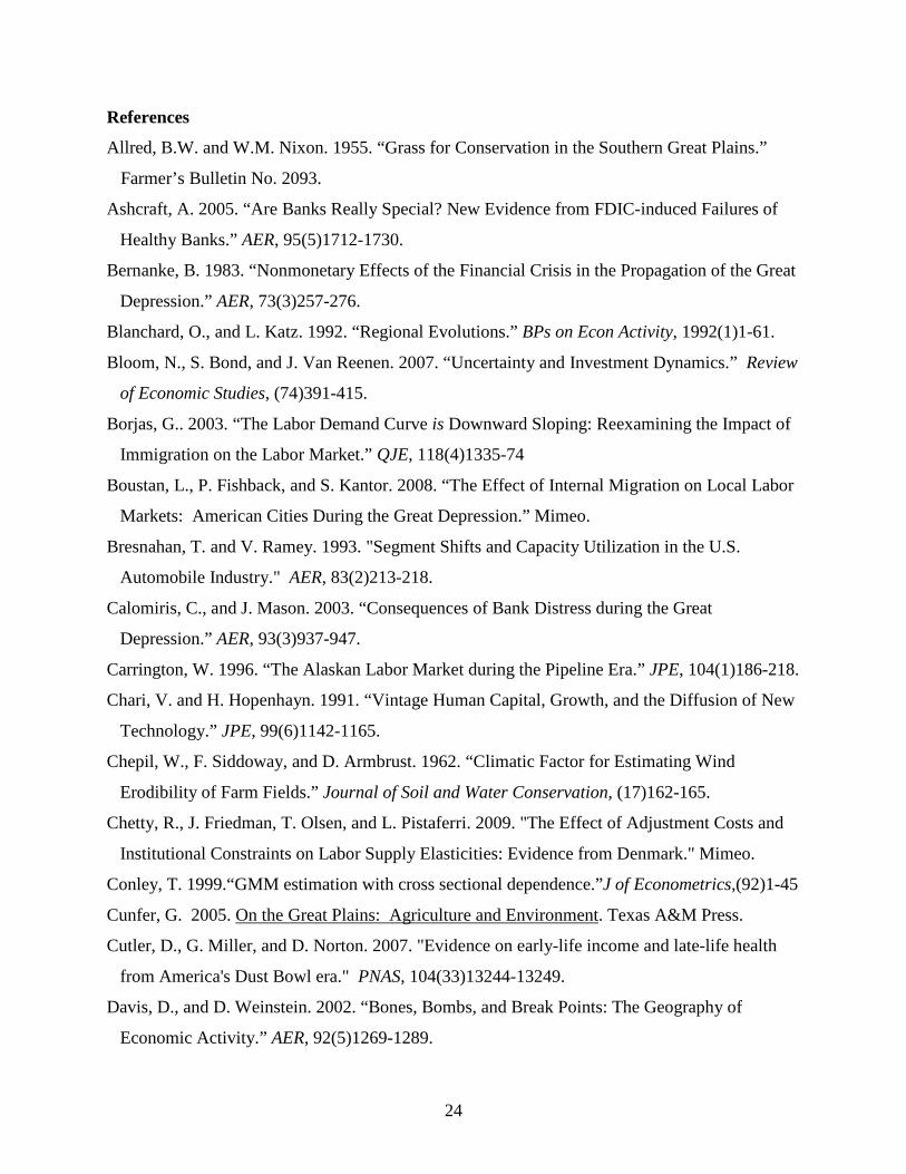
24

References

Allred, B.W. and W.M. Nixon. 1955. “Grass for Conservation in the Southern Great Plains.”

Farmer’s Bulletin No. 2093.

Ashcraft, A. 2005. “Are Banks Really Special? New Evidence from FDIC-induced Failures of

Healthy Banks.” AER, 95(5)1712-1730.

Bernanke, B. 1983. “Nonmonetary Effects of the Financial Crisis in the Propagation of the Great

Depression.” AER, 73(3)257-276.

Blanchard, O., and L. Katz. 1992. “Regional Evolutions.” BPs on Econ Activity, 1992(1)1-61.

Bloom, N., S. Bond, and J. Van Reenen. 2007. “Uncertainty and Investment Dynamics.” Review

of Economic Studies, (74)391-415.

Borjas, G.. 2003. “The Labor Demand Curve is Downward Sloping: Reexamining the Impact of

Immigration on the Labor Market.” QJE, 118(4)1335-74

Boustan, L., P. Fishback, and S. Kantor. 2008. “The Effect of Internal Migration on Local Labor

Markets: American Cities During the Great Depression.” Mimeo.

Bresnahan, T. and V. Ramey. 1993. "Segment Shifts and Capacity Utilization in the U.S.

Automobile Industry." AER, 83(2)213-218.

Calomiris, C., and J. Mason. 2003. “Consequences of Bank Distress during the Great

Depression.” AER, 93(3)937-947.

Carrington, W. 1996. “The Alaskan Labor Market during the Pipeline Era.” JPE, 104(1)186-218.

Chari, V. and H. Hopenhayn. 1991. “Vintage Human Capital, Growth, and the Diffusion of New

Technology.” JPE, 99(6)1142-1165.

Chepil, W., F. Siddoway, and D. Armbrust. 1962. “Climatic Factor for Estimating Wind

Erodibility of Farm Fields.” Journal of Soil and Water Conservation, (17)162-165.

Chetty, R., J. Friedman, T. Olsen, and L. Pistaferri. 2009. "The Effect of Adjustment Costs and

Institutional Constraints on Labor Supply Elasticities: Evidence from Denmark." Mimeo.

Conley, T. 1999.“GMM estimation with cross sectional dependence.”J of Econometrics,(92)1-45

Cunfer, G. 2005. On the Great Plains: Agriculture and Environment. Texas A&M Press.

Cutler, D., G. Miller, and D. Norton. 2007. "Evidence on early-life income and late-life health

from America's Dust Bowl era." PNAS, 104(33)13244-13249.

Davis, D., and D. Weinstein. 2002. “Bones, Bombs, and Break Points: The Geography of

Economic Activity.” AER, 92(5)1269-1289.

25

Dell, M., B. Jones, and B. Olken. 2009. “Climate Shocks and Economic Growth: Evidence from

the Last Half Century.” April, Mimeo.

Deschenes, O. and M. Greenstone. 2007. “The Economic Impacts of Climate Change: Evidence

from Agricultural Output and Random Fluctuations in Weather.” AER, 97(1)354-385.

Diamond, J. 2005. Collapse: How Societies Choose to Fail or Succeed.

Dixit, A. and R. Pindyck. 1994. Investment Under Uncertainty. Princeton Press.

Duflo, E. 2004. “The medium run effects of educational expansion: evidence from a large

school construction program in Indonesia.” JDE, (74)163-197.

Fisher, A., M. Hanemann, M. Roberts, and W. Schlenker. 2009. "Climate change and agriculture

reconsidered." Mimeo.

Fishback, P., W. Horrace, and S. Kantor. 2005. “Did New Deal Grant Programs Stimulate Local

Economies? A Study of Federal Grants and Retail Sales During the Great Depression.” JEH,

65(1)36-71.

Foster, A., and M. Rosenzweig. 1995. “Learning by Doing and Learning from Others: Human

Capital and Technical Change in Agriculture.” JPE, 103(6)1176-1209.

Griliches, Z. 1957. “Hybrid Corn: An Exploration in the Economics of Technical Change.”

Econometrica, 25(4)501-522.

Guiteras, R. 2009. “The Impact of Climate Change on Indian Agriculture.” Mimeo.

Gutmann, M. 2005. Great Plains Population and Environment Data: Agricultural Data, ICPSR.

Haines, M. 2005. Historical, Demographic, Economic, and Social Data: US, 1790-2000, ICPSR.

Hansen, Z. 2005. “Book Review of On the Great Plains,” JEH, 65(4)1162-1163.

Hansen, Z. and G. Libecap. 2004. “Small Farms, Externalities, and the Dust Bowl of the 1930s.”

JPE, 112(3)665-694.

Historical Statistics of the United States, 2006. http://hsus.cambridge.org

Hornbeck, R. 2009. “Barbed Wire: Property Rights and Agricultural Development." Forth. QJE.

Hoyt, J. 1936. “Droughts of 1930-1934.” Water-Supply Paper 680, U.S. GPO.

Hurt, D. 1981. The Dust Bowl: An Agricultural and Social History. Nelson Hall, Chicago.

--. 1985. “The National Grasslands: Origin and Development in the Dust Bowl,” in The History

of Soil and Water Conservation, eds. D. Helms and S. Flader, pp.144-157.

Janow, S., and D. McEntire. 1940. “The Migrants: Migration to California.” Land Policy Review,

July-August, pp. 24-36.

26

Leuchtenburg, W. 1963. Franklin D. Roosevelt and the New Deal, 1932-1940. H&R, NY.

Margo, R. 1997. “Wages in California during the Gold Rush.” NBER Historical WP 101.

McDonald, A. 1938. “Erosion and its Control in Oklahoma Territory.” SCS Misc Pub 301, GPO.

Mendelsohn, R., W. Nordhaus, and D. Shaw. 1994. "The impact of global warming on

agriculture: A Ricardian analysis." AER, 84(4)753-771.

Miguel, E., and G. Roland. 2006. “The Long Run Impact of Bombing Vietnam.” Mimeo

News-week. 1936. “Drought: A Merciless Sun and a Scourge of Insects Destroy Crops, Cattle

and Men – Two-thirds of the Country Afflicted.” July 18.

Phillips, S. 2007. This Land, This Nation. Cambridge University Press.

Rasmussen, W. and G. Baker. “Price-Support and Adjustment Programs From 1933 Through

1978: A Short History.” Agricultural Info Bulletin No. 424, Dept. of Ag., GPO.

Redding, S., and D. Sturm. 2008. “The Costs of Remoteness: Evidence from German Division

and Reunification.” AER, 98(5)1766-1797.

Roback, J. 1982. “Wages, Rents, and the Quality of Life.” JPE, 90(6)1257-1278.

Rosenzweig, M., and K. Wolpin. 2000. “Natural ‘Natural Experiments’ in Economics.” JEL,

38(4)827-874.

Saloutos, Theodore. 1982. The American Farmer and the New Deal. Iowa State Press.

Schlenker, W. and M. Roberts. 2009. "Nonlinear temperature effects indicate severe damages to

U.S. crop yields under climate change." Proceedings of NAS, 106(37)15594-98.

Scheffer, M., S. Carpenter, J. Foley, C. Folke, and B. Walker. 2001. "Catastrophic shifts in

ecosystems," Nature, (413)591-596.

Science. 1934. “The Recent Destructive Dust Cloud.” New Series, 79(25)473.

SCS. 1935. “Soil Erosion: A Critical Problem in American Agriculture.” GPO.

--. 1937. “Soil Conservation Districts for Erosion Control.” Misc. Pub 293, GPO.

--. 1955. “Facts About Wind Erosion and Dust Storms on the Great Plains.” Leaflet 394, USDA.

Sutch, R. 2008. "Henry Agard Wallace, the Iowa Corn Yield Tests, and the Adoption of Hybrid

Corn," NBER WP 14141.

USDA. 1940. “The Dust Bowl: Agricultural Problems and Solutions,” Ed. Ref. No. 7 July 15.

Wallace, H. 1938. “Forward” in Soils and Men: Yearbook of Agriculture. USDA.

Worster, D. 1979. Dust Bowl: The Southern Plains in the 1930s. Oxford University Press.

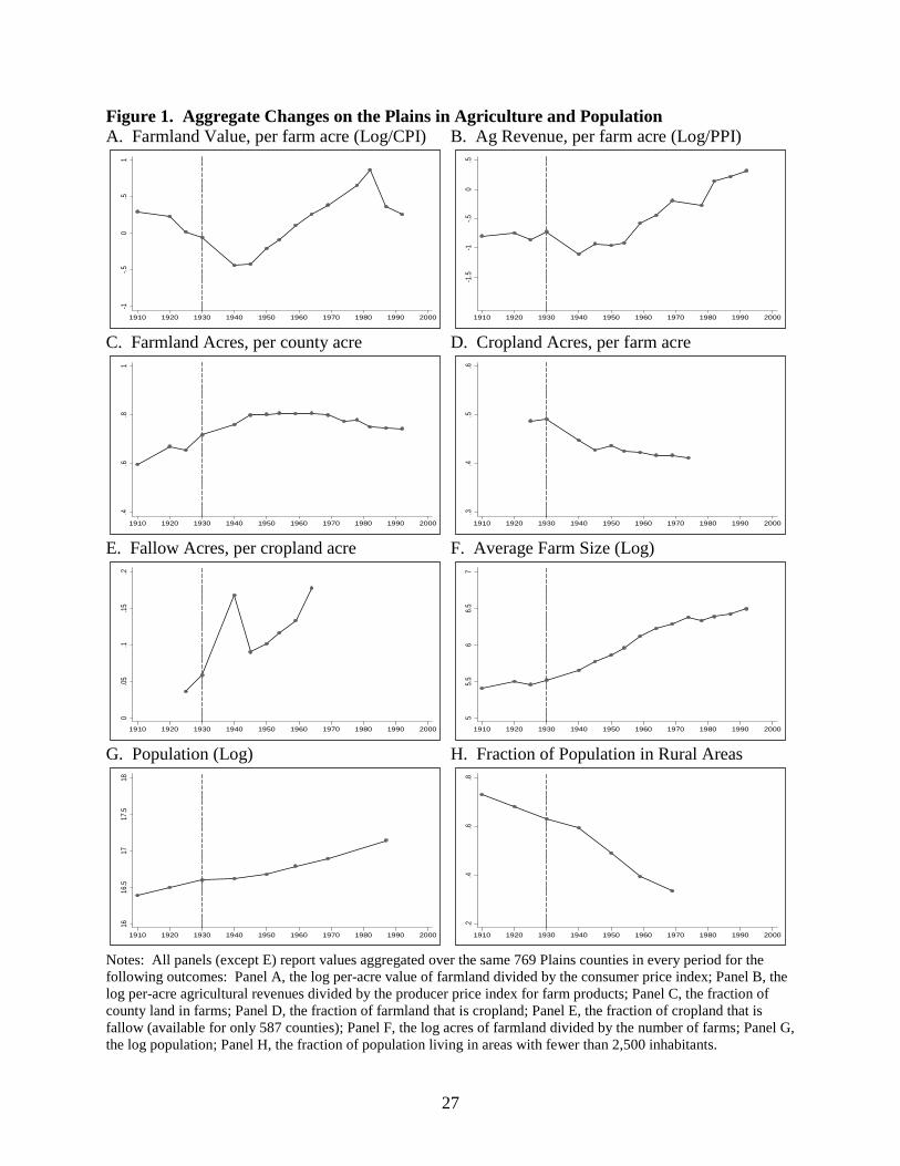
27

Figure 1. Aggregate Changes on the Plains in Agriculture and Population A. Farmland Value, per farm acre (Log/CPI)

C. Farmland Acres, per county acre

E. Fallow Acres, per cropland acre

G. Population (Log)

B. Ag Revenue, per farm acre (Log/PPI)

D. Cropland Acres, per farm acre

F. Average Farm Size (Log)

H. Fraction of Population in Rural Areas

Notes: All panels (except E) report values aggregated over the same 769 Plains counties in every period for the following outcomes: Panel A, the log per-acre value of farmland divided by the consumer price index; Panel B, the log per-acre agricultural revenues divided by the producer price index for farm products; Panel C, the fraction of county land in farms; Panel D, the fraction of farmland that is cropland; Panel E, the fraction of cropland that is fallow (available for only 587 counties); Panel F, the log acres of farmland divided by the number of farms; Panel G, the log population; Panel H, the fraction of population living in areas with fewer than 2,500 inhabitants.

-1-.5

0.5

1

1910 1920 1930 1940 1950 1960 1970 1980 1990 2000

.4.6

.81

1910 1920 1930 1940 1950 1960 1970 1980 1990 2000

0.0

5.1

.15

.2

1910 1920 1930 1940 1950 1960 1970 1980 1990 2000

1616

.517

17.5

18

1910 1920 1930 1940 1950 1960 1970 1980 1990 2000

-1.5

-1-.5

0.5

1910 1920 1930 1940 1950 1960 1970 1980 1990 2000

.3.4

.5.6

1910 1920 1930 1940 1950 1960 1970 1980 1990 2000

55.

56

6.5

7

1910 1920 1930 1940 1950 1960 1970 1980 1990 2000

.2.4

.6.8

1910 1920 1930 1940 1950 1960 1970 1980 1990 2000

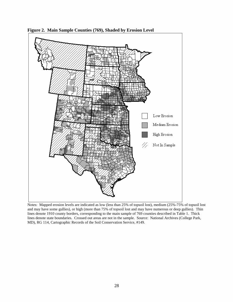
28

Figure 2. Main Sample Counties (769), Shaded by Erosion Level

Notes: Mapped erosion levels are indicated as low (less than 25% of topsoil lost), medium (25%-75% of topsoil lost and may have some gullies), or high (more than 75% of topsoil lost and may have numerous or deep gullies). Thin lines denote 1910 county borders, corresponding to the main sample of 769 counties described in Table 1. Thick lines denote state boundaries. Crossed out areas are not in the sample. Source: National Archives (College Park, MD), RG 114, Cartographic Records of the Soil Conservation Service, #149.

29

Figure 3. Log Changes in the per-Acre Value of Agricultural Land, by Erosion Level A. State-by-Year Fixed Effects

C. Lagged County Characteristics + (B)

B. 1930 County Characteristics + (A)

D. Lagged Outcome Variable + (C)

Notes: Each panel graphs the estimated coefficients (β) from versions of equation (1) in the text. For each year, the solid circles report differences in the log per-acre value of farmland for high erosion counties, relative to low erosion counties. The hollow squares report differences for medium erosion counties, relative to low erosion counties. In Panel A, these coefficients are estimated by regressing the per-acre value of farmland on the fraction of a county in a high erosion area (solid circle) and the fraction of a county in a medium erosion area (hollow square), controlling for state-by-year fixed effects. Panel B also includes as controls the interaction between each year and each county characteristic in panels B – E of Table 1. Panel C also includes as controls the interaction between each year and the available lagged values of each county characteristic in panels B – E of Table 1 (see Data Appendix). Panel D also includes as controls the interaction between each year and the outcome variable for each lagged year.

-.5-.4

-.3-.2

-.10

.1.2

.3

1910 1920 1930 1940 1950 1960 1970 1980 1990 2000

High vs. Low Medium vs. Low

-.5-.4

-.3-.2

-.10

.1.2

.3

1910 1920 1930 1940 1950 1960 1970 1980 1990 2000

High vs. Low Medium vs. Low

-.5-.4

-.3-.2

-.10

.1.2

.3

1910 1920 1930 1940 1950 1960 1970 1980 1990 2000

High vs. Low Medium vs. Low

-.5-.4

-.3-.2

-.10

.1.2

.3

1910 1920 1930 1940 1950 1960 1970 1980 1990 2000

High vs. Low Medium vs. Low

30

Table 1. County Characteristics in 1930, by Post-Dust Bowl Erosion Level Relative to Low Erosion: All Counties Medium Erosion High Erosion (3) – (2)

(1) (2) (3) (4) Panel A: Value Value of farm land & buildings, per acre in farms

3.527 0.244* 0.225 -0.019 [0.853] (0.114) (0.154) (0.106)

Value of farm land, per acre in farms

3.309 0.217 0.202 -0.014 [0.819] (0.111) (0.150) (0.103)

Value of all farm products, per acre in farms

2.107 0.258** 0.202 -0.055 [0.789] (0.100) (0.132) (0.100)

Panel B: Land-use Acres of land in farms, per county acre

0.819 0.035 -0.004 -0.039 [0.187] (0.019) (0.023) (0.020)

Acres of cropland, per acre in farms

0.491 0.035 -0.008 -0.043 [0.229] (0.031) (0.040) (0.028)

Panel C: Population and Farms Population, per 100 county acres 3.524 1.289 1.262 -0.027

[7.018] (0.824) (0.826) (0.773) Percent of population, rural areas 0.818 -0.022 0.034 0.057

[0.221] (0.030) (0.043) (0.042) Percent of population, on farms 0.542 0.020 0.040 0.020

[0.175] (0.024) (0.032) (0.032) Farms, per 100 county acres 0.328 0.163** 0.148** -0.015

[0.246] (0.026) (0.031) (0.031) Average farm size (acres) 613 -233 -307* -74

[1145] (184) (152) (142) Panel D: Cropland Allocation % Corn 0.188 0.070** 0.192** 0.122**

[0.166] (0.017) (0.027) (0.023) % Wheat 0.181 -0.043 -0.102** -0.059

[0.214] (0.027) (0.035) (0.034) % Hay 0.157 -0.044 -0.099* -0.056*

[0.177] (0.030) (0.044) (0.022) % Cotton 0.104 0.053** 0.020 -0.033

[0.209] (0.017) (0.019) (0.019) % Oats, Barley, and Rye 0.134 -0.005 -0.033* -0.028

[0.116] (0.009) (0.013) (0.010) Panel E: Animal Production Cattle, per county acre 0.056 0.011** 0.013** 0.003

[0.033] (0.003) (0.004) (0.003) Swine, per county acre 0.066 0.040** 0.055** 0.015

[0.096] (0.008) (0.012) (0.011) Chickens, per county acre 0.296 0.115** 0.116** 0.001

[0.279] (0.025) (0.034) (0.031) Notes: Column 1 reports average values for the 769 main sample counties, where counties are weighted by the acres of farmland in 1930 (counties based on 1910 borders; with at least 1000 acres of farmland in every period; and with data on each variable in Figure 1 for each period shown). The standard deviation is reported in brackets. Columns 2 and 3 report coefficients from a single regression that regresses the indicated county characteristic in 1930 on the fraction of the county in a medium erosion area and in a high erosion area (low erosion is the omitted category), conditional on state fixed effects and weighted by acres of farmland in 1930. Column 4 reports the difference between the coefficients in columns 2 and 3. Robust standard errors are reported in parentheses. ** denotes statistical significance at the 1% level, * at the 5% level.

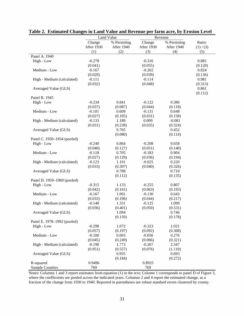
31

Table 2. Estimated Changes in Land Value and Revenue per farm acre, by Erosion Level Land Value Revenue Change

After 1930 % Persisting After 1940

Change After 1930

% Persisting After 1940

Ratio: (1) / (3)

(1) (2) (3) (4) (5) Panel A. 1940 High - Low -0.278 -0.316 0.881 (0.041) (0.055) (0.120) Medium - Low -0.167 -0.202 0.824 (0.029) (0.039) (0.136) High - Medium (calculated) -0.111 -0.114 0.981 (0.032) (0.048) (0.313) Averaged Value (GLS) 0.861 (0.112) Panel B. 1945 High - Low -0.234 0.841 -0.122 0.386 (0.037) (0.087) (0.044) (0.118) Medium - Low -0.101 0.609 -0.131 0.648 (0.027) (0.105) (0.031) (0.158) High - Medium (calculated) -0.133 1.189 0.009 -0.081 (0.031) (0.238) (0.035) (0.324) Averaged Value (GLS) 0.765 0.452 (0.080) (0.114) Panel C. 1950–1954 (pooled) High - Low -0.240 0.864 -0.208 0.658 (0.040) (0.127) (0.051) (0.140) Medium - Low -0.118 0.705 -0.183 0.904 (0.027) (0.129) (0.036) (0.194) High - Medium (calculated) -0.123 1.101 -0.025 0.220 (0.033) (0.307) (0.040) (0.326) Averaged Value (GLS) 0.788 0.710 (0.112) (0.135) Panel D. 1959–1969 (pooled) High - Low -0.315 1.133 -0.255 0.807 (0.042) (0.161) (0.063) (0.193) Medium - Low -0.167 1.001 -0.130 0.643 (0.033) (0.196) (0.044) (0.217) High - Medium (calculated) -0.148 1.331 -0.125 1.099 (0.036) (0.401) (0.050) (0.531) Averaged Value (GLS) 1.094 0.746 (0.150) (0.178) Panel E. 1978–1992 (pooled) High - Low -0.298 1.072 -0.323 1.021 (0.057) (0.197) (0.092) (0.308) Medium - Low -0.100 0.603 -0.056 0.276 (0.045) (0.249) (0.066) (0.321) High - Medium (calculated) -0.198 1.773 -0.267 2.347 (0.051) (0.557) (0.076) (1.110) Averaged Value (GLS) 0.935 0.693 (0.184) (0.272) R-squared 0.9496 0.8925 Sample Counties 769 769

Notes: Columns 1 and 3 report estimates from equation (1) in the text; Column 1 corresponds to panel D of Figure 3, where the coefficients are pooled across the indicated years. Columns 2 and 4 report the estimated change, as a fraction of the change from 1930 to 1940. Reported in parentheses are robust standard errors clustered by county.

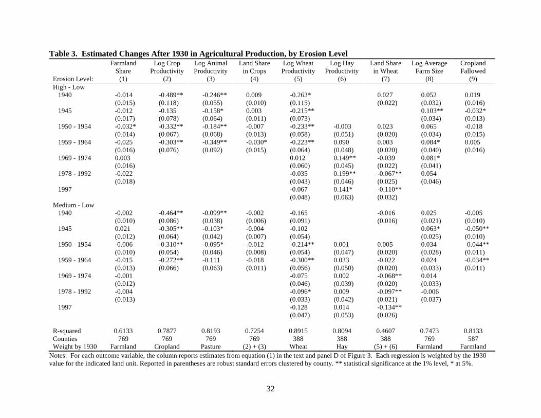
32

Table 3. Estimated Changes After 1930 in Agricultural Production, by Erosion Level Farmland

Share Log Crop

Productivity Log Animal Productivity

Land Share in Crops

Log Wheat Productivity

Log Hay Productivity

Land Share in Wheat

Log Average Farm Size

Cropland Fallowed

Erosion Level: (1) (2) (3) (4) (5) (6) (7) (8) (9) High - Low 1940 -0.014 -0.489** -0.246** 0.009 -0.263* 0.027 0.052 0.019 (0.015) (0.118) (0.055) (0.010) (0.115) (0.022) (0.032) (0.016) 1945 -0.012 -0.135 -0.158* 0.003 -0.215** 0.103** -0.032* (0.017) (0.078) (0.064) (0.011) (0.073) (0.034) (0.013) 1950 - 1954 -0.032* -0.332** -0.184** -0.007 -0.233** -0.003 0.023 0.065 -0.018 (0.014) (0.067) (0.068) (0.013) (0.058) (0.051) (0.020) (0.034) (0.015) 1959 - 1964 -0.025 -0.303** -0.349** -0.030* -0.223** 0.090 0.003 0.084* 0.005 (0.016) (0.076) (0.092) (0.015) (0.064) (0.048) (0.020) (0.040) (0.016) 1969 - 1974 0.003 0.012 0.149** -0.039 0.081* (0.016) (0.060) (0.045) (0.022) (0.041) 1978 - 1992 -0.022 -0.035 0.199** -0.067** 0.054 (0.018) (0.043) (0.046) (0.025) (0.046) 1997 -0.067 0.141* -0.110** (0.048) (0.063) (0.032) Medium - Low 1940 -0.002 -0.464** -0.099** -0.002 -0.165 -0.016 0.025 -0.005 (0.010) (0.086) (0.038) (0.006) (0.091) (0.016) (0.021) (0.010) 1945 0.021 -0.305** -0.103* -0.004 -0.102 0.063* -0.050** (0.012) (0.064) (0.042) (0.007) (0.054) (0.025) (0.010) 1950 - 1954 -0.006 -0.310** -0.095* -0.012 -0.214** 0.001 0.005 0.034 -0.044** (0.010) (0.054) (0.046) (0.008) (0.054) (0.047) (0.020) (0.028) (0.011) 1959 - 1964 -0.015 -0.272** -0.111 -0.018 -0.300** 0.033 -0.022 0.024 -0.034** (0.013) (0.066) (0.063) (0.011) (0.056) (0.050) (0.020) (0.033) (0.011) 1969 - 1974 -0.001 -0.075 0.002 -0.068** 0.014 (0.012) (0.046) (0.039) (0.020) (0.033) 1978 - 1992 -0.004 -0.096* 0.009 -0.097** -0.006 (0.013) (0.033) (0.042) (0.021) (0.037) 1997 -0.128 0.014 -0.134** (0.047) (0.053) (0.026) R-squared 0.6133 0.7877 0.8193 0.7254 0.8915 0.8094 0.4607 0.7473 0.8133 Counties 769 769 769 769 388 388 388 769 587 Weight by 1930 Farmland Cropland Pasture (2) + (3) Wheat Hay (5) + (6) Farmland Farmland

Notes: For each outcome variable, the column reports estimates from equation (1) in the text and panel D of Figure 3. Each regression is weighted by the 1930 value for the indicated land unit. Reported in parentheses are robust standard errors clustered by county. ** statistical significance at the 1% level, * at 5%.

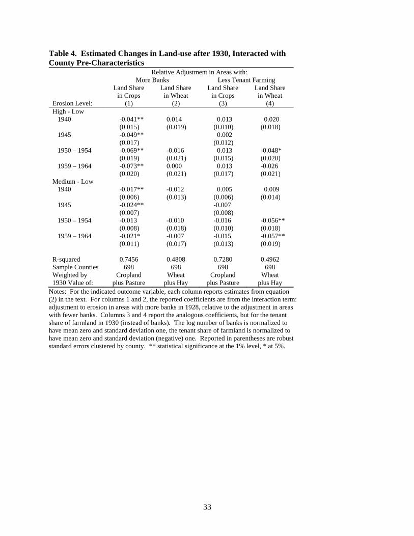
33

Table 4. Estimated Changes in Land-use after 1930, Interacted with County Pre-Characteristics

Relative Adjustment in Areas with: More Banks Less Tenant Farming Land Share

in Crops Land Share in Wheat

Land Share in Crops

Land Share in Wheat

Erosion Level: (1) (2) (3) (4) High - Low 1940 -0.041** 0.014 0.013 0.020 (0.015) (0.019) (0.010) (0.018) 1945 -0.049** 0.002 (0.017) (0.012) 1950 – 1954 -0.069** -0.016 0.013 -0.048* (0.019) (0.021) (0.015) (0.020) 1959 – 1964 -0.073** 0.000 0.013 -0.026 (0.020) (0.021) (0.017) (0.021) Medium - Low 1940 -0.017** -0.012 0.005 0.009 (0.006) (0.013) (0.006) (0.014) 1945 -0.024** -0.007 (0.007) (0.008) 1950 – 1954 -0.013 -0.010 -0.016 -0.056** (0.008) (0.018) (0.010) (0.018) 1959 – 1964 -0.021* -0.007 -0.015 -0.057** (0.011) (0.017) (0.013) (0.019) R-squared 0.7456 0.4808 0.7280 0.4962 Sample Counties 698 698 698 698 Weighted by 1930 Value of:

Cropland plus Pasture

Wheat plus Hay

Cropland plus Pasture

Wheat plus Hay

Notes: For the indicated outcome variable, each column reports estimates from equation (2) in the text. For columns 1 and 2, the reported coefficients are from the interaction term: adjustment to erosion in areas with more banks in 1928, relative to the adjustment in areas with fewer banks. Columns 3 and 4 report the analogous coefficients, but for the tenant share of farmland in 1930 (instead of banks). The log number of banks is normalized to have mean zero and standard deviation one, the tenant share of farmland is normalized to have mean zero and standard deviation (negative) one. Reported in parentheses are robust standard errors clustered by county. ** statistical significance at the 1% level, * at 5%.

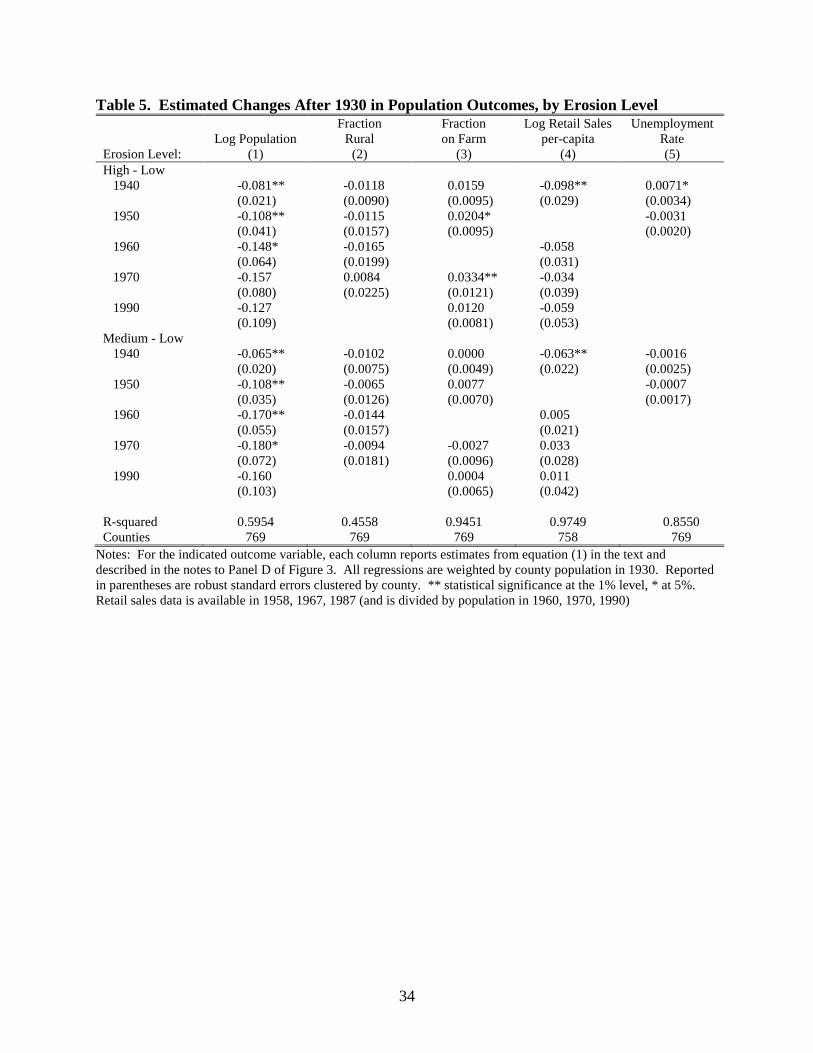
34

Table 5. Estimated Changes After 1930 in Population Outcomes, by Erosion Level

Log Population Fraction

Rural Fraction on Farm

Log Retail Sales per-capita

Unemployment Rate

Erosion Level: (1) (2) (3) (4) (5) High - Low 1940 -0.081** -0.0118 0.0159 -0.098** 0.0071* (0.021) (0.0090) (0.0095) (0.029) (0.0034) 1950 -0.108** -0.0115 0.0204* -0.0031 (0.041) (0.0157) (0.0095) (0.0020) 1960 -0.148* -0.0165 -0.058 (0.064) (0.0199) (0.031) 1970 -0.157 0.0084 0.0334** -0.034 (0.080) (0.0225) (0.0121) (0.039) 1990 -0.127 0.0120 -0.059 (0.109) (0.0081) (0.053) Medium - Low 1940 -0.065** -0.0102 0.0000 -0.063** -0.0016 (0.020) (0.0075) (0.0049) (0.022) (0.0025) 1950 -0.108** -0.0065 0.0077 -0.0007 (0.035) (0.0126) (0.0070) (0.0017) 1960 -0.170** -0.0144 0.005 (0.055) (0.0157) (0.021) 1970 -0.180* -0.0094 -0.0027 0.033 (0.072) (0.0181) (0.0096) (0.028) 1990 -0.160 0.0004 0.011 (0.103) (0.0065) (0.042) R-squared 0.5954 0.4558 0.9451 0.9749 0.8550 Counties 769 769 769 758 769

Notes: For the indicated outcome variable, each column reports estimates from equation (1) in the text and described in the notes to Panel D of Figure 3. All regressions are weighted by county population in 1930. Reported in parentheses are robust standard errors clustered by county. ** statistical significance at the 1% level, * at 5%. Retail sales data is available in 1958, 1967, 1987 (and is divided by population in 1960, 1970, 1990)

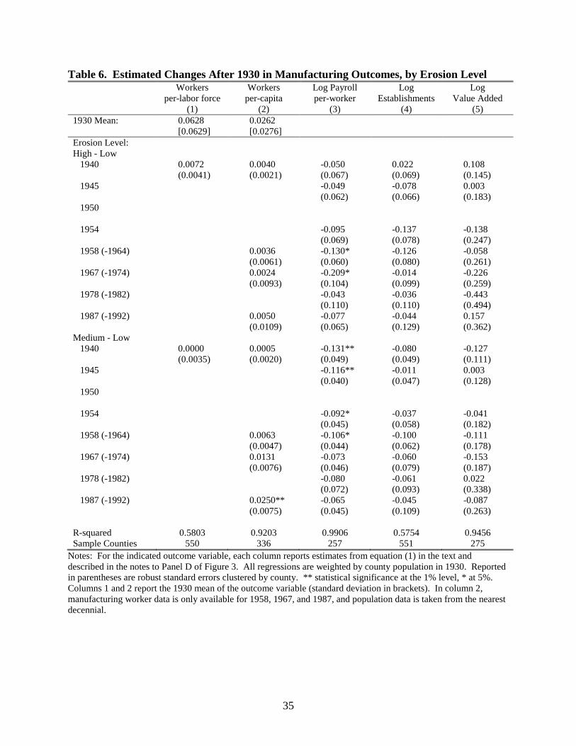
35

Table 6. Estimated Changes After 1930 in Manufacturing Outcomes, by Erosion Level Workers

per-labor force Workers

per-capita Log Payroll per-worker

Log Establishments

Log Value Added

(1) (2) (3) (4) (5) 1930 Mean: 0.0628 0.0262 [0.0629] [0.0276] Erosion Level: High - Low 1940 0.0072 0.0040 -0.050 0.022 0.108 (0.0041) (0.0021) (0.067) (0.069) (0.145) 1945 -0.049 -0.078 0.003 (0.062) (0.066) (0.183) 1950 1954 -0.095 -0.137 -0.138 (0.069) (0.078) (0.247) 1958 (-1964) 0.0036 -0.130* -0.126 -0.058 (0.0061) (0.060) (0.080) (0.261) 1967 (-1974) 0.0024 -0.209* -0.014 -0.226 (0.0093) (0.104) (0.099) (0.259) 1978 (-1982) -0.043 -0.036 -0.443 (0.110) (0.110) (0.494) 1987 (-1992) 0.0050 -0.077 -0.044 0.157 (0.0109) (0.065) (0.129) (0.362) Medium - Low 1940 0.0000 0.0005 -0.131** -0.080 -0.127 (0.0035) (0.0020) (0.049) (0.049) (0.111) 1945 -0.116** -0.011 0.003 (0.040) (0.047) (0.128) 1950 1954 -0.092* -0.037 -0.041 (0.045) (0.058) (0.182) 1958 (-1964) 0.0063 -0.106* -0.100 -0.111 (0.0047) (0.044) (0.062) (0.178) 1967 (-1974) 0.0131 -0.073 -0.060 -0.153 (0.0076) (0.046) (0.079) (0.187) 1978 (-1982) -0.080 -0.061 0.022 (0.072) (0.093) (0.338) 1987 (-1992) 0.0250** -0.065 -0.045 -0.087 (0.0075) (0.045) (0.109) (0.263) R-squared 0.5803 0.9203 0.9906 0.5754 0.9456 Sample Counties 550 336 257 551 275

Notes: For the indicated outcome variable, each column reports estimates from equation (1) in the text and described in the notes to Panel D of Figure 3. All regressions are weighted by county population in 1930. Reported in parentheses are robust standard errors clustered by county. ** statistical significance at the 1% level, * at 5%. Columns 1 and 2 report the 1930 mean of the outcome variable (standard deviation in brackets). In column 2, manufacturing worker data is only available for 1958, 1967, and 1987, and population data is taken from the nearest decennial.

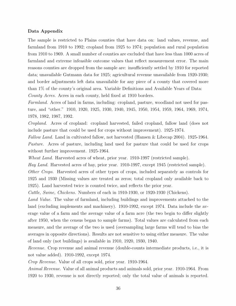
Data Appendix

The sample is restricted to Plains counties that have data on: land values, revenue, and

farmland from 1910 to 1992; cropland from 1925 to 1974; population and rural population

from 1910 to 1969. A small number of counties are excluded that have less than 1000 acres of

farmland and extreme infeasible outcome values that reflect measurement error. The main

reasons counties are dropped from the sample are: insufficiently settled by 1910 for reported

data; unavailable Gutmann data for 1925; agricultural revenue unavailable from 1920-1930;

and border adjustments left data unavailable for any piece of a county that covered more

than 1% of the county’s original area. Variable Definitions and Available Years of Data:

County Acres. Acres in each county, held fixed at 1910 borders.

Farmland. Acres of land in farms, including: cropland, pasture, woodland not used for pas-

ture, and “other.” 1910, 1920, 1925, 1930, 1940, 1945, 1950, 1954, 1959, 1964, 1969, 1974,

1978, 1982, 1987, 1992.

Cropland. Acres of cropland: cropland harvested, failed cropland, fallow land (does not

include pasture that could be used for crops without improvement). 1925-1974.

Fallow Land. Land in cultivated fallow, not harvested (Hansen & Libecap 2004). 1925-1964.

Pasture. Acres of pasture, including land used for pasture that could be used for crops

without further improvement. 1925-1964.

Wheat Land. Harvested acres of wheat, prior year. 1910-1997 (restricted sample).

Hay Land. Harvested acres of hay, prior year. 1910-1997, except 1945 (restricted sample).

Other Crops. Harvested acres of other types of crops, included separately as controls for

1925 and 1930 (Missing values are treated as zeros; total cropland only available back to

1925). Land harvested twice is counted twice, and reflects the prior year.

Cattle, Swine, Chickens. Numbers of each in 1910-1930, or 1920-1930 (Chickens).

Land Value. The value of farmland, including buildings and improvements attached to the

land (excluding implements and machinery). 1910-1992, except 1974. Data include the av-

erage value of a farm and the average value of a farm acre (the two begin to differ slightly

after 1950, when the census began to sample farms). Total values are calculated from each

measure, and the average of the two is used (oversampling large farms will tend to bias the

averages in opposite directions). Results are not sensitive to using either measure. The value

of land only (not buildings) is available in 1910, 1920, 1930, 1940.

Revenue. Crop revenue and animal revenue (double-counts intermediate products, i.e., it is

not value added). 1910-1992, except 1974.

Crop Revenue. Value of all crops sold, prior year. 1910-1964.

Animal Revenue. Value of all animal products and animals sold, prior year. 1910-1964. From

1920 to 1930, revenue is not directly reported; only the total value of animals is reported.

36

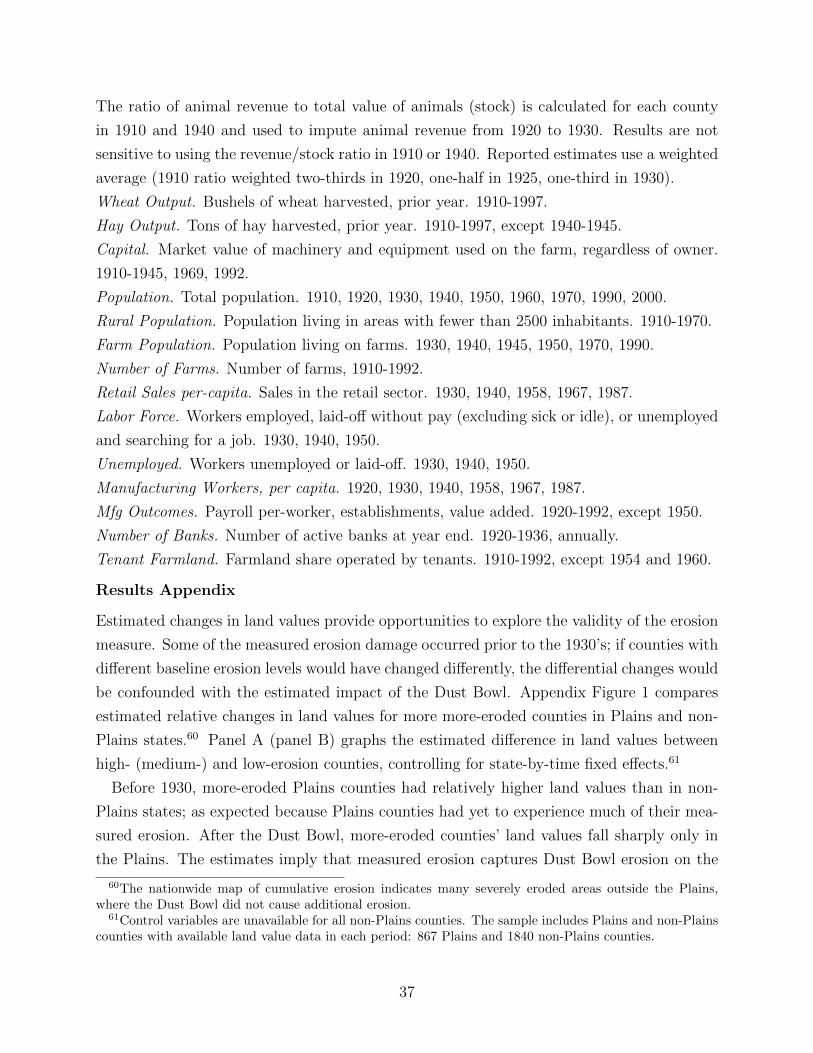
The ratio of animal revenue to total value of animals (stock) is calculated for each county

in 1910 and 1940 and used to impute animal revenue from 1920 to 1930. Results are not

sensitive to using the revenue/stock ratio in 1910 or 1940. Reported estimates use a weighted

average (1910 ratio weighted two-thirds in 1920, one-half in 1925, one-third in 1930).

Wheat Output. Bushels of wheat harvested, prior year. 1910-1997.

Hay Output. Tons of hay harvested, prior year. 1910-1997, except 1940-1945.

Capital. Market value of machinery and equipment used on the farm, regardless of owner.

1910-1945, 1969, 1992.

Population. Total population. 1910, 1920, 1930, 1940, 1950, 1960, 1970, 1990, 2000.

Rural Population. Population living in areas with fewer than 2500 inhabitants. 1910-1970.

Farm Population. Population living on farms. 1930, 1940, 1945, 1950, 1970, 1990.

Number of Farms. Number of farms, 1910-1992.

Retail Sales per-capita. Sales in the retail sector. 1930, 1940, 1958, 1967, 1987.

Labor Force. Workers employed, laid-off without pay (excluding sick or idle), or unemployed

and searching for a job. 1930, 1940, 1950.

Unemployed. Workers unemployed or laid-off. 1930, 1940, 1950.

Manufacturing Workers, per capita. 1920, 1930, 1940, 1958, 1967, 1987.

Mfg Outcomes. Payroll per-worker, establishments, value added. 1920-1992, except 1950.

Number of Banks. Number of active banks at year end. 1920-1936, annually.

Tenant Farmland. Farmland share operated by tenants. 1910-1992, except 1954 and 1960.

Results Appendix

Estimated changes in land values provide opportunities to explore the validity of the erosion

measure. Some of the measured erosion damage occurred prior to the 1930’s; if counties with

different baseline erosion levels would have changed differently, the differential changes would

be confounded with the estimated impact of the Dust Bowl. Appendix Figure 1 compares

estimated relative changes in land values for more more-eroded counties in Plains and non-

Plains states.60 Panel A (panel B) graphs the estimated difference in land values between

high- (medium-) and low-erosion counties, controlling for state-by-time fixed effects.61

Before 1930, more-eroded Plains counties had relatively higher land values than in non-

Plains states; as expected because Plains counties had yet to experience much of their mea-

sured erosion. After the Dust Bowl, more-eroded counties’ land values fall sharply only in

the Plains. The estimates imply that measured erosion captures Dust Bowl erosion on the

60The nationwide map of cumulative erosion indicates many severely eroded areas outside the Plains,where the Dust Bowl did not cause additional erosion.

61Control variables are unavailable for all non-Plains counties. The sample includes Plains and non-Plainscounties with available land value data in each period: 867 Plains and 1840 non-Plains counties.

37

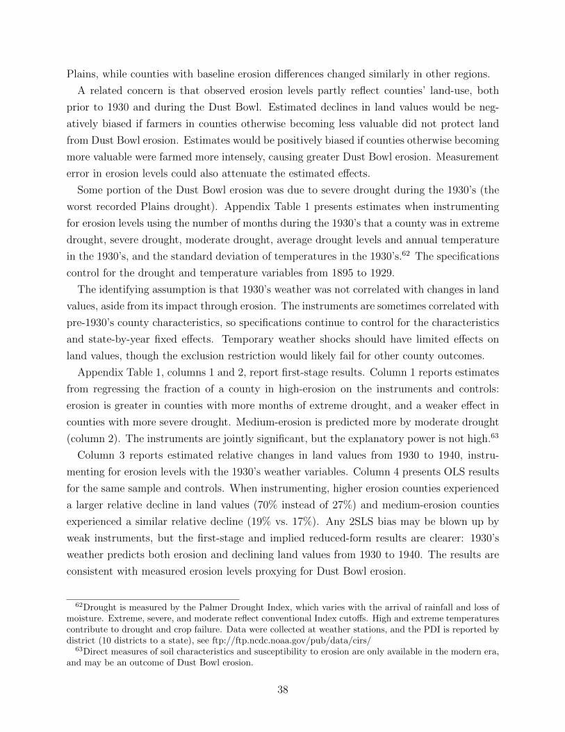
Plains, while counties with baseline erosion differences changed similarly in other regions.

A related concern is that observed erosion levels partly reflect counties’ land-use, both

prior to 1930 and during the Dust Bowl. Estimated declines in land values would be neg-

atively biased if farmers in counties otherwise becoming less valuable did not protect land

from Dust Bowl erosion. Estimates would be positively biased if counties otherwise becoming

more valuable were farmed more intensely, causing greater Dust Bowl erosion. Measurement

error in erosion levels could also attenuate the estimated effects.

Some portion of the Dust Bowl erosion was due to severe drought during the 1930’s (the

worst recorded Plains drought). Appendix Table 1 presents estimates when instrumenting

for erosion levels using the number of months during the 1930’s that a county was in extreme

drought, severe drought, moderate drought, average drought levels and annual temperature

in the 1930’s, and the standard deviation of temperatures in the 1930’s.62 The specifications

control for the drought and temperature variables from 1895 to 1929.

The identifying assumption is that 1930’s weather was not correlated with changes in land

values, aside from its impact through erosion. The instruments are sometimes correlated with

pre-1930’s county characteristics, so specifications continue to control for the characteristics

and state-by-year fixed effects. Temporary weather shocks should have limited effects on

land values, though the exclusion restriction would likely fail for other county outcomes.

Appendix Table 1, columns 1 and 2, report first-stage results. Column 1 reports estimates

from regressing the fraction of a county in high-erosion on the instruments and controls:

erosion is greater in counties with more months of extreme drought, and a weaker effect in

counties with more severe drought. Medium-erosion is predicted more by moderate drought

(column 2). The instruments are jointly significant, but the explanatory power is not high.63

Column 3 reports estimated relative changes in land values from 1930 to 1940, instru-

menting for erosion levels with the 1930’s weather variables. Column 4 presents OLS results

for the same sample and controls. When instrumenting, higher erosion counties experienced

a larger relative decline in land values (70% instead of 27%) and medium-erosion counties

experienced a similar relative decline (19% vs. 17%). Any 2SLS bias may be blown up by

weak instruments, but the first-stage and implied reduced-form results are clearer: 1930’s

weather predicts both erosion and declining land values from 1930 to 1940. The results are

consistent with measured erosion levels proxying for Dust Bowl erosion.

62Drought is measured by the Palmer Drought Index, which varies with the arrival of rainfall and loss ofmoisture. Extreme, severe, and moderate reflect conventional Index cutoffs. High and extreme temperaturescontribute to drought and crop failure. Data were collected at weather stations, and the PDI is reported bydistrict (10 districts to a state), see ftp://ftp.ncdc.noaa.gov/pub/data/cirs/

63Direct measures of soil characteristics and susceptibility to erosion are only available in the modern era,and may be an outcome of Dust Bowl erosion.

38

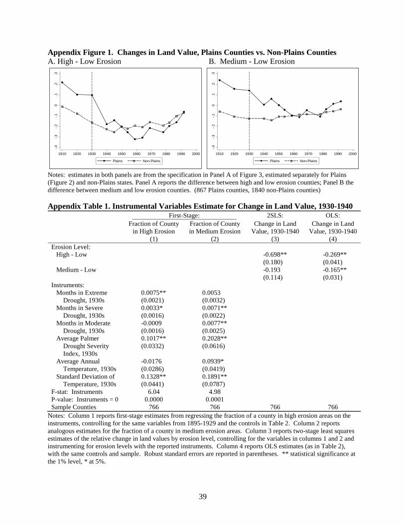
39

Appendix Figure 1. Changes in Land Value, Plains Counties vs. Non-Plains Counties A. High - Low Erosion B. Medium - Low Erosion

Notes: estimates in both panels are from the specification in Panel A of Figure 3, estimated separately for Plains (Figure 2) and non-Plains states. Panel A reports the difference between high and low erosion counties; Panel B the difference between medium and low erosion counties. (867 Plains counties, 1840 non-Plains counties)

Appendix Table 1. Instrumental Variables Estimate for Change in Land Value, 1930-1940

First-Stage: 2SLS: OLS: Fraction of County

in High Erosion Fraction of County in Medium Erosion

Change in Land Value, 1930-1940

Change in Land Value, 1930-1940

(1) (2) (3) (4) Erosion Level: High - Low -0.698** -0.269** (0.180) (0.041) Medium - Low -0.193 -0.165** (0.114) (0.031) Instruments: Months in Extreme

Drought, 1930s 0.0075** 0.0053 (0.0021) (0.0032)

Months in Severe Drought, 1930s

0.0033* 0.0071** (0.0016) (0.0022)

Months in Moderate Drought, 1930s

-0.0009 0.0077** (0.0016) (0.0025)

Average Palmer Drought Severity Index, 1930s

0.1017** 0.2028** (0.0332) (0.0616)

Average Annual Temperature, 1930s

-0.0176 0.0939* (0.0286) (0.0419)

Standard Deviation of Temperature, 1930s

0.1328** 0.1891** (0.0441) (0.0787)

F-stat: Instruments 6.04 4.98 P-value: Instruments = 0 0.0000 0.0001 Sample Counties 766 766 766 766

Notes: Column 1 reports first-stage estimates from regressing the fraction of a county in high erosion areas on the instruments, controlling for the same variables from 1895-1929 and the controls in Table 2. Column 2 reports analogous estimates for the fraction of a county in medium erosion areas. Column 3 reports two-stage least squares estimates of the relative change in land values by erosion level, controlling for the variables in columns 1 and 2 and instrumenting for erosion levels with the reported instruments. Column 4 reports OLS estimates (as in Table 2), with the same controls and sample. Robust standard errors are reported in parentheses. ** statistical significance at the 1% level, * at 5%.

-.4-.3

-.2-.1

0.1

.2.3

1910 1920 1930 1940 1950 1960 1970 1980 1990 2000

Plains Non-Plains

-.4-.3

-.2-.1

0.1

.2.3

1910 1920 1930 1940 1950 1960 1970 1980 1990 2000

Plains Non-Plains

40

Appendix Figure 2. Estimated Changes after 1930 in:A. Number of Active Banks (Log)

B. Tenant Share of Farmland

Notes: These figures graph the estimated coefficients (β) from a modified version of equation (1), described in Panel C of Figure 3. Banking data is available annually, so the regression in Panel A controls for state-by-year fixed effects and county characteristics interacted with every year. Appendix Table 2. Government Program Payments per farm acre, by Erosion Level

Relative to Low Erosion: All Counties Med. Erosion High Erosion (3) – (2)

(1) (2) (3) (4) Panel A. New Deal payments (1933-39) AAA payments 0.489 0.001 -0.027 -0.028 [0.327] (0.017) (0.023) (0.021) Public works spending 0.264 0.008 -0.033 -0.041 [0.605] (0.058) (0.064) (0.066) Relief spending 0.508 0.110 0.142 0.032 [2.435] (0.100) (0.129) (0.118) New deal loans 0.484 -0.090 -0.087 0.003 [1.126] (0.094) (0.112) (0.087) Mortgage loans guaranteed 0.112 0.001 -0.103 -0.104* [0.792] (0.040) (0.059) (0.042) Panel B. Government payments All payments, 1969 3.323 -0.245 -0.159 0.086 [2.646] (0.256) (0.284) (0.254) All payments, 1974 0.364 0.088 0.257** 0.169** [0.390] (0.056) (0.066) (0.045) All payments, 1987 16.040 -1.838* -5.511** -3.673** [13.631] (0.866) (1.076) (1.075) All payments, 1992 7.930 -0.887 -1.323* -0.436 [5.580] (0.477) (0.549) (0.472) CRP payments, 1992 1.571 0.750** 1.776** 1.026** [1.490] (0.162) (0.263) (0.245) Fraction of money from CRP, 1992 0.217 0.089** 0.185** 0.096** [0.149] (0.018) (0.027) (0.023)

Notes: Panel A reports differences in 1930’s New Deal spending across 766 counties. Panel B reports differences in government payments, conservation reserve program (CRP) payments, and fraction of payments through the CRP. Column 1 reports the mean and standard deviation in brackets. Column 2 reports the average difference for medium erosion county relative to low erosion, controlling for state fixed effects, characteristics in Panels B – E of Table 1, and lagged values of the characteristics. Columns 3 and 4 report the same average differences comparing high vs. low erosion and high vs. medium erosion. Variables and regressions are weighted by county farmland in 1930. Robust standard errors are reported in parentheses. ** statistical significance at the 1% level, * at 5%.

-.3-.2

-.10

1920 1925 1929 1933 1936

High vs. Low Medium vs. Low

-.1-.0

50

.05

.1

1910 1920 1930 1940 1950 1960 1970 1980 1990 2000

High vs. Low Medium vs. Low