The electrochemistry of electrode edges and its relevance ...koldham/Paper224-Reprint.pdf · The electrochemistry of electrode edges and its relevance to partially blocked voltammetric

ORIGINAL PAPER

The electrochemistry of electrode edges and its relevanceto partially blocked voltammetric electrodes

Jan C. Myland & Keith B. Oldham

Received: 30 September 2008 /Accepted: 15 October 2008 / Published online: 29 November 2008# Springer-Verlag 2008

Abstract Analytical mathematics and digital simulationare used to predict the response, to a potential jump, of thejunction between insulating and conducting regions of anelectrode. The simulation is carried out differentially andemploys other novel features. Concentrations in the vicinityof edges of positive and negative curvatures, as well asstraight edges, are analyzed by the model and thereby thefaradaic current densities and currents are predicted. It isshown that, in addition to the well-understood cottrelliancurrent arising from the surface of the conducting electrode,currents are generated that are proportional to the length ofthe edge and to its curvature. These results are then appliedto inlaid disks and to partially blocked electrodes. Thepossibility is explored of using the response to a potentialstep to gain information on the geometry of a partiallyblocked electrode.

Keywords Heterogeneous electrodes .

Partially blocked electrodes . Diffusion . Cottrellian current .

Digital simulation . Electrode edges . Inlaid disk electrode .

Prompt current . Potential-jump chronoamperometry

Introduction

Solid electrodes are wont to display heterogeneity forvarious reasons: on account of the exposure of differentcrystal faces, from the preferential oxidation of certain sites,from the presence in the conducting phase of impurities oralloying elements, from contamination by detritus, and

from other causes. Such surface heterogeneity is, of course,a disquieting complication for electrochemists, though itcan sometimes be turned to advantage [1]. The simplesttype of inhomogeneity is the partial occlusion of anotherwise uniform electrode by a surface feature thateffectively prevents the electrode process from occurringon some fraction of the electrode. This “partial blocking” ofan electrode has been examined by a number of authors[2–5] for a variety of repeating or random patterns of theoccluding agent. The feature possessed by partially blockedelectrodes that is absent from naked electrodes is thepronounced presence of edges; that is, junctions betweenconducting portions and insulating portions of the surface.The purpose of this article is to examine the electrochem-ical properties of edges, to show how they affect voltam-metry, and to discuss how these properties might illuminateelectrode heterogeneity.

Throughout this article, we consider only flat conductorsthat share their surface with a coplanar insulator. In earlysections, attention is confined to a small fragment of edge,but in a later section, we return to the consideration of theelectrochemistry of an electrode with multiple edges andshow how the chronoamperometric response of a partiallyblocked electrode can provide information on the configu-ration of the blockage.

We address edged electrodes, previously inactive, sub-jected to the simplest voltammetric perturbation—theimposition of a totally concentration-polarizing potentialstep—but the same principles apply to other experiments.In the immediate aftermath of the potential jump, thefaradaic response will be dominated by the cottrelliancurrent arising from the conducting portion of the plane, butas time progresses the current will significantly exceed thatpredicted by the Cottrell equation. The excess current,beyond the cottrellian component, is associated with the

J Solid State Electrochem (2009) 13:521–535DOI 10.1007/s10008-008-0713-1

J. C. Myland :K. B. Oldham (*)Department of Chemistry, Trent University,Peterborough, Ontario, Canada KJ9 7B8e-mail: [email protected]

conductor/insulator junction near which the current densityis enhanced. The electrochemistry at such edges hasreceived little voltammetric attention, but is the mainpreoccupation of the present study.

Figure 1 is a plan view of three edge fragments in whichan electronic conductor meets an adjacent insulator. Theedge in diagram (ii) is linear, this being the simplestjunction between a conductor and a coplanar insulator. Indiagram (i), the edge is concave, whereas in (iii) the edge isconvex (from the viewpoint of the conductor). A plane edgefragment has two properties: length and curvature. Thelengths of the three edges in Fig. 1 are all :. Curvature isassigned to a curve at a particular point by fitting a circle tothe curve at the point in question; the magnitude of thecurvature is then the reciprocal of the radius of that circle.Sign is (arbitrarily) allocated to the curvature κ such thatthe edges for cases (i), (ii), and (iii) have positive, zero, andnegative curvatures, respectively. An important property ofthe edge fragment is the product κ : of its curvature and itslength: this is a dimensionless quantity that crops uprepeatedly in the present article; it equals the angle throughwhich the edge turns. For the sake of definiteness, weinitially choose to study curved edges of a length such thatkj j‘ ¼ 1, so that the angle turned is one radian, asillustrated. Close to the edge, that is, at small values of xin the three diagrams, the excess current density would beexpected to differ minimally from one case compared withanother, but as time progresses the three edges will behavedifferently, in ways that we seek to discover.

There are several elements in the present research. In thefirst and second sections, the concentration and currentdensity distributions in the vicinity of a straight edge, case(ii), are addressed. This is a topic that can be handled by

analytical mathematics. In later sections, we develop andapply “differential simulation” to explore the correspondingproperties of curved edges, going on to measure the excesscurrent produced by these edges. Finally, we show how thevoltammetric current can throw light on the configurationof a partially blocked electrode.

Concentrations near a straight edge, by mathematicalanalysis

Because its lack of curvature is a simplifying feature, classicalmathematical techniques are able to predict the chronoam-perometric response of the edge diagrammed in Fig. 1 (ii).Some 28 years ago, this geometry was investigated [6] but,because that analysis was not entirely convincing, it istreated again here by a superior procedure.

Figure 2 shows a linear edge in three-dimensionalcartesian coordinates (x, y, z), with z representing distancefrom the (insulator or conductor) surface into the electrolytesolution. The x>0 half of the z=0 plane is occupied bythe electrochemically active conducting surface, whereasthe x<0 half is the surface of a coplanar insulator. Thus, the(x=0, −∞<y<∞, z=0) line is the edge separating the twohalf-planes. An electrolyte solution containing an electro-labile substrate occupies the entire z≥0 space. This solutespecies had a uniform concentration cb prior to time t = 0;at that instant, the concentration on the electrode surfacebecame zero permanently. Because we are assuming thatdiffusion is the sole operative transport mechanism, Fick’ssecond law in the form

@2c

@x2þ @2c

@z2¼ 1

D

@c

@tð1Þ

applies, where c denotes the concentration of the electrolabilespecies and D is its diffusivity. The y coordinate is absentfrom this equation because translational symmetry existsalong that axis. We seek to ascertain the concentrationdistribution at times t>0, especially in the vicinity of the edge.

Because the solution of our problem must be of the formc=cbf(x, z, D, t), dimensional constraints make it evident

x xx

(iii)(i) (ii)

Fig. 1 Each of these three plan diagrams shows a fragment of anedged electrode, each edge being of length :. Hatching is used todenote the conductor, whereas the adjoining insulator is shownshaded. In (i), the junction is concave with a positive curvature κ; in(ii), the junction is linear (κ=0); in (iii), the junction is convex with κnegative. In all cases, x represents distance measured normally fromthe edge across the conducting face of the electrode

z

x

Fig. 2 The cartesian and polar coordinate systems used to analyzestraight electrode edges. The y-axis is perpendicular to the plane of thepaper. As in Fig. 1, hatching represents the conductor with shadingindicating the insulator. Electrolyte solution occupies the space abovethe horizontal plane

522 J Solid State Electrochem (2009) 13:521–535

that the function f must operate on such dimensionlessgroups as x

� ffiffiffiffiffiDt

p; z2 þ x2ð Þ� Dtð Þ and z=x. By adopting

these ratios as the pertinent quantities, the number ofindependent variables may be reduced to two.

The origin line, x=z=0, has no special significance in acartesian system of coordinates, whereas this line is clearlyunique in the chronoamperometric experiment. According-ly, it is preferable to convert to a polar system, which we doby making the temporary replacements

r ¼ffiffiffiffiffiffiffiffiffiffiffiffiffiffiffix2 þ z2

4Dt

rð2Þ

and

q ¼ arctanz

x

� �ð3Þ

The y coordinate remains an unimportant third dimension.We need to recast Eq. (1) in terms of the new coordinatepair. This task requires straightforward application ofstandard partial differentiation techniques [7] but, becausethe derivation is lengthy, details are omitted. The surpris-ingly simple result is

@2c

@r2þ 1

rþ 2r

� �@c

@rþ 1

r2@2c

@q2¼ 0 ð4Þ

We seek to solve this equation subject to conditions thatapply during our potential-leap experiment. These includethe requirement that

c ¼ cb r ! 1; q 6¼ 0 ð5Þtogether with the boundary conditions

c ¼ 0 q ¼ 0; r 6¼ 0 ð6Þand

@c

@q¼ 0 q ¼ p; r 6¼ 0 ð7Þ

The last two constraints reflect, respectively, the completeconcentration polarization of the conductor and the lack ofany flux across the insulator surface.

A separability assumption [8, 9] will now be made. Bysetting

c r; qð Þ ¼ cb R rð ÞD qð Þ ð8Þit is postulated that the bivariate c function can be replacedby a product of two univariate functions. Such anassumption is often, though not always, successful inresolving a partial differential equation into ordinarydifferential equations. Here, the adoption of (8) leads from(4) to

r2

R

d2 R

d r2þ rþ 2r3

R

dR

d r¼ �1

D

d2 D

d q2ð9Þ

The right-hand member of this equation is independent ofρ, whereas its left side is independent of θ. The inescapableconclusion is that each side equals the same constant, whichwe take to be positive and, for future convenience,represented by μ2/4.

The equating of the right-hand member of (9) to μ2/4leads to

d2 D

d q2¼ �m2D

4ð10Þ

Subject to the requirement, stemming from condition (6),that Θ be zero when θ=0, a solution of differential equation(10) is

D ¼ constantð Þ sin mq2

� ð11Þ

However, through condition (7), there is also the constraintthat dΘ /dθ be zero when θ=π. This demands that μ be anodd integer of either sign. Inasmuch as negative integers in(11) merely duplicate their positive brethren, we henceforthignore the negative option and allow μ to adopt solely thevalues 1, 3, 5,⋯.

When the left-hand moiety of (9) is equated to μ2/4, thatequation becomes

r2d2 R

d r2þ rþ 2r3 � dR

d r� m2 R

4¼ 0 m ¼ 1; 3; 5; � � � ð12Þ

By making the substitution R(ρ)=(ρ2 /2)μ /4H(ρ2) andthereby changing first the dependent and then the indepen-dent variable, Eq. (12) is converted first to

rd2 H

d r2þ 1þ mþ 2r2 � dH

d rþ mrH ¼ 0 ð13Þ

and thence to

r2d2 H

dðr2Þ2 þ 1þ m2þ r2

� � dH

dðr2Þ þm4H ¼ 0 ð14Þ

This is a confluent hypergeometric differential equation[10] in −ρ2. Second order ordinary differential equations,such as this, invariably have two alternative solutions, butin this case one of these is imaginary. The real solution is

H r2 � ¼ constantð Þexp �r2

�M 1þ 1

4m; 1þ 12m; r

2 � ð15Þ

where M( , , ) is a Kummer function [11, chap 47].Returning to the original radial variable, we find

R rð Þ ¼ wm rm=2 exp �r2 �

M 1þ14m; 1þ 1

2m; r2

� ð16Þ

to be the solution to the radial moiety of the straight edgeproblem. Here wμ is a presently arbitrary weighting factor

J Solid State Electrochem (2009) 13:521–535 523

associated with the μ parameter. An alternative representa-tion of R(ρ) makes use of the identity

M 1þ14m; 1þ 1

2m; r2

� ¼ *m4þ 1

2

� �4

r2

� m4�1

2

expr2

2

� �Im4�

12

r2

2

� �þ Im

4þ12

r2

2

� �� ð17Þ

involving a pair of modified Bessel functions [11, chap 50].We are now in a position to assemble the complete

solution. It must be expected that the solution will involve acollection of μ values, rather than just one, so the overallsolution is

c r; qð Þ ¼ cb exp �r2 �

X1m¼1;3;��

wm rm=2M 1þ14m; 1þ 1

2m; r2

�sin 1

2mq �

ð18ÞIt remains to identify the wμ weighting factors, for whichpurpose condition (5) will be employed. It is known [11,chap 47] that, as its argument u approaches infinity, theKummer function M(a, c, u) approaches * cð Þua�c

exp uð Þ=* að Þ and therefore

c r ! 1; qð Þ ¼ cbX1

m¼1;3;��

* 1þ 12m

�* 1þ 1

4m � wm sin 1

2mq � ð19Þ

where Г( ) denotes a gamma function [11, chap 43]. Tosatisfy condition (5), the summation in (19) must equalunity for all non-zero values of θ. On comparison of thisequation with the well-known Fourier seriesX1m¼1;3;��

sin 12mq

�m

¼ p4

0 < q < p ð20Þ

it is evident that condition (5) is satisfied only if

wm ¼ 4

mp

* 1þ 14m

�* 1þ 1

2m � ¼ 2* m=4ð Þ

mp* m=2ð Þ m ¼ 1; 3; 5; � � � ð21Þ

With this identification inserted, the full solution becomes

c r; qð Þ ¼ 2cb

pexp �r2

�X1

m¼1;3;��

* m=4ð Þm* m=2ð Þ r

m=2M 1þ14m; 1þ 1

2m; r2

�sin 1

2mq �ð22Þ

or, on reverting to the original cartesian coordinates,

c x; z; tð Þ ¼ 2cb

pexp

�x2 � z2

4Dt

� X1m¼1;3;:��

* 14 m �

m* 12 m

� x2 þ z2

4Dt

� �m4

M 1þ m4; 1þ m

2;x2 þ z2

4Dt

� �sin

m2Arctan

z

x

� �n oð23Þ

In comprehensive application, the multivalued Arctan(z /x)function in Eq. (23) is replaced by 1

2 p � 1þ sgn xð Þ�fsgn x2ð Þg 1

2p � arcsin zj j� ffiffiffiffiffiffiffiffiffiffiffiffiffiffix2 þ z2

p �� to permit evaluation

for all values of x and z (except when both are zero) and toallow extension to all quadrants of the x, z plane. Althoughthe third or fourth quadrants are of no interest here, itshould be noted that Eq. (23) also applies to the problem inwhich a thin electrode sheet is immersed in an electrolytesolution without any proximal insulator.

As expected, Eq. (23) predicts an approach of c(x, z, t) tocb at large positive values of z and large negative values ofx, whereas in the limit of large positive x, it reduces to thecottrellian result

c x ! 1; z; tð Þ ¼ cberfzffiffiffiffiffiffiffiffi4Dt

p�

¼ 2cbffiffiffip

p zffiffiffiffiffiffiffiffi4Dt

p � 1

3

zffiffiffiffiffiffiffiffi4Dt

p� �3

þ 1

10

zffiffiffiffiffiffiffiffi4Dt

p� �5

� � � �" #

ð24Þ

in which erf( ) denotes the error function [11, chap 40]. Thereis also interest in the concentration profile directly above theedge itself, that is at x=0. One finds from Eq. (23) that

cð0; z; tÞ ¼ffiffiffi2

pcb

pexp

�z2

4Dt

�

X1m¼1;3;:��

ð�ÞIntfðm�1Þ=4g *ðm=4Þm*ðm=2Þ

z2

4Dt

� �m4

M 1þ m4; 1þ m

2;

z2

4Dt

� �

¼ffiffiffi2

pcb

p3=2

*ð14Þ zffiffiffiffiffiffi4Dt

p� �1=2

þ 2*ð34Þ3

zffiffiffiffiffiffi4Dt

p� �3=2

� *ð14Þ10

zffiffiffiffiffiffi4Dt

p� �5=2

� � � �

2664

3775

ð25ÞA diagram illustrating Eq. (25) appears later in this article.Note an important distinction between the last two equations.Whereas in (24), remote from the edge, the concentrationprofile obeys a polynomial expansion in odd powers ofz� ffiffiffiffiffiffiffiffi

4Dtp

, the powers involved at the edge are half-oddpowers. One consequence of this is that the concentrationgradient (and thence the current density) is infinite at the edge.

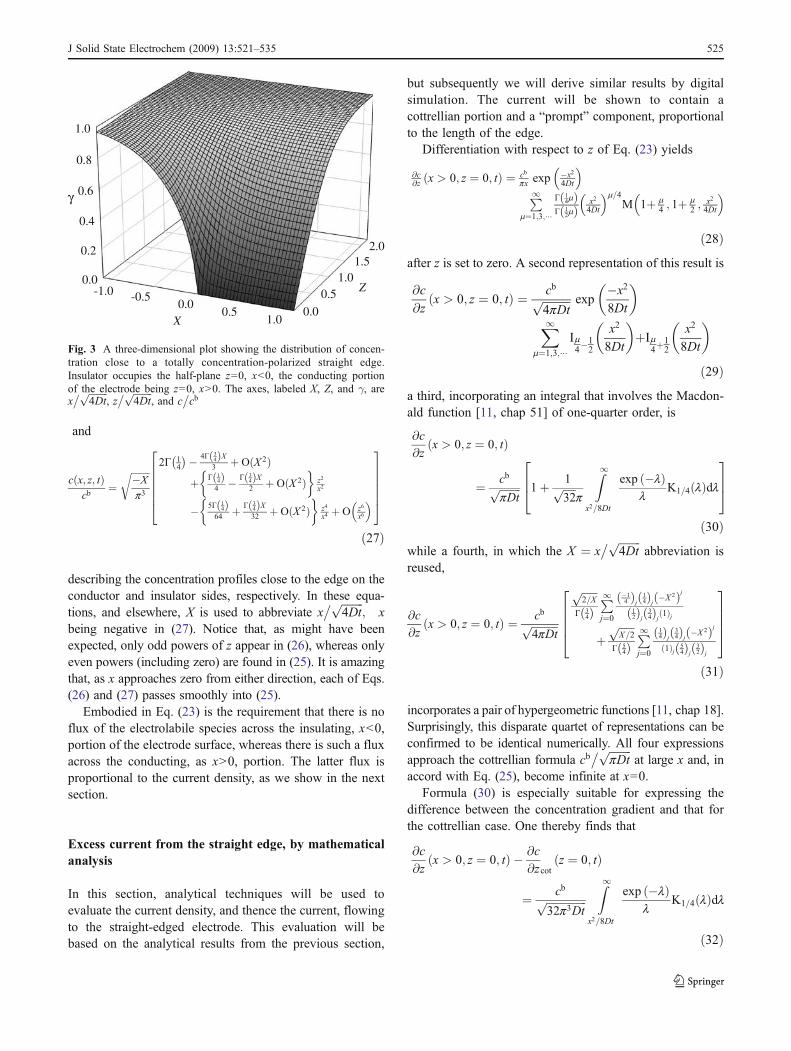
Figure 3 is a three-dimensional plot of Eq. (23). It suggeststhat the infinite concentration gradient is restricted to the(x, z)=(0, 0) line, and this is confirmed by the expansions

c x; z; tð Þcb

¼ffiffiffiffiffiX

p3

r * 14

�þ 2* 34

�X þ O X 2ð Þ� �

zx

� * 14ð Þ8 � * 3

4ð ÞX12 þ O X 2ð Þ

� z3

x3 þ O z5

x5

� �264

375

ð26Þ


and

c x; z; tð Þcb

¼ffiffiffiffiffiffiffiffi�X

p3

r 2* 14

�� 4* 34ð ÞX3 þ O X 2ð Þ

þ * 14ð Þ4 � * 3

4ð ÞX2 þ O X 2ð Þ

� z2

x2

� 5* 14ð Þ

64 þ * 34ð ÞX32 þ O X 2ð Þ

� z4

x4 þ O z6

x6

� �

2666664

3777775

ð27Þ

describing the concentration profiles close to the edge on theconductor and insulator sides, respectively. In these equa-tions, and elsewhere, X is used to abbreviate x

� ffiffiffiffiffiffiffiffi4Dt

p; x

being negative in (27). Notice that, as might have beenexpected, only odd powers of z appear in (26), whereas onlyeven powers (including zero) are found in (25). It is amazingthat, as x approaches zero from either direction, each of Eqs.(26) and (27) passes smoothly into (25).

Embodied in Eq. (23) is the requirement that there is noflux of the electrolabile species across the insulating, x<0,portion of the electrode surface, whereas there is such a fluxacross the conducting, as x>0, portion. The latter flux isproportional to the current density, as we show in the nextsection.

Excess current from the straight edge, by mathematicalanalysis

In this section, analytical techniques will be used toevaluate the current density, and thence the current, flowingto the straight-edged electrode. This evaluation will bebased on the analytical results from the previous section,

but subsequently we will derive similar results by digitalsimulation. The current will be shown to contain acottrellian portion and a “prompt” component, proportionalto the length of the edge.

Differentiation with respect to z of Eq. (23) yields

@c@z x > 0; z ¼ 0; tð Þ ¼ cb

px exp�x2

4Dt

� �P1

m¼1;3;��

* 14mð Þ

* 12mð Þ

x2

4Dt

� �m=4M 1þ m

4 ; 1þ m2 ;

x2

4Dt

� �

ð28Þafter z is set to zero. A second representation of this result is

@c

@zx > 0; z ¼ 0; tð Þ ¼ cbffiffiffiffiffiffiffiffiffiffi

4pDtp exp

�x2

8Dt

� �X1

m¼1;3;��Im4�

12

x2

8Dt

� �þIm

4þ12

x2

8Dt

� �

ð29Þa third, incorporating an integral that involves the Macdon-ald function [11, chap 51] of one-quarter order, is

@c

@zx > 0; z ¼ 0; tð Þ

¼ cbffiffiffiffiffiffiffiffipDt

p 1þ 1ffiffiffiffiffi32

pp

Z1x2=8Dt

exp �lð Þl

K1=4 lð Þdl

264

375

ð30Þwhile a fourth, in which the X ¼ x

� ffiffiffiffiffiffiffiffi4Dt

pabbreviation is

reused,

@c

@zx > 0; z ¼ 0; tð Þ ¼ cbffiffiffiffiffiffiffiffiffiffi

4pDtp

ffiffiffiffiffiffi2=X

p* 3

4ð ÞP1j¼0

�14ð Þ

j14ð Þj �X 2ð Þj

12ð Þj 3

4ð Þj 1ð Þj

þffiffiffiffiffiffiX=2

p* 5

4ð ÞP1j¼0

14ð Þj 3

4ð Þj �X 2ð Þj1ð Þj 5

4ð Þj 32ð Þj

26664

37775

ð31Þ

incorporates a pair of hypergeometric functions [11, chap 18].Surprisingly, this disparate quartet of representations can beconfirmed to be identical numerically. All four expressionsapproach the cottrellian formula cb

� ffiffiffiffiffiffiffiffipDt

pat large x and, in

accord with Eq. (25), become infinite at x=0.Formula (30) is especially suitable for expressing the

difference between the concentration gradient and that forthe cottrellian case. One thereby finds that

@c

@zx > 0; z ¼ 0; tð Þ � @c

@zcotz ¼ 0; tð Þ

¼ cbffiffiffiffiffiffiffiffiffiffiffiffiffiffiffi32p3Dt

pZ1

x2=8Dt

exp �lð Þl

K1=4 lð Þdl

ð32Þ

0.0

0.2

0.4

0.6

0.8

1.0

-0.50.0

0.51.0

0.0

0.51.0

1.52.0

Z

X

-1.0

γ

Fig. 3 A three-dimensional plot showing the distribution of concen-tration close to a totally concentration-polarized straight edge.Insulator occupies the half-plane z=0, x<0, the conducting portionof the electrode being z=0, x>0. The axes, labeled X, Z, and γ, arex� ffiffiffiffiffiffiffiffi

4Dtp

, z� ffiffiffiffiffiffiffiffi

4Dtp

, and c�cb


represents the additional current density due to theproximity of the straight edge.

If the electrode reaction involves a single electron, thenby Fick’s first and Faraday’s laws, the current density i(x, t)may be found by multiplying the concentration gradient atthe conductor surface by the diffusivity D and Faraday’sconstant F:

i x; tð Þ ¼ FD@c

@zx; 0; tð Þ ð33Þ

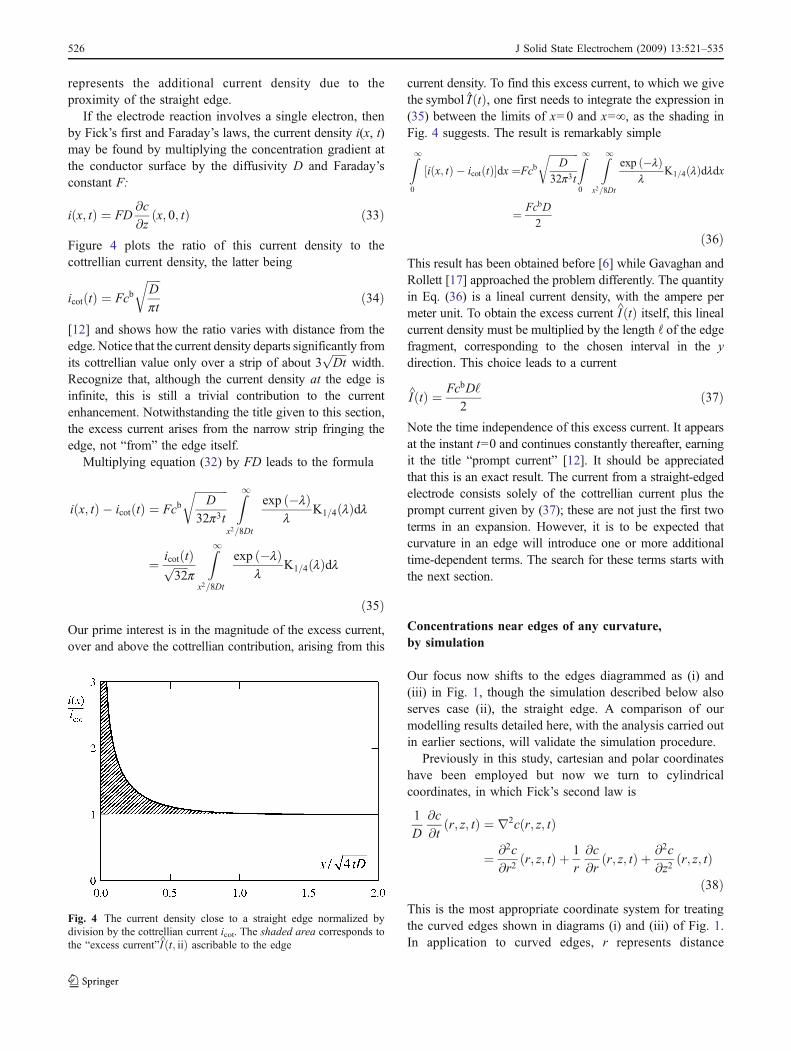
Figure 4 plots the ratio of this current density to thecottrellian current density, the latter being

icot tð Þ ¼ FcbffiffiffiffiffiD

pt

rð34Þ

[12] and shows how the ratio varies with distance from theedge. Notice that the current density departs significantly fromits cottrellian value only over a strip of about 3

ffiffiffiffiffiDt

pwidth.

Recognize that, although the current density at the edge isinfinite, this is still a trivial contribution to the currentenhancement. Notwithstanding the title given to this section,the excess current arises from the narrow strip fringing theedge, not “from” the edge itself.

Multiplying equation (32) by FD leads to the formula

i x; tð Þ � icot tð Þ ¼ FcbffiffiffiffiffiffiffiffiffiffiffiffiD

32p3t

r Z1x2=8Dt

exp �lð Þl

K1=4 lð Þdl

¼ icot tð Þffiffiffiffiffi32

pp

Z1x2=8Dt

exp �lð Þl

K1=4 lð Þdl

ð35ÞOur prime interest is in the magnitude of the excess current,over and above the cottrellian contribution, arising from this

current density. To find this excess current, to which we givethe symbol I tð Þ, one first needs to integrate the expression in(35) between the limits of x=0 and x=∞, as the shading inFig. 4 suggests. The result is remarkably simple

Z10

i x; tð Þ � icot tð Þ½ �dx ¼FcbffiffiffiffiffiffiffiffiffiffiffiffiD

32p3t

r Z10

Z1x2=8Dt

exp �lð Þl

K1=4 lð Þdldx

¼ FcbD

2

ð36ÞThis result has been obtained before [6] while Gavaghan andRollett [17] approached the problem differently. The quantityin Eq. (36) is a lineal current density, with the ampere permeter unit. To obtain the excess current I tð Þ itself, this linealcurrent density must be multiplied by the length : of the edgefragment, corresponding to the chosen interval in the ydirection. This choice leads to a current

I tð Þ ¼ FcbD‘

2ð37Þ

Note the time independence of this excess current. It appearsat the instant t=0 and continues constantly thereafter, earningit the title “prompt current” [12]. It should be appreciatedthat this is an exact result. The current from a straight-edgedelectrode consists solely of the cottrellian current plus theprompt current given by (37); these are not just the first twoterms in an expansion. However, it is to be expected thatcurvature in an edge will introduce one or more additionaltime-dependent terms. The search for these terms starts withthe next section.

Concentrations near edges of any curvature,by simulation

Our focus now shifts to the edges diagrammed as (i) and(iii) in Fig. 1, though the simulation described below alsoserves case (ii), the straight edge. A comparison of ourmodelling results detailed here, with the analysis carried outin earlier sections, will validate the simulation procedure.

Previously in this study, cartesian and polar coordinateshave been employed but now we turn to cylindricalcoordinates, in which Fick’s second law is

1

D

@c

@tr; z; tð Þ ¼ r2c r; z; tð Þ

¼ @2c

@r2r; z; tð Þ þ 1

r

@c

@rr; z; tð Þ þ @2c

@z2r; z; tð Þ

ð38ÞThis is the most appropriate coordinate system for treatingthe curved edges shown in diagrams (i) and (iii) of Fig. 1.In application to curved edges, r represents distance

Fig. 4 The current density close to a straight edge normalized bydivision by the cottrellian current icot. The shaded area corresponds tothe “excess current”I t; iið Þ ascribable to the edge


measured from the edge’s centre of curvature. We can adaptEq. (38) better to suit our purpose by replacing r by x�1=kð Þ for case (i) and case (iii), x being the distancecoordinate identified in Fig. 1. With this definition,differential equation (38) becomes

1

D

@c

@tðx; z; tÞ ¼ @2c

@x2ðx; z; tÞ � k

1� kx@c

@xðx; z; tÞ þ @2c

@z2ðx; z; tÞð39Þ

this equation being applicable not only to both curvedcases, but also to case (ii). The inclusion of the straightedge case arises because, when κ=0, the term in thisequation representing the cylindricity of the system dis-appears, leaving the cartesian version of Fick’s second law.Thus, Eq. (39) applies to all three of the geometries inFig. 1. In this equation, x=0 corresponds to the edge, x<0to the domain over the insulator, and x>0 to the domainover the conductor.

Because a representation in cylindrical coordinates isthen no longer appropriate, Eq. (39) ceases to make sensewhere x>1/κ for case (i), or where x<1/κ for case (iii).This is not a limitation in the present study, however,because our interest is confined to the narrow fringes ofinsulator and conductor on either side of the edge.

The initial condition,

c x; z; tð Þ ¼ cb; 0 < z � 1; all x; t � 0 ð40Þprescribing a preexisting concentration uniformity, applies.The crucial boundary conditions are

c x; 0; tð Þ ¼ 0 x > 0; t > 0 ð41Þand

@c

@zx; 0; tð Þ ¼ 0 x < 0; t > 0 ð42Þ

which respectively assert that the electrolabile species isabsent from the electrode surface and has no flux across theinsulator surface.

An analytical solution may exist to the equation set (39)–(42) but, at this juncture, we have found it only for the κ=0instance, as reported above. Therefore, we turn to digitalsimulation and seek an approximate prediction. As in mostsimulations [14], the first and second steps are toundimension and then discretize the variables. The threeindependent variables and the one dependent variable areundimensioned through the definitions

t ¼ Dt

‘2; z ¼ z

‘; # ¼ x

‘and g #; z; tð Þ ¼ c x; z; tð Þ

cb

ð43ÞNote that χ cannot exceed 1/κ : in case (i) and must exceed−1/κ : in case (iii), there being no restriction in case (ii).These constraints arise because it is implicit in Eq. (39) that

r be non-negative. For the sake of uniformity, the condition�1= kj j‘ð Þ < # < 1= kj j‘ð Þ is applied universally in thissection and, in view of the standard length : that we adopt,this implies that our simulation domain occupies the region

�1 < # < 1 ð44ÞAdoption of the dimensionless terms defined in (43)converts the differential equation (39) into

@2g@#2

#; z; tð Þ � k‘1� k‘#

@g@#

#; z; tð Þ þ @2g

@z2#; z; tð Þ

� @g@t

#; z; tð Þ ¼ 0

ð45Þwhile its attendant conditions, stemming from formulas(39–42) become

g #; z; 0ð Þ ¼ 1 � 1 < # < 1; z > 0 ð46Þ

g #; 0; tð Þ ¼ 0 0 <#< 1; t > 0 ð47Þand

@g@z

#; 0; tð Þ ¼ 0 � 1 < # < 0; t > 0 ð48Þ

It is this set of equations that is modelled for each of thethree cases, with κ : set to 1, 0, or −1 for cases (i), (ii), and(iii), respectively.

Discretization of the four dimensionless variables isaccomplished by the replacements

t ) kd; z ) m$; # ) n$; and g #; z; tð Þ ) gn;m;k

ð49Þ

in which variables that actually change continuously aresubstituted by quantities whose values change stepwise.Here k ¼ 1; 3; 5; � � � , m ¼ 1; 3; 5; � � �, and n ¼ � � � �5;�3;�1;þ1;þ3;þ5; � � �. Note our addiction to oddindices. The dimensionless δ and Δ quantities are smalltime and distance units respectively, of arbitrary magnitude.We choose Δ to be the reciprocal of a large even integer,typically 1,000 and, for a reason discussed later, we set δ=2Δ2/5.

For simplicity, and in line with a philosophy enunciatedearlier [15], we employ the oldest, slowest, and mostelementary modelling technique: fully explicit finite-differ-ence digital simulation. We toyed with non-uniform grids,but discarded that computation-time-saving strategy in viewof the added complication. There are only three non-standard features of our simulation. Our simulation is“differential”, rather than absolute. The boundaries of ouractive simulation space adapt to need. And our procedurefor fitting the concentration normal to the conductor surface


is to an unusual “013 polynomial”. These three abnormalfeatures are elaborated below. The simulation wasprogrammed straightforwardly in Visual Basic® and exe-cuted on a standard PC.

In addition to the two-dimensional array dedicated to themodelling of the set of equations numbered (44) through(47), we also employed a one-dimensional array wherebywe simulated the equation set

@2b

@z2z; tð Þ � @b

@tz; tð Þ ¼ 0 ð50Þ

b z; tð Þ ¼ 1 0 < z < 1; t ¼ 0 ð51Þand

b z; tð Þ ¼ 0 z ¼ 0; t > 0 ð52Þthereby modelling the Cottrell experiment. Here β signifiesthe undimensioned cottrellian concentration (c/cb)cot, dis-cretized as βm,k. The Cottrell simulation is run consecu-tively with the two-dimensional simulation because interestis in the difference between the two current densities.Moreover, a comparison is continually made betweencorresponding concentrations in the β and g arrays as ameans of economizing computation time, as describedbelow.

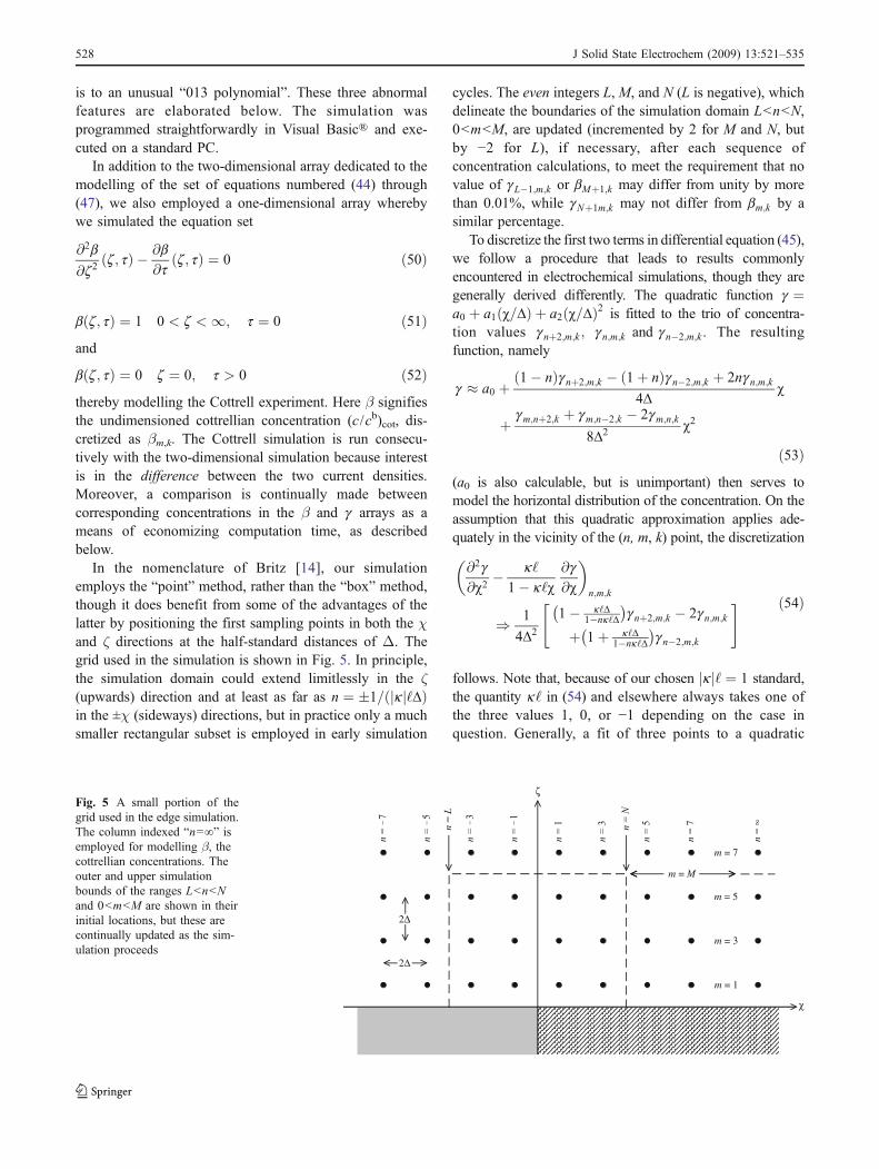
In the nomenclature of Britz [14], our simulationemploys the “point” method, rather than the “box” method,though it does benefit from some of the advantages of thelatter by positioning the first sampling points in both the χand ζ directions at the half-standard distances of Δ. Thegrid used in the simulation is shown in Fig. 5. In principle,the simulation domain could extend limitlessly in the ζ(upwards) direction and at least as far as n ¼ �1= kj j‘$ð Þin the ±χ (sideways) directions, but in practice only a muchsmaller rectangular subset is employed in early simulation

cycles. The even integers L, M, and N (L is negative), whichdelineate the boundaries of the simulation domain L<n<N,0<m<M, are updated (incremented by 2 for M and N, butby −2 for L), if necessary, after each sequence ofconcentration calculations, to meet the requirement that novalue of gL�1;m;k or bMþ1;k may differ from unity by morethan 0.01%, while gNþ1m;k may not differ from bm;k by asimilar percentage.

To discretize the first two terms in differential equation (45),we follow a procedure that leads to results commonlyencountered in electrochemical simulations, though they aregenerally derived differently. The quadratic function g ¼a0 þ a1 #=$ð Þ þ a2 #=$ð Þ2 is fitted to the trio of concentra-tion values gnþ2;m;k ; gn;m;k and gn�2;m;k . The resultingfunction, namely

g � a0 þð1� nÞgnþ2;m;k � ð1þ nÞgn�2;m;k þ 2ngn;m;k

4$#

þ gm;nþ2;k þ gm;n�2;k � 2gm;n;k8$2 #2

ð53Þ(a0 is also calculable, but is unimportant) then serves tomodel the horizontal distribution of the concentration. On theassumption that this quadratic approximation applies ade-quately in the vicinity of the (n, m, k) point, the discretization

@2g@#2

� k‘1� k‘#

@g@#

� �n;m;k

) 1

4$2

1� k‘$1�nk‘$

�gnþ2;m;k � 2gn;m;k

þ 1þ k‘$1�nk‘$

�gn�2;m;k

" # ð54Þ

follows. Note that, because of our chosen kj j‘ ¼ 1 standard,the quantity k‘ in (54) and elsewhere always takes one ofthe three values 1, 0, or −1 depending on the case inquestion. Generally, a fit of three points to a quadratic

ζ

χ

m = 1

m = 3

m = 7

m = 5

m = M

2Δ

2Δ

Fig. 5 A small portion of thegrid used in the edge simulation.The column indexed “n=∞” isemployed for modelling β, thecottrellian concentrations. Theouter and upper simulationbounds of the ranges L<n<Nand 0<m<M are shown in theirinitial locations, but these arecontinually updated as the sim-ulation proceeds


function also provides the basis for discretizing the thirdterm in differential equation (45). This leads to thefamiliar result

@2g

@z2

� �n;m;k

) gn;mþ2;k � 2gn;m;k þ gn;m�2;k

4$2 ð55Þ

To discretize the final right-hand term in Eq. (45), thetemporal derivative is replaced by a simple forwarddifference quotient:

@g@t

z; #; tð Þ ) gn;m;kþ2 � gn;m;k2d

ð56Þ

This completes the tally of terms in Eq. (45) for which wehave derived discretized equivalents. Putting them alltogether leads, after rearrangement, to

gn;m;kþ2 ¼ gn;m;k þd

2$2

c1gnþ2;m;k þ c2gn�2:m:k þ c3gn;mþ2;k

þc4gn;m�2;k � c5gn;m;k

� ð57Þ

with the coefficients c1,2,–,5 given the values listed in the firstrow of Table 1. Equation (57) shows how, during an intervalof duration 2δ, each typical point interacts diffusionally withits four neighboring points (in reality each “point” is afragment of a circular hoop, except for the straight-edge case,in which it is a straight line fragment). The formula must bemodified when m=1, because such points have only threeneighbors. There are two revised formulas, depending onwhether the m=1 point is adjacent to the insulator or theconductor. These revisions are discussed in the next paragraphand the resulting coefficients are presented as the second andthird rows of Table 1. The final two rows in the table providecoefficients for the corresponding terms in the β-updatingformulas.

Points for m=1 have only three neighbors because of theproximity of the insulator or the conductor. For the pointsadjacent to the insulator, the replacement formula, incorpo-rated into the second row of Table 1, was constructedstraightforwardly by discretizing the @2g

�@z2 term and

assigning a concentration gradient of zero to a fittedquadratic at ζ=0. For those m=1 points adjacent to theconductor, we discretized the @2g

�@z2 portion of Eq. (45)—

and also the @2b�@z2 term in (50)—by abandoning

quadratic fitting in favor of a fit to the

g ¼ b0 þ b1z$þ b3

z$

� �3

ð58Þ

polynomial. Our preference for this “013 polynomial”derives from the match that it provides to the second andthird terms in Eq. (26). To obtain a good match to reality inthe region adjoining the conductor is crucial, because this isthe region from which the faradaic current arises. The bcoefficients can be evaluated by fitting to the m=1 and m=3 points and constraining the polynomial to pass throughzero at ζ=0. With 013 polynomial fitting, this leads to thesimulation formula

@2g

@z2

� �n;1;k

) gn;3;k � 3gn;1;k4$2 ð59Þ

Had we used the customary quadratic (or “012 polynomial”)fit, the “4” in (59) would have been replaced by a “3”. Thisprovides the basis for the third row of entries in Table 1. Itmay seem irrational to use a 013 polynomial to fit thevertical concentration profile in the vicinity of the m=1point, but revert to the quadratic fit for m=3, 5, –.Surprisingly, however, both the 012 and 013 polynomialslead to identical formulas, namely Eq. (55), at points otherthan those adjacent to the electrode.

There is danger of instability in a simulation if thecoefficient of any concentration term in the concentration-updating equations is negative. In our particular problem,this implies that 1� c5d

�2$2

� � 0. This considerationdictated our choice of d ¼ 2$2

�5 as the relationship

between the magnitudes of the dimensionless time anddistance units.

To validate our simulation, we compared concentra-tions calculated exactly from the mathematical theorywith those generated by simulation for the straight edge,case (ii). Because it is the most crucial location for thesimulation, and this is where the largest discretizationerrors might be expected, we chose to compare at theedge itself, where x=χ=0. Figure 6 makes the compari-son. The line in this figure is calculated from the full Eq.

Table 1 Coefficients of the five terms in Eq. (57) during the simulation of the points indexed n and m

n m c1 c2 c3 c4 c5

Lþ 1; � � � ;�3;�1; 1; 3; � � � ;N � 1 3; 5; � � � ;M � 1 1� k‘$1�nk‘$ 1þ k‘$

1�nk‘$ 1 1 4�1;�3; � � � ; Lþ 1 1 1� k‘$

1�nk‘$ 1þ k‘$1�nk‘$ 1 No such point 3

1; 3; � � � ;N � 1 1 1� k‘$1�nk‘$ 1þ k‘$

1�nk‘$ 1 No such point 5∞ 3; 5; � � � ;M � 1 No such point No such point 1 1 2∞ 1 No such point No such point 1 No such point 3

The final two rows relate to the one-dimensional simulation of concentration β


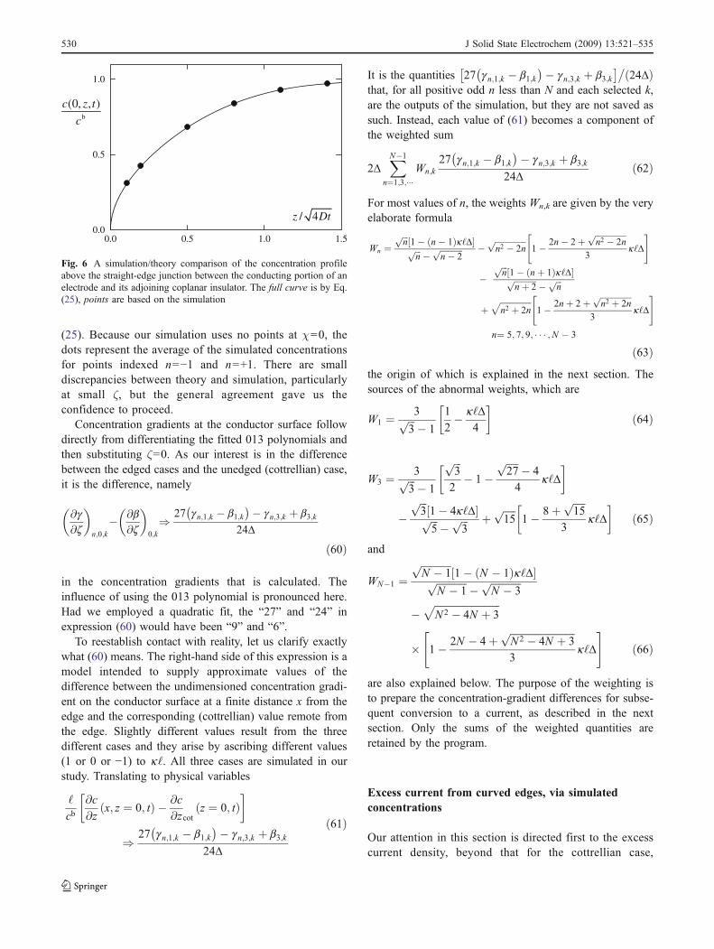
(25). Because our simulation uses no points at χ=0, thedots represent the average of the simulated concentrationsfor points indexed n=−1 and n=+1. There are smalldiscrepancies between theory and simulation, particularlyat small ζ, but the general agreement gave us theconfidence to proceed.

Concentration gradients at the conductor surface followdirectly from differentiating the fitted 013 polynomials andthen substituting ζ=0. As our interest is in the differencebetween the edged cases and the unedged (cottrellian) case,it is the difference, namely

@g@z

� �n;0;k

� @b@z

� �0;k

) 27 gn;1;k � b1;k �� gn;3;k þ b3;k

24$

ð60Þ

in the concentration gradients that is calculated. Theinfluence of using the 013 polynomial is pronounced here.Had we employed a quadratic fit, the “27” and “24” inexpression (60) would have been “9” and “6”.

To reestablish contact with reality, let us clarify exactlywhat (60) means. The right-hand side of this expression is amodel intended to supply approximate values of thedifference between the undimensioned concentration gradi-ent on the conductor surface at a finite distance x from theedge and the corresponding (cottrellian) value remote fromthe edge. Slightly different values result from the threedifferent cases and they arise by ascribing different values(1 or 0 or −1) to k‘. All three cases are simulated in ourstudy. Translating to physical variables

‘

cb@c

@zx; z ¼ 0; tð Þ � @c

@zcotz ¼ 0; tð Þ

�

) 27 gn;1;k � b1;k �� gn;3;k þ b3;k

24$

ð61Þ

It is the quantities 27 gn;1;k � b1;k �� gn;3;k þ b3;k

� ��24$ð Þ

that, for all positive odd n less than N and each selected k,are the outputs of the simulation, but they are not saved assuch. Instead, each value of (61) becomes a component ofthe weighted sum

2$XN�1

n¼1;3;��Wn;k

27 gn;1;k � b1;k �� gn;3;k þ b3;k

24$ð62Þ

For most values of n, the weights Wn,k are given by the veryelaborate formula

Wn ¼ffiffiffin

p1� ðn� 1Þk‘$½ �ffiffiffin

p � ffiffiffiffiffiffiffiffiffiffiffin� 2

p �ffiffiffiffiffiffiffiffiffiffiffiffiffiffiffin2 � 2n

p1� 2n� 2þ

ffiffiffiffiffiffiffiffiffiffiffiffiffiffiffin2 � 2n

p

3k‘$

" #

�ffiffiffin

p1� ðnþ 1Þk‘$½ �ffiffiffiffiffiffiffiffiffiffiffinþ 2

p � ffiffiffin

p

þffiffiffiffiffiffiffiffiffiffiffiffiffiffiffin2 þ 2n

p1� 2nþ 2þ ffiffiffiffiffiffiffiffiffiffiffiffiffiffiffi

n2 þ 2np

3k‘$

" #

n¼ 5; 7; 9; � � � ;N � 3

ð63Þthe origin of which is explained in the next section. Thesources of the abnormal weights, which are

W1 ¼ 3ffiffiffi3

p � 1

1

2� k‘$

4

� ð64Þ

W3 ¼ 3ffiffiffi3

p � 1

ffiffiffi3

p

2� 1�

ffiffiffiffiffi27

p � 4

4k‘$

�

�ffiffiffi3

p1� 4k‘$½ �ffiffiffi5

p � ffiffiffi3

p þffiffiffiffiffi15

p1� 8þ ffiffiffiffiffi

15p

3k‘$

� ð65Þ

and

WN�1 ¼ffiffiffiffiffiffiffiffiffiffiffiffiN � 1

p1� ðN � 1Þk‘$½ �ffiffiffiffiffiffiffiffiffiffiffiffi

N � 1p � ffiffiffiffiffiffiffiffiffiffiffiffi

N � 3p

�ffiffiffiffiffiffiffiffiffiffiffiffiffiffiffiffiffiffiffiffiffiffiffiffiffiffiN 2 � 4N þ 3

p

1� 2N � 4þ ffiffiffiffiffiffiffiffiffiffiffiffiffiffiffiffiffiffiffiffiffiffiffiffiffiffiN2 � 4N þ 3

p

3k‘$

" #ð66Þ

are also explained below. The purpose of the weighting isto prepare the concentration-gradient differences for subse-quent conversion to a current, as described in the nextsection. Only the sums of the weighted quantities areretained by the program.

Excess current from curved edges, via simulatedconcentrations

Our attention in this section is directed first to the excesscurrent density, beyond that for the cottrellian case,

0.0 0.5 1.0 1.50.0

0.5

1.0

/ 4z Dt

b

(0, , )c z t

c

Fig. 6 A simulation/theory comparison of the concentration profileabove the straight-edge junction between the conducting portion of anelectrode and its adjoining coplanar insulator. The full curve is by Eq.(25), points are based on the simulation


flowing across the conductor surface at a distance x fromthe edge and at a time t after the potential jump. We shallrepresent this current density difference by the “hatted”symbol

iðx; tÞ ¼ iðx; tÞ � icotðtÞ ¼ iðx; tÞ � FcbffiffiffiffiffiffiffiffiffiffiD=pt

pð67Þ

Though the cottrellian current density is known analyti-cally, it is the simulated version that is subtracted, thebetter to compensate for discretization errors. Mostly, wework with a dimensionless current density difference,undimensioned by division by FcbD / : and represented bya hatted iota symbol. Because we are treating a one-electron reaction, multiplication by FD is all that isrequired to convert an electrode-surface concentrationgradient into a current density; thus:

i #; tð Þ ¼ ‘ i x; tð ÞFcbD

¼ ‘

cb@c

@zx; z ¼ 0; tð Þ � @c

@zcotz ¼ 0; tð Þ

� ð68Þ

Each of our simulations generates a set of values of ið#; tÞat χ values of $; 3$; 5$; � � � ; n$; � � � and at a set of τvalues equal to kδ for odd integers k. Members of thisdiscrete set of discretized undimensioned current densitydifferences are symbolized in;k . Thus, from Eqs. (67) and(61),

in;k ¼27 gn;1;k � b1;k

�� gn;3;k þ b3;k24$

ð69Þ

Prior to weighting, the output of the simulation is simplythe undimensioned current density difference, and so a setof values of i 7 ; tð Þ at χ values of $; 3$; 5$; � � � ;n$; � � � is accessible for a set of τ values equal to kδ forodd integers k.

Areal integration is required to convert the excesscurrent density into the excess current I tð Þ associated withthe edges. We make this conversion for the three cases,symbolizing the results by I t; ið Þ, I t; iið Þ and I t; iiið Þ. Theformula

I tð Þ ¼ ‘

Z3 ffiffiffiffiDt

p

0

i x; tð Þ 1� kx½ � d x ¼ FcbD‘

Z3 ffiffit

p

0

i #; tð Þ 1� k‘#½ � d #

ð70Þapplies, with the term [1−κx] allowing for the convergent(case i), uniform (case ii), or divergent (case iii) integrationdomain. The upper integration bound reflects the findingfrom Fig. 4 that the width of the strip fringing the straightedge over which the cottrellian current is augmented isapproximately 3

ffiffiffiffiffiDt

p. In practice, our integration uses the

entire conductor surface 0 � # � N � 1ð Þ$ of the model,stopping only when the numerical values of the concentra-tion prove to be insignificantly different from the cottrellianconcentrations.

The integration in (70) is performed by breaking theintegration range into a collection of segments, each ofwidth 2Δ, except for the first, which is 3Δ wide:

I tð ÞFcbD‘

¼ZN$

0

i #; tð Þ 1� k‘$½ �d#

¼Z3$0

i #; tð Þ 1� k‘$½ �d#þXN�3

n¼3;5;��

ZnΔþ2$

n$

i #; tð Þ 1� k‘$½ �d#

ð71Þ

Because, as Fig. 4 shows, the excess current densitychanges so dramatically with distance from the edge, wemust interpolate carefully between the simulated values,and extrapolate shrewdly into the space between the edgeand the n=1 point, prior to performing the integration. Avehicle for the interpolation is provided by Eq. (26), whichshows, at least for the straight-edge case, that theexpression for the current density as a function of x has aleading term in x−1/2. Moreover, the cottrellian subtractivecontribution to i is, of course, x-independent. So we baseour fitting on the formula

i #; tð Þ ¼ constantð Þ þ anotherconstant

� � ffiffiffiffi$

#

sð72Þ

and fit a relation of this form between consecutive positiveodd n values. Each relation is designed to adopt thesimulated values in;k and inþ2;k at either end of thesegment. This is achieved by the formula

ið#; tÞ ¼ffiffiffiffiffiffiffiffiffiffiffinþ 2

pinþ2;k �

ffiffiffin

pin;k þ

ffiffiffiffiffiffiffiffiffiffiffiffiffiffiffin2 þ 2n

p ½in;k � inþ2;k �ffiffiffiffiffiffiffiffiffiΔ=#

pffiffiffiffiffiffiffiffiffiffiffinþ 2

p � ffiffiffin

p

ð73Þ

After multiplication by the 1−k‘# factor, definite integra-tion now gives

Zn$þ2$

n$

ið#; tÞ 1� k‘#½ �d#

¼ 2$

ffiffiffiffiffiffinþ2

pinþ2;k�

ffiffin

pin;kffiffiffiffiffiffi

nþ2p � ffiffi

np 1� ðnþ 1Þk‘$½ �þffiffiffiffiffiffiffiffiffiffiffiffiffiffiffi

n2 þ 2np ½in;k � inþ2;k � 1� 2nþ 2þ ffiffiffiffiffiffiffiffiffiffiffiffiffiffiffi

n2 þ 2np �

k‘$3

� �24

35

ð74Þ

This integral may be written concisely as

Zn$þ2$

n$

i #; tð Þ 1þ k‘#½ � d # ¼ 2$ Rnþ2inþ2;k þ Snin;k� � ð75Þ


where the R and S quantities may be gleaned from the right-hand side of formula (74). A careful regrouping of acollection of these integrals produces

XN�1

n¼3;5;��

Zn$þ2$

n$

i #; tð Þ 1� k‘#½ � d #

¼ 2$ RN�1iN�1;k þ S3 i3;k þXN�1

n¼5;7;��Rn þ Snð Þin;k

" #

ð76ÞThe sum Rn+Sn is, in fact, the weighting factor denoted Wn

in Eq. (63). The solitary RN−1 term leads to (66). The 0<χ<3Δ integral in (70) contributes far more than any othersegment. It has to be treated somewhat differently because,though the integral is finite, the integrand is infinite at itslower bound. Accordingly, the fitting to (71) is provided bythe i1;k and i3;k values, which leads to

Z3$0

i #; tð Þ½1� k‘#�d#

¼ 3$ffiffiffi3

p � 1

ffiffiffi3

p� 2�

ffiffiffiffiffi27

p

2� 2

� �k‘$

� i3;k þ 1� k‘$

2

� i1;k

�

ð77ÞThe coefficient of i1;k in this formula is the source of the W1

term in Eq. (64), while the coefficient of i3;k , added to S3,gives W3 in (65).

Thus it is that a suitably weighted sum of thedimensionless concentrations provides the following ex-pression for the dimensionless excess current:

I tð ÞFcbD‘

)XN�1

n¼1;3;��Wn

27gn;1;k � 27b1;k � gn;3;k þ b3;k12

ð78ÞThis model is valid for all three cases. For the straight-edge case, the value predicted in Eq. (37) for thisdimensionless excess current is 1/2. Using expression(78), the simulation produces values somewhat larger thanthis, but as the time counter k increases, the valuesreassuringly approach 0.50. There is no direct interest insimulating currents at the straight edge, however, becausethe exact theory earlier in this article is unequivocal: thecurrent beyond the cottrellian is solely the prompt current,common to all edges:

I t; iið Þ ¼ FcbD

2‘ ð79Þ

The excess current is proportional to the length of the edgeand to the diffusivity, but time independent.

The motivation for our work is primarily to investigatecurved edges, for which no theory presently exists. We seekto find the faradaic current generated by concave andconvex edges, over and above the contribution fromcottrellian and prompt currents. This is not an easy task,for it is a third order effect that we wish to measure.Therefore, a differential approach is again adopted, in thehope that discretization errors will mostly cancel. Instead ofevaluating how the excess current at a curved edge changeswith time, we measure the difference between the currentsat curved edges and those at a straight edge. Threesimulations were made, Eq. (78) then being used tocompute values of the differences I t; ið Þ � I t; iið Þ andI t; iiið Þ � I t; iið Þ undimensioned, in each case, by divisionby FcbD‘. These values are shown plotted versus

ffiffiffik

p$ in

Fig. 7. Plotting versusffiffiffik

p$ is equivalent to plotting versus

the square root of time.The figure shows that, initially, there is no voltammetric

difference between straight and curved edges: they shareidentical prompt currents. It also shows that additionalcurrent flows from curved edges, compared to straightedges, the extra current being positive for concave edgesand negative for convex edges. The differences from thestraight edge are approximately equal in magnitude, thoughopposite in sign, showing that the additional current (calledthe “augmentative current” in the next section) is propor-tional to the curvature of the edge. Furthermore, Fig. 7demonstrates that the augmentative current increases as thesquare root of time. Arguing from the established propertiesof concave circular edges, as discussed in the next section,we expected the augmentative slope to equal k=4ð Þ ffiffiffiffiffiffiffiffiffiffi

Dt=pp

,and the straight lines in the figure correspond to such a

0.00 0.02 0.04 0.06 0.08 0.10-0.010

-0.005

0.000

0.005

0.010

k Δ

b

( ,i) ( ,ii)Î t Î t

Fc D

b

( ,iii) ( ,ii)Î t Î t

Fc D

–

–

Fig. 7 Graphs of the concavely curved-minus-straight-edged andconvexly curved-minus-straight-edged currents plotted versus thesquare root of time, both the ordinate and the abscissa being suitablynormalized. The points are derived from simulation, the straight linesrepresent expectations


value. Though we could have wished for better, weconsider that the agreement between the lines and thepoints is adequate to confirm our expectation.

Conclusions and applications

We conclude that the response of an edge fragment to apotential jump is the sum of two terms, each proportional tothe length of the curve, the second term also beingproportional to the curvature of the edge and to the squareroot of time:

I tð ÞFcbD

¼ ‘

2þ k‘

4

ffiffiffiffiffiffiDt

p

rð80Þ

The second right-hand term is positive for concave edges,negative for convex edges, and absent for straight edges.We use the names “prompt” and “augmentative” todistinguish the currents, the latter name reflecting theproperty of increasing with time, in contrast to theconstancy of the prompt current and the evanescent natureof the cottrellian current.

In the context of partially blocked electrodes, edges willrarely have uniform curvature, but they will generally be“closed”. That is to say edges will enclose “islands” ofeither insulator or conductor, as portrayed by (a) and (b) inFig. 8. The integral of the curvature around a closed curveis the overall angle turned, that is 2π, and therefore theexcess current arising from an island is given by

Iisland tð ÞFcbD

¼ ‘

2þ

ffiffiffiffiffiffiffiffipDt

p

2

Ik d ‘ ¼ ‘

2�

ffiffiffiffiffiffiffiffiffiffip3Dt

pð81Þ

where the “+” sign in the augmentative term applies to anisland of conductor in a “sea” of insulator, and the “−” signto an island of insulator in a sea of conductor. Interestingly,an “atoll” geometry, as in Fig. 8c, contributes nothing to theaugmentative current.

We view Eqs. (80) and (81) as temporary descriptorsof the chronoamperometric behavior of edges. Theybecome increasingly suspect as time increases. Theywere derived for isolated edge fragments and ignore anyinfluence that one fragment may have on another.We call any such influence a “proximity effect”; item(d) in Fig. 8 illustrates three circumstances in which this

Fig. 9 A diagram showing the contribution of various currents to thetotal chronoamperometric current at an inlaid disk electrode, as timeunfolds. The cottrellian current arises from the surface of theelectrode, whereas the prompt current is from its perimeter. Theaugmentative current has its origin in the curvature of the electrodeedge. The “proximity current”, which is negative, arises fromcompetition for diffusant between different regions of the edge

(b)(a)

(c)

(d)

Fig. 8 Models of partiallyblocked electrodes. In all fourdiagrams, hatching representsconducting regions of the sur-face, insulating regions beingshaded grey. (a) represents an“island” of insulator, while (b) isa conducting island. The “atoll”topology of (c) has an island ofinsulator within an island ofconductor, which is itself withina “sea” of insulator. The geom-etry of the island in (d) results inthree places at which proximityeffects will diminish the edgecurrent


effect would be especially severe, limiting the uppertime limit for the validity of Eqs. (80) and (81).Proximity always decreases the current because twoedges are then competing for the diffusing species, sothat each goes hungry to some extent. Though it is a crudeestimate, proximity effects come into play when the twointerfering edges are at a distance of less than about 3

ffiffiffiffiffiDt

pfrom each other.

The only curved edge that has been studied deeply byelectrochemists is that separating the conductor and theinsulator surfaces in the popular inlaid disk electrode. Ifsuch an electrode has a radius a, the conductor has an areaα of πa2; the edge has a length : of 2πa and a curvature κof 1/a. There is no single exact theoretical equation knownto describe the one-electron diffusion-controlled current atthis electrode, but the five-term expansion

Idisk tð ÞFcbD

¼ a2ffiffiffiffiffiffipDt

rþ paþ

ffiffiffiffiffiffiffiffipDt

p

2� 3pDt

25aþ 3p

ffiffiffiffiffiffiffiffiffiD3t3

p

226a2ð82Þ

is known [16] to be valid to parts-per-million accuracy fortimes up to t=1.281a2/D. When rewritten as

Idisk tð ÞFcbD

¼ affiffiffiffiffiffiffiffipDt

p þ ‘

2þ k‘

4

ffiffiffiffiffiffiDt

p

r� 3pDt

25aþ 3p

ffiffiffiffiffiffiffiffiffiD3t3

p

226a2ð83Þ

the first three right-hand terms can be immediatelyidentified as the cottrellian, prompt, and augmentativecurrents, respectively, while the last two can be assignedto the proximity effect. It is instructive to assess the relativeimportance of the various currents for the inlaid diskelectrode; this is accomplished in Fig. 9. Note that theprompt current is dominant for most of the time, empha-sizing the importance of the edge in the voltammetry of thiselectrode. Beyond the confines of the graph, the promptcurrent retains its dominance and eventually contributes79% of the steady-state current.

Other authors [2, 3] have idealized the geometry ofpartially blocked electrodes by likening them to structureswith uniformly sized, neatly arranged shapes on the surfaceof an otherwise naked electrode. But, without making anypreassumption whatsoever about the geometry of a partiallyblocked electrode, what can be learned from analyzing itsresponse to a potential jump?

Let us suppose that the capacitive current has beencarefully eliminated (it, too, can throw light on thegeometry of a partially blocked electrode, but that isanother story) and that the remaining faradaic responsehas been analyzed to find the magnitudes of the compo-nents with t�1=2; t0; and t1=2 time dependences:

I tð Þ ¼ pffiffit

p þ qþ sffiffit

p þ � � � ð84Þ

Clearly, the component with t−1/2 dependence may be usedto find the total area occupied by conductor, because

comparison with the prediction of Cottrell’s equation showsthat

total conductor area ¼ffiffiffiffipD

rp

Fcbð85Þ

The total length of the interfacial lines separating insulatorfrom conductor is directly accessible from the promptcurrent. One has

total edge length ¼ 2q

FcbDð86Þ

If the ratio of total conductor area to the overall electrodearea A is small, then it is reasonable to assume that theconductor forms islands in a sea of insulator, and thattherefore s will be positive. On the other hand, if theconductor area is close to A, then the islands will likelycontain insulator and s will be negative. In either event,one can calculate the number of islands from themagnitude of the augmentative current component by theformula

number of islands ¼ sj jFcb

ffiffiffiffiffiffiffiffiffiffip3D3

p ð87Þ

and thence find the average area and perimeter of theislands. For cases in which it is the conductor thatconstitutes the islands, the formulas are

average island area ¼ total conductor area

number of islands

¼ p2pDs

ð88Þ

and

average island perimeter ¼ total edge length

number of islands

¼ 2qffiffiffiffiffiffiffiffip3D

p

sð89Þ

Similar relationships apply when the islands are composedof insulator. If both kinds of island exist, it is thedifference between the numbers that is significant.

Though relationships (85)–(89) are correct in principle,experimental conditions will need to be favorable to allowtheir successful exploitation. Being of third order, param-eter s will be particularly difficult to measure. One featureof the partially blocked geometry that may be assessedwithout knowledge of s is the ratio of the area of an averageisland to its perimeter:

average ðarea=perimeterÞ ratio ¼ pffiffiffiffiffiffiffiffip3D

p

2qð90Þ

This is a quantity with the unit of length and could beconsidered to measure the “grain size” of the conductor/


insulator mosaic. It will be large when the blocking is dueto structures of large size, small when it is somemicrostructure that is responsible.

Acknowledgements The financial support of the Natural Sciencesand Engineering Research Council of Canada is acknowledged withgratitude. Keith Oldham warmly thanks Alan Bond and Fritz Scholz,not only for their editing of this article but also for their generosity andeffort in envisaging and assembling the entire issue. Other contributorsto this issue are also thanked for their kind dedications.

References

1. Lee C-Y, Guo S-X, Bond AM, Oldham KB (2008) J ElectroanalChem 615:1

2. Amatore C, Saveant J-M, Tessier D (1983) J Electroanal Chem 147:393. Davies TJ, Banks CD, Compton RG (2005) J Solid State

Electrochem 9:797

4. Arrigan DWM (2004) Analyst 129:11575. Fletcher S, Horne MD (1999) Electrochem Commun 1:5026. Oldham KB (1981) J Electroanal Chem 198:17. Boas ML (1973) Mathematical methods in the physical sciences.

Wiley, New York8. Mathews J, Walker RL (1964) Mathematical methods of physics.

Benjamin, New York9. Morse PM, Feshbach H (1953) Methods of theoretical physics.

McGraw Hill, Boston10. Abramowitz M, Stegun AI (1964 and subsequent eds) Handbook

of Mathematical Functions, National Bureau of Standards,Washington D.C., chap 13

11. Oldham KB, Myland JC, Spanier J (2008) An atlas of functionssecond edition. Springer, New York

12. Cottrell FG (1903) Z Phys Chem 42:38513. Oldham KB (1991) J Electroanal Chem 297:31714. Britz D (2005) Digital simulation in electrochemistry. Springer,

Heidelberg15. Myland JC, Oldham KB (2005) J Electroanal Chem 576:16316. Mahon PJ, Oldham KB (2005) Anal Chem 77:610017. Gavaghan DJ, Rollett JS (1990) J Electroanal Chem 295:1


The electrochemistry of electrode edges and its relevance ...koldham/Paper224-Reprint.pdf · The electrochemistry of electrode edges and its relevance to partially blocked voltammetric

Documents