The effects of inlet sedimentation on water exchange in Maha Oya Estuary, Sri Lanka ___________________________________________________________________ Linda Nylén Ebba Ramel Examensarbete TVVR 12/5009 Division of Water Resources Engineering Department of Building and Environmental Technology Lund University

Welcome message from author
This document is posted to help you gain knowledge. Please leave a comment to let me know what you think about it! Share it to your friends and learn new things together.
Transcript

The effects of inlet sedimentation on water exchange in Maha Oya Estuary, Sri Lanka ___________________________________________________________________
Linda Nylén Ebba Ramel
Examensarbete TVVR 12/5009
Division of Water Resources Engineering Department of Building and Environmental Technology Lund University


The effects of inlet sedimentation on water
exchange in Maha Oya Estuary, Sri Lanka
Linda Nylén
Ebba Ramel
Avdelningen för Teknisk Vattenresurslära
TVVR-12/5009 ISSN-1101-9824


Postadress Box 118, 221 00 Lund Besöksadress John Ericssons väg 1Telefon dir 046-222 9657, växel 046-222 00 00 Telefax 046-2229127
E-post [email protected]
Lund Un ive rs i t y
Facu l t y o f Eng ineer ing , LTH
Depar tmen ts o f Ear th and Wate r Eng ineer ing
This study has been carried out within the framework of the Minor Field Studies (MFS) Scholarship Programme, which is funded by the Swedish International Development Cooperation Agency, Sida. The MFS Scholarship Programme offers Swedish university students an opportunity to carry out two months’ field work in a developing country resulting in a graduation thesis work, a Master’s dissertation or a similar in-depth study. These studies are primarily conducted within subject areas that are important from an international development perspective and in a country supported by Swedish international development assistance. The main purpose of the MFS Programme is to enhance Swedish university students’ knowledge and understanding of developing countries and their problems. An MFS should provide the student with initial experience of conditions in such a country. A further purpose is to widen the human resource base for recruitment into international co-operation. Further information can be reached at the following internet address: http://www.tg.lth.se/mfs The responsibility for the accuracy of the information presented in this MFS report rests entirely with the authors and their supervisors.
Gerhard Barmen Local MFS Programme Officer

i
Abstract The Maha Oya river mouth, located on the west coast of Sri Lanka, is seasonally closed by a sand bar
formed at the river mouth due to little rainfall and thus little river discharge. A new Outlet, located just
north of the Maha Oya river mouth, was created by the 2004 tsunami. The Outlet remains open all
year because of its location in the lee of an offshore breakwater. When the Maha Oya river mouth is
closed, the river discharge flows out to sea through this new Outlet via the connecting Dutch Canal.
For this thesis field measurements were undertaken over nine weeks during the dry season in Sri
Lanka. The measured data included salinities, water levels and discharges for three cross sections
close to the above mentioned tsunami Outlet. The main objective of this thesis was to investigate how
the water exchange in estuaries and river mouths is affected by sedimentation in the coastal areas of
Sri Lanka, using the Maha Oya as an experimental site. A mathematical model, HEC-RAS, was used
to calculate water surface elevations and discharges at given points for the investigated area. The
model was calibrated with the measured data. Simulations were then carried out for different openings
of the river mouth with varying discharges in Maha Oya in order to quantify the effect on the water
exchange through the Outlet.
As expected, the result of the study showed that the water exchange in the Outlet was considerably
higher for a closed river mouth than for a completely open river mouth due to the decrease of runoff in
the Dutch Canal. When the river mouth was just a few meters open and the discharge from Maha Oya
was strong the water exchange in the Outlet was large due to increased runoff in the Dutch Canal.
Overall, the Outlet created by the tsunami does not seem to have a large impact on the water exchange
in Maha Oya. However its existence might facilitate the everyday life for the people living in the area,
providing them with a passage to the sea for the periods when the river mouth is closed. The effect on
the water levels and the risk of flooding in the area is also diminished during heavy downfall thanks to
the Outlet.
Key words: Maha Oya, water exchange, seasonal closure, HEC-RAS

ii
iii
Sammanfattning Maha Oyas flodmynning, belägen på Sri Lankas västkust, stängs säsongsvis av en sandbank som
bildas vid mynningen. Denna sandbank uppkommer när flödet i floden är litet på grund av periodvis
minskad nederbörd. Ett nytt utlopp, som ligger strax norr om Maha Oya, skapades efter tsunamin
2004. Detta utlopp är öppet året runt tack vara dess läge i lä av en vågbrytare, belägen i havet nära
utloppet. När Maha Oya stängs rinner vattnet från floden ut i detta nya utlopp via den anslutande
”Dutch Canal”.
I detta examensarbete genomfördes fältmätningar i Maha Oya under nio veckors tid under torrperioden
på Sri Lanka. De mätdata som erhölls var salthalter, vattenstånd samt flöden för tre tvärsnittssektioner
nära det ovan nämnda tsunami-utloppet. Huvudsyftet med examensarbetet var att bestämma hur
vattenutbytet i en flodmynning påverkas av sedimentering i allmänhet samt att simulera effekterna av
sedimentering i en flodmynning med avseende på vattenutbyte och ombladning för ett kustnära
vattendrag i Sri Lanka (Maha Oya). En mattematisk modell, HEC-RAS, användes för att beräkna
vattennivåer och flöden för givna punkter i det undersökta området. Modellen kalibrerades med hjälp
av de insamlade data. Simuleringar av öppnandet av flodmynningen gjordes sedan för varierande flöde
i Maha Oya för att undersöka hur detta påverkade vattenutbytet.
Resultatet visade att vattenutbytet i tsunami-utloppet var högre för en stängd flodmynning än för en
helt öppen flodmynning på grund av minskat flöde i Dutch Canal. När flodmynningen endast var
några meter öppen och flödet från Maha Oya var stort var vattenutbytet i utloppet stort på grund av
ökat flöde i Dutch Canal.
Tsunami-utloppet verkar inte ha en betydande inverkan på vattenutbytet i Maha Oya. Utloppet
underlättar dock vardagen för de människor som bor i området och ger dem en passage till havet för de
perioder då flodmynningen är stängd. Påverkan av höjda vattennivåer och risken för översvämningar i
området minskar under perioder av kraftig nederbörd tack vare utloppet.
Nyckelord: Maha Oya, vattenutbyte, säsongsvis stängning, HEC-RAS

iv

v
Preface In the fall of 2011, while finishing our last courses at LTH, we learnt about the SIDA-financed
scholarship program MFS (Minor Field Study). The objective of the MFS is to give Swedish students
better knowledge about third world countries in the line with their studies. When Professor Magnus
Larson informed us about the opportunity to go to Sri Lanka to do a MFS, as a part of a master thesis
in the field of costal hydraulics, we thought this would be a great opportunity for us to learn about
costal hydraulics in a country very different from Sweden. The idea of doing our own measurements
and to actually be out in the field was appealing to us as well as the experience of how to work in a
developing country. We applied and received the MFS scholarship and left for Sri Lanka in the
beginning of 2012. The nine weeks that we spent in Sri Lanka were filled with experiences, both
cultural and personal. Even though we did not get as much field experience as we had hoped to we did
get a better understanding on the conditions in a third world country and we truly learned about life in
Sri Lanka.
Acknowledgements First we would like to thank SIDA for giving us the MFS-scholarship and the financial support to
make this field study possible. A special thanks to our supervisor professor Magnus Larson for his
excellent supervising and input on our thesis and model. We would also like to thank doctoral student
Fabio Pereira for helping us with the modeling in this thesis. In Sri Lanka we would like to thank Dr.
Nalin Wikramanayake for his supervising and the Wikramanayake family for their hospitality and for
taking us in to their home. Last but not least we would like to thank Tiran Abeyawardhana for his help
during our field measurements in Sri Lanka.
Limitations
There are a few limitations to be taken into consideration regarding this thesis. The time for the field
study was limited to nine weeks during the dry season in Sri Lanka. The size of the investigated area
was limited to Kulamulla as well as the amount of different parameters in the data that was collected.
The data gathering was also limited by the equipment we were able to employ and their accuracy. As
always our budget was limited, in this case to the amount of the MFS-scholarship which we received.

vi
vii
Disposition This report is based on the following structure
Introduction
Physical processes at costal lagoons and estuaries
Sri Lanka and its costal water bodies
Inlet sedimentation and the affect on water exchange
Maha Oya study area
Mathematical modeling
Model accuracy and sensitivity
Result of mathematical modeling
Comparison between model and data
Discussion
Conclusion

viii

ix
Table of content 1 Introduction .......................................................................................................................................... 1
1.1 Background ................................................................................................................................... 1
1.2 Objectives ...................................................................................................................................... 2
1.3 Procedure ....................................................................................................................................... 2
2 Physical Processes at Coastal Lagoons and Estuaries .......................................................................... 5
2.1 Tidal effects ................................................................................................................................... 5
2.2 Water exchange ............................................................................................................................. 5
2.2.1 Choked, restricted and leaky lagoons ..................................................................................... 6
3 Sri Lanka and its coastal water bodies ................................................................................................. 9
3.1 Climatology ................................................................................................................................... 9
3.2 Geology and geomorphology ...................................................................................................... 10
3.3 Hydrographic conditions ............................................................................................................. 10
3.3.1 Tidal conditions .................................................................................................................... 10
3.3.2 Current circulation patterns .................................................................................................. 11
4 Inlet sedimentation and the effect on water exchange ........................................................................ 13
4.1 Sediment transport and morphological change ........................................................................... 13
4.1.1 Longshore sediment transport .............................................................................................. 13
4.1.2 Onshore sediment transport .................................................................................................. 14
4.2 Saltwater intrusion ....................................................................................................................... 14
4.3 Water quality impact ................................................................................................................... 15
4.4 Mixing and retention times .......................................................................................................... 16
4.4.1 Mixing caused by wind ........................................................................................................ 17
4.4.2 Mixing caused by tide .......................................................................................................... 17
4.4.3 Mixing caused by river flow ................................................................................................. 17
4.4.4 Mixing in rivers .................................................................................................................... 18
4.4.5 Well mixed estuaries ............................................................................................................ 18
4.5 Retention times ............................................................................................................................ 18
5 Maha Oya study area .......................................................................................................................... 19
5.1 Overview ..................................................................................................................................... 19
5.1.1 Water quality ........................................................................................................................ 20
5.1.2 Climatology .......................................................................................................................... 21
5.1.3 Sediment transport and morphological change .................................................................... 21
5.1.4 Water exchange .................................................................................................................... 23
5.2 Field measurements ..................................................................................................................... 23
5.3 Data collection and analysis ........................................................................................................ 27

x
5.3.1 Discharge .............................................................................................................................. 27
5.3.2 Water levels .......................................................................................................................... 29
5.3.3 Salinity measurements .......................................................................................................... 30
6 Mathematical modeling ...................................................................................................................... 33
6.1 Description of model ................................................................................................................... 33
6.1.1 Geometry - Scenario 1 Maha Oya river mouth closed ......................................................... 33
6.1.2 Geometry - Scenario 2 Maha Oya river mouth open ............................................................ 36
6.2 Boundary conditions .................................................................................................................... 37
6.2.1 Scenario 1 ............................................................................................................................. 37
6.2.2 Scenario 2 ............................................................................................................................. 39
6.3 Properties and initial conditions .................................................................................................. 39
6.4 Method ........................................................................................................................................ 40
6.4.1 Steady flow calculations ....................................................................................................... 40
6.4.2 Unsteady flow calculations ................................................................................................... 41
6.5 Calibration of model .................................................................................................................... 43
6.6 Trace transport of salinity ............................................................................................................ 43
6.6.1 Boundary conditions ............................................................................................................. 44
7 Model sensitivity and accuracy .......................................................................................................... 45
7.1 Model response to parameter changes ......................................................................................... 45
7.2 Data uncertainty .......................................................................................................................... 46
8 Result of mathematical modeling ....................................................................................................... 49
8.1 Scenario 1- Maha Oya river mouth closed .................................................................................. 49
8.2 Scenario 2- Maha Oya river mouth opened ................................................................................. 52
8.2.1 Discharges at Maha Oya river mouth ................................................................................... 53
8.2.2 Discharges in Maha Oya ...................................................................................................... 54
8.2.3 Discharges at the Dutch Canal ............................................................................................. 55
8.2.4 Discharges at Gin Oya .......................................................................................................... 56
8.2.5 Discharges at the Outlet ........................................................................................................ 57
7.2.6 Water levels .......................................................................................................................... 57
8.3 Simulation of salinity transport ................................................................................................... 58
8.3.1 Scenario 1- Maha Oya river mouth closed ........................................................................... 58
8.3.2 Scenario 2- Maha Oya river mouth open.............................................................................. 60
8.4 Water exchange ........................................................................................................................... 63
9 Comparison between modeling and data ............................................................................................ 65
9.1 Comparison between discharges ................................................................................................. 65
9.1.1 Gin Oya (Section 1) .............................................................................................................. 65
xi
9.1.2 The Outlet (Section 2) .......................................................................................................... 67
9.1.3 Dutch Canal (section 3) ........................................................................................................ 68
9.2 Comparison between water levels ............................................................................................... 69
9.2.1 Gin Oya (section 1) .............................................................................................................. 69
9.2.2 The Outlet (section) .............................................................................................................. 70
9.2.3 Dutch Canal (section 3) ........................................................................................................ 71
10 Discussion ........................................................................................................................................ 73
11 Conclusions ...................................................................................................................................... 75
11.1 Scenario 1- Maha Oya closed .................................................................................................... 75
11.2 Scenario 2- Maha Oya open ...................................................................................................... 75
11.3 Inlet sedimentation effect on water exchange ........................................................................... 75
12 References ........................................................................................................................................ 77
12.1 Printed Reference ...................................................................................................................... 77
12.2 Web references .......................................................................................................................... 78
Appendix 1- Field data 2012-02-09 ...................................................................................................... 81
Appendix 2- Field data 2012-02-20 ...................................................................................................... 86
Appendix 3- Field data 2012-02-29 ...................................................................................................... 92
Appendix 4- Field data 2012-03-02 ...................................................................................................... 98
Appendix 5- Field data 2012-03-05 .................................................................................................... 107
Appendix 6- Graphs over discharges .................................................................................................. 113
Appendix 7- Graphs over water levels ................................................................................................ 118
Appendix 8- Graphs over salinity........................................................................................................ 128


1
1 Introduction
1.1 Background
Sri Lanka is an island in the Indian Ocean located southeast of India, see Figure 1, with an area of
65 610 km2. The population of Sri Lanka is just above 19 million (2008), the capital is Colombo and
the official languages are Sinhala and Tamil. The most important exports are textiles, tea, rubber and
gems. Even though Sri Lanka is classified as a third world
country the literacy is high (90%) and infant mortality low
(1,2%), especially compared to its neighboring countries1.
Thanks to Sri Lanka´s hydrological conditions there is no
shortage of water and 70% of the population has access to clean
drinking water (SIDA, 2012).
The Dutch (who ruled the country from 1658-1795) started building canals connecting the coastal
water bodies of Sri Lanka to each other. The largest one, the Dutch Canal, stretches from Colombo up
to Puttalam Lagoon. The canals were built to facilitate transport and affected the water exchange
between the coastal water bodies and the sea. The fishermen still use the canals for transport to the sea.
The canals affect the hydrographic climate mainly because of saltwater intrusion in periods of high
seawater levels. The risk of saltwater intrusion increases when extracting river water for irrigation and
municipal use. The saltwater intrusion becomes a problem when the rivers overflow and brackish
water floods the coastal lowlands and damages vegetation and water wells (Arulananthan, 2004).
For this study the main area of interest in Sri Lanka is around the Maha Oya River, located
approximately 40 km north of Colombo. Our visit to Sri Lanka (January to March) took place during
the dry period when rainfall on the southwest coast is scarce. This results in low river flows which can
cause seasonal closure of river mouths and estuarine inlets along the coast. The closure of an inlet
might cause problems for fishermen who no longer can travel through the inlet to reach the sea. Also
the quality of the water trapped on the inside of the bank will deteriorate, causing inconveniences for
the people living along its coast. Low river flow can also cause saltwater to intrude far upstream in the
river. If the river is used for freshwater collection the saltwater intrusion can cause serious problems
for the water quality and therefore also for the water supply.
An inlet and an outlet is technically the same thing, depending on if your perspective is from the sea
(inlet) or from land (outlet). In this thesis, inlet is used when describing general costal processes.
However, at the field site the new inlet created by the tsunami is referred to as the Outlet, in agreement
with how it is denoted by many people in Sri Lanka.
1 The same numbers for India are 65% and 5 %.
Figure 1: The location of the island Sri
Lanka (Rydberg and Wickbom, 1996).

2
1.2 Objectives
The main objective of this master thesis was to determine how the water exchange in estuaries and
river mouths is affected by inlet sedimentation in Sri Lanka. A combination of field measurements,
information gathering and mathematical modeling was employed to describe the main effects of inlet
sedimentation with regard to water exchange for coastal water bodies.
Other objectives for this thesis were:
To understand how the tide affects the water exchange at an outlet and how the tidal
fluctuations interact with the river discharge.
To get field experience and develop skill to process/analyze raw data.
To try to reproduce behavior of the field site and to simulate how the opening of the Maha
Oya inlet would influence the system.
To get better overall understanding of the Outlet at Kulamulla, which has not been studied
previously.
To experience how it is to work in a developing country with different culture, religion and habits was
also an important objective of this study.
1.3 Procedure
The three major components of this thesis are a literature review, field data collection and
mathematical modeling and simulation. First a literature review was performed on Sri Lankan
conditions and inlets to determine the main processes affecting inlet sedimentation and resulting
consequences for the water exchange in coastal lagoons, estuaries, and river mouths. General literature
on inlet processes was also consulted to obtain a proper background for investigating the effects of
inlet sedimentation on the water exchange.
The field data collection was performed during nine weeks in Sri Lanka. The original plan was to
collect field data at two different field sites which were to reflect different phenomena associated with
reduced water exchange. However only one field site was examined during our stay in Sri Lanka due
to complications in planning and our ability to move around. The field site examined included an inlet
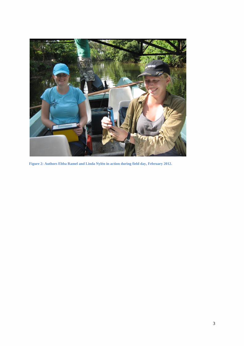
opened by the 2004 tsunami that was connected with the Maha Oya river. Figure 2 shows the authors
at the field site during a field day in February 2012.
The Maha Oya river mouth seasonally closes, forcing the remaining water in the river to take another
path. This path leads through the Dutch Canal to the investigated Outlet. North of the Outlet the Dutch
Canal proceeds further north all the way to the Chilaw lagoon. This part of the channel, which was
connected to the investigated Outlet, is called the Gin Oya river. Measurements were carried out to
trace how the discharge in the tsunami opening was affected by the ocean tide and by the discharge in
the Maha Oya river and the Gin Oya river. Measurements on salinity and water levels were also
collected at the site.
A mathematical model to describe the effects of inlet sedimentation was employed to simulate the
field data back at Lunds Tekniska Högskola in Sweden. The obtained field data was used to calibrate
the model. The purpose of the model was to reproduce the opening of the river mouth and see how
various widths of the river mouth and various discharges in Maha Oya affect the water exchange
through the Outlet. Finally, an evaluation of the mathematical models was performed to assess the
accuracy and applicability of the model.
3
Figure 2: Authors Ebba Ramel and Linda Nylén in action during field day, February 2012.

4
5
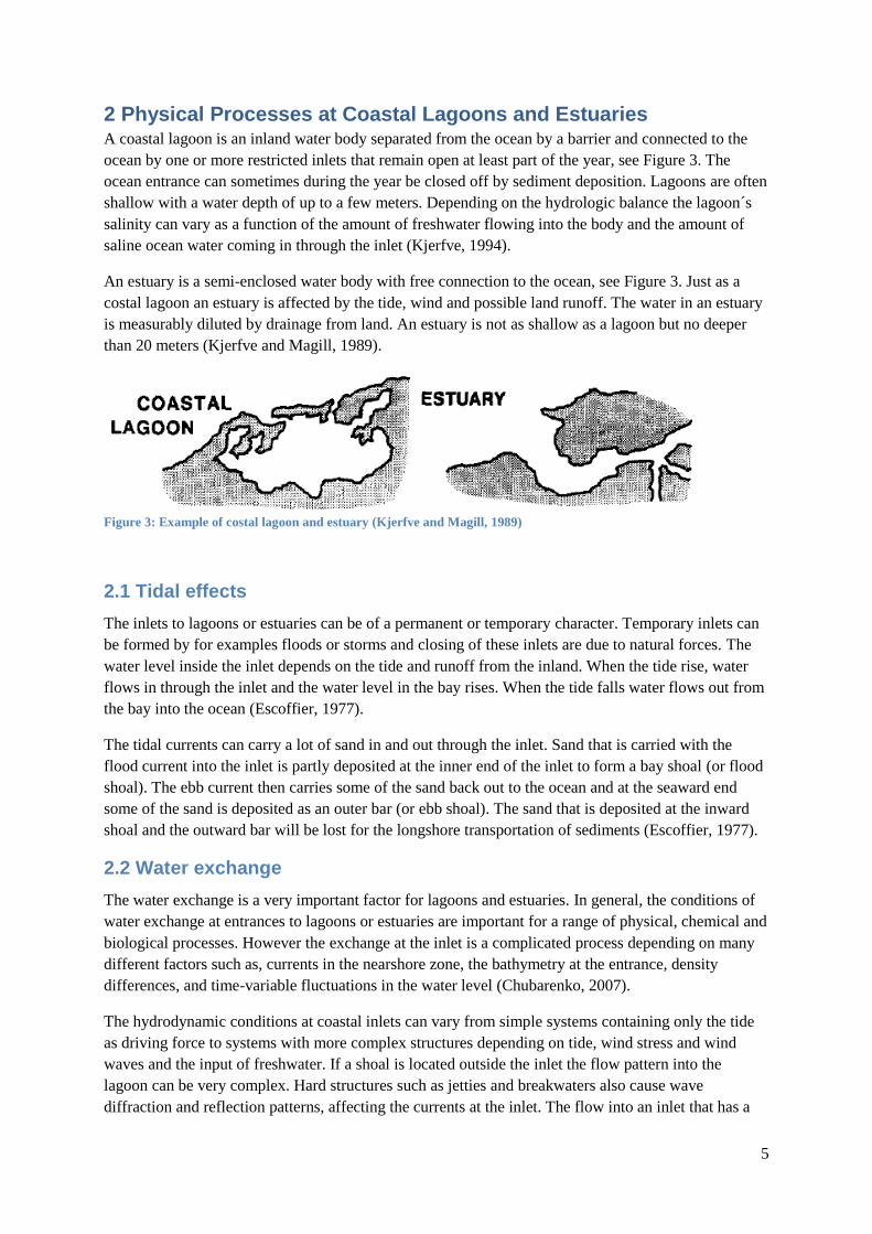
2 Physical Processes at Coastal Lagoons and Estuaries A coastal lagoon is an inland water body separated from the ocean by a barrier and connected to the
ocean by one or more restricted inlets that remain open at least part of the year, see Figure 3. The
ocean entrance can sometimes during the year be closed off by sediment deposition. Lagoons are often
shallow with a water depth of up to a few meters. Depending on the hydrologic balance the lagoon´s
salinity can vary as a function of the amount of freshwater flowing into the body and the amount of
saline ocean water coming in through the inlet (Kjerfve, 1994).
An estuary is a semi-enclosed water body with free connection to the ocean, see Figure 3. Just as a
costal lagoon an estuary is affected by the tide, wind and possible land runoff. The water in an estuary
is measurably diluted by drainage from land. An estuary is not as shallow as a lagoon but no deeper
than 20 meters (Kjerfve and Magill, 1989).
Figure 3: Example of costal lagoon and estuary (Kjerfve and Magill, 1989)
2.1 Tidal effects
The inlets to lagoons or estuaries can be of a permanent or temporary character. Temporary inlets can
be formed by for examples floods or storms and closing of these inlets are due to natural forces. The
water level inside the inlet depends on the tide and runoff from the inland. When the tide rise, water
flows in through the inlet and the water level in the bay rises. When the tide falls water flows out from
the bay into the ocean (Escoffier, 1977).
The tidal currents can carry a lot of sand in and out through the inlet. Sand that is carried with the
flood current into the inlet is partly deposited at the inner end of the inlet to form a bay shoal (or flood
shoal). The ebb current then carries some of the sand back out to the ocean and at the seaward end
some of the sand is deposited as an outer bar (or ebb shoal). The sand that is deposited at the inward
shoal and the outward bar will be lost for the longshore transportation of sediments (Escoffier, 1977).
2.2 Water exchange
The water exchange is a very important factor for lagoons and estuaries. In general, the conditions of
water exchange at entrances to lagoons or estuaries are important for a range of physical, chemical and
biological processes. However the exchange at the inlet is a complicated process depending on many
different factors such as, currents in the nearshore zone, the bathymetry at the entrance, density
differences, and time-variable fluctuations in the water level (Chubarenko, 2007).
The hydrodynamic conditions at coastal inlets can vary from simple systems containing only the tide
as driving force to systems with more complex structures depending on tide, wind stress and wind
waves and the input of freshwater. If a shoal is located outside the inlet the flow pattern into the
lagoon can be very complex. Hard structures such as jetties and breakwaters also cause wave
diffraction and reflection patterns, affecting the currents at the inlet. The flow into an inlet that has a
6
large open bay with small tidal amplitude may be dominated by the wind stress, especially under
storm conditions. Inlets of large lagoons may have strong currents due to seiching. Large freshwater
input into lagoons can create vertically stratified flows thorough tidal inlets (Seabergh, 2006).
The salinity in the lagoon depends on the ratio between fresh water input from precipitation and
groundwater and the input of saline water from the ocean. The input of oceanic saltwater is a function
of the magnitude of the tides transmitted into the bay of the lagoon. This transmission also affects the
scouring of the inlet. The morphology of the inlet controls the magnitude and lag time of the tide and
therefore also determines the pathway for the sediment transport (Conley, 1999).
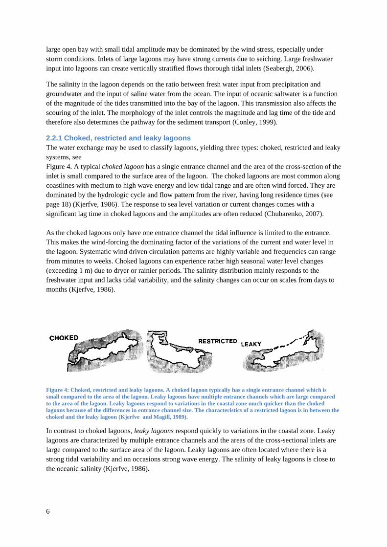
2.2.1 Choked, restricted and leaky lagoons
The water exchange may be used to classify lagoons, yielding three types: choked, restricted and leaky
systems, see
Figure 4. A typical choked lagoon has a single entrance channel and the area of the cross-section of the
inlet is small compared to the surface area of the lagoon. The choked lagoons are most common along
coastlines with medium to high wave energy and low tidal range and are often wind forced. They are
dominated by the hydrologic cycle and flow pattern from the river, having long residence times (see
page 18) (Kjerfve, 1986). The response to sea level variation or current changes comes with a
significant lag time in choked lagoons and the amplitudes are often reduced (Chubarenko, 2007).
As the choked lagoons only have one entrance channel the tidal influence is limited to the entrance.
This makes the wind-forcing the dominating factor of the variations of the current and water level in
the lagoon. Systematic wind driven circulation patterns are highly variable and frequencies can range
from minutes to weeks. Choked lagoons can experience rather high seasonal water level changes
(exceeding 1 m) due to dryer or rainier periods. The salinity distribution mainly responds to the
freshwater input and lacks tidal variability, and the salinity changes can occur on scales from days to
months (Kjerfve, 1986).
Figure 4: Choked, restricted and leaky lagoons. A choked lagoon typically has a single entrance channel which is
small compared to the area of the lagoon. Leaky lagoons have multiple entrance channels which are large compared
to the area of the lagoon. Leaky lagoons respond to variations in the coastal zone much quicker than the choked
lagoons because of the differences in entrance channel size. The characteristics of a restricted lagoon is in between the
choked and the leaky lagoon (Kjerfve and Magill, 1989).
In contrast to choked lagoons, leaky lagoons respond quickly to variations in the coastal zone. Leaky
lagoons are characterized by multiple entrance channels and the areas of the cross-sectional inlets are
large compared to the surface area of the lagoon. Leaky lagoons are often located where there is a
strong tidal variability and on occasions strong wave energy. The salinity of leaky lagoons is close to
the oceanic salinity (Kjerfve, 1986).
7
Leaky lagoons are connected to the ocean by wide tidal passes and the tidal water can easily be
transmitted into the lagoon with minimum resistance. The tide and wave characteristics can be
variable on the coasts where the leaky lagoons are located. There can be barriers of corral or sand but
the tidal currents must be strong enough to keep the openings free. The leaky lagoons often have
salinity levels close to the ocean level (Kjerfve, 1986).
Not all lagoons fit perfectly into the characteristics of choked and leaky lagoons; the restricted
lagoons represent the range between these two types. The restricted lagoons are often connected to the
ocean by two or more channels and located on coasts dominated by low or medium wave energy and
low tidal range. The inlets to the lagoon rarely close. The restricted lagoons often have well-defined
tidal circulation due to the fact that tidal water level and currents from the sea are easily transmitted
through the openings into the lagoon without any barriers. These patterns are modified by the wind
forcing and the freshwater runoff into the lagoon. Restricted lagoons are often well mixed vertically,
they are not likely to have dramatic salinity fluctuations but often have a homogeneous salinity close
to the salinity of the ocean. The salinity can vary from 1-35 ‰ depending on the freshwater input.
When a large river discharge enters the lagoon the entire lagoon may turn fresh or brackish but
normally fresh and brackish water is only found near the river mouth (Kjerfve, 1986).

8
9
3 Sri Lanka and its coastal water bodies
3.1 Climatology
Sri Lanka has a tropical monsoon climate due to the fact that the rainfall is governed by the monsoon
system over south Asia. Seasonally changing air pressure over the Asian continent generates the
monsoons (Arulananthan, 2004). Sri Lankan climate can be divided in to four monsoon seasons, the
northeast monsoon or the winter monsoon (November-February), the southwest monsoon or the
summer monsoon (May-September) and in between are the so called inter-monsoons with weaker
transitional winds. The inter-monsoon from March to April is called the first inter-monsoon and
October to November the second inter-monsoon (Wickramagamage, 2009).
The air above the Asian continent is heated during the northern summer creating rising air and low
pressure. This forces the Southwest monsoon to blow from the Indian Ocean towards the central parts
of Asian continent. During the northern winter the air over the continent cools down and creates a high
pressure. The Southwest Monsoon brings heavy rains from the Indian Ocean into southern Asia and
the northeast monsoon brings dry air from the Asia continent. Sri Lanka is situated in the centre of the
monsoon regime and experiences only minor variations in air pressure. The island is surrounded by
water on both sides and differs therefore from the general rain pattern of southern Asia. The rainfall
during October-December and April-June are the main contributors to precipitation, but Sri Lanka
obtains more rain during the Northeast monsoon than during the Southwest monsoon (Arulananthan,
2004). The rainfall during October to December accounts for about a third of the annual rainfall over
Sri Lanka (Zubair and Chandiamala, 2006).
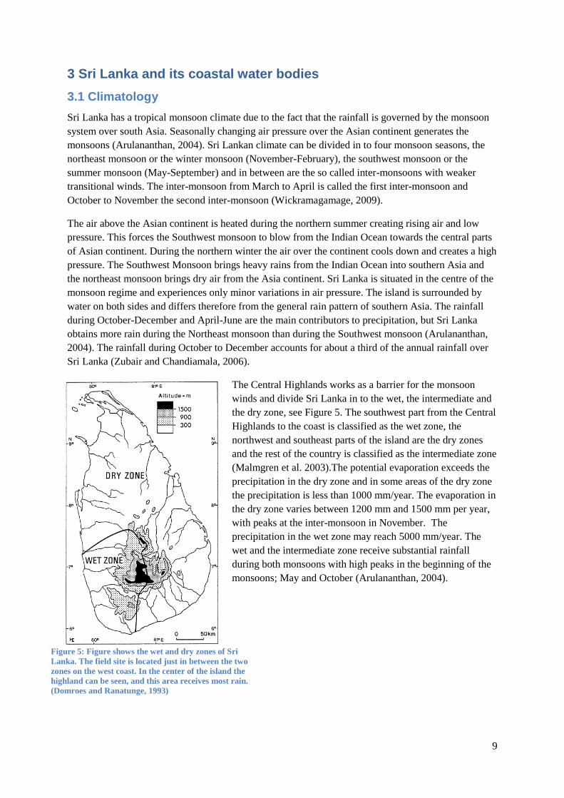
The Central Highlands works as a barrier for the monsoon
winds and divide Sri Lanka in to the wet, the intermediate and
the dry zone, see Figure 5. The southwest part from the Central
Highlands to the coast is classified as the wet zone, the
northwest and southeast parts of the island are the dry zones
and the rest of the country is classified as the intermediate zone
(Malmgren et al. 2003).The potential evaporation exceeds the
precipitation in the dry zone and in some areas of the dry zone
the precipitation is less than 1000 mm/year. The evaporation in
the dry zone varies between 1200 mm and 1500 mm per year,
with peaks at the inter-monsoon in November. The
precipitation in the wet zone may reach 5000 mm/year. The
wet and the intermediate zone receive substantial rainfall
during both monsoons with high peaks in the beginning of the
monsoons; May and October (Arulananthan, 2004).
Figure 5: Figure shows the wet and dry zones of Sri
Lanka. The field site is located just in between the two
zones on the west coast. In the center of the island the
highland can be seen, and this area receives most rain.
(Domroes and Ranatunge, 1993)
10
3.2 Geology and geomorphology
Sri Lanka is characterized by a high plateau of 1000-2500 m elevation in the central part of the island
surrounded by lowlands. The coastline around the island contains raised beaches, lagoons and dunes.
The majority of the coastal lagoons were formed after the cessation of the latest ice age. The sea level
rise after the ice age drowned the lower reaches of rivers which converted them into shallow estuaries.
Today, almost all coastal water bodies of Sri Lanka belong to the category “bar built lagoons”, situated
between the shore and a bar which was built up due to sedimentation and/or wave action. The water
quality and hydrographic conditions of the lagoons are highly dependent on the topography of the
lagoons and their connections to the sea. Several smaller lagoons with narrow entrances are seasonally
closed. Most of the variations are caused by wave action and river flooding (Arulananthan, 2004).
Coral and sandstone reefs are located 2-8 km from the coastline and are common along all the coast of
Sri Lanka (Arulananthan, 2004).
3.3 Hydrographic conditions
3.3.1 Tidal conditions
The tide generating forces are the result of gravitational attraction between the earth, sun and moon.
The water of the earth is being pulled toward the moon and sun in similarity with all other bodies on
earth. Most places in the ocean experiences two high tides and two low tides each day, this is called a
semi-diurnal tide, but there are also diurnal tides which have one high and one low tide each day
(Chubarenko, 2007).
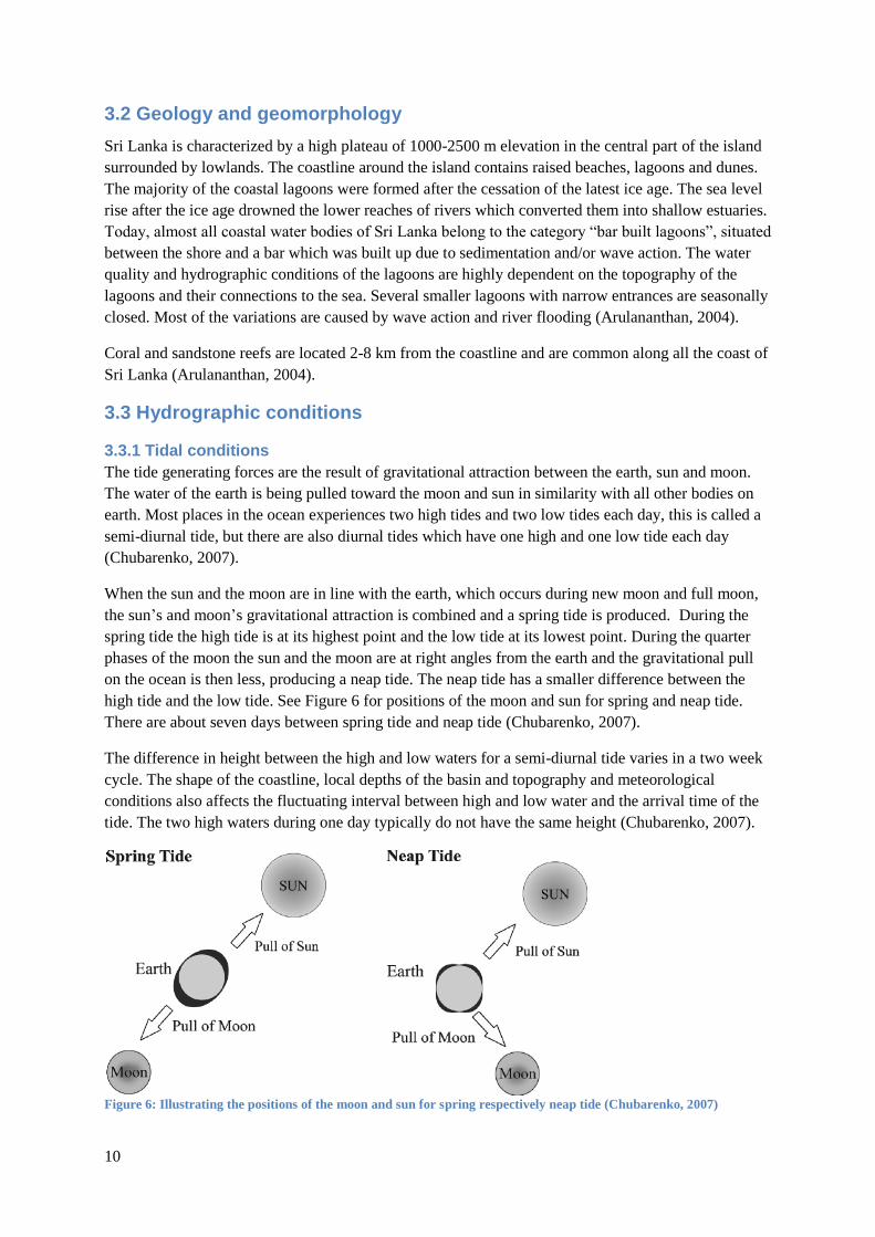
When the sun and the moon are in line with the earth, which occurs during new moon and full moon,
the sun’s and moon’s gravitational attraction is combined and a spring tide is produced. During the
spring tide the high tide is at its highest point and the low tide at its lowest point. During the quarter
phases of the moon the sun and the moon are at right angles from the earth and the gravitational pull
on the ocean is then less, producing a neap tide. The neap tide has a smaller difference between the
high tide and the low tide. See Figure 6 for positions of the moon and sun for spring and neap tide.
There are about seven days between spring tide and neap tide (Chubarenko, 2007).
The difference in height between the high and low waters for a semi-diurnal tide varies in a two week
cycle. The shape of the coastline, local depths of the basin and topography and meteorological
conditions also affects the fluctuating interval between high and low water and the arrival time of the
tide. The two high waters during one day typically do not have the same height (Chubarenko, 2007).
Figure 6: Illustrating the positions of the moon and sun for spring respectively neap tide (Chubarenko, 2007)
11
The tide around Sri Lanka is semi-diurnal. Besides the tide and associated currents there are also
surface currents in the ocean, created by the upper layer of the ocean expansion and contraction. This
is due to salinity and temperature variations causing seasonal changes in the sea level (Arulananthan,
2004).
3.3.2 Current circulation patterns
The monsoon winds over the Indian Ocean are reversing twice a year and therefore force a seasonally
reversing circulation in the upper ocean. During the summer monsoon the winds generally blow from
the southwest over the north Indian Ocean and during the winter monsoon from the northeast. The
winds are much stronger during the summer monsoon than during the winter monsoon and during the
transition months the winds are weak (Shankar et al., 2002).
Studies made on coastal currents show that there is a strong current along the east coast of India (the
East Coastal Current), a current on the west coast of India (the West India Coastal Current) and a
current along the Arabian-Sea coast of Oman. Beside these three strong currents the seasonally
reversing monsoon open-ocean currents are the most significant currents in the north of the Indian
Ocean. The current flows eastward from the western Arabian Sea to the Bay of Bengal during the
summer as a continuous current. During winter it shifts to flow the opposite direction, from east to
west. These currents are called the Summer Monsoon Current (SMC) and the Winter Monsoon
Current (WMC). The monsoon currents are shallow, restricted to the water 100 m under the surface,
compared to each other the WMC circulation is shallower then the SMC circulation. During the
summer monsoon the circulation penetrates deep and affects the movement of water mass below the
thermocline (Shankar et al., 2002). These large-scale oceanic currents are small in the coastal areas
because of the frictional forces and may be neglected when studying sediment transport and beach
evolution.

12

13
4 Inlet sedimentation and the effect on water exchange
4.1 Sediment transport and morphological change
Inlets that are located in areas with micro-tidal characteristics are dynamic and influenced by the wave
climate and river flow. The water exchange through these inlets is highly dependent on the climate and
seasonal variation of the monsoon. During the season when the river discharge is large, the
morphology of the inlets is influenced by scouring of the channels due to a high input of fresh water.
In the dry season the wave climate dominates the morphology and water exchange through the inlet
(Lam et al. 2008).
When the stream flow is low, a sandbar can form across the inlet to the lagoon and eventually close
the entrance. A long period of swell waves, inducing onshore transport, or a high longshore transport
of sediment can cause the inlet to close (Ranasinghe et al. 1999).
Thus, according to Ranasinghe et al. (1999) two main mechanisms can be used to explain inlet
closure, longshore sediment transport and onshore sediment transport, as discussed in the following.
4.1.1 Longshore sediment transport
The first mechanism is the interaction between the outlet current and the longshore current, where the
outlet current will interrupt the longshore current. This interaction will form a shoal of sand at the
updrift part of the inlet with a size and growth rate mainly depending on the intensity of the longshore
sediment transport, see Figure 7. Most often the ebb-current, going out of the inlet, will cause
sediment to form a smaller shoal downdrift of the inlet. When the inlet flow is high enough to keep the
inlet open the spit will not emerge across the inlet. However, if the inlet current is not strong enough to
remove the sediment the spit will continue to grow and eventually close the inlet. This mechanism of
inlet closure has been found to be applicable to straight shorelines with high longshore sediment
transport rates (Ranasinghe et al. 1999).
14
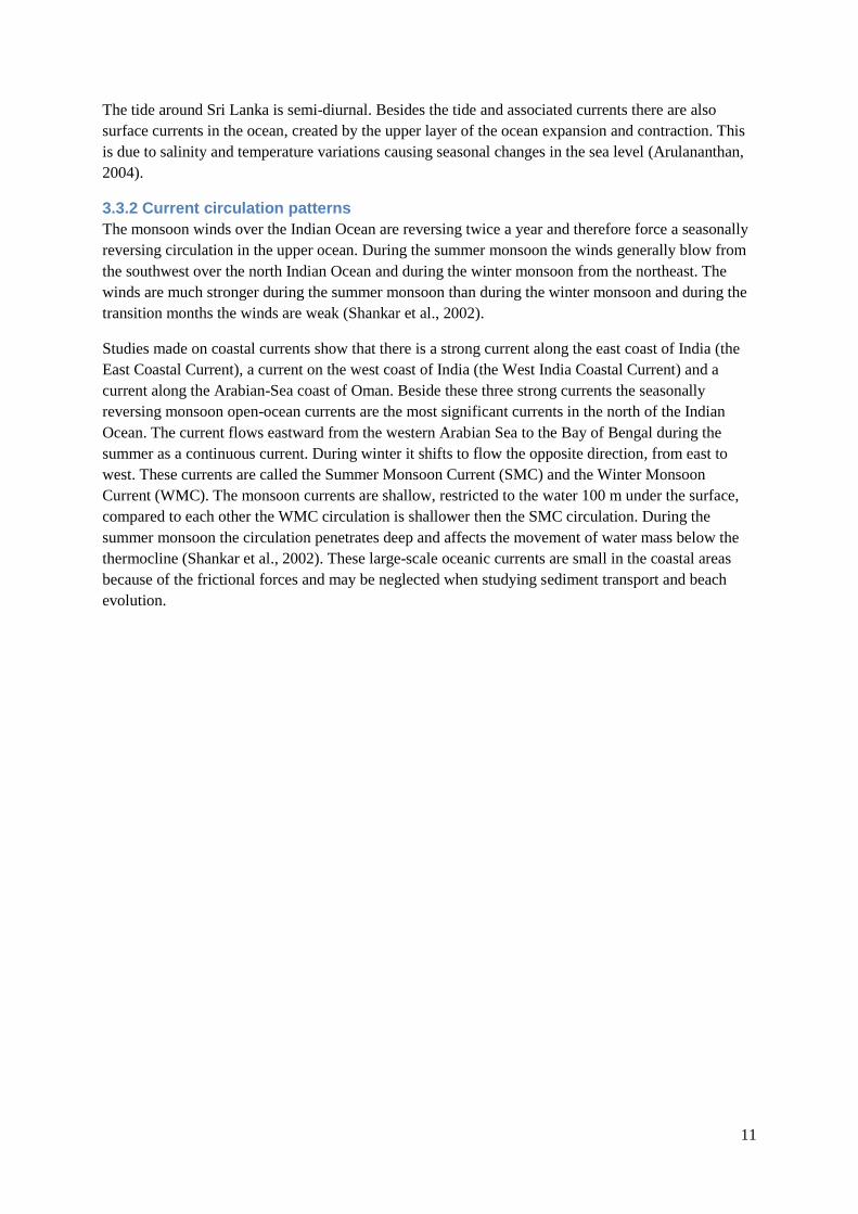
Figure 7: Sediment transport inducing closure of a tidal inlet. Mechanism 1 depends on longshore sediment transport,
whereas Mechanism 2 on onshore sediment transport. If the discharge from the stream is low, e.g., during summer,
the stream will not be able to keep the opening free of sediment and a spit will form and eventually close the inlet
completely (Ranasinghe et al. 1999).
4.1.2 Onshore sediment transport
This mechanism is only dominant in micro- or mesotidal environments, where the inlet current is
small, less than 1 m/s. The mechanism encompasses the interaction between the outlet current and the
onshore sediment transport when the longshore sediment transport rate is small. During stormy
periods, sand from the beach and surf zone will erode and move seaward forming a longshore bar at
the breaker position, see Figure 7. When the storm settles and instead periods of swell waves start, the
sediment from the longshore bar will be transported onshore. A large outlet flow will keep the inlet
clear of the onshore sediment but when the outlet flow decreases, swell waves and onshore sediment
transport acting over a longer time period will cause the inlet to close (Ranasinghe et al. 1999).
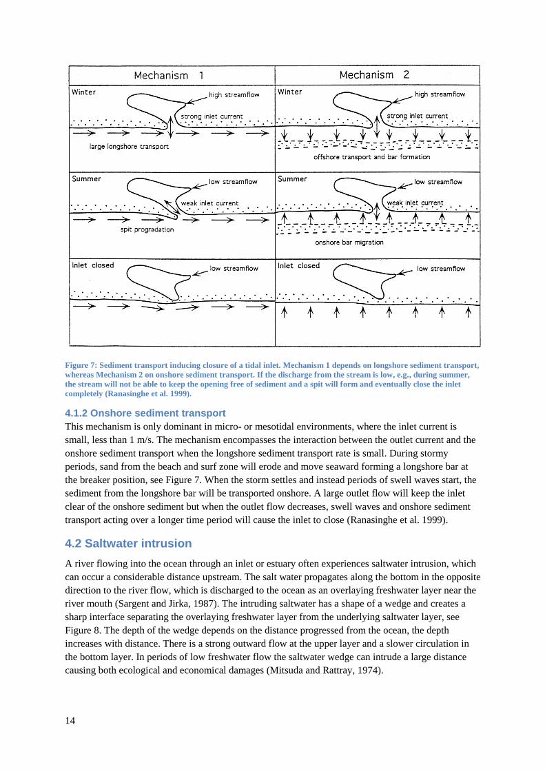
4.2 Saltwater intrusion
A river flowing into the ocean through an inlet or estuary often experiences saltwater intrusion, which
can occur a considerable distance upstream. The salt water propagates along the bottom in the opposite
direction to the river flow, which is discharged to the ocean as an overlaying freshwater layer near the
river mouth (Sargent and Jirka, 1987). The intruding saltwater has a shape of a wedge and creates a
sharp interface separating the overlaying freshwater layer from the underlying saltwater layer, see
Figure 8. The depth of the wedge depends on the distance progressed from the ocean, the depth
increases with distance. There is a strong outward flow at the upper layer and a slower circulation in
the bottom layer. In periods of low freshwater flow the saltwater wedge can intrude a large distance
causing both ecological and economical damages (Mitsuda and Rattray, 1974).
15
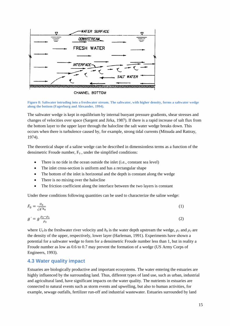
Figure 8: Saltwater intruding into a freshwater stream. The saltwater, with higher density, forms a saltwater wedge
along the bottom (Fagerburg and Alexander, 1994).
The saltwater wedge is kept in equilibrium by internal buoyant pressure gradients, shear stresses and
changes of velocities over space (Sargent and Jirka, 1987). If there is a rapid increase of salt flux from
the bottom layer to the upper layer through the halocline the salt water wedge breaks down. This
occurs when there is turbulence caused by, for example, strong tidal currents (Mitsuda and Rattray,
1974).
The theoretical shape of a saline wedge can be described in dimensionless terms as a function of the
densimetric Froude number, F0 , under the simplified conditions:
There is no tide in the ocean outside the inlet (i.e., constant sea level)
The inlet cross-section is uniform and has a rectangular shape
The bottom of the inlet is horizontal and the depth is constant along the wedge
There is no mixing over the halocline
The friction coefficient along the interface between the two layers is constant
Under these conditions following quantities can be used to characterize the saline wedge:
(1)
(2)
where U0 is the freshwater river velocity and h0 is the water depth upstream the wedge, ρ1 and ρ2 are
the density of the upper, respectively, lower layer (Harleman, 1991). Experiments have shown a
potential for a saltwater wedge to form for a densimetric Froude number less than 1, but in reality a
Froude number as low as 0.6 to 0.7 may prevent the formation of a wedge (US Army Corps of
Engineers, 1993).
4.3 Water quality impact
Estuaries are biologically productive and important ecosystems. The water entering the estuaries are
highly influenced by the surrounding land. Thus, different types of land use, such as urban, industrial
and agricultural land, have significant impacts on the water quality. The nutrients in estuaries are
connected to natural events such as storm events and upwelling, but also to human activities, for
example, sewage outfalls, fertilizer run-off and industrial wastewater. Estuaries surrounded by land

16
with a high portion of impermeable surfaces receive increased nutrient concentrations (Elsdon et al.,
2009).
The seaward side of an inlet (river mouth or estuary) is influenced by waves, storm surges and
longshore and cross-shore current systems, which influences the morphology of the opening and can
result in a sand bar, if there is deposition of sand in the inlet. This sand bar can detach the estuary or
river mouth from the ocean and interfere with the water exchange between the inlet and the sea
(Behera and Murali 2007).
If saline water in the inlet is blocked by a sand bar the water inside the bar can be described as a
stagnant pool. The saline water can then pollute fresh groundwater as well as the soil itself, damaging
surrounding ecosystems. One method to restore the freshwater-seawater mixing is to ensure sufficient
upstream flow. Sufficient inflow to the estuary reduces the stagnation of saline water and the removal
of saline water from the stagnant pool is mainly determined by the upstream discharge, the bed slope
of the upstream river, density difference between the freshwater and the saline water and the length of
the estuary (Behera and Murali 2007).
4.4 Mixing and retention times
Mixing in estuaries is primarily driven by a combination of three factors: the wind, the tide and the
river flow. Some of these factors may be more dominant than others. The mixing can also be affected
by seasonal events, such as large storms (Chanson, 2004). In a well-mixed or weakly mixed estuary
the water is homogeneous or almost homogeneous vertically. The salinity increases gradually with
distance from the surface (Arulananthan, 2004). Salt is being transported in a river mainly by
advection and longitudinal dispersion. Longitudinal dispersion implies that mixing takes place by
mass travelling in streamlines at different velocities and different directions that vary over time.
Turbulent diffusion is the transfer of mass between the streamlines and is a relatively weaker
mechanism of mixing, occurring in scales of a few meters during a time period of a few minutes
(Savenije, 2005).
Mixing (dispersion) coefficients are often based upon experimental investigations and are hard to
apply in any other system than the system investigated (Chanson, 2004).

17
4.4.1 Mixing caused by wind
Wind-induced currents contribute to mixing in estuaries, both in the vertical and horizontal direction.
Winds generate a shear stress on the water surface that will make the water surface tilt. The surface
tilts with a wind setup in the wind direction and a wind setdown in the upstream direction. The wind
must blow for some time to create a wind setup. For a well-mixed system the wind may develop water
circulation, where a bottom recirculation current is developed by the pressure difference across the
fetch. The current also develops a flow in the direction of the wind along the surface (Chanson, 2004).
Figure 9 illustrates the circulation patterns created by the wind forcing.
Figure 9: Mixing caused by wind. Figure shows wind setup and the water circulation where a bottom recirculation
current is developed by the pressure difference across the fetch. The current also develops a flow in the direction of
the wind along the surface (Chanson, 2004)
4.4.2 Mixing caused by tide
The flow in an estuary exposed to tidal motion behaves like the flow in a river but it goes back and
forth with the tide. The tide affects the downstream part of the estuarie flow and water level
fluctuations. The flood tide forces water into the estuary and causes the water level in the river mouth
to rise. The rise of the downstream water level creates backwater effects and a reversal in the flow
direction in the lower part of the river. The ebb tide will cause the water to flow out of the estuary and
lower the water level. Friction on the boundaries caused by the tidal flow will generate turbulence and
turbulent mixing (Chanson, 2004).
4.4.3 Mixing caused by river flow
The river water normally has a lower density than the water in the estuary, and this density difference
may drive a vertical circulation. The Richardson number (Rit) is a measure of how important this
circulation is compared to the tidal mixing (Savenije, 2005).
If the Rit is small the estuary is considered to be well mixed and vertical density effects do not have to
be taken into consideration. If, however, the Rit is large the estuary is strongly stratified and the flow is
affected by the density currents, for example a saltwater wedge (Chanson, 2004). The Richardson
number is defined by:
(3)
where Q is freshwater discharge, Δρ the density difference between the river and ocean water, W is
channel width and Vt is tidal velocity.
The influence of tidally driven mixing can vary considerably between spring and neap tides. The
tidally driven mixing can be significant in the transition from neap to spring tide. The estuaries tend to
be more stratified with a larger Richardson number during neap tide (Savenije, 2005).
18
4.4.4 Mixing in rivers
Natural channels are likely to have more irregularities in contrast to artificial channels contributing to
the mixing. The depth in the natural channel is likely to vary irregularly; there are also bends and
curves and irregularities along the sidewalls. These factors affect the transverse mixing in the river,
but every irregularity contributes to the dispersion as well. The dispersion coefficient is normally
higher in a natural stream than in a strait channel, which is explained by velocity differences that are
generated in a natural stream. For example, on the inside of a bend the velocity will be higher than the
average, whereas on the outside of a bend the velocity it will be lower. Thus, bends create transverse
velocity profiles (Fischer et al., 1979).
4.4.5 Well mixed estuaries
The salinity varies gradually in the longitudinal direction in a well-mixed estuary, but it is uniform
over the vertical. Such a situation develops if the tidal flow is relatively large with respect to the river
flow. Generally the salinity decreases in the upstream direction, since the freshwater inflow through
the river and direct rainfall to an estuary typically exceed the evaporation. However, in a hypersaline
estuary the salinity increases in the upstream direction since the evaporation exceeds the freshwater
inflow (Savenije, 2005).
4.5 Retention times
Retention time, or turnover time, is a measurement of how long it takes to completely exchange the
total volume of water in a water body. Retention time is an important factor for the water quality and
ecology in a water body. A costal water body with unrestricted connection to the ocean has a shorter
retention time than a water body with restricted connection to the ocean. The retention time is
dependent on different factors like river runoff, evaporation and tidal flow. According to Kjerfve and
Magill the retention time for most lagoons are found in the interval of 10 to 100 days (Kjerfve and
Magill, 1989).
19
5 Maha Oya study area
5.1 Overview
The Maha Oya River and its estuary, located about 40 km north of Colombo, have a catchment area of
1.528 km2 and is the third largest river basin in Sri Lanka. The stream length is 130 km and stretches
from Nawalapitiya to Kochchikade where it discharges into the Indian Ocean. The stream is important
for drinking water extraction and it provides 5 % of Sri Lanka´s drinking water production
(Ratnayake, 2005).
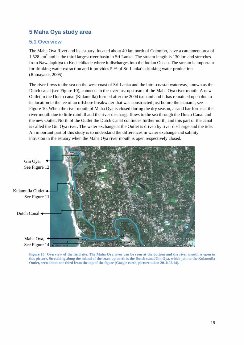
The river flows to the sea on the west coast of Sri Lanka and the intra-coastal waterway, known as the
Dutch canal (see Figure 10), connects to the river just upstream of the Maha Oya river mouth. A new
Outlet to the Dutch canal (Kulamulla) formed after the 2004 tsunami and it has remained open due to
its location in the lee of an offshore breakwater that was constructed just before the tsunami, see
Figure 10. When the river mouth of Maha Oya is closed during the dry season, a sand bar forms at the
river mouth due to little rainfall and the river discharge flows to the sea through the Dutch Canal and
the new Outlet. North of the Outlet the Dutch Canal continues further north, and this part of the canal
is called the Gin Oya river. The water exchange at the Outlet is driven by river discharge and the tide.
An important part of this study is to understand the differences in water exchange and salinity
intrusion in the estuary when the Maha Oya river mouth is open respectively closed.
Figure 10: Overview of the field site. The Maha Oya river can be seen at the bottom and the river mouth is open in
this picture. Stretching along the inland of the coast up north is the Dutch canal/Gin Oya, which join to the Kulamulla
Outlet, seen about one third from the top of the figure (Google earth, picture taken 2010.02.14).
Kulamulla Outlet,
See Figure 11
Gin Oya,
See Figure 12
Maha Oya,
See Figure 14
Dutch Canal

20
Figure 11: The Outlet at Kulamulla. In the upper part of the picture the breakwater that keeps the Outlet open can be
seen.
Figure 12: Gin Oya. Mangroves grow along the riverbank.
5.1.1 Water quality
Maha Oya flows through five important district of Sri Lanka and there are fourteen water supply
intakes along the river. Only three of them offer treatment of the water. The stream passes several
urban centers on its way to the Indian Ocean and receives much organic waste from industrial
discharge and other harmful activities in the upstream part (environmentlanka, 2012).
The area surrounding the river mouth is quite developed with both private houses and hotels. Recently
Sri Lanka has embraced a green thinking, although this seems to appeal mostly to the tourist industry
21
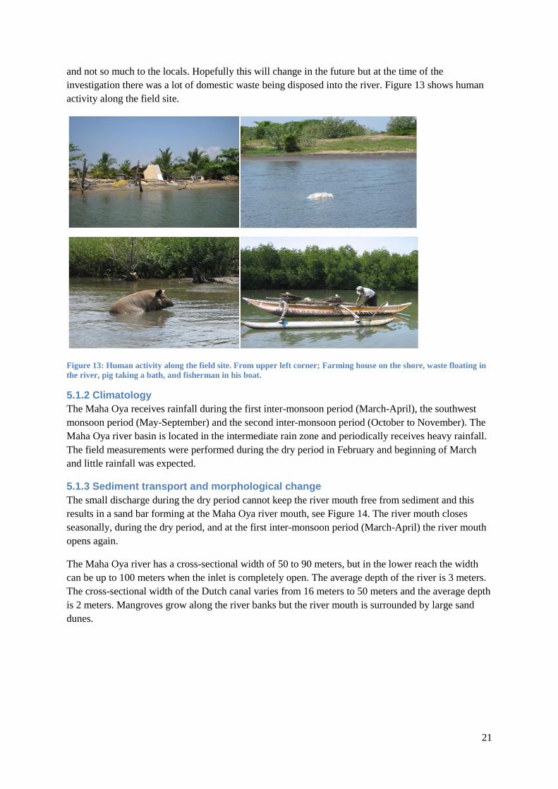
and not so much to the locals. Hopefully this will change in the future but at the time of the
investigation there was a lot of domestic waste being disposed into the river. Figure 13 shows human
activity along the field site.
Figure 13: Human activity along the field site. From upper left corner; Farming house on the shore, waste floating in
the river, pig taking a bath, and fisherman in his boat.
5.1.2 Climatology
The Maha Oya receives rainfall during the first inter-monsoon period (March-April), the southwest
monsoon period (May-September) and the second inter-monsoon period (October to November). The
Maha Oya river basin is located in the intermediate rain zone and periodically receives heavy rainfall.
The field measurements were performed during the dry period in February and beginning of March
and little rainfall was expected.
5.1.3 Sediment transport and morphological change
The small discharge during the dry period cannot keep the river mouth free from sediment and this
results in a sand bar forming at the Maha Oya river mouth, see Figure 14. The river mouth closes
seasonally, during the dry period, and at the first inter-monsoon period (March-April) the river mouth
opens again.
The Maha Oya river has a cross-sectional width of 50 to 90 meters, but in the lower reach the width
can be up to 100 meters when the inlet is completely open. The average depth of the river is 3 meters.
The cross-sectional width of the Dutch canal varies from 16 meters to 50 meters and the average depth
is 2 meters. Mangroves grow along the river banks but the river mouth is surrounded by large sand
dunes.
22
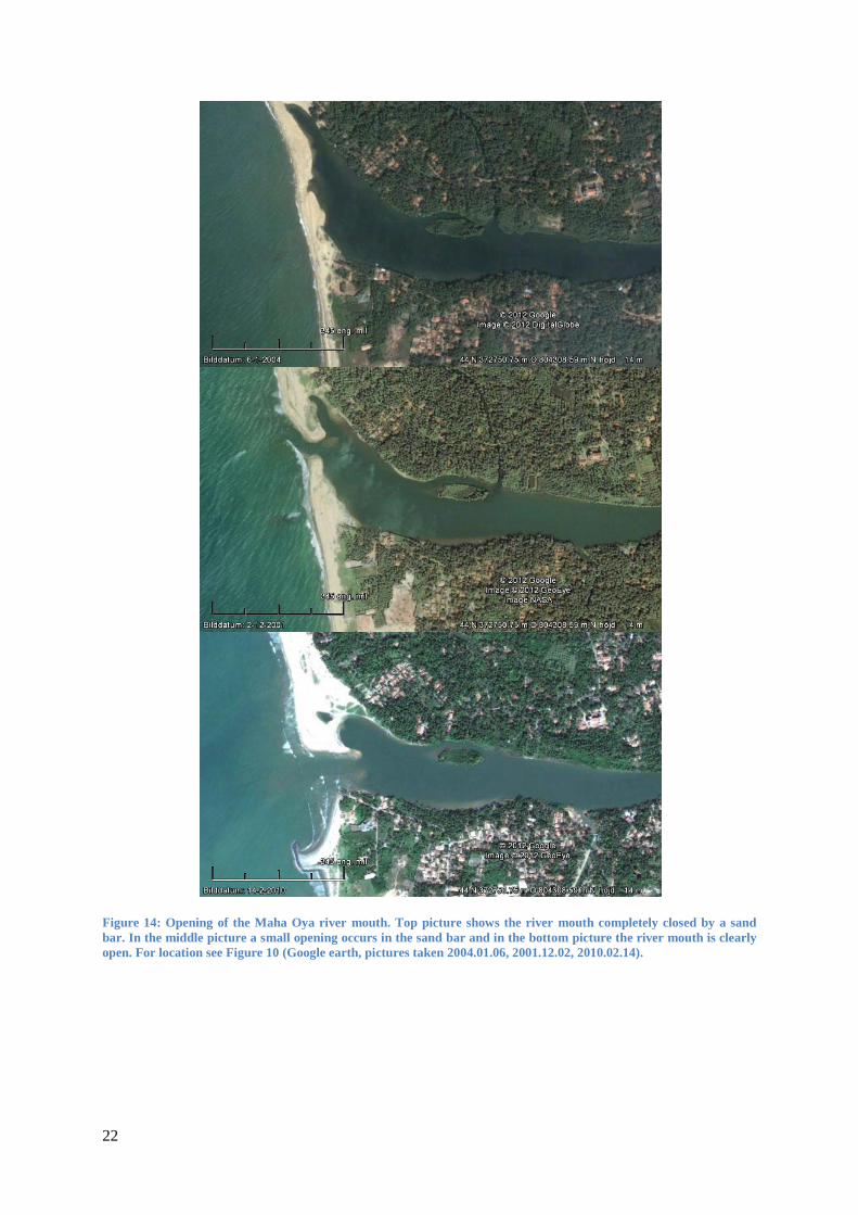
Figure 14: Opening of the Maha Oya river mouth. Top picture shows the river mouth completely closed by a sand
bar. In the middle picture a small opening occurs in the sand bar and in the bottom picture the river mouth is clearly
open. For location see Figure 10 (Google earth, pictures taken 2004.01.06, 2001.12.02, 2010.02.14).
23
5.1.4 Water exchange
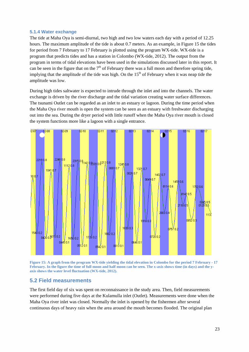
The tide at Maha Oya is semi-diurnal, two high and two low waters each day with a period of 12.25
hours. The maximum amplitude of the tide is about 0.7 meters. As an example, in Figure 15 the tides
for period from 7 February to 17 February is plotted using the program WX-tide. WX-tide is a
program that predicts tides and has a station in Colombo (WX-tide, 2012). The output from the
program in terms of tidal elevations have been used in the simulations discussed later in this report. It
can be seen in the figure that on the 7th of February there was a full moon and therefore spring tide,
implying that the amplitude of the tide was high. On the 15th of February when it was neap tide the
amplitude was low.
During high tides saltwater is expected to intrude through the inlet and into the channels. The water
exchange is driven by the river discharge and the tidal variation creating water surface differences.
The tsunami Outlet can be regarded as an inlet to an estuary or lagoon. During the time period when
the Maha Oya river mouth is open the system can be seen as an estuary with freshwater discharging
out into the sea. During the dryer period with little runoff when the Maha Oya river mouth is closed
the system functions more like a lagoon with a single entrance.
Figure 15: A graph from the program WX-tide yielding the tidal elevation in Colombo for the period 7 February - 17
February. In the figure the time of full moon and half moon can be seen. The x-axis shows time (in days) and the y-
axis shows the water level fluctuation (WX-tide, 2012).
5.2 Field measurements
The first field day of six was spent on reconnaissance in the study area. Then, field measurements
were performed during five days at the Kulamulla inlet (Outlet). Measurements were done when the
Maha Oya river inlet was closed. Normally the inlet is opened by the fishermen after several
continuous days of heavy rain when the area around the mouth becomes flooded. The original plan
24
was also to undertake field measurements when the inlet had been opened by the fishermen, however
this did not come about during the stay in Sri Lanka due to little rainfall.
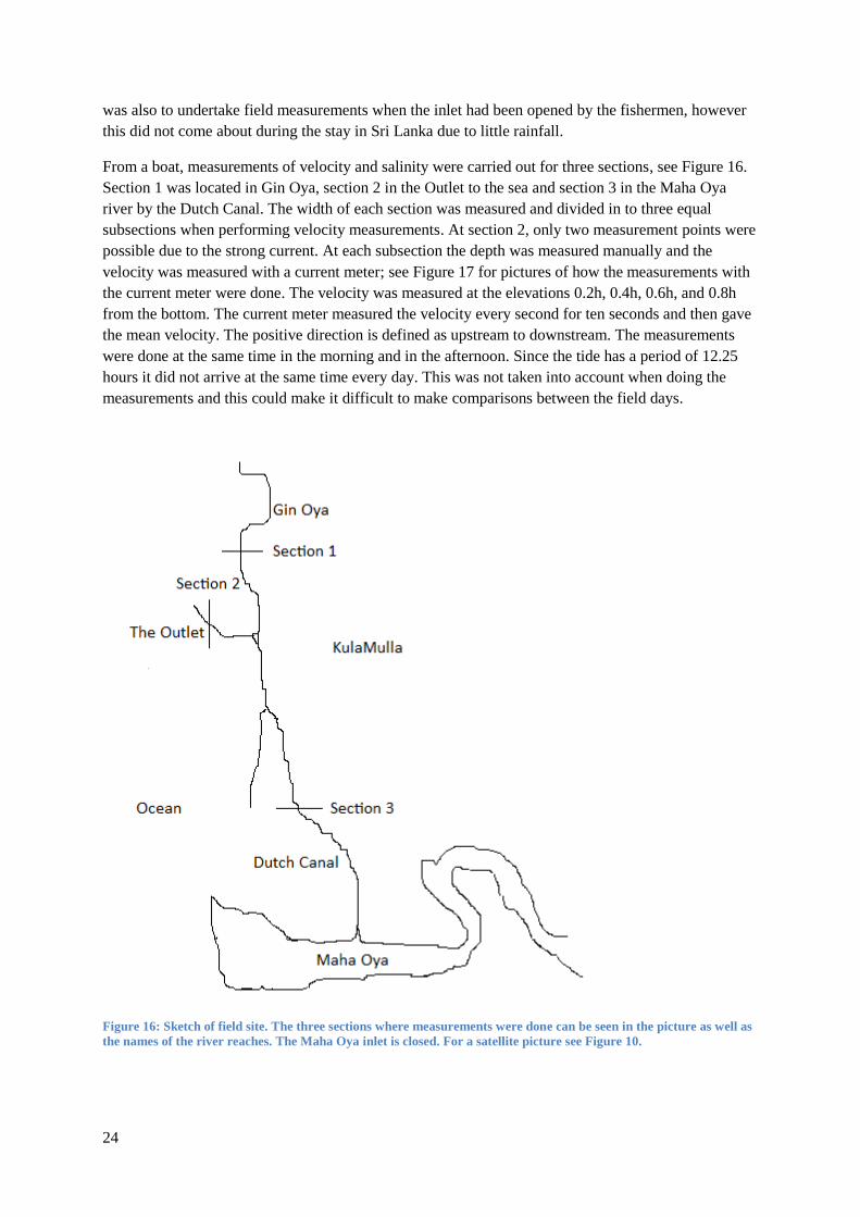
From a boat, measurements of velocity and salinity were carried out for three sections, see Figure 16.
Section 1 was located in Gin Oya, section 2 in the Outlet to the sea and section 3 in the Maha Oya
river by the Dutch Canal. The width of each section was measured and divided in to three equal
subsections when performing velocity measurements. At section 2, only two measurement points were
possible due to the strong current. At each subsection the depth was measured manually and the
velocity was measured with a current meter; see Figure 17 for pictures of how the measurements with
the current meter were done. The velocity was measured at the elevations 0.2h, 0.4h, 0.6h, and 0.8h
from the bottom. The current meter measured the velocity every second for ten seconds and then gave
the mean velocity. The positive direction is defined as upstream to downstream. The measurements
were done at the same time in the morning and in the afternoon. Since the tide has a period of 12.25
hours it did not arrive at the same time every day. This was not taken into account when doing the
measurements and this could make it difficult to make comparisons between the field days.
Figure 16: Sketch of field site. The three sections where measurements were done can be seen in the picture as well as
the names of the river reaches. The Maha Oya inlet is closed. For a satellite picture see Figure 10.

25
To calculate the discharge for each cross-section MATLAB was used. The velocities for the different
depths were integrated over depth and width for each subsection, and the discharge summarized for
the cross-section. This was done for each of the three cross-sections, both for morning and afternoon
measurements. Water levels were measured visually, at section 1, 2 and 3 with a ruler that was left on
the edge of the river bank during the day. The results are shown in chapter 5.3.
Figure 17: To the left is the display of the current meter. To the right the wading rod used to attach the current meter
at different depths can be seen.
The salinity was measured using a salinity meter and a water sampler in the middle of each cross
section in morning and afternoon; see Figure 18 for a picture of the salinity meter. Measurements were
taken at the surface and bottom. If there was a significant difference between the surface and the
bottom, a measurement was also taken in the middle of water column. The term salinity refers to the
content of dissolved salts, for example sodium (Na) and chloride (Cl) and has been defined as grams
of dissolved salts per kilogram of seawater. The salinity can be expressed in parts per thousand (‰ or
ppt) and the average value in the ocean is 35 ppt. Salinity can be determined by measuring the
conductivity in the water, where the conductivity is often given in µS/cm. Seawater often has a
conductivity of 54 000 µS/cm.

26
Figure 18: The salinity meter used in the field measurements. Water samples were taken at different depths and the
salinity was measured for each sample.

27
The hypothesis for the Outlet was that the flow would be driven by fluctuations of water levels caused
by rainfall runoff and the tidal variation. The tide has a period of 12.25 hours and does not occur at the
exact same time each day. During our field days a low tide was expected in the morning around 09.00
and a high tide in the afternoon around 15.00. High tide would presumably reverse the flow direction
in the afternoon, making the water flow from the sea upstream. We also expected to observe a
saltwater wedge penetrating into section 1 and 3.
5.3 Data collection and analysis
5.3.1 Discharge
In Table 1 the discharge for morning and afternoon can be seen for the first field day. There was a full
moon two days before (7/2) the measurements were taken, which explains the high tide. In the
morning (around 11 am) when the tide was low, the water was flowing upstream to downstream and in
the afternoon (around 3 pm) when the tide was high, the water was flowing downstream to upstream.
The river flow at section 3 (from Maha Oya) was very low in the morning.
Table 1: Measured discharge for morning and afternoon 2012-02-09 at the three sections
Field day 2012-02-09 Discharge morning [m3/s] Discharge afternoon [m
3/s]
Section 1 8.29 -8.52
Section 2 9.64 -15.13
Section 3 0.93 -5.58
Table 2 shows the results for the discharge for the second field day. The measurements at the second
field day were done after some heavy rainfall. The discharge from section 3 was significantly higher
than the first field day. The tide during this measurement was expected to be high because of the new
moon one day after the measurements. However, the flow did not reverse in the afternoon except for
in section 1. The reversed flow in section 1 was probably caused by a strong flow from section 3
penetrating into section 1 in the afternoon.
Table 2: Measured discharge for morning and afternoon 2012-02-20 at the three sections
Field day 2012-02-20 Discharge morning [m3/s] Discharge afternoon [m
3/s]
Section 1 9.65 -4.22
Section 2 23.67 10.63
Section 3 20.14 15.59
28
Table 3 shows the results from the third field day. There was a neap tide the day after the
measurements (1/3) and a low tide was expected. The river flow from Maha Oya into section 3 was
not as high as during the second field day (20/2). The flow reversed in the afternoon at all three
sections.
Table 3: Measured discharge for morning and afternoon 2012-02-29 at the three sections
Field day 2012-02-29 Discharge morning [m3/s] Discharge afternoon [m
3/s]
Section 1 12.93 -8.30
Section 2 25.21 -19.30
Section 3 9.97 -4.77
On the fourth field day (2/3) measurements were taken at three times during the day, Table 4 shows
the results. There was a reverse of the flow in the afternoon at the bottom layer in section 1, but not at
the middle or surface. The low discharge in the afternoon at section 1 can be explained by this. No
shift of direction was observed in any other of the sections. Since the discharge was flowing out to the
sea at section 2, the negative flow at the bottom at section1 was probably caused by the discharge from
section three (Maha Oya). Also, during the measurements it was difficult to keep the boat and current
meter completely fixed due to the strong current.
Table 4: Measured discharge for morning, midday and afternoon 2012-03-02 at the three sections
Field day
2012-03-02
Discharge morning [m3/s] Discharge midday [m
3/s] Discharge afternoon [m
3/s]
Section 1 8.09 9.04 1.70
Section 2 24.66 22.29 22.29
Section 3 12.47 14.56 11.57
Table 5 shows the result of the measurements taken during the final field day (5/3). A high tide was
expected since there was about to be a full moon two days after the measurements. Even so there was
no observed reversal of the flow in the afternoon.
Table 5: Measured discharge for morning and afternoon 2012-03-05 at the three sections
Field day 2012-03-05 Discharge morning [m3/s] Discharge afternoon [m
3/s]
Section 1 7.15 5.39
Section 2 16.37 10.82
Section 3 10.25 4.65
It can be seen in the tables that the flow are converging, when the direction is upstream to downstream
Section 2 receives flow from both section 1 and 3. When the flow reversed in the afternoon the flow in
Section 2 was divided between Section 1 and 3. For the measurements taken on the 20th February the
flow from Section 3 seems to be divided between Section 2 and 1. There was a small time difference
between the measurements at the different sections that could explain deviations from continuity in
flow.
29
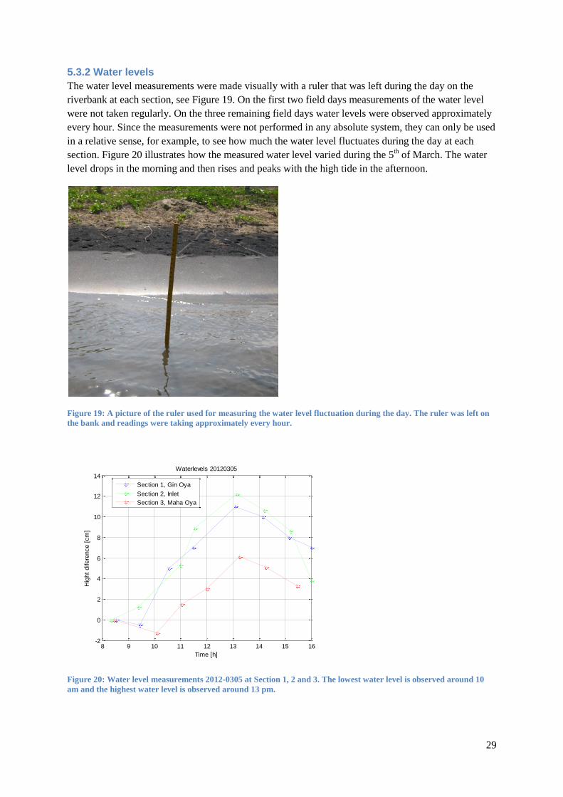
5.3.2 Water levels
The water level measurements were made visually with a ruler that was left during the day on the
riverbank at each section, see Figure 19. On the first two field days measurements of the water level
were not taken regularly. On the three remaining field days water levels were observed approximately
every hour. Since the measurements were not performed in any absolute system, they can only be used
in a relative sense, for example, to see how much the water level fluctuates during the day at each
section. Figure 20 illustrates how the measured water level varied during the 5th of March. The water
level drops in the morning and then rises and peaks with the high tide in the afternoon.
Figure 19: A picture of the ruler used for measuring the water level fluctuation during the day. The ruler was left on
the bank and readings were taking approximately every hour.
Figure 20: Water level measurements 2012-0305 at Section 1, 2 and 3. The lowest water level is observed around 10
am and the highest water level is observed around 13 pm.
8 9 10 11 12 13 14 15 16-2
0
2
4
6
8
10
12
14Waterlevels 20120305
Time [h]
Hig
ht
difere
nce [
cm
]
Section 1, Gin Oya
Section 2, Inlet
Section 3, Maha Oya

30
Limited conclusions can be made based on the water level measurements, since one ruler was used for
each section and there was no mutual reference level for the three sections. Also, the accuracy of the
measurements was affected by waves in the water, which made it difficult to do accurate readings and
occasionally the rulers were hit by boats or moved.
5.3.3 Salinity measurements
Salinity measurements were taken in the middle of all three sections in the morning and in the
afternoon. One sample was taken at the surface and one at the bottom. If there was a significant
difference between the salinity at the surface and bottom, a sample was also taken in the middle. This
was done with the intention to survey whether the water was well mixed or not. A salinity meter and a
water sampler were used to take these measurements from a boat. The salinity meter was not full-
range and could only measure salinity up to 10 ppt (parts per thousand). When this value was reached
the water sample was considered salty. Table 6 to Table 10 shows the results from the salinity
measurements during the field days.
Table 6 shows the results from the salinity measurements the first field day. Salinity measurements
were only done in the morning for this field day. The results of the measurements indicate that the
water was salt in all three sections and well mixed.
Table 6: Measurements of salinity 2012-02-09
Section 1 Section 2 Section 3
ppt Time ppt Time ppt Time
Surface >10 10.30 >10 11.40 >10 12.30
Middle >10 10.30 >10 11.40 >10 12.30
Bottom >10 10.30 >10 11.40 >10 12.30
Table 7 shows the results of the salinity measurements on the second field day. It can be seen that the
water is less salty compared to the first field day. In the morning the water had a low salinity near the
surface and a high salinity near the bottom in section 1. In the afternoon the water in section 1 had a
low salinity all over the cross-section, indicating that the high tide was not affecting section 1 with
salty water penetrating upstream. Instead the Maha Oya river from section 3 flowed into section 1
explaining the lower salinity. The salinity in section 2 was also low at the surface and higher near the
bottom, but not as high as in section 1. The salinity here also decreased in the afternoon, again
indicating that the tide had little effect on the flow and that it was the flow from Maha Oya that was
dominating. In section 3 (from Maha Oya) the salinity was low in the morning and the afternoon and
did not fluctuate much during the day. The discharge at section 3 was strong and the salinity was
therefore only measured at two depths.
Table 7: Measurements of salinity 2012-02-20
Section 1 Section 2 Section 3
ppt Time ppt Time ppt Time
Surface 5.88 09.10 1.08 09.50 0.82 10.50
Middle 9.29 09.10 3.64 09.50 - -
Bottom >10 09.10 4.87 09.50 0.74 10.50
Surface 1.13 14.50 0.82 15.20 0.67 15.50
Middle 1.30 14.50 - - - -
Bottom 1.83 14.50 0.81 15.20 0.64 15.50
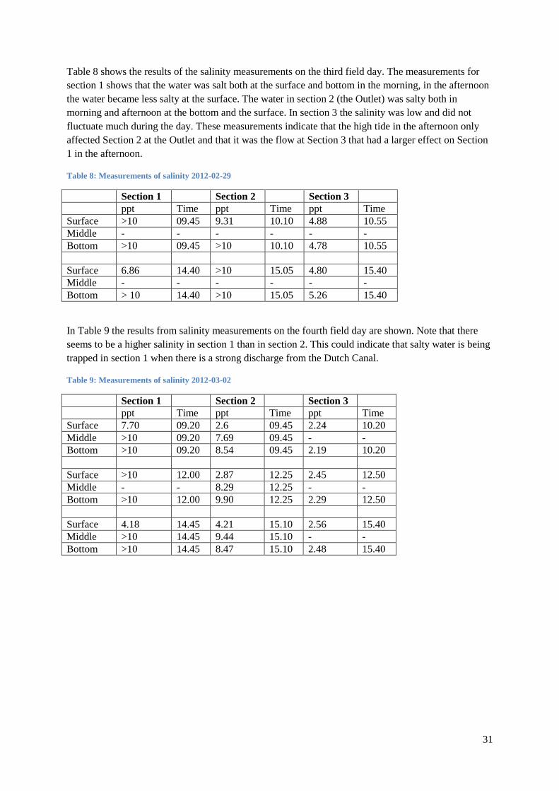
31
Table 8 shows the results of the salinity measurements on the third field day. The measurements for
section 1 shows that the water was salt both at the surface and bottom in the morning, in the afternoon
the water became less salty at the surface. The water in section 2 (the Outlet) was salty both in
morning and afternoon at the bottom and the surface. In section 3 the salinity was low and did not
fluctuate much during the day. These measurements indicate that the high tide in the afternoon only
affected Section 2 at the Outlet and that it was the flow at Section 3 that had a larger effect on Section
1 in the afternoon.
Table 8: Measurements of salinity 2012-02-29
Section 1 Section 2 Section 3
ppt Time ppt Time ppt Time
Surface >10 09.45 9.31 10.10 4.88 10.55
Middle - - - - - -
Bottom >10 09.45 >10 10.10 4.78 10.55
Surface 6.86 14.40 >10 15.05 4.80 15.40
Middle - - - - - -
Bottom > 10 14.40 >10 15.05 5.26 15.40
In Table 9 the results from salinity measurements on the fourth field day are shown. Note that there
seems to be a higher salinity in section 1 than in section 2. This could indicate that salty water is being
trapped in section 1 when there is a strong discharge from the Dutch Canal.
Table 9: Measurements of salinity 2012-03-02
Section 1 Section 2 Section 3
ppt Time ppt Time ppt Time
Surface 7.70 09.20 2.6 09.45 2.24 10.20
Middle >10 09.20 7.69 09.45 - -
Bottom >10 09.20 8.54 09.45 2.19 10.20
Surface >10 12.00 2.87 12.25 2.45 12.50
Middle - - 8.29 12.25 - -
Bottom >10 12.00 9.90 12.25 2.29 12.50
Surface 4.18 14.45 4.21 15.10 2.56 15.40
Middle >10 14.45 9.44 15.10 - -
Bottom >10 14.45 8.47 15.10 2.48 15.40
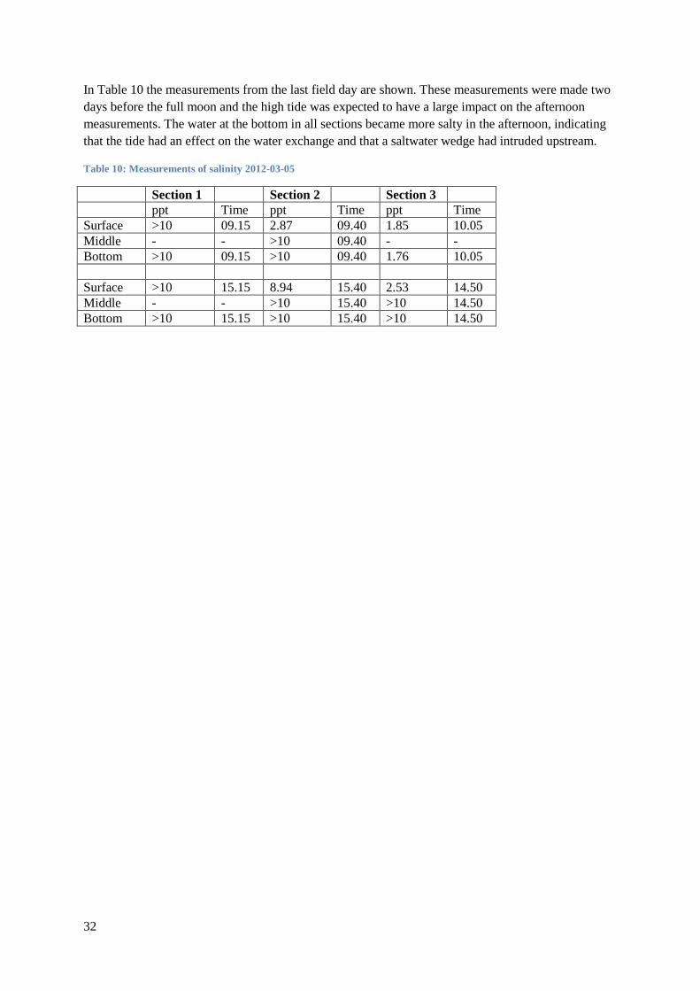
32
In Table 10 the measurements from the last field day are shown. These measurements were made two
days before the full moon and the high tide was expected to have a large impact on the afternoon
measurements. The water at the bottom in all sections became more salty in the afternoon, indicating
that the tide had an effect on the water exchange and that a saltwater wedge had intruded upstream.
Table 10: Measurements of salinity 2012-03-05
Section 1 Section 2 Section 3
ppt Time ppt Time ppt Time
Surface >10 09.15 2.87 09.40 1.85 10.05
Middle - - >10 09.40 - -
Bottom >10 09.15 >10 09.40 1.76 10.05
Surface >10 15.15 8.94 15.40 2.53 14.50
Middle - - >10 15.40 >10 14.50
Bottom >10 15.15 >10 15.40 >10 14.50
33
6 Mathematical modeling
6.1 Description of model
The program HEC-RAS was employed to create a model to reprodue the flow at the Kulamulla field
site. Two different scenarios were investigated. Scenario 1 described the conditions when the Maha
Oya river mouth was closed and scenario 2 when the river mouth was open. The simulations were
made for unsteady flow in 1-dimension and calibrated for the period 9 February to 5 March.
The objective of the modeling was to determine how the water exchange in the Outlet is affected by
inlet sedimentation. HEC-RAS was employed to investigate the main effects of inlet sedimentation
with regard to water exchange and saltwater intrusion. The simulations showed how the Kulamulla
opening is affected by a gradual opening of the Maha Oya river mouth.
6.1.1 Geometry - Scenario 1 Maha Oya river mouth closed
The geometry of the field site at Kulamulla was drawn in HEC-RAS, see Figure 21.
Figure 21: The geometry of the field site for scenario 1. The longest reach is Maha Oya which joins Section 1 (Gin
Oya) at the junction known as Kulamulla and then becomes the reach called the Outlet, which is connected to the sea.
The red lines across the river reaches represent the cross sections of the reaches. The arrows define the positive flow
direction.
Outlet
Gin Oya (Sect 1)
Gin Oy a
Dutch Canal
Ma ha O
y a
Kulamulla
None of the XS's are Geo-Referenced ( Geo-Ref user entered XS Geo-Ref interpolated XS Non Geo-Ref user entered XS Non Geo-Ref interpolated XS)
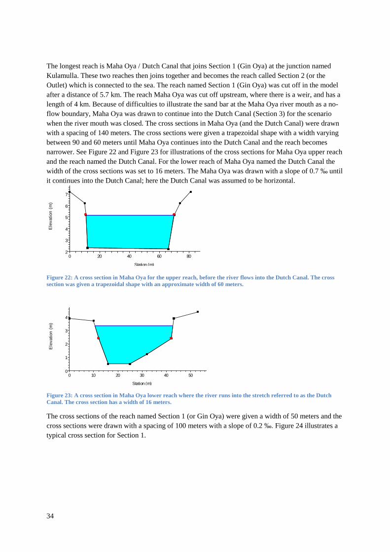
34
The longest reach is Maha Oya / Dutch Canal that joins Section 1 (Gin Oya) at the junction named
Kulamulla. These two reaches then joins together and becomes the reach called Section 2 (or the
Outlet) which is connected to the sea. The reach named Section 1 (Gin Oya) was cut off in the model
after a distance of 5.7 km. The reach Maha Oya was cut off upstream, where there is a weir, and has a
length of 4 km. Because of difficulties to illustrate the sand bar at the Maha Oya river mouth as a no-
flow boundary, Maha Oya was drawn to continue into the Dutch Canal (Section 3) for the scenario
when the river mouth was closed. The cross sections in Maha Oya (and the Dutch Canal) were drawn
with a spacing of 140 meters. The cross sections were given a trapezoidal shape with a width varying
between 90 and 60 meters until Maha Oya continues into the Dutch Canal and the reach becomes
narrower. See Figure 22 and Figure 23 for illustrations of the cross sections for Maha Oya upper reach
and the reach named the Dutch Canal. For the lower reach of Maha Oya named the Dutch Canal the
width of the cross sections was set to 16 meters. The Maha Oya was drawn with a slope of 0.7 ‰ until
it continues into the Dutch Canal; here the Dutch Canal was assumed to be horizontal.
Figure 22: A cross section in Maha Oya for the upper reach, before the river flows into the Dutch Canal. The cross
section was given a trapezoidal shape with an approximate width of 60 meters.
Figure 23: A cross section in Maha Oya lower reach where the river runs into the stretch referred to as the Dutch
Canal. The cross section has a width of 16 meters.
The cross sections of the reach named Section 1 (or Gin Oya) were given a width of 50 meters and the
cross sections were drawn with a spacing of 100 meters with a slope of 0.2 ‰. Figure 24 illustrates a
typical cross section for Section 1.
0 20 40 60 80 1002
3
4
5
6
7
8
Unateady Flow kulamulla1 Plan: Plan 10 2012-04-16
Station (m)
Ele
vation
(m
)
Legend
EG Max WS
WS Max WS
Ground
Bank Sta
.12 .09 .12
0 10 20 30 40 50 600
1
2
3
4
5
Unateady Flow kulamulla1 Plan: Plan 10 2012-04-16 The Channel Cross section 4
Station (m)
Ele
vation
(m
)
Legend
EG Max WS
WS Max WS
Ground
Bank Sta
.12 .09 .12
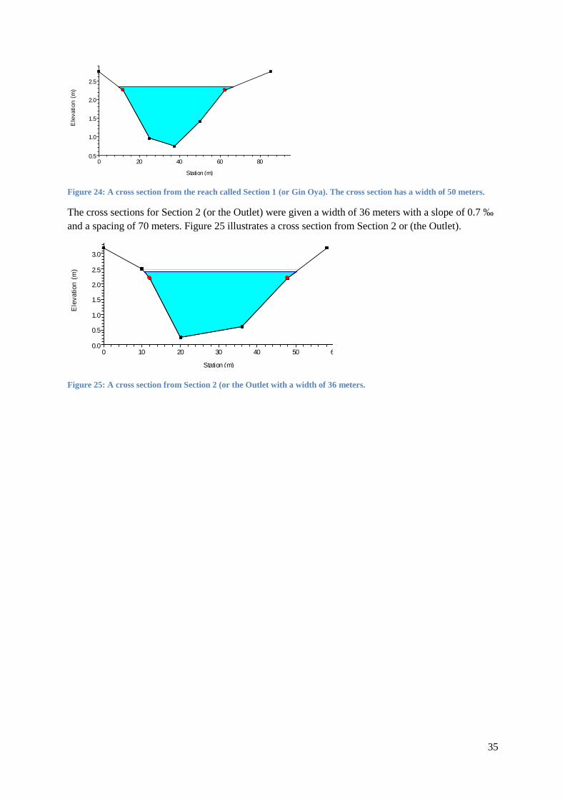
35
Figure 24: A cross section from the reach called Section 1 (or Gin Oya). The cross section has a width of 50 meters.
The cross sections for Section 2 (or the Outlet) were given a width of 36 meters with a slope of 0.7 ‰
and a spacing of 70 meters. Figure 25 illustrates a cross section from Section 2 or (the Outlet).
Figure 25: A cross section from Section 2 (or the Outlet with a width of 36 meters.
0 20 40 60 80 1000.5
1.0
1.5
2.0
2.5
3.0
Unateady Flow kulamulla1 Plan: Plan 10 2012-04-16 Gin oya cross-section 3
Station (m)
Ele
vation
(m
)Legend
EG Max WS
WS Max WS
Ground
Bank Sta
.12 .09 .12
0 10 20 30 40 50 600.0
0.5
1.0
1.5
2.0
2.5
3.0
3.5
Unateady Flow kulamulla1 Plan: Plan 10 2012-04-16 Outlet cross-section 1
Station (m)
Ele
vation
(m
)
Legend
EG Max WS
WS Max WS
Ground
Bank Sta
.04 .04 .04
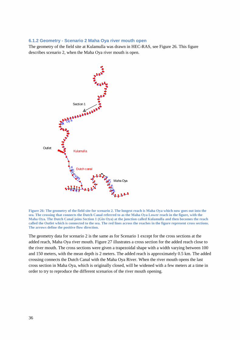
36
6.1.2 Geometry - Scenario 2 Maha Oya river mouth open
The geometry of the field site at Kulamulla was drawn in HEC-RAS, see Figure 26. This figure
describes scenario 2, when the Maha Oya river mouth is open.
Figure 26: The geometry of the field site for scenario 2. The longest reach is Maha Oya which now goes out into the
sea. The crossing that connects the Dutch Canal referred to as the Maha Oya Lower reach in the figure, with the
Maha Oya. The Dutch Canal joins Section 1 (Gin Oya) at the junction called Kulamulla and then becomes the reach
called the Outlet which is connected to the sea. The red lines across the reaches in the figure represent cross sections.
The arrows define the positive flow direction.
The geometry data for scenario 2 is the same as for Scenario 1 except for the cross sections at the
added reach, Maha Oya river mouth. Figure 27 illustrates a cross section for the added reach close to
the river mouth. The cross sections were given a trapezoidal shape with a width varying between 100
and 150 meters, with the mean depth is 2 meters. The added reach is approximately 0.5 km. The added
crossing connects the Dutch Canal with the Maha Oya River. When the river mouth opens the last
cross section in Maha Oya, which is originally closed, will be widened with a few meters at a time in
order to try to reproduce the different scenarios of the river mouth opening.
Section 1
Gin Oy a
Maha Oya
In l e t
Section 3
Mah
a O
y
a
Dutch Canal
Maha O
ya
OutletKulamulla
Dutch canal
None of the XS's are Geo-Referenced ( Geo-Ref user entered XS Geo-Ref interpolated XS Non Geo-Ref user entered XS Non Geo-Ref interpolated XS)
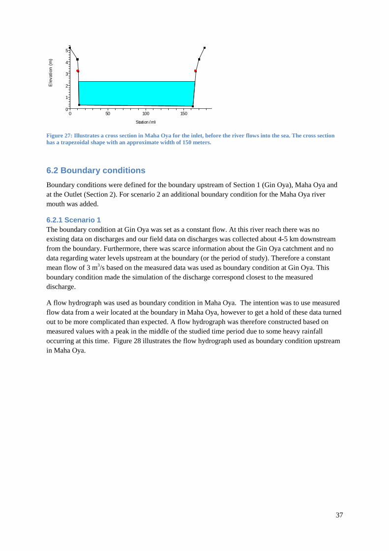
37
Figure 27: Illustrates a cross section in Maha Oya for the inlet, before the river flows into the sea. The cross section
has a trapezoidal shape with an approximate width of 150 meters.
6.2 Boundary conditions
Boundary conditions were defined for the boundary upstream of Section 1 (Gin Oya), Maha Oya and
at the Outlet (Section 2). For scenario 2 an additional boundary condition for the Maha Oya river
mouth was added.
6.2.1 Scenario 1
The boundary condition at Gin Oya was set as a constant flow. At this river reach there was no
existing data on discharges and our field data on discharges was collected about 4-5 km downstream
from the boundary. Furthermore, there was scarce information about the Gin Oya catchment and no
data regarding water levels upstream at the boundary (or the period of study). Therefore a constant
mean flow of 3 m3/s based on the measured data was used as boundary condition at Gin Oya. This
boundary condition made the simulation of the discharge correspond closest to the measured
discharge.
A flow hydrograph was used as boundary condition in Maha Oya. The intention was to use measured
flow data from a weir located at the boundary in Maha Oya, however to get a hold of these data turned
out to be more complicated than expected. A flow hydrograph was therefore constructed based on
measured values with a peak in the middle of the studied time period due to some heavy rainfall
occurring at this time. Figure 28 illustrates the flow hydrograph used as boundary condition upstream
in Maha Oya.
0 50 100 150 2000
1
2
3
4
5
6
Unateady Flow kulamulla1 Plan: Plan 10 2012-04-16
Station (m)
Ele
vation
(m
)
Legend
EG Max WS
WS Max WS
Ground
Bank Sta
.12
.09 .12

38
Figure 28: Boundary condition upstream in Maha Oya, a flow hydrograph with a peak of 20 m3/s.
At the Outlet the tide was set as a boundary condition. Predicted tide values for Colombo were used;
see Figure 29 for a plot of the used values. A water surface elevation of 2.4 meters at the was used as
reference level for the tides.
Figure 29: A plot of the tidal elevation set as a boundary condition at Section 2 (or the Outlet) for the period 09
February - 05 March. A water surface elevation of 2.4 meters at the cross section closest to the sea was used as
reference level.
0 5 10 15 20 25 30 350
5
10
15
20
River: Maha Oya Reach: Dutch Canal RS: 10.35
Simulation Time (days)
Flo
w (
m3/s
)Legend
Flow
0 5 10 15 20 25 30 352.1
2.2
2.3
2.4
2.5
2.6
2.7
2.8
River: Outlet Reach: Outlet RS: 5
Simulation Time (days)
Sta
ge
(m
)
Legend
Stage
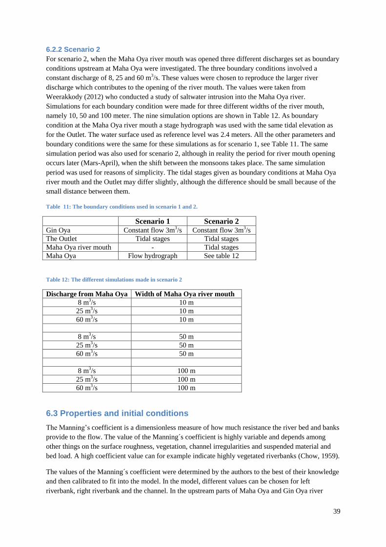
39
6.2.2 Scenario 2
For scenario 2, when the Maha Oya river mouth was opened three different discharges set as boundary
conditions upstream at Maha Oya were investigated. The three boundary conditions involved a
constant discharge of 8, 25 and 60 m3/s. These values were chosen to reproduce the larger river
discharge which contributes to the opening of the river mouth. The values were taken from
Weerakkody (2012) who conducted a study of saltwater intrusion into the Maha Oya river.
Simulations for each boundary condition were made for three different widths of the river mouth,
namely 10, 50 and 100 meter. The nine simulation options are shown in Table 12. As boundary
condition at the Maha Oya river mouth a stage hydrograph was used with the same tidal elevation as
for the Outlet. The water surface used as reference level was 2.4 meters. All the other parameters and
boundary conditions were the same for these simulations as for scenario 1, see Table 11. The same
simulation period was also used for scenario 2, although in reality the period for river mouth opening
occurs later (Mars-April), when the shift between the monsoons takes place. The same simulation
period was used for reasons of simplicity. The tidal stages given as boundary conditions at Maha Oya
river mouth and the Outlet may differ slightly, although the difference should be small because of the
small distance between them.
Table 11: The boundary conditions used in scenario 1 and 2.
Scenario 1 Scenario 2 Gin Oya Constant flow 3m
3/s Constant flow 3m
3/s
The Outlet Tidal stages Tidal stages
Maha Oya river mouth - Tidal stages
Maha Oya Flow hydrograph See table 12
Table 12: The different simulations made in scenario 2
Discharge from Maha Oya Width of Maha Oya river mouth
8 m3/s 10 m
25 m3/s 10 m
60 m3/s 10 m
8 m3/s 50 m
25 m3/s 50 m
60 m3/s 50 m
8 m3/s 100 m
25 m3/s 100 m
60 m3/s 100 m
6.3 Properties and initial conditions
The Manning’s coefficient is a dimensionless measure of how much resistance the river bed and banks
provide to the flow. The value of the Manning´s coefficient is highly variable and depends among
other things on the surface roughness, vegetation, channel irregularities and suspended material and
bed load. A high coefficient value can for example indicate highly vegetated riverbanks (Chow, 1959).
The values of the Manning´s coefficient were determined by the authors to the best of their knowledge
and then calibrated to fit into the model. In the model, different values can be chosen for left
riverbank, right riverbank and the channel. In the upstream parts of Maha Oya and Gin Oya river
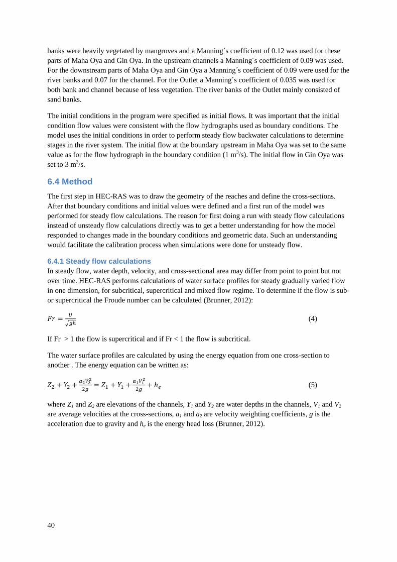
40
banks were heavily vegetated by mangroves and a Manning´s coefficient of 0.12 was used for these
parts of Maha Oya and Gin Oya. In the upstream channels a Manning´s coefficient of 0.09 was used.
For the downstream parts of Maha Oya and Gin Oya a Manning´s coefficient of 0.09 were used for the
river banks and 0.07 for the channel. For the Outlet a Manning´s coefficient of 0.035 was used for
both bank and channel because of less vegetation. The river banks of the Outlet mainly consisted of
sand banks.
The initial conditions in the program were specified as initial flows. It was important that the initial
condition flow values were consistent with the flow hydrographs used as boundary conditions. The
model uses the initial conditions in order to perform steady flow backwater calculations to determine
stages in the river system. The initial flow at the boundary upstream in Maha Oya was set to the same
value as for the flow hydrograph in the boundary condition (1 m3/s). The initial flow in Gin Oya was
set to 3 m3/s.
6.4 Method
The first step in HEC-RAS was to draw the geometry of the reaches and define the cross-sections.
After that boundary conditions and initial values were defined and a first run of the model was
performed for steady flow calculations. The reason for first doing a run with steady flow calculations
instead of unsteady flow calculations directly was to get a better understanding for how the model
responded to changes made in the boundary conditions and geometric data. Such an understanding
would facilitate the calibration process when simulations were done for unsteady flow.
6.4.1 Steady flow calculations
In steady flow, water depth, velocity, and cross-sectional area may differ from point to point but not
over time. HEC-RAS performs calculations of water surface profiles for steady gradually varied flow
in one dimension, for subcritical, supercritical and mixed flow regime. To determine if the flow is sub-
or supercritical the Froude number can be calculated (Brunner, 2012):
(4)
If Fr > 1 the flow is supercritical and if Fr < 1 the flow is subcritical.
The water surface profiles are calculated by using the energy equation from one cross-section to
another . The energy equation can be written as:
(5)
where Z1 and Z2 are elevations of the channels, Y1 and Y2 are water depths in the channels, V1 and V2
are average velocities at the cross-sections, a1 and a2 are velocity weighting coefficients, g is the
acceleration due to gravity and he is the energy head loss (Brunner, 2012).
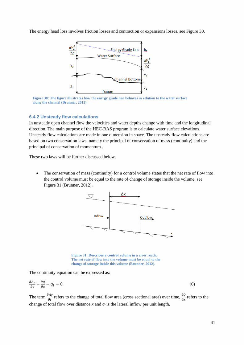
41
The energy head loss involves friction losses and contraction or expansions losses, see Figure 30.
6.4.2 Unsteady flow calculations
In unsteady open channel flow the velocities and water depths change with time and the longitudinal
direction. The main purpose of the HEC-RAS program is to calculate water surface elevations.
Unsteady flow calculations are made in one dimension in space. The unsteady flow calculations are
based on two conservation laws, namely the principal of conservation of mass (continuity) and the
principal of conservation of momentum .
These two laws will be further discussed below.
The conservation of mass (continuity) for a control volume states that the net rate of flow into
the control volume must be equal to the rate of change of storage inside the volume, see
Figure 31 (Brunner, 2012).
The continuity equation can be expressed as:
(6)
The term
refers to the change of total flow area (cross sectional area) over time,
refers to the
change of total flow over distance x and ql is the lateral inflow per unit length.
Figure 30: The figure illustrates how the energy grade line behaves in relation to the water surface
along the channel (Brunner, 2012).
Figure 31: Describes a control volume in a river reach.
The net rate of flow into the volume must be equal to the
change of storage inside this volume (Brunner, 2012).
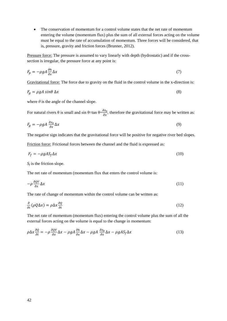
42
The conservation of momentum for a control volume states that the net rate of momentum
entering the volume (momentum flux) plus the sum of all external forces acting on the volume
must be equal to the rate of accumulation of momentum. Three forces will be considered, that
is, pressure, gravity and friction forces (Brunner, 2012).
Pressure force: The pressure is assumed to vary linearly with depth (hydrostatic) and if the cross-
section is irregular, the pressure force at any point is:
(7)
Gravitational force: The force due to gravity on the fluid in the control volume in the x-direction is:
(8)
where θ is the angle of the channel slope.
For natural rivers θ is small and sin θ≈tan θ=
, therefore the gravitational force may be written as:
(9)
The negative sign indicates that the gravitational force will be positive for negative river bed slopes.
Friction force: Frictional forces between the channel and the fluid is expressed as:
(10)
Sf is the friction slope.
The net rate of momentum (momentum flux that enters the control volume is:
(11)
The rate of change of momentum within the control volume can be written as:
(12)
The net rate of momentum (momentum flux) entering the control volume plus the sum of all the
external forces acting on the volume is equal to the change in momentum:
(13)

43
By dividing all terms with ρ and the final form of the momentum equation is obtained:
(14)
6.5 Calibration of model
A calibration of the model was performed in order to make the model correspond as closely to the
measured field data as possible. A period of one week with low discharge (1m3/s) was added to the
flow hydrographs before the investigated period (9 Feb – 5 March) started in order to warm the system
up. First a calibration for steady flow was made to adjust cross-section geometry and slopes. When the
simulations for steady flow were stable, simulations for unsteady flow were made. The first
simulations were only done for the time period one day and the boundary conditions and Manning´s
coefficient were calibrated to make the model stable. After succeeding in making stable simulations
for one day, the whole time period, 1 February to 5 March, was simulated. At first a computation
interval of one hour was used, but later this was changed to 10 minutes in order to obtain a more
accurate results.
The goal of the calibration process was to reproduce the measured values for the field days. A graph of
the measured discharge values for each section was plotted together with the simulated values in order
to be able to compare the discharges easily. When satisfactory boundary conditions had been
determined the peaks in the graphs were adjusted by changing the Manning´s coefficient. When the
graph of simulated discharge was similar or close to the graph of measured values for all three sections
the calibration process was finished. At first simulations were done for when the Maha Oya river
mouth was closed, then attempts to try to reproduce the effects of the opening of the river mouth were
done. The river mouth was opened with a width of 10, 50 and 100 meters for three different river
flows (8, 25 and 60 m3/s). (Note that no field data was obtained for the scenario when the Maha Oya
river mouth was open. These simulations were done after calibration for scenario 1 to investigate what
may happen after the opening of the river mouth).
6.6 Trace transport of salinity
Water quality was modeled in HEC-RAS by using the one-dimensional advection-dispersion equation.
The model establishes mean values over the cross sections and therefore assumes well-mixed
conditions over the cross sections. After a successful unsteady flow model was established, a water
quality analysis was performed. The simulation time from 1 February to 5 March was used for the
salinity simulations and simulations for both scenarios, Maha Oya river mouth closed respectively
open, were done.
Water quality cells were established between cross-sections and computational points were located
exactly between cross-section pairs. Boundary conditions were specified at all locations where flow
enters the system and at all tidal boundaries. Initial conditions were specified for upstream and
downstream boundaries. The one-dimensional advection-dispersion equation used by the program is:
(15)
where C is the solute concentration, t is time, z is the depth, u is the water velocity, D is the dispersion
coefficient and k is a decay coefficient.
44
Computed values on the dispersion coefficients were used in the HEC-RAS water quality model. The
water quality model estimates the dispersion coefficients based on hydraulic variables at each cross
section. The equation used to calculate the dispersion coefficient is:
(16)
The shear velocity u* is given by:
(17)
6.6.1 Boundary conditions
The boundary condition downstream at the Outlet and Maha Oya river mouth was set to the salinity of
ocean, that is, 35 000 mg/l (35 ppt). The boundary conditions upstream in Gin Oya and Maha Oya
were set to 100 mg/l (0.1 ppt). The initial conditions were set to 35 000 mg/l (35 ppt) downstream at
the Outlet and at the Maha Oya river mouth. The upstream initial conditions at Maha Oya and Gin
Oya were set to 100 mg/l (0.1 ppt). The computation cells between the cross sections were set to 100
meters in Gin Oya, 140 meters in Maha Oya and the Dutch Canal, and 70 meter in the Outlet. This
represents the distance between the cross sections in the different reaches.

45
7 Model sensitivity and accuracy The accuracy of the model can be assessed by how close the numerical solution in the model is to the
true solution. If it is assumed that the one-dimensional unsteady flow equations is a true representation
of the flow in the river system an analytical solution can give an exact solution to compare with. The
HEC-RAS program uses an implicit finite difference scheme and these solutions are only approximate.
In general, the accuracy of the model depends on the following factors (Brunner, 2012):
Assumptions and limitations in the model (e.g., the model is one-dimensional)
The quality of the geometric data (e.g., cross sections and Manning´s coefficient)
Representation of boundary conditions and initial conditions
The method employed for solving the unsteady flow equations
7.1 Model response to parameter changes
The models accuracy can be investigated by, for example, changing the time steps. If there are no
significant changes in the result when changing to a smaller time step, the numerical solution has
converged and the larger time step is probably satisfactory. The computation interval should be small
enough to accurately describe the rise and falls of the hydrographs (Brunner, 2012). In the model a
time step of one hour was first used and later this was changed to ten minutes. This made no
significant difference on the model results, indicating that the solution had converged already for the
larger time step.
The program HEC-RAS uses a Theta weighting factor that is applied to the finite difference
approximations when the unsteady flow equations is being solved. The theta factor can vary between
0.6 and 1, and a value of 1 gives the model greater stability but yields smaller numerical accuracy. For
rivers with tidal boundaries, the theta factor should be set to a value close to 0.6 in order to accurately
describe propagation of flood waves. Changing the theta value towards 0.6 is therefore important in
order to investigate the model sensitivity. A theta value of 0.6 gives the best accuracy in the solutions
of the equations, but the model may become unstable (Brunner, 2012). The Theta value in the model
was set to 1 for the first simulations and then changed towards a value of 0.6. The results for a Theta
value of 0.6 were very similar to the results with a Theta value of 1, see Table 11.
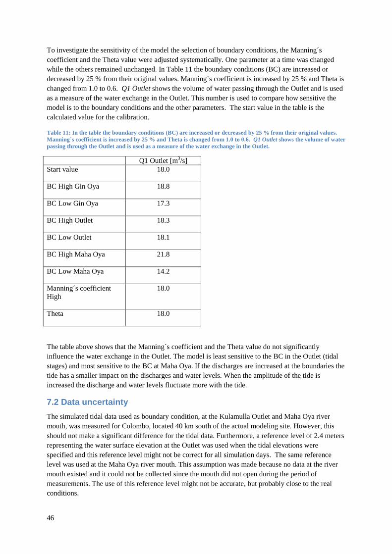
46
To investigate the sensitivity of the model the selection of boundary conditions, the Manning´s
coefficient and the Theta value were adjusted systematically. One parameter at a time was changed
while the others remained unchanged. In Table 11 the boundary conditions (BC) are increased or
decreased by 25 % from their original values. Manning´s coefficient is increased by 25 % and Theta is
changed from 1.0 to 0.6. Q1 Outlet shows the volume of water passing through the Outlet and is used
as a measure of the water exchange in the Outlet. This number is used to compare how sensitive the
model is to the boundary conditions and the other parameters. The start value in the table is the
calculated value for the calibration.
Table 11: In the table the boundary conditions (BC) are increased or decreased by 25 % from their original values.
Manning´s coefficient is increased by 25 % and Theta is changed from 1.0 to 0.6. Q1 Outlet shows the volume of water
passing through the Outlet and is used as a measure of the water exchange in the Outlet.
Q1 Outlet [m3/s]
Start value
18.0
BC High Gin Oya
18.8
BC Low Gin Oya
17.3
BC High Outlet
18.3
BC Low Outlet
18.1
BC High Maha Oya
21.8
BC Low Maha Oya
14.2
Manning´s coefficient
High
18.0
Theta
18.0
The table above shows that the Manning´s coefficient and the Theta value do not significantly
influence the water exchange in the Outlet. The model is least sensitive to the BC in the Outlet (tidal
stages) and most sensitive to the BC at Maha Oya. If the discharges are increased at the boundaries the
tide has a smaller impact on the discharges and water levels. When the amplitude of the tide is
increased the discharge and water levels fluctuate more with the tide.
7.2 Data uncertainty
The simulated tidal data used as boundary condition, at the Kulamulla Outlet and Maha Oya river
mouth, was measured for Colombo, located 40 km south of the actual modeling site. However, this
should not make a significant difference for the tidal data. Furthermore, a reference level of 2.4 meters
representing the water surface elevation at the Outlet was used when the tidal elevations were
specified and this reference level might not be correct for all simulation days. The same reference
level was used at the Maha Oya river mouth. This assumption was made because no data at the river
mouth existed and it could not be collected since the mouth did not open during the period of
measurements. The use of this reference level might not be accurate, but probably close to the real
conditions.

47
The boundary condition upstream in Maha Oya were developed from the measurements done in the
Dutch Canal. It would have been preferable to use measured flow data from an existing weir upstream
in Maha Oya and see if the model independently could reproduce the values that was measured in the
Dutch Canal. Since such data in Maha Oya turned out to be difficult to get a hold of, using the
measured flow values in the Dutch Canal when formulating the boundary conditions was the second
best thing to do. A constant mean value of 8 m3/s based on the field measurements was tested as a
boundary condition in Maha Oya. However, this boundary condition gave a poor correspondence
between simulated and measured values. A flow hydrograph was then constructed based on measured
values with a peak in the middle of the time period caused by heavy rainfall. This boundary condition
yielded a better correspondence between simulated and measured discharges. The boundary conditions
upstream in Gin Oya was set to a mean flow of 3 m3/s based on the field measurements since there
was no other information available about this boundary condition.
The cross-section geometry was based on field observations and measurements made at the site by the
authors, including recorded widths and depths at sections 1, 2 and 3 in Gin Oya, Dutch Canal and the
Outlet, respectively. Measurements in satellite pictures from Google Earth were also used.

48
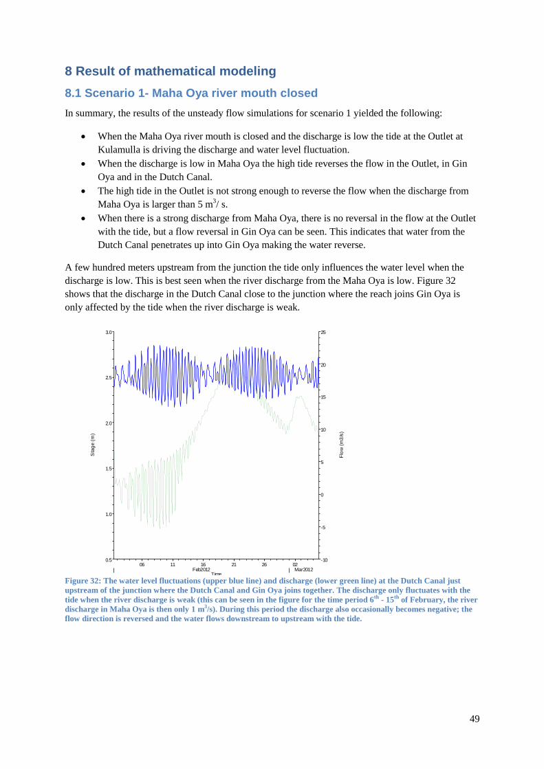
49
8 Result of mathematical modeling
8.1 Scenario 1- Maha Oya river mouth closed
In summary, the results of the unsteady flow simulations for scenario 1 yielded the following:
When the Maha Oya river mouth is closed and the discharge is low the tide at the Outlet at
Kulamulla is driving the discharge and water level fluctuation.
When the discharge is low in Maha Oya the high tide reverses the flow in the Outlet, in Gin
Oya and in the Dutch Canal.
The high tide in the Outlet is not strong enough to reverse the flow when the discharge from
Maha Oya is larger than 5 m3/ s.
When there is a strong discharge from Maha Oya, there is no reversal in the flow at the Outlet
with the tide, but a flow reversal in Gin Oya can be seen. This indicates that water from the
Dutch Canal penetrates up into Gin Oya making the water reverse.
A few hundred meters upstream from the junction the tide only influences the water level when the
discharge is low. This is best seen when the river discharge from the Maha Oya is low. Figure 32
shows that the discharge in the Dutch Canal close to the junction where the reach joins Gin Oya is
only affected by the tide when the river discharge is weak.
Figure 32: The water level fluctuations (upper blue line) and discharge (lower green line) at the Dutch Canal just
upstream of the junction where the Dutch Canal and Gin Oya joins together. The discharge only fluctuates with the
tide when the river discharge is weak (this can be seen in the figure for the time period 6th - 15th of February, the river
discharge in Maha Oya is then only 1 m3/s). During this period the discharge also occasionally becomes negative; the
flow direction is reversed and the water flows downstream to upstream with the tide.
06 11 16 21 26 02Feb2012 Mar2012
0.5
1.0
1.5
2.0
2.5
3.0
-10
-5
0
5
10
15
20
25
Plan: Plan 32 River: Maha Oya Reach: Dutch Canal RS: 10
Time
Sta
ge
(m
)
Flo
w (
m3
/s)
Legend
Stage
Flow
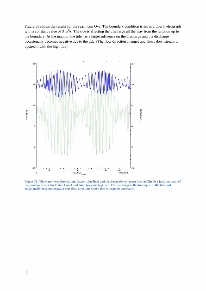
50
Figure 33 shows the results for the reach Gin Oya. The boundary condition is set as a flow hydrograph
with a constant value of 3 m3/s. The tide is affecting the discharge all the way from the junction up to
the boundary. At the junction the tide has a larger influence on the discharge and the discharge
occasionally becomes negative due to the tide. (The flow direction changes and flows downstream to
upstream with the high tide).
Figure 33: The water level fluctuations (upper blue line) and discharge (lower green line) at Gin Oya just upstream of
the junction where the Dutch Canal and Gin Oya joins together. The discharge is fluctuating with the tide and
occasionally becomes negative (the flow direction is then downstream to upstream).
06 11 16 21 26 02Feb2012 Mar2012
0.5
1.0
1.5
2.0
2.5
3.0
-10
-5
0
5
10
15
Plan: Plan 32 River: Gin Oya Reach: Gin Oya (Sect 1) RS: 10.9
Time
Sta
ge
(m
)
Flo
w (
m3
/s)
Legend
Stage
Flow
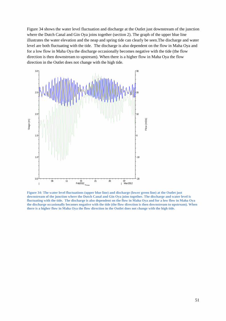
51
Figure 34 shows the water level fluctuation and discharge at the Outlet just downstream of the junction
where the Dutch Canal and Gin Oya joins together (section 2). The graph of the upper blue line
illustrates the water elevation and the neap and spring tide can clearly be seen.The discharge and water
level are both fluctuating with the tide. The discharge is also dependent on the flow in Maha Oya and
for a low flow in Maha Oya the discharge occasionally becomes negative with the tide (the flow
direction is then downstream to upstream). When there is a higher flow in Maha Oya the flow
direction in the Outlet does not change with the high tide.
Figure 34: The water level fluctuations (upper blue line) and discharge (lower green line) at the Outlet just
downstream of the junction where the Dutch Canal and Gin Oya joins together. The discharge and water level is
fluctuating with the tide. The discharge is also dependent on the flow in Maha Oya and for a low flow in Maha Oya
the discharge occasionally becomes negative with the tide (the flow direction is then downstream to upstream). When
there is a higher flow in Maha Oya the flow direction in the Outlet does not change with the high tide.
06 11 16 21 26 02Feb2012 Mar2012
0.5
1.0
1.5
2.0
2.5
3.0
-20
-10
0
10
20
30
Plan: Plan 32 River: Outlet Reach: Outlet RS: 9
Time
Sta
ge
(m
)
Flo
w (
m3
/s)
Legend
Stage
Flow

52
8.2 Scenario 2- Maha Oya river mouth opened
For scenario 2, when the Maha Oya river mouth was to be opened, three different discharges were
considered upstream at Maha Oya. The three discharges set as boundary conditions were a constant
discharge of 8, 25 and 60 m3/s. Simulations for each boundary condition were made for three widths of
the river mouth, namely 10, 50 and 100 meter. All the other parameters and boundary conditions were
the same for these simulations. The discharge was enlarged because periods of heavy rain often occurs
in the inter-monsoon period when the inlet is dug opened by the fisher men. The simulation time
employed was the same as for scenario 1 for simplicity although the opening of the river mouth
typically does not take place during this time (1 February to 5 Mars).
In summary, for the scenario when the Maha Oya river mouth is open the following results were
obtained:
In the Maha Oya river reach the tide has a larger influence on the water levels and discharge
for a wider river mouth.
For a wider river mouth the largest portion of the flow in Maha Oya discharges out at the
Maha Oya river mouth and almost no flow goes into the Dutch Canal.
The tide has the largest effect on the discharge and water level in Maha Oya when the
discharge is weak.
The results below are presented according to location. First the discharges at the Maha Oya river
mouth is presented, then plots upstream in Maha Oya before the river splits into the Dutch Canal, then
results from the Dutch Canal, Gin Oya and the Outlet. Only graphs when the river mouth was 50
meters wide are shown below. For the scenarios with 10 and 100 widths, see Appendix 6.

53
8.2.1 Discharges at Maha Oya river mouth
The plots of the discharges at the Maha Oya river mouth were very similar for the three different
widths of the mouth. Figure 35 shows three graphs of the discharge at the Maha Oya river mouth for
the case when the mouth is 50 meter open. The blue graph (lower) shows the discharge at the river
mouth when the boundary condition upstream was set as a constant flow of 8 m3/s. The red graph
(middle) shows the discharge at the river mouth for the boundary condition set as a constant flow of 25
m3/s. The green graph (upper) shows the discharge for the boundary condition set to 60 m
3/s. It can be
seen in the figures that the tide have a slightly larger effect on the discharge at the mouth when the
river discharge from upstream in Maha Oya is low. In Appendix 6, Figure 51 and Figure 52 illustrate
the graphs for the scenarios when the Maha Oya river mouth is 10 and 100 meter wide, respectively.
Figure 35: Graphs of the discharge at the Maha Oya river mouth for the scenario when the mouth is 50 meter wide.
The blue graph (lower) illustrates the discharge for the boundary condition upstream at Maha Oya set to a constant
flow of 8 m3/s. the red graph (middle) 25 m3/s, and the green graph (upper) 60 m3/s. It can be seen in the figure that
the tide have a slightly larger effect on the discharge at the river mouth when the discharge from Maha Oya is low.
0 100 200 300 400 500 600 700 800 900-5
0
5
10
15
20
25
30
35
40
45Discharge at rivermouth for a 50 meter wide river mouth
Time [h]
Dis
charg
e [
m3/s
]
Boundary condition 8 m3/s
Boundary condition 25 m3/s
Boundary condition 60 m3/s

54
8.2.2 Discharges in Maha Oya
Figure 36 shows the discharge in Maha Oya river just before the stream splits into the Dutch Canal for
the case when the mouth is 50 meter open. The blue graph shows the discharge when the boundary
condition upstream was set as a constant flow of 8 m3/s, the red 25 m
3/s, and the green 60 m
3/s. It can
be seen in the figure that the tide has a slightly larger effect on the discharge when the river discharge
from upstream in Maha Oya is low. The discharges in this graphs are also higher compared to the river
mouth in previous figure. This indicates that a small portion of the discharge goes into the Dutch
Canal. The graphs for different widths of the river mouth was very similar, the only difference was
that the tide seemed to have a slightly bigger effect on the discharge when the river mouth was wider.
Figure 53 and Figure 54 for the scenarios when the river mouth is 10 and 100 meter wide,
respectively, can be seen in Appendix 6.
Figure 36: Graphs of the discharge at the Maha Oya just upstream the split into the Dutch Canal for the scenario
when the mouth is 50 meter wide. The blue graph (lower) illustrates the discharge for the boundary condition
upstream at Maha Oya set to a constant flow of 8 m3/s, the red graph (middle) 25 m3/s, and the green graph (upper)
60 m3/s. It can be seen in the figure that the tide have a slightly larger effect on the discharge in Maha Oya when the
discharge from Maha Oya is low. The discharges in this figure are also higher than in Figure 35 (at the river mouth)
indicating that a portion of the discharge goes into the Dutch Canal.
0 100 200 300 400 500 600 700 800 900-10
0
10
20
30
40
50
60
70Discharge at Maha Oya for a 50 meter wide river mouth
Time [h]
Dis
charg
e [
m3/s
]
Boundary condition 8 m3/s
Boundary condition 25 m3/s
Boundary condition 60 m3/s
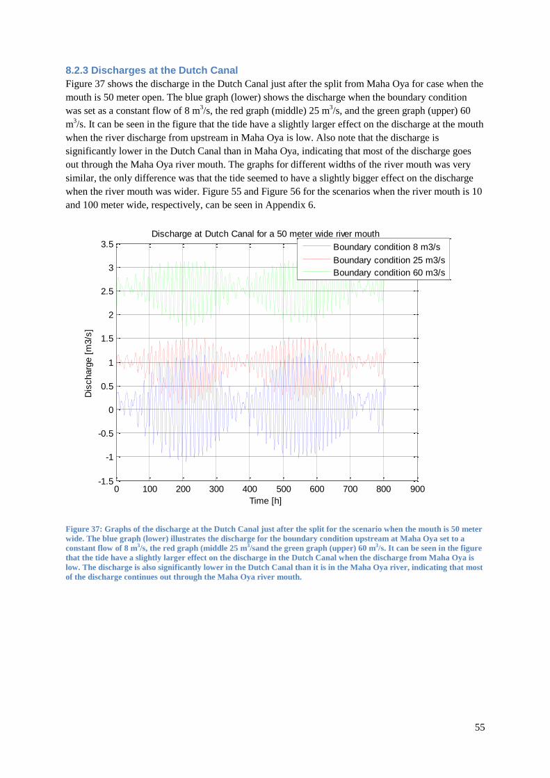
55
8.2.3 Discharges at the Dutch Canal
Figure 37 shows the discharge in the Dutch Canal just after the split from Maha Oya for case when the
mouth is 50 meter open. The blue graph (lower) shows the discharge when the boundary condition
was set as a constant flow of 8 m3/s, the red graph (middle) 25 m
3/s, and the green graph (upper) 60
m3/s. It can be seen in the figure that the tide have a slightly larger effect on the discharge at the mouth
when the river discharge from upstream in Maha Oya is low. Also note that the discharge is
significantly lower in the Dutch Canal than in Maha Oya, indicating that most of the discharge goes
out through the Maha Oya river mouth. The graphs for different widths of the river mouth was very
similar, the only difference was that the tide seemed to have a slightly bigger effect on the discharge
when the river mouth was wider. Figure 55 and Figure 56 for the scenarios when the river mouth is 10
and 100 meter wide, respectively, can be seen in Appendix 6.
Figure 37: Graphs of the discharge at the Dutch Canal just after the split for the scenario when the mouth is 50 meter
wide. The blue graph (lower) illustrates the discharge for the boundary condition upstream at Maha Oya set to a
constant flow of 8 m3/s, the red graph (middle 25 m3/sand the green graph (upper) 60 m3/s. It can be seen in the figure
that the tide have a slightly larger effect on the discharge in the Dutch Canal when the discharge from Maha Oya is
low. The discharge is also significantly lower in the Dutch Canal than it is in the Maha Oya river, indicating that most
of the discharge continues out through the Maha Oya river mouth.
0 100 200 300 400 500 600 700 800 900-1.5
-1
-0.5
0
0.5
1
1.5
2
2.5
3
3.5Discharge at Dutch Canal for a 50 meter wide river mouth
Time [h]
Dis
charg
e [
m3/s
]
Boundary condition 8 m3/s
Boundary condition 25 m3/s
Boundary condition 60 m3/s
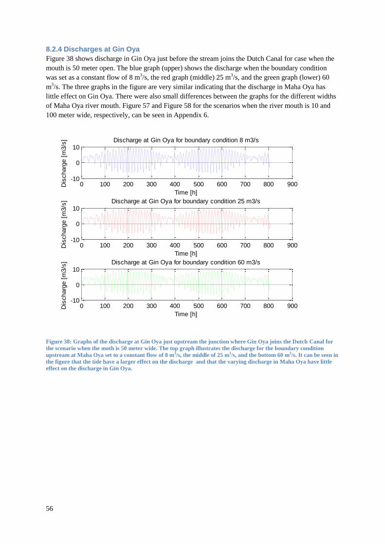
56
8.2.4 Discharges at Gin Oya
Figure 38 shows discharge in Gin Oya just before the stream joins the Dutch Canal for case when the
mouth is 50 meter open. The blue graph (upper) shows the discharge when the boundary condition
was set as a constant flow of 8 m3/s, the red graph (middle) 25 m
3/s, and the green graph (lower) 60
m3/s. The three graphs in the figure are very similar indicating that the discharge in Maha Oya has
little effect on Gin Oya. There were also small differences between the graphs for the different widths
of Maha Oya river mouth. Figure 57 and Figure 58 for the scenarios when the river mouth is 10 and
100 meter wide, respectively, can be seen in Appendix 6.
Figure 38: Graphs of the discharge at Gin Oya just upstream the junction where Gin Oya joins the Dutch Canal for
the scenario when the moth is 50 meter wide. The top graph illustrates the discharge for the boundary condition
upstream at Maha Oya set to a constant flow of 8 m3/s, the middle of 25 m3/s, and the bottom 60 m3/s. It can be seen in
the figure that the tide have a larger effect on the discharge and that the varying discharge in Maha Oya have little
effect on the discharge in Gin Oya.
0 100 200 300 400 500 600 700 800 900-10
0
10Discharge at Gin Oya for boundary condition 8 m3/s
Time [h]
Dis
charg
e [
m3/s
]
0 100 200 300 400 500 600 700 800 900-10
0
10Discharge at Gin Oya for boundary condition 25 m3/s
Time [h]
Dis
charg
e [
m3/s
]
0 100 200 300 400 500 600 700 800 900-10
0
10Discharge at Gin Oya for boundary condition 60 m3/s
Time [h]
Dis
charg
e [
m3/s
]
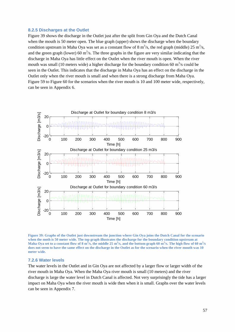
57
8.2.5 Discharges at the Outlet
Figure 39 shows the discharge in the Outlet just after the split from Gin Oya and the Dutch Canal
when the mouth is 50 meter open. The blue graph (upper) shows the discharge when the boundary
condition upstream in Maha Oya was set as a constant flow of 8 m3/s, the red graph (middle) 25 m
3/s,
and the green graph (lower) 60 m3/s. The three graphs in the figure are very similar indicating that the
discharge in Maha Oya has little effect on the Outlet when the river mouth is open. When the river
mouth was small (10 meters wide) a higher discharge for the boundary condition 60 m3/s could be
seen in the Outlet. This indicates that the discharge in Maha Oya has an effect on the discharge in the
Outlet only when the river mouth is small and when there is a strong discharge from Maha Oya.
Figure 59 to Figure 60 for the scenarios when the river mouth is 10 and 100 meter wide, respectively,
can be seen in Appendix 6.
Figure 39: Graphs of the Outlet just downstream the junction where Gin Oya joins the Dutch Canal for the scenario
when the moth is 50 meter wide. The top graph illustrates the discharge for the boundary condition upstream at
Maha Oya set to a constant flow of 8 m3/s, the middle 25 m3/s, and the bottom graph 60 m3/s. The high flow of 60 m3/s
does not seem to have the same effect on the discharge in the Outlet as for the scenario when the river mouth was 10
meter wide.
7.2.6 Water levels
The water levels in the Outlet and in Gin Oya are not affected by a larger flow or larger width of the
river mouth in Maha Oya. When the Maha Oya river mouth is small (10 meters) and the river
discharge is large the water level in Dutch Canal is affected. Not very surprisingly the tide has a larger
impact on Maha Oya when the river mouth is wide then when it is small. Graphs over the water levels
can be seen in Appendix 7.
0 100 200 300 400 500 600 700 800 900-20
0
20Discharge at Outlet for boundary condition 8 m3/s
Time [h]
Dis
charg
e [
m3/s
]
0 100 200 300 400 500 600 700 800 900-20
0
20Discharge at Outlet for boundary condition 25 m3/s
Time [h]
Dis
charg
e [
m3/s
]
0 100 200 300 400 500 600 700 800 900-20
0
20Discharge at Outlet for boundary condition 60 m3/s
Time [h]
Dis
charg
e [
m3/s
]
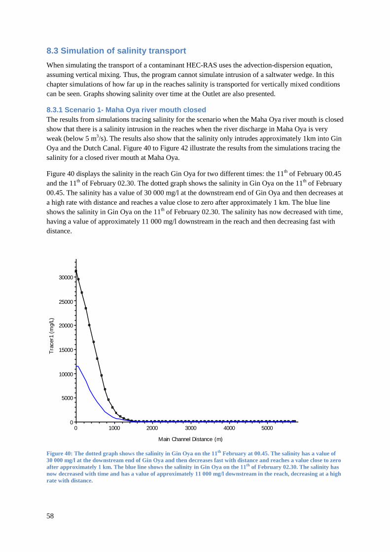
58
8.3 Simulation of salinity transport
When simulating the transport of a contaminant HEC-RAS uses the advection-dispersion equation,
assuming vertical mixing. Thus, the program cannot simulate intrusion of a saltwater wedge. In this
chapter simulations of how far up in the reaches salinity is transported for vertically mixed conditions
can be seen. Graphs showing salinity over time at the Outlet are also presented.
8.3.1 Scenario 1- Maha Oya river mouth closed
The results from simulations tracing salinity for the scenario when the Maha Oya river mouth is closed
show that there is a salinity intrusion in the reaches when the river discharge in Maha Oya is very
weak (below 5 m3/s). The results also show that the salinity only intrudes approximately 1km into Gin
Oya and the Dutch Canal. Figure 40 to Figure 42 illustrate the results from the simulations tracing the
salinity for a closed river mouth at Maha Oya.
Figure 40 displays the salinity in the reach Gin Oya for two different times: the 11th of February 00.45
and the 11th of February 02.30. The dotted graph shows the salinity in Gin Oya on the 11
th of February
00.45. The salinity has a value of 30 000 mg/l at the downstream end of Gin Oya and then decreases at
a high rate with distance and reaches a value close to zero after approximately 1 km. The blue line
shows the salinity in Gin Oya on the 11th of February 02.30. The salinity has now decreased with time,
having a value of approximately 11 000 mg/l downstream in the reach and then decreasing fast with
distance.
Figure 40: The dotted graph shows the salinity in Gin Oya on the 11th February at 00.45. The salinity has a value of
30 000 mg/l at the downstream end of Gin Oya and then decreases fast with distance and reaches a value close to zero
after approximately 1 km. The blue line shows the salinity in Gin Oya on the 11th of February 02.30. The salinity has
now decreased with time and has a value of approximately 11 000 mg/l downstream in the reach, decreasing at a high
rate with distance.
0 1000 2000 3000 4000 5000 60000
5000
10000
15000
20000
25000
30000
35000
C:\Users\Christer\Documents\HEC Data\Kulamulla3.wq38
Main Channel Distance (m)
Tra
cer1
(m
g/L
)
Leg end
11FEB2012 00:45:00-Tracer1 (mg/L)
11FEB2012 02:30:00-Tracer1 (mg/L)
Gin Oya-Gin Oya (Sect 1)

59
Figure 41 illustrates the salinity in the Dutch Canal for two different times: the 11th of February 00.45
and the 11th of February 02.30. The dotted graph shows the salinity in Dutch Canal on the 11
th of
February 00.45. The salinity has a value of 34 000 mg/l at the downstream end of the Dutch Canal,
decreasing at a high rate with distance and reaches a value close to zero after approximately 1 km. The
blue line shows the salinity in Dutch Canal on the 11th of February 02.30. The salinity has now
decreased with time and has a value of approximately 4000 mg/l downstream in the reach, decreasing
at a high rate with distance.
Figure 41: The dotted graph shows the salinity in Dutch Canal on the 11th of February 00.45. The salinity has a value
of 34 000 mg/l at the downstream end of the Dutch Canal, decreasing at a high rate with distance and reaching a value
close to zero after approximately 1 km. The blue line shows the salinity in Dutch Canal on the 11th of February 02.30.
The salinity has now decreased with time and has a value of approximately 4000 mg/l downstream in the reach,
decreasing at a high rate with distance.
0 1000 2000 3000 4000 50000
5000
10000
15000
20000
25000
30000
35000
C:\Users\Christer\Documents\HEC Data\Kulamulla3.wq38
Main Channel Distance (m)
Tra
cer1
(m
g/L
)
Leg end
11FEB2012 00:45:00-Tracer1 (mg/L)
11FEB2012 02:30:00-Tracer1 (mg/L)
Maha Oya-Dutch Canal

60
Figure 42 illustrates the salinity in the Outlet for the entire simulation period (1st February to 5
th of
March). It can be seen that the salinity varies and intrudes upstream the Outlet with the high tide.
There is only a salinity intrusion when the discharge in Maha Oya is weak, which can be seen in the
figure for the time period 1st of February to 12
th of February. During this time period the Maha Oya
had a discharge of only 1 m3/s; however, for stronger discharges in Maha Oya there is no salinity
intrusion in the Outlet.
Figure 42: The graph illustrates the salinity in the Outlet just after the junction where Gin Oya joins the Dutch Canal
for the entire simulation period (1 February to 5 March). The salinity seems to be varying with the tide when the
discharge in Maha Oya is low; for the period 1 February to 12 February the discharge in Maha Oya is only 1 m3/s.
For the remaining time period the discharge in Maha Oya is 5 m3/s or higher and there is no salinity intrusion in the
Outlet.
8.3.2 Scenario 2- Maha Oya river mouth open
Figure 43 to Figure 44 illustrate the results for the scenario when the Maha Oya river mouth is 100
meter wide and the boundary condition upstream at Maha Oya is set to a constant discharge of 25
m3/s. For the boundary condition with a flow of 8 m
3/s at Maha Oya there is a salinity intrusion at the
Maha Oya river mouth. For higher flows no salinity intrusion can be detected at the river mouth.
When the Maha Oya river mouth is wide most of the discharge from Maha Oya goes through the river
mouth and little flow goes into the split to the Dutch Canal. This is reflected in the simulations of the
salinity. The salinity in the Outlet is higher and there is a salinity intrusion in the Outlet even when the
discharge in the Maha Oya is large. This can be explained by a weak flow in the Dutch Canal and in
Gin Oya and that the tide at the Outlet has a larger influence due to low discharge in the reaches. The
high tide is strong enough to reverse the flow and with the tide the salinity can intrude into the Outlet.
Appendix 8 shows the salinity intrusion for the boundary conditions 8 and 60 m3/s.
11 13 15 17 19 21 23 25 27 29 02 04Feb2012 Mar2012
0
5000
10000
15000
20000
25000
30000
35000
C:\Users\Christer\Documents\HEC Data\Kulamulla3.wq38
Time
Tra
cer1
(m
g/L
)
Legend
Tracer1 (mg/L)
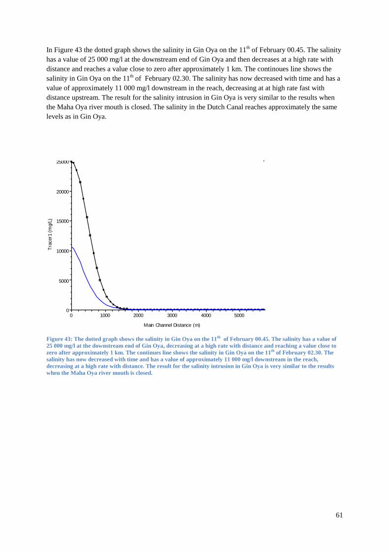
61
In Figure 43 the dotted graph shows the salinity in Gin Oya on the 11th of February 00.45. The salinity
has a value of 25 000 mg/l at the downstream end of Gin Oya and then decreases at a high rate with
distance and reaches a value close to zero after approximately 1 km. The continoues line shows the
salinity in Gin Oya on the 11th of February 02.30. The salinity has now decreased with time and has a
value of approximately 11 000 mg/l downstream in the reach, decreasing at at high rate fast with
distance upstream. The result for the salinity intrusion in Gin Oya is very similar to the results when
the Maha Oya river mouth is closed. The salinity in the Dutch Canal reaches approximately the same
levels as in Gin Oya.
Figure 43: The dotted graph shows the salinity in Gin Oya on the 11th of February 00.45. The salinity has a value of
25 000 mg/l at the downstream end of Gin Oya, decreasing at a high rate with distance and reaching a value close to
zero after approximately 1 km. The continues line shows the salinity in Gin Oya on the 11th of February 02.30. The
salinity has now decreased with time and has a value of approximately 11 000 mg/l downstream in the reach,
decreasing at a high rate with distance. The result for the salinity intrusion in Gin Oya is very similar to the results
when the Maha Oya river mouth is closed.
0 1000 2000 3000 4000 5000 60000
5000
10000
15000
20000
25000
C:\Users\Christer\Documents\HEC Data\Kulamulla3.wq38
Main Channel Distance (m)
Tra
cer1
(m
g/L
)
Leg end
11FEB2012 00:45:00-Tracer1 (mg/L)
11FEB2012 02:30:00-Tracer1 (mg/L)
Gin Oya-Sect ion 1
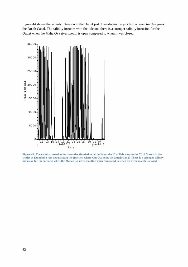
62
Figure 44 shows the salinity intrusion in the Outlet just downstream the junction where Gin Oya joins
the Dutch Canal. The salinity intrudes with the tide and there is a stronger salinity intrusion for the
Outlet when the Maha Oya river mouth is open compared to when it was closed.
Figure 44: The salinity intrusion for the entire simulation period from the 1st of February to the 5th of March in the
Outlet at Kulamulla just downstream the junction where Gin Oya joins the Dutch Canal. There is a stronger salinity
intrusion for the scenario when the Maha Oya river mouth is open compared to when the river mouth is closed,
11 13 15 17 19 21 23 25 27 29 02 04Feb2012 Mar 2012
0
5000
10000
15000
20000
25000
30000
35000
C:\Users\Christer\Documents\HEC Data\Kulamulla3.wq38
Tim e
Tra
cer1
(m
g/L
)
Legend
Tr ac er1 (m g/L)
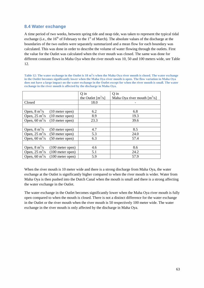
63
8.4 Water exchange
A time period of two weeks, between spring tide and neap tide, was taken to represent the typical tidal
exchange (i.e., the 16th of February to the 1
st of March). The absolute values of the discharge at the
boundaries of the two outlets were separately summarized and a mean flow for each boundary was
calculated. This was done in order to describe the volume of water flowing through the outlets. First
the value for the Outlet was calculated when the river mouth was closed. The same was done for
different constant flows in Maha Oya when the river mouth was 10, 50 and 100 meters wide, see Table
12.
Table 12: The water exchange in the Outlet is 18 m3/s when the Maha Oya river mouth is closed. The water exchange
in the Outlet becomes significantly lower when the Maha Oya river mouth is open. The flow variation in Maha Oya
does not have a large impact on the water exchange in the Outlet except for when the river mouth is small. The water
exchange in the river mouth is affected by the discharge in Maha Oya.
Q in
the Outlet [m3/s]
Q in
Maha Oya river mouth [m3/s]
Closed 18.0 -
Open, 8 m3/s (10 meter open) 6.2 6.8
Open, 25 m3/s (10 meter open) 8.9 19.3
Open, 60 m3/s (10 meter open) 23.3 39.6
Open, 8 m3/s (50 meter open) 4.7 8.5
Open, 25 m3/s (50 meter open) 5.3 24.0
Open, 60 m3/s (50 meter open) 6.3 57.4
Open, 8 m3/s (100 meter open) 4.6 8.6
Open, 25 m3/s (100 meter open) 5.1 24.2
Open, 60 m3/s (100 meter open) 5.9 57.9
When the river mouth is 10 meter wide and there is a strong discharge from Maha Oya, the water
exchange at the Outlet is significantly higher compared to when the river mouth is wider. Water from
Maha Oya is then pushed into the Dutch Canal when the mouth is small and there is a strong affecting
the water exchange in the Outlet.
The water exchange in the Outlet becomes significantly lower when the Maha Oya river mouth is fully
open compared to when the mouth is closed. There is not a distinct difference for the water exchange
in the Outlet or the river mouth when the river mouth is 50 respectively 100 meter wide. The water
exchange in the river mouth is only affected by the discharge in Maha Oya.

64
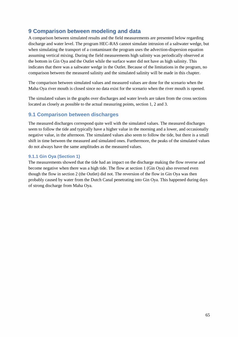
65
9 Comparison between modeling and data A comparison between simulated results and the field measurements are presented below regarding
discharge and water level. The program HEC-RAS cannot simulate intrusion of a saltwater wedge, but
when simulating the transport of a contaminant the program uses the advection-dispersion equation
assuming vertical mixing. During the field measurements high salinity was periodically observed at
the bottom in Gin Oya and the Outlet while the surface water did not have as high salinity. This
indicates that there was a saltwater wedge in the Outlet. Because of the limitations in the program, no
comparison between the measured salinity and the simulated salinity will be made in this chapter.
The comparison between simulated values and measured values are done for the scenario when the
Maha Oya river mouth is closed since no data exist for the scenario when the river mouth is opened.
The simulated values in the graphs over discharges and water levels are taken from the cross sections
located as closely as possible to the actual measuring points, section 1, 2 and 3.
9.1 Comparison between discharges
The measured discharges correspond quite well with the simulated values. The measured discharges
seem to follow the tide and typically have a higher value in the morning and a lower, and occasionally
negative value, in the afternoon. The simulated values also seem to follow the tide, but there is a small
shift in time between the measured and simulated ones. Furthermore, the peaks of the simulated values
do not always have the same amplitudes as the measured values.
9.1.1 Gin Oya (Section 1)
The measurements showed that the tide had an impact on the discharge making the flow reverse and
become negative when there was a high tide. The flow at section 1 (Gin Oya) also reversed even
though the flow in section 2 (the Outlet) did not. The reversion of the flow in Gin Oya was then
probably caused by water from the Dutch Canal penetrating into Gin Oya. This happened during days
of strong discharge from Maha Oya.

66
In the model the tide did not reverse the flow as strongly as indicated by the measurements and the
peaks in the discharge did not quite have the same amplitude. The flow reversal in Gin Oya caused by
a strong river discharge in Maha Oya was also seen in the simulations. In Figure 45 the simulated and
measured discharges can be seen. The continuous line shows the simulated discharge and the dots are
the measured values.
Figure 45: The continuous line shows the simulated discharge in Gin Oya from HEC-RAS and the dots are measured
values. The simulated discharge in general underestimated the measurements.
0 100 200 300 400 500 600 700 800 900-10
-5
0
5
10
15
Time from startday 1 Feb 09.00 to 5 March 21.00 [h]
Dis
charg
e [
m3/s
]
Comparison in Section 1 (Gin Oya)
Simulated values
Measured values

67
9.1.2 The Outlet (Section 2)
In Figure 46 the simulated and measured discharges at section 2 are presented. The continuous line
shows the simulated discharge and the dots are the measured values.
In the measurements the tide had a large impact on the discharge making the flow reverse and
becoming negative with a high tide. Overall, the flow at section 2 responded quite well to the sum of
the flow in section 1 and 3. A large flow in Maha Oya corresponded with a large flow in section 2.
A high flow in Maha Oya made the flow in section 2 (the Outlet) even higher in the model. The
negative peaks in the model are not as high as in reality. The measured negative peak on the 29th of
February could not be simulated in the model and its reason is not known.
Figure 46: The continuous line shows the simulated discharges and the dots are measured values. The simulated
values follow the same pattern as the measured value although the peaks are somewhat displaced. The negative peak
on the 29th of February could not be simulated in the model and the reason for it is not known.
0 100 200 300 400 500 600 700 800 900-20
-15
-10
-5
0
5
10
15
20
25
30
Time from startday 1 Feb 09.00 to 5 March 21.00 [h]
Dis
charg
e [
m3/s
]
Comparison in Section 2 (The outlet)
Simulated values
Measured values

68
9.1.3 Dutch Canal (section 3)
In Figure 47 the simulated and measured discharges at section 3 are presented. The continuous line
shows the simulated discharge and the dots are the measured values.
The measurements showed that the discharge at the Dutch Canal (section 3) was more even over the
day than it was in Gin Oya. The tide did not seem to have the same impact in this reach, although a
negative discharge was measured twice.
The simulated values follow the discharge from the Maha Oya given in the boundary conditions.
When the discharge from Maha Oya is large the tide does not seem to have the same impact on the
discharge in the model as in the measurements.
Figure 47: The continuous line shows simulated discharge and the dots are measured values. The tide seems to have a
larger impact on the discharge in the measurements than in the model. The tide only affects the discharge at the
Dutch Canal when the discharge from Maha Oya is low. The negative peak on the 29th of February could not be
simulated in the model.
0 100 200 300 400 500 600 700 800 900-10
-5
0
5
10
15
20
25
Time from startday 1 Feb 09.00 to 5 March 21.00 [h]
Dis
charg
e [
m3/s
]
Comparison in Section 3 (The Dutch Canal)
Simulated values
Measured values
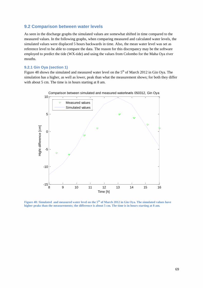
69
9.2 Comparison between water levels
As seen in the discharge graphs the simulated values are somewhat shifted in time compared to the
measured values. In the following graphs, when comparing measured and calculated water levels, the
simulated values were displaced 5 hours backwards in time. Also, the mean water level was set as
reference level to be able to compare the data. The reason for this discrepancy may be the software
employed to predict the tide (WX-tide) and using the values from Colombo for the Maha Oya river
mouths.
9.2.1 Gin Oya (section 1)
Figure 48 shows the simulated and measured water level on the 5th of March 2012 in Gin Oya. The
simulation has a higher, as well as lower, peak than what the measurement shows; for both they differ
with about 5 cm. The time is in hours starting at 8 am.
Figure 48: Simulated and measured water level on the 5th of March 2012 in Gin Oya. The simulated values have
higher peaks than the measurements; the difference is about 5 cm. The time is in hours starting at 8 am.
8 9 10 11 12 13 14 15 16-15
-10
-5
0
5
10Comparison between simulated and measured waterlevels 050312, Gin Oya
Time [h]
Hig
ht
diffe
rence [
cm
]
Measured values
Simulated values
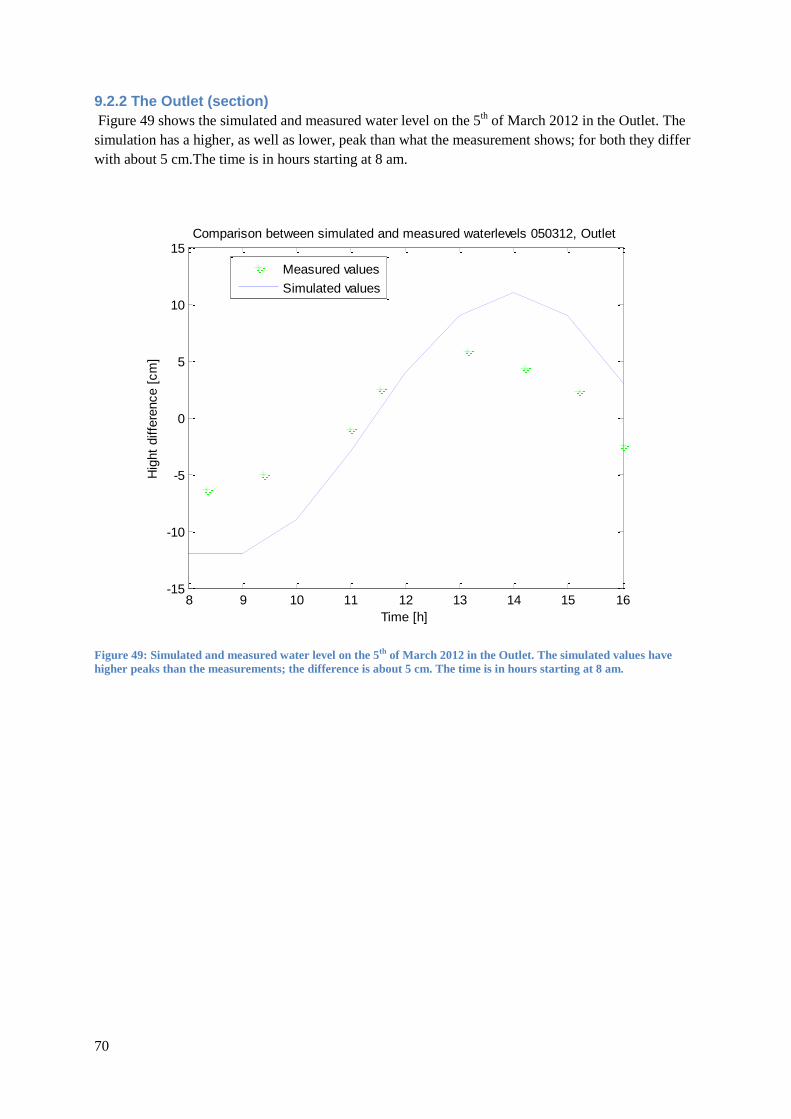
70
9.2.2 The Outlet (section)
Figure 49 shows the simulated and measured water level on the 5th of March 2012 in the Outlet. The
simulation has a higher, as well as lower, peak than what the measurement shows; for both they differ
with about 5 cm.The time is in hours starting at 8 am.
Figure 49: Simulated and measured water level on the 5th of March 2012 in the Outlet. The simulated values have
higher peaks than the measurements; the difference is about 5 cm. The time is in hours starting at 8 am.
8 9 10 11 12 13 14 15 16-15
-10
-5
0
5
10
15Comparison between simulated and measured waterlevels 050312, Outlet
Time [h]
Hig
ht
diffe
rence [
cm
]
Measured values
Simulated values
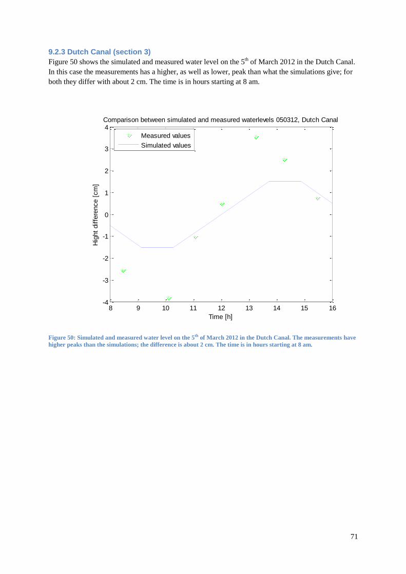
71
9.2.3 Dutch Canal (section 3)
Figure 50 shows the simulated and measured water level on the 5th of March 2012 in the Dutch Canal.
In this case the measurements has a higher, as well as lower, peak than what the simulations give; for
both they differ with about 2 cm. The time is in hours starting at 8 am.
Figure 50: Simulated and measured water level on the 5th of March 2012 in the Dutch Canal. The measurements have
higher peaks than the simulations; the difference is about 2 cm. The time is in hours starting at 8 am.
8 9 10 11 12 13 14 15 16-4
-3
-2
-1
0
1
2
3
4Comparison between simulated and measured waterlevels 050312, Dutch Canal
Time [h]
Hig
ht
diffe
rence [
cm
]
Measured values
Simulated values

72
73
10 Discussion The model can be used to determine water surface elevations and discharges at given points. This data
can then be interpreted to determine the water exchange at the Outlet and to see how this exchange is
affected by a closed respectively open river mouth. The model can also be used to see how the water
exchange at the river mouth is affected by different discharges in Maha Oya. The model does not
reproduce the measured data in great detail, but it captures the overall patterns of variation.
The calibration and validation of the mathematical model depend on the data collected during the five
field days. A larger amount of data would have helped in the calibration of the model and make it
reproduce the reality in an improved way. Better knowledge of the geometry data and boundary
conditions would probably also have made the model more accurate. The simulations made for the
scenario when the Maha Oya river mouth is open could not be compared with any actual data;
therefore it is hard to say how good these results are. However, conclusions regarding how various
widths and discharges in Maha Oya affects the water exchange at the Outlet and the river mouth can
be made, although the exact numbers contain some uncertainty.
The model exhibited the least sensitivity to the tidal boundary condition. This boundary condition was
also the most certain and based on predictions from Colombo using the program WX-tide. The
boundary condition at Maha Oya and Gin Oya are based on assumptions and observations during the
field measurements. The sensitivity analyses showed that the model was most sensitive to the
boundary condition at Maha Oya. The optimal thing to do would have been to use measured values
(either discharge or stage) at the exact locations at the boundaries. However, this was not possible due
to lack of equipment and time. The authors could not take measurements at both boundaries for every
hour during the entire simulation period and there was no data available from fixed gauges. There is a
weir located upstream in Maha Oya, but unfortunately it was not possible to get a hold of this data.
The boundary condition at Maha Oya was based on our field measurements a few kilometers
downstream and the discharge at the boundary does not need to be the same as for this measuring
point. This data is very scarce and the values between are interpolated, which may not correspond with
the reality. In reality the discharge might, for example, fluctuate more over time.
The model was not so sensitive to the boundary condition in Gin Oya as to the boundary condition in
Maha Oya, since Gin Oya has a smaller flow and therefore has smaller effects on the water exchange
in the Outlet. The boundary condition in Gin Oya was set as a constant flow since there was limited
information about this catchment. Only the data collected in this study several kilometers downstream
was avaliable. A constant flow for the entire simulation time is probably not realistic, there is probably
higher and lower discharges fluctuating over time caused by rainfall and surface runoff. Setting this
boundary condition as a constant flow also made it difficult to recreate the discharge peaks from the
measured data, but facilitated the reproduction of mean values.
The tide did not have as strong effect on the discharges (away from the Outlet and river mouth) in the
model as well as in the measurements. This can partly depend on the geometry data. Limited such data
was collected during our stay. It would have been desirable to have more data regarding the depth and
width at the Outlet. The geometry data for the other reaches was also scarce. Only depth and widths
were taken at three points; section 1, 2 and 3 in each reach. The depth at each reach was used as a
mean depth for the entire reaches. The widths for the cross sections with missing data were based on
measurements in Google Earth.
74
The calculated numbers to quantify the water exchange for the Outlet and Maha Oya can only be
compared to the scenario when the river mouth is closed respectively open and for how different
discharges in Maha Oya affect this number.
There was a lag time between the simulated and measured values when plotting the water levels.
When plotting the simulated and measured water levels, adjusted with regard to the mean water level,
the simulated water levels were higher in the Dutch Canal, but lower in Gin Oya and the Outlet.
Possibly this may indicate that the friction losses were not modeled correctly. More detailed geometry
data would have been required to simulate the friction losses more accurately. On the other hand, the
sensitivity analysis showed that changing the Manning´s coefficient had little impact on the result.
Comparisons between the output files of tidal water elevations from WX-tide and the field data was
made, showing that there was a time lag between the values from WX-tide and the field data. Peaks of
water levels occurred a few hours earlier in WX-tide than actual measured peaks in the sections. The
predictions by WX-tide are valid for Colombo, and the conditions at Maha Oya might be slightly
different. It was beyond the scope of this study to perform a detailed analysis on the accuracy of WX-
tide, which could have been validated with measurements from Colombo.
During the field measurements high salinity at the bottom and low salinity at the surface were
regularly observed, indicating that there was a saltwater wedge penetrating into the river system. No
measurements were done regarding how far this saltwater wedge propagated. This saltwater wedge
could not be simulated in the program; the program could only simulate saltwater intrusion based on
the advection-dispersion transport for a vertically mixed water body. Such conditions may prevail in
the river system when the river flow is small.

75
11 Conclusions The main objective of this study was to determine how the water exchange in estuaries and river
mouths are affected by inlet sedimentation in Sri Lanka. In order to do this, a specific river system, the
Maha Oya, was investigated using field measurements and numerical modeling.
11.1 Scenario 1- Maha Oya closed
The flow in Maha Oya dominates the water exchange in the Outlet. The size of the discharge
determines to what degree tidal flows may penetrate into the river system through the Outlet. For this
scenario the tide affected the direction of the discharge, making it negative (going upstream) when the
discharge was low and the tide was high. When the discharge in Maha Oya was high the tide was not
strong enough to change the direction of the flow. If the discharge in Maha Oya was high a negative
flow could sometimes be observed in Gin Oya, at the same time as a positive flow could be seen in the
Outlet. This indicated that the river discharge from Maha Oya was so strong that it did not only flow
out in the Outlet but it also penetrated into Gin Oya.
11.2 Scenario 2- Maha Oya open
If the river mouth is still quite small, some of the river discharge continues into the Dutch Canal. A
higher discharge gives a higher portion of this discharge continuing into the Dutch Canal. When
simulating the opening of the river mouth, it can be seen that for a wider river mouth a smaller portion
of the discharge from Maha Oya continues into the Dutch Canal. A river mouth that is 50 to 100
meters open implies that the Maha Oya and the Outlet have little influence on each other. A wide
river mouth also causes a higher tidal effect in Maha Oya compared to a small river mouth. However,
a larger discharge from Maha Oya reduces the tidal effects at the river mouth.
11.3 Inlet sedimentation effect on water exchange
The calculated water exchange for the Outlet was smaller for a fully open river mouth than for a
closed river mouth due to reduced flow in the Dutch Canal. A small opening of the river mouth and
high discharge gave a larger water exchange in the Outlet due to increased flow in the Dutch Canal.
There was a higher transport of saltwater into the Outlet when the Maha Oya river mouth was open.
This was explained by a lower discharge in the Dutch Canal. Higher discharge in Maha Oya lead to a
higher water exchange at the river mouth. A higher discharge in Maha Oya also probably leads to less
salt transport into Maha Oya.
The Outlet created by the tsunami does not seem to have a large impact on the water exchange in
Maha Oya. However its existence might facilitate the everyday life for the people living in the area,
providing them with a passage to the sea for the periods when the river mouth is closed. Also, the
effect on the water levels and the risk of flooding in the area is diminished during heavy downfall
thanks to the Outlet.

76
77
12 References
12.1 Printed Reference
Arulananthan, K. (2004). “Hydrography, costal water circulation and classification of Sri Lankan
Lagoons”. Department of oceanography, Göteborg University, C62 2004
Behera, M. R and Murali, K. (2007). “Semi empirical model for initial displacement of salt water
wedge in a bar-blocked estuary”. Journal of waterway, port, coastal and ocean engineering, 133:4
p.264-267.
Brunner, G.W. (2010). “HEC-RAS, river analysis system hydraulic reference manual”. Version 4.1
US Army Corps of Engineers, California, USA
Chanson, H. (2004). “Environmental Hydraulics for open channel flows”. The University of
Queensland, Australia, Butterworth-Heinemann
Chow, V.T. (1959). “Open channel hydraulic”. McGraw-Hill, New York
Chubarenko, I. (2007).”Physical processes in lagoons”. Assessment of the Fate and Effects of Toxic
Agents on Water Resources, p.55-8, Springer.
Conley, D. C. (1999).”Observations of the impact of a developing inlet in a bar built estuary”.
Continental Shelf Research 19, p.1733-1754
Domroes, M and Ranatunge, E. (1993). “Analysis of inter-station daily rainfall correlation during the
southwest monsoon in the wet zone of Sri Lanka”. Geografiska Annaler. Series A, Physical
Geography, Vol 75, No 3, p. 137-148
Elsdon T.S, De Bruin M.B.N.A, Diepen N.J and Gillanders B. M. (2009). “Extensive drought negates
human influence on nutrients and water quality in estuaries”. Science of the total environment. Vol
407, issue 8, p.3033-3043
Escoffier, F.F. (1977). “Hydraulics and stability of tidal inlets”. GITI report 13, U.S Army Engineer
Research Center, Fort Belvoir, Virginia, USA
Fagerburg, T.L. and Alexander, M.P. (1994). “Underwater sill construction for mitigating salt wedge
migration on the lower Mississippi River”. US army corps of engineering, Miscellaneous paper HL-94
vol.1, USA
Fischer, H. B, List. E.J, Koh, R.C.Y, Imberger. J and Brooks. N.H. (1979). “Mixing in inland and
coastal water”. Academic Press, London, p.120-130
Harleman, D.R.F. (1991).”Keulegan Legacy: Saline wedges”. Journal of hydraulic engineering. Vol
117. No. 12 Paper No. 26459
Kjerfve, B. (1986). “Comparative oceanography of coastal lagoons”. Estuarine Variability University
of South Carolina, Academic press, Columbia
Kjerfve, B. and Magill, K.E. (1989). “Geographic and hydrodynamic characteristics of shallow costal
lagoons”. Marine geology, 88, p. 187-199, Elsevier Science Publisher, Amsterdam

78
Kjerfve, B. (1994).”Coastal lagoons”. Belle W. Baruch Institute for Marine Biology and Coastal
Research, Marine Science Program, and Department of Geological Sciences,
University of South Carolina, Columbia, SC 29208, USA
Lam, NT. Stive, M.J.F.Verhagen, H.J. and Wang, Z.B. (2008). “Seasonal behaviour of tidal inlets
in a tropical monsoon area”. Proceedings of COPEDEC VII, Paper 170, Dubai, UAE.
Malmgren, B.A. Hulugalla, R. Hayashi, Y. and Mikami, T. (2003). “Precipitation trends in Sri Lanka
since the 1870s and relationships to El Niño-Southern oscillation”. International Journal of
Climatology, 23, p.1235-1252
Mitsuda, E. and Rattray, M. (1974).”Theoretical analyses of conditions in a salt wedge”. Estuarine and
coastal marine science 2, p. 375-394
Ranasinghe, R. Pattiaratchi, C. and Masselink, G. (1999). “A morphodynamic model to simulate the
seasonal closure of tidal inlets”. Coastal Engineering 37, p.1-36
Ratnayake, R. (2005).” Maha Oya Basin”. Sri Lanka Water Partnership
Rydberg, L. and Wickbom, L. (1996). “Tidal Choking and Bed Friction in Negombo Lagoon, Sri
Lanka”. Estuaries, Vol. 19, No.3, p.540-547
Sargent, F. E. and Jirka G.H. (1987). “Experiments on saline wedge”. Journal of hydraulic
engineering. Vol 113, No 10, p.1307-1324
Savenije, R. H.G. (2005). ”Salinity and tides in alluvial estuaries”. TU Delft, Delft, The Netherlands
Seabergh, W. C. (2006). “Hydrodynamics of Tidal Inlets:”. Coastal and Hydraulics Laboratory,
Engineer Research and Development Center, Vicksburg, Mississippi, USA
Shankar, D. Vinayachandran, P.N. and Unnikrishnan, A.S.(2002). ”The monsoon currents in the north
Indian Ocean”. Progress in Oceanography 52, p. 63-120
US Army corps of engineers. (1993). “Control methods for salinity intrusion in well stratified estuaries
and waterways”. Technical Letter No. 1110-2-347, department of the army, Washington, DC, USA
20314-1000
Weerakkody (2012) “Salinity Intrusion into the Maha Oya Estuary and Associated Coastal
Waterway”. TVVR 12/5003, Water Resources Engineering, LTH/Lund University
Wickramagamage, P. (2009). “Seasonality and spatial pattern of rainfall of Sri Lanka: Exploratory
factor analysis”. International Journal of Climatology, Vol. 30, No. 8, p.1235-1245
Zubair, L and Chandimala, J. (2006). “Epochal Changes in ENSO–Streamflow Relationships in Sri
Lanka”. Journal of hydrometeorology, Vol. 7, No. 6, p.1237-1246
12.2 Web references
SIDA, 2012, http://www.sida.se/Svenska/Lander--regioner/Asien/Sri-Lanka/Landfakta/-
downloaded: 2012-04-04
Environmentlanka 2012, http://environmentlanka.com/blog/2009/trends-in-water-quality-parameters-
for-river-maha-oya/- downloaded: 2012-01-26

79
Google Earth- http://www.google.com/earth/index.html- downloaded: 2012-04-01
WX-Tide, 2012, http://www.wxtide32.com/- downloaded: 2012-04-28

80
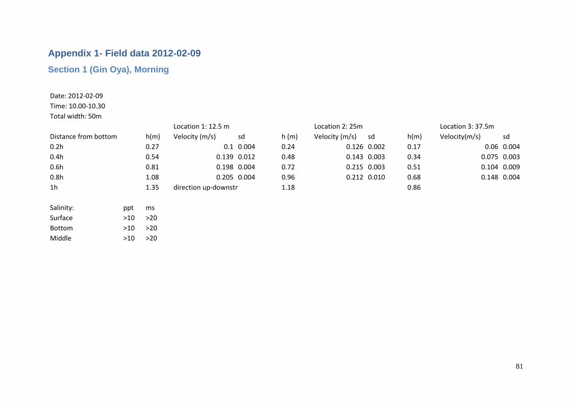
81
Appendix 1- Field data 2012-02-09
Section 1 (Gin Oya), Morning
Date: 2012-02-09 Time: 10.00-10.30 Total width: 50m
Location 1: 12.5 m
Location 2: 25m
Location 3: 37.5m
Distance from bottom
h(m) Velocity (m/s) sd
h (m) Velocity (m/s) sd
h(m) Velocity(m/s) sd
0.2h
0.27 0.1 0.004
0.24 0.126 0.002
0.17 0.06 0.004
0.4h
0.54 0.139 0.012
0.48 0.143 0.003
0.34 0.075 0.003
0.6h
0.81 0.198 0.004
0.72 0.215 0.003
0.51 0.104 0.009
0.8h
1.08 0.205 0.004
0.96 0.212 0.010
0.68 0.148 0.004
1h
1.35 direction up-downstr
1.18
0.86
Salinity: ppt ms Surface >10 >20 Bottom >10 >20 Middle >10 >20

82
Section 2 (the Outlet), Morning
Date: 2012-02-09 Time: 11.00-11.40 Total width: 31m
Location 2: ~16m
Location 3: 25m
Distance from bottom
h (m) Velocity (m/s) sd
h(m) Velocity(m/s) sd
0.2h
0.24 0.126 0.022
0.42 0.217 0.018
0.4h
0.48 0.26 0.019
0.84 0.159 0.014
0.6h
0.72 0.243 0.078
1.26 0.110 0.021
0.8h
0.96 0.257 0.033
1.50 0.18 0.011
1h
direction upstream to downstream 1.2
2.10
MEASURED FROM SURFACE!!
Salinity: ppt ms Surface >10 >20 Bottom >10 >20 Middle >10 >20
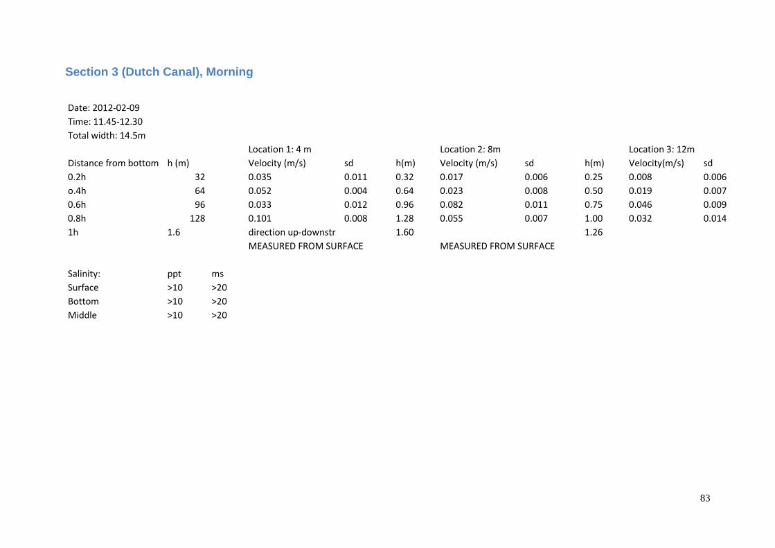
83
Section 3 (Dutch Canal), Morning
Date: 2012-02-09 Time: 11.45-12.30 Total width: 14.5m
Location 1: 4 m
Location 2: 8m
Location 3: 12m
Distance from bottom h (m)
Velocity (m/s) sd
h(m) Velocity (m/s) sd
h(m) Velocity(m/s) sd
0.2h 32
0.035 0.011
0.32 0.017 0.006
0.25 0.008 0.006
o.4h 64
0.052 0.004
0.64 0.023 0.008
0.50 0.019 0.007
0.6h 96
0.033 0.012
0.96 0.082 0.011
0.75 0.046 0.009
0.8h 128
0.101 0.008
1.28 0.055 0.007
1.00 0.032 0.014
1h 1.6
direction up-downstr
1.60
1.26
MEASURED FROM SURFACE
MEASURED FROM SURFACE
Salinity: ppt ms Surface >10 >20 Bottom >10 >20 Middle >10 >20

84
Section 1 (Gin Oya), Afternoon
Date: 2012-02-09 Time: 14.15-14.40 Total width: 50m
Location 1: 12.5 m
Location 2: 25m
Location 3: 37.5m
Distance from bottom h (m) Velocity (m/s) sd
h(m) Velocity (m/s) sd
h(m) Velocity(m/s) sd
0.2h 29 0.104 0.008
0.25 0.207 0.015
0.17 0.093 0.016
o.4h 58 0.14 0.004
0.50 0.216 0.016
0.34 0.064 0.006
0.6h 87 0.151 0.011
0.75 0.255 0.008
0.51 0.053 0.010
0.8h 116 0.124 0.006
1.00 0.219 0.022
0.68 0.071 0.010
1h 1.44 direction down- up.str
1.27
0.87
Section 2 (the Outlet), Afternoon
Date: 2012-02-09 Time: 14.45-15.00 Total width: 31m
Location 1: ~16 m
Location 2: 25m
Distance from bottom h (m) Velocity (m/s) sd
h(m) Velocity (m/s) sd
0.2h 0.25 0.020 0.011
0.42 0.480 0.041
o.4h 0.50 0.007 0.019
0.84 0.697 0.021
0.6h 0.75 0.008 0.009
1.26 0.579 0.030
0.8h 1.00 0.007 0.007 1h 1.25 direction down- up.str 0.029
1.68
MEASURED FROM SURFACE

85
Section 3 (Dutch Canal), Afternoon
Date: 2012-02-09 Time: 15.15-15.40 Total width: 14,5m
Location 1: 4 m
Location 2: 8m
Location 3: 12m
Distance from bottom h (m) Velocity (m/s) sd
h(m) Velocity (m/s) sd
h(m) Velocity(m/s) sd
0.2h 0.35 0.260 0.016
0.35 0.295 0.016
0.24 0.199 0.012
o.4h 0.70 0.255 0.007
0.70 0.294 0.019
0.48 0.174 0.010
0.6h 1.05 0.252 0.014
1.05 0.245 0.016
0.72 0.141 0.012
0.8h 1.40 0.264 0.011
1.40 0.269 0.033
0.96 0.166 0.014
1h 1.80 direction down- up.str
1.80
1.20
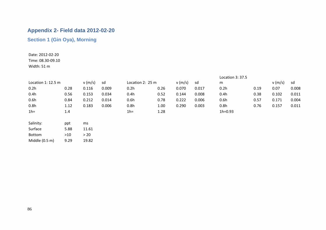
86
Appendix 2- Field data 2012-02-20
Section 1 (Gin Oya), Morning
Date: 2012-02-20 Time: 08.30-09.10 Width: 51 m
Location 1: 12.5 m
v (m/s) sd
Location 2: 25 m v (m/s) sd
Location 3: 37.5 m
v (m/s) sd
0.2h 0.28 0.116 0.009
0.2h 0.26 0.070 0.017
0.2h 0.19 0.07 0.008
0.4h 0.56 0.153 0.034
0.4h 0.52 0.144 0.008
0.4h 0.38 0.102 0.011
0.6h 0.84 0.212 0.014
0.6h 0.78 0.222 0.006
0.6h 0.57 0.171 0.004
0.8h 1.12 0.183 0.006
0.8h 1.00 0.290 0.003
0.8h 0.76 0.157 0.011
1h= 1.4
1h= 1.28
1h=0.93
Salinity: ppt ms Surface 5.88 11.61 Bottom >10 > 20 Middle (0.5 m) 9.29 19.82
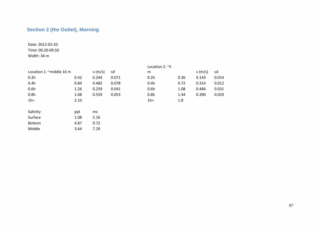
87
Section 2 (the Outlet), Morning
Date: 2012-02-20 Time: 09.20-09.50 Width: 34 m
Location 1: ~middle 16 m
v (m/s) sd
Location 2: ~5 m
v (m/s) sd
0.2h 0.42 0.244 0.071
0.2h 0.36 0.143 0.014
0.4h 0.84 0.482 0.078
0.4h 0.72 0.314 0.012
0.6h 1.26 0.259 0.041
0.6h 1.08 0.484 0.031
0.8h 1.68 0.559 0.053
0.8h 1.44 0.390 0.029
1h= 2.10
1h= 1.8
Salinity: ppt ms Surface 1.08 2.16 Bottom 4.87 9.72 Middle 3.64 7.29
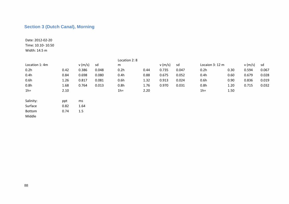
88
Section 3 (Dutch Canal), Morning
Date: 2012-02-20 Time: 10.10- 10.50 Width: 14.5 m
Location 1: 4m
v (m/s) sd
Location 2: 8 m
v (m/s) sd
Locaion 3: 12 m
v (m/s) sd
0.2h 0.42 0.386 0.048
0.2h 0.44 0.735 0.047
0.2h 0.30 0.594 0.067
0.4h 0.84 0.698 0.080
0.4h 0.88 0.675 0.052
0.4h 0.60 0.679 0.028
0.6h 1.26 0.817 0.081
0.6h 1.32 0.913 0.024
0.6h 0.90 0.836 0.019
0.8h 1.68 0.764 0.013
0.8h 1.76 0.970 0.031
0.8h 1.20 0.715 0.032
1h= 2.10
1h= 2.20
1h= 1.50
Salinity: ppt ms Surface 0.82 1.64 Bottom 0.74 1.5 Middle

89
Section 1 (Gin Oya), Afternoon
Date: 2012-02-20 Time: 14.15-14.50 Width: 51 m
location 1: 12.5 m
v (m/s) sd
Location 2: 25 m
v (m/s) sd
Location: 37.5 m
v (m/s) sd
0.2h 0.29 0.071 0.010
0.2h 0.27 0.039 0.005
0.2h 0.21 0.006 0.005
0.4h 0.58 0.047 0.017
0.4h 0.54 0.064 0.006
0.4h 0.42 0.003 0.005
0.6h 0.87 0.111 0.018
0.6h 0.81 0.086 0.016
0.6h 0.63 0.028 0.005
0.8h 1.16 0.126 0.019
0.8h 1.08 0.099 0.008
0.8h 0.84 0.053 0.005
1h= 1.46
1h= 1.37
1h= 1.04
Direction downstream
Direction downstream
Direction downstream
to upstream
to upstream
to upstream
Salinity: ppt ms Surface 1.13 2.27 Bottom 1.83 3.64 Middle (1m) 1.30 2.61
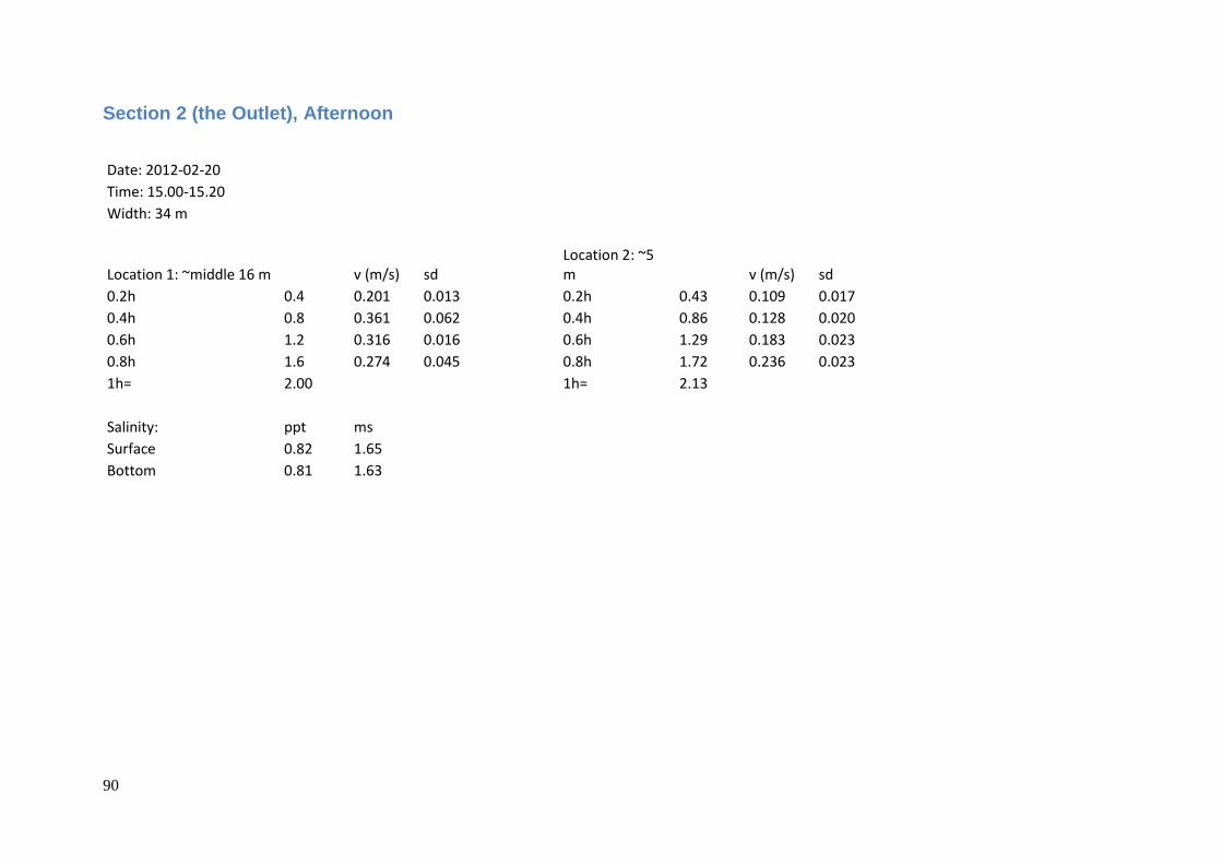
90
Section 2 (the Outlet), Afternoon
Date: 2012-02-20 Time: 15.00-15.20 Width: 34 m
Location 1: ~middle 16 m
v (m/s) sd
Location 2: ~5 m
v (m/s) sd
0.2h 0.4 0.201 0.013
0.2h 0.43 0.109 0.017
0.4h 0.8 0.361 0.062
0.4h 0.86 0.128 0.020
0.6h 1.2 0.316 0.016
0.6h 1.29 0.183 0.023
0.8h 1.6 0.274 0.045
0.8h 1.72 0.236 0.023
1h= 2.00
1h= 2.13
Salinity: ppt ms Surface 0.82 1.65 Bottom 0.81 1.63

91
Section 3 (Dutch Canal), Afternoon
Date: 2012-02-20 Time: 15.30-15.50 Width: 14.5 m
Location 1: 4 m
v (m/s) sd
Location 2: 8 m
v (m/s) sd
Location: 12 m
v (m/s) sd
0.2h 0.45 0.319 0.023
0.2h 0.45 0.604 0.058
0.2h 0.30 0.244 0.033
0.4h 0.90 0.575 0.019
0.4h 0.90 0.804 0.028
0.4h 0.60 0.354 0.023
0.6h 1.35 0.638 0.049
0.6h 1.35 0.580 0.031
0.6h 0.90 0.461 0.016
0.8h 1.80 0.568 0.041
0.8h 1.80 0.787 0.034
0.8h 1.20 0.495 0.077
1h= 2.25
1h= 2.27
1h= 1.50
Salinity: ppt ms Surface 0.67 1.34 Bottom 0.64 1.29

92
Appendix 3- Field data 2012-02-29
Section 1 (Gin Oya), Morning
Date: 2012-02-29 Time: 09.20-09.45 Total width: 50m
Location 1: 12.5 m
Location 2: 25m
Location 3: 37.5m
Distance from bottom h(m) Velocity (m/s) sd
h (m) Velocity (m/s) sd
h(m) Velocity(m/s) sd
0.2h
0.26 0.225 0.01
0.21 0.122 0.004
0.15 0.172 0.013
0.4h
0.52 0.240 0.07
0.42 0.174 0.009
0.30 0.204 0.009
0.6h
0.78 0.298 0.005
0.63 0.311 0.007
0.45 0.230 0.027
0.8h
1.04 0.306 0.006
0.84 0.333 0.013
0.60 0.292? 0.026
1h
1.30
1.04
0.75
Salinity: ppt ms Surface >10 >20 Botom >10 >20
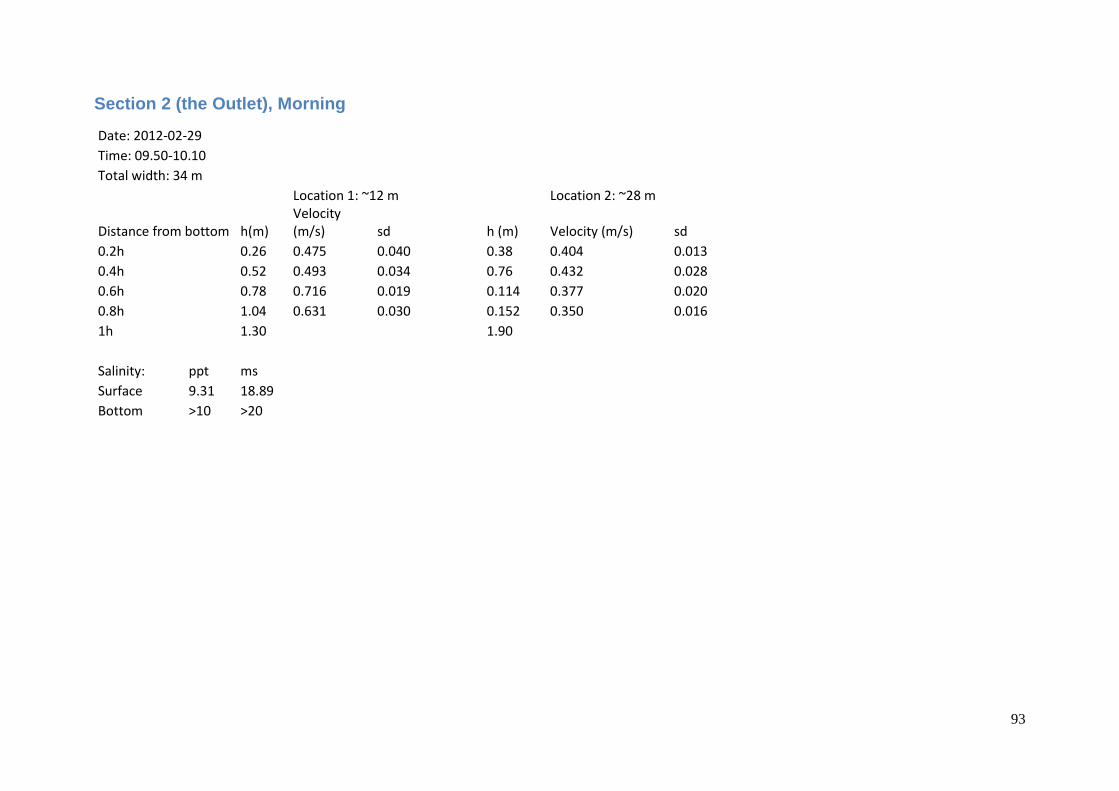
93
Section 2 (the Outlet), Morning
Date: 2012-02-29 Time: 09.50-10.10 Total width: 34 m
Location 1: ~12 m
Location 2: ~28 m
Distance from bottom h(m)
Velocity (m/s) sd
h (m) Velocity (m/s) sd
0.2h
0.26 0.475 0.040
0.38 0.404 0.013
0.4h
0.52 0.493 0.034
0.76 0.432 0.028
0.6h
0.78 0.716 0.019
0.114 0.377 0.020
0.8h
1.04 0.631 0.030
0.152 0.350 0.016
1h
1.30
1.90
Salinity: ppt ms Surface 9.31 18.89 Bottom >10 >20

94
Section 3 (Dutch Canal), Morning
Date: 2012-02-29 Time: 10.30-10.55 Total width: 14m
Location 1: 4.5 m
Location 2: 9m
Location 3: 13.5m
Distance from bottom h(m) Velocity (m/s) sd
h (m) Velocity (m/s) sd
h(m) Velocity(m/s) sd
0.2h
0.35 0.379 0.063
0.34 0.395 0.053
0.21 0.416 0.009
0.4h
0.70 0.417 0.029
0.68 0.515 0.014
0.42 0.454 0.022
0.6h
1.05 0.417 0.012
1.02 0.574 0.013
0.63 0.442 0.005
0.8h
1.40 0.573 0.048
1.36 0.527 0.032
0.84 0.424 0.007
1h
1.75
1.70
1.05
Salinity: ppt ms Surface 4.88 9.78 Bottom 4.78 9.57

95
Section 1 (Gin Oya), Afternoon
Date: 2012-02-29 Time: 14.25-14.40 Total width: 50m
Location 1: 12.5 m
Location 2: 25m
Location 3: 37.5m
Distance from bottom
h(m) Velocity (m/s) sd
h (m) Velocity (m/s) sd
h(m) Velocity(m/s) sd
0.2h
0.25 -0.107 0.009
0.22 -0.171 0.01
0.15 -0.108 0.024
0.4h
0.50 -0.182 0.015
0.44 -0.192 0.006
0.30 -0.17 0.005
0.6h
0.75 -0.15 0.014
0.66 -0.231 0.007
0.45 -0.198 0.040
0.8h
1.00 -0.153 0.017
0.88 -0.227 0.008
0.60 -0.065 0.004
1h
1.25 direction upstream
1.12
0.78
to downstream
Salinity: ppt ms Surface 6.68 13.8 Bottom >10 >20
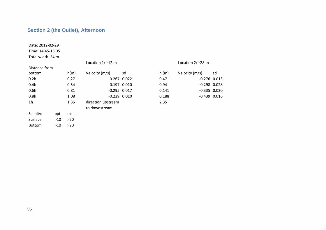
96
Section 2 (the Outlet), Afternoon
Date: 2012-02-29 Time: 14.45-15.05 Total width: 34 m
Location 1: ~12 m
Location 2: ~28 m
Distance from bottom h(m) Velocity (m/s) sd
h (m) Velocity (m/s) sd
0.2h
0.27 -0.267 0.022
0.47 -0.276 0.013
0.4h
0.54 -0.197 0.010
0.94 -0.298 0.028
0.6h
0.81 -0.295 0.017
0.141 -0.335 0.020
0.8h
1.08 -0.229 0.010
0.188 -0.439 0.016
1h
1.35 direction upstream
2.35
to downstream
Salinity: ppt ms Surface >10 >20 Bottom >10 >20
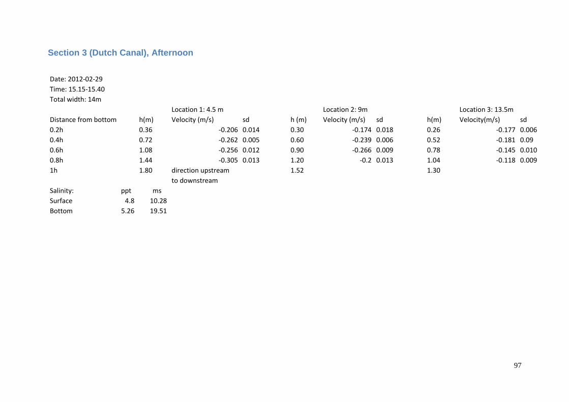
97
Section 3 (Dutch Canal), Afternoon
Date: 2012-02-29 Time: 15.15-15.40 Total width: 14m
Location 1: 4.5 m
Location 2: 9m
Location 3: 13.5m
Distance from bottom h(m) Velocity (m/s) sd
h (m) Velocity (m/s) sd
h(m) Velocity(m/s) sd
0.2h
0.36 -0.206 0.014
0.30 -0.174 0.018
0.26 -0.177 0.006
0.4h
0.72 -0.262 0.005
0.60 -0.239 0.006
0.52 -0.181 0.09
0.6h
1.08 -0.256 0.012
0.90 -0.266 0.009
0.78 -0.145 0.010
0.8h
1.44 -0.305 0.013
1.20 -0.2 0.013
1.04 -0.118 0.009
1h
1.80 direction upstream
1.52
1.30
to downstream
Salinity: ppt ms Surface 4.8 10.28 Bottom 5.26 19.51
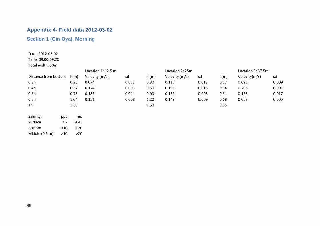
98
Appendix 4- Field data 2012-03-02
Section 1 (Gin Oya), Morning
Date: 2012-03-02 Time: 09.00-09.20
Total width: 50m
Location 1: 12.5 m
Location 2: 25m
Location 3: 37.5m
Distance from bottom h(m) Velocity (m/s) sd
h (m) Velocity (m/s) sd
h(m) Velocity(m/s) sd
0.2h
0.26 0.074 0.013
0.30 0.117 0.013
0.17 0.091 0.009
0.4h
0.52 0.124 0.003
0.60 0.193 0.015
0.34 0.208 0.001
0.6h
0.78 0.186 0.011
0.90 0.159 0.003
0.51 0.153 0.017
0.8h
1.04 0.131 0.008
1.20 0.149 0.009
0.68 0.059 0.005
1h
1.30
1.50
0.85
Salinity: ppt ms Surface 7.7 9.43 Bottom >10 >20 Middle (0.5 m) >10 >20
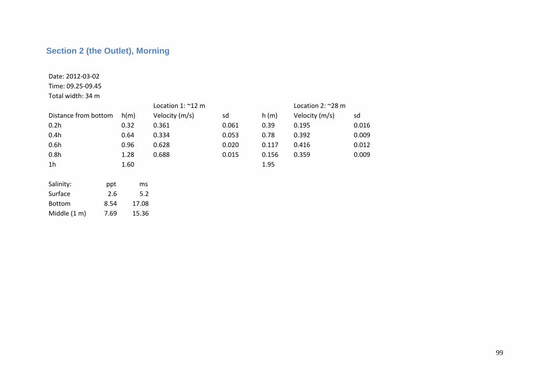
99
Section 2 (the Outlet), Morning
Date: 2012-03-02 Time: 09.25-09.45 Total width: 34 m
Location 1: ~12 m
Location 2: ~28 m
Distance from bottom h(m) Velocity (m/s) sd
h (m) Velocity (m/s) sd
0.2h
0.32 0.361 0.061
0.39 0.195 0.016
0.4h
0.64 0.334 0.053
0.78 0.392 0.009
0.6h
0.96 0.628 0.020
0.117 0.416 0.012
0.8h
1.28 0.688 0.015
0.156 0.359 0.009
1h
1.60
1.95
Salinity: ppt ms Surface 2.6 5.2 Bottom 8.54 17.08 Middle (1 m) 7.69 15.36

100
Section 3 (Dutch Canal), Morning
Date: 2012-03-02 Time: 09.55-10.20 Total width: 15,5m
Location 1: 4 m
Location 2: 8m
Location 3: 12m
Distance from bottom h(m) Velocity (m/s) sd
h (m) Velocity (m/s) sd
h(m) Velocity(m/s) sd
0.2h
0.36 0.382 0.031
0.36 0.399 0.013
0.23 0.568 0.048
0.4h
0.72 0.429 0.060
0.72 0.490 0.015
0.46 0.554 0.022
0.6h
1.08 0.397 0.031
1.08 0.765 0.003
0.69 0.575 0.034
0.8h
1.44 0.646 0.032
1.44 0.767 0.009
0.92 0.625 0.036
1h
1.80
1.80
1.16
Salinity: ppt ms Surface 2.24 4.5 Bottom 2.19 4.39
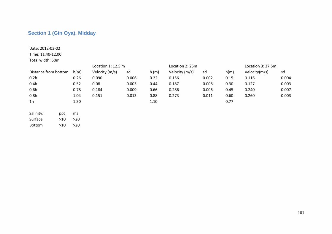
101
Section 1 (Gin Oya), Midday
Date: 2012-03-02 Time: 11.40-12.00 Total width: 50m
Location 1: 12.5 m
Location 2: 25m
Location 3: 37.5m
Distance from bottom h(m) Velocity (m/s) sd
h (m) Velocity (m/s) sd
h(m) Velocity(m/s) sd
0.2h
0.26 0.090 0.006
0.22 0.156 0.002
0.15 0.116 0.004
0.4h
0.52 0.08 0.003
0.44 0.187 0.008
0.30 0.127 0.003
0.6h
0.78 0.184 0.009
0.66 0.286 0.006
0.45 0.240 0.007
0.8h
1.04 0.151 0.013
0.88 0.273 0.011
0.60 0.260 0.003
1h
1.30
1.10
0.77
Salinity: ppt ms Surface >10 >20 Bottom >10 >20
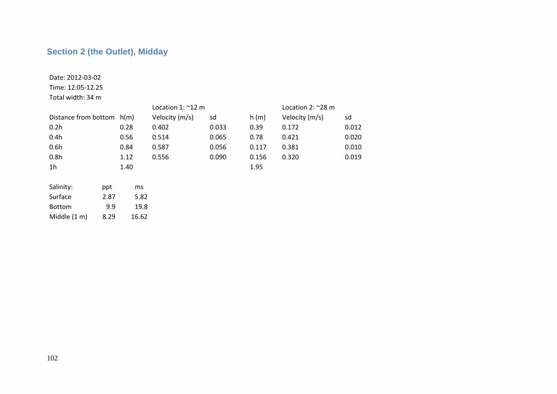
102
Section 2 (the Outlet), Midday
Date: 2012-03-02 Time: 12.05-12.25 Total width: 34 m
Location 1: ~12 m
Location 2: ~28 m
Distance from bottom h(m) Velocity (m/s) sd
h (m) Velocity (m/s) sd
0.2h
0.28 0.402 0.033
0.39 0.172 0.012
0.4h
0.56 0.514 0.065
0.78 0.421 0.020
0.6h
0.84 0.587 0.056
0.117 0.381 0.010
0.8h
1.12 0.556 0.090
0.156 0.320 0.019
1h
1.40
1.95
Salinity: ppt ms Surface 2.87 5.82 Bottom 9.9 19.8 Middle (1 m) 8.29 16.62
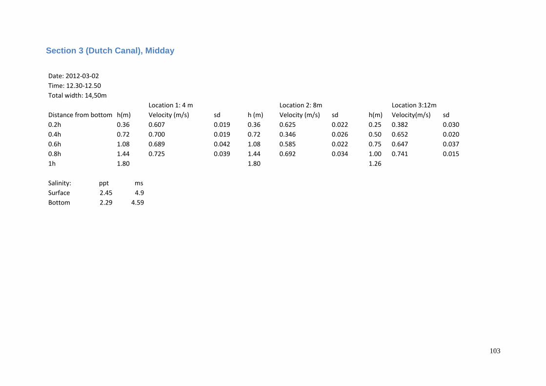
103
Section 3 (Dutch Canal), Midday
Date: 2012-03-02 Time: 12.30-12.50 Total width: 14,50m
Location 1: 4 m
Location 2: 8m
Location 3:12m
Distance from bottom h(m) Velocity (m/s) sd
h (m) Velocity (m/s) sd
h(m) Velocity(m/s) sd
0.2h
0.36 0.607 0.019
0.36 0.625 0.022
0.25 0.382 0.030
0.4h
0.72 0.700 0.019
0.72 0.346 0.026
0.50 0.652 0.020
0.6h
1.08 0.689 0.042
1.08 0.585 0.022
0.75 0.647 0.037
0.8h
1.44 0.725 0.039
1.44 0.692 0.034
1.00 0.741 0.015
1h
1.80
1.80
1.26
Salinity: ppt ms Surface 2.45 4.9 Bottom 2.29 4.59

104
Section 1 (Gin Oya), Afternoon
Date: 2012-03-02 Time: 14.25-14.45 Total width: 50m
Location 1: 12.5 m
Location 2: 25m
Location 3: 37.5m
Distance from bottom h(m) Velocity (m/s) sd
h (m) Velocity (m/s) sd
h(m) Velocity(m/s) sd
0.2h
0.25 0.083
0.22 0.053 0.006
0.15 0.008 0.005
0.4h
0.50 0.105 0.003
0.44 0.083 0.007
0.30 0.014 0.007
0.6h
0.75 0.037 0.007
0.66 0.017 0.013
0.45 0.014 0.004
0.8h
1.00 -0.053 0.006
0.88 0.077 0.004
0.60 -0.049 0.011
1h
1.25
1.10
0.77
Salinity: ppt ms Surface 4.18 8.36
Bottom >10 >20

105
Section 2 (the Outlet), Afternoon
Date: 2012-03-02 Time: 14.50-15.10 Total width: 34 m
Location 1: ~12 m
Locaction 2: ~28 m
Distance from bottom h(m) Velocity (m/s) sd
h (m) Velocity (m/s) sd
0.2h
0.22 0.308
0.37 0.089 0.012
0.4h
0.44 0.464 0.021
0.74 0.056 0.041
0.6h
0.66 0.622 0.024
0.111 0.093 0.015
0.8h
0.88 0.443 0.020
0.148 0.03 0.009
1h
1.10
1.85
Salinity: ppt ms Surface 4.21 8.47 Bottom 8.47 16.96 Middle (1 m) 9.44 18.91
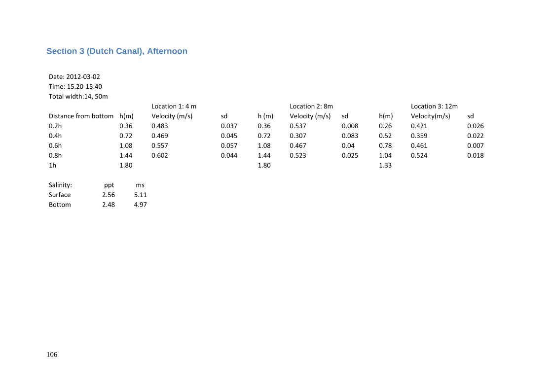
106
Section 3 (Dutch Canal), Afternoon
Date: 2012-03-02 Time: 15.20-15.40 Total width:14, 50m
Location 1: 4 m
Location 2: 8m
Location 3: 12m
Distance from bottom h(m) Velocity (m/s) sd
h (m) Velocity (m/s) sd
h(m) Velocity(m/s) sd
0.2h
0.36 0.483 0.037
0.36 0.537 0.008
0.26 0.421 0.026
0.4h
0.72 0.469 0.045
0.72 0.307 0.083
0.52 0.359 0.022
0.6h
1.08 0.557 0.057
1.08 0.467 0.04
0.78 0.461 0.007
0.8h
1.44 0.602 0.044
1.44 0.523 0.025
1.04 0.524 0.018
1h
1.80
1.80
1.33
Salinity: ppt ms Surface 2.56 5.11 Bottom 2.48 4.97
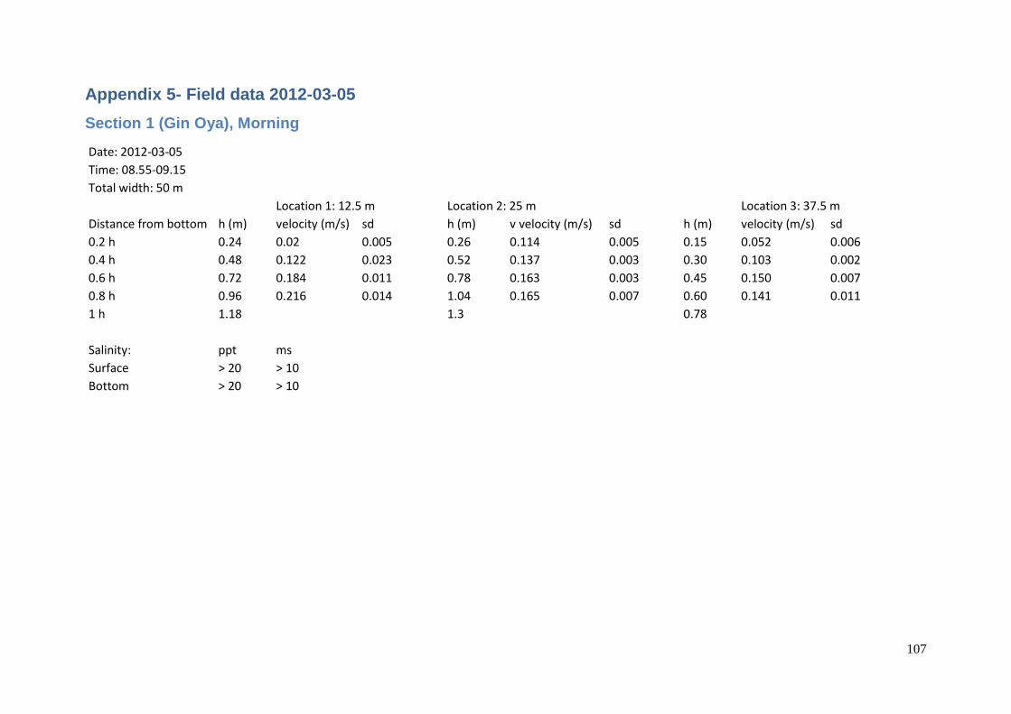
107
Appendix 5- Field data 2012-03-05
Section 1 (Gin Oya), Morning
Date: 2012-03-05 Time: 08.55-09.15 Total width: 50 m
Location 1: 12.5 m
Location 2: 25 m
Location 3: 37.5 m
Distance from bottom h (m) velocity (m/s) sd
h (m) v velocity (m/s) sd
h (m) velocity (m/s) sd
0.2 h 0.24 0.02 0.005
0.26 0.114 0.005
0.15 0.052 0.006
0.4 h 0.48 0.122 0.023
0.52 0.137 0.003
0.30 0.103 0.002
0.6 h 0.72 0.184 0.011
0.78 0.163 0.003
0.45 0.150 0.007
0.8 h 0.96 0.216 0.014
1.04 0.165 0.007
0.60 0.141 0.011
1 h 1.18
1.3
0.78
Salinity: ppt ms Surface > 20 > 10 Bottom > 20 > 10

108
Section 2 (the Outlet), Morning
Date: 2012-03-05 Time: 09.20-09.40 Total width: 31 m
Location 1: ~16 m
Location 3: ~8m
Distance from bottom h (m) velocity (m/s) sd
h (m) velocity (m/s) sd
0.2 h 0.24 0.446 0.014
0.4 0.239 0.013
0.4 h 0.48 0.373 0.051
0.80 0.158 0.010
0.6 h 0.72 0.353 0.012
1.20 0.326 0.009
0.8 h 0.96 0.458 0.011
1.60 0.197 0.010
1 h 1.22 m
2.00
Salinity: ppt ms Surface 2.87 5.63 Bottom > 20 > 10 Middle (1m) > 20 > 10
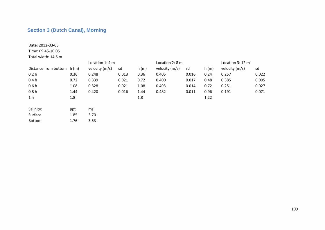
109
Section 3 (Dutch Canal), Morning
Date: 2012-03-05 Time: 09.45-10.05 Total width: 14.5 m
Location 1: 4 m
Location 2: 8 m
Location 3: 12 m
Distance from bottom h (m) velocity (m/s) sd
h (m) velocity (m/s) sd
h (m) velocity (m/s) sd
0.2 h 0.36 0.248 0.013
0.36 0.405 0.016
0.24 0.257 0.022
0.4 h 0.72 0.339 0.021
0.72 0.400 0.017
0.48 0.385 0.005
0.6 h 1.08 0.328 0.021
1.08 0.493 0.014
0.72 0.251 0.027
0.8 h 1.44 0.420 0.016
1.44 0.482 0.011
0.96 0.191 0.071
1 h 1.8
1.8
1.22
Salinity: ppt ms Surface 1.85 3.70 Bottom 1.76 3.53

110
Section 1 (Gin Oya), Afternoon
Date: 2012-03-05 Time: 15.00-15.15 Total width: 50 m
Location 1: 12.5 m
Location 2: 25 m
Location 3: 37.5 m
Sistance form bottom h (m) velocity (m/s) sd
h (m) velocity (m/s) sd
h (m) velocity (m/s) sd
0.2 h 0.28 0.077 0.005
0.22 0.047 0.003
0.16 0.082 0.003
0.4 h 0.56 0.091 0.003
0.44 0.149 0.003
0.32 0.161 0.013
0.6 h 0.84 0.173 0.006
0.66 0.199 0.005
0.48 0.071 0.007
0.8 h 1.12 0.096 0.012
0.88 0.079 0.012
0.64 0.020 0.008
1 h 1.42
1.08
0.78
Salinity: ppt ms Surface 8.26 16.53 Bottom > 20 > 10 Middle (0.5 m) > 20 > 10
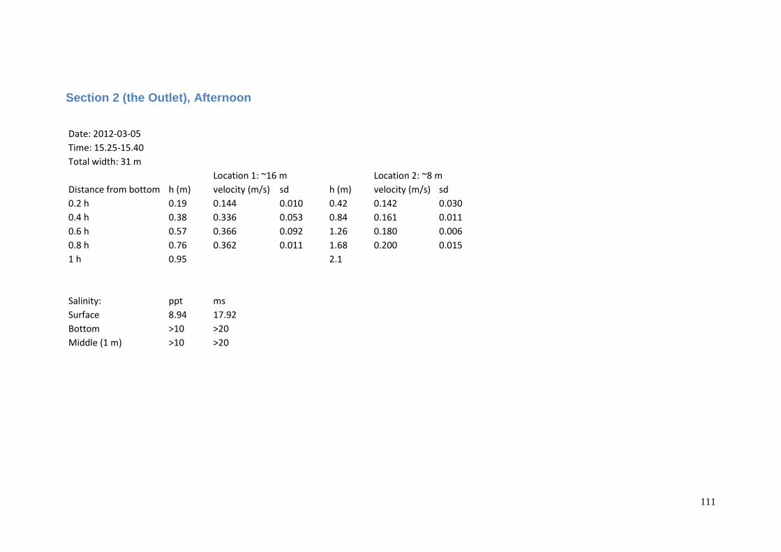
111
Section 2 (the Outlet), Afternoon
Date: 2012-03-05 Time: 15.25-15.40 Total width: 31 m
Location 1: ~16 m
Location 2: ~8 m
Distance from bottom h (m) velocity (m/s) sd
h (m) velocity (m/s) sd
0.2 h 0.19 0.144 0.010
0.42 0.142 0.030
0.4 h 0.38 0.336 0.053
0.84 0.161 0.011
0.6 h 0.57 0.366 0.092
1.26 0.180 0.006
0.8 h 0.76 0.362 0.011
1.68 0.200 0.015
1 h 0.95
2.1
Salinity: ppt ms Surface 8.94 17.92 Bottom >10 >20 Middle (1 m) >10 >20
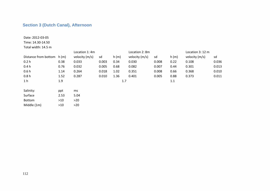
112
Section 3 (Dutch Canal), Afternoon
Date: 2012-03-05 Time: 14.30-14.50 Total width: 14.5 m
Location 1: 4m
Location 2: 8m
Location 3: 12 m
Distance from bottom h (m) velocity (m/s) sd
h (m) velocity (m/s) sd
h (m) velocity (m/s) sd
0.2 h 0.38 0.033 0.003
0.34 0.030 0.008
0.22 0.108 0.036
0.4 h 0.76 0.032 0.005
0.68 0.082 0.007
0.44 0.301 0.013
0.6 h 1.14 0.264 0.018
1.02 0.351 0.008
0.66 0.368 0.010
0.8 h 1.52 0.287 0.010
1.36 0.401 0.005
0.88 0.373 0.011
1 h 1.9
1.7
1.1
Salinity: ppt ms Surface 2.53 5.04 Bottom >10 >20 Middle (1m) >10 >20
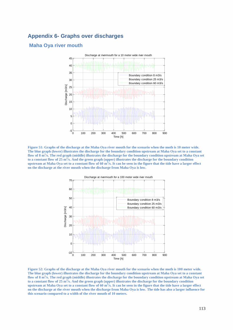
113
Appendix 6- Graphs over discharges
Maha Oya river mouth
Figure 51: Graphs of the discharge at the Maha Oya river mouth for the scenario when the moth is 10 meter wide.
The blue graph (lower) illustrates the discharge for the boundary condition upstream at Maha Oya set to a constant
flow of 8 m3/s. The red graph (middle) illustrates the discharge for the boundary condition upstream at Maha Oya set
to a constant flow of 25 m3/s. And the green graph (upper) illustrates the discharge for the boundary condition
upstream at Maha Oya set to a constant flow of 60 m3/s. It can be seen in the figure that the tide have a larger effect
on the discharge at the river mouth when the discharge from Maha Oya is low.
Figure 52: Graphs of the discharge at the Maha Oya river mouth for the scenario when the moth is 100 meter wide.
The blue graph (lower) illustrates the discharge for the boundary condition upstream at Maha Oya set to a constant
flow of 8 m3/s. The red graph (middle) illustrates the discharge for the boundary condition upstream at Maha Oya set
to a constant flow of 25 m3/s. And the green graph (upper) illustrates the discharge for the boundary condition
upstream at Maha Oya set to a constant flow of 60 m3/s. It can be seen in the figure that the tide have a larger effect
on the discharge at the river mouth when the discharge from Maha Oya is low. The tide has also a larger influence for
this scenario compared to a width of the river mouth of 10 meters.
0 100 200 300 400 500 600 700 800 900-5
0
5
10
15
20
25
30
35
40
45Discharge at rivermouth for a 10 meter wide river mouth
Time [h]
Dis
charg
e [
m3/s
]
Boundary condition 8 m3/s
Boundary condition 25 m3/s
Boundary condition 60 m3/s
0 100 200 300 400 500 600 700 800 900-10
0
10
20
30
40
50
60
70Discharge at rivermouth for a 100 meter wide river mouth
Time [h]
Dis
charg
e [
m3/s
]
Boundary condition 8 m3/s
Boundary condition 25 m3/s
Boundary condition 60 m3/s
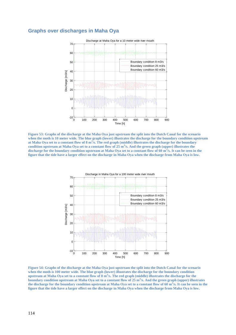
114
Graphs over discharges in Maha Oya
Figure 53: Graphs of the discharge at the Maha Oya just upstream the split into the Dutch Canal for the scenario
when the moth is 10 meter wide. The blue graph (lower) illustrates the discharge for the boundary condition upstream
at Maha Oya set to a constant flow of 8 m3/s. The red graph (middle) illustrates the discharge for the boundary
condition upstream at Maha Oya set to a constant flow of 25 m3/s. And the green graph (upper) illustrates the
discharge for the boundary condition upstream at Maha Oya set to a constant flow of 60 m3/s. It can be seen in the
figure that the tide have a larger effect on the discharge in Maha Oya when the discharge from Maha Oya is low.
Figure 54: Graphs of the discharge at the Maha Oya just upstream the split into the Dutch Canal for the scenario
when the moth is 100 meter wide. The blue graph (lower) illustrates the discharge for the boundary condition
upstream at Maha Oya set to a constant flow of 8 m3/s. The red graph (middle) illustrates the discharge for the
boundary condition upstream at Maha Oya set to a constant flow of 25 m3/s. And the green graph (upper) illustrates
the discharge for the boundary condition upstream at Maha Oya set to a constant flow of 60 m3/s. It can be seen in the
figure that the tide have a larger effect on the discharge in Maha Oya when the discharge from Maha Oya is low.
0 100 200 300 400 500 600 700 800 900-10
0
10
20
30
40
50
60
70Discharge at Maha Oya for a 10 meter wide river mouth
Time [h]
Dis
charg
e [
m3/s
]
Boundary condition 8 m3/s
Boundary condition 25 m3/s
Boundary condition 60 m3/s
0 100 200 300 400 500 600 700 800 900-10
0
10
20
30
40
50
60
70Discharge in Maha Oya for a 100 meter wide river mouth
Time [h]
Dis
charg
e [
m3/s
]
Boundary condition 8 m3/s
Boundary condition 25 m3/s
Boundary condition 60 m3/s
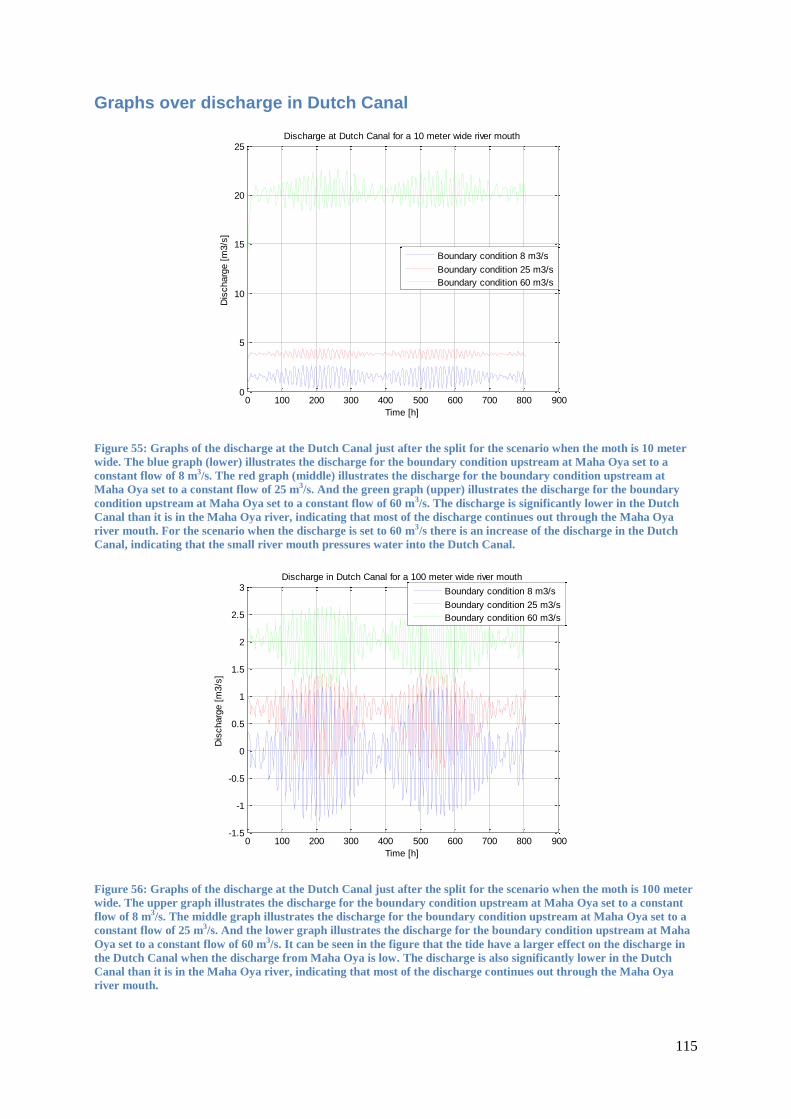
115
Graphs over discharge in Dutch Canal
Figure 55: Graphs of the discharge at the Dutch Canal just after the split for the scenario when the moth is 10 meter
wide. The blue graph (lower) illustrates the discharge for the boundary condition upstream at Maha Oya set to a
constant flow of 8 m3/s. The red graph (middle) illustrates the discharge for the boundary condition upstream at
Maha Oya set to a constant flow of 25 m3/s. And the green graph (upper) illustrates the discharge for the boundary
condition upstream at Maha Oya set to a constant flow of 60 m3/s. The discharge is significantly lower in the Dutch
Canal than it is in the Maha Oya river, indicating that most of the discharge continues out through the Maha Oya
river mouth. For the scenario when the discharge is set to 60 m3/s there is an increase of the discharge in the Dutch
Canal, indicating that the small river mouth pressures water into the Dutch Canal.
Figure 56: Graphs of the discharge at the Dutch Canal just after the split for the scenario when the moth is 100 meter
wide. The upper graph illustrates the discharge for the boundary condition upstream at Maha Oya set to a constant
flow of 8 m3/s. The middle graph illustrates the discharge for the boundary condition upstream at Maha Oya set to a
constant flow of 25 m3/s. And the lower graph illustrates the discharge for the boundary condition upstream at Maha
Oya set to a constant flow of 60 m3/s. It can be seen in the figure that the tide have a larger effect on the discharge in
the Dutch Canal when the discharge from Maha Oya is low. The discharge is also significantly lower in the Dutch
Canal than it is in the Maha Oya river, indicating that most of the discharge continues out through the Maha Oya
river mouth.
0 100 200 300 400 500 600 700 800 9000
5
10
15
20
25Discharge at Dutch Canal for a 10 meter wide river mouth
Time [h]
Dis
charg
e [
m3/s
]
Boundary condition 8 m3/s
Boundary condition 25 m3/s
Boundary condition 60 m3/s
0 100 200 300 400 500 600 700 800 900-1.5
-1
-0.5
0
0.5
1
1.5
2
2.5
3Discharge in Dutch Canal for a 100 meter wide river mouth
Time [h]
Dis
charg
e [
m3/s
]
Boundary condition 8 m3/s
Boundary condition 25 m3/s
Boundary condition 60 m3/s
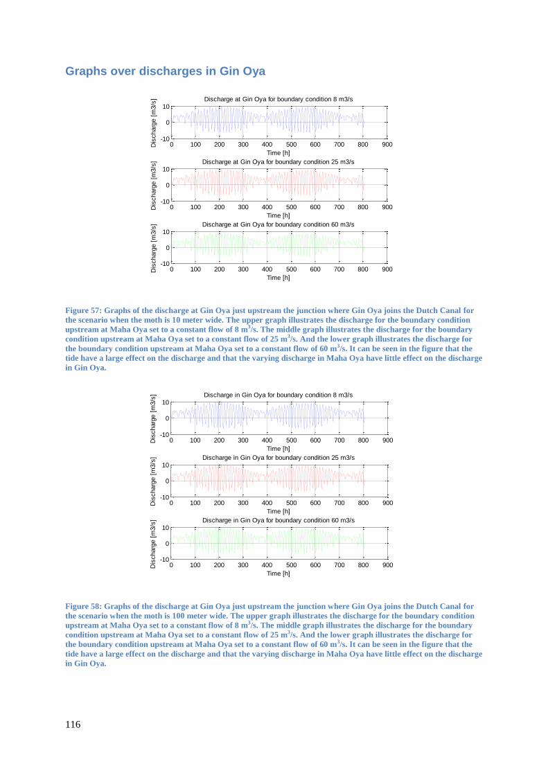
116
Graphs over discharges in Gin Oya
Figure 57: Graphs of the discharge at Gin Oya just upstream the junction where Gin Oya joins the Dutch Canal for
the scenario when the moth is 10 meter wide. The upper graph illustrates the discharge for the boundary condition
upstream at Maha Oya set to a constant flow of 8 m3/s. The middle graph illustrates the discharge for the boundary
condition upstream at Maha Oya set to a constant flow of 25 m3/s. And the lower graph illustrates the discharge for
the boundary condition upstream at Maha Oya set to a constant flow of 60 m3/s. It can be seen in the figure that the
tide have a large effect on the discharge and that the varying discharge in Maha Oya have little effect on the discharge
in Gin Oya.
Figure 58: Graphs of the discharge at Gin Oya just upstream the junction where Gin Oya joins the Dutch Canal for
the scenario when the moth is 100 meter wide. The upper graph illustrates the discharge for the boundary condition
upstream at Maha Oya set to a constant flow of 8 m3/s. The middle graph illustrates the discharge for the boundary
condition upstream at Maha Oya set to a constant flow of 25 m3/s. And the lower graph illustrates the discharge for
the boundary condition upstream at Maha Oya set to a constant flow of 60 m3/s. It can be seen in the figure that the
tide have a large effect on the discharge and that the varying discharge in Maha Oya have little effect on the discharge
in Gin Oya.
0 100 200 300 400 500 600 700 800 900-10
0
10Discharge at Gin Oya for boundary condition 8 m3/s
Time [h]D
ischarg
e [
m3/s
]
0 100 200 300 400 500 600 700 800 900-10
0
10Discharge at Gin Oya for boundary condition 25 m3/s
Time [h]
Dis
charg
e [
m3/s
]
0 100 200 300 400 500 600 700 800 900-10
0
10Discharge at Gin Oya for boundary condition 60 m3/s
Time [h]
Dis
charg
e [
m3/s
]
0 100 200 300 400 500 600 700 800 900-10
0
10Discharge in Gin Oya for boundary condition 8 m3/s
Time [h]
Dis
charg
e [
m3/s
]
0 100 200 300 400 500 600 700 800 900-10
0
10Discharge in Gin Oya for boundary condition 25 m3/s
Time [h]
Dis
charg
e [
m3/s
]
0 100 200 300 400 500 600 700 800 900-10
0
10Discharge in Gin Oya for boundary condition 60 m3/s
Time [h]
Dis
charg
e [
m3/s
]
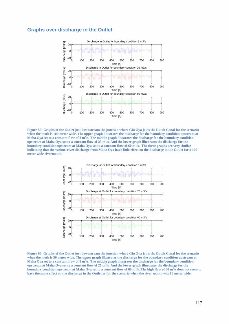
117
Graphs over discharge in the Outlet
Figure 59: Graphs of the Outlet just downstream the junction where Gin Oya joins the Dutch Canal for the scenario
when the moth is 100 meter wide. The upper graph illustrates the discharge for the boundary condition upstream at
Maha Oya set to a constant flow of 8 m3/s. The middle graph illustrates the discharge for the boundary condition
upstream at Maha Oya set to a constant flow of 25 m3/s. And the lower graph illustrates the discharge for the
boundary condition upstream at Maha Oya set to a constant flow of 60 m3/s. The three graphs are very similar
indicating that the various river discharge from Maha Oya have little effect on the discharge at the Outlet for a 100
meter wide rivermouth.
Figure 60: Graphs of the Outlet just downstream the junction where Gin Oya joins the Dutch Canal for the scenario
when the moth is 50 meter wide. The upper graph illustrates the discharge for the boundary condition upstream at
Maha Oya set to a constant flow of 8 m3/s. The middle graph illustrates the discharge for the boundary condition
upstream at Maha Oya set to a constant flow of 25 m3/s. And the lower graph illustrates the discharge for the
boundary condition upstream at Maha Oya set to a constant flow of 60 m3/s. The high flow of 60 m3/s does not seem to
have the same effect on the discharge in the Outlet as for the scenario when the river mouth was 10 meter wide.
0 100 200 300 400 500 600 700 800 900-20
0
20Discharge in Outlet for boundary condition 8 m3/s
Time [h]D
ischarg
e [
m3/s
]
0 100 200 300 400 500 600 700 800 900-20
0
20Discharge in Outlet for boundary condition 25 m3/s
Time [h]
Dis
charg
e [
m3/s
]
0 100 200 300 400 500 600 700 800 900-20
0
20Discharge in Outlet for boundary condition 60 m3/s
Time [h]
Dis
charg
e [
m3/s
]
0 100 200 300 400 500 600 700 800 900-20
0
20Discharge at Outlet for boundary condition 8 m3/s
Time [h]
Dis
charg
e [
m3/s
]
0 100 200 300 400 500 600 700 800 900-20
0
20Discharge at Outlet for boundary condition 25 m3/s
Time [h]
Dis
charg
e [
m3/s
]
0 100 200 300 400 500 600 700 800 900-20
0
20Discharge at Outlet for boundary condition 60 m3/s
Time [h]
Dis
charg
e [
m3/s
]
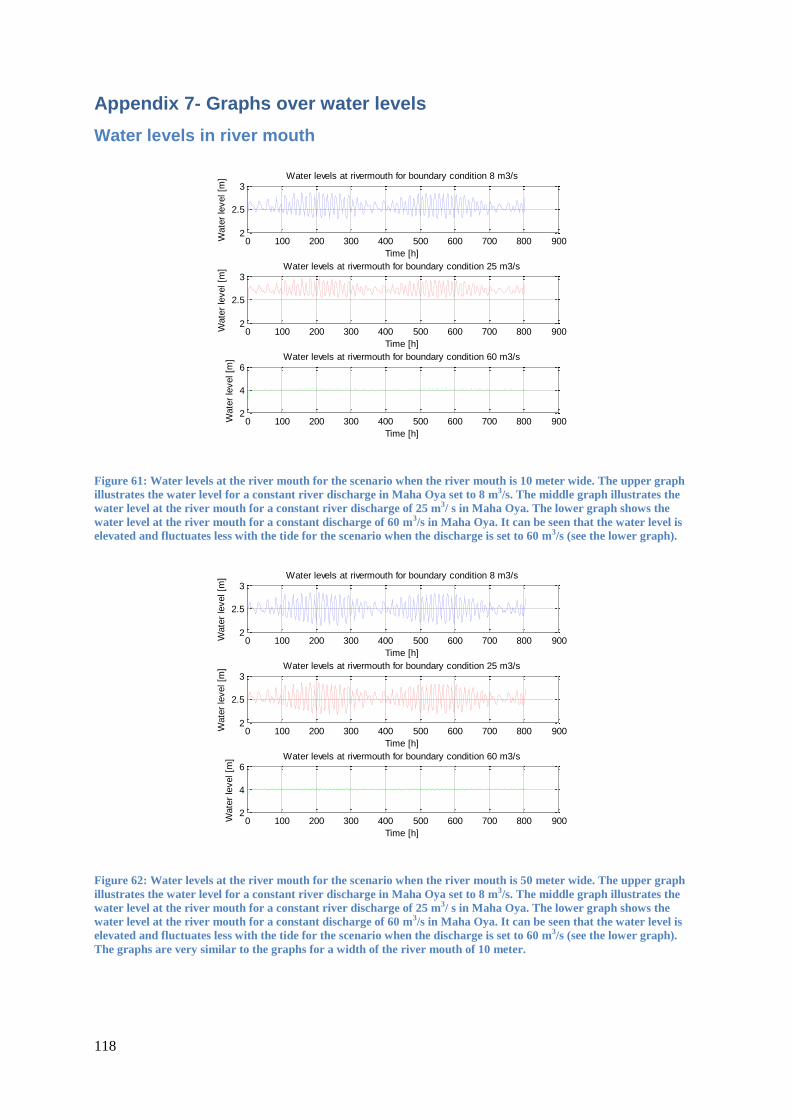
118
Appendix 7- Graphs over water levels
Water levels in river mouth
Figure 61: Water levels at the river mouth for the scenario when the river mouth is 10 meter wide. The upper graph
illustrates the water level for a constant river discharge in Maha Oya set to 8 m3/s. The middle graph illustrates the
water level at the river mouth for a constant river discharge of 25 m3/ s in Maha Oya. The lower graph shows the
water level at the river mouth for a constant discharge of 60 m3/s in Maha Oya. It can be seen that the water level is
elevated and fluctuates less with the tide for the scenario when the discharge is set to 60 m3/s (see the lower graph).
Figure 62: Water levels at the river mouth for the scenario when the river mouth is 50 meter wide. The upper graph
illustrates the water level for a constant river discharge in Maha Oya set to 8 m3/s. The middle graph illustrates the
water level at the river mouth for a constant river discharge of 25 m3/ s in Maha Oya. The lower graph shows the
water level at the river mouth for a constant discharge of 60 m3/s in Maha Oya. It can be seen that the water level is
elevated and fluctuates less with the tide for the scenario when the discharge is set to 60 m3/s (see the lower graph).
The graphs are very similar to the graphs for a width of the river mouth of 10 meter.
0 100 200 300 400 500 600 700 800 9002
2.5
3Water levels at rivermouth for boundary condition 8 m3/s
Time [h]
Wate
r le
vel [m
]
0 100 200 300 400 500 600 700 800 9002
2.5
3Water levels at rivermouth for boundary condition 25 m3/s
Time [h]
Wate
r le
vel [m
]
0 100 200 300 400 500 600 700 800 9002
4
6Water levels at rivermouth for boundary condition 60 m3/s
Time [h]
Wate
r le
vel [m
]
0 100 200 300 400 500 600 700 800 9002
2.5
3Water levels at rivermouth for boundary condition 8 m3/s
Time [h]
Wate
r le
vel [m
]
0 100 200 300 400 500 600 700 800 9002
2.5
3Water levels at rivermouth for boundary condition 25 m3/s
Time [h]
Wate
r le
vel [m
]
0 100 200 300 400 500 600 700 800 9002
4
6Water levels at rivermouth for boundary condition 60 m3/s
Time [h]
Wate
r le
vel [m
]

119
Figure 63: Water levels in the river mouth for the scenario when the river mouth is 100 meter wide. The upper graph
illustrates the water level for a constant river discharge in Maha Oya set to 8 m3/s. The middle graph illustrates the
water level at the river mouth for a constant river discharge of 25 m3/ s in Maha Oya. The lower graph shows the
water level at the river mouth for a constant discharge of 60 m3/s in Maha Oya. In contrast to the graphs for a width
of 10 and 50 meters of the river mouth, the water level for this scenario is not elevated and fluctuates with the tide for
a high river discharge from Maha Oya (see the lower graph).
0 100 200 300 400 500 600 700 800 9002
2.5
3Water levels at rivermouth for boundary condition 8 m3/s
Time [h]
Wate
r le
vel [m
]
0 100 200 300 400 500 600 700 800 9002
2.5
3Water levels at rivermouth for boundary condition 25 m3/s
Time [h]
Wate
r le
vel [m
]
0 100 200 300 400 500 600 700 800 9002
2.5
3Water levels at rivermouth for boundary condition 60 m3/s
Time [h]
Wate
r le
vel [m
]
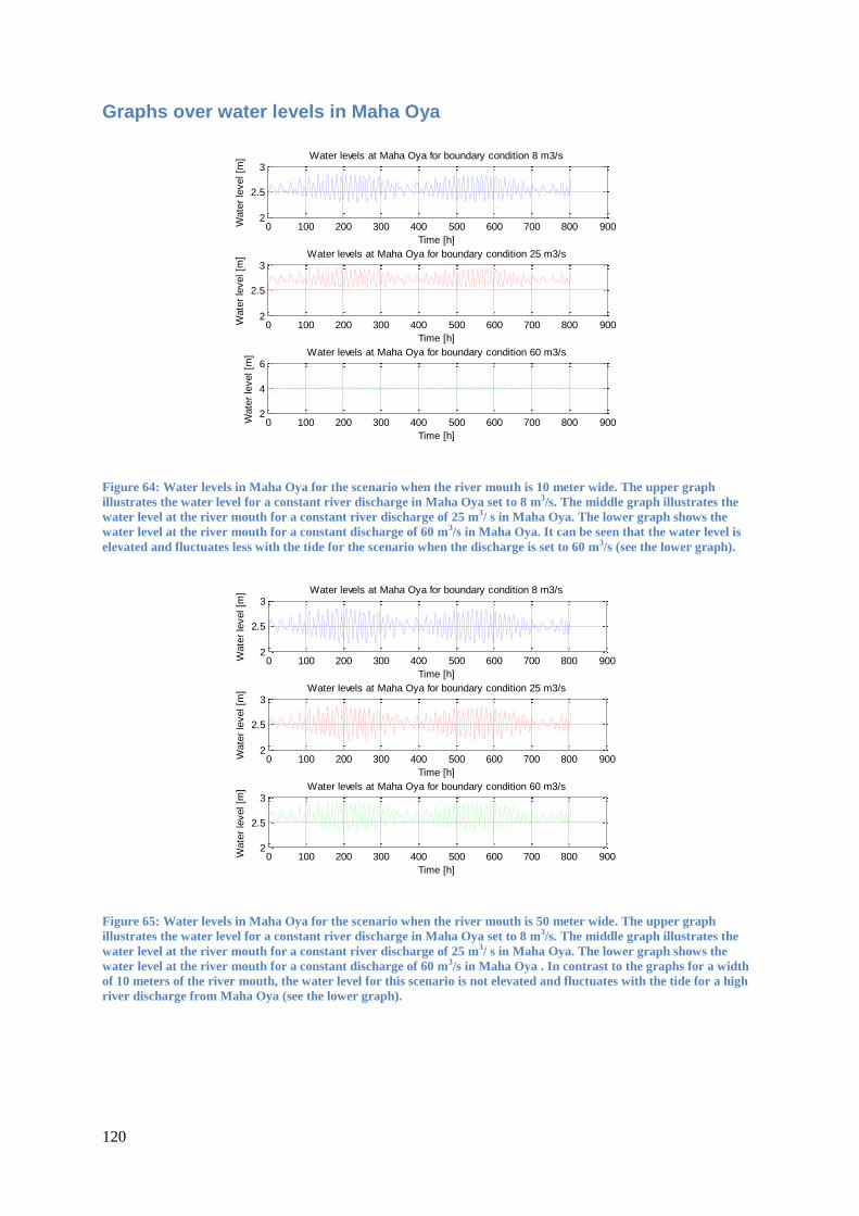
120
Graphs over water levels in Maha Oya
Figure 64: Water levels in Maha Oya for the scenario when the river mouth is 10 meter wide. The upper graph
illustrates the water level for a constant river discharge in Maha Oya set to 8 m3/s. The middle graph illustrates the
water level at the river mouth for a constant river discharge of 25 m3/ s in Maha Oya. The lower graph shows the
water level at the river mouth for a constant discharge of 60 m3/s in Maha Oya. It can be seen that the water level is
elevated and fluctuates less with the tide for the scenario when the discharge is set to 60 m3/s (see the lower graph).
Figure 65: Water levels in Maha Oya for the scenario when the river mouth is 50 meter wide. The upper graph
illustrates the water level for a constant river discharge in Maha Oya set to 8 m3/s. The middle graph illustrates the
water level at the river mouth for a constant river discharge of 25 m3/ s in Maha Oya. The lower graph shows the
water level at the river mouth for a constant discharge of 60 m3/s in Maha Oya . In contrast to the graphs for a width
of 10 meters of the river mouth, the water level for this scenario is not elevated and fluctuates with the tide for a high
river discharge from Maha Oya (see the lower graph).
0 100 200 300 400 500 600 700 800 9002
2.5
3Water levels at Maha Oya for boundary condition 8 m3/s
Time [h]W
ate
r le
vel [m
]
0 100 200 300 400 500 600 700 800 9002
2.5
3Water levels at Maha Oya for boundary condition 25 m3/s
Time [h]
Wate
r le
vel [m
]
0 100 200 300 400 500 600 700 800 9002
4
6Water levels at Maha Oya for boundary condition 60 m3/s
Time [h]
Wate
r le
vel [m
]
0 100 200 300 400 500 600 700 800 9002
2.5
3Water levels at Maha Oya for boundary condition 8 m3/s
Time [h]
Wate
r le
vel [m
]
0 100 200 300 400 500 600 700 800 9002
2.5
3Water levels at Maha Oya for boundary condition 25 m3/s
Time [h]
Wate
r le
vel [m
]
0 100 200 300 400 500 600 700 800 9002
2.5
3Water levels at Maha Oya for boundary condition 60 m3/s
Time [h]
Wate
r le
vel [m
]
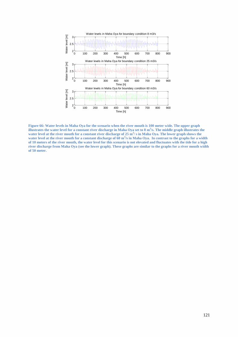
121
Figure 66: Water levels in Maha Oya for the scenario when the river mouth is 100 meter wide. The upper graph
illustrates the water level for a constant river discharge in Maha Oya set to 8 m3/s. The middle graph illustrates the
water level at the river mouth for a constant river discharge of 25 m3/ s in Maha Oya. The lower graph shows the
water level at the river mouth for a constant discharge of 60 m3/s in Maha Oya. In contrast to the graphs for a width
of 10 meters of the river mouth, the water level for this scenario is not elevated and fluctuates with the tide for a high
river discharge from Maha Oya (see the lower graph). These graphs are similar to the graphs for a river mouth width
of 50 meter.
0 100 200 300 400 500 600 700 800 9002
2.5
3Water levels in Maha Oya for boundary condition 8 m3/s
Time [h]
Wate
r le
vel [m
]
0 100 200 300 400 500 600 700 800 9002
2.5
3Water levels in Maha Oya for boundary condition 25 m3/s
Time [h]
Wate
r le
vel [m
]
0 100 200 300 400 500 600 700 800 9002
2.5
3Water levels in Maha Oya for boundary condition 60 m3/s
Time [h]
Wate
r le
vel [m
]

122
Graphs over water levels in Dutch Canal
Figure 67: Water levels in Dutch Canal for the scenario when the river mouth is 10 meter wide. The upper graph
illustrates the water level for a constant river discharge in Maha Oya set to 8 m3/s. The middle graph illustrates the
water level at the river mouth for a constant river discharge of 25 m3/ s in Maha Oya. The lower graph shows the
water level at the river mouth for a constant discharge of 60 m3/s in Maha Oya. It can be seen that the water level is
elevated and fluctuates less with the tide for the scenario when the discharge is set to 60 m3/s (see the lower graph).
Figure 68: Water levels in the Dutch Canal for the scenario when the river mouth is 50 meter wide. The upper graph
illustrates the water level for a constant river discharge in Maha Oya set to 8 m3/s. The middle graph illustrates the
water level at the river mouth for a constant river discharge of 25 m3/ s in Maha Oya. The lower graph shows the
water level at the river mouth for a constant discharge of 60 m3/s in Maha Oya. For this width of the river mouth
there is no elevation of the water level in the Dutch Canal.
0 100 200 300 400 500 600 700 800 9002
2.5
3Water levels at Dutch Canal for boundary condition 8 m3/s
Time [h]W
ate
r le
vel [m
]
0 100 200 300 400 500 600 700 800 9002
2.5
3Water levels at Dutch Canal for boundary condition 25 m3/s
Time [h]
Wate
r le
vel [m
]
0 100 200 300 400 500 600 700 800 9002
4
6Water levels at Dutch Canal for boundary condition 60 m3/s
Time [h]
Wate
r le
vel [m
]
0 100 200 300 400 500 600 700 800 9002
2.5
3Water levels at Dutch Canal for boundary condition 8 m3/s
Time [h]
Wate
r le
vel [m
]
0 100 200 300 400 500 600 700 800 9002
2.5
3Water levels at Dutch Canal for boundary condition 25 m3/s
Time [h]
Wate
r le
vel [m
]
0 100 200 300 400 500 600 700 800 9002
2.5
3Water levels at Dutch Canal for boundary condition 60 m3/s
Time [h]
Wate
r le
vel [m
]
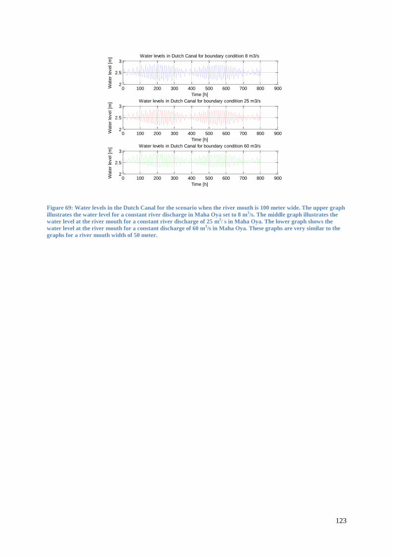
123
Figure 69: Water levels in the Dutch Canal for the scenario when the river mouth is 100 meter wide. The upper graph
illustrates the water level for a constant river discharge in Maha Oya set to 8 m3/s. The middle graph illustrates the
water level at the river mouth for a constant river discharge of 25 m3/ s in Maha Oya. The lower graph shows the
water level at the river mouth for a constant discharge of 60 m3/s in Maha Oya. These graphs are very similar to the
graphs for a river mouth width of 50 meter.
0 100 200 300 400 500 600 700 800 9002
2.5
3Water levels in Dutch Canal for boundary condition 8 m3/s
Time [h]
Wate
r le
vel [m
]
0 100 200 300 400 500 600 700 800 9002
2.5
3Water levels in Dutch Canal for boundary condition 25 m3/s
Time [h]
Wate
r le
vel [m
]
0 100 200 300 400 500 600 700 800 9002
2.5
3Water levels in Dutch Canal for boundary condition 60 m3/s
Time [h]
Wate
r le
vel [m
]
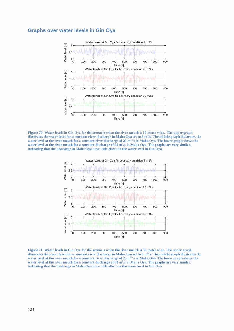
124
Graphs over water levels in Gin Oya
Figure 70: Water levels in Gin Oya for the scenario when the river mouth is 10 meter wide. The upper graph
illustrates the water level for a constant river discharge in Maha Oya set to 8 m3/s. The middle graph illustrates the
water level at the river mouth for a constant river discharge of 25 m3/ s in Maha Oya. The lower graph shows the
water level at the river mouth for a constant discharge of 60 m3/s in Maha Oya. The graphs are very similar,
indicating that the discharge in Maha Oya have little effect on the water level in Gin Oya.
Figure 71: Water levels in Gin Oya for the scenario when the river mouth is 50 meter wide. The upper graph
illustrates the water level for a constant river discharge in Maha Oya set to 8 m3/s. The middle graph illustrates the
water level at the river mouth for a constant river discharge of 25 m3/ s in Maha Oya. The lower graph shows the
water level at the river mouth for a constant discharge of 60 m3/s in Maha Oya. The graphs are very similar,
indicating that the discharge in Maha Oya have little effect on the water level in Gin Oya.
0 100 200 300 400 500 600 700 800 9002
2.5
3Water levels at Gin Oya for boundary condition 8 m3/s
Time [h]W
ate
r le
vel [m
]
0 100 200 300 400 500 600 700 800 9002
2.5
3Water levels at Gin Oya for boundary condition 25 m3/s
Time [h]
Wate
r le
vel [m
]
0 100 200 300 400 500 600 700 800 9002
2.5
3Water levels at Gin Oya for boundary condition 60 m3/s
Time [h]
Wate
r le
vel [m
]
0 100 200 300 400 500 600 700 800 9002
2.5
3Water levels at Gin Oya for boundary condition 8 m3/s
Time [h]
Wate
r le
vel [m
]
0 100 200 300 400 500 600 700 800 9002
2.5
3Water levels at Gin Oya for boundary condition 25 m3/s
Time [h]
Wate
r le
vel [m
]
0 100 200 300 400 500 600 700 800 9002
2.5
3Water levels at Gin Oya for boundary condition 60 m3/s
Time [h]
Wate
r le
vel [m
]
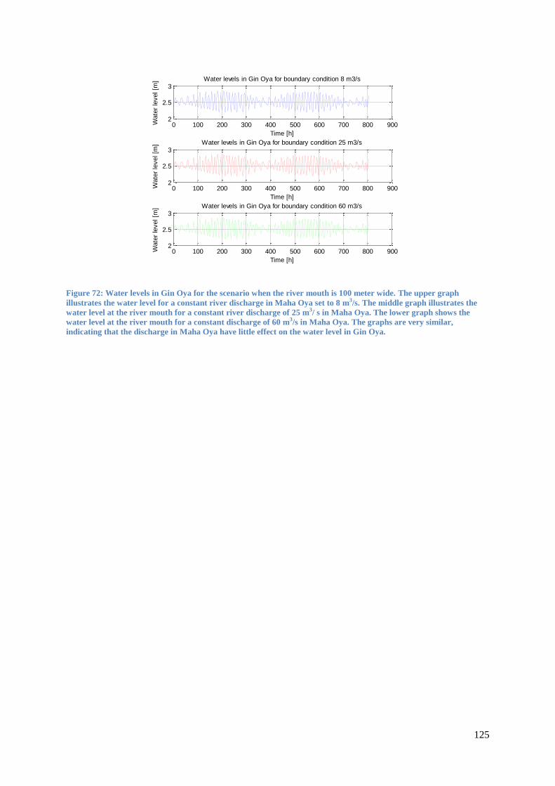
125
Figure 72: Water levels in Gin Oya for the scenario when the river mouth is 100 meter wide. The upper graph
illustrates the water level for a constant river discharge in Maha Oya set to 8 m3/s. The middle graph illustrates the
water level at the river mouth for a constant river discharge of 25 m3/ s in Maha Oya. The lower graph shows the
water level at the river mouth for a constant discharge of 60 m3/s in Maha Oya. The graphs are very similar,
indicating that the discharge in Maha Oya have little effect on the water level in Gin Oya.
0 100 200 300 400 500 600 700 800 9002
2.5
3Water levels in Gin Oya for boundary condition 8 m3/s
Time [h]
Wate
r le
vel [m
]
0 100 200 300 400 500 600 700 800 9002
2.5
3Water levels in Gin Oya for boundary condition 25 m3/s
Time [h]
Wate
r le
vel [m
]
0 100 200 300 400 500 600 700 800 9002
2.5
3Water levels in Gin Oya for boundary condition 60 m3/s
Time [h]
Wate
r le
vel [m
]
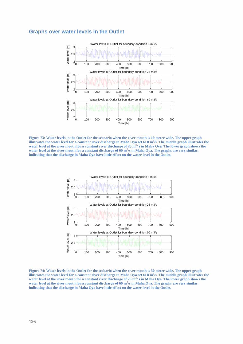
126
Graphs over water levels in the Outlet
Figure 73: Water levels in the Outlet for the scenario when the river mouth is 10 meter wide. The upper graph
illustrates the water level for a constant river discharge in Maha Oya set to 8 m3/s. The middle graph illustrates the
water level at the river mouth for a constant river discharge of 25 m3/ s in Maha Oya. The lower graph shows the
water level at the river mouth for a constant discharge of 60 m3/s in Maha Oya. The graphs are very similar,
indicating that the discharge in Maha Oya have little effect on the water level in the Outlet.
Figure 74: Water levels in the Outlet for the scebario when the river mouth is 50 meter wide. The upper graph
illustrates the water level for a constant river discharge in Maha Oya set to 8 m3/s. The middle graph illustrates the
water level at the river mouth for a constant river discharge of 25 m3/ s in Maha Oya. The lower graph shows the
water level at the river mouth for a constant discharge of 60 m3/s in Maha Oya. The graphs are very similar,
indicating that the discharge in Maha Oya have little effect on the water level in the Outlet.
0 100 200 300 400 500 600 700 800 9002
2.5
3Water levels at Outlet for boundary condition 8 m3/s
Time [h]W
ate
r le
vel [m
]
0 100 200 300 400 500 600 700 800 9002
2.5
3Water levels at Outlet for boundary condition 25 m3/s
Time [h]
Wate
r le
vel [m
]
0 100 200 300 400 500 600 700 800 9002
2.5
3Water levels at Outlet for boundary condition 60 m3/s
Time [h]
Wate
r le
vel [m
]
0 100 200 300 400 500 600 700 800 9002
2.5
3Water levels at Outlet for boundary condition 8 m3/s
Time [h]
Wate
r le
vel [m
]
0 100 200 300 400 500 600 700 800 9002
2.5
3Water levels at Outlet for boundary condition 25 m3/s
Time [h]
Wate
r le
vel [m
]
0 100 200 300 400 500 600 700 800 9002
2.5
3Water levels at Outlet for boundary condition 60 m3/s
Time [h]
Wate
r le
vel [m
]

127
Figure 75: Water levels in the Outlet for the scenario when the river mouth is 100 meter wide. The upper graph
illustrates the water level for a constant river discharge in Maha Oya set to 8 m3/s. The middle graph illustrates the
water level at the river mouth for a constant river discharge of 25 m3/ s in Maha Oya. The lower graph shows the
water level at the river mouth for a constant discharge of 60 m3/s in Maha Oya. The graphs are very similar for both
varying width of the rivermouth an various discharges in Maha Oya, indicating that the discharge and size of the
river mouth in Maha Oya have little effect on the water level in the Outlet.
0 100 200 300 400 500 600 700 800 9002
2.5
3Water levels in Outlet for boundary condition 8 m3/s
Time [h]
Wate
r le
vel [m
]
0 100 200 300 400 500 600 700 800 9002
2.5
3Water levels in Outlet for boundary condition 25 m3/s
Time [h]
Wate
r le
vel [m
]
0 100 200 300 400 500 600 700 800 9002
2.5
3Water levels in Outlet for boundary condition 60 m3/s
Time [h]
Wate
r le
vel [m
]

128
Appendix 8- Graphs over salinity
For a discharge of 60 m3/s in Maha Oya
Figure 76: Salinity intrusion in the Outlet for a boundary condition in Maha Oya set to a constant flow of 60 m3/s and
a fully open river mouth.
11 13 15 17 19 21 23 25 27 29 02 04Feb2012 Mar 2012
0
5000
10000
15000
20000
25000
30000
35000
C:\Users\Christer\Documents\HEC Data\Kulamulla3.wq38
Tim e
Tra
cer1
(m
g/L
)
Legend
Tr ac er1 (m g/L)
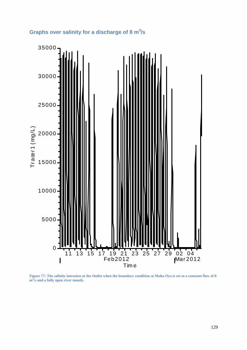
129
Graphs over salinity for a discharge of 8 m3/s
Figure 77: The salinity intrusion at the Outlet when the boundary condition at Maha Oya is set to a constant flow of 8
m3/s and a fully open river mouth.
11 13 15 17 19 21 23 25 27 29 02 04Feb2012 Mar 2012
0
5000
10000
15000
20000
25000
30000
35000
C:\Users\Christer\Documents\HEC Data\Kulamulla3.wq38
Tim e
Tra
cer1
(m
g/L
)
Legend
Tr ac er1 (m g/L)
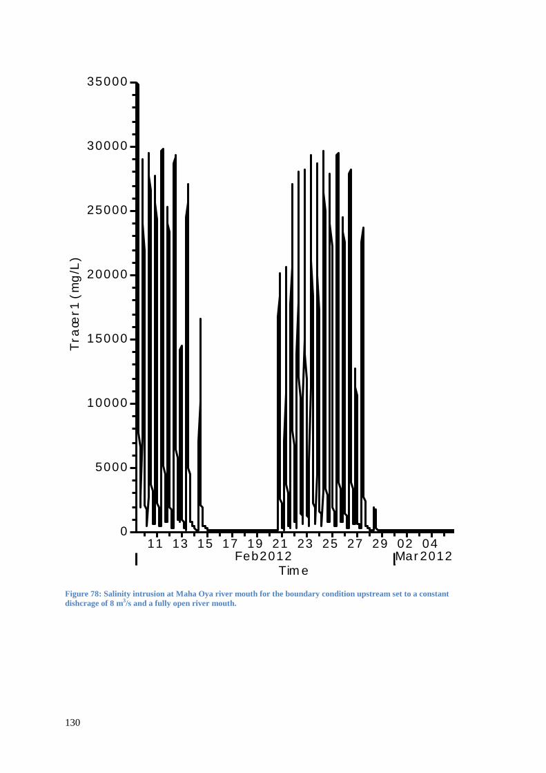
130
Figure 78: Salinity intrusion at Maha Oya river mouth for the boundary condition upstream set to a constant
dishcrage of 8 m3/s and a fully open river mouth.
11 13 15 17 19 21 23 25 27 29 02 04Feb2012 Mar 2012
0
5000
10000
15000
20000
25000
30000
35000
C:\Users\Christer\Documents\HEC Data\Kulamulla3.wq38
Tim e
Tra
cer1
(m
g/L
)Legend
Tr ac er1 (m g/L)
Related Documents