THE EFFECTS OF BOAT MOORING SYSTEMS ON SQUID EGG …

THE EFFECTS OF BOAT MOORING SYSTEMS ON SQUID EGG BEDS DURING SQUID FISHING by VUTLHARI ABSALOM MALULEKE Thesis submitted in fulfilment of the requirements for the degree Master of Technology: Mechanical Engineering in the Faculty of Engineering at the Cape Peninsula University of Technology Supervisor: Prof GJ Oliver Co-supervisor: Prof MJ Roberts Bellville 2017

CPUT copyright information The dissertation/thesis may not be published either in part (in scholarly, scientific or technical journals), or as a whole (as a monograph), unless permission has been obtained from the University

ii

DECLARATION

I, Vutlhari Absalom Maluleke, declare that the contents of this dissertation/thesis represent my own unaided work, and that the dissertation/thesis has not previously been submitted for academic examination towards any qualification. Furthermore, it represents my own opinions and not necessarily those of the Cape Peninsula University of Technology.

Signed Date

iii

ABSTRACT

In South Africa, squid fishing vessels need to find and then anchor above benthic squid

egg beds to effect viable catches. However, waves acting on the vessel produce a

dynamic response on the anchor line. These oscillatory motions produce impact forces

of the chain striking the seabed. It is hypothesised that this causes damage to the squid

egg bed beneath the vessels. Different mooring systems may cause more or less

damage and this is what is investigated in this research. The effect of vessel mooring

lines impact on the seabed during squid fishing is investigated using a specialised

hydrodynamic tool commercial package ANSYS AQWA models.

This study analysed the single-point versus the two-point mooring system’s impact on

the seabed. The ANSYS AQWA models were developed for both mooring systems

under the influence of the wave and current loads using the 14 and 22 m vessels

anchored with various chain sizes. The effect of various wave conditions was

investigated as well as the analysis of three mooring line configurations.

The mooring chain contact pressure on the seabed is investigated beyond what is

output from ANSYS AQWA using ABAQUS finite element analysis. The real-world

velocity of the mooring chain underwater was obtained using video analysis. The

ABAQUS model was built by varying chain sizes at different impact velocities. The

impact pressure and force due to this velocity was related to mooring line impact

velocity on the seabed in ANSYS AQWA.

Results show the maximum impact pressure of 191 MPa when the 20 mm diameter

chain impacts the seabed at the velocity of 8 m/s from video analysis. It was found that

the mooring chain impact pressure on the seabed increased with an increase in the

velocity of impact and chain size.

The ANSYS AQWA impact pressure on the seabed was found to be 170.86 MPa at the

impact velocity of 6.4 m/s. The two-point mooring system was found to double the

seabed mooring chain contact length compared to the single-point mooring system.

Both mooring systems showed that the 14 m vessel mooring line causes the least

seabed footprint compared to the 22 m vessel.

iv

ACKNOWLEDGEMENTS

I wish to thank:

Professor Graeme J. Oliver, Cape Peninsula University of Technology for his

guidance throughout this research.

Professor Michael J. Roberts for giving me an opportunity to do this project, his

contribution and for making funds available.

Bayworld Centre for Research and Education (BCRE) for financial and logistical

support during my studies.

South African Squid Management and Industrial Association (SASMIA) for financial

assistance with the field research at Port Elizabeth.

Cape Peninsula University of Technology for their financial contribution in support of

my attendance to The 10th South African Conference on Computational and Applied

Mechanics (SACAM).

Mr Rob Cooper for his assistance and contribution.

Dr Jean Githaiga-Mwicigi for assistance with the Port Elizabeth Trip.

Dr Tamer Abdalrahman for his contribution on ABAQUS simulations.

Mr Kevin Sack for his input on the whole project.

Lastly, my friends and family. Thank you for believing in me and encouraging me

every step of the way.

v

DEDICATION

This thesis is dedicated to my loving grandmother (Ndaheni Maria Chouke) who has been patiently waiting for me to finish my MTech.

vi

TABLE OF CONTENTS

DECLARATION .......................................................................................................... ii

ABSTRACT ................................................................................................................ iii

ACKNOWLEDGEMENTS .......................................................................................... iv

DEDICATION ............................................................................................................. v

LIST OF FIGURES ................................................................................................... viii

LIST OF TABLES ...................................................................................................... xii

GLOSSARY ............................................................................................................. xiii

CHAPTER ONE ......................................................................................................... 1

1. Project introduction..................................................................................................... 1

1.1. Introduction .......................................................................................................... 1

1.2. Background of mooring systems .......................................................................... 3

1.3. Typical fishing vessels on site .............................................................................. 5

1.4. Problem statement ............................................................................................... 6

1.5. Aim and objectives ............................................................................................... 6

1.6. Research methodology overview ......................................................................... 7

1.7. Dissertation structure ............................................................................................. 8

CHAPTER TWO ......................................................................................................... 9

2. Literature review ......................................................................................................... 9

2.1. Mooring line impact on the seafloor studies .......................................................... 9

2.2. Mooring line analysis studies .............................................................................. 17

2.3. Single-point and two-point mooring systems ...................................................... 23

CHAPTER THREE ................................................................................................... 24

3. Methods and mathematical formulations .................................................................. 24

3.1. ANSYS AQWA and ABAQUS introduction ......................................................... 24

3.1.1. ANSYS AQWA background ........................................................................ 24

3.1.2. ABAQUS background ................................................................................. 25

3.2. Mathematical formulations of the moored vessel ................................................ 26

3.2.1. Governing equations of the chain mooring line in time-domain.................... 26

3.2.2. Governing equations for the fishing vessel in time domain .......................... 32

3.3. Environmental loading ........................................................................................ 36

3.3.1. Description of waves ................................................................................... 36

3.3.2. Currents ...................................................................................................... 37

3.3.3. Winds .......................................................................................................... 37

3.4. Underwater video analysis: Experimental ........................................................... 38

3.4.1. Tracker video analysis ................................................................................ 38

CHAPTER FOUR ..................................................................................................... 42

4. Results and discussions ........................................................................................... 42

4.1. ABAQUS model for the mooring chain impact on the seabed ............................. 44

vii

4.1.1. Geometry of the model ................................................................................ 44

4.1.2. Material property definition .......................................................................... 45

4.1.3. Mesh ........................................................................................................... 46

4.1.4. Contact ....................................................................................................... 47

4.1.5. Boundary Conditions and Loading .............................................................. 48

4.1.6. Results ........................................................................................................ 50

4.1.7. Studless chain link seabed contact forces comparison with the slender rod method 65

4.2. ANSYS AQWA model description and setup ...................................................... 68

4.2.1. ANSYS AQWA simulation procedure description ........................................ 68

4.2.2. ANSYS AQWA model setup ........................................................................ 75

4.3. ANSYS AQWA model simulation results ............................................................ 79

4.3.1. ANSYS AQWA model correlation with underwater chain velocity ................ 79

4.3.2. Effect of wave height and period on the 22 m single-point moored vessel ... 83

4.3.3. Mooring system results using three configurations ...................................... 95

4.4. Summary of results: ANSYS AQWA and ABAQUS models .............................. 116

4.4.1. Single-point mooring system result overview ............................................. 121

4.4.2. Two-point mooring system result overview ................................................ 123

CHAPTER FIVE ..................................................................................................... 127

5. Conclusion ............................................................................................................. 127

6. Recommendations and future work ........................................................................ 131

REFERENCES ....................................................................................................... 133

APPENDIX/APPENDICES ..................................................................................... 139

APPENDIX A: Chain specification data .................................................................. 140

APPENDIX B: Steel and sand properties ............................................................... 141

APPENDIX C: Vessel drawings .............................................................................. 143

APPENDIX D: Vessel hydrostatic results ............................................................... 145

APPENDIX E: Studless chain drawings .................................................................. 147

APPENDIX F: Calculations ..................................................................................... 149

.....................................................................................................................................

viii

LIST OF FIGURES

Figure 1.1: A chokka squid fishing vessel (a) anchored above an active egg bed (b) . 2

Figure 1.2: Schematic of the mooring system ............................................................. 3

Figure 1.3: Photographs of the anchor system used by squid fishing vessels ............. 5

Figure 2.1: Photograph of a swing mooring showing typical damage caused by the

mooring chain to the seagrass meadow ..................................................................... 9

Figure 2.2: Schematic representation of a typical (A) ‘screw’ mooring system, (B)

‘swing’ mooring system and (C) ‘cyclone’ mooring system ....................................... 11

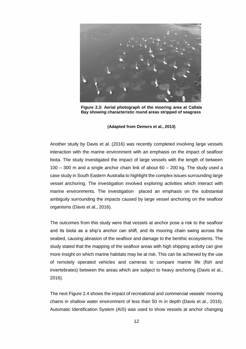
Figure 2.3: Aerial photograph of the mooring area at Callala Bay showing characteristic

round areas stripped of seagrass ............................................................................. 12

Figure 2.4: Anchor arcs based on AIS (Automatic Identification System) vessel tracking

data near the Port of Newcastle acquired from the Australian Maritime Safety Authority

(AMSA) .................................................................................................................... 13

Figure 2.5: Mean number of shoots uprooted/broken by the three anchor types (Hall in

black; Danforth in grey; Folding grapnel in white) ..................................................... 15

Figure 2.6: Stud-Link (a) and Studless Chain (b) ...................................................... 19

Figure 2.7: Diagram of large scale test setup ........................................................... 20

Figure 2.8: Suspended catenary mooring mount ...................................................... 21

Figure 2.9: Two-dimensional line configuration for forced oscillation tests ................ 21

Figure 2.10: Mooring line touchdown points resulting in time-varying boundary

condition ................................................................................................................... 22

Figure 3.1: Modelling of a dynamic mooring line using a cable connection ............... 27

Figure 3.2: Forces on a Cable Element .................................................................... 27

Figure 3.3: Local Tube Axis System ......................................................................... 31

Figure 3.4: Vessel 6-DOF rotations and translations ................................................ 33

Figure 3.5: Original underwater video image of the chain movement experiment ..... 38

Figure 3.6: Underwater video analysis using Tracker ............................................... 40

Figure 3.7: Discrete point vertical displacement ....................................................... 41

Figure 3.8: Discrete point underwater vertical velocity .............................................. 41

Figure 4.1: CAD geometry of the 20 mm diameter chain .......................................... 44

Figure 4.2: Seabed geometry ................................................................................... 45

Figure 4.3: Single chain link meshed (stud link) ........................................................ 46

Figure 4.4: Elastic foundation mesh ......................................................................... 47

Figure 4.5: Linear and Quadratic Solid elements ...................................................... 47

Figure 4.6: Chain link and seabed contact surfaces ................................................. 48

Figure 4.7: Chain-Seabed boundary conditions and loading ..................................... 49

ix

Figure 4.8: Chain velocity scatter plot ....................................................................... 49

Figure 4.9: Chain velocity radar plot ......................................................................... 50

Figure 4.10: Chain link-seabed contact stresses, pressures and forces at 1 m/s for the

20 mm diameter chain .............................................................................................. 51

































x



Figure 4.28: Seabed contact forces by the 20 mm chain .......................................... 63



Figure 4.31: Chain link-seabed contact forces (showing the 20, 16 and 14 mm chain

links) ........................................................................................................................ 65

Figure 4.32: 36 mm diameter slender rod (a) 1 m long, (b) 0.12 m long ................... 66

Figure 4.33: Contact pressure and force at 8 m/s on seabed using (a) & (b) 1 m rod, (c)

& (d) 0.12 m rod and (e) & (f) studless chain link ...................................................... 67

Figure 4.34: ANSYS AQWA Hydrodynamic Simulation Procedure ........................... 68

Figure 4.35: ANSYS AQWA Workbench project schematic ...................................... 69

Figure 4.36: Axes Systems ....................................................................................... 69

Figure 4.37: Fishing vessel cut at the waterline (vessel Lower Hull in yellow and Upper

Hull in grey). ............................................................................................................. 70

Figure 4.38: Vessel centre of mass .......................................................................... 71

Figure 4.39: Meshed vessel (22 m vessel) ............................................................... 72

Figure 4.40: Quadrilateral Panel element (QPPL) .................................................... 72

Figure 4.41: Triangular Panel element (TPPL) ......................................................... 73

Figure 4.42: The DISC Element................................................................................ 73

Figure 4.43: The TUBE Element ............................................................................... 74

Figure 4.44: Single-point moored 22 m vessel .......................................................... 75

Figure 4.45: Single-point moored 14 m vessel .......................................................... 76

Figure 4.46: Mooring line profile of the 22 m vessel single-point for 1200 s simulation

duration .................................................................................................................... 80

Figure 4.47: Mooring line profile of the 14 m vessel single-point for 1200 s simulation

duration .................................................................................................................... 81

Figure 4.48: ANSYS AQWA video analysis using Tracker ........................................ 82

Figure 4.49: Mooring chain profile for 1 𝑚 and 7 𝑠 wave height and period .............. 88

Figure 4.50: Mooring chain profile for 1 m and 10 s wave height and period ............ 89

Figure 4.51: Mooring chain profile for 2 m and 7 s wave height and period .............. 90

Figure 4.52: Mooring chain profile for 2 m and 10 s wave height and period ............ 91

Figure 4.53: Mooring chain profile for 2.5 m and 7 s wave height and period ........... 92

Figure 4.54: The effect of wave conditions on tension .............................................. 93

Figure 4.55: The effect of wave conditions on chain laid length ................................ 94

Figure 4.56: The effect of wave conditions on anchor uplift forces ............................ 94

xi

Figure 4.57: Configuration 1 - Single-point mooring system with anchor in line with

waves and current (top view) .................................................................................... 95

Figure 4.58: Configuration 2 - Single-point mooring system with anchor at an angle with

incoming waves and current, (a) top view & (b) isometric view ................................. 95

Figure 4.59: Configuration 3 - Two-point mooring system with ‘V’ shaped anchoring, (a)

top view & (b) Isometric view .................................................................................... 96

Figure 4.60: Horizontal displacements (X-direction) of the vessels in three

configurations ......................................................................................................... 101

Figure 4.61: Lateral displacements (Y-direction) of the vessels in three configurations

............................................................................................................................... 103

Figure 4.62: Vessel vertical displacements for all three configurations ................... 105

Figure 4.63: Frequency distribution of the mooring chain laid length on the seabed for

Configuration 1 ....................................................................................................... 106

Figure 4.64: Frequency distribution of the mooring chain laid length on the seabed for

Configuration 2 ....................................................................................................... 107

Figure 4.65: Mooring chain laid length for all 3 configurations ................................ 108

Figure 4.66: Mooring chain laid length for all three configurations on the 22 m vessel

............................................................................................................................... 109

Figure 4.67: Tension time-history at Fairlead - Configuration 1 and 2 ..................... 112

Figure 4.68: Tension time-history of the two-point mooring system – Configuration 3

............................................................................................................................... 114

Figure 4.69: Anchor uplift forces for the all three Configurations............................. 115

Figure 4.70: Single-point moored 22 m vessel overview (Tension (a), Laid chain length

on the seabed (b), Mooring chain-seabed contact forces (c) & Anchor uplift forces (d))

............................................................................................................................... 121

Figure 4.71: Single-point moored 14 m vessel overview (Tension (a), Laid chain length

on the seabed (b), Mooring chain-seabed contact forces (c) & Anchor uplift forces (d))

............................................................................................................................... 122

Figure 4.72: Two-point moored 22 m vessel overview (Tension on Cable 1 (a) & 2(b),

Laid chain length on the seabed on Cable 1 (c) & 2(d) ........................................... 123

Figure 4.73: Two-point moored 22 m vessel overview (Mooring chain-seabed contact

forces (a) and Anchor uplift forces on Cable 1 (b) & 2(c)) ....................................... 124

Figure 4.74: Two-point moored 14 m vessel overview (Tension on Cable 1 (a) & 2(b),

Laid chain length on the seabed on Cable 1 (c) & 2(d) ........................................... 125


forces (a) and Anchor uplift forces on Cable 1 (b) & 2(c)) ....................................... 126

xii

LIST OF TABLES

Table 4.1: Description of various models used for mooring line analysis .................. 43

Table 4.2: Steel chain properties of 20 mm chain ..................................................... 45

Table 4.3: Seabed soil properties ............................................................................. 46

Table 4.4: Element types in ANSYS AQWA ............................................................. 72

Table 4.5: 22 m vessel properties ............................................................................. 75

Table 4.6: Single-point mooring anchor coordinates for the 22 m vessel .................. 76

Table 4.7: 14 m vessel properties ............................................................................. 76

Table 4.8: Single-point mooring anchor coordinates for the 14 m vessel .................. 76

Table 4.9: Mooring chains mechanical properties ..................................................... 77

Table 4.10: Ocean environment data ....................................................................... 78

Table 4.11: Wave conditions used for motion correlation.......................................... 82

Table 4.12: Effect of wave height and period results ................................................ 83

Table 4.13: Seabed contact Pressure and Force due to various contact points velocities

................................................................................................................................. 84

Table 4.14: Single-point mooring with ‘Anchor 2’ coordinates for the 22 m vessel

(anchor at angle) ...................................................................................................... 96

Table 4.15: Single-point mooring with Anchor 2 coordinates on the 14 m vessel ...... 96

Table 4.16: Two-point mooring anchor coordinates on the 22 m vessel ................... 97

Table 4.17: Two-point mooring anchor coordinates on the 14 m vessel ................... 97

Table 4.18: Result summary of the 22 m moored vessel ........................................ 117

Table 4.19: Result summary of the 14 m moored vessel ........................................ 118

xiii

GLOSSARY

Abbreviations

BCRE - Bayworld Centre for Research and Education

FEA - Finite Element Analysis

TD -Time-Domain

FD - Frequency-Domain

LMM - Lumped Mass Method

PDEs - Partial Differential Equation

ODEs - Ordinary Differential Equations

FEM - Finite Element Method

Symbols

𝐴 : area

𝐀 : added mass matrix

𝒂𝒋⃗⃗ ⃗ : acceleration of the cable at node j

𝐁 : added mass matrix

𝑪𝒂 : added mass coefficient

𝑪𝒅 : drag coefficient

𝑪𝒎 : inertia coefficient

𝐂 : added mass matrix

𝑫 : line diameter

∆𝑫𝒆 : diameter of the element

𝐸𝐴 : axial stiffness

𝐅𝒅 : drag force on the mooring line element

𝑭𝑰𝒏𝒆𝒓𝒕𝒊𝒂 : inertial force

𝐹𝐶ℎ𝑎𝑖𝑛max 𝑡𝑒𝑛𝑠𝑖𝑜𝑛 : maximum tension force

𝐹𝑀𝑖𝑛𝑖𝑚𝑢𝑚 𝑏𝑟𝑒𝑎𝑘 𝑙𝑜𝑎𝑑 : minimum breaking force of a chain

𝐹𝐶ℎ𝑎𝑖𝑛 𝑙𝑖𝑛𝑘 𝑓𝑜𝑟𝑐𝑒 : chain link impact force

𝐹𝑦 : hydrodynamic force in the y-direction

𝐹𝑧 : hydrodynamic force in the z-direction

𝑭 ⃗⃗ ⃗ : hydrodynamic loads

�⃗⃗� 𝒉 : element external hydrodynamic loading vectors per unit length

𝑔 : gravitational constant

𝐻 : wave height.

xiv

𝑗 : node of an element (notation)

(𝑗) : element (notation)

𝐊 : impulse response functions

𝐾𝑥𝑥 : radius of gyration on 𝑥𝑥 plane

𝐾𝑦𝑦 : radius of gyration on 𝑦𝑦 plane

𝐾𝑧𝑧 : radius of gyration on 𝑧𝑧 plane

𝐿𝐵 : laid length

𝑀𝑦 : bending moment in in the y-direction

𝑀𝑧 : bending moment in in the z-direction

𝒎 : structural mass per unit length

𝒎𝒂 : cable element added mass matrix

𝐌 : the inertia matrix

�⃗⃗⃗� : bending moment vector

�⃗⃗� 𝒃𝒐𝒕 : bottom location of the cable attachment point

�⃗⃗� 𝒕𝒐𝒑 : top location of the cable attachment point

𝝆 : sea water density

𝑝 : hydrodynamic pressure

𝑟 : position vector with respect to the centre of gravity

�⃗⃗� : distributed moment load

�⃗⃗� : cable element position vector

𝑆𝑗 : the unstretched cable length from the anchor point

∆𝑺𝒆 : length of the element

𝑺𝟎 : mean wetted surface of the vessel

𝑇0 : peak period

𝑇1 : mean wave period

𝑇 : mean wave period

�⃗⃗� : tension force vector

�̇� : fluid acceleration vector

𝒖𝒇 : directional fluid particle velocity

𝒖𝒔 : transverse directional structure velocity

𝒖𝒄𝒋 : current velocity along the j-th

𝒖𝒔𝒋 : structure motion velocity along the j-th

�⃗⃗� : is the cable element shear force vector

𝑉 : flow velocity

xv

𝑣𝑖𝑚𝑝𝑎𝑐𝑡 : chain link velocity impact

�⃗⃗� : vessel displacement vector in six degrees of freedom

�̇� ⃗⃗ ⃗ : the vessel velocity vector

�⃗⃗̈� : vessel acceleration vector

𝜔 : wave frequency

∅ : velocity potential

�⃗⃗⃗� : element weight

∇ : gradient “del”

1

CHAPTER ONE

1. Project introduction

1.1. Introduction

The South African chokka squid fishery is based in the Eastern Cape between

Plettenberg Bay and Port Alfred, and is a major source of foreign revenue as the entire

catch, on average some 8000 t, is exported to Europe. Squid fishing is considered as

one of South Africa’s most valuable fisheries. Most of the catch is exported generating

approximately R500 000 000 in foreign revenue (Krusche et al., 2014). Despite South

Africa’s efforts and progress over the past decade to improve the state of its marine

resources, significant challenges remain. A report by the World Wide Fund for Nature

indicated that many of South Africa’s inshore marine resources are overexploited and

some have collapsed (World Wide Fund South Africa, 2011). Starting in 2012 the squid

industry has consecutively experienced 3 of its least productive years for a 20-year

period pushing the industry to the verge of collapse (Blignaut, 2012).

Observations by South African marine and coastal management departments have

found that the collapse possibly correlates with a change in the squid boat mooring

systems. The squid boats changed from a single-point mooring system to a two-point

mooring system which is now considered the industry standard. Divers from the South

African Department of Environmental Affairs have noticed an interaction between the

mooring chain and squid eggs (MJ Roberts 2015, personal communication, 2 July).

Commercial squid fishing is only viable when the vessels are above spawning

aggregations formed in the water column above egg beds on the seafloor (Figure 1.1

(b)). Egg beds comprise hundreds of thousands of translucent, slim and slimy egg

capsules about 15 cm in length that are glued to the bottom substrate forming massive

mats often spanning tens of meters. Hatching occurs about 3 weeks from spawning on

average. Traditionally, the fishing vessels position themselves above an egg bed using

a single-point mooring system with the anchor dropped upwind of the egg bed. A

significant part of the chain lies on the seafloor over eggs.

The fleet comprises 138 vessels ranging between 11 and 22 m in length on average

(Figure 1.1 (a)). Each vessel carries about 22 fishermen who land the squid using hand-

held jigs on fishing line. This number excludes the number of crew who are not allowed

to fish. Waves acting on the vessel set up dynamic behaviour in the mooring line which

2

rapidly lifts the chain off the seabed, dropping it back with considerable force on the

bottom (Sarkar & Eatock Taylor, 2002), and possibly damaging squid eggs. As sea and

wind conditions change daily, vessels regularly pick up anchor and relay the anchor

chain. In 2010, a new ‘double anchor system’ (two-point mooring system) was

introduced and used by about 10 vessels. This ‘V’ shaped anchor line configuration

offers vessels greater position control over the egg beds but potentially doubles the

impact of the chain on the eggs (MJ Roberts 2015, personal communication, 2 July).

In 2013, the chokka squid fishery crashed and has not fully recovered. Concern has

been raised by both fisheries managers and boat owners that the chain impact -

especially from the two-point mooring system (double anchor system) - maybe causing

excessive damage to the squid eggs reducing recruitment.

These egg masses can extend over an area as large as 10 000 m2 . This study is the

first part of an investigation into the impact of anchor chains on the seabed; it focuses

on the mechanical impact of the mooring chain system on the single and two-point

mooring systems when the 14 and 22 m squid fishing vessels are analysed. The

second part of the investigation is beyond the scope of this thesis, which will be done

after the results from the first part of the investigation are available. The results are

going to be used for studying the damage and consequences of the chain impact on

the egg beds and hatching success. The numerical investigation of the behaviour of

the mooring chain and seabed interaction in this thesis is performed using ANSYS

AQWA software to obtain structural displacement, dynamic contact length and mooring

forces in the time domain, and by ABAQUS finite element software to determine the

impact forces on the seabed.

Figure 1.1: A chokka squid fishing vessel (a) anchored above an active egg bed (b)

3

1.2. Background of mooring systems

Mooring lines are useful in securing a structure against environmental forces. The

predominant environmental forces are the wind, current and wave. Ebbesen (2013)

described the primary function of a mooring system as to impose the floater (boat or

vessel) with a horizontal stiffness to limit its horizontal motion (Ebbesen, 2013). The

design of a mooring system is such that it will resist the vessel movements and

environmental forces (Chrolenko, 2013). This is achieved by the mooring systems’

ability to provide the vessels’ required restoring forces to maintain the equilibrium

position when the environmental loads are exerted on it (Balzola, 1999).

A basic mooring system is made up of three components which are chain/rope, anchor,

and a flotation device. The stiffness of the mooring system depends on the anchor

holding capacity, anchor embedment depth and the seabed soil properties (Vineesh et

al., 2014).

Figure 1.2 is an illustration of the mooring line anchoring system using a catenary chain.

Catenary shape provides slackness for vessel horizontal excursions. The mooring line

is made up of steel chain. The chain mooring line is designed to have a degree of slack

which allows the anchor to be locked on the seabed. When the wave conditions

become severe, the slack mooring line usually prevents the anchor from dragging on

the seabed and reduces tension on the mooring chain. The slack mooring chain

imposes high mooring line stiffness on the vessel by absorbing the energy generated

and dissipates it.

Figure 1.2: Schematic of the mooring system

4

The Klusman 100−250 kg anchor mass is mostly used by the squid fishery with about

80 – 160 m of chain length using 14 – 20 mm link diameter steel chain. Catenary

moorings mainly use drag embedment anchor or the horizontal anchor. This anchor

type can only resist horizontal loads (Miedema et al., 2006). The anchor is deployed

for positioning the fishing vessel and pulled up either for re-deployment to a new

location or when the vessel goes back to the harbour. The steel chain weight ranges

between 4.36 and 10 kg/m. The chain is controlled by a winch on the vessel’s foredeck

that feeds chain through the fairlead on the vessel’s bow. Two types of chain links are

used - studless and studded.

The studded chain link is designed to prevent knot formation but is more susceptible to

fatigue failure than the studless link (ABC Moorings, 2015). Note that the description of

the studless and stud link chain is in section 2.2. In mechanics, the chain component

is characterised by the catenary stiffness (effect), low elasticity, high non-breaking

strength and mass. As shown in the previous figure, the mooring system is subjected

to varying wind, waves and current, all of which introduce dynamic behaviour into the

mooring line.

In Figure 1.2 shown, the part of the mooring line that lies on the seabed is termed

grounded chain while that suspended in the water column is the catenary. The

touchdown point is a position along the mooring where the chain begins lifting off the

seabed. This point varies as a result of the dynamic sea conditions. Pellegrino and

Ong, (2003) demonstrated that when the mooring chain is excited due to wave loading,

the chain dynamically interacts with the seabed; which creates a boundary condition

that varies in time and in space. The dynamic excitation causes a significant change in

the mooring line’s catenary profile resulting in part of the chain to lift off and drop back

down on the seabed (Yu & Tan, 2006). This is illustrated in Figure 2.10 in Chapter 2

and can be modelled using a dynamic simulation which accounts for the application of

loads on the system over time with the consideration of wave inertia forces and

structural damping.

The mooring system’s ability to provide a connection between the squid fishing vessel

and the seafloor by means of an anchor chain enhances squid catches and thus plays

an important role in the squid fishing industry. Ocean waves induce hydrodynamic

loads on the squid fishing vessel. These excited wave forces acting on the vessel

causes dynamic behaviour on the mooring chain which is anchored to the seafloor.

5

This is evident by the apparent unstable oscillatory motions of the mooring chain. When

the above phenomena take place, a significant part of the chain lying on the seafloor

lifts up and drops back down under dynamic conditions (Sarkar & Eatock Taylor, 2002).

This phenomenon was also noticed by divers by from the South African Department of

Environmental Affairs. This study will investigate and analyse the motion and the

impact force of the mooring chain on the seabed (seafloor) on the single and two-point

mooring systems.

1.3. Typical fishing vessels on site

To ensure that the problem is clearly understood, a site visit to Port Elizabeth was

undertaken to gather practical information on the mooring systems. Figure 1.3 below

shows varying inspections of the double (two-point) and single anchor (single-point)

configurations.

Specific objectives of the site visit included:

1. Familiarity with the squid fishing vessels, anchor systems and anchor

deployment methods.

20 mm

chain

diameter One anchor pulled up

Figure 1.3: Photographs of the anchor system used by squid fishing vessels

6

2. To gather information on chain specifications (chain mass per unit length, chain

length and diameter)

3. To obtain actual vessel dimensions (obtain vessel engineering drawings for

accurate modelling and vessel mass)

The information on mooring systems obtained include:

1. The chain mooring line specifications are shown in Appendix A supplied by McKinnon

Chain (PTY) LTD.

2. Vessels on-site are in the range of between 11 and 22 m.

3. The vessel operators or skippers provided enough information on the anchor

deployment methods and conditions at sea.

4. Anchor deployment: the anchor is dropped below the bow of the vessel; when the

anchor reaches the seabed, the anchor chain is then increased as the vessel moves

away from the anchor position, as this happens. The anchor drags on the seabed until

it is locked on the seabed.

5. The mooring chain length depends on the fishing depth and sea conditions.

6. Obtained vessel specific information. This consisted of knowing the steel chain sizes

of 13, 14, 16 and 20 mm in diameter which are commonly used depending on the vessel

size. The 20 mm chain is the heaviest of all the four chain sizes and is used to anchor

a vessel when the sea conditions are harsh; while the 16 mm used in conjunction with

the 20 mm for two-point mooring to provide more stability. The 20 mm and the 16 mm

are commonly used in the squid fishing industry. The single anchor vessel either uses

20, 16, 14 or 13 mm chain based on the skippers’ discretion.

1.4. Problem statement

We will investigate the effect of different mooring line systems and types in terms of

potential impact on squid egg beds.

1.5. Aim and objectives

The aim of this study is to develop numerical models for predicting the behaviour and

impact of the single-point versus the two-point mooring system. The predictions will

then be used to investigate the likelihood of the anchor chains damaging the squid

eggs.

The main objectives are divided into the following sections in order to develop

numerical models to quantify the impact force of the mooring chain on the seabed –

7

Numerical models will be used to simulate single-point mooring system versus

the two-point mooring system using the 14 and the 22 m long vessels.

The impact force and frequency of the chain on the seabed will be analysed

and quantified.

The models will be used to analyse the dynamic tension on the mooring line

and determine which mooring system has the greatest tension.

The numerical models will also be used to quantify this dynamic tension based

on various ocean conditions which best represent the real-world motion of the

mooring chain underwater and impact on the seabed.

The numerical models will be validated by video footage analysis obtained of

the mooring chain impacting the seabed at a considerable velocity.

The numerical models will be setup using methodologies from related studies

and analyses of a moored vessel at sea; software packages user and theory

guides will also be used for ensuring correct model setup.

1.6. Research methodology overview

The following methods of investigation were used in undertaking this study:

Hydrodynamic analysis – this is the moored vessel’s response in the ocean

environment; numerical simulations were performed by using a specialised

hydrodynamic analysis commercial package ANSYS AQWA for analysing the

moored vessel response. This software enables the analysis of the interaction

between the chain and the motion of a moored vessel under the influence of

ocean environment forces i.e. wave and current forces.

Finite element analysis – ABAQUS finite element analysis software was used

to determine the seabed contact forces under varying mooring chain diameter

and the impact velocity.

Video analysis – Tracker software was used to analyse the video footage

captured by marine divers when capturing the mooring chain motion impacting

the seabed. Video analysis was performed for determining the mooring chain

underwater velocity. The velocity was used for validating and calibrating the

numerical models in ANSYS AQWA and ABAQUS.

8

1.7. Dissertation structure

Chapter 2 reviews relevant literature on the impacts of the mooring lines; it also

presents common approaches used for solving the dynamics of a mooring line.

Chapter 3 presents the background of the ANSYS AQWA and ABAQUS modelling

tools. It also presents the governing equations and loads acting on the moored

vessel. Lastly, it also presents underwater video analysis of a video footage

captured by marine divers. Chapter 4 presents both ABAQUS and ANSYS AQWA

results. A table is also provided which lists and describes all the subsequent

analysis conducted in this study. Chapter 5 presents conclusions that can be drawn

from this study and also provides recommendations as well highlights main

software limitations.

9

CHAPTER TWO

2. Literature review

This chapter reviews the literature on mooring systems; it reviews studies on mooring

line impact and the seabed interaction highlighting numerical and experimental models

used.

2.1. Mooring line impact on the seafloor studies

Boat and buoy anchoring can have a negative impact on the seabed habitat through

its three stages (1) anchor laydown to the seabed, (2) anchor drag on the seabed and

(3) pulling the anchor chain from the seabed. When the anchor and chain drag on the

seabed, the seagrass is then cut and pulled from the seabed (Collins et al., 2010).

Swinging mooring chain has been observed to be scrapping the seabed leading to

coarser seabed surface. This reduced the number of seagrass species growing in the

Medina estuary, Cowes , England area that has been affected by the swinging mooring

chain (Herbert et al., 2009).

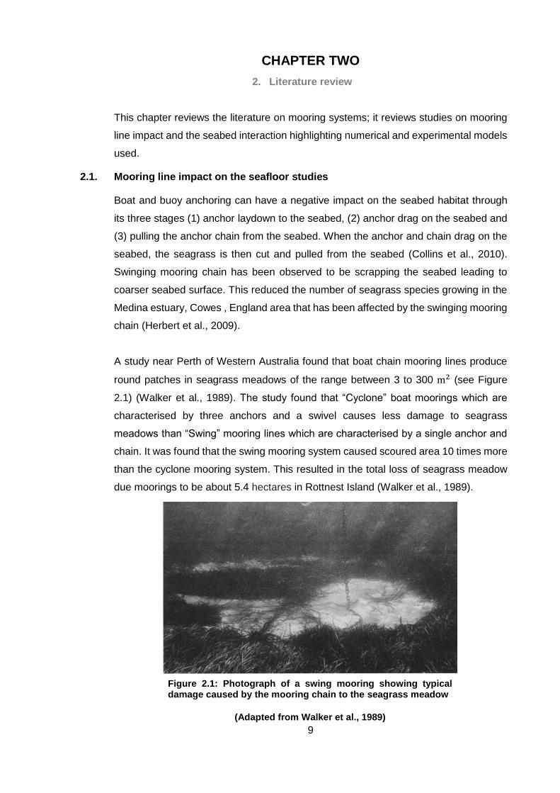
A study near Perth of Western Australia found that boat chain mooring lines produce

round patches in seagrass meadows of the range between 3 to 300 m2 (see Figure

2.1) (Walker et al., 1989). The study found that “Cyclone” boat moorings which are

characterised by three anchors and a swivel causes less damage to seagrass

meadows than “Swing” mooring lines which are characterised by a single anchor and

chain. It was found that the swing mooring system caused scoured area 10 times more

than the cyclone mooring system. This resulted in the total loss of seagrass meadow

due moorings to be about 5.4 hectares in Rottnest Island (Walker et al., 1989).

Figure 2.1: Photograph of a swing mooring showing typical damage caused by the mooring chain to the seagrass meadow

(Adapted from Walker et al., 1989)

10

Contrary to the latter study, Hastings et al. (1995) argued that “Cyclone” mooring lines

caused more damage on the seagrass meadows than “Swing” mooring lines. Their

study was conducted by comparing areal coverages obtained using aerial photography

of seagrasses and sand patches within seagrass beds taken between 1941 and 1992.

Seagrass loss was found to be caused due to the change from single anchor swing

mooring lines to cyclone mooring lines which used three chains. Cyclone mooring lines

were found to have produced three circular patches in the seagrass bed, these holes

caused 5 𝑚 radius round patches on the seafloor. Hastings et al. (1995) stated that the

study by Walker et al. (1989) only investigated the condition of seagrass meadows

observed in 1987 which neglected the rate at which seagrasses were lost due to boat

mooring lines. The two studies compared above both agree that boat chain mooring

systems cause damage to the seagrass meadows on the benthic ecosystem.

In addition to the study conducted by Hastings et al. (1995), the temporal decline of

seagrass beds was associated with the damage caused by permanent chain mooring

systems. The study showed a decrease in seagrass beds area and an increase in sand

patch area on the seafloor in relation to mooring lines; these findings were obtained in

a period between 1941 and 1992 in Rocky Bay and Thomson Bay, Rottnest Island,

Western Australia. More seagrass damage was found in Rocky Bay with 18% of

seagrass area lost between 1941 and 1992, and 13% between 1981 and 1992

(Hastings et al., 1995).

The conclusion from the study by Hastings et al. (1995) was that the decline of

seagrasses in Rocky Bay corresponds with the doubling of boat moorings and an

increase in boat size and traffic between 1981 and 1992. This loss of seagrasses was

also as a result of the change from a single anchor swing mooring line to a cyclone

mooring line with three chains. The study highlighted that the single weighed swing

mooring lines cause the least damage when compared to cyclone mooring lines as it

covers less seagrass area. Both the swing and cyclone mooring systems were found

susceptible for seafloor abrasion – a phenomenon where the seafloor surface is swept

by the mooring chain.

A similar study to Hastings et al. (1995) was conducted by Demers et al. (2013) in

Callala Bay, Australia; the study compared a ‘seagrass-friendly’ screw mooring,

cyclone mooring and a standard single anchor swing mooring line types. It was found

that ‘Swing’ mooring lines produced substantial seabed scour, stripping seagrass

11

patches of about 18 m diameter; whereas cyclone moorings produced extensive

stripped patches of about 36 m diameter on average. The screw mooring was found to

cause less seagrass scour amongst the three types of moorings on the latter studies;

this was noticed by finding a small circular scar around most ‘screw’ mooring systems.

The cyclone mooring system was found to cause the most damage which agrees with

findings from the study by Hastings et al. (1995). The three types of mooring mentioned

above are illustrated in Figure 2.2 below.

These studies by Walker et al. (1989), Hastings et al. (1995) and Demers et al. (2013)

are all in agreement that the mechanical impact of boat mooring chains causes

disturbance to seagrass meadows; this mechanical impact mostly produce stripped

areas within seagrass meadows (Demers et al., 2013). The next Figure 2.3 shows

distinctive round areas stripped of seagrass in Callala Bay mooring area obtained by

an aerial photograph.

Figure 2.2: Schematic representation of a typical (A) ‘screw’ mooring system, (B) ‘swing’ mooring system and (C) ‘cyclone’ mooring system

(Adapted from (Hastings et al., 1995).

12

Another study by Davis et al. (2016) was recently completed involving large vessels

interaction with the marine environment with an emphasis on the impact of seafloor

biota. The study investigated the impact of large vessels with the length of between

100 – 300 m and a single anchor chain link of about 60 – 200 kg. The study used a

case study in South Eastern Australia to highlight the complex issues surrounding large

vessel anchoring. The investigation involved exploring activities which interact with

marine environments. The investigation placed an emphasis on the substantial

ambiguity surrounding the impacts caused by large vessel anchoring on the seafloor

organisms (Davis et al., 2016).

The outcomes from this study were that vessels at anchor pose a risk to the seafloor

and its biota as a ship’s anchor can shift, and its mooring chain swing across the

seabed, causing abrasion of the seafloor and damage to the benthic ecosystems. The

study stated that the mapping of the seafloor areas with high shipping activity can give

more insight on which marine habitats may be at risk. This can be achieved by the use

of remotely operated vehicles and cameras to compare marine life (fish and

invertebrates) between the areas which are subject to heavy anchoring (Davis et al.,

2016).

The next Figure 2.4 shows the impact of recreational and commercial vessels’ mooring

chains in shallow water environment of less than 50 m in depth (Davis et al., 2016).

Automatic Identification System (AIS) was used to show vessels at anchor changing

Figure 2.3: Aerial photograph of the mooring area at Callala Bay showing characteristic round areas stripped of seagrass

(Adapted from Demers et al., 2013)

13

positions due to changing current, wind and swell. The conditions at sea cause vessels

to swing on their anchor chains. These changes in vessel position appeared as

anchoring arcs.

A case study by Rajasuriya et al. (2013) investigated the effects of human-induced

disturbances in Sri Lanka coral reefs. The study found that human activities such as

sewage discharges, oil discharges, destructive fishing practices, land and mangrove

destruction and tourism cause degradation of the coral reefs. Boat anchoring was found

to be one of the human disturbance factors together with net fishing (Rajasuriya et al.,

2013). Although boat moorings were found to cause damage to the coral reefs,

however, the amount the damage was not quantified.

Figure 2.4: Anchor arcs based on AIS (Automatic Identification System) vessel tracking data near the Port of Newcastle acquired from the Australian Maritime Safety Authority (AMSA)

(Adapted from Davis et al., 2016)

14

Milazzo et al., (2004) studied the effect of different anchor types in three anchoring

stages on boats anchored on seagrass beds in a marine protected area. The study

experimentally quantified the damage caused by boat anchoring by counting seagrass

shoot density after the anchoring process. Various factors were tested to quantify the

damage; these factors include the use of a chain or a rope, the use of different anchor

types and the analysis of the three anchoring stages i.e. anchor laydown, anchor drag

on the seabed and lock-in and anchor weighing. The pattern shown by each factor

tested was checked for consistency in different locations of the seagrass meadows.

The mechanical destruction of seagrass species was attributed to human activities and

boat moorings. Human activity impact was quantified to be on a large spatial scale from

1000 to 10 000 m, whereas on a smaller spatial scale, the seagrasses suffered from

the chain mooring mechanical damage from the scale of 10 to 100 m. Human activities

included sewage discharge, fish farming and construction of marinas. The mechanical

damage mainly happens in coastal regions where frequent recreational activities takes

place (Milazzo et al., 2004).

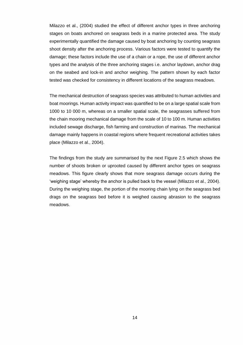
The findings from the study are summarised by the next Figure 2.5 which shows the

number of shoots broken or uprooted caused by different anchor types on seagrass

meadows. This figure clearly shows that more seagrass damage occurs during the

‘weighing stage’ whereby the anchor is pulled back to the vessel (Milazzo et al., 2004).

During the weighing stage, the portion of the mooring chain lying on the seagrass bed

drags on the seagrass bed before it is weighed causing abrasion to the seagrass

meadows.

15

Milazzo et al. (2004) also noticed that when studying boat moorings, more damage of

seagrasses seemed to be caused by anchor drag which sweeps seagrass bed, during

the forward and backwards motion of the boats (Milazzo et al., 2004). It should be noted

that this study focused upon light anchor of 4 kg in mass and the boat of about 5.5 m

in length; thus, results and conclusions made in this study are more likely to differ in

regions where long vessels, with heavy anchors and chains are used. The study cited

above clearly demonstrates that boat anchoring causes severe damage to seagrass

beds due to the mechanical impact of the anchor chains.

Francour et al. (1999) “studied the direct effects of boat moorings on seagrass beds in

the Port-Cros National Park”. The study revealed through field experiments 34

seagrass shoots destroyed on average during the boat anchoring process, especially

when the seagrass mat compactness was weak. These experiments were carried in

seven different sites; various factors which could have affected the number of uprooted

Figure 2.5: Mean number of shoots uprooted/broken by the three anchor types (Hall in black; Danforth in grey; Folding grapnel in white)

(Adapted from Milazzo et al., 2004)

16

seagrass shoots were studied. They included the density of the root mat, the seagrass

meadow density and the extent of rhizome exposure. The study noticed a clear direct

effect of anchoring whereby 20 seagrass shoots were uprooted when the anchor digs

into the seagrass bed. During the anchor weighing stage, 14 seagrass shoots on

average were also observed to be uprooted whereby the anchor was retrieved to the

boat with an electrical windlass (Francour et al., 1999).

Within the context of climate change, a study by Kininmonth et al. (2014) investigated

the impact of anchor damage within the Great Barrier Reef World Heritage Area

(GBRWHA) in Australia. The coral reefs and seagrass habitats were susceptible to

human disturbances which included boat anchoring. This disturbance of the coral reefs

seagrass habitats includes the anchor deployment, anchor retrieval and anchor chain-

seabed interaction which potentially causes loss of the coral reefs and seagrasses

(Kininmonth et al., 2014). Only 19% of approximately 20 000 km2 GBRWHA was

considered vulnerable to anchor damage. The study classified human activity such as

anchoring as a small scale disturbance to the coral reefs and seagrasses. (Kininmonth

et al., 2014).

In the study cited above, the assessment of the area exposed to anchor damage was

found to be a challenging task due to the difficulty of the oceanic environment and the

absence of real verifiable data. In GBRWHA five major ports, the deployment of the

anchor and chain drag were found not to have a direct impact on coral reefs and

seagrasses (Kininmonth et al., 2014).

It can be deduced from the literature cited above that large vessels seem to cause more

damage on the seafloor than smaller vessels. This is because large vessels require

heavy chain to be deployed for anchoring. In all cases studied here, the mooring chain

caused considerable destruction to the benthic habitat in some regions, whereas in

some regions no considerable destruction to the coral reef systems was found. Studies

here suggest that more vessel activity is more likely to cause considerable damage to

the benthic system. This view is also supported by Abadie et al. (2016) which states

that severe boat anchoring in seagrass areas eventually leads to the destruction of

seagrass meadows due to the mechanical damage of the anchoring process.

It is worth noting that this mechanical damage has various degrees of impact on

seagrasses depending on the rate and type of the anchor used, as well as the depth of

the sea and the boat size. The mechanical damage aforementioned also induce a

17

change in the nature of the seagrass substrate which generates round patches on the

seabed (anthropogenic patches) (Abadie et al., 2016).

There seems to be no consensus on which fishing practices are seafloor “friendly”

amongst boat\vessel owners as there is currently no boat anchoring standard during

fishing. However, studies cited above indicate that mooring chains used for buoys and

boats cause abrasion to the seafloor surface.

2.2. Mooring line analysis studies

Mooring line behaviour as a result of the wind, current and wave action, has received

attention by numerous studies. For example, Sluijs & Blok (1977) first established a

static analysis of mooring line forces; this was followed by a dynamic analysis which

incorporated the dynamic effects such as inertia, dynamic loading, and geometric non-

linearities and was solved mathematically by using finite difference method (Sluijs &

Blok, 1977).

Masciola et al. (2014) outlined three approaches for solving dynamic mooring line

behaviour - (1) line representation from the finite-element analysis (FEA), (2) finite-

difference method (FD), and (3) lumped-mass (LM) method. These approaches can

achieve similar results as long as an adequate fine discretisation is used; however,

simplifications have to be introduced into these models in order to reduce

computational cost which includes the omission of bending, torsion, and shear stiffness

(Masciola et al., 2014). The fact that these approaches can yield similar results was

established by Ketchman & Lou (1975) who demonstrated that LM approach gives the

same results as FEA representations when a sufficient fine discretisation is used

(Ketchman & Lou, 1975).

In alignment with these findings, Boom (1985) found that by assuming the mooring line

to be composed of an intersected set of discrete elements, that the system of partial

differential equations which is used to describe the variables along the mooring line

can be replaced by the equation of motion. This was achieved by employing the

lumped-mass and finite element methods. These methods were found to be more

applicable in the general approaches of analysing various underwater systems such as

chains and cable (Boom, 1985).

Ha (2011) describes the lumped-mass method as a continuous distribution of the mass

mooring line where a discrete distribution of lumped masses is replaced by a finite

18

number of points. The replacement of mooring line mass leads to idealising the system

as a set of non-mass linear springs and concentrated masses. Therefore, the line is

idealised into a number of lumped masses connected by a massless elastic line taking

drag and elastic stiffness into account (Ha, 2011). This “involves the grouping of all

effects of mass, external forces and internal reactions at a finite number of nodes along

the mooring line. A set of discrete equations of motion is derived from applying the

equations of dynamic equilibrium and continuity (stress/strain) to each mass”. These

equations are solved using finite difference techniques in time-domain (Boom, 1985).

The finite element method utilises interpolation functions to describe the behaviour of

a given variable internal to the discretised mooring line element in terms of the

displacements of the nodes defining the element. The equations of motions for a single

element are obtained by applying the interpolation function to kinematic relations (strain

or displacement), constitutive relations (strain or displacement) and the equations of

dynamic equilibrium. The solution procedure of the finite element method is similar to

the lumped-mass method (Boom, 1985); the study by Boom (1985) concluded that

computer codes based on FEM were proven to be less computer time efficient when

compared with the LM algorithms. The study then used the lumped-mass method to

analyse the dynamic mooring line behaviour. The model was built with a special

attention on the maximum mooring line tension. Results from the study were then

validated from oscillation model tests.

Several models were developed using the FEM approach for analysing mooring line

response to hydrodynamic forces. Vineesh et al. (2014) used the FEA approach for

solving the dynamics of a buoy anchored by a mooring chain and a spar platform under

wave, current and wind environmental forces using FEA package ANSYS 10.0

(Vineesh et al., 2014), however, this study did not consider the mooring line interaction

with the seabed.

Jameel et al. (2011) modelled mooring lines in ABAQUS as 3D tensioned beam

elements. Hybrid beam elements were used to model the mooring line; these hybrid

elements accounted for 6 DOF including displacements and axial tension as nodal

degrees of freedom of the mooring line. The axial tension of the mooring was found to

maintain the catenary’s shape. The choice of hybrid beam elements was due to their

easy convergence; linear or nonlinear truss elements can also be implemented in the

ABAQUS model, however, they have their own limitations (Jameel et al., 2011).

19

Yu & Tan (2006) developed an efficient 2D finite element model to numerically analyse

the interaction of the mooring lines with the seabed. The model was developed in the

time domain using ABAQUS. Hybrid beam elements and the Newton-Rhapson iteration

procedure were implemented. The seabed was represented by using elastic and soil

constitutive models; the coulomb model used the contact friction coefficient of 0.4. The

hydrodynamic forces acting on the mooring line were simulated using the wave height

of 3 m and period of 4 s for the simulation duration of 800 s.

The mooring line pretension was set to 36 kN and a vertical force of 3000 kN was

applied at the fairlead point. One of the outcomes from the study was that, the

environmental forces influence the mooring line predominantly on its longitudinal

profile, while the transversal profile response can be ignored in the dynamic analysis

(Yu & Tan, 2006). Kim (2003) also modelled the seafloor as an elastic foundation

between the single-point chain mooring line and multi-body floating platform (Kim,

2003).

Yang (2007) conducted a “hydrodynamic analysis of mooring lines based on optical

tracking experiments” using free and forced oscillation tests. These tests were

implemented to verify the numerical results of moored body motion. Owing to the lack

of experimental data available, the drag coefficients for chains were typically assumed

to be the same as for a rod, but with an equivalent diameter equal to twice the bar size

of the chain link. The study emphasised the difficulty of determining studless chain drag

coefficients since the chain has a complex shape which complicates experiments.

Figure 2.6 below show an example of a stud and studless chain.

Since the chain comprises of interconnected links which have the shape of oval rings,

the direct force measurement on the body (i.e. the chain link) using a force gauge is

Figure 2.6: Stud-Link (a) and Studless Chain (b)

20

difficult. The chain links are free to rotate at the interconnections to a certain extent, the

torsional motion of the chain might be a consideration in the analysis even for small

lengths of chain. Also, as compared to simple body shapes, the complex geometry of

chain links causes more complex wake flow kinematics. For these reasons, predicting

the hydrodynamic loading on moving chain is quite challenging (Yang, 2007).

The optical tracking experiments were conducted using a high-speed video camera

which provided an opportunity for exploring the feasibility of deducing Morison drag and

inertia coefficients from measured trajectories of chain and cable elements undergoing

controlled free or forced oscillations in calm water (Yang, 2007). Figure 2.7 shows the

setup of the large-scale optical testing experiment conducted in a 3D wave basin. The

basin was 45 m long, 30 m wide and 6 m deep (Yang, 2007).

The next Figure 2.8 below shows a suspended catenary mooring line with white

markers for optical computer tracking. These experiments took place in a small 3D

Figure 2.7: Diagram of large scale test setup

(Adapted from Yang, 2007)

21

wave basin whose sides were made of glass, which allowed direct measurement of line

kinematics by optical tracking. The video footage recorded by the optical tracking

camera was processed to extract time-histories of the position for all markers (Yang,

2007).

Figure 2.9 shows 2D mooring line configuration for forced oscillation tests for semi-taut

catenary mooring.

Figure 2.8: Suspended catenary mooring mount


Figure 2.9: Two-dimensional line configuration for forced oscillation tests


22

Wang et al. (2010) investigated the 3D interaction between the mooring chain and the

seabed; they described the interaction between the chain and the seabed as a very

complex process which has not been thoroughly understood yet (Wang et al., 2010).

This interaction was found to cause a significant effect on the dynamic behaviour of the

mooring chain. The interaction was as a result of the mooring chain excitation due to

the action of wave loads. This interaction created a boundary condition that varied in

time and in space (Pellegrino & Ong, 2003). The change in the mooring chain’s

longitudinal profile resulted in a significant amount of the chain length lying on the

seafloor to lift off and drop back down; the amount of the mooring chain length dropping

back on the seafloor varied with time (Yu & Tan, 2006). The following Figure 2.10

illustrates various touchdown points of the mooring line.

This problem can be solved in both frequency and time domain analysis. The frequency

domain analysis approach was first presented by Pellegrino & Ong (2003) on modelling

of seabed interaction of mooring cables (Yu & Tan, 2006). However, Frequency-

domain analysis neglects the “non-linear hydrodynamic load effects and non-linear

interaction effects between” the vessel, the mooring line and the seabed. Time-domain

simulations are preferred since they best predict the mooring line dynamics, although

they are time-consuming in nature and are mostly carried for about 3600 𝑠 (DNV, 2011).

Figure 2.10: Mooring line touchdown points resulting in time-varying boundary condition

(Adapted from Pellegrino & Ong, 2003)

23

2.3. Single-point and two-point mooring systems

As stated in the introduction, the “double anchor i.e. two-point mooring system, was

introduced into the South African squid fishery. Currently, there is no available literature

dedicated on the comparison of the singe-point and two-point mooring systems used

in the squid fishing industry between Plettenberg Bay and Port Alfred in Eastern Cape.

The subsequent damage each mooring system type causes has not been quantified.

However, studies reviewed in this thesis shows that the mooring chain interaction with

the seafloor caused abrasion to the seafloor and its species.

As cited by Demers et al. (2013) single-point mooring systems are prone to dragging

on the seabed causing a radial contact zone. However, the dynamic behaviour of a

two-point mooring has not been given much attention by researchers. Two-point

mooring systems require more deployment area than single-point mooring systems

which can cause concerns for fishermen as each of their boats is competing for the

limited resources. Single-point mooring system is easy to deploy and has less seabed

footprint in general compared to the two-point mooring system.

24

CHAPTER THREE

3. Methods and mathematical formulations

This chapter describes the methods and theory of the research problem, the way this

was modelled, and the software packages used to obtain the quantitative description

of the behaviour of squid fishing vessel anchor lines.

3.1. ANSYS AQWA and ABAQUS introduction

Two primary numerical simulation programs have been used to investigate the dynamic

response of the moored squid fishing vessels interaction with the seabed. The first is

ANSYS AQWA which was used to model the wave and current forces acting on the

moored vessel. The second is ABAQUS which was used for determining contact forces

on the seabed since ANSYS AQWA does not have this functionality. The secondary

software package used was Tracker which was used for analysing the acquired video

footage from divers on analysis the motion of the chain underwater. This section gives

the general background of ANSYS AQWA and ABAQUS software

3.1.1. ANSYS AQWA background

ANSYS AQWA has been used as the primary investigative tool in this project. It is a

toolset used for investigating effects hydrodynamic loads on marine structures. It

provides an environment for investigating the effects of the wave, wind and current

loads on floating or fixed offshore structures. This includes ships, tension leg platforms

(TLPs), semi-submersibles, renewable energy systems and breakwater design.

ANSYS AQWA uses potential flow solver, the wave loads on a structure are calculated

through a panel method which is based on potential flow theory (ANSYS AQWA, 2015).

ANSYS AQWA uses a Boundary Element Methods (BEM), or Panel Methods, or

Boundary Integral Methods (BIM) to calculate the pressures and forces on the floating

vessel. It can also conduct time-domain simulation with mooring lines attached to the

vessel. When this is done, mooring line tension forces and vessel displacement in

different wave conditions can be obtained.

ANSYS AQWA can simulate the wind, wave and current loading on the floating

structure. This can be achieved by employing 3D radiation/diffraction theory and

Morison’s equation for slender structures in regular waves in the frequency or time-

domain. The static and dynamic stability characteristics of the moored floating structure

25

under steady or unsteady environmental loads can be estimated (ANSYS AQWA,

2015).

The software simulates mooring, stability, vessel motions in regular and irregular waves

within time and frequency-domain by solving the governing equations (Eder, 2012).

This is achieved by using diffracting and non-diffracting panels; Morison elements

(TUBE, STUB and DISC) are used for slender structures i.e. the mooring line etc. While

Panel elements (QPPL and TPPL) are used for the rigid bodies i.e. the vessel hull,

defined by point masses (PMAS), fenders, articulations and elastic catenaries.

ANSYS AQWA can generate time-history of the simulated motions of floating

structures, arbitrarily connected by articulations or mooring lines, under the action of

the wind, wave and current forces. The positions and velocities of the structures are

determined at each time step by integrating the accelerations due to these forces in the

time domain, using a two-stage predictor-corrector numerical integration scheme

(ANSYS AQWA, 2015).

3.1.2. ABAQUS background

The ABAQUS software was used to simulate the contact between the chain mooring

line and the seabed. This is a finite element numerical technique used to solve

structural problems such as dynamic vibration problems, thermal connections and non-

linear statics and contact problems. In the finite element model, the entire structure acts

as a continuum. The model can handle all nonlinearities, loading and boundary

conditions.

The finite element method utilises interpolation functions to describe the behaviour of

a given variable internal to the discretised mooring line element in terms of the

displacements of the nodes defining the element. The equations of motions for a single

element are obtained by applying the interpolation function to kinematic relations

(strain/displacement), constitutive relations (strain/displacement) and the equations of

dynamic equilibrium (Allan, 2008).

ABAQUS provides an environment for pre-processing and post-processing the

behaviour of the mooring line contact with the seabed in 2D and 3D.

26

3.2. Mathematical formulations of the moored vessel

This section presents the mathematical formulations of the chain mooring line and the

fishing vessel when subjected to sea conditions. The equations of motion are used to

achieve this objective; these equations are based on the basic Newton’s second law of

motion which provides a tool for studying the relationship of the response to the

parameters governing that response. The equations of motion are modified in order to

represent the time-dependent (dynamic) terms and the nonlinear behaviour of the

vessel-mooring interaction.

3.2.1. Governing equations of the chain mooring line in time-domain

The nonlinear chain mooring line is represented by a catenary section in ANSYS

AQWA; the catenary section is assumed to have a circular profile which is represented

by a nonlinear dynamic catenary cable. The catenary section also allows the mooring

line to be made up of different section properties. The cable which represents the

mooring line is connected between the anchor and vessel Fairlead point. The dynamic

response of the catenary cable is characterised by its large axial stiffness in the

longitudinal direction compared to the lateral stiffness (transverse stiffness). When the

catenary section data is defined, ANSYS AQWA internally converts all the mooring

lines sections to a two-dimensional load/extension database with the maximum of 600

points (ANSYS AQWA, 2015).

The cable connection is modelled using Morison-type line elements subjected to

external loads – the wave, wind and current loads. Figure 3.1 shows the configuration

of a dynamic chain mooring line model discretised into a number of finite elements by

lumping each mass of an element into a corresponding node using the Lumped-Mass

method. The variables 𝑎�̂� = (𝑎1, 𝑎2, 𝑎3) indicate the unit axial vector from a node 𝑗-𝑡ℎ to

node (𝑗 + 1) − 𝑡ℎ, while the unstretched mooring line length from the anchor point to

the 𝑗-𝑡ℎ node is represented by 𝑆𝑗. The seabed is assumed to be a simple plane which

is flat and horizontal. The mud line springs shown at each node are used for modelling

the reaction force of the seabed. The springs are chosen for reducing discontinuities

and energy losses at the touchdown point of the node in the discretized chain mooring

line (ANSYS AQWA, 2015).

The depth of the mud layer shown in Figure 3.1 is indicated by �̂� which is located above

the seabed. The laid length denoted by 𝐿𝐵 of a dynamic chain mooring line interacting

27

with the seabed is measured from the anchor point to the touchdown point of a node.

The touchdown point is defined as 0.28�̂� above the seabed (ANSYS AQWA, 2015).

Various forces which act on a mooring line represented by a cable connection are

described by Equation 3.2-1 below. The single cable element is subjected to external

hydrodynamic loadings and structural inertial loading (ANSYS AQWA, 2015):

Figure 3.2: Forces on a Cable Element

(Adapted from ANSYS AQWA Theory Manual, 2015)

The motion equation of this cable element is obtained from the general Newton’s

second law of motion:

Figure 3.1: Modelling of a dynamic mooring line using

a cable connection

(Adapted Aqwa Theory Manual, 2015)

28

Equation 3.1

𝑭 = 𝒎𝒂

where 𝑭 represents all the forces acting the cable element which are cable tension,

shear, weight and hydrodynamic forces which are due to forces acting on a cable

element immersed in water with its relative motion. These terms acting on the cable

element can be written as vectors which account for the direction of the chain element,

if vectors are ignored, this will lead to an inaccurate solution, vectors are represented

by the arrow (→) and are placed on top of each term on the equation below:

𝝏�⃗⃗�

𝝏𝑺𝒆+

𝝏�⃗⃗�

𝝏𝑺𝒆+ �⃗⃗⃗� + �⃗⃗� 𝒉 = 𝒎

𝝏𝟐�⃗⃗�

𝝏𝒕𝟐 Equation 3.2

𝜕�⃗⃗�

𝜕𝑆𝑒+𝜕�⃗�

𝜕𝑆𝑒× �⃗⃗� = −�⃗⃗�

𝒎 – represents the structural mass per unit length

�⃗⃗� – represents the moment distribution loading per unit length

�⃗⃗� – represents the position of the first node of the cable element using vector

representation

∆𝑺𝒆 – is the length of the cable element

∆𝑫𝒆 – is the diameter the cable element

�⃗⃗⃗� – is the weight of the cable element

�⃗⃗� 𝒉 – represent the external hydrodynamic forces per unit length using vector

representation. �⃗⃗� 𝒉 is formulated using a modified drag force equation called the

Morison’s equation which is used for calculating the wave loads on slender

structural members.

�⃗⃗� – represent the tension force at the first node of the cable element using

vector representation

�⃗⃗⃗� – represent the bending moment at the first node of the cable element using

vector representation

�⃗⃗� – represent the shear force at the first node of the cable element using vector

representation

𝒕– represents time

𝝏– shows the partial derivative

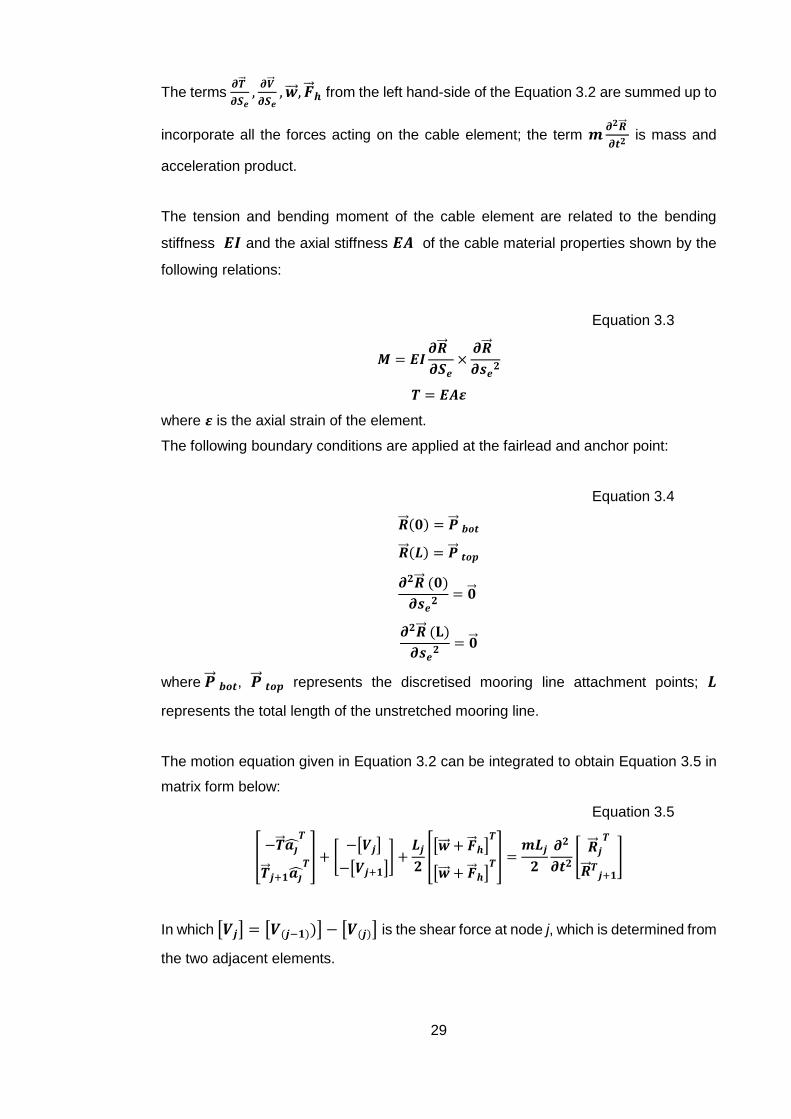
29

The terms 𝝏�⃗⃗�

𝝏𝑺𝒆,𝝏�⃗⃗�

𝝏𝑺𝒆, �⃗⃗⃗� , �⃗⃗� 𝒉 from the left hand-side of the Equation 3.2 are summed up to

incorporate all the forces acting on the cable element; the term 𝒎𝝏𝟐�⃗⃗�

𝝏𝒕𝟐 is mass and

acceleration product.

The tension and bending moment of the cable element are related to the bending

stiffness 𝑬𝑰 and the axial stiffness 𝑬𝑨 of the cable material properties shown by the

following relations:

Equation 3.3

𝑴 = 𝑬𝑰𝝏�⃗⃗�

𝝏𝑺𝒆×𝝏�⃗⃗�

𝝏𝒔𝒆𝟐

𝑻 = 𝑬𝑨𝜺

where 𝜺 is the axial strain of the element.

The following boundary conditions are applied at the fairlead and anchor point:

Equation 3.4

�⃗⃗� (𝟎) = �⃗⃗� 𝒃𝒐𝒕

�⃗⃗� (𝑳) = �⃗⃗� 𝒕𝒐𝒑

𝝏𝟐�⃗⃗� (𝟎)

𝝏𝒔𝒆𝟐= �⃗⃗�

𝝏𝟐�⃗⃗� (𝐋)

𝝏𝒔𝒆𝟐= �⃗⃗�

where �⃗⃗� 𝒃𝒐𝒕, �⃗⃗� 𝒕𝒐𝒑 represents the discretised mooring line attachment points; 𝑳

represents the total length of the unstretched mooring line.

The motion equation given in Equation 3.2 can be integrated to obtain Equation 3.5 in

matrix form below:

Equation 3.5

[−�⃗⃗� 𝒂�̂�

𝑻

�⃗⃗� 𝒋+𝟏𝒂�̂�𝑻] + [

−[𝑽𝒋]

−[𝑽𝒋+𝟏]] +

𝑳𝒋

𝟐[[�⃗⃗⃗� + �⃗⃗� 𝒉]

𝑻

[�⃗⃗⃗� + �⃗⃗� 𝒉]𝑻] =

𝒎𝑳𝒋

𝟐

𝝏𝟐

𝝏𝒕𝟐[�⃗⃗� 𝒋𝑻

�⃗⃗� 𝑻𝒋+𝟏]

In which [𝑽𝒋] = [𝑽(𝒋−𝟏))] − [𝑽(𝒋)] is the shear force at node j, which is determined from

the two adjacent elements.

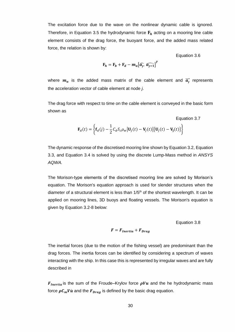
30

The excitation force due to the wave on the nonlinear dynamic cable is ignored.

Therefore, in Equation 3.5 the hydrodynamic force 𝐅𝒉 acting on a mooring line cable

element consists of the drag force, the buoyant force, and the added mass related

force, the relation is shown by:

Equation 3.6

𝐅𝒉 = 𝐅𝒃 + 𝐅𝒅 −𝒎𝒂[𝒂𝒋 ,̂ 𝒂𝒋+�̂�]𝑻

where 𝒎𝒂 is the added mass matrix of the cable element and 𝒂𝒋⃗⃗ ⃗ represents

the acceleration vector of cable element at node j.

The drag force with respect to time on the cable element is conveyed in the basic form

shown as

Equation 3.7

𝐅𝑑(𝑡) = {𝐟𝑑(𝑗) −1

2𝐶𝑑𝑆𝑐𝜌𝑤|𝐔𝑗(𝑡) − 𝐕𝑗(𝑡)|{𝐔𝑗(𝑡) − 𝐕𝐣(𝑡)}}

The dynamic response of the discretised mooring line shown by Equation 3.2, Equation

3.3, and Equation 3.4 is solved by using the discrete Lump-Mass method in ANSYS

AQWA.

The Morison-type elements of the discretised mooring line are solved by Morison’s

equation. The Morison's equation approach is used for slender structures when the

diameter of a structural element is less than 1/5th of the shortest wavelength. It can be

applied on mooring lines, 3D buoys and floating vessels. The Morison's equation is

given by Equation 3.2-8 below:

Equation 3.8

𝑭 = 𝑭𝑰𝒏𝒆𝒓𝒕𝒊𝒂 + 𝑭𝑫𝒓𝒂𝒈

The inertial forces (due to the motion of the fishing vessel) are predominant than the

drag forces. The inertia forces can be identified by considering a spectrum of waves

interacting with the ship. In this case this is represented by irregular waves and are fully

described in

𝑭𝑰𝒏𝒆𝒓𝒕𝒊𝒂 is the sum of the Froude–Krylov force 𝝆𝑽𝒖 and the he hydrodynamic mass

force 𝝆𝑪𝒎𝑽�̇� and the 𝑭𝑫𝒓𝒂𝒈 is defined by the basic drag equation.

31

This can be written as:

Equation 3.9

𝑭 = 𝝆𝝅

𝟒𝑫𝟐𝑪𝒎�̇� ⏟

Interia force term

+𝟏

𝟐𝝆𝑪𝒅𝑫𝒖|𝒖|⏟

Drag force term

since 𝝅

𝟒𝑫𝟐 = 𝑨,

This equation is further expanded for a moving body in an oscillatory flow as follows:

Equation 3.10

𝒅𝑭 = 𝝆𝑨𝑪𝒎�̇�𝒇 − 𝝆𝑨(𝑪𝒎 − 𝟏)�̇�𝒔 +𝟏

𝟐𝝆𝑫𝑪𝒅|𝒖𝒇 − 𝒖𝒔|(𝒖𝒇 − 𝒖𝒔)

= 𝝆𝑨(𝟏 + 𝑪𝒂)�̇�𝒇 − 𝝆𝑨𝑪𝒂�̇�𝒔 +𝟏

𝟐𝝆𝑫𝑪𝒅|𝒖𝒇 − 𝒖𝒔|(𝒖𝒇 − 𝒖𝒔)

where 𝑫 is the drag diameter, 𝑪𝒅 is the drag coefficient, 𝒖𝒇 is the fluid particle velocity

in the lateral direction, 𝒖𝒔 is the structure velocity in the transverse direction, 𝑪𝒎 = 𝑪𝒂 +

𝟏 represents the inertia coefficient, and 𝑨 is the cross-sectional area.

The definition of the directional dependent forces and moments of the discretised

element is shown in Figure 3.3 below.

Figure 3.3: Local Tube Axis System

(Adapted from ANSYS Aqwa Theory Manual, 2015)

32

The hydrodynamic forces and moments acting on an element are determined “with

reference to the local tube axis system by the integration of the cross-sectional over

the submerged length of L’,”

Equation 3.11

𝐹𝑦 = ∫ {1

2𝜌𝐷𝑦𝐶𝑑𝑦|�⃗� 𝑓 − �⃗� 𝑠|(𝑢𝑓𝑦 − 𝑢𝑠𝑦) + 𝜌𝐴𝐶𝑚𝑦�̇�𝑓𝑦 − 𝜌𝐴(𝐶𝑚𝑦 − 1)�̇�𝑓𝑦} 𝑑𝑥

𝐿′+𝐿𝑒1

𝐿𝑒1

𝐹𝑧 = ∫ {1

2𝜌𝐷𝑧𝐶𝑑𝑧|�⃗� 𝑓 − �⃗� 𝑠|(𝑢𝑓𝑧 − 𝑢𝑠𝑧) + 𝜌𝐴𝐶𝑚𝑧�̇�𝑓𝑧 − 𝜌𝐴(𝐶𝑚𝑧 − 1)�̇�𝑓𝑧} 𝑑𝑥

𝐿′+𝐿𝑒1

𝐿𝑒1

𝑀𝑦 = ∫ {1

2𝜌𝐷𝑧𝐶𝑑𝑧|�⃗� 𝑓 − �⃗� 𝑠|(𝑢𝑓𝑧 − 𝑢𝑠𝑧) + 𝜌𝐴𝐶𝑚𝑧�̇�𝑓𝑧 − 𝜌𝐴(𝐶𝑚𝑧 − 1)�̇�𝑓𝑧} x𝑑𝑥

𝐿′+𝐿𝑒1

𝐿𝑒1

𝑀𝑧 = −∫ {1

2𝜌𝐷𝑦𝐶𝑑𝑦|�⃗� 𝑓 − �⃗� 𝑠|(𝑢𝑓𝑦 − 𝑢𝑠𝑦) + 𝜌𝐴𝐶𝑚𝑦�̇�𝑓𝑦 − 𝜌𝐴(𝐶𝑚𝑦 − 1)�̇�𝑓𝑦} x𝑑𝑥

𝐿′+𝐿𝑒1

𝐿𝑒1

“In AQWA, a three-point Gaussian integration scheme is employed to estimate the

integral forms given by Equation 3.11” (ANSYS AQWA, 2015).

“The forces and moments on each tube element are then transformed to the fixed

reference axes (FRA) and, in addition, the moments are with respect to the centre of

gravity of the structure. The total fluid load is the summation of forces on all the

tube elements and the panel elements” (ANSYS AQWA, 2015).

3.2.2. Governing equations for the fishing vessel in time domain

To obtain the hydrodynamic response the fishing vessel at sea, the most common

approach used is the 3D panel method which is based on fluid potential theory. The

panel method is a technique for solving incompressible potential flow over thick 2D and

3D geometries (for external flow); it is used to determine the fluid velocity and the

pressure distribution, on an object (Mason, 2015). The panel method is based on the

potential flow theory assumption that the fluid is inviscid (negligible viscosity.),

incompressible, irrotational and steady. The motion of the fishing vessel is represented

by six degrees of freedom (6-DOF) rigid body translational and rotational motions which

are categorised into two – Translation (heave, sway, and surge) and Rotational (yaw,

pitch and roll) as shown in Figure 3.4 below.

33

The solution flowfield (fluid domain) is found by representing the fishing vessel surface

by a number of panels, and solving a linear set of algebraic equations which satisfies

the Laplace’s equation to determine unknown variables. The potential flow panel

method is incorporated in the Bernoulli's equation to find the fluid pressure at a given

point on the surface of the fishing vessel. The fishing vessel surface is discretised into

number panels called a mesh. Finer meshed geometries tend to yield more accurate

results. The panels below the vessel waterline are called ‘diffracting panels’, these

panels are subject to the three-dimensional panel method based on fluid potential

theory. The panels above the waterline are called ‘non-diffracting panels’.

The hydrodynamic loads are mainly caused by the interactions between the vessel and

the waves. The hydrodynamic loads acting on the fishing vessel are the drag, the wave,

and the inertia loads. Drag loads (viscous forces) on the hull of the vessel are important

when structural members are slender and wave amplitude is large and are obtained

using Morison’s equation. This is the net force opposing the vessel’s forward movement

due to the pressure and shear forces acting on the wetted surface of the vessel

(ANSYS AQWA, 2015).

Equation 3.12

[𝑭𝒅𝒎𝒋] = 𝑪𝒅𝒎[|𝒖𝒋||𝒖𝒋|] where j=1,6

“where [𝑭𝒅𝒎𝒋] is the 6×1 matrix which consists of the three Morison hull drag force

components and three Morison hull drag moment components, 𝑪𝒅𝒎 is a 6×6 Morison

drag coefficient matrix, and 𝒖𝒋(𝒋 = 𝟏, 𝟔) is the relative translational or rotational velocity

component in the structure local axis frame. The translational relative velocity (j=

Figure 3.4: Vessel 6-DOF rotations and translations

(Adapted from Ibrahim & Grace, 2010).

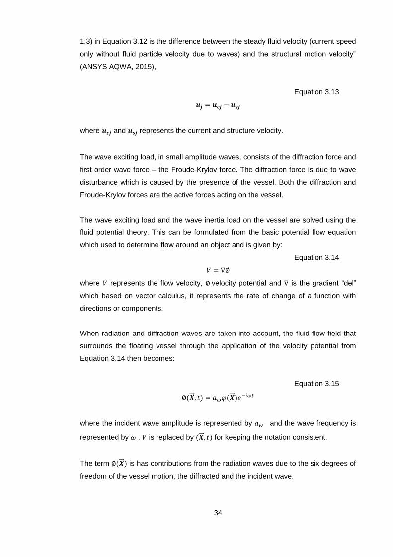
34

1,3) in Equation 3.12 is the difference between the steady fluid velocity (current speed

only without fluid particle velocity due to waves) and the structural motion velocity”

(ANSYS AQWA, 2015),

Equation 3.13

𝒖𝒋 = 𝒖𝒄𝒋 − 𝒖𝒔𝒋

where 𝒖𝒄𝒋 and 𝒖𝒔𝒋 represents the current and structure velocity.

The wave exciting load, in small amplitude waves, consists of the diffraction force and

first order wave force – the Froude-Krylov force. The diffraction force is due to wave

disturbance which is caused by the presence of the vessel. Both the diffraction and

Froude-Krylov forces are the active forces acting on the vessel.

The wave exciting load and the wave inertia load on the vessel are solved using the

fluid potential theory. This can be formulated from the basic potential flow equation

which used to determine flow around an object and is given by:

Equation 3.14

𝑉 = ∇∅

where 𝑉 represents the flow velocity, ∅ velocity potential and ∇ is the gradient “del”

which based on vector calculus, it represents the rate of change of a function with

directions or components.

When radiation and diffraction waves are taken into account, the fluid flow field that

surrounds the floating vessel through the application of the velocity potential from

Equation 3.14 then becomes:

Equation 3.15

∅(�⃗⃗� , 𝑡) = 𝑎𝜔𝜑(�⃗⃗� )𝑒−𝑖𝜔𝑡

where the incident wave amplitude is represented by 𝑎𝑤 and the wave frequency is

represented by 𝜔 . 𝑉 is replaced by (�⃗⃗� , 𝑡) for keeping the notation consistent.

The term ∅(�⃗⃗� ) is has contributions from the radiation waves due to the six degrees of

freedom of the vessel motion, the diffracted and the incident wave.

35

The potential due to wave contributions in the vessel 6-DOF may therefore be written

as:

Equation 3.16

φ(�⃗⃗� )𝑒−𝑖𝜔𝑡 = [(𝜑1 + 𝜑𝑑) +∑𝜑𝑟𝑗𝑿𝑗

𝑗=1

6

] 𝑒−𝑖𝜔𝑡

The potential functions derived above enable the resultant physical quantities such as

fluid pressure and vessel motions in time-domain to be determined.

The term Xj = uj,(1,3) and Xj = θj−3, (j = 4, 6), φ1 represents the first order wave

potential, the diffraction wave potential is represented by φd, the radiation wave

potential is represented by φrj.

The first order hydrodynamic pressure on the vessel hull is calculated by using the

linearized Bernoulli's equation below after obtaining the wave velocity potentials,

Equation 3.17

𝑝(1) = −𝜌𝜕∅(𝑋 , 𝑡)

𝜕𝑡= 𝑖𝜔𝜌𝜑(𝑋 , 𝑡)𝑒−𝑖𝜔𝑡

The nonlinear response of the fishing vessel under hydrodynamic loads is obtained by

integrating the equation of motion with respect to time in the form as proposed by

Cummins, 1962:

Equation 3.18

(𝐌 + 𝐀)�⃗⃗̈� (𝒕) + 𝐁 �̇� ⃗⃗ ⃗(𝒕) + 𝐂�⃗⃗� (𝒕) + ∫ 𝐊(𝝉) �̇� ⃗⃗ ⃗(𝒕 − 𝝉)𝒅𝝉

∞

𝟎

= 𝑭 ⃗⃗ ⃗ (𝒕)

where 𝐌 represents the inertia matrix. 𝐀 is the added mass matrix, 𝐁 is the viscous

damping and 𝐂, which are the viscous damping matrix and 𝐂 is the hydrostatic restoring

matrix . 𝐊 contains the impulse response functions. The added mass (𝐀) of the structure

occurs due to the water displaced by the structure in motion. �⃗⃗� is the 6-DOF vessel

displacements vector, �̇� ⃗⃗ ⃗ is the vessel velocity vector and �⃗⃗̈� vessel acceleration vector.

The 6 degrees of freedom (DOF) vessel displacements are represented by �⃗⃗� and the

dot symbolises differentiation with respect to time. The first dot shows differentiation

vessel displacements which gives the velocity shown by �̇� ⃗⃗ ⃗, likewise, the second dot

shows the vessel displacements differentiated twice which gives us �⃗⃗̈� which is the

acceleration of the vessel. The external force is denoted by 𝑭 ⃗⃗ ⃗ which is the

hydrodynamic loads contributions of both linear and nonlinear forces; these include the

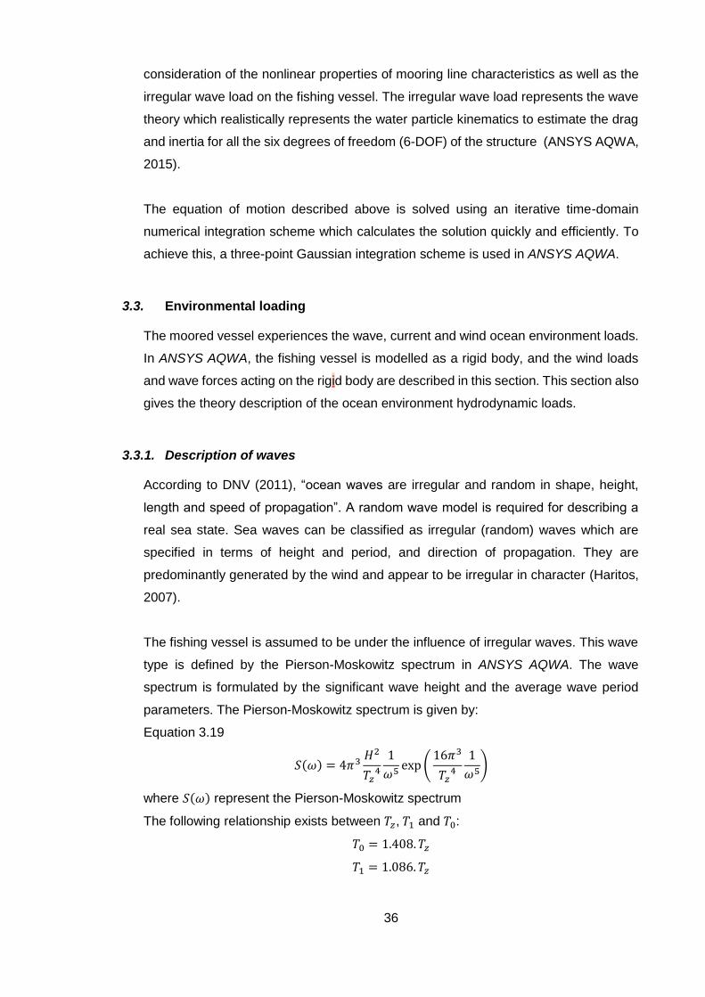
36

consideration of the nonlinear properties of mooring line characteristics as well as the

irregular wave load on the fishing vessel. The irregular wave load represents the wave

theory which realistically represents the water particle kinematics to estimate the drag

and inertia for all the six degrees of freedom (6-DOF) of the structure (ANSYS AQWA,

2015).

The equation of motion described above is solved using an iterative time-domain

numerical integration scheme which calculates the solution quickly and efficiently. To

achieve this, a three-point Gaussian integration scheme is used in ANSYS AQWA.

3.3. Environmental loading

The moored vessel experiences the wave, current and wind ocean environment loads.

In ANSYS AQWA, the fishing vessel is modelled as a rigid body, and the wind loads

and wave forces acting on the rigid body are described in this section. This section also

gives the theory description of the ocean environment hydrodynamic loads.

3.3.1. Description of waves

According to DNV (2011), “ocean waves are irregular and random in shape, height,

length and speed of propagation”. A random wave model is required for describing a

real sea state. Sea waves can be classified as irregular (random) waves which are

specified in terms of height and period, and direction of propagation. They are

predominantly generated by the wind and appear to be irregular in character (Haritos,

2007).

The fishing vessel is assumed to be under the influence of irregular waves. This wave

type is defined by the Pierson-Moskowitz spectrum in ANSYS AQWA. The wave

spectrum is formulated by the significant wave height and the average wave period

parameters. The Pierson-Moskowitz spectrum is given by:

Equation 3.19

𝑆(𝜔) = 4𝜋3𝐻2

𝑇𝑧4

1

𝜔5exp(

16𝜋3

𝑇𝑧4

1

𝜔5)

where 𝑆(𝜔) represent the Pierson-Moskowitz spectrum

The following relationship exists between 𝑇𝑧, 𝑇1 and 𝑇0:

𝑇0 = 1.408. 𝑇𝑧

𝑇1 = 1.086. 𝑇𝑧

37

where 𝑇1 is the average wave period and 𝑇0 is the maximum period, 𝜔 is the wave

frequency, 𝑇 is the average wave period and 𝐻 is the wave height.

3.3.2. Currents

Currents create significant loads on marine structures, particularly on moored vessels

and offshore structures. Currents are based on the assumption that they move in a

horizontal direction but may vary depending on the depth of water. The interaction of

currents and waves is crucial in the simulation of offshore structures. The combined

fluid particle velocity of currents and waves may increase the fluid drag force on smaller

components such as risers and mooring lines. Ocean currents contribute to the drag

force on the hull of the fishing vessel as well as increasing drag forces on the chain

mooring. Currents can be defined with a uniform or a non-uniform profile (ANSYS

AQWA, 2015).

The Agulhas Current has been described as one of the fast-flowing currents in any

ocean and reaches an estimated top speed of 2.6 𝑚/𝑠 . Its velocity depends on

variations in the equatorial current velocity, which in turn change with location, depth,

and season. It is present between Plettenberg Bay and Port Alfred region with an

estimated average flow rate of 0.2 to 0.6 𝑚/𝑠 (The Editors of Encyclopædia Britannica,

2009).

3.3.3. Winds

Wind loads not only create wind-induced waves but also directly generate drag loads

on the fishing vessel upper hull portion. The wind with a constant direction over

time, the frequency distribution of the wind speed fluctuations can be described

by means of a wind spectrum (ANSYS AQWA, 2015). However, the effects of wind

loads will be ignored in this study. This because ocean waves are wind dependent and

therefore the results of the analysis in this study remain valid. Additionally, adding the

wind will increase the number of parameters to be evaluated which will increase the

number of analysis to be done.

Thus, only the effects of the waves and currents will be considered. The wind direction

is assumed to be in the same direction as the waves and currents for simplifying the

analysis.

38

Figure 3.5: Original underwater video image of the chain movement experiment

3.4. Underwater video analysis: Experimental

As stated in the introduction, scuba scientist divers have long observed anchor chain

movement across squid egg beds. This was captured using underwater video camera;

the chain was marked with a white plastic bag. Vertical and horizontal measuring sticks

with white markers were used for calibration. Analysis of this video footage was

performed using an open source software called Tracker. This motion analysis of the

chain is later used to calibrate ANSYS AQWA and ABAQUS models ultimately to

determine the chain contact forces on the seabed. Various ocean conditions will be

evaluated for making correlations with the output from the following video analysis.

3.4.1. Tracker video analysis

A total of four video footage were obtained, the three were recorded on the double

anchor mooring and one was recorded on the single-point mooring. One of the video

footage obtained had better stability than others and thus was selected for video

analysis.

Figure 3.5 below shows an example of the original video image with labels. The

mooring chain shown has a diameter of 20 mm. The video footage analysed was

obtained from the double anchored (two-mooring) vessel.

For this experiment, a high definition video camera was used to record the 9 minutes and

47 seconds long video footage. The portion of the video that was analysed starts from

39

3 minutes and 10 seconds to 4 minutes and 3 seconds. This portion was extracted due

to better visibility and video camera stability for analysing the 2D motion of the chain.

One video camera was used, hence only the 2D motion of the chain could be analysed.

The frame rate of 50 frames per second was used for capturing the rapid motion of the

chain underwater. The frame-rate is defined as the acquisition frequency of the video

camera; high frame has a better resolution which can record the smallest detail of the

chain motion. Generally, higher frame-rates are required for tracking objects moving at

high speeds (Paredes & Taveira-Pinto, 2016).

(The original video footage of the recorded chain motion has been stored on the

following website: https://www.youtube.com/watch?v=8DB56jg1HG0&t=18s_).

The video analysis, in accordance with Paredes & Taveira-Pinto (2016), was done in

three stages (i) video linearization where the optical distortions were corrected or

minimized; (ii) calibration to match the pixel coordinates with the real world coordinates;

and (iii) video footage acquisition of the chain motion underwater.

Since all video and photo cameras have imaging distortions, video enhancement

techniques were required to improve the quality of the video footage. The large

thickness of water and suspended particulate matter between the camera and the chain

lessened the contrast of the footage as a result of light absorption and scattering by the

suspended particles in the water column. One of the techniques used to enhance the

video quality was to reduce video noise by conversion of the video image from RGB to

8-bit grayscale. This greatly improved the contrast between the chain markers and the

background allowing for easy analysis.

A margin of error is expected and thus the measurements of the video analysis

discarded as outliers. An accurate error analysis will require cameras with higher optical

quality and the optimisation of procedures used for calibration which are objectives not

pursued in this work (Paredes & Taveira-Pinto, 2016).

Figure 3.6 below shows an example of the Tracker video analysis user interface. The

video is in grayscale to improve contrast between the chain, discrete (white plastic bag)

tracking point and the background. Tracker uses a colour-based tracking technique.

The region where the colour-based operation is going to be performed is highlighted in

red. During analysis, the program searches for white colours on the selected region for

each frame of the video sequence.

https://www.youtube.com/watch?v=8DB56jg1HG0&t=18s_

40

Figure 3.6: Underwater video analysis using Tracker

Tracker also allows for the video image angle to be adjusted perpendicular to the 2D

plane movement of the mooring chain. This was done by adjusting the angle of the

origin such that it fits perpendicularly with the reference point of the video image.

About 2 m of the chain in the figure below was observed to have lifted off and dropped

back down on the seabed in sequence.

Figure 3.7 below show the vertical displacement of the tracked discrete point. This

vertical motion of the discrete point was as observed to be more dominant than the

horizontal motion. This was the expected result which was also observed in the video

footage showing the mooring chain lifting off and dropping back down at a different

frequency and speed. The velocities associated with this vertical displacement will be

used to calibrate the ANSYS AQWA model as well as to determine the seabed contact

forces using the ABAQUS model.

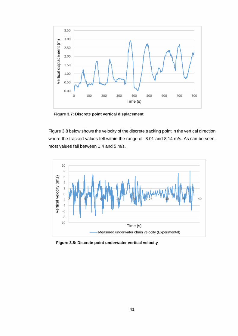
41

Figure 3.8 below shows the velocity of the discrete tracking point in the vertical direction

where the tracked values fell within the range of -8.01 and 8.14 m/s. As can be seen,

most values fall between ± 4 and 5 m/s.

0.00

0.50

1.00

1.50

2.00

2.50

3.00

3.50

0 100 200 300 400 500 600 700 800

Vert

ical dis

pla

cem

ent

(m)

Time (s)

Figure 3.7: Discrete point vertical displacement

-10

-8

-6

-4

-2

0

2

4

6

8

10

0 5 10 15 20 25 30 35 40

Vert

ical velo

city (

m\s

)

Time (s)

Measured underwater chain velocity (Experimental)

Figure 3.8: Discrete point underwater vertical velocity

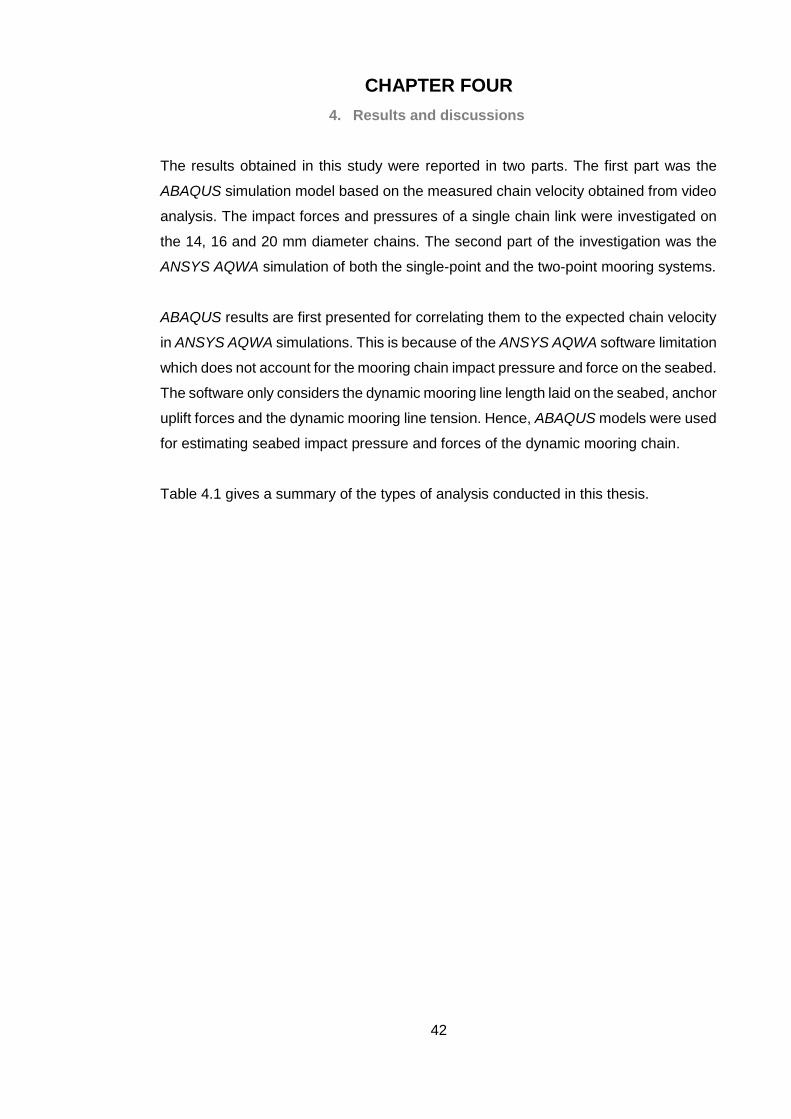
42

CHAPTER FOUR

4. Results and discussions

The results obtained in this study were reported in two parts. The first part was the

ABAQUS simulation model based on the measured chain velocity obtained from video

analysis. The impact forces and pressures of a single chain link were investigated on

the 14, 16 and 20 mm diameter chains. The second part of the investigation was the

ANSYS AQWA simulation of both the single-point and the two-point mooring systems.

ABAQUS results are first presented for correlating them to the expected chain velocity

in ANSYS AQWA simulations. This is because of the ANSYS AQWA software limitation

which does not account for the mooring chain impact pressure and force on the seabed.

The software only considers the dynamic mooring line length laid on the seabed, anchor

uplift forces and the dynamic mooring line tension. Hence, ABAQUS models were used

for estimating seabed impact pressure and forces of the dynamic mooring chain.

Table 4.1 gives a summary of the types of analysis conducted in this thesis.

43

Table 4.1: Description of various models used for mooring line analysis

Analysis Description

1:

The model was developed

for investigating the seabed

effect of three mooring chain

sizes at different velocities.

The velocities were obtained

from the underwater video

analysis.

ABAQUS chain-seabed impact

Varied chain link sizes of 14, 16 and 20 mm at 1, 3, 5, 6,

8 and 10 m/s

OUTPUT parameters: Contact force and contact

pressure

2:


for investigating seabed

impact forces based on the

slender rod method.

ABAQUS chain-seabed impact

Used 0.12 and 1 m slender rod length

Used circular 3D solid equivalent section

Varied maximum velocities of 5 and 8 m/s.

OUTPUT parameters: Contact force and contact

pressure

Made correlations with a single chain link

3:


for studying the effect of

wave height and period.

The model was also used

for investigating the wave

condition which correlates to

the observed chain impact

motion.

ANSYS AQWA time domain simulations:

Varied wave conditions:

o 1 m wave height with 7 s period




o 2.5 m wave height with 7 s period

Used 22 m single-point moored vessel

Used constant chain diameter of 20 mm with 160 m

length

OUTPUT parameters: Tension, Laid length and Anchor

uplift forces and seabed contact pressure

4:


for investigating the effects

of three mooring

configurations on the

seabed.


Used constant wave conditions: 2.5 m wave height and

7 s period

Used three mooring line configurations on the 14 and 22

m vessels (single and two-point mooring)

Used constant chain diameter of 20mm with 160 m

length


uplift forces

5:


for investigating the effect of

three chain sizes on the

seabed.


Constant wave conditions: 2.5 m wave height and 7 s

period

Constant mooring line length of 160 m

Varied chain diameter of 14, 16 and 20 mm


uplift forces

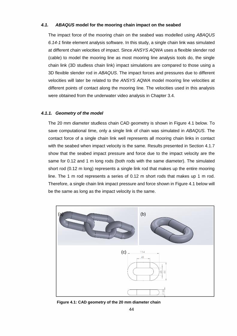
44

4.1. ABAQUS model for the mooring chain impact on the seabed

The impact force of the mooring chain on the seabed was modelled using ABAQUS

6.14-1 finite element analysis software. In this study, a single chain link was simulated

at different chain velocities of impact. Since ANSYS AQWA uses a flexible slender rod

(cable) to model the mooring line as most mooring line analysis tools do, the single

chain link (3D studless chain link) impact simulations are compared to those using a

3D flexible slender rod in ABAQUS. The impact forces and pressures due to different

velocities will later be related to the ANSYS AQWA model mooring line velocities at

different points of contact along the mooring line. The velocities used in this analysis

were obtained from the underwater video analysis in Chapter 3.4.

4.1.1. Geometry of the model

The 20 mm diameter studless chain CAD geometry is shown in Figure 4.1 below. To

save computational time, only a single link of chain was simulated in ABAQUS. The

contact force of a single chain link well represents all mooring chain links in contact

with the seabed when impact velocity is the same. Results presented in Section 4.1.7

show that the seabed impact pressure and force due to the impact velocity are the

same for 0.12 and 1 m long rods (both rods with the same diameter). The simulated

short rod (0.12 m long) represents a single link rod that makes up the entire mooring

line. The 1 m rod represents a series of 0.12 m short rods that makes up 1 m rod.

Therefore, a single chain link impact pressure and force shown in Figure 4.1 below will

be the same as long as the impact velocity is the same.

(a) (b)

(c)

Figure 4.1: CAD geometry of the 20 mm diameter chain

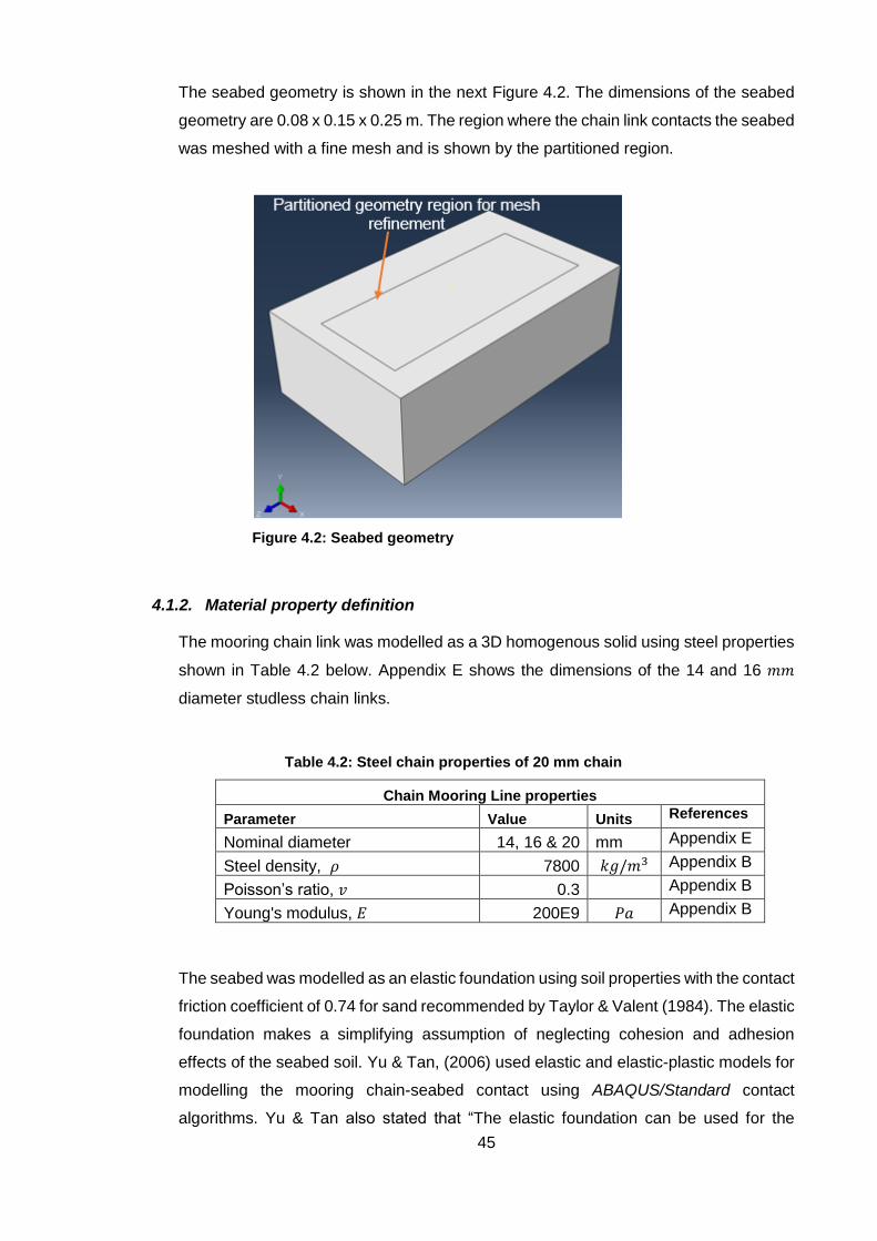
45

The seabed geometry is shown in the next Figure 4.2. The dimensions of the seabed

geometry are 0.08 x 0.15 x 0.25 m. The region where the chain link contacts the seabed

was meshed with a fine mesh and is shown by the partitioned region.

4.1.2. Material property definition

The mooring chain link was modelled as a 3D homogenous solid using steel properties

shown in Table 4.2 below. Appendix E shows the dimensions of the 14 and 16 𝑚𝑚

diameter studless chain links.

Table 4.2: Steel chain properties of 20 mm chain

Chain Mooring Line properties

Parameter Value Units References

Nominal diameter 14, 16 & 20 mm Appendix E

Steel density, 𝜌 7800 𝑘𝑔/𝑚3 Appendix B

Poisson’s ratio, 𝑣 0.3 Appendix B

Young's modulus, 𝐸 200E9 𝑃𝑎 Appendix B

The seabed was modelled as an elastic foundation using soil properties with the contact

friction coefficient of 0.74 for sand recommended by Taylor & Valent (1984). The elastic

foundation makes a simplifying assumption of neglecting cohesion and adhesion

effects of the seabed soil. Yu & Tan, (2006) used elastic and elastic-plastic models for

modelling the mooring chain-seabed contact using ABAQUS/Standard contact

algorithms. Yu & Tan also stated that “The elastic foundation can be used for the

Figure 4.2: Seabed geometry

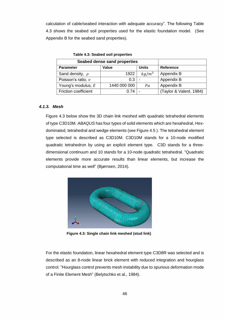
46

calculation of cable/seabed interaction with adequate accuracy”. The following Table

4.3 shows the seabed soil properties used for the elastic foundation model. (See

Appendix B for the seabed sand properties).

Table 4.3: Seabed soil properties

Seabed dense sand properties

Parameter Value Units Reference

Sand density, 𝜌 1922 𝑘𝑔/𝑚3 Appendix B

Poisson’s ratio, 𝑣 0.3 - Appendix B

Young's modulus, 𝐸 1440 000 000 𝑃𝑎 Appendix B

Friction coefficient 0.74 - (Taylor & Valent, 1984)

4.1.3. Mesh

Figure 4.3 below show the 3D chain link meshed with quadratic tetrahedral elements

of type C3D10M. ABAQUS has four types of solid elements which are hexahedral, Hex-

dominated, tetrahedral and wedge elements (see Figure 4.5 ). The tetrahedral element

type selected is described as C3D10M. C3D10M stands for a 10-node modified

quadratic tetrahedron by using an explicit element type. C3D stands for a three-

dimensional continuum and 10 stands for a 10-node quadratic tetrahedral. “Quadratic

elements provide more accurate results than linear elements, but increase the

computational time as well” (Bjørnsen, 2014).

For the elastic foundation, linear hexahedral element type C3D8R was selected and is

described as an 8-node linear brick element with reduced integration and hourglass

control. “Hourglass control prevents mesh instability due to spurious deformation mode

of a Finite Element Mesh” (Belytschko et al., 1984).

Figure 4.3: Single chain link meshed (stud link)

47

4.1.4. Contact

The chain link-seabed impact was modelled using ABAQUS/Explicit general contact.

The contact region between the chain link and the seabed is shown in Figure 4.6. The

“Explicit General contact” interaction property between the chain link and the seabed

was defined by the “normal behaviour” and “tangential behaviour” contact properties.

The “tangential behaviour” penalty contact friction coefficient of 0.74 was set.

In ABAQUS /Explicit, the solution for a particular time step is solved based on the

history of the previous step. At the end of each time step, the updated system matrices

is executed and the new system of equations is solved without iteration. If the

increments are small enough accurate results will be computed, otherwise the solution

Figure 4.4: Elastic foundation mesh

Figure 4.5: Linear and Quadratic Solid elements

(Adapted from Bjørnsen, 2014)

48

will diverge. This is due to the fact that the equilibrium is not strictly enforced (ABAQUS,

2012).

4.1.5. Boundary Conditions and Loading

The loading on the chain link was defined using “velocity field” option; velocities of 1,

3, 5, 6, 8 and 10 m/s were varied. These velocities were selected based on the

measured underwater chain velocity time-history shown in Figure 4.8. The seabed

elastic foundation was fixed on all sides except the top side where the chain link

impacts the seabed. Figure 4.7 shows boundary conditions regions and the chain-link

velocity field. The elastic foundation sides were fixed with “Encastre” boundary

condition as shown.

The ANSYS AQWA software ignores the friction of the mooring section lying on the

seabed. In reality, the seabed experiences (1) friction due to the vertical contact force

of the mooring chain, (2) friction in the longitudinal direction of the chain (when the

chain drags along its axis) and (3) friction in the transverse direction (when the mooring

chain sweeping across the seabed). Due to the complexity of analysing the mooring

chain movement in the longitudinal and transverse directions in ABAQUS, this study

this focuses on the assessment of the vertical impact of the mooring chain.

Furthermore, the underwater video footage obtained of the mooring chain impacting

the seabed showed the vertical movement of the mooring chain predominant than the

longitudinal and transverse movements. Last of all, the vertical impact assessment of

the mooring chain on the seabed was also requested by marine biologist who noticed

Figure 4.6: Chain link and seabed contact surfaces

49

an interaction between the mooring chain and the seabed as stated in the introduction

of this thesis.

Figure 4.8 shows the scatter plot of the measured chain velocity from Tracker in

Chapter 3.4. This figure shows that the most expected maximum values fall in the range

-8.01 and 8.14 m/s.

Figure 4.7: Chain-Seabed boundary conditions and

loading

-10

-8

-6

-4

-2

0

2

4

6

8

10

0 5 10 15 20 25 30 35 40

Vert

ical velo

city (

m\s

)

Time (s)


Figure 4.8: Chain velocity scatter plot

Normal direction

50

The radar plot clearly shows how the velocity is distributed in the next Figure 4.9.

4.1.6. Results

The results of the analyses are presented as CNORM (Normal Contact force),

CPRESS (Contact Pressure) and S (von Mises) stress. The stresses as a result of the

chain-link impacting the seabed at 1 and at 10 m/s are shown respectively in all three

chain-link sizes; while the stresses, contact pressures and contact forces on the

seabed for the 20, 16 and 14 mm chain links is shown by evaluating the impact at 1, 3,

5, 6, 8, and 10 m/s.

-10

-5

0

5

100

0112233344455666778889991010111111121213131314151515161617171718181919192020202121222222232323242425252526262727272828282929303030313131323233333334343435353636363737383838


Figure 4.9: Chain velocity radar plot

51

4.1.6.1. 20 mm chain results

(a) Von Mises stresses, XZ plane (b) Von Mises stresses, ZX plane (c) Von Mises stresses, 3D plane (Top of chain link) (𝑃𝑎) (Bottom of chain link)

(d) Von Mises stresses on the seabed (𝑃𝑎) (e) Von Mises stresses (Top view) (f) Contact pressure on the seabed (𝑃𝑎) (g) Contact force on the seabed (𝑁)

Figure 4.10 above show the seabed contact forces when the 20 mm chain link impacts

the seabed at 1 m/s. The average contact force at this velocity was found to be 19.41

N; while the Von Mises stress on the 20 mm chain link was found to be 6.74 MPa. It

was noticed that the Von Mises stresses on the seabed are higher than those on the

chain link. This is because the seabed is made of soil which has low elastic modulus

compared to the high elastic of steel chain link.

Figure 4.10: Chain link-seabed contact stresses, pressures and forces at 1 m/s for the 20 mm diameter chain

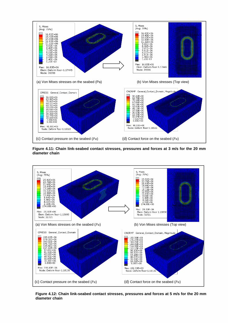
52

(a) Von Mises stresses on the seabed (Pa) (b) Von Mises stresses (Top view)

(c) Contact pressure on the seabed (𝑃𝑎) (d) Contact force on the seabed (𝑃𝑎) (a) Von Mises stresses on the seabed (𝑃𝑎) (b) Von Mises stresses (Top view)

(c) Contact pressure on the seabed (𝑃𝑎) (d) Contact force on the seabed (𝑃𝑎)



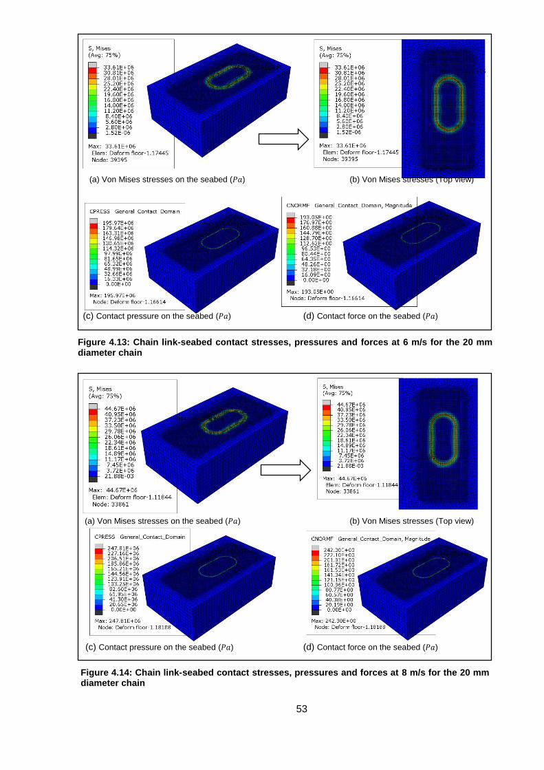
53

(a) Von Mises stresses on the seabed (𝑃𝑎) (b) Von Mises stresses (Top view)

(c) Contact pressure on the seabed (𝑃𝑎) (d) Contact force on the seabed (𝑃𝑎)

(a) Von Mises stresses on the seabed (𝑃𝑎) (b) Von Mises stresses (Top view) (c) Contact pressure on the seabed (𝑃𝑎) (d) Contact force on the seabed (𝑃𝑎)



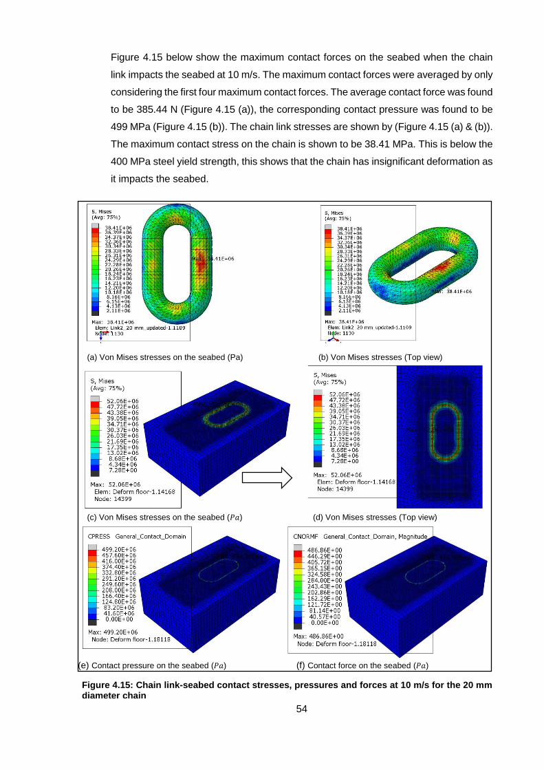
54

Figure 4.15 below show the maximum contact forces on the seabed when the chain

link impacts the seabed at 10 m/s. The maximum contact forces were averaged by only

considering the first four maximum contact forces. The average contact force was found

to be 385.44 N (Figure 4.15 (a)), the corresponding contact pressure was found to be

499 MPa (Figure 4.15 (b)). The chain link stresses are shown by (Figure 4.15 (a) & (b)).

The maximum contact stress on the chain is shown to be 38.41 MPa. This is below the

400 MPa steel yield strength, this shows that the chain has insignificant deformation as

it impacts the seabed.

(a) Von Mises stresses on the seabed (Pa) (b) Von Mises stresses (Top view)

(c) Von Mises stresses on the seabed (𝑃𝑎) (d) Von Mises stresses (Top view) (e) Contact pressure on the seabed (𝑃𝑎) (f) Contact force on the seabed (𝑃𝑎) Figure 4.15: Chain link-seabed contact stresses, pressures and forces at 10 m/s for the 20 mm diameter chain

55


(a) Von Mises stresses, XZ plane (b) Von Mises stresses, ZX plane (c) Von Mises stresses, 3D plane (Top of chain link) (𝑃𝑎) (Bottom of chain link) (d) Von Mises stresses on the seabed (𝑃𝑎) (e) Von Mises stresses (Top view)

(f) Contact pressure on the seabed (𝑃𝑎) (g) Contact force on the seabed (𝑁)

Figure 4.16: Chain link-seabed contact stresses, pressures and forces at 1 m/s for the 16 mm

diameter chain

56

(a) Von Mises stresses on the seabed (𝑃𝑎) (b) Von Mises stresses (Top view) (c) Contact pressure on the seabed (𝑃𝑎) (d) Contact force on the seabed (𝑃𝑎) (a) Von Mises stresses on the seabed (𝑃𝑎) (b) Von Mises stresses (Top view) (c) Contact pressure on the seabed (𝑃𝑎) (d) Contact force on the seabed (𝑃𝑎)



57




58

(a) Von Mises stresses, XZ plane (b) Von Mises stresses, ZX plane (c) Von Mises stresses, 3D plane (Top of chain link) (𝑃𝑎) (Bottom of chain link)

(d) Von Mises stresses on the seabed (𝑃𝑎) (e) Von Mises stresses (Top view) (f) Contact pressure on the seabed (𝑃𝑎) (g) Contact force on the seabed (𝑁)


59


(a) Von Mises stresses, XZ plane (b) Von Mises stresses, ZX plane (c) Von Mises stresses, 3D plane (Top of chain link) (𝑃𝑎) (Bottom of chain link) (d) Von Mises stresses on the seabed (𝑃𝑎) (e) Von Mises stresses (Top view)

(f) Contact pressure on the seabed (𝑃𝑎) (g) Contact force on the seabed (𝑁)


60




61




62

(a) Von Mises stresses on the seabed (𝑃𝑎) (b) Von Mises stresses (Top view) (c) Contact pressure on the seabed (𝑃𝑎) (d) Contact force on the seabed (𝑃𝑎)

4.1.6.4. Summary of velocity versus contact force graphs and equations

The next Figure 4.28, Figure 4.29 and Figure 4.30 show the velocity plot versus the

seabed contact force. As mentioned before, seabed impact velocities of 1, 3, 5, 6, 8

and 10 m/s were analysed by evaluating the 20, 16 and 14 mm diameter chain sizes.

The highest seabed contact pressure were observed to occur when the 20 mm

diameter was used, this result is what is expected as larger diameter chains have more

contact area than smaller chain sizes.

The relationship between the 20 mm chain impact velocity and the seabed contact can

be described by a cubic function, obtained by regression, as in the following equation:

Equation 4.1

𝐹𝐶ℎ𝑎𝑖𝑛 𝑙𝑖𝑛𝑘 = 1.2524𝑣3𝑖𝑚𝑝𝑎𝑐𝑡 + 17.716𝑣

2𝑖𝑚𝑝𝑎𝑐𝑡 + 96.61𝑣 + 67.912 …….20

𝑚𝑚 chain velocity impact equation


63

Figure 4.28: Seabed contact forces by the 20 mm chain

R² = 0.9383

0

50

100

150

200

250

300

350

400

450

0 2 4 6 8 10 12Conta

ct

forc

e (

N)

\pre

ssure

(M

Pa)

Velocity (m/s)

20 mm chain velocity graph

This equation can further be used for predicting seabed contact pressures and forces

for other velocity values of interest when the 20 mm diameter chain is used.

Likewise, Figure 4.29 (16 mm chain link) and Figure 4.30 (14 mm chain link) have the

cubic polynomial regression in the form the following equations:

Equation 4.2

𝐹𝐶ℎ𝑎𝑖𝑛 𝑙𝑖𝑛𝑘 = −0.19𝑣3𝑖𝑚𝑝𝑎𝑐𝑡 + 2.333𝑣

2𝑖𝑚𝑝𝑎𝑐𝑡 + 9.0115𝑣 − 8.7346….16 mm

chain velocity impact equation

Equation 4.3

𝐹𝐶ℎ𝑎𝑖𝑛 𝑙𝑖𝑛𝑘 = 0.4704𝑣3𝑖𝑚𝑝𝑎𝑐𝑡 + 6.8862𝑣

2𝑖𝑚𝑝𝑎𝑐𝑡 + 42.112𝑣 − 23.479…….14 mm

chain velocity impact equation

In Figure 4.28, Equation 4.1 can be used for determining the contact force in

Newton’s and contact pressure in mega Pascal’s. This is also true for Figure

4.29 and Figure 4.30.

64

R² = 0.9918

0

20

40

60

80

100

120

140

160

0 2 4 6 8 10 12

Conta

ct

forc

e (

N)

\pre

ssure

(M

Pa)

Velocity (m/s)


R² = 0.9696

0

20

40

60

80

100

120

140

160

180

200

0 2 4 6 8 10 12Conta

ct

forc

e (

N)

\pre

ssure

(M

Pa)

Velocity (m/s)




The reason we have chosen a cubic polynomial over a linear regression is the apparent

point of inflection observed on some of the curves more clearly than others. The reason

for the point of inflection is a more complex relationship between the velocity and impact

pressure due to the changing surface area in contact as the cylindrical (through the

thickness) chain link penetrates the substrate. The changing shape and corresponding

surface area change results in a more complex change in pressure and frictional force

than a simple linear relationship.

65

19.41

71.42

152.24152.84

191.82

385.44

19.33 53.81

84.95 107.09133.69

141.84

13.0350.40

79.09 80.43

112.58

179.84

0

50

100

150

200

250

300

350

400

450

1 3 5 6 8 10Conta

ct

forc

e (

N)

\pre

ssure

(M

Pa)

Velocity (m/s)

20 mm chain 16 mm chain 14 mm chain

Figure 4.31: Chain link-seabed contact forces (showing the 20, 16 and 14 mm chain links)

The 20 mm chain link produces the greatest seabed impact force, this was followed by

the 16 mm diameter chain link. The 14 mm diameter chain link produced the least

seabed impact force. The contact forces for the three chain sizes are all shown in

Figure 4.31 below.

4.1.7. Studless chain link seabed contact forces comparison with the slender rod

method

Slender rod method is mostly used for simplifying the chain geometry in many offshore

engineering numerical simulation codes (Garrett, 1982). The numerical simulation code

(ANSYS AQWA) used in this work also uses this method. The mooring chain is

represented by a circular section with a constant diameter. This method reduces

computational effort required to solve the complex geometry of chain links.

The equivalent diameter of the rod is obtained by 1.8𝐷, where D is the nominal chain

link diameter. In this case the equivalent diameter of the 20 mm chain is 36 mm

diameter rod.

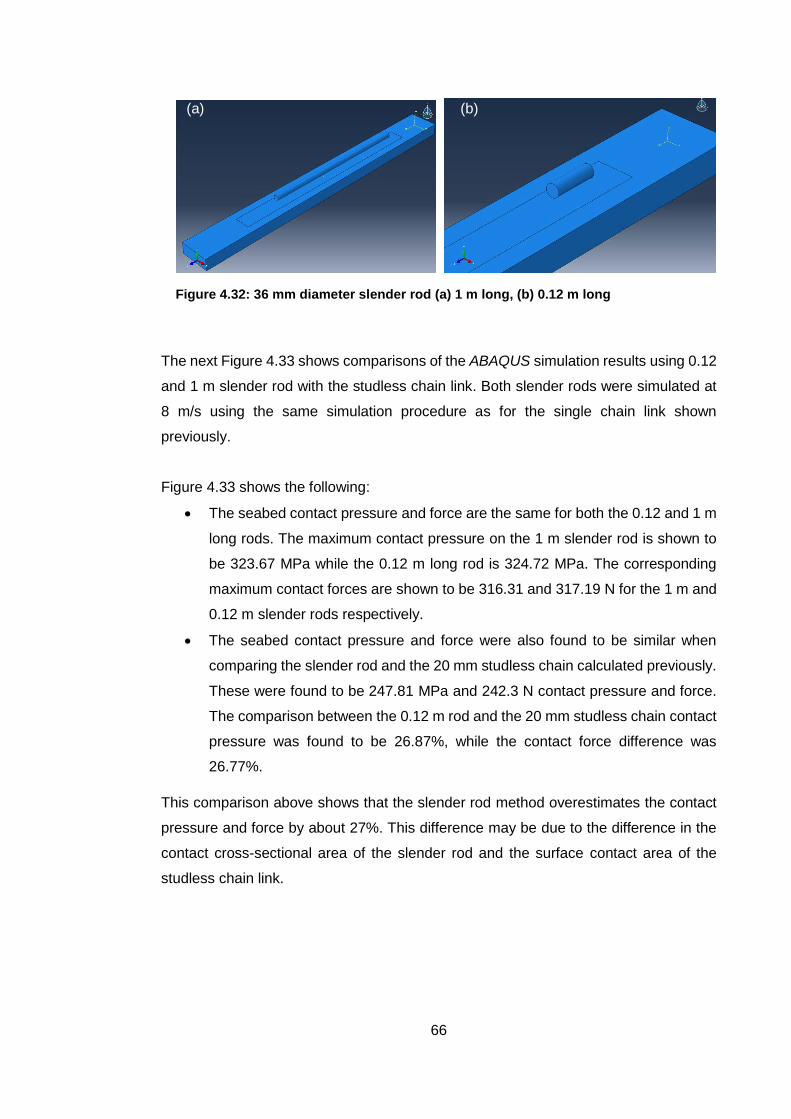
66

Figure 4.32: 36 mm diameter slender rod (a) 1 m long, (b) 0.12 m long

(a) (b)

The next Figure 4.33 shows comparisons of the ABAQUS simulation results using 0.12

and 1 m slender rod with the studless chain link. Both slender rods were simulated at

8 m/s using the same simulation procedure as for the single chain link shown

previously.

Figure 4.33 shows the following:

The seabed contact pressure and force are the same for both the 0.12 and 1 m

long rods. The maximum contact pressure on the 1 m slender rod is shown to

be 323.67 MPa while the 0.12 m long rod is 324.72 MPa. The corresponding

maximum contact forces are shown to be 316.31 and 317.19 N for the 1 m and

0.12 m slender rods respectively.

The seabed contact pressure and force were also found to be similar when

comparing the slender rod and the 20 mm studless chain calculated previously.

These were found to be 247.81 MPa and 242.3 N contact pressure and force.

The comparison between the 0.12 m rod and the 20 mm studless chain contact

pressure was found to be 26.87%, while the contact force difference was

26.77%.

This comparison above shows that the slender rod method overestimates the contact

pressure and force by about 27%. This difference may be due to the difference in the

contact cross-sectional area of the slender rod and the surface contact area of the

studless chain link.

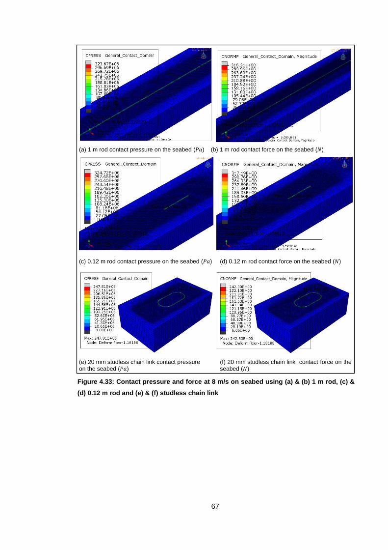
67

(a) 1 m rod contact pressure on the seabed (𝑃𝑎) (b) 1 m rod contact force on the seabed (𝑁)

(c) 0.12 m rod contact pressure on the seabed (𝑃𝑎) (d) 0.12 m rod contact force on the seabed (𝑁)

(e) 20 mm studless chain link contact pressure (f) 20 mm studless chain link contact force on the on the seabed (𝑃𝑎) seabed (𝑁)

Figure 4.33: Contact pressure and force at 8 m/s on seabed using (a) & (b) 1 m rod, (c) &

(d) 0.12 m rod and (e) & (f) studless chain link

68

4.2. ANSYS AQWA model description and setup

This section presents a description of the ANSYS AQWA modelling procedure in detail.

It also presents the model setup with the input data used in this study.

4.2.1. ANSYS AQWA simulation procedure description

The simulation procedure in ANSYS AQWA for the moored vessel can be summarised

by separating the model setup in four stages i.e. 1) Vessel construction, which is

obtained from the constructed CAD model, 2) Input data, which is the pre-processing

stage, 3) Simulation stage where the model input data are solved and 4) Result

Analysis, where the moored vessel response is obtained. These stages are shown

Figure 4.34.

Figure 4.34: ANSYS AQWA Hydrodynamic Simulation Procedure

ANSYS AQWA Workbench interface is shown in Figure 4.35. It shows workflow

defining a system of analysis. The Hydrodynamic Diffraction is the pre-processor stage

where Hydrostatic Results of the vessel are determined. This stage comprises of

defining the mass distribution of the imported CAD geometry and defining the mass

distribution of the vessel. The Hydrodynamic Diffraction static results are then obtained

which include the Centre of Gravity (CoG) Position of the vessel, Centre of Buoyancy

(CoB) Position and Metacentric Heights which are the measurement of the initial static

stability of a floating vessel.

•Solve•Post-process

•Pre-processor

•CAD

-Solidworks geometry

-Meshing

-Loads

-Environment & constraints

-Hydroynamic database

-Motion response

-Images

-Tables

-Graphs

-Animations

69

The Static Response stage analyses the initial equilibrium position of the moored

vessel. It determines the vessel starting position before the simulation is run. Both

Hydrodynamic Diffraction and Static Response results are used as input data for the

Time Domain response stage. The Time Domain Response is the dynamic analysis

stage where sea conditions are applied i.e. ocean waves and currents. The wave can

either be regular or irregular waves. This study selected irregular waves as they best

represent the real world behaviour of ocean waves. The time-history of the vessel

position, velocity, acceleration, structural forces and mooring forces results are

obtained.

Figure 4.36 shows two sets of axes used in ANSYS AQWA. They are the FRA (Fixed

Reference Axes) and the LSA (Local Set of Axes). The FRA is the Global Axis System.

This system has its origin on the mean water surface with Z axis pointing upwards, X

and Y on the mean water surface. The mean water surface is at Z=0. This axis system

does not move at any stage of the ANSYS AQWA analysis.

Figure 4.35: ANSYS AQWA Workbench project schematic

Figure 4.36: Axes Systems

(Adapted from ANSYS Aqwa Theory Manual, 2015)

70

The Local System Axis (LSA) has its origin at the CoG of the vessel, with X, Y and Z

axes parallel to the FRA when the vessel is in its initial definition position. X is along

the length of the vessel shown above, Y along the beam to port, and Z in the direction

of the cross product of X and Y. This axis system moves with the vessel.

The following steps were followed when setting up a model in ANSYS AQWA:

a) Geometry is attached – The CAD models of the both the 22 𝑚 and the 14 𝑚 vessels

were constructed in Solidworks using surfaces; the models were then exported to

ANSYS AQWA. (See Appendix C for 3D models).

b) Surface body definition – This was done in ANSYS AQWA ‘Design modeller’ where the

imported CAD geometry waterline was defined by splitting the geometry into Upper Hull

and Lower Hull. ANSYS AQWA only process surface and line bodies, hence the CAD

model was constructed in Solidworks using surface bodies instead of solid bodies.

Surface bodies are areas that can be meshed to create diffracting (submerged lower

hull) or non-diffracting elements (the exposed part of the vessel). Figure 4.37 shows

Lower Hull of a vessel below the water line.

c) Point mass definition - point mass is the mass inertia matrix that is defined via the

Radius of Gyration of the vessel. It defines the centre of mass of the vessel in 𝑥, 𝑦 and

𝑧 coordinates. The mass distribution of the vessel (mass inertia matrix) is defined

by 𝐾𝑥𝑥 = 0.34 ∗ 𝑤𝑖𝑑𝑡ℎ 𝑜𝑓 𝑡ℎ𝑒 𝑣𝑒𝑠𝑠𝑒𝑙, 𝐾𝑦𝑦 = 0.25 ∗ 𝑙𝑒𝑛𝑔𝑡ℎ 𝑜𝑓 𝑡ℎ𝑒 𝑣𝑒𝑠𝑠𝑒𝑙 and 𝐾𝑧𝑧 = 2.6 ∗

Figure 4.37: Fishing vessel cut at the waterline (vessel Lower Hull in

yellow and Upper Hull in grey).

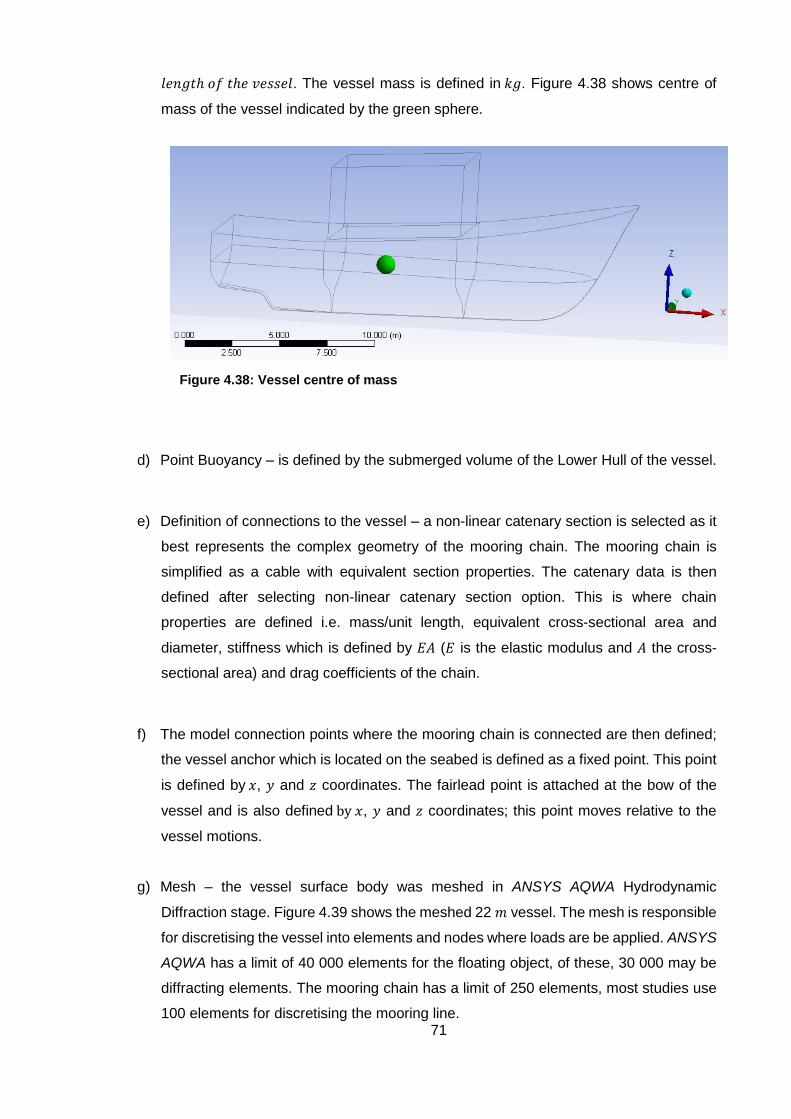
71

𝑙𝑒𝑛𝑔𝑡ℎ 𝑜𝑓 𝑡ℎ𝑒 𝑣𝑒𝑠𝑠𝑒𝑙. The vessel mass is defined in 𝑘𝑔. Figure 4.38 shows centre of

mass of the vessel indicated by the green sphere.

d) Point Buoyancy – is defined by the submerged volume of the Lower Hull of the vessel.

e) Definition of connections to the vessel – a non-linear catenary section is selected as it

best represents the complex geometry of the mooring chain. The mooring chain is

simplified as a cable with equivalent section properties. The catenary data is then

defined after selecting non-linear catenary section option. This is where chain

properties are defined i.e. mass/unit length, equivalent cross-sectional area and

diameter, stiffness which is defined by 𝐸𝐴 (𝐸 is the elastic modulus and 𝐴 the cross-

sectional area) and drag coefficients of the chain.

f) The model connection points where the mooring chain is connected are then defined;

the vessel anchor which is located on the seabed is defined as a fixed point. This point

is defined by 𝑥, 𝑦 and 𝑧 coordinates. The fairlead point is attached at the bow of the

vessel and is also defined by 𝑥, 𝑦 and 𝑧 coordinates; this point moves relative to the

vessel motions.

g) Mesh – the vessel surface body was meshed in ANSYS AQWA Hydrodynamic

Diffraction stage. Figure 4.39 shows the meshed 22 𝑚 vessel. The mesh is responsible

for discretising the vessel into elements and nodes where loads are be applied. ANSYS

AQWA has a limit of 40 000 elements for the floating object, of these, 30 000 may be

diffracting elements. The mooring chain has a limit of 250 elements, most studies use

100 elements for discretising the mooring line.

Figure 4.38: Vessel centre of mass

72

The table below shows the types of elements that are used in ANSYS AQWA and their

description.

Table 4.4: Element types in ANSYS AQWA

QPPL: This element generates pressure and hydrostatic forces only on the hull of the

vessel. Quadrilateral pressure plate of zero thickness.

Element type

Description No of Nodes

Material Property Geometric Property

QPPL Quadrilateral Panel 4 None None

TPPL Triangular Panel 3 None None

PMAS Point Mass 1 Mass Inertia

PBOY Point Buoyancy 1 Displaced mass None

TUBE Tube 2 Density Geometry

STUB Slender Tube 3 Mas and inertia Geometry

FPNT Field Point 1 None None

DISC Circular Disc 2 None Geometry

Figure 4.39: Meshed vessel (22 m vessel)

Figure 4.40: Quadrilateral Panel element (QPPL)

73

TPPL: This element generates pressure and hydrostatic forces only on the hull of the

vessel. Triangular pressure plate of zero thickness.

PMAS: The PMAS element generates mass forces only. Point mess element having

internal mass with the centre of mass coincident with a given node and specified values

of second moments of mass inertia.

PBOY: The PBOY element generates hydrostatic displacement forces only on the hull

of the vessel. This is an external point buoyancy element without mass.

DISC: The DISC element has a drag coefficient and added mass coefficient in its

normal direction. When the mass is defined, it can be assigned geometry. This can

able used to define the mooring line cross-section.

TUBE: Tubular element with uniform circular cross-section and constant wall thickness.

Forces on this element are calculated using Morison’s equation.

Figure 4.41: Triangular Panel element (TPPL)

Figure 4.42: The DISC Element

74

FPNT: The FPNT Element defines the external fluid field point element used to define

the fairlead attachment point. This element gives the pressure head amplitude at a

specified point in the external fluid domain. FPNT elements are defined in the local

axes and move with the structure in which they are defined. The anchor is defined as

a fixed point.

h) Hydrodynamic Diffraction – this stage allows the user to obtain hydrostatic results of

the vessel using wave frequencies and directions. Various parameters can be

evaluated which include Diffraction and Radiation forces on the vessel, structural

damping, Response Amplitude Operators (RAOAs), hull pressure and motions, Centre

of Gravity (CoG) Position globally, Surge, Sway, Heave, Roll, Pitch, and Yaw, the

Centre of Buoyancy (CoB) Position of the vessel, Out of Balance Forces/Weight and

Small Angle Stability Parameters such as Metacentric Heights (GMX/GMY) and

Metacentric Heights (GMX/GMY).

i) Static Response – the static response analysis calculates the equilibrium configuration

of the vessel and forms the basis for the dynamic analysis stage (Time Domain

Response) of the moored vessel.

j) Time Domain Response – the ‘Irregular Wave Response’ setting is selected in order to

apply the Irregular wave type on this stage. The current profile is also defined. The

time-history of the vessel’s position, velocity, acceleration, structural forces and

mooring forces are obtained in this stage. ANSYS AQWA has several predefined wave

models for representing various sea conditions.

Figure 4.43: The TUBE Element

75

Figure 4.44: Single-point moored 22 m vessel

4.2.2. ANSYS AQWA model setup

Figure 4.44 below shows an example of the 22 m vessel single-point mooring system

in ANSYS AQWA environment. The dark blue arrow indicates the wave applied in the

𝑋 −direction, and the purple lines show the current direction and speed. The current is

shown to be defined at the origin. The yellow round object is a clump weight of

negligible mass used as a reference point for tracking the motion of the chain.

Figure 4.44 also shows the coordinate system that will be used to present results. The

𝑋 −direction represents the horizontal displacement (surge), taken as positive

forwards; 𝑌- lateral (sway), positive to the port side, and 𝑍-the vertical displacement

(heave), positive upwards. The displacements of the vessel are calculated from its

centre of gravity. The 22 m vessel geometry was meshed using 29 566 fine elements.

Table 4.5 shows properties of the 22 m vessel ‘Point Mass’ for defining the distribution

of the centre of mass. (The detailed dimensions of the 22 m vessel can be found in

Appendix C). The vessel parameters calculation are show in Appendix F.

Table 4.5: 22 m vessel properties

Parameter Value Units

Vessel dimensions 22 (Length) x 8.7 (width) x 4.45 (depth) 𝑚

𝐾𝑥𝑥 2.72 𝑚

𝐾𝑦𝑦 5.5 𝑚

𝐾𝑧𝑧 5.72 𝑚

Mass 123 000 𝑘𝑔

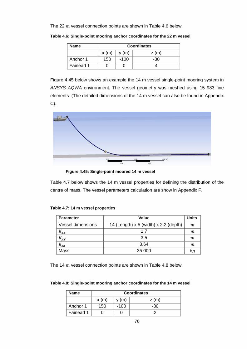
76

The 22 𝑚 vessel connection points are shown in Table 4.6 below.

Table 4.6: Single-point mooring anchor coordinates for the 22 m vessel

Name Coordinates

x (m) y (m) z (m)

Anchor 1 150 -100 -30

Fairlead 1 0 0 4

Figure 4.45 below shows an example the 14 m vessel single-point mooring system in

ANSYS AQWA environment. The vessel geometry was meshed using 15 983 fine

elements. (The detailed dimensions of the 14 m vessel can also be found in Appendix

C).

Table 4.7 below shows the 14 m vessel properties for defining the distribution of the

centre of mass. The vessel parameters calculation are show in Appendix F.

Table 4.7: 14 m vessel properties


Vessel dimensions 14 (Length) x 5 (width) x 2.2 (depth) 𝑚

𝐾𝑥𝑥 1.7 𝑚

𝐾𝑦𝑦 3.5 𝑚

𝐾𝑧𝑧 3.64 𝑚

Mass 35 000 𝑘𝑔

The 14 𝑚 vessel connection points are shown in Table 4.8 below.

Table 4.8: Single-point mooring anchor coordinates for the 14 m vessel

Name Coordinates

x (m) y (m) z (m)

Anchor 1 150 -100 -30

Fairlead 1 0 0 2

Figure 4.45: Single-point moored 14 m vessel

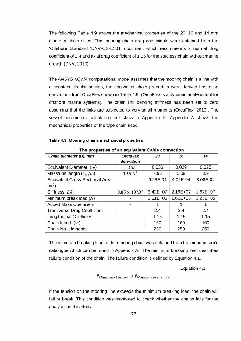
77

The following Table 4.9 shows the mechanical properties of the 20, 16 and 14 mm

diameter chain sizes. The mooring chain drag coefficients were obtained from the

‘Offshore Standard ‘DNV-OS-E301’ document which recommends a normal drag

coefficient of 2.4 and axial drag coefficient of 1.15 for the studless chain without marine

growth (DNV, 2010).

The ANSYS AQWA computational model assumes that the mooring chain is a line with

a constant circular section, the equivalent chain properties were derived based on

derivations from OrcaFlex shown in Table 4.9. (OrcaFlex is a dynamic analysis tool for

offshore marine systems). The chain link bending stiffness has been set to zero

assuming that the links are subjected to very small moments (OrcaFlex, 2010). The

vessel parameters calculation are show in Appendix F. Appendix A shows the

mechanical properties of the type chain used.

Table 4.9: Mooring chains mechanical properties

The minimum breaking load of the mooring chain was obtained from the manufacture’s

catalogue which can be found in Appendix A. The minimum breaking load describes

failure condition of the chain. The failure condition is defined by Equation 4.1.

Equation 4.1

𝐹𝐶ℎ𝑎𝑖𝑛max𝑡𝑒𝑛𝑠𝑖𝑜𝑛 > 𝐹𝑀𝑖𝑛𝑖𝑚𝑢𝑚 𝑏𝑟𝑒𝑎𝑘 𝑙𝑜𝑎𝑑

If the tension on the mooring line exceeds the minimum breaking load, the chain will

fail or break. This condition was monitored to check whether the chains fails for the

analyses in this study.

The properties of an equivalent Cable connection

Chain diameter (D), mm OrcaFlex

derivation

20 16 14

Equivalent Diameter, (𝑚) 1.8𝐷 0.036 0.029 0.025

Mass/unit length (𝑘𝑔/𝑚) 19.9 𝐷2 7.96 5.09 3.9

Equivalent Cross-Sectional Area

(𝑚2)

- 6.28E-04 4.02E-04 3.08E-04

Stiffness, 𝐸𝐴 0.85 × 108𝐷2 3.42E+07 2.19E+07 1.67E+07

Minimum break load (𝑁) - 2.51E+05 1.61E+05 1.23E+05

Added Mass Coefficient - 1 1 1

Transverse Drag Coefficient - 2.4 2.4 2.4

Longitudinal Coefficient - 1.15 1.15 1.15

Chain length (𝑚) 160 160 160

Chain No. elements 250 250 250

78

Table 4.10 below shows the ocean environment conditions selected for all the types of

analysis in this study. The Pierson-Moskowitz Irregular wave spectrum was selected

for modelling ocean waves. This wave type is considered as a developed sea state and

is a good approximation of variable and complex ocean waves. Wave height and period

were varied in some analysis; therefore, they were left out of the table. These will be

specified for each type analysis in this study.

Table 4.10: Ocean environment data


Water Density 1025 𝑘𝑔/𝑚3

Ocean Depth 30 m

Wave Type Pierson-Moskowitz (Irregular wave) -

Direction of spectrum 180 °

Current speed (Uniform) 1 m/s

The simulation duration of 1200 s (20 minutes) and a time step of 0.1 s were used, this

was to ensure the dynamics of the mooring line impacting the seabed is well captured.

(The sea depth was obtained from skippers during site visit).

79

4.3. ANSYS AQWA model simulation results

The section presents the ANSYS AQWA model results. Firstly, the ANSYS AQWA

model velocity is correlated to the measured underwater chain velocity. Secondly, the

effect of varying wave height and period mooring line impact on the seabed is

investigated. Thirdly, three mooring line configurations are studied for investigating

their effect on the seabed. Lastly, three mooring chain sizes are varied for studying

their effect on the seabed. The section also presents comparisons between the effects

of the single-point versus the two-point mooring systems.

4.3.1. ANSYS AQWA model correlation with underwater chain velocity

The ANSYS AQWA model was calibrated by correlating it with the underwater chain

velocity obtained in Chapter 3.4. The calibration was done by varying the wave height

and period while other parameters were kept constant (this effect is fully investigated

in Chapter 4.3.2). Four points along the mooring line which constantly made contact

with the seabed during the simulation were tracked. The video analysis procedure

described in Chapter 3.4 for tracking points in contact was used. This correlation

between the underwater video analysis velocity and ANSYS AQWA model velocity can

also be used for estimating realistic sea conditions.

For this analysis, both the 14 and 22 m vessels were simulated. Figure 4.46 and Figure

4.47 shows the mooring line profiles of both vessels which were anchored using the 20

mm diameter chain. The mooring line motion in the ANSYS AQWA model was

observed to behave similarly to the mooring line motion observed from the underwater

video footage.

The simulated single-point mooring system on the 22 m vessel has been stored on the

following: https://www.youtube.com/watch?v=IYRUDWr3ZT4&t=13s.

The simulated single-point mooring system on the 14 m vessel has been stored on the

following: https://www.youtube.com/watch?v=rpVwcQ7WbSc.

In Figure 4.46, the mooring line profile and tension with a time stamp are shown for 22

m single-point moored vessel for the simulation of 1200 s. The vertical (in 𝑍 direction)

and horizontal (in 𝑋 direction) components of tension are shown. The lateral (in the 𝑌-

direction) tension values has been left out as they were found insignificant. Figure 4.47

also shows the same results on the 14 m vessel.

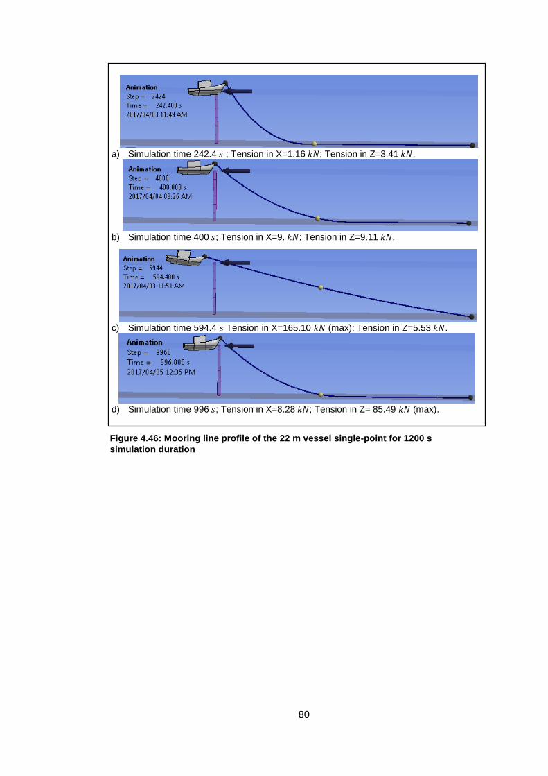
https://www.youtube.com/watch?v=IYRUDWr3ZT4&t=13s

https://www.youtube.com/watch?v=rpVwcQ7WbSc

80

a) Simulation time 242.4 𝑠 ; Tension in X=1.16 𝑘𝑁; Tension in Z=3.41 𝑘𝑁.

b) Simulation time 400 𝑠; Tension in X=9. 𝑘𝑁; Tension in Z=9.11 𝑘𝑁.

c) Simulation time 594.4 𝑠 Tension in X=165.10 𝑘𝑁 (max); Tension in Z=5.53 𝑘𝑁.

d) Simulation time 996 𝑠; Tension in X=8.28 𝑘𝑁; Tension in Z= 85.49 𝑘𝑁 (max).

Figure 4.46: Mooring line profile of the 22 m vessel single-point for 1200 s

simulation duration

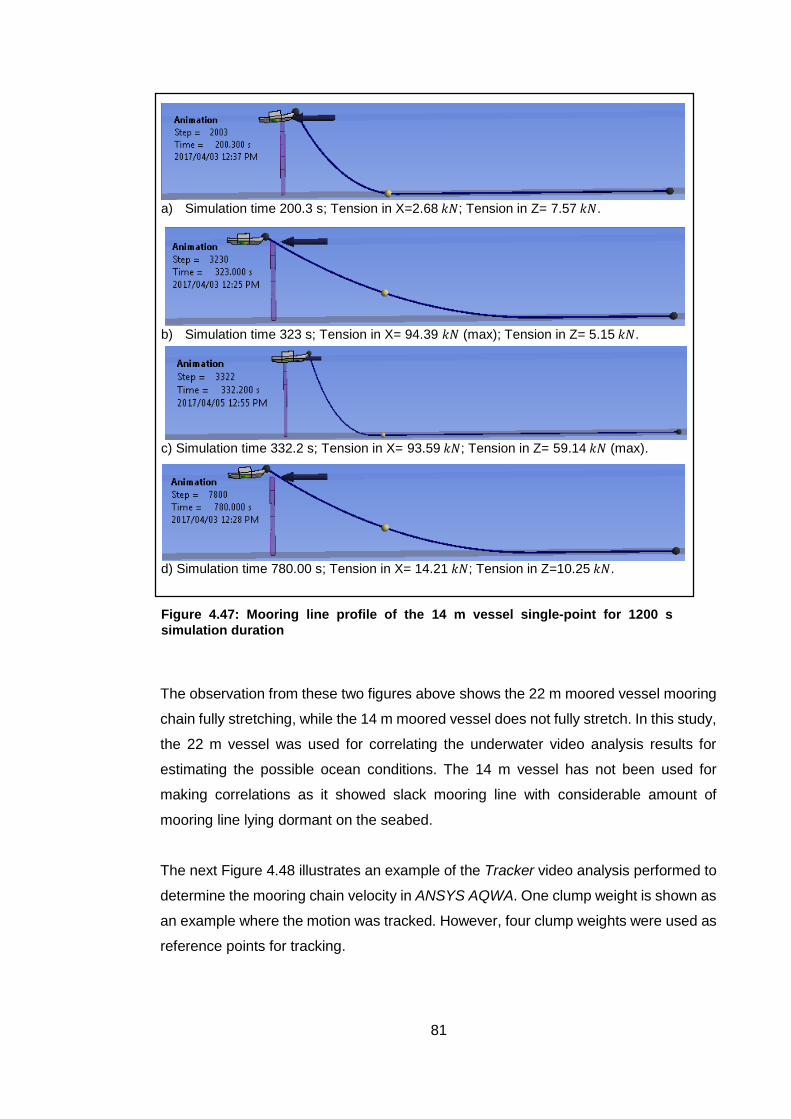
81

a) Simulation time 200.3 s; Tension in X=2.68 𝑘𝑁; Tension in Z= 7.57 𝑘𝑁.

b) Simulation time 323 s; Tension in X= 94.39 𝑘𝑁 (max); Tension in Z= 5.15 𝑘𝑁.

c) Simulation time 332.2 s; Tension in X= 93.59 𝑘𝑁; Tension in Z= 59.14 𝑘𝑁 (max).

d) Simulation time 780.00 s; Tension in X= 14.21 𝑘𝑁; Tension in Z=10.25 𝑘𝑁.

The observation from these two figures above shows the 22 m moored vessel mooring

chain fully stretching, while the 14 m moored vessel does not fully stretch. In this study,

the 22 m vessel was used for correlating the underwater video analysis results for

estimating the possible ocean conditions. The 14 m vessel has not been used for

making correlations as it showed slack mooring line with considerable amount of

mooring line lying dormant on the seabed.

The next Figure 4.48 illustrates an example of the Tracker video analysis performed to

determine the mooring chain velocity in ANSYS AQWA. One clump weight is shown as

an example where the motion was tracked. However, four clump weights were used as

reference points for tracking.

Figure 4.47: Mooring line profile of the 14 m vessel single-point for 1200 s

simulation duration

82

Figure 4.48: ANSYS AQWA video analysis using Tracker

Table 4.11 shows the results of the four points tracked in ANSYS AQWA. These results

showed good correction compared to the underwater video analysis results previously

shown in Figure 3.8. In this study, the contact velocity was obtained by finding the

average between the maximum and minimum velocities for each point. The table shows

the average seabed contact velocity of about 6.4 m/s.

Table 4.11: Wave conditions used for motion correlation

Wave condition 5: Wave height= 2.5 m; Wave period= 7 s

Velocity (m/s)

Velocity points Max Min Mean

Point 1 8.04 4.75 6.40

Point 2 7.93 4.43 6.18

Point 3 7.09 4.32 5.71

Point 4 3.00 2.30 2.65

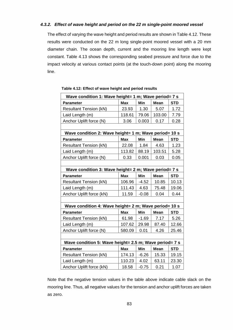
83

4.3.2. Effect of wave height and period on the 22 m single-point moored vessel

The effect of varying the wave height and period results are shown in Table 4.12. These

results were conducted on the 22 m long single-point moored vessel with a 20 mm

diameter chain. The ocean depth, current and the mooring line length were kept

constant. Table 4.13 shows the corresponding seabed pressure and force due to the

impact velocity at various contact points (at the touch-down point) along the mooring

line.

Table 4.12: Effect of wave height and period results

Wave condition 1: Wave height= 1 m; Wave period= 7 s

Parameter Max Min Mean STD

Resultant Tension (kN) 23.93 1.30 5.07 1.72

Laid Length (m) 118.61 79.06 103.00 7.79

Anchor Uplift force (N) 3.06 0.003 0.17 0.28



Resultant Tension (kN) 22.08 1.84 4.63 1.23

Laid Length (m) 113.82 88.19 103.51 5.28




Resultant Tension (kN) 106.96 -4.52 10.85 10.13

Laid Length (m) 111.43 4.63 75.48 19.06

Anchor Uplift force (kN) 11.59 -0.08 0.04 0.44




Laid Length (m) 107.62 29.98 87.40 12.66


Wave condition 5: Wave height= 2.5 m; Wave period= 7 s



Laid Length (m) 110.23 4.02 63.11 23.30

Anchor Uplift force (kN) 18.58 -0.75 0.21 1.07

Note that the negative tension values in the table above indicate cable slack on the

mooring line. Thus, all negative values for the tension and anchor uplift forces are taken

as zero.

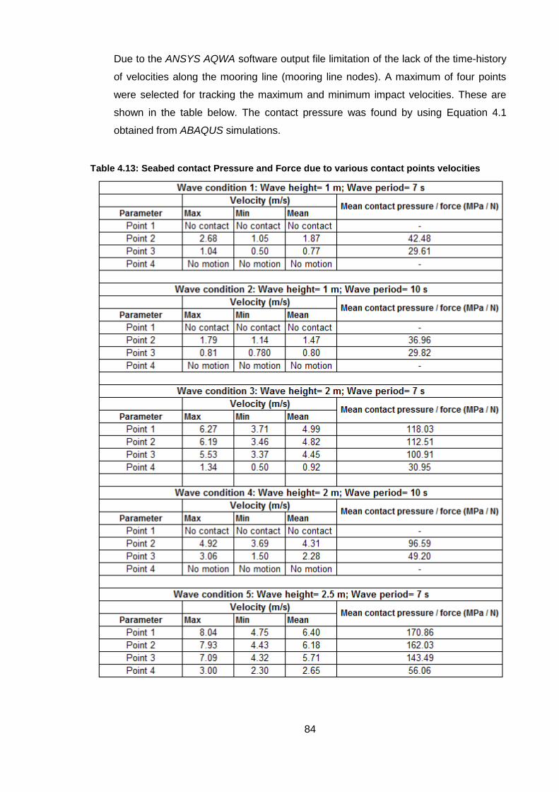
84

Table 4.13: Seabed contact Pressure and Force due to various contact points velocities

Due to the ANSYS AQWA software output file limitation of the lack of the time-history

of velocities along the mooring line (mooring line nodes). A maximum of four points

were selected for tracking the maximum and minimum impact velocities. These are

shown in the table below. The contact pressure was found by using Equation 4.1

obtained from ABAQUS simulations.

85

The outcomes of the comparison in Table 4.12 showed that wave condition 5 had the

highest mooring line length interacting with the seabed with the highest impact

pressure. This mooring line length more frequently lifts up and drops back down on the

seabed than during all the other wave conditions evaluated.

The effect of varying the wave height and period showed that the mooring line profile

is greatly influenced by the decrease in wave period and an increase in wave height.

This consequently increased the interaction of mooring line laid length with the seabed.

The corresponding mooring line impact pressure and force on the seabed also

increased when the have height was increased with a decreased wave period. This

also increased the tension at the fairlead as well as anchor uplift forces.

The increase in wave period from 7 to 10 s resulted in more slack of the mooring line

profile; while the decrease in wave period from 10 to 7 s resulted in both slack and taut

mooring line profiles when the wave height was doubled from 1 to 2 m. The increase

in the slack of the mooring line profile resulted in a portion of the mooring line laid length

on the seabed inactive. Figure 4.49 and Figure 4.50 shows the slack mooring line

profiles with a large portion of the mooring line length lying dormant on the seabed for

wave condition 1 and 2.

The comparison between wave conditions 1 and 2 shows the effect of the wave period

when the wave height is kept constant. Figure 4.49 and Figure 4.50 demonstrates this

effect on the mooring line profile showing both mooring line profiles which are almost

identical. However, wave condition 1 showed slightly higher maximum tension which

was 8.04% more than the tension in wave condition 2. The mooring line laid length on

the seabed of these wave conditions was found to be the least when all five wave

conditions were compared. Wave condition 1 also shows a slight increase of the

mooring line interaction with seabed compared to wave condition 2 (see

Figure 4.55). This outcome shows that short wave periods reduces slack on the mooring

line profile and increases mooring line seabed interaction.

The mooring line impact pressure on the seabed due to wave condition 1 and 2 was

found to be the least in all five wave conditions investigated. This can be seen in Table

4.13 which showed the maximum mooring line impact pressure of 42.48 and 36.96

MPa for wave conditions 1 and 2 respectively.

86

The mooring line length which interacts with the seabed dramatically increased when

the wave height was doubled. This increase of the mooring line interaction with seabed

was observed when comparing wave conditions 3 and 4. The comparison distinctively

showed the effect of the wave period and height as was observed from the comparisons

in wave conditions 1 and 2. Figure 4.51 and Figure 4.52 illustrates the mooring line

profile of the two wave conditions mentioned. As can be seen, the wave period of 10 𝑠

resulted in more slack of the mooring line profile with more mooring line laid length lying

on the seabed; while the wave period of 7 s (in Figure 4.51) shows both slack and taut

mooring line profiles with a large portion of the mooring line interacting with the seabed.

Figure 4.51 also shows tension for each profile at a specific time. The mooring line

touch-down point (TDP) was found to dynamically vary with time as stated in the

literature. The mooring line length interacting with the seabed for wave condition 3 was

found to be in the range of about 4.63 to 111.43 m, with the average length of about

75.48 m and a standard deviation (STD) of about 19.06 m. Wave condition 4, the

mooring line length interacting with seabed was found to be in the range of about 29.98

to 107.62 m, with the average length of about 87.40 m and a standard deviation (STD)

of about 12.66 m. As can be observed, wave condition 4 had the least mooring line laid

length interaction on the seabed when compared to wave condition 3 which showed

more frequent interaction (

Figure 4.55).

The effect of increasing the wave height from 1 to 2 m with the wave period of 10 s

showed an increase in the mooring line impact pressure on the seabed from 36.96 to

96.59 𝑀𝑃𝑎. A decrease of the wave period from 10 to 7 s with the same increase of the

wave height from 1 to 2 m showed an increase in the mooring line impact pressure on

the seabed from 42.48 to 1118.03 MPa.

The slack mooring line profile was also found to be associated with reduced tension at

the Fairlead. This tension was found to be 61.98 kN for wave condition 4 and 106.96

kN for wave condition 3 which showed an increase in tension. The corresponding

anchor uplift forces were found to be directly proportional to the tension at the Fairlead.

These forces were found to be 11.59 kN and 580.09 N for conditions 3 and 4

respectively.

Wave condition 5 (2.5 m wave height and 7 s wave period) showed the most interaction

of the mooring line with the seabed. The mooring line laid length interacting with seabed

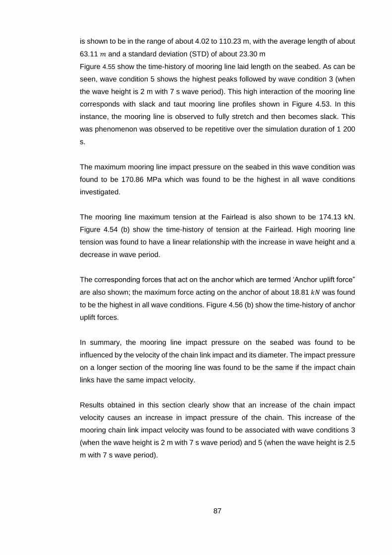
87

is shown to be in the range of about 4.02 to 110.23 m, with the average length of about

63.11 𝑚 and a standard deviation (STD) of about 23.30 m

Figure 4.55 show the time-history of mooring line laid length on the seabed. As can be

seen, wave condition 5 shows the highest peaks followed by wave condition 3 (when

the wave height is 2 m with 7 s wave period). This high interaction of the mooring line

corresponds with slack and taut mooring line profiles shown in Figure 4.53. In this

instance, the mooring line is observed to fully stretch and then becomes slack. This

was phenomenon was observed to be repetitive over the simulation duration of 1 200

s.

The maximum mooring line impact pressure on the seabed in this wave condition was

found to be 170.86 MPa which was found to be the highest in all wave conditions

investigated.

The mooring line maximum tension at the Fairlead is also shown to be 174.13 kN.

Figure 4.54 (b) show the time-history of tension at the Fairlead. High mooring line

tension was found to have a linear relationship with the increase in wave height and a

decrease in wave period.

The corresponding forces that act on the anchor which are termed ‘Anchor uplift force”

are also shown; the maximum force acting on the anchor of about 18.81 𝑘𝑁 was found

to be the highest in all wave conditions. Figure 4.56 (b) show the time-history of anchor

uplift forces.

In summary, the mooring line impact pressure on the seabed was found to be

influenced by the velocity of the chain link impact and its diameter. The impact pressure

on a longer section of the mooring line was found to be the same if the impact chain

links have the same impact velocity.

Results obtained in this section clearly show that an increase of the chain impact

velocity causes an increase in impact pressure of the chain. This increase of the

mooring chain link impact velocity was found to be associated with wave conditions 3

(when the wave height is 2 m with 7 s wave period) and 5 (when the wave height is 2.5

m with 7 s wave period).

88

(a) Initial mooring line profile, Initial Cable Tension at start = 5.51 𝑘𝑁

(b) Simulation time = 0 𝑠; Resultant Tension 0=𝑁

(c) Simulation time = 251.40 𝑠; Resultant Tension = 26.93 𝑘𝑁 (max)

(d) Simulation time = 471.4 𝑠; Resultant Tension = 7.05 𝑘𝑁

(e) Simulation time = 116.9 𝑠; Resultant Tension = 8.07 𝑘𝑁

Figure 4.49: Mooring chain profile for 1 m and 7 s wave height and period

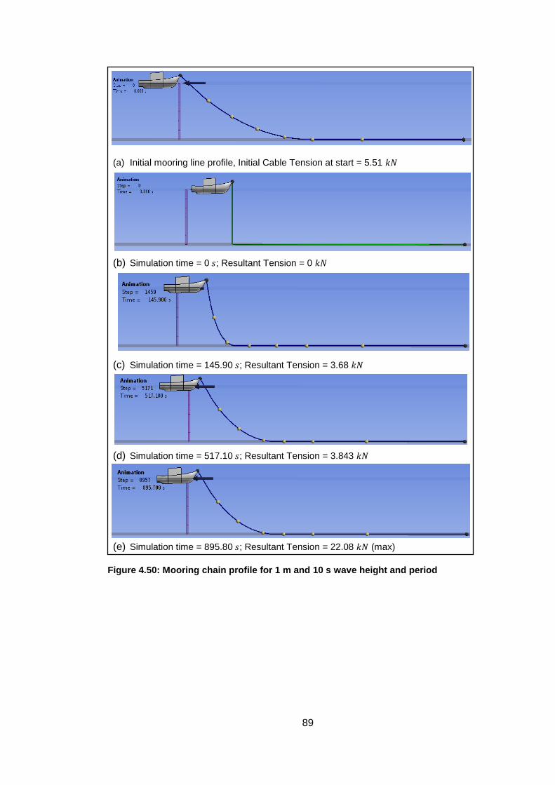
89

(a) Initial mooring line profile, Initial Cable Tension at start = 5.51 𝑘𝑁

(b) Simulation time = 0 𝑠; Resultant Tension = 0 𝑘𝑁

(c) Simulation time = 145.90 𝑠; Resultant Tension = 3.68 𝑘𝑁


(e) Simulation time = 895.80 𝑠; Resultant Tension = 22.08 𝑘𝑁 (max)


90

(a) Simulation time = 107 𝑠; Resultant Tension = 16.53 𝑘𝑁

(b) Simulation time = 259.2 𝑠; Resultant Tension = -91.82 𝑘𝑁



(e) Simulation time = 960 𝑠; Resultant Tension = 20.73 𝑘𝑁


91

(a) Simulation time = 186.5 𝑠; Resultant Tension = 7.35 𝑘𝑁

(b) Simulation time = 510.50 𝑠; Resultant Tension = 7.69 𝑘𝑁




92

(a) Simulation time = 242.1 𝑠; Resultant Tension = 5.64 𝑘𝑁

(b) Simulation time = 400 𝑠; Resultant Tension = 12.78 𝑘𝑁


(d) Simulation time 875.7𝑠; Resultant Tension = 21.44 𝑘𝑁

(e) Simulation time 1107.80 𝑠; Resultant Tension = 46.89 𝑘𝑁

Figure 4.53: Mooring chain profile for 2.5 m and 7 s wave height and period

93

(a) Wave conditions at 1 m wave height when varying 7 and 10 s periods

(b) Wave conditions at 2.5 m wave height when varying 7 and 10 s periods

Figure 4.54: The effect of wave conditions on tension

94

Figure 4.55: The effect of wave conditions on chain laid length

(a) Wave conditions at 1 m wave height when varying 7 and 10 s periods

(b) Wave conditions at 2.5 m wave height when varying 7 and 10 s periods

Figure 4.56: The effect of wave conditions on anchor uplift forces

95

Figure 4.58: Configuration 2 - Single-point mooring system with anchor at an angle with

incoming waves and current, (a) top view & (b) isometric view

4.3.3. Mooring system results using three configurations

The simulation results parameters that are of interest in this study are the vessel

displacements, the mooring chain tension, the mooring chain length laid on the seabed,

the anchor uplift forces and the seabed impact pressure and force. All these parameters

varied with time and were evaluated for 1200 s. The following three anchor

configurations were used in this study on both the 14 and 22 m vessels:

Configuration 1: Single-point mooring system with the anchor position in-line with the

vessel and the incoming waves (shown in Figure 4.57). Table 4.6 & Table 4.8 has

already provided anchor coordinates for the 22 and 14 m configurations.

Configuration 2: Single-point mooring system with the anchor position at an angle with

the vessel and incoming wave is shown in Figure 4.58.

(a) (b)

Figure 4.57: Configuration 1 - Single-point mooring system with anchor in line with waves and current (top view)

Incoming waves &

current direction

Incoming waves &

current direction

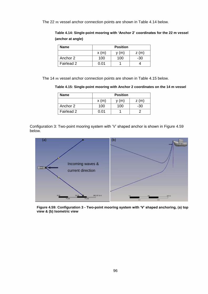
96

The 22 𝑚 vessel anchor connection points are shown in Table 4.14 below.

Table 4.14: Single-point mooring with ‘Anchor 2’ coordinates for the 22 m vessel

(anchor at angle)

The 14 𝑚 vessel anchor connection points are shown in Table 4.15 below.

Table 4.15: Single-point mooring with Anchor 2 coordinates on the 14 m vessel

Configuration 3: Two-point mooring system with ‘V’ shaped anchor is shown in Figure 4.59 below. (a) (b)

Name Position

x (m) y (m) z (m)

Anchor 2 100 100 -30

Fairlead 2 0.01 1 4

Name Position

x (m) y (m) z (m)

Anchor 2 100 100 -30

Fairlead 2 0.01 1 2

Incoming waves &

current direction

Figure 4.59: Configuration 3 - Two-point mooring system with ‘V’ shaped anchoring, (a) top view & (b) Isometric view

97

The 22 𝑚 vessel connection points with two anchors are shown in Table 4.16 below.

Table 4.16: Two-point mooring anchor coordinates on the 22 m vessel

The 14 𝑚 vessel connection points with two anchors are shown in Table 4.17 below.

Table 4.17: Two-point mooring anchor coordinates on the 14 m vessel

Name Position

x (𝑚) y (𝑚) z (𝑚)

Anchor 1 100 -100 -30

Anchor 2 100 100 -30

Fairlead 1 0.01 -1 2

Fairlead 2 0.01 1 2

The above three configurations were simulated with the wave height of 2.5 m and wave

period of 7 s.

The ANSYS AQWA model included sensitivity analysis for determining the best number

of mooring line elements for discretisation. Since the program only allows 250

maximum elements, most studies use 100 elements to discretise the mooring line. The

difference between using 100 and 250 elements was found to be 1.39%. This difference

was found by comparing the mooring line maximum tension when using 100 and 250

elements.

The maximum horizontal tension of 167.4 kN was obtained when 100 elements were

used, while the maximum horizontal tension force of 165.1 𝑘𝑁 was obtained when 250

elements were used. This study used 250 elements for discretising the mooring line.

When the three configurations are solved numerically in ANSYS AQWA, the motion

response for the 14 and 22 m vessels is obtained. The initial hydrostatic results showed

Name Position

x (m) y (m) z (m)

Anchor 1 100 -100 -30

Anchor 2 100 100 -30

Fairlead 1 0.01 -1 4

Fairlead 2 0.01 1 4

98

the 22 m vessel center of gravity of -13.24 m, while the 14 m vessel center of gravity

was -8.61 m. The full hydrostatic results which include Hydrostatic Stiffness, the center

of buoyancy and stability parameters can be found in Appendix D.

The next Figure 4.60 shows the horizontal displacements of both vessels using the

three mooring line configurations mentioned above. The displacements are calculated

at the CoG of the vessel.

When Figure 4.60 (a) & (c) are compared, the 14 m vessel in particular is shown to

have less horizontal displacements than the 22 m vessel. Since both vessels were

simulated under the same ocean conditions, this shows the effect of the mooring line

on large and small vessels. In this case, the mooring line induces high motion damping

on the 14 m vessel by counteracting the vessel motions due to the action of the wave

and current loads. However, when the wave direction changes (Configuration 2 -

anchor at an angle to the incoming wave) shown in Figure 4.60 (b), the 14 m vessel is

observed to have higher horizontal displacements than the 22 m vessel.

Since the mooring chain (line) has its highest stiffness (resistance) in the longitudinal

direction, this stiffness is low in its lateral direction (𝑌-direction). In this instance, in

Configuration 2, the 14 m vessel experienced high horizontal displacements because

of the low mooring line stiffness. The outcome from comparing results from Figure 4.60

(a) & (b) is that that the 20 mm mooring chain stiffness is low when the wave angle

changes and becomes high when the wave angle and the anchor are in the same

alignment. The 14 m vessel experienced low mooring chain stiffness in Configuration

2 and high mooring chain stiffness in Configuration 1. This shows that high mooring

chain stiffness results in less vessel displacements which agree with literature.

When Figure 4.60 (a) horizontal displacements are closely observed – Configuration 1,

this configuration shows the single-point mooring system on the 14 and 22 m vessels

with the least horizontal displacements amongst the three mooring line configurations

analysed. This is due to high mooring chain horizontal stiffness caused by the alignment

of the anchor and vessel to the incoming waves. The 22 m vessel is shown to have

slightly higher horizontal displacements than the 14 m vessel. The 22 m vessel was

displaced within the distance range of between -7.18 and +7.27 m with the STD

(Standard Deviation) of approximately 7.37, while the 14 m vessel was displaced within

the distance range of between –10.01 and 4.418 m with the STD of 2.88.

99

Additionally, the 22 m vessel was observed to have a significant portion of the mooring

line lifting off and dropping back down on the seabed compared to the 14 m vessel (in

Configuration 1). The 14 m vessel was observed to have a significant amount mooring

chain lying dormant on the seabed; only a small portion was observed to be lifting off

and dropping on the seabed. Note that the displacement range is taken from the

simulation time of 20 – 1200 s when the vessel’s initial starting position was established.

A closer look at Figure 4.60 (b) shows the single-point 14 m moored vessel in

Configuration 2 with the highest horizontal displacements in all three configurations;

this was followed by the 22 m vessel with high horizontal displacements on the same

configuration. The 22 m vessel was displaced within the distance range of between –

0.21 and +56.94 m with the STD of 7.37; while the 14 m vessel was displaced within

the distance range of between –6.57 and +54.44 m with the STD of 12.26. The

difference on the horizontal motion between the two vessels is shown by the great STD

of approximately 12.16 m on the 14 m vessel. Note that this range is taken from the

simulation time of 30 – 1200 s when the vessel’s initial starting position was established.

Figure 4.60 (c) shows the horizontal displacements of the two-point moored 14 and 22

m vessels using Configuration 3. In this configuration, the horizontal displacements of

both vessels were observed to be the second highest when the three configurations

are compared. The 22 m vessel in particular, had higher horizontal displacements than

the 14 m vessel. The 22 m vessel was displaced within the distance range of between

– 8.16 and 18.16 m with Standard Deviation two times greater than the 14 m vessel’s

Standard Deviation; while the 14 m vessel was displaced within the distance range of

between – 5.08 and 16.57 m with the STD of 3.02. Note that this range is taken from

the simulation time of 25 – 1200 s when the vessel’s initial starting position was

established.

The outcome from analysing the horizontal motion of the three configurations,

demonstrates that the anchor deployed at an angle to the incoming waves and the

vessel will result in high horizontal displacements of the vessel, especially smaller

vessels. This also implies that when the wave direction changes, the horizontal

excursions of the vessel increase accordingly. The result in the high horizontal

displacement of the both vessels is caused by low mooring chain stiffness due to the

wave approaching at an angle. This is because chain mooring lines have their highest

stiffness on their longitudinal axis.

100

The 14 m vessel showed to have less displacement because of the presence of the 20

mm mooring line when the two anchors were used. In practice, smaller vessels mostly

use smaller chain sizes of 14 and 16 mm. This shows that when the two-mooring

system is used, smaller vessels (14 m vessel for example) will result in less

displacements when the 20 mm chain is used than large vessels (22 m vessel for

example). This also shows that heavier weight chain imposes high motion resistance

to the moored vessel, especially smaller vessels.

It is evident from the three mooring line configurations that the 14 m vessel has the

least amount of mooring chain lifting off and dropping back down on the seabed. This

suggests that the seabed footprint is high when larger vessels are used since they

imposed high dynamic forces on the mooring chain. The comparisons in Figure 4.60

show that the two-point mooring system has better vessel motion restriction when the

wave angle changes. This also suggests that if the wave direction slightly changes

during fishing, the two-point moored vessels will have less vessel displacement than

single-point moored vessels. However, the two-mooring system potentially increases

the mooring line footprint of the seabed.

101

Figure 4.60: Horizontal displacements (X-direction) of the vessels in three

configurations

The next Figure 4.61 shows lateral displacements (𝑌-direction) of the three mooring

line configurations. Figure 4.61 (a) shows the single-point mooring system

102

(Configuration 1) with the least lateral displacements when compared to Configuration

1 and 2, the 14 m vessel, in this case, is shown to have slightly higher lateral

displacements than the 22 m vessel. The 22 m vessel was displaced within the distance

range of between -0.12 and 0.12 m with the STD of 0.04; while the 14 m vessel was

displaced within the distance range of between -1.66 and 0.76 m with the STD of 0.46.

Both vessels are shown to have very small lateral displacements which also indicated

by their small Standard Deviation from their mean lateral displacement values.

Configuration 2 in Figure 4.61 (b), shows the highest lateral displacements of the 14

and 22 m vessels with the anchor at an angle to the incoming waves and the vessel.

The 22 m vessel was displaced within the distance range of between 54.42 and 141.11

m with the STD of 15.54; while the 14 m vessel was displaced within the distance range

of between 20.74 and 164.35 m with the STD of 26.62. This configuration was observed

to have had a significant amount of the mooring chain sweeping on the seabed.

The 14 m vessel, in particular, showed high lateral displacements at the beginning.

After about 450 s of the simulation time, both vessels are shown to have similar lateral

displacements. This outcome is consistent with the observation made previously when

the ‘Anchor 2’ coordinates were used (anchor at an angle), where the horizontal

displacements of the single-point 14 m moored vessel were found to be the highest.

Lastly, Figure 4.61 (c), Configuration 3 - shows the lateral displacement of the two-point

14 and 22 m moored vessels. Higher lateral displacements on the 22 m vessel were

observed than on the 14 m vessel which was similar to the observation illustrated in

Figure 4.60 (c) previously. The 22 m vessel was displaced within the distance range of

between -24.21 and 15.56 m with the STD of 9.23; while the 14 m vessel was displaced

within the distance range of between -11.43 and 10.83 m with the STD of 2.95.

103

Figure 4.61: Lateral displacements (Y-direction) of the vessels in three configurations

Figure 4.62 shows the single-point moored vessels vertical displacements (𝑍-direction)

of the three configurations. Figure 4.62 (a), Configuration 1, shows the 22 m vessel

vertical displacements between the range of -0.46 and 2.36 m with the STD of 0.45;

while the 14 m vessel was displaced within the distance range of between -0.41and

104

1.64 m with the STD of 0.35. As can be seen, the 22 m vessel has higher vertical

displacements than the 14 m vessel in all three configurations.

Figure 4.62 (b), Configuration 2, shows the 22 m vessel vertical displacements between

the range of -0.41 and 2.14 m with the STD of 0.45; while the 14 m vessel was displaced

within the distance range of between -0.36 and 1.80 m with the STD of 0.35. The 22 m

vessel displacements, in this case, showed little variation when compared to the two

configurations. This observation was also similar on the 14 m vessel vertical

displacements.

Figure 4.62 (c), Configuration 3, the vertical displacements of the two-point 14 and 22

m moored vessels. The 22 m vessel vertical displacements are shown to be between

the range of -0.34 and 2.39 m with the STD of 0.45; while the 14 m vessel was displaced

within the distance range of between -0.38 and 1.74 m with the STD of 0.34.

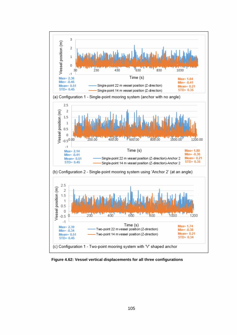
105

Figure 4.62: Vessel vertical displacements for all three configurations

106

0

200

400

600

800

1000

1200

0-5

10

-15

20

-25

30

-35

40

-45

50

-55

60

-65

70

-75

80

-85

90

-95

10

0-1

05

11

0-1

15

Single-point 22 m vessel Laid Length range (m)

0

500

1000

1500

2000

0-5

5-1

0

15

-20

25

-30

35

-40

45

-50

55

-60

65

-70

75

-80

85

-90

95

-10

0

10

5-1

10

11

5-1

20

Single-point 14 m vessel Laid Length range (m)

Figure 4.65 shows the time-variation of mooring line laid length on the seabed for the

three configurations. Figure 4.65 (a), Configuration 1, shows a comparison between

the 22 and 14 m vessels laid length from 100 to 1200 s of the simulation time. The 22

𝑚 vessel mooring line is shown to have the most frequent contact on the seabed than

the 14 m vessel. This comparison is further shown in Figure 4.63 (a) & (b) below using

frequency distribution plot of the mooring line laid length for both vessels. This figure

shows the most even distribution of the mooring chain on the 22 m vessel and was

observed to have a substantial amount of the mooring chain lifting and dropping back

on the seabed.

The 14 m vessel is shown to have an uneven distribution which implies that a large

portion of the mooring chain is lying dormant on the seabed as also was observed from

the simulation. The frequency distribution of the laid chain on the seabed overtime was

stored in bins of 5 m intervals between the minimum and maximum laid length on the

seabed. The 22 m vessel is shown to have about 75-80 meters frequently interacting

with the seabed.

(a) (b)

Figure 4.65 (b), Configuration 2, shows the comparison between the 22 and 14 m

vessels laid length with a single-point mooring with the anchor at an angle. The

frequency distribution plot of the mooring line laid length is shown in the next Figure

4.64. This figure also shows an even distribution of the mooring chain laid on the

seabed on the 22 m vessel. The 14 m vessel, similar to the previous observation (Figure

4.65 (a)), was seen to have an uneven distribution which indicated that a large portion

of the mooring line is lying dormant on the seabed.

Figure 4.63: Frequency distribution of the mooring chain laid length on the seabed for Configuration 1

107

0

200

400

600

800

1000

1200

1400

10

-15

20

-25

30

-35

40

-45

50

-55

60

-65

70

-75

80

-85

90

-95

10

0-1

05

11

0-1

15

Single-point 22 m vessel Laid Length range (m)-Anchor 2

0

500

1000

1500

2000

Laid length on Single-Point 14 mvessel -Anchor 2

(a) (b)

Figure 4.65 (c) & (d), Configuration 3, shows the laid length of the two-point moored 22

and 14 m vessels respectively; Cable 1 and Cable 2 are shown. The figure shows again

that the 22 m vessel has more seabed footprint than the 14 m vessel (Both vessels

using two-point mooring system). The amount of the laid length on the seabed of the

two-point mooring system is shown to have a slight difference when compared to the

other two configurations when considering the 22 m vessel only.

Figure 4.64: Frequency distribution of the mooring chain laid length on the seabed for Configuration 2

108

Figure 4.65: Mooring chain laid length for all 3 configurations

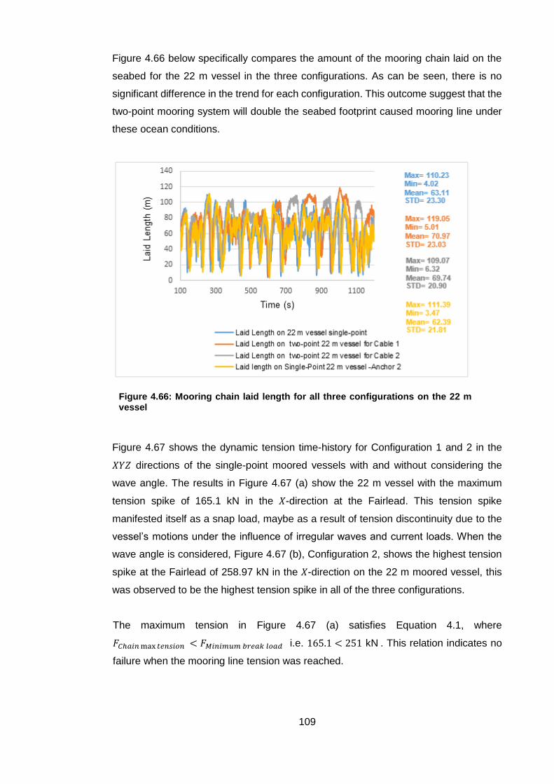
109

Figure 4.66: Mooring chain laid length for all three configurations on the 22 m vessel

Figure 4.66 below specifically compares the amount of the mooring chain laid on the

seabed for the 22 m vessel in the three configurations. As can be seen, there is no

significant difference in the trend for each configuration. This outcome suggest that the

two-point mooring system will double the seabed footprint caused mooring line under

these ocean conditions.

Figure 4.67 shows the dynamic tension time-history for Configuration 1 and 2 in the

𝑋𝑌𝑍 directions of the single-point moored vessels with and without considering the

wave angle. The results in Figure 4.67 (a) show the 22 m vessel with the maximum

tension spike of 165.1 kN in the 𝑋-direction at the Fairlead. This tension spike

manifested itself as a snap load, maybe as a result of tension discontinuity due to the

vessel’s motions under the influence of irregular waves and current loads. When the

wave angle is considered, Figure 4.67 (b), Configuration 2, shows the highest tension

spike at the Fairlead of 258.97 kN in the 𝑋-direction on the 22 m moored vessel, this

was observed to be the highest tension spike in all of the three configurations.

The maximum tension in Figure 4.67 (a) satisfies Equation 4.1, where

𝐹𝐶ℎ𝑎𝑖𝑛max 𝑡𝑒𝑛𝑠𝑖𝑜𝑛 < 𝐹𝑀𝑖𝑛𝑖𝑚𝑢𝑚 𝑏𝑟𝑒𝑎𝑘 𝑙𝑜𝑎𝑑 i.e. 165.1 < 251 kN . This relation indicates no

failure when the mooring line tension was reached.

110

The maximum tension in Figure 4.67(b) does not satisfy Equation 4.1, where

𝐹𝐶ℎ𝑎𝑖𝑛max 𝑡𝑒𝑛𝑠𝑖𝑜𝑛 > 𝐹𝑀𝑖𝑛𝑖𝑚𝑢𝑚 𝑏𝑟𝑒𝑎𝑘 𝑙𝑜𝑎𝑑 i.e. 258.97 > 251 kN. This relation shows that

the mooring line will fail when it reaches its maximum tension. However, in practice,

the anchor chain will not fail but will instead drag on the seabed. This is because

ANSYS AQWA assumes the anchor to be a fixed point whereas, in practice, the squid

fishing industry uses anchors that are always retrieved from the seabed (drag

embedded anchor). During anchor deployment, drag embedded anchors eventually

lock into the seabed sand after dragging on the seabed; anchors locked to the seabed

can be unlocked when the forces exerted upon them are greater than their holding

capacity.

The maximum tension at the vessel’s fairlead point was observed to be taking place

when the vessel moves away from the anchor position due to the action of wave and

current loads. It can be seen from Figure 4.67 that the maximum tension spike in

Configuration 2 took place once-off and has a high discrepancy with other tension plots

of below 100 kN. While on Configuration 1, the 22 m vessel showed low tension plot

discrepancy between the maximum tension and other tension plots. Another

observation is that both configurations showed a similar mean tension force of

approximately 11 kN. Both graphs show tension fluctuation which represents loss and

tension recovery as the vessel moves away and towards the anchor.

When the mooring chain reaches its maximum tension, it is also important to consider

the forces exerted on the anchor, these forces are termed - anchor uplift forces. Figure

4.69 shows that in Configuration 1, when the mooring line on the 22 m vessel reaches

its maximum tension, the anchor experiences the maximum uplift force of 18.58 kN;

while in Configuration 2, Anchor 2 experiences the maximum uplift force of 36.65 kN.

Since Klusman anchor type of between 100−250 kg is mostly used in the squid fishing

industry, the weight that anchor exerts on the seabed is 2.5 kN.

This implies that anchor uplift force on Configuration 1 is 7 times greater than the

anchor weight (with the assumption that the anchor is not embedded into the seabed);

while in Configuration 2, the anchor uplift force is 14 times greater than the anchor

weight. This finding suggests a high possibility of the anchor drag on the seabed in

these wave conditions when the maximum tension is reached and potentially causes

seabed anchor scour.

111

The 14 m vessel is shown to have low anchor uplift forces in the three configurations;

the maximum anchor uplift of 6 kN is found in Configuration 2. This shows that a change

in the wave direction influences the entire mooring chain causing it to sweep across

the seabed and ultimately to drag the anchor.

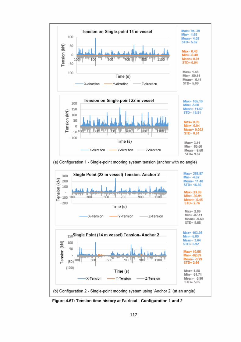
112

Figure 4.67: Tension time-history at Fairlead - Configuration 1 and 2

113

Figure 4.68, Configuration 3, shows the tension time-history in the 𝑋𝑌𝑍 directions of

the two-point moored 14 and 22 m vessels. The 22 m vessel in particular, in this

configuration, is shown to be experiencing high tension forces at the Fairlead,

especially in the 𝑋-direction. The mooring chain maximum tension is shown to be

122.91 kN on the 22 m vessel which is experienced by Cable 1. Cable 2 is shown to

have a maximum tension in the 𝑌-direction (lateral direction) of 83.76 kN. This shows

that the two anchor chains are experiencing different tension forces, especially Cable

1. When Cable 1 reaches its maximum tension, the Cable 2 was observed to be slack.

Cable 2 tension clearly shows that this anchor chain is sweeping across the seafloor.

This was also observed in Figure 4.61 (c) where the vessel 𝑌-direction maximum

displacement was 15.56 m.

When the tension forces for 14 and 22 m vessels are compared, the 22 m vessel

experiences high tension forces. This is due to high mooring chain stiffness which

increases because of large forces generated by the 22 m vessel. A notable observation

on these two vessels in the graph is that both show Cable 2 to have high lateral tension

than the horizontal and vertical components, these are shown to be 44.19 kN and

83.76 kN on the 14 and 22 m vessels respectively. Cable 1 is shown to have high

tension forces in the 𝑋-direction on both vessels of 32.18 kN and 122.91 kN respectively

on the 14 and 22 m vessels. This confirms that the two-point mooring system causes

better vessel motion restriction on both 𝑋 and 𝑌 directions. However, this doubles

seabed footprint caused by the two mooring chains as discussed before.

114

Figure 4.68: Tension time-history of the two-point mooring system – Configuration 3

115

(i) 22 𝑚 vessel, Max= 18.58 𝑘𝑁 (ii) 14 𝑚 vessel, Max= 1.19 𝑘𝑁

(a) Configuration 1 - Single-point mooring anchor uplift force (anchor with no angle)

(i) 22 𝑚, Max= 36.65 𝑘𝑁 (ii) 14 𝑚, Max= 1.42 𝑘𝑁

(b) Configuration 2 - Single-point mooring system using ‘Anchor 2’ (at an angle)

(i) 22 𝑚 vessel, Cable 1, Max= 16.98 𝑘𝑁 (ii) 22 𝑚 vessel, Cable 2, Max= 6.09 𝑘𝑁

(iii) 14 m vessel, Cable 1, Max= 0.14 𝑘𝑁 (iv) 14 𝑚 vessel, Cable 2, Max= 0.34 𝑘𝑁

(c) Configuration 3 - Laid length of the 22 & 14 𝑚 vessel two-point ‘V’ shaped anchor

Figure 4.69: Anchor uplift forces for the all three Configurations

116

4.4. Summary of results: ANSYS AQWA and ABAQUS models

This section presents a summary of the result outcomes from the ANSYS AQWA and

ABAQUS models using a single graphic. The graphic contains the ANSYS AQWA

model result output parameters which are the resultant tension at the fairlead, the

mooring chain laid length on the seabed and the anchor uplift forces. The ABAQUS

model result output parameter presented is the chain link impact force on the seabed

at different velocities.

In this analysis, the effect of chain diameters of 14, 16 and 20 mm is investigated; the

wave height of 2.5 m and wave period of 7 s were used.

The purpose of this overview is to give a concise summary of the effect of the single-

point moored vessel versus the two-point moored vessel when the 14 and 22 m vessel

sizes are investigated by varying chain diameters of 14, 16 and 20 mm. The outcome

from this analysis gives a brief comparison of the mooring system which causes the

most footprint on the seabed.

The first graphic in Section 4.4.1 presents combined result outputs of the ANSYS

AQWA and ABAQUS models on the 22 m single-point moored vessel. The second

graphic presents the same outputs when the 14 m vessel is analysed. The last four

graphics in Section 4.4.2 presents the aforementioned results when the two-point

moored vessel are investigated.

The comparison between the single-point and two-point moored 14 and 22 m vessels

using the 14, 16 and 20 mm diameter chain sizes in Section 4.4.1 and Section 4.4.2 is

summarised by the following Table 4.18 and Table 4.19. These tables show maximum

values of each parameter of the investigation.

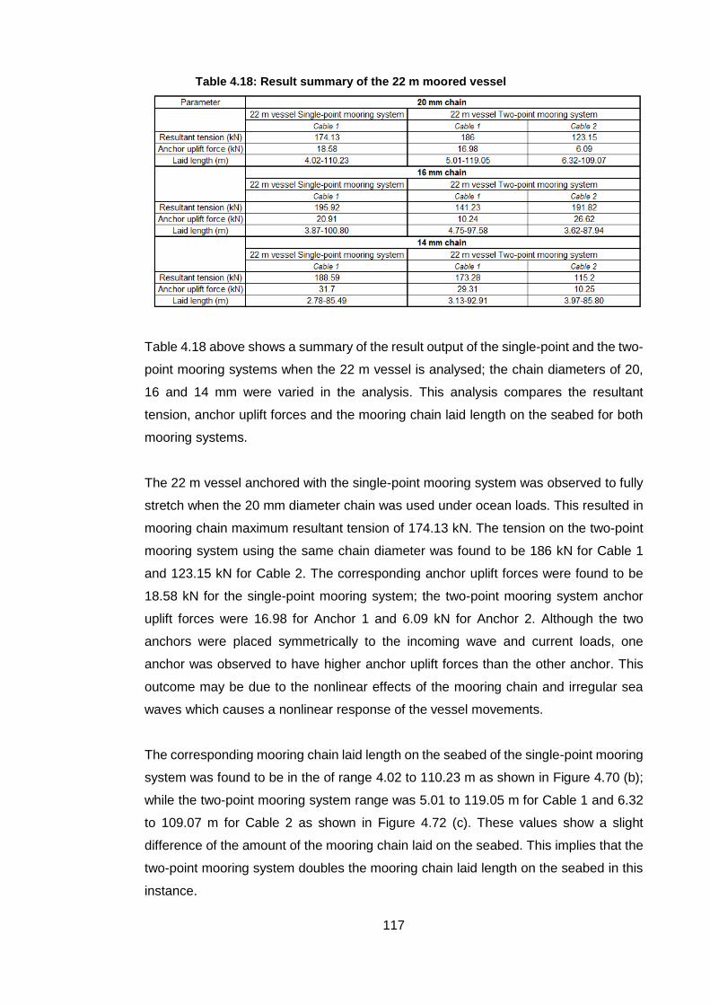
117

Table 4.18: Result summary of the 22 m moored vessel

Table 4.18 above shows a summary of the result output of the single-point and the two-

point mooring systems when the 22 m vessel is analysed; the chain diameters of 20,

16 and 14 mm were varied in the analysis. This analysis compares the resultant

tension, anchor uplift forces and the mooring chain laid length on the seabed for both

mooring systems.

The 22 m vessel anchored with the single-point mooring system was observed to fully

stretch when the 20 mm diameter chain was used under ocean loads. This resulted in

mooring chain maximum resultant tension of 174.13 kN. The tension on the two-point

mooring system using the same chain diameter was found to be 186 kN for Cable 1

and 123.15 kN for Cable 2. The corresponding anchor uplift forces were found to be

18.58 kN for the single-point mooring system; the two-point mooring system anchor

uplift forces were 16.98 for Anchor 1 and 6.09 kN for Anchor 2. Although the two

anchors were placed symmetrically to the incoming wave and current loads, one

anchor was observed to have higher anchor uplift forces than the other anchor. This

outcome may be due to the nonlinear effects of the mooring chain and irregular sea

waves which causes a nonlinear response of the vessel movements.

The corresponding mooring chain laid length on the seabed of the single-point mooring

system was found to be in the of range 4.02 to 110.23 m as shown in Figure 4.70 (b);

while the two-point mooring system range was 5.01 to 119.05 m for Cable 1 and 6.32

to 109.07 m for Cable 2 as shown in Figure 4.72 (c). These values show a slight

difference of the amount of the mooring chain laid on the seabed. This implies that the

two-point mooring system doubles the mooring chain laid length on the seabed in this

instance.

118

Table 4.19: Result summary of the 14 m moored vessel

Similarly, when observing the 16 mm diameter chain, mooring chain laid length on the

seabed on the single-point mooring system range was 3.87 to 100.80 m; while the two-

point mooring system was 4.75 to 97.58 m for Cable 1 and 3.62 to 87.94 m for Cable

2. In both mooring systems, the mooring chain laid on the seabed is shown to be

fluctuating between the minimum and maximum range values. The maximum range

occurs when the mooring is almost fully stretching, while the minimum range occurs

when the mooring chain is slack.

When observing the 14 mm diameter chain, mooring chain laid length on the seabed

on the single-point mooring system range was 2.78 to 85.49 m; while the two-point

mooring system range was 3.13 to 92.91 m for Cable 1 and 3.97 to 85.80 m for Cable

2.

The resultant tension increased from 174.13 to 195.92 kN when the chain diameter

was changed from 20 mm to 16 mm; and decreased from 195.92 kN to 188.59 kN when

the 14 mm chain diameter was used on the single-point mooring system. As can be

seen, the tension only varied slightly with the change in chain diameter in these wave

conditions.

The corresponding anchor uplift forces on the 16 𝑚𝑚 chain were found to be 20.91 kN

for the single-point mooring system; while the two-point mooring system anchor uplift

forces were 10.24 for Anchor 1 and 26.62 kN for Anchor 2. The 14 mm anchor uplift

forces on the single-point mooring system were found to be 31.7 kN; the two-point

mooring system anchor uplift forces were 29.31 for Anchor 1 and 10.25 kN for Anchor

2.

119

The following analysis compares the resultant tension, anchor uplift forces and the

mooring line laid length on the seabed for both mooring systems using the 14 m vessel.

Table 4.19 above shows a summary of the single and two-point mooring systems when

the chain diameters of 20, 16 and 14 mm were varied. When looking at the single-point

mooring system moored with the 20 mm chain, the mooring chain is shown to

experience the highest tension of 111.08 kN with the corresponding maximum anchor

uplift force of 1.19 kN. The two-point mooring system is shown to experience less

tension and maximum anchor uplift forces compared to the single-point mooring system

(using the 20 mm chain); Cable 1 experienced the maximum tension of 62.8 kN with

the maximum anchor uplift force of 0.14 kN, while Cable 2 experienced the maximum

tension of 65.89 𝑘𝑁 with corresponding maximum anchor uplift force of 0.34 kN.

The corresponding mooring chain laid length on the seabed on the two-point mooring

system of each cable was found to have the lowest minimum and maximum range

compared to the single-point mooring system. However, when both Cable 1 and 2 are

taken into account; the two-point mooring system increases the mooring chain laid

length on the seabed by 41.57% (using the 20 mm chain) compared to the single-point

mooring system. The range for Cable 1 was found to be from 44.93 to 112.69 m; while

Cable 2 was observed to have a range of 33.85 to 109.55 m. The single-point mooring

system mooring line laid length on the seabed range was found to be 24.96 to 119.04

m.

The two-point mooring system increased the mooring chain laid length on the seabed

by 50.25% when the 16 mm chain was used; while the 14 mm chain increase was

2.73%. The small increase of the 14 mm chain was due to its light weight compared to

the 16 and 20 mm mooring chains; the light weight of the 14 mm mooring chain resulted

in a large portion mooring chain length to lift-off and drop back down on the seabed

since it had less capability to resist vessel movements.

A closer look in Figure 4.71 (b) and Figure 4.75 (b), shows the single-point and the two-

point mooring systems (on the 14 m vessel) moored with the 14 mm diameter mooring

chain with the highest mooring chain laid length on the seabed. This outcome

demonstrates that smaller chain sizes frequently lifts off and drops back down on the

seabed. Figure 4.71 (c) show the 14 mm diameter chain with the least contact forces

compared to the 16 and 20 mm diameter chain contact forces. The contact forces are

shown to be increasing with an increase of the impact velocity and diameter of a chain.

120

The corresponding anchor uplift forces of the three chain sizes are shown in Figure

4.71 (d) of the 14 m single-point moored vessel. The 14 mm diameter chain is shown

to be experiencing the highest anchor uplift force of 4.48 kN while the 16 and 20 mm

diameter chains experienced 2.54 and 1.19 kN anchor uplift forces respectively.

Figure 4.75 (b) and (c) shows the corresponding anchor uplift forces of the three chain

sizes on the 14 m two-point moored vessel. The 14 mm chain showed the highest

anchor uplift force of 2.66 kN compared to the 16 and 20 mm chain sizes. The 20 mm

chain on the two-point moored 14 m vessel showed the least anchor uplift forces on

both Anchor 1 and Anchor 2.

In summary, the 14 m vessel analysis shows the single-point mooring system with

higher anchor uplift forces than the two-point mooring system when the three chain

sizes were evaluated. This observation was also found be the same when observing

the resultant tension. The two-point mooring Cable 1 and 2 each experienced almost

half the tension experienced by the single-point mooring system. Lastly, Cable 1 and

2, individually showed less mooring chain laid length on the seabed compared to the

single-point mooring laid length. However, since the two-point mooring system uses

two mooring chains, this increased the amount of mooring chain laid length interacting

with the seabed.

The 14 m vessel showed less mooring chain length of approximately 80 m interacting

with the seabed; most of the mooring line length laid inactive on the seabed. The 22

m vessel showed approximately 110 m of the mooring chain length constantly lifting off

and dropping down on the seabed. This outcome was observed on both the single-

point and two-point mooring systems.

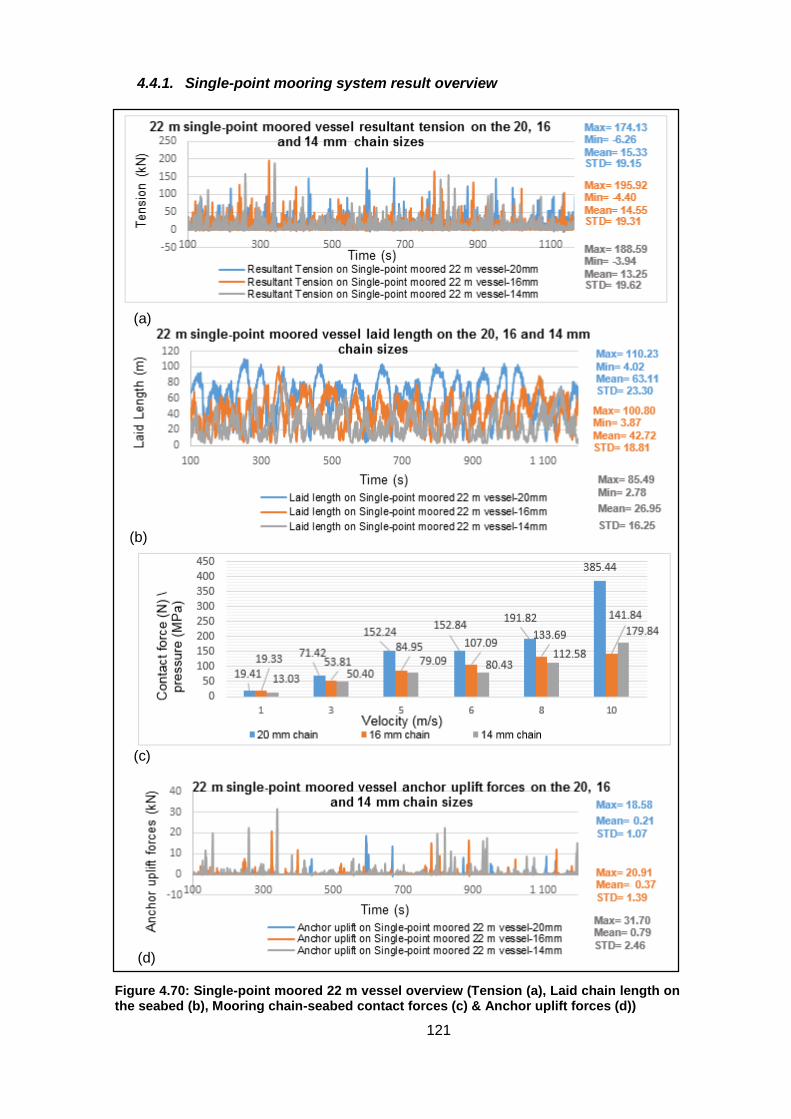
121

4.4.1. Single-point mooring system result overview

(a) (b)

(c) (d)

Figure 4.70: Single-point moored 22 m vessel overview (Tension (a), Laid chain length on the seabed (b), Mooring chain-seabed contact forces (c) & Anchor uplift forces (d))

122

(a) (b)

(c) (d) Figure 4.71: Single-point moored 14 m vessel overview (Tension (a), Laid chain length on the seabed (b), Mooring chain-seabed contact forces (c) & Anchor uplift forces (d))

123

4.4.2. Two-point mooring system result overview

(a) (b)

(c) (d)

Figure 4.72: Two-point moored 22 m vessel overview (Tension on Cable 1 (a) & 2(b), Laid chain length on the seabed on Cable 1 (c) & 2(d)

124

(a)

(b)

(c)


forces (a) and Anchor uplift forces on Cable 1 (b) & 2(c))

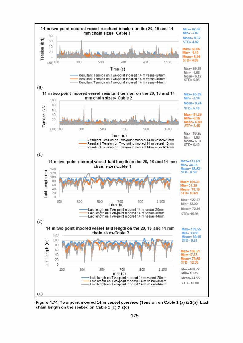
125

(a) (b)

(c) (d)

Figure 4.74: Two-point moored 14 m vessel overview (Tension on Cable 1 (a) & 2(b), Laid

chain length on the seabed on Cable 1 (c) & 2(d)

126

(a)

(b) (c)


forces (a) and Anchor uplift forces on Cable 1 (b) & 2(c))

127

CHAPTER FIVE

5. Conclusion

The objective of this work has been to numerically analyse the effect of the single-point

versus the two-point mooring systems on the seabed which are used for anchoring

squid fishing vessels. This analysis is as result of an observation made by divers from

the South African Department of Environmental Affairs who noticed an interaction

between the mooring line and benthic squid egg beds. The mooring line which is made

of steel chain was observed to impact the seabed with a noticeable velocity from the

video footage obtained. This mooring line impact is suspected to possibly destroy

benthic squid egg beds, which in consequence can be one of the causes of a decline

in squid catches in South Africa.

In this study, two numerical models were developed for investigating the effects of the

single-point and two-point mooring systems on the seabed. The primary model was

developed using ANSYS AQWA which investigated the response of the two types of

squid fishing vessels subjected to ocean loads. The secondary model was developed

using ABAQUS finite element model, this model was used for simulating the mooring

chain impact pressure and force on the seabed which is not available in ANSYS AQWA.

The mooring chain effect on the seabed due to varying the wave height and period was

investigated using the 22 m vessel. Three mooring system configurations were also

used on both the single-point and two-point mooring systems for analysing their effect

on the seabed. The effect of the three chain sizes used in the squid fishing industry

was also investigated using the 14 and 22 m fishing vessels by varying anchor chain

diameters of 14, 16 and 20 mm.

The underwater video footage captured by marine divers was analysed using Tracker

video analysis software to determine the actual impact velocity of the mooring chain on

the seabed. The impact pressure on the seabed due to the obtained velocity was

presented. The velocity from the video analysis was also used to calibrate the ANSYS

AQWA model so that it correlates to realistic ocean conditions. From the results

obtained in this study, the following conclusions are drawn:

1. The measured mooring chain impact velocity from Tracker was estimated

to be 8 m/s with an average velocity of about 5 m/s.

128

2. The ABAQUS model developed by varying velocities of 1, 3, 5, 6, 8 and 10

m/s showed a linear relationship between the mooring chain impact velocity

and pressure on the seabed. The mooring chain impact pressure on the

seabed increased as the impact velocity of the chain increased. An increase

in the diameter of the mooring chain also resulted in an increase in the

impact pressure and forces on the seabed.

3. When looking at the obtained velocity of 8 m/s of the underwater chain

impacting the seabed. The 20 mm diameter chain was found to cause the

greatest seabed impact pressure and force of 191 MPa and 191.82 N

respectively. The 16 mm diameter chain impact pressure and force on the

seabed was found to be 133 MPa and 133.69 N respectively. The 14 mm

diameter cause the least seabed impact pressure and force of 112 MPa and

112.58 N.

4. The effect of varying the wave height and period showed that a decrease in

the wave height and an increase in the wave period increased the tension

on the mooring line. This consequently resulted in a large portion of the

mooring line lifting off and dropping back down on the seabed. The mooring

line was observed to have both slack and taut profiles over the simulation

duration.

This effect was clearly observed when the wave height was increased from

1 to 2 m while keeping the wave period of 7 s constant. The corresponding

seabed impact pressure due to this effect showed a difference of 94.14%

(from 42.48 to 118.03 MPa); while a difference in tension of 126.87% (from

23.93 to 106.96 kN) was obtained. However, when the wave height was

increased from 1 to 2 m while keeping the wave period of 10 s constant; the

mooring line resulted in more slack profile. This, in consequence, led to a

significant amount of the mooring line lying dormant on the seabed. The

corresponding seabed impact pressure difference of 89.29% (from 36.96 to

96.59 MPa) was obtained; while the difference in tension of 94.93% (from

22.08 to 61.98 kN) was obtained. It can then be said that the when the wave

height doubles, the impact pressure on the seabed also doubles. This effect

was more apparent when the wave period of 7 s was present.

5. The outcomes of investigating the three mooring line configurations on both

vessel sizes showed that the two-point mooring system doubles the mooring

129

line footprint on the seabed compared to the single-point mooring system.

Each of the two mooring lines was observed to sweep across the seabed

as the ocean waves passed across the moored vessel. However, the two-

point mooring also showed less seabed footprint than the single-point

mooring system when the wave direction changes.

The 14 m moored vessel was found to have less seabed footprint on the

seabed, this was noticeable by a large portion of the mooring line which laid

dormant on the seabed. On the contrary, the 22 m vessel mooring line was

found to have a large portion which frequently interacted with the seabed.

This outcome was observed when both vessels used the same mooring

system configuration.

High tension values were found to be associated with frequent mooring line

interaction with the seabed. The anchor uplift forces were also presented

which can give more insight for further investigation such as the effect of

anchor drag on the seabed.

6. The outcomes of investigating the effect of the three mooring chain sizes

showed that the two-point mooring system increased the mooring line laid

length on the seabed by 41.57% compared to the single-point mooring

system when the 20 mm diameter was used. This increase was found to be

50.25% when the 16 mm diameter chain was used and 2.73% when the 14

mm diameter chain was used.

The 14 m vessel anchored with the 14 mm diameter chain using the single-

point mooring system was found to have the most mooring line laid length

on the seabed which frequently lifted up and down. The 22 m vessel in this

case showed the 20 mm chain with the most frequent interaction on the

seabed.

In summary, ANSYS AQWA can simulate the single-point and two-point mooring

systems. However, the software is still limited as it does not include the seabed

frictional effects and the contact force of the mooring line. ABAQUS finite element was

used to account for the seabed contact forces, these forces were simulated based on

the measured impact velocity of various points of contact along the mooring line.

Results obtained in this study indicate that the two-point mooring doubles the mooring

chain seabed contact length on the seabed. The 20 mm diameter chain was found to

130

cause up to 40% more damage than the 16 mm diameter chain in terms of impact

pressure on the seabed. If the wave direction does not change, the two-point mooring

system could cause more damage if one considers the greater footprint on the seabed

as was shown in Figure 4.66 where one of the cables alone has 8% more laid length

and there are two cables in contact so the damage will be slightly more than double the

single point mooring. We can therefore, conclude, that the two point mooring system

will cause more damage than a single point mooring system as the contact for each

cable would have to have been halved for it to have caused the same damage and this

is clearly not the case.

131

6. Recommendations and future work

Future improvements

The quality of underwater video footage needs to be improved for more accurate

analysis of the marked points along the mooring line.

The video footage data can be improved through the following methods

o The use of high-resolution camera, up 1000 frames per second and lighting is

advised for more visibility. Use of underwater lights of about 9000 lumens

without excessive glare.

o Error tracking: inconsistency in detecting the centre point of the reflective

marker (can use traffic reflective colour or reflective tape) in a recorded image,

any given marker is composed of several pixels.

Design related recommendations

o Clump weights/buoys can be installed on the section of mooring line that

interacts with the seabed in order reduce contact.

Software Limitations

For this application of ANSYS AQWA, some software limitations still exist. The main

one is that the software does not consider the seabed impact or contact force with the

associated seabed friction effects on the seabed.

Another limitation associated with the latter is that the software only outputs the time-

history of the vessel nodes and elements; only two output nodes for the mooring line

which are the anchor point (defined as fixed point) and the fairlead point where the

mooring tension is calculated. The discretised mooring line nodes and elements are

internally converted by the software to a two-dimensional load/extension database.

Lastly, another limitation is with regard to the fixed anchor assumption on the seabed

for mooring the floating structure. In the squid industry, temporary anchors are used

during fishing and retrieved from the seabed after fishing. These anchors have a high

possibility of dragging on the seabed when the mooring line tension are high. The fixed

anchor is more relevant for a permanent anchor on the seabed.

132

Future work

Anchor drag impact on the seabed with the emphasis on anchor trajectory needs to

be investigated.

The use of improved high definition cameras is required for measurements with

scientific accuracy.

The chain motion should be also be studied 3-D for eliminating the assumptions from

the 2-D video analysis.

133

REFERENCES

Abadie, A., Lejeune, P., Pergent, G. & Gobert, S. 2016. From mechanical to chemical impact

of anchoring in seagrasses: The premises of anthropogenic patch generation in Posidonia

oceanica meadows. Marine Pollution Bulletin, 109(1): 61–71.

ABAQUS. 2012. Abaqus 6.12: Getting Started with Abaqus (Interactive Edition).

ABC Moorings. 2015. Mooring Lines. http://abc-moorings.weebly.com/mooring-lines.html 2

April 2015.

Allan, B. 2008. Solutions to simple boundary and initial value problems. Applied Mechanics of

Solids. http://solidmechanics.org/text/Chapter4_1/Chapter4_1.htm 17 April 2017.

ANSYS AQWA. 2015. Aqwa Theory Manual.

Balzola, R. 1999. Mooring Line Damping In Very Large Water Depths. Massachusetts Institute

of Technology.

Belytschko, T., Ong, J.S.-J., Wing Kam Liu & Kennedy, J.M. 1984. Hourglass control in linear

and nonlinear problems. Computer Methods in Applied Mechanics and Engineering,

43(3): 251–276.

Bjørnsen, E. 2014. Chains in Mooring Systems. Master Thesis. Trondheim: Norwegian

University of Science and Technology.

Blignaut, J. 2012. Chokka industry in dire straits. SABC News: 1.

http://www.sabc.co.za/news/a/541d51804c0b3cfab72dffa583a5af00/Chokka-industry-in-

dire-straits-20120720 18 February 2015.

Boom, H.J.J. Van Den. 1985. Dynamic Behaviour of Mooring Lines. Behaviour of Offshore

Structures: 359–368.

Chrolenko, M.O. 2013. Dynamic Analysis and Design of Mooring Lines. Master Thesis.

Trondheim: Norwegian University of Science and Technology.

Collins, K.J., Suonpää, A.M. & Mallinson, J.J. 2010. The impacts of anchoring and mooring in

seagrass, Studland Bay, Dorset, UK. Underwater Technology, 29(3): 117–123.

134

Cummins, W. 1962. The impulse response function and ship motions. Schiffstechnik, 57(9):

101–109.

Davis, A.R., Broad, A., Gullett, W., Reveley, J., Steele, C. & Schofield, C. 2016. Anchors away?

The impacts of anchor scour by ocean-going vessels and potential response options.

Marine Policy, 73: 1–7.

Demers, M.C.A., Davis, A.R. & Knott, N.A. 2013. A comparison of the impact of ‘seagrass-

friendly’ boat mooring systems on Posidonia australis. Marine Environmental Research,

83: 54–62.

DNV. 2010. Offshore Standard DNV-OS-E-301 - Position Mooring.

DNV. 2011. Offshore Standard DNV-RP-H103 -Modelling And Analysis Of Marine Operations.

Ebbesen, C. 2013. Analysis of Motions and Anchor Line Forces for Floating Production Units.

Norwegian University of Science and Technology.

Eder, S. 2012. ANSYS CFD for Naval Applications.

Francour, P., Ganteaume, A. & Poulain, M. 1999. Effects of boat anchoring in Posidonia

oceanica seagrass beds in the Port‐ Cros National Park (north‐ western Mediterranean

Sea). Aquatic Conservation: Marine and Freshwater Ecosystems, 9(4): 391–400.

Garrett, D.L. 1982. Dynamic Analysis of Slender Rods. Journal of Energy Resources

Technology, 104(4): 302–306.

Ha, T.-P. 2011. Frequency and Time Domain Motion and Mooring Analyses for a Fpso

Operating in Deep Water. PhD Thesis. Newcastle: Newcastle University.

Haritos, N. 2007. Introduction to the Analysis and Design of Offshore Structures – An

Overview. Electronic Journal of Structural Engineering, 7(Special Issue: Loading on

Structures): 55–65.

Hastings, K., Hesp, P. & Kendrick, G.A. 1995. Seagrass loss associated with boat moorings

at Rottnest Island, Western Australia. Ocean & Coastal Management, 26(3): 225–246.

135

Herbert, R.J.H., Crowe, T.P., Bray, S. & Sheader, M. 2009. Disturbance of intertidal soft

sediment assemblages caused by swinging boat moorings. Hydrobiologia, 625(1): 105–

116.

Ibrahim, R.A. & Grace, I.M. 2010. Modeling of ship roll dynamics and its coupling with heave

and pitch. Mathematical Problems in Engineering, 2010: 13–18.

Jameel, M., Ahmad, S., Islam, A.B.M.S. & Jumaat, M.Z. 2011. Nonlinear Analysis of Fully

Coupled Integrated Spar-Mooring Line System. International Society of Offshore and

Polar Engineers, 8: 198–205.

Ketchman, J. & Lou, Y. 1975. Application of the finite element method to towed cable

dynamics. In OCEAN 75 Conference. IEEE: 98–107.

Kim, Y.-B. 2003. Dynamic analysis of multiple-body floating platforms coupled with mooring

lines and risers. Doctoral dissertation. Texas: Texas A&M University.

Kininmonth, S., Lemm, S., Malone, C. & Hatley, T. 2014. Spatial vulnerability assessment of

anchor damage within the Great Barrier Reef World Heritage Area, Australia. Ocean &

Coastal Management, 100: 20–31.

Krusche, P., Mia, N. & Hofmeyr, C.D. 2014. Squid exporters receive competition law

exemption. Cape Business News: 1.

Masciola, M., Jonkman, J. & Robertson, A. 2014. Extending the Capabilities of the Mooring

Analysis Program: A Survey of Dynamic Mooring Line Theories for Integration Into FAST.

In Volume 9A: Ocean Renewable Energy. ASME: 6.

Mason, W. 2015. Incompressible Potential Flow Using Panel Methods. In Applied

Computational AerodynamicsApplied Computational Aerodynamics: A Modern

Engineering Approach. 4–1.

Miedema, S.A., Kerkvliet, J., Strijbis, D., Jonkman, B. & Hatert, M.V. 2006. The digging and

holding capacity of anchors. Offshore (Conroe, TX).

Milazzo, M., Badalamenti, F., Ceccherelli, G. & Chemello, R. 2004. Boat anchoring on

Posidonia oceanica beds in a marine protected area (Italy, western Mediterranean): Effect

136

of anchor types in different anchoring stages. Journal of Experimental Marine Biology and

Ecology, 299(1): 51–62.

OrcaFlex. 2010. OrcaFlex Manual.

Paredes, G.M. & Taveira-Pinto, F. 2016. An experimental technique to track mooring cables

in small scale models using image processing. Ocean Engineering, 111: 439–448.

Pellegrino, S. & Ong, P.P.A. 2003. Modelling of Seabed Interaction in Frequency Domain

Analysis of Mooring Cables. In Proceedings of OMAE’03 22nd International Conference

on Offshore Mechanics and Arctic Engineering. 1–10.

Rajasuriya, A., Olof, L. & Ohman, M.C. 2013. Disturbances on Coral Sri Lanka : A Case Study

Reefs in. Ambio, 22(7): 474–480.

Sarkar, A. & Eatock Taylor, R. 2002. Dynamics of mooring cables in random seas. Journal of

Fluids and Structures, 16(2): 193–212.

Sluijs, M.F. van & Blok, J. 1977. The Dynamic Behavior of Mooring Lines. Offshore Technology

Conference (OTC), Houston.

Taylor, R. & Valent, P. 1984. Design Guide for Drag Embedment Anchors. Naval Civil

Engineering Lab Port Hueneme CA.

The Editors of Encyclopædia Britannica. 2009. Agulhas Current | ocean current |

Britannica.com. : 1. https://global.britannica.com/place/Agulhas-Current 6 March 2017.

Vineesh, M. V, Sabu, N. V & Manju, P.M. 2014. Finite Element Analysis of Mooring Cable.

International Journal of Engineering Research and Applications (IJERA) ISSN, (January):

13–18.

Walker, D.I., Lukatelich, R.J., Bastyan, G. & McComb, A.J. 1989. Effect of boat moorings on

seagrass beds near Perth, Western Australia. Aquatic Botany, 36(1): 69–77.

Wang, L.Z., Guo, Z. & Yuan, F. 2010. Three-dimensional interaction between anchor chain

and seabed. Applied Ocean Research, 32(4): 404–413.

137

World Wide Fund South Africa. 2011. South African Fisheries: The real facts and trends. WWF

South Africa: 1. http://www.wwf.org.za/?4900/fisheriesfactstrends 18 February 2015.

Yang, W.S. 2007. Hydrodynamic Analysis of Mooring Lines Based on Optical Tracking

Experiments. PhD: Texas. Texas A&M University.

Yu, L. & Tan, J.H. 2006. Numerical investigation of seabed interaction in time domain analysis

of mooring cables. Journal of Hydrodynamics, 18(4): 424–430.

138

139

APPENDIX/APPENDICES

140

APPENDIX A: Chain specification data

McKinnon Special Short Link Chain - SSL Chain McKinnon special Short Link Chain is a high quality carbon-steel Short Link Chain for general purpose use.

Special short link chain

Dimensions (mm) Forces

Commodity Diameter (dn)

Pitch (P) W1 W2 w2w dw G BF MPF WLL Approx mass

nom tol +/-

nom min max min max max max max kN kN tonne kg/m

CSL130 13 39 37.8 40.2 16.9 47.5 48.1 14.3 17.6 106 42.5 2.16 3.77

CSL140 14 42 40.7 43.3 18.2 51.1 51.8 15.4 18.9 123 49.3 2.51 4.36

CSL160 16 48 46.6 49.4 20.8 58.8 59.2 17.6 21.6 161 64 3.28 5.71

CSL200 20 60 58.2 61.8 26 73 74 22 27 251 101 5.12 8.92

141

APPENDIX B: Steel and sand properties

Sand properties

(https://support.prokon.com/portal/kb/articles/elastic-properties-of-soils )

https://support.prokon.com/portal/kb/articles/elastic-properties-of-soils

142

Steel properties

(http://www.engineeringtoolbox.com/young-modulus-d_417.html)

143

APPENDIX C: Vessel drawings

14 𝑚 vessel drawing

144

22 𝑚 vessel drawing

145

APPENDIX D: Vessel hydrostatic results

22 𝑚 vessel hydrostatic results

146

14 𝑚 vessel hydrostatic results

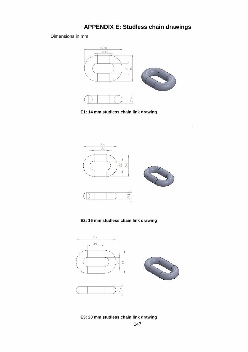
147

APPENDIX E: Studless chain drawings

Dimensions in mm

E1: 14 mm studless chain link drawing



148

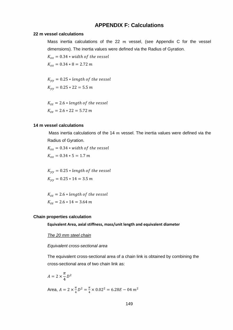
149

APPENDIX F: Calculations

22 m vessel calculations

Mass inertia calculations of the 22 𝑚 vessel, (see Appendix C for the vessel

dimensions). The inertia values were defined via the Radius of Gyration.

𝐾𝑥𝑥 = 0.34 ∗ 𝑤𝑖𝑑𝑡ℎ 𝑜𝑓 𝑡ℎ𝑒 𝑣𝑒𝑠𝑠𝑒𝑙

𝐾𝑥𝑥 = 0.34 ∗ 8 = 2.72 𝑚

𝐾𝑦𝑦 = 0.25 ∗ 𝑙𝑒𝑛𝑔𝑡ℎ 𝑜𝑓 𝑡ℎ𝑒 𝑣𝑒𝑠𝑠𝑒𝑙

𝐾𝑦𝑦 = 0.25 ∗ 22 = 5.5 𝑚

𝐾𝑧𝑧 = 2.6 ∗ 𝑙𝑒𝑛𝑔𝑡ℎ 𝑜𝑓 𝑡ℎ𝑒 𝑣𝑒𝑠𝑠𝑒𝑙

𝐾𝑧𝑧 = 2.6 ∗ 22 = 5.72 𝑚

14 m vessel calculations

Mass inertia calculations of the 14 𝑚 vessel. The inertia values were defined via the

Radius of Gyration.

𝐾𝑥𝑥 = 0.34 ∗ 𝑤𝑖𝑑𝑡ℎ 𝑜𝑓 𝑡ℎ𝑒 𝑣𝑒𝑠𝑠𝑒𝑙

𝐾𝑥𝑥 = 0.34 ∗ 5 = 1.7 𝑚

𝐾𝑦𝑦 = 0.25 ∗ 𝑙𝑒𝑛𝑔𝑡ℎ 𝑜𝑓 𝑡ℎ𝑒 𝑣𝑒𝑠𝑠𝑒𝑙

𝐾𝑦𝑦 = 0.25 ∗ 14 = 3.5 𝑚

𝐾𝑧𝑧 = 2.6 ∗ 𝑙𝑒𝑛𝑔𝑡ℎ 𝑜𝑓 𝑡ℎ𝑒 𝑣𝑒𝑠𝑠𝑒𝑙

𝐾𝑧𝑧 = 2.6 ∗ 14 = 3.64 𝑚

Chain properties calculation

Equivalent Area, axial stiffness, mass/unit length and equivalent diameter

The 20 mm steel chain

Equivalent cross-sectional area

The equivalent cross-sectional area of a chain link is obtained by combining the

cross-sectional area of two chain link as:

𝐴 = 2 ×𝜋

4𝐷2

Area, 𝐴 = 2 ×𝜋

4𝐷2 =

𝜋

4× 0.022 = 6.28𝐸 − 04 𝑚2

150

This leads to: 𝐸𝐴 = 0.854 × 108𝐷2 𝑘𝑁 (for studless chain)

= 0.854 × 1080.022 × 1000

= 3.42𝐸 + 07 𝑁

Mass/unit length is given by:

19.9𝐷2 = 19.9 × 0.022 = 7.96 𝑘𝑔/𝑚

Equivalent Diameter for the studless chain is given by:

𝐷𝐸𝑞𝑢𝑖𝑣𝑎𝑙𝑒𝑛𝑡 = 1.8𝐷 = 1.8 × 0.02 = 0.036 𝑚



Area, 𝐴 = 2 ×𝜋

4𝐷2 =

𝜋

4× 0.0162 = 4.02𝐸 − 04 𝑚2

𝐸𝐴 = 0.854 × 108𝐷2 𝑘𝑁 (for studless chain)

= 0.854 × 1080.0162 × 1000

= 2.19𝐸 + 07 𝑁


19.9𝐷2 = 19.9 × 0.0162 = 5.09 𝑘𝑔/𝑚


𝐷𝐸𝑞𝑢𝑖𝑣𝑎𝑙𝑒𝑛𝑡 = 1.8𝐷 = 1.8 × 0.016 = 0.029 𝑚



Area, 𝐴 =𝜋

4𝐷2 = 2 ×

𝜋

4× 0.0142 = 3.08𝐸 − 04 𝑚2

𝐸𝐴 = 0.854 × 108𝐷2 𝑘𝑁 (For studless chain)

= 0.854 × 1080.022 × 1000

= 1.67𝐸 + 07 𝑁


19.9𝐷2 = 19.9 × 0.0142 = 3.9 𝑘𝑔/𝑚


𝐷𝐸𝑞𝑢𝑖𝑣𝑎𝑙𝑒𝑛𝑡 = 1.8𝐷 = 1.8 × 0.014 = 0.025 𝑚

THE EFFECTS OF BOAT MOORING SYSTEMS ON SQUID EGG …

Documents