The Effectiveness and Targeting of Television Advertising

— —< <

The Effectiveness and Targeting ofTelevision Advertising

RON SHACHAR

Tel-Aviv UniversityTel-Aviv, Israel, [email protected]

BHARAT N. ANAND

Harvard Business SchoolBoston, MA [email protected]

Television networks spend about 16% of their revenues on tune-ins, whichare previews or advertisements for their own shows. In this paper, weexamine two questions. First, what is the informational content in advertis-ing? Second, is this level of expenditures consistent with profit maximiza-tion? To answer these questions, we use a new and unique micro-level paneldataset on the television viewing decisions of a large sample of individuals,matched with data on show tune-in advertisements. The difference in

(effectiveness of advertisements between ‘‘regular’’ shows about which view-)ers are assumed to have substantial information a priori and ‘‘specials’’

( )about which they have very little reveals the value of information inadvertisements and the different roles that information can play. Thenumber of exposures for each individual is likely to be correlated with theirpreferences, since networks target their audiences. We address this endogene-ity problem by controlling for observed, and integrating the unobserved,characteristics of individuals, and find that the estimated effects of tune-insare still large. Finally, we find that actual expenditures on tune-ins closelymatch the predicted optimal levels of spending.

1. Introduction

Advertising expenditures by television networks are substantial. In1995, for example, the three major networks spent approximately

We would like to thank Greg Kasparian and David Poltrack of CBS for their help inobtaining the data for this study, John W. Emerson for comments and assistance inprogramming, and Barry Nalebuff, Subrata Sen, Idit Shachar, and many of ourcolleagues for helpful discussions.

Q 1998 Massachusetts Institute of Technology.Journal of Economics & Management Strategy, Volume 7, Number 3, Fall 1998, 363]396

Journal of Economics & Management Strategy364

16% of their revenues on tune-in advertisements,1 more than twice asmuch as firms in other industries. The networks also rank among thetop ten firms in the economy in terms of dollars of advertisingexpenditures.2 This raises an obvious question: are networks spend-ing too much on advertising?3 Indeed, one may suspect that net-works underestimate their advertising costs, since these are mostlyopportunity costs; consequently, advertising expenditures might ex-ceed the optimal amount. Answering this question requires an under-standing of the effects of tune-ins on individuals’ viewing choices,since advertising revenues are a function of show ratings, which areaggregations of individual viewing decisions. In this study, we esti-mate these effects using a new and unique micro-level panel dataseton the television viewing decisions of a large sample of individuals,matched with data on show tune-ins.

The second question that we address in this paper is of moregeneral interest: what is the informational value of advertising? Aspirited debate on whether advertising is ‘‘informative’’ or ‘‘persua-sive’’ has gone on for some time.4 Understanding the relative impor-tance of informing and persuading has both positive and normativeimplications. However, distinguishing these effects empirically isdifficult. We base our solution to this identification problem on thefollowing logic: if advertising has information content, then the ef-fects of tune-ins on viewing decisions should differ across showsaccording to individuals’ prior information about each show. Forexample, individuals may possess very little information about the

Ž .timing and attributes of shows that are aired once— specials com-Ž . 5pared to shows that are aired frequently regulars . We estimate the

differential effects of tune-ins on viewing decisions for these two

1. ‘‘Tune-in’’ usually refers to an advertisement for a television show. Advertise-ments for TV shows represent a cost for the networks, and other advertisements supplytheir revenues. The ads we focus on in this paper are of the first type.

2. The networks usually air 12 minutes of commercials during each hour ofprogramming. In 1995, they used about 2 of these 12 minutes on tune-ins for theirshows. Since advertising revenues represent almost all of the networks’ revenues, andtune-ins represent most of their advertisement effort, we proxy the share of revenuesspent on advertisements as 16%. We then estimate their spending on advertising indollars, using these numbers and data on networks’ revenues.

Ž .3. Roberts and Samuelson 1988 use a different approach than ours to answer asimilar question in the context of the tobacco industry.

Ž . Ž .4. Early work on this can be traced to Galbraith 1967 and Solow 1967 ; TiroleŽ .1989, pp. 289]290 labels these as the ‘‘partial’’ view versus the ‘‘adverse’’ view ofadvertising. For models dealing explicitly with the informational effects of advertising,

Ž . Ž .see Butters 1977 and Grossman and Shapiro 1984 .5. This is similar to the oft-cited distinction between ‘‘search’’ goods and ‘‘experi-

ence’’ goods, although not identical, since regular shows have features common to bothtypes of goods.

The Effectiveness and Targeting of Television Advertising 365

kinds of shows. If there were no informational content in advertising,then the effects of tune-ins should not differ across such shows withdifferent preexisting ‘‘information stocks.’’ Thus, the product varia-tion in the data provides us with a clear way to identify the informa-tional value of advertising.6

Our estimates of the effects of tune-ins may be biased, sincenetworks generally target their tune-ins for each show towards cer-tain groups of individuals. For example, tune-ins for comedies aremore often aired during other comedies, thus targeting individualsmost likely to watch comedies in the first place. If these unobserveddifferences in individual preferences are not controlled for, the effectsof tune-ins on viewership will be upward biased. We deal explicitlywith this endogeneity problem in the estimation below. To ourknowledge, no other micro-level study addresses this issue in anydetail.7

This is the first study focusing explicitly on the effects of tune-inadvertisements on individual behavior.8 There are two main advan-tages of examining the effects of advertising in the TV industry. First,advertising is undertaken by firms using, in general, various instru-

Ž . Žments price discounts, promotions, etc. and various media televi-.sion, billboards, magazines, etc. . These different forms of advertising

may be substitutes or complements in consumption9: for example, themarginal effectiveness of magazine ads may depend on the amountof advertising generated by other means, concurrently or in the past.In order to accurately estimate the marginal effectiveness of a particu-lar form of advertising or assess the relative efficacy of alternativeforms of advertising, one would require data on the amount ofadvertising via other forms; this is usually difficult to obtain. Thisissue is of less concern in the TV industry for two reasons: first,almost all advertising by networks is in the form of tune-ins; second,the price of TV services is zero from an individual’s standpoint.Hence, we do not need to consider issues arising from the existenceof multiple advertising inputs.

6. A few previous studies attempt to distinguish informative effects from persua-sive effects in advertising, either by subjective measurement of the information content

Ž .in ads Resnik and Stern, 1978 or by econometric identification techniques similar toŽ .ours Ackerberg, 1995 . All these studies focus on single-product returns of advertising.

7. The targeting of advertising may be important in contexts of both repeat andnonrepeat purchase, and hence is likely to be an issue of general concern.

Ž . Ž .8. See, for example, Berndt 1991 or Tellis and Weiss 1995 for surveys of theliterature on the effects of advertising.

9. Strictly, the advertising itself is not consumed; rather, ads may convey informa-tion that is of value in making decisions.


Second, previous studies suggest that the returns to advertisingmay differ across products.10 These differences are useful in revealingthe different roles of advertising in influencing individual choice.However, it is difficult to compare results across studies, givennonuniformity in datasets, methodologies, or products under exami-nation. Since our dataset contains information for multiple TV showsthat, in principle, differ substantially in their attributes, we canexamine such cross-product differences within a common setting.Our focus here is only on characterizing the variation between regu-lars and specials; we plan to further exploit the product variation inthe dataset in future research on this issue.

The rest of the paper is organized as follows. We first describethe datasets used, since this assists in understanding the structure ofthe model. In Section 2, we describe the construction of the datasetand present descriptive statistics on the sample population, viewer-ship patterns, show characteristics, and characteristics of tune-ins. InSection 3, we present the model used to estimate the effects oftune-ins, and discuss identification issues. We discuss the results inSection 4, and their implications for network strategies in Section 5. InSection 6, we discuss issues for further study.

2. The Datasets

We use three datasets in this study. The first includes data on theviewing choices of about 17,000 individuals during one week inNovember 1995. The second describes the attributes of the showsoffered to these individuals by the four leading networks during thisweek. The number of tune-ins for each show and the time of theirairing constitute the third data set.

Nielsen Media Research maintains a sample of over 5000 house-Ž .holds nationwide by installing a Nielsen People Meter NPM for

each television set in the household. Using 1990 Census data, thesample is designed to reflect the demographic composition of viewersnationwide. The sample is revised regularly, ensuring, in particular,that no single household remains in the sample for more than twoyears.

The NPM uses a special remote control to record arrivals anddepartures of individual viewers, as well as the channel beingwatched on each television set. Although the NPM is calibrated for

Ž .10. For example, Batra et al. 1995 summarize the variation in estimated returnsacross products examined in prior studies. For conflicting results regarding the exis-

Ž .tence of diminishing returns to advertising, see Simon and Arndt 1980 and Rao andŽ .Miller 1975 .


measurements each minute, the data set available to Nielsen clientsprovides a record of whether or not each viewer tuned into each ofthe alternatives during each quarter hour.

The raw dataset records whether or not an individual waswatching television in each quarter hour, and if so, her choice ofnetwork. An individual who was watching television, but did notchoose any network, is coded as watching a nonnetwork channel.This might be a cable channel, PBS, or a local independent channel.Each quarter hour is defined as a time slot.

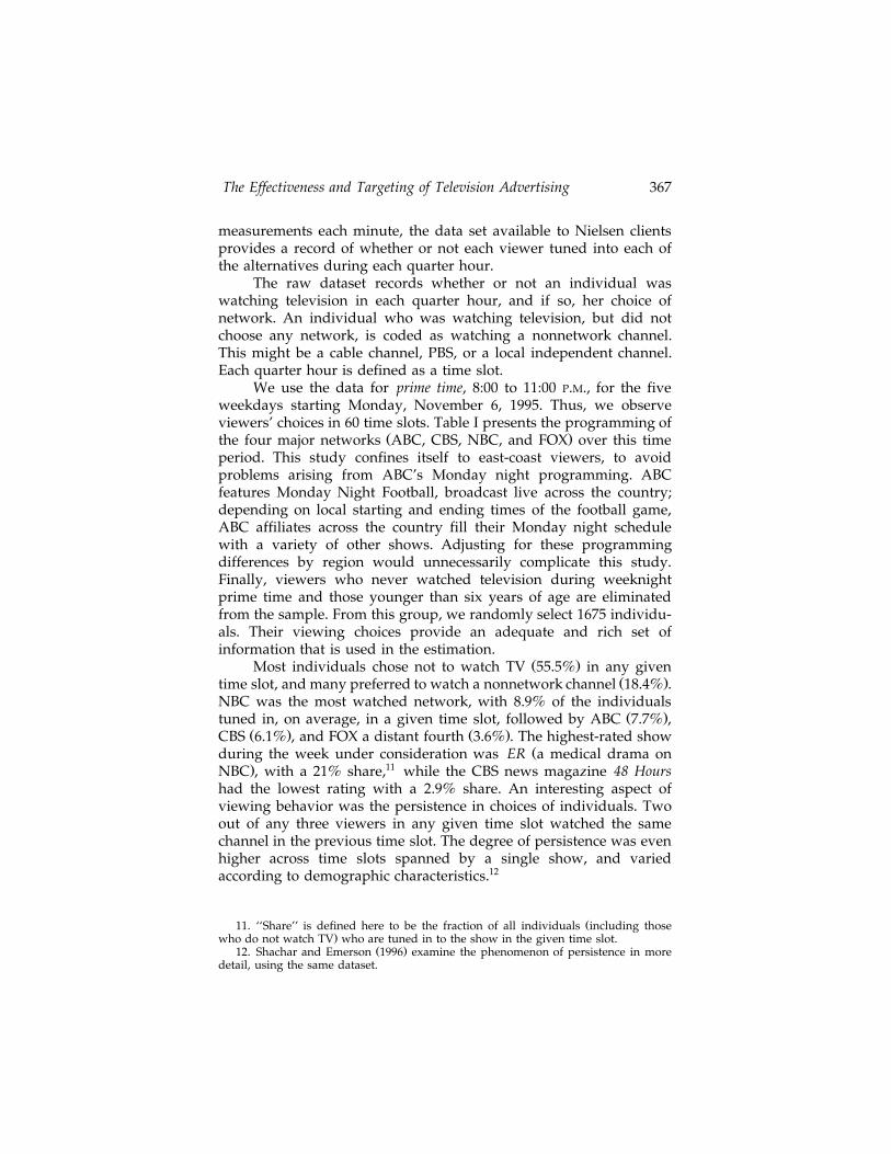
We use the data for prime time, 8:00 to 11:00 P.M., for the fiveweekdays starting Monday, November 6, 1995. Thus, we observeviewers’ choices in 60 time slots. Table I presents the programming of

Ž .the four major networks ABC, CBS, NBC, and FOX over this timeperiod. This study confines itself to east-coast viewers, to avoidproblems arising from ABC’s Monday night programming. ABCfeatures Monday Night Football, broadcast live across the country;depending on local starting and ending times of the football game,ABC affiliates across the country fill their Monday night schedulewith a variety of other shows. Adjusting for these programmingdifferences by region would unnecessarily complicate this study.Finally, viewers who never watched television during weeknightprime time and those younger than six years of age are eliminatedfrom the sample. From this group, we randomly select 1675 individu-als. Their viewing choices provide an adequate and rich set ofinformation that is used in the estimation.

Ž .Most individuals chose not to watch TV 55.5% in any givenŽ .time slot, and many preferred to watch a nonnetwork channel 18.4% .

NBC was the most watched network, with 8.9% of the individualsŽ .tuned in, on average, in a given time slot, followed by ABC 7.7% ,

Ž . Ž .CBS 6.1% , and FOX a distant fourth 3.6% . The highest-rated showŽduring the week under consideration was ER a medical drama on

. 11NBC , with a 21% share, while the CBS news magazine 48 Hourshad the lowest rating with a 2.9% share. An interesting aspect ofviewing behavior was the persistence in choices of individuals. Twoout of any three viewers in any given time slot watched the samechannel in the previous time slot. The degree of persistence was evenhigher across time slots spanned by a single show, and variedaccording to demographic characteristics.12

Ž11. ‘‘Share’’ is defined here to be the fraction of all individuals including those.who do not watch TV who are tuned in to the show in the given time slot.

Ž .12. Shachar and Emerson 1996 examine the phenomenon of persistence in moredetail, using the same dataset.


Day Network 8:00 8:30 9:00 9:30 10:00 10:30

Mon. ABC The Marshal Pro Football: Philadelphia at Dallas

CBS The Nanny Can’t HurryLove

Murphy Brown High Society Chicago Hope

NBC Fresh Princeof Bel-Air

In the House Movie: She Fought Alone

FOX Melrose Place Beverly Hills 90210 Affiliate Programming: News

Tue. ABC Roseanne Hudson Street HomeImprovement

Coach NYPD Blue

CBS The Client Movie: Nothing Lasts Forever

NBC Wings News Radio Frasier Pursuit ofHappiness

Dateline NBC

FOX Movie: Bram Stoker’s Dracula Affiliate Programming: News

Wed. ABC Ellen The DrewCarey Show

Grace UnderFire

The NakedTruth

Prime Time Live

CBS Bless thisHouse

Dave’s World Central Park West Courthouse

NBC Seaquest 2032 Dateline NBC Law & Order

FOX Beverly Hills 90210 Party of Five Affiliate Programming: News

Thu. ABC Movie: Columbo: It's All in the Game Murder One

CBS Murder, She Wrote New York News 48 Hours

NBC Friends The SingleGuy

Seinfeld Caroline inthe City

E.R.

FOX Living Single The Crew New York Undercover Affiliate Programming: News

Fri. ABC FamilyMatters

Boy MeetsWorld

Step by Step Hangin’ WithMr. Cooper

20/20

CBS Here Comes the Bride Ice Wars: USA vs The World

NBC Unsolved Mysteries Dateline NBC Homicide: Life on the Street

FOX Strange Luck X-Files Affiliate Programming: News

The purpose of this study is to examine the effects of tune-inson viewing decisions. In Section 3, we present the viewing-choicemodel that we use to estimate these effects. The structure of this

Ž .model is similar to that of Shachar and Emerson 1996 , which foundthat demographic characteristics of a show’s cast and of individuals,


table II.

Summary Statistics: IndividualDemographic Characteristics

aVariable Mean Std. Dev

Kids 0.0794 0.2704Teens 0.0627 0.2425Gen-X 0.2400 0.4272Boom 0.2764 0.4474Old 0.4191 0.4936Female 0.5319 0.4991Male 0.4681 0.4991Family 0.4304 0.4953Adult 0.8579 0.3492Income 0.8333 0.2259Educat 0.7421 0.2216Urban 0.4149 0.4929Basic 0.3642 0.4813Premium 0.3588 0.4798

a Ž .Definitions dummy variables, unless otherwise specified : ‘‘Kids’’: individual is between the ages of 7and 11. ‘‘Teens’’: individual is between the ages of 12 and 17. ‘‘Gen-X’’: individual is between the ages of18 and 34. ‘‘Boom’’: individual is between the ages of 35 and 49. ‘‘Old’’: individual is age 50 or older.‘‘Female’’: individual is a female. ‘‘Male’’: individual is a male. ‘‘Family’’: individual lives in a householdwith a female older than 18 and her kids. ‘‘Adult’’: individual is older than 18. ‘‘Income’’: there are sixlevels of income on the unit interval. ‘‘Educat’’: there are five categories of education on the unit interval.‘‘Urban’’: individual lives in an urban area. ‘‘Basic’’: individual has basic cable. ‘‘Premium’’: individual haspremium cable.

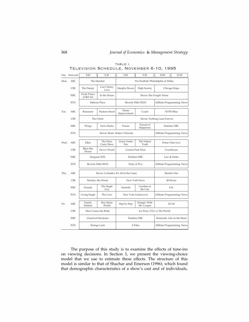
as well as five show attributes—action, comedy, romance, suspense,and fiction—are important in explaining viewing decisions. We brieflydescribe each of these variables below.

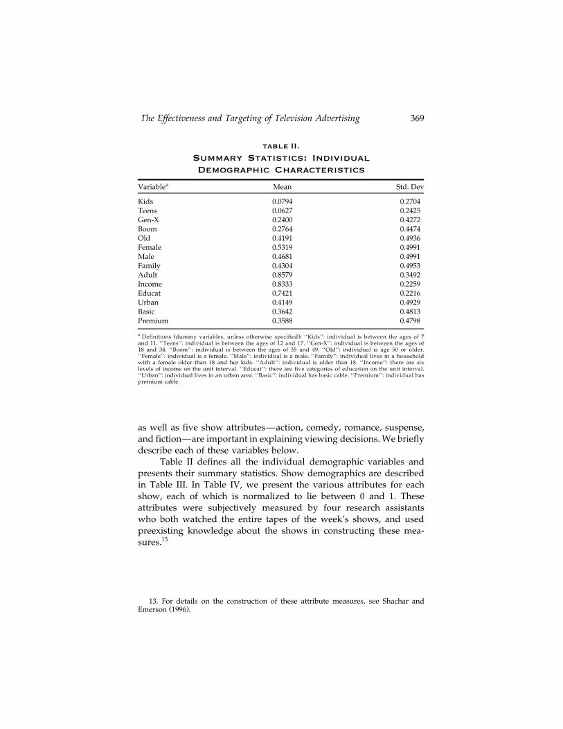
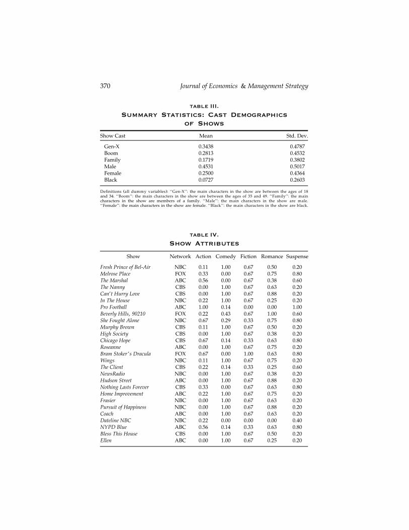
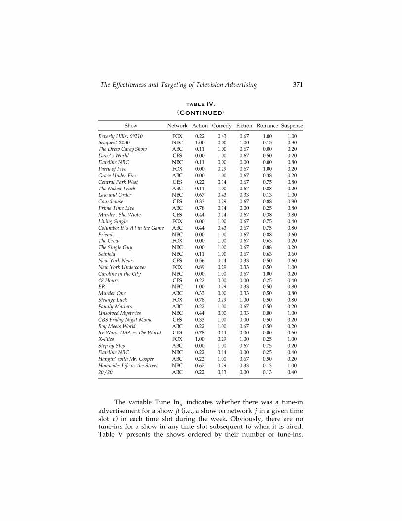
Table II defines all the individual demographic variables andpresents their summary statistics. Show demographics are describedin Table III. In Table IV, we present the various attributes for eachshow, each of which is normalized to lie between 0 and 1. Theseattributes were subjectively measured by four research assistantswho both watched the entire tapes of the week’s shows, and usedpreexisting knowledge about the shows in constructing these mea-sures.13

13. For details on the construction of these attribute measures, see Shachar andŽ .Emerson 1996 .


table III.

Summary Statistics: Cast Demographicsof Shows

Show Cast Mean Std. Dev.

Gen-X 0.3438 0.4787Boom 0.2813 0.4532Family 0.1719 0.3802Male 0.4531 0.5017Female 0.2500 0.4364Black 0.0727 0.2603

Ž .Definitions all dummy variables : ‘‘Gen-X’’: the main characters in the show are between the ages of 18and 34. ‘‘Boom’’: the main characters in the show are between the ages of 35 and 49. ‘‘Family’’: the maincharacters in the show are members of a family. ‘‘Male’’: the main characters in the show are male.‘‘Female’’: the main characters in the show are female. ‘‘Black’’: the main characters in the show are black.

table IV.

Show Attributes

Show Network Action Comedy Fiction Romance Suspense

Fresh Prince of Bel-Air NBC 0.11 1.00 0.67 0.50 0.20Melrose Place FOX 0.33 0.00 0.67 0.75 0.80The Marshal ABC 0.56 0.00 0.67 0.38 0.60The Nanny CBS 0.00 1.00 0.67 0.63 0.20Can’t Hurry Love CBS 0.00 1.00 0.67 0.88 0.20In The House NBC 0.22 1.00 0.67 0.25 0.20Pro Football ABC 1.00 0.14 0.00 0.00 1.00Beverly Hills, 90210 FOX 0.22 0.43 0.67 1.00 0.60She Fought Alone NBC 0.67 0.29 0.33 0.75 0.80Murphy Brown CBS 0.11 1.00 0.67 0.50 0.20High Society CBS 0.00 1.00 0.67 0.38 0.20Chicago Hope CBS 0.67 0.14 0.33 0.63 0.80Roseanne ABC 0.00 1.00 0.67 0.75 0.20Bram Stoker ’s Dracula FOX 0.67 0.00 1.00 0.63 0.80Wings NBC 0.11 1.00 0.67 0.75 0.20The Client CBS 0.22 0.14 0.33 0.25 0.60NewsRadio NBC 0.00 1.00 0.67 0.38 0.20Hudson Street ABC 0.00 1.00 0.67 0.88 0.20Nothing Lasts Forever CBS 0.33 0.00 0.67 0.63 0.80Home Improvement ABC 0.22 1.00 0.67 0.75 0.20Frasier NBC 0.00 1.00 0.67 0.63 0.20Pursuit of Happiness NBC 0.00 1.00 0.67 0.88 0.20Coach ABC 0.00 1.00 0.67 0.63 0.20Dateline NBC NBC 0.22 0.00 0.00 0.00 0.40NYPD Blue ABC 0.56 0.14 0.33 0.63 0.80Bless This House CBS 0.00 1.00 0.67 0.50 0.20Ellen ABC 0.00 1.00 0.67 0.25 0.20


table IV.( )Continued

Show Network Action Comedy Fiction Romance Suspense

Beverly Hills, 90210 FOX 0.22 0.43 0.67 1.00 1.00Seaquest 2030 NBC 1.00 0.00 1.00 0.13 0.80The Drew Carey Show ABC 0.11 1.00 0.67 0.00 0.20Dave’s World CBS 0.00 1.00 0.67 0.50 0.20Dateline NBC NBC 0.11 0.00 0.00 0.00 0.80Party of Five FOX 0.00 0.29 0.67 1.00 0.20Grace Under Fire ABC 0.00 1.00 0.67 0.38 0.20Central Park West CBS 0.22 0.14 0.67 0.75 0.80The Naked Truth ABC 0.11 1.00 0.67 0.88 0.20Law and Order NBC 0.67 0.43 0.33 0.13 1.00Courthouse CBS 0.33 0.29 0.67 0.88 0.80Prime Time Live ABC 0.78 0.14 0.00 0.25 0.80Murder, She Wrote CBS 0.44 0.14 0.67 0.38 0.80Living Single FOX 0.00 1.00 0.67 0.75 0.40Columbo: It’s All in the Game ABC 0.44 0.43 0.67 0.75 0.80Friends NBC 0.00 1.00 0.67 0.88 0.60The Crew FOX 0.00 1.00 0.67 0.63 0.20The Single Guy NBC 0.00 1.00 0.67 0.88 0.20Seinfeld NBC 0.11 1.00 0.67 0.63 0.60New York News CBS 0.56 0.14 0.33 0.50 0.60New York Undercover FOX 0.89 0.29 0.33 0.50 1.00Caroline in the City NBC 0.00 1.00 0.67 1.00 0.2048 Hours CBS 0.22 0.00 0.00 0.25 0.40ER NBC 1.00 0.29 0.33 0.50 0.80Murder One ABC 0.33 0.00 0.33 0.50 0.80Strange Luck FOX 0.78 0.29 1.00 0.50 0.80Family Matters ABC 0.22 1.00 0.67 0.50 0.20Unsolved Mysteries NBC 0.44 0.00 0.33 0.00 1.00CBS Friday Night Movie CBS 0.33 1.00 0.00 0.50 0.20Boy Meets World ABC 0.22 1.00 0.67 0.50 0.20Ice Wars: USA vs The World CBS 0.78 0.14 0.00 0.00 0.60X-Files FOX 1.00 0.29 1.00 0.25 1.00Step by Step ABC 0.00 1.00 0.67 0.75 0.20Dateline NBC NBC 0.22 0.14 0.00 0.25 0.40Hangin’ with Mr. Cooper ABC 0.22 1.00 0.67 0.50 0.20Homicide: Life on the Street NBC 0.67 0.29 0.33 0.13 1.0020r20 ABC 0.22 0.13 0.00 0.13 0.40

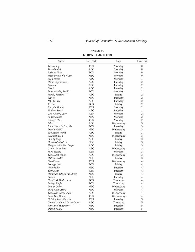
The variable Tune In indicates whether there was a tune-injtŽadvertisement for a show jt i.e., a show on network j in a given time

.slot t in each time slot during the week. Obviously, there are notune-ins for a show in any time slot subsequent to when it is aired.Table V presents the shows ordered by their number of tune-ins.


table V.

Show Tune-Ins

Show Network Day Tune-Ins

The Nanny CBS Monday 0The Marshal ABC Monday 0Melrose Place FOX Monday 0Fresh Prince of Bel-Air NBC Monday 0Pro Football ABC Monday 1Home Improvement ABC Tuesday 2Roseanne ABC Tuesday 2Coach ABC Tuesday 2Beverly Hills, 90210 FOX Monday 2Family Matters ABC Friday 2Wings NBC Tuesday 2NYPD Blue ABC Tuesday 2X-Files FOX Friday 2Murphy Brown CBS Monday 2Hudson Street ABC Tuesday 2Can’t Hurry Love CBS Monday 2In The House NBC Monday 2Chicago Hope CBS Monday 2Ellen ABC Wednesday 3Bram Stoker ’s Dracula FOX Tuesday 3Dateline NBC NBC Wednesday 3Boy Meets World ABC Friday 3Seaquest 2030 NBC Wednesday 3Step by Step ABC Friday 3Unsolved Mysteries NBC Friday 3Hangin’ with Mr. Cooper ABC Friday 3Grace Under Fire ABC Wednesday 3High Society CBS Monday 3The Naked Truth ABC Wednesday 3Dateline NBC NBC Friday 3Courthouse CBS Wednesday 4Strange Luck FOX Friday 4NewsRadio NBC Tuesday 4The Client CBS Tuesday 4Homicide: Life on the Street NBC Friday 4Frasier NBC Tuesday 4New York Undercover FOX Thursday 4Living Single FOX Thursday 4Law & Order NBC Wednesday 4She Fought Alone NBC Monday 4The Drew Carey Show ABC Wednesday 4Bless This House CBS Wednesday 4Nothing Lasts Forever CBS Tuesday 5Columbo: It ’s All in the Game ABC Thursday 5Pursuit of Happiness NBC Tuesday 5Dateline NBC NBC Tuesday 5


table V.( )Continued

Show Network Day Tune-Ins

Beverly Hills, 90210 FOX Wednesday 5The Crew FOX Thursday 5Central Park West CBS Wednesday 5Murder, She Wrote CBS Thursday 6Dave’s World CBS Wednesday 6Party of Five FOX Wednesday 6Prime Time Live ABC Wednesday 6CBS Friday Night Movie CBS Friday 6Seinfeld NBC Thursday 6Friends NBC Thursday 6The Single Guy NBC Thursday 7Ice Wars: USA vs The World CBS Friday 7Caroline in the City NBC Thursday 7Murder One ABC Thursday 8New York News CBS Thursday 820r20 ABC Friday 8ER NBC Thursday 948 Hours CBS Thursday 10

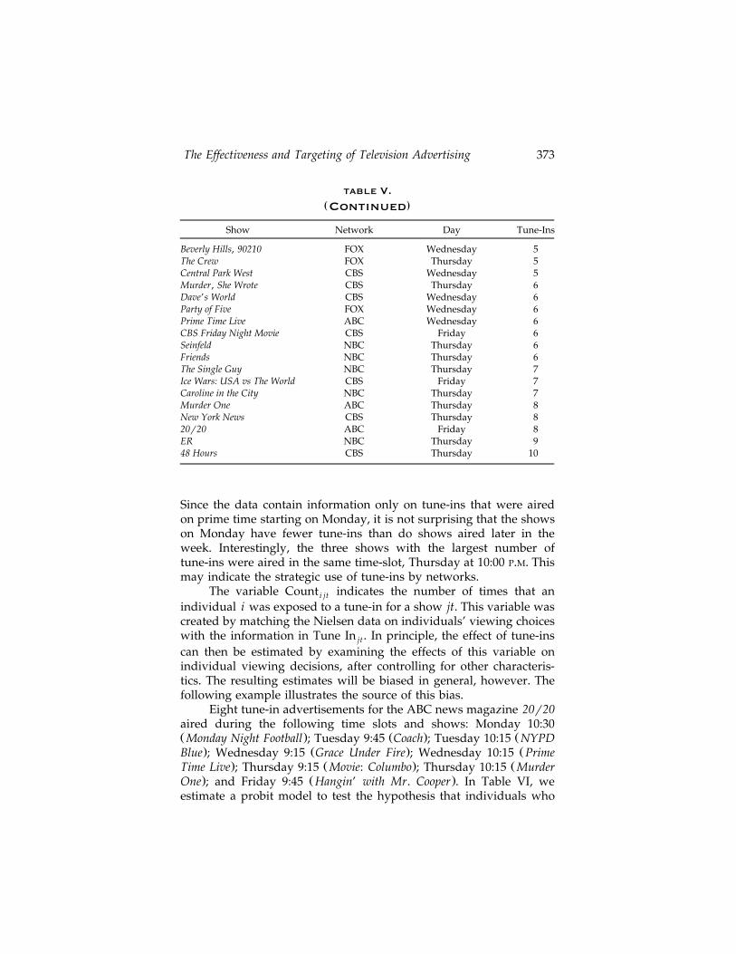
Since the data contain information only on tune-ins that were airedon prime time starting on Monday, it is not surprising that the showson Monday have fewer tune-ins than do shows aired later in theweek. Interestingly, the three shows with the largest number oftune-ins were aired in the same time-slot, Thursday at 10:00 P.M. Thismay indicate the strategic use of tune-ins by networks.

The variable Count indicates the number of times that ani jt

individual i was exposed to a tune-in for a show jt. This variable wascreated by matching the Nielsen data on individuals’ viewing choiceswith the information in Tune In . In principle, the effect of tune-insjt

can then be estimated by examining the effects of this variable onindividual viewing decisions, after controlling for other characteris-tics. The resulting estimates will be biased in general, however. Thefollowing example illustrates the source of this bias.

Eight tune-in advertisements for the ABC news magazine 20r20aired during the following time slots and shows: Monday 10:30Ž . Ž . ŽMonday Night Football ; Tuesday 9:45 Coach ; Tuesday 10:15 NYPD

. Ž . ŽBlue ; Wednesday 9:15 Grace Under Fire ; Wednesday 10:15 Prime. Ž . ŽTime Live ; Thursday 9:15 Movie: Columbo ; Thursday 10:15 Murder

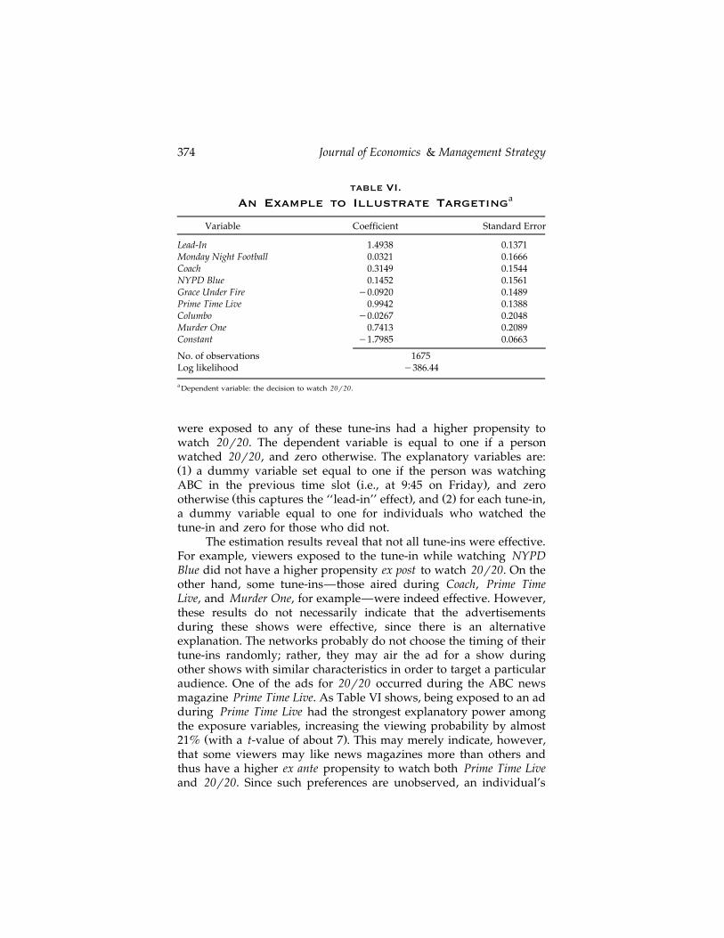
. Ž .One ; and Friday 9:45 Hangin’ with Mr. Cooper . In Table VI, weestimate a probit model to test the hypothesis that individuals who


table VI.aAn Example to Illustrate Targeting

Variable Coefficient Standard Error

Lead-In 1.4938 0.1371Monday Night Football 0.0321 0.1666Coach 0.3149 0.1544NYPD Blue 0.1452 0.1561Grace Under Fire y0.0920 0.1489Prime Time Live 0.9942 0.1388Columbo y0.0267 0.2048Murder One 0.7413 0.2089Constant y1.7985 0.0663

No. of observations 1675Log likelihood y386.44

a Dependent variable: the decision to watch 20r20.

were exposed to any of these tune-ins had a higher propensity towatch 20r20. The dependent variable is equal to one if a personwatched 20r20, and zero otherwise. The explanatory variables are:Ž .1 a dummy variable set equal to one if the person was watching

Ž .ABC in the previous time slot i.e., at 9:45 on Friday , and zeroŽ . Ž .otherwise this captures the ‘‘lead-in’’ effect , and 2 for each tune-in,

a dummy variable equal to one for individuals who watched thetune-in and zero for those who did not.

The estimation results reveal that not all tune-ins were effective.For example, viewers exposed to the tune-in while watching NYPDBlue did not have a higher propensity ex post to watch 20r20. On theother hand, some tune-ins—those aired during Coach, Prime TimeLive, and Murder One, for example—were indeed effective. However,these results do not necessarily indicate that the advertisementsduring these shows were effective, since there is an alternativeexplanation. The networks probably do not choose the timing of theirtune-ins randomly; rather, they may air the ad for a show duringother shows with similar characteristics in order to target a particularaudience. One of the ads for 20r20 occurred during the ABC newsmagazine Prime Time Live. As Table VI shows, being exposed to an adduring Prime Time Live had the strongest explanatory power amongthe exposure variables, increasing the viewing probability by almost

Ž .21% with a t-value of about 7 . This may merely indicate, however,that some viewers may like news magazines more than others andthus have a higher ex ante propensity to watch both Prime Time Liveand 20r20. Since such preferences are unobserved, an individual’s


exposure to tune-ins for 20r20 aired during Prime Time Live isendogenous14 ; hence, the estimate of its effect is biased.

To summarize, since the networks air their tune-ins duringshows with a viewing audience that has a higher ex ante propensityto watch the promoted show, the effect of exposure to an ad onviewing decisions reflects both the effectiveness of the ad and thetargeting of the network. We explicitly deal with this endogeneityproblem in the model below.

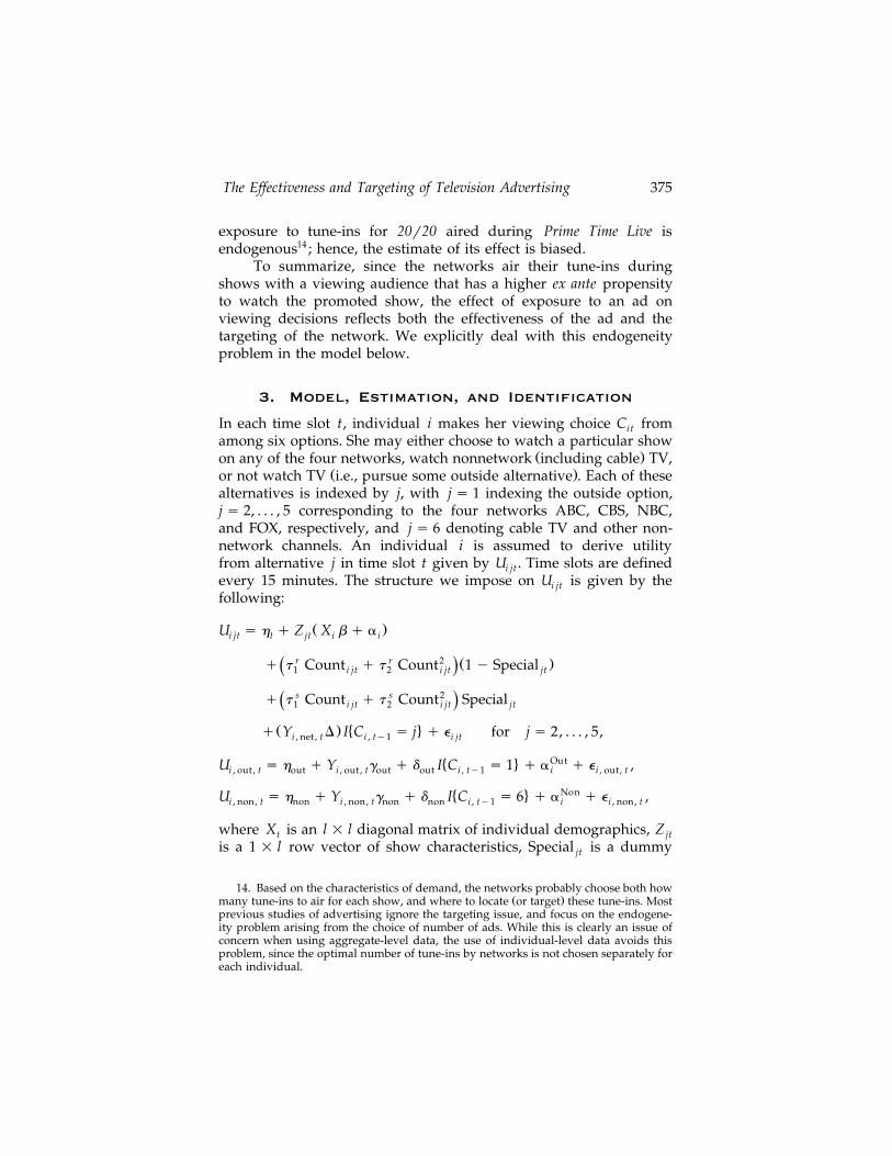
3. Model, Estimation, and Identification

In each time slot t, individual i makes her viewing choice C fromi tamong six options. She may either choose to watch a particular show

Ž .on any of the four networks, watch nonnetwork including cable TV,Ž .or not watch TV i.e., pursue some outside alternative . Each of these

alternatives is indexed by j, with j s 1 indexing the outside option,j s 2, . . . , 5 corresponding to the four networks ABC, CBS, NBC,and FOX, respectively, and j s 6 denoting cable TV and other non-network channels. An individual i is assumed to derive utilityfrom alternative j in time slot t given by U . Time slots are definedi jtevery 15 minutes. The structure we impose on U is given by thei jtfollowing:

Ž .U s h q Z X b q ai jt t jt i i

r r 2 Ž .q t Count q t Count 1 y SpecialŽ .1 i jt 2 i jt jt

q t s Count q t s Count2 SpecialŽ .1 i jt 2 i jt jt

Ž . � 4q Y D I C s j q e for j s 2, . . . , 5,i , net, t i , ty1 i jt

� 4 OutU s h q Y g q d I C s 1 q a q e ,i , out, t out i , out, t out out i , ty1 i i , out, t

� 4 NonU s h q Y g q d I C s 6 q a q e ,i , non, t non i , non, t non non i , ty1 i i , non, t

where X is an l = l diagonal matrix of individual demographics, Zt jtis a 1 = l row vector of show characteristics, Special is a dummyjt

14. Based on the characteristics of demand, the networks probably choose both howŽ .many tune-ins to air for each show, and where to locate or target these tune-ins. Most

previous studies of advertising ignore the targeting issue, and focus on the endogene-ity problem arising from the choice of number of ads. While this is clearly an issue ofconcern when using aggregate-level data, the use of individual-level data avoids thisproblem, since the optimal number of tune-ins by networks is not chosen separately foreach individual.


variable that is equal to one if the show on network j at time t is aspecial, and I is the indicator function. Y is a vector of show andi, net, t

individual characteristics such as show continuity and gender; Yi, out, t

and Y are vectors of individual characteristics such as income,i, non, t

location, age, education, and family size. The detailed structure ofutilities is provided in the Appendix.

We allow for switching costs in individual behavior, as capturedby the parameters d , d and the vector of parameters D. Forout non

example, individuals watching cable TV in a particular time slot maycontinue to watch it in the subsequent time slot due to switchingcosts, thus inducing state dependence. We estimate the switchingcosts in the decision to watch network TV, watch cable TV, or notwatch TV at all, and allow the switching costs to vary for malesŽ . Žrelative to females , and for continuation shows i.e., shows that span

.more than one time slot .The match between individual characteristics15 X and showi

characteristics Z may be an important component of preferences asjt

well. For example, males may be more likely to watch sports shows,teens to watch Beverly Hills 90210, and women to watch shows withfemale casts, less action, and more romance. Such differences inviewing behavior are used to identify the parameters b. The choice ofwhich interaction variables for show and individual characteristics,Z X , to include is essentially ad hoc.16 These variables are definedjt i

only for the various network alternatives, j s 2, . . . , 5.Individuals also may differ in their unobserved preferences, a ,i

over various kinds of shows. For example, some individuals may liketo watch comedies, while others prefer dramas. Moreover, suchheterogeneity may be important even after controlling for simpleobserved differences in preferences across people, as captured by X .iIf tune-ins for comedies are primarily placed in other comedies,viewers who are more likely to watch comedies in the first place willbe exposed to more tune-ins. Separating the effects of tune-ins fromthese unobserved differences in preferences is important for obtain-ing unbiased estimates of tune-in effects.

15. These include age, education, gender, income, and family status here.16. A more comprehensive set of interaction variables is included in Shachar and

Ž .Emerson 1996 . Our choice of which variables to include here is motivated in part bythe results of the estimation there.


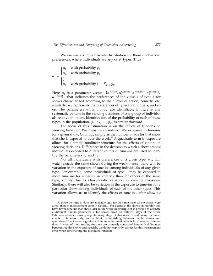
We assume a simple discrete distribution for these unobservedpreferences, where individuals are any of K types. Thus

a with probability p¡ 1 1

a with probability p2 2~a s .i ..¢a with probability 1 y Ý p .k lsk l

� Action Comedy Romance SuspenseHere a is a parameter vector— a , a , a , a ,1 1 1 1 1Fiction4a —that indicates the preferences of individuals of type 1 for1

shows characterized according to their level of action, comedy, etc;similarly, a represents the preferences of type-2 individuals, and so2on. The parameters a , a , . . . , a are identifiable if there is any1 2 Ksystematic pattern in the viewing decisions of one group of individu-als relative to others. Identification of the probability of each of thesetypes in the population, p , p , . . . , p , is straightforward.1 2 K

The focus of this estimation is on the effects of tune-ins onviewing behavior. We measure an individual’s exposure to tune-insfor a given show, Count , simply as the number of ads for that showi jtthat she is exposed to over the week.17 A quadratic term in exposureallows for a simple nonlinear structure for the effects of counts onviewing decisions. Differences in the decision to watch a show amongindividuals exposed to different counts of tune-ins are used to iden-tify the parameters t and t .1 2

Not all individuals with preferences of a given type, a , willkwatch exactly the same shows during the week; hence, there will bevariation in the exposure of tune-ins among individuals of any giventype. For example, some individuals of type 1 may be exposed tomore tune-ins for a particular comedy than for others of the sametype, simply due to idiosyncratic variation in viewing decisions.Similarly, there will also be variation in the exposure to tune-ins for aparticular show among individuals of each of the other types. Thisvariation allows us to identify the effects of tune-ins, after allowing

17. Since the tune-in data are available only for the same week as the shows wereaired, there is measurement error in Count . For example, the shows on Monday willi jthave fewer tune-ins than those later in the week. In principle, it is possible to estimatea different tune-in parameter t for shows aired on different days of the week.Estimates obtained during a preliminary stage of this research—allowing for lineareffects of tune-ins only, and without distinguishing between regular shows andspecials—did not reveal significant differences in tune-in effects for shows on differentdays. In view of these results, since we are primarily concerned here with differencesbetween regular shows and specials, we do not explicitly correct for this measurementerror when constructing the likelihood function.


for individuals’ preferences to vary in unobserved ways. The resultsof the estimation, with and without controlling for unobserved het-erogeneity, are presented in Section 4 below.

In order to estimate the variation in the effects of tune-insaccording to individuals’ prior information about a show, we sepa-

Ž .rate shows into two categories, specials new, one-time shows andregulars. Individuals may be presumed to know more about a regularshow’s characteristics—its time slot, its cast, whether it is a comedy,etc.—than about a special. If the effect of tune-ins does not depend ontheir informational content, these effects should not differ betweenspecials and regulars, i.e., t s and t s would be equal to t r and t r.1 2 1 2Thus, this provides a source of identification of the informationalcontent in advertising relative to other effects, such as persuasion or

Ž .signaling Milgrom and Roberts, 1986 .The informational content of tune-ins may be of two kinds. First,

tune-ins may simply increase awareness about the existence of ashow. Second, they may provide information about the show’s at-tributes.18 Individuals are likely to possess much more informationabout both the existence and attributes of regular shows than aboutthose of specials. For regular shows, then, the role of tune-ins may besimply to serve as reminders of the show’s existence and its at-tributes. Since most of this information could easily be conveyed viaa few tune-ins, the informational value for an individual woulddiminish as the number of tune-ins viewed increases. For specials,however, tune-ins may be important both in informing people aboutthe existence of such a show and in conveying information about itsattributes. Here, a single tune-in is unlikely to be nearly as effective;instead, a series of tune-ins may be necessary to convey informationabout the different aspects of a new show. For the same reason,although diminishing marginal effectiveness of tune-ins should applyhere as well, the rate at which these returns diminish is likely to besmaller than for regular shows. According to this simple characteriza-tion of the informational content in tune-ins, the marginal value of

Ž .tune-ins should be larger for regular shows relative to specials atlow levels of tune-ins, but should decline more rapidly as well. Moregenerally, however, the identification strategy is based on the logicthat if tune-ins convey information, their effectiveness is likely to

18. A similar distinction between the informational roles of advertising has beenŽ .made in the previous literature. Butters 1977 , for example, focuses on the role of

advertising in conveying information about a product’s existence and its price. Gross-Ž .man and Shapiro 1984 augment this to consider information about a product’s other

Ž .attributes such as location as well.


differ across shows for which viewers possess different preexistingstocks of information. We return to a discussion of these differenteffects in our presentation of the results.

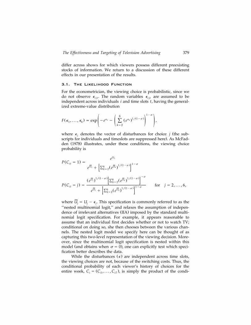
3.1. The Likelihood Function

For the econometrician, the viewing choice is probabilistic, since wedo not observe e . The random variables e are assumed to bei jt i jtindependent across individuals i and time slots t, having the general-ized extreme-value distribution

1ys6Ž .1r 1yse e1 kŽ . Ž .F e , . . . , e s exp ye y e ,Ý1 6 ž /ž /ks2

Žwhere e denotes the vector of disturbances for choice j the sub-j.scripts for individuals and timeslots are suppressed here . As McFad-

Ž .den 1978 illustrates, under these conditions, the viewing choiceprobability is

U1eŽ .P C s 1 si t 1ysŽ .1r 1ysU 6 U1 kŽ .e q Ý eks2

ysŽ . Ž .1r 1ys 1r 1ysU 6 Uj kŽ . Ž .e Ý eks2Ž .P C s j s for j s 2, . . . , 6,i t 1ysŽ .1r 1ysU 6 U1 kŽ .e q Ý eks2

where U s U y e . This specification is commonly referred to as thej j j

‘‘nested multinomial logit,’’ and relaxes the assumption of indepen-Ž .dence of irrelevant alternatives IIA imposed by the standard multi-

nomial logit specification. For example, it appears reasonable toassume that an individual first decides whether or not to watch TV;conditional on doing so, she then chooses between the various chan-nels. The nested logit model we specify here can be thought of ascapturing this two-level representation of the viewing decision. More-over, since the multinomial logit specification is nested within this

Ž .model and obtains when s s 0 , one can explicitly test which speci-fication better describes the data.

Ž .While the disturbances e are independent across time slots,the viewing choices are not, because of the switching costs. Thus, theconditional probability of each viewer’s history of choices for the

Ž .entire week, C s C , . . . , C , is simply the product of the condi-i i1 iT


tional probabilities of each of his or her choices made at each quarterhour. That is, for a type-k person,

Tk kŽ < . Ž < . Ž .f C V ; a , u s P C s j V , C ; a , u , 3.1Łi i i t i t i t i , ty1

ts1

� 4 Žwhere V s Z , X , Count , Special , Y , Y , Y alli t jt i i jt jt i, out, t i, non, t i, non, t

observed individual and show characteristics as well as the lagged.choices , and the vector u includes of all the parameters in the model

other than the a’s.Since we do not observe each viewer’s type, we integrate out

these unobservable preferences. The resulting marginal distribution is

KkŽ < . Ž < . Ž .f C V ; u , a , P s f C V ; u , a ? p 3.2Ý2 i i 1 i i k

ks1

where P is a vector of type probabilities, p , . . . , p , for K viewer1 Ktypes.

Because the e and the type probabilities are independenti t jacross individuals, the likelihood function is simply the product ofthe probabilities of each individual’s history of viewing choices. Theparameters u , a , . . . , a , and P are chosen to maximize the log-like-1 Klihood function given by

N

Ž . Ž < . Ž .log L u , a , P s log f C V ; u , a , P , 3.3Ý 2 i iis1

where N denotes the number of individuals.The estimates of the structural parameters obtained are dis-

cussed below.

4. Results

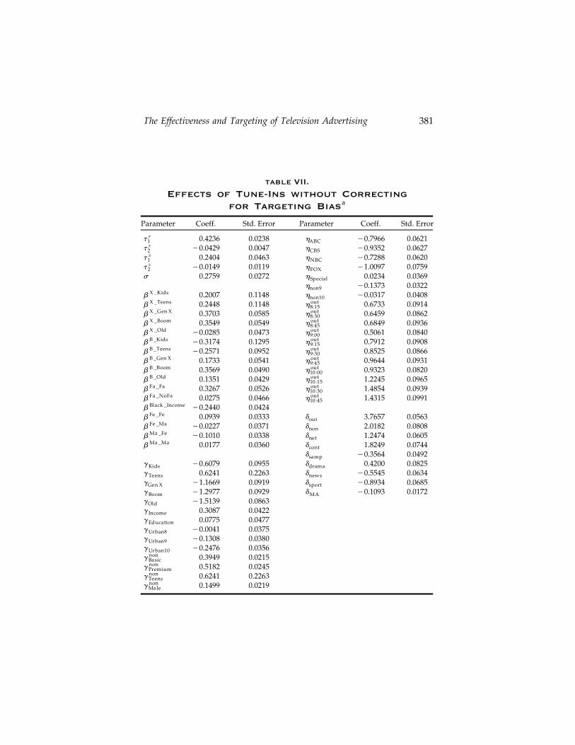
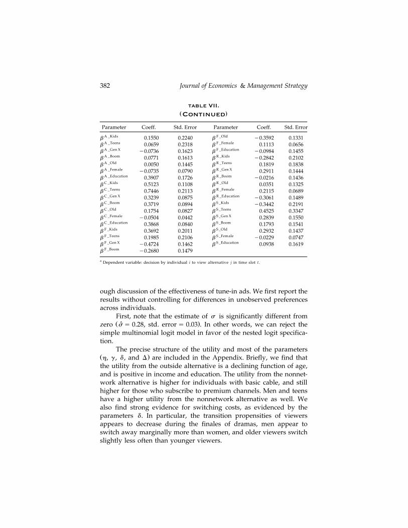
Most of the estimates in Table VII are motivated and discussedelsewhere.19 We present them briefly here and then turn to a thor-

Ž .19. See Shachar and Emerson 1996 .


table VII.

Effects of Tune-Ins without Correctingafor Targeting Bias

Parameter Coeff. Std. Error Parameter Coeff. Std. Error

rt 0.4236 0.0238 h y0.7966 0.06211 ABCrt y0.0429 0.0047 h y0.9352 0.06272 CBSst 0.2404 0.0463 h y0.7288 0.06201 NBCst y0.0149 0.0119 h y1.0097 0.07592 FOX

s 0.2759 0.0272 h 0.0234 0.0369Specialh y0.1373 0.0322non9

X Kids]b 0.2007 0.1148 h y0.0317 0.0408non10X Teens out]b 0.2448 0.1148 h 0.6733 0.09148:15X Gen X out]b 0.3703 0.0585 h 0.6459 0.08628:30X Boom out]b 0.3549 0.0549 h 0.6849 0.09368:45X Old out]b y0.0285 0.0473 h 0.5061 0.08409:00B Kids out]b y0.3174 0.1295 h 0.7912 0.09089:15B Teens out]b y0.2571 0.0952 h 0.8525 0.08669:30B Gen X out]b 0.1733 0.0541 h 0.9644 0.09319:45B Boom out]b 0.3569 0.0490 h 0.9323 0.082010:00B Old out]b 0.1351 0.0429 h 1.2245 0.096510:15Fa Fa out]b 0.3267 0.0526 h 1.4854 0.093910:30Fa NoFa out]b 0.0275 0.0466 h 1.4315 0.099110:45

b Black ]Income y0.2440 0.0424Fe Fe]b 0.0939 0.0333 d 3.7657 0.0563outFe Ma]b y0.0227 0.0371 d 2.0182 0.0808nonMa Fe]b y0.1010 0.0338 d 1.2474 0.0605netMa Ma]b 0.0177 0.0360 d 1.8249 0.0744cont

d y0.3564 0.0492sampg y0.6079 0.0955 d 0.4200 0.0825Kids dramag 0.6241 0.2263 d y0.5545 0.0634Teens newsg y1.1669 0.0919 d y0.8934 0.0685Gen X sportg y1.2977 0.0929 d y0.1093 0.0172Boom MAg y1.5139 0.0863Oldg 0.3087 0.0422Incomeg 0.0775 0.0477Educationg y0.0041 0.0375Urban8g y0.1308 0.0380Urban9g y0.2476 0.0356Urban10

nong 0.3949 0.0215Basicnong 0.5182 0.0245Premiumnong 0.6241 0.2263Teensnong 0.1499 0.0219Male


table VII.( )Continued


A Kids F Old] ]b 0.1550 0.2240 b y0.3592 0.1331A Teens F Female] ]b 0.0659 0.2318 b 0.1113 0.0656A Gen X F Education] ]b y0.0736 0.1623 b y0.0984 0.1455A Boom R Kids] ]b 0.0771 0.1613 b y0.2842 0.2102A Old R Teens] ]b 0.0050 0.1445 b 0.1819 0.1838A Female R Gen X] ]b y0.0735 0.0790 b 0.2911 0.1444A Education R Boom] ]b 0.3907 0.1726 b y0.0216 0.1436C Kids R Old] ]b 0.5123 0.1108 b 0.0351 0.1325C Teens R Female] ]b 0.7446 0.2113 b 0.2115 0.0689C Gen X R Education] ]b 0.3239 0.0875 b y0.3061 0.1489C Boom S Kids] ]b 0.3719 0.0894 b y0.3442 0.2191C Old S Teens] ]b 0.1754 0.0827 b 0.4525 0.3347C Female S Gen X] ]b y0.0504 0.0442 b 0.2839 0.1550C Education S Boom] ]b 0.3868 0.0840 b 0.1793 0.1541F Kids S Old] ]b 0.3692 0.2011 b 0.2932 0.1437F Teens S Female] ]b 0.1985 0.2106 b y0.0229 0.0747F Gen X S Education] ]b y0.4724 0.1462 b 0.0938 0.1619

b F ]Boom y0.2680 0.1479

a Dependent variable: decision by individual i to view alternative j in time slot t.

ough discussion of the effectiveness of tune-in ads. We first report theresults without controlling for differences in unobserved preferencesacross individuals.

First, note that the estimate of s is significantly different fromŽ .zero s s 0.28, std. error s 0.03 . In other words, we can reject theˆ

simple multinomial logit model in favor of the nested logit specifica-tion.

The precise structure of the utility and most of the parametersŽ .h, g , d , and D are included in the Appendix. Briefly, we find thatthe utility from the outside alternative is a declining function of age,and is positive in income and education. The utility from the nonnet-work alternative is higher for individuals with basic cable, and stillhigher for those who subscribe to premium channels. Men and teenshave a higher utility from the nonnetwork alternative as well. Wealso find strong evidence for switching costs, as evidenced by theparameters d . In particular, the transition propensities of viewersappears to decrease during the finales of dramas, men appear toswitch away marginally more than women, and older viewers switchslightly less often than younger viewers.


The b parameters suggest that ‘‘likes attract.’’ In particular,individuals prefer shows whose cast demographics are similar totheir own. For example, shows with a generation-X cast are mostpreferred by generation-X viewers, and baby boomers like to watchshows with baby boomers in the cast. Similarly, viewers prefer towatch shows about people of their own gender, and families likeshows about families more than people who live alone. Finally,

Žlow-income people prefer shows with blacks in a central role notethat we have used the income variable for individuals as a proxy for

.their race .Viewers in different age groups do not differ much in their

preference for ‘‘action.’’ However, younger viewers like comedies aswell as shows with a high fiction level. Generation-Xers tend to watchromantic shows, whereas kids do not. Kids also do not like to watchshows with a high element of suspense, relative to other viewers.Finally, women like watching romantic shows more than men; andeducated people like action and comedy, but do not appreciateromance.

4.1. Effects of Tune-Ins

We now turn to the effect of the tune-in variables, which are the focusof this study. We find that the utility from a show is a positive,concave function of the number of times the individual was exposedto its ads, indicating that while tune-ins are effective, they havediminishing returns. The first exposure to an ad for a regular showincreases the probability of watching the shows by more than 41%;the second exposure increases this probability by an additional 29%,and the third by about 17%. We interpret the strong response to thefirst few ads for regular shows as an awareness effect: viewers alreadyknow how much they like a given show, and the main purpose of thead is to remind them of the timing of the show, for example. Notethat one exposure to an ad may not be enough to achieve this effect,since viewers, while exposed, may often ignore the television duringcommercial breaks. Furthermore, some people may need more thanone reminder in order not to forget.20 Thus, the second and the third

Ž .exposures have a positive but smaller effect on the individual’sprobability of watching the promoted show.

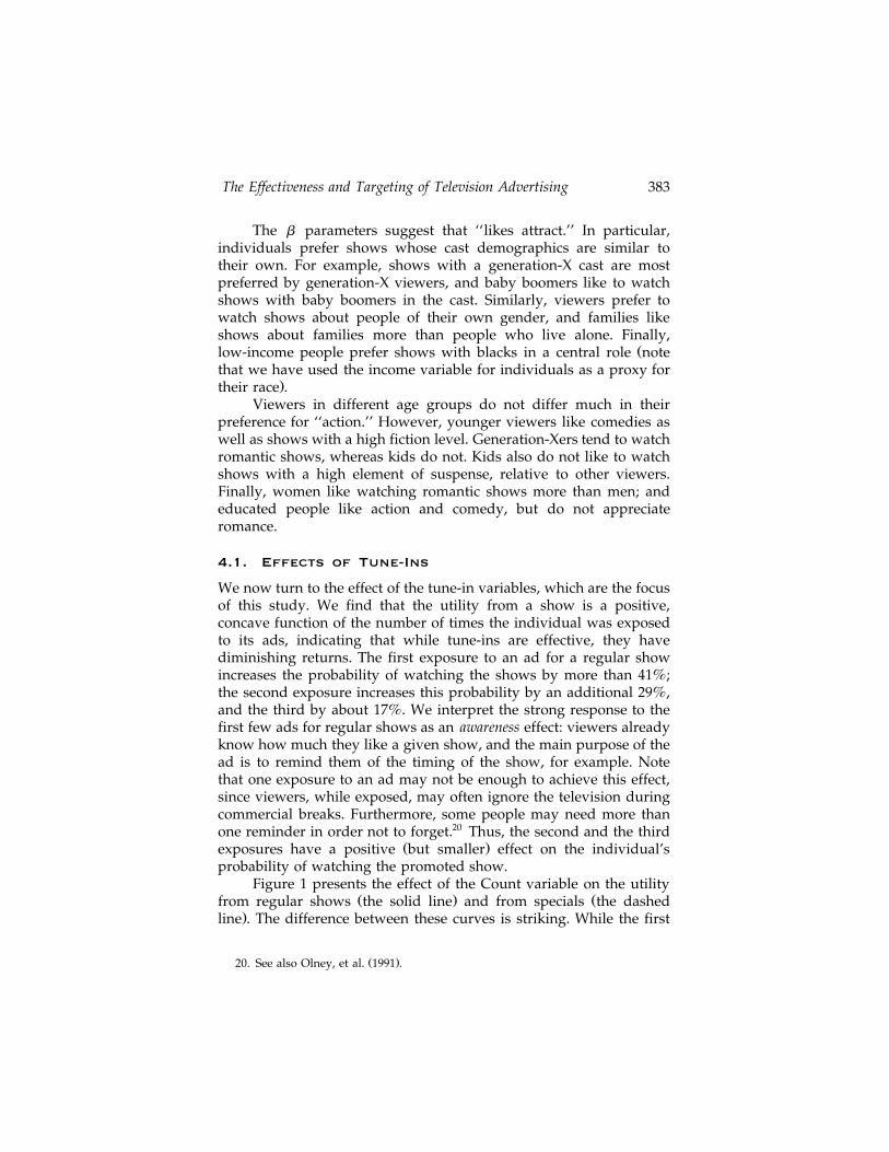
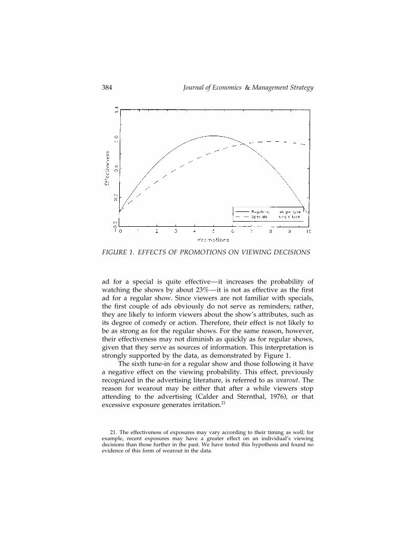
Figure 1 presents the effect of the Count variable on the utilityŽ . Žfrom regular shows the solid line and from specials the dashed

.line . The difference between these curves is striking. While the first

Ž .20. See also Olney, et al. 1991 .


FIGURE 1. EFFECTS OF PROMOTIONS ON VIEWING DECISIONS

ad for a special is quite effective—it increases the probability ofwatching the shows by about 23%—it is not as effective as the firstad for a regular show. Since viewers are not familiar with specials,the first couple of ads obviously do not serve as reminders; rather,they are likely to inform viewers about the show’s attributes, such asits degree of comedy or action. Therefore, their effect is not likely tobe as strong as for the regular shows. For the same reason, however,their effectiveness may not diminish as quickly as for regular shows,given that they serve as sources of information. This interpretation isstrongly supported by the data, as demonstrated by Figure 1.

The sixth tune-in for a regular show and those following it havea negative effect on the viewing probability. This effect, previouslyrecognized in the advertising literature, is referred to as wearout. Thereason for wearout may be either that after a while viewers stop

Ž .attending to the advertising Calder and Sternthal, 1976 , or thatexcessive exposure generates irritation.21

21. The effectiveness of exposures may vary according to their timing as well; forexample, recent exposures may have a greater effect on an individual’s viewingdecisions than those further in the past. We have tested this hypothesis and found noevidence of this form of wearout in the data.


4.2. Controlling for the Targeting Bias

The estimates of tune-in effectiveness may be biased, as discussedabove, since the variable capturing an individual’s exposure to tune-ins is probably endogenous. In order to correct for this, we estimate

Žthe effect of ads, while allowing for K-types of viewers as outlined in.Section 3 , each with potentially different preferences over the shows’Ž .attributes such as comedy and action .

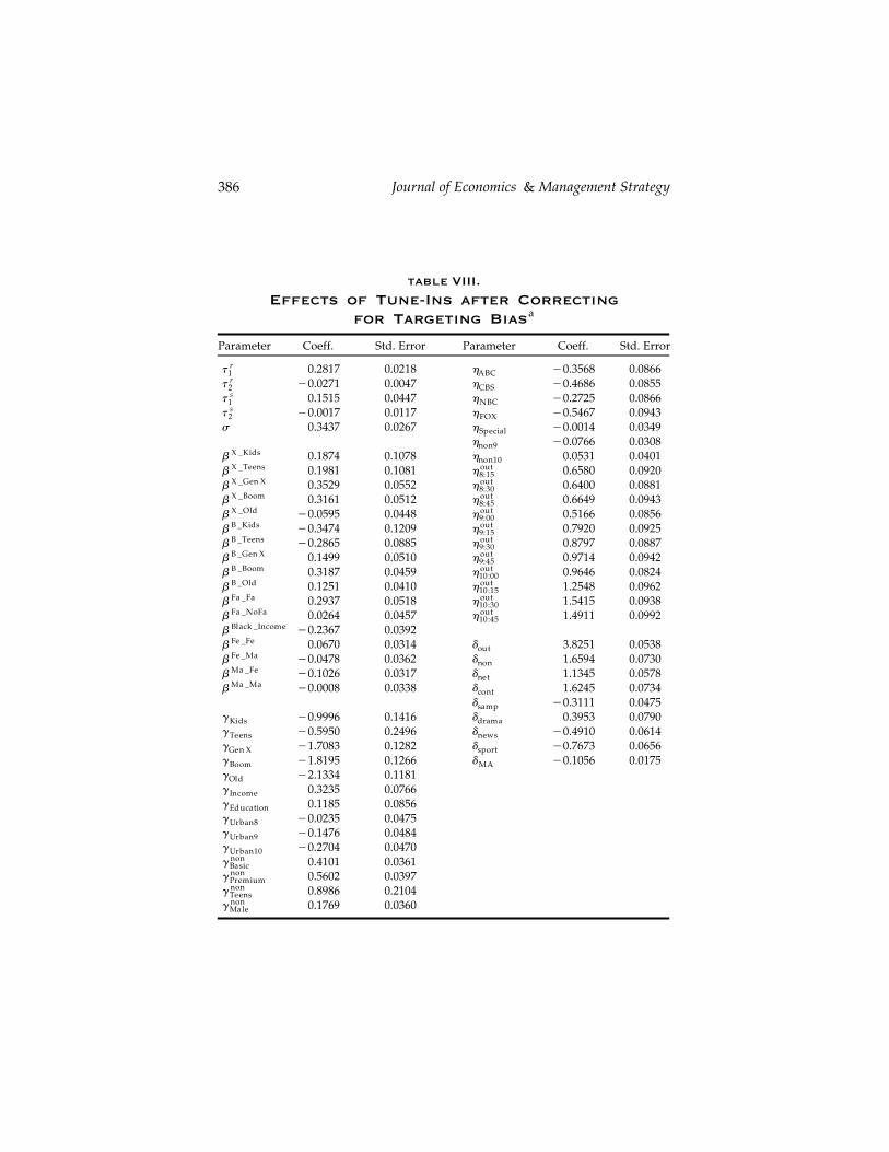
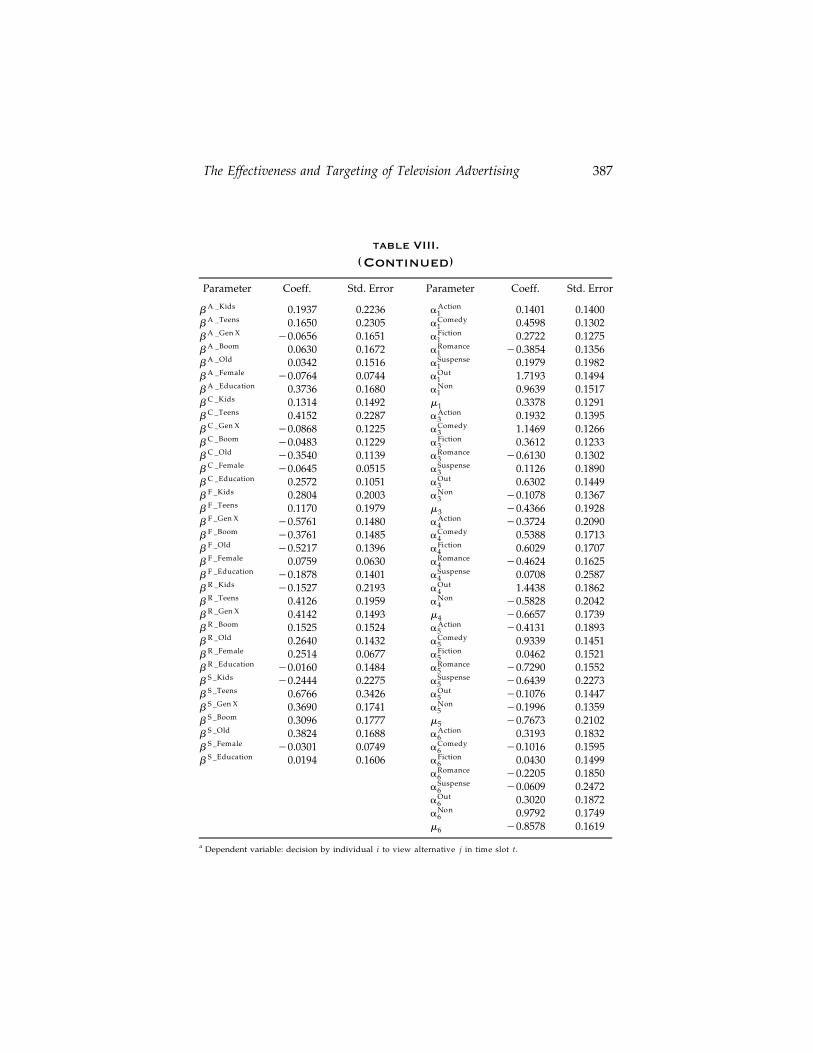
We report the results of the estimation with six types of viewersin Table VIII.22 As expected, the effectiveness of tune-ins decreaseswhen we control for unobserved heterogeneity of preferences overthe show types, as demonstrated in Figure 2. This confirms the bias inour previous estimates of the effectiveness of ads, induced by the

Ž .networks’ targeting strategies. However, notice that 1 tune-ins areŽ .still strongly effective, and 2 the difference between the effects of

tune-ins for specials and regular shows is similar to that estimatedearlier.

The six types of viewers differ substantially in their viewingpatterns. These differences can be illustrated by examining the types’distinct preferences and their viewing choices. To infer these choices,we distribute each individual in our sample to one of the types. Theprior distribution for each individual over the various types is de-fined by the estimated probabilities p , . . . , p . Based on their view-1 king history and using Bayes’s rule, we then estimate the posteriortype probability for each individual, and assign her to the group forwhich her posterior type probability is the highest.

The types are ordered in Table VIII according to their size.23 TheŽ .largest type 31.2% rarely watch television. Only 6% of them watch

the highest-rated show for this type, the football game. The secondŽ .largest type 22.3% prefer to watch shows with a high level of

suspense and romance, but dislike comedies, relative to other types.ŽThus, it is not surprising that their top five shows are ER watched

.by 36% of them , the CBS Tuesday Night Movie, Beverly Hills 90210Žwhich had, relatively, high levels of action and suspense during this

.week’s episodes , the football game, and NYPD Blue. Moreover, eachof these shows is on a different network, indicating that these viewersare not loyal to any particular network. Further, although Seinfeld is

22. We did not test for a seventh type, since adding the fifth and sixth types barelyaffected the estimated tune-in effects.

23. Group sizes are based on the estimated probabilities of an individual belongingto each type, p , . . . , p . These are calculated directly from the estimates m , . . . , m in1 6 1 6

mk Ž K m k.Table VIII, where p s e r 1 q Ý e for k s 1, . . . , 6 and m is normalized to 0.k ks1 2


table VIII.

Effects of Tune-Ins after Correctingafor Targeting Bias


rt 0.2817 0.0218 h y0.3568 0.08661 ABCrt y0.0271 0.0047 h y0.4686 0.08552 CBSst 0.1515 0.0447 h y0.2725 0.08661 NBCst y0.0017 0.0117 h y0.5467 0.09432 FOX

s 0.3437 0.0267 h y0.0014 0.0349Specialh y0.0766 0.0308non9

X Kids]b 0.1874 0.1078 h 0.0531 0.0401non10X Teens out]b 0.1981 0.1081 h 0.6580 0.09208:15X Gen X out]b 0.3529 0.0552 h 0.6400 0.08818:30X Boom out]b 0.3161 0.0512 h 0.6649 0.09438:45X Old out]b y0.0595 0.0448 h 0.5166 0.08569:00B Kids out]b y0.3474 0.1209 h 0.7920 0.09259:15B Teens out]b y0.2865 0.0885 h 0.8797 0.08879:30B Gen X out]b 0.1499 0.0510 h 0.9714 0.09429:45B Boom out]b 0.3187 0.0459 h 0.9646 0.082410:00B Old out]b 0.1251 0.0410 h 1.2548 0.096210:15Fa Fa out]b 0.2937 0.0518 h 1.5415 0.093810:30Fa NoFa out]b 0.0264 0.0457 h 1.4911 0.099210:45

b Black ]Income y0.2367 0.0392Fe Fe]b 0.0670 0.0314 d 3.8251 0.0538outFe Ma]b y0.0478 0.0362 d 1.6594 0.0730nonMa Fe]b y0.1026 0.0317 d 1.1345 0.0578netMa Ma]b y0.0008 0.0338 d 1.6245 0.0734cont

d y0.3111 0.0475sampg y0.9996 0.1416 d 0.3953 0.0790Kids dramag y0.5950 0.2496 d y0.4910 0.0614Teens newsg y1.7083 0.1282 d y0.7673 0.0656Gen X sportg y1.8195 0.1266 d y0.1056 0.0175Boom MAg y2.1334 0.1181Oldg 0.3235 0.0766Incomeg 0.1185 0.0856Educationg y0.0235 0.0475Urban8g y0.1476 0.0484Urban9g y0.2704 0.0470Urban10

nong 0.4101 0.0361Basicnong 0.5602 0.0397Premiumnong 0.8986 0.2104Teensnong 0.1769 0.0360Male


table VIII.( )Continued


A Kids Action]b 0.1937 0.2236 a 0.1401 0.14001A Teens Comedy]b 0.1650 0.2305 a 0.4598 0.13021A Gen X Fiction]b y0.0656 0.1651 a 0.2722 0.12751A Boom Romance]b 0.0630 0.1672 a y0.3854 0.13561A Old Suspense]b 0.0342 0.1516 a 0.1979 0.19821A Female Out]b y0.0764 0.0744 a 1.7193 0.14941A Education Non]b 0.3736 0.1680 a 0.9639 0.15171C Kids]b 0.1314 0.1492 m 0.3378 0.12911C Teens Action]b 0.4152 0.2287 a 0.1932 0.13953C Gen X Comedy]b y0.0868 0.1225 a 1.1469 0.12663C Boom Fiction]b y0.0483 0.1229 a 0.3612 0.12333C Old Romance]b y0.3540 0.1139 a y0.6130 0.13023C Female Suspense]b y0.0645 0.0515 a 0.1126 0.18903C Education Out]b 0.2572 0.1051 a 0.6302 0.14493F Kids Non]b 0.2804 0.2003 a y0.1078 0.13673F Teens]b 0.1170 0.1979 m y0.4366 0.19283F Gen X Action]b y0.5761 0.1480 a y0.3724 0.20904F Boom Comedy]b y0.3761 0.1485 a 0.5388 0.17134

b F ]Old y0.5217 0.1396 aFiction 0.6029 0.17074F Female Romance]b 0.0759 0.0630 a y0.4624 0.16254F Education Suspense]b y0.1878 0.1401 a 0.0708 0.25874R Kids Out]b y0.1527 0.2193 a 1.4438 0.18624R Teens Non]b 0.4126 0.1959 a y0.5828 0.20424R Gen X]b 0.4142 0.1493 m y0.6657 0.17394R Boom Action]b 0.1525 0.1524 a y0.4131 0.18935R Old Comedy]b 0.2640 0.1432 a 0.9339 0.14515R Female Fiction]b 0.2514 0.0677 a 0.0462 0.15215R Education Romance]b y0.0160 0.1484 a y0.7290 0.15525S Kids Suspense]b y0.2444 0.2275 a y0.6439 0.22735S Teens Out]b 0.6766 0.3426 a y0.1076 0.14475S Gen X Non]b 0.3690 0.1741 a y0.1996 0.13595S Boom]b 0.3096 0.1777 m y0.7673 0.21025S Old Action]b 0.3824 0.1688 a 0.3193 0.18326S Female Comedy]b y0.0301 0.0749 a y0.1016 0.15956S Education Fiction]b 0.0194 0.1606 a 0.0430 0.14996

Romancea y0.2205 0.18506Suspensea y0.0609 0.24726Outa 0.3020 0.18726

aNon 0.9792 0.17496m y0.8578 0.16196

a Dependent variable: decision by individual i to view alternative j in time slot t.


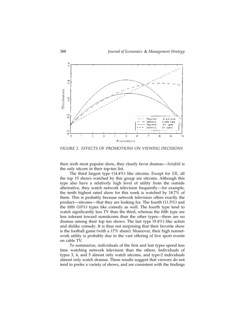
FIGURE 2. EFFECTS OF PROMOTIONS ON VIEWING DECISIONS

their sixth most popular show, they clearly favor dramas—Seinfeld isthe only sitcom in their top-ten list.

Ž .The third largest type 14.4% like sitcoms. Except for ER, allthe top 15 shows watched by this group are sitcoms. Although thistype also have a relatively high level of utility from the outsidealternative, they watch network television frequently—for example,the tenth highest rated show for this week is watched by 18.7% ofthem. This is probably because network television offers exactly the

Ž .product—sitcoms—that they are looking for. The fourth 11.5% andŽ .the fifth 10% types like comedy as well. The fourth type tend to

watch significantly less TV than the third, whereas the fifth type areless tolerant toward nonsitcoms than the other types—there are no

Ž .dramas among their top ten shows. The last type 9.4% like actionand dislike comedy. It is thus not surprising that their favorite show

Ž .is the football game with a 17% share . Moreover, their high nonnet-work utility is probably due to the vast offering of live sport eventson cable TV.

To summarize, individuals of the first and last types spend lesstime watching network television than the others. Individuals oftypes 3, 4, and 5 almost only watch sitcoms, and type-2 individualsalmost only watch dramas. These results suggest that viewers do nottend to prefer a variety of shows, and are consistent with the findings


Ž .of Goettler and Shachar 1996 . Moreover, since the networks fre-quently air a tune-in for a drama during other dramas and for asitcom during other sitcoms, the estimate of the tune-in effectivenesswould be upward-biased without controlling for the differences be-tween these types. The differences between the other types are ofsignificance as well. For example, type-1 individuals are less likely towatch any television show and thus are less exposed to tune-ins.Without controlling for differences in preferences between these indi-viduals and others, the relationship between the number of exposuresto tune-ins and the propensity to watch television would also influ-ence our estimate of t ’s.

5. Are Network Strategies Optimal?

In this section, we return to the question that we presented at theoutset: do networks’ expenditures on advertising exceed the profit-maximizing level? To answer this, we first present a simple model,

Ž .which we solve for the optimal profit-maximizing number of tune-ins for each show; then, we compare this with the actual number oftune-ins chosen by the network.

Network j should choose the number of tune-ins for show kthat maximizes its expected profit function. If the network airs Ck

Ž .tune-ins—each of length L in seconds , on average—for show k, itkloses advertising fees that depend on the ratings of the shows duringwhich these tune-ins aired. Here, we do not solve for the network’sdecision of when to air each tune-in; thus, we proxy these lostadvertising fees for each tune-in by

P ? Rating ? Lj k

where P is the fee that advertisers pay for an expected exposure ofone viewer for one second.24 Thus, for C tune-ins, the network’s lostkfees are P ? Rating ? L ? C . We proxy for Rating as the averagej k k j

Ž .rating of network j over all time slots .The network’s expected revenues from airing C tune-ins fork

show k will depend on the effect of these tune-ins on the ratings forŽ < .that show. Let E Rating C denote the expected number of viewersk k

for show k, given C . Then expected revenues are given byk

Ž < .P ? AD ? E Rating Ck k k

24. Note that an increase in the amount of tune-in time for a show—which dependson C —reduces the supply of advertising time, which may result in a decline in P askwell. We ignore this effect here.


Ž .where AD is the length in seconds of commercial advertising timekavailable during show k.25 Thus, the network’s profit function is

Ž < . Ž .p s P ? AD ? E Rating C y P ? C L ? Ratingjk k k k k k j

We substitute for L using actual figures during this week for eachkŽ < .show, and base E Rating C on our estimation results. We thenk k

solve for the profit-maximizing number of tune-ins for each show andeach network.26

We estimate the optimal number of tune-ins, CU , to be 4 forkalmost all the 58 regular shows, and higher for all the specials.27 Thereason for the lack of variation in CU across the shows can bekexplained as follows. From the first-order condition, the marginalprofit is equal to zero when

Ž < .dE Rating C rdC Lk k k k Ž .s 5.1Rating ADk k

Consider, for example, this optimization for a sitcom. For most such1 Žshows, L rAD s . If the average network rating over all itsk k 30

.shows , Rating , is close enough to the expected rating for a show,j

Ž .E Rating —which is indeed the case for most of these shows—thenkŽ .the expression on the left-hand side in equation 5.1 gives the

percentage effect of the marginal tune-in on the expected rating of theshow. For a regular show, this was estimated to be 10% of the fourthtune-in, and about 0% for the fifth tune-in; this suggests that thefourth tune-in would be profitable for almost all sitcoms, but the fifthwould not. A similar argument holds for nonsitcom regular shows aswell.

Without further distinguishing regular shows according to theirŽ .information stock some shows are better known than others and

according to the effectiveness of tune-ins across such shows, weŽcannot explain the source of actual variation in C . It should bek

25. This is equal to 6 minutes for each 30-minute segment.26. In reality networks do not advertise their shows on the other networks. This is a

rule of the game, and we take it as such. Examining the logic of this rule is beyond thescope of this study.

27. The optimal number of tune-ins for specials is 8. However, since the variance ofthe estimate of t s is high, the variance of the estimated optimal number of tune-ins is2high as well. Notice also that while we estimate the effectiveness of tune-ins forspecials to be a concave function, we cannot reject the hypothesis that the effectiveness

Žof tune-ins for specials is a linear or a convex function i.e., we cannot reject thes .hypothesis t G 0 . Thus, we would not like to make too much of this result.2


.noted, however, that this variation is small. Our model neverthelesshas two important predictions. First, regular shows should have asmaller number of tune-ins than specials. Second, regular showsshould have about 4 tune-ins, on average. As it turns out, networkstrategies are closely consistent with these implications: the average

Ž .number of tune-ins for specials is 5 with a standard deviation of 1.4 ,Ž .and for regular shows is 3.8 with a standard deviation of 2.25 . It is

not surprising that observed strategies are consistent with our firstprediction. But the consistency with our second prediction is reveal-ing, because it indicates that network executives appear to be ontarget in assessing the effect of tune-ins on viewers’ choices.

The model we have presented here is stylized.28 Nevertheless,these results do suggest that network expenditures on advertising aresimilar to the levels that maximize their respective profits.

6. Conclusion

While the expenditures on tune-in advertisements by TV networksmay appear excessive, we find that they are similar to what ispredicted by a simple model of profit maximization by the networks.Exposure to a maximum of four tune-ins for a show has a dramaticeffect on an individual’s decision to watch that show. We also findthat the effectiveness of advertising differs between specials andregular shows. Since the main difference between these kinds ofshows is in the prior information that individuals possess about each,this result is indicative of informational content in advertising.

While we have established here the value of information inadvertising, it would be interesting to examine the nature of thisinformation in more detail. The differential effectiveness of advertis-ing between specials and regular shows suggests that advertisingconveys at least two distinct types of information—information abouta show’s existence and information about its attributes. In order toidentify each of these effects, it would be useful first to construct a

28. One issue that we have not explicitly modeled, for example, is the role ofŽ .advertisements as signals see Milgrom and Roberts, 1986 ; according to this, shows

with many ads are inferred to be of higher quality, which in turn increases thepropensity to watch the show. We are not concerned with the signaling hypothesis,however, for various reasons. First, it predicts that the effectiveness of ads shouldincrease with the number of exposures, contrary to the wearout effect observed in thedata. Second, our results rest on the difference in the effectiveness of specials versusregular shows, not on the distinction between the persuasive effect and the signalingeffect, which may be viewed as one of interpretation. Finally, clarifying whether adsare signals or simply persuasive, though likely to affect the socially efficient level ofadvertisements, should not change the implications for profit maximization.


model that explicitly incorporates the uncertainty about the alterna-tives in an individual’s choice set as well as the utility derived fromeach alternative. The dataset we use may also be appropriate instructurally estimating such a model. The resulting estimates con-cerning the relative importance of each type of information may beuseful in determining a firm’s strategy, as well as in normativeanalysis.

Finally, our estimates of the effects of tune-ins allow for thepossibility of networks targeting particular audiences in schedulingtheir tune-ins. Since such strategies imply that an individual’s expo-sure to tune-ins may be correlated with her unobserved preferences,estimates that do not correct for this endogeneity will be upwardbiased. Indeed, we find the magnitude of this bias to be large in thecontext of TV tune-ins. Similar biases are likely to exist in theestimates obtained from previous studies that analyze the effects ofadvertising on the demand for yogurt, beer, tobacco, and other goods.The methodology we present in this paper may be extended to theseother contexts.

Appendix

Here we present the complete structure of the utility function. First,we define all the variables that we use:

v Variables defining individual characteristics:Kids 7]11 years old at November 1995iTeens 12]17 years oldiGen X 18]34 years oldiBoom 35]49 years oldiOld 50 years old and overiIncome On unit interval, 0 s less than $10,000, 0.20 si

between $10,000 and $15,000, 0.40 s between$15,000 and $20,000, 0.60 s between $20,000and $30,000, 0.80 s between $30,000 and $40,000,1 s $40,000 and over

Education On unit interval, 0 s 0]8 years grade school,i0.25 s 1]3 years of high school, 0.50 s 4 yearsof high school, 0.75 s 1]3 years of college,1 s 4 or more years college

Urban8PM Lives in one of 25 largest metropolitan areas, andithe time is between 8:00 P.M. and 9:00 P.M.




Basic Basic cable serviceiPremium Basic and premium serviceiMale MaleiFemale FemaleiFamily Lives with his or her familyi

v Variables defining show characteristics:Gen X Show Main characters are between the ages of 18 and 34jtBoom Show Main characters are between the ages of 35 and 49jtFamily Show Main characters are members of a familyjtMale Show Main characters are malejtFemale Show Main characters are femalejtBlack Show Main characters are blackjt

v Variables concerning show continuity:Ž .Continue Show continuity middle of showjt

Sample First quarter hour of showjtDrama Last quarter hour of dramajtSports Sports showjtNews News showjtHour Break The 9:00 and 10:00 breaks for the nonnetworkjt

alternative

Next, we present the specific structure of the utilities:

U s h q Kids ? g Kids q Teens ? g Teens q Gen X ? g Gen Xi , out, t out, t i i i

q Boom ? g Boom q Old ? g Oldi i

q Income ? g Income q Education ? g Educationi i

q Urban8PM ? g q Urban9PM ? gi Urban8 i Urban9

� 4q Urban10PM ? g q d I C s 1i Urban10 out i , ty1

q aOut q e ,i i , out, t

� 4U s h ? I 9 P.M.F t - 10 P.M. q hi , non, t non 9 non 10

� 4? I 10 P.M.F t - 11 P.M.

q Basic ? g non q Premium ? g noni Basic i Premium

non non � 4q Male ? g q Teens ? g q d I C s 6i Male i Teens non i , ty1

q aNon q e ,i i , non, t


U s h q hSpecial ? Speciali , j , t j jt

Ž X ]Kids X ]Teensq Gen X Show ? Kids ? b q Teens ? bjt i i

X ]Gen X X ]Boom X ]Old .qGen X ? b q Boom ? b q Old ? bi i i

Ž B ]Kids B ]Teensq Boom Show ? Kids ? b q Teens ? bjt i i

B ]Gen X B ]Boom B ]Old .qGen X ? b q Boom ? b q Old ? bi i i

qFamily Showjt

Fa Fa Fa NoFa] ]Ž .? Family ? b q 1 y Family ? bi i

qBlack Show ? Income ? b Black ]Incomejt i

Ž Fe ]Fe Fe ]Ma .qFemale Show ? Female ? b q Male ? bjt i i

Ž Ma ]Fe Ma ]Ma .qMale Show ? Female ? b q Male ? bjt i i

Ž A ]Kids A ]TeensqAction ? Kids ? b q Teens ? bjt i i

qGen X ? b A ]Gen X q Boom ? b A ]Boom q Old ? b A ]Oldi i i

A ]Female A ]Education Action .qFemale ? b q Education ? b q ai i i

Ž C ]Kids C ]TeensqComedy ? Kids ? b q Teens ? bjt i i

qGen X ? b C ]Gen X q Boom ? b C ]Boom q Old ? b C ]Oldi i i

C ]Female C ]Education Comedy .qFemale ? b q Education ? b q ai i i

Ž F ]Kids F ]TeensqFiction ? Kids ? b q Teens ? bjt i i

qGen X ? b F ]Gen X q Boom ? b F ]Boom q Old ? b F ]Oldi i i

F ]Female F ]Education Fiction .qFemale ? b q Education ? b q ai i i

Ž R ]Kids R ]TeensqRomance ? Kids ? b q Teens ? bjt i i

qGen X ? b R ]Gen X q Boom ? b R ]Boom q Old ? b R ]Oldi i i

R ]Female R ]Education Romance .qFemale ? b q Education ? b q ai i i

Ž S ]Kids S ]TeensqSuspense ? Kids ? b q Teens ? bjt i i


qGen X ? b S ]Gen X q Boom ? b S ]Boom q Old ? b S ]Oldi i i

S ]Female S ]Education Suspense .qFemale ? b q Education ? b q ai i i

r r 2 Ž .q t ? Count q t ? Count ? 1 y SpecialŽ .1 i jt 2 i jt jt

q t s ? Count q t s ? Count2 ? SpecialŽ .1 i jt 2 i jt jt

Žq d q d q d ? Sample q d ? Newsnet cont sample jt news jt

.qd ? Drama q d ? Sport q d ? Male ? Continuedrama jt sport jt MA i jt

� 4?I C s j q e for j s 2, . . . , 5.i , ty1 i jt

References

Ackerberg, D., 1995, ‘‘Advertising, Learning, and Consumer Choice in ExperienceGood Markets: An Empirical Examination,’’ Working Paper, Boston University.

Batra, R., D.R. Lehmann, J. Burke, and J. Pae, 1995, ‘‘When Does Advertising Have anŽ .Impact? A Study of Tracking Data,’’ Journal of Advertising Research, 35 5 , 19]32.

Berndt, E., 1991, ‘‘Causality and Simultaneity between Advertising and Sales,’’ in ThePractice of Econometrics, New York: Addison-Wesley, Chapter 8.

Butters, G.R., 1977, ‘‘Equilibrium Distributions of Sales and Advertising Prices,’’Ž .Review of Economic Studies, 44 3 , 465]491.

Calder, B. and B. Sternthal, 1976, ‘‘Television Commercial Wearout: An InformationProcessing View,’’ Journal of Marketing Research, 13, 173]186.

Galbraith, J.K., 1967, The New Industrial State, Boston: Houghton-Mifflin.Goettler, R. and R. Shachar, 1996, ‘‘Estimating Show Characteristics and Spatial

Competition in the Network Television Industry,’’ Working Paper Series H, No. 5,Yale School of Management, December.

Grossman, G. and C. Shapiro, 1984, ‘‘Informative Advertising with DifferentiatedŽ .Products,’’ Review of Economic Studies, 51 1 , 63]81.

McFadden, D., 1978, ‘‘Modelling the Choice of Residential Location,’’ in A. Karlquistet al., eds., Spatial Interaction Theory and Residential Location, North-Holland, Amster-dam.

Milgrom, P. and J. Roberts, 1986, ‘‘Price and Advertising Signals of Product Quality,’’Journal of Political Economy, 94, 796]821.

Olney, T., M. Holbrook, and R. Batra, 1991, ‘‘Consumer Responses to Advertising: TheEffects of Ad Content, Emotions, and Attitude toward the Ad on Viewing Time,’’

Ž .Journal of Consumer Research, 17 4 , 440]453.Rao, A.G. and P.B. Miller, 1975, ‘‘AdvertisingrSales Response Functions,’’ Journal of

Ž .Advertising Research, 15 2 , 7]15.Resnik, A. and B.L. Stern, 1978, ‘‘An Analysis of Information Content in Television

Advertising,’’ Journal of Marketing, 41, 50]53.


Roberts, M.J. and L. Samuelson, 1988, ‘‘An Empirical Analysis of Dynamic, NonpriceŽ .Competition in an Oligopolitistic Industry,’’ Rand Journal of Economics, 19 2 ,

200]220.Shachar, R. and J. Emerson, 1996, ‘‘How Old Should Seinfeld Be?’’ Working Paper, Yale

School of Management.Simon, J. and J. Arndt, 1980, ‘‘The Shape of the Advertising Response Function,’’

Ž .Journal of Advertising Research, 20 4 , 11]28.Solow, R., 1967, ‘‘The New Industrial State or Son of Affluence,’’ Public Interest, 9,

100]108.Tellis, G.J. and D.L. Weiss, 1995, ‘‘Does TV Advertising Affect Sales? The Role of

Ž .Measures, Models, and Data Aggregation,’’ Journal of Advertising, 24 3 , 1]11.Tirole, J., 1989, The Theory of Industrial Organization, Cambridge, MA: The MIT Press.

The Effectiveness and Targeting of Television Advertising

Documents