The Effect of woodpecker damage on the reliability of wood utility poles by Olivier Daigle A thesis presented to the University of Waterloo in fulfilment of the thesis requirement for the degree of Master of Applied Science in Civil Engineering Waterloo, Ontario, Canada, 2013 © Olivier Daigle 2013

Welcome message from author
This document is posted to help you gain knowledge. Please leave a comment to let me know what you think about it! Share it to your friends and learn new things together.
Transcript
The Effect of woodpecker damage on the reliability of wood utility poles
by
Olivier Daigle
A thesis
presented to the University of Waterloo
in fulfilment of the
thesis requirement for the degree of
Master of Applied Science
in
Civil Engineering
Waterloo, Ontario, Canada, 2013
© Olivier Daigle 2013

ii
Author’s declaration
I hereby declare that I am the sole author of this thesis. This is a true copy of the thesis, including any
required final revisions, as accepted by my examiners.
I understand that my thesis may be made electronically available to the public.

iii
Abstract
Hydro One, a major distribution of electricity in Ontario, has reported that approximately 16,000 of the
wood utility poles in its network of two million poles have been damaged by woodpeckers. With a cost
of replacement of approximately $4000 per pole, replacing all affected poles is an expensive enterprise.
Previous research conducted at UW attempted to quantify how different levels of woodpecker damage
affected the pole strength. In the course of this research, some shear failures were observed. Utility
poles being slender cantilevered structures, failures in shear are not expected.
The objectives of this study were to determine the effective shear strength of wood utility poles and to
determine the reliability of wood utility poles under different configurations, including poles that had
been damaged by woodpeckers.
An experimental programme was developed and conducted to determine the effective shear strength of
wood poles. Red Pine wood pole stubs were used for this purpose. The stubs were slotted with two
transverse half-depth cuts parallel to one another but with openings in opposite directions. A shear
plane was formed between these two slots. The specimens were loaded longitudinally and the failure
load was recorded and divided by the failure plane area to determine the shear strength. The moisture
content of each specimen was recorded and used to normalize each data point to 12 % moisture content.
The experimental study showed that the mean shear strength of the Red Pine specimens adjusted to 12 %
moisture content was 2014 kPa (COV 47.5 %) when calculated using gross shear area, and 2113 kPa
(COV 40.5 %) when calculated using net area. The shear strength of full-size pole specimens can be
represented using a log-normal distribution with a scale parameter of λ = 0.5909 and a shape parameter
of ζ = 0.5265.
iv
The reliability of Red Pine wood utility poles was determined analytically. A structural analysis model
was developed using Visual Basic for Applications in Excel and used in conjunction with Monte Carlo
simulation. Statistical distribution parameters for wind loads and ice accretion for the Thunder Bay,
Ontario region were obtained from literature. Similarly, statistical data were obtained for the modulus
of rupture and shear strength from previous research conducted at UW as well as the experimental
programme conducted in this research. The effects of various properties on reliability were tested
parametrically. Tested parameters included the height of poles above ground, construction grade, end-
of-life criterion, and various levels of woodpecker damage.
To evaluate the results of the analysis, the calculated reliability levels were compared to the annual
reliability level of 98 % suggested in CAN/CSA-C22.3 No. 60826. Results of this reliability study
showed that taller poles tend to have lower reliability than shorter ones, likely due to second-order
effects having a greater influence on taller poles. The Construction Grade, a factor which dictates the
load factors used during design, has a significant impact on the reliability of wood utility pole, with
poles designed using Construction Grade 3 having a reliability level below the 98 % threshold. Poles
designed based on Construction Grade 2 and 3 having reached the end-of-life criterion (60 % remaining
strength) had reliability below this threshold whilst CG1-designed pole reliability remained above it.
Wood poles with exploratory- and feeding-level woodpecker damage were found to have an acceptable
level of reliability. Those with nesting-level damage had reliability below the suggested limits. Poles
with feeding and nesting damage showed an increase in shear failure. The number of observed shear
failure depended on the orientation of the damage. Woodpecker damage with the opening oriented with
the neutral axis (i.e., the opening perpendicular to the direction of loading) produced a greater number
of shear failure compared to woodpecker damage oriented with the extreme bending fibres.

v
Acknowledgements
First and foremost, I would like to express my sincerest gratitude to Professor Jeffrey West and
Professor Mahesh Pandey for their patience, guidance, and kindness, and for the wealth of knowledge I
have acquired from them throughout the course of my graduate studies.
I would like to thank Douglas Hirst, Richard Morrison, Rob Sluban and Jorge Cruz for the help they
provided during the course of my experimental programme.
I would also like to thank Hydro One for providing funding for this research.
Lastly, I would like to thank all my family and friends for providing support and distraction throughout
the course of my studies.

vi
Table of contents
Author’s declaration .................................................................................................................................. ii
Abstract ..................................................................................................................................................... iii
Acknowledgements ................................................................................................................................... v
List of figures ............................................................................................................................................. x
List of tables ............................................................................................................................................ xii
Chapter 1 Introduction ............................................................................................................................... 1
1.1 Research objectives ......................................................................................................................... 3
1.2 Research approach ........................................................................................................................... 4
1.2.1 Shear strength of full-size wood poles ...................................................................................... 4
1.2.2 Reliability analysis.................................................................................................................... 5
1.3 Organization of thesis ...................................................................................................................... 7
1.4 Significance of research ................................................................................................................... 7
Chapter 2 Literature review ....................................................................................................................... 8
2.1 Design of overhead structures in Canada ........................................................................................ 8
2.1.1 Loading for wood pole design .................................................................................................. 8
2.1.1.1 Horizontal loads ................................................................................................................. 8
2.1.1.2 Vertical loads ..................................................................................................................... 9
2.1.1.3 Second-order effects .......................................................................................................... 9
2.1.2 Current standards .................................................................................................................... 12
2.1.3 Deterministic design approach................................................................................................ 12
2.1.4 Probabilistic design approach ................................................................................................. 12
2.1.5 Factors of safety ...................................................................................................................... 13
2.1.5.1 Deterministic design ........................................................................................................ 13
2.1.5.2 Construction Grade as used in deterministic design ........................................................ 14
2.1.5.3 Probabilistic design .......................................................................................................... 14
2.1.6 Deterministic wind and ice loading ........................................................................................ 16
2.1.7 Probabilistic wind and ice loading .......................................................................................... 18
2.1.8 Structural resistance ................................................................................................................ 19
2.1.8.1 Stress-based design .......................................................................................................... 20
2.1.8.2 Equivalent load concept and classification system .......................................................... 21
2.1.9 Damage limit state .................................................................................................................. 23

vii
2.2 Reliability analysis ........................................................................................................................ 23
2.2.1 Performance function .............................................................................................................. 24
2.2.2 Measure of reliability .............................................................................................................. 25
2.2.3 Monte Carlo simulation .......................................................................................................... 29
2.2.4 Previous reliability studies on transmission structures ........................................................... 29
2.3 Material properties and deterioration mechanisms of wood utility poles ...................................... 33
2.3.1 Wood bending strength ........................................................................................................... 33
2.3.2 Wood shear strength ............................................................................................................... 34
2.3.3 Adjustment factors for clear wood properties ......................................................................... 37
2.3.4 Weathering .............................................................................................................................. 38
2.3.5 Staining ................................................................................................................................... 38
2.3.6 Decay ...................................................................................................................................... 39
2.3.6.1 Brown rot ......................................................................................................................... 39
2.3.6.2 White rot .......................................................................................................................... 39
2.3.6.3 Soft rot ............................................................................................................................. 40
2.3.7 Woodpecker damage on wood utility poles ............................................................................ 40
2.3.7.1 Definition of exploratory and feeding damage ................................................................ 41
2.3.7.2 Definition of nesting damage ........................................................................................... 41
2.3.8 Previous studies on poles with woodpecker damage .............................................................. 43
2.4 Summary ........................................................................................................................................ 45
Chapter 3 Shear strength of full-size wood utility poles ......................................................................... 46
3.1 Objectives ...................................................................................................................................... 46
3.2 Specimen configuration ................................................................................................................. 47
3.3 Test configuration .......................................................................................................................... 49
3.4 Clear-wood shear strength ............................................................................................................. 50
3.5 Results ........................................................................................................................................... 51
3.5.1 Modes of failure ...................................................................................................................... 51
3.5.2 Mean shear strength ................................................................................................................ 55
3.5.3 Clear wood versus full-size shear strength ............................................................................. 56
3.5.4 Discussion on sample size ...................................................................................................... 59
3.5.5 Shear strength distribution ...................................................................................................... 60
3.6 Limitations of experimental programme ....................................................................................... 62
3.7 Summary ........................................................................................................................................ 62
viii
Chapter 4 Structural analysis model for tapered cantilever ..................................................................... 64
4.1 Pole discretization .......................................................................................................................... 64
4.2 Section properties .......................................................................................................................... 64
4.3 Loading .......................................................................................................................................... 65
4.3.1 Gravity loads ........................................................................................................................... 66
4.3.2 Lateral loads............................................................................................................................ 67
4.3.3 Second-order effects ............................................................................................................... 67
4.4 Resistance ...................................................................................................................................... 68
4.5 Analytical model ............................................................................................................................ 69
4.5.1 Typical pole configuration for analysis .................................................................................. 69
4.6 Monte Carlo simulation ................................................................................................................. 70
4.6.1 Approach to choosing a sample size ....................................................................................... 70
Chapter 5 Reliability analysis of wood utility poles ................................................................................ 72
5.1 Objectives ...................................................................................................................................... 72
5.2 Methodology .................................................................................................................................. 72
5.2.1 Design approach ..................................................................................................................... 72
5.2.2 Reliability analysis approach .................................................................................................. 73
5.2.3 Analysis model ....................................................................................................................... 73
5.3 Levels of analysis .......................................................................................................................... 74
5.3.1 Level 1 analysis ...................................................................................................................... 74
5.3.2 Level 2 analysis ...................................................................................................................... 74
5.3.3 Level 3 analysis ...................................................................................................................... 75
5.4 Discussion of Level 1 analysis ...................................................................................................... 75
5.4.1 Typical analysis results for a wood utility pole ...................................................................... 75
5.4.2 Verification of equivalent loads .............................................................................................. 78
5.5 Discussion of Level 2 analysis ...................................................................................................... 79
5.5.1 Effect of pole height on reliability .......................................................................................... 79
5.6 Discussion of Level 3 analysis ...................................................................................................... 82
5.6.1 Effect of pole height on reliability .......................................................................................... 82
5.6.1.1 Extreme wind on conductors ........................................................................................... 82
5.6.1.2 Wind on ice-covered conductors ..................................................................................... 84
5.6.1.3 Comparison of wind-only and wind-on-ice loading ........................................................ 85
5.6.2 Effect of construction grade on reliability .............................................................................. 87

ix
5.6.3 Reliability of poles having reach the end-of-life criterion ...................................................... 89
5.6.4 Effect of woodpecker damage on reliability ........................................................................... 91
5.6.4.1 Exploratory damage ......................................................................................................... 93
5.6.4.2 Feeding damage ............................................................................................................... 95
5.6.4.3 Nesting damage ............................................................................................................... 97
5.6.5 Summary ............................................................................................................................... 105
Chapter 6 Conclusions and recommendations ....................................................................................... 107
6.1 Conclusions ................................................................................................................................. 108
6.1.1 Literature review ................................................................................................................... 108
6.1.2 Shear strength of full-size wood poles .................................................................................. 108
6.1.3 Reliability analysis of wood utility poles ............................................................................. 109
6.2 Recommendations ....................................................................................................................... 111
References ............................................................................................................................................. 112
Appendix A : Summary of specimens used in experimental programme ............................................. 116
Appendix B : Location of maximum stress in cantilevered member with linear taper ......................... 118
Appendix C : Deflection of cantilevered member with linear taper ...................................................... 122
Appendix D : Derivation of section properties for wood utility poles with woodpecker damage ........ 126
Appendix E : Spreadsheet macro code for Monte Carlo analysis ......................................................... 140

x
List of figures
Figure 1.1 Non-dimensional configuration of shear test pole stub specimen ............................................ 5
Figure 2.1 Wind forces acting on a typical wood utility pole .................................................................... 9
Figure 2.2 Cantilevered non-prismatic member ...................................................................................... 10
Figure 2.3 Loading Map (CAN/CSA C22.3 No.1-10) ............................................................................ 17
Figure 2.4 Resistance and solicitation distributions ................................................................................ 25
Figure 2.5 Distribution of the performance function ............................................................................... 26
Figure 2.6 Relationship of reliability and reliability index based on normal distribution ....................... 27
Figure 2.7 Range exploratory damage dimensions observed by Hydro One [4] ..................................... 41
Figure 2.8 Range of feeding damage dimensions observed by Hydro One [4] ....................................... 42
Figure 2.9 Range of nesting damage dimensions observed by Hydro One [4] ....................................... 42
Figure 3.1 Test specimen configuration for shear-parallel-to-grain measurement (ASTM D143-09) .... 46
Figure 3.2 Non-dimensional specimen configuration for full-size pole shear strength testing ............... 48
Figure 3.3 Typical specimen used to determine full-size pole shear strength ......................................... 48
Figure 3.4 MTS 311 test frame with a specimen ready to be tested ........................................................ 50
Figure 3.5 Failed specimen with one failure plane perpendicular to the notches .................................... 52
Figure 3.6 Failed specimen with strut formed at one end ........................................................................ 53
Figure 3.7 Failed specimen with strut and two separate failure planes ................................................... 53
Figure 3.8 Untested specimen with deep check ....................................................................................... 54
Figure 3.9 Untested specimen with woodpecker damage ........................................................................ 55
Figure 3.10 Variation of measured shear strength versus gross shear area ............................................. 58
Figure 3.11 Variation of measured shear strength versus net shear area ................................................. 58
Figure 3.12 Selection of sample size based on target 95 % confidence error.......................................... 59
Figure 3.13 Probability paper plot for shear strength following a normal distribution ........................... 60
Figure 3.14 Probability paper plot for shear strength following a log-normal distribution ..................... 61

xi
Figure 3.15 Probability paper plot for shear strength following a Weibull distribution .......................... 61
Figure 4.1 Assumed shapes and orientations of woodpecker damage ..................................................... 65
Figure 4.2 Flowchart of analytical model with Monte Carlo simulation ................................................. 71
Figure 5.1 Contribution of different loads to total bending moment ....................................................... 76
Figure 5.2 Variation of flexural stress along the pole height ................................................................... 77
Figure 5.3 Variation of moment of inertia along the pole height ............................................................ 77
Figure 5.4 Level 2 analysis comparison between Class 2 poles loaded with code-specified horizontal
load and calculated critical load .............................................................................................................. 80
Figure 5.5 Level 2 analysis comparison between Class 4 poles loaded with code-specified horizontal
load and calculated critical load .............................................................................................................. 81
Figure 5.6 Variation of probability of failure versus pole class for different pole heights (wind only) .. 83
Figure 5.7 Variation of probability of failure versus pole class for different pole heights (wind on ice) 85
Figure 5.8 Comparison between wind-only and wind-on-ice loading ..................................................... 86
Figure 5.9 Variation of probability of failure for poles of different classes and construction grades ..... 89
Figure 5.10 Comparison of probability of failure for as-new and end-of-life Red Pine wood poles ...... 91
Figure 5.11 Decrease in strength in circular section due to section core loss ......................................... 92
Figure 5.12 Probability of failure for poles with exploratory damage .................................................... 94
Figure 5.13 Probability of failure for poles with feeding damage ........................................................... 97
Figure 5.14 Typical nesting damage hole dimensions ............................................................................. 98
Figure 5.15 Overall probability of failure for poles with nesting damage ............................................... 99
Figure 5.16 Probability of bending failure for poles with nesting damage ........................................... 100
Figure 5.17 Effect of nesting damage on moment of inertia for different pole classes with the shell
thickness determined based on a percentage of the cross-section diameter .......................................... 101
Figure 5.18 Probability of shear failure for poles with nesting damage ................................................ 102
Figure 5.19 Effect of nesting damage on statical moment of area for different pole class with the shell
thickness determined based on a percentage of the cross-section diameter .......................................... 103

xii
List of tables
Table 2.1 Minimum load factors based on material strength coefficient of variation [7] ....................... 13
Table 2.2 Values of υS2 based on 90 % confidence interval on sequence of failure [9] .......................... 15
Table 2.3 Values of quality factor for lattice towers [9] .......................................................................... 16
Table 2.4 Deterministic weather loading ................................................................................................. 18
Table 2.5 Probabilistic weather loading .................................................................................................. 18
Table 2.6 Equivalent horizontal loads based on pole class [6] ................................................................ 22
Table 2.7 Dimensions of pole for each class for poles made of Red Pine [6] ......................................... 23
Table 2.8 Relationship between reliability index and return period of load ............................................ 28
Table 2.9 - Probabilistic wind data for Thunder Bay, Ontario [12] ......................................................... 31
Table 2.10 Probabilistic radial ice thickness data for Thunder Bay, Ontario [12] .................................. 32
Table 2.11 Summary of modulus of rupture for Red Pine ....................................................................... 34
Table 2.12 Clear-wood shear strength of Red Pine ................................................................................. 35
Table 2.13 Strength ratios corresponding to various slopes of grain [27] ............................................... 37
Table 2.14 Adjustment factors to modify clear wood properties to achieve allowable stresses [27] ...... 38
Table 3.1 Clear wood mean shear strength parallel to grain for Red Pine [18] ....................................... 51
Table 3.2 Comparison of adjusted and unadjusted full-size pole mean shear strength ........................... 57
Table 4.1 Deterministic weather loading ................................................................................................. 66
Table 4.2 Gumbel parameters for variables related to climatic loading in Thunder Bay, Ontario .......... 66
Table 4.3 Statistical distribution parameters used for probabilistic shear and bending strength ............. 69
Table 5.1 Comparison of equivalent load between code-provided values and values calculated based on
pole dimensions ....................................................................................................................................... 78
Table 5.2 Summary of probability of failure for varying pole class and height (wind only) .................. 84
Table 5.3 Summary of probability of failure for varying pole class and height (wind on ice) ................ 86
Table 5.4 Analysis results for construction grade.................................................................................... 88

xiii
Table 5.5 Annual reliability of Red Pine wood poles in as-new and end-of-life conditions ................... 90
Table 5.6 Annual probability of failure and reliability for pole with woodpecker exploratory damage . 95
Table 5.7 Results of woodpecker damage analysis ................................................................................. 96
Table 5.8 Comparison of shear properties between pole classes with nesting damage ......................... 104

1
Chapter 1 Introduction
Wood utility poles are an essential part of transmission and electrical distribution in North America due to
their affordable nature and availability. Wood poles are widely used in a variety of configurations. For
example, in Ontario 40 000 H-frame structures [1], 6000 Gulfport structures [2] and more than two
million single-pole structures are currently used [3] in the existing transmission and distribution network.
Hydro One, a major utility company in Ontario, has observed an increase in the amount of in-service
utility poles that have been damaged by woodpeckers [4]. Not only does woodpecker damage weaken the
structure by reducing its cross-sectional area but it also allows precipitation to collect within the structure
facilitating the decay process. Since single-pole structures are slender, cantilever structures, they do not
develop significant shear loads and are expected to fail in flexure. Steenhof [5] has confirmed this
behaviour in previous research. He has also shown that woodpecker damage and decay could reduce the
flexural strength of a given pole. Furthermore, it was also found that a combination of decay and
woodpecker damage can increase the risk of shear or combination (shear and flexural) failure in the
structure. The two standards currently used in Canada for design of overhead systems do not currently
require a shear strength check given that new wood utility poles are expected to fail in flexure.
The abovementioned design standards are CAN/CSA-C22.3 No. 1 and CAN/CSA-C22.3 No. 60826, the
former being a deterministic design code whilst the latter is a reliability-based design code based on the
International Electrotechnical Commission’s International Standard 60826. For simple wood pole
structures CAN/CSA C22.3-No. 1 is favoured due to its simplicity. Because single pole structures are
slender cantilevered structures, flexure is the governing force effect. Because of this, the design standards
only consider flexural resistance of the structure to resist the bending moments due to applied forces and
second-order effect. This is evident when consulting CAN/CSA-O15, the reference for material properties

2
of wood utility poles, which does not currently provide shear strength data for full-size wood pole or clear
wood specimens [6].
Both codes offer some end-of-life guideline for wood poles. In limit states design, end-of-life is referred
to as damage limit state and is a state. A damage state is reached once a structure is deteriorated to the
point where it should be replaced or reinforced. C22.3 No. 1 suggests that a pole which has deteriorated to
60 % of pole design capacity is considered at end-of-life. C22.3 No. 60826 has two end-of-life criteria.
For poles loaded in bending, the structure is considered in a damage state if 3 % of the top displacement is
non-elastic. For poles in compression, a damage state is reached when non-elastic deformations ranging
from L/500 to L/100 are observed.
Since research [5] has shown that, under the right circumstances, shear failure can occur in deteriorated
wood structures, it would be prudent to explore the possibility of shear failures of in-service single-pole
structures and to evaluate current end-of-life criteria. An end-of-life criterion is a guideline used to
determine when a component should be replaced based on how it has deteriorated. CAN/CSA-C22.3
No. 1 states that any component having deteriorated to a point where its remaining strength is 60 % of the
design strength should be replaced or reinforced [7].
Electricity is an important resource in any developed country and the importance of its distribution
infrastructure need not be expounded upon. Being able to accurately determine the reliability level of the
infrastructure, that is, the probability that the infrastructure will survive loads to which it is subjected, is
important when determining the adequate recurrence of inspections and cost of maintenance. Although
the level of risk taken when designing using CAN/CSA C22.3 No. 1 can be altered by choosing a
construction grade, the level of risk assumed when doing so is not clear. A construction grade is chosen
based on the location of the pole, its function, and its surroundings. A more stringent construction grade
increases the factors of safety used on the loading side whilst leaving the resistance side unaffected. The
3
end-of-life criterion provided in CAN/CSA C22.3 No.1 [7] states that a pole should be replaced or
repaired if it reaches 60% or less of its original design strength. The level of risk assumed by allowing a
40% degradation of the structure is not clear. Li et al. [8] have found that the design reliability varied
greatly depending on the grade of construction and the location of the structure. When the grade of
construction was fixed the reliability achieved was inconsistent between regions where it was acceptable
in some regions but very low for others.
With the increasing reports of woodpecker damaged wood utility poles, quantifying the effects of this
damage on the infrastructure is important. As it stands, the shear strength of full-size wood poles is not
well documented which may lead to an overestimation of shear capacity of deteriorated wood poles.
Furthermore, the reliability of wood utility poles designed using CAN/CSA C22.3 No. 1 and its
associated end-of-life criterion is not clear. This knowledge is essential in order to establish an acceptable
and safe in-service utility pole inspection and replacement programme.
1.1 Research objectives
The objective of this thesis was to establish a reliability-based end-of-life criterion for woodpecker-
damaged wood utility pole structures, considering both flexural and shear failure modes. This was made
possible by:
1. Determining the reliability of wood utility poles designed per CAN/CSA C22.3 No. 1 using
analytical modeling and assessing:
a. the reliability of Class 1, 2, and 3 designs;
b. the reliability of the 60 % of original strength end-of-life design criterion;
c. the effects of woodpecker damage and decay on both flexural and shear strength
reliability;
2. Establishing the effective shear strength of wood poles by means of an experimental programme.

4
1.2 Research approach
The following section discusses the methods used to ascertain the structural reliability of wood utility
poles designed using CAN/CSA C22.3 No. 1 and the full-size shear strength of wood poles.
1.2.1 Shear strength of full-size wood poles
The shear strength of wood parallel to the grain is normally measured using small clear wood specimen
using a standard such as ASTM D143-09. Riyanto and Gupta (1998) have shown that a noticeable
difference existed between shear strength obtained from clear wood specimens and that obtained from
full-size structural lumber specimens. Full-size wood poles are highly susceptible to inherent defects such
as splits, checks, decay, and knots. Furthermore, external sources of defects such as hardware attachment
points and woodpecker damage can contribute to a decrease in strength due to a reduction in cross-
sectional area and the facilitation of decay [5]. Thus, investigating the effective shear strength of wood
poles is important in order to determine whether or not the current design approach is satisfactory and the
inspection and maintenance of in-service pole, where shear may be critical, is acceptable.
In order to determine the full-size shear strength of wood poles the specimen geometry had to be chosen
such that shear was the governing mode of failure. Figure 1.1 shows a typical specimen configuration for
direct-shear test on a pole stub specimen developed in this research study. The specimen dimensions are
based on the mean diameter of the pole stub. The effective shear strength can be calculated using the
gross shear plane area (i.e., the plane area along the dotted line shown in Figure 1.1) and the load at
failure. More details regarding how the specimen geometry was chosen can be found in Chapter 3.

5
Figure 1.1 Non-dimensional configuration of shear test pole stub specimen
A total of 36 specimens were tested including 30 undamaged specimens and six specimens with
woodpecker damage. The specimens were chosen mainly based on their diameter and available species.
The specimens were cut from left over stubs sourced from both new and in-service poles obtained from
previous research conducted at the University of Waterloo in collaboration with Hydro One.
1.2.2 Reliability analysis
The intent of the structural reliability analysis conducted in this study was to determine the inherent risk
of a wood utility pole designed using the CAN/CSA C22.3 No. 1 standard, the risk involved with using
the 60% design strength end-of-life criterion prescribed in this standard, and to determine the level of
mechanical damage and decay that can be tolerated for a given level of risk. This information is then used
to establish a best-practice single pole structure inspection and replacement approach.
A structural analysis model was developed which determines sectional shear and bending stresses in a
tapered wood member and which accounts for second-order effects. This analytical model served as the
basis for the reliability analysis.
6
A reliability analysis consists of comparing the resistance of a structure with its solicitations (i.e., the
force effects resulting from the loads applied on the structure) with the use of a performance function.
Equation (1.1) shows the basic formulation of a performance function.
(1.1)
where R is the structural resistance, S is the structural solicitation, XR,i are the random variables associated
with the resistance and XS,j are the random variables associated with the loading.
Three levels of reliability analyses can be conducted. A level 1 analysis consists of using deterministic
strength and loading data. This is the simplest form of risk analysis. It may represent the inherent
variability of the system less accurately depending on how the data is obtained. A level 2 analysis consists
of using deterministic loading with probabilistic strength. This method may be used when stochastic
material strength data is readily available but climactic data related to loading is not. Finally, a level 3
analysis consists of using fully probabilistic data set. This analysis method tends to represent the random
nature of the system most accurately. The level of complexity tends to increases as the level of the
analysis increases. For this research, level 2 and 3 analyses were performed where the random variables
relevant to the reliability of the system were identified and their appropriate statistical representation was
used in the analysis model.
Monte Carlo simulation was used to determine the reliability of the structure. Monte Carlo simulation
consists of generating a random value based on the appropriate statistical distribution for each random
variable associated with the system and applying it to the performance function. The system’s probability
of failure can then be determined based on the number of failures compared with the total number of
iterations. A large enough number of iterations is used to ensure an adequate level of accuracy.

7
1.3 Organization of thesis
Chapter 2 of the thesis presents a literature review which covers topics related to the design of wood
utility poles, reliability analysis, and material properties and deterioration of wood utility poles. Chapter 3
discusses the experimental programme conducted to determine the shear strength of full-size wood poles.
Chapter 4 presents the structural analysis model used to analyse tapered wood poles. Chapter 5 a
reliability analysis conducted on wood utility poles. Finally, Chapter 6 presents the conclusions related to
the findings of Chapter 2 to Chapter 5.
1.4 Significance of research
The research conducted for this study is significant since acceptable in-service reliability levels are not
currently defined for wood utility pole structures. Utility companies are reporting frequent deterioration
of wood poles due to woodpecker damage and decay. By defining acceptable in-service reliability levels
a condition rating system for strength reducing effects can be developed to better define pole replacement
programmes. Benefits include reduced pole replacements and improved asset management of utility
networks. As well, a more consistent level of safety in distribution lines will be achieved, reducing
unnecessary risks for maintenance workers and the public
.

8
Chapter 2 Literature review
A literature review was conducted on the design procedures of overhead structures, material properties of
wood, and risk and reliability analysis. Topics covered in this literature review include the deterministic
and probabilistic standards used to design wood utility poles, the material properties of wood and its
deterioration mechanisms, including decay and woodpecker damage, and reliability analysis conducted
using Monte Carlo simulation.
2.1 Design of overhead structures in Canada
2.1.1 Loading for wood pole design
This section offers a brief overview of the loads which act upon a typical wood utility pole.
2.1.1.1 Horizontal loads
The most important load considered is the wind pressure acting on the structure. Figure 2.1 shows the
wind acting on the components of a typical wood utility pole: the wind acting on the pole, the wind acting
on mounted hardware (e.g., a transformer), and the wind acting on the conductors. The conductors may be
covered with ice depending on the analysis being conducted. These horizontal forces cause shear and
bending stresses along the pole. They also cause the pole to deflect.

9
Figure 2.1 Wind forces acting on a typical wood utility pole
2.1.1.2 Vertical loads
Three components account for the vertical loads on wood utility poles: the weight of the conductors, the
weight of ice accreted on the wires, and the weight of any hardware attached to the pole. These vertical
loads in combination with the aforementioned deflection of the pole will cause additional moments in the
pole due to second-order effects. Second-order effects are discussed in more detailed in the next section.
Lastly, any eccentricity between a vertical load and the pole centreline will cause a moment along the
pole.
2.1.1.3 Second-order effects
The 2010 revision of CAN/CSA-C22.3 No. 1 requires that a second-order analysis be conducted during
the design process of overhead systems [7] [9]. The second-order effect (also known as P-delta effect) in
utility poles is the base moment equal to the product of the vertical loads on the structure and its

10
horizontal displacement. There are three sources of vertical loads on the pole: the weight of the wires, the
weight of the ice surrounding the wires, and the weight of any hardware mounted to the pole (e.g., a
transformer).
A wood utility pole can be described as a cantilevered, non-prismatic member (Figure 2.2). Equation (2.1)
can be used to find the deflection at any point along a wood pole subjected to a transverse point load.
Equation (2.2) is a simplification of Equation (2.1) and is used to find the maximum deflection in the
member, which corresponds to the deflection at the free end. The derivation for these equations can be
found in Appendix C.
Figure 2.2 Cantilevered non-prismatic member
(2.1)
D1
D2
L
P
x
δ(x)
Pv

11
Where D1 is the diameter at the loading point, D2 is the diameter at the ground line, L is the height of the
point load with respect to the ground line, P is the point load, and E is the modulus of elasticity. These
variables are illustrated in Figure 2.2.
(2.2)
Using Equation (2.2) to calculate the second-order effects on the pole would result in an underestimation
of the base moment caused by the second-order effects. This is due to the fact that the P-delta effect
causes further deflection of the structure which is not taken into account in Equations (2.1) and (2.2).
Thus, an amplification factor is used to correct the deflection as follows [10]:
(2.3)
where Pv is the vertical load on the structure and Pe is the Euler buckling load.
The Euler buckling load, or elastic critical buckling load, for a tapered, fixed-free end column with a
circular cross-section can be found as follows [11]:
(2.4)
Where E is the modulus of elasticity, I1 is the moment of inertia at the free end, L is the length of the
member, D1 is the diameter at the free end, and D2 is the diameter at the fixed end.
Thus, the moment due to second-order effects can be calculated as follows:
(2.5)

12
2.1.2 Current standards
There are two Canadian codes which guide the design of transmission structures: CAN/CSA C22.3 No. 1-
10 Overhead systems and CAN/CSA C22.3 No. 60826-10 Design criteria of overhead transmission lines.
C22.3 No. 1 is a deterministic design code and C22.3 No. 60826 is a probabilistic design code based on
the International Electrotechnical Commission’s International Standard 60826 which bears the same
name. Both codes offer guidance for the load and resistance design aspects of overhead structures. This
current research study focuses on the deterministic standard, CAN/CSA C22.3 No. 1 as it is the most
commonly used.
Furthermore, CAN/CSA O15-05 Wood utility poles and reinforcing stubs is used in complement to the
above when designing wood overhead structures. This code offer strength characteristics of woods used
for utility poles in Canada. The C22.3 standards are used to determine the loading on the structure and
provide, in conjunction with O15, guidance for the structural resistance of overhead structures.
2.1.3 Deterministic design approach
Deterministic design is a design approach which specifies material strengths and the loading conditions
without explicitly considering their inherent variability. To overcome this shortcoming, the material
strength and the loads are modified using strength and load factors which have been assigned based on
subjective criteria [12]. Different safety factors may be used depending on the desired level of perceived
safety. Allowable Stress Design and Working Stress Design are two design approaches which are
deterministic in nature.
2.1.4 Probabilistic design approach
Probabilistic design, also known as reliability-based design, is a design approach which considers the
variability of materials and loads in a given structure. The behaviour of materials and loads is studied and
their variability quantified using statistical distributions. These distributions are then used to calibrate the

13
design procedure such that a specified probability of failure is achieved. Two probabilistic design
approaches used in North America are the Load and Resistance Factor Design and Limit State Design
approaches.
2.1.5 Factors of safety
Factors of safety are used in design to either artificially increase the design loads, decrease the material
strength, or a combination of both. This has the benefit or increasing the level of safety of the design.
2.1.5.1 Deterministic design
In the case of deterministic design of wood utility poles, a safety factor is applied to the loads [7]. Table
2.1 shows a summary of the load factors applicable to wood overhead structures. The load factors are
categorized using three criteria: the type of load being factored, the construction grade of the design
structure, and the coefficient of variation of the structural material. CAN/CSA-C22.3 No. 60826 suggests
a default COV value of 20 % for wood poles.
Table 2.1 Minimum load factors based on material strength coefficient of variation [7]
Type of Load
Construction
grade
Minimum load factor
COV ≤ 10% 10% ≤ COV ≤ 20% COV ≥ 20%
Vertical 1 1.30 1.60 2.00
2 1.15 1.30 1.50
3 1.00 1.10 1.20
Horizontal 1 1.20 1.50 1.90
2 1.10 1.20 1.30
3 1.00 1.10 1.10
The first criterion differentiates between loads which act horizontally and vertically on the structure. For
example, a transformer attached to a structure would be considered a vertical load. Conversely, wind
acting on a structure would be considered a horizontal load.

14
2.1.5.2 Construction Grade as used in deterministic design
The construction grade (CG) is a method used to establish the importance of a structure based on its
purpose and surroundings. In other words, it is a method used to categorize the impact a failure would
have. Factors that are considered when establishing a construction grade are the proximity of the structure
to dwellings, roads, train tracks, and other important structures. Also of consideration is the importance of
the electrical lines being carried and whether communication wires are supported. For example, an
overhead structure built near a railway control facility must be designed using CG 1. A communication
wire built above a line supplying less than 750 V must be designed using CG 2 or better. CG 3 can be
used near roads and highways.
2.1.5.3 Probabilistic design
Probabilistic design of overhead transmission structure relies on both load and resistance factors. The load
factors consist of two components: the return period adjustment factor and the use factor . The
return period adjustment factor is used in cases where a return period greater than 50 years is desired for a
given load. In lieu of using statistical analysis of loading data to determine the reference load value, a
value of can be used. For example, when a 150-year return period is desired, a return period
adjustment of 1.10 is used for wind speed and 1.15 for ice thickness.
The use factor is based on the ratio of the load applied to a structure to the design load for the structure.
Since knowledge of the transmission line system is required to determine this, the factor is often taken as
unity. This is a conservative approach since the use factor is less than one. The use factor is used when
designing individual line components such that
(2.6)
where ST is the nominal load, υR is the strength factor, and RC is the nominal strength.

15
The resistance factors consists of four components: a factor relating the number of components in a
system exposed to a loading event , a coordination of strength factor , a factor relating to the quality
of the component , and a factor related to the exclusion limit of the characteristic strength . A
resultant resistance factor can be calculated such that:
(2.7)
The strength factor is dependent on both the number of components under load during a specific
loading event and the coefficient of variation of strength for this component. The strength factor decreases
as both the number of components and the COV increase. This implies that a stronger component will be
required when it acts as a system with adjacent utility poles.
The coordination of strength factor is used to dictate which component of a structural system will fail
first in order to govern the outcome of failure thereby reducing the consequences (e.g., repair time, cost of
failure) of a failure. The coordination factor is manipulated such that certain components have lower
reliability than others. A sequence of failure is established such that a component with strength R1 fails
before a component with strength R2. These components are then designed with factor υS1=1 and υS2 is
determined based on Table 2.2. Using this approach gives a 90 % confidence that component 1 will fail
before component 2.
Table 2.2 Values of υS2 based on 90 % confidence interval on sequence of failure [9]
COV or R1
0.05 0.075 0.10 0.20
COV of R2
0.05-0.10 0.92 0.87 0.82 0.63
0.10-0.40 0.94 0.89 0.86 0.66
16
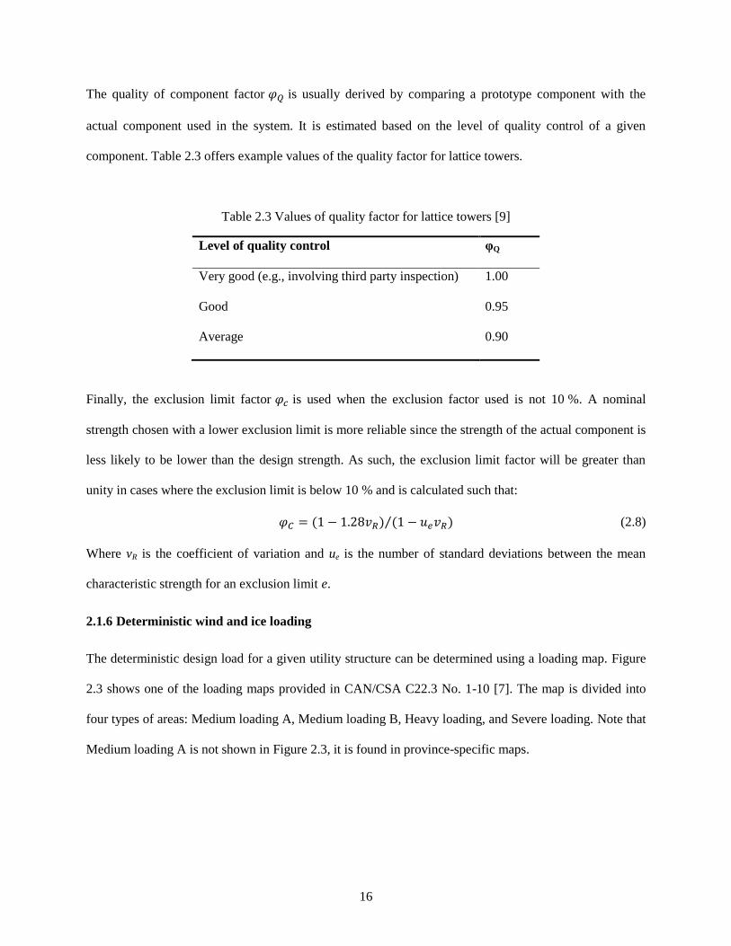
The quality of component factor is usually derived by comparing a prototype component with the
actual component used in the system. It is estimated based on the level of quality control of a given
component. Table 2.3 offers example values of the quality factor for lattice towers.
Table 2.3 Values of quality factor for lattice towers [9]
Level of quality control φQ
Very good (e.g., involving third party inspection) 1.00
Good 0.95
Average 0.90
Finally, the exclusion limit factor is used when the exclusion factor used is not 10 %. A nominal
strength chosen with a lower exclusion limit is more reliable since the strength of the actual component is
less likely to be lower than the design strength. As such, the exclusion limit factor will be greater than
unity in cases where the exclusion limit is below 10 % and is calculated such that:
(2.8)
Where vR is the coefficient of variation and ue is the number of standard deviations between the mean
characteristic strength for an exclusion limit e.
2.1.6 Deterministic wind and ice loading
The deterministic design load for a given utility structure can be determined using a loading map. Figure
2.3 shows one of the loading maps provided in CAN/CSA C22.3 No. 1-10 [7]. The map is divided into
four types of areas: Medium loading A, Medium loading B, Heavy loading, and Severe loading. Note that
Medium loading A is not shown in Figure 2.3, it is found in province-specific maps.

17
Figure 2.3 Loading Map (CAN/CSA C22.3 No.1-10)
Once the appropriate loading zone has been identified based on the location of the structure to be
designed, the loading associated with that zone can be determined using the appropriate code-provided
table, such as Table 2.4, which shows a summary of the loading conditions for each loading areas.
There are three types of loading provided by the code: loading due to ice accretion on the wires, wind
loading, and temperature loading.
The ice accretion loading is provided as a radial thickness of ice on the wire. In other words, the ice
loading is simplified by assuming that the wire has a uniform coating of ice having the thickness specified
by the code. The radial thickness of ice is used both to calculate the vertical load on the structure due to
the ice and the additional horizontal force created by increasing the area upon which wind is acting.

18
The wind loading is provided as a horizontal pressure and is assumed to act upon the structure, the ice-
coated wires, and any additional hardware mounted to the structure (e.g., a transformer).
Table 2.4 Deterministic weather loading
Loading
Conditions
Loading area
Medium
Severe Heavy A B
Radial thickness of
ice, mm 19 12.5 6.5 12.5
Horizontal
loading, N/m² 400 400 400 300
Temperature, °C -20 -20 -20 -20
Thunder Bay, Ontario will be used as a sample location throughout this study. The motivation behind this
choice is explained in Section 2.2.4. Since Thunder Bay is located in a heavy loading zone, the horizontal
wind load on the structure is assumed to be 400 N/m² and the radial thickness of ice on the wires is
assumed to be 12.5 mm.
2.1.7 Probabilistic wind and ice loading
Similar to deterministic design loads, probabilistic design loads are location dependent. However, instead
of providing a loading map with four distinct loading types, the probabilistic code offers climatic data for
a selection of Canadian cities. Table 2.5 shows the climatic data provided for the city of Thunder Bay,
Ontario in CAN/CSA-C22.3 No. 60826 [9].
Table 2.5 Probabilistic weather loading
Location
Minimum
temperature, °C
Reference wind
speed, km/h
Reference ice
thickness, mm
Thunder Bay,
Ontario -33 93 18

19
The wind speed provided in standard is based on climatic data for a given region. The reference wind
speed is the 10 minute average speed having a 50-year return period. The wind speeds are estimated using
extreme value theory which is used to determine extreme values of a probability distribution. A 50-year
return period means that the reference wind speed has a chance of occurring in a given year.
The reference wind speed is reduced using a load factor when combined wind and ice loading conditions
are used. For example, when wind and ice thickness corresponding to a 50-year return period are used, the
reference wind is reduced to 60 % of its initial value.
Similarly, the reference ice thickness provided is based on a freezing rain precipitation with a 50-year
return period. Because there are no national ice accretions records in Canada, the ice thickness values
provided in the code are estimated using an ice accretion model [9]. The predictions are based on the
Chaîné model which estimates the ice accretion caused by freezing rain or drizzle. The model reports
equivalent radial ice thickness assuming an ice density of 900 kg/m³ accumulating on a 25 mm diameter
wire at a height above ground of 10 m. A minimum radial ice thickness of 10 mm is specified for
occurrences of freezing wet snow because the model does not provide an estimate for this condition.
2.1.8 Structural resistance
The structural resistance of wood utility poles is to be designed to meet the requirements of CAN/CSA-
O15 [7]. This standard provides the moduli of rupture and elasticity for several species commonly used in
Canada. A class system is also provided which categorizes wood poles based on their dimensions.
The material strength values provided in O15 are given for wood species commonly available in Canada.
These data are provided in the form of mean values and coefficient of variation. In the case where a
deterministic design approach is used, the average strength values provided in O15 should be used for
resistance calculations. If a reliability-based design approach is used, a nominal strength value is to be
established with an exclusion limit no greater than 10 % [9]. The exclusion limit is the probability that a

20
given sample does not meet the specified strength. This holds true for strength values obtained from
literature (e.g., CAN/CSA-O15) or from testing.
2.1.8.1 Stress-based design
The code assumes that the governing mode of failure is flexure. Thus, wood poles are designed based on
their flexural resistance. A wood pole is non-prismatic which means its cross-sectional properties vary
along its length. Since bending strength is a function of the moment of inertia, which in turns is a function
of the cross-sectional diameter, the moment of inertia varies along the length of the pole. In other words,
the bending strength of a pole is not constant along its length.
If a cantilevered pole having a linearly-varying taper is loaded with a single, transverse point load, it can
be shown that the point of maximum bending stress will be where the cross-sectional diameter is 1.5
times the diameter at the point of loading. This derivation can be found in Appendix B. However,
transverse loading on wood poles are generally more complex than a single point load, as shown in
section 2.1.1. Wind will act on each wire as well as on the pole itself. Additionally, vertical loads will
contribute via second-order effects.
Thus, with a known required pole height and number and location of wires, a designer can determine the
preliminary bending moment diagram for the structure. Based on the bending moment diagram, the
minimum required section dimension can be determined using the section modulus. With the pole
dimensions now known, the bending moment diagram can be recalculated to account for the wind acting
on the pole and the second-order effects. Finally, the bending stresses along the length of the pole are
calculated and compared to the modulus of rupture to determine the adequacy of the chosen pole
dimensions. This procedure is iterated until a pole that can resist the applied loads is found.

21
2.1.8.2 Equivalent load concept and classification system
As an alternative to this process, O15 also provides a table listing the horizontal load associated with each
class. The load is assumed to act at a location 610 mm (2 feet) from the top of the pole. The load is based
on the average bending stress for each species. This table can be used to pin-point the minimum class
required for a given configuration. An adequate pole can be selected by choosing a class which has an
equivalent transverse load equal to or greater than the resultant load calculated. Knowing the required
pole height and class, the final pole dimensions can be determined by using species-specific table, an
example of which is found in Table 2.7.
Similarly to other wood products, the primary way to classify wood poles is by the species of wood from
which they are made. Within CAN/CSA-O15, the poles are further divided using a classification system.
A class is assigned to a pole of a given length based on the circumference at the top of the pole and at a
location 1.8 m from the butt of the pole. These circumferences are chosen based on the concept that a pole
of a given class should be able to resist a point load acting transversally at a point 610 mm from the top
and that the pole is of average strength. A reference ground line distance from the butt is defined for each
pole length. Table 2.6 shows the equivalent horizontal load that a specific class is expected to resist. It
should be noted that these loads should be modified by a factor of 0.95 for Red Pine poles.

22
Table 2.6 Equivalent horizontal loads based on pole class [6]
Class Horizontal Load, kN
1 20.0
2 16.5
3 13.3
4 10.7
5 8.5
6 6.7
7 5.3
8 4.3
H1 24.0
H2 28.5
H3 33.4
H4 38.7
H5 44.5
H6 50.7
The minimum length of pole provided for all species is 6.1 m (20 ft). Dimensions for longer poles are
provided by pole length increments of 5 ft (approximately 1.5 m). The maximum pole length provided
depends on the wood species. For example, dimensions are provided for Red Pine poles measuring up to
19.8 m in length and Douglas Fir poles up to 38.1 m in length. A summary of the pole dimensions for Red
Pine poles is provided in Table 2.7.
To use equivalent horizontal loads to pick an adequate pole, a resultant load must be calculated based on
all applied loads on the structure. The resultant load is assumed to be located 610 mm from the top of the
pole. The magnitude of the resultant force is then determined using the bending moment diagram of the
structure. To determine the appropriate resultant magnitude, it must be calculated based on the critical
section. As discussed previously, the critical location does not necessarily occur at the location of
maximum bending moment due to the non-prismatic nature of wood poles. The accuracy of this method
depends on how well the critical location is predicted. Although this method works well for preliminary
design, there is value in using stress-based design to verify a final design.

23
Table 2.7 Dimensions of pole for each class for poles made of Red Pine [6]
Class
1 2 3 4 5 6 7 8
Minimum circumference at top, cm
69 64 58 53 48 43 38 38
Length of pole, m
Groundline distance from butt, m*
Minimum circumference at 1.8 m from butt, cm
6.1 1.2 83 78 73 68 62 57 54 51
7.6 1.5 92 85 79 74 69 64 59 56
9.1 1.7 99 93 87 80 74 69 64 61
10.7 1.8 106 98 92 85 79 73 68 65
12.2 1.8 112 104 97 90 84 78 ― ―
13.7 2.0 117 109 102 94 88 82 ― ―
15.2 2.1 122 115 107 99 92 ― ― ―
16.8 2.3 126 118 111 103 ― ― ― ―
18.3 2.4 131 122 115 107 ― ― ― ―
19.8 2.6 135 126 117 109 ― ― ― ―
2.1.9 Damage limit state
Both codes offer some end-of-life guideline for wood poles. In limit states design, end-of-life is referred
to as damage limit state. A damage state is reached once a structure is deteriorated to the point where it
should be replaced or reinforced. C22.3 No. 1 suggests that a pole which has deteriorated to 60 % of pole
design capacity is considered at end-of-life [7]. C22.3 No. 60826 has two end-of-life criteria. For poles
loaded in bending, the structure is considered in a damage state if 3 % of the top displacement is non-
elastic [9]. For poles in compression, a damage state is reached when non-elastic deformations ranging
from L/500 to L/100 are observed. [9]
2.2 Reliability analysis
The aim of reliability-based design is to quantify the level of risk in a structure using probability and
statistics concepts. This is done by representing all the components that influence loading and resistance
as random variables. Each random variable has a statistical distribution attributed to it. The interaction

24
between these variables is defined and is used to establish the probability of failure. This section presents
different concepts used to determine the reliability of a system.
2.2.1 Performance function
Once the variability of each load and material is known, a method must be devised to combine them such
that their interaction is known. A performance function is used for this purpose. A performance function
must be used for each load effect and its associated resistance. For example, the random variables
associated with shear load and resistance must be combined to represent their interaction but are kept
separate to the random variables associated with moment load and resistance. A generic performance
function can be represented as follows:
(2.9)
where R is the system resistance and S the system solicitation (i.e., load effects).
The system is considered to have a failed if the performance function is less than zero. The probability of
failure is expressed as follows:
(2.10)
where is the probability density function of the load and is the cumulative density function
of the resistance.
Figure 2.4 shows arbitrary solicitation and resistance distributions. The overlapping region (i.e., the
shaded region) represents the occurrences where the resistance is less than the solicitation and
corresponds to the probability of failure. Figure 2.5 shows the distribution for the performance function.
The shaded region represents the probability of failure as stated in Equation (2.10).

25
Figure 2.4 Resistance and solicitation distributions
2.2.2 Measure of reliability
A system’s reliability can be defined as the probability that the system will not experience a failure. In
other words, it is the probability that the resistance exceeds the load. Reliability can be expressed as
follows:
(2.11)
Reliability is commonly represented in terms of the reliability index, β. For a normally distributed
performance function, or where the resistance is normally distributed and the load follows a Gumbel
distribution, the reliability index and probability of failure can be calculated as follows [9]:
(2.12)
where and are the mean and standard deviation of the performance function, respectively, and is
the standard normal distribution. A graphical representation of the reliability index is shown in Figure 2.5.
R(µR,σR)S(µS,σS)
f(X
)
X
failure

26
For a log-normally distributed performance function, or where the resistance follows a log-normal
distribution and the load follows a Gumbel distribution, the reliability index can be found using [9]:
(2.13)
where vR and vS are the respective coefficients of variability for the resistance and load.
Figure 2.5 Distribution of the performance function
Figure 2.6 shows the non-linear relationship which exists between reliability and the reliability index.
This non-linearity implies efforts put into increasing the reliability of a system are met with diminishing
returns.
βσz
f(X
)
X
failure

27
Figure 2.6 Relationship of reliability and reliability index based on normal distribution
Structures designed using probabilistic design methods, such as limit states design, are usually designed
with to achieve target reliability. CAN/CSA S408 is a standard which offers guidelines for the
development of limit states design standards. This standard suggests that the target reliability level should
be chosen to take into account the potential risk of failure. The risk, or cost, of failure takes into account
the potential loss of life, environmental damage, and social and economic costs [13]. S408 also suggests
that the required cost of increasing the reliability should also be considered when choosing the reliability
level [13]. Three risk classifications are offered in S408 with increasing levels of consequences: low,
medium, and high risk. These are defined as having small, considerable, and great consequences. A
structure that is required to be fully functional in the event of a disaster is an example of a structure that
would be classified as being high risk.
The Canadian Highway Bridge Design code suggests that a target lifetime reliability level of 3.75 for
most components of new bridges assuming a 75-year lifetime. This is equivalent to a yearly reliability
level of 3.50 [13] [14]. For evaluation and load rating of in-service bridges, the reliability level can be
0%
10%
20%
30%
40%
50%
60%
70%
80%
90%
100%
-5.0 -4.0 -3.0 -2.0 -1.0 0.0 1.0 2.0 3.0 4.0 5.0
Re
liab
ility
Reliability index, β

28
estimated based on the assumed system behaviour of the component, the inspection frequency and
inspection findings [14].
CSA-S408 summarizes target reliability levels for buildings with a 50-year lifetime. Where ductile
failures are predicted, the reliability level should be a minimum of 3.0, whereas brittle failure for concrete
should aim for a reliability index of 4.0 and net section fraction of steel elements should have a reliability
index of 4.5 [13].
CAN/CSA-C22.3 No. 60826 suggests three reliability levels for overhead transmission lines. These
reliability levels are based on a load return period of 50 years, 150 years, and 500 years. Table 2.8 offers a
summary of the reliability levels and their associated return period for load suggested by C22.3 No. 60826
[9]. The reliability indices were calculated assuming a normally distributed performance function. The
relationship between the return period T and the n year reliability is expressed as follows:
. (2.14)
Table 2.8 Relationship between reliability index and return period of load
Return period of load, T 50 150 500
Yearly reliability, R 0.98 to 0.99 0.993 to 0.997 0.998 to 0.999
Yearly reliability index, β 2.05 to 2.33 2.46 to 2.75 2.88 to 3.09
50-year lifetime reliability, R50 0.36 to 0.61 0.71 to 0.86 0.90 to 0.95
50-year lifetime reliability index, β50 -0.36 to 0.28 0.55 to 1.08 1.28 to 1.64
The suggested reliability indices for transmission lines are relatively lower than those suggested for
buildings and bridges. This suggests that these structures fall under different risk classification categories.

29
This is likely due to the failure of a bridge or building having much more important social and economic
consequences when compared to the failure of a utility structure.
2.2.3 Monte Carlo simulation
Monte Carlo simulation is a method that can be used to determine the probability of failure a system [15].
In this method, a performance function is elaborated and the relationship between each random variable is
explicitly stated. Using the statistical distribution associated with each variable, a random value for each
variable is produced and the performance function is evaluated. The result of this process is used to
determine whether the system has failed or not. This process is iterated and the variables randomized for
each iteration. The probability of failure can then be determined by dividing the number of failure by the
total number of iterations.
2.2.4 Previous reliability studies on transmission structures
Li et al. have conducted a study [16] in which they assessed the reliability of wood utility poles designed
CAN/CSA-C22.3 No. 1. Western red cedar poles were designed for 15 locations across Canada using
Grade 1, Grade 2, and Grade 3 construction. Both linear and non-linear design approaches were used as
per the deterministic design standard. Appropriate load factors were used based on the construction grade
and analysis type (linear and non-linear). Loads used were based on 50-year return period wind speed and
ice thickness found in CSA C22.3. The weather loads were modeled using a Gumbel distribution with an
assumed COV of 15 % for wind speed and 70 % for ice accretion. RELAN, a reliability analysis program,
was used to determine the annual reliability index for each design scenarios.
The research by Li et al. had two main conclusions: the design using the non-linear approach yielded
more reliable structures than those designed using the linear approach; the reliability index for structures
varied greatly across all 15 design locations for all construction grades. Although load factors are greater
when designing using the linear approach, their research shows that the second-order effects are
significant enough to require a stronger structure; this was even more evident for structures with added

30
mass in the form of a transformer. The variability in annual reliability index is attributed to the disparity
between the load specified in the standard and the actual weather conditions at each design location. In
other words, the loading map covers a very large area which does not fully account for local climate.
In a similar study [17], Bhuyan and Li investigate the reliability of three reference structures designed
according to North American deterministic design codes for overhead transmission structures. The
reference structures consist of a steel lattice structure, a steel pole structure, and a tangent H-frame wood
structure. The two deterministic codes used are the Canadian CSA-C22.3 No. 1 and the American
National Electrical Safety Code. The reference structures were designed for eight US locations and five
Canadian locations. Structural analyses accounting for non-linear effects were used to develop the
performance function for each structure. The reliability was determined using First-Order Reliability
Method (FORM). The study showed that the NESC design approach resulted in higher reliability when
compared to the CSA design approach. This was attributed to a special provision for structures taller than
18 m. This provision requires an extreme wind case to be analysed. This additional analysis usually
governed the design resulting in a more reliable structure. The method used to calculate the effect of wind
on conductors in NESC differs from the CSA approach which could also affect the results of the analysis.
The wind load on conductor calculated using CSA was 20 % greater than that calculated using NESC.
Finally, similar to the findings Li et al. [16], the achieved reliability between different structures and for
the same reference structures at different locations was not uniform when using CSA-C22.3.
Subramanian conducted a study [12] in which the reliability of wishbone and Gulfport structures was
evaluated. The structures were designed using five different standards: the National Electric Safety Code
(NESC, 2002), the Rural Electrification Authority (REA, 1992), the American Society of Civil Engineers
(ASCE, 1991) guidelines for electrical transmission line structures, the Canadian Standards Association
(CSA, 2001), and Ontario Hydro’s in-house design procedures. The probabilities of failure at the time of

31
installation and at the time of replacement were determined. The structures were analysed both under
extreme wind and combined wind and ice loading conditions.
The wind load distributions for both extreme wind and wind-on-ice conditions were established using
historical data from Environment Canada for Thunder Bay, Ontario and London, Ontario. The wind-on-
ice loads were determined by analyzing wind loads during ice events. Different ice residency periods
were assumed and it was concluded that assuming a period longer than three days did not significantly
affect the results of the analysis. The appropriate distributions were selected using probability paper plot.
The probabilistic wind data, based on a 50-year return period, for Thunder Bay, Ontario is summarized in
Table 2.9. The Gumbel distribution had the best fit for the wind data.
Table 2.9 - Probabilistic wind data for Thunder Bay, Ontario [12]
Wind event Mean
(km/h)
COV (%)
Gumbel parameters
α u
Extreme annual
wind speed
90.9 15.9 0.0786 84.1
Annual wind speed
on ice-covered wires
41.2 30.8 0.0898 34.5
Equation (2.15) shows the cumulative density function for the Gumbel distribution as defined in [12].
(2.15)
where
,
, , and .
The wind data in Table 2.9 is expressed in terms of wind speed. However, for analysis purposes, it is
more useful to represent the wind load as a pressure. CSA-C22.3 No. 1 suggests that wind speed can be
converted to an equivalent wind pressure as follows [7]:

32
(2.16)
where P is the resulting wind pressure in Pa, Cd is the drag coefficient, ρ is the air density in kg/m³, and V
is the wind speed in m/s. A value of can be assumed [7].
Probabilistic distributions for ice accretion are difficult to determine due to a lack of data. By studying the
suggested design values found in various North American codes (which are largely based on ice accretion
models) in conjunctions with ice accretion data from a study conducted in the province of Quebec, the
distribution coefficients shown in Table 2.10 were established by Subramanian [12] for ice accretion on
wires located in Thunder Bay, Ontario. The distribution assumes a uniform coating of ice surrounding the
wire and a 50-year return period.
Table 2.10 Probabilistic radial ice thickness data for Thunder Bay, Ontario [12]
Mean (in) COV (%)
Gumbel parameters
α u
0.44 70 4.12 0.304
The analysis results presented by Subramanian showed that the probability of failure of wishbone
structures ranged from 2 % to 0.12 % at the time of installation and from 6 % to 8 % for at the time of
replacement. For this analysis, the structure was considered to need replacement when it had deteriorated
to two thirds of its original design strength. Similarly, the Gulfport structures had a probability of failure
ranging from 0.04 % to 0.9 % at the time of installation and 1.8 % to 5.2 % at the time of replacement.
The ranges are attributed to the difference in designs due to the different standards used and the difference
in deterioration rates assumed. A faster deterioration rate will show a more rapid increase in probability of
failure over time.

33
2.3 Material properties and deterioration mechanisms of wood utility poles
The two material properties which are deemed important for new utility pole design are the modulus of
rupture and the modulus of elasticity. The modulus of rupture is important because bending is the
governing mode of failure for this type of structure. The modulus of elasticity is used when performing a
second-order analysis. In a study [5] conducted by Steenhof, it was found that combination shear-bending
failures were observed in wood poles which had previously been in service. It was determined that shear
failures occurred in specimens having some form of deterioration.
Deterioration in wood occurs in several forms. These deterioration mechanisms are categorized as
follows: weathering, decay, insect damage, and woodpecker damage. These deterioration mechanisms are
explained in further detail in this section.
2.3.1 Wood bending strength
Wood bending strength, also known as modulus of rupture (MOR), varies between wood species. There
are several publications which report modulus of rupture data for several species, including CAN/CSA-
O15-08 [6], the Canadian Department of Forestry [18], the United States Department of Agriculture [19],
the American Society for Testing and Materials [20], amongst others. The MOR data found in these
publications are summarized in Table 2.11.
In addition, a study conducted at the University of Waterloo by Steenhof has produced MOR data for both
new poles and poles which have been in service [5]. In this study, the effect of various level of
woodpecker damage on wood utility poles was investigated.
The species of wood poles tested in this study were Red Pine, Lodgepole Pine and Western Red Cedar.
The poles tested were donated by Hydro One and consisted of both new poles and poles that had been
decommissioned from their network. The poles ranged in length from approximately 10 m to 18 m and
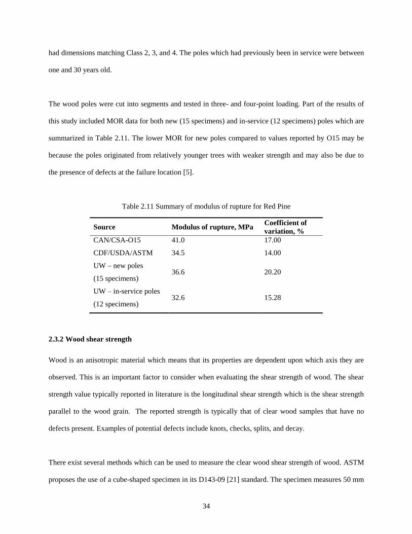
34
had dimensions matching Class 2, 3, and 4. The poles which had previously been in service were between
one and 30 years old.
The wood poles were cut into segments and tested in three- and four-point loading. Part of the results of
this study included MOR data for both new (15 specimens) and in-service (12 specimens) poles which are
summarized in Table 2.11. The lower MOR for new poles compared to values reported by O15 may be
because the poles originated from relatively younger trees with weaker strength and may also be due to
the presence of defects at the failure location [5].
Table 2.11 Summary of modulus of rupture for Red Pine
Source Modulus of rupture, MPa Coefficient of
variation, %
CAN/CSA-O15 41.0 17.00
CDF/USDA/ASTM 34.5 14.00
UW – new poles
(15 specimens) 36.6 20.20
UW – in-service poles
(12 specimens) 32.6 15.28
2.3.2 Wood shear strength
Wood is an anisotropic material which means that its properties are dependent upon which axis they are
observed. This is an important factor to consider when evaluating the shear strength of wood. The shear
strength value typically reported in literature is the longitudinal shear strength which is the shear strength
parallel to the wood grain. The reported strength is typically that of clear wood samples that have no
defects present. Examples of potential defects include knots, checks, splits, and decay.
There exist several methods which can be used to measure the clear wood shear strength of wood. ASTM
proposes the use of a cube-shaped specimen in its D143-09 [21] standard. The specimen measures 50 mm

35
wide by 50 mm deep by 63 mm high. The height is oriented with the wood grain. A 20 mm wide by
13 mm high notch is cut in the top of the specimen. The block is restrained on all sides with a jig and
loaded at the notch to determine its shear strength. Although this is the most common test used for clear
wood shear strength measurement, it does introduce non-uniform normal stresses which may impact the
results of the test [22]. Because of this, several methods have been devised which attempt to load a wood
specimen in pure shear. Table 2.12 reports the shear strength of Red Pine as reported by the Canadian
Department of Forestry [18].
Table 2.12 Clear-wood shear strength of Red Pine
Condition Average,
MPa
Coefficient of
variability, %
Green 4.90 11.10
12 % Moisture content 7.45 11.10
.
The studies by Liu et al. [22] and Xavier et al. [23] both investigated the use of the Arcan test. The Arcan
test makes use of a rectangular specimen with V-notches cut at its centre. Shear properties in all three
directions can be measure by altering the grain direction or the loading direction. These studies concluded
that the Arcan method produces similar results to other common shear measurement methods.
In a study by Odom et al. [24], the use of the Wyoming shear-test fixture was investigated to see if the
fixture produced asymmetrical loading. The Wyoming fixture also makes use of a rectangular specimen
with V-notches at its centre. One side of the specimen is fixed whilst the other is displaced. The study
found that while the fixture does not cause any asymmetrical loading, misalignment of the fixture will
cause the test to report shear strengths of specimens which are higher than their actual strengths. It is
thought that the Wyoming fixture could be an acceptable method to measure shear strength provided that
the fixture is modified to avoid misalignments.

36
Yoshihara and Matsumoto conducted a study [25] in which they used thin rectangular specimens in which
two circular holes were cut in the axial centreline and a straight slot was cut from each hole to the edge at
an angle. The angle was varied between sets of specimens. The specimen were clamped at each end and
loaded in tension. Results show that this testing method is a good alternative to the ASTM test method for
shear testing. Furthermore, the angle of the cut did not influence the results of the tests.
In a study by Riyanto and Gupta [26] different methods to determine the shear strength parallel to grain of
full-size douglas-fir sawn structural lumber were evaluated. The study was motivated by the idea that
shear strength determined using clear-wood specimen is not representative of full-size members used in
structural applications. 12 ft (3.66 m) long 2 in by 4 in (51 mm by 102 mm) Douglas-fir specimens were
tested in four different configurations including three-point bending, four-point bending, five-point
bending, and in torsion. The study made several conclusions. First, torsion testing was the only test which
produces pure shear failures. Because of this, torsion was determined to be a good testing method to
determine the shear strength of full-size specimens. Secondly, three-point bending was found the be an
appropriate method of testing shear strength as it produced loading conditions similar to that of in-situ
structural component. Lastly, a strong linear relationship was found between shear strength obtained from
full-size specimens and clear wood specimens. This linear relationship was found with specimens tested
in three-point bending, five-point bending, and torsion testing.. This is encouraging since the strength of
dimensional lumber can be determined using strength reported from clear-wood specimen testing.
Finally, a study by Steenhof [5] as observed that, for non-prismatic beams with a circular cross-section
cut from full-size wood utility poles, shear failure may occur in specimens which were weathered,
decayed, and had significant checking. These results were not expected when considering shear strength
obtained from clear-wood specimens. This finding shows that clear-wood shear testing may not be
representative of the actual shear strength of wood poles because of inherent defects found in full size
wood poles. This is discussed in further detail in section 2.3.8.

37
2.3.3 Adjustment factors for clear wood properties
ASTM D245 Standard Practice for Establishing Structural Grades and Related Allowable Properties for
Visually Graded Lumber [27] discusses the use of visual inspection to grade structural lumber. The
concept of strength ratio is discussed in this standard. The strength ratio represents the expected strength
of a given piece of structural lumber when compared to the strength of a clear piece. This ratio takes into
account grain orientation and defects such as knots and splits. Table 2.13 shows strength ratios for
bending, tension, and compression parallel to grain based on the grain orientation.
Table 2.13 Strength ratios corresponding to various slopes of grain [27]
Slope of grain
Maximum strength ratio
Bending or tension
parallel to grain
Compression parallel
to grain
1 in 6 40 % 56 %
1 in 8 53 % 66 %
1 in 10 61 % 74 %
1 in 12 69 % 82 %
1 in 14 74 % 82 %
1 in 15 76 % 100 %
1 in 16 80 % -
1 in 18 85 % -
1 in 20 100 % -
The standard also discusses allowable properties for timber design. The standard makes use of adjustment
factors which are applied to clear wood properties to account for potential defects. The allowable
properties are determined by dividing the clear wood properties by the appropriate adjustment factor.
Table 2.14 shows adjustment factors for some clear wood properties.

38
Table 2.14 Adjustment factors to modify clear wood properties to achieve allowable stresses [27]
Wood type Modulus of
elasticity in bending Bending strength
Horizontal shear
strength
Softwoods 0.94 2.1 2.1
hardwoods 0.94 2.3 2.3
Current design methods for wood poles do not take into consideration the shear strength of the structure.
As such, the only available shear strength is clear wood strength. Determining the full-size pole shear
strength is valuable in determining whether wood pole design should account for shear.
2.3.4 Weathering
Talwar explains weathering as being the effect of environmental surroundings on a wood pole [28]. This
includes the effect of the sun, rain, ambient humidity and temperature. UV light will cause photochemical
damage which leads to oxidation and discolouration of the surface layer. Changes in temperature will
increase the rate at which these effects occur. Weathering does not have a very strong effect on the wood
strength but the alternating wet and dry state of the wood may lead to surface checking which may cause
elevated moisture level within the pole and lead to decay.
2.3.5 Staining
The USDA Wood Handbook [19] describes molds and fungus stains as discoloration of sapwood due to a
microbial attack on the wood. This type of staining does not generally lead to great reduction in strength.
However, it does lead to an increase in porosity of the sapwood which can increase the moisture retained
by the wood and thus increase the chance of decay.
Chemical stains, on the other hand, are non-microbial in nature. They typically occur in instances where
lumber is slow dried or in relatively hot temperatures [19]. This type of stain is difficult to manage and
can lead to significant losses in wood quality and strength.

39
2.3.6 Decay
Information on decay of wood was collected from research by Talwar [28], McCarthy [29], and the
USDA Wood Handbook [19]. Wood decay is caused by fungi which occur in moist environment with
mild temperature, where oxygen and an adequate food source is present. Decay attacks both sapwood and
heartwood. Most forms of decay are difficult to detect unless core samples are taken and examined in the
lab which is an expensive procedure. Although there are several forms of fungi which attack wood, most
decay-causing fungi only thrives in live trees. There are three main types of fungi which will damage cut
wood.
The strength loss caused by decay is dependent on the type of decay as well as the type of wood affected
by decay. At the onset of decay, the strength loss can vary greatly. Experiments conducted on wood that
had a 1 % weight loss due to decay showed that the loss in toughness ranged between 6 % to more than
50 %. Once the weight loss is in excess of 10 %, the wood is expected to have loss 50 % or more of its
strength [19].
2.3.6.1 Brown rot
Brown rot consumes the cellulose found in wood. This fungus causes cracking along the grain. It causes
the wood to shrink and makes it extremely weak. Wood affected by brown rot can be easily identified by
its dark brown colour. Brown rot is more prevalent in softwoods.
2.3.6.2 White rot
White rot consumes both cellulose and lignin. The affected wood turns white and spongy. Unlike brown
rot, this fungus does not cause the wood to shrink and crack. White rot is more prevalent in hardwoods.

40
2.3.6.3 Soft rot
Soft rot is a shallow surface rot which stains the surface of the wood. Because soft rot is relatively
shallow, is does not greatly affect the strength of a structural member unless the member is thin. Soft rot
may cause heavy checking and splitting of the wood surface.
2.3.7 Woodpecker damage on wood utility poles
Hydro One has reported an increase in damage to their wood utility pole infrastructure caused by
woodpeckers [4]. Inspections carried between 2006 and 2010 have shown that 16,000 wood poles had
some level of woodpecker damage [30]. Hydro One reports that the observed damage can be grouped into
three distinct categories: feeding damage, exploratory damage, and nesting damage.
Woodpeckers peck tress for a variety of reasons. These reasons include drumming, foraging, and nesting
and roosting [31]. Drumming is used for communication purposes and does not produce significant
mechanical damage. Foraging is done in order to search for food. Finally, nesting and roosting cavities
are used to lay and roost eggs. The primary reason for woodpecker to target utility poles is thought to be
for nesting. The area surrounding wood poles is often cleared which offers woodpeckers great visibility of
their surroundings [31].
In order to do a structural evaluation of these damaged wood poles, their sectional properties must be
determined. In order to do this, attention must first be place on the sectional resistances which are
required. In this case, flexural and shear resistances are of interest. Work by Steenhof has shown that it is
important to consider the orientation of the damage when determining a particular sectional resistance [5].
Orienting the damage with the extreme fibres (i.e., the tension or compression fibres) will have the
greatest impact on the flexural resistance whilst orienting the damage with the neutral axis will have the
greatest impact on the shear resistance. Thus, to properly evaluate the effect of woodpecker damage on
the structure, section properties reflecting both damage orientations must be calculated.

41
2.3.7.1 Definition of exploratory and feeding damage
Figure 2.7 shows the observed range of exploratory holes found on wood utility poles [4]. The
exploratory damage category exhibits the lowest amount of damage of all three categories. It is believed
that these holes are made by woodpeckers in search of food. The shape of the hole is roughly cylindrical
with an opening size ranging from 25 to 75 mm and a depth ranging between 25 to 150 mm.
Figure 2.7 Range exploratory damage dimensions observed by Hydro One [4]
Figure 2.8 shows the range of damage which falls in the feeding damage category [4]. It is believed that
these holes are made at locations where woodpeckers think they have found food. The shape of the hole is
similar to that found in exploratory holes. However, the opening has an elliptical shape with a height
ranging from 75 to 200 mm and a width ranging from 50 to 75 mm. The hole depth ranges from 150 to
175 mm.
2.3.7.2 Definition of nesting damage
Nesting damage exhibits a form of damage that is different from exploratory and feeding damage. As the
name implies, nesting damage are holes used by woodpeckers to build their nests. Figure 2.9 shows the
shape and observed dimensions of a nesting hole [4]. The hole consists of a 100 to 175 mm opening into a

42
large cavity. The cavity can be seen as a hollowing of the core of the pole leaving a shell approximately
25 to 75 mm in thickness.
Figure 2.8 Range of feeding damage dimensions observed by Hydro One [4]
Figure 2.9 Range of nesting damage dimensions observed by Hydro One [4]

43
2.3.8 Previous studies on poles with woodpecker damage
A study by Rumsey and Woodson [32] investigated the effect of woodpecker damage on Southern Pine
wood utility poles. Eighteen poles 50 foot in lengths were set seven feet into the ground and tested by
attaching a cable two feet from the top and load was applied using a winch. Other than the two control
specimens, all poles had nesting cavities or holes having an opening diameter of three inches or more.
Four of the damaged poles failed below damaged section; these poles were treated as controls. The
capacity of each pole was estimated based on remaining cross-section at the location of holes. The fibre
strength was estimated using two different. It was found that both methods produced conservative
estimation of remaining pole strength.
In response to woodpecker damage problems reported by Hydro One, Steenhof conducted a study [5] on
the effect of woodpecker damage on wood utility poles. In this study the woodpecker damage categories
reported by Hydro One were idealized using non-dimensional parameters based on the cross-sectional
diameter. Three analytical models were defined: a bending failure model (BF), a shear failure model (SF),
and a shear-bending interaction failure module (SBIF). The BF module assumes that failure occurs once
the modulus of rupture is attained (Equation (2.17)). The SF model assumes that failure occurs once the
ultimate shear stress is attained (Equation (2.18)). Finally, the SBIF model takes into account that both
shear and bending stresses are present at any given time and that they interact with each other. An
interaction equation calibrated for wood was used (Equation (2.19)).
(2.17)
(2.18)

44
(2.19)
The accuracy of the models was affirmed with an experimental study. In this study, a total of 28 poles in
both as-new and in-service conditions were tested. The poles were cut into beams 4.25 m in length. A
total of 58 as-new and 24 in-service beams were tested. Some of the beams were tested as controls and the
rest had artificially introduced or naturally occurring damage representing the woodpecker damage levels
discussed earlier. Beams with woodpecker damage were tested with the damage oriented both with the
neutral axis and with the bending tension or compression extreme fibre. Some of the in-service beams had
decay present in addition to the woodpecker damage. The study confirmed that all three analytical models
can predict the stresses in the beams. Although the SBIF model was found to offered better predictions, it
was found that the BF and SF models both offered adequate accuracy with significantly less
computational effort.
The study also found that, although wood poles failure is generally governed by bending, that shear
failure could occur in poles with significant woodpecker damage, decay, or a combination of both. It was
observed that poles with damage oriented with the neutral axis had their failure strength reduced by less
than those with the damage oriented with the tension or compression fibres. The dominant failure mode
was bending. Nesting level damage reduced the strength by up to 40 % in as-new specimens and by up to
57 % for in-service specimens. Intermediate to severe levels of decay caused strength reduction ranging
from 47 % to 73 %.

45
2.4 Summary
Two standards are used in Canada for guidelines on the design of overhead transmission
structures: CAN/CSA-C22.3 No. 1, a deterministic design code, and CAN/CSA-C22.3
No. 60826, a probabilistic design code. C22.3 No. 1 is the most commonly used design standard.
Previous studies have been done to quantify the reliability of overhead structures designed using
CAN/CSA-C22.3 No. 1. These studies have shown that the reliability of these structures is not
uniform and is highly dependent on their geographical location. These studies did not take into
account the effect of deterioration and woodpecker damage.
Previous studies have concluded that deterioration and woodpecker damage can significantly
reduce the strength of wood utility poles. In some instances, poles were observed to fail in shear.
However, current design standards assume that flexure is the governing mode of failure for wood
utility poles and does not provide any requirements for shear strength.
Previous research has shown that wood strength properties based on clear-wood specimens differ
from the strength properties determined using full-size dimension lumber. The shear strength of
full-size wood pole specimens has not been investigated.

46
Chapter 3 Shear strength of full-size wood utility poles
This section discusses the elaboration and results of the experimental programme used to determine the
full-size shear strength of wood poles.
3.1 Objectives
Previous research has shown that shear failure in wood pole elements sometimes occurred at stresses
lower than anticipated [5]. It was hypothesised that this behaviour could be due in part to the method
normally used to determine the shear strength of wood. Figure 3.1 shows a typical test specimen for
measuring shear parallel to the wood grain. The specimen is loaded at the notch and is restrained by an
apparatus in such a way that it fails along the plane created by the notch. An important aspect of this test
specimen is that it must be free of any defect. In other words, it is a clear wood specimen. Although this
method of testing may be a good representation of the shear strength for cut timber, it may over-estimate
the shear strength of wood poles due to the inherent presence of defects in wood poles. These defects
include knots and surface damage, such as checks.
Figure 3.1 Test specimen configuration for shear-parallel-to-grain measurement (ASTM D143-09)

47
Knots are a naturally occurring defect. They are formed at the location where branches are located on the
trunk. Checks are splits at the surface of the pole which occur as the pole dries. These defects reduce the
effective cross-section of the pole which in turns reduces the cross-sectional shear strength by reducing
the area which resists shear stresses.
The goal of this experimental programme was to establish a shear strength distribution for full-size wood
pole and to compare it to strengths reported in literature.
3.2 Specimen configuration
Figure 3.2 shows a non-dimensional representation of the specimen configuration used in this study. The
specimen consists of a pole segment on which two slots have been cut. Each slot is cut to half the depth
and are on opposite sides of the pole segment (i.e., they are cut such that their bottom are oriented in the
same plane but the holes are facing opposite directions). The purpose of these slots is to change the load
path within the pole segment such that loads are concentrated within a shear plane between the two slots.
The relative dimensions were chosen such that shear was the governing mode of failure and that changes
in geometry were not so abrupt as to cause other modes of failure to occur, such as tension failures at the
top or bottom of the shear plane. Furthermore, the configuration was checked for buckling, and crushing
of the fibres at slot level. It was determined that the two modes of failures most likely to occur was shear
failure through the shear plane and crushing failure at the slot. The length of the shear plane was chosen
such that the load required to cause shear failure was approximately half that required to crush the wood
at the slot. This approach was confirmed with a pilot study where a specimen using a shear length of 1.5D
did not fail in shear. Lastly, the ends were finished such that they were as orthogonal as possible to the
longitudinal axis to ensure an even load distribution.

48
Figure 3.2 Non-dimensional specimen configuration for full-size pole shear strength testing
Figure 3.3 shows a specimen ready for testing. The ends were cut to length with a swivelling band saw to
ensure the end surfaces are level and square to the longitudinal axis. The notches were pre-cut with a
chain saw and finish using a bow saw and chisel. This approach allowed the cuts to be made in a
reasonable amount of time whilst preserving an acceptable level of precision.
Figure 3.3 Typical specimen used to determine full-size pole shear strength
The average shear strength of a given specimen is determined by taking the quotient of the failure load
and the shear plane area. The failure load is determined by analysing the data recorded during testing. A

49
summary of the specimens tested in this experimental programme, including geometric properties and
measured shear strength, can be found in Appendix A.
3.3 Test configuration
All specimens were tested in an MTS 311 loading frame with a 1500 kN capacity. The loading frame was
equipped with two platens measuring approximately 600 mm by 600 mm in size; large enough for the
larger specimens to rest completely on the platen. Figure 3.4 shows a picture of the testing setup with a
specimen ready to be tested.
The experiment was conducted in stroke control at a rate of approximately 0.6 mm/min as suggested in
ASTM D143-09 [21]. The crosshead force and displacement were recorded using a data acquisition
system at a rate of 2 Hz.

50
Figure 3.4 MTS 311 test frame with a specimen ready to be tested
3.4 Clear-wood shear strength
The main objective of the experimental programme was to determine whether there was a difference
between shear strength obtained from clear wood specimens and full-size specimens. The Canadian
Department of Forestry published a list of strength values and physical properties of all wood types
grown in Canada [18]. Table 3.1 shows a summary of shear strength for Red Pine, the wood species used
in this experimental study. Table 3.1 reports both green strength and strength at 12 % moisture content
based on a sample size of 356 specimens. Green wood strength is the strength of wood fibres fully

51
saturated with water. However, since wood in service is usually in a drier state, a second strength value is
reported, usually at a moisture content of 12 %.
Table 3.1 Clear wood mean shear strength parallel to grain for Red Pine [18]
Green wood strength, kPa Strength at 12% MC, kPa Coefficient of variability
4902 7502 11.1%
Knowing the strength at two different moisture contents is useful as it allows the determination of the
strength at any moisture content. This can be done using the following equation [19]:
(3.1)
where P12 is the strength at a moisture content of 12 %, Pg is the strength of green wood, M is the desired
moisture content in percent, and Mp is a species-dependent variable that relates the strength of green wood
to the strength-moisture content curve for dry wood. For red pine, an Mp value of 24 % is used [19]. The
relationship expressed in Equation (3.1) can be used for any mechanical property of wood (e.g., shear
strength, modulus of rupture/flexural strength).
3.5 Results
A total of 30 specimens were tested for this study. Out of these 30 specimens, four were part of a pilot
study; the remaining 26 were part of the main experimental study. A table summarizing the experimental
programme can be found in Appendix A.
3.5.1 Modes of failure
Two distinct failure modes were observed when testing the full-size shear specimens. In the first failure
mode, a single failure plane was formed between the two notches. Figure 3.5 shows an example of this
mode of failure. This is the preferred mode of failure as it indicates that the specimen failed mostly due to
the action of shear loads.

52
Figure 3.5 Failed specimen with one failure plane perpendicular to the notches
In the second mode of failure, the failure plane was still perpendicular to the two notches. However, the
formation of a strut was observed. The strut was accompanied either by a single shear plane spanning
between the two notches (Figure 3.6) or with a shear plane on each side of the strut, with a failure plane
originating from each notch (Figure 3.7). The formation of this strut is likely due to the way the load
transfers from one end of the specimen to the other. The flow of load from one end to the other is
obstructed by the two slots. Furthermore, the inherent imperfections attributable to wood may result in
specimens which are not perfect straight. This causes the failure plane to experience loads other than
shear (e.g., bending moment). However, as discussed in section 2.3.2, it is expected that a state of pure
shear will not be attained during shear strength testing of wood specimens.

53
Figure 3.6 Failed specimen with strut formed at one end
Figure 3.7 Failed specimen with strut and two separate failure planes

54
Some of the tested specimens had pre-existing damage such as deep checks (Figure 3.8) and woodpecker
damage (Figure 3.9). For those specimens with pre-existing damage, the damage was only taken into
consideration when it had an effect on the failure plane. In other words, only when the failure plane
passed through existing damage was the taken into consideration for net shear strength calculations
Figure 3.8 Untested specimen with deep check

55
Figure 3.9 Untested specimen with woodpecker damage
3.5.2 Mean shear strength
The data was first analysed with the results “as tested” and was later normalized to a 12 % moisture
content using Equation (3.1). Because moisture content was not measured during the pilot study, only 26
of the data points could be adjusted to account for moisture content.
Furthermore, the data was adjusted to account for shear plane area reduction due to existing defects (e.g.,
checks). If the specimen failed through an existing check, the shear plane area would be reduced by the
area of the check. This idea of comparing gross and net area was used to further verify the influence of
existing damage on shear strength. In the spirit of this study, only the gross area was used when fitting the
data to a distribution as it is thought to better represents the effective shear strength of a given specimen.
56
Table 3.2 shows a summary of the average shear strength for the experimental study with the different
adjustments discussed above. As expected, the average shear strength increases when it is normalized to
12 % moisture content. There is an increase of approximately 400 kPa between as tested and adjusted
values which can be explained by the fact that all but one specimen had moisture contents above 12 %.
Since drier wood is inherently stronger, lowering the moisture content is expected to yield a higher
strength value. The coefficient of variability increases by approximately 10 % from as tested to adjusted
values. This is likely caused by the use of Equation (3.1). Since the equation is non-linear, adjusting all of
the data point causes the standard deviation of the data to change non-linearly.
3.5.3 Clear wood versus full-size shear strength
When comparing the values presented in Table 3.2 with those presented in Table 3.1, it is apparent that
there exists a significant difference between the shear strength of wood measured using clear wood
samples and full-size pole samples. The reported value for clear wood samples at 12 % moisture content
is 7502 kPa. In contrast, a value of only 2014 kPa (27 % of the clear wood shear strength value) was
found when testing using full-size pole samples. There is a significant difference between the coefficients
of variability for the clear wood data and the full-size pole data. This can be attributed to the fact that only
30 specimens were tested for the full-size pole study in comparison to the 356 specimens [10] tested for
the clear wood strength values. Furthermore, more variability is expected from the full-size poles because
of the random nature of the surface damage (e.g., checks and splits, mechanical damage) on tested
specimens. As well, tested specimens were taken from both new and in-service poles, so the degree of
damage and/or deterioration varied from pole to pole.
Several factors can explain the difference between clear wood and full-size pole shear strength values: the
area of the shear plane is much greater in full-size pole specimens increasing the chance of defects, such
as knots and checks, within the shear plane affecting its strength; the poles used for full-size shear

57
strength were a combination of as new and previously in services poles. In-service poles have been
exposed to weathering effects which causes checking and decay resulting in an overall weakening of the
pole; lastly, errors in specimen geometry caused by the pole being naturally out of straightness and
introduced during the construction of the specimen may have affected the shear strength by introducing
ancillary loads (e.g., transverse tension) at the shear plane.
Table 3.2 Comparison of adjusted and unadjusted full-size pole mean shear strength
Area Moisture content Mean, kPa
Coefficient of variability
Gross as tested 1598 37.40 %
adjusted to 12 %
2014 47.50 %
Net as tested 1675 30.90 %
adjusted to 12 %
2113 40.50 %
Adjusting the shear area from gross to net area did not result in a significant change in the mean shear
strength. This is likely because only three of the specimens tested had failure planes through pre-existing
damage. However, the coefficient of variability decreased by approximately 7 %. This can be explained
by comparing Figure 3.10 and Figure 3.11 which show a plot of the shear strength of each specimen
compared to their shear area. The figures also show the mean strength value (solid line) and 95 %
confidence intervals (dashed lines). In Figure 3.10, there are three data points having shear strengths of
approximately 500 kPa corresponding to the points whose area was corrected to account for pre-existing
defects. These points can be considered outliers if compared to the rest of the data points on the chart.
Once their area was adjusted, the spread is reduced thus explaining the decrease in the coefficient of
variability.

58
Figure 3.10 Variation of measured shear strength versus gross shear area
Figure 3.11 Variation of measured shear strength versus net shear area
0.000
0.500
1.000
1.500
2.000
2.500
3.000
3.500
40000 60000 80000 100000 120000 140000 160000
τ max
, MP
a
Shear area (mm²)
0.000
0.500
1.000
1.500
2.000
2.500
3.000
3.500
40000 60000 80000 100000 120000 140000 160000
τ max
, MP
a
Shear area (mm²)
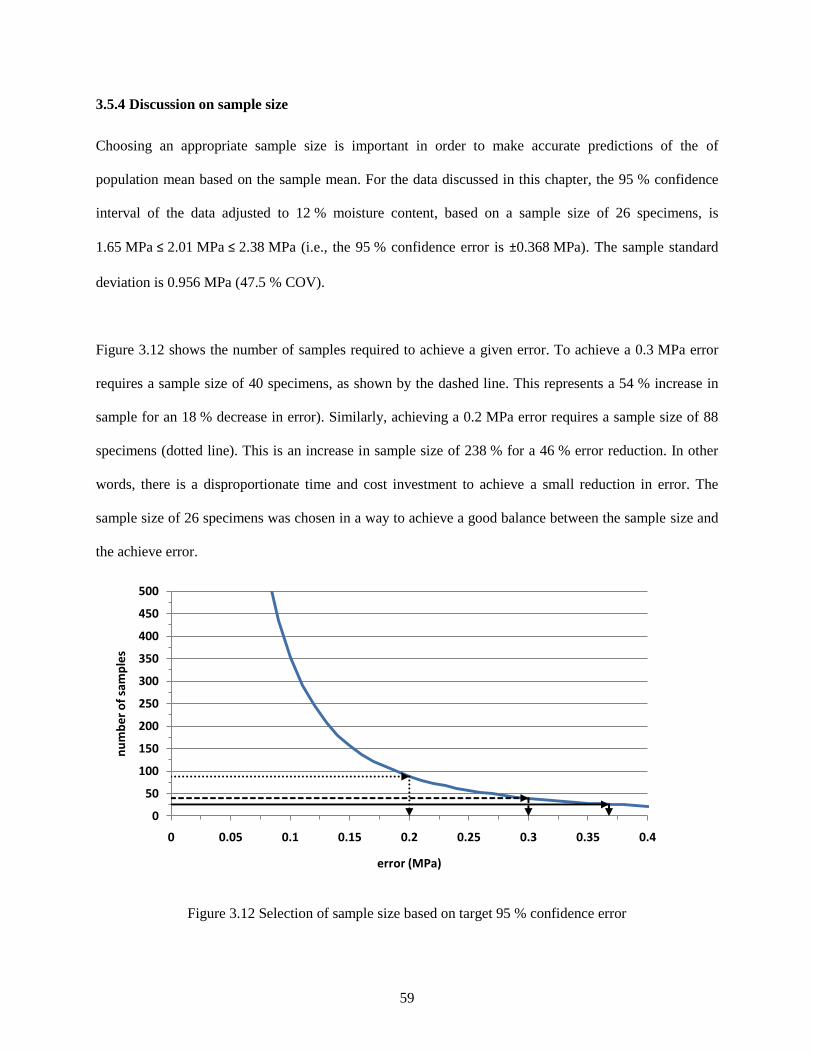
59
3.5.4 Discussion on sample size
Choosing an appropriate sample size is important in order to make accurate predictions of the of
population mean based on the sample mean. For the data discussed in this chapter, the 95 % confidence
interval of the data adjusted to 12 % moisture content, based on a sample size of 26 specimens, is
1.65 MPa ≤ 2.01 MPa ≤ 2.38 MPa (i.e., the 95 % confidence error is ±0.368 MPa). The sample standard
deviation is 0.956 MPa (47.5 % COV).
Figure 3.12 shows the number of samples required to achieve a given error. To achieve a 0.3 MPa error
requires a sample size of 40 specimens, as shown by the dashed line. This represents a 54 % increase in
sample for an 18 % decrease in error). Similarly, achieving a 0.2 MPa error requires a sample size of 88
specimens (dotted line). This is an increase in sample size of 238 % for a 46 % error reduction. In other
words, there is a disproportionate time and cost investment to achieve a small reduction in error. The
sample size of 26 specimens was chosen in a way to achieve a good balance between the sample size and
the achieve error.
Figure 3.12 Selection of sample size based on target 95 % confidence error
0
50
100
150
200
250
300
350
400
450
500
0 0.05 0.1 0.15 0.2 0.25 0.3 0.35 0.4
nu
mb
er
of
sam
ple
s
error (MPa)

60
3.5.5 Shear strength distribution
Part of the motivation for undertaking this experimental study was to use the shear strength data collected
to conduct risk analysis of wood pole structures. Any random variable used in a risk analysis must be in
the form of a statistical distribution. Thus, the data collected in the experimental programme must be
fitted to a distribution if it is to be used for risk analysis.
The data was fitted to a distribution using the Probability Paper Plot (PPP) method. In PPP, a linear
relationship is established between the data and a cumulative probability representing a given statistical
distribution. A linear curve is then fitted to the data and the distribution having the best fit is then chosen
as the appropriate distribution. The moisture-content-adjusted shear strength data was fitted to a Normal,
Log-normal, and Weibull distribution the result of which can be found in
Figure 3.13 to Figure 3.15, respectively.
Figure 3.13 Probability paper plot for shear strength following a normal distribution
All three distributions appear to be a good fit for the data with the log-normal and Weibull distributions
offering the best fit each having an R² value of approximately 0.95. For the statistical analysis, the log-
y = 1.0017x + 2.0139R² = 0.906
0.000
0.500
1.000
1.500
2.000
2.500
3.000
3.500
4.000
4.500
5.000
-2.000 -1.500 -1.000 -0.500 0.000 0.500 1.000 1.500 2.000
τ max
, MP
a
Si

61
normal distribution was used with a scale parameter value (or log-mean) of λ = 0.5909 and a shape
parameter value (or log-variance) of ζ = 0.5265. The log-normal distribution was chosen over the Weibull
distribution because it is better integrated into the software used for the analysis.
Figure 3.14 Probability paper plot for shear strength following a log-normal distribution
Figure 3.15 Probability paper plot for shear strength following a Weibull distribution
y = 0.5265x + 0.5909R² = 0.9476
-1.000
-0.500
0.000
0.500
1.000
1.500
2.000
-2.000 -1.500 -1.000 -0.500 0.000 0.500 1.000 1.500 2.000
ln(τ
max
), M
Pa
Si
y = 0.429x + 0.8191R² = 0.9518
-1.000
-0.500
0.000
0.500
1.000
1.500
2.000
-4.000 -3.000 -2.000 -1.000 0.000 1.000 2.000
ln(τ
max
), M
Pa
ln(-ln(1-Pi))

62
3.6 Limitations of experimental programme
It is quite clear from the observed failure modes that the failure mechanism found in this experimental
programme is not that of pure shear. However, a number of specimen shapes, testing apparatuses, and
experimental procedures have been evaluated in order to obtain a pure shear failure. Even the current
ASTM D143 standard, commonly used to determine clear wood shear strength, does not have specimens
that fail in a state of pure shear [16].
The shear plane is affected by non-shear stresses due to the geometry of the specimen. The specimen
configuration can be likened to single shear plane bolt connections or dowel connections used to link two
precast concrete elements. Although a double shear plane specimen could reduce non-shear stresses, such
a specimen would not eliminate these stresses and would not only be more complex to design and
construct, but would also introduce the risk of other failure modes, such as wood fibre crushing at loading
points.
Although the nature of the material leads to inherent imperfections such as checks, splits, knots, and out-
of-straightness, the intent of this experiment was to capture the effect of such imperfections on the shear
strength of wood poles. However, any significant imperfections that directly affect the failure plane
should be kept in mind when interpreting the results.
3.7 Summary
A total of 30 full-size Red Pine pole specimens were tested for shear strength. Two half-depth
slots were made along the length of each specimen such that one cut was 180 degrees from the
other. Failure was expected to happen between these slots in a plane longitudinal to the specimen.
The specimens comprised of both new poles and poles which had previously been in service. The
tested poles had varied levels of checks, splits, deterioration, and woodpecker damage.

63
Two modes of failure were observed. In the first, a single split occurred between the two slots
indicating that the failure plane was loaded mainly in shear. The second had the formation of a
single split or two splits (one originating from each slot) with a strut connecting both sides of the
failure plane indicating that bending forces were also present at the failure plane. This is likely
due to specimen geometry which causes the load to flow from one side of the cross-section to the
other causing bending stresses at the failure plane.
The mean shear strength of the Red Pine specimens adjusted to 12 % moisture content was
2014 kPa (COV 47.5 %) when calculated using gross shear area, and 2113 kPa (COV 40.5 %)
when calculated using net area (i.e., when taking into consideration pre-existing damage affecting
the plane of failure).
The mean shear strength at 12 % moisture content for full-size pole specimens was approximately
27 % of the reported clear wood shear strength values at the same moisture content level.
The shear strength of full-size pole specimens can be represented using a log-normal distribution
with a scale parameter of λ = 0.5909 and a shape parameter of ζ = 0.5265.

64
Chapter 4 Structural analysis model for tapered cantilever
This chapter discusses the approach used in the development of the structural analysis model and how it
was used to perform Monte Carlo simulations. The analytical model was developed in Excel 2010 and
macros were developed using Visual Basic for Applications to enhance the versatility of the Excel
workbook. The code written for this purpose can be found in Appendix E.
4.1 Pole discretization
The structural analysis model discretizes the pole into segments of user-specified height. This helps
identify the magnitude of loads and stresses as well as various sectional properties at different points
along the structure. This is useful since the location of failure is not constant due to the fact that wooden
utility poles are non-prismatic (i.e., the cross-section varies along the length) and because mechanical
damage can be introduced at random locations along the length which may result in failure at a location
that would does not normally govern the pole mode of failure.
Once the pole has been discretized, the location of damage is located, if applicable. Then, the section
properties are calculated for each segment. Section properties include the diameter, moment of inertia,
area, section modulus, and the first moment of area used for shear stress calculations. All these properties
are calculated taking into account any mechanical damage.
4.2 Section properties
In order to fully analyse the pole, the section properties at each discrete point needs to be determined. The
section properties vary depending upon the level of damage along the pole. Five damage scenarios are
taken into account: sections with no damage, sections with exploratory or feeding damage oriented with
the extreme fibre, sections with exploratory or feeding damage oriented with the neutral axis, sections
with nesting damage oriented with the extreme fibres, and sections with nesting damage oriented with the
neutral axis. Figure 4.1 shows the assumed shapes and orientations of woodpecker damage used in this

65
study. The set of equations used to calculate these section properties and their derivation can be found in
Appendix D.
Figure 4.1 Assumed shapes and orientations of woodpecker damage
4.3 Loading
Loads in the model are provided in one of two forms: as user-inputted deterministic loads or randomly-
generated probabilistic loads. Loading conditions always vary based on geographic location regardless of
whether the loading is deterministic or probabilistic in nature. This is due to the variability in topography,
elevation, ambient temperature and humidity, and other factors that affect the climatic conditions for a
given geographic location.
N.A. N.A.
N.A. N.A.
exploratory/feeding hole oriented
with the extreme fibres
nesting hole oriented with the extreme fibres
exploratory/feeding hole oriented with the neutral axis
nesting hole oriented with the neutral axis

66
As explained in 2.1.3, CAN/CSA-C22.3 No. 1 divides Canada into four distinct loading regions having
different wind and ice thickness, as summarized in Table 4.1. When deterministic loading is used in an
analysis, one of these four loading areas must be specified.
Table 4.1 Deterministic weather loading
Loading
Conditions
Loading area
Medium
Severe Heavy A B
Radial thickness of
ice, mm 19 12.5 6.5 12.5
Horizontal
loading, N/m² 400 400 400 300
Temperature, °C -20 -20 -20 -20
When probabilistic loading is used, the probabilistic data for a chosen geographical location must be
known in order to perform the analysis. Based on the distribution associated with each the load type, an
appropriate load value will be randomly generated for each iteration of the Monte Carlo simulation. Table
4.2 summarizes the climatic data for Thunder Bay, Ontario which was used in this study.
Table 4.2 Gumbel parameters for variables related to climatic loading in Thunder Bay, Ontario
Climatic load type α u
Annual wind speed (wind only), km/h 0.0786 84.1
Annual wind speed (wind on ice), km/h 0.0898 34.5
Annual ice thickness, in 4.12 0.304
4.3.1 Gravity loads
Gravity loads on the system are mainly based on the weight of ice-covered wires. Thus, there are a
number of user inputs that will directly affect the total gravity load: the weight of the wires used (per unit
length), the thickness of ice covering the wires, the span length of the wires, the number of wires attached
to the pole, and any elevation change between adjacent poles. All but the ice thickness are deterministic
67
variables. This means that once the user has input these variables, they will remain the same for the scope
of a Monte Carlo simulation. An ice density of 900 kg/m³ was used as specified in CAN/CSA-C22.3
No. 1 [7].
Gravity loads play a part in the flexural stressed applied on the structure in two ways. Firstly, any wire
that is eccentrically attached to the pole via a cross-arm will cause a moment in the structure. Secondly,
moments due to second-order effects are directly related to gravity loads.
4.3.2 Lateral loads
Lateral loads on the system are based on the wind acting upon both the ice-covered wires as well as the
pole itself. Wind load is the major contributor to bending and shear loads on the structure. Thus, factors
that will influence the total lateral loads are: the specified wind pressure, the thickness of ice covering the
wires, the span length of the wires, the number of wires attached to the pole, and the geometry of the pole.
The wind pressure and ice thickness are both treated as random variable in the applicable context whilst
the other variables are deterministic.
4.3.3 Second-order effects
The second-order effects are calculated by first determining the Euler buckling load for the structure
using Equation (4.1) and the lateral force resultant magnitude and location. The deflection is then
calculated using Equation (4.2) and modified using the deflection amplification factor using Equation
(4.3). Finally, the moment due to second-order effects is calculated for each segment based on the
horizontal deflection of the segment using Equation (4.4).
(4.1)

68
(4.2)
(4.3)
(4.4)
4.4 Resistance
The section shear and flexural resistance are calculated based on section properties (section modulus S,
moment of inertia I, statical moment of area Q, and section thickness at the neutral axis t) and material
strengths (bending strength σ and shear strength τ). The ultimate shear and flexural capacity are calculated
using Equations (4.5) and (4.6), respectively. Although a shear-bending interaction model can be used to
capture failure of the pole (see section 2.3.8), work by Steenhof has concluded that treating shear and
bending separately yielded reliable results [5]. These properties are calculated for each segment along the
pole length. The modulus of elasticity, modulus of rupture, and shear strength can be deterministic or
probabilistic, depending on user input.
(4.5)
(4.6)
Modulus of rupture data from CAN/CSA-O15 [6] and from a study conducted by Steenhof [5] were used
to calculate the flexural resistance. Similarly, the shear strength from the Canadian Department of
Forestry [18] and the results from the study discussed in Chapter 3 were used to determine the shear

69
strength. The desired shear and bending strengths distributed can be specified at the beginning of the
analysis. Table 4.3 offers a summary of the strength data used in this study.
Table 4.3 Statistical distribution parameters used for probabilistic shear and bending strength
Source mean COV log-mean log-variance
MOR, Steenhof, MPa 35.3 23.5% - -
MOR, CAN/CSA-O15, MPa 41.0 17.0% - -
full-size pole shear strength, MPa
- - 0.591 0.527
clear wood shear strength, MPa 4.9 11.10% - -
4.5 Analytical model
Based on a specified top and bottom pole circumference, pole length, and a segment height, the analysis
model will generate a table containing all the necessary section properties for each segment. The loads
applied on each segment are then determined based on the number of conductors, ice thickness, and pole
area. Finally, the applied shear and bending stresses are compared to the ultimate shear and bending
capacity to determine if a failure as occurred. Figure 4.2 shows a flowchart summarizing the analytical
model and Monte Carlo simulation.
4.5.1 Typical pole configuration for analysis
All analyses done in this study use a Red Pine pole with a height-above-ground of 12.2 m (40 ft) unless
otherwise specified. A three-conductor configuration is used with two conductors a distance 500 mm
from the top and the third at 800 mm from the top. Each conductor is supported by a cross arm and is
offset a distance of 700 mm from the centreline of the pole. All conductors had a weight per length of
7.26 N/m. This conductor configuration is similar to the configurations used by Subramanian [12] and by
Talwar [28] and was found to be representative of configurations used in distribution systems.

70
4.6 Monte Carlo simulation
The Monte Carlo simulation is performed by running the analysis model for a given number of iterations.
The strength properties and load effects are randomly generated for each iteration based on appropriate
cumulative distribution functions. The number of shear and bending failures are recorded and used to
determine the probability of failure of the system.
4.6.1 Approach to choosing a sample size
The sample size of a Monte Carlo simulation is the number of iterations performed over the course of a
simulation. The sample size required to reach a meaningful conclusion is dependent on the variability of
the random variables. When using a relatively small sample size, performing multiple simulations will
display significant scatter in the probability of failure of the system. Increasing the sample size will cause
the probability of failure to eventually converge towards a single answer. Although increasing the sample
size to a very large value will yield greater precision, this come at the expense of greater computational
requirements. Thus, a sample size must be chosen such that sufficient precision is achieved whilst
minimizing the time taken for each simulation. Using a sample size of 10 000 or more has shown to yield
a coefficient of variation below 5 % for the results.

71
72
Chapter 5 Reliability analysis of wood utility poles
5.1 Objectives
The goal of this Chapter is to determine the reliability of different configurations of wood utility poles
designed based on CAN/CSA-C22.3 No. 1 and CAN/CSA-O15. These configurations include different
constructions grades, different pole heights, poles which have reach their end of life based on the end-of-
life criterion stipulated in CAN/CSA-C22.3 No. 1, and poles with various levels and orientations of
woodpecker damage.
5.2 Methodology
A parametric study was used to determine the effect the above properties have on pole reliability. This
section discusses the approach used to quantify the effect of these parameters on the reliability of wood
poles.
5.2.1 Design approach
All poles in this study were designed based on the deterministic design approach discussed in section 2.1.
The design steps are summarizes as follows:
1. Choose the pole species and dimensions for the analysis based on the desired pole height.
2. Choose a conductor configuration for the analysis. At this point the number of conductors and the
weight, size, and span of the conductors is determined.
3. Assume a geographic location for the design and select the appropriate loading conditions.
4. Assuming a construction grade for the design. This affects the load factors used.
5. Use a deterministic design spreadsheet (with safety factors) to verify the pole’s compliance to
code.
a. If the pole fails, go to a sturdier pole grade or reduce the span length of the conductor(s).

73
b. If the pole is not efficiently used, i.e., the resistance is significantly greater than the
applied loads, then either go down a pole class or adjust the span length of the
conductor(s) such that the resistance and applied loads are close in value.
All poles used in this study were designed such that the maximum bending stress in the pole was
approximately 97 % of the modulus of rupture for the species. This was done to ensure that all poles
analysed were designed to the same standard. To achieve this, the wire span was altered until the desired
stress level was attained. This means that, for a given height-above-ground, a class 1 pole would support a
longer conductor span than a class 2 pole. Similarly, a pole designed using construction grade 3 would
support a longer conductor span than one designed using construction grade 1, when all other design
variable were the same.
5.2.2 Reliability analysis approach
The reliability of a given pole configuration is determined using a Monte Carlo analysis. Load and
resistance variables are randomized using statistical distributions relevant to the wood species and design
location. This is done at the beginning of each iteration of a simulation. The simulation is run for a
specified number of iterations chosen per the discussion in the section below.
The reliability of the structure is determined by comparing the number of recorded failures to the total
number of iterations. Failure is determined based on two performance functions. One performance
function related to shear and one to flexure. Both performance functions compare the resistance of the
structure to its associated load effect for each discrete segment of the pole.
5.2.3 Analysis model
All analyses discussed in this section were done based on the approach discussed in Chapter 4. The loads
used are summarized in section 4.3 and material strengths in section 4.4. All analyses are conducted
assuming the structure is located in Thunder Bay, Ontario.
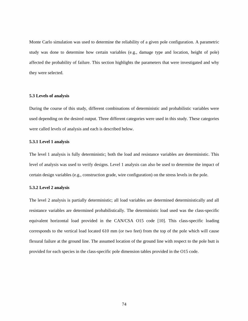
74
Monte Carlo simulation was used to determine the reliability of a given pole configuration. A parametric
study was done to determine how certain variables (e.g., damage type and location, height of pole)
affected the probability of failure. This section highlights the parameters that were investigated and why
they were selected.
5.3 Levels of analysis
During the course of this study, different combinations of deterministic and probabilistic variables were
used depending on the desired output. Three different categories were used in this study. These categories
were called levels of analysis and each is described below.
5.3.1 Level 1 analysis
The level 1 analysis is fully deterministic; both the load and resistance variables are deterministic. This
level of analysis was used to verify designs. Level 1 analysis can also be used to determine the impact of
certain design variables (e.g., construction grade, wire configuration) on the stress levels in the pole.
5.3.2 Level 2 analysis
The level 2 analysis is partially deterministic; all load variables are determined deterministically and all
resistance variables are determined probabilistically. The deterministic load used was the class-specific
equivalent horizontal load provided in the CAN/CSA O15 code [10]. This class-specific loading
corresponds to the vertical load located 610 mm (or two feet) from the top of the pole which will cause
flexural failure at the ground line. The assumed location of the ground line with respect to the pole butt is
provided for each species in the class-specific pole dimension tables provided in the O15 code.

75
This level of analysis was used to see how different material strength data sets impacted the reliability of
a structure. It was also helpful in seeing how going from a deterministic to a probabilistic strength data set
affected the reliability of a structure.
5.3.3 Level 3 analysis
The level 3 analysis is fully probabilistic. Both the resistance and load data are randomly generated from
the appropriate statistical distribution. This is the main level of analysis used for the reliability analyses
discussed in this study since it better represents the random nature of both the loads and the materials used
in a wood pole structure.
5.4 Discussion of Level 1 analysis
Level 1 analysis is fully deterministic which means there is no variability in the results of any given
analysis. Although this level of analysis may not be used directly to determine the reliability of a
structure, some useful observations can be made with respect to the behaviour of a structure.
5.4.1 Typical analysis results for a wood utility pole
A Class 1 utility pole standing 12.2 m above ground with a top circumference of 48 cm and a
circumference of 92 cm at a point 1.8 m from the butt was analysed. The conductors were configured per
the typical pole configuration discussed in section 4.5.1. Heavy loading conditions and Construction
Grade 1were assume.
Figure 5.1 shows the bending moment diagram for the pole along with the contribution different sources
to the total moment. It can be seen that the biggest contribution to the moment comes from the wind
acting on the conductors. The second-order effects also contribute a significantly to the total moment on
the structure. Finally, the wind on the pole itself (wind on support) and the moment due to weight of the
wire being eccentric to the pole have much smaller contributions to the total moment.

76
Figure 5.2 shows the bending stresses at various points along the height of the pole. The dashed vertical
line represents the ultimate bending strength of the wood. It can be observed that the stress does not vary
linearly along the pole height and that the maximum stress does not occur at the ground line, where the
maximum moment occurs.
Figure 5.1 Contribution of different loads to total bending moment
The location of maximum stress does not correspond to the location of maximum moment because wood
poles are non-prismatic member. In other words, the cross section of the member is not constant along the
pole length. Since flexural stresses are related to the moment of inertia, and the moment of inertia varies
along the length following a fourth order polynomial, the maximum stress may not be located where the
maximum load effect occurs. Figure 5.3 shows the variation of the moment of inertia along the pole
height.
0.00
2.00
4.00
6.00
8.00
10.00
12.00
14.00
-50.00 0.00 50.00 100.00 150.00 200.00
He
igh
t ab
ove
gro
un
d, m
Bending Moment, kN·m
Wind on support
Eccentricities
Wind on wires
P-Δ effects
Total moment

77
Figure 5.2 Variation of flexural stress along the pole height
Figure 5.3 Variation of moment of inertia along the pole height
0.0
2.0
4.0
6.0
8.0
10.0
12.0
-10.0 0.0 10.0 20.0 30.0 40.0 50.0
He
igh
t ab
ove
gro
un
d, m
Stress, MPa
Applied stress
Ultimate stress
0.0
2.0
4.0
6.0
8.0
10.0
12.0
000.0E+0 250.0E+6 500.0E+6 750.0E+6 1.0E+9
He
igh
t ab
ove
gro
un
d, m
Moment of inertia, mm⁴

78
5.4.2 Verification of equivalent loads
The magnitude of the equivalent loads provided in CAN/CSA-O15 was verified by using the dimensions
provided for each pole class and height and determining the load which would cause the pole to fail in
flexure assuming a modulus of rupture of 41 MPa, which is equivalent to the mean modulus of rupture
specified in CAN/CSA-O15 [6]. Two equivalent loads were calculated for each pole configuration: one
calculated assuming failure would occur at the ground line and one assuming it would occur at the
theoretical point of maximum stress (i.e., the point along the pole at which the diameter is 1.5 time the
diameter where the point load is situated). Table 5.1 offers a summary of these calculations where Pcode is
the code-specified load, PGL is the equivalent load assuming failure at the ground line, and P1.5 is the load
assuming failure at the theoretical maximum stress location.
Table 5.1 Comparison of equivalent load between code-provided values and values calculated based on
pole dimensions
Class Ltotal, m hGL, m Pcode, kN PGL, kN P1.5, kN
2 6.1 1.2 15.68 15.46 15.46
2 7.6 1.5 15.68 15.08 15.08
2 9.1 1.7 15.68 15.58 15.58
2 10.7 1.8 15.68 14.74 14.74
2 12.2 1.8 15.68 14.92 14.83
2 13.7 2.0 15.68 14.85 14.57
2 15.2 2.1 15.68 15.34 14.67
2 16.8 2.3 15.68 14.66 13.82
2 18.3 2.4 15.68 14.63 13.48
2 19.8 2.6 15.68 14.65 13.19
4 6.1 1.2 10.17 10.42 10.42
4 7.6 1.5 10.17 10.01 10.01
4 9.1 1.7 10.17 9.92 9.92
4 10.7 1.8 10.17 9.62 9.60
4 12.2 1.8 10.17 9.67 9.49
4 13.7 2.0 10.17 9.51 9.17
4 15.2 2.1 10.17 9.77 9.13
4 16.8 2.3 10.17 9.72 8.85
4 18.3 2.4 10.17 9.84 8.67
4 19.8 2.6 10.17 9.46 8.22

79
It can be observed that the code-provided equivalent load is generally greater than the predicted failure
load. It is also evident that shorter poles tend to have a greater expected failure load than taller poles. This
is due in part to the fact that the theoretical maximum stress location corresponds to the ground line for
poles shorter than 10 metres. This means that designs based on this equivalent load concept may be
under-designed, especially for design of taller poles.
5.5 Discussion of Level 2 analysis
5.5.1 Effect of pole height on reliability
A Level 2 analysis was conducted on Class 2 and Class 4 Red Pine wood poles of varying height loaded
with the O15 class-specific equivalent horizontal loads and the critical loads determined based on the
Level 1 analysis as discussed in section 5.4.2. The modulus of rupture mean and COV found in
CAN/CSA-O15 were used to randomly determine the pole bending strength.
The results of the Level 2 analysis are shown in Figure 5.4 for Class 2 poles and Figure 5.5 for Class 4
poles. In general, the probability of failure exceeded 50 % for both classes. The results based on the
calculated critical loads are relatively constant at 50 %. This is due to the applied deterministic load being
based on the geometric properties of each pole tested and the mean of the strength for Red Pine.
The results based on the code equivalent loads shows an increase in probability of failure starting at
approximately 50 % for the shorter poles and ending at 85 % to 90 % for the taller poles. This is due to
the fact that the deterministic load is specific to the class for all pole height. For the shorter poles, the
actual critical load is relatively close in magnitude compared to the critical load for taller poles.
Recalling the reliability level suggested in CAN/CSA-C22.3 No. 60826 and discussed in section 2.2.2,
some observations on the probability of failures observed in this analysis can be made. For structures
designed based on loads having a 50-year return period, the suggested reliability is 36 % to 61 % for the

80
lifetime reliability (based on a 50 year lifetime of the structure), and 98 % to 99 % for the annual
reliability. This translates into a lifetime probability of failure ranging from 39 % to 64 % and an annual
probability of failure of 1 % to 2 %. Since the loads used in this analysis are based on the material
properties of the pole and not on observed climactic data, the aforementioned probability of failure ranges
are only used to give insight on whether or not the observed probability of failure are acceptable
Were these data to represent annual probability of failure, then it can be observed that the values are
unacceptable as they are well over the 2 % recommended by C22.3. If they were to represent lifetime
probability of failure however, these values would only be deemed acceptable if the appropriate critical
loads were used in design.
Figure 5.4 Level 2 analysis comparison between Class 2 poles loaded with code-specified horizontal load
and calculated critical load
0%
10%
20%
30%
40%
50%
60%
70%
80%
90%
100%
5 10 15 20
Pro
bab
ility
of
failu
re
Pole length, m
Critical loads
code loads

81
Figure 5.5 Level 2 analysis comparison between Class 4 poles loaded with code-specified horizontal load
and calculated critical load
Thus, although the critical loads calculated in the previous section different from the code-provided load
by less than 2 kN, it can results in an increase in probability of failure of up to 40 %. Although the
equivalent load design approach is convenient and relatively straightforward, these results suggest that
this method should be avoided.
Lastly, it should be noted that the relatively high probability of failure values observed here are due to the
load being deterministic and based on the material strength. The design method used in C22.3 No. 1
incorporates safety factors on the loads. Thus, once probabilistic climactic loads are used the probability
of failure is expected to be lower. This analysis is performed in a later section.
0%
10%
20%
30%
40%
50%
60%
70%
80%
90%
100%
5 10 15 20
Pro
bab
ility
of
failu
re
Pole length, m
Critical loads
code loads

82
5.6 Discussion of Level 3 analysis
5.6.1 Effect of pole height on reliability
In this section, the reliability of poles of varying height is investigated across several classes to see if a
significant difference in reliability exists between poles of different heights. Level 3 analysis is used for
this analysis. Two loading scenarios are simulated: extreme wind and wind on ice-covered conductors.
Extreme wind refers to the wind speed distribution based on observed wind speeds over a 50 year period
whilst wind on ice-covered conductors refers to wind speed associated with icing events over the same
time period.
Three poles heights are used in this study: a pole measuring 4.9 m above ground (6.1 m long pole with
1.2 m below ground); a pole measuring 12.2 m above ground (15.2 m pole with 3.0 m below ground); and
a pole measuring 17. 2 m above ground (19.8 m pole with 2.6 m below ground). The longest and shortest
poles used represent the two extremes in terms of length for red pine wood poles. Eight classes are
available for this species; class 1 being the strongest and class 8 the weakest. The 19.8 m long poles are
only available from classes 1 through 4; the 15.2 m long poles are only available from classes 1
through 5; finally, the 6.1 m long poles are available in all eight classes. Strength data used for these
analyses are the modulus of rupture reported by Steenhof [5] and shear strength discussed in Chapter 3.
5.6.1.1 Extreme wind on conductors
Figure 5.6 shows the results of the Level 3 reliability analysis based on extreme wind loading conditions.
The first noticeable trend is the relative increase in probability of failure when going from a lower pole
class (i.e., stronger pole) to a higher pole class (i.e., weaker pole). Similarly, taller poles tend to have
greater probability of failure than shorter poles.

83
When comparing two poles of the same height but of different classes, the stronger pole will tend to be
stiffer compared to the weaker pole. This leads to an increase in top deflection which results in greater
contribution from second-order effects. This leads to a greater probability of failure for the weaker poles.
Figure 5.6 Variation of probability of failure versus pole class for different pole heights (wind only)
For poles of the same class but of different height, the taller pole has a larger surface area upon which the
wind can act leading to a relatively larger wind force on the pole. Furthermore, the taller pole will tend to
have a higher deflection at the top. Since the conductors are configured such that they are at the same
distance from the top regardless of pole height, the increase in deflection will yields larger moments due
to second-order effects. This increase in load explains why taller poles tend to have relatively higher
probability of failure.
Table 5.2 shows a summary of the annual probability of failure and reliability for the cases evaluated.
This annual reliability ranges from 99.76 % to 99.90 %. As discussed in section 2.2.2, CAN/CSA-C22.3
No. 60826 suggests an annual reliability of 98 % to 99 % for structures designed assuming a load with a
0.05%
0.10%
0.15%
0.20%
0.25%
1 2 3 4 5 6 7 8
Pro
bab
ility
of
failu
re
Pole class
HAG 4.9 m
HAG 12.2 m
HAG 17.2 m

84
50-year return period. The annual reliability of all cases discussed in this section fall above the suggested
range.
Table 5.2 Summary of probability of failure for varying pole class and height (wind only)
Height above ground, m
Pole class
Annual probability of failure
Annual reliability
4.9 1 0.10 % 99.90 %
4 0.14 % 99.86 %
8 0.18 % 99.82 %
12.2 1 0.17 % 99.83 %
4 0.19 % 99.81 %
17.2 1 0.17 % 99.83 %
4 0.24 % 99.76 %
5.6.1.2 Wind on ice-covered conductors
Figure 5.7 shows the result of the Level 3 reliability analysis based on wind on ice-covered conductors.
The first observation that can be made is that, similarly to the results of the analysis of extreme wind
conditions, reliability of shorter poles is higher than that of longer poles. For Class 1 poles, the difference
in probability of failure compared to the 4.9 m pole was approximate 65% higher for the 17.2 m pole and
52% higher for the 12.2 m pole. For Class 4 poles, a 158% difference in probability of failure was
observed for the 17.2 m pole configuration whilst the 12.2 m pole configuration only showed a 10%
difference in probability of failure relative to the 4.9 m pole. The difference in reliability between each
pole height is attributed to the second-order effects which become more significant for taller poles.
Furthermore, the difference observed between classes within the 17.2 m pole configuration may be
explained by the relative decrease in stiffness found in poles of higher class which lead to increases in
deflection and thus higher contributions from P-Δ effects.
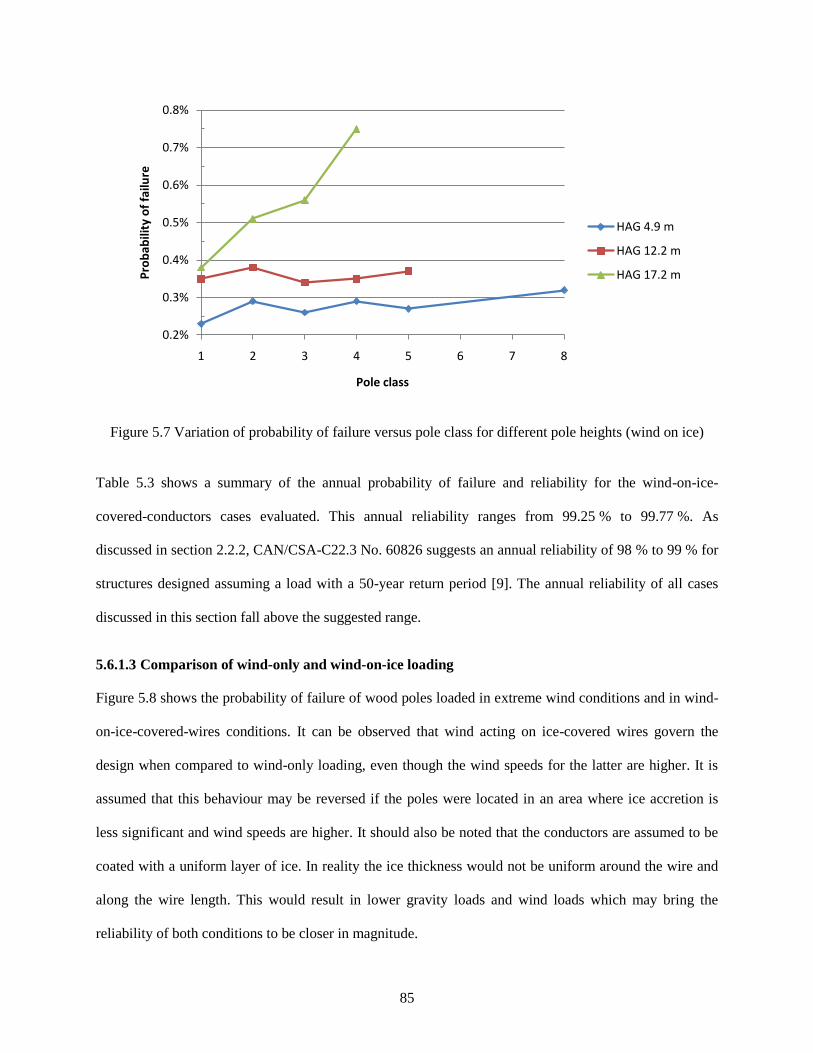
85
Figure 5.7 Variation of probability of failure versus pole class for different pole heights (wind on ice)
Table 5.3 shows a summary of the annual probability of failure and reliability for the wind-on-ice-
covered-conductors cases evaluated. This annual reliability ranges from 99.25 % to 99.77 %. As
discussed in section 2.2.2, CAN/CSA-C22.3 No. 60826 suggests an annual reliability of 98 % to 99 % for
structures designed assuming a load with a 50-year return period [9]. The annual reliability of all cases
discussed in this section fall above the suggested range.
5.6.1.3 Comparison of wind-only and wind-on-ice loading
Figure 5.8 shows the probability of failure of wood poles loaded in extreme wind conditions and in wind-
on-ice-covered-wires conditions. It can be observed that wind acting on ice-covered wires govern the
design when compared to wind-only loading, even though the wind speeds for the latter are higher. It is
assumed that this behaviour may be reversed if the poles were located in an area where ice accretion is
less significant and wind speeds are higher. It should also be noted that the conductors are assumed to be
coated with a uniform layer of ice. In reality the ice thickness would not be uniform around the wire and
along the wire length. This would result in lower gravity loads and wind loads which may bring the
reliability of both conditions to be closer in magnitude.
0.2%
0.3%
0.4%
0.5%
0.6%
0.7%
0.8%
1 2 3 4 5 6 7 8
Pro
bab
ility
of
failu
re
Pole class
HAG 4.9 m
HAG 12.2 m
HAG 17.2 m

86
Table 5.3 Summary of probability of failure for varying pole class and height (wind on ice)
Height above ground, m
Pole class
Annual probability of failure
Annual reliability
4.9 1 0.23 % 99.77 %
2 0.29 % 99.71 %
3 0.26 % 99.74 %
4 0.29 % 99.71 %
5 0.27 % 99.73 %
8 0.32 % 99.68 %
12.2 1 0.35 % 99.65 %
2 0.38 % 99.62 %
3 0.34 % 99.66 %
4 0.35 % 99.65 %
5 0.37 % 99.63 %
17.2 1 0.38 % 99.62 %
2 0.51 % 99.49 %
3 0.56 % 99.44 %
4 0.75 % 99.25 %
Figure 5.8 Comparison between wind-only and wind-on-ice loading
0.0%
0.2%
0.4%
0.6%
0.8%
1 2 3 4 5 6 7 8
Pro
bab
ility
of
failu
re
Pole class
4.9 m wind on ice
12.2 m wind on ice
17.2 m wind on ice
4.9 m wind only
12.2 m wind only
17.2 m wind only

87
5.6.2 Effect of construction grade on reliability
During the design process, the designer must decide which construction grade (CG) to use. In some cases,
the code will dictate a minimum grade; in others, the designer may have the flexibility to decide which
construction grade is appropriate. The difference between construction grades is the safety factors used to
modify the applied loads. There are three construction grades: Grade 1, Grade 2, and Grade 3. Of the
three, Grade 1 has the highest load factors and Grade 3 has the lowest.
Thus, choosing to use a lower grade will result in the assumption of higher risk. However, it is not clear
how much additional risk is assumed by using a lower construction grade. This additional risk can be
determined by analysing the same structure designed using the three construction grades and comparing
the level safety of each design.
To determine the reliability of different construction grades, 12.2 m high wood poles were designed using
all three construction grades. The design was performed using a Level 1 analysis spreadsheet which took
into consideration the appropriate load factors for each construction grade. Designs based on pole Class 1,
3, and 5 were used to see if there were any notable differences in reliability within the same construction
grade. The loading condition used was wind on ice-covered wires for all analyses since it was shown to
govern this particular pole configuration (see previous sections).
Table 5.4 summarizes the results of the analysis. When comparing the probability of failure within
Class 1, 3, and 5, a respective increase of 343 %, 385 %, and 521 % in probability of failure was observed
when using Construction Grade 2 instead of Construction Grade 1; the probability of failure increases by
approximately 786 %, 876 %, and 1016 %, respectively, when using Construction Grade 3 instead of
Construction Grade 1.

88
Table 5.4 Analysis results for construction grade
Construction grade
Pole class
Annual probability of failure
Annual reliability
CG 1 1 0.35 % 99.65 %
3 0.34 % 99.66 %
5 0.37 % 99.63 %
CG 2 1 1.55 % 98.45 %
3 1.65 % 98.35 %
5 2.30 % 97.70 %
CG 3 1 3.10 % 96.90 %
3 3.32 % 96.68 %
5 4.13 % 95.87 %
Figure 5.9 shows the relative probability of failure between each construction grade. It can be observed
that there is a reduction in reliability when using a construction grade other than CG 1. This observation
can be explained by the design approached used for all poles in this analysis. As previously discussed in
section 5.2.1, the poles were designed such that the same level of maximum stress was achieved
regardless of construction grade or class. Thus, if the construction grade is changed and the pole height
and class remain constant, the only variables that change are the load factors. Because the load factors get
progressively lower when going from CG 1 to CG 3 (i.e., the design load reduces from CG 1 to CG 3), it
stands to reason that a longer conductor span will be required to cause the same level of maximum stress
when going from CG 1 to CG 2 to CG 3. Thus, the same probabilistic load is applied to poles having the
same dimensions but varying conductor spans resulting in higher failure rates for the poles having longer
conductor spans because the resultant wind load acting on the wires is of greater magnitude as is the
gravity load due to the conductors.
Comparing the annual reliability to those suggested in CAN/CSA-C22.3 No. 60826 and discussed in
section 2.2.2 shows that the annual reliabilities of CG 1 and CG 2 poles fall within the suggested range of
98 % to 99 % for structures designed assuming a load with a 50-year return period [9]. However, all
reliability values for CG 3 poles fell below this range by at least 1 %.
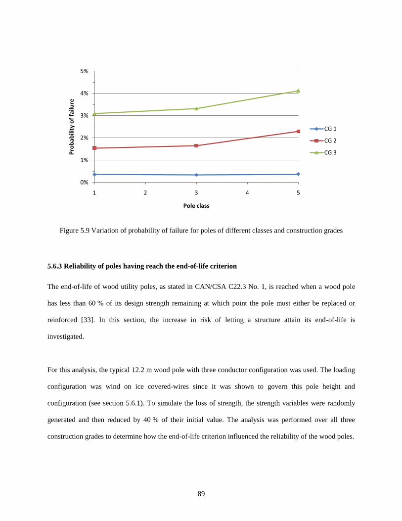
89
Figure 5.9 Variation of probability of failure for poles of different classes and construction grades
5.6.3 Reliability of poles having reach the end-of-life criterion
The end-of-life of wood utility poles, as stated in CAN/CSA C22.3 No. 1, is reached when a wood pole
has less than 60 % of its design strength remaining at which point the pole must either be replaced or
reinforced [33]. In this section, the increase in risk of letting a structure attain its end-of-life is
investigated.
For this analysis, the typical 12.2 m wood pole with three conductor configuration was used. The loading
configuration was wind on ice covered-wires since it was shown to govern this pole height and
configuration (see section 5.6.1). To simulate the loss of strength, the strength variables were randomly
generated and then reduced by 40 % of their initial value. The analysis was performed over all three
construction grades to determine how the end-of-life criterion influenced the reliability of the wood poles.
0%
1%
2%
3%
4%
5%
1 2 3 4 5
Pro
bab
ility
of
failu
re
Pole class
CG 1
CG 2
CG 3

90
Table 5.5 shows the reliability of both new design and end-of-life utility poles. As expected, there is a
notable increase in the probability of failure when the strength of a given pole is at end-of-life. Recalling
the recommended range of annual reliability of 98 % to 99 % proposed by CAN/CSA-C22.3 No. 60826
for poles designed using load with a 50-year return period [9], the following observations can be made.
Firstly, even at end-of-life conditions, all poles designed under Construction Grade 1 were within the
range prescribed by CSA. In contrast, none of the poles designed with Construction Grade 2 and 3 met the
recommended annual probability. Although this is in line with what’s expected of a pole in end-of-life
conditions, it should be pointed out that poles designed with Construction Grade 3 were below this
threshold in as-new conditions.
Table 5.5 Annual reliability of Red Pine wood poles in as-new and end-of-life conditions
Construction grade
Pole class
New design End-of-life Difference in probability of failure
Pf R Pf R
CG 1 1 0.35 % 99.65 % 1.39 % 98.61 % 1.04 %
3 0.34 % 99.66 % 1.28 % 98.72 % 0.94 %
5 0.37 % 99.63 % 1.55 % 98.45 % 1.18 %
CG 2 1 1.55 % 98.45 % 4.92 % 95.08 % 3.37 %
3 1.65 % 98.35 % 4.77 % 95.23 % 3.12 %
5 2.30 % 97.70 % 5.32 % 94.68 % 3.02 %
CG 3 1 3.10 % 96.90 % 8.28 % 91.72 % 5.18 %
3 3.32 % 96.68 % 8.76 % 91.24 % 5.44 %
5 4.13 % 95.87 % 10.21 % 89.79 % 6.08 %
Figure 5.10 shows the probability of failure of wood poles designed using all three construction grades for
both as-new (solid lines) and end-of-life (dashed lines) conditions. The CG 1 EOL values are
approximately at the level of the as-new CG 2 values. Although not as pronounced, the CG 2 EOL values
exhibit a similar behaviour with the as-new CG 3 values.

91
Figure 5.10 Comparison of probability of failure for as-new and end-of-life Red Pine wood poles
The results of this analysis show that the end-of-life criterion established by CAN/CSA-C22.3 No. 1
causes the annual reliability of CG 2 and CG 3 poles to fall below the target reliability levels suggested by
CAN/CSA-C22.3 No. 60826 and that there is ground for replacement or reinforcement of these poles. On
the other hand, the reliability of CG 1 poles was found to be within the established range even after a 40 %
reduction in strength. These results suggest that it may be appropriate to have construction-grade specific
end-of-life criteria.
5.6.4 Effect of woodpecker damage on reliability
There were two goals for the woodpecker damage analysis: determine the reliability of wood poles with
varying levels of woodpecker damage and determine the likelihood of shear failure of such poles. The
dimensions of the hole were randomly determined using equal probability and the dimensions of holes
discussed in Section 2.3.7 were used. The holes were randomly located using equal probability. The
location of holes was limited to the top half of the pole as this trend was observed in previous research
0%
2%
4%
6%
8%
10%
1 2 3 4 5
Pro
bab
ility
of
failu
re
Pole class
CG 1
CG 2
CG 3
CG 1 (EOL)
CG 2 (EOL)
CG 3 (EOL)
92
[5]. The typical 12.2 m pole discussed in section 4.5.1 was used for this analysis. The poles were assumed
to be located in Thunder Bay, Ontario and loading was assumed to be wind on ice-covered wires.
Shear failure was previously observed in new pole test specimens having significant woodpecker damage
and in-service specimens having either significant woodpecker damage or decay within the section [5].
Previous research also observed that decay typically started at the core of the pole cross-section and
propagated outward. This behaviour results in the weakening of both the shear and bending resistance of
the section. Since decay occurs closer to the neutral axis of the section, the shear resistance deteriorates
more rapidly than the bending resistance. This phenomenon is illustrated in Figure 5.11 which shows the
influence of damage at the core of a circular section. The damage is assumed to be circular and is
expressed as a fraction of the section diameter. It can be seen in Figure 5.11 that the shear resistance of
the cross-section is reduced significantly at the onset of damage whilst the bending resistance remains
relatively unaltered until the damaged area reached approximately 40 % of the section diameter.
Figure 5.11 Decrease in strength in circular section due to section core loss
0%
10%
20%
30%
40%
50%
60%
70%
80%
90%
100%
0% 20% 40% 60% 80% 100%
Re
mai
nin
g st
ren
gth
Core damage diameter (expressed as percentage of section diameter)
Bending strength
Shear strength

93
Woodpecker damage has a similar effect to the above core damage, with the added distinction that it has
an opening to one of the sides of the section. Due to this asymmetry in the damage, the orientation of the
opening has to be taken into consideration when evaluating the effect of damage on the structure. Thus,
orienting the opening with the tension or compression fibres will decrease the flexural resistance more
drastically whilst orienting it with the neutral axis (i.e., perpendicular to the direction of the horizontal
load) will have a greater impact on the shear resistance. Thus, the analysis for each level of damage was
performed twice; once with the damage oriented with the neutral axis and once with the damage oriented
with the tension or compression extreme fibres. The assumed shape of the damaged section is discussed
in section 4.2.
5.6.4.1 Exploratory damage
The exploratory damage was given equal probability of being located anywhere in the top half of the pole.
The diameter of the damage was assumed to be fixed at 76 mm (3 in). The depth of the hole varied
randomly based on equal probabilities between 25 mm and 152 mm (1 in and 6 in).
The results of the analysis conducted with exploratory damage oriented with the neutral axis (NA)
showed that it did not change the overall probability of failure of the structure. This is likely due to its
relatively small size leaving the shear and bending strength relatively unaffected. For the Class 3 and
Class 5 poles analysed, a small increase in the probability of shear failure was observed with a 0.02 %
chance of shear failure for Class 3 and 0.04 % chance of shear failure for Class 5. The few shear failures
observed occurred at the hole location. Of all the bending failures observed, less than 3 % of failures
occurred at the location of damage. This leads to the conclusion that NA-oriented exploratory damage has
very little impact on the structural reliability poles.
With the exploratory damage oriented parallel to the extreme tension or compression fibres (TC), a slight
increase in the probability of failure was observed, as shown in Figure 5.12. There were no observed

94
shear failures for all classes with this damage configuration. The influence of the damage on the failure
varied between classes. For Class 1 poles, fewer than 3 % of the poles failed at the location of damage.
For Classes 3 and 5 poles, approximately 13 % of all flexural failures observed were at the location of
damage.
Given that the dimensions of the damage does not change depending on pole class, the increase in shear
failures (NA damage) and flexural failure (TC damage) in Classes 3 and 5 can be explained by the
increased influence of the damage on the smaller sections associated with those classes.
Figure 5.12 Probability of failure for poles with exploratory damage
Table 5.6 shows a summary of the analysis conducted for pole having exploratory damage. The reliability
achieved by all poles with exploratory damage was within the target reliability range of 98 % to 99 %
suggested in CAN/CSA-C22.3 No. 60826 [9]. This suggests that pole with exploratory damage need not
be replaced if they are found in the field.
0.30%
0.35%
0.40%
0.45%
1 2 3 4 5
Pro
bab
ility
of
failu
re
Pole class
E-TC
E-NA
CG 1
Note:E-NA and CG1overlap

95
Table 5.6 Annual probability of failure and reliability for pole with woodpecker exploratory damage
Damage Class overall shear No. of failures
Pf R Pf Bending Shear
CG 1 1 0.35 % 99.65 % - 35 0
3 0.34 % 99.66 % - 34 0
5 0.37 % 99.63 % - 37 0
E-TC 1 0.35 % 99.66 % - 34 0
3 0.41 % 99.59 % - 41 0
5 0.43 % 99.57 % - 43 0
E-NA 1 0.35 % 99.65 % 0.01 % 35 1
3 0.34 % 99.66 % 0.02 % 35 2
5 0.37 % 99.63 % 0.04 % 37 4
5.6.4.2 Feeding damage
The feeding damage was given equal probability of being located anywhere in the top half of the pole.
The diameter of the damage was assumed to be fixed at 76 mm (3 in). The depth of the hole varied
randomly based on equal probabilities between 76 mm and 203 mm (3 in and 8 in).
The analysis results for the feeding damage show a similar trend to that seen with the exploratory damage.
The TC damage resulted in an overall increase in probability of flexural failure. Again, weaker classes are
affected more drastically due to their smaller dimensions relative to the woodpecker damage. Although
the woodpecker damage is randomize, the range stays constant for all pole classes. There were a few
instances of shear failure with TC damage, as seen in Table 5.7. This can be explained by the reduced
thickness closer to the neutral axis which directly affects the shear resistance of the section. As expected,
feeding damage resulted in a higher probability of failure compared to exploratory damage. A greater
number of observed flexural failures occurred at the damage location with approximately 9.1 %, 13.0 %,
and 39.4 % of total flexural failures for Classes 1, 3, and 5, respectively.
The NA feeding damage increased the overall probability of failure of pole Classes 3 and 5. This is in
contrast with the exploratory level of damage which did not affect the overall probability of failure of

96
NA-oriented damaged specimens. This can be explained by an increase in the number of observed shear
failures in this damage configuration. Class 1 poles tested showed some shear failures whereas none were
observed when testing with exploratory damage. All observed shear failures occurred at the damage
location. Again, the increase in shear failures can be explained by a greater amount of wood being
removed closer to the neutral axis.
Table 5.7 shows a summary of the analysis conducted for pole having exploratory damage. The reliability
achieved by all poles with feeding damage was within the target reliability range of 98 % to 99 %
suggested in CAN/CSA-C22.3 No. 60826 [9]. This suggests that pole with feeding damage need not be
replaced if they are found in the field.
Table 5.7 Results of woodpecker damage analysis
Damage Class overall shear
Number of failures
Pf R Pf Bending Shear
CG 1 1 0.35 % 99.65 % - 35 0
3 0.34 % 99.66 % - 34 0
5 0.37 % 99.63 % - 37 0
F-TC 1 0.44 % 99.66 % 0.01 % 44 1
3 0.46 % 99 64 % - 46 0
5 0.66 % 99.44 % 0.01 % 66 1
F-NA 1 0.35 % 99.65 % 0.05 % 35 8
3 0.38 % 99.62 % 0.20 % 38 20
5 0.45 % 99.55 % 0.32 % 45 32
Figure 5.13 shows the results of the feeding damage analysis compared with the analysis of the same pole
having no damage. Similar to exploratory damage, feeding damage shows that a neutral-axis oriented
damage is less likely to cause failure than damage oriented with the extreme tension or compression
fibres.

97
Figure 5.13 Probability of failure for poles with feeding damage
5.6.4.3 Nesting damage
Nesting damage is different than the two previous forms of damage as a significant portion of the core is
typically removed with only a shell remaining. As such, although the dimensions discussed in Section
2.3.7.2 serve their purpose in illustrating the extent of the damage caused by woodpecker nests, these
dimensions cannot be applied to all wood poles. The reason being that the shell thickness is what dictates
the remaining strength of the section and that a fixed shell thickness will have a greater effect on sections
of larger diameter. For example, the diameter of a Class 3 pole with a height-above-ground of 12.2 m
varies from 185 mm at the top to 255 mm at mid-height. With a 75 mm shell thickness, this results in a 35
mm to 105 mm nest diameter. In contrast, a Class 1 diameter will have a nest diameter ranging from 70
mm to 146 mm.
The average hole dimensions for Great and Medium Spotted Woodpeckers is 117.6 ± 24.9 mm and 111.8
± 24.3 mm, respectively [34]. Thus, the damage dimensions discussed in section 2.3.7.2 and shown in
Figure 5.14 are not adequate for all pole sizes. To correct this, the proportions of the shell thickness were
0.30%
0.40%
0.50%
0.60%
0.70%
1 2 3 4 5
Pro
bab
ility
of
failu
re
Pole class
CG 1
F-TC
F-NA

98
estimated using Figure 5.15. The shell thickness was found to range between 6 % and 18 % of the cross-
section diameter. This range was used in conjunction with the top diameter to establish a range from
which to randomize the nesting damage dimensions in the Monte Carlo simulation. The dimension of the
entrance hole was kept constant at 75 mm (3 in) [5].
Figure 5.14 Typical nesting damage hole dimensions
Figure 5.15 shows the overall probability of failure for new poles designed using Construction Grade 1 as
well as poles with nesting damage oriented with the neutral axis and with the extreme bending fibres. As
predicted, the probability of failure of damaged poles was much higher than the poles in as-new condition
with an increase in probability of failure between 4.6 to 7.8 times greater. More interesting is the effect of
the orientation of the damage with respect to the probability of failure. When the damage is oriented with
the flexural extreme fibres, the probability of failure increases as the pole diameter decreases; conversely,
when the damage is oriented with the neutral axis the probability of failure decreases as the diameter is
decreased. To explain this behaviour, it may be useful to consider the probability of bending and shear
failure separately.

99
Figure 5.15 Overall probability of failure for poles with nesting damage
Figure 5.16 shows the probability of bending failure for both damage orientations. Two things can be
observed from this graph. Firstly, the probability of bending failure is greater for damage oriented with
the extreme flexural fibre. Secondly, the probability of failure increases as the pole cross-sectional
diameter decreases.
Both of these phenomena can be explained with Figure 5.17, which shows the ratio of the damaged
moment of inertia to the as-new moment of inertia for both damage orientations at both extremes of the
remaining shell thickness (i.e., having a shell thickness corresponding to 6 % and 18 % of the diameter).
This plot is representative of the “remaining” moment of inertia for the section after damage is introduced.
A higher value translates into a smaller loss in moment of inertia which in turns means relatively lower
bending stresses for a given loading. It is clear that the remaining moment of inertia in the neutral axis
orientation is greater than for the extreme bending fibre orientation. This is due to the nest opening having
a greater impact on the moment of inertia when it is further from the centre of gravity of the cross section.
0.00%
0.50%
1.00%
1.50%
2.00%
2.50%
3.00%
1 2 3 4 5
Pro
bab
ility
of
failu
re
Pole class
TC
NA
CG 1
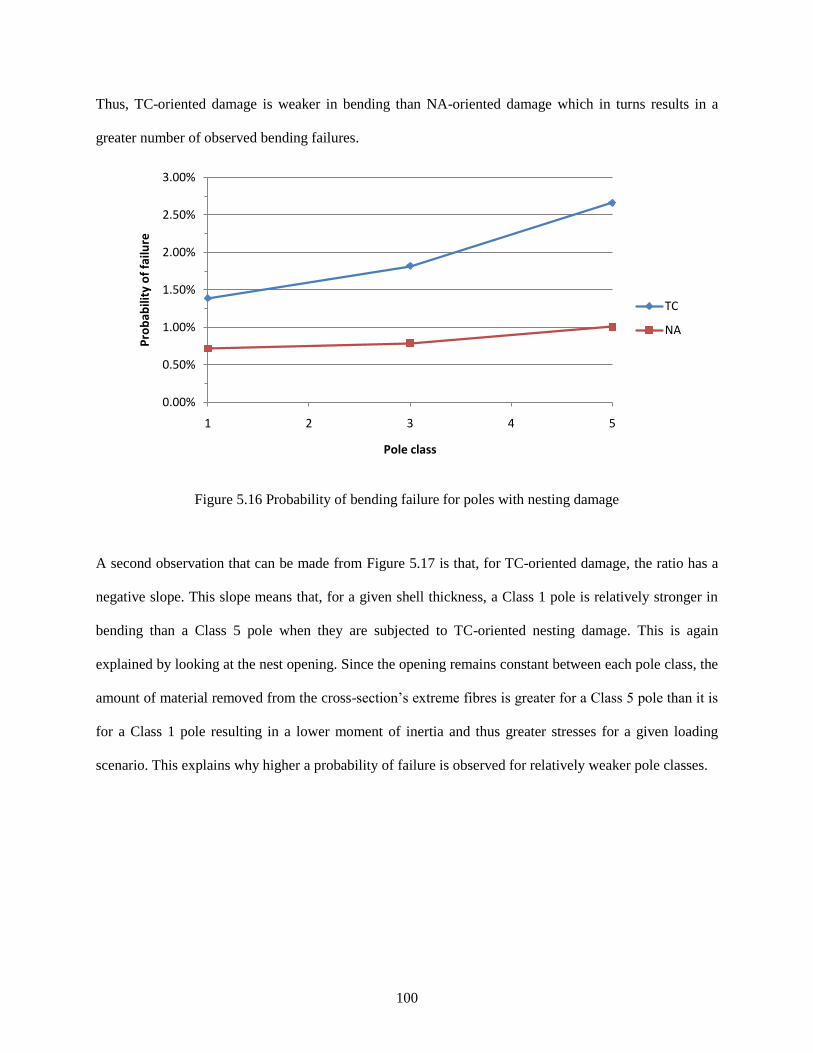
100
Thus, TC-oriented damage is weaker in bending than NA-oriented damage which in turns results in a
greater number of observed bending failures.
Figure 5.16 Probability of bending failure for poles with nesting damage
A second observation that can be made from Figure 5.17 is that, for TC-oriented damage, the ratio has a
negative slope. This slope means that, for a given shell thickness, a Class 1 pole is relatively stronger in
bending than a Class 5 pole when they are subjected to TC-oriented nesting damage. This is again
explained by looking at the nest opening. Since the opening remains constant between each pole class, the
amount of material removed from the cross-section’s extreme fibres is greater for a Class 5 pole than it is
for a Class 1 pole resulting in a lower moment of inertia and thus greater stresses for a given loading
scenario. This explains why higher a probability of failure is observed for relatively weaker pole classes.
0.00%
0.50%
1.00%
1.50%
2.00%
2.50%
3.00%
1 2 3 4 5
Pro
bab
ility
of
failu
re
Pole class
TC
NA

101
Figure 5.17 Effect of nesting damage on moment of inertia for different pole classes with the shell
thickness determined based on a percentage of the cross-section diameter
Figure 5.18 shows the probability of shear failure for each pole class for both NA and TC-oriented
damage. As expected, the probability of shear failure is greater for pole with NA-oriented nesting damage
than it is for the TC-oriented nesting damage. However, contrary to what was observed with the
probability of bending failure seen in Figure 5.16, the probability of shear failure sees an overall decrease
as the cross-sectional diameter decreases. Again, the properties that influence shear failure must be
examined to explain this behaviour.
0.00
0.10
0.20
0.30
0.40
0.50
0.60
0.70
0.80
1 2 3 4 5
Rat
io o
f I d
mg
to I n
ew
Pole class
TC 6%
TC 18%
NA 6%
NA 18%

102
Figure 5.18 Probability of shear failure for poles with nesting damage
Equation (5.1) is used to calculate the shear stress in a given cross-section. For maximum stress, the
thickness t is taken at the neutral axis of the cross-section. As shown earlier, the moment of inertia for
NA-oriented damage is relatively constant over all classes whilst TC-oriented damage has a relatively
lower relative moment of inertia. If the moment of inertia was the driving factor into this behaviour, the
slope of the lines in Figure 5.18 would be positive instead of negative. Thus, it can be concluded that the
moment of inertia is not causing this behaviour.
(5.1)
Next, the quotient
is investigated, where Q is the statical moment of area and t is the thickness of the
cross-section at the neutral axis. Figure 5.19 shows the ratio of
for an as-new pole to that of a
damaged pole for different nesting damage orientations and the two extremes of the shell thicknesses used
thickness (i.e., having a shell thickness corresponding to 6 % and 18 % of the diameter). Because higher
values of
lead to higher shear stresses, a lower ratio of new-to-damaged
means that higher shear
0.00%
0.50%
1.00%
1.50%
2.00%
2.50%
1 2 3 4 5
Pro
bab
ility
of
failu
re
Pole class
TC
NA
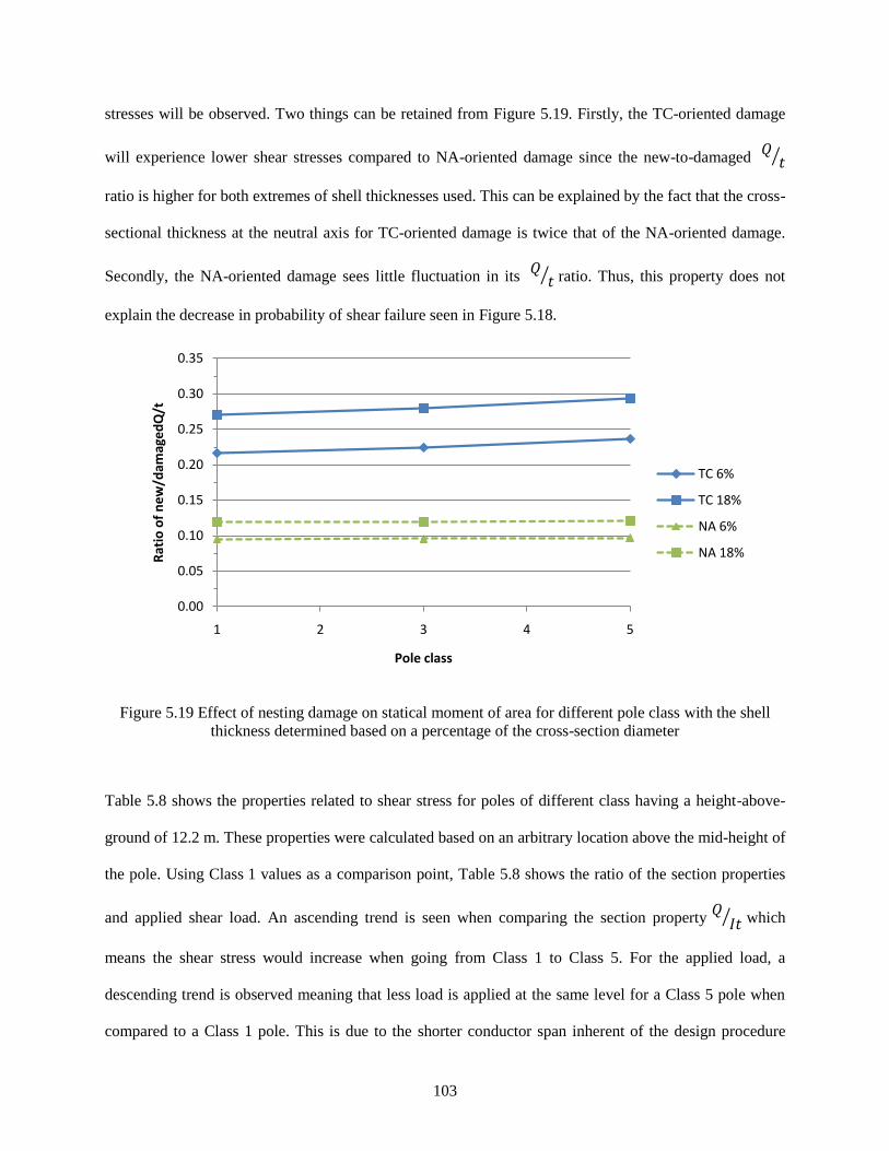
103
stresses will be observed. Two things can be retained from Figure 5.19. Firstly, the TC-oriented damage
will experience lower shear stresses compared to NA-oriented damage since the new-to-damaged
ratio is higher for both extremes of shell thicknesses used. This can be explained by the fact that the cross-
sectional thickness at the neutral axis for TC-oriented damage is twice that of the NA-oriented damage.
Secondly, the NA-oriented damage sees little fluctuation in its
ratio. Thus, this property does not
explain the decrease in probability of shear failure seen in Figure 5.18.
Figure 5.19 Effect of nesting damage on statical moment of area for different pole class with the shell
thickness determined based on a percentage of the cross-section diameter
Table 5.8 shows the properties related to shear stress for poles of different class having a height-above-
ground of 12.2 m. These properties were calculated based on an arbitrary location above the mid-height of
the pole. Using Class 1 values as a comparison point, Table 5.8 shows the ratio of the section properties
and applied shear load. An ascending trend is seen when comparing the section property
which
means the shear stress would increase when going from Class 1 to Class 5. For the applied load, a
descending trend is observed meaning that less load is applied at the same level for a Class 5 pole when
compared to a Class 1 pole. This is due to the shorter conductor span inherent of the design procedure
0.00
0.05
0.10
0.15
0.20
0.25
0.30
0.35
1 2 3 4 5
Rat
io o
f n
ew
/dam
age
dQ
/t
Pole class
TC 6%
TC 18%
NA 6%
NA 18%

104
used and the smaller surface area of a Class 5 pole compared to a Class 1 pole. When multiplying the two
ratios, it can be seen that a lower shear stress can be expected in a Class 3 and 5 poles when compared to
a Class 1 pole of the same height. This explains the relative increase in probability of shear failures for
Class 1 poles observed in Figure 5.18.
Table 5.8 Comparison of shear properties between pole classes with nesting damage
Damage Class Property
Ratio of Class 1 to Class i VQ/It
Q/It, mm-2 V, kN Q/It V
TC 6% 1 219.1E-06 11.84 1.00 1.00 1.00
3 310.1E-06 7.30 1.42 0.62 0.87
5 456.2E-06 4.32 2.08 0.36 0.76
TC 18% 1 80.4E-06 11.84 1.00 1.00 1.00
3 113.7E-06 7.30 1.41 0.62 0.87
5 167.1E-06 4.32 2.08 0.36 0.76
NA 6% 1 398.3E-06 11.84 1.00 1.00 1.00
3 553.4E-06 7.30 1.39 0.62 0.86
5 792.1E-06 4.32 1.99 0.36 0.73
NA 18% 1 146.3E-06 11.84 1.00 1.00 1.00
3 203.0E-06 7.30 1.39 0.62 0.86
5 290.3E-06 4.32 1.98 0.36 0.72
Thus, it is now possible to further explain the behaviour observed in Figure 5.15. The probability of
failure for poles having TC-oriented nesting damage is mainly governed by bending failures. Thus, the
ascending trend seen in the probability of flexural failure between classes dominates that of the
descending trend in probability of shear failure. Conversely, the probability of failure for poles having
NA-oriented nesting damage is governed by shear failure. Thus, the descending trend seen in the
probability of shear failure between pole classes governs that of the ascending trend in the probability of
flexural failure.

105
5.6.5 Summary
To determine if the calculated reliability level was acceptable, an annual probability of failure
threshold of 2 % (i.e., an annual reliability level of 98 %) was set as suggested by CAN/CSA-
C22.3 No. 60826.
The level of reliability between pole classes is relatively constant for shorter poles.
For taller poles, a descending trend in reliability was observed where Class 1 poles had a
relatively higher reliability than Class 4 poles. This is likely due to relatively lower stiffness of
weaker pole class resulting in an increase in P-Δ-related moments.
The greatest contribution in moments comes from the wind on conductors followed by the
moments due to second-order effects. The eccentricity of vertical loads and the wind acting on the
wood pole have a relatively small contribution to the total moments along the pole length.
The equivalent loads provided by the code, based on average modulus of rupture, were shown to
over-predict the critical load of poles, especially for longer poles. This is mainly due to the fact
that a single equivalent load is provided for each class whereas the critical load for each pole
length in a given class is varying. For shorter poles, the small difference between code-provided
and calculated critical loads may be due to a different assumed ground line position. This could
be solved by changing the minimum dimensions to match with the code-specified load.
Construction grade (CG) has a significant impact on pole reliability. Both CG1 and CG2 had
annual probability of failure below 2 %.
The annual probability of failure of poles designed using Construction Grade 3 was above the 2 %
threshold probability of failure suggested by CAN/CSA-C22.3 No. 60826.
Poles which have reached the end-of-life criterion of 60 % remaining strength showed a
significant increase in probability of failure. Poles designed using CG2 and CG3 had reliability
levels below the 98 % prescribed by CAN/CSA-C22.3 No. 60826 once they had reach end-of-life.
However, those designed using CG1 were above this threshold.

106
The presence of exploratory holes on a wood pole has a relatively low impact on its reliability.
All Classes and damage orientation analysed had reliability within the limits prescribed by
CAN/CSA-C22.3 No. 60826.
The presence of feeding holes on a wood utility pole resulted in a decrease in reliability. All
Classes and damage orientation analysed had reliability above the 98 % limit prescribed by
CAN/CSA-C22.3 No. 60826. However, this type of damage has the potential to trap water and
accelerate the decay process leading to potentially lower than anticipated reliability levels.
The presence of nesting holes on a wood utility pole resulted in a significant decrease in
reliability which fell below the 98 % reliability threshold. This type of damage can accumulate
water which will accelerate the decay process and further weaken the pole.

107
Chapter 6 Conclusions and recommendations
An increase in woodpecker-damaged in-service wood utility poles has been reported by Hydro One.
Being able to ascertain the effects of woodpecker damage is important when developing a pole
replacement strategy. Previous research has shown that woodpecker damage can reduce the ability of a
wood pole to resist loads. Research has also shown that woodpecker damage can lead to poles failing in
shear; this mode of failure is atypical of wood utility poles as they are slender cantilevered structures
which are typically governed by bending moment force effects.
The objectives of this study were to determine the effective shear strength of wood utility poles and to
determine the reliability of wood utility poles under different configurations, including poles that had
been damaged by woodpeckers.
The effective shear strength was determined experimentally using Red Pine wood pole stubs provided by
Hydro One. The specimens were prepared by cutting two half-diameter deep slots transversally into the
stubs. The slot openings were oriented 180° from one another and separated a distance equivalent to the
average specimen diameter. The distance between the each slot and the end of the stud was one and a half
times the average specimen diameter. The effective average shear strength was determined by loading the
specimens longitudinally, recording the maximum load, and taking the quotient of the maximum load and
the shear plane area.
The reliability of Red Pine wood utility poles was determined analytically using Visual Basic for
Applications in Excel. A structural analysis model was developed and used in conjunction with Monte
Carlo analysis. The effects of various properties on reliability were tested: the height of poles above
ground, construction grade, end-of-life criterion, and various levels of woodpecker damage.
108
6.1 Conclusions
This section highlights the findings that were made throughout the course of this study.
6.1.1 Literature review
The following are the main observations made from a review of the current literature on the topic of wood
utility poles. The literature review focused on the design, reliability, material properties, and deterioration
of wood utility poles and attempted to identify existing gaps in with respect to these particular topics.
Two standards are used in Canada for guidelines on the design of overhead transmission
structures: CAN/CSA-C22.3 No. 1, a deterministic design code, and CAN/CSA-C22.3
No. 60826, a probabilistic design code. C22.3 No. 1 is the most commonly used design standard.
Previous studies have been done to quantify the reliability of overhead structures designed using
CAN/CSA-C22.3 No. 1. These studies have shown that the reliability of these structures is not
uniform and is highly dependent on their geographical location. These studies did not take into
account the effect of deterioration and woodpecker damage.
Previous studies have concluded that deterioration and woodpecker damage can significantly
reduce the strength of wood utility poles. In some instances, poles were observed to fail in shear.
However, current design standards assume that flexure is the governing mode of failure for wood
utility poles and does not provide any requirements for shear strength.
Previous research has shown that wood strength properties based on clear-wood specimens differ
from the strength properties determined using full-size dimension lumber. The shear strength of
full-size wood pole specimens has not been investigated.
6.1.2 Shear strength of full-size wood poles
This section presents the results and conclusions obtained from the experimental programme conducted to
determine the shear strength of full-size Red Pine wood poles described in the introduction of this
chapter.
109
Two modes of failure were observed. In the first, a single split occurred between the two slots
indicating that the failure plane was loaded mainly in shear. The second had the formation of a
single split or two splits (one originating from each slot) with a strut connecting both sides of the
failure plane indicating that bending forces were also present at the failure plane. This is likely
due to specimen geometry which causes the load to flow from one side of the cross-section to the
other in such a way that bending stresses were introduced at the at the failure plane.
The mean shear strength of the Red Pine specimens adjusted to 12 % moisture content was
2014 kPa (COV 47.5 %) when calculated using gross shear area, and 2113 kPa (COV 40.5 %)
when calculated using net area (i.e., when taking into consideration pre-existing damage affecting
the plane of failure).
The mean shear strength at 12 % moisture content for full-size pole specimens was approximately
27 % of the reported clear wood shear strength values at the same moisture content level.
The shear strength of full-size pole specimens can be represented using a log-normal distribution
with a scale parameter of λ = 0.5909 and a shape parameter of ζ = 0.5265.
6.1.3 Reliability analysis of wood utility poles
This section presents the results and conclusions based on the reliability analysis of wood utility poles
conducted in this study.
To determine if the calculated reliability level was acceptable, an annual probability of failure
threshold of 2 % (i.e., an annual reliability level of 98 %) was set as suggested by CAN/CSA-
C22.3 No. 60826.
The level of reliability between pole classes is relatively constant for shorter poles.
For taller poles, a descending trend in reliability was observed where Class 1 poles had a
relatively higher reliability than Class 4 poles. This is likely due to relatively lower stiffness of
weaker pole class resulting in an increase in P-Δ-related moments.

110
The greatest contribution in moments comes from the wind on conductors followed by the
moments due to second-order effects. The eccentricity of vertical loads and the wind acting on the
wood pole have a relatively small contribution to the total moments along the pole length.
The equivalent loads provided by the code, based on average modulus of rupture, were shown to
over-predict the critical load of poles, especially for longer poles. This is mainly due to the fact
that a single equivalent load is provided for each class whereas the critical load for each pole
length in a given class is varying. For shorter poles, the small difference between code-provided
and calculated critical loads may be due to a different assumed ground line position. This could
be solved by changing the minimum dimensions to match with the code-specified load.
Construction grade (CG) has a significant impact on pole reliability. Both CG1 and CG2 had
annual probability of failure below 2 %.
The annual probability of failure of poles designed using Construction Grade 3 was above the 2 %
threshold probability of failure suggested by CAN/CSA-C22.3 No. 60826.
Poles which have reached the end-of-life criterion of 60 % remaining strength showed a
significant increase in probability of failure. Poles designed using CG2 and CG3 had reliability
levels below the 98 % prescribed by CAN/CSA-C22.3 No. 60826 once they had reach end-of-life.
However, those designed using CG1 were above this threshold.
The presence of exploratory holes on a wood pole has a relatively low impact on its reliability.
All Classes and damage orientation analysed had reliability within the limits prescribed by
CAN/CSA-C22.3 No. 60826.
The presence of feeding holes on a wood utility pole resulted in a decrease in reliability. All
Classes and damage orientation analysed had reliability above the 98 % limit prescribed by
CAN/CSA-C22.3 No. 60826. However, this type of damage has the potential to trap water and
accelerate the decay process leading to potentially lower than anticipated reliability levels.

111
The presence of nesting holes on a wood utility pole resulted in a significant decrease in
reliability which fell below the 98 % reliability threshold. This type of damage can accumulate
water which will accelerate the decay process and further weaken the pole.
6.2 Recommendations
The following recommendations are made based on the findings of the experimental programme and
reliability analysis conducted in this study.
Further testing should be done on full-size pole shear strength to improve the data on Red Pine
species and to collect new data on other common wood species used in the design of wood utility
structures;
The class-specific dimensions of Red Pine utility poles provided in CAN/CSA-O15 should be re-
evaluated to ensure that the critical failure load of all poles within a class matches the class-
specific equivalent transverse load provided in the code;
The reliability analysis conducted in this study should be expanded to include additional
geographical locations. This should include design based on all four loading types (i.e., Medium
Loading A, Medium Loading B, Heavy Loading and Severe Loading).

112
References
[1] M. Pandey, V. Ho, S. Bedi and S. Woodward, "Development of a condition assessment model for
transmission line in-service wood crossarms," Canadian Journal of Civil Engineering, pp. Vol 32,
pp. 480-489, 2005.
[2] M. D. Pandey, V. Ho, F. McCarthy and S. B. Woodward, "Experimental evaluation of remaining
strength of crossarms in Gulfport transmission line wood structures," Canadian Journal of Civil
Engineering, pp. Vol. 37, pp. 638-647, 2010.
[3] S. Datla and M. Pandey, "Estimation of life expectancy of wood poles in electrical distribution
networks," Structural Safety, pp. Vol. 28, pp. 304-319, 2006.
[4] S. Woodward and L. Day, Interviewees, Internal communications. [Interview]. 22 January 2010.
[5] M. Steenhof, Effect of woodpecker damage and wood decay of wood utility poles strength, MASc
thesis, University of Waterloo, Ontario, 2011.
[6] Canadian Standards Association, CAN/CSA-O15-08 Wood utility poles and reinforcing stubs,
Mississauga: Canadian Standards Association, 2005.
[7] Canadian Standards Association, CAN/CSA-C22.3 No. 1-10 Overhead systems, Mississauga,
Ontario: Canadian Standards Association, 2010.
[8] H. Li, G. S. Bhuyan and D. Tarampi, "Life prediciton of aging wood poles and subsequent inspeciton
practice - a case study," The International Journal for Computation and Mathematics in Electrical
and Electronic Engineering, pp. Vol. 23 No. 1, pp. 15-20, 2004.
[9] Canadian Standards Association, CAN/CSA-C22.3 No. 60826-10 Design criteria of overhead
transmission lines, Mississauga: Canadian Standards Association, 2010.
[10] Canadian Wood Council, Wood Design Manual, 5th edition, Nepean, ON, 2005.
[11] United States Department of Agriculture, "Bulletin 1724E-200 Design Manual for High Voltage

113
Transmission Lines," 2009.
[12] V. Subramanian, Reliability assessment of wood transmission line structures, MASc thesis,
University of Waterloo, 2004.
[13] Canadian Standards Association, "CAN/CSA S408-11 Guidelines for the development of limit states
design standards," Canadian Standards Asssociation, Mississauga, 2011.
[14] CHBDC Calibration Task Force, "Calibration Report for CAN/CSA-S6-06 Canadian Highway
Bridge Design Code," Canadian Standards Association, Mississauga, 2007.
[15] A. H.-S. Ang and W. H. Tang, Probability concepts in engineering, Danvers: Wiley, 2007.
[16] H. Li, J. Zhang and G. Bhuyan, "Reliability Assessment of Electrical Overhead Distribution Wood
Poles," in International Conference on Probabilistic Methods Applied to Power Systems, Stockholm,
2006.
[17] G. Bhuyan and H. Li, "Achieved Reliability of the North American Design Approach for
Transmission Overhead Structures," in International Conference on Probabilistic Methods Applied
to Power Systems, Stockholm, 2006.
[18] Department of Forestry, "Strength and related properties of woods grown in Canada (Publication No.
1104)," Edmonton, 1965.
[19] United States Department of Agriculture, Wood Handbook, Madison, WI: United States Department
of Agriculture, 1999.
[20] ASTM International, D2555-06 Standard Practice for Establishing Clear Wood Strength Values,
Conshohocken: ASTM International, 2011.
[21] ASTM International, "D143 - 09 Standard Test Methods for Small Clear Specimens of Timber,"
Conshohocken, 2009.
[22] J. Y. Liu, R. J. Ross and D. R. Rammer, "Improved Arcan Shear Test for Wood," in International
Wood Engineering Conference, New Orleans, 1996.

114
[23] J. Xavier, M. Oliveira, J. Morais and T. Pinto, "Measurement of the shear properties of clear wood
by the Arcan test," Holzforgschung, vol. 63, pp. 217-225, 2009.
[24] E. Odom, D. Blackketter and B. Suratno, "Experimental and Analytical Investigation of the Modified
Wyoming Shear-test Fixture," Experimental Mechanics, pp. 11-15, 1994.
[25] H. Yoshihara and A. Matsumoto, "Measurement of the shearing properties of wood by in-plane shear
test using a thin specimen," Wood Science Technology, vol. 39, pp. 141-153, 2005.
[26] D. S. Riyanto and R. Gupta, "A Comparison o ftest methods for evaluating shear strength of
structural lumber," Forest Products Journal, vol. 48, no. 2, pp. 83-90, 1998.
[27] ASTM International, "D245 - 06 Standard Practice for Establishing Structural Grades and Related
Allowable Properties for Visually Graded Lumber," ASTM International, West Conshohocken,
2011.
[28] S. Talwar, Condition Assessment of Utility Wood Poles, MASc thesis, University of Waterloo, 2002.
[29] F. J. McCarthy, Condition Assessment of Wooden Cross arm in 230 KV Transmission Structures,
MASc thesis, University of Waterloo, 2005.
[30] M. D. Pandey and J. S. West, "Development of a Condition Assessment Standard for Wood Poles
with Woodpecker Damage," Waterloo, 2011.
[31] R. E. Harness and E. L. Walters, "Knock on wood," IEEE Industry Applications Magazine, no.
MAR/APR, pp. 68-73, 2005.
[32] R. L. Rumsey and G. E. Woodson, "Strength Loss in Southern Pine Poles Damaged by
Woodpeckers," Forest Products Journal, vol. 23, no. 12, pp. 47-50, 1973.
[33] Canadian Standards Association, Overhead systems, Mississauga, Ontario: Canadian Standards
Association, 2010.
[34] Z. Kosinski and P. Ksit, "Nest holes of Great Spotted Woodpeckers Dendrocopos major and Middle
Spotted Woodpeckers D. medius: Do they really differ in size?," Acta Ornithologica, vol. 42, no. 1,

115
pp. 45-52, 2007.
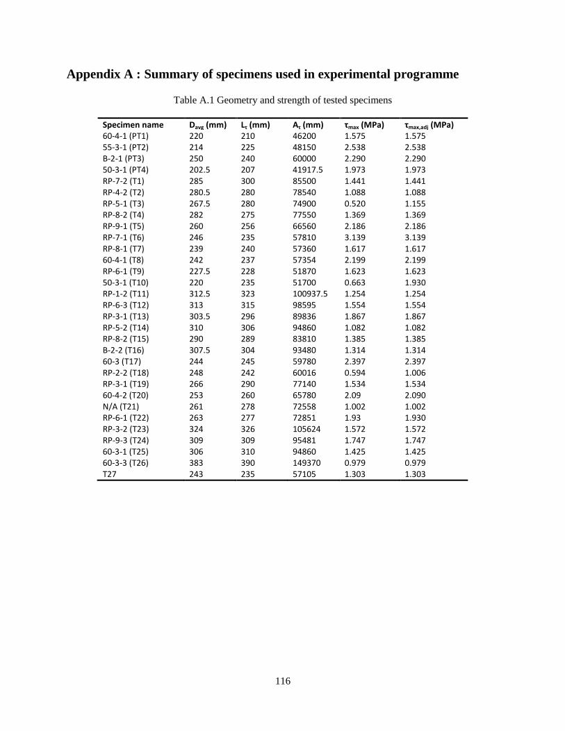
116
Appendix A : Summary of specimens used in experimental programme
Table A.1 Geometry and strength of tested specimens
Specimen name Davg (mm) Lτ (mm) Aτ (mm) τmax (MPa) τmax,adj (MPa) 60-4-1 (PT1) 220 210 46200 1.575 1.575 55-3-1 (PT2) 214 225 48150 2.538 2.538 B-2-1 (PT3) 250 240 60000 2.290 2.290 50-3-1 (PT4) 202.5 207 41917.5 1.973 1.973 RP-7-2 (T1) 285 300 85500 1.441 1.441 RP-4-2 (T2) 280.5 280 78540 1.088 1.088 RP-5-1 (T3) 267.5 280 74900 0.520 1.155 RP-8-2 (T4) 282 275 77550 1.369 1.369 RP-9-1 (T5) 260 256 66560 2.186 2.186 RP-7-1 (T6) 246 235 57810 3.139 3.139 RP-8-1 (T7) 239 240 57360 1.617 1.617 60-4-1 (T8) 242 237 57354 2.199 2.199 RP-6-1 (T9) 227.5 228 51870 1.623 1.623 50-3-1 (T10) 220 235 51700 0.663 1.930 RP-1-2 (T11) 312.5 323 100937.5 1.254 1.254 RP-6-3 (T12) 313 315 98595 1.554 1.554 RP-3-1 (T13) 303.5 296 89836 1.867 1.867 RP-5-2 (T14) 310 306 94860 1.082 1.082 RP-8-2 (T15) 290 289 83810 1.385 1.385 B-2-2 (T16) 307.5 304 93480 1.314 1.314 60-3 (T17) 244 245 59780 2.397 2.397 RP-2-2 (T18) 248 242 60016 0.594 1.006 RP-3-1 (T19) 266 290 77140 1.534 1.534 60-4-2 (T20) 253 260 65780 2.09 2.090 N/A (T21) 261 278 72558 1.002 1.002 RP-6-1 (T22) 263 277 72851 1.93 1.930 RP-3-2 (T23) 324 326 105624 1.572 1.572 RP-9-3 (T24) 309 309 95481 1.747 1.747 60-3-1 (T25) 306 310 94860 1.425 1.425 60-3-3 (T26) 383 390 149370 0.979 0.979 T27 243 235 57105 1.303 1.303

117
Table A.1 (continued) Geometry and strength of tested specimens
Specimen name MC (%) τMC (MPa) τMC,adj (MPa) 60-4-1 (PT1) - - - 55-3-1 (PT2) - - - B-2-1 (PT3) - - - 50-3-1 (PT4) - - - RP-7-2 (T1) 15.8% 1.649 1.649 RP-4-2 (T2) 16.3% 1.267 1.267 RP-5-1 (T3) 16.5% 0.610 1.355 RP-8-2 (T4) 20.5% 1.851 1.851 RP-9-1 (T5) 25.4% 3.516 3.516 RP-7-1 (T6) 22.9% 4.621 4.621 RP-8-1 (T7) 18.8% 2.058 2.058 60-4-1 (T8) 29.1% 4.033 4.033 RP-6-1 (T9) 15.9% 1.864 1.864 50-3-1 (T10) 13.2% 0.692 2.014 RP-1-2 (T11) 19.7% 1.648 1.648 RP-6-3 (T12) 13.3% 1.627 1.627 RP-3-1 (T13) 18.2% 2.326 2.326 RP-5-2 (T14) 18.4% 1.358 1.358 RP-8-2 (T15) 24.1% 2.127 2.127 B-2-2 (T16) 15.9% 1.509 1.509 60-3 (T17) 16.5% 2.812 2.812 RP-2-2 (T18) 17.3% 0.717 1.214 RP-3-1 (T19) 13.4% 1.612 1.612 60-4-2 (T20) 21.2% 2.897 2.897 N/A (T21) 17.2% 1.205 1.205 RP-6-1 (T22) 19.1% 2.483 2.483 RP-3-2 (T23) 16.1% 1.818 1.818 RP-9-3 (T24) 17.8% 2.146 2.146 60-3-1 (T25) 21.3% 1.982 1.982 60-3-3 (T26) 31.2% 1.934 1.934 T27 9.9% 1.303 1.303

118
Appendix B : Location of maximum stress in cantilevered member with linear
taper
B.1 Pole configuration
Figure B.1shows the variables used for the derivation. Note that D2 is the diameter at the ground line, not
at the butt.
Figure B.1 Tapered pole configuration
B.2 Section properties
The following equations are used to define the section properties of the structure.
(B.1)
P l1
l2
L
D2
D1
DP

119
(B.2)
(B.3)
B.3 Loading configuration
The loading configuration is idealized as a cantilevered member with a point load, P, located a distance l1
from the top of the pole.
Figure B.2 Point load on cantilevered structural member
The loads and stresses in the member are defined as follows:
(B.4)
(B.5)
P
l2 l1
x
V(x)
M(x)
P P
P∙l2
0
0
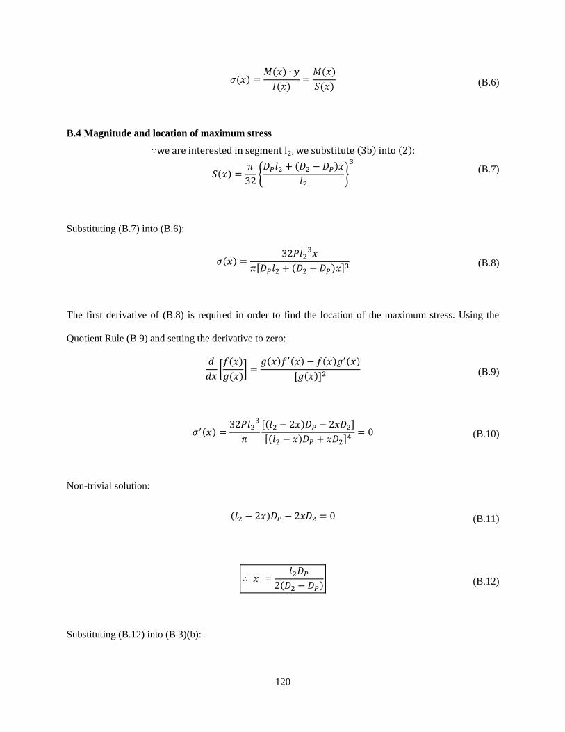
120
(B.6)
B.4 Magnitude and location of maximum stress
(B.7)
Substituting (B.7) into (B.6):
(B.8)
The first derivative of (B.8) is required in order to find the location of the maximum stress. Using the
Quotient Rule (B.9) and setting the derivative to zero:
(B.9)
(B.10)
Non-trivial solution:
(B.11)
(B.12)
Substituting (B.12) into (B.3)(b):

121
(B.13)
Substituting (B.12) into (B.8):
(B.14)

122
Appendix C : Deflection of cantilevered member with linear taper
C.1 Section properties and loading
Figure C.1 shows the variable definitions used for this derivation. The fixed end is located at end D2.
Figure C.1 Pole configuration for deflection calculations
The following equations define the section properties and loading along the member.
(C.1)
(C.2)
(C.3)
C.2 Derivation of curvature equation
The curvature of the member is defined as follows:
D1
D2
L
P
x
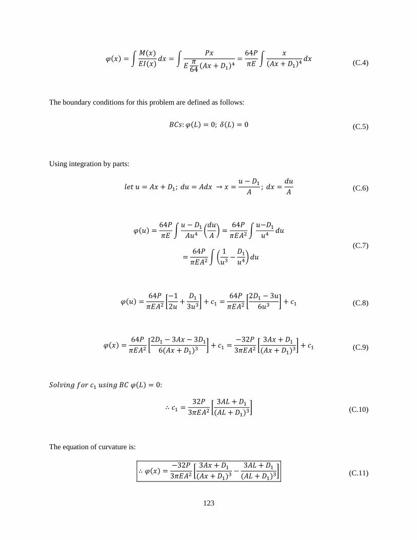
123
(C.4)
The boundary conditions for this problem are defined as follows:
(C.5)
Using integration by parts:
(C.6)
(C.7)
(C.8)
(C.9)
:
(C.10)
The equation of curvature is:
(C.11)

124
C.3 Derivation of deflection equation
Integrating the curvature equation will yield the deflection equation.
(C.12)
Using integration by parts:
(C.13)
(C.14)
(C.15)
(C.16)
(C.17)

125
(C.18)
(C.19)
(C.20)
Some alternate forms of the deflection equation:
(C.21)
(C.22)

126
Appendix D : Derivation of section properties for wood utility poles with
woodpecker damage
D.1 Sectional resistance of undamaged wood pole
Two components of structural resistance were found to be of interest for this study: shear resistance and
flexural resistance. Two sectional properties are essential in order to determine these values: the section
modulus and the first moment of the area above (or below) the neutral axis.
The ultimate flexural capacity of a member having a circular cross-section can be found using:
(D.1)
where S is the section modulus and σ is the modulus of rupture of the wood species.
The section modulus is the quotient of the moment of inertia and the maximum distance between the
centre of gravity of the cross-section and the extreme fibre. For circular cross-sections, the distance
between the centre of gravity and the extreme fibre is equivalent to the radius. Thus, the section modulus
is calculated as follows:
(D.2)
where I is the moment of inertia, c the maximum distance between the extreme fibres and the neutral axis,
and D is the diameter of the section.
The ultimate shear capacity can be determined as follows:
(D.3)
where I is the moment of inertia, t is the thickness of the section at the neutral axis (corresponding to the
diameter for a circular cross-section), τ is the shear strength parallel to the grain of the wood species, and
Q is the first moment of the area above or below the neutral axis.
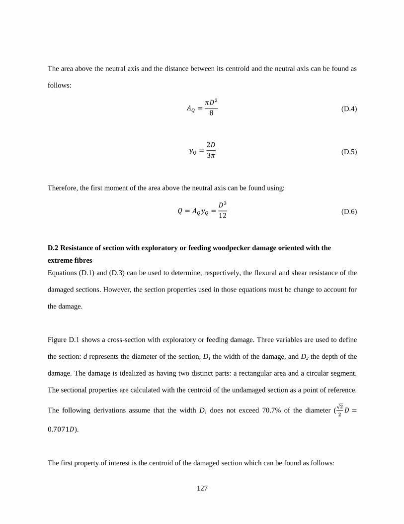
127
The area above the neutral axis and the distance between its centroid and the neutral axis can be found as
follows:
(D.4)
(D.5)
Therefore, the first moment of the area above the neutral axis can be found using:
(D.6)
D.2 Resistance of section with exploratory or feeding woodpecker damage oriented with the
extreme fibres
Equations (D.1) and (D.3) can be used to determine, respectively, the flexural and shear resistance of the
damaged sections. However, the section properties used in those equations must be change to account for
the damage.
Figure D.1 shows a cross-section with exploratory or feeding damage. Three variables are used to define
the section: d represents the diameter of the section, D1 the width of the damage, and D2 the depth of the
damage. The damage is idealized as having two distinct parts: a rectangular area and a circular segment.
The sectional properties are calculated with the centroid of the undamaged section as a point of reference.
The following derivations assume that the width D1 does not exceed 70.7% of the diameter (
).
The first property of interest is the centroid of the damaged section which can be found as follows:

128
(D.7)
where A is the respective area, y the respective centroid with respect to the centre of gravity of the
undamaged section, the circle subscript represents the attributes of the undamaged section, the rec
subscript represents the attributes of the rectangular portion of the damage, and the seg subscript
represents the attributes of the circular segment portion of the damage.
Figure D.1 Idealized cross-section at location of exploratory and feeding damage
To determine the centroid of each shape, first the height of the square must be determine. The height of
the rectangle can be found using:
(D.8)
where hseg is the height of the circular segment and is found using:
(D.9)

129
Figure D.1 shows an arbitrary circular segment with the location of its centroid defined with respect to
both the top (y1) and centroid (y2) of the circle. The angle α is defined as the angle between the vertical
line passing through the centroid of the circle and the left- or right-most edge of the circular segment and
can be found as follows:
(D.10)
Figure D.2 Circular segment
The location of the centroid of the circular segment with respect to the top of the circle containing it is
determined as follows [1]:
(D.11)
Using Equation (D.11), the location of the centroid of the circular segment can be found using:
(D.12)
The location of the rectangle’s centroid with respect to the centroid of the circle is found using:

130
(D.13)
The area of the circular segment can be found using:
(D.14)
and the area of the rectangle can be found using:
(D.15)
The moment of inertia of the section can now be determined by subtracting the moment of inertia of the
rectangle and circular segment from the moment of inertia of the undamaged section. The parallel axis
theorem is used to calculate the moment of inertia about the damage section’s centre of gravity.
(D.16)
The moment of inertia of a circle can be found in Equation (D.2). The moment of inertia of a circular
segment about the x-axis is found using [1]:
(D.17)
The moment of inertia of the rectangular element is found using:
(D.18)
The thickness of the damaged cross-section at its centroid is used when calculating the shear resistance of
the cross-section and can be found as follows:

131
(D.19)
The first moment of area above or below the centre of gravity of the section, Q, is obtained using two
different methods depending on whether the depth D2 falls above or below the centre of gravity of the
damaged section. The approach used below first assumes that D2 is above the centre of gravity and adjusts
the variables accordingly if it is below. If the damage is oriented as shown in Figure D.1, the centre of
gravity of the damaged section will always fall below that of the undamaged section. Thus, the area used
in Q is the circular segment contained between the bottom perimeter of the section and the centre of
gravity of the damaged section. The first moment of area is found as follows:
(D.20)
where Q is with respect to the centre of gravity of the damaged section.
The area can be found using [1]:
(D.21)
The centroid is found using [1]:
(D.22)
where α is found using:
(D.23)
132
If the depth of the hole falls below the centre of gravity of the damaged section, the above values can be
modified to account for this. First, the amount by which the hole goes beyond the centre of gravity is
determined using:
(D.24)
Then, the area AQ can be modified as follows:
(D.25)
The centroid y Q is modified as follows:
(D.26)
Lastly, the thickness at the centroid is modified as follows:
(D.27)
D.3 Resistance of section with nesting woodpecker damage oriented with the extreme fibres
Figure D.3 shows a cross-section with nesting damage. Three variables are used to define the section: d
represents the diameter of the section, D1 the remaining shell thickness, and D2 the opening width. The
damage is idealized as an annulus with a removed sector.

133
Figure D.3 Idealized cross-section at location of nesting damage
The centre of gravity of the damaged section with respect to the undamaged section can be calculated as
follows:
(D.28)
The area of the annulus is found using:
(D.29)
Figure D.4 shows an arbitrary sector of a hollow circle. The area and centroid of the sector can be found
using the following equations [1]:
(D.30)
(D.31)
(D.32)

134
The angle α can be found using the following:
(D.33)
Figure D.4 Sector of a hollow circle
The moment of inertia of the damaged section can be found using the parallel-axis theorem:
(D.34)
where all y values are with respect to the centre of gravity of the damaged section found using
Equation (D.28).
The moment of inertia of the annulus is found using:
(D.35)
The moment of inertia of the sector can be found using:

135
(D.36)
Next, the area below the damaged centre of gravity and its corresponding centroid are required to
calculate the first moment of area Q. The first moment of area is calculated as shown previously in
Equation (D.20). The area AQ is calculated by using Equation (D.21) to find Aseg and Aseg’, where Aseg is
found using the radius R of the full section and Aseg’ is found by using the radius . Using the
same approach with Equation (D.22) will yield the centroid of area AQ. Finally, the thickness at the centre
of gravity of the damaged section is approximated as follows:
(D.37)
D.4 Resistance of section with exploratory or feeding woodpecker damage oriented with the neutral
axis
Since shear resistance is of particular interest in this study, it is important to consider the case where
mechanical damage is oriented with the neutral axis of the member (Figure D.5) because this
configuration provides the lowest shear resistance. A similar approach to the one described in D.2 is taken
to derive the section properties.

136
Figure D.5 Exploratory and feeding damage oriented with the neutral axis
There is no need to recalculate the centre of gravity of this configuration as it is coincident with that of the
undamaged section. Thus, the centre of gravity is located a distance d/2 from the top of the section. This
has the additional benefit of simplifying the calculations for the moment of inertia, which can be
determined as follows:
(D.38)
where Irec and Iseg can be determined as follows:
(D.39)
(D.40)
The area for the first moment of area Q is calculated using:
(D.41)

137
where Aseg and Arec are found using Equations (D.14) and (D.15), respectively. The moment arm for the
first moment of area is found using:
(D.42)
Where the centroid of the rectangle and circular segment with respect to the centroid of the damaged
section are found as follows:
(D.43)
(D.44)
Lastly, the shear plane thickness is determined using:
(D.45)
D.5 Resistance of section with nesting woodpecker damage oriented with the neutral axis
The sectional properties of a section with nesting damage oriented with the neutral axis (Figure D.6) are
calculated in a similar fashion to the method used in Section D.3. In this case, the centre of gravity of the
damaged section is coincident with that of the undamaged section.

138
Figure D.6 Nesting damage oriented with the neutral axis
The moment of inertia of the section is found as follows:
where Iannulus is found using Equation (D.35) and Isec is found as follows [1]:
where α is found using Equation (D.33).
The area used for the first moment of area is found using:
The moment arm for the first moment of area is calculated as follows:
The centre of gravity of the half-annulus is found using:

139
The centre of gravity of the half-sector is found using:
Finally, the thickness of the shear plane for this scenario is:
D.6 References
[1] W. C. Young and R. G. Budynas, Roark's Formulas for Stress and Strain, McGraw-Hill, 2002.

140
Appendix E : Spreadsheet macro code for Monte Carlo analysis
Option Explicit
''''''''''''''''''''''''''''''''''''''''''''''''''''''''''''''''''''''''''''''''''''''''''''
' Author : Olivier Daigle
' Date : 21 March 2012
''''''''''''''''''''''''''''''''''''''''''''''''''''''''''''''''''''''''''''''''''''''''''''
' Name : GenerateTandG
' Type : Subroutine
' Purpose : This subroutine calls the appropriate subroutines to generate the
' table, table headers, and graphs (if they are to be generated).
' The subroutine also deletes the previous graphs and tables worksh-
' eets, if they exist.
''''''''''''''''''''''''''''''''''''''''''''''''''''''''''''''''''''''''''''''''''''''''''''
Sub MonteCarloSim()
Dim CreateGraphs As Boolean
Dim noIterations As Long
'iWS=inputs, tWS=table, mcWS=Monte Carlo, fWS=failures
Dim iWS As Worksheet, tWS As Worksheet, mcWS As Worksheet, fWS As Worksheet, lUp As Worksheet
Dim noWires As Integer 'number of wires
Dim i As Long
Dim failCount As Integer
Dim shearFailCount As Integer
Dim bendFailCount As Integer
Dim results() As Boolean
Dim outerRect As Shape
Dim innerRect As Shape
Dim rectWidth As Single
Dim hThresh As Double 'limit of hole dimensions based on fraction of diameter
Set lUp = Worksheets("Lookup")
hThresh = lUp.Cells(66, 2).Value
rectWidth = 150
failCount = 0
Set iWS = Worksheets("Inputs")
CreateGraphs = iWS.Cells(2, 5).Value
noIterations = iWS.Cells(2, 7).Value
noWires = iWS.Cells(21, 4).Value
Application.DisplayAlerts = False
On Error Resume Next 'this line prevents a meltdown if the worksheets to be deleted do not
exist
'delete MC worksheet. Create new worksheet. Add/format titles/data location
Worksheets("Monte Carlo Analysis").Delete
Worksheets("Failure Locations").Delete
Worksheets.Add(after:=Sheets(Sheets.Count)).Name = "Monte Carlo Analysis"
Worksheets.Add(after:=Sheets(Sheets.Count)).Name = "Failure Locations"
Set mcWS = Worksheets("Monte Carlo Analysis")
Set fWS = Worksheets("Failure Locations")
mcWS.Range(mcWS.Columns(1), mcWS.Columns(5)).ColumnWidth = 10.75
mcWS.Range(mcWS.Columns(1), mcWS.Columns(5)).HorizontalAlignment = xlLeft
mcWS.Cells(4, 2).Value = "Total"
mcWS.Cells(4, 3).Value = "Shear"
mcWS.Cells(4, 4).Value = "Bending"
mcWS.Cells(1, 1).Value = "Progress:"
mcWS.Cells(5, 1).Value = "Nf"
mcWS.Cells(6, 1).Value = "Pf"
mcWS.Range("A5", "A6").Characters(Start:=2, Length:=1).Font.Subscript = True
mcWS.Range("B6", "D6").NumberFormat = "0.00%"
mcWS.Range("B7", "D7").NumberFormat = "0.00"
'create progress bar
Set outerRect = mcWS.Shapes.AddShape(msoShapeRectangle, 75, 5, rectWidth, 5)
Set innerRect = mcWS.Shapes.AddShape(msoShapeRectangle, 75, 5, 0, 5)
With outerRect
.Line.Weight = 1
.Line.ForeColor.RGB = RGB(0, 0, 0)
.Fill.Visible = msoFalse

141
End With
With innerRect
.Fill.ForeColor.RGB = RGB(0, 0, 0)
.Line.Weight = 1
End With
Application.ScreenUpdating = False
For i = 1 To noIterations
Worksheets("Tables").Delete
Application.ScreenUpdating = True
mcWS.Cells(5, 2).Value = failCount
mcWS.Cells(5, 3).Value = shearFailCount
mcWS.Cells(5, 4).Value = bendFailCount
mcWS.Cells(6, 2).Value = failCount / i
mcWS.Cells(6, 3).Value = shearFailCount / i
mcWS.Cells(6, 4).Value = bendFailCount / i
mcWS.Cells(1, 5).Value = Str(i) & "/" & Str(noIterations)
innerRect.Width = (i / noIterations) * rectWidth 'change progress bar
Application.ScreenUpdating = False
Worksheets.Add(after:=Sheets(Sheets.Count)).Name = "Tables"
mcWS.Activate
Set tWS = Worksheets("Tables")
Call RandomizeVariables(iWS)
results = GenerateTable(iWS, tWS, hThresh)
'records location of failure and failure type
If results(1) Then
failCount = failCount + 1
End If
If results(2) Then
bendFailCount = bendFailCount + 1
End If
If results(3) Then
shearFailCount = shearFailCount + 1
End If
'LOCATE FAILURE HERE -> CREATE NEW SUBROUTINE
If results(1) Then
On Error GoTo 0
Call LocateFailure(i, tWS, fWS, failCount)
On Error Resume Next
End If
Next i
Worksheets("Tables").Delete
'Generate failure table headers
Application.ScreenUpdating = False
fWS.Activate
Call GenerateHeaders(fWS)
mcWS.Activate
Application.ScreenUpdating = True
'Calculate beta for total failures
mcWS.Cells(7, 1).Value = ChrW(&H3B2)
If mcWS.Cells(6, 2).Value = 0 Then
mcWS.Cells(7, 2).Value = "N/A" 'ChrW(&H221E)
Else
mcWS.Cells(7, 2).Value = -1 * Application.WorksheetFunction.Norm_S_Inv(mcWS.[B6].Value)
End If
'Calculate beta for shear failures
If mcWS.Cells(6, 3).Value = 0 Then
mcWS.Cells(7, 3).Value = "N/A" 'ChrW(&H221E)
Else
mcWS.Cells(7, 3).Value = -1 * Application.WorksheetFunction.Norm_S_Inv(mcWS.[C6].Value)
End If
'Calculate beta for bending failures
If mcWS.Cells(6, 4).Value = 0 Then
mcWS.Cells(7, 4).Value = "N/A" 'ChrW(&H221E)
Else
mcWS.Cells(7, 4).Value = -1 * Application.WorksheetFunction.Norm_S_Inv(mcWS.[D6].Value)
End If
If CreateGraphs Then
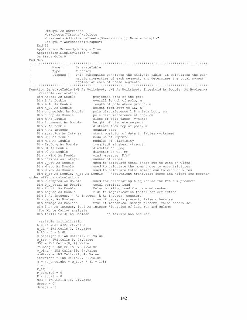
142
Dim gWS As Worksheet
Worksheets("Graphs").Delete
Worksheets.Add(after:=Sheets(Sheets.Count)).Name = "Graphs"
Set gWS = Worksheets("Graphs")
End If
Application.ScreenUpdating = True
Application.DisplayAlerts = True
On Error GoTo 0
End Sub
''''''''''''''''''''''''''''''''''''''''''''''''''''''''''''''''''''''''''''''''''''''''''''
' Name : GenerateTable
' Type : Function
' Purpose : This subroutine generates the analysis table. It calculates the geo-
' metric properties of each segment, and determines the total moment
' applied at each of these segments.
''''''''''''''''''''''''''''''''''''''''''''''''''''''''''''''''''''''''''''''''''''''''''''
Function GenerateTable(iWS As Worksheet, tWS As Worksheet, Threshold As Double) As Boolean()
'Variable declaration
Dim Atotal As Double 'projected area of the pole
Dim L As Double 'overall length of pole, m
Dim L_AG As Double 'length of pole above ground, m
Dim h_GL As Double 'height from butt to GL, m
Dim c_oneeight As Double 'pole circumference 1.8 m from butt, cm
Dim c_top As Double 'pole circumenference at top, cm
Dim m As Double 'slope of pole taper (y=mx+b)
Dim increment As Double 'height of discrete segment
Dim x As Double 'distance from top of pole, m
Dim n As Integer 'counter stop
Dim startPos As Integer 'start position of data in Tables worksheet
Dim MOR As Double 'modulus of rupture
Dim MOE As Double 'modulus of elasticity
Dim TauLong As Double 'longitudinal shear strength
Dim D1 As Double 'diameter at P_eq
Dim D2 As Double 'diameter at GL, mm
Dim p_wind As Double 'wind pressure, N/m²
Dim noWires As Integer 'number of wires
Dim V_wow As Double 'used to calculate total shear due to wind on wires
Dim M_ecc As Double 'used to calculate the moment due to eccentricities
Dim M_wow As Double 'used to calculate total moment due to wind on wires
Dim P_eq As Double, h_eq As Double 'equivalent transverse force and height for second-
order effects calculations
Dim P_sumprod As Double 'used for calculating h_eq (holds the P*h sum-product)
Dim P_v_total As Double 'total vertical load
Dim P_crit As Double 'Euler buckling load for tapered member
Dim magFac As Double 'P-delta magnification factor for deflection
Dim i As Integer, j As Integer, k As Integer 'counters
Dim decay As Boolean 'true if decay is present, false otherwise
Dim damage As Boolean 'true if mechanical damage present, false otherwise
Dim lRow As Integer, lCol As Integer 'location of last row and column
'for Monte Carlos analysis
Dim fail(1 To 3) As Boolean 'a failure has occured
'variable initialization
L = iWS.Cells(2, 2).Value
h_GL = iWS.Cells(3, 2).Value
L_AG = L - h_GL
c_oneeight = iWS.Cells(4, 2).Value
c_top = iWS.Cells(5, 2).Value
MOR = iWS.Cells(8, 2).Value
TauLong = iWS.Cells(9, 2).Value
p_wind = iWS.Cells(19, 2).Value
noWires = iWS.Cells(21, 4).Value
increment = iWS.Cells(7, 2).Value
m = (c_oneeight - c_top) / (L - 1.8)
x = 0
P_eq = 0
P_sumprod = 0
P_v_total = 0
MOE = iWS.Cells(10, 2).Value
decay = 0
damage = 0

143
startPos = 3 'first two rows are column headers
Atotal = 10 * L_AG * (diameter(c_top) + diameter(m * L_AG + c_top)) / 2 'mm^2
Atotal = Atotal / (1000) ^ 2 'm^2
Dim wiresProp() As Double 'holds the properties of the wires (incl. the forces they
generate on the structure)
ReDim wiresProp(noWires, 4) '[h_GL M_ecc P_Trans P_Vert]
For k = 1 To noWires
wiresProp(k, 1) = iWS.Cells(26, 5 + k - 1).Value 'distance from GL
wiresProp(k, 2) = iWS.Cells(33, 5 + k - 1).Value 'moment generate by eccentricity
wiresProp(k, 3) = iWS.Cells(31, 5 + k - 1).Value 'transverse loads (wind)
wiresProp(k, 4) = iWS.Cells(32, 5 + k - 1).Value 'vertical loads (weight of wire & ice)
P_eq = P_eq + wiresProp(k, 3)
P_sumprod = P_sumprod + wiresProp(k, 1) * wiresProp(k, 3)
P_v_total = P_v_total + wiresProp(k, 4)
Next k
'account for wind on structure
P_sumprod = P_sumprod + (iWS.Cells(19, 2).Value * Atotal / 1000) * L_AG ^ 2 * (2 *
diameter(c_top) / 100 + diameter(m * L_AG + c_top) / 100) / (6 * Atotal)
P_eq = P_eq + (iWS.Cells(19, 2).Value * Atotal / 1000)
'Determine equivalent load location
h_eq = P_sumprod / P_eq
D1 = diameter(m * (L_AG - h_eq) + c_top) * 10 'diameter at P_eq, mm
D2 = diameter(m * L_AG + c_top) * 10 'GL diameter, mm
P_crit = 10 ^ -3 * Application.WorksheetFunction.Pi() ^ 2 * MOE * MomInertia(D1) _
/ (4 * (h_eq * 10 ^ 3) ^ 2) * (D2 / D1) ^ 2.7 'Euler buckling load
magFac = (1 - P_v_total / P_crit) ^ -1 'deflection magnifier for second-order effects
'n represents the total number of rows in the table. although it is initialized here, it may
'change if new rows are added to the table to accomodate special cases where there is decay
'and mechanical damage.
increment = increment / 1000 'convert increments from millimetres to metres.
n = startPos
Do While x < L_AG
tWS.Cells(n, 1).Value = L_AG - x 'hGL
tWS.Cells(n, 2).Value = x 'x
tWS.Cells(n, 7).Value = m * x + c_top 'circumference
tWS.Cells(n, 8).Value = 10 * diameter(tWS.Cells(n, 7).Value) 'diameter
If x + increment >= L_AG Then
x = L_AG
tWS.Cells(n, 1).Value = L_AG - x
tWS.Cells(n, 2).Value = x
tWS.Cells(n, 7).Value = m * x + c_top
tWS.Cells(n, 8).Value = 10 * diameter(tWS.Cells(n, 7).Value)
Else
x = x + increment
n = n + 1
End If
Loop
'the following code handles special cases such as sections where the wood is decayed,
location of
'mechanical damage (woodpecker damage) and the location of P_eq
'populate arrays containing the locations of decay/damaged sections
'location(s) of decay
If iWS.Cells(5, 4).Value > 0 Then
decay = 1
Dim decayProp() As Double 'location and MOR of decayed section(s)
ReDim decayProp(iWS.Cells(5, 4).Value, 4) '[x_start, x_end, MOR, TauLong]
For i = 1 To iWS.Cells(5, 4).Value
decayProp(i, 1) = iWS.Cells(6, i + 4).Value
decayProp(i, 2) = iWS.Cells(7, i + 4).Value
decayProp(i, 3) = iWS.Cells(8, i + 4).Value
decayProp(i, 4) = iWS.Cells(9, i + 4).Value
Next i
For i = 1 To UBound(decayProp)
For j = startPos To n

144
'check if within the range of decayed section
If tWS.Cells(j, 2).Value >= decayProp(i, 1) And tWS.Cells(j, 2).Value <=
decayProp(i, 2) Then
If tWS.Cells(j, 2).Value > decayProp(i, 1) And tWS.Cells(j - 1, 2).Value
< decayProp(i, 1) Then
If j > startPos Then
tWS.Cells(j, 2).EntireRow.Insert
tWS.Cells(j, 2).Value = decayProp(i, 1)
tWS.Cells(j, 1).Value = L_AG - decayProp(i, 1)
tWS.Cells(j, 7).Value = m * decayProp(i, 1) + c_top
tWS.Cells(j, 8).Value = 10 * diameter(tWS.Cells(j, 7).Value)
n = n + 1
End If
End If
If tWS.Cells(j, 2).Value < decayProp(i, 2) And tWS.Cells(j + 1, 2).Value
> decayProp(i, 2) Then
If j < n Then
tWS.Cells(j + 1, 2).EntireRow.Insert
tWS.Cells(j + 1, 2).Value = decayProp(i, 2)
tWS.Cells(j + 1, 1).Value = L_AG - decayProp(i, 2)
tWS.Cells(j + 1, 7).Value = m * decayProp(i, 2) + c_top
tWS.Cells(j + 1, 8).Value = 10 * diameter(tWS.Cells(j + 1,
7).Value)
n = n + 1
End If
End If
End If
Next j
Next i
End If
'location(s) of mechanical damage
If iWS.Cells(12, 4).Value > 0 Then
damage = 1
Dim mechDmgProp() As Double
Dim xTopHole As Double, xBotHole As Double 'top and bottom location of the hole
'type: 1=exploratory/feeding, 2=nesting
'orientation: 1=tension/compression, 2=neutral axis
'[1, x_centre, hole diameter, hole depth, unused, orientation]
'[2, x_centre, nest depth, opening diameter, shell thickness, orientation]
'hole dimensions are given as a fraction w.r.t. the diameter at the centre.
ReDim mechDmgProp(iWS.Cells(12, 4).Value, 6)
For i = 1 To iWS.Cells(12, 4).Value
If iWS.Cells(13, i + 4).Value = "E" Or iWS.Cells(13, i + 4).Value = "F" Then
'If iWS.Cells(15, i + 4).Value >= 1 Or iWS.Cells(15, i + 4).Value < 0 Then
'this error detection is currently implemented in the function that
returns MOI & all.
'End If
mechDmgProp(i, 1) = 1
mechDmgProp(i, 4) = iWS.Cells(16, i + 4).Value 'depth of hole
mechDmgProp(i, 3) = iWS.Cells(15, i + 4).Value 'width of hole
ElseIf iWS.Cells(13, i + 4).Value = "N" Then
mechDmgProp(i, 1) = 2
mechDmgProp(i, 4) = iWS.Cells(16, i + 4).Value 'opening diameter
mechDmgProp(i, 5) = iWS.Cells(17, i + 4).Value 'shell thickness
mechDmgProp(i, 3) = iWS.Cells(15, i + 4).Value 'depth of nest
End If
mechDmgProp(i, 2) = iWS.Cells(14, i + 4).Value 'x_hole (hole location)
If iWS.Cells(18, i + 4).Value = "T/C" Then
mechDmgProp(i, 6) = 1
ElseIf iWS.Cells(18, i + 4).Value = "NA" Then
mechDmgProp(i, 6) = 2
End If
Next i
For i = 1 To UBound(mechDmgProp)
xTopHole = mechDmgProp(i, 2) - mechDmgProp(i, 3) / 2000
xBotHole = mechDmgProp(i, 2) + mechDmgProp(i, 3) / 2000
For j = startPos To n
'check if within the range of decayed section

145
If tWS.Cells(j, 2).Value >= mechDmgProp(i, 2) And tWS.Cells(j - 1, 2).Value <
mechDmgProp(i, 2) Then
'looks for the centre location of the hole and inserts a row if there is no
exact match
If tWS.Cells(j, 2).Value > mechDmgProp(i, 2) Then
If j > startPos Then
tWS.Cells(j, 2).EntireRow.Insert
tWS.Cells(j, 2).Value = mechDmgProp(i, 2)
tWS.Cells(j, 1).Value = L_AG - mechDmgProp(i, 2)
tWS.Cells(j, 7).Value = m * mechDmgProp(i, 2) + c_top
tWS.Cells(j, 8).Value = 10 * diameter(tWS.Cells(j, 7).Value)
n = n + 1
End If
End If
k = j
'looks for the upper bound of the hole and inserts a row if there is no
exact match
Do While tWS.Cells(k, 2).Value >= xTopHole And k > startPos
If tWS.Cells(k, 2).Value > xTopHole And tWS.Cells(k - 1, 2).Value <
xTopHole Then
tWS.Cells(k, 2).EntireRow.Insert
tWS.Cells(k, 2).Value = xTopHole
tWS.Cells(k, 1).Value = L_AG - xTopHole
tWS.Cells(k, 7).Value = m * xTopHole + c_top
tWS.Cells(k, 8).Value = 10 * diameter(tWS.Cells(k, 7).Value)
n = n + 1
End If
k = k - 1
Loop
k = j
'looks for the lower bound of the hole and inserts a row if there is no
exact match
Do While tWS.Cells(k, 2).Value <= xBotHole And k < n
If tWS.Cells(k + 1, 2).Value > xBotHole And tWS.Cells(k, 2).Value <
xBotHole Then
tWS.Cells(k + 1, 2).EntireRow.Insert
tWS.Cells(k + 1, 2).Value = xBotHole
tWS.Cells(k + 1, 1).Value = L_AG - xBotHole
tWS.Cells(k + 1, 7).Value = m * xBotHole + c_top
tWS.Cells(k + 1, 8).Value = 10 * diameter(tWS.Cells(k + 1,
7).Value)
n = n + 1
End If
k = k + 1
Loop
End If
Next j
Next i
End If
'This loop populates the Tables worksheet
For i = startPos To n
x = tWS.Cells(i, 2).Value
'populate section properties columns
'checks for location(s) with mechanical damage
If damage Then
j = 1
Do While j <= UBound(mechDmgProp)
xTopHole = mechDmgProp(j, 2) - mechDmgProp(j, 3) / 2000
xBotHole = mechDmgProp(j, 2) + mechDmgProp(j, 3) / 2000
'checks if the row is within a hole's range. Changes the moment of inertia and
section modulus of the section
'if that is the case.
'[1, x_centre, hole diameter, hole depth, unused, orientation]
'[2, x_centre, hole depth, opening diameter, shell thickness, orientation]
If tWS.Cells(i, 2).Value >= xTopHole And tWS.Cells(i, 2).Value <= xBotHole Then
'mechanical properties of section with exploratory or feeding damage
If mechDmgProp(j, 1) = 1 Then
If mechDmgProp(j, 3) > Threshold * tWS.Cells(i, 8).Value Then
mechDmgProp(j, 3) = Threshold * tWS.Cells(i, 8).Value
End If
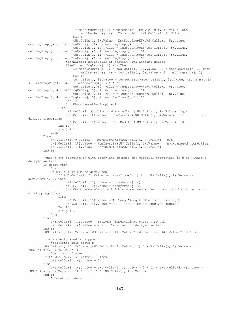
146
If mechDmgProp(j, 4) > Threshold * tWS.Cells(i, 8).Value Then
mechDmgProp(j, 4) = Threshold * tWS.Cells(i, 8).Value
End If
tWS.Cells(i, 9).Value = DmgSectPropEF(tWS.Cells(i, 8).Value,
mechDmgProp(j, 3), mechDmgProp(j, 4), 3, mechDmgProp(j, 6)) 'Q/t
tWS.Cells(i, 10).Value = DmgSectPropEF(tWS.Cells(i, 8).Value,
mechDmgProp(j, 3), mechDmgProp(j, 4), 1, mechDmgProp(j, 6)) 'I
tWS.Cells(i, 11).Value = DmgSectPropEF(tWS.Cells(i, 8).Value,
mechDmgProp(j, 3), mechDmgProp(j, 4), 2, mechDmgProp(j, 6)) 'S
'mechanical properties of section with nesting damage
ElseIf mechDmgProp(j, 1) = 2 Then
If mechDmgProp(j, 4) > tWS.Cells(i, 8).Value - 2 * mechDmgProp(j, 5) Then
mechDmgProp(j, 4) = tWS.Cells(i, 8).Value - 2 * mechDmgProp(j, 5)
End If
tWS.Cells(i, 9).Value = DmgSectPropN(tWS.Cells(i, 8).Value, mechDmgProp(j,
4), mechDmgProp(j, 5), 3, mechDmgProp(j, 6)) 'Q/t
tWS.Cells(i, 10).Value = DmgSectPropN(tWS.Cells(i, 8).Value,
mechDmgProp(j, 4), mechDmgProp(j, 5), 1, mechDmgProp(j, 6)) 'I
tWS.Cells(i, 11).Value = DmgSectPropN(tWS.Cells(i, 8).Value,
mechDmgProp(j, 4), mechDmgProp(j, 5), 2, mechDmgProp(j, 6)) 'S
End If
j = UBound(mechDmgProp) + 1
Else
tWS.Cells(i, 9).Value = MomentofArea(tWS.Cells(i, 8).Value) 'Q/t
tWS.Cells(i, 10).Value = MomInertia(tWS.Cells(i, 8).Value) 'I non-
damaged properties
tWS.Cells(i, 11).Value = SectModulus(tWS.Cells(i, 8).Value) 'S
End If
j = j + 1
Loop
Else
tWS.Cells(i, 9).Value = MomentofArea(tWS.Cells(i, 8).Value) 'Q/t
tWS.Cells(i, 10).Value = MomInertia(tWS.Cells(i, 8).Value) 'non-damaged properties
tWS.Cells(i, 11).Value = SectModulus(tWS.Cells(i, 8).Value)
End If
'checks for location(s) with decay and changes the material properties if x is within a
decayed section
If decay Then
j = 1
Do While j <= UBound(decayProp)
If tWS.Cells(i, 2).Value >= decayProp(j, 1) And tWS.Cells(i, 2).Value <=
decayProp(j, 2) Then
tWS.Cells(i, 13).Value = decayProp(j, 4)
tWS.Cells(i, 14).Value = decayProp(j, 3)
j = UBound(decayProp) + 1 'this works under the assumption that there is no
overlapping decay
Else
tWS.Cells(i, 13).Value = TauLong 'longitudinal shear strength
tWS.Cells(i, 14).Value = MOR 'MOR for non-decayed section
End If
j = j + 1
Loop
Else
tWS.Cells(i, 13).Value = TauLong 'longitudinal shear strength
tWS.Cells(i, 14).Value = MOR 'MOR for non-decayed section
End If
tWS.Cells(i, 12).Value = tWS.Cells(i, 11).Value * tWS.Cells(i, 14).Value * 10 ^ -6
'loads due to wind on support
'projected area above x
tWS.Cells(i, 15).Value = (tWS.Cells(i, 2).Value / 2) * (tWS.Cells(3, 8).Value +
tWS.Cells(i, 8).Value) * 10 ^ -3
'centroid of area
If tWS.Cells(i, 15).Value = 0 Then
tWS.Cells(i, 16).Value = 0
Else
tWS.Cells(i, 16).Value = tWS.Cells(i, 2).Value ^ 2 * (2 * tWS.Cells(3, 8).Value +
tWS.Cells(i, 8).Value) * 10 ^ -3 / (6 * tWS.Cells(i, 15).Value)
End If
'Moment and shear
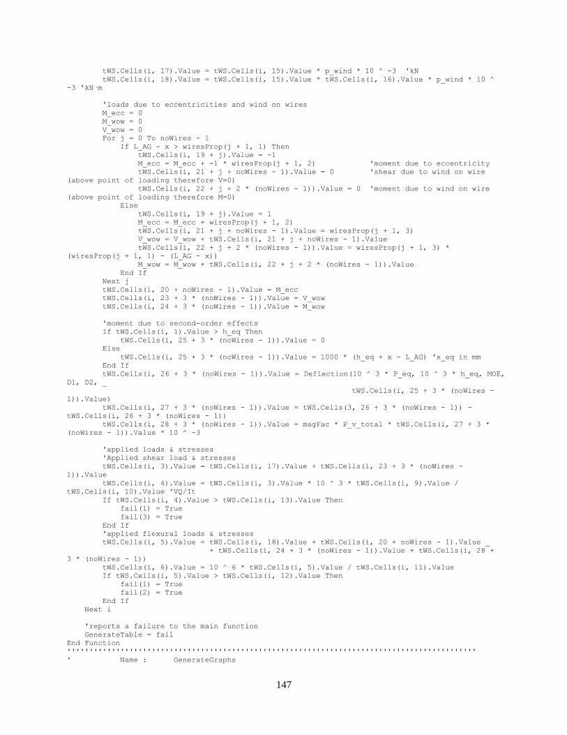
147
tWS.Cells(i, 17).Value = tWS.Cells(i, 15).Value * p_wind * 10 ^ -3 'kN
tWS.Cells(i, 18).Value = tWS.Cells(i, 15).Value * tWS.Cells(i, 16).Value * p_wind * 10 ^
-3 'kN·m
'loads due to eccentricities and wind on wires
M_ecc = 0
M_wow = 0
V_wow = 0
For j = 0 To noWires - 1
If L_AG - x > wiresProp(j + 1, 1) Then
tWS.Cells(i, 19 + j).Value = -1
M_ecc = M_ecc + -1 * wiresProp(j + 1, 2) 'moment due to eccentricity
tWS.Cells(i, 21 + j + noWires - 1).Value = 0 'shear due to wind on wire
(above point of loading therefore V=0)
tWS.Cells(i, 22 + j + 2 * (noWires - 1)).Value = 0 'moment due to wind on wire
(above point of loading therefore M=0)
Else
tWS.Cells(i, 19 + j).Value = 1
M_ecc = M_ecc + wiresProp(j + 1, 2)
tWS.Cells(i, 21 + j + noWires - 1).Value = wiresProp(j + 1, 3)
V_wow = V_wow + tWS.Cells(i, 21 + j + noWires - 1).Value
tWS.Cells(i, 22 + j + 2 * (noWires - 1)).Value = wiresProp(j + 1, 3) *
(wiresProp(j + 1, 1) - (L_AG - x))
M_wow = M_wow + tWS.Cells(i, 22 + j + 2 * (noWires - 1)).Value
End If
Next j
tWS.Cells(i, 20 + noWires - 1).Value = M_ecc
tWS.Cells(i, 23 + 3 * (noWires - 1)).Value = V_wow
tWS.Cells(i, 24 + 3 * (noWires - 1)).Value = M_wow
'moment due to second-order effects
If tWS.Cells(i, 1).Value > h_eq Then
tWS.Cells(i, 25 + 3 * (noWires - 1)).Value = 0
Else
tWS.Cells(i, 25 + 3 * (noWires - 1)).Value = 1000 * (h_eq + x - L_AG) 'x_eq in mm
End If
tWS.Cells(i, 26 + 3 * (noWires - 1)).Value = Deflection(10 ^ 3 * P_eq, 10 ^ 3 * h_eq, MOE,
D1, D2, _
tWS.Cells(i, 25 + 3 * (noWires -
1)).Value)
tWS.Cells(i, 27 + 3 * (noWires - 1)).Value = tWS.Cells(3, 26 + 3 * (noWires - 1)) -
tWS.Cells(i, 26 + 3 * (noWires - 1))
tWS.Cells(i, 28 + 3 * (noWires - 1)).Value = magFac * P_v_total * tWS.Cells(i, 27 + 3 *
(noWires - 1)).Value * 10 ^ -3
'applied loads & stresses
'Applied shear load & stresses
tWS.Cells(i, 3).Value = tWS.Cells(i, 17).Value + tWS.Cells(i, 23 + 3 * (noWires -
1)).Value
tWS.Cells(i, 4).Value = tWS.Cells(i, 3).Value * 10 ^ 3 * tWS.Cells(i, 9).Value /
tWS.Cells(i, 10).Value 'VQ/It
If tWS.Cells(i, 4).Value > tWS.Cells(i, 13).Value Then
fail(1) = True
fail(3) = True
End If
'applied flexural loads & stresses
tWS.Cells(i, 5).Value = tWS.Cells(i, 18).Value + tWS.Cells(i, 20 + noWires - 1).Value _
+ tWS.Cells(i, 24 + 3 * (noWires - 1)).Value + tWS.Cells(i, 28 +
3 * (noWires - 1))
tWS.Cells(i, 6).Value = 10 ^ 6 * tWS.Cells(i, 5).Value / tWS.Cells(i, 11).Value
If tWS.Cells(i, 5).Value > tWS.Cells(i, 12).Value Then
fail(1) = True
fail(2) = True
End If
Next i
'reports a failure to the main function
GenerateTable = fail
End Function
''''''''''''''''''''''''''''''''''''''''''''''''''''''''''''''''''''''''''''''''''''''''''''
' Name : GenerateGraphs

148
' Type : Subroutine
' Purpose : This subroutine generates moment and stress graphs with respect to
' the height of the pole. The graphs show both the applied and ultim-
' ate values on the chart.
''''''''''''''''''''''''''''''''''''''''''''''''''''''''''''''''''''''''''''''''''''''''''''
Sub GenerateGraphs(tWS As Worksheet, gWS As Worksheet, noWires As Integer)
'NOTES:
'xlCategory = x-axis
'xlValue = y-axis
'SCATTER WITH LINES 74 xlXYScatterLines
'SCATTER WITH LINES AND NO DATA MARKERS 75 xlXYScatterLinesNoMarkers
Dim Moments_1 As ChartObject
Dim Stresses_1 As ChartObject 'normal/flexural stresses
Dim MOI_1 As ChartObject
Dim Stresses_2 As ChartObject 'shear stresses
Dim Loads_1 As ChartObject
Dim lCol As Integer, lRow As Integer
lRow = tWS.[A1].SpecialCells(xlCellTypeLastCell).Row
lCol = tWS.[A1].SpecialCells(xlCellTypeLastCell).Column
gWS.Activate
gWS.PageSetup.PrintGridlines = False
gWS.Cells.Interior.Color = RGB(155, 155, 155)
Set Moments_1 = gWS.ChartObjects.Add(Left:=25, Width:=550, Top:=25, Height:=450)
Set Stresses_1 = gWS.ChartObjects.Add(Left:=600, Width:=550, Top:=25, Height:=450)
Set MOI_1 = gWS.ChartObjects.Add(Left:=600, Width:=550, Top:=500, Height:=450)
Set Stresses_2 = gWS.ChartObjects.Add(Left:=25, Width:=550, Top:=500, Height:=450)
Set Loads_1 = gWS.ChartObjects.Add(Left:=25, Width:=550, Top:=975, Height:=450)
With Moments_1.Chart
.HasTitle = True
.ChartType = xlXYScatterLinesNoMarkers
.ChartTitle.Text = "Applied and ultimate moments"
.Axes(xlCategory).HasTitle = True
.Axes(xlCategory, xlPrimary).AxisTitle.Text = "Bending Moment, kN" & Chr(183) & "m"
.Axes(xlValue).HasTitle = True
.Axes(xlValue, xlPrimary).AxisTitle.Text = "Height above ground, m"
.SeriesCollection.NewSeries
.SeriesCollection(1).Name = "Applied moment"
.SeriesCollection(1).XValues = tWS.Range(tWS.Cells(3, 5), tWS.Cells(lRow, 5))
.SeriesCollection(1).Values = tWS.Range(tWS.Cells(3, 1), tWS.Cells(lRow, 1))
.SeriesCollection.NewSeries
.SeriesCollection(2).Name = "Ultimate moment"
.SeriesCollection(2).XValues = tWS.Range(tWS.Cells(3, 12), tWS.Cells(lRow, 12))
.SeriesCollection(2).Values = tWS.Range(tWS.Cells(3, 1), tWS.Cells(lRow, 1))
End With
With Stresses_1.Chart 'xlValue xlCategory xlPrimary xlSecondary
.HasTitle = True
.ChartType = xlXYScatterLinesNoMarkers
.ChartTitle.Text = "Applied and ultimate normal stresses"
.Axes(xlCategory).HasTitle = True
.Axes(xlCategory, xlPrimary).AxisTitle.Text = "Stress, MPa"
.Axes(xlValue).HasTitle = True
.Axes(xlValue, xlPrimary).AxisTitle.Text = "Height above ground, m"
.SeriesCollection.NewSeries
.SeriesCollection(1).Name = "Applied stress"
.SeriesCollection(1).XValues = tWS.Range(tWS.Cells(3, 6), tWS.Cells(lRow, 6))
.SeriesCollection(1).Values = tWS.Range(tWS.Cells(3, 1), tWS.Cells(lRow, 1))
.SeriesCollection.NewSeries
.SeriesCollection(2).Name = "Ultimate stress"
.SeriesCollection(2).XValues = tWS.Range(tWS.Cells(3, 14), tWS.Cells(lRow, 14))
.SeriesCollection(2).Values = tWS.Range(tWS.Cells(3, 1), tWS.Cells(lRow, 1))
End With
With MOI_1.Chart

149
.HasTitle = True
.ChartType = xlXYScatterLinesNoMarkers
.ChartTitle.Text = "Moment of inertia"
.Axes(xlCategory).HasTitle = True
.Axes(xlCategory, xlPrimary).AxisTitle.Text = "Moment of inertia, mm" & ChrW(&H2074)
.Axes(xlValue).HasTitle = True
.Axes(xlValue, xlPrimary).AxisTitle.Text = "Height above ground, m"
.SeriesCollection.NewSeries
.SeriesCollection(1).Name = "Moment of inertia"
.SeriesCollection(1).XValues = tWS.Range(tWS.Cells(3, 10), tWS.Cells(lRow, 10))
.SeriesCollection(1).Values = tWS.Range(tWS.Cells(3, 1), tWS.Cells(lRow, 1))
End With
With Stresses_2.Chart
.HasTitle = True
.ChartType = xlXYScatterLinesNoMarkers
.ChartTitle.Text = "Applied and ultimate shear stresses"
.Axes(xlCategory).HasTitle = True
.Axes(xlCategory, xlPrimary).AxisTitle.Text = "Stress, MPa"
.Axes(xlValue).HasTitle = True
.Axes(xlValue, xlPrimary).AxisTitle.Text = "Height above ground, m"
.SeriesCollection.NewSeries
.SeriesCollection(1).Name = "Applied stress"
.SeriesCollection(1).XValues = tWS.Range(tWS.Cells(3, 4), tWS.Cells(lRow, 4))
.SeriesCollection(1).Values = tWS.Range(tWS.Cells(3, 1), tWS.Cells(lRow, 1))
.SeriesCollection.NewSeries
.SeriesCollection(2).Name = "Ultimate stress"
.SeriesCollection(2).XValues = tWS.Range(tWS.Cells(3, 13), tWS.Cells(lRow, 13))
.SeriesCollection(2).Values = tWS.Range(tWS.Cells(3, 1), tWS.Cells(lRow, 1))
End With
With Loads_1.Chart
.HasTitle = True
.ChartType = xlXYScatterLinesNoMarkers
.ChartTitle.Text = "Applied moments"
.Axes(xlCategory).HasTitle = True
.Axes(xlCategory, xlPrimary).AxisTitle.Text = "Bending Moment, kN" & Chr(183) & "m"
.Axes(xlValue).HasTitle = True
.Axes(xlValue, xlPrimary).AxisTitle.Text = "Height above ground, m"
.SeriesCollection.NewSeries
.SeriesCollection(1).Name = "Wind on support"
.SeriesCollection(1).XValues = tWS.Range(tWS.Cells(3, 18), tWS.Cells(lRow, 18))
.SeriesCollection(1).Values = tWS.Range(tWS.Cells(3, 1), tWS.Cells(lRow, 1))
.SeriesCollection.NewSeries
.SeriesCollection(2).Name = "Eccentricities"
.SeriesCollection(2).XValues = tWS.Range(tWS.Cells(3, 20 + (noWires - 1)), tWS.Cells(lRow,
20 + (noWires - 1)))
.SeriesCollection(2).Values = tWS.Range(tWS.Cells(3, 1), tWS.Cells(lRow, 1))
.SeriesCollection.NewSeries
.SeriesCollection(3).Name = "Wind on wires"
.SeriesCollection(3).XValues = tWS.Range(tWS.Cells(3, 24 + 3 * (noWires - 1)),
tWS.Cells(lRow, 24 + 3 * (noWires - 1)))
.SeriesCollection(3).Values = tWS.Range(tWS.Cells(3, 1), tWS.Cells(lRow, 1))
.SeriesCollection.NewSeries
.SeriesCollection(4).Name = "P-" & ChrW(&H394) & " effects"
.SeriesCollection(4).XValues = tWS.Range(tWS.Cells(3, 28 + 3 * (noWires - 1)),
tWS.Cells(lRow, 28 + 3 * (noWires - 1)))
.SeriesCollection(4).Values = tWS.Range(tWS.Cells(3, 1), tWS.Cells(lRow, 1))
.SeriesCollection.NewSeries
.SeriesCollection(5).Name = "Total moment"
.SeriesCollection(5).XValues = tWS.Range(tWS.Cells(3, 5), tWS.Cells(lRow, 5))
.SeriesCollection(5).Values = tWS.Range(tWS.Cells(3, 1), tWS.Cells(lRow, 1))
End With
End Sub
Function diameter(Circ As Double) As Double
diameter = Circ / Application.WorksheetFunction.Pi()
End Function

150
Function MomInertia(diameter As Double) As Double
MomInertia = Application.WorksheetFunction.Pi() * diameter ^ 4 / 64
End Function
''''''''''''''''''''''''''''''''''''''''''''''''''''''''''''''''''''''''''''''''''''''''''''
' Name : DmgSectPropEF
' Type : Function
' Purpose : This function is used to determine various damaged section prop-
' erties (moment of inertia, section modulus, first moment
' of area and thickness) for exploratory and feeding damage.
' Usage : The Prop argument specifies the desired property as follows:
' Prop = 1, Moment of inertia
' Prop = 2, Section modulus
' Prop = 3, Q/t
' orientation = 1, tension/compression
' orientation = 2, neutral axis
''''''''''''''''''''''''''''''''''''''''''''''''''''''''''''''''''''''''''''''''''''''''''''
Function DmgSectPropEF(diameter As Double, D1 As Double, D2 As Double, Prop As Integer,
orientation As Double) As Double
'D1 = hole diameter, D2 = depth/length of hole
Dim R As Double 'section radius
Dim ySeg As Double 'centroid of circular segment w.r.t. centroid of undamaged section
Dim ySq As Double 'centroid of square segment w.r.t. centroid of undamaged section
Dim yDmg As Double 'centroid of damaged section w.r.t. centroid of undamaged section
Dim a As Double 'angle forming the half chord length of the circular segment, see
notes for detail
Dim hSeg As Double 'height of circular segment
Dim hSq As Double 'height of square segment
Dim ASeg As Double 'area of circular segment
Dim ASq As Double 'area of square segment
Dim AFull As Double 'area of undamaged section
Dim ISeg As Double 'moment of inertia of circular segment
Dim ISq As Double 'moment of inertia of square segment
Dim IFull As Double 'moment of inertia of non-damaged section
Dim IDmg As Double 'moment of inertia of damaged section
Dim s As Double 'sin(a)
Dim c As Double 'cos(a)
Dim SectModPos As Double, SectModNeg As Double 'the two section moduli
R = diameter / 2
If D1 < diameter Then
hSeg = R - Sqr(R ^ 2 - (D1 / 2) ^ 2)
hSq = D2 - hSeg
a = Application.WorksheetFunction.Asin(D1 / (2 * R))
s = Sin(a)
c = Cos(a)
'area calculations
ASeg = R ^ 2 * (a - s * c)
ASq = hSq * D1
AFull = Application.WorksheetFunction.Pi() * R ^ 2
'centroid calculations (all w.r.t. centroid of undamaged section)
ySeg = 2 * R * (s) ^ 3 / (3 * (a - s * c))
ySq = R - hSeg - hSq / 2
yDmg = -1 * (ASeg * ySeg + ASq * ySq) / (AFull - (ASeg + ASq))
'moment of inertia calculations
IFull = Application.WorksheetFunction.Pi() * diameter ^ 4 / 64
If orientation = 1 Then
ISeg = (R ^ 4 / 4) * (a - s * c + 2 * s ^ 3 * c - 16 * (s ^ 6) / (9 * (a - s * c)))
ISq = D1 * hSq ^ 3 / 12
IDmg = IFull + AFull * yDmg ^ 2 - (ISq + ISeg + ASq * (ySq - yDmg) ^ 2 + ASeg * (ySeg
- yDmg) ^ 2)
ElseIf orientation = 2 Then
yDmg = 0
ISeg = (R ^ 4 / 12) * (3 * a - 3 * Sin(a) * Cos(a) - 2 * (Sin(a)) ^ 3 * Cos(a))
ISq = hSq * D1 ^ 3 / 12
IDmg = IFull - (ISq + ISeg)
End If
Select Case Prop
Case 1 'Return MOI
DmgSectPropEF = IDmg

151
Case 2 'Return section modulus
SectModPos = R + yDmg
SectModNeg = R - yDmg
If SectModPos <= SectModNeg Then
DmgSectPropEF = IDmg / SectModPos
Else
DmgSectPropEF = IDmg / SectModNeg
End If
Case 3 'Return Q/t
Dim t As Double 'shear plane thickness
Dim yQ As Double 'centroid of the portion of the area above/below yDmg w.r.t. yDmg
Dim AQ As Double 'area of the portion above/below yDmg
Dim Q As Double 'first moment of area AQ w.r.t. yDmg
If orientation = 1 Then
t = 2 * Sqr(R ^ 2 - yDmg ^ 2)
a = Application.WorksheetFunction.Asin(t / (2 * R))
s = Sin(a)
c = Cos(a)
yQ = R * (2 * s ^ 3 / (3 * (a - s * c)) - c)
AQ = R ^ 2 * (a - s * c)
Q = AQ * yQ
DmgSectPropEF = Q / t
If D2 > R - yDmg Then
Dim D2_ As Double 'portion of D2 located under yDmg
Dim AQ_ As Double 'area AQ with the void D1*D2_ removed
Dim yQ_ As Double 'centroid of AQ_
Dim Q_ As Double 'first moment of area AQ_ w.r.t. yDmg
t = t - D1
D2_ = D2 - (R - yDmg)
AQ_ = AQ - D1 * D2_
yQ_ = (AQ * yQ - 0.5 * D1 * D2_ ^ 2) / AQ_
Q_ = AQ_ * yQ_
DmgSectPropEF = Q_ / t
End If
ElseIf orientation = 2 Then
t = diameter - D2
AQ = 0.5 * (AFull - (ASq + ASeg))
'note: for the half circular segment, the centroid was approximated to 3a/8 where
a is the width
' of the half segment. This is the centroid of a semiparabolic area as seen
on the back
' cover of Mechanics of Materials (4th edition) by Beer et al.
yQ = (4 * R * AFull / (6 * Application.WorksheetFunction.Pi()) - (hSq * D1 ^ 2 /
8 + ASeg * D1 / 10)) / AQ
Q = AQ * yQ
DmgSectPropEF = Q / t
End If
End Select
Else
DmgSectPropEF = 1
End If
End Function
Function DmgSectPropN(diameter As Double, D2 As Double, D1 As Double, Prop As Integer,
orientation As Double) As Double
'D2 = opening diameter, D3 = shell thickness
'Equations relating to segments of solid circles and sectors of hollow circles were taken from
Roark's Formulas for
'stress and strain, 7th edition, p. 808 (appendix A).
Dim R As Double 'section radius
Dim RHollow As Double 'radius of hollowed out circle
Dim ySeg As Double 'centroid of circular segment w.r.t. centroid of undamaged section
Dim yHollow As Double 'centroid of hollowed circle w.r.t. centroid of undamaged section
Dim yDmg As Double 'centroid of damaged section w.r.t. centroid of undamaged section
Dim a As Double 'angle forming the half chord length of the circular segment, see
notes for detail
Dim hSeg As Double 'height of circular segment
Dim ASeg As Double 'area of circular segment
Dim AHollow As Double 'area of hollowed circle
Dim AFull As Double 'area of undamaged section

152
Dim ISeg As Double 'moment of inertia of circular segment
Dim IHollow As Double 'moment of inertia of hollowed circle
Dim IFull As Double 'moment of inertia of undamaged section
Dim IDmg As Double 'moment of inertia of damaged section
Dim s As Double 'sin(a)
Dim c As Double 'cos(a)
Dim SectModPos As Double, SectModNeg As Double 'the two section moduli
R = diameter / 2
RHollow = R - D1
a = Application.WorksheetFunction.Asin(D2 / (2 * R))
s = Sin(a)
c = Cos(a)
'area calculations
ASeg = a * D1 * (2 * R - D1)
AHollow = Application.WorksheetFunction.Pi() * RHollow ^ 2
AFull = Application.WorksheetFunction.Pi() * R ^ 2
'centroid calculations (all w.r.t. centroid of undamaged section)
ySeg = 2 * R * s / (3 * a) * (1 - D1 / R + 1 / (2 - D1 / R))
yDmg = -ASeg * ySeg / (AFull - (AHollow + ASeg))
'moment of inertia calculations
IFull = Application.WorksheetFunction.Pi() * diameter ^ 4 / 64
IHollow = Application.WorksheetFunction.Pi() * RHollow ^ 4 / 4 '1/4 instead of 1/64 because
R is used instead of D
If orientation = 1 Then
ISeg = R ^ 3 * D1 * ((1 - 3 * D1 / (2 * R) + D1 ^ 2 / R ^ 2 - D1 ^ 3 / (4 * R ^ 3)) * (a
+ s * c - 2 * s ^ 2 / a) + _
(D1 ^ 2 * s ^ 2 / (3 * R ^ 2 * a * (2 - D1 / R))) * (1 - D1 / R + D1 ^ 2 / (6 * R ^
2)))
IDmg = IFull + AFull * yDmg ^ 2 - (IHollow + ISeg + AHollow * yDmg ^ 2 + ASeg * (ySeg -
yDmg) ^ 2)
ElseIf orientation = 2 Then
yDmg = 0
ISeg = R ^ 3 * D1 * (1 - 3 * D1 / (2 * R) + D1 ^ 2 / R ^ 2 - D1 ^ 3 / (4 * R ^ 3)) * (a -
s * c)
IDmg = IFull - (IHollow + ISeg)
End If
Select Case Prop
Case 1 'Requested property is moment of inertia
DmgSectPropN = IDmg
Case 2 'Requested property is section modulus
SectModPos = R + yDmg
SectModNeg = R - yDmg
If SectModPos >= SectModNeg Then
DmgSectPropN = IDmg / SectModPos
Else
DmgSectPropN = IDmg / SectModNeg
End If
Case 3 'Requested property is the quotient of the first moment of area and thickness of shear
plane (Q/t)
Dim t As Double 'shear plane thickness
Dim yQ As Double 'centroid of the portion of the area above/below yDmg w.r.t. yDmg
Dim AQ As Double 'area of the portion above/below yDmg
Dim Q As Double 'first moment of area AQ w.r.t. yDmg
Dim a_ As Double 'vertical angle for hollow circular segment
Dim b As Double 'width of AQ
Dim b_ As Double 'width of hollow circular segment
Dim R_ As Double 'radius of hollow circle
Dim Amom As Double, Amom_ As Double 'portion of area of section below yDmg to find
first moment of area about yDmg
Dim y As Double, y_ As Double 'centroids w.r.t. yDmg of full portion of area
below yDmg and hollowed portion below yDmg
If orientation = 1 Then
R_ = R - D1
' this is a simplification (t is most likely slightly greater than 2t) but this is a
' conservative value and is close enough for all intents and purposes
t = 2 * D1
b = 2 * Sqr(R ^ 2 - yDmg ^ 2)
b_ = 2 * Sqr(R_ ^ 2 - yDmg ^ 2)
153
a = Application.WorksheetFunction.Asin(b / (2 * R))
a_ = Application.WorksheetFunction.Asin(b_ / (2 * R_))
If a <= Application.WorksheetFunction.Pi() / 4 Then
Amom = R ^ 2 * (a - Sin(a) * Cos(a))
y = R ^ 2 * (2 * (Sin(a)) ^ 3 / (3 * (a - Sin(a) * Cos(a))) - Cos(a))
Else
Amom = 2 * R ^ 2 * a ^ 3 * (1 - 0.2 * a ^ 2 + 0.019 * a ^ 4) / 3
y = 0.2 * R * a ^ 2 * (1 - 0.0619 * a ^ 2 + 0.0027 * a ^ 4)
End If
If a_ <= Application.WorksheetFunction.Pi() / 4 Then
Amom_ = R_ ^ 2 * (a_ - Sin(a_) * Cos(a_))
y_ = R_ ^ 2 * (2 * (Sin(a_)) ^ 3 / (3 * (a_ - Sin(a_) * Cos(a_))) - Cos(a_))
Else
Amom_ = 2 * R_ ^ 2 * a_ ^ 3 * (1 - 0.2 * a_ ^ 2 + 0.019 * a_ ^ 4) / 3
y_ = 0.2 * R_ * a_ ^ 2 * (1 - 0.0619 * a_ ^ 2 + 0.0027 * a_ ^ 4)
End If
AQ = Amom - Amom_
yQ = (Amom * y - Amom_ * y_) / AQ
ElseIf orientation = 2 Then
t = D1
a_ = a / 2
AQ = 0.5 * (Application.WorksheetFunction.Pi() * R ^ 2 -
(Application.WorksheetFunction.Pi() * RHollow ^ 2) + a_ * D1 * (2 * R - D1))
y_ = 2 * R * (Sin(a_)) ^ 2 / (3 * a_) * (1 - D1 / R + 1 / (2 - D1 / R)) 'ySector
yQ = (2 * R ^ 3 / 3 - 2 * RHollow ^ 3 / 3 - a_ * D1 * (2 * R - D1) * y_) / AQ
End If
Q = AQ * yQ
DmgSectPropN = Q / t
End Select
End Function
Function SectModulus(diameter As Double) As Double
SectModulus = Application.WorksheetFunction.Pi() * diameter ^ 3 / 32
End Function
Function MomentofArea(diameter As Double) As Double
Dim AQ As Double 'Area above centroid of cross-section
Dim yQ As Double 'Centroid of AQ
AQ = Application.WorksheetFunction.Pi() * (diameter / 4) ^ 2
yQ = 4 * (diameter / 2) / (Application.WorksheetFunction.Pi() * 3)
'Q/t=AQ*yQ/t, t=diameter
MomentofArea = AQ * yQ / diameter
End Function
''''''''''''''''''''''''''''''''''''''''''''''''''''''''''''''''''''''''''''''''''''''''''''
' Name : Deflection
' Type : Function
' Purpose : This function calculates the deflection along a tapered, cantilevered
' member. A sketch explaining the equation can be found in the "Notes"
' worksheet. The derivation of this equation can be found in the
' "Calculations" folder as "TaperedPoleDeflection.pdf"
''''''''''''''''''''''''''''''''''''''''''''''''''''''''''''''''''''''''''''''''''''''''''''
Function Deflection(P As Double, L As Double, E As Double, D1 As Double, D2 As Double, x As
Double) As Double
Deflection = 32 * P * L ^ 3 / (3 * Application.WorksheetFunction.Pi() * E * (D2 - D1) ^ 3) *
( _
(3 * L * (D2 - D1) * x + 2 * L ^ 2 * D1) / ((D2 - D1) * x + L * D1) ^ 2 _
+ (3 * D2 - 2 * D1) * ((D2 - D1) * x + L * D1) / (L * D2 ^ 3) _
+ 3 * (D1 - 2 * D2) / D2 ^ 2 _
)
End Function
''''''''''''''''''''''''''''''''''''''''''''''''''''''''''''''''''''''''''''''''''''''''''''
' Name : RandomizeVariables
' Type : Subroutine
' Purpose : This subroutine randomizes the material properties and various loa-
' ding characteristics.
''''''''''''''''''''''''''''''''''''''''''''''''''''''''''''''''''''''''''''''''''''''''''''
Sub RandomizeVariables(iWS As Worksheet)

154
Dim species As String
Dim mean As Double
Dim stDev As Double
Dim lUp As Worksheet
Dim alpha As Double
Dim beta As Double
Dim holeType As String
Dim dataSource As String
Dim lambda As Double
Dim zeta As Double
Dim location As String
Dim weatherCondition As String
Dim windAlpha As Double
Dim windu As Double
Dim iceAlpha As Double
Dim iceu As Double
Dim windSpeed As Double
Dim airDensityShapeFactor As Double
'initiate variables
Set lUp = Worksheets("Lookup")
species = iWS.Cells(6, 2).Value
holeType = iWS.Cells(13, 5).Value
dataSource = iWS.Cells(3, 5).Value
'randomize hole properties
'Equal probability randomization over a specified range.
'if rMAX and rMin are the maximum and minimum values in the range, respectively
'then a random decimal value within that range can be randomly obtained using
'Rnd * (rMAX - rMIN) + rMin, where Rnd is a random number between 0 and 1
If iWS.Cells(12, 4).Value = 1 Then
'hole location
iWS.Cells(14, 5).Value = Rnd * (lUp.Cells(64, 2).Value - lUp.Cells(63, 2).Value) +
lUp.Cells(63, 2).Value
'hole size
If holeType = "E" Then
'randomize exploratory hole dimensions
'D1 opening diameter
iWS.Cells(15, 5).Value = lUp.Cells(49, 2).Value
'D2 hole depth
iWS.Cells(16, 5).Value = Rnd * (lUp.Cells(48, 2).Value - lUp.Cells(47, 2).Value) +
lUp.Cells(47, 2).Value
ElseIf holeType = "F" Then
'randomize feeding hole dimensions
'D1 opening diameter
iWS.Cells(15, 5).Value = lUp.Cells(54, 2).Value
'D2 hole depth
iWS.Cells(16, 5).Value = Rnd * (lUp.Cells(53, 2).Value - lUp.Cells(52, 2).Value) +
lUp.Cells(52, 2).Value
ElseIf holeType = "N" Then
'randomize nesting hole dimensions
'D1 height of hole
iWS.Cells(15, 5).Value = lUp.Cells(57, 2).Value
'D2 opening diameter
iWS.Cells(16, 5).Value = lUp.Cells(58, 2).Value
'D3 shell thickness
iWS.Cells(17, 5).Value = Rnd * (lUp.Cells(60, 2).Value - lUp.Cells(59, 2).Value) +
lUp.Cells(59, 2).Value
End If
End If
'Longitudinal shear strength
If dataSource = "Literature" Then
mean = lUp.Cells(3, 2).Value
stDev = lUp.Cells(3, 3).Value * mean
iWS.Cells(9, 2).Value = Application.WorksheetFunction.NormInv(Rnd, mean, stDev)
ElseIf dataSource = "UW" Then
mean = lUp.Cells(2, 4).Value
stDev = lUp.Cells(2, 5).Value

155
iWS.Cells(9, 2).Value = Application.WorksheetFunction.LogNorm_Inv(Rnd, mean, stDev)
End If
'Modulus of rupture / bending strength
If dataSource = "Literature" Then
mean = lUp.Cells(12, 2).Value
stDev = lUp.Cells(12, 3).Value * mean
iWS.Cells(8, 2).Value = Application.WorksheetFunction.NormInv(Rnd, mean, stDev)
ElseIf dataSource = "UW" Then
mean = lUp.Cells(9, 2).Value
stDev = lUp.Cells(9, 3).Value * mean
iWS.Cells(8, 2).Value = Application.WorksheetFunction.NormInv(Rnd, mean, stDev)
End If
'MOE
mean = lUp.Cells(7, 8).Value
stDev = lUp.Cells(7, 9).Value * mean
iWS.Cells(10, 2).Value = Application.WorksheetFunction.NormInv(Rnd, mean, stDev)
'randomize climactic data
location = iWS.Cells(3, 7).Value
weatherCondition = iWS.Cells(17, 2).Value
airDensityShapeFactor = iWS.Cells(35, 2).Value
If weatherCondition = "wind-only" Then
windAlpha = Application.WorksheetFunction.Lookup(location, lUp.Range("A70:A71"),
lUp.Range("B70:B71"))
windu = Application.WorksheetFunction.Lookup(location, lUp.Range("A70:A71"),
lUp.Range("C70:C71"))
iWS.Cells(18, 2).Value = 0
ElseIf weatherCondition = "wind-on-ice" Then
windAlpha = Application.WorksheetFunction.Lookup(location, lUp.Range("A70:A71"),
lUp.Range("D70:D71"))
windu = Application.WorksheetFunction.Lookup(location, lUp.Range("A70:A71"),
lUp.Range("E70:E71"))
iceAlpha = Application.WorksheetFunction.Lookup(location, lUp.Range("A70:A71"),
lUp.Range("F70:F71"))
iceu = Application.WorksheetFunction.Lookup(location, lUp.Range("A70:A71"),
lUp.Range("G70:G71"))
'randomize ice thickness, convert to mm
iWS.Cells(18, 2).Value = 25.4 * (-Application.WorksheetFunction.Ln(-
Application.WorksheetFunction.Ln(Rnd)) / iceAlpha + iceu)
End If
windSpeed = -Application.WorksheetFunction.Ln(-Application.WorksheetFunction.Ln(Rnd)) /
windAlpha + windu
windSpeed = windSpeed / 3.6 'convert from km/h to m/s
iWS.Cells(19, 2).Value = airDensityShapeFactor * windSpeed ^ 2 'sets wind pressure
End Sub
''''''''''''''''''''''''''''''''''''''''''''''''''''''''''''''''''''''''''''''''''''''''''''
' Name : GenerateTable
' Type : Subroutine
' Purpose : This subroutine generates the analysis table. It calculates the geo-
' metric properties of each segment, and determines the total moment
' applied at each of these segments.
''''''''''''''''''''''''''''''''''''''''''''''''''''''''''''''''''''''''''''''''''''''''''''
Sub LocateFailure(iterNo As Long, tWS As Worksheet, fWS As Worksheet, fCount As Integer)
Dim i As Integer
Dim lRow As Integer
Dim sFailLocation As Double
Dim fFailLocation As Double
Dim sFailMag As Double
Dim fFailMag As Double
lRow = tWS.[A1].SpecialCells(xlCellTypeLastCell).Row
sFailMag = 0
fFailMag = 0
For i = 3 To lRow

156
'check shear failure
If tWS.Cells(i, 4).Value > tWS.Cells(i, 13).Value Then
If tWS.Cells(i, 4).Value > sFailMag Then
sFailMag = tWS.Cells(i, 4).Value
sFailLocation = tWS.Cells(i, 2).Value
End If
End If
'check flexural failure
If tWS.Cells(i, 6).Value > tWS.Cells(i, 14).Value Then
If tWS.Cells(i, 6).Value > sFailMag Then
fFailMag = tWS.Cells(i, 6).Value
fFailLocation = tWS.Cells(i, 2).Value
End If
End If
Next i
fWS.Cells(fCount + 1, 1).Value = fCount
fWS.Cells(fCount + 1, 2).Value = iterNo
If fFailMag = 0 Then
fWS.Cells(fCount + 1, 3).Value = "N/A"
Else
fWS.Cells(fCount + 1, 3).Value = fFailLocation
End If
If sFailMag = 0 Then
fWS.Cells(fCount + 1, 4).Value = "N/A"
Else
fWS.Cells(fCount + 1, 4).Value = sFailLocation
End If
End Sub
''''''''''''''''''''''''''''''''''''''''''''''''''''''''''''''''''''''''''''''''''''''''''''
' Name : GenerateHeaders
' Type : Subroutine
' Purpose : This subroutine generates headers for the sectional analysis table.
' It dynamically sizes the table based on the number of wires attached
' to the pole.
''''''''''''''''''''''''''''''''''''''''''''''''''''''''''''''''''''''''''''''''''''''''''''
Sub GenerateHeaders(fWS As Worksheet)
Dim titles(1 To 4) As String
Dim i As Integer 'counters
Dim lCol As Integer, lRow As Integer 'location of last column and row
titles(1) = "Failure No."
titles(2) = "Iteration No."
titles(3) = "Mf location, m"
titles(4) = "Vf Location, m"
For i = 1 To UBound(titles)
fWS.Cells(1, i).Value = titles(i)
Next i
'formatting
lCol = UBound(titles)
lRow = fWS.Cells(1, 1).SpecialCells(xlCellTypeLastCell).Row
fWS.Range(fWS.Cells(1, 1), fWS.Cells(1, lCol)).Font.Bold = True
fWS.Range(fWS.Columns(1), fWS.Columns(lCol)).ColumnWidth = 13
fWS.Range(fWS.Cells(1, 1), fWS.Cells(lRow, lCol)).HorizontalAlignment = xlLeft
fWS.Range(fWS.Cells(2, 1), fWS.Cells(lRow, 2)).NumberFormat = "0"
fWS.Range(fWS.Cells(2, 3), fWS.Cells(lRow, lCol)).NumberFormat = "0.00"
fWS.Cells(1, 3).Characters(Start:=2, Length:=1).Font.Subscript = True
fWS.Cells(1, 4).Characters(Start:=2, Length:=1).Font.Subscript = True
fWS.Rows(2).Select
ActiveWindow.FreezePanes = True
fWS.Cells(1, 1).Select
'this loop adds borders around each group of columns
Dim myBorders() As Variant, property As Variant
myBorders = Array(xlEdgeLeft, xlEdgeRight, xlEdgeTop, xlEdgeBottom)

157
For Each property In myBorders
With fWS.Range(fWS.Cells(1, 1), fWS.Cells(1, lCol)).Borders(property)
.LineStyle = xlContinuous
.Weight = xlThin
.ColorIndex = xlAutomatic
End With
Next property
For Each property In myBorders
With fWS.Range(fWS.Cells(2, 1), fWS.Cells(lRow, lCol)).Borders(property)
.LineStyle = xlContinuous
.Weight = xlThin
.ColorIndex = xlAutomatic
End With
Next property
End Sub
Related Documents