The effect of vessel holes on fracture behaviour in the femoral neck of the human femur Karin Odin & Sofia Rokkones Lund, June 2020 Master’s Thesis in Biomedical Engineering Faculty of Engineering, LTH Department of Biomedical Engineering Supervisors: Lorenzo Grassi, Joeri Kok, and Hanna Isaksson

Welcome message from author
This document is posted to help you gain knowledge. Please leave a comment to let me know what you think about it! Share it to your friends and learn new things together.
Transcript

The effect of vessel holes on fracturebehaviour in the femoral neck of the
human femur
Karin Odin & Sofia RokkonesLund, June 2020
Master’s Thesis inBiomedical Engineering
Faculty of Engineering, LTHDepartment of Biomedical Engineering
Supervisors: Lorenzo Grassi, Joeri Kok, and HannaIsaksson


TitleThe effect of vessel holes on fracture behaviour in the femoral neck ofthe human femur
AuthorKarin Odin & Sofia Rokkones
FiguresCreated by the authors if nothing else is indicated
Lunds UniversitetInstitutionen for biomedicinsk teknikBox 118SE-221 00 LundSverige
Copyright c©Lund University, Faculty of Engineering 2020E-husets tryckeriLund 2020


Acknowledgements
We would first of all like to thank our supervisors, Lorenzo Grassi, JoeriKok, and Hanna Isaksson. Thank you for all your encouragement andguidance throughout this project. It has been an educative time andwe have learned a lot that we can bring with us in life. Also, thank youfor your fantastic communication and presence, especially during thesecond half of the master thesis, executed during a worldwide pandemic,working from home due to social distancing constraints. Thank youalso to all the members of the Biomechanic group, making us feel verywelcome as a part of the team already from day one.

Abstract
Hip fractures are widely spread in today’s society and affect a person’squality of life. Osteoporosis is a bone disease that results in more fragilebones and an increased risk of bone fractures, including hip fractures.A method proposed for assessing the fracture risk is finite element (FE)models of the femur. These FE models proved to be effective in pre-dicting the overall mechanical behavior of human femurs, but are lessaccurate in predicting localization of stresses or strains. It is proposedthat vessel holes in the femoral neck may affect the ability of FE modelsto predict fracture location, and that they need to be accounted for.
There were two main aims for this thesis. The first, was to developan automatic method for detection and quantification of blood vesselholes present in the proximal human femur. The second, was to inves-tigate whether a micro-FE model, based on micro-CT images includingfeatures such as vessel holes, could more effectively identify local highstrains as compared to an FE model based on lower resolution clinicalCT images.
Investigating these issues, the project focused on image analysis de-veloping a method with which blood vessel holes could be quantifiedin a feasible and accurate way in both micro-CT and clinical CT im-ages. This was done by investigating vessel hole canal structures andby thickness calculation of the cortical bone. The project also focusedon developing and validating a finite element model of the femur bone,based on segmentation and mesh generation from micro-CT images.
The project resulted in proposed methods for detecting and quan-tifying vessel holes, both based on micro-CT and clinical CT images.The methods were automatic, and the results showed a 100% accuracyin the micro-CT, and 60% accuracy in the clinical CT compared tothe micro-CT. Furthermore, a micro-FE model, with a complex surfacestructure including the detected vessel holes, was developed showinghigher accuracy in strain prediction, compared to an FE model based

on clinical CT images.The conclusion was that vessel holes could be detected and quantified
fully from micro-CT images and the largest vessel holes also in clinicalCT images. Also, a micro-FE model generated based on micro-CTimages, including the vessel holes in the femoral neck, correlated betterthan a similar model based on clinical CT images to experimentallymeasured strains.

List of acronyms &abbreviations
ε - strain
ρapp - apparent density
ρash - ash density
σ - stress
BC - boundary condition
BMD - bone mineral density
CT - computed tomography
DIC - digital image correlation
E - young’s modulus
FE - finite element
FEA - finite element analyses
PDE - partial differential equation
PVE - partial volume effect
ROI - region of interest

SD - standard deviation
Contents
Acknowledgements
Abstract
List of acronyms & abbreviations
1 Introduction 1
1.1 Aim . . . . . . . . . . . . . . . . . . . . . . . . . . . . . 2
1.2 Design of the study . . . . . . . . . . . . . . . . . . . . . 2
1.3 Authors’ contribution . . . . . . . . . . . . . . . . . . . . 3
2 Background 5
2.1 Anatomy . . . . . . . . . . . . . . . . . . . . . . . . . . . 5
2.1.1 Anatomical directions . . . . . . . . . . . . . . . 5
2.1.2 Femur . . . . . . . . . . . . . . . . . . . . . . . . 5
2.2 Osteoporosis . . . . . . . . . . . . . . . . . . . . . . . . . 7
2.3 CT imaging . . . . . . . . . . . . . . . . . . . . . . . . . 9
2.4 Digital image correlation . . . . . . . . . . . . . . . . . . 9
2.4.1 Interpretation of DIC measurements . . . . . . . 10
2.5 Image segmentation . . . . . . . . . . . . . . . . . . . . . 11
2.5.1 Threshold segmentation . . . . . . . . . . . . . . 11
2.5.2 Active contour segmentation . . . . . . . . . . . . 12
2.6 Calculation of cortical bone thickness . . . . . . . . . . . 12
2.7 Finite element bone models . . . . . . . . . . . . . . . . 14
2.7.1 The finite element method . . . . . . . . . . . . . 14
2.7.2 Mesh representations . . . . . . . . . . . . . . . . 15
2.7.3 Mapping material properties to the FE model . . 15
2.8 Background research for this project . . . . . . . . . . . 17
CONTENTS
3 Materials & methods 19
3.1 Material . . . . . . . . . . . . . . . . . . . . . . . . . . . 19
3.2 Overview of the methods . . . . . . . . . . . . . . . . . . 19
3.3 Quantification of vessel holes in micro-CT . . . . . . . . 24
3.3.1 ROI in micro-CT image . . . . . . . . . . . . . . 24
3.3.2 Active contour segmentation of ROI . . . . . . . . 24
3.3.3 Surface mesh generation of femur . . . . . . . . . 26
3.3.4 Intersection method . . . . . . . . . . . . . . . . . 26
3.3.5 Circle fit . . . . . . . . . . . . . . . . . . . . . . . 29
3.3.6 Quantification . . . . . . . . . . . . . . . . . . . . 30
3.4 Quantification of vessel holes in clinical CT . . . . . . . . 31
3.4.1 Clinical CT images . . . . . . . . . . . . . . . . . 31
3.4.2 Segmentation and mesh generation of femur surface 31
3.4.3 Calculation of cortical bone thickness . . . . . . . 32
3.4.4 Quantification . . . . . . . . . . . . . . . . . . . . 32
3.5 Evaluation of vessel hole quantification . . . . . . . . . . 34
3.6 Generation of FE models . . . . . . . . . . . . . . . . . . 35
3.6.1 Surface mesh of micro-FE model . . . . . . . . . 35
3.6.2 Volume mesh of micro-FE model . . . . . . . . . 37
3.6.3 Mesh generation for standard FE model . . . . . 39
3.6.4 Mapping . . . . . . . . . . . . . . . . . . . . . . . 39
3.6.5 Boundary conditions . . . . . . . . . . . . . . . . 41
3.6.6 Simulation . . . . . . . . . . . . . . . . . . . . . . 42
3.7 Validation of the micro-FE model . . . . . . . . . . . . . 42
3.7.1 FE models used for validation . . . . . . . . . . . 42
3.7.2 Approach . . . . . . . . . . . . . . . . . . . . . . 45
3.7.3 Qualitative comparison . . . . . . . . . . . . . . . 45
3.7.4 Validation with DIC . . . . . . . . . . . . . . . . 45
4 Results 47
4.1 Quantification of vessel holes . . . . . . . . . . . . . . . . 47
4.1.1 Micro-CT . . . . . . . . . . . . . . . . . . . . . . 47
4.1.2 Clinical CT . . . . . . . . . . . . . . . . . . . . . 50
4.1.3 Evaluation . . . . . . . . . . . . . . . . . . . . . . 54
4.2 Validation of the micro-FE model . . . . . . . . . . . . . 57
4.2.1 Qualitative comparison . . . . . . . . . . . . . . . 57
4.2.2 Validation with DIC . . . . . . . . . . . . . . . . 61

CONTENTS
5 Discussion 655.1 Quantification of vessel holes . . . . . . . . . . . . . . . . 65
5.1.1 Micro-CT . . . . . . . . . . . . . . . . . . . . . . 655.1.2 Clinical CT . . . . . . . . . . . . . . . . . . . . . 665.1.3 Evaluation . . . . . . . . . . . . . . . . . . . . . . 67
5.2 Validation of the micro-FE model . . . . . . . . . . . . . 685.2.1 Qualitative comparison . . . . . . . . . . . . . . . 695.2.2 Validation with DIC . . . . . . . . . . . . . . . . 70
5.3 Future perspective . . . . . . . . . . . . . . . . . . . . . 715.4 Ethical aspects . . . . . . . . . . . . . . . . . . . . . . . 72
6 Conclusions 73
References 73
Appendix 837.1 Strain in vessel holes . . . . . . . . . . . . . . . . . . . . 83

CONTENTS

Chapter 1
Introduction
In today’s society, a large group of people are affected by osteoporosis, abone disease reducing the bone mineral density, leading to more fragilebones and a higher risk of fracture. Today, one in three women and onein five men older than 50 years will sustain an osteoporosis-related frac-ture within their lifetime [1]. In the year 2017, the number of fragilityfractures was 120 000 in Sweden. This corresponds to more than 13fractures every hour, and is estimated to increase in the coming years[2].
Hip fractures account for about 20% of all osteoporotic fracturesworldwide. Nevertheless, they account for the majority of the osteo-porotic fracture-related costs among men and women over 50 years [3].In Sweden alone, the cost of hip fractures was e823 million in 2010 [4].Worldwide, the prevalence of hip fractures is predicted to increase from1.3 million in the year 1990 to between 7.3 - 21.3 million in 2050 [5].
The most common way of diagnosing osteoporosis is to measure thebone mineral density (BMD), to get a so-called T-score. If the BMDvalue is 2.5 standard deviations (SDs) or more below the average BMDvalue for premenopausal women, the patient is considered osteoporotic[6, 7, 8]. A low BMD is connected to high fracture risk. However, amajority of the hip fractures occur in people without osteoporosis [9].
A proposed method for improved assessment of the fracture risk isby using finite element (FE) models of the femur (thigh bone), basedon patient specific information, geometry and mechanical properties de-rived from computed tomography (CT) images. Finite element analysis(FEA) can estimate the strength and fracture risk of the femur [10].
Several approaches to determine the fracture risk in the femur withFE models have been developed over the last decades. Yet, there is a
1

2 CHAPTER 1. INTRODUCTION
need for more detailed models. Recent studies have detected regions oflocal weaknesses in the femoral neck which correspond to regions whereblood vessel holes are located in the cortical bone [11]. It is suggestedthat the vessel holes, which are not accounted for in today’s FE models,may be involved in fracture initiation in the femoral neck [11, 12]. Ex-perimental results have been compared to predicted outcomes from FEmodels of femurs under load. The results correspond well in all regions,except in the superolateral region, the ”saddle-region” of the femoralneck. Here, the FE models predicted high strains that were never de-tected experimentally. Instead, the experimental results showed highstrains in several vessel holes, which the FE models did not predict.To improve the accuracy of future FE models’ ability to predict thefemur’s risk of fracture, the vessel holes are proposed to be accountedfor [13, 14].
1.1 Aim
The purpose of the thesis was to determine the presence and locationof blood vessel holes in the femoral neck and to investigate their effecton the local strain distribution. This was done by developing differentapproaches to quantify the vessel holes in the femoral neck and to buildFE models that included the characteristics of the vessel holes. Themain objectives were divided into two sub-aims, namely:
• To develop an automatic method for detection and quantificationof blood vessel holes, in terms of size and location, in both micro-CT and clinical CT images.
• To investigate whether a micro-FE model based on micro-CT im-ages, including features such as vessel holes, can more effectivelyidentify local high strains as compared to an FE model based onlower resolution clinical CT images.
1.2 Design of the study
The starting point for this master’s thesis was that clinical CT imagesand FE models based on these clinical CT images were available. Ex-perimental measurements have shown that strains locally are high in theregion of the femoral neck where a large number of blood vessel holes

1.3. AUTHORS’ CONTRIBUTION 3
usually are present. In order to investigate how the vessel holes influ-ence the bone strength and possibly affect the fracture risk of the femur,two approaches were used. First, a method was proposed for detectingand quantifying the number, size, and location of vessel holes present inthe femoral neck, both using high resolution micro-CT and clinical CTimages. Secondly, based on micro-CT images of high resolution, a wayof generating micro-FE models was developed. By introducing vesselholes in the model, they can hopefully, detect local high strains at thefemoral neck in a more accurate way.
1.3 Authors’ contribution
The thesis consists of two main parts, the image analysis and the FEmodeling. Sofia Rokkones has focused on the image analysis part, per-forming detection and quantification of the vessel holes in the femoralneck. Also, segmentation and generation of 3D meshes of the femurhave been a responsibility. The FE modeling and analysis have beendone by Karin Odin, focusing on FE modeling based on both clinicalCT and micro-CT images. The two focus areas in the project made thework more efficient and at the same time enabled close collaborationand discussion between the authors, which facilitated the progress. Thetwo authors have contributed equally to the writing of the report.

4 CHAPTER 1. INTRODUCTION

Chapter 2
Background
This chapter contains the background and theory required for this the-sis. It includes the human femur, insights in its anatomy, and fracturerisks and risk assessments as motivation for numerical analysis and mod-elling. The chapter is also presenting theory regarding techniques usedand implemented along the project.
2.1 Anatomy
2.1.1 Anatomical directions
The anatomical directions are the terms of how the human anatomy isreferred to, and can be seen in Figure 2.1. The terms most frequentlyused in this thesis are superior, proximal, lateral and posterior.
2.1.2 Femur
Anatomy of the femur
The femur is the longest bone in the human body and the most proximalpart of the human leg, connecting the pelvis with the knee (Figure 2.2).The proximal part of the femur consists of a head, neck and shaft, ascan be seen in Figure 2.2, and is the main focus in this project. Theneck connects the head with the shaft, and on the lateral side of theneck, the greater trochanter is located. Continuing distally, the lessertrochanter is positioned on the posterior side of the proximal part ofthe shaft. Femur, as a part of the hip joint, is important to enablelocomotion when walking, running, going up steps, and sitting [16].
5

6 CHAPTER 2. BACKGROUND
Figure 2.1: Anatomical applied directions on the human body [15].
Figure 2.2: Left - femur position in the body [17]. Right - posteriorview of the proximal femur’s anatomy [18].
Composition of the bone
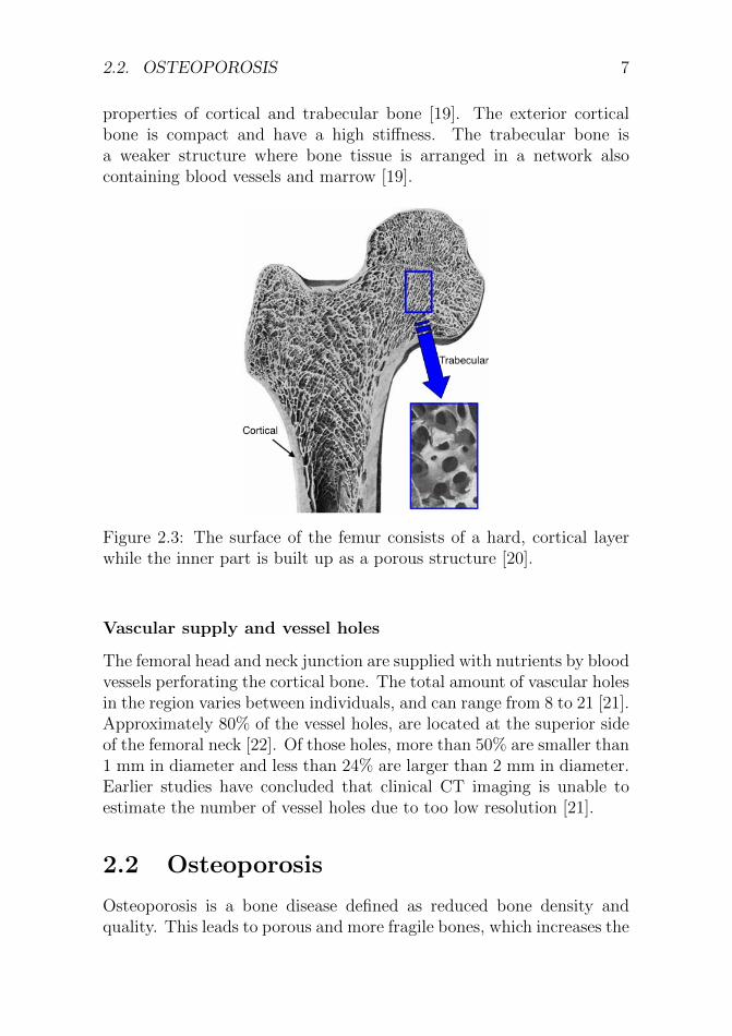
The outer surface of the femur consists of hard cortical bone, and theinside is composed of trabecular bone, a porous structure, as can beseen in Figure 2.3. The two different structures in the bone are ofgreat importance since this gives rise to highly different mechanical
2.2. OSTEOPOROSIS 7
properties of cortical and trabecular bone [19]. The exterior corticalbone is compact and have a high stiffness. The trabecular bone isa weaker structure where bone tissue is arranged in a network alsocontaining blood vessels and marrow [19].
Figure 2.3: The surface of the femur consists of a hard, cortical layerwhile the inner part is built up as a porous structure [20].
Vascular supply and vessel holes
The femoral head and neck junction are supplied with nutrients by bloodvessels perforating the cortical bone. The total amount of vascular holesin the region varies between individuals, and can range from 8 to 21 [21].Approximately 80% of the vessel holes, are located at the superior sideof the femoral neck [22]. Of those holes, more than 50% are smaller than1 mm in diameter and less than 24% are larger than 2 mm in diameter.Earlier studies have concluded that clinical CT imaging is unable toestimate the number of vessel holes due to too low resolution [21].
2.2 Osteoporosis
Osteoporosis is a bone disease defined as reduced bone density andquality. This leads to porous and more fragile bones, which increases the

8 CHAPTER 2. BACKGROUND
risk of fracture. The disease is more prevalent in the older population,and especially in older women [1].
As many as 46% of the women, and 29% of the men in Swedenabove the age of 50 years, will sustain a fracture caused by osteoporosisin their remaining lifetime. Sweden is, comparing to six other coun-tries in the EU, the country where the people have the highest risk forfragility fractures [2] (Figure 2.4a). The lifetime risk for a hip fracturespecifically, for men and women over 50 years, is also highest in Swedenamong the same six countries (Figure 2.4a). The hip fractures standfor 20% of the fragility fractures, but 57% of the total costs (Figure2.4b). In 2017, the total cost of fragility fractures in the six countriesinvestigated (according Figure 2.4a) was estimated to e37.5 billion, andis expected to increase with 27% until 2030 [2].
(a) Lifetime risk of fragility fractures,compared with CVD.
(b) Distribution of fracture type andcosts.
Figure 2.4: (a) the lifetime risk of fragility fractures after the age of50 years, compared with the equivalent risk for cardiovascular disease(CVD) in Europe, is presented. (b) the occurrence versus the cost ofdifferent fracture types are presented [2].
In addition to the large fracture risk among the people and the highcosts, a hip fracture also causes a lot of pain and reduced quality of lifefor the individual [2].
2.3. CT IMAGING 9
2.3 CT imaging
In this project, both images from clinical computed tomography (CT)and micro-CT were used. The two techniques are similar in principle,but, implemented differently and have different application areas.
Clinical CT scanning is an imaging technique based on X-ray, wherean object is exposed to X-rays from multiple angles. On the oppositeside of the object, the X-rays are detected by X-rays detectors. Theobject absorbs an amount of radiation and the total absorption dependson various factors, such as the object’s size and density. Each rotationevolves in a 2D slice of the object, a projection image. When the CThas imaged every 2D slice of the object, the slices are reconstructed,and showed as a 3D object digitally. Every slice represents a thicknessof 1-10 millimeters of the object, depending on the CT machine [23].This technique is primarily used clinically.
Micro-CT is imaging on a smaller scale, with a higher resolution.From 1 millimeter resolution in the clinical CT to 1 micron, a thousandof a millimeter and smaller in the micro-CT. In micro-CT imaging, theCT scanner is typically still and the object is rotating. The applicationareas for micro-CT are for example material science, small animals, andex-vivo imaging of human tissues [24].
The reconstruction of a CT image can be done with different set-tings, where, among others, the convolution kernel is one. The kernelis a weighting factor, filtering the CT image. There are two main pro-cesses, high-pass filtering and low-pass filtering, reconstructing the im-age into a sharpened, edge enhanced, image, respectively a smoothed,blurred image [25]. These kernels are referred to as ’hard’ and ’smooth’,respectively.
2.4 Digital image correlation
Digital image correlation (DIC) is a non-contact optical technique usedfor measuring strains and displacements during experimental testing[26]. DIC is based on digital image processing and numerical computing.The basic principle of the method is to trace physical points from areference configuration to a deformed configuration (Figure 2.5) [27].
To prepare a sample for DIC measurement, the component inves-tigated is covered with a randomized pattern, for example, black dotsspeckled on a white surface. By tracking blocks of pixels with cam-

10 CHAPTER 2. BACKGROUND
Figure 2.5: The principle of DIC [27]. A block of pixels is traced withcameras from a reference to a deformed image, resulting in full-fieldmeasurements of the displacement over a surface.
eras, the displacements at the surface can be measured, resulting in afull-field measurement of the displacements, and enabling calculationsof full-field strain data. DIC can be performed both in 2D and 3D de-pending on the setup. Using one camera, the full-field strains for a flat(2D) surface, and using two cameras the full-field displacements for a3D surface, can be generated [28].
2.4.1 Interpretation of DIC measurements
The DIC measurements can be used as a comparison to strains pre-dicted by FE models. One way of comparing strains measured by DICand predicted by FE models is by correlation analysis. The basic ideais to compare two measurements, resulting in a correlation coefficient(R), ranging from -1.0 to +1.0. The closer R is to either end of thisrange, the stronger the linear relationship between the two are [29].Commonly used is also the correlation of determination (R2), indicat-ing the amount of variance introduced in the model. In general, a highvalue of R2 is an indication that the model is a good fit for the data[30]. Another way of investigating correlation was proposed by MartinBland and Douglas Altman, named Bland-Altman analysis [29]. Bland-Altman analysis determines the difference between measurements witha graphical method, representing the measurements with a scatterplotwhere the x-axis represents the average and the y-axis represents thedifference of two measurements (Figure 2.6). A Bland-Altman plot usu-ally also includes the 95% confidence interval as marked with red lines

2.5. IMAGE SEGMENTATION 11
in the figure. A strong correlation is indicated by a small differencebetween measurements (the mean is close to zero), that the distributionof differences is equally spread around the mean and that confidenceinterval is narrow.
Figure 2.6: Example of a Bland-Altman plot used for correlation of twomeasures. The x-axis represents the average and the y-axis representsthe difference of two measurements [31]
.
2.5 Image segmentation
2.5.1 Threshold segmentation
Threshold segmentation is a digital image processing method, which canbe used to create binary images by replacing every pixel with intensityless than a selected constant (a threshold) to a black pixel, or to a whitepixel if the pixel has a greater intensity value than the constant. Thresh-olding is a powerful and simple technique for image segmentation andcan be applied both globally and locally. The selection of the thresholdcan be based on, for example, visual assessment, the histogram of tonaldistribution, optimization, or spatial information [32]. In this project,

12 CHAPTER 2. BACKGROUND
the threshold is often applied as a single threshold, and determined fromthe histogram shape and by visually examining the image.
2.5.2 Active contour segmentation
Active contour segmentation is developed to segment anatomical struc-tures [33]. The method used in this project is based on the 3D contoursegmentation method Geodesic Active Contours [34, 35]. The tech-nique is a semiautomatic active contour evolution method, where thefinal segmentation is represented by contours, the edge structure of thesegmentation. A closed surface represents an evolving contour - edgesof the closed surface grow, which makes its volume increase. The sur-face is growing with regard to internal and external forces, speeding upor slowing down the growth rate, and determining where it is allowedto grow. The surface grows according to a partial differential equation(PDE), simplified as:
Ct = (αgI − βκ)~n (2.1)
where α can be described as the region competition force and β as thesmoothing (curvature) force. Ct is the contour evolving in time step t,gI is the speed function, κ) is the mean curvature of the contour, and ~nis the unit normal to the contour. By setting α and β to 1, the methodGeodesic Active Contours is obtained.
The 3D active contour segmentation is performed stepwise. Firstly,a speed map, or probability map, is created by threshold segmentationof the image. The contour is not allowed to evolve outside of the seg-mented region. Secondly, the segmentation is initialized by seeds placedin areas to segment. At last, parameters in the active contour evolutionPDE are set, determining internal, external, and smoothing forces. Thesegmentation evolves for an optional amount of iterations, controlled bythe user [33].
2.6 Calculation of cortical bone thickness
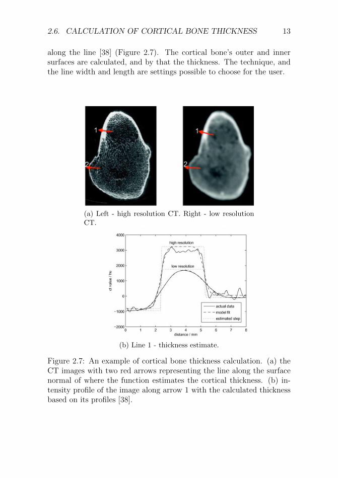
Cortical bone thickness calculation can be performed in Stradview (Ver-sion 6.05, Medical Research Imaging Group, Cambridge University, En-gineering Department) [36]. One technique for calculation of corticalbone thickness is called Cortical Bone Mapping (CBM) [37]. By fittinga piecewise constant function along the surface normal, the corticalthickness is estimated by the CT image’s density variation in intensity
2.6. CALCULATION OF CORTICAL BONE THICKNESS 13
along the line [38] (Figure 2.7). The cortical bone’s outer and innersurfaces are calculated, and by that the thickness. The technique, andthe line width and length are settings possible to choose for the user.
(a) Left - high resolution CT. Right - low resolutionCT.
(b) Line 1 - thickness estimate.
Figure 2.7: An example of cortical bone thickness calculation. (a) theCT images with two red arrows representing the line along the surfacenormal of where the function estimates the cortical thickness. (b) in-tensity profile of the image along arrow 1 with the calculated thicknessbased on its profiles [38].

14 CHAPTER 2. BACKGROUND
2.7 Finite element bone models
Two important measures for fracture estimation are stress (σ) and strain(ε). Previous studies have suggested that the fracture initiation of boneis strain-driven [39]. For this reason it is of great interest to study thestrains detected in the femur during a fall. Furthermore, it has beenshown that the yield strain depends on anatomical site [40] and, during aside-ways fall, compressive strains dominate at the superolateral femoralneck [14]. These observations are the basis of studying the compressivestrains located in the femoral neck.
The strains in this project can be described by the simplified prin-cipal strain matrix, Equation 2.2,
ε =
ε1 0 00 ε2 00 0 ε3
(2.2)
where ε1 is the major principal strain and ε3 is the minor principalstrain. In most situations, the major principal strain is a measure ofthe tensile strains and the minor principal strain a measure of the com-pressive strains. Since the femoral neck mainly experiences compressivestrains, the minor principal strains are a good way of measuring themagnitude of strains at the femoral neck.
2.7.1 The finite element method
The FE method is a numerical solution algorithm with which differentialequations can be solved approximately. The basic idea is to first dividethe region where a certain differential equation holds into many smallparts, or finite elements [41]. Instead of finding approximations thatwould hold for the entire region, approximations are made for eachelement and the total behavior is determined by assembling the responsein all finite elements. An assembly of finite elements is called a mesh.
In simplified words, an FE model is a mesh based on finite elementstogether with additional information regarding the material propertiesof the elements, the coordinate system by which the model is orientedand possible restrictions regarding the degrees of freedom. In this the-sis, the term micro-FE model is frequently being used. What is beingreferred to by this is a FE model based on high resolution micro-CTimages.
2.7. FINITE ELEMENT BONE MODELS 15
2.7.2 Mesh representations
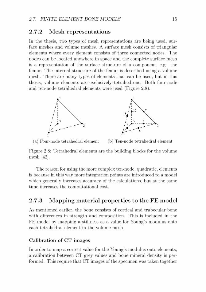
In the thesis, two types of mesh representations are being used, sur-face meshes and volume meshes. A surface mesh consists of triangularelements where every element consists of three connected nodes. Thenodes can be located anywhere in space and the complete surface meshis a representation of the surface structure of a component, e.g. thefemur. The internal structure of the femur is described using a volumemesh. There are many types of elements that can be used, but in thisthesis, volume elements are exclusively tetrahedrons. Both four-nodeand ten-node tetrahedral elements were used (Figure 2.8).
(a) Four-node tetrahedral element (b) Ten-node tetrahedral element
Figure 2.8: Tetrahedral elements are the building blocks for the volumemesh [42].
The reason for using the more complex ten-node, quadratic, elementsis because in this way more integration points are introduced to a modelwhich generally increases accuracy of the calculations, but at the sametime increases the computational cost.
2.7.3 Mapping material properties to the FE model
As mentioned earlier, the bone consists of cortical and trabecular bonewith differences in strength and composition. This is included in theFE model by mapping a stiffness as a value for Young’s modulus ontoeach tetrahedral element in the volume mesh.
Calibration of CT images
In order to map a correct value for the Young’s modulus onto elements,a calibration between CT grey values and bone mineral density is per-formed. This require that CT images of the specimen was taken together

16 CHAPTER 2. BACKGROUND
with a number of phantoms with known density of mineral bone equiv-alent material. For each phantom, the grey value is measured and bymaking a plot of the grey value vs. the density and making a linearregression, you get a linear relation describing how the bone mineraldensity depend on the average grey value.
Bonemat
The mapping can be performed using the software Bonemat [43], andfor this project an in-house Matlab implementation of Bonemat wasused, mapping each element to the corresponding coordinates of a CTimage. The average grey value of the CT image within a element isdetermined and by calibrating the grey-values to bone mineral density,each element is assigned a value for the average bone density inside,which somewhat correspond to the ash density (ρash).
There are two common ways of describing bone mineral density, ashdensity and apparent density (ρapp). The relation between the two typesof density is described in Equation 2.3 [44].
ρash/ρapp = 0.6 (2.3)
Using this relation, the density of an element can then be trans-formed to Young’s modulus (E) in MPa according to Equation 2.4 [45].
E = 6850 · ρ1.49app (2.4)
Partial Volume Effect
Partial volume effects (PVE) is an important concept influencing thequality of the material mapping. For the reason that the average greyvalue within each element is determined, elements could get mappedwith a lower density than the true density. For example, if an elementis larger than the thickness of the cortical bone, the value for the mappeddensity could be significantly lower than the density of the cortical bonewhich affects the stiffness at the surface. This behaviour needs to beconsidered, both in the modelling, and in the validation procedure.
2.8. BACKGROUND RESEARCH FOR THIS PROJECT 17
2.8 Background research for this project
It has been shown that FE models of the human femur based on clini-cal CT images can predict deformations with very high accuracy whencompared to DIC measurements, and are able to predict the femoralstrength with an error below 2% [28]. The FE models are based on clin-ical CT images, and are also taking the bone mineral density (BMD)into account. This makes it possible to include mechanical characteris-tics of the bone, and obtain accurate FE models that can be used forpredicting a patient’s fracture risk during screening [28].
Recent studies have detected regions of local weakness in the femoralneck which correspond to regions where vessel holes are perforating thecortical bone [11]. It is suggested that the vessel holes may be involvedin the failure initiation in the femoral neck [11, 12].
When experimental measurements of strain have been compared tostrains predicted by FE analyses of femurs in side-ways fall, they cor-relate well in all regions except the superior region in the femoral neck.High strains at the lateral superior region were predicted by the FEmodels, but not detected experimentally with DIC. Instead, high strainswere measured experimentally in areas where vessel holes were presentin the cortical bone. Those vessel holes are not represented by theFE models. It has been suggested that these vessel holes should beaccounted for to get more accurate FE model predictions [13, 14].

18 CHAPTER 2. BACKGROUND

Chapter 3
Materials & methods
3.1 Material
Micro-CT images (Figure 3.1) and clinical CT images (Figure 3.2) ofone human femur were used in this project. The femur is one from alarger collection of fresh-frozen cadaver femurs, approved for use by TheFinnish National Authority for Medicolegal Affairs (TEO, 5783/04/044/07).The femur had earlier been imaged with a clinical CT scanner (SiemensSomatom AS, pixel size 0.4-0.5mm, slice separation 0.6 mm, tube volt-age 120 kV, tube current 210 mAs) and with a high-resolution labo-ratory x-ray tomographic device (Nikon XT H225, isotropic voxel size52-60 µm, 100 kVp, 200 mAs). The femur came from the right sideof a female donor, 81 years old, 160 cm, and 67 kg. [14]. The clinicalscan was reconstructed with two different kernels, a smooth and a hardkernel.
3.2 Overview of the methods
This master’s thesis can be divided into two main parts. The first partwas more focused on image analysis, and to detect and quantify bloodvessel holes from both micro-CT and clinical CT images. The secondpart of the project was more focused on computational modeling, andwas to first generate a micro-FE model of the human femur and then tovalidate it using previously developed FE models. This sections gives ashort description of the overview, and each section will be described inmore detail later.
19

20 CHAPTER 3. MATERIALS & METHODS
Figure 3.1: One slice of the micro-CT scan of the femur.
(a) Smooth kernel. (b) Hard kernel.
Figure 3.2: Clinical CT scans of the human femur reconstructed with asmooth (left), and a hard (rigth) kernel.
Quantification of vessel holes in micro- and clinical CT
Part of the project aimed to quantify vessel holes, in terms of their sizeand location, in the femoral neck. The conceptual method is shown inthe flowchart in Figure 3.3. The quantification of vessel holes was sep-arated into two different approaches, one for the micro-CT and one forthe clinical CT. The micro-CT based approach started with a selectionof the region of interest (ROI) in the femoral neck, from the micro-CTimage. The ROI was segmented to extract the femur surface in detail,and a 3D geometry was obtained. The next step was to create a surfacemesh of the femur. A downscaled micro-CT image was used, to segment

3.2. OVERVIEW OF THE METHODS 21
the outer surface of the femur. A mesh of the femur surface was ob-tained. The 3D geometry of ROI and the femur surface mesh were thenused as input in a newly developed method for the detection and quan-tification of vessel holes. By fitting circles to the data, quantificationdata of vessel holes could be obtained. The clinical CT scan followedanother approach, where the femur surface first was segmented and asurface mesh was generated. Based on the surface mesh, the corticalbone thickness was calculated in the femur. By detecting non-existing,or very low thickness in the cortical bone, vessel holes were detectedin the femoral neck and quantified. The vessel holes’ data from bothapproaches were then evaluated and compared.
Figure 3.3: Flowchart over the quantification of vessel holes in micro-and clinical CT images.
22 CHAPTER 3. MATERIALS & METHODS
Generation of FE models
FE-models based on clinical CT images have previously been developedwithin our research group [10]. These were used for validation of themodels created during this project and will be referred to as the refer-ence model. An overview of the steps in the generation of FE models canbe found in the flowchart in Figure 3.4. A micro-FE model was createdby segmentation of micro-CT images resulting in a surface mesh withhigh mesh density. By creating a volume mesh, mapping mechanicalproperties onto the finite elements and defining load and boundary con-ditions, a micro-FE model was created. For comparison and validation,a third FE model was created that will be referred to as the standardFE model. This model was segmented from clinical CT images and thesurface mesh has a similar mesh as the reference model. A volume meshwas generated and mechanical properties, load and boundary conditionswere set in the same way as for the micro-FE model. Calculated strainswere compared between models.

3.2. OVERVIEW OF THE METHODS 23
Figure 3.4: Flowchart over the generation of a micro-FE model and anoverview of the FE models used for comparison and validation.
24 CHAPTER 3. MATERIALS & METHODS
3.3 Quantification of vessel holes in micro-
CT
3.3.1 ROI in micro-CT image
The aim of quantifying the vessel holes by location and size, based onthe micro-CT image required the full resolution micro-CT image to beinvestigated. The total micro-CT scan, in full resolution, could not behandled by the computer’s RAM memory. Due to this constraint, aregion of interest (ROI) of the micro-CT image was selected.
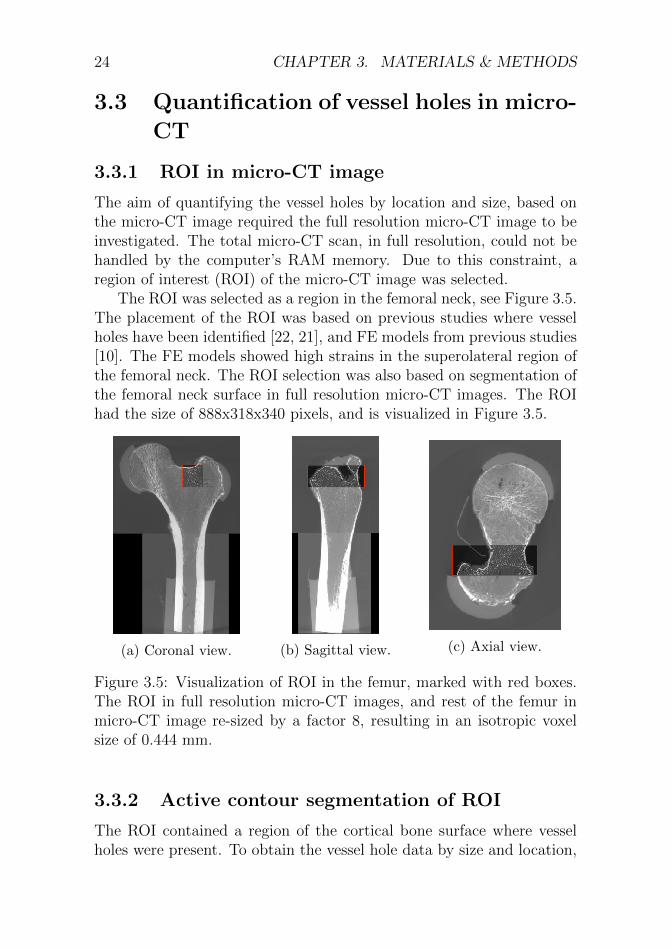
The ROI was selected as a region in the femoral neck, see Figure 3.5.The placement of the ROI was based on previous studies where vesselholes have been identified [22, 21], and FE models from previous studies[10]. The FE models showed high strains in the superolateral region ofthe femoral neck. The ROI selection was also based on segmentation ofthe femoral neck surface in full resolution micro-CT images. The ROIhad the size of 888x318x340 pixels, and is visualized in Figure 3.5.
(a) Coronal view. (b) Sagittal view. (c) Axial view.
Figure 3.5: Visualization of ROI in the femur, marked with red boxes.The ROI in full resolution micro-CT images, and rest of the femur inmicro-CT image re-sized by a factor 8, resulting in an isotropic voxelsize of 0.444 mm.
3.3.2 Active contour segmentation of ROI
The ROI contained a region of the cortical bone surface where vesselholes were present. To obtain the vessel hole data by size and location,
3.3. QUANTIFICATION OF VESSEL HOLES IN MICRO-CT 25
the vessel holes had to be defined. The next step was therefore chosento be, active contour segmentation, which is a method that can segmentstructures and contours in an image. It resulted in a segmentation of thecortical bone surface contours, including the in-growth canal structuresof the vessel holes in the cortical bone.
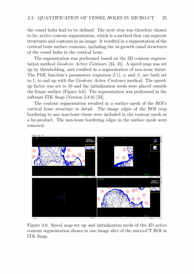
The segmentation was performed based on the 3D contour segmen-tation method Geodesic Active Contours [34, 35]. A speed map was setup by thresholding, and resulted in a segmentation of non-bone tissue.The PDE function’s parameters (equation 2.1), α and β, are both setto 1, to end up with the Geodesic Active Contours method. The speed-up factor was set to 10 and the initialization seeds were placed outsidethe femur surface (Figure 3.6). The segmentation was performed in thesoftware ITK Snap (Version 3.8.0) [33].
The contour segmentation resulted in a surface mesh of the ROI’scortical bone structure in detail. The image edges of the ROI cropbordering to any non-bone tissue were included in the contour mesh asa by-product. The non-bone bordering edges in the surface mesh wereremoved.
Figure 3.6: Speed map set up and initialization seeds of the 3D activecontour segmentation shown in one image slice of the micro-CT ROI inITK Snap.

26 CHAPTER 3. MATERIALS & METHODS
3.3.3 Surface mesh generation of femur
Resampled micro-CT
The other branch of the micro-CT based approach was to generate asurface mesh of the femur, Figure 3.3. Due to computational constraintswith the full resolution micro-CT image, and with the aim of a surfacemesh without cortical bone details, a micro-CT image downscaled by afactor 8 was used for the surface mesh generation of femur.
Segmentation of cortical bone
The next step in building the femur surface mesh was to generate a 3Dgeometry of the femur surface. The micro-CT image of the femur wasimaged with a pot around the femur’s most distal part. The femur wasimaged in several sessions, resulting in different grey value distributionsin the image, see Figure 3.5 for example. Therefore, the image wasseparated into two parts, by cropping it approximate with the bottompart as 1/3 and the top part as 2/3 of the image, viewed in the sagit-tal plane, to simplify thresholding with the varying grey values. Thesegmentation was stepwise performed in the software Seg3D (Version2.4.4) [46]. Firstly, the femur’s cortical bone was segmented by thres-hold segmentation. Secondly, the segmentation of the cortical bone wasfilled. By dilation and erosion of the segmentation the holes in the tra-becular bone were filled. Using this approach, a solid 3D-geometry wasobtained, representing the femur surface.
Mesh generation
The last step to obtain the femur surface mesh was to generate a meshof the 3D-geometry from the segmentation. To obtain a representationof the femur surface, the two segmentations, the top and bottom partsof the femur were combined to one solid part, thereafter the surfacewas sculpted to a smooth and even surface, and at last remeshed withpreserved mesh density. This was performed in the software Meshmixer[47].
3.3.4 Intersection method
The aim in the intersection method was to obtain a surface of where theROI contour mesh (which had the geometry of the vessel hole canals)

3.3. QUANTIFICATION OF VESSEL HOLES IN MICRO-CT 27
and the femur surface mesh intersected, crossed each other. The finalintersection surface was aimed to represent the vessel holes’ in-growingcanals, in the cortical bone. The intersection method contained threemain steps, mostly executed in Matlab (Version R2018a, MathWorks,Natick, NA, USA), using the toolbox iso2mesh [48] and in-house FEmesh functions.
Shrinked surface mesh of femur
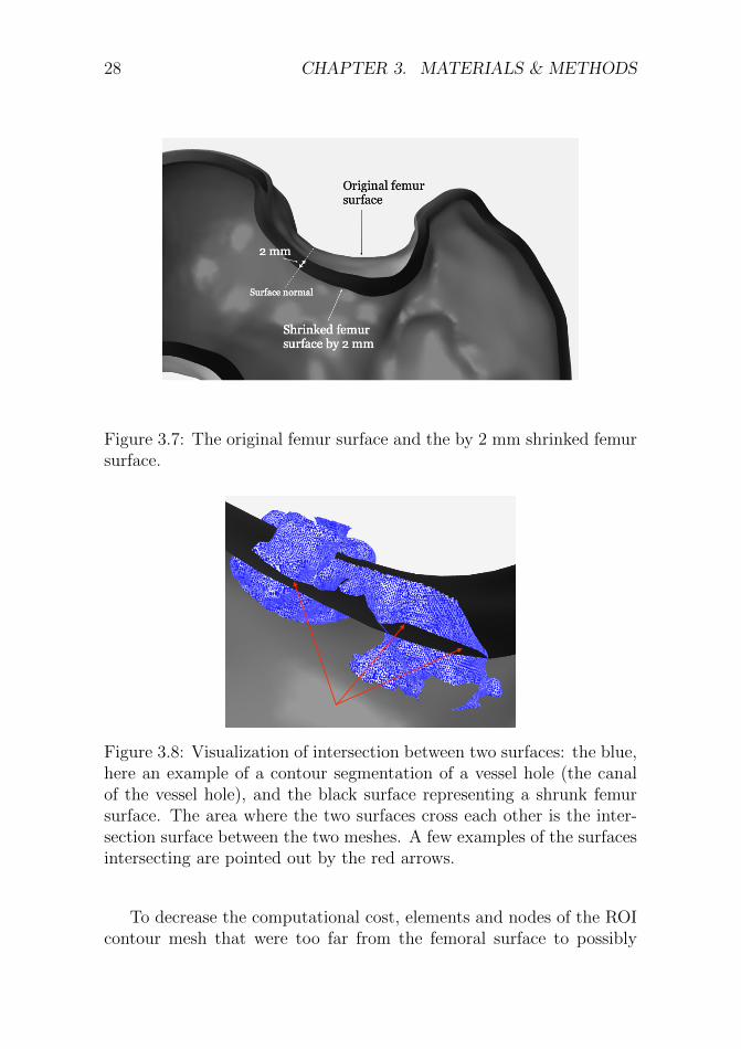
In theory, two surfaces of the same cortical bone should be aligned andintersecting almost everywhere, therefore it was concluded that the in-tersection between the ROI contour mesh and the femur surface meshwas not a good representation of the vessel hole canals. Because ofthis, the femur surface mesh was first adjusted. To obtain the most de-scriptive representation of the vessel holes’ characteristics in the corticalbone, an investigation of the role of the femur surface in the intersec-tion method was performed. The femur surface mesh was thereforemodified by decreasing its volume with different ratios, resulting in thefemur surface shrinking inwards, along the surface normal. This wasperformed in Meshmixer, Autodesk. The volume decrease of the femursurface mesh resulted in five new surface meshes, each correspondingto different distances of shrinking along the surface normal, 0.125 mm,0.25 mm, 0.5 mm, 1 mm, and 2 mm. The original femur surface andthe femur surface shrunk by 2 mm are visualized in Figure 3.7, as anexample of the concept.
Intersection of femur surface and ROI mesh
To obtain the quantification data of the vessel holes, the next step wasto calculate the intersection of the ROI contour mesh and the shrunkfemur surface meshes. The purpose with the intersection surface, wherethe meshes did cross each other, was a representation of the contoursof the vessel hole canals. A visualization of the intersection concept isshown in Figure 3.8. The intersections between the five shrunk femursurfaces, and the cropped ROI contour mesh were calculated in Matlab,with the function Surface Intersection [49]. The resulting intersectionswere investigated and evaluated before proceeding. The best apparentoutcome was achieved at depths of 0.125 mm, 0.25 mm, and 0.5 mm. Acombination of these three intersection depths was the final intersectionresult.
28 CHAPTER 3. MATERIALS & METHODS
Figure 3.7: The original femur surface and the by 2 mm shrinked femursurface.
Figure 3.8: Visualization of intersection between two surfaces: the blue,here an example of a contour segmentation of a vessel hole (the canalof the vessel hole), and the black surface representing a shrunk femursurface. The area where the two surfaces cross each other is the inter-section surface between the two meshes. A few examples of the surfacesintersecting are pointed out by the red arrows.
To decrease the computational cost, elements and nodes of the ROIcontour mesh that were too far from the femoral surface to possibly

3.3. QUANTIFICATION OF VESSEL HOLES IN MICRO-CT 29
intersect it were removed from the calculation. This was done with anin-house Matlab code based on the function PointInsideVolume [50].
Due to computational constraints, the ROI was decreased to a smallerregion, from now on referred to as the final ROI. The final ROI was themost superolateral region in the femoral neck, the region on the femoralneck close to the greater trochanter. This region included the mostpronounced vessel holes in the contour segmentation of the ROI, andcorresponds very well with the region of where the previous FE modelspredicted high strains in the femoral neck.
Removal of false intersection
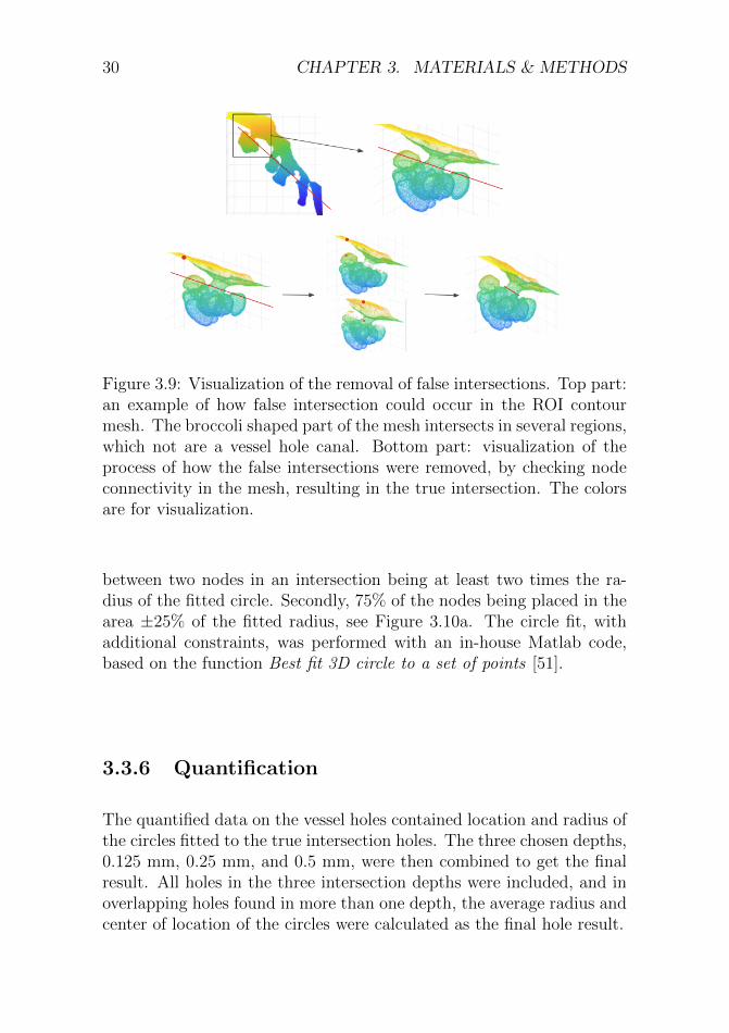
The last step in the intersection method was to determine the true inter-sections and exclude any false intersections. False intersections could forexample occur when the final ROI contour mesh and the shrunk surfacemesh intersect somewhere where there is not a vessel hole (Figure 3.9).The surface mesh intersected with the final ROI contour mesh in areasnot representing the actual in-growth of the contour evolving into thecortical bone through vessel holes. The removal of false intersectionswas performed in Matlab by verification of node connection in the finalROI contour mesh. Reference nodes were selected in the final ROI con-tour mesh, one in each intersection, and one at the contour mesh surfacewhere no vessel holes were present. One intersection surface was con-trolled at a time. The surface intersection currently investigated, wassaved in the final ROI contour mesh, while nodes in the other intersec-tion areas were removed in the final ROI mesh. The node connectionbetween the current intersection reference node and the surface mesh’sreference node, was verified. If the connection did not exist, the currentintersection surface was false. An example of the process of removal offalse intersections is visualized in the bottom part of Figure 3.9. Also,an example of nodes in a true intersection is visualized in Figure 3.10b.
3.3.5 Circle fit
To obtain the vessel hole quantification data, the true intersections (Fig-ure 3.10b) were fitted to circles, to obtain a simple but accurate rep-resentation of the size and location of the vessel holes. To determinethe vessel holes from the true intersections, constraints about circular-ity were implemented to the circle fit. First, the maximum distance
30 CHAPTER 3. MATERIALS & METHODS
Figure 3.9: Visualization of the removal of false intersections. Top part:an example of how false intersection could occur in the ROI contourmesh. The broccoli shaped part of the mesh intersects in several regions,which not are a vessel hole canal. Bottom part: visualization of theprocess of how the false intersections were removed, by checking nodeconnectivity in the mesh, resulting in the true intersection. The colorsare for visualization.
between two nodes in an intersection being at least two times the ra-dius of the fitted circle. Secondly, 75% of the nodes being placed in thearea ±25% of the fitted radius, see Figure 3.10a. The circle fit, withadditional constraints, was performed with an in-house Matlab code,based on the function Best fit 3D circle to a set of points [51].
3.3.6 Quantification
The quantified data on the vessel holes contained location and radius ofthe circles fitted to the true intersection holes. The three chosen depths,0.125 mm, 0.25 mm, and 0.5 mm, were then combined to get the finalresult. All holes in the three intersection depths were included, and inoverlapping holes found in more than one depth, the average radius andcenter of location of the circles were calculated as the final hole result.

3.4. QUANTIFICATION OF VESSEL HOLES IN CLINICAL CT 31
(a) Circularity constraint. (b) Nodes in a true intersection.
Figure 3.10: (a) visualization of one circularity constraint, 75% of thenodes in the true intersection must lie within the range ±25% of thefitted circle’s radius. (b) an example of nodes in a true intersectionbetween the ROI contour mesh and a shrunk femur surface mesh.
3.4 Quantification of vessel holes in clini-
cal CT
3.4.1 Clinical CT images
A clinical CT scan was used in this project, reconstructed with twodifferent kernels, one smooth kernel and one hard kernel (Figure 3.2).The clinical CT images have a voxel size of 0.42 mm. With the resolutionthe clinical CT images have, it is not possible to clearly see holes in thecortical bone. This approach was based on the idea of investigating thecortical bone thickness, and by detecting thin, or non-valued corticalbone thickness, vessel holes could be detected.
3.4.2 Segmentation and mesh generation of femursurface
The first step in the clinical CT based approach was to segment the cor-tical bone surface by thresholding. The result of the segmentation was

32 CHAPTER 3. MATERIALS & METHODS
a 3D geometry, represented by a surface mesh of the femur. The meshcontained 18 949 nodes, with an average distance between the nodes of0.34 mm. Considering that Stradview calculates the thickness only ona random uniform sample of the available nodes [52], it was consideredthere might be a risk for some vessel holes to be not detected because thealgorithm would not probe densely enough. Therefore, a more dense 3Dmesh, with 75 800 nodes, and the average distance between the nodes of0.17 mm, was generated. The 75 800 node mesh was created by a mod-ification of the 18 494 node mesh in Matlab, by the function TriangleSubdivide (vectorized/fast) [53]. The segmentation and mesh generationof femur surface in the clinical CT images was performed in Stradview(Version 6.05, Medical Research Imaging Group, Cambridge University,Engineering Department) [36].
3.4.3 Calculation of cortical bone thickness
The next step in the clinical CT approach was to calculate the corticalbone thickness in the femur. The calculation of the cortical bone thick-ness was performed with the technique Cortical Bone Mapping (CBM)v2 [37], in Stradview. The thickness was calculated on a random uni-form sample of the nodes in the 3D mesh along a line crossing thecortical bone, see Figure 3.11. The line was determined to have a widthof 0, as it otherwise smoothens the thickness calculation, which was notdesired.
Three different line lengths were examined (4 mm, 6 mm, and 8mm), based on the assumption that the cortical bone thickness in thefemoral neck does not exceed 2 mm. The line length is recommendedto be three times longer than the expected thickness [36].
This resulted in an investigation of 12 combinations of cortical bonethickness results, including three line lengths, two reconstruction ker-nels, and two different node densities of the surface mesh.
The results were 3D surface meshes of the cortical bone’s outer andinner surfaces, and thickness data mapped to every node in the surfaces.See Figure 3.12 for an example window of Stradview.
3.4.4 Quantification
The last step in the clinical CT based approach was the quantification,of location and size of the vessel holes.

3.4. QUANTIFICATION OF VESSEL HOLES IN CLINICAL CT 33
(a) (b)
Figure 3.11: Example of thickness calculation of the cortical bone, wherethe thickness is calculated in all nodes of the surface mesh, representedby the yellow line. The blue line represents the line of where the thick-ness was calculated along. The red dots mark the inner and outer surfaceof the cortical bone, resulting in the thickness. To the left, the wholefemur. To the right, zoomed in on the line.
Figure 3.12: An example of Stradview. To the left, the yellow linerepresenting the 3D mesh of the femur, which was based on the pinksegmentation. To the right, the 3D mesh of the femur is mapped to itscortical bone thickness. The different colours represent the measuredcortical thickness.
To identify vessel holes, we defined the minimum allowed corticalthickness to be 0.2 mm. This threshold was based on a visual inves-tigation of our images. Consequently, every point with a calculatedthickness < 0.2 mm (or failed thickness calculation) was marked as avessel hole. The vessel hole quantification was based on the numberof node holes connected in the surface mesh. Three different classesof node holes were quantified. The three approaches are presented inTable 3.1. Isolated nodes were single nodes classified as holes. Pairednodes were two nodes connected in the mesh, classified as holes. Cluster

34 CHAPTER 3. MATERIALS & METHODS
nodes were 3 or more connected nodes classified as holes.
The first two classes, isolated and paired nodes, were quantified interms of location, and by the average distance (ad) between two nodesin the mesh. In the third class, the node holes were fitted to circles,similar to the micro-CT based approach, with the Matlab function Bestfit 3D circle to a set of points [51]. The quantification of vessel holes inthe clinical CT was performed in Matlab.
Class #nodes Location Radius
Isolated nodes 1 Node location ad * 1/2Paired nodes 2 Avg. node coord. ad * 2/3Cluster nodes ≥3 Circle center Circle radius
Table 3.1: Quantification of the three different classes of holes. The twofirst classes are quantified in terms of location and the average distance(ad) between two nodes in the mesh. In the third class the nodes arefitted to circles, as in the micro-CT based approach, but without theconstraints.
3.5 Evaluation of vessel hole quantifica-
tion
The evaluation of the two approaches, the micro-CT based method andthe clinical CT based method, was first done visually by examiningperformance accuracy and by comparing the holes’ size and location,using the micro-CT result as a reference. The performance accuracy, interms of number of holes and hole location, was calculated according to
Accuracy =TN + TP
TN + TP + FN + FP(3.1)
where TN = true negative, TP = true positive, FN = false negative,and FP = false positive. The TP was the correctly quantified holesin terms of location, FN was the never detected holes, FP was thefalsely detected holes, and TN was considered as zero since there wereno correctly non detected holes.

3.6. GENERATION OF FE MODELS 35
3.6 Generation of FE models
This section describes the procedure to generate the micro-FE modeland the standard FE model. The first step of generating a surface meshwas different for the two FE models but apart from this the procedurewas the same.
3.6.1 Surface mesh of micro-FE model
The aim of this step was to obtain a surface mesh of the femur, repre-senting the cortical bone surface, including the vessel hole structure inthe femoral neck. Due to computational constraints it was not possibleto use the total micro-CT image in full resolution be the basis of thefemur surface mesh. To select and generate the best possible mesh, animage resolution investigation was performed.
Image resolution
The image resolution investigation was performed to find the most rep-resentative mesh of the femur required in this part of the project. Byreducing the micro-CT image size in three steps, the resolution was de-creased and visually investigated. The image was rescaled by factors 2,4, and 8 in ImageJ [54], resulting in four images with different resolu-tions. The rescaled micro-CT is presented in terms of data in Table 3.2and visually in Figure 3.13.
Scale factor Image size [pixels] Pixel size [mm]1 1394 x 2000 x 3110 0.05552 697 x 1000 x 1555 0.1114 348 x 500 x 776 0.2228 175 x 250 x 387 0.444
Table 3.2: Rescaled image data in the resolution investigation. Themicro-CT image scaled by different factors, including the full resolutionimage with scale factor 1.
The region depicted in Figure 3.13 were segmented. Based on thesegmentations a resolution investigation was done. After visual evalua-tion, it was decided that the majority of the femur could be represented

36 CHAPTER 3. MATERIALS & METHODS
(a) Full resolution. (b) Scaled by 2.
(c) Scaled by 4. (d) Scaled by 8.
Figure 3.13: Visualisation of one slice of each resampled micro-CT imageof the femoral neck, image and pixel size according to Table 3.2.
by the micro-CT images downscaled by a factor 8. The region of interestin the femoral neck in this part of the project was the ROI presentedin subsection 3.3.1, chosen to be based on the full resolution micro-CTimage.
Segmentation and mesh generation
The main femur surface mesh, built as a first step of the FE model gen-eration, consists essentially of the downscaled by a factor 8 micro-CTimage. Additionally, the femur surface mesh also contains a segmen-tation of the ROI, based on a full resolution micro-CT image. Therescaled micro-CT image was segmented to obtain the femur surface asa solid 3D geometry, with the same approach used in section 3.3.2. Dueto varying grey values in the micro-CT image, the femur was segmented

3.6. GENERATION OF FE MODELS 37
in two parts, resulting in a top and a bottom part. The segmentationof the full resolution ROI was performed with the aim to segment thecortical bone structure in detail, since it is the region where vessel holesare present and the region of interested in this project. The focus ofthe ROI segmentation was the cortical bone structure. The trabecularbone was removed in the ROI segmentation and replaced with the seg-mentation of the femur surface based of rescaled micro-CT images. Thesegmentations were performed in Seg3D.
Figure 3.14a shows the different segmentations, where the green andred parts are segmentations based on the resampled micro-CT images,rescaled by factor 8, see Table 3.2. The blue part of the segmentationshows the ROI and has full micro-CT resolution. In this segmentationthe vessel holes at the femoral neck are visible (Figure 3.14b).
(a) Full femur.
(b) Femoral neck.
Figure 3.14: Visualization of the three segmentations. Blue: segmenta-tion of ROI with full micro-CT resolution. Green and red: segmentationof femur performed with resampled micro-CT images.
The three segmented parts were combined, smoothed, and a solidfemur mesh was created in Meshmixer. The result was a surface meshof the femur with the ROI in more detail, and is shown in Figure 3.15.
3.6.2 Volume mesh of micro-FE model
The surface mesh is shown in Figure 3.15 and, as seen in subfigures3.15b and 3.15c, the mesh density is high enough to capture the shapeof the vessel holes. In total, the surface mesh of the full femur, Figure

38 CHAPTER 3. MATERIALS & METHODS
3.15a, had about 594 000 triangular elements. The surface mesh wassequentially re-meshed keeping the mesh density high around the ROIbut lowering the mesh density away from the ROI.
(a) Full femur. (b) Femoral neck. (c) Vessel hole.
Figure 3.15: Surface mesh generated based on full-resolution micro-CTimages and resampled micro-CT images. Surface mesh of the full femur(a), the femoral neck (b), and a vessel hole (c).
The re-meshing was performed with the software Hypermesh [55].By selecting the femur excluding the femoral neck a new surface meshcould be created stepwise, with increasingly large elements further awayfrom the ROI. The final surface mesh is visualized in Figure 3.16 andhas about 73 000 triangular elements. The smallest elements are about0.25 mm and the largest elements are about 3 mm.
Figure 3.16: Femoral neck of re-meshed surface mesh showing how theelement density gradually decreases away from the ROI.
From the surface mesh a volume mesh was generated using the optiontetra-mesh with settings growth rate = 1.3, pyramid to transition = 0.8and number of layers = 2 resulting in a mesh consisting of about 656000 ten-node tetrahedral elements.

3.6. GENERATION OF FE MODELS 39
3.6.3 Mesh generation for standard FE model
The starting point for the standard FE model was a set of surfaces thathas previously been generated from clinical CT images. The surfacesare shown in Figure 3.17a. The surfaces were meshed individually withdifferent mesh densities. The mesh was made so that the mesh densitywas the highest in the region of the femoral neck and lower in the shaftof the femur as shown in Figure 3.17b.
(a) Set of surfaces. (b) Surface mesh.
Figure 3.17: Set of surfaces and resulting surface mesh describing thestandard FE model.
From the surface mesh a volume mesh was generated in the sameway as for the micro-FE model. The volume mesh had a total of about254 000 ten-node tetrahedral elements.
3.6.4 Mapping
The mapping of material properties onto elements for the micro-FEmodel and the standard FE model was performed using both micro-CTimages of full resolution and clinical CT images. The reason for notmapping the full femur with micro-CT images was large computationaltime. Figure 3.18 shows what part of the mesh was mapped with clinicalCT and micro-CT images.
The calibration of the clinical CT images was already available, andfor the micro-CT images, the calibration was performed by measuringthe pixel value for six phantoms with known ash density. This wasdone on ten images and an average pixel value was determined for each

40 CHAPTER 3. MATERIALS & METHODS
Figure 3.18: The mesh marked in black is mapped with micro-CT im-ages and the rest of the femur is mapped with clinical CT images.
Figure 3.19: Showing the calibration of micro-CT images. The pixelvalue is measured for six phantoms with known ash-density resulting ina linear relationship between pixel value and density for the micro-CTimages.
phantom. By doing a linear regression of the pixel value vs. density,a linear relation was found (Figure 3.19). In this way the pixel valuefor a certain element could be translated into a value for its density.

3.6. GENERATION OF FE MODELS 41
The coordinates of each element are mapped to the corresponding co-ordinates in the CT image stack. An average grey value is determinedfor each element and translated into a density value (Figure 3.20). Alldensity values were subsequently converted to Young’s moduli followingEquation 2.4.
(a) Cross section of the femur shaft.
(b) Corresponding CT-image.
Figure 3.20: Young’s modulus in MPa mapped to each tetrahedral ele-ment based on the grey-value of the corresponding CT image.
3.6.5 Boundary conditions
After a volume mesh was generated and each element was mapped to thecorresponding value of Young’s modulus the positioning of the femur,the load and the boundary conditions were set. The simulation is of asideways-fall, and the aim of setting load and boundary conditions wasto replicate the experimental conditions. The femur was fixed at 10◦
adduction, 15◦ internal rotation to represent the the experimental setup[14] and the femur was fixed at the distal end of the shaft and at thelateral side of the head (Figure 3.21). In the shaft, nodes 50 mm or lessfrom the most distal node, was fixed. At the lateral side of the head,nodes 5 mm or less from the most lateral node was fixed. The load wasapplied on the external nodes of the femoral head located 5 mm of lessfrom the most medial node, and with a magnitude of 2250 N dividedon the number of nodes at which the force was applied. The choice offorce was based of the predicted fracture force in the reference model.

42 CHAPTER 3. MATERIALS & METHODS
Figure 3.21: Sketch of how the boundary conditions and load wereapplied. Femur is fixed at the shaft and at the lateral side of the head,and the force is applied at the medial side of the head to simulate asideways fall.
3.6.6 Simulation
The simulations of the sideways fall were performed using the softwareAbaqus/CAE 2018 [56]. A linear model was used applying a load asdescribed earlier fixing the nodes at the BCs in all directions. After thesimulation the major principal strains and the minor principal strainswere saved, both for individual nodes and element centroids.
3.7 Validation of the micro-FE model
This chapter will describe the procedure of validating the quality of themicro-FE model and how the results can be compared to other modelsand to experimental data. Figure 3.22 is an overview of the models usedfor validation, how modelling parameters are investigated and how themodels are later compared.
3.7.1 FE models used for validation
Validating the micro-FE model was performed comparing it to the stan-dard FE model and the reference model. The meshes of the three mod-

3.7. VALIDATION OF THE MICRO-FE MODEL 43
Figure 3.22: Overview of the FE models and validation techniques in-troduced for the validation.
els can be compared in Figure 3.23 and a summary of the number ofelements and approximate element size can be found in Table 3.3.
(a) Reference model (b) Standard FE model (c) Micro-FE model
Figure 3.23: Overview of the FE models used for validation.

44 CHAPTER 3. MATERIALS & METHODS
Model #elements Element size at neck [mm]
Reference 171760 1Standard FE 253858 0.81
Micro-FE 656391 0.31
Table 3.3: Summary of the number of elements and approximate ele-ments size at the femoral neck for the FE models.
Reference model
The reference model has previously been developed and validated byour group at the Department of Biomedical Engineering and is basedon the FE-model introduced by Grassi et al. (2016) [10]. The shape ofthe mesh is based on segmentation from clinical CT images. The modelis non-linear and the simulation is run until local failure according toa strain-based criterion. The BCs differ from the standard FE andmicro-FE model, in the way that the shaft of the femur is fixed in apot around it and the lateral side of the femur is fixed with a cup. Theload is applied at the femoral head, which also is fixed with a cup. Themodel with cups and pot is shown in Figure 3.23a. The mapping of thefemur is made exclusively with clinical CT images, and the elements atthe surface of the mesh of the femur were assigned a minimum Young’smodulus of 2.5 GPa
Standard FE model
The standard FE model has been developed by the authors as a stepin between the reference model and the micro-FE model. The surfacemesh was based on segmentation from clinical CT images and the meshdensity was similar to the mesh density of the reference model. Themodel was linear and the simulation was run setting the load to 2250Ndistributed over the external nodes located 5 mm or less from the mostmedial node. The BCs were set for the external nodes 50 mm or lessfrom the most distal part of the femur and for the external nodes 5 mmor less from the most lateral node on the femur (Figure 3.21). The meshwas mapped with micro-CT images in the ROI as shown in Figure 3.18and with clinical CT images for the rest of the femur.
3.7. VALIDATION OF THE MICRO-FE MODEL 45
Micro-FE model
The micro-FE model had a much finer mesh than the previous twomodels. Apart from this, the modelling approach was the same as forthe standard FE model.
3.7.2 Approach
By first comparing the reference model and the standard FE model withsimilar mesh density, assumed to be constant, the modelling parametersin terms of the choice of a linear model, boundary conditions and themapping strategy was investigated. The micro-FE model had a largernumber of elements and especially much smaller elements at the femoralneck. Comparing the standard FE and micro-FE models all parame-ters were kept constant except for the mesh. This comparison made itpossible to investigate the effect of having a highly refined mesh.
3.7.3 Qualitative comparison
The resulting strains for the three models were compared qualitativelyby visualizing the strains both at the femoral neck and specifically forlocations of detected vessel holes. The strain distributions were plottedfor each element and compared between the models. For the detectedvessel holes, also an average of the strains around that vessel hole wasdetermined.
3.7.4 Validation with DIC
Finally, the strains detected for the standard FE model and the micro-FE model were validated against experimental data obtained by DigitalImage Correlation (DIC) for this specific bone. The DIC measurementswere performed by our research group and have recently been published[14]. A new micro-FE mesh was created in order to have highest meshdensity in the complete DIC region according to previously describedprocedure. Except for the mesh, the model was identical to the micro-FE model. Point clouds of the external nodes were created in Matlab,both for the standard FE model and the micro-FE model, and thenodes were aligned with the point cloud for the DIC using the softwareCloudCompare [57]. Figure 3.24 shows the alignment of the nodes ofthe standard FE model and the DIC point cloud.

46 CHAPTER 3. MATERIALS & METHODS
Figure 3.24: Aligning the nodes of the standard FE model with thepoint cloud of the DIC.
An in-house developed Matlab function was used for comparing thestrains obtained experimentally with DIC and the strains detected bythe FE models. The strain in each external node of the FE modelwere compared to the strain in DIC points at a distance related tothe distance between external nodes in the DIC area. The differencebetween the predicted and measured strains was visualized both as adistribution on the femur and as correlation and Bland-Altman plots.

Chapter 4
Results
4.1 Quantification of vessel holes
The result from the quantification of the vessel holes in both micro-CTand clinical CT scans are presented in this section. Firstly, the micro-CT based approach results are presented by visualization, followed bythe quantification data in terms of location and size of the vessel holesdetected. Secondly, results of the clinical CT based approach are pre-sented in the same order, and a presentation and visualization of thebest performing combination of the clinical CT results.
4.1.1 Micro-CT
3D geometry of micro-CT ROI
The result from the first step of the micro-CT based approach wasthe mesh generated by the contour segmentation of the ROI (Figure4.1). The ROI selected in section 3.3.1, visualized again below in Figure4.2. The in-growth in the surface mesh (Figure 4.1) was the shape andstructure of the vessel hole canals, from the outer surface of the femurand into the trabecular structure.
Mesh of micro-CT femur surface
The result of the femur surface mesh generation, built of the micro-CTimages downscaled by a factor 8, was a smooth mesh of the femur surface(Figure 4.3). The smooth surface resulted in a coarser representation of
47

48 CHAPTER 4. RESULTS
(a) ROI mesh
(b) Final ROI mesh
Figure 4.1: Coronal view of the contour segmentation of the ROI surfaceand final ROI in the superolateral femoral neck, used in the micro-CTbased quantification approach. The mesh parts shaped as canals or”upside down broccoli”, were where the active contour segmentationevolved into the vessel holes canals in the cortical bone. The bubbles,or ”broccoli heads”, were the result of when the contour started to evolvein the porous trabecular bone structure. The colors are for visualization.
(a) Coronal view. (b) Sagittal view. (c) Axial view.
Figure 4.2: Visualization of thr ROI in the femur. The ROI in fullresolution micro-CT images, and rest of the femur in micro-CT imagere-sized by a factor of 8, pixel size of 0.444 mm.

4.1. QUANTIFICATION OF VESSEL HOLES 49
the femur surface, without smaller details, but still including the mainstructure.
Figure 4.3: Femur surface mesh of micro-CT scan, built from a segmen-tation of micro-CT images scaled by a factor 8. The mesh represents asmooth femur surface, excluding very small details.
Quantification data of the vessel holes in micro-CT
The quantification in the micro-CT based method resulted in the de-tection of five vessel holes in the final ROI. The five vessel holes arevisualized together with the femur surface mesh (generated in subsec-tion 3.6.1) in Figure 4.4, with corresponding radius data in Table 4.1.The vessel holes are also visualized on micro-CT scan slices of the ROI,viewed in the coronal plane (Figure 4.5). The micro-CT slice chosen foreach hole was based on the location data. The accuracy, in terms ofnumber of holes detected, in the micro-CT based approach was visuallydetermined to 1, as all holes in the region of interest were detected.

50 CHAPTER 4. RESULTS
(a) Femur with quantified vessel holes.
(b) The quantified vessel holes num-bered.
Figure 4.4: Quantified vessel holes in the final ROI visualized togetherwith the femur surface mesh.
Vessel hole 1 2 3 4 5
Radius [mm] 0.9843 0.9981 1.0015 0.6132 0.5587
Table 4.1: Radius of the five quantified vessel holes from the micro-CTbased method.
4.1.2 Clinical CT
Surface mesh of clinical CT femur surface and cortical bonethickness
The 3D geometry, generated from the clinical CT images, was the firstresult in the clinical CT based approach (Figure 4.6a). The clinical CTbased 3D geometry had some non-smooth surface areas, especially atthe shaft, the greater trochanter, and at the head. Comparing to the

4.1. QUANTIFICATION OF VESSEL HOLES 51
(a) Vessel hole 1. (b) Vessel hole 2.
(c) Vessel hole 3. (d) Vessel hole 4.
(e) Vessel hole 5.
Figure 4.5: Visualization of the quantified vessel holes shown as redcircles, plotted on micro-CT image slices of the coronal view in theROI. The micro-CT slice corresponds to the location quantified in themethod. The size of the red circle represents the determined radius ofeach vessel hole.

52 CHAPTER 4. RESULTS
micro-CT surface mesh (Figure 4.3), this geometry was not as accurate.However, at the femoral neck region the mesh did not show any clearinaccuracies.
The cortical bone thickness was mapped to the surface mesh (Figure4.6b). In the final ROI, the cortical bone thickness was estimated withinthe range of 0 - 1.67 mm.
(a) 3D-geometry of femur. (b) Cortical bone thickness in femur.
Figure 4.6: (a) the 3D geometry generated from a segmentation of theclinical CT images. (b) the cortical bone thickness mapped to the 75800 node mesh, with setting: technique=CBM v2, line width=0, andline length=4.
Quantification data of the vessel holes in clinical CT
The first result of the quantification in the clinical CT based approachwas the vessel hole quantification in the twelve combinations of differentsettings (three line lengths, two reconstruction kernels, and two mesheswith different node densities). This resulted in twelve diverse quantifi-cation data, presented in Table 4.2, in terms of number of holes detected

4.1. QUANTIFICATION OF VESSEL HOLES 53
for each combination. The accuracy of each combination is presented inTable 4.3, calculated according to equation 3.1. The highest accuracyobtained was 0.60, and the lowest was 0.20.
Scan and mesh density line l.=4 line l.=6 line l.=8
Smooth, low dense 2 1 1Hard, low dense 2 2 2
Smooth, high dense 3 2 1Hard, high dense 8 10 6
Table 4.2: Number of holes detected in the clinical CT based approach,all twelve combinations of settings presented.
Scan and mesh density line l.=4 line l.=6 line l.=8
Smooth, low dense 0.40 0.20 0.20Hard, low dense 0.40 0.40 0.40
Smooth, high dense 0.60 0.40 0.20Hard, high dense 0.44 0.36 0.38
Table 4.3: Accuracy of the quantified holes in the clinical CT basedapproach, all twelve different combinations of settings presented. Ahigh accuracy signifies more correct classified holes.
The combination that resulted in the highest accuracy was the clin-ical CT scan reconstructed with a smooth kernel, using a high densitynode mesh, and a line length of 4 mm. The result of the quantifica-tion from this combination is visualized together with the femur surfacemesh (generated in the subsection 3.6.1), in Figure 4.7. The radii of thequantified vessel holes are presented in the Table 4.4. The quantifiedvessel holes are visualized on micro-CT slices (Figure 4.8). Note thatthe clinical CT holes were not as accurately located, and were a bit off,comparing to the micro-CT holes. They quantified holes in the bothCT scan methods were though overlapping. Vessel hole 3 (Figure 4.8c)was overlapping the corresponding micro-CT hole by 1 mm, consideringtheir radii and locations.

54 CHAPTER 4. RESULTS
(a) Femur with quantified vessel holes.
(b) The quantified vessel holes num-bered.
Figure 4.7: Quantified vessel holes in the final ROI in the clinical CTscan, visualized together with the femur surface mesh.
Vessel hole 1 2 3
Radius [mm] 0.4044 0.8741 1.6376
Table 4.4: Radius of the three quantified vessel holes from the clinicalCT based method.
4.1.3 Evaluation
The evaluation of the quantification of vessel holes are presented inthis section. The final result from both the micro-CT and the clinicalCT approach are depicted together in Figure 4.9. The three vesselholes detected by the clinical CT method overlapped with vessel holesdetected by the micro-CT method.

4.1. QUANTIFICATION OF VESSEL HOLES 55
(a) Vessel hole 1. (b) Vessel hole 2.
(c) Vessel hole 3.
Figure 4.8: Visualization of the quantified vessel holes in the clinicalCT based approach shown as red circles, plotted on micro-CT imageslices of the coronal view in the ROI. The slice selection of the micro-CT images, for each vessel hole, was based on the clinical CT basedvessel hole location data, and the size of the red circle was the radius ofthe vessel hole.

56 CHAPTER 4. RESULTS
(a) Femur with quantified vessel holes.
(b) Close up of all holes quantified inthe micro-CT and the clinical CT.
Figure 4.9: Quantified vessel holes in the final ROI in both the micro-and the clinical CT images, visualized together with the femur surfacemesh. Red circles: micro-CT based quantified holes. Blue spheres:clinical CT based quantified holes.

4.2. VALIDATION OF THE MICRO-FE MODEL 57
4.2 Validation of the micro-FE model
In this section, the results for the validation of the micro-FE model willbe presented. The validation will be divided into two parts: a qualitativecomparison of the three FE models and comparison with experimentalDIC data for the standard FE model and the micro-FE model.
4.2.1 Qualitative comparison
In the qualitative comparison, the predicted values for the minor princi-pal strains were compared. First, the minor principal strains predictedby the reference model and the standard FE model were compared.Next, a comparison between the standard FE and micro-FE model wasmade. As a third step, the minor principal strains around detectedvessel holes were compared between models. In all comparisons, theminor principal strains have negative values since the femoral neck iscompressed. This means that when referring to higher minor principalstrains, the interpretation should be that these strains are more negativeand that the absolute value of the strains is higher.
Reference model and standard FE model
A comparison of the minor principal strains in the femur predicted bythe reference model and the standard FE model shows that the magni-tude of strains was similar (Figure 4.10). Both models predicted higherstrains at the posterior lateral femoral neck than in the rest of the femur.
The predicted minor principal strains for the reference model and thestandard FE model at the femoral neck (Figure 4.11) showed a similarpattern. However, the predicted strains in elements for the standard FEmodel seemed somewhat higher than for the reference model. Studyingthe femoral head, the strains were lower at the edge for the referencemodel, which could indicate a higher strength in the cortical bone forthis model.

58 CHAPTER 4. RESULTS
Figure 4.10: The predicted minor principal strains in the femur for thereference model (left) and the standard FE model (right), both showinghigher predicted strains at the posterior lateral neck than in the rest ofthe femur.
Figure 4.11: The predicted minor principal strains at the femoral neckfor the reference model (left) and the standard FE model (right). Thepredicted strains showed a similar pattern, but the magnitude of pre-dicted strains were slightly higher for the standard FE model.

4.2. VALIDATION OF THE MICRO-FE MODEL 59
Standard FE model and micro-FE model
A comparison of the minor principal strain, predicted by the standardFE model and the micro-FE model (Figure 4.12) showed that the twomodels were very similar in terms of predicted strain. Both show locallyhigher minor principal strains at the posterior lateral femoral neck thanin the rest of the femur.
Figure 4.12: The predicted minor principal strains at the femoral neckfor the standard FE model (left) and the micro-FE model (right). Bothmodels predicted higher strains at the posterior lateral neck than in therest of the femur.
The minor principal strains predicted by the standard FE model andthe micro-FE model locally in the femoral neck (Figure 4.13) showedthat the magnitude of predicted strains was similar. Also, the strainpattern was similar, but the distribution was different. For the standardFE model, the high strains were covering large areas of the posterior sideof the lateral neck. Whereas, in the micro-FE, high strains were moreconcentrated around smaller locations.

60 CHAPTER 4. RESULTS
Figure 4.13: The predicted minor principal strains at the femoral neckfor the standard FE model (left) and the micro-FE model (right). Thepredicted strains were similar in terms of magnitude, but the distribu-tion was different.
Predicted strains in vessel holes
The minor principal strains around the vessel holes detected in micro-CT were investigated for the three FE models. The minor principalstrains in external nodes around these positions were averaged (Table4.5). What is interesting to note here is that the reference model pre-dicted the lowest minor principal strain for all vessel holes, except foraround vessel hole 1. Also noticeable is that the standard FE model pre-dicted the highest (absolute) minor principal strain for all vessel holes.
Model Hole 1 Hole 2 Hole 3 Hole 4 Hole 5
Reference -0.0066 -0.0021 -0.0011 -0.0039 -0.0060Standard FE -0.0068 -0.0077 -0.0083 -0.0062 -0.0077
micro-FE -0.0054 -0.0053 -0.0070 -0.0051 -0.0061
Table 4.5: The average predicted minor principal strain in externalnodes surrounding the vessel holes for the three FE models.

4.2. VALIDATION OF THE MICRO-FE MODEL 61
The predicted minor principal strains were visualised for all modelsand all vessel holes quantified in micro-CT images. These figures areavailable in the Appendix. The predicted minor principal strains inelements around vessel holes 2 and 3 for the standard and micro-FEmodel (Figure 4.14) indicated that the standard FE model predictedslightly higher strains in external element, compared to correspondingpositions in the micro-FE model.
Figure 4.14: Visual comparison of predicted minor principal strains ina vessel hole 2 (left) and 3 (right) for the standard FE model (top) andthe micro-FE model (bottom). In corresponding positions, the standardFE model seemed to predict slightly higher strains than the micro-FEmodel.
4.2.2 Validation with DIC
The external nodes of the standard FE model and the micro-FE modelare shown, and the coloured nodes indicate which nodes of the FE mod-els are included in the area where the DIC measurements were performed(Figure 4.15). When comparing the strains obtained experimentally to
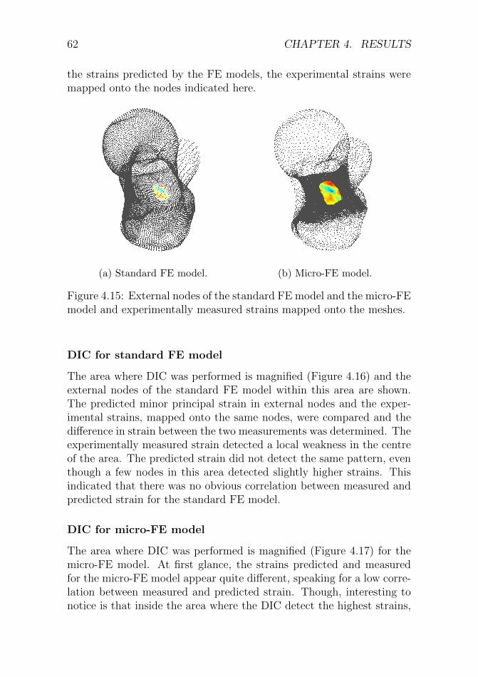
62 CHAPTER 4. RESULTS
the strains predicted by the FE models, the experimental strains weremapped onto the nodes indicated here.
(a) Standard FE model. (b) Micro-FE model.
Figure 4.15: External nodes of the standard FE model and the micro-FEmodel and experimentally measured strains mapped onto the meshes.
DIC for standard FE model
The area where DIC was performed is magnified (Figure 4.16) and theexternal nodes of the standard FE model within this area are shown.The predicted minor principal strain in external nodes and the exper-imental strains, mapped onto the same nodes, were compared and thedifference in strain between the two measurements was determined. Theexperimentally measured strain detected a local weakness in the centreof the area. The predicted strain did not detect the same pattern, eventhough a few nodes in this area detected slightly higher strains. Thisindicated that there was no obvious correlation between measured andpredicted strain for the standard FE model.
DIC for micro-FE model
The area where DIC was performed is magnified (Figure 4.17) for themicro-FE model. At first glance, the strains predicted and measuredfor the micro-FE model appear quite different, speaking for a low corre-lation between measured and predicted strain. Though, interesting tonotice is that inside the area where the DIC detect the highest strains,

4.2. VALIDATION OF THE MICRO-FE MODEL 63
the micro-FE model showed a local weakness with a few nodes showingmuch higher strains than the surroundings.
Figure 4.16: Predicted minor principal strains (left), experimental minorprincipal strains (center) and the difference between predicted and ex-perimental strains (right) for external nodes of the standard FE model.
Figure 4.17: Predicted minor principal strains (left), experimental mi-nor principal strains (center) and the difference between predicted andexperimental strains (right) for external nodes of the micro-FE model.
Correlation and Bland-Altman plots
The strains predicted by FE models and the corresponding experimentalstrains can also be visualized as correlation, and Bland-Altman plots, asshown in Figure 4.18, where the correlation of both the major and minorprincipal strains is investigated. In the correlation plots, the parameterR2 is closer to 1 for the micro-FE model indicating a better correlationbetween measured and predicted strain than the standard FE model.The stronger correlation for the micro-FE model was also indicated by

64 CHAPTER 4. RESULTS
the confidence interval in the Bland-Altman plot, showing less differencebetween measurements for the micro-FE model.
-3 -2 -1 0 1
Measured strain (%)
-3
-2
-1
0
1
P
red
icte
d s
trai
n (
%) R = 0.63
2
NRMSE = 18%
max error = 186%
y = 0.20 + 0.99x
(a) Standard FE, correlation plot.
-2 -1 0
Average (%)
-2
-1
0
1
2
D
iffe
rence
(%
)
0.66
-0.14
-0.95
(b) Standard FE, Bland-Altman plot.
-2 -1 0 1
Measured strain (%)
-2
-1.5
-1
-0.5
0
0.5
1
P
red
icte
d s
trai
n (
%) R = 0.73
2
NRMSE = 17%
max error = 104%
y = 0.18 + 0.96x
(c) micro-FE, correlation plot.
-1.5 -1 -0.5 0 0.5
Average (%)
-1
0
1
D
iffe
rence
(%
)
0.37
-0.18
-0.73
(d) micro-FE, Bland-Altman plot.
Figure 4.18: Correlation and Bland-Altman plots of the predicted andmeasured strains for the micro-FE model and the standard FE model.The correlation was stronger for the micro-FE model with a value ofR2 closer to 1, and less difference between measurements in the Bland-Altman plot.

Chapter 5
Discussion
This thesis aimed to investigate the effect of blood vessel holes on lo-cal strain distribution in the femoral neck, and determine the size andlocation of the holes.
Within this project, methods have been developed for detection andquantification of blood vessel holes from micro-CT images and clinicalCT images. It was possible to generate a micro-FE model from segmen-tation of micro-CT images, partly based on full resolution micro-CTimages. The micro-FE model predicted strains in the femoral neck bet-ter than a similar FE model based on clinical CT images.
5.1 Quantification of vessel holes
5.1.1 Micro-CT
The quantification of vessel hole in micro-CT images was developed todetect intersections, between a contour mesh of the ROI and shrunksurface meshes of the femur. The resulting intersections were fitted tocircles representing the vessel holes. The method resulted in five well-described vessel holes detected totally automatic. All holes visible inthe micro-CT image of the final ROI were detected and the size andlocation appeared correct. The only vessel hole showing tendency ofmisplacement is vessel hole 2 (Figure 4.5b), which was approximately0.3 mm dislocated when comparing the result visually. But, with a totaldiameter of the hole of 2 mm, 0.3 mm was considered to be reasonable,and this small distance will probably not make a huge difference whenimplemented in FE models. Similarly, the radius in vessel hole 3 (Figure
65

66 CHAPTER 5. DISCUSSION
4.5c), was underestimated by approximately 0.1 mm, but with the holehaving a diameter of 2 mm, that was a small error.
The number of holes detected in the micro-CT images was in agree-ment with the literature in terms of size and location. Even though thedistribution of vessel holes is very individual, studies reported an aver-age of 4 (±1) holes in the superolateral part of the femoral neck close tothe greater trochanter, and holes manually measured from less than 1mm to larger than 2 mm in diameter in general [21, 22]. The quantifiedholes in the micro-CT ranged from 1.1 mm to 2 mm in diameter, whichclearly is in the range of vessel holes measured in other studies.
However, the small errors described above, could be the result ofthe different intersection depths. The intersection depths represent thestructure of the vessel hole canals, which have different shapes in thesurface and throughout the cortical bone.
The selection of the ROI was crucial for the results obtained. Theselection was based on previous research, as knowledge of the regionwhere many vessel holes are present [21], and where high strain duringa sideways fall is measured [13, 14], the choice aimed to identify themost interesting region, and best possible for this project. The finalROI was a region with well-defined vessel holes, optimal for proposinga method for quantification of vessel holes in the femoral neck in thehuman femur.
5.1.2 Clinical CT
The clinical CT method automatically detected vessel holes based oncortical bone thickness calculation. Based on a threshold value, the ves-sel holes were determined as very thin, or zero valued thickness regions.Thereafter, the vessel holes were quantified by size and location. Threevessel holes were detected by the clinical CT method, which were lo-cated accurately when compared to the micro-CT result. These threeholes were the largest ones in the micro-CT, where they were quantifiedwith a radius of approximately 1 mm. As the clinical CT imaged had avoxel size of 0.42 mm, it was not possible to detect objects much smallerthan 1 mm. Thus, the detection of three holes shows great promise forfuture applicability of the proposed method.
The method was fairly sensitive to specific settings in the thicknesscalculation. Twelve parameter combinations were investigated in a fullfactorial scheme in order to identify the parameter set that resulted in
5.1. QUANTIFICATION OF VESSEL HOLES 67
the highest accuracy, when compared to the reference micro-CT data.Since the clinical CT scans have a lower resolution it was not possible toidentify vessel holes by eye, and the micro-CT data was chosen for thecomparison of how accurate the method performed. The false positivedetected holes were mostly found in the clinical CT scan reconstructedwith a hard kernel together with the high-density mesh. This resultcould possibly be explained with the hard kernel images having sharpedges, resulting in the cortical thickness estimated thinner in more re-gions.
A threshold of the cortical bone thickness was set to classify a nodeas a hole (0.2 mm). A value was picked for the threshold, based onthat the thickness of a hole should be zero, but with the possibility of ahole being estimated as a very thin region where a hole is present in thecortical bone. However, the sensitivity of variations in the results wereinvestigated by varying the threshold from 0.1 - 0.5 mm. It was possibleto show that the results were not very sensitive to the chosen thresholdvalue, as threshold values of 0.1 - 0.3 mm showed a very similar resultas the chosen one.
5.1.3 Evaluation
The micro-CT and clinical CT based approaches led to different results.The three vessel holes detected in the clinical CT images were overlap-ping with holes in the micro-CT result. The three holes detected withthe clinical CT method corresponded with the three largest holes (ap-proximate radii of 1 mm) detected with the micro-CT method. Thiscould possibly be expected as the clinical CT images has lower resolu-tion, thereby being more difficult to detect smaller holes.
The three overlapping holes in the two approaches were quantifieddifferently by the clinical CT method. Comparing the clinical CT withthe micro-CT as a reference, the clinical CT based approach both un-derestimated (41%) and overestimated (164%) the vessel hole size, in-dicating that the clinical CT method can detect the holes but cannotaccurately determine their size (Table 5.1).
The clinical CT based approach detected 60% of the holes the micro-CT based method detects, where the smallest one detected in the clinicalCT is of size 0.98 mm in radius according to micro-CT results. Thelargest one not detected in the clinical CT was of size 0.61 mm in radiusaccording to the micro-CT. Notably, the clinical CT detected the largest

68 CHAPTER 5. DISCUSSION
Scan Radius [mm]
Micro-CT 0.9843 0.9981 1.0015Clinical CT 0.4044 0.8741 1.6376
% ( clinmicro
) 41% 88% 164%
Table 5.1: Two top rows: Radius of the overlapping quantified vesselholes from the micro-CT and clinical CT based methods. Bottom row:Percentage of the vessel hole radius in the clinical CT in relation to themicro-CT holes’ radius.
holes, and likely those are the ones affecting the bone’s properties themost. According to literature, many vessel holes in the femoral neckare < 1 mm in diameter [21]. No holes less than 1 mm were detected inthe region of interest in this project, their effect on the predicted strainlocation and fractures in FE models will probably not be as large as thebigger holes.
5.2 Validation of the micro-FE model
The starting point for the FE modelling was the reference model thatcorrelated well with experimental data in general, but not in areas sur-rounding vessel holes. For this reason, the project aimed to investigatewhether a model with high resolution in the femoral neck could betterrepresent the strains around vessel holes and correlate measured andpredicted strains, even around vessel holes.
This was done by making a simplified FE model, and for validation,the standard FE model was created with a mesh density similar to themesh density of the reference model. In this way, the modelling tech-nique could be investigated, keeping the influence of the mesh basicallyconstant. Later comparing the standard FE model to the micro-FEmodel would give an indication of how the importance of the mesh den-sity in predicting strains in regions with vessel holes.

5.2. VALIDATION OF THE MICRO-FE MODEL 69
5.2.1 Qualitative comparison
Comparison of the standard FE model to the reference model showedthat the predicted strains outside of the ROI were fairly similar (Figure4.10). In the ROI, where the material mapping for the standard FEmodel was performed with micro-CT images, the minor principal strainswere similar in terms of where at the femur the highest strains occurred,but the magnitude of the strains was slightly higher for the standard FEmodel (Figure 4.11). Overall, this indicated that the simplified standardFE model actually could be a good comparison to the validated referencemodel.
Evaluating the influence of a fine mesh, the standard FE model andthe micro-FE model were compared, showing a very similar distributionin minor principal strain (Figure 4.12. Focusing on the superolateralfemoral neck (Figure 4.13), it was interesting to notice that the mag-nitude of the strains appeared to be similar, but the distribution wasdifferent. In standard FE, the high strains were covering large areasof the posterior side of the lateral neck. Whereas, in the micro-FE,high strains were more concentrated around smaller locations. Thisobservation was aligned with the results of minor principal strains inexternal nodes surrounding vessel holes (Table 4.5), where the stan-dard FE model predicted higher average minor principal strain thanthe micro-FE model in all positions investigated.
The fact that the reference model predicts lower principal strainsat the lateral neck could be explained by the fact that the model has alower limit of its cortical bone strength, employed by having a minimumYoung’s modulus of 2.5 GPa in external elements. In this way, theinfluence of partial volume effects (PVE) is reduced. This could alsoexplain that the reference model, in general, predicted the lowest valuefor principal strain around vessel holes (Table 4.5).
Interesting to discuss is why the predicted strains were different inthe standard and micro FE model. One problem with the standard FEmodel was the fact that it was based on clinical CT images and, hence,has a rougher and less accurate geometry. This, together with the lowermesh density, is likely to give rise to partial volume effects during themapping of the femur, causing a lower density of the cortical bone,which led to a weaker bone and higher predicted strains. Assuming themicro-FE model is better at predicting localized strains, this means thatthe areas of high strains in the standard FE model are over-predictions.
70 CHAPTER 5. DISCUSSION
5.2.2 Validation with DIC
Due to the availability of DIC measurements, it was possible to performquantitative validation of the strains predicted with the micro-FE andstandard FE models.
The DIC measurements (Figure 4.18) showed that the measuredstrains correlated better with the strains predicted by the micro-FEmodel (R2 = 0.72) than with the strains predicted by the standard FEmodel (R2 = 0.62). This allows for saying that the micro-FE model ingeneral was better at predicting strains than the standard FE modelwith lower mesh density.
The figures showing the strain measured with DIC (Figure 4.16 and4.17) are detecting an area of local weakness in the centre of the DIC-area. This area has in a previous study been correlated with a vesselhole [14]. The same clear pattern cannot be seen in the correspondingfigures of predicted strains. Studying the strains predicted by the micro-FE model, the high strains appeared to be local rather than distributedover a larger surface. One explanation for this could be that the strainspredicted by the micro-FE models were not that accurate and that thelocal high strains were caused by occasional elements with low density atthe surface. It could also be that the absence of high strains in the micro-FE model surrounding the vessel holes is an indication that the highstrains measured by DIC were not caused by deformation of the boneitself. Other underlying causes for these strains could be the remainingpresence of soft tissue, or fluids leaking out of the hole deforming thepaint.
Previous studies suggested that introducing vessel holes in FE mod-els could improve the prediction of strains [13] [12]. Based on the cur-rent results the results, this cannot be validated. However, the findingthat the strains predicted by a micro-FE model correlated better than asimilar model based on clinical CT images to experimentally measuredstrains is an indication that the mesh density is relevant and that thisis something to further look into.
Worth mentioning when discussing the results of the DIC measure-ments is that the number of comparisons was very different for the stan-dard FE model and the micro-FE model. The standard FE model hadmore distinguished outliers than the micro-FE model, which in combi-nation with the lower number of comparisons could be the reason forthe correlation to be worse for the standard FE model.

5.3. FUTURE PERSPECTIVE 71
5.3 Future perspective
The project successfully developed methods for detecting and quanti-fying blood vessel holes, both in micro-CT images and in clinical CTimages. Today, it is possible to generate a micro-FE model, from a seg-mentation of micro-CT images, partly based on full resolution micro-CTimages. The micro-FE model predicted strains in the femoral neck bet-ter than a similar FE model based on clinical CT images when comparedto experimentally measured strains.
The material used in this project was limited to only one femur.Even if automatic methods were developed and applied to this femur,a further investigation, in terms of applying the method on severalfemurs, is still required. The most immediate future evolution forthis project would be to evaluate the same methodology over multi-ple femoral anatomies. Then, it would be possible to see the effects ofthe blood vessel holes in the FE models on a larger scale, and investigatewhether FE models of other femurs will predict similar strains in vesselhole regions as the micro-CT based models in this project did. How thestrain prediction in FE modeling is affected by implementation of vesselholes considering an overall perspective, of many femurs investigated,would be something that could possibly conclude the impact of vesselholes on another level of certainty, and is a question for future studiesto address.
Due to computational resources, it was not possible to build FEmodels completely based on full-resolution micro-CT images, consist-ing of many fine elements in the whole surface mesh. A more powerfulcomputer could potentially address this limitation, and overcome theissue. It would be interesting to continue this work, looking into how aFE-model completely based on full-resolution micro-CT images wouldperform. How implementation of vessel holes in a bigger area wouldaffect the predicted strains, if that would increase the model perfor-mance even more, or if the FE model partly based on full resolutionmicro-CT images is good enough. However, with the prospect of de-veloping FE models clinically, it is not an alternative with micro-CTimages. Therefore, developing models partly based of micro-CT imagesis a more realistic way of proceeding. This is, as mentioned, somethingfor future studies to address.
This project contributed to further research by the development ofa framework with which a micro-FE model can be generated including

72 CHAPTER 5. DISCUSSION
a complex surface structure. This can be a foundation for a new way ofestimations of fracture risk in patients clinically. By further improve-ment of the method for detecting and quantifying vessel holes in clinicalCT images and including these in micro-FE models, the continuation isexciting to follow. The method could be the starting point for futurepossibilities of large scale screening of patients for high fracture risk,even in people without osteoporosis.
5.4 Ethical aspects
The CT scans used in this project were already collected in anotherstudy, and ethically approved for use (by The Finnish National Au-thority for Medicolegal Affairs, TEO, 5783/04/044/07) [14]. No newsamples were collected for this study.
The methods are today not ready for clinical implementation. Maybea patient’s need of knowing about the distribution of vessel holes in thefemoral neck is not a strong argument for such an implementation. How-ever, if the method could improve fracture risk assessments, it could inthe bigger picture be something valuable even for the patient as an in-dividual. It could contribute to improved quality of life in a patientbelonging to a risk group.
The methods in the project required CT images of human femurs,something that should be considered from an ethical aspect if the meth-ods would be further investigated with new CT scans or, implementedclinically in the future. The amount of radiation is constrained andalways aimed to be minimized in an individual. If one would re-usealready existing CT scans during the development of the method, thescreening will be reduced. Considering a clinical implementation whenscreening will be necessary, if reducing the screening to people in riskgroups or with certain diseases, the gain of the screening could possiblybe greater than the risks. If it is possible to in an early stage diagnoseand find patients at risk for fragility fractures, or having a bone dis-ease, treatments could be given to more patients. This could lead todecreased costs and improved quality of life in individuals, and possiblycould the risk of fracture be reduced, or maybe even eliminated.
Chapter 6
Conclusions
The conclusion is that vessel holes can automatically be detected andquantified fully from micro-CT images and partly from clinical CT im-ages. A micro-FE model generated based on micro-CT images, includ-ing the vessel holes in the femoral neck, correlated better than a similarmodel based on clinical CT images to experimentally measured strains.
The micro-CT based approach could accurately quantify the vesselholes, while the clinical CT based approach quantified 60% of the holesfound in the micro-CT, the largest holes in terms of radius size.
A micro-FE model was developed from micro-CT images includingthe vessel holes in the geometry of the femur. The model showed higheraccuracy in strain prediction than a similar FE model based on clin-ical CT images. The results indicated that including vessel holes inFE models could have an influence on the prediction of strains at thesuperolateral femoral neck, and should be accounted for in future FEmodels.
73

74 CHAPTER 6. CONCLUSIONS
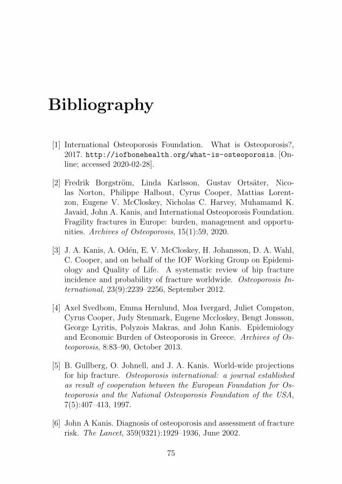
Bibliography
[1] International Osteoporosis Foundation. What is Osteoporosis?,2017. http://iofbonehealth.org/what-is-osteoporosis. [On-line; accessed 2020-02-28].
[2] Fredrik Borgstrom, Linda Karlsson, Gustav Ortsater, Nico-las Norton, Philippe Halbout, Cyrus Cooper, Mattias Lorent-zon, Eugene V. McCloskey, Nicholas C. Harvey, Muhamamd K.Javaid, John A. Kanis, and International Osteoporosis Foundation.Fragility fractures in Europe: burden, management and opportu-nities. Archives of Osteoporosis, 15(1):59, 2020.
[3] J. A. Kanis, A. Oden, E. V. McCloskey, H. Johansson, D. A. Wahl,C. Cooper, and on behalf of the IOF Working Group on Epidemi-ology and Quality of Life. A systematic review of hip fractureincidence and probability of fracture worldwide. Osteoporosis In-ternational, 23(9):2239–2256, September 2012.
[4] Axel Svedbom, Emma Hernlund, Moa Ivergard, Juliet Compston,Cyrus Cooper, Judy Stenmark, Eugene Mccloskey, Bengt Jonsson,George Lyritis, Polyzois Makras, and John Kanis. Epidemiologyand Economic Burden of Osteoporosis in Greece. Archives of Os-teoporosis, 8:83–90, October 2013.
[5] B. Gullberg, O. Johnell, and J. A. Kanis. World-wide projectionsfor hip fracture. Osteoporosis international: a journal establishedas result of cooperation between the European Foundation for Os-teoporosis and the National Osteoporosis Foundation of the USA,7(5):407–413, 1997.
[6] John A Kanis. Diagnosis of osteoporosis and assessment of fracturerisk. The Lancet, 359(9321):1929–1936, June 2002.
75

76 BIBLIOGRAPHY
[7] John A. Kanis, Frederik Borgstrom, Chris De Laet, Helena Johans-son, Olof Johnell, Bengt Jonsson, Anders Oden, Niklas Zethraeus,Bruce Pfleger, and Nikolai Khaltaev. Assessment of fracture risk.Osteoporosis International, 16(6):581–589, June 2005.
[8] International Osteoporosis Foundation. Diagnosing Os-teoporosis, 2017. https://www.iofbonehealth.org/
diagnosing-osteoporosis. [Online; accessed 2020-03-05].
[9] Ethel S. Siris, Ya-Ting Chen, Thomas A. Abbott, ElizabethBarrett-Connor, Paul D. Miller, Lois E. Wehren, and Marc L.Berger. Bone Mineral Density Thresholds for Pharmacological In-tervention to Prevent Fractures. Archives of Internal Medicine,164(10):1108–1112, May 2004. Publisher: American Medical Asso-ciation.
[10] Lorenzo Grassi, Sami P. Vaananen, Matti Ristinmaa, Jukka S. Ju-rvelin, and Hanna Isaksson. How accurately can subject-specific fi-nite element models predict strains and strength of human femora?Investigation using full-field measurements. Journal of Biomechan-ics, 49(5):802–806, March 2016.
[11] B. Helgason, S.Gilchrist, O. Ariza, J. D. Chak, G. Zheng, R. P.Widmer, S. J. Ferguson, P. Guy, and P. A. Cripton. Develop-ment of a balanced experimental–computational approach to un-derstanding the mechanics of proximal femur fractures. MedicalEngineering & Physics, 36(6):793–799, June 2014.
[12] Hassan Bahaloo, W. S. Enns-Bray, I. Fleps, O. Ariza, S. Gilchrist,R. Widmer Soyka, P. Guy, H. Palsson, S. J. Ferguson, P. A. Crip-ton, and B. Helgason. On the Failure Initiation in the ProximalHuman Femur Under Simulated Sideways Fall. Annals of Biomed-ical Engineering, 46(2):270–283, February 2018.
[13] Yekutiel Katz and Zohar Yosibash. New insights on the proximalfemur biomechanics using Digital Image Correlation. Journal ofBiomechanics, 101:109599, March 2020.
[14] Lorenzo Grassi, Joeri Kok, Anna Gustafsson, Yi Zheng, Sami P.Vaananen, Jukka S. Jurvelin, and Hanna Isaksson. Elucidating
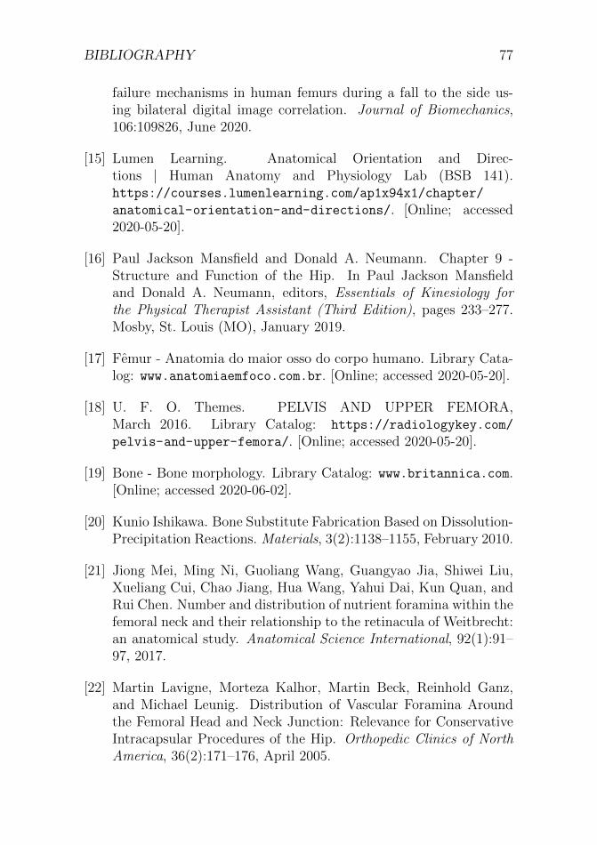
BIBLIOGRAPHY 77
failure mechanisms in human femurs during a fall to the side us-ing bilateral digital image correlation. Journal of Biomechanics,106:109826, June 2020.
[15] Lumen Learning. Anatomical Orientation and Direc-tions | Human Anatomy and Physiology Lab (BSB 141).https://courses.lumenlearning.com/ap1x94x1/chapter/
anatomical-orientation-and-directions/. [Online; accessed2020-05-20].
[16] Paul Jackson Mansfield and Donald A. Neumann. Chapter 9 -Structure and Function of the Hip. In Paul Jackson Mansfieldand Donald A. Neumann, editors, Essentials of Kinesiology forthe Physical Therapist Assistant (Third Edition), pages 233–277.Mosby, St. Louis (MO), January 2019.
[17] Femur - Anatomia do maior osso do corpo humano. Library Cata-log: www.anatomiaemfoco.com.br. [Online; accessed 2020-05-20].
[18] U. F. O. Themes. PELVIS AND UPPER FEMORA,March 2016. Library Catalog: https://radiologykey.com/
pelvis-and-upper-femora/. [Online; accessed 2020-05-20].
[19] Bone - Bone morphology. Library Catalog: www.britannica.com.[Online; accessed 2020-06-02].
[20] Kunio Ishikawa. Bone Substitute Fabrication Based on Dissolution-Precipitation Reactions. Materials, 3(2):1138–1155, February 2010.
[21] Jiong Mei, Ming Ni, Guoliang Wang, Guangyao Jia, Shiwei Liu,Xueliang Cui, Chao Jiang, Hua Wang, Yahui Dai, Kun Quan, andRui Chen. Number and distribution of nutrient foramina within thefemoral neck and their relationship to the retinacula of Weitbrecht:an anatomical study. Anatomical Science International, 92(1):91–97, 2017.
[22] Martin Lavigne, Morteza Kalhor, Martin Beck, Reinhold Ganz,and Michael Leunig. Distribution of Vascular Foramina Aroundthe Femoral Head and Neck Junction: Relevance for ConservativeIntracapsular Procedures of the Hip. Orthopedic Clinics of NorthAmerica, 36(2):171–176, April 2005.

78 BIBLIOGRAPHY
[23] U.S. Department of Health & Human Services Na-tional Institute of Biomedical Imaging and Bioengineer-ing (NIBIB). Computed Tomography (CT). https:
//www.nibib.nih.gov/science-education/science-topics/
computed-tomography-ct. [Online; accessed 2020-03-13].
[24] Micro Photonics Inc. What is Micro-CT? An Introduc-tion, February 2018. https://www.microphotonics.com/
what-is-micro-ct-an-introduction/. [Online; accessed 2020-03-13].
[25] Euclid Seeram. Computed Tomography - E-Book: Physical Prin-ciples, Clinical Applications, and Quality Control. Elsevier HealthSciences, September 2015. Google-Books-ID: DTCDCgAAQBAJ.
[26] Nick McCormick and Jerry Lord. Digital Image Correlation. Ma-terials Today, 13(12):52–54, December 2010.
[27] Bing Pan, Zhaoyang Wang, and Zixing Lu. Genuine full-fielddeformation measurement of an object with complex shape us-ing reliability-guided digital image correlation. Optics Express,18(2):1011–1023, January 2010. Publisher: Optical Society ofAmerica.
[28] Lorenzo Grassi. Femoral Strength Prediction using Finite ElementModels : Validation of models based on CT and reconstructed DXAimages against full-field strain measurements. thesis/doccomp,Lund University, 2016. ISBN: 9789177530312 9789177530305.
[29] Nurettin Ozgur Dogan. Bland-Altman analysis: A paradigm to un-derstand correlation and agreement. Turkish Journal of EmergencyMedicine, 18(4):139–141, December 2018.
[30] Coefficient of determination | Interpretation & Equation. LibraryCatalog: www.britannica.com. [Online; accessed 2020-06-06].
[31] Bland–Altman plot, May 2020. https://en.wikipedia.org/
wiki/Bland-Altman_plot. [Online; accessed 2020-06-04].
[32] Chiranji Lal Chowdhary and D. P. Acharjya. Segmentation andFeature Extraction in Medical Imaging: A Systematic Review. Pro-cedia Computer Science, 167:26–36, January 2020.

BIBLIOGRAPHY 79
[33] Paul A. Yushkevich, Joseph Piven, Heather Cody Hazlett,Rachel Gimpel Smith, Sean Ho, James C. Gee, and Guido Gerig.User-guided 3D active contour segmentation of anatomical struc-tures: Significantly improved efficiency and reliability. NeuroImage,31(3):1116–1128, July 2006.
[34] Vicent Caselles, Francine Catte, Tomeu Coll, and Francoise Di-bos. A geometric model for active contours in image processing.Numerische Mathematik, 66(1):1–31, December 1993.
[35] V. Caselles, R. Kimmel, and G. Sapiro. Geodesic active contours.In Proceedings of IEEE International Conference on Computer Vi-sion, pages 694–699, Cambridge, MA, USA, 1995. IEEE Comput.Soc. Press.
[36] Machine Intelligence Laboratory Cambridge University Depart-ment of Engineering. Stradview 6.0, 2014. https://mi.eng.cam.
ac.uk/Main/StradView. [Online; accessed 2020-05-20].
[37] G. M. Treece and A. H. Gee. Independent measurement of femoralcortical thickness and cortical bone density using clinical CT. Med-ical Image Analysis, 20(1):249–264, February 2015.
[38] G. M. Treece, A. H. Gee, P. M. Mayhew, and K. E. S. Poole. Highresolution cortical bone thickness measurement from clinical CTdata. Medical Image Analysis, 14(3):276–290, June 2010.
[39] R. K. Nalla, J. H. Kinney, and R. O. Ritchie. Mechanistic fracturecriteria for the failure of human cortical bone. Nature Materials,2(3):164–168, March 2003.
[40] Elise F Morgan and Tony M Keaveny. Dependence of yield strain ofhuman trabecular bone on anatomic site. Journal of Biomechanics,34(5):569–577, May 2001.
[41] Niels Saabye Ottosen and Hans Petersson. Introduction to the finiteelement method. Prentice Hall, New York, 1992.
[42] Element Types. http://web.mit.edu/calculix\_v2.7/
CalculiX/ccx\_2.7/doc/ccx/node25.html. [Online; accessed2020-05-24].

80 BIBLIOGRAPHY
[43] Fulvia Taddei, Enrico Schileo, Benedikt Helgason, Luca Cristo-folini, and Marco Viceconti. The material mapping strategy influ-ences the accuracy of CT-based finite element models of bones: Anevaluation against experimental measurements. Medical Engineer-ing & Physics, 29(9):973–979, November 2007.
[44] Enrico Schileo, Fulvia Taddei, Luca Cristofolini, and Marco Vice-conti. Subject-specific finite element models implementing a max-imum principal strain criterion are able to estimate failure riskand fracture location on human femurs tested in vitro. Journal ofBiomechanics, 41(2):356–367, January 2008.
[45] Elise F. Morgan, Harun H. Bayraktar, and Tony M. Keaveny. Tra-becular bone modulus–density relationships depend on anatomicsite. Journal of Biomechanics, 36(7):897–904, July 2003.
[46] Scientific Computing and Imaging Institute. Seg3D 2.4.4,2016. http://www.sci.utah.edu/cibc-software/seg3d.html.[Online; accessed 2020-04-17].
[47] Autodesk Inc. Meshmixer 3.5. http://www.meshmixer.com/. [On-line; accessed 2020-04-17].
[48] Qianqian Fang and David A. Boas. Tetrahedral mesh generationfrom volumetric binary and grayscale images. In 2009 IEEE Inter-national Symposium on Biomedical Imaging: From Nano to Macro,pages 1142–1145, Boston, MA, USA, June 2009. IEEE.
[49] Jaroslaw Tuszynski. Surface intersection, May 2020.https://se.mathworks.com/matlabcentral/fileexchange/
48613-surface-intersection. [Online; accessed 2020-06-14].
[50] Jaroslaw Tuszynski. Triangle/Ray Intersection, May 2020.https://se.mathworks.com/matlabcentral/fileexchange/
33073-triangle-ray-intersection. [Online; accessed 2020-05-14].
[51] Sam Murthy. Best fit 3D circle to a set of points, May 2020.https://se.mathworks.com/matlabcentral/fileexchange/
55304-best-fit-3d-circle-to-a-set-of-points. [Online;accessed 2020-05-14].

BIBLIOGRAPHY 81
[52] Enrico Schileo, Jonathan Pitocchi, Cristina Falcinelli, and FulviaTaddei. Cortical bone mapping improves finite element strain pre-diction accuracy at the proximal femur. Bone, 136:115348, July2020.
[53] Peter Karasev. Triangle subdivide (vectorized/fast), May 2020.https://se.mathworks.com/matlabcentral/fileexchange/
25961-triangle-subdivide-vectorized-fast. [Online; ac-cessed 2020-05-14].
[54] Dr Michael D Abramoff. Image Processing with ImageJ. Biopho-tonics International, Laurin Publishing Co. Inc, July 2004.
[55] Hyperworks 2019 | Solutions for Every Stage of Product Devel-opment. https://www.altair.com/hyperworks-2019/. [Online;accessed 2020-05-26].
[56] Abaqus Unified FEA - SIMULIATM by Dassault Systemes R©. Li-brary Catalog: www.3ds.com. [Online; accessed 2020-05-26].
[57] CloudCompare - Open Source project. https://www.
cloudcompare.org/. [Online; accessed 2020-04-17].

82 BIBLIOGRAPHY

Appendix
7.1 Strain in vessel holes
Reference model
Figure 7.1: Predicted strain in detected vessel hole 1 (top left) to 5(bottom) for the reference model.
83

84 BIBLIOGRAPHY
Standard FE model
Figure 7.2: Predicted strain in detected vessel hole 1 (top left) to 5(bottom) for the standard model.
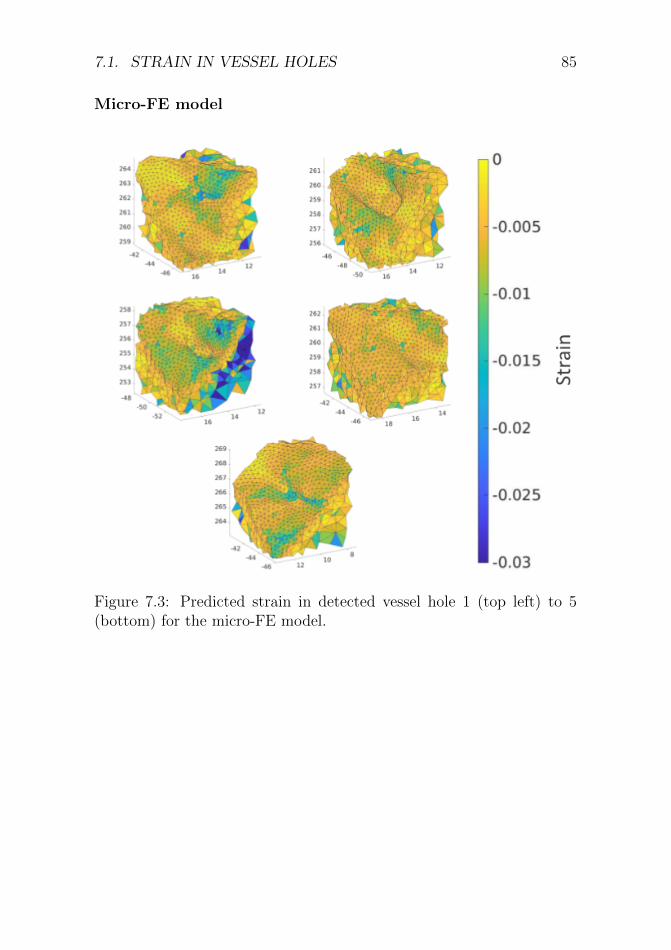
7.1. STRAIN IN VESSEL HOLES 85
Micro-FE model
Figure 7.3: Predicted strain in detected vessel hole 1 (top left) to 5(bottom) for the micro-FE model.
Related Documents