The effect of varying salinity in polymer solution

“Rheological properties of hydrophobically modified anionic polymers: The

effect of varying salinity in polymer solution”

Master’s Thesis

Petroleum Technology – Reservoir Chemistry

Peter Aarrestad Time

Department of Chemistry

University of Bergen

June 2017

i

Acknowledgements

I would like to express my gratitude to my supervisor Dr. Kristine Spildo, and co-supervisor Dr.

Ketil Djurhuus, for guiding and supporting me through to the completion of my thesis. Thanks

to PhD student Alette Løbø Viken for making time to help me and provide me with vital insight

and invaluable assistance despite being away on leave. I would also like to show express my

thankfulness to Dr. Tormod Skauge for providing technical advice.

Special Thanks to CIPR and the Department of Chemistry for allowing me to use their

laboratories and equipment. Thanks to BASF SE, Germany, for providing the polymers.

Furthermore, I would like to express my appreciation to my fellow students for maintaining a

cheerful atmosphere during these troublesome months. I would like to give a heads up to my

great partner Per Erik Svendsen for being a good human being and a terrific lab-partner.

Thanks to Jan Tore Østvold for his good friendship.

Thanks to the love of my life, Margareta Eide, for keeping up with me at my best and worst. I

would like to express my gratefulness to Ingunn and Sjur Eide for being such lovely people and

for saving me from starvation. Thanks to my parents and lovely family for always being there

for me when I need them.

Peter Aarrestad Time

Bergen, June 2017

ii

Abstract

A new class of polymers, named ‘hydrophobically modified water-soluble polymers’, has been

developed as an alternative to the more commonly used polyelectrolytes in enhanced oil

recovery (EOR) applications. These polymers are very similar to conventional polymers used

in EOR, except they have a small number of hydrophobic groups incorporated into the polymer

backbone, making them more stable at high salinities. In this study we have investigated two

hydrophobically modified anionic polymers. The polymers have the same backbone, including

anionic content, equal amounts of hydrophobic substitution, but different chemical

composition of the hydrophobes.

Characterization of the polymers was performed using a combination of steady-state shear

viscosity and dynamic oscillatory measurements. The shear viscosity and viscoelastic moduli

were measured as the salinity increased. The results were compared to the corresponding

anionic polymer without any hydrophobic substitution. As the salinity increased, the shear

viscosity decreased for both the hydrophobically modified polyacrylamide and the partly

hydrolysed polyacrylamide in the dilute regime. In the semi-dilute and concentrated regime,

the shear viscosity initially decreased with increasing salinity before it increased at higher

salinities (> 10 wt%). The lowest viscosities were observed between 5- and 10 wt% salinity.

Above the critical overlap concentration, the hydrophobically modified polymer with the

highest hydrophobe HLB generated much higher viscosities compared to its less hydrophobic

analogue. The less hydrophobic polymer only showed higher viscosities than the

polyacrylamide for salinities above 10 wt%. The elasticity of the most hydrophobic associative

polymer remained relatively unaffected by increased salinity, showing the most elastic

behaviour. The elasticity of the less hydrophobic polymer decreased at first as the salinity

increased, reaching maximum viscous behaviour at 5 wt% salinity. At salinities > 5 wt%, the

elasticity started to increase again. Both hydrophobically modified polymers displayed more

elastic behaviour than the polyelectrolyte. This behaviour can increase oil recovery, mainly in

high salinity and high permeability reservoirs through improved waterflood sweep efficiency

due to enhanced viscosity increasing properties, and the microscopic displacement efficiency

through its elasticity.

iii

Nomenclature

Variables

C Concentration [mol/L]

CMC Critical Micelle Concentration [mol/L]

Pa·s Pascal seconds

cP Centi Poise [mPa·s]

C* Critical overlap concentration [ppm]

Cη Critical concentration [ppm]

Ce Critical entanglement concentration [ppm]

ED Microscopic displacement efficiency [ppm]

ER Total displacement efficiency [ppm]

EV Volumetric sweep efficiency [ppm]

f Frequency [Hz]

G Shear modulus [Pa]

G’ Elastic modulus (storage modulus) [Pa]

G’’ Viscous modulus (loss modulus) [Pa]

G* Complex shear modulus [Pa]

I Ionic strength [mol/L]

K Absolute permeability [m2]

kr,i Relative permeability of i [dimensionless]

M Mobility ratio [dimensionless]

n Power-law index [dimensionless]

tan δ Loss factor [dimensionless]

iv

wi Mass fraction [kg/kg]

xi Mole fraction [dimensionless]

zi Valence of component i [dimensionless]

Greek letters

γ Shear strain [dimensionless]

γL Shear strain [dimensionless]

�̇� Shear rate [s-1]

�̇�𝑐 Critical hear rate [s-1]

δ Phase shift angle [°]

η Shear viscosity [cP]

η* Complex shear viscosity [cP]

η0 Zero shear viscosity [cP]

𝜂∞ Infinite shear viscosity [cP]

ηsp Specific viscosity [dimensionless]

ηs Solvent viscosity [cP]

ηR Reduced viscosity [cm3/g]

λc Relaxation time [s]

λi Mobility of i [m2/mPa·s]

λo Oil mobility [m2/mPa·s]

λw Water mobility [m2/mPa·s]

μ Viscosity [Pa·s]

μi Viscosity of i [Pa·s]

v

μo Viscosity of oil [Pa·s]

μw Viscosity of water [Pa·s]

τ Shear stress [Pa]

τL Limiting stress value [Pa]

ω Angular frequency [rad/s]

ωc Angular crossover frequency [rad/s]

Abbreviations

Abrine Brine based on molar ratio

BASF Badische Anilin- und Soda-Fabrik

CIPR Centre for Integrated Petroleum Research

CP MS Cone Plate Measuring System

EOR Enhanced Oil Recovery

HLB Hydrophilic-Lipophilic Balance

HPAM Hydrolysed Polyacrylamide

Hz Hertz [s-1]

LVE Linear Viscoelastic

mm Millimetre

NCS Norwegian Continental Shelf

OOIP Original Oil in Place

PAM Polyacrylamide

ppm Parts per million [g/g]

rpm Revolutions per minute [min-1]

vi

SI International Systems of Units

Tbrine Brine based on wt%

μm Micrometre

vii

Table of Contents

1 Introduction ............................................................................................................... 1

1.1 Thesis objective ............................................................................................................. 4

2 Background ................................................................................................................ 5

2.1 Polymers ........................................................................................................................ 5

2.1.1 What are polymers? ........................................................................................................ 5

2.1.2 Examples of common polymers ...................................................................................... 7

2.2 Polymer rheology .......................................................................................................... 8

2.2.1 Shear viscosity ................................................................................................................. 8

2.2.2 Models for shear flow ................................................................................................... 13

2.2.3 Intrinsic viscosity ........................................................................................................... 14

2.2.4 Polymer concentration and critical overlap concentration........................................... 15

2.2.5 Polymer viscoelasticity and oscillatory rheology........................................................... 18 2.2.5.1 Amplitude sweep .................................................................................................................... 20 2.2.5.2 Frequency sweep .................................................................................................................... 21

2.3 EOR polymers .............................................................................................................. 23

2.3.1 HPAM ............................................................................................................................. 23

2.3.2 Factors influencing the viscosifying ability of HPAM..................................................... 24 2.3.2.1 Molecular weight .................................................................................................................... 24 2.3.2.2 Mechanical degradation ......................................................................................................... 25 2.3.2.3 Chemical degradation – hydrolysis ......................................................................................... 25 2.3.2.4 Salinity and ion composition .................................................................................................. 27

2.3.3 Hydrohobically modified HPAM .................................................................................... 35

2.3.4 Factors influencing the viscosifying ability of HMPAM ................................................. 39 2.3.4.1 Molecular weight .................................................................................................................... 39 2.3.4.2 Mechanical degradation ......................................................................................................... 39 2.3.4.3 Chemical degradation – hydrolysis ......................................................................................... 40 2.3.4.4 Salinity and ion composition .................................................................................................. 40

3 Experimental ........................................................................................................... 43

3.1 Chemicals .................................................................................................................... 43

3.1.1 Salts used in preparation of the brine solutions ........................................................... 43

3.1.2 Salt solutions ................................................................................................................. 43

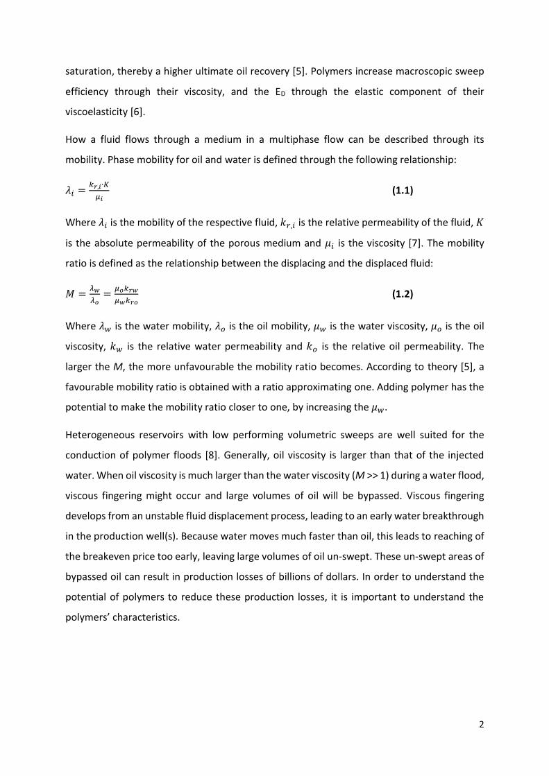
3.2 Preparation of polymer solutions ................................................................................. 44

3.2.1 Polymers ........................................................................................................................ 44

3.2.2 Preparing the polymer solutions ................................................................................... 45

3.3 Experimental apparatus and equipment ....................................................................... 47

3.3.1 Malvern Rheometer Kinexus pro+................................................................................. 47 3.3.1.1 Geometries ............................................................................................................................. 48

3.3.2 Shear viscosity measurments ........................................................................................ 49

3.3.3 Oscillatory measurements ............................................................................................. 50

3.3.4 Weighing instruments/scales ........................................................................................ 51

3.4 Development of experimental protocol ........................................................................ 51

3.4.1 Sources of error stemming from the dilutions .............................................................. 53

3.4.2 Sources of error stemming from the sampling ............................................................. 53

3.5 Uncertainties ............................................................................................................... 54

4 Results ..................................................................................................................... 55

viii

4.1 Shear viscosity measurements ..................................................................................... 55

4.2 Effect of concentration on solution viscosity measured at 10 s-1 shear rate .................... 61

4.2.1 Shear viscosity at 10 s-1 shear rate as a function of polymer concentration ................ 63

4.2.2 Shear viscosity at 10 s-1 shear rate as a function of salinity .......................................... 67

4.3 Oscillatory measurements (viscoelastic measurements) ............................................... 74

5 Discussion ................................................................................................................ 78

5.1 Shear viscosity measurements ..................................................................................... 78

5.2 Extracted shear viscosity measured at 10 s-1 shear rate ................................................. 80

5.2.1 Shear viscosities at 10 s-1 shear rate as a function of polymer concentration .............. 80

5.2.2 Shear viscosity at 10 s-1 shear rate as a function of salinity .......................................... 83

5.3 Oscillatory measurements (viscoelastic measurements) ............................................... 87

6 Summary and conclusions ........................................................................................ 90

7 Further work ............................................................................................................ 92

8 Bibliography ............................................................................................................ 93

1

1 Introduction

Ever since Edwin Drake struck oil in the first modern oil well near Titusville, Pennsylvania, the

global demand for ‘rock oil’, now called petroleum, has steadily increased. Global discovery

rates of petroleum peaked in the 1960’s, but there is no doubt that these resources are finite.

Demand and consumption has exponentially increased since the 1900’s, and predictions

project them to further increase into the 21st century [1].

The average oil recovery factor worldwide is only between 20 % and 40 % [2] and production

by primary recovery (natural depletion of reservoir pressure) results in an average recovery

rate that does not exceed 20 % in most cases [3]. Secondary recovery, defined as recovery by

using or injecting fluids originally present in the reservoir, has raised the recovery rate

significantly. Water flooding is the most common form of secondary recovery. Regardless,

even after a successful water flood, recovery rates are not higher than 30-40 % [4].

Ever-increasing demand and depletion of existing reserves worldwide have facilitated

progress to further increase recovery rates from already producing fields. Enhanced oil

recovery (EOR) involves the use of unconventional recovery methods, i.e. injection of

materials not originally present in the reservoir, such as polymers and surfactants [5]. Big leaps

in technology combined with high oil prices have increased the applicability of EOR-technology

in modern petroleum production.

The purpose of a water flood as secondary recovery technique is to displace the oil in the

reservoir towards a production well and providing pressure maintenance by replacing

produced volumes with water [5]. In contrast to conventional water flooding, the main

objective of EORs is to increase the volumetric (macroscopic) sweep efficiency, and to enhance

the displacement (microscopic) efficiency (ER), which is the product of the macroscopic sweep

efficiency (EV) and the microscopic sweep efficiency (ED). One mechanism of EOR aims towards

increasing the ED by reducing the mobility ratio between the displacing and the displaced fluid.

Another mechanism is aimed at reducing the amount of oil trapped due to the capillary forces

(microscopic entrapment). By reducing the interfacial tension between the displacing and

displaced fluids, the effect of microscopic trapping is lowered, producing a lower residual oil

2

saturation, thereby a higher ultimate oil recovery [5]. Polymers increase macroscopic sweep

efficiency through their viscosity, and the ED through the elastic component of their

viscoelasticity [6].

How a fluid flows through a medium in a multiphase flow can be described through its

mobility. Phase mobility for oil and water is defined through the following relationship:

𝜆𝑖 =𝑘𝑟,𝑖∙𝐾

𝜇𝑖 (1.1)

Where 𝜆𝑖 is the mobility of the respective fluid, 𝑘𝑟,𝑖 is the relative permeability of the fluid, 𝐾

is the absolute permeability of the porous medium and 𝜇𝑖 is the viscosity [7]. The mobility

ratio is defined as the relationship between the displacing and the displaced fluid:

𝑀 =𝜆𝑤

𝜆𝑜=

𝜇𝑜𝑘𝑟𝑤

𝜇𝑤𝑘𝑟𝑜 (1.2)

Where 𝜆𝑤 is the water mobility, 𝜆𝑜 is the oil mobility, 𝜇𝑤 is the water viscosity, 𝜇𝑜 is the oil

viscosity, 𝑘𝑤 is the relative water permeability and 𝑘𝑜 is the relative oil permeability. The

larger the M, the more unfavourable the mobility ratio becomes. According to theory [5], a

favourable mobility ratio is obtained with a ratio approximating one. Adding polymer has the

potential to make the mobility ratio closer to one, by increasing the 𝜇𝑤.

Heterogeneous reservoirs with low performing volumetric sweeps are well suited for the

conduction of polymer floods [8]. Generally, oil viscosity is larger than that of the injected

water. When oil viscosity is much larger than the water viscosity (M >> 1) during a water flood,

viscous fingering might occur and large volumes of oil will be bypassed. Viscous fingering

develops from an unstable fluid displacement process, leading to an early water breakthrough

in the production well(s). Because water moves much faster than oil, this leads to reaching of

the breakeven price too early, leaving large volumes of oil un-swept. These un-swept areas of

bypassed oil can result in production losses of billions of dollars. In order to understand the

potential of polymers to reduce these production losses, it is important to understand the

polymers’ characteristics.

3

Figure 1.1. Water flood and polymer flood comparison [9].

Polymer’s viscosity increasing properties and well-studied physical behaviour, have made

polymers applicable for implementation as EOR agents [4]. Since the mid-80’s, successful

polymer floods have been conducted at Daqing in the Yellow Sea and it has been reported

that the use of polymer flooding there has increased the recovery by 12% [10].

Figure 1.2. Comparison of production profiles for a water flood and a polymer flood showing

the economic limit for each case [11].

Traditional polymers such as partially hydrolysed polyacrylamide (HPAM) have been found to

be relatively sensitive to high shear and salinity [11]. As a result, large volumes of polymers

are often used in floods to compensate for the mechanical degradation caused by high

injection rates in order to maintain sufficient viscosity levels during a flood.

4

The use of new synthetic polymers with altered structure and composition in order to become

partly hydrophobic have been suggested [12]. These hydrophobically modified polymers are

more resistant towards the strain regular polymers degrade under and there are indications

that they do not lose their viscosifying ability with increased salinity but sometimes even

increase their viscosity [8]. Experiments have also shown that the ED can also be significantly

increased by using synthetic hydrophobically modified anionic polymers, due to the greater

elastic component in their viscoelastic properties [12]. Conclusively, an ideal polymer has a

highly viscosifying ability and a large elastic component.

1.1 Thesis objective

When evaluating hydrophobically modified polyelectrolytes for use in EOR-applications, the

challenge is to find the optimal balance between charge, hydrophobic monomer content, and

structure/hydrophobicity of the hydrophobic monomers. The ultimate goal is to obtain a

product that is water soluble, while at the same time generating as high viscosity and

viscoelasticity as possible, under the relevant reservoir conditions.

In this study, we investigate two hydrophobically modified anionic polymers. The polymers

have the same backbone, including anionic content, equal amounts of hydrophobic

substitution, but different chemical composition of the hydrophobes. The results are

compared to the corresponding anionic polymer without any hydrophobic substitution. The

goal is to provide insight into how salinity affects the interplay between intra- and

intermolecular electrostatic and hydrophobic interactions, which in turn governs the viscosity

and viscoelasticity of the polymer solutions. Is the HLB-value itself a critical parameter? If yes,

will a high or a low HLB-value be favourable for the investigated polymer structure having the

same balance between charge and hydrophobic monomer content as well as identical

polymer backbones?

5

2 Background

2.1 Polymers

2.1.1 What are polymers?

A polymer, from Greek poly ‘many’ + mer ‘member’, is a large molecule or macromolecule

composed of many repeated structural subunits. The structural units are connected to one

another in the polymer molecule, or polymer structure, by covalent bonds [13]. A single

structural unit is called a monomer. The modern definition of polymers as covalently bonded

macromolecular structures was pioneered in the 1920’s by the German organic chemist,

Hermann Staudinger [14].

Even though structures of polymers vary widely, nearly all polymers of interest can be

expressed as combinations of a limited number of different structural units [14]. Often will a

single type of a structural unit be sufficient for the representation of the entire polymer

molecule. This characteristic, namely the generation of the entire structure through repetition

of one or a few elementary units, is the basic characteristic of polymer substances [13].

Polymers range from familiar synthetic plastics, such as polystyrene, to natural biopolymers

like DNA and proteins. Their consequently large molecular mass relative to small molecule

compounds produce unique physical properties. These unique physical properties include

viscoelasticity, toughness, and a tendency to form glasses and semi-crystalline structures [15].

When a polymer dissolves into a solvent, the solution become more viscous [14]. Due to their

properties, polymers serve as thickeners in common commercial products like shampoo, paint

and ice cream. The thickening effect may be used to estimate a polymer’s molecular weight.

Polymers are large molecules moving very slowly in solution. The faster the solvent molecules

move in a liquid, the more easily the liquid will flow [16]. Therefore, when polymer molecules

dissolves into a solution, their slow motion makes the whole solution more viscous. The big

slow-moving polymer molecules get in the way of the faster-moving solvent molecules when

they try to flow. The result being that the overall speed of the whole solution slows down,

thereby increasing its viscosity. The polymer molecules will also slow down the smaller solvent

molecules through intermolecular forces [5]. If there are any attractive secondary interactions

6

between the polymer and solvent molecules, the small solvent molecules can become bound

to the polymer. When this occurs, they more or less move with the polymers slow speed.

The viscosifying ability of a polymer correlates to its hydrodynamic volume. The larger the

hydrodynamic volume, the more viscous the polymer solution will be [16]. The hydrodynamic

volume describes the volume a coiled polymer takes up in solution. With their larger size, the

polymer molecules can block more motion of the solvent molecules. Increased size, also leads

to increased secondary forces. According to the principle of summation of molecular forces,

the larger the hydrodynamic volume, the more strongly the solvent molecules will be bound

to the polymer. The larger the molecule, the more molecule there is to exert an intermolecular

force. This enhances the slowing effect exerted onto the solvent molecules.

The hydrodynamic volume, along with the radius of gyration, are the two most commonly

used parameters describing a molecule’s size. Both parameters describe the same thing, but

uses different means to arrive at a size-describing value. Dynamic light scattering determines

the hydrodynamic radius of a molecule, or macromolecule. The hydrodynamic radius is

defined as the radius of an equivalent hard sphere diffusing at the same rate as the molecule

under observation [17]. In reality, polymer solutions and their complexes do not exist as hard

spheres. Therefore, the determined hydrodynamic radius more closely reflects the apparent

size adopted by the solvated, tumbling molecule.

The definition of the radius of gyration on the other hand, is the mass weighted average

distance from the core of a molecule to each mass element in the molecule [18]. For

macromolecules with a radius greater than 10 nm, estimation of the radius of gyration takes

place using multi-angle light scattering. For molecules smaller than 10 nm, techniques such as

small angle neutron scattering (SANS) and small angle x-ray scattering (SAXS) obtain the Rg

[17].

7

2.1.2 Examples of common polymers

Polymers divide into two subgroups, natural and synthetic polymers. Natural polymeric

materials include shellac, amber, wool, silk, starches, cellulose and natural rubber. Cellulose

is the main constituent in wood and paper. Some synthetic polymers include synthetic rubber,

neoprene, nylon, polyvinyl chloride (PVC), silicone, polyacrylamide, polypropylene,

polyethylene and many more.

8

2.2 Polymer rheology

First coined by Pr. Eugene Bingham in the 1920’s: rheology, from Ancient Greek rheos ‘stream’

+ -logy ‘study of’, is formally defined as the study of deformation and flow behaviour in various

materials [19]. Rheology describes the interrelation between force, deformation and time,

where the rheological properties of materials will be determined [20].

2.2.1 Shear viscosity

The viscosity of a solution is a measure of its resistance to flow when shear forces are applied.

Shearing forces represents unaligned forces pushing one part of a body in one direction, and

another part of the body in the opposite direction [21].

Figure 2.2.1. Illustration showing how shearing forces push in one direction at the top, and in

the opposite direction at the bottom, causing shearing deformation.

The viscosity will express the magnitude of internal friction for molecules within a fluid. It is

depended on temperature, fluid behaviour and amount of force applied. The viscosity of

polymers will change depending on which external forces is applied. The dynamic (absolute)

viscosity is defined as:

9

𝜂 =𝜏

�̇� (2.2.1)

Where η (sometimes μ) is the dynamic viscosity, τ is the shear stress, and �̇� is the shear rate

in laminar flow. The dynamic viscosity is also referred to as shear viscosity. The commonly

used units for viscosity is either [Pa·s] or [cP].

Fluids will behave differently when shear is applied. Most fluids are dependent on the shear

rate. Newtonian fluids are fluids with a single linear relation between shear stress and shear

rate, where the proportionality constant is the viscosity of the fluid [11]. Water being an

example of a Newtonian fluid.

Figure 2.2.2. Viscosity function. Modified from Fig. 8-12 in [15].

Liquids of low molecular weight compounds and their solutions are often Newtonian. The non-

Newtonian behaviour (2) shows shear thinning properties (Figure 2.2.2.). This behaviour is

often observed when the material under study is a polymer solution or a melt [16].

Shear-thinning substances are not characterized through a single viscosity (Figure 2.2.2). The

viscosity at a particular velocity gradient is given by the ratio σ/(dv/dy). Pseudo-plastic

materials appear less viscous at high rates of shear than at low rates (Figure 2.2.2). Polymers

show pseudo-plastic behaviour at sufficiently high concentrations. A reduction in the viscosity

from increased shear rates indicate that viscous forces starts dominating the solution flow

10

behaviour. This happens because with increasing shear rate, the polymer molecules start to

untangle from each other and starts to align themselves with the direction of flow [11] (Figure

2.2.3).

Figure 2.2.3. Flow development of polymer solutions.

Polymers consist of flexible chain-like molecules that will deform and align when experiencing

high shear rates (Figure 2.2.3) [11]. Shear-thickening behaviour describes the opposite

behaviour.

11

Figure 2.2.4. Figure showing viscosity vs. shear rate with specific regions highlighted. 1. Upper

Newtonian plateau, 2. Shear thinning area, 3. Lower Netwonian plateau and (4. Shear

thickening area).

The upper Newtonian plateau describes the area where the viscosity is independent of the

shear rate (Figure 2.2.4) [11]. At low shear rates, the macromolecules starts aligning with the

direction of flow, reducing the amount of entanglements of the polymer chains. However, due

to the shear rate affecting the polymer solution being somewhat weak, new entanglements

will occur between the polymer molecules [11]. This equilibrium makes sure that the net

change in solution viscosity will be zero. The viscosity at this plateau where the shear forces

are infinitely low describes the zero shear viscosity, η0 (Figure2.2.4).

A critical shear rate, �̇�𝑐, arises at the end of the Newtonian plateau (Figure 2.2.4). The critical

shear rate is estimated to be the inverse of the rotational relaxation time, λc [22]. The

relaxation time defines the response time for the polymer solution to rearrange back to the

original conformation after the shear ceases [22]. Long relaxation times corresponds to high

elasticity of the polymer solution, and are a result of strong interactions between the

molecular chains [11].

Beyond the critical shear rate, the polymer solution will enter the shear thinning area of the

solution, where the viscosity will decrease and be shear dependent (Figure 2.2.4). When the

12

shear forces starts to break up the entanglement structures, the orientation of the polymer

molecules will align with the direction of shear [23]. This deformation reduces the flow

resistance and the solution viscosity.

At the lower Newtonian plateau, the viscosity will reach a minimum constant value, 𝜂∞, called

the infinite shear viscosity (Figure 2.2.4). Strong deformational forces are now at work, forcing

nearly all the molecules to untangle, stretch and align with the direction of shear. The viscosity

will at this moment be just above that of the solvent [11]. This behaviour generally does not

apply for polymer solutions below the critical overlap concentration, C*, due to a lack of

intermolecular associations between the polymer molecules [23].

The sometimes observed shear thickening area can be explained by stretching of the polymer

chains, and subsequent relaxation of the microstructure, increasing the viscosity with

increasing shear [24]. Associative polymers can sometimes experience shear thickening within

a small range of increased shear rate just above the critical overlap concentration, C* [8, 22].

Figure 2.2.5. Effect of shear on the network structure [8].

In other instances, a shear thickening can be observed at the end of a shear viscosity curve

[25]. This is not to be confused with the viscosity increase observed at high shear rates when

the flow below the rheometer spindle transition from laminar to turbulent flow. The

rheometer then records a viscosity increase at the end of the curve. This effect is more

prominent at lower polymer concentrations due to lesser stabilizing drag forces produced by

the lower viscosity samples.

13

Research exist showing how the rheology of some polyelectrolyte solutions display shear

thickening behaviour when injected into a porous medium. Polymers that show shear-

thinning behaviour in bulk can display shear-thickening in-situ. Seright et al. [26] confirmed

how when HPAM is used for enhanced oil recovery in-situ, the degree of shear thinning

reported in other studies [27] is slight or non-existent, especially compared to the level of

shear thickening that occurs at high fluxes.

2.2.2 Models for shear flow

Several empirical models exist to describe the functional form of 𝜂(𝛾)̇ in one or more of the

regions discussed in the above section. The most commonly encountered analytical form of

the shear viscosity versus shear rate relationship is the Power Law model [11]. The Power Law

model is sometimes also called the Ostwald and de Waele law, which describes the pseudo-

plastic region [11]. It is given by the expression [11]:

𝜂(𝛾)̇ = 𝐾�̇�𝑛−1 (2.2.2)

Where η is the dynamic viscosity, �̇� is the shear rate, n (constant) is the flow behaviour index,

and K is the flow consistency index. The rheological parameters of n and K is found by plotting

a logarithmic curve displaying 𝜂(𝛾)̇. Then n-1 will be the slope of log η versus log �̇�. n = 1

indicates Newtonian behaviour, n<1 indicates shear-thinning behaviour and n>1 point

towards shear-thickening behaviour. K is the viscosity (or stress) at a shear rate of 1 s-1. The

power law model has obvious shortcomings due to not being able to describe the Newtonian

plateaus, and is therefore unsuitable at high and low shear rates.

A more satisfactory model for these shear regimes is the Carreau model, formulating the

viscosity as [11]:

𝜂(𝛾)̇ = 𝜂∞ + (𝜂0 − 𝜂∞)[1 + (𝜆�̇�)2](𝑛−1)/2 (2.2.3)

Where 𝜂∞ is the infinite shear viscosity, 𝜂0 is the zero shear viscosity, 𝜆 is a time constant and

n the same as in the Power Law. The dimensionless constant, n, is typically in the range 0.4 ≤

n ≤ 1.0 for pseudo-plastic fluids [11].

14

Figure 2.2.6. Comparison of the Carreau and power law models for 𝜂(𝛾)̇. The critical shear

rate, �̇�𝑐, defined as in the figure, is related to the Carreau relaxation time, λ, as shown [11].

The Carreau model is an improvement compared to the power law model (Figure 2.2.6). Even

though the Carreau model does offer a much improved description of the viscometric data

over a wide range of shear rates, it does require four parameters compared to the power law’s

two [11]. This makes calculation of the viscosity function a more complicated procedure.

2.2.3 Intrinsic viscosity

Characterization of polymer solutions by measuring the viscosity is common. Although a

couple of defined viscosities exist. Common definitions include [11]:

Relative viscosity = 𝜂𝑟𝑒𝑙 =𝜂

𝜂0=

𝑡

𝑡0 (2.2.4)

Specific viscosity = 𝜂𝑠𝑝 =𝜂−𝜂0

𝜂0= 𝜂𝑟𝑒𝑙 − 1 (2.2.5)

Reduced viscosity = 𝜂𝑟𝑒𝑑 =𝜂𝑠𝑝

𝑐 (2.2.6)

Inherent viscosity = 𝜂𝑖𝑛ℎ = ln(𝜂𝑟𝑒𝑙

𝑐) (2.2.7)

15

Intrinsic viscosity = [𝜂] = (𝜂𝑠𝑝

𝑐)𝑐=0 = ln(

𝜂𝑟𝑒𝑙

𝑐)𝑐=0 (2.2.8)

The specific viscosity is a measure of the thickening effect of the polymer solution compared

to that of the solvent [28]. The specific viscosity is very dependent on the polymer

concentration. If the reduced viscosity is plotted against the polymer concentration, a straight

line is normally obtained. Extrapolating this line to zero polymer concentration gives the

intrinsic viscosity, [𝜂], also called the limited viscosity number [28], where there will be no

effective interactions between the polymer molecules.

The intrinsic viscosity is independent of polymer concentration, but will be dependent on the

type of solvent that is chosen [11]. Polymer molecular weight also influences the intrinsic

viscosity and can be used to obtain the viscosity average molecular weight, 𝑀𝜂, from the Mark-

Houwink equation:

[𝜂] = 𝐾𝑀𝜂𝛼 (2.2.9)

Where K and α are constants. The viscosity average molecular weight is an average between

the number average and the weight average molecular weights [28].

Increased amount of hydrophobicity will often give a lower intrinsic viscosity, due to increased

intramolecular association [8]. Solubility of the polymer will also often decrease under such

circumstances [12].

2.2.4 Polymer concentration and critical overlap concentration

Increased polymer concentration increases the viscosity [11]. The increased amount of

polymer molecules leads to increased interactions between the polymer chains [29]. This

promotes the formation of more entanglements between the polymer molecules. Molecular

entanglements and aggregates leads to an increased viscosity for the polymer solutions [8].

Entanglement in concentrated random-coil flexible polymers are considered in terms of a

network of bridges [29]. A bridge is a segment of a polymer chain which is long enough to form

one loop on itself [29]. Entanglements develop from the interpretation of random coil chains,

and are in important in determining rheological, dynamic and fracture properties [29]. Large

degrees of entanglements occur at high polymer concentrations.

16

Figure 2.2.7. Entanglements in a polymer solution [29].

The viscosity increase also leads to an increased shear rate dependency [11]. Lower polymer

concentrations causes less entanglements, reducing the amount of aggregates and thereby

the viscosity. Lower the concentration enough and the solution behaviour will be such as that

of the solvent [11].

Figure 2.2.8. Illustration showing the dilute-, semi-dilute- and concentrated regime.

In the dilute concentration regime, polymers will generate low viscosities (Figure 2.2.8). The

solution will be so diluted that the movement of the polymers will not be able affect other

polymers [30]. Due to no interactions takning place between the polymers, the viscosity will

17

increase linearly with the concentration in this regime. Concentrations above the critical

overlap concentration, C*, will lead to some entanglements occurring, constituting the semi-

dilute regime. The critical overlap concentration is the concentration where macromolecular

structures first starts to form in solution [11]. It is located at the intersection of the dilute- and

semi-dilute regime, identified by an increase in the slope of log η (log c).

The critical overlap concentration is of vital importance when investigating the properties of

polymers and the interactions that occur between polymer and solvent [15]. Further

increasing the concentration will lead to an entrance into the entangled semi-dilute regime,

where the frequent interactions of molecules allow the viscosity to reach high values.

Concentrations above the C** allows large aggregates and complex macromolecules to form.

The polymers entangle and intermolecular interactions dominate in this region [11].

Figure 2.2.9. Microstructures of associative polymers [8].

An entropy increasing process drives the formation of micellar-like structures for hydrophobic

polymers (Figure 2.2.9) [8]. This occurs through changes in the structuring of the water

surrounding the hydrophobic groups [15]. At equilibrium, associative polymers form both

intermolecular and intramolecular associations between the hydrophobic groups when

dissolved in water.

18

Figure 2.2.10. Polymer concentration intervals. Modified from Mutch et al. [31].

Graessley [32] provides a simple definition of C* that is widely accepted for demarking the

boundary separating the physical and rheological definition of dilute and semi-dilute polymer

solutions:

𝐶∗ =0.77

[𝜂] (2.2.10)

Where [η] is the intrinsic viscosity of the polymer solution.

2.2.5 Polymer viscoelasticity and oscillatory rheology

Polymers are materials that exhibit both liquid-like and solid-like characteristics, i.e., they are

viscoelastic. The word viscoelastic means that the material inhabits both elastic and viscous

properties, showing some degree of elasticity when deformational forces ceases. Elastic

materials tend to return to their original configuration when deformed through a small

displacement. Apply shear stress to an ideal solid, then for small displacements, the

displacement, which is the strain, γ, becomes proportional to the applied stress [11]. Hooke’s

law will then be valid as follows [11]:

𝜏 = 𝐺𝛾 (2.2.11)

Where γ is the strain level, τ is the shear stress and G is the shear modulus. The shear modulus

describes the viscoelastic behaviour of a material, and can be divided into an elastic storage

modulus (G’) and a viscous loss modulus (G’’) [33]. The loss modulus represents the energy

needed for the movement and rotation of molecules. The storage modulus represents the

19

energy needed for deformation and recovery of molecules [11]. The loss factor describes the

relation between the elastic and viscous modulus [11]:

𝑡𝑎𝑛 𝛿 =𝐺′′

𝐺′ (2.2.12)

Viscosity reflects the relative motion of molecules, in which energy dissipates through friction.

This is a primary characteristic of liquids. A liquid will flow until the stress has gone away,

dissipating energy as it does so [33]. In contrast, elasticity reflects the storage of energy.

Remove the deformational forces and the material will return to its initial shape and size [11].

This occurs so long as the material does not exceed a critical deformation.

In flexible polymers, the elasticity arises from the many conformational degrees of freedom

of each molecule, and from the intertwining of the polymer chains [11]. Subjected to

deformation, the individual molecules respond by adopting non-equilibrium distribution of

conformations [6]. The chains stretch and orient themselves in the direction of flow, losing

entropy underway [11]. When the deformation ceases, the molecules will relax back to a

isotropic equilibrium distribution of conformations, similar to the behaviour of a spring [15].

Viscoelasticity divides into linear and non-linear models. The Maxwell model illustrates a

viscoelastic liquid in the linear viscoelastic regime (LVE) [33]. When the deformation is small

enough not to affect the structure of the polymer solution, the model is valid. This is due to

the molecules then being able to relaxate through Brownian motions.

Within the linear viscoelastic region, the frequency dependence (angular velocity, ω) of the

moduli (G’, G’’) or (η’, η’’), gives information about the relaxation processes that are occurring

[15]. Knoll and Prud’homme defined the relationship between the moduli and the angular

frequency to give the complex shear viscosity [34]:

|𝜂∗| =1

𝜔√𝐺′2 + 𝐺′′2 (2.2.13)

Dynamic oscillatory rheometry is performed to study the polymer solutions viscoelasticity by

applying sinusoidal strain, resulting in a phase shift angle δ.

20

Figure 2.2.11. On the left: schematic representation of a typical rheometry setup, with the

sample placed between two plates. One the right: schematic stress response to oscillatory

strain deformation for an elastic solid, a viscous fluid and a viscoelastic material [35].

2.2.5.1 Amplitude sweep

Amplitude sweeps identifies the LVE-range of a polymer solution [11]. Amplitude sweeps

measure the moduli while varying the amplitude of the oscillation at a constant frequency.

Usually, the constant frequency for amplitude sweeps is set to 1 Hz. The limiting strain value,

called the yield point, γL, sits at the critical strain value where the structure of the sample

becomes ruined [36].

The region up until the yield point where the moduli stays constant, defines the linear

viscoelastic region [11] (Figure 2.2.12). The elastic modulus usually dominates within the LVE-

range. It dominates up until the yield point, where it then drops with a steeper slope than the

loss modulus, eventually crossing paths at G’ = G’’.

The yield point represents the highest amount of strain possibly applied to the solution

without breaking the interactions keeping the gel structure together [36]. Increasing the strain

above the critical threshold value, (G’ = G’’), will tear apart the structure network of the sample

and viscous behaviour will then dominate solution behaviour. The greater the yield point, the

more elastic the solution [11].

21

Figure 2.2.12. Storage modulus and loss modulus as a function of shear strain. Illustration

modified from Duffy [37].

2.2.5.2 Frequency sweep

After identifying the linear viscoelastic range, further examination through a frequency sweep

within the LVE-range will expand our knowledge of the polymer sample [11]. Frequency

sweeps measure the moduli over a set of oscillatory frequencies, with oscillatory amplitude

and temperature held constant [11]. The elastic and viscous moduli are plotted against the

angular frequency [15] (Figure 2.2.13). Frequency sweeps simulate conditions for the polymer

solutions at rest. Varying frequencies measure long and short-term behaviour [11]. High

angular frequencies resembles short-term behaviour and long-term behaviour at low angular

frequencies.

22

Figure 2.2.13. Frequency sweep. Modified from [15].

The crossover point where G’ = G’’, called the gel point, occurring at the critical angular

frequency, ωc, describes the point where there exists an equilibrium between the viscous and

the elastic forces [11]. The angular frequency at the gel point corresponds to the inverse of

the relaxation time, and describes the elasticity of the polymer solution [34]. The values of

G’(ω) and G’’(ω) at the gel point correlate to the strength of the interactions keeping the gel

structure together in the polymer solution [11]. Therefore, most often, at low frequencies,

viscous behaviour dominates. Likewise at high frequencies, elastic behaviour dominates.

23

2.3 EOR polymers

2.3.1 HPAM

Partially hydrolysed polyacrylamide (HPAM) is by far the most used polymer in EOR

applications [12]. HPAM is a copolymer of acrylamide (AM) and acrylic acid (AA) obtained by

partial hydrolysis of polyacrylamide (PAM), or by copolymerization of sodium acrylate and AA

[38].

The chemical structure of HPAM, consisting of monomers of anionic carboxylic groups (-COO-

) and amide (-CONH2) (Figure 2.3.1). Most often will the degree of hydrolysis of the acrylamide

monomers be in between 25% and 35% [39]. Considering that a relevant fraction of the

monomeric units needs to be hydrolysed (minimum 25%), is most likely related to the

formation of the corresponding salt [8].

Figure 2.3.1. Chemical structure of PAM and HPAM molecule [8].

According to general theory regarding polyelectrolyte solutions [40], the presence of

electrostatic charges along the polymer backbone is responsible for prominent stretching of

the polymeric chains in aqueous solution. This stretching occurs due to electrostatic repulsion,

24

and will eventually lead to a viscosity increase compared to HPAM’s uncharged analogue PAM

[8]. The thickening capability of HPAM stems from its high molecular weight, accompanied by

the electrostatic repulsion between the polymer coils, and between the polymeric segments

in the coil [41]. As a result, HPAM reaches high viscosities in distilled water. There, the polymer

backbone is fully stretched due to the negative charges of the acrylic acid moieties repelling

each other [42]. This repulsion result in a stretching of the polymer chains, causing a large

viscosity yield [12].

2.3.2 Factors influencing the viscosifying ability of HPAM

Several factors will influence the viscosifying ability of a polymer. While both polymer

characteristics and type of solvent play their part, several other factors also have an effect in

altering the viscosity of a polymer solution.

2.3.2.1 Molecular weight

As discussed earlier, HPAM generate high viscosities due to its high Mw and its ability to cause

electrostatic stretching through the negative charges of the acrylic acid. Large molecular

weights correlates to high viscosifying ability. In the case of HPAM, this is because larger

molecular weight of a molecule corresponds to an increase in the hydrodynamic volume [11].

Increased hydrodynamic volumes increases the viscosity of the solution.

HPAM’s high molecular weight, which allows it to be an effective thickener, will also be a

disadvantage due to high sensitivity to shear degradation [12]. Injection into a reservoir or an

underground formation destroys the polymer backbones through destructive shear forces.

The polymer chains tear apart, and the subsequent effective molecular weight lowers,

reducing the thickening capability [12]. In field cases, high molecular weight polymers are

generally used [12]. Therefore higher dosages are necessary to compensate for shear

degradation during injection [12]. This greatly affects the economics of the polymer flood.

25

The Mw of HPAM is generally in the range of 2 – 10 × 106 g/mol, and for EOR purposes

between 2 – 20 × 106 g/mol [11]. The large molecular weight of HPAM is occasionally an

obstacle when attempting filtration or circulation in a porous medium.

2.3.2.2 Mechanical degradation

Mechanical degradation, or sometimes shear degradation, occurs when polymer molecules

are subjected to high shear rates, often experienced when injected into a porous medium. As

mentioned, the polymeric backbones tear apart, reducing their effective hydrodynamic

volume and ability to increase viscosity [12].

Even though they are often used describing the same phenomena, there exists a distinction

between mechanical degradation and shear degradation. Mechanical degradation is

degradation to a molecule through mechanical means. Shear degradation is degradation

through shear deformation. The challenge regarding HPAM is that an increase in molecular

weight in order to increase viscosifying power, leads to an increase in shear sensitivity [43].

This increased shear sensitivity makes it more vulnerable to mechanical degradation.

2.3.2.3 Chemical degradation – hydrolysis

All forms of degradation will reduce the viscosity of the polymer solution, although an

increased degree of hydrolysis might sometimes result in an increased viscosity . Too much

hydrolysis will eventually result in precipitation due to lowered solubility, causing a reduction

in viscosity [11].

Water can act as an acid or as a base in a solution. If it acts as an acid, the water molecule will

donate a proton (H+). If acting as a base, it will accept a proton. For HPAM, the amide accepts

a proton becoming ammonia. Acrylamide is substituted with acrylic acid which protolyses

forming negatively charged carboxylic groups. [44].

The degree of hydrolysis is an important factor for polymer behaviour in solution. Especially

when considering physical properties such as shear stability, adsorption and thermal stability

[44]. Moreover, it is well documented that hydrolysis will continue at elevated temperatures,

26

even though commercial polymers are supplied with a stated degree of hydrolysis [12]. Usual

degrees of hydrolysis often vary from 15 – 35% in commercial polymers [11].

Figure 2.3.2. Chemical structure of polyacrylamide and partially hydrolysed polyacrylamide,

respectively. Modified from Sorbie [11].

The degree of hydrolysis is determined by how many n carboxylic groups replaces m amount

of amide groups, divided by the total amount (n + m) of monomers on the polymer chain

(Figure 2.3.2) [11]. Polyacrylamide have only amid groups on its chain. When a polymer has

an X% degree of hydrolysis, it means that X% of the amide groups on the polymer are

hydrolysed into carboxylic groups (Formula 2.3.1).

𝐷𝑒𝑔𝑟𝑒𝑒 𝑜𝑓 ℎ𝑦𝑑𝑟𝑜𝑙𝑦𝑠𝑖𝑠 = 100 ∙𝑛

𝑛+𝑚 (2.3.1)

The anions formed during hydrolysis will cause strong electrostatic repulsions that expands

the polymer molecules in solution. Increased amount of carboxylic groups along the polymer

backbone from hydrolysis thereby increases the hydrodynamic volume of the polymer chains

[11]. Increased volume of the polymer molecules triggers an increased amount of

hydrodynamic interactions between the polymer molecules and the surrounding water

molecules. This effectively increases the solution viscosity [28].

The chemical stability of the polymer molecules will drop because of the increased amount of

anions present on the polymeric chain [11]. This increase in charged carboxylic groups that is

responsible for the molecule obtaining a stretched state instead of a coiled state, will also

eventually lead to precipitation. Such precipitation occurs if a critical degree of hydrolysis is

reached [12]. Beyond this critical value, the polymer will form charge complexes with divalent

27

cations such as calcium (Figure 2.3.7). These complexes will not be soluble in water anymore,

causing a heavy drop in the solution viscosity [45]. The critical degree of hydrolysis is often

considered to be around 40%, but will depend on the type and amount of ions present in

solution [46].

Figure 2.3.3. Relative viscosity of PAM and HPAM in sodium chloride brine. The polymer

concentration is here 600 mg/L, the temperature 25 °C and the shear rate is 7.3 s-1 [11].

Ways to estimate and measure the degree of hydrolysis includes NMR (Nuclear Magnetic

Resonance), colloid titration and infrared spectroscopy [47].

2.3.2.4 Salinity and ion composition

HPAM, being a polyelectrolyte, therefore a charge-bearing molecule, means that its behaviour

will be affected around other charge-bearing particles. Connate water and brines exposes the

polymers to various ions during a polymer flood. The flexibility of the polyacrylamide chain

makes HPAM quite responsive to the ionic strength of the aqueous solvent [11]. This

responsiveness ensure HPAM’s solution properties are much more sensitive to salt/hardness

compared to a biopolymer like xanthan [11].

28

The ionic strength characterizes the polarity of a solvent or solution. The ionic strength of a

solution is the total concentration of ions in that solution. Molar ionic strength is defined as

[48]:

𝐼 =1

2∑ 𝑐𝑖 𝑧𝑖

2𝑛𝑖=1 (2.3.2)

Where I is the ionic strength of the solution, n is the number of components in the solution, c

is the molar concentration of i in the solution, and z is the charge of the specific ions.

Interactions with electrolytes cause changes in the conformation, entanglements and

orientation of the polymer molecules. These changes will affect the rheological properties of

the solution [30]. As mentioned previously, the presence of the charged functional groups

residing on the polymer chains is responsible for HPAM’s behaviour in solution, where two

interactions can occur. The two being: repulsive interactions between equally charged groups

on the polymer chain, and attractive interactions between charged groups and ions in the

solution. The net interrelationship between these interactions determines the expansion of

the polymer chains.

29

Figure 2.3.4. Viscosity versus shear rate behaviour of an HPAM solution showing the effects

of salinity and molecular weight at room temperature. Molecular weights of A = 3 x 106 g/mol

and B = 5.5 x 106 g/mol [11].

The determining factors are amount of charged units, plus type and concentration of ions in

solution [30]. Boiling this into two extremes where: one, the polymers are fully extended and

the repulsive interactions dominates. At the other extreme, the polymers are curled together

where the attractive forces dominates and repulsive charged forces are neutralized.

Ward et al. [49], showed how added salts affect the solution viscosity of HPAM-solutions

(Figure 2.3.4). Presence of electrolyte molecules found in typical oilfield brines, such as

magnesium, calcium and sodium, will reduce the viscosifying ability of the polymers. The

anionic carboxylic groups will react with monovalent and multivalent cations. This decreases

the coulombic repulsions between the negatively charged carboxylic groups, making them

contract [49]. The polymer chains then adopt a coiled state. In a coiled state, the contracted

polymer molecules will not be fully stretched any longer, which causes the viscosity of the

polymer solution to decrease [11].

30

Figure 2.3.5. Schematic of the effect of solution ionic strength on the molecular conformation

of flexible coil polyelectrolyte molecules such as HPAM [8].

At a certain critical level of the amount of acrylic acid along the polymer backbone, the

polymer will form charge complexes with divalent cations like calcium and magnesium [12].

These charge complexes result in large structures that are no longer soluble, leading to

precipitation from the solution. This reduces the viscosity heavily, and in some cases these

precipitates can block formation channels [50].

31

Figure 2.3.6. Complexion behaviour of HPAM under different conditions [8].

This phenomenon may be countered by incorporating certain functionalities into the

copolymers like sulfonate or sulfate moieties [12]. This allows the polymer chain to stay

soluble and not precipitate, even though this significantly reduces their thickening capability.

Divalent, or trivalent ions are significantly more potent when considering the screening effect

with an equimolar amount of monovalent ions [49]. Ca2+ can bind twice the amount of

carboxylic groups per ion, compared to Na+ (Figure 2.3.7).

Figure 2.3.7. Calcium ion cross-linking carboxylic groups [51].

32

This cross-linking effect caused by multivalent cations may both increase and decrease the

hydrodynamic volume of the polymers in solution [8]. Intramolecular linking causes a

reduction in solution viscosity. However, intermolecular complexes may sometimes increase

the solution viscosity by enlarging the hydrodynamic volume [51]. Increased solution polarity

and cation concentration will eventually lead to the occupation of all the un-screened anionic

groups. This makes a further increase in salt concentration have little effect in reducing the

viscosity any further [28].

Figure 2.3.8. Intrinsic viscosity of HPAM versus salt concentration for soft and hard brines [11].

Very few experiments on HPAM’s exceed salinities of 5 - 10 percent, due to this being the

salinity of typical seawater. Nonetheless, the oil business have started to research more into

salinities ranging up to 20 percent, due to formation water in some areas of the world like the

Middle East and Germany containing similar levels. New experiments conducted have

discovered some interesting trends in polymer behaviour at high salinities [45].

The research reported of chain re-expansion of polymer chains with increased salinity for

HPAM, due to cationic electrostatic repulsion effects, producing a upward concave trend for

the viscosity as a function of salinity [45]. Kedir et al. concluded that it was mainly the

electrostatic forces being responsible for this behaviour.

33

Figure 2.3.9. The influence of electrostatic chain expansion, electrostatic screening,

electrostatic chain re-expansion, and precipitation on the solution viscosity as a function of

salinity. Based on article by Kedir et al. [45].

Summed up in detail: electrostatic repulsion effects occur between the charged bodies

together with its cloud of oppositely charged ions, called an electric double layer [11].

Overlapping of two such bodies gives rise to a repulsion between the bodies [25]. The

negative-negative repulsions will expand the polymer molecules in low salt concentrations,

due to the mutual repulsion of the charged ions along the polymer chain. Increasing the salt

concentration causes the polymer chains to contract [8]. At intermediate salinities, cations

occupies more of the anionic seats on the polymer backbones, inducing minimum viscosity

34

levels. Here, the net charge between the charged bodies equals zero. These observations align

themselves with existing theory regarding HPAM’s solution behaviour [11].

Further salinity increases eventually result in positive-positive repulsions through charge

inversion, re-expanding the polymeric chains in solution (Figure 2.3.9) [45]. These positive-

positive repulsions stems from the repulsions between the screening cations now occupying

all the anionic groups (Figure 2.3.9) [52]. Viscosity elevation from the resulting increased

hydrodynamic volumes ensues, up until critical levels where precipitates starts forming.

Precipitation dramatically reduces the solution viscosity [12].

Some published research did not experience this positive-positive repulsion [49, 53]. Although

these experiments took place without the same levels of entanglement and with shorter

polymer molecules [53].

35

2.3.3 Hydrohobically modified HPAM

Hydrophobically modified polyelectrolytes have been suggested as an alternative to

traditional polyelectrolytes for enhanced oil recovery (EOR) applications involving polymers

[8]. These water soluble hydrophobically modified associative polymers are similar to

conventional polyelectrolytes like HPAM, but contain a number of hydrophobic groups

incorporated onto the hydrophilic backbone [54]. Synthetization of hydrophobically modified

polyacrylamide (HMPAM) takes place by adding hydrophobic monomers to the polymer

backbone consisting of acrylamide and acrylic acid. These small hydrophobic blocks can be

either randomly distributed along the hydrophilic chain or at the ends [8].

Figure 2.3.10. Structure of a branched hydrophobically modified polyacrylamide molecule

[55].

This configuration may improve shear resistance, temperature tolerance and salt tolerance of

the polymers in aqueous solution [55]. This is due to an increased number of combination

points producing hydrophobic intermolecular interactions. These added combination points

result in stronger network structures in solution [56]. While viscosity loss by charge screening

is observed, the non-polar hydrophobic groups will not be negatively influenced by the

addition of salt to the same degree as traditional polyelectrolytes [12].

At levels of incorporation of less than 1 mol%, the hydrophobic groups attached can

significantly change polymers EOR-performance [56]. The thickening ability of associative

polymers can be controlled by changing their molecular weight, the chemical structure of the

hydrophobic units, the nature and content of the hydrophobic groups, and their distribution

36

along the polymer backbone [57]. It has been shown how even a small increase in the length

of the hydrophobic blocks results in very pronounced viscosity enhancements [58-60].

Traditional polymers like HPAM and Xanthan rely on chain extension and physical

entanglement of solvated chains for viscosity enhancement [56]. The viscosifying ability of

HPAM stands in proportion to its molecular weight, which is irreversibly degraded by high

shear rates during injection. Increased molecular weight, which is increased in field operations

to make up for the mechanical degradation, also increases HPAM’s vulnerability to shear

degradation [11]. Hydrophobically modified polymers enhances viscosity due to large

molecular weights, like HPAM, but also due to hydrophobic associations between the different

polymer chains [57].

In aqueous solutions, these hydrophobic groups can associate and form network structures

when minimizing their exposure to the solvent [8]. Quite similar to the formation of micelles

by surfactants [56]. At critical concentrations where surfactant aggregate systems inhabits a

critical micelle concentration, the CMC, polymer systems incorporate a critical overlap

concentration (C*). Hydrophobic associative polymers will often reach the C* at lower

concentrations. This is an effect of aggregates forming at an earlier stage due to the

hydrophobic interactions [8].

These associations results in an increase in the hydrodynamic volume of the molecules,

effectively elevating the solution viscosity [33]. The potential of associative polymers becomes

apparent when using associative polymers as mobility control agents in reservoir brines of

high salinity and high divalent ion concentration. Where traditional polyelectrolytes

viscosifying ability plunges, associating polymers still remain effective [38]. Hydrophobically

modified polymers also have the ability to insert themselves onto interfaces, and thereby

reduce the interfacial tension like surfactants [54]. These capabilities make them commercially

attractive for polymer floods to increase oil production [54].

37

Figure 2.3.11. Intermolecular and intramolecular associations [8].

Several studies observed that the viscosity increases with increasing hydrophobe content [H],

and with the hydrophobic block length NH. Higher viscosities are generated from

hydrophobically modified polymers with similar molecular weight as traditional HPAM’s [57].

Increased intermolecular associations in the semi-dilute regime are responsible for this

enhancement.

The hydrophobic block length, NH, can be estimated and identified through the HLB-value. HLB

is short for hydrophilic-lipophilic balance, and is a measure of to which degree a molecule is

hydrophilic or lipophilic [61]. A molecule with a large HLB value is considered to be of

hydrophilic character, whereas a molecule with a low HLB value is considered lipophilic (Figure

2.3.12).

38

Figure 2.3.12. Classification of HLB scale [62].

The NH is an important parameter because if the length of the hydrophobic groups are not

sufficiently long, it will suppress the ability of the hydrophobic groups to make associations.

Too large, and the molecule will experience solubility issues [63]. The presence of hydrophobic

associative groups will cause the polymer molecules to become less water-soluble [8]. The

non-polar hydrophobic groups will supress the polar solvent [8]. Therefore, lowering the HLB-

value beyond a critical level, allows water-solubility issues to arise and facilitate precipitation,

effectively lowering the solution viscosity.

Figure 2.3.13. Schematic model structure of a HMPAM [8].

39

The hydrophobic groups of the associative polymers make them less water-soluble, although

the backbone of the polymer is still hydrophilic, like HPAM. These unique characteristics

allows HMPAM to have dual properties. The polymeric chains have polar and non-polar

abilities with charge bearing and non-charged entities constituting the molecule [8]. Attractive

associations between the hydrophobic groups and repulsive electrostatic interactions

between the charged units along the backbone are all at play. The overall behaviour of the

molecule will therefore be governed by which of these two forces dominate.

2.3.4 Factors influencing the viscosifying ability of HMPAM

2.3.4.1 Molecular weight

HMPAM have the ability to generate viscosities corresponding to that of HPAM requiring

much smaller molecular weights [8]. Under injection, the polymer chains of HMPAM will be

torn apart from each other, but as soon as the polymer has entered into the rock formation

and shear is reduced, the polymer network will re-aggregate [12]. The larger HPAM molecules

will often undergo irreversible degradation during injection, lowering their molecular weight

and thereby much of their viscosifying ability. The molecular weight of the associative

hydrophobically modified polyacrylamides used in studies conducted by Shi et al. [55],

averaged 7 × 106 g/mol. The works of Taylor et al. [56], produced associative polymers with

Mw of 3 × 106 g/mol.

2.3.4.2 Mechanical degradation

During injection, shear forces will break up the intermolecular network of polymers. With

HMPAM’s, the relatively weak intermolecular aggregates break up, but the polymer

backbones remain intact [12]. With intact polymer backbones, the associative polymer

networks reforms when squeezed into the reservoir and the intense shear forces ceases [12].

Intact polymer backbones allow the viscosity to build itself up to the original levels before

injection commenced [12].

40

2.3.4.3 Chemical degradation – hydrolysis

Due to HMPAM’s many similar characteristics with HPAM, hydrolysis often affects HMPAM’s

in much of the same ways [8]. An increased degree of hydrolysis might sometimes result in

increased viscosity. Too much hydrolysis will eventually result in precipitation due to lowered

solubility, causing a decrease in viscosity [8]. The salting-out effect causes such precipitations

when critical degrees of hydrolysis have been reached. Elevated temperatures sometimes

both increases and accelerates hydrolysis, such as for other polyelectrolytes.

2.3.4.4 Salinity and ion composition

Viscous aqueous solutions of hydrophobic associative polymers are less sensitive to salt

concentration compared to HPAM, given that the polymer concentration stays above a certain

concentration [12]. Niu et al. [42] evaluated in 2001 hydrophobically modified associative

polymers in a EOR-related study, comparing their viscosifying ability and recovery rate of in

the presence of salt, to that of HPAM. Niu et al. observed a 6 % higher oil recovery rate in the

respective comparative core floods conducted [42].

The overall behaviour of HMPAM is governed by the competition between the repulsive

electrostatic forces from the charged units along the polymer backbone, and the attractive

associations between the hydrophobic groups [12]. The viscosity of HMPAM generally

increases with increasing polarity of the aqueous solution (Figure 2.3.14) [8]. Increased

polarity of the aqueous solvent leads to more electrostatic screening of the hydrophilic parts

of the polymer chain [8, 11]. The hydrophobic monomers then become more repulsed from

the water [8]. Subsequently, less and less hydrophilic moieties of the hydrophilic backbone is

left unscreened, retracting the electrostatic stretching effect, thereby coiling the polymer [25].

This brings the hydrophobic groups closer together, facilitating the formation of larger

association complexes, resulting in an increased hydrodynamic radius (Figure 2.3.14) [8].

41

Figure 2.3.14. The effect of increased salinity on hydrophobically modified polymers before

eventual precipitation.

Divalent ions may also act as a cross-linker, as with HPAM [51]. The divalent ions act as bridges

between polymer monomers, forming larger aggregates, also producing increased

hydrodynamic volumes (Figure 2.3.7) [51]. Increased solution polarity amplifies this trend by

making the hydrophobes less soluble, further forcing the hydrophobic polymers into

developing micellar-like structures and aggregates that increases their hydrodynamic volume

(Figure 2.3.14) [8].

Moreover, charge screening from salt addition may also cause two opposite effects,

depending on polymer concentration [57]. On the intramolecular level, contraction of the

polymer chains will lower the viscosity. At the intermolecular level, polymolecular associations

enhances the viscosity due to less hindering of the hydrophobic associations [11].

In the dilute regime, where the polymer molecules occur in single coils, intramolecular

association is dominating. This causes the chains to further contract due to association

stimulated by electrolytes, reducing the viscosity [12]. In the semi-dilute regime on the other

hand, the solution viscosity increases. This is due to formation of stronger polymer networks

by enhanced intermolecular association. Electrolyte screening affects these networks to a

lesser extent. Several studies have observed such behaviour [8, 12, 55-57, 64].

The effect of electrolytes will also depend on the ion concentration. Depending on the salinity

being below or above a critical concentration, the viscosity may wither increase or decrease

42

[25]. As with HPAM, raising the salinity to a critical level eventually result in heavy viscosity

drops occurring due to precipitation and salting-out effects [11].

Figure 2.3.15. Schematic model of the effects of added salts [8].

An alternative way to describe the electrolyte influence on polymers in aqueous solution is

the Hofmeister-series [65]. Fundamentally, it describes how polar solvents can either stabilize

or destabilize hydrophobic molecules in solution. In theory, it describes how electrolytes

influences the polymers and the water surrounding the polymer [65]. When a solvent

stabilizes a hydrophobic molecule making in more soluble, it is salted-in. When the opposite

effect occurs, the hydrophobic molecules is salted-out.

43

3 Experimental

3.1 Chemicals

3.1.1 Salts used in preparation of the brine solutions

Preparation of the different brine solutions involved two different salts. Listing of

specifications and properties of the compounds are presented in Table 3.1.

Table 3.1. Manufacturer, purity and molar mass of salts used.

Name Formula Manufacturer Purity [%] Molar mass

[g/mol]

Sodium chloride NaCl Sigma-Aldrich® ≥ 99,8 58,44

Calcium chloride

dihydrate

CaCl2 · 2H2O Sigma-Aldrich® ≥ 99,0 147,02

3.1.2 Salt solutions

Mass fraction is defined by the following equation:

𝑤𝑖 =𝑚𝑖

𝑚𝑡𝑜𝑡 (3.1)

Where wi is the fraction of one substance with mass mi to the mass of the total mixture mtot.

Molar ratio is defined as follows:

𝑋2 =𝑛2

𝑛1+𝑛2 (3.2)

Where n1 and n2 is the molarity of the compounds.

Eight brine solutions with different compositions were prepared for the experiments

conducted with the polymers. The eight brine solutions contained concentrations ranging

from 0.1 wt% to 20 wt% salinity (Table 3.2). Two different salts were present in the brines,

with a molar ratio of NaCl to CaCl2 of 20:1 (Table 3.1).

44

Table 3.2. Concentration, molar ratio and ionic strength of the brine solutions. Calculated

uncertainties listed in appendix.

Salinity

[wt%]

Ionic strength

[M]

NaCl

[mol]

CaCl2

[mol]

NaCl

[M]

CaCl2

[M]

0.1 0,017 0,0304 0,0015 0,01523 0,0007

1 0,177 0,3042 0,0151 0,15364 0,0076

5 0,920 1,5210 0,0756 0,80054 0,0398

10 1,942 3,0421 0,1512 1,69003 0,0840

12 2,383 3,6505 0,1814 2,07413 0,1031

15 3,084 4,5631 0,2267 2,6842 0,1334

18 3,837 5,4757 0,2721 3,3388 0,1659

20 4,369 6,0841 0,3023 3,8026 0,1889

Distilled water was used as solvent for the brines. Distilled water makes sure that iron and

other ions not accounted for affect the polymer solutions. After addition of distilled water,

the brine solutions stirred with a magnetic stirrer for an hour. An hour of stirring ensured full

dissolution of all the salt. Preparation and storage of brine solutions occurred in 2000 mL

Schott® Duran flasks.

3.2 Preparation of polymer solutions

3.2.1 Polymers

The German chemical company BASF SE manufactures the polymers used in the experiments.

The polymer solutions were stored and measured at 22 °C. Mother solution storage took place

in fridges with temperatures maintained at 4 °C. Cool temperatures made sure bubbles

disappeared, as well as guaranteeing stable temperatures. Storage in fridges also protected

the polymers from light. Table 3.3 contain information about the respective polymers.

45

Table 3.3. Polymer properties.

Polymer Short HLB

[ ]

Mw

[g/mol]

Intrinsic

viscosity

[dL/g]

Hydrolysis

degree

[%]

Manufacturer

A29695 P5 12.5 17.5 30 BASF SE

A22049 P6 11.9 16.1 30 BASF SE

3.2.2 Preparing the polymer solutions

Preparation of the polymer solutions followed the Lab Method Procedure developed by BASF

SE. All mother solutions were made at an original concentration of 10 000 ppm. The

preparation procedure consisted of the following steps:

Three grams of polymer powder were weighed in on the analysis scale, poured into a plastic

tray. The brine was directly poured into the three-neck round-bottom flask. A cork base

stabilized the three-neck round bottom flask. When full, the flask was placed below the plastic

stirring device. The stirring device was mounted such that the rounded propeller connected

to the motor. Adjustment of the propeller made sure it was fully submerged in the brine.

Before and during addition of polymer powder into the flask, the motor was set to 200 rpm.

A vortex developed at the surface of the brine. When the vortex stabilized, polymer powder

was sprinkled slowly into the flask from the side opening. This sprinkling occurred in intervals.

Sprinkling in intervals ensured complete mixing, thereby preventing aggregation of lumps in

the solution.

After all the polymer powder had been added and dissolved into the solution, the rotary speed

was set to 400 rpm for 30 minutes. Stirring at high speed is crucial for the polymer powder to

dissolve into the solution. Parafilm sealed the necks of the three-necked flask to prevent

oxidation of the polymer solution, as well as hindering contamination from dust particles.

After 30 minutes, the rotary speed was reset to 200 rpm. The solution stirred at 200 rpm speed

for 16.5 more hours. After completion of this 17-hour process, the stock solution was

46

transferred to a 300 mL Duran flask with cork. As previously mentioned, storage of the flask

took place in the refrigerator to eliminate potential air bubbles in the solution, plus for

conservatory reasons. Sealing of the cork with parafilm safeguarded the polymer solution

from potential air circulation.

Figure 3.1. Polymer solution stirred at 400 rpm with parafilm sealing the necks.

After a 24-hours storage, dilution of the mother solutions took place. The dilutions were all

conducted in accordance to a pre-set procedure that was meticulously followed. This

procedure involved the solutions being shaken by hand, then stirred on a magnetic stirrer for

one hour, then placed in room temperature for 24 more hours. This was done to ensure full

dissolution, and to make sure all hydrophobic interactions had occurred before measurements

were conducted.

The polymer solutions were diluted in steps of 10 000, 5000, 3000, 2000, 1000 and 300 ppm.

This process ensures that each solution had undergone the same dilution pattern prior to

measuring. To make sure true representative samples of the mother solutions and dilutions

took place, the dilutions contained a minimum of 100 mL. The dilutions were stored in 100 mL

Duran flasks sealed with parafilm. Measurements by the rheometer occurred within 8 days to

prevent solution altercation by hydrolysis. Stock solutions showed to have long lastingness

when stored in fridges, and were able to replicate the same results two months after being

made.

47

3.3 Experimental apparatus and equipment

3.3.1 Malvern Rheometer Kinexus pro+

The viscosity measurements for all the polymer solutions were performed by a Malvern

Kinexus pro+ Rheometer®, produced by Malvern Instruments Ltd. The rheometer is a

rotational rheometer system that applies controlled shear deformation to a fluid sample. The

rheometer enables measurements of flow properties and dynamic material properties. The

rotational rheometer system comprises several key components to enable rheological

measurements of a particular sample or application:

- Rheometer base unit (PL 65 S1241 SS)

- Measuring system or geometry (CP4/40 SR1454 SS and CP2/50 SR0082 Ti)

- Temperature and environmental control unit (range -30 – 200 °C)

- Instrument software (rSpace®)

The rheometer combines with an instrument software called rSpace®. The software allows the

design of specific sequences and programs in accordance to the user’s preferences. A separate

entity controls the temperature of the machine’s cooling liquid.

Characterization of the polymer solutions in the experiments occurred through two types of

measurements. These measurements consisted of viscometry and oscillating measurements

(amplitude and frequency sweeps). The instrument measured the viscosity of the applied fluid

by rotating the spindle with a set rotational velocity that produces specific shear rates. Using

Newton’s Law, the viscosity is calculated from the measured force of resistance acted upon

the spindle.

The reliable area of the instruments measurements lies between a torque of 1 × 10−8 and

2 × 10−1 Nm. Measurements below 1 × 10−7 Nm are considered unreliable. The measurable

range generally span between 1 × 10−2 and 8 × 102 s-1 shear rate, but will depend on the

viscosity of the measured samples. Higher viscosity samples produces larger torque values

than lower viscosity samples at equally low rates of shear. This allows a higher viscosity sample

to stay within the measurable range while a less viscous sample do not. The phase angle also

have to be below 178° to ensure detection of only laminar flow [66].

48

Before each measurement, a torque mapping was conducted to ensure proper calibration of

the instrument. Before each sequence commenced, a temperature stabilization function sets

in motion to make sure the sample temperature holds 22 °C when the recordings start. The

temperature calibration takes 5 minutes, but proceeds when it reaches stability.

3.3.1.1 Geometries

The rheometer was equipped with two different geometries, the cone plate (CP) and the

double gap (DG). The experiments conducted in this Master’s Thesis used the cone plate

geometry. This was due to the CP geometry’s ability to make relatively accurate

measurements over a wide range of viscosities.

The instrument measures the resistance of the fluid to the torque applied by the geometry

when rotating. The rheometer is able to convert the recorded resistance force into other

useful parameters. The rSpace® software will then record and present these parameters.

Reliability and reproducibility is a big issue when conducting measurements using the CP.

Application of the polymer sample accurately onto the base unit proved to be a critical step.

Too much fluid on the outside of the edge of the geometry result in overestimated viscosity

measurements due to the excess drag force measured. Too little fluid result in an

underestimated viscosity value due to the inclusion of air into the area beneath the geometry.

This results in an apparently lower measured viscosity value of the sample than the fluids true

viscosity. This occurs due to the rheometer partly measuring the air viscosity. The relative

erroneous estimation is considerably larger for an under-filled sample compared to an

overfilled sample.

After each measurement, the geometry and the base unit underwent meticulous cleaning.

The cone plate and the base unit were washed and cleaned using soft wipes, distilled water

and ethanol. The cleaning process ensured that no leftovers from previous samples were

present for the upcoming measurements. The base unit used in the experiments, made in

stainless steel, have the model number PL 65 S1241 SS. Due to availability issues; two different

geometries measured the viscosity over the course of the experiments. One small geometry,

model CP4/40 SR1454 SS, and a larger one, model CP2/50 SR0082 Ti.

49

Figure 3.2. The geometry used in the early phase of the experiments, CP4/40 SR1454 SS. The

underlying base unit, PL 65 S1241 SS, is also visible on the photo [66].

Reproducibility and accuracy tests experimentally demonstrated a distinction between the

two geometries. Measurements with the small geometry in stainless steel comprised the early

stages of the experiments. Whereas use of the larger titanium geometry took place during the

latter stages.

3.3.2 Shear viscosity measurments

The Malvern Kinexus pro+® rheometer measures the shear viscosity while the rSpace®

software record and convert the measurements. The rotational shear viscosity measurements

involves the rotation of the spindle at a given rotation speed determined by a pre-set shear

rate. The shear viscosity of the polymer solutions were measured over a period where the

shear rate varied from 0.001 – 1000 s-1. This occurred for solutions with concentrations higher

than 2000 ppm. For concentrations below 2000 ppm, the shear rate varied from 0.1 – 1000 s-

1. This is due to the resulting torque while measuring low concentrations is lower than what

the instrument can measure.

The Weissenberg effect causes the climb of viscoelastic liquids up a rotating rod [67]. In our

case, the effect drags the sample up the rotating spindle and away from the measurement

area. Instead of being thrown outwards, the solution is drawn towards the rod and rises up

50

around it [67]. This is a direct consequence of the normal stress acting like a hoop stress

around the rod. This effect makes shear measurements at shear rates greater than 1000 s-1

unattainable for highly viscous samples [67].

During the experiments, recordings of every entire viscometry curve took place. Additionally,

extraction of shear viscosity values at a shear rate of 10 s-1 also took place. This ensured a

reading in the shear-thinning area considering that the polymer solutions are non-Newtonian.

The estimated circulation shear rates occurring in a reservoir away from the near-well region

are somewhere between 1 – 20 s-1 [64]. Low shear (10 s-1) gives stable viscosity values for the

different polymer solutions.

3.3.3 Oscillatory measurements

Subjecting a sample to an oscillatory sinusoidal shear deformation and determining the

resultant stress response form the basic principle of oscillatory measurements [11]. The

sample then shows either an elastic, viscous or viscoelastic response.

Amplitude sweep oscillatory measurements oscillates the spindle with an increasing

amplitude at a pre-set constant frequency. The spindle measures the moduli of the fluid, the

shear stress and the strain. Amplitude sweeps follows logarithmic steps and increases strain

with the frequency held constant in order to identify the LVE-area of the sample. In these

experiments the frequency were set at 1.0 s-1 (Hz). Amplitude sweeps produces plots of

storage and loss modulus as a function of strain (sometimes shear stress).

Setting the amplitude at a constant value and measuring the moduli and frequencies over

varying frequencies constitute a frequency sweep. The frequency range in the experiments

conducted spanned from 0.01 - 10 Hz, with a constant strain value set at 10 %. This frequency

interval resides within the LVE-range previously determined during the amplitude sweep. For

measurements on solutions with low concentrations, the frequency interval ranged from 0.01

- 5 Hz.

Using oscillating measurements, the viscoelastic behaviour and properties of the materials are

found. Presentation of the frequency sweep data displays loss and storage modulus as a

51

function of angular frequency or frequency. An alternative displays the loss factor as a function

of angular frequency.

3.3.4 Weighing instruments/scales

The scales used in the experiments presented in Table 3.4.

Table 3.4. Scales used for mass estimations.

Scale Min. Weight

[g]

Max. Weight

[g]

Uncertainty ±

[g]

Manufacturer

EW1500-2M 0,5 1500 0,01 Kern & Sohn

GmbH

XA204 DeltaRange® 0,001 81 0,0001 Mettler-Toledo

International Inc.

Pioneer®

1,0 4100 0,01 Ohaus Corp.

The weighing of the brine, polymer powder, polymer solutions and the dilutions deployed

three different scales. The analysis scale measured the polymer powder and the small

dilutions. The EW1500-2M weighed the polymer solutions and the larger dilutions. The

Pioneer® weighed the brines and mother solutions.

3.4 Development of experimental protocol

To arrive at reliable and accurate measurements, a process of identifying and eliminating the

significant sources of error took place. Descriptions of the most important factors are listed in

the below section.

As previously mentioned, the geometries of the rheometer exhibited different levels of

accuracy. The reproducibility of the smaller steel geometry proved to be less satisfactory than

that of the larger titanium one. Application of the titanium spindle effectively reduced the

deviation when measuring the viscosity.

52

The reproducibility was tested by making three dilutions from the same mother solution

containing identical amount of salt, water and polymer. The dilutions were produced with the

same storage time, stirring time and volume. From each dilution, three measurements were

conducted to examine the reproducibility. It was found that the deviations from the same

dilution were larger than the deviations from the dilution process, proving substantial

deviations stemming from the measurement process.

Table 3.5. The deviation between three different polymer solutions using two different

geometries for polymer P5 with 10 wt% salinity and 5000 ppm polymer concentration. The

deviations were calculated by subtracting the minimum value from the maximum value,

divided by the mean value.

5000 ppm

Geometry Viscosity [Pa·s] Viscosity [Pa·s] Viscosity [Pa·s] Deviation [%]

CP4/40 SR1454 SS 0,370 0,344 0,403 15,8

CP4/40 SR1454 SS 0,349 0,321 0,343 8,3

CP2/50 SR0082 Ti 0,371 0,358 0,362 3,5

Table 3.6. The deviation between three different polymer solutions using two different

geometries for polymer P5 with 10 wt% salinity and 3000 ppm polymer concentration. The

deviations were calculated by subtracting the minimum value from the maximum value,

divided by the mean value.

3000 ppm

Geometry Viscosity [Pa·s] Viscosity [Pa·s] Viscosity [Pa·s] Deviation [%]

CP4/40 SR1454 SS 0,085 0,106 0,111 27,1

CP4/40 SR1454 SS 0,079 0,079 0,064 20,6

CP2/50 SR0082 Ti 0,075 0,074 0,069 8,3

53

3.4.1 Sources of error stemming from the dilutions

Inaccurate weighing of brines, polymer powder, and polymer solutions may affect the

concentrations of the solutions, thus the viscosities. The risk of error increases further down

the dilution chain. This is due to the amount of total weightings needed for arriving at the

lower concentrations.

Heterogeneities form in both the polymer dilutions and mother solutions. The transparency

of the polymer solutions makes this phenomenon difficult to observe. Shaking of the solutions

reveal the heterogeneities. Highly concentrated regions form in the centre of the containers

and a lower concentrated region surrounds the higher concentrated region. Proper stirring

and shaking by hand sufficiently homogenizes the solutions. This results in a lower viscosity

during every step of a dilution process if not accounted for.

Figure 3.3. Schematic illustrating the effect of improper homogenization of the polymer

solutions.

3.4.2 Sources of error stemming from the sampling

The heterogeneities causing lower polymer concentrations in dilutions will often have the

opposite effect when loading a sample onto the rheometer. Sampling of polymer solutions

when loading the rheometer will often take place from the highly concentrated region of an

54

un-homogenized solution. As before, proper stirring and shaking by hand sufficiently

homogenizes the solutions.

3.5 Uncertainties

Formula used for calculations involving addition and subtraction:

∆𝒛 = √[(∆𝒙)𝟐 + (∆𝒚)𝟐] (3.3)

Formula used for calculations involving multiplication or divisions:

∆𝒛

𝒛= √[(

∆𝒙

𝒙)

𝟐

+ (∆𝒚

𝒚)

𝟐

] (3.4)

Formula used for calculating the rheometer deviations:

∆𝑧 =𝑚𝑎𝑥 −𝑚𝑖𝑛

𝑚𝑒𝑎𝑛 (3.5)

The investigated reproducibility of the polymer solutions showed how the titanium geometry

produced the best reproducibility. This resulted in a deviation of ± 3.5 – 8.3%, from the lowest

to the highest deviation respectively, for viscosity measurements at 10 s-1 shear rate. Based

on this information, and for simplicity, a ± 5% Pa·s deviation was chosen to be the estimated

uncertainty for all the measurements. This uncertainty formed the basis for the data

presented in the tables and figures found in the result section.

55

4 Results

The unpublished results and measurements conducted by Alette Løbø Viken for the partially

hydrolysed polyacrylamide Aspiro are used in the results for comparison with HMPAM [68].

Those are not data obtained from the experiments in this thesis.

4.1 Shear viscosity measurements

Figure 4.1 shows the shear viscosity curve for polymer P5 at 5000 ppm polymer concentration

with 5 wt% salinity. The shear viscosity plot reveal non-Newtonian behaviour, as expected.

Decreasing viscosity with increasing shear rate indicates shear thinning, or pseudoplastic

behaviour. Non-Newtonian behaviour can be quantified through the Power Law model. The

Power Law Index indicates how shear thinning a polymer sample is. Very shear thinning curves

have Power Law Index values close to zero, while Newtonian behaviour produces values

where n=1. P5 have a Power Law Index of 0.27 at 5000 ppm polymer concentration and 5 wt%

salinity (Table 4.1).

The upper Newtonian plateau stretches from 0.001 s-1 shear rate to the critical shear rate, 𝛾�̇�,

around 0.05 s-1 (Figure 4.1). The upper Newtonian plateau identifies the area where the shear

rate do not affect the viscosity, which is the zero shear viscosity, 𝜂0. Beyond the critical shear

rate, the shear thinning area becomes observable. Here, the viscosity decreases with

increasing shear rate.

The lower Newtonian plateau indicates where the viscosity reaches its minimum value, the

infinite shear viscosity, 𝜂∞. For the higher concentrations, the infinite shear viscosity exists at

shear rates higher than 1000 s-1. With the current sequences and equipment, these levels of

shear remains unreachable, and are rarely seen experimentally. Due to large rotational forces,

the sample will become scattered radiantly from the geometry at shear rates greater than

1000 s-1 [66]. Highlighted by the red circle, a slight increase in viscosity can be observed at high

rates of shear for the 5000 ppm P5 polymer sample, but this could also be an outlier (Figure

4.1).

56

At 300, 1000 and 2000 ppm polymer concentration for P5, the lower Newtonian range

becomes identifiable at higher levels of shear. This occurs only at 300 ppm polymer

concentration for P6.

Figure 4.1. Shear viscosity versus shear rate for polymer P5 at 5000 ppm concentration with 5

wt% salinity showing: 1. Newtonian plateau, 2. Shear thinning region and 3. potentially the

Lower Newtonian plateau.

The higher viscosities observed at the higher levels of shear for P5 with 5 wt% salinity at 300

ppm do not occur at the higher concentrations (Figure 4.2). Observed only at 300 ppm, the

shear thickening region spans from roughly 100 to 1000 s-1. The shear-thinning region

becomes smaller with a decreasing level of polymer concentration, behaving more similar to

the solvent. The slope of the shear-thinning area steepens with elevated polymer

concentration levels (Figure 4.1). These characteristics indicate how the polymer solutions

sensitivity to shear also increases with greater concentrations.

57

Figure 4.2. Shear viscosity versus shear rate for polymer P5 at 300 ppm concentration with 5

wt% salinity showing: 1. Shear thinning region and 2. Higher viscosities as a result of turbulent

flow.

Figure 4.3 display the shear viscosity as a function of shear rate for polymer P5 with 5 wt%

salinity and decreasing polymer concentration. As expected, decreasing the polymer

concentration result in a lowering of the shear viscosity. The critical shear rate seem to

increase with decreasing polymer concentration. The shear-thinning region also decreases

with decreasing polymer concentration, and the slope of the shear-thinning region steepens

when the polymer concentration increases [12] (Figure 4.3). Highly concentrated and more

viscous polymer solutions displays a greater shear sensitivity compared to lower concentrated

polymer solutions [12].

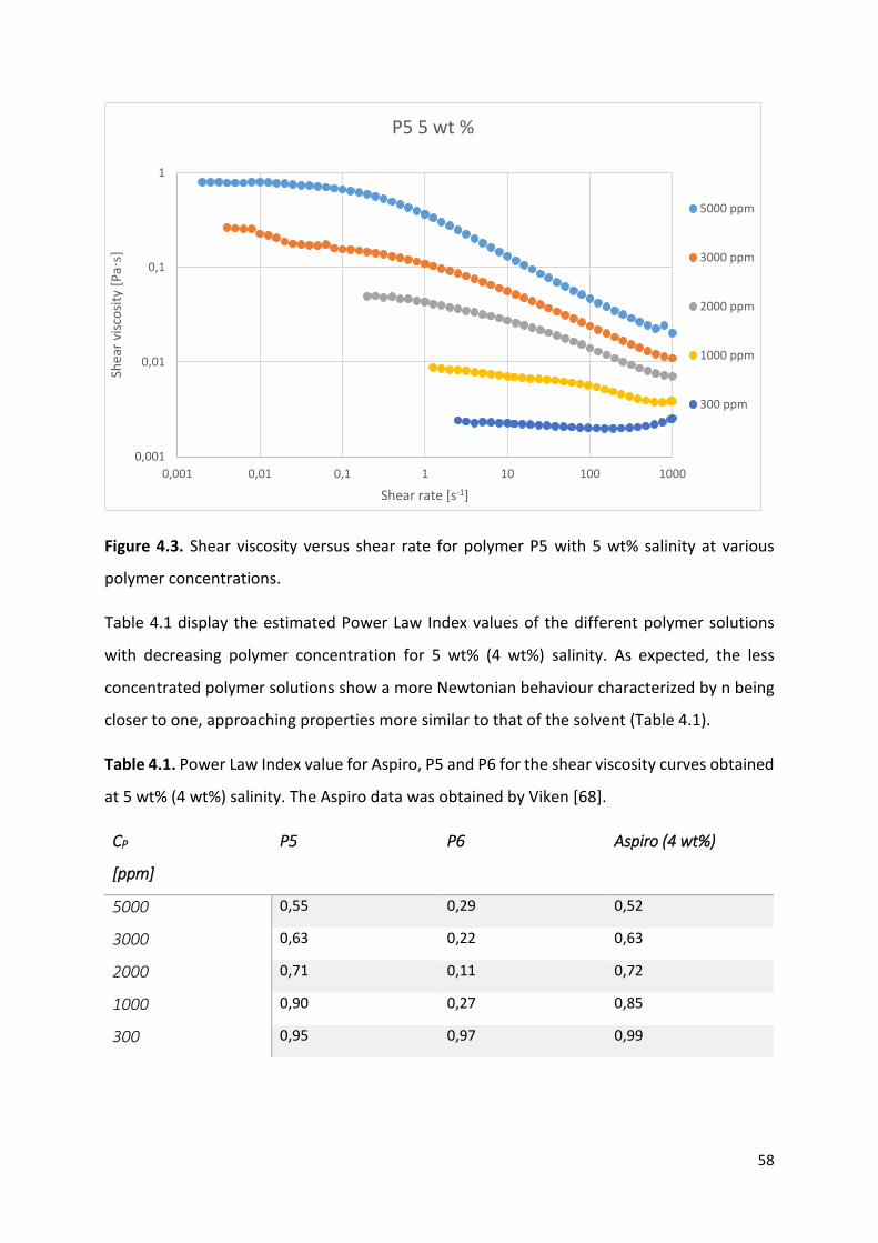
58

Figure 4.3. Shear viscosity versus shear rate for polymer P5 with 5 wt% salinity at various

polymer concentrations.

Table 4.1 display the estimated Power Law Index values of the different polymer solutions

with decreasing polymer concentration for 5 wt% (4 wt%) salinity. As expected, the less

concentrated polymer solutions show a more Newtonian behaviour characterized by n being

closer to one, approaching properties more similar to that of the solvent (Table 4.1).

Table 4.1. Power Law Index value for Aspiro, P5 and P6 for the shear viscosity curves obtained

at 5 wt% (4 wt%) salinity. The Aspiro data was obtained by Viken [68].

CP

[ppm]

P5 P6 Aspiro (4 wt%)

5000 0,55 0,29 0,52

3000 0,63 0,22 0,63

2000 0,71 0,11 0,72

1000 0,90 0,27 0,85

300 0,95 0,97 0,99

0,001

0,01

0,1

1

0,001 0,01 0,1 1 10 100 1000

Shea

r vi

sco

sity

[P

a·s]

Shear rate [s-1]

P5 5 wt %

5000 ppm

3000 ppm

2000 ppm

1000 ppm

300 ppm

59

The Power Law Indexes goes from more to less shear thinning behaviour in accordance with

increasing HLB-value of the polymers. The more hydrophobic polymers show a larger degree

of shear thinning (Figure 4.4).

Illustrated by the Power Law Index gradually increasing with decreasing polymer

concentration, revealing less shear thinning behaviour as the polymer concentration

decreases (Table 4.1). The lesser Power Law Index shown for the intermediate concentrations

of P6 is a result of the specific shear rate interval chosen. Viewing only the indexes for 5000

to 300 ppm CP for P6, the Power Law Index clearly increases (Table 4.1).

Figure 4.4. Shear viscosity versus shear rate for polymer P5 with 5 wt% salinity at various

polymer concentrations.

0,001

0,01

0,1

1

10

100

0,001 0,01 0,1 1 10 100 1000

Shea

r vi

sco

sity

[P

a s]

Shear rate [s-1]

P6 5 wt %

5000 ppm

3000 ppm

2000 ppm

1000 ppm

300 ppm

60

Figure 4.5. Shear viscosity versus shear rate for Aspiro with 4 wt% salinity at various polymer

concentrations. The Aspiro data was obtained by Viken [68].

Earlier studies have shown how the polymer viscosity decreases with increasing levels of

salinity for the acrylamide-based HMPAM [8, 12]. The same behaviour can be seen for 5000

ppm P5 polymer solutions with increasing salinity from 0.1 wt% to 10 wt% (Figure 4.6). Similar

behaviour is observed for P5 and Aspiro. At 0.1 wt% salinity, the polymer solutions have

significantly larger viscosities compared to the rest of the polymer solutions. The other

polymer solutions (> 0.1 wt%) have viscosities who are more similar to each other, with maybe

1 wt% being the exception at low rates of shear (Figure 4.6).

0,001

0,01

0,1

1

0,01 0,1 1 10 100 1000

Shea

r ra

te [

Pa

s]

Shear rate [s-1]

Aspiro 4 wt%

5000 ppm

3000 ppm

2000 ppm

1000 ppm

300 ppm

61

Figure 4.6. Shear viscosity as a function shear rate for polymer P5 with a 5000 ppm polymer

concentration containing salinities of 0.1 wt%, 1 wt% and 10 wt%. The other salinities can be

found in the Appendix.

The shear-thinning region also seem to become smaller with increasing salinity (Figure 4.6).

The amount of curves and their similar trends makes detailed characterization of each

polymer solution challenging.

4.2 Effect of concentration on solution viscosity measured at 10 s-1 shear rate

To make the data from the shear viscosity measurements easier to analyse and interpret, a

measured value from a shear rate of 10 s-1 was exctracted from each shear viscosity curve.

The readings at 10 s-1 shear rate are located within the linear viscoelastic range and at low

levels of shear. Table 4.2 and 4.3 presents the recorded shear viscosities at 10 s-1 shear rate

for all the polymer solutions of P5 and P6. Table 4.4 presents the same kind of data from

Viken’s Aspiro measurements [68].

0,01

0,1

1

10

100

0,001 0,01 0,1 1 10 100 1000

Shea

r vi

sco

sity

[P

a·s]

Shear rate [s-1]

P5 5000 ppm

0.1 wt%

1 wt%

10 wt%

62

Table 4.2. Measured viscosity at 10 s-1 for P5 associative polymer for different salt and polymer

dilutions. Viscosities are listed in Pascal seconds.

[ppm] 0,1 wt% 1 wt% 5 wt% 10 wt% 12 wt% 15 wt% 18 wt% 20 wt%

5000 0,56 0,171 0,132 0,136 0,155 0,184 0,22 0,24

3000 0,23 0,066 0,056 0,061 0,068 0,074 0,079 0,113

2000 0,088 0,033 0,028 0,034 0,040 0,041 0,042 0,047

1000 0,033 0,0097 0,0071 0,0103 0,0121 0,0154 0,0124 0,0122

300 0,0060 0,0027 0,0023 0,0023 0,0025 0,0027 0,0026 0,0027

Table 4.3. Measured viscosity at 10 s-1 for P6 associative polymer for different salt and polymer

dilutions. Viscosities are listed in Pascal seconds.

[ppm] 0,1 wt% 1 wt% 5 wt% 10 wt% 12 wt% 15 wt% 18 wt% 20 wt%

5000 0,79 0,40 0,33 0,25 0,27 0,32 0,37 0,41

3000 0,52 0,28 0,23 0,118 0,119 0,136 0,147 0,168

2000 0,25 0,194 0,138 0,095 0,076 0,087 0,078 0,093

1000 0,074 0,053 0,055 0,0033 0,003 0,039 0,025 0,030

300 0,0081 0,0030 0,0027 0,0032 0,0022 0,0028 0,0028 0,0030

63

Table 4.4. Measured viscosity at 10 s-1 for Aspiro at different salt and polymer dilutions. Data

originates from the unpublished experiments conducted by Viken [68]. Viscosities are listed in

Pascal seconds.

[ppm] 0,4 wt% 1 wt% 2 wt% 4 wt% 10 wt% 15 wt% 20 wt%

5000 0,22 0,195 0,136 0,121 0,125 0,125 0,117

3000 0,086 0,048 0,052 0,043 0,044 0,041 0,039

2000 0,042 0,020

1000 0,0130 0,0090 0,0090 0,0070 0,0070 0,0080 0,0070

300 0,0035 0,0027 0,0024 0,0027

4.2.1 Shear viscosity at 10 s-1 shear rate as a function of polymer concentration

Different concentration regimes can be seen by plotting shear viscosity as a function of

logarithmic polymer concentration for the five different polymer concentrations at 0.1 wt%

salinity for polymers P5 and P6 (Figure 4.7).

Figure 4.7. Shear viscosity versus polymer concentration at 0.1 wt% salinity and 10 s-1 shear

rate for polymer P5 and P6.

0

0,1

0,2

0,3

0,4

0,5

0,6

0,7

0,8

0,9

300 3000

Shea

r vi

sco

sity

[P

a·s]

Polymer concentration [ppm]

0.1 % salinity

P5

P6

64

The viscosity increases with increasing polymer concentration for both polymers (Figure 4.7).

P6 have a higher viscosity than P5 at all concentrations, although the difference between them

becomes smaller when the concentration decreases. Two (possibly three) The Aspiro data was

obtained by Viken [68].

Three potential concentration regimes may be observable from the measurements (Figure

4.8). A diluted regime between 300 ppm and 1000 ppm, to a more semi-dilute, or semi-dilute

entangled (concentrated regime), taking place after 1000 ppm. The transition between the

regimes occurs at sudden changes in the viscosity slope.

The measurements at 1 wt% and 5 wt% salinity respectively, show a similar behaviour, but

with a larger difference between the viscosities of P5 and P6 (Figure 4.8). The measured

viscosities of Aspiro at 1 wt% brine salinity have been integrated into the plot [68]. There can

be made a case for a semi-dilute entangled regime taking place for P6 above 1000 ppm. For

P5 and Aspiro, showing relatively similar viscosities, two different concentration regimes

possibly occurs between 1000 and 5000 ppm.

Figure 4.8. Shear viscosity versus polymer concentration at 1 wt% salinity and 10 s-1 shear rate

for polymer P5, P6 and Aspiro. The Aspiro data was obtained by Viken [68].

The shear viscosity as a function of logarithmic polymer concentration for the polymer

solutions containing 10 wt% salinity, may indicate three different concentration regimes

(Figure 4.9). The transition between the regimes occur at sudden changes in the viscosity

where two different linear viscosity lines intersect (as in Figure 2.4.8 from the theory).

0

0,1

0,2

0,3

0,4

0,5

300 3000

Shea

r vi

sco

sity

[P

a·s]

Polymer concentration [ppm]

1 % salinity

P5

P6

Aspiro

65

It can be argued from the plot that the critical overlap concentration, C*, is located

somewhere between 300 and 1000 ppm. The semi dilute regime will then go on until the

critical entanglement concentration is reached somewhere between 3000 and 5000 ppm.

As a convention, a publication by Viken et al. [64] applied the following convention when

classifying the concentration regimes: diluted concentration regime where C < C* (300 ppm),

semi-diluted regime where C > C* (1000 ppm), and entangled semi-dilute regime where C >>

C* (3000 ppm).

We know that the intrinsic viscosity, [η], for the polymers is about 17 dL/g for all polymers (P5,

P6 and Aspiro, source: BASF). This corresponds to a critical overlap concentration, C* = 453

ppm by using C* = 0.77/[η] [32].

The estimates of the critical overlap concentration (C*) qualitatively occurring somewhere

between 300 and 1000 ppm from our plots corresponds relatively good with the calculated

values from the Graessley-relation (Formula 2.2.10) [32].

Table 4.5. Quantified critical overlap concentrations for polymer P5, P6 and Aspiro calculated

using the Graessley-relation (Formula 2.2.10) [32].

Polymer P5 P6 Aspiro

C* [ppm] 440 478 453

66

Figure 4.9. Shear viscosity versus polymer concentration at 10 wt% salinity and 10 s-1 shear

rate for polymer P5, P6 and Aspiro. The Aspiro data was obtained by Viken [68].

Figure 4.10. Shear viscosity versus polymer concentration at 15 wt% salinity and 10 s-1 shear

rate for polymer P5, P6 and Aspiro. The Aspiro data was obtained by Viken [68].

Notice how the gap between P5 and P6 is much smaller for these higher salinities compared

to the intermediate salinities of 1 wt% and 5 wt% (Figure 4.10). P6 with its lower HLB-value

displays higher viscosities than both P5 and Aspiro. As the salinity increases, the gap between

the viscosity of P5 and Aspiro grows larger (Figure 4.11).

0

0,1

0,2

0,3

300 3000

Shea

r vi

sco

sity

[P

a·s]

Polymer concentration [ppm]

10 % salinity

P5

P6

Aspiro

0

0,1

0,2

0,3

0,4

300 3000

Shea

r vi

sco

sity

[P

a·s]

Polymer concentration [ppm]

15% salinity

P5

P6

Aspiro

67

Figure 4.11. Shear viscosity versus polymer concentration at 20 wt% salinity and 10 s-1 shear

rate for polymer P5, P6 and Aspiro. The Aspiro data was obtained by Viken [68].

Few changes in behaviour can be observed between the plots showing viscosity as a function

of polymer concentration for salinities above 10 wt%. Although a slight viscosity-increase take

place between each polymer solution as the salinity increases for P5 and P6. This increase

occurs from 10 wt% to 20 wt% salinity. This change becomes easier to identify in the next

section where the shear viscosity at 10 s-1 shear rate is plotted against the salinity. The plots

containing shear viscosity as a function of polymer concentration for 5 wt%, 12 wt% and 18

wt% are listed in the Appendix.

4.2.2 Shear viscosity at 10 s-1 shear rate as a function of salinity

The effect of salinity on the solution viscosity becomes easier to analyse when the variables

of polymer concentration and shear rate are held constant. As seen from the numerical values

of the viscosities from the plots in Table 4.2, 4.3 and 4.4 (Figure 4.12, 4.13 and 4.14). The

gradient of the viscosity-increase occurring at higher salinities becomes smaller and smaller

0

0,1

0,2

0,3

0,4

0,5

300 3000

Shea

r vi

sco

sity

[P

a·s]

Polymer concentration [ppm]

20 wt% salinity

P5

P6

Aspiro

68

as the polymer concentration lowers. The viscosity values at 0.1 wt% salinity have been left

out of these plots to emphasise the upward concave shape of the viscosity development.

Noticeably, the 20 wt% salinity viscosity for both P5 and P6 is higher than the viscosity at 1

wt% salinity. Albeit, this only occurs at 5000 ppm polymer concentration.

Figure 4.12. Shear viscosity as a function of salinity at 10 s-1 shear rate for polymer P5 at 5000,

3000, 2000, 1000 and 300 ppm concentrations. The exclusion of measurements for 0.1 wt%

salinity emphasizes the viscosity increase occurring at high levels of salinity.

As apparent from these three figures comparing all the five concentrations, the viscosity

increase occurring at high levels of salinity becomes smaller as the CP decreases (Figure 4.12,

4.13 and 4.14). At lower concentrations of polymer, a viscosity increase arguably becomes

negligible, or smaller than the error margins. The solution viscosity eventually flattens out and

approaches linear trends similar to that of the solvent.

0

0,1

0,2

0,3

0,4

0,5

0% 5% 10% 15% 20%

Shea

r vi

sco

sity

[P

a s]

Shear rate [s-1]

P5

5000 ppm

3000 ppm

2000 ppm

1000 ppm

300 ppm

69

Figure 4.13. Shear viscosity as a function of salinity at 10 s-1 shear rate for polymer P6 at 5000,

3000, 2000, 1000 and 300 ppm concentrations. The exclusion of measurements for 0.1 wt%

salinity emphasizes the viscosity increase occurring at high levels of salinity.

No viscosity increase takes place at the higher levels of salinity for Aspiro (Figure 4.14). The

viscosity decline as the salinity increases, subsequently reaching minimum viscosities.

Figure 4.14. Shear viscosity as a function of salinity at 10 s-1 shear rate for Aspiro at 5000,

3000, 2000, 1000 and 300 ppm concentrations. The Aspiro data was obtained by Viken [68].

0

0,1

0,2

0,3

0,4

0,5

0% 5% 10% 15% 20%

Shea

r vi

sco

sity

[P

a s]

Shear rate [s-1]

P6

5000 ppm

3000 ppm

2000 ppm

1000 ppm

300 ppm

0

0,1

0,2

0,3

0,4

0,5

0,00% 5,00% 10,00% 15,00% 20,00%

Shea

r vi

sco

sity

[P

a s]

Shear rate [s-1]

Aspiro

5000 ppm

3000 ppm

2000 ppm

1000 ppm

300 ppm

70

The plots below show how different levels of salinity affect the viscosity at 10 s-1 shear rate

for each polymer concentration (Figure 4.15, 4.16, 4.17, 4.18 and 4.19). The polymer solutions

containing 0.1 wt% salinity maintains the highest viscosity for every polymer concentration.

The viscosity then drops with increasing salinity of the brine, reaching its lowest value

somewhere between 5 wt% and 10 wt% occurring at 5000, 3000 and 2000 ppm. The viscosity

of Aspiro falls, and then stays stable at a low viscosity with increasing salinity.

The shear viscosity as a function of salinity for 5000 ppm polymer solutions reveal how the

viscosity decreases from 0.1 wt% to 5 wt% for both P5 and P6 (Figure 4.15). It reaches its

lowest value at 5 wt% for P5, and at 10 wt% for P6. For salinities higher than 10 wt%, the

viscosity increases, displaying higher values all the way up to 20 wt% salinity. This behaviour

produces an upward concave shape (4.12 and 4.13).

Figure 4.15. Shear viscosity as a function of salinity for 5000 ppm polymer solutions of P5, P6

and Aspiro at 10 s-1 shear rate. The Aspiro data was obtained by Viken [68].

For the plots representing the measured viscosities at 3000 ppm, the viscosities of the HMPAM

decrease at the intermediate salinities (Figure 4.16). P6 show a more similar behaviour to the

behaviour at 5000 ppm compared to P5. The viscosity of P5 drops quite heavily and stays low,

0

0,1

0,2

0,3

0,4

0,5

0,6

0,7

0,8

0,9

0,00% 5,00% 10,00% 15,00% 20,00%

Shea

r vi

sco

sity

[P

a·s]

10

s-1

Salinity [wt%]

5000 ppm

P5

P6

Aspiro

71

with a much less pronounced viscosity build-up taking place at the higher salinities compared

to 5000 ppm (Figure 4.16). This reduced viscosity regeneration as the CP decreases is observed

for both P5 and P6. Aspiro remain at the same viscosity as the salinity increases above the

intermediate salinities. This trend is repeated for all concentrations of Aspiro.

Figure 4.16. Shear viscosity as a function of salinity for 3000 ppm polymer solutions of P5, P6

and Aspiro at 10 s-1 shear rate. The Aspiro data was obtained by Viken [68].

At 2000 ppm polymer concentration, the same trend is observable, with a heavy drop in P5’s

viscosity compared to that of P6 (Figure 4.17). At high salinities, the viscosity build-up may still

exist, or may just be fluctuations within the error the margins of the measurements.

0

0,1

0,2

0,3

0,4

0,5

0,6

0,00% 5,00% 10,00% 15,00% 20,00%

Shea

r vi

sco

sity

[P

a·s]

10

s-1

Salinity [wt%]

3000 ppm

P5

P6

Aspiro

72

Figure 4.17. Shear viscosity as a function of salinity for 2000 ppm polymer solutions of P5, P6

and Aspiro at 10 s-1 shear rate. The Aspiro data was obtained by Viken [68].

At 1000 ppm polymer concentration, a very similar behaviour to that of 2000 ppm CP is seen

(Figure 4.18). Heavy drops in the P5 viscosity from 0.1 wt%, which stays at relatively similar

levels for all the other salinities. The viscosity decline of P6 with increasing salinity now have

a less exponential gradient. The measured viscosity at 5 wt% salinity is actually higher that

that at 1 wt% salinity, although taking the ± 5wt% deviation into consideration, it might as well

be lower. The polyelectrolyte Aspiro show no changes in behaviour with increasing salinity.

Between 10 wt% and 20 wt% salinity, the viscosities remain at constant levels, although a

higher viscosity is observed for both P5 and P6 at 15 wt% salinity.

0

0,05

0,1

0,15

0,2

0,25

0,3

0,00% 5,00% 10,00% 15,00% 20,00%

Shea

r vi

sco

sity

[P

a·s]

10

s-1

Salinity [wt%]

2000 ppm

P5

P6

Aspiro

73

Figure 4.18. Shear viscosity as a function of salinity for 1000 ppm polymer solutions of P5, P6

and Aspiro at 10 s-1 shear rate. The Aspiro data was obtained by Viken [68].

The shear viscosity as a function of salinity for 300 ppm polymer concentration drops beyond

0.1 wt% salinity, and then stays at the same viscosity for all the rest of the higher salinity

polymer solutions (Figure 4.19). Except for the viscosities at 0.1 wt% salinity, the viscosities of

P5, P6 and Aspiro (0.4 wt%) seem to be undistinguishable from each other at 300 ppm polymer

concentration (Figure 4.19). The lack of measurements at 0.1 wt% salinity for Aspiro prevents

getting confirmation about whether the viscosity of the hydrophobic polymers is lower than

that of the polyelectrolyte in the dilute regime.

0

0,02

0,04

0,06

0,08

0,1

0,00% 5,00% 10,00% 15,00% 20,00%

SHea

r vi

sco

sity

[P

a·s]

10

s-1

Salinity [wt%]

1000 ppm

P5

P6

Aspiro

74

Figure 4.19. Shear viscosity as a function of salinity for 300 ppm polymer solutions of P5, P6

and Aspiro at 10 s-1 shear rate. The Aspiro data was obtained by Viken [68].

Summed up, the upward concave viscosity trend is more pronounced for P6 compared to P5,

where the viscosities arguably flattens out at 3000 ppm CP. P6 also generate superior

viscosities compared to P5. P6 also displays a relatively more sloped viscosity decline than P5

for the higher polymer concentrations. The Aspiro have the same viscosities as P5 at the

intermediate levels of salinity.

4.3 Oscillatory measurements (viscoelastic measurements)

This section contain information about the viscoelastic behaviour of the two polymers,

assessed through plots showing the loss factor as a function of salinity at 1 rad/s angular

frequency (Formula 2.2.12). Amplitude sweeps determined the LVE-range [11]. Provided

information of the LVE-range from the amplitude sweeps, the frequency sweeps producing

the data of the following plots took place.

Viscoelasticity in polymers produce a ‘pulling effect’ on the residual oil trapped by capillary

forces [6]. Polymers that exhibit properties that are more elastic are more efficient in

recovering the residual oil [6].

0

0,002

0,004

0,006

0,008

0,01

0,00% 5,00% 10,00% 15,00% 20,00%

Shea

r vi

sco

sity

[P

a·s]

10

s-1

Salinity [wt%]

300 ppm

P5

P6

Aspiro

75

Viscoelastic measurements determines the viscous and the elastic components of the polymer

solutions [64]. Table 4.6 and Table 4.7 show the measured values for the loss factor for all the

different salinities at 1 rad/s angular frequency. A loss factor below one indicate elastically

dominated behaviour of the polymer solution [11]. A loss factor above one indicate viscously

dominated behaviour [11].

Table 4.6. Table showing the recorded values for tan delta at 1 rad/s angular frequency as a

function of salinity for polymer P5 and P6.

Salinity

[wt%]

5000 ppm 3000 ppm

P5 P6 P5 P6

0.1 0,51 0,43 0,61 0,48

1 0,97 0,60 1,50 0,54

5 1,32 0,62 0,93 0,55

10 0,85 0,74 0,65 0,73

12 0,89 0,72 0,88 0,99

15 0,78 0,84 1,30 1,09

18 0,79 0,78 1,16 0,73

20 0,56 0,75 0,49 0,91

Table 4.7. Table showing the recorded values for tan delta at 1 rad/s angular frequency as a

function of salinity for Aspiro. The Aspiro data was obtained by Viken [68].

Salinity

[wt%]

5000 ppm 3000 ppm

Aspiro Aspiro

0.4 0,90 1,44

1 0,92 1,83

2 1,10 2,09

4 1,44 2,48

10 1,38 2,87

15 1,58 2,99

20 2,09 3,96

76

The loss factor increases from 0.1 wt% to 5 wt% for polymer P5 at 5000 ppm polymer

concentration, i.e. becoming more viscously dominated (Figure 4.23). The trend reveal

elastically dominated behaviour up until 1 wt% salinity, where viscous behaviour starts to

dominate. Then the loss factor of P5 starts to decrease from 5 wt% salinity all the way to 20

wt% salinity, becoming elastically dominated yet again somewhere between 5 wt% and 10

wt% salinity. Some fluctuations occur between 10 wt% and 20 wt%, but these fall within the

error margins. P6 starts to become slightly more viscous as the salinity increases, but stays

elastically dominated the entire time for 5000 ppm polymer concentration.

The Aspiro show elastic behaviour for salinities of 0.4 wt% and 1 wt% at 5000 ppm CP.

Afterwards, the Aspiro becomes viscously dominated, and increasingly more so, albeit a

slightly lower loss factor reading at 10 wt% compared to 5 wt% (within the error margins).

Figure 4.20. The loss factor versus salinity at 1 rad/s angular frequency for 5000 ppm polymer

solutions. The Aspiro data was obtained by Viken [68].

For 3000 ppm polymer concentrations at 1 rad/s, a similar behaviour for the three polymers

can be seen. P6 shows elastic dominated behaviour along the entire curve for 3000 ppm as

well, considering the error margins. The loss factor of P6 steadily increases. P5 shows a similar

behaviour as at 5000 ppm polymer concentration, but the highest value of the loss factor is

0

0,5

1

1,5

2

2,5

0,1 1 10 100

Loss

fac

tor

Salinity [wt%]

5000, 1rad/s

P5

P6

Aspiro

77

located at 1 wt% salinity instead of at 5 wt% salinity as for the 5000 ppm CP values. The Aspiro

is viscously dominated for all the salinities at 3000 ppm polymer concentration. The elastically

dominated Aspiro becomes increasingly more viscous, same as for 5000 ppm. P5 and P6 show

also show an increase and subsequent decrease in the loss factor between 10 wt% and 20 wt%

salinity. The locally highest viscosity in this salinity range is located at 15 wt% salinity for both

P5 and P6.

Figure 4.21. The loss factor versus salinity at 1 rad/s angular frequency for 3000 ppm polymer

solutions. The Aspiro data was obtained by Viken [68].

0

1

2

3

4

0,1 1 10 100

Loss

fac

tor

Salinity [wt%]

3000, 1 rad/s

P5

P6

Aspiro

78

5 Discussion

When evaluating hydrophobically modified polyelectrolytes for use in EOR-applications, the

challenge is to find the optimal balance between charge, hydrophobic monomer content, and

structure/hydrophobicity of the hydrophobic monomers. The ultimate goal is to obtain a

product that is water soluble, while at the same time generating as high viscosity and

viscoelasticity as possible, under the relevant reservoir conditions.

In this study, we investigate two hydrophobically modified anionic polymers. The polymers

have the same backbone, including anionic content, equal amounts of hydrophobic

substitution, but different chemical composition of the hydrophobes. The results are

compared to the corresponding anionic polymer without any hydrophobic substitution. The

goal is to provide insight into how salinity affects the interplay between intra- and

intermolecular electrostatic and hydrophobic interactions, which in turn governs the viscosity

and viscoelasticity of the polymer solutions. Is the HLB-value itself a critical parameter? If yes,

will a high or a low HLB-value be favourable for the investigated polymer structure having the

same balance between charge and hydrophobic monomer content as well as identical

polymer backbones?

Based on the HLB-value of the hydrophobe, P6 has a higher degree of hydrophobicity

compared to P5. P5 is therefore expected to show a lesser tendency for hydrophobic

association than P6.

5.1 Shear viscosity measurements

The shear thinning behaviour observed in all the shear viscosity curves occur due to the

polymer molecules untangling and aligning themselves with the direction of flow [11]. The

reason less concentrated solutions behave more like Newtonian fluids relates to the degree

of entanglements of the polymer molecules in solution [11]. Solutions that are more

concentrated contain more polymer, resulting in more entanglements between the polymers,

and vice versa [28]. More entanglements brings about a more viscous solution, giving rise to

increased shear sensitivity.

79

At low rates of shear in the upper Newtonian plateau, before the critical shear rate, the shear

forces untangling the polymer molecules exist to such a small degree that an equilibrium

where the polymer molecules untangle and re-entangle takes place (Figure 2.2.4) [11]. This

equilibrium gives the zero shear viscosity. The lower Newtonian plateau where the polymer

molecules are untangled and aligned with the flow direction, gives the infinite shear viscosity

[11].

The artificially high viscosities measured at high rates of shear for the less concentrated and

less viscous polymer solutions most likely ascribe to the change from laminar to turbulent flow

in the fluid sample, and is an experimental artefact [66]. Solutions that are more viscous

generates larger drag forces, thereby stabilizing the flow. The minuscule viscosity increase

occurring at high shear rates for more viscous polymer solutions may be due to the

Weissenberg effect dragging the polymer sample away from the area beneath the spindle

[67]. In this case, it is an experimental artefact, and is a result of excess fluid outside the

spindle generating an extra drag force showing up as an increased viscosity in the

measurement data.

Feng et al. [25] observed shear thickening behaviour for HMPAM (2.25 x 106 g mol-1) at shear

rates between 1 s-1 and 10 s-1 and salinities above 1.5 M NaCl, although this was not observed

for our shear viscosity measurements (Figure 4.1).

Increased amount of entanglements leads to a higher viscosity for concentrations above the

critical overlap concentration, as explained in the theory [11]. The lower HLB-value of P6 result

in a higher viscosity compared to P5 and Aspiro, as observed in the plots from the results

(Figure 4.11). The stronger hydrophobic associations of the non-polar hydrophobic groups

causes stronger network structures in solution [55]. The viscosity is preserved and not

negatively affected by the electrostatic screening to the same degree as for the higher HLB-

value analogues [56]. These networks still remain effective at lower concentrations, making

the more hydrophobic P6 more shear thinning at similar levels of polymer concentration

compared to P5 and Aspiro (Table 4.1). Aspiro, P5 and P6 display increased Newtonian

behaviour as the CP lowers (Figure 4.3, 4.4 and 4.5). Polymer solutions with higher viscosities

contain more entanglements, making them more sensitive to applied shear (Figure 4.1 and

4.2) [11].

80

The need of larger shear forces and a larger shear intervals to untangle all the polymer

molecules produces this enhanced shear thinning behaviour [23]. The less viscous polymer

solutions display more Newtonian behaviour similar to the solvent due to their weaker and

less numerous entanglements and networks (Table 4.1).

Increased ionic strength of the brine reveal a clear decrease in viscosity. Increasing salinity

makes the polymer solution less shear thinning, confirmed by the increasing Power Law Index

(Table 4.1). The distinctly higher viscosity at 0.1 wt% salinity seen in all of the polymer

solutions compared to higher salinities stems from less cationic electrostatic screening of the

carboxylic groups on the polymer chains [11]. The polymer chains have a larger chain

extension in solutions with low ionic strength [12]. The viscosity then decreases as more

carboxylic groups become screened by cations, reducing the polymer chain extension, thereby

reducing the hydrodynamic volume [11]. The lower viscosities of Aspiro compared to P5 and

P6 in the semi-dilute entangled regime can be explained by the latter polymers hydrophobic

interactions [8].

5.2 Extracted shear viscosity measured at 10 s-1 shear rate

5.2.1 Shear viscosities at 10 s-1 shear rate as a function of polymer concentration

The lowest polymer concentrations constitute the dilute regime [11]. There, the viscosity is

expected to decline, caused by the solution reaching levels of dilution that causes the

movement of polymer molecules to not affect other polymer molecules [22]. This decline is

due to both the charge screening of the polyer backbone and enhancement of intramoelcular

association (salting out effects) [11].

According to theory, in the dilute regime, where the polymer molecules occur in single coils,

expected viscosity levels for P5, P6 and Aspiro should be equal. In fact, in a dilute system,

associative polymers with the lower HLB-values should be expected to generate lower

viscosities compared to a polymer with a larger HLB-value [8]. This is due to the single coils

with a low HLB-value being less soluble with increasing solution polarity [11]. This increases

the intramolecular associations. Their lower solubility causes them to contract more

81

extensively than their more soluble counterparts, thereby obtaining smaller hydrodynamic

volumes [8]. Their smaller hydrodynamic volumes makes them generate lower viscosities.

In the more concentrated regimes on the other hand, the longer hydrophobic chain length

responsible for lower HLB-values works the other way [8]. Here, the greater hydrophobicity

brings about higher viscosities [8]. The polymer molecules now find themselves close enough

to each other to form entanglements and complexes, facilitating intermolecular associations.

The greater hydrophobicity favours aggregation of larger molecular complexes and

entanglements because of their higher number of hydrophobic connection points [12].

Increased solution polarity amplifies this trend by making the hydrophobes less soluble [8].

This further forces them into developing micellar-like structures and aggregates that increases

their hydrodynamic volume (Figure 2.2.9) [42].

Interpretations of the plots reveal both intramolecular and intermolecular associations as the

polymer concentration increases (Figure 4.7 – 4.11). In the dilute regime, a difference in

viscosity between the three polymers cannot be identified above 1 wt% salinity (Figure 4.19).

Intramolecular forces dominates now [11]. There is no visible effect of the hydrophobic

groups, only at 0.1 wt%, which is strange (Figure 4.19). The viscosity of P6 should be lower

than both P5 and Aspiro according to theory [57]. More hydrophobic polymers are expected

to have a lower viscosity than less hydrophobic polymers in the dilute regime [8] (Figure 4.19).

At 0.1 wt% and 1 wt% salinity, entrance into the concentrated regime occurs at lower polymer

concentrations compared to their higher salinity analogues (4.7 – 4.11). The transition from

the semi-dilute into the concentrated regime appears to be happening between 1000 and

2000 ppm for the lower salinity polymer solutions (Figure 4.7).

The higher viscosities generated at low salinity polymer solutions takes place because of lesser

electrostatic shielding of the carboxylic groups on the polymer chains [57]. These carboxylic

groups are responsible for stretching the polymers chains, resulting in large hydrodynamic

volumes [8]. This prominent electrostatic stretching is a result of repulsive interactions

between the negatively charged anionic groups sitting on the polymer backbone [40].

At higher salinities around 10 wt% and 12 wt%, the concentrated regime seems not to be

reached before polymers concentrations exceed 3000 ppm (4.10 and 4.11). Here the

electrostatic shielding by cations in solution happens to a larger degree [49]. This reduces the

82

hydrodynamic volume of the polymers in solution [11]. Now the polymers will be unable to

form the same entanglements and complexes occurring at lower levels of salinity, given their

compromised extension [8].

The exact location of the critical overlap concentrations and the transition points into the

concentrated regime requires further examination and a larger number of measuring points.

Nonetheless, the linear trends of the concentration regimes arguably becomes identifieable

from the dataset (Figure 4.10). The critical overlap concentration seems to lie between 300

and 1000 ppm, judging from the plots (Figure 4.7 – 4.11). The qualitative estimations of the

critical overlap concentrations corresponds fairly well with the quantified values calculated

from the intrinsic viscosity of all the polymers, estimating the C* to be located around a 400 -

500 ppm polymer concentration (Aspiro, P5 and P6) (Table 4.5). The location of the critical

entanglement concentration where the semi-dilute entangled regime starts sits between 3000

and 5000 ppm for the polymer solutions (Figure 4.10 and 4.11).

The gap in viscosity between P5 and P6 is comparatively large at 0.1 wt% salinity (Figure 4.7).

The gap expands at the intermediate salinities of 1 wt% and 5 wt% (Figure 4.8). At 10 wt%, all

the way to 20 wt%, the difference in viscosity between the two polymers become smaller

(Figure 4.9 – 4.11). For some salinities, there can be made a case for the existence of three

different concentration regimes (4.9 – 4.11). At some other salinities, only two concentration

regimes become visible. Given that these charts only contain five measurement points, exact

determination of concentration regimes will be complicated, and there may as well exist three

concentration regimes for all the different salinities.

Noticeably, the viscosity of P5 and Aspiro stays relatively similar at low levels of salinity (4.7

and 4.8). When the ionic strength of the solution increases, the gap between them grows

larger (4.9 – 4.11). This may indicate that the viscosity of P5 increases as the ionic strength

increases. The Aspiro remains unaffected by increased ionic strength, corresponding with

existing theory regarding polyelectrolytes [11]. P6 have the highest viscosity for all the

polymer solutions.

The numerical viscosities and the entrance into the concentrated regimes occur first in the

order of Aspiro < P5 < P6. This is in accordance to the HLB-value increasing in the following

order Aspiro < P5 < P6.

83

5.2.2 Shear viscosity at 10 s-1 shear rate as a function of salinity

The initial large drop in viscosity occurring at low levels of salinity from very high viscosity

values to lower levels can be seen in all the plots (4.12 - 4.19). Sorbie experienced similar kinds

of declines for HPAM, where the major changes occurred between distilled water to 0.2 - 0.3

wt% salinity (Figure 2.3.3) [11]. The solution goes from no ions present in solution to suddenly

ions being present. The resulting electrostatic screening then goes from nonexistence to

significantly influencing the polymer solution behaviour [52]. Only a small amount of ions gives

rise to a large number of electrostatic interactions, resulting in a collapsing solution viscosity

(Figure 2.3.3) [11]. The reason many curves only show the viscosity-decreasing sections of

such plots is due to most polymer experiments never exceed the salinity levels of seawater.

Therefore, many experiments never examines polymer behaviour with salinities larger than 5

– 10 wt%.

It seems to be the case that the gap in viscosity between P5 and P6 is relatively large at 0.1

wt% salinity (Figure 4.15 – 4-17). The gap then extends at the intermediate salinities of 1 wt%

and 5 wt%. At 10 wt% salinity, all the way up to 20 wt% salinity, the difference in viscosity

between the two polymers once more becomes smaller (Figure 4.15 – 4.17). This may be a

result of the electrostatic repulsive forces being at its weakest at intermediate salinities [45].

The hydrophobic interactions, quantified by the difference in HLB-value, will then have a larger

influence on the viscosity, resulting in a large difference between the viscosity of P5 and P6

for intermediate salinities [12].

The trend seen in the plots showing shear viscosity as a function of salinity illustrates how the

viscosity both decreases and increases with rising salinity for the higher polymer

concentrations of the hydrophobic polymers (Figure 4.12 and 4.13). Three different scenarios

will here most likely be responsible for the development of the upward concave curve.

Entanglement, cationic cross-linking and electrostatic interactions could be used to explain

the viscosity behaviour of these measurements [11].

Entanglement in concentrated random-coil flexible polymers are considered in terms of a

network of bridges [29]. Increased entanglement increases the viscosity of a polymer solution.

Large degrees of entanglements occur at high polymer concentrations [8]. Entanglements will

84

be affected by the CP plus the hydrophobicity of the polymers, and would therefore not be

expected to change with increasing salinity.

The cationic cross-linking effect may either increase or decrease the hydrodynamic volume of

polymer solutions (Figure 2.3.7). Intramolecular cross-linking decreases the hydrodynamic

volume in dilute concentrations, where occupation of the anionic seats by cations reduces the

viscosity [8].

Whereas intermolecular cross-linking may increase the viscosity through the formation of

macromolecules in more concentrated concentration regimes [8]. Enhancement of the cross-

linking effect responsible for forming large macromolecules increases the viscosity up until a

critical value where the molecules become so large precipitation starts to happen (Figure

2.3.9). Precipitation reduces the viscosity. The cationic cross-linking effect works together with

hydrophobic groups to form large macromolecules even at lower CP, forming large

hydrodynamic volumes, thereby increasing the solution viscosity.

Even though the hydrophobic and the entanglement forces exerts an influence, the upward

concave trend visible from the plots showing shear viscosity as a function of salinity most likely

show a behaviour dominated by the electrostatic changes occurring [45] (Figure 4.12 and

4.13). The magnitude of the electrostatic forces seem to significantly outweigh the forces of

hydrophobic nature, even though the difference in HLB-value between P6 and P5 also seem

to play a part.

Kedir et al. reported of chain re-expansion of polymer chains with increased salinity for HPAM

due to electrostatic repulsion effects, producing the upward concave trend for the viscosity as

a function of salinity [45]. Kedir et al. concluded that it was mainly the electrostatic repulsion

forces inside the polymer entanglements being responsible for this behaviour (Figure 2.3.9).

From our results, the electrostatic contribution to the solution viscosity bahviour can be

explained as follows (Figure 4.12 - 4.19). In distilled water with low salt concentrations,

negative-negative repulsion effects expands the polymer chains in solution, increasing the

hydrodynamic volume [11]. Addition of salt to the polymer solution leads to a screening-effect

of the repulsive electrostatic forces that lowers the hydrodynamic volume [69]. At

intermediate salinities, cations occupies more of the anionic seats on the polymer backbones,

inducing minimum viscosity levels. Here, the net charge between the charged bodies equals

85

zero (Figure 2.3.3). These observations align themselves with existing theory regarding

HPAM’s solution behaviour [11].

Further salinity increase eventually result in positive-positive repulsions through charge

inversion, re-expanding the polymer chains in solution (Figure 2.3.9) [45]. These positive-

positive repulsions stems from the repulsions between the screening cations now occupying

all the anionic groups (Figure 2.3.9) [52]. Viscosity elevation from the resulting increased

hydrodynamic volumes ensues, up until critical levels of salinity, where precipitates starts

forming. Precipitation then dramatically reduces the solution viscosity [12]. Some published

research did not experience this positive-positive repulsion [49, 53]. Although these

experiments have taken place without the same levels of entanglement and with short-

chained polymer molecules.

This behaviour do not explain why such an increase do not occur for Aspiro (Figure 4.14). An

explanation may be that the hydrophobic associations contribute to the enhancement of the

entanglements. Polymer chains with their charged groups will constitute the entanglements

taking place in our polymer solutions (Figure 2.2.7) [29]. Changes in solution polarity expands,

retracts and re-expands the polymer chains forming the entanglements, thereby altering the

hydrodynamic volumes of the macromolecules [45].

Reduced polymer chain expansion may hinder the polymers in forming large entanglements

(Figure 2.3.5). Thus may be used to explain the relative decrease and subsequent increase in

viscosity as the solution polarity increases. Entanglements without the support of hydrophobic

associations would possibly not be able to entrap the same amount of polymer chains within

the macromolecules, resulting in little or no changes as the solution polarity increases.

It may also be possible that at the high concentrations, the concentration will be so high that

the electrostatic and entanglement forces marginalizes the viscosity amplifying effect of the

hydrophobic interactions. The scenario being that the concentration now will be sufficiently

high enough to form very strong entanglements. The representation of forces at work may

now be such that the viscosity measured may represent something like 90 percent

entanglement, 8 percent cationic cross-linking and 2 percent hydrophobic interactions [11].

86

In the dilute regime, where the polymer molecules occur in single coils, viscosities of both

HPAM’s and HMPAM are relatively similar [11]. This and the viscosity-increase at high salinities

for the hydrophobic polymers can be also be explained through the HLB-value of the polymers.

According to the findings of Feng et al. [25], in a dilute system, associative polymers with lower

HLB-values are expected to generate lower viscosities compared to a polymer with a larger

HLB-value. This is due to the single coils having a low HLB-value being less soluble with

increasing solution polarity [8]. Their lower solubility causes them to intramolecularly contract

more extensively than their more soluble counterparts, thereby obtaining smaller

hydrodynamic volumes. Their smaller hydrodynamic volumes makes them generate lower

viscosities [8]. This lower viscosity in the dilute regime was not observed in our measurements

(Figure 4.19).

In the more concentrated regimes, greater hydrophobicity brings about higher viscosities

(4.15 and 4.16). The polymer molecules now find themselves close enough to each other to

form entanglements and complexes [25]. The greater hydrophobicity favours aggregation of

larger molecular complexes and entanglements because of their stronger hydrophobicity [55].

Increased solution polarity amplifies this trend by making the hydrophobes less soluble (Figure

4.15 and 4.16). This further forces them into developing micellar-like structures and

aggregates that increases their hydrodynamic volume (Figure 2.2.9) [8].

Measurements by the rheometer for dilute polymer concentrations, the viscosities will

furthermore be so low that the deviations in the measurements by the rheometer reaches

critical levels. The data therefore needs more qualitatively viewing for the lower

concentrations. The data measured at higher concentrations can probably safely be viewed in

a more quantitative light.

As observed in the results, the viscosity increase occurring at high levels of salinity becomes

smaller as the CP decreases (Figure 4.12 and 4.13). At lower concentrations of polymer,

approaching the dilute regime, a viscosity increase arguably becomes negligible, through

being smaller than the error margins (Figure 4.17 – 4.19). The solution viscosity flattens out

and approaches linear trends similar to that of the solvent. Aspiro displays such a behaviour

regardless of polymer concentration, most likely due to its sensitivity to the electrostatic

screening of the carboxylic groups (Figure 4.14) [11].

87

It is observed from the results how a lower HLB-value of the polymer hydrophobe, or some

degree of hydrophobicity generates higher viscosities for all salt concentrations (Figure 4.12 –

4.14). Rosland [70] did not experience the increase in viscosity at high salinities, although

those experiments did not include levels of salinity above 5 wt%. Therefore, same as in our

experiments, the same reduction of viscosity with increasing salinity was observed for the low

levels of salinity (Figure 4.12 – 4.14).

5.3 Oscillatory measurements (viscoelastic measurements)

The viscoelasticity has been a feature that still lack understanding concerning the behaviour

of the hydrophobic groups in solvents containing divalent ions. Previous studies have shown

how the viscoelasticity is strongly influenced by the addition of hydrophobic groups in

modified polyacrylamide [64].

The inverse of the frequency at the crossover point, when G’=G’’ (loss factor = 1), gives the

relaxation time of the molecules in solution [11]. When the relaxation time have a large value,

it means the elastic component of the solution is large [34]. A large elastic component means

that the molecules can store energy. With a large viscous component, energy is lost to friction

and molecules gliding past each other [6].

The loss factor, tan δ, obtained at an angular frequency of 1 rad/s and 10% strain, is plotted

against the salinity (Figure 4.20 and 4.21) . With addition of salt and an increase in the ionic

strength, the three polymers behave differently. Increasing the strength of the hydrophobic

association seems to improve the elasticity of the polymer solutions (Table 4.6 and 4.7). This

is in accordance with the HLB-value, as the polymers display elastic behaviour in the following

order Aspiro < P5 < P6. This matches the behaviour from the experiments conducted by

Rosland [70].

As seen from the results, the balance between the elastic and the viscous contribution in the

viscoelasticity of the P6 polymer solutions seem to be relatively unaffected by the addition of

salt (Figure 4.20 and 4.21). This indicate strong entanglements and network formations [27].

P5 on the other hand, seem to at first become more viscously dominated as the salinity

increases (Figure 4.20 and 4.21). Then, as the salinity increases beyond intermediate levels,

88

the solution again becomes more elastic. Overall, P5 and P6 gradually becomes more viscous

as the salinity increases.

The increase and subsequent decrease in elasticity of P5 may be related to the drop in shear

viscosity seen in the shear viscosities extracted at 10 s-1 shear rate (Figure 4.12 and 4.13). The

electrostatic screening of the carboxylic groups on the polymer chains caused this drop by

reducing the hydrodynamic volume of the polymers, thus the viscosity [12]. The inability of

the polymer molecules to form large degrees of entanglements at intermediate salinities may

be due to the compromising of the polymers chain extension [11].

This should also be occurring for P6, but its larger degree of hydrophobicity may allow it to

form sufficient entanglements at similar levels of polymer concentration and salinity

compared to P5 (Table 4.6). This can possibly be explained by assuming that these interactions

are situated in regions where small perturbations have large implications and small variances

may possibly have great effect. Especially since the loss factor is a quotient where a relatively

small change in one of the moduli can result in a substantial alteration in the numerical value

of the loss factor [11].

At levels of salinity above 10 wt%, the viscoelasticity of P5 and P6 becomes similar and difficult

to distinguish from each other (Figure 4.20 and 4.21). Here the salinity may be so high that all

possible cationic cross-linking have occurred and the difference in hydrophobic associations

have marginal effect on the entanglements, thereby the elasticity of the polymers.

Aspiro starts out as viscously dominated, and gradually becomes more and more viscous as

the salinity increases (Table 4.7). This is most likely due to the electrostatic screening of the

polymer chains getting stronger as the salinity increases, reducing their hydrodynamic volume

and degree of entanglement [23].

P5 and P6 show little significant change in loss factor behaviour when the polymer

concentration goes from 5000 ppm to 3000 ppm (Figure 4.20 and 4.21). Aspiro becomes more

viscously dominated as the CP goes from 5000 to 3000 ppm (Figure 4.20 and 4.21). This may

be related to only entanglements contributing to the elasticity of Aspiro [27]. As the CP

decreases, the amount of entanglements decreases [11]. For comparison, the hydrophobic

polymers may rely on both hydrophobic associations and entanglements to sustain elastic

behaviour [8].

89

Some of the viscoelastic measurements in these results may be unreliable. Especially the

viscoelastic measurements for 3000 ppm polymer concentration (Figure 4.21). The section at

high salinities above 10 wt% salinity where the loss factor recordings fluctuate up and down,

can be considered implausible. The reason for the fluctuations remain unknown, although

sufficient knowledge and construction of the oscillating frequency sweep sequences may play

a part. The fact that the loss factor is a quotient may also be used to explain the fluctuations,

due to its sensitivity to small changes in the respective moduli.

The elastic behaviour of the three different polymers classifies as follows: P6 > P5 > Aspiro.

This corresponds to the HLB-value of the three polymers (Table 3.3).

90

6 Summary and conclusions

When evaluating hydrophobically modified polyelectrolytes for use in EOR-applications, the

challenge is to find the optimal balance between charge, hydrophobic monomer content, and

structure/hydrophobicity of the hydrophobic monomers. The ultimate goal is to obtain a

product that is water soluble, while at the same time generating as high viscosity and

viscoelasticity as possible, under the relevant reservoir conditions.

In this study we have investigated two hydrophobically modified anionic polymers. The

polymers have the same backbone, including anionic content, equal amounts of hydrophobic

substitution, but different chemical composition of the hydrophobes. The effect of the

chemical composition of the hydrophobe on shear viscosity and viscoelasticity for two

associative polymers was examined with varying levels of salinity. The results were compared

to the corresponding anionic polymer without any hydrophobic substitution.

For the hydrophobically modified polyelectrolytes there is a significant increase in viscosity for

polymer solutions above the critical overlap concentration, in the semi-dilute and the

entangled semi-dilute regime, regardless of hydrophobe with lower/higher HLB or salinity. P6

proved to be able to generate much higher viscosities compared to P5. In the entangled semi-

dilute regime, both polymers showed increasing viscosity when the salinity increased over 10

wt%, likely due to the onset of significant intermolecular hydrophobic interactions. The

highest viscosities occurred at 0.1 wt% for all the polymers. The lowest viscosities were found

at intermediate salinity levels of 5 wt% and 10 wt%. At salinities of 10 wt% and less, P5 showed

little difference from Aspiro. This is likely due to the interrelationship of hydrophobic

associative behaviour and electrostatic- repulsion, screening and chain re-expansion.

Both P5 and P6 displayed greater elasticity than Aspiro. Further, the elasticity of solutions of

P6 appeared to be unaffected by salinity changes, while the elasticity of P5 showed a clear

salinity dependence.

For all the different polymer concentrations and salinities, P6 display almost one order of

magnitude higher viscosity than P5, which implies a much more suited polymer for high

salinity reservoir conditions. The viscosity enhancement of P6 relative to P5 increases as the

polymer concentration decreases, confirming its superiority considering field operation floods

91

occur at polymer concentrations approximating 1000 ppm, not taking injectivity, retention

and cost into account. The results indicate that a low HLB-value will be favourable for the

investigated polymer structure with the same backbone, anionic content and equal amounts

of hydrophobic substitution.

92

7 Further work

The Malvern Kinexus pro+ rheometer used for the measurements in this thesis is designed to

perform measurements within a broad measuring range. Use of a more shear sensitive

rheometer would make it possible to measure the zero shear viscosity and more accurately

estimate the different concentration regimes for the polymer solutions.

It would also be interesting to improve the resolution of the measurements by increasing the

amount of salinity and concentration measuring points, as well as expanding the salinity

measurement area. This will give a better understanding of the viscosity development as the

salinity increases, and help to determine the critical salinity concentrations where precipitates

starts to form. Such improved plots can also be used to better identify local

maximum/minimum viscosities as the salinity increases, and determine whether these points

are the same for both polymers. The dilute, semi-dilute and entangled regimes will then

become easier to identify.

Seright et al. [26] reported differences between in-situ and bulk rheology for HPAM. Thus,

another aspect can be to perform core flood tests using the two associative polymers, thereby

measuring in-situ viscosity and correlate this to the bulk viscosity.

93

8 Bibliography

1. (EIA), U.S.E.I.A. International Energy Outlook 2016. 2017 01.06.17; Available from: https://www.eia.gov/outlooks/ieo/world.cfm.

2. Muggeridge, A., et al., Recovery rates, enhanced oil recovery and technological limits. Philosophical transactions. Series A, Mathematical, physical, and engineering sciences, 2014. 372(2006): p. 20120320-20120320.

3. Awan, R.A., A Survey of North Sea Enhanced-Oil-Recovery Projects Initiated During the Years 1975 to 2005. Society of Petroleum Engineers, 2008. 11(03): p. 16-497.

4. Abidin, A.Z., W.A. Puspasari, and W.A. Nugroho, Polymers for Enhanced Oil Recovery Technology. Procedia Chemistry, 2012. 4: p. 11 - 16.

5. Zolotukhin, A.B. and J.-R. Ursin, Introduction to Petroleum Reservoir Engineering. 2000: Høyskoleforlaget, Norwegian Academic Press.

6. Wang, D., et al., Viscous-Elastic Polymer Can Increase Microscale Displacement Efficiency in Cores, in SPE Annual Technical Conference and Exhibition. 2000, Society of Petroleum Engineers: Dallas, Texas. p. 10.

7. Lien, J.R., Reservoarteknikk I - PTEK212, U.o. Bergen, Editor. 2014: Bergen. p. 1-173. 8. Wever, D.A.Z., F. Picchioni, and A.A. Broekhuis, Polymers for enhanced oil recovery: A

paradigm for structure–property relationship in aqueous solution. Progress in Polymer Science, 2011. 36(11): p. 1558-1628.

9. Sheng, J., Synergistic Mechanisms of ASP Flooding. Upstream Pumping, 2012. 2(Fall): p. 1-6.

10. Dong, H., et al., Review of Practical Experience & Management by Polymer Flooding at Daqing, in SPE Synopsium on Improved Oil Recovery. 2008, Society of Petroleum Engineers: Tulsa, Oklahoma.

11. Sorbie, K.S., Polymer-Improved Oil Recovery. 1st ed. 1991: Springer Netherlands. 359. 12. Reichenbach-Klinke, R., et al., Associative Copolymer with Favorable Properties for

the Application in Polymer Flooding, in SPE International Symposium on Oilfield Chemistry. 2011, Society of Petroleum Engineers: The Woodlands, Texas. p. 1-11.

13. Flory, P.J., Principles of Polymer Chemistry. 1st ed. Vol. 1. 1953, Cornell University Press: Cornell University Press. 29 - 104.

14. Staudinger, H., Über Polymerisation. Berichte der deutschen chemischen Gesellschaft, 1920. 53(6): p. 1073 - 1058.

15. Berg, J.C., An Introduction to Interfaces and Colloids - The Bridge to Nanoscience. 2010, World Scientific. p. 1-773.

16. Hiemenz, P.C. and T.P. Lodge, Polymer Chemistry. 2nd ed. Vol. 2. 2007: Taylor & Francis.

17. Leszczyszyn, O. Hydrodynamic Radius - Radius of Gyration. Materials Talks 2012 15 November 2012; Available from: http://www.materials-talks.com/blog/2012/11/15/size-matters-rh-versus-rg/.

18. Kok, C.M. and A. Rudin, Relationship between the hydrodynamic radius and the radius of gyration of a polymer in solution. Macromolecular Rapid Communications, 1981. 2(11): p. 655-659.

19. Macosko, C.W., Rheology: Principles, Measurements and Applications. 1st ed. 1994, Michigan: VCH. 550.

94

20. Khan, S.A., J.R. Royer, and S.R. Raghavan, Rheology: Tools and Methods. Aviation Fuels with Improved Fire Safety. Vol. 6. 1997: National Research Council. 126.

21. Nash, W.A., Schaum's Outline of Theory and Problems of Strength of Materials. 1st ed. 1957: Schaum. 301.

22. Regalado, E.J., J. Selb, and F. Candau, Viscoelastic Behaviour of Semidilute Solutions of Multisticker Polymer Chains. Macromolecules, 1999. 32(25): p. 8580 - 8588.

23. Seright, R.S., et al., Rheology of a New Sulfonic Associative Polymer in Porous Media. Society of Petroleum Engineers, 2011. 14(06): p. 726-734.

24. Barnes, H.A., J.F. Hutton, and K. Walters, An Introduction to Rheology. Vol. 1. 1989: Elsevier Science & Technology.

25. Feng, Y., et al., Effects of NaCl on steady rheological behaviour in aqueous solutions of hydrophobically modified polyacrylamide and its partially hydrolyzed analogues prepared by post-modification. Polymer International, 2002. 51(10): p. 939 - 947.

26. Seright, R.S., et al., New Insights Into Polymer Rheology in Porous Media. SPE Journal, 2011. 16(01): p. 35-42.

27. Heemskerk, J., et al., Quantification of Viscoelastic Effects of Polyacrylamide Solutions, in SPE Enhanced Oil Recovery Symposium. 1984, Society of Petroleum Engineers: Tulsa, Oklahoma.

28. Holmberg, K., et al., Surfactants and Polymers in Aqueous Solution. 2nd ed. 2002: Wiley. 562.

29. Wool, R.P., Polymer entanglements. Macromolecules, 1993. 26(7): p. 1564-1569. 30. Lopes, L.F., B.M. Silveira, and R.B.Z.L. Moreno, Rheological Evaluation of HPAM fluids

for EOR Applications. International Journal of Engineering & Technology, 2014. 14(3): p. 1-35.

31. Mutch, K.J., J.S. van Duijneveldt, and J. Eastoe, Colloid-polymer mixtures in the protein limit. Royal Society of Chemistry, 2007. 3(2): p. 155-167.

32. Graessley, W.W., Polymer Chain Dimensions and the Dependence of viscoelastic properties on the concentration, molecular weight and solvent power. Polymer, 1980. 21(3): p. 258-262.

33. Hiemenz, P.C. and T.P. Lodge, Polymer Chemistry. 2nd ed. Vol. 9. 2007: Taylor & Francis. 608.

34. Sheng, J., Modern Chemical Enhanced Oil Recovery. 1st ed. Gulf Proffesional Publishing. Vol. 1. 2010, Elsevier: Elsevier. 648.

35. Wyss, H.M., R.J. Larsen, and D.A. Weitz, Oscillatory Rheology - Measuring the Viscoelastic Behaviour of Soft Materials. G.I.T. Laboratory Journal, 2007. 3(4): p. 68-70.

36. Hyun, K., et al., A Review of Nonlinear Oscillatory Shear Tests: Analysis and Application of Large Amplitude Oscillatory Shear (LAOS). Progress in Polymer Science, 2011. 36(12): p. 1697-1753.

37. Duffy, J. Using Rheology to Design Better Products - Yield Stress and How to Measure It. American Laboratory 2012 July 24, 2012; Available from: http://www.americanlaboratory.com/914-Application-Notes/117719-Ask-the-Expert-Using-Rheology-to-Design-Better-Products-Yield-Stress-and-How-to-Measure-It/.

38. Morgan, S.E. and C.L. McCormick, Water-soluble polymers in enhanced oil recovery. Progress in Polymer Science, 1990. 15(1): p. 103-145.

95

39. Seright, R.S., et al., Stability of Partially Hydrolyzed Polyacrylamides at Elevated Temperatures in the Absence of Divalent Cations. Society of Petroleum Engineers, 2010. 15(02): p. 1-8.

40. Stokes, R. and D. Evans, Fundamentals of Interfacial Engineering. illustrated ed. Wiley-VCH. 1997: John Wiley & Sons.

41. Lake, L.W., Enhanced Oil Recovery. 1989: Prentice Hall. 550. 42. Niu, Y., et al., Research on Hydrophobically Associating Water-soluble Polymer Used

for EOR, in SPE International Synopsium on Oilfield Chemistry. 2001, Society of Petroleum Engineers: Houston, Texas. p. 4.

43. Yu, J.F.S., J.L. Zakin, and G.K. Patterson, Mechanical degradation of high molecular weight polymers in dilute solution. Journal of Applied Polymer Science, 1979. 23(8): p. 2493-2512.

44. Kheradmand, H. and J. Francois, Hydrolysis of polyacrylamide and acrylic acid-acrylamide copolymers at neutral pH and high temperature. Polymer, 1988. 29(5): p. 860-870.

45. Kedir, A.S., et al., Re-entrant transition of aluminum-crosslinked partially hydrolyzed polyacrylamide in a high salinity solvent by rheology and NMR. Journal of Applied Polymer Science, 2016. 133(33): p. 1-12.

46. Shupe, R.D., Chemical Stability of Polyacrylamide Polymers. Society of Petroleum Engineers, 1981. 33(08): p. 1-17.

47. Kenyeres, J.S. and V. Ursu, Polyacrylamide. I. Polymer content and hydrolysis level determination by potentiometric titration. Journal of Polymer Science, 1980. 18(1): p. 275 - 281.

48. Debye, P. and E. Huckel, The theory of electrolytes: I. Lowering of freezing point and related phenomena. Physicalische Zeitschrift, 1923. 24: p. 185-206.

49. Ward, J.S. and F.D. Martin, Prediction of Viscosity for Partially Hydrolyzed Polyacrylamide Solutions in the Presence of Calcium and Magnesium Ions Society of Petroleum Engineers, 1981. 21(05): p. 1-9.

50. Chauveteau, G., K. Denys, and A. Zaitoun, New Insight on Polymer Adsorption Under High Flow Rates, in SPE/DOE Improved Oil Recovery Synopsium. 2002, Society of Petroleum Engineers: Tulsa, Oklahoma.

51. Yang, G., et al., Effects of Ca2+ bridge cross-linking on structure and pervaporation of cellulose/alginate blend membranes. Journal of Membrane Science, 2000. 175(1): p. 53 - 60.

52. Solis, F.J. and M. Olvera de la Cruz, Flexible linear polyelectrolytes in multivalent salt solutions: Solubility conditions. EPJ direct, 2001. 2(1): p. 1-18.

53. Vermolen, E.C.M., et al., Low-Salinity Polymer Flooding: Improving Polymer Flooding Technical Feasibility and Economics by Using Low-Salinity Make-up Brine, in International Petroleum Technology Conference. 2014, International Petroleum Technology Conference: Doha, Qatar. p. 15.

54. Maia, A.M.S., R. Borsali, and R.C. Balaban, Comparison between a polyacrylamide and a hydrophibically modified polyacrylamide flood in a sandstone core. Materials Science and Engineering: C, 2009. 29(2): p. 505-509.

55. Shi, L.-T., et al., Study on Properties of Branched Hydrophobically Modified Polyacrylamide for Polymer Flooding. Journal of Chemistry, 2013. 2013: p. 1-5.

96

56. Taylor, K.C. and H.A. Nasr-El-Din, Water-soluble hydrophobically associating polymers for improved oil recovery: A litterature review, in SPE International Symposium on Oilfield Chemistry. 1995, Society of Petroleum Engineers: San Antonio, Texas. p. 16.

57. Kujawa, P., et al., Effect of Ionic Strength on the Rheological Properties of Multisticker Associative Polyelectrolytes. Macromolecules, 2006. 39(1): p. 384 - 392.

58. Hill, A., F. Candau, and J. Selb, Properties of hydrophobically associating polyacrylamides: influence of the method of synthesis. Macromulecules, 1993. 26(17): p. 4521 - 4532.

59. Volpert, E., J. Selb, and F. Candau, Associating behaviour of polyacrylamides hydrophobically modified with dihexylacrylamide. Polymer, 1998. 39(5): p. 1025 - 1033.

60. Candau, F. and J. Selb, Hydropbhobically-modified polyacrylamides prepared by micellar polymerization. Advances in Colloid and Interface Science, 1999. 79(2): p. 149 - 172.

61. Greth, G.G. and J.E. Wilson, Use of the HLB system in selecting emulsifiers for emulsion polymerization. Journal of Applied Polymer Science, 1961. 5(14): p. 135 - 148.

62. Aulton, M.E., Pharmaceutics: The Science of Dosage Form Design, ed. K. Taylor. Vol. 2nd. 2001: Churchill Livingstone. 704.

63. Gaillard, N. and C. Favero, High molecular weight associative amphoteric polymers and uses thereof, S. S.A.S., Editor. 2010, Google Patents: US.

64. Løbø Viken, A., T. Skauge, and K. Spildo, Rheological properties of a hydrophobically modified anionic polymer: Effect of varying salinity and amount of hydrophobic moieties. Journal of Applied Polymer Science, 2016. 133(23): p. 1-8.

65. Zhang, Y. and P.S. Cremer, Interactions between macromolecules and ions: the Hofmeister series. Current Opinion in Chemical Biology, 2006. 10(6): p. 658-663.

66. Malvern, I.L. Kinexus pro+. 2017 01.04.2017; 01.04.2017:[Available from: http://www.malvern.com/en/products/product-range/kinexus-range/kinexus-pro-plus/.

67. Dealy, J.M. and T.K.P. Vu, The Weissenberg effect in molten polymers. Journal of Non-Newtonian Fluid Mechanics, 1977. 3(2): p. 127-140.

68. Viken, A.L., Rheological Measurements of Aspiro. Unpublished, University of Bergen. 69. Finch, C.A., Water-soluble polymers: Synthesis, solution properties and applications.

American Chemical Society, 1993. 30(1): p. 137-138. 70. Rosland, T.C., Associative Polymers for Enhanced Oil Recovery - Influence of ionic

strength and polymer hydrophobicity on rheological behaviour, in Department of Chemistry. 2016, University of Bergen: Bergen. p. 81.

97

Appendix A – Brine solutions

Table A.1. Weight parameters for NaCl and CaCl2.

Salinity

[wt%]

NaCl

[g]

CaCl2 + H2O

[g]

CaCl2

[g]

H2O

[g]

Total weight

[g]

0.1 1,78 0,29 0,22 1997,93 2000,00

1 17,78 2,94 2,22 1979,28 2000,00

5 88,89 14,71 11,11 1896,39 2000,00

10 177,77 29,43 22,22 1792,78 2000,00

12 213,33 35,32 26,66 1751,34 2000,00

15 266,66 44,15 33,33 1689,17 2000,00

18 320,00 52,98 40,00 1627,01 2000,00

20 355,55 58,87 44,44 1585,57 2000,00

Table A.2. Weight parameters for NaCl and CaCl2.

Salinity

[wt%]

NaCl

[mol]

CaCl2

[mol]

NaCl

[M]

CaCl2

[M]

XNaCl

[ ]

XCaCl2

[ ]

Ionic strength

[M]

0.1 0,0304 0,0015 0,01523 0,0007 0,00027 0,000013 0,017

1 0,3042 0,0151 0,15364 0,0076 0,002759 0,000137 0,177

5 1,5210 0,0756 0,80054 0,0398 0,0142069 0,000705 0,920

10 3,0421 0,1512 1,69003 0,0840 0,0295034 0,001465 1,942

12 3,6505 0,1814 2,07413 0,1031 0,0359557 0,001786 2,383

15 4,5631 0,2267 2,6842 0,1334 0,0460201 0,002286 3,084

18 5,4757 0,2721 3,3388 0,1659 0,0565779 0,002811 3,837

20 6,0841 0,3023 3,8026 0,1889 0,0639088 0,003175 4,369

98

Table A.3. Uncertainties for calculated parameters of the brine solutions.

Salinity

[wt%]

NaCl

[mol]

CaCl2

[mol]

NaCl

[M]

CaCl2

[M]

XNaCl

[ ]

XCaCl2

[ ]

Ionic strength

[M]

0.1 0,0002 0,0007 0,0001 0,0004 0,0000005 0,000007 0,009

1 0,0002 0,0007 0,0001 0,0004 0,0000004 0,000007 0,009

5 0,0002 0,0007 0,0002 0,0005 0,0000004 0,000007 0,01

10 0,0002 0,0007 0,0002 0,0005 0,0000003 0,000008 0,01

12 0,0002 0,0007 0,0002 0,0005 0,0000003 0,000008 0,01

15 0,0002 0,0007 0,00009 0,0004 0,00004 0,000007 0,008

18 0,0002 0,0007 0,00009 0,0004 0,000004 0,000007 0,008

20 0,0002 0,0007 0,0001 0,0004 0,0000009 0,000007 0,009

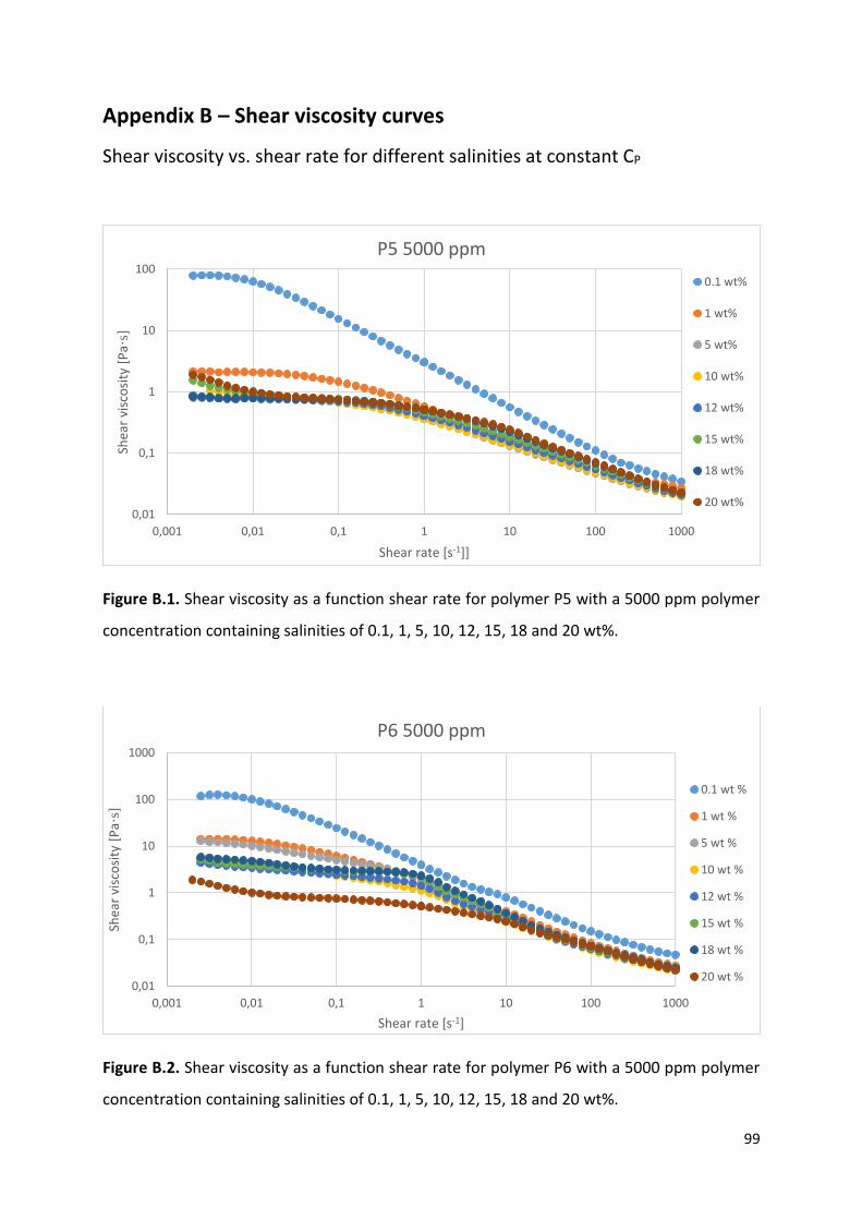
99

Appendix B – Shear viscosity curves

Shear viscosity vs. shear rate for different salinities at constant CP

Figure B.1. Shear viscosity as a function shear rate for polymer P5 with a 5000 ppm polymer

concentration containing salinities of 0.1, 1, 5, 10, 12, 15, 18 and 20 wt%.

Figure B.2. Shear viscosity as a function shear rate for polymer P6 with a 5000 ppm polymer

concentration containing salinities of 0.1, 1, 5, 10, 12, 15, 18 and 20 wt%.

0,01

0,1

1

10

100

0,001 0,01 0,1 1 10 100 1000

Shea

r vi

sco

sity

[P

a·s]

Shear rate [s-1]]

P5 5000 ppm

0.1 wt%

1 wt%

5 wt%

10 wt%

12 wt%

15 wt%

18 wt%

20 wt%

0,01

0,1

1

10

100

1000

0,001 0,01 0,1 1 10 100 1000

Shea

r vi

sco

sity

[P

a·s]

Shear rate [s-1]

P6 5000 ppm

0.1 wt %

1 wt %

5 wt %

10 wt %

12 wt %

15 wt %

18 wt %

20 wt %

100

Figure B.3. Shear viscosity as a function shear rate for polymer P5 with a 3000 ppm polymer

concentration containing salinities of 0.1, 1, 5, 10, 12, 15, 18 and 20 wt%.

Figure B.4. Shear viscosity as a function shear rate for polymer P6 with a 3000 ppm polymer

concentration containing salinities of 0.1, 1, 5, 10, 12, 15, 18 and 20 wt%.

0,001

0,01

0,1

1

10

100

0,001 0,01 0,1 1 10 100 1000

Shea

r vi

sco

sity

[P

a s]

Shear rate [s-1]

P5 3000 ppm

0.1 wt %

1 wt %

5 wt %

10 wt %

12 wt %

15 wt %

18 wt %

20 wt %

0,001

0,01

0,1

1

10

100

0,001 0,01 0,1 1 10 100 1000

Shea

r vi

sco

sity

[P

a s]

Shear rate [s-1]

P6 3000 ppm

0.1 wt %

1 wt %

5 wt %

10 wt %

12 wt %

15 wt %

18 wt %

20 wt %

101

Figure B.5. Shear viscosity as a function shear rate for polymer P5 with a 2000 ppm polymer

concentration containing salinities of 0.1, 1, 5, 10, 12, 15, 18 and 20 wt%.

Figure B.6. Shear viscosity as a function shear rate for polymer P6 with a 2000 ppm polymer

concentration containing salinities of 0.1, 1, 5, 10, 12, 15, 18 and 20 wt%.

0,001

0,01

0,1

1

10

0,001 0,01 0,1 1 10 100 1000

Shea

r vi

sco

sity

[P

a s]

Shear rate [s-1]

P5 2000 ppm

0.1 wt %

1 wt %

5 wt %

10 wt %

12 wt %

15 wt %

18 wt %

20 wt %

0,001

0,01

0,1

1

10

100

0,001 0,01 0,1 1 10 100 1000

Shea

r vi

sco

sity

[P

a s]

Shear rate [s-1]

P6 2000 ppm

0.1 wt %

1 wt %

5 wt %

10 wt %

12 wt %

15 wt %

18 wt %

20 wt %

102

Figure B.7. Shear viscosity as a function shear rate for polymer P5 with a 1000 ppm polymer

concentration containing salinities of 0.1, 1, 5, 10, 12, 15, 18 and 20 wt%.

Figure B.8. Shear viscosity as a function shear rate for polymer P6 with a 1000 ppm polymer

concentration containing salinities of 0.1, 1, 5, 10, 12, 15, 18 and 20 wt%.

0,0001

0,001

0,01

0,1

1

0,01 0,1 1 10 100 1000

Shea

r vi

sco

sity

[P

a s]

Shear rate [s-1]

P5 1000 ppm

0.1 wt %

1 wt %

5 wt %

10 wt %

12 wt %

15 wt %

18 wt %

20 wt %

0,001

0,01

0,1

1

0,01 0,1 1 10 100 1000

Shea

r vi

sco

sity

[P

a s]

Shear rate [s-1]

P6 1000 ppm

0.1 wt %

1 wt %

5 wt %

10 wt %

12 wt %

15 wt %

18 wt %

20 wt %

103

Figure B.9. Shear viscosity as a function shear rate for polymer P5 with a 300 ppm polymer

concentration containing salinities of 0.1, 1, 5, 10, 12, 15, 18 and 20 wt%.

Figure B.10. Shear viscosity as a function shear rate for polymer P6 with a 300 ppm polymer

concentration containing salinities of 0.1, 1, 5, 10, 12, 15, 18 and 20 wt%.

0,0001

0,001

0,01

0,1

1

0,01 0,1 1 10 100 1000

Shea

r vi

sco

sity

[P

a s]

Shear rate [s-1]

P5 300 ppm

0.1 wt %

1 wt %

5 wt %

10 wt %

12 wt %

15 wt %

18 wt %

20 wt %

0,001

0,01

0,1

1

0,01 0,1 1 10 100 1000

Shea

r vi

sco

sity

[P

a s]

Shear rate [s-1]

P6 300 ppm

0.1 wt %

1 wt %

5 wt %

10 wt %

12 wt %

15 wt %

18 wt %

20 wt %

104

Shear viscosity vs. shear rate for different CP with constant salinity

Figure B.11. Shear viscosity versus shear rate for polymer P5 with 0.1 wt% salinity at various

polymer concentrations.

Figure B.12. Shear viscosity versus shear rate for polymer P5 with 1 wt% salinity at various

polymer concentrations.

0,001

0,01

0,1

1

10

100

0,001 0,01 0,1 1 10 100 1000

SHea

r vi

sco

sity

[P

a s]

Shear rate [s-1]

P5 0.1 wt %

5000 ppm

3000 ppm

2000 ppm

1000 ppm

300 ppm

0,002

0,02

0,2

2

0,001 0,01 0,1 1 10 100 1000

Shea

r vi

sco

sity

[P

a s]

Shear rate [s-1]

P5 1 wt %

5000 ppm

3000 ppm

2000 ppm

1000 ppm

300 ppm

105

Figure B.13. Shear viscosity versus shear rate for polymer P5 with 5 wt% salinity at various

polymer concentrations.

Figure B.14. Shear viscosity versus shear rate for polymer P5 with 10 wt% salinity at various

polymer concentrations.

0,001

0,01

0,1

1

0,001 0,01 0,1 1 10 100 1000

Shea

r vi

sco

sity

[P

a·s]

Shear rate [s-1]

P5 5 wt %

5000 ppm

3000 ppm

2000 ppm

1000 ppm

300 ppm

0,001

0,01

0,1

1

10

0,001 0,01 0,1 1 10 100 1000

Shea

r vi

sco

sity

[P

a·s]

Shear rate [s-1]

P5 10 wt%

5000 ppm

3000 ppm

2000 ppm

1000 ppm

300 ppm

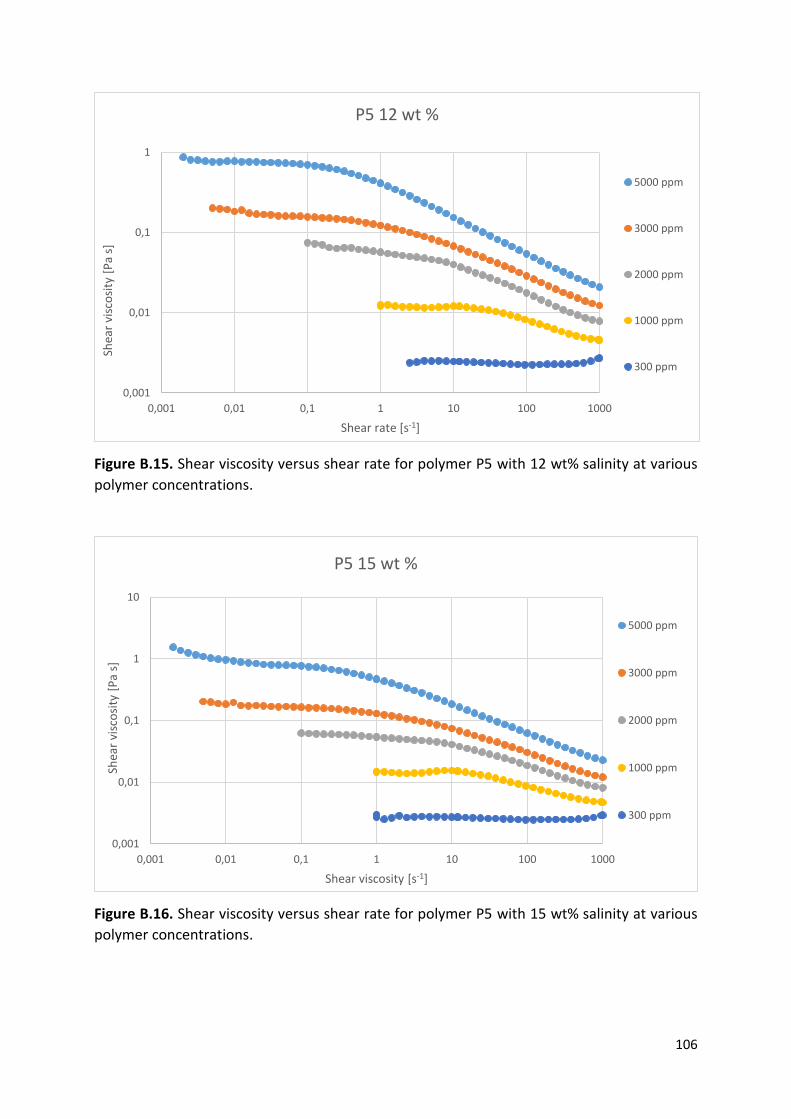
106

Figure B.15. Shear viscosity versus shear rate for polymer P5 with 12 wt% salinity at various

polymer concentrations.

Figure B.16. Shear viscosity versus shear rate for polymer P5 with 15 wt% salinity at various

polymer concentrations.

0,001

0,01

0,1

1

0,001 0,01 0,1 1 10 100 1000

Shea

r vi

sco

sity

[P

a s]

Shear rate [s-1]

P5 12 wt %

5000 ppm

3000 ppm

2000 ppm

1000 ppm

300 ppm

0,001

0,01

0,1

1

10

0,001 0,01 0,1 1 10 100 1000

Shea

r vi

sco

sity

[P

a s]

Shear viscosity [s-1]

P5 15 wt %

5000 ppm

3000 ppm

2000 ppm

1000 ppm

300 ppm

107

Figure B.17. Shear viscosity versus shear rate for polymer P5 with 18 wt% salinity at various

polymer concentrations.

Figure B.18. Shear viscosity versus shear rate for polymer P5 with 20 wt% salinity at various

polymer concentrations.

0,001

0,01

0,1

1

0,001 0,01 0,1 1 10 100 1000

Shea

r vi

sco

sity

[P

a s]

Shear rate [s-1]

P5 18 wt %

5000 ppm

3000 ppm

2000 ppm

1000 ppm

300 ppm

0,001

0,01

0,1

1

10

0,001 0,01 0,1 1 10 100 1000

Shea

r vi

sco

sity

[P

a s]

Shear rate [s-1]

P5 20 wt %

5000 ppm

3000 ppm

2000 ppm

1000 ppm

300 ppm

108

Figure B.19. Shear viscosity versus shear rate for polymer P6 with 0.1 wt% salinity at various

polymer concentrations.

Figure B.20. Shear viscosity versus shear rate for polymer P6 with 1 wt% salinity at various

polymer concentrations.

0,001

0,01

0,1

1

10

100

1000

0,001 0,01 0,1 1 10 100 1000

Shea

r vi

sco

sity

[P

a s]

Shear rate [s-1]

P6 0.1 wt %

5000 ppm

3000 ppm

2000 ppm

1000 ppm

300 ppm

0,001

0,01

0,1

1

10

100

0,001 0,01 0,1 1 10 100 1000

SHea

r vi

sco

sity

[P

a s]

Shear rate [s-1]

1 wt % P6

5000 ppm

3000 ppm

2000 ppm

1000 ppm

300 ppm

109

Figure B.21. Shear viscosity versus shear rate for polymer P6 with 5 wt% salinity at various

polymer concentrations.

Figure B.22. Shear viscosity versus shear rate for polymer P6 with 10 wt% salinity at various

polymer concentrations.

0,001

0,01

0,1

1

10

100

0,001 0,01 0,1 1 10 100 1000

Shea

r vi

sco

sity

[P

a s]

Shear rate [s-1]

P6 5 wt %

5000 ppm

3000 ppm

2000 ppm

1000 ppm

300 ppm

0,001

0,01

0,1

1

10

0,001 0,01 0,1 1 10 100 1000

Shea

r vi

sco

sity

[P

a s]

Shear rate [s-1]

P6 10 wt %

5000 ppm

3000 ppm

2000 ppm

1000 ppm

300 ppm

110

Figure B.23. Shear viscosity versus shear rate for polymer P6 with 12 wt% salinity at various

polymer concentrations.

Figure B.24. Shear viscosity versus shear rate for polymer P6 with 15 wt% salinity at various

polymer concentrations.

0,001

0,01

0,1

1

10

0,001 0,01 0,1 1 10 100 1000

Shea

r vi

sco

sity

[P

a s]

Shear rate [s-1]

P6 12 wt %

5000 ppm

3000 ppm

2000 ppm

1000 ppm

300 ppm

0,001

0,01

0,1

1

10

0,001 0,01 0,1 1 10 100 1000

Shea

r vi

sco

sity

[P

a s]

Shear rate [s-1]

P6 15 wt %

5000 ppm

3000 ppm

2000 ppm

1000 ppm

300 ppm

111

Figure B.25. Shear viscosity versus shear rate for polymer P6 with 18 wt% salinity at various

polymer concentrations.

Figure B.26. Shear viscosity versus shear rate for polymer P6 with 20 wt% salinity at various

polymer concentrations.

0,001

0,01

0,1

1

10

0,001 0,01 0,1 1 10 100 1000

Shea

r vi

sco

sity

[P

a s]

Shear rate [s-1]

P6 18 wt %

5000 ppm

3000 ppm

2000 ppm

1000 ppm

300 ppm

0,001

0,01

0,1

1

10

100

0,001 0,01 0,1 1 10 100 1000

Shea

r vi

sco

sity

[P

a s]

Shear rate [s-1]

P6 20 wt %

5000 ppm

3000 ppm

2000 ppm

1000 ppm

300 ppm

112

Appendix C

Shear viscosity vs. polymer concentration for different salinities at 10 s-1

shear rate

Figure C.1. Shear viscosity versus polymer concentration at 5 wt% salinity and 10 s-1 shear rate

for polymer P5 and P6.

Figure C.2. Shear viscosity versus polymer concentration at 12 wt% salinity and 10 s-1 shear

rate for polymer P5 and P6.

0

0,1

0,2

0,3

0,4

300 3000

Shea

r vi

sco

sity

[P

a·s]

Polymer concentration [ppm]

5 wt % salinity

P5

P6

0

0,1

0,2

0,3

300 3000

Shea

r vi

sco

sity

[P

a·s]

Polymer concentration [ppm]

12 % salinity

P5

P6

113

Figure C.3. Shear viscosity versus polymer concentration at 18 wt% salinity and 10 s-1 shear

rate for polymer P5 and P6.

0

0,1

0,2

0,3

0,4

0,5

300 3000

Shea

r vi

sco

sity

[P

a·s]

Polymer concentration [ppm]

18 wt % salinity

P5

P6