The Effect of Substance Abuse on Employment Status* by Joseph V. Terza** and Peter B. Vechnak Department of Economics, The Pennsylvania State University, University Park, PA 16802, (November, 2007) *This work was supported by the Robert Wood Johnson Foundation Substance Abuse Policy Research Program (RWJF Grant #49981). The authors are grateful to the National Institute on Alcohol Abuse and Alcoholism (in particular Deputy Director Mary C. Dufour, M.D., M.P.H. and Chief of Biometry Branch Bridget F. Grant, Ph.D.) for supplying us with the National Longitudinal Alcohol Epidemiologic Survey data. **Corresponding author, Department of Epidemiology and Health Policy Research, College of Medicine University of Florida, 1329 SW 16 St., Rm. 5278, ph: 352-265-0111 ext 85068, fax: 352- th 265-7221, email: [email protected]

Welcome message from author
This document is posted to help you gain knowledge. Please leave a comment to let me know what you think about it! Share it to your friends and learn new things together.
Transcript

The Effect of Substance Abuse on Employment Status*
by
Joseph V. Terza**and
Peter B. Vechnak
Department of Economics, The Pennsylvania State University,
University Park, PA 16802,
(November, 2007)
*This work was supported by the Robert Wood Johnson Foundation Substance Abuse PolicyResearch Program (RWJF Grant #49981). The authors are grateful to the National Institute onAlcohol Abuse and Alcoholism (in particular Deputy Director Mary C. Dufour, M.D., M.P.H. andChief of Biometry Branch Bridget F. Grant, Ph.D.) for supplying us with the National LongitudinalAlcohol Epidemiologic Survey data.
**Corresponding author, Department of Epidemiology and Health Policy Research, College ofMedicine University of Florida, 1329 SW 16 St., Rm. 5278, ph: 352-265-0111 ext 85068, fax: 352-th
265-7221, email: [email protected]
Abstract
There has been a significant amount of attention paid by health policy researchers to the
effectiveness or efficacy of interventions and policies aimed at reducing substance abuse. Equally
important are the economic costs that can be saved through effective treatment. This paper examines
the economic cost of substance abuse as measured by consequent decreases in the likelihood of
favorable employment outcomes. Our analysis extends the literature in a number of important ways.
First, previous studies focus either on effect of alcohol or a particular individual illicit drug. This
paper expands the analysis to include both alcohol and illicit drugs. Secondly, we address the
possibility that there are important qualitative effects on employment status that are not revealed by
previous analyses based on binary (employed vs. not employed) or trichotomous (out of the labor
force, unemployed, or employed) specifications of the outcome variable. We consider a more
detailed classification (out of the labor force, unemployed, employed part-time, employed full-time
blue collar, employed full-time service sector, or employed full-time white collar). With this finer
classification we are able to observe possibly important differences in abuse effects that heretofore
have gone undetected. Finally we implement an econometric method that simultaneously accounts
for the nonlinearity of the regression model and the potential endogeneity of substance abuse. The
method is applied to data taken from the 1992 National Longitudinal Alcohol Epidemiological
Survey. We find that substance abuse is endogenous and obtain results consistent with the findings
of Kenkel and Wang (1999) – that substance abusers typically land “bad jobs.”

This is of course in addition to the enormous emotional and interpersonal costs that would1
be eliminated by the eradication of substance abuse.
1. Introduction
Much of the research on substance (alcohol or illicit drug) abuse has focused on the
effectiveness or efficacy of specific interventions and policies. In these studies “effect” is typically
measured as the amount by which abuse is consequently decreased. It is equally important to
examine the potential benefits from effective alcohol and drug treatment. Such potential gains are
of course equal to the societal and economic costs imposed by current levels of substance abuse.
Rice et al. (1990) estimate the direct costs of treatment and support for substance abuse at about $9.6
billion, and the cost of abuse-related lost productivity and premature death to be around $60 billion.
This suggests that there are substantial potential economic gains to be obtained from effective
treatment programs.1
In the present paper we confine the discussion to a particular aspect of lost labor market
productivity due to substance abuse. Losses in labor market productivity follow from reductions in:
1) the likelihood of employment; 2) labor supply; 3) on-the-job performance; and 4) earnings. Each
of these components of the aggregate economic costs of substance abuse imposes substantial
hardship on individual workers and their families. Among these four types of labor market
productivity loss, the first is particularly important because the job search and matching process is
antecedent to: 1) decisions by workers (employers) regarding hours of work supplied (demanded);
2) performance by workers on the job; and 3) the payment of wages. Moreover, the process by
which potential workers “select” (are “selected”) into the various employment categories, should be
accounted for in any econometric model of the effects of substance abuse on labor supply, job
performance, or earnings. For example in models of earnings in which the researcher seeks to
The exception is Buchmueller and Zuvekas (1998).2
2
interpret the estimate of the substance abuse effect as the effect on potential earnings for randomly
chosen individuals in the population, a model of employment status (including substance abuse
effects) would be required to deal with bias due to sample selection. Similarly, in two-part or hurdle
models aimed at estimating substance abuse effects on actual earnings, the employment status model
would serve as the first (or hurdle) part of the model.
For these reasons the present paper focuses on the modeling and estimation of the effect of
substance abuse on employment status. This work will extend the literature in this area in three
important ways. First, almost all previous studies of the effects of abuse on employment status have
considered alcohol only. Included in our definition of substance abuse are alcohol and a number2
of illicit drugs (marijuana, cocaine, etc). Secondly, prior research into the effects of substance abuse
on employment status, has been based on coarse categorizations of employment status. For example
Buchmueller and Zuvekas (1998) use a binary categorization (employed vs. not employed), and
Mullahy and Sindelar (1996) use a trichomous taxonomy (employed vs. unemployed vs. out of the
labor force ). We extend their analysis to six categories by dividing the employed category into
subsets for part-time work, full-time blue collar work, full-time service sector work, and full-time
white collar work. This will allow us to examine the effect of substance abuse on job quality. In
many cases individual workers remain employed despite the fact that they are substance abusers.
For such individuals, simple two or three category models will register them as not experiencing
adverse employment effects due to substance abuse. It may, however, be the case that although such
abusers are observed to be employed, the jobs they hold are of lower quality. The present paper
extends the work of Kenkel and Wang (1999) who find that alcoholics are more likely to land jobs

3
with fewer fringe benefits, higher risk of injury, and in smaller firms. The third way in which the
present work adds to the extant body of literature on substance abuse and employment is through the
implementation of an econometric method that accounts for two important technical aspects of
models in this context – the inherent nonlinearity of the regression specification, and the endogeneity
of substance abuse. Buchmueller and Zuvekas (1998) implement a probit model which accounts for
the former but not the latter in a two-category context, and Mullahy and Sindelar (1996) use a two-
equation linear model and conventional instrumental variables estimation which accounts for
endogeneity but not nonlinearity in a three-category setting. We use the method proposed and
implemented in Terza (2001) which accounts for both nonlinearity and endogeneity in a multi-
category discrete outcome context.
Using the 1992 National Longitudinal Alcohol Epidemiological Survey (NLAES) we
estimate the six-category model. We find that substance abuse is endogenous, has a negative and
statistically significant effect on the probability of white-collar employment, and has a positive and
statistically significant effect on the probability of part-time. These results show that the multi-
category extension yields important information not only about whether or not substance abusers find
jobs, but also about the types of jobs they find. This is consistent with the Kenkel and Wang (1999)
“bad jobs” hypothesis.” Abuse is found to be endogenous.
The remainder of the paper is organized as follows. In section 2 we discuss the design of the
econometric model and how it accounts for the inherent nonlinearity of the regression and the
endogeneity of the substance abuse variable. The data and estimation results are examined in section
3. Topics for future research are given in section 4.

4
2. Econometric Model and Estimator
The objective here is the estimation of the effect of substance abuse on the probability of
being in a particular employment category (henceforth referred to as the abuse effect). Define
1 Jy = [y , . . ., y ] such that
1 if the sampled individual is observed to be in employment category j
jy =0 otherwise. (1)
Also let d denote whether (d = 1) or not (d = 0) the individual is a substance abuser. One’s first
inclination is to take a regression approach and define the abuse effect for the jth employment
category as
jÄ * = (2)
jwhere P*(y = 1 | d, w) is the probability of being in the jth employment category conditional on a
vector of observable exogenous variables (w), and d. Assuming a parametric specification for
jP*(y = 1 | d, w) (e.g. the multinomial logit model of McFadden 1973), the model could be estimated
via the maximum likelihood method. The following sample analog to (2) would serve as an to
estimate of abuse effect on the likelihood of being in the jth employment category
(3)
where denotes the estimated conditional probability of being in category j given
5
d and w, computed using the parameter estimates.
The estimator in (3) is likely to be biased, because its formulation, and the parameter
estimates upon which it is based, do not account for the potential presence of unobservable variables
j jthat are correlated with both y and d – so-called confounders. In other words, (3) ignores the
possible endogeneity of the substance abuse variable (d). Such confounders include, among other
things, unreported psychological problems, an unstable upbringing, problems at home, and chronic
pain. With this in mind, we define í to be the scalar random variable summarizing the effects of the
confounders. If d is endogenous, then (2) will not accurately represent the abuse effect because it
will spuriously attribute to d, influences on employment status that are actually due to í. Therefore,
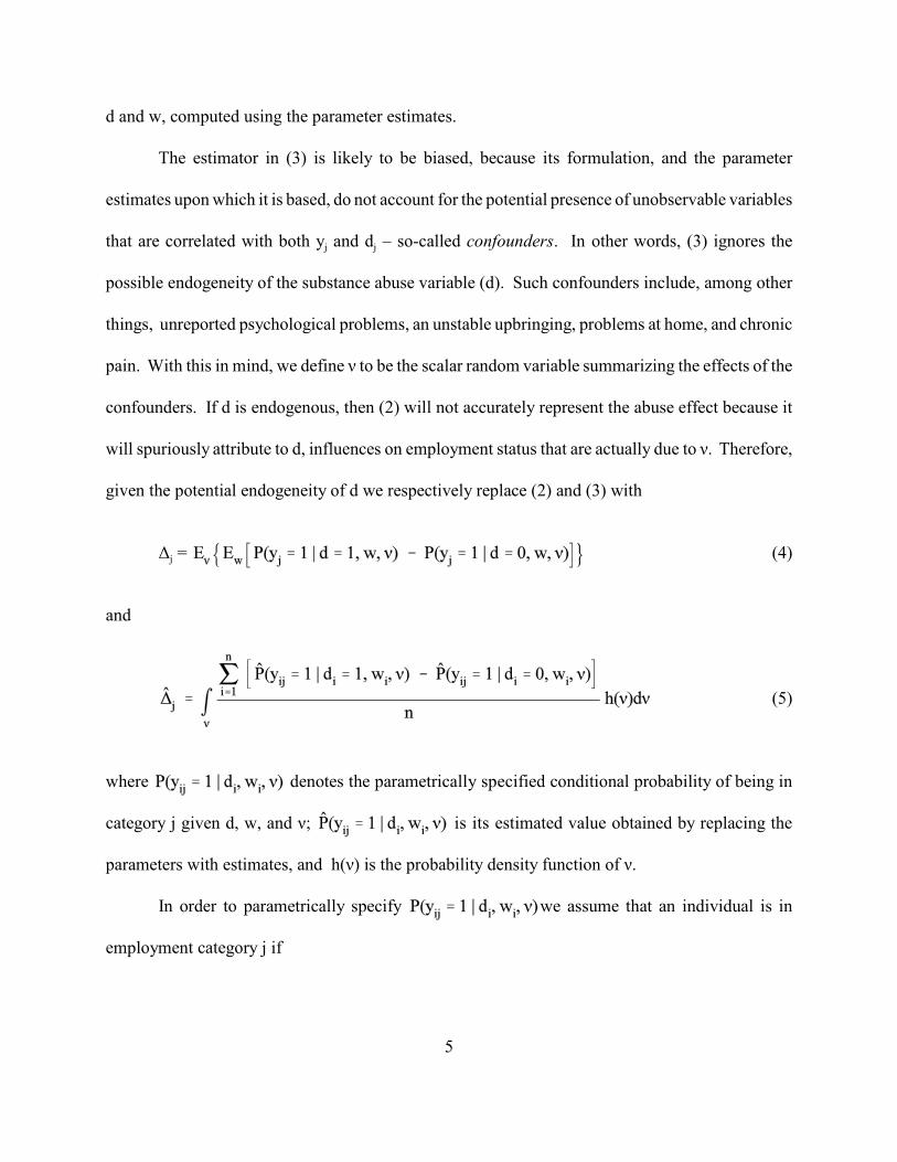
given the potential endogeneity of d we respectively replace (2) and (3) with
jÄ = (4)
and
(5)
where denotes the parametrically specified conditional probability of being in
category j given d, w, and í; is its estimated value obtained by replacing the
parameters with estimates, and h(í) is the probability density function of í.
In order to parametrically specify we assume that an individual is in
employment category j if

6
j r1 if y = max {y ; r = 1, ..., J}* *
jy =0 otherwise (6)
r r r r r rwhere y = dã + xâ + íè + u , the ã ’s are the scalar coefficients of d (the substance abuse* * * * * *
rvariable), x is a row vector of observable exogenous determinants of employment status, the â ’s*
rare the conformable column vectors of coefficient parameters; the è s are the coefficients of í, and*’
rthe u ’s are the non-systematic random components of the utility indices that are not correlated with*
1 J rx, d, or í. The vector u = [u , ... , u ] is i.i.d. log-Weibull distributed. In this context y can be* * *
viewed as the reduced form of the difference between an individual’s best wage offer within the rth
employment category, and his valuation (utility or reservation wage) for being in that employment
category. From (6)
and for (j = 2, ... , J)
(7)
r r 1 r r 1 r r 1where, for identification purposes, â = â - â , ã = ã - ã , and è = è - è . In this framework* * * * * * *
the correlation between d and í is made explicit by assuming that
d = I(zá + í > 0) (8)

7
where z is a vector of exogenous variables influencing the likelihood that an individual will be a
substance abuser, á is the conformable vector of coefficient parameters, w is vector comprising the
union of the exogenous variables in x and z, and I(•) denotes the indicator function.
If we assume a specific form for the pdf of í conditional on w, then the model is completely
parametrically specified and the full information maximum likelihood (FIML) method can be used
to obtain consistent estimates of the parameters. Suppose that (í | w) is standard normally
distributed. Given equations (7) and (8) it is easy to show that the joint pdf of y and d, conditional
on w, is
f(y, d | w) =
. (9)
jwhere P = as defined in (7) for j = 1, ... , J and ö denotes the standard normal pdf.
It follows that consistent estimates of the parameters of the model can be obtained by maximizing
the following likelihood function for a sample of size n
. (10)
where the i subscript denotes the i sample individual (i = 1, ... , n). This is the estimator suggestedth
by Terza (2001).

8
Given our assumed distribution for (í | w) and the parameter estimates, the abuse effect
estimator in (5) becomes
for j = 1, and for j = 2, ... , J it is
(11)
2 J 2 J 2 Jwhere are the FIML estimates of (ã , ..., ã , â , ..., â , è , ..., è ) obtained
from maximizing (11). A convenient feature of this model is that the endogeneity of substance abuse
2 3 Jmay be tested by a conventional Wald test of the null hypothesis that è = è = ... = è = 0 – in
which case d is exogenous.
3. Data and Estimation Results
The data came from Wave 1 (1992) of the National Longitudinal Alcohol Epidemiologic
Survey (NLAES). Wave 1 is composed of data for adults aged 18 years and older taken from a
random sample of U.S. households over the period from October of 1991 to November 1992. Two
follow-up waves were planned using the same respondents, but these waves were not funded. The
primary purpose of the NLAES is the collection of data on the incidence and prevalence of alcohol

9
abuse and dependence and associated disabilities. Fortunately for our purposes, similar information
was collected for illicit drugs. In order to represent the working age population, we restricted the
estimation sample to respondents aged 24 to 59 who answered yes to being in one of the relevant
employment categories. Respondents aged 59 and older are dropped in order to limit the number
of retirees that are present in the data. Secondly, the population under the age of 24 is dropped to
limit the presence of those who are actively pursuing their education full time. Finally, for the
purposes of the present study the out of the labor force category is intended to represent the subset
of discouraged workers. Specifically, it includes those individuals who responded yes to being
unemployed and not looking for work. This, in part, is why the older and younger sampled
individuals are excluded from the analysis. This of course deviates from the Bureau of Labor
Statistics definition of that category which includes those who are in school or retired. Mullahy and
Sindelar (1996) and Terza (2001) impose a similar age group restriction in their studies of
employment status. Full time homemakers are also excluded from the out of the labor force
category. These individuals (mostly women) choose to remain outside of the workforce for
important reasons, such as child rearing. Therefore, including them in the out of the labor force
category would likely serve to obfuscate the true effect of substance abuse on worker
discouragement.
The survey contains a wealth of information on relevant socio-economic and demographic
control variables such as age, gender, race, marital status, and geographic region of residence. There
is also detailed employment status information, including the indicators of current occupation from
which the categorical employment status outcome variables can be constructed. In addition, the
NLAES contains information on alcohol and drug use disorders based on the DSM-IV diagnosis

In addition to alcohol the following drugs were also included in the determination of d: 3
marijuana, cocaine, heroin, opiates, stimulants, sedatives, methadone, tranquilizers, andhallucinogens.
Details of the DSM-IV criteria are given in Table 1.4
10
criteria from which the binary substance abuse variable (d) was coded. The individual is defined as
a substance abuser if he meets the DSM-IV criteria for current abuse and/or dependence.3,4
The qualitative employment status variable y has six categories (j = 1, 2, .., 6) where j =1
denotes the out of the labor force category, and j = 2 denotes unemployed. Sample respondents were
asked questions about their current employment status. Individuals who are not employed but
looking for work were categorized as unemployed, and respondents who are not employed and not
looking for work are considered out of the labor force. Individuals who responded yes to being
employed were further classified as: part-time (j = 3); full-time blue collar (j = 4); full-time service
sector (j = 5); or full-time white collar (j = 6). The latter three of these represent aggregations from
the 3-digit Census Bureau Occupational Classification System. While these partitions are broadly
defined they should allow for greater insights with respect to the potential adverse effects of
substance abuse on employment. For example, consider the possibility that an individual may
remain functional and employed despite substance abuse. For such an individual, a three-category
model (out of labor force vs. unemployed vs. employed) like those implemented by Mullahy and
Sindelar (1996) and Terza (2001) will not reflect any adverse effects of substance abuse. It may,
however, be the case that, although the substance abuser is observed to be employed, the job he holds
is of lower quality. A three-category model will not capture this important result. By broadening
the employed category to include occupational groups it will be possible to observe qualitative

See Kenkel and Wang (1999): Based on the rational addiction model of Becker and Murphy5
(1988), “a rational addict will anticipate the labor market consequences of alcoholism and make jobchoices accordingly.”
Respondents who report being in none or more than one of the employment categories are6
dropped. This winnowing yields a final sample size of 22,107.
11
differences in greater detail.5,6
In addition to the information on employment status and substance abuse the NLAES
contains socio-demographic variables such as gender, race, age, region of residence, living in an
urban setting, and education level. Also, there is information pertaining to the quarter in which the
interview took place, alcoholism of a biological parent, and the number of problematic health
conditions from which an individual currently suffers. To these data we appended three additional
state-level variables: state level unemployment rate, and state beer and cigarette tax rates. These
variables are particularly important as they serve as identifying (instrumental) variables in the
specification of the substance abuse regression (8). The full list of the variables and their definitions
is given in Table 2 with summary statistics provided in Table 3. It is interesting to note that usage
patterns vary substantially according to age. We generally see a greater percentage of younger
people diagnosed as abusers. Figure 1 shows the percentage of alcohol abusers for given ages.
Figure 2 shows the percentage of abusers, by age, for any type of substance. This highlights the
importance of measuring the impact of abuse on job choice since most career decisions are made
relatively early in one’s working life. Table 4 presents some summary statistics that describe the
demographic distribution of abusive behavior.
The following specifications for x and z are used in obtaining FIML estimates of the
parameters [via maximization of (10)]

12

13
x = [CONSTANT, FEMALE, HLTHCOND, HHSIZE, MARRIED, BLACK, ASIAN,
HISPANIC, HIGHSCH, SOMECOLL, COLLEGE, MIDWEST, SOUTH, WEST,
URBAN, QTRINT2, QTRINT3, QTRINT4, UNEMPL92, AGE, AGESQ,]
z = [x, DADALC, MOMALC, ALCTAX, ALCTAXSQ, CIGTAX, CIGTAXSQ].
The FIML estimates of the parameters of (10) are reported in Table 5 and estimates of the
probit coefficients for the substance abuse regression (8) are given in Table 6. We conducted a
o 2 3 4 5 6Wald test of the null hypothesis that abuse is exogenous (H : è = è = è = è = è = 0). Exogeneity
is rejected at a 1% significance level. One of the motivations for including both alcohol and illegal
drugs in our definition of d is to eliminate possible omitted variable bias that may have plagued the
previous studies that consider alcohol abuse only. The argument is that if the abuse of other
substances is omitted from the regression specification and drug abuse is correlated with problem
drinking, then effects on employment that are actually due to drug abuse will be spuriously attributed
to alcohol. In other words, the latent presence of other types of abuse enhances the likelihood that
d will be endogenous. While our approach may have served to alleviate endogeneity due to this
source, the results of our Wald test indicate that other unobservable confounders still remain.
The abuse effects for the six employment categories, estimated as in (11), are reported in
Table 7. The corresponding t-statistics, are computed via the ä-method. The results do indeed reveal
information about the adverse effects of substance abuse on job quality that would have been masked
by a coarser categorization of employment status as in the 3-category models of Mullahy and
Sindelar (1996) and Terza (2001) [out of labor force, unemployed, employed]. To see this, note that
the sum of the estimated abuse effects over the four employed categories is -.048. Although this

14
indicates a negative net effect of substance abuse on employment in a 3-category context, it masks
the large and significant adverse intra-employment-category effects. Specifically, although the net
reduction in the likelihood of employment due to abuse is only 4.8 points, the results in the third and
sixth rows of Table 6 indicate that this number is low because substantial and significant losses in
white collar opportunities (21 points) are being offset by substantial and significant “gains” in the
probability of part-time employment (13 points) – clearly an adverse consequence of substance
abuse.
4. Future Work
The present paper represents a first pass at the topic. We have presented the estimation
results and the estimates of the abuse effects, highlighting empirical insights that the model affords
with regard to the effects of substance abuse on job quality. There are a number of potentially
interesting extensions of the basic model presented here. Recall that we eliminated homemakers
from the sample in order to more purely define the out of the labor force category as representative
of discouraged workers. A by-product of this may be the elimination of the counterintuitive positive
association between alcohol abuse and the probability of being employed for women that was found
by Mullahy and Sindelar (1996). A possible explanation for their result is that women who embrace
traditional roles may, for unobservable reasons, place a higher value on being in one of the non
employed categories. For such women, alcohol and drug abuse may make them more likely to be
employed. In our analysis this effect should be somewhat controlled given our elimination of
homemakers (mostly women) from the estimation sample. To investigate the effectiveness of our

15
sample restriction in this regard, we could estimate separate models for men and women, and
examine (test) whether or not the results differ qualitatively (i.e., with regard to sign) and/or
substantively (i.e. with regard to magnitude) between the sexes.
Another interesting question is whether the adverse employment effects that we find for
generic substance abuse differ from the effects of alcohol abuse alone. This is particularly relevant
to the present analysis because in our NLAES estimation sample, only 7.8% of drug abusers do not
also abuse alcohol. To investigate this question we could estimate the model with d defined on
alcohol abuse only and compare (test) whether the results from this model differ significantly from
those described in the previous section. A conventional Hausman-Wu-type test could be used for
this purpose (see Wu, 1973, and Hausman, 1978).
One of the attractive features of our estimation approach vs. conventional instrumental
variables is the fact that it easily affords the estimation of abuse effects for designated population
subgroups. This feature is particularly useful in the present context given the fact that important
career decisions are made relatively early in life, and younger workers are more likely to be
substance abusers. Younger substance abusers, may be doing relatively more damage to their future
income streams if they tend to land bad jobs (e.g. part-time jobs and other forms of employment that
offer limited prospects for earnings growth). To shed some light on this issue we could use the
estimation results described in the previous section to evaluate the intra-employment effects of
substance abuse among younger workers only. It would be interesting to see if job quality effects
are more severe for young workers than those for older workers.
Human capital effects can also be examined within the context of our model. Adverse abuse
effects on employment as measured in (11) could, for example, be compared to the effect of a college

16
degree. This human capital investment effect could be computed for each of the employment
categories via a formula similar to (11). Such comparisons would reveal the cost of substance abuse
in terms of how it degrades the positive effects that schooling typically has on one’s employment
prospects.

17
References
Becker, Gary and Kevin Murphy (1988). “A Theory of Rational Addiction.” Journal of PoliticalEconomy, 96 (4), pp. 675-700.
Buchmueller, Thomas C. and Samuel H. Zuvekas (1998). “Drug Use, Drug Abuse, and LaborMarket Outcomes.” Health Economics, 7. pp. 229-245.
Hausman, J.A. (1978): “Specification Tests in Econometrics,” Econometrica, 46, 1251-1271.
Kenkel, Don and Ping Wang (1999). “Are Alcoholics in Bad Jobs?” in The Economic Analysis ofSubstance Use and Abuse, Chaloupka, F.J., Grossman, M., Bickel, W.K., and H. Saffer,Chicago: University of Chicago Press.
Landry, M. (1997). Overview of Addiction Treatment Effectiveness. Rockville, MD: SubstanceAbuse and Mental Health Services Administration.
McFadden, D. (1973), “Conditional Logit Analysis of Qualitative Choice Behavior,” in Frontiersin Econometrics, Zarembka, P. (ed.), New York: Academic Press, pp. 105-142.
Mullahy and Sindelar (1996). “Employment, Unemployment, and Problem Drinking.”Journal ofHealth Economics, 15. pp. 409-434.
Rice, Dorothy P., Sander Kelman, Leonard S. Miller, and Sarah Dunmeyer (1990): The EconomicCosts of Alcohol and Drug Abuse and Mental Illness: 1985. Report Submitted to the Officeof Financing and Coverage Policy of the Alcohol, Drug Abuse, and Mental HealthAdministration, U.S. Department of Health and Human Services. San Francisco, CA:Institute for Health & Aging, University of California.
Terza, J.V. (2001): “Alcohol Abuse and Employment: A Second Look” Journal of Applied
Econometrics, forthcoming.
Wu, D. (1973): "Alternative Tests of Independence Between Stochastic Regressors andDisturbances," Econometrica, 41, 733-750.

18
Table 1: The DSM-IV Criteria
The American Psychiatric Association states that addiction is a maladaptive pattern ofsubstance use, leading to clinically significant impairment or distress, as manifested bythree (or more) of the following, occurring at any time in the same 12 month period.
1. Tolerance, as defined by either of the following: A. A need for markedly increased amounts of the substance to achieve intoxication
or desired effect. B. Markedly diminished effect with continued use of the same amount of the
substance
2. Withdrawal, as manifested by either of the following: A. The characteristic withdrawal syndrome for the substance B. The same (or a closely related) substance is taken to relieve or avoid withdrawal
symptoms
3. The substance is often taken in larger amounts or over a longer period than was intended
4. There is a persistent desire or unsuccessful efforts to cut down or control substance use
5. A great deal of time is spent in activities necessary to obtain the substance (e.g., visiting multiple doctors or driving long distances), use the substance (e.g., chain smoking), or recover from its effects
6. Important social, occupational, or recreational activities are given up or reduced because of substance use
7. The substance use is continued despite knowledge of having a persistent or recurrent physical or psychological problem that is likely to have been caused or exacerbated by the substance (e.g., current cocaine use despite recognition of cocaine-induced depression, or continued drinking despite recognition that an ulcer was made worse by alcohol consumption)
The preceding was reprinted form Landry (1997), Exhibit 2.1.

19
Table 2: Variable Definitions
Endogenous Variables
1y : 1 if out of the labor force, 0 otherwise
2y : 1 if unemployed, 0 otherwise
3y : 1 if employed part-time, 0 otherwise
4y : 1 if employed full-time blue collar, 0 otherwise
5y : 1 if employed full-time service sector, 0 otherwise
6y : 1 if employed full-time white collar, 0 otherwised: 1 if substance abuser, 0 otherwise
Variables Included in x and z
FEMALE: 1 if female, 0 if maleHLTHCOND: Count of the number of health conditions that caused problems in the past yearHHSIZE: Count variable equal to the number of people in the householdMARRIED: 1 if married, 0 otherwiseBLACK: 1 if black, 0 otherwiseASIAN: 1 if asian, 0 otherwiseHISPANIC: 1 if hispanic, 0 otherwiseHIGHSCH: 1 if a high school graduate only, 0 otherwiseSOMECOLL: 1 if some post secondary school education, 0 otherwiseCOLLEGE: 1 if a college graduate or beyond, 0 otherwiseMIDWEST, SOUTH, WEST: 1 if resides in that region, 0 otherwise (Northeast excluded)URBAN: 1 if living in an urban setting, 0 otherwiseQTRINT2, QTRINT3, QTRINT4: 1 if interview was conducted in that quarter, 0 otherwise
(first quarter 1 excluded)UNEMPL92: state unemployment rate for 1992AGE: Age in yearsAGESQ: age squared
Instrumental Variables (Included in z Only)
DADALC: 1 if biological father was an alcoholic, 0 otherwiseMOMALC: 1 if biological mother was an alcoholic, 0 otherwiseALCTAX: State level alcohol taxALCTAXSQ: Alctax squaredCIGTAX: State level cigarette taxCIGTAXSQ: Cigtax squared

20
Table 3: Summary Statistics for the Data
Variable Mean Min Max
FEMALE .520 0 1
HLTHCOND .442 0 9
HHSIZE 2.819 1 14
MARRIED .596 0 1
BLACK .137 0 1
ASIAN .026 0 1
HISPANIC .065 0 1
HIGHSCH .302 0 1
SOMECOLL .274 0 1
COLLEGE .302 0 1
MIDWEST .250 0 1
SOUTH .333 0 1
WEST .209 0 1
URBAN .740 0 1
QTRINT2 .085 0 1
QTRINT3 .278 0 1
QTRINT4 .360 0 1
UNEM PL92 .075 .032 .114
AGE 38.465 24 59
AGESQ 1567.51 576 3481
DADALC .220 0 1
MOMALC .069 0 1
ALCTAX .226 .02 1.05
ALCTAXSQ .086 .000 1.103
CIGTAX .278 .025 .5
CIGTAXSQ .090 .001 .25

21
Table 4: Demographic Statistics
Men 10,612 (48%)Women 11,495 (52%)
Black 3,031 (13.71%)Asian 568 (2.57%)Hispanic 1,444 (6.53%)
Abusers Non-Abusers
Alcohol
Any Substance
1,821 (8.24%)
1,976 (8.94%)
20,286 (91.76%)
20,131 (91.06%)
Men (alcohol)
Women (alcohol)
1,251 (11.79%)
570 (4.96%)
9,361 (88.21%)
10,925 (95.04%)
Men (all substances)
Women (all substances)
1,340 (12.63%)
636 (5.53%)
9,272 (87.37%)
10,859 (94.47%)
Black (alcohol)
Asian (alcohol)
Hispanic (alcohol)
Others (alcohol)
175 (5.77%)
15 (2.64%)
124 (8.59%)
1,507 (9.69%)
2,856 (94.23%)
553 (97.36%)
1,320 (91.41%)
15,557 (90.31%)
Black (all substances)
Asian (all substances)
Hispanic (all substances)
Others (all substances)
196 (6.47%)
15 (2.64%)
132 (9.14%)
1,633 (10.58%)
2,835 (93.53%)
553 (97.36%)
1,312 (90.86%)
15,431 (89.42%)

22
Table 5: Probit Estimates for Alcohol Abuse
Variable Coefficient T-Statistics
CONSTANT 0.084 0.471
FEMALE -0.531** -28.444
HLTHCOND 0.081** 7.989
HHSIZE -0.049** -6.802
MARRIED -0.271** -12.968
BLACK -0.229** -7.685
ASIAN -0.608** -7.315
HISPANIC -0.111** -2.960
HIGHSCH -0.093** -3.089
SOMECOLL -0.121** -3.933
COLLEGE -0.260** -8.219
MIDWEST 0.238** 7.754
SOUTH 0.044 1.316
WEST 0.168** 5.754
URBAN 0.002 0.072
QTRINT2 -0.076* -2.109
QTRINT3 -0.054* -2.238
QTRINT4 -0.018 -0.781
UNEMPL92 2.787** 3.181
AGE -0.029** -3.342
AGESQ .000 -0.271
DADALC 0.248** 11.968
MOMALC 0.326** 10.654
ALCTAX -0.395* -2.248
CIGTAX -0.276 -0.638
ALCTAXSQ 0.303701 1.698
CIGTAXSQ 0.88622 1.062
* denotes significance at the 5% level
** denotes significance at the 1% level

23
Table 6: FIML Estimates
Variable Unemployed Part Time Work Blue Collar Work Service Sector White Collar Work
Estimate t-statistic Estimate t-statistic Estimate t-statistic Estimate t-statistic Estimate t-statistic
CONSTANT 2.865* 2.31 2.620* 2.258 5.736** 4.984 3.975** 3.342 2.678** 2.378
FEM ALE -0.841** -5.254 0.836** 5.576 -2.093** -13.835 -0.573** -3.747 -0.349* -2.349
HLTHCOND -0.155* -2.795 -0.224** -4.427 -0.308** -6.126 -0.162** -3.139 -0.283** -5.884
HHSIZE 0.004 0.102 0.039 0.939 -0.116 -2.823 -0.125** -2.902 -0.241** -5.879
M ARRIED -0.090 -0.636 0.770** 5.956 0.529** 4.138 0.291** 2.186 0.655** 5.256
BLACK 0.085 0.539 -0.857* -5.67 -0.419* -2.844 0.021 0.141 -0.801** -5.509
ASIAN -0.052 -0.107 -0.156 -0.352 0.361 0.821 0.526 1.167 0.047 0.108
HISPANIC -0.038 -0.17 -0.692** -3.261 0.226* 1.121 0.205 0.974 -0.342 -1.703
HIGHSCH 0.709** 4.66 0.814* 5.68 0.954** 6.97 0.812** 5.609 1.680** 11.947
SO M ECOLL 0.811** 4.646 1.296** 7.924 0.732** 4.595 1.076** 6.485 2.506** 15.451
COLLEGE 1.004** 4.419 2.038** 9.603 0.310* 1.457 0.798** 3.603 3.603** 16.89
M IDW EST -0.013 -0.072 -0.050 -0.302 0.046 0.281 -0.155 -0.892 -0.035 -0.219
SO UTH 0.471* 2.676 0.399* 2.425 0.673** 4.163 0.390* 2.312 0.701** 4.412
W EST 0.324 1.703 0.496* 2.815 0.486* 2.786 0.365* 2.009 0.456 * 2.668
URBAN 0.126 0.87 0.325* 2.422 -0.150* -1.15 0.338* 2.432 0.385** 2.967
QTRINT2 0.082 0.361 0.094 0.444 0.154 0.739 -0.085 -0.386 -0.043 -0.207
QTRINT3 -0.054 -0.337 0.050 0.339 0.107 0.731 0.093 0.607 -0.005 -0.031
QTRINT4 0.036 0.237 0.123 0.867 0.166 1.192 0.158 1.087 0.118 0.863
UNEM PL92 -1.892 -0.319 -12.980* -2.38 -29.067** -5.415 -20.224** -3.598 -16.682* * -3.148
AGE -0.094 -1.701 -0.112* -2.166 -0.036* -0.708 -0.075 -1.426 0.003 0.069
AGESQ 0.001 1.708 0.002* 2.34 0.001* 0.908 0.001 1.62 0.000 0.215
d -0.584 -0.607 -0.123 -0.135 -0.907 -0.966 -0.845 -0.9 -1.653 -1.813

24
Table 7: Estimated Abuse Effects
Computed as in (11)
Category AbuseEffect
t-stats
Out of theLabor Force
.033 .821
Unemployed
.015 .444
EmployedPart-time
.130** 2.421
Employed Full-timeBlue Collar
.014 .288
EmployedFull-timeService
.018 .492
EmployedFull-timeWhiteCollar
-.210** -4.653
** statistically significant at less than 1%.

25
Related Documents