The effect of social spending on income inequality: An analysis for Latin American countries.

THE EFFECT OF SOCIAL SPENDING ON INCOME INEQUALITY: AN ANALYSIS FOR LATIN AMERICAN COUNTRIES.

Monica Ospina

No. 10-03

2010

1

The Effect of Social Spending on Income Inequality:

An Analysis for Latin American Countries.

By: Monica Ospina

Universidad EAFIT

Abstract

Using a panel dataset from 1980 to 2000 this paper analyzes the determinants of income inequality in Latin American countries with special attention paid to education, health, and social security expenditures. I build on previous research by solving for the endogeneity of the social spending variables in the income inequality equation. This study undertakes 2SLS and GMM methods in order to control for the correlation of some of the regressors with the disturbance term. While government expenditure affects inequality, an increase in inequality may be related to social, economic and political changes that can also affect government expenditures. Therefore, social spending is potentially endogenous in the inequality regression and, unless this source of endogeneity is accounted for, the estimated parameters will be not consistent. Results show that social spending variables are endogenous with income inequality index. Once endogeneity is controlled for, education and health expenditures have a negative effect on income inequality, while social security expenditures have no effect on income inequality. I also find that models that do not take into account endogeneity of social spending variables overestimate the effects of education and health spending.

2

The Effect of Social Spending on Income Inequality:

An Analysis for Latin American Countries.

"Latin America is highly unequal with respect to incomes, and also exhibits unequal access to education, health, water and electricity, as well as huge disparities in voice, assets and opportunities. This inequality slows the pace of poverty reduction, and undermines the development process itself” (World Bank, 2004).

Introduction

There is strong evidence that Latin America and the Caribbean form the region

with the highest average level of inequality and particularly with the highest

concentration of income at the very top. More specifically, according to the World Bank

(2004), the top 10 percent of income earners among Latin Americans earn 48% of total

income, while the poorest tenth earn just 1.6%. The equivalent figures for high-income

countries are 29.1% and 2.5%. Using the Gini Index of inequality in the distribution of

income and consumption, the Economic Commission for Latin America and the

Caribbean (ECLAC) found that Latin America and the Caribbean, from the 1970s

through the 1990s, measured nearly 10 points more unequal than Asia, 17.5 points more

unequal than the 30 countries in the Organization for Economic Cooperation and

Development (OECD), and 20.4 points more unequal than Eastern Europe.

The income distribution in Latin America has varied little over recent decades,

despite big changes in economic policies. Londoño and Székely (1998) using data from

household surveys showed that income inequality across Latin America as a whole

declined slightly in the 1970s, increased during the 1980s due the debt-crisis and a

sharp increase of inflation in a number of countries, and showed no clear pattern in the

1990s.

The concern about income distribution in Latin America is increasing, and it is not

clear if the economic model now being followed in Latin America is making matters

better or worse, at least in terms of income inequality (Morley, 2001). On one hand,

some reforms such as opening national borders, decentralization efforts, privatization of

state enterprises, and shifting away from progressive income tax systems to broad-

based taxes on consumption might be expected to shift the distribution of income even

3

more toward the rich. On the other hand, the considerable increases in social spending

and broad coverage of public education in most of Latin American countries might be an

effective instrument of distribution of income toward the poor.

Using a panel dataset from 1980 to 2000 this paper analyzes the determinants of

income inequality in Latin American countries with special attention paid to education,

health, and social security expenditures. I built on previous research by solving for the

endogeneity of the social spending variables in the income inequality equation. This

study undertakes 2SLS and GMM models in order to control for the correlation of some

of the regressors with the disturbance term. While government expenditure affects

inequality, an increase in inequality is related to social, economic and political changes

that can also affect government expenditures. Therefore, social spending is potentially

endogenous in the inequality regression and, unless this source of endogeneity is

accounted for, the estimated parameters may be inconsistent. In addition, most of the

variables that determine income inequality are also determinants of social expenditure.

Results show that social spending variables are endogenous with income inequality

index. Once endogeneity is controlled for, education and health expenditures have a

negative effect on income inequality, and social security expenditures have no effect on

income inequality. Results also show that models that don‟t take into account

endogeneity of the social spending variables overestimate the effects of education and

health spending.

The remainder of this paper is organized as follows. I first summarize previous

research concerning income inequality in Latin American countries. I then discuss the

literature concerning the determinants of income inequality, paying special attention to

social spending factors. The data and econometric model are described in the third part

of the paper, with an emphasis on endogeneity problems of social spending. Results

and conclusions are presented in parts four and five respectively.

Inequality in Latin American Countries

Why is Latin America so unequal? Lloyd-Sherlock‟s (2000), Morley (2001), the

World Bank (De Ferranti et al., 2004) offer the most comprehensive analysis of the

determinants of unequal distribution of income in Latin American countries. Surprisingly,

to the best of my knowledge, no cross-country econometric models have addressed the

4

problem of endogeneity of the right hand side variables of the income inequality equation

for Latin American countries.

Lloyd-Sherlock‟s gave a descriptive analysis of the level of inequality in Latin

America. He emphasizes that while the overall levels of social spending are much higher

than in most of Asia, the patterns of government budget allocations are very different in

the two regions: education is the dominant sector in Asia, while social security

dominates in Latin America. In addition, low income groups in Latin America are often

excluded from many areas of public welfare because of the poor administrative capacity

of the government and there are severe problems of access and quality for important

social services in Latin America such as education and public healthcare.

According to the World Bank, inequality in Latin America is mainly due to the

interlocking effects of four things: access to education is unequal; the earnings of

educated people are disproportionately high; the poor have more children with whom

they must share their income; and targeting of public spending is ineffective. De Ferranti

et al. (2004) evaluate the effect an extensive range of variables including economic,

demographic, and political determinants on income equality, but a limitation of this

important work is that they do not use present regression analysis. They contend that

the correlation across countries between educational and income inequality is clearly

positive and significant.

Morley identifies three central factors that help explain Latin America‟s high level

of inequality. First, Latin America has a highly unequal distribution of education and the

highest skill differentials for university graduates in the world. That is, Latin America let

most of its young cohorts drop out after primary school, using the money saved at the

secondary school level to expand university education. Since it is mainly the poor who

drop out of school, educational inequality rose in the 1990s in every country in the

region, except Brazil. Second, the combination of a highly skewed distribution of land

and an increase in the growth rate of the labor force in recent decades has driven down

the relative wage of the unskilled. Rural-urban migration in the twentieth century reduced

the pressure in the countryside, but at the cost of transferring inequality and low wages

for the unskilled to the urban sector. The combination of an unequal distribution of land,

rising population growth rates and a failure of the education system to absorb and

educate the young has left the region with an oversupply of poorly educated workers.

5

Third, the unusually large gap between the average incomes of the rich and those

further down the income pyramid adds to inequality.

Morley used data for sixteen countries in Latin America from 1960 to 1997,

including national income, inflation, education, economic reform indices, and land

distribution as determinants of income distribution. He used two different samples, one

for levels and the other for changes in the distribution, and estimated both fixed and

random effects model. He found that income is significant and has the inverted U-shape

that Kuznets predicted, but that this relation has been shifting in a regressive direction

over time. He concludes that giving new entrants to the labor force more education at

any level is progressive, but countries will get a much bigger reduction in inequality if

they start at the bottom, universalizing the coverage of primary education and then

broadening the coverage of secondary and university education. Finally, he found that

tax reform is unambiguously regressive, and opening up the capital account is

unambiguously progressive. However, this study does not include social expenditures, a

measure of democratization, and effect of openness to international trade, which are

presumably important policies that may influence income inequality.

Huber et al (2005) examines the determinants of inequality using a panel dataset

for 18 Latin American and Caribbean countries for the period 1970 to 1995. They use

the Gini Index of income equality as the dependent variable for multiple regressions.

They find that health and education spending has a negative impact on inequality,

meaning that such spending reduces income inequality, while social security and welfare

spending (transfers, primarily pensions) has a strong positive impact on inequality. They

use robust-cluster standard errors in order to control for correlation among errors of

observations for the same country. The problem with this method is that it requires the

errors to be uncorrelated between countries, which could be violated if unmeasured

factors affect the dependent variable in all units at the same point in time.

Literature Review: Determinants of Inequality

There is a substantial literature that examines demographic and economic

determinants of income inequality. Economic development, globalization, economic

freedom, government expenditure, education inequality, and democracy are variables

that have been regularly associated with inequality.

6

The association between economic development and income inequality was

first analyzed by Kuznets (1955) who found an upside down U-shaped curve. That is,

increased economic development is associated with increased inequality at lower levels

of development, but then shifts at some point beyond which increased development is

associated with decreasing inequality. Therefore, we would expect a positive relationship

between economic development and inequality since most of the Latin American

countries are at low or medium levels of industrialization and only few have passed the

highest point of the curve.

It is of interest to see whether various indicators of globalization have a direct

impact on inequality. Openness by both capital and trade flows have been examined in

the empirical literature for their effects on income inequality but with inconclusive results.

Barro (2000) finds that in developing countries openness to trade, non-protectionist

policies, and smaller government are associated with greater income inequality. In

contrast, Dollar and Kraay (2002) find evidence that free trade and open economic

policies lead to increased equality in a sample of eighty countries that covers over 40

decades. Milanovic (2002) finds a more complex relationship whereby openness in low-

income countries tends to benefit only the rich, but openness in higher-income countries

largely benefits the poor and middle class.

Alderson and Neilsen (1999) consider the role of foreign investment in income

inequality using an unbalanced cross-national data set for 1967 through 1994. They

improve upon previous studies by estimating random-effects regression models that

control for unmeasured country specific heterogeneity to investigate the effects of

foreign capital penetration on inequality (measured as the Gini coefficient) against the

background of an internal-developmental model of inequality. They conclude that the

relationship between income inequality and investment dependence should be revised in

light of an investment-development path relating the inflow and outflow of foreign capital

to economic development.

Rudra (2004) also investigates the relationship between openness, government

expenditures, and income distribution using a panel data set for 35 less developed

countries from 1972-1996. She finds that openness has a much more severe impact on

inequality in developing nations. Only education spending helps mitigate the adverse

effect of openness on income inequality in poorer countries, while spending on

7

healthcare, social security and welfare do not. She also finds that income distribution

tends to be much more sensitive to trade flows in developing countries than in more

industrialized nations. Her results indicate that increasing amounts of trade worsen

income distribution in the developing world if the government does not engage in certain

types of pro-poor social spending to alleviate it. Capital flows, in contrast to trade flows,

have a minimal effect on inequality in both sets of countries.

Population growth and population under 15 years of age are generally

expected to push up the level of inequality. The oversupply of unskilled young workers

depresses lower incomes and increase wage differentials (Alderson and Nielsen, 1999).

Aged population is also expected to have a positive impact on inequality. The argument

is that higher elderly population suggests lower productivity, lower savings rates, and

smaller intergenerational transfer of income (Deaton and Paxson, 1997).

Urbanization can also affect income distribution. Growth of the urban population

contributes to a higher middle class, and more employment (Boschi, 1987). Similarly, the

larger the proportion of the labor force in agriculture, the higher the degree of inequality.

As the movement of the labor force shifts from agriculture to the urban sector, low-paid

rural jobs become less important and inequality is expected to decrease. Deininger and

Squire (1996) showed that inequality in the rural samples in Latin America is generally

higher.

It is expected that democratic nations will exhibit a more favorable distribution of

income. Some studies contend that more authoritarian regimes cause income

distribution to be skewed because income will be concentrated in the hands of a few

elites who hold political power (Muller, 1988; Burkhart, 1997; and Huber et al., 2005).

Muller and Buckhard measure the presence of immediate presence of democracy in the

year of observation. Instead, Huber et al. measure the strength of the democratic

tradition and find a positive correlation with income inequality, meaning that the stronger

the democratic tradition of country the more unequal the distribution of income.

Research also examines the link between income inequality and various

measures of education. Most studies find a negative relationship between income

inequality and a country‟s average or median educational attainment. Enrollments also

are examined for their effects on income inequality. Barro (2000) finds a negative

8

relationship between primary and secondary school enrollments and income inequality

but a positive relationship between higher education enrollments and income inequality.

The relationship between secondary enrollments and income inequality may be thought

of as one which is inherently connected to development. That is, an increase in the

supply of educated workers tends to diminish the gap in wages and, thereby, decreases

income inequality. Morley (2001) finds that in Latin America the spread of education over

the last 30 years coincides with a trend towards increasing income inequality. This is a

direct result of the tendency to support only primary education rather than both primary

and secondary education. In contrast, Shanahan (1994) finds no relationship between

an expanded educational system and a country‟s degree of income inequality.

The direct relationship between educational inequality (unequal distribution of

human capital) and income inequality yields mixed results. Checchi (2000) concludes

that when the distribution of educational attainment is accounted for, the relationship

between attainment and income inequality is actually U-shaped. De Gregorio and Lee

(2002) find a positive relationship between the two; whereas, O'Neil (1995) finds a

negative relationship: “incomes have diverged despite substantial convergence in

education levels”.

The relationship between inequality and overall government spending as well

as government spending for particular services have been studied but the results are not

consistent across these various studies. Moene and Wallerstein (2001) use data for 18

OECD countries between 1980 and 1990. Controlling the unemployment rate, voter

turnout, rightist government, percent elderly and a lagged measure of expenditure,

higher inequality is associated with lower social spending. However, Moene and

Wallerstein omit differences across nations that could be correlated with both inequality

and social spending, which could lead to seriously biased estimates of the effect of

inequality. Sylwester (2002) considers how education expenditures are associated with

subsequent changes in income inequality within a cross-section of countries. After

dividing the sample into OECD and less-developed-country subsamples, he finds that

education expenditures are more strongly associated with falling income inequality in the

former group. Rudra (2004) finds that while all categories of social spending help reduce

income inequality in richer countries, the effects of social spending are much less

favorable in LDCs. In LDCs, only spending on education reduces income inequality in

9

the face of globalization. Rudra contends that education spending mitigates the adverse

effects on openness in inequality.

In Latin America the evidence for the distributive impact of social spending is

more mixed and tends to vary for different kinds of expenditures. Ferrati et al. (2004)

indicates that education spending is progressive, health spending is slightly progressive

or neutral, and that social security spending tends to be regressive.1 Deininger and

Squire (1998) find that educational expenditures are positively associated with

inequality, though causal relationships are ambiguous. Finally, Huber et al (2005) find

that health and education spending has a negative impact on inequality, while social

security and welfare spending has a strong positive impact on inequality.

Data

Using data from the World Income Inequality Database (WIID), the World Bank‟s

World Development Indicators (WDI), International Monetary Fund‟s Government

Finance Statistics (GFS), and the Polity IV dataset measure of democracy, this paper

estimates the effects government spending, and selected educational and economic

factors on income inequality. I use an unbalanced panel data set with 200 observations

from 19 Latin American and Caribbean countries, specifically Argentina, Bolivia, Brazil,

Chile, Colombia, Costa Rica, Dominican Republic, Ecuador, El Salvador, Guatemala,

Jamaica, Mexico, Nicaragua, Panama, Paraguay, Peru, Uruguay, and Venezuela. The

data span the period 1980 to 2000. With only a few exceptions, the observations are

annual.

The dependent variable for this study is income inequality, measured using the

Gini coefficient, which was obtained from the World Income Inequality Database (WIID).

This data set includes the often used GINI data developed by Deininger and Squire

(1996). Using their data has the following advantages: it is possible to compare results

with prior research, has an intuitive interpretation2, and satisfies particular standards of

quality. Only “high quality” observations are included in the analysis. The drawback of

1 Social security expenditures tend to favor the formal labor sector and benefits are unequally distributed

since they are tied with earnings. 2 The Gini coefficient has an intuitive interpretation: is a measure between 0 and 100, where 0 means

perfect equality and 100 represent perfect inequality in household and individual based distribution of incomes.

10

using this data is that there are several missing values which result in an unbalanced

dataset. There are a minimum of 2 and a maximum of 20 observations per country. I use

yearly data in order to make use of every observation and to capture the effects of

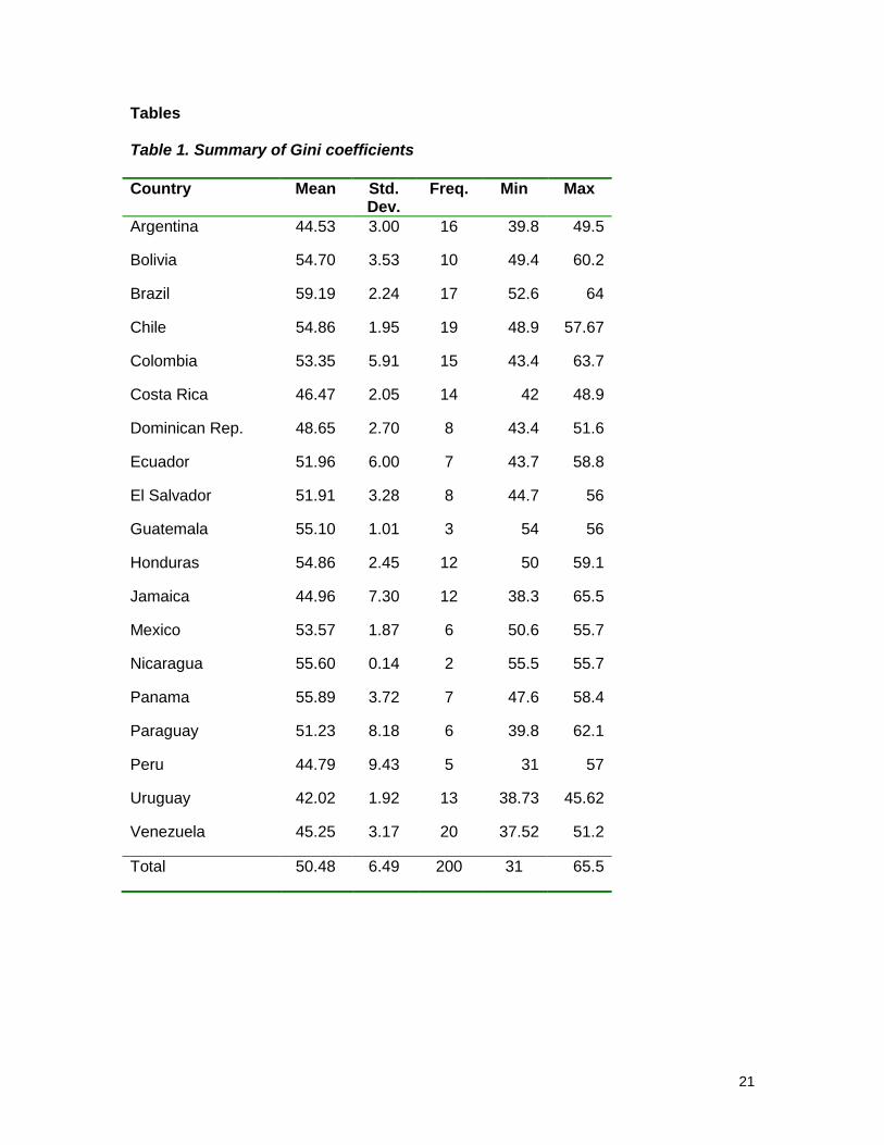
annual changes. Table 1 presents summary statistics for the Gini coefficients of Latin

American countries in the sample.

Independent Variables

I use the natural log of GDP per capita (in constant 2000 US dollars) as the

variable for economic development, which is commonly used in the literature. This

variable was retrieved from the World Bank‟s World Development Indicators (WDI). As is

also common in the literature, I include the squared value of this term as another

variable, to allow for the Kuznet‟s hypothesis of a non-linear relationship.

Two variables encompass the measures of globalization in this study: capital and

trade flows. These variables were retrieved from the WDI. Trade openness is measured

by exports and imports as a percentage of GDP. Foreign direct investment (FDI)

measures net inflows of investment as a percentage of GDP. We can expect that the

openness coefficients will be positive and significant.

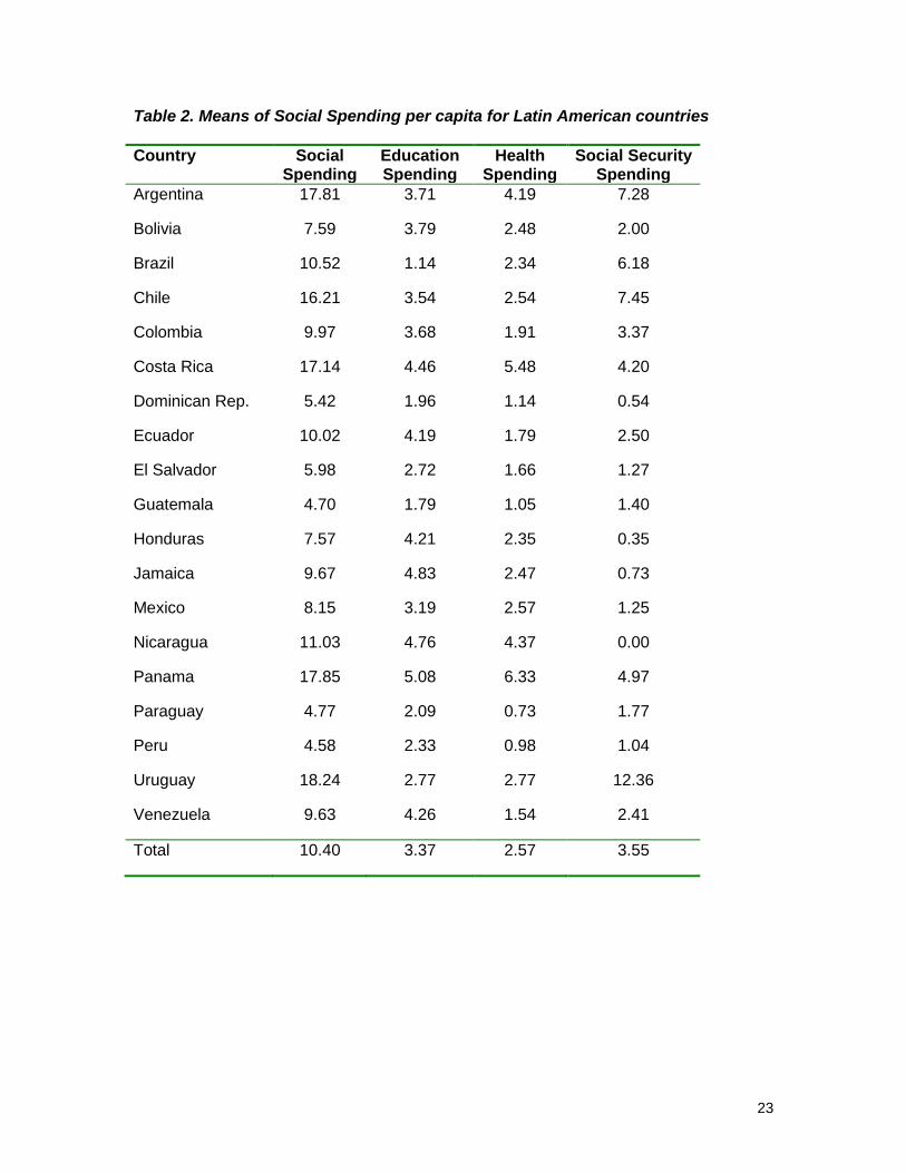
Per capita spending on health, education, social security and welfare are

reported in the International Monetary Fund‟s Government Finance Statistics (GFS). An

alternative measure of percentage of a country‟s public expenditures for each category

above is used in order to test for robustness of the spending effect on inequality. One

limitation of the expenditure data is it is not disaggregated for different levels of

education or health. Therefore, it is not straightforward to predict a sign for this variable.

We would expect a negative overall effect of government expenditure on inequality

index. Table 2 present the means for the spending variables by country.

I also include the following educational variables: gross elementary, secondary

and tertiary enrollment ratio. According to the World Bank this variable is defined as “the

ratio of total enrollment, regardless of age, to the population of the age group that

officially corresponds to the level of education shown”. These variables were also

obtained from the WDI. We expect education attainment to reduce inequality and

promote economic growth. In Latin America, primary education has been universalized

since 1970 for primary education, but not for secondary education, and so large

11

proportion of students drop out at that point. This explains the fact that educational

attainment has coincided with increasing inequality in Latin American countries in the

last 30 years. Consequently, we would expect a negative coefficient for higher education

but a positive coefficient for primary education.

The Polity IV data set is used to derive both measures. Democracy is scored on

a scale of 0 to 10 (10 being the highest) and rated by: (1) regulation, competitiveness,

and openness of executive recruitment, (2) executive constraints, and (3) regulation and

competitiveness of political competition. For this analysis I apply both measures of

democracy. Following Segura and Kaufman (2004), a democracy dummy variable is

constructed by coding any country scoring at least 7 as democratic; otherwise, they are

coded authoritarian. We expect the countries with the longer democratic traditions to

have less income inequality.

A measure of urbanization, the percentage of the population which live in urban

areas, is included in the model as determinant of inequality. We expect that more urban

countries have less income inequality. I finally test for the effect of the percentage of the

population which is 65 and older for the model predicting social security and welfare

spending and of the percentage of the population which is under 15 years of age for the

model predicting spending on health and education.

Other variables are included in the empirical model such as inflation,

unemployment, debt, deficit, among others in order to control for economic effects.

However, the estimates for these variables are either insignificant and with very small

coefficients in the inequality equation. Therefore, these variables are dropped from the

analysis.

Model

I apply the fixed effect method using time dummies and a decade dummy

variable to control for economic shocks or other time specific effects. The decade

dummy variable is particularly important to check the effects of the 1980s crisis on the

model, particularly since social spending fell during that decade. Decade dummies are

preferred to year dummies due to the small size of the sample.3 Fixed effects are useful

3 Regressions are also estimated using year dummy variables however the results don‟t change

significantively.

12

for controlling for idiosyncratic differences across countries with regard to inequality.

Country specific effects are important in this model since most of the variation occur

across units rather than over time. The intercept of the fixed effects model estimates the

differences in inequality between countries and time dummy variables capture variation

within them through time.

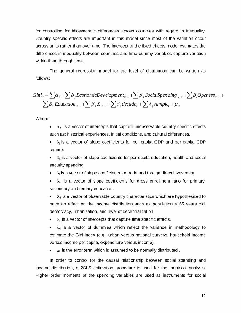
The general regression model for the level of distribution can be written as

follows:

Where:

o is a vector of intercepts that capture unobservable country specific effects

such as: historical experiences, initial conditions, and cultural differences.

j is a vector of slope coefficients for per capita GDP and per capita GDP

square.

k is a vector of slope coefficients for per capita education, health and social

security spending.

l is a vector of slope coefficients for trade and foreign direct investment

m is a vector of slope coefficients for gross enrollment ratio for primary,

secondary and tertiary education.

Xit is a vector of observable country characteristics which are hypothesized to

have an effect on the income distribution such as population > 65 years old,

democracy, urbanization, and level of decentralization.

p is a vector of intercepts that capture time specific effects.

q is a vector of dummies which reflect the variance in methodology to

estimate the Gini index (e.g., urban versus national surveys, household income

versus income per capita, expenditure versus income).

it is the error term which is assumed to be normally distributed .

In order to control for the causal relationship between social spending and

income distribution, a 2SLS estimation procedure is used for the empirical analysis.

Higher order moments of the spending variables are used as instruments for social

ittqtpitnitm

itlitkitjoit

sampledecadeXEducation

OpenessdingSocialSpenvelopmentEconomicDeGini

11

111

13

expenditure variables. This procedure was proposed by Lewbel (1997) due to the

difficulty of finding data for exogenous instrumental variables. However, the validity of

this technique relies on, among other things, the skewness of the data.

A random effect model (REM) is also estimated. REM requires equal correlations

among errors within units. Such an error structure would arise if unmeasured unit-

specific causes, such as methodical measurement differences or other unobserved

aspects of the social structure of a country, affect the dependent variable in the same

way at each point in time over the period of the data. Since this is reasonable

assumption for Latin American countries, the REM strategy is a feasible method of

estimation.

Finally, a first differenced GMM panel data model is estimated because of its

potential for obtaining consistent parameter estimates even in the presence of

measurement error and endogenous right-hand side variable. Different assumptions

about the presence of measurement errors and the endogeneity of right-hand-side

variables will have implications for the validity of specific instruments. These

assumptions can be tested in the GMM framework by the use of the Sargan test of over-

identifying restrictions.

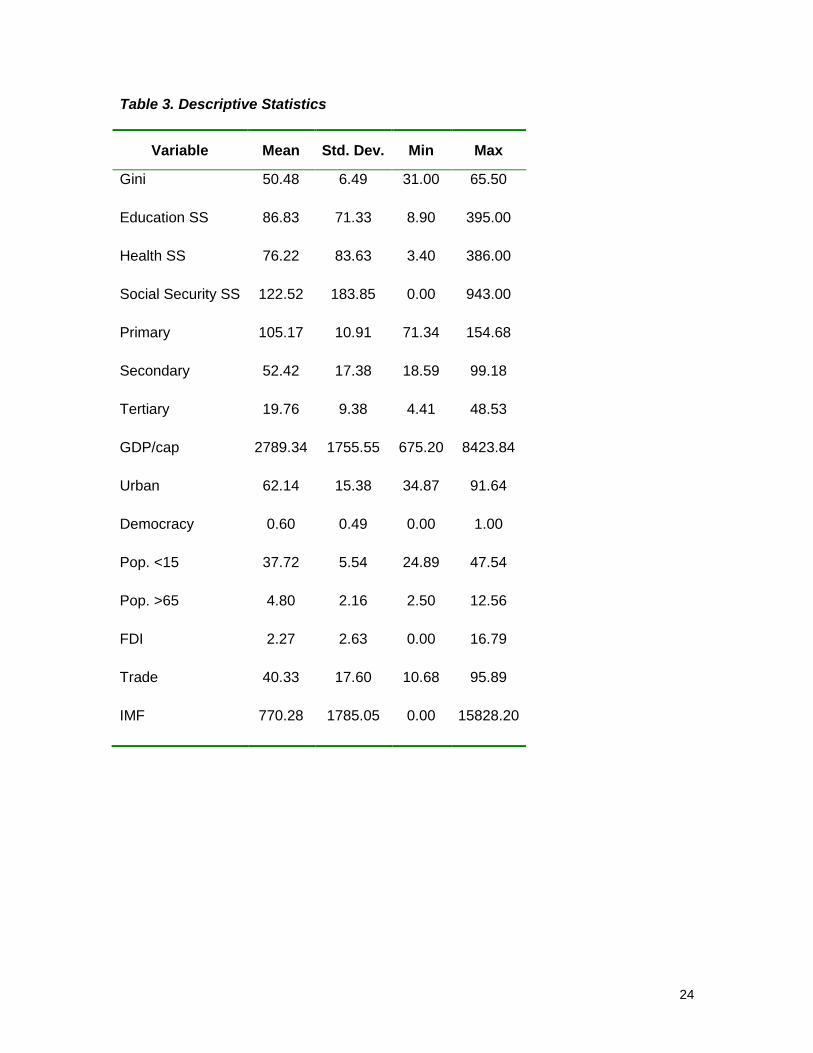
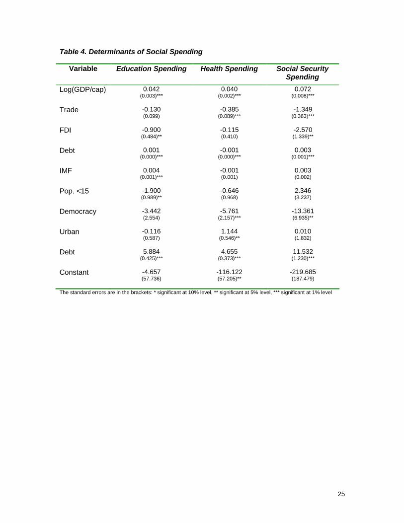
Table 3 presents the descriptive statistics for the determinants of social spending

and inequality. Results of the social spending regression are presented in Table 4 for

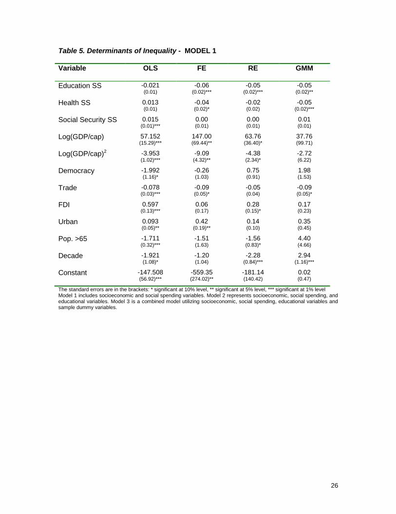
education, health and social security expenditures respectively. Table 5 presents the

results for the determinants of inequality controlling for the potential endogeneity of the

social spending variables. Three alternative models are estimated using different

econometric methods: fixed effects, random effects, and fist differenced GMM model.

Model 1 includes only socioeconomic4 and social spending variables. Model 2

represents socioeconomic, social spending, and educational variables. Model 3 is a

combined model utilizing socioeconomic, social spending, educational variables and

sample dummy variables.

4 Socioeconomic variables include economic development, openness and specific socioeconomic country

characteristics.

14

Results

The general regression model fits the data well, explaining anywhere from 45%

to 67% of the total variance in the Gini coefficient over time and across countries. In

addition, the estimates and significance of the coefficient appear to be robust and

consistent across different specifications.

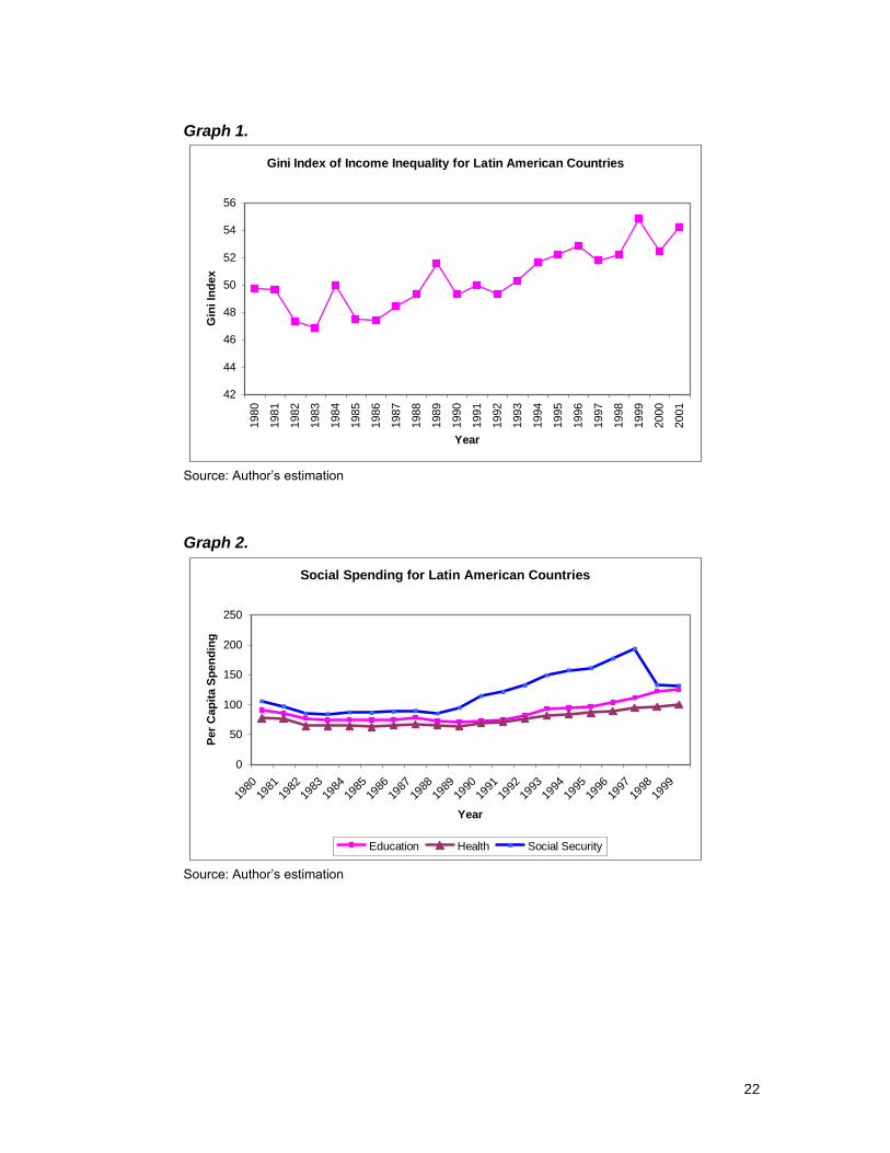
Descriptive results from this research support the assertions that there has been

a general trend toward increased within-country inequality in recent history (Graph 1).

For instance, the average within-country Gini index increased from 46.83 in 1983 to

54.80 in 1999. Descriptive statistics also reveal that there has been a trend toward

greater social spending per capita in Latin American countries in the last two decades

(Graph 2). Likewise, primary and secondary enrollments have increased over the

decades being studied. The average gross enrollment ratio increased from 52.25 in

1980, to 56.48 in 1990, to 71.67 in 2000.

Statistic analysis suggests a negative correlation between social spending and

inequality, and a positive correlation between education enrollment and inequality.

However, these correlations don‟t control for other factors that affect income inequality,

so multiple regressions analysis yield more reliable effects of social spending on income

inequality. Table 3 shows the correlations among these variables.

The fixed effects model provides the preferred estimates among the different

econometric methods used for the analysis. Random effects model gives inconsistent

estimates which could be the result of the strong assumption about constant correlation

among errors within counties. It is very probable that the unobserved effects affect the

dependent variable in different scale over the time period of the data. First differenced

GMM estimators are very limited due to the small sample that results once the

dependent variable and right hand side variables are lagged5.

Social spending estimates are consistent for every model specification.

Education and health spending estimates are positive, statistically significant, and almost

equal. On average estimates indicate that an increase of one dollar in education

spending reduces index inequality by about 0.6 percentage points, while an increase of

5 A small sample results because I am using unbalanced panel dataset, and there are a lot of missing values

in the dependent variable.

15

one dollar in health spending decreases index inequality by about 0.4 percentage

points. Social security spending seems to have no effect on income inequality. These

results provide evidence that education and health spending are slightly progressive in

income. This result by itself is not surprising. In fact, this is the same outcome of most of

the studies that have analyzed the effect of social spending in income inequality.

However, estimates from this study differ from previous ones in that the size of the effect

is lower when we control for endogeneity of the social spending variables. I consider this

statement the most important result of this study.

Economic development variables support for Kuznets‟ hypothesis: increased

economic development tends to increase inequality before a threshold of income is

reached. After this point the curve turns, so increased development lessens inequality.

The estimated parameters are almost equal for model 1 and model 2. In model 3, the

estimated parameters for log of GDP per capita and its square hold the same signs as in

model 1 and model 2, but they are not statistically significant at conventional levels. That

is, controlling for the methodology and data used to estimate the Gini index reduces the

effect of income per capita in income inequality. This result makes sense since income is

in fact the most important variable to estimate the Gini index. That is, the significative

effect of income per capital on Gini index is due to the fact that income per capita is used

to estimate the index and not because the data support Kuznets‟ hypothesis.

Trade seems to have a negative effect in income inequality, while foreign direct

investment has a positive but not statistically significant effect. The negative effect of

trade is significant at conventional levels and support the hypothesis that education

spending helps mitigate the adverse effect of openness on income inequality in poorer

countries, while social security and welfare do not.

Urbanization has a positive and significant effect on income inequality. This effect

goes against the hypothesis that growth of the urban population contributes to a higher

middle class, more employment, and less inequality. It would be interesting to find some

explanation for this atypical effect. One hypothesis is that the process of urbanization on

most Latin American countries could be a consequence of total absence of government,

bad economic conditions, and violence in rural areas, rather than a consequence of

better economic opportunities of large cities. That is, forced displacement from rural to

urban areas could generate higher levels of inequality in urban areas.

16

Aged population estimates are negative but not statistically significant on all

specifications. Unless we expect a positive coefficient for aged population, a positive

coefficient makes sense given that Latin America countries are all developing countries

with a large young population. Hence, the adverse effect of aged population in income

distribution could not be applicable for these countries.

When educational variables are considered in Model 2 and 3, secondary and

tertiary enrollments are significant at conventional levels, yet they have opposite effects

on income inequality. Secondary enrollments have a negative effect on income

distribution while tertiary enrollments have a positive effect. These findings support the

premise that secondary enrollments increase the supply of educated workers and,

thereby, decrease income inequality. In contrast, higher education increases income

inequality since it creates a large gap in wages, and it is available only for a small

percentage of the young population.

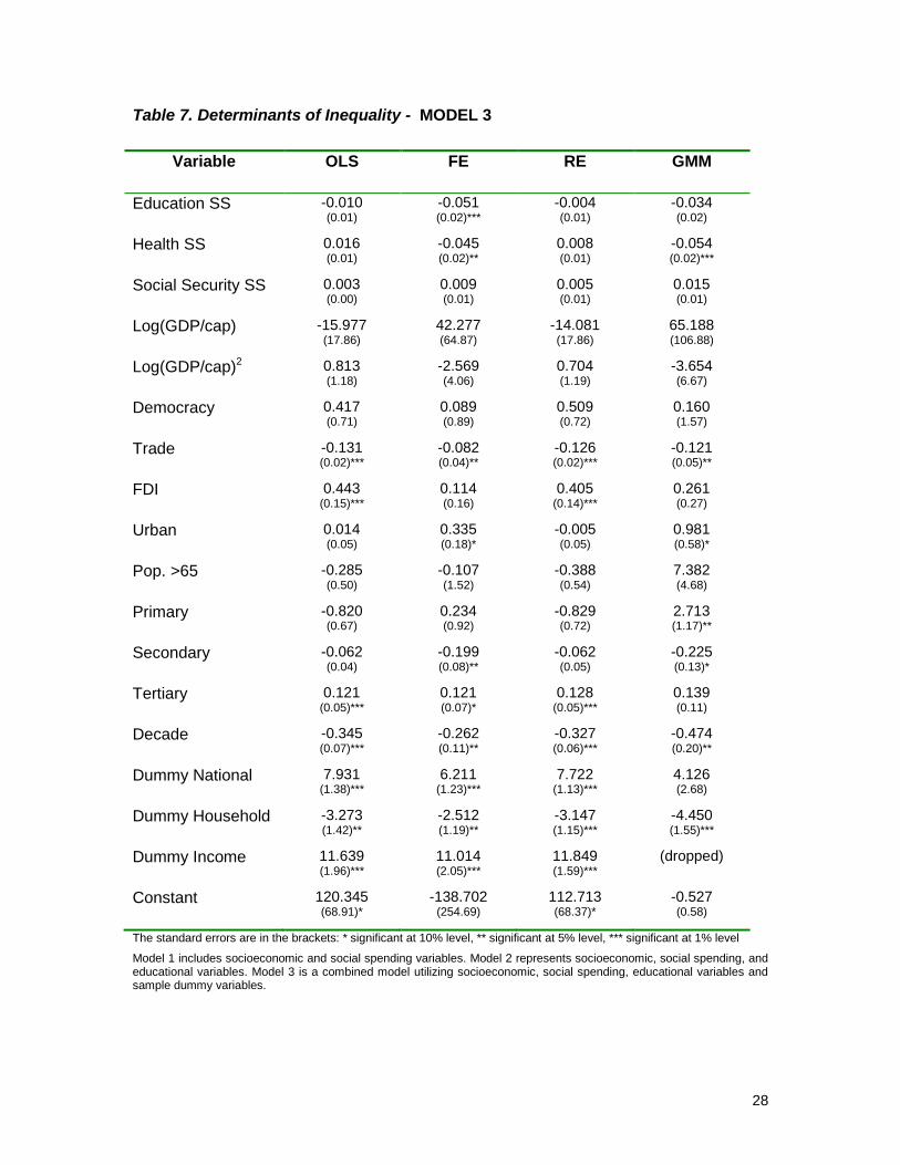
The dummy variables for the variance in methodologies are quite large. In the

case of the income vs. expenditure dummy, our results indicate that the income based

studies result in a Gini index that is 11points higher than is the case of expenditure

based studies. The national dummy suggests that a Gini index based on a national

sample is 6points higher than one based on urban sample. Finally, the household

income dummy suggests that a Gini index based on a household income is 2 points

lower than one based on income per capita.

Democracy doesn‟t have consistent estimates among specifications, yet it is not

statistically significant.

Conclusions

Many problems arrive when cross country sample are used to analyze

determinants of income inequality. First, as Huber argued, common estimators of

inequality such a Gini coefficient don‟t capture the positive benefits of education and

health spending in the short run. In general, the effect that health and education

spending has on improving human capital in the bottom half of the income distribution

would appear only with a considerable lag. Second, there is causality for some of the

variables that determine income inequality such as social expenditure and income.

17

Third, cross-country data scarcity would not allow to control for most of the endogeneity

problems that arrive for this specific model.

This analysis contributes to the literature on the determinants of cross-country

income inequality and offers new insights into the complex relationships between social

spending and income inequality. Estimated parameters are consistent and unbiased

when we control for the endogeneity of social spending in the income inequality

equation. Results show that models that don‟t take into account endogeneity of the

social spending variables overestimate the effects of education and health spending.

From a policy perspective, this research leads valuable insights on the

distributive effects of expenditures on education and health. On one hand, I found

evidence that education and health expenditures reduce income inequality in developing

countries, being more effective education than health spending. On the other hand, I

found that analogous estimates of the effect of social expenditures on income inequality

were overestimated because inappropriate econometric methods have been used in

previous studies.

Nevertheless, results from this study are not conclusive. The overall estimates of

social spending found in this study are limited in the sense that the effect of social

expenditures on income distribution depend on the allocation of these expenditures.

That is, spending on primary education will be distributive and spending on university

education regressive, so the greater the share of education spending going to primary

education, the more progressive the overall impact. The same argument holds for

different assignments of health expenditures. Problem is that there is not data that

disaggregate for lower levels of expenditures. Therefore, the overall estimate could be

misleading.

Even with the limitations of the data, this research is still able to produce results

that are valuable on their own, and which also serve as the foundation for more robust

studies in the future.

18

References

Alderson, A. S., & Nielsen, F. (1999). Income inequality, development, and dependence: A reconsideration. American Sociological Review, 64, 606-631.

Baldacci, Emanuele, Maria Teresa Guin-Sui, and Luiz de Mello, (2003), “More on the Effectiveness of Public Spending on Health Care and Education: A Covariance Structure Model,” Journal of International Development, Vol. 15, pp. 709–25.

Barro, R. J. (2000). Inequality and growth in a panel of countries. Journal of Economic Growth, 5, 5-32.

Barro, R. J., and Lee, J. W. (2000). International data on educational attainment: Updates and implications (CID Working Paper No. 42). Cambridge, MA: Center for International Development.

Burkhart, R. E. (1997). Comparative democracy and income distribution. The Journal of Politics, 59(1), 148-164.

Checchi, D. (2000). Does educational achievement help to explain income inequality? (Working Paper No. 208). Helsinki: United Nations University, World Institute for Development Economics Research (WIDER).

Deaton, A., and C. Paxson (1997) The Effects of Economic and Population Growth on National Saving and Inequality. Demography 34:97–114.

De Gregorio, J., and Lee, J. (2002). Education and income inequality: New evidence from crosscountry data. The Review of Income and Wealth, 48, 395-416.

De Ferranti, David, Guillermo E. Perry, Fancisco H.G. Ferreira, and Michael Walton. (2004). Inequality in Latin America: Breaking with History? Washington, D.C.: The World Bank.

Deininger, K., and Squire, L. (1998). A new dataset measuring income inequality. World Bank Economic Review, 10(3), 565-591.

Kraay, Aart & Dollar, David, (2001). "Growth is good for the poor," Policy Research Working Paper Series 2587, The World Bank.

ECLAC (Economic Commission of Latin America and the Caribbean) (1994). Social Panorama of Latin America 1994. Santiago de Chile: ECLAC.

Grosh, M. (1990). Social Spending in Latin America. The Story of the 1980s. World Bank Discussion Paper 106, Washington, DC: World Bank.

„„Government Finance Statistics (2004).‟‟ International Monetary Fund, Washington, DC.

Gupta, Sanjeev, Marijn Verhoeven, and Erwin Tiongson, (2002), “The Effectiveness of Government Spending on Education and Health Care in Developing

19

and Transition Economies,” European Journal of Political Economy, Vol. 18, No. 4, pp. 717–37.

Huber, E. (1996) „„Options for Social Policy in Latin America: Neoliberal versus Social Democratic Models.‟‟ In Welfare States in Transition: National Adaptations in Global Economies, edited by G. Esping-Andersen, pp. 141–191. London: Sage Publications.

Huber, Evelyne, Thomas Mustillo, and John Stephens. (2004). “Determinants of Social Spending in Latin America.” Paper delivered at the Meetings of the Society for the Advancement of Socio-Economics, Washington, D.C., July 8-11.

Huber, Evelyne, Thomas Mustillo, and John Stephens. (2004). “Social Spending and Inequality in Latin America and the Caribbean.” Paper delivered at the Meetings of the Society for the Advancement of Socio-Economics, Washington, D.C., July 8-11.

Kaufman, Robert R., and Segura-Ubiergo, Alex. (2001, July). Globalization, domestic politics, and social spending in Latin America: A time-series cross-section analysis, 1973-97.World Politics, 53, 553-587.

Kuznets, S. (1955). Economic growth and income inequality. American Economic Review, 45, 1- 28. 28

Lloyd-Sherlock, Peter (2000), "Failing the Needy: Public Social Spending in Latin America", in Journal of International Development, Vol. 12, No. 1, June 2000

Londoño, Juan Luis and Miguel Székely (1997), “Persistent Poverty and Excess Inequality: Latin America, 1970-1995”, OCE Working Paper Series, No. 357, Washington, D.C., Inter-American Development Bank (IDB).

Londoño, J. L. (1996). Poverty, inequality, and human capital development (World Bank Latin American and Caribbean Studies). Washington DC: World Bank.

Milanovic, B. (2003). "Can We Discern The Effect Of Globalization On Income Distribution? Evidence From Household Surveys," HEW 0310002, the former EconWPA.

Moene, K. and M. Wallerstein (2001): “Inequality, social insurance, and redistribution.” American Political Science Review, 95: 859-874.

Morley, Samuel. (2001). The Income Distribution Problem in Latin America and the Caribbean. Santiago: United Nations Press.

Muller, E. (1988) Democracy, Economic Development, and Income Inequality. American Sociological Review 53:50–68.

O'Neil, D. (1995). Education and income growth: Implications for cross-country inequality. Journal of Political Economy, 103, 1289-1299.

Rudra, Nita. (2004). "Openness, Welfare Spending and Inequality in the Developing World," International Studies Quarterly. Vol. 48. 48, 683-709.

20

Sylwester, K. (2002). Can education expenditures reduce income inequality? Economics of Education Review, 21, 43-52. The global poll: Multinational survey of opinion leaders 2002. (2003). Retrieved June 2, 2005, from http://siteresources.worldbank.org/NEWS/Resources/globalpoll.pdf

World Bank. (2005). World development indicators. World Bank.

World Institute for Development Economics Research (WIDER). (2005). World income inequality database. United Nations University.

21

Tables Table 1. Summary of Gini coefficients

Country Mean

Std. Dev.

Freq. Min Max

Argentina 44.53 3.00 16 39.8 49.5

Bolivia 54.70 3.53 10 49.4 60.2

Brazil 59.19 2.24 17 52.6 64

Chile 54.86 1.95 19 48.9 57.67

Colombia 53.35 5.91 15 43.4 63.7

Costa Rica 46.47 2.05 14 42 48.9

Dominican Rep. 48.65 2.70 8 43.4 51.6

Ecuador 51.96 6.00 7 43.7 58.8

El Salvador 51.91 3.28 8 44.7 56

Guatemala 55.10 1.01 3 54 56

Honduras 54.86 2.45 12 50 59.1

Jamaica 44.96 7.30 12 38.3 65.5

Mexico 53.57 1.87 6 50.6 55.7

Nicaragua 55.60 0.14 2 55.5 55.7

Panama 55.89 3.72 7 47.6 58.4

Paraguay 51.23 8.18 6 39.8 62.1

Peru 44.79 9.43 5 31 57

Uruguay 42.02 1.92 13 38.73 45.62

Venezuela 45.25 3.17 20 37.52 51.2

Total 50.48 6.49 200 31 65.5

22

Graph 1.

Gini Index of Income Inequality for Latin American Countries

42

44

46

48

50

52

54

56

1980

1981

1982

1983

1984

1985

1986

1987

1988

1989

1990

1991

1992

1993

1994

1995

1996

1997

1998

1999

2000

2001

Year

Gin

i In

dex

Source: Author‟s estimation

Graph 2.

Social Spending for Latin American Countries

0

50

100

150

200

250

1980

1981

1982

1983

1984

1985

1986

1987

1988

1989

1990

1991

1992

1993

1994

1995

1996

1997

1998

1999

Year

Per

Cap

ita S

pen

din

g

Education Health Social Security

Source: Author‟s estimation

23

Table 2. Means of Social Spending per capita for Latin American countries

Country Social Spending

Education Spending

Health Spending

Social Security Spending

Argentina 17.81 3.71 4.19 7.28

Bolivia 7.59 3.79 2.48 2.00

Brazil 10.52 1.14 2.34 6.18

Chile 16.21 3.54 2.54 7.45

Colombia 9.97 3.68 1.91 3.37

Costa Rica 17.14 4.46 5.48 4.20

Dominican Rep. 5.42 1.96 1.14 0.54

Ecuador 10.02 4.19 1.79 2.50

El Salvador 5.98 2.72 1.66 1.27

Guatemala 4.70 1.79 1.05 1.40

Honduras 7.57 4.21 2.35 0.35

Jamaica 9.67 4.83 2.47 0.73

Mexico 8.15 3.19 2.57 1.25

Nicaragua 11.03 4.76 4.37 0.00

Panama 17.85 5.08 6.33 4.97

Paraguay 4.77 2.09 0.73 1.77

Peru 4.58 2.33 0.98 1.04

Uruguay 18.24 2.77 2.77 12.36

Venezuela 9.63 4.26 1.54 2.41

Total 10.40 3.37 2.57 3.55

24

Table 3. Descriptive Statistics

Variable Mean Std. Dev. Min Max

Gini 50.48 6.49 31.00 65.50

Education SS 86.83 71.33 8.90 395.00

Health SS 76.22 83.63 3.40 386.00

Social Security SS 122.52 183.85 0.00 943.00

Primary 105.17 10.91 71.34 154.68

Secondary 52.42 17.38 18.59 99.18

Tertiary 19.76 9.38 4.41 48.53

GDP/cap 2789.34 1755.55 675.20 8423.84

Urban 62.14 15.38 34.87 91.64

Democracy 0.60 0.49 0.00 1.00

Pop. <15 37.72 5.54 24.89 47.54

Pop. >65 4.80 2.16 2.50 12.56

FDI 2.27 2.63 0.00 16.79

Trade 40.33 17.60 10.68 95.89

IMF 770.28 1785.05 0.00 15828.20

25

Table 4. Determinants of Social Spending

Variable Education Spending Health Spending Social Security Spending

Log(GDP/cap) 0.042 (0.003)***

0.040 (0.002)***

0.072 (0.008)***

Trade -0.130 (0.099)

-0.385 (0.089)***

-1.349 (0.363)***

FDI -0.900 (0.484)**

-0.115 (0.410)

-2.570 (1.339)**

Debt 0.001 (0.000)***

-0.001 (0.000)***

0.003 (0.001)***

IMF 0.004 (0.001)***

-0.001 (0.001)

0.003 (0.002)

Pop. <15 -1.900 (0.989)**

-0.646 (0.968)

2.346 (3.237)

Democracy -3.442 (2.554)

-5.761 (2.157)***

-13.361 (6.935)**

Urban -0.116 (0.587)

1.144 (0.546)**

0.010 (1.832)

Debt 5.884 (0.425)***

4.655 (0.373)***

11.532 (1.230)***

Constant -4.657 (57.736)

-116.122 (57.205)**

-219.685 (187.479)

The standard errors are in the brackets: * significant at 10% level, ** significant at 5% level, *** significant at 1% level

26

Table 5. Determinants of Inequality - MODEL 1

Variable OLS FE RE GMM

Education SS -0.021 (0.01)

-0.06 (0.02)***

-0.05 (0.02)***

-0.05 (0.02)**

Health SS 0.013 (0.01)

-0.04 (0.02)*

-0.02 (0.02)

-0.05 (0.02)***

Social Security SS 0.015 (0.01)***

0.00 (0.01)

0.00 (0.01)

0.01 (0.01)

Log(GDP/cap) 57.152 (15.29)***

147.00 (69.44)**

63.76 (36.40)*

37.76 (99.71)

Log(GDP/cap)2 -3.953 (1.02)***

-9.09 (4.32)**

-4.38 (2.34)*

-2.72 (6.22)

Democracy -1.992 (1.16)*

-0.26 (1.03)

0.75 (0.91)

1.98 (1.53)

Trade -0.078 (0.03)***

-0.09 (0.05)*

-0.05 (0.04)

-0.09 (0.05)*

FDI 0.597 (0.13)***

0.06 (0.17)

0.28 (0.15)*

0.17 (0.23)

Urban 0.093 (0.05)**

0.42 (0.19)**

0.14 (0.10)

0.35 (0.45)

Pop. >65 -1.711 (0.32)***

-1.51 (1.63)

-1.56 (0.83)*

4.40 (4.66)

Decade -1.921 (1.08)*

-1.20 (1.04)

-2.28 (0.84)***

2.94 (1.16)***

Constant -147.508 (56.92)***

-559.35 (274.02)**

-181.14 (140.42)

0.02 (0.47)

The standard errors are in the brackets: * significant at 10% level, ** significant at 5% level, *** significant at 1% level Model 1 includes socioeconomic and social spending variables. Model 2 represents socioeconomic, social spending, and educational variables. Model 3 is a combined model utilizing socioeconomic, social spending, educational variables and sample dummy variables.

27

Table 6. Determinants of Inequality - MODEL 2

Variable OLS FE RE GMM

Education SS -0.025 (0.01)**

-0.071 (0.02)***

-0.024 (0.02)

-0.042 (0.02)*

Health SS 0.044 (0.02)***

-0.038 (0.02)*

0.008 (0.02)

-0.047 (0.02)**

Social Security SS 0.017 (0.00)***

0.003 (0.01)

0.011 (0.01)

0.008 (0.01)

Log(GDP/cap) 28.649 (19.46)

161.093 (71.03)**

41.119 (27.94)

133.169 (104.95)

Log(GDP/cap)2 -2.164 (1.31)*

-9.996 (4.44)**

-2.959 (1.85)

-8.205 (6.51)

Democracy -0.164 (1.02)

0.085 (1.02)

0.992 (0.92)

1.257 (1.56)

Trade -0.066 (0.02)***

-0.103 (0.05)**

-0.072 (0.04)**

-0.128 (0.05)***

FDI 0.754 (0.17)***

0.120 (0.18)

0.440 (0.17)***

0.152 (0.26)

Urban 0.185 (0.07)***

0.553 (0.20)***

0.144 (0.08)*

1.019 (0.59)*

Pop. >65 -2.754 (0.53)***

-0.744 (1.75)

-2.494 (0.70)***

7.487 (4.69)

Primary -2.483 (0.99)***

-1.284 (1.03)

-2.616 (0.85)***

2.425 (1.15)**

Secondary -0.147 (0.06)***

-0.263 (0.10)***

-0.158 (0.07)**

-0.244 (0.13)*

Tertiary 0.083 (0.07)

0.160 (0.08)**

0.124 (0.07)*

0.195 (0.11)*

Decade -0.410 (0.08)***

-0.362 (0.13)***

-0.289 (0.09)***

-0.409 (0.20)**

Constant -20.966 (73.71)

-601.159 (278.48)**

-71.984 (106.27)

-0.506 (0.59)

The standard errors are in the brackets: * significant at 10% level, ** significant at 5% level, *** significant at 1% level Model 1 includes socioeconomic and social spending variables. Model 2 represents socioeconomic, social spending, and educational variables. Model 3 is a combined model utilizing socioeconomic, social spending, educational variables and sample dummy variables.

28

Table 7. Determinants of Inequality - MODEL 3

Variable OLS FE RE GMM

Education SS -0.010 (0.01)

-0.051 (0.02)***

-0.004 (0.01)

-0.034 (0.02)

Health SS 0.016 (0.01)

-0.045 (0.02)**

0.008 (0.01)

-0.054 (0.02)***

Social Security SS 0.003 (0.00)

0.009 (0.01)

0.005 (0.01)

0.015 (0.01)

Log(GDP/cap) -15.977 (17.86)

42.277 (64.87)

-14.081 (17.86)

65.188 (106.88)

Log(GDP/cap)2 0.813 (1.18)

-2.569 (4.06)

0.704 (1.19)

-3.654 (6.67)

Democracy 0.417 (0.71)

0.089 (0.89)

0.509 (0.72)

0.160 (1.57)

Trade -0.131 (0.02)***

-0.082 (0.04)**

-0.126 (0.02)***

-0.121 (0.05)**

FDI 0.443 (0.15)***

0.114 (0.16)

0.405 (0.14)***

0.261 (0.27)

Urban 0.014 (0.05)

0.335 (0.18)*

-0.005 (0.05)

0.981 (0.58)*

Pop. >65 -0.285 (0.50)

-0.107 (1.52)

-0.388 (0.54)

7.382 (4.68)

Primary -0.820 (0.67)

0.234 (0.92)

-0.829 (0.72)

2.713 (1.17)**

Secondary -0.062 (0.04)

-0.199 (0.08)**

-0.062 (0.05)

-0.225 (0.13)*

Tertiary 0.121 (0.05)***

0.121 (0.07)*

0.128 (0.05)***

0.139 (0.11)

Decade -0.345 (0.07)***

-0.262 (0.11)**

-0.327 (0.06)***

-0.474 (0.20)**

Dummy National 7.931 (1.38)***

6.211 (1.23)***

7.722 (1.13)***

4.126 (2.68)

Dummy Household -3.273 (1.42)**

-2.512 (1.19)**

-3.147 (1.15)***

-4.450 (1.55)***

Dummy Income 11.639 (1.96)***

11.014 (2.05)***

11.849 (1.59)***

(dropped)

Constant 120.345 (68.91)*

-138.702 (254.69)

112.713 (68.37)*

-0.527 (0.58)

The standard errors are in the brackets: * significant at 10% level, ** significant at 5% level, *** significant at 1% level

Model 1 includes socioeconomic and social spending variables. Model 2 represents socioeconomic, social spending, and educational variables. Model 3 is a combined model utilizing socioeconomic, social spending, educational variables and sample dummy variables.