The Effect of Robust Decisions on the Cost of Uncertainty in Military Airlift Operations

The Effect of Robust Decisions on the Cost ofUncertainty in Military Airlift Operations

Warren B. Powell* Belgacem Bouzaiene-Ayari* Jean Berger**Abdeslem Boukhtouta**

Abraham P. George*

*Department of Operations Research and Financial EngineeringPrinceton University, Princeton, NJ 08544

**DRDC-ValcartierQuebec, Canada

June 20, 2007

Abstract

There are a number of sources of randomness that arise in military airlift operations. How-ever, the cost of uncertainty can be difficult to estimate, and is easy to overestimate if weuse simplistic decision rules. Using data from Canadian military airlift operations, we studythe effect of uncertainty in customer demands as well as aircraft failures. The system is firstsimulated using the types of myopic decision rules widely used in the research literature.These results are then compared to decisions that result when we use robust decision ruleswhich account for the effect of decisions now on the future. These are obtained by modelingthe problem as a dynamic program, and solving Bellman’s equations using approximate dy-namic programming. The experiments show that even approximate solutions to Bellman’sequations produce decisions that substantially reduce the effect of uncertainty.

The military airlift problem involves managing a fleet of aircraft to serve demands to

move passengers or freight. The aircraft are characterized by a vector of attributes, some

of which may be dynamic, such as the current location, the earliest time when it can be

used to serve a demand, whether it is currently loaded or empty and measures of operability.

The demands are also described using features such as the type of demand, their origin,

the type of aircraft that is required to serve the demand, their priority, and arrival and

departure times. The aircraft have to be used to make decisions such as pick up and move

the demands, relocate to another location to serve demands arising there and so forth. The

demands are made up of a mixture of scheduled requests, which are known in advance, and

dynamic requests, which arrive over the course of the simulation with varying degrees of

advance notice. Other forms of uncertainty, such as random failure of equipments, can also

occur.

Military airlift (and sealift) problems have typically been modeled either as deterministic

linear (or integer) programs or with simulation models which can handle various forms of

uncertainty. Much of the work on deterministic optimization models started at the Naval

Postgraduate School with the Mobility Optimization Model (Wing et al. (1991)). Yost (1994)

describes the development of THRUPUT which is a general airlift model but which does not

capture time. THRUPUT and the Mobility Optimization Model were combined to produce

THRUPUT II (Rosenthal et al. (1997)) to obtain a model which accurately captured airlift

operations in the context of a time-dependent model. A similar model was produced by

RAND called CONOP (CONcept of OPerations), which is described in Killingsworth &

Melody (1997). Both THRUPUT II and CONOP possessed desirable features which were

merged in a system called NRMO (Baker et al. (2002)). These models could all be solved

using linear programming packages. Crino et al. (2004) addresses the problem of routing

and scheduling vehicles in the context of theater operations. The resulting model was solved

using group-theoretic tabu search.

Despite the attention given to math programming-based models, there remains consid-

erable interest in the use of simulation models, primarily because of their ability to handle

uncertainty as well as the flexibility in capturing complex operational issues. The Argonne

2

National Laboratory developed TRANSCAP to simulate the deployment of forces from Army

bases (Burke et al. (2004)). TRANSCAP uses a discrete-event simulation module developed

using the simulation language MODSIM III. The Air Mobility Command at Scott Air Force

Base uses a simulation model, AMOS (derived from an earlier model known as MASS), to

model airlift operations for policy studies. Simulation models provide for a high level of

realism, but cannot be used as a basis for studying robust decisions.

Since 1956 (Dantzig & Ferguson (1956)) there has been interest in solving these prob-

lems where decisions explicitly account for uncertainty in the future. Much of this work

has evolved within the discipline of stochastic programming, which focuses on representing

uncertainty within linear programs. Midler & Wollmer (1969) accounts for uncertainty in

demands, while Goggins (1995) proposes an extension of THRUPUT II to handle uncer-

tainty in aircraft reliability. Niemi (2000) proposes a stochastic programming model which

captures uncertainty in ground times. Morton et al. (2002) introduced SSDM (Stochastic

Sealift Deployment Model) to model sealift operations in the presence of possible attacks.

Stochastic programming is a widely used methodology for incorporating uncertainty into

mathematical programs (see Kall & Wallace (1994), Birge & Louveaux (1997)), offering two

algorithmic strategies. The first is Benders decomposition, where the recourse function is

replaced by a series of cuts (Higle & Sen (1991), Ruszczynski (2003)), but this has been found

to produce very slow convergence (Powell et al. (2004a)) and creates additional problems

when we are interested in integer solutions (Sen (2005)). The second approach uses scenario

methods, typically formulated as a single large mathematical program with nonanticipativity

constraints (Rockafellar & Wets (1991), Mulvey & Ruszczynski (1995)). Scenario methods

for multistage problems tend to grow exponentially in size, and typically require very coarse

approximations of the outcome space (as well of the underlying physical problem) to produce

computationally tractable models.

A different line of investigation uses dynamic programming to find decisions in the pres-

ence of uncertainty. Yost & Washburn (2000) uses the theory of partially observable Markov

decision processes. The resulting model, however, suffers from the classic curse of dimen-

sionality, restricting its use to very small problems.

3

Our analysis approach is based on the field of approximate dynamic programming (Bert-

sekas & Tsitsiklis (1996), Sutton & Barto (1998), Powell (2007)) which solves Bellman’s

equation by approximating the value function using statistical methods. This general strat-

egy has been adapted to multistage, stochastic optimization problems in order to combine

the power of linear programming (which is needed to handle the high dimensional problems

that arise in transportation) with the power of dynamic programming (see, for example,

Powell & Van Roy (2004)). This algorithmic strategy has been demonstrated in the con-

text of a variety of fleet management problems (Godfrey & Powell (2002), Powell et al.

(2002), Spivey & Powell (2004), Powell & Topaloglu (2004)), including the military airlift

problem (Wu et al. (2003), Powell et al. (2004b)). In addition to the academic research liter-

ature, these techniques are also being applied in industrial applications in truckload trucking

(Simao et al. (2007)), rail (Powell & Topaloglu (2005)) and business jets. ADP avoids the

need to approximate the physical problem or the information process (a challenge with both

stochastic programming and classical dynamic programming), but requires the use of good,

but suboptimal, policies.

Approximate dynamic programming helps the model produce decisions that are robust,

which is to say that they work well under different potential outcomes in the future. It

might send five aircraft to handle work that could be covered by three or four aircraft in

anticipation of possible failures. It might also position extra aircraft at locations which

can handle potential failures in nearby locations. Our interest is in estimating the cost of

different forms of uncertainty, and determining the extent to which robust decision-making

affects the cost of uncertainty.

This paper makes the following contributions. 1) It provides an optimization-based model

of airlift operations that enables as much detail as existing simulation models (comparable

to that used in Wu et al. (2006) and existing airlift simulators). 2) It demonstrates, using

data from Canadian airlift operations, that approximate dynamic programming will produce

robust solutions by showing that decisions perform better over a range of scenarios than de-

cisions produced using myopic or deterministic models. 3) We quantify the value of advance

information, and show that the value of advance information is considerably less when we

4

use robust decisions. 4) We quantify the impact of random demands and random equipment

failures with and without using robust decisions. The work demonstrates that we achieve

robust behavior, without the computational overhead of traditional stochastic programming

formulations.

Our paper also illustrates a style for modeling airlift mobility problems that strikes a

balance between the styles normally used in math programming-based models, where it is

customary to express all relationships through systems of linear equations, and those based

on simulation, where it is not unusual to present models without a single equation. Our

modeling notation provides for a much higher level of detail than is typically captured in

a linear or integer programming model. We provide explicit notation for all aspects of the

model except the transition function, which is typically tedious and of little relevance to the

algorithmic strategy.

Section 1 provides a model of the Canadian military airlift problem using the notation

and vocabulary of dynamic resource management. In section 2, we review a range of decision-

making strategies, starting with elementary rule-based policies that are commonly used in

simulation, and extending through myopic, cost-based policies, closing with the policies

derived from solving dynamic programs. Section 3 reports on a series of simulations which

address the question of estimating the cost of uncertainty, and how this estimate depends

on the type of decision function that we use. We provide concluding remarks in section 4.

1 Problem Formulation

In this section, we present a model of the Canadian airlift problem. We start by modeling

the airlift problem section 1.1 as a two-layer, heterogeneous resource allocation problem.

Section 1.2 provides the notation for modeling decisions, capturing the important property

that decisions have to be made under uncertainty. In section 1.3, we describe the evolution

in the state of the system as a result of decisions and exogenous information. We finally

present the objective function for solving the problem in section 1.5.

5

1.1 Resources

We model the problem as a two-layer, resource allocation problem, where “aircraft” and

“demands” (known as “requirements” in the military logistics community) are the objects

being managed. We represent the attributes of each layer using

a = Vector of attributes describing an aircraft,

A = Set of all possible aircraft attributes,

b = Vector of attributes of a requirement,

B = Set of all possible attributes of requirements.

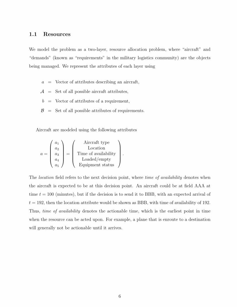
Aircraft are modeled using the following attributes

a =

a1

a2

a3

a4

a5

=

Aircraft type

LocationTime of availability

Loaded/emptyEquipment status

.

The location field refers to the next decision point, where time of availability denotes when

the aircraft is expected to be at this decision point. An aircraft could be at field AAA at

time t = 100 (minutes), but if the decision is to send it to BBB, with an expected arrival of

t = 192, then the location attribute would be shown as BBB, with time of availability of 192.

Thus, time of availability denotes the actionable time, which is the earliest point in time

when the resource can be acted upon. For example, a plane that is enroute to a destination

will generally not be actionable until it arrives.

6

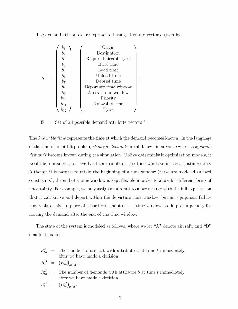
The demand attributes are represented using attribute vector b given by

b =

b1

b2

b3

b4

b5

b6

b7

b8

b9

b10

b11

b12

=

OriginDestination

Required aircraft typeBrief timeLoad time

Unload timeDebrief time

Departure time windowArrival time window

PriorityKnowable time

Type

,

B = Set of all possible demand attribute vectors b.

The knowable time represents the time at which the demand becomes known. In the language

of the Canadian airlift problem, strategic demands are all known in advance whereas dynamic

demands become known during the simulation. Unlike deterministic optimization models, it

would be unrealistic to have hard constraints on the time windows in a stochastic setting.

Although it is natural to retain the beginning of a time window (these are modeled as hard

constraints), the end of a time window is kept flexible in order to allow for different forms of

uncertainty. For example, we may assign an aircraft to move a cargo with the full expectation

that it can arrive and depart within the departure time window, but an equipment failure

may violate this. In place of a hard constraint on the time window, we impose a penalty for

moving the demand after the end of the time window.

The state of the system is modeled as follows, where we let “A” denote aircraft, and “D”

denote demands:

RAta = The number of aircraft with attribute a at time t immediately

after we have made a decision,

RAt =

(RA

ta

)a∈A ,

RDtb = The number of demands with attribute b at time t immediately

after we have made a decision,

RDt =

(RD

tb

)b∈B .

7

The resource state of our system is given by

Rt =(RA

t , RDt

).

A Java-based software library has been developed at CASTLE Laboratory at Princeton

University that captures this modeling framework. An important aspect of the model is the

flexibility inherent in the use of the attribute vector. It is quite easy to add dimensions to the

attribute vector, and there is no limit to the number or detail of the attributes. We assume

that the attribute vector is sufficiently complex that we cannot enumerate the attribute space

- even small problems can have an attribute space A with millions of elements; for complex

resources such as pilots and aircraft, the attribute space may be orders of magnitude larger.

1.2 Decisions

We assume that the aircraft are actionable resources (decisions could act on an aircraft to

change its attributes) whereas the demands are passive (an aircraft can pick up a demand,

but we cannot act on a demand by itself other than to “do nothing”). For our project,

the only decision classes were to move a demand, move empty to a location, or do nothing.

In a more general model, we could also include decisions such as repairing the aircraft,

reconfiguring the aircraft (for example, adding seats so we can handle passengers), and even

moving loads with outside aircraft, but these were not handled in our study. We use the

following notation to represent decisions:

DL = Set of decisions to move an aircraft to a specific location; this isthe set of locations we can move to,

DD = Set of decisions to serve a demand of a particular type; eachelement of DD corresponds to an element of B,

dφ = “Do nothing” decision,

D = Set of all decision types ≡ DL⋃DD

⋃dφ.

The set DL captures our ability to move to a location in anticipation of a demand that we do

not yet know about. As a result, for each decision d ∈ DD, there is an element bd ∈ B. We

8

model an element d ∈ DD as being either a single demand, or a set of two or three demands

which the dataset has already linked as potentially being served together. The same demand

can be covered by more than one decision (we can decide to serve a demand by itself, or as

part of a pair of demands or a separate group of three demands). We introduce a linking

constraint so that it cannot cover the same demand twice.

The decision vector is represented using

xtad = Number of resources with attribute a that we act on with adecision of type d using the information available at time t,

xt = The vector of decisions acting on all the aircraft at time t,

= (xtad)a∈A,d∈D .

Decisions are made using a decision function which we represent using

Xπt = Function returning a feasible decision vector xt .

In the language of dynamic programming, Xπt constitutes a policy, which is a rule for choosing

a decision given the information available. We typically have a family of decision functions

which we denote by Π, where for π ∈ Π, Xπt is a particular decision function. Our challenge,

stated formally below, is to choose the best decision function.

1.3 System dynamics

The system dynamics describes how the state of our system evolves over time. We model

physical events in continuous time (for example, departures and arrivals can occur at any

time), but we model decisions in discrete time (we use six hour time steps for our experi-

ments). For this reason, we have to model the evolution of what we know about the system

in discrete time.

The attribute vector a of an aircraft changes because of decisions and exogenous informa-

tion. There are two forms of exogenous information in our problem: exogenous changes to

9

the aircraft resource vector RAt , and exogenous changes to the vector of customer demands,

RDt . We let:

RAt = Exogenous changes to the aircraft state vector that occur be-

tween t− 1 and t.

RDt = Exogenous changes to the demand state vector that occur be-

tween t− 1 and t.

RDt typically represents new customer requests, but it also could be used to capture changes

to an existing customer request. RAt can be used to capture weather delays or equipment

failures (a plane that should have been available at time t = 192 will now be available at

t = 204). We let Wt be our general notation for exogenous information arriving between

t−1 and t (in a more general model, we can allow exogenous information that changes other

elements of the problem than just the resource vector). For our problem,

Wt = (RAt , RD

t ).

Using the standard language of probability, (W1, W2, . . . , ) represents the stochastic process

driving the system. Let Ω be the set of sample realizations of the information process, with

sample realization ω ∈ Ω given by (W1(ω), W2(ω), . . . , ). Let F be the sigma-algebra on Ω,

and let Ft be the sigma-algebra generated by (W1, W2, . . . ,Wt), where we have the standard

property that the sequence F1,F2, . . . , forms a filtration. In our notation, any variable

indexed by t is Ft-measurable.

We define a state variable St as all the information we need to make a decision (that

is, compute Xπt (St)) and compute the forward dynamics of the system. For our model, our

state variable is the same as the resource state, which is to say that St = Rt. However, for

other applications the state variable could capture weather conditions, field conditions (was

a target destroyed? what is the condition of an airbase?) and information about the enemy

(did he attack?). In even more general models, the state variable can include estimates that

are used to forecast the future (what is the likelihood that a target will be attacked?).

We model the evolution of the state of individual resources (the aircraft) using the at-

10

tribute transition function

at+1 = aM(at, dt, Wt+1)

which describes how the attribute vector changes as a result a decision dt acting on a single

entity (in our case, an aircraft) with attribute at. The details of the attribute transition

function are not important to an understanding of our model, but it is clear that we can

handle a high level of generality. For algebraic purposes, we also define the indicator function

δa′ (a, d, W ) =

1 if aM(a, d, W ) = a′

0 Otherwise.

The attribute transition function describes how a particular resource with attribute a evolves

in response to new information W and a decision d. We can apply this function to all the

resources, and produces the resource transition function represented using

Rt+1 = RM(Rt, xt, Wt+1).

The evolution of our resource vector is given by,

RAt+1,a′ =

∑a∈A

∑d∈D

δa′(a, d,Wt+1)xtad.

Flow conservation requires that

∑d∈D

xtad = RAt,a.

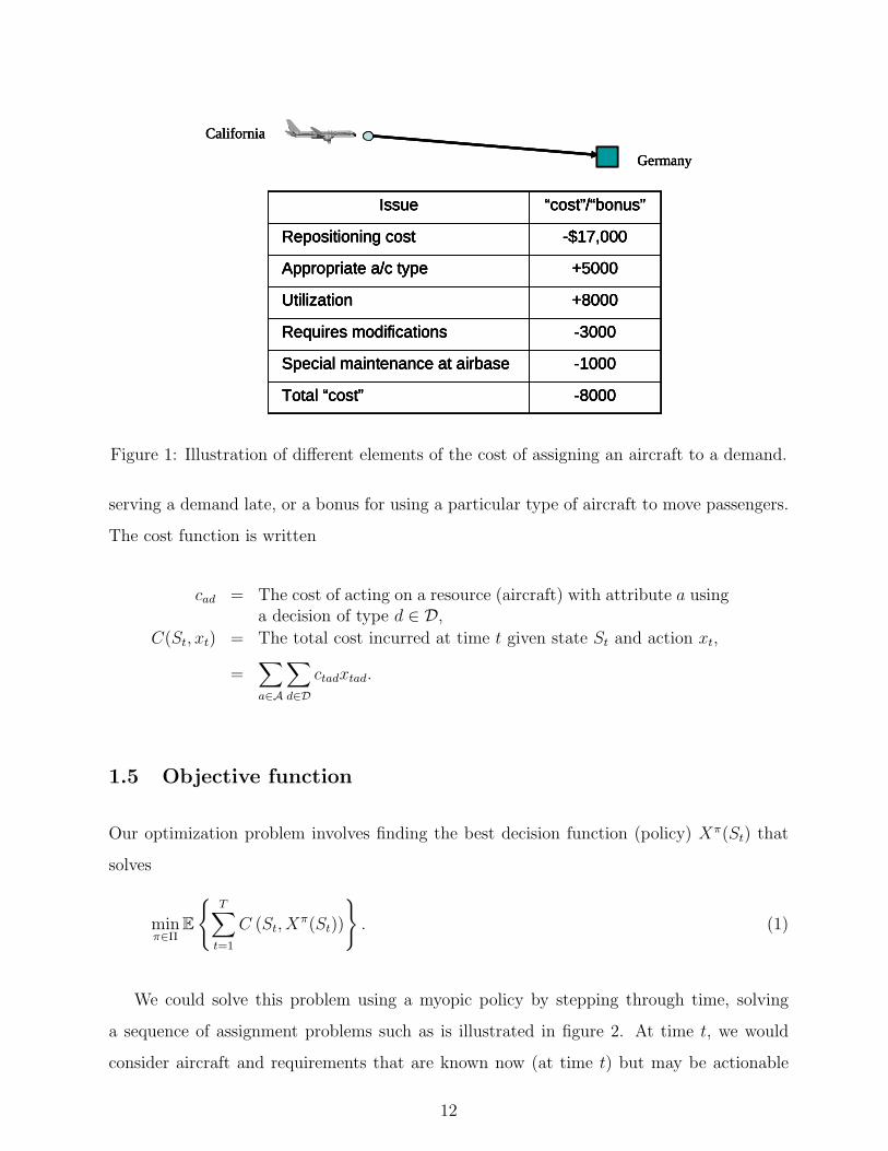
1.4 The cost function

The cost function has to capture not only the cost of activities such as moving aircraft, but

also penalties and bonuses for different types of behaviors. Figure 1 illustrates the different

types of costs that might be assessed to assign an aircraft to a demand. These will typically

be a mixture of hard-dollar and soft-dollar costs. For example, we might have a penalty for

11

California

Germany

-8000Total “cost”

-1000Special maintenance at airbase

-3000Requires modifications

+8000Utilization

+5000Appropriate a/c type

-$17,000Repositioning cost

“cost”/“bonus”Issue

-8000Total “cost”

-1000Special maintenance at airbase

-3000Requires modifications

+8000Utilization

+5000Appropriate a/c type

-$17,000Repositioning cost

“cost”/“bonus”Issue

California

Germany

California

Germany

-8000Total “cost”

-1000Special maintenance at airbase

-3000Requires modifications

+8000Utilization

+5000Appropriate a/c type

-$17,000Repositioning cost

“cost”/“bonus”Issue

-8000Total “cost”

-1000Special maintenance at airbase

-3000Requires modifications

+8000Utilization

+5000Appropriate a/c type

-$17,000Repositioning cost

“cost”/“bonus”Issue

Figure 1: Illustration of different elements of the cost of assigning an aircraft to a demand.

serving a demand late, or a bonus for using a particular type of aircraft to move passengers.

The cost function is written

cad = The cost of acting on a resource (aircraft) with attribute a usinga decision of type d ∈ D,

C(St, xt) = The total cost incurred at time t given state St and action xt,

=∑a∈A

∑d∈D

ctadxtad.

1.5 Objective function

Our optimization problem involves finding the best decision function (policy) Xπ(St) that

solves

minπ∈Π

E

T∑

t=1

C (St, Xπ(St))

. (1)

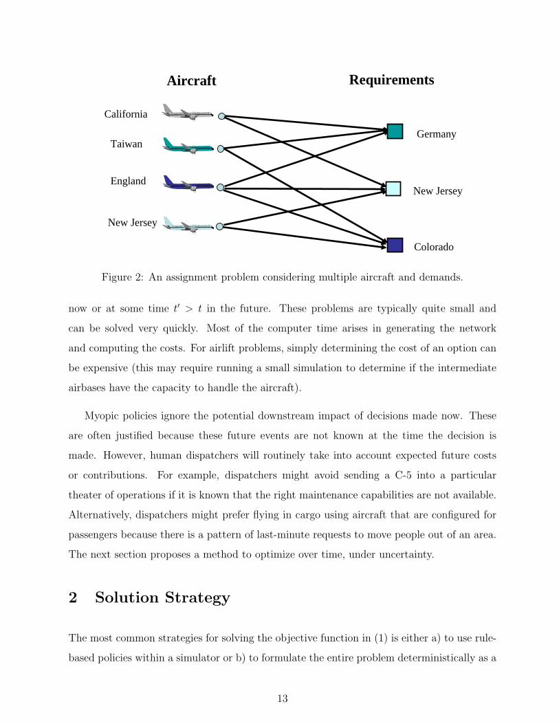
We could solve this problem using a myopic policy by stepping through time, solving

a sequence of assignment problems such as is illustrated in figure 2. At time t, we would

consider aircraft and requirements that are known now (at time t) but may be actionable

12

California

Germany

New Jersey

Colorado

Taiwan

England

New Jersey

Aircraft Requirements

Figure 2: An assignment problem considering multiple aircraft and demands.

now or at some time t′ > t in the future. These problems are typically quite small and

can be solved very quickly. Most of the computer time arises in generating the network

and computing the costs. For airlift problems, simply determining the cost of an option can

be expensive (this may require running a small simulation to determine if the intermediate

airbases have the capacity to handle the aircraft).

Myopic policies ignore the potential downstream impact of decisions made now. These

are often justified because these future events are not known at the time the decision is

made. However, human dispatchers will routinely take into account expected future costs

or contributions. For example, dispatchers might avoid sending a C-5 into a particular

theater of operations if it is known that the right maintenance capabilities are not available.

Alternatively, dispatchers might prefer flying in cargo using aircraft that are configured for

passengers because there is a pattern of last-minute requests to move people out of an area.

The next section proposes a method to optimize over time, under uncertainty.

2 Solution Strategy

The most common strategies for solving the objective function in (1) is either a) to use rule-

based policies within a simulator or b) to formulate the entire problem deterministically as a

13

single, large linear (or integer) program. Morton et al. (2002) uses stochastic programming

for a version of the sealift problem, but this technique is not able to handle the types of

complex system dynamics we wish to consider here. In this section, we show how to use the

techniques of approximate dynamic programming to solve multistage linear programs. Our

strategy is based on the concepts given in Powell (2007).

In the remainder of this section, we describe the solution of this problem using approxi-

mate dynamic programming.

2.1 Approximate Dynamic Programming

We can formulate our problem as a dynamic program. If we follow a classical model (see,

for example, Puterman (1994)), we would define a state variable St, and let Vt(St) be the

value of being in state St. Bellman’s optimality equation would then be written

Vt(St) = maxxt∈Xt

(C(St, xt) + EVt+1(St+1(St, xt, Wt+1))|St

)(2)

where the feasible region Xt is defined by

∑d∈D

xtad = RAta, (3)

xtad ≥ 0.

Here, St+1(St, xt, Wt+1) gives the state St+1 as function of the current state St, the decisions

xt and the new information Wt+1. We note that our constraint set is much simpler than

what would normally be found in a math programming formulation, which requires that all

the physics captured in the transition function be represented using set of linear equations.

Solving Bellman’s equation using standard techniques (e.g. Puterman (1994)) encounters

the classic curse of dimensionality. We avoid this by breaking the transition function into

two steps: the transition from the pre-decision state variable St to the post-decision state Sxt ,

where Sxt is the state of the system at time t, immediately after we have made a decision.

Since St = Rt for our problem (this is not the case for more general problems), we break the

14

resource transition function RM(·) into two functions which produce

Rxt = RM,x(Rt, xt), (4)

Rt+1 = RM,W (Rxt , Wt+1). (5)

Equation (4) is written by creating a version of the attribute transition function that captures

the effect of the decision dt, without capturing the effect of new information Wt+1. This would

be written

axt = aM,x(at, dt)

represented using an indicator function δa′(a, d) similar to our previous indicator function.

This allows us to write

Rxta′ =

∑a∈A

∑d∈D

δa′(at, dt)xtad.

We then let the effect of new information be captured by the change variable Rta, allowing

us to write

Rt+1,a = Rxta + Rt+1,a.

In our presentation, we focus primarily on RAt , but the expressions above apply equally to

demands.

Using the pre- and post-decision states allows us to break Bellman’s equation into two

steps, given by

Vt(St) = minxt∈Xt

(C(St, xt) + V x

t (Sxt ), (6)

V xt (Sx

t ) = E Vt+1(St+1)|Sxt , (7)

where Vt(St) is the traditional value of being in (pre-decision) state St, while V xt (Sx

t ) is the

value of being in post-decision state Sxt . Note that equation (6) is completely deterministic,

15

while equation (7) involves nothing more than an expectation (which is computationally

intractable for most applications, including ours).

The next step is to replace the function V xt (Sx

t ) with an approximation. There are a

number of strategies we can use. For our work, we used

V xt (Sx

t ) = Vt(Rxt )

=∑a∈A

Vta(Rta),

where Vta(Rta) is piecewise linear and concave in Rta, given by

Vta(Rxta) =

bRxtac∑

r=1

vta(r − 1) + (Rxta − bRx

tac)vta(bRxtac)

, (8)

where bRc is the largest integer less than or equal to R. This function is parameterized

by the slopes (vta(r)) for r = 0, 1, . . . , Rmax, where Rmax is an upper bound on the number

of resources of a particular type. This approximation has worked well in a number of fleet

management problems (Godfrey & Powell (2002), Powell & Topaloglu (2005), Topaloglu &

Powell (2006), Wu et al. (2006)).

We next solve the decision problem given by

xnt (Rt) = arg min

xt∈Xnt

(C(Rn

t , xt) + V n−1t (RM(Rx

t ))). (9)

For our application, equation (9) is an integer program (specifically, an integer multicom-

modity flow problem) which can be solved using a commercial solver. Let Vt(Rnt ) be the

objective function value obtained by solving (9). We can update our value function using

estimates of the derivative of Vt(Rt) with respect to Rt. If we compute this in a brute force

manner, we would compute

vnta = Vt(R

nt + eta)− Vt(R

nt )

where eta is a vector of 0’s with a 1 in the element corresponding to (t, a). In practice, we

often use the dual variable associated with the flow conservation constraint (3).

16

The last step of the process is to use vnt to update the value function approximation

V n−1t−1 (Rx,n

t−1) around the previous post-decision state Rx,nt−1. Assume that r = Rx,n

t−1,a is the

number of cargo aircraft with attribute a at t− 1 after we made our previous decision. We

would then update the slope corresponding to r using

vnta(r) = (1− αn−1)v

n−1ta (r) + αn−1v

nta. (10)

After this update, we might find we have a concavity violation, which is to say that we no

longer have vnta(r) ≥ vn

ta(r+1) for all r. This is easily fixed using any of the methods described

in Godfrey & Powell (2001), Topaloglu & Powell (2003) or Powell et al. (2004a). For ease of

reference, we are going to refer to the entire process of updating the value function using

V nt−1(R

xt−1) = UV (V n−1

t−1 (Rxt−1), R

x,nt−1v

nt ).

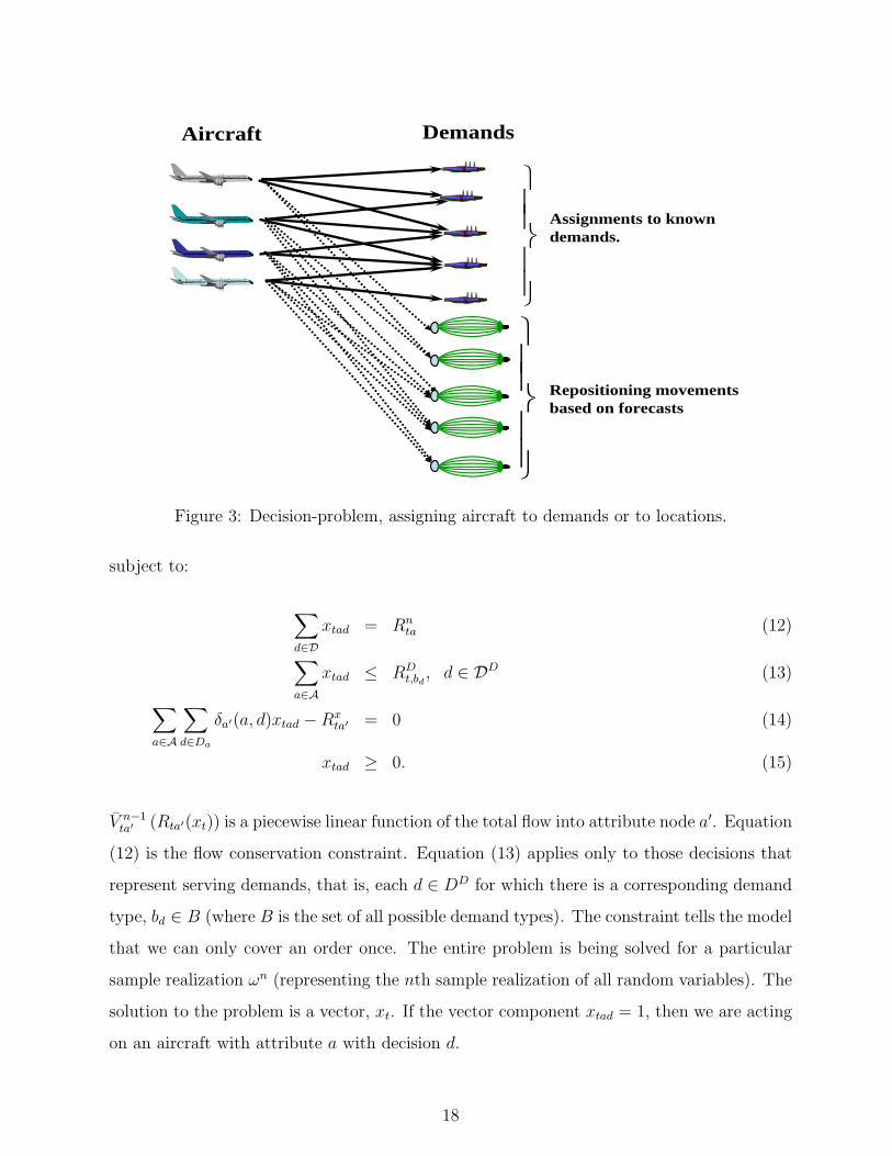
2.2 The decision problem

At any one point in time, we can assign aircraft to demands, or as movements to physical

locations (see figure 3). A movement to a different physical location has the effect of cre-

ating an aircraft with a modified vector of attributes in the future. We can also consider

decisions which modify the attributes without moving the aircraft to another location (e.g.

reconfiguring the aircraft).

We model the assignment of aircraft to demands as a network, with one node for each

aircraft (more precisely, each type of aircraft) to each demand. From each aircraft node

(these nodes may have zero, one or more than one aircraft) we either generate an assignment

arc (to a demand) or an arc to a node from which we have a series of parallel arcs which

model a piecewise linear value function. These parallel arcs capture the marginal value of

an additional aircraft with a particular set of attributes.

The problem in figure 3 is a linear program which can be mathematically expressed as

xnt = arg max

xt∈Xt

(∑a∈A

∑d∈D

ctadxtad +∑a′∈A

V n−1ta′ (Rta′(xt))

), (11)

17

Aircraft Demands

⎫⎪⎪⎬⎪⎪⎭

Assignments to known demands.

⎫⎪⎪⎬⎪⎪⎭

Repositioning movements based on forecasts

Figure 3: Decision-problem, assigning aircraft to demands or to locations.

subject to:

∑d∈D

xtad = Rnta (12)∑

a∈A

xtad ≤ RDt,bd

, d ∈ DD (13)∑a∈A

∑d∈Da

δa′(a, d)xtad −Rxta′ = 0 (14)

xtad ≥ 0. (15)

V n−1ta′ (Rta′(xt)) is a piecewise linear function of the total flow into attribute node a′. Equation

(12) is the flow conservation constraint. Equation (13) applies only to those decisions that

represent serving demands, that is, each d ∈ DD for which there is a corresponding demand

type, bd ∈ B (where B is the set of all possible demand types). The constraint tells the model

that we can only cover an order once. The entire problem is being solved for a particular

sample realization ωn (representing the nth sample realization of all random variables). The

solution to the problem is a vector, xt. If the vector component xtad = 1, then we are acting

on an aircraft with attribute a with decision d.

18

2.3 The stepsize rule

Approximate dynamic programming requires smoothing old estimates with new information,

as we do in equation (10). This is handled using a stepsize 0 < αn−1 < 1 that governs the

relative weight that is put on new information. There is an extensive literature on stepsizes

and it is important that an appropriate rule be used (see George & Powell (2006) for a review

of stepsize formulas). A popular rule is

αn =α

α + n− 1

where α between 5 and 10 seems to give good results for most dynamic programming ap-

plications. A problem with this rule is that it is necessary to find a single value of α that

works well for each attribute a ∈ A and each time period t.

The rule we used in our experiments is a stochastic stepsize rule which adapts to the data

(referred to as the “optimal stepsize algorithm,” or OSA, in George & Powell (2006)). This

rule begins by computing the error between the current estimate of the value of a resource

and the latest estimate

εnt−1,a = vn−1

t−1,a − vnta. (16)

We then smooth these errors and produce an estimate of the bias βnt−1,a (a rough estimate

of the difference between the current values and the “true” function) and the square of the

bias ¯βn

νn =νn−1

1 + νn−1 − ν, (17)

βnt−1,a = (1− νn−1) βn−1

t−1,a + νn−1εnt−1,a, (18)

¯βnt−1,a = (1− νn−1)

¯βn−1t−1,a + νn−1(ε

nt−1,a)

2. (19)

ν in equation (17) is the only tunable parameter, but we have found that ν = 0.10 is very

19

robust. We next compute an estimate of the variance of vn−1t−1,a using

(σ2)nt−1,a =

¯βnt−1,a − (βn

t−1,a)2

1 + λn−1, (20)

λn = (1− αn−1)2λn−1 + (αn−1)

2. (21)

Note that α0 = 1, which means that λ1 = 1. Finally, we compute the stepsize using

αn = 1− (σ2)n

(1 + λn−1)(σ2)n +(βn)2 . (22)

It can be shown that αn ≥ 1/n, which satisfies an important convergence criterion. This

stepsize formula also has the behavior that the stepsize decreases as (σ2)nt−1,a increases (high

noise produces smaller stepsizes). Conversely, the stepsize increases as the estimated bias

βnt−1,a increases. This is the property that allows the formula to adapt in a reasonable way to

the level of noise and any measured shift in the estimates (a common property in the initial

iterations for approximate dynamic programs).

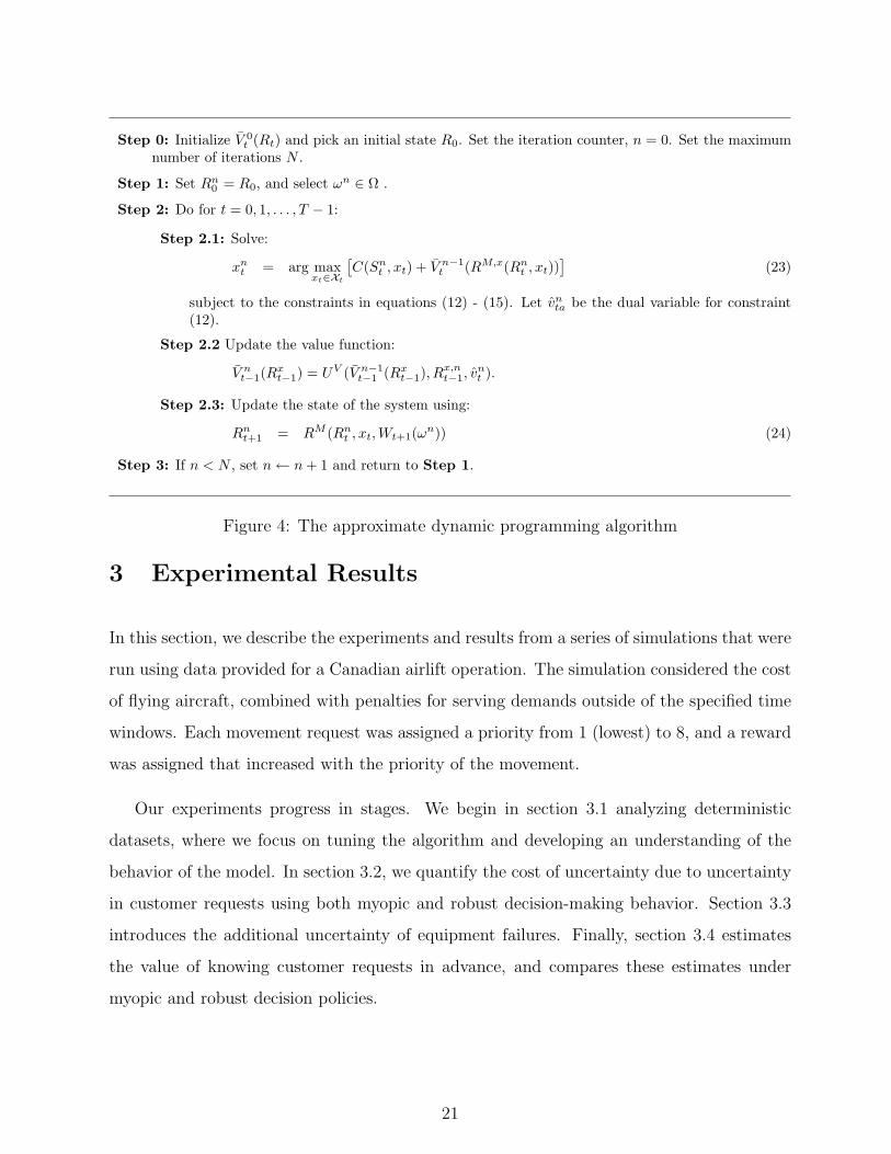
2.4 The Basic ADP Algorithm

In figure 4, we sketch a simple ADP algorithm that incorporates the features discussed in the

previous sections. At each iteration, we update the value function based on the information

we have obtained. Proper design and careful updating of the value function approximation

can produce optimizing behavior in the sense that the solution will tend to get better over

the iterations. There is no guarantee that the algorithm will produce the optimal solution,

even in the limit.

The number of iterations is determined in an ad-hoc fashion by examining the convergence

of the objective function. Another measure is to use the variance of the estimates of the

value function (σ2)nt−1,a, computed using equation (20), averaged over the attributes. This

measure is particularly useful if we are using the values to make decisions, for example, about

the value of a type of aircraft. In other policy studies, it is more important to determine if

some statistic (for example, number of flights covered late) has stabilized.

20

Step 0: Initialize V 0t (Rt) and pick an initial state R0. Set the iteration counter, n = 0. Set the maximum

number of iterations N .

Step 1: Set Rn0 = R0, and select ωn ∈ Ω .

Step 2: Do for t = 0, 1, . . . , T − 1:

Step 2.1: Solve:

xnt = arg max

xt∈Xt

[C(Sn

t , xt) + V n−1t (RM,x(Rn

t , xt))]

(23)

subject to the constraints in equations (12) - (15). Let vnta be the dual variable for constraint

(12).

Step 2.2 Update the value function:

V nt−1(R

xt−1) = UV (V n−1

t−1 (Rxt−1), R

x,nt−1, v

nt ).

Step 2.3: Update the state of the system using:

Rnt+1 = RM (Rn

t , xt,Wt+1(ωn)) (24)

Step 3: If n < N , set n← n + 1 and return to Step 1.

Figure 4: The approximate dynamic programming algorithm

3 Experimental Results

In this section, we describe the experiments and results from a series of simulations that were

run using data provided for a Canadian airlift operation. The simulation considered the cost

of flying aircraft, combined with penalties for serving demands outside of the specified time

windows. Each movement request was assigned a priority from 1 (lowest) to 8, and a reward

was assigned that increased with the priority of the movement.

Our experiments progress in stages. We begin in section 3.1 analyzing deterministic

datasets, where we focus on tuning the algorithm and developing an understanding of the

behavior of the model. In section 3.2, we quantify the cost of uncertainty due to uncertainty

in customer requests using both myopic and robust decision-making behavior. Section 3.3

introduces the additional uncertainty of equipment failures. Finally, section 3.4 estimates

the value of knowing customer requests in advance, and compares these estimates under

myopic and robust decision policies.

21

90

92

94

96

98

100

0 10 20 30 40 50

Iteration

Per

cent

cov

erag

e

Known before 0 hoursKnown before 12 hoursKnown before 24 hours

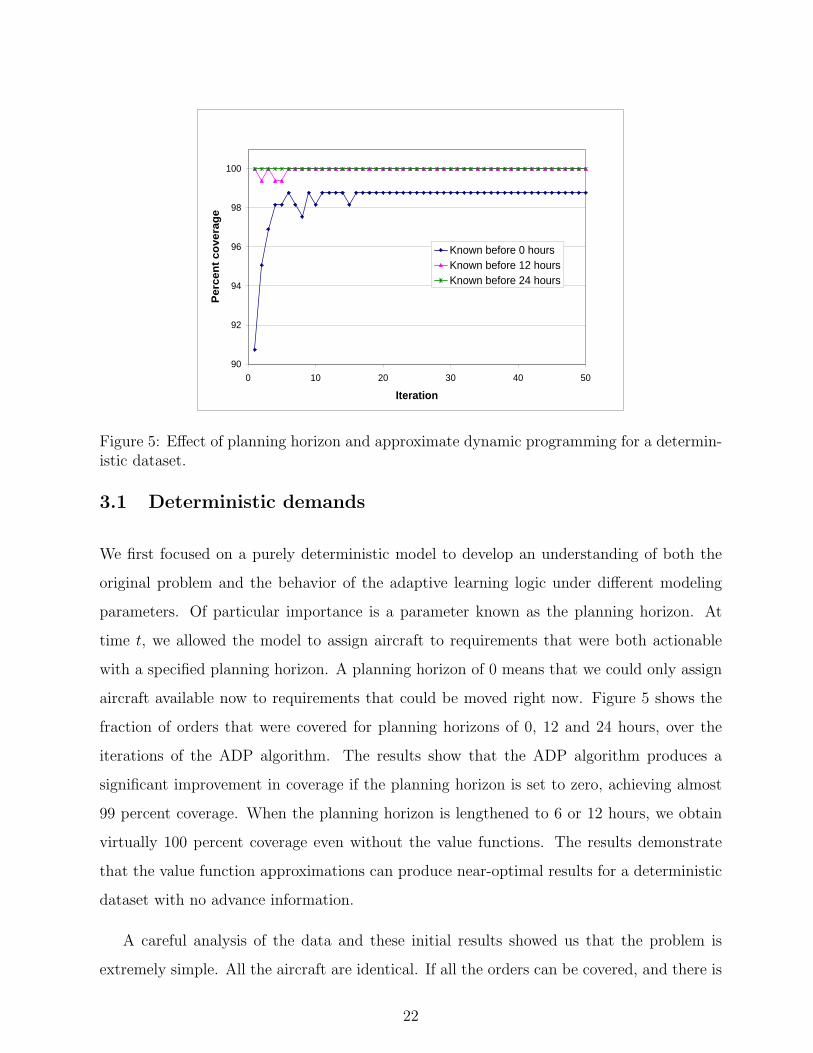
Figure 5: Effect of planning horizon and approximate dynamic programming for a determin-istic dataset.

3.1 Deterministic demands

We first focused on a purely deterministic model to develop an understanding of both the

original problem and the behavior of the adaptive learning logic under different modeling

parameters. Of particular importance is a parameter known as the planning horizon. At

time t, we allowed the model to assign aircraft to requirements that were both actionable

with a specified planning horizon. A planning horizon of 0 means that we could only assign

aircraft available now to requirements that could be moved right now. Figure 5 shows the

fraction of orders that were covered for planning horizons of 0, 12 and 24 hours, over the

iterations of the ADP algorithm. The results show that the ADP algorithm produces a

significant improvement in coverage if the planning horizon is set to zero, achieving almost

99 percent coverage. When the planning horizon is lengthened to 6 or 12 hours, we obtain

virtually 100 percent coverage even without the value functions. The results demonstrate

that the value function approximations can produce near-optimal results for a deterministic

dataset with no advance information.

A careful analysis of the data and these initial results showed us that the problem is

extremely simple. All the aircraft are identical. If all the orders can be covered, and there is

22

no differentiation between the aircraft, then looking into the future offers almost no value.

The travel times are quite short. Most movements can be made within 6 hours, and virtually

all can be made within 12 hours.

The most difficult problem we faced was the classical challenge of sequencing orders

within their time windows. Typically, in a stochastic, dynamic problem, we are trying to

serve as many orders as we can as quickly as possible. If we cannot serve all orders with

available aircraft, we determine which ones to solve using a combination of assignment costs,

the value of the order (determined by its priority) and the downstream value function. It

is the value function (which gives the value of the aircraft after the order is completed)

that helps us with the sequencing (for example, that we can serve a short demand now and

still cover another demand later). The execution times for the optimizing-simulator are not

affected by the presence of wide time windows. By contrast, wide time windows can produce

a dramatic increase in the execution times for column-generation methods (see Desrosiers

et al. (1984), Desrosiers et al. (1995), and Chen & Powell (1999)). We can obtain very high

quality solutions with tight time windows, or very wide time windows. When there is a

mixture of tight and wide time windows, we will notice a modest degradation in solution

quality (run times are the same under all scenarios).

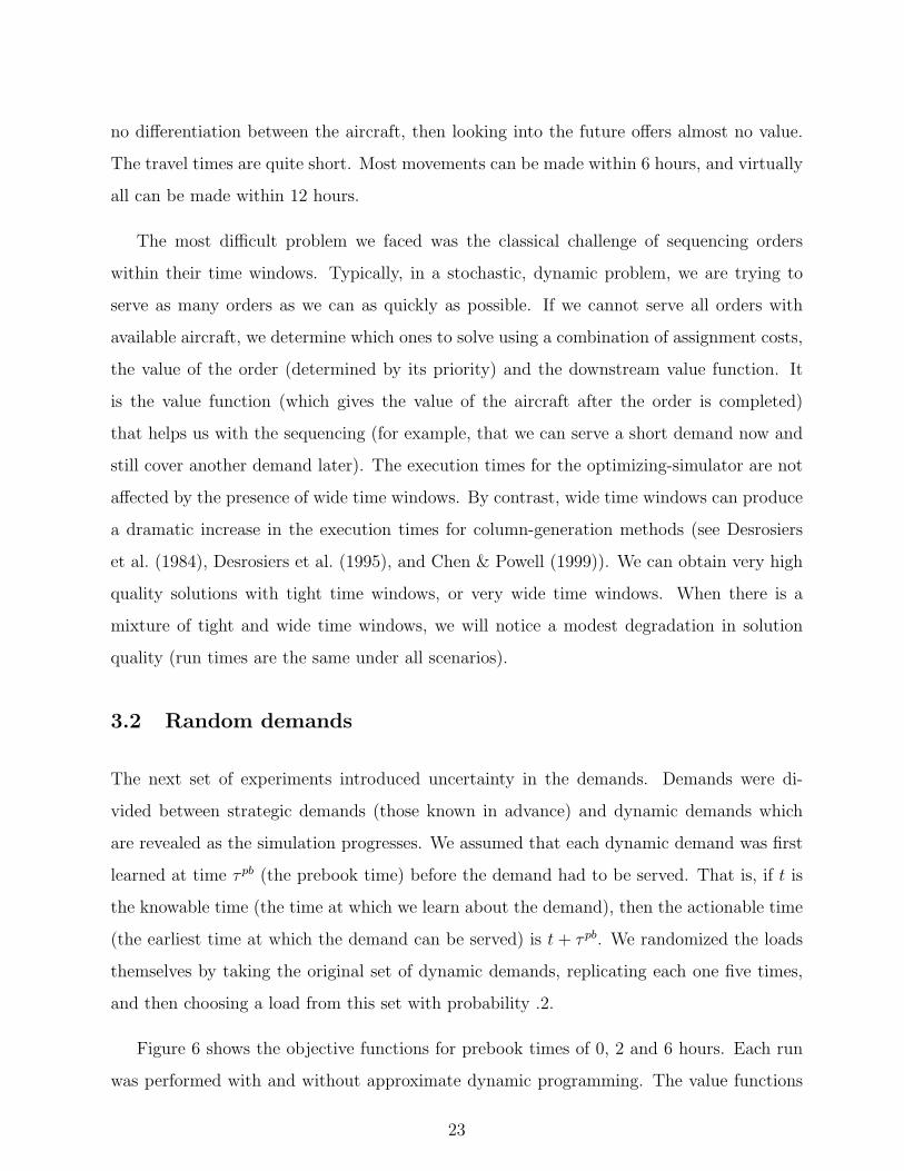
3.2 Random demands

The next set of experiments introduced uncertainty in the demands. Demands were di-

vided between strategic demands (those known in advance) and dynamic demands which

are revealed as the simulation progresses. We assumed that each dynamic demand was first

learned at time τ pb (the prebook time) before the demand had to be served. That is, if t is

the knowable time (the time at which we learn about the demand), then the actionable time

(the earliest time at which the demand can be served) is t + τ pb. We randomized the loads

themselves by taking the original set of dynamic demands, replicating each one five times,

and then choosing a load from this set with probability .2.

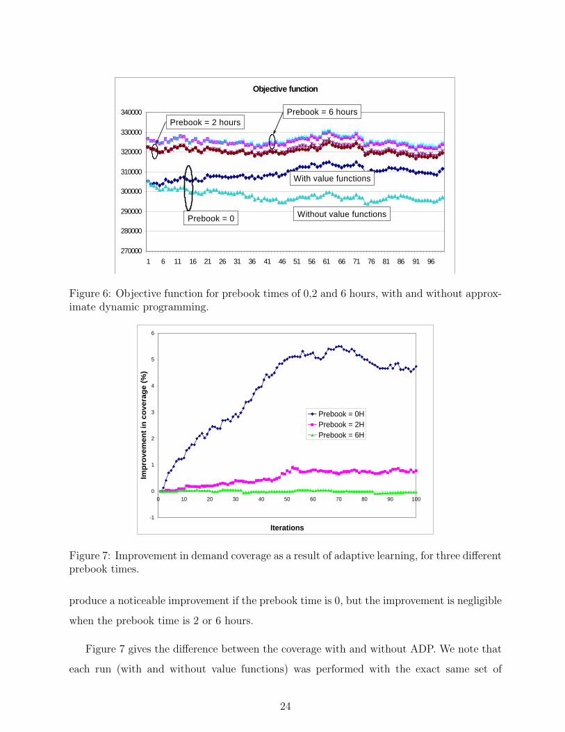
Figure 6 shows the objective functions for prebook times of 0, 2 and 6 hours. Each run

was performed with and without approximate dynamic programming. The value functions

23

Objective function

270000

280000

290000

300000

310000

320000

330000

340000

1 6 11 16 21 26 31 36 41 46 51 56 61 66 71 76 81 86 91 96

Prebook = 0

With value functions

Without value functions

Prebook = 2 hoursPrebook = 6 hours

Objective function

270000

280000

290000

300000

310000

320000

330000

340000

1 6 11 16 21 26 31 36 41 46 51 56 61 66 71 76 81 86 91 96

Prebook = 0

With value functions

Without value functions

Prebook = 2 hoursPrebook = 6 hours

Figure 6: Objective function for prebook times of 0,2 and 6 hours, with and without approx-imate dynamic programming.

-1

0

1

2

3

4

5

6

0 10 20 30 40 50 60 70 80 90 100

Iterations

Impr

ovem

ent i

n co

vera

ge (%

)

Prebook = 0HPrebook = 2HPrebook = 6H

Figure 7: Improvement in demand coverage as a result of adaptive learning, for three differentprebook times.

produce a noticeable improvement if the prebook time is 0, but the improvement is negligible

when the prebook time is 2 or 6 hours.

Figure 7 gives the difference between the coverage with and without ADP. We note that

each run (with and without value functions) was performed with the exact same set of

24

280

285

290

295

300

305

310

315

320

325

330

0 10 20 30 40 50 60 70 80 90 100

Th

ou

san

ds

Iteration

Ob

ject

ive

Fu

nct

ion

no breakdowns, with learning

with breakdowns, with learning

no breakdowns, no learning

with breakdowns, no learning

Figure 8: Objective function in the presence/absence of breakdowns with and without learn-ing.

demand realizations (we use a different random sample of demands at each iteration, but

use the exact same sample for each run).

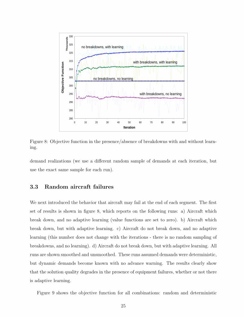
3.3 Random aircraft failures

We next introduced the behavior that aircraft may fail at the end of each segment. The first

set of results is shown in figure 8, which reports on the following runs: a) Aircraft which

break down, and no adaptive learning (value functions are set to zero). b) Aircraft which

break down, but with adaptive learning. c) Aircraft do not break down, and no adaptive

learning (this number does not change with the iterations - there is no random sampling of

breakdowns, and no learning). d) Aircraft do not break down, but with adaptive learning. All

runs are shown smoothed and unsmoothed. These runs assumed demands were deterministic,

but dynamic demands become known with no advance warning. The results clearly show

that the solution quality degrades in the presence of equipment failures, whether or not there

is adaptive learning.

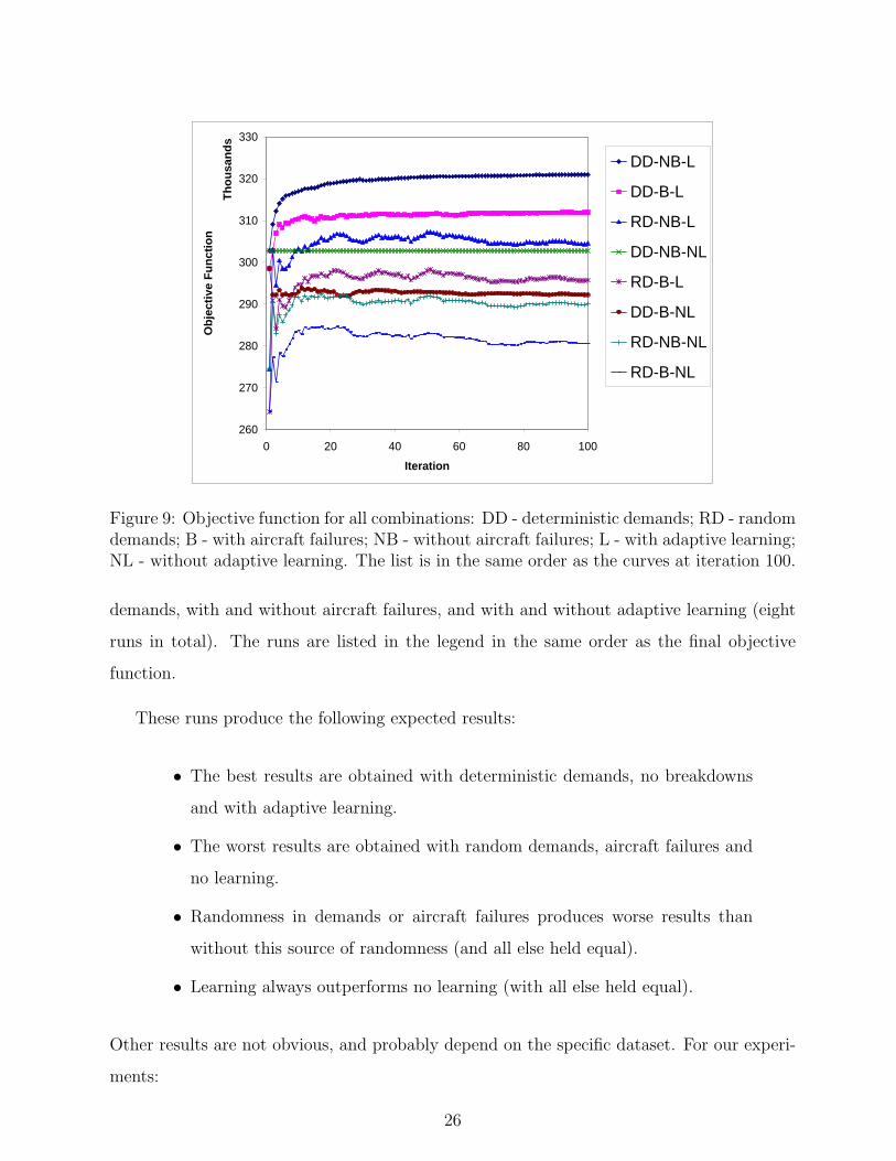
Figure 9 shows the objective function for all combinations: random and deterministic

25

260

270

280

290

300

310

320

330

0 20 40 60 80 100

Thou

sand

s

Iteration

Obj

ectiv

e Fu

nctio

n

DD-NB-L

DD-B-L

RD-NB-L

DD-NB-NL

RD-B-L

DD-B-NL

RD-NB-NL

RD-B-NL

Figure 9: Objective function for all combinations: DD - deterministic demands; RD - randomdemands; B - with aircraft failures; NB - without aircraft failures; L - with adaptive learning;NL - without adaptive learning. The list is in the same order as the curves at iteration 100.

demands, with and without aircraft failures, and with and without adaptive learning (eight

runs in total). The runs are listed in the legend in the same order as the final objective

function.

These runs produce the following expected results:

• The best results are obtained with deterministic demands, no breakdowns

and with adaptive learning.

• The worst results are obtained with random demands, aircraft failures and

no learning.

• Randomness in demands or aircraft failures produces worse results than

without this source of randomness (and all else held equal).

• Learning always outperforms no learning (with all else held equal).

Other results are not obvious, and probably depend on the specific dataset. For our experi-

ments:

26

• Randomness in demands has a more negative impact than aircraft failures,

with or without adaptive learning.

• Randomness in demands with adaptive learning outperforms deterministic

demands and no learning, when aircraft breakdowns are allowed (this result

is especially surprising).

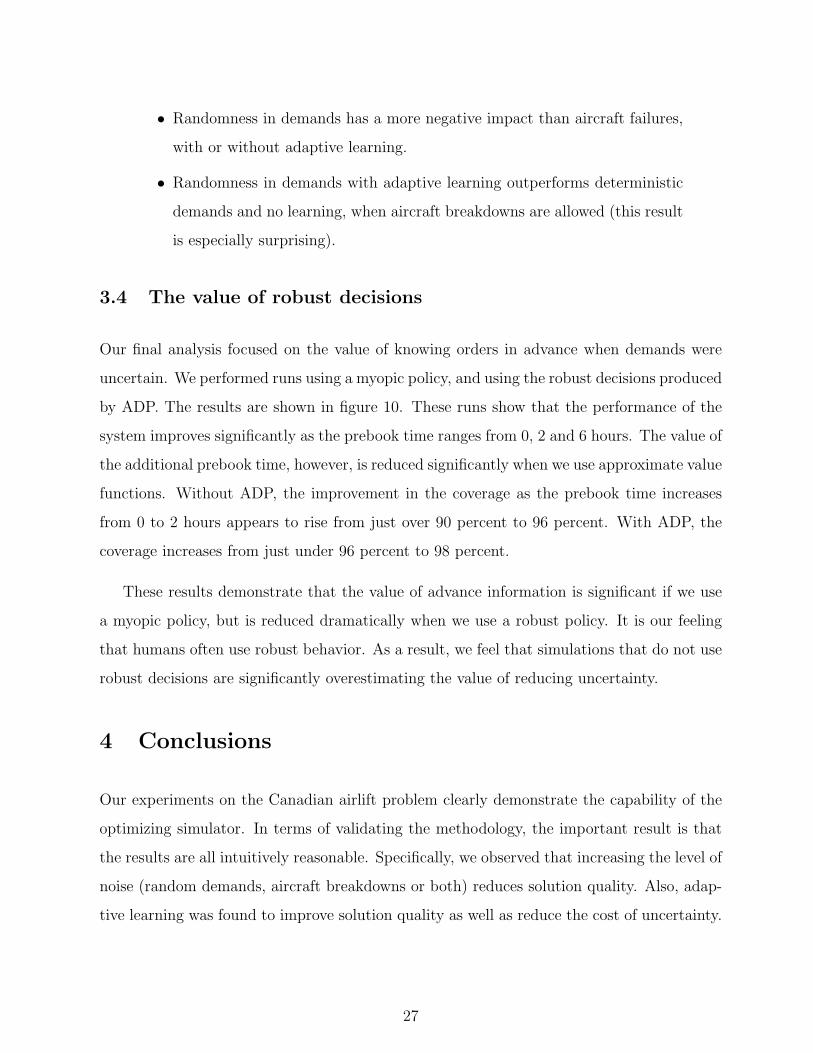
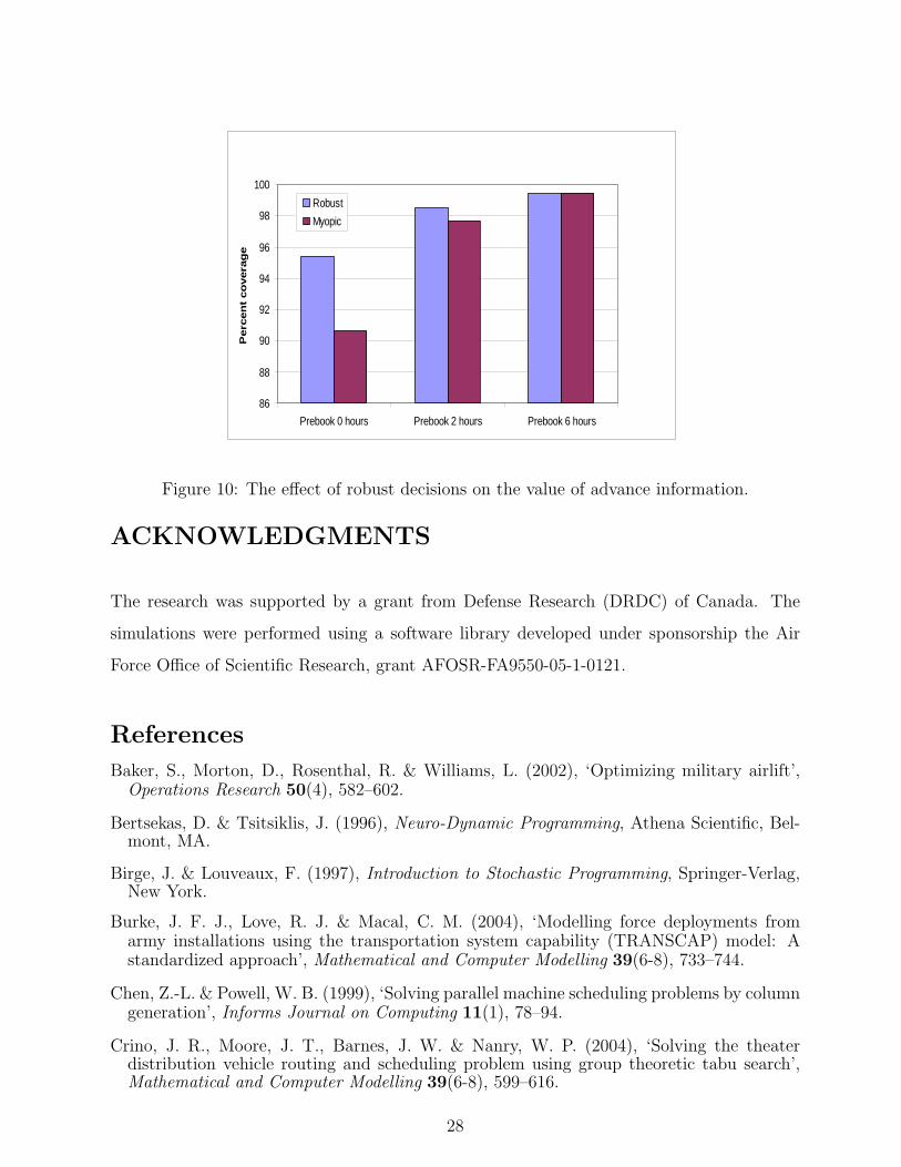
3.4 The value of robust decisions

Our final analysis focused on the value of knowing orders in advance when demands were

uncertain. We performed runs using a myopic policy, and using the robust decisions produced

by ADP. The results are shown in figure 10. These runs show that the performance of the

system improves significantly as the prebook time ranges from 0, 2 and 6 hours. The value of

the additional prebook time, however, is reduced significantly when we use approximate value

functions. Without ADP, the improvement in the coverage as the prebook time increases

from 0 to 2 hours appears to rise from just over 90 percent to 96 percent. With ADP, the

coverage increases from just under 96 percent to 98 percent.

These results demonstrate that the value of advance information is significant if we use

a myopic policy, but is reduced dramatically when we use a robust policy. It is our feeling

that humans often use robust behavior. As a result, we feel that simulations that do not use

robust decisions are significantly overestimating the value of reducing uncertainty.

4 Conclusions

Our experiments on the Canadian airlift problem clearly demonstrate the capability of the

optimizing simulator. In terms of validating the methodology, the important result is that

the results are all intuitively reasonable. Specifically, we observed that increasing the level of

noise (random demands, aircraft breakdowns or both) reduces solution quality. Also, adap-

tive learning was found to improve solution quality as well as reduce the cost of uncertainty.

27

86

88

90

92

94

96

98

100

Prebook 0 hours Prebook 2 hours Prebook 6 hours

Per

cen

t co

vera

ge

RobustMyopic

Figure 10: The effect of robust decisions on the value of advance information.

ACKNOWLEDGMENTS

The research was supported by a grant from Defense Research (DRDC) of Canada. The

simulations were performed using a software library developed under sponsorship the Air

Force Office of Scientific Research, grant AFOSR-FA9550-05-1-0121.

References

Baker, S., Morton, D., Rosenthal, R. & Williams, L. (2002), ‘Optimizing military airlift’,Operations Research 50(4), 582–602.

Bertsekas, D. & Tsitsiklis, J. (1996), Neuro-Dynamic Programming, Athena Scientific, Bel-mont, MA.

Birge, J. & Louveaux, F. (1997), Introduction to Stochastic Programming, Springer-Verlag,New York.

Burke, J. F. J., Love, R. J. & Macal, C. M. (2004), ‘Modelling force deployments fromarmy installations using the transportation system capability (TRANSCAP) model: Astandardized approach’, Mathematical and Computer Modelling 39(6-8), 733–744.

Chen, Z.-L. & Powell, W. B. (1999), ‘Solving parallel machine scheduling problems by columngeneration’, Informs Journal on Computing 11(1), 78–94.

Crino, J. R., Moore, J. T., Barnes, J. W. & Nanry, W. P. (2004), ‘Solving the theaterdistribution vehicle routing and scheduling problem using group theoretic tabu search’,Mathematical and Computer Modelling 39(6-8), 599–616.

28

Dantzig, G. & Ferguson, A. (1956), ‘The allocation of aircrafts to routes: An example oflinear programming under uncertain demand’, Management Science 3, 45–73.

Desrosiers, J., Solomon, M. & Soumis, F. (1995), Time constrained routing and schedul-ing, in C. Monma, T. Magnanti & M. Ball, eds, ‘Handbook in Operations Research andManagement Science, Volume on Networks’, North Holland, Amsterdam, pp. 35–139.

Desrosiers, J., Soumis, F. & Desrochers, M. (1984), ‘Routing with time windows by columngeneration’, Networks 14, 545–565.

George, A. & Powell, W. B. (2006), ‘Adaptive stepsizes for recursive estimation with appli-cations in approximate dynamic programming’, Machine Learning 65(1), 167–198.

George, A. & Powell, W. B. (to appear), ‘Adaptive stepsizes for recursive estimation withapplications in approximate dynamic programming’, Machine Learning.

Godfrey, G. & Powell, W. B. (2002), ‘An adaptive, dynamic programming algorithm forstochastic resource allocation problems I: Single period travel times’, Transportation Sci-ence 36(1), 21–39.

Godfrey, G. A. & Powell, W. B. (2001), ‘An adaptive, distribution-free approximation forthe newsvendor problem with censored demands, with applications to inventory and dis-tribution problems’, Management Science 47(8), 1101–1112.

Goggins, D. A. (1995), Stochastic modeling for airlift mobility, Master’s thesis, Naval Post-graduate School, Monterey, CA.

Higle, J. & Sen, S. (1991), ‘Stochastic decomposition: An algorithm for two-stage linearprograms with recourse’, Mathematics of Operations Research 16(3), 650–669.

Kall, P. & Wallace, S. (1994), Stochastic Programming, John Wiley & Sons, New York.

Killingsworth, P. & Melody, L. J. (1997), Should C17’s be deployed as theater assets?: Anapplication of the CONOP air mobility model, Technical report rand/db-171-af/osd, RandCorporation.

Midler, J. L. & Wollmer, R. D. (1969), ‘Stochastic programming models for airlift operations’,Naval Research Logistics Quarterly 16, 315–330.

Morton, D. P., Salmeron, J. & Wood, R. K. (2002), ‘A stochastic program for op-timizing military sealift subject to attack’, Stochastic Programming e-print series.http://www.speps.info.

Mulvey, J. M. & Ruszczynski, A. J. (1995), ‘A new scenario decomposition method forlarge-scale stochastic optimization’, Operations Research 43(3), 477–490.

Niemi, A. (2000), Stochastic modeling for the NPS/RAND Mobility Optimization Model,Department of Industrial Engineering, University of Wisconsin-Madison, Available:http://ie.engr.wisc.edu/robinson/Niemi.htm.

Powell, W. & Topaloglu, H. (2005), Fleet management, in S. Wallace & W. Ziemba, eds,‘Applications of Stochastic Programming’, Math Programming Society - SIAM Series inOptimization, Philadelphia.

Powell, W. B. (2007), Approximate Dynamic Programming: Solving the curses of dimen-sionality, John Wiley and Sons.

29

Powell, W. B. & Topaloglu, H. (2004), Fleet management, in S. Wallace & W. Ziemba, eds,‘Applications of Stochastic Programming’, Math Programming Society - SIAM Series inOptimization, Philadelphia.

Powell, W. B. & Van Roy, B. (2004), Approximate dynamic programming for high dimen-sional resource allocation problems, in J. Si, A. G. Barto, W. B. Powell & D. W. II, eds,‘Handbook of Learning and Approximate Dynamic Programming’, IEEE Press, New York.

Powell, W. B., Ruszczynski, A. & Topaloglu, H. (2004a), ‘Learning algorithms for separableapproximations of stochastic optimization problems’, Mathematics of Operations Research29(4), 814–836.

Powell, W. B., Shapiro, J. A. & Simao, H. P. (2002), ‘An adaptive dynamic program-ming algorithm for the heterogeneous resource allocation problem’, Transportation Science36(2), 231–249.

Powell, W. B., Wu, T. T. & Whisman, A. (2004b), ‘Using low dimensional patterns inoptimizing simulators: An illustration for the airlift mobility problem’, Mathematical andComputer Modeling 29, 657–2004.

Puterman, M. L. (1994), Markov Decision Processes, John Wiley & Sons, New York.

Rockafellar, R. & Wets, R. (1991), ‘Scenarios and policy aggregation in optimization underuncertainty’, Mathematics of Operations Research 16(1), 119–147.

Rosenthal, R., Morton, D., Baker, S., Lim, T., Fuller, D., Goggins, D., Toy, A., Turker, Y.,Horton, D. & Briand, D. (1997), ‘Application and extension of the Thruput II optimizationmodel for airlift mobility’, Military Operations Research 3(2), 55–74.

Ruszczynski, A. (2003), Decomposition methods, in A. Ruszczynski & A. Shapiro, eds,‘Handbook in Operations Research and Management Science, Volume on Stochastic Pro-gramming’, Elsevier, Amsterdam.

Sen, S. (2005), Algorithms for stochastic mixed-integer programming models, in K. Aardal,G. L. Nemhauser & R. Weismantel, eds, ‘Handbooks in Operations Research and Manage-ment Science: Discrete Optimization’, North Holland, Amsterdam.

Simao, H. P., Day, J., George, A. P., Gifford, T., Nienow, J. & Powell, W. B. (2007),An approximate dynamic programming algorithm for large-scale fleet management: Acase application, Technical Report CL-07-01, Department of Operations Research andFinancial Engineering, Princeton University.

Spivey, M. & Powell, W. B. (2004), ‘The dynamic assignment problem’, TransportationScience 38(4), 399–419.

Sutton, R. & Barto, A. (1998), Reinforcement Learning, The MIT Press, Cambridge, Mas-sachusetts.

Topaloglu, H. & Powell, W. (2006), ‘Dynamic programming approximations for stochas-tic, time-staged integer multicommodity flow problems’, Informs Journal on Computing18(1), 31–42.

Topaloglu, H. & Powell, W. B. (2003), ‘An algorithm for approximating piecewise linearconcave functions from sample gradients’, Operations Research Letters 31(1), 66–76.

Wing, V., Rice, R. E., Sherwood, R. & Rosenthal, R. E. (1991), Determining the optimalmobility mix, Technical report, Force Design Division, The Pentagon, Washington D.C.

30

Wu, T., Powell, W. & Whisman, A. (2006), The optimizing simulator: An intelligent analysistool for the military airlift problem, Technical report, Princeton University, Princeton, NJ.

Wu, T. T., Powell, W. B. & Whisman, A. (2003), The optimizing simulator: An intelli-gent analysis tool for the military airlift problem, Technical report, Princeton University,Department of Operations Research and Financial Engineering.

Yost, K. A. (1994), The thruput strategic airlift flow optimization model, Technical report,Air Force Studies and Analyses Agency, The Pentagon, Washington D.C.

Yost, K. A. & Washburn, A. R. (2000), ‘The LP/POMDP marriage: Optimization withimperfect information’, Naval Research Logistics 47(8), 607–619.

31