The effect of labor market monopsony on economic growth

This article appeared in a journal published by Elsevier. The attachedcopy is furnished to the author for internal non-commercial researchand education use, including for instruction at the authors institution

and sharing with colleagues.

Other uses, including reproduction and distribution, or selling orlicensing copies, or posting to personal, institutional or third party

websites are prohibited.

In most cases authors are permitted to post their version of thearticle (e.g. in Word or Tex form) to their personal website orinstitutional repository. Authors requiring further information

regarding Elsevier’s archiving and manuscript policies areencouraged to visit:

http://www.elsevier.com/copyright

http://www.elsevier.com/copyright

Author's personal copy

The effect of labor market monopsony on economic growth

Tavis Barr *, Udayan RoyLong Island University, Department of Economics, C.W. Post Campus, 720 Northern Boulevard, Brookville, NY 11548, United States

a r t i c l e i n f o

Article history:Received 26 November 2007Accepted 13 May 2008Available online 23 May 2008

JEL Classification:O57J42L13

Keywords:Economic growthHuman capitalMonopsonyWage share

a b s t r a c t

In this endogenous growth model, a minimum efficient scale ofproduction and workers’ home-to-work travel costs combine togive firms monopsony power, and this monopsony power leadsto slower growth. Monopsony drives the wage below the marginalproduct of labor. This lower wage leads to lower investment inhuman capital and thereby to a lower growth rate. This makesinvestment in human capital – and therefore the growth rate –suboptimal. We provide evidence from a cross-country panel tosupport our model: Urbanization, which we assume is determinedby a country’s exogenous population density and cropland area,positively impacts the wage share of output; the wage share posi-tively impacts educational attainment; higher-income countrieshave higher wage shares; and within-country upticks in the wageshare have a positive lagged effect on the growth rate.

� 2008 Elsevier Inc. All rights reserved.

1. Introduction

In this paper, we analyze and test a model of endogenous growth in which monopsony power inthe labor market has a negative effect on the rate of growth. The combination of a minimum efficientscale of production in the final-good sector and workers’ costs of home-to-work travel, in a locationmodel, creates monopsony power for employers. Workers’ homes are distributed uniformly through-out each labor market. Increasing returns in the final-good sector – which is modeled here through theassumption of a minimum efficient scale – and the resulting agglomeration, lead to the presence ofonly a finite number of firms in each labor market. As a result, the distance between any firm andits nearest competitor is non-trivial. This and the assumption that travel between home and workis costly for workers imply that a small reduction in the wage paid by a firm will not provoke all ofits employees to leave. In other words, each firm faces a rising labor supply curve, which implies

0164-0704/$ - see front matter � 2008 Elsevier Inc. All rights reserved.doi:10.1016/j.jmacro.2008.05.001

* Corresponding author. Tel.: +1 516 299 2321.E-mail address: [email protected] (T. Barr).

Journal of Macroeconomics 30 (2008) 1446–1467

Contents lists available at ScienceDirect

Journal of Macroeconomics

journa l homepage : www.e lsev ie r . com/ loca te / jmacro


monopsony power.1 Any decrease in firms’ monopsony power – which could be caused by a decreaseeither in workers’ travel costs or in the minimum efficient scale or by an increase in urban density – leadsto higher wages. Higher wages, in turn, imply a higher incentive to invest in human capital. In this way, adecrease in monopsony power increases the rate of human capital accumulation and, thereby, the rate ofgrowth of per capita GDP.

We also show that monopsony in the labor market makes the equilibrium growth rate suboptimal.The representative individual’s incentive to invest in human capital is determined by the wage. Thefictional social planner’s incentive, on the other hand, is determined by the marginal product of labor.Monopsony pulls the wage below the marginal product of labor and, thereby, makes the return to hu-man capital appear smaller to the representative individual in the decentralized economy than to thesocial planner in the command economy. Consequently, there is a perpetual underinvestment in hu-man capital, causing the equilibrium growth rate under monopsony to fall below the optimal rate.

We test the links leading from higher urbanization rates to higher wages to higher investment ineducation to higher growth rates by using a panel of 33 countries for which sufficient data are available.We find that urbanization rates – which we use as a proxy for urban density – positively impact thewage share of output; the wage share positively impacts educational attainment; higher-income coun-tries have higher wage shares; and, while the large variation of wage shares between countries does notsignificantly explain their varying growth rates, an uptick in the wage share within a country has a po-sitive effect on growth at a longer time delay than what is generally considered a business cycle period.

Models in which firms have monopsony power have appeared over the last two decades in various partsof the labor economics literature (see for example Albrecht and Jovanovic, 1986; Burdett and Mortensen,1989; Green et al., 1996). Monopsony has become a relevant view of the labor market and we believe thatthe general-equilibrium effects of monopsony on growth need to be analyzed. The source of monopsonypower in the recent literature ranges from bargaining power over firm-specific capital (Albrecht and Jova-novic, 1986) to limited arrival of information about job openings (Burdett and Mortensen, 1989) to work-ers’ unwillingness to quit for an infinitesimally better-paying job (Barr, 2002). We have chosen to modelmonopsony power based on urban structure because cross-country proxy measures for urban structureare at least somewhat obtainable; by contrast, internationally comparable data on the nature of specificcapital or job matching or quit behavior would be difficult to obtain for a large sample of countries.2

As to the empirical importance of monopsony power, Manning (2003,p. 80–81) finds that most avail-able estimates of the elasticity of labor supply are between 2 and 5, which is nowhere near infinity. (Evenan elasticity of 5 implies a wage that is 17% below the marginal product of labor.) Based on an extensiveliterature survey, Manning (2003, p. 361) argues that ‘‘monopsony can provide a much better explana-tion than perfect competition of a wide range of labor market phenomena” and goes on to list fifteen suchphenomena including wage dispersion, the observed effect of employer size on the wage, and the factthat separation rates are lower for high-wage workers. Because of the importance of the labor market,its imperfections have a strong influence on relative prices and quantities in the rest of the economy.

The theory of economic growth has paid little attention to the effect of labor market imperfectionson growth. Of course, market failure has played an important role in the theory of endogenous growth.For example, Arrow (1962) and Romer (1986) have explored knowledge spillovers in the production ofthe final good. Romer (1990) and Aghion and Howitt (1997) have used the standing-on-the-shoulders-of-giants externality in R&D. Some of these models – especially the ones that assume that inventionsare protected by patents – incorporate monopolistic competition in final-good or intermediate-goodmarkets. Barro (1990) has explored the effect on growth of government-provided infrastructure-typepublic goods that are essential to production. And yet, these models all assume perfectly competitivelabor markets. Aghion and Howitt (1997, Chapter 4) describe several models – including some of their

1 Monopsony is not to be taken literally to mean a one-buyer market. For our purposes, monopsony exists when firms faceupward-rising supply curves for labor. This happens here because the marginal worker (who travels from further away) is moreexpensive to entice than the average worker. More accurate terms for our model of the labor market would be monopsonisticcompetition or oligopsony, but we use monopsony because it is a term that appears to have stuck; see Manning (2003, p. 3).

2 Ridder and van den Berg (2003) demonstrates one means of generating cross-country estimates of monopsony power based onquit behavior, which could be analyzed to produce further evidence, however the number of countries for which such data areavailable is smaller than the number we are able to analyze using the current framework.

T. Barr, U. Roy / Journal of Macroeconomics 30 (2008) 1446–1467 1447


own – in which unemployment is caused by labor market rigidities that make it time-consuming tomatch workers and firms, and they then explore the effect on unemployment of the creative destruc-tion wrought by rapid technological progress. However, unlike our focus in this paper, these models donot discuss how labor market imperfections can affect the growth rate.

Recent papers have also examined how increased competition in the market may have additionalwelfare effects beyond simply realigning prices and output toward the Pareto optimal level. For exam-ple, Aghion and Schankerman (2004) show that when firms are not all equally productive, increasedsubstitutability between products will cause the market share of more productive firms to increaserelative to that of less productive firms, which has the additional effects of encouraging cost-reducinginvestments by low-cost firms, encouraging entry of low-cost producers, and discouraging high-costentrants. They show that when governments accept bribes, the initial market share of less productivefirms can affect the subsequent share of such firms, because they will pay politicians not to increasesubstitutability. Another welfare effect of competitiveness is illustrated by Tse (2000), who shows howproduct market distortions can lower the wage and, through the wage, the investment in education.Tse combines monopoly in the product market with industry-specific human capital to derive a con-nection between product market distortions and the return to education. We add to this list of welfareeffects by illustrating a means through which competitiveness can affect the rate of human capitalaccumulation and thereby also affect growth. Like Tse, we are interested in the idea that market dis-tortions may affect the return to education. However, we are investigating an altogether separate(though not mutually exclusive) means by which markets may be distorted: in our model, there ismonopsony in the labor market and each worker’s human capital is equally productive in all firms.We show how the resulting distortion in the return to education affects the model economy’s growthrate, and, finally, we use cross-country regressions to test for the dynamics predicted by the model.3

We follow Helsley and Strange (1990), and Kim (1990), in adapting Salop’s (1979) model of spatialmonopolistic competition in product markets to model monopsonistic competition (or, oligopsony) inlabor markets.4 Workers and firms are distributed uniformly along the unit circle. We assume that thereis a minimum efficient scale of production, possibly due to transaction costs or due to complementarityof worker effort, that implies self-employment will not be as lucrative as working for a firm. In otherwords, even under free entry not every point on the unit circle will have a firm located at it. As a result,workers must incur a cost in getting from home to work and back. Therefore, a firm that wishes to hiremore people than it currently employs will have to offer a higher wage so as to make it worthwhile forpotential employees who live farther away to accept its offer. In other words, each firm faces a rising la-bor supply curve as in monopsony or monopsonistic competition. And, as was explained earlier, thisleads to the ‘‘monopsony wedge” between the wage and the marginal product of labor.

This divergence between the wage and the marginal product of labor is the key mechanism bywhich labor market distortions affect growth in our paper. While some of the parameters underlyingmonopsony power (such as travel costs and urban structure) may potentially have other general-equi-librium price effects (for example on consumer demand), what is crucial to note is that monopsonypower, in whatever form it appears, drives a wedge between the wage and the marginal product oflabor and thereby lowers the return to human capital. Thus, while we cannot guarantee that modelsof monopsony based on other sources (such as specific capital or worker job-switching costs) wouldnot generate other general-equilibrium price effects, we can predict that, to the extent that they createa wedge between the wage and the marginal product of labor, they can be adapted without very muchcontortion to generate our endogenous growth mechanism.

Our model also shows how cross-country differences in the ease with which workers reach existingjobs lead to cross-country differences in monopsony power and, therefore, growth. Although we will

3 Tse’s model could also potentially be encapsulated into a growth model, and tested using cross-country regressions as ourmodel is. The empirical predictions of Tse’s model would be difficult to distinguish from ours, though such an exercise would befeasible if one has plausible cross-country proxy variables for monopoly power. Of course, the two models are not mutuallyexclusive. In any event, the calibration type of exercise that Tse uses to test his model empirically has value separate from theregression exercise pursued here; our model might benefit from a calibration test – though we do not pursue such an investigationhere – and a model like Tse’s might benefit from regression evidence.

4 See Duranton and Puga (2003) for a survey of urban locality models with spatially differentiated producers.

1448 T. Barr, U. Roy / Journal of Macroeconomics 30 (2008) 1446–1467


briefly discuss comparative statics, our focus is on the means by which differences in labor marketmobility generate comparative growth dynamics. This may happen through several avenues. First,taking our travel cost literally as the difficulty of commuting, countries with either denser labor mar-kets or better infrastructure will have greater labor mobility. Aghion and Schankerman (2004) inter-pret the unit cost of travel as a proxy for transport and telecommunications infrastructure, and forinstitutional barriers to economic activity. So, a reduction in the unit cost of travel is seen broadlyas an increase in competition. Aghion and Schankerman also generalize Salop (1979) by distinguishingbetween high-cost and low-cost incumbents and between high-cost and low-cost potential entrants,and by allowing cost-reducing investments by incumbents. Helsley and Strange (1990), Kim (1990),and Duranton and Puga (2003) also see the unit cost of travel as the economic loss (or, retraining cost)when there is a mismatch between the needs of an employer and the abilities of the employee.

Labor market mobility itself may be influenced by several factors. We think of the overall populationdensity of a country as an exogenous factor, since it is the result of agricultural productivity effects thatwork at a lower frequency than economic development, and is not known to be highly correlated withthe current states of the world’s economies. Infrastructure, on the other hand, is a public good that isprobably endogenous to the level of development. As a country’s output improves, we would expect itsinfrastructure to move from a primitive steady state to an advanced steady state, and the resultanttransport costs to fall from a high steady state to a low steady state; however, we expect that, unlikehuman capital, transportation infrastructure will not produce steady-state growth dynamics.5

Worker mobility is also potentially affected by social and institutional factors. More figuratively,we can think of the travel cost as a cost to cover either a psychological distance or a social distance.Thought of as a psychological cost, it reflects the idea that people take jobs that are far from their pre-ferred occupation; societies in which people have more weak ties (i.e., friendships with people whoare culturally different) might find them able to traverse this distance more easily. The social distancewould reflect the cost of finding out about a job; if social networks are sparse, or are wired such thatpeople’s connections are highly local, then finding out about a job far away (or making the contactsnecessary to receive an offer) could be costly; on the other hand, if the social network has more ran-dom connections, then it may have a ‘‘small world” property whereby information from far away iseasy to obtain (see Carayol and Roux, 2003). In any event, firms will have more monopsony powerwhen social networks are weak. Labor mobility will also be affected by political and institutional fac-tors such as the strength of labor laws (minimum wage laws, severance restrictions, etc.), and in theextreme case, political authoritarianism and civil conflict. While we think such factors are interesting,we do not have available data on these factors that we think are exogenous to the overall growth prob-lem. Our strategy will therefore be to model labor market mobility as exogenously determined by fac-tors of population density and available farmland, and, in regressions where growth is the dependentvariable, output per person will be included as a right-hand-side variable, so that any variation in labormobility will be thought of as conditional on the level of development.

The model therefore has several testable predictions. First, we use the population density and avail-able farmland as exogenous variables affecting the density of labor markets through their impact onthe urbanization rate; the model predicts that denser and less agricultural countries will be more ur-ban, and monopsony power in turn should be weaker, and the share of wages in total output higher, inmore urban countries. Second, a lower wage share should lead to less accumulation of human capital.It needs to be emphasized that this second prediction is the most unusual prediction of our model, andis not typical of endogenous growth models; while more advanced economies will clearly have a high-er wage level due to accumulation of physical and human capital, the share of wages in output is

5 We have taken population density as exogenous to the economy’s growth problem. Other papers take city size as endogenouslydetermined by technology, and have generally focussed on studying the types of arbitrage that would cause individuals todistribute themselves between cities within a country in a way that conforms to Zipf’s Law (see Black and Henderson, 1999;Cordoba, 2004; Rossi-Hansberg and Wright, 2007). The assumptions behind these models are generally that city size is limitedeither in a monocentric city by commuting costs (since a larger city requires a larger maximum commuting distance) or inspecialized cities by the total demand for goods produced by that particular city’s industry. Perpetual productivity growth, whetherexogenous or endogenous, causes migration to a particular city until the marginal worker is indifferent between migrating to twoparticular cities. By contrast, the determinants of urban density between countries are more likely found outside of the cities: Theoverall level of agricultural productivity and the available farmland per person. We take these factors as exogenous to our model.



generally determined by Cobb–Douglas coefficients, and is therefore invariant to the overall level ofeconomic development. Third, as has been extensively studied (see Barro and Lee, 1993), lower invest-ment in human capital should lead to a lower rate of growth.6

The rest of the paper is as follows: Section 2 describes and then analyzes the equilibrium growthpath of our model. Section 3 compares the equilibrium and optimal growth paths. Section 4 discusseswhat the data have to say about the predictions of our model. Section 5 concludes the paper.

2. Work-related travel and monopsony

In this section, we develop our model of monopsony in the labor market. We show that monopsonyleads to lower wages and that lower wages in turn lead to lower returns to the accumulation of humancapital and, therefore, to slower growth.

2.1. Workers and firms

We assume an economy that is segmented into various localities, each of which may be thought ofas a self-contained labor market. Each locality resembles a unit circle and is populated by L individualswho live uniformly distributed over the unit circle. Any increase in the economy’s population leads,we assume, to a proportionate increase in the number of localities but not to any change in L, whichis the population density of each locality.7

At any time t, there are Nt firms in each locality, indexed n ¼ 1;2; . . . ;Nt . The firms that exist at t didnot exist at s < t and will not exist at s0 > t; each instant in time has its own set of Nt very short-livedfirms. These Nt firms are evenly distributed along the unit circle at the locations xt ,xt þ 1=Nt ; xt þ 2=Nt ; . . . ; xt þ ðNt � 1Þ=Nt , where xt is a sequence of i.i.d. random variables.8

At time t, firm n announces a wage, wnt , and uses Lnt units of labor (supplied by the individuals whoaccept its job offer) to produce the final good, Y, using the following technology:

Ynt ¼htLnt ; if Lnt P F;

0; otherwise;

�ð1Þ

where F is the minimum amount of labor at which production is possible (hereafter, minimum effi-cient scale), and ht is each worker’s endowment of human capital at time t.9 As we will show later,the decreasing minimum efficient scale implied by this production function is crucial to ensuring theexistence of monopsonistic power. It means that even under free entry not every point on the unit circle

6 Although our model suggests that a lower wage share should lead to lower growth only through its effect on human capitalaccumulation, we do not wish to preclude the idea that the wage share may affect growth in other ways.

7 We will show later that this assumption is necessary to remove the empirically dubious prediction – known as the scale effect– that more populous countries grow faster. Although we have not modeled population density, it seems plausible to us that thevarious costs and benefits of population density that would bear on the determination of the equilibrium population density in amodel in which population density is endogenous would be independent of the overall population of a country. Also, ourassumption is, in essence, consistent with a well-known regularity in the distribution of city sizes: the power law. This law statesthat the relative frequency of cities of a given size remains the same across countries and over time. In other words, a doubling of acountry’s population will double the number of cities of population x, for every x. See Fujita, Krugman, and Venables (1999, pp.215–216). In the empirical section of this paper, we assume that a country’s urbanization rate is a good proxy for the populationdensity of a typical self-contained labor market in that country.

8 The main effect of assuming this continuous and random relocation of firms is that no worker is systematically unlucky, in thesense of having higher travel-to-work costs than another worker. As a result, we can analyze the dynamics of the economy within arepresentative agent framework. If the locations of workers and of firms are both permanently set, a worker who happens to belocated farther away from the nearest firm than another worker, would be permanently disadvantaged. The continuous randomrelocation of firms assumed here levels the playing field for all workers and simplifies our analysis by making each worker arepresentative agent. The continuous random relocation of infinitely-lived workers would give identical results if firms areinfinitely-lived and stationary. See Section 2.10 for more on this issue.

9 Our interpretation of this minimum efficient scale is that either there are prohibitive transaction costs when the good isproduced by too small a firm, or that there are complementarities in work effort between individual workers that will not becaptured unless a single agent (i.e., firm owner) is able to capture the external effects of these complementarities. As a result,workers will subject themselves to the monopsony rent of a firm because that firm is more productive than they would be if self-employed. Not wanting to decide between these interpretations, and not wanting to pollute the model with extra terms, we simplydeclare that employment cannot fall below some level F.



will have a firm located at it; there will always exist some space on the unit circle between neighboringfirms. As home-to-work travel is costly, the typical firm will be able to hold on to some of its employees –especially those who live nearby – even if its wage is a shade lower than that paid by other firms. That is,the competition for workers that each firm faces from its neighboring firms will never be as intense asunder perfect competition. In other words, the labor market will be monopsonistic.10

We assume that each individual is endowed with one unit of labor. An employee of firm n who livesa distance d away from the firm needs bd units of labor to travel between home and work and, there-fore, earns ð1� bdÞhtwnt in wage income. A worker will, naturally, accept the job where wage incomeis highest.11

2.2. The supply of workers

In any given locality (or, unit circle), firm n is located a distance 1=Nt away from firms n� 1 andnþ 1, its immediate neighbors. We assume that a worker – hereafter, the marginal worker – lives a dis-tance dnt from firm n and, therefore, a distance ð1=NtÞ � dnt from firm nþ 1, and is indifferent betweenworking for these two firms. Assuming that firm n pays the wage wnt and all other firms pay the wagewt , dnt can be determined from ð1� bdntÞhtwnt ¼ ½1� bðð1=NtÞ � dntÞ�htwt to be

dnt ¼wnt � 1� b

Nt

� �wt

bðwnt þwtÞ: ð2Þ

We assume that it is so costly for a worker to live in one locality and go to work in another, that inequilibrium no worker will live in one locality (or, unit circle) and work in another. It then follows thatthe number of workers who live within a distance dnt of firm n is also the number of workers workingin firm n. This number is, therefore, 2Ldnt .12

2.3. Travel costs

To determine the amount of labor employed by a typical firm, such as firm n, we need to calculatethe amount of labor spent on travel by the firm’s 2Ldnt employees; it is only the remaining labor thatcan be used in production.

An employee who lives a distance s from firm n spends bs units of labor in travel (and, therefore,supplies 1� bs units of labor to the firm). Therefore, the total labor spent on travel by the employees offirm n is:

Tnt ¼ 2LZ dnt

0bsds ¼ Lbd2

nt: ð3Þ

2.4. The supply of labor

It follows that the labor supply facing firm n is

Lnt ¼ 2Ldnt � Lbd2nt ¼ Lð2dnt � bd2

ntÞ; ð4Þ

10 Our results are true even if we assume that all individuals do not necessarily have the same endowment of human capital attime t. Under such an assumption, we can show that as long as all individuals begin with the same initial endowment h0, they willhave the same human capital at all t. Therefore, the assumption of common ht serves to simplify exposition without affecting thegenerality of our results.

11 In a larger, non-literal sense, the labor needed for travel, bd, is meant to represent the loss of productivity that occurs when aworker is employed in a job (represented by the firm’s address) that is not her dream job (represented by her home address).Therefore, b could have several interpretations such as those discussed in the Introduction. Also, note that wnt is the real wage paidto effective labor.

12 Although the expression for dnt in Eq. (2) is adequate for the purpose of investigating the symmetric equilibrium of our model,it is not applicable for values of wnt that are ‘‘too high”. To see why, note that when wnt ¼ wt þ b=Nt , even the workers who sharethe same address as firm nþ 1 would be willing to work for firm n. If wnt rises even infinitesimally above wt þ b=Nt , all employeesof firm nþ 1 would switch to firm n. This implies a discontinuous increase in dnt at wnt ¼ wt þ b=Nt . Similar discontinuities occur atstill higher values of wnt as the other firms suffer the fate of firm nþ 1. See Salop (1979) for a detailed discussion.



where dnt is given by Eq. (2). We assume 2Nt > b to ensure that this labor supply is positively sloped.That is, it can be checked that oLnt=ownt > 0 if 2Nt > b.

It can also be checked that firm n’s elasticity of labor supply is

�nt �wnt

Lnt� oLnt

ownt¼

2ð1� bdntÞ 2� bNt

� �wntwt

bð2dnt � bd2ntÞðwnt þwtÞ2

> 0: ð5Þ

The positive sign follows from our assumptions that 1� bdnt , the labor supplied by the marginalemployee, is positive; that 2Nt > b; and that Lnt > 0, which implies, via Eq. (4), that 2dnt � bd2

nt > 0.

2.5. Profit maximization under monopsony

At any time t, firm n chooses wnt to maximize profit,

pnt ¼ Ynt �wnthtLnt; ð6Þsubject to its labor supply, Eq. (4). Ignoring the Lnt < F outcome, we get pnt ¼ ð1�wntÞhtLnt , and thefirst-order condition for its maximization – subject to Eqs. (2) and (4) – yields

1�wnt

wnt¼ 1�nt

: ð7Þ

Denoting the effective labor employed in firm n by htLnt , we see that the left-hand side of Eq. (7)represents the monopsony wedge between the marginal product of effective labor – which is unityfor the Lnt > F case; see Eq. (1) – and the wage paid to effective labor, wnt . Referring to the size of thiswedge loosely as the extent of firm n’s monopsony power, Eq. (7) implies

Lemma 1. A firm’s monopsony power is inversely related to the elasticity of its labor supply.

2.6. Free entry

We assume that firms enter the final-good sector as long as they expect to be profitable.13 Now, Eq.(7) implies that

wnt ¼�nt

1þ �nt< 1; ð8Þ

which in turn implies that the equilibrium level of profits must always be positive:pnt ¼ ð1�wntÞhtLnt > 0. This provides an unending incentive for new firms to enter the final-good sec-tor. Therefore, Nt , the number of firms on the unit circle, is limited only by the requirement that Lnt

must not fall below F, the minimum amount of labor that a firm needs to be productive.14 Therefore,Eq. (4) implies that, ignoring integer issues, free-entry equilibrium must satisfy

13 Our free-entry assumption is a reminder that monopsonistic competition is a more accurate term for our model thanmonopsony.

14 It may be surprising that firms in this equilibrium earn positive profits by paying w < 1 and earningpnt ¼ ð1�wntÞhtLnt ¼ ð1�wÞhtF > 0, even though there is free entry. A free-entry equilibrium in which firms make strictlypositive profits can exist when the outcome at each instant t is the subgame perfect equilibrium of the following two-stage game:first, an infinite number of potential firms decide whether or not to enter the final-good sector. Then, in the second stage, theentrants simultaneously choose (a) their locations on the unit circle, and (b) the wages they would pay their workers. To see theoutcome of this game, consider the stage-two equilibrium first, taking the number of entrants, Nt , as given, and comparing it to N(see Eq. (11)). Clearly, for the Nt 6 N case, the wage given by Eq. (8) and employment Lnt given by Eq. (4), with dnt ¼ 0:5=Nt , areNash equilibria. For the Nt P N þ 1 case, it can be shown that the stage-two equilibrium is as follows: A subgroup E of N firms willbe distributed evenly on the unit circle – exactly as in the Nt ¼ N case – such that member of subgroup E is a distance 1=N awayfrom its two closest neighbors from within subgroup E. These firms pay the wage w ¼ 1, hire F workers each, and earn zero profits:pnt ¼ ð1�wÞhtLnt ¼ 0. Each of the remaining Nt � N firms may locate anywhere on the unit circle – it does not matter where. Asfor their chosen wages, if such a firm is located a distance x from the nearest member of the aforementioned subgroup E of firms, itwill pay a wage that is infinitesimally less than 1� bx, hire zero units of labor, and earn zero profits. (It can be checked that nounilateral deviation from this outcome can leave any firm better off.) It follows that in stage one, when potential firms must decidewhether or not to enter, the number of entrants in the subgame perfect equilibrium must be exactly N. Therefore, our free-entryoutcome with strictly positive profits is formally the subgame perfect equilibrium of this two-stage game.



Lnt ¼ Lð2dnt � bd2ntÞ ¼ F: ð9Þ

This quadratic equation has two solutions for dnt , which is the distance between firm n and its mar-ginal (or, most distant) employee. But only one of these two solutions satisfies the assumption that1� bdnt , the labor supplied by the marginal employee, is positive. This solution is

dnt ¼ d ¼ 1b� 1�

ffiffiffiffiffiffiffiffiffiffiffiffiffiffi1� bF

L

s !; ð10Þ

a constant for all firms n and for all times t. (We assume bF < L throughout to ensure a real solution.)This leads us to:

Lemma 2. There is a distance d such that all workers who live within that distance of a firm – and nonethat live farther away – will work for that firm in equilibrium at any time t. Moreover, d is increasing in thecost of unit-distance travel, b, and in the minimum efficient scale, F, but decreasing in the density of workerson the unit circle, L. Moreover, if bF=L tends to zero, so does d.

To see why this is so, recall that in free-entry equilibrium each firm will employ F units of labor. Itfollows that if F increases, each firm will have to hire more employees – after all, 1� bx, the labor sup-plied by an employee who lives a distance x from the firm, does not change when F increases. To hiremore employees, the firm must hire people from farther away, which implies an increase in d. As forthe effect of b on d, an increase in b, the labor required for unit-distance travel, implies that each em-ployee now provides less labor to her employer. Therefore, each employer must hire more employeesto meet her unchanged need for F units of labor. Therefore, once again, d must increase. Finally, an in-crease in L implies a higher density of potential employees in every locality (or, unit circle). Therefore,each firm can now meet its need for F units of labor by hiring from a smaller segment of the unit circle.That is, d decreases.

2.7. Symmetric equilibrium

Given that all firms produce the same good, using the same technology, and given that firms andworkers are distributed uniformly on the unit circle, it is reasonable to assume – as we will prove later– that in equilibrium all firms pay the same wage, wt .

By substituting wnt ¼ wt in Eq. (2) we get dnt ¼ dt ¼ 1=ð2NtÞ. (This is intuitive: In a symmetric equi-librium with Nt firms on the unit circle, the marginal employee must be located exactly halfway be-tween two neighboring firms, which are a distance 1=Nt apart.) Eq. (10) then yields

Nt ¼ N ¼ 12d¼ b

2� 1�


L

s !�1

; ð11Þ

a constant at all times t. This implies:

Lemma 3. The equilibrium number of firms, N, is decreasing in b and F and increasing in L: that is,dN=db < 0, dN=dF < 0, and dN=dL > 0. Moreover, as bF=�L tends to zero, N tends to infinity.

Eqs. (5) and (10) plus the symmetry condition, wnt ¼ wt , then yield

�nt ¼ � ¼LbF� 1 > 0; ð12Þ

a constant for all firms and for all time.15 We have therefore established:

Proposition 1. The equilibrium value of the elasticity of labor supply, �, is decreasing in b and F andincreasing in L: that is, d�=db < 0, d�=dF < 0, and d�=dL > 0. Moreover, as bF=L tends to zero, � tends toinfinity, reflecting the transformation of the labor market from monopsony to perfect competition.

15 Recall that we have assumed bF < L to ensure real solutions for d and N.



Note that bF=L > 0 ensures monopsony in the labor market and bF=L ¼ 0 implies perfect competi-tion. Therefore, the main lesson of Proposition 1 is that the existence of monopsony in our model de-pends on a combination of commuting costs, dispersed locations of workers and firms, and aminimum efficient scale in production.

The equilibrium wage follows from Eqs. (7) and (12):

wnt ¼ w ¼ �1þ � ¼ 1� bF

L< 1; ð13Þ

a constant for all firms and for all time. This implies:

Proposition 2. The equilibrium wage is decreasing in b and F and increasing in L: dw=db < 0, dw=dF < 0,and dw=dL > 0. Moreover, if bF=L decreases to zero, the labor market approaches perfect competition andw increases to unity, the marginal product of effective labor.

Note that an increase in the number of workers does not cause wages to fall. Instead, a bigger work-force attracts more firms, and the resulting stiffer competition among firms for workers leads, coun-terintuitively, to a higher wage.16 This counterintuitive link between the size of the workforce and thewage is used in the urbanization literature – see Helsley and Strange (1990), Kim (1990), and Durantonand Puga (2003) – to model the formation of cities. As more people migrate to a city, wages rise, therebycausing further migration and further wage increases. This attractive force is balanced by the repulsiveforce exerted by the costs of urban congestion.

Finally, let us consider the fraction, l, of each locality’s endowment of labor that is employed inproduction. The free-entry condition, Eq. (9), implies that each of the N firms in the final-good sectoremploys F units of labor. Therefore, l ¼ NF=L ¼ NLð2d� bd2Þ=L. As N ¼ 1=ð2dÞ – see Eq. (11) – we get

l ¼ Lð2d� bd2Þ2dL

¼ 1� b � d2¼ 1

21þ


L

s !< 1; ð14Þ

by way of Eq. (10). This implies:

Lemma 4. The fraction of all labor that is employed in production, l, is decreasing in b and F andincreasing in L: that is, dl=db < 0, dl=dF < 0, and dl=dL > 0. Moreover, as bF=L tends to zero, l tends tounity.

Note that the effects of b, F and L on l are the same as those on N, the number of firms. This is ex-actly what one would expect: When the number of firms increases, workers’ commuting distances de-crease and, therefore, a larger fraction of available labor can be put to productive use.

Having determined the equilibrium wage, w, and the labor utilization rate, l, we can now focus oneach individual’s equilibrium wage income. We saw in the second paragraph of Section 2.1 that thedistance that worker i must travel between home and work at time t – let us denote this by zit – isa random number (between 0 and d). Therefore, worker i’s wage income at time t, ð1� bzitÞwht , is alsorandom.

We assume, however, that a perfectly competitive insurance market is available for this uncer-tainty. It can then be checked that at instant t, individual i signs the following location-insurance con-tract: she pays b � ððd=2Þ � zitÞ �wht to the insurer when ðd=2Þ � zit is positive and is paid that sameamount by the insurer when ðd=2Þ � zit is negative. As a result, every worker ends up withð1� b � ðd=2ÞÞwht � lwht in income from work, irrespective of the length of her commute.17

16 This is a crucial link in the chain of reasoning that leads to the motivating prediction of our empirical analysis in Section 4.Under monopsony, higher population density leads to higher wages, which provides a higher incentive for investment in humancapital, which leads to faster growth. The typical intuition of competitive analysis, on the other hand, is that more people meanslower wages, which leads to a starkly contrasting prediction that higher population density leads to slower growth. The contrastbetween the two approaches is right here, in the relation between population density and the wage.

17 Our assumptions regarding location in the second paragraph of Section 2.1 imply that zit is a sequence of i.i.d. random variablesover time. Therefore, zit is re-drawn at every instant, so that for any time interval of positive Lebesgue measure, there is an infinitenumber of independent and identically distributed draws of zit . Therefore, for any non-trivial time interval, every worker will earnthe same wage income. Therefore, although we have assumed insurance to simplify the exposition, the outcome would beessentially the same without insurance.



Assuming that all workers own the same number of shares in the economy’s firms, it follows thatthe income of every individual at time t is

yt ¼ lwht þ1L

XN

n¼1

pnt ; ð15Þ

where pnt denotes the profit of firm n at time t.

2.8. Maximization of lifetime utility

Each individual must decide how much of her income to consume and how much to invest inhuman capital. Every unit of unconsumed income is converted into one unit of additional humancapital:

_ht ¼ yt � ct: ð16Þ

Formally, we assume that each individual’s maximization problem is to choose consumption, ct , tomaximize lifetime utility

U ¼Z 1

0e�qt c1�r

t � 11� r

dt; ð17Þ

where q > 0 is the rate of time preference and r > 0 is the reciprocal of the (constant) elasticity ofmarginal utility, subject to Eqs. (15) and (16), taking wt as given. (Of course, we also assume r–1.)

The present-value Hamiltonian for this maximization problem is

Ht ¼ e�qt c1�rt � 11� r

þ kt � lwht þ1L

XN

n¼1

pnt � ct

!; ð18Þ

where kt is the discounted shadow price of human capital. The first-order conditions are oHt=oct ¼ 0and oHt=oht ¼ � _kt and, respectively, they yield the equations e�qtc�r

t ¼ kt and ktlw ¼ � _kt .These two equations yield the Euler equation:

qþ r_ct

ct¼ �

_kt

kt¼ lw; ð19Þ

which yields the constant equilibrium growth rate of consumption:

g ¼_ct

ct¼ lw� q

r ; ð20Þ

where both w and l have been determined earlier – see Eqs. (13) and (14) – in terms of the parametersof our model.

Recall from Section 2.7 that l is the fraction of the economy’s endowment of labor that is actuallyused in production. Therefore, it follows from Eq. (1) that per capita income is

yt ¼lLht

L¼ lht; ð21Þ

which implies that yt and ht must grow at the same rate in equilibrium: _yt=yt ¼ _ht=ht . Further, it can beshown that the unique equilibrium of our model is also the steady state equilibrium in which ht growsat the same rate as ct (a formal proof is available upon request). Consequently, we conclude that hu-man capital, output, and consumption, all grow at the rate g, which, therefore, may justifiably be calledthe equilibrium growth rate of the economy.

We saw in Section 2.7 that if there is a decrease in either b or F or an increase in L, then both w andl increase. Eq. (20) then implies:

Proposition 3. The equilibrium growth rate of per capita consumption, per capita output, and humancapital is decreasing in b and F but increasing in L: that is, og=ob < 0, og=oF < 0, and og=oL > 0. Moreover,this growth rate is inversely related to both the rate of time preference and the elasticity of marginal utility:



that is, og=oq < 0 and og=or < 0. As bF=L tends to zero, g tends to ð1� qÞ=r, its highest, competitivelevel.18

The effects of b, F, and L on the growth rate, g, work through two channels. To see this, consider anincrease in L. (The effects of b and F work analogously.) First, an increase in L, the population density ofa typical locality (or, self-contained labor market), leads to an increase in N, the number of firms on theunit circle. As a result, workers find jobs closer to home and, therefore, spend less labor on home-to-work travel. This leads to an increase in l, the fraction of all labor that is used in production. Moreover,the increase in N leads to greater competition among firms over workers, which leads to an increase inw, the wage.19 And, as is clear from Eq. (20), these increases in l and w boost the growth rate.

Note also that while og=oL > 0 does imply that countries with higher worker densities in labor mar-kets will grow faster, it does not imply that countries with higher populations will grow faster. Recallfrom Section 2.1 that we have assumed that each country is composed of multiple localities that func-tion as self-contained and island-like labor markets. We have also assumed that increases in popula-tion lead to proportionate increases in the number of localities and, therefore, have no effect onpopulation density. In this way, we avoid all empirically dubious scale effects. Moreover, our modelof the labor market is not intended to describe rural or agricultural labor markets. Therefore, L is bestdefined as the density of workers in urban labor markets, and it is this density that is positively relatedto growth in our model.

Now, the share of output that is invested in education in equilibrium is se � _ht=yt � ð _ht=htÞ � ðht=ytÞ. ByEqs. (20) and (21), we get

se ¼gl¼ 1

r� w� q

l

� �: ð22Þ

As a result, Proposition 2 and Lemma 4 then lead us to the following:

Proposition 4. The share of income that is invested in education is decreasing in b and F but increasing inL: that is, dse=db < 0, dse=dF < 0, and dse=dL > 0.

Note that the effects of b, F, and L on investment in education ðseÞ have the same sign as their effectson the number of firms ðNÞ, the elasticity of each firm’s labor supply ð�Þ, the wage rate ðwÞ, the utili-zation of labor ðlÞ, and the growth rate ðgÞ.

Also, recall, from Eq. (15), that per capita wage income at time t is lwht and, from Eq. (21), that percapita output is lht . It follows that the share of wage income in output is lwht=lht , which is nothingbut the wage, w. Our model therefore predicts that the wage share of output, the share of output thatis invested in education, and the economy’s growth rate, must all move in the same direction, either upor down. We test this prediction in Section 4.

The Euler equation, Eq. (19), represents the equalization of qþ rg, the permanent instantaneouscost of the deferred gratification that is necessary for the accumulation of an additional unit of humancapital, and lw, the permanent instantaneous benefit from an additional unit of human capital. Theonly reward for thrift in our model is lw, which is the additional wage income associated with addi-tional human capital. Monopsony, by reducing the wage, reduces the only incentive that people haveto accumulate human capital. This reduces the growth rate.

2.9. Physical capital

Although we have excluded physical capital from our model to make its logic more transparent, wewish to emphasize that the inclusion of physical capital does not affect our results in any substantialway (though it does introduce transitional dynamics, whereas the economy above is always in steadystate). Formally, we state the following proposition, whose proof is available upon request:

18 This is because, as we saw from Lemma 4 and Proposition 2, l and w both tend to unity when bF=L tends to zero.19 See Duranton and Puga (2003, pp. 24–25).



Proposition 5. Consider an economy that is identical to the one discussed so far, except that (a) theproduction function, Eq. (1), is replaced by

Ynt ¼AKa

ntðhtLntÞ1�a; if Knt P 0 and Lnt P F;

0; otherwise;

(

where Knt is the amount of physical capital rented by firm n at time t at the competitive real rental rate, rt ,and (b) the accumulation equation – Eq. (16): _ht ¼ yt � ct – is replaced by its natural counterpart,_ht þ _kt ¼ yt � ct, where kt is the per capita stock of physical capital at time t. In this economy, the effectof b, F, and L on the steady state equilibrium growth rate is unchanged: dg=db < 0, dg=dF < 0, anddg=dL > 0, exactly as in Proposition 3.

In this case, the new Euler equation retains Eq. (19) but further requires that qþ rg ¼ r must alsohold, where r is the steady state real rental rate of physical capital.

2.10. Short-lived firms

We now return to our assumption that the firms in any locality (or, unit circle) are continuouslyand randomly relocated; see Section 2.1 and Footnote 8. As this assumption implies that a firm staysat a given location for just one instant, it may seem unduly restrictive. However, we have developed aseparate model (available upon request) with infinitely-lived workers and infinitely-lived firms withpermanent addresses on the unit circle, and that model predicts, just as this section’s model does, thatan increase in population density ðLÞ leads to higher wages, to greater investment in education, and tofaster growth. In other words, the predictions that motivate our empirical analysis in Section 4 are notdependent on our assumption of short-lived (or continuously and randomly relocated) firms. On theplus side, the model in the present paper is a lot clearer than the model with infinitely-lived firms.

Also, it is well-known that the assumption of infinitely-lived households in neoclassical growththeory is not meant to be taken literally. In the interpretation of Barro and Sala-i-Martin (2005; p.86), ‘‘Each household contains one or more adult, working members of the current generation. In mak-ing plans, these adults take account of the welfare and resources of their prospective descendants. Wemodel this intergenerational interaction by imagining that the current generation maximizes utilityand incorporates a budget constraint over an infinite horizon. . . .The immortal family correspondsto finite-lived individuals who are connected through a pattern of operative intergenerational trans-fers based on altruism.” As no lower bound is postulated for the longevity of a typical generation, eachinstant in the life of the immortal family can represent one generation, and a firm that lives for an in-stant can be thought of as a firm that lives as long as a typical generation.20

Using infinitely-lived firms does require a simplification: In Section 2.3 we suppose that workerspay for commuting with a shorter workday. If worker and firm positions were fixed, this would implythat workers further away from the firm would permanently work fewer hours, giving them a lowerperceived return to human capital and therefore a slower rate of productivity growth. Since this out-come may seem extreme, our model with infinitely-lived firms assumes that the time spent by work-ers on home-to-work travel cuts into one’s leisure but does not reduce one’s remunerated labor. Inother words, a worker close to the firm and one far from the firm work the same hours, earn the sameincomes, and have the same return from education. The only difference is that the worker located farfrom the firm enjoys less leisure. Any two workers are indistinguishable in terms of their economicbehavior. This sameness makes the model a representative agent model that can be analyzed in theusual manner.

To sum up, the links between urban structure, monopsony, wages, return to education, investmentin education, and economic growth can be established with or without the assumption of short-livedfirms.

20 Moreover, as was mentioned in Footnote 8, the results of this section are also true in a model with stationary firms andcontinuously and randomly relocated workers, both infinitely-lived. Assuming that a moment in time represents a generation, ourresults, therefore, apply to a world in which firms are infinitely-lived and stationary but each generation of a family finds its ownnew place to live.



3. Equilibrium and optimum

We now compare the decentralized equilibrium outcome discussed above with the Pareto optimalsolution to the social planner’s problem.

3.1. The optimum outcome

At every instant t, the social planner must decide: (1) how many firms there should be in the final-good sector in each locality (or, unit circle), (2) where should each firm be located on the unit circle,and (3) of the L workers on each unit circle, which worker should work for which firm. In order to min-imize the labor spent on travel, the social planner would want Nt , the number of firms, to be large.However, Nt must not be so large that some firms end up with less than F units of labor, which isthe minimum labor a firm needs to be productive; see Eq. (1).

These considerations – it is straightforward to show – imply (i) that for each locality the socialplanner will place all Nt firms uniformly on the unit circle, each a distance 1=Nt away from its nearestneighbors; (ii) all workers that live within a distance 1=2Nt of a firm will be employed in that firm; and(iii) Nt will be such that each firm will employ exactly F units of labor, the minimum labor needed forproduction.

Note, however, that these are exactly the properties of the decentralized market outcome of Section2. It follows that the social planner will choose Nt ¼ N� ¼ N, where N is given by Eq. (11). Conse-quently, the fraction of the economy’s endowment of labor that is actually used to produce the finalgood will be lt ¼ l� ¼ NF=L ¼ l, where l is exactly as it was in Eq. (14) for the decentralized marketeconomy.

Therefore, the per capita output in the command economy is once again given by Eq. (21). The so-cial planner’s optimization problem is then to choose ct to maximize the lifetime utility of the represen-tative individual – U in Eq. (17) – subject to Eqs. (16) and (21). By setting up the Hamiltonian as before– Ht ¼ e�qtðc1�r

t � 1Þ=ð1� rÞ þ kt � ðlht � ctÞ – and working out the first-order conditions, we get thesocial planner’s Euler equation:

qþ r_ct

ct¼ �

_kt

kt¼ l: ð23Þ

As before, it can be shown that in the optimum outcome ct , ht , and yt all grow at the same rate. Thisgrowth rate is, therefore,

g� ¼_ct

ct¼ l� q

r: ð24Þ

The comparative static effects of b, F, L, q, and r on N�(=N), l�(=l), and g� follow in a straightfor-ward manner from Eqs. (11), (14), and (24).

3.2. Optimum and equilibrium compared

As the equilibrium wage is w < 1 – see Eq. (13)– we see that the equilibrium growth rate undermonopsony is lower than the optimal growth rate: g ¼ ðlw� qÞ=r < ðl� qÞ=r ¼ g�. Monopsony –which, recall, exists when bF=L > 0 – keeps the equilibrium wage below unity, which is the marginalproduct of (effective) labor; see Eq. (1). The representative individual in the decentralized economyearns lwht , in wage income, plus profits, which are taken as given. Therefore, every additional unitof human capital at time t is perceived to yield an additional income of lw at every subsequent mo-ment. The social planner, on the other hand, sees per capita output as given by Eq. (21) and under-stands that the return to human capital is actually l > lw. In this way, monopsony, by keeping thewage below the marginal product, causes the representative individual in the decentralized economy tohave a suboptimal incentive to accumulate human capital. As a result, an economy characterized by amonopsonistic labor market grows at a suboptimal rate.



It is also straightforward to show – from Eqs. (21) to (24)– that the optimal share of education spend-ing in total output is s�e � _ht=yt � ð _ht=htÞ � ðht=ytÞ ¼ g�=l, and that another consequence of monopsonyis that the equilibrium level of investment in education under monopsony is suboptimal: s�e ¼g�=l > g=l ¼ se, because g� > g.

Summing up this section’s results, we state the following

Proposition 6. Under monopsony, the equilibrium growth rate is lower than the optimal growth rateðg < g�Þ, and the equilibrium share of education spending in output is lower than the optimal shareðse < s�eÞ. However, the equilibrium number of firms is equal to the optimal number of firms ðN ¼ N�Þ.

Finally, recall from Proposition 2 that as bF=L tends to zero, the wage, w, tends to unity, which is themarginal product of effective labor. Moreover, as is clear from Eq. (14), l approaches unity as bF=Ltends to zero. Therefore, as monopsonistic competition in the labor market turns into perfect competition,the equilibrium rate of investment in education and the equilibrium rate of growth both increase to theirrespective optimal values.

4. Empirical results

Our theory suggests three testable hypotheses. We will list them in the order that they appear inour model, starting with the labor market and moving through to educational attainment, and finallythe growth rate. First, monopsony power should be weaker and hence the wage share of output shouldbe larger in economies with denser labor markets, both because of lower travel costs and potentiallyalso because of more extensive social networks. Second, investment in education should be higher ineconomies where there is a larger wage share of output. Our model also suggests that the rate ofgrowth should be higher when there is more investment in education; this particular insight iswell-known (see Lucas, 1988), and has been substantiated empirically by Barro and Lee (1993); how-ever, we will add to such results by placing them in the context of how the wage share affects the levelof investment in human capital.

Finally, our model suggests that countries with a higher wage share of output should grow faster. Itis well-known that real wages are higher during the peaks of business cycles (Dunlop, 1938; Tarshis,1939), and to the extent that growth is generated by business cycle peaks, estimates of the relation-ship between wages and growth will pick up this effect. However, we think that estimating the rela-tionship between the wage share and growth is of a broader interest for two reasons. First, theDunlop–Tarshis result is an empirical one, not a theoretical one. It has been most frequently explainedas a result of imperfect product market competition (see Rotemberg and Woodford, 1990); however,to the extent that short bouts of growth may produce cyclical peaks, our model may also provide anexplanation for this phenomenon. Second, between-country cyclical effects should be less pronouncedif we compare observations of countries over several years, during which they pass through bothpeaks and troughs of the business cycle.

None of the above hypotheses, if confirmed, would provide definitive evidence in favor of our mod-el, as any of them could potentially result from other influences on the economy (e.g., the demand foreducation could be higher in more urbanized settings simply because the skills provided by educationare more productive in urban jobs). Nevertheless, we would like to at least observe whether the modelis generally consistent with some basic empirical observations; hopefully these observations will alsohave at least some implications for theory. We offer simple tests of our hypotheses that could likely berefined if more elaborate data were available, but which we think are at least sufficient to suggestwhether or not the model is plausible. To conduct the tests, we formed a panel of country-level datafrom four sources. We use data on the investment and government shares of output, GDP per capita,and growth of GDP per capita from Version 6.1 of Heston et al. (2002) 21; data on the fraction of thepopulation over 25 that had attained a secondary school education, broken down by gender, from Barro

21 The variables are ci, cg, rgdpch, and grgdpch, respectively; our model would be most ideally tested by examining the impact ofwages and schooling on growth per worker; however, doing so would cut our sample size in half. We have therefore stuck with theconventional per capita measure of GDP growth.



and Lee (2000)22; data on population density and the percent of a country’s surface that is permanentcropland from World Bank (2004); and data on the employee compensation, operating surplus of privateunincorporated enterprises (OSPUE), indirect taxes, and current GDP from United Nations (1985, 1990,1995, and 1997).23

While there was little difficulty obtaining data for a given country and year on GDP, and its con-sumption, investment, and wage shares, other variables did substantially restrict the size of our sam-ple. First, our data on the wage share of output needed to be adjusted to account for the self-employed(see Gollin, 2002 and Bernanke and Gürkaynak, 1993). The measure for the wage share that we use is

Employee compensationGDP� Indirect taxes� OSPUE

:

In other words, we measure corporate employee compensation as a fraction of corporate income.Conventionally, OSPUE is considered at least partly labor income, since it reflects the income of theself-employed, which, especially in developing countries with large informal sectors, largely resultsfrom their labor expenditure. However, monopsony power only directly affects the wage sharethrough its impact on the wages of corporate employees; the appropriate measure of its effect, there-fore, should be the wage share of output within the corporate sector, which we have measured above. Inthis way our measure is also immune to the problem that the corporate sector comprises a smallershare of output in poorer countries. Data on OSPUE were available for a much smaller sample of coun-tries than those for which national income statistics were available; most observations of OSPUE datebetween 1986 and 1996, although we have observations in our sample dating as far back as 1975. Be-cause the year-to-year variation in the data is quite noisy (especially the measure of indirect taxes),we used a five-year unweighted moving average of the variable. The second variable that heavily re-stricted our sample was the fraction of the labor force with a primary and/or secondary education,which was only available for every fifth year; this time, we imputed intermediate values using a mov-ing average.24

Finally, we restricted our sample to observations in which GDP, GDP growth, education, and urbanpopulation variables were non-missing, so that differences in sample selectivity would not affect theresults when variables were added to our regressions. Additionally, because the level of net indirecttaxes has some outlier observations, it is possible for the computed wage share to be less than zeroor greater than one. Not wishing to have our results driven by outliers, we restricted our sample towage shares between 0.4 and 0.8. We are left with a sample of 369 observations from 32 countries.25

Table 1 gives means for all of the variables used for each sample.Our model suggests that the variables under consideration are determined simultaneously. We

take a country’s population density and cropland area as exogenous; some may object that fertilityand migration are determined by economic circumstances, however our view is that these variableswere largely determined before the process of industrialization began. We have attempted to mitigateany endogeneity problems by considering the effects of these variables at a lag, and, in some specifi-cations, by using differences-in-differences estimates. Given the exogenous variables, we have the fol-

22 The percent attaining at least a secondary education was that attaining a secondary education plus that attaining a tertiaryeducation. Because these data were only available for five-year intervals, we used a moving average to interpolate values for otheryears.

23 Observations for 1986 through 1996 were taken from the 1997 Yearbook; for 1984–85 from the 1995 Yearbook; for 1980–1984 from the 1990 Yearbook; and for 1975–1979 from the 1985 Yearbook. Data on employee compensation, indirect taxes, andGDP were taken from Table 1.3. This measure of current GDP was used only to calculate the wage share measures. Data on OSPUEwere taken from Table 1.3 where available. For some countries, OSPUE was not available in Table 1.3 but was available for residenthouseholds in Table 1.6. Examination of countries where OSPUE data were available in both tables suggested that the differencesbetween these two measures (essentially the income of unincorporated travelling salesmen and international consultants) werenegligible, and therefore it was legitimate to substitute the OSPUE data from Table 1.6 where they were not available in Table 1.3.

24 Data on education were also available from World Bank (2004), but contained even fewer observations in the relevant timeperiod than that from Barro and Lee (2000).

25 The countries in our final sample are Australia, Belgium, Botswana, Bulgaria, Canada, Colombia, Congo (Republic), CzechRepublic, Denmark, Ecuador, Finland, France, Hungary, Italy, Jamaica, Japan, Korea (South), Mauritius, Netherlands, New Zealand,Peru, Philippines, Poland, Portugal, Slovak Republic, Spain, Sweden, Switzerland, Thailand, Tunisia, the United Kingdom, and theUnited States.



lowing simultaneous hypotheses: (1) a denser population with fewer agricultural prospects, will bemore urban; (2) a more urban country, because of lower travel costs and higher social network den-sity, will have a higher wage share of output; (3) the wage share of output, in turn, influences educa-tional attainment; (4) educational attainment, in turn, influences the rate of growth. We thereforehave a four-equation system:

Urban Density ¼ a1 þ b1 � Topography ð25ÞWage Share ¼ a2 þ b2 � Urban Density ð26Þ

Education ¼ a3 þ b3 �Wageshare ð27ÞGrowth ¼ a4 þ b4 � Education ð28Þ

If each of the variables in the system above is taken to represent one variable in the dataset, thenthe system is just identified. In practice, we wish to overidentify the system a bit so that we can addthe wage share, e.g., to the fourth equation and see what happens. We have therefore used two vari-ables (population density and cropland density) as instruments for urban density. Finally, we havemeasured education (specifically, the fraction of those over 25 with at least a secondary education)separately for men and women. The third equation above therefore in practice consists of twoequations.

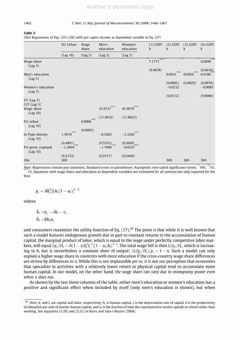
Table 2 estimates the system above using three-stage least squares, except that in the last equationwe merely look at GDP per capita instead of growth as a beginning benchmark. All regressions in all ofour tables include year dummies, though we do not report their coefficients. The first three equationsof our system (which comprise four equations in practice since we estimate men’s and women’s edu-cation separately) are as predicted by the model above: population density strongly has a positive andstatistically significant effect on the percentage of a country that is urban, while cropland density has anegative and statistically significant effect; more urban countries have a higher wage share, and thewage share, in turn, has a positive and significant effect on the level of education (both at the 1% level).The final three columns show regressions of GDP per capita on the wage share and education. As canbe seen, higher-income countries have a larger wage share of output; note that we are just looking atthe wage share within the corporate sector, so that this controls for the fact that the wage share ishigher in countries with larger corporate sectors. This suggests that the wage share of higher-incomecountries is larger for more than just the reasons discussed by Gollin (2002).

Note also that the relationship between the wage share and education is not predicted by moststandard growth models, either of the neoclassical or endogenous variety. A standard Cobb–Douglasproduction function would predict that more educated workforces will have a higher wage level,but will still have the same wage share. This point is worth emphasizing a bit, since it would suggestrethinking the cross-country determinants of human capital accumulation if widely replicated. Con-sider, e.g., an endogenous growth model (of the Uzawa-Lucas type) with both physical and humancapital, such as

Table 1Means of selected variables

Variable Mean Std. Dev. Min. Max. No. Obs.

GDP/k 9.3446 0.7540 7.4434 10.4131 369Per capita growth 2.2028 3.5790 �16.2883 11.2552 369Wage share (Lag 5) 0.6629 0.0827 0.4020 0.7944 369Women’s education (Lag 5) 31.0810 19.9674 2.4200 93.0000 369Men’s education (Lag 5) 48.7022 21.3142 5.5340 92.3633 369I/Y (Lag 5) 22.3639 7.2161 3.0337 42.6151 369G/Y (Lag 5) 14.1701 7.1364 3.0603 46.6381 369Pct perm cropland (Lag 10) 2.9734 3.8828 0.0035 14.7567 369ln Popn density (Lag 10) 4.0038 1.6412 0.3775 6.2552 369Percent urban (Lag 10) 64.4608 18.2434 10.2000 96.4000 369

Note: Education, wage share, investment, and government spending variables reported at a five-year lag from GDP variables.Population density and cropland are reported at a 10-year lag.



yt ¼ Akat ½lthtð1� utÞ�1�a

where

_kt ¼yt � dkt � ct

_ht ¼bhtut

and consumers maximize the utility function of Eq. (17).26 The point is that while it is well known thatsuch a model features endogenous growth due in part to constant returns in the accumulation of humancapital, the marginal product of labor, which is equal to the wage under perfectly competitive labor mar-kets, will equal oyt=olt ¼ Að1� aÞka

t l�at ½ð1� utÞht �1�a. The total wage bill is then ltoyt=olt , which is increas-

ing in ht but is nevertheless a constant share of output: ðltoyt=oltÞ=yt ¼ 1� a. Such a model can onlyexplain a higher wage share in countries with more education if the cross-country wage share differencesare driven by differences in a. While this is not implausible per se, it is not our perception that economiesthat specialize in activities with a relatively lower return to physical capital tend to accumulate morehuman capital. In our model, on the other hand, the wage share can vary due to monopsony power evenwhen a does not.

As shown by the last three columns of the table, either men’s education or women’s education has apositive and significant effect when included by itself (only men’s education is shown), but when

Table 23SLS Regressions of Eqs. (25)–(28) with per capita income as dependent variable in Eq. (27)

Pct Urban Wageshare

Men’seducation

Women’seducation

(1)-GDP/k

(2)-GDP/k

(3)-GDP/k

(4)-GDP/k

(Lag 10) (Lag 5) (Lag 5) (Lag 5)

Wage share(Lag 5)

7.1771*** 6.0698***

(0.4078) (0.4618)Men’s education

(Lag 5)0.0541*** 0.0424*** 0.0186***

(0.0085) (0.0029) (0.0070)Women’s education

(Lag 5)�0.0152 �0.0083

(0.0112) (0.0086)I/Y (Lag 5)G/Y (Lag 5)Wage share

(Lag 10)32.0157*** 41.9870***

(11.0632) (11.8623)Pct urban

(Lag 10)0.0066***

(0.0003)ln Popn density

(Lag 10)1.3919*** �0.3265 �2.3282***

(0.4891) (0.5353) (0.5666)Pct perm cropland

(Lag 10)�1.3694*** �1.7040*** �0.8527***

(0.2152) (0.2317) (0.2446)Obs 369 369 369 369

Note: Regressions contain year dummies. Standard errors in parentheses. Asymptotic two-tailed significance levels: *10%; **5%;***1%. Equations with wage share and education as dependent variables are estimated for all systems but only reported for thefirst.

26 Here, kt and lt are capital and labor, respectively; ht is human capital, d is the depreciation rate of capital, b is the productivityof education per unit of teacher human capital, and ut is the fraction of time the representative worker spends in school rather thanworking. See equations (5.20) and (5.21) in Barro and Sala-i-Martin (2004).



included together, the coefficients take opposite signs. One might read the coefficients as saying thatwomen’s education is the better proxy for the country’s overall level of human capital, and that giventhis level, countries with higher (i.e., more unequal) levels of men’s education do worse. The final col-umn of Table 2 shows that the wage share and education variables become insignificant when in-cluded together, suggesting that they are proxies for the same effect. While the standard errors aretoo large for us to draw any strong conclusions, this does suggest that education levels may play alarge part in the higher wage shares of industrialized economies, which is worth separateinvestigation.27

Table 3 repeats the system of equations in Table 2, but this time with the real per capita growthrate as the dependent variable in the final equation. We have attempted to follow the overall formof Barro and Lee (1993), Table 5, as a benchmark case, with a couple of modifications. Barro andLee regress the rate of growth on 10-year lagged values of GDP per capita, male and female secondaryschool completion rates, the investment and government shares of output, life expectancy, the blackmarket premium on foreign exchange, and anticipated political instability. They find that higher pastGDP predicts lower growth (which they consider as showing convergence conditional on the level of

Table 33SLS Regressions of Eqs. (25)–(28)

Pct urban Wageshare

Men’seducation

Women’seducation

(1) –Growth/k

(2) –Growth/k

(3) –Growth/k

(Lag 10) (Lag 5) (Lag 5) (Lag 5)

GDP/k (Lag 5) �0.9938** 0.0919 �1.1638(0.4804) (0.7272) (1.3728)

Wage share(Lag 5)

7.5124* 7.3121

(4.4451) (6.3375)Men’s education

(Lag 5)0.0430 0.0646

(0.0532) (0.0573)Women’s

education(Lag 5)

�0.0961* �0.0806

(0.0568) (0.0575)I/Y (Lag 5) 0.0796** 0.0387 0.0647*

(0.0331) (0.0288) (0.0362)G/Y (Lag 5) �0.0882*** �0.0795*** �0.0780***

(0.0297) (0.0298) (0.0299)Wage share

(Lag 10)30.3566*** 38.4432***

(11.2254) (12.0131)Pct urban (Lag

10)0.0056***


(Lag 10)1.1054** �0.1529 �2.1318***

(0.5227) (0.5880) (0.6087)Pct perm

cropland(Lag 10)

�1.6305*** �2.0329*** �1.0879***

(0.2247) (0.2545) (0.2630)Obs. 369 369 369

Note: Regressions contain year dummies. Equations with wage share and education as dependent variables are estimated for allsystems but only reported for the first. Standard errors in parentheses. Asymptotic two-tailed significance levels: *10%; **5%;***1%.

27 Note that this is a comparative static result, and in our framework, this could result from more developed countries havingmore transportation and communication infrastructure, which could make labor more mobile and therefore reduce (but noteliminate) monopsony power.



human capital); that male secondary school attainment predicts higher growth but, controlling forthis, female secondary school attainment predicts lower growth (which they attribute to an effect sim-ilar to the one we discussed about Table 2 above); that past investment spending ðI=YÞ increasesgrowth, but past government spending ðG=YÞ decreases it; that life expectancy increases growth;and that black market premia and political instability decrease it.

While attempting to preserve this overall framework for comparability, we have modified it in afew ways. First, because our wage share variable is available for a narrower time frame than the othervariables, we consider the independent variables at five and ten year lags rather than ten and twentyyear lags. Second, Barro and Lee use lagged endogenous variables as instruments, whereas we useother exogenous variables (specifically, population and cropland density) as motivated by our modelabove. Finally, we do think it important to include the investment, government spending, and laggedGDP variables to control for business cycle effects. But because our model has a narrower focus, we donot consider the effects of political instability, life expectancy, and the black market premium on for-eign exchange rates.

We are able to replicate all of Barro and Lee’s coefficients for the relevant variables when we use afull sample of countries (this result is not shown but is available on request); however, the availabilityof the wage share data substantially reduces the size of our sample, and so the coefficient on male edu-cation is generally insignificant in this subsample and not even positive for all of our specifications.The overall effect of the wage share is significant, and loses its significance (though only about a thirdof its magnitude) when education is included. Curiously, the sample only displays the conditional

Table 43SLS Regressions of Eqs. (25)–(28) with Fixed Effects

Pct urban Wageshare

Men’seducation

Women’seducation

(1) –Growth/k

(2) –Growth/k

(3) –Growth/k

(Lag 10) (Lag 5) (Lag 5) (Lag 5)

GDP/k (Lag 5) �1.9748*** �0.7502 �3.4306(0.5963) (0.8596) (11.6710)

Wage share(Lag 5)

16.7017*** 18.9930

(5.1498) (78.9913)Men’s education

(Lag 5)0.1730* 0.2315

(0.0887) (0.3281)Women’s education

(Lag 5)�0.5895*** �0.2917

(0.1672) (1.1228)I/Y (Lag 5) 0.0541 0.1966* 0.0063

(0.0356) (0.1087) (0.8018)G/Y (Lag 5) �0.1135*** �0.2382*** �0.0689

(0.0337) (0.0859) (0.7168)Wage Share

(Lag 10)�36.4570*** �11.8547

(10.6936) (11.9663)Pct Urban

(Lag 10)0.0052***


(Lag 10)1.8837*** 1.5513*** 0.4015

(0.4921) (0.5121) (0.5459)Pct perm cropland

(Lag 10)�1.8236*** �1.8549*** �0.6684***

(0.2113) (0.2227) (0.2364)Obs. 369 369 369

Note: Regressions contain year dummies and country dummies. Equations with wage share and education as dependentvariables are estimated for all systems but only reported for the first. Standard errors in parentheses. Asymptotic two-tailedsignificance levels: *10%; **5%; ***1%.



convergence found by Barro and Lee when the wage share is included.28 Note also that the effect of thewage share is controlling for the level of GDP per capita, meaning that it implies that countries with awage share that is uncharacteristically high for their level of development will grow faster. The positivecoefficient for lagged investment share and the negative coefficient for lagged government spendingshare are as found in the literature.

Table 4 includes country fixed effects, making it a differences-in-differences estimate, which allowus to ask the question of which factors might move a country from a low-growth to a high-growtheconomy. If there is not much within-country movement of this sort, then adding fixed effects willmake the data more noisy, and indeed we can see that the effect of the wage share on education losesits significance, as do the effects of past government and investment spending. In any event, the re-sults do not change much from Table 3, though they are slightly more in line with standard predic-tions. This time, men’s education is a significant predictor of economic growth when included byitself, and the effect of the wage share not only becomes an insignificant predictor of growth wheneducation is added, but substantially falls in magnitude (the education variables, on the other hand,lose significance in predicting growth when the wage share is added to the right-hand side, but donot change their magnitude much).

Overall, then, we think the data do not suggest any serious inconsistencies between our model andthe basic observed relationships between population density, wages, human capital accumulation, andgrowth. Population density increases the wage share. A higher wage share significantly increases edu-cation of both men and women. High income countries have larger wage shares, and this effect is par-tially collinear with the effect of education on income. Finally, the wage share has a positive andsignificant effect on the growth rate, and this effect overlaps heavily with the effect of education ongrowth.

5. Conclusion

Factor markets, just like product markets, have imperfections. To the extent that these imperfec-tions alter the rate of investment, whether in human capital or physical capital, they may alter the rateof growth. We have identified a very specific mechanism whereby monopsony power drives the wagebelow the marginal product of labor and thereby distorts the worker’s incentive to invest in humancapital so that it does not reflect the true productivity effects of such investment. We have providedevidence that this mechanism at least plausibly exists: First, the wage share of output is positively andsignificantly impacted by population density, which, as we interpret it, will lower workers’ travel costsand undercut firms’ monopsony power. Second, the level of education is positively and significantlyimpacted by a change in the wage share of output; this is a result that is predicted by our modeland inconsistent with many others, so while we do not view it as definitive supporting evidence, itdoes suggest an empirical puzzle that ought to be studied more. Third, high income countries havehigher wage shares of output, and this relationship is a proxy for the effect of education on output(or vice versa). Finally, the wage share of output positively predicts growth, and differences-in-differ-ences estimates show that countries that increase their wage share grow faster subsequently.

Both the theory and the evidence beg other questions that would be useful for future research. On atheoretical level, it would be interesting to know the growth dynamics of more complex labor mar-kets. For example, we have only examined the effect of monopsony on an economy with a singlemonopsonistic sector; on the other hand, monopsony power may also affect the rate of employmentin non-monopsonistic sectors (for example, the rate of self-employment or participation in partner-ships), which may have altogether different effects on growth. Tse (2000) has shown the way in whicha sector with a monopolistic product market may impact output in a two-sector model, and Aghionand Schankerman (2004) have shown the importance of uneven firm productivity in determiningthe rate of investment. While the simplicity of our one-sector model has its appeal, it would also be

28 Barro and Lee find a negative lagged coefficient for GDP per capita, which they interpret as showing that a country with highoutput relative to its human capital stock should subsequently converge to the output level consistent with its human capitalstock, i.e., it should grow slowly.



useful to know how monopsony power affects growth when its extent is uneven. Moreover, Tse’smodel assumes that the self-employment sector, where there is no market power, has low human cap-ital requirements, while the endogenous growth models of Romer (1990) and others assume that self-employment is entrepreneurial and inventive. These two views need to be reconciled in a multi-sectormodel.

Empirically, our estimates were meant to test the overall plausibility of our model; more exhaus-tive estimates would be useful. Our principle difficulty is in the small available sample size, whichmainly results from the small number of country-year cells for which careful estimates of the wageshare of output are available. Because these are historical data, the only real option to expand thedataset is to use a more crude estimate of the wage share, which many would find unappealing. Itwould also be helpful if we had a more direct cross-country estimate of monopsony power; one pos-sible solution would be to use the estimator suggested by Ridder and van den Berg (2003), but the vari-ables required for this estimator would further restrict our data set substantially, and the resultingdata would not overlap well with the available measures of the wage share.

In future empirical work, the effect of monopsony power on the accumulation of skills ought to beexamined in more detail. For example, workers of different skill levels may be subject to differentamounts of monopsony, and the extent to which their rate of investment in human capital is distortedwill therefore also be differently affected. This, in turn, may not only affect the overall rate of growth,but the types of technologies that are developed by an economy. A second, related point is thatmonopsony power may be stronger or have different effects in different industries, and economieswith larger wage shares may grow faster in some industries but not in others.

More research is also needed into the cross-country determinants of monopsony power. Populationdensity has a demonstrable effect on the wage share of output, which in itself is interesting, but begsthe question exactly why and how. Is it that workers in more densely populated areas simply havelower travel costs, or are they better able to share information with each other about alternativeemployment, or are there perhaps skill interactions between urban workers, or possibly culturalnorms, that somehow give them more bargaining power with their employers? The data at our dis-posal do not enable us to answer these questions.

Finally, our mechanism needs to be disentangled from others that might produce similar effects.Imperfect competition in product markets, for example, may have an effect on the wage share of out-put. Moreover, the dynamics of economic growth are entangled both theoretically and empiricallywith the dynamics of the business cycle. The degree to which fast-growing economies are experienc-ing a cyclical peak, which may (for reasons unspecified) exhibit a high wage share, needs to be distin-guished from a mechanism that runs in the reverse direction, whereby a high wage share causeseconomies to grow faster and may even produce short-term cyclical effects. While our data use lagsthat are longer than a typical business cycle, there is insufficient theoretical distinction between along-term growth spurt and an extra-long business cycle for us to know how to distinguish the effectsempirically. We think that these questions together provide ample material for future research, andwe hope that the present work has provided sufficient evidence that they are questions worth asking.

Acknowledgement

We would like to thank James Schmitz, Caroline Hoxby, Kevin Bowman, and an anonymous refereefor valuable comments and suggestions. The usual caveat applies.

References

Aghion, P., Howitt, P., 1997. Endogenous Growth Theory. The MIT Press, Cambridge, MA.Aghion, P., Schankerman, M., 2004. On the welfare effects and political economy of competition-enhancing policies. Economic

Journal 114, 800–824.Albrecht, J.W., Jovanovic, B., 1986. The efficiency of search under competition and monopsony. Journal of Political Economy 94,

1246–1257.Arrow, K.J., 1962. The economic implications of learning by doing. Review of Economic Studies 75, 155–173.Barr, T., 2002. Monopsony Power and the Returns to Skill. Columbia University Ph.D. Dissertation.Barro, R.J., 1990. Government spending in a simple model of endogenous growth. Journal of Political Economy 98, S103–S125.



Barro, R.J., Lee, J.-W., 1993. Losers and Winners in Economic Growth. NBER Working Paper No. 4341. National Bureau ofEconomic Research, Cambridge, Massachusetts; 1990; <http://www.nber.org/papers/w4341>.

Barro, R.J., Lee, J.-W., 2000. International Data on Educational Attainment: Updates and Implications. CID Working Paper No. 42,April 2000; <http://www.cid.harvard.edu/ciddata/ciddata.html>.

Barro, R.J., Sala-i-Martin, X., 2004. Economic Growth. The MIT Press, Cambridge, MA.Bernanke, B.S., Gürkaynak, R., 1993. Is Growth Exogenous? Taking Mankiw, Romer, and Weil Seriously. NBER Working Paper No.

8365; National Bureau of Economic Research, Cambridge, Massachusetts. <http://www.nber.org/papers/w8365>.Black, D., Henderson, V., 1999. A theory of urban growth. Journal of Political Economy 107, 252–284.Burdett, K., Mortensen, D.T., 1989. Equilibrium Wage Differentials and Employer Size. Discussion Paper No. 860; Northwestern

Center for Mathematical Studies, 1989.Carayol, N., Roux, P., 2003. Self-Organizing Innovation Networks: When Do Small Worlds Emerge? Cahiers du GRES No. 2003-8,

Toulouse.Cordoba, J., 2004. On the Distribution of City Sizes. Working Paper, Rice University.Dunlop, J., 1938. The movement of real and money wage rates. Economic Journal 48, 413–434.Duranton, G., Puga, D., 2003. Micro-foundations of Urban Agglomeration Economies. NBER Working Paper No. 9931; National

Bureau of Economic Research, Cambridge, Massachusetts. <http://www.nber.org/papers/w9931>.Fujita, M., Krugman, P., Venables, A.J., 1999. The Spatial Economy: Cities, Regions, and International Trade. The MIT Press,

Cambridge, MA.Gollin, D., 2002. Getting income shares right. Journal of Political Economy 110, 458–474.Green, F., Machin, S., Manning, A., 1996. The employer-size wage effect: can dynamic monopsony provide an explanation?

Oxford Economic Papers 48, 433–455.Helsley, R.W., Strange, W.C., 1990. Matching and agglomeration economies in a system of cities. Regional Science and Urban

Economics 20, 189–212.Heston, A., Summers, R., Aten, B., 2002. Penn World Tables Version 6.1. Center for International Comparisons at the University of

Pennsylvania.Kim, S., 1990. Labor heterogeneity, wage bargaining, and agglomeration economies. Journal of Urban Economics 28, 160–177.Lucas, R.E., 1988. On the mechanics of economic development. Journal of Monetary Economics 22, 3–42.Manning, A., 2003. Monopsony in Motion: Imperfect Competition in Labor Markets. Princeton University Press, Princeton, NJ.Ridder, G., van den Berg, G., 2003. Measuring labor market friction: a cross-country comparison. Journal of the European

Economic Association 1, 224–244.Romer, P.M., 1986. Increasing returns and long-run growth. Journal of Political Economy 94, 1002–1037.Romer, P.M., 1990. Endogenous technological change. Journal of Political Economy 98, S71–S102.Rossi-Hansberg, E., Wright, M.L.J., 2007. Urban structure and growth. Review of Economic Studies 74, 597–624.Rotemberg, J.J., Woodford, M., 1990. Cyclical Markups: Theories and Evidence. National Bureau of Economic Research,

Cambridge, Massachusetts; NBER Working Paper No. 3534; <http://www.nber.org/papers/w3534>.Salop, S., 1979. Monopolistic competition with outside goods. Bell Journal of Economics 10, 141–156.Tarshis, L., 1939. Changes in real and money wages. Economic Journal 49, 150–154.Tse, C.Y., 2000. Monopoly, human capital accumulation and development. Journal of Development Economics 61, 137–174.United Nations 1985, 1990, 1995, 1997. National Accounts Statistics: Main Aggregates and Detailed Tables. Publishing Division,

United Nations, New York; 1985, 1990, 1995, 1997.World Bank, 2004. World Development Indicators 2004. <http://publications.worldbank.org/ecommerce/catalog/

product?item_id=631625>.


The effect of labor market monopsony on economic growth

Documents