Sebelas Maret Business Review Vol. 4 Issue 1, pp. 1 - 12 ISSN: 2528-0627 (print) / 2528-0635 (online) Copyright © Magister Manajemen Universitas Sebelas Maret Homepage: https://jurnal.uns.ac.id/smbr The Effect of Indonesian Government’s Debt to the US and Greece on Composite Stock Price Index in ASEAN-5 and Australia Nugroho Saputro* Faculty of Economics and Business, Universitas Sebelas Maret, Indonesia Abstract Global economic crisis has become a nightmare for other countries, when the crisis is originated from a multipower country. A financial crisis that hit European countries (Greece) in 2010 and the United States (US) in 2011 can be categorized as financial crisis that caused by high state’s debt that leads to default. The response to financial crisis is reflected in capital market players’ reaction, where other countries will respond to a particular endemic financial crisis. The objectives of this research are (1). Analyze the Impulse Response Function (IRF) of the Composite Stock Price Index of the US on Composite Stock Price Index in Indonesia, Malaysia, Singapore, Vietnam, Thailand and Australia. (2). Analyze the Impulse Response Function (IRF) of the Composite Stock Price Index of Greece on the Composite Stock Price Index in Indonesia, Malaysia, Singapore, Vietnam, Thailand and Australia. (3). Analyze the Forecasting Error Variance Decomposition (FEVD) of the Composite Stock Price Index of Indonesia on the Composite Stock Price Index of Malaysia, Singapore, Vietnam, Thailand and Australia. The analysis will be conducted using VAR (Vector Auto regression). The result shows that all variables are responded to the financial crisis that happened in Greece and the US. This is reflected by the shocks created by the financial crisis in ASEAN-5 countries and Australia. On the other hand, the Composite Stock Price Index of Indonesia is also affected by Malaysia and Singapore. Keywords: Global Financial Crisis, Government’s Debt, ASEAN-5, Australia, Stock Price Index. 1. Introduction A ratification of debt agreement by Barack Obama on 2nd August 2011, allows for fundamental transformation in world economics. The agreement between the Government of the United States (US) and the United States Congress, on debt value triggering a reaction from global exchange player. The US debt is recorded at US$14.3 Trillion, with 30 percent of it comes from foreign investor, and the other 70 percent of domestic investor. The quantity of debt owned by the Government of the United States has wide effect due to the US Gross Domestic Product (GDP) at US$15 Trillion. This value constitute 25 percent of total world GDP, which amounted to US$60 Trillion (Kontan, 2011). Decreased or low Gross Domestic Product (GDP) has a negative effect on economic growth. The effect shown on the decrease of economic growth. Slow economic growth has various effect on the society life. The effect of economics fluctuation can be seen in a country unstable condition, which known as financial crisis. Bloomberg (2011) is quoting several statements of analyst such as, ‘the economic condition is on the edge of a cliff” (Martin Feldstein, Harvard University) and Ben Bernanke (Chairman Federal Reserve) in one of his speech states that ‘right at this moment, the possibility of the US fall into recession is only reach 50 percent’. Those statements indicate a recession that may occur to the US economy, which will affect world economic condition. The US recession in 2011, can be * Corresponding author at Jl. Ir Sutami No.36 A, Pucangsawit, Kec. Jebres, Kota Surakarta, Jawa Tengah 57126. Email: [email protected]

Welcome message from author
This document is posted to help you gain knowledge. Please leave a comment to let me know what you think about it! Share it to your friends and learn new things together.
Transcript

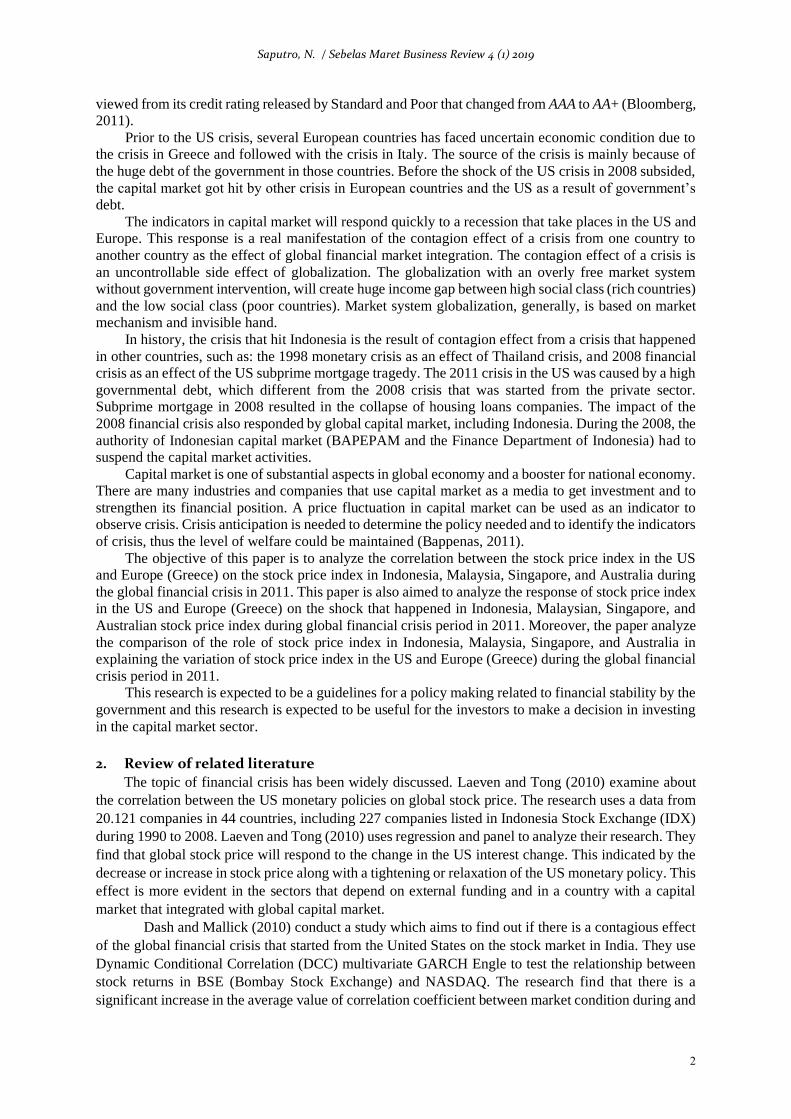
Sebelas Maret Business Review Vol. 4 Issue 1, pp. 1 - 12 ISSN: 2528-0627 (print) / 2528-0635 (online) Copyright © Magister Manajemen Universitas Sebelas Maret Homepage: https://jurnal.uns.ac.id/smbr
The Effect of Indonesian Government’s Debt to the US and Greece on Composite Stock Price Index in ASEAN-5 and Australia
Nugroho Saputro*
Faculty of Economics and Business, Universitas Sebelas Maret, Indonesia
Abstract Global economic crisis has become a nightmare for other countries, when the crisis is originated from a multipower country. A financial crisis that hit European countries (Greece) in 2010 and the United States (US) in 2011 can be categorized as financial crisis that caused by high state’s debt that leads to default. The response to financial crisis is reflected in capital market players’ reaction, where other countries will respond to a particular endemic financial crisis. The objectives of this research are (1). Analyze the Impulse Response Function (IRF) of the Composite Stock Price Index of the US on Composite Stock Price Index in Indonesia, Malaysia, Singapore, Vietnam, Thailand and Australia. (2). Analyze the Impulse Response Function (IRF) of the Composite Stock Price Index of Greece on the Composite Stock Price Index in Indonesia, Malaysia, Singapore, Vietnam, Thailand and Australia. (3). Analyze the Forecasting Error Variance Decomposition (FEVD) of the Composite Stock Price Index of Indonesia on the Composite Stock Price Index of Malaysia, Singapore, Vietnam, Thailand and Australia. The analysis will be conducted using VAR (Vector Auto regression). The result shows that all variables are responded to the financial crisis that happened in Greece and the US. This is reflected by the shocks created by the financial crisis in ASEAN-5 countries and Australia. On the other hand, the Composite Stock Price Index of Indonesia is also affected by Malaysia and Singapore. Keywords: Global Financial Crisis, Government’s Debt, ASEAN-5, Australia, Stock Price Index.
1. Introduction A ratification of debt agreement by Barack Obama on 2nd August 2011, allows for fundamental
transformation in world economics. The agreement between the Government of the United States (US)
and the United States Congress, on debt value triggering a reaction from global exchange player. The
US debt is recorded at US$14.3 Trillion, with 30 percent of it comes from foreign investor, and the
other 70 percent of domestic investor. The quantity of debt owned by the Government of the United
States has wide effect due to the US Gross Domestic Product (GDP) at US$15 Trillion. This value
constitute 25 percent of total world GDP, which amounted to US$60 Trillion (Kontan, 2011).
Decreased or low Gross Domestic Product (GDP) has a negative effect on economic growth. The effect shown on the decrease of economic growth. Slow economic growth has various effect on the
society life. The effect of economics fluctuation can be seen in a country unstable condition, which
known as financial crisis. Bloomberg (2011) is quoting several statements of analyst such as, ‘the
economic condition is on the edge of a cliff” (Martin Feldstein, Harvard University) and Ben Bernanke
(Chairman Federal Reserve) in one of his speech states that ‘right at this moment, the possibility of the
US fall into recession is only reach 50 percent’. Those statements indicate a recession that may occur
to the US economy, which will affect world economic condition. The US recession in 2011, can be
* Corresponding author at Jl. Ir Sutami No.36 A, Pucangsawit, Kec. Jebres, Kota Surakarta, Jawa Tengah 57126. Email:
Saputro, N. / Sebelas Maret Business Review 4 (1) 2019
2
viewed from its credit rating released by Standard and Poor that changed from AAA to AA+ (Bloomberg,
2011).
Prior to the US crisis, several European countries has faced uncertain economic condition due to
the crisis in Greece and followed with the crisis in Italy. The source of the crisis is mainly because of
the huge debt of the government in those countries. Before the shock of the US crisis in 2008 subsided,
the capital market got hit by other crisis in European countries and the US as a result of government’s
debt.
The indicators in capital market will respond quickly to a recession that take places in the US and
Europe. This response is a real manifestation of the contagion effect of a crisis from one country to
another country as the effect of global financial market integration. The contagion effect of a crisis is
an uncontrollable side effect of globalization. The globalization with an overly free market system
without government intervention, will create huge income gap between high social class (rich countries)
and the low social class (poor countries). Market system globalization, generally, is based on market
mechanism and invisible hand.
In history, the crisis that hit Indonesia is the result of contagion effect from a crisis that happened
in other countries, such as: the 1998 monetary crisis as an effect of Thailand crisis, and 2008 financial crisis as an effect of the US subprime mortgage tragedy. The 2011 crisis in the US was caused by a high
governmental debt, which different from the 2008 crisis that was started from the private sector.
Subprime mortgage in 2008 resulted in the collapse of housing loans companies. The impact of the
2008 financial crisis also responded by global capital market, including Indonesia. During the 2008, the
authority of Indonesian capital market (BAPEPAM and the Finance Department of Indonesia) had to
suspend the capital market activities.
Capital market is one of substantial aspects in global economy and a booster for national economy.
There are many industries and companies that use capital market as a media to get investment and to
strengthen its financial position. A price fluctuation in capital market can be used as an indicator to
observe crisis. Crisis anticipation is needed to determine the policy needed and to identify the indicators
of crisis, thus the level of welfare could be maintained (Bappenas, 2011).
The objective of this paper is to analyze the correlation between the stock price index in the US
and Europe (Greece) on the stock price index in Indonesia, Malaysia, Singapore, and Australia during
the global financial crisis in 2011. This paper is also aimed to analyze the response of stock price index
in the US and Europe (Greece) on the shock that happened in Indonesia, Malaysian, Singapore, and
Australian stock price index during global financial crisis period in 2011. Moreover, the paper analyze
the comparison of the role of stock price index in Indonesia, Malaysia, Singapore, and Australia in
explaining the variation of stock price index in the US and Europe (Greece) during the global financial
crisis period in 2011.
This research is expected to be a guidelines for a policy making related to financial stability by the
government and this research is expected to be useful for the investors to make a decision in investing
in the capital market sector.
2. Review of related literature
The topic of financial crisis has been widely discussed. Laeven and Tong (2010) examine about
the correlation between the US monetary policies on global stock price. The research uses a data from
20.121 companies in 44 countries, including 227 companies listed in Indonesia Stock Exchange (IDX)
during 1990 to 2008. Laeven and Tong (2010) uses regression and panel to analyze their research. They
find that global stock price will respond to the change in the US interest change. This indicated by the
decrease or increase in stock price along with a tightening or relaxation of the US monetary policy. This
effect is more evident in the sectors that depend on external funding and in a country with a capital
market that integrated with global capital market.
Dash and Mallick (2010) conduct a study which aims to find out if there is a contagious effect
of the global financial crisis that started from the United States on the stock market in India. They use
Dynamic Conditional Correlation (DCC) multivariate GARCH Engle to test the relationship between
stock returns in BSE (Bombay Stock Exchange) and NASDAQ. The research find that there is a
significant increase in the average value of correlation coefficient between market condition during and

Saputro, N. / Sebelas Maret Business Review 4 (1) 2019
3
before crisis. Therefore, it can be concluded that there is a connection between global financial crisis
and India stock market.
In line with the research of Dash and Mallick (2010), another research is conducted by Adamu,
(2010), he investigates the effect of global financial crisis on Nigeria economics condition. However,
the research is more focused on qualitative analysis of several economics aspects such as Foreign Direct
Investment (FDI) and stock investment, the trend of oil price decline, aid, and commercial loan. The
result show that financial crisis leads to the decline in commodities price, export quantity, portfolio,
and lower FDI.
Another researcher, Zhang et al. (2009), examine about the effect of the US credit crisis on
Asia Pacific economic condition. The research uses data from several countries such as Japan, South
Korea, China, Indonesia, Malaysia, Singapore, Thailand, Philippines, Australia, and New Zealand. The
data is analyzed using a methodology that is developed by International Monetary Fund (IMF) namely
Global Integrated Monetary and Fiscal (GIMF). The GIMF is developed further by Hong Kong’s
authority into eight regions version, which aims to uncover heterogenic economics structure in East
Asia countries. The result shows that the credit crisis in the US has a huge effect on Asia Pacific
economic condition through financial and trade connection.
3. Theoretical Framework Capital Flight
Capital flight is related with a condition with high uncertainty and risk, in term of economic and
non-economic. This condition motivate investors to bring their fund abroad, in order to avoid losses if
they keep their fund in the country. Capital flight happens because of investors’ fear of assets loss due
to domestic currency depreciation, government’s default, sudden change in capital management policy
and money and capital market policy, or fiscal policy that can cause great loss to capital owners
(Lensink et al., 2000).
A more moderate definition is delivered by Mankiw (2006) who define net capital outflow as the
total debt provided by domestic investor to other countries (abroad) deducted by debt provided by
international investor into the country. Mankiw emphasizes on the difference in capital outflows minus
capital inflows. Other researcher, Salvatore (1996) defines capital flight as transfer of funds overseas
by citizen or domestic companies to obtain the largest or safest income or interest, without considering
whether their country need the fund or not.
Schineller (1997) defines capital flight as short-term capital outflow to foreign countries whether
recorder or not, which is speculative, by non-bank sector. Capital flight is measured by adding short-
term capital flows with net error and omission on the balance of payments. Capital outflow is used to
measure the recorded component, while net error and omission is to measure the unrecorded component.
Capital flight also refers to the reduction of reserve fund due to devaluation issues, because the debit
value on the balance of payments (reduction in assets) is the same with private capital outflow
(Krugman and Obstfeld, 1999). Cross-country capital flows
Appleyard and Jr (1995) propose several reason for cross-country capital investment, A
company will invest its capital across countries in response to the growing and expanding market. This
hypothesis is supported by an empirical study that states if there is a positive relationship between the
Gross Domestic Product (GDP) of beneficiary country and the quantity of incoming FDI. Along with
the above reason, service and processing production from developed countries will increase their
service in order to meet the demand, which is growing as a result of increased per capita income in the
country of destination. This is also the reason for developed countries to invest their capital to other
countries. Another reason is the effort to ensure access to basic material and the amount of material
reserves, thus it encourages developed countries to invest their capital into the targeted country.
Differences in tariff and non-tariff barriers in host country may also be the reason why capital inflows
occur. Low wages is another consideration for cross-country investment. Huge human resource in
developing countries, which leads to low wages, has become the target for investment especially in the
production of goods with labor-intensive technology. Another strong consideration is the needs to

Saputro, N. / Sebelas Maret Business Review 4 (1) 2019
4
ensure and strengthen the market share, while multinational companies also offer similar product to the
market. Risk diversification is another consideration for investor in investing their fund to other
countries. A higher return for cross-country investment because of the low competitiveness of local
companies against foreign companies in the country. Such condition can happened due to the
management’s superiority and skills possessed by foreign companies compared to the domestic
companies. International capital flow theory states that capital will flow to the most profitable place
(country). Under such circumstance global output will be maximum.
Table 3. Financial Crisis with Global Impact: 1980-2008
Origin of Shock,
Country, and Date of
Event
External Shock
Characteristics Spreading Mechanism Affected Countries
1 2 3 4
12 August, 1982,
Mexico experienced a
default of its foreign
debt from its banking
sector. Until December
of the same year, the
exchange rates of Peso
had been depreciated
for 100 percent.
During 1980 - 1985,
commodity prices
crashed for 31 percent.
US short-term interest
rates increased for 7
percent, which marked
the highest level since
Great Depression.
Excessive funding to
Mexico from the US
banking, diversion
from developing
country.
All countries in Latin
America region
experience default,
except Chile, Colombia
and Costa Rika.
In September 1992,
Finland money market
changed to floating rate
which leads to
exchange rate system
crisis (Exchange Rate
Mechanism (ERM)).
High interest rate in
Germany. Rejection
from Denmark against
Maastricht Treaty.
Hedge Funds. All countries with
European Monetary
System except
Germany.
In 20 December 1994,
Mexico announced a
devaluation to Peso at
15 percent. This leads
to trust crisis, and later
in March 15th 1995,
Peso got devaluated at
100 percent rate.
Starting on 1994 the US
Federal Reserve,
increase the interest rate
(federal funds rate) for
2.5 percent.
There was a huge sales
in mutual fund in
Latin America
countries such as
Argentina and Brazil.
Uncertainties in
banking condition and
capital flight in
Argentina.
Argentina is the most
suffering country with
almost 20 percent
deposit losses in early
1995, while Brazil is
second in list.
In 2 July 1997,
Thailand announced
that Baht will develop
its exchange rates. In
January 1998, Baht is
depreciated for 113
percent.
Yen is depreciated for
51 percent on US
Dollar during April
1995-April 1997. The
relation between Asian
currencies with US
Dollar created
appreciation on Yen.
Japanese banking
provide loans to
Thailand, which leads
to withdrawal from
Asian countries.
European banks also
widraw their fund
from Korea due to the
effect.
Indonesia, Korea,
Malaysia, and
Philippines are the most
severely affected by the
crisis. Singapore’s
financial market and
Hong Kong also caught
in shock.
Origin of Shock,
Country, and Date of
Event
External Shock
Characteristics Spreading Mechanism Affected Countries
1 2 3 4

Saputro, N. / Sebelas Maret Business Review 4 (1) 2019
5
In 18 August 1998,
Russia experienced a
default on Domestic
Bonds. Between July
1998 and January 1999,
Ruble is depreciated for
262 percent. On 2
September 1998,
LTCM went bankrupt.
Due to its link on
Russian currency and
highly profitable
instruments, LTCM
went bankrupt.
Margin call and hedge
funds are triggered by
sales in developing
countries and other
highly profitable
markets. Difficulty in
differentiating
between the
contagious effect from
Russia and fear of
LTCM bankruptcy.
Aside from several ex-
Soviet Republic
countries, Hong Kong,
Brazil, and Mexico are
the most affected
countries. Almost all
developing countries
are affected by the
crisis.
In 13 January, 1999,
Brazil did a devaluation
and develop its
currency in 1 February.
Between January and
early February, there
was a depreciation at 70
percent.
A semi-controlled
exchange policy that
was adopted in July
1994, which aims to
stabilize inflation is
abandoned.
There was increased
volatility in several
major capital market,
while the spread of
Argentina get wider.
The capital market in
Argentina and Chile
were competing each
other for several days.
The prolonged effect on
Argentina economics is,
Brazil become the
biggest partner.
22 February 2001,
Turkey devaluate and
develop its currency
(Lira).
Facing a substantive
financial needs, in the
end of November 2000,
a rumor about the
withdrawal of foreign
debt in Turkish banks
has resulted in a capital
flight outflow, thus
within an overnight the
interest rate increased
up to 2000 percent.
There is an indication
that the Turkey crisis
was caused by investors
from Argentina.
However, by
considering the strength
of Argentina’s
economic fundamental
at that time, it is quite
difficult to say if it was
an effect of contagion.
In 23 December 2001
The President of
Argentina announced
that there is a possibility
of default.
Following several wave
of capital flight and
bank deposit flight, on
the 1st December 2001
capital control policy is
established.
The banking deposit in
Uruguay reached more
than 30 percent,
because the banks in
Argentina received
deposit from Uruguay
banks. There was a
significant effect on
economics activities
(trades and tourism) in
Uruguay.
Uruguay and Brazil
should be on a much
smaller scale.
In the end of 2007,
there was a Subprime
Mortgage crisis, where
bank provide credits for
various housing loans.
Housing loans securities
emerge due to easy
money policy that
implemented by Alan
Greenspan during 2001-
2003. The effect of this
crisis was felt in 2008.
The impact of the crisis
was felt in the world oil
price which continues
to increase, even
reaching 110 US dollars
per barrel. In 10
October 2008 the
world's exchanges are
falling.
There was a volatility
in several capital
market in the world.
All US trading partners
felt a negative effect,
some sectors with
foreign capital tend to
move its location to
other countries.
Source: IMF, International Financial Statistics, Reinhart, Rogoff and Savesteno as quoted in Prasetyantoko
(2008:26-18) with modification.

Saputro, N. / Sebelas Maret Business Review 4 (1) 2019
6
Portfolio theory
The theory of portfolio choice that affect asset are Mishkin (2007) wealth, when a person’s
wealth increases, thus he/she will have more resource to acquire assets, expected return refers to the
rate of return expected by acquiring certain assets, risk is the level of uncertainty that related to asset in
relative terms to other assets, liquidity refers to how quickly and easily an asset is converted into cash.
The history of crisis
Prasetyantoko (2008) defines crisis as financial instability, a drastic changes in financial
assets price. The financial assets are shares (stocks), bonds, mortgages, futures, as well as
various securities and other derivative products. Financial crisis is not a new phenomenon,
financial crisis has happened in several countries such as explicitly displayed in Table 3.
Table 4. The US Crisis in 2008
Source: Tempo (2008) in Minister of Information (Menkoinfo), 2008.
The movement or spread of financial turmoil, which started from a superpower country, has a
huge impact on some countries. Table 3 and Table 4 illustrate the respond to crisis (financial turmoil)
as a series of an economics degradation process. The effect of the crisis could take days, months, or
years to get noticed.
4. Research Method
Data source and type
This research uses secondary data, which consist of Composite stock price data (US Dow Jones
Index-DJI and Greece Athens Stock Exchange-ATHE); The composite stock price data in five ASEAN
countries (1). Indonesia (JKSE), (2). Malaysia (KLSE), (3). Singapura (STI), (4). Thailand (SET), and
(5). Vietnam (VHINDEX), and Australia (AORD). The observation period is starting from the Greece
default, April 2010 to December 2011.
Vector Auto regression (VAR)
VAR is a continuation of monetarist criticism of the Keynesian. Some characteristics of VAR
show an alignment to monetarist, the first VAR method is developed on the basis of criticism on the
previous large models. Secondly, VAR offers a simple model with minimalist amount of variable, with
the independent variable is lag of all endogenous variables. Thirdly, VAR is a continuation of causality
April ----->
New Century
Financial's housing
finance company
went bankrupt
28 August ----->
Sachsen
Landesbank in
Germany collapsed
due to investment in
housing loans
3 September ----->
German financial institutions (IKB)
admit investment in
subprime mortgages
is lost up to USD 1
billion
17 February ----->
The British
nationalized
Northern Rock
17 March ----->
Bear Stearns
collapsed and was
bought by JP
Morgan Chase with an American
government
guarantee worth
USD 30 billion
29 September <-----
The British
government took
over Bradford &
Bingley
25 September <-----
Washington Mutual
collapsed and bought
JP Morgan
16 September <-----
Fed injects AIG for
USD 85 billion
15 September <-----
Lehman Brothers
went bankrupt
5 September <-----
Fannie Mae and
Freddie Mac were
taken over by the American
government
30 September
France, Belgium,
Luxembourg work
together to save
Dexia
3 Oktober <-----
The American
Congress passed a $ 700 billion bailout
program
6 Oktober <-----
Germany launches
USD 68 billion to
support Hypo Real
Estate
8 Oktober <-----
Britain prepares £
50 billion (US $ 87
billion) bailout
10 Oktober <-----
Stock market
indexes were falling
again
Saputro, N. / Sebelas Maret Business Review 4 (1) 2019
7
test and, VAR characteristic cannot be separated from Granger’s causality test characteristic such as,
focused on identity study. Most of the identity can be found in monetarist reasoning such as the quantity
of money theory (MV=PT), inflation and interest rate correlation (i=r + p), and other identities (Thomas,
1997).
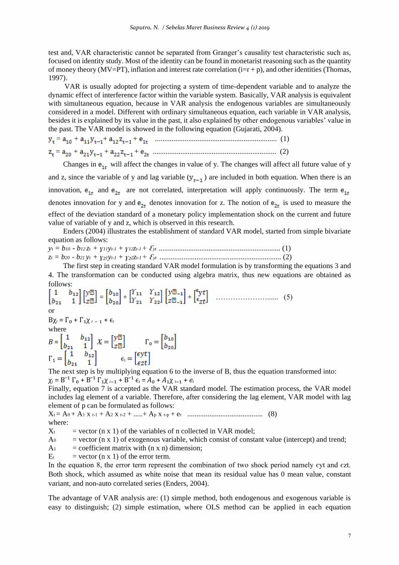
VAR is usually adopted for projecting a system of time-dependent variable and to analyze the
dynamic effect of interference factor within the variable system. Basically, VAR analysis is equivalent
with simultaneous equation, because in VAR analysis the endogenous variables are simultaneously
considered in a model. Different with ordinary simultaneous equation, each variable in VAR analysis,
besides it is explained by its value in the past, it also explained by other endogenous variables’ value in
the past. The VAR model is showed in the following equation (Gujarati, 2004).
= + + + .................................................................. (1)
= + + + ................................................................... (2)
Changes in will affect the changes in value of y. The changes will affect all future value of y
and z, since the variable of y and lag variable ( ) are included in both equation. When there is an
innovation, and are not correlated, interpretation will apply continuously. The term
denotes innovation for y and denotes innovation for z. The notion of is used to measure the
effect of the deviation standard of a monetary policy implementation shock on the current and future
value of variable of y and z, which is observed in this research.
Enders (2004) illustrates the establishment of standard VAR model, started from simple bivariate
equation as follows:
yt = b10 - b12 zt + ɣ11yt-1 + ɣ12zt-1 + Ɛyt .................................................................. (1)
zt = b20 - b21 yt + ɣ21yt-1 + ɣ22zt-1 + Ɛyt .................................................................. (2)
The first step in creating standard VAR model formulation is by transforming the equations 3 and
4. The transformation can be conducted using algebra matrix, thus new equations are obtained as
follows:
= + + …………………...... (5)
or
Bχₜ = Γ₀ + Γ₁χ ₜ ₋ ₁ + ϵₜ where
B = Xₜ = Γ₀ =
Γ₁ = ϵₜ =
The next step is by multiplying equation 6 to the inverse of B, thus the equation transformed into: χₜ = Bˉ¹ Γ₀ + Bˉ¹ Γ₁χ ₜ₋₁ + Bˉ¹ ϵₜ = A₀ + A₁χ ₜ₋₁ + еₜ Finally, equation 7 is accepted as the VAR standard model. The estimation process, the VAR model includes lag element of a variable. Therefore, after considering the lag element, VAR model with lag
element of p can be formulated as follows: Xt = A0 + A1 x t-1 + A2 x t-2 + .....+ Ap x t-p + et ......................................... (8)
where:
Xt = vector (n x 1) of the variables of n collected in VAR model;
A0 = vector (n x 1) of exogenous variable, which consist of constant value (intercept) and trend;
A1 = coefficient matrix with (n x n) dimension;
Et = vector (n x 1) of the error term.
In the equation 8, the error term represent the combination of two shock period namely єyt and єzt.
Both shock, which assumed as white noise that mean its residual value has 0 mean value, constant
variant, and non-auto correlated series (Enders, 2004).
The advantage of VAR analysis are: (1) simple method, both endogenous and exogenous variable is
easy to distinguish; (2) simple estimation, where OLS method can be applied in each equation

Saputro, N. / Sebelas Maret Business Review 4 (1) 2019
8
separately; (3) the forecast result, which obtained using this method, in many cases has better result
compared to complex simultaneous equations. Moreover, VAR analysis is a useful analysis tool, either
to understand interrelationship of economics variables or in establishment of a structured economics
model (Gujarati, 2004).
Impulse Response Function (IRF)
According to (Enders, 2004), IRF is an instrument that can be used to track the response of endogenous
variables value in the current period and future period, when there is shock or changes in the current
interference variable value. Mathematical illustration of IRF instrument is presented by the
representation of vector moving average of VAR model. In order to obtain the vector moving average
representation, the equation 13 should be formed from the transformation of the equations below:
= + + + .................................................................. (9a)
= + + + ................................................................… (9b)
In the equation 9a and 9b, the term ai0 is defined as the i element of the vector of A1, aij is defined
as the element of line i and column of j of the matrix A, and eit is defined as the i element of vector et.
The next step to obtain the representation of vector moving average from the VAR model is by
transforming the equation of 9a and 9b in matrix notation, thus an equation 10 is obtained as follows:
= + + ................................................… (10)
By assuming that equation 10 has fulfilled stability test, thus the equation can be transformed into
more solid equation as follows:
...............................… (11)
The error term of equation 11 is translated in the following form:
................................… (12)
After the error term is translated, thus the last step is by combining the equation 11 and equation
12. Therefore, the representation of vector moving average from the VAR model is as follows:
...(13)
To simplify the equation 13, a notation of фi can be used. In this term, the notation of фi is defined
as a matrix of 2 x 2, which include the element of фjk (i). Mathematically, the notation of фi can be
translated as follows:
...............................… ……………………(14)
The simplification of vector moving average form in equation 13 by involved the notation of ф as
translated in equation 14, generates the following equation:
...............................… ….(15)
Finally, the equation of 15 is the final representation of vector moving average from the VAR
model. In the equation 15, the IRF of VAR model is represented by 4 coefficients unit, namely
ф11(i), ф12(i), ф21(i), and ф22(i).
Forecasting Error Variance Decomposition
A method that can be used to examine the changes in a variable, which represented by the changes
in its variance of error, that affected by other variables is Forecast Error Decomposition of Variance
(FEDV). FEDV is conducted to see the relative contribution of a variable in explaining its endogenous
variable variability. This method can characterize the dynamic structures in VAR model. By using this
method the power and weakness of each variable in affecting other variables in a long-term can be
calculated.
Unit Root Test

Saputro, N. / Sebelas Maret Business Review 4 (1) 2019
9
k
t=1 k t=1
Unit Root Test can be viewed as stationary test, because the objective of the test is to examine
whether certain coefficient in an autoregressive model has the value of one or not (Thomas, 1997). Unit
root tests can be performed by estimating the following autoregressive models with the OLS method,
which known as DF test (Dickey-Fuller) and ADF test (Augmented Dickey-Fuller):
DXt = a0 + a1 BXt + ∑ bt Bt DXt …………………………………………….. (16)
DXt = c0 + c1T + c2 BXt + ∑ dt Bt DXt ……………………………………… (17)
where; DXt = Xt – X t-1, BX = X t-1, T= the trend of time; and Xt is the variable observed during the
period of t while B is the backward lag operator.
The DF and ADF value, after calculated, that used in hypothesis test (a1=0 and c2=0) is represented
by the ratio of t in the regression coefficient of BXt in equation 17. The lag value of k is determined by
k=N 1/3, where N is the quantity of observation. If the regression coefficient of a1 and c2 is not significant
at a certain DF and ADF significance level, it can be concluded that the data observed is not stationary
and must be continued with integration degree test until stationary data is obtained.
Integration degree test
The integration degree test is performed if the root test of the observed data unit is not stationary.
This test is performed to know at what degree or order of differentiation the observed data is stationary.
Time series data is said to be integrated to the degrees of d or written as I(d), if the data needs to be
differentiated as much as d times to become a stationary data. Integration degree test is similar or is an
extension of the unit root test, which can be performed using OLS.
VAR model stability test
The VAR model in optimum lag should be stable. Unstable VAR model will generate invalid
result on the VAR model. The stability of VAR model can be identified using two methods. The first
method is by identify the inverse roots characteristic of polynomial AR. In this method VAR method is
considered stable if all values of the inverse roots have a modulus value that is lower than one. The
second method is by identify the modulus value in a unit circle. A VAR model is considered stable if
all of its modulus values are located within the unit-circle (Enders, 2004).
5. Result and Discussion
Stationary Test
The result of stationary test from the eight countries is presented in Table 5.
Table 5 Result of Stationary Test
Stock Price
Prob Augmented Dickey-Fuller test
statistic
Lag Length: 0*
DJI 0.4961
ATHE 0.8715
JKSE 0.4681
STI 0.5053
SET 0.3565
KLSE 0.5076
VHINDEX 0.1842
AORD 0.3250
From the stationary test on the data in level or ordo 0 [(0)] above, we can see the absolute statistic
ADF (tα) value that is smaller than Mackinnon critical value in each α, thus we can say that the data is
not stationary. To find the degree of data integration, data integration test is needed (testing on the
differentiation level) until there is stationary data in the same level.

Saputro, N. / Sebelas Maret Business Review 4 (1) 2019
10
Integration Level Testing
The result of ADF testing on the eight stock price in ordo 1 [I(1)] can be seen in the following
table.
Table 6. Result of Integration Level Testing
Stock price Prob Augmented Dickey-Fuller test statistic
Lag Length: 1
DJI 0.0000
ATHE 0.0000
JKSE 0.0000
STI 0.0000
SET 0.0000
KLSE 0.0000
VHINDEX 0.0000
AORD 0.0000
The result of stationary testing in the first differentiation level testing in all stock prices in this
study is presented in the ordo 1 (one). The stationary testing result shows that all stationary data has
significance level below 1 percent. This means that the stock price in US, Greece, Malaysia, Indonesia,
Singapore, Thailand, Vietnam, and Australia is integrated in the first degree. This also means that all
countries in this study have long term relationship. Further analysis is performed on the data that have
been transformed into the first differentiation level.
Determination of optimum lag
The determination of optimum lag can be identified through Akaike Info Criterion (AIC), Schwarz
Criterion (SC), and Hannan-Quinn Criterion (HQ).
Table 7. Optimum Lag Testing Result
Lag LogL LR FPE AIC SC HQ
0 -18394.75 NA 6.50e+30 93.65266 93.73356 93.68472
1 -14296.80 8008.214 7.90e+21 73.12364 73.85167* 73.41215
2 -14147.75 285.2004 5.12e+21* 72.69083* 74.06599 73.23579*
3 -14096.70 95.59371 5.48e+21 72.75676 74.77906 73.55817
4 -14066.59 55.17411 6.52e+21 72.92920 75.59863 73.98706
5 -14027.80 69.48258 7.44e+21 73.05751 76.37407 74.37182
6 -13978.18 86.87339* 8.03e+21 73.13067 77.09437 74.70143
7 -13931.33 80.09759 8.82e+21 73.21798 77.82881 75.04520
8 -13883.71 79.48712 9.67e+21 73.30134 78.55931 75.38501
Source: Result of Eviews 6 analysis
* indicates lag order selected by the criterion
The selection of optimum lag is performed through SC method developed by Canova (2003),
which serves as better criteria because it gives higher level of penalty to the additional variable that
reduce the degree of freedom. Based on the criteria, the candidate for optimum lag is selected according
to its lag in which SC has the minimum or lag 1.
VAR model stability testing
The stability of VAR model can be identified based on two methods, first identify the value of
inverse roots of polynomial AR characteristics and identify the modulus value in unit circle.

Saputro, N. / Sebelas Maret Business Review 4 (1) 2019
11
Table 8. The Result of Polynomial Characters Model Stability Testing
Root Modulus
0.995783 0.995783
0.987074 0.987074
0.967662 0.967662
0.940859 - 0.030243i 0.941345
0.940859 + 0.030243i 0.941345
0.910509 0.910509
0.843789 0.843789
0.134397 0.134397 Source: Result of Eviews 6 analysis
No root lies outside the unit circle.
VAR satisfies the stability condition.
The result of the first model stability (Table 8) shows value under 1, this means VAR model is
stable because all inverse-roots value have modulus lower than 1. In the Figure 1, we can also see that
VAR model is stable because all modulus values are in the unit-circle.
Figure 1. VAR Model Stability Testing
Source: Result of Eviews 6 analysis
FEDV Indonesia (JKSE) Analysis
The variability of stock price in Indonesia on the stock price in ASEAN-4 and Australia can be
explained in Table 9. We can see the composition of JKSE and stock price in ASEAN-4 and Australia
in explaining the variability of stock price in Indonesia. In the first period, JKSE is the variable that has
the strongest role in determining the variability of JKSE (100%). The variability is decreasing in the
tenth period, its effect reduced into 88.4 percent and contrary, the variability of stock index in other
countries increases. We can observe that in Table 9, Malaysia (KLSE) has 2.65 percent effects in the
tenth period, and most importantly Singapore (STI) has 6.73 percent of effect on the volatility in
Indonesia. Other countries have less contribution on the existing volatility.
-1.5
-1.0
-0.5
0.0
0.5
1.0
1.5
-1.5 -1.0 -0.5 0.0 0.5 1.0 1.5
Inverse Roots of AR Characteristic Polynomial

Saputro, N. / Sebelas Maret Business Review 4 (1) 2019
12
Table 9. FEDV Analysis on Indonesian Composite Index (JKSE)
Variance Decomposition of DJKSE:
Period DJKSE DKLSE DSET DSTI DVHINDEX DAORD
1 100 0 0 0 0 0
2 98.700 0.212 0.814 0.018 0.058 0.194
3 97.054 0.505 1.837 0.036 0.147 0.417
4 95.483 0.812 2.802 0.048 0.249 0.603
5 94.047 1.121 3.666 0.055 0.360 0.748
6 92.739 1.428 4.435 0.058 0.478 0.859
7 91.541 1.735 5.117 0.059 0.604 0.941
8 90.437 2.041 5.722 0.059 0.738 1.000
9 89.415 2.347 6.258 0.058 0.878 1.040
10 88.462 2.653 6.733 0.058 1.025 1.066
Source: Result of Eviews 6 analysis
6. Conclusion and Suggestion Financial crisis in US (Dow Jones) affects or trigger a response (shocks) in ASEAN-5 and
Australia. It also has a positive shock, except Vietnam which responds negatively. Financial crisis in
Greece (ATHE) affects or trigger a response (shocks) in ASEAN-5 and Australia. This shock is positive,
except in Indonesia in which the crisis receives negative response. Malaysia (KLSE) has 2.65 percent
of effect in the tenth period and more importantly Singapore (STI) plays a role in the existing volatility
with 6.73 percent. Other countries have less contribution in the volatility of Indonesian composite index
(IHSG).
The annual growth of capital market can be considered high, all from go-public companies,
number of investor who interested to invest their capital in the capital market, and various derivative
products from capital market. Study on financial management regarding capital market and portfolio
needs to be developed to provide operational standard for the parties that are active in the capital market.
Generally, the government has to be careful on the crisis from other countries, because investor will
react to it in timely manner. That is why the fundamental aspect of a country has to be strong in order
to anticipate too high shocks.
References Adamu, A. (2010), “The Effects Of Global Financial Crisis On Nigerian Economy”, Nasarawa State University. Appleyard, D.R. and Jr, A.J.F. (1995), Internasional Economics, Second., Irwin, New York. Bappenas, T.E.T. (2011), Krisis Keuangan Eropa: Dampak Terhadap Perekonomian Indonesia. Bloomberg. (2011), “Ekonomi AS tersedot Gravitasi?”, Bloomberg Businessweek, September, pp. 18–19. Canova, R. (2003), Three Essays on Updating Forecasts in Vector Autoregression Models, Canada. Dash, A.K. and Mallick, H. (2010), “Contagion Effect of Global Financial Crisis on Stock Market in India”, JEL. Enders, W. (2004), “Applied Econometric Time Series”, Wiley Series in Probability and Statistic, Second edi., John
Wiley and Son, Inc, New York. Gujarati, D.N. (2004), Basic Econometrics, Four Editi., McGraw-Hill International Edition, Singapore. Kontan. (2011), “Krisis Utang AS Bisa Memicu Krisis Baru”, Kontan, 29 July, p. 1. Krugman, P.R. and Obstfeld, M. (1999), Ekonomi Internasional: Teori Dan Kebijakan, Raja Grafindo Perkasa, Jakarta. Laeven, L. and Tong, H. (2010), U.S. Monetary Shocks and Global Stock Prices, No. WP/10/278. Lensink, R., Hermes, N. and Murinde, V. (2000), “Capital Flight and Political Risk”, The Journal of Internasional
Money and Finance. Mankiw, G.N. (2006), Pengantar Ekonomi Makro (Terjemahan), Ketiga., Salemba Empat, Jakarta. Mishkin, F.S. (2007), The Economics of Money, Banking and Financial Market, 6th ed., Wesley, New York. Prasetyantoko, A. (2008), “Bencana Finansial: Stabilitas Sebagai Barang Publik”, Kompas Gramedia, Jakarta. Salvatore, D. (1996), Internasioanal Economics, Prentice Hall Inc, New Jersey. Schineller, L.M. (1997), “An Econometric Model of Capital Flight from Developing Countries”, Internasioanal
Discussion Paper No. 594, Federal Reserve Board. Thomas, R. (1997), Modern Econometrics: An Introduction, Eddison-Wesley, England. Zhang, Z., Zhang, W. and Han, G. (2009), How Does The US Credit Crisis Affect The Asia-Pacific Economies? Analysis
Based On A General Equilibrium Model, No. 12/2009.
Related Documents