The University of Nottingham The Effect of Ethanol-Gasoline Blends on SI Engine Energy Balance and Heat Transfer Characteristics Taleb Alrayyes, BEng (Hons) GEORGE GREEN LIBRARY OF SCIENCE AND ENGINEERING Thesis submitted to the University of Nottingham for the degree of Doctor of Philosophy September 2010

Welcome message from author
This document is posted to help you gain knowledge. Please leave a comment to let me know what you think about it! Share it to your friends and learn new things together.
Transcript
The University of
Nottingham
The Effect of Ethanol-Gasoline Blends on SI Engine Energy Balance and Heat Transfer Characteristics
Taleb Alrayyes, BEng (Hons)
GEORGE GREEN LIBRARY OF SCIENCE AND ENGINEERING
Thesis submitted to the University of Nottingham for the degree of Doctor of Philosophy
September 2010
Table of contents
Contents
CONTENTS ...................................................................................................... I
ABSTRA.CT ..................................................................................................... v
ACKNOWLEDGMENT .............................................................................. VII
N OMEN CLA TURE ................................................................................... VIII
ABBREVIATIONS .......................................................................................... x
CHAPTER! INTRODUCTION ................................................................ 1
1.1 Overview .......................................................................................................................... 1 1.1.1 European biofuels policy ......................................................................................... 3
1.2 Objective .......................................................................................................................... 4
1.3 Thesis layout .................................................................................................................... 5
CHAPTER 2 LITERA TURE REVIEW .................................................... 7
2.1 Introduction ..................................................................................................................... 7
2.2 Ethanol Production ......................................................................................................... 7 2.2.1 The production process ............................................................................................ 8
2.3 Net energy and Green house gases .................................................................................. 9
2.4 Comparison of ethanol and gasoline properties ......................................................... 10
2.5 Emissions ........................................................................................................................ 14
2.6 Engine Combustion behaviour ..................................................................................... 18
2.7 The use ofethanol in direct injection spark ignition engines (DIS) engines) ........... 19
2.8 Other alcohol considered as alternative fuel ............................................................... 21
2.9 Concluding comments ................................................................................................... 22
CHAPTER 3 EXPERIMENTAL TEST FACILITIES .......................... 23
3.1 Introduction ................................................................................................................... 23
3.2 Engine description and Test Cell Facilities ................................................................. 23
T Alrayyes I University of Nottingham
Table of contents
3.2.1 Fuel delivery circuit. .............................................................................................. 25
3.3 Engine Data Acquisition and Sensor Calibration ....................................................... 25 3.3.1 Engine Pressure and Temperature ......................................................................... 25 3.3.2 Engine Encoder and TOe allocation ..................................................................... 26 3.3.3 Fuel Flow Measurement ........................................................................................ 27 3.3.4 Coolant and air flow rate Measurement: ................................................................ 28 3.3.5 AFR sensor ............................................................................................................ 29 3.3.6 Exhaust gas analysis .............................................................................................. 29
3.4' Engine management system A TI ................................................................................. 30
3.5 dSPACE control and data acquisition system ............................................................ 31
3.6 Main Measurement and calculations ........................................................................... 33 3.6.1 In-cylinder pressure data and mean effective pressure (MEP) .............................. 33 3.6.2 Burned mass fraction (EGR & Residual mass fraction) ........................................ 35
3.7 Errors and repeatability ............................................................................................... 38
3.8 Sum ma ry & Conclusion ................................................................................................ 40
CHAPTER 4 BASIC COMPARISON BETWEEN GASOLINE· ETHANOL MIXTURES ........................................................ 41
4.1 Introduction ................................................................................................................... 41
4.2 Experimental fuels ........................................................................................................ 41
4.3 Selection of experimental comparison parameters ..................................................... 42
4.4 AFRstoich, calorific value and adiabatic name temperature ....................................... 42
4.5 Power output and fuel consumption ............................................................................ 45
4.6 Spark timing (ST) and MBT determination ............................................................... 46
4.7 Emissions ......................................................................................................................... 48 4.7.1 CO and CO2 emissions .......................................................................................... 48 4.7.2 NOx emissions ....................................................................................................... 49 4.7.3 HC emissions ......................................................................................................... 51 4.7.4 H20 level and equivalence ratio ............................................................................ 52
4.8 Combustion efficiency ................................................................................................... 54
4.9 Summary and discussion ............................................................................................ , .. 55
CHAPTER 5 THE EFFECT OF ETHANOL ON ENGINE COMBUSTION BEHA VIOUR ............................................. 57
5.1 Introduction ................................................................................................................... 57
5.2 Combustion Process characterization ......................................................................... 58
5.3 Rassweiler and Withrow Method ................................................................................ 59
5.4 Calculating polytropic index ........................................................................................ 60
T Alrayyes II University of Nottingham
Table of contents
5.5 Comparison between laminar flame speed of ethanol and gasoline ......................... 61
5.6 Effect of ethanol blends on burning duration ............................................................. 63 5.6.1 Different speeds, loads and spark timing ............................................................... 63 5.6.2 Sensitivity to change charge composition (Xb & q» ............................................... 65
5.7 Combustion stability and tolerance to x". .................................................................... 66
5.8 Summary and discussion .............................................................................................. 67
CHAPTER 6 OVERVIEW OF THE ENGINE ENERGY BALANCE 69
6.1 Introduction ................................................................................................................... 69
6.2 Energy balance for the engine ...................................................................................... 70
6.3 Exhaust gas energy ........................................................................................................ 70
Exhaust heat capacity, Cp •exh .............................................................................................. 71
6.3.1 Exhaust gas temperature measurement and correction .......................................... 72
6.4 Heat transfer to the coolant .......................................................................................... 74 6.4.1 Effect of heat rejection to coolant on engine warm-up .......................................... 75
6.5 Heat loss to ambient, Qamb . .......................................................................................... 76
6.6 Energy balance results .................................................................................................. 77
6.7 Summary and discussion .............................................................................................. 79
CHAPTER 7 TIME AVERAGE ENGINE HEAT TRANSFER DURING FULLY WARM UP OPERATION ....................................... 82
7.1 Introduction ................................................................................................................... 82
7.2 Background .................................................................................................................... 83 7.2.1 Engine running on gasoline ................................................................................... 85 7.2.2 Gasoline-ethanol blends ......................................................................................... 87
7.3 Effect of External EGR ................................................................................................. 88
7.4 Evaluation of the heat transfer to the exhaust port, flexhpt ..................................... 90
7.4.1 Measured heat transfer to the exhaust port ............................................................ 91 7.4.2 Exhaust port heat correlations ................................................................................ 93
7.5 Heat conducted back to the cylinder head, ~hman .................................................. 95
7.6 Results and discussion ................................................................................................... 9S
CHAPTER 8 IN-CYLINDER GAS PROPERTIES AND INSTANTANEOUS HEAT LOSS TO THE CYLINDER WALL.99
8.1 Introduction .................................................................................................................... 99
8.2 Calculating in-cylinder gas properties ........................................................................ 99
T Alrayyes III University of Nottingham
Table of contents
8.2.1 In-cylinder temperature ......................................................................................... 99 8.2.2 Calculating in-cylinder f for different fuel mixtures ......................................... 102
8.3 Charge temperature and mixture preparation ......................................................... 104
8.4 Instantaneous spatially-averaged heat loss to the cylinder walls ............................ 106
8.5 In-cylinder gas-side surface temperature .................................................................. 107
8.6 Calibration of the Hohenberg correlation ................................................................. 107
8.7 Evaluation of the Hohenberg correlation, ................................................................. 108
8.8 Effect of gasoline-ethanol blends at different ratios on the instantaneous heat loss ..... 109
8.9 Further parameters variation .................................................................................... III 8.9.1 Effect of burned mass fraction, Xb ....................................................................... III 8.9.2 Effect of equivalence ratio, cp ............................................................................... 112 8.9.3 Effect of spark timing, ST ................................................................................... 112
8.10 Summary and discussion ....................................................................................... 113
CHAPTER 9 D ISCUSSI 0 N .................................................................... 116
Summary and discussion ......................................................................... · ............................ 116
Future work ........................................................................................................................... 124
CHAPTER 10 CONCLUSION ................................................................. 125
APPENDICES ............................................................................................... 228
A.I Conversion from dry to wet analysis ........... , ........................................... " ........... 228
A.2 EGR derivation ....................................................................................................... 231
A.3 Properties of the different fuel blends .................................................................. 232
A.4 Derivation of the EGR correction factor 189) ...................................................... 238
A.S Measurements and calculation uncertainties ....................................................... 240
T Alrayyes IV University of Nottingham
ABSTRACT
Abstract
"The Effect of Ethanol-Gasoline Blends on SI Engine Energy Balance and Heat Transfer Characteristics"
Taleb Alrayyes
Ethanol is one of a group of hydrocarbon fuels produced from bio-mass which
is attracting interest as an alternative fuel for spark ignition engines. Major
producers of ethanol include Brazil, from sugar cane, and the USA, from com.
Reasons for the growing interest in ethanol include economic development,
security of fuel supply and the reduction of net emissions of carbon dioxide
relative to levels associated with the use of fossil fuels. Unlike gasoline, which
is a mixture of hydrocarbon compounds suited to meet a range of start and
operating requirements, ethanol is a single component fuel with characteristics
which make engine cold starting difficult, for example. Hence, ethanol is
generally used in a blend with gasoline, accounting for <5% in EU pump-grade
gasoline to 85% by volume for so called flex-fuel vehicles.
Although ethanol is already available in the marketplace, there are aspects of
its effects on engine behaviour that are unresolved, including its effects on
engine thermal behaviour and heat transfer. These have been investigated in
the experimental study presented in this thesis. The aims of this work included
determining the effect of ethanol content in blends on combustion
characteristics, energy balance, gas-side heat transfer rate and cylinder
instantaneous heat transfer.
This study covers a range of loads, speeds, spark timings, equivalence ratios
and EGR levels representative of every day vehicle use, and has been restricted
to fully warm operating conditions. The investigations have been carried out
on a modern design of direct injection, spark ignition engine. The performance
of different ethanol-gasoline blends has been compared at conditions of
matched brake power output.
The emissions data for NO, HC, CO and C02, which was used to calculate
combustion efficiency, show a decrease in their levels proportional to the
T Alrayyes v University of Nottingham
ABSTRACT
increase in ethanol content in the fuel blend. This is owing to an increase in
combustion efficiency and change in chemical structure and physiochemical
properties.
Compared to gasoline, running on 85% ethanol produces slightly faster rates of
burning in rapid burn stages of combustion. Typically, the reductions in rapid
burn angle are 4%. Results show that the effects do not vary in proportion to
the ethanol content in the fuel blend. This is attributable to the fact that, at low
and medium ethanol content, the enhancement in combustion gained by
oxygen availability is offset by its higher enthalpy of vaporisation and lower
heat content.
Energy balance data show an improvement in thermal efficiency proportional
to the increase in ethanol ratio. This is due to improvement in combustion
efficiency and a reduction in coolant and exhaust losses.
Results for gas-side heat rejection show that a correlation developed for
engines run on gasoline can be used without any modification. The heat
rejection rate has been inferred from measurements of heat rejection to coolant
adjusted to allow for the contribution of engine rubbing friction. The apparent
insensitivity to ethanol content is attributed to a combination of factors. These
include the increase in fuel flow rate for a given energy supply being offset in
its effect on charge flowrate by a reduction in stoichiometric air/fuel ratio.
Gas-side heat transfer results from both the exhaust port and the cylinder show
a clear decrease when running on 85% ethanol compare to gasoline. This
reduction was also observed in the total measured heat loss to coolant.
The magnitude and phasing of instantaneous heat loss is not sensitive to the
use of ethanol during combustion. However, as the combustion starts to
terminate, lower heat loss for medium and high ethanol content was observed
due to the reduction in the combustion product temperature. The results from
the C 1 C2 correlation and instantaneous heat transfer are comparable.
T Alrayyes VI University of Nottingham

Acknowledgment
Acknowledgment
I would like to express my sincere gratitude to Professor Paul Shayler, my
supervisor at the Engines Research Group, for his support and guidance
throughout the course of this researching and writing this thesis. Thanks is
also given to the technical staff, Geoff Fryer and John Cl~ke, for ensuring that
the test facility was kept in top notch working order, and especially John
McGhee, for his advice and encouragement. Many thanks also go Ford Motor
Company for the provision of the test engine and financial backing. I am also
grateful for all the members of the engine groups, particularly Dr Theo Law for
helping advising and support during much of the research.
Amongst others, special thoughts go to Dr Antonino La Rocca, the Warden of
Sherwood hall, and all my fellow tutors for their endless patience and
friendship.
Finally, and by no means last in importance, I would like to thank my parents
and my brother Momen who have supported me throughout my education.
T Alrayyes VII University of Nottingham
Nomenclature
Nomenclature
1. Symbols
A Area m2
CA Crank angle 0
cp Specific heat at constant pressure J/kgK
Cv Specific heat at constant volume J/kgK
d diameter m
he Heat transfer coefficient W/m2 K
~fK enthalpy of vaporisation J/kg Aho
f molar enthalpy of formation kJlkmol
k Thermal conductivity W/mK
L Piston stroke m
m Mass kg
m Mass flow rate kg/s
N Engine speed rpm P Pressure N/m2
Ph brake Power W
Qch Heat released due to combustion J
QLHV Fuel lower heating value MJ/kg
Qloss heat loss J/CA
Q Heat transfer rate kW ." q Heat flux W/rn2
t Time s
T Temperature K
Tf{,a Effective gas temperature K
Tadd Adiabatic flame temperature K V Cylinder volume m3
Vd Swept Volume m3
Vp Mean piston speed mls
Xb Burned mass fraction % -XI Wet mole fraction of substance i %,ppm -. XI Dry mole fraction of substance i %,ppm
y(Gamma) Ratio of specific heat
1'/c Combustion efficiency %
1'/( Thermal efficiency %
T Alrayyes VIII University of Nottingham
ABSTRACT
e Crank angle 0
I' Dynamic Viscosity kg/ms p Density kg/m3 rp Air-Fuel Equivalence ratio
2. Subscripts
ambo Ambient b Burned charge comp Compression cyl Cylinder eff. Effective exh Exhaust exh.man. Exhaust manifold f Friction f Fuel fc fresh charge g Gas pt Port stoich Stoichiometric tot Total u Un-burned charge
T Alrayyes IX University of Nottingham
Abbreviations
Abbreviations
AFR ATDC BMEP BSFC BTDC CA co C0 2
COV CR DI DISI DOHC ECU EGR EOC EVC EVO
EX¥
FDA FlD FMEP FTP-75 GHG HC 110 IMEP
IVC IVO KLSA MAP
MBT MFB MON NO
N02
NOx
T Alrayyes
Air-Fuel Ratio After Top Dead Centre Brake Mean Effective Pressure Brake Specific Fuel Consumption Before Top Dead Centre Crank Angle Carbon Monoxide
Carbon Dioxide Coefficient of Variability Compression ratio Direct Injection Direct Injection Spark Ignition
Double Over Head Cam Engine Control Unit External Gas Recirculation End of Combustion Exhaust Valve Closing Exhaust Valve Opening Ethanol ratio, where X¥ represents the volumetric fraction of ethanol in the gasoline-ethanol blend Flame Development Angle (0-10% MFB) Flame Ionisation Detector Friction Mean Effective Pressure Federal Test Procedure 75 Green House Gases Unburned Hydrocarbon Input/Output
Indicated Mean effective Pressure Input Valve Closing Inlet Valve Opening Knock Limit Spark Advance
Manifold Absolute Pressure
Maximum Brake Torque Mass Fraction Burned Motor Octane Number Nitric Oxide
Nitrogen Monoxide Nitrogen Oxides
x University of Nottingham
Abbreviations
02 PFI PM PROMETS RBA
RON
rpm RVP
SAE SGDI SI ST TDe UEGO ULG VVT
WOT
T Alrayyes
Oxygen Port Fuel Injection Particulate Matter PROgram for Modelling Engine Thermal Systems Rapid Burning Angle (10-90% MFB) Research Octane Number
revolution per minute Reid Vapor Pressure
Society of Automotive Engineering Spray Guided Direct Injection Spark Ignition Spark Timing Top Dead Centre Universal Exhaust Gas Oxygen (Sensor) UnLeaded Gasoline Variable Valve Timing Wide Open Throttle
XI University of Nottingham
CHAPTER 1, Introduction
CHAPTER 1 Introduction
1.1 Overview
The topics investigated in this thesis relate to the use of ethanol mixed with
gasoline at different proportions in SI engines. The use of ethanol in SI engines
can be traced back to the end of the Nineteenth Century, when Henry Ford
designed a car that used ethanol as fuel. Gasoline later gained prominence as
fuel refined for SI engines due to the availability and cheap supply of crude oil
[1]. In the last few years, however, ethanol has again attracted attention as an
automotive fuel. This renewed interest in ethanol and alternative fuels in
general is driven by several factors.
First, there is an increased awareness that fossil fuel reserves are finite. The
International Energy Agency now estimates that world production will peak in
2010-2020 and then start to decrease sharply as illustrated in Figure 1.1 [2]. As
a result, finding alternatives to fossil fuel is becoming a commercial priority.
Second, the demand for fuel in the developing world is rising, driven by
emerging economic powers such as China, India, and Brazil. For instance
China's demand grew at a phenomenal 7.2% annual logarithmic rate between
1991 and 2006 [3]. If that trend were to continue, by 2020 China would be
consuming 20 million barrels per day (about as much as the u.s. is currently
consuming), and by 2030 that amount would have doubled again to 40 million
barrels per day [3].
Third, there are concerns over nsmg levels of greenhouse gases in the
atmosphere and the potential for this to cause climate change with serious
consequences on society have also focused attention on ethanol once again.
Ethanol has a great potential to limit CO2 emissions if the whole "well-to
wheel" cycle is considered, as illustrated in Figure 1.2. The CO2 emitted when
ethanol is burned in an engine can be re-captured from the atmosphere by
growing crops that are then used to produce the ethanol, thus completing a
cycle. It is clear that at least part of the C02 emissions can be avoided by using
T Alrayyes 1 University of Nottingham
CHAPTER 1, Introduction
such a renewable cycle, although the emissions associated with each stage, as
well as the net reduction compared to alternative energy source must be
examined with care.
Finally, increase in ethanol use has also been stimulated by concerns about oil
supply disruptions due to the unstable political situation in regions that export
crude oil. This came sharply into attention particularly after the 1973174 fuel
crisis [IJ.
Biofuels are today the only direct substitute for fossil fuels in transport that are
available on a significant scale, and the most commonly produced biofuel is
ethanol [IJ. Ethanol can be used today in ordinary vehicle engines without
major modification (unmodified for low blends or with cheap modifications to
accept high blends) [4]. Whilst other fuels, or energy carrier, such as hydrogen,
have not achieved large-scale viability and will require major changes to
vehicle fleets and the fuel distribution system.
Ethanol production has more than doubled between 1993 and 2006 [2J. As
shown in Figure 1.3, USA and Brazil are the biggest producers of ethanol.
accounting for 70% of total worldwide production [2]. Both countries took
serious steps towards increasing the usage of ethanol as fuel. For instance, the
Brazilian government made mandatory the blending of ethanol with gasoline,
at proportions fluctuating between 10% and 25%. The bulk of ethanol
produced in the USA is mixed with gasoline at low proportions, 10% or EIO,
as oxygenate and, to a lesser extent, as fuel for E85 flex-fuel vehicles.
In the EU, the production and the use of ethanol, and biofuels in general, are
still very limited compared to those of the USA and Brazil [1]. The ED is
responsible for just around 7% of the global production of ethanol [2]. Most of
the fuel produced in the EU is biodiesel, in which EU is the market leader [1].
At the moment, Sweden is the leading European user of ethanol [2]. Sweden
has the largest E85 flexible-fuel vehicle fleet in Europe, with a sharp growth
from 717 vehicles in 2001 to around 200,000 in 2010 [2]. However, most of
the ethanol consumed in the country is imported [2],
T Alrayyes 2 University of Nottingham
CHAPTER 1, Introduction
1.1.1 European biofuels policy
Although Europe currently makes a modest contribution to the total production
and use of biofuels, the EU has strategies and action plans in place to raise the
production and promote the use ofbiofue1s as alternative to fossil fuel [5, 6]:
• In 2003, the EU adopted Directive 2003/30/EC2 on the promotion of
the use of biofuels for transport. This "biofuels directive" urged
Member- States to set indicative targets for a minimum proportion of
biofuels to be put in place in the market. These targets were set at 2%
in 2005 then growing by 0.75 annually, to reach 5.75% in 2010. These
percentages were calculated on the basis of the energy content of the
fuel.
• Directive 2003/96/EC3, in 2003, which was the EU's framework for
the taxation of energy products and electricity, was amended to allow
Member States to grant tax reductions and/or exemptions in favour of
renewable fuels under certain conditions.
• In February 2006, the EU Commission published a new
Communication entitled "An EU Strategy for Biofuels", preparing the
ground for a review of the Biofuels Directive by the end of 2006 that
might include mandatory targets instead of the indicative ones set in
2003. The aim of the strategy was to further promote biofuels in the EU,
to prepare for their large-scale use, and to explore opportunities for
developing countries to build plants producing biofuels.
Although the Biofuels Progress Report [7] showed that the 5.75% target set by
the EU was not reached, those measures and action plans did increase biofuels
usage tenfold between 2003 and 2010, as shown in Figure 1.4. Between 2008
and 2009, ethanol consumption increased by 31.9%, representing a share of
19.3% of the total biofuels consumption as shown in Figure 1.5.
Although ethanol has been used as fuel for spark ignition engines since the
earliest days of the automotive industry, its recent increasing use in the EU in
blends with gasoline raises question about its effects on engine performance
and emissions. Modem engines for the EU market are required to meet most of
the stringent emissions regulations in the world. EU customers demands high
level of refinement, performance and reliability of their vehicles. Meeting
T Alrayyes 3 University of Nottingham
CHAPTER 1, Introduction
regulations and customer expectations leaves little room for unknown effects
of fuel quality and it is this area which the author work has focused on.
1.2 Objective
The objective of this thesis is to establish the effect of different gasoline
ethanol blends, containing up to 85% ethanol, on engine performance,
combustion speed, energy balance and heat transfer characteristics of a SODI
engine. In order to achieve these objectives, a number of specific tasks were
undertaken, which include:
• The design and commission of a test rig used to carry out all the
experimental tests included in this thesis.
• Several tests were carried out on a wide range of engine running
conditions to evaluate the effects of increasing ethanol content in a
gasoline-ethanol blend on:
T Alrayyes
o the physicochemical and combustion properties of the fuel,
including stoichiometric AFR, calorific value, MBT, and
adiabatic flame temperature. Also, the subsequent effect of
these properties on power output and fuel consumption.
o the main regulated emissions and combustion efficiency
o combustion duration, combustion stability and EaR tolerance.
o exhaust temperature and heat capacity.
o energy balance inside the engine, including the thermal
efficiency, heat loss to coolant, heat loss to ambient and heat
loss to exhaust.
o gas-to-wall heat transfer, and any required modifications to the
C 1 C2 correlation to allow for changes in the fuel heating value
and other fuel properties.
o other sources contributing to the heat rejection to coolant
including: exhaust port, heat conducted back from exhaust
manifold, and friction.
o instantaneous heat loss to coolant and in-cylinder temperature
and properties.
4 University of Nottingham
CHAPTER 1, Introduction
1.3 Thesis layout
Chapter 2 describes a review of the published literature relevant to the study
presented in this thesis, with a focus on ethanol production, main properties,
and effects on engine performance and emissions.
Chapter 3 covers details of the test engine and the experimental facilities
developed to meet the objective of the thesis.
The main body of the thesis is concerned with heat transfer characteristics and
the combustion behaviour of the engine. The physiochemical and combustion
properties of the fuel blends, which are important to understand these
characteristics, are examined in Chapter 4. Calorific values, AFRstoich, adiabatic
flame temperatures as well as MBT (and its effect on engine power, output and
fuel consumption) were calculated. Also, emission levels for different fuel
blends were measured at different running conditions, and used to calculate
combustion efficiency.
In Chapter 5, the Rassweiler and Withrow method was used to calculate and
compare bum durations for different fuel blends. Several methods to calculate
appropriate polytropic index values were assessed. Gasoline and ethanol
laminar flame speeds were calculated and compared. The effects of changing
an engine's running conditions such as speed, load and spark timing (or charge
composition by changing EGR or equivalence ratio) were evaluated for the
different fuel blends. Finally, the effect of increasing ethanol ratios on
combustion stability and tolerance to EGR was studied.
The manner in which the total energy released by the fuel is distributed
between brake output, coolant energy, and exhaust loss for different fuel
blends is described in Chapter 6. The chapter also establishes the effect of
increasing ethanol content on key characteristics that will affect engine
performance and power output, including thermal efficiency, exhaust
temperature and coolant heat rejection rate.
In Chapter 7, the validity of using the C 1 C2 correlation to predict gas-side heat
rejection to coolant when the engine runs on ethanol-gasoline blends is
assessed. Different sources that contribute to the total heat transfer to coolant
were also indentified which include: exhaust port, friction, and heat conducted
T Alrayyes 5 University of Nottingham
CHAPTER 1, Introduction
back to the engine block. The contributions of each of these sources, as well as
the effects of adding ethanol, were evaluated.
Heat rejection to the coolant is examined further in Chapter 8, which includes
predictions of the instantaneous heat loss value and phasing for different
gasoline-ethanol blends using an empirical correlation (the Hohenburg
correlation). This chapter also investigates the in-cylinder charge preparation
(the temperature between Ive and ST) that is expected to be affected by
differences in ethanol physiochemical properties.
A discussion of the findings of these investigations, as well as
recommendations for further work that could enhance these findings, are
included in Chapter 9. A series of conclusions drawn from the work are also
presented.
T Alrayyes 6 University of Nottingham
CHAPTER 2, Literature review
CHAPTER 2 Literature review
2.1 Introduction
This chapter contains a detailed overvIew of the current knowledge
surrounding the subject of production, properties and consequences of ethanol
use in SI engines.
An important factor when consider the relative merits and drawbacks of any
fuel product is its sustainability, both in terms of the dependability of its supply
and the robustness of its production process. For that reason, the first section of
this literature review will cover the production and net energy balance of the
complete ethanol cycle. The properties of ethanol, which must be well
understood in order to ful1y comprehend their effects, will be examined in the
second section of this review.
The chapter will then proceed to review the effect of using ethanol on the
engine characteristics, including its emissions and combustion behaviour. This
will be approached with a specific focus on the use of ethanol in Direct
Injection SI engines. Finally, the last section will look into the use of other
alcohol-based blends as alternative fuels.
Despite the extensive research literature that has been produced over the past
few years, no material was found that directly investigates the effects of
ethanol on energy balance, or on heat transfer characteristics. This highlights a
notable gap in the current body of knowledge on the topic, which this study
endeavours to address.
2.2 Ethanol Production
The main barrier to the commercialisation of ethanol is its high cost of
production compared to that of gasoline. This cost is largely determined by
that of biomass feedstock, which can account for up to 40% of the final price
of ethanol [8]. However, recent increases in the price of crude oil in the last
few years have helped close the gap between gasoline and ethanol prices [9].
T Alrayyes 7 University of Nottingham
CHAPTER 2, Literature review
Various types of feedstock are used to produce ethanol; the majority are either
sugar crops, such as sugar cane and sweet sorpham, or starchy crops such as
corn and cassava. Sugar cane is the preferred raw material for ethanol
production in Brazil, India, and South Africa, whereas corn is used in the USA
and sugar beet in France [10]. Current research efforts in the field of ethanol
production are focused on using lignocellulosic materials as feedstock,
otherwise known as "second-generation" production techniques. This includes
agricultural residuals (e.g wheat straw, corn stalks, soybean residues, and sugar
cane bagasse), forest residues, industrial waste (from the pulp and paper
industry) and municipal solid waste [10]. The main reason for promoting a
shift to ethanol production from lignocellulosic biomass is the latter's
availability and its low prices compared to food crops. Furthermore, it has a
higher net energy balance, which makes it more attractive from an
environmental point of view. However, the complex structure of
lignocellulosic biomass is a barrier to its utilization, as it makes it resistant to
degradation (thus more difficult to convert into sugar) [1].
2.2.1 The production process
Ethanol production methods depend on the feedstock used, as shown in Figure
2.1. Ethanol production from sugar crops is relatively simple: micro-organisms
use the sucrose present in sugar crops directly without any external hydrolysis
[9]. Starchy crops such as corn, however, contain larger and more complex
carbohydrates that need to be broken down by hydrolysis into simpler sugar
prior to fermentation [1, 10]. For the lignocellulose transformation, the degree
of complexity is higher. The three major components of any cellulosic material
are cellulose (40% to 60% of the dry weight), hemicellulose (20% to 40%),
and lignin (10 to 25%). Only Cellulose and Hemicellulose can be converted
into sugar, whereas Lignin cannot because of its resistance to biological
degradation. However, it can be used to produce electricity and/or heat [10].
For both crops and lignocellulosic biomass, the fermentation and distillation
steps are basically identical. If the ethanol is to be used in automotive engines,
its water content must be close to zero in order to reduce the corrosive effect of
the fuel. An extra step in ethanol fuel production is therefore needed to
dehydrate the alcohol [1].
T Alrayyes 8 University of Nottingham
CHAPTER 2, Literature review
2.3 Net energy and Green house gases
The net energy of ethanol and the green house gases, GHG, produced during
its whole production cycle (Figure 1.2) has been the subject of extensive
scholarly debate [11]. The main question has always been "how much energy
from non-renewable sources does ethanol production consume compared to the
energy generated by the ethanol fuel produced?" [12]. Results addressing this
question have varied significantly between different researchers. Indeed,
whereas some researchers found that a negative net GHG, others found a
positive net energy, ranging from small to significant improvement in both net
energy and GHG [11]. The difference in net energy results is mainly attributed
to the different types of feedstock used to produce ethanol and/or the
assumptions about the system boundaries and key parameters during the net
energy calculations [13, 14].
Farrel et al. [II] and Kim [15] found that including the input energy of co
products, which are inevitably generated when ethanol is produced, would
significantly and positively affect the net energy as well as reduce the
calculated GHGs. Co-products that are generated include C02 (during
fermentation), distillers grains, com gluten feed. and com oil. These co
products have a positive economic value. For example, C02 can be marketed
for use in the food processing industry, including the production of carbonated
beverages and flash·freezing applications. Distillers' grains and com gluten
feed can also be used for animal feed, thereby saving the energy required to
produce ethanol, and positively affecting the energy shift [11].
Feedstock also has a significant effect on both GHG and net energy. Farrell
[11] compared the net energy and GHG of ethanol that is produced from
different feedstock, across data obtained from different researchers. These data
showed clearly that ethanol produced from cellulosic material has a much
higher net energy and lower GHG than the one produced from com corps.
Although using cellulosic material showed a significant improvement in net
energy, the amount of petroleum that is required to produce ethanol is higher
than when using other feedstock where other non-renewable source such as
coal and natural gases are also used. This could be disadvantageous since one
of the objectives of using ethanol is to reduce dependence on foreign oil [11].
T Alrayyes 9 University of Nottingham
CHAPTER 2, Literature review
2.4 Comparison of ethanol and gasoline properties
While gasoline is complex and contains variable mixtures of hydrocarbon and
additives [16], ethanol is a single alcohol. The lower molecular weight, change
in Hie ratio, and the presence of oxygen will cause a significant difference in
the properties of ethanol compared to gasoline. Table 2.1 shows a comparison
between the respective properties of ethanol and gasoline [17]. Table 2.1
shows that ethanol has a lower RVP, heat content and AFRstoich, but a higher
enthalpy of vaporisation, RON, and MON compared to conventional gasoline.
Two characteristics that differ between ethanol and gasoline, and would have a
significant effect on engine performance, are volatility and octane number.
Volatility
The volatility of the fuel is of extreme importance since the combustion inside
the engine occurs when the fuel is at vapour state. Fuel with low volatility is
often associated with liquid fuel being inducted into the cylinder especially at
cold start or at low ambient temperature [17). The liquid fuel inducted into the
cylinder can be responsible for an increase in He and CO emissions and thus
poor efficiency. Volatility also influences cold-start fuel economy. This is
because spark-ignition engines start on very rich mixtures and continue to run
on rich mixtures until they reach their normal operating conditions, this is to
ensure adequate vaporisation of fuel. Consequently, increasing the volatility of
the fuel will decrease the fuel consumption at cold start, and thus He emissions [16].
The volatility of the fuel is expressed in terms of either a distillation curve or
Reid vapour pressure (RVP). Adding ethanol to gasoline will have a profound
effect on both these measures.
Wallner et al. [18] compared the distillation curve of ethanol and gasoline. The
results showed that gasoline, as a mixture of hydrocarbons, exhibited typical
evaporation behaviour, with an initial boiling point of around 25°C and a final
boiling point of 215°C. In contrast, ethanol, being a single alcohol, has a
defined boiling point temperature of 78°C. As a result, adding ethanol to
gasoline will alter the fuel distillation curve. Topgu et al. [19] measured the
effect of increasing ethanol content up to 60% on the distillation curve using
the standard test method for distillation, ASTM D-86.
T AIrayyes 10 University of Nottingham
CHAPTER 2, Literature review
The results showed that the initial boiling point at 10%, 90%, and final
distillation are almost independent of ethanol content levels, while the other
distillation temperature decreased as ethanol content rose. The same results
were also obtained by He et al. [20], D'Ornellas [21] and Hsieh et al. [22],
who studied the effect of increasing ethanol content up to 30%.
Reid vapour pressure (RVP) is the most common measure of the volatility of
gasoline, the higher the RVP of the fuel, the more volatile it is. Although
ethanol has a lower molecular weight than gasoline, it has a lower RVP
because of the hydrogen bonding in the hydroxyl group [23].
In a study carried out by Kar et al. [24], the ATSM standard test method was
adapted to measure the RVP for different ethanol-gasoline blends. The results
illustrated that RVP does not correlate linearly with ethanol content levels in
the blend. As shown in Figure 2.2, initially as the ethanol proportion increased
in the blend, RVP also rose. This was the case for all ethanol ratios up to 10%-
20%, but then RVP falls eventually as the blend nears pure ethanol value.
Ethanol in general does not mix well with hydrocarbon due to its polar
intermolecular force. When ethanol is added to gasoline in low proportions, the
non-polar species of gasoline disperse the polar alcohol molecules, thus
disturbing the stabilizing hydrogen bonding network, and causing the alcohol
to behave as if its RVP was much higher [23]. Such an effect is at its strongest
for blends with a 10-20% ethanol concentration [24].
As ethanol ratios increase further, a positive azeotrope is fonned between
ethanol and some of the hydrocarbons in the gasoline, for instance, benzene,
cyclohexane and n-heptane, which results in a lower RVP [24]. The results
also illustrate that the maximum value of RVP is affected by temperature.
Thus, as temperature increases, the Reid vapour pressure value also increases
for all different fuel blends The same trend was also obtained by Pumphrey et
al. [25], Silva et al. [26] and Hsieh [22]. However, the maximum value ofRVP
was found to lie at between 5 and 10% of ethanol content. The values of RVP
were found to be slightly higher in these studies than the aforementioned one,
as measured by Kar et al. [24], especially at low ethanol content levels. This is
presumably due to the different gasoline types used by the various research
teams. Gasoline has different Reid vapour pressure values depending on
weather conditions. In hot weather, those gasoline components with a higher
T Alrayyes 11 University of Nottingham
CHAPTER 2, Literature review
molecular weight (and thus lower volatility) are used in order to avoid vapour
lock in the fuel lines and pre-ignition behaviour. In contrast, in cold weather,
gasoline will have a higher Reid vapour pressure so as to avoid problems
related to cold start [16].
Volatility characteristics can also be affected by the enthalpy of vaporisation,
hjg, of the fuel. As shown in Table 2.1, ethanol has a much higher hjg than
typical gasoline (three times higher). Surprisingly, little research has been
published on the effect of adding ethanol to gasoline. Balbin et al. [27] found
that increasing ethanol content level up to 20% of the total blend will linearly
increase the enthalpy of vaporisation. The enthalpies of vaporisation for
different fuel blends were derived from vapour pressure data using the
Clausius-Clapeyron equation. Kar et al. [24] used the same methodology to
calculate the effect of increasing ethanol content until the fuel blend is pure
ethanol as shown in Figure 2.3. From zero and up to a 20% ethanol content
level, the results of their study correspond to the findings of Balbin et al. [27].
However, at higher levels the value first decreases then appears to flatten out
between 30% and 60% ethanol content levels. Beyond the 60% ethanol content
mark, the value begins to increase again.
Resistance to knock
Abnormal combustion can take several forms, principally pre-ignition and self
ignition. Pre-ignition occurs at hot surfaces such as the exhaust valve. Self
ignition, which can be characterised as knocking. occurs when the remaining
unburned gas mixture ignites spontaneously as a result of an increase in
pressure and temperature due to the advancing flame front. Pre-ignition can
lead to self-ignition and vice versa [16]. Abnormal combustion, if severe, can
cause major damage, and even when not severe, it can cause undesirable noise,
which can be perceived as a 'knocking' sound by the vehicle operator [17].
Furthermore, energy released by a knock is not converted into useful work.
Instead, it is dissipated through pressure waves and increased radiant heat.
Knock will also affect the power output by limiting the compression ratio. CR,
and spark timing. Increasing the CR should improve the engine's performance
and power output. Increasing CR is limited by engine knock characteristics. A
knock will also affect spark timing by retarding it from its Minimum advance
T Alrayyes 12 University of Nottingham
CHAPTER 2, Literature review
for Best Torque ignition timing, MBT. Retarding ignition timing to avoid a
knock is referred to as knock limit spark advance (KLSA) [16].
The Research Octane Number (RON) and Motor Octane Number (MON) are
the most common measures of a fuel resistance to knock [17]. The higher their
values are, the better anti-knock characteristics of the fuel. As shown in Table
2.t, RON and MON for gasoline are typically in the range 92-98 and 80-90
respectively. RON and MaN values for pure ethanol are 107 and 89
respectively. The effect of adding ethanol at low ratios was studied by several
research teams. Hsieh et al. [22] showed that increasing ethanol content will
linearly increase the octane number of the fuel. The tests were carried on
gasoline-ethanol blends containing up to 30% ethanol (low ethanol content),
increasing ethanol content to 30% increased RON by 7.5%. The same results
were also obtained by Silva et al. [26], Palmer [28], Wu et al. [29] and Abdel
et al. [30]. Szybist [31] measured MaN and RON for EtO, E50 and E85, and
compared the results to those of regular unleaded gasoline. The results
illustrated that the blending response of RON and MON as a function of
ethanol content is highly nonlinear at high ethanol content levels. There was a
substantial octane improvement between gasoline and E 1 0, and between E 10
and ESO. However, between E50 and E85 there was very little difference in
either RON or MON; surprisingly, until the writing of this work, no literature
was found of RON and MaN measurements for high ethanol content that
could either support or refute these results.
Some of the previous research investigated the effect ethanol has on some
engine variables and parameters relating to knock engine characteristics,
including the CR limit and the knock limit spark advance (KLSA). Nakata et
al. [32] investigated the effect of adding ethanol on KLSA in engines running
at low speed, with WOT and a CR of 13.5 [32]. The results illustrated that
increasing ethanol content allowed a more advanced KLSA. E I 0 advanced
KLSA by 4°. At E50 and E85, there was no need to advance ignition from
MBT. The same results were also found by Yucesu et al. [33]. In their study,
KLSA was allocated for different gasoline-ethanol blends containing ethanol
ratios of up to 60% at various CRs ranging between 8 and 13. For all eRs,
KLSA advanced as ethanol content increased. At E40 and E60 ethanol content,
spark timing reached MBT without spotting any knocks.
T Alrayyes 13 University of Nottingham
CHAPTER 2, Literature review
Caton et al. [34] studied the performance and knock characteristics of EID and
E85 in comparison to regular gasoline. The results showed that for E85, MBT
can be maintained up to a CR of about 13.5, whereas MBT could not be
maintained for gasoline and 10% ethanol blend past a CR of 9.0. The same
results were also found by Szybist et al. [31], who investigated knock-limited
CR of ethanol-gasoline blends to identify the potential for improved operating
efficiency. CRs ranged between 9.2 and 12.87, with the engine running at
different loads and speeds. The test results illustrated that while high ethanol
blends, E85 and E50, were not knock-limited under any running conditions,
gasoline and EI0 became knock-limited as the compression ratio increased.
Under knock-limited conditions, retarding ST will reduce power output. Stein
at al [35], evaluated a dual-fuel system, where gasoline as primary engine fuel,
was delivered through PFI injectors, whereas E85, as the secondary engine
fuel, was delivered as needed to prevent knock. It was found that under
turbocharged conditions with a 12.0 compression ratio configuration. The
maximum amount of E85 required to prevent knocking at peak load was about
60% of the total fuel delivered, which is effectively about E50.
2.5 Emissions
Current European legislation sets limits on the amount of regulated emissions
that can be produced by motor vehicles. Those legislations were driven by
their toxicity and concerns over human health, in addition to the emissions'
detrimental impact on the environment and their potential global warming
effect. These limits have been getting tighter over the last 20 years, as shown
in Table 2.2 [36]. As illustrated in Table 2.2, the main regulated emissions are
CO, NOx, and He emissions.
The environmental and health concerns, as well as issues regarding the engine
emissions have led to increasingly tighter emission regulations in Europe as
stated above. In Euro 4 and earlier regulations, the manufacturers of flexible
fuelled vehicles were allowed to use only the conventional (gasoline) fuel in
the certification testing. From Euro 5, which took effect in September 2009,
both fuels (gasoline with 5 and 85 % ethanol mixtures) must be used at the
certification testing. Testing at low ambient conditions will also be demanded
T Alrayyes 14 University of Nottingham
CHAPTER 2, Literature review
for both fuels from 2011 [36]. All of these regulations required a clear
understanding of the effect of ethanol on emissions produced.
Many studies concentrated on the effect of using ethanol as oxygenate to
enhance combustion on regulated emissions [20, 22,28, 29, 37] with gasoline
ethanol blends containing up to 30% ethanol. Ethanol was perceived as a
viable substitute for MTBE, which was widely used as oxygenate during the
90s but was later proven to cause contamination of drinking water aquifers
[38]. Several studies have also been carried out to examine the emissions
characteristics of engines running on higher ethanol ratios, in the range from
50% to pure ethanol [18,32,39-45].
The effect of ethanol content on the level of CO produced was very evident in
the literature reviewed [20, 22, 37, 42, 44, 45]. Indeed, when ethanol was used,
CO production was reduced dramatically compared to when using gasoline.
The decrease was significant even for low ethanol content (5 and 10%). He et
al. [20], in a study carried out on a port-injection gasoline engine, illustrated
that adding 10% ethanol in a gasoline ethanol mixture would decrease the level
of CO by 4.8% to 7%, depending on the speed and equivalence ratio. The
study also shows the effect of ethanol to be more significant at rich fuel
charges. The same trend was also obtained by Palmer et al. [28]. Some studies
[22, 45] showed that CO levels will be reduced even more significantly, by up
to 30% with 10% ethanol content, when an open loop fuel system was
employed, as a result of the leaning effect of ethanol. Increasing ethanol
percentage in gasoline-ethanol blends will affect CO further. The literature
reviewed [42, 44] illustrated a linear relation between an increasing ethanol
ratio in ethanol-gasoline blends and the decrease in the level of CO emissions,
until the blend is entirely made up of pure ethanol.
NOx and He results, on the other hand, showed a clear variation among the
different research studies [18,20,22,29,41,42,44,45].
In a study carried out by Wallner et al. [18], NOx emissions were found to be
decreasing as ethanol percentages increased. The decrease was observed even
at low ethanol percentages. The scale of the NOx emission reduction was
dependent on engine load; at high load, there was up to a 45 % decrease in
NOx emissions between gasoline and E85. The same result was reached by
T Alrayyes 15 University of Nottingham
CHAPTER 2, Literature review
other researchers who studied the effect of using ethanol at low [20] and high
[42,44] content on NOx emissions produced.
The same results were also obtained by Varde et 01. [43] at high ethanol
percentage. However, with mixtures containing low ethanol content (EIO and
E22), the produced NOx emissions were comparable to those produced from
gasoline
Some studies [22, 37, 45] showed a completely different trend between
increasing ethanol content and NOx emission levels under particular running
conditions. In other cases, increasing ethanol content led to an increase in NOx
values.
The main reason for the variation in NOx results is that some of these studies
were carried out for engines operating on specific cycles [22,45]. This means
that relative air-to-fuel ratios were not controlled directly to ensure it was kept
constant for different fuel blends (open loop system). As a result, introducing
ethanol will cause a leaning effect on the engine, which will in turn affect NOx
emissions. NOx level in the exhaust is greatly influenced by the relative air-to
fuel ratio inside the cylinder, its maximum value thus occurs when the charge
is slightly lean, but decreases as the charge becomes richer or leaner [17].
The different fuelling systems inside the engines under investigation could be
another reason for the variation in NOx results. For instance, the one equipped
with a carburetion system will have a wider range relative air-to-fuel ratio than
those with port-injection or direct injection systems. In addition, using a
carburetion system is going to limit the cooling effect of ethanol compared to
engines equipped with a port-injection system, and to an even larger extent
compared to those equipped with a direct-injection system. The cooling effect
of ethanol as a result of its higher heat of vaporisation is considered to be the
primary reason for the decrease in NOx emissions (lower in-cylinder
temperature) [20, 22, 41,42,44].
He also showed a variation in the results amongst different researchers; while
some studies [18, 20, 22, 42, 43, 45] showed a decrease in He as a result of
increasing ethanol content in the fuel blends, other studies [39-41] showed a
different trend.
The reasons for the variation in the NOx emission results mentioned above are
also applicable to variations in He results. The increase in RVP [24] as ethanol
T Alrayyes 16 University of Nottingham
CHAPTER 2, Literature review
content also increases (especially at higher ethanol ratio) will have a more
significant effect on those engines equipped with a carburetion fuel system
than on those equipped with a port-injection or a direct-injection system. Less
fuel is evaporated in a carburetion system at high ethanol ratios, and some fuel
drops might even reach the combustion stroke without being vaporized. As a
result, HC increases due to insufficient combustion at high ethanol ratios. The
above can thus explain the results obtained by Huang et al. [40]. Their study
was carried out on a single-cylinder SI engine equipped with a carburetted fuel
system. The fuel blends investigated included gasoline, E15, E30 and E50. The
results illustrated an initial decrease in HC levels at low ethanol concentrations
(E15 and E30) which was then followed by an increase in HC levels at E50.
Another reason for the variation in results is injection timing. Advance
injection timing in a direct injection engine, aimed at increasing the amount of
fuel injected to compensate for the lower heat content of ethanol, will also lead
to an increase in He as a result of piston wetting, as shown in Price et al. [41].
FID is used to measure HC. The FID response is proportional to C atoms in
each molecule. In alcohol, the C is bonded to an 0 in an R-O-H group, where
R is an Alkyl radical, and gives a response of about 50 to 85% of a C
atom[41]. The same is true for the FID response to aldehydes. Failure to
recognize this and to determine relative response factors properly, contributed
to the variation in results among researchers [23].
As shown in Table 2.2, gasoline engines are exempted from particulate matter
(PM) standards through to the Euro 4 stage, but direct-injection engines will be
subjected to regulations for Euro 5 and Euro 6. Price et al. [41] explored the
effect of adding ethanol and methanol to gasoline on emissions of ultra-fine
PM. Particulate number concentration and size distribution were measured
using a combustion DMS500. The data were presented for different AFR,
loads, ignition timings and injection timings. The results illustrated that the
accumulation mode number PM concentration was significantly lower for an
85% alcohol blend than for the 30% one or gasoline, particularly for rich fuel
mixtures. In addition, the PM response to relative AFR was found to be less
pronounced for the 85% alcohol blends than the rest ofthe blends.
So far, aldehydes were not designated as regulated pollutant emissions,
presumably because aldehyde levels in SI engine emissions running on pure
T Alrayyes 17 University of Nottingham
CHAPTER 2, Literature review
gasoline are relatively small [23]. Although aldehyde emissions are not
regulated, aldehydes are one of the products of the photochemical reaction
between hydrocarbons and nitrogen oxides that causes the smog phenomenon.
For that reason, understanding the effect of ethanol on aldehyde emissions is of
extreme importance. The aldehydes are formed from the partial oxidation of
fuel that had remained after flame extinction at low temperatures. Aldehyde
composition is dependent on the fuel that has been used. While the oxidation
of ethanol at low temperatures (270°C-300°C) will mainly produce
acetaldehyde as an initial product, the oxidation of methanol will produce
formaldehyde [23].
Several studies have shown a clear increase in aldehyde emissions when
alcohol fuels are used [43, 46-50]. For example, Yarde et aT. [43] investigated
the effect of using ethanol as fuel on acetaldehyde, which is the main aldehyde
produced by ethanol. The result showed that E85 showed a significant increase
in acetaldehyde compared to pure gasoline and lower ethanol blends,
particularly at low loads.
2.6 Engine Combustion behaviour
The use of ethanol in SI engines is expected to affect the engine performance
and combustion behaviour. This is due to ethanol's physical and chemical
properties, which differ from those of gasoline, as stated above.
Several researchers studied the effect of ethanol on engine combustion
behaviour. Malcolm et al. [51] examined the combustion behaviour of blends
of gasoline, isooctane and a variety of alcohols under part-load engine
operation at 1500 rpm, with port fuel injection. The tested fuels were gasoline,
E85 and isooctane, with ethanol content levels at 25% and 85%, as well as a
blend with 25% butanol content. The tests were carried out in an optical SI
engine and the combustion duration was tested using high-speed crank-angle
resolved natural light imaging in conjunction with in-cylinder pressure analysis
over batches of 100 cycles. It was found that E85 shows a faster mass fraction
burned traces and faster flame radius growth than the rest of the fuel for most
test cases, irrespective of the change in spark timing. The same results were
also obtained by Yeliana et al.[52], who studied the effects on combustion
duration of blending ethanol with gasoline at different proportions (up to 85%
T Alrayyes 18 University of Nottingham
CHAPTER 2, Literature review
ethanol content, in 20% gradual increments). One-dimensional single zone and
two zone analyses have been conducted to calculate the mass fraction burned
using the cylinder pressure and volume data. In both analyses, E85 showed a
decrease in the combustion duration compared to that for all other fuel blends.
The decrease was clear at both FDA and RBA. For the other fuel mixtures,
with low and medium ethanol content FDA showed a linear decrease as
ethanol ratio increased. RBA on the other hand, show very little difference
between the various fuel blends.
The same FDA results were also obtained by Cairns et al. [53]. However, RBA
showed comparable results between different fuel blends, including E85.
Other researchers (Varde et al. [43], Yoon et al. [42J and Wallner et al. [18])
found different results where ethanol, whether at high or low content levels,
exhibited no effects on either FDA or RBA.
2.7 The use of ethanol in direct injection spark ignition engines (DISI engines)
Until recently, the vast majority of flexi-fuel engines were equipped with port-
fuel injection systems (PFI) [53]. Currently, however, there is significant and
growing interest in the use of DISI engines. The DISI engine has the potential
to improve engine performance through changing volumetric efficiency and
increasing the compression ratio. This is achieved through better use of the
enthalpy of vaporisation and of the anti-knock characteristics, as compared to a
conventional PFI engine [54]. Since ethanol has a higher octane number and a
higher enthalpy of vaporisation compared to gasoline, the use of ethanol is
expected to enhance the thermodynamics benefits ofDI engines [44].
Brewster [55] studied the potential benefits of using ethanol in a turbocharged
DI research engine powered by a centrally mounted air assistant injector. It
was suggested that the injector used could offer improved low-temperature
starting characteristics for ethanol. In addition, the system will allow a
disconnection between fuel metering and fuel delivery, allowing for the
increase in the fuel consumption required for ethanol direct injection at a high
specific output. Based on the current production turbocharged SI engine torque
levels, ethanol results indicated a lower boost pressure, a lower exhaust
temperature, more optimized ignition timing, and a higher thermal efficiency.
T Alrayyes 19 University of Nottingham
CHAPTER 2, Literature review
Furthermore, using ethanol demonstrated a significant reduction in excess
fuelling at higher speeds and loads.
In another recent study, carried out by the same researcher, Brewster et al. [56]
evaluated the performance of a spray-guided direct injection, SODI, when
anhydrous ethanol (EI00) and hydrated ethanol (E93h, E87h, E80h) are used
as fuels. The SODI engine had a compression ratio of 10.4:1, the experiments
were carried out at high loads. The results illustrated that the key differences
arising from fuel water content were reduced burn rate requiring an advance in
ignition timing. Another effect of increasing ethanol water content was an
increased fuel mass flow rate and a decrease in engine emissions of NOx, as
well as an increase in HC. The results also illustrate that higher ethanol content
blends would have a higher potential for running at increased compression
ratio.
The cold start problem associated with using ethanol was also another driving
factor behind the increased interest in the gasoline 01 engine as a way to
improve cold start performance. Kapus et al. [57] performed a comparison
between E85 and EIOO in an optical single cylinder powered by a direct
injection system at a crank speed of 200 rpm and with fluids controlled at
20°C. The results illustrated that by using multiple pulse fuel injections during
the induction and compression strokes will improve the start on ethanol.
Cairns et al. [53] carried out a study to evaluate the performance of a potential
future biofuel during advanced spark SI engine. This was conducted on a
multi-cylinder 01 research engine. Three gasoline/ethanol blends and three
gasoJine/butanol blends were considered in this study. Some of the conclusions
drawn up from the study include: firstly, alcohol blends generally perform
better at slightly later injection timings and marginally lower fuel pressures.
Secondly, while increasing ethanol content will increase EOR tolerance at low
and high loads, due to the decrease in combustion duration. it will not have any
effect on excess air tolerance. Finally, there was a strong synergy between SI
engine downsizing and fuel containing low to moderate amounts of alcohol.
Such a combination allowed a significant improvement in fuel economy to be
made over the engine's driving cycle.
Cairns et al. [53] also studied the effect of ethanol on deposit formation in the
injector, which is an important factor in a 01 engine. The results illustrate that
T Alrayyes 20 University of Nottingham
CHAPTER 2, Literature review
EIO produces a relatively thicker layer of deposit on the injector face
compared to gasoline. E85 tests, on the other hand, showed relatively
immaculate fuel injectors. The same results were also obtained by Taniguchi et
al. [44]. Their study showed that ElOO suppressed injector deposit fonnation.
The reduction in injector deposit fonnation starts to manifest itself when the
engine is running on E50. The reduction in injector deposit when ethanol is
used is presumably caused by the reductions in both injector nozzle
temperature and the amount of aromatics and sulphur contents in the fuel.
2.8 Other alcohol considered as alternative fuel
Early interest in biofuels concentrated on methanol usage [53, 58]. However,
problems such as corrosive behaviour, vapour lock and lower energy density
compared to both gasoline and ethanol (50% and 24% less than gasoline and
ethanol respectively) turned the attention more towards ethanol [53, 59]. There
is an increased interest in higher alcohol such as propanol (C3), butanol (C4)
and pentanol (C5) [47]. Higher alcohol fuels generally have a higher energy
density (and hence better fuel economy), better water tolerance, volatility
control, and lower RVP compared to ethanol. However, some benefits
associated with ethanol, such as enthalpy of vaporisation and anti-knock
behaviour will typically reduce [46, 53]
Some research studies were carried out to look into the effect of higher alcohol
blends on engine perfonnance. Yacoub et al. [47] compared a wide range of
CI-C5 alcohol fuel blends' effects on anti-knock behaviour. The engine
operating conditions were optimized for each (CI-C5) blend with two
different values of matched oxygen mass content (2.5 and 5.0 per cent). It was
concluded that, whilst adding lower alcohols (CI, C2, and C3) to UTG96
improved knock resistance, blends with higher alcohols (C4, CS) showed
degraded knock resistance when compared to neat gasoline. The same results
were also obtained by Gautam et al. [60]. The study also concluded that
increasing oxygen content by adding any alcohol will increase the flame speed.
Bata et al. [61] studied the effect of various butanol/gasoline blends on the
perfonnance of a 2.21 naturally-aspirated research engine. The results showed a
6.4 % increase in specific fuel consumption when using 20% butanol, but
under limited test conditions. The fuel blends illustrated a higher thennal
T Alrayyes 21 University of Nottingham
CHAPTER 2, Literature review
efficiency and lower specific fuel consumption compared to both methanol and
ethanol.
In another recent study [51] carried out in an optical SI engine to examine the
effect of alcohol blends on combustion behaviour. The addition of 25%
butanol to iso-octane did not affect appreciably the combustion characteristics
of iso-octane for fixed-ignition timings. However, for lean conditions. the
combustion process slowed down marginally with butanol addition. When
ignition timing is optimized, the addition of 25% butanol to iso-octane was
shown to make it burn faster than pure iso-octane.
2.9 Concluding comments
The literature review covers a wide range of subjects related to ethanol. These
subjects are related, either directly or indirectly, to the study presented in this
thesis and intended to set the study in context.
There has been extensive research on the effect of using ethanol blended with
gasoline at different proportions on engine characteristics such as emissions
and combustion behaviour. These two characteristics were also covered in this
thesis. The variation in previous literature meant that a more thorough and
robust understanding of the effect of ethanol is required. In addition most of
these research studies were carried out on engines equipped with either port
fuel injection system or carburettors. Limited number of studies were carried
on a direct-injection engine, particularly a spray-guided direct-injection engine
such as the one that was used in this study.
Despite extensive research by the author, no literature was found investigating
the effect of using ethanol-gasoline blends on energy balance and heat transfer
characteristics. This indicates a gap in the knowledge relating to this subject
that this thesis is trying to tackle.
T Alrayyes 22 University of Nottingham
CHAPTER 3 Experimental test facilities
CHAPTER 3 Experimental test facilities
3.1 Introduction
The experimental data presented in the thesis were recorded on an engine test
facility developed by the author. This chapter deals with the development of
the test facility, data acquisition and test rig control systems based on
dSP ACE, Simulink and AIl softwares.
The analysis of combustion behaviour, energy balance and heat transfer
characteristics are the main focus of this work. The main experimental
considerations were the accurate measurement of coolant and fuel flow rate,
in-cylinder pressure and coolant, exhaust and inlet air temperature under fully
warm conditions. For that reason a standard reference point was chosen for
regular repeatability tests to ensure that the accuracy of the data was
maintained across the course of the experimental tests. In addition, several
techniques were used to eliminate any noise which could affect the readings
The engine was also instrumented to measure brake output, speed, manifold
pressure and emissions.
3.2 Engine description and Test Cell Facilities
The experimental studies was carried out on a prototype, four cylinders inline,
1.6L Spray Guided Direct Injection, SODI, gasoline engine manufactured by
Ford motor company as shown in Figure 3.1 the engine specification can be
found in detail in Table 3.1.
SODI engines are currently being proposed as the next generation of Direct
Injection Spark Ignition, DISI, engine because of their expected fuel economy
advantages and lower emissions over their corresponding waH-guided 01
engine and PFI engines [54]. The spray guided combustion process is
characterised by the way the fuel is injected to the combustion chamber. As
illustrated in Figure 3.2, the fuel injected forms a hollow cone at the injection
nozzle [62]. DISI engines in general have a fuel economy advantage over
T Alrayyes 23 University of Nottingham
CHAPTER 3 Experimental test facilities
corresponding PFI engines; this is largely due to lower pumping loss resulting
from higher MAP, better mixture properties due to lean/dilute operation, lower
heat losses due to charge cooling effects and the higher compression ratio
enabled by charge cooling effects. Potential disadvantages of the DISI engine
include higher friction losses, which increase due to higher peak pressure,
lower combustion efficiency and higher combustion phasing losses [54]. In the
case of SODI engines combustion efficiency is higher and combustion phasing
losses is lower, which result in a significant improvement in the fuel economy
for SODI engine over that of wall- guided system [63].
A Froude Consine eddy current dynamometer was coupled to the engine via a
'straight through' gearbox supplied by Ford (running in top gear) and prop
shaft. The dynamometer offered two modes of operation: constant speed and
constant load.
The standard starter motor in the engine was retained for cranking but the
alternator was disconnected to allow it to run without external electrical errors.
The waste heat generated by both the engine and the dynamometer were
dissipated via an external cooling system. The external cooling system
consisted of a Carter Ml3 series external forced convection cooling tower,
water pump and a Bowman heat exchanger that replaces the standard vehicle
radiator as shown in Figure 3.3.
The basic engine coolant circuit consists of a thermostat and a bypass system.
During the warm up period, coolant is circulated round the engine by means of
a water pump and fed back to the inlet through a bypass line in the thermostat
housing. The thermostat opens at a coolant temperature of approximately
90°C, and at that point a portion of the coolant flow is diverted to the external
cooling system. The two coolant paths are shown in Figure 3.3. The engine
coolant is a 50:50 mixture of water and ethylene glycol.
Exhaust gases were vented to the atmosphere via the laboratory extraction
system using a standard exhaust pipe with minimum re-routing to suit the
layout of the test bed. A dummy closed coupled catalyst body was used purely
to provide the connection between the exhaust manifold and exhaust pipe.
Two 12V 70Ah batteries were used on the test facilities. One was used solely
to crank the engine and the other was used to power the ECU and other engine
ancillaries.
T Alrayyes 24 University of Nottingham
CHAPTER 3 Experimental test facilities
3.2.1 Fuel delivery circuit
As shown in Figure 3.4, the fuel system in the engine under investigation
consists of low and high pressure circuits. The low pressure system is used to
provide an initial pressure in order to prevent vapour bubble formation during
hot start and high pressure operation. The system consists of the electrical fuel
pump with an integrated pressure limiting valve and low pressure regulator. A
pressure gauge was used to adjust the pressure regulator to a pressure between
5 to 6 bar. The high pressure system includes a cam driven high pressure pump
which able to generate an injection pressure ranging between 40-120 bar, a fuel
rail which acts as a pressure accumulator for the injected fuel, a high pressure
regulator which limits the pressure in the fuel rail and finally a fuel rail
pressure sensor which measures the actual pressure inside the fuel rail.
The pressure inside the rail was fixed to 70 bar pressure and the change in
amount of fuel supplied occurred only through change the injectors pulse
width.
The engine employs a gasoline direct injection strategy, with injection fixed to
an early value of. 60° A TDC. The early injection results in a fairly
homogeneous fuel air mixture at ignition in order to avoid retaining any
unburned fuel in the exhaust.
Ethanol is a strong aggressive solvent which has the potential to cause failure
to fuel system rubber components. In addition, in higher concentrations it can
cause corrosion to fuel system components made from brass, steel and
aluminium. These problems are exacerbated when the ethanol is left inside the
engine for a long period of time, if the engine was not modified for the use of
ethanol. For that reason and as the engine under investigation was not modified
to operate as a flex i-fuel engine, two fuel tanks were used; one for pure
gasoline and the other for an ethanol-gasoline mixture. After each test the
engine was flushed with gasoline to make sure that no ethanol was retained.
3.3 Engine Data Acquisition and Sensor Calibration
3.3.1 Engine Pressure and Temperature
In-cylinder pressure was measured in two out of the four cylinders using
Kistler 6123A piezoelectric pressure transducer (250 bar range). Each
T Alrayyes 25 University of Nottingham
CHAPTER 3 Experimental test facilities
transducer was connected to a Kistler 5011 charge amplifier. The transducer
was flush mounted in the cylinder head to prevent any 'ringing' effect induced
by a narrow passage between combustion chamber and sensing element. The
transducers and amplifiers were calibrated in pairs to 150 bar on a Budenberg
dead weight tester as shown in Figure 3.5.
All other engine pressures were measured using cost effective KuHte PT 2054
pressure transducers employing a silicon diaphragm and a strain gauge bridge.
Pressure measurements were taken in the intake and exhaust manifold. These
low power transducers had an accuracy of 0.01% and a resolution of 0.001%.
The Kulite pressure sensors were calibrated on the dead weight tester.
All temperatures, for oil, coolant, fuel and exhaust gas were measured using
Nickel-Chromium (K type) thermocouples probes, these were used owing to
their vast junction measuring range and the relatively large emf sensitivity per
1°C change [64]. For most temperature measurements, a 3 mrn diameter
insulated hot junction which has 5 seconds response time was used. 0.5 mrn
diameter wires, which have a response time of 1 second, were used to measure
the exhaust port surface. The thinner thermocouples were used purely for
installation purposes. The response times for both thermocouples types are
acceptable for steady state tests. The signals from the thermocouples were
passed through AD595 thermocouple amplifiers which also act as cold
junction compensation.
The thermocouples were calibrated in a thermostatic oil bath, the reading from
the thermocouples was monitored using the data acquisition system and
compared to a platinum resistance thermocouple (PRT) reading also placed
within the oil bath. Figure 3.6 shows an example of the thermocouple'S
calibration.
3.3.2 Engine Encoder and TDC allocation
To monitor and record the crank shaft position, a Hohner W4D91R (W series)
incremental optical encoder was connected to the crank shaft. The encoder has
two outputs; the first creating one pulse every half a degree of a crankshaft
rotation to trigger the data acquisition system, and one creating a single pulse
every complete revolution (i.e. every 3600 rotation). The encoder one pulse
every revolution marker was set to match TDC in the cylinder. TOe represents
T Alrayyes 26 University of Nottingham
CHAPTER 3 Experimental test facilities
a datum which all angular measurement refers to. Any error in its location will
obviously be passed through as a constant offset for such a measurement. The
exact location ofTDC is of extreme importance for in-cylinder pressure related
measurement.
The TDC was calibrated for cylinder I. Initially, TDC was set manually via the
dial guage indicator and extension bar resting on the piston crOM}. Then, an
A VL 428 tool was used to obtain a more accurate impression of the position of
TDe. The A VL sensor was installed in place of the spark plug in cylinder 1.
The sensor evaluates the distance between the sensor tip and the piston crown
by measuring the varying capacitance between the two. The sensor then
generates a voltage that represents the relative distances. The location of TDC
can be then interpolated from the data. The TDC location obtained from the
sensor was aligned with the TDC location given by shaft encoder. Figure 3.7
shows the difference between TDC according to the A VL tool and the signal
from the encoder.
The correction of the TDC location obtained from the encoder was made
through an offset in the data acquisition software.
In order to distinguish between TDC at intake stroke and at exhaust stroke, a
comparison between the pressures at both points were carried out as part of the
Simulink model. The TDC point with higher pressure is the combustion stroke
TDC.
3.3.3 Fuel Flow Measurement
An accurate fuel flow measurement is essential as the heat transfer
measurement and the overall energy balance determination and quantification
within the engine depend largely upon the fuel delivered to the engine. An
Elite CMF025 Coriolis type flow meter was used to measure the fuel flow rate.
The flow meter is connected to an Elite RFT9739 transmitter which has an
output current proportional to the mass flow rate of fuel in kg/hour in ranges of
4-20mA. These currents were converted to a voltage by connecting four 100 n resistors in parallel across the current outputs to give a voltage output of 0.1 V
at zero flow rate (4mA).
The flow meter uses the Coriolis effect to measure the mass flow of a fluid.
The fluid travels through dual curved tubes. A vibration is applied to the tubes
T Alrayyes 27 University of Nottingham
CHAPTER 3 Experimental test facilities
at their natural frequency using a drive coil and a feedback circuit. As the
liquid flows through the tube, it is forced to take on the vertical movement of
the tube as shown in Figure 3.8. When the tube is moving upward during half
of its cycle, the liquid flowing into the meter pushes down on the tube. Having
been forced upward, the liquid flowing out of the meter resists having its
vertical motion decreased by pushing up on the tube. This action causes the
tube to twist, as shown in Figure 3.8. The biggest advantage of the Coriolis
design is that it measures mass flow instead of volumetric flow. Since mass is
unaffected by changes in pressure, temperature, viscosity and density,
reasonable fluctuations of these parameters in the fluid line have no affect on
the accuracy of the meter, which can approach 0.05% of mass flow. It is of
particular importance in this study to be able to measure the mass flow rate of
different fuel mixtures.
In order to calibrate the Coriolis flow meter, the gasoline from a header tank
passed through the Coriolis flow meter and was collected in a container placed
on a weighing scale, while the filling process was timed. The corresponding
voltage was recorded using the data acquisition system. This process was
repeated at different flow rates. The flow rate was changed using a needle
valve placed at the entrance of the Coriolis flow meter. The mass flow rate was
calculated and plotted as the function of the recorded voltage output and a
linear relation between the voltage output and mass flow rate was drawn from
the graph.
3.3.4 Coolant and air flow rate Measurement:
The coolant flow rate was measured using an Endress and Hauser
electromagnetic type flow meter. In the electromagnetic flow meter, voltage is
induced when coolant flow crosses the lines of a magnetic field, which
provides a direct indication of the volumetric flow rate, as shown in Figure 3.9.
The main advantage of these flow meters is that they do not create any
resistance to the coolant flow, since they do not use any moving part within the
coolant passage.
The electromagnetic flow meter was calibrated using the same technique used
to calibrate Coriolis flow meter (see section 3.3.4). However, a Peristaltic
pump was used to pump the coolant into the electromagnetic flow meter owing
T Alrayyes 28 University of Nottingham
CHAPTER 3 Experimental test facilities
to the high flow rate of the coolant inside the engine which cannot be matched
by a header tank.
A standard mass air flow (MAF) sensor was used to measure the mass air flow
at the air intake manifold. This is a hotwire anemometer monitored by the
ECU [62].
3.3.5 APR sensor
AFR is monitored primarily usmg a MEXA-700 Lambda portable AIF
analyzer which measures air-to-fuel ratio (AlF), excess air ratio (Lambda) and
oxygen concentration with a wide range DEGO sensor. The sensor was
mounted in the exhaust system in the pre-cat exhaust. The system can be
calibrated to be used with different fuels by adjusting the fuel coefficient, Le.
WC and OIC ratio. This will prove beneficial in acquiring data for different
gasoline-ethanol blends.
3.3.6 Exhaust gas analysis
Engine exhaust gas composition was analysed using a Horiba MEXA-7000
engine emissions analysis system which comprised of a number of individual
analysers. The exhaust sample was drawn through heated lines using a heated
pump. These lines are kept at a constant temperature of 190°C to ensure that
the exhaust samples arrive to the emissions analysis system in a fully vaporised
state.
A flame ionisation detector (FID) was used to detect the concentration of the
unburned HCs in the exhaust gas. NOx Level was measured using a heated
vacuum chemiluminescence analyzer. CO and C02 concentration were
measured using the well-established infrared gas tilter type analyser, and
finally exhaust gas oxygen (02) was measured using a paramagnetic oxygen
analyzer. Because of the nature of the CO2, CO and O2 analysers, water vapour
in the exhaust must be kept to a minimum before entering the analyzers. For
this reason, the exhaust sample passes through a cooler drier unit to cool the
gases and condense the majority of the water content in the exhaust gas. The
gas that passes through the cooler drier is cooled to SoC and a portion of the
exhaust gas's mass in the form of water is lost before being analysed by the
CO, CO2 and O2 analysers (dry analysis). To obtain true values for the
T Alrayyes 29 University of Nottingham
CHAPTER 3 Experimental test facilities
concentration in the raw 'dry' exhaust system, a correlation is applied in the
post processing of the raw data. The correlation is a function of lambda value
and the ethanol ratio inside the fuel as following,
"'* x x = i I (0.0733£ + 0.1287).1(3£-1.1678) (3.3.1)
Where X; is the dry mole fraction, X; is the true value (wet mole fraction) and
E is the ethanol ratio. For more detail about the methods used to develop the
correlation, see Appendix 1.
All gas analyzers must be calibrated regularly. The analyzers require zero
calibration and span calibration. The zero calibration is performed with a gas
that contains none of the analyte gas to which the analyzer responds. For
example, pure nitrogen is perfect for zeroing either oxygen or carbon dioxide
analyzers, because it contains neither oxygen nor carbon dioxide. Calibration
grade span gases, with a precisely defined concentration of the analyte gas to
which the analyzer responds, were used to calibrate each individual analyser.
Table 3.2 shows the different span gases used to calibrate each analyser.
3.4 Engine management system A TI
An Electronic system in a car consists of an Electronic Control Unit (ECU),
sensors, setpoint generators and actuators. The sensors are used to detect the
parameters of the electronic system, such as mass air flow rate, coolant
temperature and engine temperature. The setpoints register the settings which
the driver has specified with his or her operating control, such as pedal
position; the sensors and set points produce the input signals to the ECU which
then analyses and processes them. Actuators (e.g. ignition coil and fuel
injectors) receive the electrical signals produced by the ECU and convert it
into physical variables [62]. The command centre of the engine's ECU is a
small microprocessor (function processor) with a program memory (EPROM),
which stores all algorithms for control processes.
The A TI system, used in the test rig, is an integrated calibration measurement
solution which allows access to the ECU for calibration, logging measurement
T Alrayyes 30 University of Nottingham
CHAPTER 3 Experimental test facilities
data and managing calibration data changes [65]. A specially constructed ECU
is used for the test rig; the lab ECU differs from the production ECU version in
the fact that the flash EPROM was replaced by an IC socket. The M5 emulator
module is plugged into this socket with the aid of a custom Tool Adapter
Board (TAB) which has been tailored to the ECU's micro processor to
simulate the EPROM by means of a RAM. This will provide direct access to
ECU calibration parameters and make it possible to modify the different
parameters both directly and online. A PC, connected to the M5 emulator via
high speed USB port (12MB/s at full speed), was used to perform the control
operation through an ATI software package known as ATl's VISIONTM as
shown Figure 3.10. ATl's VISIONTM is a graphical interface software which
allows its operator to calibrate, monitor and control the different Engine
variables in the strategy file [65]. Among the engine operating variables which
were most frequently changed were throttle position, ignition timing, required
lambda value and EGR. In order to change any of these variables, some of the
management structures related to this particular variable must be disabled first,
in order to enable alteration of the variable without any external effect. For
example, all new engines are torque based system structures which means that
all performance demands placed on the engine are converted into torque
requirements. The torque coordinator prioritizes the torque demands from
internal and external power consumers. The resulting required torque is
proportional to fuel, air and ignition timing. The torque is adjusted by
calculating the required cylinder charge and subsequently the required throttle
valve angle. Therefore, in order to allow for straight control of the throttle
position, the torque structure which is related to so many variables has to be
disabled first.
3.5 dSP ACE control and data acquisition system
dSPACE is a hardware and software package [66]. The basic concept of the
dSP ACE system is task sharing. While the software package provides
experimental environment and serves for the user interface, the dSP ACE
hardware takes over the real time calculation.
MATLAB/Simulink was used for modelling, analysis and offline simulation. It
provides an interactive graphical environment and a customizable set of block
T Alrayyes 31 University of Nottingham
CHAPTER 3 Experimental test facilities
libraries. Within Simulink, Real-Time Workshop, RTW, was used to generate
and execute stand-alone C code for the SimuJink model. Real time
interference, RTI, blocks are the link between dSPACE's real-time hardware
and the MATLAB/Simulink development software. It extends the C code
generator RTW so that the Simulink model can be easily implemented on
dSPACE real-time hardware. The interaction between dSP ACE software,
hardware and Simulink is shown in Figure 3.11.
Communication with the test rig occurred though the appropriate 110 cards,
described in the following section. Signals produced by the engine sensor were
received by 110 cards and displayed for the user via a network communication
link between the dSPACE system and a PC, using a dSPASCE software
package known as ControlDesk. ControlDesk provides the interface which
allows the user to interact with the system. Using a variety of virtual
instrumentation, data was captured at user-specified lengths and intervals. An
example of a ControlDesk page is shown in Figure 3.12
Here is the list of the boards which were used as part of the dSpace hardware
system.
DS 1005 PPC Processor
The board featured a Motorola PowerPC 750 processor running at 480 MHz.
The DS 1 005 board provides the computing power for the real-time system and
also function as an interface to the 110 boards and the host PC. It
communicates to the 110 boards via 32 bit peripheral high speed (PHS) bus
that has a transfer rate up to 20 Mbyte/s.
Slow AID converter (DS2003)
The system comprises of two DS2003 multi channel < AID converters; they
include two independent AID converters with 32 AID input channels (single
ended). The AID converter resolution is programmable over a range of 4-16
bit. Each channel is software programmable for a range of ±5V or ± 1 OV. The
sampling time is dependent on the number of channel used; while sampling
two channels will give a sample time of 5.7 \-Is, sampling 32 channels will
increase the sample rare to 72.5 \-Is (16 bit).
The two boards were used for time-based sampling. On the first board, the
temperature thermocouple signals were sampled. On the other board, pressure
transducers, dynamometer load and speed and fuel flow rate were sampled.
T Alrayyes 32 University of Nottingham
CHAPTER 3 Experimental test facilities
Fast AID converter (DS 2004)
The DS2004 board has 16 parallel independent AID converter channels, with a
resolution of 16 bits. The sampling rate is 800 ns per channel. The
measurement modes plus four external trigger inputs enable the conversion of
both single measurement values and whole sample bursts. The board was used
for the in-cylinder pressure transducers. The data acquisition system was
triggered every half-degree of crank shaft rotation by the optical shaft encoder.
The hardware trigger block from RTI was used to trigger the crank resolved
sampling, by half degree encoder signal to sample the in-cylinder pressure.
Ds4002 timing and Digital 1/0
DS4002 timing was primarily used to calculate engine speed using the 0.5
degree square wave output from the encoder. The frequency-to-digital RTI
block was used to time sample each rising and falling edge, and then output a
digital signal proportional to the frequency of the pulses. The data is then
processed to obtain a value for engine rotational speed.
The arrangement of the individual boards, together with an explanation of how
they are integrated in the system is shown in Figure 3.13.
3.6 Main Measurement and calculations
3.6.1 In-cylinder pressure data and mean effective pressure (MEP)
In-cylinder pressure was measured over 100 cycles by the piezoelectric
sensors. The piezoelectric sensors are differential sensors and need to be
referenced to a known pressure at a given point in order to obtain an absolute
pressure. Therefore, in-cylinder pressure at BDC during the intake stroke was
sensibly assumed to be equal to the pressure in the intake manifold.
In order to reduce sensitivity to noise, single cycle smoothing of the pressure
data was carried out using a simple 3-point rectangular (un-weighted)
Algorithm. The algorithm replaces each data point with an average of adjacent
points:
D ( h) p;+I(raw) + p;(raw) + P;-I (raw) L smoot = ~;"':---'----------':'-"----
I 3 (3.6.1)
T Alrayyes 33 University of Nottingham
CHAPTER 3 Experimental test facilities
For i=2 to m-I, the reduction in random noise is approximatelyJ;,., where m=
smooth width. Figure 3.14 illustrates an example of a log pressure vs. log
volume graph, for both raw pressure and smooth averaged data.
While torque is an important technique for measuring the ability of an engine
to perform work, the difference in engine size makes it hard for the researcher
or reader to understand the significance of a particular torque compared to the
maximum torque inside the cylinder. For example, while 100 Nm torque is
almost the maximum torque for a 1.4L 81 engine; it is a medium torque for a
2.0L 81 engine. For that reason, mean effective pressure, MEP, is considered to
be a more useful way to express work output. MEP is a relative performance
measurement which scales the engine/gas work output to the engine
displacement. Details of the calculation of brake, indicated, gross and pump
mean effective pressure are described below,
BMEP is defined the engine work out per cylinder to the engine displacement
as following,
p. _ 2:rNT b - 60
2P. 4:rT BMEP= b =-
VdN /60
(3.6.2)
(3.6.3)
where Pb is brake power output, T is the torque (Nm), N is the engine speed
(rpm) and Vd is the swept volume. IMEP is defined as the work transfer from
gas to piston per cylinder per unit swept volume. In-cylinder pressure is used
to calculate the work transferred from the gas to the piston. IMEP is calculated
using the following equation,
X2
JPdV IMEP = J¥.,,1 = ...... xl __
VJ VJ (3.6.4)
where ~,I is delivered per cycle, P is the instantaneous cylinder pressure
measured and dV is the change in the cylinder volume from the previous
T Alrayyes 34 University of Nottingham
CHAPTER 3 Experimental test facilities
sample. The values of XI and X2 vary depending on whether gross or net IMEP
is measured.
IMEPnel includes all four strokes with x/=O° and Xl =720°. IMEPgross includes
only the compression and expansion stroke with x,=180° and x2=540°.
The difference between IMEPnel and IMEPgross represents the pumping loss
during inlet and exhaust stroke,
P MEP = IMEP net - IMEP gross (3.6.5)
The accuracy of IMEP calculations is mainly dependent on pressure/volume
phasing. Figure 3.15 demonstrates that an error of lOin TDe location can
cause an error as high as 6% on the IMEP n at low load and 4.5% at high load.
This highlights the importance of accurately locating TDe, as detailed in
section 3.3.2.
Other sources of error which could affect pressure readings and IMEP
calculation include error in pressure pegging, clearance volume estimation and
transducer temperature variation (which can change the transducer calibration
factors) [17].
3.6.2 Burned mass/raction (EGR & Residual mass/raction)
Residual mass fraction, Xr, is defined as fraction of the exhaust gas that is left
in the cylinders from previous cycle,
(3.6.6)
where m, is residual mass and mlat is the total intake charge,
(3.6.7)
The main factors which affect the residual fraction magnitude are inlet and
exhaust pressure, valve timing, compression ratio, exhaust system dynamics
and engine speed [17]. Its magnitude will have a significant effect on the
T Alrayyes 35 University of Nottingham
CHAPTER 3 Experimental test facilities
engine volumetric efficiency, performance and emissions produced by the
change in the thermodynamics properties of the in-cylinder charge. For that
reason, accurate knowledge of the Xr is required.
Although the engine has variable valve timing, VVT, technical problems in the
signal coming from the VVT sensors forced the author to fix the IVO and EVC
at OOBTDC which means zero overlap between exhaust and inlet valves.
The most common way to quantify cylinder residual fraction is by extracting
an in-cylinder charge sample during compression, however, this would require
complex instrumentation, and it was beyond the scope of this work to perform
such an experiment. Instead, Xr was determined through the ideal gas law.
Since both IVO and EVC are fixed at OOBTDC Xr will be trapped at the
clearance volume with temperature equal to the exhaust temperature before the
exhaust port Texh, the pressure, P, was assumed to be equal to in-cylinder
pressure just before IVO. Hence, mr can be calculated from the following
equation,
m = p v:.'earenct'
r R7;xh (3.6.8)
In order to verify equation 3.9, it was compared with correlations developed by
Heywood [17] and Winborn [67]. and measured values obtained from
Bonatesta [68] at 0 overlapping between EVe and IVO.
Heywood [17] use the following equation to calculate Xr as part of engine cycle
simulation,
x = ] + Texh 'c Pm _ Pm ( [ ( ) ( )
(r-l)/Y l) r T m P,xh Pexh (3.6.9)
Where Texlb T Tn> P"" Pexh and rc are exhaust temperature, manifold temperature.
manifold pressure, exhaust pressure and compression respectively
Winborn [67] developed the following correlation,
T Alrayyes 36 University of Nottingham
CHAPTER 3 Experimental test facilities
1 x =------
I' (1 + 2(~ -1)1]vC
Where '1v is the volumetric efficiency,
. AFR+I-EGR C IS constant = -----
AFR-AFR.EG R
(3.6.10)
(3.6.11)
Figure 3.16 shows a comparison between equation 3.9, Heywood [17] and
Winborn [67] equations, and measured values. The data illustrates that there is
a small difference between the results from the different equations, especially
between Winborn and equation 3.9; the measured value showed a 2% higher
value on average than that calculated by equation 3.9. The difference can be
attributed to a difference in the compression ratio between the two engines,
11.5:1 compared to 9:1 for the engine used by Bonatesta [68]. Equation 3.9
was assumed to be accurate to calculate x,. inside the engine during this study.
All data demonstrated a decrease in x,. as the load increase. This was due to the
increase in inlet to exhaust pressure ratio.
EGR can be defined as the ratio of the mass flow rate of the recycled gas and
the total induced mixture, expressed as percentage.
EGR(%)=(. mEGR. )xlOO mEGR+mu;r
(3.6.12)
The EGR percentage was calculated using Horiba emission equipment. A
sample of the intake gas was drawn using a vacuum pump, filtered and sent to
the cooler dryer travelling going through a carbon oxide analyser to measure
the concentration of C02 present. The EGR level can be obtained by
comparing the C02 concentration in the manifold subtracted by atmospheric
CO2 (-0.03%) with that of the exhaust (minus atmospheric):
T Alrayyes 37 University of Nottingham
CHAPTER 3 Experimental test facilities
(3.6.13)
where x;: is the dry percentage of C02 in the inlet manifold, Xamb is the C02 in
the ambient air (-0.03%) and x: is the dry amount in the exhaust. See
Appendix 2 for more detail about the method used to develop equation 3.14.
The burned gas mass in the fresh charge before combustion is the sum of the
circulated and residual gas masses
(3.6.14)
Hence, the burned mass fraction, Xb can be expressed as following,
mil XII = ----"---
ma + mfoel + mil (3.6.15)
3.7 Errors and repeatability
The test rig which is used in this study was constructed and instrumented by
the author. Most of these instrumentations has been used for the first time or
has not been used for a period before its use in the current rig. Reliability of
the results is the most important part of any experiment, and several potential
sources of error could be present in the data acquisition system. Some of these
errors can be quantified and sorted, such as noise. The reliability of the test,
nevertheless, can be influenced by external factors which will affect the
measurement. Ambient temperature, pressure and engine aging are the most
obvious factors which can have an effect on the accuracy of the measurement.
In this study, a standard reference point at BMEP of 4.7 bar, 2000 rpm speed,
MBT spark timing (14 °BTDC) and AFRstoich was chosen to perform a
repeatability test. A total of 20 repeatability tests were carried out during the
course of the 18 months of experimental tests. The main aim of the
repeatability test is to quantify the effect of any external influence and to make
T Alrayyes 38 University of Nottingham
CHAPTER 3 Experimental test facilities
sure that all instrumentations are working in a satisfactory manner before
commencing any test.
Figure 3.17 shows an example of the data measured during the repeatability
tests. Table 3.3 details the parameters measured and calculated during 18
months of experiments. Air temperature was found to vary a lot during the
course of the experiment with COV=10%, temperature varying between 20-
30°C depending on the time of the year, weather conditions and the number of
engines running inside the lab.
Engine speed, load output, fuel rail pressure and lambda all displayed less than
1 % COY which indicates that engine operating conditions are well controlled
and repeatable.
The greatest variation was found to concern HC and NOx emissions
measurement, with COY = 7 and 4.3 % respectively. This variation can be
attributed to the low values being measured and the sensitivity of both
emissions to change in inlet air temperature.
The overall results illustrate a reasonable repeatability with COY < 3%,
especially regarding heat transfer to coolant and fuel mass flow rate, which
have a significant influence on the heat transfer characteristics comparisons. In
real world applications, an even greater variation will naturally occur.
Random error related to noise could have significant effect on the data derived
from the experiment. For that reason, eliminating or at least reducing noise
effect is vital. During the course of this study, several techniques, such as low
pass filter for some transducers, were used to eliminate and reduce noise. Both
crank and time domain trigger systems data were acquired over long periods.
Pressure data was acquired from 100 consecutive cycles. The data was
averaged and the moving average technique was used, as explained in detail in
section 3.6.1, to eliminate the effect of noise on pressure data related
calculations.
The rest of the readings were acquired over 75 seconds with time samples of
O.1s, which means that there were 750 samples for each test point. Before
averaging the samples, the noise spike was removed from the data sets to avoid
any shift in the data. This was achieved by removing any data point outside the
domain (x ± fSo), where x is the samples mean, So is the standard deviation of
T Alrayyes 39 University of Nottingham
CHAPTER 3 Experimental test facilities
the mean, and the degree of freedom "f' is determined as 2 for 95% confidence
level.
Estimate of the uncertainties in some of the measurements and calculations are
shown in Appendix A.S.
3.8 Summary & Conclusion
The chapter has described the engine test facilities developed to calculate
combustion behaviour, heat transfer and energy balance with different ethanol
ratio inside the engine. The repeatability test showed a reasonable degree of
accuracy with COV<3%. The test rig performed in a satisfactory manner
during the data acquisition phase. The data has been processed analysed and
presented in the following sections.
T Alrayyes 40 University of Nottingham
CHAPTER 4, Basic comparison between gasoline-ethanol mixtures
CHAPTER 4 Basic comparison between gasoline-ethanol mixtures
4.1 Introduction
The most obvious difference between gasoline and ethanol is that the latter is a
single species that might be viewed as partially oxidized hydrocarbon [69], the
former is complex and composed of variable mixtures of hydrocarbons [23].
The presence of oxygen in ethanol, coupled with its lower molecular weight
and HlC ratio, will cause substantial differences physiochemical and
combustion properties for ethanol compared to gasoline. In this study, the
effect of adding ethanol on gasoline to form different fuel blend on
fundamental parameters including AFRstoich, adiabatic flame temperature and
heating value will be investigated.
In addition, this section is concerned with the evaluation of the engine
performance including power output, BSFC, MBT, emissions and combustion
efficiency while operating at various gasoline-ethanol blends.
The above characteristics will have a significant effect on the engine's
combustion behaviour, energy balance and heat transfer characteristics that are
the main concern of this thesis.
4.2 Experimental fuels
Experiments were carried out on different gasoline-ethanol blends. Ethanol and
gasoline were mixed on a volume basis. The blends were mixed just before
carrying out the test in order to avoid any absorption of moisture from
atmosphere, which can cause phase separation. Phase separation can occur
because ethanol is miscible with water while gasoline is not [69]. Phase
separation between ethanol and gasoline occurs when the amount of water
absorbed exceeds a tolerance level, which will depend on the ethanol ratio of
the fuel blend [70]. Water contamination of fuel has a destructive effect on
lubricants. It attacks additives, induces base oil oxidation and interferes with
oil film production. It also results in corrosion of mechanical components.
T Alrayyes 41 University of Nottingham
CHAPTER 4, Basic comparison between gasoline-ethanol mixtures
Four blends were tested including 10% (EI0), 20% (E20), 50% (E50) and 8S
% (E85) ethanol ratio. The volume fractions were chosen for several reasons.
E 1 0 was of interest as it is already of use in US markets and is being
considered for the EU market [1]. E20 and E50 were selected to provide fuels
with moderate content which are already used by countries such as Brazil [1].
Finally, E85 has already emerged in some markets, such as USA and Sweden
[1], and was required to provide information about the effect fuel with high
ethanol content on the engine performance. In addition, a wide range of
ethanol ratios were used to aid characterisation of the physical and the
chemical properties that might not be linear.
The key properties of the different fuel mixtures are summarized in Table 4.1.
The gasoline used in this study is a premium unleaded gasoline which was
referred to as ULG in all the figures. For simplicity and for the purpose of the
calculation, gasoline was assumed to have a chemical structure of C8.26HlS.S
[71].
4.3 Selection of experimental comparison parameters
Several potential bases for comparison were considered before starting the
experimental work, including constant mass charge, fixed throttle position and
constant brake power output. Constant brake power output was selected.
Speed, load, spark timing and equivalence ratio were kept constant. This is to
insure a direct comparison between the different fuel blends, with change in
ethanol content in the fuel as the only variable. Running the engine on different
fuel blends with either throttle position or in-cylinder charge mass fixed would
. affect the power output, as discussed in more detail in the following sections.
This means that, in addition to increasing ethanol content in the gasoline
ethanol mixtures, there will be other factors that would affect the engine
performance.
4.4 AFRstoich, calorific value and adiabatic flame temperature
AFRstoich, adiabatic flame temperature and calorific value of the fuel are
fundamental parameters that have an effect on the engine combustion and
performance. This section is concerned with calculating the effect of adding
ethanol at different ratios on all these parameters.
T Alrayyes 42 University of Nottingham
CHAPTER 4, Basic comparison between gasoline-ethanol mixtures
Stoichiometric air! fuel ratio, AFRstoich
AFRstoich, is defined as the ratio of air (oxidizer) to fuel by mass needed to
completely burn a quantity of fuel [71]. Mixing of gasolinelethanol at various
ratios will have an effect on fuel composition and thus AFRstoich. The AFRstoich
of the different fuel mixture was determined by considering simple atomic
balance for the overall chemical equation for complete combustion as follows,
where n, 1102, 1lc02, nH20 and nN2 are number of moles of ethanol, air, C02, H20
and N2, respectively. More detail of the calculation are shown in Appendix 3.
Figure 4.1 shows the calculated effect of increasing ethanol ratio on AFRslOich,
HlC ratio and OIC ratio. The data illustrate that AFRslOich will decrease as the
ethanol percentage increase in the fuel mixture. The decrease in AFRstoich is
mainly due to the increase in 02 content and change in HlC ratio in the fuel
mixture. Comparing the gradients of OIC ratio and HlC ratio curves in Figure
4.1 illustrates that OIC ratio has far greater effect on AFRstoich than H/C ratio.
Calorific value
Calorific value or heating value, QHV. of a fuel is defined as the magnitude of
the heat of reaction at constant pressure or constant volume at standard
temperature (usually 25°C) for a complete combustion of a unit mass of the
fuel. The heating value at constant pressure is more commonly used, the
different between the heating values is small [17].
The heating value is divided into upper or higher heating value, QHHV, and
lower heating value, QLHV. QHHvis the heat of combustion calculated assuming
that all of the water vapour formed in the products has condensed into water.
On the other hand, QLHV is calculated assuming that there is no water
condensed in the products. QLHV is more commonly used to express the energy
content of the fuel. The heating value of the different fuel mixture was
determined from the heat of enthalpy of reaction, thus [71],
QLHv=-(enthalpy o/reaction)=-(Hprod- Hreac) (4.4.2)
T Alrayyes 43 University of Nottingham
CHAPTER 4, Basic comparison between gasoline-ethanol mixtures
Detailed calculation of the QLHV for different fuel blends is found in Appendix
3. Calculated data are plotted in Figure 4.2. The data illustrate a linear relation
between ethanol content and QLHV of the fuel. Increasing ethanol content in the
fuel blend will decrease QLHV. QLHV has decreased from 42 to 29 MJ/kg from
gasoline to Ethanol. The value of QLHV can be related to ethanol volume
percentage in the mixture, E, by
QLHV= -16.474E+ 42.863 (MJ / kg) (4.4.3)
Adiabatic flame temperature,Tadd
The definition of Tadd is dependent on how the combustion process is
completed, constant volume or constant pressure process. The constant volume
adiabatic flame temperature, Todd,vol, is a result of a complete combustion inside
the engine without any work transferred into the piston, and with no heat
transfer or changes in kinetic or potential energy (constant internal energy).
The constant pressure adiabatic flame temperature, Toddpress. is the temperature
that results from a complete combustion process that takes place with no heat
transfer or changes in kinetic or potential energy (constant enthalpy process).
Todd. vol is higher than Todd.press because some of the energy in Todd,press is used to
change the volume of the system (i.e. generate work).
Internal combustion engines cover several degrees of crank shaft rotation
during the combustion process, so there will be a change in volume. For that
reason, the constant pressure definition was used to calculate Todd for the
different fuel blends. For the constant pressure definition, the absolute enthalpy
of the reactants at the initial state equals the absolute enthalpy of the products
at the final state as follows:
H reac (7;, P) = ~rod rFadd,' P) (4.4.4)
The enthalpy is calculated by,
T Alrayyes 44 University of Nottingham
CHAPTER 4, Basic comparison between gasoline-ethanol mixtures
H = L nJhi.; + cp,,(T; - 298 )] (4.4.5) '0'0/
The enthalpies of the reactants were calculated assuming an initial temperature
TI of 298 K. The enthalpy of formation of air is equal to zero, hi" = 0, at Tinit =
298 K. h ;,1 for fuel, for both gasoline and ethanol, is calculated from a
polynomial function from Turns [71] for a reference state of zero enthalpy at
298 K and 1 atm,
( 02 03 0 4 0-' ) h ,°=4184 a,0+a2 -+a3 -+a4 --a, -+a6 2 3 4 5
(4.4.6)
where the coefficients for gasoline and ethanol are shown in Table 4.3, The
enthalpy of the combustion products, which is based on temperature, was taken
from Rogers and Mayhew [72].
The calculated data were plotted in Figure 4.2. The data illustrates a small
decrease in adiabatic temperature between gasoline and ethanol (::::: 3%).
4.5 Power output and fuel consumption
The energy output of the engine is largely a function of the amount of heat
released in the combustion chamber; heat release is dependent on the
properties of the fuel burned and the amount of air available. QLHV of ethanol
(27.74 MJlkg) is approximately 63% that of gasoline (43.66 MJlkg). while
AFRstoich of ethanol and gasoline is 9 and 14.52, respectively. The amount of
energy that can be released per unit mass of air is proportional to the QLlW
divided by AFRstoich. Consequently in this case, despite the lower heat content
of ethanol compared to gasoline, its lower AFRstoich enables an equivalent or
even greater amount of energy to be released for a given amount of air, as
illustrated in the equations below;
T Alrayyes 45 University of Nottingham
CHAPTER 4, Basic comparison between gasoline-ethanol mixtures
Gasoline: (4.5.1)
CS26HISS +12.135(0 2 +3.78N2 ) = 8.26C02 + 7.75H20+ 45.63N2 +4.86MJ
Figure 4.3 shows an example of the effect of increasing ethanol ratio in the fuel
blend on the engine brake output at WOT, constant speed and fix ST. WOT
and constant speed creates a constant mass flow of air for the different fuel
blend tests, assuming constant temperature conditions. The results illustrate
that as ethanol ratio increases, BMEP output also increases. The data shows a
4.8% improvement in BMEP between gasoline and E85. The improvement in
BMEP is also obvious for small ethanol percentages, such as E 1 0 and E20, that
are currently commonly used as oxygenates and octane boosters. The
improvement in brake output can also be attributed to cooling effect of ethanol
as a result of its higher enthalpy of vaporisation. The cooling effect will
increase the air density and hence increase the mass of air introduced.
The combined effect of AFRstoich and QLHV illustrate also that less air is
required for ethanol to get the same power output as gasoline. This will afiect
internal dilution especially at low load, as shown in Figure 4.4, due in the
decrease in MAP.
This increase in brake output will be at the expense of BSFC due to the lower
QLHV of ethanol as shown in Figure 4.5. The results show a clear increase in
BSFC as ethanol ratio increases.
4.6 Spark timing (ST) and MDT determination
Spark timing, ST, has significant effects on combustion behaviour, energy
balance and emissions. If combustion starts too late, peak pressure and
temperature will reduce and work transfer from gas to piston during the
expansion stroke decreases, consequently reducing brake work output. On the
other hand, if combustion starts early in the cycle, a large amount of work will
transfer from the piston to the gases at the end of the compression stroke, thus
reducing work output. The ST that gives maximum engine torque and
minimum brake specific consumption at fixed speed is referred to as maximum
brake torque timing, MBT [17]. MBT is mainly dependent on speed and load.
T Alrayyes 46 University of Nottingham
CHAPTER 4, Basic comparison between gasoline-ethanol mixtures
As the speed increases, MBT will advance from TDC since combustion
duration, in crank angle degrees, will increase. Increasing load will retard
MBT due to the reduction in the combustion duration [17].
MBT was determined at fixed load by changing the mixture flow (increasing
or decreasing throttle position) to maintain constant speed for different ST.
Figure 4.6 shows the effect of changes in ST location on BSFC and manifold
air pressure, MAP. As shown in Figure 4.6 , minimum MAP is quit flat and it
is hard to allocate exactly where MBT is. In general, the engine is calibrated so
that ST is slightly retarded (at the beginning of the flat line).
An alternative approach to determine MBT was used to verify the previous
method. A ST sweep was carried out at constant MAP (minimum MAP
obtained from previous method was chosen) and constant speed. The test
started from significantly retarded ST until a drop in torque or the knock limit
was encountered. A comparison between the two methods is shown in Figure
4.7. The data show a torque increase as ST is advanced until the curve is flat at
maximum load. Both methods yield the same result.
In order to investigate the effect of adding ethanol on MBT, ST sweeps were
conducted for different fuel blends at constant speed and torque as shown in
Figure 4.8. The data illustrate that there was very little change in ST as ethanol
ratio increase. Table 4.2 shows the MBT location for different fuel mixtures at
part and high load. MBT location in the table was obtained from fitting a
quadratic polynomial to the ST sweeps with R2>O.9. The data illustrate again
that there is no significant difference between MBT for different fuel blends.
E85 had a very slightly retarded MBT compared to gasoline.
The introduction of EGR has an effect on MBT location due to the change in
combustion duration of the in-cylinder charge. As EGR increased in the
mixture, ST has to advance in order to maintain MBT timing and thermal
efficiency. The relation between MBT with no EGR, 80, and MBT when EGR
is introduced, 8, for both E85 and gasoline is plotted in Figure 4.9. From the
plotted data, 80 and 8 are related by,
T Alrayyes 47 University of Nottingham
CHAPTER 4, Basic comparison between gasoline-ethanol mixtures
For gasoline: fhGR = Boe3.23EGR (4.6.1)
For E85: BEGR = O.99BaeJ.(JHUR (4.6.2)
4.7 Emissions
The SI engine is a major source of emissions; the regulated emissions that are
produced by SI engine are CO, He and NOx emissions. In addition there are
aldehyde emissions that are not yet regulated and particulate matter, PM, that
are regulated for DIS I engines. Increasingly tighter regulations mean that
greater understanding of the effect using ethanol on those emissions is
required. Although the effect of using ethanol has been extensively studied by
several researchers, there was variation in the results as discussed in detail at
the literature review in Chapter 2. Furthermore, the majority of these tests were
carried out on PFI engine, and the rest were carried out in a wall guided DIS I
engine. The only exception is Price et al. [41 ]who looked at the effect of
ethanol in an SGDI engine. The study investigated PM without looking at any
of the other emissions. For that reason, it was essential to understand the effect
of using ethanol in SGDI engines. In addition, the exhaust composition was
used to calculate the combustion efficiency for different fuel blends.
The work here focused on comparing the emissions produced when the engine
is running on different fuel blends. The tests we carried out at different running
conditions, varying f/J, EGR and ST.
The introduction of ethanol was expected to have an effect on the emissions
produced due to the change in the chemical composition of the different fuel
blends including the higher HlC ratio and the availability of oxygen in the fuel.
Regulated emissions were sampled using a Horiba exhaust gas analyzer, see
section 3.3.6 for more details.
4.7.1 CO and CO2 emissions
While C02 is formed as a result of complete combustion of fuel, CO is formed
at high temperature when there is insufficient oxygen to form C02. That is why
CO mainly forms during the combustion stroke where rich fuel/air mixtures
and high temperature products are available, and then freezes in the expansion
stroke as temperature reduces.
T Alrayyes 48 University of Nottingham
CHAPTER 4, Basic comparison between gasoline-ethanol mixtures
It is well established that fuel/air equivalence ratio, fIJ, is the main parameter
that affects CO and C02 emissions in an SI engine [17]. Figure 4.10 shows CO
and C02 emissions as function of fIJ for different fuel blends. The results
demonstrate that on the lean side, C02 level rise as fIJ decreases due to the
reduction in fuel quantity. At the rich side, CO2 mass fraction drops as rp
increases due to the reduction in the oxygen available for complete
combustion. CO emissions, on the other hand, are very small at the lean charge
but not zero due to the high temperature inside the combustion chamber.
However, as fIJ increases over 1, CO mass fraction increases steadily due to
insufficient O2 for combustion. This result indicates that high concentration of
CO can be avoided by running lean or even at stoichiometric. However, SI
engine has to run rich at starting up to avoid stalling especially at low
temperatures (which appears to be particularly a problem when running with
ethanol) and at WOT to increase maximum power.
Adding ethanol to the fuel had a significant effect on both CO and C02 as
illustrated in Figure 4.10. Increasing ethanol percentage in the mixture
decreases C02 mass fraction for lean mixtures until fIJ reaches 1.1, then C02
does not change between the different fuel blends. The reduction in C02 is
attributed to the change in HlC and OIC ratios. The effect of HIC ratio change
on CO2 emissions was calculated from the atomic balance in chemical equation
4.1, assuming complete combustion. The calculated data were plotted in Figure
4.11. The data illustrate a decrease in C02 as ethanol ratio rises (HiC ratio
increase). As shown later in this chapter, when rp > 1, increasing ethanol ratio
improves the combustion efficiency as shown in Figure 4.19, therefore
increasing C02 fraction. The combined effect of H/C ratio and combustion
efficiency can explain the unchanged C02 at rich fuel/air ratio.
The reduction in CO at rich fuel/air ratio as ethanol content increase is a direct
result of the increase in combustion efficiency.
4.7.2 NOx emissions
Oxides of Nitrogen (NOx) are harmful emissions that contribute to the
formation of acid rain and photochemical smog [17]. NOx refer to both NO
and N02 emissions. In SI engines, NO dominates NOx composition with
contributions between 70-90% of the total [17]. The most widely approved
T Alrayyes 49 University of Nottingham
CHAPTER 4, Basic comparison between gasoline-ethanol mixtures
mechanism for the thermal formation of NO emissions is that of Zeldovich
[17]. The mechanism comprise of three different steps,
O+N2 ~NO+N
N+02~NO+O
N+OH~NO+H
(4.7.1)
(4.7.2)
(4.7.3)
High combustion temperature causes the oxygen molecules to dissociate to
atomic oxygen which initiates nitric oxide formation; subsequently in-cylinder
temperature and availability of oxygen are the main parameters that affect NO
formation. In other words, higher burned gas temperature results in higher rate
of NOx formation. The rate of the reaction in equation 4.11 to 4.13 is slower
than the combustion rate and for that reason the majority of NO is formed
behind the flame [17]. N02 is generated through the conventional mechanism
as follows,
(4.7.4)
NOx emissions are mainly influenced by EGR, ignition timing and
equivalence ratio; all of which have a direct impact on in-cylinder temperature
and oxygen availability.
Figure 4.12 shows NOx emissions as a function of equivalence ratio for
different fuel blends. For all fuel mixtures, the maximum formed NOx is found
near qJ= 0.9. Reducing peak temperature can significantly reduce NOx
emissions. This can be achieved by re-circulating some of the exhaust back to
the combustion chamber using EGR. The effect of EGR is to increase the heat
capacity of the charge, thus, reducing the peak: combustion temperature. The
reduction in temperature will cause a reduction in NOx emissions, as shown in
Figure 4.13. However, EGR also decreases the combustion rate, making stable
combustion more difficult to achieve. This results in increased He emissions,
as shown in Figure 4.15 [73].
T Alrayyes 50 University of Nottingham
CHAPTER 4, Basic comparison between gasoline-ethanol mixtures
Another method to reduce NOx emissions is by retarding ignition timing.
Retarding ignition timing moves the peak pressure away from TDC, thus,
reducing peak pressure and temperature due to the increase in volume. The
effect of ignition timing is shown in Figure 4.14.
Data in Figure 4.12, Figure 4.13 and Figure 4.14 illustrate clearly that NOx is
decreasing as ethanol ratio increases. The decrease is small between gasoline
and E50 followed by a large decrease between E50 and E85. The decrease in
NOx emissions is mainly attributed to the decrease in local flame temperature.
While it was beyond the scope of this study to measure the combustion
temperature directly, adiabatic flame temperature was calculated using the
emission constituent. See appendix 3 and section 4.4 for more details. Figure
4.2 shows a clear reduction of adiabatic flame temperature as ethanol ratio
increase. Previous research showed a clear correlation between adiabatic flame
temperature and NOx emissions [74]. Furthermore, increasing ethanol content
will decrease hfg as shown in Figure 2.3. This will create a cooling effect
before combustion and subsequently decrease in in-cylinder temperature.
Another minor factor to consider is that, for the same load and speed, internal
dilution will increase slightly as ethanol ratio increases, as shown in Figure
4.4.
4.7.3 He emissions
HC emissions are formed as a result of incomplete combustion of the
hydrocarbon fuel. As mentioned in Chapter 2 and Chapter 3, a FID is used to
measure HC. FID response is proportional to C atoms in each molecule. In
alcohol, the C is bonded to 0 in R-O-H group where R is an Alkyl radical
gives a response of about 50 to 85% of a C atom [41]. A correction factor
based on the average of FID response to alcohol, 65%, was used. A linear
relation between ethanol content and FID response was assumed.
Figure 4.15 & Figure 4.16 illustrate that increasing ethanol ratio will cause a
significant decrease in HC emissions for aU equivalence ratios conditions.
There was up to a 30% decrease in HC emissions between gasoline and E85.
There are several mechanisms that could cause the formation of He emissions
for SI engines [17] such as flame quenching, filling of the crevice with
unburned mixture, oil layer absorbing the fuel vapour during intake and
T Alrayyes 51 University of Nottingham
CHAPTER 4, Basic comparison between gasoline-ethanol mixtures
compression then releasing these vapours during expansion and exhaust and
finally incomplete combustion or total misfire that could occurs as a result of
poor combustion quality.
Flame quenching and crevice volume do not change significantly between
different blends. The polar nature of ethanol molecules means that they cannot
be absorbed easily by lubricating oil that has a non-polar nature. However, this
is not expected to be significant enough to explain the obvious trend for the
decrease in HC emissions. Although ethanol is an oxygenate fuel, the oxygen
availability for the different blends was the same since the comparison was
based on fixed equivalence ratio, f{J. However, the fact that oxygen is contained
within the fuel might have enhanced the HC oxidation due to higher surface
connection and better mixing between fuel and oxygen. The fuel chemical
components of ethanol and gasoline are quite different. The increase of ethanol
ratio in fuel blend will lead to the reduction of aromatics and oletins and other
hazardous high-octane additives commonly used to replace TEL lead in
gasoline. Studies indicated that fuel with higher aromatic and olefins will
produce higher concentrations of reactive hydrocarbons [17] and subsequently
increasing ethanol ratio will decrease HC.
4.7.4 H20 level and equivalence ratio
H20 is produced from the combustion process. Although there are no health
risks or environmental concerns associated with the production of H20, the
level of H20 in the exhaust will affect exhaust temperature and subsequently
some of the engine operations; this will be discussed in more detail in the
following chapters.
H20 was not measured directly; instead, it was calculated from the measured
exhaust constituents (HC, CO, O2, C02 and NOx). Based on combustion
balance, the overall reaction can be written as follows [17],
np',26HI5,' +n2C2H,DH+ n; (02 +3.76Nl)-+np(Xc.,H,CaHh +x('()CO+x('(~cq +XO..ol + (4.7.5)
xN,N1 +xN(~Nq +xNoNO+xH,oHP+XH,1f1 )
T Alrayyes 52 University of Nottingham
CHAPTER 4, Basic comparison between gasoline-ethanol mixtures
where n. and n2 are the number of moles for gasoline and ethanol respectively,
'X;* is the dry mole fraction and is related to the wet mole fraction ~ by
X; = (1-XHP)X;*, From the combustion balance H20 can be calculated using
the following equation,
(4.7.6)
Where A & B is the number of H and C moles respectively in the products and
equal to:
B = 8.26n. - 2n2
A = 15.5n) - 6n2
2
A comparison of H20 emissions for different gasoline-ethanol blends is plotted
in Figure 4.17. H20 increased as ethanol ratio increased in the fuel. This is due
to changing chemical composition, namely increase in Hie and ole ratio.
Figure 4.11 shows the effect of Hie and ole ratio change on H20 mass
fraction calculated from the atomic balance in chemical equation 4.1, assuming
complete combustion.
The engine is fitted with a UEGO sensor that is linked to the EeU and is used
to measure directly the equivalence ratio. However the accuracy of the sensor
varies across different operating conditions; for this reason a calculation of
equivalence ratio based on combustion balance, equation 4.15, is performed.
The fuel! air equivalence ration is given by:
(4.7.7)
Where,
24.27 - 18 .27 X noz = 2
T Alrayyes 53 University of Nottingham
CHAPTER 4, Basic comparison between gasoline-ethanol mixtures
B
Figure 4.18 shows a comparison between calculated and measured value, the
results show good agreement with less than 5% variation.
4.8 Combustion efficiency
Engine combustion efficiency is an important parameter showing the quality of
combustion inside the cylinder; it defines the fraction of chemical energy that
has been released inside the combustion chamber:
17 e = . Q m f UlV
(4.8.1)
The combustion inefficiency, and subsequently the efficiency, was calculated
using combustible emissions i.e. CO, H2 and HC. The chemical energy of these
combustible emissions represents the combustion inefficiency [17],
(4.8.2)
where the lower heat value of CO and H2 are 10.1 MJlkg and 120 MJlkg
respectively. The composition of unburned HC is not known. However, in this
study Hie ratio was assumed to be the same as the fuel blend used to run the
engine and the heating value can be assumed to between (29-43MJlkg)
depending on the fuel blend.
Figure 4.19 shows the combustion efficiency of the different fuel blend as
function of equivalence ratio, qJ. Increasing ethanol content in the fuel blends
gives an increase in the combustion efficiency. This increase in efficiency
becomes more significant as qJ increase and the charge becomes richer. There
was a 10% increase in combustion efficiency between gasoline and E85 at qJ =
1.2. The data also illustrate that there is a non-linear relationship between
T Alrayyes 54 University of Nottingham
CHAPTER 4, Basic comparison between gasoline-ethanol mixtures
increasing ethanol content and combustion efficiency. While there was not any
significant change in efficiency between gasoline and ElO or E50 and E85,
there was an obvious improvement in efficiency for E 1 0 and E20, then E20
and E50.
The improvement in combustion efficiency is due to the oxygen availability in
ethanol. Increasing ethanol ratio in the mixture increases oxygen availability in
the fuel, thus, oxygen mass fraction in the fuel will increase as shown in Figure
4.20. Figure 4.20 illustrates that the increase in oxygen mass fraction as
ethanol ratio increases is even higher as rp increases. This can explain the
bigger improvement in combustion efficiency at higher rp.
Also, the data clearly show that for all fuel blends, combustion efficiency is
substantially affected by equivalence ratio rp. On the rich side, there was rapid
decrease in combustion efficiency due to lack of the oxygen available for
complete combustion.
4.9 Summary and discussion
The aim of this chapter was to perform a basic comparison between the
different fuel blends that were used through the course of this study. This
included the effect of ethanol on AFRstoich, QLHV, Tadd, MBT, BSFC, power
output, emissions and combustion efficiency. All these characteristics will
have a significant effect on the engine's combustion behaviour, energy balance
and heat transfer which are going to be discussed in more detail in the
following chapters.
The change in the chemical composition of the fuel mixture as ethanol content
increase, particularly the increase in HlC ratio and Oxygen content, was
expected to affect the above properties.
An increase in ethanol ratio leads to decrease in AFRstoich, QLHI', and to lesser
extent Tadd, The reduction in QLHV value was illustrated in the increase in
BSFC as ethanol ratio rise. The lower ethanol QLHV did not affect the engine
power output. On the contrary, engine power output, for a fixed throttle
position, increased slightly as ethanol ratio increased. This is attributed to the
decrease of AFRstoich.
MBT location, which is important for future calibration of flexi-fuel engine,
did not change among the different fuel blends.
T Alrayyes 55 University of Nottingham
CHAPTER 4, Basic comparison between gasoline-ethanol mixtures
The change in chemical composition was expected to affect the emissions
produced by the engine. Increasing ethanol ratio shows a decrease in CO, C02,
HC and NOx emissions for most running conditions. H20, on the other hand,
showed a clear rise in its level.
Change in CO2 and H20 levels is a direct result to the increase in HlC ratio.
CO and HC mass fraction reduce due to the improvement in combustion
efficiency as ethanol ratio increases. HC mass fraction also decreases as a
result of other factors including the polar nature of ethanol that will reduce the
amount of fuel absorbed by the lubricating oil and the reduction in high octane
booster additives such as aromatics and olefins that contribute to He
emissions. NOx formation is mainly influenced by the local peak. temperature
that was affected by both lower adiabatic flame temperature and the higher
enthalpy of vaporisation for ethanol.
The decrease in emissions level, particularly with higher ethanol ratio,
indicates that using ethanol has the potential to contribute to the effort to
comply with increasingly tight emissions regulations.
As mentioned previously, increasing ethanol will increase combustion
efficiency as particularly at rich mixtures. This is attributed to the oxygen
content of ethanol that enhances combustion.
T Alrayyes 56 University of Nottingham
CHAPTER 5, The effect of ethanol on engine combustion behaviour
CHAPTERS
5.1 Introduction
The effect of ethanol on engine combustion behaviour
The main objective of the work presented in this chapter is to understand the
effect of ethanol on combustion behaviour. Although the effect of ethanol on
combustion behaviour was studied by several researchers, the variation in the
results among those researches (see section 2.6) illustrated a need for a better
understanding of ethanol effects. This is particularly important in this thesis
since combustion behaviour has a significant effect on the energy balance and
heat transfer characteristics that are studied in more detail in later chapters.
This will happen through the effect of combustion duration on in-cylinder gas
and exhaust temperature.
Burning rate and burn duration in CA have a significant effect on the
combustion behaviour. There is a clear agreement among researchers that
faster burn duration is a favourable characteristic [17]. Shorter bum duration
produce more robust and repeatable combustion pattern since it allows a higher
level of EGR and leaner mixture within the normal constraints of engine
smoothness and response. Higher EGR and lean mixture will allow more
emission control by reducing NOx emissions without increasing He level. In
addition, at part load, fuel consumption will reduce due to the reduction in
pumping work and decrease in gas temperature and hence heat transfer [17].
In this chapter, the effect of changing unburned gas composition by increasing
ethanol percentage in the fuel blend will be evaluated. Experimental data was
obtained for different running conditions including different speeds, loads, ST,
equivalence ratio and EGR as shown in Table 5.1. The Rassweiler and
Withrow [75] method was used to estimate the burn duration in the engine.
T Alrayyes 57 University of Nottingham
CHAPTER 5, The effect of ethanol on engine combustion behaviour
Furthermore, the effect of increasing ethanol concentration on combustion
stability and EGR tolerance was evaluated
5.2 Combustion Process characterization
A Mass fraction burned (MFB) profile as a function of crank angle provides a
convenient basis for defining various stages of combustion processes by their
crank angle duration. MFB can be defined as the percentage of the cylinder
charge that has been burned at a certain instant after spark discharge.
At the initial part of the curve, immediately after the spark discharge, the air
fuel mixture burns at a low rate. The charge burn rate starts to increase until it
reaches its maximum about half way through the burning process, and then
decreases to zero as the burning process ends. The previous stages of
combustion process and energy release can be characterized in three main
definitions [17]:
Flame development angle, FDA is the crank angle duration that starts
immediately after spark discharge until a small but significant fraction of the
cylinder charge has been burned or fuel energy has been released. This fraction
is usually 10% [17]. However, some researchers used 2% or 5 % MFB [17]. In
this study a 10% MFB limit is used to avoid errors associated with small fuel
heat release at early stages of MFB.
Rapid burn angle, RBA is the crank angle interval where the bulk of the
cylinder charge is burned. It starts after the FDA stage and continues until the
end of the flame propagation process. Heywood [17] defines the RBA as crank
angle interval that covers 10% to 90% of the MFB. The Heywood definition is
adopted in this thesis. 90% MFB limit was chosen to avoid errors associated
with locating the end of combustion since the final stage of combustion is hard
to identify[68]. In addition, the fuel energy released by the fuel as the
combustion terminates is comparable to other heat process that occur at the
same time and the MFB only increases slightly over a large number of CA
degrees.
Overall burning angle is defined as the sum of the two previous burn angles.
T Alrayyes 58 University of Nottingham
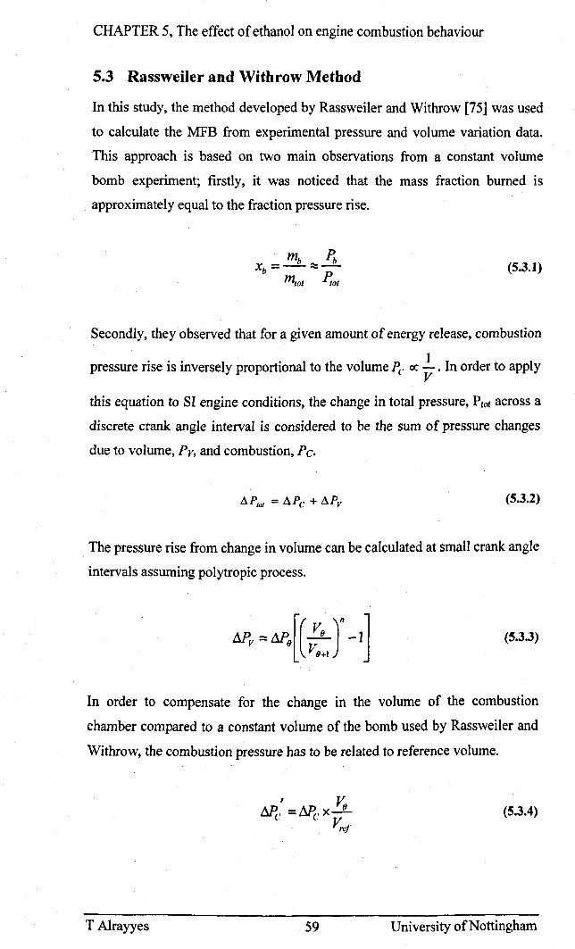
CHAPTER 5, The effect of ethanol on engine combustion behaviour
5.3 Rassweiler and Withrow Method
In this study, the method developed by Rassweiler and Withrow [75] was used
to calculate the MFB from experimental pressure and volume variation data.
This approach is based on two main observations from a constant volume
bomb experiment; firstly, it was noticed that the mass fraction burned is
approximately equal to the fraction pressure rise.
(5.3.1)
Secondly, they observed that for a given amount of energy release, combustion
pressure rise is inversely proportional to the volume Pc: ex: ~ • In order to apply
this equation to SI engine conditions, the change in total pressure, PIOI across a
discrete crank angle interval is considered to be the sum of pressure changes
due to volume, Pv, and combustion, Pc.
(5.3.2)
The pressure rise from change in volume can be calculated at small crank angle
intervals assuming polytropic process.
(5.3.3)
In order to compensate for the change in the volume of the combustion
chamber compared to a constant volume of the bomb used by Rassweiler and
Withrow, the combustion pressure has to be related to reference volume.
T Alrayyes
, V-M::: = M::: x_9
Vrcl
59
(5.3.4)
University of Nottingham
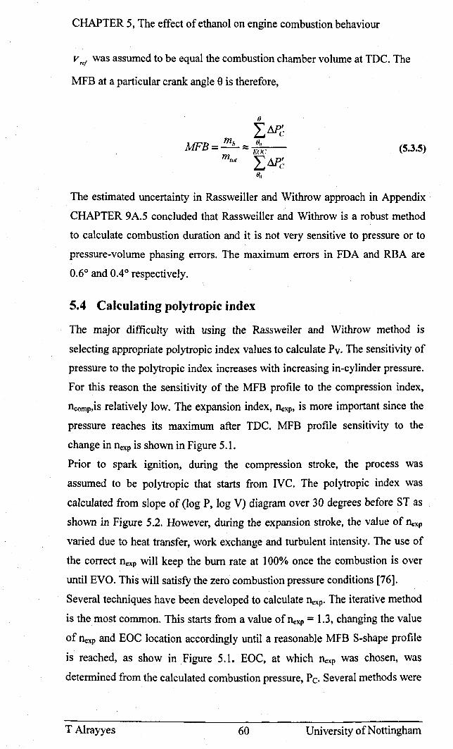
CHAPTER 5, The effect of ethanol on engine combustion behaviour
V T(f was assumed to be equal the combustion chamber volume at TDC. The
MFB at a particular crank angle 0 is therefore,
(5.3.5)
The estimated uncertainty in Rassweiller and Withrow approach in Appendix
CHAPTER 9A.5 concluded that Rassweiller and Withrow is a robust method
to calculate combustion duration and it is not very sensitive to pressure or to
pressure-volume phasing errors. The maximum errors in FDA and RBA are
0.60 and 0.40 respectively.
5.4 Calculating polytropic index
The major difficulty with using the Rassweiler and Withrow method is
selecting appropriate polytropic index values to calculate Pv. The sensitivity of
pressure to the polytropic index increases with increasing in-cylinder pressure.
For this reason the sensitivity of the MFB profile to the compression index,
l1comp,is relatively low. The expansion index, Ilexp, is more important since the
pressure reaches its maximum after TDC. MFB profile sensitivity to the
change in Ilexp is shown in Figure 5.1.
Prior to spark ignition, during the compreSSIon stroke, the process was
assumed to be polytropic that starts from Ive. The polytropic index was
calculated from slope of (log P, log V) diagram over 30 degrees before ST as
shown in Figure 5.2. However, during the expansion stroke, the value of Ilexp
varied due to heat transfer, work exchange and turbulent intensity. The use of
the correct nexp will keep the burn rate at 100% once the combustion is over
until EVO. This will satisfy the zero combustion pressure conditions [76].
Several techniques have been developed to calculate Ilexp. The iterative method
is the most common. This starts from a value of Ilexp = 1.3, changing the value
of Ilexp and EOC location accordingly until a reasonable MFB S-shape profile
is reached, as show in Figure 5.1. EOC, at which Ilexp was chosen, was
determined from the calculated combustion pressure, Pc. Several methods were
T Alrayyes 60 University of Nottingham
CHAPTER 5, The effect of ethanol on engine combustion behaviour
proposed to determine EOe including 'first negative index', 'sum negative
index' and 'negligible Pc fraction index'. 'First negative index' assumes that
EOe is located when the first negative Pc occurs. 'Sum negative index'
assumes that Eoe occurred when three consecutive negative Pc take place.
The second method is seen as more robust since it reduces the influence of
noise. Finally, with 'negligible Pc fraction index', Eoe is defined when Pc
becomes a negligible fraction of the total pressure ( Pc ::; 0.02p,'J/)' Any of the
previous methods can be used as part of the iterative method.
Another method to calculate Ilexp is pyl.IS index [77] which is a simple
alternative technique to iterative method. pyl.lS index simply uses the point
where py1.l5 reaches its maximum then adds IOoeA to allocate Eoe and
subsequently determine a value of l1exp that satisfies the S-shape profile.
Wiseman et al. [76] also proposed a method where Ilexp is calculated without
the need to determine EOe. Wiseman calculated the value of nc:xp over small
interval just before EYO that satisfies Pc equal to zero after combustion
terminates.
Figure 5.3 shows a comparison between the different techniques proposed to
calculate Ilexp for different running conditions. With the exception of Wiseman
method, there was not a significant change among the different methods. The
Wiseman index appears to be overestimating the combustion duration
especially for medium and high loads.
In this study, the iterative method was used to determine Ilexp t with EOe was
allocated using 'negligible Pc fraction index'. EOe was determined when Pc
becomes a negligible fraction of the total pressure ( Pc ::; 0.02 Ph.' ) at three
consecutive steps. This method was seen to be more robust since it reduced the
influence of noise and it was easier to use to define EOe.
5.5 Comparison between laminar flame speed of ethanol and
gasoline
Burning rate is often expressed in terms of a turbulent burning velocity.
Turbulent flames can be treated as an array of laminar flamelets with no
turbulence structure residing within them [17]. Therefore, understanding of
laminar combustion is important to understand flame turbulent combustion.
T Alrayyes 61 University of Nottingham
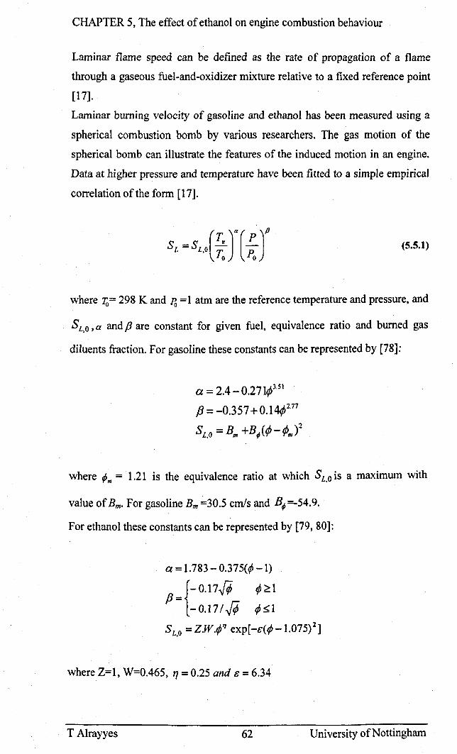
CHAPTER 5, The effect of ethanol on engine combustion behaviour
Laminar flame speed can be defined as the rate of propagation of a flame
through a gaseous fuel-and-oxidizer mixture relative to a fixed reference point
[17].
Laminar burning velocity of gasoline and ethanol has been measured using a
spherical combustion bomb by various researchers. The gas motion of the
spherical bomb can illustrate the features of the induced motion in an engine.
Data at higher pressure and temperature have been fitted to a simple empirical
correlation of the form [17].
(5.5.1)
where 1'0= 298 K and Po =1 atm are the reference temperature and pressure, and
S L,O ,a and p are constant for given fuel, equivalence ratio and burned gas
diluents fraction. For gasoline these constants can be represented by [78]:
a = 2.4 - 0.271¢3.SI
f3 = -0.357 + 0.1~2.77
Sl,O = Bm +B~(¢-¢mi
where tPm = 1.21 is the equivalence ratio at which SL,O is a maximum with
value of Bm. For gasoline Bm =30.5 cmls and B; =-54.9.
For ethanol these constants can be represented by [79, 80]:
a = 1.783 - 0.375(rp -1)
{- O.l7/¢ rp ~ 1 p-
- - 0.17/ -# rp ~ 1
8L,o =Z.W.rp'7 exp[-c(¢-1.075)2]
where Z=1, W=0.465, 11 = 0.25 and c = 6.34
T Alrayyes 62 University of Nottingham
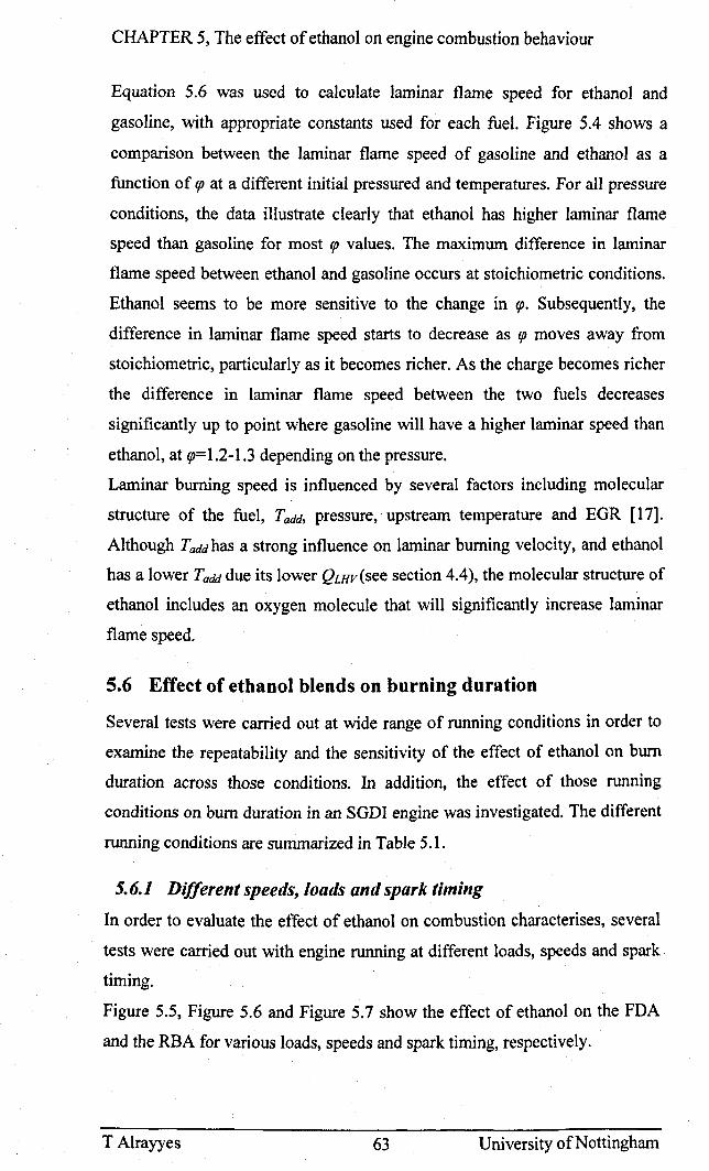
CHAPTER 5, The effect of ethanol on engine combustion behaviour
Equation 5.6 was used to calculate laminar flame speed for ethanol and
gasoline, with appropriate constants used for each fuel. Figure 5.4 shows a
comparison between the laminar flame speed of gasoline and ethanol as a
function of rp at a different initial pressured and temperatures. For all pressure
conditions, the data illustrate clearly that ethanol has higher laminar flame
speed than gasoline for most rp values. The maximum difference in laminar
flame speed between ethanol and gasoline occurs at stoichiometric conditions.
Ethanol seems to be more sensitive to the change in rp. Subsequently, the
difference in laminar flame speed starts to decrease as rp moves away from
stoichiometric, particularly as it becomes richer. As the charge becomes richer
the difference in laminar flame speed between the two fuels decreases
significantly up to point where gasoline will have a higher laminar speed than
ethanol, at rp=I.2-1.3 depending on the pressure.
Laminar burning speed is influenced by several factors including molecular
structure of the fuel, Tadd, pressure, upstream temperature and EOR [17].
Although Taddhas a strong influence on laminar burning velocity, and ethanol
has a lower Tadd due its lower QLHV(see section 4.4), the molecular structure of
ethanol includes an oxygen molecule that will significantly increase laminar
flame speed.
5.6 Effect of ethanol blends on burning duration
Several tests were carried out at wide range of running conditions in order to
examine the repeatability and the sensitivity of the effect of ethanol on burn
duration across those conditions. In addition, the effect of those running
conditions on burn duration in an SODI engine was investigated. The different
running conditions are summarized in Table 5.1.
5.6.1 Different speeds, loads and spark timing
In order to evaluate the effect of ethanol on combustion characterises, several
tests were carried out with engine running at different loads, speeds and spark
timing.
Figure 5.5, Figure 5.6 and Figure 5.7 show the effect of ethanol on the FDA
and the RBA for various loads, speeds and spark timing, respectively.
T Alrayyes 63 University of Nottingham
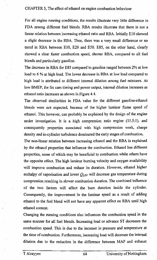
CHAPTER 5, The effect of ethanol on engine combustion behaviour
For all engine running conditions, the results illustrate very little difference in
FDA among different fuel blends. RBA results illustrate that there is not a
linear relation between increasing ethanol ratio and RBA. Initially EIO showed
a slight decrease in the RBA. Then, there was a very small difference or no
trend in RBA between EI0, E20 and E50. E85, on the other hand, clearly
showed a clear faster combustion speed, shorter RBA, compared to all fuel
blends and particularly gasoline.
The decrease in RBA for E85 compared to gasoline ranged between 2% at low
load to 6 % at high load. The lower decrease in RBA at low load compared to
high load is attributed to different internal dilution among fuel mixtures. At
low BMEP, for fix cam timing and power output, internal dilution increases as
ethanol ratio increases as shown in Figure 4.4.
The observed similarities in FDA value for the different gasoline-ethanol
blends were not expected, because of the higher laminar flame speed of
ethanol. This however, can probably be explained by the design of the engine
under investigation. It is a high compression ratio engine (11.5: 1), and
consequently properties associated with high compression work, charge
density and in-cylinder turbulence dominated the early stages of combustion.
The non-linear relation between increasing ethanol and the RBA is explained
by the ethanol properties that influence the combustion. Ethanol has different
properties, some of which may be beneficial to combustion while others have
the opposite effect. The high laminar burning velocity and oxygen availability
will improve combustion and reduce its duration. However, ethanol higher
enthalpy of vaporisation and lower QLHV will decrease gas temperature during
compression resulting in slower combustion duration. The combined influence
of the two factors will affect the burn duration inside the cylinder.
Consequently, the improvement in the laminar speed as a result of adding
ethanol to the fuel blend will not have any apparent effect on RBA until high
ethanol content.
Changing the running conditions also influences the combustion speed in the
same manner for all fuel blends. Increasing load or advance ST decreases the
combustion speed. This is due to the increase in pressure and temperature at
the time of combustion. Furthermore, increasing load will decrease the internal
dilution due to the reduction in the difference between MAP and exhaust
T Alrayyes 64 University of Nottingham
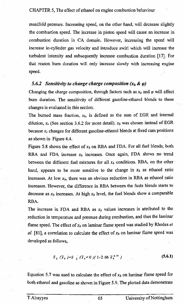
CHAPTER 5, The effect of ethanol on engine combustion behaviour
manifold pressure. Increasing speed, on the other hand, will decrease slightly
the combustion speed. The increase in piston speed will cause an increase in
combustion duration in CA domain. However, increasing the speed will
increase in-cylinder gas velocity and introduce swirl which will increase the
turbulent intensity and subsequently increase combustion duration [17]. For
that reason burn duration will only increase slowly with increasing engine
speed.
5.6.2 Sensitivity to change charge composition (Xb & rp)
Changing the charge composition, through factors such as Xb and (jJ will affect
burn duration. The sensitivity of different gasoline-ethanol blends to these
changes is evaluated in this section.
The burned mass fraction, Xb, is defined as the sum of EGR and internal
dilution, x, (See section 3.6.2 for more detail). Xb was chosen instead of EGR
because x, changes for different gasoline-ethanol blends at fixed cam positions
as shown in Figure 4.4.
Figure 5.8 shows the effect of Xb on RBA and FDA. For all fuel blends, both
RBA and FDA increase Xb increases. Once again, FDA shows no trend
between the different fuel mixtures for all Xb conditions. RBA, on the other
hand, appears to be more sensitive to the change in Xb as ethanol ratio
increases. At low Xb, there was an obvious reduction in RBA as ethanol ratio
increases. However, the difference in RBA between the fuels blends starts to
decrease as Xb increases. At high Xb level, the fuel blends show a comparable
RBA.
The increase in FDA and RBA as Xb values increases is attributed to the
reduction in temperature and pressure during combustion, and thus the laminar
flame speed. The effect of Xb on laminar flame speed was studied by Rhodes et
al. [81], a correlation to calculate the effect of Xh on laminar flame speed was
developed as follows,
(5.6.1)
Equation 5.7 was used to calculate the effect of Xh on laminar flame speed for
both ethanol and gasoline as shown in Figure 5.9. The plotted data demonstrate
T Alrayyes 6S University of Nottingham
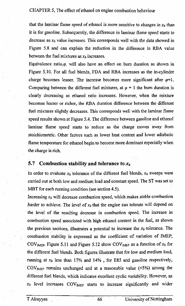
CHAPTER 5, The effect of ethanol on engine combustion behaviour
that the laminar flame speed of ethanol is more sensitive to changes in Xb than
it is for gasoline. Subsequently, the difference in laminar flame speed starts to
decrease as Xb value increases. This corresponds well with the data showed in
Figure 5.8 and can explain the reduction in the difference in RBA value
between the fuel mixtures as Xb increases.
Equivalence ratio, <p, will also have an effect on burn duration as shown in
Figure 5.10. For all fuel blends, FDA and RBA increases as the in-cylinder
charge becomes leaner. The increase becomes more significant after <p=I.
Comparing between the different fuel mixtures, at rp = 1 the burn duration is
clearly decreasing as ethanol ratio increases. However, when the mixture
becomes leaner or richer, the RBA duration difference between the different
fuel mixtures slightly decreases. This corresponds well with the laminar flame
speed results shown at Figure 5.4. The difference between gasoline and ethanol
laminar flame speed starts to reduce as the charge moves away from
stoichiometric. Other factors such as lower heat content and lower adiabatic
flame temperature for ethanol begin to become more dominant especially when
the charge is rich.
5.7 Combustion stability and tolerance to Xb
In order to evaluate Xh tolerance of the different fuel blends, Xb sweeps were
carried out at both low and medium load and constant speed. The ST was set to
MBT for each running condition (see section 4.5).
Increasing Xb will decrease combustion speed, which makes stable combustion
harder to achieve. The level of Xb that the engine can tolerate will depend on
the level of the resulting decrease in combustion speed. The increase in
combustion speed associated with high ethanol content in the fuel, as shown
the previous sections, illustrates a potential to increase the Xb tolerance. The
combustion stability is expressed as the coefficient of variation of IMEP,
COVIMEP. Figure 5.11 and Figure 5.12 show COVIMEP as a function ofxb for
the different fuel blends. Both figures illustrate that for low and medium load,
running at Xb less than 17% and 14% , for E85 and gasoline respectively,
COVIMEP remains unchanged and at a reasonable value «5%) among the
different fuel blends, which indicates excellent cyclic variability. However, as
Xb level increases COY IMEP starts to increase significantly and wider
T Alrayyes 66 University of Nottingham
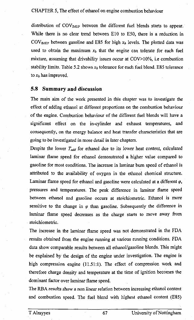
CHAPTER 5, The effect of ethanol on engine combustion behaviour
distribution of COVIMEP between the different fuel blends starts to appear.
While there is no clear trend between E 1 0 to ESO, there is a reduction in
COVIMEP between gasoline and E85 for high Xb levels. The plotted data was
used to obtain the maximum Xb that the engine can tolerate for each fuel
mixture, assuming that drivability issues occur at COY> 10%, i.e combustion
stability limits. Table 5.2 shows Xb tolerance for each fuel blend. E85 tolerance
to Xb has improved.
5.8 Summary and discussion
The main aim of the work presented in this chapter was to investigate the
effect of adding ethanol at different proportions on the combustion behaviour
of the engine. Combustion behaviour of the different fuel blends will have a
significant effect on the in-cylinder and exhaust temperatures, and
consequently, on the energy balance and heat transfer characteristics that are
going to be investigated in more detail in later chapters.
Despite the lower Tadd for ethanol due to its lower heat content, calculated
laminar flame speed for ethanol demonstrated a higher value compared to
gasoline for most conditions. The increase in laminar burn speed of ethanol is
attributed to the availability of oxygen in the ethanol chemical structure.
Laminar flame speed for ethanol and gasoline were calculated at a different qJ.
pressures and temperatures. The peak difference in laminar flame speed
between ethanol and gasoline occurs at stoichiometric. Ethanol is more
sensitive to the change in qJ than gasoline. Subsequently the difference in
laminar flame speed decreases as the charge starts to move away from
stoichiometric.
The increase in the laminar flame speed was not demonstrated in the FDA
results obtained from the engine running at various running conditions. FDA
data show comparable results between all ethanol/gasoline blends. This might
be explained by the design of the engine under investigation. The engine is
high compression engine (11.51: 1). The effect of compression work and
therefore charge density and temperature at the time of ignition becomes the
dominant factor over laminar flame speed.
The RBA results show a non linear relation between increasing ethanol content
and combustion speed. The fuel blend with highest ethanol content (E85)
T Alrayyes 67 University of Nottingham
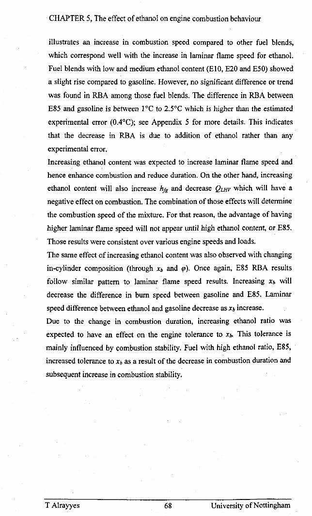
CHAPTER 5, The effect of ethanol on engine combustion behaviour
illustrates an increase in combustion speed compared to other fuel blends,
which correspond well with the increase in laminar flame speed for ethanol.
Fuel blends with low and medium ethanol content (EIO, E20 and E50) showed
a slight rise compared to gasoline. However, no significant difference or trend
was found in RBA among those fuel blends. The difference in RBA between
E85 and gasoline is between 1°C to 2.5°C which is higher than the estimated
experimental error (OAOC); see Appendix 5 for more details. This indicates
that the decrease in RBA is due to addition of ethanol rather than any
experimental error.
Increasing ethanol content was expected to increase laminar flame speed and
hence enhance combustion and reduce duration. On the other hand, increasing
ethanol content will also increase hfg and decrease QLHV which will have a
negative effect on combustion. The combination of those effects will determine
the combustion speed of the mixture. For that reason, the advantage of having
higher laminar flame speed will not appear until high ethanol content, or E85.
Those results were consistent over various engine speeds and loads.
The same effect of increasing ethanol content was also observed with changing
in-cylinder composition (through Xb and f{J). Once again, E85 RBA results
follow similar pattern to laminar flame speed results. Increasing Xb will
decrease the difference in burn speed between gasoline and E85. Laminar
speed difference between ethanol and gasoline decrease as Xb increase.
Due to the change in combustion duration, increasing ethanol ratio was
expected to have an effect on the engine tolerance to Xh. This tolerance is
mainly influenced by combustion stability. Fuel with high ethanol ratio, E85,
increased tolerance to Xb as a result of the decrease in combustion duration and
subsequent increase in combustion stability.
T Alrayyes 68 University of Nottingham
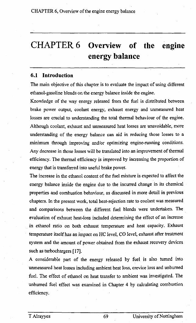
CHAPTER 6, Overview of the engine energy balance
CHAPTER 6
6.1 Introduction
Overview of the energy balance
• engine
The main objective of this chapter is to evaluate the impact of using different
ethanol-gasoline blends on the energy balance inside the engine.
Knowledge of the way energy released from the fuel is distributed between
brake power output, coolant energy, exhaust energy and unmeasured heat
losses are crucial to understanding the total thermal behaviour of the engine.
Although coolant, exhaust and unmeasured heat losses are unavoidable, more
understanding of the energy balance can aid in reducing those losses to a
minimum through improving and/or optimizing engine-running conditions.
Any decrease in those losses will be translated into an improvement of thermal
efficiency. The thermal efficiency is improved by increasing the proportion of
energy that is transferred into useful brake power.
The increase in the ethanol content of the fuel mixture is expected to affect the
energy balance inside the engine due to the incurred change in its chemical
properties and combustion behaviour, as discussed in more detail in previous
chapters. In the present work, total heat-rejection rate to coolant was measured
and comparisons between the different fuel blends were undertaken. The
evaluation of exhaust heat-loss included determining the effect of an increase
in ethanol ratio on both exhaust temperature and heat capacity. Exhaust
temperature itself has an impact on HC level, CO level, exhaust after treatment
system and the amount of power obtained from the exhaust recovery devices
such as turbochargers [17].
A considerable part of the energy released by fuel is also turned into
unmeasured heat losses including ambient heat loss, crevice loss and unburned
fuel. The effect of ethanol on heat transfer to ambient was investigated. The
unburned fuel effect was examined in Chapter 4 by calculating combustion
efficiency.
T Alrayyes 69 University of Nottingham
CHAPTER 6, Overview of the engine energy balance
Finally, energy balance comparison between the different fuel blends was
carried out. Furthermore, the effect of different running conditions on energy
balance was studied.
6.2 Energy balance for the engine
The distribution of the energy released by the fuel combustion is given by the
energy balance. For a control volume which surrounds the engine, the steady
flow energy conservation equation is [17],
(6.2.1)
where mjQLHv is the rate of the fuel energy input, Ph is the brake power,
Qoolanl is the heat transferred to the coolant, Qamh. is the ambient heat loss,
H exh,ic represents the exhaust enthalpy loss due to incomplete combustion and
Hexh • .f is the sensible exhaust energy flux relative to a datum of zero at a
reference temperature, Tref. A datum state of 298 K and 1 atm pressure was
chosen. The estimated error in energy balance calculation is shown in
Appendix A.S.
Under constant engine running conditions, the rate of fuel energy input is
dependent on the fuel mixture used by the engine. QLHV and the mass flow rate
of the fuel vary between the different mixtures, as shown in chapter 4. Ph was
calculated from the dynamometer torque output using equation 3.3. Hrxh./c was
determined from the combustion efficiency calculated in section 4.8. The
methods that have been used to calculate Q'""lanl' Hexh ..• and Qllrnh. are explained
in detail in the following sections.
6.3 Exhaust gas energy
The exhaust gas energy flux is calculated from the following equation:
(6.3.1)
T Alrayyes 70 University of Nottingham
CHAPTER 6, Overview of the engine energy balance .
where Texh is the exhaust temperature at the exhaust port exit and en is the ,-,x!t
mean specific heat capacity of the exhaust gas. The method that was used to
measure and calculate the different variables and the effect of increasing
ethanol ratio are presented in the following sections.
Exhaust heat capacity, cp •exh
The heat capacity of the exhaust gases, Cp • .:xh' has an effect on the thermal
condition inside the engine by affecting the exhaust gas temperature.
Subsequently, Cp,.:xh affect exhaust energy and the amount of heat lost to the
exhaust port. Cp . .:xh can be determined from the exhaust gas composition, as
follows:
c = ~ xc p,exh ~j j PI (6.3.2)
Where Xi and C PI are mass fraction and heat capacity of the exhaust constituent,
respectively. The values of cPI
for the exhaust constituent was obtained from
Roger and Mayhew [72]. Figure 6.1 shows the effect of increasing ethanol
ratio on cp,exh as a function of Texh. The data illustrate clearly that there is an
increase in Cp,.:xh as the ethanol ratio increases. This increase is attributed to the
change in exhaust composition and particularly to the increase in water
composition inside the exhaust, as explained in detail in Chapter 4 and
illustrated in Figure 4.17.
The increase in water content is due to the change in the HIC ratio of fuel and
the increase in oxygen content when the ethanol ratio increases.
The data also illustrates that the rise in Texh will increase CNxh for all fuel
blends.
The estimated error in Cp,exh calculation is around 1.9 % as show in Appendix
A.5.6. On Average, Cp,.:xh increases by 4% between ULG and E85 which is
higher than any experimental error.
T Alrayyes 71 University of Nottingham
CHAPTER 6, Overview of the engine energy balance
6.3.1 Exhaust gas temperature measurement and correction
Texh has a significant effect on the engine's performance and heat transfer
characteristics. Texh will influence the amount of heat rejected to the coolant,
either through the exhaust port, or conducted back into the cylinder. In
addition, it gives an indication of the in-cylinder gas temperature especially
after combustion.
Texh can also affect other parts of the engine, such as the turbocharger's
perfonnance (if used) and, further down the stream, on the after-treatment
system. Texh has an effect on the time needed for the catalytic converter to
reach operating temperature; this is particularly significant in the case of a cold
start. Koehlen et al. [82] suggested that 80% of the HC emissions measured
over the entire FTP-75 drive cycle are emitted within the first 20 seconds after
the engine is started.
Texh was measured using a thermocouple located at the exhaust port exit in two
cylinders as described in Chapter 3.
Correction of exhaust temperature measurements
The thennocouple tips were inserted into the centre of the gas flow. The
equilibrium temperature of the thermocouple is reached when the heat transfers
by radiation to the exhaust walls, and the conduction along the supporting
wires is balanced by convective heat-transfer from the gas. Since the exhaust
wall and the thermocouple mount are generally cooler than the gas, the heat
transfer by conduction and radiation will be from the thermocouple to the
connecting leads and to the exhaust port wall respectively. As a result, this
equilibrium temperature will be lower than true time-averaged temperature.
This is referred to as radiation and conduction error.
Rogers and Mayhew [72] suggested that errors in thermocouple readings can
be compensated for by using the energy balance between convection gain and
radiation loss using the following formula:
(6.3.3)
Rearranging the equation, we find:
T Alrayyes 72 University of Nottingham
CHAPTER 6, Overview of the engine energy balance
T:Xh_tru:= ~r o;xh_meas - T:xh_Wall) + T:xh_meas e
(6.3.4)
where Texh_'rue is the true exhaust temperature, Texh_meu .. is the actual measured
value, Texh_wuU is the exhaust port wall temperature, and both hr and he are,
respectively, effective radiative and convective heat transfer coefficients for
the thermocouple tips.
For a turbulent flow perpendicular to a wire, the convective coefficient is
determined to be [72]:
(6.3.5)
where the characteristic dimension is the thermocouple' s diameter and the gas
properties are evaluated according to the measured exhaust temperature.
For a special case of a grey body radiation within a black or large enclosure
(which represents the thermocouple within the exhaust port), the radiative heat
transfer is given as [72]:
(6.3.6)
where (J is the Stefan-Boltzman constant, E is the emissivity of the
thermocouple surface. The value of e is in the 0.2 to 0.8 range. An e value of
0.5 was used for the purpose of this study. Figure 6.2 shows a comparison
between the measured Texh value and the true Texh value for different fuel
mixtures. The results illustrate that the real value is typically 8.5-10% higher
than the measured equivalent. These results correspond perfectly to the
findings of Yuen [83] and Caton [84], where it has been established that the
average temperature is typically 10% higher than the measured value. For that
reason, the average temperature used in this thesis is going to be estimated by
multiplying the measured Texh by a factor of 1.1.
Figure 6.3 shows the effect of an increasing ethanol ratio on Texh. The result
illustrates clearly that increasing an ethanol ratio will decrease Ttxh. This can be
T Alrayyes 73 University of Nottingham
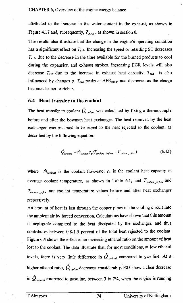
CHAPTER 6, Overview of the engine energy balance
attributed to the increase in the water content in the exhaust, as shown in
Figure 4.17 and, subsequently, Cp,exh' as shown in section O.
The results also illustrate that the change in the engine's operating condition
has a significant effect on rexh. Increasing the speed or retarding ST decreases
Texh, due to the decrease in the time available for the burned products to cool
during the expansion and exhaust strokes. Increasing EGR levels will also
decrease Texh due to the increase in exhaust heat capacity. Texh is also
influenced by changes rp. Texh peaks at AFRstoich and decreases as the charge
becomes leaner or richer.
6.4 Heat transfer to the coolant
The heat transfer to coolant Qcoolanl was calculated by fixing a thermocouple
before and after the bowman heat exchanger. The heat removed by the heat
exchanger was assumed to be equal to the heat rejected to the coolant, as
described by the following equation:
Q.,)()/anl = m c",,/anl C p~,)()/anl _ h<jim: - T.:,m/unI _ a}lff ) (6.4.1)
where mcoolant is the coolant flow-rate, cp is the coolant heat capacity at
average coolant temperature, as shown in Table 6.1, and T.:'H,/un/_h<iorc and
T.:"olunt _ufler are coolant temperature values before and after heat exchanger
respectively.
An amount of heat is lost through the copper pipes of the cooling circuit into
the ambient air by forced convection. Calculations have shown that this amount
is negligible compared to the heat dissipated by the exchanger, and thus
contributes between 0.8-1.5 percent of the total heat rejected to the coolant.
Figure 6.4 shows the effect of an increasing ethanol ratio on the amount of heat
lost to the coolant. The data illustrate that, for most conditions, at low ethanol
levels, there is very little difference in Qcoolanl compared to gasoline. At a
. higher ethanol ratio, Qcoolanl decreases considerably. E85 show a clear decrease
in Qcoo/ant compared to gasoline, between 3 to 7%, when the engine is running
T Alrayyes 74 University of Nottingham
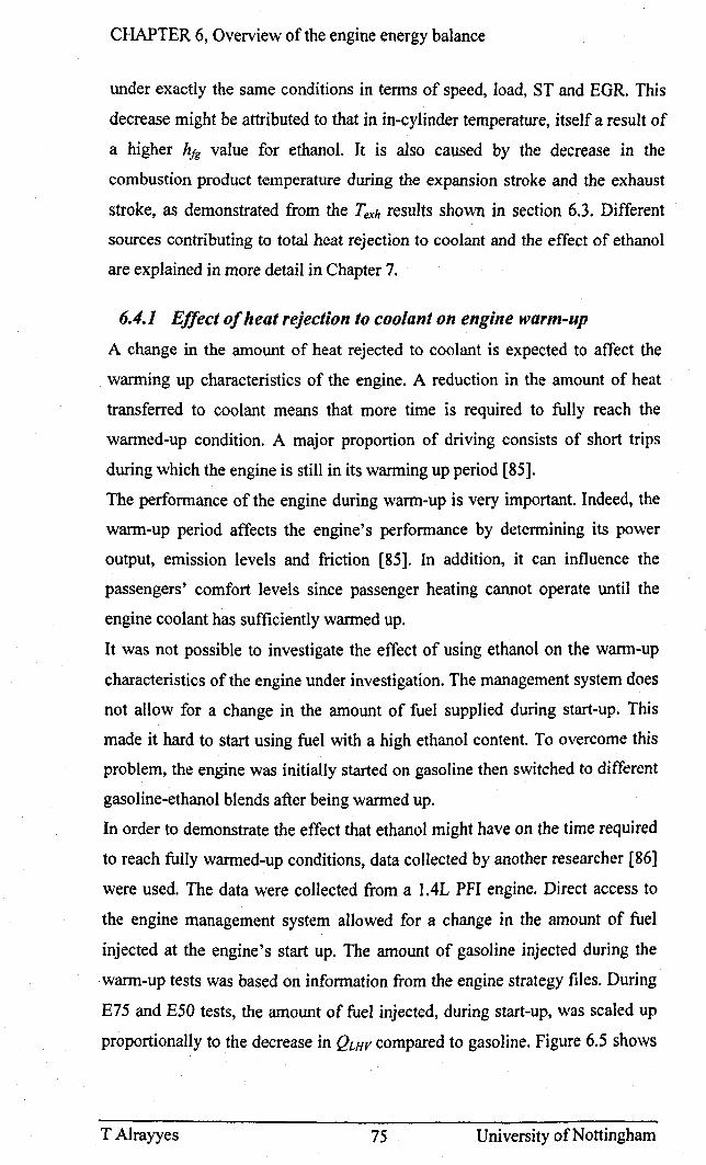
CHAPTER 6, Overview of the engine energy balance
under exactly the same conditions in terms of speed, load, ST and EGR. This
decrease might be attributed to that in in-cylinder temperature, itself a result of
a higher hjg value for ethanol. It is also caused by the decrease in the
combustion product temperature during the expansion stroke and the exhaust
stroke, as demonstrated from the Texh results shown in section 6.3. Different
sources contributing to total heat rejection to coolant and the effect of ethanol
are explained in more detail in Chapter 7.
6.4.1 Effect of heat rejection to coolant on engine warm-up
A change in the amount of heat rejected to coolant is expected to affect the
warming up characteristics of the engine. A reduction in the amount of heat
transferred to coolant means that more time is required to fully reach the
warmed-up condition. A major proportion of driving consists of short trips
during which the engine is still in its warming up period [85].
The performance of the engine during warm-up is very important. Indeed, the
warm-up period affects the engine's performance by determining its power
output, emission levels and friction [85]. In addition, it can influence the
passengers' comfort levels since passenger heating cannot operate until the
engine coolant has sufficiently warmed up.
It was not possible to investigate the effect of using ethanol on the warm-up
characteristics of the engine under investigation. The management system does
not allow for a change in the amount of fuel supplied during start-up. This
made it hard to start using fuel with a high ethanol content. To overcome this
problem, the engine was initially started on gasoline then switched to different
gasoline-ethanol blends after being warmed up.
In order to demonstrate the effect that ethanol might have on the time required
to reach fully warmed-up conditions, data collected by another researcher [86]
were used. The data were collected from a tAL PFI engine. Direct access to
the engine management system allowed for a change in the amount of fuel
injected at the engine's start up. The amount of gasoline injected during the
. warm-up tests was based on information from the engine strategy files. During
E75 and E50 tests, the amount of fuel injected, during start-up, was scaled up
proportionally to the decrease in QLHV compared to gasoline. Figure 6.S shows
T Alrayyes 75 University of Nottingham
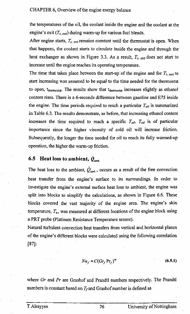
CHAPTER 6, Overview of the engine energy balance
the temperatures of the oil, the coolant inside the engine and the coolant at the
engine's exit (Te, exi,) during warm-up for various fuel blends.
After engine starts, Te, exit remains constant until the thermostat is open. When
that happens, the coolant starts to circulate inside the engine and through the
heat exchanger as shown in Figure 3.3. As a result, Te, exit does not start to
increase until the engine reaches its operating temperature.
The time that takes place between the start-up of the engine and for Te, exit to
start increasing was assumed to be equal to the time needed for the thermostat
to open, tthennostat. The results show that tthennostat increases slightly as ethanol
content rises. There is a 6-seconds difference between gasoline and E75 inside
the engine. The time periods required to reach a particular Toil is summarized
in Table 6.3. The results demonstrate, as before, that increasing ethanol content
increases the time required to reach a specific Toil. TOil is of particular
importance since the higher viscosity of cold oil will increase friction.
Subsequently, the longer the time needed for oil to reach its fully warmed-up
operation, the higher the warm-up friction.
6.5 Heat loss to ambient, Qamb.
The heat loss to the ambient, Qamh., occurs as a result of the free convection
heat transfer from the engine's surface to its surroundings. In order to
investigate the engine's external surface heat loss to ambient, the engine was
split into blocks to simplify the calculations, as shown in Figure 6.6. These
blocks covered the vast majority of the engine area. The engine's skin
temperature, Tw, was measured at different locations of the engine block using
a PRT probe (Platinum Resistance Temperature sensor).
Natural turbulent convection heat transfers from vertical and horizontal planes
of the engine's different blocks were calculated using the following correlation
[87]:
(6.5.1)
where Gr and Pr are Grashof and Prandtl numbers respectively. The Prandtl
numbers is constant based on Tfand Grashofnumber is defined as
T Alrayyes 76 University of Nottingham
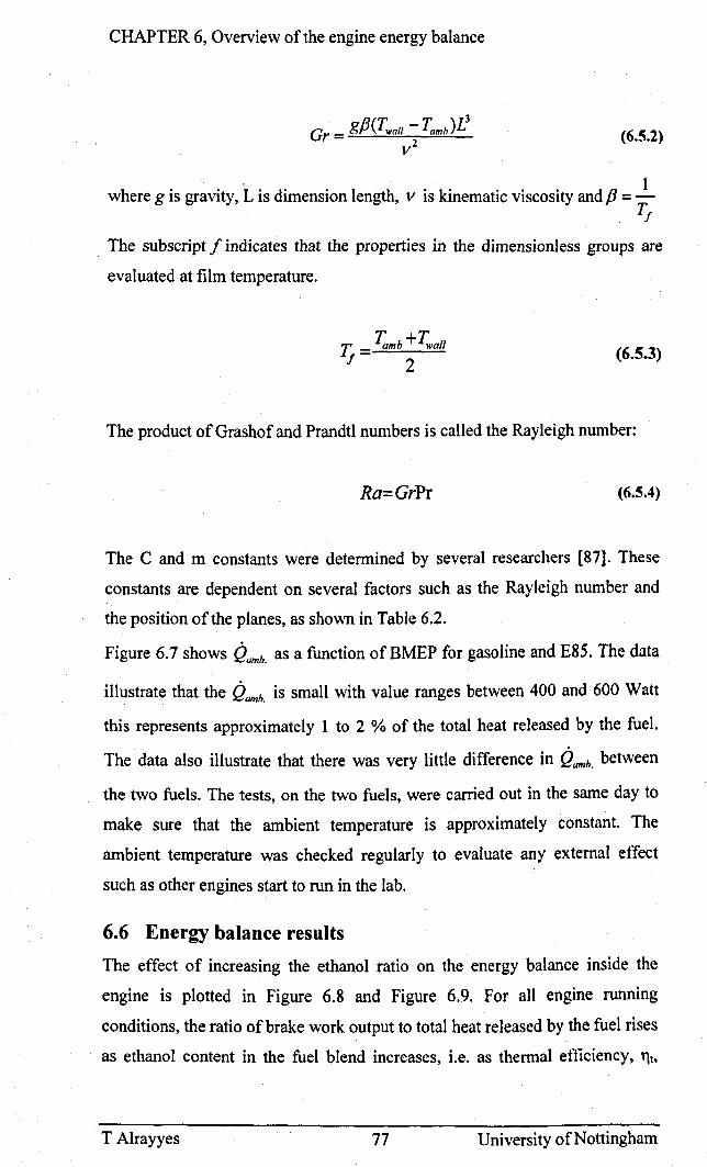
CHAPTER 6, Overview of the engine energy balance
(6.5.2)
where g is gravity, L is dimension length, v is kinematic viscosity and P = _1 Tf
The subscript f indicates that the properties in the dimensionless groups are
evaluated at film temperature.
T:mb +Twall 2
(6.5.3)
The product of Grashof and Prandtl numbers is called the Rayleigh number:
Ra=GrPr (6.5.4)
The C and m constants were determined by several researchers [87]. These
constants are dependent on several factors such as the Rayleigh number and
the position of the planes, as shown in Table 6.2.
Figure 6.7 shows Qumh. as a function ofBMEP for gasoline and E85. The data
illustrate that the Qumh. is small with value ranges between 400 and 600 Watt
this represents approximately 1 to 2 % of the total heat released by the fuel.
The data also illustrate that there was very little difference in Qum", between
the two fuels. The tests, on the two fuels, were carried out in the same day to
make sure that the ambient temperature is approximately constant. The
ambient temperature was checked regularly to evaluate any external effect
such as other engines start to run in the lab.
6.6 Energy balance results
The effect of increasing the ethanol ratio on the energy balance inside the
engine is plotted in Figure 6.8 and Figure 6.9. For all engine running
conditions, the ratio of brake work output to total heat released by the fuel rises
as ethanol content in the fuel blend increases, i.e. as thermal efficiency, T\h
T Alrayyes 77 University of Nottingham
CHAPTER 6, Overview of the engine energy balance
improves. The increase in 11t ranges between 0.5% to 3%. The increase in 111
suggests that the penalty in BSFC associated with the increase in the QLHvof
ethanol has the potential to decrease. Figure 6.10 shows a comparison between
the reduction in QLHV and the increase in BSFC compared to gasoline as
ethanol content increases. The results illustrate that the reduction in BSFC is
less than that expected by the reduction in QLHV, While E85 has 40% lower
heat content, it shows 28% to 32% lower BSFC. This can be explained by
improvements in thermal efficiency.
Exhaust and coolant energy levels showed comparable results between the
different fuel blends. The improvement in combustion efficiency, 11c.
demonstrated in section 4.8 is the main reason for the increase in 111. In order to
evaluate the effects of combustion efficiency on thermal efficiency, the former
was taken into consideration in the energy balance ((mJ*QLHv*1'/c)) as shown in
Figure 6.11 and Figure 6.12. In addition, 1'/c was taken into account when
comparing the distribution of heat released as a result of combustion, rather
than the expected total heat released by the fuel.
These results clearly show that the combustion efficiency contributed to the
majority of the improvements in thermal efficiency, especially at low and
medium ethanol ratios. Nevertheless, there was still an improvement in thermal
efficiency particularly when comparing between E85 and gasoline. Thermal
efficiency values still increased from 0.5% to 1.5% between E85 and gasoline.
This is explained by the decrease in the coolant and exhaust energy losses as
shown in Figure 6.11 and Figure 6.12. The decrease in these energy losses is
ultimately transferred into useful brake work and subsequently into an
improvement in thermal efficiency. The variation in the levels of decrease in
exhaust and coolant energy losses and, in some cases, the absence of this
decrease, is attributed to experimental error. The level of decrease in the
engine losses between E85 and gasoline is small (ranging between 0.5 % and 2
%.) Subsequently, any small errors in the measurements could influence the
results.
The results show a small difference between the various fuel blends. These
differences could be due to experimental errors instead of the effect of fuel
content. The experimental error was estimated in Appendix A5.8. The results
show that the inaccuracy is around ± 1 %, ± 1.25% and ±0.7% for thermal
T Alrayyes 78 University of Nottingham
CHAPTER 6, Overview of the engine energy balance
efficiency, coolant energy percentage and exhaust energy percentage
respectively.
Although the difference in energy balance between the fuel blends was, in
some cases, lower than the experimental error, there was consistency in the
results over the different engine running conditions. The tests at those running
conditions were taken at different days. In addition, the improvement in
thermal efficiency was obvious in BSFC results.
The results in Figure 6.11 and Figure 6.12 also illustrate that changes in the
engine's running conditions influence the in-cylinder energy balance for all
fuel blends. By increasing speed, coolant-loss percentage decreases, whereas
the exhaust energy percentage increases. This is due to the reduction in the
time available for the charge to cool and the increase in the exhaust
temperature. Increasing the load leads to a significant rise in the percentage of
brake load, a decrease in coolant energy losses and an increase in the
percentage of energy lost to the exhaust. This is attributed to an increase in
combustion efficiency, peak in-cylinder temperature and exhaust temperature.
6.7 Summary and discussion
The main objective of this chapter was to investigate the effect of ethanol on
the energy balance inside the engine. The energy released by the fuel is
distributed between brake output, coolant energy, exhaust energy and
unmeasured heat loss. The unmeasured heat loss includes the un-combusted
fuel, crevice losses and heat losses to ambient.
Section 4.7 show that increasing ethanol content influences the exhaust's
different constituent levels. The change meant that the exhaust's heat capacity,
Cp,cxh , changes accordingly. The Cp,cxh results, calculated in this chapter,
illustrate a marked rise as ethanol content increases as a result of increasing
water level in the exhaust.
The increase in Cp,cxh is also demonstrated in the measured exhaust
temperature values, Texh. Increasing ethanol content illustrates a clear decrease
in Texh at various engine running conditions. Texh is also affected by the
engine's running conditions. Retarding ST or increasing speed increases Texh
due to the reduction in the time available for the in-cylinder charge to cool
T Alrayyes 79 University of Nottingham
CHAPTER 6, Overview of the engine energy balance
down. Increasing BMEP or EGR level, on the other hand, decreases exhaust
temperatures due to a rise in the Cp,cxh values.
A reduction in Texh could have a considerable effect on emission levels,
particularly at warming-up. The reduction in exhaust temperature levels would
increase the time needed for the catalyst to reach its operating temperature.
This would increase the level of the engine's tail pipe emissions, especially at
cold start. The reduction in Texh also affects HC and CO after flame
combustion. Texh can additionally have an effect on the amount of heat loss to
the coolant. Texh affects the levels of exhaust-port heat loss and heat conducted
back into the engine through the exhaust manifold.
The decrease in Texh and the higher hjg of ethanol suggest that heat transfer to
coolant will decrease as ethanol content increases. The results confirmed this
expectation. However, the effect of ethanol appears only at medium and high
ethanol content (E50 & E85). Low ethanol content fuel blends show
comparable results to gasoline ones. At low ethanol content, the oxygen
availability dominates the combustion more than the increase in hjg, which
would eliminate the cooling effect of ethanol. The decrease in heat rejection to
coolant will affect the warm-up characteristics of the engine. By increasing
ethanol content, more time is required to reach normal operation temperature.
This would be reflected as an increase in fuel consumption, friction and
emissions.
Heat lost to ambient shows comparable results between E85 and gasoline. This
was expected, since the coolant inside the engine will keep the engine's skin
temperature at approximately constant levels. The change in coolant
temperature and flow rate, when running on E85, was not big enough to affect
the engine's skin temperature.
Energy balance is affected by the changes in exhaust temperature and heat
transfer to coolant. The energy balance data illustrate a considerable
improvement in the thermal efficiency as ethanol content increases. This
improvement in thermal efficiency was consistent over various engine running
conditions. This is attributed mainly to the increase in combustion efficiency,
as was demonstrated in section 4.8. The decrease in exhaust energy and
coolant energy percentages also contribute to an improvement in thermal
T Alrayyes 80 University of Nottingham
CHAPTER 6, Overview of the engine energy balance
efficiency, particularly at E85. The increase in thermal efficiency decreases the
penalty in BSFC as a result of the lower QLHV of ethanol.
T Alrayyes 81 University of Nottingham
CHAPTER 7, Time average engine heat transfer
CHAPTER 7
7.1 Introduction
Time average engine heat transfer during fully warm up operation
A detailed understanding of the heat transfer to coolant is essential, The
amount of heat transfer to cylinder wall will have an impact on the work
transferred to the piston and, subsequently, on specific power and efficiency
levels. Engine knock behaviour will also be influenced by both heat transfer to
the cylinder wall during the compression stroke, and by heat transfer from the
hot exhaust valve and piston. The emission formation will be affected as a
result of the change in gas temperature, due to heat transfer both within the
engine cycle and in the exhaust system, where after burning of CO and HC
occurs. Friction will also contribute to heat rejection to coolant and get affected
by it. Friction will be influenced by both changes to oil temperature, and thus
to its viscosity, and by piston and liner thermal distortion [17J.
As shown in Chapter 6, running the engine on ethanol-gasoline blends
containing medium and high ethanol levels affected the heat rejection rate to
coolant, Qcoolant.
Qcoolanris the sum of various instances of heat transfer from the combustion
chamber, the exhaust port and other engine components, each of which has a
different heat transfer mechanism. In the present work, the effect of ethanol .
levels on the different heat sources that contribute to Qcoolanl was evaluated.
The gas-side heat rejection rate to coolant was predicted using C 1 C2
correlation, and then compared to the measured values. The C 1 C2 correlation
is a time-averaged heat transfer correlation that was developed by The
University of Nottingham for thermal modelling, using the PROMETs
software [88, 89]. The main advantage of using time-averaged heat transfer
correlation is its simplicity compared to instantaneous spatially-averaged heat
T Alrayyes 82 University of Nottingham
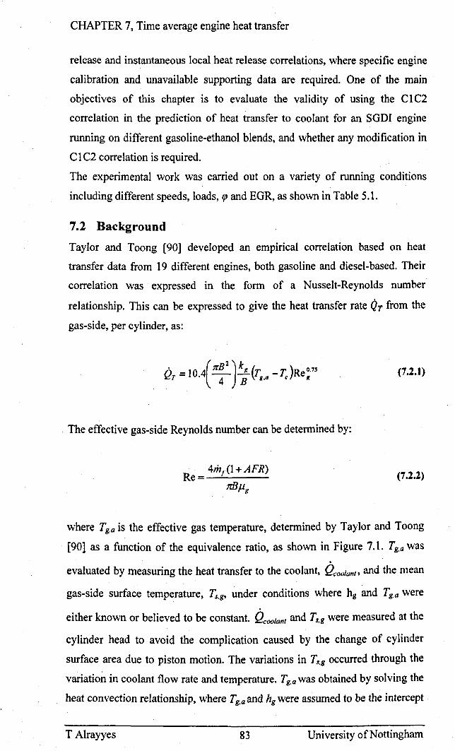
CHAPTER 7, Time average engine heat transfer
release and instantaneous local heat release correlations, where specific engine
calibration and unavailable supporting data are required. One of the main
objectives of this chapter is to evaluate the validity of using the C 1 C2
correlation in the prediction of heat transfer to coolant for an SOOI engine
running on different gasoline-ethanol blends, and whether any modification in
C 1 C2 correlation is required.
The experimental work was carried out on a variety of running conditions
including different speeds, loads, f{J and EGR, as shown in Table 5.1.
7.2 Background
Taylor and Toong [901 developed an empirical correlation based on heat
transfer data from 19 different engines, both gasoline and diesel-based. Their
correlation was expressed in the form of a Nusselt-Reynolds number
relationship. This can be expressed to give the heat transfer rate Qr from the
gas-side, per cylinder, as:
(7.2.1)
The effective gas-side Reynolds number can be detennined by:
Re = _4m.....,:· 1_(_1 +_A_F_'R_) (7.2.2)
where Tg,Q is the effective gas temperature, determined by Taylor and Toong
[90] as a function of the equivalence ratio, as shown in Figure 7.1. Tg,Q was
evaluated by measuring the heat transfer to the coolant, Q"oolanl' and the mean
gas-side surface temperature, Ts,g, under conditions where hg and Tg.a were
either known or believed to be constant. Qcoolanl and T"g were measured at the
cylinder head to avoid the complication caused by the change of cylinder
surface area due to piston motion. The variations in T"g occurred through the
variation in coolant flow rate and temperature. Tg,a was obtained by solving the
heat convection relationship, where Tg,Q and hg were assumed to be the intercept
T Alrayyes 83 University of Nottingham
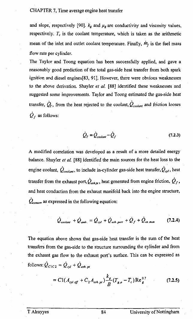
CHAPTER 7, Time average engine heat transfer
and slope, respectively [90]. kg and ).lg are conductivity and viscosity values,
respectively. Tc is the coolant temperature, which is taken as the arithmetic
mean of the inlet and outlet coolant temperature. Finally, mj is the fuel mass
flow rate per cylinder.
The Taylor and Toong equation has been successfully applied, and gave a
reasonably good prediction of the total gas-side heat transfer from both spark
ignition and diesel engines[83, 91]. However, there were obvious weaknesses
to the above derivation. Shayler et al. [88] identified these weaknesses and
suggested some improvements. Taylor and Toong estimated the gas-side heat
transfer, G, from the heat rejected to the coolant, Qcoolanl and friction looses
Q f as follows:
(7.2.3)
A modified correlation was developed as a result of a more detailed energy
balance. Shayler et al. [88] identified the main sources for the heat loss to the
engine coolant, Qcoolanl' to include in-cylinder gas-side heat transfer, Q,y, , heat
transfer from the exhaust port, ~hPt' heat generated from engine friction, Q!,
and heat conduction from the exhaust manifold back into the engine structure,
{{xman' as expressed in the following equation:
(7.2.4)
The equation above shows that gas-side heat transfer is the sum of the heat
transfers from the gas-side to the structure surrounding the cylinder and from
the exhaust gas flow to the exhaust port's surface. This can be expressed as
follows: QCIC2 = QCYI + Qexh,pt
(7.2.S)
T Alrayyes 84 University of Nottingham
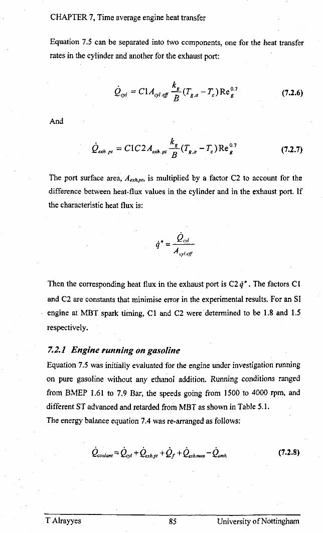
CHAPTER 7, Time average engine heat transfer
Equation 7.5 can be separated into two components, one for the heat transfer
rates in the cylinder and another for the exhaust port:
. k QCY/ = CIAcyl.eff ; (Tg,a - TJRe~·7 (7.2.6)
And
(7.2.7)
The port surface area, Aexh.pt, is multiplied by a factor C2 to account for the
difference between heat-flux values in the cylinder and in the exhaust port. If
the characteristic heat flux is:
." Qevl q = . A,yl.e.U·
Then the corresponding heat flux in the exhaust port is C2 q" . The factors C 1
and C2 are constants that minimise error in the experimental results. For an SI
engine at MBT spark timing, C 1 and C2 were determined to be 1.8 and 1.5
respectively.
7.2.1 Engine running on gasoline
Equation 7.5 was initially evaluated for the engine under investigation running
on pure gasoline without any ethanol addition. Running conditions ranged
from BMEP 1.61 to 7.9 Bar, the speeds going from 1500 to 4000 rpm, and
different ST advanced and retarded from MBT as shown in Table 5.1.
The energy balance equation 7.4 was re-arranged as foHows:
~OOlant = ~1 + f!eXhPt + 0, + Oexhman - Q,mb. (7.2.8)
T Alrayyes 85 University of Nottingham
CHAPTER 7, Time average engine heat transfer
Qcoolanl represents the total heat transfer to coolant, both directly and through
the oil. Gas-side heat transfer from both QCYI and QXIfJI was determined using
equation 7.5. The effective gas cylinder area, Acylejf, used in the equation is
defined in [92]. Acyl.eff is smaller than the combustion chamber area at the point
when the piston is at its lowest position, because the liner is not always
exposed to the cylinder gas. The Acyl.eff is defined as:
(7.2.9)
Where A pc and ~eaa are the piston-crown area and the cylinder-head
combustion chamber area respectively. f(x/L) is a polynomial function that
relates the local heat flux at any point down the liner to the same value as
calculated at the top of the liner (which is always exposed to the cylinder gas),
where x is the distance of a given point down the line from TDC, and L is the
cylinder stroke.
May et 01. [92] solved the polynomial function and found it be:
(7.2.10)
To evaluate the heat generated due to friction, Q/, mechanical friction losses
have to be predicted. Mechanical friction losses can be obtained from IMEP
and BMEP calculations where:
FMEP = IMEP"uI - RMEP (7.2.11)
IMEPnel was obtained from the in-cylinder pressure data (see section 3.6.1).
BMEP was obtained from measuring the torque absorbed by the dyno.
Therefore Q/ is calculated as:
T Alrayyes 86 University of Nottingham
CHAPTER 7, Time average engine heat transfer
Qr = FMEPx JT.t x N /60 (7.1.12)
Qexh.man is the rate of heat conduction to the head from the exhaust manifold
flange. In a study carried out by Imabeppu et af. [93J on a 2.0L DOHC SI
engine operating at fully warm-up conditions, it was found that Q~xhman is
related to the exhaust port's heat flux 4:xhp/, through the following expression:
Q. ." exh.man = aqex.pt (7.1.13)
Where a is constant and equal to 0.0042 m2 for a cast-iron exhaust manifold.
The result from Imabeppu et 01. [93] suggested that Q,xhman accounts for 8-
12% of the total heat transferred to the engine structure. However, the value of
the constant 0 and the percentage of heat conducted back will depend on the
exhaust manifold and gasket material. For example, Hayden [94] found that
using a fibre gasket can reduce the heat transfer to as little as Y4 of the rate
measured when a metal gasket is used. The engine used in this study has a steel
exhaust manifold and a metal gasket that conform well with the predictions of
Imabeppu et af. [93].
Finally, heat transfer to the ambient, ~mb' generally has a small effect on
overall energy balance, accounting typically for 400 to 600W under natural
convection conditions, as shown in section 6.5.
The rate of heat rejection to the coolant, Qcoolunf' is a value measured as shown
in section 6.4.
Figure 7.2 illustrates a comparison between the actual measured heat transfer
to coolant and the predicted equivalent from equation 7.8 for pure gasoline.
The results show a good agreement between the predicted and the measured
values within a 10% accuracy limit.
7.2.2 Gasoline-ethanol blends
The main aim of this section is to establish the validity of using the C 1 C2 .
correlation to predict the gas-side heat loss rate to the coolant, Q'IC2' and to
T Alrayyes 87 University of Nottingham
CHAPTER 7, Time average engine heat transfer
determine whether any modification is required when ethanol at different
blends is used. Q:;lC2 was predicted using equation 7.2 in exactly the same
manner explained in the preceding section 7.2.1, as such, Cl and C2 remain
constant. The Tg,Q value used was the same as the one developed by Taylor and
Toong [90], as shown in Figure 7.1.
When the engine was running on pure gasoline, the values used for kg and Ilg,
which are both highly dependent on temperature, were assumed to be the same
as those of air at Tg,Q. When running on ethanol mixtures, however, the
AFRstoich is going to decrease as the ethanol ratio increases in the fuel.
Consequently, this would affect the chemical properties of the in-cylinder
charge and the validity of this assumption has to be examined.
A comparison between the conductivity and viscosity of air and ethanol-air
mixtures for different AFR equivalence ratios is plotted in Figure 7.3. The
results illustrate that there is no significant difference in conductivity between
the air and ethanol-air mixtures. The viscosity of air, on the other hand,
appears to be slightly higher than that of an air-ethanol mixture at rich fuel
mixtures. Air viscosity is around 4.5% higher at equivalence ratio 1.5 and
around 2.5% higher at AFRstoich. The difference is. nonetheless. still relatively
small. In addition, the majority of the engine cycle is dominated by the
properties of the exhaust that are closer to air properties. For this reason, the
assumption that Ilg is equal to that of air at different ethanol ratios is still valid.
Comparisons between the predicted values of Q'oolom, obtained using equation
7.2, and the measured values for different ethanol-gasoline blends, are plotted
in Figure 7.4. The results illustrate a good agreement between predicted and
measured values.
The previous results show clearly that the CIC2 correlation is able to predict
heat transfer to coolant values without any need to modify Cl, C2 or Tg,Q. The
reason for this is discussed in more detail in section 7.6.
7.3 Effect of External EGR
Introducing EGR will have a significant effect on the heat loss rate to the
coolant. To investigate the effect of EGR on heat rejection rate, several tests
were undertaken at both MBT, where ST needed to be advanced, and different
T Alrayyes 88 University of Nottingham
CHAPTER 7, Time average engine heat transfer
ST. The tests were performed with the BMEP ranging from 1.61 to 4.75 Bar
and the EGR ranging from 5 to 30 % depending on the load.
The introduction of EGR to the SI engine will affect the heat rejection rate
through the increase in the overall charge mass, the increase in the inlet gas
temperature and, finally, the increase in the thermal capacity per unit mass of
charge.
Increasing the intake charge temperature will increase the gas-side heat
rejection rate. Lundin et al. [95] and Povolny el al. [96] studied the effect of
variation in inlet charge temperatures on Qcoolant. They found that the effective
in-cylinder gas temperature needed to be corrected to a reference inlet
manifold temperature according to the relation:
T g,a= ~,a,298 +0.35(7; - 298) (7.3.1)
where T, is the gas temperature at the intake manifold and T g,a,298 is the
average effective gas temperature for an inlet gas temperature of 298K. The
variation of T g,a,298 is shown in Figure 7.1.
The increase in charge mass as a result of EGR is taken into account through
the redefining of the Reynolds number as follows:
Re = _4m-,' ,:...-{_1 +_A_F_'R_)_/{_I-_E_G_R_) 1rBpg
(7.3.2)
The increase in inlet charge temperature and mass will increase the heat
transfer to the coolant as accounted for in equations 7.14 and 7.15. However,
the use of EGR will also increase the thermal capacity of the cylinder charge
and, hence, reduce the heat rejected to coolant. The effect of an increase in
thermal capacity can therefore be accounted for by applying a correction factor
FeaR to the prediction [89], as follows:
T Alrayyes 89 University of Nottingham
CHAPTER 7, Time average engine heat transfer
. . Q::IC2_EGR = F'eGR(kIC2 (7.3.3)
where FECR = 1-EG R. The method that has been used to develop FeGR is
explained in detail in Appendix 4.
A comparison between measured and predicted Qcoolant values at different
EGR percentages for an engine running on gasoline is plotted in Figure 7.5.
The results clearly shows an improvement in the prediction when the
correction factor, FeCR' was used.
Several tests were carried out in order to evaluate the validity of using the FeGR
to predict Qcoolant values for different gasoline-ethanol fuel blends, as sho'Ml in
Figure 7.6 and Figure 7.7.
The engine was running on E50 and E85, with the BMEP ranging from 1.61 to
4.75 Bar and the EGR ranging from 5 to 30 %, depending on the load. The
data illustrate clearly that the prediction values correspond well to measured
values within the 10% limit.
7.4 Evaluation of the heat transfer to the exhaust port, ilahPt
The heat transfer to coolant through the exhaust port, Qexhpl' represents a
considerable percentage of the total heat transfer to coolant due to the high
exhaust speed and temperature. Taylor [97] suggested that around 20% of the
total heat transferred to the coolant is through the exhaust port, Imabeppu [93]
suggested that it is more typically between 24-27%. With the stricter emissions
regulations, understanding Qexh'PI is becoming increasingly essential. The
energy loss through the exhaust affects the ability to get the after-treatment
system to the required temperature, especially at cold temperatures i.e. losing
energy will cause the system to take longer to reach its maximum effectiveness
and will result in higher tail-pipe emissions.
This section is concerned with the effect of ethanol on the heat loss to the
exhaust port. The heat transfer to the exhaust port has a pulsating nature. When
the exhaust valves are open the heat transfer is treated as a forced convection,
while it is treated as a natural convection when the exhaust valves are closed.
T Alrayyes 90 University of Nottingham
CHAPTER 7, Time average engine heat transfer
Heat transfer by natural convection can be ignored since it is small compared
to the forced convection equivalent.
7.4.1 Measured heat transfer to the exhaust port
In order to evaluate the heat loss to the cylinder wall, two thermocouples were
fitted at the start and the exit of the exhaust port of cylinder 1 and cylinder 3 as
shown in Figure 7.8. Qexh.pt was calculated from the ~emperature difference
between the start and the exit of the exhaust port. The drop in temperature was
assumed to be due to the Qexh,pt. This is assuming that kinetic energy loss and
the heat generated by flow resistance in the piping is insignificant compared to
Qexh,Pf' Hence, QeXh.pt was calculated using the following:
(7.4.1)
r;xh_OU,'e,& r;xh_lnlet are measurable values, the exhaust mass flow rate, !hex"
was calculated from knowing the fuel flow rate, AFR and Xb levels. Cp,e:'(h was
calculated from the exhaust constituents and exhaust temperature (both
measurable values) as shown in section 6.4.3. Tests were carried out with the
engine running at different speeds, loads, ignition timings, equivalence ratios
and EGR levels as shown in Table 5.1. Those ranges were chosen to
investigate not only the effect of the different fuel blends over a wide range of
running condition but also the consistency and the repeatability of the results.
Figure 7.9 shows the QexhPI for different fuel blends as a function of load,
speed, EGR and ffJ. Data for all running conditions illustrate a decrease in
QeXh.pt as ethanol ratios increase; this decrease is more obvious at higher
ethanol ratios, i.e. E50 and E85, where there is approximately a 5% decrease in
Qexh,pt between gasoline and E85.
The main factors that are affecting Qexh,PI are the exhaust mass flow rate, the
surface temperature and the exhaust temperature, Texh. Figure 7.10 illustrates
that the exhaust surface temperature does not change with increasing ethanol
T Alrayyes 91 University of Nottingham
CHAPTER 7, Time average engine heat transfer
levels due to coolant circulation, which keeps the engine's surface temperature
constant. Exhaust surface temperature was taken at three different locations of
the exhaust port and on two different cylinders. Mass flow rate decreased
slightly for higher ethanol contents as shown in Figure 7.11. Finally, with
increasing ethanol content, Texh decreased considerably due to the increase in
Cp,exh of the exhaust (i.e. an increase in the water content of the exhaust) as
shown in Figure 6.3. The decrease Texh is the main reason for the reduction in
Qexhpt. The small decrease in exhaust mass flow rate also contributed to this
decrease.
The change in engine running conditions also affects Qexh,pt. For all fuel
mixtures, increasing load and speed shows an increase in the Qexh,pt due to the
increase in exhaust mass flow rate and temperature. Equivalence ratio up to
AFRstoich does not show any change in (lxh,pt. However, as the charge becomes
rich, Qexh.pt start to decrease. This is mainly due to the decrease in Texh and in
the exhaust mass flow rate. Increasing EGR level does not show any effect on
Qexh.pt. The combined effect of decreasing Texh and increasing mass flow rate
as EGR levels increase explains the unchanged heat loss between different
EGR percentages.
The contribution of the measured Qexh,pt to the total heat released to the coolant
is shown in Figure 7.12, the results illustrate that the contribution level
remained between 15 to 20 % of the total heat rejected to the coolant. These
results are lower than would have been suggested by previous studies (Taylor
[90] suggested around 20% and Imabeppu [93] suggested between 24-27%).
The lower value of the measured exhaust port heat loss can be explained by the
thermocouple readings at the exhaust port inlet. Due to the complex geometry
of the exhaust port, it was hard to place the thermocouple accurately at the
exhaust port inlet; instead it was placed as close as possible. This meant that
the exhaust gas might have already cooled slightly before reading the
thermocouples. In addition, it is hard to place the thermocouples accurately in
the middle of the exhaust port, the closer the thermocouple to the surface the
T Alrayyes 92 University of Nottingham
CHAPTER 7, Time average engine heat transfer
more the readings are affected by the cooling of the surface. Furthermore, the
exhaust port has a pulsating nature while the thermocouples have a time-based
one. This might cause an error in the thermocouples' reading.
The underestimated measurements of the heat lost to the exhaust port are
acceptable for the purpose of this study since a comparison between the
different fuel blends is the main objective.
7.4.2 Exhaust port heat correlations
Several correlations have been developed over the years to predict the heat
transfer to the exhaust port. These correlations were developed assuming a
quasi-steady forced convection heat transfer to the exhaust port. The heat
transfer coefficient can be defined from the Nusselt Reynolds relation as
follows:
And:
k h=a exh Reb dexh.PI
4mf {l + AFR) Re pI = --"----
Pexhmiexh,PI
(7.4.2)
(7.4.3)
where kexh is thermal conductivity and Jlexh is dynamic viscosity. Both values
are dependent on exhaust temperature, the properties of air were used for
simplicity. The coefficients a and b are dependent on the correlation used. The
variation in correlation coefficients can be attributed to the difference in the
geometry of each engine that the correlation was developed on [98]. The
variation in geometry will alter the flow pattern inside each engine and,
subsequently, affect f2eXh.Pt. In addition, the pulsating nature based on valve
events, as well as the pipe length, can significantly change the flow pattern and
heat transfer relationship [98]. .
In order to determine the best correlation for predicting Q&!.fhpl' the heat
transfer calculated from the different correlations in Table 7.1 was compared to
T Alrayyes 93 University of Nottingham
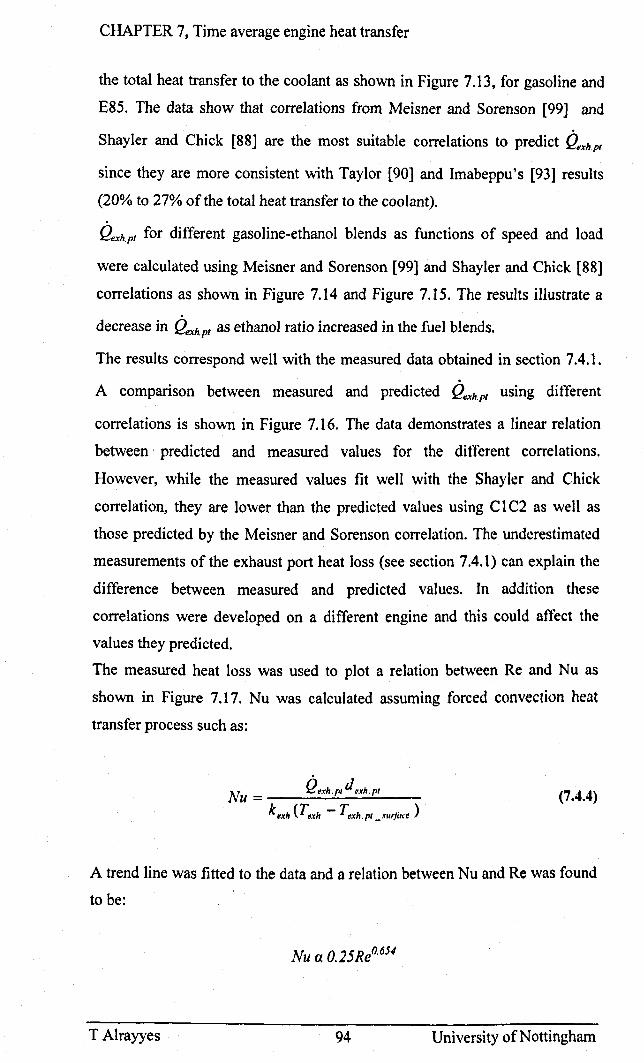
CHAPTER 7, Time average engine heat transfer
the total heat transfer to the coolant as shown in Figure 7.13, for gasoline and
E85. The data show that correlations from Meisner and Sorenson [99] and
Shayler and Chick [88] are the most suitable correlations to predict Qexh,pI
since they are more consistent with Taylor [90] and Imabeppu's [93] results
(20% to 27% of the total heat transfer to the coolant).
Qexh.pt for different gasoline-ethanol blends as functions of speed and load
were calculated using Meisner and Sorenson [99] and Shayler and Chick [88]
correlations as shown in Figure 7.14 and Figure 7.15. The results illustrate a
decrease in Qexh.pt as ethanol ratio increased in the fuel blends.
The results correspond well with the measured data obtained in section 7.4.1.
A comparison between measured and predicted Qexh,pt using different
correlations is shown in Figure 7.16. The data demonstrates a linear relation
between' predicted and measured values for the ditferent correlations.
However, while the measured values fit well with the Shayler and Chick
correlation, they are lower than the predicted values using C 1 C2 as well as
those predicted by the Meisner and Sorenson correlation. The underestimated
measurements of the exhaust port heat loss (see section 7.4.1) can explain the
difference between measured and predicted values. In addition these
correlations were developed on a different engine and this could affect the
values they predicted.
The measured heat loss was used to plot a relation between Re and Nu as
shown in Figure 7.17. Nu was calculated assuming forced convection heat
transfer process such as:
A7 Qtxh,P' d, .. rh.,., JVU = ---......:----'---
k exh (T exh - T exh. pI _ .tllrjilt'C )
(7.4.4)
A trend line was fitted to the data and a relation between Nu and Re was found
to be:
Nu a O.25Reo.654
T Alrayyes 94 University of Nottingham
CHAPTER 7, Time average engine heat transfer
7.5 Heat conducted back to the cylinder head, C!.xhman
As mentioned previously, part of the exhaust energy is conducted across the
cylinder head/exhaust manifold flange face. The magnitude of Qxhman will be
dependent on the type of gasket used. Imabeppu et al. [93] found that Q.xhman
is a function of the exhaust port heat flux, ilxhp" as shown in equation 7.13.
As a result, the decrease in Qexh,pt for medium and high ethanol content fuels
will reduce the amount of heat conducted back to the engine as shown in
Figure 7.18. The data in figure 7.18 was calculated using equation 7.13.
To confinn these findings, ~xhman was also calculated using the coolant
energy balance shown in equation 7.4. A comparison between the different fuel
mixtures for various running conditions is shown in Figure 7.19. The results
illustrate that up to E50 there is no clear trend between increasing ethanol
ratios and heat conducted back to the cylinder. E85, on the other hand, shows a
slight decrease in C!exhman for different engine running conditions. The results
correspond well to the data obtained from equation 7.13.
Figure 7.20 shows Q.xhman, as calculated from the coolant energy balance, as a
function of iJ:xhpt. The results illustrate that there was an approximate linear
relationship between ~xhman and iJ:XhPt. These results agree with the findings
of Imabeppu et a1. [93]. The value of a, however. varied between 0.0048 m2
and 0.0053 m2, depending on the fuel blends. The change in the value of a can
be attributed to the change in Texh among the different fuel blends which will
change the relation between iJ:xhpt and C!exhman' In addition, the experimental
. error associated with the C 1 C2 correlation, FMEP, and Qc:o()lllnt calculations
can contribute to the variations in the value of a.
7.6 Results and discussion
The main aim of the work presented in this chapter was to investigate the
effect of gasoline-ethanol blends at different proportions on the gas-side heat
transfer to coolant, both from the cylinder and exhaust port. Furthermore. it
T Alrayyes 95 University of Nottingham
CHAPTER 7, Time average engine heat transfer
was desired to establish whether the C 1 C2 correlation reqUires any
modification to allow for changes in fuel heating values and other fuel
properties.
Results obtained in section 6.4 demonstrate a clear decrease in the total heat
rejection to coolant, ~oolant' for high and medium ethanol content fuel blends
(E50 & E85). The reasons for this decrease were investigated in this chapter by .
examining the different heat sources that contribute to Q.oolantaS shown in
Figure 7.21. Different sources include the in-cylinder gas-side heat transfer (
QCYI ), exhaust port heat loss (Qexh.POrl)' heat generated from engine friction ( Qf
) and heat conduction from the exhaust manifold ( Qah.man ).
Both the predicted and measured results showed that Qe.'hI'Orl and Q,,'h.mtln
decrease for fuel blends with medium and high ethanol contents as a result of
the decrease in Texh• This decrease will contribute to the total decrease in the
measured ~oolant.
The in cylinder gas side heat transfer, QCYI, is expected to change as ethanol
content increases in the fuel blends due to the physical properties of ethanol.
Indeed, ethanol has a higher enthalpy of vaporisation. As a result, increasing
ethanol will have a cooling effect on the in-cylinder charge leading to a
decrease in in-cylinder peak temperature. However, using ethanol will also
increase combustion speed, as illustrated in chapter 5, resulting in higher peak
pressure and temperatures. The combined effect of these two factors will
determine the in-cylinder temperature and hence Qcyl.
The NOx emission results in section 4.6.3 show a reduction in NOx levels
when ethanol ratios increase in the fuel blend. This reduction indicates a
decrease in the local in-cylinder peak temperatures. Furthermore, the decrease
in Texh illustrates a decrease in the product of combustion or the in-cylinder gas
temperatures later on in the combustion stroke, which has a considerable effect
Qcyl' Both the NOx emissions and Texh data illustrate a decrease in in-cylinder
temperature at high ethanol content and, subsequently, in QCJ'" This decrease
T Alrayyes 96 University of Nottingham
CHAPTER 7, Time average engine heat transfer
is expected to contribute to the total decrease in ({'oolant. The Qeyl for different
fuel blends were predicted using equation 7.6 as part of C I C2 correlation as
shown in Figure 7.22. The CIC2 correlation was found to agree well with the
measured values within the 10% limit range without any need for modification
for CI or C2 values. The data in Figure 7.22 illustrate that, in most cases, E85
showed a lower Qcyl than the rest of the fuel mixtures. Using E85 reduces heat
rejection rates to between 0.5 and 3% compared to gasoline. These results
correspond well with the author's prediction of the effect of ethanol as
mentioned above.
The decrease in Qeyl is accounted for through the change in Re without the
need to change C 1 or Tg.a• The Re number decreases when the engine is
running on E85 compared to the rest of the fuel blends as shown in Figure
7.23. Although E85 showed a decrease in Qcyl' the results do not illustrate any
clear trend between increasing ethanol ratios and Q,:vl. This might be explained
by the confidence limit and experimental discrepancy associated with C 1 C2
correlation where change in Qcyl can be too small to be resolved by the C I C2
correlation. QCIC2 can be predicted within an accuracy of a 10% limit. In
addition, the increase in combustion efficiency for low ethanol ratios can have
a more dominant effect on increasing in-cylinder temperatures than the cooling
effect of ethanol or the decrease in Texh.
Qexh.P()rt was also predicted using the CIC2 correlation in equation 7.7. C2 in
equation 7.7 represents the ratio of exhaust port heat flux and cylinder heat
flux. C2 will remain constant since the ratio is constant for all fuel blends as
shown in Figure 7.24. The measured Q.:xh'l'tJrt value was used to calculate C2.
In summary, it is believed that the CIC2 correlation can be used to predict gas
side heat transfer without any modification. The change that is expected in
Q'YI is accounted for through a decrease in Re without the need to change C 1
or Tg.a• C2 remains constant since the ratio of exhaust port heat flux and
cylinder heat flux show very little difference between the various gasoline
ethanol blends.
T Alrayyes 97 University of Nottingham
CHAPTER 7, Time average engine heat transfer
Finally, Qf shows comparable results between the different fuel blends and
will not affect the change in QccHllanl
EGR affects the gas-side heat transfer through increasing the heat capacity of
the charge, the inlet charge temperature and the mass flow rate of the charge.
The effect of EGR was accounted for by using correlations to account for the
increase in heat capacity and inlet temperatures. A modified Reynolds
definition was also used to account for the increase in mass fraction. This kept
the accuracy of the prediction within the 10% limit. This modification for EGR
also appeared also to correspond well to the predictions of heat transfer to the
coolant when gasoline-ethanol blends at different percentages were used.
T Alrayyes 98 University of Nottingham
CHAPTER 8, In-cylinder gas properties and instantaneous heat loss
CHAPTER 8 In-cylinder gas properties and instantaneous heat loss to the cylinder wall.
8.1 Introduction
Heat transfer to the coolant from different engine components was discussed in
detail in Chapter 7. However, these investigations have all been based on
cycle-averaged heat transfer. In this chapter, the effect of ethanol on the
instantaneous spatially-averaged heat loss is investigated. The temporal change
in heat loss across the cycle is important in explaining the effect that the
ethanol has on some of the engine's characteristics, such as power output.
engine efficiency and thermal NOx formation. The effect of higher ethanol
content on some of the in-cylinder charge properties and charge preparation
was also studied.
The . heat loss was predicted from the pressure data using a correlation
developed by Hohenberg [100]. The Hohenberg correlation has been used
extensively to predict heat loss for both gasoline and diesel engines. The use of
this correlation to predict heat loss for different gasoline-ethanol blends has
never been examined until this work was undertaken. In this chapter. the
validity of the Hohenberg correlation for different gasoline-ethanol mixtures is
going to be evaluated.
8.2 Calculating in-cylinder gas properties
8.2.1 In-cylinder temperature
The cyclic variation of average the in-cylinder gas temperature, T"
is required
to calculate the heat loss to the cylinder wall. The measurement of Tg is
extremely difficult as it requires access to the cylinder. In addition, the gas
temperature also varies according to location, with the biggest difference in
temperature between burned and un-burned areas. It was beyond the scope of
this work to measure Tg directly. Instead, the average temperature was
T Alrayyes 99 University of Nottingham
CHAPTER 8, In-cylinder gas properties and instantaneous heat loss
estimated. In order to estimate Tg, the engine cycle was divided into three
separate parts as shown in Figure 8.1. Firstly, the induction cycle until Ive.
Secondly, the close part of the cycle between IVC to EVO and, finally, the
exhaust stroke, starting from EVO until the end of the cycle.
In the induction stroke, the Tg is small and will be close to the cylinder's
surface temperature. Heat loss to the cylinder wall during induction is small
compared to the compression, combustion or exhaust part of the cycle. Tg
during the induction stroke is assumed to be constant and equal to the Tg at
Ive.
The ideal gas law was used to calculate the gas temperature during the close
part of the cycle, i.e. between IVC and EVO, thus
(8.2.1)
In-cylinder pressure, p. is a measurable value as shown in section 3.6.1.
Instantaneous cylinder volume. V, is calculated from our knowledge of the
engine's geometry. The mass of the in-cylinder charge. m"harlle, includes the
inducted air and fuel as well as any external EGR and any internal dilution.
During the exhaust stroke, when the exhaust valve is open, the in-cylinder
pressure drops considerably until they reach exhaust manifold pressure. The
charge temperature during the exhaust stroke was determined by assuming the
process during blowdown to be isentropic. thus:
(8.2.2)
The pressure variation is known and T EVO can be calculated from ideal gas law
as described above. Although the exhaust stroke is not isentropic. it is believed
to be a good approximation of the real value. The temperature trend obtained
in this study was similar to that obtained by previous studies such as May e/ al.
[92] and Caton and Heywood [84].
T Alrayyes 100 University of Nottingham
CHAPTER 8, In-cylinder gas properties and instantaneous heat loss
A comparison between the different fuel blends is shown in Figure 8.2 and
Figure 8.3. The results illustrate that, in both cylinders, there is not a clear
trend between increasing ethanol content and the calculated in-cylinder
temperature. In cylinder 1, however, there was a small increase in Tg for E85
when compared with gasoline.
The results of the calculated bulk in-cylinder gas temperature, Tg, do not
correspond to the expectation of the author. Indeed, the increase in ethanol
content in the fuel blend was expected to decrease Tg• This expectation was
based on the reduction in the total measured heat transfer to the coolant,
(Lm/ant , decreases in NOx level, decreases in Texh and increases in hlg as
ethanol content rises, as discussed in detail in section 7.6.
The calculated Tg is a function of the measured pressure and the mass of the
charge, mcharge. The pressure reading does not show any significant variation
either in the measured 100 consecutive cycle pressure data or at the standard
reference point, as shown in section 3.7. mc:harge was calculated from the
measurement of the total fuel flow rate to the engine and the measured Lambda
value. The fuel flow rate was assumed to be equally divided between the four
cylinders. The Lambda value was measured at the exhaust manifold and
assumed to be equal in the four cylinders. However, the assumption that m"harge
is equal in the different cylinders is not necessarily accurate. There might be
differences in the mcharge and AFR values among the different cylinders. This is
due to the variation in the amount of fuel injected into each cylinder (which
might be caused by the injectors' manufacturing tolerances) or the amount of
air drawn by each cylinder. For that reason, in this section, m"hllrge is going to
be calculated using ideal gas law instead, which would be as follows:
(8.2.3)
where TEVO was assumed to be equal to the measured temperature before the
exhaust port. Since the temperature at EVO is higher than the one measured
before the exhaust port, the calculated mass charge, m"harge.calc will be higher
T Alrayyes 101 University of Nottingham .
CHAPTER 8, In-cylinder gas properties and instantaneous heat loss
than the actual value. However, this study is a comparative study and the main
purpose is to compare the different fuel mixtures.
mcharge,ca/c was used to calculate the in-cylinder bulk temperature, Tg,cab using
equation 8.1. The results illustrate that, during combustion, there is no
correlation between ethanol content and temperature magnitude and phasing as
shown in Figure 8.4. However, by the end of combustion, the combustion
products' temperature slightly decreases at high and medium ethanol ratios
(E50 and E85), this corresponds well to the measured decrease in Texh.
Peak calculated temperature; however, does not appear to be in line with the
NOx emissions as there was no clear decrease in peak Tg with higher ethanol
levels. This can be attributed to the fact that NOx is affected by the local
temperature rather than the bulk average temperature. The decrease in
adiabatic flame temperature as ethanol content increase, as shown in Figure
4.2, could explain the reduction in NOx level.
8.2.2 Calculating in-cylinder r for different fuel mixtures
As shown in Chapter 4, higher ethanol content in the gasoline/ethanol blend
will affect the fuel's physiochemical properties and the exhaust composition.
These changes might have an effect on the in-cylinder charge heat capacity
and, subsequently, on the in-cylinder charge heat capacity ratio. f, used in net
heat release calculations. This section is concerned with the method used to
calculate f and the potential effect of increasing ethanol levels on the f value.
The calculation of f was based on dividing the cylinder into two zones: a
fresh charge zone and a burned zone. The fresh charge consists of the fuel-air
mixture and the unburned region consists of the products of the combustion.
Heat capacity, Cpt calculated for the fresh charge and the products of
combustion was based on polynomial correlations as detailed in Appendix 3.
Although ethanol has a higher cp than gasoline and subsequently a different ')',
as shown in Figure 8.5; nonetheless, Figure 8.6 illustrates that this ditference
in cp between gasoline-air and ethanol-air mixtures is very small. This is
explained by the change in AFRstoich between gasoline and E85. As a result, the
y difference between the two mixtures is very small as shown in Figure 8.7. On
average, E85-air mixtures had around a 0.3% increase in y value over that of an
gasoline-air mixture. A correlation that relates y to temperature was developed,
T Alrayyes 102 University of Nottingham
CHAPTER 8, In-cylinder gas properties and instantaneous heat loss
by the author, based on the y average between the E85-air mixture and the
gasoline-air mixture, calculated as follows:
r Ie == 6 xl 0-8 T2 - 0.0002T + 1.4063 (8.2.4)
where T is the temperature in Kelvin (K). The burned gas heat capacity, Cp.b,
was calculated from the emissions composition measured at different running
conditions. Figure 8.8 shows Cp.h as a function of temperature for the engine
running on different loads, at gasoline, E50 and E85. The results illustrate
clearly that Cp.b is sensitive to changes in temperature and fuel composition.
Increasing ethanol content produces a clear increase in the Cp.b of the emissions
for a given temperature. The results also show that Cp.b is not sensitive to a
change in load. A correlation was developed based on the average emission
produced at different loads, as follows:
If 275<T(K)<1 000
If T(K» 1 000
Where,
At= 0.0003
A2=0.0222E+0.955
Bl=0.0205E+0.2063
B2=0.1159E+0.1776
(8.2.S)
(8.2.6)
where E is the ethanol ratio and T is the temperature in K. The methods that
were used to develop these correlations are described in detail in Appendix 3.
Subsequently, the heat capacity ratio for the burned charge, rho can be
calculated using the following equation:
Cp " r,,= . Cp•h -R"
(8.2.7)
T Alrayyes 103 University of Nottingham
CHAPTER 8, In-cylinder gas properties and instantaneous heat loss
At each CA degree, the mass average heat capacity ratio of the fresh charge
and the burned charge, r, is calculated through the following equation:
(8.2.8)
where Xb is the burned gas fraction in fresh charged, which includes internal
dilution and EGR. MFB is the mass fraction burned.
The temperature of the diluted unburned gas, T", is calculated by assuming a
polytropic compression after IVC. The temperature of the burned gas, Tb. was
calculated assuming that when an element burns it instantaneously mixes with
the already-burnt gas, hence the average mean temperature for the burned gas
is [17]:
(8.2.9)
Figure 8.9 shows an example of y during the engine cycle for different fuel
mixtures when the engine is running at constant BMEP 4.75 bar and 2000 rpm.
8.3 Charge temperature and mixture preparation
In the DIS I engine, there is a limited amount of time for fuel to evaporate and
mix with the air to form a combustible charge. The evaporation of the fuel
happens in two stages [41]:
When the liquid fuel is injected directly into the cylinder during the
induction stroke, part of it evaporates by absorbing heat from the
surrounding air and the combustion chamber's surfaces which will
decrease in-cylinder temperature as a result.
During the compression stroke, the rest of the liquid fuel evaporates as
a result of the increase in temperature and pressure.
The two temperature parameters (the drop in temperature after injection and its
rise during compression) were considered by several studies [24, 41] in an
attempt to evaluate the mixture preparation characteristics. Price el al. [41] and
Dodge [101] found that in a DISI engine running at homogenous operation, the
T Alrayyes 104 University of Nottingham
CHAPTER 8, In-cylinder gas properties and instantaneous heat loss
majority of the fuel is vaporised during the compression stroke. For this
reason, an increase in temperature during the compression stroke can be
considered as an indication of the amount of heat required to evaporate the
fuel. In this section, the effect of higher levels of ethanol content on the fuel
vaporisation process and its potential cooling effect are assessed by calculating
Tcomp, the temperature increase between IVe and ST, as shown in Figure 8.10
and Figure 8.11. The results illustrate that, for all running conditions. whilst
E 10 and E20 show comparable Tcomp values to that of gasoline. the results for
ESO and E8S show a clear decrease in Tcomp with E8S showing the lowest Tcomp.
The non-linear relation between Tcomp and an increase in ethanol content can be
explained by the fact that Tcomp is proportional to several relations that are
themselves inter-related. During the compression stroke. the piston work
exerted on the charge is divided into three components: latent heat used to
vaporise the liquid fuel, a change in internal energy and the heat transferred to
the coolant through cylinder walls. Heat transferred to the wall can be ignored
due to the small difference between the wall temperature and the charge
temperature during compression, thus:
(8.3.1)
(8.3.2)
From equations 8.10 and 8.11, and from assuming constant work. J U and
subsequently Tcomp is a function of the mass of the charge, m"harge. the constant
volume-specific heat capacity, Cv• and the enthalpy of vaporisation. hfg. The
increase in hlg as ethanol content increases. as shown in Figure 2.3, means that
a higher percentage of the piston work is going into vaporizing the fuel than
turned into a gain in internal energy and, hence, Tcomp will decrease. However.
the increase of Cv as ethanol content increases will have an opposite effect, as
shown in Figure 8.12. The combined effect of these two factors means that the
cooling effect of increasing ethanol content will not manifest itself until
medium ethanol contents, as is indicated by the decrease in the compression
stroke temperature, Tcomp.
T Alrayyes 105 University of Nottingham
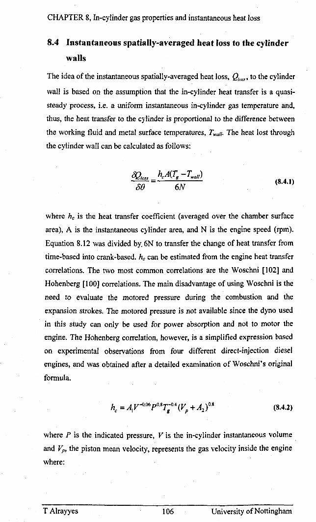
CHAPTER 8, In-cylinder gas properties and instantaneous heat Joss
8.4 Instantaneous spatially-averaged heat loss to the cylinder
walls
The idea of the instantaneous spatially-averaged heat loss, Q/n",' to the cylinder
wall is based on the asswnption that the in-cylinder heat transfer is a quasi
steady process, i.e. a uniform instantaneous in-cylinder gas temperature and,
thus, the heat transfer to the cylinder is proportional to the difference between
the working fluid and metal surface temperatures, Twall. The heat lost through
the cylinder wall can be calculated as follows:
~/oss _ hcA(~ - Twall ) ---88 6N
(8.4.1)
where he is the heat transfer coefficient (averaged over the chamber surface
area), A is the instantaneous cylinder area, and N is the engine speed (rpm).
Equation 8.12 was divided by.6N to transfer the change of heat transfer from
time-based into crank-based. he can be estimated from the engine heat transfer
correlations. The two most common correlations are the Woschni [102] and
Hohenberg [100] correlations. The main disadvantage of using Woschni is the
need to evaluate the motored pressure during the combustion and the
expansion strokes. The motored pressure is not available since the dyno used
in this study can only be used for power absorption and not to motor the
engine. The Hohenberg correlation, however, is a simplified expression based
on experimental observations from four different direct-injection diesel
engines, and was obtained after a detailed examination of Woschni's original
formula.
h = A V-o·06 pO.8r-o·4 (V + A )0.8 e 1 g P 2 (8.4.2)
where P is the indicated pressure, V is the in-cylinder instantaneous volume
and Vp, the piston mean velocity, represents the gas velocity inside the engine
where:
T Alrayyes 106 University of Nottingham
CHAPTER 8, In-cylinder gas properties and instantaneous heat loss
Vp =4LN160 (8.4.3)
The mean value of the constants Al and A2 were found to be 130 and 1.4
respectively. A2 represents the effect of combustion-produced turbulence and
heat loss due to radiation.
8.S In-cylinder gas-side surface temperature
The gas-side surface temperature, Twall. is maintained below a certain
temperature though coolant circulation in order to avoid thermal stress that
could lead to fatigue cracking and the deterioration of the oil film [17]. Twall
varies with the location, cycle variation and engine running condition. The
swing in surface temperature during the engine cycle is very small, it being
around 7 K [17]. Spatially-averaged in-cylinder gas-side surface temperatures
typical range between 370 K and 450 K depending on the running condition
[17]. Tg between ST to EVO during the engine cycle lies between 750 K and
2500 K. Thus, the temperature difference between gas and wall is large and
changes in wall temperature will have only a small influence on the predicted
gas-to-wall heat transfer. For that reason. it is safe to assume the surface
temperature to be constant and averaged between 370 K and 450 K.
8.6 Calibration of the Hohenberg correlation
As mentioned above, the Hohenberg correlation was originally developed for
diesel engines. Consequently, AI and A2 need to be recalculated in order to
calibrate the correlation for the engine under investigation.
Assuming a constant A2, AI was determined by directly relating the amount of
fuel chemical energy released to heat transfer into: work, sensible energy and
heat loss to the chamber wall, assuming negligible crevice losses such as:
(8.6.1)
where Qgross, ~et and {Joss are gross heat release, net heat release and heat
loss respectively. ~et is defined as the energy that is transformed into sensible
T Alrayyes 107 University of Nottingham
CHAPTER 8, In-cylinder gas properties and instantaneous heat loss
energy and real work within the combustion chamber. Assuming that the
chamber's contents are a semi-perfect gas, ~et can be calculated from (171:
OQne/ = _Y_p6V +_I_V6p y-l y-l
(8.6.2)
As shown in Figure 8.13, AI was found to have an average of 68.2 to satisfy
equation 8.15 for different running conditions and different fuel blends.
8.7 Evaluation of the Hohenberg correlation,
The Hohenburg correaltion was initially developed for diesel engine and has
been widely used to predict Qloss in SI engines running on gasoline. The
validity of using Hohenberg to predict heat loss for an SI engine running on
different ethanol ratios has never been properly examined. The main aim of
this section is to evaluate the robustness of the Hohenberg correlation in
predicting Qloss at different ethanol ratios. This was carried out through three
different techniques.
Firstly, the proportion of the total gross heat release energy to the total energy
released by the fuel (mf x QLHV) for different fuel mixtures was calculated as
shown in Figure 8.14. The total gross heat profile is obtained through the
integration of Qgross in equation 8.15 from ST to EVa.
For all fuel blends, the percentage of gross heat release ranged from 92% to
78% as the charge become richer, rp > 1. E85 appears to have higher percentage
of gross heat release compared to the rest of the fuel mixtures. particularly at
rich charge. The results correspond we]] with combustion etliciency results. as
shown in Figure 4.19. The difference between the combustion efficiency
values and the percentage of gross heat release values is probably due to
crevice losses.
Secondly. the Qloss value. as predicted using the Hohenberg correlation. was
compared to the measured heat loss rate to the coolant. The heat transfer to
coolant as a result of friction. exhaust port and heat conducted back into the
T Alrayyes 108 University of Nottingham
CHAPTER 8, In-cylinder gas properties and instantaneous heat loss
cylinder head were all subtracted from QC(}(}/anl to leave only the contribution of
the cylinder wall (see section 7.2 for more detail) as follows:
(8.7.1)
Qloss was transferred from the instantaneous CA domain heat loss (J/oCA) to
the time-domain-averaged heat loss (J/s), QCYI' using the following equation:
_ f720 Q /" .. «(J)x N
II 60x2 (8.7.2)
Figure 8.15 shows a comparison between measured and predicted heat loss.
The results show a good agreement between the two values, within the 10%
limit. All fuel mixtures showed approximately the same trend during the
various running conditions.
Finally, the heat predicted from the Hohenberg correlation was compared to
the one predicted using the C 1 C2 correlation (equation 7.6 in section 7.2) as
shown in Figure 8.16. The results show a good agreement between the two
correlations in most predicted heat loss values. At high heat loss, however, the
Hohenberg prediction appears to be around 10% higher than the equivalent
C 1 C2 correlation prediction. All fuel blend results show approximately the
same relation between the two correlations.
The three techniques illustrate clearly that the Hohenberg correlation can be
used to predict instantaneous heat loss to the cylinder wall for all
gasoline/ethanol blends.
8.8 Effect of gasoline-ethanol blends at different ratios on the
instantaneous heat loss
Several tests were carried out with the engine running at a wide range of
speeds and loads (with speeds ranging from 1500 to 4000 rpm and loads
ranging from 1.26 to 8 bar BMEP,) in order to evaluate the effect of ethanol on
heat loss magnitude and phasing.
T Alrayyes 109 University of Nottingham
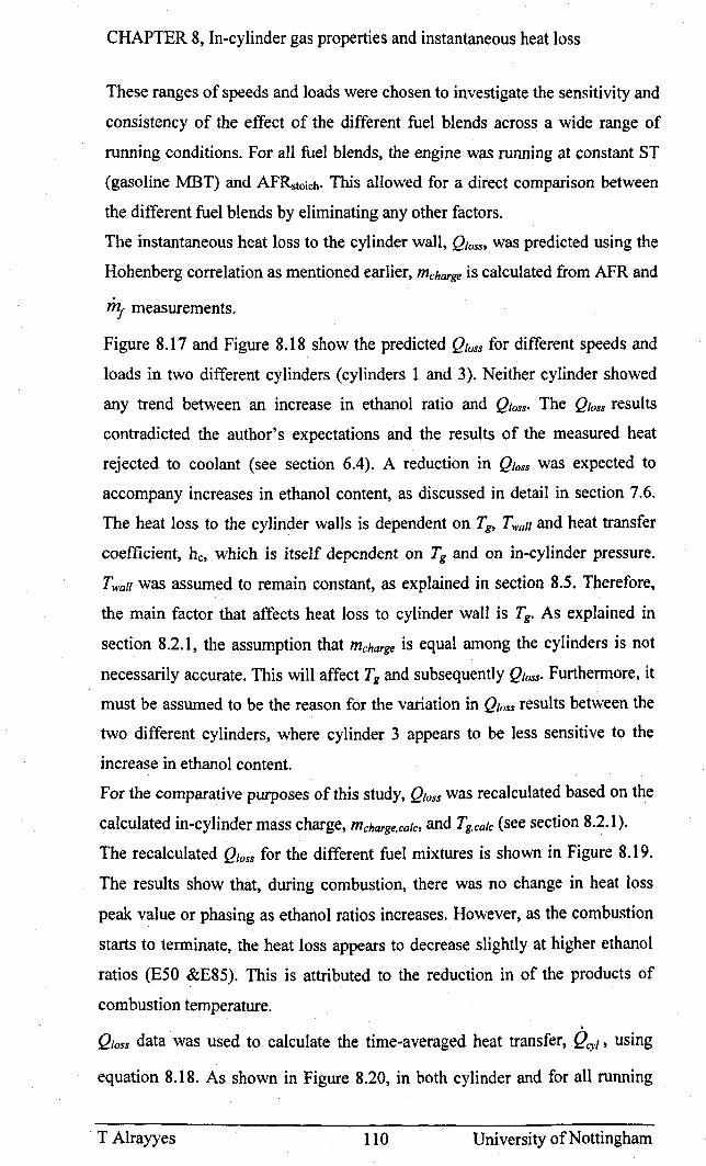
CHAPTER 8, In-cylinder gas properties and instantaneous heat loss
These ranges of speeds and loads were chosen to investigate the sensitivity and
consistency of the effect of the different fuel blends across a wide range of
running conditions. For all fuel blends, the engine was running at constant ST
(gasoline MBT) and AFRstoieh. This allowed for a direct comparison between
the different fuel blends by eliminating any other factors.
The instantaneous heat loss to the cylinder wall, Qloss, was predicted using the
Hohenberg correlation as mentioned earlier, mcharge is calculated from AFR and
m.r measurements.
Figure 8.17 and Figure 8.18 show the predicted Qloss for different speeds and
loads in two different cylinders (cylinders 1 and 3). Neither cylinder showed
any trend between an increase in ethanol ratio and Qloss. The Qloss results
contradicted the author's expectations and the results of the measured heat
rejected to coolant (see section 6.4). A reduction in Qloss was expected to
accompany increases in ethanol content, as discussed in detail in section 7.6.
The heat loss to the cylinder walls is dependent on Tg, Twall and heat transfer
coefficient, he, which is itself dependent on Tg and on in-cylinder pressure.
Twall was assumed to remain constant, as explained in section 8.5. Therefore.
the main factor that affects heat loss to cylinder wall is Tg• As explained in
section 8.2.1, the assumption that mcharge is equal among the cylinders is not
necessarily accurate. This will affect Tg and subsequently Qloss. Furthermore. it
must be assumed to be the reason for the variation in Qloss results between the
two different cylinders, where cylinder 3 appears to be less sensitive to the
increase in ethanol content.
For the comparative purposes of this study. Qloss was recalculated based on the
calculated in-cylinder mass charge. mcharge.calc, and Tg.calc (see section 8.2.1).
The recalculated Qloss for the different fuel mixtures is shown in Figure 8.19.
The results show that, during combustion, there was no change in heat loss
peak value or phasing as ethanol ratios increases. However, as the combustion
starts to terminate, the heat loss appears to decrease slightly at higher ethanol
ratios (ESO &E8S). This is attributed to the reduction in of the products of
combustion temperature. .
Qloss data was used to calculate the time-averaged heat transfer, Qcyl' using
equation 8.18. As shown in Figure 8.20, in both cylinder and for all running
T Alrayyes 110 University of Nottingham
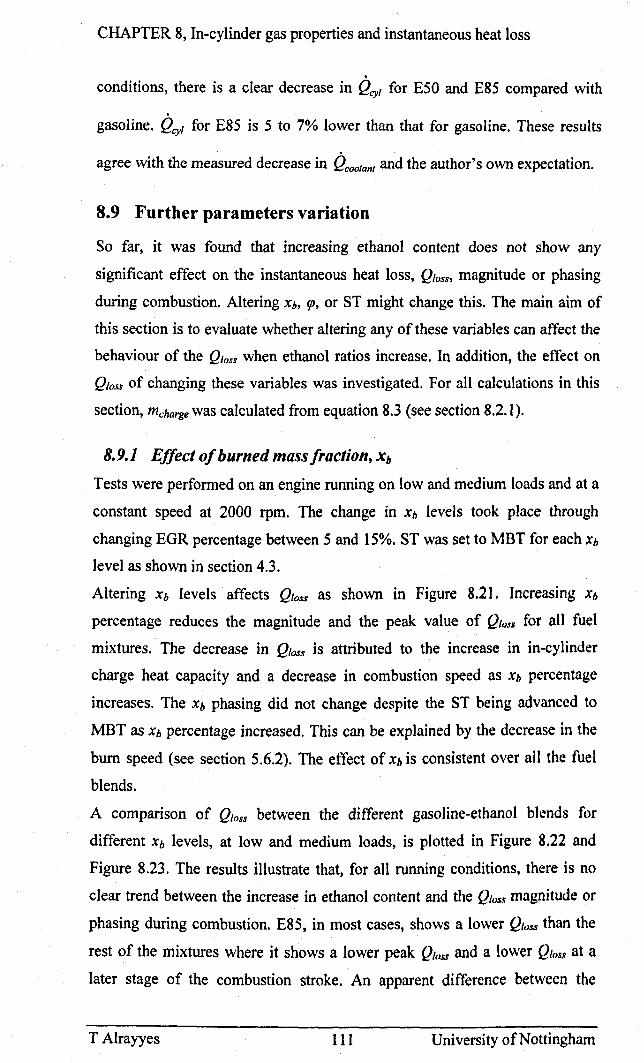
CHAPTER 8, In-cylinder gas properties and instantaneous heat loss
conditions, there is a clear decrease in Qcyl for ESO and E85 compared with
gasoline. Qcyl for E85 is 5 to 7% lower than that for gasoline. These results
agree with the measured decrease in Qcoolant and the author's own expectation.
8.9 Further parameters variation
So far, it was found that increasing ethanol content does not show any
significant effect on the instantaneous heat loss, Qloss, magnitude or phasing
during combustion. Altering Xb, 'P, or ST might change this. The main aim of
this section is to evaluate whether altering any of these variables can affect the
behaviour of the Q,oss when ethanol ratios increase. In addition, the effect on
Qloss of changing these variables was investigated. For all calculations in this
section, mcharge was calculated from equation 8.3 (see section 8.2.1).
8.9.1 Effect o/burned mass/raction, Xb
Tests were performed on an engine running on low and medium loads and at a
constant speed at 2000 rpm. The change in Xh levels took place through
changing EGR percentage between 5 and 15%. ST was set to MBT for each Xh
level as shown in section 4.3.
Altering Xb levels affects Qloss as shown in Figure 8.21. Increasing Xb
percentage reduces the magnitude and the peak value of Qloss for all fuel
mixtures. The decrease in Qloss is attributed to the increase in in-cylinder
charge heat capacity and a decrease in combustion speed as Xb percentage
increases. The Xb phasing did not change despite the ST being advanced to
MBT as Xh percentage increased. This can be explained by the decrease in the
burn speed (see section 5.6.2). The effect of Xh is consistent over all the fuel
blends.
A comparison of Qloss between the different gasoline-ethanol blends for
different Xb levels, at low and medium loads, is plotted in Figure 8.22 and
Figure 8.23. The results illustrate that, for all running conditions, there is no
clear trend between the increase in ethanol content and the Qloss magnitude or
phasing during combustion. E85, in most cases, shows a lower Qloss than the
rest of the mixtures where it shows a lower peak Q/oss and a lower Qloss at a
later stage of the combustion stroke. An apparent difference between the
T Alrayyes 111 University of Nottingham
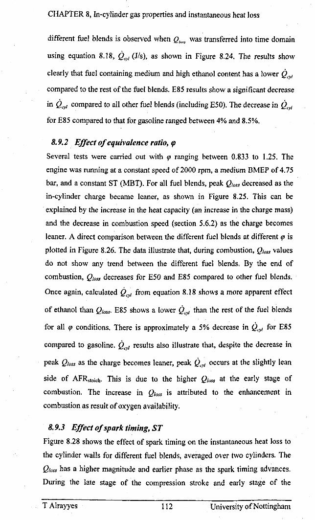
CHAPTER 8, In-cylinder gas properties and instantaneous heat loss
different fuel blends is observed when Q,o... was transferred into time domain
using equation 8.18, QCYI (J/s), as shown in Figure 8.24. The results show
clearly that fuel containing medium and high ethanol content has a lower Q''YI
compared to the rest of the fuel blends. E85 results show a significant decrease
in Qerl compared to all other fuel blends (including E50). The decrease in (Jeri
for E85 compared to that for gasoline ranged between 4% and 8.5%.
8.9.2 Effect 0/ equivalence ratio, tp
Several tests were carried out with ({J ranging between 0.833 to 1.25. The
engine was running at a constant speed of 2000 rpm, a medium BMEP of 4.75
bar, and a constant ST (MBT). For all fuel blends, peak Qloss decreased as the
in-cylinder charge became leaner, as shown in Figure 8.25. This can be
explained by the increase in the heat capacity (an increase in the charge mass)
and the decrease in combustion speed (section 5.6.2) as the charge becomes
leaner. A direct comparison between the different fuel blends at different ({J is
plotted in Figure 8.26. The data illustrate that, during combustion, Qloss values
do not show any trend between the different fuel blends. By the end of
combustion, Qloss decreases for E50 and E85 compared to other fuel blends.
Once again, calculated Qerl from equation 8.18 shows a more apparent effect
of ethanol than Qloss. E85 shows a lower Q"YI than the rest of the fuel blends
for all ({J conditions. There is approximately a 5% decrease in Q,yl for E85
compared to gasoline. Q'YI results also illustrate that, despite the decrease in
peak Qloss as the charge becomes leaner, peak Qq/ occurs at the slightly lean
side of AFRstoich. This is due to the higher Qloss at the early stage of
combustion. The increase in Qloss is attributed to the enhancement in
combustion as result of oxygen availability.
8.9.3 Effect olspark timing, ST
Figure 8.28 shows the effect of spark timing on the instantaneous heat loss to
the cylinder walls for different fuel blends, averaged over two cylinders. The
Qloss has a higher magnitude and earlier phase as the spark timing advances.
During the late stage of the compressIOn stroke and early stage of the
T Alrayyes 112 University of Nottingham
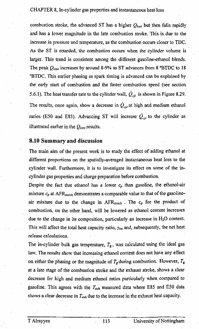
CHAPTER 8, In-cylinder gas properties and instantaneous heat loss
combustion stroke, the advanced ST has a higher Qloss but then falls rapidly
and has a lower magnitude in the late combustion stroke. This is due to the
increase in pressure and temperature, as the combustion occurs closer to TDC.
As the ST is retarded, the combustion occurs when the cylinder volume is
larger. This trend is consistent among the different gasoline-ethanol blends.
The peak Qloss increases by around 8-9% as ST advances from 8 °BTDC to 18
°BTDC. This earlier phasing as spark timing is advanced can be explained by
the early start of combustion and the faster combustion speed (see section
5.6.1). The heat transfer rate to the cylinder wall, QCYI is shown in Figure 8.29.
The results, once again, show a decrease in Qey} at high and medium ethanol
ratios (E50 and E85). Advancing ST will increase {ley/ to the cylinder as
illustrated earlier in the Qloss results.
8.10 Summary and discussion
The main aim of the present work is to study the effect of adding ethanol at
different proportions on the spatially-averaged instantaneous heat loss to the
cylinder wall. Furthermore, it is to investigate its effect on some of the in
cylinder gas properties and charge preparation before combustion.
Despite the fact that ethanol has a lower cp than gasoline. the ethanol-air
mixture cp at AFRstoich demonstrates a comparable value to that of the gasoline
air mixture due to the change in AFRstoich . The cp for the product of
combustion, on the other hand, will be lowered as ethanol content increases
due to the change in its composition, particularly an increase in .hO content.
This will affect the total heat capacity ratio, /'101 and, subsequently t the net heat
release calculations.
The in-cylinder bulk gas temperature, Tg , was calculated using the ideal gas
law. The results show that increasing ethanol content does not have any effect
on either the phasing or the magnitude of Tg during combustion. However, Tg
at a late stage of the combustion stroke and the exhaust stroke, shows a clear
decrease for high and medium ethanol ratios particularly when compared to
gasoline. This agrees with the Texh measured data where E85 and E50 data
shows a clear decrease in Texh due to the increase in the exhaust heat capacity.
T Alrayyes 113 University of Nottingham
CHAPTER 8, In-cylinder gas properties and instantaneous heat loss
The higher enthalpy of vaporisation, hfg , for ethanol is expected to increase the
cooling effect inside the cylinder before combustion. In DISI engines. the
majority of fuel is expected to vaporise during the compression stroke. The
heat required to vaporise the fuel will affect the increase in temperatures
during the compression stroke, Tcomp. For that reason, Tcomp was used as an
indication of the amount of heat required to vaporise the fuel. Tcomp was
calculated from the temperature difference between IVC and ST. High and
medium ethanol contents show a clear decrease in Tcomp. E85, in particular,
showed a significant decrease in Tcomp compared to the rest of the fuels,
including E50. This is explained by the increase in hfg and in the fuel flow rate
(higher BSFC).
The Hohenberg correlation was used to predict instantaneous heat loss to
cylinder. The correlation, which was originally developed for diesel engines,
was calibrated by comparing gross heat released, as calculated from the first
law of thermodynamics, to the heat released from the combusted fuel. Several
techniques were used to validate the use of the Hohenberg correlation to
predict the heat loss for different gasoline-ethanol mixtures. That included
comparing the gross heat release to the heat release by the fuel, and comparing
the predicted heat transfer rate to the measured one as well as to that predicted
using the C 1 C2 correlation. The results illustrate that the Hohenberg
correlation can be used to predict the instantaneous heat loss for the ditTerent
gasoline-ethanol mixtures.
The results also illustrate that there is very little difference in the heat loss
magnitude, peak value, and phasing between the different fuel blends during
combustion. E85 shows, in some cases, a slight decrease in peak heat loss. The
heat loss magnitude at both the later stages of the combustion stroke and then
at the exhaust stroke, shows a decrease for medium and high ethanol contents.
These results were consistent over different running conditions, including
different speeds, BMEPs, Xb and f/J.
The heat transfer in the time domain (J/s) shows a clearer effect of ethanol than
the heat loss in the crank angle domain. Both E85 and E50 show a clear
decrease in heat transfer rate. However, E85 shows a more significant
reduction in heat transfer rate than E50. This reduction is attributed to the
reduced product of combustion temperature.
T Alrayyes 114 University of Nottingham
CHAPTER 8, In-cylinder gas properties and instantaneous heat loss
The more pronounced effect of E85 compared to E50 might explain the C 1 C2
correlations results in Chapter 7. While the C 1 C2 correlation shows a clear
decrease in the predicted heat transfer for E85. E50 predictions show
comparable results to the rest of the fuel blends. The decrease in heat transfer
rate for E50 might be too small to be observed within the confidence limit of
C 1 C2 correlation.
T Alrayyes 115 University of Nottingham
Discussion
CHAPTER 9 Discussion
Summary and discussion
This thesis describes the effects of using ethanol/gasoline blends at ditferent
proportions on the engine's combustion behaviour, energy balance and heat
transfer characteristics.
The contribution of the presented work to knowledge could be divided into two
categories: firstly the effect of ethanol on
• energy balance inside the engine.
• cycle average heat transfer characteristics including the effect different
sources.
• the validity of using C 1 C2 correlation and whether any modification is
required to compensate for the change in heating value and other fuel
properties.
• crank angle resolved heat transfer and charge preparation.
Despite the extensive research literature that has been produced over the past
few years, no material was found that directly investigates the effects of
ethanol on the abovementioned subjects. This highlights a notable gap in the
current body of knowledge on the topic, which this study endeavours to
address.
Secondly, the effect of ethanol on:
• in-cylinder combustion behaviour.
• exhaust composition, heat capacity and temperature.
As shown in Chapter 2, several researchers studied the effect of ethanol on the
aforementioned characteristics. However, there was variation in the results
among researchers. This variation might be attributed to the use of different
engines particularly different fuelling systems and compression ratios. The
majority of these studies were carried out on a port fuel injection engine. Some
were carried out on a wall guided direct injection engine. This study was
carried on a spray guided direct injection engine with high compression ratio
(11.5: 1) that has never been examined before.
T Alrayyes 116 University of Nottingham
Discussion
For the purpose of this study, an engme test rig was designed and
commissioned. Accurate measurements of the engine's power-out (load and
speed), fuel consumption, coolant flow rate, temperatures and in-cylinder
pressure were prerequisites of the design. Since the objective of this study was
to evaluate the effect of different ethanol/gasoline blends on various engine
characteristics, the engine was operated at a steady state, with all running
conditions and engine variables kept constant. This permitted a direct
comparison between the different fuel blends, with change in ethanol content
in the fuel as the only variable. Direct access to the ECU, in order to modify,
adjust and fix different engine variables was possible through A TI software
and hardware. Among variables that were most commonly modified were
EGR, spark timing, and equivalence ratio.
The addition of ethanol to gasoline changes the chemical composition of the
fuel blends; particularly, it increases the H/C ratio and O2 content of the fuel.
This change was expected to affect the physiochemical and combustion
properties of the fuel. The work presented in this thesis starts by assessing the
effects of increasing ethanol content in gasoline/ethanol blends on the
combustion properties, including AFRstoich, QLHV and Tadd. The results indicate
a decrease in all three properties. The reduction in QLHV is also illustrated by a
measured BSFC rise that accompanies increases in ethanol content. However.
the decrease in QLHV did not affect the power output of the engine. On the
contrary, for high ethanol content, the effect of the combined reduction in
AFRstoich and QLHV was to produce a slightly higher engine power output for
the same throttle position. Hence, higher total power output can be achieved
using ethanol compared to standard gasoline at the expense of BSFC.
The effect of increasing ethanol content on emission and H20 levels was
evaluated at different engine running conditions. Increasing the ethanol ratio
shows a decrease in CO, CO2, HC and NOx emissions for most running
conditions. H20 level, on the other hand, clearly rises for higher ethanol
content. CO2 and H20 levels change as a direct result of differing chemical
structure between gasoline and ethanol; in particular increase in H/C ratio and
02 content. The reduction in NOx levels is attributed to the lower Tadd and the
higher hfg of ethanol. The levels of CO and HC emissions decrease due to the
improvement in combustion efficiency that is observed as ethanol content
T Alrayyes 117 University of Nottingham
Discussion
increases. Plotting the combustion efficiency of the different fuel blends as a
function of ffJ shows a clear increase in combustion efficiency as ethanol
content increases, particularly for rich mixtures. This is attributed to the
oxygen content of the fuel. Oxygen mass fraction in the fuel increases from
approximately 0% for gasoline to 35% for E85.
Decreased emissions level, particularly at higher ethanol ratios, indicate that
using ethanol can contribute to the wider efforts of ensuring compliance with
increasingly tight emission regulations.
The combustion characteristics and, subsequently, the engine's heat transfer
characteristics were also expected to be affected by changes in the
physiochemical properties associated with the increase in ethanol content.
Despite lower Tadd of ethanol due to its lower QlHV, the calculated laminar
flame speed for ethanol is found to be higher than that of gasoline, with the
peak difference occurring at AFRstoich. This increase is attributed to the
presence of oxygen in ethanol chemical's structure. The effect of using ethanol
on both FDA and RBA was investigated at various engine running conditions.
The combustion duration was determined using the Rasweiler and Withrow
methods based on the in-cylinder pressure data. The data illustrate that, despite
the higher laminar flame speed of ethanol, FDA values were comparable for all
fuel blends. This can be explained by the high compression ratio engine under
investigation (11.5: 1).
Indeed, as a result of this high compression ratio, the effects of compression
work and, therefore, charge density and temperature dominated flame
initiation. RBA data, on the other hand, show a clear increase in combustion
speed, decrease in RBA, for E85 compared to gasoline and other fuel blends.
which corresponds well with the rise in laminar flame speed of ethanol. The
RBA results, nevertheless, do not show a linear relation between increasing
ethanol content and RBA. Fuel blends with low and medium ethanol content
(E 10, E20 and E50) show a slight reduction in RBA compared to gasoline.
However, there is no significant difference, nor trend, in RBA amongst those
fuel blends.
The non-linear relation between RBA and ethanol content can be explained by
the differences in ethanol's properties. Indeed, whilst ethanol with a higher
laminar flame speed and oxygen content will decrease RBA, lower Qwv and
T Alrayyes 118 University of Nottingham
Discussion
higher hfg levels in ethanol will have the opposite effect. For that reason, the
effect of increasing ethanol will only appear for blends with high ethanol
content.
Changing the in-cylinder charge composition, either by changing ffJ or Xb,
shows a significant effect on laminar flame speed for both ethanol and
gasoline. Ethanol laminar flame speed appears to be more sensitive to variation
in any of these two variables. As a result, the peak difference in laminar flame
speed between the two fuels occurs at AFRstoich and low Xb level. This
difference starts to decrease as the charge moves away from AFRstoich or Xh
level increases. The RBA results correspond well to the laminar flame speed
trend where, once again, E85 has a lower RBA than gasoline at AFRs10ich and
low Xb level. As Xb levels rise or the charge moves away from AFRsioich. the
difference in RBA between the two fuels decreases.
The tolerance for Xb when using different fuel blends. which is mainly affected
by combustion duration, was studied using COY of IMEP. The results showed
a slight increase in Xb tolerance for E85 compared to other fuel blends. This
indicates that, in addition to the reduction in NOx levels for E85, further
decreases in NOx can occur due to the increase in tolerable Xh ratio.
The study of the heat transfer characteristics inside the engine started with an
engine energy balance evaluation for different fuel mixtures. There was an
investigation of how the energy released by the fuel was distributed between
brake output, coolant energy, exhaust energy and heat loss to ambient. As
ethanol content increases, exhaust heat capacity, Cp,exh, also increases due to
exhaust composition, particularly the increase in H20 content. For all running
conditions, lower cp•exh was also manifested in a marked decrease in the
exhaust temperature, Texh, as ethanol content increased. Lower Texh can have
significant effects on various engine characteristics. A reduction in Ttxh could
considerably effect emission levels, particularly during warm-up. The decrease
in Texh would increase the time needed for the catalyst to reach its operating
temperature. This would increase tail-pipe emissions, especially at low
temperature start. Reduced Texh will also atfect HC and CO after flame
combustion. Nevertheless, the increase in ethanol content shows a decrease in
HC and CO levels regardless of Texh .• Decreasing Texh can also affect the
T Alrayyes 119 University of Nottingham
Discussion
exhaust energy-powered devices such as the turbocharger (if used). Finally Texh
has an effect on total heat rejected to coolant by affecting the amount of heat
transferred though the exhaust port, conducted back to the engine head and
heat transferred to the cylinder wall after end of combustion, during the
expansion and the compression strokes. The decrease in Texh and the higher hjg
of ethanol, which will have a cooling effect on the charge before combustion,
indicate a potential decrease in the heat rejection to coolant. The measured heat
rejection to coolant, QcooJant' confirms this expectation. However, the effect of
ethanol on heat rejection to coolant appeared only at medium and high ethanol
content (E50 & E85). E85 particularly showed a marked decrease in Q"HlJant
compared to all other fuel blends. Low ethanol content fuel blends exhibited
comparable results to gasoline. At low ethanol content, oxygen availability,
which enhances combustion, dominates the combustion more than the increase
in hjg• This eliminates the cooling effect of ethanol.
Although lower total heat rejection to coolant was not significant enough to
require a radical change in the design of the cooling system, it was expected to
change the warm up characteristics. Data obtained from the PFI engine show a
clear increase in the time required by the thermostat to open as well as the time
required to reach a particular oil temperature, i.e. an increase in the time
required to reach the engine's operating temperature. This would be reflected
in an increase in friction, fuel consumption and emissions. This effect could be
more extensively quantified in future work. Measurements of heat lost to
ambient produced comparably similar results for both E85 and gasoline. This
was expected since the coolant inside the engine maintains the engine's skin
temperature at an approximately constant level.
Energy balance results showed a clear increase in thermal etliciency as ethanol
content increased for all running conditions. This is noticeable even for low
ethanol content. The results also illustrate that the improvement in combustion
efficiency is the primary reason for the increased thermal efficiency. In
addition, the slight decrease in heat Joss to exhaust and coolant, at high ethanol
content, was translated into an improvement in thermal etliciency as more
work was transferred to the piston.
T Alrayyes 120 University of Nottingham
Discussion
The improvement in thermal efficiency is reflected in the BSFC. The results
show that the increase in the BSFC associated with a decrease in the QLHvof
ethanol was less than expected. In addition, the reviewed literature shows that
using ethanol has the potential of increasing the compression ratio due to its
high anti-knock resistance relative to gasoline. This will increase thermal
efficiency even further. Indeed, the thermal efficiency of an SI engine running
on ethanol has the potential to be comparable to that of a diesel engine.
The C 1 C2 correlation was used to predict gas-side heat transfer to coolant,
QCY/ and Qexh.por/' C 1 C2 is a time-averaged correlation that was developed at
The University of Nottingham and proved to be reliable in predicting Q ... tHI/<JnI
for both diesel and SI engines. The correlation has been used extensively for
engine thermal modelling as part of the PROMETs software package. One of
the objectives of this thesis was to evaluate the validity of the CIC2 correlation
in predicting heat transfer for different gasoline-ethanol blends, as well as
establishing whether any modifications in the CI, C2 or Tg,effconstants were
required. This would be useful in future work when modelling engine thermal
conditions when running on different ethanol-gasoline blends. Comparisons of
the measured and predicted values of QCIH,'anl show that the C 1 C2 correlation
can be used to predict gas-side heat transfer without any need to modify the
correlation. This was unexpected since Q,y/ was anticipated to decrease as
ethanol content increased and, subsequently, produce a change in CI and Tg.eff.
The expected reduction in QCY/ was based on the following reasons:
firstly, the increase in hfg as ethanol content increases, results in a cooling
effect inside the cylinder. Secondly, reduced NOx emission levels observed
with increasing ethanol content indicates lower peak in-cylinder temperature.
Finally, the decrease in Texh illustrates a corresponding decrease in the
temperature of the products of combustion, which has a considerable etTect on
total heat loss. Using the C 1 C2 correlation to predict Qql for different
gasoline-ethanol blends showed that the Q,YI for E85 was lower than for other
fuel mixtures, which corresponds well with the author's expectations. The
decrease in Q'YI is accounted for by a lower Re number without the need to
T Alrayyes 121 University of Nottingham
Discussion
modify either CI or Tg,a. Although E85 showed a decrease in Q.y" the results
do not illustrate any clear correlation between a higher ethanol ratio and the
Qey/ value. This might be explained by the confidence limit associated with the
CIC2 correlation where change in Q~YI can be too small to be resolved by this
correlation. In addition, the increase in combustion efficiency for low ethanol
content can have more a dominant effect on increasing in-cylinder temperature
than the cooling effect of ethanol, or the decrease in Texh.
The 'C2' constant in the CIC2 correlation represents the ratio of exhaust port
heat flux to cylinder heat flux. C2 will thus remain constant since the ratio is
found to be constant for all fuel blends. As mentioned previously, the results
illustrate a clear decrease in Qeotl/ant for medium and high ethanol contents. The
decrease in Qey/ contributes to the total decrease in Qe'H,ltlnl' Other sources that
contribute to QCIHI/anl are heat transfer from the exhaust port, Qexhpor" heat
generated from engine friction, Q friction, and heat conducted from the exhaust
manifold back into the engine structure, Qex.man. A significant proportion of
total heat transfer to coolant is from the exhaust port. The exhaust port heat
transfer was both measured and predicted using empirical correlations. The
effect of increasing ethanol content was evaluated. Both predicted and
measured results showed a clear decrease in QUhl'or, as ethanol content
increased. This is attributed mainly to the decrease in Texh. The slight decrease
in the Re number for medium to high ethanol content is another reason for the
decrease in Qexhport. The calculated exman value also decreased as ethanol
content increased. Q friction' on the other hand, showed similar results for
different fuel blends. The decrease in both QuhPort and Q.xmc," contributed to
the total decrease in Q'~H)lanl •
Further investigation of the heat transfer to the cylinder wall was carried out.
Pressure data was used to predict instantaneous heat loss to the cylinder walls
(J/CA), Qloss using the Hohenburg empirical correlation. Qlo.u gives an insight
into the temporal heat flux variation during the engine cycle, which includes
T Alrayyes 122 University of Nottingham
Discussion
heat loss magnitude and phasing. The validity of using the Hohenburg
correlation, which had been calibrated for the engine under investigation, to
calculate the instantaneous heat transfer coefficients for the different ethanol
gasoline blends had to be examined. Several techniques were used, including
comparing the predicted heat loss using the Honhenburg correlation to both the
actual measured value, and to the one predicted by the C 1 C2 correlation.
Furthermore, gross heat release was compared to the expected heat released by
the fuel. The results from the different techniques confirmed the validity of
using the Hohenburg correlation.
During combustion, heat loss magnitude and phasing showed comparable
values for the different fuel blends. E85, in some cases, showed a lower peak
heat loss than the rest of the ethanol-gasoline blends. After combustion, during
the later stage of the combustion stroke and the exhaust stroke, E85 and E50
heat loss decreased slightly relative to other fuel blends. The increase in heat
loss is attributed to the lower temperature of the product of combustion. This
was indicated by the decrease in measured exhaust temperature and an increase
in the calculated heat capacity. Reduced heat loss later on in the combustion
stroke is reflected in decreased heat rejection rate in the time domain (J/s)
where the effect of ethanol was more obvious. Both E85 and E50 showed a
clear decrease in heat transfer rate. However, E85 exhibited a more significant
decrease in the heat transfer rate than that seen with E50.
The more pronounced effect of E85 on heat transfer rate compared to E50
would explain the C 1 C2 correlation results. While the C 1 C2 correlation
showed a clear decrease in the predicted heat transfer for E85, its E50
prediction indicated results that were comparable to the other fuel blends. The
decrease in the heat transfer rate for E50 is probably too small to be observed
within the confidence limit of the C 1 C2 correlation.
In a DISI engine, most of the injected fuel is vaporised during the compression
stroke, causing a cooling effect on the charge. The use of ethanol is expected to
increase this cooling effect due to its higher enthalpy of vaporisation and rise
in the amount of fuel injected. The effect of ethanol was assessed by
calculating the temperature increase, T comp, between IVe and ST. E50 and E85
show a reduction in Tcomp compared to the rest of the fuel blends. This
T Alrayyes 123 University of Nottingham
Discussion
reduction illustrates that bigger portion of the piston work during the
compression stroke is going to vaporise E85 than gasoline.
Future work
The work presented in the thesis concentrates on the effect of gasoline-ethanol
mixtures on the combustion behaviour and heat transfer characteristics during
fully warmed-up conditions only. Further work investigating the effect of
ethanol on heat transfer characteristics during warming-up conditions is of
extreme importance. Indeed, the presence of ethanol is expected to affect the
time and the amount of fuel required for the engine to reach its fully warmed
up conditions. Moreover, changing the engine's warm up characteristics will
have a significant effect on emissions, friction levels, power output and fuel
consumption. A clear understanding of the effect of ethanol on those
characteristics would greatly assist in developing strategies for a more rapid
flexi-fuel engine warm-up.
A more detailed understanding of the effect of ethanol on in-cylinder heat
transfer characteristics can also be achieved through measurement of
instantaneous wall temperature. Wall temperature should be measured at
different locations inside the combustion chamber using fast-response
thermocouples. The different locations can include the cylinder liner. piston
and cylinder head. Temperature measurements can be used to provide the heat
flux profile. This will allow for an assessment of the impact of increasing
ethanol content on instantaneous spatial variation of heat transfer flux. The
results would provide a qualitative insight into differences between ditl'erent
fuel mixtures, and would also illustrate the quantitative differences in heat
transfer rates. It also could validate the use of classical heat transfer
correlations when applied to different fuel mixtures.
Further work investigating the heat transfer characteristics and combustion
behaviour for different fuel blends should be carried out for other engine
designs, with a particular focus on alternative fuelling systems, namely port
fuel injection or wall-guided DISI engines. In addition, engines with different
compression ratios, either turbocharged or naturally aspirated, could be used.
The sensitivity of ethanol to all these changes should be properly investigated.
T Alrayyes 124 University of Nottingham
Conclusion
CHAPTER 10 Conclusion
The principle conclusion of this thesis includes:
• Increasing ethanol ratio showed a clear improvement in the engine
performance including decreasing in the main regulated emissions,
improvement in combustion efficiency and increase in maximum
BMEP. This improvement was obvious even at low ethanol ratio.
• While FDA is comparable for all fuel blends, increasing ethanol
decrease RBA compare to pure gasoline. However, this decrease is not
linear. A small decrease is observed at EI0, but no further decrease
occurs until E85. E85 exhibits a lower RBA compared to all other fuel
blends particularly gasoline.
• Increasing ethanol content improves thermal efficiency, mainly due to
the increase in combustion efficiency. Also, due to the decrease in
exhaust and coolant losses.
• The decrease in the heat transfer rate to the coolant, as ethanol ratio
increase, is due to the decrease in cylinder heat loss, exhaust heat loss
and heat conducted back to the engine block.
• The C 1 C2 correlation can be used to predict heat loss without need for
any modification.
• Instantaneous heat loss during combustion does not change among
different fuel mixtures, however it decrease later on in the combustion
stroke.
The following details the conclusion of each chapter in the thesis:
Chapter 4
• Increasing ethanol ratio in the gasoline-ethanol blend causes an
obvious decrease in AFRstoich, the calorific value and, to a lesser extent,
the adiabatic flame temperature.
T Alrayyes 125 University of Nottingham
Conclusion
• Although ethanol has a lower a calorific value, increasing ethanol
content increases the power output for a constant throttle position due
to the decrease in AFRstoich. This will be at the expense of BSFC.
• Increasing ethanol ratio has a significant influence on exhaust
composition. Increasing ethanol ratio decreases CO, CO2, HC and NOx
emission levels for most running conditions. H20 levels, on the other
hand, increase.
• Significant improvements in combustion efficiency are obtained as
ethanol ratios increase, particularly using rich mixtures.
Chapter 5
• Despite the higher laminar flame speed of ethanol, different gasoline
ethanol blends have comparable FDA values under different running
conditions. The compression work. turbulent flow and charge density
dominate flame initiation in the high compression ratio engine under
investigation (11.5: 1).
• There is no linear trend between increasing ethanol content and RBA.
A small decrease is observed at E 1 O. but no further decreases occur
until E85. E85 exhibits a lower RBA compared to all other fuel blends.
particularly gasoline.
• Ethanol's laminar flame speed is more sensitive to changes in charge
composition, such as qJ and Xb. than gasoline. As a result. the difference
in laminar flame speeds start to be reduced as Xb increases or the charge
moves away from AFRstoich. The RBA data show the same trend where
the E85 data indicate a reduction in RBA compared to gasoline at
AFRstoich. The difference between the two fuels starts to decrease as rp
or Xb changes.
• High ethanol ratios will slightly increase Xb tolerance as a result of
shorter combustion duration.
Chapter 6
• Increasing ethanol ratios increases exhaust heat capacity as a result of
changes in exhaust composition. in particular, higher water content.
This is responsible for reduction in exhaust temperature.
T Alrayyes 126 University of Nottingham
Conclusion
• The heat rejection rate to coolant decreases at medium and high ethanol
ratios.
• The decreases in heat rejection to coolant, and in the exhaust
temperature, affect the engine's warm up characteristics. Running on
fuel containing medium and high ethanol content increases the time
required for the engine to reach operating temperature.
• Increasing ethanol content improves the engine's thermal efficiency
considerably compared to gasoline. This is attributed mainly to the
increase in combustion efficiency. The decrease in heat losses to the
exhaust and coolant also contribute to the improvement in thermal
efficiency.
Chapter 7
• The C 1 C2 correlation can be used to predict gas-side heat transfer to
coolant for different gasoline-ethanol blends without need for
modification.
• In the C 1 C2 correlation, the decrease in Re for E85 compensated for
the expected decrease in the cylinder heat loss to coolant without the
need to modify either C 1 or T g,a' The expected decrease in cylinder heat
loss is attributed to the decrease in the total heat rejection to coolant,
NOx emission levels, and exhaust temperature.
• The ratio of the heat flux-to-exhaust to the heat-flux-to-cylinder
remains constant. Subsequently, C2, which represents this ratio in the
C 1 C2 correlation, is unchanged.
• Other coolant heat sources also contribute to the total decrease in heat
rejection to coolant for medium and high ethanol content fuel mixtures.
Both measured and predicted exhaust heat loss and heat conducted
back into the engine decrease for medium and high ethanol content as a
result of reduced exhaust temperature.
Chapter 8
• There is little difference in instantaneous heat loss magnitude and
phasing among the fuel blends during combustion. As the combustion
T Alrayyes 127 University of Nottingham
Conciusion
terminates and into the exhaust stroke, heat loss becomes lower for
medium and high ethanol content.
• The predicted heat loss in the time domain (J/s) shows a more apparent
effect of ethanol compared to the heat loss in the CA domain (J/CA).
Both £50 and £85 show a clear decrease in the heat loss with £85
exhibiting a more pronounced decrease.
• Due to ethanol's higher enthalpy of vaporisation and the increase in the
amount of fuel injected, E50 and E85 blends show a higher cooling
effect in the compression stroke than the other fuel blends.
In summary, the use of ethanol in SI engines has the advantage of reducing
most regulated emissions, as well as improving combustion and thermal
efficiency. This effect is noticeable even at low ethanol contents. However,
contrary to assumptions, there is no linear trend between increasing ethanol
content and any change in combustion and heat transfer characteristics. The
effect of ethanol on these characteristics manifests itself only at medium to
high ethanol levels. E85 has the most pronounced effect on increasing
combustion speed and decreasing heat losses to coolant and exhaust. Finally,
the C 1 C2 correlation can be used, without any modification, to predict gas-side
heat loss for different gasoline-ethanol mixtures. This is particularly important
for future modelling of engine running on different gasoline-ethanol blends.
Apart from Sweden, the use of ethanol in the EU is still limited to low
proportion ethanol-gasoline blends (ranging from 5% to 10%). According to
the finding of this thesis, the current level of ethanol use does not affect the
combustion and heat transfer characteristics. However, plans towards reducing
dependence on fossil fuels push towards the use of alternative fuels such as
ethanol. The changes in engine combustion and heat transfer characteristics,
when running on high percentage ethanol blends, should be taken into account
in future flexi-fuel engine design.
T Alrayyes 128 University of Nottingham
References
References
1. E.V. Thuijl, C.J. Roos, and L.W.M. Beurskens, "An overview of biofuel technologies, market and policies in Europe". Energy research centre of the Netherlands: Amsterdam 2003.
2. Renewable Fuel Association, RF A. (2006). "FROM NICHE TO NATION, ETHANOL INDUSTRY OUTLOOK", http://www.mda.state.mLus/renewablefuels/documentsIRF Aoutlook 20 06.pdf, Accessed Feb. 2010.
3. J.D. Hamilton, "Understanding Crude Oil Prices", NBER Working Paper No. w14492 2008.
4. EurObserv'ER Website. "Biofuels Barometer", http://www.eurobserver.orglpdflbaro 198.pdf, Accessed Feb. 2010.
5. The European Association for Bioindustries Website. (June 2007). "Biofuels in Europe", http://www.europabio.org/positions/Biofuels EuropaBio%20position Final.pdf, Accessed Feb. 2010.
6. R Schnepf, "European Union Biofuels Policy and Agriculture: An Overview". Congressional Research Service, 2006.
7. European Commission Website. (2007). "Biofuels Progress Report'\ http://ec.europa.eulenergy/energy policy/doc/07 biofuels progress re port en.pdf, Accessed Feb. 2010.
8. Z.O. Sivers M, Olsson L, B Hahn-Hagerdal "Cost analysis of ethanol from willow using recombinant Escheri-chia coli", Biotechnol Prog, lO:p.555-560, 1994.
9. J.R. Mielenz. "Ethanol production from biomass: technology and commercialization status", Current Opinion in Microbiology, 4: p. 324-329,2001.
10. J. Zaldivar, J. Nielsen and L. Olsson, "Fuel ethanol production from lignocellulose: a challenge for metabolic engineering and process integration", Applied Microbiology and Biotechnology, 56: p. 17-34, 2001.
11. A.E. Farrell, RJ. Plevin, B.T. Turner, A.D. Jones, M. O'Hare and D.M. Kammen, "Ethanol Can Contribute to Energy and Environmental Goals", Science, 311: p. 506 - 508.
T Alrayyes 129 University of Nottingham
References
12. H. Shapouri, J. Duffield and M. Wang, "The energy balance of corn ethanol revisited", TRANSACTIONS OF THE ASAE, 46 (4): p. 959-968,2003.
13. RS. Chambers, RA. Herendeen, J.J. Joyce and P.S. Penner, "Gasohol: Does It or Doesn't It Produce Positive Net Energy?" Science, 206(4420): p. 789 - 795, 1979.
14. C. Cleveland, "Net energy from the extraction of oil and gas in the United States", ENERGY, 30(5): p. 769-782, 2005.
15. S. Kim and B.E. Dale, "Life cycle assessment of various cropping systems utilized for producing biofuels: Bioethanol and biodiesel", Biomass and Bioenergy, 29: p. 426--439, 2005.
16. R Stone, "Introduction to Internal Combustion Engines" Pal grave, 1999.
17. J.B. Heywood, "Internal Combustion Engine Fundamentals" McGrawHill Book Company, 1988.
18. T. Wallner and S.A. Miers, "Combustion Behaviour of Gasoline and GasolinelEthanol Blends in a modern Direct-Injection 4-Cylinder Engine", SAE Technical PaperNo. 2008-01-0077, 2008.
19. T. Topgul, H. Yucesu, C. Cinar and A. Koca, "The effects of ethanolunleaded gasoline blends and ignition timing on engine performance and exhaust emissions", Renewable Energy, 2006: p. 2534-2542, 2006.
20. B. He, J. Wang, J. Hao, X. Yan and J. Xiao. "A study on emission characteristics of an EFI engine with ethanol blended gasoline fuels ", Atmospheric Environment, 37: p. 949-957,2003.
21. C.V. D'Ornellas, "The effect of ethanol on gasoline oxidation stability", SAE Technical Paper No. 2001-01-3582, 2001.
22. W. Hsieh, R Chen, T. Wu and T. Lin, "Engine performance and pollutant emission of an SI engine using Ethanol-gasoline blend fuels", Atmospheric Environment, 36: p. 403-410., 2002.
23. RM. Bata, A.C. Elrod and RW. Rice, "Emissions From IC Engines Fueled With Alcohol-Gasoline Blends: A Literature Review", Journal of Engineering for Gas Turbines and Power, 111(3): p. 424-431, 1989.
24. K. Kar, T. Last, C. Haywood and R. Raine, "Measurement of Vapor Pressure and Enthalpies of Vaporization of Gasoline and Ethanol Blends and Their effects on Mixture Preparation in an SI Engine", SAE Technical Paper No. 2008-01-0317, 2008.
T Alrayyes 130 University ofNottingharn
References
25. J.I.B. J. A. Pumphrey, and W. A. Scheller, "Vapour pressure measurements and predictions for alcohol-gasoline blends", Fuel, 79: p. 1405-1411,2000.
26. Rd. Silva, R Catalufta, E.W.d. Menezes, D. Samios and C.M.S. Piatnicki, "Effect of additives on the antiknock properties and Reid vapor pressure of gasoline", Fuel, 84: p. 951-959, 2005.
27. RM. Balabin, RZ. Syunyaeva and S.A. Karpova, "Molar enthalpy of vaporization of ethanol-gasoline mixtures and their colloid state", Fuel, 86(3): p. 323-327, 2007.
28. F.H. Palmer, "Vehicle performance of Gasoline containing oxygenates". IMeche conference publication: London, UK. International conference on petroleum based and automotive applications, 1986.
29. C.-W. Wu, R-H. Chenb, J.-Y. Pua and T.-H. Lina, "The influence of air-fuel ratio on engine performance and pollutant emissions of an SI engine using ethanol gasoline blended fuel", Atmospheric Environment, 38(40): p. 7093-7100 2004.
30. A.A. Abdel-Rahman and M.M. Osman, "Experimental investigation on varying the compression ratio of SI engine working under ditferent ethanol-gasoline fuel blends", International Journal of Energy Research, 21: p. 31-40., 1997.
31. l. Szybist, M. Foster, W.R Moore, K. Confer, A. Youngquist and R Wagner, "Investigation of Knock Limited Compression Ratio of Ethanol Gasoline Blends", SAE Technical Paper No. 2010-01-0619, 2010.
32. K. Nakata, S. Utsumi, A. Ota and K. Katsunori. "The Effect of Ethanol fuel on Spark Ignition Engine ", SAE Technical Paper No. 2006-01· 3380,2006.
33. H. Yucesu, T. Topgtll, C. <;inar and M. Okur, "Effect of ethanol· gasoline blends on engine performance and exhaust emissions in different compression ratio", Applied Thermal Engineering, 26: p. 2272-2278, 2006.
34. P.A. Caton, L.1. Hamilton and 1.S. Cowart, "An Experimental and Modelling Investigation into the Comparative Knock and Performance Characteristics of E85, Gasohol [EI0] and Regular Unleaded Gasoline [87 (R+M)/2]", SAE Technical Paper No. 2007-01-0473, 2007.
35. RA. Stein, C.l. House and T.G. Leone, "Optimal Use of E85 in a Turbocharged Direct Injection Engine", SAE International Journal of Fuels and Lubricants, 2: p. 670-682, 2009.
T Alrayyes 131 University of Nottingham
References
36. C. Sandstrom, "Measurement Technology for Emissions from Ethanol Fuelled Vehicles". AVL, 2009.
37. K. Knapp, F.D. Stump and S.B. Tejada, "The Effect of Ethanol Fuel on the Emissions of Vehicle Over a Wide range of Temperature", Jouranl of the Air & Waste Management Association, 48: p. 646-653, 1998.
38. F. Nadim, P. Zack, G.E. Hoag and S. Liu, "United States experience with gasoline additive", Energy Policy, 29(1): p. 1-5,2001.
39. R. Bechtold and J.B. Pullman, "Driving cycle economy, emissions and photochemical reactivity using alcohol fuels and gasoline". SAE Technical Paper No. 800260, 1980.
40. Z. Huang, H. Miao, L. Zhou and D. Jiang, "Combustion characteristics and hydrocarbon emissions of a spark ignition engine fuelled with gasoline-oxygenate blends", Proceedings of the IMeche, Part D: Journal of Automobile Engineering, 214: p. 341-3462000.
41. P. Price, B. Twiney, R. Stone, K. Kar and H. Walmsley, "Particulate and Hydrocarbon Emissions from a Spray Guided Direct Injection Spark Ignition Engine with Oxygenate Fuel Blends", SAE Technical Paper No. 2007-01-0472,2007.
42. S.H. Yoon, S.Y. Ha, H.G. Roh and C.S. Lee, "Effect of bioethanol as an alternative fuel on the emissions reduction characteristics and combustion stability in a spark ignition engine", Proceedings of the IMeche, Part D: Journal of Automobile Engineering, 223: p. 941-951. 2009.
43. K. Varde, A. Jones, A. Knutsen, D. Mertz and P. Yu. "Exhaust emissions and energy release rate from a controlled spark ignition Engine using ethanol blends", Proceedings of the IMeche, Part D: Journal of Automobile Engineering, 221: p. 933-941,2006.
44. S. Taniguchi, K. Yoshida and Y. Tsukasaki, "Feasibility study of Ethanol Applications to A Direct Injection Gasoline Engine". SAE Technical Paper No. 2007-01-20372007.
45. D. Bresenham and J. Reisel, "The effect of High Ethanol Blends on Emissions from Small Utility Engines", SAE Technical Paper No. 1999-01-3345, 1999.
46. M. Gautam, D. W.M. II and D. Carder, "Emissions characteristics of higher alcohol/gasoline blends". Proceedings of IMeche, Part A: Journal of Power and Energy, 214: p. 165-182, 2000.
47. Y. Yacoub, R. Bata and M. Gautam, "The performance and emission characteristics of C l-C5 alcohol-gasoline blends with matched oxygen
T Alrayyes 132 University of Nottingham
References
content in a single-cylinder spark ignition engine", Proceedings of IMeche, Part A: Journal of Power and Energy, 212: p. 363·379, 1998.
48. S.G. Poulopoulos, D.P. Samaras and C.J. Philippopoulos, "Regulated and unregulated emissions from an internal combustion engine operating on ethanol-containing fuels", Atmospheric Environment, 35(26): p. 4399-4406, 2001.
49. R. Magnusson, C. Nilsson and B. Andersson, "Emissions of aldehydes and ketones from a two-stroke engine using ethanol and ethanol· blended gasoline as fuel", Environmental Science and Technology, 36(8): p. 1656-1664.,2002.
50. L.H. Browning, J.F. Nebolon and R.K. Pefley, "Research Investigation of Alcohol Usage in Spark Ignition Engines", Society of Automotive Engineers, Inc: p. 367-376, 1983
51. J.S. Malcolm, P.G. Aleiferis, A.R. Todd, A. Cairns, A. Burne, H. Blaxill, H. Hoffmann and J. Rueckauf, itA Study of Alcohol Blended Fuels in a New Optical Spark-Ignition Engine". IMechE: London, Internal Combustion Engines:Performance, Fuel Economy and Emissions, 2007.
52. Y. Yeliana, C. Cooney, J. Worm and J.D. Naber, "The Calculation of Mass Fraction Bum of Ethanol-Gasoline Blended Fuels Using Single and Two-Zone Models", SAE Technical Paper No. 2008-01-0320 2008.
53. A. Cairns, P. Stansfield, N. Fraser, H. Blaxill, M. Gold. J. Rogerson and C. Goodfellow, "A Study of Gasoline-Alcohol Blended Fuels in an Advanced Turbocharged DIS I Engine." SAE Technical Paper No. 2009-01-0138,2009.
54. A.C. Alkidas and S.H.E. Tabry, "Contributor to the fuel economy advantage of DISI engine over PFI engine." SAE Technical Paper No. 2003-01-3101,2003.
55. S. Brewster, "Initial Development of a Turbo-charged Direct Injection E100 Combustion System", SAE Technical Paper No. 2007-01-3625, 2007.
56. S. Brewster, D. Railton, M. Maisey and R. Frew, "The Effect of E 1 00 Water Content on High Load Performance of a Spray Guide Direct Injection Boosted Engine", SAE Technical Paper No. 2007-01-2648, 2007.
57. P.E. Kapus, A. Fuerhapter, H. Fuchs and G.K. Fraidl, "Ethanol Direct Injection on Turbocharged SI Engines - Potential and Challenges". SAE Paper Technical No. 2007-01-1408,2007.
T Alrayyes 133 University of Nottingham
References
58. T. Suga and Y. Hamazaki, "Development of Honda Flexible Fuel Vehicle", SAE Technical Paper No. 922276, 1992.
59. 1.S. Cowart, W.E. Boruta, J.D. Dalton, R.F. Dona, F.L. Rivard II, R.S. Furby, lA. Piontkowski, R.E. Seiter and R.M. Takai, "Powertrain Development of the 1996 Ford Flexible Fuel Taurus", SAE Technical Paper No. 952751.
60. M. Gautam and D.W. Martin, "Combustion characteristics of higheralcohol/gasoline blends", Proceedings of IMeche, Part A: Journal of Power and Energy, 214, 2000.
61. R.M. Bata, C. Elrod and T.P. Lewandowski, "Butanol as a Blending Agent with Gasoline for I. C. Engines", SAE Technical Paper No. 890434, 1989.
62. Bosch, "Gasoline-Engine Management" Professional Engineering Publishing Ltd., 2004.
63. G.A. Szekey and A.C. Alkidas, "Combustion Charactarisitics of a Spray-Guided Direct-Injection Stratified-Charge engine with a HighSquish Piston", SAE Technical Paper No. 2005-01·1937, 2005.
64. "Manufacture handbook, Guide to Thermocouple and resistance thermometry". Issue 6, TC limited. ,
65. Accurate Technologies Inc company website. http://www.accuratetechnologies.com. Accessed May 2007.
66. dSPACE GmbH company website. http://www.dspaceinc.com/ww/enlinc/home.cfm. Accessed Jan. 2007.
67. L.D. Winborn, "The Cold operation of SI engines and the significance of fuel losses, oil dilution, and mixture gas/fuel ratio", PhD Thesis. University of Nottingham, 2001.
68. F. Bonatesta, "The charge bum characteristics of a gasoline engine and the influence of valve timing", PhD Thesis, University of Nottingham. 2006.
69. F. YUksel and B. YUkseI, "The use of ethanol-gasoline blend as a fuel in an SI engine", Renewable Energy, 29: p. 1181·1191., 2004.
70. Monica B. Gramajo de Doz, Carlos M. Bonatti and H.N. S6limo. "Water Tolerance and Ethanol Concentration in Ethanol-Gasoline Fuels at Three Temperatures", Energy & Fuels, 18 (2): p. 334-337, 2004.
71. S.R. Tums, "An introduction to combustion, concepts and applications" McGRA W-HILL Book Company, 2000.
T Alrayyes 134 University of Nottingham
References
72. G.F.C. Rogers and Y.R. Mayhew, "Thermodynamic and Transport Properties of Fluids" Blackwell Publishers Ltd, 1975.
73. N.J. Darnton, "Fuel Consumption and Pollutant Emissions of Spark Ignition Engines During Cold-Started Drive Cycles", PhD thesis Thesis, University of Nottingham, 1995.
74. N. Nabi, H. Ogawa and N. Miyamoto, "Nature of Fundamental Parameters Related to Engine Combustion for a Wide Range of Oxygenated Fuels", SAE Technical Paper No. 2002-01-2853, 2002.
75. G.M. Rassweiler and L. Withrow, "Motion Pictures of Engine Flame Propagation Model for SI Engines". SAE Journal (Tans), 42: p. 185-204, 1938.
76. P.J. Shayler and M.W. Wiseman, "SI engine combustion processes ", SAE Technical Paper No. 900351, 1990.
77. M.FJ. Burnt and A. Emtage, "Evaluation of Burn Rate Routines and Analysis Errors ", SAE Technical Paper No. 970037. 1997.
78. M. Metghalchi and J.C. Keck, "Laminar flame velocity Propane-Air mixtures at high temperature and pressure", Combustion and Flame, 38: p. 143-154, 1980.
79. S.Y. Liao, D.M. Jiang, Z.H. Huang, K. Zeng and Q. Cheng. "Determination of the laminar burning velocities for mixtures of ethanol and air at elevated temperatures", Applied Thermal Engineering, 27(2-3): p. 374-380,2007.
80. O.L. GuIder, "Correlation of Laminar Combustion Data for Alternative S.l. Engine Fuels", SAE Technical Paper No. 841000, 1984.
81. D.B. Rhodes and I.C. Keck, "Laminar Burning Speed Measurements of Indolene-Air-Diluent Mixtures at High Temperature and Pressure", SAE Technical Paper No. 850047, 1985.
82. C. Koehlen, E. Holder and O. Vent, "Investigationof Post Oxidation and Its Dependency on Engine Combustion and Exhaust Manifbld Design." SAE Technical Paper No. 2002-01-0744, 2002.
83. H.C.R. Yuen, "An Investigation of Thermal Condition in Spark Ignition Engines", PhD Thesis, University of Nottingham, 1995.
84. I.A. Caton and J.B. Heywood, "An Experimental and Analytical Study of Heat Transfer in an Engine Exhaust Port", Int. J. l~eat Mass Transfer, 24(4): p. 581-595, 1981.
T Alrayyes 135 University of Nottingham
References
85. J.A. Kaplan and J.B. Heywood, " Modeling the Spark Ignition Engine Warm-Up Process to Predict Component Temperatures and Hydrocarbon Emissions", SAE Technical Paper No. 910302 1991.
86. B. Waters, "Personal Communication". University of Nottingham, 2010.
87. J.P. Holman, "Heat Transfer" McGraw Hill Book Company, 1989.
88. PJ. Shayler, J.P. Chick and T. Ma, "Correlation of Engine Heat Transfer for Heat Rejection and Warm-Up Modelling ", SAE Technical PaperNo. 971851,1997.
89. P.J. Shayler, W.S. IJaylis and J.P. Chick. "The Effect of EGR and turbocharging on Engine Heat Rejection Rate". IMechE conference, 1999.
90. C.F. Taylor and T.Y. Toong, "Heat Transfer in Internal Combustion Engines", SAE Technical PaperNo. 670931,,1967.
91. PJ. Shayler, SJ. Christian and T. MA, "A Model for the Investigation of the Temperature, How flow and Friction Characteristics During Engine Warm-up", SAE Technical PaperNo. 931153,1993.
92. PJ. Shayler, S.A. MAY and T. Ma, "Heat Transfer to the Combustion Chamber Walls in Spark Ignition Engine", SAE Technical Paper No. 950686, 1995.
93. S. Imabeppu, H. Shimonosono, Y. Hirano, K. Fujigaya and K. Inoue. "Deveopment of a Method for Predicting Heat Transfer to Engine Coolant", SAE Technical Paper No. 931114, 1993.
94. D.J. Hayden, " Investigation and Modelling of Thermal Condition in Spark Ignition Engine and after Treatment Systems", PhD thesis Thesis, University of Nottingham, 1995.
95. B.T. Lunden, J.H. Povolny and L.J. Chelko, "Correlation of Cylinder Head Temperature and Coolant Heat Rejection of a Multi-Cylinder Liquid Cooled Engine of 1710 cubic inch Displacement,". NASA report 931, 1949.
96. J.H. Povolny, L.J. Bogdan and LJ. Chelko, "Cylinder Head Temperatures and Coolant Heat Rejection of a Multi-Cylinder Liquid Cooled Engine of 1650 cubic inch Displacement", NACA TN 2069, 1950
97. C.F. Taylor, "The Internal Combustion Engine in Theory and Practice" MIT Press, 1985.
T Alrayyes 136 University of Nottingham
References
98. C. Depcik and D. Assanis, "A Universal Heat Transfer Correlation for Intake and Exhaust Flows in an Spark-Ignition Internal Combustion Engine", SAE Technical PaperNo. 2002-01-0372,2002.
99. S. Meisner and S.C. Sorenson, "Computer Simulation of Intake and Exhaust Manifold Flow and Heat Transfer", SAE Technical Paper No. 860242, 1986.
100. G.F. Hohenberg, "Advance approaches for heat transfer calculation." SAE Technical Paper No. 790825, 1979.
101. L.G. Dodge, "Fuel Preparation Requirements for Direct-Injected SparkIgnition Engines", SAE Technical Paper No. 962015, 1996.
102. G. Woschni, "A Universally Applicable Equation for the Instantaneous Heat Transfer Coefficient in the Internal Combustion Engine", SAE Technical PaperNo. 670931, 1967.
103. S.D. Hires and G.L. Pochmara, "An Analytical Study of Exhaust Gas Heat Loss in Piston Engine Exhaust Port", SAE Technical Paper No. 760767, 1976.
104. J.A.Caton and J.B. Heywood, "An Experimental and Analytical Study of Heat Transfer in an Engine Exhaust Port", Int. J. Heat Mass Transfer, 24(4): p. 581-595, 1981.
105. National Institute of Standards and Technology (NIST) http://www.physics.nist.gov/cuulUncertainty/, Accessed Dec. 2010.
106. "Product Information: Micro Motion Coriolis Flow meter", FisherRosemount, 1995.
107. "Technical Information: Promag F Electromagnetic Flow Measuring System". Endress+Hauser, 1996.
108. "Instruction Manual". Horiba, 2001.
109. A.L. Randolph, "Methods of Processing Cylinder-Pressure Transducer Signals to Maximize Data Accuracy", SAE Technical Paper No. 900170, 1990.
110. M.FJ. Brunt and C.R. Pond, "Evaluation of Techniques for Absolute Cylinder Pressure Correction", SAE Technical Paper No. 970036. 1997.
T Alrayyes 137 University of Nottingham
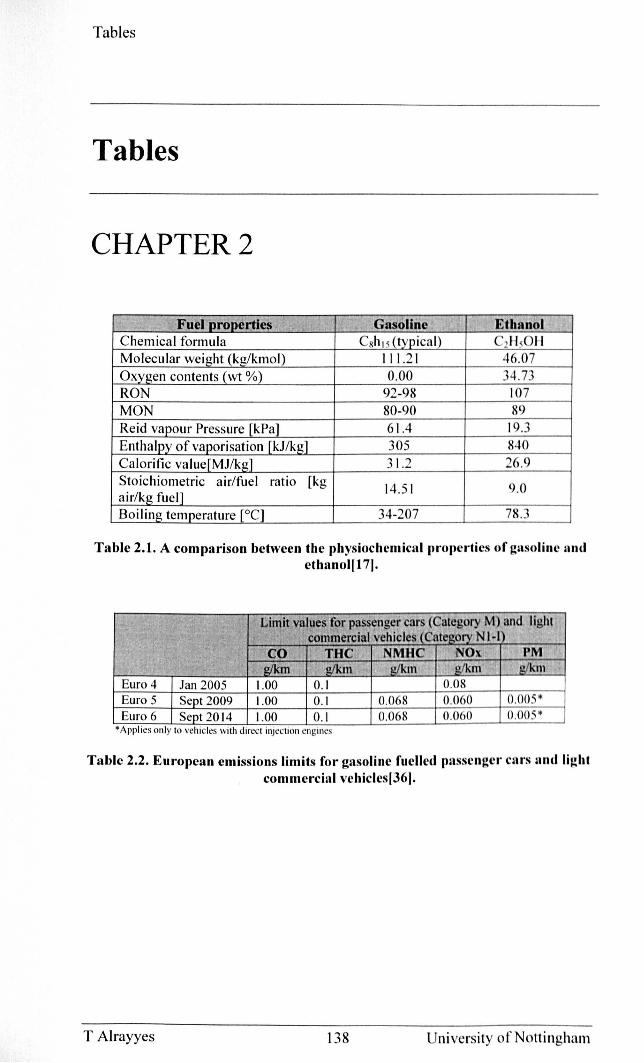
Tables
Tables
CHAPTER 2
Fuel properties I- Gasoline Ethanol Chemical formula CRh 15 (typical) C2HsOH Molecular weight (kg/kmol) 111.21 46 .07 Oxygen contents (wt %) 0.00 34.73 RON 92-98 107 MON 80-90 89 Reid vapour Pressure [kPa] 61.4 19.3 Enthalpy of vaporisation rkJ/kg 1 305 840 Calorific valuerMJ/kgl 31.2 26.9 Stoichiometric air/fuel ratio [kg
14 .5 1 9.0 air/kg fuell Boiling temperature [0C] 34-207 78 .3
Table 2.t. A comp~lrison between the physiochcmicnl p."operties of gllsoline and ethanol[17[.
" Limit values for passenger cars (Category M) and light commercial vehicles (Category Nl-I)
CO THC NMHC N01 PM g/km g/km gtkm Wkm Wkm
Euro 4 Jan 2005 1.00 0.1 0.08 Euro 5 Sept 2009 1.00 0.1 0.068 0.060 0.005'" Euro 6 Sept 20 14 1.00 0.1 0.068 0.060 0.005 '"
·Applles on ly to vehicles with direc t IIlJcctl on t! l1glllCS
Tnble 2.2. European emissions limits for gasoline fucllcd pnsscngcl' CIlI'S IUld liJ.!ht commercinl vehicles[361.
T Alrayyes 138 University of Nottingham
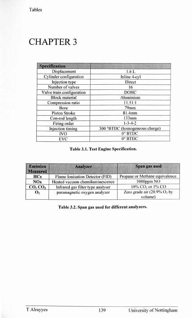
Tables
CHAPTER 3
Specification r, t 1" ,"" ,~
Displacement 1.6 L Cylinder configuration Inline 4-cyl
Iniection type Direct Number of valves 16
Valve train configuration DOHC Block material Aluminium
Compression ratio I 1.51: I Bore 79mm
Piston Stroke 81.4mm Con-rod length 133mm
Firing order 1-3-4-2 Iniection timing 300 °BTDC (homogeneous charge)
TVO 0° BTDC EVC 0° BTDC
Table 3.1. Test Engine Specification.
Emission Analyzer ! Span eas used Measured :.;
HCs Flame Ionisation Detector (FID) Propane or Melhane equi va lence. NOx Heated vacuum chemiluminescence SOOOppm NO
CO, CO2 Infrared gas filter type analyser 10% CO? or 1% CO O2 paramagnetic oxygen analyzer Zero grade air (20.9% Ol b
volume)
Table 3.2. Span gas used for differcnt anlllyzcrs.
T Alrayyes 139 Univer ity of Nottingham
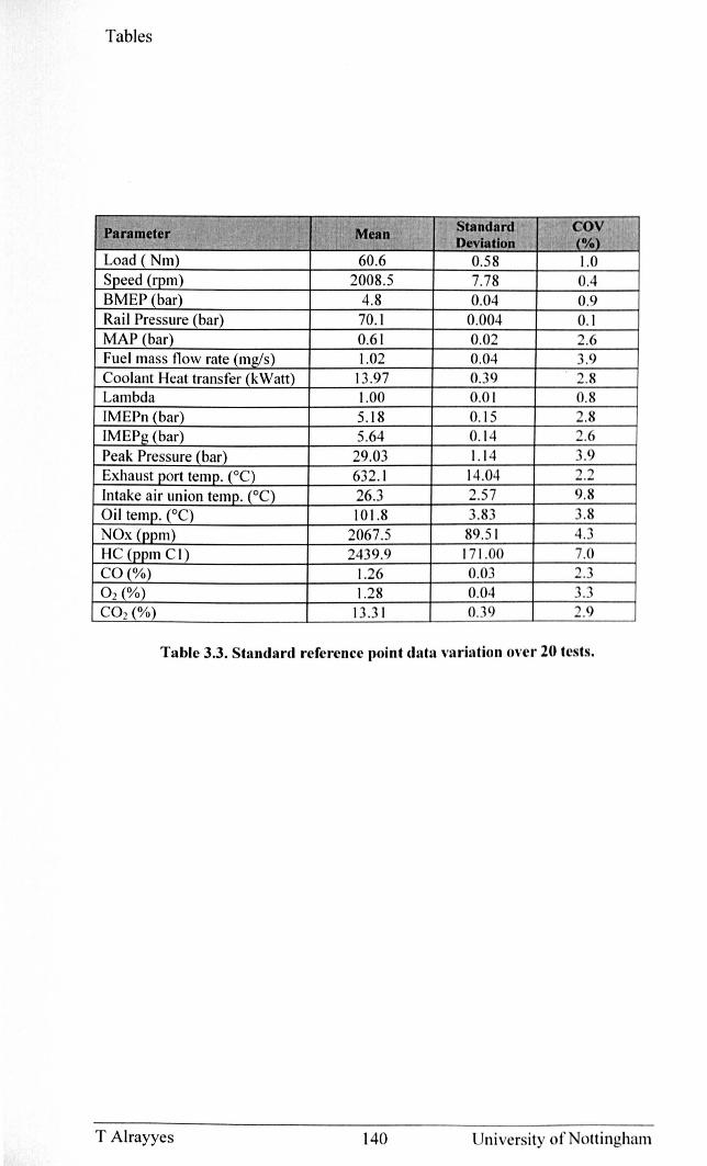
Tables
Parameter .. , Standard COY Mean
Deviation (%) .~
Load (Nm) 60.6 0.5 8 1.0 Speed (rpm) 2008 .5 7.78 0.4 BM EP (bar) 4.8 0.04 0.9 Rail Pressure (bar) 70.1 0.004 0. 1 MAP (bar) 0.61 0.02 2.6 Fuel mass flow rate (mg/s) 1.02 0.04 3.9 Coo lant Heat transfer (kWatt) 13.97 0.39 2.8 Lambda 1.00 0.0 1 0.8 IM EPn (bar) 5.18 0. 15 2.8 IM EPg (bar) 5.64 0.14 2.6
Peak Pressure (bar) 29.03 1.1 4 3.9 Exhaust port temp. (0C) 632 .1 14.04 2.2 Intake a ir union temp. (0C) 26.3 2.57 9.8 Oil temp. (0C) 101.8 3.83 3.8 NOx (ppm) 2067 .5 89.5 1 4.3 HC (ppm C I) 2439.9 17 1.00 7.0 CO (%) 1.26 0.03 2.3 O2 (%) 1.28 0.04 3.3 CO2 (%) 13.3 1 0.39 2.9
Table 3.3. Standard reference point data variation over 20 tests.
T Alrayyes 140 Uni versity of Nottingham
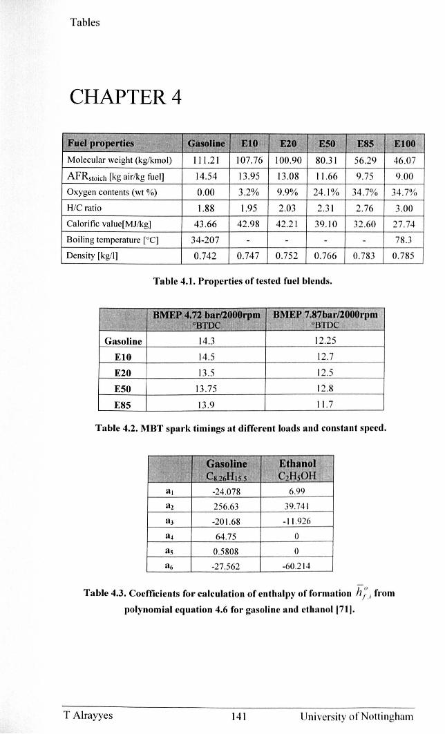
Tables
CHAPTER 4
Fuel properties Gasoline EI0 E10 E50 E85 EI00
Molecular we ight (kg/kmol) 111.2 1 107.76 100.90 80 .3 1 56.29 46 .07
AFR stoich [kg air/kg fuel] 14.54 \3 .95 13.08 11 .66 9.75 9.00
Oxygen contents (wt %) 0.00 3.2% 9.9% 24. 1% 34 .7% 34.7%
H/C ratio 1.88 1.95 2.03 2.3 1 2.76 3.00
Calorific value[MJ/kg] 43 .66 42.98 42 .2 1 39. 10 32.60 27.74
Boiling temperature [0C] 34-207 - - - - 78 .3
Density [kg/I] 0.742 0.747 0.752 0.766 0.783 0.785
Table 4.1. Properties of tested fu el blends.
BMEP 4.72 barllOOOrpm BMEP 7.87bar/lOOOrpm °BTDC °BTDe
Gasoline 14.3 12.25
EtO 14.5 12.7
E20 13.5 12.5
E50 13.75 12. 8
E85 13.9 I I. 7
Table 4.2. MBT spark timings at different loads a nd consta nt speed.
Gasoline Ethanol it C8.26HI S.5 C2HsOH
al -24.078 6.99
a2 256.63 39.74 1
a3 -20 1.68 - 11.926
a~ 64.75 0
a~ 0.5808 0
a6 -27.562 -60.2 14
Table 4.3. Coefficients for calculation of enth:llp), of formntion h ;.1 from
polynomial equation 4.6 for gasoline lUld ethanol 1711.
T Alrayyes 141 Uni versity of Notti ngham
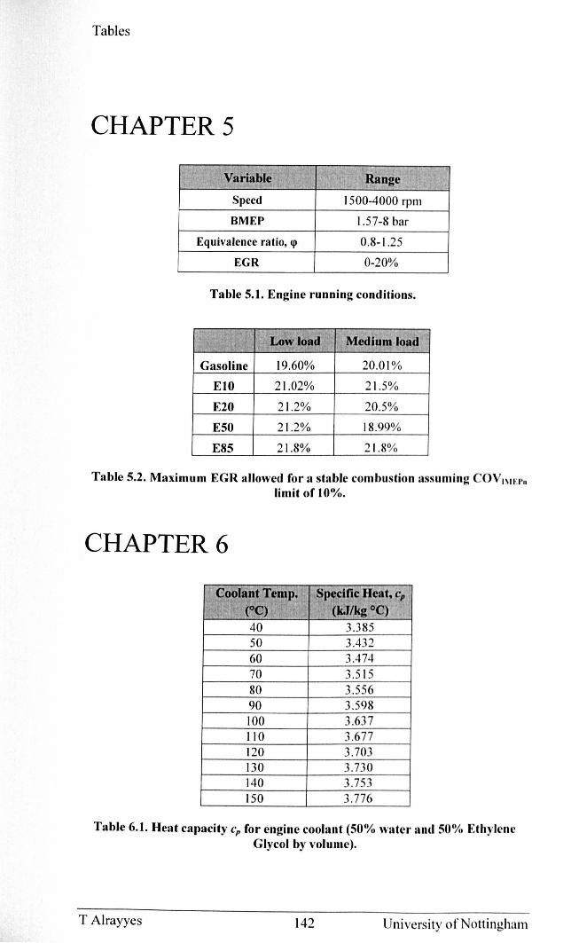
Tables
CHAPTERS
,.' Variable Range
Speed 1500-4000 rpm
BMEP 1.57-8 bar
Equivalence ratio, <p 0.8-1 .25
EGR 0-20%
Table 5.1. Engine running conditions.
, Lowload Medi,am load
Gasoline 19.60% 20.01 %
EIO 2 1.02% 21.5%
E20 2 1.2% 20.5%
E50 2 1.2% 18.99%
E85 2 1.8% 2 1. 8%
Table 5.2. Maximum EGR allowed for a stable combustion assuming OVIW~ l'n limit ofl 0%.
CHAPTER 6
Coolant Temp. Specific Heat, cp
(OC) (lw/kg 0c) 40 3.385 50 3.432 60 3.474 70 3.5 15 80 3.556 90 3.598 100 3.63 7 110 3.677 120 3.703 130 3. 730 140 3.753 150 3.776
Table 6.1. Heat capacity cp for engine coolant (50% water ~1I1d 50% Ethylene Glycol by volume).
T Alrayyes 142 University of Nottingham
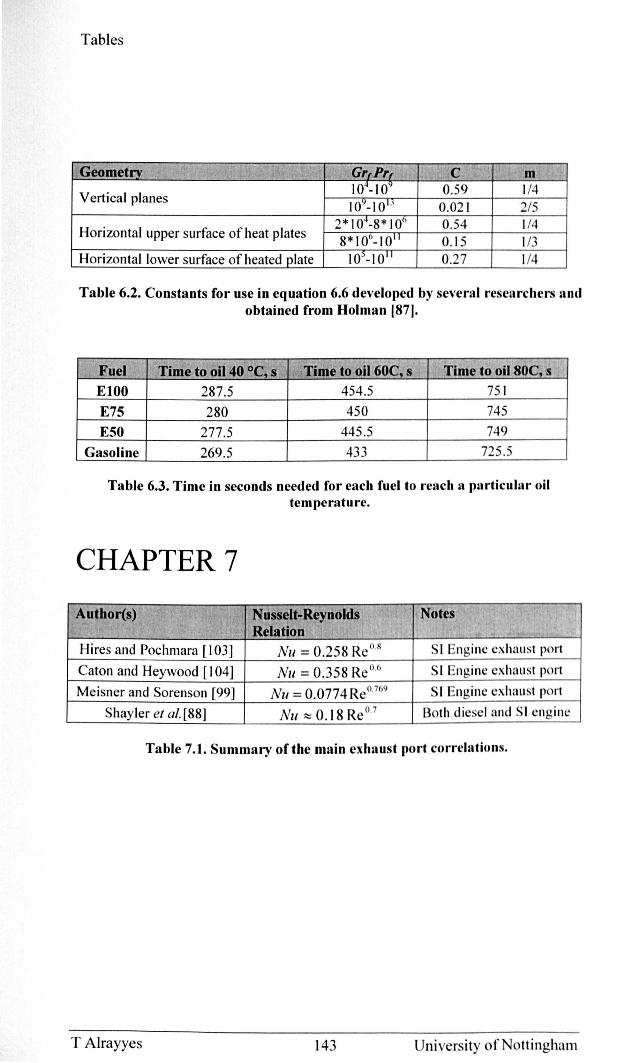
Tables
Geometry e. " ·-;"L-·! ~t" Gr,Pr, C "', m
Vertical planes 104_IO~ 0.59 1/4 10~_IO' o 0.021 2/5
Horizontal upper surface of heat plates 2* I 04_8 * 100 0.54 1/4 8* I 0°_1 0" 0.15 1/3
Horizontal lower surface of heated plate 105 -lO" 0.27 1/4
Table 6.2. Constants for use in equation 6.6 developed by several researchers and obtained from Holman 1871.
Fuel Time to oil 40 oc, s Time to oil 60C, s Time to oil SOC. s EIOO 287.5 454.5 751
E75 280 450 745
E50 277.5 445.5 749
Gasoline 269.5 433 725 .5
Table 6.3. Time in seconds needed for each fuel to reach a particular oil temperature.
CHAPTER 7
Author(s) N usselt-Reynolds '';, Notes " .. Relation
Hires and Pochmara [103] Nu = 0.258 Re o.s SI Engine exhatlst port
Caton and Heywood [104] Nu = 0.358 Reoo SI Engine exhallst port
Meisner and Sorenson [99] Nu = 0.0774 Reo.769 SI Engine exhaust port
Shayler et al. [88] Nu ~ 0.18 Re o.7 Both diesc l and SI cngine
Table 7.1. Summary of the main exhaust (lort correilltions.
T Alrayyes 143 University of Nottingham
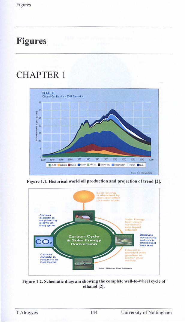
Figures
Figures
CHAPTER 1
35
30
~ !2. 25
~ " ~ 20 "Ii
~ <0 15
~ iii 10
PEAK OIL Oil and Gas liquids - 2004 Scenarios
0". 1930 1940 1950 1960 1910 1980 1980 2000 2010 2020 2030 2040 2050
I US-48 Europe I IM"a . Other . ME8st . H""vyetc. . Deepwater 0 1'01., I NGL
Figure 1.1. Historical world oil production and projection of trend [2].
C rbo n dl ox id9 Is recycl e d by p l onts as lh y grow
ro J sod as ru I burns
B io m ass contai n in g carbon is proc05sod Into fU9 1
Figure 1.2. Schematic diagram showing the complete well-to-wheel cycle of ethanol [2].
T Alrayyes 144 University of Nottingham
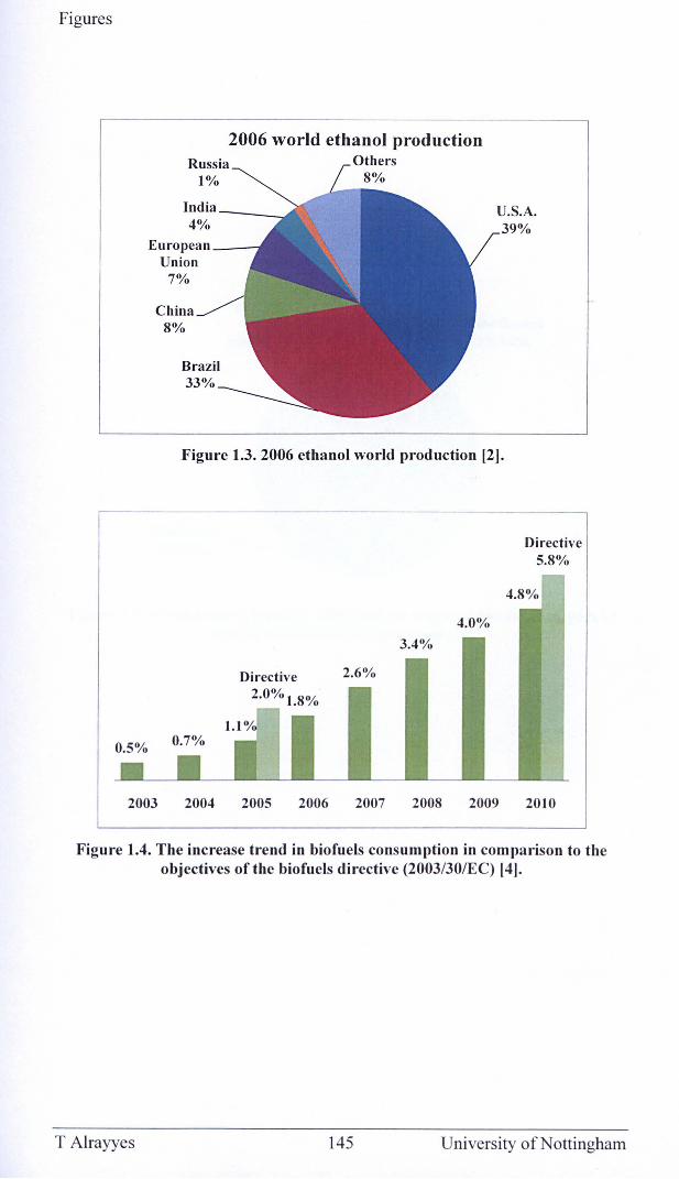
Figures
Russia 1%
2006 world ethanol production
India __ _
4% Eu ropean __
Union 7%
China 8%
U.S.A. 39%
Figure 1.3. 2006 ethanol world production [2].
Directive 5.8%
2003 2004 2005 2006 2007 2008 2009 20 I 0
Figure 1.4. The increase trend in biofuels consumption in comparison to the objectives of the biofuels directive (2003/301EC) [4].
T Alrayyes 145 University of Nottingham
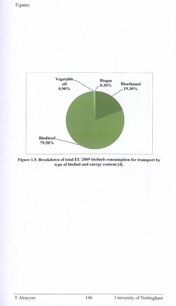
Figures
Biodiesel 79.50%
Vegetable oil
0.90%
Biogas 0.30% Bioethanol
19.30%
Figure 1.5. Breakdown of total EU 2009 biofuels consumption for transport by type of biofuel and energy content.[4].
T Alrayyes 146 University of Nottingham
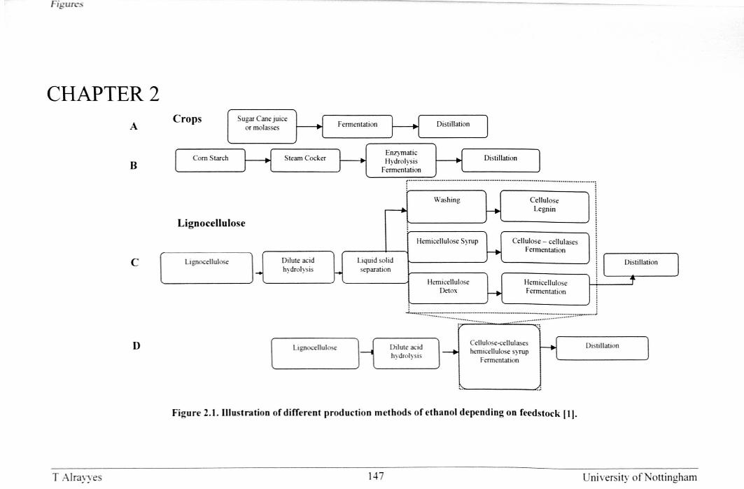
igurc:s
CHAPTER 2 A
B
C
D
T Alrayyes
Crops Sugar Cane juice or molasses
Com Starch Steam Cocker
Lignocellulose
[ u.-,,",~ ) Dilute acid
• hydrolysis
F ermentat ion Distill ation
f-.
EnZ)matic Hydrolysis
Fermentation
Distillation
[ ............... ................................................. ............................ ... ......... : :
Washing Cellulose
~ r-+ Legn in
Hemicellulose Syrup Cellulose - cellulases
Liquid solid 1-+ Fermentation
separation
Hemicellulose Hemicellulose Detox 1-+ Fermentation
~~"r::::::::::::::::::::::::::::::: ................ -..... ···· .. ·· ..... ~~·.~:: .. :::~:::::::::::::~~:tn ... u • • ,;
l
DIlute acid h~drolysis C~m- ]~,'-___ _ Cellulose-cellulases
hemicellulose S)TUp
Fermentation
Disllllation
... ~ /.,
Figure 2.1. Illustration of different production methods of ethanol depending on feedstock (II.
Distillation
J .1'
14 ni versity of Nott ingham
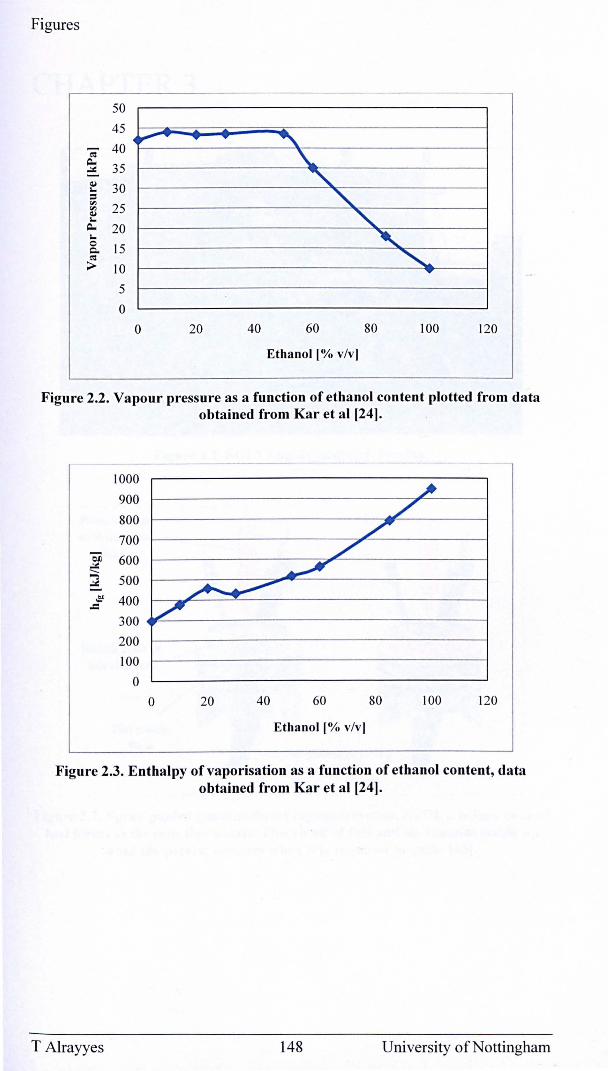
Figures
50
45
~ 40 ~ 35 Q,I 30 ... ::I
'" 25 '" Q,I ... Q., 20 ... 0 15 c. C'l
:;> 10
.,..... .... "-"" " "-"-
"-~ ....
5
0
o 20 40 60 80 100 120
Ethanol 1% v/v l
Figure 2.2. Vapour pressure as a function of ethanol content plotted from data obtained from Kar et al [24].
---------1000
900
800
700 eD 600 ..x --..., 500 ..x ~ 400 .c
300
~ /
/ ./ ~
~ ~
200
100
0
o 20 40 60 80 100 120
Ethanol 1% v/v l
Figure 2.3. Enthalpy of vaporisation as a function of ethanol content, data obtained from Kar et al [24].
T Alrayyes 148 University of Nottingham
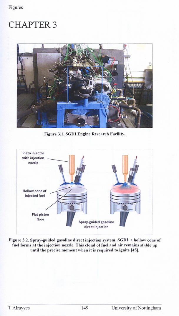
Figures
CHAPTER3
Figure 3.1. SGDI Engine Research Facility.
Piezo injector with injection
nozzle
Hollow cone of injected fuel
Flat piston floor
Spray-guided gasoline direct Injection
Figure 3.2. Spray-guided gasoline direct injection system, SGDI, a hollow cone of fuel forms at the injection nozzle. This cloud of fuel and air remains stable up
until the precise moment when it is required to ignite [45].
T Alrayyes 149 University of Nottingham
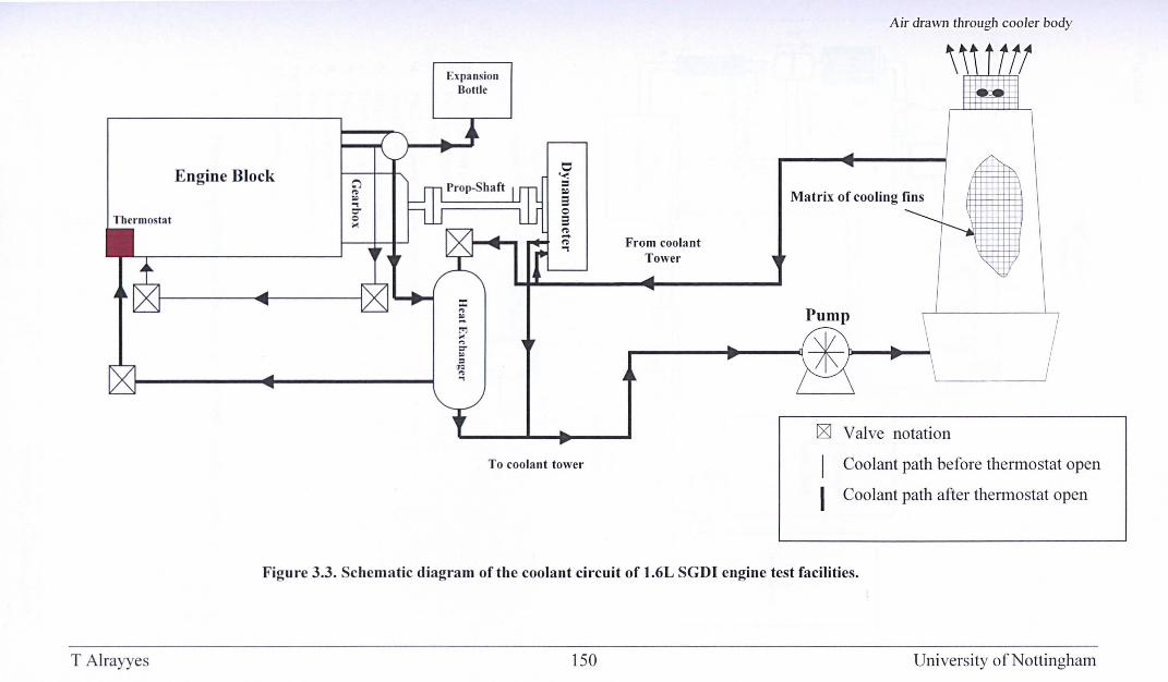
Thermosta t
T Alrayyes
Engine Block
Expansion Bottle
~ ,., .,
o 0....: :: ~
3 o 3 ~ -~ ""I
To coolant tower
From coolant Tower
Air drawn through cooler body
Matrix of cooling fins
[gJ Valve notation
Coolant path before thermostat open
Coolant path after thermostat open
Figure 3.3. Schematic diagram of the coolant circuit of 1.6L SGDI engine test facilities.
150 University of Nottingham
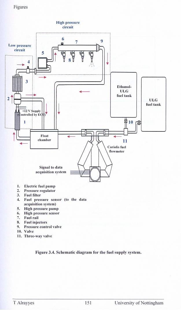
Figures
High pressure circuit
Low pressure circuit
3
5
12 V ~upply 1 1 ntrolle~ by )
, , 1 : , , ,
Float chamber
6
Signal to data acquisition system
I. Electric fuel pump 2. Pressure regulator 3. Fuel filter 4. Fuel pressure sensor (to the data
acquisition system) 5. High pressure pump 6. High pressure sensor 7. Fuel rail 8. Fuel injectors 9. Pressure control valve 10. Valve II. Three-way valve
1
EthanolULG
fuel tank ULG
fuel tank
Figure 3.4. Schematic diagram for the fuel supply system.
T Alrayyes 151 University of Nottingham
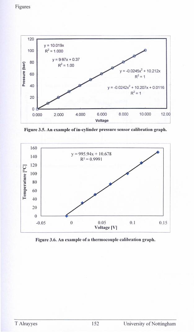
Figures
120
100
- 80 ~
III
So ! 60 :J 1/1 1/1 ! a.. 40
20
0
0.000
y = 10.019x
R2 = 1.000
y = 9.97x + 0.37
R2 = 1.00
2.000 4.000
y = -0.02451 + 10.212x R2 = 1
y = -0.0242x2 + 10.207x + 0.0116
R2 = 1
6.000
Voltage
8.000 10.000 12.0
Figure 3.5. An example of in-cylinder pressure sensor calibration graph.
160
140
- 120 U £.....
100 Q,I I. :I - 80 ell I. Q,I
Q. 60 5 Q,I
E-- 40
20
0
-0 .05
y = 995 .94x + 10.678 R2 = 0.999 1
o 0.05 Voltage [V]
0.1 0.15
Figure 3.6. An example of a thermocouple calibration graph.
T Alrayyes 152 University of Nottingham
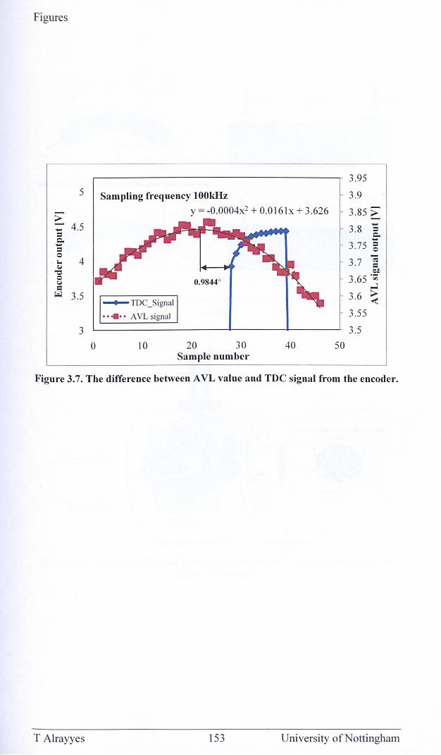
Figures
3.95
5 Sampling frequency 100kHz 3.9
E y = -0.0004x2 + 0.0161 x + 3.626 3.85 E
4.5 -- 3.8 = = Q.. Q.. -- 3.75 ; = 0 -; l... 4 3.7 Q,j = "Q eJ)
0 0.9844° 3.65 .~ C.)
= ...:.l ~ 3.5 3.6 > ~TDC_Signal < .. .... AVL signal 3.55
3 3.5
0 10 20 30 40 50 Sample number
Figure 3.7. The difference between A VL value and TDC signal from the encoder.
T Alrayyes 153 University of Nottingham
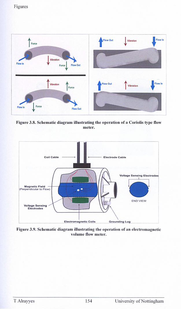
Figures
tFIOWOUI t Vibration
t Vibration tFIOWOUI t Vibration
FlowOul
Figure 3.8. Schematic diagram illustrating the operation of a Coriolis type flow meter.
Coil Cable
Magnetic Field IIP,.men,jlcIJlar 10 Flow)
Voltage Sensing Electrodes
Electrode Cable
END VIEW
L-____________________ ~~~~~~~~~ _____ G~ro~undln Lu~ __ __
Figure 3.9. Schematic diagram illustrating the operation of an electromagnetic volume flow meter.
T Alrayyes 154 University of Nottingham
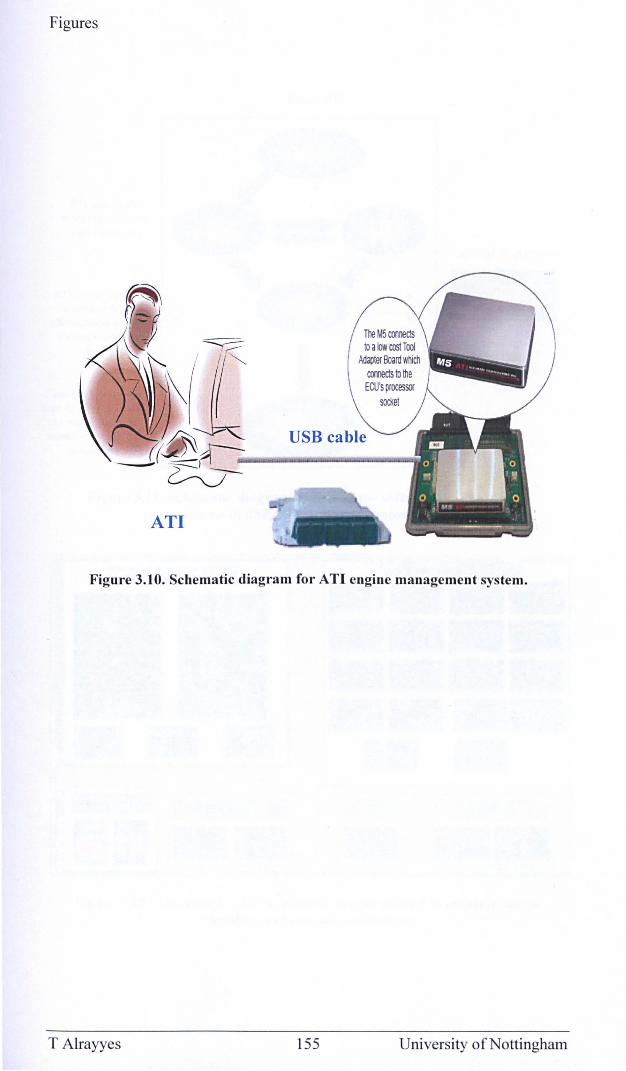
Figures
ATI
The M5 ronneds to a low cost Too
Ad..,ter Board Which comedstothe ECU's processa
socket
USB cable
Figure 3.10. Schematic diagram for ATI engine management system.
T Alrayyes 155 University of Nottingham
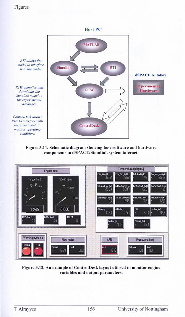
Figures
RTf allows the model to interface
with the model
RTW compiles and downloads the
Simulink model to the experimental
hardware
ControlDesk allows user to interface with
the experiment, to monitor operating
conditions
Host PC
dSPACE Autobox
f:xperimental Hardw~re
Figure 3.11. Schematic diagram showing how software and hardware components in dSPACE/Simulink system interact.
Engine data
Figure 3.12. An example of ControlDesk layout utilised to monitor engine variables and output parameters.
T Alrayyes 156 University of Nottingham
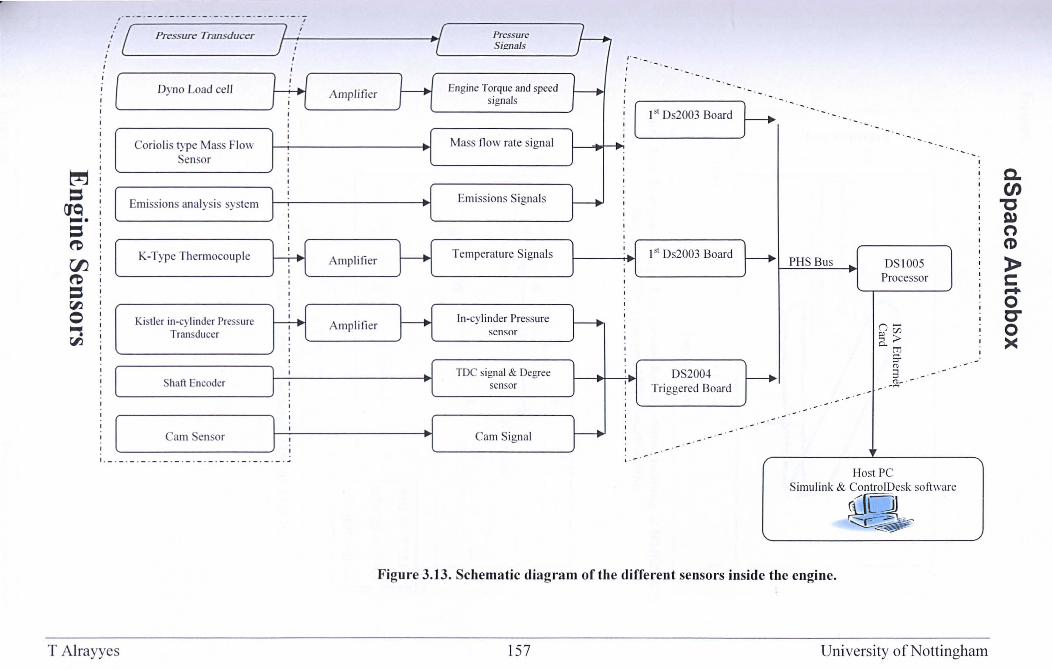
~ = ~ -. = (D
00 (D
= r.I1 o ~ r.I1
- - - - - - -_ . _ . _ -_ . _ -_ . _-_ . _ -- --
Pressure Transducer
Dyno Load cell
Coriolis type Mass Flow Sensor
Emissions analys is system
K-Type Thermocouple
Kistler in-cylinder Pressure Transducer
Shaft Encoder
Cam Sensor
, ,
I ._ . _ . _ . - . - . - . - . - . - . -. - . - . - . - . - . - . ~
T Alrayyes
Amplifier
Amplifier
Amplifier
Pressure Si.!!1lals
Engine Torque and speed signals
Mass fl ow rate signal
Emissions Signals
Temperature Signals
In-cylinder Pressure sensor
TDe signal & Degree sensor
Cam Signal
,- -
[-~~~;()(); B~ard }--+
lSI Ds2003 Board
DS2004 Tri ggered Board
PHS Bus
. -.
DS l005 Processor
() Ci3 ~ ~ Q. (Tl
S-(1)
:3 ; _ (1)_ • -...
Host PC Simulink & Control Desk software
.~~ "-~
Figure 3.13. Schematic diagram of the different sensors inside the engine.
157 University of Nottingham
c. CJ) "C Q) (") (1)
» s:::: ~ o CO ><
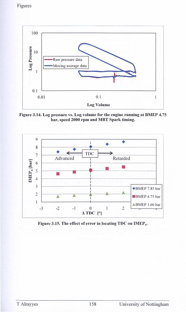
Figures
100
f: ~ 10 rn ~ P: - Raw pressure data
~ - Moving average data ~
0.1
0.01 0.1
Log Volume
Figure 3.14. Log pressure vs. Log volume for the engine running at BMEP 4.75 bar, speed 2000 rpm and MBT Spark timing.
9 I • •
8 ... • • ... I TDC I ... 7
'i:' Advanced I Retarded
~ 6 I .c ~ • - • c 5 ~ • • T
~ I
4 I
3 I I + BMEP 7.85 bar
2 I
'" .. A .& i~ . BMEP 4.75 bar
1 " BMEP 1.60 bar
-3 -2 -I 0 I 2 ATDC [0]
Figure 3.15. The effect of error in locating TDC on IMEP n.
T Alrayyes 158 University of Nottingham
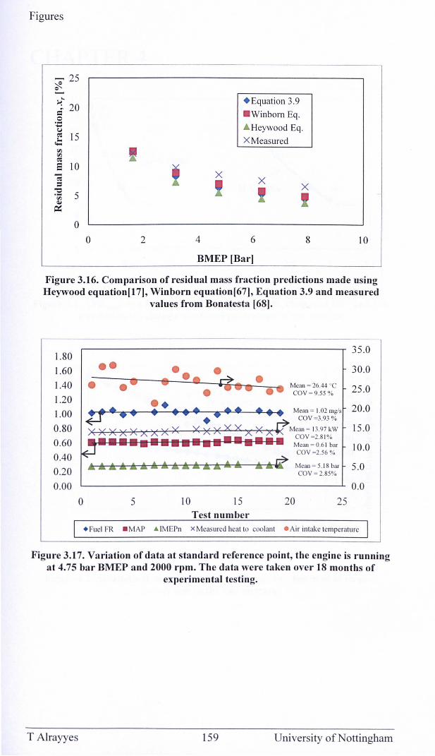
Figures
- 25 ~ Q
~ .... 20
• Equation 3.9
== . Winborn Eq .
. 9 .... "' Heywood Eq . <:J eo: 15 XMeasured c!:: ~ ~ eo: S LO e; X
X = X "0 .~ 5 QJ
~
0
0 2 4 6 8 10
BMEP [Bar]
Figure 3.16. Comparison of residual mass fraction predictions made using Heywood equation[17], Winborn equation[67], Equation 3.9 and measured
values from Bonatesta [68].
1.80
1.60 •• 1.40 • • 1.20
1.00
0 .80
0 .60
0.40
0.20
0.00
0 5
+ Fuel FR - MAP
•• • Mean = 26.44 DC
• COV = 9.55 %
•• • •• • • • • ••• Mean = 1.02 mgls • ~ COY =3.93 %
10
X X)( X X X X X +< Mean = 13.97 kW COV - 2.S I% Mean = 0.6 1 bar
OV =2.56 %
15 20
Test number
Mean = 5. IS bar COV = 2.S5%
25
35.0
30.0
25 .0
20 .0
15.0
10.0
5.0
0.0
& IMEPn x Measured heat to coolant • Air intake temperature
Figure 3.17. Variation of data at standard reference point, the engine is running at 4.75 bar BMEP and 2000 rpm. The data were taken over 18 months of
experimental testing.
T Alrayyes 159 University of Nottingham
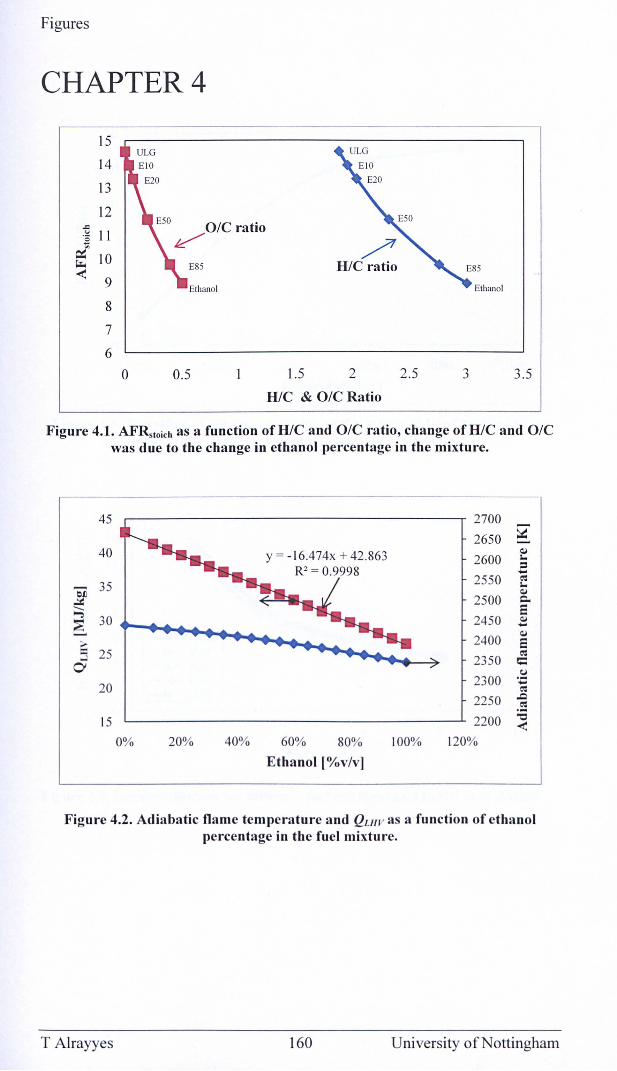
Figures
CHAPTER 4
15
14
13
12 ..c:
Ethanol
'" 11 J 10 ~ <:
9 HlC ratio
8
7
6
0 0.5 1.5 2 2.5 3 3.5
HlC & O/C Ratio
Figure 4.1. AFRstoich as a function ofHlC and O/C ratio, change ofH/C and O/C was due to the change in ethanol percentage in the mixture.
45 2700
2650 g 40 ~
2600 I-
= -35 2550 ~ I-
OJ') ~
~ 2500 Q.,
;::;; 30
E ~
2450 ~ -~ > 2400 E :3 25 2350
~
0 C .~
20 2300 -~ 2250 .c
.:': 15 2200 "C
<: 0% 20% 40% 60% 80% 100% 120%
Ethanol [%v/v]
Figure 4.2. Adiabatic flame temperature and QUfJ/ as a function of ethanol percentage in the fuel mixture.
T Alrayyes 160 University of Nottingham
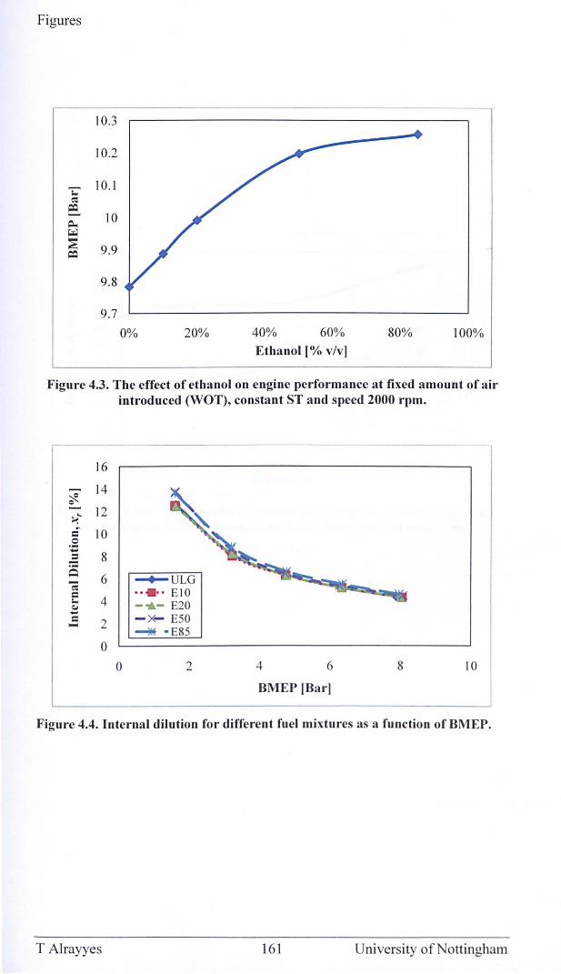
Figures
]0.3
10.2
'i:' 10.1 ell
~ 10 Po. ~
~ 9.9 = 9.8
9.7 0% 20% 40% 60%
Ethanol [% v/v] 80% 100%
Figure 4.3. The effect of ethanol on engine performance at fixed amount of air introduced (WOT), constant ST and speed 2000 rpm.
,.---------------------
16
~ 14 ~ = l-<'- 12
== 10 .:= ... 8 ~
~ -; 6 ~ULG
c •• • •• E tO J,., 4 - .. - E20 Q,I - -~ E50 c 2 ....
- E85 ~
0
0 2 4 6 8 10
BMEP [Barl
Figure 4.4. Internal dilution for different fuel mixtures as a function of BMEP.
T Alrayyes 161 University of Nottingham
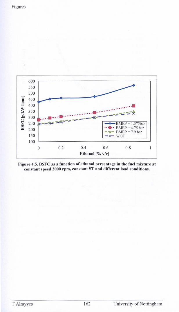
Figures
600 550 500
'i:" 450 = 0 -= 400 ~ 350 ~ --~ 300 U
250 r.. 00 ~ 200
150 100
0 0.2 0.4
.... -............ ...... ..,---- --- ---~ BMEP = 1.575bar •• • •• BMEP = 4.75 bar -oA- BMEP = 7.9 bar - x- WOT
0.6 0.8
Ethanol [% v/v]
Figure 4.5. BSFC as a function of ethanol percentage in the fuel mixture at constant speed 2000 rpm, constant ST and different load conditions.
T Alrayyes 162 University of Nottingham
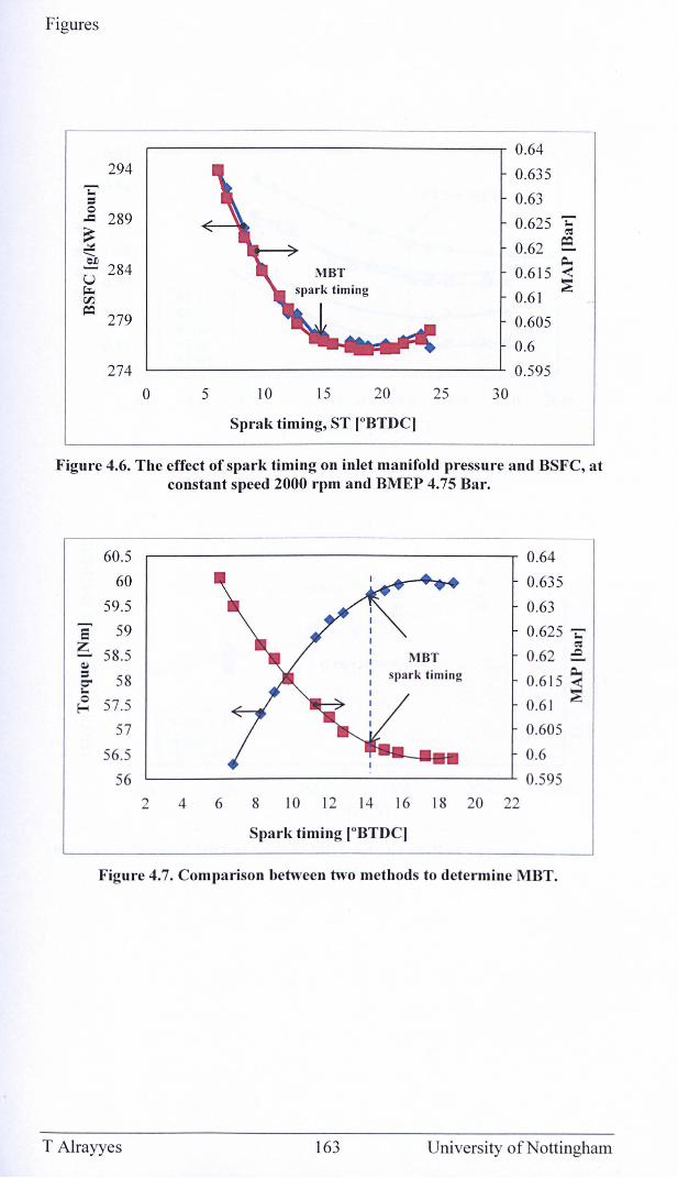
Figures
0.64 294 0.635
'i:"' 0.63 = 0
.c 289 0.625 'i:"' ~ ~
.:I: 0.62 ES. ---~ 284 0.615 ~ U roo. 0.61 rJJ ~
279 0.605
0.6
274 0.595
0 5 10 15 20 25 30
Sprak timing, ST [OBTDC]
Figure 4.6. The effect of spark timing on inlet manifold pressure and BSFC, at constant speed 2000 rpm and BMEP 4.75 Bar.
60.5
60
59.5 ~
59 E ~ 58.5 ~
= 58 0" 1.0 0 57.5 ~
57
56.5
56
,.--------------------r 0.64
MBT spark timing
0.635
0.63
0.625 'i:"' ~
0.62 e 0.61 5 ~ 0.6 1
0.605
0.6 L..-_______________ --'- 0.595
2 4 6 8 10 12 14 16 18 20 22
Spark timing [OBTDC]
Figure 4.7. Comparison between two methods to determine MBT.
T Alrayyes 163 University of Nottingham
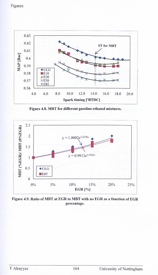
Figures
0.63
0.62 ST for MBT
0.6\ 'i:' t/ ~
0.6 e:.
~ 0.59 + ULG
0.58 . EIO .A E20
0.57 X E50 )K E85
0.56
4.0 6.0 8.0 10.0 12.0 14.0 \6 .0 18.0 20.0
Spark timing [OBTDC]
Figure 4.8. MBT for different gasoline-ethanol mixtures.
,.-.. 2.5 ~ C,!) ~ ~ 2 Y = 1.0002e32258x • • Q
Q "-' \ ~ ~ 1.5 ~ --,.-.. ~ C,!) ~ ~ Q
"-' 0.5 I +ULG I ~ ~ . E85 ~
0
0% 5% \0% 15% 20% 25% EGR [%]
Figure 4.9. Ratio ofMBT at EGR to MBTwith no EGR as a function ofEGR percentage.
T Alrayyes 164 University of Nottingham
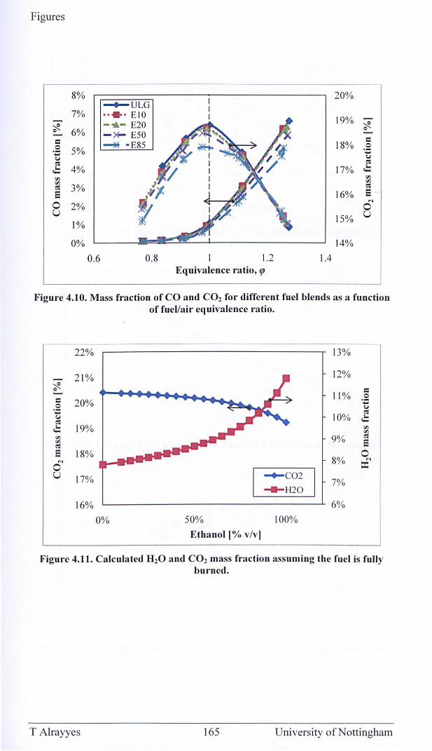
Figures
8% 20% ~ULG
7% •• • •• £10 19% - - .. - E20 ~ ~ 6%
0 0 -x- E50 ....... = ~ - E85 18% = 0 5% .5: ;: ..... tJ tJ co: co: .;: 4% 17% .;:
'" '" '" '" co: 3% co: 8 16% 8 0
N
2% 0 u 15% U
1%
0% 14%
0.6 0.8 1.2 1.4 Equivalence ratio, lfJ
Figure 4.10. Mass fraction of CO and CO2 for different fuel blends as a function of fuel/air equivalence ratio.
22% 13%
21% 12% -~ = 0
11% 0 = 20% ;: 0 tJ ''':
10% co:
tJ .:: co: .:: 19% '" '" '" 9% co: '" 8 co: 8 18% 0
N 8% N
0 == u 17% ...... C02 7%
_ H2O
16% 6%
0% 50% 100%
Ethanol [% v/v]
Figure 4.11. Calculated H20 and CO2 mass fraction assuming the fuel is fully burned.
T Alrayyes 165 University of Nottingham
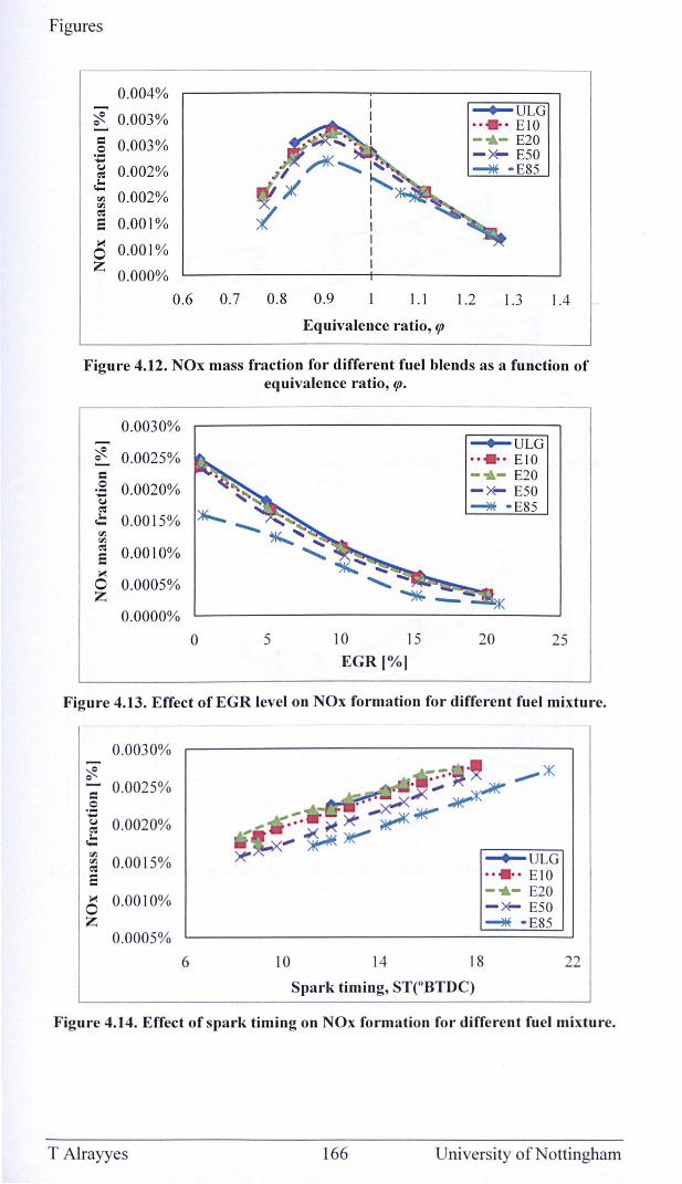
Figures
0.004% ~
~ ~ 0.003% ....... = 0.003% 0 .: (j 0.002% e':
c!:: ~ ~
0.002% e': e 0.001% Ii< 0.001% 0 Z
0.000%
0.6 0.7 0.8 0.9 1.1
Equivalence ratio, lfJ
~ULG •• • •• EIO --.- E20 -*- E50 ~ - E85
1.2 1.3 1.4
Figure 4.12. NOx mass fraction for different fuel blends as a function of equivalence ratio, lfJ.
0.0030% ~
~ ~ 0.0025%
= .S: 0.0020% .... (j
e': ~ .:: 0.0015%
~ ~ e': 0.00 10% e Ii< 0 0.0005% Z
0.0000%
0 5 10 15
EGR [%]
~ULG •• • •• EIO --.- E20 -x- E50 ~ - E85
20 25
Figure 4.13. Effect of EGR level on NOx formation for different fuel mixture.
0.0030%
:::R ~
= 0.0025% .S: .... (j 0.0020% e': J... .... ~
0.0015% ~
e': e Ii< 0.0010% 0 Z
0.0005%
6 10 14 18
Spark timing, STeBTDC)
~ULG .. .. . EIO --.- E20 -*- E50 ~ - E85
22
Figure 4.14. Effect of spark timing on NOx formation for different fuel mixture.
T Alrayyes 166 University of Nottingham
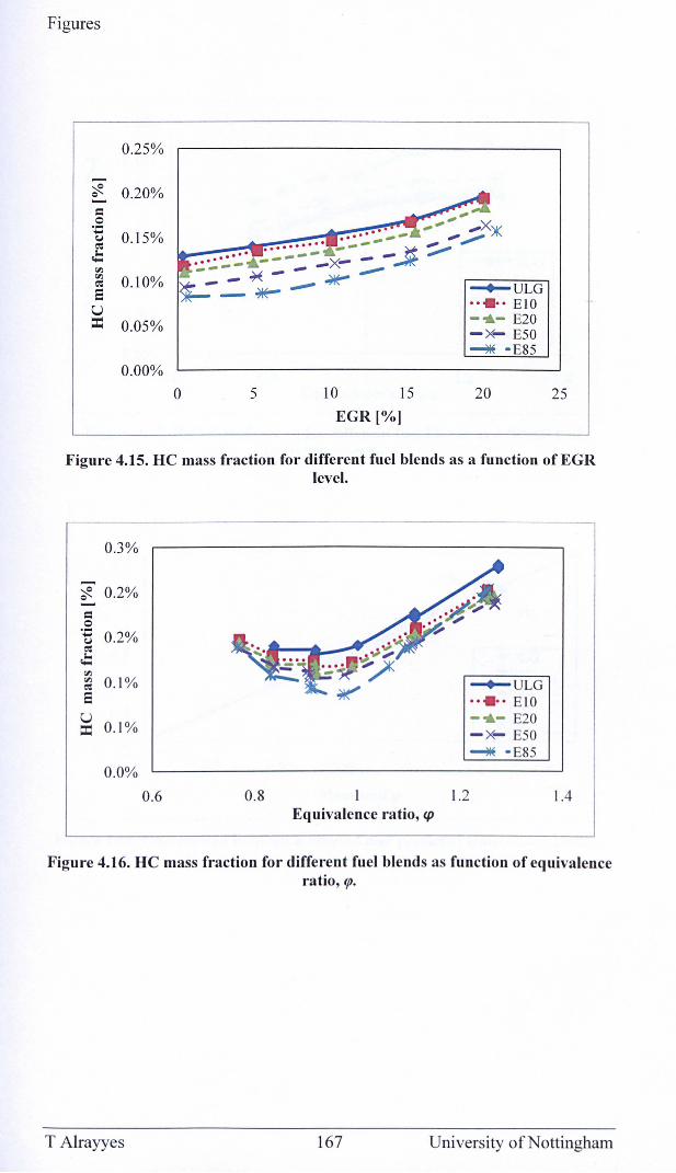
Figures
0.25%
....... ~ c 0.20%
= 0 .:
0.15% (oJ
~
.!: '" '" 0.10% ~ ~ULG E U
•• • •• EtO
== 0.05% -0&- E20 -x- E50 ~ - E85
0.00%
0 5 10 15 20 25
EGR[%]
Figure 4.15. HC mass fraction for different fuel blends as a function of EGR level.
0.3%
~ c 0.2%
= .9 .... 0.2% (oJ
~
.!: '" '" 0.1% ~
E U
0.1% ==
0.0%
0.6 0.8 1.2 Equivalence ratio, cp
~ULG • ••• • E tO -0&- E20 -x- E50 ~ - E85
1.4
Figure 4.16. HC mass fraction for different fuel blends as function of equivalence ratio, fP.
T Alrayyes 167 University of Nottingham
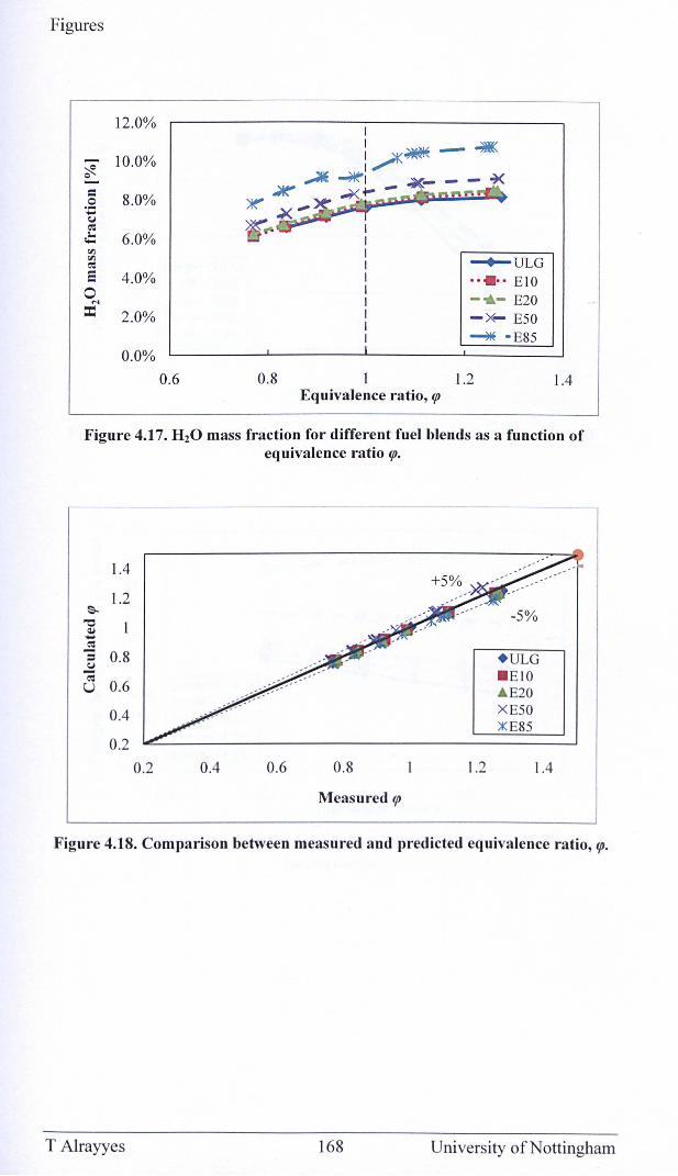
Figures
12.0% I I
-~ ~ 10.0% : ~-~ 0 ~~I ~_ - - ~
= 8.0% ~ -¥..+--0 ~ ¥,-:;: CJ
~~ ~
c!:: 6.0% '" '" .......... ULG ~ e 4.0% •• • •• EI O 0 - .. - E20 M
== 2.0% -x- E50 ~ - E85
0.0% 0.6 0.8 1.2 1.4
Equivalence ratio, lfJ
Figure 4.17. H20 mass fraction for different fuel blends as a function of equivalence ratio lfJ.
1.4
1.2 ~
"0 Q,j --.!
0.8 = CJ ';
0.6 U
0.4
0.2 0.2 0.4 0.6 0.8
Measured lfJ
1.2
-5%
+ ULG - EIO A E20 X E50 ::K E85
1.4
Figure 4.18. Comparison between measured and predicted equivalence ratio, lfJ.
T Alrayyes 168 University of Nottingham
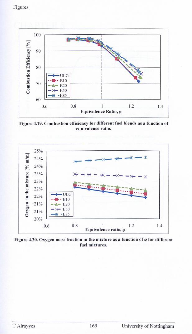
Figures
>. (,j
= Q,l .c::; s ~
= .9 .... '" =
100
90
80
..0 70 E o u
60
0.6
-+-ULG •• • •• EIO _ .. _ E20 I-------t---------..:!~--___I
-~ E50 ~ - E85
0.8 1.2 1.4 Equivalence Ratio, lfJ
Figure 4.19. Combustion efficiency for different fuel blends as a function of equivalence ratio.
25% ~
E 24% --E ~ ~
24% --Q,l 23% I.
= .... 23% .~
E Q,l 22% -= .... = 22% .-= 21 % Q,l ~ >. 21 % ~
0 20%
-+-ULG •• • •• EIO
- .. - E20 -~ E50 ~ - E85
0.6
* - * - ~- -x- -~-x
---&----" ..... .. .. ..... -0.8 1 1.2
Equivalence ratio, tp 1.4
Figure 4.20. Oxygen mass fraction in the mixture as a function of tp for different fuel mixtures.
T Alrayyes 169 University of Nottingham
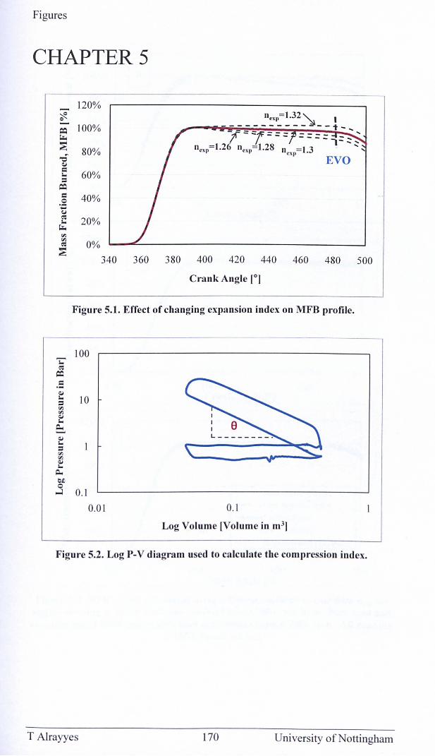
Figures
CHAPTERS
- 120% ~ ~ -~ 100% ~
~ 80% "C ~ c
60% I.
= ~ c 40% .~ .... CJ ~ 20% I. ~
'" '" 0% ~
~ 340 360 380 400 420 440 460 480 500
Crank Angle [oJ
Figure 5.1. Effect of changing expansion index on MFB profile.
0.1
Log Volume [Volume in m3J
Figure 5.2. Log P-V diagram used to calculate the compression index.
T Alrayyes 170 University of Nottingham
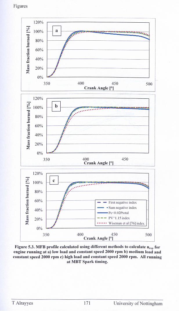
Figures
~
~ Q
"0 Q,j
= 100
= ..c = 0 .:
<:J ~ .:: Vi Vi ~
~
~
~ Q
"0 Q,j
= 100
= ..c
= .~ -<:J ~ .:: Vi Vi ~
~
~ Q
"0 Q,j
= 100
= ..c
= 0 '';:
<:J ~ .:: Vi Vi eo: ~
120%
100%
80%
60%
40%
20%
0%
120%
100%
80%
60%
40%
20%
0%
120%
100%
80%
60%
40%
20%
0%
350
350
400 450 Crank Angle [0J
..............
400 450 Crank Angle [0J
........ ..... .
- - First negati ve index
I----jt:---------j - - Sum negative index - Pc<O.02Ptotal
I--- -#---------j - - - PVA 1.15 index • • • ••• Wiseman et al [76] index
350 400 450 Crank Angle [0J
500
500
Figure 5.3. MFB profile calculated using different methods to calculate neXII for engine running at a) low load and constant speed 2000 rpm b) medium load and constant speed 2000 rpm c) high load and constant speed 2000 rpm. All running
at MBT Spark timing.
T Alrayyes 171 University of Nottingham
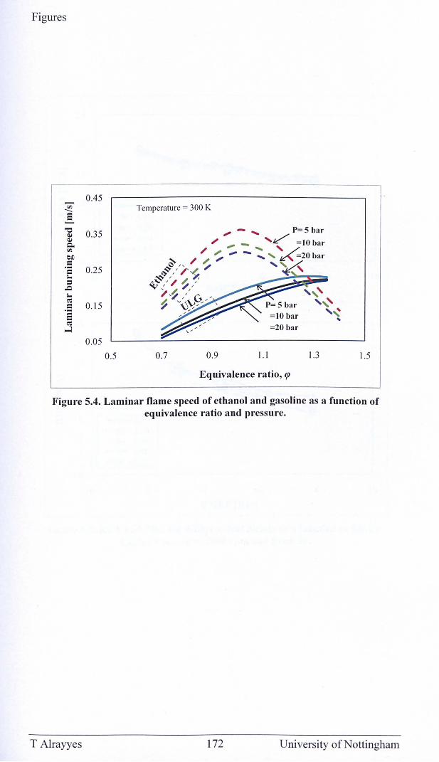
Figures
0.45
~ 0.35 ~ Q.
'" OIl
= ·2 0.25 loo
= ~ loo
.s 0.15 S eo:
...:l 0.05
Temperature = 300 K
0.5 0.7 0.9 1.1 1.3 1.5
Equivalence ratio, lfJ
Figure 5.4. Laminar flame speed of ethanol and gasoline as a function of equivalence ratio and pressure.
T Alrayyes 172 University of Nottingham
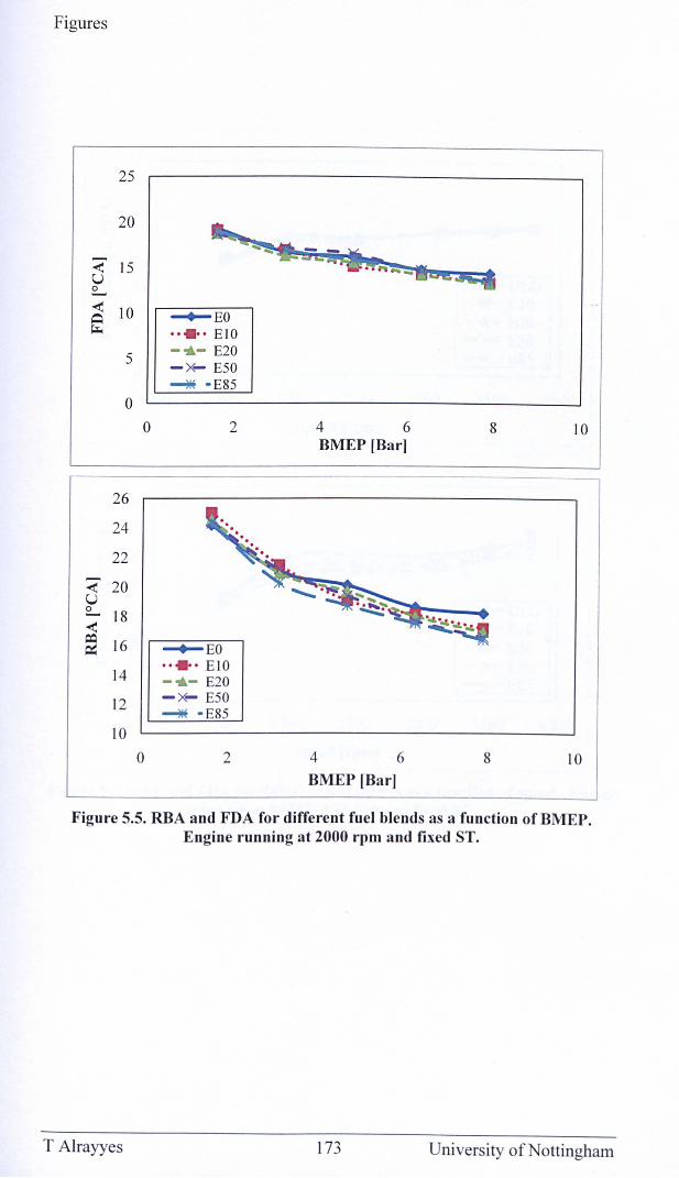
Figures
25
20
<" 15 U £..... -< 10 ~ -+-EO ~ •• • •• EIO
5 - .. - E20 -x- E50 ~ - E85
0 0 2 4 6 8 10
BMEP [Bar]
26
24
22
<" 20 U £..... 18 -< ga 16 -+-EO
14 ••••• EIO - .. - E20
12 -~ E50 ~ - E85
10
0 2 4 6 8 10 BMEP [Bar]
Figure 5.5. RBA and FDA for different fuel blends as a function ofBMEP. Engine running at 2000 rpm and fixed ST.
T Alrayyes 173 University of Nottingham
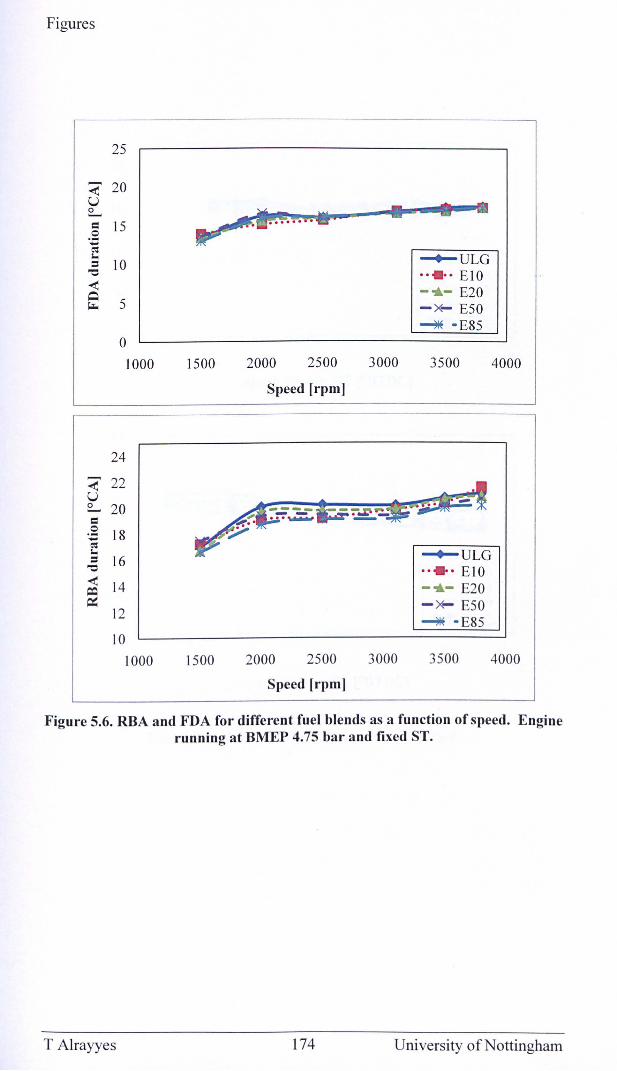
Figures
25
<' 20 U e..... = 15 .2 -I:<: I.
= 10 "0
< ~ 5 ~
0 1000
24
<' 22 U e..... 20 = .2 18 -I:<: I.
= 16 "0
< 14 ~
12
10 1000
1500 2000 2500 3000
Speed [rpm]
1500 2000 2500 3000
Speed [rpm]
-+-ULG •• • •• EIO - .. - E20 -x- E50 ~ - E85
3500
-+-ULG •• • •• EIO - .. - £20 -~ E50 ~ - E85
4000
3500 4000
Figure 5.6. RBA and FDA for different fuel blends as a function of speed. Engine running at BMEP 4.75 bar and fixed ST.
T Alrayyes 174 University of Nottingham
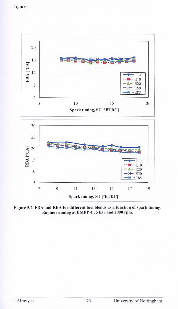
Figures
20
16 <" u ° ~ 12 < ~ ~
8
4
5
30
25
<" 20 U ~
< 15 ~
10
5 7
10 15
Spark timing, ST [OBTDC]
9 11 13 15
Spark timing, ST [OBTDC]
~ULG .. .. . EIO - .. - E20 -x- E50 ~ - E85
~ULG •• • •• E IO - .. - E20 -~ E50 ~ - E85
17
20
19
Figure 5.7. FDA and RBA for different fuel blends as a function of spark timing. Engine running at BMEP 4.75 bar and 2000 rpm.
T Alrayyes 175 University of Nottingham
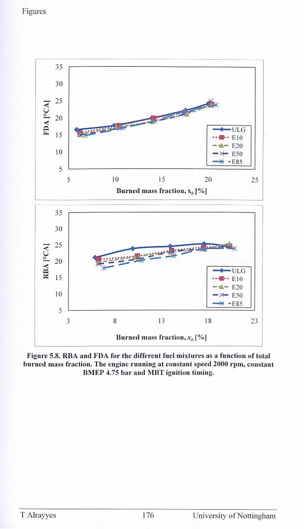
Figures
35
30
<" 25 U ~ 20 -< ~ ~ 15
10
5
35
30
<" 25 U ~ 20 -< ;! 15
10
5
5
3
~ ~ .4i£S5f--- -+-ULG •• • •• EIO
10 15 20
Burned mass fraction, xb [%]
8 13 18
Burned mass fraction,xb [%]
- .. - E20 - x- E50
~ - E85
-+-ULG •• • •• E IO
- .. - E20 - *- E50 ~ - E85
25
23
Figure 5.8. RBA and FDA for the different fuel mixtures as a function of total burned mass fraction. The engine running at constant speed 2000 rpm, constant
BMEP 4.75 bar and MBT ignition timing.
T Alrayyes 176 University of Nottingham
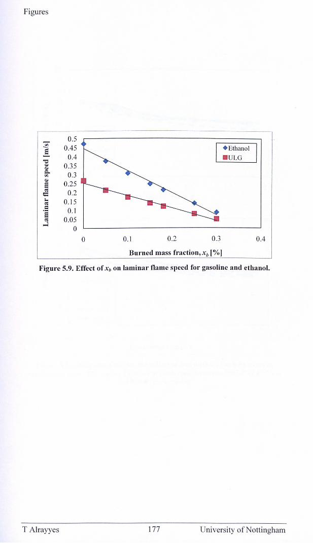
Figures
0.5 ';j'
0.45 --8 ~ 0.4 "0 QI 0.35 QI c.. 0.3 '" QI
0.25 8 ~ 0.2 c I. 0.15 ~
.S 0.1 8 ~ 0.05
...:l 0
0 0.1 0.2 0.3
Burned mass fraction,xb [%]
+ Ethanol . ULG
0.4
Figure 5.9. Effect of Xb on laminar flame speed for gasoline and ethanol.
T Alrayyes 177 University of Nottingham
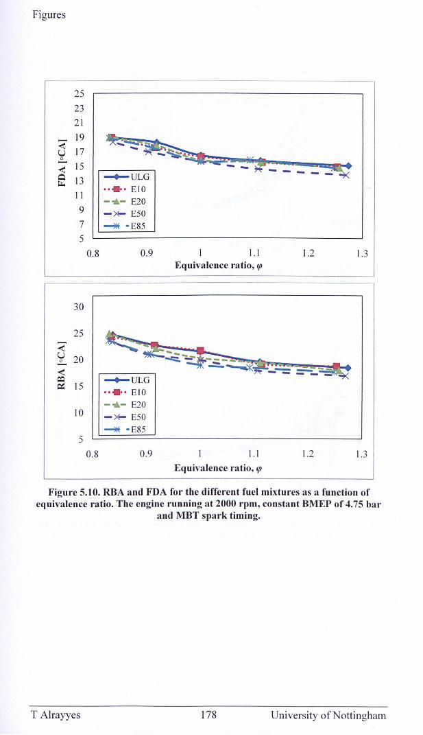
Figures
25 23 21
<" 19
U 17 ~
< 15 ~ 13 ~
11 9 7 5
0.8
30
25
<" U 20 ~
< ~ 15
10
5 0.8
~ULG
•• • •• EIO
--&- E20
- x- E50 ~ - E85
0.9
~ULG
•• • •• EIO
--&- E20
- *", E50
~ - E85
0.9
- -
1.1 Equivalence ratio, lfJ
1.1
Equivalence ratio, lfJ
-----
1.2
1.2
-~
1.3
1.3
Figure 5.10. RBA and FDA for the different fuel mixtures as a function of equivalence ratio. The engine running at 2000 rpm, constant BMEP of 4.75 bar
and MBT spark timing.
T Alrayyes 178 University of Nottingham
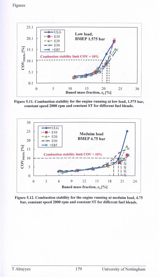
Figures
25.1
20.1
~ 0 15 .1 -t: \oJ
.; 10.1 0 U
5.1
0.1
0
~ULG
•• • •• EIO
-'Il- E20 -x- E50 ~ - E85
Low load, BMEP 1.575 bar
Combustion stability limit COY = 10%
5 10 15 20
III III II I II I
Buned mass fraction, xb [%] 25 30
Figure 5.11. Combustion stability for the engine running at low load, 1.575 bar, constant speed 2000 rpm and constant ST for different fuel blends.
30
25
20
~ 0 15 c
co. \oJ
~ 10 >-0
5 U
0
0
~ULG
•• • •• E IO -'Il- E20 -x- E50 ~ - E85
Meduim load BMEP 4.75 bar
Combustion tability limit COY = 10% / ---------- --------- / r
3 6 9 12 15 18
Buned mass fraction,xb [% ]
21 24
Figure 5.12. Combustion stability for the engine running a t meduim load, 4.75 bar, constant speed 2000 rpm and constant ST for different fuel blends.
T Alrayyes 179 University of Nottingham
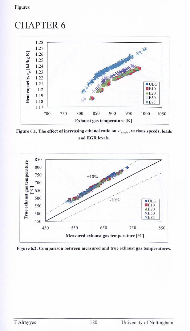
Figures
CHAPTER 6
1.28 1.27
~ 1.26 bJ) 1.25 ,.:(
;;;;; ,.:( 1.24 ~
Q. 1.23 (j
~ 1.22 .~ 1.21 ~ + ULG Q. 1.2 ~
_ EIO (j ... 1.19 ~ ~
1.18 ==
.A E20
0- XE50 :K E85
1.17 700 750 800 850 900 950 1000 1050
Exhaust gas temperature [K]
Figure 6.1. The effect of increasing ethanol ratio on C",exh' various speeds, loads
and EGR levels.
~ 850 -= 800 .... ~ -~ 750 Q.
S ~ 700 ... V1 -...
~~650 .... V1
600 = ~ .c ~ 550 ~
~
= 500 -E-o 450
... ··< 10%
450 550 650 750
Measured exhaust gas temperature [0C)
+ ULG _ EtO .A E20 XE50 :K E85
850
Figure 6.2. Comparison between measured and true exhaust gas temperatures.
T Alrayyes 180 University of Nottingham
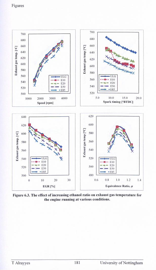
Figures
700 700
680 680
U 660 U 660 .:!... ° ci. 640 Q. 640
... ~ = = ., ., 620 ...
~~-... '" 620 '" eo: eo: OIl OIl 600 ... ... '" 600 '" ::s ::s eo: ~. eo: 580 ..c
..c ..: ..: (ool 580 ~ 560 ~ULG ~VLG
•••• •• EI O 560 .... .. E I O 540
- .. - E20 - .. - E20
520 - x- E50 540 - x- E50
........ - E85 ........ - E85
500 520
1000 2000 3000 4000 5.0 10.0 15.0 20.0
Speed (rpm( Spark timing (OBT DC(
640 620
620 600
U U 600 2- 580 .:!... Q.
ci. = ., E 580
... 560 !! '" eo:
'" OIl
eo: ... OIl '" 540 560 ::s ... eo: '" ::s ..c eo: ..: ..c (ool ..: 540 ~ULG 520 ~ULG (ool
.... .. EI O ...... EI O
520 -.- E20 500 -.- E20
- - E50 - - E50 ........ - E85 ........ - E85
500 480
0 10 20 30 0.6 0.8 1.0 1.2 1.4
EG R( % ( Eq uiva lence Ratio, f{J
Figure 6.3. The effect of increasing ethanol ratio on exhaust gas temperature for the engine running at various conditions.
T Alrayyes 181 University of Nottingham
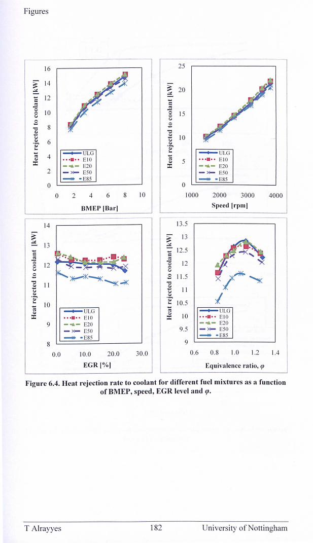
Figures
16
:s 14 ..::.::
C 12 e<: "0 o 10 c.J o -
2
o
14
:s ..::.:: 13 .... c e<: "0 o c.J o -.-' QJ s... 10
9
8
o
0.0
~ULG •• •••• EIO - ... - E20 - x- ESO - - E8S
2 4 6 8 10
BMEP IBarl
~ULG •••••• EIO - ... - E20 - x- ESO - - E8S
10.0 20.0 30.0
EGR I%I
25
:s 20 ..::.:: -c e<:
g 15 c.J o -'0
~ 10 c.J QJ .-' QJ s... .... ~ 5 :r:
o
~ULG
•••••• ElO - ... - E20
-- ESO - - E85
1000 2000 3000
Speed Irpml
13 .5
13
_ 12.5 c ~ o o c.J
o -'0
12
11.5
~ II QJ .-'
~ 10.5 .... e<:
:I: 10 ~ULG •••••• EIO - ... - E20
9.5 - x- ESO - - E85
9
0.6 0.8 1.0 1.2
Equivalence ratio, ffJ
4000
1.4
Figure 6.4. Heat rejection rate to coolant for different fuel mixtures as a function ofBMEP, speed, EGR level and lfJ.
T Alrayyes 182 U ni versity of N ottingharn
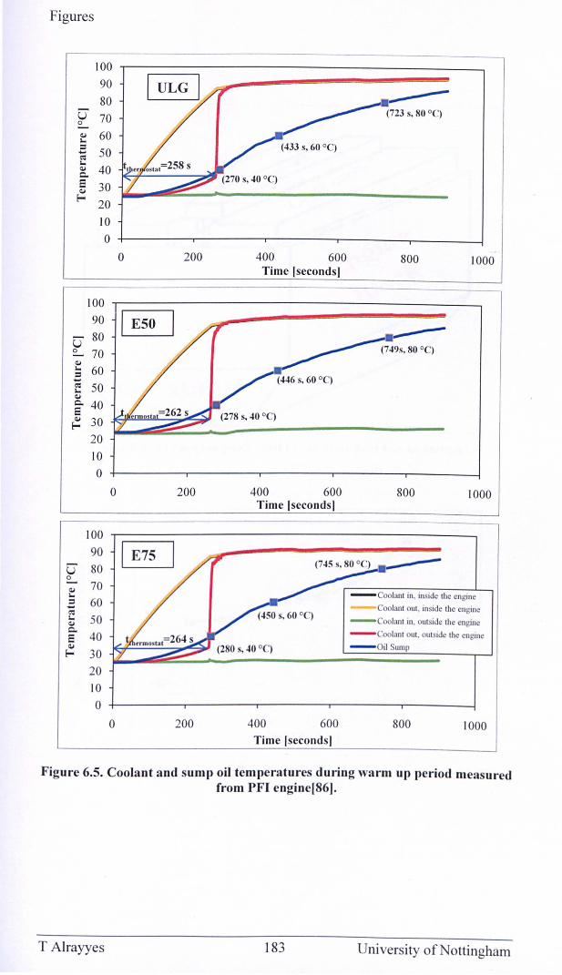
Figures
100 90 80
U 70 (723 s, 80 °C) 0
Q,) 60 lo. :::
50 ..... e<: lo. Q,) 40 c. E 30 Q,)
f- 20 10 0
0 200 400 600 800 1000 Time [seconds I
100
~ 90 80 ~7;'::-;O . c)
U 0 70
Q,) lo. 60 :::
(446 s, 60 °C) ..... e<: 50 lo. Q,)
c. 40 E Q,) 30 f-
20 10 0
0 200 400 600 800 1000 Time Isecondsl
100 90 ~ -
U 80 0
Q,) 70 lo. ::: 60 -- oolant Ollt, inside the eng-ine ..... e<: lo. 50 - oolant in, outside the engine Q,)
c. 40 - Coolant out , outside the engine E
Q,) - Oil Sump f- 30
20 10 0
0 200 400 600 800 1000 Time Iseconds l
Figure 6.5. Coolant and sump oil temperatures during warm up period measured from PFI enginer86] .
T Alrayyes 183 University of Nottingham
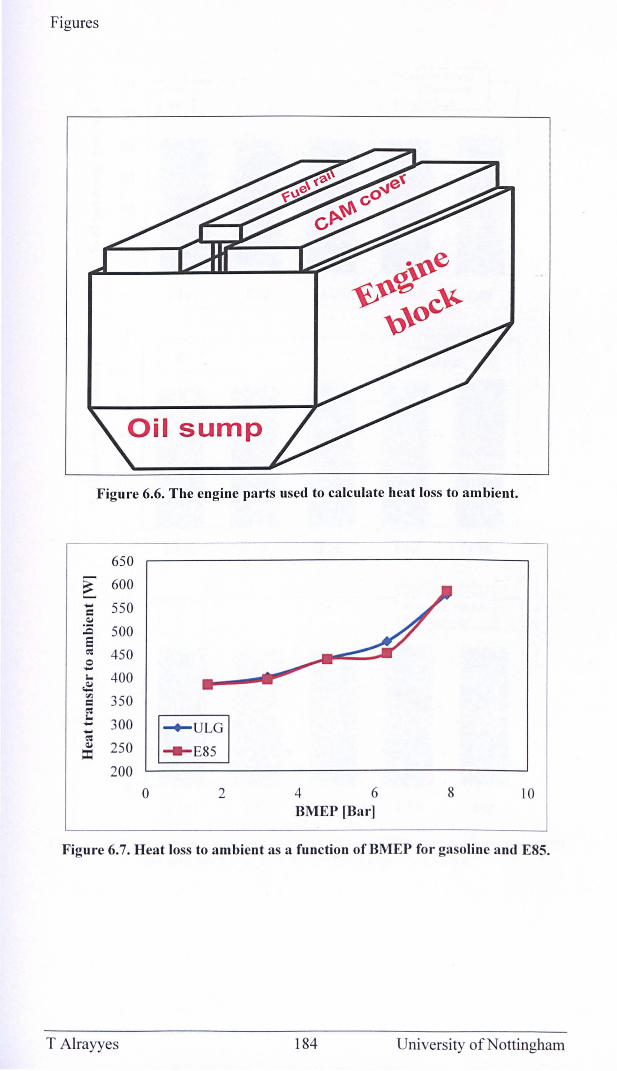
Figures
Figure 6.6. The engine parts used to calculate heat loss to ambient.
650
~ 600 ~ 550 c Q,j
:c e 500 ~ 450 0 ~
1.0 400 ~ '" 350 c ~ 1.0
300 ~
I : ULGI ~
~ Q,j 250 - E85 ==
200 0 2 4 6 8 10
BMEP [Bar]
Figure 6.7. Heat loss to ambient as a function ofBMEP for gasoline and E8S.
T Alrayyes 184 University of Nottingham
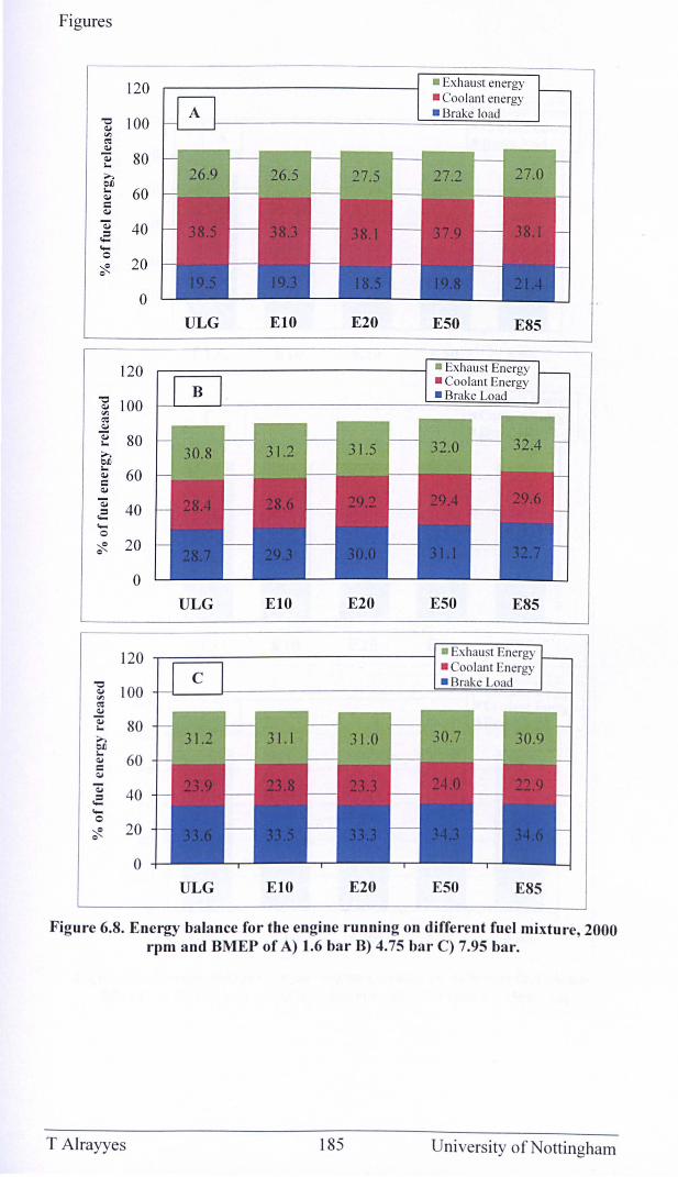
Figures
120
1S 100 til ~ ~
~ I-;>, Of) I~ :: ~
80
60
40
20
o
120
1S 100 til ~ ~
~ 80 ;>, Of)
~ 60 c ~
] 40 .... o ~ 20
o
- Exhaust energy - Coo lant energy - B load
26.5 27.5 27.0
ULG EIO E20 E50 E85
ULG EIO E20 E50 E85
120 r-;:====;-----------j
] 100 +-L-__ ~--------------------~===========L~ ~ ~
~ 80 ;>, Of)
~ 60 c ~
~ 40 .... o ~ 20
o ULG EIO E20 E50 E85
Figure 6.8. Energy balance for the engine running on different fuel mixture, 2000 rpm and BMEP of A) 1.6 bar B) 4.75 bar C) 7.95 bar.
T Alrayyes 185 University of Nottingham
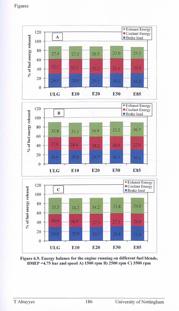
Figures
120 -.---===-------------1 . Exhaust Energy "0 • Coolant Energy ~ • Brake load ~ 100 +-~==~--------------------~======~~ ~
~ I.
g 80 I. ~
~ 60
"0 ~
40
20
o ULG EIO E20 E50 E85
• Exhaust Energy 120 .......---==:------------1 . Coolant Energy
'" ~ 100 +--~=~----------~========~ ~ I.
80
60
40
20
o ULG EIO E20 E50 E85
• Exhaust Energy 120 ..,------,==------------1 . Coolant Energy
1 00 -l-~~:!.------------=======r
80
60
40
20
o ULG EIO E20 E50 E85
Figure 6.9. Energy balance for the engine running on different fuel blends, BMEP =4.75 bar and speed A) 1500 rpm B) 2500 rpm C) 3500 rpm
T Alrayyes 186 University of Nottingham
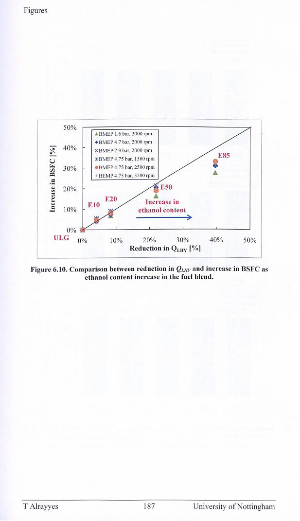
Figures
50%
~ 40% <:> -
30%
20%
10%
0% ULG 0%
ABMEP 1.6 bar, 2000 rpm
• BMEP 4.7 bar, 2000 rpm
x BMEP 7.9 bar, 2000 rpm
x BMEP 4.75 bar, 1500 rpm
• BMEP 4.75 bar, 2500 rpm
+ BEMP 4.75 bar, 3500 rpm
• E10 Increase in
10%
ethanol content )
20% 30% Reduction in QUIV [%]
E85
40% 50%
Figure 6.10. Comparison between reduction in Qu/V and increase in BSFC as ethanol content increase in the fuel blend.
T Alrayyes 187 University of Nottingham
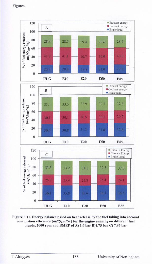
Figures
... o ~
120
20
o
120
28.5
ULG EIO
ULG EIO
ULG EIO
• Exhaust energy • Coolant energy • load
29.4 28.6
E20 E50 E85
E20 E50 E85
• Exhaust Energy • Coolant Energy
E20 E50 E85
Figure 6.11. Energy balance based on heat release by the fuel taking into account combustion efficiency (m/Qw v*'lc) for the engine running on different fuel
blends, 2000 rpm and BMEP of A) 1.6 bar B)4.75 bar C) 7.95 bar
T Alrayyes 188 University of Nottingham
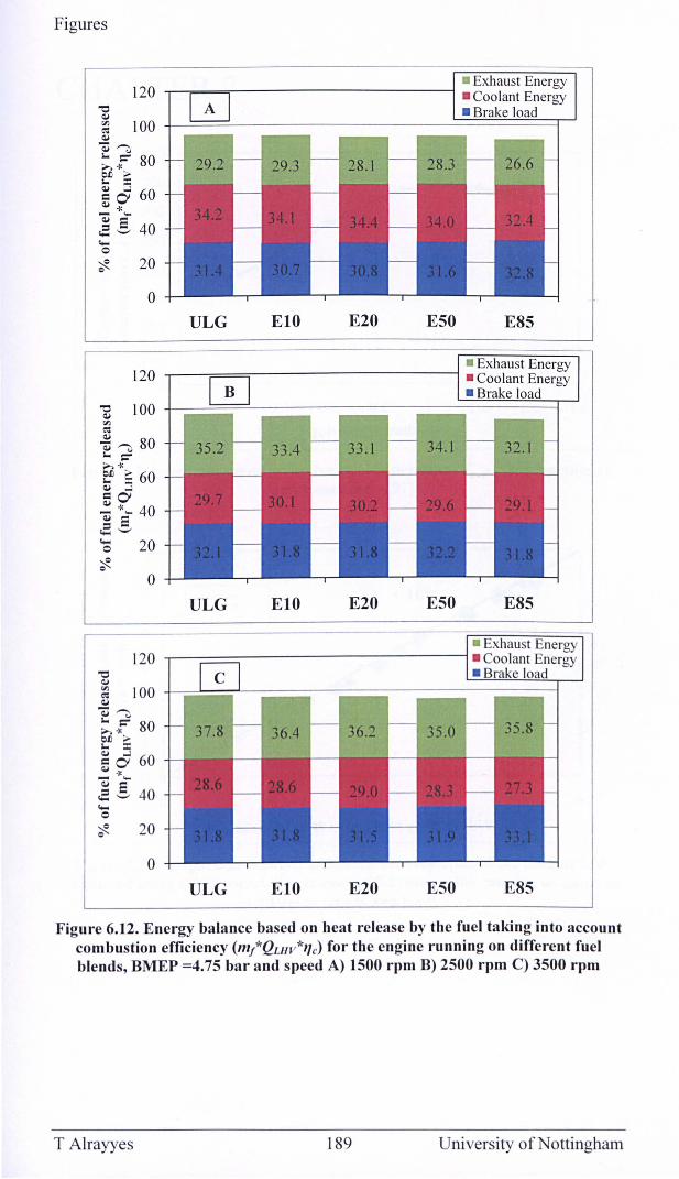
Figures
• Exhaust Energy 120 ...,-----.===,,---------------l • Coolant Energy
~ • Brake load ~ 100 +-~==~--------------~==========~ ~
~~ ~_;: 80 10. :I:
~ 0 60 ~ -x ~E ..= '-' 40 .... o ~ 20
o ULG
28.1 28.3 26.6
EIO E20 E50 E85
120 -,----==~------------j
.... o
o
120
~ 20
o
ULG
ULG
EIO E20 E50 E85
EIO E20 E50 E85
Figure 6.12. Energy balance based on heat release by the fuel taking into account combustion efficiency (m/QulV*llc) for the engine running on different fuel blends, BMEP =4.75 bar and speed A) 1500 rpm B) 2500 rpm C) 3500 rpm
T Alrayyes 189 University of Nottingham
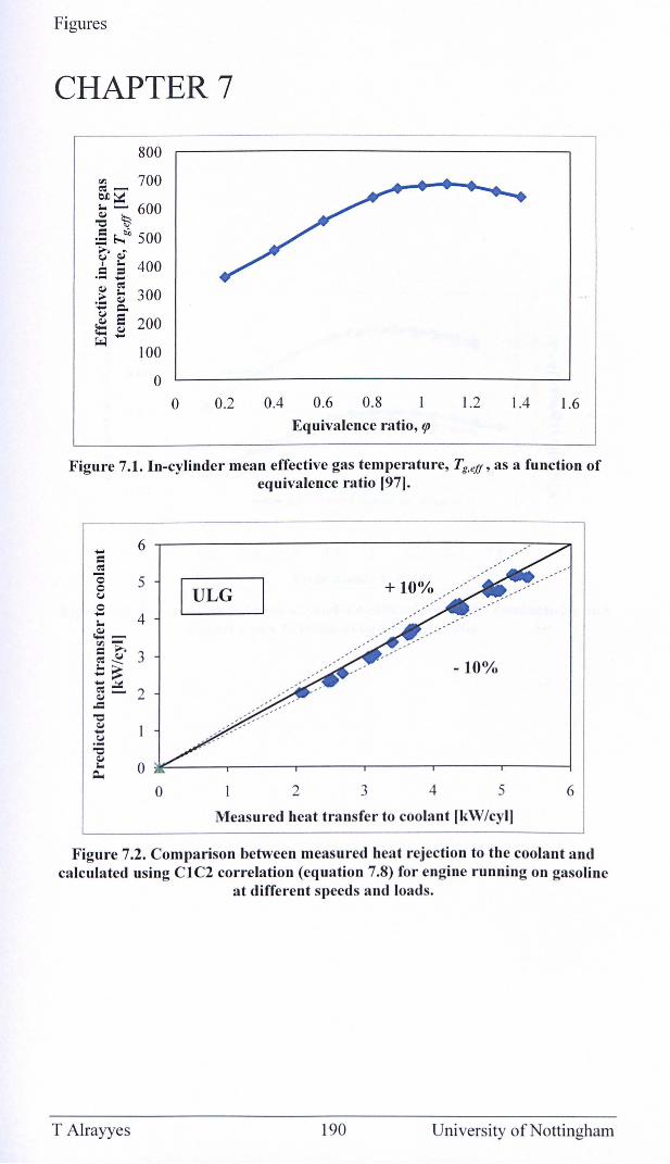
Figures
CHAPTER 7
800
'" 700 ~ -0Jl~ .. - 600 ~ ~ :E ~~ 500 ~~ ~ ; 400 .- ...-Q) ~
.:= ~ 300 - Q..
~ e 200 .... Q)
~-100
o o 0.2 0.4 0.6 0.8 1.2 1.4 1.6
Equivalence ratio, lfJ
Figure 7.1. In-cylinder mean effective gas temperature, Tg,eff' as a function of equivalence ratio [97].
...- 6 = ~
'0 5 +10% 0 ULG c.J 0 - 4 .. ~-"'-= ~ 3 ~ c.J .. -- -10% -~ -.::t: ~ - 2 Q)
.c '"0 Q) -.~
'"0 Q) .. 0 ~
0 2 3 4 5 6
Measured heat transfer to coolant fkW Icyl]
F igure 7.2. Comparison between measured heat rejection to the coolant and calculated using CIC2 correlation (equation 7.8) for engine running on gasoline
at different speeds and loads.
T Alrayyes 190 University of Nottingham
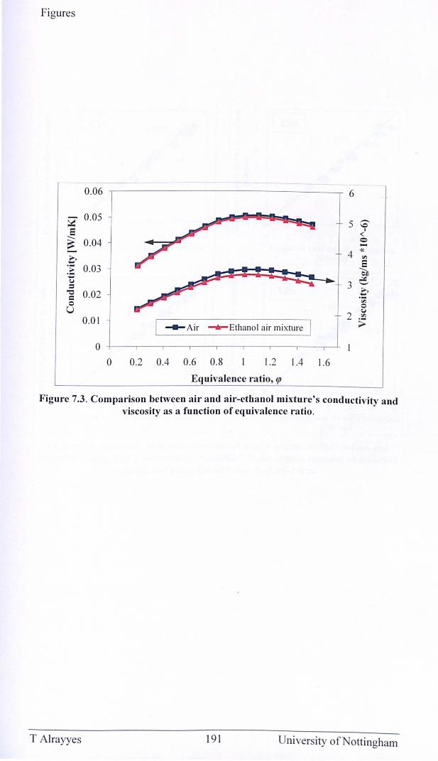
Figures
0.06 6
~ 0.05 /*1 I I I I I q 5 .-..
\C E I
< -- 0.04 Q
~ 7 1 -4 ·x
.0 '" E :~ 0.03 I ! ! ~ --...
~ !! C.J
3 '-" = .0 ~ 0.02 = 'r;; 0 0
U 2
C.J
'" 0.01 - Air -'-Ethanol air mixture ~
0
0 0.2 0.4 0.6 0.8 1.2 1.4 1.6
Equivalence ratio, lfJ
Figure 7.3. Comparison between air and air-ethanol mixture's conductivity and viscosity as a function of equivalence ratio.
T Alrayyes 191 University of Nottingham
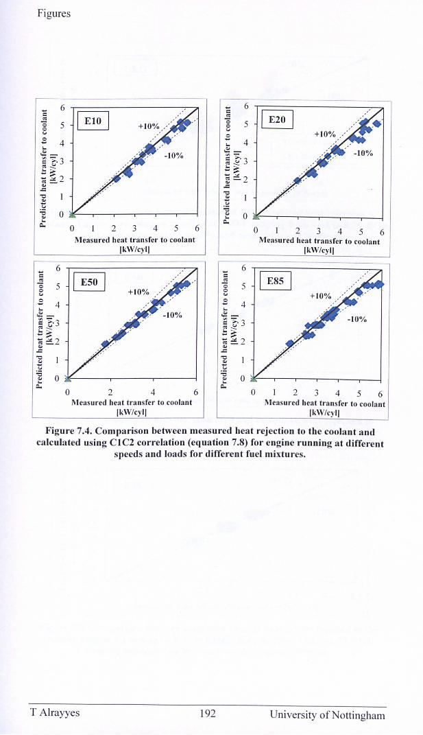
Figures
C «I '0 o CJ
o ...
6
5
4
... 6 C «I '0 5 0 CJ
E ... 4 ~-VJ ~,.., C CJ') «1--.::~ ~ :'2 .. ..c ~
~ .~ ~
0 .. ... c..
0
-10%
o 2 3 4 5 6 Measured heat transfer to coolant
I kW/cyl I
~
2 4 Measured heat transfer to coolant
I kW/cyl I
6
... 6 c «I '0 5 0 CJ
0 ... 4 ...
~-"'-C ..... "I «I CJ .)
::~ ~ :'2 ..c ~ .. ... . ~ ~ .. 0 ... c..
... 6 C «I '0 5 0 CJ
E 4 ... ~-~ ~3 «1--.::~ ~:. 2 .. ..c ~ .. ... . ~ ~
0 .. ... c..
o
0
§J
2 3 4 5 6 Measured heat transfer to coolant
IkW/cyl1
§]
2 3 4 5 6 Measured heat transfer to coolant
IkW/cy l1
Figure 7.4. Comparison between measured heat rejection to the coolant and calculated using CIC2 correlation (equation 7.8) for engine running at different
speeds and loads for different fuel mixtures.
T Alrayyes 192 University of Nottingham
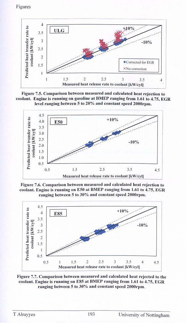
Figures
0 4 -~ 3.5 -C':I
ULG I. 1.= 3 ~ .... '" u c ..... C':I=: 2.5 I.~ --
-10%
--C':I c 2 ~ .c..:s "0 0
0 ~ u 1.5 - + Corrected for EGR
.~ XNo correction "0 ~ I. ~
1.5 2 2.5 3 3.5 4 Measured heat release rate to coolant [kW/cyIJ
Figure 7.5. Comparison between measured and calculated heat rejection to coolant. Engine is running on gasoline at BMEP ranging from 1.61 to 4.75, EGR
level ranging between 5 to 20% and constant speed 2000rpm.
---4.5
0 - 4.0 E50 ~ -C':I 3.5 I. 1.= ~ .... 3.0 '" u c ..... C':I=: 2.5 I.~ ---- 2.0 C':I c ~ C':I .c _
1.5 0 "0 0 ~ u 1.0 -.~
"0 0.5 ~ I. ~ 0.5 1.5 2.5 3.5 4.5
Measured heat release rate to coolant IkW/cyl]
Figure 7.6. Comparison between measured and calculated heat rejection to coolant. Engine is running on E50 at BMEP ranging from 1.61 to 4.75, EGR
ranging between 5 to 30% and constant speed 2000rpm.
0 4.5 -~ 4 -C':I E85
I. 3.5 I. = ~ ....
3 '" u c ..... C':I=: 2.5 I.~ ---- 2 C':I c ~ C':I .c _
1.5 "0 0 0
~ u - I .~ "0 ~ 0.5 I. ~
0.5 1.5 2 2.5 3 3.5 4 4.5 Measured heat release rate to coolant IkW/cYII
Figure 7.7. Comparison between measured and calculated heat rejected to the coolant. Engine is running on E85 at BMEP ranging from 1.61 to 4.75, EGR
ranging between 5 to 30% and constant speed 2000rpm.
T Alrayyes 193 University of Nottingham
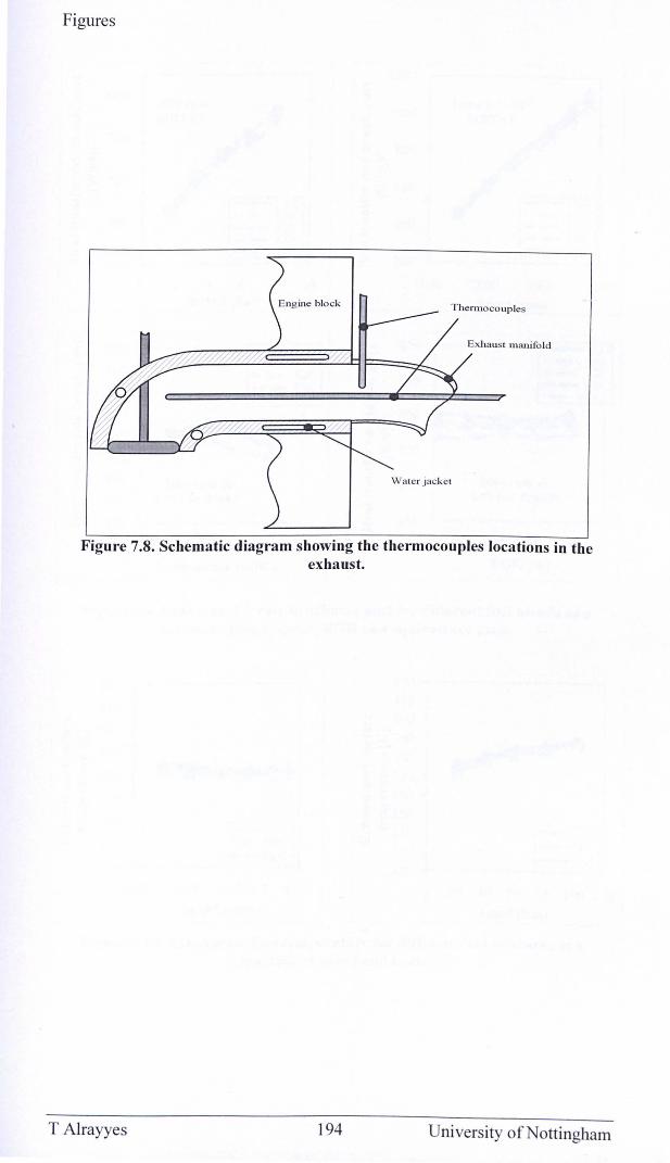
Figures
Thenno co uples
Exha us t m anifo ld
W a te r jacke t
Figure 7.8. Schematic diagram showing the thermocouples locations in the exhaust.
T Alrayyes 194 University of Nottingham
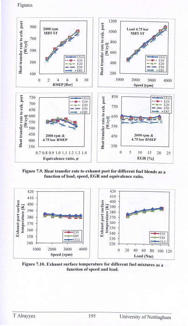
Figures
.... J,.,
g, 900 ..c ;.< Q,j
o 700 .... Q,j -.... ;>., ~ C.J
~ ~ 500 ~-In c: ~ J,., .... .... ~ Q,j
::
....
300
100
5 750 c. .c 700
~ 650 o ~ = 600 .... ;>.,
~ ~ 550 ~ -500 c: ~ 450 ...
400
350
o
2000 rpm MBTST
2 4
~ULG •• •• •• E IO - .... - E20 - x- ESO - - E85
6 8 10 BMEP IBarl
2000 rpm & 4.75 bar BMEP
-+-- ULG •• •• •• E IO - .... - E20 - x- E50 - - E85
0.7 0.8 0.9 1.0 1.1 1.2 1.3 1.4
Equivalence ratio, ffJ
.... J,.,
o c.
1200
..c 1000 ;.< Q,j
S 800 Q,j= ... ;>., ~ C.J J,.,--
J,., ~ 600 ~-In c: ~ 400 -.... ~ :: 200
1000
1::: 850 o c.
..c 750 ;.< Q,j
S _ 650 ~>. ~ C.J J,., --
J,., ~ 550 ~-In c: ~ 450 ...
350
o
Load 4.75 bar MBTST
5
--+-- ULG •• •• •• E IO - .... - E20 -x- ESO - - E85
2000 3000 4000 Speed Irpml
--+-- ULG •• •• •• E IO - .... - E20 - x- E50 - - E85
2000 rpm & 4.75 bar BM EP
10 15 20 25
EGR[%I
Figure 7.9. Heat transfer rate to exhaust port for different fuel blends as a function of load, speed, EGR and equivalence ratio.
420 .,---------
4 10 Q,j
~ ~ 400 ~ -; 390 ... J,.,
5 E 380 c.~ t; ~ 370 ::s ~ ~ 360 ;.< ...
W 350
340
1000 2000 3000 4000 Speed (rpm)
420 .,------------, 410
~ 400 ~:::c:: 390 ::s-.: ~ 380 5 E 370 c.~
.... ~ 360 '" c. ; E 350 ~ ~ 340 ---E50
w 330 ---E85
320 f--._-,----,.---=::;: ....... ==::;:U=L=G:.j
o 20 40 60 80 100 120
Load (Nm)
Figure 7.10. Exhaust surface temperature for different fuel mixtures as a function of speed and load.
T Alrayyes 195 University of Nottingham
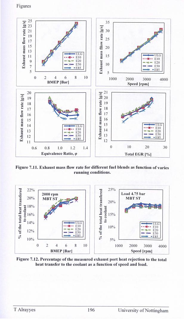
Figures
v; 25 35 'Os! 23
'" --~ 21 ~ 30 -eo: ~ I. 19 -~ eo: I. 25 0 17 ~ !;:
'" 15 0
'" 2 20 eo: e 13 '" ~ULG '" - II eo: 15 ~ULG
'" •• •• •• EIO e ::I •• •• •• EIO eo: 9 -.- E20 - -.- E20 .c: '" 10 ~ -x- E50 ::I
- x- E50 ... 7 - E85 eo: - .c:
- - E85 5 ~ ... 5 0 2 4 6 8 10 1000 2000 3000 4000
BMEP IBarl Speed rrpm]
20 V; 21 ~ --19 ~ 20 ~ ~ ~ 18 - 19 - eo: eo: I. I. 17 ~ 18 ~ 0
17 0 16 !;: !;:
'" '" 15 '" 16 '" eo: eo: e e 14 ~ULG -15 ~ULG - •• •• •• EIO '" •• •• •• EIO '" 13 ::I 14 -.- E20 ::I -.- E20 eo: eo:
- x- E50 .c: 13 - x- E50 .c: 12 ~ - - E85 ~
- - E85 ... ... II 12
0.6 0.8 1.0 1.2 1.4 0 10 20 30
Equ ivalence Ratio, ffJ Total EGR I % I
Figure 7.11. Exhaust mass flow rate for different fuel blends as function of varies running conditions.
~ 22% ~ I.
~ '" 20% c eo: I.
::: c 18% eo: eo: ~-
:: g 16% eo: e,;
- 0 .£ - 14% ~
.c: -... 12% 0
~ Q 10%
0 2
~ LG •• •• •• 10 -.- E20 - x- ESO - - E85
4 6
BMEP IBarl
8 10
~ 25% ~ I.
~ '" ; 20% I. --_ c eo: eo: ~-:: g 15% eo: e,;
o.E -~ 10% .c: -... 0
~ Q 5%
Load 4.75 bar MBTST
--+- ULG •• •• •• EIO -.- E20 - x- E50 - - E85
1000 2000 3000 4000 Speed Irpml
Figure 7.12. Percentage of the measured exhaust port heat rejection to the total heat transfer to the coolant as a function of speed and load.
T Alrayyes 196 University of Nottingham
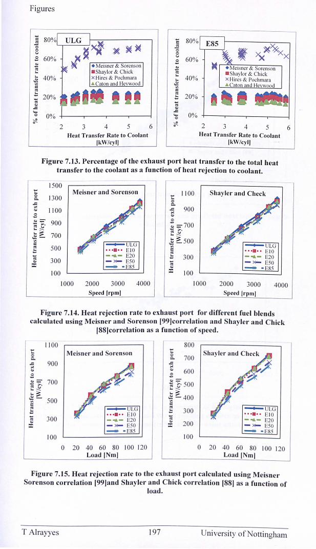
Figures
..... 80% ..... = 80% <.: = '0
~ ~~ ~
f ><x~»xXX 0 0 u 0 0 60%
(j
60% ..... 0 ., .... .... ., <.: .... .. <.: .. 40%
.. 40% ~ ..
'" ~ = '" <.: = !:: <.: 20% 20% .. .... ....
<.: .... ., <.: ..c: ., ... ..c: 0 0% ... 0% 0
::R ::R ~
5 6 2 " 4 2 3 4 ~ J 5 Heat Transfer Rate to Coolant Heat Transfer Rate to Coolant
IkW/cyll I kW/cyl I
Figure 7.13. Percentage of the exhaust port heat transfer to the total heat transfer to the coolant as a function of heat rejection to coolant.
1500 .... Meisner and Sorenson 1100 Shayler and Check .. .... 0 1300 Q. .. 0 ..c: Q.
>< 1100 ..c: 900 ., >< 0 ., .... 0 .,= 900 .... >. -: = 700 <.: (j .. -- .... >. .. ~ <.: U
700 .. --~- ~ ~ 500 '" = - ULG .......... ULG <.: 500 '" .. •••••• EIO = ...... EI O .... <.: ..... -.- E20 .. 300 -.- E20 <.: 300 .... ., - x- E50 .... - x- E50 :r: <.:
- - E85 .,
- - E85 100 :r: 100
6
1000 2000 3000 4000 1000 2000 3000 4000 Speed Irpml Speed Irpml
Figure 7.14. Heat rejection rate to exhaust port for different fuel blends calculated using Meisner and Sorenson [99]correlation and Shayler and Chick
[88]correlation as a function of speed.
1100 800 .... .... .. Meisner and orenson .. Iwyler and C heck 0 0 700 Q. Q.
..c: 900 ..c:
~ >< >< ., 600 .,
:= := ., = 700 .,= .... >. ~ C 500 <.: (j .. --.. -- .. ~ .. ~ ~- 500 ~ - 400 '" = = <.: _ ULG <.: .......... ULG .!: .. 300 ...... E IO .... .. .... E IO .... ....
300 -.- E20 <.: -.- E20 <.: ., ., 200 :r: -_ E50 :r: -~ E50 - - E85 - - E85 100 100
0 20 40 60 80 100 120 0 20 40 60 80 100 120 Load INml Load INml
Figure 7.15. Heat rejection rate to the exhaust port calculated using Meisner Sorenson correlation [99]and Shayler and Chick correlation [88] as a function of
load.
T Alrayyes 197 University of Nottingham
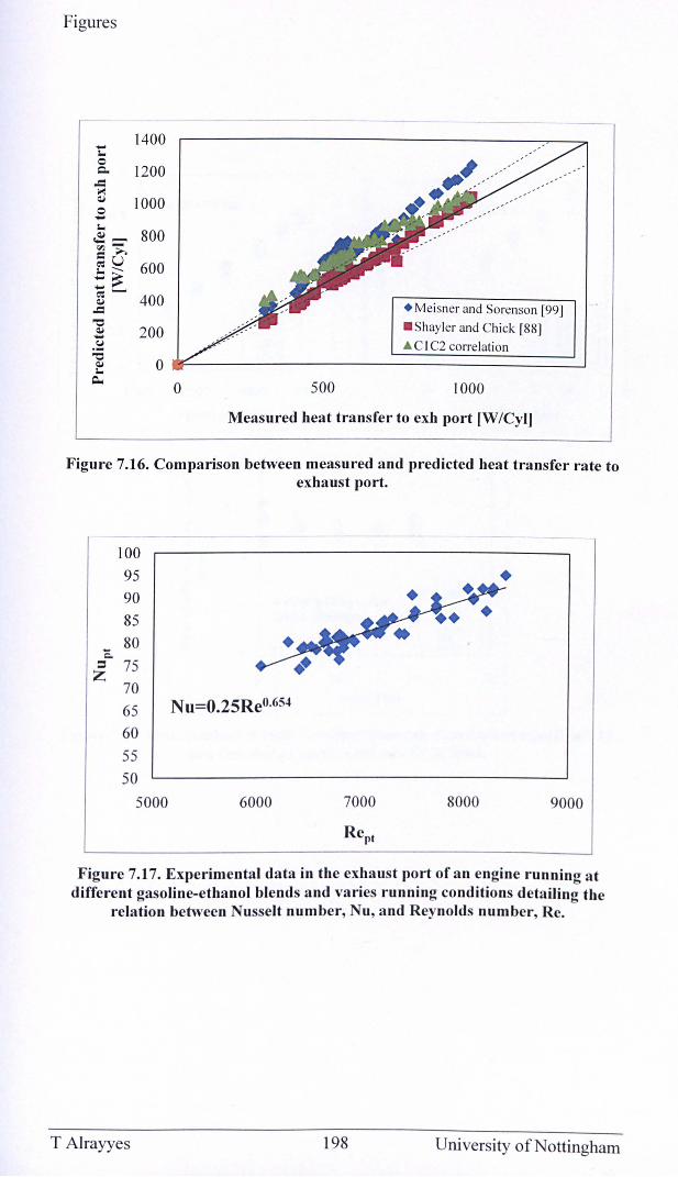
Figures
,----- ------------ -
.... -0 c.
.Q ~ ~
0 .... -~ ~ ~ -c: ..... ~U I. ....... .... ~ ~ ~ ~
.Q
"0 ~ -.~
"0 ~ -~
1400
1200
1000
800
600
400
200
0 0 500
• Meisner and Sorenson [99]
. Shayler and Chick [88]
.. C I C2 correlation
1000
Measured heat transfer to exh port [W/Cyl]
Figure 7.16. Comparison between measured and predicted heat transfer rate to exhaust port.
c..
100 95 90 85 80
i 75 70 65 60 55 50
5000
•
N u=O.25Reo.654
6000 7000 8000 9000
Figure 7.17. Experimental data in the exhaust port of an engine running at different gasoline-ethanol blends and varies running conditions detailing the
relation between Nusselt number, Nu, and Reynolds number, Re.
T Alrayyes 198 University of Nottingham
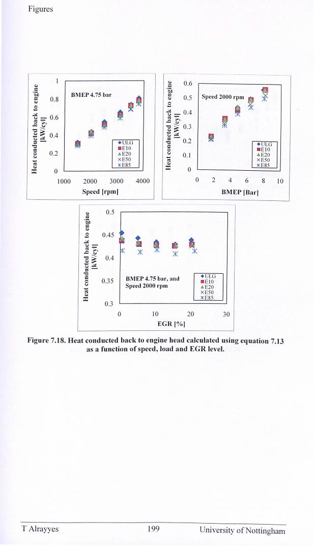
Figures
<I)
c 'eD ~ 0.8 o --t3 - 0.6 <.:-..cG' "O~ ~..:.:: 0.4 ="0 C o 0.2 c.;
-<.: <I)
::t 0
1000
BMEP4.75 bar
+ ULG _ E IO . E20 x E50 x ESS
~ 0.6 'eD ~ 0.5 o --t3 _ 0.4 <.:-
if 0.3 1:j..:.:: =-"0 0.2 c o c.; 0.1
o 2000 3000 4000
Speed Irpml
<I) 0.5 c 'eD c <I)
0 0.45 --..:.:: c.;~
<.:-..cG' ::K "0 -- 0.4 <I)~ 1:j..:.:: =-"0 c BMEP 4.75 bar, and 0 0.35 c.; Speed 2000 rpm .... <.: <I)
::t 0.3
o
::K
0 10 20 EGR/% I
Speed 2000 rpm ~
2
+ ULG - EIO . E20 x E50 x E8S
4 6
+ ULG - EIO . E20 x ESO XESS
8
BMEP IBarl
30
10
Figure 7.18. Heat conducted back to engine head calculated using equation 7.13 as a function of speed, load and EGR level.
T Alrayyes 199 University of Nottingham
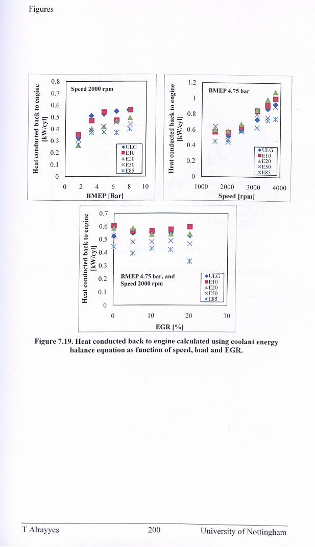
Figures
--- ---0.8 1.2
~ ~ c Speed 2000 rpm c BMEP4.75 bar .. ·Sn 0.7 ·Sn c c
t' ~ ~
0 0.6 • 0 - , • -ti = 0.5 & .. ..:.:: 0.8
~)K CJ - • c:o:s-c:o:s .....
* i i 0.6 ~ CJ
~ )K az ~ 0.4
I )K )K
ti ..:.:: 0" ti..:.:: )K ~ :: ~ .-' ::-
'1:) + ULG '1:) 0.4 c 0.2 c + ULG 0 _ EI O 0
- EI O CJ A E20 CJ ..... - 0.2 A E20 c:o:s 0.1 x E50 c:o:s
X E50 ~ ~
:c: x ES5 ::c x E85 0 0
0 2 4 6 8 10 1000 2000 3000 4000 BMEP [Barl Speed [rpml
~ 0.7 c
·Sn 0.6 • c ~
0 0.5 .....
X X X ..:.:: X CJ - )K )K c:o:s-~ C O.4 )K '1:)-- )K ~~ ti ..:.:: 0.3 ::-
'1:) 0.2 BMEP4.75 bar, and + ULG c
- E IO 0 Speed 2000 rpm CJ A E20 ..... 0.1 x E50 c:o:s ~ x E85 ::
0
0 10 20 30
EGRI%I
Figure 7.19. Heat conducted back to engine calculated using coolant energy balance equation as function of speed, load and EGR.
T Alrayyes 200 University of Nottingham
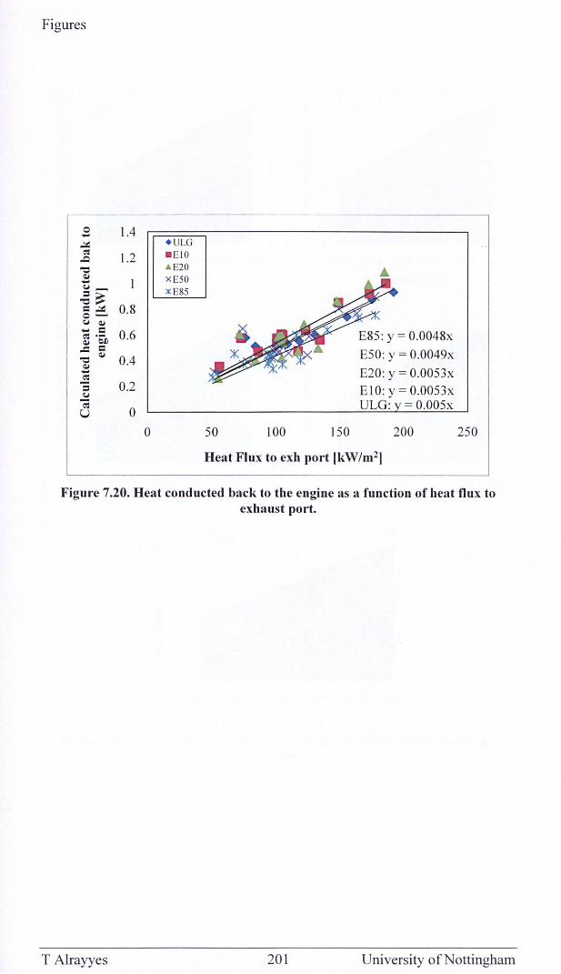
Figures
0 1.4 ..... .!:I: . ULG ~
1.2 _ EI O .Q "0 £ E20 ~ X E50 ..... ~- x E85 .;~
0.8 =.!:I: 0-~ ~ ..... = 0.6 ~ .-~ bJ)
-= = E50: y = 0.0049x "0 ~
0.4 ~ ..... E20: y = 0.0053x ..:s = 0.2 E 1 0: y = 0.0053x ~
-; 0 U
ULG: = 0.005x
0 50 100 150 200 250
Heat Flux to exh port [kW/m2]
Figure 7.20. Heat conducted back to the engine as a function of heat flux to exhaust port.
T Alrayyes 201 University of Nottingham
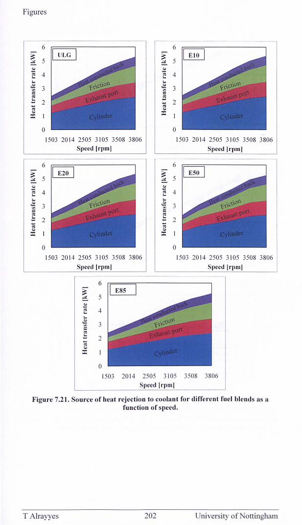
Figures
6
~ 5 ~ -E 4 ~
~ 3 = ~
.:: 2 -~ ~
:I:
o 1503 2014 2505 3105 3508 3806
Speed [rpml
1503 2014 2505 3105 3508 3806 Speed Irpml
6
5
4
3
2
o
1503 2014 2505 3105 3508 3806 Speed [rpml
1503 2014 2505 3105 3508 3806 Speed Irpml
1503 20 14 2505 3105 3508 3806 Speed Irpml
Figure 7.21. Source of heat rejection to coolant for different fuel blends as a function of speed.
T Alrayyes 202 University ofNottingharn
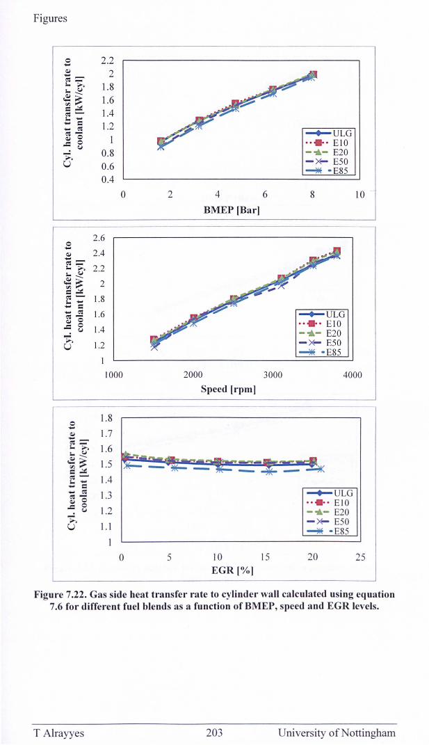
Figures
.s 2.2
o ..... Q) .....
2 1.8 1.6 1.4 1.2
I 0.8 0 .6 0.4
2.6
2.4 eo: = ;.. ;>.. 2.2 ;..~
~:s ~~ E:; 1.8
2
..... c: ~ ~ 1.6 .c: 8 1.4 ...: ;>.. U 1.2
1
o
1000
o 1.8 ..... ~ 1.7 eo: = ~ ~ 1.6 ~:s ~~ eo:-;.. .... ..... c: .... eo: ~o
.c: 0 • <:J
~ U
1.5
1.4
1.3
1.2
1.1
I
o
2
5
4
BMEP [Bar]
2000
Speed [rpm]
10 EGR[%]
6
3000
15
--+-ULG .. .. . E IO - .. - E20 -~ E50 ~ - E85
8
--+-ULG •• • •• EIO - .. - E20 - x- E50 ~ - E85
10
4000
--+-ULG .. .. . EIO - .. - E20 -~ E50 ~ - E85
20 25
Figure 7.22. Gas side heat transfer rate to cylinder wall calculated using equation 7.6 for different fuel blends as a function of BMEP, speed and EGR levels.
T Alrayyes 203 University of Nottingham
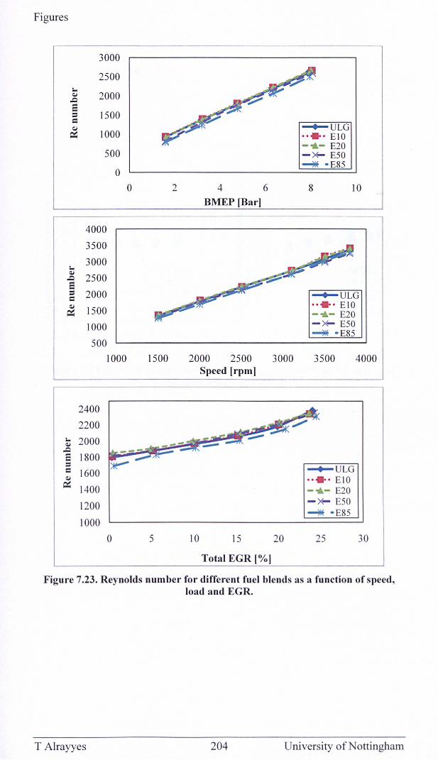
Figures
4000
3500
3000 1.0 ~
2500 .c e = 2000 ~ULG = ~ 1500
.. .. . EIO ~ - .. - E20
1000 -x- E50 ~ - E85
500 1000 1500 2000 2500 3000 3500 4000
Speed [rpm]
2400
2200 1.0 2000 ~ --- ---.c e 1800 = ~ ~ULG = 1600 ~ •• • •• E IO ~ 1400 - .. - E20
1200 -~ E50 ~ - E85
1000
0 5 10 15 20 25 30
Total EGR [% ]
Figure 7.23. Reynolds number for different fuel blends as a function of speed, load and EGR.
T Alrayyes 204 University of Nottingham
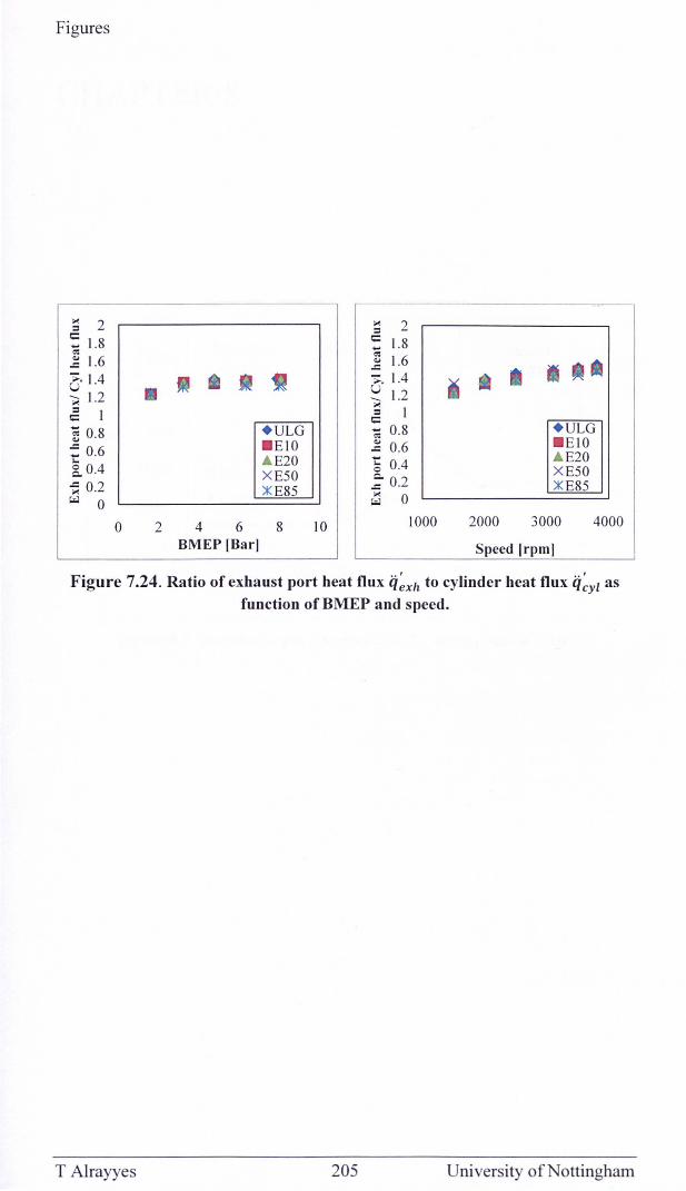
Figures
~ 2 r: 1.8 ~
~ 1.6 CI A ~ 1.2 ~ I ~ 0.8 :: 0.6 ~ OA ~ 0.2 W 0
0 2
. ULG
. EIO AE20 XE50 ::K E85
4 6 8 BMEP [Barl
10
~ 2 r: 1.8 ~
~ 1.6 ~I A
::: 1.2 ~ I
t:: ~ 0.8 ~ 0.6 ~ OA .; 0.2 ~ 0
1000 2000
. ULG
. E IO A E20 XE50 ::K E85
3000 4000
Speed Irpml
Figure 7.24. Ratio of exhaust port heat flux q~xh to cylinder heat flux q~Yl as function of BMEP and speed.
T Alrayyes 205 University of Nottingham
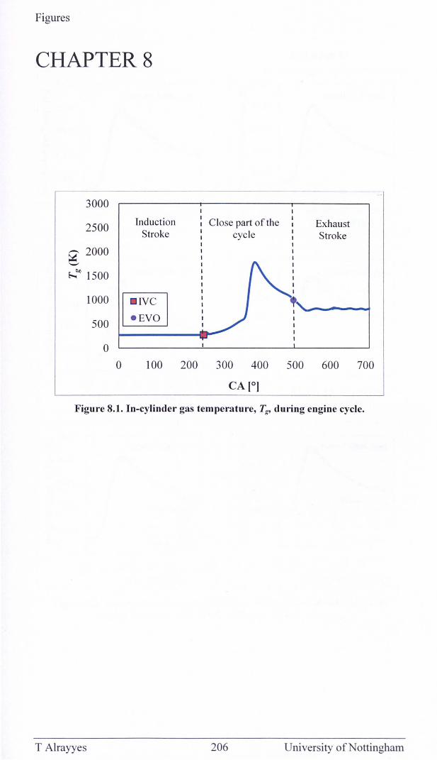
Figures
CHAPTER 8
----
3000
2500 Induction Close part of the Exhaust Stroke cycle Stroke
~ 2000 --Eo-. ().o 1500
1000
~ 500 - Eva
0 0 100 200 300 400 500 600 700
CA [0]
Figure 8.1. In-cylinder gas temperature, Tg, during engine cycle.
T Alrayyes 206 University of Nottingham
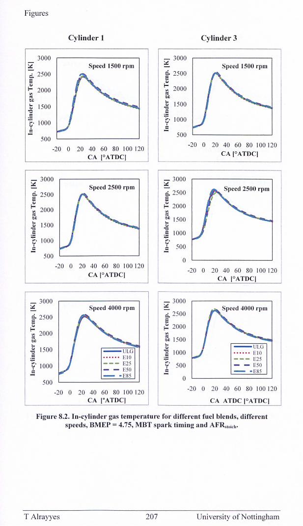
Figures
3000
~ ci. 2500 E ~
~ 2000 Vl e<l ell
~ 1500 'C oS ;;, 1000 (j I
C ..... 500
Cylinder 1
Speed 1500 rpm
-20 0 20 40 60 80 100 120 CA rOATDq
_ 3000 ::(
~ 2500 ~
E:; 2000 e<l ell
~ 1500 'C oS ;;, 1000 (j
I C
500
_ 3000 ::(
~ 2500 ~
~ 2000 e<l ell I...
~ 1500 c
~ 1000 c
500
Speed 2500 rpm
-20 0 20 40 60 80 100120 CA IOATDq
Speed 4000 rpm
•••••• EI O --- E25 - - E50 - - E85
-20 0 20 40 60 80 1001 20 CA IOATDq
~ 3000
~ 2500 ~
E:; 2000 e<l ell
~ 1500 'C c
~ 1000 I
C - 500
_ 3000 ::(
ci. 2500 E ~ 2000 Vl e<l
~ 1500 ~
'C oS 1000 ;;, (j
C 500 -o
- 3000 ::(
C. 2500 E ~ 2000 Vl
~ 1500 I... ~
] 1000 ;;, 'f 500 c
o
Cylinder 3
Speed 1500 rpm
-20 0 20 40 60 80 100120 CA rOATDq
-20 0 20 40 60 80 100 120 CA IOATDq
•••••• EtO --- E25 - - E50 - - E85
-20 0 20 40 60 80 1001 20
CA ATDC IOATDq
Figure 8.2. In-cylinder gas temperature for different fuel blends, different speeds, BMEP = 4.75, MBT spark timing and AFRstoich '
T Alrayyes 207 University of Nottingham
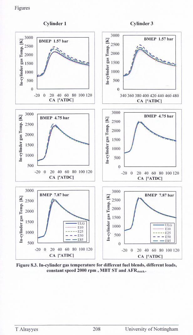
Figures
Cylinder 1
_3000 :::.=: BMEP 1.57 bar ci: 2500 E ~ 2000
'" ~ 1500 IQ,j
] 1000 ;;. 't 500 c - o
_ 3000
-20 0 20 40 60 80 100120 CA IOATDq
:::.=: BMEP 4.75 bar
~ 2500 Q,j
: 2000 ~ ell I-Q,j
"0 c ;;. "" I C -
1500
1000
500
3000
:::.=: 2500 ci. E ~ 2000
'" ~ ~ 1500 Q,j
"0 C
..... "" I C
1000
500
-20 0 20 40 60 80 100120 CA IOATOq
BMEP 7.87 bar
--ULG •.• •• . ••. EIO
----- E25 - - - E50 - - E85
-20 0 20 40 60 80 100120
CA IOATOq
3000 ~ -:- 2500 c. E ~ 2000
'" ~ 1500 IQ,j
] 1000 ;;. 't 500 c
o
Cylinder 3
BMEP 1.57 bar
340360380400420440460480 CA IOATDq
3000
:::.=: 2500 ci. ~ 2000
F-o
'" ~ 1500 IQ,j
"0 1000 .: G' 500 I C
o
3000 ~ -:- 2500 c.
~ 2000
'" ~ 1500 IQ,j
] 1000 ;;. 't 500 c
o
BMEP 4.75 bar
-20 0 20 40 60 80 100120 CA IOATDq
BMEP 7.87 bar
--ULG .• •.• •..• EIO
----- E25 - - - E50 - - E85
-20 0 20 40 60 80 1001 20
CA IOATOq
Figure 8.3. In-cylinder gas temperature for different fuel blends, different loads, constant speed 2000 rpm, MBT ST and AFRstoich .•
T Alrayyes 208 University of Nottingham
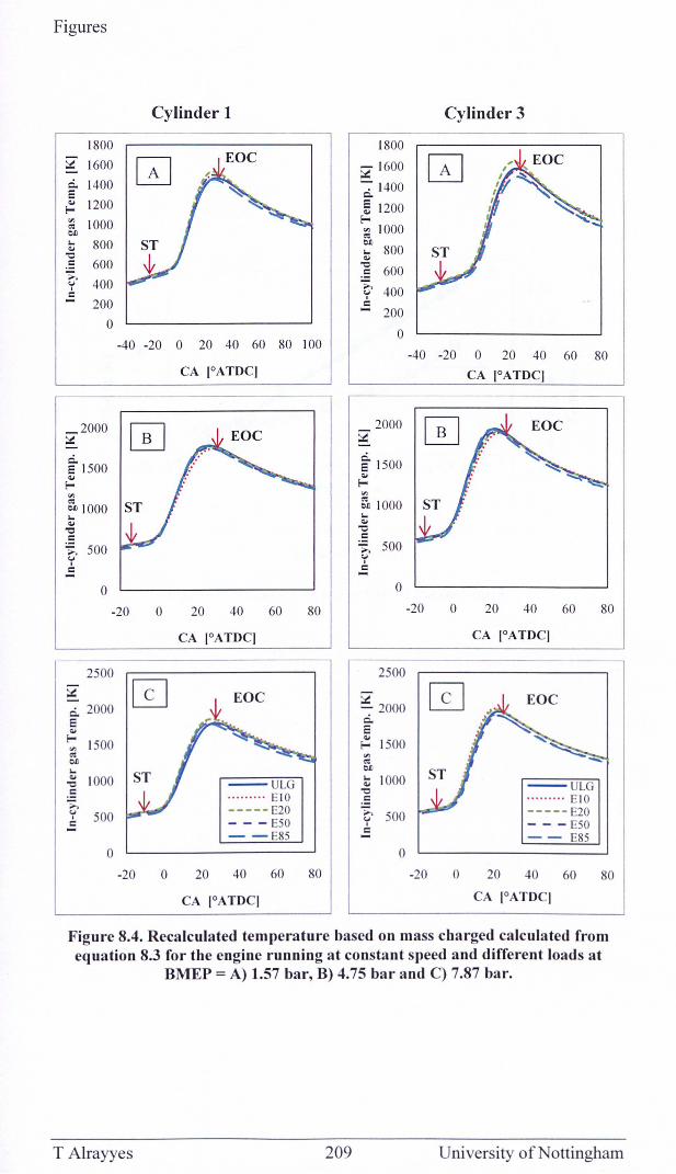
Figures
Cylinder 1 Cylinder 3
1800 1800 ~ 1600 0 ~ 1600 0 Eoe c.. 1400 c.. 1400 = .. 1200 ~ 1200 E-'" 1000 E-~ ~ 1000 en ... 800 en .. 800 "0 ... .. c 600 "0
..... c 600 <.I 400 ..... ,
400 c <.I - 200 , c
200 0
0 -40 -20 0 20 40 60 80 100
-40 -20 0 20 40 60 80 CA IOATOq CA IOATOq
_2000 ~
2000 ~ Eoe ~ ~
c.. t 1500 = 1500 .. .. E- E-
'" '" ~ 1000 ST ~ 1000 ... ... .. ..
"0 "0
.: .: 500 ~ 500 ~
<.I Y C: c -
0 0
-20 0 20 40 60 80 -20 0 20 40 60 80
CA IOATOq CA IOATOq
2500 2500
~ [£] Eoe ~ 2000 [£] Eoe c.. 2000 = c.. .. = E- 1500 ~ 1500 ~~--'" ~ '" en ~ ... en .. 1000 ~ 1000 "0 --ULG - ULG c "0
~ .. ...... . EtO c .. .... ... EtO
<.I 500 ----- E20 ..... 500 ----- E20 , - - - ESO <.I
C , - - - -50 - - E85
c -- E85
0 0
-20 0 20 40 60 80 -20 0 20 40 60 80
CA IOATDq CA IOATOq
Figure 8.4. Recalculated temperature based on mass charged calculated from equation 8.3 for the engine running at constant speed and different loads at
BMEP = A) 1.57 bar, B) 4.75 bar and C) 7.87 bar.
T Alrayyes 209 University of Nottingham
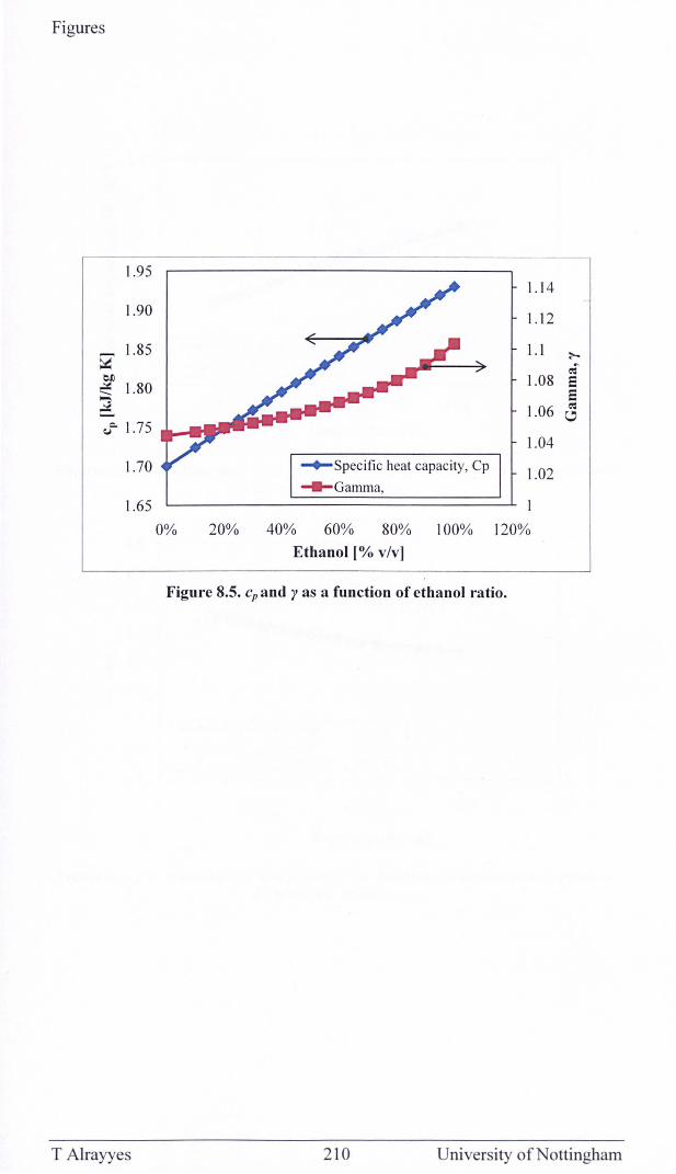
Figures
1.95
1.90
~ 1.85 ~
!l __ 1.80
~
1.1 4
1.12
1.1 ~
1.08 5
CJC- 1. 75 .L.-4 ........ ~-5
1.06 ~
1.70
1.65
T Alrayyes
~Specific heat capacity, Cp
_ Gamma,
1.04
1.02
0% 20% 40% 60% 80% 100% 120%
Ethanol [% v/v]
Figure 8.5. cp and y as a function of ethanol ratio.
210 University of Nottingham
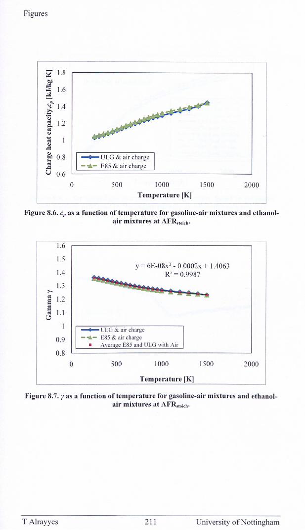
Figures
.... ~ ~ -= ~
0.8 OJ) I. ~ -= u 0.6
0
--..- ULG & air charge
-.-- £85 & air charge
500 1000 Temperature [KJ
1500 2000
Figure 8.6. cp as a function of temperature for gasoline-air mixtures and ethanolair mixtures at AFRstoich.
1.6
1.5
1.4
1.3 >-~ 1.2 S S
1.1 ~
Co-'
0.9
0.8 0
y = 6E-08x2 - 0.0002x + 1.4063 R2 = 0.9987
~ ULG & air charge
- .. - E85 & ai r charge • Average E85 and ULG with Ai r
500 1000
Temperature [KJ
1500 2000
Figure 8.7. 'I as a function of temperature for gasoline-air mixtures and ethanolair mixtures at AFRstoich.
T Alrayyes 211 University of Nottingham
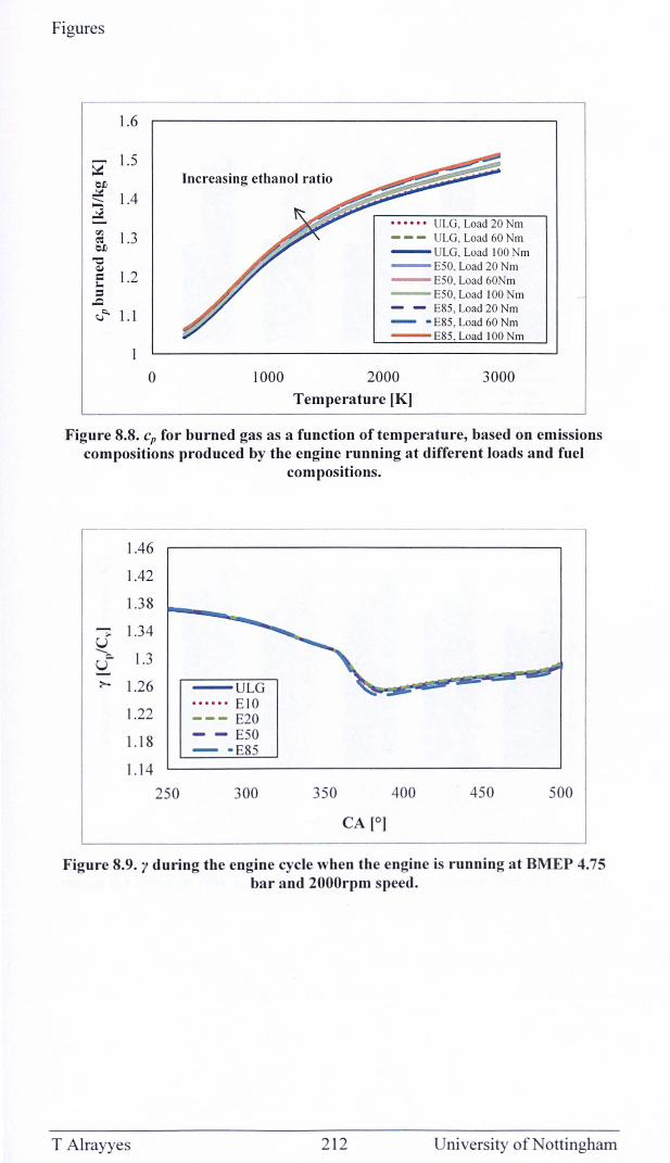
Figures
1.6
~ 1.5
OJ) ~ 1.4 --..., ~ ........ ~ 1.3 ~ OJ)
~ <II
1.2 c 10. ::: .:. ","'" 1.1
o
Increasing ethanol ratio
1000
•••••• ULG, Load 20 Nm - - - ULG, Load 60 Nm - ULG, Load 100 Nm - ESO, Load 20 Nm - ESO, Load 60Nm - ESO, Load 100 Nm - - E85, Load 20 Nm - - E8S, Load 60 Nm - E85,Load 100Nm
2000 Temperature [KJ
3000
Figure 8.8. cp for burned gas as a function of temperature, based on emissions compositions produced by the engine running at different loads and fuel
compositions.
--
1.46
1.42
1.38
"""'; 1.34 U .......
1.3 Q.
~ :- 1.26 - ULG
1.22 •••••• E I 0 --- E20
1.18 - - E50 - E85
1.14
250 300 350 400 450 500
CA [0J
Figure 8.9. "I during the engine cycle when the engine is running at BMEP 4.75 bar and 2000rpm speed.
T Alrayyes 212 University ofNottingharn
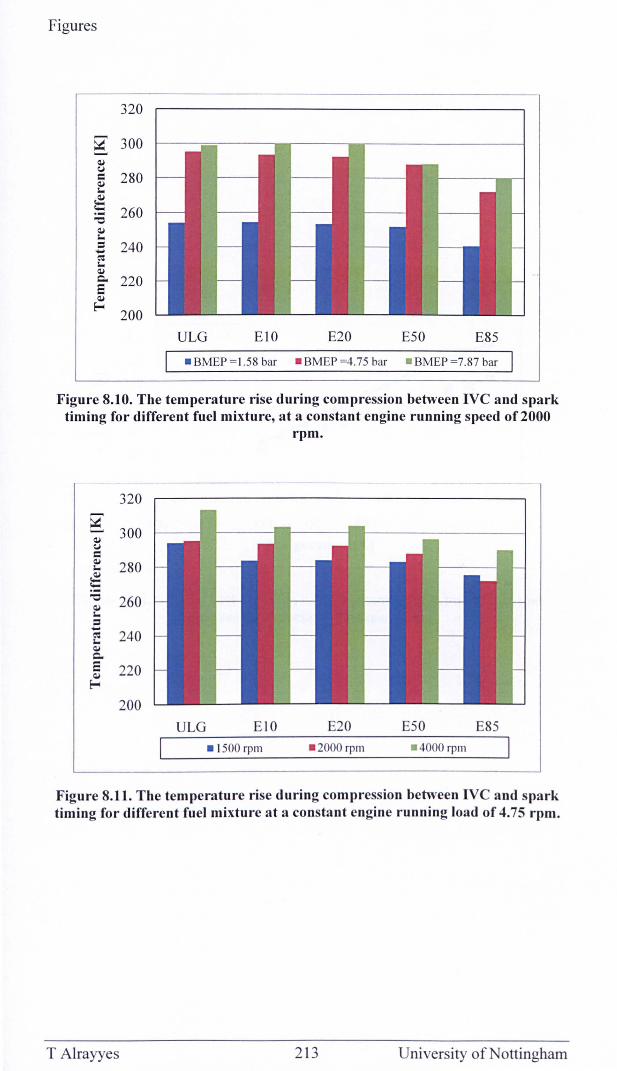
Figures
320
g 300 Qj ~ = 280 Qj I.
~ ~ 260 "0 Qj I. ::I 240 ..... ~ I. Qj Q., 220 E Qj
Eo-; 200
ULG EI0 E20 E50 E85
- BMEP = 1.58 bar - BMEP =4.75 bar - BMEP =7.87 bar
Figure 8.10. The temperature rise during compression between IVC and spark timing for different fuel mixture, at a constant engine running speed of 2000
rpm.
320
g 300
Qj ~
= Qj
280 I.
~ !: "0 260 Qj I. ::I .....
240 ~ I. Qj Q.,
E 220 Qj
Eo-;
200 ULG EIO E20 E50 E85
- 1500 rpm - 2000 rpm - 4000 rpm
Figure 8.11. The temperature rise during compression between IVC and spark timing for different fuel mixture at a constant engine running load of 4.75 rpm.
T Alrayyes 213 University of Nottingham
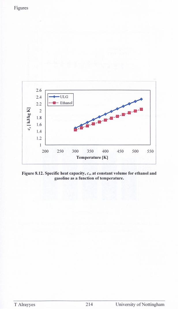
Figures
- --
2.6
2.4 ~ULG
2.2 •• •• • Ethanol
~ 2 • •• eJ) ••••• .::( 1.8 •• ~ ••••• .::(
1.6 •••• '" •••• <:.J
1.4
1.2
1 200 250 300 350 400 450 500 550
Temperature [K]
Figure 8.12. Specific heat capacity, cv, at constant volume for ethanol and gasoline as a function of temperature.
T Alrayyes 214 University of Nottingham
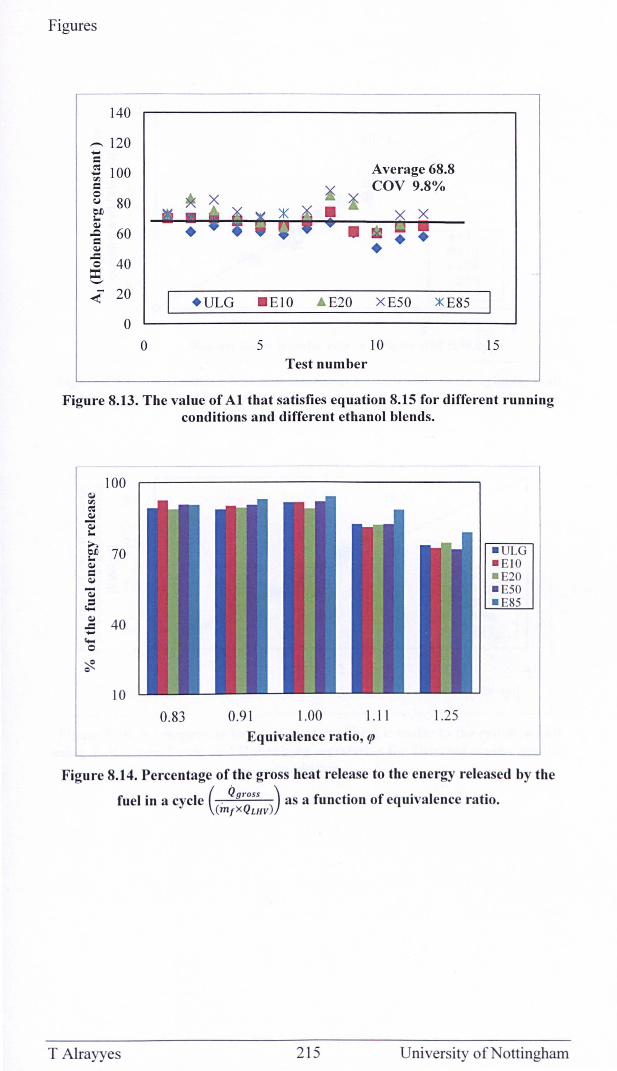
Figures
140
-120 .... c .fS 100 '" c 0 CJ 80 t=J) :.. ~
60 .Q C ~
..c 40 0 e
< 20
o o
Average 68.8 COY 9.8%
X
• + ULG - E10 . E20 x E50 ::I( E85
5 10 15 Test number
Figure 8.13. The value of Al that satisfies equation 8.15 for different running conditions and different ethanol blends.
100 ~
'" ~ ~
~ :.. ....
- ULG ell 70 :.. ~ - EIO c - E20 ~
~ - E50 .;: - E85 ~
40 ..c .... '-0
~ 0
10
0.83 0.91 1.00 1.11 1.25
Equivalence ratio, tp
Figure 8.14. Percentage of the gross heat release to the energy released by the
fuel in a cycle ( . Qgross ) as a function of equivalence ratio. (m,x QLHv)
T Alrayyes 215 University of Nottingham
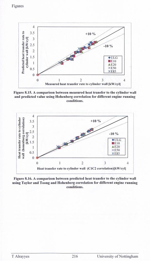
Figures
4
.E 3.5 QJ +10% -E ~ 3 '-~
~~ . 2.5 -10 % (\1-
.= =; 2 .... .. (\I ~
~ ~ 1.5 + ULG "0 "0 . EIO QJ .S . E20 .~~ ~ <.J 0.5 X E50 ~ 0 ~~ ________________________ ~==~==E=85==~
o 2 3 4 Measured heat transfer rate to cylinder wall [kW/cyll
Figure 8.15. A comparison between measured heat transfer to the cylinder wall and predicted value using Hohenberg correlation for different engine running
conditions.
4 '- -QJ C -g .g 3.5 :.: (\I
~'E 3 o '-.... ;3 _2.5 ~ ~ E ~~ 2 '-E~ ~ C ..::.:: 1.5
<IJ QJ -C C (\I 0 '-.:: .... '-'
+10%
-10 %
+ ULG . EtO . E20 XE50 ~ E85 ~ =; 0.5
~ ~ 0 ~~------------------------------------------~ o 2 3 4
Heat transfer rate to cylinder wall (CIC2 correlation)lkW/cyll
Figure 8.16. A comparison between predicted heat transfer to the cylinder wall using Taylor and Toong and Hohenberg correlation for different engine running
conditions.
T Alrayyes 2 16 University of Nottingham
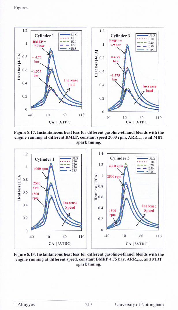
Figures
1.2 1.2 Cylinder 1 - ULG Cylinder 3 - ULG
•••••• EIO •••••• EIO BMEP= --- E20 BMEP=
--- E20 7.9 bar - - E50 - - E50
- - E85 - - E85
<' <' u U 0.8 ;; 0.8 --..., '"
'" '" '" .£ .£ 0.6 ~ 0.6 .... ~ :I: <U :I:
0.4 0.4
0.2 0.2
0 0
-40 10 60 11 0 -40 10 60 11 0
CA IOATOq CA IOATDq
Figure 8.17. Instantaneous heat loss for different gasoline-ethanol blends with the engine running at different BMEP, constant speed 2000 rpm, A RRstoich and MBT
spark timing.
1.2 1.4
Cylinder 1 - ULG Cylinder 3 - ULG •••••• EIO •••••• E IO --- E20 1.2 --- E20 - - E50 - - E50 - - E85 - - E85
< < 1 ~ 0.8 U --..., :::.. '" ~ 0.8 '" .£ 0.6 .£ - .... ~ ~ <U :: 0.6 :I:
0.4 0.4
1500
0.2 0.2
0 0
-40 10 60 110 -40 10 60 110
CA IOATOq CA IOATOq
Figure 8.18. Instantaneous heat loss for different gasoline-ethanol blends with the engine running at different speed, constant BMEP 4.75 bar, ARRstoich and MBT
spark timing.
T Alrayyes 217 University of Nottingham
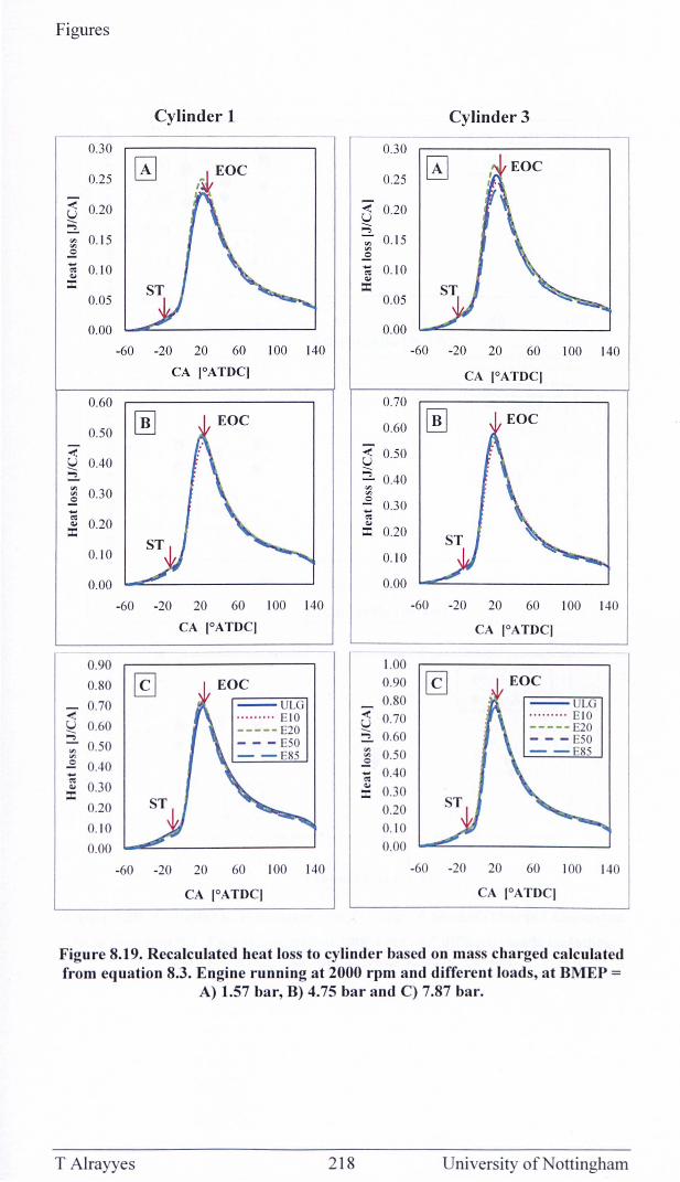
Figures
Cylinder 1 Cylinder 3
0.30 0.30
0.25 ~ 0.25 ~ ~ 0.20 -< 0.20 U -- U :::::.. ;:; V> 0. 15 V> 0.15 V>
.£ V>
.£ ..... 0.10 ..... 0.10 ~
~ ~
:c ~
:c 0.05 0.05
0.00 0.00
-60 -20 20 60 100 140 -60 -20 20 60 100 140
CA IOATOq CA IOATOq
0.60 0.70
0.50 ~ 0.60 ~ -< -< 0.50 U 0.40 U ;:; ;:; 0.40 V>
0.30 V>
V> V>
.£ .£ 0.30 ..... ..... ~
0.20 ~
~ ~
:I: :c 0.20 ST
0. 10 0.10
0.00 0.00
-60 -20 20 60 100 140 -60 -20 20 60 100 140
CA IOATOq CA IOATOq
0.90 1.00
0.80 @] 0.90 @] EOC
0.70 --ULG 0.80 --ULG -< . ..... ... E IO -< 0.70 . . ...... . E IO U 0.60 ----- E20
U ----- E20 ;:; 0.50 - - - E50
;:; 0.60 - - - E50 V> V>
0.50 - - E85 V> - - E85 V>
.£ 0.40 .£ ~ ~ 0.40 ~ 0.30 ~
0.30 :c :c 0.20 0.20
0.10 0.10
0.00 0.00
-60 -20 20 60 100 140 -60 -20 20 60 100 140
CA IOATOq CA IOATOq
Figure 8.19. Recalculated heat loss to cylinder based on mass charged calculated from equation 8.3. Engine running at 2000 rpm and different loads, at BMEP =
A) 1.57 bar, B) 4.75 bar and C) 7.87 bar.
T Alrayyes 218 University of Nottingham
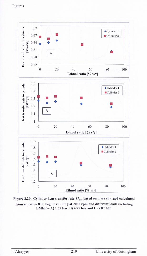
Figures
s.. 0.7 41 "0 C
>. 0.67 I' e.>
0 ... -0.64 ~~ 41 -- .... ~ e.>
s..--s..~ ~::. '" c ~ s.. ... ... ~ 41 :r:
s.. 41
"0 C
>.
0.61
0.58
0.55
1.9
1.8 e.> o 1.7 --~ >. 16 ~ e.> • s.. --
~ ~ 1.5 '" ; 1.4 s.. --; 1.3 41
:r: 1.2
0
o
o
• •
• •
• •
20
• •
20
• • • •
20
•
40 60 Ethnol ratio [% v/v)
40
• •
60
Ethnol ratio [% v/v]
, 40 60
Ethnol ratio [% v/v)
I + Cylinder I 1 . Cylinder 2 I
80 100
+ Cylinder I I . Cylinder 2
80
• •
+ Cylinder I
. Cylinder2
, 80
100
100
Figure 8.20. Cylinder heat transfer rate, Q Cyl ,based on mass charged calculated
from equation 8.3. Engine running at 2000 rpm and different loads including BMEP = A) 1.57 bar, B) 4.75 bar and C) 7.87 bar.
T Alrayyes 219 University of Nottingham
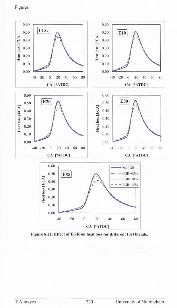
Figures
0.60 0.60
0.50 IULGI 0.50 IElOl -< -< U 0.40 U 0.40 ....... ....... .., .., til 0.30 til 0.30 til til
.9 .9 - 0.20 - 0.20 ~ ~ ~ ~
::I: ::t 0.10 0.10
0.00 0.00
-40 -20 0 20 40 60 80 -40 -20 0 20 40 60 80
CA IOATDq CA ,oATDq
0.60 0.60
0.50 IE201 0.50 IESol -< -< U 0.40 U 0.40 ....... ....... .., .., til 0.30 til 0.30 til til
.9 .9 - 0.20 - 0.20 ~ ~ ~ ~
:c :c 0. 10 0.10
0.00 0.00
-40 -20 0 20 40 60 80 -40 -20 0 20 40 60 80
CA ,oATOq CA ,oATOq
0.60 --NoEGR
0.50 IESsl ......... EGR=05%
-< ----- EGR= IO% U 0.40 .......
- - - EG R=15% .., til 0.30 til
.9 - 0.20 ~ ~
:c 0.10
0.00
-40 -20 0 20 40 60 80
CA ,oATOq
Figure 8.21. Effect ofEGR on heat loss for different fuel blends.
T Alrayyes 220 University of Nottingham
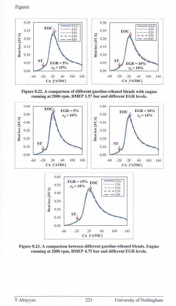
Figures
- --0.30 0.30
--ULG --ULG
0.25 .... . ... . E IO ----- E20
0.25 .... .. .. . EIO ----- E20
~ U 0.20 -.. :2
- - - E50 - - E85
~ - - - E50 U 0.20 - - E85 ;;;;
'" '" '" 0.15 ~ '" 0.15 ~ .... .... 0:: 0:: .. 0. 10 ::c
.. 0.1 0 :c
0.05 0.05
0.00 0.00 Xb~ 18%
-60 -20 20 60 100 140 -60 -20 20 60 100 140 CA [OATOq CA IOATOq
Figure 8.22. A comparison of different gasoline-ethanol blends with engine running at 2000 rpm, BMEP 1.57 bar and different EGR levels.
0.60
0.50
~ U 0.40 ;;;;
'" '" 0.30 ~ .... 0:: .. 0.20 ::c
0. 10
0.00
-60 -20 CA
~ U -.. :2 '" '" ~ .... 0:: .. :c
20
EGR=5% Xb~ 10%
60 100 140 IOATOq
0.60
EGR = 15% 0.50 Xb ~ 18%
0.40
0.30
0.20
0. 10
0.00
-60 -20
0.60
0.50
~ U 0.40 ;;;;
'" '" 0.30 ~ .... 0:: .. 0.20 :c
0. 10
0.00
-60 -20
EOC ULG
.. .. .. ... EIO ----- E20 - - - E50 - - E85
20 60 100 CA IOATOq
20
EGR= 10% Xb~ 14%
60 100 140 CA IOATOq
140
Figure 8.23. A comparison between different gasoline-ethanol blends. Engine running at 2000 rpm, BMEP 4.75 bar and different EGR levels.
T Alrayyes 221 University of Nottingham
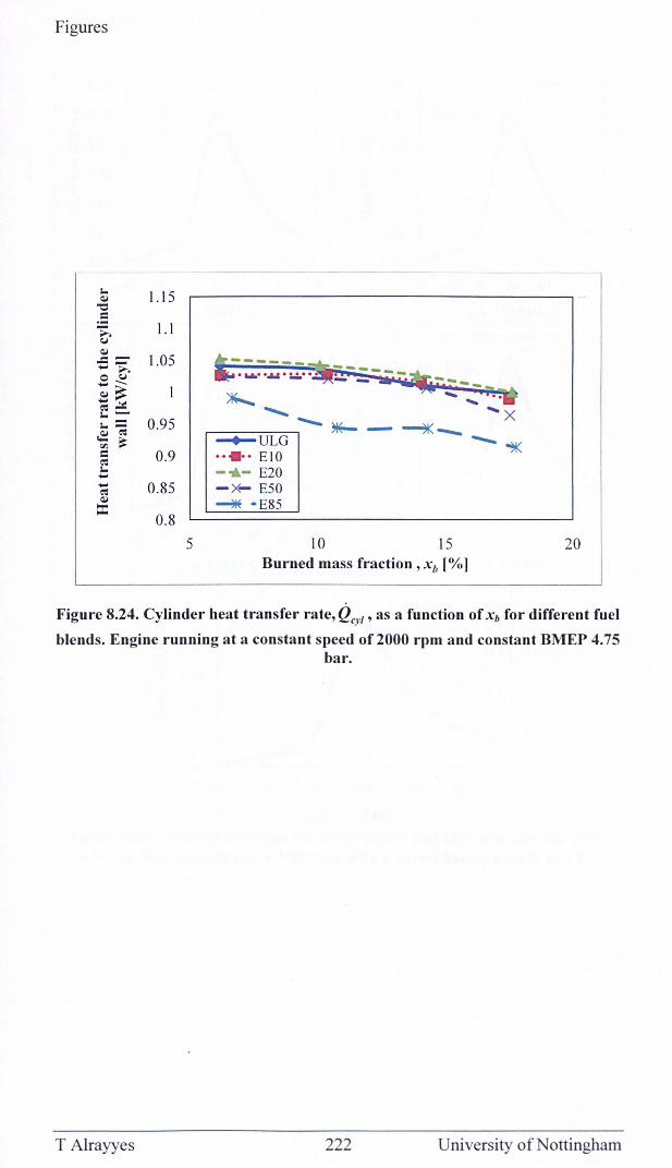
Figures
'" 1.15 Q,j
"0 .5
1.1 >. <:J Q,j
1.05 -== - ~ o <:J ---Q,j~ -~ E- """ ..... X ",= 0.95 ---- ~- ~--Q,j ~
';; ~ -+-ULG ----~ c 0.9 .. .. . EIO ~
'" - ... - E20 -- 0.85 - x- E50 ~ Q,j
~ - E85 =: 0.8
5 10 15 20 Burned mass fraction ,xb [%]
Figure 8.24. Cylinder heat transfer rate, Q CY/ , as a function of Xb for different fuel
blends. Engine running at a constant speed of 2000 rpm and constant BMEP 4.75 bar.
T Alrayyes 222 University of Nottingham
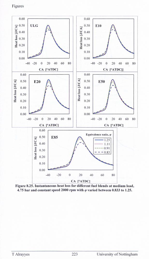
Figures
0.60 0.60
~ 0.50 ULG 0.50 EIO U ~ ~ 0.40 ~ 0.40 ~
::.. ~ ~
£ 0.30 ~ 0.30 - £ ~ -:t 0.20 ~ 0.20 QJ
:c 0. 10 0.10
0.00 0.00
-40 -20 0 20 40 60 80 -40 -20 0 20 40 60 80
CA IOATOCI CA IOATOCl]
0.60 0.60
< 0.50 E20 ~ 0.50 E50 U u --.. --.. ::.. ::.. 0.40 0.40 ~
~ ~ ~ £ £ 0.30 - 0.30 - ~ ~ QJ QJ ::c 0.20 ::c 0.20
0.10 0.10
0.00 0.00
-40 -20 0 20 40 60 80 -40 -20 0 20 40 60 80
CA IOATOCI CA IOATOC]
0.60
0.50 E85 Equiva lence ratio, ({J
~ U -- 1.25 ;::; 0.40 .. .. .. ... 1. 11 ~ ----- 0.9 1 '" 0.30 £ - - - 0.83 -~ QJ 0.20 ::c
0.10
0.00
-40 -20 0 20 40 60 80
CA IOATOC]
Figure 8.25. Instantaneous heat loss for different fuel blends at medium load, 4.75 bar and constant speed 2000 rpm with ffJ varied between 0.833 to 1.25.
T Alrayyes 223 University of Nottingham
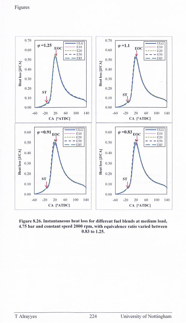
Figures
0.70
0.60
0.50 -<t: U ;::; 0.40
'" '" .!2 ..... 0.30 ~ ... :c
0.20
0.10
0.00
0.60
0.50
25 0.40 ;:;
'" .2 0.30 ..... ~ ... :c 0.20
0.10
0.00
--ULG . .. . . . ... E IO
----- E20
tp =1.25 EOC
- - - E50 - - E85
ST
-60 -20 20 60 100 140
CA IOATOq
tp =0.91 EOC --ULG . .. . . .... E IO
----- E20 - - - E50
J, - - E85
ST
-60 -20 20 60 100 140
CA IOATOq
0.70
0.60
0.50 -<t: U ;:;; 0.40
'" '" .!2 ..... 0.30 ~ ... :c
0.20
0. 10
0.00
0.60
0.50
25 0.40 ;:;
'" ~ 0.30 ..... ~ ... :c 0.20
0.10
0.00
tp =1.1 EOC
--ULG . .. .. .. .. E IO
----- E20 - - - E50 - - E85
-60 -20 20 60 100 140
CA IOATOq
tp =0.83 EOC --ULG .. .. . .. . . E IO
J, ----- E20 - - - E50 - - E85
-60 -20 20 60 100 140
CA IOATOq
Figure 8.26. Instantaneous heat loss for different fuel blends at medium load, 4.75 bar and constant speed 2000 rpm, with equivalence ratio varied between
0.83 to 1.25.
T Alrayyes 224 University of Nottingham
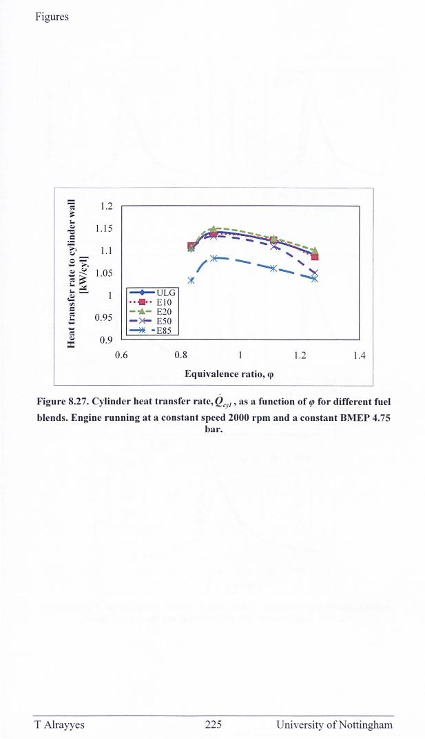
Figures
--; 1.2 ~ I.. cu 1.15 "Q
= .-~ 1.1 (,j , 0= /~ -- , ..........
~--4 cu (,j 1.05 ..... ---~~ ~ I..,.:t: I..~ ~ULG ~ •• • •• EIO '" = - .. - E20 ~ 0.95 I.. - x- E50 ..... ..... --* - E85 ~ cu 0.9
== 0.6 0.8 1.2 1.4
Equivalence ratio, <p
Figure 8.27. Cylinder heat transfer rate, Q CY/ ,as a function of lfJ for different fuel
blends. Engine running at a constant speed 2000 rpm and a constant BMEP 4.75 bar.
T Alrayyes 225 University of Nottingham
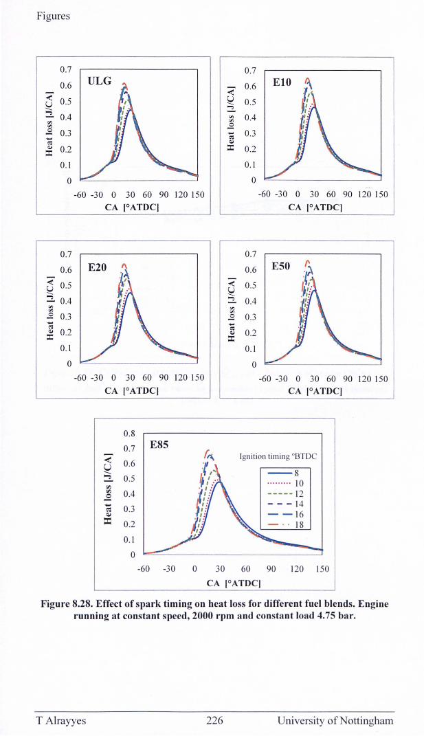
Figures
0.7
0.6
< 0.5 U --::::. 0.4 '" '" .£ 0.3 .... eo:! Q) 0.2 :r:
0.1
0
0.7
0.6
< 0.5 U ....... ::::. 0.4 '" '" .£ 0.3 -eo:! Q) 0.2 :r:
0.1
o
-60 -30 0 30 60 90 120 150 CA [OATOq
E20
-60 -30 0 30 60 90 120 150
CA [OATOq
0.8
0.7 E85
<" 0.6 U ~ 0.5 ~ ~ 0.4 oS - 0.3 ~ Q,j
== 0.2
0. 1
0
-60 -30 0
< u ....... ..., '" '" .£ .... eo:! Q)
:r:
<" U ....... ::::. '" '" .£ .... eo:! Q)
::c
30
0.7
0.6
0.5
0.4
0.3
0.2
0. 1
0
0.7
0.6
0.5
0.4
0.3
0.2
0.1
0
EIO
-60 -30 0 30 60 90 120 150
CA [OATOq
E50
-60 -30 0 30 60 90 120 150 CA [OATOq
Ignition timing °BTDC
--8 .. ... .. .. 10 ----- 12 - - - 14 -- 16 _ .. 18
60 90 120 150
CA [OATOq
Figure 8.28. Effect of spark timing on heat loss for different fuel blends. Engine running at constant speed, 2000 rpm and constant load 4.75 bar.
T Alrayyes 226 University of Nottingham
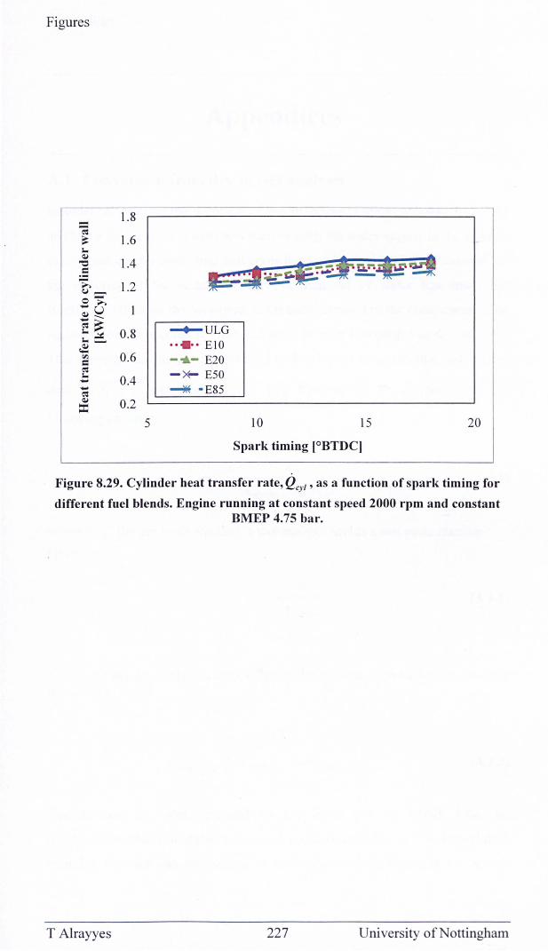
Figures
l.8 --; ~ l.6 l. Q,j
1.4 "Q .: ~ 1.2 ~~ 0-- ~ Q,jU ----eo:~
0.8 ~ULG l.,.::.:: l.~ •• ••• EIO ~ "l 0.6 -"IL- E20 = eo: - x- E50 l. 0.4 -- ~ - E85 eo: Q,j 0.2
== 5 10 15 20
Spark timing [OBTDC]
Figure 8.29. Cylinder heat transfer rate, Q CY/ , as a function of spark timing for
different fuel blends. Engine running at constant speed 2000 rpm and constant BMEP 4.75 bar.
T Alrayyes 227 University of Nottingham
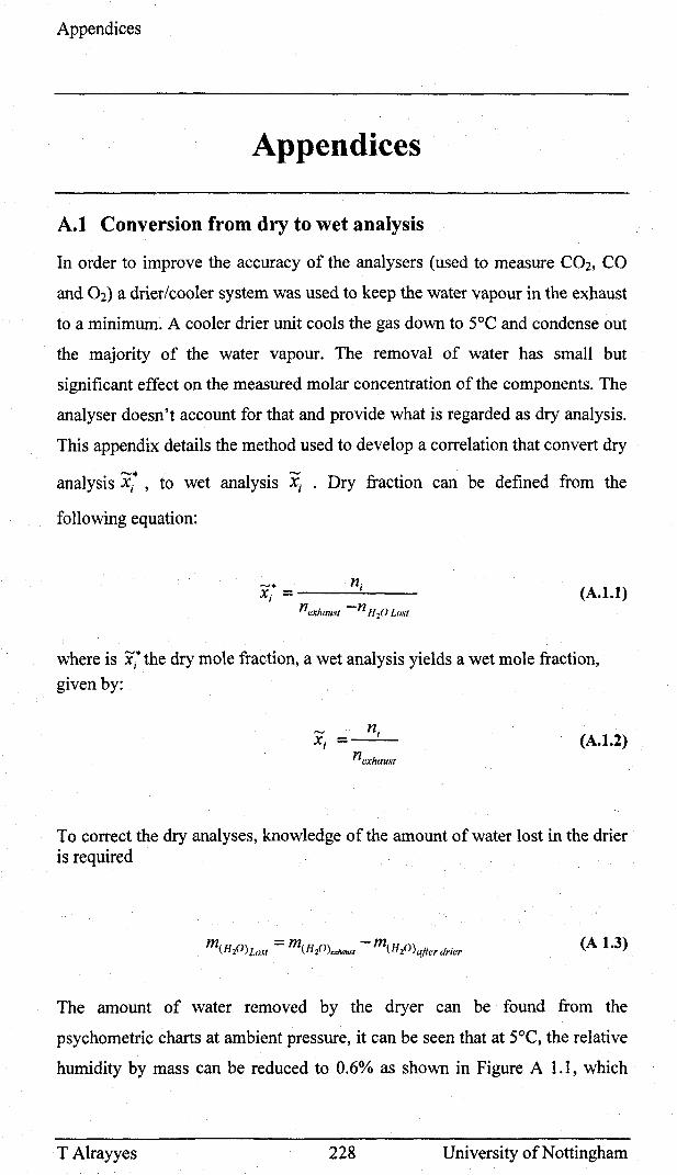
Appendices
Appendices
A.1 Conversion from dry to wet analysis
In order to improve the accuracy of the analysers (used to measure CO2, CO
and 02) a drier/cooler system was used to keep the water vapour in the exhaust
to a minimum. A cooler drier unit cools the gas down to SOC and condense out
the majority of the water vapour. The removal of water has small but
significant effect on the measured molar concentration of the components. The
analyser doesn't account for that and provide what is regarded as dry analysis.
This appendix details the method used to develop a correlation that convert dry
analysis ~. , to wet analysis ~ . Dry fraction can be defined from the
following equation:
~.. nj Xi = -----=--- (A.1.1)
n exhaust - n H20 Lost
where is Xi· the dry mole fraction, a wet analysis yields a wet mole fraction,
given by:
(A. 1.2) nexhaust
To correct the dry analyses, knowledge of the amount of water lost in the drier is required
(A 1.3)
The amount of water removed by the dryer can be found from the
psychometric charts at ambient pressure, it can be seen that at SoC, the relative
humidity by mass can be reduced to 0.6% as shown in Figure A 1.1, which
T Alrayyes 228 University of Nottingham
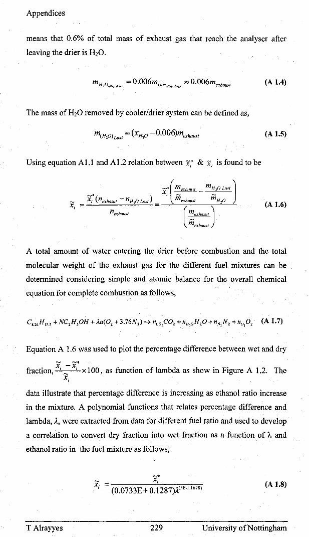
Appendices
means that 0.6% of total mass of exhaust gas that reach the analyser after
leaving the drier is H20.
mH 0 = 0.006mc' ::::; 0.006m h . 2 after drier .JUS after drier ex aWit
(A 1.4)
The mass of H20 removed by cooler/drier system can be defined as,
mCH 0) = (XH 0 - O.OO6)mexhaust 2 Lost 2
(~ 1.5)
Using equation A1.1 and A1.2 relation between x/ & XI is found to be
(A 1.6)
A total amount of water entering the drier before combustion and the total
molecular weight of the exhaust gas for the different fuel mixtures can be
determined considering simple and atomic balance for the overall chemical
equation for complete combustion as follows,
Equation A 1.6 was used to plot the percentage difference between wet and dry
-. fraction, Xi :: Xi xl 00, as function of lambda as show in Figure A 1.2. The
Xi
data illustrate that percentage difference is increasing as ethanol ratio increase
in the mixture. A polynomial functions that relates percentage difference and
lambda, A, were extracted from data for different fuel ratio and used to develop
a correlation to convert dry fraction into wet fraction as a function of A. and
ethanol ratio in the fuel mixture as follows,
-. -- Xi Xi = (O.0733E + 0.1287)A(3E-J.1678)
(A 1.8)
T Alrayyes 229 University of Nottingham
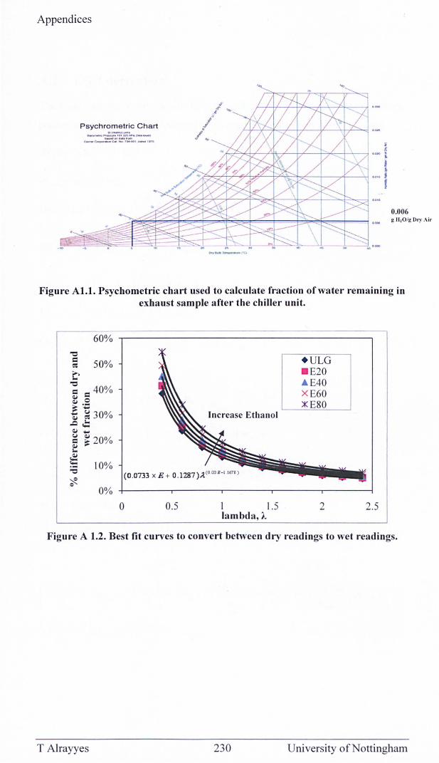
Appendices
'.,
Psychrometric Chart *,_1 __ _ =-"::'!,:;""' jtw~
c-... ~_e... _ ~I _I~
0.006 g I-I,O/g Dry Air
Figure ALl. Psychometric chart used to calculate fraction of water remaining in exhaust sample after the chiller unit.
60% "0 = SO% + ULG ell
C - E20 "0 A E40 = = 40% XE60 QJ 0 ~~ ::K E80 .G ~ 30% Increase Ethanol QJ I. .c .... QJ .. C.I ~
= ~ 20% ~ I.
~ .... 10% .-"0
~ 0
0%
0 O.S 1 I.S 2 2.S lambda, A.
Figure A 1.2. Best fit curves to convert between dry readings to wet readings.
T Alrayyes 230 University of Nottingham
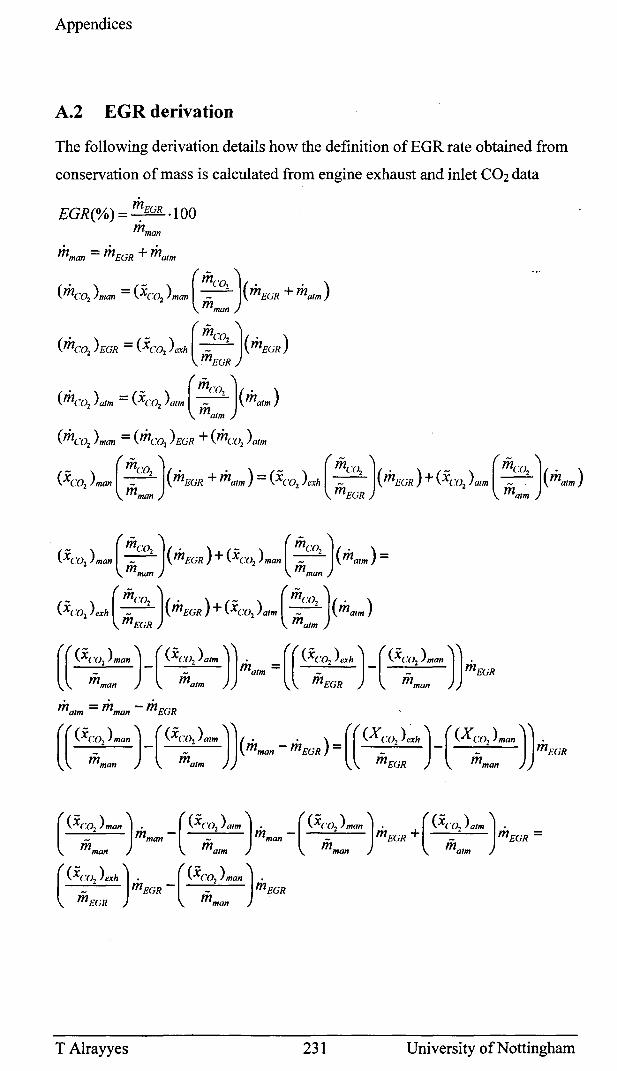
Appendices
A.2 EGR derivation
The following derivation details how the definition of EGR rate obtained from
conservation of mass is calculated from engine exhaust and inlet C02 data
EGR(%) = ~EGR .100
T Alrayyes 231 University of Nottingham
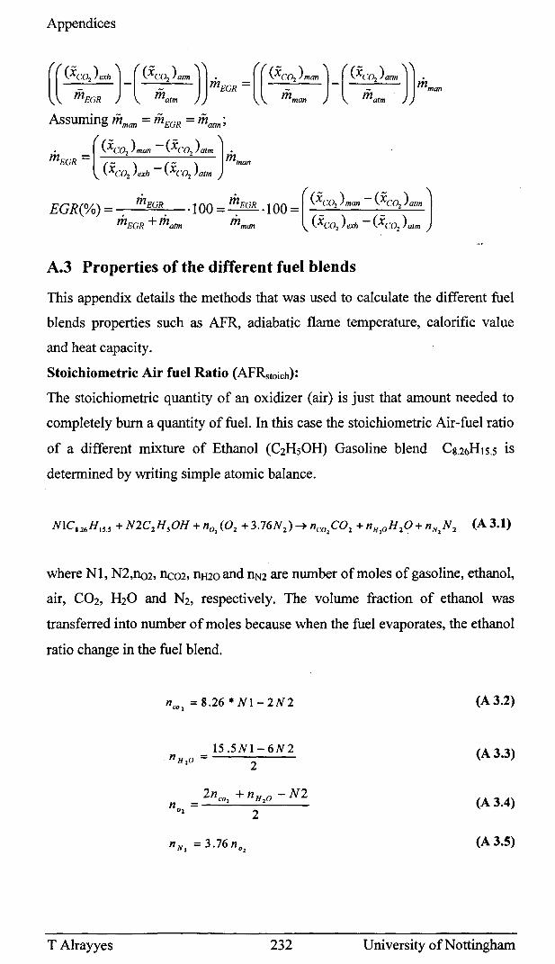
Appendices
A.3 Properties of the different fuel blends
This appendix details the methods that was used to calculate the different fuel
blends properties such as AFR, adiabatic flame temperature, calorific value
and heat capacity.
Stoichiometric Air fuel Ratio (AFRstoich):
The stoichiometric quantity of an oxidizer (air) is just that amount needed to
completely burn a quantity of fuel. In this case the stoichiometric Air-fuel ratio
of a different mixture of Ethanol (C2HsOH) Gasoline blend Cg.26HlS.S is
determined by writing simple atomic balance.
where Nt, N2,n02, Ilc02, nH20 and nN2 are number of moles of gasoline, ethanol,
air, CO2, H20 and N2, respectively. The volume fraction of ethanol was
transferred into number of moles because when the fuel evaporates, the ethanol
ratio change in the fuel blend.
nC01
= 8.26· NI- 2N2 (A 3.2)
15 .5NI- 6N2 n H:O = 2 (A 3.3)
(A 3.4)
n N: = 3.76 no: (A 3.5)
T Alrayyes 232 University of Nottingham
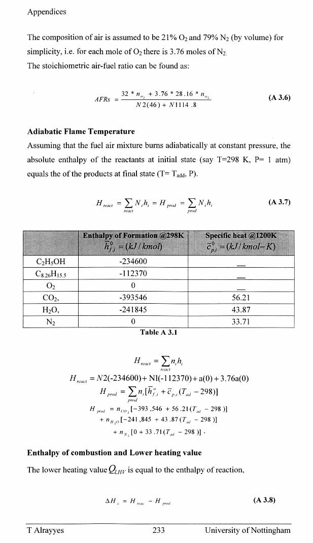
Appendices
The composition of air is assumed to be 21 % O2 and 79% N2 (by volume) for
simplicity, i.e. for each mole of O2 there is 3.76 moles ofN2
The stoichiometric air-fuel ratio can be found as:
A FRs 32 * n o, + 3.76 * 28 . 16 * n o,
N 2 ( 46 ) + NIl 14 .8
Adiabatic Flame Temperature
(A 3.6)
Assuming that the fuel air mixture bums adiabatically at constant pressure, the
absolute enthalpy of the reactants at initial state (say T=298 K, P= 1 atm)
equals the of the products at final state (T= Tadd, P).
~."
'-
C2HsOH
C826H lS.5
0 2
CO2,
H2O,
N2
H reac( = L N;h; = H prod = L N;h; (A 3.7) react prod
Enthalpy of Formation @l98K Specific heat @1200K -0
c~,; = (kJ / kmol-K) hf,i = (k.!lkmol) ,.:'
-234600
-112370
0 -
-393546 56.2 1
-241845 43 .87
0 33.71 Table A 3.1
reacl
Hreuc, = N2(-234600)+ Nl(-112370)+ a(O) + 3.76a(0)
H prod = I nJh;'J + CpJ (TUd - 298)] prod
H prod = n('() , [-393 ,546 + 56.2I(T"d - 298)]
+ n" ,o [-241 ,845 + 43 .87 (Tad - 298)]
+ n N , [0 + 33 .71 (Tad - 298)] .
Enthalpy of combustion and Lower heating value
The lower heating value Q LHV is equal to the enthalpy of reaction,
~ H c = H rca,. - H prod . (A 3.8)
T Alrayyes 233 University of Nottingham
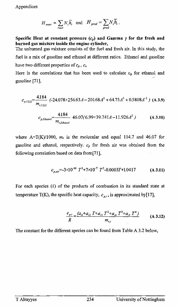
Appendices
H react = L N/i; and H prod = 'IN}i; . react prod
Specific Heat at constant pressure (cp) and Gamma J' for the fresh and burned gas mixture inside the engine cylinder, The unburned gas mixture consists of the fuel and fresh air. In this study, the
fuel is a mix of gasoline and ethanol at different ratios. Ethanol and gasoline.
have two different properties of cp , Cv
Here is the correlations that has been used to calculate cp for ethanol and
gasoline [71],
Cp,ULG= 4.184 (-24.078+256.63A - 201.68A2 + 64.75A3 + 0.5808A-2 ) (A 3.9)
mr,ULG
4.184 2 Cp,Ethanol= 46.07(6.99+39.74IA -11.926A )
mr,Ethanol
(A 3.10)
where A=T(K)/lOOO, mr is the molecular and equal 114.7 and 46.07 for
gasoline and ethanol, respectively. cp for fresh air was obtained from the
following correlation based on data from [7 1],
(A 3.11)
For each species (i) of the products of combustion in its standard state at
temperature T(K), the specific heat capacity, C p,;' is approximated by[17],
Cp,; (ail+a;2 T+ai3 T 2+a;4 T 3+a;5 T4)
R m,,; (A 3.12)
The constant for the different species can be found from Table A 3.2 below,
T Alrayyes 234 University of Nottingham
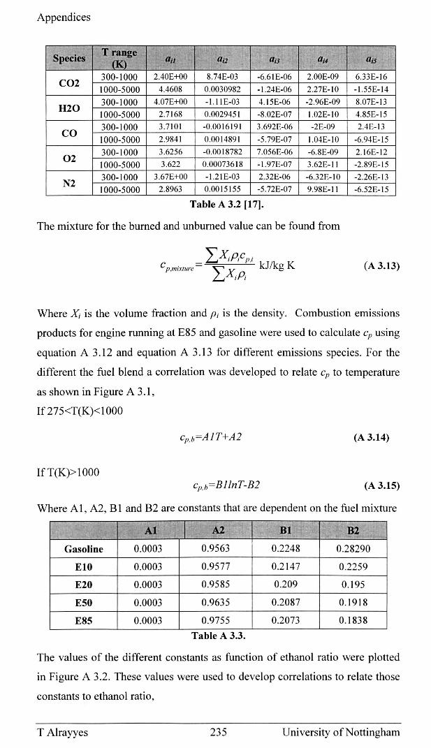
Appendices
Species T range
0/1 au al3 al4 al5 ;'
(K)
CO2 300-1000 2.40E+00 8.74E-03 -6.6 IE-06 2.00E-09 6.33E-16
1000-5000 4.4608 0.0030982 -1.24E-06 2.27E-IO -1.55E-14
300-1000 4.07E+00 -1.11 E-03 4.15E-06 -2.96E-09 8.07E-13 H2O
1000-5000 2.7168 0.0029451 -8.02E-07 1.02E-IO 4.85E-15
300-1000 3.7101 -0.0016191 3.692E-06 -2E-09 2.4E-13 CO
1000-5000 2.9841 0.0014891 -5 .79E-07 1.04E-IO -6.94E-15
300-1000 3.6256 -0.0018782 7.056E-06 -6.8E-09 2.16E-12 02
1000-5000 3.622 0.00073618 -1.97E-07 3.62E-II -2.89E-15
300-1000 3.67E+00 -1.21 E-03 2.32E-06 -6.32E-IO -2.26E-13 N2
1000-5000 2.8963 0.0015155 -5.72E-07 9.98E-II -6.52E-15
Table A 3.2 [17].
The mixture for the burned and unburned value can be found from
IXiPiCp,i C p,mixture = '"'X kllkg K
~ iPi
(A 3.13)
Where X; is the volume fraction and Pi is the density. Combustion emissions
products for engine running at E85 and gasoline were used to calculate cp using
equation A 3.12 and equation A 3.13 for different emissions species. For the
different the fuel blend a correlation was developed to relate cp to temperature
as shown in Figure A 3.1,
If 275<T(K)<1 000
cp,b=A 1 T+A2 (A 3.14)
If T(K» 1 000 cp,b=BllnT-B2 (A 3.15)
Where AI, A2, Bland B2 are constants that are dependent on the fuel mixture
Al I A2 BI B2
Gasoline 0.0003 0.9563 0.2248 0.28290
EIO 0.0003 0.9577 0.2147 0.2259
E20 0.0003 0.9585 0.209 0.195
E50 0.0003 0.9635 0.2087 0.1918
E85 0.0003 0.9755 0.2073 0.1838
Table A 3.3.
The values of the different constants as function of ethanol ratio were plotted
in Figure A 3.2. These values were used to develop correlations to relate those
constants to ethanol ratio,
T Alrayyes 235 University of Nottingham
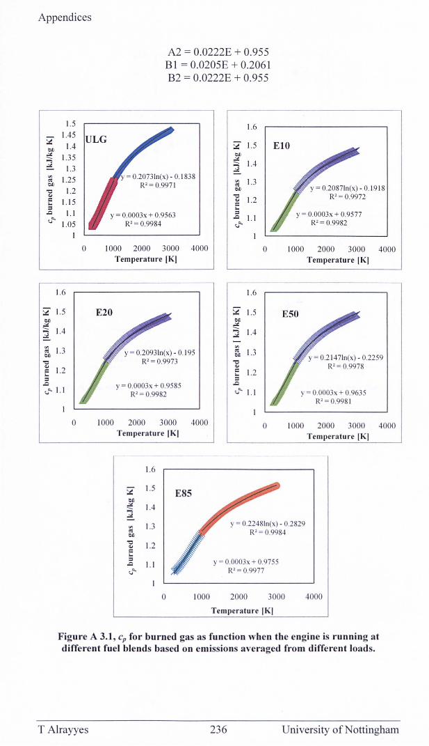
Appendices
A2 = 0.0222E + 0.955 Bl = 0.0205E + 0.2061 B2 = 0.0222E + 0.955
1.6 1.5 :;z 1.45 1)1) 1.4
..:.::
ULG ~ 1.5 EI0
j 1.35 1.3
~ 1.25 ~ 1.2 '" E 1.15 :: .c 1.1 ",'" 1.05
1.6
~ 1.5 1)1)
..:.:: ~ 1.4
; 1. 3 1)1)
~
~ 1.2 ... :: .c ",'" 1. 1
I
o
o
y = 0.2073 In(x) - 0.1838 R'= 0.997 1
y = 0.0003x + 0.9563 R' = 0.9984
1000 2000 3000 4000 Temperature IKI
E20
y = 0.2093 In(x) - 0.195 R' = 0.9973
y = 0.0003x + 0.9585 R' = 0.9982
1000 2000 3000 4000 Temperature IKI
1.6
~ 1.5
E85 1)1)
..:.:: 1.4 --....
..:.::
VI ..: 1.3 1)1)
~ 1.2 '" c ... :: .c 1.1 ",'"
0 1000
1)1) ..:.:: j 1.4
; 1.3 1)1)
] 1.2 c ... :: .c 1.1 ",'"
1.6
~ 1.5 1)1)
..:.:: --:2 1.4
'" ~1.3 ~
'" E 1.2 :: .c ",'" 1.1
o
o
y = 0.2087In(x) - 0.19 18 R' = 0.9972
y = 0.0003x + 0.9577 R'= 0.9982
1000 2000 3000 4000 Temperature IKI
E50
y = 0.2 14 7In(x) - 0.2259 R' = 0.9978
y = 0.0003x + 0.9635 R'= 0.998 1
1000 2000 3000 4000 Temperature IKI
y = 0.2248In(x) - 0.2829 R' = 0.9984
y = 0.0003x + 0.9755 R'= 0.9977
2000 3000
Temperature IKI 4000
Figure A 3.1, cp for burned gas as function when the engine is running at different fuel blends based on emissions averaged from different loads.
T Alrayyes 236 University of Nottingham
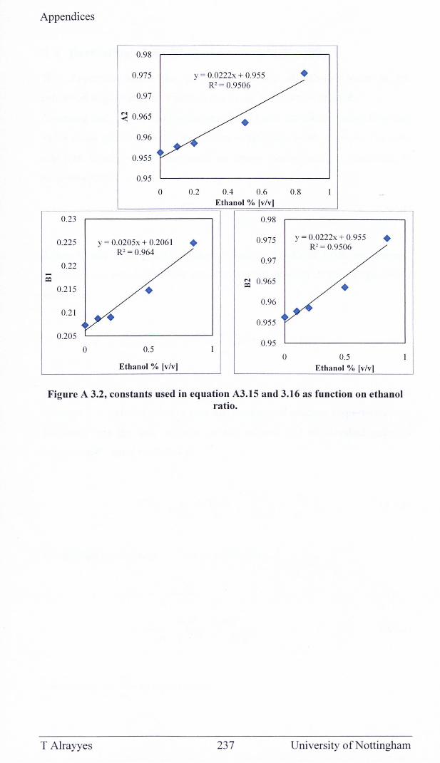
Appendices
0.98
0.975 y = 0.0222x + 0.955 • R2 = 0.9506
0.97
~ 0.965 • 0.96
0.955
0.95
0 0.2 0.4 0.6 0.8 Ethanol % Iv/vi
---0.23 0.98
0.975 Y = 0.0222x + 0.955 • R2 = 0.9506 0.225 Y = 0.0205x + 0.206 1 • R2= 0.964
0.22 0.97
M 0.965 CO • CO
0.2 15 • 0.96
0.95 5 0.2 1 •
0.205
0 0.5 0.95
0 0.5 Ethanol % Iv/vi Ethanol % Iv/vi
Figure A 3.2, constants used in equation A3.15 and 3.16 as function on ethanol ratio.
T Alrayyes 237 University of Nottingham
Appendices
A.4 Derivation of the EGR correction factor [89]
This Appendix details the derivation and the assumption made In the
correction to gas-side heat rejection due to the introduction ofEGR.
Assuming that, for a given Engine speed and Load, the effect on fuel flow rate
and residual gas fraction due to changes in throttling losses is small. The Gas
side heat transfer can be corrected for charge heat capacity C according to
proportionality
(A 4.1)
Where 0 and EGR denote properties with and without EGR respectively.
Expressed per unit mass of the fuel, the thermal capacity of the charge can be
defined as:
C' = ..5:.... = m fC p,f+mac p,a + mexhc p,exh + mrc pr (A 4.2)
mf mf
Where m is the mass per cycle and cp the specific heat capacity, while the
subscript f, a, exh and r denote fuel, air, exhaust and residual, respectively.
Assuming that the heat capacity of the exhaust and the residual gases IS
approximately equal to that of air.
C'=CPf+(AFJl+ EGR )+ mrJcpa .1\ l-EGR mf
The residual gas fraction, x r , can be defined as :
mr xr = -----'---
ma +mf +m~x
mr{l-EGR) =--~----
mf {1-EGR+AFR)
Substituting for mr in equation A 4.3 mf
(A 4.3)
(A 4.4)
T Alrayyes 238 University of Nottingham
Appendices
C' =c +(AFll+ Xr (1-EGR+AFR»))C pi .1\ l-EGR pa
(A 4.5)
C' And h . EGR· • b t e ratIo -,- IS gIven y:
Co
C~(1R = C pf (1- EGR) + (AFR + X rEUR (1- EGR + AFR»c pa
C~ (1-EGR)(cpf + (AFR + xro(l + AFR»cpa ) (A. 4.6)
Since AFR »1, and EGR <1 equation A 4.6 can be approximated to:
C~GR ,.., cpf(I-EGR)+(AFR(I+xrElJR»cpa --,..,
C~ (l-EGR)(cpf + (AFR(xrO +1)cpa ) (A 4.7)
For spark ignition engine, the residual fraction varies typically from 7% at full
load to 20% at light load. For otherwise similar operating conditions the
residual fraction x r for the case with EGR will be lower than the equivalent
case without EGR because of throttling differences required maintaining the
correct AirlFuel ratio. However, since EGR is not used at full load we can
assume x, ~ 10% and equation A 4.7 can be simplified further:
C~C;R cpf(l- EGR) + 1.IAFRcpa -- ~ --...:.;'--------....:......-
C~ (1- EGR)(c pf + 1.1AFRc pa)
1 ~---
(l-EGR) (A 4.8)
T Alrayyes 239 University of Nottingham
Appendices
A.5 Measurements and calculation uncertainties
Because of the comparative nature of this study, any experimental error could
have an effect on the data and subsequently the drawn conclusion. The
difference between various fuel mixtures can be due to experimental error
rather than the fuel content. For that reason, it was very important to estimate
the error in the experiment.
There are mainly two types of errors associated with experimental results: the
"precision" and the "accuracy". Precision is related to the random errors inside
the experiment including noise. Accuracy is related to the existence of
systematic error associated with the instruments used. An instrument can be
assessed for systematic errors only by calibration against an appropriate
standard. The systematic errors of the instruments are usually provided by the
manufacturers. The random error is assessed by repeated measurements made
under identical conditions[105]. As mentioned in section 3.7, at each running
condition, the data were averaged over 750 samples. The standard error of the
mean, Estand, was used to express the precision of the mean value of repeated
tests such as[105]
E _ S
.<land - ..In-I (A 5.1)
where s is the standard deviation and n is the number of readings.
A.5.l Estimation of the error in temperature,fuel massflow rate,
coolant flow rate and AFR.
As mentioned in section 3.7, all temperature measurements were taken using K
type thermocouple. The inaccuracy of the thermocouples according to the
manufacturer, associated with the systematic error, is ±1.5°C or ±O.4% [64].
Figure A1.1 shows standard error of the mean, Estand.Temp, calculated from
equation A 5.1, for exhaust and coolant temperatures. The data were taken
from engine running at different speeds, BMEPs and fuel mixtures. The results
illustrate clearly that Estand,Temp is lower than 0.2 °C for the vast majority of the
tests. For that reason, systematic error is assumed to the major source of the
temperature measurement error. Hence, thermocouples uncertainty, E Temp is
assumed to be ±1.5°C or ±0.4%.
T Alrayyes 240 University of Nottingham
Appendices
According to the manufacturers, the accuracy of the fuel and coolant flow
meters are 0.05% and 0.5% respectively [106, 107]. The standard errors of the
mean, Estand, of both measurements are shown in Figure A 5.2 and Figure A 5.4
for different running conditions. The percentage of Estand compare to the mean
value of the sample is shown in Figure A 5.3 and Figure A 5.5. Percentage of
EStand for both fuel and coolant flow rate are lower than 0.1 %. The uncertainties'
in the measurement for fuel and coolant flow rate, E. & E. ,are m fuel m,"oolanl
assumed to be ±0.1 % and ±0.5% respectively.
According to the manufacturer, the accuracy in the measurement of CO, C02,
HC, NOx, and 02 are +1%, +1%, +1%, 1.5% and 1.5% respectively [108].
The standard error of the mean and its percentage compare to the mean value
are plotted in Figure A 5.6. The data illustrate that error percentage is lower
than 0.2%, 0.3%, 0.4% and 0.04% for NOx, HC, CO and CO2 emissions. Once
again those random errors are much smaller than that of the manufacturer
accuracy. Consequently, the error in the experiment was assumed to be equal
to the manufacturer accuracy.
A.S.2 Errors in pressure measurements
There are several sources of error that can affect in-cylinder pressure readings.
These errors have been widely discussed and analysed by several
researches[ 1 09, 11 0]. The main sources of errors are:
• Inaccurate pressure referencing (pegging).
• Thermal shock or short term drift or intra-cycle drift.
• Incorrect crank angle phasing with pressure data.
• Inaccurate transducer calibration and sensor non linearity.
• Long term drift or inter-cycle.
• Noise.
Several measures were taken to eliminate some of the error sources mentioned
in the list above in order to insure accurate pressure readings. For example, to
eliminate noise, pressure data was averaged over 100 consecutive cycles.
Regarding transducer calibration and no linearity as a source of error, extra
care was taken when calibrating both in cylinder transducer and manifold
pressure sensor. In addition, modem pressure transducers are affected by small
T Alrayyes 241 University of Nottingham
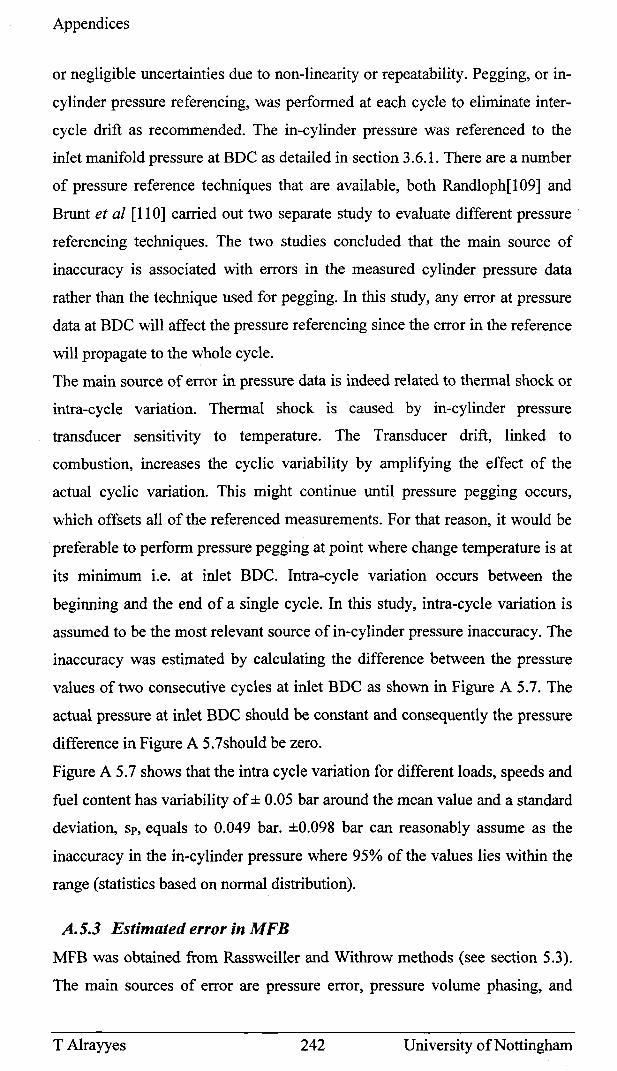
Appendices
or negligible uncertainties due to non-linearity or repeatability. Pegging, or in
cylinder pressure referencing, was performed at each cycle to eliminate inter
cycle drift as recommended. The in-cylinder pressure was referenced to the
inlet manifold pressure at BDC as detailed in section 3.6.1. There are a number
of pressure reference techniques that are available, both Randloph[109] and
Brunt et at [110] carried out two separate study to evaluate different pressure'
referencing techniques. The two studies concluded that the main source of
inaccuracy is associated with errors in the measured cylinder pressure data
rather than the technique used for pegging. In this study, any error at pressure
data at BDC will affect the pressure referencing since the error in the reference
will propagate to the whole cycle.
The main source of error in pressure data is indeed related to thermal shock or
intra-cycle variation. Thermal shock is caused by in-cylinder pressure
transducer sensitivity to temperature. The Transducer drift, linked to
combustion, increases the cyclic variability by amplifying the effect of the
actual cyclic variation. This might continue until pressure pegging occurs,
which offsets all of the referenced measurements. For that reason, it would be
preferable to perform pressure pegging at point where change temperature is at
its minimum i.e. at inlet BDC. Intra-cycle variation occurs between the
beginning and the end of a single cycle. In this study, intra-cycle variation is
assumed to be the most relevant source of in-cylinder pressure inaccuracy. The
inaccuracy was estimated by calculating the difference between the pressure
values of two consecutive cycles at inlet BDC as shown in Figure A 5.7. The
actual pressure at inlet BDC should be constant and consequently the pressure
difference in Figure A 5.7should be zero.
Figure A 5.7 shows that the intra cycle variation for different loads, speeds and
fuel content has variability of ± 0.05 bar around the mean value and a standard
deviation, Sp, equals to 0.049 bar. ±0.098 bar can reasonably assume as the
inaccuracy in the in-cylinder pressure where 95% of the values lies within the
range (statistics based on normal distribution).
A.5.3 Estimated error in MFB
MFB was obtained from Rassweiller and Withrow methods (see section 5.3).
The main sources of error are pressure error, pressure volume phasing, and
T Alrayyes 242 University of Nottingham
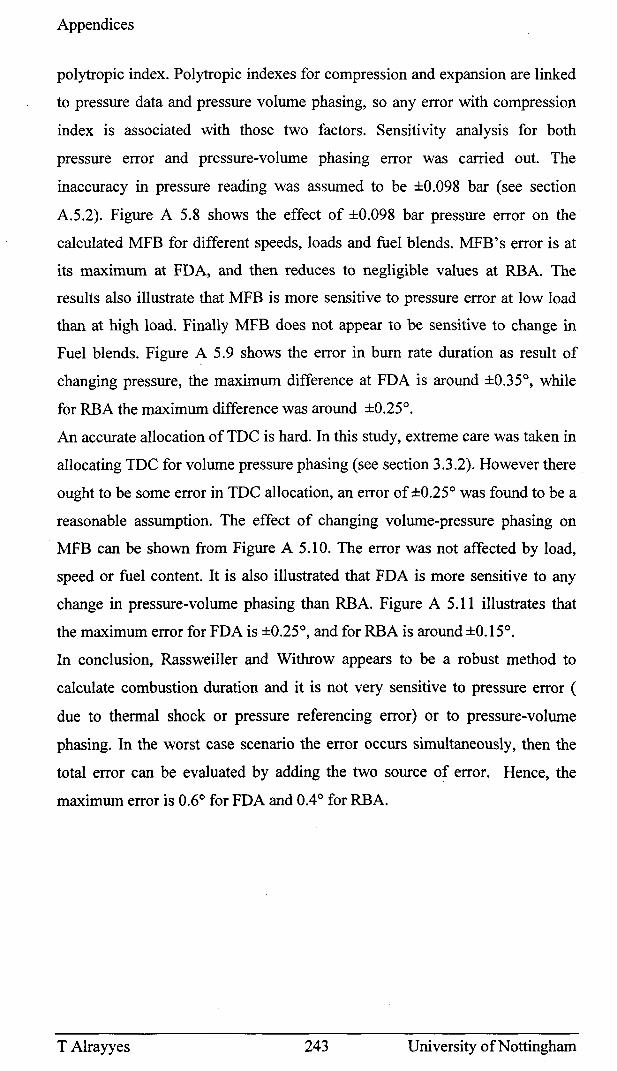
Appendices
polytropic index. Polytropic indexes for compression and expansion are linked
to pressure data and pressure volume phasing, so any error with compression
index is associated with those two factors. Sensitivity analysis for both
pressure error and pressure-volume phasing error was carried out. The
inaccuracy in pressure reading was assumed to be ±0.098 bar (see section
A.5.2). Figure A 5.8 shows the effect of ±0.098 bar pressure error on the·
calculated MFB for different speeds, loads and fuel blends. MFB' s error is at
its maximum at FDA, and then reduces to negligible values at RBA. The
results also illustrate that MFB is more sensitive to pressure error at low load
than at high load. Finally MFB does not appear to be sensitive to change in
Fuel blends. Figure A 5.9 shows the error in burn rate duration as result of
changing pressure, the maximum difference at FDA is around ±0.35°, while
for RBA the maximum difference was around ±0.25°.
An accurate allocation of TDC is hard. In this study, extreme care was taken in
allocating TDC for volume pressure phasing (see section 3.3.2). However there
ought to be some error in TDC allocation, an error of ±0.25° was found to be a
reasonable assumption. The effect of changing volume-pressure phasing on
MFB can be shown from Figure A 5.10. The error was not affected by load,
speed or fuel content. It is also illustrated that FDA is more sensitive to any
change in pressure-volume phasing than RBA. Figure A 5.11 illustrates that
the maximum error for FDA is ±0.25°, and for RBA is around ±0.15°.
In conclusion, Rassweiller and Withrow appears to be a robust method to
calculate combustion duration and it is not very sensitive to pressure error (
due to thermal shock or pressure referencing error) or to pressure-volume
phasing. In the worst case scenario the error occurs simultaneously, then the
total error can be evaluated by adding the two source of error. Hence, the
maximum error is 0.6° for FDA and 0.4° for RBA.
T Alrayyes 243 University of Nottingham
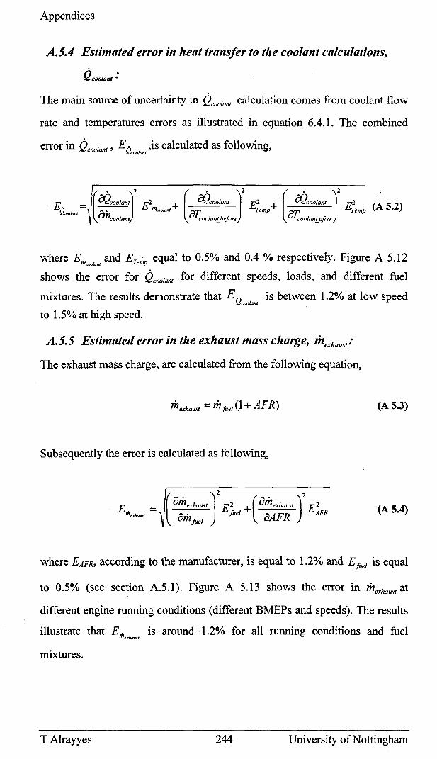
Appendices
A.5.4 Estimated error in heat transfer to the coolant calculations,
Qcoolant:
The main source of uncertainty in Qcoolanl calculation comes from coolant flow
rate and temperatures errors as illustrated in equation 6.4.1. The combined
error in Q'oolant' En ,is calculated as following, c r4:0010nl
E- = (k.oolanl
Ef200lanl E2. + Ef2oolantEi: + Ef200lant Ei: (A 5 2) ( . J2 (.)2 (. J2 Cincoolanl m"oolant OI;oolan!..b~fore emp OI;oolan!..after emp •
where EmeGOIUnl and ETemp equal to 0.5% and 0.4 % respectively. Figure A 5.12
shows the error for QCOOlant for different speeds, loads, and different fuel
mixtures. The results demonstrate that E Qcoo/anl is between 1.2% at low speed
to 1.5% at high speed.
A.5.5 Estimated error in the exhaust mass charge, "'exhaust:
The exhaust mass charge, are calculated from the following equation,
mexhaust = m foel (1 + AFR) (A 5.3)
Subsequently the error is calculated as following,
E. = (Omexhaust J2 E2 + (OmeXhoust )2 E2 m._" am foel foel oAFR AFR
(A 5.4)
where EAFR, according to the manufacturer, is equal to 1.2% and E foel is equal
to 0.5% (see section A.5.1). Figure A 5.13 shows the error in mexhaust at
different engine running conditions (different BMEPs and speeds). The results
illustrate that Em"hmul
is around 1.2% for all running conditions and fuel
mixtures.
T Alrayyes 244 University of Nottingham
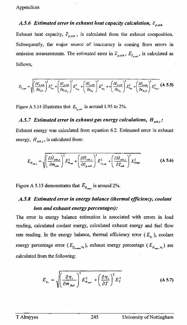
Appendices
A.5.6 Estimated error in exhaust heat capacity calculation, Cp,exh
Exhaust heat capacity, Cp,exh' is calculated from the exhaust composition.
Subsequently, the major source of inaccuracy is coming from errors in
emission measurements. The estimated error in Cp,exh' Ecp,exIr' is calculated as
follows,
Figure A 5.14 illustrates that Ec is around 1.95 to 2%. . p,txh
A.5.7 Estimated error in exhaust gas energy calculations, if exh s :
Exhaust energy was calculated from equation 6.2. Estimated error in exhaust
energy, if exh,s' is calculated from:
E, = (aiIexh,s J2 E: + (aiIexh,s J2 E2 + (aiIexh,s J2 E2 H aJo • a . maJo a- ifp aJo aT Temp , mexh C p,exh . exh (A 5.6)
Figure A 5.15 demonstrates that Efr is around 2%. em.s
A.5.S Estimated error in energy balance (thermal efficiency, coolant
loss and exhaust energy percentages):
The error in energy balance estimation is associated with errors in load
reading, calculated coolant energy, calculated exhaust energy and fuel flow
rate reading. In the energy balance, thermal efficiency error (El1,), coolant
energy percentage error (EQcookm' %), exhaust energy percentage (E if w.,. %) are
calculated from the following:
( a'l, )2 E~ + (a'll )2 E2 (A 5.7) a . m foel aT T m foel
T Alrayyes 245 University of Nottingham
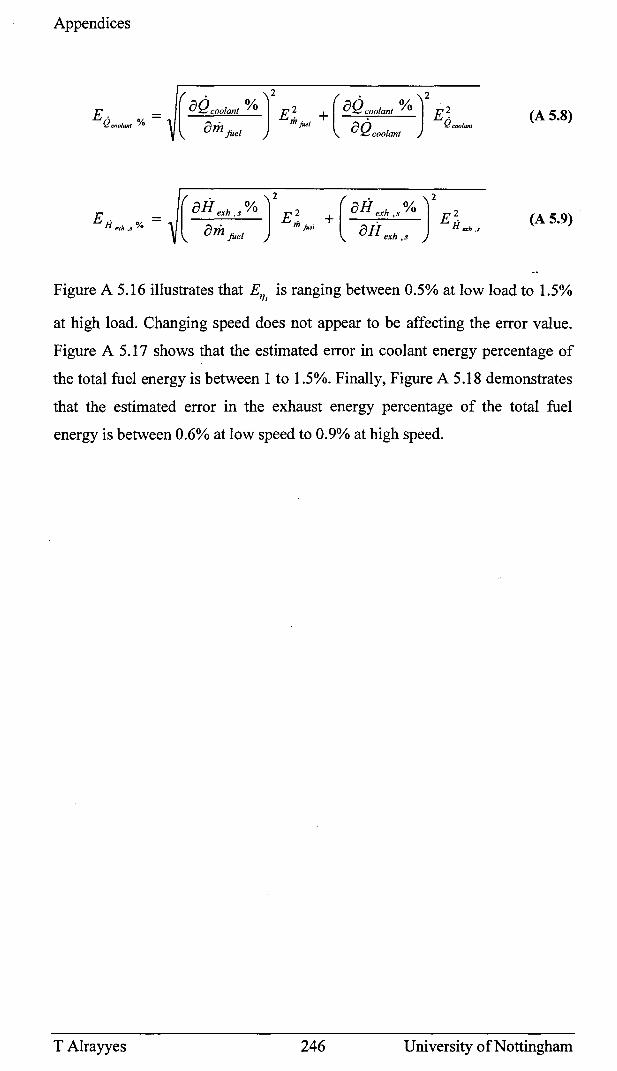
Appendices
E. 0 = (8QCOOlant % J2 E~ + (8Q~O(}lant % J2 E~ QcooiunJ Yo 8riz foei 8Q Qcoo/an/
foel coolant
(A 5.8)
E . = ( 8 if exh ," % J 2 E 1: + ( 8 if :xh ," % J 2 E ~ H exh ,3 % a rh m fuel a H H ah .1
foel exh , .•
(A 5.9)
Figure A 5.16 illustrates that ET/' is ranging between 0.5% at low load to 1.5%
at high load. Changing speed does not appear to be affecting the error value.
Figure A 5.17 shows that the estimated error in coolant energy percentage of
the total fuel energy is between 1 to 1.5%. Finally, Figure A 5.18 demonstrates
that the estimated error in the exhaust energy percentage of the total fuel
energy is between 0.6% at low speed to 0.9% at high speed.
T Alrayyes 246 University of Nottingham
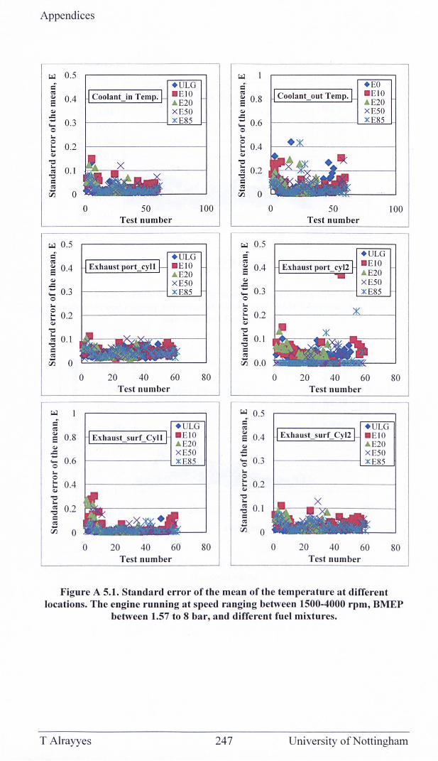
Appendices
>.ol 0.5 C ell E 0.4 QJ .c :: 0.3 o ~
o t:: 0.2 QJ
'0
; 0.1 '0 c ell
cn 0
>.ol 0.5 C ell E 0.4 QJ
~ ... 0.3 o ~ o :: 0.2 QJ
'0
; 0.1 '0 c ell
cn 0
>.ol
C ell E 0.8 QJ .c :: 0.6 o ~
o :: 0.4 QJ
'0 ~
~ 0.2 c ell -rJl 0
o
o
o
50 100 Test number
20 40 60 80 Test number
20 40 60 80 Test number
C ell E 0.8 QJ .c :: 0.6 o ~
o :: 0.4 QJ
'0
; 0.2 '0 c ell
cn 0
>.ol 0.5 C ell E 0.4 QJ .c :: 0.3 o ~ o :: 0.2 QJ
'0
; 0.1 '0 c ell
~ 0.0
>.ol 0.5 c ell QJ
E 0.4 QJ .c -'0 0.3 ~ o ~ ~ QJ
'0 ~
0.2
~ 0.1 c ell -rJl o
o 50 100 Test number
o 20 40 60 80 Test number
o 20 40 60 80 Test number
Figure A 5.1. Standard error of the mean of the temperature at different locations. The engine running at speed ranging between 1500-4000 rpm, BMEP
between 1.57 to 8 bar, and different fuel mixtures.
T Alrayyes 247 University of Nottingham
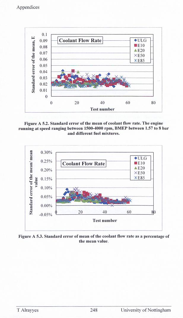
Appendices
0.1 ~
= 0.09 CiS
0.08 ~
S ~ 0.07
-= - 0.06 ~ 0 I. 0.05 0 I.
0.04 I. ~
"0 0.03 I. CiS
"0 0.02 = CiS 0.01 -rJ:J
0
Coolant Flow Rate 1-----
0 20 40 60
Test number
+ ULG - EI0 . E20 XE50 ~ E85
80
Figure A 5.2. Standard error of the mean of coolant flow rate. The engine running at speed ranging between 1500-4000 rpm, BMEP between 1.57 to 8 bar
and different fuel mixtures.
= 0.30% CiS ~
S 0.25%
+ ULG -... Coolant Flow Rate - EIO = CiS . E20 ~ 0.20% S x E50 ~ -= ~ 0.15% ~ E85 - = ~-o CiS I. ... 0.10% 0 I. I. ~
0.05% "0 I. CiS
"0 0.00% = CiS -rFJ -0.05% Test number
Figure A 5.3. Standard error of mean of the coolant flow rate as a percentage of the mean value.
T Alrayyes 248 University of Nortingham
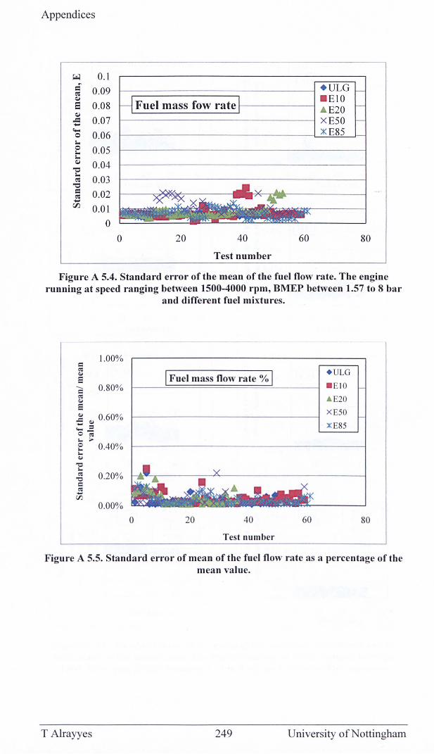
Appendices
~ 0.1 c 0.09 ~ a. S 0.08 a. -= 0.07 -
1,==============:;----1 • ULG - EI0 Fuel mass row rate f-------t ... E20
~--------------------------~ XE50 .... 0.06 0
::I(
-0 0.05 --a. 0.04 "0 - 0.03 ~ "0 c 0.02 ~ -rf1
0.01
0
0 20 40 60 80
Test number
Figure A 5.4. Standard error of the mean of the fuel flow rate. The engine running at speed ranging between 1500-4000 rpm, BMEP between 1.57 to 8 bar
and different fuel mixtures.
1.00% c (\I ~
E ....... 0.80% c (\I ~
E ~ 0.60% .c ~ - ::s .... -o (\I
J... .. 0 0.40% J... J... ~
-0 J... (\I 0.20% -0 c (\I -(J)
0.00%
0
I Fuel mass flow rate % I
20 40
Test number
60
+ ULG
- EIO
& E20
X E50
): E85
80
Figure A 5.5. Standard error of mean of the fuel flow rate as a percentage of the mean value.
T Alrayyes 249 University of Nottingham
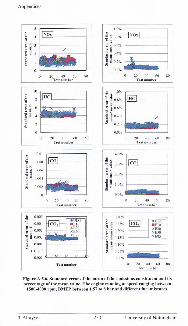
Appendices
'" .c -'-o
~~
o
o
0.01
0.008
:: c 0.006 '" 0: ~ '" ;; E 0.004 ~ c 0: -rn 0.002
o
~ O.OOS -'Q 0.004 ~~ :: c 0.003 '" 0:
~ E 0.002 0: ~
; 0.001 -rn 1.1 E-1 7
-0.00 1
20 40 60 80 Test number
20 40 60 80 Test number
o 20 40 60 80 Test number
Test number
1.0%
'" .c ~ ~ 0.8% 0';: ... > e ; 0.6% t '" ~.: 0.4% 0: c ~ 0:
C '" .s E 0.2% rn
0.0%
o
~ '" 1.0% ::.= ~ ~ 0.8% o c :: 0:
~ E 0.6% ... --.g ; 0.4% c '" .s E
rn 0.2%
'" .c '" - :l '-o 0: ... > o c t gj ~ E ... --0: C ~ 0:
C '" .s E rn
'" .c '" - :l '--o 0: ... > o c ... 0: ... '" ~ E ... --0: C ~ 0:
C '" .s E rn
0.0%
4.0%
3.0%
2.0%
1.0%
0.0%
0.30%
0.2S%
0.20%
O. IS%
0.10%
O.OS%
0.00%
o
o
o
20 40 60 Test number
20 40 60 Test number
20 40 60 Test number
+ ULG - EIO AE20 XESO :t::
80
80
80
20 40 60 80 Test number
Figure A 5.6. Standard error of the mean of the emissions constituent and its percentage of the mean value. The engine running at speed ranging between
1500-4000 rpm, BMEP between 1.57 to 8 bar and different fuel mixtures.
T Alrayyes 250 University of Nottingham
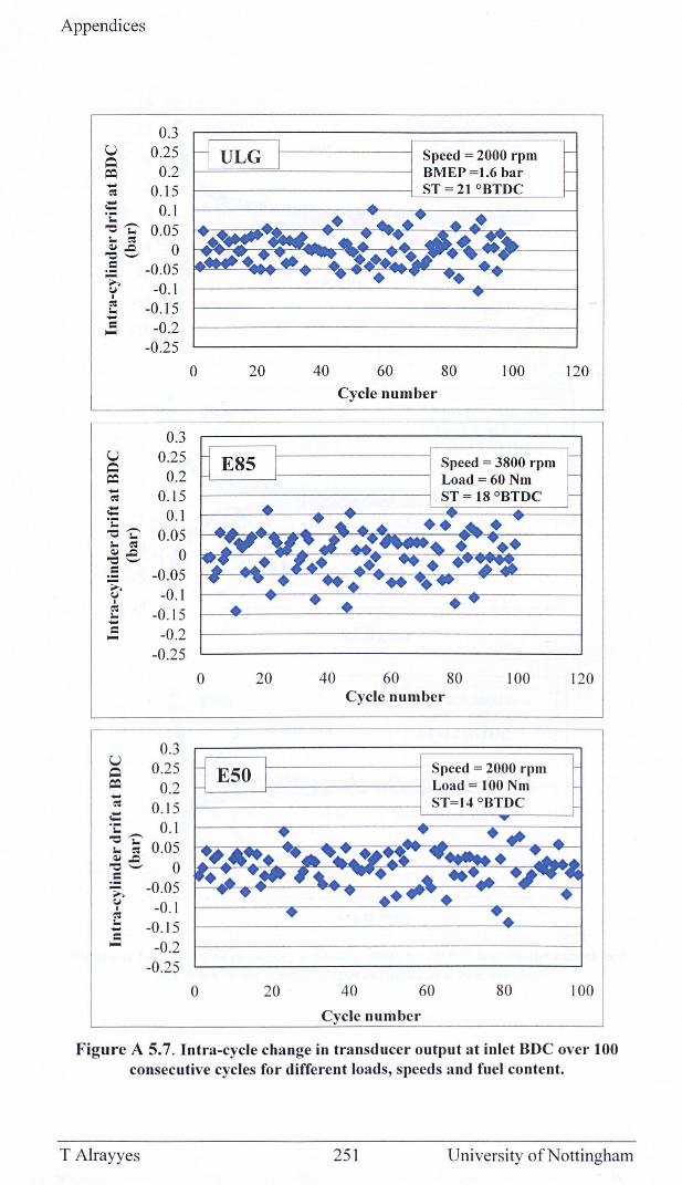
Appendices
U ~ ~ ....
e<: .-::: 'i: "'C~ I. e<: ~,.Q "0 '-' .S ~
C.I I
e<: I. .... = ....
U ~ ~ ....
e<: .::: 'i: "O'i:' I. e<: ~,.Q
"0 '-' .S ~
C.I I
e<: I. .... = ....
....
0.3 0.25
0.2 0.15
0.1 0.05
0 -0.05
-0.1 -0.15
-0.2 -0.25
0.3 0.25
0.2 0.15
0.1 0.05
0 -0.05
-0.1 -0.15
-0.2 -0.25
0.3 0.25
0.2
~ 0.15 I. 0.1 "O'i:' I. e<: 0.05 ~,.Q "0'-' 0 = ;: -0.05 G' I -0.1 E .... -0.15 = .... -0.2
-0.25
0 20
0 20
o 20
40
40
60
Speed = 2000 rpm BMEP =1.6 bar ST =21 °BTDC
80 100
Cycle number
60
Speed = 3800 rpm Load = 60 Nm ST = 18 °BTDC
80 100 Cycle number
40
Speed = 2000 rpm Load = 100 Nm ST=14°BTDC
60 80
Cycle number
120
120
100
Figure AS. 7. Intra-cycle change in transducer output at inlet BDC over 100 consecutive cycles for different loads, speeds and fuel content.
T Alrayyes 251 University of Nottingham
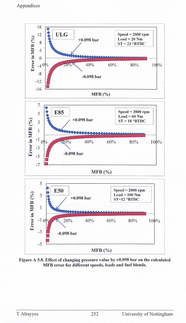
Appendices
Figure A 5.8. Effect of changing pressure value by ±O.098 bar on the calculated MFB error for different speeds, loads and fuel blends.
T Alrayyes 252 University of Nottingham
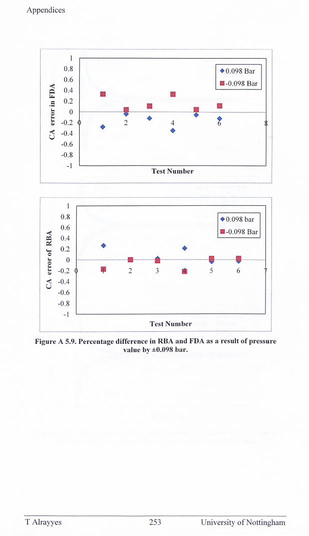
Appendices
1
0.8 . 0.098 Bar 0.6
- -0.098 Bar -< ~ 0.4 • • ~
.S 0.2
• • • • l. 0 0 • • l. • t l. -0.2 2 4 Q,) • -< -0.4 • U -0.6
-0 .8
-1 Test Number
1
0.8 . 0.098 bar 0.6
- -0.098 Bar -< ~ 0.4
• • '- 0.2 0 - ..... - -l. 0 0 - - .. .. l. , l. -0.2 2 3 • 5 6 Q,)
-< -0.4 U
-0.6
-0.8
-I Test Number
Figure A 5.9. Percentage difference in RBA and FDA as a result of pressure value by ±O.098 bar.
T Alrayyes 253 University of Nottingham
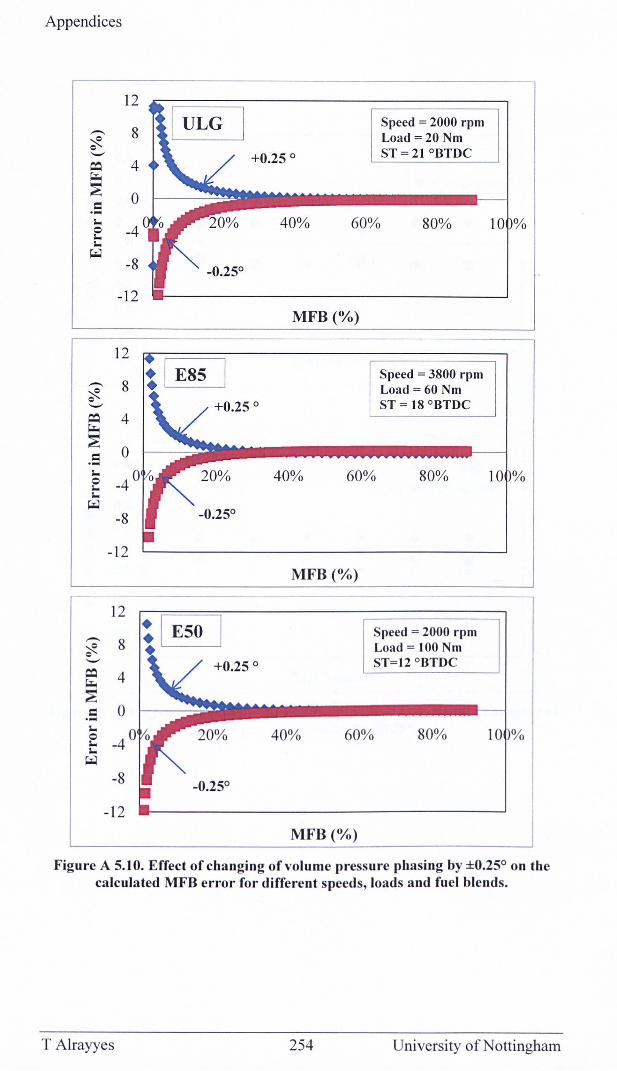
Appendices
12
.--, 8 ~ Q '-'
~ 4 ~
~ 0 .s ... 0 -4 ... ... ~
-8
-12
12
.--, 8 ~ Q
'-'
~ 4 ~
~ 0 C .-...
0 ... ... ~
-8
-12
12
.--, 8 ~ Q
'-'
~ 4 ~
~ C 0 .-... 0
-4 ... ... ~
-8
-12
ULG Speed = 2000 rpm Load =20 Nm
+0.25 0 ST =21 °BTDC
-0.250
+0.25 0
-0.25°
40% 60% 80%
MFB (%)
Speed = 3800 rpm Load =60 Nm ST = 18 °BTDC
40% 60% 80%
MFB (%)
40% 60%
MFB(%)
Speed = 2000 rpm Load = 100 Nm ST= 12 °BTDC
80%
10
10 %
Figure A 5.10. Effect of changing of volume pressure phasing by ±0.25° on the calculated MFB error for different speeds, loads and fuel blends.
T Alrayyes 254 University of Nottingham
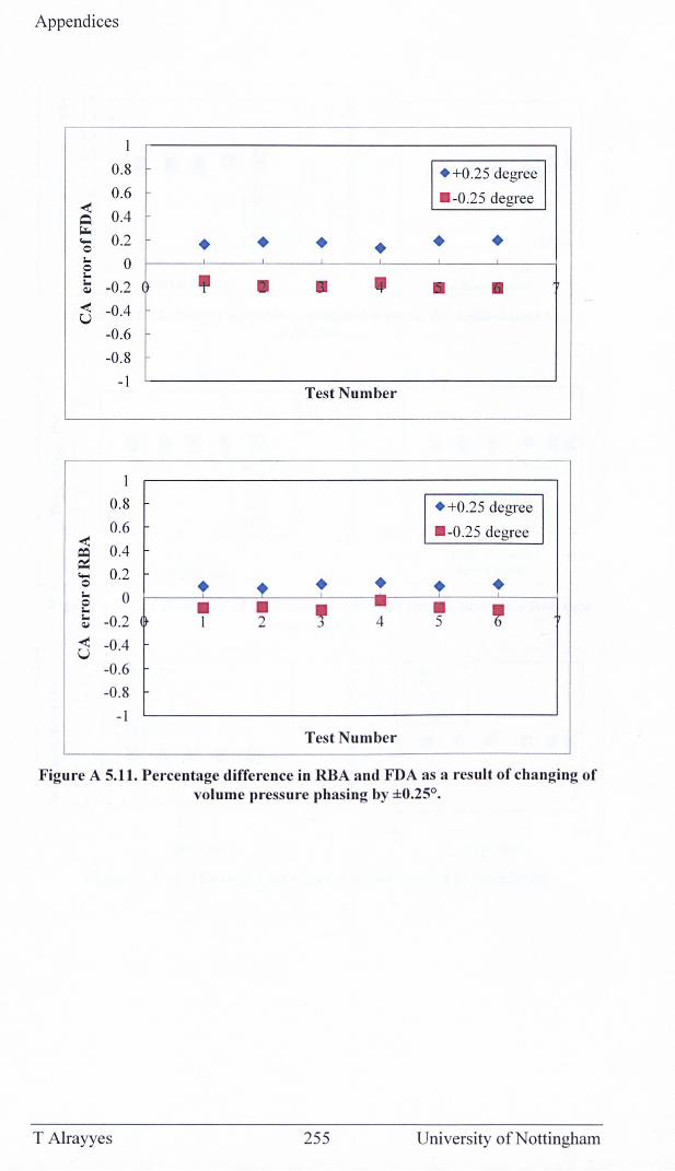
Appendices
1
0.8 + +0.25 degree 0.6 - -0.25 degree -<
~ 0.4 ~
0.2 • .... • • • • • 0 l. 0 0 l. • '" l. -0.2 • • • • cu
-< -0.4 U
-0.6
-0.8
-1 Test Number
1
0.8 + +0.25 degree 0.6 - -0.25 degree -<
~ 0.4 .... 0.2 • 0 • • • • • l. 0 0 • • • • l. , , l. -0.2 1 2 4 5 cu
-< -0.4 U
-0.6
-0.8
-I
Test Number
Figure A 5.11. Percentage difference in RBA and FDA as a result of changing of volume pressure phasing by ±O.2So.
T Alrayyes 255 University of Nottingham
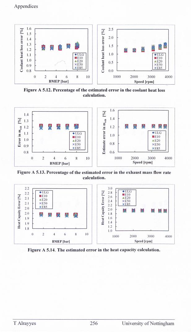
Appendices
~ Q
... 0 ... ... .. '" '" ~ .... «S .. ..c .... c «S
'0 0 u
~ Q
-;; E~
c ... 0 ... ... ""
1.6 2.5 ~
1.5 Q
... 2.0 1.4 0 ... ... 1.3 • ..
'" 1.5 '" 1.2 ~ .... 1.0 1.1 + ULG «S ..
- E IO ..c 1.0 A E20 ....
c 0.5 XE50 ..:: 0.9 x E85 0
0 0.8 u 0.0
0 2 4 6 8 10 1000 2000 3000 4000 BMEP Ibarl Speed Irpm)
Figure A 5.12. Percentage of the estimated error in the coolant heat loss calculation.
1.6 1.4 ~ Q
1.3 -;; 1.4 E~
1.2 .:: 1.2 ...
1.1 + ULG 0 ... 1.0 - E IO ... 1.0 ..
AE20 .. AE20 .... 0.8 x E50 «S x E50 0.9 E XE85 c.::: x E85 0.8 '" 0.6 "" 0 2 4 6 8 10 1000 2000 3000 4000
BMEP Ibarl Speed Irpm)
Figure A 5.13. Percentage of the estimated error in the exhaust mass flow rate calculation.
2.2
~ 2.2
" 2. 1 ... 0 2 .1 ... ... "" 2.0 .f' 2.0 .. Co
'" 1.9 u ';; 1.9 OJ
:: 1.8
0
+ ULG - E IO AE20 x E50 x E85
2 4 6 8 10
8M EP Ibarl
3.0
~ 2.8 + ULG " _ E IO ... 2.6 AE20 0 ... 2.4 x E50 ... "" 2.2 x E85 C . ; 2.0 • • • • •• Co
1.8 .. u
1.6 ';; .!: 1.4
1.2 1.0
1000 2000 3000 4000
peed Irpllli
Figure A 5.14. The estimated error in the heat capacity calculation.
T Alrayyes 256 University of Nottingham
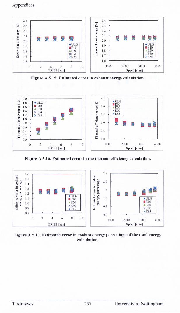
Appendices
2.4 2.4
~ 2.3 ::R 2.3 " " .., ..,
2.2 bJ) 2.2 bJ) ... ... ... ... 2.1 = 2. 1 = ... • CJ -- 2.0 '" 2.0 '" ::>
~ eo ..c 1.9
+ ULG ~ 1.9 + ULG
'" - E I O ... _ E IO ... ... ... 1.8 & E20 0 1.8 & E20 0 ... ... x E50 ... x E50 ...
1.7 ~ 1.7 x E85 ~ X E85
1.6 1.6
0 2 4 6 8 10 1000 2000 3000 4000
BMEP Ibarl Speed Irpml
Figure A 5.15. Estimated error in exhaust energy calculation.
2.0 2. 5 ~ 1.8 + ULG ~ + ULG " _ EIO ... 1.6 - E IO ... 2.0 & E20 0 ... & E20 0 ... 1.4
... x E50 ... x E50 ... ... x E85 .., 1.2 x E85 .., 1.5 v
5 v
1.0 = • . ;:; ... ..:: 0.8
.;:; 1.0 * • • .... ..:: • ... ....
-; 0.6 ... -; e 0.4 e 0.5 ... ... ...
..c 0.2 ::: f-
0.0 f= 0.0
0 2 4 6 8 10 1000 2000 3000 4000
BMEP Ibarl Speed Irpml
Figure A 5.16. Estimated error in the thermal efficiency calculation.
1.6 2.5
= = '" 1.5 eo - ... - ... o bJ) o bJ) 2.0 o '" 1.4
o eo v_ v_
= = = = . - '" 1.3 .. .- ... v ... v 1.5 ... ... o ... o ...
1.2 ... ... t: Q. ... C. ... .., + ULG ... ..,
-= ... 1.1 - E I O -= ... 1.0 + ULG ... bJ) ... bJ) - ... - ... - E IO '" ... 1.0 & E20 '" ... = = c c
0,c QJ x E50 "';: e.; 0. - & E20 '" 0.9 '" x E50 ~ X E85 ~
0.8 x E85 0.0
0 2 4 6 8 10 1000 2000 3000 4000
B IEP Ibarl peed Irpml
Figure A 5.17. Estimated error in coolant energy percentage of the total energy calculation.
T Alrayyes 257 University of Nottingham
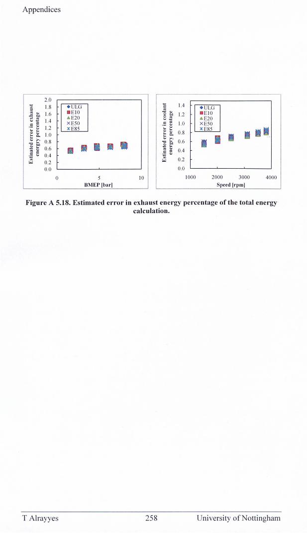
Appendices
2.0
i 1.8 ~ ~ 1.6 "" '" ~ = 1.4
.;: ~ 1.2 o b c: Q. 1.0 ~ ~ 0.8 ~f:O ",'" 0.6 .~ ~ 0.4 '" '-l 0.2
0.0
o
+ ULG - EIO . E20 x E50 x E85
5 BMEP !bar!
10
= 1.4 '" g ~ 1.2 '-'-.: ~ 1.0 5 ~ c: ~ 0.8 ... >.
B ~ 0.6
~ ~ 0.4 ',c ~
~ 0.2
0.0
1000
+ ULG - EIO . E20 x E50 x E85
• I • 2000 3000
Speed !rpm! 4000
Figure A 5.18. Estimated error in exhaust energy percentage of the total energy calculation.
T Alrayyes 258 University of Nottingham
Related Documents