Welcome message from author
This document is posted to help you gain knowledge. Please leave a comment to let me know what you think about it! Share it to your friends and learn new things together.
Transcript


THE ECONOMICS OF GROWTH
The MIT PressCambridge, MassachusettsLondon, England
Philippe Aghion and Peter Howitt
with the collaboration of Leonardo Bursztyn

© 2009 Massachusetts Institute of Technology
All rights reserved. No part of this book may be reproduced in any form by any electronic or mechanical means (including photocopying, recording, or information storage and retrieval) without permission in writing from the publisher.
For information about special quantity discounts, please email [email protected]
This book was set in Times Roman by SNP Best-set Typesetter Ltd., Hong Kong.Printed and bound in the United States of America.
Library of Congress Cataloging-in-Publication Data
Aghion, Philippe.The economics of growth / Philippe Aghion and Peter W. Howitt. p. cm.Includes bibliographical references and index.ISBN 978-0-262-01263-8 (hardcover : alk. paper)1. Economic development. I. Howitt, Peter. II. Title. HD82.A5452 2009338.9—dc22 2008029818
10 9 8 7 6 5 4 3 2 1
Contents
Preface xvii
Why This Book? xvii
For Whom? xviii
Outline of the Book xix
Acknowledgments xxi
Introduction 1
I.1 Why Study Economic Growth? 1
I.2 Some Facts and Puzzles 1
I.2.1 Growth and Poverty Reduction 1
I.2.2 Convergence 2
I.2.3 Growth and Inequality 4
I.2.4 The Transition from Stagnation to Growth 5
I.2.5 Finance and Growth 5
I.3 Growth Policies 6
I.3.1 Competition and Entry 7
I.3.2 Education and Distance to Frontier 8
I.3.3 Macroeconomic Policy and Growth 10
I.3.4 Trade and Growth 10
I.3.5 Democracy and Growth 11
I.4 Four Growth Paradigms 12
I.4.1 The Neoclassical Growth Model 12
I.4.2 The AK Model 13
I.4.3 The Product-Variety Model 14
I.4.4 The Schumpeterian Model 15
PART I: BASIC PARADIGMS OF GROWTH THEORY 19
1 Neoclassical Growth Theory 21
1.1 Introduction 21
1.2 The Solow-Swan Model 21
1.2.1 Population Growth 24
1.2.2 Exogenous Technological Change 27
1.2.3 Conditional Convergence 29
1.3 Extension: The Cass-Koopmans-Ramsey Model 31
1.3.1 No Technological Progress 31
viii
1.3.2 Exogenous Technological Change 37
1.4 Conclusion 39
1.5 Literature Notes 39
Appendix 1A: Steady State and Convergence in the Cass-Koopmans-Ramsey Model 40
Appendix 1B: Dynamic Optimization Using the Hamiltonian 43
Problems 45
2 The AK Model 47
2.1 Introduction 47
2.1.1 The Harrod-Domar Model 48
2.2 A Neoclassical Version of Harrod-Domar 49
2.2.1 Basic Setup 49
2.2.2 Three Cases 51
2.3 An AK Model with Intertemporal Utility Maximization 52
2.3.1 The Setup 53
2.3.2 Long-Run Growth 54
2.3.3 Welfare 55
2.3.4 Concluding Remarks 55
2.4 The Debate between Neoclassical and AK Advocates, in a Nutshell 56
2.5 An Open-Economy AK Model with Convergence 60
2.5.1 A Two-Sector Closed Economy 61
2.5.2 Opening up the Economy with Fixed Terms of Trade 62
2.5.3 Closing the Model with a Two-Country Analysis 64
2.5.4 Concluding Comment 66
2.6 Conclusion 66
2.7 Literature Notes 67
Problems 67
3 Product Variety 69
3.1 Introduction 69
3.2 Endogenizing Technological Change 69
3.2.1 A Simple Variant of the Product-Variety Model 70
3.2.2 The Romer Model with Labor as R&D Input 74
3.3 From Theory to Evidence 77
3.3.1 Estimating the Effect of Variety on Productivity 77
Contents
ix
3.3.2 The Importance of Exit in the Growth Process 79
3.4 Conclusion 80
3.5 Literature Notes 81
Problems 82
4 The Schumpeterian Model 85
4.1 Introduction 85
4.2 A One-Sector Model 85
4.2.1 The Basics 85
4.2.2 Production and Profi ts 86
4.2.3 Innovation 87
4.2.4 Research Arbitrage 88
4.2.5 Growth 89
4.2.6 A Variant with Nondrastic Innovations 90
4.2.7 Comparative Statics 91
4.3 A Multisector Model 92
4.3.1 Production and Profi t 92
4.3.2 Innovation and Research Arbitrage 94
4.3.3 Growth 95
4.4 Scale Effects 96
4.5 Conclusion 99
4.6 Literature Notes 100
Problems 101
5 Capital, Innovation, and Growth Accounting 105
5.1 Introduction 105
5.2 Measuring the Growth of Total Factor Productivity 106
5.2.1 Empirical Results 107
5.3 Some Problems with Growth Accounting 109
5.3.1 Problems in Measuring Capital, and the Tyranny of Numbers 109
5.3.2 Accounting versus Causation 112
5.4 Capital Accumulation and Innovation 113
5.4.1 The Basics 114
5.4.2 Innovation and Growth 116
5.4.3 Steady-State Capital and Growth 116
5.4.4 Implications for Growth Accounting 118
Contents
x
5.5 Conclusion 119
5.6 Literature Notes 119
Appendix: Transitional Dynamics 120
Problems 121
PART II: UNDERSTANDING THE GROWTH PROCESS 127
6 Finance and Growth 129
6.1 Introduction 129
6.2 Innovation and Growth with Financial Constraints 130
6.2.1 Basic Setup 130
6.2.2 Innovation Technology and Growth without Credit Constraint 132
6.2.3 Credit Constraints: A Model with Ex Ante Screening 132
6.2.4 A Model with Ex Post Monitoring and Moral Hazard 134
6.3 Credit Constraints, Wealth Inequality, and Growth 136
6.3.1 Diminishing Marginal Product of Capital 136
6.3.2 Productivity Differences 139
6.4 The Empirical Findings: Levine’s Survey, in a Nutshell 142
6.4.1 Cross-Country 143
6.4.2 Cross-Industry 145
6.5 Conclusion 147
6.6 Literature Notes 147
Problems 148
7 Technology Transfer and Cross-Country Convergence 151
7.1 Introduction 151
7.2 A Model of Club Convergence 152
7.2.1 Basics 152
7.2.2 Innovation 153
7.2.3 Productivity and Distance to Frontier 154
7.2.4 Convergence and Divergence 156
7.3 Credit Constraints as a Source of Divergence 158
7.3.1 Theory 159
7.3.2 Evidence 161
7.4 Conclusion 163
7.5 Literature Notes 165
Problems 166
Contents
xi
8 Market Size and Directed Technical Change 169
8.1 Introduction 169
8.2 Market Size in Drugs 169
8.2.1 Theory 169
8.2.2 Evidence 171
8.3 Wage Inequality 173
8.3.1 The Debate 174
8.3.2 The Market-Size Explanation 176
8.4 Appropriate Technology and Productivity Differences 182
8.4.1 Basic Setup 182
8.4.2 Equilibrium Output and Profi ts 183
8.4.3 Skill-Biased Technical Change 184
8.4.4 Explaining Cross-Country Productivity Differences 185
8.5 Conclusion 186
8.6 Literature Notes 187
Problems 188
9 General-Purpose Technologies 193
9.1 Introduction 193
9.2 Explaining Productivity Slowdowns 196
9.2.1 General-Purpose Technologies in the Neoclassical Model 196
9.2.2 Schumpeterian Waves 198
9.3 GPT and Wage Inequality 204
9.3.1 Explaining the Increase in the Skill Premium 204
9.3.2 Explaining the Increase in Within-Group Inequality 206
9.4 Conclusion 210
9.5 Literature Notes 211
Problems 212
10 Stages of Growth 217
10.1 Introduction 217
10.2 From Stagnation to Growth 217
10.2.1 Malthusian Stagnation 217
10.2.2 The Transition to Growth 222
10.2.3 Commentary 224
10.3 From Capital Accumulation to Innovation 226
10.3.1 Human-Capital Accumulation 226
Contents

xii
10.3.2 Physical-Capital Accumulation 227
10.4 From Manufacturing to Services 230
10.5 Conclusion 232
10.6 Literature Notes 232
Problems 233
11 Institutions and Nonconvergence Traps 237
11.1 Introduction 237
11.2 Do Institutions Matter? 238
11.2.1 Legal Origins 239
11.2.2 Colonial Origins 240
11.3 Appropriate Institutions and Nonconvergence Traps 243
11.3.1 Some Motivating Facts 243
11.3.2 A Simple Model of Distance to Frontier and Appropriate Institutions 246
11.4 Conclusion 258
11.5 Literature Notes 261
Problems 263
PART III: GROWTH POLICY 265
12 Fostering Competition and Entry 267
12.1 Introduction 267
12.2 From Leapfrogging to Step-by-Step Technological Progress 267
12.2.1 Basic Environment 268
12.2.2 Technology and Innovation 269
12.2.3 Equilibrium Profi ts and Competition in Level and Unlevel Sectors 269
12.2.4 The Schumpeterian and “Escape-Competition” Effects 271
12.2.5 Composition Effect and the Inverted U 272
12.2.6 Empirical Evidence 274
12.3 Entry 274
12.3.1 The Environment 276
12.3.2 Technology and Entry 276
12.3.3 Equilibrium Innovation Investments 277
12.3.4 The Effect of Labor Market Regulations 278
12.3.5 Main Theoretical Predictions 279
Contents

xiii
12.3.6 Evidence on the Growth Effects of Entry 279
12.3.7 Evidence on the Effects of (De)Regulating Entry 280
12.4 Conclusion 281
12.5 Literature Notes 282
Problems 283
13 Investing in Education 287
13.1 Introduction 287
13.2 The Capital Accumulation Approach 288
13.2.1 Back to Mankiw, Romer, and Weil 288
13.2.2 Lucas 292
13.2.3 Threshold Effects and Low-Development Traps 295
13.3 Nelson and Phelps and the Schumpeterian Approach 297
13.3.1 The Nelson and Phelps Approach 297
13.3.2 Low-Development Traps Caused by the Complementarity between R&D and Education Investments 300
13.4 Schumpeter Meets Gerschenkron 302
13.4.1 A Model of Distance to Frontier and the Composition of Education Spending 302
13.4.2 Cross-Country and Cross-U.S.-State Evidence 307
13.5 Conclusion 311
13.6 Literature Notes 312
Problems 314
14 Reducing Volatility and Risk 319
14.1 Introduction 319
14.2 The AK Approach 321
14.2.1 The Jones, Manuelli, and Stacchetti Model 321
14.2.2 Counterfactuals 324
14.3 Short-versus Long-Term Investments 326
14.3.1 The Argument 326
14.3.2 Motivating Evidence 327
14.3.3 The AABM Model 329
14.3.4 Confronting the Credit Constraints Story with Evidence 339
14.3.5 An Alternative Explanation for the Procyclicality of R&D 340
14.4 Risk Diversifi cation, Financial Development, and Growth 341
14.4.1 Basic Framework 341
Contents

xiv
14.4.2 Analysis 343
14.4.3 Equilibrium Dynamics 345
14.5 Conclusion 347
14.6 Literature Notes 348
Problems 349
15 Liberalizing Trade 353
15.1 Introduction 353
15.2 Preliminary: Back to the Multisector Closed-Economy Model 355
15.2.1 Production and National Income 355
15.2.2 Innovation 357
15.3 Opening Up to Trade, Abstracting from Innovation 358
15.3.1 The Experiment 358
15.3.2 The Effects of Openness on National Income 360
15.4 The Effects of Openness on Innovation and Long-Run Growth 363
15.4.1 Step-by-Step Innovation 363
15.4.2 Three Cases 364
15.4.3 Equilibrium Innovation and Growth 365
15.4.4 Scale and Escape Entry 365
15.4.5 The Discouragement Effect of Foreign Entry 366
15.4.6 Steady-State Aggregate Growth 367
15.4.7 How Trade Can Enhance Growth in All Countries 368
15.4.8 How Trade Can Reduce Growth in One Country 369
15.5 Conclusion 371
15.6 Literature Notes 372
Problems 374
16 Preserving the Environment 377
16.1 Introduction 377
16.2 The One-Sector AK Model with an Exhaustible Resource 377
16.3 Schumpeterian Growth with an Exhaustible Resource 379
16.4 Environment and Directed Technical Change 381
16.4.1 Basic Setup 381
16.4.2 Equilibrium Outputs and Profi ts 382
16.4.3 Taxing Dirty Production 384
16.4.4 Equilibrium Innovation 385
16.4.5 Growth and the Cost of Taxing Dirty Output 387
Contents
xv
16.4.6 Evidence of Directed Technical Change Effects in the Energy Sector 389
16.4.7 Concluding Remarks 390
16.5 Literature Notes 391
Appendix: Optimal Schumpeterian Growth with an Exhaustible Resource 392
Problems 395
17 Promoting Democracy 399
17.1 Introduction 399
17.2 Democracy, Income, and Growth in Existing Regressions 399
17.2.1 Irrelevance Results When Controlling for Country Fixed Effects 400
17.2.2 No Apparent Correlation between Democracy and Public Policy 400
17.3 Democracy, Entry, and Growth: A Simple Model 401
17.3.1 Production and Profi ts 402
17.3.2 Entry and Incumbent Innovation 402
17.3.3 Politics and the Equilibrium Probability of Entry 405
17.3.4 Main Prediction 407
17.4 Evidence on the Relationship between Democracy, Growth, and Technological Development 407
17.4.1 Data and Regression Equation 407
17.4.2 Basic Results 408
17.5 Democracy, Inequality, and Growth 410
17.5.1 The Model 410
17.5.2 Solving the Model 411
17.5.3 Discussion 413
17.6 Conclusion 414
17.7 Literature Notes 414
Problems 415
CONCLUSION 417
18 Looking Ahead: Culture and Development 419
18.1 What We Have Learned, in a Nutshell 419
18.2 Culture and Growth 420
Contents
xvi
18.2.1 Regulation and Trust 422
18.2.2 Investing in Children’s Patience 425
18.3 Growth and Development 429
18.3.1 Growth through the Lens of Development Economics 429
18.3.2 The Case for Targeted Growth Policy 434
18.4 Conclusion 439
Appendix: Solving the Doepke-Zilibotti Model 441
Appendix: Basic Elements of Econometrics 443
A.1 The Simple Regression Model 443
A.2 The Ordinary Least Squares Estimator 444
A.3 Multiple Regression Analysis 446
A.4 Inference and Hypothesis Testing 447
A.5 How to Deal with the Endogeneity Problem 449
A.6 Fixed-Effects Regressions 452
A.7 Reading a Regression Table 453
References 457
Index 477
Contents
Preface
Why This Book?
To learn about economic growth you need formal theory, for organizing the facts, clarifying causal relationships, and drawing out hidden implications. In growth economics, as in other areas of economics, an argument that is not disciplined by a clear theoretical framework is rarely enlightening.
Our experience with graduates and undergraduates at Brown and Harvard has taught us, however, that the theory needed to understand the substantive issues of economic growth is much simpler than what is found in most modern text-books. You do not need to master all the subtleties of dynamic programming and stochastic processes in order to learn what is essential about such issues as cross-country convergence, the effects of fi nancial development on growth, and the consequences of globalization. The required tools can be acquired quickly by anyone equipped with elementary calculus and probability theory.
These considerations are what motivated us to write The Economics of Growth. We believe that what is going on at the frontiers of research on economic growth can also be made accessible to undergraduates, as well as to policy makers who have not been to graduate school for many years, even though gaining this access requires learning some basic tools and models. Although there are many other excellent books on growth economics,1 those that focus on theory are either too removed from policy and empirical applications or too involved with formal technicalities to be useful or interesting to the uninitiated reader wanting to learn about the substantive issues, while other books that focus on substantive issues are not as concerned with formal models as is necessary. None of them present the main facts and puzzles, propose simple tools and models to explain these facts, acquaint the reader with frontier material on growth—both theoretical and empirical— or initiate the reader into thinking about growth policy. What follows is our attempt to fi ll this gap.
To bring the reader up to date on the frontiers of the subject, we have had to write a comprehensive book. In the fi rst part we introduce all the major growth paradigms (neoclassical, AK, product-variety, and Schumpeterian), and then in subsequent chapters we show how these paradigms can be used to analyze various aspects of the growth process and to think about the design of growth policy. The
1. For example, Weil (2008), C. Jones (1998), Barro and Sala-i-Martin (1995a), Helpman (2004), and Acemoglu (2008a, forthcoming). Modesty does not prevent us from also including Aghion and Howitt (1998a).
xviii Preface
book is also comprehensive in its account of the most recent contributions and debates on growth: in particular, we acquaint the reader with the literature on directed technical change and its applications to wage inequality; we provide simple presentations of recent models of industrialization and the transition to modern economic growth; we show simple models of trade, competition, and growth with fi rm heterogeneity; we analyze the relationships between growth and fi nance, between growth, volatility and risk, between growth and the environ-ment, and between growth and education; we refl ect on the recent debates on institutions versus human capital as determinants of growth; and we introduce the reader to the nascent literature on growth and culture.
Although comprehensive, the book does not provide an unbiased survey of all points of view. On the contrary, it is opinionated in at least two respects. First, in order to keep the book from getting too big, we had to be selective in the material covered on each topic. At the end of each chapter, however, we include literature notes that provide the reader with extensive references on the subject and, in particular, direct her to the corresponding chapter(s) in the Handbook of Economic Growth (Aghion and Durlauf 2005), the most recent compendium of research on economic growth. Second, even though we repeatedly use the AK or product-variety models in the text or in problem sets, we do not hide our prefer-ence for the Schumpeterian model, which we use more systematically than the others when analyzing the growth process and when discussing the design of growth policy.
For Whom?
The book is aimed at three main audiences. The fi rst is graduate students. The book can be taught in its entirety in a one-semester graduate growth course. It can also be used as part of a growth and development sequence, in which case one can start with the fi rst four chapters, then move on to the chapters on fi nance (and wealth inequality), convergence, directed technical change (and appropriate technologies), stages of growth, institutions, democracy, and education, and the concluding chapter (on culture and development). The book can also be used for topics courses—for example, in trade or in industrial organization (with the general-purpose technologies, competition, and trade chapters) or in labor eco-nomics (with the chapters on directed technical change and general-purpose technologies that analyze the issue of wage inequality, and of course the chapter on education). In each case, the book provides the graduate student with easy
xix
access to frontier material, and hopefully it should spur many new research ideas.
The second target group is intermediate or advanced undergraduate students. In particular, the fi rst four chapters of the book have been conceived so as to make the basic growth paradigms fully accessible to students who have no more background than elementary notions of calculus (derivatives, maximization) and a very basic knowledge of economic principles. One can then complete the undergraduate course or sequence by using some of the other chapters of the book—for example, the chapters on stages of growth, fi nance, convergence, institutions, education, and volatility. The more advanced material, which can be skipped at the undergraduate level, is put in starred sections and problems. (Prob-lems with two stars are the most diffi cult.)
The third audience is that of professional economists in government or in international fi nancial institutions who are involved in advising governments on growth and development policies. With parsimonious use of models and equa-tions, the book provides them with the basic paradigms (part I), and also with the tools (chapters 11–18), to think about the design of growth policy.
More generally, this book can be used by any reader with a basic mathematical background who is interested in learning about the mechanics of growth and development.
Outline of the Book
The book comprises three parts. Part I presents the main growth paradigms: the neoclassical model (chapter 1), the AK model (chapter 2), Romer’s product-variety model (chapter 3), and the Schumpeterian model (chapter 4). Chapter 5 concludes part I by introducing physical capital into a growth model with endog-enous innovation, in order to provide a theoretical framework for interpreting the results of growth accounting.
Part II builds on the main paradigms to shed light on the dynamic process of growth and development. Chapter 6 analyzes the relationship between fi nancial constraints, innovation, and growth, and then the relationship between fi nancial constraints, wealth inequality, and growth. Chapter 7 analyzes the phenomenon of “club convergence,” in other words, why some countries manage to converge to growth rates of the most advanced countries whereas other countries continue to fall further behind. Chapter 8 introduces the notion of directed technical change and uses it to analyze wage inequality or to explain persistent productivity
Preface
xx
differences across countries. Chapter 9 introduces the notion of general-purpose technology and explains why new technological revolutions can produce both temporary slowdowns and accelerating wage inequality. Chapter 10 analyzes how an economy can evolve from a stagnant Malthusian agricultural economy into a persistently growing industrial economy, or from an economy that accumulates capital to an innovating economy, or from a manufacturing to a service economy. Chapter 11 discusses the role of institutions in the growth process, and introduces the notion of appropriate growth institutions to understand why different institu-tions or policies can be growth enhancing in countries at different levels of development.
Part III focuses on growth policies. Chapter 12 analyzes the growth effects of liberalizing product market competition and entry. Chapter 13 analyzes the growth effects of education policy. Chapter 14 focuses on the relationship between risk, fi nancial development, and growth. Chapter 15 discusses the effects of trade liber-alization. Chapter 16 analyzes how growth can be sustained in an economy with environmental or resource constraints. And Chapter 17 investigates the relationship between democracy and growth.
Chapter 18 concludes the book by summarizing the main conclusions from previous chapters and then by linking growth to culture and to modern develop-ment economics.
Finally, the appendix acquaints the reader with basic notions of econometrics, so that without any prior knowledge this chapter should allow her to read and understand all the empirical sections and tables in the book.
Preface

Acknowledgments
We are primarily indebted to all the students and colleagues on whom we tested the material of this book until we felt we had achieved our goal of making it broadly accessible. Our students at Brown and Harvard, especially Quamrul Ashraf, Leonardo Bursztyn, Filipe Campante, Alberto Cavallo, Azam Chaudhry, Quo-Hanh Do, Georgy Egorov, Jim Feyrer, Phil Garner, David Hemous, Michal Jerzmanowski, Takuma Kunieda, Kalina Manova, Daniel Mejia, Erik Meyersson, Stelios Michalopoulos, Petros Milionis, Malhar Nabar, Manabu Nose, Omer Ozak, and Isabel Tecu, have taught us at least as much as we have taught them.
We are also grateful for feedback from those individuals who attended our lectures at University College London, the Stockholm School of Economics, the University of Zurich, the University of Bonn, the University of Munich, the University of Kiel, the Paris School of Economics, the New Economic School in Moscow, the Di Tella University in Buenos Aires, the CEPII in Paris, Javeriana University in Bogota, the 2001 NAKE Workshop at the Vrije Universiteit Amster-dam and the 2005 NAKE School at the University of Maastricht, Wuhan Uni-versity, and the IMF Institute.
Our simple reformulations of the main growth paradigms owe a lot to joint modeling efforts with Daron Acemoglu, Marios Angeletos, Philippe Bacchetta, Abhijit Banerjee, David Mayer-Foulkes, Gianluca Violante and Fabrizio Zili-botti. Our concern for matching growth theories with data and empirics grew out of a long-standing collaboration with our colleagues Richard Blundell and Rachel Griffi th from the London Institute of Fiscal Studies, and also from joint work with Alberto Alesina, Yann Algan, Nick Bloom, Robin Burgess, Pierre Cahuc, Diego Comin, Gilbert Cette, Thibault Fally, Johannes Fedderke, Joonkyung Ha, Caroline Hoxby, Enisse Kharroubi, Kalina Manova, Ioana Marinescu, Costas Meghir, Susanne Prantl, Romain Ranciere, Steven Redding, Stefano Scarpetta, Andrei Shleifer, Francesco Trebbi, Jerome Vandenbussche, and John Van Reenen. We have benefi ted over the years from numerous discussions on various aspects of growth theory with our colleagues Pol Antras, Costas Azariadis, Robert Barro, Flora Bellone, Roland Benabou, Francesco Caselli, Guido Cozzi, Elias Dinopou-los, Esther Dufl o, Steve Durlauf, Oded Galor, Gene Grossman, Elhanan Helpman, Wolfgang Keller, Tom Krebs, Chris Laincz, Ross Levine, Robert Lipsey, Greg Mankiw, Borghan Narajabad, Pietro Peretto, Thomas Piketty, Francesco Ricci, Paul Segerstrom, Andrei Shleifer, Enrico Spolaore, David Weil, Martin Weitzman, Jeff Williamson, Marios Zachariadis, and Luigi Zingales. Finally, our views on growth policy design have been greatly infl uenced over the past years by discus-sions and collaborations with Erik Berglof, Elie Cohen, Mathias Dewatripont,

xxii
Steven Durlauf, William Easterly, Ricardo Hausmann, Martin Hellwig, Andreu Mas-Colell, Jean Pisani-Ferry, Ken Rogoff, Dani Rodrik, Andre Sapir, Nicholas Stern, and Federico Sturzenegger.
We have greatly benefi ted from our association with the Institutions, Organiza-tion and Growth (IOG) Group at the Canadian Institute for Advanced Research. There, we particularly benefi ted from continuous feedback from Elhanan Helpman, George Akerlof, Tim Besley, Daniel Diermayer, James Fearon, Patrick Francois, Joel Mokyr, Roger Myerson, Torsten Persson, Joanne Roberts, Jim Robinson, Ken Shepsle, Guido Tabellini, and Dan Trefl er.
The encouragement and support of Daron Acemoglu, Kenneth Arrow, Robert Barro, Olivier Blanchard, Oliver Hart, Martin Hellwig, Edmund Phelps, Mark Schankerman, Robert Solow, Jean Tirole, and Fabrizio Zilibotti over the years have been invaluable to us.
The book would never have been completed on time without the active col-laboration of graduate students at Harvard. Here our biggest debt is to Leonardo Bursztyn, who worked with us on the literature reviews, provided the background notes for the econometric appendix, collaborated with us on the environment chapter, produced all the fi gures, proofread the material, and coordinated the team that produced the problem sets and solutions. In this endeavor, Leonardo worked with David Hemous, Dorothée Rouzet, Thomas Sampson, and Ruchir Agarwal.
We owe special thanks to John Covell from MIT Press, who managed the tour de force of getting the book to be ready on time in spite of initial delays in deliv-ering the manuscript, and provided us with all the support we needed along the way to completion. In particular, Nancy Lombardi did an outstanding job in supervising the copyediting of the manuscript and then handling the page proofs until the book was ready to print.
Sarah Chaillet did us an immeasurable favor by offering one of her paintings for the book cover.
Philippe Aghion is infi nitely thankful to Benedicte Berner whose sense of humor, “joie de vivre,” and continuous faith in this project have been so essential for its completion.
Peter Howitt’s biggest debt is to Pat Howitt for the loving support, lively spirit, and uncommonly good sense that contributed more than words can describe.
Acknowledgments
Introduction
I.1 Why Study Economic Growth?
Economic growth is commonly measured as the annual rate of increase in a country’s gross domestic product (GDP). Why should anyone care about this dry statistic instead of focusing on more specifi c welfare, consumption, or happiness indicators? Perhaps the most compelling reason is that economic growth is what mainly determines the material well-being of billions of people. In economically advanced countries, economic growth since the industrial revolution has allowed almost the entire population to live in a style that only a privileged handful could have afforded a hundred years ago, when per capita GDP was a small fraction of what it is today. Indeed, growth in some sectors of the economy, especially the medical and pharmaceutical sectors, has allowed almost everyone to live a longer and healthier life than could have been expected by anyone in the 19th century, no matter what position a person held on the economic ladder. In contrast, the lack of economic growth in the poorest countries of the world has meant that living conditions for hundreds of millions of people are appalling by the standards of rich countries; per capita income levels in many 21st-century countries are much lower than they were in 19th-century Europe. To understand why the human race has become so much wealthier and why our wealth is shared so inequitably among the inhabitants of the world, we need to understand what drives economic growth.
I.2 Some Facts and Puzzles
Our fi rst goal is to provide the reader with analytical tools to understand the growth process. The basic theoretical paradigms are laid out in part I. Then part II analyzes various facts and puzzles raised by world growth history. The follow-ing subsections present some examples of these facts and puzzles.
I.2.1 Growth and Poverty Reduction
A number of economists argue that growth is the best way to achieve massive reduction in poverty. For example, table I.1 summarizes a study by Deaton and Dreze (2002), showing a substantial reduction in the fraction of Indian population below the poverty line. The reduction is particularly important for urban areas (from 39.1% in 1987–88 to 12% in 1999–2000).
At the same time, table I.2 from Rodrik and Subramanian (2004) shows a marked acceleration in GDP growth between the 1970s and the 20 years that
Introduction2
followed. What caused growth to accelerate in India in the 1980s? Was the cause a favorable external environment, fi scal stimulus, trade liberalization, internal liberalization, the green revolution, public investment, or, as Rodrik and Subramanian argue, an attitudinal shift on the part of the national government toward a probusiness approach? A defi nitive answer to this question would be invaluable to many other countries desperate to grow their way out of poverty.
I.2.2 Convergence
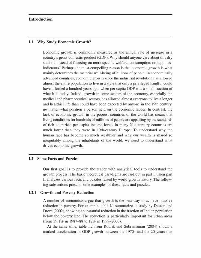
Figure I.1 shows how the average growth rate of countries over the period 1960–2000 (on the vertical axis) varies with the country’s proximity to the world productivity frontier (on the horizontal axis). The measure of proximity is simply the country’s productivity at the beginning of the period (in 1960) divided by U.S. productivity also in 1960. We see that more advanced countries tend to grow more slowly. What explains this “convergence” phenomenon? Is it the fact that rich countries have high levels of physical and human capital per person and hence are running into diminishing returns to the accumulation of more capital? Is it the fact that poor countries can catch up to rich ones technologically by making use of inventions that have taken place in the rest of the world?
Another interesting fact about convergence is that although there is a general tendency for countries to grow faster when they are further below the world productivity frontier, the very poorest of countries tend to grow more slowly than
Table I.1Poverty Reduction in India Headcount Ratios (Percentage)
Offi cial Methodology Adjusted Estimates
1987–88 1993–94 1999–2000 1987–88 1993–94 1999–2000
Rural 39.4 37.1 26.9 39 33 26.3Urban 39.1 32.9 24.1 22.5 17.8 12
Offi cial: Consumption data from Planning Commission Sample SurveyAdjusted: Consumption data from improved comparability and price indices
Table I.2India in Cross Section: Mean of Growth Rate of Output per Worker, 1970–2000
1970–80 1980–90 1990–2000
Mean of growth rate 0.77 3.91 3.22
Introduction 3
the rest. So, instead of converging, these very poor countries as a group seem to be diverging. In other words, it seems that economic growth is characterized by “club convergence.” The rich and middle income countries in the “club” tend to grow faster the further behind they fall, while the poor countries that are not members just keep falling further behind. Quah (1996, 1997) has shown that the world distribution of per capita income is becoming more and more “twin peaked,” with most countries lying at the top and the bottom levels of income. What explains this pattern?
In particular, one of the most dramatic changes of the 20th century was the revival of economic growth in many formerly poor Asian countries, which appear to have joined the convergence club during the fi nal decades of the century. From the 1960s until now, countries like South Korea, China, and India have grown much faster than the rest of the world, and they are continuing to close the gap in per capita income that separates them from the richest countries of the world. What accounts for their success?
Why have other poor countries not also joined the convergence club? Is this due to poor geographical conditions? Or to the absence of institutions to protect private investments and entrepreneurship? Or to the inability of poor countries to attract credit, diversify risk, or fi nance infrastructure? Or to insuffi cient human capital?
Figure I.1Cross-country convergence
.05
.025
0
–.025
–.05
0 .2 .6.4
Gro
wth
rat
e
GDP (per worker) relative to the United States
SOUTH AFRICA
CHILE
MEXICO
BOLIVIA
DEM REP.
COLOMBIAFIJI
IRAN
BRAZIL
EQUADORPARAGUAY
EGYPTMOROCCO
ZIMBABWE
PAKISTANCAMEROONINDIA
THAILAND
MALAWIKENYA
INDONESIA
TANZANIA
UGANDABURUNDI
ETHIOPIA
NEPALBANGLADESHNIGER
MOZAMBIQUEZAMBIAPHILIPPINES
MADAGASCARMALI PAPUA NE
ARGENTINA
VENEZUELA
URUGUAY
PERU
Introduction4
I.2.3 Growth and Inequality
What is the relationship between growth and inequality? The fact that per capita income is growing more rapidly in very rich countries than in very poor countries implies that inequality at the national level is increasing as growth takes place. But Sala-i-Martin (2006) argues that the last decades of the 20th century actually witnessed a reduction in world income inequality at the individual level, because there are so many individuals in countries like India and China whose incomes are catching up to the world average. Does this mean that growth necessarily reduces inequality? Or does reduced inequality reduce growth? Or does the rela-tionship between growth and inequality change over time, as suggested by the famous “Kuznets curve”? (Kuznets argued that as countries begin to industrialize, inequality tends to rise, but that during a later phase of growth the income distri-bution begins to compress.)
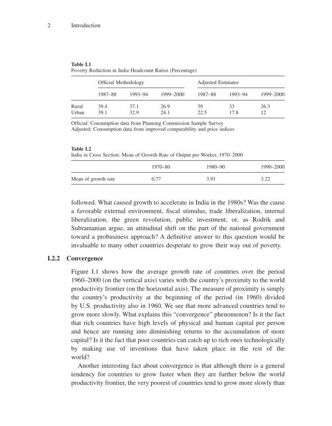
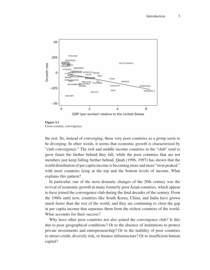
In fact the Kuznets curve remained the common wisdom on growth and inequality up until the closing decades of the 20th century. But then the economic profession changed its mind, based on the fact that in many advanced countries, especially the United States and the United Kingdom, wages of skilled workers rose much more rapidly than less skilled wages. More specifi cally, fi gure I.2 shows that the college wage premium, equal to the ratio of the average wage of
0.65
0.55
0.45
0.35
0.7
0.6
0.5
0.4
0.3
0.2
0.1
1939 1949 19691959 1979 1989 1996
Co
lleg
e w
age
pre
miu
mR
elative sup
ply o
f colleg
e skills
Year
College wage premiumRelative supply of college skills
Figure I.2Relative supply of college skills and college premium
Introduction 5
college graduates to the average wage of high school graduates, and depicted by the curve with fewer dots, has been sharply increasing since 1980.
Surprisingly, fi gure I.2 also shows that the relative supply of skilled labor, equal to the ratio between the number of college graduates and the total labor force, and depicted by the curve connecting the dark dots, was also increasing, more rapidly so since 1970. What is surprising is that, at fi rst sight, an increase in the relative supply of skilled labor should lead to a reduction in the wage premium as skilled labor becomes relatively less scarce. How can we reconcile these two facts? How can we explain that during that period, there was also an increase in “residual” wage inequality—that is, inequality within groups of people having the same measurable characteristics (education, experience, gender, occu-pation, etc.)? Was this a by-product of globalization, with wages of low-skilled people being depressed by competition from low-wage countries that were begin-ning to export to the rich countries? Was it the result of changing labor-market laws and regulations? Or did it result from skill-biased technical change, which enhances the productivity of highly skilled workers while automating the jobs of the less skilled? And if it was skill-biased technical change, where does the bias come from?
I.2.4 The Transition from Stagnation to Growth
Growth is a recent phenomenon: it took off very rapidly in the United Kingdom and then in France toward the mid-1800s. During most of human history, eco-nomic growth took place at a glacial pace. According to Maddison’s (2001) esti-mates, per capita GDP in the world economy was no higher in 1000 than in year 1, and only 53 percent higher in 1820 than in 1000, implying an average growth rate of only 1/19th percent over those 820 years. But then growth increased up to 0.5 percent from 1820 to 1870, and it kept increasing to achieve a peak rate of nearly 3 percent from 1950 to 1973. Was the earlier period of stagnation the result of Malthusian pressure of population on limited natural resources, or was it something else? And why did growth suddenly take off in the 19th century? More generally, how can we explain other transitions such as the transition from agriculture to manufacturing, and then from manufacturing to services, or from industrial economies that accumulate capital to economies in which growth relies primarily on innovation?
I.2.5 Finance and Growth
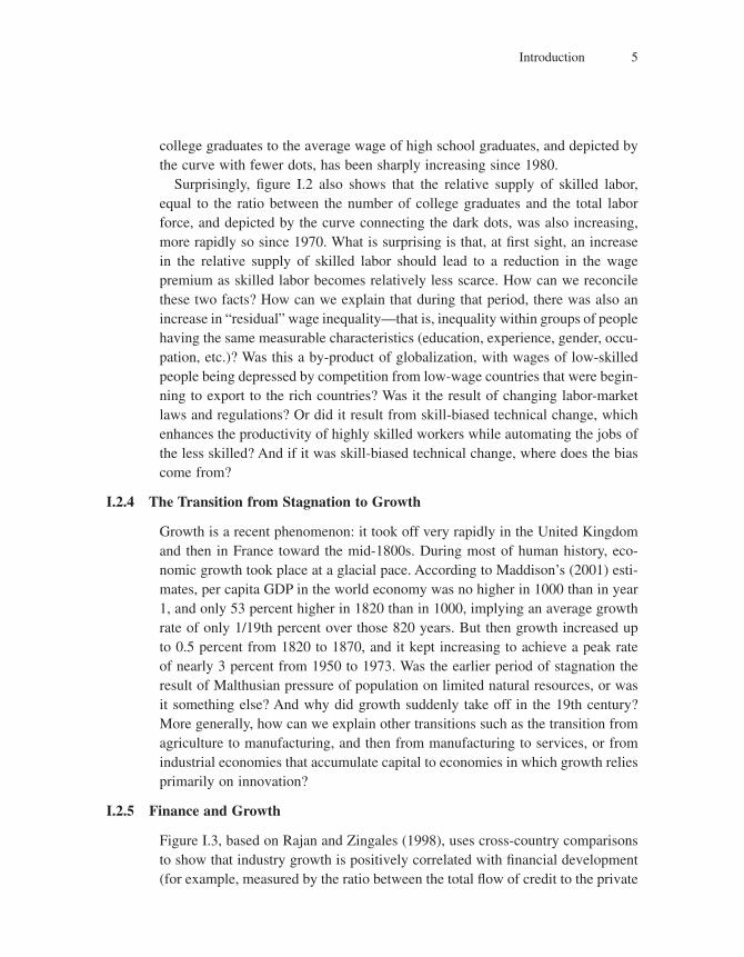
Figure I.3, based on Rajan and Zingales (1998), uses cross-country comparisons to show that industry growth is positively correlated with fi nancial development (for example, measured by the ratio between the total fl ow of credit to the private
Introduction6
sector in a country in a given year, divided by the country’s GDP that year). Is fi nance a cause of growth or just a symptom? That is, does fi nancial development allow a country to grow faster, or is it just that countries that grow fast also happen to use a lot of fi nance? Of course this question matters a lot because if fi nance causes growth, then a country wanting to grow faster should maybe reform its fi nancial institutions, whereas if fi nance is just a symptom, then fi nancial reform will provide the trappings of growth without the growth. At the same time, if fi nance does cause growth, then just how does that relationship work? Is fi nance an important determinant of cross-country convergence or divergence? How does fi nance interact with other policies, in particular macroeconomic policies aimed at stabilizing the business cycle? How can we explain that capital does not fl ow from rich to poor countries, as stressed by Lucas (1990)?
I.3 Growth Policies
The second purpose of this book is to equip the reader with paradigms and empiri-cal methods to think about growth policy design, which we do in part III. Various countries and regions have recently tried to come up with adequate “growth diagnostics,” that is, with analyses of the most binding constraints to growth and
.1
.05
0
–.05
–.1
–.15
0 0.2 0.4 0.6 0.8
Pre
dic
ted
ind
ust
ry g
row
th
Financial development (domestic credit)
Figure I.3Industry growth and fi nancial development
Introduction 7
of how to defi ne the appropriate set and sequence of growth-enhancing reforms.
I.3.1 Competition and Entry
Innovation is a vital source of long-run growth, and the reward for innovation is monopoly profi t, which comes from being able to do something that your rivals haven’t yet been able to match. Economists since Schumpeter have argued that this analysis implies a trade-off between growth and competition. Tighter anti-trust legislation would reduce the scope for earning monopoly profi ts, which would lower the reward to innovation, which should reduce the fl ow of innovation and hence reduce the long-run growth rate.
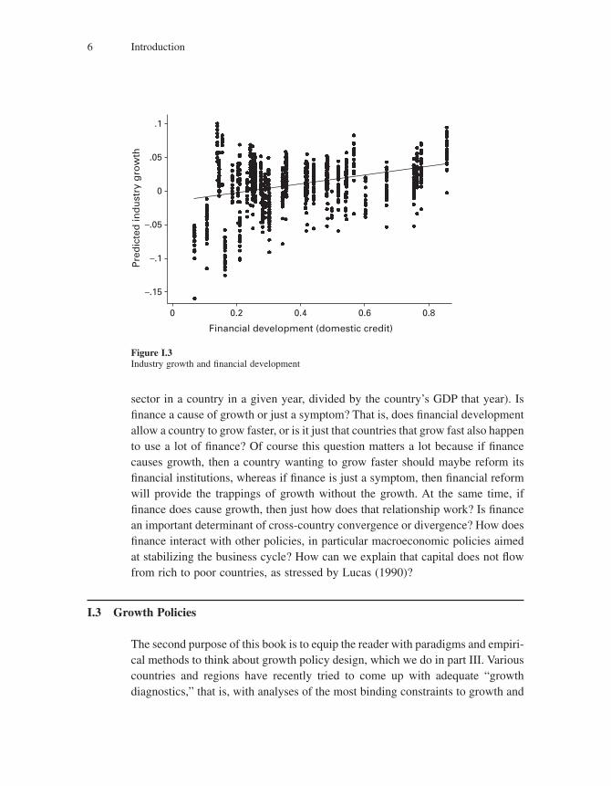
It is not easy, however, to fi nd convincing evidence of this Schum-peterian trade-off. Indeed, historians and econometricians have produced evi-dence to the contrary—evidence that more competitive societies and industries tend to grow faster than their less competitive counterparts. More recent evidence points to an inverted-U-shaped relationship between growth and competition, as shown in fi gure I.4. Figure I.4 shows how innovation
Pro
du
ctiv
ity
gro
wth
Degree of product market competition
Figure I.4Innovation and product market competition
Introduction8
(measured by the fl ow of new patents) or productivity growth on the vertical axis varies with the degree of product market competition on the horizontal axis (where competition is inversely measured by the ratio of fi rm rents to value added or to the asset value of the fi rm). How can we explain this inverted-U pattern? Why does the Schumpeterian trade-off appear only at high levels of competition?
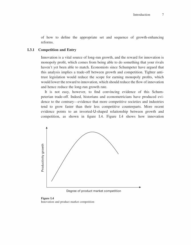
Figure I.5 depicts how fi rm-level productivity growth (on the vertical axis) reacts to an increase in the rate of new fi rm entry in the fi rm’s sector (horizontal axis). The upper line depicts the average reaction of fi rms that are initially more productive than the median fi rm in the sector. The lower line represents the reac-tion of fi rms that are less productive than the median. How can we explain that the more advanced fi rms react positively to a more intense competition by new entrants, whereas less advanced fi rms react negatively? What policy implications can we derive from this observation?
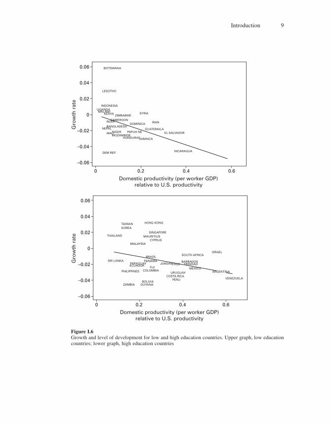
I.3.2 Education and Distance to Frontier
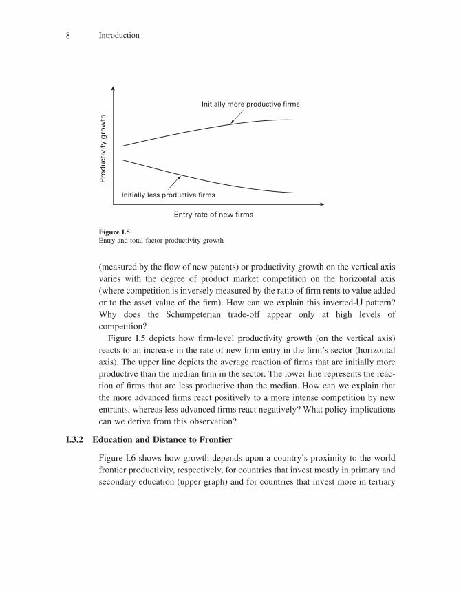
Figure I.6 shows how growth depends upon a country’s proximity to the world frontier productivity, respectively, for countries that invest mostly in primary and secondary education (upper graph) and for countries that invest more in tertiary
Pro
du
ctiv
ity
gro
wth
Entry rate of new firms
Initially more productive firms
Initially less productive firms
Figure I.5Entry and total-factor-productivity growth
Introduction 9
0.06
0.04
0.02
0
–0.02
–0.04
–0.06
0 0.2 0.60.4
Gro
wth
rat
e
Domestic productivity (per worker GDP) relative to U.S. productivity
DEM REP.
IRAN
SYRIAZIMBABWE
CAMEROON
INDONESIA
BOTSWANA
LESOTHO
MALI EL SALVADORGUATEMALA
DOMINICA
JAMAICAHONDURAS
NICARAGUA
MOZAMBIQE
MALAWI
PAPUA NE
KENYAUGANDA
NEPALBANGLADESH
NIGER
INDIA
0.06
0.04
0.02
0
–0.02
–0.04
–0.06
0 0.2 0.60.4
Gro
wth
rat
e
Domestic productivity (per worker GDP) relative to U.S. productivity
SOUTH AFRICA
CHILEJORDAN
MEXICO
ISRAEL
BARBADOSTRINIDAD
BOLIVIAGUYANA
COLOMBIAFIJI
BRAZIL
HONG KONG
SINGAPOREMAURITIUS
CYPRUSMALAYSIA
TAIWANKOREA
PANAMAPARAGUAYECUADOR
SRI LANKA
THAILAND
ZAMBIA
PHILIPPINES ARGENTINA
VENEZUELA
URUGUAY
PERUCOSTA RICA
Figure I.6Growth and level of development for low and high education countries. Upper graph, low education countries; lower graph, high education countries
Introduction10
education (lower graph). Comparing the two graphs, we see that countries that are close to frontier productivity and invest more in tertiary education (these are the countries to the right of the lower graph) do signifi cantly better than countries that are close to the frontier and invest less in tertiary education (these are the countries to the right of the upper graph). However, investing in tertiary education does not make much of a difference for countries that are far from the world productivity frontier (growth rates are comparable for countries to the left of the upper graph, and for countries to the left of the lower graph).
Why is higher education more growth enhancing for countries (or regions) that are more developed? More generally, is education so important for growth, and how should countries organize their education systems in order to maximize growth?
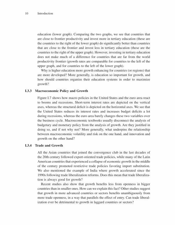
I.3.3 Macroeconomic Policy and Growth
Figure I.7 shows how macro policies in the United States and the euro area react to booms and recessions. Short-term interest rates are depicted on the vertical axes, whereas the structural defi cit is depicted on the horizontal axes. We see that the United States reduces its interest rates and increases budget defi cits a lot during recessions, whereas the euro area barely changes these two variables over the business cycle. Macroeconomic textbooks usually disconnect the analysis of budgetary and monetary policy from the analysis of growth. Are they justifi ed in doing so, and if not why not? More generally, what underpins the relationship between macroeconomic volatility and risk on the one hand, and innovation and growth on the other hand?
I.3.4 Trade and Growth
All the Asian countries that joined the convergence club in the last decades of the 20th century followed export-oriented trade policies, while many of the Latin American countries that experienced a collapse of economic growth in the middle of the century promoted restrictive trade policies favoring import substitution. We also mentioned the example of India where growth accelerated since the 1990s following trade liberalization reforms. Does this mean that trade liberaliza-tion is always good for growth?
Recent studies also show that growth benefi ts less from openness in bigger countries than in smaller ones. How can we explain this fact? Other studies suggest that growth in more advanced countries or sectors benefi ts unambiguously from more trade openness, in a way that parallels the effect of entry. Can trade liberal-ization ever be detrimental to growth in laggard countries or sectors?
Introduction 11
2.0
1.5
1.0
0.5
0.0
–0.5
–1.0
–1.5
–2.0
–2.5
–3.03.0 –2.0 –1.0 0.0 2.01.0
Cha
nge
in s
hort
-ter
m in
tere
st r
ates
Change in the government structural deficit (% of GDP)
2000
2001
2002 20031999
2004
2.0
1.5
1.0
0.5
0.0
–0.5
–1.0
–1.5
–2.0
–2.5
–3.03.0 –2.0 –1.0 0.0 2.01.0
Cha
nge
in s
hort
-ter
m in
tere
st r
ates
Change in the government structural deficit (% of GDP)
2000
2001
2004
20031999
2002
Figure I.7Macropolicy reactions to booms and recessions in the Euro area and the United States
What are the main channels whereby trade may enhance growth and innova-tion? What do data tell us about the relative importance of these channels? How should trade reforms be implemented in countries that differ in size or in their levels of development?
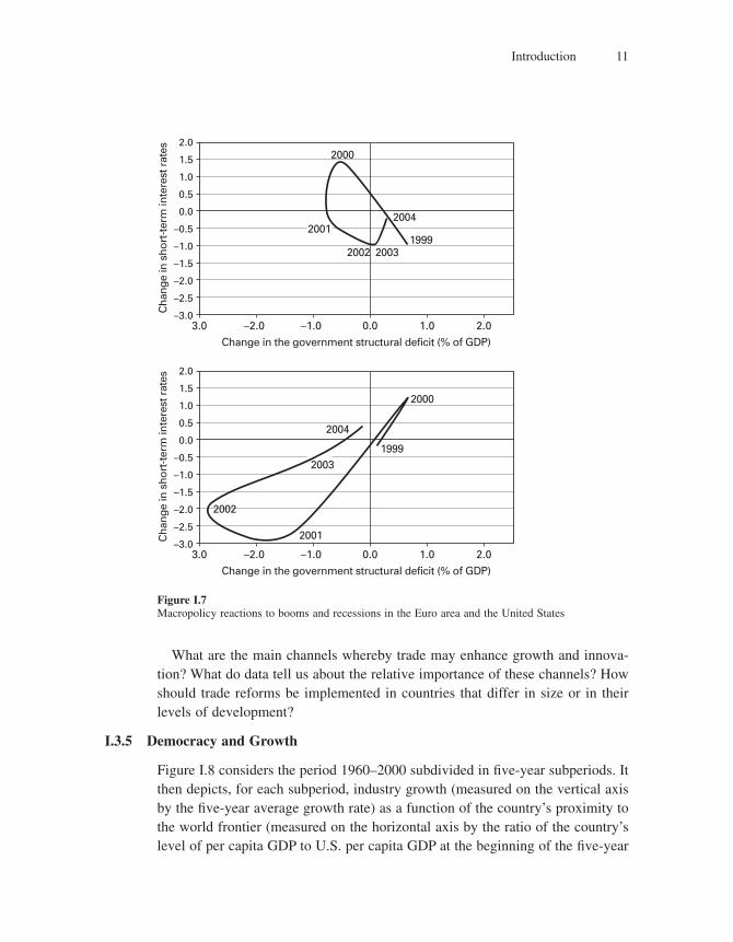
I.3.5 Democracy and Growth
Figure I.8 considers the period 1960–2000 subdivided in fi ve-year subperiods. It then depicts, for each subperiod, industry growth (measured on the vertical axis by the fi ve-year average growth rate) as a function of the country’s proximity to the world frontier (measured on the horizontal axis by the ratio of the country’s level of per capita GDP to U.S. per capita GDP at the beginning of the fi ve-year
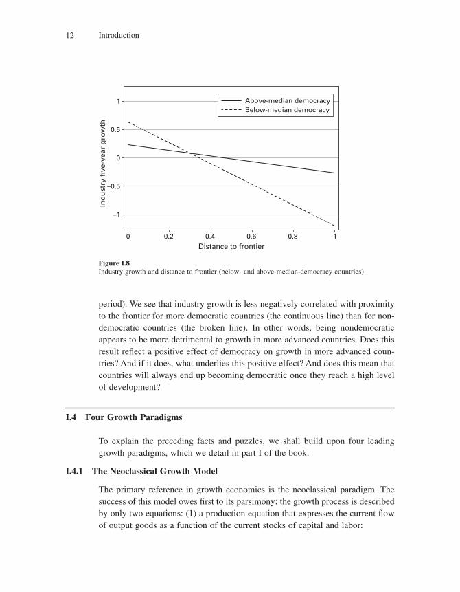
Introduction12
period). We see that industry growth is less negatively correlated with proximity to the frontier for more democratic countries (the continuous line) than for non-democratic countries (the broken line). In other words, being nondemocratic appears to be more detrimental to growth in more advanced countries. Does this result refl ect a positive effect of democracy on growth in more advanced coun-tries? And if it does, what underlies this positive effect? And does this mean that countries will always end up becoming democratic once they reach a high level of development?
I.4 Four Growth Paradigms
To explain the preceding facts and puzzles, we shall build upon four leading growth paradigms, which we detail in part I of the book.
I.4.1 The Neoclassical Growth Model
The primary reference in growth economics is the neoclassical paradigm. The success of this model owes fi rst to its parsimony; the growth process is described by only two equations: (1) a production equation that expresses the current fl ow of output goods as a function of the current stocks of capital and labor:
1
0.5
0
–0.5
–1
0 10.2 0.60.4 0.8
Ind
ust
ry f
ive-
year
gro
wth
Distance to frontier
Above-median democracyBelow-median democracy
Figure I.8Industry growth and distance to frontier (below- and above-median-democracy countries)
Introduction 13
Y AK L= −α α1
where A is a productivity parameter and where a < 1 so that production involves decreasing returns to capital, and (2) a law of motion that shows how capital accumulation depends on investment (equal to aggregate savings) and capital depreciation:
�K sY K= −δ
where sY denotes aggregate savings and dK denotes aggregate depreciation of capital.
What also makes this model the benchmark for growth analysis is, paradoxi-cally, its implication that, in the long run, economic growth does not depend on economic conditions. In particular, economic policy cannot affect a country’s long-run growth rate. Specifi cally, per capita GDP Y/L cannot grow in the long run unless we assume that productivity A also grows over time, which Solow (1956) refers to as “technical progress.” As we will see in chapter 1, the problem is that in this neoclassical model, technical progress cannot be explained or even rationalized. To analyze policies for growth, one needs a theoretical framework in which productivity growth is endogenous, that is, dependent upon character-istics of the economic environment. That framework must account for long-term technological progress and productivity growth, without which decreasing returns to capital and labor would eventually choke off all growth.
I.4.2 The AK Model
The fi rst version of endogenous growth theory is the so-called AK theory. AK models do not make an explicit distinction between capital accumulation and tech-nological progress. In effect they just lump together the physical and human capital whose accumulation is studied by neoclassical theory with the intellectual capital that is accumulated when technological progress is made. When this aggregate of different kinds of capital is accumulated, there is no reason to think that diminishing returns will drag its marginal product down to zero, because part of that accumula-tion is the very technological progress needed to counteract diminishing returns. According to the AK paradigm, the way to sustain high growth rates is to save a large fraction of GDP, some of which will fi nd its way into fi nancing a higher rate of technological progress and will thus result in faster growth.
Formally, the AK model is the neoclassical model without diminishing returns. The theory starts with an aggregate production function that is linear homoge-neous in the stock of capital:
Introduction14
Y AK=
with A a constant. If capital accumulates according to the same equation
�K sY K= −δ
as before, then the economy’s long-run (and short-run) growth rate is simply
gK
KsA= = −
�δ
which is increasing in the saving rate s.AK theory presents a “one-size-fi ts-all” view of the growth process. It applies
equally to advanced countries that have already accumulated capital and to coun-tries that are far behind. Like the neoclassical model, it postulates a growth process that is independent of developments in the rest of the world, except insofar as international trade changes the conditions for capital accumulation. Yet it is a useful tool for many purposes when the distinction between innovation and accumulation is of secondary importance.
We present the AK model in chapter 2, where we show how it can be used to analyze terms-of-trade effects in the context of an open economy. In later chapters we use the model when analyzing the transition from a Malthusian economy to an economy with positive long-run growth, when analyzing the relationship between fi nancial constraints, wealth inequality and growth, when discussing the relationship between volatility, risk, and growth, and when looking at the inter-play between growth and culture.
I.4.3 The Product-Variety Model
The second wave of endogenous growth theory consists of “innovation-based” growth models, which themselves belong to two parallel branches. One branch is the product-variety model of Romer (1990), in which innovation causes pro-ductivity growth by creating new, but not necessarily improved, varieties of products. This paradigm grew out of the new theory of international trade and emphasizes the role of technology spillovers.
It starts from a Dixit and Stiglitz (1977) production function of the form
Y K dit it
Nt
= ∑ α
0
in which there are Nt different varieties of intermediate product, each produced using Kit units of capital. By symmetry, the aggregate capital stock Kt will be
Introduction 15
divided up evenly among the Nt existing varieties equally, with the result that we can reexpress the production function as
Y N Kt t t= −1 α α
According to this function, the degree of product variety Nt is the economy’s aggregate productivity parameter, and its growth rate is the economy’s long-run growth rate of per capita output. More product variety raises the economy’s production potential because it allows a given capital stock to be spread over a larger number of uses, each of which exhibits diminishing returns. Thus, in-creased product variety is what sustains growth in this mode. New varieties, that is, new innovations, themselves result from R&D investments by researchers–entrepreneurs who are motivated by the prospect of (perpetual) monopoly rents if they successfully innovate.
Note that here there is just one kind of innovation, which always results in the same kind of new product.
Also, this model predicts no important role for exit and turnover; indeed, increased exit can do nothing but reduce the economy’s GDP, by reducing the variety variable Nt that uniquely determines aggregate productivity. Thus there is no role for “creative destruction,” the driving force in the Schumpeterian growth paradigm.
Yet the product-variety model, which we present in chapter 3, can be used in various contexts where competition and turnover considerations are not so impor-tant. For example, we use it when analyzing the source of persistent productivity differences across countries in chapter 8, or when analyzing the relationship between risk, diversifi cation, and growth in chapter 14.
I.4.4 The Schumpeterian Model
The fourth and fi nal paradigm1 is the other branch of innovation-based theory, developed in Aghion and Howitt (1992)2 and subsequently elaborated in Aghion and Howitt (1998a). This paradigm grew out of modern industrial organization theory and is commonly referred to as Schumpeterian growth theory because it focuses on quality-improving innovations that render old products obsolete and
1. The semiendogenous model of Jones C. (1995b), in which long-run economic growth depends uniquely on the rate of population growth, might be thought of as a fourth paradigm. However, this model has little to say about growth policy, since it predicts that long-run growth is independent of any policy that does not affect population growth.
2. An early attempt at providing a Schumpeterian approach to endogenous growth theory was by Segerstrom, Anant, and Dinopoulos (1990).
Introduction16
hence involves the force that Schumpeter called creative destruction. We present it in chapter 4 and then use it and extend it in the subsequent chapters of the book.
Schumpeterian theory begins with a production function specifi ed at the indus-try level:
Y A Kit it it= < <−1 0 1α α α,
where Ait is a productivity parameter attached to the most recent technology used in industry i at time t. In this equation, Kit represents the fl ow of a unique inter-mediate product used in this sector, each unit of which is produced one-for-one by fi nal output or, in the most complete version of the model, by capital. Aggre-gate output is just the sum of the industry-specifi c outputs Yit.
Each intermediate product is produced and sold exclusively by the most recent innovator. A successful innovator in sector i improves the technology parameter Ait and is thus able to displace the previous product in that sector, until it is dis-placed in turn by the next innovator. Thus a fi rst implication of the Schumpeterian paradigm is that faster growth generally implies a higher rate of fi rm turnover, because this process of creative destruction generates entry of new innovators and exit of former innovators.
Although the theory focuses on individual industries and explicitly analyzes the microeconomics of industrial competition, the assumption that all industries are ex ante identical gives it a simple aggregate structure. In particular, it is easily shown that aggregate output depends on the aggregate capital stock Kt according to the Cobb-Douglas aggregate per-worker production function:
Y A Kt t t= −1 α α
where the labor-augmenting productivity factor At is just the unweighted sum of the sector-specifi c Ait’s. As in neoclassical theory, the economy’s long-run growth rate is given by the growth rate of At, which here depends endogenously on the economy-wide rate of innovation.
There are two main inputs to innovation, namely, the private expenditures made by the prospective innovator and the stock of innovations that have already been made by past innovators. The latter input constitutes the publicly available stock of knowledge to which current innovators are hoping to add. The theory is fl exible in modeling the contribution of past innovations. It encompasses the case of an innovation that leapfrogs the best technology available before the innova-tion, resulting in a new technology parameter Ait in the innovating sector i, which is some multiple g of its preexisting value. And it also encompasses the case of
Introduction 17
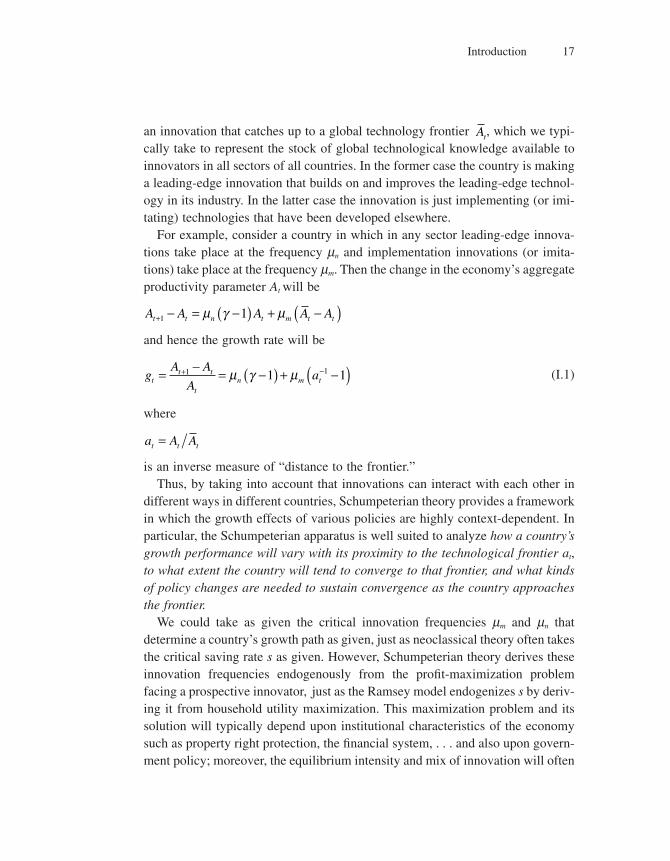
an innovation that catches up to a global technology frontier At, which we typi-cally take to represent the stock of global technological knowledge available to innovators in all sectors of all countries. In the former case the country is making a leading-edge innovation that builds on and improves the leading-edge technol-ogy in its industry. In the latter case the innovation is just implementing (or imi-tating) technologies that have been developed elsewhere.
For example, consider a country in which in any sector leading-edge innova-tions take place at the frequency mn and implementation innovations (or imita-tions) take place at the frequency mm. Then the change in the economy’s aggregate productivity parameter At will be
A A A A At t n t m t t+ − = −( ) + −( )1 1μ γ μ
and hence the growth rate will be
gA A
Aat
t t
tn m t= − = −( ) + −( )+ −1 11 1μ γ μ (I.1)
where
a A At t t=
is an inverse measure of “distance to the frontier.”Thus, by taking into account that innovations can interact with each other in
different ways in different countries, Schumpeterian theory provides a framework in which the growth effects of various policies are highly context-dependent. In particular, the Schumpeterian apparatus is well suited to analyze how a country’s growth performance will vary with its proximity to the technological frontier at, to what extent the country will tend to converge to that frontier, and what kinds of policy changes are needed to sustain convergence as the country approaches the frontier.
We could take as given the critical innovation frequencies mm and mn that determine a country’s growth path as given, just as neoclassical theory often takes the critical saving rate s as given. However, Schumpeterian theory derives these innovation frequencies endogenously from the profi t-maximization problem facing a prospective innovator, ,just as the Ramsey model endogenizes s by deriv-ing it from household utility maximization. This maximization problem and its solution will typically depend upon institutional characteristics of the economy such as property right protection, the fi nancial system, . . . and also upon govern-ment policy; moreover, the equilibrium intensity and mix of innovation will often
Introduction18
depend upon institutions and policies in a way that varies with the country’s dis-tance to the technological frontier a.
Equation (I.1) incorporates Gerschenkron’s (1962) “advantage of backward-ness,” in the sense that the further the country is behind the global technology frontier (i.e., the smaller is at) the faster it will grow, given the frequency of implementation innovations. As in Gerschenkron’s analysis, the advantage arises from the fact that implementation innovations allow the country to make larger quality improvements the further it has fallen behind the frontier. As we shall see, this is just one of the ways in which distance to the frontier can affect a country’s growth performance.
In addition, growth equations like (I.1) make it quite natural to capture Ger-schenkron’s idea of “appropriate institutions.”3 Suppose indeed that the institu-tions that favor implementation innovations (that is, that lead to fi rms emphasizing mm at the expense of mn) are not the same as those that favor leading-edge innova-tions (that is, that encourage fi rms to focus on mn): then, far from the frontier a country will maximize growth by favoring institutions that facilitate implementa-tion; however, as it catches up with the technological frontier, to sustain a high growth rate the country will have to shift from implementation-enhancing institu-tions to innovation-enhancing institutions as the relative importance of mn for growth is also increasing. As we will see in chapter 11, failure to operate such a shift can prevent a country from catching up with the frontier level of GDP per capita.
3. See Acemoglu, Aghion, and Zilibotti (2006) for a formalization of this idea.

I BASIC PARADIGMS OF GROWTH THEORY

1 Neoclassical Growth Theory
1.1 Introduction
The starting point for any study of economic growth is the neoclassical growth model, which emphasizes the role of capital accumulation. This model, fi rst constructed by Solow (1956) and Swan (1956), shows how economic policy can raise an economy’s growth rate by inducing people to save more. But the model also predicts that such an increase in growth cannot last indefi nitely. In the long run, the country’s growth rate will revert to the rate of technological progress, which neoclassical theory takes as being independent of economic forces, or exogenous. Underlying this pessimistic long-run result is the principle of dimin-ishing marginal productivity, which puts an upper limit to how much output a person can produce simply by working with more and more capital, given the state of technology.
We have a more optimistic view of the contribution that economic policy can make to long-run growth, because we believe that the rate of technological prog-ress is determined by forces that are internal to the economic system. Specifi cally, technological progress depends on the process of innovation, which is one of the most important channels through which business fi rms compete in a market economy, and the incentive to innovate depends very much on policies with respect to competition, intellectual property, international trade, and much else. But the neoclassical model is still a useful one, because its analysis of how capital accumulation affects national income, real wages, and real interest rates for any given state of technology is just as valid when technology is endogenous as when it is exogenous. Indeed, neoclassical theory can be seen as a special case of the theory we develop in this book, the special limiting case in which the marginal productivity of efforts to innovate has fallen to zero. A good way to learn a theory is to start with a simple and instructive special case. Accordingly, this fi rst chapter is devoted to an account of the neoclassical growth model.
1.2 The Solow-Swan Model
Consider an economy with a given supply of labor and a given state of techno-logical knowledge, both of which we suppose initially to be constant over time. Suppose labor works with an aggregate capital stock1 K. The maximum amount
1. Of course, K is an aggregate index of the different capital goods and should be interpreted broadly so as to include human as well as physical capital.
Chapter 122
of output Y that can be produced depends on K according to an aggregate produc-tion function
Y F K= ( )We assume that all capital and labor are fully and effi ciently employed, so F(K) is not only what can be produced but also what will be produced.
A crucial property of the aggregate production function is that there are dimin-ishing returns to the accumulation of capital. If you continue to equip people with more of the same capital goods without inventing new uses for the capital, then a point will be reached eventually where the extra capital goods become redun-dant except as spare parts in the event of multiple equipment failure, and where therefore the marginal product of capital is negligible. This idea is captured for-mally by assuming the marginal product of capital to be positive but strictly decreasing in the stock of capital:
′( ) > ′′( ) <F K F K K0 0and for all (1.1)
and imposing the Inada conditions:2
limK K
F K F K→∞ →
′( ) = ′( ) = ∞00
and lim (1.2)
Because we are assuming away population growth and technological change, the only remaining force that can drive growth is capital accumulation. Output will grow if and only if the capital stock increases. Assume that people save a constant fraction s of their gross income3 Y, and that the constant fraction d of the capital stock disappears each year as a result of depreciation. Because the rate at which new capital accumulates equals the aggregate fl ow of savings4 sY and the rate at which old capital wears out is d K. therefore the net rate of increase of the capital stock per unit of time (i.e., net investment) is
I sY K= − δ (1.3)
Assume that time is continuous. Then net investment is the derivative of K with respect to time, which we write using dot notation as �K. So, using the
2. The second condition in equation (1.2) is a regularity condition made for convenience. Specifi cally, as we will indicate, it ensures the existence of a nondegenerate stationary state in the model.
3. We are assuming no taxes, so that national income and output are identical.
4. Recall that with no taxes, no government expenditures, and no international trade, savings and investment are identical. That is, savings and investment are just two different words for the fl ow of income spent on investment goods rather than on consumption goods.
Neoclassical Growth Theory 23
aggregate production function to substitute for Y in equation (1.3), we have
�K sF K K= ( ) − δ (1.4)
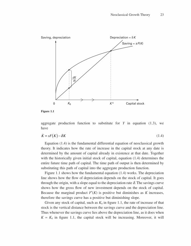
Equation (1.4) is the fundamental differential equation of neoclassical growth theory. It indicates how the rate of increase in the capital stock at any date is determined by the amount of capital already in existence at that date. Together with the historically given initial stock of capital, equation (1.4) determines the entire future time path of capital. The time path of output is then determined by substituting this path of capital into the aggregate production function.
Figure 1.1 shows how the fundamental equation (1.4) works. The depreciation line shows how the fl ow of depreciation depends on the stock of capital. It goes through the origin, with a slope equal to the depreciation rate d. The savings curve shows how the gross fl ow of new investment depends on the stock of capital. Because the marginal product F′(K) is positive but diminishes as K increases, therefore the savings curve has a positive but diminishing slope.
Given any stock of capital, such as K0 in fi gure 1.1, the rate of increase of that stock is the vertical distance between the savings curve and the depreciation line. Thus whenever the savings curve lies above the depreciation line, as it does when K = K0 in fi gure 1.1, the capital stock will be increasing. Moreover, it will
Saving, depreciation Depreciation = δ K
Saving = s F(K)
Capital stockK *K00
dKdt
Figure 1.1
Chapter 124
continue to increase monotonically, and it will converge in the long run to K*, the capital stock at which the two schedules intersect. Thus K* is a unique, stable, stationary state of the economy.5
The economic logic of this dynamic analysis is straightforward. When capital is scarce it is very productive, so national income will be large in relation to the capital stock, and this fact will induce people to save more than enough to offset the wear and tear on existing capital. Thus the capital stock K will rise, and hence national income F(K) will rise. But because of diminishing marginal productivity, national income will not grow as fast as the capital stock, with the result that savings will not grow as fast as depreciation. Eventually depreciation will catch up with savings; at that point the capital stock will stop rising, and growth in national income will therefore come to an end.
Therefore, any attempt to boost growth by encouraging people to save more will ultimately fail. An increase in the saving rate s will temporarily raise the rate of capital accumulation, by shifting the savings curve up in fi gure 1.1, hence raising the gap between it and the depreciation line, but it will have no long-run effect on the growth rate, which is doomed to fall back to zero. The increase in s will, however, cause an increase in the long-run levels of output and capital as a result of the temporary burst of growth in K; that is, the new intersection point defi ning K* will have shifted to the right.
Likewise, an increase in the depreciation rate d will produce a temporary reduc-tion in growth by shifting the depreciation line up, hence creating a negative gap between the savings curve and the depreciation line. But again the change in the country’s growth rate will not last indefi nitely. As K approaches its new lower level, the growth rate will rise back up to zero. The levels of output and capital will be permanently lower as a result of this increase in d; that is, the new inter-section point defi ning K* will have shifted to the left.
1.2.1 Population Growth
The same pessimistic conclusion regarding long-run growth follows even with a growing population. To see this point, we make explicit that output depends not just on capital but also on labor, by writing the production function as
5. Technically, there is another steady state at K = 0, where national income is zero and both savings and depreciation are zero. But this degenerate steady state is unstable; as long as the initial stock K0 is positive, then K will approach the positive steady state K*.
Note how we use the Inada conditions (1.2). The second one guarantees that, starting from the origin, the saving curve at fi rst rises above the depreciation line. The fi rst one guarantees that eventually the slope of the saving curve will fall below that of the depreciation line. Together these imply that as K increases, the saving curve must eventually cross the depreciation line from above, as it does at K*.
Neoclassical Growth Theory 25
Y F K L= ( ),
Suppose that this production function is concave,6 implying that the marginal product of capital is again a diminishing function of K, holding L constant. Suppose also that the aggregate production function exhibits constant returns to scale; that is, F is homogeneous of degree one in both arguments:
F K L F K L K Lλ λ λ λ, , for all , ,( ) = ( ) > 0 (1.5)
This formula makes sense under our assumption that the state of technology is given, for if capital and labor were both to double, then the extra workers could use the extra capital to replicate what was done before, thus resulting in twice the output.
Suppose that everyone in the economy always supplies one unit of labor per unit of time, and that there is perpetual full employment. Thus the labor input L is also the population, which we suppose grows at the constant exponential rate n per year.
With constant returns to scale, output per person y ≡ Y/L will depend on the capital stock per person k ≡ K/L. That is, equation (1.5) implies that, in the special case where l = 1/L,
Y L F K L L F K L= ( ) = ( ), ,1
so
y f k= ( ) (1.6)
where f is the per capita production function:
f k F k( ) = ( ),1
indicating what each person can produce using his or her share of the aggregate capital stock. In the Cobb-Douglas case
Y K L= < <−α α α1 0 1,
the per capita production function can be written as
y f k k= ( ) = α
6. Concavity of a production function is a multidimensional version of diminishing returns. Formally,
F is concave if ∂∂
2
2 0F
K< ,
∂∂
2
2 0F
L< , and
∂∂
∂∂
∂∂ ∂
2
2
2
2
2 2F
K
F
L
F
K L≥
⎛
⎝⎜
⎞
⎠⎟ .
Chapter 126
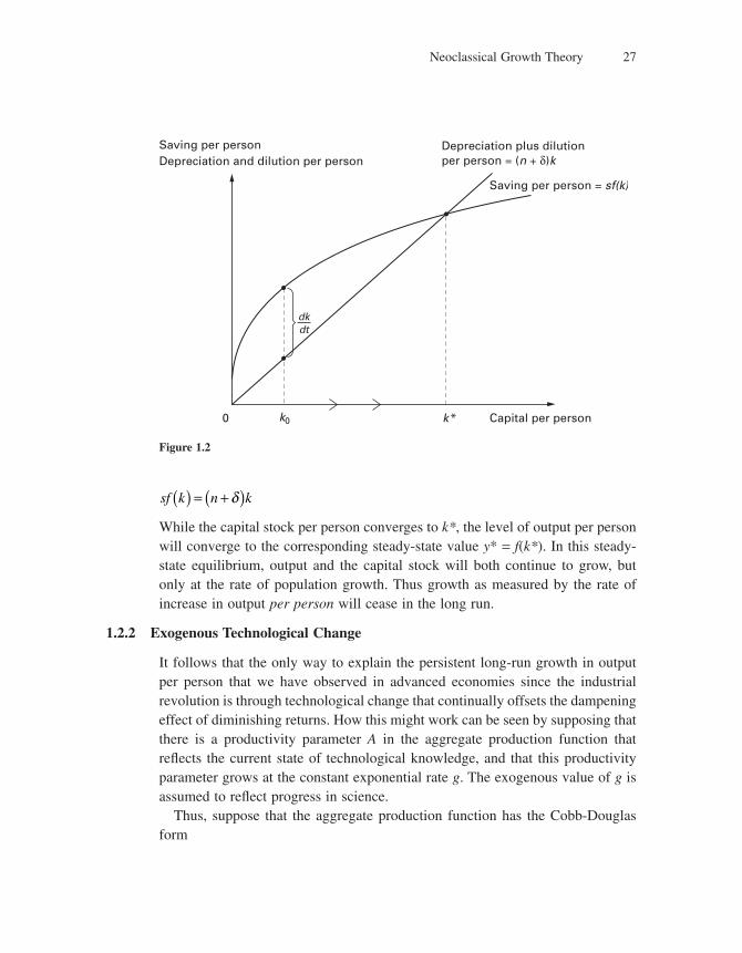
The rate at which new saving raises k is the rate of saving per person, sy. The rate at which depreciation causes k to fall is the amount of depreciation per person d k. In addition, population growth will cause k to fall at the annual rate nk (each additional person reduces the amount of capital per person, given the aggregate amount K). The net rate of increase in k is the resultant of these three forces, which by equation (1.6) is7
�k sf k n k= ( ) − +( )δ (1.7)
Note that the differential equation (1.7) governing the capital-labor ratio is almost the same as the fundamental equation (1.4) governing the capital stock in the previous section, except that the depreciation rate is now augmented by the population growth rate and the per capita production function f has replaced the aggregate function F. Also, the per capita function f will have the same shape as the aggregate function F,8 so the per capita savings curve sf(k) in fi gure 1.2 will look just like the savings curve in fi gure 1.1.
As fi gure 1.2 shows, diminishing returns will again impose an upper limit to capital per person. That is, eventually a point will be reached where all of people’s saving is needed to compensate for depreciation and population growth. This point is the steady-state9 value k*, defi ned by the condition
7. More formally, it follows from basic calculus that
� � �k K L LK L= − 2
Since L grows at the constant exponential rate n, we have �L L = n; hence,
� �k K L nk= −
As in the previous section, we have
�K sY K= −δ
so
�K L sy k= −δ
and
�k sy n k= − +( )δ
Equation (1.7) follows from this and the per capita production function (1.6).
8. Since f(k) = F(k, 1), therefore ′( ) = ( )f kk
F k∂∂
,1 which is decreasing in k because of the
assumption that F is concave.
9. The aggregate capital stock is not stationary, but growing at the same steady rate as the work force.
Neoclassical Growth Theory 27
sf k n k( ) = +( )δ
While the capital stock per person converges to k*, the level of output per person will converge to the corresponding steady-state value y* = f(k*). In this steady-state equilibrium, output and the capital stock will both continue to grow, but only at the rate of population growth. Thus growth as measured by the rate of increase in output per person will cease in the long run.
1.2.2 Exogenous Technological Change
It follows that the only way to explain the persistent long-run growth in output per person that we have observed in advanced economies since the industrial revolution is through technological change that continually offsets the dampening effect of diminishing returns. How this might work can be seen by supposing that there is a productivity parameter A in the aggregate production function that refl ects the current state of technological knowledge, and that this productivity parameter grows at the constant exponential rate g. The exogenous value of g is assumed to refl ect progress in science.
Thus, suppose that the aggregate production function has the Cobb-Douglas form
Saving per personDepreciation and dilution per person
Depreciation plus dilution per person = (n + δ)k
Saving per person = sf(k)
Capital per personk *k00
dkdt
Figure 1.2
Chapter 128
Y AL K= ( ) −1 α α (1.8)
This way of writing the production function makes technological progress equiva-lent to an increase in the “effective” supply of labor AL, which grows not at the rate of population growth n but at the rate of growth of population plus the growth rate of productivity10 n + g.
Formally, the only difference from the model of the previous section is that we have everywhere replaced the labor input L by the number of “effi ciency units” of labor AL. We can now fi nd a steady state in terms of capital per effi -ciency unit:
κ = K
AL
and output per effi ciency unit, which we can write, using equation (1.8) as
ϕ κ α= =Y
AL
The rate at which new saving raises k is the rate of saving per effi ciency unit sy. The rate at which depreciation causes k to fall is the amount of depreciation per person dk. In addition, growth in the number of effi ciency units, at the rate n + g, causes k to fall at the annual rate (n + g)k. As before, the net rate of increase in k is the resultant of these three forces:
�κ κ δ κα= − + +( )s n g (1.9)
which is almost identical to equation (1.7) of the previous section with a change in notation from k to k, except that the growth rate n of labor input has now been replaced by the growth rate n + g of the number of “effi ciency units” of labor. As before, k will approach a unique steady-state value k* in the long run, while j approaches its steady state j* = (k*)a.
Although output per effi ciency unit does not grow in the long run, the same is no longer true of output per person:
10. That A enters the aggregate production function multiplicatively with L is in most cases a very special assumption, amounting to what is sometimes referred to as “Harrod neutrality” or “purely labor-augmenting technical change.” There is no good reason why technological change should always take this form; it just leads to tractable steady-state results. In the present Cobb-Douglas framework, however, the assumption of Harrod neutrality is innocuous. That is, because all factors enter multiplicatively in a Cobb-Douglas production function, it would make no observable difference if A multiplied L, K, or both.
Neoclassical Growth Theory 29
Y L A A= =ϕ κ α
whose growth rate can be expressed as
G A A g= + = +� � �ακ κ ακ κ
In the long run, when k approaches k*, the time derivative �κ approaches zero, so the growth rate G approaches the exogenous rate of technological change g:
G g t→ → ∞as
But in the short run, as before, the growth rate can rise above g temporarily as a result of an increase in the saving rate s, which raises the rate of increase in the capital stock per effi ciency unit k according to the fundamental differential equa-tion (1.9).
Intuitively, the growth rate of output per person does not fall to zero because as capital accumulates, the tendency for the output/capital ratio to fall because of diminishing returns to capital is continually offset by technological progress. The economy approaches a steady state in which the two confl icting forces of dimin-ishing returns and technological progress exactly offset each other and the output/capital ratio is constant. Although the height of the steady-state growth path will be determined by such parameters as the saving rate s, the depreciation rate d, and the rate of population growth n, the only parameter affecting the growth rate is the exogenous rate of technological progress g.
1.2.3 Conditional Convergence
One of the main questions that growth economics addresses is whether poor countries are likely to catch up with rich ones. If so, we say there is cross-country convergence. The neoclassical model answers this question with a qualifi ed yes. That is, suppose country 1 has a lower per capita GDP than country 2. Then the theory predicts that this difference in per capita GDPs will tend to disappear over time if the two countries share the same technology (as defi ned by the production function F and the path At of effi ciency units per person) and the same fundamental determinants of capital accumulation (the saving rate s, the depreciation rate d, and the population growth rate n), but not otherwise. This prediction is known as conditional convergence, because it says that convergence is conditional on having the same technology and fundamental variables.
The reason why the model implies conditional convergence is simple. If two countries have the same fundamentals and share the same technology, then they
Chapter 130
will each be converging to the same steady state, and therefore they will be con-verging to each other. Otherwise they will generally be converging to different steady states and therefore not to each other.
More specifi cally, suppose the steady-state level of GDP per effi ciency unit of labor is ϕ1 1 1* = y At t in country 1 and ϕ 2 2 2* = y At t in country 2, where yit and Ait are, respectively, GDP per person and effi ciency units per worker in country i along the country’s long-run growth path. If the two countries have the same technology and the same fundamental determinants, then A1t = A2t and ϕ ϕ1 2* *= , so their long-run levels of GDP per person will be same: y1t = y2t. But if they have different technologies and fundamentals, then there is no reason why their long-run levels of GDP per person should be the same.
The empirical literature on convergence has tested a somewhat stronger version of conditional convergence, namely, that there should be convergence conditional on countries having the same fundamental determinants (s, n, d) of capital accumulation. This version has been suggested by proponents of the neo-classical model who believe that as a working hypothesis we should assume that all countries share the same technology, so all that remains to guarantee conver-gence is that countries have the same steady state j*. These economists believe that cross-country technology differences are not important because science and technology are global resources available to all countries; they claim that what really separates countries economically is capital accumulation, not technology.
Empirical tests of conditional convergence focus on whether poor countries tend to grow faster than rich ones, after controlling for the fundamental determi-nants of capital accumulation. As you can see in fi gure 1.2, a country that starts further behind the steady state k* will have a faster rate of capital accumulation, and hence a large growth rate of per capita GDP. Of course, this comparison only works for two countries with the same steady states; if a rich country also had a higher k*, then it might be further behind its steady state than the poor country, and therefore might be growing faster than the poor one.
Authors in this empirical literature often estimate equations of the form
10 1 2T
y
yy X ut T
tt t t⋅ = + + ++log logβ β β
where Xt is a vector of variables (such as s, d, and n) that control for the deter-minants of steady-state output per person. The left-hand side of this equation is the growth rate of the economy measured over an interval of T years. Thus the
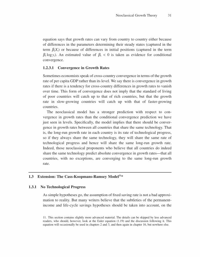
Neoclassical Growth Theory 31
equation says that growth rates can vary from country to country either because of differences in the parameters determining their steady states (captured in the term b2Xt) or because of differences in initial positions (captured in the term b1 log yt). An estimated value of b1 < 0 is taken as evidence for conditional convergence.
1.2.3.1 Convergence in Growth Rates
Sometimes economists speak of cross-country convergence in terms of the growth rate of per capita GDP rather than its level. We say there is convergence in growth rates if there is a tendency for cross-country differences in growth rates to vanish over time. This form of convergence does not imply that the standard of living of poor countries will catch up to that of rich countries, but that the growth rate in slow-growing countries will catch up with that of faster-growing countries.
The neoclassical model has a stronger prediction with respect to con-vergence in growth rates than the conditional convergence prediction we have just seen in levels. Specifi cally, the model implies that there should be conver-gence in growth rates between all countries that share the same technology. That is, the long-run growth rate in each country is its rate of technological progress, so if they always share the same technology, they will share the same rate of technological progress and hence will share the same long-run growth rate. Indeed, those neoclassical proponents who believe that all countries do indeed share the same technology predict absolute convergence in growth rates—that all countries, with no exceptions, are converging to the same long-run growth rate.
1.3 Extension: The Cass-Koopmans-Ramsey Model11*
1.3.1 No Technological Progress
As simple hypotheses go, the assumption of fi xed saving rate is not a bad approxi-mation to reality. But many writers believe that the subtleties of the permanent-income and life-cycle savings hypotheses should be taken into account, on the
11. This section contains slightly more advanced material. The details can be skipped by less advanced readers, who should, however, look at the Euler equation (1.19) and the discussion following it. This equation will occasionally be used in chapters 2 and 3, and then again in chapter 16, but nowhere else.
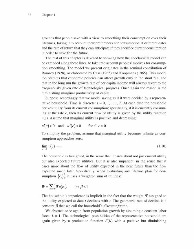
Chapter 132
grounds that people save with a view to smoothing their consumption over their lifetimes, taking into account their preferences for consumption at different dates and the rate of return that they can anticipate if they sacrifi ce current consumption in order to save for the future.
The rest of this chapter is devoted to showing how the neoclassical model can be extended along these lines, to take into account peoples’ motives for consump-tion smoothing. The model we present originates in the seminal contribution of Ramsey (1928), as elaborated by Cass (1965) and Koopmans (1965). This model too predicts that economic policies can affect growth only in the short run, and that in the long run the growth rate of per capita income will always revert to the exogenously given rate of technological progress. Once again the reason is the diminishing marginal productivity of capital.
Suppose accordingly that we model saving as if it were decided by a represen-tative household. Time is discrete: t = 0, 1, . . . , T. At each date the household derives utility from its current consumption; specifi cally, if it is currently consum-ing at the rate c, then its current fl ow of utility is given by the utility function u(c). Assume that marginal utility is positive and decreasing:
′( ) > ′′( ) < >u c u c c0 0 0and for all
To simplify the problem, assume that marginal utility becomes infi nite as con-sumption approaches zero:
limc
u c→
′( ) = ∞0
(1.10)
The household is farsighted, in the sense that it cares about not just current utility but also expected future utilities. But it is also impatient, in the sense that it cares more about the fl ow of utility expected in the near future than the fl ow expected much later. Specifi cally, when evaluating any lifetime plan for con-sumption ct
T{ }0, it uses a weighted sum of utilities:
W u ctt
T= ( ) < <∑ β β
01, 0
The household’s impatience is implicit in the fact that the weight b t assigned to the utility expected at date t declines with t. The geometric rate of decline is a constant b that we call the household’s discount factor.
We abstract once again from population growth by assuming a constant labor force: L = 1. The technological possibilities of the representative household are again given by a production function F(K) with a positive but diminishing
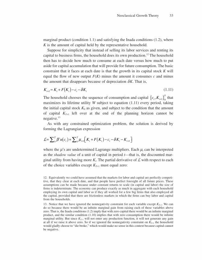
Neoclassical Growth Theory 33
marginal product (condition 1.1) and satisfying the Inada conditions (1.2), where K is the amount of capital held by the representative household.
Suppose for simplicity that instead of selling its labor services and renting its capital to business fi rms, the household does its own production.12 The household then has to decide how much to consume at each date versus how much to put aside for capital accumulation that will provide for future consumption. The basic constraint that it faces at each date is that the growth in its capital stock K will equal the fl ow of new output F(K) minus the amount it consumes c and minus the amount that disappears because of depreciation dK. That is,
K K F K c Kt t t t t+ = + ( ) − −1 δ (1.11)
The household chooses the sequence of consumption and capital c Kt t
T, +{ }1 0
that maximizes its lifetime utility W subject to equation (1.11) every period, taking the initial capital stock K0 as given, and subject to the condition that the amount of capital KT+1 left over at the end of the planning horizon cannot be negative.13
As with any constrained optimization problem, the solution is derived by forming the Lagrangian expression
L= ( ) + + ( ) − − −⎡⎣ ⎤⎦∑ ∑ + +β μ δtt
T
t t t t t t
Tu c K F K c K K
0 1 10
where the m’s are undetermined Lagrange multipliers. Each mt can be interpreted as the shadow value of a unit of capital in period t—that is, the discounted mar-ginal utility from having more Kt. The partial derivative of L with respect to each of the choice variables except KT+1 must equal zero:
12. Equivalently we could have assumed that the markets for labor and capital are perfectly competi-tive, that they clear at each date, and that people have perfect foresight of all future prices. These assumptions can be made because under constant returns to scale (in capital and labor) the size of fi rms is indeterminate. The economy can produce exactly as much in aggregate with each household employing its own capital and labor as if they all worked for a few big fi rms that also employed all the capital, provided that there are frictionless markets in which the fi rms can buy labor and capital from the households.
13. Notice that we have ignored the nonnegativity constraint for each variable except KT+1. We can do so because there would be an infi nite marginal gain from raising each of these variables above zero. That is, the Inada conditions (1.2) imply that with zero capital there would be an infi nite marginal product, and the similar condition (1.10) implies that with zero consumption there would be infi nite marginal utility. But since KT+1 will not enter any production function, it will not generate any gain at all if we raise it above zero. So if we ignored the nonnegativity constraint on KT+1 the household would gladly choose to “die broke,” which would make no sense in this context because capital cannot be negative.
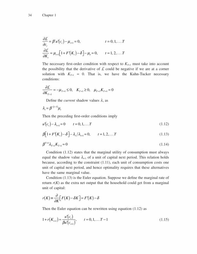
Chapter 134
∂∂∂∂
L
Lc
u c t T
KF K
t
tt t
tt t
= ′( ) − = =
= + ′( ) −⎡⎣ ⎤⎦ −
+
+
β μ
μ δ μ
1
1
0 0 1
1
, , , . . .
tt t T= =0 1 2, , , . . .
The necessary fi rst-order condition with respect to KT+1 must take into account the possibility that the derivative of L could be negative if we are at a corner solution with KT+1 = 0. That is, we have the Kuhn-Tucker necessary conditions:
∂∂L
KK K
TT T T T
++ + + += − ≤ ≥ =
11 1 1 10 0 0μ μ, ,
Defi ne the current shadow values l t as
λ β μtt
t= − −( )1
Then the preceding fi rst-order conditions imply
′( ) − = =+u c t Tt tλ 1 0 0 1, , . . . (1.12)
β δ λ λ1 0 1 21+ ′( ) −⎡⎣ ⎤⎦ − = =+F K t Tt t t , , , . . . (1.13)
β λTT TK+
+ + =11 1 0 (1.14)
Condition (1.12) states that the marginal utility of consumption must always equal the shadow value lt+1 of a unit of capital next period. This relation holds because, according to the constraint (1.11), each unit of consumption costs one unit of capital next period, and hence optimality requires that these alternatives have the same marginal value.
Condition (1.13) is the Euler equation. Suppose we defi ne the marginal rate of return r(K) as the extra net output that the household could get from a marginal unit of capital:
r KK
F K K F K( ) ≡ ( ) −⎡⎣ ⎤⎦ = ′( ) −∂∂
δ δ
Then the Euler equation can be rewritten using equation (1.12) as
1 0 1 111
+ ( ) =′( )′( ) = −+
+
r Ku c
u ct Tt
t
tβ, , , . . . (1.15)

Neoclassical Growth Theory 35
which is a familiar condition for optimal consumption smoothing over time, namely, that the marginal rate of substitution between consumption this period and next must equal the marginal rate of transformation 1 + r(Kt+1).
Condition (1.14) is the transversality condition, which states that either the terminal capital stock must be zero or it must be valueless (lT+1 = 0). That is, you must not plan to die leaving anything valuable unconsumed.
1.3.1.1 Continuous Time, Infi nite Horizon14
To understand how consumption and the capital stock evolve over time, it is helpful to take the limit as the time period shrinks to zero and as the planning horizon becomes infi nitely long. First, express the discount factor b as
βρ
=+1
1
where r > 0 is the household’s subjective discount rate, or rate of time preference. Next, when the time period is short, we can approximate fi rst-order differences by derivatives. Thus we can write, by approximation,15
′( ) − ′( ) = ′′( )+u c u c u c ct t t t1 �
where
�c dc dtt t=
Dividing through by u′(ct), we can rewrite the preceding equation as
′( )′( ) =
′′( )′( ) ++u c
u c
u c
u cct
t
t
tt
1 1�
The Euler equation (1.15) then becomes
1
1
1
11
βρ
+( ) = ++
=′′( )′( ) +
r r
u c
u cct
tt�
14. For an alternative treatment using the Hamiltonian method, see appendix 1B.
15. Indeed we have
limdt
t dt tt t
u c u c
dtu c c
→
+′( ) − ′( ) = ′′( )0
�

Chapter 136
But when the time period is short the rate of time preference r and the rate of return r will be small, so we have16
1
11
++
+ −ρ ρr
r�
Therefore, the continuous-time approximation of the Euler equation is
′′( )′( ) = −
u c
u cc rt
tt� ρ (1.16)
1.3.1.2 The Canonical Euler Equation
Whenever we shall apply this Euler formula in the next chapter, we will do it in the special isoelastic case:
u cc( ) = −
−
−1 1
1
ε
ε (1.17)
where e > 0.17 In this case, individuals have the same elasticity of substitution 1/e between present and future consumption18 no matter the level of consumption. This is the key parameter defi ning the household’s desire to smooth consumption over time, and in this class of utility functions that desire is independent of the level of consumption.
Using the fact that in this case
′( ) = ′′( ) = −− − +( )u c c u c cε εε; 1
16. This can be seen as a fi rst-order Taylor-series approximation to the function G rr
ρ ρ,( ) = +
+11
around the point (r, r) = (0, 0). That is, G(r, r) � G(0, 0) + rG1(0, 0) + rG2(0, 0) = 1 + r − r, where Gi is the partial derivative of G with respect to its i th argument.
17. Note that as e → 1, c
c1 11
− −−
→ ( )ε
εln .
18. The elasticity of substitution between ct and ct+1 is an inverse measure of the sensitivity of the marginal rate of substitution u′(ct+1)/u′(ct) to a change in the consumption ratio ct+1/ct. The greater the elasticity of substitution the more you would have to change the consumption ratio in response to a change in the rate of return r in order to restore the equilibrium condition (1.15). Formally the elastic-ity is
η = −′( ) ′( )
′( ) ′( )⎡⎣ ⎤⎦( )
⎧⎨⎪
⎩⎪
⎫⎬+
+
+
+
c c
u c u c
d u c u c
d c ct t
t t
t t
t t
1
1
1
1
⎪⎪
⎭⎪
−1
In this case we have u′(c) = c−e so h = 1/e.
Neoclassical Growth Theory 37
the preceding Euler equation becomes
− = −ε ρ�c c rt t (1.18)
or equivalently, if ct is growing at the rate g
r g= +ρ ε (1.19)
This is the canonical form of the Euler equation one fi nds in all graduate textbooks. The intuition behind it is simple. We can interpret r as an interest rate. That is, if the representative household saves one unit today, then capital will be higher by the amount 1 + r next period. Likewise the household could “borrow” one unit, by con-suming it today, which would cause capital to be lower by 1 + r next period. Equation (1.19) tells us what the equilibrium rate of interest must be in a steady state19 where the representative household’s consumption and capital are growing at the rate g.
Consider fi rst the case where g equals zero. Then in a steady state the repre-sentative household must have a constant capital stock. So it must be neither borrowing nor saving. But this household is impatient (b < 1), so if there were no cost of borrowing it would prefer to borrow. Therefore, the rate of interest, which is the cost of borrowing, must be high enough to persuade the household not to borrow. According to equation (1.19) that steady-state interest rate is the rate of time preference r.
Suppose now that g is positive. Then in a steady state the representative house-hold must be saving each period by enough to make its capital stock grow at the rate g. It takes a bigger interest rate to persuade the household to save than it does just to persuade it not to borrow. Specifi cally, equation (1.19) shows us that for every percentage point rise in the growth rate g, the equilibrium interest rate must rise by e percentage points.
The Euler equation serves two purposes in growth theory. In the neoclassical model it shows us how the steady-state level of capital depends on the rate of technological progress g, which we do in the next section. The other purpose of the Euler equation is to show how the growth rate depends on the rate of time preference in theories of endogenous growth; we do so in chapter 3 where we analyze Romer’s model of endogenous technical change.
1.3.2 Exogenous Technological Change
It is possible to add technological progress to the Cass-Koopmans-Ramsey model, just as we did with the Solow-Swan model, and thereby make growth sustainable
19. Appendix 1A shows that the economy will indeed converge to its steady state.
Chapter 138
in the long run. Technological progress is typically added by supposing, as in equa-tion (1.8), that the aggregate production function can be written as F(K, AL), where F exhibits constant returns to scale and where A is an exogenous productivity param-eter that grows at the constant exponential rate g > 0. As before, the parameter A can be interpreted as the number of “effi ciency units” per unit of labor. Because we are assuming for simplicity that L = 1, we can write the aggregate production function more economically as F(K, A).
The model is exactly the same as in the case of no technological progress, except that the constant quantity of labor input has been replaced by the growing number of effi ciency units A. This change allows the stock of capital to grow indefi nitely without driving the marginal product below the rate of time prefer-ence, because the effect of diminishing returns is now offset by the continual rise in productivity.
To characterize the equilibrium growth path, assume that instantaneous utility is given by the isoelastic function (1.17). Then, from equation (1.18), we know that
�c c r= −( )ρ ε
where
r F K A= ( ) −1 , δ
is the equilibrium net rate of return on capital, with the marginal product of capital now being the partial derivative F1.
The assumption that F exhibits constant returns implies that the marginal product F1, depends only on the ratio20 K/A. Therefore, K and A can both grow at the exogenous rate g without driving the marginal product below the rate of time preference r. A steady state will thus exist with positive growth if the ratio K/A satisfi es
g F K A= ( ) ( ) − −⎡⎣ ⎤⎦1 1ε δ ρ,
20. Setting l = 1/A in the defi nition (1.5) of constant returns to scale, we have
F K A AF K A, ,( ) = ( )1
Differentiating both sides with respect to K we have:
F K A F K A1 1 1, ,( ) = ( )which shows that the marginal product of capital (the left-hand side) is a function of the ratio K/A.
Neoclassical Growth Theory 39
In this steady state,21 capital, consumption, and output all grow at the exoge-nous rate g. The growth path will be optimal if and only if the following modifi ed transversality condition22 also holds:
ρ ε+ −( ) >1 0g
1.4 Conclusion
The main lesson to take from the neoclassical model is that, in the long run, economic growth (that is, growth in per capita GDP) is driven by technological change. Without technological change an economy can perhaps grow for a while by accumulating capital, but eventually that growth will be choked off by the diminishing marginal product of capital. With technological change, however, growth can be sustained; and indeed the economy will converge to a steady state in which the rate of economic growth is exactly equal to the rate of (Harrod-neutral) technological progress.
The main limitation of the neoclassical model is that it provides no account of the rate of technological progress, which it takes as given by some unspecifi ed process that generates scientifi c discovery and technological diffusion. So although the model provides a concise account of a country’s growth path (the time path of GDP per person) and shows how that path can be raised or lowered by forces such as thrift and fertility, it offers no economic explanation for persistent cross-country differences in growth, other than to say that some countries must have a faster rate of technologi-cal progress than others. This limitation will be addressed by the various endogenous growth models that we present in the following chapters, in all of which the rate of technological progress will be shown to depend on economic forces.
1.5 Literature Notes
The pioneering articles were published almost simultaneously by Solow (1956) and Swan (1956), and present the neoclassical growth model with exogenous saving rates. The neoclassical growth models with endogenous consumer optimization were subsequently developed in the seminal papers of Cass (1965) and Koopmans (1965).
21. Because K. = gK in the steady state, consumption is given by the law of motion: gK = F(K, A) − dK − c.
22. This condition is necessary and suffi cient for the transversality condition (1.26) to hold in the steady state that we have just described. Although it imposes a direct restriction on the set of allow-able parameter values, it is not nearly as arbitrary as it might seem. On the contrary, it is a necessary condition for there to be a fi nite upper bound to lifetime utility.
Chapter 140
The neoclassical framework provided the benchmark for many subsequent exten-sions and applications developed over the last decades. In particular, (1) Sidrauski (1967) develops an extension of the framework that includes money and infl ation; (2) Brock and Mirman (1972) analyze the neoclassical model with uncertainty; (3) Blanchard (1985) presents a version of the neoclassical model with fi nite horizon, analyzing the impact of government spending, debt, and defi cits; (4) Barro (1990) studies more generally the implications of government spending in the model; (5) probably the best known extension of the neoclassical model is the paper by Mankiw, Romer, and Weil (1992), who include human capital as a third factor of production to reconcile the neoclassical model with existing evidence on convergence rates; (6) Caselli and Ventura (2000) allow for various forms of household heteroge-neity within the Cass-Koopmans-Ramsey model (Stiglitz 1969 had previously devel-oped a model with heterogeneous agents but nonoptimizing saving functions); and (7) following Laibson’s (1997) insights on hyperbolic time discounting, Barro (1999a) analyzes the neoclassical model with nonconstant time-preference rates.
For a synthetic presentation of the neoclassical model, we refer our readers to the excellent handbook survey by Jones and Manuelli (2005).
Appendix 1A: Steady State and Convergence in the Cass-Koopmans-Ramsey Model
Using equation (1.12) and the defi nition of r(K), we can re-express the continuous-time Euler equation (1.16) as
�λ λ ρ λ ρ δ= −( ) = − ′( ) +⎡⎣ ⎤⎦r F K (1.20)
Next, using the same approximation devices as before, the constraint (1.11) can be written in continuous time as
�K F K c K= ( ) − ( ) −λ δ (1.21)
where c(l) is the level of consumption that makes marginal utility equal to l. That is, c(l) is the solution to the fi rst-order condition (1.12).
Finally, in the limit as the time horizon T goes to infi nity, the transversality condition (1.14) can be written as23
limt
te K→∞
− =ρ λ 0 (1.22)
23. Note that as the time period shrinks to zero, the discount factor bT+1 = (1 + r)−(T+1) becomes e−r(T+1).
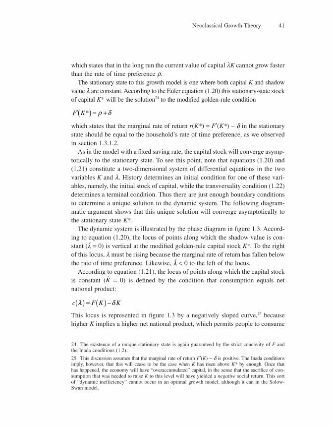
Neoclassical Growth Theory 41
which states that in the long run the current value of capital lK cannot grow faster than the rate of time preference r.
The stationary state to this growth model is one where both capital K and shadow value l are constant. According to the Euler equation (1.20) this stationary-state stock of capital K* will be the solution24 to the modifi ed golden-rule condition
′( ) = +F K* ρ δ
which states that the marginal rate of return r(K*) = F′(K*) − d in the stationary state should be equal to the household’s rate of time preference, as we observed in section 1.3.1.2.
As in the model with a fi xed saving rate, the capital stock will converge asymp-totically to the stationary state. To see this point, note that equations (1.20) and (1.21) constitute a two-dimensional system of differential equations in the two variables K and l. History determines an initial condition for one of these vari-ables, namely, the initial stock of capital, while the transversality condition (1.22) determines a terminal condition. Thus there are just enough boundary conditions to determine a unique solution to the dynamic system. The following diagram-matic argument shows that this unique solution will converge asymptotically to the stationary state K*.
The dynamic system is illustrated by the phase diagram in fi gure 1.3. Accord-ing to equation (1.20), the locus of points along which the shadow value is con-stant ( �λ = 0) is vertical at the modifi ed golden-rule capital stock K*. To the right of this locus, l must be rising because the marginal rate of return has fallen below the rate of time preference. Likewise, �λ < 0 to the left of the locus.
According to equation (1.21), the locus of points along which the capital stock is constant ( �K = 0) is defi ned by the condition that consumption equals net national product:
c F K Kλ δ( ) = ( ) −
This locus is represented in fi gure 1.3 by a negatively sloped curve,25 because higher K implies a higher net national product, which permits people to consume
24. The existence of a unique stationary state is again guaranteed by the strict concavity of F and the Inada conditions (1.2).
25. This discussion assumes that the marginal rate of return F′(K) − d is positive. The Inada conditions imply, however, that this will cease to be the case when K has risen above K* by enough. Once that has happened, the economy will have “overaccumulated” capital, in the sense that the sacrifi ce of con-sumption that was needed to raise K to this level will have yielded a negative social return. This sort of “dynamic ineffi ciency” cannot occur in an optimal growth model, although it can in the Solow-Swan model.
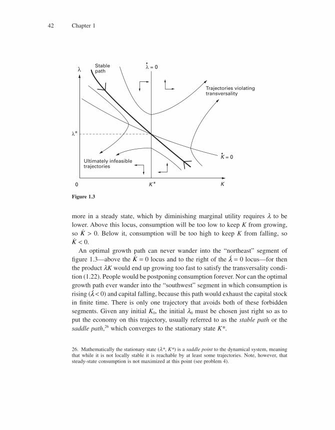
Chapter 142
more in a steady state, which by diminishing marginal utility requires l to be lower. Above this locus, consumption will be too low to keep K from growing, so �K > 0. Below it, consumption will be too high to keep K from falling, so �K < 0.
An optimal growth path can never wander into the “northeast” segment of fi gure 1.3—above the �K = 0 locus and to the right of the �λ = 0 locus—for then the product lK would end up growing too fast to satisfy the transversality condi-tion (1.22). People would be postponing consumption forever. Nor can the optimal growth path ever wander into the “southwest” segment in which consumption is rising ( �λ < 0) and capital falling, because this path would exhaust the capital stock in fi nite time. There is only one trajectory that avoids both of these forbidden segments. Given any initial K0, the initial l0 must be chosen just right so as to put the economy on this trajectory, usually referred to as the stable path or the saddle path,26 which converges to the stationary state K*.
Ultimately infeasibletrajectories
Trajectories violatingtransversality
Stablepath
K * K0
λ = 0
K = 0
λ
λ*
Figure 1.3
26. Mathematically the stationary state (l*, K*) is a saddle point to the dynamical system, meaning that while it is not locally stable it is reachable by at least some trajectories. Note, however, that steady-state consumption is not maximized at this point (see problem 4).
Neoclassical Growth Theory 43
So, as in the case of a fi xed saving rate, the model will exhibit no growth in the long run. A temporary increase in thrift, modeled as a fall in the rate of time preference r, would disturb the phase diagram by shifting the stationary state K* to the right. This shift would cause net investment to increase until it reached the new golden-rule capital stock. But eventually growth would come to an end, and again the reason is the diminishing marginal product of capital. That is, if ever K were to rise above K*, then the diminishing marginal product of capital would have brought the marginal rate of return below the rate of time preference, and the household would no longer be willing to accumulate more capital.
Appendix 1B: Dynamic Optimization Using the Hamiltonian
Consider a representative infi nitely lived individual whose lifetime utility func-tion is
W e u c t dtpt= ( )⎡⎣ ⎤⎦−∞
∫0
where c(t) is the time path of consumption per person, u(.) is an instantaneous utility function exhibiting positive but diminishing marginal utility, and r a posi-tive rate of time preference. To simplify the analysis we abstract once again from population growth by assuming a constant labor force: L = 1. Then, with continu-ous market clearing, perfect competition, perfect foresight, and no exter-nalities, the economy will follow an optimal growth path. That is, it will maximize W subject to the constraint that consumption plus investment must equal net national product:
�K F K K c= ( ) − −δ (1.23)
subject to the historically predetermined value of capital.Along an optimal growth path, capital should be increasing whenever its net
marginal product F′(K) − d is greater than the rate of time preference r, and decreasing whenever it is less. That is, the rate of time preference can be inter-preted as the required rate of return on capital, the rate below which it is not optimal to continue equipping workers with as much capital. This together with the fi rst Inada condition (1.2) implies that growth cannot be sustained indefi nitely. For doing so would require capital to grow without limit, which would eventually drive the net marginal product of capital below the rate of time preference.
Chapter 144
To see this point more formally,27 recall that from the theory of optimal control, the level of consumption at each point of time must maximize the Hamiltonian:
H u c F K K c= ( ) + ( ) − −⎡⎣ ⎤⎦λ δ
where l is the shadow value of investment, evaluated in current utils. According to equation (1.23) the term in square brackets is net investment. Thus the Hamilto-nian is analogous to the familiar concept of net national product—consumption plus net investment—the only difference being that the Hamiltonian measures both consumption and net investment in units of utility rather than units of goods.
A necessary fi rst-order condition for maximizing the Hamiltonian is
∂∂H
c= 0
or equivalently that the marginal utility of consumption equals the shadow value of investment:
′( ) =u c λ (1.24)
The shadow value l is itself determined as the present value of the stream of extra utils that would be created by a marginal unit of capital. Equivalently28 we can defi ne it in terms of the Euler equation:
�λ ρλ= − ∂∂
H
K
or equivalently
ρλ λ δ λ= ′( ) −( ) +F K � (1.25)
Finally, the following transversality condition must hold:
27. For the mathematical details of optimal growth theory, see Arrow and Kurz (1970). A brief summary of the mathematics of intertemporal optimization in continuous time is provided in Aghion and Howitt (1998a), appendix to chapter 1.
28. As in standard consumer theory, if we start on an optimal path, then the marginal benefi t of having an extra unit of net national product is independent of how that marginal unit is allocated between consumption and investment. Suppose, therefore, that all the extra NNP resulting from a marginal unit of capital is always exactly consumed. Then the increment to the capital stock will be permanent, and the marginal value will be
λ τ τ δ τρ τt e u c F K dt
t( ) = ′ ( )⎡⎣ ⎤⎦ ′ ( ) −⎡⎣ ⎤⎦{ }− −( )∞
∫By routine calculus, this is equivalent to the pair of conditions (1.25) and (1.26) provided that the optimality condition (1.24) can be invoked to replace the marginal utility at each date in the integral. The transversality condition is needed in order to ensure that the integral converges.
Neoclassical Growth Theory 45
limt
te K→∞
− =ρ λ 0 (1.26)
The Euler equation (1.25) can be interpreted as an equilibrium asset-pricing condition in a world where the numéraire is current utils and everyone is risk-neutral. The right-hand side of equation (1.25) shows the incremental fl ow of income, including capital gain, that can rationally be anticipated by an individual who holds an incremental unit of K.29 The ratio of this income fl ow to the “asset price” l must equal the “competitive rate of interest” r. The transversality condi-tion (1.26) is the condition that rules out the kind of ineffi ciency involved in accumulating capital forever without consuming it.
Substituting for l = u′(c) in equation (1.25) in turn delivers the Euler equation, namely,
′′( )′( ) = − ′( ) −⎡⎣ ⎤⎦
u c
u cc F K� ρ δ
Problems
1. Present the main assumption of the Solow-Swan model. What type of convergence is predicted by the model? What is the long-run effect of short-run growth-enhancing policies (such as an increase in the saving rate)?
2. Conditional convergence in the Solow model
This problem illustrates algebraically the concept of conditional convergence, using a Cobb-Douglas production function. Assume that output per capita can be written as y = Aka and that population grows at rate n, the depreciation rate is d, and there is no technical progress.
a. Using the steady-state condition in the chapter, express the saving rate as a function of the per capita steady-state level of capital, k*.
b. Using the dynamic equation for capital accumulation of capital, express the growth rate of capital, �k k, as a function k/k*. Interpret the result.
3. Land in the Solow model
Assume a production function that takes a Cobb-Douglas form in capital K, labor L, and land C:
Y Ae K L Cgt= α β λ
where A > 0, g > 0 (rate of technological progress), a > 0, b > 0, l > 0, and a + b + l = 1. The amount of land, C, is fi xed.
Labor grows at the constant rate n > 0, capital depreciates at rate d > 0, and the saving rate is exoge-nously given at the level of s.
29. That is, the extra K will raise the fl ow of output by an amount equal to the net marginal product F′(K) − d, each unit of which has a utility value of l, and it will also allow the holder to benefi t from the increase in the utility value of the unit (or suffer the loss if negative) at the rate l
..

Chapter 146
Defi ne k ≡ K/Y, the capital-output ratio.
a. Write down the growth rates of capital stock and output as functions of k.
b. Using the results from item 3a, write down the growth rate of the capital-output ratio as a function of k.
c. Defi ning steady state as a situation in which k is constant, compute the steady-state value of k.
d. Compute the steady-state growth rate of output. Is it positive?
e. Compute the steady-state growth rate of output per capita. Is it positive? Explain how this value depends on the growth rate of technological progress g and the presence of land.
4. The Golden Rule of capital accumulation and dynamic ineffi ciency in the Solow model
Consider the Solow model presented in the chapter.
a. Assuming the economy is in steady state (at per capita capital level k*), and for given levels of the parameters A, n, d, s, and g, write down the level of per capita consumption as a function of k*.
b. For what level of k* is per capita consumption in steady state maximized? This condition is called the golden rule of capital accumulation.
c. Rewrite the preceding condition as a function of the saving rate, instead of per capita capital stock.
d. Explain why an economy that is saving more than the rate implied by the golden rule is dynami-cally ineffi cient; that is, its per capita consumption at all points in time could be increased by reducing the saving rate.
5. Stone-Geary preferences (based on Barro and Sala-i-Martin 1995a)
Consider the Cass-Koopmans-Ramsey model presented in the chapter, with the following formulation for households’ instantaneous utility function (called Stone-Geary preferences):
u cc c( ) =
−( ) −−
−11
1
ε
ε
where c ≥ 0 represents the subsistence level of per capita consumption.
a. What is the intertemporal elasticity of substitution for the new form of the utility function? For c > 0, how does the elasticity change as c increases?
b. Consider the Euler equation with the rate of consumption growth on the right-hand side, as seen in the chapter. How would this equation change under the Stone-Geary formulation of preferences?
c. How would the growth rate of consumption change as c increases? Provide some intuition for this result.
6. Measuring the speed of convergence in the Solow model
Consider the capital growth rate equation for a Cobb-Douglas aggregate production function, �k k = sk−(1 − a) − (n + g + d).
a. Compute the speed of convergence b ≡ −∂ ( �k k)/∂ log(k), that is, by how much the capital growth rate declines as the capital stock increases in a proportional sense.
b. How does an increase in a affect b?
c. How does b evolve over time? Compute the speed of convergence in steady state b*.
d. By log-linearizing the capital growth equation in the neighborhood of the steady state, show that �k k ≅ −b*[log(k/k*)], where k* is the steady-state level of per capita capital.

2 The AK Model
2.1 Introduction
The neoclassical model presented in the previous chapter takes the rate of tech-nological change as being determined exogenously, by noneconomic forces. There is good reason, however, to believe that technological change depends on economic decisions, because it comes from industrial innovations made by profi t-seeking fi rms and depends on the funding of science, the accumulation of human capital, and other such economic activities. Technology is thus an endogenous variable, determined within the economic system. Growth theories should take this endogeneity into account, especially since the rate of technological progress is what determines the long-run growth rate.
Incorporating endogenous technology into growth theory forces us to deal with the diffi cult phenomenon of increasing returns to scale. More specifi cally, people must be given an incentive to improve technology. But because the aggregate production function F exhibits constant returns in K and L alone, Euler’s theorem tells us that it will take all of the economy’s output to pay capital and labor their marginal products in producing fi nal output, leaving nothing over to pay for the resources used in improving technology.1 Thus a theory of endogenous technol-ogy cannot be based on the usual theory of competitive equilibrium, which requires that all factors be paid their marginal products.
Arrow’s (1962) solution to this problem was to suppose that technological progress is an unintended consequence of producing new capital goods, a phe-nomenon dubbed “learning by doing.” Learning by doing was assumed to be purely external to the fi rms responsible for it. That is, if technological progress
1. Euler’s theorem states that if F is homogeneous of degree 1 in K and L (the defi nition of constant returns), then
F K L K F K L L F K L1 2, , ,( ) + ( ) = ( ) (E)
where Fi is the partial derivative with respect to the ith argument. The marginal products of K and L are F1 and F2, respectively. So if K and L are paid their marginal products, then the left-hand side is the total payment to capital (price F1 times quantity K) plus the total payment to labor, and the equa-tion states that these payments add up to total output.
To verify Euler’s theorem take the equation
F K L F K Lλ λ λ, ,( ) = ( ) (C)
that defi nes homogeneity of degree one, and differentiate both sides with respect to l at the point l = 1. Since equation (C) must hold for all l > 0, therefore the two derivatives must be equal, implying equation (E).
Chapter 248
depends on the aggregate production of capital and fi rms are all very small, then they can all be assumed to take the rate of technological progress as being given independently of their own production of capital goods. So each fi rm maximizes profi t by paying K and L their marginal products, without offering any additional payment for their contribution to technological progress.
Learning by doing formed the basis of the fi rst model of endogenous growth theory, which is known as the AK model. The AK model assumes that when people accumulate capital, learning by doing generates technological progress that tends to raise the marginal product of capital, thus offsetting the tendency for the marginal product to diminish when technology is unchanged. The model results in a production function of the form Y = AK, in which the marginal product of capital is equal to the constant A.
The AK model predicts that a country’s long-run growth rate will depend on eco-nomic factors such as thrift and the effi ciency of resource allocation. In subsequent chapters we will develop alternative models of endogenous growth that emphasize not thrift and effi ciency but creativity and innovation, which we see as the main driving forces behind economic growth. But given its historical place as the fi rst endogenous growth model, the AK paradigm is an important part of any economist’s tool kit. Accordingly we devote this chapter to developing the AK model and to summarizing the empirical debate that took place in the 1990s between its proponents and proponents of the neoclassical model of Solow and Swan.
2.1.1 The Harrod-Domar Model
An early precursor of the AK model was the Harrod-Domar model,2 which assumes that the aggregate production function has fi xed technological coeffi cients:
Y F K L AK BL= ( ) = { }, min ,
where A and B are the fi xed coeffi cients. Under this technology, producing a unit of output requires 1/A units of capital and 1/B units of labor; if either input falls short of this minimum requirement, there is no way to compensate by substituting the other input.
With a fi xed-coeffi cient technology, there will either be surplus capital or surplus labor in the economy, depending on whether the historically given supply of capital is more or less than (B/A) times the exogenous supply of labor. When
2. See Harrod (1939) and Domar (1946).
The AK Model 49
AK < BL, which is the case that Harrod and Domar emphasize, capital is the limiting factor. Firms will produce the amount
Y AK=
and hire the amount (1/B)Y = (1/B)AK < L of labor.Now, with a fi xed saving rate, we know that the capital stock will grow accord-
ing to the same equation as in the neoclassical model:
�K sY K= − δ (2.1)
These last two equations imply
�K sAK K= − δ
so that the growth rate of capital will be
g K K sA= = −� δ
Because output is strictly proportional to capital, g will also be the rate of growth of output. It follows immediately that the growth rate of output is increasing in the saving rate s.
The problem with the Harrod-Domar model is that it cannot account for the sustained growth in output per person that has taken place in the world economy since the industrial revolution. To see this point, let n be the rate of population growth. Then the growth rate of output per person is g − n. But if this is positive, then so is the growth rate of capital per person K/L, since K also grows at the rate g. Eventually a point will be reached where capital is no longer the limiting factor in the production function. That is, K/L will eventually exceed the limit B/A above which labor becomes the limiting factor. From then on we will instead have Y = BL, implying that Y will grow at the same rate as L; that is, output per person Y/L will cease to grow.
2.2 A Neoclassical Version of Harrod-Domar
2.2.1 Basic Setup
The fi rst AK model that could account for sustained growth in per capita output was that of M. Frankel (1962), who was motivated by the challenge of construct-ing a model that would combine the virtues of the Solow-Swan and Harrod-Domar models. As in Solow-Swan, this model would display perfect competition,

Chapter 250
substitutable factors (with Cobb-Douglas production technologies), and full employment. As in Harrod-Domar, the model would generate a long-run growth rate that depends on the saving rate.
Frankel built his model on the foundation of learning by doing. He recognized that because individual fi rms contribute to the accumulation of technological knowledge when they accumulate capital,3 the AK structure of the Harrod-Domar model does not require fi xed coeffi cients. Instead, he assumed that each fi rm j ∈ {1, 2, . . . , N} has a production function of the form
y Ak Lj j j= −α α1
where kj and Lj are the fi rm’s own employment of capital and labor, and A is (aggregate) productivity. Aggregate productivity in turn depends upon the total amount of capital that has been accumulated by all fi rms, namely,
A A kjj
N
= ⋅⎛
⎝⎜⎞
⎠⎟=∑0
1
η
where h is a positive exponent that refl ects the extent of the knowledge externali-ties generated among fi rms.
For simplicity assume that
Lj = 1
for all j; let
K kjj
N
==
∑1
denote the aggregate capital stock; and let
Y yjj
N
==
∑1
denote the aggregate output fl ow.Since all fi rms face the same technology and the same factor prices, they will
hire factors in the same proportions, so that
k K N jj = for all
3. He called it “development” rather than “knowledge.”
The AK Model 51
This expression in turn implies that in equilibrium
A A K= 0η
Hence individual outputs are all equal to
y A K K Nj = ( )0η α
and therefore aggregate output is
Y NA K K N= ( )0η α
which can be written as
Y AK= +α η (2.2)
where A = A0N1−a.The model is then closed by assuming a constant saving rate, which generates
the same capital accumulation equation (2.1) as in Solow-Swan and Harrod-Domar. Using the output equation (2.2) to substitute for Y in this equation we have
�K sAK K= −+α η δ
so the growth rate of the capital stock is
g K K sAKK = = −+ −� α η δ1 (2.3)
2.2.2 Three Cases
We now analyze the dynamic path of the economy defi ned by equation (2.3). Three cases must be considered.
1. a + h < 1
In this case the extent of knowledge spillovers h is not suffi ciently strong to counteract the effect 1 − a of decreasing returns to individual capital accumula-tion, and the long-run growth rate is zero. The case produces the same aggregate dynamics as the Solow-Swan model with no technological progress and no popu-lation growth, which we analyzed in the previous chapter. That is, according to equation (2.3) there is a steady-state capital stock at which the growth rate gK of capital is zero, namely,
K sA* = ( ) − −( )δ α η1 1 (2.4)
If K were to rise above K*, the growth rate would turn negative, since in this case equation (2.3) makes gK a decreasing function of K. Thus K would fall back to
Chapter 252
its steady state, at which the growth rate of capital is zero and therefore the growth rate of output (2.2) is zero.
2. a + h > 1
In this case learning externalities are so strong that the aggregate economy experi-ences an ever-increasing growth rate. That is, again equation (2.4) defi nes a unique steady-state capital stock but it is no longer stable, because gK is now an increasing function of K, so that if K were to rise above K* it would keep on rising, at an ever-increasing rate. This is known as the explosive growth case.
3. a + h = 1
In this knife-edge case, learning externalities exactly compensate decreasing returns to individual capital accumulation, so that the aggregate production func-tion becomes an AK function, namely,
Y AK=
Thus the aggregate growth rate becomes
g K K sA= = −� δ
which is nothing but the Harrod-Domar growth rate, now obtained as the long-run growth rate in a model with substitutable factors and full market clearing. In other words, as capital increases, output increases in proportion, even though there is continual full employment of labor and even though there is substitutability in the aggregate production function, because knowledge automatically increases by just the right amount. Unlike in the Harrod-Domar model, here an increase in the saving propensity s will increase the growth rate permanently even though output per person is growing at a positive rate (namely, g − n = g).
2.3 An AK Model with Intertemporal Utility Maximization
Romer (1986)4 developed a Ramsey version of the AK model, in which the con-stant saving rate is replaced by intertemporal utility maximization by a represen-
4. Romer actually laid out more than an AK model, inasmuch as his approach allowed for general production and utility functions and assumed that there were strictly increasing social returns to capital. What we present here is the limiting special case that many followers have extracted from Romer’s analysis, in which there are constant social returns to capital and an isoelastic utility function.
The AK Model 53
tative individual, again with the assumption that individuals do not internalize the externalities associated with the growth of knowledge.
2.3.1 The Setup
Romer assumed a production function with externalities of the same sort as con-sidered previously and focused on the case in which the labor supply per fi rm was equal to unity and the rate of capital depreciation was zero (d = 0). Saving is determined by the owner of the representative one-worker fi rm, whose dynamic optimization problem is to
max u c e dt k Ak ctt( ) = −−∞
∫ ρ αsubject to �0
where k is the capital stock of the individual fi rm, y = Akα is its output, c = ct is the current consumption of its owner-worker, and A denotes aggregate pro-ductivity that is taken as given by each individual fi rm.5
As in the previous section, aggregate productivity depends upon the aggregate capital stock, namely,
A A K= 0η
where
K kj
N= ∑1
Assuming a constant intertemporal elasticity of substitution as in the previous
chapter, namely, u cc( ) =
−−
−1 1
1
ε
ε, one obtains the Euler condition6
− = − −ε ρ α α�c c Ak 1
Having rational expectations, individuals correctly anticipate that all fi rms will employ the same capital in equilibrium (given that these fi rms are all identical), so
K Nk=
5. This maximization problem is the same as that of the Cass-Koopmans-Ramsey model analyzed in the previous chapter, but in the limiting case where the length of the time period has shrunk to zero, so time has become continuous.
6. This Euler condition follows from our analysis of the Ramsey model in the previous chapter, but in this case the net private marginal product of capital is F1(k,A) − d = a Aka−1 − 0 = a Aka−1.
Chapter 254
and therefore the preceding Euler condition can be written as
− = − + −ε ρ α η α η�c c A N k01 (2.5)
2.3.2 Long-Run Growth
Aggregate output Y is given by the same equation (2.2) as in the Frankel model, because
Y Ny NA K K N AK= = ( ) = +0
η α α η
Again there are three cases to consider depending on the exponent a + h.
1. a + h < 1
In the case of decreasing returns, again growth will vanish asymptotically as in the neoclassical model without technological progress. To see this point, assume, on the contrary, that the growth rate is bounded above zero. The following argument shows that this assumption leads to a contradiction. Positive growth implies that the capital stock k will converge to infi nity over time, imply-ing that the right-hand side of equation (2.5) must converge to r, since the expo-nent a + h − 1 is negative, and in turn implying that the growth rate �c/c will become negative, a result which contradicts our assumption of positive growth.
2. a + h > 1
In the case of increasing returns to capital, then, as in the Frankel model, there will be explosive growth. This can be seen using the Euler equation (2.5). Specifi cally, if growth is positive in the long run, then the capital stock k converges to infi nity over time. This result, together with the fact that a + h > 1, implies that the right-hand side of equation (2.5) converges to negative infi nity, which in turn implies that the growth rate �c/c must converge to infi nity.
3. a + h = 1
In the AK case where there are constant social returns to capital, then, as in the Frankel model, the economy will sustain a strictly positive but fi nite growth rate g, in which diminishing private returns to capital are just offset by the external improvements in technology A that they bring about. More precisely, in a steady state, consumption and output will grow at the same rate, so this case (2.5) implies
g c c A N= = −( )� α ρ εη0
The AK Model 55
In particular, we see that the higher the discount rate r (that is, the lower the propensity to save), or the lower the intertemporal elasticity of substitution mea-sured by 1/e, the lower will be the steady-state growth rate g.
2.3.3 Welfare
So far we have just reproduced the results already generated by the model with a constant saving rate. However, moving to a Ramsey model where savings behavior results from explicit intertemporal utility maximization allows us to also conduct a welfare analysis. In particular one can show that, because individuals and individual fi rms do not internalize the effect of individual capital accumula-tion on knowledge A when optimizing on c and k, the equilibrium growth rate g = (aA0Nh − r)/e is less than the socially optimal rate of growth. More formally, the social planner who internalizes the knowledge externalities induced by indi-vidual capital accumulation would solve the dynamic program
max e u c dt k A Nk k ctt
−∞ ( ) = ( ) −∫ ρ η αsubject to � 00
That is, he would internalize the fact that A = A0(Nk)h when choosing k. When
u cc( ) =
−−
−1 1
1
ε
ε, we obtain the Euler equation
− = − +( ) + −ε ρ α η η α η�c c A N k01
With constant social returns to capital (a + h = 1), this yields the socially optimal rate of growth
g N A g N A* = −( ) > = −( )η ηρ ε α ρ ε0 0
2.3.4 Concluding Remarks
First, although growth has been endogenized, it relies entirely on external (and therefore unremunerated) accumulation of knowledge. Introducing rewards to technological progress, as we shall do in the following chapters, adds a new dimension of complexity, because it moves us away from a world of perfect competition into a world of imperfect competition among large individual fi rms.
Second, in the case where a + h = 1, cross-country variations in parameters such as a and r will result in permanent differences in rates of economic growth. Thus the simple AK approach does not predict conditional convergence in income
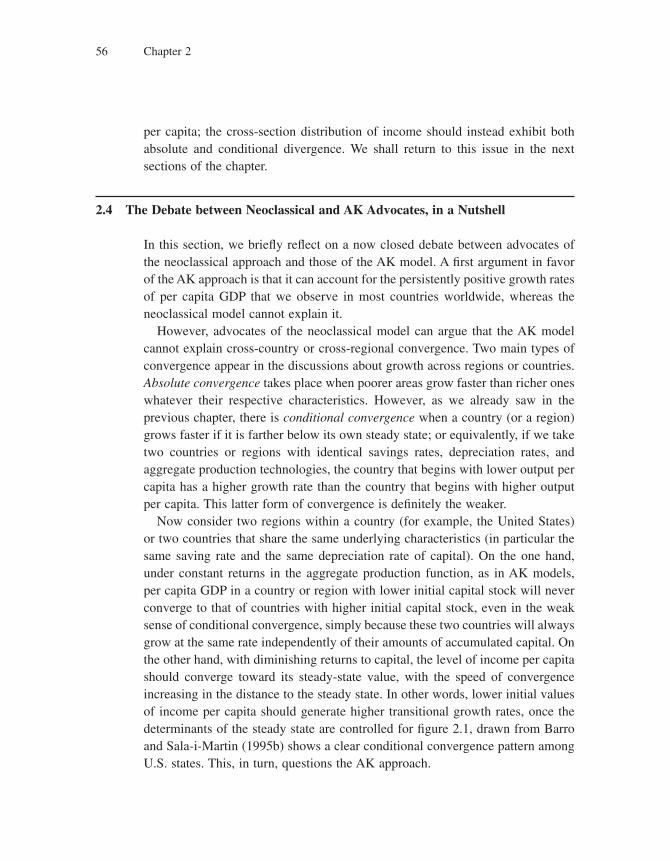
Chapter 256
per capita; the cross-section distribution of income should instead exhibit both absolute and conditional divergence. We shall return to this issue in the next sections of the chapter.
2.4 The Debate between Neoclassical and AK Advocates, in a Nutshell
In this section, we briefl y refl ect on a now closed debate between advocates of the neoclassical approach and those of the AK model. A fi rst argument in favor of the AK approach is that it can account for the persistently positive growth rates of per capita GDP that we observe in most countries worldwide, whereas the neoclassical model cannot explain it.
However, advocates of the neoclassical model can argue that the AK model cannot explain cross-country or cross-regional convergence. Two main types of convergence appear in the discussions about growth across regions or countries. Absolute convergence takes place when poorer areas grow faster than richer ones whatever their respective characteristics. However, as we already saw in the previous chapter, there is conditional convergence when a country (or a region) grows faster if it is farther below its own steady state; or equivalently, if we take two countries or regions with identical savings rates, depreciation rates, and aggregate production technologies, the country that begins with lower output per capita has a higher growth rate than the country that begins with higher output per capita. This latter form of convergence is defi nitely the weaker.
Now consider two regions within a country (for example, the United States) or two countries that share the same underlying characteristics (in particular the same saving rate and the same depreciation rate of capital). On the one hand, under constant returns in the aggregate production function, as in AK models, per capita GDP in a country or region with lower initial capital stock will never converge to that of countries with higher initial capital stock, even in the weak sense of conditional convergence, simply because these two countries will always grow at the same rate independently of their amounts of accumulated capital. On the other hand, with diminishing returns to capital, the level of income per capita should converge toward its steady-state value, with the speed of convergence increasing in the distance to the steady state. In other words, lower initial values of income per capita should generate higher transitional growth rates, once the determinants of the steady state are controlled for fi gure 2.1, drawn from Barro and Sala-i-Martin (1995b) shows a clear conditional convergence pattern among U.S. states. This, in turn, questions the AK approach.
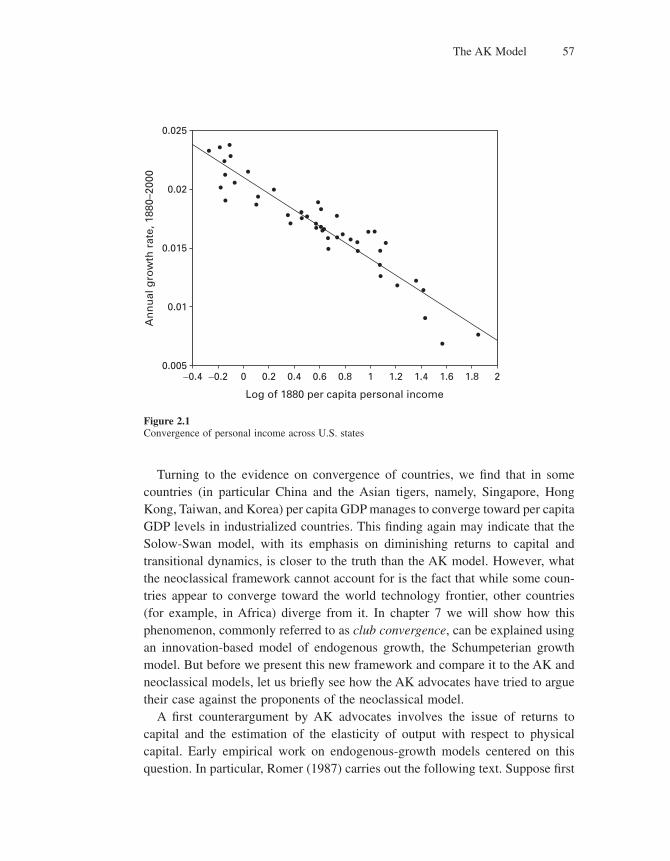
The AK Model 57
Turning to the evidence on convergence of countries, we fi nd that in some countries (in particular China and the Asian tigers, namely, Singapore, Hong Kong, Taiwan, and Korea) per capita GDP manages to converge toward per capita GDP levels in industrialized countries. This fi nding again may indicate that the Solow-Swan model, with its emphasis on diminishing returns to capital and transitional dynamics, is closer to the truth than the AK model. However, what the neoclassical framework cannot account for is the fact that while some coun-tries appear to converge toward the world technology frontier, other countries (for example, in Africa) diverge from it. In chapter 7 we will show how this phenomenon, commonly referred to as club convergence, can be explained using an innovation-based model of endogenous growth, the Schumpeterian growth model. But before we present this new framework and compare it to the AK and neoclassical models, let us briefl y see how the AK advocates have tried to argue their case against the proponents of the neoclassical model.
A fi rst counterargument by AK advocates involves the issue of returns to capital and the estimation of the elasticity of output with respect to physical capital. Early empirical work on endogenous-growth models centered on this question. In particular, Romer (1987) carries out the following text. Suppose fi rst
0.025
0.02
0.015
0.01
0.005−0.4 0 0.80.4 1.2 1.6−0.2 0.2 10.6 1.4 1.8 2
An
nu
al g
row
th r
ate,
188
0–20
00
Log of 1880 per capita personal income
Figure 2.1Convergence of personal income across U.S. states
Chapter 258
that the consumption good is produced according to a Cobb-Douglas production function as in the simplest version of the Solow-Swan model:
Y K AL= ( ) < <−α α α10 1,
Under perfect competition in the market for fi nal goods, and given the assumption of constant returns to scale implicit in this Cobb-Douglas function, the coeffi -cients a and (1 − a) should be equal to the shares of capital and labor in national income, respectively, that is approximately 1
3 and 23 in the U.S. case. To
see why, notice that under perfect competition for fi nal goods, capital and labor are each paid their marginal products. The share of labor in national income is thus equal to
∂∂
Y
LL K A L L Y= −( ) = −( )− −1 11α αα α α
and similarly
∂∂
Y
KK K A L K Y= =− − −α αα α α1 1 1
Now, using both time series and cross-section data, Romer estimated the true elasticity of fi nal goods output with respect to physical capital to be higher than the value 1
3 predicted by the Solow-Swan model, and perhaps lying in the range between 0.7 and 1.0. This result in turn appeared to be consistent with the existence of externalities to capital accumulation, as captured by the formaliza-tion A ≈ Kh in the AK model. Such externalities imply that the elasticity of fi nal output with respect to physical capital will be larger than the share of capital income in value added.
A second counterargument involves the speed of convergence predicted by the neoclassical model. First, it is intuitive that the lower a is, that is, the more decreas-ing returns to capital are, the faster convergence will be over time, since decreasing returns are the source of convergence. And indeed, in the limit case where a = 1, that is, in the constant returns case, convergence never happens! This negative cor-relation between a and the speed of convergence can be formally established (see problem 5 from chapter 1). Now, performing a cross-country regression as specifi ed in section 1.2.3, Mankiw, Romer, and Weil (1992) fi nd that the rate at which coun-tries converge to their steady states is slower than that predicted by a Solow-Swan model with a capital share of one third. The empirically observed speed of conver-
The AK Model 59
gence suggests a share of broad capital in output of around 0.7–0.8. One explanation may again be the existence of externalities in capital accumulation of the kind emphasized by AK models. However, Mankiw, Romer, and Weil propose an alter-native explanation, which boils down to augmenting the Solow-Swan model by including human capital on top of physical capital. They specify the following constant-returns production function:
Y K H AL= ( ) − −α β α β1
Using a simple proxy for the rate of investment in human capital, they argue that this technology is consistent with the cross-country data. Their cross-section regressions indicate that both a and b are about 1/3, suggesting that the AK model is wrong in assuming constant returns to broad capital.
Interestingly, the elasticity of output with respect to the investment ratio
becomes equal to αα β1− − in the augmented model, instead of
αα1−
. In other
words, the presence of human capital accumulation increases the impact of physical investment on the steady-state level of output. Moreover, the Solow-Swan model augmented with human capital can account for a very low rate of convergence to steady states. It is also consistent with evidence on international capital fl ows; see Barro, Mankiw, and Sala-i-Martín (1995) and Manzocchi and Martin (1996). Yet the constant-returns specifi cation of Mankiw, Romer, and Weil delivers the same long-run growth predictions as the basic Solow-Swan model.
Overall, empirical evidence regarding returns to capital tends to discriminate in favor of decreasing returns, and hence in favor of the neoclassical growth model. Mankiw, Romer, and Weil claim that the neoclassical growth model is correct not only in assuming diminishing returns, but also in suggesting that effi ciency grows at the same rate across countries.
True, their augmented model suffers from the same basic problem as the origi-nal Solow model, namely, that it cannot explain sustained long-run growth. But here the line of defense is to say that the model can still explain growth on the transition path to the steady state, and that such transition may last for many years so that the data would not allow us to tell apart transitional growth from steady-state growth.
However, another criticism to the augmented neoclassical model came from Benhabib and Spiegel (1994). Their point is that the neoclassical and
Chapter 260
Mankiw-Romer-Weil models all predict that growth can increase only as a result of a higher rate of factor accumulation. However, based on cross-country panel data, they argue that the countries that accumulated human capital most quickly between 1965 and 1985 have not grown accordingly, and more importantly, they show that long-run growth appears to be related to the initial level of human capital. This fi nding in turn suggests that, when trying to explain the historical experience of developing countries, one should turn to models in which techno-logy differs across countries and in which human capital stock promotes tech-nological catch-up and/or innovation. We will return to this topic in chapter 13.
Overall, if the AK model appears to be dominated by the neoclassical model, one must still come to grip with the fact that growth appears to be sustained over time, and also positively correlated with variables such as human capital stocks. Building new endogenous growth models that account for those facts, as well as convergence, will be a main challenge of the theories developed in the next chapters.
2.5 An Open-Economy AK Model with Convergence
In this section we present a recent attempt at saving the AK model from the criti-cism that it cannot explain convergence. This attempt, developed by Acemoglu and Ventura (2002), henceforth AV, links to international trade and the notion of terms of trade. The idea is to show that, if we take into account that countries are tied together by international trade, even AK models can exhibit convergence in growth rates. They can do so because in an open economy the parameter A will depend on the country’s terms of trade. If it keeps growing faster than the rest of the world, the supply of its goods on world markets will keep growing relative to the supply of foreign goods, which will drive down their relative price. The terms of trade will fall, lowering A and therefore lowering the country’s growth rate until it converges with the growth rate of the rest of the world. In such a world each country will look like an AK model for given terms of trade, and yet it will converge, not because of a diminishing physical marginal product of capital but because of a diminishing value of the marginal product of capital. The argument is clever and logically tight, even though one may object to it on empirical grounds.
Here we present in stages a simplifi ed version of the AV model, with constant savings rates. First we study a closed economy with two sectors—a fi nal sector and an intermediate sector. Next we assume that production in the fi nal sector

The AK Model 61
requires as input not just the domestically produced intermediate product but also a foreign intermediate product, under the assumption that the relative price of that foreign product (the inverse of this country’s terms of trade) is given. This produces a similar version of the AK model, one in which A depends positively on the terms of trade. Finally we close the model off by supposing that the foreign country is just like the domestic country but possibly with a different saving rate. In this last model the terms of trade will depend inversely on this country’s capital stock relative to the foreign country’s.
2.5.1 A Two-Sector Closed Economy
The fi nal good Y and the intermediate good X are both produced under perfect competition. The fi nal good is produced with capital K and intermediates accord-ing to
Y K X= −α α1 (2.6)
and the intermediate is produced with the fi nal good one for one.Let the fi nal good Y be the numéraire. Then the unit price of good Y is equal
to one, and this is also the unit cost of producing the intermediate good. Since markets are perfectly competitive, the price of intermediate good X is equal to its unit cost; thus it is also equal to one. Given these assumptions, the demand for the intermediate good X is determined by profi t maximization in the fi nal sector. That is, the optimal X maximizes fi nal-sector profi ts:
Π = −−K X Xα α1
The fi rst-order condition for this problem is
1 1−( ) =−α α αK X
or equivalently
X K= −( )11α α
Substituting back into equation (2.6) we obtain
Y K= −( )−
11
αα
α
So even though the production function (2.6) has a diminishing marginal product of capital, we still have an AK model, with Y = AK, where the marginal product of capital A is a constant given by
Chapter 262
A = −( )−
11
αα
α
The reason is that the production technology for the fi nal good has constant returns with respect to K and X, both of which are produced with K.
Now, let us assume a constant saving rate so that we can close the model with the same capital accumulation equation as in the Solow model, namely,7
�K sY K= − δ
Then, as in the Frankel model analyzed in section 2.2, the country’s growth rate depends positively on its saving rate according to
g K K sA s= = − = −( ) −−
� δ α δα
α11
2.5.2 Opening up the Economy with Fixed Terms of Trade
Now suppose that producing the Y good requires not just X but also a foreign-produced intermediate product Xf, according to the production function
Y K X X f= ( )− −
αα α1
21
2
Both X and Xf are tradable goods; however, capital is not tradable.As before, since it takes one unit of fi nal good to produce one unit of X, and
since the market for X is perfectly competitive, the price of X is unity. Suppose the price pf of the foreign good is given. Then domestic producers of Y will choose X and Xf to solve the problem
max,X X
f f ff
K X X X p Xαα α1
21
2
− −
( ) − −⎧⎨⎪
⎩⎪
⎫⎬⎪
⎭⎪
7. This is not quite the same as in the neoclassical model because Y is not the country’s GDP, just its production of the fi nal good, some of which is used as an input to the intermediate sector. However, Y is proportional to GDP because
GDP Value added in final sector Value added in intermediat= + ee sector= −( ) +
= −( ) − −( )= −( ) =
−
−
Y X
K K
K Y
0
1 1
1
1 1
1
α α
α α α
αα α
αα
so the parameter s is actually the country’s saving rate, as conventionally defi ned, multiplied by the constant a.
The AK Model 63
which yields
X Y=−⎛
⎝⎜⎞⎠⎟
1
2
α (2.7)
p X Yf f =−⎛
⎝⎜⎞⎠⎟
1
2
α (2.8)
Substituting back into the production function yields
Y p Kf=−⎛
⎝⎜⎞⎠⎟ ( )
−− −1
2
11
2α
αα α
α (2.9)
So again we have an AK model, with Y = AK, where now the constant marginal product of capital A depends negatively on the relative price of foreign goods (that is, positively on the country’s terms of trade, which are just 1/pf):
A pf=−⎛
⎝⎜⎞⎠⎟ ( )
−− −1
2
11
2α
αα α
α
The reason is that, as pf goes up, the domestic country needs to spend more on the imported inputs that are combined with capital, thus lowering the amount of income it can generate from an extra unit of capital.
It follows that the growth rate depends not just on saving but also on the terms of trade:
g K K sA s pf= = − =−⎛
⎝⎜⎞⎠⎟ ( ) −
−− −
� δ α δα
α αα1
2
11
2 (2.10)
Now assume that the domestic country can only export good X in exchange for good Xf, and suppose that “initially” the domestic growth rate exceeds the world growth rate. Then the foreign demand for the country’s exported good X will not grow as fast as the country’s demand for Xf, implying that the relative price of the foreign good pf must increase so as to preserve trade balance. This increase in turn will tend to bring the domestic country’s growth rate down to the world level. To see how this process might work in more detail, in the next subsection we will suppose that the rest of the world consists of a single country that behaves just like the domestic country.

Chapter 264
2.5.3 Closing the Model with a Two-Country Analysis*
Suppose that the rest of the world consists of a single country, just like the domestic country, except possibly with a different saving rate sf. This foreign country will produce its fi nal good using the same technology as used in the domestic country, so that its output of fi nal product and its use of its own inter-mediate product and this country’s will be determined as before except that from the foreign country’s point of view the price of imported intermediate products is 1/pf instead of pf.
Proceeding as before, we see that the foreign country will import the amount FX of the domestic country’s intermediate good, where FX is given by
11
2p F Yf X f( ) =
−⎛⎝⎜
⎞⎠⎟
α
which is the same as equation (2.8) except that Y has been replaced by the foreign production Yf and pf by 1/pf.
By analogy to equation (2.9) we have
Y p Kf f f= −⎛⎝⎜
⎞⎠⎟
( )−
−1
2
11
2α
αα α
α
where Kf is the foreign capital stock.8 From these last two equations
F p KX f f=−⎛
⎝⎜⎞⎠⎟ ( )
+1
2
11
2α α α
α
But FX is not just the foreign country’s imports; it is also the domestic country’s exports. And trade balance imposes that this fi gure in turn be equal to the value (in domestic goods) of the domestic country’s imports, namely, pfXf, because exports are what we use to buy imports. So from equations (2.8) and (2.9) we have
F p KX f=−⎛
⎝⎜⎞⎠⎟ ( )− −1
2
11
2α α α
α
* Although section 2.5.3 does not involve advanced mathematics, it does involve several lengthy derivations that some readers may wish to avoid.
8. Note that the exponent of pf in this equation is the negative of the exponent of pf in the analogous domestic equation (2.9). This is the case because the price of the other country’s intermediate product is pf for the domestic country but 1/pf for the foreign country.

The AK Model 65
By equating the right-hand sides of these last two equations, we can solve for the equilibrium relative price of foreign goods:
p kf R= α
where kR is the relative capital stock:
kK
KRf
=
If the domestic capital stock grows faster than the foreign stock, kR will rise, so will the relative price pf of foreign intermediates, and hence the domestic growth rate will fall. This decrease will stabilize kR. More formally, we have, from the domestic growth equation (2.10),
�K K s p s kf R=−⎛
⎝⎜⎞⎠⎟ ( ) − =
−⎛⎝⎜
⎞⎠⎟
−−
− −−
− −1
2
1
2
11
2
11
2α δ α δ
αα α
α
αα α
and, from the analogous foreign growth equation,9
�K K s p s kf f f f f R=−⎛
⎝⎜⎞⎠⎟ ( ) − =
−⎛⎝⎜
⎞⎠⎟
−−
−−
−1
2
1
2
11
2
11
2α δ α δ
αα α
α
αα α
Since the growth rate of the relative stock kR is just the differential growth rate �K/K − �Kf/Kf, these last two equations imply
�k k sk s kR R R f R=−⎛
⎝⎜⎞⎠⎟
−⎡
⎣⎢
⎤
⎦⎥
−− − −1
2
11
2
1
2α
αα α α
This is a stable ordinary differential equation with the unique steady state
ks
sRf
* =⎛
⎝⎜
⎞
⎠⎟
−1
1 α
The steady state is asymptotically stable because the right-hand side of the dif-ferential equation is decreasing in kR. So the growth rate of kR will approach zero,
9. Again, the coeffi cient of pf in one equation is the negative of the coeffi cient in the other, because the price of the other country’s intermediate is pf for the domestic country but 1/pf for the foreign country. Hence the coeffi cient of kR in one equation is also the negative of the coeffi cient in the other.
Chapter 266
implying that the growth rates of K and Kf will approach each other—convergence.
2.5.4 Concluding Comment
We have now seen how the AV model delivers convergence through inter-national trade and its effects on capital accumulation. Faster growth in the domestic economy increases the price of the imported intermediate good, thus resulting in a deterioration of the country’s terms of trade, which in turn reduces the rate of capital accumulation. Unfortunately, the model is not fully consistent with empirical evidence. In particular, the prediction that growth reduces a country’s terms of trade is counterfactual. So although the AV model is an instructive extension of AK theory to the case of an open economy, in the end it too cannot account for the evidence on cross-country convergence.
2.6 Conclusion
In the previous chapter we saw that the neoclassical model provides the standard for parsimoniously modeling growth and convergence. However, the model leaves the rate of technological change exogenous and hence unexplained; there-fore, it cannot explain sustained long-run growth. In this chapter we have shown that the AK model can explain long-run growth using the same basic assumptions as the neoclassical model but adding knowledge externalities among fi rms that accumulate physical capital. However, the AK model does not provide a convinc-ing explanation for convergence.
In our view the underlying source of the diffi culties faced by the AK model is that it does not make an explicit distinction between capital accumula-tion and technological progress. In effect it just lumps together the physical and human capital whose accumulation is studied by neoclassical theory with the intellectual capital that is accumulated when technological progress is made. So starting with the next chapter we will focus mainly on innovation-based models that make explicit the distinction between capital accumulation and technological progress. Innovation-based models do a better job of fi tting the data with respect to long-run growth and convergence, and they also generate a rich set of predictions on the determinants of growth across fi rms and industries, in contrast with the high level of aggregation in neoclassical and AK models.
The AK Model 67
2.7 Literature Notes
The fi rst AK models go back to Harrod (1939) and Domar (1946), who assume an aggregate production function with fi xed coeffi cients. Frankel (1962) develops the fi rst AK model with substitutable factors and knowledge externali-ties, with the purpose of reconciling the positive long-run growth result of Harrod-Domar with the factor-substitutability and market-clearing features of the neoclassical model. The Frankel model has a constant saving rate as in Solow (1956), whereas Romer (1986) develops an AK model with intertemporal con-sumer maximization. The idea that productivity could increase as the result of learning-by-doing externalities was most forcefully pushed forward by Arrow (1962).
Lucas (1988) developed an AK model where the creation and transmission of knowledge occur through human capital accumulation. Rebelo (1991) uses AK models to explain how heterogeneity in growth experiences can be the result of cross-country differences in government policy. King and Rebelo (1990) use the AK model to analyze the effect of fi scal policy on growth. Jones, Manuelli, and Stacchetti (2000) again use the AK framework to analyze the effect of macro-economic volatility on growth. And Acemoglu and Ventura (2002) use the AK model to analyze the effects of terms of trade on growth.
For a comprehensive account of the AK growth literature, we again refer the readers to the handbook survey by Jones and Manuelli (2005).
Problems
1. Derive the expression for the neoclassical and AK models and contrast their main results with respect to convergence and long-run growth. Based on the evidence presented in the chapter, do you think one of the frameworks fi nds more support from the data?
2. Endogenous growth with transitional dynamics
Consider the following production function for the economy: Y = AK + BKaL1−a, where A > 0, B > 0, and 0 < a < 1. Assume depreciation at rate d, population growth at rate n, and a constant saving rate s.
a. Does this production function satisfy the neoclassical properties from section 2.2?
b. Show, by writing down the growth rate of per capita capital stock as a function of per capita capital stock, that this specifi cation allows for transitional dynamics.
c. Assuming sA > n + d, what is the growth rate of per capita capital when k → ∞?
3. *Justifi cation for the AK model: Human capital
Consider a simple model of human capital in which production is given by Y K A Lt t t t= ( )−1 α α and A
is a measure of the effi ciency of labor, such that the productive capacity of the stock of labor, or level
Chapter 268
of human capital, is H = AL. Then Y K Ht t t= −1 α α. A proportion sk of income is invested in physical capital, and a proportion sh in human capital. The depreciation rates are respectively dk and dh. The population does not grow.
a. Find the equilibrium physical capital to human capital ratio, using the condition that both invest-ments must yield the same return.
b. Show that the production function can be written as an AK function, and fi nd the growth rate.
4. Justifi cation for the AK model: Government expenditure (based on Barro, 1990)
This problem has two purposes. First, it provides a justifi cation for the presence of constant returns in the aggregate production function. Second, it introduces a major mechanism through which the government can affect the output level and its rate of growth. The crucial assumption is that govern-ment expenditures affect the productivity of privately owned factors. A possible interpretation of this production function is that g represents the infrastructure provided by the government. The better the roads are, the more effi cient capital and labor will be.
The saving rate is endogenously determined as in Cass-Koopmans-Ramsey with a CES utility func-tion. Output per capita depends on public expenditure on a public good g, as well as on capital. That is,
y Akt t t= < <−1 0 1α αγ αwhere
Public expenditure is fi nanced by a proportional tax on income t. The government cannot borrow; hence it must always have a balanced budget.
a. Find the dynamic equation for consumption in a competitive economy. What does it depend on?
b. Show that, in equilibrium, output is given by an AK production function. That is, that it can be expressed as being proportional to the stock of capital.
c. How can the government maximize growth in a competitive economy? What happens when there are no taxes? What happens when t = 1?
d. Is the competitive equilibrium socially optimal? Why?
3 Product Variety
3.1 Introduction
The inability of the AK paradigm to produce a convincing model of long run growth and convergence motivated a second wave of endogenous growth theory, consisting of innovation-based growth models, which themselves belong to two parallel branches. One branch is the product-variety model of Romer (1990), according to which innovation causes productivity growth by creating new, but not necessarily improved, varieties of products.
The other branch of innovation-based theory, developed by Aghion and Howitt (1992), grew out of modern industrial organization theory and is com-monly referred to as Schumpeterian growth theory, because it focuses on quality-improving innovations that render old products obsolete and hence involves the force that Schumpeter called creative destruction.
This chapter presents Romer’s product-variety model. The next chapter will develop the Schumpeterian version of endogenous growth theory. Section 3.2.1 presents a simple product-variety model in which fi nal output is used as R&D input. Section 3.2.2 presents a variant in which labor is used as R&D input. Section 3.3 confronts the model with empirical evidence.
3.2 Endogenizing Technological Change
The model we present in this section builds on the idea that productivity growth comes from an expanding variety of specialized intermediate products. Product variety expands gradually because discovering how to produce a larger range of products takes real resources, including time. The model formalizes an old idea that goes back to A. A. Young (1928), namely, that growth is induced and sustained by increased specialization.
For each new product there is a sunk cost of product innovation that must be incurred just once, when the product is fi rst introduced, and never again. The sunk costs can be thought of as costs of research, an activity that results in inno-vations that add to the stock of technological knowledge. In this case, technologi-cal knowledge consists of a list of blueprints, each one describing how to produce a different product, and every innovation adds one more blueprint to the list.
What makes this approach different from an AK model is not just the sunk cost of product development, but also the fact that fi xed costs make product markets monopolistically competitive rather than perfectly competitive. Imper-fect competition creates positive profi ts, and these profi ts act as a reward for the

Chapter 370
creation of new products. This process is important because it allows the economy to overcome the problem created by Euler’s theorem, which we discussed in the previous chapter; that is, the problem that under perfect competition all of output would go to those who supplied K and L, with nothing left over to compensate those who provide the technological knowledge underlying A.
3.2.1 A Simple Variant of the Product-Variety Model
There is a fi xed number L of people, each of whom lives forever and has a con-stant fl ow of one unit of labor that can be used in manufacturing. For simplicity we suppose that no one has a demand for leisure time, so each person offers her one unit of labor for sale inelastically (that is, no matter what the wage rate). Her utility each period depends only on consumption, according to the same isoelastic function that we presented in connection with the Cass-Koopmans-Ramsey model in chapter 1:
u cc( ) =−
>−1
10
ε
εε,
and she discounts utility using a constant rate of time preference r. As we saw in chapter 1, this means that in steady state the growth rate g and the interest rate r must obey the Euler equation, which can be written as
gr
=− ρε (3.1)
Final output is produced under perfect competition, using labor and a range of intermediate inputs, indexed by i in the interval [0, Mt], where Mt is our measure of product variety. The fi nal-good production function at each date t is
Y L x dit i
Mt= − ∫1
0
α α (3.2)
where Yt is output, and each xi is the amount of intermediate product i used as input. Labor input is always equal to the fi xed supply L. The coeffi cient a lies between zero and one.1
1. We attach a time subscript t to Mt and Yt because product variety and fi nal-good production will be growing over time in a steady state. However, we leave the time subscript off xi because, as we will see, the output of each intermediate product will be constant over time.
Product Variety 71
Each intermediate product is produced using the fi nal good as input, one for one. That is, each unit of intermediate product i produced requires the input of one unit of fi nal good.
According to equation (3.2), product variety enhances overall productivity in the economy. To see how this relationship works, let Xt be the total amount of fi nal good used in producing intermediate products. According to the one-for-one technology, Xt must equal total intermediate output:
X x dit i
Mt= ∫0
Now suppose that each intermediate product is produced in the same amount x. (This will indeed be the case in equilibrium, as we will see shortly.) Then x = Xt /Mt . Substituting this into the production function (3.2) yields
Y L X M di M L Xt t t
M
t t
t= ( ) =− − −∫1
0
1 1α α α α α (3.3)
which is increasing in Mt given the factor inputs L and Xt:
∂ ∂ = −( ) >Y M Y Mt t t t1 0α
The fi nal good is used for consumption and investment (in producing blue-prints). Its only other use is in producing intermediate products. So the economy’s gross domestic product (GDP) is fi nal output Yt minus the amount used in inter-mediate production:
GDP Y Xt t t= − (3.4)
Each intermediate product is monopolized by the person who created it. The monopolist seeks to maximize the fl ow of profi t at each date, measured in units of fi nal good:
Πi i i ip x x= −
where pi is the price in units of fi nal good. That is, her revenue is price times quantity, and her cost is equal to her output, given the one-for-one technology.
Since the price of an input to a perfectly competitive industry is the value of its marginal product, therefore we have2
2. Strictly speaking, the derivative ∂Yt /∂xi makes no mathematical sense, because a change in a single xi would have no measurable effect on the integral in equation (3.2). But it does make economic

Chapter 372
p Y x L xi t i i= ∂ ∂ = − −α α α1 1 (3.5)
Therefore the monopolist’s profi t depends on her output according to
Πi i iL x x= −−α α α1
She will choose xi so as to maximize this expression, which implies the fi rst-order condition
∂ ∂ = − =− −Πi i ix L xα α α2 1 1 1 0
It follows that the equilibrium quantity will be the same constant in every sector i:
x L= −α α2
1 (3.6)
and so will the equilibrium profi t fl ow:3
Π = − −1 2
1αα
α αL (3.7)
Substituting Xt = Mt x into the production relation (3.3) and then again into the defi nition (3.4), we see that fi nal-good output and the economy’s GDP will both be proportional to the degree of product variety:
Y M L xt t= −1 α α
sense, because our assumption that there is a continuum of intermediate products is itself just an approximation. What we are really saying is that output depends on the sum of contributions from a large discrete number M of intermediate products, each of which makes a small contribution:
Y L xt i
M= − ∑1
1
α α (Y)
and we are approximating this production function by assuming a continuum of products. The deriva-tive of the production function (Y) is indeed given by expression (3.5).
3. By defi nition
Πi i ip x= −( )1
Using equation (3.5) to substitute for pi and then equation (3.6) to substitute for xi we get
Πi L L L=⎛
⎝⎜⎜
⎞
⎠⎟⎟ −
⎡
⎣⎢⎢
⎤
⎦⎥⎥
− −
−
−α α αα α
α
α12
1
1 211
Expression (3.7) follows directly from this because the term in square brackets equals 1−α
α .
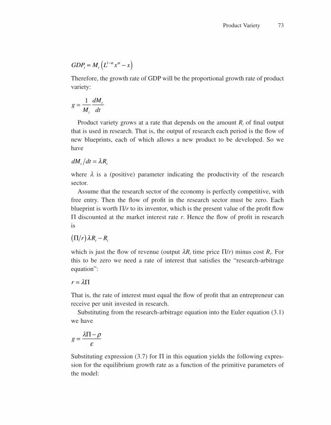
Product Variety 73
GDP M L x xt t= −( )−1 α α
Therefore, the growth rate of GDP will be the proportional growth rate of product variety:
gM
dM
dtt
t=1
Product variety grows at a rate that depends on the amount Ri of fi nal output that is used in research. That is, the output of research each period is the fl ow of new blueprints, each of which allows a new product to be developed. So we have
dM dt Rt t= λ
where l is a (positive) parameter indicating the productivity of the research sector.
Assume that the research sector of the economy is perfectly competitive, with free entry. Then the fl ow of profi t in the research sector must be zero. Each blueprint is worth Π/r to its inventor, which is the present value of the profi t fl ow Π discounted at the market interest rate r. Hence the fl ow of profi t in research is
Π r R Rt i( ) −λ
which is just the fl ow of revenue (output lRt time price Π/r) minus cost Ri. For this to be zero we need a rate of interest that satisfi es the “research-arbitrage equation”:
r = λΠ
That is, the rate of interest must equal the fl ow of profi t that an entrepreneur can receive per unit invested in research.
Substituting from the research-arbitrage equation into the Euler equation (3.1) we have
g =−λ ρ
εΠ
Substituting expression (3.7) for Π in this equation yields the following expres-sion for the equilibrium growth rate as a function of the primitive parameters of the model:
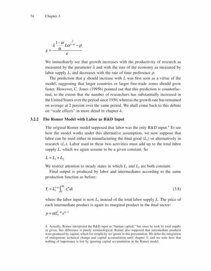
Chapter 374
gL
=
− −−λ αα
α ρ
ε
α1 2
1
We immediately see that growth increases with the productivity of research as measured by the parameter l and with the size of the economy as measured by labor supply L, and decreases with the rate of time preference r.
The prediction that g should increase with L was fi rst seen as a virtue of the model, suggesting that larger countries or larger free-trade zones should grow faster. However, C. Jones (1995b) pointed out that this prediction is counterfac-tual, to the extent that the number of researchers has substantially increased in the United States over the period since 1950, whereas the growth rate has remained on average at 2 percent over the same period. We shall come back to this debate on “scale effects” in more detail in chapter 4.
3.2.2 The Romer Model with Labor as R&D Input
The original Romer model supposed that labor was the only R&D input.4 To see how the model works under this alternative assumption, we now suppose that labor can be used either in manufacturing the fi nal good (L1) or alternatively in research (L2). Labor used in these two activities must add up to the total labor supply L, which we again assume to be a given constant. So
L L L= +1 2
We restrict attention to steady states in which L1 and L2 are both constant.Final output is produced by labor and intermediates according to the same
production function as before:
Y L x dit i
Mt= − ∫11
0
α α (3.8)
where the labor input is now L1 instead of the total labor supply L. The price of each intermediate product is again its marginal product in the fi nal sector:
p L x= − −α α α11 1
4. Actually, Romer interpreted the R&D input as “human capital,” but since he took its total supply as given, this difference is purely terminological. Romer also supposed that intermediate products were produced by capital, which for simplicity we ignore in this presentation. We defer the integration of endogenous technical change and capital accumulation until chapter 5, and we note here that nothing of importance is lost by ignoring capital accumulation in the Romer model.
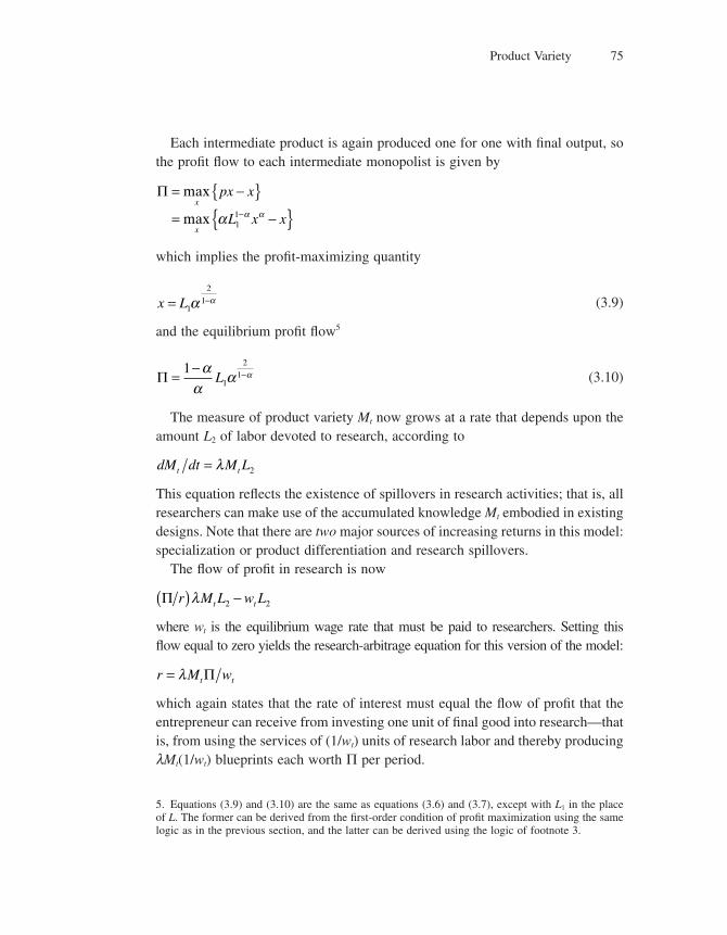
Product Variety 75
Each intermediate product is again produced one for one with fi nal output, so the profi t fl ow to each intermediate monopolist is given by
Π = −{ }= −{ }−
max
maxx
x
px x
L x xα α α11
which implies the profi t-maximizing quantity
x L= −1
2
1α α (3.9)
and the equilibrium profi t fl ow5
Π =− −1
1
2
1α
αα αL (3.10)
The measure of product variety Mt now grows at a rate that depends upon the amount L2 of labor devoted to research, according to
dM dt M Lt t= λ 2
This equation refl ects the existence of spillovers in research activities; that is, all researchers can make use of the accumulated knowledge Mt embodied in existing designs. Note that there are two major sources of increasing returns in this model: specialization or product differentiation and research spillovers.
The fl ow of profi t in research is now
Π r M L w Lt t( ) −λ 2 2
where wt is the equilibrium wage rate that must be paid to researchers. Setting this fl ow equal to zero yields the research-arbitrage equation for this version of the model:
r M wt t= λ Π
which again states that the rate of interest must equal the fl ow of profi t that the entrepreneur can receive from investing one unit of fi nal good into research—that is, from using the services of (1/wt) units of research labor and thereby producing lMt(1/wt) blueprints each worth Π per period.
5. Equations (3.9) and (3.10) are the same as equations (3.6) and (3.7), except with L1 in the place of L. The former can be derived from the fi rst-order condition of profi t maximization using the same logic as in the previous section, and the latter can be derived using the logic of footnote 3.
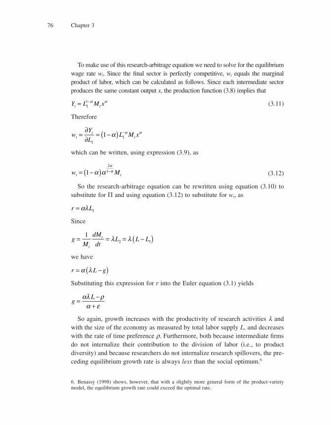
Chapter 376
To make use of this research-arbitrage equation we need to solve for the equilibrium wage rate wt. Since the fi nal sector is perfectly competitive, wt equals the marginal product of labor, which can be calculated as follows. Since each intermediate sector produces the same constant output x, the production function (3.8) implies that
Y L M xt t= −11 α α (3.11)
Therefore
wY
LL M xt
tt=
∂∂
= −( ) −
111 α α α
which can be written, using expression (3.9), as
w Mt t= −( ) −12
1α ααα (3.12)
So the research-arbitrage equation can be rewritten using equation (3.10) to substitute for Π and using equation (3.12) to substitute for wt, as
r L= αλ 1
Since
gM
dM
dtL L L
t
t= = = −( )12 1λ λ
we have
r L g= −( )α λ
Substituting this expression for r into the Euler equation (3.1) yields
gL
=−
+αλ ρ
α ε
So again, growth increases with the productivity of research activities l and with the size of the economy as measured by total labor supply L, and decreases with the rate of time preference r. Furthermore, both because intermediate fi rms do not internalize their contribution to the division of labor (i.e., to product diversity) and because researchers do not internalize research spillovers, the pre-ceding equilibrium growth rate is always less than the social optimum.6
6. Benassy (1998) shows, however, that with a slightly more general form of the product-variety model, the equilibrium growth rate could exceed the optimal rate.
Product Variety 77
3.3 From Theory to Evidence
3.3.1 Estimating the Effect of Variety on Productivity
A recent paper by Broda, Greenfi eld, and Weinstein (2006), henceforth BGW, exploits trade data to test for the effects of product variety on productivity levels and growth. If we believe in the mechanism described previously, trade should raise productivity because producers gain access to new imported varieties of inputs (the level effect); moreover, trade and the resulting increase in input variety should reduce the cost of innovation and thus result in more variety creation in the future (the growth effect). Also, the impact of increased product variety on productivity should depend upon the elasticity of substitution among different varieties of a good, and/or upon shifts in expenditures shares among new, remain-ing, and disappearing goods. In particular, increasing the number of varieties should not have much of an effect on productivity if new varieties are close sub-stitutes for existing varieties or if the share of new varieties is small relative to existing ones.
BGW analyze bilateral trade fl ows between 73 countries over the period 1994–2003. Using import data in the six-digit Harmonized System (HS) product catego-ries, they compute elasticities of substitution and supply for about 200 import sectors in each country. They consider the production function
Y A L xt t t it
Mt= ( ) ( )− ∑1
1
α υα υ
where a ∈ (0, 1) is one minus the share of labor in output and u ∈ (0, 1) measures the elasticity of substitution between varieties of input goods xit, with a higher u corresponding to more substitutable inputs.
If we focus on equilibria where all input goods are used with the same intensity xt, the preceding equation becomes
Y A L M xt t t t t= ( ) −1 α α υ α
If each input is produced one for one with capital, then
Y A L M Kt t t t t= ( ) − −( )1 1α υ α υ α
where Kt = Mt xt is the aggregate capital stock. Taking logs, we obtain
ln ln ln ln lnY A L K Mt t t t t= −( ) +( ) + + −( )1 1α α υ α υ
Differentiating both sides with respect to time, we obtain
Chapter 378
� � �Y
Y
L
L
K
KBt
t
t
t
t
tt= −( ) + +1 α α ˆ
where
BA
A
M
Mtt
t
t
t
= −( ) + −( )1 1α υ α υ� �
is total factor productivity (TFP) growth, also known as the Solow residual.7 This measure of TFP growth has two components: a product-variety component captured by the term in �Mt
/Mt and a quality component embodied in the term in �At
/At. BGW are primarily interested in the contribution of variety to total pro-ductivity growth.
According to the preceding equation, a lower u (that is, a lower degree of substitutability between inputs) or a higher share of the intermediate goods a should result in a higher impact of increased variety on TFP.
BGW estimate elasticities separately for each good and importing country and then regress per capita GDP on these elasticities. They fi nd no strong relationship between income per capita and the elasticity of substitution across countries. The typical (median) country experienced a net increase in varieties of 7.1 percent over 10 years in the typical (median) sector, which is about 0.7 percent per year. BGW then show that the growth in new varieties over the period 1994–2003 increased productivity by 0.13 percent per year for the typical country in the sample.
The relationship between variety and productivity is even lower for developed countries: “Most of the productivity growth in many of the largest countries cannot be accounted for by new imports” (BGW, 21). In particular the United States has the second-smallest gain among developed countries from imported variety. BGW summarize their fi ndings as follows:
The median developed country’s productivity growth was about 2 percent per year, but the median contribution of imported variety growth to productivity was only 0.1 percent per year, suggesting that for the typical developed country, new imported varieties are only a small part of the story behind their productivity growth. The impact of new varieties on developing countries is substantially higher. The typical developing country saw its productivity rise by 0.13 to 0.17 percent per year (depending on the sample) due to new imported varieties. (BGW, 22)
7. TFP and the Solow residual will be explained in more detail in chapter 5.
Product Variety 79
One might argue that BGW underestimate the effects of variety in more devel-oped countries. In particular, their approach does not take into account inputs that are not imported, and these are likely to be more numerous in developed coun-tries. Nevertheless, the effects of variety on productivity and on productivity growth appear to be relatively small, even in less developed economics.
3.3.2 The Importance of Exit in the Growth Process
An important limitation of the product-variety model is that it assumes away obsolescence of old intermediate inputs. Indeed, if old intermediate inputs were to disappear over time, the variety term in the preceding Solow residual would go down, and thus so would the economy’s per capita GDP.
In ongoing work with Pol Antras and Susanne Prantl, we have combined UK establishment-level panel data with the input-output table to estimate the effect on TFP growth arising from growth in high-quality input in upstream industries, and also from exit of obsolete input-producing fi rms in upstream industries. Specifi cally, we take a panel of 23,886 annual observations on more than 5,000 plants in 180 four-digit industries between 1987 and 1993, together with the 1984 UK input-output table, to estimate an equation of the form
g Z r uijt jt jt ijt i j t ijt= + + + + + + +− − −β β β β0 1 1 2 1 3 1Entry Exit Est Ind Y
where gijt is the productivity growth rate of fi rm i in industry j. The fi rst regressor Entryjt−1 is the entry measure, calculated as the increase in the fraction of input to the production of good j which is provided by foreign fi rms (foreign fi rms are more likely to account for entry that takes place at frontier technological level). The second regressor Exitjt−1 is our measure of exit of obsolete upstream input-producing fi rms: we use the fraction of employment accounted for by upstream exiting fi rms, thereby putting more weight on large exiting fi rms than on small ones. Establishment (Esti), industry (Indj), and year (Yrt) effects are included, along with the other controls in Zijt−1 including a measure of the plant’s market share.
The result of this estimation is a signifi cant positive effect of both upstream quality improvement and upstream input-production exit. These results are robust to taking potential endogeneity into account by applying an instrumental variable approach, using instruments similar to those of Aghion, Blundell, and colleagues (2006). The effects are particularly strong for plants that use more intermediate inputs—that is, plants with a share of intermediate product use above the sample median. Altogether, the results we fi nd are consistent with the view that quality-improving innovation is an important source of growth. The results, however, are
Chapter 380
not consistent with the horizontal innovation model, in which there should be nothing special about the entry of foreign fi rms, and according to which the exit of upstream fi rms should if anything reduce growth by reducing the variety of inputs being used in the industry.
Comin and Mulani (2007) have produced additional evidence to the effect that exit as well as entry is important to the growth process. Using a sample of U.S. fi rms, they show that, according to two measures of turnover in industry leader-ship that they construct, turnover is positively related to earlier R&D. Again, this fi nding is evidence of a creative-destruction element in the innovation process that one would not expect to fi nd if the primary channel through which innovation affected economic growth was increasing product variety. Indeed, the product-variety theory has little to say at all about how productivity varies across fi rms in an industry, let alone how the productivity ranking would change over time.
In addition to these results, Fogel, Morck, and Yeung (2008) have produced evidence to the effect that innovation is linked to the turnover of dominant fi rms. Using data on large corporate sectors in 44 different countries over the 1975–96 period, they fi nd that economies whose top 1975 corporations declined more grow faster than other countries with the same initial per capita GDP, level of educa-tion, and capital stock. Again, this evidence of an association between growth and enterprise turnover has no counterpart in the horizontal-innovation theory.
In order to formalize the notion of (technical or product) obsolescence, one needs to move away from horizontal models of product development à la Dixit and Stiglitz (1977) into vertical models of quality improvements, as we will do in the next chapter.
3.4 Conclusion
In this chapter we have presented the product-variety model of endogenous growth. In this model, growth is driven by innovations that lead to the introduc-tion of new (input) varieties. Productivity growth is driven both by the increased specialization of labor that works with an increasing number of intermediate inputs and by the research spillovers whereby each new innovator benefi ts from the whole existing stock of innovations. Ideas are nonrival, which means they can be freely used by new innovators in their own research activities. And they are excludable in the sense that each new innovation is rewarded by monopoly rents. It is the prospect of these rents that motivates research activities aimed at discovering new varieties.
Product Variety 81
A limitation of this model is that it does not capture the role of exit or turnover in the growth process, which Schumpeter refers to as creative destruction. Indeed, exit is detrimental to growth in this model as it reduces input specialization. Yet recent empirical work points at a strong correlation between productivity growth and exit or turnover of fi rms and inputs. In the next chapter we present an alterna-tive model of endogenous technical change, where exit and creative destruction feature prominently.
3.5 Literature Notes
Romer (1987) developed a precursory model of growth with expanding variety, where growth is sustained in the long run by the fact that output is produced with an expanding set of inputs, which in turn prevents aggregate capital from running into decreasing returns. The improved division of labor over time is itself made possible by output growth, which makes it possible to pay the fi xed costs of pro-ducing an ever-expanding set of inputs. Romer used the framework of monopo-listic competition introduced by Dixit and Stiglitz (1977) and extended by Ethier (1982). Romer (1990) completes the description of the product-variety model by introducing an R&D sector that generates blueprints for new inputs as a result of voluntary profi t-motivated horizontal innovations. Technological change was thereby endogenized.
The framework has been extended in several directions, and we refer the reader to the excellent Handbook of Economic Growth chapter by Gancia and Zilibotti (Aghion and Durlauf 2005). Grossman and Helpman (1991a, chapter 3) present a didactic treatment of a framework with expansion of consumer products that enter the utility function (as in Spence 1976) instead of intermediate products entering the production function. Rivera-Batiz and Romer (1991) and Grossman and Helpman (1991b) have used the framework to analyze the effects of market integration on growth. More recently, the idea of directed technological change was integrated by Acemoglu and Zilibotti (2001) into a framework of growth with expanding variety, to analyze implications of the skill-technology comple-mentarity for the persistence of productivity differences across countries.
C. Jones (1995b) challenges the model for generating scale effects for which he could not fi nd any evidence based on U.S. time series (see chapter 4). In con-trast, Kremer (1993b) argued that the hypothesis of a positive relation between world per capita growth and world population (or the world aggregate output) might be correct over very long periods of time.

Chapter 382
Problems
1. What is the “engine” of growth in the product variety model? Explain. Compare it to the element driving endogenous growth in the AK framework. What does this comparison imply in terms of pro-growth policy design in both settings?
2. “Labor-or-intermediates” model
Consider a variant of the Romer model from section 3.2.2. Assume that labor is not used in fi nal good production, but is used as the unique input in the intermediate goods production. Assume the fi nal good production function is given by
Y x dit i t
Mt= ∫ ,α
0
Also, suppose that 1/Mt units of labor are required to produce one unit of any intermediate good. As in the model presented in the chapter, suppose dMt /dt = lMtL2, where L2 is labor allocated to R&D. Defi ne Lx ≡ L − L2 as the amount of labor allocated to production of intermediates.
a. What is the equilibrium level of intermediate good production?
b. What is the equilibrium price of a unit of any intermediate good?
c. Looking at a balanced-growth equilibrium in which wages and technology grow at the same rate, compute the maximal profi t for intermediate producers.
d. Write down the research arbitrage condition.
e. Compute the equilibrium growth rate of the economy.
3. *Economic integration and trade (based on Rivera-Batiz and Romer 1991 and Gancia and Zilibotti 2005)
Consider the Romer model with labor as the unique R&D input from section 3.2.2. We have
seen that the economy’s equilibrium growth rate of output was given by gL= −+
αλ ρα ε .
Now, suppose two identical countries with fi xed labor endowment L = L* (the star denotes the economy originally foreign).
a. If the two countries merge and become a unique economy, what will be its growth rate of output?
We will now look at what happens when, instead, trade is introduced between the two economies. Suppose that, before trade starts, M M0 0= ∗ (time zero denotes the moment trade starts). Suppose, in addition, that the two economies produce, before trade, disjoint subsets of intermediate goods (special-ization). When trade is introduced, each monopolist can therefore sell its product in two markets. Finally, assume that the production function of varieties depends only on the degree of domestic varieties.
b. Compute the equilibrium profi ts and wages after trade is introduced.
c. Write down the research arbitrage condition after trade is introduced. Compare it to the one in the closed economy case. Discuss the result.
d. Now, assume M M0 0< ∗ . Suppose that trade is introduced and that exchange equalizes wages and interest rates across countries. What is the innovation fl ow in the home country?
e. Write down the research arbitrage condition for the foreign country. What will happen in the long run?
f. Can we talk about specialization of the two economies here? Discuss.
Product Variety 83
4. **Innovation, imitation, and product cycles (based on Helpman 1993 and Gancia and Zilibotti 2005)
Consider a two-region model of labor only used for intermediate goods production (as in
problem 2). The aggregate fi nal food production function is Y x dit i t
Mt= ∫ ,α
0, and intermediates are
manufactured with 1/Mt units of labor in both regions. Assume that R&D, producing new goods, is performed in the North only and that costless imitation takes place in the South at a constant rate i. Once a good is copied in the South, it is produced by competitive fi rms. Therefore, at every point in time, there is a range Mt
N of goods produced by monopolists in the North and a range MtS of goods
that have been copied and are produced in the South by competitive fi rms. The rate of introduction of new goods is g = (dMt/dt)Mt, and M M Mt t
NtS= + . Since imitation is instantaneous and occurs at
rate i, we have that dM dt M iMtS
tS
tN( ) = . Finally, assume, as in problem 3, that innovation requires
labor, that is, dMt/dt = lMtL2, where L2 is labor allocated to R&D in the North.
a. Show that in a steady state in which the ratio MtN/ Mt
S is constant the following condi-
tions must hold: M
M i
N
=+γ
γ and M
M
i
i
S
=+γ .
b. What is the price ( ptN) charged by Northern intermediate fi rms before imitation takes place? What
is the price ( ptS) charged by Southern fi rms producing imitated goods?
c. Show that the labor market-clearing condition for the North can be written as AtNx/At + g/l = L.
d. Using the fact that profi ts per product are a fraction (1 − a) of total revenue in the North
pNx, show that profi ts in the North can be written as π αα
γλ
N tN
tN
Nw
AL= − −⎛
⎝⎜⎞⎠⎟
1.
e. Write down the research arbitrage condition for innovators in the North. (Hint: Because there could be imitation, the effective discount rate for innovators is now r + m). Show that
it can be written as 1− −( ) + = +αα
λ γ γγ
Lm
r mN .
f. Suppose r > g. What is the impact of a reduction in m (e.g., as the result of a tightening of intel-lectual property rights) on the profi tability of innovation and on growth? What happens if r < g ? Give an intuition for the results. (Hint: Take a log linear approximation of the condition in item e.)
g. Using the condition found in item 4a and the one in item 4e, write down the effect of a reduction of m in the share of goods manufactured in the North.
5. *Social optimum in the Romer (1990) model
Consider the model from section 3.2.2. Now, instead of looking at the market equilibrium, we focus on the socially optimal allocation, from a social planner with one-period horizon. The
planner seeks to maximize GDP L x di xt i
M
i
Mt t= −− ∫ ∫11
0 0
α α .
a. Solve for the social planner’s allocation of intermediate input. Compare it to the market equilibrium level. Explain your results.
b. What is the social planner’s allocation of labor to R&D activities?
c. Compare the effi cient growth rate of the economy given by the social planner’s maximization problem to the market equilibrium growth rate. Interpret your fi ndings.

4 The Schumpeterian Model
4.1 Introduction
This chapter develops an alternative model of endogenous growth, in which growth is generated by a random sequence of quality-improving (or “vertical”) innovations. The model grew out of modern industrial organization theory,1 which portrays innovation as an important dimension of industrial competition. It is called Schumpeterian because it embodies the force that Schumpeter (1942) called “creative destruction”; that is, the innovations that drive growth by creating new technologies also destroy the results of previous innovations by making them obsolete.
Section 4.2 presents a simple one-sector Schumpeterian model, in which it is always the same product that is improved by innovation. This one-sector model contains the essential ideas of the Schumpeterian approach. For most empirical purposes, however, the one-sector model is too simple. Accordingly, section 4.3 develops a multisector Schumpeterian model, in which many different products are improved by innovation each year. Section 4.4 shows how allowing a mixture of horizontal and vertical innovations can shed new light on the “scale effect” discussed in the previous chapter.
4.2 A One-Sector Model
4.2.1 The Basics
There is a sequence of discrete time periods t = 1, 2, . . . In each period there is a fi xed number L of individuals, each of whom lives for just that period and is endowed with one unit of labor services, which she supplies inelastically. Her utility depends only on her consumption and she is risk-neutral, so she has the single objective of maximizing expected consumption.
People consume only one good, called the “fi nal” good, which is produced by perfectly competitive fi rms using two inputs—labor and a single intermediate product—according to the Cobb-Douglas production function2
Y A L xt t t= −( )1 α α (4.1)
1. See Tirole (1988).
2. By working through problem 2 of this chapter the reader can verify that nothing of substance is implied by the fact that At and L are raised to the same power in equation (4.1).

Chapter 486
where Yt is output of the fi nal good in period t, At is a parameter that refl ects the productivity of the intermediate input in that period, and xt is the amount of intermediate product used. The coeffi cient a lies between zero and one. The economy’s entire labor supply L is used in fi nal-good production. As in the neo-classical model, we refer to the product AtL as the economy’s effective labor supply.
The intermediate product is produced by a monopolist each period, using the fi nal good as all input, one for one. That is, for each unit of intermediate product, the monopolist must use one unit of fi nal good as input. Final output that is not used for intermediate production is available for consumption and research, and it constitutes the economy’s gross domestic product (GDP):3
GDP Y xt t t= − (4.2)
4.2.2 Production and Profi ts
Growth results from innovations that raise the productivity parameter At by improving the quality of the intermediate product. Before analyzing the process that generates innovations, this section describes what happens in each period once At has been determined, and shows that in equilibrium the intermediate monopolist’s profi t and the economy’s GDP are both proportional to the effective labor supply AtL.
The monopolist at t maximizes expected consumption by maximizing her profi t Πt, measured in units of the fi nal good:
Πt t t tp x x= −
where pt is the price of the intermediate product relative to the fi nal good. That is, her revenue is price times quantity ptxt, and her cost is her input of fi nal good, which must equal her output xt.
Recall that the equilibrium price of a factor of production used in a perfectly competitive industry equals the value of its marginal product. Thus the monopo-
3. Recall the national accounting identity:
GDP ≡ + + +Consumption Investment Government purchases Net exports
Our model economy has no foreign sector, no government spending, and no investment in physical or human capital. However, we do have investment in intellectual capital, in the form of research. So we have
GDP ≡ +Consumption Investment
Hence equation (4.2).
The Schumpeterian Model 87
list’s price will be the marginal product of her intermediate product in the fi nal sector, which according to the production function (4.1) is
p Y x A L xt t t t t= = − −∂ ∂ α α α( )1 1 (4.3)
Therefore, the monopolist chooses the quantity xt that maximizes
Πt t t tA L x x= −−α α α( )1 (4.4)
which implies an equilibrium quantity4
x A Lt t= −α α2
1 (4.5)
and an equilibrium profi t
Πt tA L= ≡ −( )+−π π α α
αα, 1
1
1 (4.6)
that are both proportional to the effective labor supply AtL.Substituting from equation (4.5) into the production function (4.1) and the GDP
equation (4.2), we see that fi nal output and the economy’s GDP will also be pro-portional to AtL:
Y A Lt t= −ααα
2
1
GDP A Lt t= −( )−α ααα
2
1 21 (4.7)
4.2.3 Innovation
In each period there is one person (the “entrepreneur”) who has an opportunity to attempt an innovation. If she succeeds, the innovation will create a new version of the intermediate product, which is more productive than previous versions. Specifi cally, the productivity of the intermediate good in use will go from last period’s value At−1 up to At = gAt−1, where g > 1. If she fails, then there will be
4. The fi rst-order condition for the maximization problem is
αα α2 1 1 1 0A L xt t( ) − =
− −
from which equation (4.5) follows directly. Substituting from equation (4.5) into equation (4.4) yields equation (4.6).
Chapter 488
no innovation at t and the intermediate product will be the same one that was used in t − 1, so At = At−1.
In order to innovate, the entrepreneur must conduct research, a costly activity that uses the fi nal good as its only input. As indicated earlier, research is uncer-tain, for it may fail to generate any innovation. But the more the entrepreneur spends on research, the more likely she is to innovate. Specifi cally, the probability mt that an innovation occurs in any period t depends positively on the amount Rt of fi nal good spent on research, according to the innovation function
μ φt t tR A= ( )/ *
where At∗ = gAt−1 is the productivity of the new intermediate product that will
result if the research succeeds. The reason why the probability of innovation depends inversely on At
∗ is that as technology advances it becomes more complex and thus harder to improve upon. So it is not the absolute amount of research expenditure Rt that matters for success but the productivity-adjusted expenditure Rt / At
∗, which we denote by nt.For concreteness, assume that the innovation function takes the Cobb-Douglas
form
φ λ σn n( ) = (4.8)
where l is a parameter that refl ects the productivity of the research sector and the elasticity s lies between zero and one. Thus the marginal product of (productivity-adjusted) research in generating innovations is positive but decreasing:
′( ) = > ′′( ) = −( ) <− −φ σλ φ σ σ λσ σn n n n1 20 1 0and
4.2.4 Research Arbitrage
If the entrepreneur at t successfully innovates, she will become the intermediate monopolist in that period, because she will be able to produce a better product than anyone else. Otherwise, the monopoly will pass to someone else chosen at random who is able to produce last period’s product.
Thus the reward to a successful innovator is the profi t Π t∗ that she will earn as
a result. Since she succeeds with probability f(nt), her expected reward is
φ nt t( )Π*
But the research will cost her Rt whether she succeeds or not; so her net benefi t from research is
The Schumpeterian Model 89
φ( )R A Rt t t t/ * *Π −
The entrepreneur will choose the research expenditure Rt that maximizes this net benefi t, which implies that Rt must satisfy the fi rst-order condition
′ − =φ ( )R A At t t t/ * */ *Π 1 0
which we can write, using equation (4.6), as the “research arbitrage” equation:
′( ) =φ πn Lt 1 (R)
The right-hand side of equation (R) is the marginal cost of research. The left-hand side is the marginal benefi t of research—the incremental probability of innovation times the value of a successful innovation. The marginal benefi t is decreasing in nt because the marginal product of the innovation function f is decreasing in nt. Any parameter change that raises the marginal benefi t schedule or lowers the marginal cost will increase the equilibrium research intensity nt.
The research arbitrage equation implies that the productivity-adjusted level of research nt will be a constant n, and hence the probability of innovation mt will also be a constant m = f(n). Under the Cobb-Douglas innovation function (4.8) we have
n L= ( ) −σλπ σ1
1
and5
μ λ σπσσ
σ= ( )− −
1
1 1L (4.9)
4.2.5 Growth
The rate of economic growth is the proportional growth rate of per capita GDP (GDPt/L), which according to equation (4.7) is also the proportional growth rate of the productivity parameter At:
gA A
Att t
t
=− −
−
1
1
5. We assume l and p are small enough that m < 1.
Chapter 490
It follows that growth will be random. In each period, with probability m the
entrepreneur will innovate, resulting in gA A
Att t
t
= − = −− −
−
γ γ1 1
1
1; and with
probability 1 − m she will fail, resulting in gA A
Att t
t
= − =− −
−
1 1
1
0. The growth
rate will be governed by this probability distribution every period, so by the law of large numbers the mean of the distribution
g E gt= ( ) = ⋅ −( )μ γ 1
will also be the economy’s long-run average growth rate.To interpret this formula, note that m is not just the probability of an innova-
tion each period but also the long-run frequency of innovations—that is, the fraction of periods in which an innovation will occur. Also, g − 1 is the pro-portional increase in productivity resulting from each innovation. Thus the formula expresses a simple but important result of Schumpeterian growth theory:
proposition 1 In the long run, the economy’s average growth rate equals the frequency of innovations times the size of innovations.
Using equation (4.9) to replace m in the preceding formula, we see that the average growth rate is
g L= ( ) −( )− −λ σπ γσσ
σ
1
1 1 1 (G)
4.2.6 A Variant with Nondrastic Innovations
Up to this point we have implicitly assumed that the intermediate monopolist can charge any price to the fi nal good producers without fearing entry by a potential competitor. In industrial organization theory this assumption is called the drastic innovation case (see Tirole, 1988).
Suppose, however, that there is a competitive fringe of fi rms able to produce a “knockoff” product that is perfectly substitutable for the monopolist’s interme-diate product but costs c > 1 units of fi nal output to produce. Then the incumbent monopolist cannot charge more than c in equilibrium, since otherwise the com-petitive fringe could profi tably undercut her price. Thus we have the limit-price constraint:
pt ≤ χ
The Schumpeterian Model 91
When c > 1/a, this limit price constraint is not binding because the price chosen by the monopolist in the absence of a competitive fringe is6 1/a. This is the drastic innovation case analyzed previously.
In this section we consider the nondrastic innovation case, where c < 1/a and hence the limit-price constraint is binding. Since the monopolist’s price is still the marginal product of the intermediate product, it must still obey equa-tion (4.3), so substituting pt = c into equation (4.3) yields the equilibrium quantity
x A Lt t= ( ) −α χ α1
1
The monopolist’s equilibrium profi t is thus
Πt t t t tp x x A L= − = = −( )( ) −π π χ α χ α, 11
1
where now the profi t parameter p is an increasing function7 of the competitive fringe’s cost c.
Other than this change, the economy functions just as in the drastic case. In particular, the research intensity n is still governed by the research arbitrage equation (R) and the average growth rate is still determined by equation (G), except that the parameter p in both of these equations is now an increasing func-tion of the competitive fringe’s cost parameter c.
4.2.7 Comparative Statics
According to the growth equation (G), our analysis yields the following comparative-statics implications for the average growth rate g:
1. Growth increases with the productivity of innovations l. This result points to the importance of education, and particularly higher education, as a growth-
6. Substituting from equation (4.5) into equation (4.3) yields p = 1/a.
7. That is,
d
d
d
d
χχ χ
χ χχ
χ
χ
α
α α
α
−( )⎛
⎝⎜⎜
⎞
⎠⎟⎟
= + −( ) ⎛
⎝⎜⎜
⎞
⎠⎟⎟
=
−
−−
−−
−−
1
1
11
11
11
11 11
11
1
− −−
⎛
⎝⎜
⎞
⎠⎟
−χα
which is greater than zero in the nondrastic case because c−1 > a.
Chapter 492
enhancing device. Countries that invest more in higher education will achieve a higher productivity of research, and will also reduce the opportunity cost of research by increasing the aggregate supply of skilled labor.
2. Growth increases with the size of innovations, as measured by the productivity improvement factor g. This result follows directly from Proposition 1, together with the result (4.9) that shows that the frequency of innovation is independent of g. The result in turn points to a feature that will become important when we discuss cross-country convergence. A country that lags behind the world technol-ogy frontier has what Gerschenkron (1962) called an advantage of backwardness. That is, the further it lags behind the frontier, the bigger the productivity improve-ment it will get if it can implement the frontier technology when it innovates, and hence the faster it can grow.
3. Growth increases with the degree of property-rights protection, as measured by c. That is, a higher c may refl ect stronger patent protection, which increases the cost of imitating the current technology in the intermediate sector. Thus it should lead to more intense research, as it raises the profi t that accrues to a suc-cessful innovator. This in turn should result in higher growth.
4. Growth decreases with the degree of product market competition. That is, a lower c may refl ect an increased ability of other fi rms to compete against the incumbent monopolist, which lowers the value of a successful innovation. This prediction is at odds with most recent empirical studies, starting with the work of Nickell (1996) and Blundell, Griffi th, and Van Reenen (1999). Chapter 12 will revisit the relationship between competition and growth.
5. An increase in the size of population should also bring about an increase in growth by raising the supply of labor L. This “scale effect” was also seen in the product-variety model of the previous chapter, and it has been challenged in the literature. In section 4.4 we will see how this questionable comparative-statics result can be eliminated by considering a model with both horizontal and vertical innovations.
4.3 A Multisector Model
4.3.1 Production and Profi t
In this section we allow for multiple innovating sectors in the economy. Suppose there is not one intermediate product but a continuum, indexed on the interval [0, 1]. The fi nal-good production function is now
The Schumpeterian Model 93
Y L A x dit it it= − −∫1 1
0
1α α α (4.10)
where each xit is the fl ow of intermediate product i used at t, and the productivity parameter Ait refl ects the quality of that product. In any period the productivity parameters will vary across intermediate products because of the randomness of the innovation process.
According to equation (4.10), the fi nal output produced by each intermediate product is determined by the production function
Y A L xit it it= ( ) −1 α α (4.11)
which is identical to the production function (4.1) of the one-sector model.
Each intermediate product has its own monopoly, and its price equals its mar-ginal product in the fi nal sector, which according to equation (4.11) is
p Y x A L xit it it it it= = ( ) − −∂ ∂ α α α1 1
Therefore, the monopolist in sector i chooses the quantity xit that maximizes her profi t:
Πit it it it it it itp x x A L x x= − = ( ) −−α α α1 (4.12)
which implies an equilibrium quantity:8
x A Lit it= −α α2
1 (4.13)
and an equilibrium profi t:
Πit itA L= π (4.14)
where the parameter p is the same as in the analogous equation (4.6) of the one-sector model.
The aggregate behavior of the economy depends on the aggregate productivity parameter
8. The fi rst-order condition for the maximization problem is
α α α2 1 1 1 0A L xit it( ) − =− −
from which equation (4.13) follows directly. Substituting from equation (4.13) into equation (4.12) yields equation (4.14).
Chapter 494
A A dit it= ∫0
1
which is just the unweighted numerical average of all the individual productivity parameters. In particular, fi nal output and GDP in this multisector economy are determined by exactly the same equations as in the one-sector economy of the previous section, but with At now being this average, instead of being the pro-ductivity parameter of the economy’s only intermediate product.
More specifi cally, using equation (4.13) to substitute for each xit in the produc-tion function (4.10) yields the same formula as before for fi nal output:
Y A Lt t= −ααα
2
1
As before, the economy’s GDP equals the output of fi nal good Yt minus the amount used up in producing each of the intermediate products. Since each inter-mediate product is produced one for one using fi nal output,
GDP Y x dit t it= − ∫0
1
Using equation (4.13) to substitute for each xit in this integral and combining it with the preceding formula for Yt yields
GDP A Lt t= −( )−α ααα
2
1 21
which is identical to equation (4.7). So again the economy’s GDP is proportional to its effective labor supply At L.
4.3.2 Innovation and Research Arbitrage
Innovation in each sector takes place exactly as in the one-sector model. Specifi -cally, there is a single entrepreneur in each sector who spends fi nal output in research and innovates with probability f(nit) = λ σnit, where now nit is the research expenditure in sector i relative to the target productivity in sector i:
n R Ait it it= / *
where Ait* = gAi,t−1 is the productivity parameter if she succeeds.The entrepreneur chooses the research expenditure Rit that maximizes her net
benefi t:
φ( )R A Rit it it it/ * *Π −
The Schumpeterian Model 95
where Πit* is her profi t if she succeeds. Therefore Rit must satisfy the fi rst-order condition
′ − =φ ( )R A Ait t t t/ * */ *Π 1 0
which we can write, using equation (4.14), as the research arbitrage equation
′( ) =φ πn Lit 1 (R)
This is exactly the same as the research arbitrage equation in the one-sector model, so it solves for the same constant productivity-adjusted research and fre-quency of innovation:
n L L= ( ) = ( )− − −σλπ μ λ σπσ σσ
σ1
1
1
1 1and
One important feature of this model is that the probability of innovation m is the same in all sectors, no matter what the starting level of productivity Ai,t−1. This might seem surprising, because the reward Πit* = pgAi,t−1L to a successful innova-tion is higher in more advanced sectors. But this advantage is just offset by the fact that the cost of innovating at any given rate is also correspondingly higher because what matters is research expenditure relative to the target productivity level gAi,t−1. As we will see, this feature allows a simple characterization of the aggregate growth rate in the economy.
4.3.3 Growth
Since per capita GDP is again proportional to the aggregate productivity param-eter At, therefore the economy’s growth rate is again the proportional growth rate of At:
gA A
Att t
t
=− −
−
1
1
(4.15)
In this case, however, the aggregate growth rate is no longer random, because bad luck in some sectors will be offset by good luck in others.
In each sector i we have
AA
Aiti t
i t
=−
⎧⎨⎩
⎫⎬⎭
−
−
γ μμ
,
,
1
1 1
with probability
with probability (4.16)
By the law of large numbers we know that the fraction of sectors that innovate each period will be m. Therefore, the economy-wide average At can be expressed
Chapter 496
as m times the average Ait among sectors that innovated at t plus (1 − m) times the average among sectors that did not:
A A At t t= + −( )μ μ1 21
Now the average A2t among sectors that did not innovate at t is just last period’s economy-wide average At−1, because these sectors are drawn at random from the economy and each of them has the same productivity parameter as last period. By the same logic, the average A1t among sectors that did innovate is just g times the average of these same fi rms’ productivity parameters last period—that is, gAt−1. So we have
A A At t t= + −( )− −μγ μ1 11
It follows from this and equation (4.15) that the growth rate each period will equal the constant
g = ⋅ −( )μ γ 1
which is the same as the long-run average growth rate of the one-sector model. Substituting equation (4.9) into this formula produces the same expression (G) as before, implying the same comparative-statics results as before.
4.4 Scale Effects*
Both the innovation-based growth theories we have seen so far, the product-variety model with just horizontal innovations and the Schumpeterian model with just vertical innovations, predict that increased population leads to increased growth. This prediction is implied because increased population raises the size of the market that can be captured by a successful entrepreneur and also because it raises the supply of potential researchers.
This prediction has been challenged, however, on empirical grounds. In par-ticular, C. Jones (1995b) has pointed out that the number of scientists and engi-neers engaged in R&D has grown almost ninefold since 1953 with no signifi cant trend increase in productivity growth. The present section shows how the coun-terfactual scale effect can be eliminated from the theory by allowing for both horizontal and vertical innovations.
The way to deal with this problem in Schumpeterian theory is to incorporate A. Young’s (1998) insight that as population grows, proliferation of product
* The analysis in this section is rather terse, and can be skipped on fi rst reading.
The Schumpeterian Model 97
varieties reduces the effectiveness of research aimed at quality improvement by causing it to be spread more thinly over a larger number of different sectors, thus dissipating the effect on the overall rate of productivity growth.
So the fi rst thing we need to do is assume a fi nal-good production function that allows for a variable number of intermediate products:
Y L M A x dit it it
M= ( ) − −∫1 1
0
α α α (4.17)
which is the same production function (4.10) as before except that now the inter-mediate products are indexed over the interval [0, M] instead of [0, 1]. Thus M is our measure of product variety.
This production function is the same as the one assumed in the product-variety model of the previous chapter, except that (1) each product has its own unique pro-ductivity parameter Ait instead of having Ait = 1 for all products, and (2) we assume that what matters is not the absolute input L of labor but the input per product L/M. Thus the contribution of each intermediate product to fi nal output is now
Y A x L Mit it it= ( )− −1 1α α α
which indicates that as the number of intermediate products goes up, there will be less labor to work with each one, so each will contribute less to fi nal output unless the quality Ait or the quantity xit is increased.9
The next thing we have to do is model the process by which product variety increases. The simplest scheme is to suppose that each person has a probability y of inventing a new intermediate product, with no expenditure at all on research. Suppose also that the exogenous fraction e of products disappears each year. If population is constant, then each year the length Mt of the list of intermediate products will change by the amount
ψ εL Mt−
and will eventually stabilize10 at a steady-state value
9. The production function is a special case of the one that Benassy (1998) showed does not neces-sarily yield a positive productivity effect of product variety.
10. That is, the difference equation
M M L Mt t t+ = + −1 ψ ε
starting at M0 has the unique solution
M L M Lt
t= ( ) + −( ) − ( )⎡⎣ ⎤⎦ψ ε ε ψ ε1 0
which converges to (y/e)L as t → ∞ because (1 − e) is between zero and one.

Chapter 498
M L= ( )ψ ε
which is proportional to population. So if population were to increase perma-nently, the number of products would eventually grow in proportion.
Thus in the long run the fi nal-good production function will be
Y A x dit it it
M= ( ) − −∫ε ψ α α α1 1
0
and the contribution of each intermediate product to fi nal output will be
Y A xit it it= ( ) − −ε ψ α α α1 1
which does not depend at all on the size of the economy.Proceeding as before we see that the price of each intermediate product will
be its marginal product in the fi nal sector:
p Y x A xit it it it it= = ( ) − − −∂ ∂ α ε ψ α α α1 1 1 (4.18)
Therefore, the monopolist in sector i chooses the quantity xit that maximizes her profi t
Πit it it it it it itp x x A x x= − = ( ) −− −α ε ψ α α α1 1
which implies an equilibrium quantity
x Ait it= ( )−α ε ψα2
1
and an equilibrium profi t
Πit itA= ( )π ε ψ
where the parameter p is the same as in the analogous equation (4.6) of the one-sector model.
According to these equations, both the monopolist’s equilibrium quantity and equilibrium profi t are independent of the scale of the economy as measured by population L, because her demand function (4.18) is independent of L. As a result, the net benefi t to research will be independent of scale, and so will the equilibrium intensity of research, the frequency of innovation, and the economy’s growth rate. More specifi cally, the net benefi t will be
φ φ π ε ψn R n n Ait it it it it it( ) − = ( ) ( ) −⎡⎣ ⎤⎦Π* *
which is maximized by nit satisfying the research arbitrage equation
The Schumpeterian Model 99
′( ) ( ) =φ π ε ψnit 1
which can be solved for a constant n that depends positively on the equilibrium amount of labor per product (e/y) but is independent of scale. Therefore, the frequency of innovation m = f(n) and the growth rate g = m ⋅ (g − 1) are also independent of scale.
4.5 Conclusion
It may be useful to contrast again the Schumpeterian growth paradigm to the two alternative models of endogenous growth analyzed previously. The fi rst was the AK model of chapter 2, according to which knowledge accumulation is a seren-dipitous by-product of capital accumulation. Here thrift and capital accumulation were the keys to growth, not creativity and innovation. The second endogenous growth model was the product-variety model of chapter 3, in which innovation causes productivity growth by creating new, but not necessarily improved, varieties of products.
Compared to the AK model, both the Schumpeterian model and the product-variety model have the advantage of presenting an explicit analysis of the innova-tion process underlying long-run growth. Compared to the product-variety model, the Schumpeterian model assigns an important role to exit and turnover of fi rms and workers, which, as we argued at the end of the previous chapter, is consistent with an increasing number of recent studies demonstrating that labor and product market mobility are key elements of a growth-enhancing policy near the techno-logical frontier.11
This is not to say that the Schumpeterian model is free of problems. We have already discussed the problem of the scale effect of increased population on growth, but we have also argued that this diffi culty can be resolved within the Schumpeterian paradigm. Another diffi culty with the model as presented so far is the absence of capital, which growth-accounting exercises (Jorgenson 1995; A. Young 1995) have shown to be quite important. Chapter 5 will show how to
11. As we will see in subsequent chapters, the Schumpeterian model also has the advantage of allow-ing for entrepreneurs to make the choice between implementation and frontier innovation, and for this choice to vary with distance to the frontier, something that does not fi t easily into the product-variety model. This allows the Schumpeterian model to generate context-specifi c policy implications and comparative-statics predictions, dependent particularly on a country’s distance to the frontier.
Chapter 4100
introduce capital into the analysis in such a way as to make it consistent with these exercises. Another problem with the theory is the assumption of perfect fi nancial markets; in reality, R&D fi rms rely very much on capital markets, which seem to work much better in some countries than in others. The issue of fi nancial constraints will be dealt with in chapter 6. Another issue is convergence, which we examine in chapter 7, where we will show that the model implies a form of club-convergence consistent with the evidence of Durlauf and Johnson (1995) and Quah (1993, 1997); the key is that in Schumpeterian theory convergence occurs through productivity, by means of a process of technology transfer, as well as through capital accumulation. Finally, as indicated previously, the impli-cation of the fi rst-generation of Schumpeterian models to the effect that more product market competition is harmful to growth runs counter to much evidence. We address this issue in chapter 12, where we will show that various other effects can be found in more sophisticated versions of the theory, which imply a more complicated relationship between competition and growth, one that fi nds con-siderable support in the data.
4.6 Literature Notes
The earliest attempts at providing a Schumpeterian approach to endogenous growth theory were by Segerstrom, Anant, and Dinopoulos (1990), who modeled sustained growth as arising from a succession of product improvements in a fi xed number of sectors, but with no uncertainty in the innovation process, and Corriveau (1991), who produced a discrete-time model with uncertainty about cost-reducing process innovations. What we present here is a simplifi ed version of the model we laid out in Aghion and Howitt (1988, 1992), using modeling techniques from industrial organization theory (Tirole 1988, chap. 10, and Reinganum 1989). Grossman and Helpman (1991a, 1991b) built on this frame-work to analyze the relationship between trade and growth, and between growth and the product cycle.
On the scale-effect debate, C. Jones (1995b) has developed a “semiendoge-nous” model in which the scale effect is dissipated by the diminishing returns to ideas in research, with the implication that population growth is the only long-run determinant of economic growth. The approach was further developed by Kortum (1997) and Segerstrom (1998). Our alternative “fully endogenous” approach was developed by several Schumpeterian endogenous models without scale effects; in particular, see Howitt (1999), Aghion and Howitt (1998a, chap. 12),
The Schumpeterian Model 101
Dinopoulos and Thompson (1998), and Peretto (1998). See also the recent con-tribution of Dinopoulos and Syropoulos (2006) which argues that efforts to build increasing barriers to entry are what dissipate the scale effect. Segerstrom (2000) and C. Jones (2005) point out that small changes in the assumptions of the fully endogenous model can result in drastic changes in its conclusions with respect to scale effects. However, Ha and Howitt (2006) use U.S. data to compare the two main varieties of R&D-based growth models without scale effects, and con-clude that the Schumpeterian model without scale effects is more consistent with the long-run trends in R&D and TFP than semiendogenous growth theory. Other texts, such as Laincz and Peretto (2004) and Ulku (2005), point in the same direction, using U.S. data as well.
Problems
1. Both the product-variety and the Schumpeterian models predict scale effects, namely, that a larger population (a larger population of researchers) would predict faster growth. How would you empiri-cally test this prediction?
2. A variant of the basic Schumpeterian model
Consider the basic one-sector model from section 4.2. The difference here is simply that fi nal-good production is given by Y A L xt t t= −ψ α α1 , where 0 < y ≤ 1. Write down intermediate-good monopolists’ profi ts, the research arbitrage condition, and the growth rate of ouput in the economy.
3. Welfare analysis in the basic Schumpeterian model
Consider again the model from section 4.2. Now, instead of looking at the market equilibrium, we focus on the socially optimal allocation, from a social planner with one-period horizon. The planner seeks to maximize GDPt = (AL)1−axa − x.
a. Solve for the social planner’s allocation of intermediate input. Compare it to the market equilibrium value. Explain your results.
b. What is the social planner’s adjusted level of innovation expenditures n?
c. Compare the effi cient growth rate of the economy given by the social planner’s maximization problem to the market equilibrium growth rate. Explain why it could be greater and why it could be lower than the market equilibrium one.
d. Compare your results to the ones in problem 5 from chapter 3.
4. Semiendogenous growth and scale effects (based on Jones, 1995b)
Consider a generalized Romer (1990) model from chapter 3 with the following innovation technology: �A = dL2Af, where f < 1 and L2 is the amount of labor devoted to R&D activities. Assume that total
labor increases at rate n and �L/L = n, and defi ne g ≡ �A /A.
a. Explain why in balanced-growth path (BGP), L2 = lL, where l ∈ (0,1) is a constant.
b. Looking at the steady state, where �g/g = 0, compute g.
c. Is there still some type of scale effect in this model? How would you test the predictions of this model in the data?
Chapter 4102
5. The continuous-time version of the Schumpeterian model, I
The next two problems will guide the reader through the continuous-time version of the Schumpete-rian model.
Assume individuals have linear intertemporal preferences: u y y e dr( ) = −∞
∫ ττ τ
0, where r is the
rate of time preference, also equal to the interest rate. There are L individuals in the economy, and each individual is endowed with one unit fl ow of labor, so L is also equal to the aggregate fl ow of labor supply.
Output of the consumption good is produced at any time using an intermediate good according to
y Ax= α
where 0 < a < 1 and x denotes the fl ow of intermediate good used in fi nal good production.
Innovations consist of the invention of a new variety of intermediate good that replaces the old one, and whose use raises the technology parameter A by the constant factor g > 1.
The economy’s fi xed stock of labor L has two competing uses. It can produce the intermediate good one for one, and it can be used in research.
a. Assuming labor-market clearing at any period, write the labor-market clearing condition that must hold at each period, with x representing the amount of labor used in manufacturing and n the amount ol labor used in research.
When the amount n is used in research, innovations arrive randomly with a Poisson arrival rate ln, where l > 0 is a parameter indicating the productivity of the research technology. The fi rm that succeeds in innovating can monopolize the intermediate sector until replaced by the next innovator.
Also, output, profi ts, and wages are all multiplied by g each time a new innovation occurs.
b. Derive and explain why the amount of labor devoted to research is determined by the following arbitrage condition (where wt is the wage rate before innovation t + 1 and Vt+1 is the value of innova-tion t + 1):
w Vt t= +λ 1
This arbitrage equation governs the dynamics of the economy over its successive innovations. Together with the labor-market equation, it constitutes the backbone of the model.
The value Vt+1 is determined by the following asset equation:
rV n Vt t t t+ + + += −1 1 1 1π λ
c. Interpret the different terms of the preceding asset equation.
6. The continuous-time version of the Schumpeterian model, II
In this problem, the reader will derive the equilibrium level of R&D and the steady-state growth rate in the continuous-time Schumpeterian model.
a. Using the intermediate good producers optimization problem to choose x, show that equilibrium profi ts for intermediate good producers are

The Schumpeterian Model 103
π ααt tw x= −1
b. Using the labor market-clearing condition and your result from the previous item, show that the research arbitrage condition can be rewritten as
1
1
=
− −( )+
λγ α
αλ
L n
r n
This allows us to write the steady-state equilibrium R&D, n, as a function of the parameters of the economy.
In a steady state, the fl ow of consumption good (or fi nal output) produced during the time-interval between the tth and the (t + 1)st innovation is
y A x A L nt t t= = −( )ˆ ˆα α
Also,
y yt t+ =1 γ
c. Take the log of yt. By how much is this value increased every time an innovation occurs?
d. Show that the average growth rate of the economy in steady state is g = l n ln g . (Hint: Take a unit-time interval, say between t and t + 1, and note that ln y (t + 1) = ln y (t ) + (ln g ) e (t ), where e (t) is the number of innovations between t and t + 1. Use the properties of the Poisson distribution to compute E[ln y(t + 1) − ln y(t)]).
e. What are the effects on the growth rate of the economy and on n of (i) an increase in the size of the labor market L; (ii) a reduction of the interest rate r; (iii) a decrease in the degree of market com-petition a; (iv) an increase in the size of innovation g and/or in the productivity of R&D l?

5 Capital, Innovation, and Growth Accounting
5.1 Introduction
Neoclassical theory and AK theory focus on capital accumulation, whereas the product-variety and Schumpeterian theories focus on innovations that raise pro-ductivity. One way to judge the competing theories is to ask how much of growth is attributable to the accumulation of physical and human capital, and how much is the result of productivity growth. The question can be studied using growth accounting, a method fi rst invented by Solow (1957). This chapter shows how growth accounting works.
Economists who have conducted growth accounting exercises in many econo-mies (for example, Jorgenson 1995) have concluded that a lot of economic growth is accounted for by capital accumulation. These fi ndings raise a number of issues that we also deal with in this chapter. For one thing, the results of growth account-ing are very sensitive to the way capital is measured. We will discuss some cases in which there is reason to believe that capital is systematically mismeasured. One of these cases concerns the claim by Alwyn Young (1995) that most of the extraordinary growth performance of Singapore, Hong Kong, Taiwan, and South Korea can be explained by factor accumulation, not technological progress. Hsieh (2002) argues that these results are no longer true once one corrects for the over-estimates of capital accumulation in the data.
Another issue raised by growth accounting has to do with the difference between accounting relationships and causal relationships. We will show in this chapter that even though there is evidence that somewhere between 30 and 70 percent of the growth of output per worker in OECD countries can be “accounted for” by capital accumulation, nevertheless these results are consistent with the neoclassical model which implies that in the long run all the growth in output per worker is caused by technological progress.
In this chapter we also show how capital can be introduced into the Schumpe-terian model that we are using as a main workhorse model throughout the book. The result is a hybrid model in which capital accumulation takes place as in the neoclassical model but productivity growth arises endogenously as in the Schumpeterian model. The hybrid model is consistent with the empirical evi-dence on growth accounting, as is the neoclassical model. But the causal explana-tion that it provides for economic growth is quite different from that of the neoclassical model.
Chapter 5106
5.2 Measuring the Growth of Total Factor Productivity
When people mention productivity, often what they are referring to is labor productivity, which is output per worker: y = Y/L. But this particular measure of productivity confounds the effects of capital accumulation and technological progress, both of which can raise output per worker. To see this point, suppose that output depends on capital and labor according to the familiar Cobb-Douglas production function:
Y BK L= −α α1 (5.1)
where the parameter B refl ects the state of technology. Dividing both sides by L, we see that output per worker equals
y Bk= α (5.2)
where k = K/L is the capital stock per worker. According to equation (5.2), labor productivity y depends positively on the technology parameter B but also on the capital stock per worker k.
A better measure of productivity is the parameter B. This parameter tells us not just how productive labor is, but also how productively the economy uses all the factors of production. For this reason, B is called total factor productivity, or just TFP.
Our measure of economic growth is the growth rate G of output per person. Under the simplifying assumption that the population and labor force grow at the same rate, G is also the growth rate of output per worker. So from equation (5.2) we can express the growth rate as1
G B B k k= +� �α (5.3)
According to equation (5.3), the growth rate is the sum of two components: the rate of TFP growth (B
./B) and the “capital-deepening” component (ak
./k). The fi rst
one measures the direct effect of technological progress, and the second measures
1. Taking natural logs of both sides of equation (5.2) we get
ln ln lny B k= + α
Differentiating both sides with respect to time we get
� � �y y B B k k= + α
which is the same as equation (5.3) because G = y./y by defi nition.
Capital, Innovation, and Growth Accounting 107
the effect of capital accumulation. The purpose of growth accounting is to deter-mine the relative size of these two components.
If all the variables in equation (5.3) could be observed directly, then growth accounting would be very simple. However, this is not the case. For almost all countries we have time-series data on output, capital, and labor, which allow us to observe G and k
./k, but there are no direct measures of B and a. Growth
accounting deals with this problem in two steps. The fi rst step is to estimate a using data on factor prices, and the second step is to estimate TFP growth (B
./B)
using a residual method. These two steps work as follows.First, we must make the assumption that the market for capital is perfectly
competitive. Under that assumption, the rental price of capital Rk should equal the marginal product of capital. Differentiating the right-hand side of equation (5.1) to compute the marginal product of capital, we then get2
R Y Kk = α
which we can rewrite as
α = R K Yk
That is, a equals the share of capital income (the price Rk times the quantity K) in national income (Y). This share can be computed from directly observed data once we observe the factor price Rk.
To conduct the second step of growth accounting we just rewrite the growth equation (5.3) as
� �B B G k k= − α
which says that the rate of TFP growth (B./B) is the residual left over after we
subtract the capital-deepening term from the observed growth rate G. Once we have estimated a using factor prices, we can measure everything on the right-hand side. This measure of TFP growth is known as the Solow residual.
5.2.1 Empirical Results
From the national accounts it appears that wage and salaries account for about 70 percent of national income in the United States. In other countries the number is roughly the same. So to a fi rst-order approximation the share of capital is about 0.3, and to get a rough estimate of TFP growth we can set a equal to 0.3. Using
2. That is, Rk = ∂Y/∂K = aBKa−1L1−a = aBKaL1−a/K = aY/K.
Chapter 5108
this value of a and measures of capital stocks constructed from the Penn World Tables (Heston et al. 2002), we can break down the average growth rate from 1960 to 2000 of all OECD countries. The results are shown3 in table 5.1. The fi rst column is the average growth rate G of output per worker over this 40-year period. The second column shows the corresponding TFP growth rate estimated over that period, and the third column is the other (capital-deepening) component of growth. The fourth and fi fth columns indicate the percentage of growth that is accounted for by TFP growth and capital deepening, respectively. As this table indicates, TFP growth accounts for about two-thirds of economic growth in OECD countries, while capital deepening accounts for one third.
Economists such as Jorgenson (1995) have conducted more detailed and disag-gregated growth-accounting exercises on a number of OECD countries, in which they estimate the contribution of human as well as physical capital. They tend to come up with a smaller contribution of TFP growth and a correspondingly larger contribution of capital deepening (both physical and human capital deepening) than indicated in table 5.1. In the United States, for example, over the period from 1948 to 1986, Jorgenson and Fraumeni (1992) estimate a TFP growth rate of 0.50 percent, which is about 30 percent of the average growth rate of output per hour of labor input instead of the roughly 58 percent reported for the United States in table 5.1.4
The main reason why these disaggregated estimates produce a smaller contri-bution of TFP growth than reported in table 5.1 is that the residual constructed in the disaggregated estimates comes from subtracting not only a physical-capital-deepening component but also a human-capital-deepening component. Since the middle of the 20th century, all OECD countries have experienced a large increase in the level of educational attainment of the average worker, that is, a large increase in human capital per person. When the contribution of this human capital deepening is also subtracted, we are clearly going to be left with a smaller residual than if we just subtract the contribution of physical capital deepening. But whichever way we compute TFP growth it seems that capital
3. We thank Professor Diego Comin of the Harvard Business School for his help in compiling the capital stock estimates underlying this table.
4. Their table 5 indicates that on average output grew at a 2.93 percent rate and that labor input (hours times quality) grew at a 2.20 percent rate. It also indicates that 58.1 percent of the contribution of labor input came from hours, implying an average growth rate in hours of (.581 ⋅ 2.20 =) 1.28 percent and an average growth rate in output per hour worked of (2.93 − 1.28 =) 1.65 percent. Their estimate of the residual was 0.50 percent, which is 30.3 percent of the growth rate of output per hour worked.
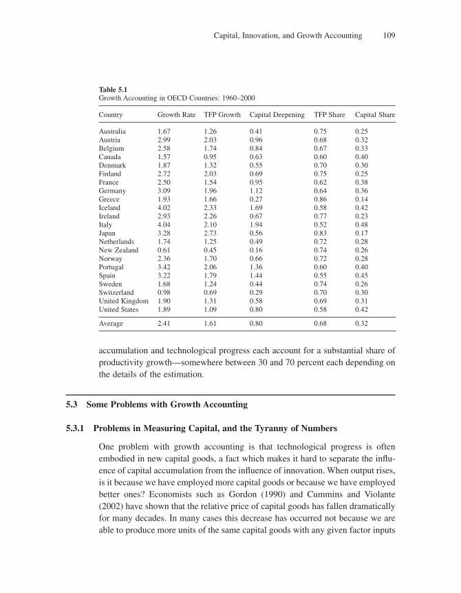
Capital, Innovation, and Growth Accounting 109
accumulation and technological progress each account for a substantial share of productivity growth—somewhere between 30 and 70 percent each depending on the details of the estimation.
5.3 Some Problems with Growth Accounting
5.3.1 Problems in Measuring Capital, and the Tyranny of Numbers
One problem with growth accounting is that technological progress is often embodied in new capital goods, a fact which makes it hard to separate the infl u-ence of capital accumulation from the infl uence of innovation. When output rises, is it because we have employed more capital goods or because we have employed better ones? Economists such as Gordon (1990) and Cummins and Violante (2002) have shown that the relative price of capital goods has fallen dramatically for many decades. In many cases this decrease has occurred not because we are able to produce more units of the same capital goods with any given factor inputs
Table 5.1Growth Accounting in OECD Countries: 1960–2000
Country Growth Rate TFP Growth Capital Deepening TFP Share Capital Share
Australia 1.67 1.26 0.41 0.75 0.25Austria 2.99 2.03 0.96 0.68 0.32Belgium 2.58 1.74 0.84 0.67 0.33Canada 1.57 0.95 0.63 0.60 0.40Denmark 1.87 1.32 0.55 0.70 0.30Finland 2.72 2.03 0.69 0.75 0.25France 2.50 1.54 0.95 0.62 0.38Germany 3.09 1.96 1.12 0.64 0.36Greece 1.93 1.66 0.27 0.86 0.14Iceland 4.02 2.33 1.69 0.58 0.42Ireland 2.93 2.26 0.67 0.77 0.23Italy 4.04 2.10 1.94 0.52 0.48Japan 3.28 2.73 0.56 0.83 0.17Netherlands 1.74 1.25 0.49 0.72 0.28New Zealand 0.61 0.45 0.16 0.74 0.26Norway 2.36 1.70 0.66 0.72 0.28Portugal 3.42 2.06 1.36 0.60 0.40Spain 3.22 1.79 1.44 0.55 0.45Sweden 1.68 1.24 0.44 0.74 0.26Switzerland 0.98 0.69 0.29 0.70 0.30United Kingdom 1.90 1.31 0.58 0.69 0.31United States 1.89 1.09 0.80 0.58 0.42
Average 2.41 1.61 0.80 0.68 0.32
Chapter 5110
but because we are able to produce a higher quality of capital goods than before, so that the price of a “quality-adjusted” unit of capital has fallen. For example, it costs about the same as 10 years ago to produce one laptop computer, but you get much more computer for that price than you did 10 years ago. But by how much has the real price fallen? That is a diffi cult question to answer, and national income accountants, having been trained to distrust subjective manipulation of the data, probably adjust too little to satisfy growth economists.
To some extent this problem affects not so much the aggregate productivity numbers as how that productivity is allocated across sectors. Griliches (1994) has argued, for example, that the aircraft industry, which conducts a lot of research and development (R&D), has exhibited relatively little TFP growth while the airline industry, which does almost no R&D, has exhibited a lot of TFP growth. If we were properly to adjust for the improved quality of modern aircraft, which fl y more safely and more quietly, using less fuel and causing less pollution than before, then we would see that the aircraft industry was more productive than the TFP numbers indicate. But at the same time we would see that productivity has not really grown so much in the airline industry, where we have been under-estimating the increase in their quality-adjusted input of aircraft. More generally, making the proper quality adjustment would raise our estimate of TFP growth in upstream industries but lower it in downstream industries. In aggregate, however, these two effects tend to wash out.
A bigger measurement problem for aggregate TFP occurs when a country’s national accounts systematically overestimate the increase in capital taking place each year. Pritchett (2000) argues that such overestimating happens in many countries because of government ineffi ciency and corruption. Funds are appropri-ated for the stated purpose of building public works, and the amount is recorded as having all been spent on investment in (public) physical capital. But in fact much of it gets diverted into the pockets of politicians, bureaucrats, and their friends instead of being spent on capital. Since we do not have reliable estimates of what fraction was really spent on capital and what fraction was diverted, we do not really know how much capital accumulation took place. We just know that it was less than reported. As a result it is hard to know what to make of TFP numbers in many countries, especially those with high corruption rates.
A similar problem is reported by Hsieh (2002), who has challenged Alwyn Young’s (1995) claim that the Eastern “Tigers” (Singapore, Hong Kong, Taiwan, and South Korea) accomplished most of their remarkable growth performance through capital accumulation and the improved effi ciency of resource allocation,
Capital, Innovation, and Growth Accounting 111
not through technological progress. Hsieh argues that this fi nding does not stand up when we take into account some serious overreporting of the growth in capital in these countries.
According to Young’s estimates, GDP per capita grew in Hong Kong by 5.7 percent a year over 1966–92. Over 1966–90, Singapore’s GDP per capita grew by 6.8 percent a year, South Korea’s also by 6.8 percent, and Taiwan’s by 6.7 percent. Growth in GDP per worker was between one and two percentage points less, refl ecting large increases in labor force participation, but even the per-worker growth rates are very high in comparison to other countries.
Young adjusts for changes in the size and mix of the labor force, including improvements in the educational attainment of workers, to arrive at estimates of the Solow residual. For the same time periods as before, he fi nds that TFP growth rates were 2.3 percent a year for Hong Kong, 0.2 percent for Singapore, 1.7 percent for South Korea, and 2.1 percent for Taiwan. He argues that these fi gures are not exceptional by the standards of the OECD or several large developing countries.
Hsieh argues, however, that there is clearly a discrepancy between these numbers and observed factor prices, especially in Singapore. His estimates of the rate of return to capital, drawn from observed rates of returns on various fi nancial instruments, are roughly constant over the period from the early 1960s through 1990, even though the capital stock rose 2.8 percent per year faster than GDP. As we saw in the neoclassical model, technological progress is needed in order to prevent diminishing marginal productivity from reducing the rate of return to capital when such dramatic capital deepening is taking place. The fact that the rate of return has not fallen, then, seems to contradict Young’s fi nding of negli-gible TFP growth. The obvious explanation for this apparent contradiction, Hsieh suggests, is that the government statistics used in growth accounting have systematically overstated the growth in the capital stock. Hsieh argues that such overstatements are particularly likely in the case of owner-occupied housing in Singapore.
Hsieh also argues that instead of estimating TFP growth using the Solow residual method we should use the “dual” method, which consists of estimating the increase in TFP by a weighted average of the increase in factor prices. That is, if there were no TFP growth, then the marginal products of labor and capital could not both rise at the same time. Instead, either the marginal product of labor could rise while the marginal product of capital falls, a process that would take place if the capital labor ratio k were to rise, or the reverse could take place if k were to fall. Using this fact one can estimate TFP growth as the growth in total
Chapter 5112
factor income that would have come about if factor prices had changed as they did but there had been no change in K or L. By this method he fi nds that in two out of the four Tiger cases TFP growth was approximately the same as when computed by the Solow residual, but that in the cases of Taiwan and Singapore the dual method produces substantially higher estimates. In the case of Singapore he estimates annual TFP growth of 2.2 percent per year using the dual method versus 0.2 percent per year using the Solow residual.
5.3.2 Accounting versus Causation
When interpreting the results of growth accounting, it is important to keep in mind that an accounting relationship is not the same thing as a causal relationship. Even though capital deepening might account for as much as 70 percent of the observed growth of output per worker in some OECD countries, it might still be that all of the growth is caused by technological progress. Consider, for example, the case in which the aggregate production function is
Y A L K= − −1 1α α α
as in the neoclassical model, where technological progress is exogenous.5 As we saw in chapter 1, A is the number of effi ciency units per worker, and its growth rate is the rate of labor-augmenting technological progress.
Comparing this to equation (5.1), we see that it implies total factor productivity equal to
B A= −1 α
which implies a rate of TFP growth equal to 1 − a times the rate of labor-augmenting technological progress:
� �B B A A= −( )1 α
Now, as we have seen, in the long run the neoclassical model implies that the growth rate of output per worker in the long run will be the rate of labor-augmenting technological progress A
./A:
� �A A y y=
In that sense, long-run economic growth is caused entirely by technological pro-gress in the neoclassical model, and yet the model is consistent with the decom-position reported in table 5.1, because it says that the rate of TFP growth is
5. And also, as we shall see later in this chapter, in the Schumpeterian framework once capital has been introduced.
Capital, Innovation, and Growth Accounting 113
� �B B y y= −( )1 α
Given the evidence that a is about 0.3, this last equation implies that TFP growth is about 70 percent of the rate of economic growth, which is consistent with the evidence in table 5.1.
Of course, once we take into account the accumulation of human as well as physical capital, then the estimated rate of TFP growth falls to about 30 percent of economic growth. But that is just what we would get from the preceding model if we interpreted K not as physical capital but as a broad aggregate that also includes human capital, in which case a should be interpreted not as the share of physical capital in national income but the share of all capital in national income. Simple calculations such as the one reported by Mankiw, Romer, and Weil (1992) suggest that this share ought to be about two-thirds of national income, in which case the preceding models would again be consistent with the growth-accounting evidence, since it would imply a rate of TFP growth of about one-third the rate of economic growth, even though again the model would imply that in the long run the cause of economic growth is entirely technological progress.
To see what is going on here, recall that the capital-deepening component of growth accounting measures the growth rate that would have been observed if the capital-labor ratio had grown at its observed rate but there had been no technological progress. The problem is that if there had been no technological progress, then the capital-labor ratio would not have grown as much. For example, in the neoclassical model we saw that technological progress is needed in order to prevent diminishing returns from eventually choking off all growth in the capital-labor ratio. In that sense technological progress is the underlying cause of both the components of economic growth—not just of TFP growth but also of capital deepening. What we really want to know in order to understand and possibly control the growth process is not how much eco-nomic growth we would get under the implausible scenario of no technological progress and continual capital deepening but rather how much economic growth we would get if we were to encourage more saving, or more R&D, or more education, or more competition, and so on. These causal questions can only be answered by constructing and testing economic theories. All growth accounting can do is help us to organize the facts to be explained by these theories.
5.4 Capital Accumulation and Innovation
In this section we develop a hybrid neoclassical/Schumpeterian model that includes both endogenous capital accumulation and endogenous technological progress in one model. As we shall see, it provides a causal explanation of long-
Chapter 5114
run economic growth that is the same as that of the simpler Schumpeterian model without capital, except that there is now an additional explanatory variable that can affect the growth rate, namely, the saving rate. The model provides a more complete explanation of growth-accounting results than does the neoclassical model because it endogenizes both of the forces underlying growth, whereas the neoclassical model endogenizes only one of them.
5.4.1 The Basics
As in the multisectoral model of the previous chapter, there are three kinds of goods: a fi nal good, labor, and a continuum of specialized intermediate products. But now we assume that the fi nal good is storable, in the form of capital, and the intermediate goods are produced with capital. In other words, we can interpret the intermediate products as the services of specialized capital goods, like com-puters and automobiles.
There is a constant population of L individuals, each endowed with one unit of skilled labor that she supplies inelastically. The fi nal good is produced under perfect competition according to the production function
Y L A x dit it it= < <− −∫1 1
0
10 1α α α α, (5.4)
where each xit is the fl ow of intermediate input i. For simplicity, we set L = 1.
Each intermediate input is produced according to the production function
x Kit it=
where Kit is the amount of capital used as input. So the local monopolist’s cost is now RkKit = Rkxit. Her price is again the marginal product
p Y x A xit t it it it= = − −∂ ∂ α α α1 1
She will choose xit to maximize her profi t
Πit it it kt itA x R x= −−α α α1 (5.5)
where Rkt is the rental rate of capital, which implies the quantity6
x R Ait kt it= ( )2 −α α1
1 (5.6)
6. Equation (5.6) follows directly from the fi rst-order condition
∂ ∂Πit it it it ktx A x R= − =− −α α α2 1 1 0
Capital, Innovation, and Growth Accounting 115
The rental rate is determined in the market for capital, where the supply is the historically predetermined capital stock Kt and the demand is the sum of all
sectors’ demands K di x diit it0
1
0
1
∫ ∫= . Using equation (5.6), we can write the equi-
librium condition as
K R A di R At kt it kt t= ( ) = ( )− −∫ α αα α21
10
1 21
1 (5.7)
where A A dit it= ∫0
1 is again the average productivity parameter. Let
κ t t tK A=
denote the aggregate capital stock per effective worker (recall that L = 1). Then equation (5.7) solves for
Rkt t= 2 −1α κ α (5.8)
so the equilibrium rental rate is a decreasing function of the capital stock per effective worker. Comparing equations (5.6) mid (5.7) we see that
x A K A Ait it t t it t= ( ) = κ (5.9)
Substituting from equations (5.8) and (5.9) into equation (5.5), we see that
Πit t itA= ( )�π κ (5.10)
where the productivity-adjusted profi t function
�π κ α α κ αt t( ) = 1−( )
is increasing in the capital stock per effective worker kt, because an increase in kt reduces the monopolist’s per-unit cost of production, which is Rkt. This depen-dency of profi ts on the capital stock per effective worker plays an important role in the workings of the model.
Using equation (5.9) to substitute for each xit, we can rewrite equation (5.4) as
Y A di At it t t t= =∫ κ κα α0
1 (5.11)
which is the production function used in the neoclassical model. In particular, the average productivity parameter At is labor-augmenting productivity.7
7. In this analysis Yt is not just the aggregate production of the fi nal good but also the economy’s GDP, because it equals consumption plus investment, the latter consisting of research plus the produc-tion of new capital goods.
Chapter 5116
5.4.2 Innovation and Growth
In every period t there is an entrepreneur in each sector i who can possibly inno-vate. If successful, she will become the local monopolist next period, with a productivity parameter Ait = gAi,t−1, where g > 1. Her probability of success is mt = f(nt) = lns
t, where nt = Rit/Ait* and Ait* = gAit is the target productivity level. So she will choose her research expenditure Rit to maximize her net benefi t
φ R A Rit it it it* *( ) −Π
where Πit* is her profi t if she succeeds. The fi rst-order condition is
′ ( ) − =φ R A Ait it it it* * *Π 1 0
which we can write, using equation (5.10) as the research arbitrage equation,
′ ( ) ( ) =φ π κnt t� 1 (R)
Thus the productivity-adjusted level of research nt is an increasing function of the capital stock per effective worker kt because, as we have seen, an increase in kt increases the monopoly profi t that constitutes the reward for innovation. Since, as before, the productivity growth rate gt is the frequency of innovations f(nt) times the size (g − 1), therefore productivity growth is also an increasing function of the capital stock per effective worker:8
g g gt t= ( ) ′ >� �κ , 0
As in the neoclassical model, there is a fi xed saving rate s and a fi xed deprecia-tion rate d, so the aggregate capital stock Kt will evolve according to
K K sY Kt t t t+ − = −1 δ (5.12)
which states that net investment equals gross investment sYt minus depreciation dKt.
5.4.3 Steady-State Capital and Growth
The appendix to this chapter shows that the growth rate gt and the capital-stock per effective worker kt will converge over time to steady-state values g and k, as defi ned by
8. More specifi cally, we can solve equation (R) for nt t= ( )⎡⎣ ⎤⎦ −σλπ κ σ�1
1 and μ λ σλπ κσσ
t t= ( )⎡⎣ ⎤⎦ −� 1 ,
so we have � �g t tκ γ λ σλπ κσσ( ) = −( ) ( )⎡⎣ ⎤⎦ −1 1 .
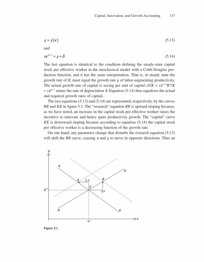
Capital, Innovation, and Growth Accounting 117
g g= ( )� κ (5.13)
and
s gκ δα − = +1 (5.14)
The last equation is identical to the condition defi ning the steady-state capital stock per effective worker in the neoclassical model with a Cobb-Douglas pro-duction function, and it has the same interpretation. That is, in steady state the growth rate of Kt must equal the growth rate g of labor-augmenting productivity. The actual growth rate of capital is saving per unit of capital sY/K = sA1−aKa/K = ska−1 minus the rate of depreciation d. Equation (5.14) thus equalizes the actual and required growth rates of capital.
The two equations (5.13) and (5.14) are represented, respectively, by the curves RR and KK in fi gure 5.1. The “research” equation RR is upward sloping because, as we have noted, an increase in the capital stock per effective worker raises the incentive to innovate and hence spurs productivity growth. The “capital” curve KK is downward sloping because according to equation (5.14) the capital stock per effective worker is a decreasing function of the growth rate.
On one hand, any parameter change that disturbs the research equation (5.13) will shift the RR curve, causing k and g to move in opposite directions. Thus an
R
K
A
Z
B
K
R
s
λ
κ
g
g*
κ∗
Figure 5.1
Chapter 5118
increase in the size of innovations g or the effi ciency of research l will shift RR up. This shift will raise long-run growth, as in the Schumpeterian model of chapter 4, but it will also reduce the long-run capital stock per effective worker.
On the other hand, any parameter change that disturbs the capital equation (5.14) will shift the KK curve, causing k and g to move in the same direction. Thus an increase in the saving rate s or a decrease in the depreciation rate d will raise the long-run stock of capital per worker, as in the neoclassical model, but it will also raise the long-run growth rate because, as we have already empha-sized, the rise in k will strengthen the incentive to do productivity-enhancing research.
5.4.4 Implications for Growth Accounting
Like the neoclassical model, the preceding hybrid model implies that in the long run the economy’s growth rate will equal the rate of labor-augmenting tech-nological progress g. But this equality does not mean that economic growth is caused by nothing other than technological progress, because g is now endoge-nous, so we cannot meaningfully speak of it as causing anything.
An analogy from supply and demand theory might help. That theory implies that the quantity that people trade must equal the amount supplied. But this equivalence does not mean that trading volume is caused by nothing other than supply, because the quantity supplied is itself an endogenous variable. We know that the amount traded generally depends on the conditions underlying both supply and demand, although there is one exception to this rule, namely, the case of a vertical supply curve, where supply is completely inelastic, in which case a change in supply is the only thing that can change the equilibrium quantity traded.
Likewise in growth theory, in general the long-run growth rate will be infl u-enced by conditions underlying the research arbitrage equation that governs innovation, but also by the conditions underlying the steady-state capital equation. One exception would be the case in which the RR curve was perfectly horizontal, where the rate of technological progress did not respond to capital accumulation, in which case innovation would be the only force governing the long-run growth rate. This is the case of neoclassical growth theory.
So, for example, when the incentives to perform R&D change, the change will result in a higher g, which we can meaningfully attribute to the force of innova-tion, since it was the innovation side of the economy that was altered. In this case the hybrid model agrees with the Solow model. But changes in the saving rate s
Capital, Innovation, and Growth Accounting 119
will displace the KK curve in fi gure 5.1 to the right, again causing g to go up, and in this case the change is attributable to capital accumulation, since it was a change in thrift not a change in innovation that caused the shift.
In both of these cases a growth accountant will ultimately conclude that the fraction a of the change in growth was accounted for by capital deepening and 1 − a by TFP growth, as implied by the Cobb-Douglas production function (5.11), as we explained in section 5.3.2. Yet in one case it was all caused by innovation, and in the other case it was all caused by capital accumulation.
As these examples illustrate, in order to estimate the extent to which growth is caused by either of these two forces, we need to identify the causal factors that shift the two curves, estimate by how much they shift the curve, estimate the slopes of the curves, and then measure the amount by which the causal factors have changed over the time period in question. One of the main objects of the rest of this book will be to identify the causal factors that shift curves like these, and to survey some of the evidence that would allow us to say what factors have been primarily respon-sible for economic growth at different times and in different countries.
5.5 Conclusion
In this chapter, we have refl ected upon the debates and controversies raised by recent studies on growth accounting. In particular, we have questioned A. Young’s (1995) claim that most of the Asian growth was due to factor accumulation, not innovation. We have stressed the importance of measurement issues, in particular that arising from the fact that technological progress is also embodied in new capital goods. More generally, we have questioned the use of accounting relation-ships for establishing causal relationships between GDP growth and the contribu-tions of factor accumulation and technical progress. And we have argued that moving from an accounting to a causal relationship is a particularly delicate step in the context of a Schumpeterian model augmented with capital accumulation, where the capital stock and the innovation rate are jointly determined and infl u-ence each other.
5.6 Literature Notes
The method of growth accounting was fi rst introduced by Solow (1957) and later developed in Kendrick (1961) and especially by Denison (1962). Jorgenson and Griliches (1967) extended and refi ned the analysis by considering changes in the
Chapter 5120
quality of capital and labor, and by building a “dual approach” to growth account-ing in which the Solow residual is calculated using the growth rates of factor prices instead of factor quantities. This idea was also exploited more recently by Hsieh (2002), who applied it to the study of East Asian countries and refuted previous fi ndings by A. Young (1995).
Griliches (1973) outlined a research program in which R&D spending is emphasized as a main determinant of the TFP growth rate. This approach was implemented in a number of analyses for fi rms and industries in the United States (such as Griliches and Lichtenberg 1984 and Griliches 1988) and was used by Coe and Helpman (1995) on aggregate data for OECD countries to analyze the knowledge spillovers induced by trade.
More recent works, such as Knight, Loayza, and Villanueva (1993), Islam (1995), and Caselli, Esquivel, and Lefort (1996), used panel data techniques in growth accounting and concluded that a large fraction of the cross-country income variance remains unexplained. King and Levine (1994), Klenow and Rodriguez-Clare (1997), Prescott (1998), and Hall and Jones (1999) addressed this issue using a calibration approach instead and concluded that large effi ciency differ-ences across countries need to be assumed in order to explain the data.
We refer our readers to the excellent Handbook of Economic Growth surveys by Caselli (2005) and Jorgenson (2005) on growth accounting and cross-country income differences.
Appendix: Transitional Dynamics
The dynamic evolution of aggregate capital Kt and productivity At are governed by
K sA K Kt t t t+−= + −( )1
1 1α α δ
A g K A At t t t+ + += + ( )⎡⎣ ⎤⎦1 1 11 �
The fi rst equation follows directly from equations (5.12) and (5.11), and the second one is the productivity-growth equation.
As in the neoclassical model, we can write this as one single difference equa-tion in the capital stock per effective worker kt = Kt /At. Dividing each side of the fi rst equation by the corresponding side of the second, and then rearranging, yields
κ κ κ δ καt t t tg s+ ++ ( )⎡⎣ ⎤⎦ = + −( )1 11 1� (5.15)
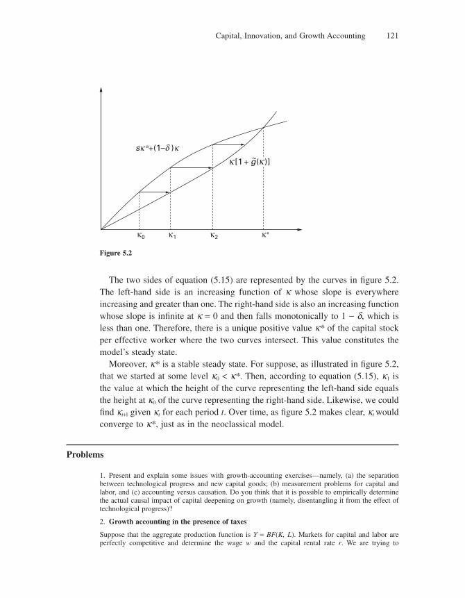
Capital, Innovation, and Growth Accounting 121
The two sides of equation (5.15) are represented by the curves in fi gure 5.2. The left-hand side is an increasing function of k whose slope is everywhere increasing and greater than one. The right-hand side is also an increasing function whose slope is infi nite at k = 0 and then falls monotonically to 1 − d, which is less than one. Therefore, there is a unique positive value k* of the capital stock per effective worker where the two curves intersect. This value constitutes the model’s steady state.
Moreover, k* is a stable steady state. For suppose, as illustrated in fi gure 5.2, that we started at some level k0 < k*. Then, according to equation (5.15), k1 is the value at which the height of the curve representing the left-hand side equals the height at k0 of the curve representing the right-hand side. Likewise, we could fi nd kt+l given kt for each period t. Over time, as fi gure 5.2 makes clear, kt would converge to k*, just as in the neoclassical model.
Problems
1. Present and explain some issues with growth-accounting exercises—namely, (a) the separation between technological progress and new capital goods; (b) measurement problems for capital and labor, and (c) accounting versus causation. Do you think that it is possible to empirically determine the actual causal impact of capital deepening on growth (namely, disentangling it from the effect of technological progress)?
2. Growth accounting in the presence of taxes
Suppose that the aggregate production function is Y = BF(K, L). Markets for capital and labor are perfectly competitive and determine the wage w and the capital rental rate r. We are trying to
κ0 κ1 κ2 κ*
[1 + g( )]~sk a+(1–d )k
Figure 5.2
Chapter 5122
decompose output growth �Y
Y into TFP growth
�BB
, capital deepening, and growth of the working
population, under different tax schemes.
a. Show that output growth is � � � � � � �Y
Y
B
B
BF K
Y
K
K
BF L
Y
L
L
B
Bs
K
Ks
L
LK L
K L= + + = + + . Interpret sK and
sL. How can we estimate TFP growth empirically?
b. Assume fi rms issue equities to fi nance their capital purchases, and r is the required rate of return on equities. Earnings, net of wages, are taxed at rate t1. Write FK and FL as a function of factor prices
and the tax rate, and derive the decomposition of �Y
Y. Is the preceding strategy still valid? What
empirical measures of sK and sL should we use to estimate TFP growth accurately?
c. Assume there is a tax t2 on fi rms’ total output (and t1 = 0). Answer the same questions as in part b.
d. Assume the tax rates on value added by capital and labor differ: fi rms pay a tax rate tK on capital payments rK and tL on the wage bill wL. The average tax rate, weighted by shares in total victor
income, is trK
t Yt
wL
t YtK L=
−( ) +−( )1 1 . Answer the same questions as in part b.
3. Effects of policy changes on capital accumulation and innovation
Consider the model of section 5.4. We want to estimate the impact of different policy measures on the long-run levels of capital per effective worker m and the long-run productivity growth rate g. For each of the following cases, rewrite the research arbitrage condition and the equations of the curves RR and KK in fi gure 5.1, and explain how the steady-state values of m and g compare to the baseline model.
a. R&D is subsidized at rate s; that is, the effective cost for the researcher of investing one unit of the fi nal good in R&D becomes 1 − s.
b. Antitrust laws are toughened, so that there is a probability p each period that the innovator will lose his monopoly power and realize zero profi ts even when no new innovation occurs in the sector. The probability of a successful innovation remains lnit per period.
c. An investment tax credit of rate t is eliminated. For this question we also assume that the savings rate is a function of the interest rate and the tax credit: s = s(r + t), s′ > 0.
4. “Dual method” and estimates of the Solow residual (based on A. Young 1995 and Hsieh 2002)
This problem contrasts Young’s and Hsieh’s methods for estimating TFP growth. They rely, respec-tively, on growth in the stocks of capital and labor and on growth in factor prices. The purpose of this exercise is to disentangle the contributions of factor accumulation and TFP in the postwar growth of the East Asian “Tigers.” We consider a generic aggregate production function with capital and labor, which earn returns W and R. We assume factor payments exhaust output: Y = RK + WL.
a. Show that the growth rate of output is given by
� � � � �Y
Ys
K
K
R
Rs
L
L
W
WK L= +⎛⎝⎜
⎞⎠⎟
+ +⎛⎝⎜
⎞⎠⎟
where sRK
YK ≡ and sWL
YL ≡ are the share of capital and labor in total income. (Hint: Note that
�YY
d Y
dt= ln
.) What is the Solow residual equal to?
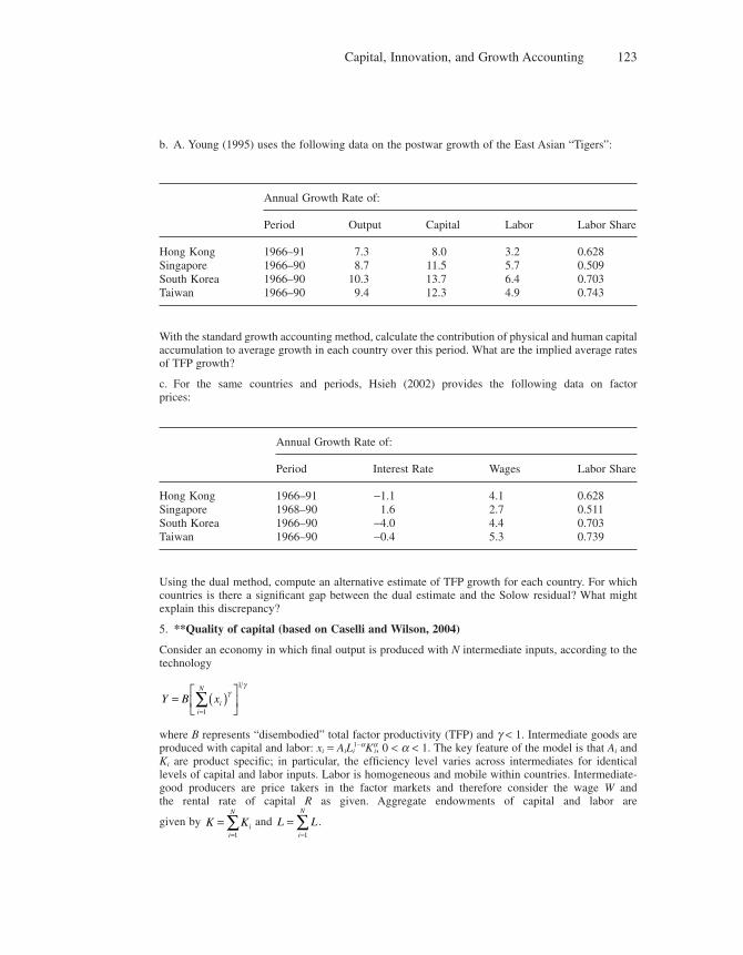
Capital, Innovation, and Growth Accounting 123
b. A. Young (1995) uses the following data on the postwar growth of the East Asian “Tigers”:
Annual Growth Rate of:
Period Output Capital Labor Labor Share
Hong Kong 1966–91 7.3 8.0 3.2 0.628Singapore 1966–90 8.7 11.5 5.7 0.509South Korea 1966–90 10.3 13.7 6.4 0.703Taiwan 1966–90 9.4 12.3 4.9 0.743
With the standard growth accounting method, calculate the contribution of physical and human capital accumulation to average growth in each country over this period. What are the implied average rates of TFP growth?
c. For the same countries and periods, Hsieh (2002) provides the following data on factor prices:
Annual Growth Rate of:
Period Interest Rate Wages Labor Share
Hong Kong 1966–91 −1.1 4.1 0.628Singapore 1968–90 1.6 2.7 0.511South Korea 1966–90 −4.0 4.4 0.703Taiwan 1966–90 −0.4 5.3 0.739
Using the dual method, compute an alternative estimate of TFP growth for each country. For which countries is there a signifi cant gap between the dual estimate and the Solow residual? What might explain this discrepancy?
5. **Quality of capital (based on Caselli and Wilson, 2004)
Consider an economy in which fi nal output is produced with N intermediate inputs, according to the technology
Y B xii
N
= ( )⎡⎣⎢
⎤⎦⎥
=∑ γ
γ
1
1
where B represents “disembodied” total factor productivity (TFP) and g < 1. Intermediate goods are produced with capital and labor: xi = AiLi
1−aKai, 0 < a < 1. The key feature of the model is that Ai and
Ki are product specifi c; in particular, the effi ciency level varies across intermediates for identical levels of capital and labor inputs. Labor is homogeneous and mobile within countries. Intermediate-good producers are price takers in the factor markets and therefore consider the wage W and the rental rate of capital R as given. Aggregate endowments of capital and labor are
given by K Kii
N
==∑
1
and L Li
N
==∑
1
.
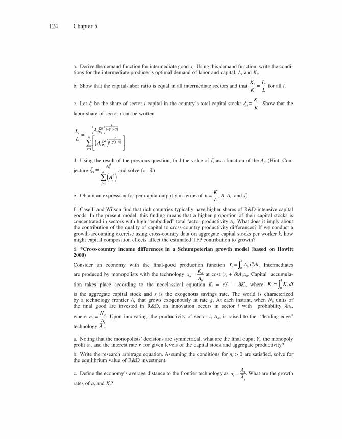
Chapter 5124
a. Derive the demand function for intermediate good xi. Using this demand function, write the condi-tions for the intermediate producer’s optimal demand of labor and capital, Li and Ki.
b. Show that the capital-labor ratio is equal in all intermediate sectors and that K
K
L
Li i= for all i.
c. Let xi be the share of sector i capital in the country’s total capital stock: ξ iiK
K≡ . Show that the
labor share of sector i can be written
L
L
A
A
i i j
i jj
N=
( )( )⎡
⎣⎢
⎤
⎦⎥
1− 1−( )
1− 1−( )=
∑
ξ
ξ
αγ
γ α
αγ
γ α
1
d. Using the result of the previous question, fi nd the value of xi as a function of the Aj. (Hint: Con-
jecture ξδ
δi
i
jj
N
A
A
=( )
=∑
1
and solve for d.)
e. Obtain an expression for per capita output y in terms of kK
L≡ , B, Ai, and xi.
f. Caselli and Wilson fi nd that rich countries typically have higher shares of R&D-intensive capital goods. In the present model, this fi nding means that a higher proportion of their capital stocks is concentrated in sectors with high “embodied” total factor productivity Ai. What does it imply about the contribution of the quality of capital to cross-country productivity differences? If we conduct a growth-accounting exercise using cross-country data on aggregate capital stocks per worker k, how might capital composition effects affect the estimated TFP contribution to growth?
6. *Cross-country income differences in a Schumpeterian growth model (based on Howitt 2000)
Consider an economy with the fi nal-good production function Y A x dit it it= ∫ α
0
1
. Intermediates
are produced by monopolists with the technology xK
Aitit
it
= at cost (rt + d)Aitxit. Capital accumula-
tion takes place according to the neoclassical equation K.t = sYt − dKt, where K K dit it= ∫0
1
is the aggregate capital stock and s is the exogenous savings rate. The world is characterized by a technology frontier At that grows exogenously at rate g. At each instant, when Nit units of the fi nal good are invested in R&D, an innovation occurs in sector i with probability lnit,
where nN
Aitit
t
≡ . Upon innovating, the productivity of sector i, Ait, is raised to the “leading-edge”
technology At .
a. Noting that the monopolists’ decisions are symmetrical, what are the fi nal ouput Yt, the monopoly profi t pt, and the interest rate rt for given levels of the capital stock and aggregate productivity?
b. Write the research arbitrage equation. Assuming the conditions for nt > 0 are satisfi ed, solve for the equilibrium value of R&D investment.
c. Defi ne the economy’s average distance to the frontier technology as aA
Att
t
= . What are the growth
rates of at and Kt?
Capital, Innovation, and Growth Accounting 125
d. Derive the steady-state values of a and K given n and g. How do changes in the savings rate, the probability of success of R&D, and the growth rate of the frontier technology affect the steady state?
e. Under which condition does a country conduct no R&D? What, in this case, is its rate of produc-tivity growth? Why can we say this model exhibits “club convergence”?
f. Decompose long-run log output into a productivity component and a capital-deepening component. If we run a cross-sectional regression of log output per capita on the log of the capital stock, what assumption do we need to make for the coeffi cient to be unbiased? Is this assumption satisfi ed in the model?


II UNDERSTANDING THE GROWTH PROCESS

6 Finance and Growth
6.1 Introduction
All the basic paradigms that we presented in part I of this book imply that eco-nomic growth depends on investment of one sort or another. According to neo-classical and AK theories, what drives growth is investment in physical and human capital. According to product-variety and Schumpeterian theories, what matters is investment in technology, in the form of research. In the hybrid model of the last chapter, investment in capital and technology are both important.
However, none of these theories analyzed the diffi culties that a fi rm might have fi nancing the investments that drive growth. None of them made any mention of the role that banks and other fi nancial intermediaries might have in mitigating such diffi culties. This silence is understandable because a basic theoretical para-digm focuses on the fundamental mechanisms of the growth process, whereas fi nance is like the lubrication that reduces frictions and thereby enables the machinery to function. Presenting each theory without the complicating factor of fi nancial frictions helps us to see the fundamental mechanisms more clearly.
In order to see the role that fi nance plays in the growth process, however, we need to go beyond these idealized models and take frictions into account. When we do, we see that fi nancial markets and fi nancial intermediaries play an impor-tant role, which varies a lot from country to country. For example, people are willing to save more, and hence make more available to investors, in a country with effi cient and trustworthy banks than in a country where banks are likely to waste their depositors’ wealth through bad loans or even swindles. Banks can also help by risk pooling. That is, by collecting savings from many people and investing them in a large diversifi ed range of projects, a bank allows even small savers to take advantage of the law of large numbers and get a reasonably safe rate of return; the losses on bad projects will tend to be offset by the gains on good projects. In addition, well-functioning banks can channel savings toward the most effi cient uses. Finally, and perhaps most importantly, banks can also help to alleviate agency problems by monitoring investors and making sure that they are making productive use of their loans rather than spending them on private consumption or otherwise defrauding the ultimate lenders. Many of these roles are also served by stock markets, private equity fi rms, and venture capitalists, all of which help to identify, fi nance, and monitor good investment projects.
In his survey article on fi nance and growth in the Handbook of Economic Growth, Ross Levine (2005, p. 868) summarizes as follows the existing research on this topic: “Taken as a whole, the bulk of existing research suggests that
Chapter 6130
(1) countries with better functioning banks and markets grow faster; (2) simulta-neity bias does not seem to drive these conclusions, and (3) better functioning fi nancial systems ease the external fi nancing constraints that impede fi rm and industrial expansion, suggesting that this is one mechanism through which fi nan-cial development matters for growth.”
So when seeking a more detailed understanding of the growth process than we fi nd in any of the frictionless paradigms laid out in the previous fi ve chapters, one of the fi rst complicating factors that we should introduce is fi nancial con-straints. Accordingly, this chapter begins part II of the book by showing how one might take these constraints into account. The chapter comprises three main parts. First, we introduce fi nancial constraints into the Schumpeterian growth frame-work and show explicitly how intermediaries that provide external fi nance to innovators by channeling savings and mitigating agency problems can enhance growth. We provide two alternative models: in the fi rst one, banks provide screen-ing services to identify good projects, and in the second one, banks provide ex post monitoring to make it diffi cult for the borrower to abscond with borrowed money. Next, we introduce credit constraints in a simple AK model to analyze the relationship between credit constraints, wealth inequality, and growth. Finally, we review some of the voluminous empirical evidence underlying Levine’s summary statement of the role of fi nance in the growth process.
6.2 Innovation and Growth with Financial Constraints
In this section, we introduce fi nancial constraints into the multisector Schum-peterian growth model of chapter 4.
6.2.1 Basic Setup
First we set up a model without fi nancial constraints. The model is almost identi-cal to that of chapter 4, except for two small changes. The fi rst is that individuals now live for two periods instead of one. In the fi rst period of life an individual works in the fi nal-good sector. In the second period she may become an entre-preneur and/or an intermediate monopolist, and if she becomes an entrepreneur she may use the wage earned in the fi rst period to fi nance research.
The economy has a fi xed population L, which we normalize to unity. Everyone is endowed with one unit of labor services in the fi rst period and none in the second, and is risk neutral. There is one fi nal good, produced under perfect com-petition by labor and a continuum of intermediate inputs according to
Finance and Growth 131
Y L A x dit it it= < <− −∫1 1
0
10 1α α α α, (6.1)
where xit is the input of the latest version of intermediate good i and Ait is the pro-ductivity parameter associated with it. The fi nal good is used for consumption, as an input to R&D, and also as an input to the production of intermediate products. At any date t, one old person in each intermediate sector i has an opportunity to innovate in that sector. If successful, she will become the monopolist in sector i for period t; if not, the monopoly will pass to another old person at random.
Here we introduce the second difference from the model of chapter 4. That is, we suppose now that the starting technology in any given sector i at date t does not have the productivity parameter Ai,t−1 of that sector last period; instead it has the average At−1 = ∫1
0 Ai,t−1di across all sectors last period. So an entrepreneur that
succeeds in innovating will have the productivity parameter Ait = gAt, where g > 1 is the size of innovations, while the monopolist in a noninnovating sector will have Ait= At−1.
Let m be the probability that an innovation occurs in any sector i at time t (in equilibrium, as we shall see, this probability will be constant over time and the same for all sectors). Then a fraction m of sectors (those who have innovated) will have productivity gAt−1 while the remaining fraction (1 − m) will have At−1. The average across all sectors will therefore be
A A At t t= + −( )− −μγ μ1 11
implying that the growth rate of average productivity is
gA A
At t
t
=−
= −( )−
−
1
1
1μ γ (6.2)
In each intermediate sector where an innovation has just occurred, the monopo-list is able to produce any amount of the intermediate good one for one with the fi nal good as input. Her price will be the marginal product of her intermediate good:
p A xit it it= − −α α α1 1
As we saw in the previous chapters, profi t maximization by the intermediate-good producer in sector i yields the equilibrium profi t
Πit itA= π
where π α ααα≡ −( )
+−1
1
1 ; gross output of the fi nal good will be
Chapter 6132
Y At t= ϕ (6.3)
where ϕ ααα= −
21 ; and the economy’s GDP will also be proportional to the average
productivity parameter At; so the rate of economic growth will again equal the productivity growth rate g.
6.2.2 Innovation Technology and Growth without Credit Constraint
For concreteness we assume a special case of the innovation technology specifi ed in the model of chapter 4, where the elasticity parameter s is equal to 1
2 :
μ φ λ λ= = >( ) ( ) ,R A R At t t t/ * / * 1 2 0 (6.4)
where Rt is the amount of fi nal good spent on R&D in a given sector at time t and A*t = gAt−1 is the target productivity level. It follows that the R&D cost of innovating with probability m is equal to
R At t= * /ψμ2 2 (6.5)
where y = 2/l2 is a parameter that measures the cost of innovation.The entrepreneur will again choose the research expenditure Rt so as to maxi-
mize her expected payoff. According to equation (6.5), choosing Rt is equivalent to choosing the innovation probability m. So her profi t-maximization problem is to choose the m that maximizes
μπ ψμA At t* * /− 2 2 (6.6)
Thus the equilibrium probability of innovation is
μ π ψ= (6.7)
From this and equation (6.2), the equilibrium growth rate is
g = ( ) −( )π ψ γ 1
which is identical to the equilibrium growth rate of the model in chapter 4 when the elasticity parameter s in the innovation production function is equal to 1
2 .
6.2.3 Credit Constraints: A Model with Ex Ante Screening
Each innovator at date t is a young person with access to the wage income wt−1. Thus to invest Rt in an R&D project she must borrow L = Rt − wt−1, which we suppose is strictly positive, from a lender. In the previous section we implicitly assumed that the activity of borrowing did not cost any resources or create any contracting problems that might impede investments. The expected profi t (6.6)
Finance and Growth 133
that was being maximized was the total expected return to be shared by the entrepreneur and her creditor.
In this section we introduce a cost of borrowing. In particular, we suppose (fol-lowing King and Levine 1993b) that in addition to the entrepreneurs in our model there are other people seeking to fi nance projects that are in fact not feasible under any circumstances. Then the bank must pay a cost to screen loan applications, since a loan to someone with an infeasible project will not be repaid.
Let q be the probability that a borrower coming to a bank is capable (has a feasible project), while 1 − q is the probability that the borrower’s project will yield no payoff at all. A bank can determine whether or not a given project is feasible by paying a cost equal to fRt units of the fi nal good. Then it will require a repayment of fRt /q from each feasible project in order to break even,l and the combined payoff to an entrepreneur and her bank will be the expected profi t of a successful innovation minus the R&D cost and the screening cost:
μπ θA R f Rt t t* − −
(Note that we are assuming for simplicity, as we did in chapter 4, that the project takes no time, so there is no discounting of the expected return mpA*t.)
Since the R&D cost of innovating with probability m is given by equation (6.5), the combined payoff can be written as
μπ θ ψμA f At t* * /− +( )1 22
which is equal to the expected profi t (6.6) in the case of no credit constraints, minus the screening cost. Maximizing this combined payoff results in an equi-librium probability of innovation equal to
μ πθ ψ
=+( )1 f
From this and equation (6.2), the corresponding equilibrium growth rate is
gf
=+( ) −( )π
θ ψγ
11
1. Let P be the repayment from a feasible project. Then the bank’s expected profi t from screening a project will be
θP f Rt−
because its expected revenue will be the probability q that the project is feasible times the payment P, whereas the cost will be fRt with certainty. Therefore, expected profi t is zero only if P = fRt/q.
Chapter 6134
Therefore, the higher the screening cost f, the lower will be the frequency of innovations and the lower will be the equilibrium growth rate. Countries with more effi cient banks should have a lower f and hence a higher growth rate.
6.2.4 A Model with Ex Post Monitoring and Moral Hazard
Banks do more than screen loan applications. They also monitor the lender’s performance during the term of a loan contract to guard against the possibility of fraud. Our second model of credit constraints and growth focuses on ex post monitoring, and is based on Aghion, Banerjee, and Piketty (1999). It introduces the important notion of the credit multiplier.
6.2.4.1 Credit Multiplier and R&D Investment
Again, each entrepreneur is a young person with access to the wage income wt−1, who must borrow L = Rt − wt−1. Suppose now that what makes it diffi cult to borrow is that the borrower might default. A bank will monitor the borrower, thereby making it costly for the borrower to default, but not impossible. Specifi -cally, by paying a cost hRt, where 0 < h < 1, the entrepreneur can hide the result of a successful innovation and thereby avoid repaying. The cost parameter h is an indicator of the bank’s effectiveness in monitoring; a well-functioning bank makes fraud very diffi cult. The cost also refl ects the effectiveness of legal institu-tions in protecting creditors’ rights; in a country where courts rarely enforce loan contracts, it is relatively easy to avoid repaying.
The entrepreneur must pay the hiding cost at the beginning of the period, when she decides whether or not to be dishonest. She will be dishonest when it is in her self-interest, namely, when the following incentive-compatibility constraint is violated:
hR R R wt t t t t≥ ( ) −( )−μ Γ 1 (6.8)
where Γ is the interest factor on the loan and mt(Rt) is the probability of innovat-ing at date t given the R&D investment Rt, as determined by equation (6.4). The right-hand side of equation (6.8) is the expected saving from deciding to be dis-honest; that is, by being dishonest you can avoid making the repayment, which is the interest factor Γ times the loan amount, in the event the project succeeds, which happens with probability m.
The only potential lenders in this overlapping-generation model are other young people, who will lend only if the expected repayment equals the loan amount. Thus, even though there is no time cost to the project, there will be a positive interest factor on the loan, given by the arbitrage condition
Finance and Growth 135
μt tR( ) =Γ 1
which states that for every dollar lent out, the expected repayment (Γ with prob-ability m) must equal one. Using this arbitrage condition to substitute for Γ, we see that the incentive-compatibility condition (6.8) boils down to an upper limit on the entrepreneur’s investment:
Rh
w w Rt t t t≤−
= =− −1
1 1 1ν ˆ (6.9)
The parameter � is commonly referred to as the credit multiplier. A higher cost h of hiding innovation revenue implies a larger credit multiplier.
6.2.4.2 Innovation and Growth under Binding Credit Constraint
The constraint (6.9) will be binding if Rt is less than the R&D cost of achieving the innovation probability (6.7) that would be undertaken in the absence of fi nan-cial constraints, given the cost function (6.5):
ν γ π ψw At t− −< ( )1 12 2 (6.10)
The equilibrium wage wt−1 is the marginal product of labor, which under the Cobb-Douglas specifi cation in equation (6.1) equals (1 − a) times fi nal output Yt−1, which together with equation (6.3) implies
w At t− −=1 1ω
where w = (1 − a)j.Thus we can rewrite condition (6.10) as
ν γπ ψω< ( )2 2 (6.11)
It follows that entrepreneurs are less likely to face a credit constraint when either fi nancial development is higher, as measured by �, or entrepreneurs’ initial wealth w as a fraction of aggregate output is higher. This conclusion follows because a large � implies a large cost of defrauding a creditor, which makes creditors willing to lend more, and a large w gives entrepreneurs more wealth, which makes them better able to self-fi nance when creditors are unwilling.
Whenever equation (6.11) holds, the equilibrium growth rate is obtained by substituting the constrained investment Rt = �wt−1 into the innovation production function (6.4) and then using equation (6.2) and the defi nition of y to arrive at
gh = −( ) ( )γ νω γ ψ1 2
Chapter 6136
which is monotonically increasing in fi nancial development as measured by � and in entrepreneur’s wealth as measured by w. Note that gh does not depend on productivity-adjusted profi t p, because, although a higher profi t rate would make entrepreneurs want to do more research, it does not affect the incentive-compatibility constraint, and hence does not make lenders willing to fi nance any more research. Thus it is only when the credit constraint is not binding that higher profi tability translates into faster growth.
When equation (6.11) does not hold, then the growth rate is the same as it was in the absence of credit constraints, namely,
g = −( ) = ( ) −( )μ γ π ψ γ* 1 1
In this case, profi tability again matters, but fi nancial development and the wealth of entrepreneurs no longer matters.
6.3 Credit Constraints, Wealth Inequality, and Growth
It is often believed that policies aimed at equalizing the distribution of wealth and income are detrimental to growth, because taxing the wealthy discourages individuals from investing and innovating. But it has been shown by Banerjee and Newman (1993) and Galor and Zeira (1993) that when credit constraints are present, then reducing wealth inequality can actually have a stimulating effect on growth. So one of the important ways in which fi nance can matter for the growth process is by changing the relationship between inequality and growth. As we will see, this effect can go in either direction, depending on the precise circum-stances of the economy.
6.3.1 Diminishing Marginal Product of Capital
Credit markets allow a separation between the ownership of capital and the employ-ment of capital. When there is a diminishing marginal product of capital, growth can be enhanced by spreading the employment of capital equally over many enter-prises, which can be accomplished by having those who own little capital borrow from those who own a lot. Credit constraints impede this process, and are thus detrimental to growth. This is the basic idea behind the model of this section, which is similar to the one suggested by Benabou (1996). In this model, credit constraints generate a negative relationship between wealth inequality and growth.
Finance and Growth 137
The basic structure of the model is the same as the AK model of Frankel that we studied in chapter 2. There are N individual producers. At the start of period t, individual j owns ej units of capital, so the aggregate capital stock is K et j
N= ∑1.
Each produces fi nal output according to the production function
y Akj j= < <α α, 0 1
where kj is the amount of capital that the individual employs. A person can employ more than he owns by borrowing the difference kj − ej, or he can employ less than he owns and lend the difference.
Because of knowledge spillovers, the productivity parameter A that each pro-ducer takes as given depends on the aggregate capital stock according to2
A A Kt= −0
1 α
Growth in the capital stock is given by the accumulation equation
K K sY Kt t t t+ − = −1 δ
where s is the saving rate, d is the depreciation rate, and Yt is aggregate output.Suppose there is an unequal wealth distribution; that is, ej varies across indi-
vidual producers. Then there will be an incentive for individuals with more than the average amount of capital to lend some of their capital to those with less, because of the diminishing marginal product of capital. That is, the amount of production that the lender sacrifi ces by lending a small amount of capital instead of employing it himself will be less than what the borrower can produce with that loaned capital, because the borrower is starting with a smaller capital stock than the lender. So between them they can produce a larger total as a result of the loan.
Indeed it is easy to see that aggregate output is maximized when each producer employs the same amount of capital. That is, setting kj = Kt /N for all j maximizes total output
Y A kt j
N= ∑ α1
2. In general, the Frankel model specifi es A = A0Kht. Here we consider only the knife-edge AK case
where h = 1 − a.
Chapter 6138
subject to the adding-up constraint3
k Kj
N
t1∑ = (6.12)
A simple way to introduce credit constraints is to assume as before that an individual who owns ej cannot employ more than kj = �ej, where � > 1 is again the credit multiplier. When � = +∞, capital markets are perfect and individuals face no borrowing constraint, whereas in the opposite case, where � = 1, credit simply becomes unavailable. We will concentrate on these two extreme cases in this section.
Consider fi rst the case of perfect capital markets. In this case, there will be a common interest rate r at which people can borrow or lend all the capital they want. An individual’s income will be the amount produced minus the cost of borrowing (or plus the interest income from lending):
Ak r k ej j jα − −( )
The individual will choose to employ the amount that maximizes his income, implying the fi rst-order condition
α αAk rj− − =1 0
So all producers will produce the same amount
k A rj = ( ) −α α1
1
which by the adding-up constraint (6.12) implies kj = Kt/N, exactly as in the Frankel model. So again we will have fi nal output equal to
Y AN K N AKt t t= ( ) =α
3. The Lagrangean for this maximization problem is
L = + −( )∑∑A k K kj t j
NN α λ11
and the fi rst-order conditions are
∂∂
Lk
Ak jj
j= − =−α λα 1 0 for all
which can be rewritten as
k A jj = ( ) −α λ α1
1 for all
which states that all the kj’s should be equal. Under the adding-up constraint (6.12) this equation implies kj = Kt /N for all j.
Finance and Growth 139
where A = A0N 1−a, and the growth rates of capital and output will both equal
g sA= − δ
Next, consider the other extreme case, where there is no borrowing at all. With no borrowing, there cannot be any lending either, so each producer will employ nothing more or less than his own capital:
k ej j=
But as we have already seen, this case will result in a smaller total output than if all employed the same amount. Therefore aggregate output will be less than in the case of perfect capital markets:
Y AKt t<
and the growth rate of capital will also be less:
gsY K
KsAt t
t
= − < −δ δ
If everyone’s capital grows at the same rate, then g will also be the growth rate of output,4 so output will also grow more slowly than in the case of perfect capital markets.
It follows that when capital markets are perfect, policies that redistribute wealth have no direct effect on growth, because the employment of capital is always equalized in the marketplace even if ownership is not. But when credit constraints are so severe as to eliminate borrowing, wealth redistribution that reduces inequal-ity of ownership will raise growth by reducing the inequality of employment.5
6.3.2 Productivity Differences
In the previous model all individual producers were equally productive, and it was for that reason that growth was maximized by having them employ equal amounts of capital. In reality there are large productivity differences across indi-vidual producers, a fact which implies that growth is enhanced by having unequal employment of capital, with more being employed by the more productive indi-viduals. Credit markets can therefore facilitate the growth process by allowing
4. Next period’s output will be Y A g K g K g A Kt t j
N
t+− −= +( )⎡⎣ ⎤⎦ +( )⎡⎣ ⎤⎦ = +( )∑1 0
1
1 011 1 1
α α α
k g Yj
N
tα
11∑ = +( ) .
5. Indeed it follows from the theorems of Rothschild and Stiglitz (1976) that any mean-preserving reduction in the dispersion of kj will raise output Y A kt j
N= ∑ α1
and hence will raise the growth rate g = s(Yt/Kt) − d.

Chapter 6140
the more productive individuals to borrow from the less productive ones. This is the idea behind our second model, which is based on Kunieda (2008). In this model, credit constraints can generate a positive relationship between inequality and growth; indeed, growth is maximized is having all of the capital owned by a single individual—the most effi cient one.
The basic structure is the same as in the previous model, except that we con-sider here the extreme case where there is no diminishing marginal productivity at the individual level: a = 1. We also allow the credit multiplier to take on any value � ≥ 1 instead of looking only at the extremes of 1 and +∞ as we did in the previous model.
The production function of each producer j is
y kj j j= τ
where the individual productivity parameters tj vary across individuals, with
τ τ τ1 2> > >� N
The producer will choose to employ the amount kj that maximizes his profi t
τ j j j jk r k e− −( ) (6.13)
subject to the credit constraint
k ej j≤ ν
The solution to this constrained maximization problem depends on how pro-ductive the individual is.
1. If tj > r, then profi t (6.13) is strictly increasing in the amount employed, so the individual will employ the maximal amount �ej allowed by the credit constraint.
2. If tj < r, then the individual can earn more from lending than producing, so he will employ nothing and lend the amount ej.
3. If tj = r, then profi t will be independent of kj, so the individual will be willing to employ any amount between 0 and the upper limit �ej.
Equilibrium in the capital market requires total employment to equal the aggre-gate stock of capital Kt. This is achieved by an equilibrium rate of interest that equals the productivity parameter tm of some marginal producer m. All individuals j < m will fall into case 1, and all individuals j > m will fall into case 2. Aggregate employment will equal the marginal producer’s employment plus the maximal amount that all those in case 1 can employ, so the equilibrium condition is6
6. We defi ne e0 = 0 so that the summation in equation (6.14) makes sense when m = 1.
Finance and Growth 141
k e Km j
m
t+ =−∑ν0
1 (6.14)
Since the marginal producer is in case 3, we need
0 ≤ ≤k em mν (6.15)
Thus capital-market equilibrium requires7
e K ej
m
t j
m
0
1
0
−∑ ∑≤ ≤ν (6.16)
Condition (6.16) says that employment by those individuals more productive than m cannot exceed Kt and that if m were to employ the maximal amount allowed by the credit constraint, then employment would be at least Kt. The condition determines the identity of the marginal producer m, because there is almost always just one value of m for which it can hold. The exception is the case where
K et j
nν = ∑0 for some individual n, in which case we could make either n or
n + 1. the marginal producer.We can now see what happens when credit constraints become tighter, that is,
when the credit multiplier � is reduced. Suppose fi rst that the most productive individual has no spare borrowing capacity, which happens if Kt /� ≥ e1 and m > 1. In this case, all the producers j < m who are more productive than the marginal producer will have to reduce employment when � falls, while the marginal pro-ducer takes up the slack, unless the marginal producer does not have enough wealth to borrow that much extra capital, in which case someone even less pro-ductive will become the new marginal producer. By reallocating capital from more productive to less productive individuals, this tightening of credit will reduce total output.
More specifi cally, total output in this case is
Y k k k et m m j jm
m m m mm= + = +− −∑ ∑τ τ τ ν τ
0
1
0
1
which together with the market-clearing condition (6.14) implies
Y K et m t j m jm= + −( )−∑τ ν τ τ0
1
so we have
∂∂Y
etj m j
m
ντ τ= −( ) >−∑0
10
since tj > tm, for all j < m.
7. To derive equation (6.16), use equation (6.14) to substitute for km in equation (6.15), then divide all three expressions in the resulting pair of inequalities by � and add ej
m
0
1−∑ to all of them.
Chapter 6142
Next consider the case where Kt /� < el. In this case the credit constraint is loose enough that all capital will be employed by the most productive individual, so output will be the maximum possible amount:
Y Ktmax = τ1
In either case, as in the previous model, the growth rate will be
g s Y Kt t= ( ) − δ
so a reduction in the credit multiplier will reduce growth by reducing Yt, except in the case where the most productive individual has spare borrowing capacity, in which case g = st1 − d, which is independent of the credit multiplier.
Note that this model can produce a positive relationship between growth and inequality, in the sense that when credit constrants are very tight the economy will grow faster if all of the capital is owned by individual 1 than if everyone owned the same amount Kt /N, because in the latter case borrowing constraints would prevent all of the capital from being employed most productively, whereas in the former case it would not.
This conclusion does not mean, however, that any increase in inequality would raise growth, for what matters is not just that ownership be concentrated but that it be concentrated in the hands of the most talented individuals. So a reduction of inequality that took wealth from rich but not very talented individuals and redistributed it to poor but talented individuals would result in an increase in growth, just as in the previous model.
6.4 The Empirical Findings: Levine’s Survey, in a Nutshell
Most of the empirical literature on fi nance and growth has been concerned with cross-country or panel regressions of the form
g X ui i i i= + + +β β β0 1 2Findev
where gi is the average growth rate in country i during the period or subperiod, Findevi is the country’s level of fi nancial development (either at the beginning of the period or averaged over the period), Xi is a vector of controls (policy variables, education, political stability, initial income per capita, etc), and ui is a noise term.
As explained in Levine’s survey, empirical papers on fi nance and growth differ in terms of: (1) whether they look at cross-country data (like King and Levine
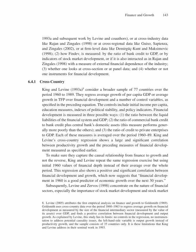
Finance and Growth 143
1993a and subsequent work by Levine and coauthors), or at cross-industry data like Rajan and Zingales (1998) or at cross-regional data like Guiso, Sapienza, and Zingales (2002), or at fi rm-level data like Demirgüç-Kunt and Maksimovic (1998); (2) how Findevi is measured: by the ratio of bank credit to GDP, or by indicators of stock market development, or if it is also interacted as in Rajan and Zingales (1998) with a measure of external fi nancial dependence of the industry; (3) whether one looks at cross-section or at panel data; and (4) whether or not one instruments for fi nancial development.
6.4.1 Cross-Country
King and Levine (1993a)8 consider a broader sample of 77 countries over the period 1960 to 1989. They regress average growth of per capita GDP or average growth in TFP over fi nancial development and a number of control variables, as specifi ed in the preceding equation. The controls include initial income per capita, education measures, indexes of political stability, and policy indicators. Financial development is measured in three possible ways: (1) the ratio between the liquid liabilities of the fi nancial system and GDP; (2) the ratio of commercial bank credit to bank credit plus central bank’s domestic assets (this measure performs gener-ally more poorly than the others); and (3) the ratio of credit to private enterprises to GDP. Each of these measures is averaged over the period 1960–89. King and Levine’s cross-country regression shows a large and signifi cant correlation between productivity growth and the preceding measures of fi nancial develop-ment measured as specifi ed earlier.
To make sure they capture the causal relationship from fi nance to growth and not the reverse, King and Levine repeat the same regression exercise but using initial 1960 values of fi nancial depth instead of their average over the whole period. This regression also shows a positive and signifi cant correlation between fi nancial development and growth, which now suggests that “fi nancial develop-ment in 1960 is a good predictor of economic growth over the next 30 years.”
Subsequently, Levine and Zervos (1998) concentrate on the nature of fi nancial sectors, especially the importance of stock market development and stock market
8. Levine (2005) attributes the fi rst empirical analysis on fi nance and growth to Goldsmith (1969). Goldsmith uses cross-country data over the period 1860–1963 to regress average growth on fi nancial development as measured by the size of the fi nancial intermediary sector (measured by the value of its assets) over GDP, and fi nds a positive correlation between fi nancial development and output growth. As explained by Levine, this study has its limits: no controls in the regression, no instrumen-tation to address potential causality issues, the left-hand-side variable is output growth instead of productivity growth, and the sample consists of 35 countries only. It is these limitations that King and Levine address in their seminal work in 1993.
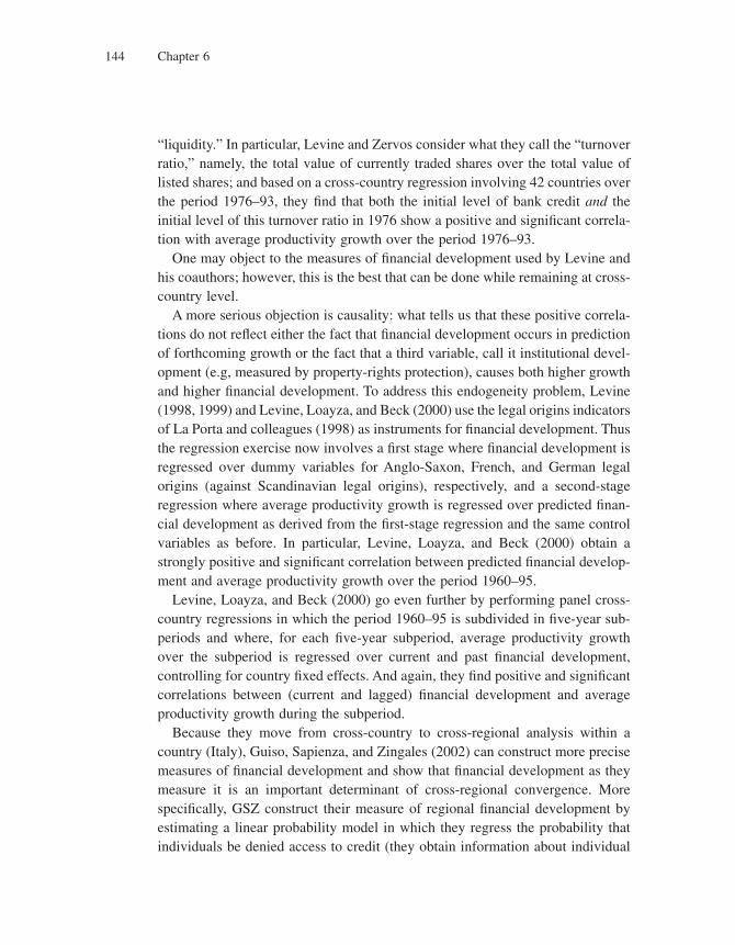
Chapter 6144
“liquidity.” In particular, Levine and Zervos consider what they call the “turnover ratio,” namely, the total value of currently traded shares over the total value of listed shares; and based on a cross-country regression involving 42 countries over the period 1976–93, they fi nd that both the initial level of bank credit and the initial level of this turnover ratio in 1976 show a positive and signifi cant correla-tion with average productivity growth over the period 1976–93.
One may object to the measures of fi nancial development used by Levine and his coauthors; however, this is the best that can be done while remaining at cross-country level.
A more serious objection is causality: what tells us that these positive correla-tions do not refl ect either the fact that fi nancial development occurs in prediction of forthcoming growth or the fact that a third variable, call it institutional devel-opment (e.g, measured by property-rights protection), causes both higher growth and higher fi nancial development. To address this endogeneity problem, Levine (1998, 1999) and Levine, Loayza, and Beck (2000) use the legal origins indicators of La Porta and colleagues (1998) as instruments for fi nancial development. Thus the regression exercise now involves a fi rst stage where fi nancial development is regressed over dummy variables for Anglo-Saxon, French, and German legal origins (against Scandinavian legal origins), respectively, and a second-stage regression where average productivity growth is regressed over predicted fi nan-cial development as derived from the fi rst-stage regression and the same control variables as before. In particular, Levine, Loayza, and Beck (2000) obtain a strongly positive and signifi cant correlation between predicted fi nancial develop-ment and average productivity growth over the period 1960–95.
Levine, Loayza, and Beck (2000) go even further by performing panel cross-country regressions in which the period 1960–95 is subdivided in fi ve-year sub-periods and where, for each fi ve-year subperiod, average productivity growth over the subperiod is regressed over current and past fi nancial development, controlling for country fi xed effects. And again, they fi nd positive and signifi cant correlations between (current and lagged) fi nancial development and average productivity growth during the subperiod.
Because they move from cross-country to cross-regional analysis within a country (Italy), Guiso, Sapienza, and Zingales (2002) can construct more precise measures of fi nancial development and show that fi nancial development as they measure it is an important determinant of cross-regional convergence. More specifi cally, GSZ construct their measure of regional fi nancial development by estimating a linear probability model in which they regress the probability that individuals be denied access to credit (they obtain information about individual
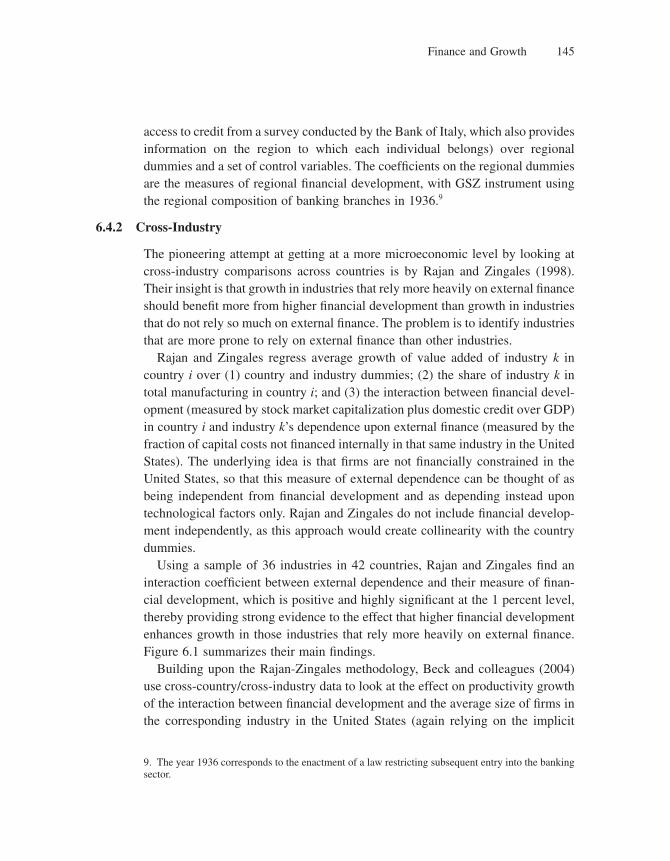
Finance and Growth 145
access to credit from a survey conducted by the Bank of Italy, which also provides information on the region to which each individual belongs) over regional dummies and a set of control variables. The coeffi cients on the regional dummies are the measures of regional fi nancial development, with GSZ instrument using the regional composition of banking branches in 1936.9
6.4.2 Cross-Industry
The pioneering attempt at getting at a more microeconomic level by looking at cross-industry comparisons across countries is by Rajan and Zingales (1998). Their insight is that growth in industries that rely more heavily on external fi nance should benefi t more from higher fi nancial development than growth in industries that do not rely so much on external fi nance. The problem is to identify industries that are more prone to rely on external fi nance than other industries.
Rajan and Zingales regress average growth of value added of industry k in country i over (1) country and industry dummies; (2) the share of industry k in total manufacturing in country i; and (3) the interaction between fi nancial devel-opment (measured by stock market capitalization plus domestic credit over GDP) in country i and industry k’s dependence upon external fi nance (measured by the fraction of capital costs not fi nanced internally in that same industry in the United States). The underlying idea is that fi rms are not fi nancially constrained in the United States, so that this measure of external dependence can be thought of as being independent from fi nancial development and as depending instead upon technological factors only. Rajan and Zingales do not include fi nancial develop-ment independently, as this approach would create collinearity with the country dummies.
Using a sample of 36 industries in 42 countries, Rajan and Zingales fi nd an interaction coeffi cient between external dependence and their measure of fi nan-cial development, which is positive and highly signifi cant at the 1 percent level, thereby providing strong evidence to the effect that higher fi nancial development enhances growth in those industries that rely more heavily on external fi nance. Figure 6.1 summarizes their main fi ndings.
Building upon the Rajan-Zingales methodology, Beck and colleagues (2004) use cross-country/cross-industry data to look at the effect on productivity growth of the interaction between fi nancial development and the average size of fi rms in the corresponding industry in the United States (again relying on the implicit
9. The year 1936 corresponds to the enactment of a law restricting subsequent entry into the banking sector.
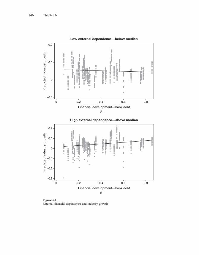
Chapter 6146
Figure 6.1External fi nancial dependence and industry growth
Financial development—bank debt
0 0.2 0.4 0.6 0.8
0.2
0.1
0
–0.1
–0.2
–0.3
Pre
dic
ted
ind
ust
ry g
row
th
High external dependence—above median
Pre
dic
ted
ind
ust
ry g
row
th
Financial development—bank debt
0 0.2 0.4 0.6 0.8
0.2
0.1
0
–0.1
Low external dependence—below median
A
B
Finance and Growth 147
assumption that only technological factors, not fi nancial market frictions, deter-mine this average size in the United States). They fi nd that higher fi nancial development enhances growth in those industries that comprise a higher fraction of small fi rms. This result is consistent with previous work by Bernanke, Gertler, and Gilchrist (1999) suggesting that smaller fi rms face tighter credit constraints than large fi rms.
6.5 Conclusion
In this chapter we have introduced fi nancial constraints into the Schumpeterian growth framework and confronted the prediction that growth should increase with fi nancial development using existing empirical evidence from cross-country and cross-industry data. We have also discussed the relationship between wealth inequality and growth in an economy with credit constraints.
In the next chapter we will go one step further and show that by interacting a country’s level of fi nancial development with its level of technological develop-ment, one can account for observed convergence and divergence patterns. In chapter 14 we will again bring fi nancial constraints into the picture, but this time to analyze the interplay between macroeconomic volatility and growth, and the potentially growth-enhancing role of countercyclical fi scal policies.
6.6 Literature Notes
The pioneering authors to point out the importance of the relationship between fi nance and growth include Bagehot (1873), Schumpeter (1912). Gurley and Shaw (1955), Goldsmith (1969), and McKinnon (1973).
Ever since, much has been done to improve our understanding of the issue, on both theoretical and empirical grounds. On the theory side, it has been empha-sized that fi nancial intermediaries, markets, or contracts can (1) help produce and process information and improve resource allocation (Boyd and Prescott 1986), (2) allocate capital in a more effi cient way by producing better information on fi rms and funding more promising fi rms (Greenwood and Jovanovic 1990), (3) enhance the rate of technological innovation by identifying entrepreneurs with the best chances of successfully starting new productive processes (King and Levine 1993b), (4) boost corporate governance and therefore infl uence growth (Bencivenga and Smith 1993), (5) facilitate the trading, hedging, and pooling of risk with positive implications for growth (Acemoglu and Zilibotti 1997),
Chapter 6148
(6) promote the accumulation of physical and human capital in economies with wealth inequality and credit constraints and thereby accelerate economic growth (Banerjee and Newman 1993; Galor and Zeira 1993; Aghion and Bolton 1997; Piketty 1997), and (7) lower transaction costs and promote greater specialization, innovation, and growth (Greenwood and Smith 1996).
Our formulation of the credit multiplier closely follows Bernanke and Gertler (1989).
On the empirical side; following pioneering work by Goldsmith (1969), the fi rst seminal contribution is by King and Levine (1993a), who used cross-country data to analyze whether fi nancial development predicts long-run economic growth, capital accumulation, and productivity growth. The second seminal con-tribution is the paper by Rajan and Zingales (1998) that explored multicountry sectoral-level data and the extent to which corresponding sectors depend upon external fi nance in the United States, to produce regressions that control for country fi xed effects and truly capture the causality from fi nancial development to growth (i.e., that address the issue of the endogeneity of fi nancial develop-ment). Demirgüç-Kunt and Maksimovic (1998) used a similar methodology to analyze the relationship between growth and fi nance at the fi rm level. Levine and Zervos (1998) add measures of stock market development and study the relation-ship between these latter measures and economic growth. Several econometric techniques have been recently used to get more precise measures of the role of the fi nancial sector on economic growth, such as panel data (Levine, Loayza, and Beck 2000; Rousseau and Wachtel 2000) and time-series analysis (Rousseau and Wachtel 1998; Arestis, Demetriades, and Luintel 2001). Case studies have also been undertaken, such as Jayaratne and Strahan (1996), who examine individual states of the United States, and Guiso, Sapienza, and Zingales (2002), for indi-vidual regions of Italy.
A complete and extensive survey on the topic of this chapter can be found in Levine (2005).
Problems
1. Present different channels whereby fi nancial development can foster growth. Levine, Loayza, and Beck (2000) use the legal origins indicators of La Porta and colleagues (1998) as instruments for fi nancial development in cross-country regressions. Explain intuitively how legal origins (i.e., the type of legal system adopted by a country) can affect subsequent fi nancial development.
2. Causal effect of fi nancial development on economic growth
As discussed in the empirical section, though there exists a correlation between measures of fi nancial development and economic growth, it is very diffi cult to establish causality. To address this
Finance and Growth 149
endogeneity problem, Levine (1998, 1999) and Levine, Loayza, and Beck (2000) use the legal origins indicators of La Porta and colleagues (1998) as instruments for fi nancial development. That is, the regression exercise involves a fi rst stage where fi nancial development is regressed over dummy vari-ables for Anglo-Saxon, French and, German legal origins (against Scandinavian legal origins), respectively, and a second-stage regression where average productivity growth is regressed over pre-dicted fi nancial development as derived from the fi rst-stage regression and the same control variables as were used in the basic regression exercise.
Do you think legal origins is a good instrument to establish causality between fi nancial development and growth? Discuss.
Can you think of any innovative ways to fi nd exogenous variation in fi nancial development (either across country or within country) to test the hypothesis that fi nancial development has a causal effect on economic growth?
3. Liquidation value and R&D
Consider the model with ex ante screening presented in the beginning of the chapter. In the basic case, when the capable innovator is unsuccessful, the project yields a payoff of zero. Instead, now consider a case in which, when the capable innovator is unsuccessful, the project yields an expected payoff of gNt, for g < 1. This payoff can be interpreted as a liquidation value of the unsuccessful project. Assume that the liquidation value is completely observable by the bank when the project fails, and thus the innovator cannot run away with it.
Then the combined payoff to the capable innovator and her bank will be the expected profi t of a successful innovation plus the expected liquidation value of an unsuccessful innovation minus the R&D cost minus the screening cost
μδ μ γφ
A N fN
t tt
− + −( ) −1 1
a. Solve for the equilibrium probability of innovation and the optimal growth rate.
b. Show that the bank’s lending is greater if the liquidation value is greater.
4. *Income distribution and human capital
The economy lasts for two periods. In period 1, an individual works for wage w, consumes c, saves s, and decides the level of education investment on behalf of his child, e. He dies at the end of the period. Utility of household i is given by
U c bi i i= + −( ) < <α α αlog log1 0 1where
in which bi is the consumption of the child. The innate abilities of children vary across households, and therefore the cost of education varies across households. Assume that the cost of education for household i is qiei. In the second period, individuals receive a wage w(e). Based on the Mincerian regression, assume that w′(e) > 0 and w″(e) < 0. Assume that households can lend at interest rate r and borrow at interest rate R. The rate of borrowing and lending may differ based on contractual frictions present in the economy.
a. Consider the case in which the credit-market frictions are absent and therefore R = r. Characterize the household’s decision problem. Show that the choice of education is independent of the form of the utility function.
b. Now introduce a case in which, owing to contractual problems, no one is willing to lend money to the households. That is, the households can lend at r, but cannot borrow going from period 1 to period 2 (or R = +∞). Show that the education and consumption decisions are no longer separable.
c. Discuss how the results in parts a and b differ based on (i) the relative weight the household places on its children’s consumption as measured by a; (ii) the initial level of income as measured by wi.

7 Technology Transfer and Cross-Country Convergence
7.1 Introduction
The history of cross-country income differences exhibits mixed patterns of con-vergence and divergence. The most striking pattern over the long run is the “great divergence”—Pritchett (1997) estimates that the proportional gap in living stan-dards between the richest and poorest countries grew more than fi vefold from 1870 to 1990. More recent evidence (after 1960) points to convergence—the results of Barro and Sala-i-Martin (1992a), Mankiw, Romer, and Weil (1992), and Evans (1996) seem to imply that most countries are converging to parallel growth paths. But many poor countries are continuing to diverge—the propor-tional gap in per capita income between Mayer-Foulkes’s (2002) richest and poorest convergence groups grew by a factor of 2.6 between 1960 and 1995, and the proportional gap between Maddison’s (2001) richest and poorest groups grew by a factor of 1.75 between 1950 and 1998.
Thus it seems that there has been “club convergence” since the mid-20th century. Most rich and middle-income countries belong to the convergence club, the group with a common long-run growth rate, whereas many poor countries have been excluded from that club and have strictly lower long-run growth rates.
Club convergence poses a problem for neoclassical theory, which implies absolute convergence in growth rates and thus implies that all countries should be members of the same club. It also poses a problem for AK theory, which implies independent growth rates, suggesting that there should be no convergence club at all. However, it does not pose a problem for Schumpeterian theory. The main purpose of this chapter is to show how Schumpeterian theory can account for club convergence by taking into account the important phenomenon of “tech-nology transfer” and the related idea of “distance to the frontier.”
We start with Gerschenkron’s (1962) observation that a country far from the world technology frontier has a certain “advantage of backwardness,” because it can grow rapidly simply by adopting technologies that have already been devel-oped in more advanced countries. We model that advantage by supposing that in every country the technology that a successful innovator gets to implement embodies ideas from around the world, so “technology transfer” takes place from other countries whenever an innovation takes place.
Technology transfer will stabilize the gap between rich and poor countries, thus allowing the poor countries to grow as fast as the rich, but only if the poor countries devote resources to innovation, because innovation is the process
Chapter 7152
through which technology is transferred. If a country fails to innovate, then it will stagnate while the rest of the world continues to advance. The convergence club will consist of the countries that continue to innovate.
The reason why innovation is necessary for technology transfer to take place is that technological knowledge is often tacit and circumstantially specifi c.1 It cannot simply be copied and transplanted costlessly to another country. Instead, the receiving country must invest resources in order to master the technology and adapt it to local conditions. This investment may not look like the frontier R&D that takes place in leading industrial countries, but analytically it has all the same characteristics as R&D—it is a costly activity that builds on the ideas of others to create something new in a particular environment.2 Although implementing a foreign technology may be easier than inventing an entirely new one, this is a difference in degree, not in kind.
7.2 A Model of Club Convergence
7.2.1 Basics
The model is the same as the multisectoral Schumpeterian model of chapter 4, except for the specifi cation of the innovation technology. Time is discrete. Indi-viduals live for one period and have linear preferences in consumption. There is one fi nal good, which is produced by labor and intermediate products according to
Y L A x dit it it= < <− −∫1 1
0
10 1α α α α,
where xit is the input of intermediate product i and Ait is its productivity parameter. We set L = 1.
The fi nal good is produced under perfect competition, so the price of each intermediate good equals its marginal product:
p A xit it it= − −α α α1 1
As in previous chapters, each intermediate good i is produced one for one by a monopolist, using the fi nal good as input. The monopolist will choose xit to maximize her profi t
1. See Arrow (1969) and Evenson and Westphal (1995).
2. Cohen and Levinthal (1989) and Griffi th, Redding, and Van Reenan (2004) have also argued that R&D by the receiving country is a necessary input to technology transfer.
Technology Transfer and Cross-Country Convergence 153
Πit it it it it it itp x x A x x= − = −−α α α1
which gives the equilibrium quantity
x Ait it= −α α2
1
and profi t
Πit itA= π *
where π α ααα= −( )
+−1
1
1 is the same constant as before.The probability of success m of the potential innovator in each sector is again
an increasing function f(n) of her productivity-adjusted research expenditure n = Rit /Ait*, where Rit is her R&D expenditure and Ait* her target productivity level. As in the previous chapter, she chooses the probability m to maximize her expected payoff
μ μπ μΠit it itR n A− = − ( )⎡⎣ ⎤⎦� (7.1)
where ñ(m) is her productivity-adjusted R&D cost—the value of n such that f(n) = m.
7.2.2 Innovation
At this point we make a small but important departure from the basic Schumpet-erian model. In that basic model we assumed an innovation production function in which the marginal product of research f′(n) becomes infi nite when no research is done.3 This assumption is equivalent to assuming that the marginal cost ñ′(m) is zero when m = 0. For example, in the previous chapter the innovation cost function was ñ(m) = ym2/2, which has ñ′(0) = 0. This feature helps to simplify the analysis in the same way that the Inada conditions help to simplify the neo-classical model, namely, by ruling out corner solutions. More specifi cally, it means that some research will always be done, no matter how small the productivity-adjusted profi t p, because otherwise there would be a positive mar-ginal gain and a zero marginal cost.
For understanding club convergence it is important to drop this simplifying assumption, so as to allow for the possibility that some countries might do no research. Accordingly we now assume that
�n μ ημ ψμ( ) = + 2 2 (7.2)
3. That is, with f(n) = lns we have f′(n) = slns−1, which approaches ∞ as n → 0 because s < 1.

Chapter 7154
where both parameters h and y are strictly positive.4 The marginal cost is now
� ′( ) = +n μ η ψμ
which is strictly positive even when m = 0. In addition, we assume
η ψ π+ <
which will guarantee that the equilibrium innovation probability is less than one.
With this new form of the innovation cost function, there are two cases to consider:
Case 1 If
η π<
then the reward to an innovation is large enough (relative to the cost) that produc-ers will innovate at a positive rate. That is, the fi rst-order condition for maximiz-ing equation (7.1) is
� ′( ) =n μ π
whose solution is
μ π η ψ= −( ) > 0
Case 2 If
π η≤
then the conditions are so unfavorable to innovation in this country that producers will not innovate. That is, the fi rst-order condition for maximizing equation (7.1) has no positive solution, so the maximization problem is solved by setting m = 0.
7.2.3 Productivity and Distance to Frontier
Assume that a successful innovator in any sector gets to implement a technology with a productivity parameter equal to a level At, which represents the world
4. This implies that the innovation production function has the form
φ λn n( ) = + −( )� �2 (I)
where l = (2/y)1/2 and � = h(2y)−1/2. The function lns that we were using before also has the form (I) when s = 1/2, in which case we have � = h = 0.

Technology Transfer and Cross-Country Convergence 155
technology frontier and which grows at a rate g determined outside the country. So each productivity parameter Ait will evolve according to
AAAit
t
i t
=−
⎧⎨⎪
⎩⎪
⎫⎬⎪
⎭⎪−
with probabilitywith probability
μμ, 1 1
The fact that a successful innovator gets to implement At is a manifestation of the kind of technology transfer that Keller (2002) calls “active”; that is, domestic R&D makes use of ideas developed elsewhere in the world.5
It follows that the country’s average productivity parameter A A dit it= ∫0
1 will
evolve according to
A A At t t= + −( ) −μ μ1 1 (7.3)
That is, in the fraction m of sectors that innovate productivity is At, whereas in the remaining fraction productivity is the same as in period t − 1.
The country’s distance to the world technology frontier is measured inversely by the ratio of its average productivity parameter to the global frontier parameter:
a A At t t=
We call the ratio at the country’s “proximity” to the frontier. Dividing both sides of equation (7.3) by At, we see that at will evolve according to
ag
at t= + −+ −μ μ1
1 1 (7.4)
There is a unique steady-state proximity a*, which is defi ned by setting at = at+1 in equation (7.4):
ag
g* =
+( )+
1 μμ
(7.5)
5. Aghion, Howitt, and Mayer-Foulkes (2005) explore the more general case:
AbA b A
Aitt i t
i t
=+ −( )
−−
−
1
11
1
,
,
with probability
with probability
μμμ
⎧⎨⎪
⎩⎪
⎫⎬⎪
⎭⎪
where b is a real number between 0 and 1.

Chapter 7156
Moreover, this is a stable steady state because the coeffi cient of at−1 in equation (7.4) lies between zero and one.6 Therefore, a* will be the country’s long-run proximity to the frontier.
7.2.4 Convergence and Divergence
The fi rst result from this model is as follows:
Result 1 All countries with p > h will grow at the same rate in the long run.
In other words, all countries that innovate at a positive rate will converge to the same growth rate. The reason for this convergence result is that, because of technology transfer, the further behind the frontier a country is initially, the bigger the average size of its innovations:
γ − = − = +( ) −− −1 1 1 11 1A A g at t t
Because the country’s growth rate is just the frequency times the size of innovations,7
gt = −( )μ γ 1
Therefore, the further behind the frontier the country is, the higher its growth rate will be. This fact limits how far behind the frontier a country can fall, because
6. Subtracting a* from both sides of equation (7.4) and using the fact that μ μ− = − −+
ag
a* *1
1
yields
a ag
a at t− = −+
−( )−* *1
1 1
μ
Starting with an initial proximity a0 and iterating on this formula shows that
a ag
a at
t
− = −+
⎛⎝⎜
⎞⎠⎟
−( )* *1
1 0
μ
which approaches zero as t → ∞.
7. To see this point, note that, by defi nition,
gA
Ag
a
att
t
t
t
= − = +( )⎛⎝⎜
⎞⎠⎟
−− −1 1
1 1 1
Using equation (7.4) to replace at in this formula yields
g ga g
g
att t
= +( ) + −+
⎛⎝⎜
⎞⎠⎟
− = + −⎛⎝⎜
⎞⎠⎟
= −( )− −
11
11
11 1
1 1
μ μ μ μ γ

Technology Transfer and Cross-Country Convergence 157
eventually it will get so far behind that its growth rate will be just as large as the growth rate of the frontier, at which point the gap will stop increasing.
Formally, we get the result because in this case m > 0 (case 1), so the country’s steady-state proximity (7.5) will be strictly positive. In turn, in the long run,At will be proportional to At:
A a At t= >* 0
Therefore, the long-run growth rate will be the growth rate g of the world pro-ductivity frontier:
A
A
a A
a A
A
Agt
t
t
t
t
t
+ + += = = +1 1 1 1*
*
However, we also have the following results:
Result 2 All countries with p ≤ p will stagnate in the long run.
That is, countries with poor macroeconomic conditions, legal environment, education system, or credit markets will not innovate in equilibrium, and there-fore they will not benefi t from technology transfer, but will instead stagnate. Formally, for these countries the fact that m = 0 means that their equilibrium proximity to the frontier a* is zero.
Together these two results help to explain the facts about club convergence discussed in the introduction (section 7.1). That is, there is one group of countries that are converging to parallel growth paths (i.e., with identical long-run growth rates) and another group of countries that are falling further and further behind.
Notice that even countries that are converging to parallel growth paths are not necessarily converging in levels. That is, one country’s steady-state proximity to the frontier (7.5) can differ from another’s if they have different values of the critical parameters p, h, and y:
Result 3 For countries with p > h, a* is increasing in p and decreasing in h and y.
Intuitively, if a country improves its education system, for example (thereby reducing the cost parameters h and y), it will start to grow faster for a while. As it approaches closer to the frontier, the fact that its size of innovations is getting smaller will bring its growth rate back to g, but the end result will be that it is now permanently closer to the frontier. This result helps us to account for the fact that there are systematic and persistent differences across countries in the

Chapter 7158
level of productivity. That is, convergence in levels is not absolute but condi-tional. In our model, two countries will end up with the same productivity levels in the long run if they have the same parameter values, but not otherwise.
Finally, the following result is derived from equation (7.5):
Result 4 For countries p > h, a* is decreasing in g.
That is, a speedup of the global frontier will result in a spreading out of the cross-country productivity distribution. Howitt and Mayer-Foulkes (2005) have used this result to shed light on the “great divergence” discussed in section 7.1. Their argument is that some time around or after the industrial revolution there was a speedup in world technology growth associated with the spread of scientifi c methodology and its application to industrial R&D. Countries that did not take part directly in this change (those whose parameter values remained the same) eventually benefi ted from technology transfer at an increased rate, but only after they fell further behind. In the long run they were able to grow at the new higher rate but only because their increasing distance to the frontier raised the size of innovations in those countries.
Elsewhere (Aghion and Howitt 2006) we have also used this result to help explain why the gap between Europe and the United States stopped closing some time in the 1970s or 1980s and started rising again. Our argument was that from the end of World War II until some time in the 1970s or 1980s, Europe was catching up to the frontier, but that during the 1990s there was an acceleration of productivity growth in the United States, associated with the revolution in information technology, which caused the frontier growth rate to increase. Because for the most part this wave of frontier innovations did not initiate in Europe, it could not produce a higher European growth rate until Europe had fallen further behind the frontier.
7.3 Credit Constraints as a Source of Divergence*
The preceding framework can be further developed by assuming that while the size of innovations increases with the distance to the technological frontier (because of technology transfer), the frequency of innovations depends upon the ratio between the distance to the technological frontier and the current stock of skilled workers. Howitt and Mayer-Foulkes (2005) show that this enriched frame-work can explain not only why some countries converge while others stagnate
*This section is more diffi cult than average and can be skipped.
Technology Transfer and Cross-Country Convergence 159
but also why even countries with a positive long-run growth rate may diverge. Benhabib and Spiegel (2005) develop a similar account of divergence and show the importance of human capital in the process.
In this section we instead explore credit constraints as a reason why the fre-quency of innovations might fall when a country falls further behind the frontier. We develop a model, based on Aghion, Howitt, and Mayer-Foulkes (2005), that combines elements of the previous section’s model and the previous chapter’s Schumpeterian model of fi nancial constraints.
7.3.1 Theory
We modify the model of the previous section by supposing that research aimed at making an innovation in t must be done at period t − 1. If we assume perfectly functioning fi nancial markets, then nothing happens to the model. But as we already saw in chapter 6, when credit markets are imperfect, an entrepreneur may face a borrowing constraint that limits her investment to a fi xed multiple � of her accumulated net wealth. As in chapter 6, this credit multiplier comes from the possibility that the entrepreneur might defraud her creditor. The multiplier will be bigger in countries where it is more costly to get away with fraud.
We assume a two-period overlapping-generations structure in which the accu-mulated net wealth of an entrepreneur at t is her wage income wt−1 from last period. So she cannot spend more than �wt−1 in research. Since the cost of inno-vating at any rate m is ñ(m)Ait* and the target productivity parameter Ait* is the frontier At, her probability of innovation cannot exceed μt, where
�n A wt t tμ ν( ) = −1 (7.6)
The wage rate wt−1 is the marginal product of labor, which, as we saw in the last chapter, is proportional to At−1:
w At t− −=1 1ω
So dividing equation (7.6) by At and using the fact that At grows at rate g, we can re-express equation (7.6) in terms of our proximity variable:
�n at tμ ων( ) = −1 (7.7)
where w = w /(1 + g). Equation (7.7) determines mt as an increasing function of the credit multiplier � and of lagged proximity at−1. Using the specifi cation (7.2), we can rewrite it as8
8. As explained in footnote 4, f is the innovation production function implied by the cost function ñ.
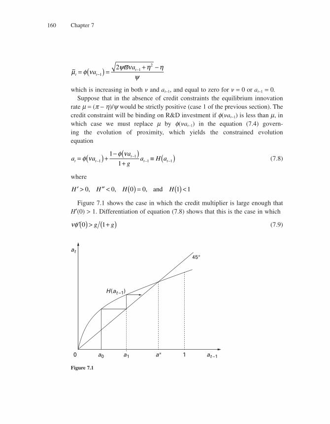
Chapter 7160
μ φ νψϖν η η
ψt tta
a= ( ) =
+ −−
−1
122
which is increasing in both � and at−1, and equal to zero for � = 0 or at−1 = 0.Suppose that in the absence of credit constraints the equilibrium innovation
rate m = (p − h)/y would be strictly positive (case 1 of the previous section). The credit constraint will be binding on R&D investment if f(�at−1) is less than m, in which case we must replace m by f(�at−1) in the equation (7.4) govern-ing the evolution of proximity, which yields the constrained evolution equation
a aa
ga H at t
tt t= ( ) +
− ( )+
≡ ( )−−
− −φ νφ ν
11
1 1
1
1 (7.8)
where
′ > ′′ < ( ) = ( ) <H H H H0 0 0 0 1 1, , , and
Figure 7.1 shows the case in which the credit multiplier is large enough that H′(0) > 1. Differentiation of equation (7.8) shows that this is the case in which
νφ′( ) > +( )0 1g g (7.9)
0 a0 a1 at –1
at
H(at –1)
a* 1
45°
Figure 7.1
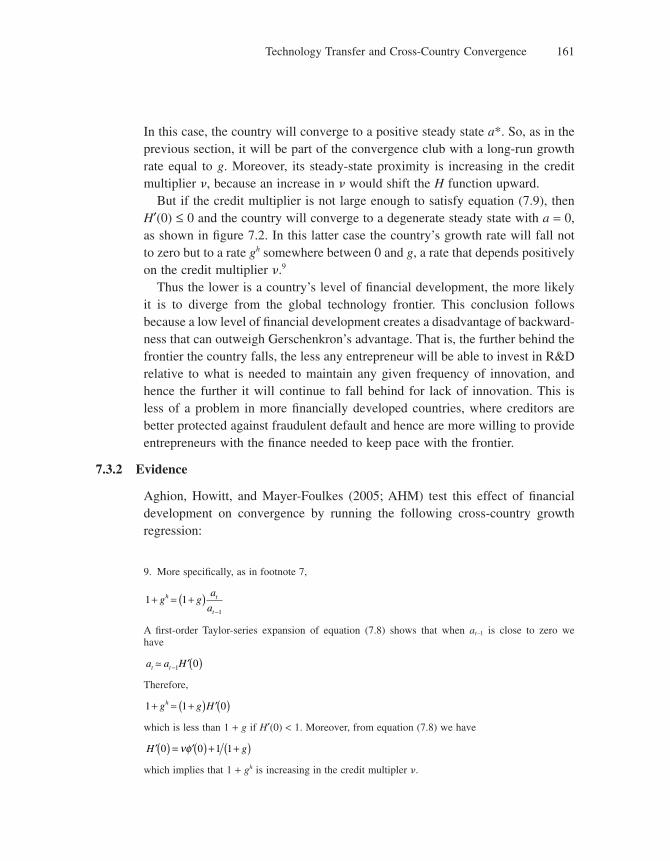
Technology Transfer and Cross-Country Convergence 161
In this case, the country will converge to a positive steady state a*. So, as in the previous section, it will be part of the convergence club with a long-run growth rate equal to g. Moreover, its steady-state proximity is increasing in the credit multiplier �, because an increase in � would shift the H function upward.
But if the credit multiplier is not large enough to satisfy equation (7.9), then H′(0) ≤ 0 and the country will converge to a degenerate steady state with a = 0, as shown in fi gure 7.2. In this latter case the country’s growth rate will fall not to zero but to a rate gh somewhere between 0 and g, a rate that depends positively on the credit multiplier �.9
Thus the lower is a country’s level of fi nancial development, the more likely it is to diverge from the global technology frontier. This conclusion follows because a low level of fi nancial development creates a disadvantage of backward-ness that can outweigh Gerschenkron’s advantage. That is, the further behind the frontier the country falls, the less any entrepreneur will be able to invest in R&D relative to what is needed to maintain any given frequency of innovation, and hence the further it will continue to fall behind for lack of innovation. This is less of a problem in more fi nancially developed countries, where creditors are better protected against fraudulent default and hence are more willing to provide entrepreneurs with the fi nance needed to keep pace with the frontier.
7.3.2 Evidence
Aghion, Howitt, and Mayer-Foulkes (2005; AHM) test this effect of fi nancial development on convergence by running the following cross-country growth regression:
9. More specifi cally, as in footnote 7,
1 11
+ = +( )−
g ga
ah t
t
A fi rst-order Taylor-series expansion of equation (7.8) shows that when at−1 is close to zero we have
a a Ht t� − ′( )1 0
Therefore,
1 1 0+ +( ) ′( )g g Hh �
which is less than 1 + g if H′(0) < 1. Moreover, from equation (7.8) we have
′( ) = ′( ) + +( )H g0 0 1 1νφ
which implies that 1 + gh is increasing in the credit multipler �.
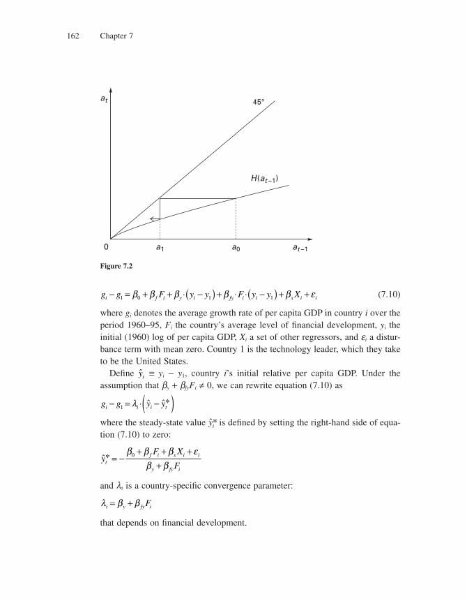
Chapter 7162
g g F y y F y y Xi f i y i fy i i x i i− = + + ⋅ −( ) + ⋅ ⋅ −( ) + +1 0 1 1β β β β β ε (7.10)
where gi denotes the average growth rate of per capita GDP in country i over the period 1960–95, Fi the country’s average level of fi nancial development, yi the initial (1960) log of per capita GDP, Xi a set of other regressors, and ei a distur-bance term with mean zero. Country 1 is the technology leader, which they take to be the United States.
Defi ne yi ≡ yi − y1, country i’s initial relative per capita GDP. Under the assumption that by + bfyFi ≠ 0, we can rewrite equation (7.10) as
g g y yi i i t− = ⋅ −( )1 λ ˆ ˆ*
where the steady-state value ˆ*yi is defi ned by setting the right-hand side of equa-tion (7.10) to zero:
yF X
Ftf i x i i
y fy i
* = −+ + +
+β β β ε
β β0
and li is a country-specifi c convergence parameter:
λ β βi y fy iF= +
that depends on fi nancial development.
0 a0a1 at –1
at
H(at –1)
45°
Figure 7.2

Technology Transfer and Cross-Country Convergence 163
A country can converge to the frontier growth rate if and only if the growth rate of its relative per capita GDP depends negatively on the initial value yi, that is, if and only if the convergence parameter li is negative. Thus the likelihood of convergence will increase with fi nancial development, as implied by the preced-ing theory, if and only if
β fy < 0
The results of running this regression using a sample of 71 countries are shown in table 7.1, which indicates that the interaction coeffi cient bfy is indeed signifi -cantly negative for a variety of different measures of fi nancial development and a variety of different conditioning sets X. The estimation is by instrumental vari-ables, using a country’s legal originsl0 and its legal origins interacted with the initial GDP gap (yi − y1) as instruments for Fi and Fi(yi − y1). The data, estimation methods, and choice of conditioning sets X are all taken directly from Levine, Loayza, and Beck (2000), who found a strongly positive and robust effect of fi nancial intermediation on short-run growth in a regression identical to equation (7.10) but without the crucial interaction term Fi(yi − y1) that allows convergence to depend upon the level of fi nancial development.
AHM show that the results of table 7.1 are surprisingly robust to different estimation techniques, to discarding outliers, and to including possible interaction effects between the initial GDP gap and other right-hand-side variables.
7.4 Conclusion
We have seen that once technology transfer is taken into account, a country’s long-run growth rate may no longer depend on the parameters of that country, because as long as the country remains in the convergence club its growth rate will be the global rate of technological progress, which may be unaffected by local conditions. All the domestic parameter changes that would have changed the country’s growth rate in the absence of technology transfer will now change its relative productivity level.
Thus for convergence club members the Schumpeterian model looks much like the neoclassical model with an exogenous long-run growth rate, where policy changes also have only level effects. The difference is that in the Schumpeterian
10. See LaPorta and colleagues (1998) for a detailed explanation of legal origins and their relevance as an instrument for fi nancial development.

Tabl
e 7.
1G
row
th, F
inan
cial
Dev
elop
men
t, an
d In
itial
GD
P G
ap
Fina
ncia
l D
evel
opm
ent
(F)
Con
ditio
ning
Set
(X
)
Priv
ate
Cre
dit
Liq
uid
Lia
bilit
ies
Ban
k A
sset
sC
omm
erci
al-C
entr
al B
ank
Em
pty
Polic
yaFu
llbE
mpt
yPo
licya
Fullb
Em
pty
Polic
yaFu
llbE
mpt
yPo
licya
Fullb
Coe
ffi ci
ent
esti
mat
esβ f
−0.0
15−0
.013
−0.0
16−0
.029
−0.0
30−0
.027
−0.0
19−0
.020
−0.0
220.
000
0.03
10.
013
(−0.
93)
(−0.
68)
(−0.
78)
(−1.
04)
(−0.
99)
(−0.
90)
(−1.
07)
(−1.
03)
(−1.
12)
(0.0
0)(0
.17)
(0.0
7)β y
1.50
7***
1.19
3*1.
131
2 .64
8***
2.38
8**
2.38
4**
1.89
1***
1.33
5*1.
365
7.16
65.
279
5.64
5(3
.14)
(1.8
6)(1
.49)
(3.1
2)(2
.39)
(2.1
1)(3
.57)
(1.9
3)(1
.66)
(1.0
4)(0
.73)
(0.7
2)β f
y—
——
——
——
——
0.06
1***
0.06
3***
0.06
3***
0.07
6***
0.07
7***
0.07
3***
0.08
1***
0.08
1***
.0.
081*
**−0
.110
−0.1
00−0
.102
(−5.
35)
(−5.
10)
(−4.
62)
(−3.
68)
(−3.
81)
(−3.
55)
(−5.
07)
(−4.
85)
(−4.
46)
(−1.
29)
(−1.
18)
(−1.
14)
Inst
rum
ent
test
p-v
alue
s1s
t-st
age
F-t
est:
F0.
0000
0.00
140.
0024
0.00
440.
0032
0.00
420.
0000
0.00
000.
0000
0.26
540.
2180
0.17
041s
t-st
age
F-t
est:
F(y
−y1)
0.00
000.
0000
0.00
000.
0690
0.00
780.
0088
0.00
100.
0003
0.00
110.
5160
0.27
430.
2962
1st` -s
tage
F-t
est:
L(y
−y1)
0.00
000.
0000
0.00
010.
0003
0.00
020.
0022
0.00
000.
0000
0.00
000.
2329
0.23
150.
4516
Sarg
an t
est
0.53
720.
7255
0.55
730.
2217
0.39
520.
3627
0.84
860.
8816
0.82
790.
9661
0.88
610.
9223
C-t
est
for
L(y
−y1)
0.37
730.
7013
0.46
540.
2700
0.35
490.
2799
0.99
400.
9642
0.84
240.
9482
0.76
800.
8240
C-t
est
for
(y−y
1)0.
6475
0.77
900.
7781
0.62
400.
6341
0.62
260.
7699
0.99
440.
9784
0.97
000.
9818
0.93
20Sa
mpl
e si
ze71
6363
7163
6371
6363
7163
63
The
dep
ende
nt v
aria
ble
g −
g 1 is
the
aver
age
grow
th r
ate
of p
er c
apita
rea
l GD
P re
lativ
e to
the
Uni
ted
Stat
es, 1
960–
95; F
is a
vera
ge fi
nanc
ial d
evel
opm
ent 1
960–
95 u
sing
fou
r al
tern
ativ
e m
easu
res;
an
d y
− y 1
is
the
log
of p
er c
apita
GD
P in
196
0 re
lativ
e to
the
Uni
ted
Stat
es.
a. T
he p
olic
y co
nditi
onin
g se
t in
clud
es a
vera
ge y
ears
of
scho
olin
g in
196
0 (s
choo
l), g
over
nmen
t si
ze (
gov)
, infl
atio
n (p
i), b
lack
mar
ket
prem
ium
(bm
p), a
nd o
penn
ess
to t
rade
(tr
ade)
.b.
The
ful
l co
nditi
onin
g se
t in
clud
es t
he p
olic
y se
t pl
us i
ndic
ator
s of
rev
olut
ions
and
cou
ps (
revc
), p
oliti
cal
assa
ssin
atio
ns (
assa
ss),
and
eth
nic
dive
rsity
(av
elf)
.E
stim
atio
n is
by
IV u
sing
L (
lega
l or
igin
s) a
nd L
(y −
y1)
as
inst
rum
ents
for
F a
nd F
(y −
y1)
. The
num
bers
in
pare
nthe
ses
are
t-st
atis
tics.
Sig
nifi c
ance
at
the
1%, 5
%, a
nd 1
0% l
evel
is
deno
ted
by
***,
**,
and
*, r
espe
ctiv
ely.
Technology Transfer and Cross-Country Convergence 165
model, policy affects the level of productivity, not just the level of physical or human capital per person.
The Schumpeterian approach also helps to account for who belongs to the convergence club and what the growth rate will be for nonmember countries. Moreover, one can easily modify the model so as to endogenize the common growth rate of the club members, by assuming that the world technology frontier grows at a rate that depends positively on the innovation rates mj in all countries j. For example,
g j j
n= ∑ β μ1
where the coeffi cient bj measures the extent to which innovations in country j add to the world’s stock of technological knowledge. With this formulation, the common growth rate of leading countries depends on conditions with respect to the costs and benefi ts of innovation in all the countries undertaking leading-edge R&D.
7.5 Literature Notes
Convergence is one of the most studied topics in the growth literature. A fi rst approach explains convergence as a result of decreasing returns in physical or human capital accumulation. This is the neoclassical approach pioneered by Solow (1956) and subsequently developed by Mankiw, Romer, and Weil (1992) and Barro and Sala-i-Martin (1991, 1995a).
In particular Barro and Sala-i-Martin (1991) have stressed the distinction between absolute convergence (poor countries tend to grow faster per capita than rich ones) and conditional convergence (an economy grows faster the further it is from its own steady-state value). Another important distinction made by Barro and Sala-i-Martin (1992a) is between (1) the fact that growth rates of poor coun-tries are lower than those of their rich counterparts (which they call b-divergence) and (2) the increasing dispersion of income per capita across countries over time (which they call s-divergence).
More recent studies have analyzed the effect of convergence on the world distribution of income. Thus Pritchett (1997) estimates a large increase in the proportional gap in living standards between the richest and poorest countries between 1870 and 1990 (which he refers to as “divergence, bid time”). Sala-i-Martin (2006) gets different results when looking at a more recent time period (1970 to 2000) and claims that there was an overall reduction in global income inequality (which he refers to as “convergence, period”).
Chapter 7166
Based again upon the neoclassical framework, several empirical studies have tried to estimate the speed of convergence using panel data techniques, based on cross-country data, such as Islam (1995) and Caselli, Esquivel, and Lefort (1996), and regional data (Canova and Marcet 1995).
A second approach explains convergence as resulting primarily from cross-country knowledge spillovers. The most natural formulation of this approach uses the Schumpeterian framework, in particular Howitt (2000), who explains club convergence; Howitt and Mayer-Foulkes (2005), who explain convergence and divergence; Keller (2004), who links spillovers and geographical proximity; and more recently Eaton and Kortum (2001), who link convergence with spillovers and trade. The role of credit constraints as a source of divergence is analyzed by Aghion, Howitt, and Mayer-Foulkes (2005).
Evidence on the club-convergence and “twin-peaks” phenomena can be found in the work of Quah (1993, 1996, 1997), Durlauf and Johnson (1995), and Mayer-Foulkes (2002).
Problems
1. Contrast the factors driving convergence in the Schumpeterian and AK models. Describe intui-tively how the Schumpeterian approach can explain “club convergence.”
2. Convergence concepts
Suppose the world consists of fi ve countries whose outputs are given by
Y Aegt1 =
Y AB
tegt
2 1= +
+⎛⎝⎜
⎞⎠⎟
Y Bek
tt
3
1
1 2=+
+
⎛⎝⎜
⎞⎠⎟
Y Aeg
tt
4
1
1=+
+⎛⎝⎜
⎞⎠⎟
Y B e elt kt5 = +( )−
where A, B, k, and g are all positive and l > g.
a. Which countries converge to the same growth rates as t → ∞?
b. Which countries converge to the same growth paths as t → ∞?
c. A model exhibits conditional convergence if countries with the same underlying parameters always converge to the same growth paths regardless of the initial conditions. Does the model in section 7.2 exhibit conditional convergence?
3. Alternative diffusion technologies, part 1
Consider a model identical to the one that is given in section 7.2, except that the R&D investment equation is given by

Technology Transfer and Cross-Country Convergence 167
N c A
e At t
t
= ( )= −( )
μα βμ 1
where a, b > 0.
a. Write down the maximization problem of an innovator at time t.
b. Solve for the equilibrium probability of innovation m.
c. Give a condition on a, b, and p that guarantees a positive innovation rate in equilibrium.
d. Solve for the steady-state proximity to frontier, a*. How does a* depend on a and b?
4. *Alternative diffusion technologies, part 2
Consider the model in section 7.2, but with the following innovation technology:
Ag A
Aitt it
it it
=+( )
−⎧⎨ −
−
1
11
1
with probability
with probability
μμ⎩⎩
N c a
a A
it it t
itit
t t
= ( )= +
⎛⎝⎜
⎞⎠⎟
−
−
μ
ημ δ μ1
2
12
2
where At = (1 + g)At−1 as before.In this economy the size and the cost of innovations both depend on the economy’s current technol-
ogy level.
a. Write down the maximization problem of an innovator in sector i at time t.
b. Noting from part a that the equilibrium probability of innovation must be constant across sectors, solve for the equilibrium probability of innovation mt.
c. Show that the proximity to frontier at satisfi es the following difference equation:
ag
gat
tt= +
+ −1
1 1
μ
d. What is the steady-state proximity to frontier, a*, in this economy?
e. Give intuition for why the proximity to frontier converges to this steady state.
f. Suppose that the R&D investment equation was given by
N a Ait itit
t t= +⎛⎝⎜
⎞⎠⎟ −ημ δ μ2
12.
How will the proximity to frontier evolve in this case?
5. Skilled-labor-based technology transfer (based on Howitt and Mayer-Foulkes 2005)
Suppose R&D requires skilled labor. Specifi cally, let the probability of innovation in sector i at time t, mit, be given by
μ ηη η
itit it
t
S Z
A= < <
−1
0 1,
where Sit is the skill level of the innovator and Zit is the amount of fi nal good invested in R&D in sector i. The remainder of the model is the same as in section 7.2.

Chapter 7168
a. Show that an innovator with skill level Sit chooses her R&D investment such that
μ η πη
ηit
it
t
S
A= −( )⎡⎣ ⎤⎦
−
11
b. Assume that the skill level of innovators in a country is proportional to the country’s average pro-ductivity the previous period: Sit = xAt−1. Derive a difference equation governing at.
c. Solve for the steady-state growth rate g* and proximity to frontier a*. How do the steady-state solutions depend on the quality-of-education parameter x?
6. *Stochastic technology transfer (based on Eaton and Kortum 2002 and Melitz 2003)
Consider the following variant of the model presented in section 7.2. There is one potential innovator per sector per period. To innovate, the entrepreneur must pay a fi xed cost d. Her productivity Ait is then drawn from a uniform distribution on [Ait−1, At ].
a. Show that the innovator will choose to pay the fi xed cost if and only if δ π≤ +( )−2 1A At it .
b. What restriction on d ensures innovation when Ait is drawn from a uniform distribution on [0, At ]?
c. Show that if d satisfi es the restriction from part b, then
Eaa
git
it= ++( )
⎛
⎝⎜
⎞
⎠⎟−1
21
11
2
2
d. Suppose d satisfi es the restriction from part b in every sector. Use the law of large numbers to argue that
aa
gt
t= ++( )
⎛
⎝⎜
⎞
⎠⎟−1
21
11
2
2
Find the steady-state proximity to frontier a*, assuming that the innovator always pays the fi xed cost.
e. Suppose d = xAt . Show that the innovator pays the fi xed cost if and only if ait−1 ≤ â, where
a g= −⎛⎝⎜
⎞⎠⎟
+( )12
1ξ
π
f. Describe the dynamics governing proximity to the frontier in the case â > a* and in the case â < a*, where a* is the steady-state proximity to frontier derived in part d. (Hint: You may fi nd it useful to plot Eait as a function of ait−1.)
8 Market Size and Directed Technical Change
8.1 Introduction
In all the innovation-based growth models we have seen so far, innovations take place with the same average frequency in all intermediate sectors. In reality, however, some sectors are persistently more innovative than others. A major reason for this difference among sectors has to do with their size. Other things equal, it is more profi table to innovate in a larger sector because a successful innovator has a larger market there. As a result, technical change tends to be directed more toward larger sectors than smaller ones.
The present chapter explores the “market-size” effect on the direction of tech-nical change and draws out some of its economic implications. It is based on a series of papers by Acemoglu with different coauthors, and it is organized as follows. We begin in section 8.2 with an important microeconomic example, namely, the pharmaceutical industry, where innovations are systematically directed toward drugs that are used by wealthier customers. Section 8.3 shows how the market-size effect can help to explain the recent upsurge in wage inequal-ity in developed countries. Section 8.4 shows how the same market-size effect can help account for cross-country productivity differences, using an explanation that is different from the one presented in the previous chapter.
8.2 Market Size in Drugs
8.2.1 Theory
Consider a small open economy in discrete time. The economy is populated by one-period-lived individuals. Each period, there are two kinds (or groups) of individuals, indexed by j ∈ {1,2}. There are three goods in the economy: a basic good that everyone needs to consume and two types of drugs, also indexed by j ∈ {1,2}. Each drug is produced one for one using the basic good. Group j only cares for drug j. Let Ajt denote the quality of drug j at date t, and xjt the quantity of drug j produced at date t.
An individual i who belongs to group j derives utility from consuming the fi nal good and the drug, according to
U c A xit it jt ijt= ( ) ( )−1 α α
where cit is individual i’s consumption of the basic good and xijt is her consump-tion of drug j, at date t.

Chapter 7160
μ φ νψϖν η η
ψt tta
a= ( ) =
+ −−
−1
122
which is increasing in both � and at−1, and equal to zero for � = 0 or at−1 = 0.Suppose that in the absence of credit constraints the equilibrium innovation
rate m = (p − h)/y would be strictly positive (case 1 of the previous section). The credit constraint will be binding on R&D investment if f(�at−1) is less than m, in which case we must replace m by f(�at−1) in the equation (7.4) govern-ing the evolution of proximity, which yields the constrained evolution equation
a aa
ga H at t
tt t= ( ) +
− ( )+
≡ ( )−−
− −φ νφ ν
11
1 1
1
1 (7.8)
where
′ > ′′ < ( ) = ( ) <H H H H0 0 0 0 1 1, , , and
Figure 7.1 shows the case in which the credit multiplier is large enough that H′(0) > 1. Differentiation of equation (7.8) shows that this is the case in which
νφ′( ) > +( )0 1g g (7.9)
0 a0 a1 at –1
at
H(at –1)
a* 1
45°
Figure 7.1

Technology Transfer and Cross-Country Convergence 161
In this case, the country will converge to a positive steady state a*. So, as in the previous section, it will be part of the convergence club with a long-run growth rate equal to g. Moreover, its steady-state proximity is increasing in the credit multiplier �, because an increase in � would shift the H function upward.
But if the credit multiplier is not large enough to satisfy equation (7.9), then H′(0) ≤ 0 and the country will converge to a degenerate steady state with a = 0, as shown in fi gure 7.2. In this latter case the country’s growth rate will fall not to zero but to a rate gh somewhere between 0 and g, a rate that depends positively on the credit multiplier �.9
Thus the lower is a country’s level of fi nancial development, the more likely it is to diverge from the global technology frontier. This conclusion follows because a low level of fi nancial development creates a disadvantage of backward-ness that can outweigh Gerschenkron’s advantage. That is, the further behind the frontier the country falls, the less any entrepreneur will be able to invest in R&D relative to what is needed to maintain any given frequency of innovation, and hence the further it will continue to fall behind for lack of innovation. This is less of a problem in more fi nancially developed countries, where creditors are better protected against fraudulent default and hence are more willing to provide entrepreneurs with the fi nance needed to keep pace with the frontier.
7.3.2 Evidence
Aghion, Howitt, and Mayer-Foulkes (2005; AHM) test this effect of fi nancial development on convergence by running the following cross-country growth regression:
9. More specifi cally, as in footnote 7,
1 11
+ = +( )−
g ga
ah t
t
A fi rst-order Taylor-series expansion of equation (7.8) shows that when at−1 is close to zero we have
a a Ht t� − ′( )1 0
Therefore,
1 1 0+ +( ) ′( )g g Hh �
which is less than 1 + g if H′(0) < 1. Moreover, from equation (7.8) we have
′( ) = ′( ) + +( )H g0 0 1 1νφ
which implies that 1 + gh is increasing in the credit multipler �.

Chapter 7162
g g F y y F y y Xi f i y i fy i i x i i− = + + ⋅ −( ) + ⋅ ⋅ −( ) + +1 0 1 1β β β β β ε (7.10)
where gi denotes the average growth rate of per capita GDP in country i over the period 1960–95, Fi the country’s average level of fi nancial development, yi the initial (1960) log of per capita GDP, Xi a set of other regressors, and ei a distur-bance term with mean zero. Country 1 is the technology leader, which they take to be the United States.
Defi ne yi ≡ yi − y1, country i’s initial relative per capita GDP. Under the assumption that by + bfyFi ≠ 0, we can rewrite equation (7.10) as
g g y yi i i t− = ⋅ −( )1 λ ˆ ˆ*
where the steady-state value ˆ*yi is defi ned by setting the right-hand side of equa-tion (7.10) to zero:
yF X
Ftf i x i i
y fy i
* = −+ + +
+β β β ε
β β0
and li is a country-specifi c convergence parameter:
λ β βi y fy iF= +
that depends on fi nancial development.
0 a0a1 at –1
at
H(at –1)
45°
Figure 7.2
Technology Transfer and Cross-Country Convergence 163
A country can converge to the frontier growth rate if and only if the growth rate of its relative per capita GDP depends negatively on the initial value yi, that is, if and only if the convergence parameter li is negative. Thus the likelihood of convergence will increase with fi nancial development, as implied by the preced-ing theory, if and only if
β fy < 0
The results of running this regression using a sample of 71 countries are shown in table 7.1, which indicates that the interaction coeffi cient bfy is indeed signifi -cantly negative for a variety of different measures of fi nancial development and a variety of different conditioning sets X. The estimation is by instrumental vari-ables, using a country’s legal originsl0 and its legal origins interacted with the initial GDP gap (yi − y1) as instruments for Fi and Fi(yi − y1). The data, estimation methods, and choice of conditioning sets X are all taken directly from Levine, Loayza, and Beck (2000), who found a strongly positive and robust effect of fi nancial intermediation on short-run growth in a regression identical to equation (7.10) but without the crucial interaction term Fi(yi − y1) that allows convergence to depend upon the level of fi nancial development.
AHM show that the results of table 7.1 are surprisingly robust to different estimation techniques, to discarding outliers, and to including possible interaction effects between the initial GDP gap and other right-hand-side variables.
7.4 Conclusion
We have seen that once technology transfer is taken into account, a country’s long-run growth rate may no longer depend on the parameters of that country, because as long as the country remains in the convergence club its growth rate will be the global rate of technological progress, which may be unaffected by local conditions. All the domestic parameter changes that would have changed the country’s growth rate in the absence of technology transfer will now change its relative productivity level.
Thus for convergence club members the Schumpeterian model looks much like the neoclassical model with an exogenous long-run growth rate, where policy changes also have only level effects. The difference is that in the Schumpeterian
10. See LaPorta and colleagues (1998) for a detailed explanation of legal origins and their relevance as an instrument for fi nancial development.
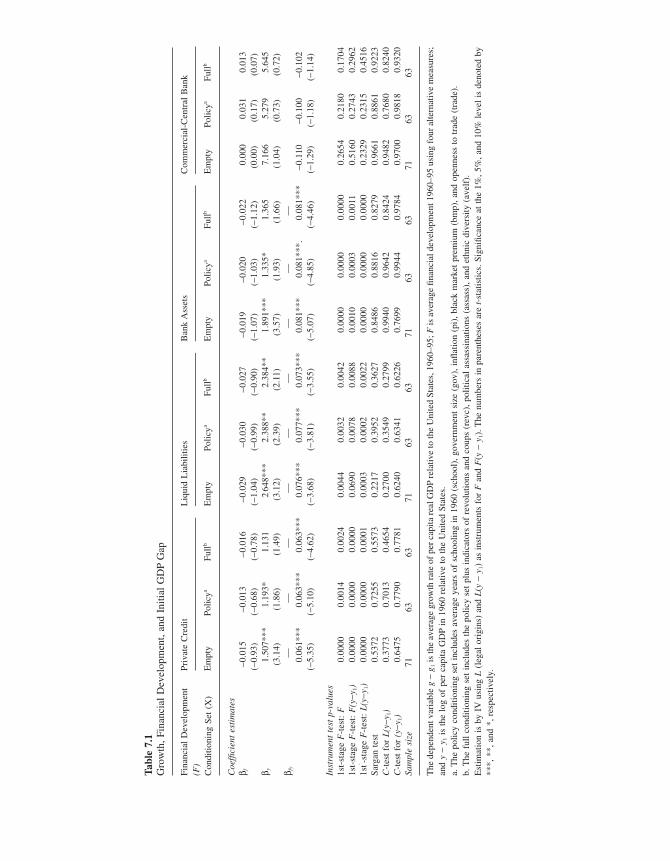
Tabl
e 7.
1G
row
th, F
inan
cial
Dev
elop
men
t, an
d In
itial
GD
P G
ap
Fina
ncia
l D
evel
opm
ent
(F)
Con
ditio
ning
Set
(X
)
Priv
ate
Cre
dit
Liq
uid
Lia
bilit
ies
Ban
k A
sset
sC
omm
erci
al-C
entr
al B
ank
Em
pty
Polic
yaFu
llbE
mpt
yPo
licya
Fullb
Em
pty
Polic
yaFu
llbE
mpt
yPo
licya
Fullb
Coe
ffi ci
ent
esti
mat
esβ f
−0.0
15−0
.013
−0.0
16−0
.029
−0.0
30−0
.027
−0.0
19−0
.020
−0.0
220.
000
0.03
10.
013
(−0.
93)
(−0.
68)
(−0.
78)
(−1.
04)
(−0.
99)
(−0.
90)
(−1.
07)
(−1.
03)
(−1.
12)
(0.0
0)(0
.17)
(0.0
7)β y
1.50
7***
1.19
3*1.
131
2 .64
8***
2.38
8**
2.38
4**
1.89
1***
1.33
5*1.
365
7.16
65.
279
5.64
5(3
.14)
(1.8
6)(1
.49)
(3.1
2)(2
.39)
(2.1
1)(3
.57)
(1.9
3)(1
.66)
(1.0
4)(0
.73)
(0.7
2)β f
y—
——
——
——
——
0.06
1***
0.06
3***
0.06
3***
0.07
6***
0.07
7***
0.07
3***
0.08
1***
0.08
1***
.0.
081*
**−0
.110
−0.1
00−0
.102
(−5.
35)
(−5.
10)
(−4.
62)
(−3.
68)
(−3.
81)
(−3.
55)
(−5.
07)
(−4.
85)
(−4.
46)
(−1.
29)
(−1.
18)
(−1.
14)
Inst
rum
ent
test
p-v
alue
s1s
t-st
age
F-t
est:
F0.
0000
0.00
140.
0024
0.00
440.
0032
0.00
420.
0000
0.00
000.
0000
0.26
540.
2180
0.17
041s
t-st
age
F-t
est:
F(y
−y1)
0.00
000.
0000
0.00
000.
0690
0.00
780.
0088
0.00
100.
0003
0.00
110.
5160
0.27
430.
2962
1st` -s
tage
F-t
est:
L(y
−y1)
0.00
000.
0000
0.00
010.
0003
0.00
020.
0022
0.00
000.
0000
0.00
000.
2329
0.23
150.
4516
Sarg
an t
est
0.53
720.
7255
0.55
730.
2217
0.39
520.
3627
0.84
860.
8816
0.82
790.
9661
0.88
610.
9223
C-t
est
for
L(y
−y1)
0.37
730.
7013
0.46
540.
2700
0.35
490.
2799
0.99
400.
9642
0.84
240.
9482
0.76
800.
8240
C-t
est
for
(y−y
1)0.
6475
0.77
900.
7781
0.62
400.
6341
0.62
260.
7699
0.99
440.
9784
0.97
000.
9818
0.93
20Sa
mpl
e si
ze71
6363
7163
6371
6363
7163
63
The
dep
ende
nt v
aria
ble
g −
g 1 is
the
aver
age
grow
th r
ate
of p
er c
apita
rea
l GD
P re
lativ
e to
the
Uni
ted
Stat
es, 1
960–
95; F
is a
vera
ge fi
nanc
ial d
evel
opm
ent 1
960–
95 u
sing
fou
r al
tern
ativ
e m
easu
res;
an
d y
− y 1
is
the
log
of p
er c
apita
GD
P in
196
0 re
lativ
e to
the
Uni
ted
Stat
es.
a. T
he p
olic
y co
nditi
onin
g se
t in
clud
es a
vera
ge y
ears
of
scho
olin
g in
196
0 (s
choo
l), g
over
nmen
t si
ze (
gov)
, infl
atio
n (p
i), b
lack
mar
ket
prem
ium
(bm
p), a
nd o
penn
ess
to t
rade
(tr
ade)
.b.
The
ful
l co
nditi
onin
g se
t in
clud
es t
he p
olic
y se
t pl
us i
ndic
ator
s of
rev
olut
ions
and
cou
ps (
revc
), p
oliti
cal
assa
ssin
atio
ns (
assa
ss),
and
eth
nic
dive
rsity
(av
elf)
.E
stim
atio
n is
by
IV u
sing
L (
lega
l or
igin
s) a
nd L
(y −
y1)
as
inst
rum
ents
for
F a
nd F
(y −
y1)
. The
num
bers
in
pare
nthe
ses
are
t-st
atis
tics.
Sig
nifi c
ance
at
the
1%, 5
%, a
nd 1
0% l
evel
is
deno
ted
by
***,
**,
and
*, r
espe
ctiv
ely.

Technology Transfer and Cross-Country Convergence 165
model, policy affects the level of productivity, not just the level of physical or human capital per person.
The Schumpeterian approach also helps to account for who belongs to the convergence club and what the growth rate will be for nonmember countries. Moreover, one can easily modify the model so as to endogenize the common growth rate of the club members, by assuming that the world technology frontier grows at a rate that depends positively on the innovation rates mj in all countries j. For example,
g j j
n= ∑ β μ1
where the coeffi cient bj measures the extent to which innovations in country j add to the world’s stock of technological knowledge. With this formulation, the common growth rate of leading countries depends on conditions with respect to the costs and benefi ts of innovation in all the countries undertaking leading-edge R&D.
7.5 Literature Notes
Convergence is one of the most studied topics in the growth literature. A fi rst approach explains convergence as a result of decreasing returns in physical or human capital accumulation. This is the neoclassical approach pioneered by Solow (1956) and subsequently developed by Mankiw, Romer, and Weil (1992) and Barro and Sala-i-Martin (1991, 1995a).
In particular Barro and Sala-i-Martin (1991) have stressed the distinction between absolute convergence (poor countries tend to grow faster per capita than rich ones) and conditional convergence (an economy grows faster the further it is from its own steady-state value). Another important distinction made by Barro and Sala-i-Martin (1992a) is between (1) the fact that growth rates of poor coun-tries are lower than those of their rich counterparts (which they call b-divergence) and (2) the increasing dispersion of income per capita across countries over time (which they call s-divergence).
More recent studies have analyzed the effect of convergence on the world distribution of income. Thus Pritchett (1997) estimates a large increase in the proportional gap in living standards between the richest and poorest countries between 1870 and 1990 (which he refers to as “divergence, bid time”). Sala-i-Martin (2006) gets different results when looking at a more recent time period (1970 to 2000) and claims that there was an overall reduction in global income inequality (which he refers to as “convergence, period”).

Chapter 7166
Based again upon the neoclassical framework, several empirical studies have tried to estimate the speed of convergence using panel data techniques, based on cross-country data, such as Islam (1995) and Caselli, Esquivel, and Lefort (1996), and regional data (Canova and Marcet 1995).
A second approach explains convergence as resulting primarily from cross-country knowledge spillovers. The most natural formulation of this approach uses the Schumpeterian framework, in particular Howitt (2000), who explains club convergence; Howitt and Mayer-Foulkes (2005), who explain convergence and divergence; Keller (2004), who links spillovers and geographical proximity; and more recently Eaton and Kortum (2001), who link convergence with spillovers and trade. The role of credit constraints as a source of divergence is analyzed by Aghion, Howitt, and Mayer-Foulkes (2005).
Evidence on the club-convergence and “twin-peaks” phenomena can be found in the work of Quah (1993, 1996, 1997), Durlauf and Johnson (1995), and Mayer-Foulkes (2002).
Problems
1. Contrast the factors driving convergence in the Schumpeterian and AK models. Describe intui-tively how the Schumpeterian approach can explain “club convergence.”
2. Convergence concepts
Suppose the world consists of fi ve countries whose outputs are given by
Y Aegt1 =
Y AB
tegt
2 1= +
+⎛⎝⎜
⎞⎠⎟
Y Bek
tt
3
1
1 2=+
+
⎛⎝⎜
⎞⎠⎟
Y Aeg
tt
4
1
1=+
+⎛⎝⎜
⎞⎠⎟
Y B e elt kt5 = +( )−
where A, B, k, and g are all positive and l > g.
a. Which countries converge to the same growth rates as t → ∞?
b. Which countries converge to the same growth paths as t → ∞?
c. A model exhibits conditional convergence if countries with the same underlying parameters always converge to the same growth paths regardless of the initial conditions. Does the model in section 7.2 exhibit conditional convergence?
3. Alternative diffusion technologies, part 1
Consider a model identical to the one that is given in section 7.2, except that the R&D investment equation is given by

Technology Transfer and Cross-Country Convergence 167
N c A
e At t
t
= ( )= −( )
μα βμ 1
where a, b > 0.
a. Write down the maximization problem of an innovator at time t.
b. Solve for the equilibrium probability of innovation m.
c. Give a condition on a, b, and p that guarantees a positive innovation rate in equilibrium.
d. Solve for the steady-state proximity to frontier, a*. How does a* depend on a and b?
4. *Alternative diffusion technologies, part 2
Consider the model in section 7.2, but with the following innovation technology:
Ag A
Aitt it
it it
=+( )
−⎧⎨ −
−
1
11
1
with probability
with probability
μμ⎩⎩
N c a
a A
it it t
itit
t t
= ( )= +
⎛⎝⎜
⎞⎠⎟
−
−
μ
ημ δ μ1
2
12
2
where At = (1 + g)At−1 as before.In this economy the size and the cost of innovations both depend on the economy’s current technol-
ogy level.
a. Write down the maximization problem of an innovator in sector i at time t.
b. Noting from part a that the equilibrium probability of innovation must be constant across sectors, solve for the equilibrium probability of innovation mt.
c. Show that the proximity to frontier at satisfi es the following difference equation:
ag
gat
tt= +
+ −1
1 1
μ
d. What is the steady-state proximity to frontier, a*, in this economy?
e. Give intuition for why the proximity to frontier converges to this steady state.
f. Suppose that the R&D investment equation was given by
N a Ait itit
t t= +⎛⎝⎜
⎞⎠⎟ −ημ δ μ2
12.
How will the proximity to frontier evolve in this case?
5. Skilled-labor-based technology transfer (based on Howitt and Mayer-Foulkes 2005)
Suppose R&D requires skilled labor. Specifi cally, let the probability of innovation in sector i at time t, mit, be given by
μ ηη η
itit it
t
S Z
A= < <
−1
0 1,
where Sit is the skill level of the innovator and Zit is the amount of fi nal good invested in R&D in sector i. The remainder of the model is the same as in section 7.2.

Chapter 7168
a. Show that an innovator with skill level Sit chooses her R&D investment such that
μ η πη
ηit
it
t
S
A= −( )⎡⎣ ⎤⎦
−
11
b. Assume that the skill level of innovators in a country is proportional to the country’s average pro-ductivity the previous period: Sit = xAt−1. Derive a difference equation governing at.
c. Solve for the steady-state growth rate g* and proximity to frontier a*. How do the steady-state solutions depend on the quality-of-education parameter x?
6. *Stochastic technology transfer (based on Eaton and Kortum 2002 and Melitz 2003)
Consider the following variant of the model presented in section 7.2. There is one potential innovator per sector per period. To innovate, the entrepreneur must pay a fi xed cost d. Her productivity Ait is then drawn from a uniform distribution on [Ait−1, At ].
a. Show that the innovator will choose to pay the fi xed cost if and only if δ π≤ +( )−2 1A At it .
b. What restriction on d ensures innovation when Ait is drawn from a uniform distribution on [0, At ]?
c. Show that if d satisfi es the restriction from part b, then
Eaa
git
it= ++( )
⎛
⎝⎜
⎞
⎠⎟−1
21
11
2
2
d. Suppose d satisfi es the restriction from part b in every sector. Use the law of large numbers to argue that
aa
gt
t= ++( )
⎛
⎝⎜
⎞
⎠⎟−1
21
11
2
2
Find the steady-state proximity to frontier a*, assuming that the innovator always pays the fi xed cost.
e. Suppose d = xAt . Show that the innovator pays the fi xed cost if and only if ait−1 ≤ â, where
a g= −⎛⎝⎜
⎞⎠⎟
+( )12
1ξ
π
f. Describe the dynamics governing proximity to the frontier in the case â > a* and in the case â < a*, where a* is the steady-state proximity to frontier derived in part d. (Hint: You may fi nd it useful to plot Eait as a function of ait−1.)

8 Market Size and Directed Technical Change
8.1 Introduction
In all the innovation-based growth models we have seen so far, innovations take place with the same average frequency in all intermediate sectors. In reality, however, some sectors are persistently more innovative than others. A major reason for this difference among sectors has to do with their size. Other things equal, it is more profi table to innovate in a larger sector because a successful innovator has a larger market there. As a result, technical change tends to be directed more toward larger sectors than smaller ones.
The present chapter explores the “market-size” effect on the direction of tech-nical change and draws out some of its economic implications. It is based on a series of papers by Acemoglu with different coauthors, and it is organized as follows. We begin in section 8.2 with an important microeconomic example, namely, the pharmaceutical industry, where innovations are systematically directed toward drugs that are used by wealthier customers. Section 8.3 shows how the market-size effect can help to explain the recent upsurge in wage inequal-ity in developed countries. Section 8.4 shows how the same market-size effect can help account for cross-country productivity differences, using an explanation that is different from the one presented in the previous chapter.
8.2 Market Size in Drugs
8.2.1 Theory
Consider a small open economy in discrete time. The economy is populated by one-period-lived individuals. Each period, there are two kinds (or groups) of individuals, indexed by j ∈ {1,2}. There are three goods in the economy: a basic good that everyone needs to consume and two types of drugs, also indexed by j ∈ {1,2}. Each drug is produced one for one using the basic good. Group j only cares for drug j. Let Ajt denote the quality of drug j at date t, and xjt the quantity of drug j produced at date t.
An individual i who belongs to group j derives utility from consuming the fi nal good and the drug, according to
U c A xit it jt ijt= ( ) ( )−1 α α
where cit is individual i’s consumption of the basic good and xijt is her consump-tion of drug j, at date t.
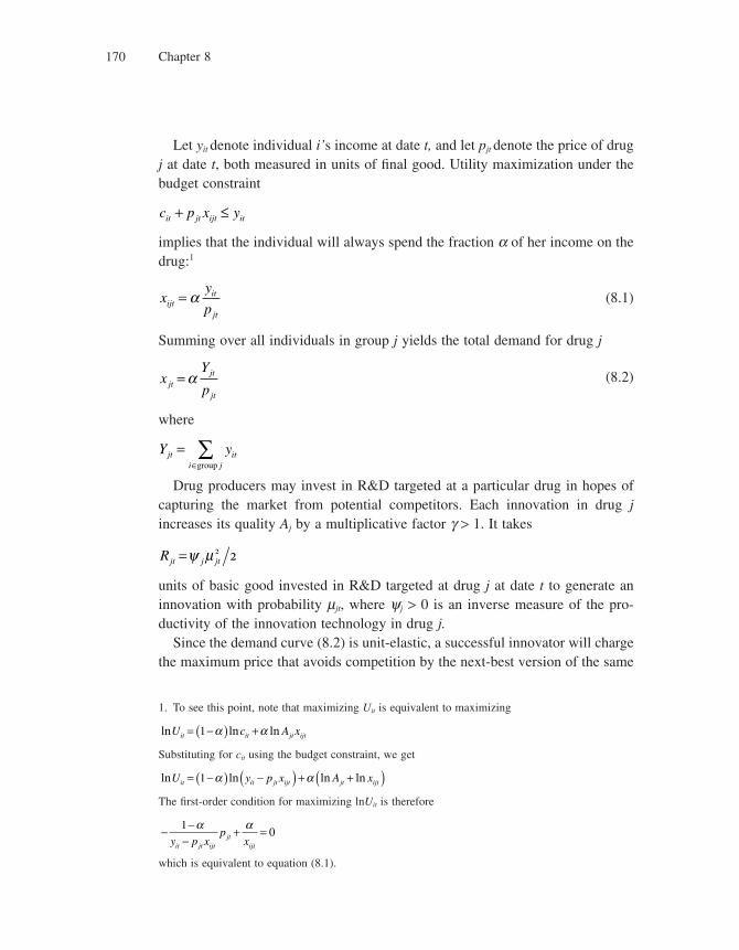
Chapter 8170
Let yit denote individual i’s income at date t, and let pjt denote the price of drug j at date t, both measured in units of fi nal good. Utility maximization under the budget constraint
c p x yit jt ijt it+ ≤
implies that the individual will always spend the fraction a of her income on the drug:1
xy
pijtit
jt
= α (8.1)
Summing over all individuals in group j yields the total demand for drug j
xY
pjtjt
jt
= α (8.2)
where
Y yjt iti j
=∈∑group
Drug producers may invest in R&D targeted at a particular drug in hopes of capturing the market from potential competitors. Each innovation in drug j increases its quality Aj by a multiplicative factor g > 1. It takes
Rjt j jt=ψ μ 2 2
units of basic good invested in R&D targeted at drug j at date t to generate an innovation with probability mjt, where yj > 0 is an inverse measure of the pro-ductivity of the innovation technology in drug j.
Since the demand curve (8.2) is unit-elastic, a successful innovator will charge the maximum price that avoids competition by the next-best version of the same
1. To see this point, note that maximizing Uit is equivalent to maximizing
ln ln lnU c A xit it jt ijt= −( ) +1 α α
Substituting for cit using the budget constraint, we get
ln ln ln lnU y p x A xit it jt ijt jt ijt= −( ) −( ) + +( )1 α α
The fi rst-order condition for maximizing ln Uit is therefore
− −−
+ =10
α αy p x
pxit jt ijt
jtijt
which is equivalent to equation (8.1).
Market Size and Directed Technical Change 171
drug.2 Assume that every innovation is copied after one period. Then the maximum price the successful innovator could charge is g, since this is the cost at which the competitive fringe could produce and sell a quantity g of the next-best version that yields the same benefi t as one unit of the innovator’s new version. Therefore, the profi t from innovating in drug j at date t is
Π jt jtjt
jtjtp
Y
pY= −( ) =
−⎛⎝⎜
⎞⎠⎟
11α γ
γα
The equilibrium fl ow of innovations in drug j results from the maximization by a potential innovator of her expected payoff:
maxμ
μ γγ
α ψ μjt
jt jt j jtY−⎛
⎝⎜⎞⎠⎟
−⎧⎨⎪
⎩⎪
⎫⎬⎪
⎭⎪1
22
which yields
μ γγ
α ψjt jt jY=−⎛
⎝⎜⎞⎠⎟
1
In particular, the higher the relative market size for drug j, as measured by Yjt, or the higher the productivity of R&D on drug j, as measured inversely by yj, the higher the fl ow of innovations in that drug at date t.
8.2.2 Evidence
In their empirical analysis, Acemoglu and Linn (2004) estimate an equation of the form
E N Z X M X Z uct c ct ct ct c t, exp ln⎡⎣ ⎤⎦ = + + +( )β β1 2
where Nct is the fl ow of new drug approvals by the Food and Drug Administration (FDA), Mct denotes the potential market size, Xct is a vector of controls, and Zc controls for drug-category fi xed effects.
To deal with potential endogeneity problems, the authors explore the exoge-nous component of market size associated with demographic trends. More spe-cifi cally, they consider
2. That is, the successful innovator’s profi t will be
Π j j j j jj
j
p x x YY
p= − = −α α
which is maximized by choosing the highest possible price pj.
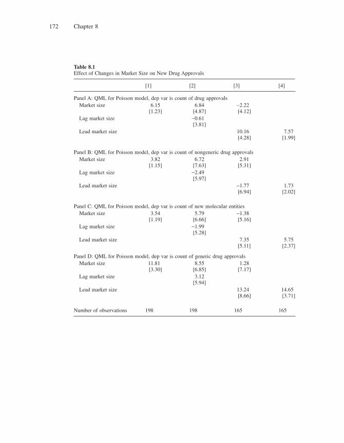
Chapter 8172
Table 8.1Effect of Changes in Market Size on New Drug Approvals
[1] [2] [3] [4]
Panel A: QML for Poisson model, dep var is count of drug approvals Market size 6.15
[1.23]6.84
[4.87]−2.22[4.12]
Lag market size −0.61[3.81]
Lead market size 10.16[4.28]
7.57[1.99]
Panel B: QML for Poisson model, dep var is count of nongeneric drug approvals Market size 3.82
[1.15]6.72
[7.63]2.91
[5.31] Lag market size −2.49
[5.97] Lead market size −1.77
[6.94]1.73
[2.02]
Panel C: QML for Poisson model, dep var is count of new molecular entities Market size 3.54
[1.19]5.79
[6.66]−1.38[5.16]
Lag market size −1.99[5.28]
Lead market size 7.35[5.11]
5.75[2.37]
Panel D: QML for Poisson model, dep var is count of generic drug approvals Market size 11.81
[3.30]8.55
[6.85]1.28
[7.17] Lag market size 3.12
[5.94] Lead market size 13.24
[8.66]14.65[3.71]
Number of observations 198 198 165 165
Market Size and Directed Technical Change 173
M z ict ca ata
= ∑where iat is the income of individuals in age group a at time t in the United States, and zca is the average expenditure share on drugs of category c in the total income of individuals of age a (this does not change much over time).
The demographic data come from the Current Population Survey,3 1965–2000. The variable iat is computed for fi ve-year age bracket groups for 0–5 to 90 years and older. Drug categories obey the FDA classifi cation (there are 20 major drug categories, divided into 159 subcategories). Data on drug use (zca) come from the Medical Expenditure Panel Survey, which covers US households over the period 1996–98. This survey includes age and income data for each household member, for a total of 28,000 individuals, and it provides information on the list of pre-scription drugs used by each person and the amount she spends on each drug. One can then compute drug expenditure and use by each age bracket, and divide this number by income or population to construct an income-based or popula-tion-based measure of zca.
Table 8.1 summarizes the main fi ndings. It shows a positive and signifi cant value of b0 (b0 = 6.15; standard error 1.23, thus signifi cant at the 1% level). This in turn points to a signifi cant effect of market size on innovation fl ow for each category of drug.
8.3 Wage Inequality
The fi rst application of the notions of market size and directed technical change was Acemoglu’s (1998) explanation of the upsurge of wage inequality since the early 1980s in several developed countries. Acemoglu was particularly concerned with the following puzzle concerning the evolution of wage inequality between educational groups: the wage ratio between college graduates and high-school graduates rose substantially in countries like the United States and the United Kingdom between the early 1980s and the mid-1990s even while the relative supply of college-educated workers increased. In the United States, for example, Autor, Krueger, and Katz (1998) show that the ratio of “college-equivalents” (defi ned as the number of workers with a college degree plus 0.5 of the number of workers with some college education) to “noncollege equivalents” (defi ned as the complementary set of workers) increased at an average rate of 3.05 percent
3. Available at www.census.gov/cps/.
Chapter 8174
between 1970 and 1995, up from an average rate of 2.35 percent between 1940 and 1970. In the meantime, the ratio between the average weekly wages of college and high school graduates went up by more than 25 percent during the period 1970–95, after having fallen by 0.11 percent a year on average during the previ-ous period.4
8.3.1 The Debate
Various attempts have been made at explaining the observed upsurge in educa-tional wage inequality—in particular, trade liberalization, deunionization, and skill-biased technical change (SBTC).
The trade explanation is fairly straightforward and directly inspired by the standard Heckscher-Ohlin theory of international trade: in a nutshell, a globaliza-tion boom should drive up the demand for skilled labor in the developed coun-tries, where skilled labor is cheap relative to developing countries, and it should drive down the relative demand for unskilled labor, which is relatively expensive in developed countries.
Unfortunately, trade liberalization is not supported by the evidence. First, as argued by Krugman and others, how could trade liberalization have such a big impact on wage inequality in a country like the United States where trade with non-OECD countries represents no more than 2 percent of GDP? Second, this explanation would imply a fall in prices of less skill-intensive goods relative to prices of more skill-intensive goods in developed countries, but empirical studies fi nd little evidence of this in either the United States or Europe during the 1980s. A third implication of the trade explanation is that labor should be reallocated from low-skill to high-skill industries, or from those sectors in developed coun-tries that are most exposed to international competition to the other sectors. However, Berman, Bound, and Griliches (1994) for the United States and Machin (1996) for the United Kingdom found that only a minor part of the shift away from manual/blue-collar workers to nonmanual/white collars was due to between-industry changes, the remaining 70 or 80 percent being entirely attributable to
4. A second puzzle is that wage inequality has also increased sharply within educational and age groups: in particular, Machin (1996) fi nds that the residual standard deviation in hourly earnings has increased by 23 percent in the United Kingdom and by 14 percent in the United States over the period between 1979 and 1993; equally intriguing is the fact that the rise in within-group wage inequality started to occur before the rise in between-group inequality and accounts for a substantial fraction of the overall increase in income inequality (Katz and Autor 1999); the fi nal part of this puzzle is that the increase in within-group inequality has mainly affected the temporary component of income whereas the increase in between-group inequality has mainly affected the permanent component of income (Blundell and Preston 1999). This second puzzle is addressed in chapter 9.
Market Size and Directed Technical Change 175
within-industry shifts. Finally, the Heckscher-Ohlin theory would predict that the ratio of skilled to unskilled employment should have gone down in skill-intensive industries in developed economies, a prediction which again was not borne out.
To the extent that unionization is often positively correlated with wage com-pression,5 some economists also perceived deunionization6 as an important source of the observed increase in wage inequality.7 However, the attempt to attribute the increase in wage inequality to deunionization failed largely on the basis of the following “timing” considerations: on the one hand, in the United Kingdom the rise in wage inequality started in the mid-1970s while union density kept increasing until 1980; on the other hand, in the United States deunionization began in the 1950s at a time when wage inequality was relatively stable.8
Meanwhile, a number of empirical studies have pointed to a signifi cant impact of skill-biased technical change on the evolution of wage inequality. For example, using R&D expenditures and computer purchases as measures of technical prog-ress, Berman, Bound, and Griliches (1994) found that these two factors could account for as much as 70 percent of the move away from production to nonpro-duction labor over the period 1979–87. Murphy and Welch (1992) fi nd that the share of college labor has increased substantially in all sectors since the mid-1970s, a fi nding which, together with the observed increase in the college premium, provides further evidence of skill-biased technical change. More recently, based on the data reported in Autor, Krueger, and Katz (1998), Acemoglu (2002) estimates that the relative productivity of college graduates has increased from 0.157 in 1980 to 0.470 in 1990 (whereas this relative productivity had risen at a lower rate prior to the early 1980s).
Why did we observe a sharp increase in the college premium in countries like the United States shortly after the relative supply of skilled labor also increased? The existing literature provides two main answers to this puzzle: on the one hand,
5. For example, R. Freeman (1993) showed that the standard deviation of within-fi rm log wages in the United States was 25 percent lower in unionized fi rms compared to nonunionized fi rms.
6. For example, according to Machin (1997), in the United Kingdom union density among male workers fell from 54 percent in 1980 to 38 percent in 1990; in the United States the percentage of private sector workers that are unionized fell from 24 percent in 1980 to less than 12 percent in 1990.
7. For example, Card (1996) and Fortin and Lemieux (1997).
8. While deunionization (organizational change) and trade liberalization do not fully explain the recent evolution in wage inequality, nevertheless we believe that these factors can become more signifi cant when analyzed in relation to skill-biased technical change (see, for example, Acemoglu, Aghion, and Violante 2001 on deunionization and SBTC and Garcia-Peñalosa and Koebel 1998 and Acemoglu 1998 on trade liberalization and SBTC).

Chapter 8176
Katz and Murphy (1992) argue that the sharp increase in the college premium during the 1980s was the combined result of (1) secular skill-biased technical change at a constant pace over the past 50 years and (2) the temporary fall in the college premium caused by the baby-boom-driven increase in the relative supply of skilled labor in the early 1970s; before moving back to its secular path, the college premium was bound to increase at an accelerated rate. The alternative view is that there has been an acceleration in skill-biased technical change since the 1970s. The fi rst convincing piece of evidence in this respect was provided by Krusell and colleagues (2000): based on an aggregate production function in which physical equipment is more substitutable to unskilled labor than to skilled labor,9 they argue that the observed acceleration in the decline of the relative price of production-equipment goods since the mid-1970s10 could account for most of the variation in the college premium over the past 25 years. In other words, the rise in the college premium could largely be attributed to an increase in the rate of (capital-embodied) skill-biased technical progress. This argument, however, does not fully answer our fi rst puzzle; in particular, we still need to understand what would have caused the acceleration in SBTC measured by Krusell and colleagues (2000); second, we also need to reconcile this hypothesis and the evidence on the price of (quality-adjusted) equipment goods with the fact that the recent upsurge in productivity growth follows a long period of slower productivity growth.
8.3.2 The Market-Size Explanation
The following model is adapted from Acemoglu (1998, 2002). The basic idea has two parts. The fi rst part is the same as the scale effect that we saw in Chapter 4. That is, if you can invent improved versions of an intermediate product that is used by a particular kind of labor (either skilled or unskilled) then, other things equal, there is more profi t to be earned by improving a product that is used by the more abundant kind of labor. So as people become more highly educated, and skilled labor therefore becomes more abundant, technological progress becomes increasingly directed towards products that are used by skilled people.
The second part of market-size explanation is that technological progress in products that are used by a particular kind of labor raises the equilibrium wage rate of that kind of labor, by raising its marginal product. Therefore, when increas-
9. See also Stokey (1996), who analyzes the implications of capital-skill complementarity for trade, using a similar modeling approach.
10. See Gordon (1990).
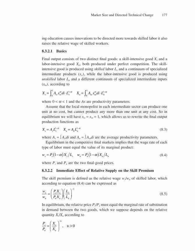
Market Size and Directed Technical Change 177
ing education causes innovations to be directed more towards skilled labor it also raises the relative wage of skilled workers.
8.3.2.1 Basics
Final output consists of two distinct fi nal goods: a skill-intensive good Xs and a labor-intensive good Xu, both produced under perfect competition. The skill-intensive good is produced using skilled labor Ls and a continuum of specialized intermediate products (xis), while the labor-intensive good is produced using unskilled labor Lu and a different continuum of specialized intermediate inputs (xiu), according to
X A x di L X A x di Ls is is s u iu iu u= ⋅ = ⋅− −∫ ∫α α α α1
0
1 1
0
1
where 0 < a < 1 and the As are productivity parameters.Assume that the local monopolist in each intermediate sector can produce one
unit at no cost, but cannot produce any more than one unit at any cost. So in equilibrium we will have xis = xiu = 1, which allows us to rewrite the fi nal output production functions as
X A L X A Ls s s u u u= =− −1 1α α (8.3)
where As = ∫ Aisdi and Au = ∫ Aiudi are the average productivity parameters.Equilibrium in the competitive fi nal markets implies that the wage rate of each
type of labor must equal the value of its marginal product:
w P X L w P X Ls s s s u u u u= −( ) = −( )1 1α α (8.4)
where Ps and Pu are the two fi nal-good prices.
8.3.2.2 Immediate Effect of Relative Supply on the Skill Premium
The skill premium is defi ned as the relative wage ws/wu of skilled labor, which according to equation (8.4) can be expressed as
w
w
P X
P X
L
Ls
u
s s
u u
s
u
=⎛⎝⎜
⎞⎠⎟
⎛⎝⎜
⎞⎠⎟
−1
(8.5)
In equilibrium, the relative price Ps/Pu must equal the marginal rate of substitution in demand between the two goods, which we suppose depends on the relative quantity Xs/Xu according to
P
P
X
Xs
u
s
u
=⎛
⎝⎜
⎞
⎠⎟ >
−υ
υ, 0
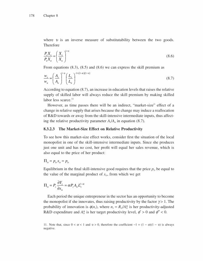
Chapter 8178
where u is an inverse measure of substitutability between the two goods. Therefore
P X
P X
X
Xs s
u u
s
u
=⎛
⎝⎜
⎞
⎠⎟
−1 υ
(8.6)
From equations (8.3), (8.5) and (8.6) we can express the skill premium as
w
w
A
A
L
Ls
u
s
u
s
u
=⎛
⎝⎜
⎞
⎠⎟
⎛
⎝⎜
⎞
⎠⎟
− − + −( ) −( )1 1 1 1υ α υ
(8.7)
According to equation (8.7), an increase in education levels that raises the relative supply of skilled labor will always reduce the skill premium by making skilled labor less scarce.11
However, as time passes there will be an indirect, “market-size” effect of a change in relative supply that arises because the change may induce a reallocation of R&D towards or away from the skill-intensive intermediate inputs, thus affect-ing the relative productivity parameter As/Au in equation (8.7).
8.3.2.3 The Market-Size Effect on Relative Productivity
To see how this market-size effect works, consider fi rst the situation of the local monopolist in one of the skill-intensive intermediate inputs. Since she produces just one unit and has no cost, her profi t will equal her sales revenue, which is also equal to the price of her product:
Πis is is isp x p= =
Equilibrium in the fi nal skill-intensive good requires that the price pis be equal to the value of the marginal product of xis, from which we get
Πis ss
iss is sP
Y
xP A L=
∂∂
= −α α1
Each period the unique entrepreneur in the sector has an opportunity to become the monopolist if she innovates, thus raising productivity by the factor g > 1. The probability of innovation is f(ns), where ns = Ris/Ais* is her productivity-adjusted R&D expenditure and Ais* is her target productivity level, f′ > 0 and f″ < 0.
11. Note that, since 0 < a < 1 and u > 0, therefore the coeffi cient −1 + (1 − a)(1 − u) is always negative.
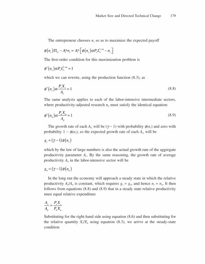
Market Size and Directed Technical Change 179
The entrepreneur chooses ns so as to maximize the expected payoff
φ φ α αn A n A n P L ns is i s i s s s s( ) − = ( ) −⎡⎣ ⎤⎦−Π * * 1
The fi rst-order condition for this maximization problem is
′ ( ) =−φ α αn P Ls s s1 1
which we can rewrite, using the production function (8.3), as
′ ( ) =φ αnP X
Ass s
s
1 (8.8)
The same analysis applies to each of the labor-intensive intermediate sectors, where productivity-adjusted research nu must satisfy the identical equation:
′ ( ) =φ αnP X
Auu u
u
1 (8.9)
The growth rate of each Ais will be (g − 1) with probability f(ns) and zero with probability 1 − f(ns), so the expected growth rate of each Ais will be
g ns s= −( ) ( )γ φ1
which by the law of large numbers is also the actual growth rate of the aggregate productivity parameter As. By the same reasoning, the growth rate of average productivity Au in the labor-intensive sector will be
g nu u= −( ) ( )γ φ1
In the long run the economy will approach a steady state in which the relative productivity As/Au is constant, which requires gs = gu, and hence ns = nu. It then follows from equations (8.8) and (8.9) that in a steady state relative productivity must equal relative expenditure
A
A
P X
P Xs
u
s s
u u
=
Substituting for the right-hand side using equation (8.6) and then substituting for the relative quantity Xs/Xu using equation (8.3), we arrive at the steady-state condition
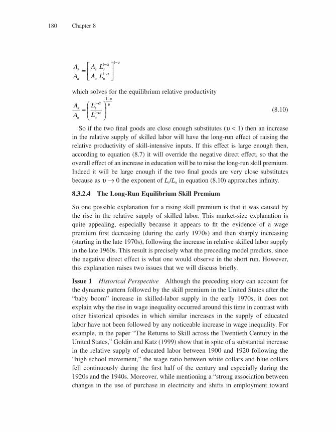
Chapter 8180
A
A
A
A
L
Ls
u
s
u
s
u
=⎡
⎣⎢
⎤
⎦⎥
−
−
−1
1
1α
α
υ
which solves for the equilibrium relative productivity
A
A
L
Ls
u
s
u
=⎛
⎝⎜
⎞
⎠⎟
−
−
−1
1
1α
α
υυ
(8.10)
So if the two fi nal goods are close enough substitutes (u < 1) then an increase in the relative supply of skilled labor will have the long-run effect of raising the relative productivity of skill-intensive inputs. If this effect is large enough then, according to equation (8.7) it will override the negative direct effect, so that the overall effect of an increase in education will be to raise the long-run skill premium. Indeed it will be large enough if the two fi nal goods are very close substitutes because as u → 0 the exponent of Ls/Lu in equation (8.10) approaches infi nity.
8.3.2.4 The Long-Run Equilibrium Skill Premium
So one possible explanation for a rising skill premium is that it was caused by the rise in the relative supply of skilled labor. This market-size explanation is quite appealing, especially because it appears to fi t the evidence of a wage premium fi rst decreasing (during the early 1970s) and then sharply increasing (starting in the late 1970s), following the increase in relative skilled labor supply in the late 1960s. This result is precisely what the preceding model predicts, since the negative direct effect is what one would observe in the short run. However, this explanation raises two issues that we will discuss briefl y.
Issue 1 Historical Perspective Although the preceding story can account for the dynamic pattern followed by the skill premium in the United States after the “baby boom” increase in skilled-labor supply in the early 1970s, it does not explain why the rise in wage inequality occurred around this time in contrast with other historical episodes in which similar increases in the supply of educated labor have not been followed by any noticeable increase in wage inequality. For example, in the paper “The Returns to Skill across the Twentieth Century in the United States,” Goldin and Katz (1999) show that in spite of a substantial increase in the relative supply of educated labor between 1900 and 1920 following the “high school movement,” the wage ratio between white collars and blue collars fell continuously during the fi rst half of the century and especially during the 1920s and the 1940s. Moreover, while mentioning a “strong association between changes in the use of purchase in electricity and shifts in employment toward
Market Size and Directed Technical Change 181
more educated labor” (p. 25), Goldin and Katz report no sharp widening of the wage distribution prior to the 1970s. Obviously, any explanation of the recent patterns in wage inequality really needs to integrate the distinguishing features of the past 20 years from previous episodes if it is to be taken as comprehensive. This observation does not invalidate the importance of market-size and labor-supply effects, but it does suggest that any explanation that would rely primarily upon these effects may not be fully satisfactory from a historical point of view. However, Acemoglu (2002) convincingly argues that models of directed techni-cal change can be useful in understanding the rise of the factory system in the 19th century, in relation to the increased supply of unskilled labor induced by the migration of rural populations to cities.
Issue 2 Market-Size Effect and Productivity Slowdown In a highly infl uential paper, C. Jones (1995a) points out that although OECD countries have experi-enced substantial increases in the average duration of schooling and in R&D levels during the past 50 years, there has been no apparent payoff in terms of faster growth: if anything, measured productivity growth has slowed, especially between the mid-1970s and the early 1980s.12 These fi ndings appear to be at odds with R&D-based models of growth that predict that the innovation rate should signifi cantly increase when the supply of skilled labor s increases. The market-size model is actually more subtle in the sense that it predicts a change in the direction—not the speed—of technological change. Yet the growth rate as derived from the preceding model should still increase following a (discontinuous) increase in relative skilled-labor supply, which is still at variance with Jones-style evidence, at least up until the mid-1990s. To reconcile the market-size explana-tion with this evidence, Acemoglu (2000) invokes the existence of decreasing returns in R&D aimed at skill-biased technical progress. Now, while individual researchers might experience decreasing returns in their R&D activities, it is not clear why the whole economy should: the exception would be if individual innovations were more like secondary discoveries induced by an economy-wide
12. For example, the annual growth rate in the United States has declined by 1.8 percent on average since the 1970s. The decline has been most pronounced in the service sector, and more generally the productivity slowdown appears to be mainly attributable to a decline in disembodied productivity growth. Indeed, since the early 1970s the rate of embodied technical progress has accelerated (see McHugh and Lane 1987; Greenwood and Yorukoglu 1997; Hornstein and Krusell 1996; and Comin 2000), and the bulk of this acceleration, e.g., as measured by the decline in the quality-adjusted price of equipment goods, appears to be attributable to computers and other information-processing goods. This contrast, again, points to the important role played by the new information technologies and their diffusion during the past 20 years.
Chapter 8182
fundamental breakthrough, which becomes more and more incremental over time. We shall come back to these issues in chapter 9.
8.4 Appropriate Technology and Productivity Differences*
Acemoglu and Zilibotti (2001) used a directed technical change model to explain the persistence of productivity differences between North and South, even though no institutional barriers to the adoption of technologies discovered in the North exist in the South. Suppose technological innovation takes place in the North and that the South does not enforce property rights on innovations imported from the North. Then, innovators in the North can only extract rents from selling new technologies in the northern market. It follows that innovation will not respond to market size and skill endowment in the South, but only to those in the North, which in turn implies that the dynamics of relative productivities in skilled- and unskilled-intensive sectors (the a variable in the previous section), will only be determined by skill endowments in the North. Thus it will generally be inappro-priate for the South, with the result that output per worker is higher in the South than in the North, even though both regions have access to the same technological opportunities.
More formally, consider the following variant of the directed technical change model, with horizontal innovations. This section closely follows Gancia and Zilibotti (2005). Consider a world divided into North and South.
8.4.1 Basic Setup
Time is continuous and at each period the North produces a continuum of measure one of variety goods, under perfect competition. Variety goods are indexed by i ∈ [0,1], and together they give rise to a composite fi nal output fi nal
Y y dii= ( )∫exp log ,0
1
which is taken as numeraire.Each variety good i is produced using skilled labor, unskilled labor, and inter-
mediate input used by each type of labor. Namely, intermediate inputs (L,�) with � in the interval [0,AL] are used by unskilled workers only, whereas intermediate inputs (H,�) with � in the interval [0,AH] are used by skilled workers only.
*This is a diffi cult section that may be skipped by the novice reader.
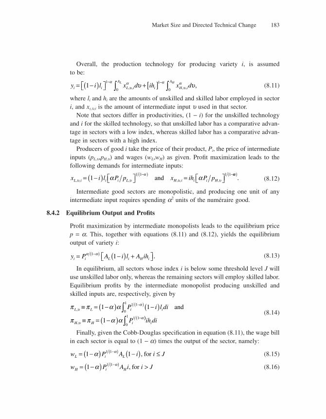
Market Size and Directed Technical Change 183
Overall, the production technology for producing variety i, is assumed to be:
y i l x d ih x di i L i
A
i H i
AL H= −( )⎡⎣ ⎤⎦ + [ ]− −∫ ∫11
0
1
0
αυ
α αυ
αυ υ, , , , , (8.11)
where li and hi are the amounts of unskilled and skilled labor employed in sector i, and xz,u,i is the amount of intermediate input u used in that sector.
Note that sectors differ in productivities, (1 − i) for the unskilled technology and i for the skilled technology, so that unskilled labor has a comparative advan-tage in sectors with a low index, whereas skilled labor has a comparative advan-tage in sectors with a high index.
Producers of good i take the price of their product, Pi, the price of intermediate inputs (pL,u,pH,u) and wages (wL,wH) as given. Profi t maximization leads to the following demands for intermediate inputs:
x i l P p x ih P pL i i i L H i i i H, , , , , ,υ υα
υ υα α= −( ) ⎡⎣ ⎤⎦ = ⎡⎣ ⎤⎦−( ) −
11 1 1 1
andαα( )
. (8.12)
Intermediate good sectors are monopolistic, and producing one unit of any intermediate input requires spending a2 units of the numéraire good.
8.4.2 Equilibrium Output and Profi ts
Profi t maximization by intermediate monopolists leads to the equilibrium price p = a. This, together with equations (8.11) and (8.12), yields the equilibrium output of variety i:
y P A i l A ihi i L i H i= −( ) +⎡⎣ ⎤⎦−( )α α1 1 . (8.13)
In equilibrium, all sectors whose index i is below some threshold level J will use unskilled labor only, whereas the remaining sectors will employ skilled labor. Equilibrium profi ts by the intermediate monopolist producing unskilled and skilled inputs are, respectively, given by
π π α α
π π α α
υα
υα
L L i i
H H i
P i l di
P
,
,
≡ = −( ) −( )≡ = −( )
−( )
−(∫1 1
1
1 1
0
1
1 1
and
))∫ ih dii0
1 (8.14)
Finally, given the Cobb-Douglas specifi cation in equation (8.11), the wage bill in each sector is equal to (1 − a) times the output of the sector, namely:
w P A i i JL i L= −( ) −( ) ≤−( )1 11 1α α , for (8.15)
w P A i i JH i H= −( ) >−( )1 1 1α α , for (8.16)
Chapter 8184
Defi ning PL ≡ P0, PH ≡ P1 and diving equations in (8.15) by their counterparts in sectors 0 and 1, we obtain
P P i i Ji L= −( ) ≤− −( )11 α , for
P P i i Ji H= >− −( )1 α , for
Now, to maximize Y, expenditures across goods must be equalized, thus
P y P y P yi i H L= =1 0
This, together with the full employment of skilled and unskilled labor, implies that labor is evenly distributed among sectors, that is
l L J h H Ji i= = −( ), 1
Finally, in the cut-off sector i = J, the skilled and unskilled technologies are equally profi table:
P J P JL H11 1−( ) =− −( ) − −( )α α
Together, the preceding equations imply:
J
J
P
P
A
A
H
LH
L
H
L1
1 1 1 2
−=
⎛⎝⎜
⎞⎠⎟
=⎛⎝⎜
⎞⎠⎟
−( ) −α
(8.17)
The higher the relative endowment of skill (H/L) and the skill-bias of technology (AH/AL), the larger the fraction of sectors using the skill-intensive technology (1 − J).
Finally, integrating Piyi over [0,1], using equations (8.13) and (8.17), and the fact
that the consumption aggregate is the numéraire (so that exp ln Pdii0
11∫⎡
⎣⎢⎤⎦⎥
= ), we
can re-express aggregate output as
Y A L A HL H= −( ) ( ) + ( )⎡⎣
⎤⎦exp 1
1 2 1 2 2
(8.18)
8.4.3 Skill-Biased Technical Change
In the preceding subsection we took the technology parameters AH and AL as given. Now, we endogenize them by looking at innovation incentives and the resulting equilibrium skill-bias of technology, (AH/AL). Assume that to increase AL or AH by one unit (that is, the cost of inventing an additional “unskilled” or an additional “skilled” intermediate input) costs m units of the numéraire. Invent-ing a new “skilled” input yields instantaneous profi ts equal to
Market Size and Directed Technical Change 185
π α α αH HP H= −( ) −( )1 1 1 (8.19)
Similarly, inventing a new “unskilled” input yields instantaneous profi ts equal to
π α α αL LP L= −( ) −( )1 1 1
Now, balanced growth requires that the innovation intensity be the same on both types of inputs, which in turn requires that
π πL H=
Balanced growth in turn implies that AH and AL grow at the same rate, so that the ratio AH/AL remains constant over time as well as the cut-off index J, and the price PL and PH.
Plugging pL = pH into equation (8.19) and using equation (8.17), we get
A
A
J
J
H
LH
L
=−
=1 (8.20)
8.4.4 Explaining Cross-Country Productivity Differences
So far, our analysis was focused on the case of one country, the North. Consider now a second country, the South. The South is identical to the North, except that skilled labor is more scarce in the South than in the North, namely
H L H LS S <
Now, let us assume that intellectual property rights are not enforced in the South and that there is no trade between North and South. This in turn implies that intermediate producers in the North cannot sell goods or copyrights to the South, so that they can only collect rents from the South on their innovations. On the other hand, producers in the South can copy the new technologies invented in the North at a small but positive cost, so that they will choose to simply imitate the technologies invented in the North instead of investing in innovation.
But then the North and the South will end up using the same technologies, with
A A H LH L =
because the skill-bias is entirely determined by the factor endowment of the North, which in turn follows from the fact that the North is the only market for (northern) innovations.
Chapter 8186
Apart from that, the equilibrium output in the South is similar as the preceding expression ( ) for the equilibrium output in the North, except that we must replace the skilled and unskilled labor endowments H and L in the North by HS and LS for the South:
Y A L A HSL
SH
S= −( ) ( ) + ( )⎡⎣⎢
⎤⎦⎥
exp 11 2 1 2 2
We are now ready to answer the following questions: Are technologies appropriate for the skill endowment of the countries where they are developed? What happens to aggregate productivity if they are used in a different economic environment?
It is easy to show that expression Y is maximized for AH/AL = H/L. This is nothing but the previous condition (8.20). In other words, the equilibrium skill-bias AH/AL is optimally adapted to the northern skill composition H/L. However, the equilibrium skill bias ignores the relative factor endowments in the South, so that the new technologies developed in the North are inappropriate for the needs of the South. It follows that output per capita, Y/(L + H) is greater in the North than in the South.
This productivity difference is the result of a technology-skill mismatch, and it can help explain the existence of substantial differences in TFP even across countries that have access to the same technology. Acemoglu and Zilibotti (2001) argue that this mismatch can account for one third to one half of the total factor productivity gap between the United States and developing countries. The idea that the choice of appropriate technology depends on factor endowments also features in the analysis of Caselli and Coleman (2000).
8.5 Conclusion
In this model we have explored the idea that innovative fi rms may decide on how to allocate their R&D efforts across several sectors of the economy, and that their equilibrium decisions will ultimately depend upon both the relative effi ciency of R&D investments across the various sectors and the relative size of rents that can be generated by innovating in each sector. The latter in turn depend upon the relative incomes of the potential consumers of the various goods or on the size of the labor force whose productivity can be enhanced by innovating in each particular sector. We provided evidence that market-size effects were at work in the drug industry, and we analyzed implications of the market-size approach for wage inequality and the nonconvergence between South and North.
Market Size and Directed Technical Change 187
8.6 Literature Notes
The theory presented in this chapter is based on a series of recent papers by Daron Acemoglu and coauthors. Yet the idea of biased technological change goes back to an earlier literature. Hicks (1932) had already suggested that technological progress would economize on the more expensive factor.
Related to Hicks’s idea, the late 1950s and early 1960s saw the emergence of an “induced innovation” literature. In particular, Nelson (1959) discussed the composition of research spending and the amount spent on what he called “basic” research. Arrow (1962) studied the optimality of the resource allocation for inven-tions from the viewpoint of welfare economics. Kennedy (1964) introduced the idea of “innovation possibilities frontier” that takes into account the trade-off between different types of innovation.
Kennedy (1964) also discussed the issue of relative factor share in the economy and its relation with induced innovations, concluding that these latter would push the economy to an equilibrium with constant relative-factor share. Such points were addressed by Samuelson (1965) and Drandakis and Phelps (1965), among others.
Fellner (1961) studied the factor-saving aspect of inventions and argued that competitive fi rms would lean toward a relative labor-saving invention only if they would expect wages to rise faster than capital-good rentals. Habakkuk (1962) asserted that labor scarcity, by increasing wages, would induce fi rms to search for labor-saving inventions, spurring technological progress.
Atkinson and Stiglitz (1969) analyzed the idea that technological progress could improve one technique of production but not other techniques of producing the same product, under their concept of “localized” technical progress.
Because of its lack of strong microfoundations, interest in this literature faded away until the late 1990s when the models analyzed in this chapter were fi rst published. These microfounded models of directed technical change feature the existence of market-size effects (absent in most of the earlier literature mentioned previously, with the exception of works such as Schmookler 1966) and were mostly developed by Acemoglu and coauthors.
The main applications of the framework have been (1) to skill-biased technical change and wage inequality (Acemoglu 1998; and Kiley 1999); (2) to interna-tional trade inducing skill-biased technical change (Acemoglu 2003a); (3) to explaining the constancy of factor shares (Acemoglu 2003b); and (4) to explain-ing the persistence of productivity differences across countries that have equal access to new technologies (Acemoglu and Zilibotti 2001).

Chapter 8188
Acemoglu (2002) presented a theoretical synthesis of the framework, and we also refer the reader to the Handbook of Economic Growth survey by Gancia and Zilibotti (2005, sec. 4).
Problems
1. Explain how taking into account market-size effects and directed technical change might shed light on why there is less incentive to develop vaccines for diseases that are more common in poorer countries. Explain why market-size effects can explain the recent surge in wage inequality.
2. Product variety and directed technological change
Consider a mass 1 of identical consumers with preference given by the utility function
U eC
dtt= −−
−−∞
∫ δθ
θ
1
0
11
where C t C Cs u( ) = +( )ρ ρ ρ1
is a consumption aggregator over two fi nal goods produced according to
Y x L dis i s s
Ns= −∫ ,α α1
0
Y x L diu i u u
Nu= −∫ ,α α1
0
where xi,� is the i intermediate input used in the sector intensive in L�, and N� is the number of varieties in this sector. The markets for fi nal goods are perfect, but the producers of intermediate goods are monopolists. It costs one unit of fi nal good to produce one intermediate good. By spending Z units of fi nal good, an entrant faces a probability l�Z of discovering a new intermediate good in the sector intensive in L�. There is free entry into research. We will normalize prices such that it costs 1 to get
C(t) = 1; so p ps u
ρρ
ρρ
ρρ
− −
−
+⎛
⎝⎜
⎞
⎠⎟ =1 1
1
1.
a. Compute the profi t for an intermediate good as a function of p�, the price of Y�.
b. Compute the price ratio between the two fi nal goods; derive the wage premium as a function of Ns and Nu. Show that the elasticity of substitution between the two factors is given by
σ αρρ
= −−
11
.
c. We now focus on the steady state. State the research-arbitrage equation. Compute the value of a fi rm as a function of the profi t and the interest rate. Taking the ratio for the two sectors, defi ne price
and a market-size effects. Then fi nd the ratio N
Ns
u
as a function of L
Ls
u
.
d. When is an increase in the supply of skilled labor going to increase the wage premium? Compare with the quality-ladder case.
e. Express the Euler equation. Compute the growth rate of the economy.
3. **Endogenous factors supply
Consider the model presented in section 8.3. This problem will make endogenous the endowment of skilled and unskilled workers. Time is discrete, and there is a continuum of agents (of mass 1). Instead of living for one period, an agent may die with probability 1 − d each period. A mass d of new agents

Market Size and Directed Technical Change 189
are born each period. When agent z is born, he is unskilled; he can choose to start working immediately or to acquire education in order to become skilled. If he decides to get educated, he won’t be able to work for T(z) periods (note that the agent knows how long it is going to take him to get educated), where T(z) is distributed according to a distribution Q(T), such that q(t) > 0 for any t ≥ 0 (Q is the cumulative distribution function and q is the probability distribution function). We consider an economy in steady state where the skill premium and a remain constant, and we assume that if someone is indifferent he will choose to become educated.
There is no friction in the fi nancial market, and a person born at s has the following lifetime expected utility:
E U c t stz
t
( ) = +( )=∑δ
0
An innovation increases the productivity of an intermediate good Ai by a factor g and happens with probability nb if someone invests n in R&D. Contrary to the benchmark model we assume that the monopoly right is given until a new innovation is made.
a. Show that the interest rate is given by r =+1
1 δ and that wages increase at the growth rate of the
economy g.
b. Show that there is a stationary cutoff value T above which people won’t get educated.
c. Compute the threshold as a function of the skill premium, rate of interest, and growth rate in the economy (you can forget the integer constraint on T).
d. Show that the relative supply is given by
L
L
Q T
Q Ts
u
=( )
− ( )1
e. Show that the present value of the monopoly right (from the following period) on the intermediate good i is
V
rg
ii=
+ +−
⎛⎝⎜
⎞⎠⎟
π
γ
β
11
f. Compute the research-arbitrage equation; show that the following relation still holds:
ω λρ α
ρ αρρ
αρ=−( )
−( ) −( ) + −−
2 211 1
11
g. Give an equation that fully characterizes T as a function of the parameters of the economy (you can use the expression of the growth rate in problem 2). Explain why it is possible to get several equilibria. What is the intuition? Will growth necessarily be the same in these equilibria?
4. *Knowledge spillovers
Consider the following variation of the model presented in section 8.3. Innovation now requires the hiring of scientists that are in fi xed supply (S). Moreover, instead of having one entrepreneur each period who has the possibility of displacing the monopolist, there is now free entry in the innovation sector (we will consider that the probability that there is more than one innovation per period is 0—think that the time interval this time is very short). A local entrepreneur in the unskilled sector who
hires siu scientists will innovate successfully with probability η
δ δ
us u
iuiu
A A
As
12
12
− +
, 0 < d ≤ 1. If he
succeeds, he will be the monopolist for good iu next period, using a technology Aiu(t + 1) = gAiu(t). (And similarly a local entrepreneur in the skilled sector who hires sis scientists will innovate with
probability η
δ δ
su s
isis
A A
As
12
12
− +
.)
Chapter 8190
Note that sections 8.3.2.1, 8.3.2.2, and 8.3.2.3 still apply in this context.
a. Explain what the functional form A A
As u
iu
12
12
− +δ δ
means.
b. State the free-entry condition in R&D and the scientists’ market-clearing condition.
c. Prove that the growth rate of Au is given by
A A
A
A
ASu
tut
ut u
st
ut u
+−
−= −( ) ⎛
⎝⎜⎞⎠⎟
11
2
1γ η
δ
d. Compute the skill premium and the growth rate of the economy in steady state.
e. When is the skill premium going to increase if the relative supply of skilled workers in the population increases? Compare with the baseline model (look at what happens when d = 0); provide an intuition to explain the departure from the baseline model. Typically economists would agree that r > 0, but there is some debate on how large it is. Explain why this model may help to explain better than the baseline model the historical increase in the skill premium if r is not very large.
5. **Skilled labor as the input for R&D
We consider a model similar to the one introduced in section 8.3; however, this time R&D requires hiring skilled labor instead of using a fi nal good. Moreover, instead of having one entrepreneur each period who has the possibility of displacing the monopolist, there is now free entry in the innovation sector (the probability that there is more than one innovation per period is 0). A local entrepreneur in the unskilled sector who hires hiu units of skilled labor will successfully innovate with
probability η A A
Ahs u
iuiu
1 2 1 2
(A As u1 2 1 2
represents knowledge spillover). If he succeeds he will be the
monopolist for good iu next period, using a technology Aiu(t + 1) = gAiu(t). (And similarly a local entrepreneur in the skilled sector who hires his units of skilled labor will innovate with probability
η A A
Ahs u
isis
1 2 1 2
.)
a. State the free-entry condition in R&D.
b. Prove that the growth rate of Au is given by
A A
A
A
AHu
tut
ut
st
ut u
+ − = −( ) ⎛
⎝⎜
⎞
⎠⎟
1 1 2
1γ η
where Hu is the total amount of skilled labor used in the R&D of the unskilled sector
c. Prove that in a steady state where a is constant, the following relations still hold:
ω λρ α
αρρ
αρ=−( )
−−
−a1
11
1
a =−( )
−λρ α
ρ1
1
provided that we redefi ne l conveniently.
d. Find, l (assume that the supply of skilled labor is large enough so that your computation makes sense). Find the growth rate and the wage premium. What is the effect of an increase in the supply of skilled labor on the wage premium? And on the growth rate? Comment.

Market Size and Directed Technical Change 191
6. **Appropriate technology and growth (based on Basu and Weil 1998)
Here, technologies are specifi c to particular combinations of inputs.
First suppose a one-country world where output per worker is given by
Y A K t K= ( ), α
where A(K,t) is the level of technology for capital-labor ratio K at time t.Suppose there exists a maximal level of technology for each value of K given by A*(K) = BK1−a.
(There is a limit for the development of new technologies for any capital-labor ratio.) Assume also that A*′(K) > 0. Finally, defi ne k ≡ ln(K).
Let us assume that when a country produces at a log capital-labor ratio k, learning by doing uni-formly improves the level of all technologies using a capital-labor ratio in a symmetric neighborhood around k. In particular, suppose that the level of technology at capital-labor ratio j improves according to the following:
dA j t
dtA j A j t k j k
,,
( ) = ( ) − ( )⎡⎣ ⎤⎦ − < < +
=
β γ γ* if
otherwise0
where A*( j) is the highest level of technology attainable at capital-labor ratio j.Finally, assume there exists x > k0 such that A(j,0) > 0 for all j > x and A(k0,0) > 0. (This simply
means that at the beginning of time, there was no technology available for high enough levels of capital-labor ratios.) Defi ne R = A(K,t)/A*(K) as the ratio of used technology to its maximal level.
a. Show that output per worker can be rewritten as Y = RBK.
We now look at the steady state of this economy, in which k grows at a constant rate g and R = R* is constant.
b. Show that in steady state R* = (1 − e−bg /g). What is the sign of ∂R*/∂g? Is there any “penalty” for fast growth in this setting? Provide intuition for your fi nding. (Hint: Solve the ordinary differential equation for A(k,t) using ebx as the integrating factor.)
Now, assume a constant saving rate s so that K. = sY − dK.
c. Show that in steady state g = sR*B − d. Show graphically that the steady-state level of technology ratio R* is unique and that it does not depend on initial conditions.
Assume now that the world is composed of two countries and that technology fl ows freely between them, as well as local learning-by-doing spillovers:
dA j t
dtA j A j t k j ki i
i
,,
( ) = ( ) − ( )⎡⎣ ⎤⎦ − < < +{ }=∑β γ γ* 1
1
2
where 1 {} is the indicator function and i designates the country. This simply means that when the countries are within the same neighborhood of capital-labor ratios, technology can be simultaneously improved by spillovers from both countries.
Let us look at the case in which the two countries end up in a steady state where they both grow at the same rate g. Let s1 and s2 be the saving rates for the two countries, and R*1 and R*2 the steady-state technology ratios, and assume, without loss of generality, that sl > s2.
d. Show that if both countries grow at rate g in steady state and s1 > s, then R*1 < R*2. Explain how this result implies that country 1 has a higher level of capital per worker than country 2 at all times. Let d be the steady-state difference between the leader country’s log capital-labor ratio k1 and the follower’s k2.
e. Using reasoning analogous to item b, derive the steady-state ratios R*1 = 1 − e−b(2g −d)/g and R*2 = 1 − e−b(2g +d)/g. Explain why the two countries will grow at the same steady-state rate g only if d < g.

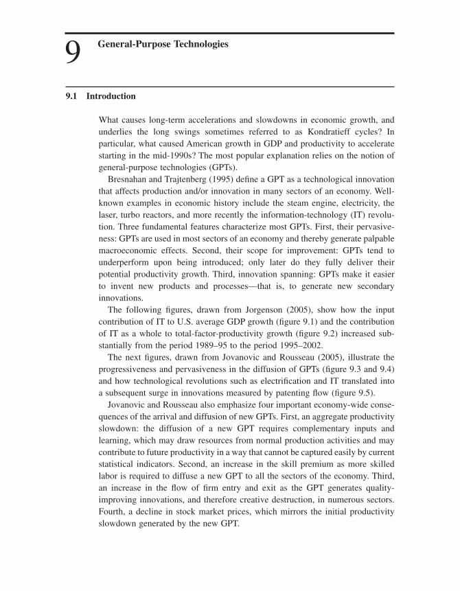
9 General-Purpose Technologies
9.1 Introduction
What causes long-term accelerations and slowdowns in economic growth, and underlies the long swings sometimes referred to as Kondratieff cycles? In particular, what caused American growth in GDP and productivity to accelerate starting in the mid-1990s? The most popular explanation relies on the notion of general-purpose technologies (GPTs).
Bresnahan and Trajtenberg (1995) defi ne a GPT as a technological innovation that affects production and/or innovation in many sectors of an economy. Well-known examples in economic history include the steam engine, electricity, the laser, turbo reactors, and more recently the information-technology (IT) revolu-tion. Three fundamental features characterize most GPTs. First, their pervasive-ness: GPTs are used in most sectors of an economy and thereby generate palpable macroeconomic effects. Second, their scope for improvement: GPTs tend to underperform upon being introduced; only later do they fully deliver their potential productivity growth. Third, innovation spanning: GPTs make it easier to invent new products and processes—that is, to generate new secondary innovations.
The following fi gures, drawn from Jorgenson (2005), show how the input contribution of IT to U.S. average GDP growth (fi gure 9.1) and the contribution of IT as a whole to total-factor-productivity growth (fi gure 9.2) increased sub-stantially from the period 1989–95 to the period 1995–2002.
The next fi gures, drawn from Jovanovic and Rousseau (2005), illustrate the progressiveness and pervasiveness in the diffusion of GPTs (fi gure 9.3 and 9.4) and how technological revolutions such as electrifi cation and IT translated into a subsequent surge in innovations measured by patenting fl ow (fi gure 9.5).
Jovanovic and Rousseau also emphasize four important economy-wide conse-quences of the arrival and diffusion of new GPTs. First, an aggregate productivity slowdown: the diffusion of a new GPT requires complementary inputs and learning, which may draw resources from normal production activities and may contribute to future productivity in a way that cannot be captured easily by current statistical indicators. Second, an increase in the skill premium as more skilled labor is required to diffuse a new GPT to all the sectors of the economy. Third, an increase in the fl ow of fi rm entry and exit as the GPT generates quality-improving innovations, and therefore creative destruction, in numerous sectors. Fourth, a decline in stock market prices, which mirrors the initial productivity slowdown generated by the new GPT.
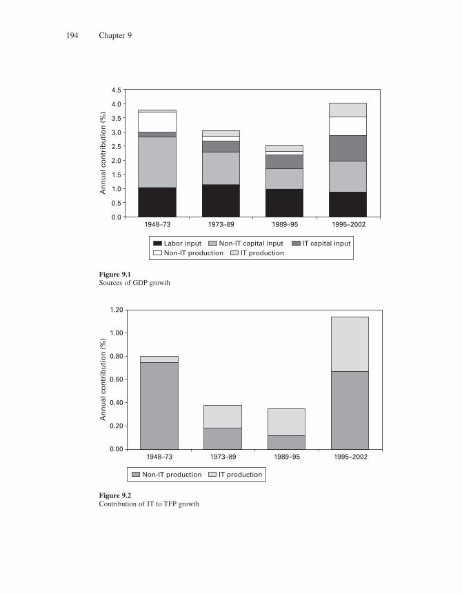
Chapter 9194
Labor input Non-IT capital inputNon-IT production IT production
IT capital input
1948–73
An
nu
al c
on
trib
uti
on
(%
)
4.5
4.0
3.5
3.0
2.5
2.0
1.5
1.0
0.5
0.01973–89 1989–95 1995–2002
Figure 9.1Sources of GDP growth
Non-IT production IT production
1948–73
An
nu
al c
on
trib
uti
on
(%
)
1.20
1.00
0.80
0.60
0.40
0.20
0.001973–89 1989–95 1995–2002
Figure 9.2Contribution of IT to TFP growth
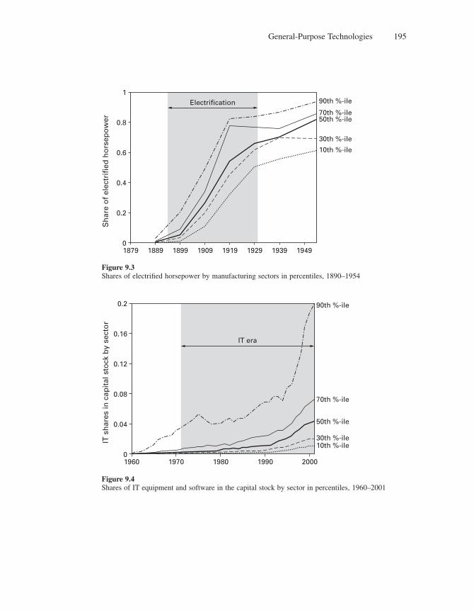
General-Purpose Technologies 195
1879 1889 1899 19491939192919191909
Sh
are
of
elec
trif
ied
ho
rsep
ow
er
1
0.8
0.6
0.4
0.2
0
Electrification 90th %-ile
70th %-ile50th %-ile
30th %-ile
10th %-ile
Figure 9.3Shares of electrifi ed horsepower by manufacturing sectors in percentiles, 1890–1954
1960 1970 1980 1990 2000
IT s
har
es in
cap
ital
sto
ck b
y se
cto
r
0.2
0.16
0.12
0.08
0.04
0
IT era
90th %-ile
70th %-ile
50th %-ile
30th %-ile10th %-ile
Figure 9.4Shares of IT equipment and software in the capital stock by sector in percentiles, 1960–2001
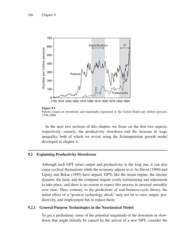
Chapter 9196
In the next two sections of this chapter, we focus on the fi rst two aspects, respectively—namely, the productivity slowdown and the increase in wage inequality, both of which we revisit using the Schumpeterian growth model developed in chapter 4.
9.2 Explaining Productivity Slowdowns
Although each GPT raises output and productivity in the long run, it can also cause cyclical fl uctuations while the economy adjusts to it. As David (1990) and Lipsey and Bekar (1995) have argued, GPTs like the steam engine, the electric dynamo, the laser, and the computer require costly restructuring and adjustment to take place, and there is no reason to expect this process to proceed smoothly over time. Thus, contrary to the predictions of real-business-cycle theory, the initial effect of a “positive technology shock” may not be to raise output, pro-ductivity, and employment but to reduce them.
9.2.1 General-Purpose Technologies in the Neoclassical Model
To get a preliminary sense of the potential magnitude of the downturn or slow-down that might initially be caused by the arrival of a new GPT, consider the
1790 1810 1830 1850 1870 1890 1910 1930 19501970 1990
Nu
mb
er p
er m
illio
n p
erso
ns
700
600
500
400
300
200
100
0
Electrification
Patents
IT
Trademarks
Figure 9.5Patents issued on inventions and trademarks registered in the United States per million persons, 1790–2000
General-Purpose Technologies 197
following variant of the neoclassical model, where the new GPT can reduce growth by inducing obsolescence of existing capital:
�k sBk n g k= − + + +( )α δ β
where
1. kK
Legt= and y
Y
LeBkgt= = α denote, respectively, the capital stock and
aggregate output, both per effi ciency unit of labor;
2. s is the saving rate;
3. the parameters d, n, g, and b denote, respectively, the rate of capital deprecia-tion, the rate of population growth, the (exogenous) rate of labor-augmenting technological progress, and the rate of capital obsolescence.
Obsolescence works just like physical depreciation in reducing k. because it
causes capital to be scrapped. Moreover, the faster the rate of innovation, the faster the rate of obsolescence, because capital used by fi rms whose products are replaced by an innovation will be scrapped. Accordingly, we assume that both g and b are proportional to the innovation rate m:
β μ η= −( )1
and
g = μσ
where h is the scrap value of each unit of obsolete capital and s denotes the size of innovations (in the basic Schumpeterian framework of chapter 4, s = g − 1). The growth rate of output per person is thus given by
G y y g k k g
sBk n
= + = += − −⎡⎣ ⎤⎦ + −( ) − −( )⎡⎣ ⎤⎦
−
� �αα δ α σ α η μα 1 1 1
(9.1)
Now consider the following thought experiment. Starting from a steady state with G = g, suppose the discovery of a new GPT raises the innovation rate m. The immediate effect on the growth rate G is obtained by differentiating equation (9.1):
∂∂G
gμ
α σ α η σ α αβ= −( ) − −( ) = − −( )1 1 1
Chapter 9198
Taking α = 2 3 as in Mankiw, Romer, and Weil (1992), b = 0.04 as in Caballero and Jaffe (1993), and g = 0.02 from U.S. data, we thus obtain an elas-ticity of growth with respect to m equal to
μμ σ μ
α αβg
G Gg
∂∂
∂∂
= = − − = −11 1
So, for example, a 10 percent increase in m, which would raise long-run growth by 10 percent (from 2 percent per year to 2.2 percent per year) will on impact reduce growth by 10 percent (from 2 percent to 1.8 percent). Furthermore, using equation (9.1) with the calibration (a = 2/3, b = 0.04, g = 0.02, d = 0.02, n = 0.01), one can show that it will take about two decades for the growth rate to rise back up to 2 percent and more than half a century for aggregate output to catch up with the time path it would have followed had the new GPT (and the resulting shock to m) not arrived.1 This example illustrates the potential magnitude of the macroeconomic impact of major technological change for reasonable parameter values.
9.2.2 Schumpeterian Waves
An alternative explanation for slowdowns has been developed by Helpman and Trajtenberg (1998a) using the Schumpeterian apparatus where R&D resources can alternatively be used in production. The basic idea of this model is that GPTs do not come ready to use off the shelf. Instead, each GPT requires an entirely new set of intermediate goods before it can be implemented. The discovery and development of these intermediate goods is a costly activity, and the economy must wait until some critical mass of intermediate components has been accumu-lated before it is profi table for fi rms to switch from the previous GPT. During the period between the discovery of a new GPT and its ultimate implementation, national income will fall as resources are taken out of production and put into R&D activities aimed at the discovery of new intermediate input components.
9.2.2.1 The Schumpeterian Model with Labor as R&D Input
As a useful fi rst step toward a Helpman-Trajtenberg-type model, consider the following variant of the basic Schumpeterian model of chapter 4, where labor is used as R&D input. The fi nal good is produced with a single intermediate product according to
1. For similar results in a Schumpeterian endogenous growth framework, see Howitt (1998).
General-Purpose Technologies 199
Y A xt t= < <α α, 0 1
The intermediate good x is produced one for one with labor, so x also denotes the labor used in manufacturing the intermediate input.
Labor can also be used in research, to produce innovations. Specifi cally, an innovation arrives each period with probability ln, where n is the aggregate amount of research labor. A new innovation multiplies the productivity parameter At by g > 1, so At+1 = gAt if an innovation occurs at t + 1. The labor-market clear-ing condition is
L n x= +
which says that the aggregate labor supply L each period equals the sum of labor demands in research and manufacturing.
Each period, the entrepreneur with an opportunity to innovate will want to maximize the expected payoff
λn w nt tΠ + −1
That is, she has to pay the going wage rate wt for each unit of research labor, and with probability ln she will succeed and will therefore be able to monopolize the intermediate sector next period, earning the profi t Πt+1. The fi rst-order condition for maximizing this expected payoff with respect to n is the research-arbitrage equation
wt t= +λΠ 1
To compute the equilibrium profi t Πt+1, note that the successful innovator will be able to charge a price equal to the marginal product:
pY
xA xt
tt+
++
−= =11
11∂
∂α α
so that
Πtx
t tA x x w x+ +−
+= −{ }1 11
1max α α
The fi rst-order condition for this maximization is
A x wt t+−
+=12 1
1α α
The demand for manufacturing labor is thus
x x t t= ( ) =+−
+−� ω α ωα α
1
21
1
11
Chapter 9200
where wt = Wt /At is the productivity-adjusted wage rate. So the equilibrium profi t is
Πt t tA+ + += ( )1 1 1�π ω
where
�π ω α α ωαα
αα( ) = −( )
+− −1
1
1 1
is decreasing in w.In steady state the allocation of labor between research and manufacturing
remains constant over time, and so does the productivity-adjusted wage rate w. Using the fact that At+1 = gAt if the entrepreneur succeeds, and dividing through by At, the research arbitrage equation becomes
ω λγπ ω= ( )�
which pins downs the equilibrium-adjusted wage w. The labor-market-clearing condition
L n x= + ( )� ω
then determines the equilibrium research employment, and the average growth rate is
g n= −( )λ γ 1
That is, with probability ln output grows by the proportional amount g − 1.Note that this is a one-sector economy where each innovation corresponds by
defi nition to a major technological change (i.e., to the arrival of a new GPT), and thus where growth is uneven (fi gure 9.6) with the time path of output being a random step function.
But although it is uneven, the time path of aggregate output as depicted in the fi gure does not involve any slump. Accounting for the existence of slumps requires an extension of the basic Schumpeterian model, which brings us to the Helpman-Trajtenberg model.
9.2.2.2 The Helpman-Trajtenberg Model
As before, there are L workers who can engage either in production of existing intermediate goods or in research aimed at discovering new intermediate goods. Again, each intermediate good is linked to a particular GPT. We follow Helpman and Trajtenberg in supposing that before any of the intermediate goods associated

General-Purpose Technologies 201
with a GPT can be used profi tably in the fi nal-goods sector, some minimal number of them must be available. We lose nothing essential by supposing that this minimal number is one. Once the good has been invented, its discoverer profi ts from a patent on its exclusive use in production, exactly as in the basic Schumpeterian model reviewed earlier.
Thus the difference between this model and our basic model is that now the discovery of a new generation of intermediate goods comes in two stages. First a new GPT must come, and then the intermediate good must be invented that implements that GPT. Neither can come before the other. You need to see the GPT before knowing what sort of good will implement it, and people need to see the previous GPT in action before anyone can think of a new one. For simplicity we assume that no one directs R&D toward the discovery of a new GPT. Instead, the discovery arrives as a serendipitous by-product of learning by doing with the previous one.
The economy will pass through a sequence of cycles, each having two phases, as indicated in fi gure 9.7. GPTi arrives at time ti. At that time the economy enters phase 1 of the ith cycle. During phase 1, the amount n of labor is devoted to research. Phase 2 begins at time ti + Δi when this research discovers an
0 t2 t3 tt1
ln (Y) = ln Output
ln (Y0)
ln γ
ln γ
ln γ
Figure 9.6
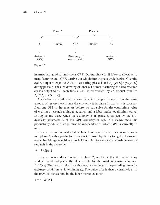
Chapter 9202
intermediate good to implement GPTi. During phase 2 all labor is allocated to manufacturing until GPTi+1 arrives, at which time the next cycle begins. Over the cycle, output is equal to Ati
F(L − n) during phase 1 and A F L A F Lt ti i+ ( ) = ( )Δ γ during phase 2. Thus the drawing of labor out of manufacturing and into research causes output to fall each time a GPT is discovered, by an amount equal to Ati
[F(L) − F(L − n)].A steady-state equilibrium is one in which people choose to do the same
amount of research each time the economy is in phase 1; that is, n is constant from one GPT to the next. As before, we can solve for the equilibrium value of n using a research-arbitrage equation and a labor-market-equilibrium curve. Let wj be the wage when the economy is in phase j, divided by the pro-ductivity parameter A of the GPT currently in use. In a steady state this productivity-adjusted wage must be independent of which GPT is currently in use.
Because research is conducted in phase 1 but pays off when the economy enters into phase 2 with a productivity parameter raised by the factor g, the following research-arbitrage condition must hold in order for there to be a positive level of research in the economy
ω λγπ ω1 2= ( )�
Because no one does research in phase 2, we know that the value of w2 is determined independently of research, by the market-clearing condition L = �x(w2). Thus we can take this value as given and regard the preceding research-arbitrage condition as determining w1. The value of n is then determined, as in the previous subsection, by the labor-market equation
L n x= + ( )� ω1
ti + Δi ti+1 ti (Slump) (Boom)
Phase 1
Arrival ofGPTi
Arrival ofGPTi+1
Discovery ofcomponent i
Phase 2
Figure 9.7
General-Purpose Technologies 203
The average growth rate will be the frequency of innovations times the size g − 1, for exactly the same reason as in the basic model. The frequency, however, is determined a little differently than before because the economy must pass through two phases. An innovation is implemented each time a full cycle is completed. The frequency with which this implementation occurs is the inverse of the expected length of a complete cycle. This in turn is just the expected length2 of phase 1 plus the expected length of phase 2:
1 1λ μ μ λμλ
nn
n+ = +
Thus the growth rate will be
gn
n= −( )
+γ μλ
μ λ1
which is positively affected by anything that raises research.The size of the slump ln[F(L)] − ln[F(L − n)] that occurs when each GPT
arrives is also an increasing function of n, and hence it will tend to be positively correlated with the average growth rate.
One further property of this cycle worth mentioning is that, as Helpman and Trajtenberg point out, the wage rate will rise when the economy goes into a slump. That is, because there is no research in phase 2, the normalized wage must be low enough to provide employment for all L workers in the manufacturing sector, whereas with the arrival of the new GPT the wage must rise to induce manufacturers to release workers into research. This brings us directly to the next section on wage inequality.
We conclude this section with one fi nal remark. In the preceding model, the discovery of a new GPT leads initially to a fall in output. In reality, however, what we observe looks more like a slowdown but still with positive growth. The most obvious way to reconcile the theory with this observation is to extend the model by assuming that the economy consists not of one sector but of many, and
2. The length Δ of phase 1 is a random variable that is distributed geometrically with parameter ln; that is,
Prob Δ =( ) = −( ) =−i n n i
iλ λ1 1 21, , , . . .
Since the expected value of a geometrically distributed random variable is the inverse of the para-meter, therefore the expected length of phase 1 is 1/ln. Likewise, the length of phase 2 is geometri-cally distributed with parameter m, so its expected length is 1/m.
Chapter 9204
that each sector experiments with the new GPT. Following the discovery of the GPT, some sectors will discover the complementary input that suits them before other sectors, and the accelerated growth of the former will compensate for the output fall of the latter. So the aggregate growth rate may dip for a while before fi nally taking off, but it will not necessarily turn negative.3
9.3 GPT and Wage Inequality
In this section we develop an explanation for increased wage inequality between and within educational groups, which is based on the notion of GPT. We argue that this explanation is consistent with the observed dynamic pattern of the wage premium in the United States and the United Kingdom since 1970, and that it does a better job than the market-size theory at dealing with the following two issues raised in chapter 8.
Issue 1 Labor Market History Unlike in the recent period, the increase in supply of educated labor associated with the high school movement of the 1920s did not result in a comparable increase in the skill premium (see Goldin and Katz 1998).
Issue 2 Productivity Slowdown The market-size explanation cannot account for the concurrence of the rise in skill premium with a productivity slowdown from the mid-1980s until the mid-1990s in the United States.
In addition, we will argue that the GPT explanation is consistent with (1) the increase in within-group inequality affecting primarily the temporary component of income (Blundell and Preston 1999) and (2) the observed increase in the experience premium.
9.3.1 Explaining the Increase in the Skill Premium
Figure 9.8, also drawn from Jovanovic and Rousseau (2005), shows that although the skill premium fell during the latter years of electrifi cation, it rose with the IT wave after 1978.
In this subsection we show how the Helpman-Trajtenberg model of the previ-ous section can account for the rise in the skill premium during the IT revolution.4
3. In Aghion and Howitt (1988a, chap. 8) we develop such a model, and argue that the diffusion of a new GPT to the whole economy will typically follow a logistic pattern over time.
4. In section 9.4 we argue that a GPT explanation is also consistent with the early-20th-century drop in the skill premium.
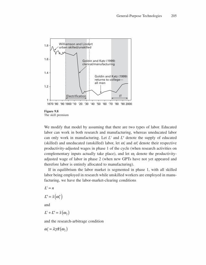
General-Purpose Technologies 205
We modify that model by assuming that there are two types of labor. Educated labor can work in both research and manufacturing, whereas uneducated labor can only work in manufacturing. Let Ls and Lu denote the supply of educated (skilled) and uneducated (unskilled) labor, let w s
1 and w u1 denote their respective
productivity-adjusted wages in phase 1 of the cycle (when research activities on complementary inputs actually take place), and let w2 denote the productivity-adjusted wage of labor in phase 2 (when new GPTs have not yet appeared and therefore labor is entirely allocated to manufacturing).
If in equilibrium the labor market is segmented in phase 1, with all skilled labor being employed in research while unskilled workers are employed in manu-facturing, we have the labor-market-clearing conditions
L ns =
L xu u= ( )� ω1
and
L L xs u+ = ( )� ω2
and the research-arbitrage condition
ω λγπ ω1 2s = ( )�
1870 ‘80 ‘90 1900 ‘10 ‘20 ‘30 ‘40 ‘50 ‘60 ‘70 ‘80 ‘90 2000
1.8
1.6
1.4
1.2
1Electrification
Goldin and Katz (1999)clerical/manufacturing
Williamson and Linderturban skilled/unskilled
Goldin and Katz (1999)returns to college—all men
IT
Figure 9.8The skill premium
Chapter 9206
which expresses the wage of skilled labor as being equal to the expected value of investing (skilled) labor in R&D for discovering complementary inputs to the new GPT.
The labor market will be truly segmented in phase 1 if and only if w s1 defi ned
by this research-arbitrage condition satisfi es
ω ω1 1s u>
which in turn requires that Ls not be too large. Otherwise the labor market remains unsegmented, with n < Ls,
ω ω1 1s u=
in equilibrium. In the former case, the arrival of a new GPT raises the skill premium (from 0 to w s
1/w u1 − 1) at the same time as it produces a productivity
slowdown because labor is driven out of production.
9.3.2 Explaining the Increase in Within-Group Inequality
Perhaps the most intriguing feature of the upsurge in wage inequality is that it took place to a large extent within control groups, no matter how narrowly those groups are identifi ed (e.g., in terms of experience, education, gender, industry, occupation).
Measurement problems provide an obvious fi rst explanation for this puzzle. For example, a PhD from a top economics department should be valued more than a PhD from a lesser place, even though both PhDs may involve the same number of years “in school.” Similarly, different jobs may involve different learning-by-doing and/or training opportunities, thereby leading to wage differ-ences among workers with the same level of seniority. But even when controlling for measurement problems, a substantial amount of residual wage inequality remains to be explained.
Another explanation5 is that skill-biased technical change enhanced not only the demand for observed skills as described earlier but also the demand for unobserved skills or abilities. Although theoretically appealing, this explanation is at odds with econometric work (Blundell and Preston 1999) showing that the within-group component of wage inequality in the United States and United Kingdom is mainly transitory, whereas the between-group component accounts for most of the observed
5. See Acemoglu (1998), Heckman, Lochner, and Taber (1998), Galor and Moav (2000), and Rubinstein and Tsiddon (1999) for models of within-group inequality based on differences in innate ability.
General-Purpose Technologies 207
increase in the variance of permanent income. The explanation based on un-observed innate abilities also fails to explain why the rise in within-group inequality has been accompanied by a corresponding rise in individual wage instability (see Gottschalk and Moffi tt 1994). In the remaining part of this section, we argue that the diffusion of a new technological paradigm can affect the evolution of within-group wage inequality in a way that is consistent with these facts.
9.3.2.1 GPT and the Adaptability Premium
Building on recent work by Violante (2002), Aghion, Howitt, and Violante (2000) argue that the diffusion of a new GPT raises within-group wage inequality pri-marily because the rise in the speed of embodied technical progress associated with the diffusion of the new GPT increases the market premium to those workers who adapt quickly to the leading-edge technology.
In terms of the preceding model, let us again assume that all workers have the same level of education but that once a new GPT has been discovered, only a fraction a of the total labor force can adapt quickly enough to the new technology so that they can work on looking for a new component that complements the GPT. The other workers that did not successfully adapt have no alternative but to work in manufacturing. Let w1
Adapt denote the productivity-adjusted wage rate of adaptable workers in phase 1 of the cycle, whereas w l denotes the wage of nonadaptable workers. Labor market clearing implies
αL n=
1 1−( ) = ( )α ωL x�
and
L x= ( )� ω2
whereas research arbitrage for adaptable workers in phase 1 implies
ω λγπ ω1 2Adapt = ( )�
Assume a is small enough to generate a positive adaptability premium:
ω ω1 1Adapt >
Up to this point in our argument we have just repeated the analysis of the previous section, replacing skilled and unskilled workers with adaptable and nonadaptable workers. A GPT raises the adaptability premium just the same way as it raises the skill premium. But there are two important differences between
Chapter 9208
skill and adaptability. The fi rst is that whereas we can measure a worker’s skill level, albeit imperfectly, using years of schooling, we have no way of measuring a worker’s adaptability. This inability means that no matter how we group workers in terms of observable characteristics, there will still be within-group variability in wages because of unobserved differences in adaptability.
The second difference between skill and adaptability is that to the extent that skill is associated with education, it is a persistent characteristic of a worker, especially a prime-age worker. Adaptability is not necessarily a persistent char-acteristic; it may be largely a matter of luck. Some people can catch on to one particular new technology but not to others. It is this random element of adapt-ability that makes our GPT-based explanation of within-group inequality consis-tent with rising wage instability.
To be more specifi c, take the extreme case in which each time a new technol-ogy arrives every worker has the same probability a of being adaptable to that new technology, regardless of whether he was or was not adaptable to any past technology. In that case, the variance of each worker’s prospective wage prior to the arrival of a new GPT is equal to6
V = −( ) −( )α α ω ω1 1 1
2Adapt
which is increasing in g and l.Thus the approach based on the notion of GPT can shed light not only on the
observed evolution of the college premium (preceding subsection) but also on the increase in residual wage inequality. Furthermore, it does so in a way that can be made consistent with at least two puzzling facts: fi rst, to the extent that residual wage inequality has to do with the stochastic nature of workers’ adapt-ability to the newest vintage more than with innate ability, the rise in within-group inequality induced by the diffusion of a new GPT should primarily affect the transitory component of income, in line with the empirical work of Blundell and Preston (1999); second, the increase in residual wage inequality should be mirrored by a rise in individual lifetime wage instability as documented by Gottschalk and Moffi tt (1994).
9.3.2.2 GPT and the Experience Premium
Another puzzle is that the return to experience has increased at the same time as the skill premium. Aghion, Howitt, and Violante (2002) again appeal to a GPT
6. Recall that if a random variable is equal to x0 with probability p and xl with probability 1 − p, then its variance is p(1 − p) (x1 − x0)2. In this case, p = a, x0 = w1
Adapt, and x1 = w1.

General-Purpose Technologies 209
argument to explain this fact. Their explanation is that the pervasiveness of a GPT means that past experience can be more easily transferred by an adaptable worker who moves from one sector to another. This factor in turn increases the ex ante value of experience, that is, the experience premium.
More formally, using the summary presentation by Hornstein, Krusell, and Violante (2005), consider an overlapping-generations model with two-period-lived individuals. Each cohort of individuals, of measure one, works throughout its two periods of life. Technological progress produces innovations that multiply productivity by the factor g > 1. In each period there are only two sectors, a new sector and an old sector. We denote the new sector by its age, namely 0, and similarly we denote the old sector by 1. Output in each sector i is
Y A hi i i= −1 α
where Ai is productivity and hi is the effective labor input in sector i. We have
A A0 1 = γ
Adaptability Constraint
All young workers can immediately adapt to the new technology and thus work in sector 0, each providing one unit of labor input; however, only a fraction s of old workers can relocate to the new technology.
Learning Parameter
An old worker that does not relocate can provide 1 + h units of labor to sector 1, where the parameter h refl ects on-the-job learning in what was the leading-edge sector when the worker was young.
Transferability Parameter
An individual who worked in the leading-edge last period and is moving to the new leading-edge this period can transfer some of the knowledge she acquired on the previous leading-edge. That is, every such worker can supply 1 + th limits of labor input to the new sector, where the transferability parameter t measures the generality of the technology.
We thus have
h0 1 1= + +( )σ τη
h1 1 1= −( ) +( )σ η
Chapter 9210
That is, the labor input supplied to the new sector is the unit input from the unit mass of young workers plus the 1 + th supplied by each of the s adaptable old workers, while the labor input supplied to the old sector is the 1 + h supplied by each of the 1 − s nonadaptable workers.
Assuming perfect competition, all wages equal their marginal products:
ωii
i
Y
h= ∂
∂
where wi is the wage per unit of labor input in sector i. Thus
ωω
γ γσ τησ η
α α
1
0
1 0
1
1 1 1
1 1=
⎛⎝⎜
⎞⎠⎟
=+ +( )−( ) +( )
⎛⎝⎜
⎞⎠⎟
− −h
h
The average wage of an old worker will be
σ τ ω σ η ω1 1 10 1+( ) + −( ) +( )n
because the fraction s will earn w0 for each of their 1 + th units of labor input supplied to sector 0 while the fraction 1 − s earn w1 for each of their 1 + h units in sector 1. Since all young workers earn w0, the equilibrium experience premium, defi ned as the average wage of old workers relative to the average wage of young workers, is given by
x = +( ) + −( ) +( )σ τη σ η ω ω1 1 1 1 0
which in turn is unambiguously increasing in t. So the arrival of a new GPT, which increases the parameter t of generality or transferability, will raise the experience premium of adaptable workers (fi rst term on the right-hand side); it also has the indirect effect of raising the experience premium of nonadaptable workers, because by increasing the total supply of adaptable labor it reduces the wage of young workers.
9.4 Conclusion
In this chapter we have developed very simple models to capture the notion of general-purpose technologies and to analyze why the arrival of a new GPT can generate a productivity slowdown and at the same time an increase in between-group and within-group wage inequality as well as a surge in the experience premium. We can compare the analysis of wage inequality based on GPT to the alternative explanation based on market size and directed technical change that
General-Purpose Technologies 211
we developed in chapter 8. The advantage of the GPT explanation is fourfold. First, whereas the market-size explanation cannot explain the fall in the skill premium in the 1920s, when there was a rise in the relative supply of skills, the GPT explanation is consistent with this fact, since the 1920s was a period in which the GPT of electrifi cation was entering the mature stage in which the wave of innovations was dying out and the technology was becoming more user-friendly, thereby generating less of a premium on skills needed to use it. Second, as we have seen, the GPT explanation is consistent with the productivity slow-down that took place when the skill premium started to rise in the 1970s. Third, the GPT explanation also accounts for the fact that the rise in within-group inequality starting in the last quarter of the 20th century mainly affected transitory income. And fourth, the GPT story provides an explanation for the observed rise in the experience premium.
9.5 Literature Notes
Although formal analysis of GPTs was not developed before 1992; the idea that long-run cycles may result from technological change goes back to Kondratieff (1925). For more recent evidence on long swings and Schumpeterian waves of innovation see Gordon (1999).
Many economic historians have studied episodes of major technological change. Here we refer the reader to the enlightening studies of Von Tunzelmann (1978) on the steam engine, David (1990) on the parallel between “the computer and the dynamo,” and Lipsey and Bekar (1995) on “enabling technologies.” Authors such as Freeman, Clark, and Soete (1982) and Freeman and Perez (1988) analyzed the notion of “technoeconomic paradigm,” which, as Lipsey, Bekar, and Carlaw (1998) point out, is much broader than a GPT, as it refers to a systematic relationship among products, processes, and the organizations and institutions that coordinate economic activity.
Mokyr (1990) distinguishes between “micro inventions” (improving existing technologies and responding to economic incentives) and “macro inventions” (usually unrelated to incentives, emerging from radically new ideas, without obvious precedent) . These latter inventions are quite similar to new GPTs: both prevent growth from coming to a halt, both involve widespread complemen-tarities, and both provide ground for supporting micro inventions. Lipsey, Bekar, and Carlaw (2005) provide a sweeping history of technological change based on the fundamental notion of the GPT.
Chapter 9212
The fi rst theoretical analysis of GPTs was by Bresnahan and Trajtenberg (1995), who coined the phrase “general-purpose-technology” and defi ned it as having three main features: pervasiveness, technological dynamism, and inno-vational complementarities. They argued that technologies have a treelike struc-ture, with a few prime movers located at the top and all other technologies radiating out from them. Helpman and Trajtenberg (1998a, 1998b) extended the Bresnahan-Trajtenberg model by turning it into the fi rst general-equilibrium GPT growth model. Aghion and Howitt (1998b) developed a Schumpeterian model of GPTs to explain the slowdowns and increase in wage inequality that follow the arrival of a new GPT. Schumpeterian waves of innovation also feature in the work of Jovanovic and Rob (1990) and Cheng and Dinopoulos (1992), where each fundamental innovation is followed by a sequence of increasingly more incremental innovations.
A main reference on GPTs is the book edited by Helpman (1998), which presents the main models and also applications to topics such as the effect of GPTs on factor markets (Harris’s chapter), the rise in obsolescence of capital as a consequence of faster technological progress (Howitt’s chapter), and the effects of GPTs on incen-tives for vertical integration (Bresnahan and Gambardella’s chapter).
We also refer our readers to three chapters in the Handbook of Economic Growth (Aghion and Durlauf, 2005): (1) the chapter by Jovanovic and Rousseau on GPTs, which studies two of the most important examples in U.S. modern history, namely, electricity and information technology, especially regarding their dynamic effects on productivity and the skill premium; (2) the chapter by Hornstein, Krusell, and Violante, which discusses the impact of GPTs on wage inequality between and within educational groups; and (3) the chapter by Jorgenson. which analyzes the IT revolution in the light of growth accounting.
Problems
1. Explain intuitively how the arrival of a new GPT can generate a productivity slowdown and at the same time an increase in between-group and within-group wage inequality as well as a surge in the experience premium. Compare and contrast the analysis of wage inequality based on GPT to the alternative explanation based on market size and directed technical change developed in chapter 8.
2. *Moore’s law and learning by doing
(This problem is adapted from Jovanovic and Rousseau 2002; it studies in a very stylized model the potential impact of a sector where costs decrease sharply—following Moore’s law—as is the case in the IT sector.)
A fi nal good is produced according to Y AL K ALk kK
L= = =⎛
⎝⎜⎞⎠⎟
−1 α α α , where L is the labor force
growing at a rate n, and K is a capital good. In this stylized model, the only capital is IT goods that (nonrealistically) do not depreciate and that benefi t from knowledge spillover, so that the cost of
General-Purpose Technologies 213
production follows Moore’s law: producing one additional unit of capital requires 1
q
K
B= ⎛
⎝⎜⎞⎠⎟
−β
units
of fi nal good. The two sectors are perfectly competitive, and fi rms do not internalize the spillover (so they take q as given). The fi nal good is taken to be the numéraire.
Consumers have the following utility:
U e c dttt= −∞
∫ ρ
0
a. What is the price of capital p? Prove that
α αAk rpdp
dt− = −1
where r is the rate of interest.
b. Show that in steady state, g nc =− −
αβα β1
.
c. Let zK
L=
− −
−
1
1
α β
α . Show that z. = −az + b, where a and b are two constants to be
determined. Solve for the transition path of K. Comment on the effect of a and b on the speed of convergence.
d. We introduce a second capital good X such that Y = AL1−a−gKaXg = ALkaxg. The good X is produced one for one with the fi nal good and depreciates at the rate d. Show that the
previous analysis is still valid as long as A is replaced by A Ar
* =+
⎛⎝⎜
⎞⎠⎟
−γδ
γγ1 and a is replaced by
α αγ
* =−1
.
3. **Endogenizing the growth rate
(In this exercise we extend the model presented in section 9.2.2.2 by endogenizing the growth rate and the slump in production.)
We consider a setup similar to the one presented in section 9.2.2.2. Time is discrete, and there is a unit mass of risk-neutral consumers (with discount rate b). A fi nal good is produced according to Y = A1−axaL1−a, where x is an intermediary input produced by a monopoly with one unit of fi nal good. A is the quality of the intermediary input, and L is the amount of labor force working in the fi nal-good sector. When a new intermediary input is invented, its quality is g > 1 times the quality of the previ-ous one (we assume that innovation is drastic).
In phase o, a GPT has just been invented, but the economy still uses the old technology (and so the old intermediary good), and research is conducted to discover the specifi c technology to imple-ment the new GPT in the intermediate-good sector by the R&D departments of potential competitors to the current monopolist. If a competitor succeeds, he becomes the new monopolist, and the economy enters phase n; he succeeds with probability lono where no is the amount of labor hired in research by this company. The value lo is suffi ciently small that the probability that two competitors will dis-cover the new intermediate input simultaneously is negligible.
In phase n, the specifi c input has been invented, so the new technology is used. A new GPT may arrive at a Poisson rate m.
We consider a steady-state equilibrium in the sense that zZ
Aiit
t
= is constant (where Z can be
consumption, wages, profi ts, or the value of a fi rm; i = o; n denotes which phase is the current one; and At is the technology used).
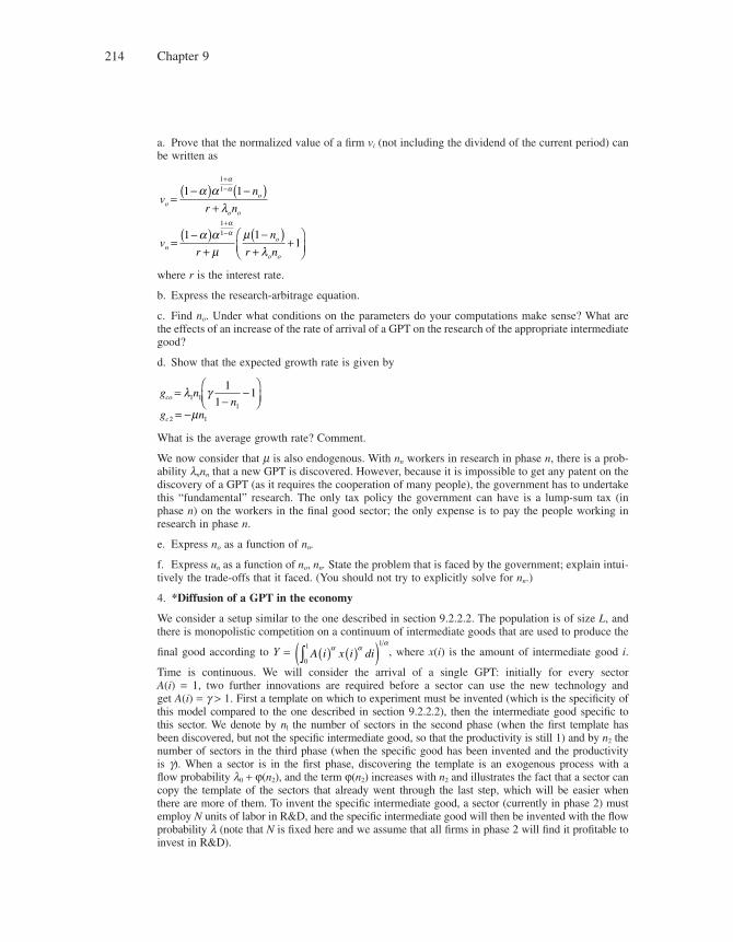
Chapter 9214
a. Prove that the normalized value of a fi rm vi (not including the dividend of the current period) can be written as
vn
r noo
o o
=−( ) −( )
+
+−1 1
1
1α αλ
αα
vr
n
r nno
o o
=−( )
+−( )
++
⎛⎝⎜
⎞⎠⎟
+−1 1
1
1
1α αμ
μλ
αα
where r is the interest rate.
b. Express the research-arbitrage equation.
c. Find no. Under what conditions on the parameters do your computations make sense? What are the effects of an increase of the rate of arrival of a GPT on the research of the appropriate intermediate good?
d. Show that the expected growth rate is given by
g nnco =
−−
⎛⎝⎜
⎞⎠⎟
λ γ1 11
1
11
g nc2 1= −μ
What is the average growth rate? Comment.
We now consider that m is also endogenous. With nn workers in research in phase n, there is a prob-ability lnnn that a new GPT is discovered. However, because it is impossible to get any patent on the discovery of a GPT (as it requires the cooperation of many people), the government has to undertake this “fundamental” research. The only tax policy the government can have is a lump-sum tax (in phase n) on the workers in the fi nal good sector; the only expense is to pay the people working in research in phase n.
e. Express no as a function of nn.
f. Express un as a function of no, nn. State the problem that is faced by the government; explain intui-tively the trade-offs that it faced. (You should not try to explicitly solve for nn.)
4. *Diffusion of a GPT in the economy
We consider a setup similar to the one described in section 9.2.2.2. The population is of size L, and there is monopolistic competition on a continuum of intermediate goods that are used to produce the
fi nal good according to Y = A i x i di( ) ( )( )∫ α αα
0
1 1
, where x(i) is the amount of intermediate good i.
Time is continuous. We will consider the arrival of a single GPT: initially for every sector A(i) = 1, two further innovations are required before a sector can use the new technology and get A(i) = g > 1. First a template on which to experiment must be invented (which is the specifi city of this model compared to the one described in section 9.2.2.2), then the intermediate good specifi c to this sector. We denote by nl the number of sectors in the second phase (when the fi rst template has been discovered, but not the specifi c intermediate good, so that the productivity is still 1) and by n2 the number of sectors in the third phase (when the specifi c good has been invented and the productivity is g). When a sector is in the fi rst phase, discovering the template is an exogenous process with a fl ow probability l0 + ϕ(n2), and the term ϕ(n2) increases with n2 and illustrates the fact that a sector can copy the template of the sectors that already went through the last step, which will be easier when there are more of them. To invent the specifi c intermediate good, a sector (currently in phase 2) must employ N units of labor in R&D, and the specifi c intermediate good will then be invented with the fl ow probability l (note that N is fi xed here and we assume that all fi rms in phase 2 will fi nd it profi table to invest in R&D).
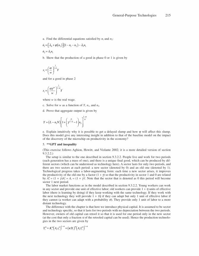
General-Purpose Technologies 215
a. Find the differential equations satisfi ed by nl and n2:
�n n n n n1 0 2 1 2 1 11= + ( )⎡⎣ ⎤⎦ − −( ) −λ ϕ λ
�n n2 1 1= λ
b. Show that the production of a good in phase 0 or 1 is given by
xw
Yi = ⎛⎝⎜
⎞⎠⎟
−α α1
1
and for a good in phase 2
xw
Yi =⎛⎝⎜
⎞⎠⎟
−αγ α α1
1
where w is the real wage.
c. Solve for w as a function of Y, n1, and n2.
d. Prove that aggregate output is given by
Y L n N n= −( ) + −⎛⎝⎜
⎞⎠⎟
⎡
⎣⎢⎢
⎤
⎦⎥⎥
−
−
11
2
1
1 1γα
α
αα
e. Explain intuitively why it is possible to get a delayed slump and how ϕ will affect this slump. Does this model give any interesting insight in addition to that of the baseline model on the impact of the discovery of the microchip on productivity in the economy?
5. **GPT and inequality
(This exercise follows Aghion, Howitt, and Violante 2002; it is a more detailed version of section 9.3.2.2.)
The setup is similar to the one described in section 9.3.2.2. People live and work for two periods (each generation has a mass of one), and there is a unique fi nal good, which can be produced by dif-ferent sectors (which can be understood as technology here). A sector lasts for only two periods, and there are two sectors at each period: a new sector (denoted by 0) and an old one (denoted by 1). Technological progress takes a labor-augmenting form: each time a new sector arises, it improves the productivity of the old one by a factor (1 + g) so that the productivity in sector 1 and 0 are related by A0
t = (1 + g )A1t = At = (1 + g )t. Note that the sector that is denoted as 0 this period will become
sector 1 next period.The labor market functions as in the model described in section 9.3.2.2. Young workers can work
in any sector and provide one unit of effective labor; old workers can provide 1 + h units of effective labor (there is learning by doing) if they keep working with the same technology. If they work with the next technology they will provide 1 + th if they can adapt but only 1 unit of effective labor if they cannot (a worker can adapt with a probability s). They provide only 1 unit of labor to a more distant technology.
The difference with the chapter is that here we introduce physical capital. It is assumed to be sector and technology specifi c, so that it lasts for two periods with no depreciation between the two periods. However, owners of old capital can retool it so that it is used for one period only in the new sector (at the cost that only a fraction k of the retooled capital can be used). Hence the production technolo-gies in the two sectors are given by
Y K A x D A xt t t t t t t0 0 1 0 1
= ( ) + ( ) ( )− −α α α ακ
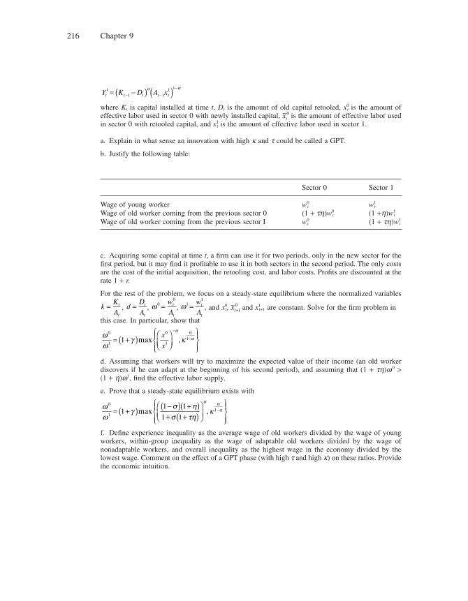
Chapter 9216
Y K D A xt t t t t1
1 11 1
= −( ) ( )− −
−α α
where Kt is capital installed at time t, Dt is the amount of old capital retooled, x0t is the amount of
effective labor used in sector 0 with newly installed capital, xt0 is the amount of effective labor used
in sector 0 with retooled capital, and x1t is the amount of effective labor used in sector 1.
a. Explain in what sense an innovation with high k and t could be called a GPT.
b. Justify the following table:
Sector 0 Sector 1
Wage of young worker w0t w1
t
Wage of old worker coming from the previous sector 0 (1 + th)w0t (1 +h)w1
t
Wage of old worker coming from the previous sector I w0t (1 + th)w1
t
c. Acquiring some capital at time t, a fi rm can use it for two periods, only in the new sector for the fi rst period, but it may fi nd it profi table to use it in both sectors in the second period. The only costs are the cost of the initial acquisition, the retooling cost, and labor costs. Profi ts are discounted at the rate 1 + r.
For the rest of the problem, we focus on a steady-state equilibrium where the normalized variables
kK
At
t
= , dD
At
t
= , ω 00
= w
At
t
, ω11
= w
At
t
, and x0t, xt+1
0 and x1t+1 are constant. Solve for the fi rm problem in
this case. In particular, show that
ωω
γ κα α
α0
1
0
111= +( ) ⎛
⎝⎜⎞⎠⎟
⎧⎨⎪
⎩⎪
⎫⎬⎪
⎭⎪
−
−max ,x
x
d. Assuming that workers will try to maximize the expected value of their income (an old worker discovers if he can adapt at the beginning of his second period), and assuming that (1 + th)w 0 > (1 + h)w1, fi nd the effective labor supply.
e. Prove that a steady-state equilibrium exists with
ωω
γσ ησ τη
κα α
α0
111
1 1
1 1= +( ) −( ) +( )
+ +( )⎛
⎝⎜⎞
⎠⎟⎧⎨⎪
⎩⎪
⎫⎬⎪
⎭⎪−max ,
f. Defi ne experience inequality as the average wage of old workers divided by the wage of young workers, within-group inequality as the wage of adaptable old workers divided by the wage of nonadaptable workers, and overall inequality as the highest wage in the economy divided by the lowest wage. Comment on the effect of a GPT phase (with high t and high k) on these ratios. Provide the economic intuition.
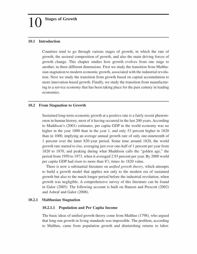
10 Stages of Growth
10.1 Introduction
Countries tend to go through various stages of growth, in which the rate of growth, the sectoral composition of growth, and also the main driving forces of growth change. This chapter studies how growth evolves from one stage to another, in three different dimensions. First we study the transition from Malthu-sian stagnation to modern economic growth, associated with the industrial revolu-tion. Next we study the transition from growth based on capital accumulation to more innovation-based growth. Finally, we study the transition from manufactur-ing to a service economy that has been taking place for the past century in leading economies.
10.2 From Stagnation to Growth
Sustained long-term economic growth at a positive rate is a fairly recent phenom-enon in human history, most of it having occurred in the last 200 years. According to Maddison’s (2001) estimates, per capita GDP in the world economy was no higher in the year 1000 than in the year 1, and only 53 percent higher in 1820 than in 1000, implying an average annual growth rate of only one-nineteenth of 1 percent over the latter 820-year period. Some time around 1820, the world growth rate started to rise, averaging just over one-half of 1 percent per year from 1820 to 1870, and peaking during what Maddison calls the “golden age,” the period from 1950 to 1973, when it averaged 2.93 percent per year. By 2000 world per capita GDP had risen to more than 81/2 times its 1820 value.
There is now a substantial literature on unifi ed growth theory, which attempts to build a growth model that applies not only to the modern era of sustained growth but also to the much longer period before the industrial revolution, when growth was negligible. A comprehensive survey of this literature can be found in Galor (2005). The following account is built on Hansen and Prescott (2002) and Ashraf and Galor (2008).
10.2.1 Malthusian Stagnation
10.2.1.1 Population and Per Capita Income
The basic ideas of unifi ed growth theory come from Malthus (1798), who argued that long-run growth in living standards was impossible. The problem, according to Malthus, came from population growth and diminishing returns to labor.
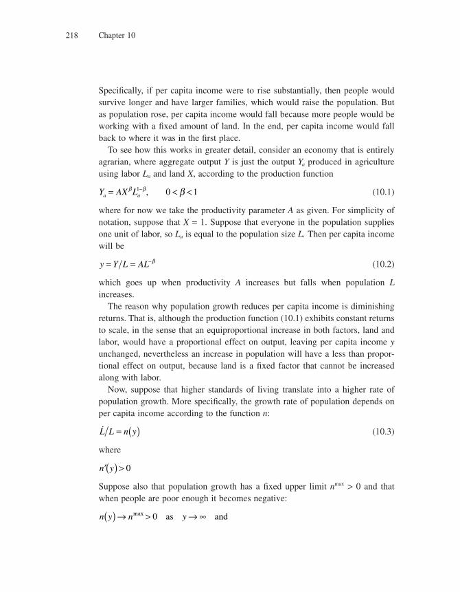
Chapter 10218
Specifi cally, if per capita income were to rise substantially, then people would survive longer and have larger families, which would raise the population. But as population rose, per capita income would fall because more people would be working with a fi xed amount of land. In the end, per capita income would fall back to where it was in the fi rst place.
To see how this works in greater detail, consider an economy that is entirely agrarian, where aggregate output Y is just the output Ya produced in agriculture using labor La and land X, according to the production function
Y AX La a= < <−β β β1 0 1, (10.1)
where for now we take the productivity parameter A as given. For simplicity of notation, suppose that X = 1. Suppose that everyone in the population supplies one unit of labor, so La is equal to the population size L. Then per capita income will be
y Y L AL= = −β (10.2)
which goes up when productivity A increases but falls when population L increases.
The reason why population growth reduces per capita income is diminishing returns. That is, although the production function (10.1) exhibits constant returns to scale, in the sense that an equiproportional increase in both factors, land and labor, would have a proportional effect on output, leaving per capita income y unchanged, nevertheless an increase in population will have a less than propor-tional effect on output, because land is a fi xed factor that cannot be increased along with labor.
Now, suppose that higher standards of living translate into a higher rate of population growth. More specifi cally, the growth rate of population depends on per capita income according to the function n:
�L L n y= ( ) (10.3)
where
′( ) >n y 0
Suppose also that population growth has a fi xed upper limit nmax > 0 and that when people are poor enough it becomes negative:
n y n y( ) → > → ∞max 0 as and
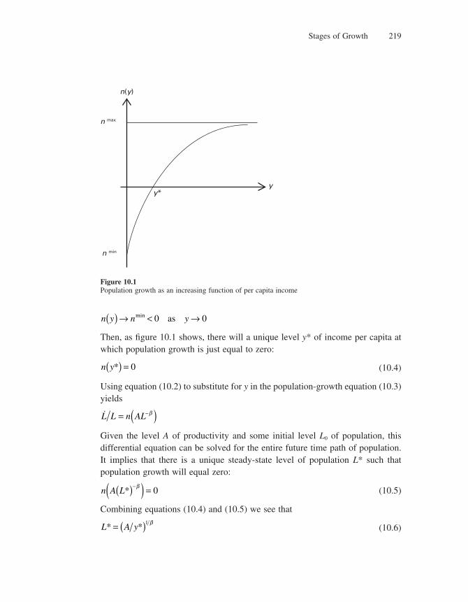
Stages of Growth 219
n y n y( ) → < →min 0 0as
Then, as fi gure 10.1 shows, there will a unique level y* of income per capita at which population growth is just equal to zero:
n y*( ) = 0 (10.4)
Using equation (10.2) to substitute for y in the population-growth equation (10.3) yields
�L L n AL= ( )−β
Given the level A of productivity and some initial level L0 of population, this differential equation can be solved for the entire future time path of population. It implies that there is a unique steady-state level of population L* such that population growth will equal zero:
n A L*( )( ) =−β0 (10.5)
Combining equations (10.4) and (10.5) we see that
L A y* *= ( )1 β (10.6)
n(y)
n max
yy*
n min
Figure 10.1Population growth as an increasing function of per capita income

Chapter 10220
Population will stabilize at the level L* in the long run, no matter where it starts. That is, if initially L were to exceed L*, then per capita income y = AL−b would be less than y* and therefore L would fall back toward L*. As long as L > L*, the same force would be at work, so that L would in fact converge to L* from above. By the same reasoning, if L were to start below L*, then it would converge to L* from below.
Now the fact that population converges to L* in the long run implies that per capita income, which depends on population according to equation (10.2), will converge to the corresponding value y*. In other words, per capita income will ultimately stagnate, not growing beyond the level y*.
10.2.1.2 The Effects of a Productivity Increase
The Malthusian stagnation result was demonstrated on the assumption of a given level of total factor productivity. Could productivity growth save people from stagnation? As it turns out this is not so easy.
Level Increase
Consider fi rst the case of a once-over increase in productivity to the new level A′ > A. If the economy were initially at its steady-state level with
L L A y= = ( )* *1 β
and
Y L y= *
then the productivity increase would at fi rst raise per capita income, from y* to
′ > =− −A L AL yβ β *
But this short-run increase in per capita income would start the Malthusian process at work again. Because per capita income is now above the level y*, the population will start to rise, and this increase will start to bring per capita income back down again. This process will continue until per capita income has fallen back to the level that just eliminates population growth—that is, until it has fallen back to its initial level y*.
Note that although the increase in productivity will have no lasting effect on income per capita, it will have a lasting effect on the size of population. Indeed, it is because of this lasting effect on population size that there is no lasting effect on per capita income. More formally, equation (10.6) indicates that the steady-
Stages of Growth 221
state population size L* is an increasing function of productivity. Galor (2005) reviews a great deal of historical evidence confi rming this prediction of Malthu-sian theory, evidence that more technologically advanced countries and regions, as well as those with a higher quality of land, did not have a much higher standard of living but did have a much higher population density, as compared to those with less advanced technology and inferior land quality.
Steady Productivity Growth
The analysis has so far taken the productivity parameter as being an exogenous constant, perhaps subject to occasional increases but not steady growth. However, there was considerable growth in the world’s stock of technological knowledge prior to the industrial revolution, not as a result of large-scale organized R&D of the sort we are familiar with in advanced countries nowadays but as the result of a combination of the cumulative buildup of lessons learned from experience, creative experimentation by scholars, the need to deal with environmental crises, and the natural human propensity to tinker with things. It is generally agreed, however, that technological progress was a slow process in the Malthusian era. Although there were probably periods in which great discoveries were made (fi re, the wheel, the windmill, . . .), there were also long periods of relative technologi-cal stagnation.
Suppose we take this factor into account by allowing for some steady exoge-nous drift in the productivity parameter A. Then our conclusions would be not quite as pessimistic as under Malthusian theory but almost. Specifi cally, suppose that
�A A g= , a positive constant
Then according to equation (10.2) the growth rate of per capita income will be1
� � �y y A A L L g n y= − = − ( )β β (10.7)
This is a stable differential equation that now converges not to y* but to a some-what higher level �y, the level that satisfi es the stationary condition
n y g�( ) = β (10.8)
1. It follows immediately from equation (10.2) that
ln ln lny A L= − β
Taking derivatives of both sides of this equation with respect to time produces equation (10.7).
Chapter 10222
If g is close to zero, then �y will be close to the level y* of Malthusian theory. As long as2 g < bnmax, which undoubtedly was true for almost all of human history, technological progress will still not produce sustained growth in per capita income. Instead, it will just affect the level at which stagnation occurs.
10.2.2 The Transition to Growth
10.2.2.1 Agriculture and Manufacturing
The long period of stagnation ended around the time of the industrial revolution, when some countries started reallocating resources away from agriculture and toward manufacturing. To see how this shift might happen, suppose that there is a latent manufacturing technology which has not yet been economically viable, but which, as we shall see, will become viable once technology has progressed enough.
Manufacturing output Ym is produced by labor alone, according to
Y ALm m= (10.9)
The productivity parameter A is assumed for simplicity to be the same as in agriculture. Total output is now
Y Y Ya m= +
and the two sectors will compete for the given labor supply L
L L La m+ = (10.10)
The two production functions (10.9) and (10.1) are the same except that one uses land while the other does not. So whether the manufacturing technology is used or not will depend on how much land there is relative to labor. When popu-lation is very small, there is a lot of land for each person to work with, so no one will produce using the manufacturing technology because it does not take advan-tage of this abundant factor. But if population were to rise beyond a critical level, then it would be profi table to activate the manufacturing technology in order to escape the land constraint.
10.2.2.2 Wages and Industrialization
To see how this process works, suppose the economy is in a Malthusian equilib-rium with a rate of technological progress g, which we can suppose is very close
2. If g > bnmax, then population growth will not be able to undo the effect of productivity increases, because equation (10.7) indicates that the growth rate of per capita income cannot fall below g − bnmax > 0.

Stages of Growth 223
to zero, so per capita income has stagnated at the level �y. According to equation (10.8), population will be growing at the rate g/b. The real wage rate will equal the marginal product of labor
� �w AL y= −( ) = −( )−1 1β ββ
which will be constant over time.Someone wanting to hire labor to produce output using the manufacturing
technology would earn a profi t equal to
Πm m m mY wL A w L= − = −( )� �
So as long as the stock of knowledge is relatively low, A will be less than �w, and it will not be profi table to use the manufacturing technology. But if A continues to grow, then at some point it will surpass �w, which remains constant in the Malthusian equilibrium. At this point it becomes profi table to activate the manu-facturing sector, and industrialization begins.
Once manufacturing has started, free entry guarantees that the profi t rate IIm will be zero, so the wage rate will equal the productivity parameter
w A=
The agricultural sector will also have to pay that wage, so its profi t (excluding the rent to the fi xed factor land) will be
Πa a a a aAL wL A L L= − = −( )− −1 1β β
Employment in the agricultural sector La will then be chosen to maximize profi t, and the fi rst-order condition determining this profi t-maximizing choice is
∂∂Πa
aaL
A L= −( ) −⎡⎣ ⎤⎦ =−1 1 0β β
which solves for the constant value
La = −( )11β β
From this point on, while agricultural labor remains constant, manufacturing labor will equal
L L Lm a= −
which will continue to rise over time, since La is constant and the total labor supply L will continue to grow, starting at the Malthusian rate n( �y).

Chapter 10224
10.2.2.3 Sustainable Growth
Not only will population continue to grow, but it will accelerate, and the rate of economic growth y
./y will rise from its previous rate of zero to a new steady-state
value equal to the rate of technological progress g. To see how this process works, notice that income per capita is now
y Y L A L L L AL La a= = −( ) + −1 β
Over time the agricultural share will approach zero, since La is constant and L becomes infi nitely large. Income per capita will thus become approximately equal to A and therefore will grow without bound, approaching the growth rate g of productivity. And the population growth rate will approach its upper limit nmax.
This transition from stagnation to growth takes place because the gradual accretion of knowledge has allowed people to escape from the limitations of land, especially from the diminishing marginal returns to labor applied to fi xed land which kept wages and per capita income from taking off. Once freed from land, people are no longer subject to diminishing returns, and there is nothing to choke off growth in per capita income.
10.2.3 Commentary
The preceding analysis focuses on industrialization as the key to making the transition from stagnation to growth. Other theories focus on human-capital accumulation. For example, Galor and Weil (2000) construct an overlapping-generations model in which people derive utility from consumption and from the quantity and quality of children, where “quality” means the amount of human capital invested in the child.
In their model, the rate of technological progress is assumed to depend on the size of population, through a scale effect, and on the amount of human capital per person. The scale effect triggers the escape from Malthusian stagnation by gradually raising the rate of technological progress. At fi rst the resulting increase in productivity growth leads to a population explosion, but at some point there is a demographic transition that brings population growth under control without per capita income having to fall. This demographic transition comes from a tilting of the quality-quantity trade-off; that is, a faster rate of technological progress raises the rate of return to human-capital investment because human capital is most valuable during periods of rapid technological change.3 People respond to
3. See our discussion of the Nelson and Phelps (1966) view of human capital in chapter 13.
Stages of Growth 225
the increased skill premium by substituting more investment in quality for increased quantity of children.
The Galor-Weil theory has the advantage of predicting not only the industrial revolution but also the demographic revolution that took place around the same time; population growth did indeed start to fall. However, Mokyr and Voth (2006) have questioned this line of analysis on the grounds that there is little evidence that Europe was in a Malthusian trap in 1700. Population and per capita income had been rising together in many regions even though Malthusian theory implies that a rise in population should depress per capita income. Likewise, the population in England was roughly constant between 1700 and 1750, long before the industrial revolution that was supposed to have been triggered by the scale effect of a large population. Nor can historians fi nd evi-dence of the skill premium that the human capital theory predicts should have induced the tilting of the quality-quantity trade-off that caused the demographic transition.
Mokyr and Voth suggest alternative factors that might have kept output from taking off before the industrial revolution. One is the development of a scientifi c culture among a critical mass of craftsmen and business people, the factor stressed by Howitt and Mayer-Foulkes (2005). Another is the set of institutions that protect property rights. Suppose, for example, that anyone could steal another person’s capital at a cost of s. Then no one would accumulate capital beyond the level K = s because to do so would result in losing everything to a thief. In an AK model, that limit on capital accumulation would bring growth to an end until some institutional change raised the cost s of stealing someone else’s property.
The evidence will probably never settle the dispute among these competing theories of the transition from stagnation to growth. For, as Mokyr and Voth admit, there was only one industrial revolution, and one data point is just not enough. As a result, the Mokyr-Voth critique of Malthusian theories is not deci-sive, especially when we take into account that there is two-way causation between population and income, and that there may be long lags involved in these causal relationships. For example, the fact that population and per capita income were rising simultaneously in many regions of Europe before the industrial revo-lution might have been the joint effect of a gradual improvement in technology; perhaps the rise in per capita income would have been reversed eventually if the industrial revolution had not taken place.
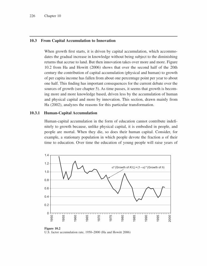
Chapter 10226
10.3 From Capital Accumulation to Innovation
When growth fi rst starts, it is driven by capital accumulation, which accommo-dates the gradual increase in knowledge without being subject to the diminishing returns that accrue to land. But then innovation takes over more and more. Figure 10.2 from Ha and Howitt (2006) shows that over the second half of the 20th century the contribution of capital accumulation (physical and human) to growth of per capita income has fallen from about one percentage point per year to about one half. This fi nding has important consequences for the current debate over the sources of growth (see chapter 5). As time passes, it seems that growth is becom-ing more and more knowledge based, driven less by the accumulation of human and physical capital and more by innovation. This section, drawn mainly from Ha (2002), analyzes the reasons for this particular transformation.
10.3.1 Human-Capital Accumulation
Human-capital accumulation in the form of education cannot contribute indefi -nitely to growth because, unlike physical capital, it is embodied in people, and people are mortal. When they die, so does their human capital. Consider, for example, a stationary population in which people devote the fraction u of their time to education. Over time the education of young people will raise years of
195
0
195
5
196
0
196
5
1970
1975
198
0
198
5
199
0
199
5
20
00
1.4
1.2
1.0
0.8
0.6
0.4
0.2
0
α* (Growth of K/L) + (1 – α) * (Growth of h)
Figure 10.2U.S. factor accumulation rate, 1950–2000 (Ha and Howitt 2006)

Stages of Growth 227
schooling per person s at the rate u. But if the fraction d of people per year die, and those who die have on average s years of schooling, then these deaths will reduce s at the rate ds. The net effect of education and death is to make average years of schooling change at the rate
�s u s= − δ
which means that average years of schooling will go to a steady-state value (where s
. = 0) of
s u* = δ
According to Mincer (1974), human capital per person h can be represented as an exponentially increasing function of years of schooling
h e s= θ
which means that human capital per person will approach a steady-state level
h e u* = θ δ
Increasing the fraction of time spent on education will raise this steady-state level of human capital per person, but it cannot result in a permanent increase in the growth rate of human capital per person. Therefore, at some point the direct contribution of human-capital accumulation to economic growth must come to an end.
This is not to say, however, that human capital eventually ceases to be impor-tant for economic growth. On the contrary, because R&D is a human-capital-intensive activity, therefore as growth becomes more and more dependent on innovation, it also becomes more and more dependent on the level (and quality!) of educational attainment per person.
10.3.2 Physical-Capital Accumulation
In contrast to human capital, there is no limit to how much physical capital a person can accumulate. Yet even physical-capital accumulation is becoming less important than innovation as a source of growth. To understand this trend we reproduce the hybrid neoclassical-Schumpeterian model that includes both capital accumulation and innovation, which we developed in chapter 5, and we analyze its dynamic evolution.
The basic idea of this analysis is that as an economy develops following indus-trialization, it goes through a process of “capital deepening,” in which the emer-gent capital-intensive manufacturing technology becomes equipped. As we saw
Chapter 10228
in chapter 5, a higher productivity-adjusted capital stock creates a scale effect that encourages more innovation, because a successful innovator gets a bigger reward in a wealthier economy. But as in the neoclassical model, the higher pro-ductivity-adjusted capital stock lowers the marginal product of capital, which weakens the impact of capital accumulation on growth. So over time the contribu-tion of capital accumulation to growth decreases while the contribution of innova-tion increases.
10.3.2.1 The Hybrid Model
The fi nal good in this hybrid model is produced under perfect competition accord-ing to the production function
Y L A x dit it it= < <− −∫1 1
0
10 1α α α α,
where each xit is the fl ow of intermediate input i. For simplicity, we set L = 1. Each intermediate input is produced according to the production function
x Kit it=
where Kit is the amount of capital used as input. In equilibrium, each sector will produce at a level xit that is proportional to the productivity parameter Ait. When we put these equilibrium values into the production function, we get a neoclassi-cal aggregate production function of the form
Y A L Kt t t= ( ) −1 α α
where Kt is the aggregate capital stock and the labor-augmenting productivity variable At is just the average across all sectors of the individual productivity parameters: A A dit it= ∫0
1.
As we saw in chapter 5, there are three fundamental equations driving the economy. First, there is the neoclassical law of motion for the capital stock:
K K sY Kt t t t+ − = −1 δ (K)
where s is the saving rate and d is the depreciation rate.Next, there is the productivity-growth equation:
A A
Ag nt t
tt t
+ − = = −( ) ( )1 1γ φ (G)
where g is the size of innovations, nt is the productivity-adjusted research expen-diture in each sector, and f(nt) is the innovation rate.
Stages of Growth 229
The fi nal equation is the research-arbitrage condition:
′( ) ( ) =φ π κnt t� 1 (R)
where kt = Kt/At is the productivity-adjusted capital stock and �π (kt) is each monopolist’s productivity-adjusted profi t, which is increasing in kt. The research-arbitrage equation makes nt an increasing function of kt, so the productivity-growth rate determined by equation (G) is also an increasing function of kt.
Each period, given the historically predetermined value of kt, the research-arbitrage equation (R) determines the research intensity nt; then Kt and At change according to equations (K) and (G), which then determine kt+1; and the process is repeated next period, ad infi nitum.
The steady state of the model is a situation in which all three variables g, n, and k are constant over time. The steady-state conditions are
g n= −( ) ( )γ φ1
′( ) ( ) =φ π κn � 1
s gκ δα − = +1
The fi rst two are just steady-state versions of equations (G) and (R), while the last one is the familiar neoclassical condition that requires the growth rate of capital per effi ciency unit of labor (that is, the growth rate of k) to be constant.
Now consider an economy that is at an early stage of growth, with an adjusted capital stock k0 far below its steady-state value. In that economy, capital accu-mulation is very rapid while productivity growth is slow. But as kt rises up to its steady-state value, the contribution of capital accumulation to growth will slow down while innovation and productivity growth speed up.
More specifi cally, we can write the aggregate production function as
Y At t t= κ α
so if Gt is the growth rate of output, then we can express the growth factor 1 + Gt as the product of two factors:
1 1 1 1+ = =⎛⎝⎜
⎞⎠⎟
⎛⎝⎜
⎞⎠⎟
+ + +GY
Y
A
Att
t
t
t
t
t
κκ
α
where the fi rst factor represents the contribution of innovation and productivity growth, while the second factor represents the contribution of capital deepening. Over time, as kt approaches its steady state, the second factor falls to unity, as in
Chapter 10230
the neoclassical model, so that in the steady state, capital deepening contributes nothing to growth. And as this is happening, the fi rst factor will be increasing over time because
A
Ag nt
tt t
+ = + = + −( ) ( )1 1 1 1γ φ
and, as we have seen, nt increases as kt rises to its steady-state value. Thus in the steady state, innovation and productivity growth contribute even more to eco-nomic growth, both absolutely and relative to capital accumulation, than they did in the earlier stages of growth.
10.4 From Manufacturing to Services
Another dramatic structural change that takes place in an advanced economy is the shift from manufacturing to services. This trend predates the outsourcing movement that many have blamed for the loss of manufacturing jobs in the United States, and it has taken place to a similar extent in all advanced economies, not just the United States. This fact suggests that there is something more fundamen-tal at work than U.S. trade policies. This section shows how we can account for the movement using a model of nonbalanced growth developed by Acemoglu and Guerrieri (2006).
The key feature of services sectors that we focus on is that they are not as capital intensive as manufacturing sectors. To simplify the analysis, we make the extreme assumption that whereas manufacturing requires both labor and capital, services require only labor. Specifi cally, the output of the manufacturing sector is
Y AK LM M= −α α1
and the output of the service sector is4
Y ALS S=
where K is the economy’s capital stock; and the labor inputs must add up to the population L:
L L LM S+ =
4. Note that we are not assuming differential technological progress in the two sectors as was done, for example, by Baumol (1967). Although it may be true that productivity growth is slower in services, it is very hard to know for certain whether it is or not given the diffi culty of measuring the output of services.
Stages of Growth 231
We also assume that fi nal output is produced using services and manufactures according to a production function in which they are complementary inputs. Indeed, we make the extreme assumption that services and manufactures must be combined in fi xed proportions:
Y Y YM S= { }min ,
Then given the stock of capital K, the level of productivity A, and the size of the labor force L, labor will be allocated across the two sectors in such a way as to result in equal output:
K L L LM Mα α1− = −( )
Defi ne the economy-wide capital-labor ratio as
k K L=
and the manufacturing share of employment as
λ = L LM
Then we have
kα αλ λ1 1− = −
Denote by
�λ k( )the solution to this equation. As the economy accumulates more capital per worker, the manufacturing share of employment falls:
d dk�λ < 0
Indeed, as the capital-labor ratio goes to infi nity, manufacturing employment falls to zero:
limk
k→∞
( ) =�λ 0
Aggregate output can then be written as
Y AL k= − ( )⎡⎣ ⎤⎦1 �λ
Suppose again that saving is a fi xed proportion of output. Then,
� �K sAL k K= − ( )⎡⎣ ⎤⎦ −1 λ δ
from which we have
Chapter 10232
� �k sA k n k= − ( )⎡⎣ ⎤⎦ − +( )1 λ δ
Assume that the long-run growth rate g of A is positive. Then in the long run k will indeed rise without bound, manufacturing share of employment will fall to zero, and per capita income will approach
Y L AL L A= − ∞( )⎡⎣ ⎤⎦ =1 �λ
which grows at the rate g.
10.5 Conclusion
In this chapter we fi rst presented the Malthusian model where agricultural output is produced with labor and a fi xed factor, and where labor supply (population) in turn evolves over time at a rate that depends upon the current level of output per capita. Population increases if current per capita GDP is high, and it decreases if current per capita GDP is low. We saw that this model predicts long-term stagna-tion, with per capita GDP converging to the steady-state level at which population does not increase or decrease. Then we added an AK manufacturing technology to this model, and we saw that when the knowledge parameter becomes suffi -ciently high, people start moving from agriculture to manufacturing, at which point the economy escapes from stagnation.
In the subsequent sections, we modeled the transition from capital accumula-tion to innovation, and then the transition from manufacturing to services. One important limitation of these models, which makes them all appear somewhat mechanical, is that they do not capture the idea that the transition from one pro-duction mode to another may require the introduction of new institutions: new ways of regulating or deregulating markets, new fi nancial systems, new ways of organizing fi rms. Private incentives to move from old to new institutions will typically not coincide with the socially optimal or growth-maximizing paths. This important issue of institutional transition will be taken up in chapter 11.
10.6 Literature Notes
Primary references on the transition process from Malthusian stagnation to growth are the papers by Galor and Weil (2000), Hansen and Prescott (2002), and Ashraf and Galor (2008).
Stages of Growth 233
While Galor and Weil emphasize demographic transition as a key feature of the industrial revolution, Mokyr and Voth (2006) stress the importance of both the development of a scientifi c culture among a critical mass of craftsmen and business people, and the setting up of institutions that protect property rights.
The transition from capital accumulation to innovation has been analyzed by Ha (2002). And the transition from manufacturing to services is modeled by Acemoglu and Guerrieri (2006).
For exhaustive references and comprehensive accounts of the literature and debates on the subject, we refer the reader to the Handbook of Economic Growth surveys by Galor (2005) and Mokyr (2005).
Problems
1. Present the mechanisms that related population growth and income per capita in the Malthusian model and how they imply long-run stagnation of income per capita. Can technological progress produce sustained growth in per capita income in the setting? Explain.
2. *Skilled labor and manufacturing
Consider the following version of the economy studied in sections 10.2.1 and 10.2.2.The number of births per period is B = b(y)L where y is per capita income, L is population,
b′(y) > 0, b(y) → b as y → ∞, and b(y) → 0 as y → 0.Each person has a probability d > 0 of dying per period.Output is produced using the agricultural technology
Y A t LA = ( ) ∈( )−1 0 1β β, ,
where A is a productivity parameter with exogenous growth rate g.
a. Solve for the steady state of this economy assuming g > b(b − d). Is it stable? Why is the assump-tion necessary? How does faster productivity growth affect the steady state?
b. Now suppose there is also a manufacturing technology:
Y A t SM = ( )
where S is the skilled labor supply. Each agent chooses at birth whether to become a skilled worker and work in manufacturing or an unskilled worker and work in agriculture. To become skilled an agent must pay a fi xed cost F. Suppose the economy faces an exogenously given constant interest rate r.
Explain why no agents born at time t will choose to become skilled if
w e d F w e dM r t
t
A r t
tτ τ τ τλ τ λ τ( ) − < ( )− +( ) −( )∞ − +( ) −( )∞
∫ ∫where wM is the manufacturing wage and wA is the wage in agriculture.
c. Assume g = 0. Find a condition on A under which all agents will choose to work in agriculture.
d. Does there exist a level of A such that all agents will choose to become skilled?
Chapter 10234
3. Property rights
Suppose each agent has access to an AK production technology, Yj = AKj, where Y is output, K is capital, A is an economy-wide productivity parameter, with growth rate l, and j indexes agents.
Suppose, K.j = Yj − Cj − dKj − G, where C is consumption and G is government expenditure per
capita.Assume that any agent can expropriate any other agent’s capital at cost s.
a. What will the equilibrium values and growth rates of Kj and Cj be?
b. Now suppose that s depends on the level of government expenditure; for instance, it could be a measure of the extent of property rights or law enforcement. Assume σ = G . What level of G will a benevolent government choose?
c. Assuming the existence of a benevolent government, what are the steady-state growth rates of Kj and Cj?
4. Physical capital and innovation
Consider an economy similar to that in section 10.3.2 except that the fi nal good is produced using physical capital, in addition to labor and intermediate inputs, according to
Y x K A L dit it t it= < <− − − −∫ α β α β α β α β1 1
0
10 1,
where x is intermediate input use, K is capital use, and A measures the quality of the inter-mediate input. The fi nal good is used on a one-for-one basis for consumption, physical-capital investment, and intermediate-input production. Intermediate inputs are produced by monopolists. To invent an intermediate of quality Ait = gAit−1 with probability mt an entrepreneur must spend
N Ait itt
t= +⎛⎝⎜
⎞⎠⎟−γ μ δμ1
2
2
As usual we normalize the total labor force to one.
a. Taking the amount of capital used in fi nal-good production as given, solve for xit and the monop-olist’s profi ts pit in equilibrium.
b. Show that the equilibrium probability of innovation in sector i is
μ λ δ
βα
itt
it
K
A=
⎛⎝⎜
⎞⎠⎟
−−1
where l is a constant you should determine. How does the capital stock affect the growth rate? Will the duality of intermediate inputs tend to converge over time?
c. Suppose the economy faces an exogenously determined capital rental rate r. Show that
r A
kdiit
tβα
αα
α βα
=⎛⎝⎜
⎞⎠⎟
−
− −−
∫2
1
1
1
0
1
d. Solve for mt in a symmetric equilibrium in which Ait = At∀i.
e. Suggest modeling techniques that could he used to make r endogenous.
5. *Agricultural productivity and industrialization (based on Matsuyama 1992)
This question considers the relationship between agricultural productivity and industrialization.

Stages of Growth 235
Suppose there are two sectors, agriculture and manufacturing, and a single factor of production, labor. Output in manufacturing is given by
Y t A t L tM M( ) = ( ) ( )⎡⎣ ⎤⎦α
while output in agriculture is given by
Y t B L tA A( ) = ( )⎡⎣ ⎤⎦β
where a,b ∈ (0, 1) and manufacturing productivity A may vary over time. Suppose the total labor force is constant and normalized to one and that the labor market is competitive.
a. Solve for LM(t) and LA(t) as a function of A(t) and the relative price of the manufacturing good p(t).
b. Suppose intratemporal consumption preferences are defi ned over the consumption aggregate
C t C t C C tA M( ) = ( ) −⎡⎣ ⎤⎦ ( )⎡⎣ ⎤⎦−η η1
where h ∈ (0, 1) and C > 0. Show that this implies
1−( ) ( ) −⎡⎣ ⎤⎦ = ( ) ( )η ηC t C p t C tA M
c. Use market clearing and the preceding results to show
C
BL t L t L tM M M= − ( )⎡⎣ ⎤⎦ −
−− ( )⎡⎣ ⎤⎦ ( )−
11
11β βη
ηβα
d. Explain why there must be a unique solution for LM(t).
e. How does the proportion of labor allocated to manufacturing change as agricultural productivity increases?
f. Suppose A.(t) = YM(t). Solve for the growth rate of C(t), and discuss how it depends on agricultural
productivity. Provide some intuition for this result.
6. **Nonbalanced growth (based on Kongsamut, Rebelo, and Xie 2001)
Consider an economy with three sectors—agriculture (A), manufacturing (M), and services (S). At time t, output in the three sectors is given by
A B L Xt A tA
t=M B L Xt M t
Mt=
S B L Xt S tS
t=
where LJ denotes labor allocated to sector J = A, M, S, and X is a productivity parameter with exoge-nous growth rate g. The total labor force is constant and is normalized to one, and all goods are pro-duced under perfect competition.
A representative consumer has preferences such that at time t she seeks to maximize
U A A M S St t t t= −( ) +( )β γ θ
where A > 0, S > 0, and b + g + q = 1.
a. Use labor market clearing to solve for the equilibrium prices of agriculture pA and services pS rela-tive to manufacturing.
Chapter 10236
b. Use consumer optimization to show
p A A M p S SA t t S t−( )= =
+( )β γ θ
c. Defi ne a balanced growth path as an equilibrium in which the growth rates of At, Mt, and St are constant and equal. Show that such an equilibrium does not exist.
d. Defi ne a generalized balanced growth path as an equilibrium in which the growth rates of Mt and pAAt + pSSt are constant. Show that such an equilibrium exists if and only if BSA = BAS .
e. Solve for �LtA , �Lt
M,and �LtS in equilibrium. Discuss.
11 Institutions and Nonconvergence Traps1
11.1 Introduction
Do institutions matter for growth? A common prediction of the growth models with endogenous innovation in the preceding chapters is that they do! For example, the analysis in chapters 3 and 4 would suggest that long-run growth would be best enhanced by some combination of good property-rights protection (to protect the rents of innovators against imitation) and a good education system (to increase the effi ciency of R&D activities and the supply of skilled manufacturing labor). Our discussion of convergence clubs in chapter 7 predicts that the same policies or institutions would also increase a country’s ability to join the convergence club.
That institutions should infl uence economic development had already been con-vincingly argued by economic historians, in particular by Douglas North (see North and Thomas 1973; North 1990) and subsequently by Engerman and Sokoloff (1997, 2000). Thus, North and Thomas explain how the institutional changes brought about by trade and commercial activities led to the Glorious Revolution in 17th-century England. And North (1990) argues that the development of sedimentary agriculture followed the Neolithic revolution, which introduced communal property rights.
North (1990) defi nes institutions as the “rules or constraints on individual behavior” which in turn may be either formal (political constitutions, electoral rules, formal constraints on the executive, . . .) or informal (culture, social norms, . . .). Greif (1994, 2006) extends the notion of institution so that it encom-passes not only the rules of the game as in North, but more generally all forms of economic organizations and fi nally the set of beliefs that shape the interaction between economic agents.
Two research teams over the past 10 years have made pathbreaking contribu-tions showing the importance of institutions for economic development using historical cross-country data. A fi rst team (see La Porta et al. 1998, 1999; Djankov et al. 2003; Glaeser et al. 2004) has emphasized legal origins as a determinant of institutions such as investors’ rights, debt collection systems, or entry regulations. A second team (see Acemoglu, Johnson, and Robinson 2001, 2002; Acemoglu and Johnson 2005) has focused on colonial origins as a determinant of a country’s institutions. These two lines of research have spurred heated debates, which we shall refl ect upon in section 11.2.
Should we recommend the same institutions to all countries? The endogenous growth models developed in previous chapters suggest we should. In particular, they call for better property-rights protection and higher education investment
1. This chapter was jointly written with Erik Meyersson.
Chapter 11238
in all countries under all latitudes. However, in Economic Backwardness in Historical Perspective, Gerschenkron (1962) argues that relatively backward economies could more rapidly catch up with more advanced countries by intro-ducing “appropriate institutions” that are growth-enhancing at an early stage of development but may cease to be so at a later stage.
Thus countries like Japan or Korea managed to achieve very high growth rates from 1945 up until the 1990s with institutional arrangements involving long-term relationships between fi rms and banks, the predominance of large conglomerates, and strong government intervention through export promotion and subsidized loans to the enterprise sector. These policies in turn depart signifi cantly from the more market-based and laissez-faire institutional model pioneered by the United States and cur-rently advocated for all countries as part of the so-called Washington consensus.
In section 11.3 we reconcile new growth theories with Gerschenkron’s views, thereby addressing the concern that growth theory can only deliver universal, one-size-fi ts-all policy prescriptions (legal reforms to enforce property rights, invest-ment climate favorable to entrepreneurship, education, macrostability, . . .) to maximize the growth prospects of a country or sector, and does not apprehend structural transformations in the process of convergence. More specifi cally, we analyze some general implications of the notion of “distance-dependent” appropri-ate institutions, by which we mean institutions that are growth enhancing only for countries at a certain stage of technological development. Technological develop-ment in turn is measured by a country’s current productivity divided by current frontier productivity (the variable a in chapter 7). In particular, we show how the failure to adapt institutions to technological development may generate nonconver-gence traps whereby a country’s average productivity (or per capita GDP) remains bounded away from frontier levels. The section is organized as follows: Section 11.3.1 provides empirical evidence to motivate the notion of appropriate institution. Section 11.3.2 then develops a simple model of appropriate institutions and growth, and illustrates the notion of nonconvergence traps for countries that fail to adapt their institutions and policies as they develop.
11.2 Do Institutions Matter?
In this section2 we briefl y discuss two main attempts at showing a causal rela-tionship between economic institutions (property-rights protection, investors’ protection, . . .) and economic performance measured by the aggregate income or
2. We encourage the student to look at the appendix at the back of the book before reading this section.
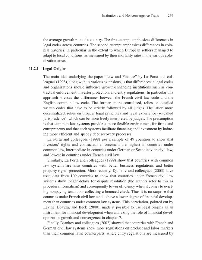
Institutions and Nonconvergence Traps 239
the average growth rate of a country. The fi rst attempt emphasizes differences in legal codes across countries. The second attempt emphasizes differences in colo-nial histories, in particular in the extent to which European settlers managed to adapt to local conditions, as measured by their mortality rates in the various colo-nization areas.
11.2.1 Legal Origins
The main idea underlying the paper “Law and Finance” by La Porta and col-leagues (1998), along with its various extensions, is that differences in legal codes and organizations should infl uence growth-enhancing institutions such as con-tractual enforcement, investor protection, and entry regulations. In particular this approach stresses the differences between the French civil law code and the English common law code. The former, more centralized, relies on detailed written codes that have to be strictly followed by all judges. The latter, more decentralized, relies on broader legal principles and legal experience (so-called jurisprudence), which can be more freely interpreted by judges. The presumption is that common law systems provide a more fl exible environment for fi rms and entrepreneurs and that such systems facilitate fi nancing and investment by induc-ing more effi cient and speedy debt recovery processes.
La Porta and colleagues (1998) use a sample of 49 countries to show that investors’ rights and contractual enforcement are highest in countries under common law, intermediate in countries under German or Scandinavian civil law, and lowest in countries under French civil law.
Similarly, La Porta and colleagues (1999) show that countries with common law systems are also countries with better business regulations and better property-rights protection. More recently, Djankov and colleagues (2003) have used data from 109 countries to show that countries under French civil law systems show longer delays for dispute resolution (the authors refer to this as procedural formalism) and consequently lower effi ciency when it comes to evict-ing nonpaying tenants or collecting a bounced check. Thus it is no surprise that countries under French civil law tend to have a lower degree of fi nancial develop-ment than countries under common law systems. This correlation, pointed out by Levine, Loayza, and Beck (2000), made it possible to use legal origins as an instrument for fi nancial development when analyzing the role of fi nancial devel-opment in growth and convergence in chapter 7.
Finally, Djankov and colleagues (2002) showed that countries with French and German civil law systems show more regulations on product and labor markets than their common lawn counterparts, where entry regulations are measured by
Chapter 11240
the number of procedures entrepreneurs have to go through when creating a new fi rm.
A main limitation of this approach is that it remains cross-sectional, and in particular does not control for country or region fi xed effects. Another problem with this approach is that it does not explain why France, which initiated the civil law system, performs much better than its colonial transplants. In fact, France itself performs rather well in all the above regressions. This brings us to the second approach based on colonial origins.
11.2.2 Colonial Origins
In their paper “The Colonial Origins of Comparative Development,” Acemoglu, Robinson, and Johnson (2001), henceforth AJR, found a clever instrument for economic institutions in colonized countries, namely, the mortality rate of European settlers in these countries. Their idea is that (1) European colon-izers could decide the extent to which they truly wish to settle in the new colony and build institutions rather than just extract resources; (2) this decision depends upon how well colonizers could adapt to the local climate and geography, which in turn is refl ected in mortality rates of European bishops, sailors, and soldiers from local illnesses; and (3) institutions created during the colonization period persist after independence.
In other words, in colonies where they could truly settle, Europeans would try to replicate their own institutions, whereas colonies where they do not settle would be primarily used as extractive states, with little investment in institutions, in particular to protect property rights. Europeans would thus typically choose to settle in colonies where the disease risk was lower. And mortality rates, recorded by soldiers, bishops, and sailors between the 17th and the 19th centuries, should refl ect that risk.
More precisely, AJR perform a two-stage least-square regression3 where (1) they regress per capita GDP of a country in the sample on expropriation risk, which is what we call the second-stage regression, and (2) they regress expropriation risk on settlers’ mortality rates, which is what we call the fi rst-stage regression. Table 11.1 shows the results from this two-stage regression procedure. The second-stage regression is shown at the top of the table; the fi rst stage is shown at the bottom. The fi rst two columns show the OLS regression of per capita GDP in 1995 on expropriation not instrumented by settler mortality (column 2 includes only the
3. See the appendix.
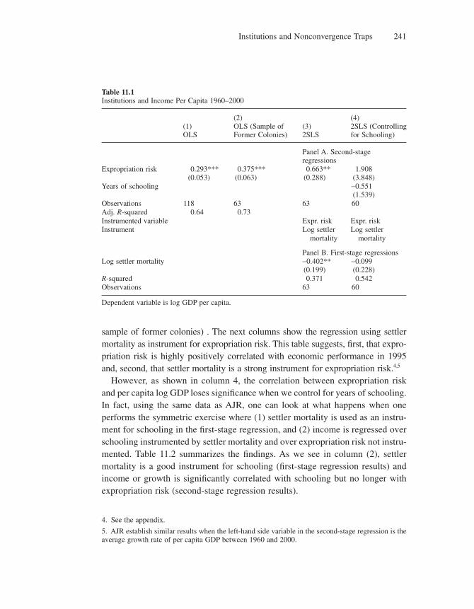
Institutions and Nonconvergence Traps 241
sample of former colonies) . The next columns show the regression using settler mortality as instrument for expropriation risk. This table suggests, fi rst, that expro-priation risk is highly positively correlated with economic performance in 1995 and, second, that settler mortality is a strong instrument for expropriation risk.4,5
However, as shown in column 4, the correlation between expropriation risk and per capita log GDP loses signifi cance when we control for years of schooling. In fact, using the same data as AJR, one can look at what happens when one performs the symmetric exercise where (1) settler mortality is used as an instru-ment for schooling in the fi rst-stage regression, and (2) income is regressed over schooling instrumented by settler mortality and over expropriation risk not instru-mented. Table 11.2 summarizes the fi ndings. As we see in column (2), settler mortality is a good instrument for schooling (fi rst-stage regression results) and income or growth is signifi cantly correlated with schooling but no longer with expropriation risk (second-stage regression results).
Table 11.1Institutions and Income Per Capita 1960–2000
(1)OLS
(2)OLS (Sample of Former Colonies)
(3)2SLS
(4)2SLS (Controlling for Schooling)
Panel A. Second-stage regressions
Expropriation risk 0.293***(0.053)
0.375***(0.063)
0.663**(0.288)
1.908(3.848)
Years of schooling −0.551(1.539)
Observations 118 63 63 60Adj. R-squared 0.64 0.73Instrumented variable Expr. risk Expr. riskInstrument Log settler Log settler
mortality mortality
Panel B. First-stage regressionsLog settler mortality −0.402**
(0.199)−0.099(0.228)
R-squared 0.371 0.542Observations 63 60
Dependent variable is log GDP per capita.
4. See the appendix.
5. AJR establish similar results when the left-hand side variable in the second-stage regression is the average growth rate of per capita GDP between 1960 and 2000.
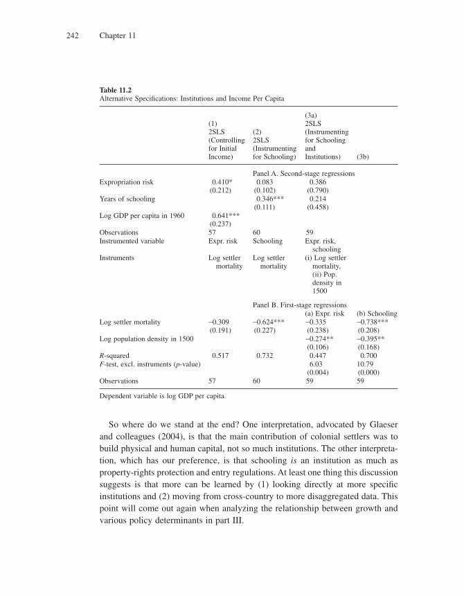
Chapter 11242
Table 11.2Alternative Specifi cations: Institutions and Income Per Capita
(1)2SLS (Controlling for Initial Income)
(2)2SLS (Instrumenting for Schooling)
(3a)2SLS (Instrumenting for Schooling and Institutions) (3b)
Panel A. Second-stage regressionsExpropriation risk 0.410*
(0.212)0.083
(0.102)0.386
(0.790)Years of schooling 0.346***
(0.111)0.214
(0.458)Log GDP per capita in 1960 0.641***
(0.237)Observations 57 60 59Instrumented variable Expr. risk Schooling Expr. risk,
schoolingInstruments Log settler
mortalityLog settler
mortality(i) Log settler
mortality, (ii) Pop. density in 1500
Panel B. First-stage regressions(a) Expr. risk (b) Schooling
Log settler mortality −0.309(0.191)
−0.624***(0.227)
−0.335(0.238)
−0.738***(0.208)
Log population density in 1500 −0.274**(0.106)
−0.395**(0.168)
R-squared 0.517 0.732 0.447 0.700F-test, excl. instruments (p-value) 6.03
(0.004)10.79(0.000)
Observations 57 60 59 59
Dependent variable is log GDP per capita.
So where do we stand at the end? One interpretation, advocated by Glaeser and colleagues (2004), is that the main contribution of colonial settlers was to build physical and human capital, not so much institutions. The other interpreta-tion, which has our preference, is that schooling is an institution as much as property-rights protection and entry regulations. At least one thing this discussion suggests is that more can be learned by (1) looking directly at more specifi c institutions and (2) moving from cross-country to more disaggregated data. This point will come out again when analyzing the relationship between growth and various policy determinants in part III.
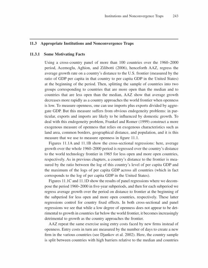
Institutions and Nonconvergence Traps 243
11.3 Appropriate Institutions and Nonconvergence Traps
11.3.1 Some Motivating Facts
Using a cross-country panel of more than 100 countries over the 1960–2000 period, Acemoglu, Aghion, and Zilibotti (2006), henceforth AAZ, regress the average growth rate on a country’s distance to the U.S. frontier (measured by the ratio of GDP per capita in that country to per capita GDP in the United States) at the beginning of the period. Then, splitting the sample of countries into two groups corresponding to countries that are more open than the median and to countries that are less open than the median, AAZ show that average growth decreases more rapidly as a country approaches the world frontier when openness is low. To measure openness, one can use imports plus exports divided by aggre-gate GDP. But this measure suffers from obvious endogeneity problems: in par-ticular, exports and imports are likely to be infl uenced by domestic growth. To deal with this endogeneity problem, Frankel and Romer (1999) construct a more exogenous measure of openness that relies on exogenous characteristics such as land area, common borders, geographical distance, and population, and it is this measure that we use to measure openness in fi gure 11.1.
Figures 11.1A and 11.1B show the cross-sectional regressions: here, average growth over the whole 1960–2000 period is regressed over the country’s distance to the world technology frontier in 1965 for less open and more open countries, respectively. As in previous chapters, a country’s distance to the frontier is mea-sured by the ratio between the log of this country’s level of per capita GDP and the maximum of the logs of per capita GDP across all countries (which in fact corresponds to the log of per capita GDP in the United States).
Figures 11.1C and 11.1D show the results of panel regressions where we decom-pose the period 1960–2000 in fi ve-year subperiods, and then for each subperiod we regress average growth over the period on distance to frontier at the beginning of the subperiod for less open and more open countries, respectively. These latter regressions control for country fi xed effects. In both cross-sectional and panel regressions we see that while a low degree of openness does not appear to be det-rimental to growth in countries far below the world frontier, it becomes increasingly detrimental to growth as the country approaches the frontier.
AAZ repeat the same exercise using entry costs faced by new fi rms instead of openness. Entry costs in turn are measured by the number of days to create a new fi rm in the various countries (see Djankov et al. 2002). Here, the country sample is split between countries with high barriers relative to the median and countries
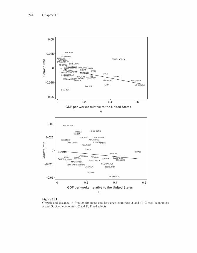
Chapter 11244
0.05
0.025
0
–0.025
–0.05
0 0.2 0.60.4
Gro
wth
rat
e
GDP per worker relative to the United States
A
SOUTH AFRICA
CHILE
MEXICO
BOLIVIA
DEM REP.
COLOMBIAFIJI
IRAN
BRAZIL
EQUADORPARAGUAY
EGYPTMOROCCO
ZIMBABWE
PAKISTANCAMEROONINDIA
THAILAND
MALAWIKENYA
INDONESIA
TANZANIA
UGANDABURUNDI
ETHIOPIA
NEPALBANGLADESHNIGER
MOZAMBIQUEZAMBIAPHILIPPINES
MADAGASCARMALI PAPUA NE
ARGENTINA
VENEZUELA
URUGUAY
PERU
0.05
0.025
0
–0.025
–0.05
0 0.2 0.60.4
Gro
wth
rat
e
GDP per worker relative to the United States
COSTA RICA
HONG KONG
BOTSWANA
TAIWANKOREA
LESOTHO
CAPE VERDE
BENINZAMBIA
BURUNDISYRIA
MALAYSIAGABON
SINGAPORE
CYPRESS
SEYCHELL
JAMAICA
GUATEMALA
PANAMA
MAURITIUS
JORDAN
NAMIBIA
BARBADOS
ISRAEL
TRINADAD
NICARAGUA
GUYANA
RWANDA
SENEGAL
GUINEA
MAURITANIA
HONDURAS
DOMINICA
EL SALVADOR
B
Figure 11.1Growth and distance to frontier for more and less open countries: A and C, Closed economies; B and D, Open economies; C and D, Fixed effects
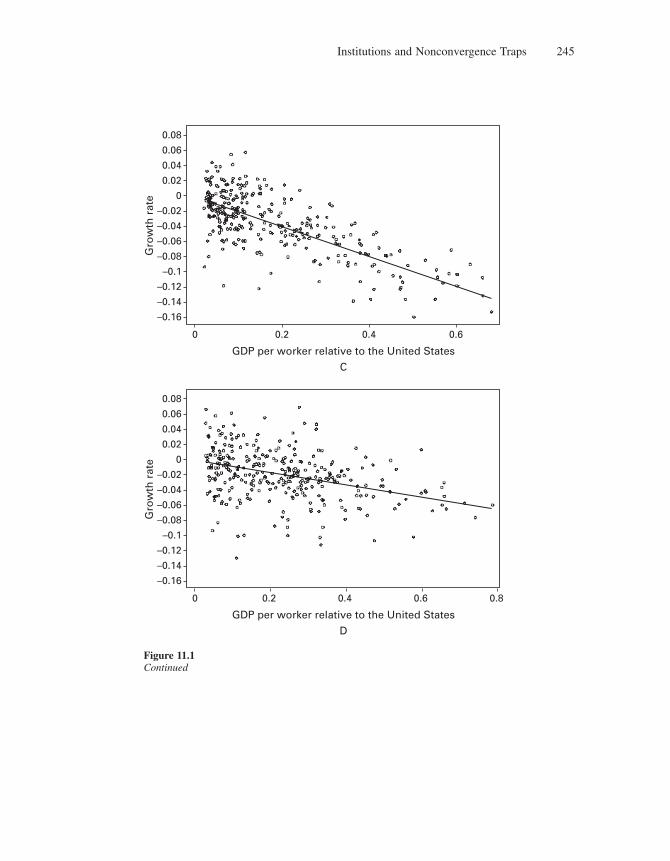
Institutions and Nonconvergence Traps 245
Figure 11.1Continued
0.08
0.06
0.04
0.02
0
–0.02
–0.04
–0.06
–0.08
–0.1
–0.12
–0.14
–0.16
0 0.2 0.6 0.80.4
Gro
wth
rat
e
GDP per worker relative to the United States
D
0.08
0.06
0.04
0.02
0
–0.02
–0.04
–0.06
–0.08
–0.1
–0.12
–0.14
–0.16
0 0.2 0.60.4
Gro
wth
rat
e
GDP per worker relative to the United States
C
Chapter 11246
with low barriers relative to the median. Figures 11.2A and 11.2B show the cross-sectional regressions, for high and low barrier countries, respectively, whereas fi gures 11.2C and 11.2D show the panel regressions for the same two subgroups of countries. Both types of regressions show that while high entry barriers do not appear to be detrimental to growth in countries far below the world frontier, they become increasingly detrimental to growth as the country approaches the frontier.
These two empirical exercises point to the importance of interacting institu-tions with level of development in growth regressions: openness is particularly growth enhancing in countries that are closer to the technological frontier; entry is more growth enhancing in countries or sectors that are closer to the technologi-cal frontier; in chapter 13 we will see that higher (in particular, graduate) educa-tion tends to be more growth enhancing in countries or in U.S. states that are closer to the technological frontier, whereas primary and secondary (possibly undergraduate) education tends to be more growth enhancing in countries or in U.S. states that are farther below the frontier.
In the next section we model the notion of appropriate growth institution, and then we analyze the possibility that a country may remain stuck with institutions that might have been growth enhancing at earlier stages of development but that prevent fast growth as the country moves closer to the world technology frontier.
11.3.2 A Simple Model of Distance to Frontier and Appropriate Institutions
11.3.2.1 The Setup
The following setup combines the innovation model in chapter 4 with the con-vergence model in chapter 7. In each country, a unique fi nal good, which also serves as numéraire, is produced competitively using a continuum of intermediate inputs according to
Y A x dit it it= −∫ 1
0
1 α α (11.1)
where Ait is the productivity in sector i at time t, xit is the fl ow of intermediate good i used in general good production again at time t. and a ∈ [0, 1].
As in chapter 4 (nondrastic innovation case), ex post each intermediate good producer has a constant marginal cost equal to 1 and faces a competitive fringe of imitators that force her to charge a limit price pit = c > 1. Consequently, equi-librium monopoly profi ts (gross of the fi xed cost) in sector i at date t are simply given by
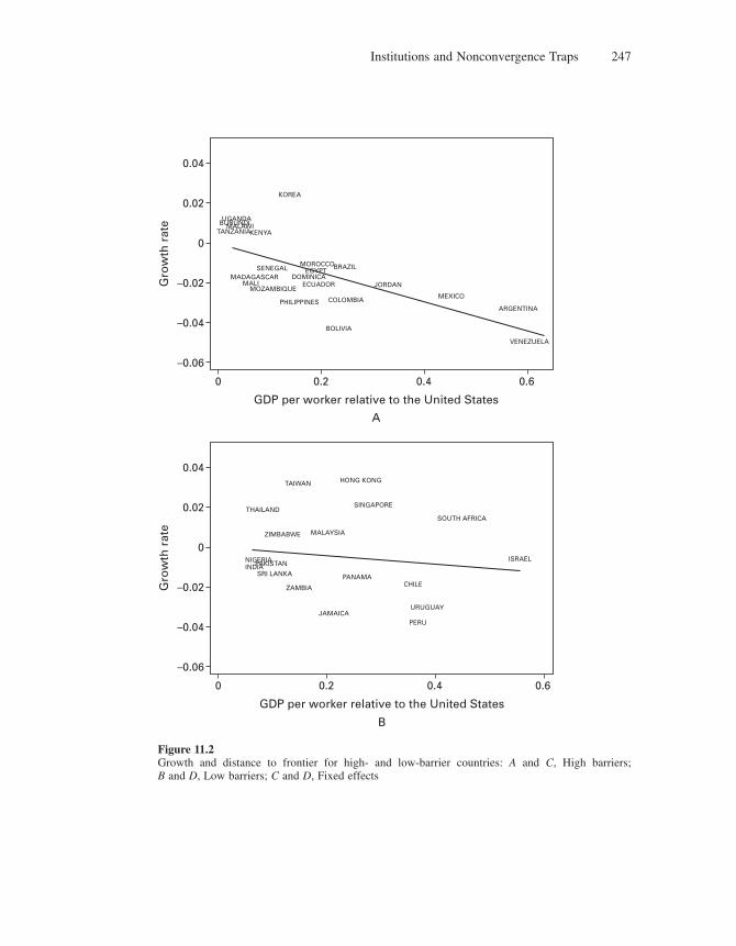
Institutions and Nonconvergence Traps 247
Figure 11.2Growth and distance to frontier for high- and low-barrier countries: A and C, High barriers; B and D, Low barriers; C and D, Fixed effects
0.04
0.02
0
–0.02
–0.04
–0.06
0 0.2 0.60.4
Gro
wth
rat
e
GDP per worker relative to the United States
B
SOUTH AFRICA
CHILE
ISRAEL
ZIMBABWE
INDIA
THAILAND
MALAYSIA
HONG KONG
SINGAPORE
PANAMA
ZAMBIA
JAMAICA
TAIWAN
PAKISTAN
SRI LANKA
NIGERIA
URUGUAY
PERU
0.04
0.02
0
–0.02
–0.04
–0.06
0 0.2 0.60.4
Gro
wth
rat
e
GDP per worker relative to the United States
A
MEXICO
BOLIVIA
COLOMBIA
BRAZIL
DOMINICAEGYPT
MOROCCO
MALAWIKENYATANZANIA
UGANDABURUNDI
ECUADORMOZAMBIQUE
JORDAN
PHILIPPINES
MADAGASCARMALI
SENEGAL
KOREA
ARGENTINA
VENEZUELA
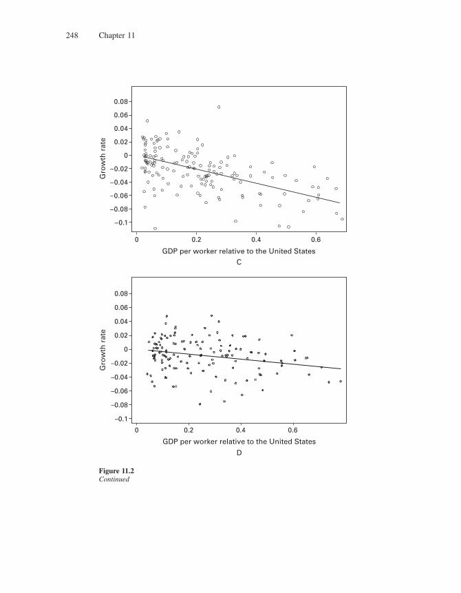
Chapter 11248
Figure 11.2Continued
0.08
0.06
0.04
0.02
0
–0.02
–0.04
–0.06
–0.08
–0.1
0 0.2 0.60.4
Gro
wth
rat
e
GDP per worker relative to the United States
D
C
0.08
0.06
0.04
0.02
0
–0.02
–0.04
–0.06
–0.08
–0.1
0 0.2 0.60.4
Gro
wth
rat
e
GDP per worker relative to the United States

Institutions and Nonconvergence Traps 249
π πit itA=
where π χ α χ α≡ −( )( ) −11
1
Again let
A A dit it≡ ∫0
1
denote the average productivity in the country at date t, and let At denote the productivity at the world frontier. We take this frontier productivity to grow at the constant rate g from one period to the next, that is,
A g At t= +( ) −1 1
Let at = At/At denote the country’s proximity to the world technology frontier, our inverse measure of the country’s distance to the technological frontier at date t.
A main departure from the convergence model in chapter 7 lies in the equation for productivity growth.
11.3.2.2 Two Sources of Productivity Growth
Intermediate fi rms have two ways to generate productivity growth: (1) they can imitate existing world frontier technologies; (2) they can innovate upon the previ-ous local technology.More specifi cally, we assume
A A Ait t t= +− −η γ1 1
where hAt−1 and gA1−1 refer to the imitation and innovation components of pro-ductivity growth, respectively. Imitations use the existing frontier technology at the end of period (t − 1), and thus they multiply At−1; whereas innovations build on the knowledge stock of the country, and therefore they multiply At−1. In other words, this extended model combines the Schumpeterian model of chapter 4 where an innovating sector multiplies its previous productivity by a factor g > 1 with the convergence model of chapter 7 where an innovating sector catches up with the technology frontier.
Integrating over all sectors of the economy, we have
A A At t t= +− −η γ1 1 (11.2)
Dividing both sides of equation (11.2) by At and using the fact that
A g At t= +( ) −1 1
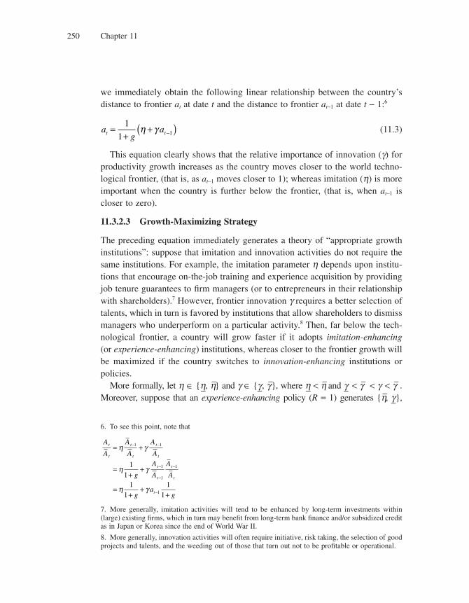
Chapter 11250
we immediately obtain the following linear relationship between the country’s distance to frontier at at date t and the distance to frontier at−1 at date t − 1:6
ag
at t=+
+( )−1
1 1η γ (11.3)
This equation clearly shows that the relative importance of innovation (g) for productivity growth increases as the country moves closer to the world techno-logical frontier, (that is, as at−1 moves closer to 1); whereas imitation (h) is more important when the country is further below the frontier, (that is, when at−1 is closer to zero).
11.3.2.3 Growth-Maximizing Strategy
The preceding equation immediately generates a theory of “appropriate growth institutions”: suppose that imitation and innovation activities do not require the same institutions. For example, the imitation parameter h depends upon institu-tions that encourage on-the-job training and experience acquisition by providing job tenure guarantees to fi rm managers (or to entrepreneurs in their relationship with shareholders).7 However, frontier innovation g requires a better selection of talents, which in turn is favored by institutions that allow shareholders to dismiss managers who underperform on a particular activity.8 Then, far below the tech-nological frontier, a country will grow faster if it adopts imitation-enhancing (or experience-enhancing) institutions, whereas closer to the frontier growth will be maximized if the country switches to innovation-enhancing institutions or policies.
More formally, let h ∈ {h_, h} and g ∈ {g_, g}, where h_ < h and g_ < g < g < g . Moreover, suppose that an experience-enhancing policy (R = 1) generates {h, g_},
6. To see this point, note that
A
A
A
A
A
A
g
A
A
A
A
ga
g
t
t
t
t
t
t
t
t
t
t
t
= +
= 11+
+
= 11+
++
− −
−
−
−
−
η γ
η γ
η γ
1 1
1
1
1
1
11
7. More generally, imitation activities will tend to be enhanced by long-term investments within (large) existing fi rms, which in turn may benefi t from long-term bank fi nance and/or subsidized credit as in Japan or Korea since the end of World War II.
8. More generally, innovation activities will often require initiative, risk taking, the selection of good projects and talents, and the weeding out of those that turn out not to be profi table or operational.

Institutions and Nonconvergence Traps 251
in other words, is better for imitation but worse for frontier innovation; however, an innovation-enhancing policy (R = 0) generates {h_, g}, in other words, is better at producing frontier innovation but relatively worse at facilitating imitation.
For simplicity, we shall assume that
1+ = +g η γ
so that, by equation (11.3), a country that pursues an innovation-based strategy and lies exactly on the technological frontier will grow exactly at rate g. In other words, this assumption endogenizes the frontier growth rate as stemming from innovation-based growth.
The productivity growth equation (11.3) becomes
ag
at t=+
+( )−1
1 1η γ (11.4)
under experience-enhancing institutions, and
ag
at t=+
+( )−1
1 1η γ (11.5)
under innovation-enhancing institutions. The two relationships are depicted by the two lines R = 1 and R = 0 in fi gure 11.3. The fi gure clearly shows that experi-ence-enhancing institutions achieve higher growth (that is, higher level of at for given at−1)9 for low values of at−1 but lower growth for high values of at−1.
The cutoff point â at which the two lines intersect is simply calculated by equating the right-hand sides of the two preceding equations, which in turn yields
a =−−
η ηγ γ
Thus it is growth maximizing that countries with at−1 < â adopt an experience-enhancing strategy, whereas countries with at−1 > â switch to an innovation-enhancing strategy. Moreover, a country that follows this growth-maximizing
9. The domestic growth rate at date t is equal to
A
A
a A
a A
a
agt
t
t t
t t
t
t− − − −
= = +( )1 1 1 1
1
This rate is thus maximized whenever at is maximized for given at−1.
Chapter 11252
plan will always achieve a growth rate higher than g, and it will also ultimately converge to the world technology frontier, that is, at = 1.
Two important questions arise at this point. First, will institutions actually change when they should; in other words, how do equilibrium institutions at various stages of development compare with the growth-maximizing institutions? Second, what happens if institutions do not change early enough as a country develops? These are the questions we address in the remaining part of the chapter.
11.3.2.4 Decentralized Equilibrium
So far, we have treated (h, g) directly as (aggregate) institutional variables. In reality, however, the average levels of h and g result from decentralized decisions made by economic agents that operate in a particular institutional environment.
In this section, we consider the decentralized interactions between fi rm owners and fi rm managers. Firm owners can decide whether or not to keep old managers that turn out to be “untalented” for one more period on the job. Keeping existing
1
at
at–1
R = 1
R = 0
45°
a
Figure 11.3

Institutions and Nonconvergence Traps 253
managers on the job enhances experience but is detrimental to innovation: that is, it increases h, but reduces g at the fi rm level. Ultimately, as we shall see later, fi rm owners’ decisions whether or not to maintain old untalented managers on the job will depend on the underlying institutional environment (in particular on the parameters e and p). In other words, a given set of institutional parameters will correspond to equilibrium average levels of h and g across fi rms in the economy. These levels will generally differ from the growth-maximizing policy analyzed previously.
More formally, suppose that intermediate fi rms are run by managers who live for two periods and are employed by fi rm owners who also live for two periods and maximize profi ts. Each period, the current manager is paid a fi xed share m of the fi rm’s profi ts. And at the beginning of each period, the manager can improve the fi rm’s productivity both by imitating the frontier technology and by innovating upon the local technology:
A i t A i t Ait t t= ( ) + ( )− −η γ, ,1 1
where h(i, t) and g (i, t) denote the manager’s imitation and innovation intensities on fi rm i at time t.
There are two types of managers: talented and untalented. All young managers imitate with the same intensity h(i, t) = h, and all old managers can imitate with intensity h(i, t) = h + e, where e measures the old manager’s experience acquired on the job. However, only the talented managers can innovate, with intensity g (i, t) = g, whereas g (i, t) = 0 for untalented managers. There is a fraction l of talented managers in the economy, and a manager’s talent is publicly revealed only after one period of work.
The institutional aspect we shall consider here is the extent to which unsuc-cessful managers are shut down or instead renewed by the fi rm owner whenever they are revealed to be untalented after one period on the job. Refi nancing old managers allows the fi rm’s owner to take advantage of the experience and also the retained earnings of these managers. However, keeping old (untalented) managers may prevent the fi rm’s owner from having the possibility of selecting potentially more talented young managers; this inability to recruit talent in turn stifl es innovation. Thus, here; the experience-enhancing strategy means that fi rms maintain their managers, whereas the innovation-enhancing strategy means that fi rms replace old untalented managers by new managers.
More formally, assuming that managers are ready to use all their retained earn-ings to maintain their jobs, the fi rm’s owner will choose to renew an old untal-ented manager whenever
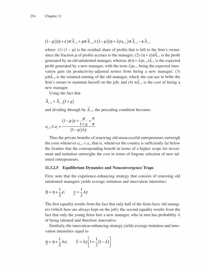
Chapter 11254
1 11 2 1 1 1−( ) +( ) + ≥ −( ) +( ) −− − − − −μ η ε π μπ μ η λγ π κA A a A At t t t t
where: (1) (1 − m) is the residual share of profi ts that is left to the fi rm’s owner, since the fraction m of profi ts accrues to the manager; (2) (h + e)pAt−1 is the profi t generated by an old untalented manager, whereas p(h + lgat−1)At−1 is the expected profi t generated by a new manager, with the term lgat−1 being the expected inno-vation gain (in productivity-adjusted terms) from hiring a new manager; (3) mpAt−2 is the retained earning of the old manager, which she can use to bribe the fi rm’s owner to maintain herself on the job; and (4) kAt−1 is the cost of hiring a new manager.
Using the fact that
A A gt t− −= +( )1 2 1
and dividing through by At−1, the preceding condition becomes
a a gt r− ≤ =
−( ) +1+
+
−( )1
1
1
μ ε μ κπ
μ λγ
Thus the private benefi ts of renewing old unsuccessful entrepreneurs outweigh the costs whenever at−1 < ar, that is, whenever the country is suffi ciently far below the frontier that the corresponding benefi t in terms of a higher scope for invest-ment and imitation outweighs the cost in terms of forgone selection of new tal-ented entrepreneurs.
11.3.2.5 Equilibrium Dynamics and Nonconvergence Traps
First, note that the experience-enhancing strategy that consists of renewing old untalented managers yields average imitation and innovation intensities:
η η ε γ λγ= +12
; =1
2
The fi rst equality results from the fact that only half of the fi rms have old manag-ers (which here are always kept on the job); the second equality results from the fact that only the young fi rms hire a new manager, who in turn has probability l of being talented and therefore innovative.
Similarly, the innovation-enhancing strategy yields average imitation and inno-vation intensities equal to
η η λε γ λγ λ= +12
; = + −( )⎡⎣⎢
⎤⎦⎥
11
21
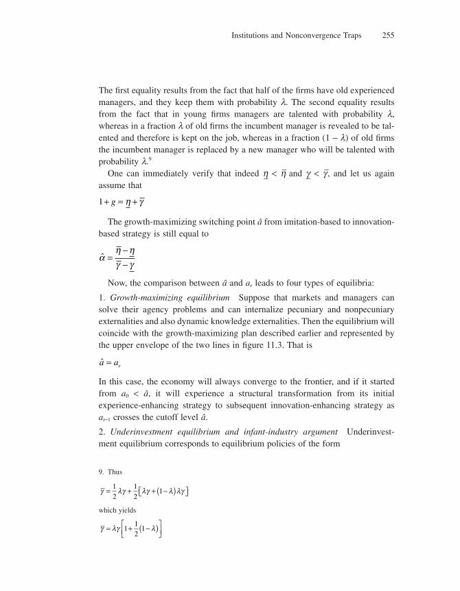
Institutions and Nonconvergence Traps 255
The fi rst equality results from the fact that half of the fi rms have old experienced managers, and they keep them with probability l. The second equality results from the fact that in young fi rms managers are talented with probability l, whereas in a fraction l of old fi rms the incumbent manager is revealed to be tal-ented and therefore is kept on the job, whereas in a fraction (1 − l) of old fi rms the incumbent manager is replaced by a new manager who will be talented with probability l.9
One can immediately verify that indeed h_ < h and g_ < g , and let us again assume that
1+ = +g η γ
The growth-maximizing switching point â from imitation-based to innovation-based strategy is still equal to
αη ηγ γ
=−−
Now, the comparison between â and ar leads to four types of equilibria:
1. Growth-maximizing equilibrium Suppose that markets and managers can solve their agency problems and can internalize pecuniary and nonpecuniary externalities and also dynamic knowledge externalities. Then the equilibrium will coincide with the growth-maximizing plan described earlier and represented by the upper envelope of the two lines in fi gure 11.3. That is
a ar=
In this case, the economy will always converge to the frontier, and if it started from a0 < â, it will experience a structural transformation from its initial experience-enhancing strategy to subsequent innovation-enhancing strategy as at−1 crosses the cutoff level â.
2. Underinvestment equilibrium and infant-industry argument Underinvest-ment equilibrium corresponds to equilibrium policies of the form
9. Thus
γ λγ λγ λ λγ= 12
+ + −( )⎡⎣ ⎤⎦12
1
which yields
γ λγ λ= + −( )⎡⎣⎢
⎤⎦⎥
112
1
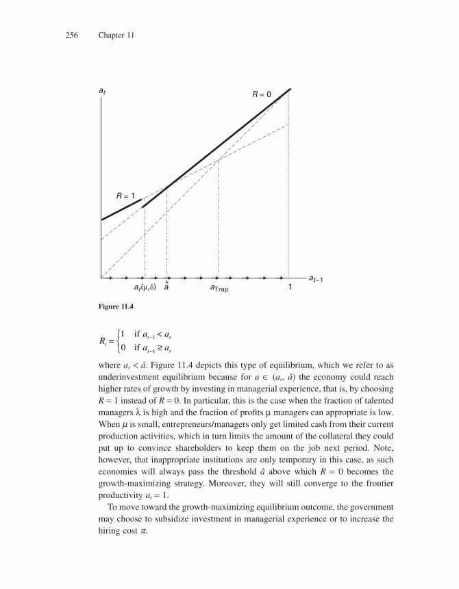
Chapter 11256
Ra a
a att r
t r
=<≥
⎧⎨⎩
−
−
1
01
1
if
if
where ar < â. Figure 11.4 depicts this type of equilibrium, which we refer to as underinvestment equilibrium because for a ∈ (ar, â) the economy could reach higher rates of growth by investing in managerial experience, that is, by choosing R = 1 instead of R = 0. In particular, this is the case when the fraction of talented managers λ is high and the fraction of profi ts μ managers can appropriate is low. When m is small, entrepreneurs/managers only get limited cash from their current production activities, which in turn limits the amount of the collateral they could put up to convince shareholders to keep them on the job next period. Note, however, that inappropriate institutions are only temporary in this case, as such economies will always pass the threshold â above which R = 0 becomes the growth-maximizing strategy. Moreover, they will still converge to the frontier productivity at = 1.
To move toward the growth-maximizing equilibrium outcome, the government may choose to subsidize investment in managerial experience or to increase the hiring cost p.
1aTrapar(μ,δ)
at
at–1
R = 1
R = 0
a
Figure 11.4
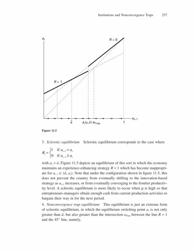
Institutions and Nonconvergence Traps 257
3. Sclerotic equilibrium Sclerotic equilibrium corresponds to the case where
Ra a
a att r
t r
=<≥
⎧⎨⎩
−
−
1
01
1
if
if
with ar > â. Figure 11.5 depicts an equilibrium of this sort in which the economy maintains an experience-enhancing strategy R = 1 which has become inappropri-ate for at−1 ∈ (â, ar). Note that under the confi guration shown in fi gure 11.5, this does not prevent the country from eventually shifting to the innovation-based strategy as at−1 increases, or from eventually converging to the frontier productiv-ity level. A sclerotic equilibrium is more likely to occur when m is high so that entrepreneurs-managers obtain enough cash from current production activities to bargain their way in for the next period.
4. Nonconvergence trap equilibrium This equilibrium is just an extreme form of sclerotic equilibrium, in which the equilibrium switching point ar is not only greater than â, but also greater than the intersection aTrap between the line R = 1 and the 45° line, namely,
1aTrapar(μ,δ)
at
at–1
R = 1
R = 0
a
Figure 11.5
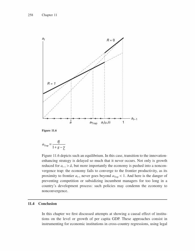
Chapter 11258
agTrap =
1+ −η
γ
Figure 11.6 depicts such an equilibrium. In this case, transition to the innovation-enhancing strategy is delayed so much that it never occurs. Not only is growth reduced for at−1 > â, but more importantly the economy is pushed into a noncon-vergence trap: the economy fails to converge to the frontier productivity, as its proximity to frontier at−1 never goes beyond aTrap < 1. And here is the danger of preventing competition or subsidizing incumbent managers for too long in a country’s development process: such policies may condemn the economy to nonconvergence.
11.4 Conclusion
In this chapter we fi rst discussed attempts at showing a causal effect of institu-tions on the level or growth of per capita GDP. These approaches consist in instrumenting for economic institutions in cross-country regressions, using legal
1aTrap ar(μ,δ)
at
at–1
R = 1
R = 0
a
Figure 11.6
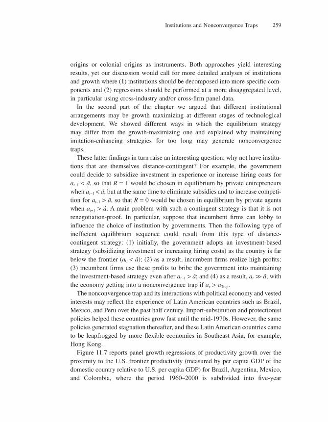
Institutions and Nonconvergence Traps 259
origins or colonial origins as instruments. Both approaches yield interesting results, yet our discussion would call for more detailed analyses of institutions and growth where (1) institutions should be decomposed into more specifi c com-ponents and (2) regressions should be performed at a more disaggregated level, in particular using cross-industry and/or cross-fi rm panel data.
In the second part of the chapter we argued that different institutional arrangements may be growth maximizing at different stages of technological development. We showed different ways in which the equilibrium strategy may differ from the growth-maximizing one and explained why maintaining imitation-enhancing strategies for too long may generate nonconvergence traps.
These latter fi ndings in turn raise an interesting question: why not have institu-tions that are themselves distance-contingent? For example, the government could decide to subsidize investment in experience or increase hiring costs for at−1 < â, so that R = 1 would be chosen in equilibrium by private entrepreneurs when at−1 < â, but at the same time to eliminate subsidies and to increase competi-tion for at−1 > â, so that R = 0 would be chosen in equilibrium by private agents when at−1 > â. A main problem with such a contingent strategy is that it is not renegotiation-proof. In particular, suppose that incumbent fi rms can lobby to infl uence the choice of institution by governments. Then the following type of ineffi cient equilibrium sequence could result from this type of distance-contingent strategy: (1) initially, the government adopts an investment-based strategy (subsidizing investment or increasing hiring costs) as the country is far below the frontier (a0 < â); (2) as a result, incumbent fi rms realize high profi ts; (3) incumbent fi rms use these profi ts to bribe the government into maintaining the investment-based strategy even after at−1 > â; and (4) as a result, ar >> â, with the economy getting into a nonconvergence trap if ar > aTrap.
The nonconvergence trap and its interactions with political economy and vested interests may refl ect the experience of Latin American countries such as Brazil, Mexico, and Peru over the past half century. Import-substitution and protectionist policies helped these countries grow fast until the mid-1970s. However, the same policies generated stagnation thereafter, and these Latin American countries came to be leapfrogged by more fl exible economies in Southeast Asia, for example, Hong Kong.
Figure 11.7 reports panel growth regressions of productivity growth over the proximity to the U.S. frontier productivity (measured by per capita GDP of the domestic country relative to U.S. per capita GDP) for Brazil, Argentina, Mexico, and Colombia, where the period 1960–2000 is subdivided into fi ve-year
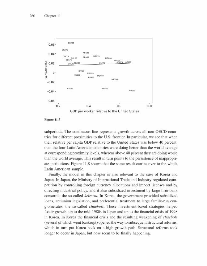
Chapter 11260
subperiods. The continuous line represents growth across all non-OECD coun-tries for different proximities to the U.S. frontier. In particular, we see that when their relative per capita GDP relative to the United States was below 40 percent, then the four Latin American countries were doing better than the world average at corresponding proximity levels, whereas above 40 percent they are doing worse than the world average. This result in turn points to the persistence of inappropri-ate institutions. Figure 11.8 shows that the same result carries over to the whole Latin American sample.
Finally, the model in this chapter is also relevant to the case of Korea and Japan. In Japan, the Ministry of International Trade and Industry regulated com-petition by controlling foreign currency allocations and import licenses and by directing industrial policy, and it also subsidized investment by large fi rm-bank consortia, the so-called keiretsu. In Korea, the government provided subsidized loans, antiunion legislation, and preferential treatment to large family-run con-glomerates, the so-called chaebols. These investment-based strategies helped foster growth, up to the mid-1980s in Japan and up to the fi nancial crisis of 1998 in Korea. In Korea the fi nancial crisis and the resulting weakening of chaebols (several of which went bankrupt) opened the way to subsequent structural reforms, which in turn put Korea back on a high growth path. Structural reforms took longer to occur in Japan, but now seem to be fi nally happening.
0.06
0.04
0.02
0
–0.02
–0.04
–0.06
0.2 0.80.60.4
Gro
wth
rat
e
GDP per worker relative to the United States
MEX95
MEX90MEX85
BRA85
BRA80
BRA90
BRA70
COL90
COL80COL70
COL95
COL85
COL75
BRA95
BRA75
MEX70MEX80
ARG70ARG75
ARG95
ARG80
ARG85ARG90
MEX75
Figure 11.7
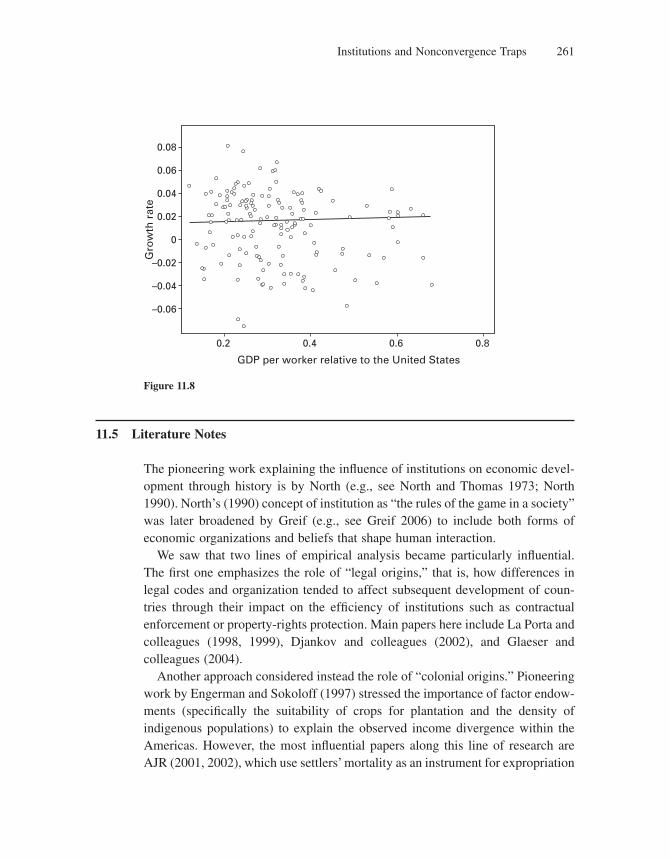
Institutions and Nonconvergence Traps 261
11.5 Literature Notes
The pioneering work explaining the infl uence of institutions on economic devel-opment through history is by North (e.g., see North and Thomas 1973; North 1990). North’s (1990) concept of institution as “the rules of the game in a society” was later broadened by Greif (e.g., see Greif 2006) to include both forms of economic organizations and beliefs that shape human interaction.
We saw that two lines of empirical analysis became particularly infl uential. The fi rst one emphasizes the role of “legal origins,” that is, how differences in legal codes and organization tended to affect subsequent development of coun-tries through their impact on the effi ciency of institutions such as contractual enforcement or property-rights protection. Main papers here include La Porta and colleagues (1998, 1999), Djankov and colleagues (2002), and Glaeser and colleagues (2004).
Another approach considered instead the role of “colonial origins.” Pioneering work by Engerman and Sokoloff (1997) stressed the importance of factor endow-ments (specifi cally the suitability of crops for plantation and the density of indigenous populations) to explain the observed income divergence within the Americas. However, the most infl uential papers along this line of research are AJR (2001, 2002), which use settlers’ mortality as an instrument for expropriation
0.08
0.06
0.04
0.02
0
–0.02
–0.04
–0.06
0.2 0.80.60.4
Gro
wth
rat
e
GDP per worker relative to the United States
Figure 11.8

Chapter 11262
risk. The idea is that the initial conditions faced by colonizers should affect the objectives they pursue in the new colonies (for example, extraction versus settle-ment). These objectives, in turn, should affect current institutions in the corre-sponding countries.
More recently, AJR (2005) emphasized the interaction between European countries’ access to Atlantic trade and their premodern institutions to explain the divergence within Europe right before the industrial revolution took place. Nunn (2008) assesses the long-term economic impact of Africa’s slave trades within that continent. Banerjee and Iyer (2005) focus on a single country, India, evaluat-ing the long-run effects of different land tenure systems set up by the British in that nation.
The Handbook of Economic Growth chapter by AJR (2005) presents a com-plete summary of the framework they have used to study the impact of institutions and the empirical evidence they have gathered on the topic.
The primary reference on the issue of appropriate institutions is Gerschenk-ron’s (1962). In this celebrated essay the author argues that relatively backward economies, such as Germany, France, and Russia during the 19th century, adopted particular policies and arrangements that were growth enhancing given their early stage of development but could cease to be so at a later stage of development. The author also pointed out that some “noncompetitive” arrangements, including long-term relationships between fi rms and banks, large fi rms, and state interven-tion, could make it easier for middle-income countries to catch up to more advanced economies.
Recent empirical work has tested the extent to which growth-enhancing poli-cies or institutions may vary with a country’s or sector’s level of development as measured by the distance between its own productivity and the corresponding frontier productivity. Thus, using data from the OECD sectoral database, Griffi th, Redding, and Van Reenen (2003) constructed a measure of distance to frontier for each industry in each country and year, and found evidence consistent with the observation that R&D and innovation become more important as an economy approaches the world technology frontier: they found a statistically highly sig-nifi cant negative relationship between distance to frontier and R&D intensity.
Acemoglu, Johnson, and Mitton (2003) found evidence that industry-level and aggregate concentration is greater in poorer countries (more distant from the frontier). These results are consistent with the idea that market selection is less important there, whereas fi rms tend to be larger in countries farther below the technological frontier.
Institutions and Nonconvergence Traps 263
Related works that also build on Gerschenkron’s insight include Stiglitz (1995) and Hausmann and Rodrik (2003), both of which call for greater government intervention in less developed countries where market failures tend to be more intense than in more advanced market economies. However, Shleifer and Vishny (1999) have stressed the greater scope for government failure in less developed nations, where checks on governments are typically weaker.
The fi rst systematic attempt at modeling the notion of appropriate institutions and the notion of institutional trap is the paper by Acemoglu, Aghion, and Zilibotti (2006). This approach has been subsequently extended or applied to analyze various aspects of growth policy design. Here, we refer the reader to Aghion and Howitt’s (2006) survey article on “appropriate growth policy.”
Problems
1. It has long been known that countries that have poor economic growth also have bad “institutions.” A substantial challenge for empirical research has been to identify a causal link between institutions and economic growth. To solve this identifi cation problem, we need to fi nd exogenous variation in institutions. The following exogenous variations in institutions have been proposed to support the hypothesis that “bad institutions” cause poor economic growth: (1) distance from the equator as a proxy for European infl uence (by Hall and Jones 1999); (2) difference in legal codes and organiza-tions as determined (by La Porta et al. 1998, 1999); (3) mortality rates faced by potential colonial settlers as a proxy for institutional development during the era of colonization in the post-1500 world (by AJR 2005). Discuss the plausibility of each of these as a good instrument for institutions. Can you think of any innovative ways to fi nd exogenous variation in institutions to test the hypothesis that institutions have a causal effect on economic growth?
2. Mechanism for institutional persistence
The model and empirical evidence presented in this chapter raise an important question: Why do governments not choose institutions and policies that favor the investment-based strategy when the country is in its early stages of development and then switch to policies supporting innovation and selection as the country approaches the frontier? Acemoglu, Aghion, and Zilibotti (2006) argue that the answer lies in the political economy of government intervention. Policies that favor the investment-based strategy create and enrich their own supporters. When economic power buys politi-cal power. it becomes diffi cult to reverse policies that have an economically and politically powerful constituency. Consequently, societies may remain trapped with “inappropriate institutions” and rela-tively backward technologies.
How can you test this claim using micro evidence? Acemoglu, Aghion, and Zilibotti (2006) discuss the example of South Korea: they suggest that close links between government offi cials and the chaebols had turned into major obstacles to progress and that convergence and growth came to an end during the Asian crisis. If the Asian crisis served as an exogenous negative shock to the political power of the economically powerful constituency in South Korea, what evidence would you look for to verify the hypothesis presented here? If you had access to all possible sources of data, what would be your empirical strategy to identify the causal effect of a change in the “appropriateness of institu-tions” on economic growth?
3. Institutions-versus-geography debate
Most poor countries are located in the tropics. Sachs (2001) interprets this evidence to mean that geography is one of the fundamental causes of underdevelopment. Geography matters because disease
Chapter 11264
environments and agricultural productivity are directly dependent on geographic conditions. For example, countries that are most exposed to widespread malaria tend to lie between the tropics.
AJR (2001), however, argue that the underdevelopment of tropical countries can be traced to his-torical colonial institutions. They argue that countries in which the European settlers faced greater mortality are the countries in which they chose not to settle and instead adopted “extractive institu-tions.” However, in countries in which they faced lower mortality they chose to settle and therefore adopted good rule of law.
Discuss the plausibility of the two hypotheses. What evidence would you provide to support or refute the two hypotheses?

III GROWTH POLICY

12 Fostering Competition and Entry
12.1 Introduction
Is product market competition good or bad for growth? Innovation-based models (see chapters 3 and 4) seem to provide an unambiguous answer to this question: namely, market competition is bad for growth, the reason being that competition reduces the monopoly rents that induce fi rms to innovate. By the same token, more intense imitation discourages technological innovations and growth. Hence the importance of preserving intellectual property rights through an adequate system of (international) patent protection.
Unfortunately, the prediction that competition is bad for growth turns out to be highly counterfactual. Indeed, empirical work (e.g., Nickell 1996; Blundell, Griffi th, and Van Reenen 1995) points to a positive correlation between product market competition (as measured either by the number of competitors in the same industry or by the inverse of a market share or profi tability index) and productivity growth within a fi rm or industry. This evidence, in turn, appears to be more consistent with the view (e.g., Porter 1990) that product market competi-tion is good for growth because it forces fi rms to innovate in order to survive.
How can we reconcile the evidence with the theory? When does competition foster or discourage innovation? Section 12.2 will focus on the relationship between competition among incumbent fi rms and innovation. There, we replace the assumption made earlier—that incumbent innovators are automatically leap-frogged by their rivals—by a more gradualist (“step-by-step”) technological progress assumption. This in turn will generate an inverted-U relationship between competition and productivity growth.
Section 12.3 will analyze the relationship between entry and innovation, showing that incumbent fi rms respond differently to an increased entry threat depending on their initial distance from the technological frontier in the corre-sponding industry. It will also consider how entry interacts with labor market regulation, showing how the positive effects of increased entry on productivity growth are reduced by proworker regulations.
12.2 From Leapfrogging to Step-by-Step Technological Progress
Based on Aghion, Harris, and Vickers (1997) and Aghion and colleagues (2001), in this section we shall replace the leapfrogging assumption in the Schumpeterian model (with incumbent innovators being systemically overtaken
Chapter 12268
by outside researchers) with a less radical step-by-step assumption. That is, a fi rm that is currently m steps behind the technological leader in its industry must catch up with the leader before becoming a leader itself. This step-by-step assumption can be rationalized by supposing that an innovator acquires tacit knowledge that cannot be duplicated by a rival without engaging in its own R&D to catch up. Once it has caught up, we suppose that no patent protects the former leader from Bertrand competition.
This change leads to a richer analysis of the interplay between product market competition, innovation, and growth by allowing fi rms in an industry to be neck and neck. A higher degree of product market competition, by making life more diffi cult for neck-and-neck fi rms, will encourage them to innovate in order to acquire a signifi cant lead over their rivals.
12.2.1 Basic Environment
More formally, suppose that time is discrete and that there is a unit mass of identical consumers. Each of them lives for one period and supplies a unit of labor inelastically. Moreover, her utility depends upon the amounts consumed from a continuum of sectors:
u x djt jt= ∫ ln0
1
in which each xj is the sum of two goods produced by duopolists in sector j:
x x xj Aj Bj= +
The logarithmic structure of this utility function implies that in equilibrium individuals spend the same amount on each basket xj.1 We normalize this common amount to unity by using current expenditure as the numéraire for the prices pAj and pBj at each date. Thus the representative household chooses each xAj and xBj to maximize xAj + xBj subject to the budget constraint pAjxAj + pBjxBj = 1; that is, the household will devote the entire unit expenditure to the less expensive of the two goods.
1. That is, the representative consumer will choose the xj’s to maximize u = ∫ l
o lnxjdj subject to the budget constraint ∫1
0 pjxjdj = E. The fi rst-order condition is
∂ ∂u x x p jj j j= =1 λ for all
where l is a Lagrange multiplier. Together with the budget constraint, this fi rst-order condition implies
p x E jj j = =1 λ for all
Fostering Competition and Entry 269
12.2.2 Technology and Innovation
Each fi rm produces using labor as the only input, according to a constant-returns production function, and takes the wage rate as given. Thus the unit costs of production cA and cB of the two fi rms in an industry are independent of the quanti-ties produced. Now, let ki denote the technology level of duopoly fi rm i in some industry j; that is, one unit of labor currently employed by fi rm i generates an output fl ow equal to
A i A Biki= =γ , ,
where g > 1 is a parameter that measures the size of a leading-edge innovation. Equivalently, it takes g −ki units of labor for fi rm i to produce one unit of output.
For expositional simplicity, we assume that knowledge spillovers between the two fi rms in any intermediate industry are such that neither fi rm can get more than one technological level ahead of the other. That is, if a fi rm already one step ahead innovates, the lagging fi rm will automatically learn to copy the leader’s previous technology and thereby remain only one step behind. Thus, at any point in time, there will be two kinds of intermediate sectors in the economy: (1) level or neck-and-neck sectors where both fi rms are at technological par with one another and (2) unlevel sectors, where one fi rm (the leader) lies one step ahead of its competitor (the laggard or follower) in the same industry.2
By spending the R&D cost ψ n n( ) = 2 2 in units of expenditure, a leader (or frontier) fi rm moves one technological step ahead, with probability n. We call n the “innovation rate” or “R&D intensity” of the fi rm. We assume that a follower fi rm can move one step ahead with probability h, even if it spends nothing on R&D, by copying the leader’s technology. Thus n2/2 is the R&D cost of a fol-lower fi rm moving ahead with probability n + h. Let n0 denote the R&D intensity of each fi rm in a neck-and-neck industry, and let n−1 denote the R&D intensity of a follower fi rm in an unlevel industry. If n1 denotes the R&D intensity of the leader in an unlevel industry, note that n1 = 0, since our assumption of automatic catch-up means that a leader cannot gain any further advantage by innovating.
12.2.3 Equilibrium Profi ts and Competition in Level and Unlevel Sectors
We can now determine the equilibrium profi ts of fi rms in each type of sector and link them with product market competition. Consider fi rst an unlevel sector where
2. Aghion and colleagues (2001) analyze the more general case where there is no limit to how far ahead the leader can get. However, unlike in this chapter, that paper provides no closed-form solution for the equilibrium R&D levels and the steady-state industry structure.
Chapter 12270
the leader’s unit cost is c. She is constrained to setting a price p1 ≤ gc because gc is the rival’s unit cost, so at any higher price the rival could profi tably undercut her price and steal all her business. Thus the leader’s profi t will be
π1 1 1 1= −p x cx
Since the leader is able to capture the whole market, her revenue will be the total consumer expenditure on that sector, which we have normalized to unity:
p x1 1 1=
She will therefore choose x1 to
max 1
11
11
−{ }= ≤
cx
px
csubject to γ
In other words, she will choose the maximal feasible price: p1 = gc, because at any lower price her revenue p1x1 would be the same, but her cost cx1 = c/p1 would be higher. So her equilibrium profi t will be
π γ1 1 111 1 1= − = − = − −cx c p
The laggard in the unlevel sector will be priced out of the market and hence will earn a zero profi t:
π− =1 0
Consider now a level sector. If the two fi rms engaged in open price competition with no collusion, the equilibrium price would fall to the unit cost c of each fi rm, resulting in zero profi t. At the other extreme, if the two fi rms colluded so effec-tively as to maximize their joint profi ts and shared the proceeds, then they would together act like the leader in an unlevel sector, each setting p = gc (we assume that any third fi rm could compete using the previous best technology, just like the laggard in an unlevel sector) and each earning a profi t equal to p1/2.
So in a level sector both fi rms have an incentive to collude. Accordingly, we model the degree of product market competition inversely by the degree to which the two fi rms in a neck-and-neck industry are able to collude. (They do not collude when the industry is unlevel because the leader has no interest in sharing her profi t.) Specifi cally, we assume that the profi t of a neck-and-neck fi rm is
π π0 111
21= −( ) ≤ ≤Δ Δ,
Fostering Competition and Entry 271
and we parameterize product market competition by Δ, that is, one minus the fraction of a leader’s profi ts that the level fi rm can attain through collusion. Note that Δ is also the incremental profi t of an innovator in a neck-and-neck industry, normalized by the leader’s profi t.
We next analyze how the equilibrium research intensities n0 and n−1 of neck-and-neck and backward fi rms, and consequently the aggregate innovation rate, vary with our measure of competition Δ.
12.2.4 The Schumpeterian and “Escape-Competition” Effects
In each level sector, each fi rm chooses its innovation intensity n0 so as to maxi-mize its expected profi t level. Suppose for simplicity that the fi rm looks only one period ahead. Suppose also that only one of the two neck-and-neck fi rms has the opportunity to innovate. Then the potential innovator’s expected profi t not includ-ing R&D cost will be p1 with probability n0 and p0 with probability 1 − n0. So n0 will be chosen so as to maximize the expected profi t net of R&D cost:
n n n0 1 0 0 021 2π π+ −( ) −
resulting in
n0 1 0= −π π
or, in terms of our measure of competition Δ,
n0 1= Δπ (12.1)
In each unlevel sector, the laggard chooses its innovation intensity n−1 so as to maximize its expected profi t net of R&D cost:
n h n− −+( ) −1 0 12 2π
resulting in
n− = = −( )1 0 11π πΔ (12.2)
So we see that the effect of competition on innovation depends on the situation. In unlevel sectors, equation (12.2) reveals the standard Schumpeterian effect that results from reducing the rents that can be captured by a follower who succeeds in catching up with its rival by innovating. In such sectors an increase in competi-tion, as measured by Δ, will discourage innovation.
But in level sectors, equation (12.1) indicates a positive effect of competition on innovation. This occurs because of what we call an escape-competition effect;
Chapter 12272
that is, more competition induces neck-and-neck fi rms to innovate in order to escape from a situation in which competition constrains profi ts.
On average, an increase in product market competition will have an ambiguous effect on growth. It induces faster productivity growth in currently neck-and-neck sectors and slower growth in currently unlevel sectors. The overall effect on growth will thus depend on the (steady-state) fraction of level versus unlevel sectors. But this steady-state fraction is itself endogenous, since it depends upon equilibrium R&D intensities in both types of sectors. We proceed to show under which condition this overall effect is an inverted U, and at the same time we will derive additional predictions for further empirical testing.
12.2.5 Composition Effect and the Inverted U
In a steady state, the fraction of sectors ml that are unlevel is constant, as is the fraction m0 = 1 − ml of sectors that are level. The fraction of unlevel sectors that become leveled each period will be n−1 + h, so the sectors moving from unlevel to level represent the fraction (n−1 + h)m1 of all sectors. Likewise, the fraction of all sectors moving in the opposite direction is n0m0, since one of the two fi rms innovates with probability n0. In steady state, the fraction of fi rms moving in one direction must equal the fraction moving in the other direction:
n h n− +( ) = −( )1 1 0 11μ μ
which can be solved for the steady-state fraction of unlevel sectors:
μ10
1 0
=+ +−
n
n h n (12.3)
This implies that the aggregate fl ow of innovations in all sectors is3
In h n
n h n=
+( )+ +−
−
2 1 0
1 0
Substituting in this equation for the R&D intensities n0 and n−1 using equations (12.1) and (12.2) yields
Ih
h=
−( ) +⎡⎣ ⎤⎦+
2 1 1 1
1
Δ Δπ ππ
3. I is the sum of the two fl ows: (n−1 + h)m1 + n0(1 − m1). But since the two fl ows are equal,
I = 2(n−1 + h)m1. Substituting for m1 using equation (12.3) yields In h n
n h n=
+( )+ +−
−
2 1 0
1 0
.
Fostering Competition and Entry 273
Therefore, the effect of competition on innovation is measured by the derivative
dI
d hh
ΔΔ=
+−( ) +⎡⎣ ⎤⎦
21 21
11
ππ
π
which is positive when there is the least amount of competition (at Δ = 12) and
diminishes as competition increases (since d I
d
2
2 0Δ
< ). Whether or not the effect eventually turns negative depends on the size of the help factor h. Specifi cally, the effect will be negative when there is the greatest amount of competition (at Δ = 1) if and only if h < p1. In summary, we have the following proposition:
proposition 1 If h < p1, then aggregate innovation I follows an inverted-U pattern: it increases with competition Δ for small enough values of Δ and decreases for large enough Δ. When h ≥ p1, then innovation always increases with competi-tion but at a decreasing rate.
The inverted-U shape results from a “composition effect” whereby a change in competition changes the steady-state fraction of sectors that are in the level state, where the escape-competition effect dominates, versus the unlevel state, where the Schumpeterian effect dominates. At one extreme, when there is not much product market competition, there is not much incentive for neck-and-neck fi rms to innovate, and therefore the overall innovation rate will be highest when the sector is unlevel. Thus the industry will be quick to leave the unlevel state (which it does as soon as the laggard innovates) and slow to leave the level state (which will not happen until one of the neck-and-neck fi rms innovates). As a result, the industry will spend most of the time in the level state, where the escape-competition effect dominates (n0 is increasing in Δ). In other words, if the degree of competition is very low to begin with, an increase in competition should result in a faster average innovation rate.
At the other extreme, when competition is initially very high, there is little incentive for the laggard in an unlevel state to innovate. Thus the industry will be slow to leave the unlevel state. Meanwhile, the large incremental profi t p1 − p0 gives fi rms in the level state a relatively large incentive to innovate, so that the industry will be relatively quick to leave the level state. As a result, the industry will spend most of the time in the unlevel state where the Schumpeterian effect is the dominant effect. In other words, if the degree of competition is very high to begin with, an increase in competition should result in a slower average inno-vation rate.
Chapter 12274
12.2.6 Empirical Evidence
Aghion, Bloom, and colleagues (2005) test these predictions using a fi rm-level panel data set of UK fi rms listed on the London Stock Exchange between 1970 and 1994. Competition measures are computed using fi rm-level accounting data, and innovation output, measured by citation-weighted patenting, is derived using the National Bureau of Economic Research (NBER) patents database.4
Competition is measured by the Lerner Index (LI), or price cost margin. LI is itself defi ned by operating profi ts net of depreciation and of the fi nancial cost of capital5 divided by sales,
LIOperating profit Financial cost
Sales= −
averaged across fi rms within the industry.Aghion, Bloom, and colleagues (2005) then proceed to estimate the equation
E p c x ejt jt jt
g c xjt jt,⎡⎣ ⎤⎦ = ( )+ ′{ }β
where pjt is the patenting measure, cjt is the competition measure for industry j at date t, and xjt represents a complete set of time and industry dummy variables. Figure 12.1 summarizes the fi ndings.
The fi gure shows that if we restrict the set of industries to those above the median degree of neck-and-neckness, the upward-sloping part of the inverted-U relationship between competition and innovation is steeper than if we consider the whole sample of industries.
12.3 Entry
Until now, competition policy in Europe has emphasized competition among incumbent fi rms, while paying insuffi cient attention to entry. Entry, as well as exit and turnover of fi rms, is more important in the United States than in Europe.
4. See Hall, Jaffe, and Trajtenberg (2000). The NBER database contains the patents taken out in the U.S. patent offi ce, which is where innovations are effectively patented internationally, dated by the time of application.
5. The capital stock is measured using the perpetual inventory method. The inverted-U shape is robust to excluding this fi nancial cost from the Lerner measure, principally because it is relatively small and constant over time.
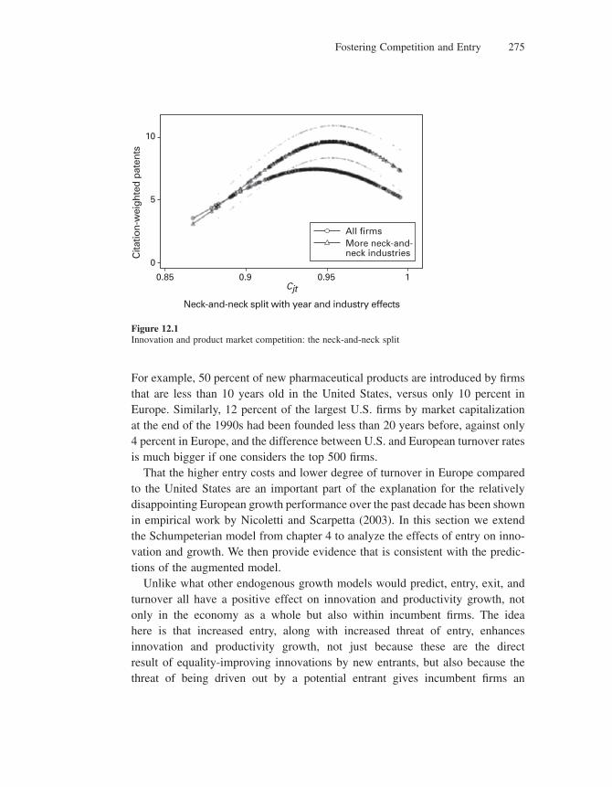
Fostering Competition and Entry 275
For example, 50 percent of new pharmaceutical products are introduced by fi rms that are less than 10 years old in the United States, versus only 10 percent in Europe. Similarly, 12 percent of the largest U.S. fi rms by market capitalization at the end of the 1990s had been founded less than 20 years before, against only 4 percent in Europe, and the difference between U.S. and European turnover rates is much bigger if one considers the top 500 fi rms.
That the higher entry costs and lower degree of turnover in Europe compared to the United States are an important part of the explanation for the relatively disappointing European growth performance over the past decade has been shown in empirical work by Nicoletti and Scarpetta (2003). In this section we extend the Schumpeterian model from chapter 4 to analyze the effects of entry on inno-vation and growth. We then provide evidence that is consistent with the predic-tions of the augmented model.
Unlike what other endogenous growth models would predict, entry, exit, and turnover all have a positive effect on innovation and productivity growth, not only in the economy as a whole but also within incumbent fi rms. The idea here is that increased entry, along with increased threat of entry, enhances innovation and productivity growth, not just because these are the direct result of equality-improving innovations by new entrants, but also because the threat of being driven out by a potential entrant gives incumbent fi rms an
All firmsMore neck-and-neck industries
10
5
0
0.85 0.9 0.95 1
Cita
tion-
wei
ghte
d pa
tent
s
Neck-and-neck split with year and industry effects
Cjt
Figure 12.1Innovation and product market competition: the neck-and-neck split
Chapter 12276
incentive to innovate in order to escape entry, through an effect that works much like the escape-competition effect described previously. This “escape-entry” effect is particularly strong for fi rms close to the world technology frontier. For fi rms further behind the frontier, the dominant effect of entry threat is a “discour-agement” effect that works much like the Schumpeterian appropriability effect described earlier.
12.3.1 Environment
Here we use again our workhorse multisector model in discrete time. All agents live for one period. In each period t a fi nal good (henceforth the numéraire) is produced in each state by a competitive sector using a continuum of intermediate inputs, according to the technology
Y A x dit it it= −∫ 1
0
1 α α
where xit denotes the quantity of the intermediate input produced in sector i at date t, Ait is the productivity parameter associated with the latest version of inter-mediate product i, and a ∈ (0, 1). The fi nal good, which we take to be the numéraire, is used in turn for consumption, as an input to R&D, and also as an input to the production of intermediate products.
In each intermediate sector i only one fi rm (a monopolist) is active in each period. Thus the variable i refers both to an intermediate sector (industry) and to the intermediate fi rm that is active in that sector. Like any other agent in the economy, intermediate producers live for one period only, and property rights over intermediate fi rms are transmitted within dynasties. Intermediate fi rms choose how much to produce in order to maximize profi ts, taking into account that the price at which they sell their intermediate good to the fi nal sector is equal to the marginal productivity of that good. As we saw in chapter 4, the equilibrium profi t for each intermediate fi rm takes the form
π πit itA= (12.4)
where
π αα
α α= −⎛⎝⎜
⎞⎠⎟
−1 2
1
12.3.2 Technology and Entry
Let At denote the new frontier productivity at date t and assume that
A g At t= +( ) −1 1

Fostering Competition and Entry 277
with 1 + g = g > 1. We shall again emphasize the distinction already made in the previous section between sectors in which the incumbent producer is “neck-and-neck” with the frontier and those in which the incumbent fi rm is far below the frontier.
At date t an intermediate fi rm can either be close to frontier, with productivity level Ait−1 = At−1 (type-1 sector i), or far below the frontier, with productivity level Ait−1 = At−2 (type-2 sector i).
Before they produce and generate profi ts, fi rms can innovate to increase their productivity. Each innovation increases the fi rm’s productivity by the factor g. For innovation to be successful with probability z, a type-j intermediate fi rm with j ∈ {1, 2} at date t must invest
c cz Ait it j= −2 2
Intermediate fi rms are subject to an entry threat from foreign producers. Let p denote the probability that an entrant shows up. Liberalization corresponds to an increase in p. Foreign entrants at date t are assumed to operate with the end-of-period frontier productivity At.
If the foreign fi rm manages to enter and competes with a local fi rm that has a lower productivity, it takes over the market and becomes the new incumbent fi rm in the sector. If it competes with a local fi rm that has the same productivity, however, Bertrand competition drives the profi ts of both the local and the foreign fi rm to zero. Now, suppose that potential entrants observe the postinnovation technology of the incumbent fi rm before deciding whether or not to enter. Then the foreign fi rm will fi nd it profi table to enter only if the local fi rm has a postin-novation productivity level lower than the frontier. However, the foreign fi rm will never enter in period t if the local fi rm has achieved the frontier productivity level At. Therefore, the probability of actual entry in any intermediate sector i is equal to zero when the local fi rm i was initially close to the frontier and has suc-cessfully innovated, and it is equal to p otherwise.
12.3.3 Equilibrium Innovation Investments
Using equation (12.4) together with the preceding innovation technology, we can analyze the innovation decisions made by intermediate fi rms that are close and the decisions of fi rms that are far below the frontier. Consider fi rst fi rms that are initially far below the frontier at date t. If they choose to innovate with probability z, then their profi t, not including the cost of innovation, will be pAt−1 with prob-ability (1 − p)z, which is the probability that they innovate and no entry occurs; and it will be pAt−2 with probability (1 − p)(1 − z), the probability of no
Chapter 12278
innovation and no entry. If entry occurs they earn no profi t. Therefore, their expected profi t, including the cost of innovation, will be
1 1 1 21 22
2−( ) + −( ) −( ) −− − −p z A p z A cz At t tπ π
They will choose the probability z that maximizes this expression; the fi rst-order condition of this maximization problem yields the probability
z p c2 1 1= −( ) −( )( )γ π (12.5)
Next consider fi rms that are initially close to the frontier. Their expected profi t will be pAt if they innovate (with probability z) and pAt−1 if they fail to innovate and no entry occurs [with probability (1 − p)(1 − z)], so they will choose their probability of innovation so as to maximize
z A p z A cz At t tπ π+ −( ) −( ) −− −1 1 212
1
so that
z p c1 1= − +( )( )γ π (12.6)
We interpret an increase in the threat of product entry p as a liberalization reform. Straightforward differentiation of equilibrium innovation intensities with respect to p yields
∂∂
∂∂
z
pc
z
pc1 20 1 0= > = − −( ) <π π γ;
In other words, increasing the threat of product entry (e.g., through trade liber-alization) encourages innovation in advanced fi rms and discourages it in back-ward fi rms. The intuition for these comparative statistics is immediate. The higher the threat of entry, the more instrumental innovations will be in helping incum-bent fi rms already close to the technological frontier to retain the local market. However, fi rms that are already far behind the frontier have no chance to win over a potential entrant. Thus, in that case, a higher threat of entry will only lower the expected net gain from innovation, thereby reducing ex ante incentives to invest in innovation.
12.3.4 The Effect of Labor Market Regulations
Next, consider the effects of changes in labor market regulations. A proemployer change in regulation will raise the profi t parameter p, so the qualitative effect on investments will be given by the derivatives
Fostering Competition and Entry 279
∂ ∂ ∂ ∂z p c z p g c1 21 0 1 0π γ π= − +( ) > = −( ) >;
Hence, proemployer labor market regulations encourage innovation in all fi rms.
However, if we look at the cross-partial derivatives with respect to reform p and labor regulation p, we get
∂∂ ∂
∂∂ ∂
21
221 0 0
z
pc
z
pg c
π π= > = − <;
Thus a more proemployer labor regulation—that is, a higher p—increases the positive impact of entry on innovation investments in type-1 industries.
12.3.5 Main Theoretical Predictions
Let us summarize our two main fi ndings:
1. Liberalization (as measured by an increase in the threat of entry) encourages innovation in industries that are close to the frontier and discourages innovation in industries that are far from it. Productivity, output, and profi ts should thus be raised by more in industries and fi rms that are initially more advanced.
2. Proworker labor market regulations discourage innovation and growth in all industries, and the negative effect increases with liberalization.
12.3.6 Evidence on the Growth Effects of Entry
These theoretical predictions have been corroborated by a variety of empirical fi ndings. First, Aghion, Blundell, Griffi th, Howitt, and Prantl (2006), henceforth ABGHP, investigate the effects of entry threat on TFP growth of UK manufactur-ing establishments, using panel data with over 32,000 annual observations of fi rms in 166 different four-digit industries over the 1980–93 period. They estimate the equation
Y E d E dijt jt it jt it i t ijt= + + + ∗ + + +α β γ δ η τ ε (12.7)
where Yijt is TFP growth in fi rm i, industry j, and year t; h and t are fi xed estab-lishment and year effects; Ejt is the industry entry rate, measured by the change in the share of UK industry employment in foreign-owned plants; and dit is the fi rm’s proximity to the world technological frontier in the corresponding industry, measured by the log of the ratio between that fi rm and the frontier-level labor productivity.
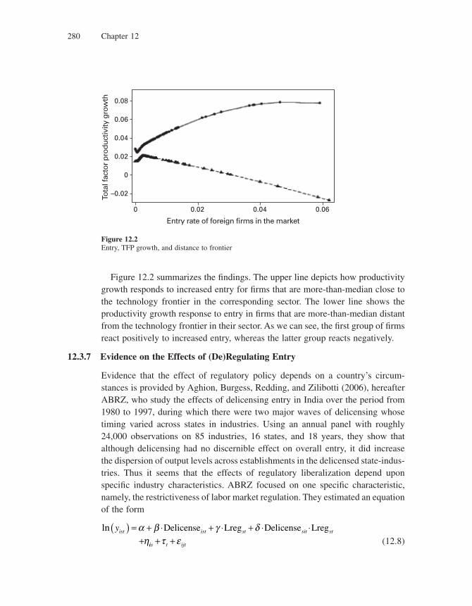
Chapter 12280
Figure 12.2 summarizes the fi ndings. The upper line depicts how productivity growth responds to increased entry for fi rms that are more-than-median close to the technology frontier in the corresponding sector. The lower line shows the productivity growth response to entry in fi rms that are more-than-median distant from the technology frontier in their sector. As we can see, the fi rst group of fi rms react positively to increased entry, whereas the latter group reacts negatively.
12.3.7 Evidence on the Effects of (De)Regulating Entry
Evidence that the effect of regulatory policy depends on a country’s circum-stances is provided by Aghion, Burgess, Redding, and Zilibotti (2006), hereafter ABRZ, who study the effects of delicensing entry in India over the period from 1980 to 1997, during which there were two major waves of delicensing whose timing varied across states in industries. Using an annual panel with roughly 24,000 observations on 85 industries, 16 states, and 18 years, they show that although delicensing had no discernible effect on overall entry, it did increase the dispersion of output levels across establishments in the delicensed state-indus-tries. Thus it seems that the effects of regulatory liberalization depend upon specifi c industry characteristics. ABRZ focused on one specifi c characteristic, namely, the restrictiveness of labor market regulation. They estimated an equation of the form
ln yist ist st sit st( ) = + ⋅ + ⋅ + ⋅ ⋅+α β γ δ
ηDelicense Lreg Delicense Lreg
iis t ijt+ +τ ε
(12.8)
0.08
0.06
0.04
0.02
0
–0.02
0 0.02 0.04 0.06
Tota
l fac
tor
prod
uctiv
ity g
row
th
Entry rate of foreign firms in the market
Figure 12.2Entry, TFP growth, and distance to frontier
Fostering Competition and Entry 281
where yist is real output, Delicense is a dummy that switches when the state-industry is delicensed, and Lregst is a measure of the degree of proworker regula-tion. Although the coeffi cient b was statistically insignifi cant, the interaction coeffi cient d was highly signifi cantly negative, indicating that one of the charac-teristics of an industry that makes it grow faster as a result of deregulation is the absence of restrictive labor market regulation. This fi nding suggests a comple-mentarity between different kinds of regulatory policy that needs to be taken into account when designing progrowth policies. Relaxation of entry barriers may not succeed in promoting growth if not accompanied by other changes that are favor-able to business development.
That the overall effect b of delicensing should be negligible is consistent with the preceding theoretical model. Indeed, this model says that the marginal effect of entry threat on average incumbent innovation or productivity growth will be positive only if the threat already exceeds some threshold level. In fact, Aghion, Blundell, and colleagues (2004) fi nd that the effect of (foreign) entry on average productivity growth among incumbent fi rms is positive in the United Kingdom. That the effect is higher in the United Kingdom than in India is explained easily in the model by the fact that entry is more open in the United Kingdom than in India, together with the fact that a higher fraction of UK sectors are close to their world frontier.
Generally speaking, the message is again that the reaction to the threat of entry posed by liberalization is different for “advanced” and “backward” state-indus-tries in the same sector. Removing barriers to entry incentivizes competitive advanced state-industries to invest in new production and management practices but may have the opposite effect on “backward” state-industries that have little chance of competing in the new environment.
12.4 Conclusion
What have we learned from our analysis in this chapter? First, we have seen that empirical evidence supports the prediction of an inverted-U relationship between competition and innovation. Second, the evidence also supports the prediction that entry and delicensing have a more positive effect on growth in sectors or countries that are closer to the technological frontier, but have a less positive effect on sectors or countries that lie far below the frontier. These fi ndings can be explained through suitable extensions of the Schumpeterian model. At the same time, they question the other models of endogenous growth. First, AK
Chapter 12282
models make no prediction on the relationship between competition and growth, since they assume perfect competition from the start. The product-variety model predicts a negative effect of competition (which in that model corresponds to a higher degree of substitutability a between intermediate inputs) on innovation and growth, as a higher a results in lower rents to reward new product innovators. It also suggests that entry should always be growth enhancing to the extent that it leads to higher product variety.
The fi ndings in this chapter have important policy implications. First, they go directly against the belief that existing national or European “champions” are best placed to innovate at the frontier or that these should be put in charge of selecting new research projects for public funding. Disregarding entry was no big deal during the 30 years immediately after World War II when European industries were still far behind their counterparts in the United States; however, now that Europe has come closer to the world technology frontier, it needs to open up its markets in order to foster growth. Another implication is that domestic-economy competition and entry policies should be accompanied by complementary poli-cies aimed at helping workers and capital reallocate from the laggard sectors that suffer from such policies to the more advanced sectors that benefi t from these same policies. A last implication concerns the relationship between growth and democracy: as we shall argue in chapter 17, democracy facilitates entry. This in turn may explain the fi nding that democracy is more positively correlated with growth in more advanced sectors and countries.
12.5 Literature Notes
The relationship between competition and innovation/entry has fi rst been exten-sively analyzed by standard IO theory. Here we refer the reader to Tirole (1988). The idea that innovation should decline with competition, as more competition reduces the monopoly rents that reward successful innovators, has been most forcefully formulated by Dasgupta and Stiglitz (1980), but this idea also underlies the spatial competition model of Salop (1977) and the symmetric product differ-entiation model of Dixit and Stiglitz (1977). The same effect features in the fi rst generation of Schumpeterian growth models, in particular Aghion and Howitt (1992), Grossman and Helpman (1991a), and Caballero and Jaffe (1993).
Some empirical studies have found a positive correlation between monopoly power and innovations (see, for example, Crépon, Duguet, and Mairesse 1998); however, most recent empirical studies, in particular Geroski (1995), Nickell

Fostering Competition and Entry 283
(1996), and Blundell, Griffi th, and Van Reenen (1999), point to a positive correla-tion between product market competition and innovative output.
Some early analyses pointed instead at the existence of an inverted-U relation-ship between product market competition and innovation, starting with Scherer (1967)—however, without explaining why and without testing the robustness of this empirical fi ndiing.
A fi rst theoretical attempt at extending the Schumpeterian model in order to generate the possibility of a positive correlation between competition and innova-tion was by Aghion, Dewatripont, and Rey (1999), who built on previous work by Hart (1983) and Schmidt (1997) showing that competition could act as an incentive scheme in fi rms with “satisfi cing” managers.
Aghion, Harris, and Vickers (1997) and then Aghion, Harris, and colleagues (2001) introduced step-by-step innovations into the Schumpeterian framework, thereby generating an inverted-U relationship between competition and innova-tion. The inverted-U relationship was subsequently tested on a UK fi rm-level panel by Aghion and colleagues (2005).
The fi rst empirical analysis of the relationship between entry, innovation, and growth is by Nicoletti and Scarpetta (2003) using cross-country data from the OECD. Subsequently, Aghion and colleagues (2004; 2006) introduced entry into the Schumpeterian framework, with predictions on the interplay between distance to frontier, entry, and innovation, which they confronted to UK fi rm-level panel data.
For an extensive analysis of the relationship between competition, innovation, and growth, we refer the reader to Aghion and Griffi th (2005).
Problems
1. Present one argument for why product market competition promotes growth and one argument predicting the opposite effect. Looking at the inverted-U prediction of the relationship between competition and growth presented in the chapter, explain intuitively the “escape-competition effect” and the “Schumpeterian effect.” What does this imply in terms of growth-promoting policy?
2. More on the inverted-U pattern (based on Aghion, Bloom, et al. 2005)
This exercise extends a bit the model presented in section 12.2.We consider the setup of section 12.2.
a. Explain why the expected technological gap is given by m1; show that it increases with competition.
b. Compute the optimal degree of competition; comment on the effect of g and h.
Chapter 12284
c. In their empirical study Aghion, Bloom, and colleagues use the following measure of competition:
c = −1 Average lerner index
Compute this empirical measure in this theoretical setup. Comment.
3. *Cournot versus Bertrand competition, I (based on Aghion, Harris, and Vickers 1997)
This problem uses a setup similar to the one presented in section 12.2 and compares the impact of Cournot and Bertrand competition.
There is a representative consumer with preference defi ned as
U C t L t e dtrt= ( )⎡⎣ ⎤⎦ − ( ){ } −∞
∫ ln0
where L is the labor supply (perfectly elastic then) and C(t) is a consumption index defi ned as ln lnC t q t dii( )⎡⎣ ⎤⎦ = ( )⎡⎣ ⎤⎦∫0
1, where qi is the number of goods consumed from the industry i ∈ [0, 1]. In
each industry i there is a duopoly. One fi rm x in industry i can produce one unit of consumption good i using γ −ki
x (g >1) units of labor where k xi is the technological level achieved by fi rm x in sector i. As
in the chapter, we assume that the technological gap between two fi rms cannot be greater than one step and that a fi rm innovates with a Poisson rate z by employing z2
2 units of labor; in addition, if it
is one step behind, there is a Poisson rate of h that it innovates by mere spillover (and if the gap is wider, the Poisson rate to innovate by spillover is infi nite). We index by 1 the leader in a sector when it is unleveled (and by −1 the laggard) and by 0 the two fi rms in leveled sectors.
The wage is normalized at 1, and we focus on a steady state. Also, note that contrary to the model presented in the chapter we do not assume that in the level case only one fi rm can innovate (but the probability that both do innovate is negligible).
a. Show that the consumer spends piqi = 1 on each good.
b. Assuming that the fl ow of profi ts only depends on the gap in the sector, show that
z1 0=
z r h z a b r h a− = +( ) + ( ) + +( ) − +( ) +1
2
0
2 22 2
z s r h a0
22= − + +( ) +
where zl denotes the investment undertaken by a fi rm in position l, a = p1 − p0, and b = p0 − p.If a ≥ b, when does a fi rm undertake more investment?
c. Compute the share of leveled sectors l.
4. *Cournot versus Bertrand competition, II
This problem is a continuation of the previous one.
a. Show that the growth rate of consumption is given by g = 2lz0ln(g). To do so,
i. Denoting by g0 the proportional increase in the aggregate consumption index when a fi rm in a level sector innovates and by g1 the proportional increase in aggregate output when a fi rm in an unlevel sector innovates, prove (mathematically or heuristically) that
gd C t
dtz z h=
( )⎡⎣ ⎤⎦ = ( ) + −( ) +( ) ( )−
lnln ln2 10 0 1 1λ γ λ γ
ii. Explain why g0g1 = g.
iii. Conclude.

Fostering Competition and Entry 285
b. We consider now the cases of Bertrand (indexed by B) and Cournot (indexed by C) competition. Prove that in this case the fl ow of profi t in a sector is in fact independent of the level of the technol-ogy. Show that
aB = −γγ
1
bB = 0
aC =−( ) +( )
+( )γ γ
γ1 3 1
4 12
bC =−( ) +( )
+( )γ γ
γ1 3
4 12
Note that aB > aC + bC.
c. Then show that when h = r = 0,
g
gB
C
=+ +
++
⎛
⎝
⎜⎜⎜⎜
⎞
⎠
⎟⎟⎟⎟
+1
7 13 1
1 2
3 1
4
2γγ γ
γ
Is Cournot or Bertrand competition better for growth? Explain.
5. **Patent race and Stackelberg competition (based on Etro 2004)
This problem compares the effect of Stackelberg competition versus Cournot competition on who is going to undertake research.
We consider a market where a monopolist gets a fl ow of profi ts p. The monopolist and n competi-tors can engage in research to discover a new patent with value V > p (innovation is drastic, so that the discovery of the new patent kills the market for the old version). Time is continuous, and if a fi rm engages a fl ow z of resources in research, it faces a Poisson rate of success of ze
i (0 < e < 1). There is a fi xed cost in entering the patent race of F < V.
a. Show that the incumbent solves
max ,�
� �
��
��
z
jj
n
jj
n
z V z
r z zF z
z V
r zz
ε
ε
ε
ε
π π+ −
+ +− > +
+=
= =∑ ∑
1 1
0 0if if⎧⎧⎨⎪
⎩⎪
⎫⎬⎪
⎭⎪
and the entrant i solves
max ,z
i i
jj
n i ii
z V z
r z zF z z
ε
ε
−
+ +− > =
⎧⎨⎪
⎩⎪
⎫⎬⎪
⎭⎪=∑ �
1
0 0 0if if
b. We consider the case of a Cournot Nash equilibrium.
i. For a fi xed n, show that the incumbent undertakes less research than an entrant, and that if n is large enough, the incumbent does not undertake any research.

Chapter 12286
ii. Under free entry, what is the effect of a decrease in the fi xed cost F? (We assume that V is large enough so that there is a large number of entrants, and you can consider it as a real in writing the free entry condition.) Comment.
c. We now consider the case of Stackelberg competition; that is, the monopolist can choose its level of investment before the other fi rms (and then take their reaction into account).
i. Explain why Stackelberg competition looks natural in this setup.
ii. For a fi xed n, show that an entrant chooses to invest more if the incumbent invests more and that the incumbent invests less than an entrant. Compare the aggregate rate of innovation under Cournot and Stackelberg competition.
d. Still in the Sackelberg setup, but with free entry,
i. Prove that the entrant invests z V F= −( )⎡⎣ ⎤⎦ −ε ε1
1 . Comment.
ii. Prove that the aggregate amount of research by entrants decreases with the amount of investment undertaken by the incumbent.
iii. Prove that the incumbent will invest �z V= ( ) −ε ε1
1 , compare it with the investment of the entrant, and compare it with the Nash equilibrium case.
iv. What is the effect of a decrease in the fi xed cost on the aggregate amount of R&D?
13 Investing in Education
13.1 Introduction
Does education matter for growth? Which kind of education investment matters most? How best to allocate public funds between primary, secondary, and tertiary education? These are questions that preoccupy governments. For example, they feature prominently in the so-called Lisbon Agenda set by countries in the Euro-pean Union as part of an effort to reduce the growth gap between the European Union and the United States. A fi rst look at the United States versus the European Union in 1999–2000 shows that 37.3 percent of the U.S. population aged 25–64 had completed a higher education degree, against only 23.8 percent of the EU population. This educational attainment comparison is mirrored by that on tertiary education expenditure, with the United States devoting 3 percent of its GDP to tertiary education versus only 1.4 percent in the European Union. Is this European defi cit in tertiary education investment a big deal for growth?
In this chapter, we look at what existing growth models have to say on this type of question. A fi rst class of models emphasizes capital accumulation. Within that class, the neoclassical reference is Mankiw, Romer, and Weil (1992), hence-forth MRW, and the AK reference is the celebrated article by Lucas (1988). Both papers emphasize human capital accumulation as a source of growth. MRW is an augmented version of the Solow model with human capital as an additional accumulating factor of production, and in particular human capital accumulation slows down the convergence to the steady state by counteracting the effects of decreasing returns to physical capital accumulation. In Lucas, human capital accumulates at a speed proportional to the existing stock of human capital, which in turn leads to a positive long-run growth rate. Whether on the transition path to the steady state (in MRW) or in steady state (in Lucas), the rate of growth depends upon the rate of accumulation of human capital, not upon the stock of human capital.
A second approach, which goes back to the seminal contribution by Nelson and Phelps (1966) and the subsequent empirical work by Benhabib and Spiegel (1994), describes growth as being driven by the stock of human capital, which in turn affects a country’s ability to innovate or to catch up with more advanced countries.1 By linking the stock of human capital (measured either by the fl ow of
1. Barro and Sala-i-Martín (1995a, chap. 13) also used a large sample of countries during the time period 1965–85 to regress the average growth rate on several macroeconomic variables, including educational attainment and public spending on education as a fraction of GDP. Their main fi ndings are (1) that educational attainment (measured by average years of schooling) is signifi cantly
Chapter 13288
education spending or by school attainment) to the process of technological change, this approach helps answer questions, for example, on how to maximize growth through a proper design of education spending policy.
However, this second approach raises a number of empirical problems. First, the correlation between growth and education ceases to be signifi cant once we restrict the analysis to OECD countries or when we control for country fi xed effects. Second, the positive correlation between education—measured by stocks—and growth found in the overall country samples may refl ect reverse causalities from growth to education. In this chapter we present potential solu-tions to these problems. In particular, we argue that signifi cant correlations between education spending and growth can be restored even if we restrict the analysis to OECD countries by (1) decomposing total education spending or attainment into different types or levels (for example, between primary/secondary and tertiary education, or between pregraduate and postgraduate education) and (2) interacting the different types of education spending or attainment with a country’s or region’s distance to the technology frontier, adapting the appropriate institution idea introduced in chapter 11.
The chapter is organized as follows. Section 13.2 summarizes the growth models based on human capital accumulation. Section 13.3 presents the Nelson-Phelps approach and discusses its limits. Section 13.4 extends the Nelson-Phelps framework by embedding it into a model of appropriate education systems, and then addresses the empirical questions raised by previous regression exercises.
13.2 The Capital Accumulation Approach
13.2.1 Back to Mankiw, Romer, and Weil
13.2.1.1 The Model
To refresh memories, it might be useful to start the chapter by reminding our-selves of the Mankiw, Romer, and Weil (1992) model. What the model does is simply to extend the Solow model by introducing human capital on top of physi-cal capital and raw labor as a third factor of production:
correlated with subsequent growth (with a correlation coeffi cient at around 0.05), although if we decom-pose the aggregate measure of educational attainment, the impact of primary education remains largely insignifi cant, and (2) that public spending on education also has a signifi cantly positive effect on growth: a 1.5 percent increase of the ratio of public education spending to GDP during the period 1965–75 would have raised the average growth rate during the same period by 0.3 percent per year.
Investing in Education 289
Y AK H L= − −α β α β1
where human capital H may also accumulate over time.Even if H does not accumulate, differences in schooling across countries
now partly account for differences in GDP per capita across countries. Taking L = L = 1, so that GDP is equal to GDP per capita, let us consider two countries, i and j, that have the same steady-state capital/output ratio: Ki
ss/Yiss = Kj
ss/Yjss. The
ratio of country i’s steady-state level of output to country j’s is given by
Y
Y
AH
AHiss
jss
i
j
=⎛
⎝⎜
⎞
⎠⎟
−β
β
α1
1
so that the difference in GDP per capita across the two countries is entirely explained in this case by differences in schooling.
Now, suppose that human capital does accumulate as physical capital does. Then, the complete model with physical and human capital accumulation boils down the following system of three equations:
Y AK Ht t t= α β
dK
dts Y Kt
k t t= − δ
dH
dts Y Ht
h t t= − δ
Dividing the last two equations by Kt and Ht, respectively, we obtain the steady-state values:
Ks sk h* =
⎛⎝⎜
⎞⎠⎟
− − −11
1β β α β
δ
Hs sk h* =
⎛⎝⎜
⎞⎠⎟
− − −β β α β
δ
11
1
and
Ys sk h* =
⎛⎝⎜
⎞⎠⎟+
− −α β
α β
α β
δ
1
1
Thus, as with the Solow model, no long-run growth of per capita GDP is pre-dicted by the MRW model, which again follows from decreasing returns, now to
Chapter 13290
physical and to human capital accumulation. However, the MRW model also implies that a government policy that would maintain a positive rate of human capital accumulation would also guarantee a positive long-run rate of growth. For example, suppose that
H etmt=
where m > 0. Then the economy will grow at a long-run rate of mb.In MRW, human capital accumulation slows down the convergence to the
steady state by counteracting the effects of decreasing returns to physical capital accumulation. In the Lucas model we shall present in the next subsection, the assumption that human capital accumulates at a speed proportional to the existing stock of human capital leads to a positive long-run growth rate, even in the absence of human capital accumulation by the government.
13.2.1.2 Development Accounting2
The MRW model predicts a positive relationship between per capita GDP and physical and human capital intensities. It can thus be used to analyze the deter-minants of cross-country differences in per capita GDP, in other words, to perform “development accounting.” Thus, for example, if we assume that the aggregate production function takes the form
Y K H AL= ( ) − −α β α β1
where L grows at rate n and A grows at rate g, and physical and human capital depreciates at the same rate d, then we have
Y L A K Y H Y AX= ( ) ( ) =− − − −αα β
βα β1 1
The physical capital intensity is computed in steady state, using the fact that in steady state we have
K YI Y
n gK=
+ +δ
where IK/Y is the physical investment intensity, and
H YI Y
n gH=
+ +δ
2. Here we closely follow Banerjee and Dufl o (2005).
Investing in Education 291
where IH /Y is the human capital investment intensity.MRW use the ratio
cov
var
log , log
log
Y L X
Y L
[ ][ ]
where cov[log Y/L, log X] is the covariance between log Y/L and log X across countries, and var[log Y/L] is the variance of log Y/L across countries, to measure the fraction of cross-country income differences that can be explained by differ-ences in physical and human capital investment intensities, and they fi nd a ratio of 78 percent.
Subsequent studies by Klenow and Rodriguez-Clare (1997) and by Caselli (2005) have extended this development accounting framework, in particular by coming up with refi ned measures for human and physical capital investments and stock.
13.2.1.3 Discussion
A main challenge to the MRW model comes from Benhabib and Spiegel (1994), who simply refuted the role of human capital accumulation as a driver of growth. Using cross-country estimates of physical and human capital stocks over the 1965–85 period, they perform the growth-accounting regressions suggested by a neoclassical production function à la MRW, namely,
ln ln ln ln
ln ln
ln ln
ln ln
y y A A
K K
L L
H H
τ τ
τ
τ
τ
αβγ
− = −+ −( )+ −( )+ −( )
0 0
0
0
0
++ −ln lnε εt 0
where et is the error term. They fi nd that g is insignifi cant. This fi nding in turn implies that log differences in human capital over time have no effect on log differences in income. In other words, human capital accumulation does not matter for growth. See fi gure 13.1.
Why then did MRW fi nd signifi cant effects of schooling on per capita GDP levels (which imply that the rate of growth of schooling should have a signifi cant effect on the growth rate of per capita GDP)? Benhabib and Spiegel’s answer is that MRW use school enrollment as a proxy for average level of human capital, which in turn assumes that the economy is already . . . in a steady state!

Chapter 13292
Krueger and Lindahl (2001), however, disagree with Benhabib and Spiegel: using panel data over 110 countries between 1960 and 1990, choosing the number of years in education instead of the logarithm of that number to measure human capital,3 and correcting for measurement errors, they fi nd signifi cant correlations between growth and both the stocks and accumulation rates of human capital. However, these correlations become insignifi cant once the cross-country sample is restricted to OECD countries.
13.2.2 Lucas
Inspired by Becker’s (1964) theory of human capital, Lucas (1988) considers an economy populated by (infi nitely lived) individuals who choose at each date how
Log difference in human capital
Log
dif
fere
nce
in in
com
e
1.5
1
0.5
0
–0.5
–1–0.5 0 0.5 1 1.5 2 2.5
Figure 13.1Income versus human capital (Benhabib and Spiegel 1994)
3. This change was in turn motivated by the so-called Mincerian approach to human capital, whereby the value of one more year in schooling is measured by the wage increase that is forgone by the individual who chooses to study during that year instead of working. This amounts to measuring the value of a human capital stock by the log of the current wage rate earned by an individual. And that log was shown by Mincer to be positively correlated with the number of years spent at school by the individual, after estimating an equation of the form
lnw a a n= +0 1
The Mincerian approach can itself be criticized, however, for (1) assuming perfectly competitive labor markets, (2) ignoring the role of schools as selection devices, and (3) ignoring interpersonal and intertemporal knowledge externalities.
Investing in Education 293
to allocate their time between current production and skill acquisition (or school-ing), where skill acquisition increases productivity in future periods. Thus, if h denotes the current human capital stock of the representative agent and u denotes the fraction of his or her time currently allocated to production, then the two basic equations of the Lucas model are
y k uH= ( ) −β β1 (13.1)
which describes the way human capital affects current production (k denotes the physical capital stock, which evolves over time according to the same differential equation as in the Solow or Ramsey model, namely, k
. = y − c, where c is current
consumption), and
�H H u= −( ) >δ δ1 0, (13.2)
which spells out how current schooling time (1 − u) affects the accumulation of human capital.4 The reader will have certainly noticed the similarity between equation (13.2) and the differential equation that describes the growth of the leading-edge technology parameter A in chapter 4 or the equation that describes the accumulation of horizontal innovations in the product-variety model of chapter 3. However, in contrast to the nonrival technological knowledge embod-ied in innovations, human capital acquisition does not necessarily involve exter-nalities (or “spillovers”) across individuals of the same generation. Yet the assumption that human capital accumulation involves constant returns to the existing stock of human capital produces a positive growth rate in steady state equal to
g u= −( )δ 1 *
where u* is the optimal allocation of individuals’ time between production and education.5 Education effort (1 − u*) can in turn be shown to depend negatively
4. If learning by doing rather than education were the primary source of human capital accumulation, equation (13.2) should be replaced by something like
�h hu= δ
That is, the growth of human capital increases with production.
5. That is, u* maximizes the representative consumer’s intertemporal utility
ce dtt t
1
0 1
−−∞
−∫σ
ρ
σ
subject to equations (13.1) and (13.2) and k. = y − c.

Chapter 13294
on the rate of time preference r and the coeffi cient of relative risk aversion s and positively on the productivity of schooling measured by d, therefore displaying comparative static properties similar to the steady-state R&D investment in chap-ters 3 and 4.
The Lucas model is elegant, but at the same time also stylized in its description of the return to education. For example, in this model an individual’s returns to education remain constant over his or her whole lifetime, an assumption that is at odds both with the empirical evidence on education and with Becker’s theory of human capital. Becker (1964) indeed suggests that returns to education tend to decrease over the lifetime of an individual. One easy way to deal with this objection is to reformulate the Lucas model in the context of an overlapping-generations framework where individuals inherit the human capital accumulated by their parents.6
For example, consider the following simplifi ed version of the Lucas model, with discrete time and successive generations of two-period-lived individuals. In her fi rst period of life, an individual chooses how to share her time between pro-duction and human capital accumulation. Human capital accumulates according to
H H u H2 1 11− = −( )δ (13.3)
where H1 (resp. H2) is the individual’s stock of human capital in period 1 (resp. period 2), and u still denotes the fraction of time u spent on production in period 1.
The individual chooses u to
maxu
H u H1
1
2
1
1 1
( )−
+ ( )−
⎧⎨⎪
⎩⎪
⎫⎬⎪
⎭⎪
− −σ σ
σβ
σ
subject to equation (13.3), where b is the discount factor.The fi rst-order condition for this maximization is simply
u u− −− + −( )⎡⎣ ⎤⎦ =σ σβδ δ1 1 0
or equivalently
u u= =+ ( )
*1
1
δ βδ σ
6. See d’Autume and Michel (1994) for a systematic analysis of the overlapping-generations version of the Lucas model.
Investing in Education 295
which is decreasing in d and b.Thus the equilibrium growth rate
g u= −( )δ 1 *
is increasing in the productivity of schooling d and decreasing with the rate of time preference, which itself is inversely measured by b.
13.2.3 Threshold Effects and Low-Development Traps
Consider the following extremely simple overlapping-generations model with human accumulation: there is a continuum of overlapping-generations families, in which each individual lives for two periods. All individuals born at date t inherit the aggregate human capital accumulated by the previous generation of individuals born at date t − 1, that is,
h h Hti
t t1 1 2 1, , ,≡ = − (13.4)
where
H h dit ti
2 1 2 1, ,− −= ∫Thus, if for simplicity we assume that individuals of a same generation are identi-cal and of total mass equal to one (so that total population remains constant equal to two), we have
h ht t1 2 1, ,= −
where h2,t−1 is the human capital accumulated by an individual born at date t − 1.
Next, we must specify how human capital accumulates during the lifetime of an individual. We shall assume, for all t,
h v v ht t t2 1 11, ,= + ( )⋅⎡⎣ ⎤⎦−γ θ (13.5)
where u is the fraction of time allocated to education by a young individual born at date t, g (ut−1) is a positive number that is nondecreasing in the amount of time ut−1 devoted to education by the previous generation, and q < 1.7
The complementary time 1 − u is allocated to production activities, and to simplify the argument to the extreme, we will assume that an individual with
7. See section 13.3.2 for an alternative model that has multiple development paths but that does not rely on intertemporal threshold externalities, that is, in which g (u) ≡ g = constant.
Chapter 13296
current human capital endowment h contributes a marginal product equal to h and therefore earns a wage also equal to h.8 Therefore, an individual born at date t (with initial skills h1,t) will choose how much time u to spend in education so as to maximize his or her intertemporal utility of consumption. Assuming linear preferences and letting r denote the discount factor, the optimal education time u* solves the maximization program
max
:
, ,
, ,
vt t
t t
v h h
h v h
1
1
1 2
2 1
−( ) +
= +( )ρ
γ θsubject to (13.6)
A special case occurs when g is a constant. Then, we obtain the unique solution
v* = ( ) −ρθγ θ1
1
which in turn corresponds to a unique steady-state growth path, at rate
gh
hvt
t
* *= = + = + ( )−
−2
2 1
11 1,
,
θθ
θγ δθγ
As in the Lucas model, we see that g* is an increasing function of the productivity of education measured by g and a decreasing function of the rate of time
preference r (where ρ =+1
1 r).
However, the more interesting case considered by Azariadis and Drazen (1990) occurs when the education technology in equation (13.6) displays positive thresh-old externalities. In particular, suppose that
γγ
γv
v v
v vt
t
t−
−
−
( ) =≤
>⎧⎨⎪
⎩⎪1
1 0
1 0
if
if
where 0 < u0 < 1 and γ γ� . Then, if the previous generation has insuffi ciently invested in education, and therefore g (ut−1) = γ , investing in education tends to become unattractive for the current generation as well; hence the possibility of a low-growth path where all successive generations invest too little in education. This low-growth path, or “low-development trap,” can naturally coexist with a high-growth path where all generations invest at least u0 in education and there-fore g (ut−1) ≡ γ for all t.
8. Equivalently, we could assume that all individuals are self-employed and that the self-employment technology is linear, with s working-time units producing h⋅s units of output, where h denotes the individual’s current human capital endowment.
Investing in Education 297
More precisely, a low-growth steady-state equilibrium will involve the station-ary educational attainment level v, where
v v h v ht t= −( ) + +( )arg max , ,1 11 1ρ γ θ
that is, v = ( ) −ρθγ θ1
1 , with corresponding growth rate
g v= + ⋅ = + ( ) −1 1 1γ γ ρθγθθ
θ
Similarly, the high-growth equilibrium will involve the educational attainment level v , where
v v h v hv
t t= −( ) + + ⋅( )arg max , ,1 11 1ρ γ θ
that is, v = ( ) −ρθγ θ1
1 , with correspondingly high growth rate
g v= + ⋅ = + ( ) −1 1 1γ γ ρθγθθ
θ
For these two equilibria to actually coexist, it is necessary and suffi cient that υ¯
< u0 < υ, a requirement which in turn imposes restrictions on the parameters u0, r, q, γ
¯ and γ .
In short, the existence of threshold externalities in the education technology case naturally leads to a multiplicity of steady-state growth paths, including a low-development trap where insuffi cient investment in education in the past dis-courages further skill acquisition and thereby future growth. Thus Azariadis and Drazen provide a perhaps more natural story than Lucas (1988) for why countries with unequal initial human-capital endowments may keep growing at different rates forever. But they also suggest a role for government intervention in the education sector, namely, to avoid low-development traps and thereby promote high sustained growth.9
9. Becker, Murphy, and Tamura (1990) develop a similar model but one in which individuals decide also about “fertility,” that is, about how many children they wish to have. Assuming that the returns to human capital investments increase with the human capital stock, the authors show the existence of multiple equilibria. One equilibrium corresponds to a “development trap,” with a high rate of population growth but low levels and low growth rates of individual human capital. The other equi-librium instead corresponds to a low rate of population growth but also to high levels and rapid growth of human capital per head. The contrast with the Solow-Swan model is interesting: here, the rate of population growth is negatively correlated with the rate of productivity growth.
Chapter 13298
13.3 Nelson and Phelps and the Schumpeterian Approach
13.3.1 The Nelson and Phelps Approach
Nelson and Phelps (1966) did not have a model of endogenous growth with endogenous R&D and innovation, but they were already thinking of growth as being generated by productivity-improving adaptations, whose arrival rate would depend upon the stock of human capital. More formally, Nelson and Phelps would picture a world economy in which, in any given country, productivity grows according to an equation of the form
�A f H A A= ( ) −( )where again A denotes the frontier technology (itself growing over time at some exogenous rate) and H is the current stock of human capital in the country. A higher stock of human capital would thus foster growth by making it easier for a country to catch up with the frontier technology. Benhabib and Spiegel (1994) tested a slightly augmented version of the Nelson-Phelps model in which human capital not only facilitates the adaptation to more advanced technologies, but also makes it easier to innovate at the frontier, according to a dynamic equation of the form
�A f H A A g H A= ( ) −( ) + ( )γwhere the second term captures the innovation component of growth.
Using cross-country regressions of the increase in the log of per capita GDP over the period 1965–85 as a linear function of the sum of logs of human capital stocks over all the years between 1965 and 1985, Benhabib and Spiegel found a signifi cantly positive correlation between h and g. More specifi cally, Benhabib and Spiegel perform the regression
ln ln ln ln
ln ln
ln ln
ln
y y A A
K K
L L
Htt
τ τ
τ
ττ
αβ
γτ
− = −+ −( )+ −( )+
=∑
0 0
0
0
0
1⎛⎛⎝⎜
⎞⎠⎟
+ −ln lnε ετ 0
and fi nd a positive and signifi cant g. This in turn implies that human capital stock is positively correlated with output growth. Moreover, Benhabib and Spiegel fi nd
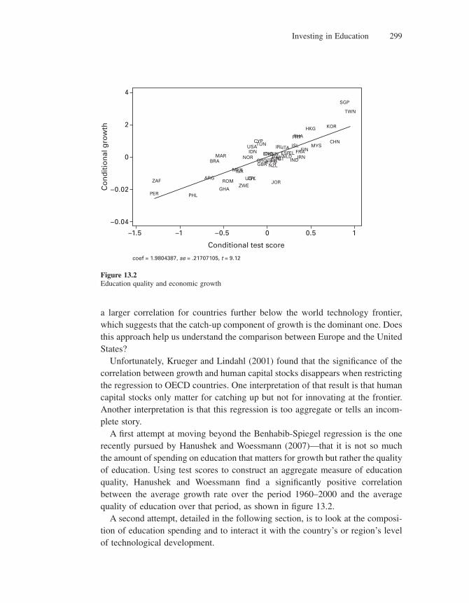
Investing in Education 299
a larger correlation for countries further below the world technology frontier, which suggests that the catch-up component of growth is the dominant one. Does this approach help us understand the comparison between Europe and the United States?
Unfortunately, Krueger and Lindahl (2001) found that the signifi cance of the correlation between growth and human capital stocks disappears when restricting the regression to OECD countries. One interpretation of that result is that human capital stocks only matter for catching up but not for innovating at the frontier. Another interpretation is that this regression is too aggregate or tells an incom-plete story.
A fi rst attempt at moving beyond the Benhabib-Spiegel regression is the one recently pursued by Hanushek and Woessmann (2007)—that it is not so much the amount of spending on education that matters for growth but rather the quality of education. Using test scores to construct an aggregate measure of education quality, Hanushek and Woessmann fi nd a signifi cantly positive correlation between the average growth rate over the period 1960–2000 and the average quality of education over that period, as shown in fi gure 13.2.
A second attempt, detailed in the following section, is to look at the composi-tion of education spending and to interact it with the country’s or region’s level of technological development.
4
2
0
–0.02
–0.04
10.50–0.5–1.5 –1
Co
nd
itio
nal
gro
wth
coef = 1.9804387, se = .21707105, t = 9.12
Conditional test score
GHA
ROMZWE
JOR
L
ISRMEX
MAR NORGBR
INDN
N
PLRRIYEE
GGR
G TT
EL
GRCNLDESF
FINMYS
CHN
HKG KOR
SGP
TWN
PRTTHA
FRA
NZL
ENGCHNIRN
ITAIRL ISL
CPLUGY
IDNUSA
CYPTUN
BRA
PHL
ARG
PER
ZAF
Figure 13.2Education quality and economic growth
Chapter 13300
13.3.2 Low-Development Traps Caused by the Complementarity between R&D and Education Investments
The following model, inspired by Acemoglu (1997) and Redding (1996), delivers multiple development paths as in the Azariadis-Drazen model, although under more natural assumptions about human-capital accumulation. In particular, the following story does not rely on intertemporal threshold externalities in human-capital accumulation.
There is again a continuum of overlapping generations of individual workers each of whom lives for two periods and has preferences
u c c c c1 2 1 2,( ) = + δ
where d is the discount factor. All individuals are born with one unit of human capital (hl,t ≡ 1 for all t) and, by investing the fraction � of their working time to education when young, individuals can end up with h2,t = 1 +g ⋅ �q units of human capital, where g is now constant and 0 < q < 1.
There is also a continuum of overlapping generations of entrepreneurs, who can produce only when old according to the linear technology
y A hj ti
ti
j t, ,+ + += ⋅1 1 1
where (a) Ait+1 denotes entrepreneur i’s productivity at date t + 1 (which itself
depends on whether or not the entrepreneur has innovated the existing leading-edge technology A At t
i= max available to him or her upon birth at date t; (b) hj,t+1 is the human capital of the j—worker employed by the entrepreneur at date t + 1.
The time-path of productivity parameters Ait is then governed by the following
innovation technology: by investing a nonmonetary cost equal to amA, entrepre-neurs can increase productivity from A (the current leading edge) to lA with probability m, where l > 1 and 0 < m < 1.
Now assume that individual workers remain self-employed when young, pro-ducing output (1 − �)A where (1 − �) is production time and A denotes the current leading-edge technology,10 aid when old are randomly matched with fi rms from which they earn the fraction b of output surplus.11 Then the optimal allocation of working time between current production and education will solve the following maximization program:
10. The analysis would remain essentially unchanged if A were instead taken to be the average technology.
11. We assume a one-to-one matching process between fi rms and workers, based on the implicit assumption that fi rms are capacity constrained and can employ at most one worker.
Investing in Education 301
maxv
v A v A1 1 1−( ) + + −[ ] +( ){ }βρ μλ μ γ θ
This yields the optimal education time
v* = + −( )⎡⎣ ⎤⎦⎛⎝⎜
⎞⎠⎟
−min ,1 11
1βρθγ μλ μ θ
which is an increasing function of the probability of innovation m.The entrepreneurs, in turn, will choose R&D effort (i.e., m) to
maxμ
θμ μα ρ β μλ μ γV A v A( ) = − + −( ) + −( )⋅ +( ){ }1 1 1
Hence
μα ρ λ γ βθ
*if
otherwise=
< −( ) +( ) −( )⎧⎨⎪
⎩⎪
1 1 1 1
0
v
,
thus the more workers invest in education (i.e., the higher u) the more will entre-preneurs invest in R&D.
This strategic complementarity between workers’ education decisions and fi rms’ R&D decisions will not surprisingly open the possibility for multiple steady-state growth paths, including a low-development trap. Such a trap will
involve m* = 0 and therefore υ υ βρθγ θ* = = ( ) −1
1 . For it to exist we simply need
α δ β λ γ βρθγ θ> −( ) −( ) + ( )⎛⎝⎜
⎞⎠⎟
−1 1 11
1 .
Conversely, a high-growth equilibrium will involve m* = 1 and therefore
υ υ λβρθγ θ* = = ( ) −1
1 . In order for a high-growth steady-state path to exist, we need
α δ β λ γ λβρθγ θ< −( ) −( ) + ( )⎛⎝⎜
⎞⎠⎟
−1 1 11
1 .
The corresponding growth rates will be g = g = ln l in the high-growth equilib-rium and g = g = 0 in the low-development trap.12
Two quick remarks conclude our analysis in this section. First, be cause of the strategic complementarity between R&D and education, we did not have to intro-duce threshold externalities in the accumulation of human capital in order to gener-ate multiple equilibria and low-development traps. Second, targeted education
12. Had we introduced an intertemporal human capital externality, of the kind assumed in theprevious section, namely y1t = (1 − d)Ht−1, where H h dit t
i
i− −= ∫1 2 1, , the analysis would remain identical except that g = ln l + ln(1 − d)(1 + g ⋅ v θ ) and g = ln(1 − d) (1 + g ⋅ vθ
) ≠ 0. Interestingly, in that case the growth differential g − g is magnifi ed by the fact that the high-growth equilibrium also displays a higher rate of human capital accumulation.
Chapter 13302
policies and R&D subsidies appear as substitutable instruments for moving the economy away from a low-development trap. In practice, however, education sub-sidies may be easier to monitor than R&D subsidies to industries (the scope for diversion and manipulation being presumably larger in the latter case).
13.4 Schumpeter Meets Gerschenkron
Suppose that, as in Benhabib and Spiegel (1994), productivity growth can be generated either by implementing (or imitating) the frontier technology or by innovating on past technologies. As in Benhabib and Spiegel, the relative impor-tance of innovation increases as a country or region moves closer to the technol-ogy frontier. However, departing from Benhabib and Spiegel, different types of education spending lie behind implementation and innovation activities. In par-ticular, investment in tertiary education should have a bigger effect on a country’s ability to make leading-edge innovations, whereas primary and secondary educa-tion are more likely to affect the country’s ability to implement existing (frontier) technologies. Then, the closer a country is to the world technology frontier, the more growth enhancing it is for that country to invest in tertiary education. Conversely, the farther below the frontier this country is, the more growth enhancing it is for that country to invest in primary or secondary education. Interestingly, when regressing productivity growth on the various kinds of educa-tion spending and their interaction with the country’s distance to frontier, we recover signifi cant correlation results even when restraining the regression to OECD countries. In other words, this approach helps address the Krueger-Lindahl irrelevance puzzle.
13.4.1 A Model of Distance to Frontier and the Composition of Education Spending13
13.4.1.1 A Toy Model
As in previous chapters, the fi nal good is produced according to
y A x dit it it= −∫ 1
0
1 α α
where the intermediate good xit is itself produced one for one using the fi nal good as input. We know that the equilibrium profi t of fi rm i is equal to
13. The analysis in this section is drawn from Vandenbussche, Aghion, and Meghir (2006), hence-forth VAM.
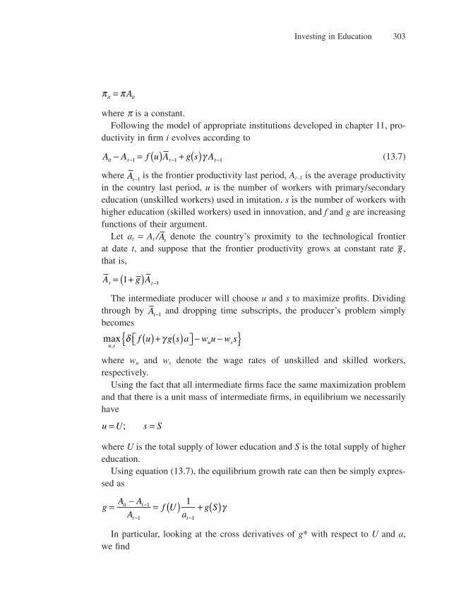
Investing in Education 303
π πit itA=
where p is a constant.Following the model of appropriate institutions developed in chapter 11, pro-
ductivity in fi rm i evolves according to
A A f u A g s Ait t t t− = ( ) + ( )− − −1 1 1γ (13.7)
where At−1 is the frontier productivity last period, At−1 is the average productivity in the country last period, u is the number of workers with primary/secondary education (unskilled workers) used in imitation, s is the number of workers with higher education (skilled workers) used in innovation, and f and g are increasing functions of their argument.
Let at = At /At denote the country’s proximity to the technological frontier at date t, and suppose that the frontier productivity grows at constant rate g , that is,
A g At t= +( ) −1 1
The intermediate producer will choose u and s to maximize profi ts. Dividing through by At−1 and dropping time subscripts, the producer’s problem simply becomes
max,u s
u sf u g s a w u w sδ γ( ) + ( )⎡⎣ ⎤⎦ − −{ }where wu and ws denote the wage rates of unskilled and skilled workers, respectively.
Using the fact that all intermediate fi rms face the same maximization problem and that there is a unit mass of intermediate fi rms, in equilibrium we necessarily have
u U s S= =;
where U is the total supply of lower education and S is the total supply of higher education.
Using equation (13.7), the equilibrium growth rate can then be simply expres-sed as
gA A
Af U
ag Sit t
t t
= − = ( ) + ( )−
− −
1
1 1
1 γ
In particular, looking at the cross derivatives of g* with respect to U and a, we fi nd

Chapter 13304
∂∂ ∂
2
2
10
g
a Uf U
a
* = − ′( ) <
In other words, a marginal increase in the fraction of workers with lower educa-tion enhances productivity growth all the less the closer the country is to the world technology frontier.
Note, however, that the cross derivative
∂∂ ∂
2g
a S
*
is equal to zero. Thus this model is too simple to deliver the symmetric prediction that the closer a country is to the frontier the more growth-enhancing it is to invest more in tertiary education in that country.
13.4.1.2 Cobb-Douglas Growth Technologies
As in the previous subsection, intermediate fi rms can increase productivity either by imitating frontier technologies or by innovating upon existing technologies in the country. However, imitation and innovation can be performed by both types of workers, even though the elasticity of highly educated labor (skilled labor) is larger for innovation, whereas the elasticity of low-education labor (unskilled labor) is higher in imitation.
More formally, we focus on the following class of productivity-growth functions:
A A u s A u s Ait it m i t m i t t n i t n i t t= = +−−
−−
−11
11
1, , , , , , , ,α σ φ φγ (13.8)
where um,i,t (resp. sm,i,t) is the amount of unskilled (resp. skilled) labor used in imitation in sector i at time t, un,i,t (resp. sn.,i,t) is the amount of unskilled (resp. skilled) units of labor used by sector i in innovation at time t, s (resp. f) is the elasticity of unskilled labor in imitation (resp. innovation), and g > 0 measures the relative effi ciency of innovation compared to imitation in generating produc-tivity growth.
We shall assume the following:
assumption 1 The elasticity of skilled labor is higher in innovation than in imitation, and conversely for the elasticity of unskilled labor, that is, f < s.
Let wu,tAt−1 (resp. ws,tAt−1) denote the current price of unskilled (resp. skilled) labor. Then the total labor cost of productivity improvement by intermediate fi rm i at time t is equal to
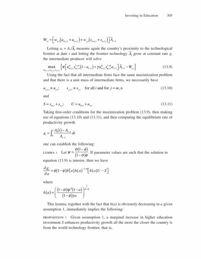
Investing in Education 305
W w u u w s s Ai t u t m i t n i t s t m i t n i t t, , , , , , , , , , ,= +( ) + +( )⎡⎣ ⎤⎦ −1
Letting at = At /At measure again the country’s proximity to the technological frontier at date t and letting the frontier technology At grow at constant rate g, the intermediate producer will solve
max, , , , , ,, ,
, , , , , ,u s s
m i t m i t t n i tm i t m i t n i t
u s a u sπ γσ σ φ111−
−−( ) + nn i t t t i ta A W, , ,1
1 1−
− −⎡⎣ ⎤⎦ −{ }φ (13.9)
Using the fact that all intermediate fi rms face the same maximization problem and that there is a unit mass of intermediate fi rms, we necessarily have
u u s s i j m nj i t j t j i t j t, , , , , ,; ,≡ ≡ =for all and for (13.10)
and
S s s U u um t n t m t n t= + = +, , , ,; (13.11)
Taking fi rst-order conditions for the maximization problem (13.9), then making use of equations (13.10) and (13.11), and then computing the equilibrium rate of productivity growth
gA i A
Adit
t t
t
= ( ) − −
−∫ 1
10
1
one can establish the following:
lemma 1 Let ψσ φ
σ φ=
−( )−( )1
1. If parameter values are such that the solution to
equation (13.9) is interior, then we have
∂∂
ga
h a h a h a U St = −( ) ′( ) ( ) ( ) −⎡⎣ ⎤⎦− −φ φ φ1 1
where
h aa
a( ) =
−( ) −( )−( )
⎛⎝⎜
⎞⎠⎟
−1 1
1
1
σ ψφ γ
σ σ φ
This lemma, together with the fact that h(a) is obviously decreasing in a given assumption 1, immediately implies the following:
proposition 1 Given assumption 1, a marginal increase in higher education investment S enhances productivity growth all the more the closer the country is from the world technology frontier, that is,

Chapter 13306
∂∂ ∂
2
0g
a St >
And a marginal increase in lower education investment U enhances productivity growth all the less the closer the country is from the world technology frontier, that is,
∂∂ ∂
2
0g
a Ut <
The intuition underlying this proposition follows directly from the Rybczynski theorem in international trade. Stated in the context of a two-sector–two-input economy, this theorem says that an increase in the supply of input in the sector that uses that input more intensively should increase “output” in that sector more than proportionally. To transpose this result to the context of our model, consider the effect of an increase in the supply of skilled labor, keeping the supply of unskilled labor fi xed and for given a. Given that skilled workers contribute rela-tively more to productivity growth and profi ts if employed in innovation rather than in imitation (our assumption 1), the demand for additional skilled labor will tend to be higher in innovation. But then the marginal productivity of unskilled labor should also increase more in innovation than in imitation; hence, a net fl ow of unskilled workers should also move from imitation into innovation. This in turn will enhance further the marginal productivity of skilled labor in innovation, thereby inducing an ever greater fraction of skilled labor to move to innovation. Now, the closer the country is to the technology frontier (that is, the higher a), the stronger this Rybczynski effect, as a higher a increases the effi ciency of both skilled and unskilled labor in innovation relative to imitation. A second, reinforc-ing, reason is that an increase in the fraction of skilled labor reduces the amount of unskilled labor available in the economy, hence reducing the marginal produc-tivity of skilled labor in imitation, all the more the closer the country is to the frontier.
13.4.1.3 Back to Krueger and Lindahl
Before we confront this prediction with evidence on higher education, distance to frontier, and productivity growth, let us go back to Krueger and Lindahl’s irrelevance result, namely, that human capital stocks and growth are no longer signifi cantly correlated when restricting cross-country panel regressions to OECD countries. More specifi cally, consider two countries, 1 and 2, that have the same total human capital stock and lie at the same distance from the world technology
Investing in Education 307
frontier. The only difference is that country 1 is better endowed in highly educated labor whereas country 2 is better endowed in unskilled labor.
Thus
H H H1 2= =
but
H S U U S= + = +1 1 2 2
where
S S1 2>
Which of these two countries grows faster? The answer depends upon these countries’ proximity to the world technology frontier. Namely, country 1 will grow faster if the two countries are suffi ciently close to frontier, because country 1 is better endowed in what is most important for growth close to the frontier. And country 2 will grow faster if both countries are far from frontier, since country 2 is better endowed in what is more important for growth far below the frontier. Yet the two countries have the same total amount of human capital.
This reasoning just shows that the total stock of human capital is not a suffi cient statistic to predict the growth rate of a country. In addition, one needs to know about the composition of human capital in the country and about the country’s proximity to the world technology frontier in order to predict the growth rate in that country.
13.4.2 Cross-Country and Cross-U.S.-State Evidence
13.4.2.1 Cross-Country Evidence
Vandenbussche, Aghion, and Meghir (2006), henceforth VAM, confront the preceding prediction with cross-country panel evidence on higher education, distance to frontier, and productivity growth. Aghion, Bouston, Hoxby, and Vandenbussche (2005), henceforth ABHV, test the theory on cross-U.S.-state data. Each approach has its pros and cons. Cross-U.S.-state analysis uses a much richer data set and also good instruments for higher and lower education spend-ing. However, a serious analysis of the growth impact of education spending across U.S. states must take into account an additional element not considered in previous models, namely, the effects on the migration of skilled labor across states at different levels of technological development. In contrast, cross-country analysis can safely ignore the migration; however, the data are sparse and the
Chapter 13308
instruments for educational spending are weak (consisting mainly of lagged spending). In the remaining part of the section we shall consider the two pieces of empirical analysis in turn.
VAM consider a panel data set of 22 OECD countries over the period 1960–2000, which they subdivide into fi ve-year subperiods. Output and investment data are drawn from Penn World Tables 6.1 (2002) and human capital data from Barro and Lee (2000). The Barro and Lee data indicate the fraction of a country’s popu-lation that has reached a certain level of schooling at intervals of fi ve years, so they use the fraction that has received some higher education together with their measure of TFP (constructed assuming a constant labor share of 0.65 across country) to perform the following regression:
gj t j t j t j t j t, , , , ,= + + + ∗(− −α α α α0 1 1 2 3 1Prox Fraction Prox Fraction )) + +v uj j t,
where gj,t is country j’s growth rate over a fi ve-year period, Proxj,t−1 is country j’s proximity to the technological frontier at t − 1 (i.e., 5 years before), Fractionj,t is the fraction of the working-age population with some higher education, and uj is a country’s fi xed effect. The proximity and human capital variables are instru-mented with their values at t − 2, and the equation is estimated in differences to eliminate the fi xed effect. The results are shown in table 13.1.
Before controlling for country fi xed effects, VAM obtain a statistically signifi -cant coeffi cient of −1.87 for the human capital variable and a statistically signifi -cant coeffi cient of 2.37 for the interaction variable, indicating that indeed higher education matters more as a country gets closer to the frontier. Controlling for country fi xed effects removes the signifi cance of the coeffi cients; however, this signifi cance is restored once countries are regrouped into subregions and country fi xed effects are replaced by group fi xed effects. This result in turn suggests that cross-country data on only 22 countries are too sparse for signifi cant regression results to survive when we control for country fi xed effects.
To see how this result translates in terms of the effect of an additional year of schooling of higher education, they perform the following regression in logs:
g N N v uj t j t j t j t j t j j, , , , ,= ′ + ′ ′ + ′ + ′ ∗( ) + ′ + ′− −α α α α0 1 1 2 3 1Prox Prox ,,t
where this time Prox′j,t−1 is the log of the closeness to the technological frontier and Nj,t is the average number of years of higher education of the population. The econometric technique employed is the same as before. Before controlling for country fi xed effects, VAM fi nd the coeffi cient of the number of years to be 0.105 and of little signifi cance, but the coeffi cient of the interaction variable to be equal to 0.368 and signifi cant. This result again demonstrates that it is more important to expand years of higher education close to the technological frontier.
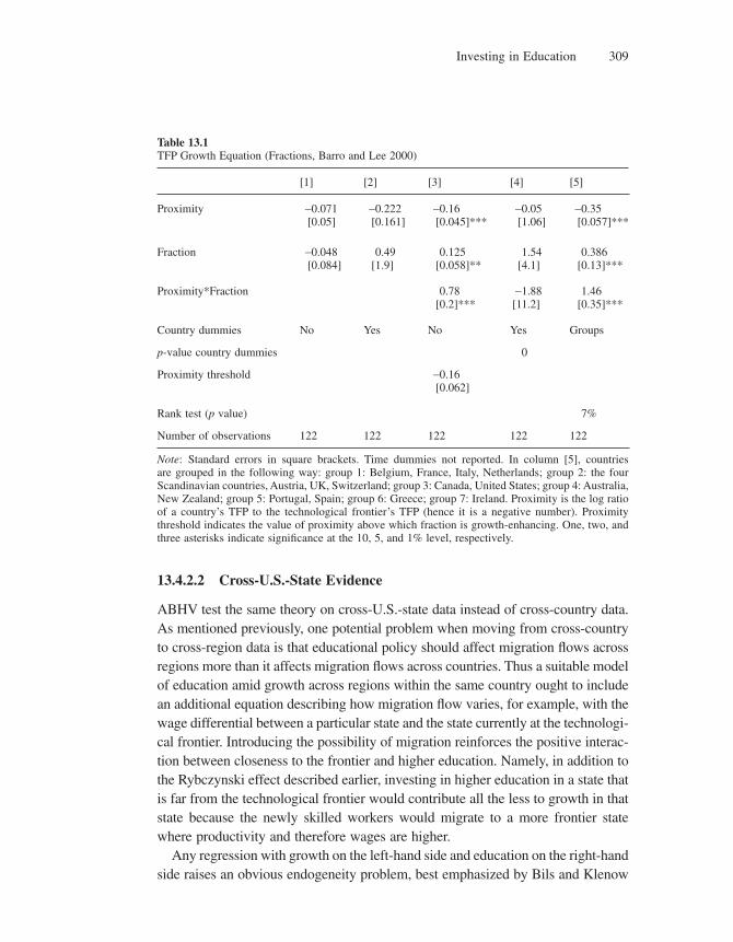
Investing in Education 309
13.4.2.2 Cross-U.S.-State Evidence
ABHV test the same theory on cross-U.S.-state data instead of cross-country data. As mentioned previously, one potential problem when moving from cross-country to cross-region data is that educational policy should affect migration fl ows across regions more than it affects migration fl ows across countries. Thus a suitable model of education amid growth across regions within the same country ought to include an additional equation describing how migration fl ow varies, for example, with the wage differential between a particular state and the state currently at the technologi-cal frontier. Introducing the possibility of migration reinforces the positive interac-tion between closeness to the frontier and higher education. Namely, in addition to the Rybczynski effect described earlier, investing in higher education in a state that is far from the technological frontier would contribute all the less to growth in that state because the newly skilled workers would migrate to a more frontier state where productivity and therefore wages are higher.
Any regression with growth on the left-hand side and education on the right-hand side raises an obvious endogeneity problem, best emphasized by Bils and Klenow
Table 13.1TFP Growth Equation (Fractions, Barro and Lee 2000)
[1] [2] [3] [4] [5]
Proximity −0.071[0.05]
−0.222[0.161]
−0.16[0.045]***
−0.05[1.06]
−0.35[0.057]***
Fraction −0.048[0.084]
0.49[1.9]
0.125[0.058]**
1.54[4.1]
0.386[0.13]***
Proximity*Fraction 0.78[0.2]***
−1.88[11.2]
1.46[0.35]***
Country dummies No Yes No Yes Groups
p-value country dummies 0
Proximity threshold −0.16[0.062]
Rank test (p value) 7%
Number of observations 122 122 122 122 122
Note: Standard errors in square brackets. Time dummies not reported. In column [5], countries are grouped in the following way: group 1: Belgium, France, Italy, Netherlands; group 2: the four Scandinavian countries, Austria, UK, Switzerland; group 3: Canada, United States; group 4: Australia, New Zealand; group 5: Portugal, Spain; group 6: Greece; group 7: Ireland. Proximity is the log ratio of a country’s TFP to the technological frontier’s TFP (hence it is a negative number). Proximity threshold indicates the value of proximity above which fraction is growth-enhancing. One, two, and three asterisks indicate signifi cance at the 10, 5, and 1% level, respectively.

Chapter 13310
(2000). Here, as in the preceding cross-country panel regressions, the endogeneity problem can be stated as follows: If states or countries choose their composition of education spending according to the model, then we should see the composition of educational investments being highly correlated with technology and productiv-ity, and therefore the regressions would say nothing about causality.
However, the great advantage of moving from cross-country to cross-state analysis is that we have access to a natural source of exogenous variation in education investment, namely, political economy considerations that may lead the Congress or other federal authorities to misallocate the funding to higher education across states. For example, because it has a representative on a congres-sional commission for higher education, a far-from-the-frontier state may end up mistakenly receiving excessive funding for research-related education. Con-versely, because of local political economy considerations, a close-to-the-frontier state may end up mistakenly focusing its investment in primary education, neglecting higher education.
In other words, political economy considerations and politicians’ ability and incentive to deliver “pork” to their constituencies provide a natural source of instruments that predict states’ tendencies to make exogenous “mistakes” when investing in education.
The actual instruments used in ABHV are as follows:
1. For research-university education: whether a state has a congressman on the appropriations committee that allocates funds for research universities but not other types of schools.
2. For “lowbrow” postsecondary education (community colleges, training schools): whether the chairman of the state’s education committee represents voters whose children attend one- or two-year postsecondary institutions.
3. For primary and secondary education: whether the overall political balance on the state’s supreme court interacts with the state school fi nance system.
Then, using annual panel data over the period 1970–2000, ABHV perform a two-stage procedure whereby (1) in fi rst-stage regressions, the various kinds of educational spending are regressed over their respective instruments, and (2) the growth rate in each state and year is regressed over the instruments for the various kinds of educational spending, the state’s proximity to the frontier, and the inter-action between the two, controlling for state and year fi xed effects. We refer our readers to ABHV for the detailed regression results, which are summarized in fi gure 13.3.
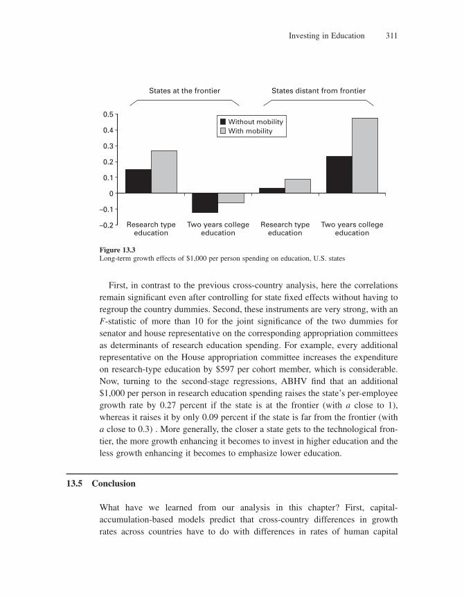
Investing in Education 311
First, in contrast to the previous cross-country analysis, here the correlations remain signifi cant even after controlling for state fi xed effects without having to regroup the country dummies. Second, these instruments are very strong, with an F-statistic of more than 10 for the joint signifi cance of the two dummies for senator and house representative on the corresponding appropriation committees as determinants of research education spending. For example, every additional representative on the House appropriation committee increases the expenditure on research-type education by $597 per cohort member, which is considerable. Now, turning to the second-stage regressions, ABHV fi nd that an additional $1,000 per person in research education spending raises the state’s per-employee growth rate by 0.27 percent if the state is at the frontier (with a close to 1), whereas it raises it by only 0.09 percent if the state is far from the frontier (with a close to 0.3) . More generally, the closer a state gets to the technological fron-tier, the more growth enhancing it becomes to invest in higher education and the less growth enhancing it becomes to emphasize lower education.
13.5 Conclusion
What have we learned from our analysis in this chapter? First, capital-accumulation-based models predict that cross-country differences in growth rates across countries have to do with differences in rates of human capital
Without mobilityWith mobility
States at the frontier States distant from frontier
Research typeeducation
Research typeeducation
Two years collegeeducation
Two years collegeeducation
0.5
0.4
0.3
0.2
0.1
0
–0.1
–0.2
Figure 13.3Long-term growth effects of $1,000 per person spending on education, U.S. states
Chapter 13312
accumulation. And these models can be used to perform development accounting or to generate low-development traps. Second, Schumpeterian models that emphasize the interplay between human capital stocks and the innovation process have potential for delivering policy recommendations. Yet, when looking at educational spending as a whole, not much can be said from looking at cross-OECD comparisons. However, once one distinguishes between imitation and frontier innovation and maps these two sources of productivity growth to different segments of the education system, then one can come up with relevant policy recommendations, even for OECD countries or regions. In particular, the theoreti-cal and empirical analyses in the previous section suggest that countries with productivities far from the technological frontier should put more emphasis on primary/secondary education, whereas countries that are closer to the frontier should put more emphasis on tertiary education. Thus, for European countries to put the emphasis on primary/secondary education was fi ne as long as Europe was technologically far from the United States: at that stage, Europe was relying more on imitation as a main source of growth. But that now that Europe has moved closer to the productivity frontier, the potential of imitation is wearing out, and thus it becomes more urgent to invest more in higher education in order to foster innovation. Similarly, the closer a U.S. state is to the current frontier productivity, the more its growth will be enhanced by investing more in research education instead of two-year colleges. More recent work has extended this analysis by looking at growth and the governance of universities. Thus Aghion, Dewatripont, and colleagues (2007) use the same data as in ABHV to show that growth in more advanced states also benefi ts more from having more autonomous universi-ties, where autonomy is measured either by the fraction of private universities in the state or by an index measuring the extent to which public universities can make decisions (hiring, student recruitment, salaries, . . .) without state interfer-ence. They also show that research education funding and autonomy are strategic complements: that is, more research education funding is more growth enhancing in states with more autonomous universities.
13.6 Literature Notes
A fi rst approach to the relationship between education and growth emphasizes the importance of human capital accumulation as a source of economic growth. Within the neoclassical framework, the main reference is Mankiw, Romer, and
Investing in Education 313
Weil (1992). Within the AK framewok, the main reference is Lucas (1988), who was himself directly inspired by Becker’s (1964) theory of human capital. This paradigmatic framework builds on a model developed by Uzawa (1965) in which existing human capital is the unique input in the education sector.
Several extensions have been suggested to this approach, such as Rebelo (1991), which introduces physical capital into the human-capital-accumulation equation and then looks at the effect of taxation policies on steady-state growth. A shortcoming of the Lucas model was the assumption that an individual’s returns to education remain constant over her entire lifetime. Azariadis and Drazen (1990) deal with this objection by reformulating the theory using an overlapping-generations (OLG) model where individuals inherit the human capital accumu-lated by their parents. Azariadis and Drazen point to the existence of multiple steady-state growth paths, including low-development traps in which insuffi cient investment in education in the past discourages further skill acquisition and thereby future growth. Glomm and Ravikumar (1992) address the issue of het-erogeneous access to human capital across individuals of the same generation, assessing its impact on the dynamics of inequality and growth, as depending on the adopted system of education (public or private). This topic is also analyzed by Benabou (1996). For a systematic analysis of OLG versions of the Lucas model, see d’Autume and Michel (1994).
An early test of the implication of the Lucas model is provided by Romer (1990), who found evidence that the initial level of literacy (but not the change in literacy) predicted output growth. Barro and Sala-i-Martin (1995) also address empirically the relationship between education and growth based on a large sample of countries between 1965 and 1985, fi nding signifi cantly positive effect of education attainment and public spending on education on subsequent growth. Barro (1997) and Caselli, Esquivel, and Lefort (1996) examine the differential impact of male and female education on growth.
A second approach to the relationship between education and growth goes back to the seminal contribution of Nelson and Phelps (1966), where the stock of human capital affects a country’s ability to innovate or catch up with more advanced countries. This approach was extended by Benhabib and Spiegel (1994), where human capital not only facilitates adaptation to more advanced technolo-gies, but also makes it easier to innovate at the frontier. Benhabib and Spiegel then confronted the prediction of a positive relationship between growth and the stock of human capital to cross-country panel data. However, more recent work by Krueger and Lindahl (2001) concludes that the signifi cance of the correlation
Chapter 13314
between growth and human capital stocks disappears when restricting the regres-sion to OECD countries, leading one to think that education only matters for catching up but not for innovating at the frontier.
Vandenbussche, Aghion, and Meghir (2006) and Aghion, Boustan, and col-leagues (2005) build on the idea of appropriate institutions (see chapter 11) to analyze the relationship between growth and the composition of human capital, under the assumption that human capital does not affect innovation and imple-mentation uniformly: primary/secondary education tends to produce imitators, whereas tertiary (especially graduate) education is more likely to produce innova-tors. The fi rst of these two papers confronts this prediction to cross-OECD-country panel data, whereas the latter paper confronts the same prediction to cross-U.S.-state panel data. For an extensive survey on the topic of this chapter, see Krueger and Lindahl (2001).
Problems
1. Explain how education accumulation fosters growth in the neoclassical and AK models. Describe how education stock might matter instead. Finally, provide some intuition for why the composition of education for promoting growth may change with a country’s distance to the world technological frontier.
2. Human capital accumulation in the neoclassical growth model (based on Mankiw, Romer, and Weil 1992)
In this problem, we solve Mankiw, Romer, and Weil’s augmented version of the Solow growth model. Output is produced using physical capital, human capital, and raw labor with a Cobb-Douglas tech-nology: Y = AKaHbL1−a−b where the level of technology A is assumed to be constant. Human and physical capital depreciate at the same exogenous rate d. The labor force grows at rate n. Constant fractions of output sh and sk are invested in human and physical capital accumulation, respectively.
We also assume a + b < 1; that is, there are decreasing returns to the accumulation of both forms of capital.
a. Let y, h, and k be the levels of output, human capital, and physical capital per capita: yY
L≡ ,
hH
L≡ , and k
K
L≡ . What are the growth rates of k and h?
b. Solve for the steady-state values of h, k, and y. Show that
yAs s
nh k* =
+( )⎛
⎝⎜
⎞
⎠⎟+
− −β α
α β
α β
δ
1
1
What are the growth rate of GDP per capita and the growth rate of GDP in the steady state?
c. Assume now that a + b = 1. What are the growth rates of k and h? Can there be positive long-run growth of GDP per capita?
d. Show that the steady-state log income per capita is
Investing in Education 315
ln ln ln ln lny A s s nt t k h( ) = ( ) +− −
( ) +− −
( ) − +− −
+( )αα β
βα β
α βα β
δ1 1 1
while the standard neoclassical growth model yields
ln ln ln lny A s nt t k( ) = ( ) +−
( ) −−
+( )αα
αα
δ1 1
e. How does the presence of human capital accumulation affect the impact of the savings rate sk on GDP per capita? The impact of population growth?
3. **Skill acquisition and human capital externalities (based on Lucas 1988)
We consider a version of the Lucas model that allows for externalities in human capital accumula-tion. Agents are infi nitely lived and maximize their lifetime utility. Per-period utility is
u cct( ) =−
−1
1
σ
σ, and the discount rate is r.
Each period, they allocate a fraction u of their time to production and (1 − u) to the acquisition of human capital. Current production is
y k uh h= ( ) −β β γ1
where h is the average level of human capital in the economy and captures human capital spillovers. Human capital growth takes the form
�h h ut t t= −( ) > >δ δ ξξ 1 0 0, ,
a. If x < 1, can human capital accumulation sustain long-run growth of the economy?
b. Assume for the rest of the problem that skill acquisition has constant returns (x = 1). Set up the Lagrangian for the representative household’s problem. Note that there are two constraints, the evolu-tion of the physical capital stock and the evolution of the human capital stock. Derive the fi rst-order conditions for the choice of c and u and the equations for the change in the shadow prices of human and physical capital.
c. Using the fi rst-order conditions, express the growth rate of consumption as a function of k, h, and u. Note that in equilibrium h = h.
d. On a balanced growth path, human capital, physical capital, and consumption must grow at con-stant rates gh, gk, and gc, respectively, and the share of time spent in production u is constant. Show
that these growth rates are linked by g g gk c h= = − +−
⎛⎝⎜
⎞⎠⎟
1
1
β γβ and gh = d (1 − u).
e. Using the fi rst-order conditions and the evolution of the shadow prices of human and physical capital, solve for the growth rate of human capital (note that agents take the average stock of human capital h as given). Show that
gc = − +− +( ) −
−( )11
β γσ β γ γ
δ ρ
f. A social planner internalizes the effect of h on output. Does the socially optimal allocation of time between production and skill acquisition differ from the private equilibrium? Using a similar approach to part e, solve for the growth rate of consumption implied by the social planner’s choice of u. How does the gap between the socially optimal and the equilibrium growth rates depend on g ?

Chapter 13316
4. *Growth and the composition of education (based on Aghion, Boustan, and colleagues 2005)
Here we allow both types of workers to be employed in fi nal goods production as well as in imitation and innovation. The fi nal good is produced with the technology
y A u s x dit t f t f t i t= ( )− −
∫ , , ,β β α α1 1
0
1
where uf and sf are unskilled and skilled labor in the fi nal goods sector. Monopolists produce
intermediate goods xi,t one for one using the fi nal good as input. Their output is x A u si t t f t f t, , ,=−
−αα
δ β β
11
and their profi ts pi,t = dAtubf,tsf,t
1−b. The dynamics of productivity are given by
A A u s A A u s At t m t m t t t n t n t t+− −− = −( ) +1
1 1, , , ,
σ σ σ σγ
The fi rst component is the improvement in technology driven by imitation, and the second component is driven by innovation. We assume s > 1
2 . Labor market equilibrium requires sf,t + sm,t + sn,t = S and uf,t + um,t + un,t = U.
a. Given a competitive fi nal-goods sector, what are the unskilled and skilled wages as a function of uf and sf?
b. The representative intermediate producer chooses um,t, un,t, sm,t, and sn,t to maximize period t + 1 profi ts. Derive the fi rst-order conditions for these labor demands. Dropping time subscripts, show that the skill intensities in imitation and in innovation are given by
s
u
a
am
m
= − −⎛⎝⎜
⎞⎠⎟
−1 11
2 1σσ γ
σ
s
u
a
an
n
=−
−⎛⎝⎜
⎞⎠⎟
−σσ γ
σ
1
11
2 1
where aA
A≡ is the proximity of the country to the technological frontier. How do these elasticities
depend on a and s?
c. If the amount of skilled labor S − sf used in technology improvement increases, how is the alloca-tion of each type of workers between imitation and innovation affected? Do both activities expand? Give an intuitive explanation.
d. Solve for the relative wage of skilled workers and the skill intensity of the fi nal-goods sector. How do they depend on the parameter a?
e. Solve for the equilibrium growth rate of technology as a function of S − sf and U − uf. How do the relative contributions of skilled and unskilled labor to growth evolve when proximity to the fron-tier increases?
5. **Human capital and technology diffusion (based on Benhabib and Spiegel 2005)
This is a variation on the Nelson and Phelps model where catch-up parameters may depend on distance to the frontier, refl ecting, for instance, the diffi culty for less advanced countries of adopting distant, less “appropriate” technologies.
a. First consider the original model of technology diffusion:
�A f h A A g h At t t t= ( ) −( ) + ( )
Investing in Education 317
For simplicity we assume a constant human capital stock. The frontier technology grows at rate g > g(h), so that At = A0eg t. Show that
A Af
f g ge
f
f g gA et
g f t gt= −− +
⎛⎝⎜
⎞⎠⎟
+− +
⎛⎝⎜
⎞⎠⎟
−( )0 0
where f = ,f(h) and g = g(h).
What is limt
t
t
A
A→∞ ? Does the country’s productivity eventually grow at the same rate as the frontier?
b. Now we allow the rate of technology diffusion to depend on distance to the frontier for each level of human capital stock. As distance to the frontier increases, the catch-up rate may be dampened, in par-ticular, by large differences in factor proportions between the frontier country and the follower that render frontier innovations more diffi cult to adopt. Productivity grows according to the following equation:
�A f hA
AA A g h At
t
tt t t= ( )⎛
⎝⎜⎞⎠⎟
−( ) + ( )
The other assumptions are unchanged. Show that
A A e eA
A
f
f g g
f
f g gtgt f g g t= −
+ −⎛⎝⎜
⎞⎠⎟
++ −
⎡
⎣⎢⎢
⎤
⎦⎥⎥
− + −( )−
00
0
1
What is limt
t
t
A
A→∞ if f > g − g? if f < g − g? Interpret.
6. *Low-skill, low-development traps (based on Redding 1996)
In this problem, we examine the possibility of multiple equilibria stemming from strategic complemen-tarities between investment in education and R&D. There is a continuum of overlapping generations of individuals who live for two periods. Workers maximize their lifetime consumption in a linear form u(c1, c2) = cl + c2. They are born at the beginning of period t with an endowment of human capital h1,t ≡ 1. When young, they allocate a fraction ut of their time to production, earning utAt, and the remain-der to education. Their human capital when old is then h2,t = 1 + g (1 − ut)q, where 0 < q < 1.
Entrepreneurs choose R&D spending at time t and hire one old worker at time t + 1 to produce yt+1 = At+1ht+1. The price of the good is normalized to 1. A fraction a of revenues goes to the worker and 1 − a to the entrepreneur. The R&D technology is as follows: by incurring a cost dmAt, an inno-vation of size l (such that At+1 = lAt) occurs with probability m.
a. Set up the workers’ maximization problem. What is the optimal fraction of time devoted to educa-tion in the fi rst period? How does it change if m increases?
b. For u given, derive the entrepreneur’s choice of R&D spending. Show that it is a threshold deci-sion, that is, m* = 1 or m* = 0. Why do we say that the model displays strategic complementarity between investment in education and R&D spending?
c. Under what condition does a low-development trap exist, with no productivity growth? What then is the human capital investment u?
d. Under what condition does a steady-state path with positive productivity growth exist? What then is the human capital investment u? What is the rate of growth of technology?
e. Suppose the economy is initially in a zero-growth trap. The government decides to implement a subsidy of s per unit of time spent in education, so that young workers earn utAt + (1 − ut)s. What is the minimum subsidy required to move the economy to the high-growth steady state? How does it depend on d and g ?

14 Reducing Volatility and Risk
14.1 Introduction
Macroeconomic textbooks generally present the view that there is a perfect dichotomy between (1) macroeconomic policy (budget defi cit, taxation, money supply), whose primary aim is to stabilize the economy, and (2) long-run eco-nomic growth, which is either taken to be exogenous or assumed to depend only upon structural characteristics of the economy (property-rights enforcement, market structure, market mobility, and so forth). Thus, although common wisdom states that growth requires macroeconomic (or price) stability, conventional macro theory contains no explicit link between macropolicy and long-run growth.
The idea that growth and business cycles should be analyzed separately is deeply rooted in the history of economic thought. For example, the Keynesian multiplier/accelerator (or “oscillator”) model analyzed fl uctuations of aggregate output around an exogenous trend. Meanwhile, the Harrod-Domar and neoclas-sical growth models analyzed a long-run deterministic growth path of aggregate output while ignoring business cycle fl uctuations. As Kaldor pointed out in the mid-1950s, “As a pure cyclical model, the oscillator model had little resemblance to the cyclical fl uctuations in the real world, where successive booms carry pro-duction to successively higher levels.”1
The real business cycle (RBC) literature of the 1980s (e.g., Kydland and Prescott 1982; Long and Plosser 1983), with its emphasis on productivity shocks as a main source of persistent fl uctuations, could be seen as a preliminary step toward overcoming the traditional division of macroeconomic theory between trend and cycles. However, based on the same kind of production technologies as in the neoclassical growth literature, the RBC models were unable to account for a trend that was causally related to the business cycle.
One attempt at overcoming the dichotomy between short-run fl uctuations and long-run growth came with the AK wave of endogenous growth models. This approach introduced productivity shocks in an AK model à la Romer (1986). We refer the reader to pioneering contributions in the late 1980s by King and Rebelo (1986) and Stadler (1990). The most recent contribution to this line of research is by Jones, Manuelli, and Stachetti (2000), henceforth JMS, which updates the pioneering work of Phelps (1962).
1. The same criticism also applies to other versions of the oscillator model (e.g., Hicks 1950) where an exogenous linear trend is superimposed on the original cycle model.
Chapter 14320
Another wave of volatility and growth models uses the Schumpeterian para-digm. In this approach, the relationship between volatility and growth is governed by research-arbitrage equations. A fi rst attempt at explaining the cyclicality of R&D investments over the business cycle relies on the idea that new ideas are quickly imitated (see Barlevy 2007), so that it is more profi table to innovate in booms when these ideas are most profi table. A second attempt relies on the exis-tence of credit constraints. The idea is that, in the absence of credit constraints, recessions should encourage fi rms to reorganize, innovate, or reallocate to new markets. Schumpeter himself summarized that view as follows: “[Recessions] are but temporary. They are means to reconstruct each time the economic system on a more effi cient plan.” However, credit constraints will affect fi rms’ ability to innovate in recessions; typically, in a recession, current earnings are reduced, and therefore so is the fi rm’s ability to borrow in order to innovate. This “Schumpet-erian” approach delivers the prediction that the lower the level of fi nancial devel-opment, the more negative the correlation between macroeconomic volatility and growth. This in turn suggests that macroeconomic policy may directly affect long-run growth, in particular to the extent that it can either counteract or, at the opposite, amplify the effect of credit constraints on the cyclical composition of fi rms’ investments.
Another attempt at linking volatility and growth is the stochastic growth model by Acemoglu and Zilibotti (1997), henceforth AZ. There, the idea is that each new activity involves a fi xed cost, and, therefore, less developed economies can only fi nance a limited number of activities. Hence the limited scope for risk diversifi cation in these economies, which in turn pushes them to choose inferior but safer technologies. At the same time the fact that less developed economies cannot diversify idiosyncratic risks makes these economies more volatile, and therefore more vulnerable to shocks.
The chapter is organized as follows. Section 14.2 presents the AK approach by JMS and discusses its implications. Section 14.3 uses the Schumpeterian approach to analyze the cyclicality of R&D investments and the prediction that volatility is more detrimental to growth in economies with lower levels of fi nan-cial development. This section also discusses Schumpeterian models of the cycli-cality of R&D that are not based on credit market imperfections. Section 14.4 presents the Acemoglu and Zilibotti model of risk diversifi cation and growth. Section 14.5 concludes by summarizing our main fi ndings in this chapter.
Reducing Volatility and Risk 321
14.2 The AK Approach
The idea here is that macroeconomic volatility may affect long-run growth through its effects on aggregate savings and investment (recall that in the AK framework, growth is entirely driven by capital accumulation). Thus higher volatility will increase the supply of savings if individuals wish to save more for precautionary motives; but higher volatility will tend to reduce the demand for investment by reducing the risk-adjusted rate of return on investment. Phelps (1962) showed that which of these two effects dominates depends upon the representative household’s elasticity of intertemporal substitution. JMS (2000) validate Phelps’s fi ndings in a modern setting.
14.2.1 The Jones, Manuelli, and Stacchetti Model
We present here a simple overlapping-generations version of the JMS model. Consider an economy populated by a continuum of two-period-lived individuals. Each member of generation t (call her Mrs. t) is born in period t and has an intertemporal utility function:
Uc c
t
ty
to
=( )
−+
( )−
< < <−
+
−1
1
1
1 10 1 0
σ σ
σβ
σβ σ, ,
where cyt = ct is Mrs. t’s consumption when young, and c o
t+1 is her consumption when old; b is the discount factor; and s is the elasticity of marginal utility, otherwise known as the coeffi cient of relative risk aversion. Alternatively, e = 1/s is the intertemporal elasticity of substitution. The size of each generation is constant and normalized to equal unity. The economy comprises only one good, which can be consumed or used as capital.
At any date t, the economy’s aggregate output depends on kt, the amount of capital saved in period t − 1, according to the stochastic AK technology
y u kt t t=
where ut, is an aggregate productivity shock, independently and identically distributed with
Eu At = > 1
Chapter 14322
Each period’s output is divided between the young and the old in fi xed propor-tions, with the fraction g going to the old.2 Thus the old will consume gyt. The young will consume ct, and their savings will be kt+1, the amount of capital used next period; that is,
c k u kt t t t+ = −( )+1 1 γ (14.1)
When the representative member of generation t is old her consumption will be
c u kto
t t+ + +=1 1 1γ
so although she can determine kt+1 at date t, her consumption when old will be uncertain, depending on the random productivity shock ut+1, which will not be realized until next period. Accordingly, she will choose ct and kt+1 so as to maximize expected utility:
Ec u k
t t t1
1 1
1
1 1
−+ +
−
−+ ( )
−
⎧⎨⎪
⎩⎪
⎫⎬⎪
⎭⎪
σ σ
σβ
γσ
subject to the budget constraint (14.1).Since the budget constraint says that ct and kt+1 can be traded off one for one,
optimality requires that the expected marginal utility of ct must equal the expected marginal utility of kt+1. That is, the fi rst-order condition for expected utility maximization is
c E u kt t t− −
+−
+−= ( )σ σ σ σβγ 1
11
1
Thus the equilibrium ratio of savings to consumption ϕ = kt+1/ct is invariant over time:
ϕ = ( )⎡⎣
⎤⎦
−+−βγ σ σ σ
11
11
E ut (14.2)
2. One way to rationalize this approach is to assume that output depends on capital and labor according to
y u k Lt t t= α
that only the young can supply labor, that each young person has a fi xed labor supply, and that there is a competitive labor market. In this case the wage rate will equal the marginal product
w u k Lt t t= −α α 1
so the income wtL of the young will be the constant fraction a of aggregate output.
Reducing Volatility and Risk 323
and the expected growth rate g in turn depends positively on this ratio, namely,3
11
11 1 1+ =⎛
⎝⎜
⎞
⎠⎟ =
⎛
⎝⎜
⎞
⎠⎟ =
+−( )+ + +g E
y
yE
u k
yAt
t
t t
t
ϕϕ
γ (14.3)
We are now able to address the question, How does the average growth rate g vary with macroeconomic volatility? We represent an increase in volatility by a mean-preserving spread of the distribution of aggregate productivity shocks ut for all t. According to equations (14.2) and (14.3), this will raise growth if and only if it raises the saving-consumption ratio ϕ. This in turn will happen if and only if it raises the expression:
E ut+−( )1
1 σ
Now from the uncertainty literature we know that if h(u) is concave in u, then any mean-preserving spread of u reduces the expected value E[h(u)]; similarly, if h(u) is convex in u, then any mean-preserving spread of u increases the expected value E[h(u)].
Here, the function we are interested in is h(u) = u1−s, which is concave if the elasticity of marginal utility s is less than unity and convex if s > 1. Thus the answer to the preceding question depends on whether the intertemporal elasticity of substitution e = 1/s is greater or less than unity. If e is greater than one, then u1−s is concave, and therefore an increase in volatility reduces expected growth. In this case, the dominant effect of volatility is to reduce the risk-adjusted return
3. To get the last equality, recall fi rst that
c k yt t t+ = −( )+1 1 γ
k ct t+ =1 ϕ
E u At+( ) =1
Thus,
Ey
yE
u k
y
E uk
y
Ac
c
t
t
t t
t
tt
t
t
t
+ + +
++
⎛
⎝⎜
⎞
⎠⎟ =
⎛
⎝⎜
⎞
⎠⎟
= ( )
=+( )
1 1 1
11
1 1
ϕϕ −−( )
=+
−( )γ
γAϕ
ϕ11
Chapter 14324
on investment and thereby discourage savings. If instead, as it appears to be in most countries according to aggregate consumption studies, the elasticity of substitution is less than one, then u1−s is convex, and therefore volatility increases expected growth. In this case, the dominant effect of volatility is to increase pre-cautionary savings.
Thus, according to the AK approach, growth should increase with volatility for observed values of the intertemporal elasticity of substitution e.
14.2.2 Counterfactuals
A fi rst prediction of the AK approach, derived in the previous subsection, is that volatility and growth should be positively correlated for realistic values of the intertemporal elasticity of substitution parameter. However, the empirical work of Ramey and Ramey (1995), henceforth RR, suggests the opposite. Specifi cally, RR consider cross-sectional data from 92 countries and regress average growth over aggregate volatility. Annual growth is computed as the log difference of per capita income obtained from the Penn World Tables mark 6.1. Aggregate volatil-ity is measured by the country-specifi c standard deviation of annual growth over the 1960–92 period. Ramey and Ramey also construct an estimate of the volatility due to exogenous shocks to growth by fi ltering the time series fi rst. They fi rst fi nd a negative correlation between the standard deviation of per capita annual growth rates and the average growth rate. Second, the correlation between volatil-ity and growth appears to move from negative to negligible once the cross-country regression is restricted to OECD countries. Third, they fi nd that the negative correlation between volatility and growth persists when one controls for average investment over GDP. These fi ndings, summarized in table 14.1, are clearly at odds with existing theories. Yet no attempt has been made to explain them.
A second prediction of the AK approach is that volatility should affect growth only through its effects on total savings, or equivalently, on total investment. However, Aghion, Angeletos, Banerjee, and Manova (2005), henceforth AABM, show that controlling for total investment over GDP reduces the (negative) cor-relation between volatility and growth (or the positive correlation between good shocks and growth) by only 20 percent and without reducing the signifi cance of these correlation terms.
This fi nding in turn implies that total investment cannot be the main channel whereby a stabilizing macroeconomic policy may affect growth through affecting the impact of volatility.
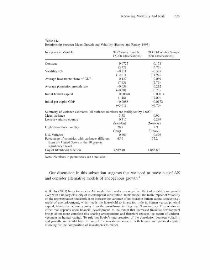
Reducing Volatility and Risk 325
Our discussion in this subsection suggests that we need to move out of AK and consider alternative models of endogenous growth.4
Table 14.1Relationship between Mean Growth and Volatility (Ramey and Ramey 1995)
Independent Variable 92-Country Sample(2,208 Observations)
OECD-Country Sample(888 Observations)
Constant 0.0727(3.72)
0.158(5.73)
Volatility (s) −0.211(−2.61)
−0.385(−1.92)
Average investment share of GDP 0.127(7.63)
0.069(2.76)
Average population growth rate −0.058(−0.38)
0.212(0.70)
Initial human capital 0.00078(1.18)
0.00014(2.00)
Initial per capita GDP −0.0088(−3.61)
−0.0172(−5.70)
Summary of variance estimates (all variance numbers are multiplied by 1,000)Mean variance 3.58 0.99Lowest-variance country 0.317
(Sweden)0.299
(Norway)Highest-variance country 28.7
(Iraq)2.9
(Turkey)U.S. variance 0.663 0.596Percentage of countries with variances different
from the United States at the 10 percent signifi cance level
65.9 52.2
Log of likelihood function 3,589.40 1,883.80
Note: Numbers in parentheses are t-statistics.
4. Krebs (2003) has a two-sector AK model that produces a negative effect of volatility on growth even with a unitary elasticity of intertemporal substitution. In his model, the main impact of volatility on the representative household is to increase the variance of uninsurable human capital shocks (e.g., spells of unemployment), which leads the household to invest too little in human versus physical capital, taking the economy away from the growth-maximizing von Neumann ray. This is also an effect that depends upon fi nancial development, to the extent that increased fi nancial development brings about more complete risk-sharing arrangements and therefore reduces the extent of underin-vestment in human capital. To rule out Krebs’s interpretation of the correlation between volatility and growth, we would have to control for investment rates in both human and physical capital, allowing for the composition of investments to matter.
Chapter 14326
14.3 Short-versus Long-Term Investments
In this section we analyze an alternative route for analyzing the relationship between volatility and growth. This route emphasizes the distinction between short-run capital investments and long-term productivity-enhancing investments. Examples of long-term growth-enhancing investments include R&D, IT equip-ment, and organizational capital. Macroeconomic volatility will affect fi rms’ choice between these two types of investments, and differently so depending upon the extent to which fi rms are credit constrained. In particular, this approach can explain why the relationship between volatility and growth is more negative for non-OECD countries than for OECD countries, an important difference between the two being precisely that OECD countries are less credit constrained than non-OECD countries.
14.3.1 The Argument
The theoretical argument in AABM, which we formalize in this section, can be summarized as follows: In the absence of credit constraints, long-run growth-enhancing investments tend to be countercyclical, as they often take place at the expense of directly productive activities. Because the return to the latter is lower in recessions as a result of lower demand for the manufactured good, so will the opportunity cost of long-run productivity-enhancing investments also be lower. Hence there is a possibility of a growth-enhancing effect of recessions.5
However, things become quite different when credit market imperfections prevent fi rms from innovating and reorganizing in recessions: in a recession, current earnings are reduced, and therefore so is the fi rm’s ability to borrow in order to innovate. This reduced ability, in turn, implies that the lower fi nancial development is, the more the anticipation of recessions will discourage R&D investments if these are decided before fi rms know the realization of the aggregate shock (since fi rms anticipate that with higher probability their R&D investment will not pay out in the long run, as it will not survive the liquidity shock). Then recessions will have a damaging effect on R&D and growth.
5. This “opportunity-cost” argument was fi rst spelled out by R. Hall (1991), who constructed a model where a constant labor force is allocated between production and the creation of organizational capital (in contrast to real business cycle models where the choice of activities is between production and leisure). Subsequent work by Bean (1990), Gali and Hammour (1991), Saint-Paul (1993), and Nickell (1996) looked for empirical evidence supporting the existence of an opportunity-cost effect. Using a VAR estimation method on a cross-OECD panel data set, Saint-Paul (1993) showed that the effect of demand fl uctuations on productivity growth was stronger when demand fl uctuations are more transitory. More recently, Nickell (1996) found evidence that more reorganization takes place during recessions.
Reducing Volatility and Risk 327
A natural implication of this argument is that macroeconomic policies that stabilize the business cycle should be more growth enhancing in countries and sectors that are more fi nancially constrained. Thus Aghion and Marinescu (2007) use cross-country panel data to argue that countercyclical fi scal policies—that is, fi scal policies that involve higher budget defi cits during recessions—are more growth enhancing the lower the country’s level of fi nancial development. Aghion and Kharroubi (2007) use the Rajan-Zingales (1998) methodology (see chapter 6) to look at cross-country/cross-industry panel data showing that countercyclical fi scal policies are more growth enhancing in sectors that are both more heavily dependent upon external fi nance and also located in countries with lower levels of fi nancial development.
14.3.2 Motivating Evidence
That credit constraints affect the relationship between aggregate volatility and growth comes out very clearly in the following regression exercise, done by AABM. Annual growth is computed as the log; difference of per capita income obtained from the Penn World Tables mark 6.1. As in Ramey and Ramey (1995), aggregate volatility is measured by taking the country-specifi c standard deviation of annual growth over the 1960–95 period. Financial development is measured by the ratio of private credit—that is, the value of loans by fi nancial intermediar-ies to the private sector—over GDP. Data for 71 countries on fi ve-year interval averages between 1960 and 1995 (1960–64, 1965–69, etc.) were fi rst compiled by Levine, Loyaza, and Beck (2000); an annual dataset was more recently prepared and made available by Levine on his Web page.6
Then, building upon Ramey and Ramey who studied the response of long-term growth to volatility and upon Levine, Loayza, and Beck who focused on the direct effects of credit constraints on growth, AABM estimate the basic equation
g y Xi i i i i i i i= + ⋅ + ⋅ + ⋅ + ⋅ ∗ + ⋅ +α α α α α β ε0 1 2 3 4Vol Priv Vol Priv
where yi is the initial income in country i, gi denotes the average rate of productivity growth in country i over the whole period 1960–95; Voli is the measure of aggregate volatility, Privi is the average measure of fi nancial development over the period 1960–95, Xi is a vector of country-specifi c controls, and ei is the noise term.
6. Private credit is the preferred measure of fi nancial development by Levine, Loayza, and Beck because it excludes credit granted to the public sector and funds coming from central or development banks. AABM also conduct sensitivity analysis with two alternative measures of credit constraints: liquid liabilities and bank assets.
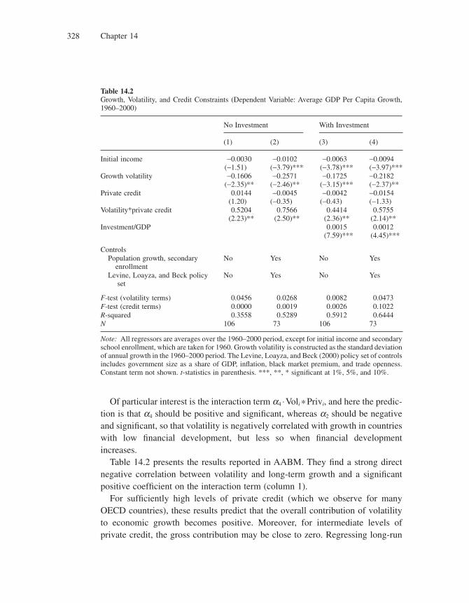
Chapter 14328
Of particular interest is the interaction term a4 ⋅ Voli * Privi, and here the predic-tion is that a4 should be positive and signifi cant, whereas a2 should be negative and signifi cant, so that volatility is negatively correlated with growth in countries with low fi nancial development, but less so when fi nancial development increases.
Table 14.2 presents the results reported in AABM. They fi nd a strong direct negative correlation between volatility and long-term growth and a signifi cant positive coeffi cient on the interaction term (column 1).
For suffi ciently high levels of private credit (which we observe for many OECD countries), these results predict that the overall contribution of volatility to economic growth becomes positive. Moreover, for intermediate levels of private credit, the gross contribution may be close to zero. Regressing long-run
Table 14.2Growth, Volatility, and Credit Constraints (Dependent Variable: Average GDP Per Capita Growth, 1960–2000)
No Investment With Investment
(1) (2) (3) (4)
Initial income −0.0030(−1.51)
−0.0102(−3.79)***
−0.0063(−3.78)***
−0.0094(−3.97)***
Growth volatility −0.1606(−2.35)**
−0.2571(−2.46)**
−0.1725(−3.15)***
−0.2182(−2.37)**
Private credit 0.0144(1.20)
−0.0045(−0.35)
−0.0042(−0.43)
−0.0154(−1.33)
Volatility*private credit 0.5204(2.23)**
0.7566(2.50)**
0.4414(2.36)**
0.5755(2.14)**
Investment/GDP 0.0015(7.59)***
0.0012(4.45)***
Controls Population growth, secondary
enrollmentNo Yes No Yes
Levine, Loayza, and Beck policy set
No Yes No Yes
F-test (volatility terms) 0.0456 0.0268 0.0082 0.0473F-test (credit terms) 0.0000 0.0019 0.0026 0.1022R-squared 0.3558 0.5289 0.5912 0.6444N 106 73 106 73
Note: All regressors are averages over the 1960–2000 period, except for initial income and secondary school enrollment, which are taken for 1960. Growth volatility is constructed as the standard deviation of annual growth in the 1960–2000 period. The Levine, Loayza, and Beck (2000) policy set of controls includes government size as a share of GDP, infl ation, black market premium, and trade openness. Constant term not shown. t-statistics in parenthesis. ***, **, * signifi cant at 1%, 5%, and 10%.
Reducing Volatility and Risk 329
growth on volatility alone without accounting for the direct and interacted effects of fi nancial development could thus produce an insignifi cant coeffi cient. This possibility may explain why Ramey and Ramey fi nd a strong negative effect of volatility on growth in the full cross section but a nonsignifi cant one in the OECD sample. In columns 3 and 4, AABM estimate the preceding equation for the OECD countries only and fi nd coeffi cients similar to the ones we fi nd for the entire sample.
Finally, AABM show that the growth impact of both volatility itself and its interaction with private credit are little affected by the inclusion of investment as a control. Risk arguably affects savings rates and investment, and investments fuel growth. However, controlling for the ratio of investment to GDP reduces the coeffi cient on volatility by only 20 percent, suggesting that 80 percent of the total effect of volatility on growth goes by way of a channel other than the rate of investment.
These fi ndings question the AK approach. Next we present an approach, directly inspired by second-wave endogenous growth models, that explores the impact of volatility on entrepreneurs’ arbitrage between short-term capital and long-term innovative investment.
14.3.3 The AABM Model
Time is discrete and indexed by t. There is a continuum of two-period-lived entrepreneurs, which are all ex ante identical. Entrepreneurs are risk neutral and consume only in the last period of their lives. Each entrepreneur born in period t has initial wealth (or human capital endowment that can generate income using a one-for-one technology) Wt, and this wealth is proportional to the knowledge level Tt, with wt = Wt / Tt denoting the knowledge-adjusted wealth of an individual upon birth.
14.3.3.1 Aggregate Volatility
Suppose that at each date t, aggregate productivity At fl uctuates around a bench-mark level Tt, which we refer to as the stock of knowledge at date t. We denote by at the ratio At / Tt; therefore, a low value of at corresponds to a bad productivity shock, whereas a high value of at corresponds to a good productivity shock. In the absence of aggregate volatility, productivity would coincide with the level of knowledge, namely, At = Tt. We introduce aggregate volatility in the model by letting
ln ln lnA T at t t= + (14.4)
Chapter 14330
where at, represents an exogenous aggregate productivity (or demand) shock in period t.7
As in real business cycle (RBC) models, the shock is assumed to follow a random process of the form
ln lna at t t= +−ρ ε1 (14.5)
where et is normally distributed so that the expectation of the productivity level At is equal to the level of knowledge Tt, and where r ∈ [0, 1) measures the per-sistence of the exogenous aggregate shock. Note that Tt can be interpreted as the “trend” in productivity.
14.3.3.2 Timing and Payoff Functions
In the fi rst period of her life, an entrepreneur must decide on how to allocate her initial wealth endowment between short-run capital investments Kt and long-term R&D investments Zt. To ensure a balanced-growth path, we assume that, as for initial wealth, the costs of capital and R&D investments are also proportional to current knowledge Tt, and thus denote by kt = Kt/Tt and zt = Zt / Tt the knowledge-adjusted holdings of capital and R&D investments, respectively. Thus the entrepreneur faces the budget constraint
k z wt t+ ≤
Short-run capital investment at date t generates income
Πt t tA k= ( )π
at the end of the same period, where the profi t function p is increasing and concave. Thus, in the short-run, the entrepreneur produces according to a completely standard Cobb-Douglas production technology with productivity parameter At.
Next, long-term R&D investment at date t generates income at date t + 1 only in the next period and only if the fi rm can meet an adjustment cost that arises at the end of period t and whose realization is specifi c to the fi rm. We call this an idiosyncratic shock. Why introduce these shocks on top of aggregate volatility? Simply to have a role for credit, with fi rms that faced a low shock lending to fi rms that faced a high shock. This adjustment cost amounts to a liquidity shock,
7. We assume that et is normally distributed with mean equal to (−s2/2) and variance equal to s2 (so that the expectation of the productivity level At is equal to the level of knowledge Tt). The parameters r ∈ [0, 1) and s > 0 measure, respectively, the persistence and volatility of the exogenous aggregate shock. Note that Tt can be interpreted as the “trend” in productivity.
Reducing Volatility and Risk 331
the magnitude of which remains unknown until the end of period t. Like all other variables, the adjustment cost is assumed to be proportional to the current knowl-edge level Tt, and we denote by ct the knowledge-adjusted adjustment cost of R&D. The realization of this cost is uncertain ex ante when the entrepreneur decides on how to allocate her wealth between short- and long-term investment. Let F(c) denote the cumulative distribution function associated with the probability distribution over c.
The initial R&D investment pays out in period t + 1 only if the adjustment cost has been met, in which case the entrepreneur recoups her adjustment cost and in addition realizes the long-term profi t in period t + 1:
Πt t tV q z+ += ( )1 1
where q(zt) is the probability that the R&D investment is successful and Vt+1 is the value of a new innovation (which we will spell out). As in previous chapters, we assume that q is increasing and concave. Thus either the entrepreneur can meet the adjustment cost of R&D, in which case she innovates and recoups the cost, or she cannot meet that cost, and in that case nothing happens in period t + 1.
For simplicity, we shall focus on the special case where the value of innovation only depends upon next period’s productivity:
V At t+ +=1 1 (14.6)
14.3.3.3 Growth Equation
Now we turn our attention to growth and the dynamics of knowledge over time. Suppose that only the R&D investments zt contribute to long-run growth, with knowledge accumulating over time at a rate proportional to the aggregate rate of innovation in the economy, namely,
ln lnT T q z ft t t t+ − = ( )1 (14.7)
where ft, denotes the fraction of entrepreneurs who manage to meet their adjust-ment cost of R&D. Finally, the long-run average growth rate is simply equal to the long-term average, or the expectation over all possible realizations of at, of the right-hand side of the equation.
14.3.3.4 Perfect Credit Markets and the Opportunity Cost Effect
In this subsection we assume perfect capital markets, so that ft = 1, since then all entrepreneurs can freely borrow in order to meet their R&D adjustment costs.
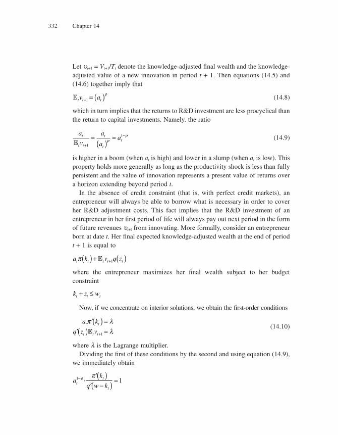
Chapter 14332
Let ut+1 = Vt+1/Tt denote the knowledge-adjusted fi nal wealth and the knowledge-adjusted value of a new innovation in period t + 1. Then equations (14.5) and (14.6) together imply that
Et t tv a+ = ( )1
ρ (14.8)
which in turn implies that the returns to R&D investment are less procyclical than the return to capital investments. Namely. the ratio
a
v
a
aat
t t
t
t
tE +
−=( )
=1
1ρ
ρ (14.9)
is higher in a boom (when at is high) and lower in a slump (when at is low). This property holds more generally as long as the productivity shock is less than fully persistent and the value of innovation represents a present value of returns over a horizon extending beyond period t.
In the absence of credit constraint (that is, with perfect credit markets), an entrepreneur will always be able to borrow what is necessary in order to cover her R&D adjustment costs. This fact implies that the R&D investment of an entrepreneur in her fi rst period of life will always pay out next period in the form of future revenues ut+l from innovating. More formally, consider an entrepreneur born at date t. Her fi nal expected knowledge-adjusted wealth at the end of period t + 1 is equal to
a k v q zt t t t tπ( ) + ( )+E 1
where the entrepreneur maximizes her fi nal wealth subject to her budget constraint
k z wt t t+ ≤
Now, if we concentrate on interior solutions, we obtain the fi rst-order conditions
a k
q z vt t
t t t
′( ) =′( ) =+
π λλE 1
(14.10)
where l is the Lagrange multiplier.Dividing the fi rst of these conditions by the second and using equation (14.9),
we immediately obtain
ak
q w ktt
t
1 1− ⋅′( )
′ −( ) =ρ π
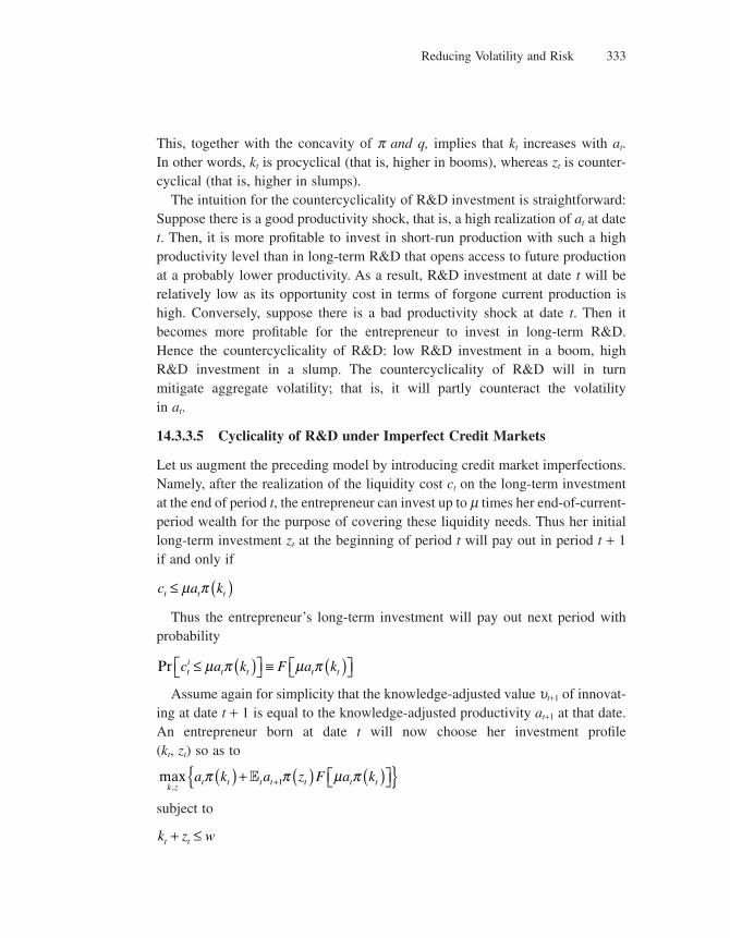
Reducing Volatility and Risk 333
This, together with the concavity of p and q, implies that kt increases with at. In other words, kt is procyclical (that is, higher in booms), whereas zt is counter-cyclical (that is, higher in slumps).
The intuition for the countercyclicality of R&D investment is straightforward: Suppose there is a good productivity shock, that is, a high realization of at at date t. Then, it is more profi table to invest in short-run production with such a high productivity level than in long-term R&D that opens access to future production at a probably lower productivity. As a result, R&D investment at date t will be relatively low as its opportunity cost in terms of forgone current production is high. Conversely, suppose there is a bad productivity shock at date t. Then it becomes more profi table for the entrepreneur to invest in long-term R&D. Hence the countercyclicality of R&D: low R&D investment in a boom, high R&D investment in a slump. The countercyclicality of R&D will in turn mitigate aggregate volatility; that is, it will partly counteract the volatility in at.
14.3.3.5 Cyclicality of R&D under Imperfect Credit Markets
Let us augment the preceding model by introducing credit market imperfections. Namely, after the realization of the liquidity cost ct on the long-term investment at the end of period t, the entrepreneur can invest up to m times her end-of-current-period wealth for the purpose of covering these liquidity needs. Thus her initial long-term investment zt at the beginning of period t will pay out in period t + 1 if and only if
c a kt t t≤ ( )μ π
Thus the entrepreneur’s long-term investment will pay out next period with probability
Pr c a k F a kti
t t t t≤ ( )⎡⎣ ⎤⎦ ≡ ( )⎡⎣ ⎤⎦μ π μ π
Assume again for simplicity that the knowledge-adjusted value ut+1 of innovat-ing at date t + 1 is equal to the knowledge-adjusted productivity at+1 at that date. An entrepreneur born at date t will now choose her investment profi le (kt, zt) so as to
max,k z
t t t t t t ta k a z F a kπ π μ π( ) + ( ) ( )⎡⎣ ⎤⎦{ }+E 1
subject to
k z wt t+ ≤
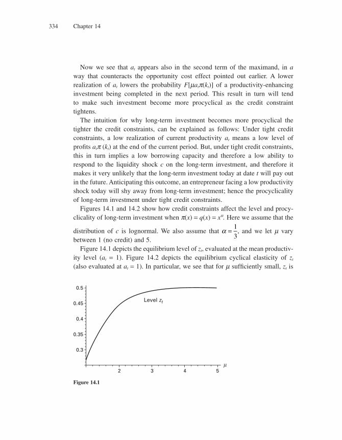
Chapter 14334
Now we see that at appears also in the second term of the maximand, in a way that counteracts the opportunity cost effect pointed out earlier. A lower realization of at lowers the probability F[matp(kt)] of a productivity-enhancing investment being completed in the next period. This result in turn will tend to make such investment become more procyclical as the credit constraint tightens.
The intuition for why long-term investment becomes more procyclical the tighter the credit constraints, can be explained as follows: Under tight credit constraints, a low realization of current productivity at means a low level of profi ts atp (kt) at the end of the current period. But, under tight credit constraints, this in turn implies a low borrowing capacity and therefore a low ability to respond to the liquidity shock c on the long-term investment, and therefore it makes it very unlikely that the long-term investment today at date t will pay out in the future. Anticipating this outcome, an entrepreneur facing a low productivity shock today will shy away from long-term investment; hence the procyclicality of long-term investment under tight credit constraints.
Figures 14.1 and 14.2 show how credit constraints affect the level and procy-clicality of long-term investment when p(x) = q(x) = xa. Here we assume that the
distribution of c is lognormal. We also assume that α = 1
3, and we let m vary
between 1 (no credit) and 5.Figure 14.1 depicts the equilibrium level of zt, evaluated at the mean productiv-
ity level (at = 1). Figure 14.2 depicts the equilibrium cyclical elasticity of zt (also evaluated at at = 1). In particular, we see that for m suffi ciently small, zt is
0.5
0.45
0.4
0.35
0.3
2 3 4 5
Level zt
Figure 14.1
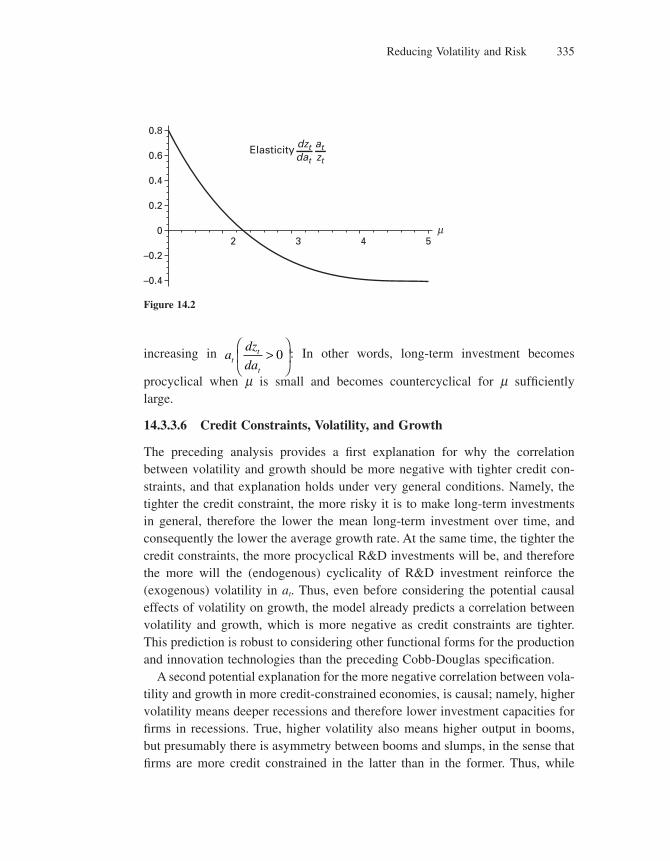
Reducing Volatility and Risk 335
increasing in adz
datt
t
>⎛
⎝⎜
⎞
⎠⎟0 : In other words, long-term investment becomes
procyclical when m is small and becomes countercyclical for m suffi ciently large.
14.3.3.6 Credit Constraints, Volatility, and Growth
The preceding analysis provides a fi rst explanation for why the correlation between volatility and growth should be more negative with tighter credit con-straints, and that explanation holds under very general conditions. Namely, the tighter the credit constraint, the more risky it is to make long-term investments in general, therefore the lower the mean long-term investment over time, and consequently the lower the average growth rate. At the same time, the tighter the credit constraints, the more procyclical R&D investments will be, and therefore the more will the (endogenous) cyclicality of R&D investment reinforce the (exogenous) volatility in at. Thus, even before considering the potential causal effects of volatility on growth, the model already predicts a correlation between volatility and growth, which is more negative as credit constraints are tighter. This prediction is robust to considering other functional forms for the production and innovation technologies than the preceding Cobb-Douglas specifi cation.
A second potential explanation for the more negative correlation between vola-tility and growth in more credit-constrained economies, is causal; namely, higher volatility means deeper recessions and therefore lower investment capacities for fi rms in recessions. True, higher volatility also means higher output in booms, but presumably there is asymmetry between booms and slumps, in the sense that fi rms are more credit constrained in the latter than in the former. Thus, while
0.8
0.6
0.4
0.2
0
–0.2
–0.4
2 3 4 5
Elasticity dztdat
atzt
Figure 14.2
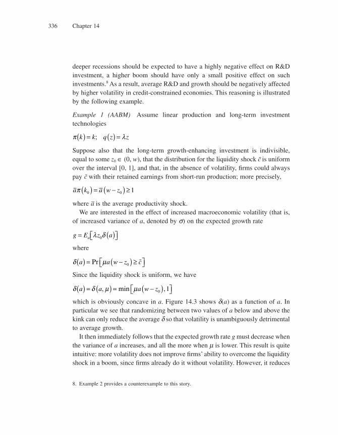
Chapter 14336
deeper recessions should be expected to have a highly negative effect on R&D investment, a higher boom should have only a small positive effect on such investments.8 As a result, average R&D and growth should be negatively affected by higher volatility in credit-constrained economies. This reasoning is illustrated by the following example.
Example 1 (AABM) Assume linear production and long-term investment technologies
π λk k q z z( ) = ( ) =;
Suppose also that the long-term growth-enhancing investment is indivisible, equal to some z0 ∈ (0, w), that the distribution for the liquidity shock c is uniform over the interval [0, 1], and that, in the absence of volatility, fi rms could always pay c with their retained earnings from short-run production; more precisely,
a k a w zπ 0 0 1( ) = −( ) ≥
where a is the average productivity shock.We are interested in the effect of increased macroeconomic volatility (that is,
of increased variance of a, denoted by s) on the expected growth rate
g E z aa= ( )⎡⎣ ⎤⎦λ δ0
where
δ μa a w z c( ) = −( ) ≥⎡⎣ ⎤⎦Pr 0 �
Since the liquidity shock is uniform, we have
δ δ μ μa a a w z( ) = ( ) = −( )⎡⎣ ⎤⎦, min ,0 1
which is obviously concave in a. Figure 14.3 shows d(a) as a function of a. In particular we see that randomizing between two values of a below and above the kink can only reduce the average d so that volatility is unambiguously detrimental to average growth.
It then immediately follows that the expected growth rate g must decrease when the variance of a increases, and all the more when m is lower. This result is quite intuitive: more volatility does not improve fi rms’ ability to overcome the liquidity shock in a boom, since fi rms already do it without volatility. However, it reduces
8. Example 2 provides a counterexample to this story.
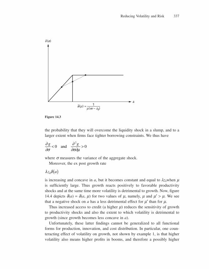
Reducing Volatility and Risk 337
the probability that they will overcome the liquidity shock in a slump, and to a larger extent when fi rms face tighter borrowing constraints. We thus have
∂∂
∂∂ ∂
g g
σ σ μ< >0 0
2
and
where s measures the variance of the aggregate shock.Moreover, the ex post growth rate
λ δz a0 ( )is increasing and concave in a, but it becomes constant and equal to lz0when m is suffi ciently large. Thus growth reacts positively to favorable productivity shocks and at the same time more volatility is detrimental to growth. Now, fi gure 14.4 depicts d(a) = d(a, m) for two values of m, namely, m and m′ > m. We see that a negative shock on a has a less detrimental effect for m′ than for m.
Thus increased access to credit (a higher m) reduces the sensitivity of growth to productivity shocks and also the extent to which volatility is detrimental to growth (since growth becomes less concave in a).
Unfortunately, these latter fi ndings cannot be generalized to all functional forms for production, innovation, and cost distribution. In particular, one coun-teracting effect of volatility on growth, not shown by example 1, is that higher volatility also means higher profi ts in booms, and therefore a possibly higher
(a)δ
aa( ) =
(w – z0)1
Figure 14.3
Chapter 14338
ability for fi rms to innovate during booms. The following example illustrates this “resurrecting effect” of higher volatility.
Example 2 (AABM) Suppose that
cc p
p=
−( )⎧⎨⎩
with probability
with probability0 1
Suppose, as in example 1, that the R&D investment is indivisible and equal to z0, that
π w z q z−( ) = ( ) =0 0 1
and that at ∈ [a_, a] with E(at) = 1.Then, if m < c, only a fraction of fi rms will manage to overcome their liquidity
shocks in the absence of volatility, that is, if
a ≡ 1
However, if volatility becomes suffi ciently high that ac>μ
, then the occurrence
of a boom will allow all fi rms to overcome their liquidity shocks and thereby innovate.
This “resurrection” effect cannot be fi rst-order; otherwise, we would have observed a positive correlation between volatility and growth in the cross-country
(a, )μδ
(a, )μδ
(a, ’)μδ
a0
’>μ μ
Figure 14.4
Reducing Volatility and Risk 339
regressions, and we did not. And if we restrict attention to functional forms such that the overall correlation between volatility and growth is negative, then the causal effect pointed out in example 1 will dominate.
14.3.4 Confronting the Credit Constraints Story with Evidence
In a recent paper, Barlevy (2007) challenges the view that credit constraints are the main explanation for the observed procyclicality of R&D investments. He looks at the Compustat database, which includes larger fi rms, but these account for most of R&D expenditures in the United States. What Barlevy fi nds is that R&D is procyclical even among this subgroup of fi rms, even though it may be argued that large fi rms are less credit constrained than small fi rms (see Bernanke and Gertler, 1989). Barlevy goes further and shows that the reduction in R&D expenditure during recessions is even more pronounced for fi rms that hold at least $50 million in cash over a year.
Now, Barlevy himself acknowledges that this fi nding is not enough to invalidate the preceding credit-constraint story. Indeed large fi rms and/or fi rms with large cash holdings may well be those that face binding credit constraints, for example, due to the combination of big investment needs and of the intangibility of their assets, and the cash holdings may be precisely the way for such fi rms to make sure they can overcome liquidity shocks.
In fact, a recent study by Berman, Eymard, Aghion, Askhenazy, and Cette (2007), henceforth BEAAC, uses a French fi rm-level panel dataset covering 13,000 fi rms over the period 1980–2000 to test the predictions of AABM. Credit constraints are measured at fi rm level by a fi rm’s ability to obtain new bank loans, which turns out to depend upon the fi rm’s credit record vis-à-vis its trade credi-tors. More specifi cally, fi rms that fail to repay their trade creditors are put on a blacklist called “Payment Incident,” and being included on that list affects fi rms’ ability to access credit in the future. Using the interaction between this fi rm-level instrument and a variable that refl ects the dependence of the fi rm’s industry upon external fi nance, and controlling for fi rm size, BEAAC show (1) that R&D spend-ing is more positively correlated with sales in more credit-constrained fi rms; (2) that higher volatility of sales has an asymmetric effect on R&D investments: these are more harmed in slumps than they are encouraged in booms; and (3) that higher volatility is more harmful to productivity growth in more credit-constrained fi rms.
Chapter 14340
14.3.5 An Alternative Explanation for the Procyclicality of R&D
To account for why even fi rms with deep pockets tend to have procyclical R&D, Barlevy (2007)9 proposes the following explanation, also developed using the Schumpeterian paradigm: Because fi rms are afraid of being quickly imitated, they adopt a shortsighted attitude when it comes to innovating. This in turn explains why fi rms will concentrate their R&D efforts in booms where the gains from innovating are larger.
More formally, consider a simple overlapping-generations model where fi rms live for two periods. Innovation in the fi rst period gives access to positive profi t in the current period and also in the next period provided the innovation is not imitated. Moreover, current productivity-adjusted profi ts are equal to at where at. ∈ {a_, a}, with a_ < a.
Then, if c(z) denotes the productivity-adjusted cost of innovating with probability z, a fi rm will choose z = z(at) to solve
maxz
t t tz a q E a a c zε δ+ −( ) ( )⎡⎣ ⎤⎦ − ( ){ }+1 1
where q is the probability of imitation, d ∈ (0, 1) is the discount factor, e refl ects the extent to which the fi rm can benefi t from the innovation in the short run, and
E a a pa p at t t t+ −( ) = + −( )1 1
where a−t is equal to a (resp. a_) when at = a_(resp. a).Now, even if e < 1 so that it takes time for the fi rm to fully learn how to
implement the innovation, yet for q suffi ciently large (high imitation) or for d suffi ciently small (high impatience), we clearly have
z a z a( ) < ( )that is, procyclical R&D investment.
One problem with this explanation is that it relies on the assumption that R&D investments yield immediate results. There is surely truth to the idea that fi rms target the implementation of innovations strategically over the business cycle (see Shleifer 1986), but still there is a big time gap between R&D investments and innovation results.
9. See also Francois and Lloyd-Ellis (2003).
Reducing Volatility and Risk 341
14.4 Risk Diversifi cation, Financial Development, and Growth
Acemoglu and Zilibotti (1997), henceforth AZ, propose an alternative explana-tion for the Ramey and Ramey (1995) fi nding that the correlation between volatil-ity and growth is more negative in less (fi nancially) developed economies. The basic idea in AZ is that, because each new activity involves a fi xed cost, econo-mies at an early stage of development can only fi nance a limited number of intermediate industries. This drawback limits the scope for risk diversifi cation in these economies, in turn inducing agents to choose inferior but safer technologies. At the same time the fact that less developed economies cannot diversify idio-syncratic risks makes these economies more volatile than more developed economies.
The development process goes through several stages: fi rst, a period of primi-tive accumulation where aggregate output is highly volatile; second, a take-off phase where the economy achieves higher fi nancial development with more scope for risk diversifi cation; third, a developed phase with high and steady growth that relies on a high degree of risk diversifi cation. Thus the growth process is slow and volatile at early stages of development, and then speeds up and stabilizes in later stages of development.
14.4.1 Basic Framework
More formally, suppose that time is discrete and that the economy is populated by a continuum of two-period-lived individuals. Total population is constant, and each generation has a unit mass (L = 1). Individuals born at date t are assumed to consume only in period t + 1,10 and they face uncertainty over the state of nature to be realized in this next period. There is a continuum of equally likely states of nature s ∈ [0, 1]. Agents have the following (expected) utility function, inducing unit relative risk aversion:
E U c c dst t ts
+ +( ) = ( )∫1 10
1log (14.11)
where cst+1 is agent’s consumption of the fi nal good in period (t + 1) if state s is
realized.
10. This assumption is for simplicity. Acemoglu and Zilibotti (1997) assume that agents consume in both periods. It is also possible to study the case of a general constant relative risk aversion (CRRA) utility function.

Chapter 14342
The production side of the economy is described as follows: The unique fi nal good is produced by the unit mass continuum of individuals using capital and labor, according to the AK technology
Y K L Ks t s t t s t, , ,= − −α α α1 1
where Ks,t denotes the aggregate amount of physical capital in the economy in period t and state s. Because we assume a constant population Lt normalized to unity, and all individual fi rms are identical so that
K K di Ks t s t s t, , ,= ⋅ =∫in equilibrium, we have Ys,t = Ks,t.
Capital in turn can be produced in two ways: (1) through a risky but more advanced technology, which uses existing intermediate industries, thereby pro-ducing some state-contingent amount of output (xs): namely, industry i produces positive output only if state s = i occurs; if this industry does not exist in the country, then the risky technology generates zero output in state s = i; (2) through a “safe technology” (xΦ) that generates output no matter the realization of the state of nature. We thus have
K x xs t s t s t, , , ,= =− −1 1Φ (14.12)
Let At ∈ [0, 1] denote the number (mass) of intermediate industries generating state-contingent production at date t. What limits this number to lie below one in less developed economies is that operating each inter-mediate activity involves a fi xed cost. More precisely, it requires a fi xed cost equal to
MD
xi xi =
−( ) −( )⎧⎨⎪
⎩⎪
⎫⎬⎪
⎭⎪max ,0
1
with x ∈ (0, 1), to operate industry i. Thus industries i ≤ x have no fi xed-cost require-ment, whereas in industries i > x the fi xed cost increases linearly with the index i.
The intermediate industry i produces capital using the fi nal good, according to the production function
xRF i s F M
i si i i
, == ≥⎧
⎨⎩
if and
otherwise0
where Fi is the amount of fi nal good input, and R > 0 is the rate of return on this technology.
Reducing Volatility and Risk 343
The safe technology is also linear, with
x r ssΦ, , ,= ∀ ∈[ ]φ 0 1
where r < R. Thus the safe technology yields a lower rate of return than the risky technology.
All markets are assumed to be competitive, and a fi rm’s output is entirely distributed to the holders of securities in that fi rm.
When young, agents work in the fi nal-good sector and earn the competitive wage
∂∂Y
Lw Y Ks t
s t s t s t,
, , ,= = −( ) = −( )1 1α α
At the end of this period, agents decide in which assets to save this wage revenue. In other words, they make portfolio decisions. They may decide to invest their savings in a set of risky securities ({Fi}i∈[0,At]
), consisting of state-contingent claims to the output of the intermediate industries that are currently operational in the country. Or they may invest their savings in the safe technology.
14.4.2 Analysis
Given the risky and safe technologies that we have specifi ed, the i security entitles its owner to a claim to R units of capital in state i (as long as the minimum size con-straint is satisfi ed, which is always the case in equilibrium), and otherwise to nothing. Savings invested in the safe technology give the return rate r in all states of nature.
Since the risky securities yield symmetric returns, it is optimal for the risk-averse agents to hold a symmetric portfolio, with Fi ≡ F for all i ∈ [0, At]. We refer to this as a balanced portfolio.
If the economy is suffi ciently developed that it can fi nance all contingent intermediate activities, then At = 1, so that a balanced portfolio of risky securities bears no risk. In this case, since R > r, nobody will invest in the safe technology.
If the economy is less developed so that At < 1, then individuals face a trade-off between risk and rate of return. More formally, the representative young agent at date t solves the optimal portfolio problem
max log log,φ
φ φt tF
t t t t tA RF r A r+[ ]+ −( ) [ ]1 (14.13)
subject to
φt t t tA F w+ ≤ (14.14)
Chapter 14344
(Note that each individual takes the range of securities offered At as given.)From fi rst-order conditions, we immediately get
φtt
tt
A R
R rAw* =
−( )−
1 (14.15)
FF A
R r
R rAw i A
i Ai t
tt
t t
t
,
,* =
( ) ≡ −−
∀ ≤
∀ >
⎧
⎨⎪
⎩⎪0
(14.16)
The FF schedule in fi gure 14.5 depicts the resulting demand for any available risky asset F(At) as a function of the number At of intermediate industries that are active. The FF schedule is upward sloping, which in turn captures a complemen-tarity in the demand for risky assets: the demand for each asset grows with the variety of intermediate industries. What happens here is that the more numerous active intermediate activities are, the better risk diversifi cation is. This improve-ment in turn encourages savers to shift their investments away from the safe asset into high-productivity risky projects. Such complementarity hinges on risk aversion being suffi ciently high.11
Now we know, given At, how much individuals are ready to invest in each activity. The equilibrium measure of active industries A*t is then simply deter-mined as the maximum industry index i such that the fi xed cost Mi can be fi nanced by the amount of savings F(At). In other words, it satisfi es the fi xed-point condition
F A Mt At( )*
*=
In fi gure 14.5, the equilibrium is given by the intersection between the two schedules FF and MM, where MM depicts the A → MA mapping. Intuitively, A*t is the largest number of industries for which the fi xed-cost requirement can be met, subject to the demand of securities being given by F(A).
As the economy grows, so does wage income and therefore so does the stock of savings over time. In equilibrium, this growth induces an expansion of the number of active intermediate industries A*t. Looking at fi gure 14.5: growth
11. Suppose agents were risk averse, but only moderately so. Suppose, in particular, that they were so little risk averse that they would decide not to hold any safe asset in their portfolio. Then, an expansion in the set of risky securities would induce agents to spread their savings (whose total amount is predetermined) over a larger number of assets. In this case, assets would be substitutes rather than complements.
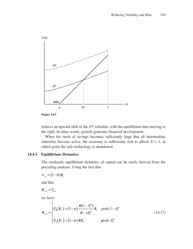
Reducing Volatility and Risk 345
induces an upward shift of the FF schedule, with the equilibrium thus moving to the right. In other words, growth generates fi nancial development.
When the stock of savings becomes suffi ciently large that all intermediate industries become active, the economy is suffi ciently rich to afford A*t = 1, at which point the safe technology is abandoned.
14.4.3 Equilibrium Dynamics
The stochastic equilibrium dynamics of capital can be easily derived from the preceding analysis. Using the fact that
w Ks t t, = −( )1 α
and that
K Yt t+ +=1 1
we have
KF K
R A
R rAR prob A
F K RK
t
B tt
t
t t
G t t
+ =( ) = −( ) −
−−
( ) = −( )1
11
1
1
α
α
( ).
*
**
pprob At. *
⎧
⎨⎪⎪
⎩⎪⎪
(14.17)
A
F(A)
1A*x
FF
MM
FF’
Figure 14.5
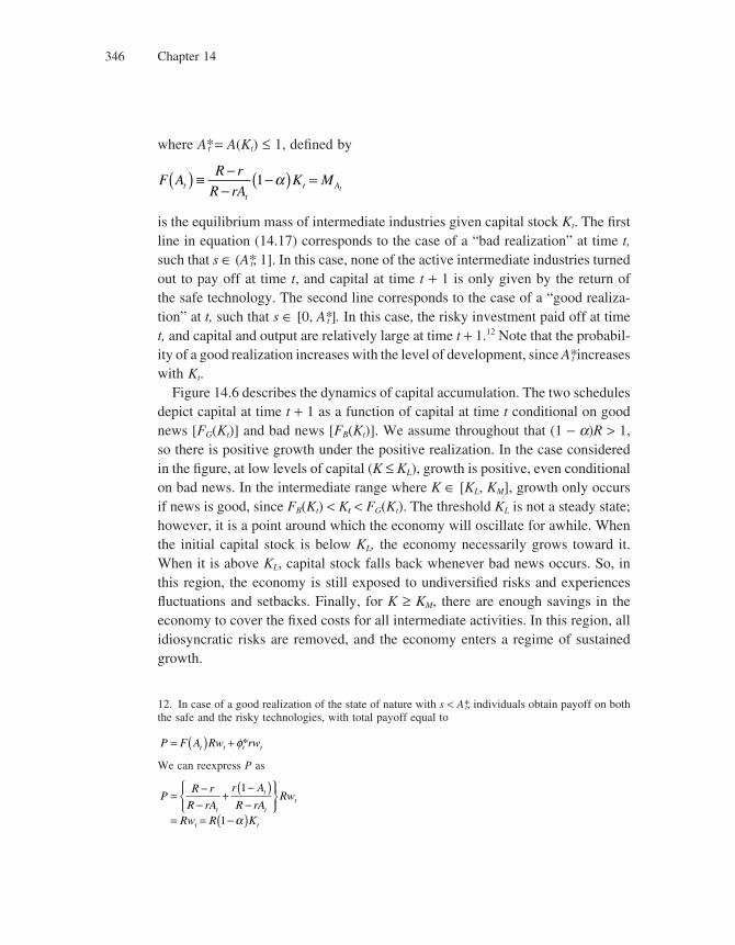
Chapter 14346
where A*t = A(Kt) ≤ 1, defi ned by
F AR r
R rAK Mt
tt At
( ) ≡ −−
−( ) =1 α
is the equilibrium mass of intermediate industries given capital stock Kt. The fi rst line in equation (14.17) corresponds to the case of a “bad realization” at time t, such that s ∈ (A*t, 1]. In this case, none of the active intermediate industries turned out to pay off at time t, and capital at time t + 1 is only given by the return of the safe technology. The second line corresponds to the case of a “good realiza-tion” at t, such that s ∈ [0, A*t ]. In this case, the risky investment paid off at time t, and capital and output are relatively large at time t + 1.12 Note that the probabil-ity of a good realization increases with the level of development, since A*t increases with Kt.
Figure 14.6 describes the dynamics of capital accumulation. The two schedules depict capital at time t + 1 as a function of capital at time t conditional on good news [FG(Kt)] and bad news [FB(Kt)]. We assume throughout that (1 − a)R > 1, so there is positive growth under the positive realization. In the case considered in the fi gure, at low levels of capital (K ≤ KL), growth is positive, even conditional on bad news. In the intermediate range where K ∈ [KL, KM], growth only occurs if news is good, since FB(Kt) < Kt < FG(Kt). The threshold KL is not a steady state; however, it is a point around which the economy will oscillate for awhile. When the initial capital stock is below KL, the economy necessarily grows toward it. When it is above KL, capital stock falls back whenever bad news occurs. So, in this region, the economy is still exposed to undiversifi ed risks and experiences fl uctuations and setbacks. Finally, for K ≥ KM, there are enough savings in the economy to cover the fi xed costs for all intermediate activities. In this region, all idiosyncratic risks are removed, and the economy enters a regime of sustained growth.
12. In case of a good realization of the state of nature with s < A*t, individuals obtain payoff on both the safe and the risky technologies, with total payoff equal to
P F A Rw rwt t t t= ( ) + φ*
We can reexpress P as
PR r
R rA
r A
R rARw
Rw R Kt
t
tt
t t
= −−
+−( )−
⎧⎨⎪
⎩⎪
⎫⎬⎪
⎭⎪= = −( )
1
1 α
Aghion_15_Ch14.indd 346 11/25/2008 3:35:30 PM
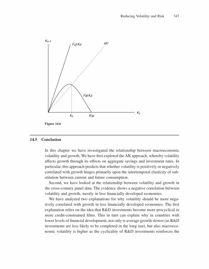
Reducing Volatility and Risk 347
14.5 Conclusion
In this chapter we have investigated the relationship between macroeconomic volatility and growth. We have fi rst explored the AK approach, whereby volatility affects growth through its effects on aggregate savings and investment rates. In particular, this approach predicts that whether volatility is positively or negatively correlated with growth hinges primarily upon the intertemporal elasticity of sub-stitution between current and future consumption.
Second, we have looked at the relationship between volatility and growth in the cross-country panel data. The evidence shows a negative correlation between volatility and growth, mostly in less fi nancially developed economies.
We have analyzed two explanations for why volatility should be more nega-tively correlated with growth in less fi nancially developed economies. The fi rst explanation relies on the idea that R&D investments become more procyclical in more credit-constrained fi lms. This in turn can explain why in countries with lower levels of fi nancial development, not only is average growth slower (as R&D investments are less likely to be completed in the long run), but also macroeco-nomic volatility is higher as the cyclicality of R&D investments reinforces the
45°Kt+1
FG(Kt)
FB(Kt)
KL KMKt
Figure 14.6
Chapter 14348
volatility of aggregate productivity. The second explanation relies on the idea that less developed economies are less able to diversify risk: this implies both that aggregate output will be more volatile and also that agents will tend to invest more in safe but inferior technologies in order to escape risk.
14.6 Literature Notes
In the traditional post-Keynesian literature, growth and business cycles were analyzed separately. Thus Harrod-Domar’s model of long-run growth would have no cycle in it, and Samuelson’s oscillator would be detrended.
This dichotomy between trend and cycles was fi rst questioned by the real busi-ness cycle literature of the 1980s (see Kydland and Prescott 1982; Long and Plosser 1983). According to the RBC approach, fl uctuations are an integral part of the growth process, as both of them result from productivity shocks.
King and Rebelo (1986) and Stadler (1990) were fi rst to analyze the impact of volatility on long-run growth, using AK models. More recently, Jones, Manuelli, and Stachetti (2000) perfected this line of research and updated an idea by Phelps (1962) on how macroeconomic volatility would affect long-run growth through its effects on aggregate savings and investment: the conclusion is that volatility could hurt growth by decreasing total investment. Nevertheless, for reasonable values of the parameters of the model, the correlation between volatility and growth should be positive, as more volatility would induce more precautionary savings.
Cross-country evidence by Ramey and Ramey (1995) suggested, however, that the correlation between growth and macroeconomic volatility is clearly negative. Additional evidence of the detrimental effects of volatility on growth can be found in the work of Bruno (1993) on infl ation and growth, and Hausmann and Gavin (1996) for Latin American countries.
First attempts at analyzing the relationship between volatility and growth using the Schumpeterian paradigm include the work of Gali and Hammour (1991), Caballero and Hammour (1994), Bean (1990), and Aghion and Saint-Paul (1998). More recently, Barlevy (2007) and Francois and Lloyd-Ellis (2003) revisited the relationship between growth and cycles, looking at the combined effects of creative destruction and of implementation-cycle types of externalities as in Shleifer (1986). Finally, AABM (2005) introduced credit constraints into the Schumpeterian framework and analyzed how, depending upon how binding
Reducing Volatility and Risk 349
the credit constraint is, macroeconomic volatility can affect fi rms’ choice between short-run capital investments and long-term productivity-enhancing investments.
Their framework has been used to analyze the relationship between long-run growth and the choice of exchange-rate regimes (see Aghion, Bacchetta, et al., 2006), and the relationship between growth and the countercyclicality of budget-ary policies (Aghion and Marinescu 2007; Aghion and Kharroubi 2007).
Comin and Gertler (2006) provided evidence on the procyclicality of R&D at the medium-term frequencies and the countercyclicality of the relative price of capital. Comin, Gertler, and Santacreu (2008) looked at the connection between long-run growth and short-term fl uctuations from the opposite angle. Using a simplifi ed version of Comin and Gertler (2006), they explored the short- and medium-term effects of a shock about the arrival rate of future technologies on output productivity, employment, the relative price of capital, and the stock market.
Finally, the Acemoglu and Zilibotti model developed in section 14.4 has given rise to subsequent contributions, both theoretical and empirical, in particular by Koren and Tenreyro (2007).
A detailed presentation of the main topics of this chapter can be found in Aghion and Banerjee (2005).
Problems
1. Explain intuitively how a lower level of fi nancial development can imply a more negative correla-tion between macroeconomic volatility and growth.
2. Short and long-term investment (based on Aghion, Angeletos, and colleagues 2005)
This problem solves a version of the AABM model. We consider an economy populated by two-period-lived entrepreneurs who allocate their initial wealth w between short-term capital investments kt and long-term R&D investments zt, and maximize their expected terminal wealth. Profi ts in the fi rst period are pt = atka
t, a ≤ 1. The dynamics of the productivity parameter at are given by at = eta rt−1,
where 0 < r < 1 and Et−1(et) = 1. At the end of the fi rst period, entrepreneurs face an adjustment cost ct which is distributed normally on [0, 1]. If the cost is met, profi ts in the second period are pt+1 = at+1za
t ; otherwise, profi ts in the second period are zero. Assume fi rst that markets are complete.
a. Write the entrepreneur’s fi rst-order conditions for kt and zt. Solve for the optimal ratio of capital
expenses to R&D expenses k
zt
t
. What is its cyclical behavior? Interpret.
Next, assume that credit markets are imperfect. Entrepreneurs can only invest up to m times their fi rst-period profi ts to pay for the adjustment cost.
b. What is the probability that the long-term investment will pay off? Show that for at large enough—that is, when a suffi ciently good shock occurs—credit constraints do not change the optimal composi-tion of investment.
Chapter 14350
c. Suppose that ak at
t
< ( )1
μ *, where k* (at) is the investment in capital under perfect markets. Use
the entrepreneur’s expected wealth maximization problem to solve for the ratio k
zt
t
. What is its
cyclical behavior? Interpret.
3. *Imitation and procyclical R&D (based on Barlevy 2007)
Consider an overlapping-generations model where a representative fi rm exists for two periods and hires labor for production (lt) and R&D (zt). Its total labor input is constrained to be lt + zt = 1. When zt units of labor are employed in R&D. the fi rm innovates with probability zt. In addition to the wage bill, which is independent of zt, it incurs a cost of c per unit of labor in R&D. If it does not innovate, it realizes profi ts of atlt in period t and zero in period t + 1. If it innovates, it makes a profi t of egatlt
in period t, where γε
> 1. There is a probability q that a successful innovation will be imitated, in
which case profi t at t + 1 is driven to zero by competition with the entrant. Otherwise, profi t at t + 1 is at+1lt+1 = at+1, as there is no R&D in the second period. The discount factor is d. Productivity can take two values {1, a}, with a > 1, and follows a process of the form Etat+1 = pat + (1 − p)a−t.
We assume c is small, c < d(1 − p)(1 + a).
a. What is the expected total profi t over the two periods, as a function of zt, at, a−t, and the parameters of the model?
b. Derive the fi rm’s optimal choice of z for the two states of the economy, z(1) and z(a).
c. If q = 1 (absence of patent protection), what is the sign of z(a) − z(1)? Is R&D procyclical or countercyclical?
d. If q = 0 (perfect protection against imitation), what is the sign of z(a) − z(1)? Is R&D procyclical or countercyclical? How does this expression depend on the parameters d and p?
4. *Exchange-rate regime, volatility, and productivity growth (based on Aghion, Bacchetta, and colleagues 2006)
This problem examines the impact of exchange-rate volatility on productivity growth under different exchange-rate regimes. We assume that there is a single good produced by a continuum of measure one of two-period-lived fi rms according to the technology y A lt t t= , where lt is the labor input. The price level is determined by purchasing power parity. It is equal to the exchange rate after normalizing foreign prices to one: Pt = St. Under fi xed exchange rates, St = S is a constant. Under fl exible exchange rates, St fl uctuates around its mean E(St) = S. Wages are set in nominal terms one period ahead as Wt = wAtE(Pt).
At the end of period t, fi rm i faces a liquidity cost C it = ciPtAt. The random component ci has a
concave cumulative distribution function F over the interval [0, c]. In order to meet this cost, fi rms can borrow up to m − 1 times their period-t profi t (we assume m < 4w c). Let qt be the fraction of fi rms that survive the shock. At period t + 1, these fi rms innovate and realize value Pt+1At+1 = Pt+1gAt. We also assume g is high enough that it is always profi table for a fi rm to try to overcome the liquidity shock.
a. Given that producers maximize their total wealth over the two periods, derive the demand for labor and profi t in period t.
b. Calculate the probability of innovation qt as a function of S, m, and w.
c. What is the expected productivity growth rate of the economy? Is it higher under fi xed or fl exible exchange rates? What is the growth gap between the two regimes when m → ∞?
d. Assume for the rest of the problem that there are stochastic shocks to productivity: At = Ateut, where At = rt−1gAt−1 + (1 − rt−1)At, and ut is a mean-zero shock of variance s 2
u. What is the modifi ed demand for labor and profi t in period t?
Reducing Volatility and Risk 351
e. Suppose interest-rate parity holds (in logs) when exchange rates are fl exible: st = Et−1st + ln(1 + i*) − ln(1 + it) + ht. Here st = ln(St), i and i* are the domestic and foreign nominal interest rate, and ht has mean zero and variance s 2
h (under fi xed exchange rates, we normalize st = 0). The central bank follows a Taylor rule and sets ln(1 + it) = ln(1 + i*) + f1st + f2ut. Assume there are no bubbles, that is, lim
it t iE s
→∞ + = 0. Solve for st as a function of the monetary and real shocks ht and ut.
f. What is the probability of innovation under fi xed and fl exible exchange rates if s 2u = 0? if
s 2h = 0? Which regime yields the highest growth in each case?
5. **Timing of innovation and timing of adoption (based on Comin and Gertler, 2006)
Suppose a fi nal good is produced with a continuum of intermediate inputs, where the producer of each intermediate good realizes profi ts pt = dAt per period; At follows a process of the form At+1 = rAt + (1 − r)A + et+l, with 0 < r < 1, A > 0, and Et(et+l) = 0. The development of a new input takes place in two stages. First, each innovator i spends an amount Ri
t of the fi nal good in research, which leads
to ϕ
RR
t
ti
( )η new innovations. Rt is the average amount of research spending in the economy and
captures congestion effects. The innovator can then sell each design in the next period, for the expected price EtPt+l, to an “adopter” who develops it into a marketable good. Second, for each design he has purchased at or before date t, the adopter chooses a level of spending Zt so that the product becomes usable with a probability λ Zt , l > 0. He earns monopoly profi ts from a successful innova-tion; hence the value for the adopter of a product that has been developed is Vt = pt + bEtVt+l. We assume free entry in both innovation and adoption of technologies. The discount factor is noted b.
a. Using the condition of free entry into innovation, obtain the level of Rt for given expected prices.
b. Find the value Wt of an innovation that has not yet been adopted. as a function of Zt, EtVt+l, and EtWt+l. Derive the optimal choice of Zt. What is the equilibrium relationship between Pt and Wt?
c. Solve for the value of a developed product Vt. How does an increase in the aggregate productivity parameter At affect Vt and Wt?
d. Are research spending Rt and adoption spending Zt procyclical or countercyclical? Explain these results intuitively.

15 Liberalizing Trade
15.1 Introduction
In this chapter we examine the consequences for productivity growth and innova-tion of interaction between countries. We concentrate on international trade in goods, but as we shall see, when we introduce trade in goods, the nature of inter-national fl ows in knowledge also becomes very important to the results.
One may think of several reasons why trade should increase world income and enhance productivity growth. First, trade openness increases the size of markets that can be appropriated by successful innovators, or it increases the scale of production and therefore the scope for learning-by-doing externalities. This market-size effect should be more important for smaller countries that increase market size by a higher proportion when opening up to trade. Thus, when regress-ing growth over “openness” and its interaction with the size of the domestic economy (for example, as measured by the log of population), one should fi nd that the interaction coeffi cient between country size and openness is negative. And indeed this is what Alesina, Spolaore, and Wacziarg (2005) fi nd when they regress growth over country openness and size, using cross-country panel data.1
Second, trade induces knowledge spillovers from more advanced to less advanced countries and sectors. Thus one should expect the interaction between openness and initial income in the growth regressions to be negative; that is, growth is less enhanced by openness in more advanced countries. To the extent that knowledge tends to fl ow from richer to poorer countries, it is not surprising that the more advanced a country already is, the less it should benefi t from knowledge spillovers inducing trade. This knowledge spillover effect has been
1. A natural measure of openness would have been imports plus exports over GDP. However, this raises an obvious endogeneity problem: a positive correlation between imports/exports and growth may refl ect the fact that a booming country imports and exports more. To deal with this problem, we follow Frankel and Romer (1999) who instrument the value of imports plus exports over GDP using a simple “gravity model” where trade fl ows depend upon a country’s geographical characteristics such as the extent of common borders with neighboring countries, access to the sea, and the size of the country in population and in surface terms. This instrumentation strategy helps make sure that we capture the causal effect of trade openness on growth and not the reverse causality or the effect of third omitted variables that might affect both trade and growth.
Chapter 15354
analyzed at length by Keller (2004). It also underlies the work of Sachs and Warner (1995).2
There is an additional effect of trade on growth that is not captured in the preced-ing discussion, namely, that trade liberalization tends to enhance product market competition, by allowing foreign producers to compete with domestic producers. This in turn should enhance domestic productivity for at least two reasons. First, it forces the most unproductive fi rms out of the domestic market. Thus Trefl er (2004) shows that trade liberalization in Canada resulted in a 6 percent increase in average productivity. Second, as in chapter 12, it forces domestic fi rms to innovate in order to escape competition with their new foreign counterparts.
In the following sections we develop a synthetic framework that embodies all these potential effects that trade may have on productivity growth and innovation.3 In section 15.2 we outline a simple multisector Schumpeterian model of a closed economy, much like the one developed at greater length in chapter 4, which will serve as a reference point for our analysis of an open economy. In section 15.3 we examine the immediate impact of trade on sectoral productivities and the level of national income, by taking two economies of the sort described in section 15.2 and allowing them to trade costlessly with each other. In that section we take productivities in the domestic and foreign sectors as given. In section 15.4 we show how trade affects the innovation process and use this analysis to study the long-run growth effects of trade between the two economies studied in the previous section, but now focusing on endogeneizing productivity and its dynamics in both countries.
Overall the theory shows that there are good reasons for supposing that trade has a positive impact on both the level and the growth rate of a country’s national income. However, the analysis in this chapter also points to possible exceptions to this general supposition. In particular, small economies that have the potential for becoming world leaders in some sectors but have not yet realized that potential seem to be the most likely to lose as a result of international trade.
2. Additional evidence on trade and research spillovers is provided in an important paper by Coe and Helpman (1995). For each country they construct measures of domestic and foreign R&D capital stocks, where the latter are weighted averages of the domestic stocks of trade partners. They fi nd that foreign R&D appears to have a benefi cial effect on domestic productivity and that the effect increases in strength with the degree of openness. Hence, not only are there important spillovers, but there is also some evidence that these are mediated by trade. However, one may argue that even if a correlation is observed between domestic productivity and foreign research, this may simply represent the outcome of common demand or input price shocks. Weighting the contribution of foreign research using data on bilateral trade fl ows, as in Coe and Helpman, is likely to mitigate this problem but will not overcome it altogether.
3. In chapter 2 we saw yet another potential effect of trade on growth: a terms-of-trade effect whereby trade allows small countries to avoid the consequences of decreasing returns to capital accumulation.
Liberalizing Trade 355
15.2 Preliminary: Back to the Multisector Closed-Economy Model
In the next sections we introduce trade into the Schumpeterian model of chapter 4. First we review the closed-economy version of the model, introducing the notion of national income.
15.2.1 Production and National Income
There is a single country in which a unique fi nal good, which also serves as numéraire, is produced competitively using a continuum of intermediate inputs according to
Y L A x dit it it= < <− −∫1 1
0
10 1α α α α, (15.1)
where L is the domestic labor force, assumed to be constant, Ait is the quality of intermediate good i at time t, and xit is the fl ow quantity of intermediate good i being produced and used at time t.
In each intermediate sector there is a monopolist producer who uses the fi nal good as the sole input, with one unit of fi nal good needed to produce each unit of intermediate good. The monopolist’s cost of production is therefore equal to the quantity produced xit. The price pit at which she can sell this quantity of intermediate good to the competitive fi nal sector is the marginal product of inter-mediate good i in the fi nal-good production function (15.1).
As we showed in chapter 4, the monopolist will choose the level of output that maximizes profi ts, namely,
x A Lit it= −( )α α2 1 (15.2)
resulting in the profi t level
π πit itA L= (15.3)
where π α ααα≡ −( )
+−1
1
1 .The equilibrium level of fi nal output in the economy can be found by substitut-
ing the xit’s into equation (15.1), which yields
Y A Lt t= ϕ (15.4)
where At is the average productivity parameter across all sectors
A A dit it= ∫0
1
Chapter 15356
and ϕ ααα= −
2
1 .4
We are interested in the equilibrium level of national income Nt which is not quite the same as fi nal sector output Yt, because some of the fi nal goods are used up in producing the intermediate products that in turn are used in producing the fi nal output. There are only two forms of income—wage income and profi t income. Each of the L workers is employed in the fi nal-goods sector, where he is paid his marginal product. So according to the production function (15.1) total wage income is the fraction 1 − a of fi nal output:
W L Y L Yt t t= × = −( )∂ ∂ 1 α
Profi ts are earned by the local monopolists who sell intermediate products to the fi nal sector. (There are no profi ts in the fi nal-good sector because that sector is perfectly competitive and operates under constant returns to scale.) Since each monopolist charges a price equal to5 1/a and has a cost per unit equal to 1, there-fore the profi t margin pit − 1 on each unit sold can be written as (1 − a)pit, which means that total profi ts equal
Πt it it it itp x dt p x dt= −( ) = −( )∫ ∫1 10
1
0
1α
And since the price pit is the marginal product of the ith intermediate product, therefore equation (15.1) implies
p x dt Y x x dt Yit it t it it t0
1
0
1
∫ ∫= ( ) =∂ ∂ α
So from the last two lines we have
Πt tY= −( )1 α α
Gathering results, we see that national income is
N W Yt t t t= + = −( )Π 1 2α (15.5)
4. To derive this expression for Yt, substitute the xit’s into equation (15.1) to get
Y L A A L di
L A A di
t it it
it it
= ( )= ( )
− − −( )
−( ) −
∫1 1 2 1
0
1
2 1 1
0
1
α α α α
α α α α
α
α ∫∫= ζ A Lt
5. That is, since the fi nal-good market in which the intermediate product is sold is perfectly competi-tive, therefore its price equals its marginal product:
p Y x L A xit t it t it= = − − −∂ ∂ α α α α1 1 1
Using equation (15.2) to substitute for xit in this equation yields pit = 1/a.
Liberalizing Trade 357
From equations (15.4) and (15.5) we see that national income is strictly propor-tional to average productivity and to population:
N A Lt t= −( )1 2α ϕ (15.6)
It follows from this last result that the growth rate of national income is also the growth rate of productivity:
� �N N A A gt t t t t= =
15.2.2 Innovation
Productivity growth comes from innovations. In each sector at each date there is a unique entrepreneur with the possibility of innovating in that sector. She is the incum-bent monopolist, and an innovation would enable her to produce with a productivity (quality) parameter Ait = gAi,t−1 that is superior to that of the previous monopolist by the factor g > 1. Otherwise her productivity parameter stays the same: Ait = Ai,t−1. In order to innovate with any given probability m she must spend the amount
c Ait i tμ τ φ μ( ) = −( )⋅ ( )⋅ −1 1,
of fi nal good in research, where t > 0 is a subsidy parameter that represents the extent to which national policies encourage innovation, and f is a cost function satisfying
φ 0 0( ) =
and
′( ) > ′′( ) > >φ μ φ μ μ0 0 0, for all
Thus the local entrepreneur’s expected profi t net of research cost is
V E c
L A LA Ait it it
i t i t i t
= − ( )= + −( ) − −( ) ( )− − −
π μμπ γ μ π τ φ μ, , ,1 1 11 1
She will choose the value of m that maximizes these expected profi ts.Each local entrepreneur will choose a frequency of innovations m that maxi-
mizes Vit. The fi rst-order condition for an interior maximum is ∂Vit/∂m = 0, which can be expressed as the research-arbitrage equation
′( ) = −( ) −( )φ μ π γ τL 1 1 (15.7)
If the research environment is favorable enough (i.e., if t is large enough), or the population large enough, so that
Chapter 15358
′( ) > −( ) −( )φ π γ τ0 1 1L
then the unique solution m to the research-arbitrage equation (15.7) is positive, so in each sector the probability of an innovation is that solution (m = m) which is an increasing function of the size of population L and of the policies favoring innovation t. Otherwise there is no positive solution to the research-arbitrage equation, so the local entrepreneur chooses never to innovate (m = 0).
Since each Ait grows at the rate g − 1 with probability m, and at the rate 0 with probability 1 − m, therefore the expected growth rate of the economy is
g = −( )μ γ 1
So we see that countries with a larger population and more favorable innovation conditions will be more likely to grow, and if they grow will grow faster than countries with a smaller population and less favorable innovation conditions.
15.3 Opening Up to Trade, Abstracting from Innovation
Now, let us open trade in goods (both intermediate and fi nal) between the domes-tic country and the rest of the world, and we fi rst take productivities in all domes-tic and foreign sectors to be given. Productivity-enhancing innovations are introduced in the next section.
To keep it simple, suppose that there are just two countries, “home” and “foreign,” which differ in terms of the size of population and the policies favoring innovation. Suppose that the range of intermediate products in each country is identical, that they produce exactly the same fi nal product, and that there are no transportation costs. Within each intermediate sector the world market can then be monopolized by the producer with the lowest cost. We use asterisks to denote foreign-country variables.
15.3.1 The Experiment
Consider the following conceptual experiment. To begin with, each country does not trade, and hence behaves just like the closed economy described in the previ-ous section. Then at time t we allow countries to trade costlessly with each other. The immediate effect of this opening up is to allow each country to take advan-tage of greater productive effi ciency. In the home country, fi nal-good production will equal
Y Y di L A x dit it it it= = < <∫ ∫− −
0
1 1 1
0
10 1α α α αˆ , (15.8)

Liberalizing Trade 359
where Âit is the higher of the two initial productivity parameters:
ˆ max{ , }A A Ait it it= *
Likewise in the foreign country fi nal-good production will equal
Y Y di L A x dit it it it* * * *= = ( ) < <∫ ∫− −
0
1 1 1
0
10 1
α α α αˆ ( ) , (15.9)
The profi t of a monopolist will now be higher than it was under autarky, because she can now sell to both countries. Specifi cally, if she charges the price pit, then fi nal-good producers in each country will buy good i up to the point where its marginal product equals pit:
x A L p x A L pit it it it it it= ( ) = ( )− −ˆ ˆα αα α1
1
1
1and * * (15.10)
Adding these two equations and rearranging, we see that her price will depend on total sales Xit = xit + x*it according to
p L L A Xit it it= +( ) ( )− − −α α α α*1 1
1ˆ (15.11)
which is the same as the demand relationship in the closed economy6 except that now we have global sales relative to global population instead of local sales rela-tive to local population on the right-hand side. Accordingly, the monopolist’s profi t pit will equal revenue pitXit minus cost Xit:
π αα α α
it it it it it it itp X X A L L X X= − = ( ) +( ) −− −ˆ 1 1
*
As in the case of the closed economy, the monopolist will choose the level of output that maximizes pit, namely,
X A L Lit it= +( ) −( )ˆ * α α2 1
resulting in the same price
pit = 1 α
as before and the profi t level
π πit itA L L= +( )ˆ * (15.12)
where once again π α ααα≡ −( )
+−1
1
1
Substituting the prices pit = 1/a into the demand functions (15.10) yields
6. See footnote 5.

Chapter 15360
x A L x A Lit it it it= =−( ) −( )ˆ ˆα αα α2 1 2 1and * *
and substituting these into the production functions (15.8) and (15.9), we see that fi nal-good production in the two countries will be proportional to their populations:
Y A L Y A Lt t t t= =ϕ ϕˆ ˆand * * (15.13)
where once again ϕ ααα= −
2
1 and where Ât is the cross-sectoral average of the Âit’s:
ˆ ˆA A dit it= ∫0
1
15.3.2 The Effects of Openness on National Income
Within each country, national income is still equal to the sum of wage income and profi t income. As before, wage income in each country is earned in the fi nal sector:
W Y A L
W Y A L
t t t
t t t
= −( ) = −( )= −( ) = −( )
1 1
1 1
α α ζ
α α ζ
ˆ
ˆ* * *
Profi t income in each country depends on the fraction of the intermediate monop-olies that resides in that country. Defi ne
λitit itA A= >⎧
⎨⎪
⎩⎪
⎫⎬⎪
⎭⎪1
0
if *
otherwise
So lit is an indicator of whether the monopoly resides in the home country, and 1 − lit is an indicator of whether it resides in the foreign country. (For simplicity we assume that there are no sectors in which Ait = A*it.) According to equation (15.12), total profi ts across all sectors monopolized by each country will be
Π
Π
t it it
t it it
L L A di
L L A di
= +( )= +( ) −( )
∫∫
π λ
π λ
*
* *
ˆ
ˆ0
1
0
11
Therefore, national income in the two countries is
N Y Y Y dit t it it it= −( ) + −( ) +∫1 10
1α α α λ ( )* (15.14)
N Y Y Y dit t it it it* * *= −( ) + −( ) −( ) +∫1 1 1
0
1α α α λ ( ) (15.15)
Liberalizing Trade 361
which can be rewritten as
N A L A L L dit t it it= −( ) + −( ) +( )⎡⎣⎢
⎤⎦⎥∫1 1
0
1α α α λ ϕˆ ˆ *
N A L A L L dit t it it* * *= −( ) + −( ) −( ) +( )⎡
⎣⎢⎤⎦⎥∫1 1 1
0
1α α α λ ϕˆ ˆ
15.3.2.1 The Selection Effect
One way in which international trade can raise a country’s national income is through the selection effect of increased competition (see Melitz 2003). That is, fi rms can buy intermediate products from the most effi cient producer. This is bad news for the less effi cient producer, who is forced to exit, but it raises aggregate incomes by increasing the overall level of effi ciency with which the economy converts labor input into fi nal output (by means of intermediate products).
To see how this effect works in the present model, note that when the world economy is opened up to trade, total world income is the sum of equations (15.14) and (15.15), namely,
N N Y Y Y Y
LA L A
t t t t t t
t t
+ = −( ) +( )∗ + −( ) +( )∗
= −( ) +( )*
*
1 1
1 2
α α α
α ϕ ˆ ˆ
whereas when the world economy was closed it was7
N N LA L At t t t+ = −( ) +* * *1 2α ϕ( )
Comparing these two formulas, we see that the total world income has been raised by international trade because the average productivity parameter Ât is generally larger than either At or A*t. That is, in sectors where the home country gets the monopoly we have Âit = Ait, while in all other sectors Âit > Ait, so the average of all the Âit’s is bigger than the average of all the Ait’s. Likewise, it is also bigger than the average of all the A*it’s.
15.3.2.2 Scale Effect
We saw earlier that smaller countries appear to gain more from openness than larger countries. The present model helps us to see why this statement might be accurate. As we have seen, the home country’s national income was
N A Lt t= −( )1 2α ϕ
7. This is the sum of equation (15.6) for each country.
Chapter 15362
when it was closed, and then changed to
′ = −( ) + −( ) +( )⎡⎣⎢
⎤⎦⎥∫N A L A L L dit t it it1 1
0
1α α α λ ϕˆ ˆ *
We would like to see what the model implies about how the gains from open-ness depend upon population, holding constant the initial level of technological development. To do so, suppose that the home and foreign countries started at equal levels of technological development. That is, in half of the sectors the home country starts with higher productivity and captures the monopoly, while in the other half the foreign country captures the monopoly, and on average the produc-tivity of the monopolies in either country is the same as the global average, namely, Ât. In that case the home country’s national income after opening up to trade would be
′ = −( ) + −( )( ) +( )⎡⎣ ⎤⎦= −( ) + −( )
N A L A L L
A L
t t t
t
1 1 1 2
1 1 12
α α α ϕ
α ϕ α α
ˆ ˆ
ˆ
*
22( ) −( )L L At* ˆ ϕ
so the proportional gain from openness is
′= +
+( )−⎛
⎝⎜⎜
⎞
⎠⎟⎟
N
N
A
A
L L
Lt
t
t
t
ˆ1
2 1
αα
*
It follows directly that the smaller the country, as measured by L, the larger the proportional gain. This scale effect works entirely through the profi t component of national income. By opening up to international trade, technologically advanced intermediate producers can now sell their products to a larger market. The smaller the market was before opening up, the bigger this gain will be.
15.3.2.3 Backwardness
We also saw that technologically less advanced countries seemed to gain more from openness. To see why this conclusion might be true, let us control for size by supposing that the home and foreign countries are of equal size (L = L*). Then going through the same exercise as before we see that the relative gain from openness is
′=
++
+( )∫N
N
A
A
A di
At
t
t
t
it it
t
1
1
2
10
1
α
α λ
α
ˆ ˆ
where the fi rst term represents wage income and the second profi t income, both relative to pretrade national income.
Liberalizing Trade 363
In this case the effect is not quite as clear-cut as in the case of the scale effect. The reason is that opening up to trade will defi nitely raise wage income, since workers will be working with more advanced intermediate inputs and hence will be more productive, but it might not raise the home country’s profi t income. In the extreme case where the home country lags behind the foreign country in every sector, we would fi nd that lit = 0 in all sectors i, so the profi t component of national income would vanish as a result of openness (i.e., the case in which opening up to trade would make the country a mere assembler of imported com-ponents). In that case, the gain in wage income might not be enough to compen-sate for the loss of profi t income.
Nevertheless, even in this extreme case, we can say unambiguously that if the country starts far enough behind the rest of the world, it will defi nitely gain from international trade, and will gain more in relative terms the further behind it starts. That is, if the initial productivity level At of the home country is less than Â/(1 + a) to begin with, then even the fi rst component in the preceding expression for N ′t /Nt will exceed unity, and the smaller At is, the higher it will be.
This analysis of backwardness should warn us, however, that although inter-national trade raises total world income, through the selection effect, there is no guarantee that it will raise national income in every country.
15.4 The Effects of Openness on Innovation and Long-Run Growth
15.4.1 Step-by-Step Innovation
Assume the following step-by-step innovation process in a given sector i. In the country where the monopoly currently resides, the country is on the global technol-ogy frontier for sector i, and the local entrepreneur will aim at making a frontier innovation that raises the productivity parameter from Âit to gÂit. If successful, that country will retain a global monopoly in intermediate product i. In the other country, the local entrepreneur will be trying to catch up with the frontier by imple-menting the current frontier technology. If she succeeds and the frontier entrepre-neur fails to advance the frontier that period, then the lagging country will have caught up, both countries will be on the frontier, and then we can suppose that each entrepreneur will monopolize the market for product i in her own country. But if the frontier entrepreneur does advance the frontier, then the entrepreneur in the lagging country will still remain behind and will earn no profi t income.
Over time, the lead in each sector will tend to pass from country to country, as long as the lagging sector is innovating. (Otherwise the leader will remain the
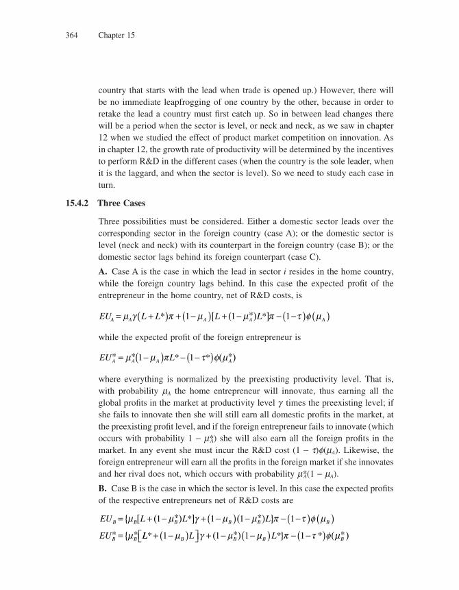
Chapter 15364
country that starts with the lead when trade is opened up.) However, there will be no immediate leapfrogging of one country by the other, because in order to retake the lead a country must fi rst catch up. So in between lead changes there will be a period when the sector is level, or neck and neck, as we saw in chapter 12 when we studied the effect of product market competition on innovation. As in chapter 12, the growth rate of productivity will be determined by the incentives to perform R&D in the different cases (when the country is the sole leader, when it is the laggard, and when the sector is level). So we need to study each case in turn.
15.4.2 Three Cases
Three possibilities must be considered. Either a domestic sector leads over the corresponding sector in the foreign country (case A); or the domestic sector is level (neck and neck) with its counterpart in the foreign country (case B); or the domestic sector lags behind its foreign counterpart (case C).
A. Case A is the case in which the lead in sector i resides in the home country, while the foreign country lags behind. In this case the expected profi t of the entrepreneur in the home country, net of R&D costs, is
EU L L L LA A A A A= +( ) + −( ) + − − −( ) ( )μ γ π μ μ π τ φ μ* * *1 1 1[ ( ) ]
while the expected profi t of the foreign entrepreneur is
EU LA A A A* * * * *= −( ) − −( )μ μ π τ φ μ1 1 ( )
where everything is normalized by the preexisting productivity level. That is, with probability mA the home entrepreneur will innovate, thus earning all the global profi ts in the market at productivity level g times the preexisting level; if she fails to innovate then she will still earn all domestic profi ts in the market, at the preexisting profi t level, and if the foreign entrepreneur fails to innovate (which occurs with probability 1 − m*A) she will also earn all the foreign profi ts in the market. In any event she must incur the R&D cost (1 − t)f(mA). Likewise, the foreign entrepreneur will earn all the profi ts in the foreign market if she innovates and her rival does not, which occurs with probability m*A(1 − mA).
B. Case B is the case in which the sector is level. In this case the expected profi ts of the respective entrepreneurs net of R&D costs are
EU L L L
EU
B B B B B B
B B
= + − + −( ) − − −( ) ( )=
{ [ ( ) ] ( ) }
{
μ μ γ μ μ π τ φ μ
μ
1 1 1 1* * *
* * LL L LB B B B* * * *+ −( )⎡⎣ ⎤⎦ + − −( ) − −( )1 1 1 1μ γ μ μ π τ φ μ( ) } * ( )
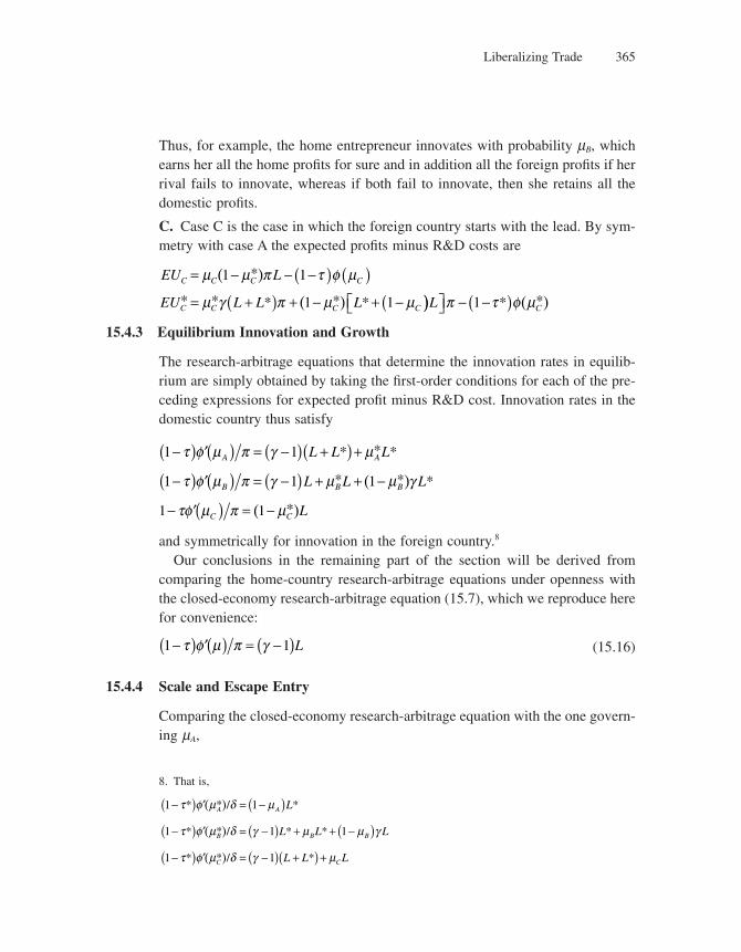
Liberalizing Trade 365
Thus, for example, the home entrepreneur innovates with probability mB, which earns her all the home profi ts for sure and in addition all the foreign profi ts if her rival fails to innovate, whereas if both fail to innovate, then she retains all the domestic profi ts.
C. Case C is the case in which the foreign country starts with the lead. By sym-metry with case A the expected profi ts minus R&D costs are
EU L
EU L L L
C C C C
C C C C
= − − −( ) ( )= +( ) + − + −(
μ μ π τ φ μ
μ γ π μ μ
( )
( )
1 1
1 1
*
* * * * * ))⎡⎣ ⎤⎦ − −( )L Cπ τ φ μ1 * *( )
15.4.3 Equilibrium Innovation and Growth
The research-arbitrage equations that determine the innovation rates in equilib-rium are simply obtained by taking the fi rst-order conditions for each of the pre-ceding expressions for expected profi t minus R&D cost. Innovation rates in the domestic country thus satisfy
1 1−( ) ′( ) = −( ) +( ) +τ φ μ π γ μA AL L L* * *
1 1 1−( ) ′( ) = −( ) + + −τ φ μ π γ μ μ γB B BL L L* * *( )
1 1− ′( ) = −τφ μ π μC C L( )*
and symmetrically for innovation in the foreign country.8
Our conclusions in the remaining part of the section will be derived from comparing the home-country research-arbitrage equations under openness with the closed-economy research-arbitrage equation (15.7), which we reproduce here for convenience:
1 1−( ) ′( ) = −( )τ φ μ π γ L (15.16)
15.4.4 Scale and Escape Entry
Comparing the closed-economy research-arbitrage equation with the one govern-ing mA,
8. That is,
1 1−( ) ′ = −( )τ φ μ δ μ* * / *( )A A L
1 1 1−( ) ′ = −( ) + + −( )τ φ μ δ γ μ μ γ* * / * *( )B B BL L L
1 1−( ) ′ = −( ) +( ) +τ φ μ δ γ μ* * / *( )C CL L L
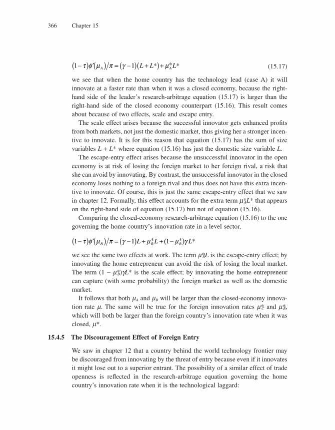
Chapter 15366
1 1−( ) ′( ) = −( ) +( ) +τ φ μ π γ μA AL L L* * * (15.17)
we see that when the home country has the technology lead (case A) it will innovate at a faster rate than when it was a closed economy, because the right-hand side of the leader’s research-arbitrage equation (15.17) is larger than the right-hand side of the closed economy counterpart (15.16). This result comes about because of two effects, scale and escape entry.
The scale effect arises because the successful innovator gets enhanced profi ts from both markets, not just the domestic market, thus giving her a stronger incen-tive to innovate. It is for this reason that equation (15.17) has the sum of size variables L + L* where equation (15.16) has just the domestic size variable L.
The escape-entry effect arises because the unsuccessful innovator in the open economy is at risk of losing the foreign market to her foreign rival, a risk that she can avoid by innovating. By contrast, the unsuccessful innovator in the closed economy loses nothing to a foreign rival and thus does not have this extra incen-tive to innovate. Of course, this is just the same escape-entry effect that we saw in chapter 12. Formally, this effect accounts for the extra term m*AL* that appears on the right-hand side of equation (15.17) but not of equation (15.16).
Comparing the closed-economy research-arbitrage equation (15.16) to the one governing the home country’s innovation rate in a level sector,
1 1 1−( ) ′( ) = −( ) + + −τ φ μ π γ μ μ γB B BL L L* * *( )
we see the same two effects at work. The term m*BL is the escape-entry effect; by innovating the home entrepreneur can avoid the risk of losing the local market. The term (1 − m*B)gL* is the scale effect; by innovating the home entrepreneur can capture (with some probability) the foreign market as well as the domestic market.
It follows that both mA and mB will be larger than the closed-economy innova-tion rate m. The same will be true for the foreign innovation rates m*C and m*B, which will both be larger than the foreign country’s innovation rate when it was closed, m*.
15.4.5 The Discouragement Effect of Foreign Entry
We saw in chapter 12 that a country behind the world technology frontier may be discouraged from innovating by the threat of entry because even if it innovates it might lose out to a superior entrant. The possibility of a similar effect of trade openness is refl ected in the research-arbitrage equation governing the home country’s innovation rate when it is the technological laggard:
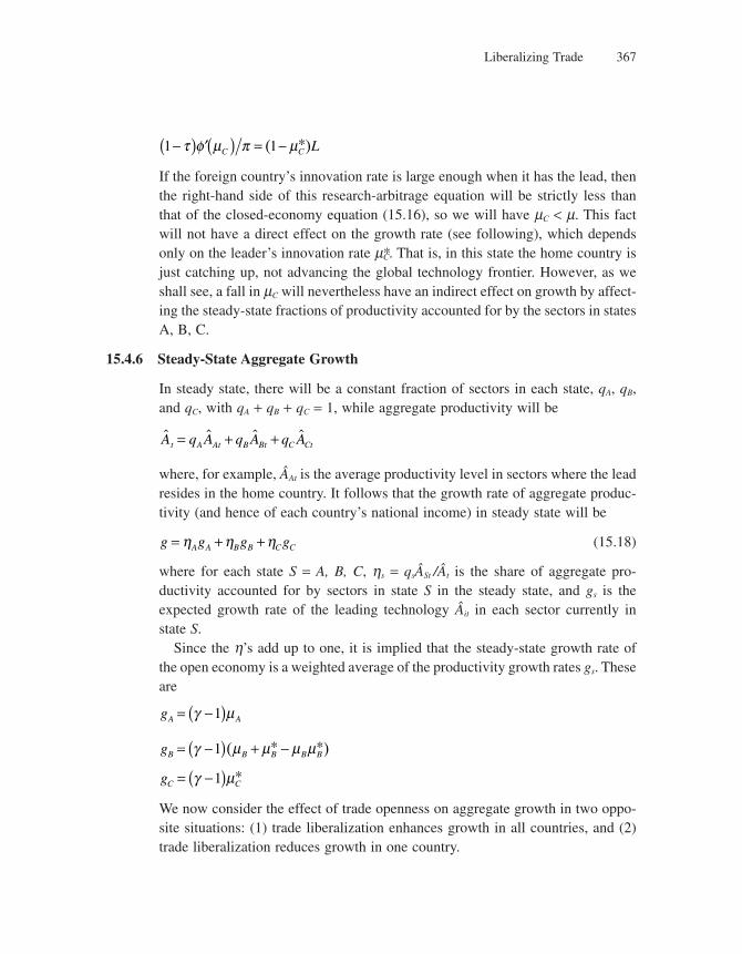
Liberalizing Trade 367
1 1−( ) ′( ) = −τ φ μ π μC C L( )*
If the foreign country’s innovation rate is large enough when it has the lead, then the right-hand side of this research-arbitrage equation will be strictly less than that of the closed-economy equation (15.16), so we will have mC < m. This fact will not have a direct effect on the growth rate (see following), which depends only on the leader’s innovation rate m*C. That is, in this state the home country is just catching up, not advancing the global technology frontier. However, as we shall see, a fall in mC will nevertheless have an indirect effect on growth by affect-ing the steady-state fractions of productivity accounted for by the sectors in states A, B, C.
15.4.6 Steady-State Aggregate Growth
In steady state, there will be a constant fraction of sectors in each state, qA, qB, and qC, with qA + qB + qC = 1, while aggregate productivity will be
ˆ ˆ ˆ ˆA q A q A q At A At B Bt C Ct= + +
where, for example, ÂAt is the average productivity level in sectors where the lead resides in the home country. It follows that the growth rate of aggregate produc-tivity (and hence of each country’s national income) in steady state will be
g g g gA A B B C C= + +η η η (15.18)
where for each state S = A, B, C, hs = qsÂSt /Ât is the share of aggregate pro-ductivity accounted for by sectors in state S in the steady state, and gs is the expected growth rate of the leading technology Âit in each sector currently in state S.
Since the h’s add up to one, it is implied that the steady-state growth rate of the open economy is a weighted average of the productivity growth rates gs. These are
gA A= −( )γ μ1
gB B B B B= −( ) + −γ μ μ μ μ1 ( )* *
gC C= −( )γ μ1 *
We now consider the effect of trade openness on aggregate growth in two oppo-site situations: (1) trade liberalization enhances growth in all countries, and (2) trade liberalization reduces growth in one country.
Chapter 15368
15.4.7 How Trade Can Enhance Growth in All Countries
Suppose fi rst that one country, say the home country, is less innovative than the other, in the sense that its closed-economy innovation rate m is less than the foreign country’s innovation rate when closed m*. Suppose also that the discour-agement effect of foreign entry is so great that once it is exposed to foreign trade the home country does no research in sectors where it is a laggard. That is, the preceding research-arbitrage equation governing mC cannot be satisfi ed by any positive mC, so instead the equilibrium innovation rate of the home country in state C is mC = 0. Suppose, however, that all the other innovation rates are positive in all three states.
In this case, what will happen is that the home country will eventually lose the technology lead in all sectors. In the steady state the fraction of sectors in state C will become qC = 1, while qA = qB = 0. Thus, according to the steady state, all profi t income will be earned in the foreign country, and the growth rate of national income in all countries will be
g gC C= = −( )γ μ1 *
Since m*C is larger than the foreign innovation rate m* before opening up to trade, therefore trade will raise the foreign growth rate. Since both countries grow at the same rate in the open economy, and by assumption the foreign country grew faster than the home country before trade, therefore trade will raise the growth rate in the home country as well.
This result illustrates how trade can allow productivity growth even in coun-tries that do not innovate, something that was not possible without foreign trade. For example, as we saw in chapter 7, a country with a low level of fi nancial development might end up stagnating relative to the rest of the world. In the present model, if the policies favoring innovation t in the home country are per-verse enough, then the country will not innovate at all when it is closed, and hence will have a zero growth rate when closed. Yet when it is open to trade it will grow as fast as the most innovative country.
The reason for this effect is what Keller (2004) calls the direct channel of technology transfer. Productivity of workers in the fi nal sector in the noninnovat-ing country can grow despite the lack of domestic innovation because they are able to work with imported intermediate products whose quality continues to grow as a result of foreign innovations. In this sense trade can act as a substitute for innovation in some countries while it acts as a spur to innovation in others.
Liberalizing Trade 369
As another example, suppose that neither country innovates when it is a laggard. Then the fractions qA and qB of sectors in which each country has a lead will remain constant over time. If the home country has a smaller innovation rate than the foreign country (i.e., mA < m*C) then average productivity of sectors in state C will grow without bound relative to average productivity of sectors in state A, so in the steady state we will again have qC = 1 and g = (g − 1)m*C. Again both countries will have their growth rates raised by trade.
Finally, in the case where both countries are identical (L = L* and t = t*), then by symmetry the growth rate will be
g g gB A B B
B A B B B
B
= −( ) +
= −( ) −( ) + −( )⎡⎣ ⎤⎦= −( ) −( )
1
1 1 2
1 1
2
η η
γ η μ η μ μ
γ η μAA B B B B+⎡⎣ ⎤⎦ + −( ) −( )η μ γ μ μ1 1
which is larger than the closed-economy growth rate (g − 1)m not only because of the scale and escape-entry effects that make mA and mB both larger than m, which is why the fi rst term on the right-hand side of this last expression is greater than (g − 1)m, but also because of a duplication effect. That is, when sectors are level, then there are two possible frontier innovators, so even if one fails to advance the frontier, the other might; this possibility accounts for the second term on the right-hand side of the last line.
15.4.8 How Trade Can Reduce Growth in One Country
The fact that trade raises growth in both countries when either the countries are symmetrical or one country fails to innovate when behind suggests that trade will usually raise growth in both countries. But there can be exceptions. These excep-tions, of course, must involve countries that are asymmetrical. For example, consider the case of a small country (home) whose policies used to be very unfa-vorable to innovation but which has recently undertaken a reform to make the country more innovative. Suppose these policies have been so successful that just before opening up to trade, the home country has a faster growth rate than the foreign country:
μ μ> *
but the reforms have been so recent that the home country is still behind the foreign country in all sectors. Then immediately after the opening up to trade all monopolies will reside in the foreign country; that is, all sectors will be in case C. Now suppose furthermore that the discouragement effect is large enough that
Chapter 15370
the home country does not innovate when behind (mC = 0). Then, as we have seen, all monopolies will remain forever in the foreign country.
This is the case in which, as we saw previously, the home country’s level of national income might actually fall when trade is opened up, because the increased effi ciency of the selection effect might be outweighed by the loss of profi ts from the home-country monopolists that are forced out of business by foreign competi-tion. What we can now see is that whether or not national income falls at fi rst, the home country’s growth rate from then on may be lower than if it had never opened up to trade.
More specifi cally, if it had not opened up for trade, then the home country’s growth rate would have remained equal to
g = −( )γ μ1
whereas under open trade its growth rate will be that of each sector in case C, namely,
′ = −( )g Cγ μ1 *
So the home country growth rate will be reduced by trade if and only if m*C < m. Now we know from our preceding analysis that m*C must exceed the innovation rate that the foreign country would have experienced under autarky:
μ μC* *>
but this fact does not guarantee that it exceeds the innovation rate that the home country would have experienced under autarky. Indeed if m*C is close enough to m*, then it will be strictly less than m, and the home country’s growth rate will indeed be reduced by trade.
This is where our assumption that the home country is small comes into play. For if it is very small relative to the foreign country, then the scale effect of trade on the foreign innovation rate m*C will be small. Since we are assuming that the home country never innovates when behind, therefore there is no escape-entry effect on m*C, so if the home country is small enough, then m*C will indeed be close enough to m* that it falls below m and the home country’s growth rate is dimin-ished by trade.
So we have a presumption that if there are instances where trade is bad for growth, they are probably in small countries that start off far behind the global technology frontier. We also have an example of how economic reform needs to be sequenced properly in order to have its desired effect. That is, generally speak-
Liberalizing Trade 371
ing a country’s growth prospects are enhanced by liberalizing trade and by removing barriers to innovation. But if these reforms are undertaken simultane-ously, then their full benefi ts might not be realized. Instead, it might be better to remove the barriers to innovation fi rst and then to wait until several domestic industries have become world leaders before removing the barriers to interna-tional trade.
15.5 Conclusion
In this chapter we analyzed the effects of opening up to trade on domestic pro-ductivities and on innovation incentives. We saw that international trade raises total world income for several reasons. First, it selects the most productive pro-ducer in each sector. Second, it allows the most advanced producer in each sector to sell to a larger market. Third, it allows backward sectors to catch up with the technological frontier. Then we turned our attention to trade and innovation. By increasing market size, trade increases the size of ex post rents that accrue to successful innovators, thereby encouraging R&D investments. Moreover, by increasing product market competition, trade encourages innovations aimed at escaping competition by more advanced fi rms in the domestic economy. However, it may discourage innovation by laggard fi rms. This discouragement effect in turn introduces the possibility that trade may sometimes reduce growth, in particular in small countries that are far below the world technology frontier. Our analysis in fact suggests that it might be better to remove barriers to innovation prior to fully liberalizing trade in such countries.
A natural next step is to confront the predictions derived in this chapter to the data. In a nutshell, we saw the following:
• Selection effects predict a positive effect of measures of openness on income. In addition, trade will increase the productivity of the fi nal sector everywhere.
• Scale effects predict
• A negative impact from the interaction of openness and size on income; that is, smaller countries should gain proportionately more from openness than large countries.
• A negative impact from the interaction of openness and size on growth; that is, smaller countries should gain proportionately more from openness than large countries.
• Backwardness effects predict
Chapter 15372
• An ambiguous effect from the interaction of openness and distance from the technological frontier on income. As long as the distance is not excessive, the impact should be positive; the greater the distance, the greater the proportionate gain from openness. However, where the distance from the frontier is too great, the impact can be reversed.
• An ambiguous effect from the interaction of openness and distance from the technological frontier on growth. While fi rms that are the technological leader or that are at level pegging with the technological leader should increase innovation under trade liberalization, fi rms that lag behind the technological leader may decrease pro-ductivity growth if the lag is large enough. The net effect is ambiguous.
Aghion, Fedderke, Howitt, Kulatane, and Viegi (2008), or AFHKV, test for these effects in a middle-income-country context, namely, using South African manufacturing sector data. South Africa is interesting as a natural experiment of gradual liberalization in a country that is sectorally heterogeneous and suffers from signifi cant internal market monopolies. Their results confi rm a positive direct impact of trade liberalization on productivity growth. Moreover, the results suggest that the direct effect of liberalization operates through the impact of the liberalization on product market competition and the pricing power of domestic producers. The results also confi rm that the greatest positive impact of trade lib-eralization is on small rather than large domestic sectors; however, no differential impact of the liberalization on sectors that are far from or close to international technological frontiers could be found.
15.6 Literature Notes
The theoretical literature on trade and growth is broad, in contrast to the limited set of empirical papers on the subject. Having already mentioned the main empiri-cal studies in section 15.1, here we concentrate on the theory.
The idea that trade openness should generate both static gains (higher quality or variety of products) and dynamic gains (faster rate of innovation) has been stressed most forcefully by Grossman and Helpman (1989, 1991a, 1991b) and by Rivera-Batiz and Romer (1991). In particular, what induces faster productivity growth following trade liberalization is both (1) that successful innovators have access to larger rents as market size increases and (2) that knowledge spillovers operate across borders. Note that the market-size effect of trade amounts to a scale effect of the kind questioned by C. Jones (1995a and b), which we discussed in chapter 4.
Liberalizing Trade 373
However, extending the Rivera-Batiz and Romer model to the case of two countries with different initial productivity levels, Devereux and Lapham (1994) show that trade openness may inhibit innovation in the initially poorer country.
Helpman (1993) used the expanding-variety model to analyze the interplay between trade and imitation. In his model, R&D and innovation (which here amounts to the introduction of new products) occur in the most developed region referred to as “the North.” Then, costless imitation takes place in the South at a constant rate. The interesting result is that tighter intellectual property rights protection does not necessarily enhance growth, unlike what would happen in a closed economy. On the one hand, reducing the scope for imitation increases the expected lifetime of a product, a result which is good for northern innovators’ rents. On the other hand, fi rms in the North spend more time producing, which in turn raises the demand for (skilled) labor, therefore the wage, and therefore the cost of innovation, in the North. This latter effect may sometimes dominate. See Gancia (2003) for an interesting extension of the Helpman model.
Terms-of-trade effects have been mostly analyzed by Ventura (1997) and by Acemoglu and Ventura (2002). In particular, as shown in chapter 2, introducing terms-of-trade effects can restore convergence in a multicountry AK model.
Young (1991) and Grossman and Helpman (1995) have developed models of trade and growth based on learning-by-doing externalities. The main idea in Young (1991) is that opening up to trade may inhibit learning by doing in less developed economies that may then specialize in more traditional production activities where learning-by-doing opportunities have already been exhausted. More generally, Grossman and Helpman (1995) show that whether trade will accelerate or slow down long-run growth in a country relative to autarky depends upon the effect of trade on the country’s specialization and also on whether or not learning-by-doing spillovers are international in scope. Moreover, as already stressed by Krugman (1987), trade does not lead to convergence in growth rates of income per capita across countries when learning-by-doing spillovers are national in scope, whereas it does lead to convergence when learning-by-doing spillovers are international in scope.
Finally, the interplay between trade, fi rm heterogeneity, and average productiv-ity has become a main focus of trade economics following the pioneering work by Melitz (2003). However, this literature does not analyze the impact of trade on innovation by incumbent fi rms, as we do in this chapter.
Eaton and Kortum (2001) develop a tractable, generalized Ricardian trade model with stochastic technology differences. Trade fl ows are shaped by the interaction of productivity-based comparative advantage and geographic location,
Chapter 15374
and bilateral trade follows a gravity equation. Since the model is static, the state of technology is exogenously given and there is no role for research and development.
For further references on this subject, we refer the reader to Ventura’s (2005) and Alesina, Spolaore, and Wacziarg’s (2005) Handbook of Economic Growth chapters, and to Helpman (2004).
Problems
1. Explain intuitively the following three reasons why trade openness may increase world income and enhance productivity growth: (a) the market-size effect; (b) the knowledge spillover effect; (c) the product-market-competition effect.
2. Static effects of trade liberalization
This question concerns the static effects of opening up to trade, as discussed in section 15.3.Let Nt denote national income under autarky and N ′t denote national income under trade.
a. Suppose Ait = a ∈ [0, 1] ∀i ∈ [0, 1], and let A*it be independently uniformly distributed on [0, 1] ∀i ∈ [0, 1]. Show that
Aa
t = +2
2
1
2
b. Evaluate JN
Nt
t
= ′.
c. Calculate ∂∂
J
L and ∂
∂J
a. Relate these derivatives to the scale effect and the backwardness
effect discussed in sections 15.3.2.2 and 15.3.2.3.
d. Suppose that small countries have higher productivity in fewer sectors. In particular, assume that
the home country has higher productivity in a fraction L
L L+ * of sectors and that both countries
have the same average productivity in sectors in which they have a higher productivity. Does a smaller country gain more from trade under these assumptions?
3. *Dynamic effects of trade liberalization
This question concerns the dynamic effects of opening up to trade, as discussed in section 15.4.
Consider two symmetric countries with L = L* = 1 and t = t* = 0. Suppose further that φ μ μ( ) =2
2.
a. What is the equilibrium probability of innovation in the two countries under autarky?
b. Suppose now that the two countries start to trade. Solve for mA, mB, and mC. Under what conditions is mB > mA? is mA > mC? Discuss.
c. Explain why in steady state
q q q qA A A A C A B B B= + −( ) −( ) + −( )μ μ μ μ μ1 1 1
Provide similar expressions for qB and qC.
d. Using symmetry to set qA = qC, solve for steady-state qA and qB.

Liberalizing Trade 375
4. **Trade and learning by doing.
Consider a two-country (South and North), two-sector (traditional and modern) model in which labor is the only factor of production.
In the traditional sector the production technology is Zt = LTt.
In the modern sector the production technology is Yt = AtLMt .
Modern-sector labor productivity evolves according to A.t = Yt; that is, there is learning by doing
in the modern sector.Each country has a representative consumer with preferences Ut = Z a
tYt1−a.
There is no savings or investment.The South has fi xed labor supply LS, and AS
0 = 1.The North has fi xed labor supply LN, and AN
0 = 1 + e, where e > 0.
a. Suppose the South is in autarky. Solve for the equilibrium of this economy and show that
�AA
LtS
tS S= −( )1 α
b. Now suppose there is free trade between North and South, but that there are no knowledge spill-overs across countries.
i. Solve for the equilibrium at t = 0 assuming both countries have nonzero production in the modern sector.
ii. Why is L
LS
N
>−
+( )αα
ε1
1 a necessary condition for the equilibrium found in part i to exist?
iii. Derive a condition guaranteeing that at t = 0 modern-sector labor productivity grows faster in the North than in the South.
iv. Assume the conditions from parts ii and iii both hold. What happens to the location of modern sector production when
A
A
L
LtN
tS
S
N
> −1 αα
v. Show that there exists T > 0 such that for all t > T, �AA
LtN
tN
N= .
vi. Deduce that in the long run the equilibrium growth rate of real consumption is the same in both countries. Discuss the importance of the terms of trade in generating this result.
vii. Repeat the question assuming that the elasticity of substitution between traditional and modern goods is greater than one:
U Z Yt t t= +⎡
⎣⎢
⎤
⎦⎥ >
− − −1
2
1
21
1 1 1σσ
σσ
σσ
σ,
Discuss the difference from the results obtained with Cobb-Douglas preferences.

16 Preserving the Environment1
16.1 Introduction
A growing number of observers and policy makers have been alerting public opinion to the existence of serious environmental dangers associated with growth. First, growth precipitates the depletion of exhaustible energy resources (coal, oil, . . .). This in turn led some individuals or groups particularly concerned with ecology back in the 1970s (and especially after the oil shock hit the industrialized countries) to argue that zero growth was the only sustainable long-run objective. Second, growth induces a deterioration of the environment, for example, through CO2 emissions that may eventually gravely damage production and life on earth. The Al Gore movie, An Inconvenient Truth, and the Stern Report (2006) on the economic costs of not reducing CO2 emissions have contributed to turning this issue into a top headline and prompting government heads in the G8 to act quickly on it.
In this chapter, we analyze how new growth theories can integrate the envi-ronmental dimension, and in particular how endogenous innovation and directed technical change make it possible to reconcile the sustained growth objective with the constraints imposed by exhaustible resources or the need to maintain the environment.
The chapter is organized as follows. Section 16.2 introduces an exhaustible resource constraint in the AK model. Section 16.3 introduces that constraint in the Schumpeterian growth model. We will see that the one-sector AK model can no longer explain positive long-run growth once we make production dependent on an exhaustible resource, whereas sustainable growth can be restored neverthe-less in a world with endogenous innovation. Finally, section 16.4 uses the directed technical change model of chapter 8 to analyze the growth effect of a tax on dirty production activities, as well as how this tax should be chosen so as to maintain the environment in the long run.
16.2 The One-Sector AK Model with an Exhaustible Resource
We consider the following variant of the one-sector AK growth model. Time is continuous, and aggregate output is produced according to the production technology
1. This chapter was written with the collaboration of Leonardo Bursztyn.
Chapter 16378
Y AKR= >φ φ, 0 (16.1)
where K is the current aggregate capital stock and R is the current fl ow of extracted resource. If we denote the current stock of natural resource by S, then we simply have
�S R= − (16.2)
Capital accumulates over time as in the Solow or AK model with constant savings rate, according to
�K sY K= −δ (16.3)
where s is the constant savings rate and d is the constant rate of capital depreciation.
In the absence of an exhaustible resource (that is, with just Y = AK), such an economy would grow forever at rate
gK
KsA= = −
�δ
However, things change dramatically once the exhaustible resource is intro-duced. More precisely, we now show that positive growth can no longer be sus-tained in the long run.
To see this point, note that in the long run the rate of extraction R must fall to zero, since otherwise the stock S would become negative in fi nite time. But from equations (16.1) and (16.3) we have
�KK
sAR= −φ δ
so therefore the growth rate �K
K must converge to −d < 0, which of course means
that the capital stock K must also fall to zero in the long run. Since R and K are both falling to zero, therefore Y = AKRf must also fall to zero in the long run. In other words, not just the growth rate but even the level of output will vanish in the long run in this AK model with exhaustible resource.
The reason for this no-growth result can be simply explained as follows: In order to sustain growth in this AK model, it is necessary that the fl ow of extracted resource R become arbitrarily small as time goes to infi nity. Otherwise, the resource stock S and therefore the output fl ow Y would vanish in fi nite time. Now, to counteract the effect of R going to zero, that is, to maintain production in spite
Preserving the Environment 379
of saving increasingly on the resource factor, requires technical progress. However, technical progress requires capital accumulation, and therefore an acceleration of resource-consuming production . . . and therefore a more intense use of the exhaustible resource. In other words, this AK economy with exhaus-tible resources looks like a snake that would eat its own tail in order to survive.
16.3 Schumpeterian Growth with an Exhaustible Resource
In contrast to the one-sector AK model, growth can be sustained in a Schumpet-erian world with innovations. The basic idea is that in a such a world one can conceive of technical progress and innovations that are distinct from the accu-mulation of physical capital, and in particular innovations that are greener (less resource-intensive) than capital accumulation.
More formally, suppose that the economy is populated by a continuum of mass M = 1 of one-period-lived individuals, each of whom is endowed with one unit of labor that she can allocate between manufacturing or research activities. Final output is produced according to
Y L A x R= − −1 1α α α φ (16.4)
where L is the fl ow of labor employed in production (manufacturing labor), A and x denote the productivity and quantity of intermediate input, respectively, and R again denotes the current fl ow of extracted resource, so that the stock of natural resources still evolves over time according to
�S R= −
Labor can be used either in manufacturing the fi nal good (L) or in research to produce innovations (n); thus labor-market clearing imposes that
L n+ = 1
The intermediate producer uses the fi nal good one for one to produce her intermediate input. Taking the fi nal good as numéraire, and assuming that the fi nal-good sector is competitive, the intermediate producer can sell her intermedi-ate product to the fi nal sector at price
p xY
xL A x R( ) = = − − −∂
∂α α α α φ1 1 1
She chooses x to maximize profi ts, solving
Chapter 16380
π = ( ) −{ }maxx
p x x x
which yields
x ALR= − −α αφα
2
1 1
which, in turn yields (after substituting the x’s in the expression for Y)
Y LAR= − −ααα
φα
2
1 1 (16.5)
Now suppose that the government can impose that R decreases over time at an exponential rate, according to
�R qR= −
with q > 0,2 so that S remains always positive. Can positive growth still be sustained in that case? Using equation (16.5) and taking logarithmic derivatives, one has
� � �Y
Y
A
A
R
Rg qA= + = −φ φ
where gA is the rate of productivity growth.Now, suppose that productivity growth results from innovations and that inno-
vations result from R&D labor, so that the rate of productivity growth can be expressed as
g nA = −( )γ λ1
where n is the equilibrium amount of R&D labor, g is the size of innovations, and l is an R&D productivity parameter.
Overall, the economy will sustain positive growth in the long run whenever
γ λ φ−( ) >1 n q
or
nq>
−( )φ
γ λ1 (16.6)
Given the preceding labor-market-clearing condition, this outcome is possible if and only if the right-hand side of equation (16.6) is less than the total available labor supply, which we normalize to unity:
2. In the appendix to this chapter we solve for the social planner problem in the case where prefer-ences are isoelastic, and show that the optimal solution involves a constant q.
Preserving the Environment 381
φγ λ
q
−( ) <1
1
for this is the necessary and suffi cient condition for there to be enough R&D labor available in order to offset the deleterious effects of resource depletion through innovation. The condition will be satisfi ed if the productivity of R&D l or the size of innovation g are suffi ciently large, or if the depletion rate q is suf-fi ciently small.
Thus, in contrast to the one-sector AK model where growth can never be sus-tained when fi nal production requires the use of an exhaustible resource, growth can be sustained in a Schumpeterian world where innovations save on the use of the resource (whereas technical progress involved a more intensive use of the resource in the AK model).
Note that our analysis in this section has implicitly assumed that innovations are “green,” that is, do not exhaust resources or do not degrade the environment. In the next section we remove this restrictive assumption and look at whether governments can sustain growth by taxing the wrong kind of innovations, that is, by appropriately directing technical change.
16.4 Environment and Directed Technical Change
We now move to a world with both clean and dirty innovation activities. On the one hand, dirty activities deplete the stock of environmental capital; on the other hand, environment regenerates at some exogenous rate w. When the clean and dirty input baskets are perfect substitutes in producing fi nal output, the effect of a tax on dirty production activities will be to encourage innovation in the clean production technologies instead.
16.4.1 Basic Setup
Time t is discrete. Final output each period is
YY Y S
tct dt t=
+ >⎧⎨⎩
⎫⎬⎭
if
otherwise
0
0 (16.7)
where Yct is output produced by a clean process, Ydt is output produced by a dirty process, and St is the environmental stock. According to equation (16.7) no pro-duction is possible once St has disappeared.
Dirty production causes the environment to deteriorate. Specifi cally, the change in the environmental stock is
Chapter 16382
S S Y St t dt t+ − = − +1 φ ω (16.8)
where the parameter f > 0 indicates the impact of dirty production and the param-eter w ≥ 0 indicates the rate at which the environment can regenerate through natural processes.
Equation (16.8) imposes a speed limit on dirty production. Specifi cally it implies that Ydt cannot grow faster than w in the long run. To see how this process works, divide both sides by St and you see that the growth rate (St+1 − St)/St cannot exceed w. Therefore if Ydt were to grow steadily at the rate g > w, then the nega-tive term on the right-hand side of equation (16.8) would grow faster than the positive term, so the right-hand side would eventually become negative, at which time St would start to fall, eventually resulting in environmental disaster: St ≤ 0.
Suppose the economy starts at date 0 with S0 > 0. We now proceed to examine under what conditions an environmental disaster will occur, how a tax on dirty production might avert the disaster, and how the economy’s growth path would be affected by such a tax.
16.4.2 Equilibrium Outputs and Profi ts
16.4.2.1 Production with a Given Allocation of Labor
Each period, the production functions for fi nal output are
Y L A x di Y L A x dic c ci ci d d di di= =− − − −∫ ∫1 1
0
1 1 1
0
1α α α α α α (16.9)
where 0 < a < 1, Lc and Ld are the amounts of labor allocated to producing clean and dirty output, respectively, the x’s are quantities of specialized intermediate inputs, and the A’s are the associated productivity parameters. Each specialized input is produced one for one using fi nal output.
Let fi nal output be the numéraire. Then the price of each component of fi nal output is unity. Final output is produced under perfect competition, so the equi-librium price of each specialized input is the value of its marginal product:
p L A x p L A xci c ci ci di d di di= =− − − − − −α αα α α α α α1 1 1 1 1 1
Each specialized input is produced by a monopolist, who chooses her output level by maximizing profi t
π πcix
ci ci ci dix
di di dici di
p x x p x x= −{ } = −{ }max max
which yields the equilibrium quantities
Preserving the Environment 383
x A L x A Lci ci c di di d= =− −α αα α2
1
2
1
and the equilibrium profi ts
π αα
π ααci ci di dix x= − = −1 1
Substituting the equilibrium quantities into equation (16.9), we obtain the expressions
Y A L Y A Lc c c d d d= =− −α ααα
αα
2
1
2
1 (16.10)
where Ac = ∫Acidi is the average productivity of the clean intermediate inputs and Ad = ∫Adidi is the average productivity of the dirty intermediate inputs.
16.4.2.2 The Allocation of Labor between Clean and Dirty Production
The competitive producers of fi nal output take as given the wage rate w. So they will hire labor in each use (clean and dirty) up to the point where its marginal product equals w. From equation (16.9), the two marginal products are
∂ ∂ ∂ ∂Y L Y L Y L Y Lc c c d d d= −( ) = −( )1 1α α
which can be reexpressed, using equation (16.10), as
∂ ∂ ∂ ∂Y L A Y L Ac c d d= −( ) = −( )− −1 12
1
2
1α α α ααα
αα
It follows that the marginal product of labor cannot equal w in both uses, except in the case where Ac = Ad. Assuming that this unlikely case does not occur, w will equal the marginal product of labor in the sector with the higher average productivity, and no labor will be allocated to the other sector.3
If the clean sector were more productive than the dirty sector (Ac > Ad), then no labor would be allocated to the dirty sector (Ld = 0), so no dirty output would be produced (Yd = 0). In this case, equation (16.8) implies that St would remain positive forever, so environmental deterioration would not be a problem.
In the alternative case, in which the dirty sector is more productive than the clean sector (Ad > Ac), only the dirty technology would be used, so according to equation (16.8), an environmental disaster would ensue if dirty output grew faster
3. That way producers in both sectors will be hiring the profi t-maximizing quantity of labor, which is zero in the sector where the wage exceeds labor’s marginal product.

Chapter 16384
than the environmental regeneration rate w. We now proceed to examine the effect of a tax of dirty output aimed at averting this disaster.
16.4.3 Taxing Dirty Production
Suppose that Ad > Ac and that the government imposes a tax on dirty production. Specifi cally, fi nal producers must pay a tax t on each unit of dirty output pro-duced. Then the after-tax price of dirty output becomes 1 − t.
In the clean sector, for any given allocation of labor Lc, all prices, outputs, and profi ts will remain the same as before, because the tax does not directly affect that sector.
In the dirty sector, the price of each specialized input will now equal the after-tax value of its marginal product:
p L A xdi d di di= −( ) − − −1 1 1 1τ α α α α
so each specialized monopolist will choose her output level by maximizing profi t
πdix
di di didi
p x x= −{ }max
which yields the equilibrium quantities
x A Ldi di d= −( ) − −11
1
2
1τ αα α
and the equilibrium profi ts
π ααdi dix= −1
Substituting the quantities into equation (16.9), we obtain
Y A Ld d d= −( ) − −1 1
2
1τ αα
α
αα (16.11)
The wage rate in this case will be the value of the marginal product of labor. In the clean sector this will still be given by
∂ ∂Y L Y L Ac c c c= −( ) = −( ) −1 12
1α α ααα
but now in the dirty sector it will be
1 1 1 1 11
1
2
1−( ) = −( ) −( ) = −( ) −( )− −τ τ α τ α αα
αα∂ ∂Y L Y L Ad d d d
Again, production will take place only in the sector where the marginal product of labor has the highest value. So production will remain all dirty if

Preserving the Environment 385
11
1−( ) >−τ α A Ad c
but otherwise it will switch to being all clean. Accordingly the minimal tax needed to convert the economy to clean production is
τ αmin = − ( ) −1
1A Ac d (16.12)
16.4.4 Equilibrium Innovation
Suppose the economy is in a stationary equilibrium with a constant allocation of labor (Lc, Ld) and a constant tax rate t. If the economy is producing only dirty output, then equation (16.11) implies that the growth rate g of fi nal output will be the growth rate of average productivity across all dirty intermediates (Adt − Ad,t−1)/Ad,t−1. Alterna-tively, if just clean output is produced, then the fi rst part of equation (16.10) implies g = (Act − Ac,t−1)/Ac,t−1. Productivity growth in turn comes from innovations.
In each intermediate sector, each period, there is one potential innovator—the “entrepreneur”—who can hire labor in the hope of inventing a better version of that sector’s product that can be put into use next period. Consider a type-j inter-mediate good, where j ∈ {c, d} indicates clean or dirty. If the entrepreneur last period was successful, then she will be the monopoly producer this period, with a productivity parameter equal to g Aj,t−1, where g > 1 indicates the size of innovations and Aj,t−1 is last period’s average productivity parameter across all type-j intermedi-ates. If the entrepreneur was not successful, then the monopoly this period will be awarded to someone with a productivity parameter equal to Aj,t−1.
In order to innovate with probability z, an entrepreneur must devote ez units of labor to R&D. She will choose z to maximize her expected discounted profi t net of R&D cost:
maxz
jt tz w zβπ ε−{ }−1
where b is a discount factor, wt−1 is the wage rate, and pjt is the monopoly profi t earned if successful. So if she is undertaking R&D, the fi rst-order condition
βπ εjt tw= −1 (16.13)
must hold.
16.4.4.1 Innovation When Only Clean Output Is Produced
Suppose that the economy is producing only clean output. Then the wage rate is the marginal product of labor in clean production:
Chapter 16386
w At c t−−
−= −( )1
2
111 α α
αα
,
and it follows from the results of section 16.4.2.1 that the monopoly profi t of a successful innovator of a clean input will be
π αα
αα
α γαct ct c t cx A L= − = − −
−1 1 2
11,
Substituting for wt−1 and pct in equation (16.13) yields
Lc = εαβγ
There is a fi xed supply of labor, normalized to equal unity. Labor can be used for manufacturing or research. So the labor-market-clearing condition is
L zc + =ε 1
where ez is the R&D labor hired by clean entrepreneurs (no dirty R&D is performed because monopoly profi t is zero in the inactive dirty sector). Therefore, the equilibrium probability of innovation in each clean intermediate sector is
z = −1 1
ε αβγ
which we assume to be positive.
16.4.4.2 Innovation When Only Dirty Output Is Produced
Suppose alternatively that only dirty output is produced. Then the wage rate is the value of the marginal product of labor in dirty production:
w At d t− − −−= −( ) −( )1
1
1
2
111 1τ α αα
αα
,
and, from the results of section 16.4.3, the profi t of a successful innovator is
π αα
αα
τ α γα αdt dt d t dx A L= − = − −( ) − −
−1 1
11
1
2
11,
Substituting for wt−1 and pdt in equation (16.13) yields
Ld = εαβγ
Preserving the Environment 387
In this case, the labor-market-clearing condition is
L zd + =ε 1
where ez is the R&D labor hired by dirty entrepreneurs. Therefore, the equilib-rium probability of innovations will be exactly the same as when the economy is producing only clean output:
z = −1 1
ε αβγ
Notice that the equilibrium probability of innovations does not vary with the tax rate t, because even though an increase in t reduces the profi t of a successful innovator, it also reduces the wage that must be paid to the R&D workers, in exactly the same proportion.
16.4.5 Growth and the Cost of Taxing Dirty Output
As we have seen, the growth rate of fi nal output will equal the growth rate of average productivity in the active sector:
g gA A
AAjt j t
j tj
= =− −
−
,
,
1
1
where the active sector j is either c or d depending on whether the tax rate t is above or below the minimal rate (16.12) needed to encourage clean production.
In either case, in each period t, each entrepreneur in the active sector will innovate with probability z, so by the law of large numbers the fraction z of intermediates in the active sector will have a productivity equal to g Aj,t−1, while the remaining 1 − z will have a productivity equal to Aj,t−1. Therefore, average productivity in the active sector will be
A z A z Ajt j t j t= + −( )− −γ , ,1 11
so the growth rate will be
g z= −( ) = −⎛⎝⎜
⎞⎠⎟
−( )γε αβγ
γ11 1
1
which is the same whether the economy is producing clean or fi nal output, and which is also independent of the tax rate t.
It follows that without a tax on dirty production the economy will eventually face an environmental disaster if
Chapter 16388
1 11
ε αβγγ ω−
⎛⎝⎜
⎞⎠⎟
−( ) > (16.14)
because without the tax only dirty output will be produced and its growth rate will exceed the speed limit w for averting disaster.
It also follows that imposing a tax on dirty production does not require any sacrifi ce of long-run growth, which can proceed at the same rate (16.14) as without the tax. Indeed, the tax raises growth in the very long run by averting the disaster that would have brought growth to a sudden end. The mechanism at work is directed technical change. The tax that discourages dirty innovation also encourages clean innovation, with no effect on the overall rate of innovation.
This does not mean that the tax is entirely costless. On the contrary, according to equation (16.10), switching to clean production would immediately reduce fi nal output by the factor Ad/Ac. Thus, the tax reduces the level of the economy’s growth path but not its growth rate.
Finally, our analysis implies that the tax on dirty production need not be per-manent. This is because it activates innovation in clean intermediates while stop-ping innovation in dirty intermediates, causing Ac to grow at the rate shown in equation (16.14) while Ad stagnates. Therefore, Ac eventually becomes larger than Ad. At this point the tax could be eliminated because even without any tax advan-tage the economy would continue to produce only clean output.
Remark So far, we have assumed that
Y Y Yc d= +
so that the clean and dirty input baskets Yc and Yd are perfect substitutes in fi nal consumption. Now, instead, suppose that
Y Y Yc d= +( )1 1ε ε ε
where e < 1. Would all the preceding conclusions still go through? The answer is no.
More specifi cally, when the two baskets become suffi ciently complementary in fi nal consumption, then inducing innovation on clean inputs will end up increasing the relative price of the dirty basket (which consequently becomes scarcer). But in turn, this result will encourage potential innovators to target the dirty input sectors instead—unless the tax on dirty production is maintained over time. Also, when the two baskets are suffi ciently complementary, taxing the dirty basket will also limit the growth rate of fi nal output.

Preserving the Environment 389
16.4.6 Evidence of Directed Technical Change Effects in the Energy Sector
In an important American Economic Review paper published in 2002, Popp uses U.S. patent data from 1970 to 1994 to study the effect of energy prices on energy-effi cient innovations.
On the left-hand side of the regression equation, Popp uses patenting to measure innovation. For that purpose, 11 subcategories of patents are identifi ed as being energy savers (6 groups pertaining to energy supply, such as solar energy, and 5 groups relating to energy demand, such as methods of reusing industrial waste heat). All patents granted in the United States between 1970 and 1993 for all those technology groups are being considered. The dependent variables of the innovation regression are the ratios of the number of successful nongovernment U.S. patent applications for technology fi eld i in year t over the total number of successful nongovernment U.S. patent applications for the same year for all pairs (i, t). By using such a dependent variable, Popp can measure the response of innovative effort in the direction of saving energy as a response to changes in energy prices.
On the right-hand side of the regression equation, the following explanatory variables are used: (1) energy prices, from the State Energy Price and Expendi-ture Report (see Popp, 2000), in constant 1987 dollars (both current-period energy prices and lagged energy prices); (2) technology-specifi c variables (that can help explain individual trends for the 11 groups) and government R&D expenditures, instrumented by lagged federal energy R&D and a dummy for the lagged political party of the president; and (3) the existing stock of knowledge on which inventors can build.4 Popp constructs two different measures of the knowledge stocks for the innovation regressions: (1) a simple stock of previously granted U.S. patents (no concerns for the “quality” of inventions) and (2) a stock of patents weighted by the productivity estimates (concern for the quality and number of patents). The regression results are shown in table 16.1.
In particular, we see a signifi cant impact from both energy prices and the quality of the stock of knowledge available to the inventor on directed
4. Considering this stock as exogenous instead of estimating it (as Popp does) would entail not con-sidering the effects of current research on future research (for instance, the existence of diminishing returns to research that would make future research more diffi cult).
To construct measures for the stocks of knowledge to inventors from 1970 to 1991, Popp uses data on patent citations (previous patents cited by a new patent that work as an indicator of previous knowledge used by the inventor).
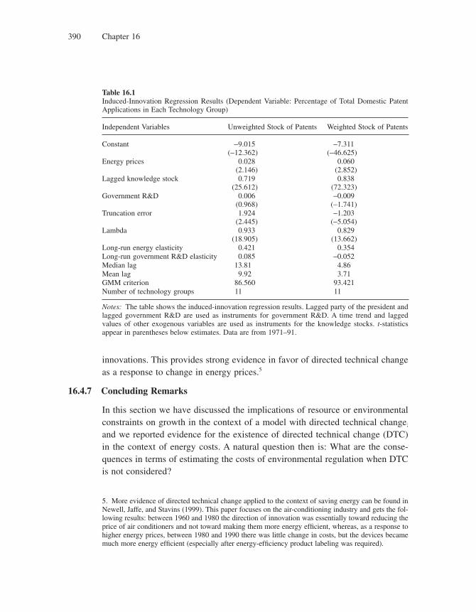
Chapter 16390
innovations. This provides strong evidence in favor of directed technical change as a response to change in energy prices.5
16.4.7 Concluding Remarks
In this section we have discussed the implications of resource or environmental constraints on growth in the context of a model with directed technical change; and we reported evidence for the existence of directed technical change (DTC) in the context of energy costs. A natural question then is: What are the conse-quences in terms of estimating the costs of environmental regulation when DTC is not considered?
Table 16.1Induced-Innovation Regression Results (Dependent Variable: Percentage of Total Domestic Patent Applications in Each Technology Group)
Independent Variables Unweighted Stock of Patents Weighted Stock of Patents
Constant −9.015(−12.362)
−7.311(−46.625)
Energy prices 0.028(2.146)
0.060(2.852)
Lagged knowledge stock 0.719(25.612)
0.838(72.323)
Government R&D 0.006(0.968)
−0.009(−1.741)
Truncation error 1.924(2.445)
−1.203(−5.054)
Lambda 0.933(18.905)
0.829(13.662)
Long-run energy elasticity 0.421 0.354Long-run government R&D elasticity 0.085 −0.052Median lag 13.81 4.86Mean lag 9.92 3.71GMM criterion 86.560 93.421Number of technology groups 11 11
Notes: The table shows the induced-innovation regression results. Lagged party of the president and lagged government R&D are used as instruments for government R&D. A time trend and lagged values of other exogenous variables are used as instruments for the knowledge stocks. t-statistics appear in parentheses below estimates. Data are from 1971–91.
5. More evidence of directed technical change applied to the context of saving energy can be found in Newell, Jaffe, and Stavins (1999). This paper focuses on the air-conditioning industry and gets the fol-lowing results: between 1960 and 1980 the direction of innovation was essentially toward reducing the price of air conditioners and not toward making them more energy effi cient, whereas, as a response to higher energy prices, between 1980 and 1990 there was little change in costs, but the devices became much more energy effi cient (especially after energy-effi ciency product labeling was required).
Preserving the Environment 391
Several papers have tried to estimate these consequences and concluded that ignoring DTC overstates the costs of environmental regulation (see Grübler and Messner 1998; Manne and Richels 2004; Messner 1997; Buonanno, Carraro, and Galeotti 2003; Nordhaus 2002; Sue Wing 2003). The measure of the overstate-ment of costs depends on specifi c characteristics of the models found in these papers, namely, the possibility of crowding out in R&D toward energy-saving innovations.
As an example, Popp (2004) modifi es the standard Nordhaus model of climate change (DICE model) to allow for induced innovation in the energy sector. After some calibration and simulation exercises and allowing for the possibility of crowding out across different kinds of R&D investment, he concludes that ignor-ing DTC overstates the welfare costs of an optimal tax policy by 9.4 percent in the base case (where partial—50 percent—crowding out is allowed).
16.5 Literature Notes
The importance of the environment has been increasingly acknowledged in both policy-making and academic circles. This is particularly the case for the relation-ship between economic growth and natural resources.
One focus on the relationship between economic development and the environ-ment has been the study of the so-called environmental Kuznets curve, that is, an inverted-U relationship between levels of country income and indicators of environmental quality (air and water pollution, for instance). The pioneering studies of such relationships were conducted by Grossman and Krueger (1991, 1995), using cross-country analyses with various environmental indicators. Those studies started a whole branch of literature discussing the validity of such reduced-form relationships (for an extensive discussion on the topic, see Dasgupta et al. 2002; Harbaugh, Levinson, and Wilson 2002).
On the relationship between growth and the environment, pioneering work has been done by Nordhaus (1974, 1977), who addressed the consequences of eco-nomic growth on the conservation of the environment and ways in which natural resources could put constraints on growth.
More specifi cally on the issue of climate change, the same author later devel-oped (see, for instance, Nordhaus 1993) a dynamic integrated model of climate change and the economy (the DICE model), which extended the neoclassical Ramsey model with equations representing geophysical relationships (emissions equation, concentrations equation, climate-change equation, climate-damage
Chapter 16392
equation) and their relationships with economic outcomes. The analysis of eco-nomic activity and its consequences in terms of climate change has been the subject of a recent and extensive report conducted by Stern (2006).
Still in the exogenous growth framework, Stockey (1998) analyzed pollution in terms of an AK model delivering an inverted-U relationship between per capita income and environmental quality and the result of nonsustainability of long-run growth (nonpositive growth).
Several recent studies have shown that the predictions of exogenous growth models are debatable, especially if one allows for the possibility of (endogenous) directed technical change (DTC). Recent empirical papers have presented evi-dence of induced technical change, namely, that energy prices affect the choice of the type of innovations (see Popp 2002 for the effect of energy prices on energy-saving innovations and Newell, Jaffe, and Stavins 1999 for the specifi c case of the air-conditioning industry).
Given the observed existence of directed technical change in energy-saving innovations, many recent papers, such as Grübler and Messner (1998), Manne and Richels (2004), Messner (1997), Buonanno, Carravo, and Galeotti (2003), Nordhaus (2002), and Sue Wing (2003), have attempted to discuss how much the costs of environmental regulation are overestimated when DTC is not considered.
The debate on the appropriate measure of costs of climate change has become an important topic of research in the fi eld, with the acknowledgment of the impor-tance of taking factors such as risk, uncertainty, and discounting into account in the analysis, as pointed out by Weitzman (2007) and Dasgupta (2008).
Appendix: Optimal Schumpeterian Growth with an Exhaustible Resource
In this appendix we solve the problem of a social planner who chooses the optimal research intensity and depletion rate of a natural resource, but then lets fi rms choose intermediate production to maximize profi ts. This solution will give us an optimal growth rate and an optimal rate q* at which to reduce the fl ow R of the exhaustible resource over time to maximize the intertemporal utility of the representative agent.
Suppose that the representative individual has isoelastic preferences, with instantaneous utility for fi nal-good consumption given by
u cc( ) =−
−1
1
σ
σ
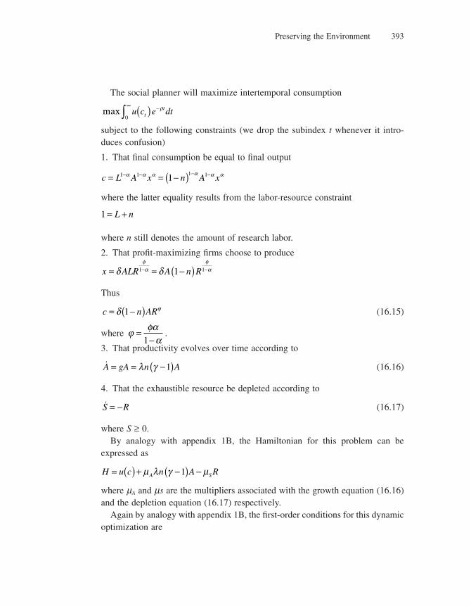
Preserving the Environment 393
The social planner will maximize intertemporal consumption
max u c e dttt( ) −∞
∫ ρ
0
subject to the following constraints (we drop the subindex t whenever it intro-duces confusion)
1. That fi nal consumption be equal to fi nal output
c L A x n A x= = −( )− − − −1 1 1 11α α α α α α
where the latter equality results from the labor-resource constraint
1 = +L n
where n still denotes the amount of research labor.
2. That profi t-maximizing fi rms choose to produce
x ALR A n R= = −( )− −δ δφα
φα1 11
Thus
c n AR= −( )δ ϕ1 (16.15)
where ϕ φαα
=−1
.
3. That productivity evolves over time according to
�A gA n A= = −( )λ γ 1 (16.16)
4. That the exhaustible resource be depleted according to
�S R= − (16.17)
where S ≥ 0.By analogy with appendix 1B, the Hamiltonian for this problem can be
expressed as
H u c n A RA S= ( ) + −( ) −μ λ γ μ1
where mA and ms are the multipliers associated with the growth equation (16.16) and the depletion equation (16.17) respectively.
Again by analogy with appendix 1B, the fi rst-order conditions for this dynamic optimization are
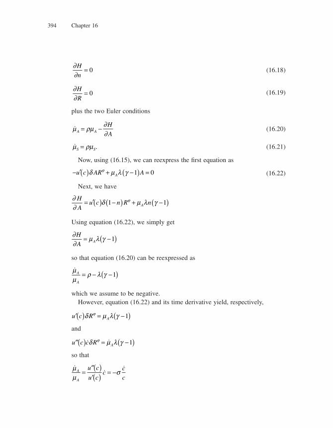
Chapter 16394
∂∂H
n= 0 (16.18)
∂∂
H
R= 0 (16.19)
plus the two Euler conditions
�μ ρμA A
H
A= − ∂
∂ (16.20)
�μ ρμS S= . (16.21)
Now, using (16.15), we can reexpress the fi rst equation as
− ′( ) + −( ) =u c AR AAδ μ λ γϕ 1 0 (16.22)
Next, we have
∂∂
H
Au c n R nA= ′( ) −( ) + −( )δ μ λ γϕ1 1
Using equation (16.22), we simply get
∂∂
H
A A= −( )μ λ γ 1
so that equation (16.20) can be reexpressed as
�μμ
ρ λ γA
A
= − −( )1
which we assume to be negative.However, equation (16.22) and its time derivative yield, respectively,
′( ) = −( )u c R Aδ μ λ γϕ 1
and
′′( ) = −( )u c c R A� �δ μ λ γϕ 1
so that
��
�μμ
σA
A
u c
u cc
c
c=
′′( )′( ) = −
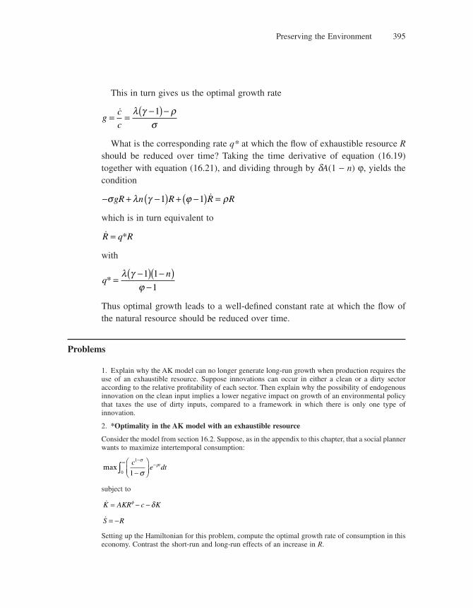
Preserving the Environment 395
This in turn gives us the optimal growth rate
gc
c= =
−( ) −� λ γ ρσ1
What is the corresponding rate q* at which the fl ow of exhaustible resource R should be reduced over time? Taking the time derivative of equation (16.19) together with equation (16.21), and dividing through by dA(1 − n) ϕ, yields the condition
− + −( ) + −( ) =σ λ γ ϕ ρgR n R R R1 1 �
which is in turn equivalent to
�R q R= *
with
qn
* =−( ) −( )
−λ γ
ϕ1 1
1
Thus optimal growth leads to a well-defi ned constant rate at which the fl ow of the natural resource should be reduced over time.
Problems
1. Explain why the AK model can no longer generate long-run growth when production requires the use of an exhaustible resource. Suppose innovations can occur in either a clean or a dirty sector according to the relative profi tability of each sector. Then explain why the possibility of endogenous innovation on the clean input implies a lower negative impact on growth of an environmental policy that taxes the use of dirty inputs, compared to a framework in which there is only one type of innovation.
2. *Optimality in the AK model with an exhaustible resource
Consider the model from section 16.2. Suppose, as in the appendix to this chapter, that a social planner wants to maximize intertemporal consumption:
maxc
e dtt1
0 1
−−∞
−⎛⎝⎜
⎞⎠⎟∫
σρ
σ
subject to
�K AKR c K= − −φ δ
�S R= −
Setting up the Hamiltonian for this problem, compute the optimal growth rate of consumption in this economy. Contrast the short-run and long-run effects of an increase in R.

Chapter 16396
3. *A variant of the directed-technical-change model with R&D externalities between the clean and dirty sectors
Consider a variant of the model from section 16.4. The fi nal-good production function and the equa-tion for the change in environmental stock are the same here as in the chapter and given by
YY Y S
tct dt t=
+ >⎧⎨⎩
⎫⎬⎭
if
otherwise
0
0
and
S S Y St t dt t+ − = − +1 φ ω
However, at each period the input baskets Yc and Yd are now produced according to
Y A x Y A xc c c d d d= =− −1 1α α α α
With respect to the innovation side of the economy, innovators may still invest in R&D targeted at a particular type of input. Let j ∈ {c, d} denote the kind of input—clean or dirty—produced in sector i. No matter in which sector they occur, innovations are assumed to increase productivity by the same multiplicative factor g > 1. Moreover, R&D efforts in both sectors make use of a common fi xed factor, which results in R&D costs for each innovation activity being an increasing function of the total R&D intensity.
More specifi cally, it costs Aj[e(zj)2 + q(zj + zh)2]/2 units of fi nal output spent on R&D targeted at input basket j to generate an innovation on that input with probability zj, where zj and zh denote the R&D intensities on inputs j and h ≠ j
a. Compute specialized monopolists’ profi ts and the equilibrium values for Yc, Yd, and Y.
b. Working on the innovators’ problem, fi nd the equilibrium R&D intensities zc, zd.
Now, suppose dirty-input monopolists’ profi ts are taxed at rate t > 0 so that they are reduced to pd(1 − t) instead of pd.
c. What are the new R&D intensities zc , zd with the introduction of the tax rate?
d. How does an increase in t affect the growth rates of Ad and Ac?
4. **Sustainable growth and optimality in the directed-technical-change model with R&D externalities
Consider the model from the previous problem.
a. Show that the dynamic equation for the change in environmental stock can be rewritten as
S S Y tt
t
d
t= +( ) − +( )⎡⎣
⎤⎦ ≥
=
− +∑1 1 10 0
1 1ω φ ωττ
τ ,
b. Looking at a steady state with Ydt = Yd0(1 + gAd)t, show that the expression in the previous item can be rewritten as
S SY
g
gt
t d
A
A
d
d= +( ) −−
−++
⎛⎝⎜
⎞⎠⎟
⎡
⎣⎢⎢
⎤
⎦⎥⎥
⎧⎨⎪
⎩⎪
⎫⎬⎪
⎭⎪1 1
1
100ω φ
ω ω
c. What is the upper bound for gAd for growth to be sustainable (i.e., non-negative in steady state)?
d. Argue that another necessary condition for sustainable growth is fYd0 ≤ (w − gAd)S0. Interpret this condition.
Suppose the economy has a government that is interested in maximizing the net present value of consumption minus R&D effort cost and that ignores the R&D externalities between the clean and
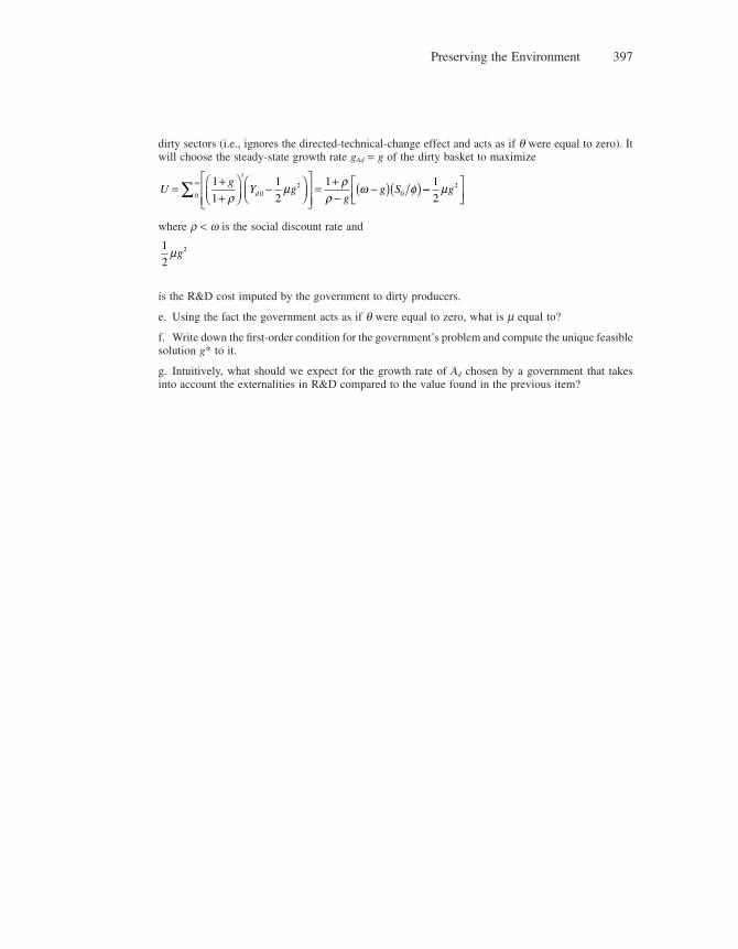
Preserving the Environment 397
dirty sectors (i.e., ignores the directed-technical-change effect and acts as if q were equal to zero). It will choose the steady-state growth rate gAd = g of the dirty basket to maximize
Ug
Y gg
g St
d= ++
⎛⎝⎜
⎞⎠⎟
−⎛⎝⎜
⎞⎠⎟
⎡
⎣⎢⎢
⎤
⎦⎥⎥
= +−
−( )( )∞∑ 1
1
1
2
10
2
0 0ρμ ρ
ρω φ −−⎡
⎣⎢⎤⎦⎥
1
22μg
where r < w is the social discount rate and
1
22μg
is the R&D cost imputed by the government to dirty producers.
e. Using the fact the government acts as if q were equal to zero, what is m equal to?
f. Write down the fi rst-order condition for the government’s problem and compute the unique feasible solution g* to it.
g. Intuitively, what should we expect for the growth rate of Ad chosen by a government that takes into account the externalities in R&D compared to the value found in the previous item?

17 Promoting Democracy
17.1 Introduction
Does democracy enhance or hamper economic growth? Recent empirical studies on the subject (see section 17.2) suggest no clear relationship between democracy and growth in cross-country panel regressions once we control country fi xed effects. However, one may think of various channels whereby democracy should affect per capita GDP growth. A fi rst channel is that democracy reduces corrup-tion and thus facilitates entry and exit, which in turn facilitates innovation and technical progress. A second channel is that democracy pushes for more redistri-bution from rich to poor, and that redistribution in turn affects growth. In section 17.3 we explore the fi rst channel: we introduce political economy considerations into the entry model of chapter 12. And we show that democracy enhances entry, which in turn is more growth-enhancing in more advanced countries and sectors. This prediction of a positive interaction between democracy, entry, and techno-logical development is tested in section 17.4. The second channel is explored in section 17.5. There we present a model by Persson and Tabellini (1994)1 where the redistribution policy is chosen by the median voter. The more unequal the distribution of wealth, the higher the median voter’s demand for redistribution. Redistribution in turn affects growth negatively as it discourages capital accumulation.
17.2 Democracy, Income and Growth in Existing Regressions
Cross-country regressions by Barro (1999a) point to a positive correlation between income and democracy, that is, richer countries tend to be more democratic. Similarly, Aghion, Alesina, and Trebbi (2004) show that richer countries tend to have less insulated political institutions, where insulation is measured by the extent to which the political system is presidential instead of parliamentary and/or representatives are elected through majority rule rather than through proportional rule.
However, these relationships are between democracy and income, not democracy and growth. Moreover, the emphasis is on the causality from income to democracy, not the causality from democracy to income or income growth.
1. A continuous-time variant of that model, developed in parallel by Alesina and Rodrik (1994), is presented in the problem set section to this chapter.
Chapter 17400
Two recent studies have contributed to lowering our hopes of uncovering any interesting effect of democracy on growth. The fi rst study, by Acemoglu, Johnson, Robinson, and Yared (2005), henceforth AJRY, shows that the positive correlation between democracy and income in cross-country regressions disappears once we move to panel data and control for country fi xed effects. The second study, by Mul-ligan, Gil, and Sala-i-Martin (2004), henceforth MGS, has produced cross-country regressions over the period 1960–90 showing that democracy is uncorrelated with policies such as education spending, pensions and welfare, corporate taxation, open-ness to trade, and other policies that should affect barriers to entry. In the remaining part of this section we describe these two studies in somewhat greater detail.
17.2.1 Irrelevance Results When Controlling for Country Fixed Effects
Being primarily interested by the causality from income to democracy, and using cross-country panel data over the period 1960–2000, Acemoglu, Johnson, and colleagues (2005), AJRY, estimate the regression model
d d y X uit it it it t i it= + + + + +− − −α γ β μ δ1 1 1
where dit. measures democracy in country i at date t,2 yit−1 is country i’s per capita GDP in period t − 1, Xit−1 are covariates, mt controls for time effects, di controls for country fi xed effects, and uit is the error term. Each time period lasts for fi ve years.
AJRY fi nd that the estimate for g becomes insignifi cant once we control for country fi xed effects. And indeed, fi gure 17.1, which plots changes in these two measures of democracy as a function of the change in GDP per capita over the period 1970–2003, shows no signifi cant relationship between democracy and income per capita.
17.2.2 No Apparent Correlation between Democracy and Public Policy
Using a cross-section of 142 countries over the whole period 1960–90, Mulligan, Gil, and Sala-i-Martin (2004), MGS, estimate the effect of democracy, measured by the same Polity index as in AJRY, on a whole range of policies: redistribution policies such as government consumption, education spending, and social spend-ing, and policies affecting entry and turnover such as death penalty, military spending, civil liberties, state religion, conscription, and open trade.
2. AJRY use both the Freedom House indicator and the Polity indicator to measure democracy. The former index is constructed for each country as an aggregate score based on the answers to such questions as “Are there free elections?”; “Are there competitive parties?”; “Does the opposition enjoy power?” The Polity code refl ects the openness of the political process and the constraints on govern-ment executives. Freedom and Polity scores are computed for each country for each year between 1970 and 2003.
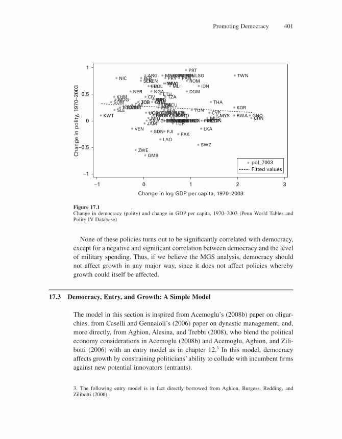
Promoting Democracy 401
None of these policies turns out to be signifi cantly correlated with democracy, except for a negative and signifi cant correlation between democracy and the level of military spending. Thus, if we believe the MGS analysis, democracy should not affect growth in any major way, since it does not affect policies whereby growth could itself be affected.
17.3 Democracy, Entry, and Growth: A Simple Model
The model in this section is inspired from Acemoglu’s (2008b) paper on oligar-chies, from Caselli and Gennaioli’s (2006) paper on dynastic management, and, more directly, from Aghion, Alesina, and Trebbi (2008), who blend the political economy considerations in Acemoglu (2008b) and Acemoglu, Aghion, and Zili-botti (2006) with an entry model as in chapter 12.3 In this model, democracy affects growth by constraining politicians’ ability to collude with incumbent fi rms against new potential innovators (entrants).
NPLMARCOGURY
BEN
BFA
GINGTMHNDSLVGABZMBTGO
ARG
BOL
BWA
CAF
CHN
CIV
CMR
DOMETH
FJI
GHA
GMB
GNQ
IDNIRN
JOR
KEN
KHM
KOR
KWT
LAO
LKA
LSO
MDG
MEXMLI
MWI
NER NGA
NIC
PAK
PER
PRT
ROM
RWA
SDN
SLE
SOM
SWZ
TCD THA
TUN
TWN
TZA
VEN
ZWE
Ch
ang
e in
po
lity,
197
0–20
03
–1 0 1 2 3
Change in log GDP per capita, 1970–2003
DZAECUZAF
PHL
SENBRAMNG
PRYESPGRCHUN
PANPOL
BTN
CYP
IRLMUSMYS
PRKSGPAUSAUTBELCANCHE COLCRI CUBDNKFINGBR INDITAJPNNLD NORNZLSWETUR
USA
CHLOMNSYRTTO
JAMMRT
SAU
UGA
1
0.5
0
–0.5
–1
pol_7003Fitted values
Figure 17.1Change in democracy (polity) and change in GDP per capita, 1970–2003 (Penn World Tables and Polity IV Database)
3. The following entry model is in fact directly borrowed from Aghion, Burgess, Redding, and Zilibotti (2006).
Chapter 17402
17.3.1 Production and Profi ts
Time is discrete, and all agents live for one period. There is one fi nal good pro-duced competitively using a continuum of intermediate inputs, indexed from 0 to 1, according to the technology
y A x dit it it= −∫ 1
0
1 α α
where xit is the quantity of intermediate input produced in sector i at date t, Ait is a productivity parameter that measures the quality of the intermediate input i in producing the fi nal good, and the parameter a ∈ (0, 1). The fi nal good can be used either for consumption, or as an input in the process of production of inter-mediate goods, or for investments in innovation.
In each intermediate sector i, only one fi rm (a monopolist) is active in each period, and it produces intermediate input i using fi nal output as input, one for one. Since the fi nal-good sector is competitive, the intermediate monopolist i sells its intermediate good to the fi nal-good sector at a price equal to its marginal cost:
p A xit it it= ( ) −α α1 (17.1)
Then, profi t maximization yields the choice
x Ait it= −α α2
1
and the equilibrium profi t
π πit it= Α (17.2)
where πα
α α≡ −⎛⎝⎜
⎞⎠⎟
−11
2
1 .
Substituting for xit in the production function for fi nal output, we also get
y At t= ϕ (17.3)
where
A A dit it= ∫0
1
is the average productivity at date t and ϕ is a constant.
17.3.2 Entry and Incumbent Innovation
Let p denote the probability that a potential entrant shows up in any intermediate sector. The government directly chooses this parameter, but it is subject to
Promoting Democracy 403
infl uence activities by incumbent fi rms that want to prevent entry. We consider these infl uence activities in more detail in the next subsection.
There are only two types of intermediate fi rms: advanced fi rms, with frontier productivity Ait = At, and backward fi rms with below-frontier productivity
A Ait t= 1
γ, where frontier productivity At, grows at a constant rate over time,
namely,
A At t= −γ 1
with g > 1.We focus on technologically advanced entry; accordingly, each potential
entrant arrives at date t with the current leading-edge technology At . An advanced incumbent fi rm can use its fi rst-mover advantage to block entry and thereby retain its monopoly power. However, if the incumbent fi rm fails to reach the new tech-nological frontier, and if entry occurs in the corresponding sector, then Bertrand competition will take place between the incumbent and the entrant. As a result of Bertrand competition, the technologically dominated incumbent will be elimi-nated and replaced by the entrant.
We assume that to innovate at date t an intermediate fi rm must incur the R&D cost citAit−1 (where Ait−1 denotes its current productivity), and innovating in turn allows the incumbent fi rm to multiply its productivity by the factor g. We assume cit to be random and independently and identically distributed across intermediate sectors, with cit ∈ {0, c}, and
Pr Prc c cit it=( ) = =( ) =01
2
The effect of entry threat (as parametized by p) on incumbent innovation will depend on the marginal benefi t that the incumbent expects to receive from an innovation given p.
Consider fi rst an incumbent who was an advanced fi rm last period. If she innovates, then she will remain a frontier fi rm this period, and hence will be immune to entry.4 Her profi t will then be equal to pAt. If she fails to innovate, then with probability p she will be eliminated by entry and earn zero profi t, while
4. As in chapter 12, we implicitly assume that entry entails a positive sunk cost, and that a potential entrant observes whether the incumbent fi rm in its target sector has innovated or not, before deciding whether or not to enter. If the incumbent fi rm managed to innovate and thereby to move to current frontier productivity, then entering would yield zero ex post profi t to the entrant. Anticipating this outcome, the potential entrant will decide not to pay the sunk cost of entry.
Chapter 17404
with probability 1 − p she will survive the entry threat (as entry is not occurring) and thereby earn profi t pAt−1. Thus an advanced fi rm with innovation cost cit will innovate whenever
π γ π γ− −( )⎡⎣ ⎤⎦ = − +( ) >1 1p p cit (17.4)
and then its profi t will be
π πγit it itc A= −( ) −1 (17.5)
In particular, we see from equation (17.4) that an increase in entry threat encour-ages this incumbent to innovate. Intuitively, a fi rm close to the frontier responds to increased entry threat by innovating more in order to escape the entry threat.
Next, consider an incumbent who was a backward fi rm last period, and who will therefore remain behind the frontier even if he manages to innovate, since the frontier will also advance by the factor g. For this fi rm, profi ts will be zero if entry occurs, whether he innovates or not, because he cannot catch up with the frontier. Thus he will innovate whenever
π γ1 1−( ) −( ) >p cit (17.6)
in which case his profi t will be
π πγit it itp c A= −( ) −⎡⎣ ⎤⎦ −1 1
where the fi rst term is the profi t gain from innovation that will be realized with probability (1 − p), the probability that no potential entrant shows up in the cor-responding sector. Thus in this case innovation incentives depend negatively on the entry threat p. Intuitively, the fi rm that starts far behind the frontier is discour-aged from innovating as much by an increased entry threat because he is unable to prevent the entrant from destroying the value of his innovation.
We assume that initially the entry rate p is equal to zero, and we make the following assumption (assumption 1):
π γ −( ) <1 c
so that, absent any entry threat, no fi rm with innovation cost equal to c ever innovates.
Using these assumptions, one can determine the steady-state fraction of advanced fi rms conditional upon p = 0. Thus, suppose that an advanced fi rm that successfully innovates at date t starts out in period t + 1 as an advanced fi rm. All
Promoting Democracy 405
other fi rms start out as backward fi rms. Moreover, with exogenous probability h, a backward fi rm at the end of period t is replaced by a new, advanced fi rm at date t + 1. If at denotes the fraction of advanced fi rms at t, then it satisfi es the dynamic equation
a z a h z at A t A t+ = + −( )1 1
where
z cA = =( ) =Pr 01
2
is the probability that an advanced fi rm innovates if p = 0.In particular the steady-state fraction of advanced fi rms is simply
ah
h
h
h* =
− −( ) =+1 1
2
112
17.3.3 Politics and the Equilibrium Probability of Entry
Suppose that entry policy p is determined each period by a politician who cares about current consumption but may also respond to bribes. Following Acemoglu, Aghion, and Zilibotti (2006), or AAZ, we assume that the politician’s payoff is equal to HAt, where H > 0, if she chooses the policy that maximizes current output yt, and to Bt otherwise, where Bt denotes the bribe that the politician may receive from private fi rms to limit entry. The parameter H refl ects the aggregate welfare concerns of politicians, or the effectiveness of checks and balances that the political system imposes on politicians, and we use it as our proxy for democracy.
To compute the equilibrium bribe that incumbent fi rms are willing to pay to prevent moving from initial entry probability p0 = 0 to p > 0, we need to compute the equilibrium payoffs for each type of fi rm (advanced or backward) and for each cost realization cit = 0 or c as a function of p.
Consider fi rst an advanced fi rm. If this fi rm’s innovation cost is zero, then the fi rm will always innovate, and its postinnovation profi t pg is independent of the entry probability. However, if the innovation cost is c, this fi rm will lose from higher entry threat only if the threat p becomes suffi ciently high that condition (17.4) holds. Then; indeed; using expression (17.5) for profi ts, the fi rm will lose Ait−1 = At times the amount
Chapter 17406
π πγ π γ− −( ) = − −( )c c 1
which is positive by assumption 1. Thus the maximum bribe that advanced fi rms as a group would be ready to pay to prevent an increase in entry threat from zero to p is given by
B p A a ca t p c( ) = − −( )⎡⎣ ⎤⎦ ⋅ − +( )>⎡⎣ ⎤⎦* π γ π γ1 1
1
where 1[p(g−1+p)>c] is equal to one whenever equation (17.4) holds and to zero otherwise.
Now, consider a backward (or below-frontier) fi rm. Such a fi rm will innovate if and only if cit = 0 by assumption 1, no matter the entry probability. And it will lose from a higher threat of entry, whether it innovates or not, just because this reduces its probability of survival. If the fi rm turns out to have low
innovation cost (cit = 0), it innovates and therefore loses A Ait t− =1
1
γ times the
amount
πγ πγ1 1− −( )⎡⎣ ⎤⎦ =p p
if the entry probability increases from 0 to p. If the fi rm turns out to have high
innovation cost (cit = c), it will not innovate and therefore loses A Ait t− =1
1
γ times
the amount
π π1 1− −( )⎡⎣ ⎤⎦ =p p
if the entry probability increases from 0 to p. Since, ex ante, the fi rm has equal probabilities 1
2 to have high or low innovation costs, the maximum bribe back-ward fi rms as a group are willing to pay to prevent an increase in entry threat from zero to p, is equal to
B p A a p pb t( ) = −( ) +⎛⎝⎜
⎞⎠⎟
11
1
2
1
2γπγ π*
where the fi rst (resp. second) term in the bracket is the expected loss incurred by backward fi rms with low (resp. high) innovation cost.
Altogether, incumbent fi rms will successfully prevent the increase in entry threat from zero to p whenever p is greater than p* such that the politician is just indifferent between accepting and refusing the aggregate bribe in order not to increase the entry threat from zero to that probability, namely,
B p B p B p HAa b t* * *( ) = ( ) + ( ) = (17.7)
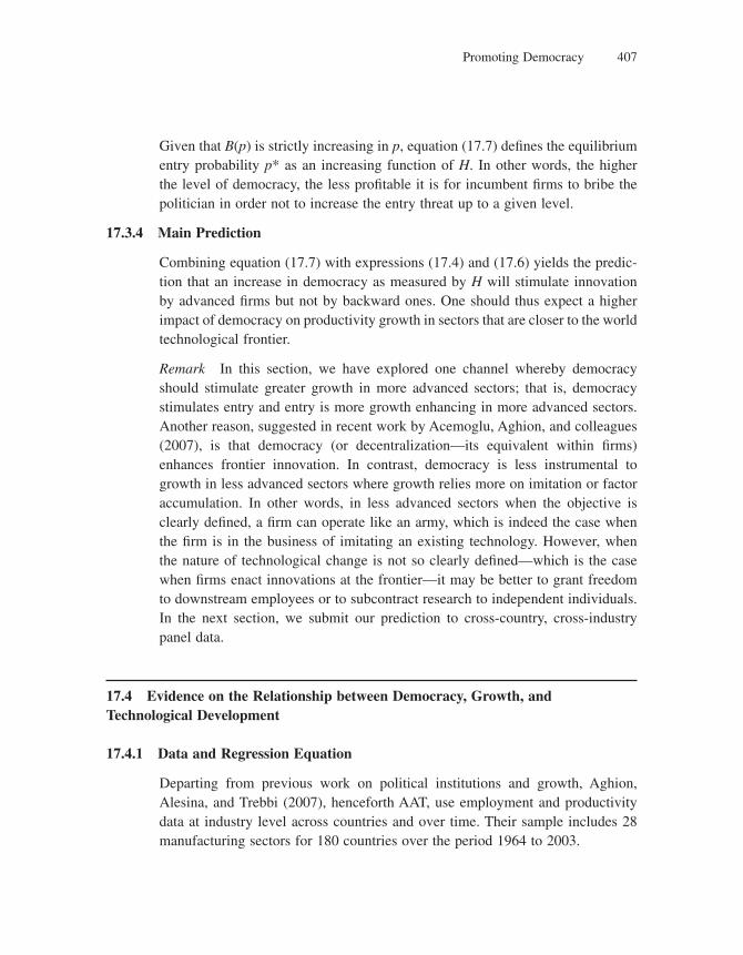
Promoting Democracy 407
Given that B(p) is strictly increasing in p, equation (17.7) defi nes the equilibrium entry probability p* as an increasing function of H. In other words, the higher the level of democracy, the less profi table it is for incumbent fi rms to bribe the politician in order not to increase the entry threat up to a given level.
17.3.4 Main Prediction
Combining equation (17.7) with expressions (17.4) and (17.6) yields the predic-tion that an increase in democracy as measured by H will stimulate innovation by advanced fi rms but not by backward ones. One should thus expect a higher impact of democracy on productivity growth in sectors that are closer to the world technological frontier.
Remark In this section, we have explored one channel whereby democracy should stimulate greater growth in more advanced sectors; that is, democracy stimulates entry and entry is more growth enhancing in more advanced sectors. Another reason, suggested in recent work by Acemoglu, Aghion, and colleagues (2007), is that democracy (or decentralization—its equivalent within fi rms) enhances frontier innovation. In contrast, democracy is less instrumental to growth in less advanced sectors where growth relies more on imitation or factor accumulation. In other words, in less advanced sectors when the objective is clearly defi ned, a fi rm can operate like an army, which is indeed the case when the fi rm is in the business of imitating an existing technology. However, when the nature of technological change is not so clearly defi ned—which is the case when fi rms enact innovations at the frontier—it may be better to grant freedom to downstream employees or to subcontract research to independent individuals. In the next section, we submit our prediction to cross-country, cross-industry panel data.
17.4 Evidence on the Relationship between Democracy, Growth, and Technological Development
17.4.1 Data and Regression Equation
Departing from previous work on political institutions and growth, Aghion, Alesina, and Trebbi (2007), henceforth AAT, use employment and productivity data at industry level across countries and over time. Their sample includes 28 manufacturing sectors for 180 countries over the period 1964 to 2003.
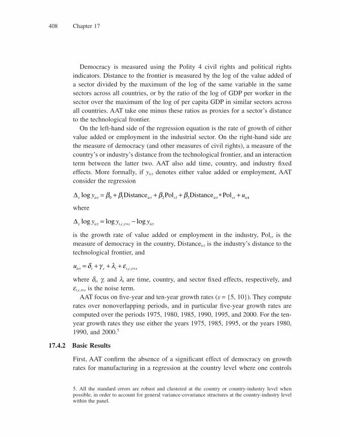
Chapter 17408
Democracy is measured using the Polity 4 civil rights and political rights indicators. Distance to the frontier is measured by the log of the value added of a sector divided by the maximum of the log of the same variable in the same sectors across all countries, or by the ratio of the log of GDP per worker in the sector over the maximum of the log of per capita GDP in similar sectors across all countries. AAT take one minus these ratios as proxies for a sector’s distance to the technological frontier.
On the left-hand side of the regression equation is the rate of growth of either value added or employment in the industrial sector. On the right-hand side are the measure of democracy (and other measures of civil rights), a measure of the country’s or industry’s distance from the technological frontier, and an interaction term between the latter two. AAT also add time, country, and industry fi xed effects. More formally, if yict denotes either value added or employment, AAT consider the regression
Δs ict ict cl ict ct icy ulog = + + + ∗ +β β β β0 1 2 3Distance Pol Distance Pol tt
where
Δs ict i c t s icty y ylog log log, ,= −+
is the growth rate of value added or employment in the industry, Polct is the measure of democracy in the country, Distanceict is the industry’s distance to the technological frontier, and
uict t c i i c t s= + + + +δ γ λ ε , ,
where dt, gc and li are time, country, and sector fi xed effects, respectively, and ei,c,t+s is the noise term.
AAT focus on fi ve-year and ten-year growth rates (s = {5, 10}). They compute rates over nonoverlapping periods, and in particular fi ve-year growth rates are computed over the periods 1975, 1980, 1985, 1990, 1995, and 2000. For the ten-year growth rates they use either the years 1975, 1985, 1995, or the years 1980, 1990, and 2000.5
17.4.2 Basic Results
First, AAT confi rm the absence of a signifi cant effect of democracy on growth rates for manufacturing in a regression at the country level where one controls
5. All the standard errors are robust and clustered at the country or country-industry level when possible, in order to account for general variance-covariance structures at the country-industry level within the panel.
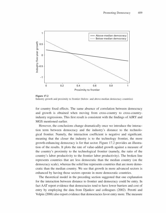
Promoting Democracy 409
for country fi xed effects. The same absence of correlation between democracy and growth is obtained when moving from cross-country to cross-country-industry regressions. This fi rst result is consistent with the fi ndings of AJRY and MGS mentioned earlier.
However, the conclusions change dramatically once we introduce the interac-tion term between democracy and the industry’s distance to the technolo-gical frontier. Namely, the interaction coeffi cient is negative and signifi cant. meaning that the closer the industry is to the technology frontier, the more growth-enhancing democracy is for that sector. Figure 17.2 provides an illustra-tion of the results. It plots the rate of value-added growth against a measure of the country’s proximity to the technological frontier (namely, the ratio of the country’s labor productivity to the frontier labor productivity). The broken line represents countries that are less democratic than the median country (on the democracy scale), whereas the solid line represents countries that are more demo-cratic than the median country. We see that growth in more advanced sectors is enhanced by having those sectors operate in more democratic countries.
The theoretical model in the preceding section suggested that one explanation for the interaction between distance to frontier and democracy could be entry. In fact AAT report evidence that democracies tend to have lower barriers and cost of entry by employing the data from Djankov and colleagues (2002). Perotti and Volpin (2006) also report evidence that democracies favor entry more. The measure
Ind
ust
ry f
ive-
year
gro
wth
0 0.2 0.4 0.6 0.8 1
Proximity to frontier
1
0.5
0
–0.5
–1
Above-median democracyBelow-median democracy
Figure 17.2Industry growth and proximity to frontier (below- and above-median democracy countries)
Chapter 17410
of entry barriers in AAT, borrowed from Djankov and colleagues, is the number of bureaucratic procedures needed for a fi rm to enter the market. This is important for our story because we argue that democracy matters for more advanced sectors of the economy because of the need for more entry and competition in sectors close to the technological frontier where innovation is especially important for growth.
But this is not enough to conclude that entry is truly the reason behind the positive correlation between democracy and growth in more advanced sectors. In addition, one needs to make sure that, once controlling for entry barriers, the effect of democracy and of its interaction with technological development remains signifi cant. Unfortunately, using the Djankov and colleagues’ index (the number of procedures needed to start up a new fi rm) as a proxy for entry does not affect the preceding regression results in any signifi cant way. However, when replacing the number of procedures with the effective level of entry in the sector, measured by the growth rate in the number of establishments, AAT fi nd that the effect of democracy is substantially reduced. This fi nding suggests that the entry channel at least partly explains why democracy may be conducive to growth in sectors closer to the technological frontier rather than other less advanced sectors. Overall, there is evidence of a differential effect of democracy across sectors and countries at different stages of development.
17.5 Democracy, Inequality, and Growth
In parallel contributions, Persson and Tabellini (1994) and Alesina and Rodrik (1994) analyze the relationship between inequality, democratic voting, and growth. They develop models in which redistribution from rich to poor is detri-mental to growth as it discourages capital accumulation. More inequality is then also detrimental to growth because it results in the median voter becoming poorer and therefore demanding more redistribution.
17.5.1 The Model
More formally, consider an economy populated by a continuum of overlapping generations. Each individual lives for two periods. An individual i born at date t − 1 has intertemporal utility function
U c d c dti
ti
ti
ti
− −( ) = +1 1, ln ln
where c it−1 denote individual i’s consumption when young (in period t − 1) and
dit denote the individual’s consumption when old (in period t).
Promoting Democracy 411
Individual i starts out with initial income endowment
y w e kti i
t− −= +( )1 1 (17.8)
where w is an average endowment of basic skills available to all individuals, and ei is an extra skill endowment specifi c to individual i. Richer individuals have more positive eis, poorer individuals have more negative eis. We assume that the mean value of ei across individuals is equal to zero.
Note the term kt−1 on the right hand side of equation (17.8). This term encap-sulates an AK externality: all individuals born at date t − 1 benefi t from the general knowledge embodied in the accumulated aggregate capital kt−1.
This initial income is divided between consumption c ii−1 and investment k i
t:
y c kti
ti
ti
− −= +1 1 (17.9)
Finally, consumption of the old is assumed to be equal to
d k kti
t ti
t t= −( ) +1 θ θ (17.10)
where the variable qt measures the level of redistribution. When qt = 1, all indi-viduals consume the same amount when old.
The timing of events is the following within each period: (1) at the beginning of period t − 1 young voters choose the level of redistribution qt that will apply to them when old; (2) each individual i chooses her investment k i
t.
17.5.2 Solving the Model
17.5.2.1 Equilibrium Growth Rate for Given Redistribution Policy
Take fi rst the redistribution policy qt as given. Individual i will choose her invest-ment k i
t to solve
max ln lnk
ti
ti
ti
c d− +{ }1
subject to equations (17.9) and (17.10).In other words, individual i will choose k i
t to
max ln lnk
it t
it t
it t
ti
w e k k k k+( ) −⎡⎣ ⎤⎦ + −( ) +⎡⎣ ⎤⎦{ }−1 1 θ θ
The fi rst order condition for this maximization is
1 1
11w e k k k kit t
i
t
t ti
t t+( ) −=
−( )−( ) +−
θθ θ
Chapter 17412
or equivalently
2 1 1 1−( ) = −( ) +( ) −−θ θ θt ti
ti
t t tk w e k k (17.11)
Not surprisingly, the more negative ei, the lower the investment k it.
Now. using the fact that
k k dit ti= ∫
and integrating equation (17.11) over all individuals i, we obtain
2 1 1 1−( ) = −( ) +( ) −−θ θ θt t ti
t t tk w e k k
or equivalently
2 1 1−( ) = −( ) −θ θt t t tk wk (17.12)
The equilibrium growth rate between period t − 1 and period t is then simply given by
gk
k
w et
t
t
ti
t
= − =−( ) +( )
−−
−1
11
21
θθ
which is clearly decreasing in the level of redistribution qt. The intuition is simply that more redistribution discourages individual capital accumulation.
17.5.2.2 Political Equilibrium and the Effect of Inequality on Growth
So far, we have taken the level of redistribution qt as given. Now, we endogenize it as the equilibrium outcome of a median voter game among all individuals. A fi rst step is to analyze the preferred redistribution policy of individual i with initial skills w + ei.
This individual would choose the redistribution level qt that maximizes
V w e k k k kti
tk
it t
it t
it t
ti
θ θ θ( ) = +( ) −⎡⎣ ⎤⎦ + −( ) +⎡⎣ ⎤⎦{ }−max ln ln1 1
The optimal qt (from the point of view of individual i) satisfi es
dV
dti
tθ= 0
where, using the envelope theorem, and then equation (17.12)
dV
dk k
kk k
wkti
tt t
it
t
tt t
it
t
tθ
θθ
θθ
= − + = − +−( )
−∂∂
12
2 (17.13)
Promoting Democracy 413
Because the function
θθt
t22−( )
is increasing in qt, we obtain the redistribution qt, which is preferred by individual i, is a decreasing function of k i
t and therefore a decreasing function of her initial endowment w + ei. In other words, poorer individuals have higher demand for redistribution. The preceding equation also shows that individual preferences over redistribution are single-peaked. This in turn implies that the equilibrium redistribution policy in a majority voting game is the redistribution chosen by the median voter.6
Now the more unequal the skill distribution, the more negative the idiosyn-cratic skill em of the median voter, and therefore the higher her demand q(em) for redistribution. This in turn will result in a lower equilibrium growth rate
ge w e
e
m m
m=
− ( )( ) +( )− ( ) −
1
21
θ
θ
17.5.3 Discussion
Persson and Tabellini (1994) test the predictions of this model using postwar data on 56 countries. Regressing growth on income equality in a cross-section of these countries, they fi nd that the better the relative position of the middle quintile of income (which they take to refl ect a higher degree of income equality), the higher the average annual growth rate over the period 1960–85. Moreover, this positive correlation between income equality and growth is found to be signifi cant only for democracies, not for nondemocracies.
Using the Gini coeffi cient as the measure for income inequality, and a some-what different cross-country sample over the period 1960–85, Alesina and Rodrik (1994) also fi nd a negative correlation between inequality and growth. However, they do not fi nd a signifi cant interaction between the democracy dummy and the Gini coeffi cient. More recent studies have questioned the robustness of the rela-tionship between inequality and growth, and therefore the robustness of the fi nd-ings and predictions in this section.7
6. Here we refer the reader to the classic political economy textbook by Persson and Tabellini (2000).
7. In particular, see Banerjee and Dufl o (2003).
Chapter 17414
17.6 Conclusion
In this chapter we have looked at the causal relationship between democracy and growth. Starting from the negative fi nding that democracy and growth are uncor-related in cross-country data, we moved the analysis forward by (1) looking at cross-industry data; (2) interacting democracy with technological development at sectoral level, and (3) looking at the specifi c role of entry. In particular, we saw that democratic institutions favor growth in sectors of the economy that are more technologically advanced. Then in the second part of the chapter we discussed the relationship between democracy, inequality, and growth.
The fact that growth is increasingly enhanced by democracy as a country becomes more technologically advanced does not imply that countries should automatically move to democracy as they develop. Indeed, as we saw in chapter 11, countries may get stuck with political institutions that become increasingly inappropriate as they move closer to the technological frontier. However, there is an idea, neither precisely formalized by the existing literature nor extensively confronted with data, that economic growth requires the development of an edu-cated middle class that eventually pushes for the transition to democracy. We saw this process at work in South Korea, South Africa, Latin America, and the Soviet bloc. The big exception so far is of course China, but for how much longer?
17.7 Literature Notes
Existing analyses of the relationship between democracy and growth address both the causality from income or growth to democracy or the reversed causation.
Przeworski and Limongi (1993) present a summary of theoretical arguments in the direction of both positive and negative effects of democracy on growth. Then, as we discussed in section 17.5, Persson and Tabellini (1994) suggest that democracy tends to magnify the negative correlation between inequality and growth. In a fi rst attempt at looking at democracy and growth in the data and using cross-country panel regressions (but not controlling for country fi xed effects), Barro (1996) points at a nonlinear relationship whereby more democracy enhances growth at low levels of political freedom but reduces growth when a moderate level of freedom has already been achieved.
Looking at the reverse causation from growth to democracy, Barro (1999a) points out that higher levels of income predict increases in democracy (measured
Promoting Democracy 415
by an indicator of electoral rights). Aghion, Alesina, and Trebbi (2004) endoge-nize the choice of political institutions and show that richer countries tend to have less insulated political systems (i.e., there is a higher degree of expost control over the politician once appointed).
Recent work by Acemoglu, Johnson, Robinson, and Yared (2005) shows that the positive correlation between democracy and income in cross-country regres-sions disappears once one controls for country fi xed effects in cross-country panel regressions. Similarly, Mulligan, Gil, and Sala-i-Martin (2004) show that democ-racy is uncorrelated with several policy variables that affect growth (such as education spending, pensions and welfare, and openness to trade). However Aghion, Alesina, and Trebbi (2007) show that signifi cant correlations between democracy and growth reappear once we allow for interaction terms between democracy and countries’ or industries’ levels of technological development.
Regarding the impact of electoral rules (such as presidentialism versus parlia-mentarianism) on economic outcomes, an extensive treatment can be found in Persson and Tabellini (2003). Finally, we refer the reader to a forthcoming book edited by Helpman on Institutions and Economic Performance, for frontier work on the subject.
Problems
1. Explain intuitively how democracy can promote innovation and technical progress. Why does democracy affect growth more positively in more advanced countries?
2. *The factor distribution of income and economic growth (based on Alesina and Rodrik 1994)
This problem presents a model related to Persson and Tabellini (1994) presented in the chapter. The main idea is that the saving behavior of capitalists and workers is different, and hence the pattern of ownership of the means of production can affect economic growth.
Consider an economy with two types of individuals, workers and capitalists. Workers supply inelastically one unit of labor, do not save, and consume all their income. The capitalists own all the stock of capital, do not work, consume, and save. Output depends on public expenditure on a public good, g, as well as on labor and capital (see Barro 1990). That is,
y Ak l= < <− −α α αγ α1 1 0 1where
The labor endowment is constant and normalized to unity.
Public expenditure is fi nanced by a tax on the return to capital, t. The government cannot borrow; hence it must always have a balanced budget. Tax revenues can be spent on transfers to workers as well as on the provision of g. Let l ∈ [0, 1] be the share of government revenue that is transferred to workers. Transfers are then ltk,
a. Explain why the government budget constraint implies
Chapter 17416
γ λ τ= −( )1 k
The representative capitalist faces the following problem:
max logU c e dt
k r k c
k k t
k
=
= −( ) −
−∞
∫ ρ
τ0
subject to �
where ck is the capitalist’s consumption level. Similarly, denote a worker’s consumption by cl. Her consumption decision problem is then given by
max logU c e dt
c w k
l l t
l
=
= +
−∞
∫ ρ
λτ0
subject to
where w is the wage, which is equal to the marginal product of labor.
The government chooses l and t at each point in time to maximize the weighted average of the welfare of the two groups. Let b ∈ [0, 1] be the weight given to workers’ welfare, and (1 − b) that of capitalists’ welfare.
b. Find the dynamic equation for the capitalists’ consumption. What are the steady-state rates of growth of capital and of workers’ consumption? Express the steady-state rate of growth of the economy in terms of model parameters and the policy instruments only.
c. How does the steady-state rate of growth depend on l and t? Find the values of these two policy instruments that maximize the steady-state growth rate.
d. Suppose the government maximizes the welfare of the capitalists (i.e., b = 0). Which values of l and t will it choose?
e. Suppose the government cares also about the welfare of the workers (i.e., b > 0). Obtain the fi rst-order conditions for welfare maximization. Examine them to see that whenever workers’ welfare enters the welfare function, the growth rate is not maximized. Show that if b ≥ [(1 − a)A]1/a/r, then the optimal transfers value is l** = 1 − [(1 − a)A]1/a/br and the optimal tax rate is t** = br. What are the optimal values of l and t if the preceding restriction is not satisfi ed?
3. *Majority voting, the distribution of factor endowments and economic growth (based on Alesina and Rodrik 1994)
Consider the same economy as in the previous problem, except that now all individuals own some labor and some capital, although in different proportions. Let li and ki denote the amount of labor and of capital owned by agent i. Let k denote the aggregate stock of capital. Then her relative factor endowment is given by
σ σii
iil
k k= ∈ ∞[ )0,
The tax system is the same as before, except that there are no transfers (l = 0). The instantaneous-utility function is logarithmic for all agents. All agents save and borrow at the risk-free interest rate.
a. Show that the rate of growth of individual consumption is the same for all agents.
b. Which is the tax rate that maximizes the growth rate?
c. Which is the tax rate preferred by individual i?
d. If the tax rate is chosen by majority voting, is there a relationship between inequality and growth?

CONCLUSION

18 Looking Ahead: Culture and Development
Let us conclude our journey into the economics of growth by pointing out uncharted territory, at issues that should preoccupy growth economists but have yet remained largely unexplored. Our main focus in this chapter will be on culture and on the relationship between growth, development, and industrial policy. But before we proceed, let us step back and briefl y review what we have learned from our discussions in the previous chapters.
18.1 What We Have Learned, in a Nutshell
Part I laid down the main growth paradigms. We fi rst analyzed the benchmark neoclassical growth model and showed why this model can explain cross-country convergence but not long-run growth. Then we moved to the AK model of growth and saw that this model can explain long-run growth but not convergence in the context of a closed economy. Yet this model may explain convergence in the context of an open economy subject to terms-of-trade effects. Then we analyzed the two leading models of growth with endogenous innovation. In the product-variety model, innovations lead to new products and to an improved division of labor between a larger number of intermediate activities. In the Schumpeterian model, innovations lead to better products; thus new innovations displace old inputs. We saw how equilibrium innovation and growth depend upon the basic characteristics of the economy, in particular the extent of property-rights protec-tion, the effi ciency of the innovation technology, and the size of the economy. We also discussed the scale-effect criticism and argued that it can be addressed without losing the main features and implications of innovation-based models. Finally, we revisited growth accounting in models with endogenous innovation.
In part II we used the growth paradigms to understand several facts about the growth process. In particular, we tried to explain (1) why some countries con-verge and others do not; (2) the role of fi nancial development in helping conver-gence; (3) why wage inequality has increased over the past decades in developed economies while productivity has gone through an initial period of slowdown; (4) why, in the process of development, countries go through different stages of growth (for example, from a Malthusian agricultural economy to an industrial economy that accumulates capital, and then from an accumulating industrial economy to an economy based on innovation and services); and (5) why different institutions tend to be growth enhancing at different stages of development, and why the failure to make the required institutional transitions can generate non-convergence traps.
Chapter 18420
In part III we looked at growth-enhancing policies in more detail. First, we saw that competition and entry can be growth enhancing in spite of reducing post inno-vation rents. We showed that competition and entry enhance growth mostly in sectors and countries that are more technologically advanced, whereas they may discourage growth in less advanced sectors. Then we saw that education invest-ments can have large effects on growth, both because they help counteract the effect of diminishing returns on physical capital accumulation and because they enhance technological progress. We saw that the complementary relationship between edu-cation and R&D investments can generate multiple equilibria and the existence of low developmental traps. We also argued that while primary and secondary educa-tion tend to be more growth enhancing in countries or regions that are far below the technological frontier, tertiary education is more growth enhancing in countries or regions that are more technologically advanced. Then we turned to the relation-ship between volatility and growth. We saw that macroeconomic volatility has two counteracting effects on savings and, therefore, on growth. Then we argued that volatility tends to be more detrimental to growth in countries or sectors that are less fi nancially developed (or, equivalently, that are subject to tighter credit con-straints), thereby suggesting that countercyclical macroeconomic policies might be more growth enhancing in such countries or sectors. We also saw that countries with less complete asset markets are more vulnerable to risk, which in turn may prevent them from converging towards higher levels of development. Then we analyzed the effects of trade openness. In particular, we saw that trade openness can enhance growth for at least three reasons: it increases the scale of the economy; it generates knowledge spillovers; and it fosters competition and weeds out the less productive fi rms. This in turn can explain why trade liberalization tends to be more growth enhancing in smaller countries and/or in more advanced sectors. We then turned our attention to environmental policy, and showed how it can be appriopri-ately designed to encourage clean innovations and thereby guarantee sustainable growth. Finally, we identifi ed several channels whereby democracy can affect growth. A fi rst channel is through the median voter’s mechanism. A second channel is through the entry that democracy fosters.
18.2 Culture and Growth
One could view the process of economic growth and the design of growth policy as consisting of several layers. A fi rst layer is that of direct incentives to innova-tion and capital accumulation: subsidies to capital investment, R&D subsidies,
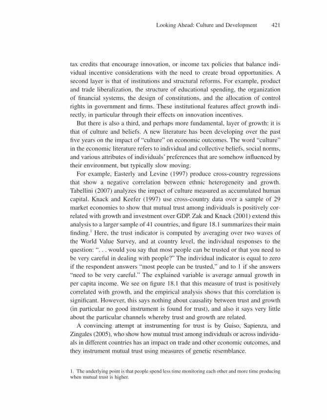
Looking Ahead: Culture and Development 421
tax credits that encourage innovation, or income tax policies that balance indi-vidual incentive considerations with the need to create broad opportunities. A second layer is that of institutions and structural reforms. For example, product and trade liberalization, the structure of educational spending, the organization of fi nancial systems, the design of constitutions, and the allocation of control rights in government and fi rms. These institutional features affect growth indi-rectly, in particular through their effects on innovation incentives.
But there is also a third, and perhaps more fundamental, layer of growth: it is that of culture and beliefs. A new literature has been developing over the past fi ve years on the impact of “culture” on economic outcomes. The word “culture” in the economic literature refers to individual and collective beliefs, social norms, and various attributes of individuals’ preferences that are somehow infl uenced by their environment, but typically slow moving.
For example, Easterly and Levine (1997) produce cross-country regressions that show a negative correlation between ethnic heterogeneity and growth. Tabellini (2007) analyzes the impact of culture measured as accumulated human capital. Knack and Keefer (1997) use cross-country data over a sample of 29 market economies to show that mutual trust among individuals is positively cor-related with growth and investment over GDP. Zak and Knack (2001) extend this analysis to a larger sample of 41 countries, and fi gure 18.1 summarizes their main fi nding.1 Here, the trust indicator is computed by averaging over two waves of the World Value Survey, and at country level, the individual responses to the question: “. . . would you say that most people can be trusted or that you need to be very careful in dealing with people?” The individual indicator is equal to zero if the respondent answers “most people can be trusted,” and to 1 if she answers “need to be very careful.” The explained variable is average annual growth in per capita income. We see on fi gure 18.1 that this measure of trust is positively correlated with growth, and the empirical analysis shows that this correlation is signifi cant. However, this says nothing about causality between trust and growth (in particular no good instrument is found for trust), and also it says very little about the particular channels whereby trust and growth are related.
A convincing attempt at instrumenting for trust is by Guiso, Sapienza, and Zingales (2005), who show how mutual trust among individuals or across individu-als in different countries has an impact on trade and other economic outcomes, and they instrument mutual trust using measures of genetic resemblance.
1. The underlying point is that people spend less time monitoring each other and more time producing when mutual trust is higher.
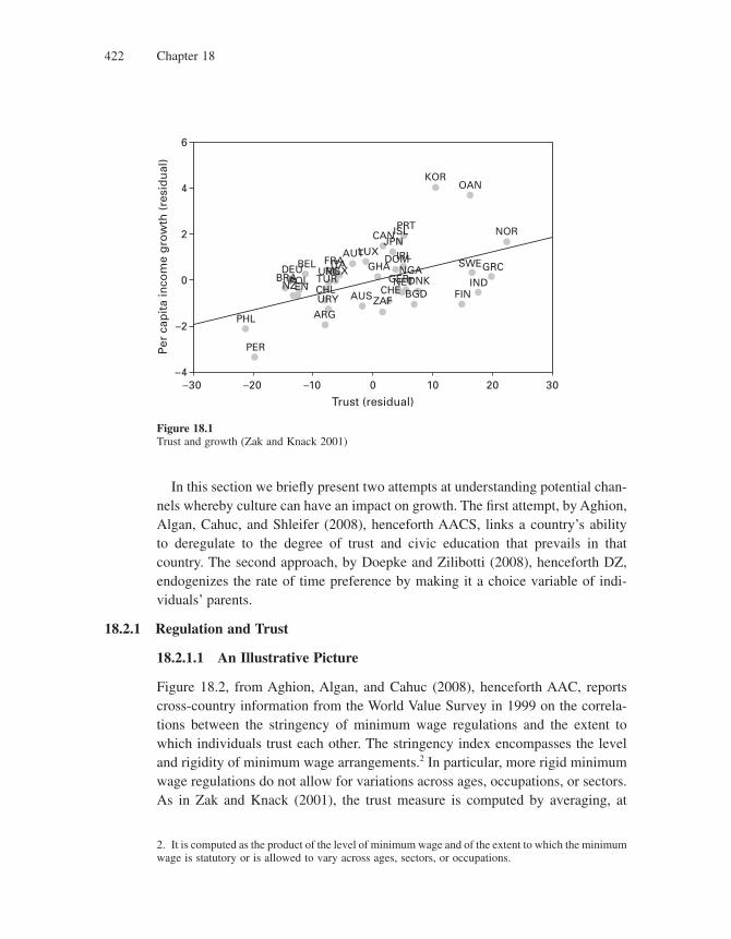
Chapter 18422
In this section we briefl y present two attempts at understanding potential chan-nels whereby culture can have an impact on growth. The fi rst attempt, by Aghion, Algan, Cahuc, and Shleifer (2008), henceforth AACS, links a country’s ability to deregulate to the degree of trust and civic education that prevails in that country. The second approach, by Doepke and Zilibotti (2008), henceforth DZ, endogenizes the rate of time preference by making it a choice variable of indi-viduals’ parents.
18.2.1 Regulation and Trust
18.2.1.1 An Illustrative Picture
Figure 18.2, from Aghion, Algan, and Cahuc (2008), henceforth AAC, reports cross-country information from the World Value Survey in 1999 on the correla-tions between the stringency of minimum wage regulations and the extent to which individuals trust each other. The stringency index encompasses the level and rigidity of minimum wage arrangements.2 In particular, more rigid minimum wage regulations do not allow for variations across ages, occupations, or sectors. As in Zak and Knack (2001), the trust measure is computed by averaging, at
Figure 18.1Trust and growth (Zak and Knack 2001)
2. It is computed as the product of the level of minimum wage and of the extent to which the minimum wage is statutory or is allowed to vary across ages, sectors, or occupations.
6
4
2
0
–2
–4–30 30–20 20–10 100
Per
cap
ita
inco
me
gro
wth
(re
sid
ual
)
Trust (residual)
PHL
PER
PRT
IRLBEL
BRA
FRA DOMGRC
NOR
OANKOR
ITA
CAN
URY
TURMEX
BGDDNKGERNET
FIN
SWE
IND
ARG
URGENNZPOL
AUSCHL
ZAFCHE
NGA
ISL
DEU GHA
JPNLUXAUT
Looking Ahead: Culture and Development 423
country level, the individual answers to the question “can most people be trusted.” (The only difference is that AAC use three waves of the World Value Survey, not two.) We see a signifi cantly negative correlation between trust and the strin-gency of the minimum wage regulations, with countries like France lying at the low trust/high regulation end of the spectrum and Sweden and Finland lying at the opposite end, that is, high trust/low regulation. AAC argue that this correlation refl ects a two-way causality between regulation and trust in labor markets. Namely, more stringent and/or higher minimum wage regulations discourage decentralized experimentation by workers and employers, which in turn tends to perpetuate the lack of trust between them. Further, distrust between employers and employees induces the median voter to vote for a more stringent minimum wage regulation so as to limit her ex post risk.
AAC extend this logic to other sectors of the economy. More importantly, they try to explain the striking fact that there is a higher demand for regulation in countries where distrust is higher, not only among individuals, but also between individuals and the country’s government and other public institutions.
18.2.1.2 A Toy Model
The following model accounts for the positive interplay between beliefs in coop-eration and regulation, with a causality running in both directions. On the one hand, when individuals have low trust in the civic behavior of other individuals,
Figure 18.2Distrust and state regulation of minimum wages (WVS database and AAC)
0.6
0.4
0.2
0
Reg
ula
tio
n o
f m
inim
um
wag
e
Distrust0.2 0.4 0.6 0.8 1
R2 = 0.65
Aus
AutBg
Cd
Czr
DkFin
Fra
Ger
Hg
Ita
Jp
MxNth
Nw
Pol
Pt
Sp
Swd
Uk
USA

Chapter 18424
they fear negative externalities from other individuals’ production activities. Individuals then vote for more stringent regulations that limit the scope of pro-ductive activities and thereby protect against the negative externalities. On the other hand, more stringent regulations reduce individuals’ incentives to invest in civic education aimed at increasing productivity while reducing the negative externalities on other individuals because the opportunity to directly interact with other individuals in productive activities is reduced by the regulations.
To detail the argument further, consider the following timing of moves. First, individuals choose the level of their investment in civic education. Thus, each individual ends up being either educated or uneducated. Educated individuals share two virtues: they are more productive and they generate lower externalities on other individuals. Uneducated individuals are less productive, generate more negative externalities on other individuals, and are uncivil. Second, given their beliefs as to how many individuals are educated, individuals vote on whether or not to regulate the economy, that is whether or not to forbid productive activities. In this frame-work, there are two stable equilibria. In the fi rst there is zero investment in educa-tion and public authorities forbid productive activities because people are uncivil. The second equilibrium is characterized by positive investment, fi rst in education, and then in civic individuals who allow public authorities to authorize productive activities. The second equilibrium pareto-dominates the fi rst.
More formally, consider an economy with a continuum of identical risk-neutral individuals of mass one. There are two goods in the economy: labor and a numéraire good produced with labor. The timing of events is detailed as follows:
1. Individuals can either invest a fi xed amount i > 0 to be educated or not invest at all. Educated individuals are able to produce one unit of the numéraire good and do not generate externalities when they produce. Uneducated people produce y < 1 and generate a negative externality which costs � to everyone. Education is a private investment. It is assumed that education is observable but not verifi able.
2. People vote to authorize or forbid production. It is assumed that public authori-ties can forbid production activity at zero cost. It is impossible to forbid the production of the uneducated and to authorize the production of people because education is not verifi able.
3. People produce if this is authorized.
For simplicity, we assume that investment has positive private returns if the productive activity is authorized:
Looking Ahead: Culture and Development 425
1− >i y
and that the social returns of production are negative if people are not educated
y < �
Now, let a denote the share of educated people as anticipated by each indi-vidual. At the voting stage, production is authorized if and only if this maximizes individuals’ expected utility, namely whenever
α α+ −( ) −( ) >1 y i�
or equivalently
α α> + −+ −
=i y
y
��l
(18.1)
Moving back to the investment stage, the private returns of (civic) education investment are positive if and only if the productive activity is authorized in the next step. Thus, the best reply of each individual is to invest in education if a > a and not to invest if a < a. This implies that there are two (stable) equilibria. In the fi rst equilibrium, all individuals invest in education (a = 1) and it is optimal to authorize the productive activity. In the second equilibrium, nobody invests in education (a = 0) and the productive activity is not authorized. The second equi-librium clearly pareto-dominates the fi rst because social welfare amounts to zero in the equilibrium without education and to 1 − i > 0 in the equilibrium with education.
This line of analysis is potentially important because it suggests that maintain-ing lower levels of regulation, which in turn have been shown to be growth enhancing, particularly in more advanced sectors and countries, may require investing in mutual trust. The diffi culty of course is how to design policies that can durably move a country from a low-trust/high-regulation equilibrium, as we currently see in France or Italy, to a high-trust/low-regulation equilibrium, as currently exemplifi ed by the Scandinavian countries.
18.2.2 Investing in Children’s Patience
18.2.2.1 The Argument
Doepke and Zilibotti (2008) propose a neo-weberian theory of culture and growth. The basic idea is that parents can invest in their children’s degree of patience, which in turn will affect the children’s choice between current consumption and

Chapter 18426
capital accumulation. Investments in children’s work ethic and patience respond to economic incentives that depend on the occupation in which a family (or dynasty) is engaged. Some professions require young workers to sacrifi ce con-sumption and put in high labor effort, but then offer high rewards later in life. This is typically the case for professions that entail the acquisition of skills over the life cycle, such as artisanry and trade (the most common activities of the preindustrial middle class). Other occupations, such as unskilled labor in agricul-ture, provide fl atter returns over the life cycle. Finally, there are occupations (in particular landowning) that are characterized neither by hard work nor by delayed consumption.
Given these differences between occupations, parents who anticipate their children to be artisans or merchants have a stronger incentive to instill patience in their children, since this will help them endure early sacrifi ces and enjoy their future success. Over centuries, the preindustrial middle class became the patient class. This attribute became a major advantage once new opportunities for capital accumulation arose with the industrial revolution. At that point, the thrifty middle class had a cultural edge that allowed it to exploit the new investment-based technology: this is the “spirit” that the development of capitalism required. Doepke and Zilibotti’s theory can thus explain the rise of the bourgeoisie, which possessed a new ethic and a different culture from the landowning elite, and the demise of the aristocracy after the industrial revolution.
18.2.2.2 The Doepke-Zilibotti Model
In this section, we present a simplifi ed version of Doepke and Zilibotti (2008) where the only endogenous preference asset is patience, labor supply is exoge-nous, and there is no occupational choice. We focus on the relationship between patience and physical capital accumulation, that is, the process describing the heyday of the industrial revolution, after patience levels had already diverged across social classes during the preindustrial period. The economy is populated by overlapping generations of altruistic people who live for four periods, two as children and two as adults. People work throughout both adult periods (young and old), and their earnings may vary over time as the result of occupational choice (which will be ignored here) and physical investment decisions. Agents consume and make economic decisions only when they are adult. At the begin-ning of adulthood, every agent gives birth to a single child.
All adults have the same basic preferences. However, patience, that is, the relative weight of old versus young adult consumption in utility, is endogenous. In particular, patience is determined during an agent’s childhood as a result of
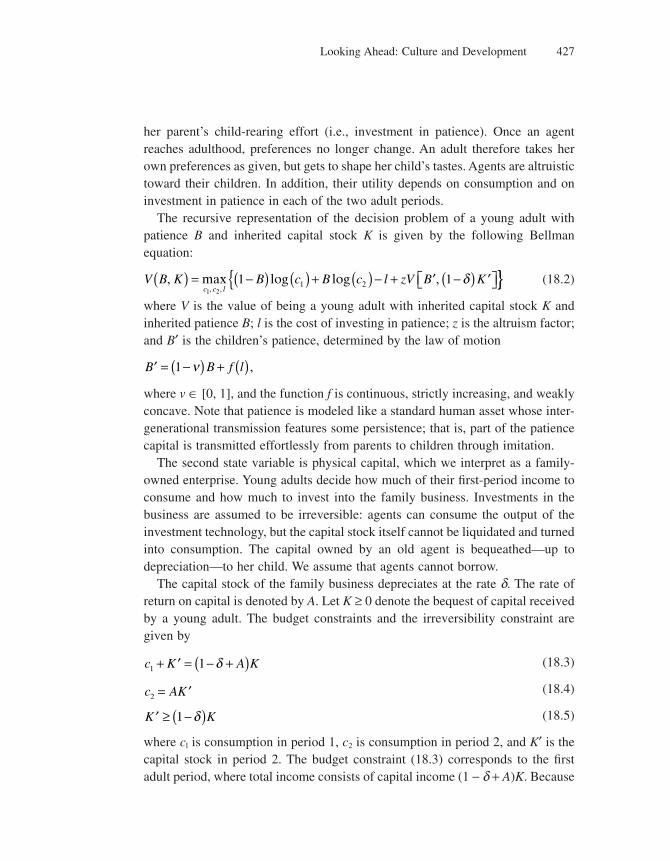
Looking Ahead: Culture and Development 427
her parent’s child-rearing effort (i.e., investment in patience). Once an agent reaches adulthood, preferences no longer change. An adult therefore takes her own preferences as given, but gets to shape her child’s tastes. Agents are altruistic toward their children. In addition, their utility depends on consumption and on investment in patience in each of the two adult periods.
The recursive representation of the decision problem of a young adult with patience B and inherited capital stock K is given by the following Bellman equation:
V B K B c B c l zV B Kc c l
, max log log ,, ,
( ) = −( ) ( ) + ( ) − + ′ −( ) ′⎡⎣ ⎤⎦{1 2
1 11 2 δ }} (18.2)
where V is the value of being a young adult with inherited capital stock K and inherited patience B; l is the cost of investing in patience; z is the altruism factor; and B′ is the children’s patience, determined by the law of motion
′ = −( ) + ( )B B f l1 ν ,
where v ∈ [0, 1], and the function f is continuous, strictly increasing, and weakly concave. Note that patience is modeled like a standard human asset whose inter-generational transmission features some persistence; that is, part of the patience capital is transmitted effortlessly from parents to children through imitation.
The second state variable is physical capital, which we interpret as a family-owned enterprise. Young adults decide how much of their fi rst-period income to consume and how much to invest into the family business. Investments in the business are assumed to be irreversible: agents can consume the output of the investment technology, but the capital stock itself cannot be liquidated and turned into consumption. The capital owned by an old agent is bequeathed—up to depreciation—to her child. We assume that agents cannot borrow.
The capital stock of the family business depreciates at the rate d. The rate of return on capital is denoted by A. Let K ≥ 0 denote the bequest of capital received by a young adult. The budget constraints and the irreversibility constraint are given by
c K A K1 1+ ′ = − +( )δ (18.3)
c AK2 = ′ (18.4)
′ ≥ −( )K K1 δ (18.5)
where cl is consumption in period 1, c2 is consumption in period 2, and K′ is the capital stock in period 2. The budget constraint (18.3) corresponds to the fi rst adult period, where total income consists of capital income (1 − d + A)K. Because
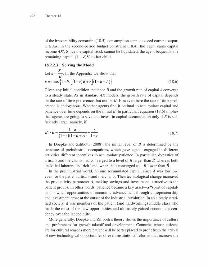
Chapter 18428
of the irreversibility constraint (18.5), consumption cannot exceed current output: cl ≤ AK. In the second-period budget constraint (18.4), the agent earns capital income AK′. Since the capital stock cannot be liquidated, the agent bequeaths the remaining capital (1 − d)K′ to her child.
18.2.2.3 Solving the Model
Let kK
K= ′
. In the Appendix we show that
k z B z A= − −( ) +⎡⎣ ⎤⎦ − +( ){ }max ,1 1 1δ δ (18.6)
Given any initial condition, patience B and the growth rate of capital k converge to a steady state. As in standard AK models, the growth rate of capital depends on the rate of time preference, but not on K. However, here the rate of time pref-erence is endogenous. Whether agents fi nd it optimal to accumulate capital and patience over time depends on the initial B. In particular, equation (18.6) implies that agents are going to save and invest in capital accumulation only if B is suf-fi ciently large, namely, if
B Bz A
z
z> ≡ −
−( ) − +( ) −−
ˆ 1
1 1 1
δδ (18.7)
In Doepke and Zilibotti (2008), the initial level of B is determined by the structure of preindustrial occupations, which gave agents engaged in different activities different incentives to accumulate patience. In particular, dynasties of artisans and merchants had converged to a level of B larger than B, whereas both unskilled laborers and rich landowners had converged to a B lower than B.
In the preindustrial world, no one accumulated capital, since A was too low, even for the patient artisans and merchants. Then technological change increased the productivity parameter A, making savings and investments attractive to the patient groups. In other words, patience became a key asset—a “spirit of capital-ism”—when opportunities of economic advancement through entrepreneurship and investment arose at the outset of the industrial revolution. In an already strati-fi ed society, it was members of the patient (and hardworking) middle class who made the most of the new opportunities and ultimately gained economic ascen-dency over the landed elite.
More generally, Doepke and Zilibotti’s theory shows the importance of culture and preferences for growth takeoff and development. Countries whose citizens are for cultural reasons more patient will be better placed to profi t from the arrival of new technological opportunities or even institutional reforms that increase the
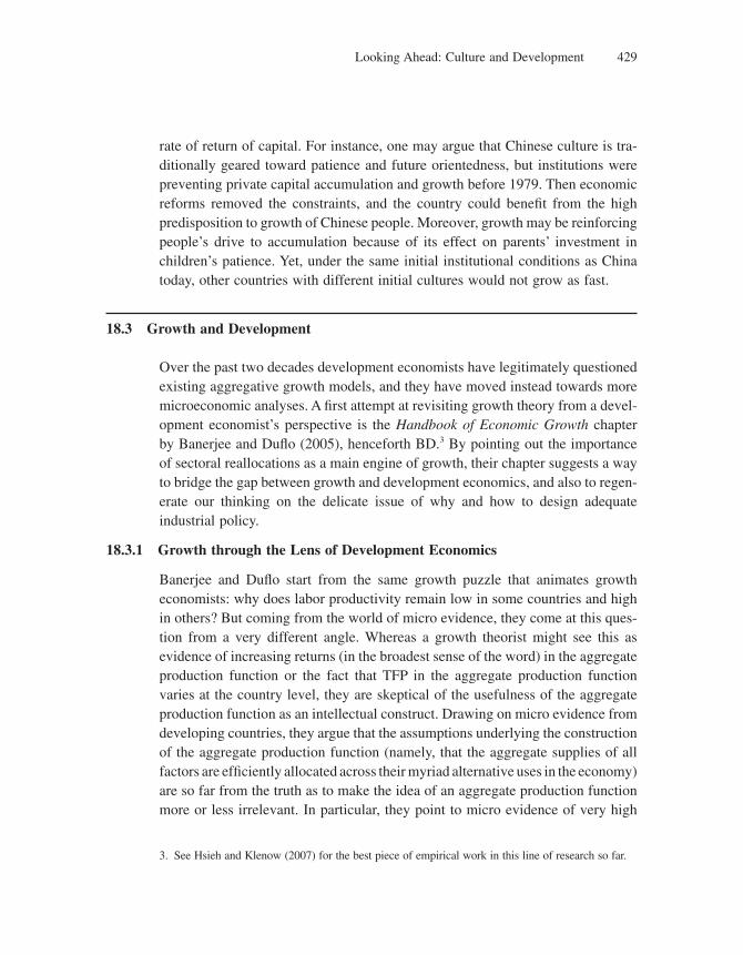
Looking Ahead: Culture and Development 429
rate of return of capital. For instance, one may argue that Chinese culture is tra-ditionally geared toward patience and future orientedness, but institutions were preventing private capital accumulation and growth before 1979. Then economic reforms removed the constraints, and the country could benefi t from the high predisposition to growth of Chinese people. Moreover, growth may be reinforcing people’s drive to accumulation because of its effect on parents’ investment in children’s patience. Yet, under the same initial institutional conditions as China today, other countries with different initial cultures would not grow as fast.
18.3 Growth and Development
Over the past two decades development economists have legitimately questioned existing aggregative growth models, and they have moved instead towards more microeconomic analyses. A fi rst attempt at revisiting growth theory from a devel-opment economist’s perspective is the Handbook of Economic Growth chapter by Banerjee and Dufl o (2005), henceforth BD.3 By pointing out the importance of sectoral reallocations as a main engine of growth, their chapter suggests a way to bridge the gap between growth and development economics, and also to regen-erate our thinking on the delicate issue of why and how to design adequate industrial policy.
18.3.1 Growth through the Lens of Development Economics
Banerjee and Dufl o start from the same growth puzzle that animates growth economists: why does labor productivity remain low in some countries and high in others? But coming from the world of micro evidence, they come at this ques-tion from a very different angle. Whereas a growth theorist might see this as evidence of increasing returns (in the broadest sense of the word) in the aggregate production function or the fact that TFP in the aggregate production function varies at the country level, they are skeptical of the usefulness of the aggregate production function as an intellectual construct. Drawing on micro evidence from developing countries, they argue that the assumptions underlying the construction of the aggregate production function (namely, that the aggregate supplies of all factors are effi ciently allocated across their myriad alternative uses in the economy) are so far from the truth as to make the idea of an aggregate production function more or less irrelevant. In particular, they point to micro evidence of very high
3. See Hsieh and Klenow (2007) for the best piece of empirical work in this line of research so far.
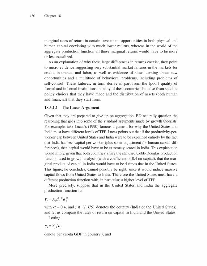
Chapter 18430
marginal rates of return in certain investment opportunities in both physical and human capital coexisting with much lower returns, whereas in the world of the aggregate production function all these marginal returns would have to be more or less equalized.
As an explanation of why these large differences in returns coexist, they point to micro evidence suggesting very substantial market failures in the markets for credit, insurance, and labor, as well as evidence of slow learning about new opportunities and a multitude of behavioral problems, including problems of self-control. These failures, in turn, derive in part from the (poor) quality of formal and informal institutions in many of these countries, but also from specifi c policy choices that they have made and the distribution of assets (both human and fi nancial) that they start from.
18.3.1.1 The Lucas Argument
Given that they are prepared to give up on aggregation, BD naturally question the reasoning that goes into some of the standard arguments made by growth theorists. For example, take Lucas’s (1990) famous argument for why the United States and India must have different levels of TFP. Lucas points out that if the productivity-per-worker gap between United States and India were to be explained entirely by the fact that India has less capital per worker (plus some adjustment for human capital dif-ferences), then capital would have to be extremely scarce in India. This explanation would imply, given that both countries’ share the standard Cobb-Douglas production function used in growth analysis (with a coeffi cient of 0.4 on capital), that the mar-ginal product of capital in India would have to be 5 times that in the United States. This fi gure, he concludes, cannot possibly be right, since it would induce massive capital fl ows from United States to India. Therefore the United States must have a different production function with, in particular, a higher level of TFP.
More precisely, suppose that in the United States and India the aggregate production function is:
Y A L Kj j j j= −1 α α
with a = 0.4, and j ∈ {I, US} denotes the country (India or the United States); and let us compare the rates of return on capital in India and the United States.
Letting
y Y Lj j j=
denote per capita GDP in country j, and
Looking Ahead: Culture and Development 431
k K Lj j j=
denote per capita investment in capital in country j, we have
y A kj j j= α
Assuming perfect credit markets in both countries, we then have
ry
kA kj
jj=
∂∂
= −α α 1 (18.8)
where rj denotes the rate of return on capital, equal to the marginal productivity of capital, in country j.
In 1990 the ratio of per capita GDP levels between the United States and India was
y yU S I = 11
Moreover, BD estimate a productivity ratio between the two countries, equal to
A AU S I = 2
But then, using the fact that from equation (18.8) we have
y y r r A AU S I I U S U S I= ( ) ( )− −α
α α1
1
1
the ratio rI /rUS should be approximately equal to 5. This, together with the fact that the average real stock market return in the United States is at around 9 percent, would suggest a 45 percent rate of return in India. However, if there are individual projects in India that earn more than a 45 percent rate, the average rate of return on capital is much lower.
BD take the view that this whole reasoning is fl awed. They point out that a difference in marginal product of capital of that magnitude is actually quite common within the same subeconomy, and there is no evidence that capital automatically fl ows to equalize returns.
Similarly they question the value of trying to use evidence on convergence (or the lack of it) to say something on the nature of returns to scale in production. Given the lack of equalization of returns across fi rms, the same production func-tion can generate very different outcomes: two economies with identical tech-nologies may grow very differently depending on whether the marginal unit of capital fl ows to the more productive fi rms rather than the less productive fi rms.
Chapter 18432
18.3.1.2 Moving Beyond Endogenous Growth Models?
Finally they argue that the available micro evidence is not fully accounted for by existing endogenous growth models. They fi rst consider the AK model where knowl-edge externalities are generated by aggregate (human) capital accumulation,
Y K Ki Hi
H= ( )α η
where KiH is the human capital investment by fi rm i and KH is the aggregate human
capital stock in the economy. This would explain why average interest rates on capital are lower in poorer countries: being more poorly endowed in aggregate capital, externalities should be lower in these countries. However, externalities should be much larger than estimated in recent empirical studies (for example, Acemoglu and Angrist 2000; Dufl o 2004) in order to generate the preceding productivity differential between the United States and India.
Then BD turn their attention to endogenous differences in technology, as gen-erated, for example, by the Schumpeterian models. They calculate that if the gap between rates of return on capital in the United States and India had to be fully explained by differences in productivities in an aggregative model, the ratio of total factor productivities between the United States and India should be at least equal to 2. However, TFP grows at a rate of 1 to 1.5 percent per year in the United States. Even at a rate of 1.5 percent per year, it would take 45 years for U.S. TFP to grow by 200 percent. Or, put in other words, if this was the story we would see India in 2000 using U.S. machines of 1950. However, BD quote a recent report by the McKinsey Global Institute saying that in many Indian industries the best fi rms use close-to-frontier technologies.
BD are careful not to say that this evidence points toward a wholesale rejection of the endogenous growth models. Yet they feel that these models miss something important—to explain, for example, why some fi rms or industries have access to the latest technologies but others do not requires moving away from an aggrega-tive growth approach and explicitly introducing cross-fi rm heterogeneity into the analysis.
In an admittedly speculative section of their paper, BD go on to ask whether it is possible to explain the entire Indo-U.S. productivity gap simply based on fi rm-level heterogeneity (they do not claim that this is the entire explanation, just ask whether it could be). They start from a model where each fi rm i produces according to
Y AL K= γ α
Looking Ahead: Culture and Development 433
where g < 1 − a. In other words, there are decreasing returns at the fi rm level. However, fi rm i has access to at most K(i) units of capital. Profi t maximization by fi rm i implies that the demand for labor for a fi rm that invests K(i) is equal to
L iA K i
w( ) = ( )⎡
⎣⎢⎢
⎤
⎦⎥⎥
−γ α γ1
1
Labor-market clearing implies that
L L i di= ( )∫or equivalently
w AK i di
Ly=
( )⎡⎣
⎤⎦
⎡
⎣
⎢⎢⎢⎢
⎤
⎦
⎥⎥⎥⎥
=∫ −
−
γ γα γ
γ1
1
1
where y is average output per worker. Now, since a < 1 − g, the mapping
K i( )⎡⎣
⎤⎦
−α γ1
1 is concave in K(i), and therefore more heterogeneity in K(i) reduces
the integral K idi
( )⎡⎣
⎤⎦
−∫ α γ1
1 . Therefore, greater heterogeneity in India could help
explain the Indo-U.S. gap.However, based on some rough calibration to micro data, BD fi nd that the
reduction in aggregate per capita output generated by the heterogeneity between small and large fi rms in India is not suffi cient to explain the discrepancy in average rates of return between the United States and India. The main reason it fails is that given the extent of decreasing returns that is consistent with the
observed profi t shares (which in the model would be equal to α
γ1− ), the extent
of heterogeneity that would be required to explain the Indo-U.S. gap is simply not in the data. In particular, the large (and therefore, because of decreasing returns, ineffi cient) Indian fi rms would have to be much larger than the largest fi rms in the United States, which is not what we fi nd in the data.
Finally, BD obtain a better fi t between the model and the data by introducing heterogeneous fi xed costs leading to heterogeneous productivities. More pre-cisely, they consider a heterogeneous population of fi rms where each fi rm i pro-duces according to
Y AL K K= −( )γ α
Chapter 18434
where K is the fi xed cost required to access technology A, and where again a + g < 1. Introducing fi xed costs makes it possible that larger fi rms also have larger marginal products (which seems to fi t the Indian case) and that the average product gap between small and large fi rms be large even if marginal products are similar (which again seems to fi t the facts). BD then concentrate on the case where K takes three possible values (K1 < K2 < K3) corresponding to Al < A2 < A3 and show that in principle it could explain most of the Indo-U.S. gap, without straining credibility too much.
Note that this explanation means that productivity differences matter after all, even though it is by taking into account the existence of cross-fi rm heterogeneity that we can explain the discrepancy between average and marginal returns. Note that this model does not explain the heterogeneity in productivity levels across fi rms, and explaining it would presumably bring us back to something closer to the model in chapter 7 on convergence with credit constraints, but with cross-fi rm heterogeneity instead of cross-country heterogeneity.
One additional factor that may further explain the lower average rates of return in India compared to the United States and the discrepancy between average and marginal returns is the complementarity between small and large fi rms in the production process in India. The most productive Indian fi rms could well be almost as productive as their U.S. counterparts. Yet average productivity is more likely to be driven by the lower tail when the production process involves strong complementarities—for example, if the production of a whole range of intermedi-ate components is subcontracted to small ineffi cient fi rms (see Kremer (1993a) and Jones 2008).
Overall, taking a development economist’s approach, Banerjee and Dufl o make us revisit the various growth paradigms, starting from the aggregative neoclassi-cal model and leading us toward a model that appears to be more closely related to the Schumpeterian growth paradigm, but adequately enriched, in particular by fully integrating the heterogeneity across fi rms and/or sectors.
18.3.2 The Case for Targeted Growth Policy
Over the past decades governments and policy advisers have become suspicious about policies targeted at particular sectors, because such policies allow govern-ments to “pick winners” in a discretionary fashion. But what if one could use market information together with information on the size of externalities to come up with suitable targeted policies? Although this is a research area where essen-tially everything remains to be done, we would like to provide the reader with two insights that may guide further thinking on this question.
Looking Ahead: Culture and Development 435
The fi rst insight, suggested by Young (1991), Lucas (1993), and more recently Hausmann and Klinger (2007), is that successful growth stories are ones involv-ing gradual processes whereby neighboring sectors experiment with new tech-nologies one after the other because experimentation involves learning-by-doing externalities across sectors. The second insight, from Kremer (1998), is that governments may use or simulate market mechanisms to determine the amount of R&D subsidies to targeted industries.
18.3.2.1 Learning-by-Doing Externalities and Industrial Policy
The notion that the existing pattern of specialization may limit the evolution of comparative advantage over time has not received much attention in the growth literature so far. In the product variety model analyzed in chapter 3, the current set of inputs displays the same degree of imperfect substitutability with respect to any new input that might be introduced and, therefore, does not make one new input more likely than any other: This property stems directly from the fully symmetric nature of the Dixit-Stiglitz model of product differentiation on which the Romer model is built.
To illustrate the notion of industrial niches in the simplest possible way, con-sider the following toy example. Individuals each live for one period. There are four potential sectors in the economy, which we number from 1 to 4, but only one sector, namely sector 1, is active at date zero. Thus the economy at date 0 can be represented by the 4-tuple
Ω0 1 0 0 0= ( ), , ,
where the number 1 (resp. 0) in column i refers to the corresponding sector i being currently active (resp. inactive). At date t, a sector that is active produces at the frontier productivity level At = (1 + g)t. Once activated a sector automati-cally remains active forever. Aggregate output at date t is
Y A N At t t t= =
where Nt is the number of active sectors at date t.R&D investments activate new sectors, but there is a cost of learning about
faraway sectors. Specifi cally, there is a fi xed R&D cost g (1 + g)t of activating a sector in period t, but this is only possible if (1) the sector is adjacent to an already active sector or (2) the R&D cost g (1 + g)t−1 was also incurred in that sector last period.

Chapter 18436
Consider fi rst the economy under laissez-faire. Being populated by one-period lived individuals, the economy will never invest in a sector that is not adjacent to a sector already active. At best, a local entrepreneur will fi nd it optimal to activate a sector adjacent to an already active sector. This will be the case whenever
γ θ<
where q is the fraction of output that can be appropriated by a private innovator. Note, however, if
θ γ<
private fi rms will not explore new sectors, even neighboring ones, even though it might be socially optimal to do so.
Going back to the former case, the laissez-faire sequence of active sectors will be
Ω1 1 1 0 0= ( ), , ,
Ω2 1 1 1 0= ( ), , ,
Ωt t= ( ) ≥1 1 1 1 3, , , ,
Now consider a social planner. The social planner will invest in sector 2 in period 1, whenever the cost g (1 + g) of doing so is less than the net present revenue of activating sector 2, namely
A
r
g
r gt
tt 1
1
1 +( )=
+−=
∞
∑
that is whenever
γ <−1
r g
For g suffi ciently close to r or for g suffi ciently small, this inequality is automati-cally satisfi ed, in which case it will also be optimal to invest in sector 3 in period 2 because at that date sector 3 will be adjacent to an already active sector (namely sector 2).
But in addition, when g is suffi ciently small, it will be optimal to invest in sector 4 in period 1, because that will allow sector 4 to be activated in period 2 whereas otherwise it can only be activated in period 3. Investing in period 1 instead of period 2 in sector 4 will yield an additional

Looking Ahead: Culture and Development 437
A r2 1+( )and will cost an additional g (1 + g). So, if g is small enough, namely if
γ <++
1
1
g
r,
the optimal sequence of active sectors will be
Ω1 1 1 0 0= ( ), , ,
Ω2 1 1 1 1= ( ), , ,
Ωt t= ( ) ≥1 1 1 1 3, , , ,
The laissez-faire equilibrium is suboptimal here because people do not invest far enough away from already active sectors. In this example, output will be lower than optimal in period 2 (3A2 versus 4A2) because individuals were not farsighted enough to invest in sector 4, which was too far away from already active sectors, in period 1.
Thus this model suggests a role for targeted industrial policy: namely to over-come the potential underinvestment in new sectors.4 In the model we just devel-oped, investment inertia results from insuffi cient appropriability. In practice they may also result from the existence of credit constraints or the unavailability of complementary inputs.
The idea that the product space is heterogeneous, with an uneven density of active product lines, and that the current density distribution of active sectors has an impact on the evolution of comparative advantage, is taken to the data by Hausmann and Klinger (2006), henceforth HK. A main fi nding in HK is that the probability of a country exporting product i in year t + 1, is positively and sig-nifi cantly correlated with the country’s density around product i in year t.
18.3.2.2 The Kremer Mechanism
Kremer (1998) designed a market-based mechanism for buying out pharmaceuti-cal patents. Kremer’s mechanism is based on ex post reward for inducing the
4. In particular, if targeted subsidies were to be implemented by a government, we conjecture that such subsidies should be more growth enhancing (1) if they target sectors that are currently inactive but close “input-wise” to already active sectors, and (2) if the country experiences low levels of fi nan-cial development and/or low labor mobility and/or low levels of education. Part 1 implies that the tar-geted sectors are likely to benefi t from learning-by-doing externalities from existing sectors. Part 2 makes it less likely that market forces would spontaneously take advantage of these externalities.
Chapter 18438
socially optimal amount of R&D. The basic idea is to make use of the informa-tion conveyed by the laissez-faire patent price V in order to fi x the optimal price at which the social planner (government) will repurchase the innovations to put them in the public domain. Putting innovations in the public domain in turn removes the (static) monopoly distortion created by patents.
Directly inspired by the mechanism-design literature,5 the Kremer “scheme” can be described as follows:
1. The innovator obtains a patent for his or her innovation.
2. The (“laissez-faire”) price of the patent is revealed through an auction for the exclusive right to implement the innovation. Suppose that the laissez-faire value V emerges as the equilibrium price in this (say, fi rst-price) auction; that is, p0 = V.
3. With probability (1 − e) the government repurchases the innovation from the inventor at a price p1 = m ⋅ V that tries to approximate the social value of innova-tion V*. With probability e, the patent remains in the hands of the winner of the auction. Note that e needs to be strictly positive in order for private bidders to fi nd it worth their while to come and participate in the auction. However, e should not be too large in order for innovation incentive to remain socially optimal and also for (static) monopoly distortions to be largely removed. The multiplier
mP
V= 1 should typically be greater than 1. For example, in the case of phar-
maceutical innovations, Kremer estimates at about 2 the average value of m.
What makes this proposal attractive in our view is that it does a good job at elicit-ing information about the value of innovations and also that, insofar as e remains small, the scheme removes all incentives to engage in (duplicative) imitation activities while at the same time eliminating the (static) monopoly distortions generated by innovations in the absence of imitations.
However, the scheme raises a number of questions. First, how does one compute the multiplier m? The value of m will typically depend on parameters such as the productivity of research or the elasticity of substitution between intermediate inputs, which the government is unlikely to know. Second, what guarantees that the equilibrium price that emerges in the auction is actually equal to the true value of the innovation under laissez-faire (i.e., to V)? In particular, when e is
5. In particular by the literature on Nash and subgame perfect implementation under symmetric information. (Primary references in this literature are Maskin 1977; Moore and Repullo 1986.)
Looking Ahead: Culture and Development 439
small, will private bidders still have adequate incentive to acquire information about V?
Third, what would prevent the innovator from colluding with potential bidders in order to (artifi cially) increase the auction price p0 far above the true (private) value of the innovation V?6
Fourth, is the scheme adapted to the case of multiple successive innovations? There are actually several aspects to this question. In particular, how can the government make sure that by putting a fi rst (fundamental) innovation in the public domain “too soon” it will not discourage other researchers from engaging in the development activities that are required in order to give (full) value to that innovation?7 Another aspect of the same question about successive innovations has to do with the case where subsequent innovations may substitute for (rather than complement) the fi rst innovation.8 For example, what should happen in the case where subsequent innovations, especially when put in the public domain, reduce the (laissez-faire) value of the current innovation?9
Overall, Kremer’s idea is interesting and important, not least because it sug-gests that by using the market mechanism at the margin one can come up with policies that take sectoral diversity into account while minimizing the scope for discretionarity.
18.4 Conclusion
In this chapter we have raised two particular themes, culture and sectoral devel-opment, that are highly relevant to growth but where a lot more research remains to be done. But there are other important issues for growth economists to look at that either have been barely touched on or simply not addressed at all. For
6. Well aware of this latter problem, the author proposes to use not the winning bid but the third or fourth bid price as the basis for computing the multiplier. But then the concern about information acquisition by private bidders might end up being dramatically reinforced.
7. On the other hand, the proposed mechanism would ensure that potential inventors of subsequent complementary innovations will assume that the earlier good is being sold at marginal cost.
8. In particular, this system may fail to provide adequate incentives for the invention of durable goods. This failure is because the expectation that future substitutes will be placed in the public domain, and hence sold at marginal cost, may reduce current demand for durable patented goods.
9. Here, Kremer suggests that the government repurchase the fi rst innovation at its private value p0 = V and then later resume the auction process for the overall package of innovations. But this in turn presupposes that the government will know in advance whether the fi rst innovation is to be sub-stituted for by subsequent innovations, and that it also knows how many successive innovations of this kind are to take place in the future, two heroic assumptions!
Chapter 18440
example, (1) the impact of fi nancial bubbles and regulations on innovation and growth; (2) the interplay between growth, the design of the tax system, and the composition of government spending; (3) the contribution of basic science and open research to growth.
Another important question relates to the dynamics of institutions and policies. In the previous chapters, we have seen that different institutions and policies tend to be growth enhancing at different stages of development. And in chapter 11 we saw that failure to implement the required institutional reforms may lead a country into a nonconvergence trap. Then what guarantees that institutions and policies will change in a timely fashion? For example, Acemoglu and colleagues (2007) show that fi rms tend to decentralize more when they become more tech-nologically advanced, and that this evolution towards more decentralization is also growth enhancing. Aghion, Alesina, and Trebbi (2008) show that more advanced countries tend to be more democratic, which again is a growth-enhancing dynamic pattern. However, institutional transition is not automatic. For example, some countries in continental Europe fi nd it diffi cult to liberalize markets, particularly labor and services markets, or to reform their higher educa-tion system. Also, while Latin America and South Africa have managed to democratize, China has not. Will China eventually change its political regime? Will Japan become more open to trade? Will Korea reduce the power of its con-glomerate fi rms?
More generally, what are the main obstacles to institutional change: Vested interests and the existing distribution of economic and/or political power? Beliefs about gains and losses from structural reforms? Is there a role for international incentives in prompting changes? To what extent can wars or economic and fi nancial crises help reduce the power of vested interests? For example, it is argued that the fi nancial crisis of the late 1990s stimulated reforms in Scandinavia and in Southeast Asia by weakening vested interests opposed to such reforms. Similarly, the crisis of 1929 and the two World Wars spurred entrepreneurship and growth in Europe during the postwar period by dramatically reducing the power of rentiers in European countries. It is also argued that the prospect of becoming members of the European Union has prompted structural reforms in Central Europe, and that the prospect of becoming a member of the World Trade Organization may foster democracy in China or Russia. This whole issue of institutional change awaits further investigation.
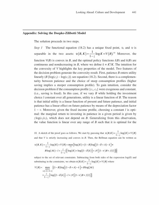
Looking Ahead: Culture and Development 441
Appendix: Solving the Doepke-Zilibotti Model
The solution proceeds in two steps.
Step 1 The functional equation (18.2) has a unique fi xed point, u, and u is
separable in the two assets: υ B Kz
K V B, log( ) =−
+ ( )1
1.10 Moreover, the
function V(B) is convex in B, and the optimal policy functions l(B) and k(B) are continuous and nondecreasing in B, where we defi ne k ≡ K′/K. The intuition for the convexity of V highlights the key properties of the model. Two features of the decision problem generate the convexity result. First, patience B enters utility linearly (B [log(c2) − log(c1)]; see equation (18.2). Second, there is a complemen-tarity between patience and the choice of steep consumption profi les (higher saving implies a steeper consumption profi le). To gain intuition, consider the decision problem if the consumption profi le {c1, c2} were exogenous and constant. (i.e., saving is fi xed). In this case, if we vary B while holding the investment choice l constant over all generations, utility is a linear function of B. The reason is that initial utility is a linear function of present and future patience, and initial patience has a linear effect on future patience by means of the depreciation factor 1 − v. Moreover, given the fi xed income profi le, choosing a constant l is opti-mal: the marginal return to investing in patience in a given period is given by z log(c2/cl), which does not depend on B. Generalizing from this observation, the value function is linear over any range of B such that it is optimal for the
10. A sketch of the proof goes as follows. We start by guessing that υ B Kz
K V B, log( ) =−
( ) + ( )11
and that V is strictly increasing and convex in B. Then, the Bellman equation can be written as
υ δB Kz
K V B K B A kl k
, log max log log,
( ) =−
( ) + ( ) = ( ) + −( ) − +( ) −⎡⎣ ⎤⎦{11
1 1 ++
( ) − +−
( ) + −( )( )⎡⎣ ⎤⎦ + −( ) + ( )⎡⎣ ⎤⎦(B Ak lz
zK k zV B f llog log log
11 1δ ν ))}
subject to the set of relevant constraints. Subtracting from both sides of the expression log(K) and
substituting in the constraints, we obtain υ B Kz
K V B, log( ) =−
( ) + ( )11
where
V B B A k B Akl
k A
( ) = −( ) − +( ) −⎡⎣ ⎤⎦{ +∈[ ]
∈ − − +[ ]
max log log, ,
,0 1
1 1
1 1δ δ
δ (( )
+−
−( )( )⎡⎣ ⎤⎦ − + −( ) + ( )⎡⎣ ⎤⎦}z
zk l zV B f l
11 1log δ ν
Chapter 18442
current and future members of a dynasty to hold their savings level fi xed. However, in general saving does vary with B, so that the consumption profi le {c1, c2} depends on patience. Given that B is the relative weight on utility late in life, it is optimal to choose high saving (and thus a steep lifetime consumption profi le) when B is high. As we increase B, the slope of the value function therefore increases. The optimal l increases too, since the marginal benefi t of being patient increases with the steepness of the wage profi le. Thus the value function is convex.
Step 2 The growth rate of capital satisfi es the following equation:
k z B z A= − −( ) +⎡⎣ ⎤⎦ − +( ){ }max ,1 1 1δ δ (18.8)
To see this, take the fi rst order condition with respect to K′ in the maximization
(18.2), after substituting for V B Kz
K V B, log( ) =−
+ ( )1
1. We get:
1
1 1
1−− + −
= +−
B
A k
B
k
z
z kδ
Rearranging terms (i.e., solving for k) and taking into account the irreversibility condition, yields equation (18.8).
Appendix: Basic Elements of Econometrics1
In this appendix we provide our readers with a few basic elements to understand the econometric tables of this book. For more details, we refer our readers to Wooldridge (2006) and Stock and Watson (2007).
A.1 The Simple Regression Model2
Let x and y be two variables, and suppose we are interested in explaining y in terms of x, or, in other words, to estimate how y varies with changes in x. For instance, y refers to the average growth rate of GDP in a country over a certain time period, and x refers to some explanatory factor, such as the average level of education in the country over the period. A simple way of writing such a relation-ship is with the equation
y x u= + +β β0 1 (A.1)
which we refer to as a simple linear regression equation.The right-hand-side variable x is called the explanatory (or independent) variable,
whereas the left-hand-side variable y is called the explained (or dependent) variable. The variable u is called the error term or disturbance factors other than x that affect y.
For given value of u, b1 is a slope parameter that measures the extent to which a change in x affects y. But to focus on this ceteris paribus effect of x on y, without having to deal with the effects of u, we need a restriction on the relationship between x and u. The restriction is simply to assume that x and u are uncorrelated; namely, if the former varies, then the latter does not, so that we can indeed look at the ceteris paribus effect of changes in x on y.
More formally, we assume that the average value of u does not depend on the value of x, namely,
E u x E u( ) = ( ) = 0
In other words, for any x, the average of the unobservables is the same: this is called the zero conditional mean assumption. The value of zero comes from a normalization; indeed, we can always rewrite the model, changing the intercept, so that this average becomes equal to zero.
Using this assumption, together with the linearity of the expectation operator, we have
1. This chapter was written making unrestrained use of notes by Leonardo Bursztyn.
2. The fi rst four sections of this appendix draw on chapters 2, 3, and 4 of Wooldridge (2006).
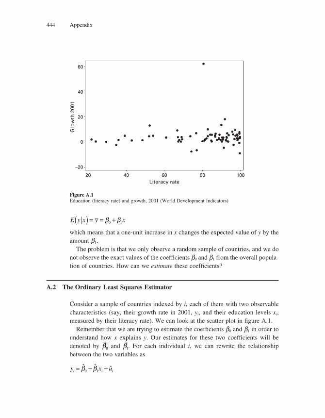
Appendix444
E y x y x( ) = = +β β0 1
which means that a one-unit increase in x changes the expected value of y by the amount b1.
The problem is that we only observe a random sample of countries, and we do not observe the exact values of the coeffi cients b0 and b1 from the overall popula-tion of countries. How can we estimate these coeffi cients?
A.2 The Ordinary Least Squares Estimator
Consider a sample of countries indexed by i, each of them with two observable characteristics (say, their growth rate in 2001, yi, and their education levels xi, measured by their literacy rate). We can look at the scatter plot in fi gure A.1.
Remember that we are trying to estimate the coeffi cients b0 and b1 in order to understand how x explains y. Our estimates for these two coeffi cients will be denoted by β0 and β1. For each individual i, we can rewrite the relationship between the two variables as
y x ui i i= + +ˆ ˆ ˆβ β0 1
Gro
wth
200
1
20 40 60 80 100Literacy rate
60
40
20
0
–20
Figure A.1Education (literacy rate) and growth, 2001 (World Development Indicators)
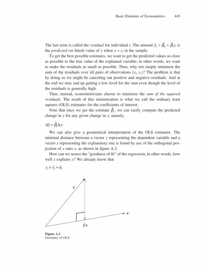
Basic Elements of Econometrics 445
The last term is called the residual for individual i. The amount yi = β0 + β1xi is the predicted (or fi tted) value of y when x = xi in the sample.
To get the best possible estimates, we want to get the predicted values as close as possible to the true value of the explained variable; in other words, we want to make the residuals as small as possible. Then, why not simply minimize the sum of the residuals over all pairs of observations (xi, yi.)? The problem is that by doing so we might be canceling out positive and negative residuals. And at the end we may end up getting a low level for the sum even though the level of the residuals is generally high.
Thus, instead, econometricians choose to minimize the sum of the squared residuals. The result of this minimization is what we call the ordinary least squares (OLS) estimates for the coeffi cients of interest.
Note that once we get the estimate β1, we can easily compute the predicted change in y for any given change in x, namely,
Δ Δˆ ˆy x= β1
We can also give a geometrical interpretation of the OLS estimator. The minimal distance between a vector y representing the dependent variable and a vector x representing the explanatory one is found by use of the orthogonal pro-jection of y onto x, as shown in fi gure A.2.
How can we assess the “goodness of fi t” of the regression, in other words, how well x explains y? We already know that
y y ui i i= =ˆ ˆ
y
x
xβ
Figure A.2Geometry of OLS
Appendix446
Let us defi ne the total sum of squares SST ≡ −( )=∑ y yii
n2
1
. That the
OLS estimates minimize the sum of squared residuals implies that the vector (yi − y)i is orthogonal to the vector (ui)i, so that, by the Pythagorean theorem,
SST = −( ) += =∑ ∑ˆ ˆy y uii
n
ii
n2
1
2
1
The fi rst term on the right-hand side of this equation is the explained sum of squares (SSE), and the second term is the residual sum of squares (SSR). And SST measures the total sample variation in the dependent variable (how spread out it is in the sample).
The goodness of fi t, called the R2 (or coeffi cient of determination), is then simply defi ned by
R2 = SSE SST
This is simply the ratio of the explained variation compared to the total variation: it is the fraction of the sample variation in y that is explained by x. This ratio always lies between 0 and 1 because SSE ≤ SST.
A.3 Multiple Regression Analysis
We can extend the simple regression model by adding explanatory variables on the right-hand side of the regression equation and thus explicitly controlling for many other factors that simultaneously affect the dependent variable.
For example, why assume that education is the only observable factor that affects growth? Competition, property-rights protection, fi nancial development, and others are factors that are also relevant to the growth process.
We thus write
y x x x uk k= + + + ⋅ ⋅ ⋅ + +β β β β0 1 1 2 2
Each bj tells us about the effect on y of a change in xj holding fi xed all the other explanatory variables and the error term u. To extend the logic of the simple linear regression model, we make the zero-conditional-mean assumption:
E u x x xk1 2 0, , . . . ,( ) =
Basic Elements of Econometrics 447
The OLS method estimates bj again by minimizing the sum of the squared residuals ui, where
ˆ ˆ ˆ ˆ ˆ, , ,u y x x xi i i i k k i= − + + + ⋅ ⋅ ⋅ +⎡⎣ ⎤⎦β β β β0 1 1 2 2
A simple interpretation of βj is that it measures the impact of a unit change in xj on y, namely,
Δ Δˆ ˆy xj j= β
Dummy variables and interaction effects: If the explanatory variable is binary, we can create a dummy variable to compute its effect on the dependent variable. For instance, we could be interested in estimating the impact of being male on personal earnings. For that purpose, we create a dummy variable that has value one if the individual is male and zero otherwise. If we run a wage regression on that dummy variable, the interpretation on its coeffi cient will be exactly the one we are looking for.
Sometimes we might think that the effect of an explanatory variable on the dependent variable varies when the value of another variable changes. For instance, we could think that education matters more for growth the more demo-cratic a country is. In this case, there is an interaction effect between education and democracy. The effect of education on growth varies with its degree of democratization. To estimate this effect, we create a variable given by the product of education with the degree of democratization, and we use the notation * to write this product on the right-hand side of the regression equation; for example, we denote the interaction variable by e * d if e denotes education and d denotes democracy. The interpretation of a coeffi cient of 0.01, for instance, will be that once the level of democratization is increased by one unit, the effect of one more unit of education on growth is increased by 0.01.
A.4 Inference and Hypothesis Testing
In order to test hypotheses about the parameters in the regression model, we need to know the distributions of the estimates βj . In turn we derive these distributions under the assumption that u is normally distributed in the population (normality assumption). Because of suitable properties of the normal distribution, it turns out that this implies that OLS-estimated coeffi cients will also be normally dis-tributed (for a proof, look at the appendix to chapter 4 in Wooldridge 2006).
Appendix448
Then, even though the true bj’s are unknown, we can “hypothesize” about the value of these parameters and test such hypotheses based on the OLS estimates βj . Given that the sample estimates have sampling errors, the idea is pretty simple: is the observed estimate of a coeffi cient consistent with a formulated hypothesis about the true parameter?
For example, based on our sample and estimation, can we reject the hypothesis that the coeffi cient on a right-hand-side variable, say “competition,” is different from zero in the total population of countries? In other words, can our regression tell us that competition indeed affects the predicted growth rate in the overall population of countries? If we can reject such a hypothesis, we say that the esti-mated coeffi cient is signifi cantly different from zero, or statistically signifi cant.
Now, an important result in statistics is that the ratio of an estimated coeffi cient to its standard error (a measure of the precision of its estimation) has a known distribution: the t-distribution. Thus by computing this ratio for a specifi c βj we get the t-statistic for βj , which we denote by tβ j
.Before testing the null hypothesis that bj = 0, we need to determine the signifi -
cance level we are willing to work with. Loosely speaking, if we reject the hypothesis that bj = 0 at the 5 percent signifi cance level (the most commonly used one) there is a chance of 95 percent that the true parameter is actually different from zero. The lower the signifi cance level at which we reject the hypothesis, the more confi dent we are that the true parameter is actually different from zero.
Under the hypothesis that bj = 0, then, tβ j has a t-distribution with zero mean.
Under the alternative hypothesis that bj ≠ 0, the expected value of tβ j is different
from zero. Therefore, if the observed value of tβ j is either suffi ciently negative
or suffi ciently positive, we have evidence against the hypothesis that bj = 0.The rule of thumb that we use to determine the degree of signifi cance of a
regression coeffi cient is that a coeffi cient is statistically signifi cant whenever its t-statistic (the ratio between its estimated value and its standard error) is greater than 2 or less than −2.
Thus in the following regression, where the standard error for each coeffi cient is put in parentheses right underneath the coeffi cient,
Growth Years_of_educ Health� = + × + ×( )
0 66 0 0626 0 00250 021 0 02
. . .. . 44( )
n R= =408 0 322, .
education is signifi cant but health is not.
Basic Elements of Econometrics 449
In many cases, instead of selecting a signifi cance level a priori, we may choose to answer the question. Based on the observed value of the t-statistic, what is the smallest signifi cance level at which the null hypothesis would be rejected? This level is known as the p-value of the test. For instance, if the p-value is less than 0.05, then null hypothesis is rejected at the 5 percent level. If it is greater than 0.05, it is not rejected at that level. The p-value summarizes the strength or weak-ness of the empirical evidence against the null hypothesis. The smaller its value, the greater is the strength of the evidence against the null hypothesis. In other words, a small value suggests that the coeffi cient is indeed statistically different from zero.
Finally, one can test for the hypothesis that several coeffi cients are simultane-ously equal to zero. The relevant distribution here is the F-distribution, but the underlying logic is the same as before, with a high level of the computed F-sta-tistic providing evidence against the null hypothesis that the coeffi cients are all equal to zero.
A.5 How to Deal with the Endogeneity Problem3
We raise the endogeneity problem in several chapters of the book—in particular, the chapter on fi nance, the chapter on democracy, and the chapter on education.
Remember the zero conditional mean assumption, whereby the average value u does not depend on the value of explanatory variables. It turns out that in many cases, this assumption is not satisfi ed. For example, suppose that the true model is
Growth Education Ability= + × + × +β β β0 1 2 u
where we expect that in reality ability affects growth positively (b2 > 0). When-ever the zero-conditional-mean assumption holds for an explanatory variable, we say it is exogenous. When this assumption does not hold, we say that the explana-tory variable is endogenous. For example, the latter case occurs if ability is not fully observable and may be part of the error term u or may be correlated with education.
This fi rst cause for endogeneity is referred to as the omitted-variable bias. How can we assess the bias? Suppose that education and ability are positively
3. This section draws on chapter 15 from Wooldridge (2006) and chapter 12 from Stock and Watson (2007).
Appendix450
correlated. In particular, if education is increased, so is ability—for example, as a result of selection by schools. Then, by not considering the effect of ability on growth, we assign an additional effect of education on growth that should have been attributed to ability instead.
Another potential source of endogeneity is the reverse-causality problem: namely, the left-hand-side variable may be affecting the level of the right-hand-side variable. For example, countries that grow faster can afford higher spending in education. In that case, we may end up overestimating the causal effect of education on growth (if the effect is positive in both directions).
This problem of reverse causality is quite pervasive. For example, suppose you are trying to assess the impact of slave trades on the economic development of African countries. You estimate
GDP_per_capita Number_of_traded_slavesi i iu= + +β β0 1
for country i. What could possibly go wrong in this regression?It may be that some countries display bad unobservable features (say, a distant
history of wars) which made them poorer, and being poor in turn made these countries more prone to engaging in slave trades. By looking at b1, we would not be simply measuring the impact of slave trades on economic development.
One way to deal with the endogeneity problem is to use instrumental variables (IV). A good instrumental variable is a variable that is correlated with the endo-genous variable (instrument relevance condition), but not with the error term (instrument exogeneity), and we want such a variable to “replace” the original endogenous variable.
It is as if the endogenous variable x had two components: one component that is correlated with u (which causes the endogeneity problem) and a component that is uncorrelated with u. Using an IV amounts to only considering the exoge-nous component of x. In the previous example, when ability is omitted, education could have as instrument the number of siblings per individual (which affects the average level of education negatively, but is not correlated with ability). And the number of traded slaves could have as instrument the distance of each country to the major port outside of Africa where slaves were shipped to (see Nunn 2008).
In terms of the econometric technique, if the instruments satisfy both condi-tions, we proceed to the so-called two-stage least squares (2SLS) estimation method. The idea is fairly simple: suppose z is an instrument for x. In the fi rst stage, we regress
Basic Elements of Econometrics 451
x z= + +γ γ ε0 1
using the OLS method. We thus obtain the part of x that is predicted by z and that is exogenous (since z is exogenous), namely,
x z= +γ γ0 1
We then replace x by x in the original regression, and run that regression
y x e= + +δ δ0 1 ˆ
again using the OLS method. This is our second stage.How can we check that these two conditions for instrument validity (namely,
the relevance and the exogeneity conditions) are indeed satisfi ed? Here is how we proceed:
1. Instrument relevance: When there is a single endogenous explanatory vari-able, one way to check for the relevance of the instruments is to test the hypothesis that the coeffi cients on the instruments for the variable are all zero in the fi rst-stage regression, computing the F-statistic. As a rule of thumb, if the fi rst-stage F-statistic is greater than 10, one should not worry about instrument relevance.
2. Instrument exogeneity: When the number of instruments is less than the number of endogenous explanatory variables being instrumented for, it is not possible to test the hypothesis that the instruments are exogenous. However, if there are more instruments than the number of endogenous explanatory variables, it is possible to test if the “extra” instruments are exogenous under the assumption that there are enough valid instruments to identify the coeffi cients of interest. This is called an overidentifying restrictions test.4
There are different ways of dealing with the endogeneity problem. In chapter 6 we present a paper by Rajan and Zingales (1998) that used cross-industry,
4. For example, suppose that we have two instruments (z1 and z2) for one endogenous explanatory variable (x). The idea of the test is fairly simple: we assume that one instrument is exogenous, and we test whether, conditional on this assumption, the other instrument is also exogenous. The underly-ing intuition for this test is the following: we could compute two different 2SLS estimators, one of which would take the fi rst instrument as exogenous, the other estimator taking the second instrument as exogenous. If the second instrument is truly exogenous, the estimator from the second regression should be close to the estimator from the fi rst regression. If the two instruments produce very different estimates, it is reasonable to conclude that one or both of these instruments are not exogenous. More generally, we proceed by getting the 2SLS residuals of the second-stage regression using all instru-ments and all exogenous variables and then by regressing those residuals on all instruments and exogenous variables. If the instruments are in fact exogenous, then their coeffi cients in the latter regression should all be zero. This is the hypothesis to be tested. The test statistic is commonly called the J-statistic.
Appendix452
cross-country data to assess the extent to which growth in industries that rely more heavily on external fi nance should benefi t more from higher fi nancial devel-opment than growth in industries that do not rely so much on external fi nance. The problem is to identify those industries that are more prone to rely on external fi nance than other industries. Here is where the endogeneity problem appears. To deal with it, the authors make use, as a control variable, of the interaction between fi nancial development (measured by stock market capitalization plus domestic credit over GDP) in country i and industry k’s dependence upon external fi nance (measured by the fraction of capital costs not fi nanced internally in that same industry in the United States). The underlying idea is that fi rms are not fi nancially constrained in the United States, so that this measure of external dependence can be thought of as being independent from fi nancial development and to depend instead upon technological factors only.
Using a sample of 36 industries in 42 countries, Rajan and Zingales fi nd an interaction coeffi cient between external dependence and their measure of fi nan-cial development, which is positive and highly signifi cant at the 1 percent level, thereby providing strong evidence to the effect that higher fi nancial development enhances growth in industries that rely more heavily on external fi nance.
A.6 Fixed-Effects Regressions5
Consider, for example, the effect of income taxes on labor productivity, compar-ing different states of the United States. We want to estimate the regression
Productivity Taxi i iu= + × +β β0 1
It might well be the case that, in addition to income taxes, other factors that vary across states could be affecting the level of labor productivity. If we observed these factors, we could control for them as additional explanatory variables. If not, we can still do something, if we think these omitted factors are constant over time.
More precisely, we can look at our observations in different periods of time, say from year 1 to year T, so that each observation refers to a specifi c state in a specifi c year. When we have observations for the same entities at two or more periods of time, we say we have panel data. Going back to our example, we can get over the problem of omitted variables by using what we call a fi xed-effects regression model. The regression looks like
5. This section draws on chapter 10 from Stock and Watson (2007).
Basic Elements of Econometrics 453
Productivity Tax State State Statit it n= + × + × + × + ⋅ ⋅ ⋅ + ×β β α α α0 1 1 1 2 2 een itu+
Here, each Statej is a dummy (or binary) variable that is constant over time and has value one if the observation is in state j and value zero if not. These are called state fi xed effects, because they vary across states but are the same (fi xed) for each state across time.
Equivalently, for each state j, the regression line will be
Productivity Taxjt x jt j= + +β β α0 1
In other words, the fi xed effects create a different intercept for the regression line corresponding to each state, which captures the omitted variables that are present in each state and that are constant over time. For state j, the intercept will be b0 + aj. The slope coeffi cient will be the same for all states.
We can also control for fi xed effects that are constant across entities but change over time: these are called time fi xed effects. The idea is to create dummies that take value one if the observation is at a specifi c time period and zero otherwise, regardless of the location of the observation.
Sometimes, controlling for too many fi xed effects destroys the signifi cance of regression coeffi cients. This is the case, for example, when we control for country fi xed effects in cross-country panel regressions of growth on education.
A.7 Reading a Regression Table
At this stage, the reader should be able to interpret a regression table.We fi rst present a table based on the paper by Acemoglu, Robinson, and
Johnson (2001) described in chapter 17. Table A.1 presents the results from dif-ferent regressions on the impact of institutions on per capita income. Institutions are measured by expropriation risk and instrumented by the log of settler mortatil-ity. The idea is that in former colonies, wherever the initial disease conditions were particulary deleterious for settlements, colonizers focused their activity on extraction and expropriation activities, thereby generating worse institutions.
Let us focus on columns 1 and 3. The fi rst column reports the OLS estimation (without the use of the proposed instrument). It is found that the quality of institu-tions (as measured inversely by expropriation risk) positively and signifi cantly affects income per capita (at the 1 percent level). By looking at the third column, we observe that the coeffi cient on institutions for the 2SLS procedure is still sig-nifi cant (at the 5 percent level) and has a higher magnitude. This result suggests
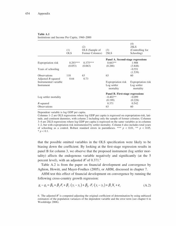
Appendix454
Table A.1Institutions and Income Per Capita, 1960–2000
(1)OLS
(2)OLS (Sample of Former Colonies)
(3)2SLS
(4)2SLS (Controlling for Schooling)
Panel A. Second-stage regressionsExpropriation risk 0.293***
(0.053)0.375***
(0.063)0.663**
(0.288)1.908
(3.848)Years of schooling −0.551
(1.539)Observations 118 63 63 60Adjusted R-squared 0.64 0.73Instrumented variable Expropriation risk Expropriation riskInstrument Log settler Log settler
mortality mortality
Panel B. First-stage regressionsLog settler mortality −0.402**
(0.199)−0.099(0.228)
R-squared 0.371 0.542Observations 63 60
Dependent variable is log GDP per capita.Columns 1–2 are OLS regressions where log GDP per capita is regressed on expropriation-risk, lati-tude, and continent dummies, with column 2 including only the sample of former colonies. Columns 3–4 are 2SLS regressions where log GDP per capita is regressed on the same variables as in columns 1–2, but with expropriation risk instrumented by settler mortality. Column 4 also includes total years of schooling as a control. Robust standard errors in parentheses. *** p < 0.01, ** p < 0.05, * p < 0.1.
that the possible omitted variables in the OLS specifi cation were likely to be biasing down the coeffi cient. By looking at the fi rst-stage regression results in panel B for column 3, we observe that the proposed instrument (log settler mor-tality) affects the endogenous variable negatively and signifi cantly (at the 5 percent level), with an adjusted R2 of 0.371.6
Table A.2 is from the paper on fi nancial development and convergence by Aghion, Howitt, and Mayer-Foulkes (2005), or AHM, discussed in chapter 7.
AHM test this effect of fi nancial development on convergence by running the following cross-country growth regression:
g g F y y F y y Xi f i y i fy i i x i i− = + + ⋅ −( ) + ⋅ ⋅ −( ) + +1 0 1 1β β β β β ε (A.2)
6. The adjusted R2 is computed adjusting the original coeffi cient of determination by using unbiased estimators of the population variances of the dependent variable and the error term (see chapter 6 in Wooldridge 2006).
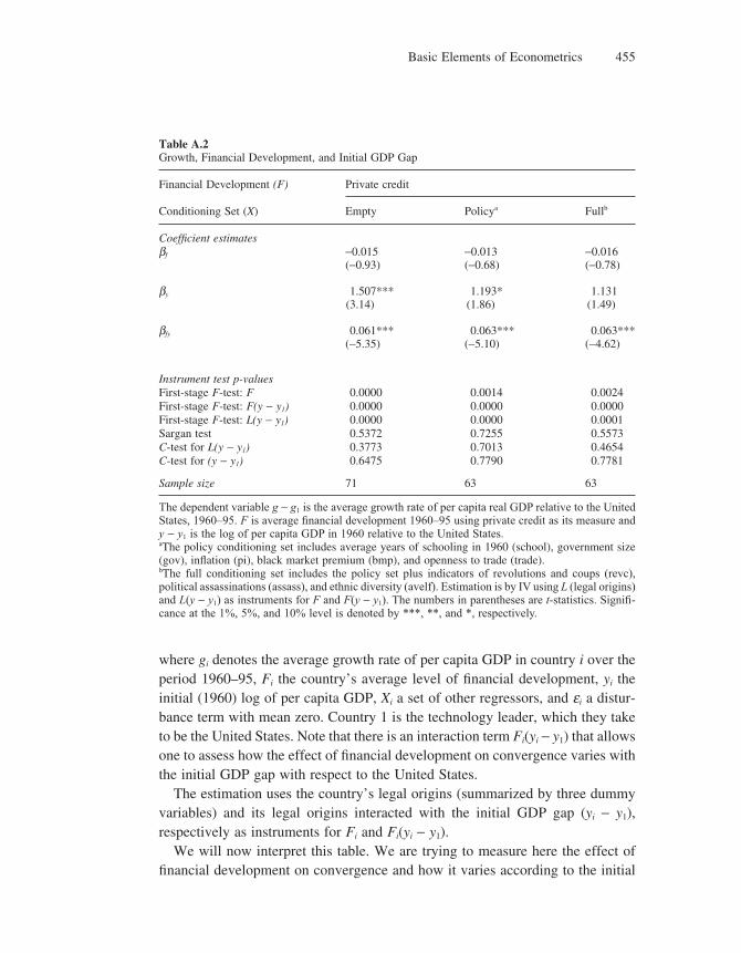
Basic Elements of Econometrics 455
where gi denotes the average growth rate of per capita GDP in country i over the period 1960–95, Fi the country’s average level of fi nancial development, yi the initial (1960) log of per capita GDP, Xi a set of other regressors, and ei a distur-bance term with mean zero. Country 1 is the technology leader, which they take to be the United States. Note that there is an interaction term Fi(yi − y1) that allows one to assess how the effect of fi nancial development on convergence varies with the initial GDP gap with respect to the United States.
The estimation uses the country’s legal origins (summarized by three dummy variables) and its legal origins interacted with the initial GDP gap (yi − y1), respectively as instruments for Fi and Fi(yi − y1).
We will now interpret this table. We are trying to measure here the effect of fi nancial development on convergence and how it varies according to the initial
Table A.2Growth, Financial Development, and Initial GDP Gap
Financial Development (F) Private credit
Conditioning Set (X) Empty Policya Fullb
Coeffi cient estimatesbf −0.015
(−0.93)−0.013(−0.68)
−0.016(−0.78)
by 1.507***(3.14)
1.193*(1.86)
1.131(1.49)
bfy 0.061***(−5.35)
0.063***(−5.10)
0.063***(−4.62)
Instrument test p-valuesFirst-stage F-test: F 0.0000 0.0014 0.0024First-stage F-test: F(y − y1) 0.0000 0.0000 0.0000First-stage F-test: L(y − y1) 0.0000 0.0000 0.0001Sargan test 0.5372 0.7255 0.5573C-test for L(y − y1) 0.3773 0.7013 0.4654C-test for (y − y1) 0.6475 0.7790 0.7781
Sample size 71 63 63
The dependent variable g − g1 is the average growth rate of per capita real GDP relative to the United States, 1960–95. F is average � nancial development 1960–95 using private credit as its measure and y − y1 is the log of per capita GDP in 1960 relative to the United States.aThe policy conditioning set includes average years of schooling in 1960 (school), government size (gov), infl ation (pi), black market premium (bmp), and openness to trade (trade).bThe full conditioning set includes the policy set plus indicators of revolutions and coups (revc), political assassinations (assass), and ethnic diversity (avelf). Estimation is by IV using L (legal origins) and L(y − y1) as instruments for F and F(y − y1). The numbers in parentheses are t-statistics. Signi� -cance at the 1%, 5%, and 10% level is denoted by ***, **, and *, respectively.
Appendix456
distance of the country’s GDP to the American GDP. In the table, private credit is used as the measure of fi nancial development. The second column controls for “policy” indicators, which include average years of schooling in 1960 (school), government size (gov), infl ation (pi), black market premium (bmp), and openness to trade (trade). The coeffi cient bf is not statistically signifi cant; by is signifi cant at the 10 percent level. The interpretation of the latter coeffi cient is that a higher level of initial GDP compared to the United States would translate into a higher average growth rate over the period also compared to the United States: an increase of one unit in the difference between country i’s initial log GDP and the American one increases on average 1.193 percent of the difference in the average growth rate of country i compared to the American one over the period of interest. The coeffi cient bfy is signifi cant at the 1 percent level and is negative, which means that the likelihood of convergence will increase with fi nancial development.
The table also provides p-values for instrument tests. The F tests for signifi -cance all yield highly signifi cant results (p-values below 0.01), providing evi-dence in favor of the strength of the proposed instruments.
The Sargan and C tests are overidentifying restrictions tests. As mentioned in the section on IV estimation, we would want all the coeffi cients from the regres-sion of the 2SLS residuals on all instruments and exogenous variables to be sta-tistically insignifi cant. The high levels of the p-values for those tests indicate that we cannot reject such null hypothesis, which provides evidence that the instru-ments are not affecting growth through an omitted nonfi nancial variable.

References
Abramovitz, M. (1986). “Catching Up, Forging Ahead, and Falling Behind.” Journal of Economic History, 46, 385–406.
Acemoglu, D. (1997). “Training and Innovation in an Imperfect Labour Market.” Review of Economic Studies, 64, 445–464.
Acemoglu, D. (1998). “Why Do New Technologies Complement Skills? Directed Technical Change and Wage Inequality.” Quarterly Journal of Economics, 113, 1055–1090.
Acemoglu, D. (2002). “Technical Change, Inequality, and the Labor Market.” Journal of Economic Literature, 40, 7–72.
Acemoglu, D. (2003a). “Patterns of Skill Premia.” Review of Economic Studies, 70, 199–230.
Acemoglu, D. (2003b). “Labor and Capital-Augmenting Technical Change.” Journal of the European Economic Association, 1, 1–37.
Acemoglu, D. (2008a). Introduction to Modern Economic Growth. Forthcoming.
Acemoglu, D. (2008b). “Oligarchic versus Democratic Societies.” Journal of the European Economic Association, 6, 1–44.
Acemoglu, D., P. Aghion, C. Lelarge, J. Van Reenen, and F. Zilibotti. (2007). “Technology, Informa-tion, and the Decentralization of the Firm.” Quarterly Journal of Economics, 4, 1759–1799.
Acemoglu, D., P. Aghion, and G. L. Violante. (2001). “Deunionization, Technical Change, and Inequality.” Carnegie-Rochester Conference Series on Public Policy.
Acemoglu, D., P. Aghion, and F. Zilibotti. (2006). “Distance to Frontier, Selection, and Economic Growth.” Journal of the European Economic Association, 37–74.
Acemoglu, D., and J. Angrist. (2000). “How Large Are Human Capital Externalities? Evidence from Compulsory Schooling Laws.” NBER Macroannual, 9–59.
Acemoglu, D., and V. Guerrieri. (2006). “Capital Deepening and Non-Balanced Economic Growth.” NBER Working Paper No. 12475.
Acemoglu, D., and S. Johnson. (2005). “Unbundling Institutions.” Journal of Political Economy, 113, 949–995.
Acemoglu, D., S. Johnson, and T. Mitton. (2003). “Institutions and Market Structure.” Mimeo, MIT.
Acemoglu, D., S. Johnson, and J. Robinson. (2005). “Institutions as a Fundamental Cause of Long-Run Growth.” In P. Aghion and S. N. Durlauf. (Eds.), Handbook of Economic Growth. Amsterdam: Elsevier North-Holland.
Acemoglu, D., S. Johnson, J. Robinson, and P. Yared. (2005). “Income and Democracy.” CEPR Discussion Paper No. 5273.
Acemoglu, D., and J. Linn. (2004). “Market Size in Innovation: Theory and Evidence from the Pharmaceutical Industry.” Quarterly Journal of Economics, 119, 1049–1090.
Acemoglu, D., J. A. Robinson, and S. Johnson. (2001). “The Colonial Origins of Comparative Devel-opment: An Empirical Investigation.” American Economic Review, 91, 1369–1401.
Acemoglu, D., J. A. Robinson, and S. Johnson. (2002). “Reversal of Fortune: Geography and Institu-tions in the Making of the Modern World Income Distribution.” Quarterly Journal of Economics, 117, 1231–1294.
Acemoglu, D., J. A. Robinson, and S. Johnson. (2005a). “Institutions as a Fundamental Cause of Long-Run Growth.” In P. Aghion and S. N. Durlauf (Eds.). Handbook of Economic Growth. Elsevier North-Holland, Amsterdam.
Acemoglu, D., J. A. Robinson, and S. Johnson. (2005b). “The Rise of Europe: Atlantic Trade, Insti-tutional Change and Economic Growth.” American Economic Review, 95, 546–579.
Acemoglu, D., and J. Ventura. (2002). “The World Income Distribution.” Quarterly Journal of Eco-nomics, 117, 659–694.
References458
Acemoglu, D., and F. Zilibotti. (1997). “Was Prometheus Unbound by Chance? Risk, Diversifi cation, and Growth.” Journal of Political Economy, 105, 709–775.
Acemoglu, D., and F. Zilibotti. (2001). “Productivity Differences.” Quarterly Journal of Economics, 116, 563–606.
Aghion, P., A. Alesina, and F. Trebbi. (2004). “Endogenous Political Institutions.” Quarterly Journal of Economics, 119, 565–611.
Aghion, P., A. Alesina, and F. Trebbi. (2008). “Democracy, Technology, and Growth.” In E. Helpman (Ed.). Institutions and Economic Performance. Cambridge, MA: Harvard University Press.
Aghion, P., Y. Algan, and P. Cahuc. (2008). “Can Policy Interact with Culture? Minimum Wage and the Quality of Labor Relations.” NBER Working Paper No. 14327.
Aghion, P., Y. Algan, P. Cahuc, and A. Shleifer. (2008). “Regulation and Distrust.” Mimeo, Harvard University.
Aghion, P., G. M. Angeletos, A. Banerjee, and K. Manova. (2005). “Volatility and Growth: Financial Development and the Cyclical Behavior of the Composition of Investment.” Mimeo, Harvard University.
Aghion, P., P. Bacchetta, R. Ranciere, and K. Rogoff. (2006). “Exchange Rate Volatility and Productivity Growth: The Role of Financial Development.” CEPR Discussion Paper No. 5629.
Aghion, P., and A. Banerjee. (2005). “Volatility and Growth.” Clarendon Lectures in Economics. Oxford, UK: Oxford University Press.
Aghion, P., A. Banerjee, and T. Piketty. (1999). “Dualism and Macroeconomic Volatility.” Quarterly Journal of Economics, 114, 1359–1397.
Aghion, P., N. Bloom, R. Blundell, R. Griffi th, and P. Howitt. (2005). “Competition and Innovation: An Inverted-U Relationship.” Quarterly Journal of Economics, 120, 701–728.
Aghion, P., R. Blundell, R. Griffi th, P. Howitt, and S. Prantl. (2004). “Entry and Productivity Growth: Evidence from Microlevel Panel Data.” Journal of the European Economic Association, 2, 265–276.
Aghion, P., R. Blundell, R. Griffi th, P. Howitt, and S. Prantl. (2006). “The Effects of Entry on Incumbent Innovation and Productivity.” CEPR Discussion Paper No. 5323.
Aghion, P., and P. Bolton. (1997). “A Trickle Down Theory of Growth and Development.” Review of Economic Studies, 64, 151–172.
Aghion, P., L. Boustan, C. Hoxby, and J. Vandenbussche. (2005). “Exploiting States’ Mistakes to Identify the Causal Effect of Higher Education on Growth.” Mimeo, Harvard University.
Aghion, P., R. Burgess, S. Redding, and F. Zilibotti. (2006). “The Unequal Effects of Liberalization: Evidence from Dismantling the License Raj in India.” CEPR Discussion Paper No. 5492.
Aghion, P., M. Dewatripont, C. Hoxby, A. Mas-Colell, and A. Sapir. (2007). “Why Reform Europe’s Universities?” Bruegel Policy Brief.
Aghion, P., M. Dewatripont, and P. Rey. (1999). “Competition, Financial Discipline, and Growth.” Review of Economic Studies, 66, 825–852.
Aghion, P., and S. N. Durlauf (Eds.). (2005). Handbook of Economic Growth. Amsterdam: Elsevier North-Holland.
Aghion, P., J. Fedderke, P. Howitt, C. Kulatane, and N. Viegi. (2008). “Testing Creative Destruction in an Opening Economy: The Case of the South African Manufacturing Industries.” Mimeo, Harvard University.
Aghion, P., and R. Griffi th. (2005). Competition and Growth: Reconciling Theory and Evidence. Cambridge, MA: MIT Press.
References 459
Aghion, P., C. Harris, P. Howitt, and J. Vickers. (2001). “Competition, Imitation and Growth with Step-by-Step Innovation.” Review of Economic Studies, 68, 467–492.
Aghion, P., C. Harris, and J. Vickers. (1997). “Competition and Growth with Step-by-Step Innovation: An Example.” European Economic Review, Papers and Proceedings, 771–782.
Aghion, P., and P. Howitt. (1988). “Growth and Cycles through Creative Destruction.” Mimeo, MIT.
Aghion, P., and P. Howitt. (1992). “A Model of Growth through Creative Destruction.” Econometrica, 60, 323–351.
Aghion, P., and P. Howitt. (1998a). Endogenous Growth Theory. Cambridge, MA: MIT Press.
Aghion, P., and P. Howitt. (1998b). “On the Macroeconomic Effects of Major Technological Change.” In E. Helpman (Ed.). General Purpose Technologies and Economic Growth. Cambridge, MA: MIT Press.
Aghion, P., and P. Howitt. (2006). “Joseph Schumpeter Lecture: Appropriate Growth Policy: A Unify-ing Framework.” Journal of the European Economic Association, 4, 269–314.
Aghion, P., P. Howitt, and D. Mayer-Foulkes. (2005). “The Effect of Financial Development on Convergence: Theory and Evidence.” Quarterly Journal of Economics, 120, 173–222.
Aghion, P., P. Howitt, and G. L. Violante. (2000). “General Purpose Technology and Within-Group Inequality.” CEPR Discussion Paper No. 2474.
Aghion, P., P. Howitt, and G. L. Violante. (2002). “General Purpose Technology and Wage Inequal-ity.” Journal of Economic Growth, 7, 315–345.
Aghion, P., and E. Kharroubi. (2007). “Cyclical Budgetary Policy and Growth: A Sectoral Analysis. Mimeo, Harvard University.
Aghion, P., and I. Marinescu. (2007). “Cyclical Budgetary Policy and Economic Growth: What Do We Learn from OECD Panel Data?” Mimeo, Harvard University.
Aghion, P., and G. Saint-Paul. (1998). “Uncovering Some Causal Relationships between Productivity Growth and the Structure of Economic Fluctuations: A Tentative Survey.” Labour, 12, 279–303.
Alesina, A., and D. Rodrik. (1994). “Distributive Politics and Economic Growth.” Quarterly Journal of Economics, 109, 465–490.
Alesina, A., E. Spolaore, and R. Wacziarg. (2005). “Trade, Growth and the Size of Countries.” In P. Aghion and S. N. Durlauf (Eds.). Handbook of Economic Growth. Amsterdam: Elsevier North-Holland.
Arestis, P., P. O. Demetriades, and K. B. Luintel. (2001). “Financial Development and Economic Growth: The Role of Stock Markets.” Journal of Money, Credit, and Banking, 33, 16–41.
Arrow, K. J. (1962). “The Economic Implications of Learning by Doing.” Review of Economic Studies, 29, 155–173.
Arrow, K. J. (1969). “Classifi catory Notes on the Production and Transmission of Technological Knowledge.” American Economic Review, Papers and Proceedings, 59, 29–35.
Arrow, K. J., and M. Kurz. (1970). Public Investment, the Rate of Return and Optimal Fiscal Policy. Baltimore: Johns Hopkins University Press.
Ashraf, Q., and O. Galor. (2008). “Malthusian Population Dynamics: Theory and Evidence.” Working Papers 2008-6, Brown University, Department of Economics.
Atkinson, A. B., and J. E. Stiglitz. (1969). “A New View of Technological Change.” Economic Journal, 79, 573–578.
Autor, D., A. Krueger, and L. Katz. (1998). “Computing Inequality: Have Computers Changed the Labor Market?” Quarterly Journal of Economics, 113, 1169–1214.
Azariadis, C., and A. Drazen. (1990). “Threshold Externalities in Economic Development.” Quarterly Journal of Economics, 105, 501–526.
References460
Banerjee, A., and E. Dufl o. (2003). “Inequality and Growth: What Can the Data Say? Journal of Economic Growth, 8, 267–299.
Banerjee, A., and E. Dufl o. (2005). “Growth Theory through the Lens of Development Economics.” In P. Aghion and S. N. Durlauf (Eds). Handbook of Economic Growth. Amsterdam: Elsevier North-Holland.
Banerjee, A., and L. Iyer. (2005). “History, Institutions, and Economic Performance: The Legacy of Colonial Land Tenure Systems in India.” American Economic Review, 95, 1190–1213.
Banerjee, A., and A. Newman. (1993). “Occupational Choice and the Process of Development.” Journal of Political Economy, 101, 274–298.
Barlevy, G. (2007). “On the Cyclicality of Research and Development.” American Economic Review, 97, 1131–1164.
Barro, R. J. (1990). “Government Spending in a Simple Model of Endogenous Growth.” Journal of Political Economy, 98, 103–125.
Barro, R. J. (1996). “Democracy and Growth.” Journal of Economic Growth, 1, 1–27.
Barro, R. J. (1997). Determinants of Economic Growth: A Cross-Country Empirical Study. Cam-bridge, MA: MIT Press.
Barro, R. J. (1999a). “The Determinants of Democracy.” Journal of Political Economy, 107, S158–S183.
Barro, R. J. (1999b). “Laibson Meets Ramsey in the Neoclassical Growth Model.” Quarterly Journal of Economics, 114, 1125–1152.
Barro, R. J., and J. W. Lee. (2000). “International Data on Educational Attainment Updates and Implications.” NBER Working Paper No. 791.
Barro, R. J., N. G. Mankiw, and X. Sala-i-Martin. (1995). “Capital Mobility in Neoclassical Models of Growth.” American Economic Review, 85, 103–115.
Barro, R., and X. Sala-i-Martin. (1991). “Convergence across States and Regions.” Brookings Papers on Economic Activity, 1, 107–182.
Barro, R. J., and X. Sala-i-Martin. (1992a). “Convergence.” Journal of Political Economy 100, 223–251.
Barro, R. J., and X. Sala-i-Martin. (1992b). “Public Finance in Models of Economic Growth.” Review of Economic Studies, 59, 645–661.
Barro, R. J., and X. Sala-i-Martin. (1995a). Economic Growth. New York: McGraw-Hill.
Barro, R. J., and X. Sala-i-Martin. (1995b). “Technological Diffusion, Convergence and Growth.” CEPR Discussion Paper No. 1255.
Barro, R. J., and X. Sala-i-Martin. (1997). “Technological Diffusion, Convergence, and Growth.” Journal of Economic Growth, 2, 1–27.
Basu, S., and D. N. Weil. (1998). “Appropriate Technology and Growth.” Quarterly Journal of Eco-nomics, 113, 1025–1054.
Baumol, W. (1967). “Macroeconomics of Unbalanced Growth: The Anatomy of Urban Crisis.” American Economic Review, 57, 415–426.
Baumol, W. (1986). “Productivity Growth, Convergence and Welfare: What the Long Run Shows.” American Economic Review, 76, 1072–1085.
Baumol, W., J. Blackman, S. A. Batey, and E. N. Wolff. (1989). Productivity and American Leader-ship. Cambridge MA: MIT Press.
Baumol, W., and E. N. Wolff. (1988). “Productivity Growth, Convergence and Welfare: Reply.” American Economic Review, 78, 1155–1159.
Bean. C. R. (1990). “Endogenous Growth and the Procyclical Behaviour of Productivity.” European Economic Review, 34, 355–363.
References 461
Beck, T., A. Demirgüç-Kunt, L. Laeven, and R. Levine. (2004). “Finance, Firm Size, and Growth.” NBER Working Paper No. W10983.
Becker, G. (1964). Human Capital. New York: Columbia University Press.
Becker, G., K. Murphy, and R. Tamura. (1990). “Human Capital, Fertility and Economic Growth.” Journal of Political Economy, 98, part 2, 513–537.
Benabou, R. (1996). “Inequality and Growth.” In B. S. Bernanke and J. Rotemberg (Eds.). NBER Macroeconomics Annual 11. Cambridge, MA: MIT Press.
Benassy, J.-P. (1998). “Is There Always Too Little Research in Endogenous Growth with Expanding Product Variety?” European Economic Review, 42, 61–69.
Bencivenga, V. R., and B. D. Smith. (1993). “Some Consequences of Credit Rationing in an Endog-enous Growth Model.” Journal of Economic Dynamics and Control, 17, 97–122.
Benhabib, J., and M. M. Spiegel. (1994). “The Role of Human Capital in Economic Development: Evidence from Aggregate Cross-Country Data.” Journal of Monetary Economics, 34, 143–173.
Benhabib, J., and M. M. Spiegel. (2005). “Human Capital and Technology Diffusion.” In P. Aghion and S. N. Durlauf (Eds.). Handbook of Economic Growth. Amsterdam: Elsevier North-Holland.
Berman, E., J. Bound, and Z. Griliches. (1994). “Changes in the Demand for Skilled Labor within U.S. Manufacturing: Evidence from the Annual Survey of Manufacturers,” Quarterly Journal of Economics, 109, 367–397.
Berman, N., L. Eymard, P. Aghion, P. Askhenazy, and G. Cette. (2007). “Credit Constraints and the Cyclicality of R&D: Lessons from French Firm-Level Panel Data.” Mimeo, Banque de France.
Bernanke, B., and M. Gertler. (1989). “Agency Costs, Net Worth and Business Fluctuations.” Ameri-can Economic Review, 79, 14–31.
Bernanke, B., M. Gertler, and S. Gilchrist. (1999). “The Financial Accelerator in a Quantitative Busi-ness Cycle Framework.” In J. Taylor and M. Woodford (Eds.). Handbook of Macroeconomics. Amsterdam: North-Holland.
Bils, M., and P. Klenow. (2000). “Does Schooling Cause Growth?” American Economic Review, 90, 1160–1183.
Blanchard, O. (1985). “Debt, Defi cits, and Finite Horizons.” Journal of Political Economy, 93, 223–247.
Blundell, R., R. Griffi th, and J. Van Reenen. (1995). “Dynamic Count Data Models of Technological Innovation.” Economic Journal, 105, 333–344.
Blundell, R., R. Griffi th, and J. Van Reenen. (1999). “Market Share, Market Value and Innovation in a Panel of British Manufacturing Firms.” Review of Economic Studies, 66, 529–554.
Blundell, R., and I. Preston. (1999). “Inequality and Uncertainty: Short-Run Uncertainty and Perma-nent Inequality in the US and Britain.” Mimeo, University College, London.
Boyd, J. H., and E. C. Prescott. (1986). “Financial Intermediary-Coalitions.” Journal of Economic Theory, 38, 211–232.
Bresnahan, T., and A. Gambardella. (1998). “The Division of Inventive Labor and the Extent of the Market.” In E. Helpman (Ed.). General Purpose Technologies and Economic Growth. Cambridge, MA: MIT Press.
Bresnahan, T., and M. Trajtenberg. (1995). “General Purpose Technologies: Engines of Growth?” Journal of Econometrics, 65, 83–108.
Brock, W., and L. Mirman. (1972). “Optimal Economic Growth under Uncertainty: The Discounted Case.” Journal of Economic Theory, 4, 497–513.
Broda, C., J. Greenfi eld, and D. Weinstein. (2006). “From Groundnuts to Globalization: A Structural Estimate of Trade and Growth.” NBER Working Paper No. 12512.
Bruno, M. (1993). Crisis, Stabilization and Economic Reform: Therapy by Consensus. Oxford, UK: Clarendon Press.
References462
Buonanno, P., C. Carraro, and M. Galeotti. (2003). “Endogenous Induced Technical Change and the Costs of Kyoto.” Resource and Energy Economics, 25, 11–34.
Caballero, R. J., and M. Hammour. (1994). “The Cleansing Effects of Recessions.” American Eco-nomic Review, 84, 1350–1368.
Caballero, R., and A. Jaffe. (1993). “How High Are the Giants’ Shoulders? An Empirical Assessment of Knowledge Spillovers and Creative Destruction in a Model of Economic Growth.” NBER Macro-economic Annual, 15–74.
Canova, F., and A. Marcet. (1995). “The Poor Stay Poor: Nonconvergence across Countries and Regions.” CEPR Discussion Paper No. 1265.
Card, D. (1996). “The Effects of Unions on the Structure of Wages: A Longitudinal Analysis.” Econometrica, 64, 957–979.
Caselli, F. (2005). “Accounting for Cross-Country Income Differences.” In P. Aghion and S. N. Durlauf (Eds). Handbook of Economic Growth. Amsterdam: Elsevier North-Holland.
Casselli F., and W. J. Coleman. (2001). “Cross-Country Technology Diffusion: The Case of Comput-ers.” American Economic Review, Papers and Proceedings, 91, 328–335.
Caselli, F., G. Esquivel, and F. Lefort. (1996). “Reopening the Convergence Debate: A New Look at Cross-Country Growth Empirics.” Journal of Economic Growth, 1, 363–389.
Caselli, F., and N. Gennaioli. (2006). “Dynastic Management.” CEP Discussion Paper No. 741.
Caselli, F, and J. Ventura. (2000). “A Representative Consumer Theory of Distribution.” American Economic Review, 90, 909–926.
Caselli, F., and D. J. Wilson. (2004). “Importing Technology.” Journal of Monetary Economics, 51, 1–32.
Cass, D. (1965). “Optimum Growth in an Aggregative Model of Capital Accumulation.” Review of Economic Studies, 32, 233–240.
Cheng, L. K., and E. Dinopoulos. (1992). “Schumpeterian Growth and International Business Cycles.” American Economic Review, Papers and Proceedings, 82, 409–414.
Coe, D. T., and E. Helpman. (1995). “International R&D Spillovers.” European Economic Review, 39, 859–887.
Cohen, W. M., and D. A. Levinthal. (1989). “Innovation and Learning: The Two Faces of R&D.” Economic Journal, 99, 569–596.
Comin, D. (2000). “An Uncertainty-Driven Theory of the Productivity Slowdown: Manufacturing.” Mimeo, Harvard University.
Comin, D., and M. Gertler. (2006). “Medium-Term Business Cycles.” American Economic Review, 96, 523–551.
Comin, D., M. Gertler, and A. M. Santacreu. (2008). “International Medium Term Business Cycles.” Mimeo.
Comin, D., and S. Mulani. (2007). “A Theory of Growth and Volatility at the Aggregate and Firm Level.” Proceedings, Federal Reserve Bank of San Francisco.
Corriveau, L. (1991). “Entrepreneurs, Growth and Cycles.” PhD dissertation. University of Western Ontario.
Crépon, B., E. Duguet, and J. Mairesse. (1998). “Research, Innovation, and Productivity: An Econo-metric Analysis at the Firm Level.” NBER Working Paper No. 6696.
Cummins, J. G., and G. L. Violante. (2002) “Investment-Specifi c Technical Change in the United States (1947–2000): Measurement and Macroeconomic Consequences.” Review of Economic Dynamics, 5, 243–284.
Dasgupta, S. (2008). “Discounting Climate Change.” Review of Environmental Economics and Policy, forthcoming.
References 463
Dasgupta, S., B. Laplante, H. Wang, and D. Wheeler. (2002). “Confronting the Environmental Kuznets Curve.” Journal of Economic Perspectives, 16, 147–168.
Dasgupta, P., and J. Stiglitz. (1980). “Industrial Structure and the Nature of Innovative Activity.” Economic Journal, 90, 266–293.
d’Autume, A., and P. Michel. (1994). “Education et Croissance.” Revue d.Économie Politique, 104, 457–499.
David, P. A. (1990). “The Dynamo and the Computer: An Historical Perspective on the Modern Productivity Paradox.” American Economic Review, 80, 355–361.
Deaton, A., and J. Dreze. (2002). “Poverty and Inequality in India: A Reexamination.” Working Paper 107, Princeton University.
De Gregorio, J. (1996). “Borrowing Constraints, Human Capital Accumulation, and Growth.” Journal of Monetary Economics, 37, 49–71.
DeLong, B. (1988). “Productivity Growth, Convergence and Welfare: Comment.” American Eco-nomic Review, 78, 1138–1154.
Demirgüç-Kunt, A., and V. Maksimovic. (1998). “Law, Finance, and Firm Growth.” Journal of Finance, 53, 2107–2137.
Denison, E. F. (1962). “Sources of Growth in the United States and the Alternatives before Us.” Supplement Paper 13. Committee for Economic Development, New York.
Devereux, M., and B. J. Lapham. (1994). “The Stability of Economic Integration and Endogenous Growth.” Quarterly Journal of Economics, 59, 299–305.
Dinopoulos, E., and C. Syropoulos. (2006). “Rent Protection as a Barrier to Innovation and Growth.” Economic Theory, 32, 309–332.
Dinopoulos, E., and P. Thompson. (1998). “Schumpeterian Growth without Scale Effects.” Journal of Economic Growth, 3, 313–335.
Dixit, A. K., and J. E. Stiglitz. (1977). “Monopolistic Competition and Optimum Product Diversity.” American Economic Review, 67, 297–308.
Djankov, S, R. La Porta, F. Lopez-de-Silanes, and A. Shleifer. (2002). “The Regulation of Entry.” Quarterly Journal of Economics, 117, 1–37.
Djankov, S., R. La Porta, F. Lopez-de-Silanes, and A. Shleifer. (2003). “Courts.” Quarterly Journal of Economics, 118, 453–517.
Doepke, M., and F. Zilibotti. (2008). “Occupational Choice and the Spirit of Capitalism.” Quarterly Journal of Economics, 123, 747–795.
Domar, E. D. (1946). “Capital Expansion, Rate of Growth, and Employment.” Econometrica, 14, 137–147.
Dowrick. S., and D. Nguyen. (1989). “OECD Comparative Economic Growth, 1950–1985: Catch-up and Convergence.” American Economic Review, 79, 1010–1030.
Drandakis, E., and E. Phelps. (1965). “A Model of Induced Invention, Growth and Distribution.” Economic Journal, 76, 823–840.
Dufl o, E. (2004). “The Medium Run Consequences of Educational Expansion: Evidence from a Large School Construction Program in Indonesia.” Journal of Development Economics, 74, 163–197.
Durlauf, S., and P. Johnson. (1995). “Multiple Regimes and Cross-Country Growth Behavior.” Journal of Applied Econometrics, 10, 365–384.
Easterly, W. (2005). “National Policies and Economic Growth.” In P. Aghion and S. N. Durlauf (Eds.). Handbook of Economic Growth. Amsterdam: Elsevier North-Holland.
Easterly, W., and R. Levine. (1997). “Africa’s Growth Tragedy: Policies and Ethnic Divisions.” Quarterly Journal of Economics, 112, 1203–1250.
References464
Eaton, J., and S. Kortum. (2001). “Technology, Trade, and Growth: A Unifi ed Framework.” European Economic Review, Papers and Proceedings, 45, 742–755.
Eaton, J., and S. Kortum. (2002). “Technology, Geography, and Trade.” Econometrica, 70, 1741–1779.
Engerman, S. L., and K. L. Sokoloff. (1997). “Factor Endowments, Institutions, and Differential Growth Paths among New World Economies.” In S. Haber (Ed.). How Latin America Fell Behind. Stanford, CA: Stanford University Press.
Engerman, S. L., and K. L. Sokoloff. (2000). “History Lessons: Institutions, Factor Endowments, and the Paths of Development in the New World.” Journal of Economic Perspective, 14, 217–232.
Ethier, W. J. (1982). “National and International Returns to Scale in the Modern Theory of Interna-tional Trade.” American Economic Review, 72, 389–405.
Etro, F. (2004). “Innovation by Leaders.” Economic Journal, 114, 281–303.
Evans, P. (1996). “Using Cross-Country Variances to Evaluate Growth Theories.” Journal of Eco-nomic Dynamics and Control, 20, 1027–1049.
Evenson, R. E., and L. E. Westphal. (1995). “Technological Change and Technology Strategy.” In T. N. Srinivasan and J. Behrman (Eds.). Handbook of Development Economics, vol. 3A. Amsterdam: Elsevier.
Fellner, W. (1961). “Two Propositions in the Theory of Induced Innovations.” Economic Journal, 71, 305–308.
Fogel, K., R. Morck, and B. Yeung. (2008). “Big Business Stability and Economic Growth: Is What’s Good for General Motors Good for America?” Journal of Financial Economics, forthcoming.
Fortin, N. M., and T. Lemieux. (1997). “Institutional Changes and Rising Wage Inequality: Is There a Linkage?” Journal of Economic Perspectives, 11, 75–96.
Francois, P., and H. Lloyd-Ellis. (2003). “Animal Spirits through Creative Destruction.” American Economic Review, 93, 530–550.
Frankel, J., and D. Romer. (1999). “Does Trade Cause Growth?” American Economic Review, 89, 379–399.
Frankel, M. (1962). “The Production Function in Allocation of Growth: A Synthesis.” American Economic Review, 52, 995–1022.
Freedom House. (2004). Freedom in the World. Website and book, Washington DC.
Freeman, C., J. Clark, and L. Soete. (1982). Unemployment and Technical Innovation: A Study of Long Waves and Economic Development. London: Francis Pinter.
Freeman, C., and C. Perez. (1988). “Structural Crises of Adjustment, Business Cycles and Investment Behaviour.” In G. Dosi et al. (Eds.). Technical Change and Economic Theory. London: Francis Pinter.
Freeman, R. B. (1993). “How Much Has Deunionization Contributed to the Rise in Male Earnings Inequality?” In S. Danziger and P. Gottschalk (Eds.). Uneven Tides: Rising Inequality in America. New York: Russell Sage Foundation.
Gali, J., and M. Hammour. (1991). “Long-Run Effects of Business Cycles.” Papers 540. Columbia University.
Galor, O. (2005). “From Stagnation to Growth: Unifi ed Growth Theory.” In P. Aghion and S. N. Durlauf (Eds.). Handbook of Economic Growth. Amsterdam: Elsevier North-Holland.
Galor, O., and O. Moav. (2000). “Ability Biased Technological Transition, Wage Inequality within and across Groups, and Economic Growth.” Quarterly Journal of Economics, 115, 469–497.
Galor, O., and D. N. Weil. (2000). “Population, Technology and Growth: From the Malthusian Regime to the Demographic Transition.” American Economic Review, 110, 806–828.
References 465
Galor, O., and J. Zeira. (1993). “Income Distribution and Macroeconomics.” Review of Economic Studies, 60, 35–52.
Gancia, G. (2003). “Globalization, Divergence and Stagnation.” IIES Seminar Paper 720.
Gancia, G., and F. Zilibotti. (2005). “Horizontal Innovation in the Theory of Growth and Develop-ment.” In P. Aghion and S. N. Durlauf (Eds.). Handbook of Economic Growth. Amsterdam: Elsevier North-Holland.
Garcia-Peñalosa, C., and B. Koebel. (1998). “International Trade, Material Prices and Wages.” Mimeo, Nuffi eld College, Oxford.
Geroski, P. (1995). Market Structure, Corporate Performance and Innovative Activity. Oxford, UK: Oxford University Press.
Gerschenkron, A. (1962). Economic Backwardness in Historical Perspective: A Book of Essays. Cambridge, MA: Belknap Press of Harvard University Press.
Glaeser, E., R. La Porta, F. Lopez-de-Silanes, and A. Shleifer. (2004). “Do Institutions Cause Growth?” Journal of Economic Growth, 9, 271–303.
Glomm, G., and B. Ravikumar. (1992). “Public versus Private Investment in Human Capital Endog-enous Growth and Income Inequality.” Journal of Political Economy, 100, 813–834.
Goldin, C., and L. M. Katz. (1998). “The Origins of Technology-Skill Complementarity.” Quarterly Journal of Economics, 113, 693–732.
Goldin, C., and L. F. Katz. (1999). “The Returns to Skill across the Twentieth Century in the United States.” NBER Working Paper No. 7126.
Goldsmith, R. W. (1969). Financial Structure and Development. New Haven, CT: Yale University Press.
Gordon, R. J. (1990). The Measurement of Durable Goods Prices. Chigaco: University of Chicago Press.
Gordon, R. J. (1999). “U.S. Economic Growth since 1870: One Big Wave?” American Economic Review, Papers and Proceedings, 89, 123–128.
Gottschalk, P., and R. Moffi tt. (1994). “The Growth of Earnings Instability in the US Labour Market.” Brookings Papers on Economic Activity, 2, 217–272.
Greenwood, J., and B. Jovanovic. (1990). “Financial Development, Growth, and the Distribution of Income.” Journal of Political Economy, 98, 1076–1107.
Greenwood, J., and B. Smith. (1996). “Financial Markets in Development, and the Development of Financial Markets.” Journal of Economic Dynamics and Control, 21, 145–181.
Greenwood, J., and M. Yorukoglu. (1997). “1974.” Carnegie-Rochester Series on Public Policy, 46, 49–95.
Greif, A. (1994). “Cultural Beliefs and the Organization of Society: A Historical and Theoretical Refl ection on Collectivist and Individualist Societies.” Journal of Political Economy, 102, 912–950.
Greif, A. (2006). Institutions and the Path to the Modern Economy. New York: Cambridge University Press.
Griffi th, R., S. Redding, and J. Van Reenan. (2004). “Mapping the Two Faces of R&D: Pro-ductivity Growth in a Panel of OECD Industries.” Review of Economics and Statistics, 86, 883–895.
Griliches, Z. (1973). “Research Expenditures and Growth Accounting.” In B. R. Williams (Ed.). Science and Technology in Economic Growth. New York: Macmillan.
Griliches, Z. (1979). “Issues on Assessing the Contribution of Research and Development to Produc-tivity Growth.” Bell Journal of Economics, 10, 92–116.
References466
Griliches, Z. (1988). “Productivity Puzzles and R&D: Another Explanation.” Journal of Economic Perspectives, 2, 9–21.
Griliches, Z. (1994). “Productivity, R&D, and the Data Constraint.” American Economic Review, 84, 1–23.
Griliches, Z., and F. Lichtenberg. (1984). “R&D and Productivity Growth at the Industry Level: Is There Still a Relationship?” In Z. Griliches (Ed.). R&D, Patents, and Productivity. Chicago: Univer-sity of Chicago Press.
Grossman, G., and E. Helpman. (1989). “Product Development and International Trade.” Journal of Political Economy, 97, 1261–1283.
Grossman, G., and E. Helpman. (1991a). Innovation and Growth in the World Economy. Cambridge, MA: MIT Press.
Grossman, G. M., and E. Helpman. (1991b). “Quality Ladders in the Theory of Growth.” Review of Economic Studies, 58, 43–61.
Grossman, G. M., and E. Helpman. (1991c). “Quality Ladders and Product Cycles.” Quarterly Journal of Economics, 106, 557–586.
Grossman, G. M., and E. Helpman. (1991d). “Trade Knowledge Spillovers and Growth.” European Economic Review, 35, 517–526.
Grossman, G., and E. Helpman. (1995). “Technology and Trade.” In G. Grossman and K. Rogoff (Eds.). Handbook of International Economics, vol. 3. Amsterdam: Elsevier.
Grossman, G. M., and A. B. Krueger. (1991). “Environmental Impact of a North American Free Trade Agreement.” NBER Working Paper No. 3914.
Grossman, G. M., and A. B. Krueger. (1995). “Economic Growth and the Environment.” Quarterly Journal of Economics, 110, 353–377.
Grübler, A., and S. Messner. (1998). “Technological Change and the Timing of Mitigation Measures.” Energy Economics, 20, 495–512.
Guiso, L., P. Sapienza, and L. Zingales. (2002). “Does Local Financial Development Matter?” NBER Working Paper No. 8922.
Guiso, L., P. Sapienza, and L. Zingales. (2005). “Does Culture Affect Economic Outcomes?” Journal of Economic Perspectives, 20, 23–48.
Gurley, J. G., and E. S. Shaw. (1955). “Financial Aspects of Economic Development.” American Economic Review, 45, 515–538.
Ha, J. (2002). “From Factor Accumulation to Innovation: Sustained Economic Growth with Changing Components.” Mimeo, Brown University.
Ha, J., and P. Howitt. (2006). “Accounting for Trends in Productivity and R&D: A Schumpeterian Critique of Semi-Endogenous Growth Theory.” Journal of Money, Credit, and Banking, 39, 733–774.
Habakkuk, H. J. (1962). American and British Technology in the Nineteenth Century: Search for Labor Saving Inventions. Cambridge, UK: Cambridge University Press.
Hall, B. H., A. Jaffe, and M. Trajtenberg. (2000). “Market Value and Patent Citations: A First Look.” NBER Working Paper No. W7741.
Hall, R. E. (1991). “Recessions as Reorganizations.” NBER Macroeconomics Annual.
Hall, R. E., and C. I. Jones. (1999). “Why Do Some Countries Produce So Much More Output Per Worker Than Others?” Quarterly Journal of Economics, 114, 83–116.
Hansen, G., and E. Prescott. (2002), “Malthus to Solow.” American Economic Review, 92, 1205–1217.
Hanushek, E. A., and L. Woessmann. (2007). “The Role of Education Quality for Economic Growth.” Policy Research Working Paper Series 4122, World Bank.
References 467
Harbaugh, B., A. Levinson, and D. Wilson. (2002). “Reexamining the Empirical Evidence for an Environmental Kuznets Curve.” Review of Economics and Statistics, 84, 541–551.
Harris, R. (1998). “The Internet as a GPT: Factor Market Implications.” In E. Helpman (Ed.). General Purpose Technologies and Economic Growth. Cambridge, MA: MIT Press.
Harrod, R. F. (1939). “An Essay in Dynamic Theory.” Economic Journal, 49, 14–33.
Hart, O. (1983). “The Market Mechanism as an Incentive Scheme.” Bell Journal of Economics, 14, 366–382.
Hauk, E., and M. Saez-Marti. (2002). “On the Cultural Transmission of Corruption.” Journal of Economic Theory, 107, 311–335.
Hausmann, R., and M. Gavin. (1996). “Securing Stability and Growth in a Shock Prone Region: The Policy Challenge for Latin America.” InterAmerican Development Bank Working Paper 315.
Hausmann, R., and D. Rodrik. (2003). “Economic Development as Self-Discovery.” Journal of Development Economics, 72, 603–633.
Hausmann, R., D. Rodrik, and A. Velasco. (2005). “Growth Diagnostics.” Mimeo, Harvard University.
Heckman, J. J., L. Lochner, and C. Taber. (1998). “Explaining Rising Wage Inequality: Explorations with a Dynamic General Equilibrium Model of Labor Earnings with Heterogeneous Agents.” Review of Economic Dynamics, 1, 1–58.
Helpman, E. (1993). “Innovation, Immitation, and Intellectual Property Rights.” Econometrica, 61, 1247–1280.
Helpman, E. (Ed.). (1998). General Purpose Technologies and Economic Growth. Cambridge, MA: MIT Press.
Helpman, E. (2004). The Mystery of Economic Growth. Cambridge, MA: Belknap Press of Harvard University Press.
Helpman, E. (Ed.). Institutions and Economic Performance. Cambridge, MA: Harvard University Press, forthcoming.
Helpman, E., and M. Trajtenberg. (1998a). “A Time to Sow and a Time to Reap: Growth Based on General Purpose Technologies.” In Helpman, E. (Ed.). General Purpose Technologies and Economic Growth. Cambridge, MA: MIT Press.
Helpman, E., and M. Trajtenberg. (1998b). “Diffusion of General Purpose Technologies.” In E. Helpman (Ed.). General Purpose Technologies and Economic Growth. Cambridge, MA: MIT Press.
Heston, A., R. Summers, and B. Aten. (2002). “Penn World Table Version 6-1.” Center for National Comparisons at the University of Pennsylvania (CICUP).
Hicks, J. (1932). The Theory of Wages. London: Macmillan.
Hicks, J. R. (1950). A Contribution to the Theory of the Trade Cycle. New York: Oxford University Press.
Hornstein, A., and P. Krusell. (1996). “Can Technology Improvements Cause Productivity Slow-downs?” NBER Macroeconomics Annual, 11, 209–259.
Hornstein, A., P. Krusell, and G. L. Violante. (2005). “The Effects of Technical Change on Labor Market Inequalities.” In P. Aghion and S. N. Durlauf (Eds.). Handbook of Economic Growth. Amsterdam: Elsevier North-Holland.
Howitt, P. (1998). “Measurement, Obsolescence, and General Purpose Technologies.” In E. Helpman (Ed.). General Purpose Technologies and Economic Growth. Cambridge, MA: MIT Press.
Howitt, P. (1999). “Steady Endogenous Growth with Population and R&D Inputs Growing.” Journal of Political Economy, 107, 715–730.
References468
Howitt, P. (2000). “Endogenous Growth and Cross-Country Income Differences.” American Eco-nomic Review, 90, 829–846.
Howitt, P., and D. Mayer-Foulkes. (2005). “R&D, Implementation and Stagnation: A Schumpeterian Theory of Convergence Clubs.” Journal of Money, Credit and Banking, 37, 147–177.
Hsieh, C.-T. (2002). “What Explains the Industrial Revolution in East Asia? Evidence from the Factor Markets.” American Economic Review, 92, 502–526.
Hsieh, C.-T., and P. J. Klenow. (2007). “Misallocation and Manufacturing TFP in China and India.” NBER Working Paper No. 13290.
Islam, N. (1995). “Growth Empirics: A Panel Data Approach.” Quarterly Journal of Economics, 110, 1127–1170.
Jacoby, H. G. (1994). “Borrowing Constraints and Progress through School: Evidence from Peru.” Review of Economics and Statistics, 76, 151–160.
Jayaratne, J., and P. E. Strahan. (1996). “The Finance-Growth Nexus: Evidence from Bank Branch Deregulation.” Quarterly Journal of Economics, 111, 639–670.
Jones, C. (1997). “On the Evolution of the World Income Distribution.” Journal of Economic Per-spectives, 11, 19–36.
Jones, C. (1998). Introduction to Economic Growth. New York: W.W Norton.
Jones, C. (2008). “Intermediate Goods, Weak Links, and Superstars: A Theory of Economic Develop-ment.” Mimeo, UC Berkeley.
Jones, C. I. (1995a). “Time Series Tests of Endogenous Growth Models.” Quarterly Journal of Eco-nomics, 110, 495–525.
Jones, C. I. (1995b). “R&D-Based Models of Economic Growth.” Journal of Political Economy, 103, 759–784.
Jones, C. I. (2005). “Growth and Ideas.” In P. Aghion and S. N. Durlauf (Eds.). Handbook of Eco-nomic Growth. Amsterdam: Elsevier North-Holland.
Jones, C. I. (1999). “Growth: With or without Scale Effects.” American Economic Review, 89, 139–144.
Jones, L. E., and R. E. Manuelli. (2005). “Neoclassical Models of Endogenous Growth: The Effects of Fiscal Policy, Innovation, and Fluctuations.” In P. Aghion and S. N. Durlauf (Eds.). Handbook of Economic Growth. Amsterdam: Elsevier North-Holland.
Jones, L., R. Manuelli, and E. Stacchetti. (2000). “Technology and Policy Shocks in Models of Endogenous Growth.” Federal Reserve Bank of Minneapolis Working Paper 281.
Jorgenson, D. W. (1995). Productivity. Cambridge, MA: MIT Press.
Jorgenson, D. W. (2005). “Accounting for Growth in the Information Age.” In P. Aghion and S. N. Durlauf (Eds.). Handbook of Economic Growth. Amsterdam: Elsevier North-Holland.
Jorgenson, D. W., and B. M. Fraumeni. (1992). “Investment in Education and US Economic Growth.” Scandinavian Journal of Economics, 94, 51–70.
Jorgenson, D. W., and Z. Griliches. (1967). “The Explanation of Productivity Change.” Review of Economic Studies 34, 249–280.
Jovanovic, B., and R. Rob. (1990). “Long Waves and Short Waves: Growth through Intensive and Extensive Search.” Econometrica, 58, 1391–1409.
Jovanovic, B., and P. L. Rousseau. (2002). “Moore’s Law and Learning-by-Doing.” Review of Economic Dynamics, 5, 356–375.
Jovanovic, B., and P. L. Rousseau. (2005). “General Purpose Technologies.” In P. Aghion and S. Durlauf (Eds.). Handbook of Economic Growth. Amsterdam: Elsevier North-Holland.
Judd, K. L. (1985). “On the Performance of Patents.” Econometrica, 53, 567–585.
References 469
Katz, L., and D. Autor. (1999). “Changes in the Wage Structure and Earnings Inequality.” In Ashenfelter, O. and E. Card (Eds.). Handbook of Labor Economics. Amsterdam: Elsevier North-Holland.
Katz, L., and K. Murphy. (1992). “Changes in Relative Wages: Supply and Demand Factors.” Quarterly Journal of Economics, 105, 35–78.
Keller, W. (2002). “Technology Diffusion and the World Distribution of Income: The Role of Geog-raphy, Language, and Trade.” University of Texas, unpublished.
Keller, W. (2004). “International Technology Diffusion.” Journal of Economic Literature, 42, 752–782.
Kendrick, J. W. (1961). Productivity Trends in the United States. Princeton, NJ: Princeton University Press.
Kennedy, C. (1964). “Induced Bias in Innovation and the Theory of Distribution.” Economic Journal, 74, 541–547.
Kiley, M. (1999). “The Supply of Skilled Labor and Skill-Biased Technological Progress.” Economic Journal, 109, 708–724.
King, R. G., and R. Levine. (1993a). “Finance and Growth: Schumpeter Might Be Right.” Quarterly Journal of Economics, 108, 717–738.
King, R. G., and R. Levine. (1993b). “Finance, Entrepreneurship, and Growth: Theory and Evidence.” Journal of Monetary Economics, 32, 513–542.
King, R. G., and R. Levine. (1994). “Capital Fundamentalism, Economic Development, and Eco-nomic Growth.” Carnegie-Rochester Conference Series on Public Policy, 40, 259–292.
King, R. G., and S. Rebelo. (1986). “Business Cycles with Endogenous Growth.” Mimeo.
King, R. G., and S. Rebelo. (1990). “Public Policy and Economic Growth: Developing Neoclassical Implications.” Journal of Political Economy, 98, S126–S150.
Klenow, P. J., and A. Rodriguez-Clare. (1997). “The Neoclassical Revival in Growth Economics: Has It Gone Too Far?” In B. S. Bernanke and J. J. Rotemberg (Eds.). NBER Macroeconomics Annual, 1997. Cambridge, MA: MIT Press.
Knack, S., and P. Keefer. (1997). “Does Social Capital Have an Economic Payoff? A Cross-Country Comparison.” Quarterly Journal of Economics, 112, 1251–1288.
Knight, M., N. Loayza, and D. Villanueva. (1993). “Testing the Neoclassical Theory of Economic Growth.” IMF Staff Papers, 40, 512–541.
Kondratieff, N. (1925). The Long Wave Cycle. New York: Richardson and Snyder.
Kongsamut, P., S. Rebelo, and D. Xie. (2001). “Beyond Balanced Growth.” Review of Economic Studies, 68, 869–882.
Koopmans, T. C. (1965). “On the Concept of Optimal Economic Growth.” In The Econometric Approach to Development Planning. Amsterdam: North-Holland.
Koren, M., and S. Tenreyro. (2007). “Volatility and Development.” Quarterly Journal of Economics, 122, 233–287.
Kortum, S. (1997). “Research, Patenting, and Technological Change.” Econometrica, 65, 1389–1419.
Krebs, T. (2003). “Growth and Welfare Effects of Business Cycles in Economies with Idiosyncratic Human Capital Risk.” Review of Economic Dynamics, 6, 846–868.
Kremer, M. (1993a). “The O-Ring Theory of Economic Development.” Quarterly Journal of Eco-nomics, 108, 551–575.
Kremer, M. (1993b). “Population Growth and Technological Change: One Million B.C. to 1990.” Quarterly Journal of Economics, 108, 681–716.
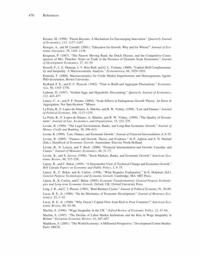
References470
Kremer, M. (1998). “Patent Buyouts: A Mechanism for Encouraging Innovation.” Quarterly Journal of Economics, 113, 1137–1167.
Krueger, A., and M. Lindahl. (2001). “Education for Growth: Why and for Whom?” Journal of Eco-nomic Literature, 39, 1101–1136.
Krugman, P. (1987). “The Narrow Moving Band, the Dutch Disease, and the Competitive Conse-quences of Mrs. Thatcher: Notes on Trade in the Presence of Dynamic Scale Economies.” Journal of Development Economics, 27, 41–55.
Krusell, P., L. E. Ohanian, J.-V. Rios-Rull, and G. L. Violante. (2000). “Capital-Skill Complementar-ity and Inequality: A Macroeconomic Analysis.” Econometrica, 68, 1029–1053.
Kunieda, T. (2008). Macroeconomics for Credit Market Imperfections and Heterogeneous Agents. PhD dissertation, Brown University.
Kydland, F. E., and E. C. Prescott. (1982). “Time to Build and Aggregate Fluctuations.” Economet-rica, 50, 1345–1370.
Laibson, D. (1997). “Golden Eggs and Hyperbolic Discounting.” Quarterly Journal of Economics, 112, 443–477.
Laincz, C. A., and P. F. Peretto. (2004). “Scale Effects in Endogenous Growth Theory: An Error of Aggregation, Not Specifi cation.” Mimeo.
La Porta, R., F. Lopez-de-Silanes, A. Shleifer, and R. W. Vishny. (1998). “Law and Finance.” Journal of Political Economy, 106, 1113–1155.
La Porta, R., F. Lopez-de-Silanes, A. Shleifer, and R. W. Vishny. (1999). “The Quality of Govern-ment.” Journal of Law, Economics, and Organization, 15, 222–279.
Levine, R. (1998). “The Legal Environment, Banks, and Long-Run Economic Growth.” Journal of Money, Credit and Banking, 30, 596–613.
Levine, R. (1999). “Law, Finance, and Economic Growth.” Journal of Financial Intermediation, 8, 8–35.
Levine, R. (2005). “Finance and Growth: Theory and Evidence.” In P. Aghion and S. N. Durlauf (Eds.). Handbook of Economic Growth. Amsterdam: Elsevier North-Holland.
Levine, R., N. Loayza, and T. Beck. (2000). “Financial Intermediation and Growth: Causality and Causes.” Journal of Monetary Economics, 46, 31–77.
Levine, R., and S. Zervos. (1998). “Stock Markets, Banks, and Economic Growth.” American Eco-nomic Review, 88, 537–558.
Lipsey, R., and C. Bekar. (1995). “A Structuralist View of Technical Change and Economic Growth.” Bell Canada Papers on Economic and Public Policy, 3, 9–75.
Lipsey, R., C. Bekar, and K. Carlaw. (1998). “What Requires Explanation.” In E. Helpman (Ed.). General Purpose Technologies and Economic Growth. Cambridge, MA: MIT Press.
Lipsey, R., K. Carlaw, and C. Bekar. (2005). Economic Transformations: General Purpose Technolo-gies and Long-term Economic Growth. Oxford, UK: Oxford University Press.
Long, J. B., and C. I. Plosser. (1983). “Real Business Cycles.” Journal of Political Economy, 91, 39–69.
Lucas, R. E., Jr. (1988). “On the Mechanics of Economic Development.” Journal of Monetary Eco-nomics, 22, 3–42.
Lucas, R. E., Jr. (1990). “Why Doesn’t Capital Flow from Rich to Poor Countries?” American Eco-nomic Review, 80, 92–96.
Machin, S. (1996). “Wage Inequality in the UK.” Oxford Review of Economic Policy, 12, 47–64.
Machin, S. (1997). “The Decline of Labor Market Institutions and the Rise in Wage Inequality in Britain.” European Economic Review, 41, 647–657.
Maddison, A. (2001). “The World Economy: A Millennial Perspective.” Development Centre Studies. Paris: OECD.
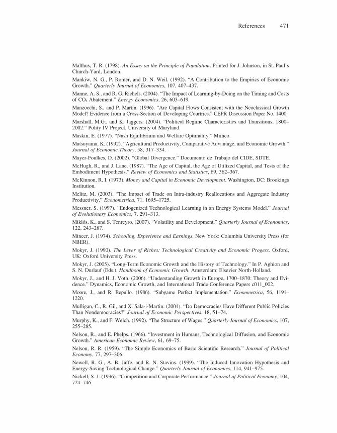
References 471
Malthus, T. R. (1798). An Essay on the Principle of Population. Printed for J. Johnson, in St. Paul’s Church-Yard, London.
Mankiw, N. G., P. Romer, and D. N. Weil. (1992). “A Contribution to the Empirics of Economic Growth.” Quarterly Journal of Economics, 107, 407–437.
Manne, A. S., and R. G. Richels. (2004). “The Impact of Learning-by-Doing on the Timing and Costs of CO2 Abatement.” Energy Economics, 26, 603–619.
Manzocchi, S., and P. Martin. (1996). “Are Capital Flows Consistent with the Neoclassical Growth Model? Evidence from a Cross-Section of Developing Courtries.” CEPR Discussion Paper No. 1400.
Marshall, M.G., and K. Jaggers. (2004). “Political Regime Characteristics and Transitions, 1800–2002.” Polity IV Project, University of Maryland.
Maskin, E. (1977). “Nash Equilibrium and Welfare Optimality.” Mimeo.
Matsuyama, K. (1992). “Agricultural Productivity, Comparative Advantage, and Economic Growth.” Journal of Economic Theory, 58, 317–334.
Mayer-Foulkes, D. (2002). “Global Divergence.” Documento de Trabajo del CIDE, SDTE.
McHugh, R., and J. Lane. (1987). “The Age of Capital, the Age of Utilized Capital, and Tests of the Embodiment Hypothesis.” Review of Economics and Statistics, 69, 362–367.
McKinnon, R. I. (1973). Money and Capital in Economic Development. Washington, DC: Brookings Institution.
Melitz, M. (2003). “The Impact of Trade on Intra-industry Reallocations and Aggregate Industry Productivity.” Econometrica, 71, 1695–1725.
Messner, S. (1997). “Endogenized Technological Learning in an Energy Systems Model.” Journal of Evolutionary Economics, 7, 291–313.
Miklós, K., and S. Tenreyro. (2007). “Volatility and Development.” Quarterly Journal of Economics, 122, 243–287.
Mincer, J. (1974). Schooling, Experience and Earnings. New York: Columbia University Press (for NBER).
Mokyr, J. (1990). The Lever of Riches: Technological Creativity and Economic Progess. Oxford, UK: Oxford University Press.
Mokyr, J. (2005). “Long-Term Economic Growth and the History of Technology.” In P. Aghion and S. N. Durlauf (Eds.). Handbook of Economic Growth. Amsterdam: Elsevier North-Holland.
Mokyr, J., and H. J. Voth. (2006). “Understanding Growth in Europe, 1700–1870: Theory and Evi-dence.” Dynamics, Economic Growth, and International Trade Conference Papers c011_002.
Moore, J., and R. Repullo. (1986). “Subgame Perfect Implementation.” Econometrica, 56, 1191–1220.
Mulligan, C., R. Gil, and X. Sala-i-Martin. (2004). “Do Democracies Have Different Public Policies Than Nondemocracies?” Journal of Economic Perspectives, 18, 51–74.
Murphy, K., and F. Welch. (1992). “The Structure of Wages.” Quarterly Journal of Economics, 107, 255–285.
Nelson, R., and E. Phelps. (1966). “Investment in Humans, Technological Diffusion, and Economic Growth.” American Economic Review, 61, 69–75.
Nelson, R. R. (1959). “The Simple Economics of Basic Scientifi c Research.” Journal of Political Economy, 77, 297–306.
Newell, R. G., A. B. Jaffe, and R. N. Stavins. (1999). “The Induced Innovation Hypothesis and Energy-Saving Technological Change.” Quarterly Journal of Economics, 114, 941–975.
Nickell, S. J. (1996). “Competition and Corporate Performance.” Journal of Political Economy, 104, 724–746.
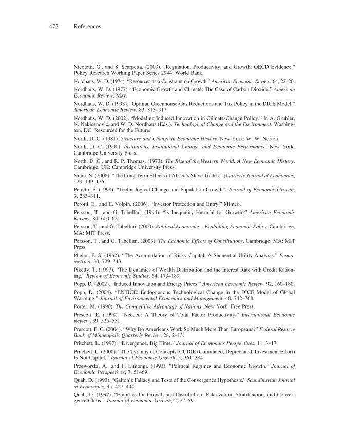
References472
Nicoletti, G., and S. Scarpetta. (2003). “Regulation, Productivity, and Growth: OECD Evidence.” Policy Research Working Paper Series 2944, World Bank.
Nordhaus, W. D. (1974). “Resources as a Constraint on Growth.” American Economic Review, 64, 22–26.
Nordhaus, W. D. (1977). “Economic Growth and Climate: The Case of Carbon Dioxide.” American Economic Review, May.
Nordhaus, W. D. (1993). “Optimal Greenhouse-Gas Reductions and Tax Policy in the DICE Model.” American Economic Review, 83, 313–317.
Nordhaus, W. D. (2002). “Modeling Induced Innovation in Climate-Change Policy.” In A. Grübler, N. Nakicenovic, and W. D. Nordhaus (Eds.). Technological Change and the Environment. Washing-ton, DC: Resources for the Future.
North, D. C. (1981). Structure and Change in Economic History. New York: W. W. Norton.
North, D. C. (1990). Institutions, Institutional Change, and Economic Performance. New York: Cambridge University Press.
North, D. C., and R. P. Thomas. (1973). The Rise of the Western World: A New Economic History. Cambridge, UK: Cambridge University Press.
Nunn, N. (2008). “The Long Term Effects of Africa’s Slave Trades.” Quarterly Journal of Economics, 123, 139–176.
Peretto, P. (1998). “Technological Change and Population Growth.” Journal of Economic Growth, 3, 283–311.
Perotti, E., and E. Volpin. (2006). “Investor Protection and Entry.” Mimeo.
Persson, T., and G. Tabellini. (1994). “Is Inequality Harmful for Growth?” American Economic Review, 84, 600–621.
Persson, T., and G. Tabellini. (2000). Political Economics—Explaining Economic Policy. Cambridge, MA: MIT Press.
Persson, T., and G. Tabellini. (2003). The Economic Effects of Constitutions. Cambridge, MA: MIT Press.
Phelps, E. S. (1962). “The Accumulation of Risky Capital: A Sequential Utility Analysis.” Econo-metrica, 30, 729–743.
Piketty, T. (1997). “The Dynamics of Wealth Distribution and the Interest Rate with Credit Ration-ing.” Review of Economic Studies, 64, 173–189.
Popp, D. (2002). “Induced Innovation and Energy Prices.” American Economic Review, 92, 160–180.
Popp, D. (2004). “ENTICE: Endognenous Technological Change in the DICE Model of Global Warming.” Journal of Environmental Economics and Management, 48, 742–768.
Porter, M. (1990). The Competitive Advantage of Nations. New York: Free Press.
Prescott, E. (1998). “Needed: A Theory of Total Factor Productivity.” International Economic Review, 39, 525–551.
Prescott, E. C. (2004). “Why Do Americans Work So Much More Than Europeans?” Federal Reserve Bank of Minneapolis Quarterly Review, 28, 2–13.
Pritchett, L. (1997). “Divergence, Big Time.” Journal of Economics Perspectives, 11, 3–17.
Pritchett, L. (2000). “The Tyranny of Concepts: CUDIE (Cumulated, Depreciated, Investment Effort) Is Not Capital.” Journal of Economic Growth, 5, 361–384.
Przeworski, A., and F. Limongi. (1993). “Political Regimes and Economic Growth.” Journal of Economic Perspectives, 7, 51–69.
Quah, D. (1993). “Galton’s Fallacy and Tests of the Convergence Hypothesis.” Scandinavian Journal of Economics, 95, 427–444.
Quah, D. (1997). “Empirics for Growth and Distribution: Polarization, Stratifi cation, and Conver-gence Clubs.” Journal of Economic Growth, 2, 27–59.
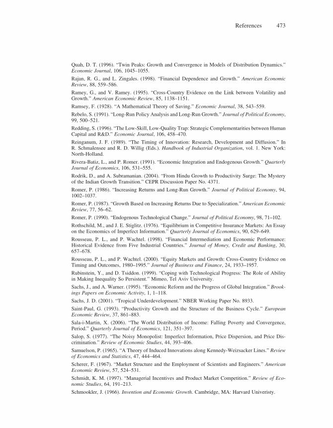
References 473
Quah, D. T. (1996). “Twin Peaks: Growth and Convergence in Models of Distribution Dynamics.” Economic Journal, 106, 1045–1055.
Rajan, R. G., and L. Zingales. (1998). “Financial Dependence and Growth.” American Economic Review, 88, 559–586.
Ramey, G., and V. Ramey. (1995). “Cross-Country Evidence on the Link between Volatility and Growth.” American Economic Review, 85, 1138–1151.
Ramsey, F. (1928). “A Mathematical Theory of Saving.” Economic Journal, 38, 543–559.
Rebelo, S. (1991). “Long-Run Policy Analysis and Long-Run Growth.” Journal of Political Economy, 99, 500–521.
Redding, S. (1996). “The Low-Skill, Low-Quality Trap: Strategic Complementarities between Human Capital and R&D.” Economic Journal, 106, 458–470.
Reinganum, J. F. (1989). “The Timing of Innovation: Research, Development and Diffusion.” In R. Schmalensee and R. D. Willig (Eds.). Handbook of Industrial Organization, vol. 1. New York: North-Holland.
Rivera-Batiz, L., and P. Romer. (1991). “Economic Integration and Endogenous Growth.” Quarterly Journal of Economics, 106, 531–555.
Rodrik, D., and A. Subramanian. (2004). “From Hindu Growth to Productivity Surge: The Mystery of the Indian Growth Transition.” CEPR Discussion Paper No. 4371.
Romer, P. (1986). “Increasing Returns and Long-Run Growth.” Journal of Political Economy, 94, 1002–1037.
Romer, P. (1987). “Growth Based on Increasing Returns Due to Specialization.” American Economic Review, 77, 56–62.
Romer, P. (1990). “Endogenous Technological Change.” Journal of Political Economy, 98, 71–102.
Rothschild, M., and J. E. Stiglitz. (1976). “Equilibrium in Competitive Insurance Markets: An Essay on the Economics of Imperfect Information.” Quarterly Journal of Economics, 90, 629–649.
Rousseau, P. L., and P. Wachtel. (1998). “Financial Intermediation and Economic Performance: Historical Evidence from Five Industrial Countries.” Journal of Money, Credit and Banking, 30, 657–678.
Rousseau, P. L., and P. Wachtel. (2000). “Equity Markets and Growth: Cross-Country Evidence on Timing and Outcomes, 1980–1995.” Journal of Business and Finance, 24, 1933–1957.
Rubinstein, Y., and D. Tsiddon. (1999). “Coping with Technological Progress: The Role of Ability in Making Inequality So Persistent.” Mimeo, Tel Aviv University.
Sachs, J., and A. Warner. (1995). “Economic Reform and the Progress of Global Integration.” Brook-ings Papers on Economic Activity, 1, 1–118.
Sachs, J. D. (2001). “Tropical Underdevelopment.” NBER Working Paper No. 8933.
Saint-Paul, G. (1993). “Productivity Growth and the Structure of the Business Cycle.” European Economic Review, 37, 861–883.
Sala-i-Martin, X. (2006). “The World Distribution of Income: Falling Poverty and Convergence, Period.” Quarterly Journal of Economics, 121, 351–397.
Salop, S. (1977). “The Noisy Monopolist: Imperfect Information, Price Dispersion, and Price Dis-crimination.” Review of Economic Studies, 44, 393–406.
Samuelson, P. (1965). “A Theory of Induced Innovations along Kennedy-Weizsacker Lines.” Review of Economics and Statistics, 47, 444–464.
Scherer, F. (1967). “Market Structure and the Employment of Scientists and Engineers.” American Economic Review, 57, 524–531.
Schmidt, K. M. (1997). “Managerial Incentives and Product Market Competition.” Review of Eco-nomic Studies, 64, 191–213.
Schmookler, J. (1966). Invention and Economic Growth. Cambridge, MA: Harvard Univeristy.
References474
Schumpeter, J. A. (1912). Theorie der Wirtschaftlichen Entwicklung. Leipzig: Dunker & Humblot.
Schumpeter, J. A. (1942). The Theory of Economic Development, Cambridge, MA: Harvard Univer-sity Press.
Segerstrom, P. S. (1998). “Endogenous Growth without Scale Effects.” American Economic Review, 88, 1290–1310.
Segerstrom, P. S. (2000). “The Long-Run Growth Effects of R&D Subsidies.” Journal of Economic Growth, 5, 277–305.
Segerstrom, P. S., T. Anant, and E. Dinopoulos. (1990). “A Schumpeterian Model of the Product Life Cycle.” American Economic Review, 80, 1077–1092.
Shleifer, A. (1986). “Implementation Cycles.” Journal of Political Economy, 94, 1163–1190.
Shleifer, A., and R. Vishny. (1999). The Grabbing Hand: Government Pathologies and Their Cures. Cambridge, MA: Harvard University Press.
Sidrauski, M. (1967). “Rational Choice of Patterns of Growth in a Monetary Economy.” American Economic Review, 57, 534–544.
Solow, R. M. (1956). “A Contribution to the Theory of Economic Growth.” Quarterly Journal of Economics, 70, 65–94.
Solow, R. (1957). “Technical Change and the Aggregate Production Function.” Review of Economics and Statistics, 39, 312–320.
Spence, M. (1976). “Product Selection, Fixed Costs, and Monopolistic Competition.” Review of Economic Studies, 43, 217–235.
Stadler, G. (1990). “Business Cycle Models with Endogenous Technology.” American Economic Review, 80, 763–778.
Stern, N. (2006). The Economics of Climate Change: The Stern Review. Cambridge, UK: Cambridge University Press.
Stiglitz, J. E. (1969). “Distribution of Income and Wealth among Individuals.” Econometrica, 37, 382–397.
Stiglitz, J. E. (1995). Whither Socialism? Cambridge, MA: MIT Press.
Stock, J. H., and M. W. Watson. (2007). Introduction to Econometrics. Boston: Addison Wesley Companion, Pearson.
Stockey, N. L. (1998). “Are There Limits to Growth?” International Economic Review, 39, 1–31.
Stokey, N. (1996). “Free Trade, Factor Returns, and Factor Accumulation.” Journal of Economic Growth, 1, 421–447.
Sue Wing, I. (2003). “Induced Technical Change and the Cost of Climate Policy.” Technical Report 102, MIT Joint Program on the Science and Policy of Global Change.
Swan, T. W. (1956). “Economic Growth and Capital Accumulation.” Economic Record, 32, 334–361.
Tabellini, G. (2007). “Culture and Institutions: Economic Development in the Regions of Europe.” Mimeo, Bocconi University.
Tirole, J. (1988). The Theory of Industrial Organization. Cambridge, MA: MIT Press.
Trefl er, D. (2004). “The Long and Short of the Canada-U.S. Free Trade Agreement.” American Eco-nomic Review, 94, 870–895.
Ulku, H. (2005). “An Empirical Analysis of R&D-Based Growth Models.” Mimeo, Manchester University.
Uzawa, H. (1965). “Optimal Technical Change in an Aggregative Model of Economic Growth.” International Economic Review, 6, 18–31.
Vandenbussche, J., P. Aghion, and C. Meghir. (2006). “Growth, Distance to Frontier and Composition of Human Capital.” Journal of Economic Growth, 11, 97–127.
References 475
Ventura, J. (1997). “Growth and Interdependence.” Quarterly Journal of Economics, 112, 57–84.
Ventura, J. (2005). “A Global View of Economic Growth.” In P. Aghion and S. N. Durlauf (Eds.). Handbook of Economic Growth. Amsterdam: Elsevier North-Holland.
Violante, G. L. (2002). “Technological Acceleration, Skill Transferability and the Rise in Residual Inequality.” Quarterly Journal of Economics, 117, 297–338.
Von Tunzelmann, G. N. (1978). Steam Power and British Industrialization to 1860. Oxford, UK: Clarendon Press.
Weil, D. (2008). Economic Growth, 2nd ed. Boston: Addison Wesley.
Weitzman, M. (2007). “A Review of the Stern Review on the Economics of Climate Change.” Journal of Economic Literature, 45, 703–724.
Wooldridge, J. (2006). Introductory Econometrics: A Modern Approach. South Western College Publishing, Thompson Learning.
Young, A. (1991). “Learning by Doing and the Dynamic Effects of International Trade.” Quarterly Journal of Economics, 106, 369–405.
Young, A. (1995). “The Tyranny of Numbers: Confronting the Statistical Realities of the East Asian Growth Experience.” Quarterly Journal of Economics, 110, 641–680.
Young, A. (1998). “Growth without Scale Effects.” Journal of Political Economy, 106, 41–63.
Young, A. A. (1928). “Increasing Returns and Economic Progress.” Economic Journal, 38, 527–542.
Zak, P. J., and S. Knack. (2001). “Trust and Growth.” Economic Journal, 111, 295–321.


Index
Absolute convergence, 56Acemoglu, D., 1, 8, 18, 60–67, 81, 147, 169,
171, 173, 175, 176, 181, 182, 186–188, 206, 230, 233, 237, 240, 243–244, 261–264, 300, 320, 341, 349, 373, 400, 401, 405, 415, 432, 440, 453
Adaptability premium, 207–209Advantage to backwardness (Gerschenkron),
18, 238, 262, 362–363Aggregate capital stockin neoclassical growth model, 21–24in product-variety growth model, 77–78
Aggregate production functionin AK growth model, 51, 53in Harrod-Domar model, 48–49in neoclassical growth model, 21–23trade liberalization and, 367
Aghion, P., 1, 2, 8, 15, 18, 43, 69, 79, 81, 100, 134, 148, 155, 158, 159, 161, 166, 175, 204, 207–209, 212, 215–216, 243–244, 263, 267–269, 274, 279, 280, 282–284, 302, 307–308, 310–312, 314, 316, 324–328, 339, 348–351, 372, 399, 401, 404–405, 407, 415, 422, 454
Aghion-Angeletos-Banerjee-Manova model of volatility/risk reduction, 324, 326–339
aggregate volatility and, 329–330argument for, 326–327credit constraints and, 331–339described, 325–327evidence for, 327–329growth equation, 331opportunity cost effect and, 331–334payoff function, 330–331perfect credit markets and, 331–333research and development and, 330–335, 338–340, 347–349
timing function, 330–331Agriculture sector, stages of economic growth
and, 222, 224AK growth model, 47–68Acemoglu-Ventura model, 60–67club convergence and, 57, 151comparison with neoclassical growth model, 56–60, 319
comparison with product-variety growth model, 69–70, 99
comparison with Schumpeterian growth model, 99, 281–282
conclusion, 66described, 13–14, 47–48education in, 287, 290, 292–295, 313environmental preservation and, 377–379, 392
Frankel model, 49–52, 67
Harrod-Domar model as precursor to, 48–49, 52, 67, 319, 348
introduction, 47–48Jones-Manuelli-Stacchetti model of volatility/risk reduction, 321–324
learning by doing as basis of, 47–48, 50
limitations of, 66, 99literature notes, 67long-run growth in, 51–52, 54–55, 59–60manufacturing in, 232microdevelopment and, 431–432open-economy model with convergence, 60–66
Ramsey version with intertemporal utility maximization, 52–56, 67
sustainable economic growth and, 224and volatility/risk reduction, 319–325, 342, 347, 348
Alesina, A., 353, 374, 399, 401, 407, 410, 413, 415, 416
Algan, Y., 422American Economic Review, 389Anant, T., 15, 100Angeletos, G. M., 324–327, 348–351Angrist, J., 432Antras, P., 79Appropriate institutions (Gerschenkron), 18,
238, 243–264decentralized equilibrium and, 252–254economic growth and, 246–252equilibrium dynamics and, 257–258experience-enhancing, 250–252, 254–255imitation-enhancing, 250–252innovation-enhancing, 250–252, 254–255nonconvergence traps and, 257–260
Arestis, P., 148Arrow, K. J., 47, 67, 152, 187Ashraf, Q., 217, 232Asian tiger economiesclub convergence and, 3, 57economic growth of, 57, 105, 110–111
Askhenazy, P., 339Aten, B., 108Atkinson, A. B., 187Autor, D., 173–175Azariadis, C., 296, 313
Bachetta, R., 349–351Backwardnessadvantage to (Gerschenkron), 18, 238, 262, 362–263
democracy and, 403–405, 407trade liberalization and, 362–363, 371–372

Index478
Balanced portfolio approach to risk diversifi cation, 343–345
Banerjee, A., 134, 136, 148, 262, 290, 324–327, 348–351, 413, 429
Banerjee-Dufl o model of development economics, 429–434
Barlevy, G., 320, 339, 340, 348, 350Barro, R. J., 40, 45, 56, 59, 68, 151, 165,
287–288, 308, 309, 313, 399, 414–415Basu, S., 191Baumol, W., 230Bean, C. R., 326, 348Beck, T., 144–149, 163, 239, 327, 328Becker, G., 292–294, 297, 313Bekar, C., 196, 211Benabou, R., 136, 313Bencivenga, V. R., 147Benassy, J.-P., 76, 97Benhabib, J., 59–60, 158–159, 287, 291, 292,
298–299, 302, 313, 316–317Berman, E., 174, 175Berman, N., 339Bernanke, B., 147, 148, 339Bertrand competition, 277, 403Bils, M., 309–310Blanchard, O., 40Bloom, N., 274, 283–284Blundell, R., 79, 92, 174, 204, 206, 208, 267,
274, 279, 281–284Bolton, P., 148Bound, J., 174, 175Boustan, C., 314Boustan, L., 283, 307, 310–311, 316Boyd, J. H., 147Bresnahan, T., 193, 212Bribery, politics of entry and, 405–407Brock, W., 40Broda, C., 77–79Bruno, M., 348Buonanno, P., 391, 392Burgess, R., 280, 283, 404–405Bursztyn, L., 377, 443
Caballero, R. J., 197–198, 282, 348Cahuc, P., 422Canada, trade liberalization in, 354Canova, F., 166Capital accumulation. See also Human capital;
Intellectual capital; Physical capitalaccumulation equation, 137in AK growth model, 56–60by Asian tiger economies, 105in economies with wealth inequality, 147–148education and, 288–297, 312–313
environmental preservation and, 378in growth accounting, 109–115in hybrid model with endogenous technological progress, 117–119
innovation versus, 109–112, 226–228Lucas approach to, 287, 290, 292–295Mankiw-Romer-Weil model of convergence, 58–60, 288–292
in neoclassical growth model, 21–24, 35–36parental investment in children’s patience, 422, 425–429, 441–442
problems in measuring, 109–112in product-variety growth model, 74risk diversifi cation and, 345–347in Schumpeterian growth model, 105as stage of economic growth, 226–228technological progress compared with, 66transnational dynamics in, 120–121
Capital deepeningin growth accounting, 113as stage of economic growth, 227–228
Capital-labor ratio, 231in neoclassical growth model, 26–27, 29, 33
Capital market equilibrium, under credit constraints, 140–142
Capital stockin AK growth model, 51in hybrid model with endogenous capital accumulation and technological progress, 113–119, 120–121
in neoclassical growth model, 21–24Card, D., 175Carlaw, K., 211Carraro, C., 391, 392Caselli, F., 40, 120, 123–124, 166, 186, 291,
313, 401Cass, D., 32, 37–42, 70Cass-Koopmans-Ramsey model, 31–39, 53convergence in, 40–42exogenous technological change in, 37–39lack of technological progress in, 31–37steady state in, 40–42
Cette, G., 339Chaebols, 260Channel savings, fi nancial development and,
129Cheng, L. K., 212Chinaclub convergence and, 3, 57income levels in, 4lack of democracy in, 440patience and future orientation in, 429
Clark, J., 211Climate change, 391–392

Index 479
Closed economygrowth rate of, 369opening up, 62–63two-sector, 61–62
Club convergence, 3, 11–12, 57basic setup, 152–153distance to world productivity frontier and, 151, 154–156
divergence and, 156–163innovation and, 153–154productivity and, 154–156Schumpeterian growth model and, 57, 163–165
technology transfer and, 151–158Cobb-Douglas production functionin AK growth model, 57–58under binding credit constraint, 135–136education and, 304–306in hybrid model with endogenous capital accumulation and technological progress, 117–119
nature of, 16, 106in neoclassical growth model, 25, 27–28in Schumpeterian growth model, 85–86, 88, 89
TFP growth and, 117–119volatility/risk reduction and, 330, 335
Coe, D. T., 120, 353, 354Coeffi cient of determination, 446Cohen, W. M., 152Coleman, W. J., 186College wage premium, 4–5, 173–176,
180–181, 204, 208Collusion, 270Colonial period, origins of institutions and,
240–242, 261–262Comin, D., 80, 108, 181, 349, 351Comparative statics, in Schumpeterian growth
model, 91–92Competitioncomposition effect, 272–273economic growth and, 7–8, 267–286education and, 304–306effect on innovation, 267, 272–273entry and, 8, 80, 274–281equilibrium profi ts and, 269–271escape-competition effect, 271–273innovation and, 267introduction, 267inverted U, 272–273, 283product market, 92, 267Schumpeterian effect, 271–273, 283trade liberalization and, 354
Complementarity, in risk diversifi cation, 344
Composition effect, 272–273Conditional convergence, 165in AK growth model, 56–60in neoclassical growth model, 29–31
Constant returns to capital, in AK growth model, 52, 54–55, 58–59
Consumption smoothing, in neoclassical growth model, 31–39
Convergence. See also Club convergence; Cross-country convergence
absolute, 56in AK growth model, 56–62appropriate institutions and non-convergence traps, 243–264
conditional, 29–31, 56–60, 165in growth rates, 31nature of, 2–3in neoclassical growth model, 29–31, 40–42, 165–166
non-convergence traps, 243–246, 257–260, 440in Schumpeterian growth model, 57, 100, 163–165
technology transfer and, 151–158Corriveau, L., 100Corruptiondemocracy and, 399politics of entry and, 405–407
Country fi xed effects, 400Creative destruction (Schumpeter)lack of, in AK growth model, 15nature of, 15–16, 85
Credit constraints, 132–142diminishing marginal product of capital and, 136–139
fi nancial development and, 132–142, 158–163, 164
innovation and growth under binding, 135–136
innovation technology and, 132, 135–136introducing, 138model with ex ante screening, 132–134model with ex post monitoring and moral hazard, 134–136
productivity differences under, 139–142, 158–163, 164
screening costs, 132–134as source of divergence, 158–163, 164and volatility/risk reduction, 320, 331–339
Credit multiplierconcept of, 134investment in research and development (R&D) and, 134–135
productivity growth under credit constraints, 140, 159
Index
Absolute convergence, 56Acemoglu, D., 1, 8, 18, 60–67, 81, 147, 169,
171, 173, 175, 176, 181, 182, 186–188, 206, 230, 233, 237, 240, 243–244, 261–264, 300, 320, 341, 349, 373, 400, 401, 405, 415, 432, 440, 453
Adaptability premium, 207–209Advantage to backwardness (Gerschenkron),
18, 238, 262, 362–363Aggregate capital stockin neoclassical growth model, 21–24in product-variety growth model, 77–78
Aggregate production functionin AK growth model, 51, 53in Harrod-Domar model, 48–49in neoclassical growth model, 21–23trade liberalization and, 367
Aghion, P., 1, 2, 8, 15, 18, 43, 69, 79, 81, 100, 134, 148, 155, 158, 159, 161, 166, 175, 204, 207–209, 212, 215–216, 243–244, 263, 267–269, 274, 279, 280, 282–284, 302, 307–308, 310–312, 314, 316, 324–328, 339, 348–351, 372, 399, 401, 404–405, 407, 415, 422, 454
Aghion-Angeletos-Banerjee-Manova model of volatility/risk reduction, 324, 326–339
aggregate volatility and, 329–330argument for, 326–327credit constraints and, 331–339described, 325–327evidence for, 327–329growth equation, 331opportunity cost effect and, 331–334payoff function, 330–331perfect credit markets and, 331–333research and development and, 330–335, 338–340, 347–349
timing function, 330–331Agriculture sector, stages of economic growth
and, 222, 224AK growth model, 47–68Acemoglu-Ventura model, 60–67club convergence and, 57, 151comparison with neoclassical growth model, 56–60, 319
comparison with product-variety growth model, 69–70, 99
comparison with Schumpeterian growth model, 99, 281–282
conclusion, 66described, 13–14, 47–48education in, 287, 290, 292–295, 313environmental preservation and, 377–379, 392
Frankel model, 49–52, 67
Harrod-Domar model as precursor to, 48–49, 52, 67, 319, 348
introduction, 47–48Jones-Manuelli-Stacchetti model of volatility/risk reduction, 321–324
learning by doing as basis of, 47–48, 50
limitations of, 66, 99literature notes, 67long-run growth in, 51–52, 54–55, 59–60manufacturing in, 232microdevelopment and, 431–432open-economy model with convergence, 60–66
Ramsey version with intertemporal utility maximization, 52–56, 67
sustainable economic growth and, 224and volatility/risk reduction, 319–325, 342, 347, 348
Alesina, A., 353, 374, 399, 401, 407, 410, 413, 415, 416
Algan, Y., 422American Economic Review, 389Anant, T., 15, 100Angeletos, G. M., 324–327, 348–351Angrist, J., 432Antras, P., 79Appropriate institutions (Gerschenkron), 18,
238, 243–264decentralized equilibrium and, 252–254economic growth and, 246–252equilibrium dynamics and, 257–258experience-enhancing, 250–252, 254–255imitation-enhancing, 250–252innovation-enhancing, 250–252, 254–255nonconvergence traps and, 257–260
Arestis, P., 148Arrow, K. J., 47, 67, 152, 187Ashraf, Q., 217, 232Asian tiger economiesclub convergence and, 3, 57economic growth of, 57, 105, 110–111
Askhenazy, P., 339Aten, B., 108Atkinson, A. B., 187Autor, D., 173–175Azariadis, C., 296, 313
Bachetta, R., 349–351Backwardnessadvantage to (Gerschenkron), 18, 238, 262, 362–263
democracy and, 403–405, 407trade liberalization and, 362–363, 371–372

Index478
Balanced portfolio approach to risk diversifi cation, 343–345
Banerjee, A., 134, 136, 148, 262, 290, 324–327, 348–351, 413, 429
Banerjee-Dufl o model of development economics, 429–434
Barlevy, G., 320, 339, 340, 348, 350Barro, R. J., 40, 45, 56, 59, 68, 151, 165,
287–288, 308, 309, 313, 399, 414–415Basu, S., 191Baumol, W., 230Bean, C. R., 326, 348Beck, T., 144–149, 163, 239, 327, 328Becker, G., 292–294, 297, 313Bekar, C., 196, 211Benabou, R., 136, 313Bencivenga, V. R., 147Benassy, J.-P., 76, 97Benhabib, J., 59–60, 158–159, 287, 291, 292,
298–299, 302, 313, 316–317Berman, E., 174, 175Berman, N., 339Bernanke, B., 147, 148, 339Bertrand competition, 277, 403Bils, M., 309–310Blanchard, O., 40Bloom, N., 274, 283–284Blundell, R., 79, 92, 174, 204, 206, 208, 267,
274, 279, 281–284Bolton, P., 148Bound, J., 174, 175Boustan, C., 314Boustan, L., 283, 307, 310–311, 316Boyd, J. H., 147Bresnahan, T., 193, 212Bribery, politics of entry and, 405–407Brock, W., 40Broda, C., 77–79Bruno, M., 348Buonanno, P., 391, 392Burgess, R., 280, 283, 404–405Bursztyn, L., 377, 443
Caballero, R. J., 197–198, 282, 348Cahuc, P., 422Canada, trade liberalization in, 354Canova, F., 166Capital accumulation. See also Human capital;
Intellectual capital; Physical capitalaccumulation equation, 137in AK growth model, 56–60by Asian tiger economies, 105in economies with wealth inequality, 147–148education and, 288–297, 312–313
environmental preservation and, 378in growth accounting, 109–115in hybrid model with endogenous technological progress, 117–119
innovation versus, 109–112, 226–228Lucas approach to, 287, 290, 292–295Mankiw-Romer-Weil model of convergence, 58–60, 288–292
in neoclassical growth model, 21–24, 35–36parental investment in children’s patience, 422, 425–429, 441–442
problems in measuring, 109–112in product-variety growth model, 74risk diversifi cation and, 345–347in Schumpeterian growth model, 105as stage of economic growth, 226–228technological progress compared with, 66transnational dynamics in, 120–121
Capital deepeningin growth accounting, 113as stage of economic growth, 227–228
Capital-labor ratio, 231in neoclassical growth model, 26–27, 29, 33
Capital market equilibrium, under credit constraints, 140–142
Capital stockin AK growth model, 51in hybrid model with endogenous capital accumulation and technological progress, 113–119, 120–121
in neoclassical growth model, 21–24Card, D., 175Carlaw, K., 211Carraro, C., 391, 392Caselli, F., 40, 120, 123–124, 166, 186, 291,
313, 401Cass, D., 32, 37–42, 70Cass-Koopmans-Ramsey model, 31–39, 53convergence in, 40–42exogenous technological change in, 37–39lack of technological progress in, 31–37steady state in, 40–42
Cette, G., 339Chaebols, 260Channel savings, fi nancial development and,
129Cheng, L. K., 212Chinaclub convergence and, 3, 57income levels in, 4lack of democracy in, 440patience and future orientation in, 429
Clark, J., 211Climate change, 391–392
Index 479
Closed economygrowth rate of, 369opening up, 62–63two-sector, 61–62
Club convergence, 3, 11–12, 57basic setup, 152–153distance to world productivity frontier and, 151, 154–156
divergence and, 156–163innovation and, 153–154productivity and, 154–156Schumpeterian growth model and, 57, 163–165
technology transfer and, 151–158Cobb-Douglas production functionin AK growth model, 57–58under binding credit constraint, 135–136education and, 304–306in hybrid model with endogenous capital accumulation and technological progress, 117–119
nature of, 16, 106in neoclassical growth model, 25, 27–28in Schumpeterian growth model, 85–86, 88, 89
TFP growth and, 117–119volatility/risk reduction and, 330, 335
Coe, D. T., 120, 353, 354Coeffi cient of determination, 446Cohen, W. M., 152Coleman, W. J., 186College wage premium, 4–5, 173–176,
180–181, 204, 208Collusion, 270Colonial period, origins of institutions and,
240–242, 261–262Comin, D., 80, 108, 181, 349, 351Comparative statics, in Schumpeterian growth
model, 91–92Competitioncomposition effect, 272–273economic growth and, 7–8, 267–286education and, 304–306effect on innovation, 267, 272–273entry and, 8, 80, 274–281equilibrium profi ts and, 269–271escape-competition effect, 271–273innovation and, 267introduction, 267inverted U, 272–273, 283product market, 92, 267Schumpeterian effect, 271–273, 283trade liberalization and, 354
Complementarity, in risk diversifi cation, 344
Composition effect, 272–273Conditional convergence, 165in AK growth model, 56–60in neoclassical growth model, 29–31
Constant returns to capital, in AK growth model, 52, 54–55, 58–59
Consumption smoothing, in neoclassical growth model, 31–39
Convergence. See also Club convergence; Cross-country convergence
absolute, 56in AK growth model, 56–62appropriate institutions and non-convergence traps, 243–264
conditional, 29–31, 56–60, 165in growth rates, 31nature of, 2–3in neoclassical growth model, 29–31, 40–42, 165–166
non-convergence traps, 243–246, 257–260, 440in Schumpeterian growth model, 57, 100, 163–165
technology transfer and, 151–158Corriveau, L., 100Corruptiondemocracy and, 399politics of entry and, 405–407
Country fi xed effects, 400Creative destruction (Schumpeter)lack of, in AK growth model, 15nature of, 15–16, 85
Credit constraints, 132–142diminishing marginal product of capital and, 136–139
fi nancial development and, 132–142, 158–163, 164
innovation and growth under binding, 135–136
innovation technology and, 132, 135–136introducing, 138model with ex ante screening, 132–134model with ex post monitoring and moral hazard, 134–136
productivity differences under, 139–142, 158–163, 164
screening costs, 132–134as source of divergence, 158–163, 164and volatility/risk reduction, 320, 331–339
Credit multiplierconcept of, 134investment in research and development (R&D) and, 134–135
productivity growth under credit constraints, 140, 159
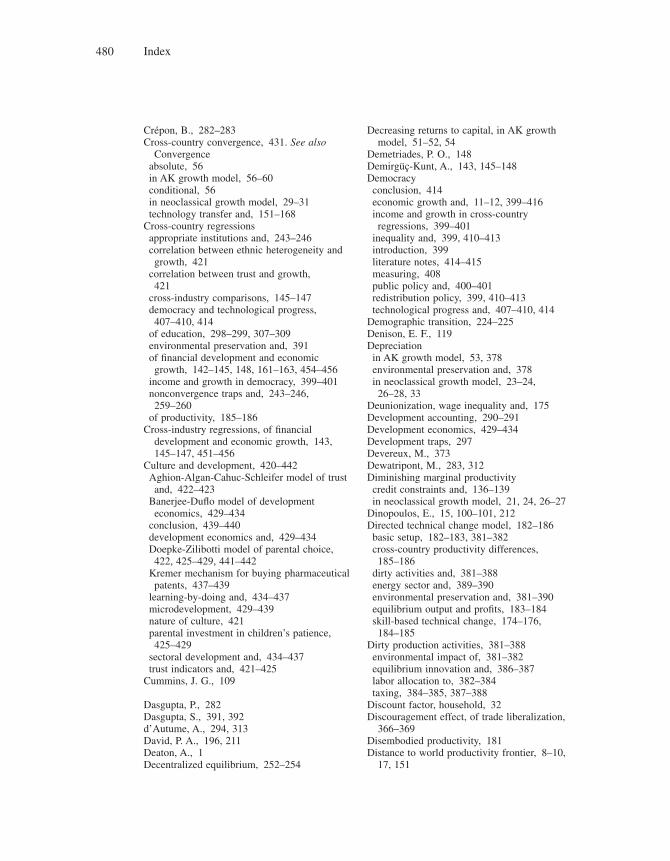
Index480
Crépon, B., 282–283Cross-country convergence, 431. See also
Convergenceabsolute, 56in AK growth model, 56–60conditional, 56in neoclassical growth model, 29–31technology transfer and, 151–168
Cross-country regressionsappropriate institutions and, 243–246correlation between ethnic heterogeneity and growth, 421
correlation between trust and growth, 421
cross-industry comparisons, 145–147democracy and technological progress, 407–410, 414
of education, 298–299, 307–309environmental preservation and, 391of fi nancial development and economic growth, 142–145, 148, 161–163, 454–456
income and growth in democracy, 399–401nonconvergence traps and, 243–246, 259–260
of productivity, 185–186Cross-industry regressions, of fi nancial
development and economic growth, 143, 145–147, 451–456
Culture and development, 420–442Aghion-Algan-Cahuc-Schleifer model of trust and, 422–423
Banerjee-Dufl o model of development economics, 429–434
conclusion, 439–440development economics and, 429–434Doepke-Zilibotti model of parental choice, 422, 425–429, 441–442
Kremer mechanism for buying pharmaceutical patents, 437–439
learning-by-doing and, 434–437microdevelopment, 429–439nature of culture, 421parental investment in children’s patience, 425–429
sectoral development and, 434–437trust indicators and, 421–425
Cummins, J. G., 109
Dasgupta, P., 282Dasgupta, S., 391, 392d’Autume, A., 294, 313David, P. A., 196, 211Deaton, A., 1Decentralized equilibrium, 252–254
Decreasing returns to capital, in AK growth model, 51–52, 54
Demetriades, P. O., 148Demirgüç-Kunt, A., 143, 145–148Democracyconclusion, 414economic growth and, 11–12, 399–416income and growth in cross-country regressions, 399–401
inequality and, 399, 410–413introduction, 399literature notes, 414–415measuring, 408public policy and, 400–401redistribution policy, 399, 410–413technological progress and, 407–410, 414
Demographic transition, 224–225Denison, E. F., 119Depreciationin AK growth model, 53, 378environmental preservation and, 378in neoclassical growth model, 23–24, 26–28, 33
Deunionization, wage inequality and, 175Development accounting, 290–291Development economics, 429–434Development traps, 297Devereux, M., 373Dewatripont, M., 283, 312Diminishing marginal productivitycredit constraints and, 136–139in neoclassical growth model, 21, 24, 26–27
Dinopoulos, E., 15, 100–101, 212Directed technical change model, 182–186basic setup, 182–183, 381–382cross-country productivity differences, 185–186
dirty activities and, 381–388energy sector and, 389–390environmental preservation and, 381–390equilibrium output and profi ts, 183–184skill-based technical change, 174–176, 184–185
Dirty production activities, 381–388environmental impact of, 381–382equilibrium innovation and, 386–387labor allocation to, 382–384taxing, 384–385, 387–388
Discount factor, household, 32Discouragement effect, of trade liberalization,
366–369Disembodied productivity, 181Distance to world productivity frontier, 8–10,
17, 151
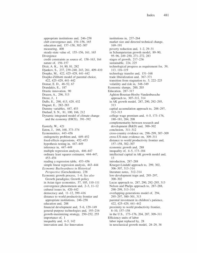
Index 481
appropriate institutions and, 246–258club convergence and, 154–156, 165education and, 157–158, 302–307measuring, 408steady-state value of, 155–156, 161, 165
Divergencecredit constraints as source of, 158–163, 164nature of, 156–157
Dixit, A. K., 14, 80, 81, 282Djankov, S., 237, 239–240, 243, 261, 409–410Doepke, M., 422, 425–429, 441–442Doepke-Zilibotti model of parental choice,
422, 425–429, 441–442Domar, E. D., 48–52, 67Drandakis, E., 187Drastic innovation, 90Drazen, A., 296, 313Dreze, J., 1Dufl o, E., 290, 413, 429, 432Duguet, E., 282–283Dummy variables, 447, 453Durlauf, S. N., 81, 100, 166, 212Dynamic integrated model of climate change
and the economy (DICE), 391–392
Easterly, W., 421Eaton, J., 166, 168, 373–374Econometrics, 443–456endogeneity problem and, 449–452fi xed-effects regressions, 452–453hypothesis testing in, 447–449inference in, 447–449multiple regression analysis, 446–447ordinary least squares estimator, 444–447, 453–454
reading a regression table, 453–456simple linear regression analysis, 443–444
Economic Backwardness in Historical Perspective (Gerschenkron), 238
Economic growth process, 1–6. See also Growth paradigms; Growth policy
in Asian tiger economies, 57, 105, 110–111convergence phenomenon and, 2–3, 11–12cultural issues in, 420–442democracy and, 11–12, 399–416distance to world productivity frontier and appropriate institutions, 246–258
education and, 288fi nancial development and, 5–6, 129–149general-purpose technologies and, 193–216growth-maximizing strategy, 250–252, 255importance of, 1inequality and, 4–5, 142innovation and. See Innovation
institutions in, 237–264market size and directed technical change, 169–191
poverty reduction and, 1–2, 29–31in Schumpeterian growth model, 89–90, 95–96, 249–250, 271–272, 283
stages of growth, 217–236sustainable, 224, 225technological progress as requirement for, 39, 113, 116–119
technology transfer and, 151–168trade liberalization and, 367–371transition from stagnation to, 5, 222–225volatility and risk in, 348–349
Economic slumps, 200, 203Education, 287–317Aghion-Boustan-Hoxby-Vandenbussche approach to, 307–311, 314
in AK growth model, 287, 290, 292–295, 313
capital accumulation approach to, 288–297, 312–313
college wage premium and, 4–5, 173–176, 180–181, 204, 208
complementarity between research and development (R&D) and, 300–302
conclusion, 311–312cross-country evidence on, 298–299, 307–309cross-US-state evidence on, 309–311distance to world productivity frontier and, 157–158, 302–307
economic growth and, 288inequality of, 4–5, 173–184intellectual capital in AK growth model and, 13
introduction, 287–288Krueger-Lindahl approach to, 299, 302, 306–307, 313–314
literature notes, 312–314low-development traps and, 295–297, 300–302
Lucas approach to, 287, 290, 292–295, 313Nelson and Phelps approach to, 287–288, 298–299, 313–314
overlapping-generations model of, 294, 295–297, 300–301, 313
parental investment in children’s patience, 422, 425–429, 441–442
proximity to world productivity frontier, 8–10, 157–158
in the U.S., 173–176, 204, 287, 309–311Effi ciency units of laborlabor input replaced by, 28in neoclassical growth model, 28–29, 38
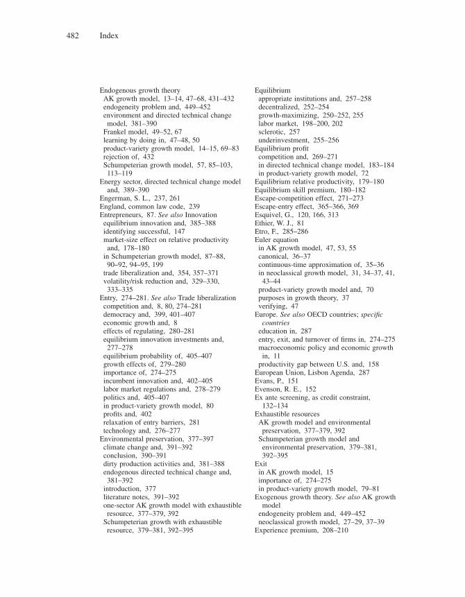
Index482
Endogenous growth theoryAK growth model, 13–14, 47–68, 431–432endogeneity problem and, 449–452environment and directed technical change model, 381–390
Frankel model, 49–52, 67learning by doing in, 47–48, 50product-variety growth model, 14–15, 69–83rejection of, 432Schumpeterian growth model, 57, 85–103, 113–119
Energy sector, directed technical change model and, 389–390
Engerman, S. L., 237, 261England, common law code, 239Entrepreneurs, 87. See also Innovationequilibrium innovation and, 385–388identifying successful, 147market-size effect on relative productivity and, 178–180
in Schumpeterian growth model, 87–88, 90–92, 94–95, 199
trade liberalization and, 354, 357–371volatility/risk reduction and, 329–330, 333–335
Entry, 274–281. See also Trade liberalizationcompetition and, 8, 80, 274–281democracy and, 399, 401–407economic growth and, 8effects of regulating, 280–281equilibrium innovation investments and, 277–278
equilibrium probability of, 405–407growth effects of, 279–280importance of, 274–275incumbent innovation and, 402–405labor market regulations and, 278–279politics and, 405–407in product-variety growth model, 80profi ts and, 402relaxation of entry barriers, 281technology and, 276–277
Environmental preservation, 377–397climate change and, 391–392conclusion, 390–391dirty production activities and, 381–388endogenous directed technical change and, 381–392
introduction, 377literature notes, 391–392one-sector AK growth model with exhaustible resource, 377–379, 392
Schumpeterian growth with exhaustible resource, 379–381, 392–395
Equilibriumappropriate institutions and, 257–258decentralized, 252–254growth-maximizing, 250–252, 255labor market, 198–200, 202sclerotic, 257underinvestment, 255–256
Equilibrium profi tcompetition and, 269–271in directed technical change model, 183–184in product-variety growth model, 72
Equilibrium relative productivity, 179–180Equilibrium skill premium, 180–182Escape-competition effect, 271–273Escape-entry effect, 365–366, 369Esquivel, G., 120, 166, 313Ethier, W. J., 81Etro, F., 285–286Euler equationin AK growth model, 47, 53, 55canonical, 36–37continuous-time approximation of, 35–36in neoclassical growth model, 31, 34–37, 41, 43–44
product-variety growth model and, 70purposes in growth theory, 37verifying, 47
Europe. See also OECD countries; specifi c countries
education in, 287entry, exit, and turnover of fi rms in, 274–275macroeconomic policy and economic growth in, 11
productivity gap between U.S. and, 158European Union, Lisbon Agenda, 287Evans, P., 151Evenson, R. E., 152Ex ante screening, as credit constraint,
132–134Exhaustible resourcesAK growth model and environmental preservation, 377–379, 392
Schumpeterian growth model and environmental preservation, 379–381, 392–395
Exitin AK growth model, 15importance of, 274–275in product-variety growth model, 79–81
Exogenous growth theory. See also AK growth model
endogeneity problem and, 449–452neoclassical growth model, 27–29, 37–39
Experience premium, 208–210
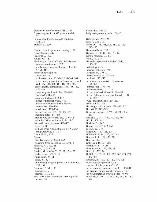
Index 483
Explained sum of squares (SSE), 446Explosive growth, in AK growth model,
52Ex post monitoring, as credit constraint,
134–136Eymard, L., 339
Factor prices, in growth accounting, 107F-distributions, 449Fedderke, J., 372Fellner, W., 187Final output. See also Trade liberalizationmarket-size effect and, 177in Schumpeterian growth model, 85–86, 97–98, 114
Financial developmentconclusion, 147credit constraints, 132–142, 158–163, 164cross-country regressions of economic growth and, 142–145, 148, 161–163, 454–456
cross-industry comparisons, 143, 145–147, 451–456
economic growth and, 5–6, 129–149, 161–163, 454–456
empirical fi ndings, 142–147impact of fi nancial crises, 440innovation and growth with fi nancial constraints, 130–136
introduction, 129–130Levine’s survey, 129–130, 142–144literature notes, 147–148productivity differences and, 139–142volatility/risk reduction and, 341–347
Fixed-effects regressions, 452–453Fogel, K., 80Food and Drug Administration (FDA), new
drug approvals, 171–173Fortin, N. M., 175Francecivil law code, 239–240, 262transition from stagnation to growth, 5
Francois, P., 340, 348Frankel, J., 243, 353Frankel, M., 49–50, 53, 62, 67, 136–137Frankel model, 49–52, 67basic setup, 49–51cases, 51–52diminishing marginal product of capital and, 137, 138
Fraumeni, B. M., 108Freeman, C., 211Freeman, R. B., 175Free-trade zones, in product-variety growth
model, 74
F-statistics, 449, 451Fully endogenous growth, 100–101
Galeotti, M., 391, 392Gali, J., 326, 348Galor, O., 136, 148, 206, 217, 221, 224,
232–233Gambardella, A., 212Gancia, G., 81–83, 182, 188, 373Garcia-Peñalosa, C., 175Gavin, M., 349General-purpose technologies (GPT),
193–216advantage of, 211characteristics of, 193conclusion, 210–211consequences of, 193–196defi ned, 193, 212explaining productivity slowdowns, 196–204
introduction, 193–196literature notes, 211–212in the neoclassical model, 196–198in the Schumpeterian growth model, 197, 198–204
wage inequality and, 204–210Gennaioli, N., 401Germany, civil law code, 239–240, 262Geroski, P., 282–283Gerschenkron, A., 18, 92, 151, 238, 262,
263Gertler, M., 147, 148, 339, 349, 351Gil, R., 400, 415Gilchrist, S., 147Glaeser, E., 237, 242, 261Glomm, G., 313Goldin, C., 180–181, 204Goldsmith, R. W., 143, 147, 148Gordon, R. J., 109, 176, 211Gore, A., 377Gottschalk, P., 207, 208Greenfi eld, J., 77–79Greenwood, J., 147, 148, 181Greif, A., 237, 261Griffi th, R., 79, 92, 152, 262, 267, 274, 279,
282–284Griliches, Z., 110, 119–120, 174, 175Gross domestic product (GDP)acceleration in growth of, 1–2as measure of economic growth, 1, 110–111in product-variety growth model, 71–73in Schumpeterian growth model, 93–94
Grossman, G. M., 81, 100, 267, 282, 372, 373, 391
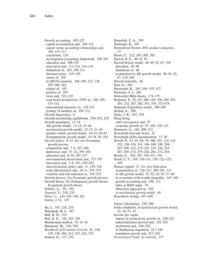
Index484
Growth accounting, 105–125capital accumulation and, 109–115causal versus accounting relationships and, 105, 112–113
conclusion, 119development accounting framework, 290–291education and, 290–291innovation and, 113–114, 116–119limitations of, 105, 109–113literature notes, 119–120nature of, 105in OECD countries, 108–109, 112, 120, 259–260, 262
origins of, 105purpose of, 107taxes and, 121–122total factor productivity (TFP) in, 106–109, 111–112
transnational dynamics in, 120–121tyranny of numbers in, 109–112
Growth diagnostics, 6Growth-maximizing equilibrium, 250–252, 255Growth paradigms, 12–18AK growth model, 13–14, 47–68neoclassical growth model, 12–13, 21–45product-variety growth model, 14–15, 69–83Schumpeterian growth model, 15–18, 85–103
Growth policy, 6–12. See also Economic growth process
competition and, 7–8, 267–286democracy and, 11–12, 399–416education and, 8–10, 287–317environmental preservation and, 377–397innovation and, 7–8, 203, 250–252macroeconomic policy and, 11, 319, 348trade liberalization and, 10–11, 353–375volatility and risk reduction in, 319–352
Growth process. See Economic growth processGrowth theory. See Endogenous growth theory;
Exogenous growth theoryGrübler, A., 391, 392Guerreri, V., 230, 233Guiso, L., 143–145, 148, 421Gurley, J. G., 147
Ha, J., 101, 226, 233Habakkuk, H. J., 187Hall, B. H., 274Hall, R. E., 120, 263, 326Hamiltonian method, 35, 43–45Hammour, M., 326, 348Handbook of Economic Growth, 81, 120,
129–130, 188, 212, 233, 262, 374Hansen, G., 217, 232
Hanushek, E. A., 299Harbaugh, B., 391Harmonized System (HS) product categories,
77Harris, C., 212, 267–269, 283Harrod, R. F., 48–52, 67Harrod-Domar model, 48–49, 52, 67, 319described, 48–49limitations of, 48as precursor to AK growth model, 48–49, 52, 67, 319, 348
Harrod neutrality, 28Hart, O., 283Hausmann, R., 263, 349, 435, 437Heckman, J. J., 206Heckscher-Ohlin theory, 174–175Helpman, E., 81, 83, 100, 120, 198, 200–201,
203, 212, 267, 282, 353, 354, 372–374Helpman-Trajtenberg model, 200–205Heston, A., 108Hicks, J. R., 187, 319Hong Kongclub convergence and, 57economic growth of, 57, 105, 110–112
Hornstein, A., 181, 209, 212Household discount factor, 32Household utility maximization, 17, 45Howitt, P., 15, 43, 69, 79, 100, 101, 124–125,
155, 158–159, 161, 166–168, 198, 204, 207–209, 212, 215–216, 225, 226, 263, 267–269, 274, 279, 282–284, 372, 454
Hoxby, C., 283, 307, 310–311, 316Hsieh, C.-T., 105, 110–111, 120, 122–123,
429Human capital, 13. See also Educationaccumulation of, 226–227, 289–295, 313in AK growth model, 51–52, 54–55, 57–60in economies with wealth inequality, 147–148growth accounting and, 108, 113labor as R&D input, 74Mincerian approach to, 292in neoclassical growth model, 40
Hypothesis testing, 447–449
Import substitution, 259–260Inada conditions, in neoclassical growth model,
22, 32–33, 43Income per capitaimpact of productivity growth on, 220–222industrialization process and, 222–223institutions and, 240–242in Malthusian stagnation, 217–220population growth and, 217–220
Inconvenient Truth, An (movie), 377
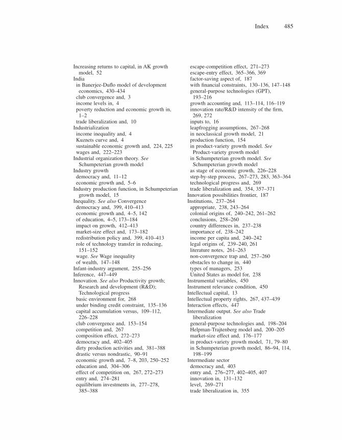
Index 485
Increasing returns to capital, in AK growth model, 52
Indiain Banerjee-Dufl o model of development economics, 430–434
club convergence and, 3income levels in, 4poverty reduction and economic growth in, 1–2
trade liberalization and, 10Industrializationincome inequality and, 4Kuznets curve and, 4sustainable economic growth and, 224, 225wages and, 222–223
Industrial organization theory. See Schumpeterian growth model
Industry growthdemocracy and, 11–12economic growth and, 5–6
Industry production function, in Schumpeterian growth model, 15
Inequality. See also Convergencedemocracy and, 399, 410–413economic growth and, 4–5, 142of education, 4–5, 173–184impact on growth, 412–413market-size effect and, 173–182redistribution policy and, 399, 410–413role of technology transfer in reducing, 151–152
wage. See Wage inequalityof wealth, 147–148
Infant-industry argument, 255–256Inference, 447–449Innovation. See also Productivity growth;
Research and development (R&D); Technological progress
basic environment for, 268under binding credit constraint, 135–136capital accumulation versus, 109–112, 226–228
club convergence and, 153–154competition and, 267composition effect, 272–273democracy and, 402–405dirty production activities and, 381–388drastic versus nondrastic, 90–91economic growth and, 7–8, 203, 250–252education and, 304–306effect of competition on, 267, 272–273entry and, 274–281equilibrium investments in, 277–278, 385–388
escape-competition effect, 271–273escape-entry effect, 365–366, 369factor-saving aspect of, 187with fi nancial constraints, 130–136, 147–148general-purpose technologies (GPT), 193–216
growth accounting and, 113–114, 116–119innovation rate/R&D intensity of the fi rm, 269, 272
inputs to, 16leapfrogging assumptions, 267–268in neoclassical growth model, 21production function, 154in product-variety growth model. See Product-variety growth model
in Schumpeterian growth model. See Schumpeterian growth model
as stage of economic growth, 226–228step-by-step process, 267–273, 283, 363–364technological progress and, 269trade liberalization and, 354, 357–371
Innovation possibilities frontier, 187Institutions, 237–264appropriate, 238, 243–264colonial origins of, 240–242, 261–262conclusions, 258–260country differences in, 237–238importance of, 238–242income per capita and, 240–242legal origins of, 239–240, 261literature notes, 261–263non-convergence trap and, 257–260obstacles to change in, 440types of managers, 253United States as model for, 238
Instrumental variables, 450Instrument relevance condition, 450Intellectual capital, 13Intellectual property rights, 267, 437–439Interaction effects, 447Intermediate output. See also Trade
liberalizationgeneral-purpose technologies and, 198–204Helpman-Trajtenberg model and, 200–205market-size effect and, 176–177in product-variety growth model, 71, 79–80in Schumpeterian growth model, 86–94, 114, 198–199
Intermediate sectordemocracy and, 403entry and, 276–277, 402–405, 407innovation in, 131–132level, 269–271trade liberalization in, 355
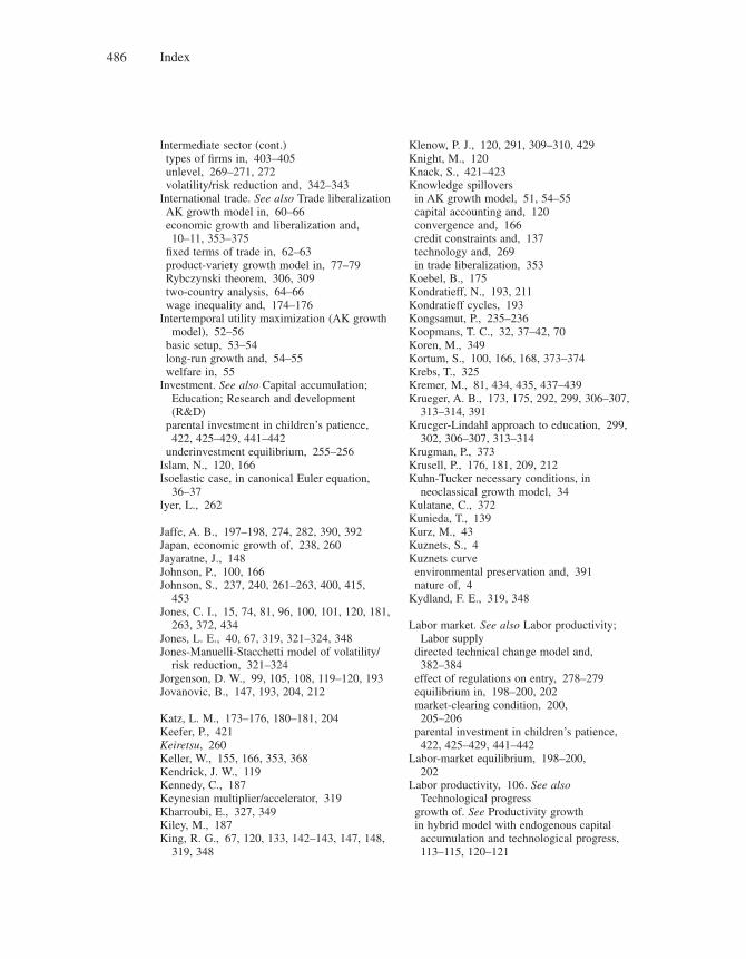
Index486
Intermediate sector (cont.)types of fi rms in, 403–405unlevel, 269–271, 272volatility/risk reduction and, 342–343
International trade. See also Trade liberalizationAK growth model in, 60–66economic growth and liberalization and, 10–11, 353–375
fi xed terms of trade in, 62–63product-variety growth model in, 77–79Rybczynski theorem, 306, 309two-country analysis, 64–66wage inequality and, 174–176
Intertemporal utility maximization (AK growth model), 52–56
basic setup, 53–54long-run growth and, 54–55welfare in, 55
Investment. See also Capital accumulation; Education; Research and development (R&D)
parental investment in children’s patience, 422, 425–429, 441–442
underinvestment equilibrium, 255–256Islam, N., 120, 166Isoelastic case, in canonical Euler equation,
36–37Iyer, L., 262
Jaffe, A. B., 197–198, 274, 282, 390, 392Japan, economic growth of, 238, 260Jayaratne, J., 148Johnson, P., 100, 166Johnson, S., 237, 240, 261–263, 400, 415,
453Jones, C. I., 15, 74, 81, 96, 100, 101, 120, 181,
263, 372, 434Jones, L. E., 40, 67, 319, 321–324, 348Jones-Manuelli-Stacchetti model of volatility/
risk reduction, 321–324Jorgenson, D. W., 99, 105, 108, 119–120, 193Jovanovic, B., 147, 193, 204, 212
Katz, L. M., 173–176, 180–181, 204Keefer, P., 421Keiretsu, 260Keller, W., 155, 166, 353, 368Kendrick, J. W., 119Kennedy, C., 187Keynesian multiplier/accelerator, 319Kharroubi, E., 327, 349Kiley, M., 187King, R. G., 67, 120, 133, 142–143, 147, 148,
319, 348
Klenow, P. J., 120, 291, 309–310, 429Knight, M., 120Knack, S., 421–423Knowledge spilloversin AK growth model, 51, 54–55capital accounting and, 120convergence and, 166credit constraints and, 137technology and, 269in trade liberalization, 353
Koebel, B., 175Kondratieff, N., 193, 211Kondratieff cycles, 193Kongsamut, P., 235–236Koopmans, T. C., 32, 37–42, 70Koren, M., 349Kortum, S., 100, 166, 168, 373–374Krebs, T., 325Kremer, M., 81, 434, 435, 437–439Krueger, A. B., 173, 175, 292, 299, 306–307,
313–314, 391Krueger-Lindahl approach to education, 299,
302, 306–307, 313–314Krugman, P., 373Krusell, P., 176, 181, 209, 212Kuhn-Tucker necessary conditions, in
neoclassical growth model, 34Kulatane, C., 372Kunieda, T., 139Kurz, M., 43Kuznets, S., 4Kuznets curveenvironmental preservation and, 391nature of, 4
Kydland, F. E., 319, 348
Labor market. See also Labor productivity; Labor supply
directed technical change model and, 382–384
effect of regulations on entry, 278–279equilibrium in, 198–200, 202market-clearing condition, 200, 205–206
parental investment in children’s patience, 422, 425–429, 441–442
Labor-market equilibrium, 198–200, 202
Labor productivity, 106. See also Technological progress
growth of. See Productivity growthin hybrid model with endogenous capital accumulation and technological progress, 113–115, 120–121
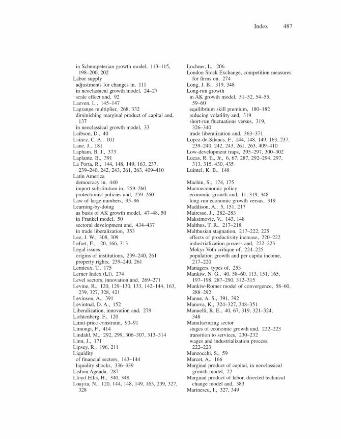
Index 487
in Schumpeterian growth model, 113–115, 198–200, 202
Labor supplyadjustments for changes in, 111in neoclassical growth model, 24–27scale effect and, 92
Laeven, L., 145–147Lagrange multiplier, 268, 332diminishing marginal product of capital and, 137
in neoclassical growth model, 33Laibson, D., 40Laincz, C. A., 101Lane, J., 181Lapham, B. J., 373Laplante, B., 391La Porta, R., 144, 148, 149, 163, 237,
239–240, 242, 243, 261, 263, 409–410Latin Americademocracy in, 440import substitution in, 259–260protectionist policies and, 259–260
Law of large numbers, 95–96Learning-by-doingas basis of AK growth model, 47–48, 50in Frankel model, 50sectoral development and, 434–437in trade liberalization, 353
Lee, J. W., 308, 309Lefort, F., 120, 166, 313Legal issuesorigins of institutions, 239–240, 261property rights, 239–240, 261
Lemieux, T., 175Lerner Index (LI), 274Level sectors, innovation and, 269–271Levine, R., 120, 129–130, 133, 142–144, 163,
239, 327, 328, 421Levinson, A., 391Levintnal, D. A., 152Liberalization, innovation and, 279Lichtenberg, F., 120Limit-price constraint, 90–91Limongi, F., 414Lindahl, M., 292, 299, 306–307, 313–314Linn, J., 171Lipsey, R., 196, 211Liquidityof fi nancial sectors, 143–144liquidity shocks, 336–339
Lisbon Agenda, 287Lloyd-Ellis, H., 340, 348Loayza, N., 120, 144, 148, 149, 163, 239, 327,
328
Lochner, L., 206London Stock Exchange, competition measures
for fi rms on, 274Long, J. B., 319, 348Long-run growthin AK growth model, 51–52, 54–55, 59–60
equilibrium skill premium, 180–182reducing volatility and, 319short-run fl uctuations versus, 319, 326–340
trade liberalization and, 363–371Lopez-de-Silanes, F., 144, 148, 149, 163, 237,
239–240, 242, 243, 261, 263, 409–410Low-development traps, 295–297, 300–302Lucas, R. E., Jr., 6, 67, 287, 292–294, 297,
313, 315, 430, 435Luintel, K. B., 148
Machin, S., 174, 175Macroeconomic policyeconomic growth and, 11, 319, 348long-run economic growth versus, 319
Maddison, A., 5, 151, 217Mairesse, J., 282–283Maksimovic, V., 143, 148Malthus, T. R., 217–218Malthusian stagnation, 217–222, 225effects of productivity increase, 220–222industrialization process and, 222–223Mokyr-Voth critique of, 224–225population growth and per capita income, 217–220
Managers, types of, 253Mankiw, N. G., 40, 58–60, 113, 151, 165,
197–198, 287–290, 312–315Mankiw-Romer model of convergence, 58–60,
288–292Manne, A. S., 391, 392Manova, K., 324–327, 348–351Manuelli, R. E., 40, 67, 319, 321–324,
348Manufacturing sectorstages of economic growth and, 222–223transition to services, 230–232wages and industrialization process, 222–223
Manzocchi, S., 59Marcet, A., 166Marginal product of capital, in neoclassical
growth model, 22Marginal product of labor, directed technical
change model and, 383Marinescu, I., 327, 349

Index488
Market-clearing conditionunder credit constraints, 141–142environmental preservation and, 380–381labor market, 200, 205–206
Market-size effect, 169–191conclusion, 186debate concerning, 174–176directed technological change and, 182–186evidence for, 171–173introduction, 169literature notes, 187–188in pharmaceutical industry, 169–172on relative productivity, 178–180theory of, 169–171in trade liberalization, 353wage inequality and, 173–182
Martin, P., 59Maskin, E., 438Mayer-Foulkes, D., 151, 155, 158–159, 161,
166–168, 225, 454McHugh, R., 181McKinnon, R. I., 147Meghir, C., 302, 307–308, 314Melitz, M., 168, 361, 373Messner, S., 391, 392Michel, P., 294, 313Microdevelopment, 429–439Mincer, J., 227, 292Mincerian approach to human capital, 292Mirman, L., 40Mitton, T., 262Moav, O., 206Modern industrial organization theory. See
Schumpeterian growth modelMoffi tt, R., 207, 208Mokyr, J., 211, 225, 233Monopoly profi ts. See also Profi tsdemocracy and, 402economic growth and, 7–8in product-variety growth model, 71–72in Schumpeterian growth model, 86–87, 90–94, 98, 355–358, 393
Moore, J., 438Moore’s law, 212–213Moral hazard, ex post monitoring as credit
constraint and, 134–136Morck, R., 80Mulani, S., 80Mulligan, C., 400, 415Multiple regression analysis, 446–447Multisector Schumpeterian growth model,
92–96, 100basic setup, 130–132economic growth in, 95–96
fi nancial constraints in, 130–136innovation in, 94–95, 276production in, 92–94profi ts in, 92–94research arbitrage in, 94–95trade liberalization and, 355–358
Murphy, K., 175–176, 297
National Bureau of Economic Research (NBER), 274
National income, trade liberalization and, 355–357, 360–363
Neck-and-neck sectors, innovation and, 269–271
Nelson, R. R., 187, 224, 287, 298–299, 313Neoclassical growth model, 21–45as benchmark for growth analysis, 13, 40capital accumulation in, 21–24, 35–36Cass-Koopmans-Ramsey extension of, 31–42, 53
comparison with AK growth model, 56–60, 319
conclusion, 39convergence in, 29–31, 40–42, 165–166described, 12–13, 21dynamic optimization using Hamiltonian in, 35, 43–45
fundamental equation of, 23–24general-purpose technologies in, 196–198in hybrid model, 228–230hybrid with endogenous capital accumulation and technological progress, 113–119, 120–121
introduction, 21limitations of, 39literature notes, 39–40Solow-Swan model, 21–31
Newell, R. G., 390, 392New fi rm entry. See EntryNewman, A., 136, 148Nickell, S. J., 92, 267, 274, 326Nicoletti, G., 275, 283Nonconvergence traps, 257–260, 440cross-country regressions and, 243–246, 259–260
equilibrium dynamics and, 257–258, 259–260Nondrastic innovation, 90–91Nordhaus, W. D., 391, 392Normality assumption, 447–449North, D. C., 237, 261Nunn, N., 262, 450
OECD countries. See also Europe; specifi c countries
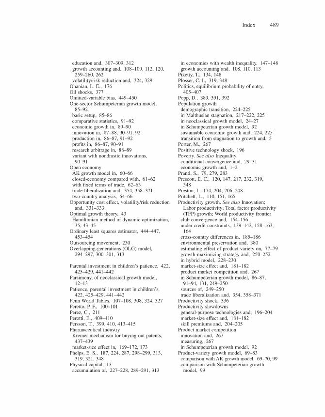
Index 489
education and, 307–309, 312growth accounting and, 108–109, 112, 120, 259–260, 262
volatility/risk reduction and, 324, 329Ohanian, L. E., 176Oil shocks, 377Omitted-variable bias, 449–450One-sector Schumpeterian growth model,
85–92basic setup, 85–86comparative statistics, 91–92economic growth in, 89–90innovation in, 87–88, 90–91, 92production in, 86–87, 91–92profi ts in, 86–87, 90–91research arbitrage in, 88–89variant with nondrastic innovations, 90–91
Open economyAK growth model in, 60–66closed-economy compared with, 61–62with fi xed terms of trade, 62–63trade liberalization and, 354, 358–371two-country analysis, 64–66
Opportunity cost effect, volatility/risk reduction and, 331–333
Optimal growth theory, 43Hamiltonian method of dynamic optimization, 35, 43–45
Ordinary least squares estimator, 444–447, 453–454
Outsourcing movement, 230Overlapping-generations (OLG) model,
294–297, 300–301, 313
Parental investment in children’s patience, 422, 425–429, 441–442
Parsimony, of neoclassical growth model, 12–13
Patience, parental investment in children’s, 422, 425–429, 441–442
Penn World Tables, 107–108, 308, 324, 327Peretto, P. F., 100–101Perez, C., 211Perotti, E., 409–410Persson, T., 399, 410, 413–415Pharmaceutical industryKremer mechanism for buying out patents, 437–439
market-size effect in, 169–172, 173Phelps, E. S., 187, 224, 287, 298–299, 313,
319, 321, 348Physical capital, 13accumulation of, 227–228, 289–291, 313
in economies with wealth inequality, 147–148growth accounting and, 108, 110, 113
Piketty, T., 134, 148Plosser, C. I., 319, 348Politics, equilibrium probability of entry,
405–407Popp, D., 389, 391, 392Population growthdemographic transition, 224–225in Malthusian stagnation, 217–222, 225in neoclassical growth model, 24–27in Schumpeterian growth model, 92sustainable economic growth and, 224, 225transition from stagnation to growth and, 5
Porter, M., 267Positive technology shock, 196Poverty. See also Inequalityconditional convergence and, 29–31economic growth and, 1–2
Prantl, S., 79, 279, 283Prescott, E. C., 120, 147, 217, 232, 319,
348Preston, I., 174, 204, 206, 208Pritchett, L., 110, 151, 165Productivity growth. See also Innovation;
Labor productivity; Total factor productivity (TFP) growth; World productivity frontier
club convergence and, 154–156under credit constraints, 139–142, 158–163, 164
cross-country differences in, 185–186environmental preservation and, 380estimating effect of product variety on, 77–79growth-maximizing strategy and, 250–252in hybrid model, 228–230market-size effect and, 181–182product market competition and, 267in Schumpeterian growth model, 86–87, 91–94, 131, 249–250
sources of, 249–250trade liberalization and, 354, 358–371
Productivity shock, 336Productivity slowdownsgeneral-purpose technologies and, 196–204market-size effect and, 181–182skill premiums and, 204–205
Product market competitioninnovation and, 267measuring, 267in Schumpeterian growth model, 92
Product-variety growth model, 69–83comparison with AK growth model, 69–70, 99comparison with Schumpeterian growth model, 99
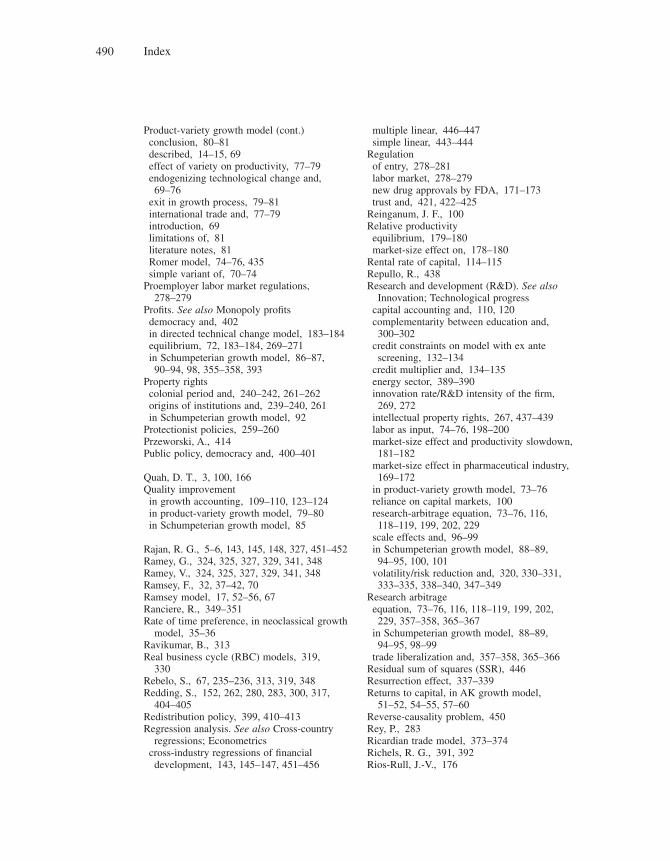
Index490
Product-variety growth model (cont.)conclusion, 80–81described, 14–15, 69effect of variety on productivity, 77–79endogenizing technological change and, 69–76
exit in growth process, 79–81international trade and, 77–79introduction, 69limitations of, 81literature notes, 81Romer model, 74–76, 435simple variant of, 70–74
Proemployer labor market regulations, 278–279
Profi ts. See also Monopoly profi tsdemocracy and, 402in directed technical change model, 183–184equilibrium, 72, 183–184, 269–271in Schumpeterian growth model, 86–87, 90–94, 98, 355–358, 393
Property rightscolonial period and, 240–242, 261–262origins of institutions and, 239–240, 261in Schumpeterian growth model, 92
Protectionist policies, 259–260Przeworski, A., 414Public policy, democracy and, 400–401
Quah, D. T., 3, 100, 166Quality improvementin growth accounting, 109–110, 123–124in product-variety growth model, 79–80in Schumpeterian growth model, 85
Rajan, R. G., 5–6, 143, 145, 148, 327, 451–452Ramey, G., 324, 325, 327, 329, 341, 348Ramey, V., 324, 325, 327, 329, 341, 348Ramsey, F., 32, 37–42, 70Ramsey model, 17, 52–56, 67Ranciere, R., 349–351Rate of time preference, in neoclassical growth
model, 35–36Ravikumar, B., 313Real business cycle (RBC) models, 319,
330Rebelo, S., 67, 235–236, 313, 319, 348Redding, S., 152, 262, 280, 283, 300, 317,
404–405Redistribution policy, 399, 410–413Regression analysis. See also Cross-country
regressions; Econometricscross-industry regressions of fi nancial development, 143, 145–147, 451–456
multiple linear, 446–447simple linear, 443–444
Regulationof entry, 278–281labor market, 278–279new drug approvals by FDA, 171–173trust and, 421, 422–425
Reinganum, J. F., 100Relative productivityequilibrium, 179–180market-size effect on, 178–180
Rental rate of capital, 114–115Repullo, R., 438Research and development (R&D). See also
Innovation; Technological progresscapital accounting and, 110, 120complementarity between education and, 300–302
credit constraints on model with ex ante screening, 132–134
credit multiplier and, 134–135energy sector, 389–390innovation rate/R&D intensity of the fi rm, 269, 272
intellectual property rights, 267, 437–439labor as input, 74–76, 198–200market-size effect and productivity slowdown, 181–182
market-size effect in pharmaceutical industry, 169–172
in product-variety growth model, 73–76reliance on capital markets, 100research-arbitrage equation, 73–76, 116, 118–119, 199, 202, 229
scale effects and, 96–99in Schumpeterian growth model, 88–89, 94–95, 100, 101
volatility/risk reduction and, 320, 330–331, 333–335, 338–340, 347–349
Research arbitrageequation, 73–76, 116, 118–119, 199, 202, 229, 357–358, 365–367
in Schumpeterian growth model, 88–89, 94–95, 98–99
trade liberalization and, 357–358, 365–366Residual sum of squares (SSR), 446Resurrection effect, 337–339Returns to capital, in AK growth model,
51–52, 54–55, 57–60Reverse-causality problem, 450Rey, P., 283Ricardian trade model, 373–374Richels, R. G., 391, 392Rios-Rull, J.-V., 176
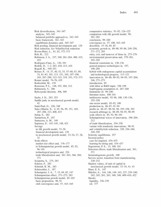
Index 491
Risk diversifi cation, 341–347analysis, 343–345balanced portfolio approach to, 343–345basic framework, 341–343equilibrium dynamics and, 345–347
Risk pooling, fi nancial development and, 129Risk reduction. See Volatility/risk reductionRivera-Batiz, L., 81, 82, 372–373Rob, R., 212Robinson, J. A., 237, 240, 261–264, 400, 415,
453Rodriguez-Clare, A., 120, 291Rodrik, D., 1–2, 263, 410, 413, 416Rogoff, K., 349–351Romer, P., 14, 37, 40, 52, 53, 57–60, 67, 69,
74, 81–83, 101, 113, 151, 165, 197–198, 243, 287–290, 312–315, 319, 353, 372–373
Romer model, 74–76, 435Rothschild, M., 139Rousseau, P. L., 148, 193, 204, 212Rubinstein, Y., 206Rybczynski theorem, 306, 309
Sachs, J. D., 263, 353Saddle path, in neoclassical growth model,
42Saint-Paul, G., 326, 348Sala-i-Martin, X., 4, 45, 56, 59, 151, 165,
287–288, 313, 400, 415Salop, S., 282Samuelson, P., 187Santacreu, A. M., 349Sapienza, P., 143–145, 148, 421Savingsin AK growth model, 51–56fi nancial development and, 129in neoclassical growth model, 23–24, 27, 28, 32
Scale effectsmarket-size effect and, 176–177in Schumpeterian growth model, 85, 92, 96–101
technological progress and, 224trade liberalization and, 361–363, 366, 369, 371
Scarpetta, S., 275, 283Scherer, F., 283Schmidt, K. M., 283Schmookler, J., 187Schumpeter, J. A., 7, 15, 69, 85, 147Schumpeterian effect, 271–273, 283Schumpeterian growth model, 85–103basic proposition, 90, 91club convergence and, 57, 163–165
comparative statistics, 91–92, 124–125comparison with AK growth model, 99, 281–282
conclusion, 99–100convergence in, 57, 100, 163–165described, 15–18, 69, 85economic growth in, 89–90, 95–96, 249–250, 271–272, 283
entry, exit, and turnover of fi rms in, 275–276environmental preservation and, 379–381, 392–395
fi nancial constraints in, 130–136general-purpose technologies in, 197, 198–204
hybrid with endogenous capital accumulation and technological progress, 113–121
innovation in, 86–88, 90–92, 94–95, 197–204, 246, 271–273
introduction, 85with labor as R&D input, 198–199leapfrogging assumption of, 267–268limitations of, 99–100literature notes, 100–101multisector model, 92–96, 100, 130–136, 355–358
one-sector model, 85–92, 100production in, 86–87, 91–94profi ts in, 86–87, 90–94, 98, 355–358, 393research arbitrage in, 88–89, 94–95, 98–99scale effects in, 85, 92, 96–101Schumpeterian waves of innovation, 198–204, 212
of trade liberalization, 354–358variant with nondrastic innovations, 90–91and volatility/risk reduction, 320, 326–340, 349–350
Sclerotic equilibrium, 257Sectoral policycase for targeted, 434–435learning-by-doing and, 434–437
Segerstrom, P. S., 15, 100, 101Selection effects, trade liberalization and, 361,
371Semiendogenous growth, 100Service sector, transition from manufacturing,
230–232Shadow values, of unit of capital in
neoclassical growth model, 33–34, 41, 43Shaw, E. S., 147Shleifer, A., 144, 148, 149, 163, 237, 239–240,
242, 243, 261, 263, 340, 348, 409–410, 422Shocksliquidity, 336–339oil, 377
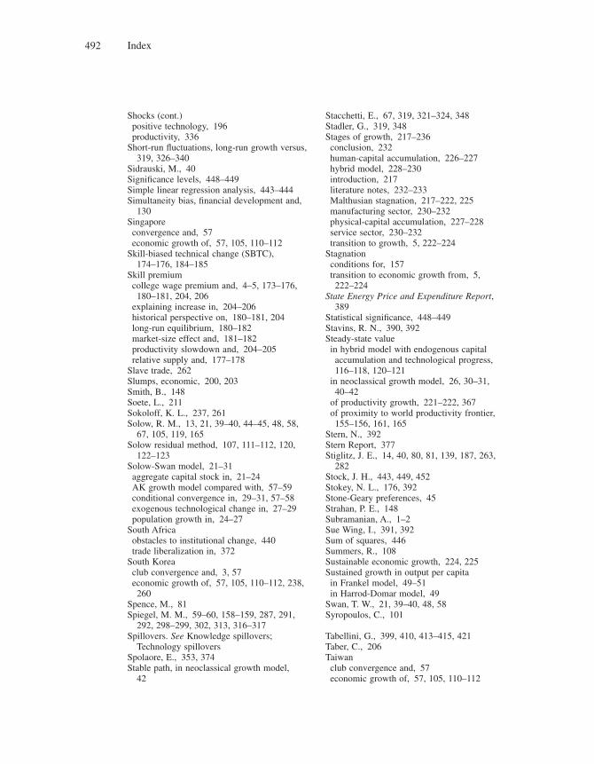
Index492
Shocks (cont.)positive technology, 196productivity, 336
Short-run fl uctuations, long-run growth versus, 319, 326–340
Sidrauski, M., 40Signifi cance levels, 448–449Simple linear regression analysis, 443–444Simultaneity bias, fi nancial development and,
130Singaporeconvergence and, 57economic growth of, 57, 105, 110–112
Skill-biased technical change (SBTC), 174–176, 184–185
Skill premiumcollege wage premium and, 4–5, 173–176, 180–181, 204, 206
explaining increase in, 204–206historical perspective on, 180–181, 204long-run equilibrium, 180–182market-size effect and, 181–182productivity slowdown and, 204–205relative supply and, 177–178
Slave trade, 262Slumps, economic, 200, 203Smith, B., 148Soete, L., 211Sokoloff, K. L., 237, 261Solow, R. M., 13, 21, 39–40, 44–45, 48, 58,
67, 105, 119, 165Solow residual method, 107, 111–112, 120,
122–123Solow-Swan model, 21–31aggregate capital stock in, 21–24AK growth model compared with, 57–59conditional convergence in, 29–31, 57–58exogenous technological change in, 27–29population growth in, 24–27
South Africaobstacles to institutional change, 440trade liberalization in, 372
South Koreaclub convergence and, 3, 57economic growth of, 57, 105, 110–112, 238, 260
Spence, M., 81Spiegel, M. M., 59–60, 158–159, 287, 291,
292, 298–299, 302, 313, 316–317Spillovers. See Knowledge spillovers;
Technology spilloversSpolaore, E., 353, 374Stable path, in neoclassical growth model,
42
Stacchetti, E., 67, 319, 321–324, 348Stadler, G., 319, 348Stages of growth, 217–236conclusion, 232human-capital accumulation, 226–227hybrid model, 228–230introduction, 217literature notes, 232–233Malthusian stagnation, 217–222, 225manufacturing sector, 230–232physical-capital accumulation, 227–228service sector, 230–232transition to growth, 5, 222–224
Stagnationconditions for, 157transition to economic growth from, 5, 222–224
State Energy Price and Expenditure Report, 389
Statistical signifi cance, 448–449Stavins, R. N., 390, 392Steady-state valuein hybrid model with endogenous capital accumulation and technological progress, 116–118, 120–121
in neoclassical growth model, 26, 30–31, 40–42
of productivity growth, 221–222, 367of proximity to world productivity frontier, 155–156, 161, 165
Stern, N., 392Stern Report, 377Stiglitz, J. E., 14, 40, 80, 81, 139, 187, 263,
282Stock, J. H., 443, 449, 452Stokey, N. L., 176, 392Stone-Geary preferences, 45Strahan, P. E., 148Subramanian, A., 1–2Sue Wing, I., 391, 392Sum of squares, 446Summers, R., 108Sustainable economic growth, 224, 225Sustained growth in output per capitain Frankel model, 49–51in Harrod-Domar model, 49
Swan, T. W., 21, 39–40, 48, 58Syropoulos, C., 101
Tabellini, G., 399, 410, 413–415, 421Taber, C., 206Taiwanclub convergence and, 57economic growth of, 57, 105, 110–112
Index 493
Tamura, R., 297Taxationof dirty production activities, 384–385, 387–388
growth accounting in presence of, 121–122Taylor-series approximations, 36t distributions, 448–449Technological progress. See also General-
purpose technologies (GPT); Innovation; Productivity growth; Research and development (R&D); Technology transfer
in AK growth model, 13capital accumulation compared with, 66democracy, 407–410, 414directed technical change model, 182–186, 381–390
embodied, 181endogenous, 47–48, 69–76, 432entry and, 276–277exogenous, 27–29, 37–39experience premium and, 209–210general-purpose technologies (GPT), 193–216
in hybrid model with endogenous capital accumulation, 117–119
institutions and, 237–264leapfrogging versus step-by-step, 267–273, 283, 363–364
market-size effect and, 169–191in neoclassical growth model, 13, 21, 27–29, 31–39, 111
population growth and, 224in product-variety growth model, 69–76as requirement for growth, 39, 113, 116–119skill-biased technical change (SBTC), 174–176, 184–185
technology spillovers and, 14–15, 75, 80Technology frontieradvantage to backwardness (Gerschenkron) and, 18, 238, 262, 362–363
economic growth and proximity to, 17Technology spillovers, 14–15in product-variety growth model, 75, 80
Technology transfer, 151–168concept of, 151conclusion, 163–165credit constraints as source of divergence, 158–163, 164
literature notes, 165–166model with club convergence, 152–158role in stabilizing gap between rich and poor countries, 151–152
trade liberalization and, 368–369Tenreyro, S., 349
Terms-of-trade effects, of trade liberalization, 354, 373
TFP. See Total factor productivity (TFP) growth
Thomas, R. P., 237, 261Thompson, P., 100–101Threshold externalities, 296–297Tirole, J., 85, 90, 100, 282Total factor productivity (TFP) growth, 106accounting versus causation and, 105, 112–113
basic growth equation, 106–107comparison of U.S. and India, 430–434dual method, 111–112, 119–120, 122–123education and, 308effects of productivity increase, 220–222empirical results, 107–109entry and, 279–280estimating, 107–108general-purpose technologies and, 193, 194
in growth accounting, 106–109, 111–112in product-variety growth model, 77–78Solow residual method, 107, 111–112, 120, 122–123
Trade liberalization, 10–11, 353–375. See also Entry; International trade
Aghion-Fedderke-Howitt-Kulatane-Vogt test for effects, 372
backwardness effects, 362–363, 371–372conclusion, 371discouragement effect of foreign entry, 366–369
economic growth and, 367–371enhanced product market competition and, 354
impact on long-run growth, 363–371innovation and, 354, 357–371introduction, 353–354knowledge spillover effect, 353literature notes, 372–374market-size effect, 353multisector Schumpeterian growth model of, 355–358
national income and, 355–357, 360–363Ricardian trade model, 373–374scale effects, 361–363, 366, 369, 371Schumpeterian growth model of, 354–358selection effects, 361, 371static and dynamic gains in, 372terms-of-trade effects, 354, 373
Trajtenberg, M., 193, 198, 200–201, 203, 212, 274
Transferability parameter, 209–210
Index494
Transversality condition, in neoclassical growth model, 34, 35
Trebbi, F., 399, 401, 407, 415Trefl er, D., 354Trusteconomic growth and, 421–425regulation and, 421, 422–425
Tsiddon, D., 206t-statistics, 448–449Turnoverin AK growth model, 15importance of, 274–275in product-variety growth model, 81in Schumpeterian growth model, 16turnover ratio of fi nancial sectors, 144
Two-stage least squares (2SLS), 450–451, 453–454
Ulku, H., 101Underinvestment equilibrium, 255–256Unifi ed growth theory, 217. See also Stages of
growthUnionization, wage compression and, 175United Kingdomcollege wage premium in, 4–5, 204competition measures in, 274English common law and, 239product-variety growth model in, 79–80transition from stagnation to growth, 5, 281wage inequality and, 174–176, 204, 206–210
United Statesannual growth rate in, 181in Banerjee-Dufl o model of development economics, 430–434
college-equivalents in, 173–174college wage premium and, 4–5, 173–176, 204
cross-country comparisons and, 243–246, 259–261
cross-industry comparisons of fi nancial development and economic growth, 143, 145–147, 451–456
cross-US-state evidence on education, 309–311
directed technical change model and energy sector, 389–390
education in, 173–176, 204, 287, 309–311entry, exit, and turnover of fi rms in, 274–275gross domestic product growth and, 193, 194
growth accounting and, 108, 109institutional models of, 238long-run equilibrium skill premium in, 180–181
macroeconomic policy and economic growth in, 11
productivity gap between Europe and, 158product-variety growth model in, 78–79transition from manufacturing to service in, 230–232
wage inequality, 174–176, 204, 206–210Unlevel sectors, innovation and, 269–271, 272Uzawa, H., 313
Vandenbussche, J., 283, 302, 307–308, 310–311, 314, 316
Van Reenen, J., 92, 152, 262, 267, 282–283Ventura, J., 40, 60–67, 373, 374Vickers, J., 267–269, 283Viegi, N., 372Villanueva, D., 120Violante, G. L., 109, 175, 176, 207–209, 212,
215–216Vishny, R. W., 144, 148, 149, 163, 237, 239,
261, 263Volatility/risk reduction, 319–352Aghion-Angeletos-Banerjee-Manova model of, 324, 326–339
AK approach to, 319, 321–325, 342, 347, 348conclusion, 347–348credit constraints and, 320, 331–339fi nancial development and, 341–347introduction, 319–320Jones-Manuelli-Stacchetti model of, 321–324literature notes, 348–349Ramey-Ramey model of, 327–329, 341research and development (R&D) and, 320, 330–331, 333–335, 338–340, 347–349
resurrecting effect of higher volatility, 337–339
risk diversifi cation and, 341–347Schumpeterian approach to, 320, 325–341, 348–349
Volpin, E., 409–410Von Tunzelmann, G. N., 211Voth, H. J., 225, 233
Wachtel, P., 148Wacziarg, R., 353, 374Wage inequalityadaptability premium and, 207–209college wage premium, 4–5, 173–176, 180–181, 204, 208
experience premium and, 208–210general-purpose technologies and, 204–210
market-size effect and, 173–182skill premium and, 173–182, 204–206

Index 495
transferability parameter and, 209–210in the United Kingdom, 174–176, 204, 206–210
in the U.S., 174–176, 204, 206–210within-group, 206–210
Wang, H., 391Warner, A., 353Watson, M. W., 443, 449, 452Weil, D. N., 40, 58–60, 113, 151, 165, 191,
197–198, 224, 232–233, 287–290, 312–315
Weinstein, D., 77–79Weitzman, M., 392Welch, F., 175Welfare analysis, in AK growth model, 55Westphal, L. E., 152Wheeler, D., 391Wilson, D. J., 123–124, 391Within-group wage inequality, 206–210Woessmann, L., 299Wooldridge, J., 443, 447, 449, 454World productivity frontier. See also
Convergence; Distance to world productivity frontier; Productivity growth
appropriate institutions and, 246–258education and, 8–10, 302–307nature of, 2–3nonconvergence traps and, 257–258
World Value Survey, 421, 423
Xie, D., 235–236
Yared, P., 400, 415Yeung, B., 80Yorukoglu, M., 181Young, A. A., 69, 96–97, 99, 105, 110–111,
119, 120, 122–123, 373, 435
Zak, P. J., 421–423Zeira, J., 136, 148Zero conditional mean assumption, 443–444,
449Zervos, S., 143–144, 148Zilibotti, F., 1, 2, 8, 18, 81–83, 147, 182,
186–188, 243–244, 263, 280, 283, 320, 341, 349, 401, 404–405, 422, 425–429, 441–442
Zingales, L., 5–6, 143–145, 148, 327, 421, 451–452

Related Documents