THE ECOLOGICAL SUSTAINABILITY OF POTATO PRODUCTION IN THE SANDVELD REGION OF THE WESTERN CAPE: NUTRIENT AND WATER USE EFFICIENCIES by MALCOLM JEREMY KAYES THESIS PRESENTED IN PARTIAL FULFILMENT OF THE REQUIREMENTS FOR THE DEGREE OF MASTER OF AGRICULTURAL SCIENCES AT STELLENBOSCH UNIVERSITY AGRONOMY DEPARTMENT, FACULTY OF AGRISCIENCES Supervisor: Prof. MARTIN STEYN (UNIVERSITY OF PRETORIA) Co-supervisor: Prof. ANGELINUS FRANKE (UNIVERSITY OF THE FREE STATE) Co-supervisor: Dr PIETER SWANEPOEL (STELLENBOSCH UNIVERSITY) DECEMBER 2019

Welcome message from author
This document is posted to help you gain knowledge. Please leave a comment to let me know what you think about it! Share it to your friends and learn new things together.
Transcript

THE ECOLOGICAL SUSTAINABILITY OF POTATO PRODUCTION IN THE SANDVELD REGION OF THE WESTERN CAPE:
NUTRIENT AND WATER USE EFFICIENCIES
by
MALCOLM JEREMY KAYES
THESIS PRESENTED IN PARTIAL FULFILMENT OF THE REQUIREMENTS FOR THE
DEGREE OF MASTER OF AGRICULTURAL SCIENCES
AT
STELLENBOSCH UNIVERSITY
AGRONOMY DEPARTMENT, FACULTY OF AGRISCIENCES
Supervisor: Prof. MARTIN STEYN (UNIVERSITY OF PRETORIA)
Co-supervisor: Prof. ANGELINUS FRANKE (UNIVERSITY OF THE FREE STATE)
Co-supervisor: Dr PIETER SWANEPOEL (STELLENBOSCH UNIVERSITY)
DECEMBER 2019

i
December 2019
DECLARATION
By submitting this thesis electronically, I declare that the entirety of the work contained therein is
my own, original work, that I am the sole author thereof (save to the extent explicitly otherwise
stated), that reproduction and publication thereof by Stellenbosch University will not infringe any
third party rights and that I have not previously in its entirety or in part submitted it for obtaining
any qualification.
Date: ……………………………………
Copyright © 2019 Stellenbosch University All rights reserved
Stellenbosch University https://scholar.sun.ac.za

ii
ACKNOWLEDGEMENTS
If the research does not cause some form of stir in society, reassess its need.
Acknowledgement goes out towards the following people for supporting me for the last two years.
To my friends and family for making the journey easier and more enjoyable and for always
believing in me no matter what. Particular gratitude goes out to my fiancée for putting up with the
many hours away from home and in the field and for encouraging me to be the best I can. Without
my supervisors Prof. Martin Steyn, Prof. Linus Franke and Dr Swanepoel, this project and MSc
thesis would not be possible or up to the standard I hope it adheres to. The knowledge I have
gained working alongside, whom I consider, leading researchers in the South African agricultural
industry, will carry with me for the rest of my life. To Yara Africa Fertiliser (Pty.) Ltd., in particular
Piet Brink and Simba Ltd. for providing the funding as well as support in the field and with obtaining
data. Thanks go out to the Agricultural Research Council for providing weather data when needed
as well as to Julian Conrad and his team from Geohydrological and Spatial Solutions International
(Pty.) Ltd. for their support and contribution to the project. Notable is the support provided from
Potatoes South Africa (PSA), particularly the Piketberg Branch. A very important thank you goes
to the farmers who all supported the research. Their hospitality and kindness towards an outsider
was incredible and made each trip to the Sandveld an enjoyable and interesting one. Majority of
my knowledge regarding potatoes, fertilisation and centre-pivot irrigation was obtained alongside
them and my supervisors. Finally, to all MSc students who helped me during long hot days of
equipment installations and removals and not to forget yield analysis. Without all of your
contributions, this MSc would surely not have been completed.
Stellenbosch University https://scholar.sun.ac.za

iii
PREFACE
This thesis is presented as a compilation of six chapters. Each chapter is introduced separately
and is written according to the style of the South African Journal of Plant and Soil.
Chapter 1 Introduction (including aim and objectives)
Chapter 2 Literature Review
Chapter 3 Materials and Methods
Chapter 4 Results and Discussion
Chapter 5 Conclusion and Recommendations
Chapter 6 References
Appendices I, II and III
Stellenbosch University https://scholar.sun.ac.za

iv
CONTENTS
CHAPTER 1: INTRODUCTION ..................................................................................................... 1
1.1 Study background.................................................................................................................. 1
1.2 Aim and objectives ................................................................................................................ 7
CHAPTER 2: LITERATURE REVIEW ........................................................................................... 9
2.1 Resource use efficiency ........................................................................................................ 9
2.2 Soil and water ...................................................................................................................... 10
2.2.1 Soil physics .......................................................................................................................... 10
2.2.2 Water requirements ............................................................................................................. 11
2.2.3 The role of roots in the uptake of water .............................................................................. 12
2.2.4 Irrigation systems ................................................................................................................ 13
2.2.5 Efficiency of irrigation systems ............................................................................................ 14
2.2.6 Irrigation scheduling ............................................................................................................ 16
2.2.6.1 Irrigation scheduling practices ........................................................................................ 17
2.2.6.2 Reference evapotranspiration, actual evapotranspiration and water availability .......... 18
2.2.7 Drainage and soil water movement .................................................................................... 27
2.2.7.1 Direct methods of measuring soil water movement and drainage ................................ 27
2.2.7.2 Indirect methods of measuring soil water content, movement and drainage ................ 29
2.3 Water-use efficiency ............................................................................................................ 32
2.3.1 Factors affecting water use efficiency ................................................................................. 34
2.4 Fertilisation .......................................................................................................................... 35
2.4.1 Nutrient use efficiency ......................................................................................................... 35
2.4.2 Nitrogen ............................................................................................................................... 37
2.4.2.1 Nitrogen source (ammonium vs. nitrate) ........................................................................ 37
2.4.2.2 Nitrogen crop requirement .............................................................................................. 37
2.4.2.3 Nitrogen leaching ............................................................................................................ 39
2.4.2.4 Nitrogen management .................................................................................................... 39
Stellenbosch University https://scholar.sun.ac.za

v
2.4.3 Phosphorus ......................................................................................................................... 40
2.4.3.1 Phosphorus source ......................................................................................................... 40
2.4.3.2 Phosphorus crop requirement ........................................................................................ 40
2.4.3.3 Phosphorus leaching ...................................................................................................... 41
2.4.3.4 Phosphorus management .............................................................................................. 42
2.4.4 Potassium ............................................................................................................................ 43
2.4.4.1 Potassium source ........................................................................................................... 43
2.4.4.2 Potassium crop requirement .......................................................................................... 43
2.4.4.3 Potassium leaching......................................................................................................... 44
2.4.4.4 Potassium management ................................................................................................. 44
2.4.5 Calcium ................................................................................................................................ 45
2.4.6 Magnesium .......................................................................................................................... 45
2.4.7 Sulphur ................................................................................................................................ 46
2.5 Synopsis .............................................................................................................................. 47
CHAPTER 3: MATERIALS AND METHODS .............................................................................. 48
3.1 Locality and experimental design ........................................................................................ 48
3.2 Data collection ..................................................................................................................... 50
3.3 Irrigation system evaluations ............................................................................................... 51
3.4 Irrigation amount.................................................................................................................. 53
3.5 Leaching requirement .......................................................................................................... 54
3.6 Crop evapotranspiration ...................................................................................................... 55
3.7 Soil water content and water movement in the soil ............................................................ 57
3.8 Drainage .............................................................................................................................. 59
3.9 Soil sampling ....................................................................................................................... 62
3.10 Interception of solar radiation .............................................................................................. 63
3.11 Nutrient content in plant matter ........................................................................................... 64
3.12 Tuber nutrient content and nutrient use efficiency .............................................................. 65
Stellenbosch University https://scholar.sun.ac.za

vi
3.13 Tuber yield and quality ........................................................................................................ 65
3.14 Weather data ....................................................................................................................... 67
CHAPTER 4: RESULTS AND DISCUSSION .............................................................................. 68
4.1 Evaluation of irrigation systems .......................................................................................... 68
4.2 Drainage and leaching ........................................................................................................ 70
4.2.1 Water inputs and losses ...................................................................................................... 70
4.2.2 Estimated water requirements ............................................................................................ 86
4.2.2.1 Basal crop coefficient curves .......................................................................................... 86
4.2.2.2 Irrigation requirements .................................................................................................... 91
4.2.3 Irrigation water quality ....................................................................................................... 100
4.2.4 Soil water content .............................................................................................................. 102
4.2.5 Water use efficiency .......................................................................................................... 112
4.2.6 Nutrient leaching................................................................................................................ 114
4.2.7 Leachate EC levels ........................................................................................................... 128
4.3 Plant nutrient uptake ......................................................................................................... 130
4.3.1 Leaf tissue nutrient content ............................................................................................... 130
4.3.2 Tuber nutrient content ....................................................................................................... 134
4.3.3 Nutrient use efficiency ....................................................................................................... 138
4.3.4 Nutrient balance ................................................................................................................ 142
4.4 Tuber yield and size distribution........................................................................................ 146
4.4.1 Tuber yield ......................................................................................................................... 146
4.4.2 Tuber size distribution ....................................................................................................... 148
CHAPTER 5: CONCLUSIONS AND RECOMMENDATIONS .................................................. 151
CHAPTER 6: REFERENCES .................................................................................................... 163
APPENDIX I ................................................................................................................................ 204
APPENDIX II ............................................................................................................................... 209
APPENDIX III .............................................................................................................................. 214
Stellenbosch University https://scholar.sun.ac.za

vii
I. LIST OF TABLES
Table 2.1. Different concepts used to calculate potential evapotranspiration (ETo). Modified table
from Bormann (2011). ........................................................................................................... 19
Table 2.2. The crop coefficients of potato crops reported in various studies. Modified table from
Parent and Anctil (2012). ....................................................................................................... 24
Table 2.3. Different methods used to calculate water use efficiency in potato production
systems. ................................................................................................................................. 33
Table 3.1. Information regarding locality, equipment installation, planting date, emergence and
harvest date of the studied fields. Fields 1 to 9 are labelled according to their planting dates
(1 = earliest planted and 9 = last planted)............................................................................. 51
Table 4.1. Efficiency parameters of centre-pivot irrigation systems as well as the average flow
rates of water and rotation times taken to complete one cycle at 100% of the systems
speed. .................................................................................................................................... 69
Table 4.2. Total water inputs (rainfall and irrigation) and losses (drainage) recorded for the
different Sandveld sites. Drainage was not measured at the extensively monitored fields. 72
Table 4.3. Duration (days) of each stage of the basal crop coefficient curve and the calculated
mean for all autumn, winter and summer planted fields. The Kcb(ini) was used from
planting to crop emergence; Kcb(mid) from the duration of 100% canopy cover and
Kcb(end) at crop termination. ................................................................................................ 91
Table 4.4. Basal crop coefficient values adjusted to suit climatic conditions for the Sandveld
region. .................................................................................................................................... 91
Table 4.5. Evapotranspiration (mm) calculated using the LINTUL DSS potato model and basal
crop coefficient curves calculated using weather parameters obtained from each field. ..... 92
Table 4.6. The sodium and salinity hazard classes for irrigation water. The sodium hazard
classes are calculated using the sodium absorption ratio. The EC is well correlated with the
dissolved salt content of water (Fertasa 2016). .................................................................. 100
Stellenbosch University https://scholar.sun.ac.za

viii
Table 4.7. Quality parameters for the different irrigation water sources. Salinity hazard class is
determined based on the SAR and the electrical conductivity. .......................................... 102
Table 4.8. Water use efficiency and IWUE obtained within the Sandveld region. Calculated was
the potential WUE and IR using outputs provided by LINTUL POTATO DSS model and the
ratio between actual irrigation application (AI) and IR as estimated using the Kcb curves 113
Table 4.9. Chemical composition of the different irrigation water sources. Fields 2 and 5 shared
the same water source, as well as Fields 3, 4 and 8. ......................................................... 114
Table 4.10. Extent of nutrients leached per season in intensively monitored fields. ................. 127
Table 4.11. Leaf analysis conducted for Fields 2 to 9 approximately every 30 to 40 days. Leaf
sampling commenced once good vegetative growth was established. Field 1 data is
missing due to the need for sampling made clear after its early termination due to late blight
(Phytophthora infestans). .................................................................................................... 133
Table 4.12. Tuber nutrient contents from the yield analysis conducted for each monitored field.
The pith analysis was selected to represent the entire tuber nutrient content due to the
large proportion of the pith in comparison to the skin and medulla. ................................... 135
Table 4.13. Nutrient content for the skin of potato tubers harvested from monitored fields. .... 136
Table 4.14. Nutrient content of the medulla section of potato tubers harvested from monitored
fields. .................................................................................................................................... 136
Table 4.15. Nutrient removal as influenced by the DM yield of tubers harvested from monitored
fields. .................................................................................................................................... 137
Table 4.16. Total input of each nutrient element per field for the entire cropping cycle through
fertiliser applications. Fertiliser regimes were generally similar within the region and applied
on a weekly basis. ............................................................................................................... 138
Table 4.17. Mean values of the nutrient efficiency parameters obtained in the Sandveld region,
taken from all nine (extensively and intensively) monitored fields. AUE = Agronomic use
efficiency. ............................................................................................................................. 139
Stellenbosch University https://scholar.sun.ac.za

ix
Table 4.18 Nutrient use efficiency obtained for all monitored fields from earliest planted to latest
planted. ................................................................................................................................ 140
Table 4.19. The nutrient uptake efficiency for each field monitored in the study. ..................... 140
Table 4.20. Nitrogen nutrient balance conducted for intensively monitored fields. Residual refers
to the nutrients left in the soil after harvest or lost via runoff and plant nutrient removal
includes both tuber and haulm nutrient removal. ................................................................ 143
Table 4.21. Phosphorus nutrient balance conducted for intensively monitored fields. Residual
refers to the nutrients left in the soil after harvest or lost via runoff and plant nutrient
removal includes both tuber and haulm nutrient removal. .................................................. 143
Table 4.22. Potassium nutrient balance conducted for intensively monitored fields. Residual
refers to the nutrients left in the soil after harvest or lost via runoff and plant nutrient
removal includes both tuber and haulm nutrient removal. .................................................. 144
Table 4.23. Calcium nutrient balance conducted for intensively monitored fields. Residual refers
to the nutrients left in the soil after harvest or lost via runoff and plant nutrient removal
includes both tuber and haulm nutrient removal. ................................................................ 145
Table 4.24. Sulphur nutrient balance conducted for intensively monitored fields. Residual refers
to the nutrients left in the soil after harvest or lost via runoff and plant nutrient removal
includes both tuber and haulm nutrient removal. ................................................................ 145
Table 4.25. Magnesium nutrient balance conducted for intensively monitored fields. Residual
refers to the nutrients left in the soil after harvest or lost via runoff and plant nutrient
removal includes both tuber and haulm nutrient removal. .................................................. 145
Table 4.26. Potato tuber yield, simulated potential tuber yield and the ratio of actual to potential
yield for monitored Sandveld fields. .................................................................................... 148
Stellenbosch University https://scholar.sun.ac.za
x
II. LIST OF FIGURES
Figure 3.1. The shaded area indicates the borders of the Sandveld region in South Africa.
Selected studied fields were located within this area. .......................................................... 48
Figure 3.2. Accumulated monthly precipitation and average minimum and maximum
temperatures for 2018 in the Sandveld region, compared with the thirteen-year average
(2005 – 2018). Source: Agricultural Research Council. ....................................................... 49
Figure 3.3. Distribution of equipment used to measure water and nutrient inputs and losses in
selected potato fields under centre-pivot irrigation. Intensively monitored (left) and
extensively monitored (right) fields varied with regards to equipment used. ....................... 50
Figure 3.4. Example of a basal crop coefficient curve from FAO-56 (Allen et al. 1998) ............. 56
Figure 3.5. Placement of Decagon soil capacitance probes along a planting ridge and the depth
at which each sensor is located. Temperature was measured along with the sensor placed
at a depth of 10 cm. ............................................................................................................... 57
Figure 3.6. Placement of Chameleon logger sensors at depths of 15, 30 and 50 cm. When
connected to the sensors the logger reads three sensors and displays a colour (LED light)
for each sensor depth; red, green and blue, depending on the measured resistance. The
three colours represent a tension of >50 kPa, 20–50 kPa and 0–20 kPa, respectively
(Stirzaker et al. 2017). A tension of 0 kPa indicates a soil that is saturated and > 50 kPa
represent a dry soil. ............................................................................................................... 59
Figure 3.7. The positioning of the drainage lysimeter within the soil profile, including the depth
and distance from the pivot track. The drainage lysimeter was installed either side of the
second- or third-wheel track. ................................................................................................. 59
Figure 3.8. Components of the drainage lysimeter and their location with relation to each other
(Decagon Devices Drain Gauge G3 manual, 2018). ............................................................ 60
Figure 3.9. Installation of the drainage lysimeter. a) final assembled lysimeter placed upside
down prior to installation to protect the fibreglass wick from bending or snapping; b)
lysimeter sitting in its final location before being buried and tubers replanted; c) installation
of the drainage sensor and suction pipe before refilling the pit. ........................................... 61
Stellenbosch University https://scholar.sun.ac.za

xi
Figure 3.10. Illustration of the measurement of light interception with a ceptometer (illustration
by C du Raan). Below-canopy measurements are taken from the centre of one row to the
centre of the next row. Measurements above the canopy are taken facing north so as to not
cast a shadow over the instrument. ...................................................................................... 63
Figure 4.1. Total volumes of water (mm) applied during crop growth of each field under
surveillance according to the electromagnetic flow meter and pressure transducer
measurements. ...................................................................................................................... 71
Figure 4.2. Daily fluctuations in water losses (drainage and ET) and inputs (rainfall and
irrigation) during crop growth for Field 1 planted in autumn. The dates span from date of
planting to date of harvest. The daily irrigation was terminated early due to late blight
(phytophthora infestans) occurrence. ................................................................................... 74
Figure 4.3. Daily fluctuations in water losses (drainage and ET) and inputs (rainfall and
irrigation) during crop growth for autumn planted Field 2. The dates span from date of
planting to date of harvest. .................................................................................................... 75
Figure 4.4. Daily fluctuations in water losses (drainage and ET) and inputs (rainfall and
irrigation) during crop growth for autumn planted Field 3. The dates span from date of
planting to date of harvest. .................................................................................................... 76
Figure 4.5. Daily fluctuations in water inputs (rainfall and irrigation) of Field 4 from planting
(winter) to harvest. The irrigation frequency increased toward the end of the season during
the end of September/beginning of October months due to an increase in temperature and
ET demand. ........................................................................................................................... 78
Figure 4.6. Daily fluctuations in water losses (drainage and ET) and inputs (rainfall and
irrigation) during crop growth for Field 5. The dates span from date of planting to date of
harvest. .................................................................................................................................. 79
Figure 4.7. Daily fluctuations in water losses (drainage and ET) and inputs (rainfall and
irrigation) during crop growth for Field 6. The dates span from date of planting to date of
harvest. .................................................................................................................................. 80
Stellenbosch University https://scholar.sun.ac.za

xii
Figure 4.8. Daily fluctuations in water losses (drainage and ET) and inputs (rainfall and
irrigation) during crop growth for Field 7 (winter planted). The dates span from date of
planting to date of harvest. .................................................................................................... 81
Figure 4.9. Daily fluctuations in water losses (drainage and ET) and inputs (rainfall and
irrigation) during crop growth for Field 8 (summer planted). The dates span from date of
planting to date of harvest. .................................................................................................... 84
Figure 4.10. Daily fluctuations in water losses (drainage and ET) and inputs (rainfall and
irrigation) during crop growth for a summer planted field (Field 9). The dates span from date
of planting to date of harvest. Weather data is missing from date of planting until the 20th
December. ............................................................................................................................. 85
Figure 4.11. Basal crop coefficient curves calculated using FAO-56 adjusted Kcb(mid) and
Kcb(end) values to meet the specific climatic conditions. The curves allow for the estimation
of crop ET at various stages of crop growth. ........................................................................ 88
Figure 4.12. Proposed standardised basal crop coefficient curves to estimate ET for potato
crops in the Sandveld region during different planting periods (autumn, winter and
summer). ................................................................................................................................ 89
Figure 4.13. Cumulative irrigation requirements calculated using crop ET demands from the
basal crop coefficient curve [IR(kcb)] and LINTUL potato model [IR(LINTUL)] compared to
actual irrigation applied throughout the season. Leaching requirement is also calculated for
each method. ......................................................................................................................... 94
Figure 4.14. Cumulative irrigation requirements calculated using crop ET demands from the
basal crop coefficient curve [IR(kcb)] and LINTUL potato model [IR(LINTUL)] compared to
actual irrigation applied throughout the season. Leaching requirement is also calculated for
each method. ......................................................................................................................... 94
Figure 4.15. Cumulative irrigation requirements calculated using crop ET demands from the
basal crop coefficient curve [IR(kcb)] and LINTUL potato model [IR(LINTUL)] compared to
actual irrigation applied throughout the season. Leaching requirement is also calculated for
each method. ......................................................................................................................... 95
Stellenbosch University https://scholar.sun.ac.za

xiii
Figure 4.16. Cumulative irrigation requirements calculated using crop ET demands from the
basal crop coefficient curve [IR(kcb)] and LINTUL potato model [IR(LINTUL)] compared to
actual irrigation applied throughout the season. Leaching requirement is also calculated for
each method. ......................................................................................................................... 95
Figure 4.17. Cumulative irrigation requirements calculated using crop ET demands from the
basal crop coefficient curve [IR(kcb)] and LINTUL potato model [IR(LINTUL)] compared to
actual irrigation applied throughout the season. Leaching requirement is also calculated for
each method. ......................................................................................................................... 96
Figure 4.18. Cumulative irrigation requirements calculated using crop ET demands from the
basal crop coefficient curve [IR(kcb)] and LINTUL potato model [IR(LINTUL)] compared to
actual irrigation applied throughout the season. Leaching requirement is not necessary for
this field due to the presence of a shallow clay layer, causing a water table. ...................... 96
Figure 4.19. Cumulative irrigation requirements calculated using crop ET demands from the
basal crop coefficient curve [IR(kcb)] and LINTUL potato model [IR(LINTUL)] compared to
actual irrigation applied throughout the season. Leaching requirement is also calculated for
each method. ......................................................................................................................... 98
Figure 4.20. Cumulative irrigation requirements calculated using crop ET demands from the
basal crop coefficient curve [IR(kcb)] and LINTUL potato model [IR(LINTUL)] compared to
actual irrigation applied throughout the season. Leaching requirement is also calculated for
each method. ......................................................................................................................... 99
Figure 4.21. Cumulative irrigation requirements calculated using crop ET demands from the
basal crop coefficient curve [IR(kcb)] and LINTUL potato model [IR(LINTUL)] compared to
actual irrigation applied throughout the season. Leaching requirement is also calculated for
each method. ......................................................................................................................... 99
Figure 4.22. Water classes from irrigation sources based on EC and SAR. The markers
represent the irrigation water class for the different fields. ................................................. 101
Figure 4.23. DFM capacitance probe measurements of soil water contents in the root zone
(top), top roots (middle) and buffer zone (bottom) of Field 2. ............................................. 103
Stellenbosch University https://scholar.sun.ac.za

xiv
Figure 4.24. DFM capacitance probe measurements of soil water contents in the root zone
(top), top roots (middle) and buffer zone (bottom) of Field 7 in the Sandveld. .................. 103
Figure 4.25. DFM capacitance probe measurements of soil water contents in the root zone
(top), top roots (middle) and buffer zone (bottom) of Field 5 in the Sandveld. .................. 104
Figure 4.26 DFM capacitance probe measurements of soil water contents in the root zone (top),
top roots (middle) and buffer zone (bottom) of Field 3 in the Sandveld. ............................ 104
Figure 4.27. DFM capacitance probe measurements of soil water contents in the root zone
(top), top roots (middle) and buffer zone (bottom) of Field 9 in the Sandveld. Data collection
was incomplete due to poor cellular reception and the partial and sporadic collection of data
throughout the growing season as illustrated by the incomplete soil water content lines. 105
Figure 4.28. Field 2 Decagon capacitance probe soil water content data from a depth of 0-50 cm
at 10 cm intervals. The missing data at 10 cm depth is due to sensor malfunctioning. ..... 107
Figure 4.29. Field 3 Decagon capacitance probe soil water content data from a depth of 0-50 cm
at 10 cm intervals. ............................................................................................................... 107
Figure 4.30. Field 5 Decagon capacitance probe data from a depth of 0-50 cm at 10 cm
intervals................................................................................................................................ 108
Figure 4.31. Field 7 Decagon capacitance probe data from 0-50 cm depth excluding the 40 cm
depth due to a faulty probe.................................................................................................. 108
Figure 4.32. Field 8 Decagon capacitance probe data from a depth of 0-40 cm at 10 cm
intervals. 50 cm probe data is missing due to a faulty sensor. Gap in data was due to
battery failure. ...................................................................................................................... 109
Figure 4.33. Field 9 Decagon capacitance probe data from a depth of 0-40 cm, with readings at
10 cm intervals. 50 cm probe data missing due to a faulty sensor. Gap in data was due to
battery failure. ...................................................................................................................... 109
Figure 4.34. Chameleon probe data for Field 2, (top) west inserted probe and (bottom) east
inserted probe. The colours red, blue and green represent a tension of >50 kPa, 20–50 kPa
and 0–20 kPa, respectively. A tension of 0 kPa indicates a soil that is saturated and >50
Stellenbosch University https://scholar.sun.ac.za

xv
kPa represents a dry soil. Lines indicate the link between logger reading taken throughout
the season. .......................................................................................................................... 110
Figure 4.35. Chameleon probe data for Field 7, (top) probe inserted in the east section of the
field, (bottom) probe inserted into the west side of the field. The colours red, blue and green
represent a tension of >50 kPa, 20–50 kPa and 0–20 kPa, respectively. A tension of 0 kPa
indicates a soil that is saturated and >50 kPa represents a dry soil. Lines indicate the link
between logger reading taken throughout the season. ...................................................... 111
Figure 4.36. Chameleon probe data for Field 3. Top is the east-side, bottom is the West side.
The colours red, blue and green represent a tension of >50 kPa, 20–50 kPa and 0–20 kPa,
respectively. A tension of 0 kPa indicates a soil that is saturated and >50 kPa represents a
dry soil. Lines indicate the link between logger reading taken throughout the season. ..... 112
Figure 4.37. Nutrient leaching from Field 3 as measured from drainage solution collected
fortnightly from the drainage lysimeter. ............................................................................... 115
Figure 4.38. Cumulative macronutrient leaching compared to drainage collected for Field 3. . 116
Figure 4.39. Nutrient leaching from Field 2 as measured from fortnightly drainage solution
collected from the drainage lysimeter. ................................................................................ 118
Figure 4.40. Cumulative macronutrient leaching compared to drainage amounts for Field 2. . 119
Figure 4.41. Nutrient leaching from Field 5 as measured from drainage solution collected
fortnightly from the drainage lysimeter. ............................................................................... 120
Figure 4.42. Cumulative macronutrient leaching compared to drainage amounts for Field 5. . 121
Figure 4.43. Nutrient leaching from Field 8 as measured from drainage solution collected
fortnightly from the drainage lysimeter. ............................................................................... 123
Figure 4.44. Cumulative macronutrient leaching compared to drainage amounts for Field 8. . 124
Figure 4.45. Nutrient leaching from Field 9 as measured from drainage solution collected
fortnightly from the drainage lysimeter. ............................................................................... 125
Figure 4.46. Cumulative macronutrient leaching compared to drainage amounts for Field 9. . 126
Stellenbosch University https://scholar.sun.ac.za

xvi
Figure 4.47. Variation in drainage solution EC throughout crop growth for intensively monitored
fields. .................................................................................................................................... 129
Figure 4.48. Size distribution of harvested tubers. From top to bottom is the earliest to latest
planted fields. Rule for size classification: Baby (5-50g), Small (50-100g), Medium (90-
170g), Medium-Large (150-250g), Large (>250g ............................................................... 150
Stellenbosch University https://scholar.sun.ac.za

xvii
III. LIST OF ABREVIATIONS
AE Application Efficiency
AET Actual Evapotranspiration
AI Actual Irrigation
ARC Agricultural Research Council
AUE Agronomic Use Efficiency
Ca Calcium
CU Coefficient of Uniformity
CUHH Coefficient of Uniformity (Heermann and Hein)
DAE Days after Emergence
DAP Days after Planting
DCT Divergence Control Tube
DM Dry Matter
DU Distribution Uniformity
DUlq Distribution Uniformity of the lowest quarter (25%)
E Evaporation
EC Electrical Conductivity
ET Evapotranspiration
ETo Potential Evapotranspiration
FI Fractional Interception
GWR Gross Water Requirement
IR Irrigation Requirement
IWP Irrigation Water Productivity
IWUE Irrigation Water Use Efficiency
K Potassium
Kc Crop Coefficient
Kcb Basal Crop Coefficient Curve
Stellenbosch University https://scholar.sun.ac.za
xviii
LAI Leaf Area Index
LR Leaching requirement
Mg Magnesium
N Nitrogen
Na Sodium
NUE Nutrient Use Efficiency
NUpE Nutrient Uptake efficiency
NUtE Nutrient Utilisation efficiency
P Phosphorus
PAR Photosynthetically Active Radiation
RUE Resource Use Efficiency
S Sulphur
SG Specific Gravity
SWB Soil Water Balance
SWC Soil Water Content
SWCC Soil Water Characteristic Curve
SWRC Soil Water Retention Curve
TWR Total Water Requirement
WUE Water Use Efficiency
Stellenbosch University https://scholar.sun.ac.za

xix
IV. ABSTRACT
Uncertainty regarding the rate at which water and nutrients move and are distributed throughout
the soil profile is key in managing potato production systems in the Sandveld region of the
Western Cape. The sandy soils with low nutrient and water holding capacities complicate irrigation
water management and fertiliser practices. Information on efficient water management practices
is scarce due to the difficulties of measuring water losses to the environment. Thus, the aim of
this study was to quantify inputs and losses in potato production systems in the Sandveld region
to close the gap in knowledge with regards to water and nutrient leaching under current
management practices. The study was conducted on nine potato fields (processing cultivar
FL2108 and table cultivar Sifra) between March 2018 and March 2019 under centre-pivot
irrigation systems. Water inputs were monitored with flow meters and pressure transducers.
Nutrient and water losses (drainage and leaching) was assessed using drainage lysimeters and
soil water movement throughout the profile was monitored with the use of capacitance probes.
Tuber yield was determined when the crop was mature, and soil-water balance components as
well as water and nutrient-use efficiencies were calculated. The regular evaluation of irrigation
systems is recommended to prevent over or under application of water to combat inefficiencies
and meet the evapotranspiration demands of the crop. The simulation of evapotranspiration
through adjusted basal crop coefficient curves to meet the demands of the specific areas was
indicated to be a good measure of crop water use. Evapotranspiration values obtained ranged
from 188 to 647 mm. Irrigation is generally not adjusted to crop physiological needs, resulting in
over application of water, particularly during winter due to the effect that rainfall has on the
increased potential of drainage. The rainfall recorded ranged from 54 to 271 mm. Substantial
drainage occurred in summer planted crops as a result of irrigation water exceeding crop
requirements. However, as a result of the rapid depletion of water in the soil profiles due to low
water holding capacities, farmers cannot leave substantial room in the profile for rainfall. Weather
station data and soil capacitance probes provided good information regarding the potential
occurrence of drainage events and are recommended as management tools. Large nutrient
losses were associated with substantial drainage, occurring on average at 70 kg N ha-1, 52 kg P
ha-1 and 138 kg K ha-1. Drainage collected ranged from 4 to 302 mm per season. Water use
efficiency observed was average (65.4 to 122.2 kg mm-1), which is accredited to low yields and
high drainage losses in winter. Yields ranged from 34.7 to 118.2 t ha-1. Relatively low yields in
winter and autumn resulted from cool temperatures and less available solar radiation in these
periods. Yields during winter where below 60 t ha-1, compared to summer crops, which yielded
59.0 and 118.2 t ha-1.
Key words: water-use efficiency, nutrient use efficiency, nutrient leaching, drainage lysimeter, soil
water balance, evapotranspiration.
Stellenbosch University https://scholar.sun.ac.za
1
CHAPTER 1: INTRODUCTION
1.1 Study background
The rising human population paired with current political agendas to push economic growth, has
led to increased pressure on the earth’s natural resources and ecosystems (Reid et al. 2005). An
estimated global population increase from 7 to 9.7 billion people by 2050 will place a burden on
agricultural production to ensure worldwide food security (FAOSTAT 2016). Tilman et al. (2011)
forecasted an increase in global crop demand (human foods, livestock and fish feeds) of 100 to
110% from 2005 to 2050. Therefore, the growth and improved efficiency of the agricultural sector
is an important component in reducing global hunger and malnutrition. However, paired with this
demand on agriculture to rapidly develop and perform is a concern regarding sustainability within
crop production systems, with emphasis being on the effects that certain farming management
practices have on local ecological habitats (Kashyap and Panda 2001; Mueller et al. 2012).
In the 1960s, the world saw a threat to humanity through one of its largest known issues, famine,
which was leading up to affect the globe and seen to be inevitable in developing countries (Pingali
2012). These events gave rise to the start of the ‘Green Revolution’ in the 1960s and 1970s,
resulting in the use of hybrid plants, chemical fertilisers, pesticides and fungicides. This aided
developing countries by increasing crop yields to supply the increasing population’s demand with
a staple food diet and vanquish hunger, ultimately achieving this without having to convert more
land to agricultural cultivation (Pingali 2012). The high yields came with detrimental consequences
as farms turned into monocultures and mechanised operations. After a few years, pests and weed
resistance increased as well as loss of soil organic carbon due to heavy tillage and an increased
use of fertilisers, causing the combined pollution and contamination of groundwater as well as
rivers (Stewart et al. 2006; Erisman et al. 2007; Meier et al. 2015; Capellesso et al. 2016).
Inevitably, the effects of the ‘Green Revolution’, once portrayed as the world’s saving grace, aided
the rise of global temperatures and CO2 emissions, leading to overall degradation of the earth
and its resources (Van Pham and Smith 2014).
Stellenbosch University https://scholar.sun.ac.za

2
Potato (Solanum tuberosum) is a crop that aided in eliminating world hunger due to the tuber’s
ability to feed significant numbers of people with high calorie input from cultivation of less land
(Brown and Henfling 2014; Haverkort et al. 2015). Potato tubers are grown worldwide, being the
fourth most important crop following rice, maize and wheat (FAOSTAT 2016). This importance is
a factor of the crop’s versatile adaptive range, combined with its simplicity of cultivation (Devaux
et al. 2014). The tuber’s stable nutritional status allows it to be a staple diet in developing countries
and due to its scarce status in global trade markets it is not at risk to political agenda, unlike some
major cereals, thus, it is a crop that is highly recommended by the World Food and Agriculture
Organisation (FAO) as a food security product. Developing countries and majority of the hungry
depend on agriculture and its related values to provide nutrition as well as a livelihood. Potato
cropping systems thus, provide direct access to either nutritious food or an income through trade
with little vulnerability from food price fluctuations (Devaux et al. 2014).
Potatoes are the most important vegetable crop grown in South Africa (Joubert et al. 2010). South
Africa is the third largest producer of potatoes within Africa, following Algeria and Egypt
(FAOSTAT 2016). The industry has developed into the largest vegetable crop within the country
(Van Zyl and Van der Merwe 2016). The production area of potato cultivation in South Africa
amounts to approximately 50 to 60 thousand hectares, but fluctuates yearly (Potatoes South
Africa 2019). The versatility and relative ease in cultivation contributes to the distribution of
production areas within South Africa (Devaux et al. 2014). Within the country, there are 16 distinct
geographical regions where potato cultivation occurs. The main regions being northern Limpopo,
the Sandveld area of the Western Cape, as well as the east and western regions of the Free State
(Steyn et al. 2016). South Africa consists of climates varying from dry winters and rainy summers
in the interior to a Mediterranean-type climate in the southwestern coastal areas that are
characterised by hot dry summers and cool, rainy winters. Therefore, planting time varies
considerably within the country. Most inland regions within South Africa are limited to only
producing potatoes during the summer season due to winter frosts. In the Limpopo Province,
rainy summers are too hot for tuber production, which is attributed to by low altitudes. Therefore,
potatoes are only grown in the winter and early spring (May-Sept) under irrigation within this
region. The Free State potato production areas are susceptible to frost due to higher altitudes and
a lower latitude than the Limpopo region and hence, potato production can only take place during
summers when rain events occur.
Stellenbosch University https://scholar.sun.ac.za
3
The fluctuating market prices in the country however, puts strain on producers and the
infrastructure of potato production systems. As a result, there has been a rapid decline in the area
of land under potato cultivation from the 1990s to 2019, with a reduction of 13 500 ha (Potatoes
South Africa 2019). The decline was not matched by a decrease in productivity within the country
as yields were increased. Yield, in terms of million bags of 10 kg, has grown exponentially from
the mid-1990s until 2018, with the exception of 2002. The increase in yield was attributed to an
increase in irrigation technology, improved cultivars and cultivation techniques (Haverkort et al.
2013; Zyl and Van der Merwe 2016). The shift towards irrigated systems in 1993 due to the
instability of market prices and unreliability of rainfall resulted in a more productive and stable
industry. With this shift came a surge in inputs and energy resulting in affected resource use
efficiencies and over application of nutrients. Producers have the equipment to irrigate, but there
is a lack of tools, knowledge and understanding of what stage as well as at what rates to apply
water and nutrients.
The term “sustainability” is regarded as a multifaceted concept with little agreement regarding its
dimensions between academics (Pretty 2008). There have been various works on determining
principles to measure agricultural sustainability under differing ecosystems (Lin and Routray
2003; Pretty 2008; Kareemulla et al. 2017). Sustainability however, can generally be regarded as
the production of high-quality produce with the efficient use of resource inputs. Safeguarding and
improving the conditions of natural resources and ecosystems as well as the social and economic
status of the producers, is at the forefront of this concept (SAIP 2019). Ecological sustainability
within potato production systems in South Africa has been studied extensively by Steyn et al.
(2016) using resource use efficiency parameters such as land, water, chemicals, fertiliser, energy
and seed. The 16 regions within South Africa varied significantly in resource use efficiency. Farms
within these regions also varied, depending on differing management practices implemented.
High resource use efficiency regions were reported to be the Mpumalanga highveld, southern
Cape and western Free State. High input areas with low resource use efficiency were the
Sandveld and Gauteng regions. Low resource use efficiency within the Gauteng region is
historically due to the majority of farmers previously producing vegetable crops. The high nutrient
requirement of many vegetable production systems in this area has resulted in farmers
transferring high fertiliser application rates into newly formed potato cropping systems. Previous
vegetable cultivation may also have resulted in high levels of residual elements left in the rooting
zone. The lack of knowledge for correct water and nutrient application on potato crops has led to
higher inputs in the area.
Stellenbosch University https://scholar.sun.ac.za

4
The rise in agriculture production of potatoes in the Sandveld has led to increased discussions
regarding the region’s ecological sustainability (De Wit 2013). The Sandveld area is one of the
locations in South Africa with the highest number of potato growers. There are currently 82
commercial producers (Potatoes South Africa 2019). The location’s sandy soils and low relief
topography as well as a surplus of groundwater availability have contributed to the use of centre-
pivot irrigation and the growth of the area’s potato industry (Archer et al. 2009). Its total regional
contribution to the processing industry within South Africa is 14% (Potatoes South Africa 2019).
Potatoes are grown in both the winter and summer seasons in the region’s Mediterranean-type
climate (Taljaard 1986). Due to the Sandveld’s location being near the Atlantic Ocean, the wind
coming off the sea keeps temperatures cool enough in the summer for production and prevents
frost in the winter months (Haverkort et al. 2013). However, due to low and sporadic rainfall, and
an ever-changing climate, irrigation is required to ensure adequate supply of water to achieve
economically feasible yields (Archer et al. 2009). An abundance of good quality ground water and
high economic returns has aided the industry’s expansion in the area (Archer et al. 2009). The
Sandveld’s sandy soil texture results in uncertainty with regards to the rate and distribution with
which water and nutrients moves through the profile. This leads to ambivalence when it comes to
fertiliser and water application rates and timing. Over application is a common occurrence and
can cause detrimental ecological and economic impacts due to lower resource use efficiency and
increased leaching. Leaching of nutrients occurs easily since the soil has a low clay content and
consequently a low cation exchange capacity, resulting in ions not being held by the soil particles
and translocation of nutrients down the soil profile taking place (Bleam 2016). The rate of
percolation as well as loss of nutrients and water is generally considered quicker in sandy soils
(Hillel 2004). A shallow root system, such as that of potato crops, will magnify the problem of
leaching as its capacity to absorb large amounts of nutrients is limited (Hillel 2004). Nutrients in
sandy soils are considered leached below the root zone of the potato crop, which is in general
around 40 to 60 cm deep (Ahmadi et al. 2011; Rykaczewska 2015). However, most water is taken
up in the first 10 to 15 cm of the soil profile (Alva 2008; Stalham and Allan 2001) with 90% of the
roots being located in the upper 25 cm (Shrestha et al. 2010).
Stellenbosch University https://scholar.sun.ac.za

5
Because the Sandveld region is arid or semi-arid, with rainfall averaging 150 to 300 mm per
annum, farmers rely on borehole irrigation to produce potatoes. Sound irrigation management,
including irrigation scheduling, is critical for optimising potato production efficiency, whilst
minimising its impact on the environment. The future increase in the Sandveld’s average
temperatures and decrease in rainfall, as forcasted by Archer et al. (2009), will further result in
the application of larger quantities of irrigation water and may lead to lower groundwater recharge.
The controversial topic of groundwater recharge with climate change is complicated further by a
study done in the Sandveld region using system dynamics modelling (De Wit 2013). This study
concludes that at no point up to 2030 is depletion of the underground aquifer an issue for farmers
within the area. The increase in irrigation and nutrient application will nonetheless lead to losses
through leaching and drainage, negatively impacting producers as well as the natural habitat
(Mueller et al. 2012; Steyn et al. 2016). The use of water can be improved through the application
of optimal irrigation practices and scheduling, which is essentially governed by crop
evapotranspiration (ET) (Kashyap and Panda 2001). A crop’s evapotranspiration will shift as the
growth stages change and therefore, water requirements will follow this trend. This change in ET
needs to be accounted for in order to attain high water use efficiency, minimise drainage and
reduce ground water contamination (Kashyap and Panda 2001). One of the biggest issues faced
in the cultivation of potatoes in the Sandveld region is the uncertainties that farmers face during
the application of water and nutrients through irrigation with regards to rates and timing. The
primary management strategies for sandy soils should be to apply appropriate rates of water and
nutrients at critical periods of crop growth (Shrestha et al. 2010). The use of controlled-release
fertilisers coated by sulphur or polymer could be a possible strategy to reduce nitrogen leaching.
However, studies on controlled-release fertilisers in potato production systems have shown both
positive (Hutchinson et al. 2003) and negative results (Waddell et al. 1999). The primary
limitations are economic and ensuring that fertiliser release rates meet the nitrogen requirements
of the crop (Zebarth and Rosen 2007). Farmers are often reluctant to use scheduling equipment
in their irrigation systems or keep to broad guidelines of nutrient and irrigation management
practices. This can be attributed to by high costs of equipment, unavailability or lack of access
and the time required in setting up and monitoring these systems. Another limitation to farmers is
the paucity of information on nutrient and irrigation management tailored for the Sandveld region.
There is a lack of knowledge in nutrient and water requirements in this area, resulting in over
application, which in turn leads to nutrient and water waste into the environment, which has a
negative ecological impact (Hillel 2004; Tilman et al. 2011).
Stellenbosch University https://scholar.sun.ac.za

6
The Sandveld is dominated by agricultural production with the main ecological constraints being
on the conversion of natural vegetation to cultivated land, pressure of groundwater availability
and climate change (De Wit 2013). The conversion of fynbos vegetation into potato production
systems and arable land is of particular concern as it is at present threatening the diversity of
fynbos in the Sandveld. The topic of conservation is discussed extensively within the region due
to the fynbos established within its borders. This floral system is classified as the Cape Floral
Kingdom and contains over 1 500 species of vascular plants, making this vegetation unique to
the area and considered important to preserve (Archer et al. 2009). The high levels of irrigation
used threaten the ecosystem by potentially reducing groundwater levels and water quality
(Franke et al. 2011). The movement of excess nutrients into the environment such as nitrates and
phosphates can cause eutrophication as well as affect human health through contaminated water
sources used for drinking (Stewart et al. 2006). The response to environmental degradation is
however, advancing towards “sustainable intensification” in order to prevent agriculture further
affecting ecological systems, and aiding increasing yields on landscapes classified with poor
fertility (Matson and Vitousek 2006; Burney et al. 2010; Tilman et al. 2011; Mueller at al. 2012).
There is thus a movement to reduce the agricultural impact on the environment through reducing
nutrient overuse and crop inputs, such as excessive tillage and over-irrigation wherever possible
(Carter and Sanderson 2001).
Research worldwide has been conducted on the effects of reduced tillage on soil properties. The
positive impacts of conservation tillage have been illustrated extensively in the Western Cape
(Agenbag and Maree 1989; Botha 2013; Wiese 2013). Wiese (2013), conducted a study in the
Swartland region of the Western Cape, the research confirmed that tillage influenced both soil
water and mineral nitrogen content. This is reported to be attributed to by increased rates of
infiltration and reduced soil water evaporation (Page et al. 2013). This is in agreement with Taylor
et al. (2012), whom researched conservation agriculture in KwaZulu-Natal. Even for the
contrasting climatic regions and varying soil types, both KwaZulu-Natal and the Western Cape
researches concluded that under conservation tillage systems plant available water was
significantly greater than under conventional tillage. However, even with all the positive reports
on conservation tillage, it still has not fully been adopted within the Sandveld region, as it is difficult
to implement within potato production systems due to the destructive nature of the harvesting
process.
Stellenbosch University https://scholar.sun.ac.za
7
New and improved management practices are therefore, required to prevent the collapse of the
ecosystem within this region, at the same time maintaining the potato industry by closing the yield
gap. The yield gap refers to the potential yield that can be obtained in an area in comparison to
the observable yield (Mueller et al. 2012; Haverkort et al. 2015). The pressure associated with
the demand to increase yields is sometimes conflicting with the requirements of long-term
ecological sustainability (Harris 1996). Without scientific evidence of the best management
practices to ensure sustainable intensification, progress will not be possible. There is substantial
room for improvement in production efficiency through management practices (Steyn et al. 2016).
Sustainability of irrigation within agricultural systems is reliant on efficient management practices
to enhance crop productivity. Information of such management practices are hard to find due to
a lack of proof regarding actual losses to the environment. Thus, leaching and drainage need to
be quantified, allowing strategies to better manage input resources to be devised.
1.2 Aim and objectives
The aim of this study was to quantify inputs and losses occurring in potato production systems in
the Sandveld region of the Western Cape. The study was conducted in order to close the gap in
knowledge with regard to water and nutrient leaching under current management practices. The
research did not look at altering management strategies to improve production, but investigated
current potato cropping inputs and losses and through that, recommendations of how best to
improve efficiencies along with further enhancements to the research can be made. The benefit
of quantifying losses and system inefficiencies for producers will allow them to optimise production
and reduce unnecessary input costs. Apart from agronomic and economic benefits towards
farmers of improved nutrient and water use efficiencies, the need to protect the fragile ecosystem
present within the Sandveld region is also evident. Nutrient leaching into groundwater and water
sources, as well as refining and preventing excessive waste of water, should be limited. By
understanding the causes of drainage, crop evapotranspiration changes and climatic conditions
throughout the growth cycle, management practices to optimise inputs and resource use
efficiency can be recommended as well as future research requirements. To address these
needs, the study was approached through four objectives:
Stellenbosch University https://scholar.sun.ac.za

8
1. To assess the efficiency of irrigation systems with regards to water application in the
Sandveld growing region.
2. To compare actual water application with simulated crop irrigation requirements and
identify crop water needs for specific growing seasons to assess potential over- or under-
irrigation.
3. To quantify drainage and assess the effect of irrigation water and rainfall on drainage
accumulation and water use efficiency as well as to investigate methods of irrigation
scheduling to improve efficient water use in the region.
4. To compare actual yields with simulated attainable yields and explore management
strategies that can be implemented to increase nutrient use efficiency.
Stellenbosch University https://scholar.sun.ac.za

9
CHAPTER 2: LITERATURE REVIEW
2.1 Resource use efficiency
This literature review aims at exploring the concept of water and nutrient use efficiency to
understand the possible environmental implications for potato producers in the Sandveld region
and the knowledge required to move towards a more sustainable industry.
Resource use efficiency (RUE) has been used as a tool to measure ecological and financial
sustainability in potato production regions. It is a parameter that differs substantially between
locations as well as within production areas as farming practices, income, access and availability
of resources all vary (Haverkort et al. 2014; Steyn et al. 2016). Measuring RUE can potentially
provide information regarding optimising various management techniques to prevent waste,
protect the environment and close yield gaps. The wide range of parameters affecting RUE
however, brand it a dynamic form of monitoring sustainability of systems. Indicating the effect of
various components on RUE is a study by Haverkort et al. (2014) on the ecological footprints of
potato production systems in Chile. The research concluded that large farms showed a lower land
footprint, due to access to improved technologies compared to small farms with lower incomes.
The application of more water and fertiliser by the larger farms however, resulted in higher CO2
emissions and water use. An increase in the availability of resources can hence, result in lower
RUE (Haverkort et al. 2014). The land footprint is not only a management and human-based
factor but is further complicated by climatic and locality effects, as shown by Steyn et al. (2016).
The areas that were located at mid-altitudes and under irrigation resulted in the highest land use
efficiency due to stable temperatures in the summer months. Dryland potato production regions
relying on rainfall only, such as KwaZulu-Natal and the northern parts of the Eastern Cape,
showed low land-use efficiency due to unreliable rainfall patterns during the growing season. In
addition, the land area available for potato production is viewed to implicate RUE. Thus, the
combination of various factors such as technology, available resources and environmental
conditions have an impact on the measurement of sustainability. It is common in potato production
systems to see an over-use of inputs (water and nutrients) by producers due to uncertainty of the
optimal amounts required. Therefore, the application of ‘too much rather than too little’ results in
economic and environmental vulnerability due to large amounts of resources required.
Stellenbosch University https://scholar.sun.ac.za

10
A problem in the Sandveld region is, due to the very sandy nature of the soil, that all the nutrients
are considered leached below the average reported root zone of the potato crop of 30 to 40 cm
(Ahmadi et al. 2011). It is even assumed that the nutrients can be lost below the maximum
reported root depth of 1 m (Iwama 2008). However, this will not be the case in all regions and
greatly depends on the nature and classification of soil forms. Some areas within the Sandveld
may contain different layered zones within 1 m of the soil profile, which could lock up ions through
chemical reactions or act as a physical barrier slowing down percolation (Hillel 2004). In loamy
soils, with a clay content around 15%, more roots are distributed throughout a soil profile and the
plant can use nutrients more efficiently during the season (Ahmadi et al. 2011).
2.2 Soil and water
2.2.1 Soil physics
Potato farming systems are viewed to use excessive tillage in comparison to no-tillage or
minimum tillage systems often found in the Western Cape. The tillage practices produce low
levels of crop residue in a growing year (Carter and Sanderson 2001). Both tillage and low crop
residue loads negatively affect soil quality and structure (Aziz et al. 2013; Swanepoel et al. 2015;
Swanepoel et al. 2018). Soil structure plays a pivotal role in the movement of water, carbon
dioxide and oxygen exchange as well as root penetration. Various processes affect soil structure
and include wetting and drying cycles, animal activity and organic or inorganic cementing agents
(Scherer et al. 1996). Under potato production systems, due to the destructive nature of required
mechanical disturbance during planting and harvesting, coupled with low organic matter and low
clay contents, aggregate stability is generally poor and often difficult to maintain (Scherer et al.
1996). Water and nutrient movement within a soil profile is dependent on hydrologic
characteristics such as soil-water characteristic curves and permeability function (Rahimi and
Rahardjo 2015). An important component of soil water and nutrient movement is soil permeability
(Hu et al. 2017). Soil permeability is a physical property of soil influenced by the size, shape and
continuity of the pore spaces, which in turn depends on soil structure, texture and bulk density
(Scherer et al. 1996). Soil pore spaces can be influenced by compaction. The most susceptible
soils to compaction are those with low organic matter, high proportions of silt and clay and that
appear to be wet (Johansen et al. 2015). However, sandy soils like those present within the
Sandveld region may be compacted because of the formation of weak aggregates. A common
contributing factor of compaction is the result of the use of heavy machinery during cultivation,
Stellenbosch University https://scholar.sun.ac.za

11
which causes an increase in soil bulk density, a decrease in macro-pore space, and overall
porosity, which impedes drainage and can reduce aeration and limit root growth. However, there
is limited literature and reports on the effect of soil resistance on root growth in potatoes (Stalham
et al. 2007). It is stated by Stalham et al. (2007) that all cultivation equipment causes some form
of compaction and any temporary effect on root growth has an impact on soil water and nutrient
availability to the roots. In controlled field experiments, there is evidence that reduced yields of
potato crops occur due to compaction both in the topsoil and subsoil from the use of heavy
machinery (Hatley et al. 2005; Johansen et al. 2015). A series of experiments reported that soil
compaction delayed emergence, reduced leaf appearance and ground cover, decreased the
duration of canopy cover and negatively affected light interception. All these factors combined will
reduce yield (Stalham et al. 2007). For optimal growing conditions, the top 30 to 60 cm of the soil
profile for potato production should be loose, moist, relatively free of rocks and excessive plant
residue prior to planting (Johansen et al. 2015).
The presence of soil compaction results in the use of rippers, subsoilers and para-ploughs. This
can affect the RUE of potato production. A study carried out in sandy soils in potato production
systems in Atlantic Canada on the effects of four different tillage practices ranging from
conventional tillage to conservation tillage over a three year period indicated that, although soil
compaction between 10 to 30 cm increased, it did not reach a level detrimental to root growth and
that potato yield and quality were not adversely influenced by tillage practices (Carter et al. 2005).
This was in agreement with Carter and Sanderson (2001), who reported that potato yield and
quality were similar between various types of tillage and timing of tillage compared to conservation
tillage. A significance was however, discovered in the improved soil carbon levels and structural
stability of the soil where conservation tillage had been practised in both reports (Carter and
Sanderson 2001; Carter et al. 2005). Hopwever, the literature shows controversial results as a
study done by Wallace and Bellinder (1989) reported a 22% yield reduction in potato production
when reduced tillage was compared with conventional tillage.
2.2.2 Water requirements
Potato is reported to use water relatively efficiently in comparison to other crops (Shahnazari et
al. 2007; Vreugdenhil et al. 2011). The crop’s water requirement depends on the total seasonal
evapotranspiration (ET), which can be reliant on various factors, including irrigation frequency as
well as soil matric potential. A study conducted by Kang et al. (2004) noted an increase in potato
ET as both irrigation frequency and soil matric potential increased. Haverkort (1982)
Stellenbosch University https://scholar.sun.ac.za

12
recommended 400 to 800 mm of water during the growing season for good potato crop growth.
Ali et al. (2016) suggested the application of 450 to 600 mm of water in 28 to 30 irrigation events
to be made in arid to semi-arid regions. Total water requirements for a potato crop, however, vary
in the literature between 190 to 800 mm (Kang et al. 2004; Fleisher at al. 2008; Parent and Anctil
2012). These dissimilar figures arise from the differing climatic regions, soil variability, cultivars,
irrigation management and methods as well as how water use is defined. Research into the effect
of different irrigation methods on crop yield and water use efficiency (WUE) indicated that for
sprinkler irrigated crops the water requirement was between 490 to 760 mm, with trickle irrigated
treatments requiring 565 to 850 mm (Unlu et al. 2006). Irrigation method and management play
a key role in the efficiency of farming systems. Poor soil water management has been reported
to lead to a large difference between actual and potential yield (yield gap) of 20 to 30 t ha-1 (Supit
et al. 2010).
2.2.3 The role of roots in the uptake of water
A crop’s root length and distribution are important factors to consider in agricultural systems in
terms of profile wetting depth and the effective rooting depth of the crop. The effective rooting
depth is the depth of soil used by the main body of the plant roots to obtain majority of the stored
soil water and plant nutrients. The amount of crop-available water is critically dependent on the
depth of the effective rooting zone. The effective rooting zone is difficult to estimate or assume,
as root systems are very sensitive to soil conditions, which are a factor of both the environment
and managerial practices (Greenwood et al. 2010). Due to potato’s shallow root system and low
capacity to recover after water stress, tubers are susceptible to heat and drought stress (Shock
et al. 2007; Iwama 2008; Monneveux et al. 2013; Monneveux et al. 2014). Due to the Sandveld’s
soil properties having a low nutrient and water holding capacity, soil water levels in the root zone
can deplete rapidly. The climatic conditions in the region, particularly in the summer months, result
in the root zone temperatures reaching detrimental levels if not managed correctly.
Root development begins before plants emerge from the soil and advance from below ground
nodes on the stem. Tuber roots are classified as fibrous and highly branched with adventitious
roots forming at the base of the developing sprouts (Cutter 1978; Darling et al. 1977; Wohleb et
al. 2014). The root distribution in terms of both depth and density for potato crops has been
studied extensively in various countries. There are conflicting views on the temporal pattern of
root growth and various rooting depths have been reported for potato crops (Stalham and Allen
2001; Wang et al. 2006; Iwama 2008; Ahmadi et al. 2011). Stalham and Allen (2001) indicated
Stellenbosch University https://scholar.sun.ac.za

13
that the majority of root growth was within the top 30 cm of the soil profile. Opena and Porter
(1999) also reported the concentration of potato roots within a 30 cm depth. However, another
study showed that roots are able to extend up to 1 m in depth (Iwama 2008), depending on various
factors such as water and nutrient availability as well as soil texture. Wolfe et al. (1983) reported
active potato root growth at a 1.5 m depth. There is little clear evidence to support the assumption
that potatoes have shallow root depths as large variations in values are reported in the literature.
Root length is known to vary immensely between regions, within regions as well as in the same
crop (Iwama 2008). It is however, generally agreed upon that potato crops have a shallower and
less dense root system compared to various other field crops (Cutter 1978; Iwama 2008;
Wohleb et al. 2014). There are many contrasting root length densities reported. Ahmadi et al.
(2011) reported root length density values of 10 to 16 cm cm-3. Iwama (2008) indicated values of
12 to 17 cm cm-3 and Parker et al. (1991) reported a value of 10 cm cm-3. The rooting density
decreases with depth throughout a soil profile. It is noted that roots deeper down are still able to
contribute significantly to crop water requirements, regardless of the soil water content status of
horizons closer to the surface (Stalham and Allen 2004). Maximum depth of water extraction is
reported to be able to occur at depths of 90 to 120 cm, which can be reached 55 to 75 days after
emergence (Stalham and Allen 2004).
2.2.4 Irrigation systems
Potatoes are produced under a number of irrigation methods and systems. A challenging aspect
of irrigating in potato production systems in sandy soil conditions is with regards to keeping soil
water content at field capacity within the effective rooting zone, due to low water-holding
capacities of the sandy soils (Reyes-Cabrera et al. 2016). Root growth is often associated with
water movement and availability within a profile and can be manipulated through irrigation
techniques. The most common irrigation systems in potato production include seepage irrigation,
surface drip irrigation, subsurface drip irrigation, centre-pivot booms, or sprinklers (Deng et al.
2006). Each system has its benefits and issues, but it is known that most irrigation systems do
not distribute water uniformly over a field (Ali et al. 2016). Often water application is not adequate
to supply the demands of the crop and meet the average soil water deficits (Greenwood et al.
2010). When using centre-pivot systems there is a potential to save up to 55% on irrigated water
when compared with seepage irrigation, but seepage irrigation ensures nutrients remain available
within the effective root zone for longer (Liao et al. 2016). In another study drip irrigation was
shown to be more efficient in contrast to sprinkler and micro jet systems. Surface drip irrigation is
Stellenbosch University https://scholar.sun.ac.za
14
reported to have a higher WUE than that of subsurface drip systems. However, no significant
advantage can be viewed in implementing subsurface irrigation over surface drip (Onder et al.
2005). Relating irrigation scheduling to plant physiology is key in optimising inputs (Fabeiro et al.
2001). Increasing irrigation management through improved knowledge of physiological growth
cycle demands, can increase yields and profit for producers as well as enhance ecological
sustainability by negating environmental degradation through over application (Shock et al. 2007).
The potato plant is more sensitive to water stress than many other crops, as highlighted by several
authors (Shock et al. 1998; Fabeiro et al. 2001; Yuan et al. 2003; Shock et al. 2007). Jefferies
(1995) and Epstein and Grant (1973) indicated that in potato production systems, water stress
becomes evident when the soil water potential drops below -25 kPa and a value below -45 kPa
leads to severe water stress (Kang et al. 2004).
The most susceptible stage to water stress is often argued. Alva (2008) states that the tuber
initiation stage is the most critical for water stress, while another report suggests that tuber bulking
and ripening are particularly sensitive to water stress (Fabeiro et al. 2001). Irrigation strategies
that lead to large water deficit during the stages of ripening, growth or tuber bulking are however,
not advisable. Once an understanding of the need for water at varying physiological stages is
made then the link between soil properties and climatic conditions on water movement should be
acknowledged. The response to water stress is dependent on the soil and climatic conditions
found in the location of production and no single recommendation on irrigation scheduling can be
provided to all production systems (Alva 2004).
2.2.5 Efficiency of irrigation systems
Irrigation system evaluations are key in determining unnecessary losses of water and to aid the
improvement of production with regards to RUE (Ali et al. 2000). For the purpose of this study,
only centre-pivot evaluations will be discussed. It should be noted that sprinkler irrigation systems
such as centre-pivots apply water more uniformly than surface irrigation methods (Hsiao et al.
2007).
To determine the efficiency of a centre-pivot irrigation system an evaluation must be conducted
in order to detect any defects (Ali et al. 2000; Griffiths 2006; Koegelenberg and Breedt 2003).
Stewart and Nielsen (1990) reported the factors required to improve irrigation efficiency under
varying crops. The most commonly known parameters for evaluation are: application efficiency
(AE), the coefficient of uniformity (CU), distribution uniformity (DU), water consumption and
Stellenbosch University https://scholar.sun.ac.za

15
distribution uniformity efficiencies (Heermann and Hein 1968; Basheer et al. 2015). Application
efficiency is affected by evaporation losses and wind drift as this determines what proportion of
the water applied by the system reaches the soil surface. One of the first and most commonly
used methods of calculating uniformity is the Christiansen Uniformity Coefficient (CU), developed
in 1942. It provides a measure of the average deviation from the mean application depth by
measuring the depth of water applied caught by a catch can (King et al. 1999). However, this
method was improved upon by Heermann and Hein (1968) who included the distance of each
catch can from the centre of the pivot, changing CU to CUHH. Distribution uniformity on the other
hand is an indicator of the unevenness of water application and is taken as the percentage of the
average application amount in the lowest quarter of the field and is termed (DUlq). The formulas
that can be used are described by Ali et al. (2016), using the methods of Christiansan (1942),
Merriam et al. (1980) and Asough and Kiker (2002). The distribution of water by a centre-pivot is
affected by design and operational factors (nozzle characteristics and operational pressure) as
well as climatic factors (wind speed and water droplet evaporation) and management practices
(height the sprinklers hang from the soil and crop surface) (Keller and Bliesner 1990; Zhang et al.
2013b). Efficient irrigation is dependent on good uniformity in order to avoid over or under-
irrigation to minimise crop variability (Zhang et al. 2013b). However, irrigation can be uniform, but
inefficient as reported by Baum et al. 2005.
Ali et al. (2016) concluded that these evaluation parameters could be affected by different
operating speeds which determine the water application rate. High operating speeds showed a
negative response to DUlq and CUHH however, it showed a positive influence on the AE of centre-
pivot systems. Clemmens and Dedrick (1994) reported AE values for well-designed centre-pivot
systems to be between 75 and 90%, DUlq values of 78 to 90% and CUHH values of 86 to 94%.
Savva and Frenken (2002), who aided the development of the FAO norms, report that CUHH
should be >85%. Reinders (2013) presents centre-pivot norms as: CUHH >85%, DUlq >75% and
system efficiency >80%. In comparison, maximum CUHH and DUlq values of 91% and 85%
respectively, were reported by El-Wahed (2016) when studying the effect of pressure and riser
height on DUlq and WUE for sprinkler irrigation systems. Zhang et al. (2013b) also indicated the
effect of pressure on CUHH of sprinkler irrigation systems. The results showed that the CUHH
decreased rapidly if the pressure was below the manufacturers range and changed very little
when within the manufacturers range. The effect of decreased CUHH due to low pressures can
also be observed for centre-pivot systems.
Stellenbosch University https://scholar.sun.ac.za

16
2.2.6 Irrigation scheduling
Irrigation scheduling plays a key role in root growth development and distribution throughout the
soil profile. Studies that have been conducted on the effects of irrigation frequency and quantity
on root growth show that crops irrigated less frequently for parts of the season had deeper
maximum rooting depths than frequently irrigated crops (Stalham and Allen 2001; Stalham and
Allen 2004) The root structure however, was considerably sparser in terms of root length density.
These crops also showed an ability to extract water and nutrients from considerable distances
ahead of their root tips. Therefore, it may be viable to assume that maximum rooting depth is not
always the maximum depth of water extraction and underestimations are made (Stalham and
Allen 2004). However, this is contested by a study conducted by Ahmadi et al. (2011), which
concluded that there was no statistical significance between the root length density of partial root-
zone drying, deficit irrigation or full irrigation strategies. Stalham and Allen (2004) indicated that
partial deficit root zone irrigation did not affect overall crop water use or plant growth, which is in
agreement with Saeed et al. (2008). Dalla Costa et al. (1997) and Greenwood (2010) also showed
that less water is wasted from excessive drainage and evaporation when partial deficit irrigation
was used, compared with full irrigation methods which keeps the root zone near field capacity at
all times. However, a study carried out in a semi-arid region in Spain on the effects of deficit
irrigation on three different stages of growth namely vegetative growth, tuber bulking and ripening
or maturing stages, noted that the effect of water deficit on tuber size and quality was significant
during the vegetative growth and ripening stages (Fabeiro et al. 2001), where a water deficit early
on during the vegetative growth stage resulted in smaller tubers due to the production of more
tubers per plant and therefore, lower mass per unit. Another study, conducted by Badr et al.
(2012), indicates a decrease in potato yield when deficit irrigation is practiced. This is attributed
mainly to a decrease in tuber mass, as tuber mass is more sensitive than tuber number to deficit
irrigation practices. The affected yield in response to this irrigation strategy was observed clearly,
when water supply was less than 20% of the crop ET. This advocates that potatoes are sensitive
to moderate water deficits and is in agreement with Fabeiro et al. (2001) and Alva (2004), who
concluded that deficit irrigation generally showed negative impacts on tuber yield and quality, with
the emphasis being on the crop sensitivity during tuber set and tuber bulking (Van Loon 1981).
However, a study conducted by Carli et al. (2014) suggests that decreased irrigation and water
application after tuberisation resulted in a limited effect on tuber yield and had a positive impact
on WUE. Due to the negatives associated with under-irrigating potato crops, over-irrigation often
takes place, which increases the potential for disease development, large losses of nutrients
through leaching and erosion due to surface runoff (Shock et al. 2007). This is evidence of a need
Stellenbosch University https://scholar.sun.ac.za
17
to optimise irrigation to crop water requirements and various techniques used to do this are
essential in improving the sustainability of irrigated production systems.
2.2.6.1 Irrigation scheduling practices
Producers generally practice different irrigation strategies and rates according to set schedules
and history. Only a few producers in the Sandveld implement scientific methods of calculating ET
or soil water content to optimise water use efficiency. Scientific methods determining irrigation
amounts and scheduling are at the forefront of improving water use efficiency in agriculture.
Irrigation scheduling can be carried out using either atmospheric, plant-based or soil water
measurements (Jones 2004). In full irrigation practices, the soil profile to the effective rooting
depth is supplied and maintained near field capacity. This practice is often cause of excessive
water and nutrient drainage as well as leaching. Deficit irrigation practices on the other hand apply
less water than required to meet the crop’s ET demand without reducing crop growth. Deficit
irrigation varies according to a specific crop’s sensitivity to water shortages and the stage of
growth the crop is in as well as environmental conditions. Sensitivity to water shortages generally
occur more during flowering and seed development for various crops. It is generally perceived
that deficit irrigation does not affect crop growth unless it inhibits ET. Evapotranspiration remains
constant with a decrease in available water until a critical threshold of soil available water is
reached. Once the critical threshold is passed, ET decreases linearly with a further decrease in
available water until wilting point. In order to understand the crop water requirement, determining
water inputs and losses into the cropping system is key and will affect varying irrigation strategies.
It is evident that there is a strong correlation between tuber yields and the rate of water consumed
by potato ET in a specific location (Bošnjak et al. 2012). Irrigation scheduling can play a pivotal
role in preventing unwanted losses of water through ET. An example is scheduling irrigation
during the evenings, which is shown to reduce ET losses due to less evaporation and transpiration
occurring, allowing sufficient wetting of the soil profile to a suitable depth. (Evans and Sadler.
2008).
Stellenbosch University https://scholar.sun.ac.za

18
2.2.6.2 Reference evapotranspiration, actual evapotranspiration and water availability
2.2.6.2.1 Indirect methods:
2.2.6.2.1.1 Climatological approach
Evaporation refers to the loss of water from soil surfaces, lakes, reservoirs and water intercepted
by vegetation. The term transpiration is used in reference to the evaporation of water from within
the leaves of the vegetation in question via the process of water vapour flux through leaf stomata
(Dingman 1992). Much research has focused on potential evapotranspiration (ET), which refers
to the loss of water vapour to the atmosphere via the processes of transpiration and evaporation
from the soil’s surface or plant surfaces (Allen et al. 1998; Rey 1999; McMahon et al. 2013). Many
different definitions regarding ET have been proposed. A review by Granger (1989) identified five
definitions however, it was concluded that only three of those five were applicable.
Reference evapotranspiration (ETo), which refers to the ET of a short grass surface under non
stressed conditions where unlimited water supply is available, can be used as an estimate for
irrigation scheduling and management (Dingman 1992; Evans and Sadler 2008). Many methods
exist in the modelling of ETo (Table 2.1). All methods incorporate three main concepts: the
radiation-based concept, which takes into account solar radiation and temperature; the
aerodynamic concept, including humidity and wind speed parameters and the combination
equations, which combine the radiation and aerodynamic models. The ETo can then be used to
calculate actual crop ET (AET), which considers soil water status or the number of days after
rainfall (Ritchie 1972; Feddes et al. 1978). However, various factors can affect ET, including leaf
area index (LAI) and crop height (Rey 1999). A study under a Mediterranean climate by Katerji
and Rana (2008) concluded that due to the differing heights of various crops, different responses
to air vapour pressure deficit occur. This is agreed upon by Lecina et al. (2003).
Stellenbosch University https://scholar.sun.ac.za

19
Table 2.1. Different concepts used to calculate potential evapotranspiration (ETo). Modified table from Bormann (2011).
Concept Authors
Combination equations Penman (1948)
Penman-Monteith (1965)
Rijtema (1968)
Aerodynamic equations
(Temperature based) Blaney and Criddle (1950)
Haude (1955)
Schendel (1967)
(Wind speed based) Dalton (1802)
Trabert (1896)
Meyer (1926)
Albrecht (1950)
Brockamp and Wenner (1963)
WMO (1966)
Mahringer (1970)
Radiation equations Turc (1961)
Jensen and Haise (1963)
Ritchie (1972)
Priestley and Taylor (1972)
Doorenbos and Pruitt (1977)
Given the arid and semiarid conditions found around the west coast of the Western Cape, the
choice of model is crucial (Bormann 2011). However, according to a study conducted by Jensen
et al. (1990), which took into account 20 different models to calculate ETo by analysing lysimeter
measurements, the Penman method, which was improved by Monteith (1965), proved to be the
superior calculation method which was agreed upon by Kashyap and Panda (2001). The Penman-
Monteith model is the most commonly used equation to calculate ETo from a vegetated surface
(Equation (1)). It is often also referred to as the FAO-56 reference crop or standardized reference
Stellenbosch University https://scholar.sun.ac.za

20
ET equation (Allen et al. 1998). However, the Penman-Monteith model is said to suffer from the
inability to have correct values for canopy resistance (Katerji and Rana 2006).
𝐸𝑇𝑝−𝑚 =1
𝜆
∆(𝑅𝑛 − 𝐺) + 𝜌𝑎𝐶𝑎(𝑉𝑎
∗ − 𝑉𝑎)𝑟𝑎
∆ + 𝛾 (1 +𝑟𝑠
𝑟𝑎)
(1)
where:
ETp-m is the Penman-Montieth potential evapotranspiration (mm day-1);
Rn is the daily net radiation at the vegetated surface (MJ m-2 day-1);
G is the soil heat flux (MJ m-2 day-1);
Ca is the specific heat of the air (MJ kg-1 °C-1);
ra is the atmospheric resistance to water vapour transport (s m-1);
rs is the surface resistance (s m-1);
V*a – Va is the vapour pressure deficit (kPa);
ρa is the mean density of the air at a constant pressure (kg m-3);
𝛄 is the psychometric constant (kPa °C-1);
𝛌 is the latent heat of vaporisation (MJ kg-1);
Δ is the slope of the saturation vapor pressure curve at air temperature (kPa °C-1).
A hypothetical reference crop is then adopted using the following parameters: height 0.12 m,
albedo 0.23 and surface resistance 70 s m-1 (Allen et al. 1998) and Equation (1) becomes
Equation (2):
𝐸𝑇𝐹𝐴𝑂 =0.408∆(𝑅𝑛 − 𝐺) + 𝛾
900𝑇𝑎 + 273
𝑢2(𝑉𝑎∗ − 𝑉𝑎)
∆ + 𝛾(1 + 0.34𝑢2)(2)
where:
ETFAO is the daily reference crop evapotranspiration or FAO-56 reference crop evapotranspiration
given in mm day-1;
Ta is the mean daily air temperature at a height of 1.5 m (°C);
U2 is the average daily wind speed at height of 2 m (m s-1).
Stellenbosch University https://scholar.sun.ac.za

21
Detailed explanation of reference crop ET and the development of its equation can be found in
the literature (Allen et al. 1998; McVicar et al. 2005). The FAO-56 reference crop equation is
generally used as the preferred method globally (McMahon et al. 2013). The ETFAO generally
differs from the AET of a specific crop under standard growing conditions (McMahon et al. 2013).
In order to calculate AET, crop coefficients (Kc) must be taken into consideration.
Crop coefficient values are required for accurate estimations of irrigation requirements for different
crops in a specific location (Kashyap and Panda 2001). Crop coefficients play a vital role in
providing technical support with regards to saving irrigation water to improve efficiency,
specifically in arid climates (Qiufan et al. 2016). Crop coefficients are used to estimate the actual
water use of a crop and are expressed as a fraction of the potential evaporative demands (Wright
1982). Various crop coefficients can be calculated either on the basis of the vegetative canopy
cover or dual crop coefficients. Canopy cover coefficients were developed by Grattan et al. (1998)
and Ojo (2000). However, this method has limitations, as it does not account for the role that soil
evaporation plays in the ET of a crop during its early development. Dual crop coefficients on the
other hand, as researched by Wright (1982), split the total crop coefficient into soil evaporation
and basal crop fractions. The basal crop fraction considers the stage between planting and full
canopy cover, where evaporation of the bare soil surface plays a large role and physical
characteristics of crops at full canopy cover differ (Ahmed 1997).
There are various methods used to calculate Kc. The Kc values take into account crop
characteristics and soil water status (Allen et al. 1998, McMahon et al. 2013). For arid regions,
such as the Western Cape, the need to take into deliberation atmospheric advection may need to
be conducted. However, Allen et al. (1998) cautions against such practices. A study conducted
by Kashyap and Panda (2001) estimated Kc values of a potato crop in a sub-humid region. This
was carried out taking the ratio of the daily ET calculated using a direct method from an in-field
instalment of a lysimeter and the calculated ETo computed by different equations that use climatic
data [Equation (3)]. The results show that Kc was lowest at the initial growth stage (0.42) and
increased constantly up until the reproductive phase, where it reached its highest value 55 to 57
days after planting (DAP) (1.41), it then decreased as the tubers matured. Results obtained by
Kashyap and Panda (2001) were in general agreement with the values given by Doorenbos and
Pruit (1977) (Table 2.2). In comparison, Allen et al. (1998) suggests the use of much higher values
during all the stages of growth, except the reproductive stage. Different crop coefficient values
however, have been reported and recommended by various researchers (Table 2.2)
Stellenbosch University https://scholar.sun.ac.za

22
Another method of calculating Kc is through measuring canopy cover or solar radiation
interception. Much research has shown that total yield of many crops is related to solar radiation
interception (Sibma 1970). Canopy cover and LAI are commonly used to measure light
interception and vice versa (Khurana and McLaren 1982; Boyd et al. 2002). Factors such as
transpiration, photosynthesis, evaporation and yield are all affected by LAI, which plays a role in
the radiation interception throughout crop growth (Gordon et al. 1997). Light interception of a
crop’s canopy is dependent upon its LAI (area of leaves in m2 per area of soil in m2), which
consecutively regulates the percentage of the soil covered by green leaves. There is a strong
correlation between the percentage of light intercepted, LAI and the percentage of ground covered
by green leaves (Haverkort 2007). Haverkort et al. (2015) reports a linear relationship between
LAI and light interception between LAI values of 0 and 3, with 100% light interception at a LAI of
≥3 and none at a LAI of 0. The LAI of ≥3 corresponding to 100% ground cover by potato crops
was previously reported (Haverkort et al. 1991). However, Wright (1982) reported the use of 3.5
at 100% canopy cover. The percentage canopy cover calculated using LAI could then be used as
a crop factor to estimate crop ET (Equation (5)). Light interception can be measured with a
ceptometer or remote sensing. Various research has indicated that at the stage of maximum leaf
area expansion, radiation interception efficiency is at its optimum (Haverkort et al. 1991). Scott
and Wilcockson (1978) were the first to relate light-use efficiency to the total amount of dry matter
accumulation in potato (DM), which has extensively been researched (Khurana and McLaren
1982; Kabat et al. 1995; Kooman and Haverkort 1995; Haverkort 2007). The rate of leaf expansion
is determined by temperature. Solar-radiation readings can be used to calculate LAI using the
Lambert-Beer equation [Equation (4)] (Tarkalson et al. 2012). Haverkort et al. (1991) concluded
that canopy cover determined for a crop is an accurate method to estimate solar radiation
interception. This statement disputed earlier findings by Firman and Allen (1989), who indicated
that canopy cover should not be used to measure light interception, as it does not consider the
effect that the density of the canopy has on light interception. They concluded that in order to
estimate light interception, LAI is the more accurate canopy measure. Boyd et al. (2002) indicated
that canopy cover and the percentage light interception calculated using the Lambert-Beer law
was exceedingly more interrelated than ground cover and LAI within potato production systems.
However, there was still a high correlation between LAI and ground cover, even under differing
management practices. The percentage soil cover by green leaves can ensure an acceptable
estimation of intercepted radiation (Burstall and Harris 1983). This can also be carried out using
the standard grid method as described by Burstall and Harris (1983).
Stellenbosch University https://scholar.sun.ac.za

23
The use of ceptometers to measure fractional interception of photosynthetically active radiation
(PAR) by the canopy is recommended. However, it is more costly than the use of solarimeters,
which measure total solar radiation (Haverkort 2007). The assumption that above and below
canopies spectral composition are insignificant with the use of solarimeters must be made. The
solarimeters however, tend to overestimate values as it does not distinguish between green and
brown leaves as well as stems.
𝐾𝑐 =𝐸𝑇𝑐
𝐸𝑇0(3)
𝐼 = 𝐼𝑜𝑒−𝑘(𝐿𝐴𝐼) (4)
𝐸𝑇𝑐 = 𝐸𝑇𝑜 × (𝐿𝐴𝐼
3) (5)
where:
I signifies below canopy solar radiation readings (ground level);
Io represents above canopy readings solar radiation readings;
k is the light extinction coefficient.
The light extinction coefficient or radiation extinction coefficient refers to the efficiency with which
a crop’s green leaf area intercepts solar radiation (Muurinen and Peltonen-Sainio 2006). It has
been reported to have differing values in various locations. A value of 0.4 has been reported in
the literature (Khurana and McLaren 1982; Burstall and Harris 1983; Haverkort et al. 1991).
However, more recent research conducted by Zhou et al. (2016) and Zhou et al. (2017) in a
temperate climate within Denmark estimated k as 0.72. Haverkort et al. (2013) reported the use
of the extinction coefficient value of 1 in Southern Africa.
The relationship between LAI and light interception can be quantified by the extinction coefficient
(Monsi and Saeki 1953). When crops have canopies with larger extinction coefficients, a loss in
LAI will have a smaller effect on the fraction of light interception, compared to a crop with a lower
extinction coefficient (Fletcher et al. 2013).
Stellenbosch University https://scholar.sun.ac.za

24
Table 2.2. The crop coefficients of potato crops reported in various studies. Modified table from Parent and Anctil (2012).
Studies
Growing season average
Seedling
Sprout development
Vegetative growth
Tuber initiation
Tuber bulking
Maturation
Doorenbos and Pruitt (1977) 0.78 - 0.50 0.80 - 1.10 0.72
Hane and Pumphrey (1984) - - 0.30 - - 0.80 -
Allen et al. (1998) 0.92 - 0.80 0.98 - 1.15 0.75
Kashyap and Panda (2001) 0.78 - 0.42 0.85 - 1.27 0.57
Allen and Wright (2002) 0.51 0.20 0.31 0.64 0.77 0.73 0.36
Karanja (2006) 0.80 - - - - - -
Sahin et al. (2007) 0.60 - - - - - -
Ferreira and Gonçalves (2007) 0.86 - - - - - -
Bos et al. (2009) - - - - - 1.15 0.35
Siebert and Döll (2010) - - 0.35 - - 1.15 0.50
Parent and Anctil (2012) 0.73 0.27 - 0.63 0.91 0.81 0.78
Stellenbosch University https://scholar.sun.ac.za
25
2.2.6.2.1.2 Water balance
A method for estimating soil water availability to crops throughout the season is through
conducting soil water balances (SWB). This method is based on the ideologies of conservation
of mass in a one-dimensional degree within a crop’s effective rooting zone (Lazzara and Rana
2010). It can be used as an indirect method of calculating ET (Lazzara and Rana 2010). It is
a method mainly used in irrigated crop production systems (Parent and Anctil 2012). Soil water
balances can be used as an important tool to improve water use efficiency. However, accuracy
of various models is placed under scrutiny and there is a need to closely evaluate each model
within a range of cropping systems and its viability within a certain region, or specific location
within a region. It is often problematic to quantify all components of the method accurately.
Therefore, simplifications are often made (Lazzara and Rana 2010). For example, capillary
rise is often neglected when there is no shallow water table present and on a flat topography,
surface runoff can be considered negligible.
The SWB is made up of various components. The main components include soil water
dynamics and ET. Soil water dynamics are often calculated using the ‘tipping bucket’ approach
or Richards equation. Indirect methods include climatological parameters as the input into
various equations. There are various models, with the ability of calculating a water balance,
that use varying components as their input parameters. Adaptation of models are conducted
in order to best suit a particular environment or location. It can be noted that various potato
models, in particular, have been adapted from systems that were initially created for maize
(Zea mays) or cereal crops (Paredes et al. 2018). Models therefore have varying structures,
disparate approaches and focus on differing procedures (Paredes et al. 2018). However, they
can be regarded as an essential tool in determining crop available water as well as ecological
impacts caused by nutrients (Soldevilla-Martinez 2013). Due to growing concerns regarding
the over-application of water and the increased limitation of its availability as a resource in
certain regions, models can be used to advise producers in irrigation scheduling throughout
growing seasons in order to optimise WUE and provide decisions towards the economic
feasibility of irrigation equipment (Haverkort et al. 2015). Many potato and other crop models
exist. A review by Raymundo et al. (2014) reports the availability of over 30 models for potato
production systems, with a few of those models being more specific for sweet potato
production (Ipomoea batatas).
Modelling the SWB can vary according to parameters present, but all possess the same
fundamentals. The fundamentals being a balance between water inputs irrigation (I), rainfall
(P) and to little effect capillary rise (Cr), as well as water lost through ET, run-off (R) and
drainage (D). Change in soil water content ΔSWC taken from the difference between the final
soil water content (W2) and the initial soil water content (W1). Different variations of the water
Stellenbosch University https://scholar.sun.ac.za

26
balance are present, as illustrated by Equation (6) (McMahon et al. 2013), Equation (7) (Parent
and Anctil 2012) and Equation (8) (Hillel 2012; Hanks and Ashcroft 1980). A major source of
error with the SWB method is the difficulty to establish deep drainage measurements
(Farahani et al. 2007). Assumptions often have to be made when using the water balance
application. Often, unless a shallow water table is present, Cr is considered negligible along
with runoff if the crop is grown on a flat terrain or sandy soil profiles are present, as these are
associated with high infiltration capacities (Parent and Anctil 2012).
𝑃 = 𝐸𝑇 + 𝑅 + ∆𝑆𝑊 (6)
∆𝑆𝑊𝐶 = 𝐼 + 𝑃 + 𝐶𝑟 − 𝐸𝑇 – 𝑅 − 𝐷 (7)
𝐴𝐸𝑇 = (𝑊1 + 𝑃 + 𝐼) − (𝑊2 + 𝐷 + 𝑅) (8)
2.2.6.2.2 Direct methods:
2.2.6.2.2.1 Weighing lysimeter
Evapotranspirometers (mainly referred to as weighing lysimeters) have been used for over
300 years (Howell et al. 1991; Lazzara and Rana 2010). Weighing lysimeters have been
extensively developed and researched in the last 80 years for the measurement of ET (Howell
et al. 1991; Schneider et al. 1998; Xu et al. 1998; Clawson et al. 2009). Only a weighing
lysimeter can be used to determine ET directly using the mass balance of water. A non-
weighing lysimeter can only be used to indirectly determine ET from the volume balance
(Howell et al. 1991). The weighing lysimeter in the research of well-watered crops is often
considered the reference technique to test other ET measurement methods. The precision of
weighing lysimeters in measuring ET is reported between 0.05 to 0.02 mm (Howell et al. 1991).
However, ET accuracy depends on various factors such as crop height, cultivation practices
as well as the structure of the lysimeter. A severe limitation as stated by Wegehenkel and
Gerke (2013) is that in high radiation climates, such as those present in regions with
Mediterranean-type regions, like the Sandveld, there can be an overestimation of ET due to
an oasis effect. The oasis effect is a result of differing thermal regimes occurring between the
lysimeter and surrounding soil. This effect is however, dependent on the spatial gap between
the soil and lysimeter.
Stellenbosch University https://scholar.sun.ac.za

27
2.2.7 Drainage and soil water movement
Deep drainage or soil water flux is seen as an important process in ecosystems as it removes
excess soluble salts from plant root zones and provides ground water recharge. However, it
also affects the efficiency of agricultural systems, especially where irrigation is occurring. An
understanding of deep drainage in agricultural systems will allow the adaptation for more
efficient farming practices (Gunawardena et al. 2011). Gee et al. (2009) stated that there is no
standard method to measure soil water flux. Their study concluded that direct measurements
of water flux are principally restricted to lysimeters. Allison et al. (1994) studied various
methods, direct and indirect, to determine ground water recharge. The study concluded
indirect estimations such as Darcy’s flux measurements and the SWB are the least effective.
Direct methods such as tracer methods were reported to be the most effective, particularly in
arid regions and lysimeter methods were particularly useful in coarse textured soils. Indirect
estimations can be carried out by measuring certain soil characteristics. This can be done
using tensiometers, frequency domain reflectometry, time domain reflectometry heat-pulse
probes, electrical resistivity topography, and ground penetrating radar, to name a few
(Weihermüller et al. 2007; Meissner et al. 2010).
2.2.7.1 Direct methods of measuring soil water movement and drainage
2.2.7.1.1 Drainage lysimeter
Drainage lysimeters (also known as volume lysimeters) are based on the concept of volume
balance (Howell et al. 1991). The Greek words lysis and metron, from which lysimeter is
derived, means to ‘measure movement’ (Aboukhaled et al. 1982). They are made up of a
rectangular or circular container placed within the soil profile to measure vertical water
movement (Howell et al. 1991). Lysimeters vary in size and dimensions according to their use,
however, it was cautioned by Kohnke et al. (1940) that no one-lysimeter structure should be
considered standard and the design should be adapted according to the required outputs,
climatic, pedological and geological conditions. There is much debate regarding the shape of
lysimeters and the different shape uses (Duncan et al. 2016). Circular lysimeters are much
more robust, but the representativeness of the surface area in comparison to row crop
geometry is often questioned (Howell et al. 1991). Rectangular shaped lysimeters are more
commonly used for weighing lysimeters, but the width must take into account the row spacing
of crops (Howell et al. 1991). There are various reports available on the efficiency of differing
lysimeter models along with their advantages and disadvantages (Zhu et al. 2002; Masarik et
al. 2004; Arauzo et al. 2010). Due to lysimeters being placed in a singular location within a
field, representation of entire field conditions is questioned as soil uniformities vary within given
Stellenbosch University https://scholar.sun.ac.za

28
plots. However, Gu et al. 2014 reported that they can be considered sufficiently representative
of field parameters. It is conveyed that drainage lysimeters are suitable for long-term
measurements as they rely on physical and not chemical methods (Gunawardena et al. 2011).
In previous years a major issue with drainage lysimeters has been the process of preferential
flow along the side walls of the structure, however in recent years this has been overcome in
models such as the passive capillary lysimeter or Gee passive capillary lysimeter (Corwin
2000). Various field methods to quantify soil water drainage have been studied, with reports
of passive capillary lysimeters giving better estimates (Gee et al. 2002; Jabro et al. 2008).
The first equilibrium tension lysimeter, which the passive capillary lysimeter is based upon was
developed by Brye et al. (1999). This device was developed to maintain the equilibrium
between the lysimeter and soil mass. Masarik et al. (2004) improved this design by introducing
an automated tension control system to mimic the soil water matric potential within the soil
profile. This was further improved upon by Gee et al. (2003) who placed a divergence control
tube over the wick in order to minimize water divergence. In previous studies, it was noted that
when determining nutrient leaching from the soil, errors in the measurement of drainage and
nutrient concentrations would occur. This was suggested to be an issue when using the widely
implemented porous ceramic suction cup samplers, which result in the modification of the soil
solution chemical composition during extraction (Marques et al. 1996). Marques et al. (1996)
stated that ceramic suction samplers should not be implemented in the extraction of soil
solution for chemical analysis. Due to the passive capillary lysimeters ability to only collect
drainage water, it is able to eliminate contamination and is suitable for nutrient chemical
analysis of drainage solution. (Arauzo et al. 2010). Arauzo et al. (2010) studied the efficiency
of leachate collection from a Gee passive capillary lysimeter on alluvial soils and obtained
results of 101 ± 1% (mean ± standard deviation). These results coincided with those reported
by Zhu et al. (2002) in tilled and untilled plots on silty loam soils. However, Van der Velde et
al. (2005) disagreed with these reports and concluded that wick lysimeters overestimate
drainage under tropical conditions.
Kim et al. (2011) conducted a study on the accuracy of sensors within a passive capillary
lysimeter compared to actual drainage collected by suction pumps. The study concluded that
lysimeters closely matched sampled drainage water with an r2 value of 0.95. The same study
observed the effect of different irrigation strategies (frequency) used, on potato, sugar beet
and malting barley and the effect this had on drainage accumulation. Results showed that low
irrigation frequency (30 mm per irrigation cycle) gave rise to larger amounts of drainage
accumulation than a higher irrigation frequency (15 mm per irrigation cycle). The explanation
being that there was an increased potential of water loss via the processes of evaporation and
Stellenbosch University https://scholar.sun.ac.za
29
transpiration before water movement into the root zone of the crop in more frequently irrigated
plots.
The placement of drainage lysimeters should typically take place in the soil profile where it will
not impede root growth. Installation is considered one of the harder processes and can lead
to the modification of the soil around the lysimeters location, which may in turn lead to the
process of preferential flow and alter the soils natural drainage (Arauzo et al. 2010).
2.2.7.1.2 Suction cups
Hart and Lowery (1997) described various types of suction cups as well as their advantages.
They are also known in the literature as porous tubes, suction lysimeters or pressure vacuum
lysimeters (Parizek and Lane 1970). This equipment can measure nutrient contents of soil
water in the profile at various depths. However, the flux of water past the device is not
measured. Installation of this type of equipment is very simple and easy (Weihermüller et al.
2007). A negative pressure is required for the operation of these devices and is created by a
vacuum pump. Water is then extracted via capillary suction which is the action that causes
water from moist soil to move into the pores of the suction cup. The water is then held by a
suction which causes the cup to become sealed from the pressure of the air allowing a vacuum
to be drawn into the suction cup, resulting in the movement of water from the soil into the cup,
if the tension in the soil becomes less than 1 atm (101.325 kPa) (Parizek and Lane 1970).
There is however, conflict on the optimum height of applied suction (Brandi-Dohrn et al. 1996;
Weihermüller et al. 2005). Weihermüller et al. (2005) concluded that suction applied is
dependent on soil parameters and soil water content. Conjecture has been made by Hansen
and Harris (1975) that suction cups have a predilection for monitoring chemical conformation
of larger soil pores to the expenditure of smaller soil pores. Other negatives associated were
reported by Jiménez et al. (2013) with regards to limited sampling size and the ease of
potential contamination of samples.
2.2.7.2 Indirect methods of measuring soil water content, movement and drainage
Various sensors such as tensiometers, capacitance probes and resistance blocks are
available for the determination of soil water content or soil water potential and have been
researched expressively (Morgan et al. 2001; Nolz et al. 2013). The difference in
measurement of SWC should not be preferred over soil water potential and vice versa as the
ability of a given soil to supply water to plant roots is governed by both SWC and potential
(Greenwood et al. 2010). Concerning irrigation requirement, the soil water retention curve is
Stellenbosch University https://scholar.sun.ac.za

30
required to measure the missing parameter, no matter which sensor is preferred (Greenwood
et al. 2010).
2.2.7.2.1 Soil water content
Soil water content is directly proportional to the dielectric constant, which is dependent on the
electrical resistivity of a soil. Electrical resistivity has been extensively researched (McCarter
1984; Chen et al. 2010; Parsons and Bandaranayake 2009; Muñoz-Castelblanco et al. 2011;
Pandey et al. 2015). Dielectric sensors or capacitance probes such as frequency domain
reflectometry and time domain reflectometry have been studied extensively (Fares and Alva
2000a; Bello et al. 2019). Advantages of these sensors are their low cost, non-destructive
installation and high accuracy (Bello et al. 2019).
The dielectric constant of the soil is strongly dependent on the polarization of its molecules
and is correlated to the change in soil water content (Fares and Alva 2000b; Wu et al. 2011).
This correlation is reliant on soil-type and the frequency range of the device (Fares and Alva
2000b). However, various researchers concluded within a wide range of soil types, that the
capacitance probe method is independent of soil type (Hoekstra and Delaney 1974), as the
volumetric water content and electrical value (calibration curve) is generally linear for the
majority of soils (Mead et al. 1995). This was disputed by Kuraz and Matousek (1977) and Bell
et al. (1987). The two studies concluded that soil bulk density and type influenced capacitance
probes significantly. A study by Bello et al. (2019) concluded that clay loam soils had linear
calibration functions compared to polynomial functions required for sandy loam soils. So, the
recommendation of calibration for differing soil types can be justified to improve accuracy of
measurements (Varble and Chávez 2011). Careful consideration of calibration methods
should take place as factory calibration recommendations have been reported by various
studies to not achieve required accuracies (Malazian et al. 2011; Varble and Chávez 2011;
Nolz et al. 2013). Therefore, the recommendation of site-specific calibrations can be made
(Geesing et al. 2004). It is well studied that within soils there is a decrease in electrical
resistivity with an increase in water content (Muñoz-Castelblanco et al. 2011; Piegari and Maio
2013; Pandey et al. 2015). The dielectric value of water is 80 compared to that of soils, which
is between 2 and 5. Therefore, more water results in a higher dielectric constant (Morgan et
al. 2001). Due to sandy soils’ low water holding ability, its total water content and dielectric
constant are low, even at field capacity. The water holding ability of sand at field capacity is
generally low (<0.10 m3 m-3) (Parsons and Bandaranayake 2009). Bandaranayake et al.
(2007) reported a field capacity value, for Entisol soils containing >95% sand, of 0.08 m3 m-3
which coincides with what was reported by Obreza et al. (1997). Research has showed that
Stellenbosch University https://scholar.sun.ac.za

31
dry sands have a very high electrical resistivity (Muñoz-Castelblanco et al. 2011). A study
conducted by Pandey et al. (2015) concluded that an increase in SWC in sandy soils
decreased the soil’s electrical resistivity. This was also reported in a previous study (McCarter
1984). However, the rate of decrease reduced significantly for water contents over 10%.
Resistivity was also found to decrease linearly with an increase in the soil’s relative density,
but this relationship was found to be negligible at higher water contents. At a water content
(>16%) sandy soils showed a constant resistivity. However, a main concern with the dielectric
method and the use of sensors working on the concept of time domain reflectometry is in the
application of fine-grained soils, where a dielectric dispersion may occur due to water situated
within particle aggregations in clays (Cosenza and Tabbagh 2004).
2.2.7.2.2 Soil water potential
Literature empathizes the relationship between soil matric “suction” potential and SWC. This
relationship is referred to as the soil water characteristic curve (SWCC) or sometimes termed
the soil water retention curve (SWRC) (Fredlund 2002; Masrouri et al. 2008; Malaya and
Sreedeep 2011; Toll et al. 2013; Aldaood et al. 2015). The SWCC is dependent on soil texture
and porosity as well as many other factors (Suriya et al. 2015). As soil suction decreases soil
volumetric water content increases (Singh and Kuriyan 2003). In-field use of SWCCs for the
estimation of suction is discouraged due to the effect of hysteresis associated with drying and
wetting (Fredlund et al. 2011; Iiyama 2016). However, the use of SWCCs to measure suction
produce a smaller percentage error in sandy soils than in clay soils, as reported by Fredlund
et al. (2011). Tensiometers and resistivity sensors are common devices used to measure soil
matric potential (Singh and Kuriyan 2003). The usefulness of tensiometers to measure soil
suction potential is reported by Singh and Kuriyan (2003). They are often used in irrigation
scheduling as they are easily managed and provide a reliable measurement of soil water
status and the energy required by plant roots to absorb water from soil (Maddah et al. 2014).
The total energy at which the soil holds onto water can be split into two groups: the matric
potential (including capillary suction) and osmotic potential (including solute suction) (Richards
1974; Masrouri et al. 2008). Osmotic potential is present in soils influenced by high plasticity
clays or due to the presence of dissolved salts (Blatz et al. 2008).
Tensiometers were first developed in the 1900’s by Richards (1928) with the design and shape
commonly known today, as reported by Tarantino et al. (2008). In the 1970’s and 80’s
tensiometers able to measure a suction of 0 to 40 kPa were made available (Tarantino et al.
2008). However, developments by Ridley and Burland (1995) introduced a tensiometer that
can measure suctions up to 1 500 kPa, which is considered the permanent wilting point of
Stellenbosch University https://scholar.sun.ac.za

32
plants (Tarantino and Mongiovi 2003). Therefore, up until recently tensiometers had a limited
range in measuring suction (<90 kPa) (Tarantino et al. 2008). Tensiometers have been
reported in the literature to be useful for measuring soil suction between a range of 0 to 100
kPa (Blatz et al. 2008; Mendes et al. 2008). Bulut and Leong (2008) reported difficulty in
measuring suction below 100 kPa. However, a study by Toll et al. (2013) reported that under
the use of high suction tensiometers, direct measurements of up to 2 500 kPa could be made,
but with most measurements in soils being limited to 1 000 kPa. The possible use of high
suction tensiometers within field applications was also reported by Cui et al. (2007).
Nolz et al. 2013 conducted a study on two different types of sensors measuring soil water
potential. The study concluded that the Decagon manufactured MPS-1 had a larger sensor to
sensor variation than the Watermark sensor (Irrometer Company, Inc. Riverside California,
America). The recommended factory calibration was also reported to give inaccurate results.
This was also suggested to be an issue in a study carried out by Malazian et al. (2011), where
optimised common calibrations had to be developed. Morgan et al. (2001) concluded that the
effective range of Watermark resistance blocks and tensiometers in sandy soils to be between
-5 and -20 kPa. An issue arising with the use of tensiometers is if air bubbles form in the
tensiometer reservoir, re-pressurization or a suction must occur which requires their removal
(Toll et al. 2013). However, Mendes et al. (2008) reported that tensiometers can be left in field
for long-term measurements. Parsons and Bandaranayake (2009) also concluded that sensor
to sensor variation can be an issue in soils with a narrow water content range. Another
negative with regards to the use of standard tensiometers is the delay in response to pore
water pressure change (Evans and Lam 2002).
2.3 Water-use efficiency
Water availability has a strong impact on RUE in agricultural cropping systems. A method of
determining the efficiency of water in a production system is through the calculation of a crop’s
WUE. There is debate and confusion regarding the term “water use efficiency” and its
preferred definition. The application efficiency is generally associated with system operations.
Therefore, its use in the agricultural sector can lead to much debate. Water use efficiency is
often defined as the increase in crop productivity per unit of water consumed or used (Fabeiro
et al. 2001). However, this term contains a few drawbacks as we refer to it as a biological
response ratio and not an efficiency term (Evans and Sadler 2008). The term WUE was
criticised by Monteith (1993) as having no theoretical limits as a reference, which would be
the case if efficiency were regarded from an engineering perspective. The term refers more to
Stellenbosch University https://scholar.sun.ac.za
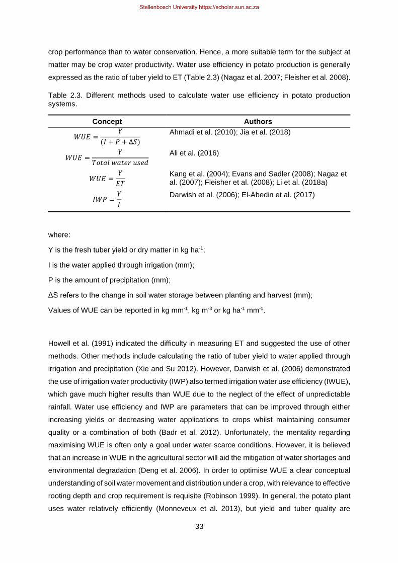
33
crop performance than to water conservation. Hence, a more suitable term for the subject at
matter may be crop water productivity. Water use efficiency in potato production is generally
expressed as the ratio of tuber yield to ET (Table 2.3) (Nagaz et al. 2007; Fleisher et al. 2008).
Table 2.3. Different methods used to calculate water use efficiency in potato production systems.
Concept Authors
𝑊𝑈𝐸 =𝑌
(𝐼 + 𝑃 + ∆𝑆)
Ahmadi et al. (2010); Jia et al. (2018)
𝑊𝑈𝐸 =𝑌
𝑇𝑜𝑡𝑎𝑙 𝑤𝑎𝑡𝑒𝑟 𝑢𝑠𝑒𝑑
Ali et al. (2016)
𝑊𝑈𝐸 =𝑌
𝐸𝑇
Kang et al. (2004); Evans and Sadler (2008); Nagaz et al. (2007); Fleisher et al. (2008); Li et al. (2018a)
𝐼𝑊𝑃 =𝑌
𝐼
Darwish et al. (2006); El-Abedin et al. (2017)
where:
Y is the fresh tuber yield or dry matter in kg ha-1;
I is the water applied through irrigation (mm);
P is the amount of precipitation (mm);
ΔS refers to the change in soil water storage between planting and harvest (mm);
Values of WUE can be reported in kg mm-1, kg m-3 or kg ha-1 mm-1.
Howell et al. (1991) indicated the difficulty in measuring ET and suggested the use of other
methods. Other methods include calculating the ratio of tuber yield to water applied through
irrigation and precipitation (Xie and Su 2012). However, Darwish et al. (2006) demonstrated
the use of irrigation water productivity (IWP) also termed irrigation water use efficiency (IWUE),
which gave much higher results than WUE due to the neglect of the effect of unpredictable
rainfall. Water use efficiency and IWP are parameters that can be improved through either
increasing yields or decreasing water applications to crops whilst maintaining consumer
quality or a combination of both (Badr et al. 2012). Unfortunately, the mentality regarding
maximising WUE is often only a goal under water scarce conditions. However, it is believed
that an increase in WUE in the agricultural sector will aid the mitigation of water shortages and
environmental degradation (Deng et al. 2006). In order to optimise WUE a clear conceptual
understanding of soil water movement and distribution under a crop, with relevance to effective
rooting depth and crop requirement is requisite (Robinson 1999). In general, the potato plant
uses water relatively efficiently (Monneveux et al. 2013), but yield and tuber quality are
Stellenbosch University https://scholar.sun.ac.za
34
particularly susceptible to soil water deficits (Sharafzadeh et al. 2011). A factor significantly
affecting water uptake in potato crops is root growth, as indicated by Liao et al. (2016) that
potato yields are controlled by the soil water status in the top 20 to 30 cm of the soil profile. Its
shallow root system results in poor suction capacity and if soils become too dry, water
becomes the most limiting factor (Sharafzadeh et al. 2011). To sustain potato production and
yields it is not recommended to let the soil water potential drop below -20 kPa (matric potential)
within the rooting zone (Bailey 1990). Therefore, deficit irrigation is not a recommended
practice for potato production. Irrigation is not the only factor affecting WUE, as a study by
Ierna and Mauromicale (2018) showed. They concluded that WUE was negatively influenced
by irrigation and positively enhanced by fertilisation. Both low and medium fertiliser rates
(NPK: 50, 25, 75 kg ha-1 and 100, 50, 150 kg ha-1, respectively) allowed maximising water use
when plants where irrigated 25 mm at plant emergence only.
2.3.1 Factors affecting water use efficiency
Many factors such as soil texture, crop variety, root growth and distribution affect the WUE of
a crop (Katerji and Mastrorilli 2009; Ahmadi et al. 2010; Ahmadi et al. 2014). Kang et al. (2004)
concluded that potato WUE was affected by both soil matric potential and irrigation frequency.
In their study lower application rates applied more frequently resulted in a higher WUE. They
also reported that the highest WUE was obtained at a soil matric potential of -25 kPa and an
irrigation frequency of once a day. Wang et al. (2006) also concluded that a relatively high
irrigation frequency enhanced WUE as well as potato yield and a reduction in irrigation
frequency showed significant decreases in yield. Irrigation technique also plays a major role
in the WUE or IWP of crops. El-Abedin et al. (2017) concluded that in potato cropping systems
full irrigation techniques produced the highest IWP, followed by deficit irrigation and then
partial root zone drying. For potatoes, similar results were reported by Liu et al. (2006) and
Ahmadi et al. (2014). This contradicts reports by Jovanovic et al. (2010) that in potato
production, higher IWP values were obtained when partial root zone drying irrigation was
practiced compared to deficit irrigation. This suggests controversial reports in the literature.
Management practices also play a role in WUE, as shown by Zhao et al. (2014) in a rainfed
agricultural system in China. This study reported the benefits of ridge-furrow full plastic
mulching on WUE and potato yields. Water use efficiency values ranged between 16.7 and
20.4 kg ha-1 mm-1 for full plastic mulching. This is in agreement with Li et al. (2018b). Li et al.
(2018b) reported an increase in WUE under plastic mulching (28.7%) and straw mulching
(5.6%). This was particularly evident in potato cropping systems applied with <400 mm of
water. The effect of mulching on increased WUE or IWP is due to decreased soil evaporation,
warmer topsoil temperatures and increased water holding. Another study by Li et al. (2018a)
Stellenbosch University https://scholar.sun.ac.za

35
concluded that compared to no mulching, plastic mulching increased WUE by 31.7%. Katerji
and Mastrorilli (2009) showed the effect of soil texture on WUE. It was concluded that there
was a decrease in WUE for potato, sunflower, maize and sugar beet when grown in clay soils.
Water use efficiency values in clay and loam for potato were reported at 16.1 and 21.0 kg m-3
respectively. Water use efficiency and IWP values differ around the world and between crops.
In China, typical WUE values of 0.46 kg m-3 for potato were reported (Deng et al. 2006). To
show the difference in WUE of various crops, Hu et al. (2001) reported values of grasses at
0.26 to 0.41 kg m-3 and shrubbery at 0.28 to 0.32 kg m-3. Nutrient application has also been
shown to influence the WUE of crops. A study on the interaction of fertigation on nitrogen (N)
use efficiency by Jia et al. (2018) concluded that drip fertigation increased both WUE and N
use efficiency 1.4 to 2.0-fold and this practice can be recommended on sandy soils. Darwish
et al. (2006) reported IWP values of 7.7 to 8.6 kg m-3. This is similar to values stated by
Darwish et al. (2003). Duan and Zhang (2000) in a study in China reported WUE values for
wheat (Triticum spp.; 0.8 – 1.32 kg m-3), Maize (1.70 – 1.74 kg m-3), sorghum (Sorghum spp.;
1.91 kg m-3) and soybean (Glycine max; 0.57 kg m-3) under irrigation. In contrast, a study in
Southern Libya by El-Wahed (2016) reported a WUE value of 0.75 kg m-3 for barley (Hordeum
vulgare) under sprinkler irrigation. This study indicated the effect of operating pressure and
sprinkler heights on WUE. An operating pressure of 200 kPa, 250 kPa and 300 kPa produced
WUE values of 0.39, 0.52 and 0.68 kg m-3 respectively, with sprinkler heights of 100, 125 and
150 cm producing WUE values of 0.48, 0.52 and 0.59 kg m-3 respectively. From this it was
concluded that higher sprinkler height and operating pressure increased WUE. A previous
study conducted by Steyn et al. (2016) reported an average of 78 kg mm-1 for potato
production in South Africa, so generally, anything ≥78 kg mm-1 is acceptable.
2.4 Fertilisation
2.4.1 Nutrient use efficiency
Research into nutrient use efficiency (NUE) is imperative in the move towards more
sustainable production systems, particularly in locations where soils have low nutrient holding
capacities. Given the adverse economic and environmental impacts of excessive nutrient
application, particularly associated with N and P, it is imperative to research nutrient use
efficiencies to minimise detrimental impacts on the environment (Fageria et al. 2008). The
potato crop is a nutrient responsive plant. However, when shallow-rooted crops are grown on
sandy soils, excessive use of nutrients can potentially result in environmental damage and
high production costs. The improvement of NUE can thus be used as a strategy to address
the issue of sustainability and improve yields (Tiwari et al. 2018).
Stellenbosch University https://scholar.sun.ac.za

36
Nutrient use efficiency refers to the portion of nutrient taken up by the crop as a percentage of
applied nutrient. However, studies on the NUE of potato crops have been limited to agronomic
practices or soil management and ecological as well as physiological concepts have been
neglected (Tiwari et al. 2018). In potato production, most research emphasises on improving
site-specific fertilisation efficiency through nutrient management in the soil (Zebarth and
Rosen 2007). Much of the research is specific to N use efficiency, but the methods can be
utilised for all nutrients (Kutra and Aksomaitiene 2003; Weih et al. 2011; Hu et al. 2014; Swain
et al. 2014; Gitari et al. 2018; Tiwari et al. 2018). The different terms and calculations used
are described by Tiwari et al. (2018). This study also reports NUE of potato crops to be best
defined as the tuber yield obtained per unit of nutrient supply (fertiliser and residual). Moll et
al. (1982) reports nutrient use efficiency as the total plant nutrients taken up at maturity per
unit of nutrient supplied from fertiliser and mineral N. However, they assume that throughout
the crop growth cycle, from planting to harvest, any nutrient (they referred to N) is available,
which creates conceptual issues. The study concludes that nutrient uptake efficiency (NUpE)
and nutrient utilisation efficiency (NUtE) should be considered as they form important
components in the overall NUE throughout crop growth. In research conducted by Gitari et al.
(2018) on the uptake of N and P in potato intercropping systems, the calculations of plant
nutrient uptake were taken as the sum of the product of the plant tissue dry mass and nutrient
concentration. The NUpE was calculated as the ratio of the total plant nutrient uptake and
nutrient supply. This coincides with the methods used by Errebhi et al. (1998), Zebarth et al.
(2004), Kołodziejczyk (2014) and Tiemens-Hulscher et al. (2014). However, the calculation of
NUE by Gitari et al. (2018) was conducted with the inclusion of potato equivalent yield, which
considers the market price of potatoes.
There are numerous terms and methods determining NUE, but the outcome is aimed to
provide information on strategies to improve NUE in cropping systems. Improving the NUE of
cropping systems can be established through decreasing nutrient application whilst
maintaining yields or by increasing both yield and nutrient application (Tiwari et al. 2018).
Other methods include gene manipulation, selective breeding i.e. enhancing photosynthetic
capacity by manipulating Ribulose-1,5-bisphosphate carboxylase/oxygenase (RuBisCo)
activity (Weih et al. 2011).
The look into the macro elements and their impact on the potato cropping system will aid
understanding of nutrient-soil-plant interactions and the best management practices needed
to ensure an economically and environmentally sustainable system.
Stellenbosch University https://scholar.sun.ac.za

37
2.4.2 Nitrogen
Nitrogen (N) is the most limiting nutrient in potato production, especially when cultivation
occurs on sandy soils (Munoz et al. 2005). The effect of N on tuber yield has been extensively
researched (Bélanger et al. 2000; Kavvadias et al. 2012; Hu et al. 2014; Van Dingenen et al.
2019). However, the response of various fertiliser application rates is cultivar dependant (Van
den Berg et al. 1996; Mokrani et al. 2018). If N is available to the plant at high rates, there is
a positive response on both vegetative growth and light interception (Oliveira 2000). Therefore,
farmers often apply N at higher rates than the minimum requirement (Lemaire and Gastal
1997). N stress in potato has negative impacts on photosynthesis and the partitioning of
assimilates (Jin et al. 2015).
2.4.2.1 Nitrogen source (ammonium vs. nitrate)
Potatoes prefer N in the form of nitrate (NO3-), instead of ammonium (NH4
+). Current research
is targeting improved NUpE in potato production systems with emphasis on reducing excess
leaching of nitrate into water sources (Davenport et al. 2005). There are two notable processes
defining NUpE: the plant’s ability to absorb N from the soil and its ability to convert that N into
a usable form within its organs (Saravia et al. 2016). The high solubility of nitrate in water
means the ion will not be easily adsorbed by soil colloids or organic matter, which is commonly
present in low concentrations in potato production systems due to the nature of the soil profiles
used as growth mediums. The uptake of nutrients goes hand in hand with the distribution and
quantity of water applied to the soils, therefore irrigation and nutrient management are likely
to be correlated. A study carried out by Saravia et al. (2016) shows the importance that water
plays in NUpE and that N uptake is reduced greatly for all varieties used in the experiment
under drought conditions. A lack of water limits the availability of NO3- by reducing its mobility
in the soil plant system due to the decrease in denitrification and increase in mineralization
(Saravia et al. 2016). This indicates that maximum fertiliser-use can be achieved with low N
applications under well-watered conditions.
2.4.2.2 Nitrogen crop requirement
Rates and timing of N is dependent on different production regions and cultivars (Alva 2008).
A study conducted by Westermann and Davis (1992) indicated that the cultivar Russet
Burbank had N uptake rates of 2.4 to 4.0 kg ha-1 day-1. In sandy soils, Lauer (1985)
recommends N application rates of 340 kg ha-1. Potato has a low N requirement during its
early development from emergence to tuber initiation (Alva 2004). However, pre-planting N
application is seen as important to maintain yield and stimulate tuber initiation
Stellenbosch University https://scholar.sun.ac.za
38
(Roberts et al. 1991; Rens et al. 2018). Zotarelli et al. (2014) reported that maximum daily N
uptake occurred during the tuber bulking phase, which was 55 to 70 days after planting. The
study showed that nitrogen applied at plant emergence and tuber initiation was more beneficial
than application at planting. Application at these later stages ensured the availability of N in
the soil between 30 and 80 days after planting, which coincides with the maximum daily N
uptake. The application of 112 kg ha-1 and above at plant emergence was recommended and
during the tuber initiation stage 56 kg ha-1 or below, as no significant benefit was seen in
applying > 56 kg ha-1 at this stage. These findings are in agreement with da Silva et al. (2018),
concluding that N application at emergence and tuber initiation are important in improving the
NUpE, but da Silva et al. (2018) emphasized the importance of N application at planting.
Rens et al. (2016) reported that splitting N application between planting and tuber initiation to
be a good management strategy to potentially reduce the N fertilisation requirement.
The decrease in NUpE with increased fertiliser application is reported in the literature
(Zebarth et al. 2004; Zotarelli et al. 2014; da Silva et al. 2018) for most cereal crops nitrogen
uptake efficiency has been reported between 40 to 50% (Hallberg 1987). Applied fertiliser
uptake efficiency has been reported in potato by various authors to be below 55%, depending
on weather and N fertiliser management (Jiao et al. 2013; Rens et al. 2016). However,
Westermann et al. (1988) reported higher N uptake efficiency at 60% and 80% for pre-plant
and in-season applications, respectively. The low N uptake efficiency leads to higher N
applications, particularly on coarse textured soils where N is known to be very mobile and
leach easily. da Silva et al. (2018) reported findings of 18% fertiliser NUpE for pre-plating
applications, 44% at planting and 62% at tuber initiation. Zotarelli et al. (2014) concluded that
N application at emergence and tuber initiation resulted in the highest N use efficiency, with
values of 49 to 71% for an N rate of 100 kg ha-1.
It is important for production managers to monitor the N status in plant tissue as well as soil N
status (Vos 1999). This can be carried out extensively throughout the growing season by a
petiole test and soil analysis. A study conducted on the effects of pre-plant and in-season N
practices using petiole tests by Alva (2009) indicated that NO3- accumulated during the first 80
days after emergence within the shoots, is then translocated to the tubers in the subsequent
period. It was also reported that at close to 100 DAP, the majority of the shoot and tuber
nutrient accumulation was complete due to the low demand of N towards the end of the
growing season. This stage can be referred to as the tuber-bulking phase. During this phase
the roots’ capacity to uptake nutrients is significantly reduced due to the decline in root growth.
However, in a study conducted by Waterer (1997), the accumulation of NO3- took place up to
88 DAP and significantly influenced the yield obtained at the end of the growing season. Both
the experiments concluded that petiole N concentrations are high in the early stages of the
Stellenbosch University https://scholar.sun.ac.za

39
season and decrease towards the end of the growth period, with a sharp decline during the
tuber bulking phase and that excessive N late in the season potentially retards tuber maturity
(Waterer 1997; Alva 2009). Highest N demand is determined by variety and is a factor of the
length of the growth season, root growth and distribution as well as the time taken to reach
maturity. A study carried out by Iwama (2008) on the effect of genotype on root mass indicated
that there was no significant relationship between cultivar and fertiliser rate on the potato crop,
however, there was a large effect on root mass with an increase in fertiliser rate. The root
mass was increased significantly.
2.4.2.3 Nitrogen leaching
Due to potato’s effective root system being limited to the upper soil layers (Alva 2008), it results
in a decreased NUpE with particular effect on N. Soil characteristics, climatic factors and
irrigation techniques and methods have an impact on the fate of nutrients. Sprinkler irrigation
is often associated with high levels of leaching, where high water applications are correlated
with large levels of N leaching (Alva 2004). Woli et al. (2016) reported that NO3- leaching was
higher with longer irrigation intervals, larger irrigation amounts and higher N application rates.
This was the result of more water being applied in longer irrigation intervals and larger
amounts of water per irrigation event leading to deeper drainage. This effect was pronounced
in production systems on sandier, lighter textured soils. However, the method of irrigation is
not seen to have a significant effect on NUpE (da Silva et al. 2018). Liao et al. (2016) concluded
that even though yield was not affected, sprinkler irrigation caused higher soil N leaching from
the top 20 cm of a sandy soil profile, compared to seepage irrigation. Even under well-
managed irrigation scheduling and techniques there is still a risk of N leaching (Waddell et al.
2000).
2.4.2.4 Nitrogen management
The number of fertiliser applications during the growth season has been studied extensively.
Vos (1999) conducted a study in the Netherlands on the effect of split N fertiliser regimes
compared to single dose applications. The experiment indicated that up to 80% of the total N
in the ‘Russet Burbank’ potato cultivar was absorbed between 20 and 60 days after sprout
emergence. Saravia et al. (2016) reported that additional N applied 45 DAP was ineffective at
inducing more tubers to initiate as the process at this time is nearing its end or at completion.
A study carried out on the Chinese potato variety KX 13 by Sun et al. (2012), indicated that
split dressing N was more efficient than applying the majority of the N source at once. This
study concluded that N-application of 100 kg N ha-1 at planting followed by a top dressing of
Stellenbosch University https://scholar.sun.ac.za
40
50 kg N ha-1 one week before the tuber bulking stage, which was approximately 35 days after
sprout emergence, accumulated the most DM. This high tuber DM yield can be associated
with high transportation efficiency of assimilates from the above ground plant tissue to the
tuber after tuberisation. The experiment also indicated that without N application at planting,
N topdressing did not improve yields. If the initial rate of N supply is not adequate enough it
results in the crop growth rate being affected, resulting in smaller leaves and a lack of vigour
which in turn can influence and cause a depression in the rate of increase in the fraction of
light interception. If N is available to the plant at high rates, there is a positive response on
both vegetative growth and light interception (Oliveira 2000), thus, resulting in more
photosynthetic assimilates being produced and transported to the tuber for growth (Vos 1999).
Therefore, often farmers apply N at higher rates than the minimum requirement (Lemaire and
Gastal 1997). The outcomes reported by Vos (1999) align with Sun et al. (2012), that splitting
N fertiliser applications can lead to more efficient utilisation by the plant and no significant
negative impacts on tuber DM yield were viewed. It can be concluded that tuber yield and
quality are strongly affected by the rate and timing of N fertilisation (Munoz et al. 2005; Alva
2009; Woli 2016).
2.4.3 Phosphorus
2.4.3.1 Phosphorus source
Phosphorus (P) is considered critical in potato production systems and plays an important role
in enhancing potato yield and quality. Potato tubers have a high P requirement and uses P
inefficiently (Rosen et al. 2014). Phosphorus is considered the second most limiting nutrient
in agricultural systems following N. Studies have shown its significant role in canopy
development and LAI (Dyson and Watson 1971, Sale 1973, Jenkins and Ali 1999). A study
conducted by Allison et al. (2001) on the effects of foliar versus soil applied P on potato
concluded that foliar P had no effect on tuber yield or number and is not recommended for
use in potato cropping systems. Chen et al. (2006) compared leaching losses of P from a rock
phosphate and water-soluble source. The study reported that 96.6% of the water-soluble P
applied had leached compared to 0.3 to 3.8% of the rock phosphate source and that this
source is recommended on sandy soils.
2.4.3.2 Phosphorus crop requirement
Due to its lack of mobility and solubility in soils, P uptake and utilisation is often poor by crops.
Irrigation management as well as soil drying and wetting cycles have been strongly linked to
soil P availability (Suriyagoda et al. 2014). Phosphorus is associated with cellular energy,
Stellenbosch University https://scholar.sun.ac.za

41
respiration and photosynthesis. The nutrient contributes to early development of the potato
crop and is reported to increase the number of large tubers (Fernandes and Soratto 2016). A
study conducted by Fernandes and Soratto (2016) on P uptake with regards to varying
cultivars, indicated that varieties differ with regard to their response to P fertilisation. The
variety Mondial produced a crop with higher tuber mass and had a higher available P use
efficiency than the cultivar Agata. Mondial produced lower tuber numbers per plant and
therefore, was able to allocate more carbohydrates to tuber growth, resulting in a larger mean
tuber mass. These results agree with a study carried out by Fernandes et al. (2017) and
conclude that DM accumulation is highest in the Mondial variety when compared to other
commercially popular cultivars. Fernandes et al. (2017) showed that P fertilisation increased
plant growth and tuber DM yield up to rates of 500, 250, 125 kg P2O5 ha-1 with regards to soils
containing low, medium and high initially available P, respectively. Phosphorus use efficiency
is especially notable in potato production systems, due to the shallow root systems often
reported, resulting in limited P uptake. A study conducted by Sun et al. (2015) on the effects
of various irrigation strategies (full irrigation, deficit irrigation, partial root zone drying) and P
fertilisation on P use efficiency and WUE in potato production systems indicated that WUE
increased significantly due to P application and not by irrigation regime. It was also concluded
that P had a positive influence on leaf/tuber/plant total DM, leaf area, total plant P uptake and
WUE. Negative effects were reported on the ratio of root:leaf area, stomata conductance, root
P partitioning and P utilization efficiency. The high WUE can be attributed to the lower stomatal
conductance when P fertiliser was applied. This resulted from a lower soil water content
caused by a higher leaf area associated with P application on the crop’s canopy. This was in
agreement with a study conducted by Motalebifard et al. (2013), which concluded that P
significantly influenced WUE, ET, tuber numbers and tuber yield of a potato crop. In contrast,
another study conducted in the United States of America by He et al. (2011) showed that
irrigation influenced stable and recalcitrant P fractions within the soil by redistributing and
mobilising P. A difference of 91 mg P kg-1 within the field studies suggests that three-year
consecutive irrigation lowers the top 20 cm of the soil P by an average of 5.4%.
2.4.3.3 Phosphorus leaching
Research on P losses via the process of leaching has received very little attention compared
to losses occurring from erosion and run-off (Fortune et al. 2005). Fortune et al. (2005)
concluded that P losses through leaching are environmentally significant and contribute
towards the detrimental effects of eutrophication, which initiates at 20 to 30 µg P L-1. However,
the leaching losses (kg P ha-1) are insignificant in economic terms for producers, so very little
attention is paid to P leaching. Movement of P in soils is influenced by the rate at which P is
Stellenbosch University https://scholar.sun.ac.za

42
applied and the reaction of P within the soil (Reddy et al. 1980). Atalay (2001) concluded that
soil particle size and soil type related to P sorption in profiles and that the presence of organic
matter played a large role in P sorption in Entisol soil profiles.
2.4.3.4 Phosphorus management
Soil testing is generally the most common method for determining the crop P requirement and
additions needed. There are various methods used: the Olsen sodium bicarbonate extraction
method is more commonly used on alkaline soils, whereas the Bray I or Mehlich I or III are
used on more acidic soils (Maier et al. 1989). Various placement and timing methods of P
fertilisation have been suggested and recommended. The general methods include pre-plant
broadcasting or broadcasting within the season, band placement near the seed during planting
or as a liquid source during crop growth. A study conducted by Hawkins (1954) showed that
banding applications of P resulted in better growth response when compared to broadcasting
applications. This was confirmed by Sparrow et al. (1992) and Kelling and Speth (1997).
The effect of P on tuber specific gravity (SG) has been reported to vary according to the soil
test P levels. If soil P levels are low, additional P application increases SG (Rosen et al. 2014).
This coincides with studies by Roberts et al. (1984) and Sanderson et al. (2002). If soil P levels
are high, then additional P has very little effect on tuber SG (Laboski and Kelling 2007). A
decrease in tuber SG with high rates of P application has also been observed (Freeman et al.
1998). The potato crop generally takes up greater proportions of P later on in the season,
compared to N and K (Roberts et al. 1991). Its absorbance of P is most rapid from 40 to 60
days after emergence (Kelling et al. 1998). However, in-season application of P with irrigation
water is successful when potato roots are shallow and close to the soil surface
(Rosen et al. 2014). Soils vary largely in terms of P content and availability. The type of clay,
organic matter and soil chemistry determines the availability of P, also known as labile P.
Phosphorus rate factor and the cultivar used determines uptake of other nutrients. Soils low
in P availability have been viewed to result in the uptake of 3 to 4 times more N, K, Ca, Mg
and S when P fertilisation has taken place up to a rate of 500 kg P2O5 ha-1 (Fernandes et al.
2017). Thus, the application of P implicates the absorption of other mineral ions as well as its
own.
Stellenbosch University https://scholar.sun.ac.za

43
2.4.4 Potassium
2.4.4.1 Potassium source
The most common sources of potassium (K) are K–chloride, K–sulphate and K–nitrate.
Various research concludes that differing K–sources have an effect on yield as well as SG.
Potassium chloride has a negative influence on SG, however, Toolangi (1995) reported that
the reduced SG is mainly caused by the chloride ion. A study conducted by Davenport and
Bentley (2001) did not detect any influence of K–source on tuber SG. In contradiction to this
Kumar et al. (2007), who studied nine various K–sources and their effects on tuber yield and
quality parameters, observed an increase in both yield and tuber SG when the sources K–
sulphate and K–nitrate was used in comparison to K–chloride. This study concluded that for
the growth of processing tubers, the source K–sulphate should be the preferred over K–
chloride. The sulphate form results in a higher DM percentage, therefore, increasing the crisp
yield and reducing oil content percentage. Similar findings were reported by Yakimenko and
Naumova (2018). However, both studies concluded that the influence of K–source on SG and
tuber yield are cultivar-dependent.
2.4.4.2 Potassium crop requirement
Potassium is a nutrient that is taken up in the greatest quantity in potato production systems
(Ati et al. 2012). Various studies agree that it has a great effect on both tuber yield and quality
(Hannan et al. 2011; Ati et al. 2012; Khan et al. 2012). According to Khan et al. (2012) and
Hannan et al. (2011), quality parameters such as DM content, starch concentrations, vitamin
C contents as well as colour and taste are largely affected. The optimum application rate of K
in potato cropping depends on soil characteristics. Rates recommended vary slightly in the
literature. A study conducted by Hannan et al. (2011) reported tuber yield to plateau at 150 kg
K ha-1 with the greatest yield at 182 kg K ha-1. These results correspond to Khan et al. (2012),
who stated that 150 kg K ha-1 satisfied potato plant K requirements when using murate and
sulphate sources. A study carried out on WUE under different irrigation methods and K
applications by Ati et al. (2012), however, recommends that in order to achieve the highest
yields, 600 kg K2SO4 ha-1 (270 kg K ha-1) can be applied when using drip or furrow irrigation
systems. However, high application of K can reduce DM contents and there is an inverse
relationship between K and reducing sugars (Hannan et al. 2011). The plant growth stage
when maximum tuber K accumulation occurs is between 30 and 60 days after planting. Tubers
at this stage are able to accumulate up to 78% of the total required K (Hannan et al. 2011).
The rate of K application also influences the number of tubers that form. Low and excessively
high rates of K significantly reduce the number of tubers (Kavvadias et al. 2012). Trehan and
Stellenbosch University https://scholar.sun.ac.za

44
Sharma (2002) reported the need of K early on in potato crop growth in order to promote early
root production, however, root uptake efficiency of K by potato varies considerably between
cultivars and is affected by the root:shoot DM accumulation (Trehan and Claassen 1998). An
optimum K uptake efficiency was reported by Trehan and Claassen (2000) and was
determined by time, as there was an increase in K-influx with an increase in time. The same
study concluded that shoot and root growth was dependent on K availability at the early growth
stages and the growth ratio was higher at higher K levels. A shoot K content of 4 to 5% is
adequate to produce 90% of maximum shoot growth rate, which is achieved quicker if soil
solution K is optimum early on, compared to plants grown at low K concentrations. These
conclusions were agreed upon by Trehan et al. 2005.
2.4.4.3 Potassium leaching
Potassium is a mobile ion and therefore, leaching of significant amounts may occur in cropping
systems. The leaching of K is dependent on various soil factors such as organic matter
content, clay percentage and the concentration of other cations present within the soil solution
(Kolahchi and Jalali 2006; Jalali and Rowell 2009). Potassium leaching is specifically notable
in coarse textured soils such as those commonly used in potato production systems. A study
by Spiers and Besson (1992) reported the significance of K leaching on sandy soils. It is also
noted that the presence of accompanying anions influences the rate at which K is leached.
Sharma and Sharma (2013) concluded that K leaching in the presence of other anions follows
the order of SO42- < H2PO4
2 -< NO3- = Cl-. This effect has also been described by Hingston et
al (1972) and Sposito et al. (1983). Also presented was higher losses in K through leaching
as observed when the application of K was high followed by regular irrigation or rainfall events.
2.4.4.4 Potassium management
It is a common practice to apply the entire quantity of K at the time of planting as a basal
dressing. Davenport and Bentley (2001) and Kumar et al. (2007) reported no significant benefit
in the split application of K. Gunadi (2016) indicated a positive response of tuber yield to the
split application of K fertilisers between planting and six weeks after planting. In sandy soils
the reduction of K application at planting by split application, can reduce the increased
potential of leaching (Sitthaphanit et al. 2009). Methods of determining K requirement are
described by Li et al. (2015) and include soil testing, agronomic efficiency and K balance in
the plant-soil system. The study showed a negative K balance, which concurs that mining of
K is occurring as more K is moving out of the system than is being applied through fertiliser.
Stellenbosch University https://scholar.sun.ac.za
45
2.4.5 Calcium
The importance of Calcium (Ca) in plant physiology is described in the literature
(Burstrom 1968; Palta 1996; Palta 2010). The tuber bulking stage is seen as important with
regards to the application of Ca fertilisers, with the largest effect on tuber Ca concentrations
occurring at this physiological stage (Gunter et al. 2000). However, Ca application during the
early stages of tuber development have been shown to reduce the incidence of internal brown
spot (Olsen et al. 1996). If calcium is withheld during tuber initiation, negative symptoms can
occur (Davies 1998).
Different forms of Ca fertilisers are available. Water-soluble forms include Ca–nitrate and Ca–
chloride, which usually come blended with urea or urea ammonium nitrate (Ozgen et al. 2006).
Ozgen et al. (2006) studied the effects of various sources of Ca (Ca–nitrate and Ca–chloride)
and their combined effects with or without gypsum on tuber Ca concentrations and internal
brown spot. Results concluded that soluble Ca application without gypsum increases tuber Ca
concentrations and reduced internal brown spot. This was agreed upon by Karlsson and
Palta (2002). Results regarding this topic are, however, controversial as a study by
Simmons et al. (1988) indicated that gypsum increased tuber Ca concentrations. Another
study by Simmons and Kelling (1987) found gypsum and Ca–nitrate to be more effective than
gypsum alone. A study on the effect of calcitic lime in potato production indicated that liming
either reduced or did not affect yield or tuber number (Maier et al. 2002). Studies of liming in
potato production systems have reported contradictory results (Sparrow and Salardini 1997).
However, the benefits of practices to increase soil pH in slightly acidic Entisol soils under
potato production by 0.6 to 3.1 (pHwater) have been reported by Maier et al. (2002). Calcium
fertiliser timing, rates and placement play a vital role in the increase in tuber Ca concentrations
(Kratzke and Palta 1986). The presence of functional roots on the tuber and tuber-stolon
junction means that in order to increase tuber Ca concentrations, Ca placement must be close
to the tuber as is indicated by Kratzke and Palta (1986). The sandy soils on which potato
production often occurs are typically low in Ca due to constant irrigation and the depletion of
soluble Ca in the profile, therefore, it is important to supplement soluble Ca in sandy soils as
tuber Ca deficiencies are common (Kleinhenz et al. 1999).
2.4.6 Magnesium
The importance of Magnesium (Mg) and its physiological effects on plants is reported in the
literature (Cakmak and Kirkby 2007). However, it is often considered the “forgotten nutrient”
(Cakmak and Yazici 2010). Orlovius and McHoul (2015) described a clear increase in leaf Mg
concentrations with the application of Mg fertilisers. The study compared the mean increase
Stellenbosch University https://scholar.sun.ac.za

46
in leaf Mg concentrations between Kierserite and calcined magnesite. It was concluded that
kierserite performed better due to a higher solubility of Mg. Mikkelsen (2011) reported
significant variability of Mg fertilisers with regards to their water solubility. The solubility of Mg
is an important factor to consider regarding sustainable agricultural systems (Gransee and
Führs 2013). The effects of these differing water solubilities are described by Sher (2002).
More soluble Mg sources include Epsom salts (Mg–sulphate), serp-super A and serp-super B
(Hanly et al. 2005). Fertiliser type and soil properties are factors affecting the effectiveness of
Mg sources (Hanly et al. 2005). Mondy and Ponnampalam (1986) compared the effect of
Epsom salts and Dolomite on potato tuber quality. The results show that Epsom salts
produced higher nitrogen within the potatoes whereas tubers receiving dolomite were
significantly higher in manganese and cadmium contents. Both sources of fertilisers increased
Fe and Al concentrations within the tubers. Fertiliser regimes of Mg vary widely between
regions and countries (Ristimaki 2007). Grzebisz (2013) stated that Mg fertilisation should
focus on its effect on N management as it plays a role in the plant’s ability to access and utilize
N. However, Allison et al. (2001) reported no significant effect on potato production There is
large competition involved between various cations, particularly notable is the antagonism
between Ca and Mg (Gericke 2018). Gericke (2018) indicated the higher affinity of potato roots
to absorb Ca2+ ions than hydrated Mg2+ ions. However, increasing the Mg content in the tuber
was easier than increasing the Ca content due to the higher mobility of Mg in the plants.
2.4.7 Sulphur
A shortage of Sulphur (S) has a negative effect on sugars, asparagine and other amino acids
in potato (Elmore et al. 2010). However, Barczak and Nowak (2015) indicated the potato crop’s
low requirement for S. The study concluded that irrespective of the fertiliser source and rate,
sulphur application did increase the tuber’s N, S and Mg concentrations whilst decreasing Ca
tuber content. Sulphur is usually applied as sulphate through sources such as Mg–sulphate,
zinc–sulphate, K–sulphate, gypsum and others (Alva et al. 2008; Barczak and Nowak 2015).
Sulphur is leached as sulphate and dissolved organic S and is potentially one of the more
important factors affecting S depletion (Zhao and McGrath 1994). A study by Eriksen (2009)
using lysimeters reported values of sulphate leaching of 1 to 60 kg S ha-1 y-1. Up to 100 kg S
ha-1 y-1 leaching has been reported by Guzys and Aksomaitiene (2005). Alva et al. (2008)
concluded that the application of gypsum caused increased levels of Ca and sulphate in
leachate in fine sand. The high loading of Ca results in the displacement and leaching of other
cations such as Mg.
Stellenbosch University https://scholar.sun.ac.za

47
2.5 Synopsis
With water becoming increasingly scarce, methods to improve irrigation efficiency are
becoming imperative (Greenwood et al. 2010). Irrigation scheduling and practices can
potentially optimise WUE, along with enhancing the economic and environmental
sustainability of irrigated agriculture (Levidow et al. 2014). Water use is only effective when
best management practices are combined alongside technology (Levidow et al. 2014).
However, if used poorly, irrigation technology can cause unnecessary losses affecting overall
sustainability and water productivity. The difficulty is to get farmers to view WUE as saving
water instead of the perception of solely maximising net revenue (Knox et al. 2012). Most
irrigation scheduling is carried out on the bases of farmers past experience and subjective
judgements and is often controlled by the availability and cost of water to farmers
(Greenwood et al. 2010, Knox et al. 2012).
This literature review has indicated a lack of knowledge with regards to irrigation and
fertilisation management in potato production systems in sandy textured soils. Little is known
about the movement of fertiliser and water past the effective rooting depth and the losses that
are occurring from these production systems. The following study will touch on the inputs and
losses in potato production systems in the Sandveld region of the Western Cape in order to
optimise and recommend better management practices, to avoid unnecessary waste and the
negative environmental impacts that may be occurring. Water availability to potato crops is
thus, essential for controlling productivity with importance to arid and semi-arid climates and
plays an important role in the nutrient uptake from the soil profile and fertiliser applications.
The potato crop has a very sensitive response to water deficits and its shallow root zone
impact on the water and nutrient use efficiency (Shock et al. 2007; Monneveux et al. 2013;
Monneveux et al. 2014). Therefore, special emphasis is on the adoption of practices to
improve water and nutrient use efficiencies (Badr et al. 2012). This ensures the need for
extensive research on the sustainability of irrigation in these climatic areas to optimise
irrigation and nutrient management strategies.
Stellenbosch University https://scholar.sun.ac.za
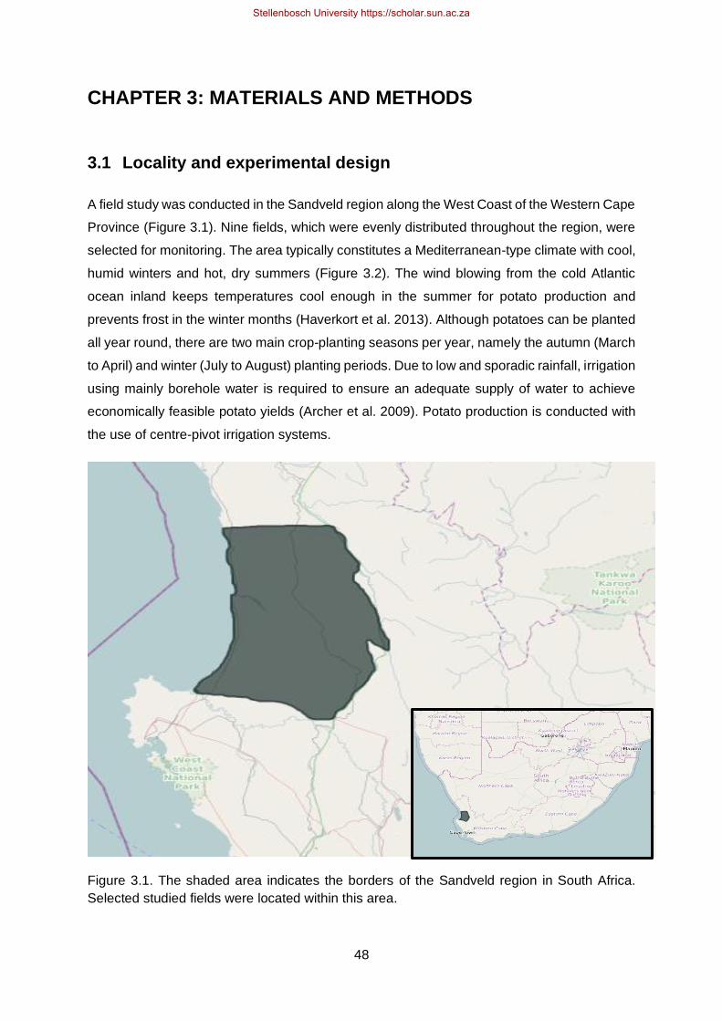
48
CHAPTER 3: MATERIALS AND METHODS
3.1 Locality and experimental design
A field study was conducted in the Sandveld region along the West Coast of the Western Cape
Province (Figure 3.1). Nine fields, which were evenly distributed throughout the region, were
selected for monitoring. The area typically constitutes a Mediterranean-type climate with cool,
humid winters and hot, dry summers (Figure 3.2). The wind blowing from the cold Atlantic
ocean inland keeps temperatures cool enough in the summer for potato production and
prevents frost in the winter months (Haverkort et al. 2013). Although potatoes can be planted
all year round, there are two main crop-planting seasons per year, namely the autumn (March
to April) and winter (July to August) planting periods. Due to low and sporadic rainfall, irrigation
using mainly borehole water is required to ensure an adequate supply of water to achieve
economically feasible potato yields (Archer et al. 2009). Potato production is conducted with
the use of centre-pivot irrigation systems.
Figure 3.1. The shaded area indicates the borders of the Sandveld region in South Africa.
Selected studied fields were located within this area.
Stellenbosch University https://scholar.sun.ac.za

49
Figure 3.2. Accumulated monthly precipitation and average minimum and maximum
temperatures for 2018 in the Sandveld region, compared with the thirteen-year average
(2005 – 2018). Source: Agricultural Research Council.
Field work commenced in March 2018 and was conducted over a period of one year,
terminating in March 2019. Commercial potato producers were selected, in order to give an
indication of large-scale production practices within the region. Selection was based on a
survey conducted by Steyn et al. (2016), which identified high and low resource using farmers
in the region. A combination of both high and low resource use producers was then selected
and the cultivars FL2108 or Sifra was grown in the studied fields. Six fields were intensively
monitored, while a further three fields were extensively monitored (Table 3.1). The study
spanned over a period of two seasons, namely autumn/winter (March-August 2018) and
summer (October-November 2018) planted crops. Planting dates varied throughout the year
and was eclectic between farmers, giving a wider range of growth conditions during cropping
cycles. Production practices were not prescribed to the producers and only current farming
practices carried out in the area were monitored.
0
5
10
15
20
25
30
35
0
10
20
30
40
50
60
70
80
Jan Feb Mar Apl May Jun Jul Aug Sep Oct Nov Dec
Te
mp
era
ture
(°C
)
Ra
infa
ll (m
m)
Sandveld weather data
Rainfall 2018 Long term rainfall mm
Long term max temp °C Long term min temp °C
Temp max 2018 Temp min 2018
Stellenbosch University https://scholar.sun.ac.za

50
3.2 Data collection
Each field was fractionated into four equal quarters and each segment was given a compass
heading (i.e. NE, NW, SE, SW). The differences in equipment installation between the
intensively and extensively monitored fields is illustrated by Error! Reference source not f
ound.. Equipment used to monitor water input through rainfall and irrigation, drainage and
leaching past the root zone and soil water content within each field was installed during the
same date. Installation took place two to three weeks after the field was planted (Table 3.1),
preferably just before or directly after crop emergence. Fields were visited fortnightly for data
collection and soil solution sampled during those visits (intensive fields).
Figure 3.3. Distribution of equipment used to measure water and nutrient inputs and losses in selected potato fields under centre-pivot irrigation. Intensively monitored (left) and extensively monitored (right) fields varied with regards to equipment used.
Stellenbosch University https://scholar.sun.ac.za

51
Table 3.1. Information regarding locality, equipment installation, planting date, emergence and
harvest date of the studied fields. Fields 1 to 9 are labelled according to their planting dates
(1 = earliest planted and 9 = last planted).
Type Field Location Altitude Installation Planting Emergence Harvest
(masl) date date date
Inte
ns
ive
*Field 2 32°36’53.85”S 219 24-Apr-18 28-Mar-18 10-Apr-18 16-Aug-18
18°27’43.97”E
Field 3 32°36’40”S 133 22-May-18 02-May-18 04-Jun-18 23-Oct-18
18°27’30”E
*Field 5 32°22’0.19”S 219 22-Aug-18 27-Jun-18 30-Jul-18 15-Nov-18
18°41’57.7”E
Field 7 32°50’45.3”S 47 07-Aug-18 31-Jul-18 21-Aug-18 27-Nov-18
18°33’03.3”E
*Field 8 32°38'5.46”S 115 23-Oct-18 11-Oct-18 01-Nov-18 07-Feb-19
18°28'33.67"E
Field 9 32°25’20.74”S 8 04-Dec-18 30-Nov-18 06-Dec-18 27-Mar-19
18°20’21.87”E
Ex
ten
siv
e
Field 1 32°41’1.88”S 92 14-Mar-18 03-Mar-18 29-Mar-18 20-Jul-18
18°42’18.15”E
Field 4 32°37’23.5”S 123 10-Jul-18 25-Jun-18 21-Jul-18 13-Nov-18
18°27’27.0”E
Field 6 32°37’31.3”S 110 06-Aug-18 09-Jul-18 06-Aug-18 13-Nov-18
18°37’22.2”E
*Fields where equipment was installed after plant emergence. The water flow meter for Field
7 was installed earlier than the other equipment on the 10th of July 2018. For Field 8 the water
flow meter was installed after all the other equipment, on the 6th November 2018.
3.3 Irrigation system evaluations
Irrigation system performance tests were conducted on all centre-pivots during the early
stages of crop growth (Koegelenberg and Breedt 2003; Griffiths 2006). Detailed evaluations
were carried out to assess centre-pivots with regards to nozzle packages, working pressure,
application efficiency and distribution uniformity. Working pressure at the centre and end of
the system was measured using calibrated manual pressure gauges. Manual rain gauges
were packed out at 5 m intervals along the length of the system (excluding the first 20% of the
pivot, as recommended by Koegelenberg and Breedt (2003)). The system was then placed
on a 25 to 30% speed setting or pre-set irrigation amount (e.g. 10 mm) and run over the rain
Stellenbosch University https://scholar.sun.ac.za

52
gauges. The volume of water collected by each rain gauge was then recorded and the different
uniformity and efficiency parameters assessed. Application efficiency (AE) indicates the
portion of water applied by the sprinklers that reached the soil surface and thereby determines
the wind drift and evaporation losses that occurred (Equations 3.1 and 3.2). The uniformity
coefficient of Heerman and Hein (CUHH) gives an indication of how evenly the distribution of
applied water is within the irrigated area and was calculated using the Heerman and Hein
(1968) modified equation (Equations 3.3 and 3.4). The distribution uniformity of the lower
quarter (DUlq) compares the average of the lowest 25% of measurements with the average
value of all other measurements to determine if significant under irrigation is occurring on a
specific area (Equation 3.5). The maximum rate at which water was being applied at the outer
end of the pivot was also measured, using a tipping bucket rain gauge and datalogger or a
manual rain gauge and stopwatch. This gives an indication of the runoff risk for the specific
soil and irrigation system combination.
AE = 100 [𝑁𝐴
𝐺𝐴 ] (3.1)
𝐺𝐴 = 𝐹𝑟
(𝐴 × 10) × 𝑅𝑠
(3.2)
𝐶𝑈𝐻𝐻 = 100 [1 −∑ 𝑆𝑖|𝑉𝑖 − 𝑉𝑝|𝑛
𝑖=1
∑ 𝑉𝑖𝑆𝑖𝑛𝑖=1
] (3.3)
𝑉𝑝 = ∑ 𝑉𝑖𝑆𝑖
𝑛𝑖=1
∑ 𝑆𝑖𝑛𝑖=1
(3.4)
𝐷𝑈𝑙𝑞 = 100 [𝑄𝑙
𝑁𝐴] (3.5)
where:
NA indicates the net application (mm) of water by the centre-pivot
GA is the average gross application (mm) as calculated by Equation (10)
Fr is the water flow rate in m3 h-1
A is the field area (ha)
Rs is the systems rotation time at a specific speed setting (h)
Stellenbosch University https://scholar.sun.ac.za
53
n is the number of rain gauges used in the evaluation
i is the number used to tag a particular rain gauge with i = 1 being closest to the centre of the
pivot and i = n for the outermost rain gauge from the centre
Si refers to the distance of the nth rain gauge from the pivot centre
Vi is the volume of water collected in each rain gain (ith)
Vp is the weighted average of the volume of water collected
Ql is the average of the lowest 25% readings taken from the rain gauges.
The speed of the pivot was measured by timing the periods that the wheels moved and
remained stationary. This was conducted on the outermost set of wheels as they travel fastest
to cover the further distance. The test was carried out at a 25 to 30% speed setting on the
pivot. Each time the wheels halted; a peg was placed into the soil in-line with the centre of the
wheel hub. This was replicated a total of four times and the distance between each peg
measured.
The flow rate of water through the system was measured using the installed electromagnetic
flow meter. As a check, a clamp-on ultrasonic water flow meter was used to measure the
accuracy of the flow meter readings. The flow rate readings were then compared to actual
application volumes collected by the packed-out rain gauges.
3.4 Irrigation amount
Irrigation amounts were continuously logged by electromagnetic flow meters and pressure
transducers with dataloggers (Equations 3.6 and 3.7)1. These were installed on all centre-
pivot irrigation systems. The flow meters and pressure transducers allowed the monitoring of
irrigation times, pressures and volumes, as well as a check to assess the accuracy of the
equipment against each other. The pressure transducers were located at the centre of the
pivot where the water entered the main pipe leading to the boom. Readings taken by the
pressure transducer loggers were manually downloaded every fortnight during site visits. The
flow meters were installed on the main pipeline leading into the pivot system. The flow meters
were able to measure when the irrigation system was turned on and off and log the duration
the system was on at each irrigation cycle, as well as measure the volume of water flowing
through it to give accurate readings of irrigation volumes. The readings were then transmitted
by GPRS telemetry. An assumption was made that the flow meter readings were more
accurate than the pressure transducers readings.
1 Running time was calculated on a pressure of > 40 kPa. (1L m-2 = 1 mm)
Stellenbosch University https://scholar.sun.ac.za

54
𝐸𝐹𝑀 = 𝐹𝑡
(𝐴 × 10 000) (3.6)
𝑃𝑇 = 𝑅𝑡 × [𝐹𝑟 × 1000]
(𝐴 × 10 000)(3.7)
where:
EFM refers to the water application (mm) measured by the electromagnetic flow meter;
PT is the water application (mm) measured by the pressure transducer;
Ft is the total flow indicated by the electromagnetic flow meter (in litres);
Rt is the running time of the centre-pivot (h).
A refers to the area under the centre-pivot boom (ha)
Fr is the water flow rate in m3 h-1.
Water samples used for irrigation of each field were collected from the water sources. The
samples were kept at 4°C along with the soil solution samples and later sent to a lab for nutrient
analysis. Application of nutrients (IN, kg m-3) to each field due to the presence of elements
within irrigation water (Nw) was determined at the end of the season (Equation 3.8), using the
total amount of water applied (WT) in m3 per hectare.
𝐼𝑁 = 𝑁𝑤 × 𝑊𝑇 (3.8)
3.5 Leaching requirement
The leaching requirement (LR) was calculated for each intensively monitored field. For the
irrigation water a threshold electrical conductivity (EC) value of 170 mS m-1 was used as the
maximum permissible conductivity allowed without major yield reduction (Fertasa 2016). The
leaching requirement (Equation 3.9) allowed for a yield reduction of 10% was then calculated.
𝐿𝑅 = 𝐸𝐶𝑖𝑤
(5𝐸𝐶𝑠 − 𝐸𝐶𝑖𝑤)(3.9)
where:
ECiw refers to the electrical conductivity of the water source used for irrigation;
ECs is the level of soil salinity level is allowed to occur, resulting in a 10% yield reduction
(250 mS m-1) in potato production (Fertasa 2016).
Stellenbosch University https://scholar.sun.ac.za

55
In order to calculate the total water requirement (TWR), including the irrigation water needed
to leach out excess salts, the gross water requirement (GWR) (water requirement taking into
account losses occurring during application) must be multiplied by the LR as indicated in
Equation 3.10.
𝑇𝑊𝑅 = (𝐺𝑊𝑅 × 𝐿𝑅 ) + 𝐺𝑊𝑅 (3.10)
At the end of crop growth WUE and IWUE or IWP (kg mm-1) was calculated using fresh tuber
yield (Ty) in kg ha-1 and total irrigation and rainfall amounts for the season (mm)
(Equations 3.11 and 3.12). It refers to the kg of fresh tubers produced per mm of water applied
through irrigation or irrigation plus rainfall.
𝑊𝑈𝐸 = 𝑇𝑦
𝑖𝑟𝑟𝑖𝑔𝑎𝑡𝑖𝑜𝑛 + 𝑟𝑎𝑖𝑛𝑓𝑎𝑙𝑙 (3.11)
𝐼𝑊𝑈𝐸 = 𝑇𝑦
𝑖𝑟𝑟𝑖𝑔𝑎𝑡𝑖𝑜𝑛 (3.12)
3.6 Crop evapotranspiration
Crop evapotranspiration (ET) was calculated using the FAO-56 basal crop coefficient (Kcb)
curve method (Allen et al. 1998) A graphical curve was produced for each field, using
measurements made during the season. A basal crop coefficient [Kcb(ini)] of 0.15 was used
from date of planting to date of crop emergence. The values of the basal crop coefficient at
full (100%) canopy cover [Kcb(mid)] to the end of full canopy cover and end of full canopy
cover to senescence [Kcb(end)] were adjusted Kcb(adj.) for climatic conditions using
Equation 3.13.
𝑘𝑐𝑏(𝑎𝑑𝑗.) = 𝑘𝑐𝑏(𝑡𝑎𝑏𝑙𝑒) + [0.04(𝑈2 − 2)] − 0.004(𝑅𝐻𝑚𝑖𝑛 − 45) (ℎ𝑚𝑎𝑥
3)
0.3
(3.13)
where:
Kcb(table) refers to the FAO-56 values for Kcb(mid) (1.10) and Kcb(end) (0.65)
(Allen et al. 1998);
Stellenbosch University https://scholar.sun.ac.za

56
RHmin is the average of the minimum relative humidity calculated during the period of full
canopy cover [Kcb(mid)] or decrease in growth from full canopy cover to senescence
[Kcb(end)];
U2 refers to the average wind speed at a 2 m height during the different periods;
hmax is the maximum plant height reached at full growth, which was taken as 0.6 m
(Allen et al. 1998).
The determination of 100% canopy cover was taken as 650-degree days from crop emergence
(Haverkort et al. 2015). Full canopy cover was ended at 100 DAP. Basal crop factor for the
end of growth [Kcb(end)] was taken as 120 DAP and if crop growth exceeded 120 days, then
Kcb(ini) was assumed at 140 DAP, whereafter if irrigation proceeded then the crop coefficient
remained Kcb(ini). However, if irrigation seized from 140 DAP, ET was terminated. The Kcb
values between these points were then calculated using linear-regression to produce a full
season curve. An example of the curves produced is illustrated in Figure 3.4.
Figure 3.4. Example of a basal crop coefficient curve from FAO-56 (Allen et al. 1998)
The LINTUL DSS potato model (Haverkort et al. 2015) was also used to estimate ET
requirements for each crop using various factors such as climatic and soil properties as input
parameters.
From the simulated ET (mm) requirement from the Kcb curves and LINTUL DSS model,
irrigation requirements (mm) (IR) was calculated, using each centre-pivot’s AE
(Equation 3.14).
0.0
0.2
0.4
0.6
0.8
1.0
1.2
0 20 40 60 80 100 120
Ba
sa
l cro
p c
oe
ffic
ien
t
Days after planting
Standard basal crop coefficient curve
Cropdevelopment
100% canopy coverLate season
Initial stage
Stellenbosch University https://scholar.sun.ac.za

57
𝐼𝑅 = 𝐸𝑇
(𝐴𝐸 ÷ 100)(3.14)
3.7 Soil water content and water movement in the soil
Soil water content and water movement through the profile were monitored using Decagon
soil capacitance probes, DFM (Dirk Friedhelm Mercker) multifunctional soil capacitance
probes (with telemetry) and Chameleon sensors. The intensively monitored fields contained
all three types of probes and the extensive fields contained only DFM probes. The reason for
the use of a wide variety of soil probes was to compare the accuracy of each probe in these
sandy soils to recommend the most suitable to use in those conditions in addition to viewing
water movement throughout the soil profile. Data from the Decagon logger was downloaded
every fortnight. The DFM probes were linked to the network and continuously sent data to a
local website. Chameleon data was not continuously logged, but instantaneous readings were
taken by farmers and the data logged was downloaded to the network every two weeks, during
site visits.
One set of Decagon capacitance probes, consisting of five sensors, was installed in each
intensively monitored field (Figure 3.5). The sensors were installed at depths of 10, 20, 30, 40
and 50 cm on the ridge (Figure 3.5). The probes were connected to a Campbell CR200
datalogger and measured change in dielectric constant of the soil, which is altered by the
volumetric water content of the soil.
Figure 3.5. Placement of Decagon soil capacitance probes along a planting ridge and the
depth at which each sensor is located. Temperature was measured along with the sensor
placed at a depth of 10 cm.
A 12 V battery was used to power the data-logger. The battery voltage was checked at every
site visit and when voltage dropped below 12.5 V, the battery was swapped. For Fields 8 and
Stellenbosch University https://scholar.sun.ac.za

58
9 gravimetric soil water content (ω) was measured by removing soil near the Decagon probes
at the depth of each sensor, 0 to 10, 10 to 20, 20 to 30, 30 to 40 and 40 to 50 cm. The time of
soil removal was recorded to compare the results with the logger readings in order to gauge
the accuracy of the DFM and Decagon probes. The removed soil was placed in brown paper
bags, which were then inserted into a plastic bag and sealed. Samples were weighed in the
lab in the paper bag and plastic bag. The plastic bag was then removed and the paper bag
along with the soil placed in an oven at 108 °C for five days. Once dried, the samples were
removed, weighed and the ω was determined using Equation 3.15. The Decagon and DFM
probes measure volumetric soil water content. Therefore, the gravimetric water contents
determined were multiplied with the bulk density of the soils as determined by soil analysis in
order to obtain volumetric soil water content.
Empty paper bags and plastic bags of the same size and dimensions used for sampling were
weighed and the weights noted. Empty paper bags were also placed in the oven at 108 °C for
the same duration as the soil samples to obtain a dried mass. The weights were then deducted
during the calculations in order to get the weight of the soil alone.
𝜔 = 𝑆𝑊 − 𝑆𝐷
𝑆𝐷 (3.15)
where:
ω refers to gravimetric water content (kg kg-1 or g g-1);
SW refers to the wet soil mass (kg);
SD is the soil mass after drying (kg).
Chameleon sensors were placed at 15, 30, 50 cm depths from the top of the planting ridge.
Two sets of Chameleon sensors were placed in each field, alongside the DFM probes
(refer to Error! Reference source not found.) Unlike the Decagon probes, these sensors w
ere placed at different depths in the same augured whole within the row as illustrated in Figure
3.6. The sensor is coated with gypsum, which allows soil water to move through the coating
whilst creating a constant EC (Stirzaker et al. 2014). Located in the centre of the gypsum
coating is two gold-plated electrodes that measure resistance across a medium, mimicking
the suction required by plant roots in order to absorb water from the soil. Due to the fact that
the sensors measure soil tension (water potential, not water content), they do not require
calibration for differing soil types. The sensors, however, differ from that of a gypsum block as
they do not measure the resistance across the gypsum. Loggers for the gypsum sensors were
given to farmers who were instructed to take three readings per week.
Stellenbosch University https://scholar.sun.ac.za

59
Figure 3.6. Placement of Chameleon logger sensors at depths of 15, 30 and 50 cm. When
connected to the sensors the logger reads three sensors and displays a colour (LED light) for
each sensor depth; red, green and blue, depending on the measured resistance. The three
colours represent a tension of >50 kPa, 20–50 kPa and 0–20 kPa, respectively (Stirzaker et
al. 2017). A tension of 0 kPa indicates a soil that is saturated and > 50 kPa represent a dry
soil.
Two DFM probes were installed per field, on all fields. The probes were installed on opposite
sides of the pivot road (refer to Error! Reference source not found.) and logged data from a
depth of 10 to 60 cm at 10 cm increments. At each depth, the probes also logged temperature
readings (DFM Software Solutions 2015).
3.8 Drainage
Drainage and leaching were measured through the use of drainage lysimeters, which were
installed in intensively monitored fields and located 3 to 10 m from the centre road of the
centre-pivot field. Lysimeters were located along the second- or third-wheel track from the
centre of the pivot (depending on field size), but 3 to 5 m to the side of the track (Figure 3.7).
Figure 3.7. The positioning of the drainage lysimeter within the soil profile, including the depth
and distance from the pivot track. The drainage lysimeter was installed either side of the
second- or third-wheel track.
60 cm
40 cm
1 m
3 – 5 m
Stellenbosch University https://scholar.sun.ac.za

60
The type of drainage lysimeter selected was a passive capillary lysimeter, which consists of
two main components (Figure 3.8): a divergence control tube (DCT) and a fibreglass wick.
The function of the fibreglass wick was to create a hanging water column to mimic the tension
of the surrounding soil, preventing an effect commonly occurring in other types of lysimeters
known as the boundary layer effect due to water ponding at the bottom of the lysimeter.
Therefore, due to the fibreglass wick this form of lysimeter has an increased efficiency of water
capture and improved accuracy of results (Gee at al. 2002; Jabro et al. 2008).
Figure 3.8. Components of the drainage lysimeter and their location with relation to each other
(Decagon Devices Drain Gauge G3 manual, 2018).
The 1 m depth to which the drainage lysimeters were installed was due to most root growth of
potato crops generally being confined to the top 40 to 60 cm soil layer (Ahmadi et al. 2011;
Rykaczewska 2015). Therefore, the soil solution collected by the lysimeter was assumed to
be the water and nutrients that had drained beyond the effective rooting zone and could not
be taken up by the roots. For installation of drainage lysimeters, the planted seed tubers or
young potato plants were carefully removed and a pit was dug to a depth of 40 cm
(Figure 3.9), where the DCT was placed to collect an undisturbed monolith of soil
(40 – 100 cm depth). The location selected for the monolith collection was not the final
destination where the lysimeter was placed, but ~5 m to the side. The DCT was carefully
hammered into the soil, dug open around the edges and blocked at the bottom to remove an
Stellenbosch University https://scholar.sun.ac.za

61
undisturbed soil core. A separate pit was dug to a depth of 1 m where the lysimeter was
installed.
Figure 3.9. Installation of the drainage lysimeter. a) final assembled lysimeter placed upside
down prior to installation to protect the fibreglass wick from bending or snapping; b) lysimeter
sitting in its final location before being buried and tubers replanted; c) installation of the
drainage sensor and suction pipe before refilling the pit.
When the 1 m depth was reached, a hole with 25 cm diameter was augured to a final depth
of approximately 185 cm (from original soil surface) to facilitate the extension tube containing
the hanging fibre glass wick. Diatomaceous earth was added to the bottom of the DCT to
improve contact with the fibreglass wick. All components were attached and a rope fastened
to the bottom side of the DCT where it attaches to the fibreglass wick and reservoir. The
equipment was carefully lowered into the hole, ensuring the DCT was placed in the original
potato row and not the furrow. Thereafter, the soil was carefully placed back into the pit in the
same order it was removed and the tubers re-planted into rows on top of the lysimeter with
the same inter-row spacing. A water depth and EC sensor were lowered to the bottom of the
drainage lysimeters extension tube to measure the depth, temperature and EC of collected
drainage water at half-hourly intervals. This data was recorded by an EM50 Meter-group
datalogger that was connected to the sensor. Drainage solution (Dc) was removed every
fortnight from the drainage lysimeters using a suction pump (mm). Conversion (from mL to
a) b) c)
Stellenbosch University https://scholar.sun.ac.za

62
mm) of solution sucked out (Sc) was made (Equation 3.16)2, taking into account the area of
the DCT (cm2).
𝐷𝑐 = (𝑆𝐶
𝐴𝐷𝐶𝑇 ) × 10 (3.16)
Samples from the drainage lysimeters were collected fortnightly with the use of a suction
pump. The pump was connected to extraction tubes protruding from the standpipes and the
water volumes collected were placed into 500 mL bottles, taken back to the lab and the
collected volume measured accurately. The samples were stored at 4°C and sent to a lab for
nutrient analyses at a later date. Nutrient analyses results included pH readings as well as
macro- (NH4-N, NO3-N, Ca, Mg, K, Na, SO4 and H2PO4 in mg L-1) and micronutrients (Fe, Mn,
Cu, Zn and B in µg L-1, and Cl in mg L-1)3. These results were converted to kg nutrient per
hectare using Equation 3.17.
𝑁𝑆 = 𝐷𝑐 × 𝑁𝐶 (3.17)
where:
Ns is the amount of nutrient leached in kg ha-1;
NC is the quantity of nutrient leached per m-3 of drainage water;
DC was converted from mm to m3 for the calculation and multiplied by 10 000 in order to
quantify the leaching per hectare.
3.9 Soil sampling
Soil samples were collected at three depths using a hand auger: 0 to 30 cm, 30 to 60 cm and
60 to 90 cm at the beginning of each crop cycle as well as during yield analysis, seven to ten
days prior to field harvest. The first soil samples were collected during the installation of the
other equipment about two to three weeks after planting had taken place. For sampling, the
field was split into quarters and within each quarter, six random sub-samples were taken (three
samples taken between the row and three samples on the plant row) and mixed to give a
representation of the entire quarter of the field. Samples were sent for standard soil analyses,
including exchangeable acidity, pHKCl, and macronutrient status. Nutrient contents were then
converted from mg kg-1 to kg ha-1 using Equations 3.18 and 3.19.
2 1 ml cm2 = 10 mm; AreaDCT is 506.7 cm2 3To calculate the amount of nutrient leached in kg ha-1, mg L-1 was converted to kg m3 and drainage from mm to m3.
Stellenbosch University https://scholar.sun.ac.za

63
Due to pre-planting fertiliser applications, nutrients from these additions were already present
in the soil before sampling. Fertiliser applied before sampling was assumed to reflect in the
soil analysis results and were therefore, deducted from results obtained by the soil analysis.
𝑊𝑠 = 𝐵𝜌 × 𝐷 × 10 000 (3.18)
𝑆𝑁 = 𝑊𝑠 × 𝑁𝐶𝑇 (3.19)
where:
Ws is the mass of a hectare of soil to a depth of 90 cm (kg ha-1);
Bρ is the bulk density of the soil calculated during the soil analysis (kg m3);
D is the depth soil samples were taken too (m);
SN is the nutrient content present in the soil (kg ha-1);
NCT is the nutrient content from the analysis (ppm or mg kg-1).
3.10 Interception of solar radiation
Fractional interception (FI) of solar radiation was calculated from photosynthetically active
radiation (PAR) measurements taken with an AccuPAR LP–80 ceptometer (Equation 3.20).
Radiation levels were measured every fortnight, weather permitting, during cloudless days.
Three random locations in each field’s quarter was used, giving twelve readings per field. At
each location one reading was recorded above canopy and two below canopy. The readings
below canopy were taken in different rows within the same vicinity. The below canopy readings
were taken by placing the ceptometer diagonally from the centre of one ridge to the centre of
the neighbouring ridge and from the two readings at each site an average was taken
(Figure 3.10).
Figure 3.10. Illustration of the measurement of light interception with a ceptometer (illustration
by C du Raan). Below-canopy measurements are taken from the centre of one row to the
centre of the next row. Measurements above the canopy are taken facing north so as to not
cast a shadow over the instrument.
Stellenbosch University https://scholar.sun.ac.za

64
𝐹𝐼 = 1 −𝑃𝐴𝑅(𝑏𝑒𝑙𝑜𝑤)
𝑃𝐴𝑅(𝑎𝑏𝑜𝑣𝑒)(3.20)
Crops were monitored throughout their growth cycles for any signs of visual deficiencies as
well as any incidences of pests and diseases. Field 1 was infected by late blight (Phytophthora
infestans) and Field 9 during the middle of its growth period had light green leaf colouring.
Nothing notable, however, was reported in the other fields and crop growth was good.
The solar radiation data obtained is not discussed in the results and discussion section, refer
to Appendix IIIb.
3.11 Nutrient content in plant matter
Leaf analysis was carried out, which commenced approximately one to two weeks after
emergence, when the crop was established, and was conducted roughly every four weeks
(every 2nd site visit) until crop desiccation. Ten leaves were collected randomly in each quarter
of the field to give a representative sample of each field. The representative samples were
therefore, made up of 40 leaves per field during each collection. Leaves were rinsed with de-
ionised water to remove any chemical or fertiliser residues and dried in an oven at 60°C for
seven days, removed and sent to a lab for standard nutrient analyses, including N, P, K, Ca,
Mg, S (%) and Na, Fe, Mn, Cu, Zn, B (mg kg-1).
The haulm nutrient content was only calculated for Fields 8 and 9 by cutting the aboveground
plant parts at the soil surface just prior to senescence. The removal of two times 1 m strips
randomly selected from each quarter of the field was carried out. Giving a total of 8 m from
which above ground plant biomass was removed. The removed residue was then dried at
60°C for seven to ten days, milled and sent to a lab for nutrient analysis. The results were then
converted from % to kg ha-1 using the known row spacing and area of removed biomass. The
results for Fields 8 and 9 were very similar. The assumption that the haulm nutrient content,
from the average values between Fields 8 and 9, was the same for the variety Sifra and
FL2108 was made to estimate total plant nutrient removal for all fields. The nutrient content of
the root systems was assumed negligible.
Stellenbosch University https://scholar.sun.ac.za

65
3.12 Tuber nutrient content and nutrient use efficiency
The amount of nutrients removed by tubers (Tc) from harvest was calculated using the tuber
pith nutrient content and DM yield (DMy) (Equation 3.21). The nutrient content (%) of the pith
Np alone was used as the nutrient removal by tubers due to the weight of the skin and medulla
being negligible in comparison.
𝑇𝑐 = 𝑁𝑝 × 𝐷𝑀𝑦 (3.21)
Nutrient uptake efficiency, nutrient utilisation efficiency and nutrient harvest index (NHI) was
calculated using tuber and haulm nutrient contents (plant nutrient removal) in kg ha-1, nutrient
application through water and fertiliser and DMy (kg ha-1) (Zebarth et al. 2004; Trehan, 2009;
Kolodziejczyk 2014; Tiemens-Hulscher et al. 2014; Gitari et al. 2018) (Equations 3.22, 3.23
and 3.24).
𝑁𝑈𝑝𝐸 = 𝑁𝑢𝑡𝑟𝑖𝑒𝑛𝑡 𝑟𝑒𝑚𝑜𝑣𝑎𝑙(𝑡𝑢𝑏𝑒𝑟+ℎ𝑎𝑢𝑙𝑚)
𝑁𝑢𝑡𝑟𝑖𝑒𝑛𝑡 𝑎𝑑𝑑𝑖𝑡𝑖𝑜𝑛𝑠(𝑓𝑒𝑟𝑡.+𝑤𝑎𝑡𝑒𝑟)(3.22)
𝑁𝑈𝑡𝐸 = 𝐷𝑀𝑦
𝑁𝑢𝑡𝑟𝑖𝑒𝑛𝑡 𝑟𝑒𝑚𝑜𝑣𝑎𝑙(𝑡𝑢𝑏𝑒𝑟+ℎ𝑎𝑢𝑙𝑚)(3.23)
𝑁𝐻𝐼 = 𝑁𝑢𝑡𝑟𝑖𝑒𝑛𝑡 𝑟𝑒𝑚𝑜𝑣𝑎𝑙 𝑜𝑓 𝑡ℎ𝑒 𝑡𝑢𝑏𝑒𝑟
𝑁𝑢𝑡𝑟𝑖𝑒𝑛𝑡 𝑟𝑒𝑚𝑜𝑣𝑎𝑙 𝑜𝑓 𝑡ℎ𝑒 ℎ𝑎𝑢𝑙𝑚(3.24)
where:
NUpE and NUtE is given as a ratio (kg kg-1) and NHI as a %.
3.13 Tuber yield and quality
At the end of each growing season, tuber yield (Equation 3.25) and SG were determined.
Within each quarter of the field, one row of 10 m length at two randomly designated positions
was harvested, giving a total of eight 10 m row-length samples. However, for Field 8, due to
the small field size (2.3 ha), 5 m strips were measured. All the tubers within the measured row
were removed, classed according to their sizes and weighed. Classes included baby
(5–50 g), small (50–100 g), medium (90–170 g), medium-large (150–250 g) and large
(>250 g). From each harvested strip, 10 randomly selected medium-sized tubers were placed
into a paper bag and taken to the laboratory for quality analysis. In total 20 medium-sized
Stellenbosch University https://scholar.sun.ac.za

66
tubers were removed from each quarter, giving a total of 80 tubers removed for analysis per
field. Tubers were rinsed in tap water to remove any soil fixed onto the tuber surfaces. Specific
gravity was determined and calculated according to Schippers (1976), after which tubers were
rinsed in de-ionised water to remove any residual chemicals or fertilisers. Specific gravity
results obtained by Simba Ltd were also noted for each field on which the variety FL2108 was
grown in order to check the accuracy of the equipment used in the lab to measure SG. Results
given by Simba were more accurate and hence an average specific gravity of 1.083 was used
in the study for that variety, from those results. Tubers were then air dried for five to ten
minutes to remove water and processed. The first step of processing was to remove the skin
of each tuber using a hand-held potato peeler, the medulla was then removed by peeling the
layer below the skin twice around the circumference of the tuber. Tubers were then chopped
into thin slices to sample the pith. All sections (skin, medulla and pith) were kept separate
throughout. Samples of each section for each quarter where then put into a paper bag and
placed into a drying oven at 60°C for seven days. Once dried, samples were removed, milled
and sent to a lab for nutrient analysis. These results were then used during nutrient balance
calculations.
Actual tuber yields were compared to the LINTUL DSS potato model (Haverkort et al. 2015)
simulations to assess the yield gap and identify yield-limiting factors.
Fresh tuber yield (Ty) in t ha-1 was calculated using Equation 3.25:
𝑇𝑦 = (𝐴ℎ𝑎
𝑅𝑤 × 𝑅𝐿) × 𝑇𝑤 (3.25)
where,
Aha is the area of 1 ha in m2;
Rw is the row width (m);
Tw is the tuber mass collected within the sampled row length RL (m).
From these results tuber DM yield (kg ha-1) (Equation 3.26) was calculated using a DM content
(DM%) of 21.7 and 20.9 for FL2108 and Sifra, respectively. The DM percentage for the variety
Sifra (Fields 8 and 9) was determined by randomly selecting five medium-sized tubers per
strip during the yield analysis sampling. The tubers were weighed (kg), chopped up and dried
at 60°C for seven days and weighed again (Equation 3.27). However, this was not conducted
for fields where FL2108 was grown. The SG results obtained for this cultivar were used to
calculate DM percentage using a conversion table (Agriculture Victoria 2010; Haverkort 2018).
Stellenbosch University https://scholar.sun.ac.za

67
The DMy was then used to calculate nutrient use efficiency (NUE) (kg kg-1) (Equation 3.28) for
each macro element. Nutrient use efficiency is the amount of tuber DM (kg) produced per kg
of nutrient applied via fertiliser and water (N(fert+water)).
𝐷𝑀𝑦 = %𝐷𝑀 × 𝑇𝑦 (3.26)
%𝐷𝑀 = 𝐷𝑟𝑦 𝑡𝑢𝑏𝑒𝑟 𝑚𝑎𝑠𝑠
𝐹𝑟𝑒𝑠ℎ 𝑡𝑢𝑏𝑒𝑟 𝑚𝑎𝑠𝑠 × 100 (3.27)
𝑁𝑈𝐸 =𝐷𝑀𝑦
𝑁(𝑓𝑒𝑟𝑡+𝑤𝑎𝑡𝑒𝑟)(3.28)
The agronomic use efficiency (AUE) (kg kg-1) (Equation 3.29) was also calculated using fresh
tuber mass and nutrient application (kg ha-1) through fertiliser alone (Nfert). The equation was
modified from literature (Dobermann 2005; Abbasi et al. 2011; Gholipouri and Kandi 2012;
Hu et al. 2014), as this study did not include a control crop with no fertiliser application.
𝐴𝑈𝐸 =𝑇𝑦
𝑁𝑓𝑒𝑟𝑡.(3.29)
3.14 Weather data
Daily weather data (temperature, relative humidity, solar radiation, wind speed and rainfall)
was recorded using automatic weather stations. Stations were set up prior to the study on the
farms where Fields 1, 3, 4, and 8 were located. Campbell Scientific automatic weather stations
were set up on all other farms containing fields of study (Fields 2, 5, 7 and 9), except Field 6.
The data used for Field 6 was collected from a nearby weather station belonging to the
Agricultural Research Council (ARC). Set up stations included CRX10 or CR300 series
dataloggers with manual connection as well as telemetry. Any missing data due to delayed
installation of weather stations was filled in using other weather stations in the nearby vicinity
of the fields.
Stellenbosch University https://scholar.sun.ac.za

68
CHAPTER 4: RESULTS AND DISCUSSION
4.1 Evaluation of irrigation systems
The efficiency values for the different Sandveld pivots are presented in Table 4.1. The average
CUHH obtained in this study was 88%. The minimum acceptable norm for this parameter is
85% (Heerman and Hein 1968). The maximum CUHH obtained was 93% (Field 4) and the
minimum 81% (Field 2). All fields thus, performed above the acceptable norm for this
parameter, with the exception of Field 2 and Field 5, which also performed poorly in terms of
DUlq at 72 and 70%, respectively (acceptable norm is ≥75%). An average DUlq of 80% was
obtained in this study and a maximum of 89% (Field 4), suggesting generally good application
uniformity in the region. The results obtained for CUHH and DUlq align with values reported in.
Clemmens and Dedrick (1994), ranging from 78 to 90% for DUlq and 86 to 94% for CUHH and
are within the recommended norms of >85% CUHH and >75% DUlq as reported by Savva and
Frenken (2002) and Reinders (2013)
The AE for Fields 2, 6 and 8, given in red (Table 4.1), indicate values below the acceptable
norm of 80% (Reinders 2013). However, Clemmens and Dedrick (1994) suggested that a well-
designed centre-pivot irrigation system has an AE ranging from 75 to 90%. For the fields with
low AE the actual application of water during each irrigation cycle, therefore, differs to that of
the farmer’s knowledge and can be influential on overall yield and water applied. For Fields 2,
6 and 8 substantial proportions of the water that entered the pivot’s centre did not reach the
soil surface (24, 23 and 36%, respectively). For Field 2 the low AE, along with low CUHH and
DUlq values elucidates the need to over irrigate by approximately 25% to ensure that all parts
of the field received sufficient water to attain acceptable yields. Similarly, Field 6’s low AE
could be attributed to the very low pressure (50 kPa) measured at the last tower
(normal pressures can range from 70 kPa to 500 kPa, depending on sprayer type). The low
pressure resulted in a gross application of 5.3 mm of water when the control panel was set for
10 mm. A decrease in pressure below the manufacturer’s range has a negative effect on the
uniformity coefficient (Zhang et al. 2013b). In contrast, during the evaluation of Field 8’s centre-
pivot system, climatic conditions influenced the overall AE. Due to the pivot’s sprinklers
hanging quite a distance from the soil surface, the high winds that occurred during the
assessment, resulted in the erratic spread of water. The wind during the system evaluation
was recorded at 20.4 km h-1, while wind speeds below 18 km h-1 are preferred during an
assessment. The effect of wind drift on water losses was assessed by Playán et al. (2005).
The study conducted in Spain concluded that wind drift and evaporation losses amounted to
Stellenbosch University https://scholar.sun.ac.za

69
15.4 and 8.5% for day and night irrigation, respectively. However, this study was conducted
on sprinkler solid-sets. Frequent high winds are an issue in the Sandveld area and therefore,
the dropping of nozzle heights and selection of appropriate nozzle types may increase AE.
Table 4.1. Efficiency parameters of centre-pivot irrigation systems as well as the average flow
rates of water and rotation times taken to complete one cycle at 100% of the systems speed.
Type Field
CUHH
(%)
DUlq
(%)
AE
(%)
Flow rate
(m3 h-1)
Rotation
time (h)
Area
(ha)
Norm ≥85 ≥75 ≥80
Ex
ten
siv
e Field 1 91 84 89 90 6.5 25.61
Field 4 93 89 99 85 6.9 20.81
Field 6 89 84 77 67 6.8 20.28
Inte
ns
ive
Field 2 81 72 76 70 4.4 11.22
Field 3 89 79 96 81 7.5 20.36
Field 5 84 70 99 74 5.2 11.73
Field 7 88 83 93 93 6.6 20.9
Field 8 91 86 64 14 2.4 2.27
Field 9 85 76 93 72 6.5 19.67
Average 88 80 87 72 6 17
Values in red are below the acceptable norms as stated in literature (Savva and Frenken 2002;
Koegelenberg and Breedt 2003; Reinders 2013). CUHH refers to the coefficient of uniformity
(Heerman and Hein), DUlq is the distribution uniformity of the lowest quarter and AE refers to
the application efficiency.
From the results obtained in the Sandveld it is evident that various factors play a role in the
efficiency of an irrigation system such as design, climatic and managerial aspects. The
manufacturers operating pressure and sprinkler height of centre-pivot irrigation systems plays
a key role in the system efficiency.
The majority of the fields had acceptable irrigation system efficiencies, which indicated relative
uniform application of water across Sandveld fields. Over- or under-irrigation generally did not
occur because of faulty sprinklers. Under current practices, irrigation system evaluations are
Stellenbosch University https://scholar.sun.ac.za

70
non-existent. The evaluation of pivots is only conducted during purchase and installation by
the manufacturer or irrigation agent. The use of brackish water and harsh climatic conditions,
however, will cause a rapid deterioration in pivot structures, affecting the efficiency of water
application negatively. Therefore, the need to periodically evaluate system efficiencies and
correct inefficient parameters to meet the upper limits of the acceptable norms discussed in
the literature is evident. The ARC (2004) suggests the evaluation of centre-pivots after every
growing season (annually), to protect the pivot during months when it is not in use and ensure
minimal problems at the start of the following season. The improvements will not only decrease
unwanted water losses and improve the accuracy of water application, but improve the WUE
of potato production. The brackish water can result in the rapid corrosion of galvinised piping
used for centre-pivot irrigation structures. The potential reasons contributing to corrosion are
caused by the use of water with a low pH leading to acid corrosion as it causes a rapid attack
of Zn coating within the pipe’s inner walls and mechanical wear can result from substantial
solids suspended in the water. In certain cases, farmers in the Sandvled with poor irrigation
water quality have fixed a polyvinyl chloride pipe along the top of the main booms’ original
galvinised pipe (Della Rovere et al. 2013). The water is then run through the polyvinyl chloride
pipe instead of the main pipe to increase the pivot’s lifespan. However, water quality was only
measured once for each field throughout the season and the periodic evaluation throughout
the season is required to observe the change in water quality throughout the season as
farmers in the Sandveld irrigate from various water sources throughout growing periods.
4.2 Drainage and leaching
4.2.1 Water inputs and losses
Figure 4.1 gives a comparison between the total volumes of water (mm) applied during the
cropping season of each field under surveillance. Results are according to the electromagnetic
flow meter and pressure transducer measurements. Water application for six of the nine fields
according to the pressure transducers were slightly lower (average of 4.5% less) than that of
the flow meters, with the exception of Fields 3, 8 and 9 (average of 6.4% higher). The
comparison suggests that using pressure transducers may result in a slight under- or over-
estimation of total water use. However, due to the large capital investment required for
electromagnetic flow meters with telemetry, the pressure transducers may still be considered
as a cost-effective alternative (about 75% saving), with relatively good accuracy. The
sequence of fields from left to right in Figure 4.1 follows the order of planting from the earliest
to latest date and generally indicates an increase in irrigation amount with delay in planting
date, with the exception of Field 6, which was affected by a shallow water table and Field 9,
Stellenbosch University https://scholar.sun.ac.za

71
which was situated 200 m from the ocean, resulting in lower average summer temperatures
at this location. Due to Field 9 being situated so close to the coastline, cool winds from the
ocean blew over the field and often mist and fog was noted at this location.
Table 4.2 presents the planting date, total rainfall, irrigation and drainage amounts (for
intensively monitored fields) recorded per field. In the Sandveld, one extensive (Field 1) and
one intensively monitored centre-pivot (Field 2) were planted in March 2018, when conditions
of higher temperatures and low rainfall prevailed (Figures 4.2 and 4.3 respectively). All
relevant data for all the fields is presented in Table 4.2, while daily irrigation and rainfall
amounts as well as cumulative drainage collected by lysimeters are presented in Figures 4.2
to 4.10. The producers of both Fields 1 and 2 irrigated frequently (daily) early in the crop
growing season and decreased irrigation due to recurrent rainfall events occurring in the
months of June and July. Field 1 received a total of 260 mm irrigation and 271 mm of rainfall,
while Field 2 received 486 mm irrigation and 258 mm rainfall.
Figure 4.1. Total volumes of water (mm) applied during crop growth of each field under surveillance according to the electromagnetic flow meter and pressure transducer measurements.
During periods of rainfall and cool weather (low ET), drainage increased dramatically
(Figure 4.3) due to very low water holding capacity and rapid drainage of the sandy soils. This,
0
200
400
600
800
1000
Field 1 Field 2 Field 3 Field 4 Field 5 Field 6 Field 7 Field 8 Field 9
To
tal w
ate
r a
pp
lied
(m
m)
Flow Meter Pressure Transducer
Stellenbosch University https://scholar.sun.ac.za

72
together with slight over-irrigation at times, resulted in a total cumulative drainage of 205 mm
recorded for Field 2 (Table 4.2). When substantial water inputs (rainfall or irrigation) occurred
during periods of low ET, drainage accumulation increased. This trend is observed throughout
all fields where drainage was monitored (Field 2, 3, 5, 7, 8 and 9), with only one outlier
(Field 7). Field 2 had a higher total water input than Field 3 (Figure 4.4). However, drainage
accumulation was lower and the yield obtained was acceptable at 51.6 t ha-1. In the Sandveld
region with the variety FL2108, producers are aiming for a production of 50 t ha -1. Note that
the detailed yield results are presented in section 4.41 (Table 4.26)
Table 4.2. Total water inputs (rainfall and irrigation) and losses (drainage) recorded for the different Sandveld sites. Drainage was not measured at the extensively monitored fields.
Field 3 was planted in May, when temperatures were low (average of 17.2°C) and significant
rainfall occurred. A total of 232 mm rainfall and 313 mm irrigation was recorded
(Table 4.2, Figure 4.4). The increased frequency of irrigation by the farmer during July 2018
was attributed to by drier and hotter conditions than the preceding months (Figure 4.4).
Substantial drainage of 296 mm was collected by the drainage lysimeter. However, most of
this drainage occurred during cool, rainy periods. The yield obtained was lower than the target
yield of 50 t ha-1 at 41.5 t ha-1.
Type Field Plant date Rain
(mm)
Irrigation
(mm)
Drainage
measured (mm)
Inte
ns
ive
Field 2 28 Mar 258 486 205
Field 3 2 May 232 313 296
Field 5 27 June 143 562 74
Field 7 31 July 71 486 4
Field 8 11 Oct 54 913 233
Field 9 30 Nov 36 648 302
Ex
ten
siv
e Field 1 3 Mar 271 260 -
Field 4 25 June 155 545 -
Field 6 9 July 154 381 -
Stellenbosch University https://scholar.sun.ac.za

73
Fields 4 and 5 (Figures 4.5 and 4.6, respectively) were both planted late June 2018. Although
planting occurred during mid-winter, substantially less rainfall (155 mm and 143 mm,
respectively) was recorded, compared to the crops planted in May. Fields 4 and 5 grew into
hot, drier summer months until harvest in mid-November. Only 74 mm of drainage was
recorded for Field 5, with the majority of it occurring during periods of rainfall in September
(Figure 4.6). Yields obtained were 57.5 and 49.8 t ha-1 for Fields 4 and 5, respectively.
Stellenbosch University https://scholar.sun.ac.za

74
Figure 4.2. Daily fluctuations in water losses (drainage and ET) and inputs (rainfall and irrigation) during crop growth for Field 1 planted in autumn. The dates span from date of planting to date of harvest. The daily irrigation was terminated early due to late blight (phytophthora infestans) occurrence.
0
5
10
15
20
25
30
35
Da
ily r
ain
fall,
irr
iga
tio
n a
nd
ET
(m
m)
Field 1
Daily Irrigation (mm) Rainfall (mm) Daily ET(Kcb)
Stellenbosch University https://scholar.sun.ac.za
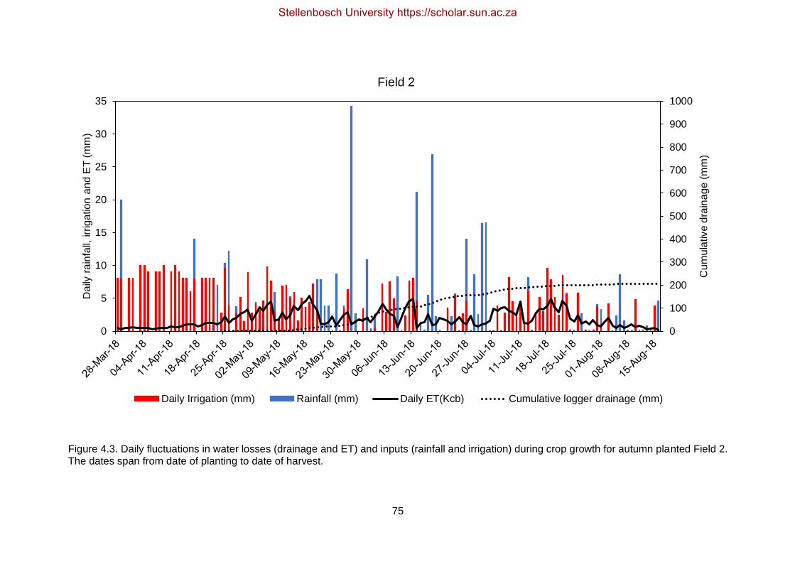
75
Figure 4.3. Daily fluctuations in water losses (drainage and ET) and inputs (rainfall and irrigation) during crop growth for autumn planted Field 2. The dates span from date of planting to date of harvest.
0
100
200
300
400
500
600
700
800
900
1000
0
5
10
15
20
25
30
35
Cu
mu
lative
dra
ina
ge
(m
m)
Da
ily r
ain
fall,
irr
iga
tio
n a
nd
ET
(m
m)
Field 2
Daily Irrigation (mm) Rainfall (mm) Daily ET(Kcb) Cumulative logger drainage (mm)
Stellenbosch University https://scholar.sun.ac.za

76
Figure 4.4. Daily fluctuations in water losses (drainage and ET) and inputs (rainfall and irrigation) during crop growth for autumn planted Field 3. The dates span from date of planting to date of harvest.
0
100
200
300
400
500
600
700
800
900
1000
0
5
10
15
20
25
30
35
Cu
mu
lative
dra
ina
ge
(m
m)
Da
ily r
ain
fall,
irr
iga
tio
n a
nd
ET
(m
m)
Field 3
Daily Irrigation (mm) Rainfall (mm) Daily ET(Kcb) Cumulative logger drainage (mm)
Stellenbosch University https://scholar.sun.ac.za

77
Field 6 and Field 7 (Figures 4.7 and 4.8, respectively) were planted in late June and the end
of July respectively and were harvested mid to late November. The two crops received 154
and 71 mm of rainfall, respectively, throughout the cropping season. Crop water requirements
were generally high due to growth occurring mostly throughout the hot and dry summer
months from September to November, with October and November having average daily
maximum temperatures (Appendix IIIa) of 30 oC and 28 oC, respectively, for the region. For
Field 7, where the least rainfall occurred for the fields planted in July, a total of 486 mm of
irrigation was recorded, which was similar to the water application of June planted fields. No
substantial drainage occurred in this field, only 4 mm was measured by the lysimeter sensor
(no drainage solution was removed by the suction pump) throughout the season in spite of the
large irrigation amount. The low drainage can be explained by the little amount of rainfall
received (71 mm), as well as the observation that the subsoil (0.5 – 1.0 m depth) was dry at
the time of planting. It is, therefore, likely that the excess irrigation did not surpass the storage
capacity of the soil profile and was thus used to refill the profile as the season progressed.
The farmer consequently, had control over the majority of the water being applied to this field.
The yield as well as the WUE (Table 4.8) obtained were high (53.9 t ha-1 and 96.7 kg mm-1
respectively). During crop growth, it was noted that canopy cover was incomplete and at
various stages, vegetative growth lacked vigour. A possible explanation can be that the farmer
under-irrigated during the vegetative growth stage and could have increased his irrigation
frequency earlier on, potentially resulting in higher yields whilst maintaining a good WUE.
In Field 6 only 381 mm was irrigated. This lower irrigation amount as well as good WUE of
95.7 kg mm-1 (Table 4.8) can be explained by the presence of a clay layer at a 30 to 50 cm
depth within the soil profile, which limited deep drainage, and created better utilisation of the
higher rainfall (154 mm) recorded at this site. Total seasonal irrigation requirement was,
therefore, less compared with other crops grown during the same time of year, as more water
was held by the duplex soil. This indicates the positive influence on WUE of a limiting layer
that curbed deep drainage (none of the other fields contained any form of clay layer within 1
m of the soil profile).
Stellenbosch University https://scholar.sun.ac.za

78
Figure 4.5. Daily fluctuations in water inputs (rainfall and irrigation) of Field 4 from planting (winter) to harvest. The irrigation frequency increased
toward the end of the season during the end of September/beginning of October months due to an increase in temperature and ET demand.
0
5
10
15
20
25
30
35
Da
ily r
ain
fall,
irr
iga
tio
n a
nd
ET
(m
m)
Field 4
Daily Irrigation (mm) Rainfall (mm) Daily ET(Kcb)
Stellenbosch University https://scholar.sun.ac.za

79
Figure 4.6. Daily fluctuations in water losses (drainage and ET) and inputs (rainfall and irrigation) during crop growth for Field 5. The dates span
from date of planting to date of harvest.
0
100
200
300
400
500
600
700
800
900
1000
0
5
10
15
20
25
30
35
Cu
mu
lative
dra
ina
ge
(m
m)
Da
ily r
ain
fall,
irr
iga
tio
n a
nd
ET
(m
m)
Field 5
Daily Irrigation Rainfall (mm) Daily ET(Kcb) Cumulative logger drainage (mm)
Stellenbosch University https://scholar.sun.ac.za

80
Figure 4.7. Daily fluctuations in water losses (drainage and ET) and inputs (rainfall and irrigation) during crop growth for Field 6. The dates span from date of planting to date of harvest.
0
5
10
15
20
25
30
35
Da
ily r
ain
fall,
irr
iga
tio
n a
nd
ET
(m
m)
Field 6
Daily Irrigation (mm) Rainfall (mm) Daily ET(Kcb)
Stellenbosch University https://scholar.sun.ac.za

81
Figure 4.8. Daily fluctuations in water losses (drainage and ET) and inputs (rainfall and irrigation) during crop growth for Field 7 (winter planted). The dates span from date of planting to date of harvest.
0
50
100
150
200
250
300
350
0
5
10
15
20
25
30
35
Cu
mu
lative
dra
ina
ge
(m
m)
Da
ily r
ain
fall,
irr
iga
tio
n a
nd
ET
(m
m)
Field 7
Daily Irrigation Rainfall (mm) Daily ET(Kcb) Cumulative logger drainage (mm)
Stellenbosch University https://scholar.sun.ac.za

82
The increase in drainage occurring over winter periods when ET demands are low and rainfall
events more frequent corresponds to Kengni et al. (1994). However, in their study this was
reported below a depth of 0.8 m during the intercrop period for maize when soils were bare
and ET low. However, it was reported that 90% of the drainage occurring was a result of
rainfall. This should be considered during early crop stages of winter planted fields before
canopy cover is developed and majority of the soil is uncovered. Meissner et al. (2010) also
indicated an increase in drainage accumulation caused by rainfall. Also noted was the effect
of increased precipitation and water inputs on the tendency to over-estimate drainage
accumulation when lysimeters functioning with a passive wick are used. The over-estimation
was reported to occur in sandy soils in particular, due to the rise of a mismatch between the
wick and soil suction.
It was hypothesised before the start of the study that summer planted fields would incur less
drainage during the season than winter planted crops due to a lesser amount of rainfall
occurring as well as higher temperatures and ET associated with the time of year. However,
this was not always the case, as indicated by Figures 4.9 and 4.10. Both Fields 8 and 9
produced substantial drainage (233 mm and 302 mm respectively). On average, each
irrigation application was higher than winter planted fields. Cumulative reference
evapotranspiration (ETo) over the entire growth period for Field 8 was high at 790 mm. Water
applications of between 8 and 15 mm per irrigation cycle was applied to this field. Irrigation
frequency for both fields was high. The growth period for Field 8 was 126 days of which
irrigation was applied on 101 days. This can be attributed to the hot temperatures, high ET
demand and windy conditions in summer months, resulting in producers applying irrigation
frequently. The same trend is seen for Field 9. However, for Field 8 the AE for the centre-pivot
was very low (refer to Table 4.1), which necessitated the application of more water than was
required by the crop. Thus, over irrigation occurred to make up for the substantial loss of water
between the nozzles and soil surface. The start of irrigation for Field 9 occurred on the 4th of
December 2018 and continued until harvest. The dips seen in daily irrigation in Figure 4.10
are due to the halting of irrigation in order to apply chemical sprays, but once this was
completed, irrigation continued. Generally, farmers practice pre-planting irrigation in the
Sandveld and do not commence irrigation again until sprout emergence. The reason for
drainage in summer months can be attributed to the high irrigation frequency early in the
season. However, during the mid to late growth period of the crops, application frequency is
not necessarily too high, but rather the irrigation amounts per irrigation cycle were too high.
Just prior to crop emergence both producers started irrigating. Emergence occurs at a much
faster rate in summer months and hence the profile still contains substantial water from pre-
planting application. During the early crop development there is a large portion of bare soil,
Stellenbosch University https://scholar.sun.ac.za

83
therefore evaporation from the bare soil surface is high. Once canopy cover starts to develop,
less evaporation is occurring and transpiration increases. However, due to the large irrigation
applications, more water is entering the soil profile than is lost via the process of ET, resulting
in a build-up of soil profile water. Field capacity is eventually reached and exceeded, resulting
in drainage accumulation. Drainage accumulation for Field 8 reaches 10.6 mm just 23 days
after emergence. A total irrigation amount of 913 mm was applied to this field. However, for
Field 8 it is evident that the substantial water application exceeding the crop water requirement
resulted from the very low AE of the centre-pivot. Even though total accumulated drainage for
the season was substantial, the yield for Field 8 was exceptionally high at 118.2 t ha-1 and
contributed to an excellent WUE (122.2 kg mm-1). Similarly, Field 9 produced a good yield of
59 t ha-1 and WUE of 86.2 kg mm-1. For Field 9, a comparable trend is seen to Field 8.
However, each irrigation application per cycle is lower than for Field 8, between 6 to 8 mm.
This is due to a lower ET throughout the season (Field 9 was situated <1 km from the Atlantic
Ocean), so less water is used by the crop. Irrigation frequency early in the season was high
and field saturation was reached earlier, with a large accumulation of drainage being more
notable quicker in this field than Field 8. At 23 days after emergence, Field 9 already
accumulated 42 mm of drainage. Later in the season (13th of January onwards), drainage
accumulation increased. This was attributed to high irrigation amounts. Throughout the
season, a total of 44% of the water input into Field 9 by rainfall and irrigation was lost as
drainage.
The over irrigation through high irrigation frequencies early in the season and substantial water
application during summer planted fields is also used as a strategy in the Sandveld to prevent
wind damage. The high winds in the area often pick up sand in the field, which moves through
the crop causing a sand blasting effect. Thus, irrigation strategies to keep the surface wet
prevent the movement of sand particles. This particularly contributed to the over-irrigation that
occurred on Field 9, in an effort to curb wind damage through sandblasting of plants, especially
late in the season when canopy cover started to drop.
Stellenbosch University https://scholar.sun.ac.za

84
Figure 4.9. Daily fluctuations in water losses (drainage and ET) and inputs (rainfall and irrigation) during crop growth for Field 8 (summer planted). The dates span from date of planting to date of harvest.
0
100
200
300
400
500
600
700
800
900
1000
0
5
10
15
20
25
30
35
Cu
mu
lta
ive
dra
ina
ge
(m
m)
Da
ily r
ain
fall,
irr
iga
tio
n a
nd
ET
(m
m)
Field 8
Daily Irrigation (mm) Rainfall (mm) Daily ET(Kcb) Cumulative logger drainage (mm)
Stellenbosch University https://scholar.sun.ac.za

85
Figure 4.10. Daily fluctuations in water losses (drainage and ET) and inputs (rainfall and irrigation) during crop growth for a summer planted field (Field 9). The dates span from date of planting to date of harvest. Weather data is missing from date of planting until the 20th December.
0
100
200
300
400
500
600
700
800
900
1000
0
5
10
15
20
25
30
35
Cu
mu
lative
dra
ina
ge
(m
m)
Da
ily r
ain
fall,
irr
iga
tio
n a
nd
ET
(m
m)
Field 9 water inputs and losses
Daily Irrigation (mm) Rainfall (mm) Daily ET(Kcb) Cumulative logger drainage (mm)
Stellenbosch University https://scholar.sun.ac.za

86
The water application on all fields, with the exception of Field 9, was within the suggested
range for good potato growth (Haverkort 1982; Kang et al. 2004, Fleisher at al. 2008; Parent
and Anctil 2012). Only for Field 7, did low soil water potentially cause a difference between
actual yield and potential yield (Table 4.26), but this effect was minor (actual yield was only
7% lower than potential yield). Irrigation scheduling in the Sandveld, however, is not altered
according to plant physiological demands, as is suggested by Fabeiro et al. (2001). The
reason being due to the sandy nature of the soil profiles, soils tend to dry out rapidly, which is
not conducive to potato production as the crop is sensitive to water stress (Shock et al. 1998;
Fabeiro et al. 2001; Yuan et al. 2003; Shock et al. 2007). Therefore, farmers tend to over-
irrigate because of the fear that crops may suffer drought stress due to the low water holding
capacity of the sandy soils. Thus, producers over irrigate to stay on the ‘safe side’. Concerning
drainage, the observations seen for all fields vary from that reported by Vázquez et al. (2005),
which indicated that the greater drainage occurred during early crop development of
vegetables due to a larger application of water than used by the ET demand. This difference
is better observed in summer planted fields where rainfall does not play a substantial role.
Drainage does occur early on, however; Field 9 shows a gradual increase in drainage during
early crop development and a steeper cumulative drainage curve occurring towards the middle
of the season from early January to the end of February due to the high application rate. This
is also seen in Field 8, which indicates an increase in drainage accumulation in the second
half of each growth period. Bošnjak et al. (2012) reported the positive correlation between
water consumed by a potato crop and tuber yield. Fields in the Sandveld that produced little
drainage showed an agreement with this statement. Field 7, which produced negligible
drainage over the entire season, used water efficiently and produced a yield close to the
potential yield as calculated by the LINTUL DSS potato model. Fields 3 and 9, on the other
hand, incurred large amounts of drainage, resulting in lower yields produced compared to the
simulated potential yields (Table 4.26).
4.2.2 Estimated water requirements
4.2.2.1 Basal crop coefficient curves
The basal crop coefficient curves (Figure 4.11) were calculated for each individual field
monitored within the Sandveld. When producing the Kcb curves the assumption of uniform
ideal crop growing conditions in each field was made (Jayanthi et al. 2007). The figures
obtained in this study generally mimic the trend illustrated by Allen et al. (2005), Benli et al.
(2006), Miao et al. (2016) and Mohktari et al. (2018). For autumn and winter planted fields
such as Fields 1, 2, 3 and 4, where the time the crop was in the field extended >130 days,
Stellenbosch University https://scholar.sun.ac.za

87
curves started to diverge from the typical Kcb curves depicted in literature (Allen et al. 1998).
The divergence stems from the crop generally dying by 120 DAP. However, it is assumed ET
ceases ≥140 DAP unless irrigation is applied if the crop is in the field longer than140 days.
Hence, the graphical trend seen for Fields 2, 4 and 5. A similar curve was seen for mustard
(Brassica juncea) by Gupta et al. (2017). The curves for crops grown during warmer periods
follow the more typically depicted basal crop coefficient curve (Allen et al.1998). The warmer
temperatures and higher solar radiation are conducive to rapid crop development and hence
termination and harvesting of the crop occurred earlier at about 120 DAP.
The fields planted in March (autumn) had a shorter period from planting to emergence due to
higher temperatures occurring during March and April (Figure 4.12 and Table 4.3). On the
other hand, the fields planted in the middle of winter (May to early July) had longer periods
between planting and emergence (Figure 4.12), extending from 28 to 33 days (Fields 3, 4, 5
and 6). The fields planted after the end of July had shorter periods between planting and crop
emergence. The shortest period being 6 days (Field 9). The length and steepness of the
curves in Figures 4.11 and 4.12 are dependent on climatic conditions. Between emergence
and 100% canopy cover, winter planted crops (June to July) averaged 49 days, compared to
autumn planted crops (March to April) which averaged 36 days (Table 4.3). The maximum
length for June to July plantings was 52 days (Field 6). The summer grown Field 8, on the
other hand, reached 100% canopy cover rapidly at 31 days. The duration period of 100%
canopy cover was extended (52 days) in crops grown during warmer conditions with higher
solar radiation (Figures 4.11 and 4.12), compared to those grown in winter periods (22 days).
Stellenbosch University https://scholar.sun.ac.za

88
Figure 4.11. Basal crop coefficient curves calculated using FAO-56 adjusted Kcb(mid) and Kcb(end) values to meet the specific climatic conditions. The curves allow for the estimation of crop ET at various stages of crop growth.
0.0
0.5
1.0
1.5
0 40 80 120 160
Basal cro
p c
oeff
icie
nt
Days after planting
Field 1
0.0
0.5
1.0
1.5
0 40 80 120 160
Basal cro
p c
oeff
icie
nt
Days after planting
Field 2
0.0
0.5
1.0
1.5
0 40 80 120 160
Basal cro
p c
oeff
icie
nt
Days after planting
Field 3
0.0
0.5
1.0
1.5
0 40 80 120 160
Basal cro
p c
oeff
icie
nt
Days after planting
Field 4
0.0
0.5
1.0
1.5
0 40 80 120 160
Basal cro
p c
oeff
icent
Days after planting
Field 5
0.0
0.5
1.0
1.5
0 40 80 120 160
Basal cro
p c
oeff
icie
nt
Days after planting
Field 6
0.0
0.5
1.0
1.5
0 40 80 120 160
Basal cro
p c
oeff
icie
nt
Days after planting
Field 7
0.0
0.5
1.0
1.5
0 40 80 120 160
Basal cro
p c
oeff
icie
nt
Days after planting
Field 8
0.0
0.5
1.0
1.5
0 40 80 120 160
Basal cro
p c
oeff
icie
nt
Days after planting
Field 9
Stellenbosch University https://scholar.sun.ac.za

89
Figure 4.12. Proposed standardised basal crop coefficient curves to estimate ET for potato crops in the Sandveld region during different planting periods (autumn, winter and summer).
0.0
0.2
0.4
0.6
0.8
1.0
1.2
0 20 40 60 80 100 120 140 160
Ba
sa
l cro
p c
oe
ffic
ien
t
Days after planting
Autumn planted fields
0.0
0.2
0.4
0.6
0.8
1.0
1.2
0 20 40 60 80 100 120 140 160
Basal cro
p c
oeff
icie
nt
Days after planting
Winter planted fields
0.0
0.2
0.4
0.6
0.8
1.0
1.2
0 20 40 60 80 100 120 140 160
Ba
sa
l cro
p c
oe
ffic
ien
t
Days after planting
Summer planted fields
Stellenbosch University https://scholar.sun.ac.za

90
All Kcb(mid) and Kcb(end) (Table 4.4) values were adjusted to account for the impact of
differences in aerodynamic roughness between the potato crop and reference grass crop as
discussed by Pereira et al. (1999). Allen et al. (1998), Allen et al. (2011) and Allen and Pereira
(2009) recommended Kcb(ini), Kcb(mid) and Kcb(end) values for the production of Kcb curves
for potato crops. On average, Sandveld fields had a 3.7% higher adjusted Kcb(mid) value than
that suggested by FAO-56 (Allen et al. 1998) for potato crops, with the exception of Field 1,
which had a 3.7% lower adjusted Kcb(mid) value. The same was seen for Kcb(end), which
had a 9.5% higher adjusted value. Fields 1 and 9, however, produced 13.1 and 13.7% lower
Kcb(end) values, respectively. Overall, this suggests a general slight under-estimation when
calculating ET using FAO-56 (Allen et al. 1998) values for the Sandveld region. Therefore,
Sandveld Kcb values must be estimated regionally to ensure more accurate approximation of
irrigation requirements, compared to the FAO reported values. The regional adjustment of Kcb
values was also suggested by Gupta et al. (2017). The Kcb(mid) and Kcb(end) values
obtained in this study are higher than those reported by Paredes et al. (2018), who calibrated
the potential Kcb(mid) and Kcb(end) of potato crops in Italy (also a Mediterranean-type
climate) and obtained values of 1.10 and 0.35, respectively. Sousa and Pereira (1999),
likewise reported a value of 1.10 for Kcb(mid). The Kcb(mid) values obtained in the Sandveld
were more in line with those reported by Trebejo and Midmore (1990) and Slatni et al. (2011)
at 1.15 and 1.12, respectively. The Kcb values, however, represent mainly the transpiration
component of ET and may have under-estimated seasonal ET demand, particularly during the
early stages of crop development when more evaporation from the bare soil surface takes
place (Rosa et al. 2012). It was reported for maize crops that the evaporative component of
ET is 80% during the initial growth period, with an average of 41% throughout growth
(Zhao et al. 2013). For wheat the average contribution of evaporation to total seasonal ET
demand was reported at 30% (Zhang et al. 2003; Zhang et al. 2013a) and 26% (Kang et al.
2003). However, all studies indicated highest evaporative (E) contribution to ET demand
during early crop stages. The over-simplification of the Kcb curve may, therefore, miscalculate
potential ET (Mohktari et al. 2018). It is suggested that the dual crop coefficient is a more
precise estimation when crops do not completely cover the soil surface, as the evaporation
component will be estimated more accurately. However, the evaporative component is often
difficult to calculate (Zhao et al. 2013).
Stellenbosch University https://scholar.sun.ac.za
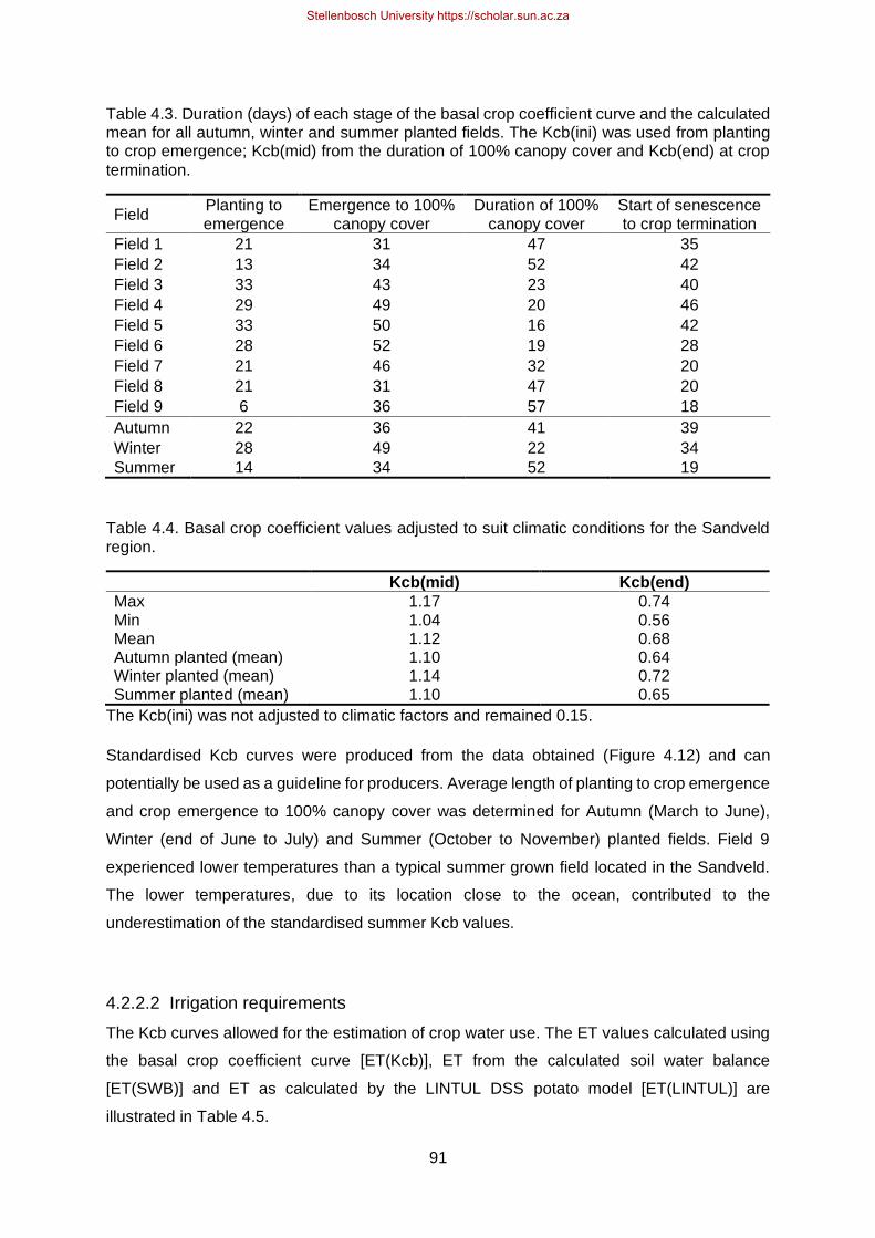
91
Table 4.3. Duration (days) of each stage of the basal crop coefficient curve and the calculated mean for all autumn, winter and summer planted fields. The Kcb(ini) was used from planting to crop emergence; Kcb(mid) from the duration of 100% canopy cover and Kcb(end) at crop
termination.
Field Planting to emergence
Emergence to 100% canopy cover
Duration of 100% canopy cover
Start of senescence to crop termination
Field 1 21 31 47 35
Field 2 13 34 52 42
Field 3 33 43 23 40
Field 4 29 49 20 46
Field 5 33 50 16 42
Field 6 28 52 19 28
Field 7 21 46 32 20
Field 8 21 31 47 20
Field 9 6 36 57 18
Autumn 22 36 41 39
Winter 28 49 22 34
Summer 14 34 52 19
Table 4.4. Basal crop coefficient values adjusted to suit climatic conditions for the Sandveld region.
Kcb(mid) Kcb(end)
Max 1.17 0.74 Min 1.04 0.56 Mean 1.12 0.68 Autumn planted (mean) 1.10 0.64 Winter planted (mean) 1.14 0.72 Summer planted (mean) 1.10 0.65
The Kcb(ini) was not adjusted to climatic factors and remained 0.15.
Standardised Kcb curves were produced from the data obtained (Figure 4.12) and can
potentially be used as a guideline for producers. Average length of planting to crop emergence
and crop emergence to 100% canopy cover was determined for Autumn (March to June),
Winter (end of June to July) and Summer (October to November) planted fields. Field 9
experienced lower temperatures than a typical summer grown field located in the Sandveld.
The lower temperatures, due to its location close to the ocean, contributed to the
underestimation of the standardised summer Kcb values.
4.2.2.2 Irrigation requirements
The Kcb curves allowed for the estimation of crop water use. The ET values calculated using
the basal crop coefficient curve [ET(Kcb)], ET from the calculated soil water balance
[ET(SWB)] and ET as calculated by the LINTUL DSS potato model [ET(LINTUL)] are
illustrated in Table 4.5.
Stellenbosch University https://scholar.sun.ac.za

92
For most fields, the LINTUL model produced ET values much higher than those calculated
using the Kcb curves (Fields 1 to 6). The difference in calculated water use ranged from 12.9
to 217.3 mm (Fields 2 and 3, respectively). Field 1, 2, 6, 8 and 9 differed between the two
calculation methods by only ≤10%. The ET(SWB) for Field 3, 7 8 and 9 was closer to the
ET(Kcb) than ET(LINTUL). The ET(SWB) values were high for all fields, with the exception of
Field 3, where ET(SWB) was lower than calculated ET(LINTUL). The ET(SWB) calculations
varied from ET(Kcb) and ET(LINTUL) for Field 3 by 64 and 153 mm respectively. The average
deviation between ET(Kcb) and ET(SWB), for all fields, is 141 mm, whereas the average
deviation between ET(LINTUL) and ET(SWB) is 161 mm.
Theoretically the total ET values over the season cannot exceed cumulative seasonal ETo,
due to Kcb values <1 for majority of the season. For Fields 2 and 5 the ET(SWB) exceeded
the ETo by far. The high values can potentially be attributed to the slopes of these two fields,
as runoff was observed. However, runoff is not reflected in the SWB calculation, which
probably contributed to the over estimation of ET. Thus, it can be assumed that the ET (Kcb)
estimated slightly more representative water use values for the region.
Table 4.5. Evapotranspiration (mm) calculated using the LINTUL DSS potato model and basal crop coefficient curves calculated using weather parameters obtained from each field.
Field ETo ET(Kcb) ET(SWB) ET(LINTUL)
Field 1 320 188 - 210
Field 2 373 266 550 279
Field 3 310 195 259 412
Field 4 531 321 - 438
Field 5 558 346 628 450
Field 6 420 305 - 323
Field 7 543 478 568 403
Field 8 790 647 743 607
Field 9 392 368 405 341
Figures 4.13 to 4.21 indicate the simulated irrigation requirements according to calculated ET,
taking into account system efficiencies. Irrigation requirement increases from winter to
summer planted crops due to the conducive conditions for more rapid growth as well as higher
temperatures and ETo occurring. Winter planted crops required less water due to colder, wetter
and cloudier climatic conditions. The first planted field, Field 1, had a total calculated ET(Kcb)
of 188 mm. Irrigation application was low at 260 mm, which was 19% more than the simulated
IR(Kcb) and only 9% higher than the simulated IR(LINTUL). When taking into account the
leaching requirement to remove the build-up of excess salts (Table 4.7), then the total irrigation
Stellenbosch University https://scholar.sun.ac.za

93
application carried out by the farmer is only 5 mm more than the simulated water requirement
[LR(LINTUL)] (Figure 4.13). However, throughout the season, from planting to harvest,
irrigation application is on average 39% higher than the water requirement simulated from
IR(LINTUL), including the LR and 43% higher throughout the season than the calculated
IR(Kcb), including the LR. Field 2 (Figure 4.14) showed a similar trend to Field 1. However,
Field 2’s irrigation application was substantially higher throughout crop growth in comparison
to the simulated Kcb and LINTUL irrigation requirements. The ET(Kcb) for Field 2 was 266
mm, with actual irrigation application being 486 mm. The actual application was 136 mm
higher than the simulated IR(Kcb) and 119 mm higher than the simulated IR(LINTUL)
(Figure 4.14). When taking into consideration the leaching requirement, the simulated
irrigation requirement for the season was 371 mm and 389 mm (Kcb and LINTUL,
respectively). This is 24% and 20% less than the actual irrigation application at the end of the
season. For Field 3 (Figure 4.15) the crop was in the field for an extended period (174 days).
During the early stages of crop development, IR(Kcb) is larger than the irrigation application
(2nd May until the 13th June). This can be attributed to the commencing of irrigation only with
crop emergence (4th June). However, the soil profile was irrigated prior to planting and hence,
ET took place as the soil contained sufficient water until emergence. From the 13 th June
onwards the irrigation application exceeded the IR simulated by Kcb and LINTUL until
October, when it dropped below the IR(LINTUL) again. The IR(Kcb) and cumulative irrigation
application followed a similar trend for Field 3, although IR(Kcb) always remained lower than
the actual irrigation application throughout the season. For this field, irrigation application was
27% less and 35% more than the IR(LINTUL) and IR(Kcb) respectively. When LR is
considered, irrigation applied still differed from the required water application by 33 and 30%
for IR(Kcb) and IR(LINTUL), respectively.
The fields planted end of June and early July (Fields 4, 5 and 6) had similar ET (Kcb) values,
ranging from 305 to 346 mm for the season. Fields 4 and 5 had similar total water inputs
(rainfall and irrigation) with total irrigation applications (562 and 545 mm, respectively) being
41 and 19% higher for Field 4 with regards to the simulated IR(Kcb) and IR(LINTUL)
respectively. For Field 6 (Figure 4.18), on the other hand, the irrigation application and
simulated water requirements followed the same trend until early September where after the
simulated water requirements exceeded the actual irrigation application. Final simulated
IR(Kcb) and IR(LINTUL) for Field 6 were 3.8 and 9.2% higher than the actual irrigation
application, suggesting only slight under-irrigation. However, the soil profile contained a water
table and hence LR was not required. The applied water was thus held in the soil profile for
longer periods, particularly during colder conditions.
Stellenbosch University https://scholar.sun.ac.za

94
Figure 4.13. Cumulative irrigation requirements calculated using crop ET demands from the basal crop coefficient curve [IR(kcb)] and LINTUL potato model [IR(LINTUL)] compared to actual irrigation applied throughout the season. Leaching requirement is also calculated for each method.
Figure 4.14. Cumulative irrigation requirements calculated using crop ET demands from the basal crop coefficient curve [IR(kcb)] and LINTUL potato model [IR(LINTUL)] compared to actual irrigation applied throughout the season. Leaching requirement is also calculated for each method.
0
100
200
300
400
500
600
700
800
900
1000
1100
1200
01-Mar 21-Mar 10-Apr 30-Apr 20-May 09-Jun 29-Jun 19-Jul 08-Aug
Irrig
atio
n w
ate
r (m
m)
Field 1
Actual irrigation IR(Kcb) IR(LINTUL) LR(Kcb) LR(LINTUL)
0
100
200
300
400
500
600
700
800
900
1000
1100
1200
01-Mar 21-Mar 10-Apr 30-Apr 20-May 09-Jun 29-Jun 19-Jul 08-Aug 28-Aug
Irrig
atio
n w
ate
r (m
m)
Field 2
Actual irrigation IR(Kcb) IR(LINTUL) LR(Kcb) LR(LINTUL)
Stellenbosch University https://scholar.sun.ac.za

95
Figure 4.15. Cumulative irrigation requirements calculated using crop ET demands from the basal crop coefficient curve [IR(kcb)] and LINTUL potato model [IR(LINTUL)] compared to actual irrigation applied throughout the season. Leaching requirement is also calculated for each method.
Figure 4.16. Cumulative irrigation requirements calculated using crop ET demands from the basal crop coefficient curve [IR(kcb)] and LINTUL potato model [IR(LINTUL)] compared to actual irrigation applied throughout the season. Leaching requirement is also calculated for each method.
0
100
200
300
400
500
600
700
800
900
1000
1100
1200
10-Apr 05-May 30-May 24-Jun 19-Jul 13-Aug 07-Sep 02-Oct 27-Oct 21-Nov
Irrig
atio
n w
ate
r (m
m)
Field 3
Actual irrigation IR(Kcb) IR(LINTUL) LR(Kcb) LR(LINTUL)
0
100
200
300
400
500
600
700
800
900
1000
1100
1200
09-Jun 29-Jun 19-Jul 08-Aug 28-Aug 17-Sep 07-Oct 27-Oct 16-Nov 06-Dec
Irrig
atio
n w
ate
r (m
m)
Field 4
Actual irrigation IR(Kcb) IR(LINTUL) LR(Kcb) LR(LINTUL)
Stellenbosch University https://scholar.sun.ac.za

96
Figure 4.17. Cumulative irrigation requirements calculated using crop ET demands from the basal crop coefficient curve [IR(kcb)] and LINTUL potato model [IR(LINTUL)] compared to actual irrigation applied throughout the season. Leaching requirement is also calculated for each method.
Figure 4.18. Cumulative irrigation requirements calculated using crop ET demands from the basal crop coefficient curve [IR(kcb)] and LINTUL potato model [IR(LINTUL)] compared to actual irrigation applied throughout the season. Leaching requirement is not necessary for this field due to the presence of a shallow clay layer, causing a water table.
0
100
200
300
400
500
600
700
800
900
1000
1100
1200
09-Jun 29-Jun 19-Jul 08-Aug 28-Aug 17-Sep 07-Oct 27-Oct 16-Nov 06-Dec
Irrig
atio
n w
ate
r (m
m)
Field 5
Actual irrigation IR(Kcb) IR(LINTUL) LR(Kcb) LR(LINTUL)
0
100
200
300
400
500
600
700
800
900
1000
1100
1200
29-Jun 19-Jul 08-Aug 28-Aug 17-Sep 07-Oct 27-Oct 16-Nov 06-Dec
Irrig
atio
n w
ate
r (m
m)
Field 6
Actual irrigation IR(Kcb) IR(LINTUL) LR(Kcb) LR(LINTUL)
Stellenbosch University https://scholar.sun.ac.za

97
Field 7 (Figure 4.19) showed similar irrigation application to simulated IR. The application of
water was only slightly higher than the simulated IR until the end of October, whereafter it
dropped below the IR(Kcb). The irrigation water used for this field was very saline (Table 4.7)
and hence leaching may be required to prevent the build-up of salts. When the LR is taken
into consideration then the IR(Kcb) and IR(LINTUL) where 18.5 and 3.5% higher than actual
application. Therefore, it can be noted that only slight under irrigation occurred. It can be
assumed that under-irrigation occurred during the middle of the season and onwards, as
irrigation exceeded the calculated ET during the early stages of crop development. Field 8 had
very large simulated water requirements for IR(Kcb) and IR(LINTUL) (1011 and 949 mm,
respectively). The simulated irrigation requirement, due to Field 8’s low AE (64%), increased
disproportionally, resulting in very high estimated irrigation needs. Irrigation application was
9.7 and 3.8% less than the simulated requirement. The simulated IR compared to actual
application goes up to of 13.2 and 7.5% (IR(Kcb) and IR(LINTUL), respectively) when LR is
taken into consideration. For Field 9 the irrigation requirement was underestimated due to
missing weather data during the early crop period (30th November to 20th December).
For all curves, IR(Kcb) followed a similar trend to the actual irrigation applied, with curves
levelling off towards the end of the season, whereas ET(LINTUL) produced constantly
increasing simulated IR. Differences of 10% and under between simulated water requirements
and irrigation application show good agreement. The LINTUL DSS potato model estimates
crop physiology according to growth degree-days. Crop emergence was calculated by LINTUL
using a sprout growth rate of 0.7 mm per degree-day above 0 °C, therefore, the emergence
date as calculated by LINTUL DSS varied from that visually noted for the Kcb curves.
However, for both LINTUL and the Kcb curves, the duration (days) from emergence to 100%
canopy cover was calculated with the same assumption. This was estimated using the value
reported by Haverkort et al. (2015) of 650-degree days from crop emergence to full canopy
cover. Where the two methods differ substantially is in the calculation of ET. The LINTUL DSS
model uses a dual crop coefficient approach, estimating both ET and bare soil evaporation.
LINTUL DSS uses a set Kcb(mid) value of 1.1, which is not adjusted for Sandveld climatic
conditions. The Kcb values for both Kcb(mid) and Kcb(end) were adjusted when using the Kcb
curves. The bare soil evaporation component is calculated as 1/3 of the daily ETo for LINTUL
DSS, however, for Kcb curves the evaporation component was excluded and the calculation
made primarily on the transpiration component. The soil cover estimated by LINTUL DSS is
calculated using the assumption that maximum soil cover is reached at a LAI of 3. Thereafter,
soil cover is assumed to remain 100% until haulm killing. However, if the crop naturally dies
off, the model makes an error. It has been shown from Eddy covariance measurements that
ET shows a declining trend in the second half of the growing season. As leaves senesce, ET
Stellenbosch University https://scholar.sun.ac.za

98
declines irrespective of weather conditions (Personal Communication, AC. Franke;
unpublished data).
Given that ET was not measured directly in the Sandveld, it cannot be stated which method
was more accurate as both depend on a set of assumptions. However, the use of the ET(SWB)
gives us an independent estimate of ET, which indicates different values to those obtained by
the Kcb curve and LINTUL DSS potato model.
Figure 4.19. Cumulative irrigation requirements calculated using crop ET demands from the basal crop coefficient curve [IR(kcb)] and LINTUL potato model [IR(LINTUL)] compared to actual irrigation applied throughout the season. Leaching requirement is also calculated for each method.
0
100
200
300
400
500
600
700
800
900
1000
1100
1200
19-Jul 08-Aug 28-Aug 17-Sep 07-Oct 27-Oct 16-Nov 06-Dec
Irrig
atio
n w
ate
r (m
m)
Field 7
Actual irrigation IR(Kcb) IR(LINTUL) LR(Kcb) LR(LINTUL)
Stellenbosch University https://scholar.sun.ac.za

99
Figure 4.20. Cumulative irrigation requirements calculated using crop ET demands from the basal crop coefficient curve [IR(kcb)] and LINTUL potato model [IR(LINTUL)] compared to actual irrigation applied throughout the season. Leaching requirement is also calculated for each method.
Figure 4.21. Cumulative irrigation requirements calculated using crop ET demands from the basal crop coefficient curve [IR(kcb)] and LINTUL potato model [IR(LINTUL)] compared to actual irrigation applied throughout the season. Leaching requirement is also calculated for each method.
0
100
200
300
400
500
600
700
800
900
1000
1100
1200
17-Sep 07-Oct 27-Oct 16-Nov 06-Dec 26-Dec 15-Jan 04-Feb 24-Feb
Irrig
atio
n w
ate
r (m
m)
Field 8
Actual irrigation IR(Kcb) IR(LINTUL) LR(Kcb) LR(LINTUL)
0
100
200
300
400
500
600
700
800
900
1000
1100
1200
06-Nov 06-Dec 05-Jan 04-Feb 06-Mar 05-Apr
Irrig
atio
n w
ate
r (m
m)
Field 9
Actual irrigation IR(Kcb) IR(LINTUL) LR(Kcb) LR(LINTUL)
Stellenbosch University https://scholar.sun.ac.za

100
4.2.3 Irrigation water quality
The threshold level of irrigation water for potato growth is considered 170 mS m-1
(Fertasa 2016). This value is the maximum permissible conductivity allowed without yield loss
occurring. Producers generally believe that the water sources for irrigation in the area are
slightly saline. Both the SAR and EC of the irrigation water used on each field was determined
to acknowledge the salinity hazard of the irrigation water applied (Table 4.6, Figure 4.22) in
order to determine whether a percentage of leaching and drainage was required.
Table 4.6. The sodium and salinity hazard classes for irrigation water. The sodium hazard classes are calculated using the sodium absorption ratio. The EC is well correlated with the dissolved salt content of water (Fertasa 2016).
Hazard class Value Description
Sodium Hazard
S1 <10 mmol dm-3 Suitable irrigation water, provided there is a low salinity hazard
S2 10 – 18 mmol dm-3
Good irrigation water for use on well-drained sandy soils. The addition of gypsum is advisable on sandy soils. If applied on clay soils salinity will increase over time.
S3 18 – 26 mmol dm-3
Use only with good management practices on well-drained soils. Unsuitable on soils with poor drainage.
S4 >26 mmol dm-3 Unsuitable for irrigation water
Salinity Hazard
C1 <25 mS m-1 No salinity hazard
C2 25 – 75 mS m-1 Avoid saline sensitive crops and ensure a reasonable degree of leaching is practiced
C3 75 – 225 mS m-1
Use salt resistant crops and ensure periodic leaching is practiced. Only recommended on well-drained soils.
C4 >225 mS m-1 Unsuitable for irrigation water. Under extreme conditions can be applied on sandy soils.
The class of analysed water sources ranged from C2:S1 to C4:S1 (Table 4.7). The
recommended leaching requirement for each field with the acceptable yield reduction of 10%
is relatively low for the region in most cases and ranged from 0.04 to 0.27 (Table 4.7).
However, due to the crop rotation in the area (one-year cropping, four to six years fallow) the
need for leaching of salts is low to negligible as there is potentially not a substantial build-up
of salts in the soil. The ceasing of irrigation and only rainfall events occurring in fallow periods
Stellenbosch University https://scholar.sun.ac.za

101
will result in the leaching of salts out of the effective rooting zone for potato crops. This is in
agreement with Vaughan and Letey (2015), whose study indicated that crops grown under
irrigation with saline water produced greater yields when seasonal rainfall occurred. The
rainfall caused excess salts to leach to greater depths in the soil profile. It was also shown that
factors that potentially reduce yield such as high saline conditions contributed to the increase
in N leaching. Shalhevet (1994) reported that in well-drained soils under irrigation, system
inefficiencies caused adequate leaching of excess salts. However, due to the long rotation
periods in potato cropping systems and the relatively low leaching requirements observed for
most of the fields monitored (Table 4.7), the leaching of salts should not be prioritised in potato
production systems in the Sandveld, as it was not observed to be an issue in the area under
normal field conditions.
Figure 4.22. Water classes from irrigation sources based on EC and SAR. The markers represent the irrigation water class for the different fields.
0
2
4
6
8
10
12
14
16
18
20
22
24
26
28
30
32
34
36
10 75 140 205 270
So
diu
m A
bd
orp
tio
n R
atio
Conductivity mS.m-1 @25°C
Irrigation water classes
Field 2 Field 5 Field 1 Field 3 Field 4 Field 8 Field 7 Field 6 Field 9
Stellenbosch University https://scholar.sun.ac.za

102
Table 4.7. Quality parameters for the different irrigation water sources. Salinity hazard class is determined based on the SAR and the electrical conductivity.
Water Source Field ECIW
(mS m-1) SAR
(Ratio) Class
Leaching Requirement (ratio)
1 2 and 5 51 3.1 *C2S1 0.04
2 3, 4 and 8 69 5.4 *C2S1 0.06
4 1 90 3.1 *C3S1 0.08
5 9 177 4.4 *C3S1 0.16
6 6 106 6.4 *C3S1 0.09
7 7 265 9.6 *C4S1 0.27
*refer to Table 4.6.
4.2.4 Soil water content
Data from DFM capacitance probes, which were installed in each field directly after planting,
are represented in Figures 4.23 to 4.27. The DFM probes give relative soil water content
values (scale 0 – 100) and not absolute soil water contents (fraction of percentage soil water).
These sensors generally gave a good indication of changes in soil water contents over the
growing season. In Figure 4.23 the periods of very wet conditions correspond with the deep
drainage collected, due to substantial rain from late May to early July (compare with
Figure 4.3), can clearly be observed for Field 2. In the example for Field 7 (Figure 4.24), the
slightly dry subsoil and gradual increase in water content thereof can be noted. The two
distinguished increases in soil water content observed (Figure 4.24, for 18 September and 23
October) both occurred after large water inputs through rainfall and irrigation. Field 5, which
was grown during a similar time of year to Field 7, showed a very different tendency. The
stepwise increase and decrease in soil water content can be viewed more easily as illustrated
by Figure 4.25 (16 September to 4 November). The cause of this was due to very little rain
occurring from the end of September to harvest. October was in general a hotter and drier
month in the region as illustrated by the high daily ET (refer to Figure 4.6) and therefore, there
was an increased frequency in soil water fluctuations due to the rapid depletion of profile water
through wetting and drying. This stepwise wetting and drying clearly indicates the irrigation
management of the field. The peaks above the upper readily available water limit shown for
the root zone (0 to 50 cm) and top roots (0 to 20 cm) occurred at dips in daily ET and coincided
with drainage accumulation. For Field 3, (Figure 4.26, compare with Figure 4.4) during the
beginning of June there was a dip in daily ET and rainfall events occurring and hence, the
incline in water contents observed for the root zone and top root zones. This coincided with
the start of drainage collection from the 20th of June until the 4th of July, when conditions for
this field were cold, cloudy and large amounts of rainfall occurred, causing an increase in
drainage accumulation. The spikes in water content (1 July, 15 July, 7 August and 25 August)
are in accord with the increase in drainage accumulation happening after large rainfall events
Stellenbosch University https://scholar.sun.ac.za

103
and is a trend seen throughout Figures 4.23 to 4.27. The decline in water content viewed from
the start of July to the middle of July in all zones for Field 3 (root zone (0 to 50 cm), top roots
(0 to 20 cm) and buffer zone (60 cm) was attributed to a decrease in rainfall, low irrigation
amounts and frequency as well as an increase in ET rate. Water input through rainfall and
irrigation as well as ET directly affect drainage accumulation, which in turn influences the soil
water content fluctuations.
Figure 4.23. DFM capacitance probe measurements of soil water contents in the root zone (top), top roots (middle) and buffer zone (bottom) of Field 2.
Figure 4.24. DFM capacitance probe measurements of soil water contents in the root zone
(top), top roots (middle) and buffer zone (bottom) of Field 7 in the Sandveld.
70
60
50
40
30
30 26
22
18
14
160
140
120
100
80
Vo
lum
etri
c w
ater
co
nte
nt
(mm
mm
-1)
%
-20
0
20
40
60
80
-20 0 20 40 60 80
-20
0
20
40
60
80
20 May 01 Jun 10 Jun 20 Jun 01 Jul 10 Jul 20 Jul 01 Aug
220
200
180
160
140
120
-20
0
20
40
60
80
90
80
70
60
-20
0
20
40
60
80
30
25
20
15
-20
0
20
40
60
80
Vo
lum
etri
c w
ater
co
nte
nt
(mm
mm
-1)
%
01 Sep 10 Sep 20 Sep 01 Oct 10 Oct 20 Oct 01 Nov 10 Nov 20 Nov
Stellenbosch University https://scholar.sun.ac.za

104
Figure 4.25. DFM capacitance probe measurements of soil water contents in the root zone (top), top roots (middle) and buffer zone (bottom) of Field 5 in the Sandveld.
Figure 4.26 DFM capacitance probe measurements of soil water contents in the root zone (top), top roots (middle) and buffer zone (bottom) of Field 3 in the Sandveld.
05 Sep 10 Sep 15 Sep 20 Sep 25 Sep 01 Oct 05 Oct 10 Oct 15 Oct 20 Oct 25 Oct 01 Nov
26
22
18
14
-20
0
20
40
60
80
150
130
110
90
80
70
60
50
40
-20 0 20 40 60 80
Vo
lum
etri
c w
ater
co
nte
nt
(mm
mm
-1)
%
-20
0
20
40
60
80
-40
-20
0
20
40
60
80
60
20
16
12
8
65
55
45
35
-40
-20
0
20
40
60
80
120
100
80
60
Vo
lum
etri
c w
ater
co
nte
nt
(mm
mm
-1)
-40
-20
0
20
40
60
80
%
01 Jun 10 Jun 20 Jun 01 Jul 10 Jul 20 Jul 01 Aug 10 Aug 20 Aug
Stellenbosch University https://scholar.sun.ac.za

105
Data collection by DFM probes linked with telemetry was generally seamless, except in places
where cell phone reception was unreliable. This was especially problematic for some of the
fields due to the mountainous topography surrounding fields. As a result, for some of the fields,
data from only one probe, or in some cases no data, could be retrieved from those farms. This
was the case for various fields, but is clearly demonstrated by the graphical representation of
soil water content throughout the season for Field 9 (Figure 4.27).
Figure 4.27. DFM capacitance probe measurements of soil water contents in the root zone (top), top roots (middle) and buffer zone (bottom) of Field 9 in the Sandveld. Data collection was incomplete due to poor cellular reception and the partial and sporadic collection of data
throughout the growing season as illustrated by the incomplete soil water content lines.
The Decagon sensors showed a similar trend to the DFM probes. However, some data points
are missing for various sensors and periods in certain monitored fields (Figures 4.28 to 4.33)
due to logger problems or dysfunctional sensors. Decagon (volumetric water content) values
were lower than those given by the DFM probes. When compared to random gravimetric
sampling (data not presented) Decagon values were closer and more accurate, however, the
use of soil water monitoring tools in this study was not aimed at obtaining actual soil water
content data, but to observe the fluctuation in profile water with drainage accumulation.
During this study, producers did not have access to the capacitance probe data and, therefore,
did not manage irrigation scheduling accordingly. However, it is believed that these probes
24
20
16
12
65
55
45
140
120
100
80
Vo
lum
etri
c w
ater
co
nte
nt
(mm
mm
-1)
-40 -20 0 20 40 60 80
-20
0
20
40
60
80
%
-40
-20
0
20
40
60
80
10 Dec 20 Dec 01 Jan 10 Jan 20 Jan 01 Feb 10 Feb 20 Feb 01 Mar
Stellenbosch University https://scholar.sun.ac.za

106
can be valuable irrigation scheduling tools in order to decrease drainage and optimise
irrigation management. Fields 8 and 9 had battery failure over December, resulting in missing
data points. However, a general decreasing trend in soil water content (%) during the period
of no data collection was observed.
The Chameleon soil water potential sensors, which were also evaluated at the intensively
monitored fields in the Sandveld, unfortunately gave poor response in the very sandy soils
present. The sensors inserted into the east section of Field 3 showed very different soil water
movement to the readings given by the sensors inserted into the west end of the field. The
east sensor results indicated a lower soil water potential than the west, for the depth of 25 cm
and 50 cm (green and red colours). This does slightly coincide with the DFM data for that
section; however, conditions were not very dry during the early part of the season as
suggested by the Chameleon data. In the case of Field 7, Chameleon data suggested
saturated conditions throughout the entire season, which does not follow the observed soil
water content trends from the DFM or Decagon probes. The DFM and Decagon probes
illustrate a drier soil profile during the early cropping season and an increase in soil water
content towards harvest. Field 2 showed a similar trend. The result is that the colour patterns
mainly remained blue, (Figure 4.34 to 36) suggesting that the soils were consistently very wet,
which does not agree with the DFM or Decagon data. Therefore, these sensors cannot supply
producers with useful information to make good management decisions in the Sandveld
region, due to the nature of the soil texture. The reason for the constant readings of field
saturation is due to the inability of the Chameleon sensors to equilibrate with the sandy
textured soils because of the sudden drop in unsaturated hydraulic conductivity when these
soils dry out rapidly.
Stellenbosch University https://scholar.sun.ac.za

107
Figure 4.28. Field 2 Decagon capacitance probe soil water content data from a depth of 0-50 cm at 10 cm intervals. The missing data at 10 cm depth is due to sensor malfunctioning.
Figure 4.29. Field 3 Decagon capacitance probe soil water content data from a depth of 0-50 cm at 10 cm intervals.
0
5
10
15
20
25
30
10-May 20-May 30-May 09-Jun 19-Jun 29-Jun 09-Jul 19-Jul 29-Jul 08-Aug 18-Aug 28-Aug
So
il w
ate
r co
nte
nt (%
)Field 2
10 cm 20 cm 30 cm 40 cm 50 cm
0
5
10
15
20
25
30
19-Jun 29-Jun 09-Jul 19-Jul 29-Jul 08-Aug 18-Aug 28-Aug 07-Sep 17-Sep
So
il w
ate
r co
nte
nt (%
)
Field 3
10 cm 20 cm 30 cm 40 cm 50 cm
Stellenbosch University https://scholar.sun.ac.za

108
Figure 4.30. Field 5 Decagon capacitance probe data from a depth of 0-50 cm at 10 cm intervals.
Figure 4.31. Field 7 Decagon capacitance probe data from 0-50 cm depth excluding the 40 cm depth due to a faulty probe.
0
5
10
15
20
25
30
18-Aug 28-Aug 07-Sep 17-Sep 27-Sep 07-Oct 17-Oct 27-Oct 06-Nov 16-Nov
So
il w
ate
r co
nte
nt (%
)Field 5
10 cm 20 cm 30 cm 40 cm 50 cm
0
5
10
15
20
25
30
21-Jul 04-Aug 18-Aug 01-Sep 15-Sep 29-Sep 13-Oct 27-Oct 10-Nov 24-Nov 08-Dec
So
il w
ate
r co
nte
nt (%
)
Field 7
10 cm 20 cm 30 cm 50 cm
Stellenbosch University https://scholar.sun.ac.za

109
Figure 4.32. Field 8 Decagon capacitance probe data from a depth of 0-40 cm at 10 cm intervals. 50 cm probe data is missing due to a faulty sensor. Gap in data was due to battery failure.
Figure 4.33. Field 9 Decagon capacitance probe data from a depth of 0-40 cm, with readings at 10 cm intervals. 50 cm probe data missing due to a faulty sensor. Gap in data was due to battery failure.
0
5
10
15
20
25
30
24-Nov 08-Dec 22-Dec 05-Jan 19-Jan 02-Feb 16-Feb
So
il w
ate
r co
nte
nt (%
)Field 8
10 cm 20 cm 30 cm 40 cm
0
5
10
15
20
25
30
16-Nov 06-Dec 26-Dec 15-Jan 04-Feb 24-Feb 16-Mar 05-Apr
So
il w
ate
r co
nte
nt (%
)
Field 9
10 cm 20 cm 30 cm 40 cm 50 cm
Stellenbosch University https://scholar.sun.ac.za

110
Figure 4.34. Chameleon probe data for Field 2, (top) west inserted probe and (bottom) east
inserted probe. The colours red, blue and green represent a tension of >50 kPa, 20–50 kPa
and 0–20 kPa, respectively. A tension of 0 kPa indicates a soil that is saturated and >50 kPa
represents a dry soil. Lines indicate the link between logger reading taken throughout the
season.
Stellenbosch University https://scholar.sun.ac.za
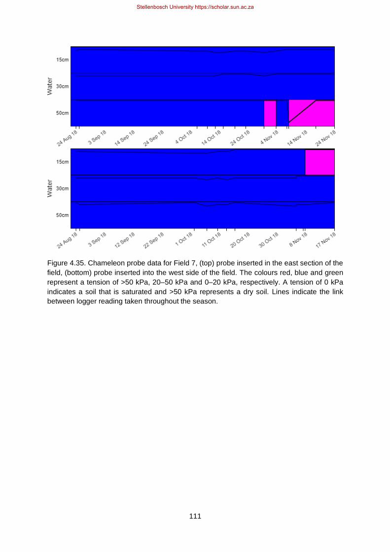
111
Figure 4.35. Chameleon probe data for Field 7, (top) probe inserted in the east section of the
field, (bottom) probe inserted into the west side of the field. The colours red, blue and green
represent a tension of >50 kPa, 20–50 kPa and 0–20 kPa, respectively. A tension of 0 kPa
indicates a soil that is saturated and >50 kPa represents a dry soil. Lines indicate the link
between logger reading taken throughout the season.
Stellenbosch University https://scholar.sun.ac.za

112
Figure 4.36. Chameleon probe data for Field 3. Top is the east-side, bottom is the West side.
The colours red, blue and green represent a tension of >50 kPa, 20–50 kPa and 0–20 kPa,
respectively. A tension of 0 kPa indicates a soil that is saturated and >50 kPa represents a
dry soil. Lines indicate the link between logger reading taken throughout the season.
4.2.5 Water use efficiency
Water use efficiencies, calculated using yield and total water input by rainfall and irrigation
(Ali et al. 2016), ranged from 65.4 (Field 1) to 122.2 kg mm-1 (Field 8) with an average of
85 kg mm-1 (Table 4.8). The average WUE falls above the acceptable WUE of 75 to
80 kg mm-1 as reported by Steyn et al. (2016). The average WUE of winter plantings was
79.5 kg mm-1. Four out of the nine fields did not achieve WUE values above the acceptable
norm. These low WUE values can be ascribed to a combination of factors. During winter
months, the yield potential of potatoes is generally lower due to less available solar radiation,
although in some cases other factors (e.g. disease occurrence and seed problems) resulted
in the low yields. Large winter rainfall events also resulted in substantial unproductive water
losses through drainage (or runoff) for some of the fields, resulting in low WUE. All four of the
fields with lower WUE (75 to 80 kg mm-1) received substantial rainfall (143 – 271 mm) during
the crop growing season, which added considerably to the total amount of water these crops
received, and affected the WUE negatively. Results obtained in this study were much lower
Stellenbosch University https://scholar.sun.ac.za

113
than those reported in a Mediterranean climate in Italy by Katerji and Mastrorilli (2009) for clay
(161 kg mm-1) and loam (210 kg mm-1) soils. The values reported by Katerji and Mastrorilli
(2009) were, however, calculated using yield and estimated crop ET. Higher results however,
can be anticipated in clay and loam soils as the sandy soils present in the Sandveld, have
lower water holding abilities. Sandveld producers can also not be expected to leave substantial
room for rainfall in the soil profile due to low water holding capacities, as this could result in
water stress and yield losses, should a sudden hot spell occur.
When excluding the effect of rainfall in the calculation of WUE and referring to IWUE
(Darwish et al. 2006; El-Abedin et al. 2017) results show a higher efficiency ranging from 89
to 134 kg mm-1, which are higher than those reported by Darwish et al. (2006).
Darwish et al. (2006) reported IWUE ranging from 0.80 to 1.06 kg DM m-3 (equivalent to 40 –
53 kg mm-1, if a DM content of 20% is assumed), in a dry Mediterranean climate located in
Bekaa, Lebanon. Ahmadi et al. (2014) reported IWUE values of 173 and184 kg mm-1 for the
cultivars Ramos and Agria, respectively, in Shiraz, Iran where the climate is warm with an
average annual rainfall of 386 mm. The average IWUE of 113.2 kg mm-1 obtained in the
Sandveld is less than the lower range indicated by Ahmadi et al. (2014) on silty-clay loam soils
for the variety Ramos. The WUE and IWUE generally decreased with an increase in water
supply, which is in agreement with other reports in the literature (Fabeiro et al. 2001; Kashyap
and Panda 2003; Yuan et al. 2003; Darwish et al. 2006; Ierna et al. 2011; Ierna and
Mauromicale 2012). Ierna and Mauromicale (2012) stated the ability to reduce irrigation
amounts by 77 mm year-1 when irrigating at 100% of the maximum ET from tuber initiation to
50% of the tuber growth only, whilst still obtaining high IWUE and tuber quality, indicating the
importance of altering irrigation management according to crop phase.
Table 4.8. Water use efficiency and IWUE obtained within the Sandveld region. Calculated was the potential WUE and IR using outputs provided by LINTUL POTATO DSS model and the ratio between actual irrigation application (AI) and IR as estimated using the Kcb curves
Field WUE
(kg mm-1)
IWUE
(kg mm-1)
*Potential WUE
(kg mm-1)
**AI:IR(Kcb)
Field 1 65.4 133.4 87.0 1.23
Field 2 69.3 106.1 62.6 1.39
Field 3 76.2 132.6 141.5 1.54
Field 4 82.0 105.5 103.0 1.68
Field 5 70.7 88.6 95.3 1.57
Field 6 95.7 134.3 100.7 0.96
Field 7 96.7 111.0 104.1 0.95
Field 8 122.2 129.4 92.4 0.90
Field 9 86.2 91.0 131.4 0.63
*calculated from the potential yield given by the LINTUL POTATO DSS model and irrigation and rainfall applied to the fields. ** Ratio of actual irrigation (AI) to the irrigation requirement calculated by the Kcb curve.
Stellenbosch University https://scholar.sun.ac.za

114
4.2.6 Nutrient leaching
It is evident that nutrient leaching is substantial and may be attributed to the high levels of
rainfall or irrigation received, following the same trend as drainage accumulation. To illustrate
this, more leaching was obtained from Field 3 (Figure 4.37) early in the season, particularly
during the sprouting and vegetative period, followed by a decrease in nutrient leaching
throughout crop growth. Large rainfall events occurred during the month of June, coinciding
with early crop development, whereafter rainfall occurrences decreased, the plant roots
developed deeper and plant nutritional requirements increased. From the second to the third
sampling date (27 June to 9 July) the leaching and loss of nutrients below the root zone for N,
P and K was 19, 27.8 and 24.2 kg ha-1, respectively. The applied fertiliser on Field 3 during
the fourth week after crop emergence (Appendix I), which was prior to the second leachate
sampling date, was slightly higher for N and K than the previous weeks at 27 kg N ha -1,
24.5 kg K ha-1. However, the amount of P applied between weeks three and four after crop
emergence, was similar to prior applications. The increase in leaching can be accredited to
high rainfall events and due to this, irrigation frequency was reduced. A total amount of
58.4 mm rainfall and irrigation occurred at this time. The drop in irrigation resulted in the
decreased leachate accumulation for Na, S, Mg and Ca, which are present in the irrigation
water sources (Table 4.9) at relatively high concentrations (1.01 kg Na ha-1 mm-1, 0.04 kg S
ha-1 mm-1, 0.13 kg Mg ha-1 mm-1 and 0.05 kg Ca ha-1 mm-1). After this point, nutrient leaching
decreased, following a similar trend as the decrease in drainage water collected (Figure 4.38).
Table 4.9. Chemical composition of the different irrigation water sources. Fields 2 and 5 shared the same water source, as well as Fields 3, 4 and 8.
Field pH Total-N P K Ca Mg S Na
mg L-1
Field 1 7.2 4.37 0.09 1.37 34.4 22.0 10.9 95.5
Field 2 7.8 6.07 0.31 1.83 3.8 7.1 2.0 45.0
Field 3 7.2 0.00 1.13 1.34 5.2 12.9 4.4 100.6
Field 4 7.2 0.00 1.13 1.34 5.2 12.9 4.4 100.6
Field 5 7.8 6.07 0.31 1.83 3.8 7.1 2.0 45.0
Field 6 6.7 0.00 <0.75 <10 12.2 15.8 6.1 143.6
Field 7 7.7 0.00 <0.75 <10 36.6 48.0 18.5 375.8
Field 8 7.2 0.00 1.13 1.34 5.2 12.9 4.4 100.6
Field 9 4.3 7.86 <0.75 12.34 43.8 61.9 115.5 194.4
Stellenbosch University https://scholar.sun.ac.za

115
Figure 4.37. Nutrient leaching from Field 3 as measured from drainage solution collected fortnightly from the drainage lysimeter.
0
50
100
150
200
250
300
350
400
450
500
Nu
trie
nt
lea
ch
ing
(kg
ha
-1)
Field 3
Total-N H2PO4 K Ca Mg S Na
Stellenbosch University https://scholar.sun.ac.za

116
Figure 4.38. Cumulative macronutrient leaching compared to drainage collected for Field 3.
Field 2 (Figure 4.39) shows a different trend than Field 3, with nutrient leaching low during the
first soil solution collection and increasing during the second collection. However, the
explanation remains the same and is a tendency that is seen in all fields where drainage was
collected. The spikes in nutrient leaching coincided with major water applications to fields
through rainfall or when large amounts of irrigation were applied. Nutrient leaching for Field 2
(Figures 4.39 and 4.40) at the first sampling date (22 May) was generally low with 13.5 kg N
ha-1, 6.42 kg P ha-1, 25.3 kg K ha-1. The reason being that March, April and May 2018 were
hotter and drier months with less rainfall. Hence, there was larger water movement out of the
soil profile due to ET and less movement of nutrients downwards. Between sampling dates
one and two
500
400
300
200
100
0
100
200
300
400
500
600
700
800
900
1000
1100
1200
1300
Nu
trie
nt
lea
ch
ing
(kg
ha
-1)
Field 3
drainage cumulative Ca cumulative N
cumulative P cumulative K cumulative Mg
cumulative S cumulative Na cumulative drainage
Dra
ina
ge
(mm
)
Stellenbosch University https://scholar.sun.ac.za

117
(2 May to 14 June) the field received 106 mm of rainfall, with a large rainfall event occurring
on the 28th of May (34.2 mm). Within this period, there was 12 irrigation cycles applying a total
of 71.2 mm, resulting in a total of 177.2 mm water being applied to the field. After the second
sampling date, rainfall and irrigation application gradually decreased, resulting in less drainage
(Figure 4.40). The total nutrients leached for the season from Field 2 was higher than that of
Field 3 for K, Ca, Mg, S nutrients, however, 296 mm of soil solution drained from Field 3,
compared to 205 mm in Field 2. The higher Mg and S leaching for Field 2 was not attributed
to additions from irrigation water, as Mg and S concentrations in the irrigation water were lower
(0.07 kg Mg ha-1 mm-1 and 0.02 kg S ha-1 mm-1) than for Field 3. Only 5 kg ha-1 more Mg and
2 kg ha-1 more S fertiliser were applied to Field 2 than Field 3. However, the fertiliser regime
for Field 2 used seven products containing S, applied over 13 applications (pre-planting up
until week three). In comparison, Field 3 used four products containing S, all applied prior to
crop emergence. The spreading of fertiliser application and higher water input (refer to
Table 4.2 and Figures 4.3) during the early crop development on Field 2 may have attributed
to the higher leaching of S. The explanation for the higher Mg leaching that occurred in
Field 2 is most likely a result of the presence of more Mg in the soil profile (0 – 90 cm), as
illustrated by the soil analysis (Appendix II).
Field 5 (Figures 4.41 and 4.42) followed the same leaching trend (advanced leaching with
larger drainage accumulation), however, less nutrients leached throughout the cropping period
compared to the other monitored fields. This is a result of less drainage occurring (only 74 mm
in total) throughout the season.
Stellenbosch University https://scholar.sun.ac.za

118
Figure 4.39. Nutrient leaching from Field 2 as measured from fortnightly drainage solution collected from the drainage lysimeter.
0
50
100
150
200
250
300
350
400
450
500
2018/05/22 2018/06/14 2018/06/27 2018/07/11 2018/07/23 2018/08/07
Nu
trie
nt
lea
ch
ing
(kg
ha
-1)
Field 2
Total-N H2PO4 K Ca Mg S Na
Stellenbosch University https://scholar.sun.ac.za

119
Figure 4.40. Cumulative macronutrient leaching compared to drainage amounts for Field 2.
500
400
300
200
100
0
100
200
300
400
500
600
700
800
900
1000
1100
1200
1300
2018/05/22 2018/06/14 2018/06/27 2018/07/11 2018/07/23 2018/08/07
Nu
trie
nt
lea
ch
ing
(kg
ha
-1)
Field 2
drainage cumulative drainage cumulative N
cumulative K cumulative Ca cumulative Mg
cumulative S cumulative Na cumulative P
Dra
ina
ge
(mm
)
Stellenbosch University https://scholar.sun.ac.za

120
Figure 4.41. Nutrient leaching from Field 5 as measured from drainage solution collected fortnightly from the drainage lysimeter.
0
50
100
150
200
250
300
350
400
450
500
2018/09/10 2018/10/01 2018/10/30 2018/11/06
Nu
trie
nt
lea
ch
ing
(kg
ha
-1)
Field 5
Total-N H2PO4 K Ca Mg S Na
Stellenbosch University https://scholar.sun.ac.za

121
Figure 4.42. Cumulative macronutrient leaching compared to drainage amounts for Field 5.
500
400
300
200
100
0
100
200
300
400
500
600
700
800
900
1000
1100
1200
1300
2018/09/10 2018/10/01 2018/10/30 2018/11/06
Nu
trie
nt
lea
ch
ing
(kg
ha
-1)
Field 5
drainage cumulative drainage cumulative N
cumulative P cumulative K cumulative Ca
cumulative Na cumulative Mg cumulative S
Dra
ina
ge
(mm
)
Stellenbosch University https://scholar.sun.ac.za

122
The highest nutrient leaching was recorded for the two summer planted crops. For Field 8
(Figures 4.43 and 4.44) the rapid incline in nutrient leaching in Figure 4.43 was a result of 26.2
mm of rainfall received on the 7th of December, which occurred between the second and third
sample dates (5 December to 7 January). Irrigation was not adjusted according to the rainfall
received and between the sampling dates a total of 310.2 mm irrigation was applied, giving a
total water input from rainfall and irrigation of 350.2 mm for this period. The cumulative nutrient
leaching for Field 8 was substantially more than the other fields, amounting to
900 kg Ca ha-1, 814 kg S ha-1 and 409 kg Na ha-1. This can be attributed to the high amount
of irrigation water applied (913 mm). The application of Ca, S and Na through irrigation water
alone for Field 8 amounted to 48 kg Ca ha-1, 40.3 kg S ha-1 and 919 kg Na ha-1 for the season.
Field 9 produced 302 mm of drainage due to a high irrigation frequency, resulting in large
nutrient losses below the root zone (Figures 4.45 and 4.46). The high leaching rates observed
follows the trend of drainage collected (Figure 4.46). Total accumulated nutrients for the
season were highest for Na > S > Ca, amounting to 1221 kg Na ha-1, 927 kg S ha-1 and
542 kg Ca ha-1 and can be largely accredited to the irrigation water. The analysed water source
contained 1.94 kg Na ha-1 mm-1, 1.15 kg S ha-1 mm-1 and 0.44 kg Ca ha-1 mm-1. Between
sampling dates 30th of January and 19th of February the N, K, Ca, Mg, and S contents in the
leachate decreased, however, irrigation application remained the same. This decrease can be
attributed to the crop growth stage, which coincided with tuber initiation and bulking. The
decrease in leaching from the third sample date to the fifth (19 February to 27 March) was due
to the reduction in irrigation amount and frequency.
Stellenbosch University https://scholar.sun.ac.za

123
Figure 4.43. Nutrient leaching from Field 8 as measured from drainage solution collected fortnightly from the drainage lysimeter.
0
50
100
150
200
250
300
350
400
450
500
2018/11/27 2018/12/05 2019/01/07 2019/01/30 2019/02/07
Nu
trie
nt
lea
ch
ing
(kg
ha
-1)
Field 8
Tot-N H2PO4 K Ca Mg S Na
Stellenbosch University https://scholar.sun.ac.za

124
Figure 4.44. Cumulative macronutrient leaching compared to drainage amounts for Field 8.
500
400
300
200
100
0
100
200
300
400
500
600
700
800
900
1000
1100
1200
1300
2018/11/27 2018/12/05 2019/01/07 2019/01/30 2019/02/07
Nu
trie
nt
lea
ch
ing
(kg
ha
-1)
Field 8
drainage cumulative Na cumulative drainage
cumulative N cumulative P cumulative K
cumulative Ca cumulative Mg cumulative S
Dra
ina
ge
(mm
)
Stellenbosch University https://scholar.sun.ac.za

125
Figure 4.45. Nutrient leaching from Field 9 as measured from drainage solution collected fortnightly from the drainage lysimeter.
0
50
100
150
200
250
300
350
400
450
500
2019/01/07 2019/01/30 2019/02/19 2019/03/06 2019/03/27
Nu
trie
nt
lea
ch
ing
(kg
ha
-1)
Field 9
Tot-N H2PO4 K Ca Mg S Na
Stellenbosch University https://scholar.sun.ac.za
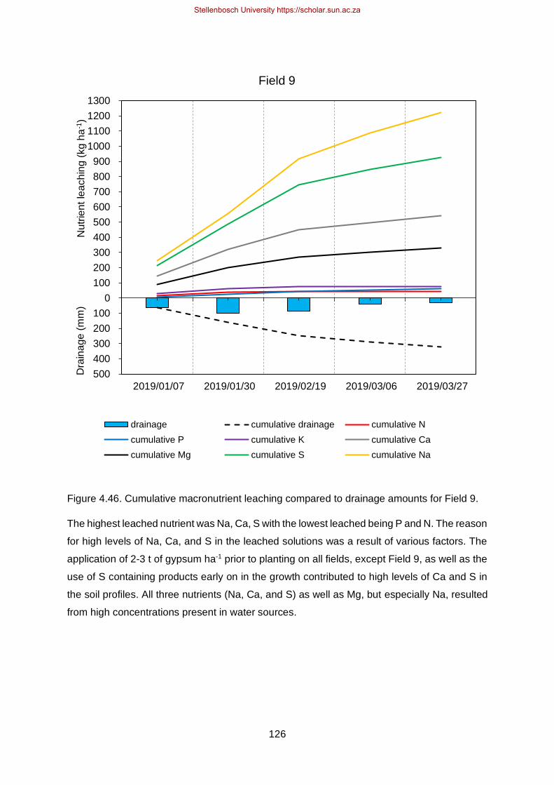
126
Figure 4.46. Cumulative macronutrient leaching compared to drainage amounts for Field 9.
The highest leached nutrient was Na, Ca, S with the lowest leached being P and N. The reason
for high levels of Na, Ca, and S in the leached solutions was a result of various factors. The
application of 2-3 t of gypsum ha-1 prior to planting on all fields, except Field 9, as well as the
use of S containing products early on in the growth contributed to high levels of Ca and S in
the soil profiles. All three nutrients (Na, Ca, and S) as well as Mg, but especially Na, resulted
from high concentrations present in water sources.
500
400
300
200
100
0
100
200
300
400
500
600
700
800
900
1000
1100
1200
1300
2019/01/07 2019/01/30 2019/02/19 2019/03/06 2019/03/27
Nu
trie
nt
lea
ch
ing
(kg
ha
-1)
Field 9
drainage cumulative drainage cumulative N
cumulative P cumulative K cumulative Ca
cumulative Mg cumulative S cumulative Na
Dra
ina
ge
(mm
)
Stellenbosch University https://scholar.sun.ac.za

127
It is generally assumed that nitrate and sulphate are the most easily leached from soils due to
their negative charge. However, the results in Table 4.10 indicate that large quantities of the
cations Mg, Ca and K leached from these sandy soils due to the lack of cation exchange sites
associated with the soil type. In some instances (Fields 3 and 9) there were also large amounts
of P leached, with Field 3 reaching 160 kg of leached P per ha-1 and Field 9 reaching 60 kg P
ha-1. Phosphorus is generally an immobile ion that is easily precipitated by other ions
(Degryse et al. 2013; Vet et al. 2014). The high amounts of leached P in certain fields indicates
the sensitivity of the Sandveld cropping system and the ease at which all nutrients are leached
below the effective rooting depth of a potato plant, especially in occurrence with large water
application from rainfall events.
Table 4.10. Extent of nutrients leached per season in intensively monitored fields.
The results obtained in this study indicate the low capacity of the sandy profiles to bind cations
such as Ca2+, K+, Mg2+ and Na+ as well as anions. This is in agreement with previous studies
(Chantigny et al. 2004; Yang et al. 2007). Tahir and Marshchner (2017) studied the effects of
clay addition to nutrient leaching in sandy soils. The study concluded that the addition of clay
considerably increased fertiliser nutrient retention. When compared to pure sandy soils, clay
amended soils resulted in 83% more N and double the P retention.
Although substantial P leaching was observed for some fields in this study, the amounts were
generally far less than that reported by Chen et al. (2006), who indicated that 97% of P applied
through water-soluble fertilisers was leached from sandy soils and < 1% was leached when
using dolomite phosphate rock. The dolomite phosphate rock, which acted as a slower
releasing fertiliser, produced better results when used in acidic sandy soils. However, the
study also concluded that 68 to 99.9% of the leached P was in the readily available form,
which is problematic for aquatic systems as it is easily available to algae, increasing the
potential risk of eutrophication. In the present study an average of 52 kg P ha-1 leached below
Nutrient leached kg ha-1
Field N P K Ca Mg S Na
2 86 11 166 268 94 314 242
3 118 160 160 242 43 170 372
5 34 15 17 152 38 112 116
7 0 0 0 0 0 0 0
8 66 16 273 900 173 814 409
9 44 60 76 542 332 927 1221
Mean 70 52 138 421 136 467 472
Max 118 160 273 900 332 927 1221
Min 34 11 17 152 38 112 116
Stellenbosch University https://scholar.sun.ac.za

128
1 m depth. Highest P leaching was recorded for Field 3 (160 kg P ha-1) and the lowest in
Field 7 (0 kg P ha-1).
A study in Zimbabwe showed that 54% of applied N was leached from the 0 to 0.5 m soil
profile, following heavy rainfall on sandy soils (Hagmann 1994). Results obtained for the
Sandveld showed the same trend in leachate increase after large rainfall events. It was evident
that in the Sandveld region, farmers prefer the use water-soluble fertiliser products for
practicality reasons and hence the majority of nutrients are applied through fertigation via the
centre-pivot, with the exception of gypsum, which may increase the potential for leaching to
occur.
The total loss of nutrients via leaching is highly dependent on the amount of drainage
associated with excessive water from rainfall or over-irrigation, which is in agreement with
Shepherd and Bennet (1998) and Jiang et al. (2011). The rate of nutrient losses in sandy soils,
however, varies considerably within the literature. Ruskowska et al. (1984) indicated that with
no influence from fertiliser rate, only 5 kg K ha-1 leached from sandy soils. This was
considerably lower than results obtained in the present study. The high nutrient leaching can
potentially be attributed to the use of water-soluble fertilisers in the Sandveld region.
Catanzaro et al. (1998) showed that the use of liquid fertilisers increased leachate of N
collected in a chrysanthemum pot trial by 14 to 20%. Yang et al. (2007) indicated that the use
of chemical fertilisers alone in sandy soils increased P concentration in leachate 10 to 20
times, compared to a control. The combination of high-water inputs into the field (rainfall and
irrigation) as well as the use of water-soluble fertilisers applied even during rainfall events in
a practice referred to as ‘high tech fertigation’. This practice results in the application of high
concentrations of nutrients to the soil through the centre-pivot to maintain nutrient levels within
the profile.
4.2.7 Leachate EC levels
The drainage lysimeter sensor measured EC of the collected solution throughout the growing
season (Figure 4.47). For all fields, with the exception of Field 7, the leachate EC reached
values above 150 mS m-1. For Fields 2 and 5 the leachate collected started below
150 mS m-1 but once drainage occurred, within a day or two, the EC moved just above
170 mS m-1. The leachate for Fields 2 and 5 reached a maximum EC of 228 and 202 mS m-1,
respectively. Field 2 remained above the 170 mS m-1 for 39 days when it then declined to
96 mS m-1 and remained at a relatively stable EC until the end of the season, with dips at 91
and 106 days after the lysimeter was installed. These dips in EC were attributed to drainage
solution removal. For Field 5 the EC remained stable from day 12 to day 70 when it then
Stellenbosch University https://scholar.sun.ac.za

129
declined sharply to 8.3 mS m-1 and remained low thereafter. At day 70, 30 mm of soil solution
was removed and from then on 42.1 mm of irrigation was applied, however, very little drainage
(0.6 mm) occurred from day 70 to the end of growth. Field 3 started with a very high EC of
388.5 mS m-1, but this reduced throughout the season, reaching below the 150 mS m-1 39
days after lysimeter installation. This was after substantial water application had occurred
through rainfall and irrigation (refer to Figure 4.4) along with a period of low ET. Therefore,
drainage accumulated and possibly caused a dilution of EC within the drainage lysimeter. The
leachate collected during summer grown fields (Fields 8 and 9) had substantially higher EC
levels throughout the season in comparison to winter grown fields. Field 8 remained below
100 mS m-1 until 36 days after the drainage lysimeter was installed. The EC then increased
(180.1 mS m-1) and remained above 150 mS m-1 for the rest of the season, then declined to
below 170 mS m-1 102 days after lysimeter installation. Field 9, which was located close to the
ocean, maintained a leachate solution EC above 225 mS m-1 throughout the season.
Figure 4.47. Variation in drainage solution EC throughout crop growth for intensively monitored fields.
0
50
100
150
200
250
300
350
400
450
1 15 29 43 57 71 85 99 113 127 141 155
EC
(m
S/m
)
Day after lysimeter installation
Field 2 EC (mS/m) Field 5 EC (mS/m) Field 3 EC (mS/m)
Field 7 EC (mS/m) Field 8 EC (mS/m) Field 9 EC (mS/m)
Stellenbosch University https://scholar.sun.ac.za

130
A study conducted by Letey et al. (2011) indicated that negative effects caused by irrigating
with saline water were significantly moderated by rainfall due to a dilution effect. Both summer-
grown fields in the Sandveld maintained a higher EC value throughout the season, which can
be attributed to the higher irrigation frequency and amounts, quality of irrigation water and lack
of rainfall (refer to Figures 4.9 and 4.10). It was evident that for winter planted crops the
leachate EC levels were lower and was attributed to substantial and periodic rainfall events,
which leached out and diluted excess salts. However, the effect of fertiliser application, which
is carried out on a weekly basis in the Sandveld region, cannot be neglected on the role it may
play on the EC levels of the collected leachate. Large pre-planting application of fertilisers may
have resulted in initially high EC values observed at the start of the seasons, which coincides
with when majority of the N leaching occurred and can be attributed to small crops and shallow
root systems during this period. The reduction in leachate EC levels observed later on in the
crop seasons was due to a decline in fertiliser applications.
4.3 Plant nutrient uptake
4.3.1 Leaf tissue nutrient content
The amount of leaching partly depends on the capacity of a potato plant to uptake nutrients at
various stages during the growth cycle. This can be illustrated through leaf samples analysed
throughout the season, as well as nutrient content within the tuber during harvest. Leaf
samples showed similar trends, with N and K being present at high concentrations throughout
growth, followed by Ca. Nitrogen dropped slightly towards the end of the growth cycle,
whereas Ca is found at higher concentrations at the end of growth than during the start
(Table 4.11).
Six out of the nine fields under observation showed a decrease in N content for samples
conducted 67 days after emergence (DAE) and onwards, with the exception of Fields 3 and
9. The latest leaf samples taken were at 92 DAE. Deficient N values are regarded as below
4.5% (Haifa Group Ltd (2019) and Yara UK Fertiliser (Pty) (2019)). Fernandes and Soratto
(2016) reported an N leaf content of 5.1% (51 g kg-1) between 29 and 33 DAE. This coincides
with the average value of 5.7% obtained in the present study for fields sampled at a similar
time (26 – 35 DAE). Kolbe and Stephan-Beckmann (1997) reported the maximum value of
leaf N concentration at 30 DAE, which also coincides with values obtained in the present study,
where leaf samples were taken during a similar time (26 – 35 DAE). The N values attained
were between 5.13 and 6.16%. However, samples taken within 14 DAE showed excessive
leaf N concentrations (>7.0%). The high N concentrations indicate high absorption and
Stellenbosch University https://scholar.sun.ac.za

131
translocation of N during the early stages of growth, which coincides with the vegetative stage.
Towards the end of the tuber-bulking stage, a decline in leaf tissue N content is observed. At
the time of maximum N plant uptake (55 – 65 DAP), as reported by Zotarelli et al. (2015), leaf
tissue values for fields analysed (Fields 2, 3, 7, 8 and 9) close to this time ranged from 4.38 to
6.16% (norm: 4.5 – 6.5%), indicating that N levels in these crops were adequate for growth.
Field 9, however, had slightly low leaf N levels at 4.38%, but was not deficient. The N values
obtained in the current study are higher than the values reported by Ries and Monnerat (2000),
who indicated an average leaflet N value of 3.99% 48 DAE. Maximum leaf tissue organic and
inorganic component contents are said to be reached 45 to 50 DAE and highest growth rates
between 30 and 45 DAE (Kolbe and Stephan-Beckmann 1997).
Sufficient P content in the leaf early in the season is regarded as 0.44% (Walworth and
Muniz 1993). Phosphorus leaf tissue values in the literature are reported to be very low in
potato crops and range from 0.21 to 0.55%. (Walworth and Muniz 1993; Rocha et al. 1997;
Ries and Monnerat 2000; Fernandes and Soratto 2016). The average leaf P content for the
region (0.53%), conducted during this study, was within the range reported in the literature
(Walworth and Muniz 1993; Rocha et al. 1997; Ries and Monnerat 2000; Fernandes and
Soratto 2016). Fields sampled 10 to 41 DAE showed excess P concentrations ranging from
0.60 to 0.83%. All K concentrations were below the recommended norms (4 – 10%) throughout
the growth cycle. Sharma and Arora (1987) indicated a decrease in potato leaf K content with
an increase in DAE. An average value of 3.12% for K was observed from all leaf samples
conducted in the present study. The Mg concentrations measured ranged from 0.33 to 1.65%,
with 66% of the samples producing average results >0.5%. Fernandes and Soratto (2016)
reported an average of 0.7% leaf Mg content with no effect of site, cultivar or P rate on the
content of N, K, Ca, Mg, S, B, Cu, Fe and Mn. In comparison, Bergmann (1992) stated an
adequate range in leaf tissue Mg content between 0.25 and 0.8% for potato crops and sugar
beet. Values below or above this range will result in deficient or excess Mg contents,
respectively. According to the values stated by Bergmann (1992), 50% of the leaf samples
had an average Mg leaf content of >0.8% and therefore, average leaf Mg concentrations
(0.76%) in this study were in agreement with those reported in the literature. The low levels of
K observed in the present study can possibly be attributed to the antagonism between K+ and
Mg2+ ions. Ries and Monnerat (2000) reported a similar effect. To indicate this antagonistic
behaviour between cations, Addiscott (1974) reported a decrease in both Mg and Ca with an
increase in K2SO4 fertiliser application. The high Ca levels observed in the leaf tissue could
also be a contributing factor to the low K contents observed. An average of 1.49% Ca, with a
maximum value of 3.03% was recorded. The adequate levels of Ca in the leaf tissue can be
accredited to the high levels of Ca seen in the soil analysis due to the practice of gypsum
Stellenbosch University https://scholar.sun.ac.za

132
application prior to planting. All S levels were within normal ranges, with the exception of
Field 8.
The S values for Field 8 dropped below 0.25% towards the end of the growth cycle
(67 – 90 DAE). The adequate S levels can be attributed to both pre-planting gypsum
applications as well as the application of K2SO4 fertiliser, resulting in an abundance of S
movement through the plant root zone.
Stellenbosch University https://scholar.sun.ac.za

133
Table 4.11. Leaf analysis conducted for Fields 2 to 9 approximately every 30 to 40 days. Leaf sampling commenced once good vegetative growth was established. Field 1 data is missing due to the need for sampling made clear after its early termination due to late blight (Phytophthora infestans).
Leaf nutrient content (%)
Field DAP N P K Ca Mg S Na
Field 2
27 7.04 0.64 3.82 1.18 0.63 0.34 0.02
55 5.78 0.57 2.84 1.70 0.90 0.38 0.06
105 3.73 0.42 4.34 1.90 0.90 0.38 0.17
Field 3
43 5.91 0.60 3.63 1.22 0.39 0.40 0.03
68 6.16 0.69 4.30 0.97 0.42 0.36 0.07
96 5.08 0.46 3.79 2.14 0.66 0.31 0.07
Field 4
46 6.21 0.66 3.22 0.97 0.38 0.40 0.03
82 5.00 0.53 3.07 1.15 0.44 0.31 0.04
102 4.16 0.46 2.23 3.03 0.88 0.30 0.11
Field 5 96 5.01 0.52 3.70 1.90 0.98 0.35 0.08
125 3.22 0.38 2.14 2.52 0.91 0.28 0.37
Field 6
28 7.57 0.78 2.83 0.70 0.40 0.48 0.02
84 5.81 0.53 3.01 1.08 0.73 0.35 0.11
113 3.12 0.35 2.21 2.40 1.12 0.31 0.84
Field 7
21 6.32 0.83 3.76 0.77 0.33 0.36 0.02
62 6.08 0.60 3.86 1.15 0.50 0.42 0.03
91 3.44 0.26 2.36 2.91 0.95 0.29 0.28
Field 8
47 5.13 0.74 3.29 0.68 0.35 0.35 0.08
55 5.54 0.67 3.48 1.01 0.45 0.37 0.06
88 3.67 0.39 2.56 1.90 1.09 0.24 0.45
111 2.77 0.38 2.33 1.96 1.40 0.21 0.84
Field 9
38 6.12 0.61 3.06 0.69 0.87 0.38 0.18
61 4.38 0.38 2.38 1.05 1.65 0.34 0.47
81 5.17 0.36 2.68 0.88 0.98 0.40 0.47
Mean 5.10 0.53 3.12 1.49 0.76 0.34 0.20
Max 7.57 0.83 4.34 3.03 1.65 0.48 0.84
Min 2.77 0.26 2.14 0.68 0.33 0.21 0.02
Stellenbosch University https://scholar.sun.ac.za
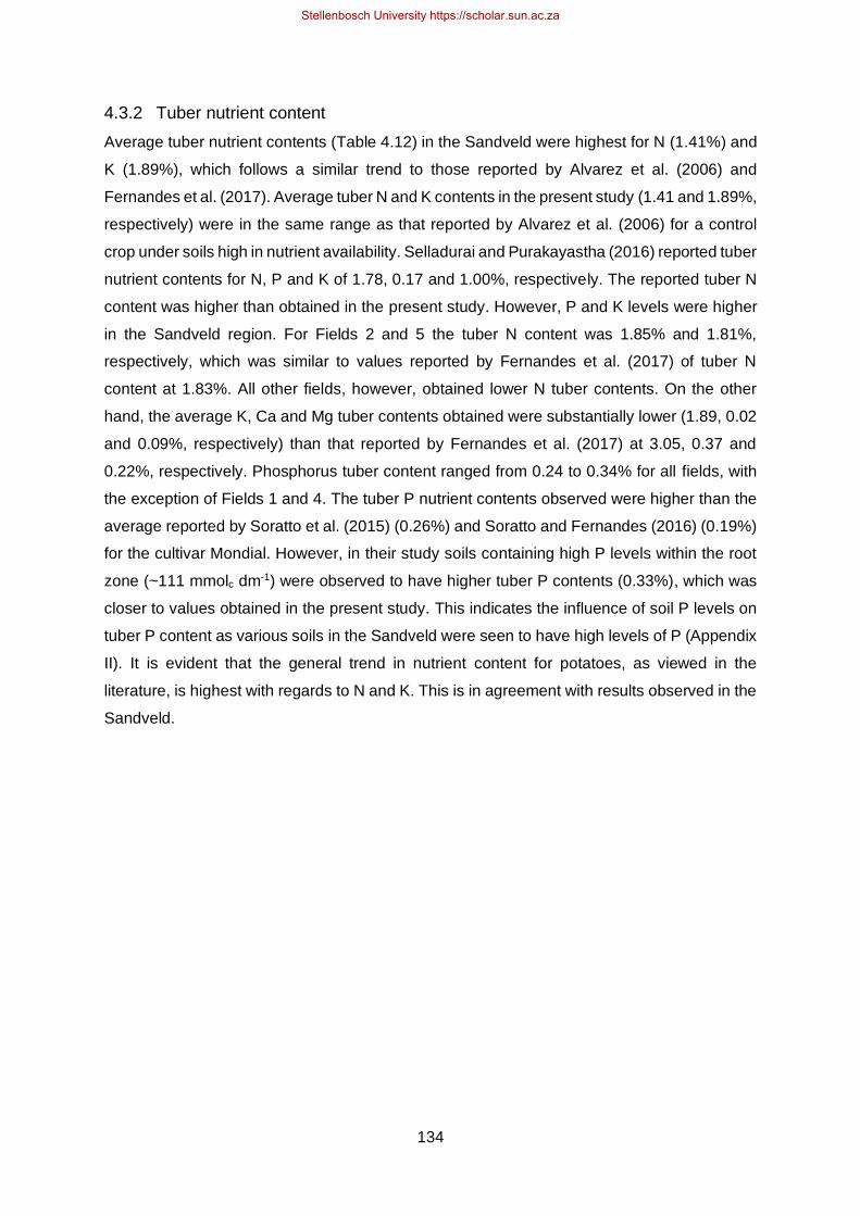
134
4.3.2 Tuber nutrient content
Average tuber nutrient contents (Table 4.12) in the Sandveld were highest for N (1.41%) and
K (1.89%), which follows a similar trend to those reported by Alvarez et al. (2006) and
Fernandes et al. (2017). Average tuber N and K contents in the present study (1.41 and 1.89%,
respectively) were in the same range as that reported by Alvarez et al. (2006) for a control
crop under soils high in nutrient availability. Selladurai and Purakayastha (2016) reported tuber
nutrient contents for N, P and K of 1.78, 0.17 and 1.00%, respectively. The reported tuber N
content was higher than obtained in the present study. However, P and K levels were higher
in the Sandveld region. For Fields 2 and 5 the tuber N content was 1.85% and 1.81%,
respectively, which was similar to values reported by Fernandes et al. (2017) of tuber N
content at 1.83%. All other fields, however, obtained lower N tuber contents. On the other
hand, the average K, Ca and Mg tuber contents obtained were substantially lower (1.89, 0.02
and 0.09%, respectively) than that reported by Fernandes et al. (2017) at 3.05, 0.37 and
0.22%, respectively. Phosphorus tuber content ranged from 0.24 to 0.34% for all fields, with
the exception of Fields 1 and 4. The tuber P nutrient contents observed were higher than the
average reported by Soratto et al. (2015) (0.26%) and Soratto and Fernandes (2016) (0.19%)
for the cultivar Mondial. However, in their study soils containing high P levels within the root
zone (~111 mmolc dm-1) were observed to have higher tuber P contents (0.33%), which was
closer to values obtained in the present study. This indicates the influence of soil P levels on
tuber P content as various soils in the Sandveld were seen to have high levels of P (Appendix
II). It is evident that the general trend in nutrient content for potatoes, as viewed in the
literature, is highest with regards to N and K. This is in agreement with results observed in the
Sandveld.
Stellenbosch University https://scholar.sun.ac.za

135
Table 4.12. Tuber nutrient contents from the yield analysis conducted for each monitored
field. The pith analysis was selected to represent the entire tuber nutrient content due to the
large proportion of the pith in comparison to the skin and medulla.
Tuber nutrient content (%)
Field N P K Ca Mg S Na
Field 1 1.53 0.24 1.66 0.01 0.09 0.12 0.03
Field 2 1.85 0.31 1.76 0.02 0.10 0.14 0.03
Field 3 1.54 0.31 1.97 0.01 0.11 0.14 0.05
Field 4 1.01 0.26 1.66 0.01 0.09 0.11 0.04
Field 5 1.81 0.34 1.84 0.02 0.10 0.15 0.04
Field 6 1.21 0.30 1.72 0.01 0.09 0.12 0.04
Field 7 1.22 0.31 2.03 0.02 0.10 0.13 0.05
Field 8 1.10 0.31 2.20 0.02 0.08 0.10 0.04
Field 9 1.38 0.33 2.17 0.02 0.09 0.14 0.07
Mean 1.41 0.30 1.89 0.02 0.09 0.13 0.04
Max 1.85 0.34 2.20 0.02 0.11 0.15 0.07
Min 1.01 0.24 1.66 0.01 0.08 0.10 0.03
A clear trend in tuber nutrient content distribution between the skin, medulla and pith was
observed (Tables 4.12, 4.13 and 4.14). The proportion of total tuber nutrients that were present
in the tuber skin alone were observed to be greater than the proportion of total nutrients that
was present in the flesh of the tubers (pith and medulla) (Table 4.13). The high proportion of
nutrients in the skin may be a result of direct uptake from the soil across the periderm, as
suggested by Subramanian et al. (2011). This follows a similar trend as reported by Boydston
et al. (2018) and is in agreement with Trehan and Sharma (1996) and Sulaiman (2005). The
average nutrient contents observed in the Sandveld within the skin for N (2.30%), K (3.52%)
and P (0.41%) where higher compared to the tuber flesh (pith), followed by S, Mg, Ca and Na.
The reason for the concentration difference in the tubers is reported to be a factor of the
mobility of ions within the plant. Calcium is passively transported through the plant in the
transpiration stream. Due to the low transpiration rate of tubers, less Ca was present in tubers
analysed in the Sandveld (0.02%) compared to aboveground plant parts, as illustrated by leaf
analysis results. Nitrogen and K, on the other hand, are easily re-translocated from
aboveground plant parts to the tuber and hence, are present at much higher concentrations
within the tubers. Tubers are generally considered high in K concentrations (White et al. 2009).
The contribution of the nutrients in the tuber skin to overall tuber nutrient content would,
however, be small in comparison to the pith due to the minor mass that the skin contributed to
total tuber mass. This is the reason for excluding the skin nutrient contents when calculating
tuber nutrient removal. Nutrient uptake and distribution are reported to be largely controlled
by cultivar factors (LeRiche et al. 2006), if soil nutrient content is not limiting. However, there
Stellenbosch University https://scholar.sun.ac.za

136
was no substantial differences observed between nutrient contents of the skin, medulla and
pith for the cultivars Sifra and FL2108 used in the present study.
Table 4.13. Nutrient content for the skin of potato tubers harvested from monitored fields.
Skin nutrient content (%)
Field N P K Ca Mg S Na
Field 1 2.59 0.31 3.51 0.09 0.16 0.16 0.02
Field 2 2.99 0.38 2.99 0.09 0.15 0.18 0.02
Field 3 2.78 0.50 3.64 0.09 0.18 0.16 0.02
Field 4 1.88 0.44 4.22 0.08 0.15 0.15 0.03
Field 5 2.81 0.53 3.14 0.12 0.17 0.18 0.04
Field 6 1.99 0.46 2.99 0.08 0.14 0.18 0.03
Field 7 2.36 0.41 4.36 0.08 0.15 0.17 0.04
Field 8 1.63 0.35 3.76 0.08 0.12 0.11 0.06
Field 9 1.66 0.29 3.09 0.07 0.15 0.18 0.09
Mean 2.30 0.41 3.52 0.08 0.15 0.16 0.04
Max 2.99 0.53 4.36 0.12 0.18 0.18 0.09
Min 1.63 0.29 2.99 0.07 0.12 0.11 0.02
Table 4.14. Nutrient content of the medulla section of potato tubers harvested from monitored
fields.
Medulla nutrient content (%)
Field N P K Ca Mg S Na
Field 1 1.37 0.31 2.42 0.03 0.09 0.12 0.02
Field 2 1.40 0.35 2.50 0.03 0.09 0.12 0.03
Field 3 1.33 0.36 2.72 0.03 0.10 0.12 0.03
Field 4 0.83 0.26 1.87 0.02 0.06 0.07 0.03
Field 5 1.49 0.37 2.29 0.04 0.09 0.12 0.04
Field 6 1.14 0.35 2.29 0.03 0.09 0.11 0.04
Field 7 1.22 0.31 2.27 0.02 0.09 0.11 0.05
Field 8 0.93 0.30 2.08 0.03 0.06 0.08 0.06
Field 9 0.97 0.30 2.32 0.03 0.07 0.12 0.10
Mean 1.18 0.32 2.31 0.03 0.08 0.11 0.04
Max 1.49 0.37 2.72 0.04 0.10 0.12 0.10
Min 0.83 0.26 1.87 0.02 0.06 0.07 0.02
The maximum nutrient removal for all fields by tubers was 541 kg K ha-1, 271 kg N ha-1,76 kg
P ha-1, 4.9 kg Ca ha-1, 18 kg Mg ha-1, 24 kg S ha-1 and 11 kg Na ha-1, which was obtained by
Field 8. The high values can be attributed to the very high yield obtained. However, tuber
nutrient removal (Table 4.15) did not indicate a clear correlation with yield for all fields
monitored, which is in agreement with values reported in the literature. Average N removal by
tubers in the Sandveld was 167 kg ha-1. Trehan et al. (2008) reported the removal of 120 to
140 kg N ha-1 for potatoes grown in India. Sandveld tuber N removal was also more than the
Stellenbosch University https://scholar.sun.ac.za

137
tuber nutrient removal as reported by Haase et al. (2007) (127 kg N ha-1) under organic farming
conditions in Germany, producing a crop of 31 t ha-1. Rens et al. (2016) reported tuber N
removal of 117 and 142 kg ha-1 for cultivars Atlantic and FL1867, respectively, for crops
receiving a total fertiliser application of 225 kg N ha-1. Average tuber N removal in the Sandveld
was 52% greater than that reported by Mohamed et al. (2017). The present study obtained
higher N, P, K and S tuber nutrient removal than that reported in Brazil by Fernandes et al.
(2017). However, the Ca and Mg tuber nutrient removal observed in the Sandveld was
substantially lower than the values reported by Fernandes et al. (2017) for soils with medium
P availability (36 mg dm-3). Selladurai and Purakayastha (2016) reported N, P and K tuber
content of 104, 10 and 58 kg ha-1 respectively, for chemical applied fertilisers. However, the
fertiliser rates used in their study were much lower than those used in Sandveld farming
practices. Jarrell and Beverly (1981) showed that an increase in DM production of plants and
the higher DM yielding varieties resulted in a dilution effect of nutrients, however, this effect
was not observed in the present study.
Table 4.15. Nutrient removal as influenced by the DM yield of tubers harvested from monitored fields.
Tuber nutrient removal (kg ha-1)
Field Yield
t DM ha-1 N P K Ca Mg S Na
Field 1 7.5 115 18 125 0.8 6.4 9.0 2.0
Field 2 11.2 207 35 196 1.7 11 16 3.4
Field 3 9.0 139 28 178 0.9 10 13 4.3
Field 4 12.5 126 33 207 1.2 11 14 5.0
Field 5 10.8 196 36 199 2.2 11 16 4.4
Field 6 11.1 134 33 191 1.1 10 13 4.2
Field 7 11.7 143 36 237 2.0 11 15 5.4
Field 8 24.7 271 76 541 4.9 18 24 11
Field 9 12.3 170 40 267 2.8 11 18 9.1
Mean 12.3 167 37 238 2.0 11 15 5.4
Max 24.7 271 76 541 4.9 18 24 11
Min 7.5 115 18 125 0.8 6.4 9.0 2.0
Dry matter yield was calculated from an average SG value obtained for variety FL2108 of 1.083, which was converted to a DM content of 21.7%. For the variety Sifra the DM content was measured directly, giving an average of 20.9% for Fields 8 and 9.
The high tuber nutrient content and tuber nutrient removal of N and K is attributed to the high
demand of both these nutrients by potato crops and reflects the high fertiliser application rates
practiced in the region (Table 4.16). The low tuber removal of Ca is a result of the low mobility
and distribution of Ca in the plants. It is evident from the literature and results that there is an
Stellenbosch University https://scholar.sun.ac.za

138
effect of soil available P on the tuber P content. It is clear that tuber nutrient content is also a
factor of the uptake and utilisation of various nutrients by potato crops.
Table 4.16. Total input of each nutrient element per field for the entire cropping cycle through fertiliser applications. Fertiliser regimes were generally similar within the region and applied on a weekly basis.
Fertilisation (kg ha-1) Field N P K Ca Mg S
Field 1 240 118 217 457 6 296
Field 2 302 125 459 841 46 679
Field 3 294 189 454 924 41 677
Field 4 294 189 454 888 41 635
Field 5 302 125 459 841 46 679
Field 6 277 156 522 671 24 468
Field 7 288 167 495 603 59 433
Field 8 294 189 454 924 41 677
Field 9 302 118 443 217 8 106
Average 288 153 440 708 34 517
Maximum 302 189 522 924 59 679
Minimum 240 118 217 217 6 106
4.3.3 Nutrient use efficiency
Table 4.17 indicates the mean AUE values obtained from the study. The least applied nutrients
through fertilisation, such as P and Mg, resulted in high AUE (378 and 2718 kg of yield
obtained per kg of nutrient applied for P and Mg, respectively). It is evident that there was an
increase in AUE with decreased fertiliser rates or an increase in yield. The effect of a decrease
in AUE with increased fertiliser application is clearly observed for Field 9. The least amount of
Ca in the region (217 kg ha-1) was applied to this field owing to no gypsum application prior to
planting. Due to this low Ca application, Ca AUE was the highest at 272 kg kg-1. The results
are in agreement with those of Hu et al. (2014), who concluded that AUE decreases with
increasing fertiliser rates, unless tuber yield is significantly increased. This was also concluded
by Gholipouri and Kandi (2012), who reported that 100 kg of N was more effective than 200
kg N, and is also aligned with results reported by Abbasi et al. (2011). Agronomic use-
efficiency, however, is viewed as not an appropriate measure of NUE when comparing various
management practices such as differing water regimes. It does, however, provide an accurate
assessment of NUE for systems that are stable concerning soil organic N content and in crops
that have negligible root nutrient contents (Dobermann 2005), such as is seen in the Sandveld
region.
Stellenbosch University https://scholar.sun.ac.za

139
Table 4.17. Mean values of the nutrient efficiency parameters obtained in the Sandveld region, taken from all nine (extensively and intensively) monitored fields. AUE = Agronomic use efficiency.
Nutrient use efficiency parameters N P K Ca Mg S Na
Haulm (kg ha-1) 37.3 5.8 25.6 26.1 10.8 4.2 6.3 Nutrient utilisation efficiency (kg kg-1)
60 286 48 434 548 618 1041
Nutrient uptake efficiency (kg kg-1)
0.67 0.28 0.57 0.04 0.19 0.03 0.02
Nutrient harvest index (%)
81 85 89 7 50 77 44
AUE (kg kg-1) 198 378 133 97 2718 154
Improving NUE of potato plants is key in improving sustainability of production
(Tiwari et al. 2018). The particular improvement of N use efficiency is key in reducing the
adverse impact of N loss to the environment as well as financial implications toward producers
(Fageria et al. 2008). Nutrient use efficiency refers to the DM production per unit of nutrient
taken up by the plant. (Zebarth et al. 2004; Dobermann 2005; Abbasi et al. 2011; Hirose 2011;
Weih et al. 2011; Gholipouri and Kandi 2012; Hu et al. 2014; Sapkota et al. 2014; Xu et al.
2015; Gitari et al. 2018; Jia et al. 2018; Tiwari et al. 2018). Change in NUE can be attributed
to variation in the acquisition of the particular nutrient in question by the plant, referred to as
nutrient uptake efficiency (NUpE) as well as factors that influence the efficiency at which the
crop utilises the absorbed nutrient, known as nutrient utilisation efficiency (NUtE).
Nutrient use efficiency follows a similar trend to AUE. Results from this study (Table 4.18)
indicated that NUE on average for all fields were in the general order Mg > P > N > K > Na >
S > Ca. All fields, except Fields 8 and 9 (25.4 and 24.6 kg kg-1, respectively), had a low Ca
use efficiency, ranging from 9.6 to 15.5 kg kg-1 which can be attributed to the low mobility of
the Ca ion within the soil and plant as well as large applications prior to planting in the form of
gypsum. Magnesium use efficiency was high for the area (111 kg kg-1) and is a result of the
very low application of Mg in potato cropping systems. Fields 7 and 9 showed low Mg use
efficiency (36.3 and 30.1 kg kg-1 respectively), which was caused by a higher presence of Mg
in the irrigation water. Nutrient use efficiency generally increased with an increase in DM yield,
which agrees with the findings of Gitari et al. (2018). However, a higher availability and
application of nutrients can negatively affect NUE. This is clearly indicated by Fields 2 and 6,
which obtained very similar DM yields (11.2 and 11.1 t ha-1, respectively) (Table 4.18). Field 2
had a lower application of nutrients P, K, Mg and Na from fertiliser and water application than
Field 6, resulting in a 26, 21, 6 and 60% higher P use efficiency, K use efficiency, Mg use
efficiency and Na- use efficiency respectively. Field 6 had a lower application of N, Ca and S,
Stellenbosch University https://scholar.sun.ac.za
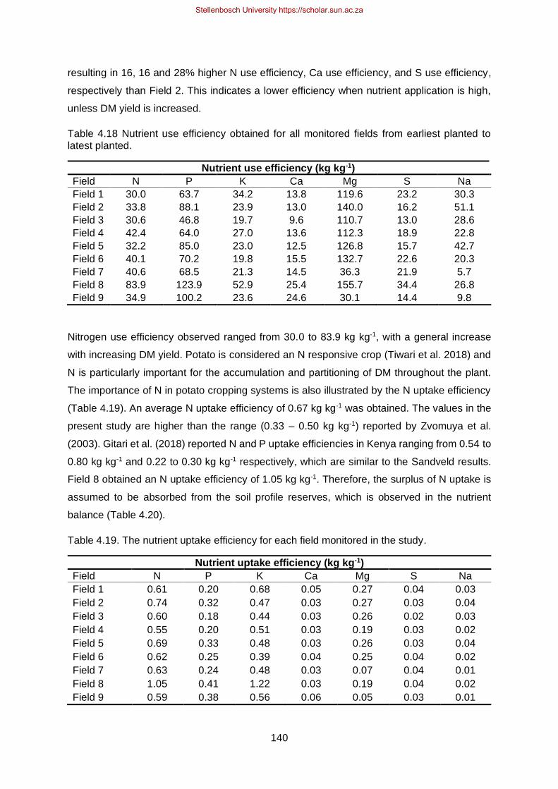
140
resulting in 16, 16 and 28% higher N use efficiency, Ca use efficiency, and S use efficiency,
respectively than Field 2. This indicates a lower efficiency when nutrient application is high,
unless DM yield is increased.
Table 4.18 Nutrient use efficiency obtained for all monitored fields from earliest planted to latest planted.
Nutrient use efficiency (kg kg-1)
Field N P K Ca Mg S Na
Field 1 30.0 63.7 34.2 13.8 119.6 23.2 30.3
Field 2 33.8 88.1 23.9 13.0 140.0 16.2 51.1
Field 3 30.6 46.8 19.7 9.6 110.7 13.0 28.6
Field 4 42.4 64.0 27.0 13.6 112.3 18.9 22.8
Field 5 32.2 85.0 23.0 12.5 126.8 15.7 42.7
Field 6 40.1 70.2 19.8 15.5 132.7 22.6 20.3
Field 7 40.6 68.5 21.3 14.5 36.3 21.9 5.7
Field 8 83.9 123.9 52.9 25.4 155.7 34.4 26.8
Field 9 34.9 100.2 23.6 24.6 30.1 14.4 9.8
Nitrogen use efficiency observed ranged from 30.0 to 83.9 kg kg-1, with a general increase
with increasing DM yield. Potato is considered an N responsive crop (Tiwari et al. 2018) and
N is particularly important for the accumulation and partitioning of DM throughout the plant.
The importance of N in potato cropping systems is also illustrated by the N uptake efficiency
(Table 4.19). An average N uptake efficiency of 0.67 kg kg-1 was obtained. The values in the
present study are higher than the range (0.33 – 0.50 kg kg-1) reported by Zvomuya et al.
(2003). Gitari et al. (2018) reported N and P uptake efficiencies in Kenya ranging from 0.54 to
0.80 kg kg-1 and 0.22 to 0.30 kg kg-1 respectively, which are similar to the Sandveld results.
Field 8 obtained an N uptake efficiency of 1.05 kg kg-1. Therefore, the surplus of N uptake is
assumed to be absorbed from the soil profile reserves, which is observed in the nutrient
balance (Table 4.20).
Table 4.19. The nutrient uptake efficiency for each field monitored in the study.
Nutrient uptake efficiency (kg kg-1)
Field N P K Ca Mg S Na
Field 1 0.61 0.20 0.68 0.05 0.27 0.04 0.03
Field 2 0.74 0.32 0.47 0.03 0.27 0.03 0.04
Field 3 0.60 0.18 0.44 0.03 0.26 0.02 0.03
Field 4 0.55 0.20 0.51 0.03 0.19 0.03 0.02
Field 5 0.69 0.33 0.48 0.03 0.26 0.03 0.04
Field 6 0.62 0.25 0.39 0.04 0.25 0.04 0.02
Field 7 0.63 0.24 0.48 0.03 0.07 0.04 0.01
Field 8 1.05 0.41 1.22 0.03 0.19 0.04 0.02
Field 9 0.59 0.38 0.56 0.06 0.05 0.03 0.01
Stellenbosch University https://scholar.sun.ac.za

141
The K uptake efficiency for Field 8 showed a similar trend to N. A value larger than 1 was
obtained (1.22 kg kg-1), therefore 0.22 kg kg-1 of the K taken up by the plant was provided by
a source other than fertiliser or water application and can then be presumed to have been
provided by the soil (Table 4.22). The average uptake efficiency for K in the region was
0.57 kg kg-1. These high values indicate the importance and efficiency with which the potato
plant absorbs both N and K. Lower values for P, Ca, Mg, S and Na, 0.28, 0.04, 0.19, 0.03 and
0.02 kg kg-1, respectively, were obtained in the study. Nutrients such as S and Na, however,
are not required in large amounts by potato plants. The average results obtained in this study
for NUtE ranged from 60 to 1041 kg kg-1 (N and Na, respectively) (Table 4.17). The high Na
utilisation efficiency is due to the small concentration of Na present within the plant; therefore,
the utilisation of nutrients present in small concentrations is high and increases with an
increasing DM yield. The same is observed for nutrients P, Ca, Mg and S (286, 434, 548 and
618 kg kg-1 respectively) However, potato plants require these nutrients in smaller quantities
than N and K (refer to Table 4.12). The Sandveld region has a mean N utilisation efficiency
and K utilisation efficiency of 60 and 48 kg kg-1 respectively. The lower values are accredited
to the high presence of these nutrients in the plant due to a higher uptake efficiency and the
requirement of these nutrients in larger concentrations than others, particularly during the
vegetative growth stage.
Nutrient harvest Index refers to the ratio of tuber nutrient uptake to plant nutrient uptake. Since
nutrients within the roots have little influence on nutrient partitioning within the potato plant,
root nutrient content is assumed negligible. Nutrient harvest index is a parameter that indicates
the partitioning and re-translocation of nutrients from aboveground vegetative parts to tuber
growth and the efficiency at which the crop utilises the absorbed nutrients for tuber production.
Different crops utilise nutrients differently. Lopez-Bellido et al. (2003) reported mean N harvest
index values of 82% for faba bean (Vicia faba). Results in this study show that the mean N
harvest index for potato crops in the Sandveld region was 81%, with the lowest value of 76%
(Field 1) (Table 4.17). This indicates that potato is efficient at re-translocating N from the
aboveground plant system to tubers. However, da Silva et al. (2018) produced lower results
than obtained in the present study (81%), with an average N harvest index of 65% for potato
production under differing irrigation methods, with sprinklers producing the highest N harvest
index of between 66 to 70%. Zebarth et al. (2004) showed mean results of N harvest index at
69% for 20 cultivars grown in Canada, with rates of 100 kg ha-1 banded at planting.
Fageria (2014) reported a relationship between grain harvest index and yield, however, no
correlation between N harvest index and potato yield was observed in the present study. The
N harvest index did not increase with an increase in utilisation efficiency of N, as was
suggested by Fawcett and Frey (1983). The relationship between nutrient harvest index and
Stellenbosch University https://scholar.sun.ac.za

142
the fertiliser rate and environment is reported to be very complex and varies among cultivars
(Zebarth et al. 2004). However, nutrient harvest index is an important parameter that indicates
the efficiency with which absorbed nutrients are translocated from the vegetative plant parts
to the tuber. The mobility of an ion also plays a role in its re-translocation, as seen with Ca
(7% Ca harvest index).
4.3.4 Nutrient balance
Nutrient balance calculations were conducted to estimate the residual nutrient content, which
refers to the applied nutrients, left in the soil after harvest (to a depth of 1 m) or lost by runoff.
Negative values indicate that more nutrients were taken up by the crop than was supplied
through fertilisers and water application. It can be assumed that negative nutrient balances
resulted from a supply of nutrients to the crop by the soil.
The N inputs and losses (Table 4.20) for Field 2 and 3 are balanced, with only 1.1 kg N ha-1
left in the soil and or lost as runoff and 0.2 kg N ha-1 taken up by the plant, in excess of nutrient
and water application, from the soil, respectively. For Fields 5 and 9 large amounts of N
application occurred from irrigation water, which resulted in an excess of N left in the profile
or lost as runoff. Field 5 had a residual value of 69 kg N ha-1 and Field 9 102 kg N ha-1.
Field 2 also had a large application of N through irrigation water, however, substantial leaching
occurred at 86 kg N ha-1, in comparison to Fields 5 and 9 (34 and 44 kg N ha-1, respectively).
Field 8, on the other hand, mined substantial amounts of N from the soil profile (80 kg N ha-1)
as a result of large yields obtained.
Giletto and Echeverria (2013) reported residual soil N at harvest, ranging from 54.2 to
62.5 kg ha-1 to a depth of 60 cm in the soil profile. The same study reported that inputs of 299
kg N ha-1 resulted in N outputs of 235 kg ha-1. The loss of N via plant removal and leaching
was larger in the present study. Roy et al. (2001) indicated that at high fertiliser rates (150%
of the recommended rate) resulted in positive nutrient balances. This was difficult to report on
in the present study due to the application of similar fertiliser rates in the Sandveld. Therefore,
the nutrient balance was mainly determined by leaching and plant nutrient removal rates. The
results obtained in the Sandveld are consistent with those reported by Shepherd and
Postma (2000) and Giletto and Echeverria (2013), who concluded that the amount of water
drained and amount of N applied as fertiliser influenced the residual N remaining in the soil
after harvest. Due to the long rotation period of potato crops, it can be assumed that the
majority of the N left in the soil after harvest will be lost during the fallow periods.
Stellenbosch University https://scholar.sun.ac.za

143
Table 4.20. Nitrogen nutrient balance conducted for intensively monitored fields. Residual refers to the nutrients left in the soil after harvest or lost via runoff and plant nutrient removal includes both tuber and haulm nutrient removal.
Nitrogen (kg ha-1)
Field Fertiliser Water Leached Plant nutrient removal Residual
Field 2 302 30 86 244 1.1
Field 3 294 0.0 118 176 -0.2
Field 5 302 34 34 233 69
Field 7 288 0.0 0 180 108
Field 8 294 0.0 66 308 -80
Field 9 302 51 44 207 102
The results showed substantial amounts of P left in the soil profiles or lost as runoff at the end
of the crop seasons (Table 4.21). Field 3 was the only intensively monitored field where the
crop used more P than was applied by fertiliser and water, with an excess of 1.5 kg P ha-1
having been taken up from the soil by the crop. However, contributing to the low P negative
value was the substantial P leached of 160 kg ha-1. All the other monitored fields where
drainage was collected had positive residual values ranging from 17 to 101 kg P ha-1. Field 8
had a large application of P through fertiliser and water with very little leached, hence the
reason for the large amount of P left in the soil profile. The results indicate that large amounts
of P are not used by the crop or lost, thus, potentially resulting in a build-up or runoff loss, as
reported by Alva et al. (2011).
Table 4.21. Phosphorus nutrient balance conducted for intensively monitored fields. Residual refers to the nutrients left in the soil after harvest or lost via runoff and plant nutrient removal includes both tuber and haulm nutrient removal.
Phosphorus (kg ha-1)
Field Fertiliser Water Leached Plant nutrient removal Residual
Field 2 125 1.5 11 41 76
Field 3 189 3.5 160 34 -1.5
Field 5 125 1.7 15 42 70
Field 7 167 4.1 0 41 129
Field 8 189 10.3 16 82 101
Field 9 118 4.9 60 46 17
Potassium was taken up by the crop in excess from the soil in very large quantities
(Table 4.22) in Field 8 (374 kg K ha-1), however, this was caused by the substantial removal
of K from plant uptake (tuber and haulm) (567 kg K ha-1) and the large levels leached
(273 kg K ha-1). The large mining of K by the crop in Field 8 indicates the availability of
substantial K in the profile from previous crops. Fields 2 and 3 had similar nutrient inputs and
losses, which resulted in similar K levels left in the soil profile or lost as runoff (80 and
Stellenbosch University https://scholar.sun.ac.za

144
95 kg K ha-1, respectively). Fields 5 and 9 did not incur large levels of leached K below a 1 m
depth, compared to the other monitored fields. However, Fields 5 and 9 had large applications
of K onto the fields (from fertiliser and water), resulting in large amounts of K assumed to be
left in the soil profile preceeding harvest.
Table 4.22. Potassium nutrient balance conducted for intensively monitored fields. Residual refers to the nutrients left in the soil after harvest or lost via runoff and plant nutrient removal includes both tuber and haulm nutrient removal.
Potassium (kg ha-1)
Field Fertiliser Water Drainage Plant nutrient removal Residual
Field 2 459 8.9 166 222 80
Field 3 454 4.2 160 203 95
Field 5 459 10.3 17 224 228
Field 7 495 55.0 0 263 287
Field 8 454 12.2 273 567 -374
Field 9 443 80.0 76 292 154
There was a negative Ca and S balance (70 and 94 kg ha-1) (Tables 4.23 and 4.24) in the
profile of Field 9 due to no application of gypsum prior to cropping. Substantial amounts of Ca
and S were left in the soil profile or lost as runoff for Fields 2, 3 and 5 after harvest as a result
of pre-planting gypsum application. These amounts left in the soil profile ranged from 41 to
683 kg Ca ha-1 and 355 to 559 kg S ha-1. Field 8, on the other hand, had large amounts of Ca
and S inputs into the soil profile. However, a loss of 900 kg Ca ha-1 occurred, resulting in lower
levels left in the soil or lost as runoff (41 kg Ca ha-1). Sulphur was also leached in large
amounts at 814 kg S ha-1, resulting in the excess plant uptake of S from the soil profile of
126 kg S ha-1. Magnesium was mined by the crops in Fields 2 and 8 (Table 4.25). A total of
35 and 44 kg Mg ha-1, respectively, was likely obtained from the soil profiles. Plant nutrient
removal was similar for all fields, ranging from 21 to 29 kg Mg ha-1. Application of large
amounts of Mg through fertilisers is not practiced in the region and ranged from 8 to
46 kg Mg ha-1. However, Mg is present in large concentrations in irrigation water and hence
the substantial application of Mg through irrigating is observed, which influenced the large
leached rates obtained.
Stellenbosch University https://scholar.sun.ac.za

145
Table 4.23. Calcium nutrient balance conducted for intensively monitored fields. Residual refers to the nutrients left in the soil after harvest or lost via runoff and plant nutrient removal includes both tuber and haulm nutrient removal.
Calcium (kg ha-1)
Field Fertiliser Water Drainage Plant nutrient removal Residual
Field 2 841 18.5 268 28 564
Field 3 924 16.4 242 27 672
Field 5 841 21.4 152 28 683
Field 7 603 201.2 0 28 776
Field 8 924 47.7 900 31 41
Field 9 217 283.9 542 29 -70
Table 4.24. Sulphur nutrient balance conducted for intensively monitored fields. Residual refers to the nutrients left in the soil after harvest or lost via runoff and plant nutrient removal includes both tuber and haulm nutrient removal.
Sulphur (kg ha-1)
Field Fertiliser Water Drainage Plant nutrient removal Residual
Field 2 679 9.7 314 20 355
Field 3 677 13.8 170 17 504
Field 5 679 11.2 112 20 559
Field 7 433 102.0 0 19 516
Field 8 677 40.3 814 28 -126
Field 9 106 748.5 927 22 -94
Table 4.25. Magnesium nutrient balance conducted for intensively monitored fields. Residual refers to the nutrients left in the soil after harvest or lost via runoff and plant nutrient removal
includes both tuber and haulm nutrient removal.
Substantial positive nutrient balances obtained in this study indicate that in general, over
application of nutrients in potato cropping systems is occurring in the Sandveld region.
However, in certain cases (in fields that negative nutrient balances occurred) it was observed
that a larger uptake of nutrients by crops, compared to what was applied through fertiliser and
irrigation water took place. Abdul Mojid and Wyseure (2014) reported similar findings for N
and K when fertiliser application did not meet the nutrient requirement of the crop. However,
Magnesium (kg ha-1)
Field Fertiliser Water Drainage Plant nutrient removal Residual
Field 2 46 34.4 94 21 -35
Field 3 41 40.2 43 21 17
Field 5 46 39.8 38 22 26
Field 7 59 264.2 22 301
Field 8 41 117.3 173 29 -44
Field 9 8 401.0 332 22 55
Stellenbosch University https://scholar.sun.ac.za

146
in the Sandveld, nutrient application was sufficient to meet crop nutrient removal, with the
exception of Field 8 with regards to N and K. Field 8 produced substantial yields, which
resulted in large plant nutrient removal. The negative nutrient balances reported in the present
study arise from the high levels of nutrients lost by leaching below the root zone due to the
low nutrient holding capacities of the sandy soils. Although, in the cases when less nutrients
were applied than was taken up by the crop and lost by drainage, it indicates that nutrients
are available in the soil from previous crops and adjustment of fertiliser applications to soil
analysis may be a possible future strategy to prevent substantial nutrient losses. However, the
extent at which nutrients are lost due to rainfall during fallow periods must be investigated.
The large requirement of N and K is observed through the high levels of plant removal,
followed by P. Calcium, Mg and S are removed in smaller and similar quantities. The large
amounts of P, Ca and S, left in the soil after leaching and cropping can be ascribed to various
factors. The low absorption and leaching of P (in most cases) is due to the lack of mobility
within the soil profile and binding/precipitation with other ions. Calcium is reported as an
immobile ion in soil and does not move through the profile easily, however, there is a great
input of Ca and S into these systems and great losses by leaching occurred. The lack of uptake
efficiency for Ca and S resulted in a build-up in soil profiles.
It is expected that residual values obtained in the study (Tables 4.20 to 4.25) should
correspond with soil analyses results (Appendix II). A comparison was conducted; however,
the agreement was poor. One possible explanation is that soil samples were conducted to a
depth of 0 to 90 cm, therefore a large mass of soil was used. Thus, a small error (in sampling
or nutrient analysis), may result in huge errors in the calculated nutrient amount (kg ha-1)
present in the soil. Another possible reason is that drainage was collected at a depth of 1 m
and soil samples were only conducted to a depth of 90 cm. Therefore, the exclusion of 10 cm
of soil occurred, which per ha and field contributed to a substantial amount of nutrients not
accounted for in the soil analysis.
4.4 Tuber yield and size distribution
4.4.1 Tuber yield
Yield potentials calculated using the LINTUL DSS potato model (Haverkort et al. 2015)
assume no abiotic or biotic limitations to crop growth. The results obtained varied from
46.2 t ha-1 for the early March planting to 89.9 t ha-1 for the late November planting. The highest
actual yield obtained between the studied sites for the variety FL2108 and Sifra were
57.5 t ha-1 and 118.2 t ha-1, respectively. The cultivar FL2108 used in the majority of the sites
Stellenbosch University https://scholar.sun.ac.za

147
is not as high a yielding variety as Sifra. Yield potentials were lowest for the March plantings
due to these crops growing mostly through the cloudy winter months, when available solar
radiation was the most limiting factor to production. Yield potentials increased with later
planting dates (May and June), as these crops grew into spring and early summer, when more
solar radiation was available. Crops planted in July grew into the hot and dry summer months,
which caused more heat stress, as seen for Field 7, in spite of more available radiation,
resulting in a yield suppressing effect, which agrees with reports by Zhou et al. (2016) and
Paul et al. (2016). However, summer planted crops (Fields 8 and 9) obtained 132 and 65% of
the calculated yield potential, suggesting negligible negative effect of heat stress on the crops.
This may at least partly be explained by the fact that crops were irrigated frequently with large
amounts of water, which helped to cool the canopy down and thus created conditions
conducive for growth. Field 9, due to its location close to the Atlantic Ocean, had a cooler
microclimate caused by cool winds blowing from the cold ocean. However, often fog from the
ocean blew over this field, resulting in a lowered yield potential due to less available solar
radiation.
The actual yields achieved ranged from 34.7 t ha-1 (Field 1) to 118.2 t ha-1 (Field 8), which
were 75 and 132% of the calculated potential yield, respectively. It is reported that high
temperatures reduce the crop’s photosynthetic capacity and increase respiration, resulting in
reduced radiation use efficiency and thus, biomass accumulation (Haverkort et al. 2013).
However, the cardinal temperatures affecting photosynthesis and radiation use efficiency as
used by the LINTUL DSS potato model, penalises photosynthesis severely when hot
temperatures occur. The radiation use efficiency of 2.5 g DM MJ-1 PAR used in the model,
under optimal conditions, is perhaps also too low and needs to be reassessed (Personal
Communication, AC Franke; unpublished data). Therefore, the fields producing yields higher
than the potential yields (Fields 2 and 8) was a result of the model penalising photosynthesis
at temperatures above 30 °C. Both Fields 2 and 8 obtained substantial periods of high
temperatures (Appendix IIIa). It was also indicated that ET cooling leads to lower canopy
temperatures compared to ambient temperatures, reducing the heat experienced by the crop
during summer months and that the inclusion of ET cooling in the model may improve yield
simulations (Personal Communication, AC Franke; unpublished data).
Actual yields higher than 66% of the yield potential are acceptable, while values above 75%
can be considered good. Yield potential during the winter growing periods in the Sandveld is
limited by less available solar radiation (Ierna 2009; Zhou et al. 2016). Tang et al. (2018)
indicated a positive correlation between yield and total radiation during the growth period of
potato crops in North China, which is in agreement with a study conducted in South Africa by
Steyn et al. (2016). In spite of the wide range of yields recorded, actual yields for seven of the
Stellenbosch University https://scholar.sun.ac.za

148
monitored fields were above 75% of the potential, which suggests that available resources
were used efficiently. Fields 3 and 9 obtained an actual yield of 54 and 65% of the potential
yield attainable, respectively. A number of factors can cause these low values. Field 3 received
large amounts of rainfall and therefore, leaching of nutrients was high, resulting in less
availability for uptake. Early crop development also occurred during cool temperatures and
lack of solar radiation. Field 9, on the other hand, was planted in summer and received
sufficient solar radiation, however, similarly to Field 3, temperatures were cool throughout crop
growth. Substantial leaching also occurred in Field 9 due to over irrigation, potentially affecting
yields negatively.
Table 4.26. Potato tuber yield, simulated potential tuber yield and the ratio of actual to potential yield for monitored Sandveld fields.
4.4.2 Tuber size distribution
Across all fields, 44.8% of the tubers were classified as medium and 30.7% as small
(Figure 4.48). A maximum of 56.4% (Field 7) was observed for the medium classed tubers
and a minimum of 26.8% (Field 5). Field 5 produced the highest proportion of tubers in the
small class (60.1%), with Field 8 producing the lowest number of small tubers (8.4%). Only
66% of the fields under observation produced large tubers, with Fields 5, 3 and 1 producing
no tubers in the large class. The highest proportion of large tubers observed for cultivar
FL2108 was for Field 6 (6.0%). This high proportion of large tubers can be attributed to the
Type Field Tuber yield
(t ha-1)
Potential yield
(t ha-1)
Actual : potential yield
Inte
ns
ive
Field 2 51.6 46.6 1.11
Field 3 41.5 77.1 0.54
Field 5 49.8 67.2 0.74
Field 7 53.9 58.0 0.93
Field 8 118.2 89.3 1.32
Field 9 59.0 89.9 0.65
Ex
ten
siv
e Field 1 34.7 46.2 0.75
Field 4 57.5 71.8 0.80
Field 6 51.2 53.9 0.95
Stellenbosch University https://scholar.sun.ac.za

149
clay layer producing a water table, resulting in an abundance of water and nutrient availability
within the tuber zone during the bulking phase. In general, FL2108 is not a large tuber
producing cultivar, which is preferred by the crisp processing industry. In comparison, the
cultivar Sifra (Fields 8 and 9) produced 25.6 and 1.8% tubers classed as large, respectively.
Overall Field 8 produced the better tuber size distribution. Field 1 was infected by late blight
(Phytophthora infestans), which could have attributed to poor tuber bulking and development
due to early senescence. The crop for this field was terminated early and the low total water
and nutrient amounts applied will have resulted in smaller tubers developed. In contrast, Field
3 was observed as a healthy crop throughout growth, with the application of adequate water
and nutrients. However, temperatures were low with an average of 15.9°C for the growth
season. Walworth and Carling (2002) suggest that larger tubers are favoured by irrigation.
However, the results obtained for Field 3 contradict this statement, as more than adequate
amounts of water was available. The lack of large tuber production may have been influenced
by the amount of drainage occurring due to an oversupply of water (rain and irrigation),
resulting in nutrient leaching and a lack of sufficient available nutrients. The proportion of
tubers classed as medium, medium-large and large was lowest for the March planted fields
and increased for May and June as well as November and December plantings, with the
exception of Field 7 (which was slightly under irrigated). The increase in the portion of larger
tubers occurred with the increase in temperature and available solar radiation, which improved
the plant’s ability to utilise resources more efficiently due to an increased photosynthetic
activity and production of assimilates. Therefore, the increase in tuber size distribution is
directly correlated with an increase in yield.
Stellenbosch University https://scholar.sun.ac.za

150
Figure 4.48. Size distribution of harvested tubers. From top to bottom is the earliest to latest planted fields. Rule for size classification: Baby (5-
50g), Small (50-100g), Medium (90-170g), Medium-Large (150-250g), Large (>250g
0 10 20 30 40 50 60 70 80 90 100
Field 9
Field 8
Field 7
Field 6
Field 5
Field 4
Field 3
Field 2
Field 1
%
Large Medium-Large Medium Small Baby
Stellenbosch University https://scholar.sun.ac.za

151
CHAPTER 5: CONCLUSIONS AND RECOMMENDATIONS
The aim of this study was to quantify inputs and losses occurring in potato production systems
in the Sandveld region of the Western Cape. The study was conducted in order to close the
gap in knowledge with regard to water and nutrient leaching under current management
practices. The research did not look at altering management strategies to improve production,
but investigated current potato cropping inputs and losses and through that, recommendations
of how best to improve efficiencies along with further enhancements to the research can be
made. The benefit of quantifying losses and system inefficiencies for producers will allow them
to optimise production and reduce unnecessary input costs. Apart from agronomic and
economic benefits for farmers of improved nutrient and water use efficiencies, the need to
protect the fragile ecosystem present within the Sandveld region is also evident. Nutrient
leaching into groundwater and water sources, as well as refining and preventing excessive
waste of water, should be limited. By understanding the causes of drainage, crop
evapotranspiration changes and climatic conditions throughout the growth cycle, management
practices to optimise inputs and resource use efficiency can be recommended as well as future
research requirements. To address these needs, the study was approached through four
objectives:
1. To assess the efficiency of irrigation systems with regards to water application in the
Sandveld growing region.
2. To compare actual water application with simulated crop irrigation requirements and
identify crop water needs for specific growing seasons to assess potential over- or
under-irrigation.
3. To quantify drainage and assess the effect of irrigation water and rainfall on drainage
accumulation and water use efficiency as well as to investigate methods of irrigation
scheduling to improve efficient water use in the region.
4. To compare actual yields with simulated attainable yields and explore management
strategies that can be implemented to increase nutrient use efficiency.
The set objectives were addressed as follows in the study:
Stellenbosch University https://scholar.sun.ac.za

152
Objective 1: To assess the efficiency of irrigation systems with regards to water
application in the Sandveld growing region.
The lack of knowledge regarding the efficiency of irrigation systems was indicated for the
region. Irrigation systems are generally only evaluated during installation. Due to the harsh
climatic conditions as well as brackish water used, it is notable that the irrigation structures
and equipment deteriorate over time. Therefore, the need for repeated evaluations of centre-
pivot efficiencies in the region is evident, as it is currently non-existent. The majority of the
efficiency parameters evaluated were above the acceptable norms as provided within the
literature (Clemmens and Dedrick 1994; Savva and Frenken 2002; Reinders 2013; Abd El-
Wahed 2016). Efficiency parameter values for the application efficiency (AE), coefficient of
uniformity (CUHH) and distribution uniformity of the lowest quarter (DUlq) ranged from 64 to
99%, 81 to 93% and 70 to 89%, respectively. There is, however, still room for improvement,
which can be conducted through the periodic evaluation of irrigation systems (~ every one to
two years) with the goal of improving parameters to > 90%. This should contribute to an
increase in water use efficiency (WUE) and reduction in unnecessary water losses.
Fields 2, 6 and 8 produced application efficiency values below the acceptable norm (76, 77
and 64%, respectively) resulting in the need to over-irrigate by 24, 23 and 36%, respectively
in order to apply the correct quantity of water. The low AE values caused the producer’s
perception of the amount of water being applied to vary from the actual irrigation application.
This was clearly indicated for Field 6. The famer set the pivot to apply 10 mm of water per
cycle when the actual application was 5.3 mm. The cause of poor AE is a result of various
factors. Field 6 was observed to have a very low operating pressure (50 kPa) measured at the
last pivot tower (normal operating pressures range from 70 to 500 kPa) and therefore, this
contributed to the reduced application of water. On the other hand, Field 8 showed a low AE
due to the large height of the spray nozzle heads from the crop surface, as well as the nozzles
used, which produced fine droplets. Due to the windy conditions where the field was situated,
the high nozzle heights and fine spray resulted in large water dispersion. A preventative
measure is to drop the nozzle head heights closer to the crop and replace the spray nozzles
with ones that produce larger droplets to reduce the effect of wind dispersion. Other efficiency
parameters such as CUHH and DUlq were acceptable for all fields, with the exception of Fields
2 and 5, which were located on the same farm. The low CUHH and DUlq values resulted in the
non-uniform application of water and water-soluble fertilisers throughout the field causing an
uneven crop, affecting the yields negatively. The monitoring of the location of faulty nozzles
was carried out during the system evaluation. Faulty nozzles should be replaced in order to
correct and improve the distribution of water along the center-pivot boom.
Stellenbosch University https://scholar.sun.ac.za

153
Further to this is the recommendation to producers to monitor total water application during
the season, which can be conducted satisfactorily with the use of electromagnetic flow meters
or pressure transducers, as illustrated from the results. Pressure transducers are a more
viable tool when cost is a factor, as it is an instrument that provides a cost saving of up to
75%, compared to flowmeters. The pressure transducers also gave an accurate measure of
water application, with readings only varying from electromagnetic flow meters by 4.5 to 6.4%
on average.
The overall improvement of irrigation system efficiencies and monitoring of water applications
will cause an increase in the accuracy of applied water to meet the simulated crop water
requirements, which is discussed in Objective 2 of the study.
Objective 2: To compare actual water application with simulated crop irrigation
requirements and identify crop water needs for specific growing seasons to assess
potential over- or under-irrigation.
From Objective 1 it was observed that actual irrigation application varied from that of the
perceived amount being applied by the farmers. Generally, producers tend to over apply water
in order to combat losses due to system inefficiencies and rapid water loss occurring from the
sandy textured soil profiles. Therefore, with improved application efficiencies will come the
need to match simulated crop water requirements to optimise water use efficiencies (WUE).
Crop evapotranspiration (ET) for the studied Sandveld fields were quantified by developing
basal crop coefficient curves for autumn, winter and summer planted fields. The need for the
adjustment of standard FAO Kcb values was observed. Basal crop coefficient values used for
100% canopy cover until senescence [Kcb(mid)] were 3.7% higher than the standard FAO-56
values suggested by (Allen et al. 1998). The basal crop coefficient curve values used for the
end of crop growth [Kcb(end)] were on average 9.5% higher than the FAO suggested value.
This resulted in the under-estimation of crop water demands if standard FAO values are used
for the Sandveld. That also iterates the need for specific field adjustments or seasonal
adjustments as crops planted in autumn and summer reached 100% ground cover quicker
and remained at full canopy cover for longer than crops planted in winter. This also indicates
the need to alter irrigation application according to crop ET demand, which is not commonly
practiced by growers in the region. The recommended [Kcb(ini)] values remain the same at
0.15 for the different planting periods, [Kcb(mid)] and [Kcb(end)] values suggested for the
Sandveld region are shown in Table 5.1.
Stellenbosch University https://scholar.sun.ac.za

154
Table 5.1: Adjusted basal crop coefficient values for various planting periods, which can be
used to create a basal crop coefficient curve to estimate crop water requirements for potatoes
grown in the Sandveld region.
Basal crop coefficient values
Kcb(mid) Kcb(end)
Autumn planted 1.10 0.64 Winter planted 1.14 0.72 Summer planted 1.10 0.65
The suggested basal crop coefficient curves provided a better estimation of total seasonal ET,
compared to that calculated using the soil water balance method and LINTUL DSS potato
model.
The ET obtained from the basal crop coefficient curves ranged from 188 to 647 mm for the
season. Crops planted in autumn had lower ET demand (188 – 266) than winter and summer
planted crops (305 – 346 mm and >350 mm, respectively). The basal crop coefficient values
slightly under-estimated ET, due to the underestimation of the evaporative component (E).
However, the ET(Kcb) estimations were a more realistic reflection of regional crop ET. The ET
simulated using soil water balances (SWB) over-estimated crop water requirements, due to
the runoff being assumed negligible during calculations, which was not always the case, as
observed in Fields 2 and 5. The LINTUL DSS model also provided a good estimation of crop
ET, however, errors occurred if the crop was allowed to die off naturally, and the assumption
is made that ET during the second half of the season declines linearly, which is not the case,
as was illustrated by Eddy covariance measurements (Personal Communication, AC Franke;
unpublished data). Therefore, it is evident that adjusted Kcb curves can be a useful tool for
irrigation scheduling in the Sandveld region. Further investigation into the ET(SWB) and the
effect of runoff on ET estimation is required as well as the adjustment of the LINTUL DSS
model to account for the non-linear decrease in ET during the second half of the season.
Various studies have been conducted on different irrigaiton strategies in potato cropping
systems in order to optimise water management and improve WUE (Kashyap and Panda
2003; Yuan et al. 2003; Badr et al. 2012). The alteration of irrigation to crop physiological
demands has indicated that the sensitive stages to water requirements are the vegetative and
ripening stages (Fabeiro et al. 2001). Stalham and Allen (2004) suggested that partial deficit
irrigation techniques do not affect overall plant growth. Carli et al. (2014) indicated the potential
to increase WUE when decreasing water application after tuberisation, which had a limited
effect on tuber yield. Alenazi et al. (2016) indicated the ability to increase WUE by applying
75% of the crop ET at the tuber bulking stage, without a negative influence on yield, in an arid
Stellenbosch University https://scholar.sun.ac.za
155
region of Saudi Arabia. Other studies have however, indicated decreased yields due to deficit
irrigation (Alva 2004; Badr et al. 2012). However, due to the rapid depletion of water from the
very sandy soil profiles in the Sandveld growing area, farmers have limited opportunity to
employ most of the above strategies, since the soils hold so little water, which means they can
also not leave substantial room for rainfall in the profile.
One of the few strategies available to Sandveld growers is to match irrigation with crop water
requirements during different growth stages. Currently irrigation is not altered according to
crop needs in most cases, resulting in an over application of water, particularly during winter
grown crops due to the effect that rainfall has on the increased potential of drainage to occur.
The need to evaluate the effect of rainfall and over irrigation on drainage and quantifying the
amount of drainage occurring in Sandveld potato fields was assessed in Objective 3.
Objective 3: To quantify drainage and assess the effect of irrigation water and rainfall
on drainage accumulation and water use efficiency as well as to investigate methods
of irrigation scheduling to improve efficient water use in the region.
Water application through irrigation in winter-grown periods ranged from 260 to 582 mm and
was dependent on rainfall occurrence. With the inclusion of rainfall, winter-grown crops in
2018 received total water inputs for the season ranging from 531 to 744 mm. The actual water
application was therefore, substantially larger than the irrigation requirement (IR) which was
calculated using the ET demand as discussed in Objective 2 and the AE of irrigation systems
as discussed in Objective 1. It was clearly observed that high water inputs through irrigation
and rainfall during periods of low ET demand, resulted in an increase in drainage
accumulation. Drainage amounts during winter periods ranged from 4 to 296 mm. The
application of pre-planting irrigation contributed to the quicker saturation of soil profiles. This
was clearly observed for Field 7, which had a dry sub-soil profile at planting. The field applied
similar irrigation amounts to Field 2, however, it received 71 mm of rainfall compared to 486
mm. The drier soil profile contributed to the lack of drainage collected (4 mm) as well as good
WUE was measured and hence, may be a strategy to consider for producers and future
research.
Summer grown fields, on the other hand, produced large amounts of drainage due to the
practice of high frequency irrigation during this period as a result of high temperatures and
wind speeds during the summer months. Due to higher average temperatures, the emergence
of above-ground potato growth occurs rapidly (7 – 14 days from planting to emergence).
Therefore, this results in the profile still containing significant water from pre-planting irrigation
applications. The wet soil profile, along with large water inputs (648 and 913 mm) and high
Stellenbosch University https://scholar.sun.ac.za

156
irrigation frequency and amounts resulted in profile saturation and large amounts of drainage
occurring (233 – 302 mm, respectively).
An average WUE of 85 kg mm-1 was obtained in the study. This average lies above the
acceptable norm, which ranges from 75 to 80 kg mm-1 (Steyn et al. 2016), with winter grown
crops obtaining 79.5 kg mm-1 and summer grown 104.2 kg mm-1. The reason for lower WUE
obtained during winter periods results from the lower yield potential due to a lack of available
solar radiation and increased disease pressure (Field 1). Large rainfall events occurring during
winter also give rise to substantial drainage accumulation for some of the fields, contributing
to a low WUE. All fields with WUE values lower than the acceptable norm received substantial
rainfall (between 143 and 271 mm) during the cropping season. When excluding rainfall, IWUE
values indicated a higher efficiency, ranging from 88 to 134 kg mm-1. However, the effect of
rainfall cannot be ignored due to its large impact on leaching. Summer grown crops produced
larger WUE values (86.2 and 122.2 kg mm-1). The higher average temperatures, increased
solar radiation and the lack of (or much less) rainfall contribute to an increased WUE as
conditions were more conducive for increased yields than winter grown crops. The need for
over application of water in order to combat the build-up of salts from the use of brackish
irrigation water was mentioned by growers. This should be studied further, although only
summer planted crops showed a tendency of drainage having higher EC levels
(>170 mS m-1) for long periods. This was caused by the high frequency of irrigation and lack
of rainfall associated with the time of year. The leachate for winter grown fields generally
remained at lower EC levels due to substantial rainfall occurring, which resulted in the natural
leaching of salts out of the profile. The leaching requirement calculated for the year was low,
ranging from 0.04 to 0.27. However, irrigation water sources were only measured once for
each field and, due to farmers using various water sources, is subject to variation throughout
the cropping season. Hence, constant measurement of the water source EC is recommended
for future research. It is evident that due to the crop rotation of potato systems (one-year
cropping, four to six years fallow) the need for leaching is negligible, as natural leaching will
occur during winter periods when fields are fallow.
Farmers in the region did not have any form of device or tool to measure / assess soil water
content, while a few were seen to dig soil pits once a week or every two weeks to observe the
wetness of the soil. Generally, irrigation took place according to past experiences. Weather
station data provided good information regarding the potential occurrence of drainage events
and is recommended as an indicator. The use of basal crop coefficient curves for different
planting times (autumn, winter and spring) in combination with ETo (available from local
weather stations) gave a good indication of actuall crop ET. This technique can, therefore, be
recommended for producers in the area to obtain an indication of crop water demands
Stellenbosch University https://scholar.sun.ac.za

157
(Objective 2). Although using the adjusted basal crop coefficient curves may cause a slight
under-estimate of ET, as the actual evaporation occurring during the early stages of crop
development is unknown, this method will be a more accurate measure of ET, compared to
current practices. A potential strategy for producers to also use, is to irrigate according to
canopy cover, which can be estimated with the eye or calculated using a 1 m2 grid. The canopy
cover factor can then be multiplied by the reference ET (ETo) obtained by a nearby weather
station, to give a good estimation of ET. Soil probes, such as capacitance probes, gave a good
indication of soil-water movement within the profile and can be recommended as an irrigation
management tool. Although, due to the mountainous topography, data collection via telemetry
was incomplete for a lot of the studied fields, the use of hand-held dataloggers for DFM probes
is advised. The movement of water indicated by the probes also gave an indication of when
drainage accumulation will occur, as peaks in soil water content as indicated by the DFM
graphical illustrations, coincided well with drainage collection. Decagon probes were the more
accurate measure of volumetric soil water content. However, the probes are less practical for
commercial use as readings must be periodically downloaded with a laptop in the field,
batteries need changing every fortnight and the cost of equipment is substantial in comparison
with DFM probes. Chameleon sensors, on the other hand, were not good indicators of the soil
water content in these sandy soils. Sensors did not correlate well with the Decagon and DFM
probes as readings within the same fields gave different values and often suggested saturated
conditions throughout the season when soil water content was suggested otherwise by the
DFM or Decagon probes. Hence, Chameleon sensors are not suggested for use as irrigation
scheduling tools within the Sandveld. The very sandy soil texture results in the inability of the
Chameleon sensors to equilibrate with the soil profile due to the low unsaturated hydraulic
conductivity of the sand.
It was clear that nutrient leaching was directly correlated with the drainage of water. As
drainage increased, so did the increase in the amount of nutrients lost below the effective root
zone of potato crops [~30 cm; Opena and Porter (1999)]. This was particularly notable when
large rainfall events or over-irrigation occurred. The wide use of water-soluble fertiliser
products in the area contributed to the high levels of nutrient leaching recorded. The alteration
of irrigation management to rainfall events was observed for winter-grown crops, but due to
the application of water-soluble fertilisers through ‘high-tech fertigation’, also took place on
days when substantial rainfall occurred or days preceding rainfall events. This contributed to
the saturation of soil profiles, drainage as well as the loss of nutrients during winter periods.
The need for a combination of water-soluble, less water-soluble and slow release fertilisers
should be evaluated as a potential mitigation strategy for alleviating large nutrient losses. It
was observed that large losses of Ca and S occurred due to the general practice of pre-plant
Stellenbosch University https://scholar.sun.ac.za

158
gypsum applications in the region. This resulted in a mean loss of 421 kg Ca ha-1 and 467 kg
S ha-1 through drainage below a 1 m depth of the soil profile. Sodium and Mg were also
leached at high levels due to these elements being present in large quantities in the irrigation
water sources (472 and 136 kg ha-1, respectively). The large amount of P leaching, with an
average of 52 kg P ha-1 and a maximum of 160 kg P ha-1 leached, was unexpected. However,
this is attributed to the high P levels measured in the soil during equipment installation
(Appendix II). On average, 70 kg N ha-1 and 138 kg K ha-1, were leached. However, high levels
of the applied N and K was absorbed by the crop (0.67 kg N and 0.57 kg K taken up per kg
applied). The effect of nutrient application and losses on nutrient use efficiency is, therefore,
evident and addressed in Objective 4.
Objective 4: To compare actual yields with simulated attainable yields and explore
management strategies that can be implemented to increase nutrient use efficiency.
Seven of the nine monitored fields produced actual yields >75% of the potential yield, as
calculated by the LINTUL DSS potato model, indicating the general efficient use of resources
in the region. A major limitation to the attainable yield was the amount of solar radiation during
the growth period as well as the heat factor. During winter periods, less solar radiation is
available in comparison to summer months, hence yield potential for summer months is higher.
However, crops that grew into hot, drier months had an increased possibility to incur heat
stress, which had a potentially negative effect on yields.
Nutrient use efficiency generally increased with an increase in dry matter (DM) accumulation,
however, it was negatively affected by high applications of nutrients. Fertiliser practices in the
region were similar, with a mean application of 288 kg N ha-1, 153 kg P ha-1 and 440 kg K ha-
1. Maximum application was 302, 189 and 522 kg ha-1 (N, P and K, respectively) and minimum
240, 118 and 217 kg ha-1 (N, P and K). The minimum application, however, occurred for Field
1, which was infected by late blight (Phytophthora infestans) towards the end of the season,
and hence, the crop was terminated early. Fields 2 and 6 clearly indicated the effect of nutrient
application on nutrient use efficiency, as both fields obtained similar DM yields. The nutrients
applied in lower amounts resulted in an increase in nutrient use efficiency. Due to the similar
fertilisation practices, changes in nutrient use efficiency were mainly a result of variation in DM
production for the different fields. Fields with high DM production (Fields 4 and 8) produced
good nutrient use efficiency values. All fields, with the exception of Field 9, obtained excellent
Mg use efficiency. This is attributed to by Mg not being applied in large quantities in these
potato production systems. The Mg applied was a result of irrigation water and hence, the
reason for Field 9 having a low Mg use efficiency. Calcium and S had low use efficiency values
Stellenbosch University https://scholar.sun.ac.za

159
due to the application of gypsum and S containing products early in the season. The nutrient
use efficiency of various elements is also a result of the uptake efficiency of nutrients by the
plant. The nutrients with low nutrient use efficiencies, except P, were absorbed at lower rates
by the potato crop, as illustrated by the nutrient uptake efficiency. Potato crops are large users
of N and K and hence, the reason for good N use efficiency and K use efficiency values ranging
from 30 to 83.9 and 19.7 to 52.9 kg kg-1, respectively. The P use efficiency values obtained in
the study ranged from 46.8 to 123.9 kg kg-1, but P uptake efficiency was low on average in the
region (28%). This is due to P being applied at lower rates than other nutrients. It is therefore,
clear that a decrease in nutrient supply while maintaining or improving yields is a potential
strategy relevant for low fertile soils such as those present within the Sandveld region.
Conversely, nutrient use efficiency (NUE) can be improved through an increased application
of fertilisers. However, an increase in yield must occur. The amount of leaching observed in
the study suggests a decrease in nutrient application to be the more ideal approach, as large
amounts of applied nutrients are not absorbed by the plant and are lost through drainage
below the effective rooting depth of potato cropping systems. Sandveld producers do not alter
nutrient fertiliser rates according to soil analysis results. Often commercial farmers have a
standardised regime for the majority of the fields located on a farm. The reduction in nutrient
level to balance those present within the soil profile is recommended as a possible strategy to
overcome high levels of nutrient leaching from soils in the Sandveld region and to optimise
NUE. Large residual values obtained by nutrient balances indicated that large amounts of
nutrients are left in the soil profile after harvest. It is also evident from negative nutrient
balances that it cannot be assumed there are no nutrients in the soil profiles available prior to
planting. This, along with the large levels of applied nutrients left in the soils indicated by
positive nutrient balances (on average 85 kg P ha-1, 530 kg Ca ha-1 and 349 kg S ha-1) after
harvest, may be used by a follow-up crop or result in reduced fertiliser need for the next potato
cropping season and requires further investigation. However, it indicates the need to reassess
fertiliser application rates required in potato cropping systems in the Sandveld region.
General conclusion
Drainage accumulation is a result of substantial rainfall during winter-grown crops and over
application through high irrigation frequencies and applications in summer planted fields.
Nutrient leaching is directly correlated with increased drainage. The need to evaluate centre-
pivot irrigation system efficiencies and further investigate the alteration of irrigation
management according to crop growth stages is evident, as well as the reassessment of
current fertiliser application rates and products used to increase nutrient use efficiencies.
Stellenbosch University https://scholar.sun.ac.za

160
Limitations of this research study
There were various limitations noted during the study:
Soil samples were collected during equipment installation, which was after pre-planting
fertilisation took place. Therefore, nutrients present in the analysis were not a true
representation of pre-planting soil conditions. However, all of the pre-planting fertilisation was
accounted for when looking at the soil analysis results and assumed to be present. The
fertiliser application was deducted from soil analysis results in order to obtain a more accurate
estimation of nutrients within the soil prior to planting. Soil bulk density values were used from
soil samples sent to the laboratory for analyses. This was not representative of the true bulk
density of the field. However, values were similar between the fields and for the two separate
sampling periods (during equipment installation and yield analysis).
Concerning the soil-water balance, runoff was assumed negligible. However, it was observed
in certain fields that runoff may have occurred, particularly in sloped fields along wheel tracks.
Water balances were conducted in order to measure inputs and outputs against each other to
observe if substantial losses may have occurred. There were no large errors in measurement
indicated.
The destructive nature of installing the drainage lysimeter affected a large area within the field.
It would be recommended looking into the use of an auger the size and depth of the lysimeter
to disturb less of the surrounding profile. However, in this study the best practices that could
be conducted with the equipment provided were carried out. Care was taken to ensure that
soil was placed back into the profile as it was removed and tubers were planted with the same
in-row spacing and depth as initial conditions.
The dry matter percentages for the variety FL2108 were calculated using specific gravity and
converted using tables (Haverkort 2018). This may not be a true representation of the DM %
as it is cultivar dependent. However, results were similar (slightly lower) to the DM measured
for Field 8 and 9 for Sifra, which is what was expected. A standard specific gravity value of
1.083 for the variety FL2108 was assumed due to errors that occurred in the measurement
procedure, due to the lack of specialised equipment available. Hence, the average values
provided by Simba Ltd for the variety FL2108 over a wide range of fields and planting dates
in the Sandveld for 2018 was used.
The importance of haulm nutrient removal was noted too late in the study. Therefore, this was
only carried out for Fields 8 and 9. Results for both fields were similar and hence, the average
Stellenbosch University https://scholar.sun.ac.za

161
of nutrients removed by the haulm in both fields was used. However, this may not be
representative of the variety FL2108 as both Fields 8 and 9 were planted to the cultivar Sifra.
Recommendations for future research
The effect of irrigation system efficiencies should be further assessed with regards to
correcting inefficient parameters and evaluating the effect of corrections on WUE. For
example, the height of the sprinkler heads for Field 8 should be evaluated and the effect it
may have on increased AE. Increased application efficiency along with the alteration of
irrigation scheduling according to the basal crop coefficient curves should be evaluated and
the effect that this method of estimating ET may have on yield and WUE in the Sandveld
region should be investigated. Using an ET estimation method alongside the use of soil
capacitance probes to schedule irrigation should be researched together with the variation of
lower limits of water depletion that are permitted before water is applied and this should be
assessed in the context of its impact on WUE.
Together with the monitoring of water application to reduce drainage and nutrient leaching
there is a need to assess the use of water-soluble, less water-soluble and slow release
fertiliser products during winter periods to alleviate large nutrient leaching losses occurring
due to substantial rainfall events. The use of less water-soluble fertilisers may result in
decreased leaching of nutrients due to a slower release. The practicality of applying fertilisers
in a solid form rather than through irrigation water can be placed under scrutiny as certain
farmers indicated that currently used broadcasters had varying spreading distances to the
distances chemical spray booms used. Therefore, the purchasing of new equipment to
standardise spray roads would need to be undertaken. The application of fertilisers will better
be understood with the reassessment of the nutrient uptake curve for potato crops in the
Sandveld region during autumn, winter and summer planted crops to observe the need of
different nutrients at various stages. This may help optimise fertiliser regimes for specific
cropping seasons in the area. The effect of nutrient leaching due to rainfall and over
application of nutrients, may be alleviated by the use of deep rooting cover crops immediately
after potato production. This is currently being conducted in other parts of South Africa
(Personal Communication, JM Steyn; unpublished data), but it will be beneficial to observe
the impact this may have in the Sandveld. The study on the effects that a deep rooting cover
crop would have on nutrient absorption may prevent groundwater contamination. Furthermore,
the understanding of the movement of nutrients in soil profiles within the Sandveld during
fallow periods could give an indication of the movement of nutrients post crop growth as well
as the effect that winter rainfall may have on nutrients when a crop is not grown or the field is
Stellenbosch University https://scholar.sun.ac.za
162
under natural vegetation. The monitoring of nutrient levels in groundwater sources after crop
growth should be conducted and will better aid the understanding of the environmental impact
that potato production may have in the region. The monitoring of salts in the soil as well as the
periodic evaluation of irrigation water quality throughout the season will also give a clearer
indication of whether there is a need for water application to leach excess salts and the
alteration of water salinity throughout the growth periods. With all of these suggested studies,
it will be necessary to quantify the cost and economics of growing potatoes with regard to
potential savings by preventing excessive nutrient leaching and improving WUE.
The use of hydrogels as soil conditioners has been studied extensively (Agaba et al. 2011;
Demitri et al. 2013; Guilherme et al. 2015). The main advantage of the use of hydrogels as
soil conditioners is the ability to control the release of stored water as the soil dries. Hydrogel
is able to absorb significant amounts of water by swelling and retaining the water (and
nutrients) within its structure (Fredric 1994). The ability of hydrogels to increase WUE has
been indicated by Narjary et al. (2013) due to their ability to absorb up to 500 to 600 times
their weight. Bhardwaj et al. (2007) concluded that mixing super absorbents (cross-linked
polyacrylamides) with sandy soils may decrease rates of water drainage and increase
availability of water and nutrients to crops. There have, however, been inconsistent reports in
the literature regarding benefits for crop growth (Ingram and Yeager 1987; Viero et al. 2002;
Green et al. 2004; Rowe et al. 2005). Abd El-Rehim (2006) indicated increased performance
in faba bean (Vicia faba) production when using hydrogels as a soil conditioner. On the other
hand, Green et al. (2004) concluded that the application of hydrogels did not sustain yields
under reduced irrigation in the production of two bean cultivars in Colorado.
The use of hydrogels as soil conditioners within potato production systems in the Sandveld
region should be assessed as a potential strategy to alleviate significant water and nutrient
losses as well as improve water and nutrient use efficiencies.
Stellenbosch University https://scholar.sun.ac.za

163
CHAPTER 6: REFERENCES
Abbasi A, Zabihi-e-Mahmoodabad R, Jamaati-e-Somarin S. 2011. Study of nitrogen fertilizer
effect on agronomic nitrogen use efficiency, yield and nitrate accumulation in potato
tubers cultivars in Ardabil Region (Iran). Advanced Environmental Biology 5: 566–572.
Abd El‐Rehim HA. 2006. Characterization and possible agricultural application of
polyacrylamide/sodium alginate crosslinked hydrogels prepared by ionizing radiation.
Journal of Applied Polymer Science 101: 3572–3580.
Abdul Mojid M, Wyseure GC. 2014. Fertility response of potato to municipal wastewater and
inorganic fertilizers. Journal of Plant Nutrition 37: 1997–2016.
Aboukhaled A, Alfaro A, Smith M. 1982. Lysimeters: FAO irrigation and drainage paper
No. 39: 68.
Addiscott TM. 1974. Potassium and the absorption of calcium and magnesium by potato plants
from soil. Journal of the Science of Food and Agriculture 25: 1165–1172.
Agaba H, Orikiriza LJ, Obua J, Kabasa JD, Worbes M, Hüttermann A. 2011. Hydrogel
amendment to sandy soil reduces irrigation frequency and improves the biomass of
Agrostis stolonifera. Agricultural Sciences 2: 544–550.
Agenbag GA, Maree PC. 1989. The effect of tillage on soil carbon, nitrogen and soil strength
of simulated surface crusts in two cropping systems for wheat (Triticum aestivum). Soil
and Tillage Research 14: 53–65.
Agriculture Victoria (Australian Government). 2010. Potatoes: factors affecting dry matter.
[Online] Available at: http://agriculture.vic.gov.au/agriculture/horticulture/vegetables/
vegetables-a-z/potatoes/potatoes-factors-affecting-dry-matter [Accessed 13 August
2019].
Ahmadi S, Plauborg F, Andersen MN, Reza A, Jensen CR, Hansen S. 2011. Effects of
irrigation strategies and soils on field grown potatoes: root distribution. Agricultural Water
Management 98: 1280–1290.
Ahmadi SH, Agharezaee M, Kamgar-Haghighi AA, Sepaskhah AR. 2014. Effects of dynamic
and static deficit and partial root zone drying irrigation strategies on yield, tuber sizes
distribution, and water productivity of two field grown potato cultivars. Agricultural Water
Management 134: 126–136.
Stellenbosch University https://scholar.sun.ac.za

164
Ahmadi SH, Andersen MN, Plauborg F, Poulsen RT, Jensen CR, Sepaskhah AR, Hansen S.
2010. Effects of irrigation strategies and soils on field grown potatoes: Yield and water
productivity. Agricultural Water Management 97: 1923–1930.
Ahmed Rashid H. 1997. Estimating crop water requirements of a command area using
multispectral video imagery and geographic information systems. PhD dissertation.
Biological and Irrigation Engineering Department. Utah State University. Logan, Utah.
Aldaood A, Bouasker M, Al-Mukhtar M. 2015. Soil–Water Characteristic Curve of Gypseous
Soil. Geotechnical and Geological Engineering 33: 123–135.
Alenazi M, Wahb-Allah MA, Abdel-Razzak HS, Ibrahim AA, Alsadon A. 2016. Water regimes
and humic acid application influences potato growth, yield, tuber quality and water use
efficiency. American Journal of Potato Research 93: 463–473.
Ali AB, Hong L, Elshaikh NA, Basheer A, Haofang Y. 2016. Impact of Center Pivot Sprinkler
Speed and Water Regimes on Potato Crop Productivity. International Journal of
Agriculture and Biology 18: 1174–1180.
Ali MH, Shui LT, Yan KC, Eloubaidy AF, Foong KC. 2000. Modelling water balance
components and irrigation efficiencies in relation to water requirements for double-
cropping systems. Agricultural Water Management 46: 167–182.
Allen RG, Pereira LS, Howell TA, Jensen ME. 2011. Evapotranspiration information reporting:
I. Factors governing measurement accuracy. Agricultural Water Management
98: 899–920.
Allen RG, Pereira LS, Raes D, Smith M. 1998. Crop evapotranspiration-Guidelines for
computing crop water requirements-FAO Irrigation and drainage paper 56. ETc–Dual
crop coefficient (Kc = Kcb + Ke) FAO, Rome 300: Chapter 7.
Allen RG, Pereira LS, Smith M, Raes D, Wright JL. 2005. FAO-56 dual crop coefficient method
for estimating evaporation from soil and application extensions. Journal of Irrigation and
Drainage Engineering. 131: 2–13.
Allen RG, Pereira LS. 2009. Estimating crop coefficients from fraction of ground cover and
height. Irrigation Science 28: 17–34.
Allison GB, Gee GW, Tyler SW. 1994. Vadose-zone techniques for estimating groundwater
recharge in arid and semiarid regions. Soil Science Society of America Journal
58: 6–14.
Stellenbosch University https://scholar.sun.ac.za

165
Allison MF, Fowler JH, Allen EJ. 2001. Effects of soil-and foliar-applied phosphorus fertilizers
on the potato (Solanum tuberosum) crop. The Journal of Agricultural Science
137: 379–395
Alva A, Fan M, Qing C, Rosen C, Ren H. 2011. Improving nutrient-use efficiency in Chinese
potato production: experiences from the United States. Journal of Crop Improvement
25: 46–85.
Alva AK, Paramasivam S, Fares A, Delgado JA, Mattos Jr D, Sajwan K. 2006. Nitrogen and
irrigation management practices to improve nitrogen uptake efficiency and minimize
leaching losses. Journal of Crop Improvement 15: 369–420.
Alva AK. 2008. Setpoints for potato irrigation in sandy soils using real-time, continuous
monitoring of soil-water content in soil profile. Journal of Crop Improvement
21: 117–137.
Alva AK. 2009. Effects of Various Preplant and In‐Season Nitrogen Management Practices
for Potatoes on Plant and Soil Nitrogen Status. Communications in Soil Science and
Plant Analysis 40: 649–659.
Alva L. 2004. Potato nitrogen management. Journal of Vegetable Crop Production
10: 97–132.
Alvarez CE, Amin M, Hernández E, González CJ. 2006. Effect of compost, farmyard manure
and/or chemical fertilizers on potato yield and tuber nutrient content. Biological
Agriculture and Horticulture 23: 273–286.
Arauzo M, Martínez-Bastida JJ, Valladolid M, Díez JA. 2010. Field evaluation of Gee Passive
Capillary Lysimeters for monitoring drainage in non-gravelly and gravelly alluvial soils:
A useful tool to estimate nitrogen leaching from agriculture. Agricultural Water
Management 97: 465–474.
ARC (Agricultural Research Council)-Institute for Agricultural Engineering. 2004. A manual for
the installation, management and maintenance of irrigation systems. Irrigation User’s
Manual, pp. 16–20. Chapter 10.
Archer E, Conrad J, Munch Z, Opperman D, Tadross M, Venter J. 2009. Climate change,
groundwater and intensive commercial farming in the semi-arid northern Sandveld,
South Africa. Journal of Integrative Environmental Sciences 6: 139–155.
Ascough GW, Kiker GA. 2002. The effect of irrigation uniformity on irrigation water
requirements. Water SA 28: 235–242.
Stellenbosch University https://scholar.sun.ac.za

166
Atalay A. 2001. Variation in phosphorus sorption with soil particle size. Soil and Sediment
Contamination 10: 317–335.
Ati AS, Iyada AD, Najim SM. 2012. Water use efficiency of potato (Solanum tuberosum L.)
under different irrigation methods and potassium fertilizer rates. Annals of Agricultural
Sciences 57: 99–103.
Aziz I, Mahmood T, Islam KR. 2013. Effect of long-term no-till and conventional tillage
practices on soil quality. Soil and Tillage Research 131: 28–35.
Badr MA, El-Tohamy WA, Zaghloul AM. 2012. Yield and water use efficiency of potato grown
under different irrigation and nitrogen levels in an arid region. Agricultural Water
Management 110: 9–15.
Bailey R. 1990. Irrigated crops and their management. Farming press books.
Bandaranayake WM, Parsons LR, Borhan MS, Holeton JD. 2007. Performance of a
capacitance-type soil water probe in a well-drained sandy soil. Soil Science Society of
America Journal 71: 993–1002.
Barczak B, Nowak K. 2015. Effect of sulphur fertilisation on the content of macro-elements
and their ionic ratios in potato tubers. Journal of Elementology 20: 37–47.
Basheer AK, Ali AB, Elshaikh NA, Alhadi M, Altayeb OA. 2015. Performance’s Comparison
Study between Center Pivot Sprinkler and Surface Irrigation System. International
Journal of Engineering Works 2: 6–10.
Baum MC, Dukes MD, Miller L. 2005. Analysis of residential irrigation distribution uniformity.
Journal of Irrigation and Drainage Engineering 131: 336–341.
Bélanger G, Walsh JR, Richards JE, Milburn PH, Ziadi N. 2000. Yield response of two potato
cultivars to supplemental irrigation and N fertilization in New Brunswick. American
Journal of Potato Research 77: 11–21.
Bell JP, Dean TJ, Hodnett MG. 1987. Soil moisture measurement by an improved capacitance
technique, Part II. Field techniques, evaluation and calibration. Journal of Hydrology
93: 79–90.
Bello ZA, Tfwala, CM, van Rensburg LD. 2019. Investigation of temperature effects and
performance evaluation of a newly developed capacitance probe. Measurement
140: 269–282.
Stellenbosch University https://scholar.sun.ac.za
167
Benli B, Kodal S, Ilbeyi A, Ustun H. 2006. Determination of evapotranspiration and basal crop
coefficient of alfalfa with a weighing lysimeter. Agricultural Water Management
81: 358–370.
Bergmann W. 1992. Nutritional disorders of plants: visual and analytical diagnosis. Jena
(Germany) Gustav Fischer Verlag
Bhardwaj AK, Shainberg I, Goldstein D, Warrington DN, J Levy G. 2007. Water retention and
hydraulic conductivity of cross-linked polyacrylamides in sandy soils. Soil Science
Society of America Journal 71: 406–412.
Blaney HF, Criddle WD. 1950. Determining water requirements in irrigated areas from
climatological and irrigation data. USDA Soil Conservation Service Tech Paper 96, pp.
48.
Blatz JA, Cui YJ, Oldecop L. 2008. Vapour equilibrium and osmotic technique for suction
control. Geotechnical and Geological Engineering 26: 661–673.
Bleam WF. 2016. Chapter 4 Ion Exchange. In: Soil and Environmental Chemistry (2nd Edn).
Wisconsin: Academic Press, Elsevier, pp. 148–185.
Bormann H. 2011. Sensitivity analysis of 18 different potential evapotranspiration models to
observed climatic change at German climate stations. Climatic Change 104: 729–753.
Bošnjak D, Mačkić K, Gvozdanović-Varga J, Ilin Ž. 2012. Potato yield and evapotranspiration
depending on pre-irrigation soil moisture. Research Journal of Agricultural Science
44: 19–24.
Botha PB. 2013. The effect of long-term tillage practices on selected soil properties in the
Swartland wheat production area of the Western Cape. MSc Thesis, Stellenbosch
University, South Africa.
Boyd NS, Gordon R, Martin RC. 2002. Relationship between leaf area index and ground cover
in potato under different management conditions. Potato Research 45: 117–129.
Boydston RA, Navarre DA, Collins HP, Chaves-Cordoba B. 2018. The Effect of Vine Kill
Method on Vine Kill, Tuber Skinning Injury, Tuber Yield and Size Distribution, and Tuber
Nutrients and Phytonutrients in Two Potato Cultivars Grown for Early Potato Production.
American Journal of Potato Research 95: 54–70.
Brandi‐Dohrn FM, Dick RP, Hess M, Selker JS. 1996. Suction cup sampler bias in leaching
characterization of an undisturbed field soil. Water Resources Research 32: 1173–1182.
Stellenbosch University https://scholar.sun.ac.za

168
Brown CR, Henfling JW. 2014. A history of the potato. In: Navarre, R.; Pavek M (eds), The
potato- botany, production and uses. (1st edn). Oxfordshire, pp 1–11.
Brye KR, Norman JM, Bundy LG, Gower ST. 1999. An equilibrium tension lysimeter for
measuring drainage through soil. Soil Science Society of America Journal 63: 536–543.
Bulut R, Leong EC. 2008. Indirect measurement of suction. Geotechnical and Geological
Engineering 26: 633–644.
Burney JA, Davis SJ, Lobell DB. 2010. Greenhouse gas mitigation by agricultural
intensification. Proceedings of the national Academy of Sciences 107: 12052–12057.
Burstall L, Harris PM. 1983. The estimation of percentage light interception from leaf area
index and percentage ground cover in potatoes. The Journal of Agricultural Science
100: 241–244.
Burstrom HG. 1968. Calcium and plant growth. Biological Reviews 43: 287–316.
Cakmak I, Kirkby EA. 2007. Role of magnesium nutrition in growth and stress tolerance.
International Fertiliser Society. Proceeding 612.
Cakmak I, Yazici AM. 2010. Magnesium: a forgotten element in crop production. Better Crops
94: 23–25.
Capellesso AJ, Cazella AA, Schmitt Filho AL, Farley J, Martins DA. 2016. Economic and
environmental impacts of production intensification in agriculture: comparing
transgenic, conventional, and agroecological maize crops. Agroecology and
Sustainable Food Systems 40: 215–236.
Carli C, Yuldashev F, Khalikov D, Condori B, Mares V, Monneveux P. 2014. Effect of different
irrigation regimes on yield, water use efficiency and quality of potato (Solanum
tuberosum L.) in the lowlands of Tashkent, Uzbekistan: a field and modelling
perspective. Field Crops Research 163: 90–99.
Carter MR, Holmstrom D, Sanderson JB, Ivany J, DeHaan R. 2005. Comparison of
conservation with conventional tillage for potato production in Atlantic Canada: crop
productivity, soil physical properties and weed control. Canadian Journal of Soil Science
85: 453–461.
Carter MR, Sanderson JB. 2001. Influence of conservation tillage and rotation length on
potato productivity, tuber disease and soil quality parameters on a fine sandy loam in
eastern Canada. Soil and Tillage Research 63: 1–13.
Stellenbosch University https://scholar.sun.ac.za

169
Catanzaro CJ, Williams KA, Sauve RJ. 1998. Slow release versus water soluble fertilization
affects nutrient leaching and growth of potted chrysanthemum. Journal of Plant Nutrition
21: 1025–1036.
Chantigny MH, Angers DA, Morvan T, Pomar C. 2004. Dynamics of pig slurry nitrogen in soil
and plant as determined with 15 N. Soil Science Society of America Journal
68: 637–643.
Chen GC, He ZL, Stoffella PJ, Yang XE, Yu S, Calvert D. 2006. Use of dolomite phosphate
rock (DPR) fertilizers to reduce phosphorus leaching from sandy soil. Environmental
Pollution 139: 176–182.
Chen RP, Chen YM, Xu W, Yu X. 2010. Measurement of electrical conductivity of pore water
in saturated sandy soils using time domain reflectometry (TDR) measurements.
Canadian Geotechnical Journal 47: 197–206.
Christiansan JE. 1942. Irrigation by Sprinkler. Agricultural Experiment Station, California Agric.
Exp. Bull. No. 570. University of California, Berkely, California, USA.
Clawson EL, Hribal SA, Piccinni G, Hutchinson RL, Rohli RV, Thomas DL. 2009. Weighing
lysimeters for evapotranspiration research on clay soil. Agronomy Journal 101: 836–
840.
Clemmens AJ, Dedrick AR. 1994. Irrigation Techniques and Evaluations. Advanced Series in
Agricultural Sciences 22: 64–103.
Corwin DL. 2000. Evaluation of a simple lysimeter-design modification to minimize sidewall
flow. Journal of Contaminant Hydrology 42: 35–49.
Cosenza P, Tabbagh A. 2004. Electromagnetic determination of clay water content: role of
the microporosity. Applied Clay Science 26: 21–36.
Cui YJ, Tang AM, Mantho AT, De Laure E. 2007. Monitoring field soil suction using a miniature
tensiometer. Geotechnical Testing Journal 31: 95–100.
Cutter EG. 1978. Structure and development of the potato plant. In: The Potato Crop. Springer,
Boston, MA. pp. 70–152
da Silva ALBR, Zotarelli L, Dukes MD, Agehara S, Asseng S, van Santen E. 2018. Irrigation
method and application timing effect on potato nitrogen fertilizer uptake efficiency.
Nutrient Cycling in Agroecosystems 112: 253–264.
Stellenbosch University https://scholar.sun.ac.za
170
Dalla Costa L, Delle Vedove G, Gianquinto G, Giovanardi R, Peressotti A. 1997. Yield, water
use efficiency and nitrogen uptake in potato: influence of drought stress. Potato
Research 40: 19–34.
Darling HM, Davis Co, Plaisted RL, Rich AE, Schoenemann JA, Simpson GW. 1977. Structure
of the Potato Plant. In: Potatoes: Production, Storing, Processing. pp. 28–34.
Darwish T, Atallah T, Hajhasan S, Chranek A. 2003. Management of nitrogen by fertigation of
potato in Lebanon. Nutrient Cycling in Agroecosystems 67: 1–11.
Darwish TM, Atallah TW, Hajhasan S, Haidar A. 2006. Nitrogen and water use efficiency of
fertigated processing potato. Agricultural Water Management 85: 95–104.
Davenport JR, Bentley EM. 2001. Does potassium fertilizer form, source, and time of
application influence potato yield and quality in the Columbia Basin? American Journal
of Potato Research 78: 311–318.
Davenport JR, Milburn PH, Rosen CJ, Thornton RE. 2005. Environmental impacts of potato
nutrient management. American Journal of Potato Research 82: 321–328.
Davies HV. 1998. Physiological mechanisms associated with the development of internal
necrotic disorders of potato. American Journal of Potato Research 75: 37–44.
Decagon Devices, Inc. 2018. Drain gauge G3 Passive Capillary Lysimeter operator’s manual.
Degryse F, Ajiboye B, Armstrong RD, McLaughlin MJ. 2013. Sequestration of phosphorus-
binding cations by complexing compounds is not a viable mechanism to increase
phosphorus efficiency Soil Science Society of America Journal 77: 2050–2059.
Della Rovere CA, Silva R, Moretti C, Kuri SE. 2013. Corrosion failure analysis of galvanized
steel pipes in a water irrigation system. Engineering Failure Analysis
33: 381–386.
Demitri C, Scalera F, Madaghiele M, Sannino A, Maffezzoli A. 2013. Potential of cellulose-
based superabsorbent hydrogels as water reservoir in agriculture. International Journal
of Polymer Science 2013.
Deng XP, Shan L, Zhang H, Turner NC. 2006. Improving agricultural water use efficiency in
arid and semiarid areas of China. Agricultural Water Management 80: 23–40.
Devaux A, Kromann P, Ortiz O. 2014. Potatoes for sustainable global food security. Potato
Research 57: 185–199.
Stellenbosch University https://scholar.sun.ac.za

171
De Wit M, Crookes DJ. 2013. Improved decision-making on irrigation farming in arid zones
using a system dynamics model. South African Journal of Science. 109: 1–8.
DFM Software Solutions. 2015. User guide for DFM continuous logging probe. DFM Solutions
Software Manual.
Dingman SL. 1992. Physical Hydrology, Prentice Hall, Upper Savage, New Jersey.
Dobermann AR. 2005. Nitrogen use efficiency-state of the art. Agronomy and Horticulture-
Faculty Publications 316: 1–16.
Doorenbos J, Pruitt WO. 1977. Guidelines for predicting crop water requirements, Irrigation
and Drainage Paper No. 24. FAO, Rome, Italy.
Duan A, Zhang J. 2000. Water use efficiency of grain crops in irrigated farmland in China.
Transactions of the Chinese Society of Agricultural Engineering 16: 41–44.
Duncan MJ, Srinivasan MS, McMillan H. 2016. Field measurement of groundwater recharge
under irrigation in Canterbury, New Zealand, using drainage lysimeters. Agricultural
Water Management 166: 17–32.
Dyson PW, Watson DJ. 1971. An analysis of the effects of nutrient supply on the growth of
potato crops. Annals of Applied Biology 69: 47–63.
El-Abedin TKZ, Mattar MA, Alazba AA, Al-Ghobari HM. 2017. Comparative effects of two
water-saving irrigation techniques on soil water status, yield, and water use efficiency in
potato. Scientia Horticulturae 225: 525–532.
Elmore JS, Dodson AT, Muttucumaru N, Halford NG, Parry MAJ, Mottram DS. 2010. Effects
of sulphur nutrition during potato cultivation on the formation of acrylamide and aroma
compounds during cooking. Food Chemistry 122: 753–760.
El-Wahed MA, Medici M, Lorenzin G. 2016. Sprinkler irrigation uniformity: Impact on the crop
yield and water use efficiency. Journal of Engineering Thermophysics 25: 117–125.
Epstein E, Grant WJ. 1973. Water Stress Relations of the Potato Plant under Field
Conditions 1. Agronomy Journal 65: 400–404.
Eriksen J. 2009. Soil Sulphur cycling in temperate agricultural systems. Advances in
Agronomy 102: 55–89.
Erisman JW, Bleeker A, Galloway J, Sutton MS. 2007. Reduced nitrogen in ecology and the
environment. Environmental Pollution 150: 140–149.
Stellenbosch University https://scholar.sun.ac.za

172
Errebhi M, Rosen CJ, Gupta SC, Birong DE. 1998. Potato yield response and nitrate leaching
as influenced by nitrogen management. Agronomy Journal 90: 10–15.
Evans NC, Lam JS. 2002. Soil moisture conditions in vegetated cut slopes and possible
implications for stability. Geotechnical Engineering Office, Civil Engineering
Department. GEO report No.140: 17–23.
Evans RG, Sadler EJ. 2008. Methods and technologies to improve efficiency of water use.
Water Resource Research. 44: 1–15.
Fabeiro CMDSOF, de Santa Olalla FM, De Juan JA. 2001. Yield and size of deficit irrigated
potatoes. Agricultural Water Management 48: 255–266.
Fageria NK, Baligar VC, Li YC. 2008. The role of nutrient efficient plants in improving crop
yields in the twenty first century. Journal of Plant Nutrition 31: 1121–1157.
Fageria NK. 2014. Nitrogen harvest index and its association with crop yields. Journal of Plant
Nutrition 37: 795–810.
FAOSTAT. 2016. Food and Agriculture Organization of the United Nations. [Online]
Available at: http://www.fao.org/faostat/en/#rankings/commodities_by_country
[Accessed 9 June 2019].
Farahani HJ, Howell TA, Shuttleworth WJ, Bausch WC. 2007. Evapotranspiration: progress
in measurement and modelling in agriculture. Transactions of the American Society of
Agricultural and Biological Engineering 50: 1627–1638.
Fares A, Alva AK. 2000a. Evaluation of capacitance probes for optimal irrigation of citrus
through soil moisture monitoring in an entisol profile. Irrigation Science 19: 57–64.
Fares A, Alva AK. 2000b. Soil water components based on capacitance probes in a sandy
soil. Soil Science Society of America Journal 64: 311–318.
Fawcett JA, Frey KJ. 1983. Associations among nitrogen harvest index and other traits within
two Avena species. Proceedings of the Iowa Academy of Science 90: 150–153.
Feddes RA, Kowalik PJ, Zaradny H. 1978. Simulation of field water use and crop yield.
Simulation monographs. Pudoc, Wageningen, pp.9–30.
Fernandes AM, Soratto RP, Souza EDFCD, Job ALG. 2017. Nutrient uptake and removal by
potato cultivars as affected by phosphate fertilization of soils with different levels of
phosphorus availability. Revista Brasileira de Ciência do Solo 41: 1–23.
Stellenbosch University https://scholar.sun.ac.za

173
Fernandes AM, Soratto RP. 2016. Phosphorus fertilizer rate for fresh market potato cultivars
grown in tropical soil with low phosphorus availability. American Journal of Potato
Research 93: 404–414.
Ferreira TC, Gonçalves DA. 2007. Crop-yield/water-use production functions of potatoes
(Solanum tuberosum, L.) grown under differential nitrogen and irrigation treatments in a
hot, dry climate. Agricultural water management 90: 45–55.
Fertasa. 2016. Chapter 2 Water quality for agriculture. In: Fertilizer Association of Southern
Africa, Fertilizer Handbook. pp 92–104.
Firman DM, Allen EJ. 1989. Relationship between light interception, ground cover and leaf
area index in potatoes. The Journal of Agricultural Science 113: 355–359.
Fleisher DH, Timlin DJ, Reddy VR, 2008. Elevated carbon dioxide and water stress effects on
potato canopy gas exchange, water use, and productivity. Agricultural and Forest
Meteorology 148: 1109–1122.
Fletcher AL, Johnstone PR, Chakwizira E, Brown HE. 2013. Radiation capture and radiation
use efficiency in response to N supply for crop species with contrasting canopies. Field
Crops Research 150: 126–134.
Fortune S, Lu J, Addiscott TM, Brookes PC. 2005. Assessment of phosphorus leaching losses
from arable land. Plant and Soil 269: 99–108.
Franke AC, Steyn JM, Ranger KS, Haverkort AJ. 2011. Developing environmental principles,
criteria, indicators and norms for potato production in South Africa through field
surveys and modelling. Agricultural Systems 104: 297–306.
Fredlund DG, Sheng D, Zhao J. 2011. Estimation of soil suction from the soil-water
characteristic curve. Canadian geotechnical journal 48: 186–198.
Fredlund DG. 2002. Use of soil-water characteristic curves in the implementation of
unsaturated soil mechanics. In Proceedings of the 3rd International Conference on
Unsaturated Soils, Recife, Brazil 3: 887–902.
Fredric L. 1994. A swell idea. Chemistry in Britain 30: 652–656.
Freeman KL, Franz PR, De Jong RW. 1998. Effect of phosphorus on the yield, quality and
petiolar phosphorus concentrations of potatoes (cvv. Russet Burbank and Kennebec)
grown in the krasnozem and duplex soils of Victoria. Australian Journal of Experimental
Agriculture 38: 83–93.
Stellenbosch University https://scholar.sun.ac.za

174
Gee GW, Newman BD, Green SR, Meissner R, Rupp H, Zhang ZF, Keller JM, Waugh WJ,
Van der Velde M, Salazar J. 2009. Passive wick fluxmeters: Design considerations and
field applications. Water Resources Research 45: 1–18
Gee GW, Ward AL, Caldwell TG, Ritter JC. 2002. A vadose zone water fluxmeter with
divergence control. Water Resources Research 38: 16–1.
Gee GW, Zhang ZF, Ward AL. 2003. A modified vadose zone fluxmeter with solution collection
capability. Vadose Zone Journal 2: 627–632.
Geesing D, Bachmaier M, Schmidhalter U. 2004. Field calibration of a capacitance soil water
probe in heterogeneous fields. Soil Research 42: 289–299.
Gholipouri A, Kandi MAS. 2012. Evaluating of nitrogen use efficiency's as affected by different
nitrogen fertilizers levels on potato varieties. Advances in Environmental Biology
6: 774–779.
Giletto CM, Echeverría HE. 2013. Nitrogen balance for potato crops in the southeast pampas
region, Argentina. Nutrient Cycling in Agroecosystems 95: 73–86.
Gitari HI, Karanja NN, Gachene CK, Kamau S, Sharma K, Schulte-Geldermann E. 2018.
Nitrogen and phosphorous uptake by potato (Solanum tuberosum L.) and their use
efficiency under potato-legume intercropping systems. Field Crops Research
222: 78–84.
Gordon R, Brown DM, Dixon MA. 1997. Estimating potato leaf area index for specific cultivars.
Potato Research 40: 251–266.
Granger RJ. 1989. A complementary relationship approach for evaporation from non-
saturated surfaces. Journal of Hydrology 111: 31–38.
Gransee A, Führs H. 2013. Magnesium mobility in soils as a challenge for soil and plant
analysis, magnesium fertilization and root uptake under adverse growth conditions.
Plant and Soil 368: 5–21.
Grattan S, Bowers W, Dong A, Snyder R, Carroll J, George W. 1998. New crop coefficients
estimate water use of vegetables, row crops. California Agriculture 52: 16–21.
Green CH, Foster C, Cardon GE, Butters GL, Brick M, Ogg B. 2004. Water release from cross-
linked polyacrylamide. In Conference. Proceedings for the Annual. Hydrology. Days,
pp. 10–12.
Stellenbosch University https://scholar.sun.ac.za

175
Greenwood DJ, Zhang K, Hilton HW, Thompson AJ. 2010. Opportunities for improving
irrigation efficiency with quantitative models, soil water sensors and wireless technology.
The Journal of Agricultural Science 148: 1–16.
Griffiths B. 2006. In-field evaluation of irrigation system performance. MSc thesis submitted to
University of KwaZulu-Natal.
Grzebisz W. 2013. Crop response to magnesium fertilization as affected by nitrogen supply.
Plant and Soil 368: 23–39.
Gu L, Liu P, Shao L, Wang J, Dong S, Zhao B, So HB, Sun W, Zhang J, Zhao B. 2014. A
lysimeters study of Chinese wheat and maize varieties: I. The lysimeters-rain shelter
facility and the growth and water use of wheat. Soil and Tillage Research 144: 133–140.
Guilherme MR, Aouada FA, Fajardo AR, Martins AF, Paulino AT, Davi MF, Rubira AF, Muniz
EC. 2015. Superabsorbent hydrogels based on polysaccharides for application in
agriculture as soil conditioner and nutrient carrier: A review. European Polymer Journal
72: 365–385.
Gunadi N. 2016. Response of potato to potassium fertilizer sources and application methods
in andisols of West Java. Indonesian Journal of Agricultural Science 10: 65–72.
Gunawardena TA, McGarry D, Robinson JB, Silburn DM. 2011. Deep drainage through
Vertosols in irrigated fields measured with drainage lysimeters. Soil Research
49: 343–354.
Gunter C, Ozgen S, Karlsson B, Palta J. 2000. 589 Calcium application at preemergence and
during bulking may improve tuber quality and grade. HortScience 35: 498B–498.
Gupta A, Sarangi A, Singh DK. 2017. Estimation of crop coefficients and water productivity of
mustard (Brassica juncea) under semi-arid conditions. Current Science 113: 264–271.
Guzys S, Aksomaitiene R. 2005. Migration of sulphur in limed soils differing in agricultural
management. Nutrient Cycling in Agroecosystems 71: 191–201.
Haase T, Schüler C, Heß J. 2007. The effect of different N and K sources on tuber nutrient
uptake, total and graded yield of potatoes (Solanum tuberosum L.) for processing.
European Journal of Agronomy 26: 187–197.
Hagmann J. 1994. Lysimeter measurements of nutrient losses from a sandy soil under
conventional-till and ridge-till in semi-arid Zimbabwe. In 13. International Conference on
Soil Tillage for Crop Production and Protection of the Environment, Aalborg (Denmark),
24-29 Jul 1994. KVL, ISTRO.
Stellenbosch University https://scholar.sun.ac.za

176
Haifa Group. 2019. Crop guide: potato nutritional requirements. [Online] Available at:
https://www.haifa-group.com/crop-guide/field-crops/crop-guide-potato/nutrients-
growing-potatoes [Accessed 5 February 2019].
Hallberg GR. 1987. Agricultural chemicals in ground water: Extent and implications. American
Journal of Alternative Agriculture 2: 3–15.
Hane DC, Pumphrey FV. 1984. Yield-evapotranspiration relationships and seasonal crop
coefficients for frequently irrigated potatoes. American potato journal 61: 661–668.
Hanks RJ and Ashcroft GL. 1980. Applied Soil Physics Advanced Series in Agricultural
Sciences 8. Springer-Verlag, New York.
Hanly JA, Loganathan P, Currie LD. 2005. Effect of serpentine rock and its acidulated products
as magnesium fertilisers for pasture, compared with magnesium oxide and Epsom salts,
on a Pumice Soil. 1. Dry matter yield and magnesium uptake. New Zealand Journal of
Agricultural Research 48: 451–460.
Hannan A, Arif M, Ranjha AM, Abid A, Fan XH and Li YC. 2011. Using soil potassium
adsorption and yield response models to determine potassium fertilizer rates for potato
crop on a calcareous soil in Pakistan. Communications in Soil Science and Plant
Analysis 42: 645–655.
Hansen EA, Harris AR. 1975. Validity of Soil-Water Samples Collected with Porous Ceramic
Cups 1. Soil Science Society of America Journal 39: 528–536.
Harris JM. 1996. World agricultural futures: regional sustainability and ecological limits.
Ecological Economics 17: 95–115.
Hart GL, Lowery B. 1997. Axial-radial influence of porous cup soil solution samplers in a sandy
soil. Soil Science Society of America Journal 61: 1765–1773.
Hatley D, Wiltshire J, Basford B, Royale S, Buckley D, Johnson P. 2005. Soil compaction and
potato crops. Research review 260: 1–57.
Haude W. 1955. Zur Bestimmung der Verdunstung auf möglichst einfachr Weise.
Haverkort AJ, Franke AC, Engelbrecht FA, Steyn JM. 2013. Climate change and potato
production in contrasting South African agro-ecosystems 1. Effects on land and water
use efficiencies. Potato Research 56: 31–50.
Haverkort AJ, Franke AC, Steyn JM, Pronk AA, Caldiz DO, Kooman PL. 2015. A Robust
Potato Model: LINTUL-POTATO-DSS. Potato Research 58: 313–327.
Stellenbosch University https://scholar.sun.ac.za

177
Haverkort AJ, Sandana P, Kalazich J. 2014. Yield Gaps and Ecological Footprints of Potato
Production Systems in Chile. Potato Research. 57: 13–31.
Haverkort AJ. 1982. Water management in potato production. International Potato Center,
Lima, Peru, pp. 1–22.
Haverkort AJ. 1990. Ecology of Potato Cropping Systems in Relation to Latitude and Altitude.
Agricultural Systems. 32: 251–272.
Haverkort AJ. 2007. Potato crop response to radiation and daylength. In: Potato Biology and
Biotechnology Elsevier Science BV. pp. 353–365.
Haverkort AJ. 2018. Potato handbook: crop of the future. Aardappelwereld BV, Netherlands.
Haverkort AJ. Uenk D, Veroude H, Van de Waart M. 1991. Relationships between ground
cover, intercepted solar radiation, leaf area index and infrared reflectance of potato
crops. Potato Research 34: 113–121.
Hawkins A. 1954. Time, method of application, and placement of fertilizer for efficient
production of potatoes in New England. American Potato Journal 31: 106–113.
He Z, Zhang H, Zhang M. 2011. Irrigation-induced changes in phosphorus fractions of Caribou
sandy loam soil under different potato cropping systems. Soil Science 176: 676–683.
Heermann DF, Hein PR. 1968. Performance characteristics of self-propelled center-pivot
sprinkler irrigation system. Transactions of the American Society of Agricultural
Engineers 2: 11–15.
Hillel D. 2004. Part III The liquid phase.In: Introduction to Environmental Soil Physics (1st
Edn). Academic Press, Elsevier, Massachusetts, pp. 91–167.
Hillel D. 2012. Applications of soil physics. Academic Press, Elsevier, Massachusetts,
pp. 198–201.
Hingston FJ, Posner AM and Quirk JP. 1972. Anion adsorption by goethite and gibbsite. I. The
role of the proton in determining adsorption envelopes. Journal of Soil Science.
23: 177–192.
Hirose T. 2011. Nitrogen use efficiency revisited. Oecologia 166: 863–867.
Hoekstra P and Delaney A. 1974. Dielectric properties of soils at UHF and microwave
frequencies. Journal of Geophysical Research 79: 1699–1708.
Stellenbosch University https://scholar.sun.ac.za

178
Howell TA, Schneider AD and Jensen ME. 1991. History of lysimeter design and use for
evapotranspiration measurements. In Lysimeters for evapotranspiration and
environmental measurements, pp. 1–9.
Hsiao TC, Steduto P, Fereres E. 2007. A systematic and quantitative approach to improve
water use efficiency in agriculture. Irrigation Science 25: 209–231.
Hu DW, Sun ZP, Li TL, Yan HZ, Zhang H. 2014. Nitrogen nutrition index and its relationship
with N use efficiency, tuber yield, radiation use efficiency, and leaf parameters in
potatoes. Journal of Integrative Agriculture 13: 1008–1016.
Hu DW, Sun ZP, Li TL, Yan HZ, Zhang H. 2014. Nitrogen nutrition index and its relationship
with N use efficiency, tuber yield, radiation use efficiency, and leaf parameters in
potatoes. Journal of Integrative Agriculture 13: 1008–1016.
Hu S, Zhu H, Chen Y. 2017. One-dimensional horizontal infiltration experiment for determining
permeability coefficient of loamy sand. Journal of Arid Land 9: 27–37.
Hu ZH, Wang ZG, Gao HX, Wang LJ. 2001. Research on water changes and water use
efficiency in Loess gully region in Western Shanxi Province. Journal of Shanxi
Agricultural University 21: 248–251.
Hutchinson C, Simonne E, Solano P, Meldrum J, Livingston-Way P. 2003. Testing of
controlled release fertilizer programs for seep irrigated Irish potato production. Journal
of Plant Nutrition 26: 1709–1723.
Ierna A, Mauromicale G. 2012. Tuber yield and irrigation water productivity in early potatoes
as affected by irrigation regime. Agricultural Water Management 115: 276–284.
Ierna A, Mauromicale G. 2018. Potato growth, yield and water productivity response to
different irrigation and fertilization regimes. Agricultural Water Management 201: 21–26.
Ierna A, Pandino G, Lombardo S, Mauromicale G. 2011. Tuber yield, water and fertilizer
productivity in early potato as affected by a combination of irrigation and fertilization.
Agricultural Water Management 101: 35–41.
Ierna A. 2009. Influence of harvest date on nitrate contents of three potato varieties for off-
season production. Journal of Food Composition and Analysis 22: 551–555.
Iiyama I. 2016. Differences between field-monitored and laboratory-measured soil moisture
characteristics. Soil Science and Plant Nutrition 62: 416–422.
Stellenbosch University https://scholar.sun.ac.za
179
Ingram DL, Yeager TH. 1987. Effects of irrigation frequency and a water-absorbing polymer
amendment on Ligustrum growth and moisture retention by a container medium. Journal
of Environmental Horticulture 5: 19–21.
Iwama K. 2008. Physiology of the potato: new insights into root system and repercussions for
crop management. Potato Research 51: 333–353.
Jabro JD, Kim Y, Evans RG, Iversen WM, Stevens WB. 2008. Passive capillary sampler for
measuring soil water drainage and flux in the vadose zone: Design, performance, and
enhancement. Applied Engineering in Agriculture 24: 439–446.
Jalali M, Rowell DL. 2009. Potassium leaching in undisturbed soil cores following surface
applications of gypsum. Environmental Geology 57: 41–48.
Jarrell WM, Beverly RB. 1981. The dilution effect in plant nutrition studies. Advances in
Agronomy 34: 197–224.
Jayanthi H, Neale CM, Wright JL. 2007. Development and validation of canopy reflectance-
based crop coefficient for potato. Agricultural Water Management 88: 235–246.
Jefferies RA. 1995. Physiology of crop response to drought. In: Haverkort AJ, MacKerron DKL
(eds) Potato ecology and modelling of crops under conditions limiting growth,
pp. 61–74.
Jenkins PD, Ali H. 1999. Growth of potato cultivars in response to application of phosphate
fertiliser. Annals of Applied Biology 135: 431–438.
Jensen ME, Burman RD, Allen RG. 1990. Evapotranspiration and irrigation water
requirements. ASCE.
Jensen ME, Haise HR. 1963. Estimating evapotranspiration from solar radiation. Proceedings
of the American Society of Civil Engineers. Journal of the Irrigation and Drainage
Division 89: 15–41.
Jia L, Qin Y, Chen Y, Fan M. 2018. Fertigation improves potato production in Inner Mongolia
(China). Journal of Crop Improvement 32: 648–656.
Jiang Y, Zebarth B, Love J. 2011. Long-term simulations of nitrate leaching from potato
production systems in Prince Edward Island, Canada. Nutrient Cycling in
Agroecosystems 91: 307–325.
Jiao F, Wu J, Yu L, Zhai R, 2013. 15 N tracer technique analysis of the absorption and
utilisation of nitrogen fertiliser by potatoes. Nutrient Cycling in Agroecosystems
95: 345–351.
Stellenbosch University https://scholar.sun.ac.za

180
Jiménez S, Plaza BM, Segura ML, Contreras JI, Lao MT. 2013. Characterization of Porous
Cups and Modified Suction Probes for the Extraction of the Soil Solution.
Communications in Soil Science and plant Analysis 44: 447–455.
Jin VL, Schmer MR, Wienhold BJ, Stewart CE, Varvel GE, Sindelar AJ, Follett RF, Mitchell
RB, Vogel KP. 2015. Twelve years of stover removal increases soil erosion potential
without impacting yield. Soil Science Society of America Journal 79: 1169–1178.
Johansen TJ, Thomsen MG, Løes AK, Riley H. 2015. Root development in potato and carrot
crops–influences of soil compaction. Acta Agriculturae Scandinavica, Section B—Soil &
Plant Science 65: 182–192.
Jones HG. 2004. Irrigation scheduling: advantages and pitfalls of plant-based methods.
Journal of Experimental Botany 55: 2427–2436.
Joubert C, Phahlane N, Jooste A, Dempers C, Kotze L. 2010. Comparative advantage of
potato production in seven regions of South Africa. Joint 3rd African Association of
Agriculture Economists and 48th Agricultural Economists Association of South Africa
Conference 308: 2016–5111.
Jovanovic Z, Stikic R, Vucelic-Radovic B, Paukovic M, Brocic Z, Matovic G, Rovcanin S,
Mojevic M. 2010. Partial root-zone drying increases WUE, N and antioxidant content in
field potatoes. European Journal of Agronomy 33: 124–131.
Kabat P, Marshall B, van den Broek BJ, Vos J, van Keulen H. 1995. Modelling and
parameterization of the soil-plant-atmosphere system: a comparison of potato growth
models. Wageningen Academic Publishers, Wageningen, pp. 439–501.
Kang S, Gu B, Du T, Zhang J. 2003. Crop coefficient and ratio of transpiration to
evapotranspiration of winter wheat and maize in a semi-humid region. Agricultural Water
Management 59: 239–254.
Kang Y, Wang FX, Liu HJ, Yuan BZ. 2004. Potato evapotranspiration and yield under different
drip irrigation regimes. Irrigation Science 23: 133–143.
Karanja F. 2006. CROPWAT model analysis of crop water use in six districts in Kenya.
Discussion paper. Department of meteorology, University of Nairobi, pp. 41.
Kareemulla K, Venkattakumar R, Samuel M. 2017. An analysis on agricultural sustainability
in India. Current Science 112: 258–266.
Stellenbosch University https://scholar.sun.ac.za

181
Karlsson BH, Palta JP. 2002. Enhancing tuber calcium by in-season calcium application can
reduce tuber bruising during mechanical harvest. In XXVI International Horticultural
Congress: Potatoes, Healthy Food for Humanity: International Developments in
Breeding 619: 285–291.
Kashyap PS, Panda RK. 2001. Evaluation of evapotranspiration estimation methods and
development of crop-coefficients for potato crop in a sub-humid region. Agricultural
Water Management 50: 9–25.
Kashyap PS, Panda RK. 2003. Effect of irrigation scheduling on potato crop parameters under
water stressed conditions. Agricultural water management 59: 49–66.
Katerji N, Mastrorilli M. 2009. The effect of soil texture on the water use efficiency of irrigated
crops: results of a multi-year experiment carried out in the Mediterranean region.
European journal of agronomy 30: 95–100.
Katerji N, Rana G. 2006. Modelling evapotranspiration of six irrigated crops under
Mediterranean climate conditions. Agricultural and Forest Meteorology 138: 142–155.
Katerji N, Rana G. 2008. Crop evapotranspiration measurements and estimation in the
Mediterranean region. (CRA-SCA edn), p 173
Kavvadias V, Paschalidis C, Akrivos G, Petropoulos D. 2012. Nitrogen and potassium
fertilization responses of potato (Solanum tuberosum) cv. Spunta. Communications in
Soil Science and Plant analysis 43: 176–189.
Keller J, Bliesner RD. 1990. Sprinkle and trickle irrigation. Van Nostrand Reinhold, New York,
pp. 652
Kelling KA, Speth PE. 1997. Influence of phosphorus rate and timing on Wisconsin potatoes.
Proceedings of the Wisconsin Annual Potato Meetings 10: 33–41.
Kelling KA, Wilner SA, Hensler RF, Massie LM. 1998. Placement and irrigation effects on
nitrogen fertilizer use efficiency. Proceedings of Wisconsin’s Annual Potato Meetings
11: 79–88.
Khan MZ, Akhtar ME, Mahmood-ul-Hassan M, Mahmood MM, Safdar MN. 2012. Potato tuber
yield and quality as affected by rates and sources of potassium fertilizer. Journal of Plant
Nutrition 35: 664–677.
Khurana SC, McLaren JS. 1982. The influence of leaf area, light interception and season on
potato growth and yield. Potato Research 25: 329–342.
Stellenbosch University https://scholar.sun.ac.za

182
Kim Y, Jabro JD, Evans RG. 2011. Wireless lysimeters for real-time online soil water
monitoring. Irrigation Science 29: 423–430.
King BA, Stark JC, Kincaid DC 1999. Irrigation uniformity. Bull. No. 824. University of Idaho,
College of Agriculture. Moscow, Idaho 83844, USA
Kleinhenz MD, Palta JP, Gunter CC, Kelling KA. 1999. Impact of Source and Timing of
Calcium and Nitrogen Applications on Atlantic Potato Tuber Calcium Concentrations and
Internal Quality. Journal of the American Society for Horticultural Science 124: 498–506.
Knox JW, Kay MG, Weatherhead EK. 2012. Water regulation, crop production, and
agricultural water management—Understanding farmer perspectives on irrigation
efficiency. Agricultural Water Management 108: 3–8.
Koegelenberg FH, Breedt HT. 2003. Manual for the Evaluation of Irrigation Systems.
Agricultural Research Council, Institute for Agricultural Engineering, Pretoria,
South Africa.
Kohnke H, Dreibelbis FR, Davidson JM. 1940. A survey and discussion of lysimeters and a
bibliography on their construction and performance (No. 372). US Department of
Agriculture.
Kolahchi Z, Jalali M. 2006. Simulating leaching of potassium in a sandy soil using simple and
complex models. Agricultural Water Management 85: 85–94.
Kolbe H, Stephan-Beckmann S. 1997. Development, growth and chemical composition of the
potato crop (Solanum tuberosum L.). I. Leaf and stem. Potato Research 40: 111–129.
Kolodziejczyk M. 2014. Effectiveness of nitrogen fertilization and application of microbial
preparations in potato cultivation. Turkish Journal of Agriculture and Forestry
38: 299–310.
Kooman PL, Haverkort AJ. 1995. Modelling development and growth of the potato crop
influenced by temperature and daylength: LINTUL-POTATO. In: Haverkort AJ
MacKerron DKL (eds) Potato ecology and modelling of crops under conditions limiting
growth 3: 41–59.
Kratzke MG, Palta JP. 1985. Evidence for the existence of functional roots on potato tubers
and stolons: Significance in water transport to the tuber. American Potato Journal
62: 227–236.
Stellenbosch University https://scholar.sun.ac.za

183
Kumar P, Pandey SK, Singh BP, Singh SV, Kumar D. 2007. Influence of source and time of
potassium application on potato growth, yield, economics and crisp quality. Potato
Research 50: 1–13.
Kuraz V, Matousek J. 1977. New dielectric soil moisture meter for field measurement of soil
moisture. ICID Bull the International Commission on Irrigation and Drainage.
Kutra G and Aksomaitiene R. 2003. Use of nutrient balances for environmental impact
calculations on experimental field scale. European Journal of Agronomy 20: 127–135.
Laboski CA, Kelling KA. 2007. Influence of fertilizer management and soil fertility on tuber
specific gravity: a review. American Journal of Potato Research 84: 283–290.
Lauer DA. 1985. Nitrogen Uptake Patterns of Potatoes with High-Frequency Sprinkler-Applied
N Fertilizer 1. Agronomy journal 77: 193–197.
Lazzara P, Rana G. 2010. The use of crop coefficient approach to estimate actual
evapotranspiration: a critical review for major crops under Mediterranean climate. Italian
Journal of Agrometeorol 2: 25–39.
Lecina S, Martınez-Cob A, Pérez PJ, Villalobos FJ, Baselga JJ. 2003. Fixed versus variable
bulk canopy resistance for reference evapotranspiration estimation using the Penman-
Monteith equation under semiarid conditions. Agricultural Water Management
60: 181–198.
Lemaire G, Gastal F. 1997. N uptake and distribution in plant canopies. In: Diagnosis of the
nitrogen status in crops, Springer, Berlin, Heidelberg, pp. 3–43.
LeRiche EL, Wang-Pruski G, Zheljazkov VD. 2006. Mineral concentration and distribution in
tubers of fertilized and unfertilized potato cultivars Shepody and Russet Burbank as
determined by VP-SEM/EDS. Canadian Journal of Plant Science 86: 1349–1353.
Letey J, Hoffman GJ, Hopmans JW, Grattan SR, Suarez D, Corwin DL, Oster JD, Wu L,
Amrhein C. 2011. Evaluation of soil salinity leaching requirement guidelines. Agricultural
Water Management 98: 502–506.
Levidow L, Zaccaria D, Maia R, Vivas E, Todorovic M, Scardigno A. 2014. Improving water-
efficient irrigation: Prospects and difficulties of innovative practices. Agricultural Water
Management 146: 84–94.
Li Q, Li H, Zhang L, Zhang S, Chen Y. 2018b. Mulching improves yield and water-use
efficiency of potato cropping in China: A meta-analysis. Field Crops Research
221: 50–60.
Stellenbosch University https://scholar.sun.ac.za
184
Li Q, Li H, Zhang S. 2018a. Yield and water use efficiency of dryland potato in response to
plastic film mulching on the Loess Plateau. Acta Agriculturae Scandinavica, Section B—
Soil & Plant Science 68: 175–188.
Li S, Duan Y, Guo T, Zhang P, He P, Johnston A, Shcherbakov A. 2015. Potassium
management in potato production in Northwest region of China. Field Crops Research
174: 48–54.
Liao X, Su Z, Liu G, Zotarelli L, Cui Y, Snodgrass C. 2016. Impact of soil moisture and
temperature on potato production using seepage and center pivot irrigation. Agricultural
Water Management 165: 230–236.
Lin Z, Routray J. 2003. Operational indicators for measuring agricultural sustainability in
developing countries. Environmental Management 31: 34–46.
Liu F, Shahnazari A, Andersen MN, Jacobsen SE, Jensen CR. 2006. Effects of deficit irrigation
(DI) and partial root drying (PRD) on gas exchange, biomass partitioning, and water use
efficiency in potato. Scientia Horticulturae 109: 113–117.
López-Bellido RJ, López-Bellido L, López-Bellido FJ, Castillo JE. 2003. Faba bean (Vicia faba
L.) response to tillage and soil residual nitrogen in a continuous rotation with wheat
(Triticum aestivum L.) under rainfed Mediterranean conditions. Agronomy Journal 95:
1253–1261.
Maddah M, Olfati JA, Maddah M. 2014. Perfect Irrigation Scheduling System Based on Soil
Electrical Resistivity. International journal of vegetable science 20: 235–239.
Mahringer W. 1970. Verdunstungsstudien am neusiedler. Archiv für Meteorologie, Geophysik
und Bioklimatologie, Serie B 18: 1–20.
Maier NA, McLaughlin MJ, Heap M, Butt M, Smart MK. 2002. Effect of current-season
application of calcitic lime and phosphorus fertilization on soil pH, potato growth, yield,
dry matter content, and cadmium concentration. Communications in Soil Science and
Plant Analysis 33 2145–2165.
Maier NA, Potocky-Pacay KA, Jacka JM, Williams CMJ. 1989. Effect of phosphorus fertiliser
on the yield of potato tubers (Solanum tuberosum L.) and the prediction of tuber yield
response by soil analysis. Australian Journal of Experimental Agriculture 29: 419–431.
Malaya C, Sreedeep S. 2011. Critical review on the parameters influencing soil-water
characteristic curve. Journal of Irrigation and Drainage Engineering 138: 55–62.
Stellenbosch University https://scholar.sun.ac.za
185
Malazian A, Hartsough P, Kamai T, Campbell GS, Cobos DR, Hopmans JW. 2011. Evaluation
of MPS-1 soil water potential sensor. Journal of Hydrology 402: 126–134.
Marques R, Ranger J, Gelhaye D, Pollier B, Ponette Q, Goedert O. 1996. Comparison of
chemical composition of soil solutions collected by zero‐tension plate lysimeters with
those from ceramic‐cup lysimeters in a forest soil. European Journal of Soil Science
47: 407–417.
Masarik KC, Norman JM, Brye KR, Baker JM. 2004. Improvements to measuring water flux in
the vadose zone. Journal of Environmental Quality 33: 1152–1158.
Masrouri F, Bicalho KV, Kawai K. 2008. Laboratory hydraulic testing in unsaturated soils.
Geotechnical and Geological Engineering 26: 691–704.
Matson PA, Vitousek PM. 2006. Agricultural intensification: Will land spared from farming be
land spared for nature? Conservation Biology 20: 709–710.
McCarter WJ. 1984. The electrical resistivity characteristics of compacted clays.
Geotechnique 34: 263–267.
McMahon TA, Peel MC, Lowe L, Srikanthan R, McVicar TR. 2013. Estimating actual, potential,
reference crop and pan evaporation using standard meteorological data: a pragmatic
synthesis. Hydrology and Earth System Sciences 17: 1331–1363.
McVicar TR, Li LT, Van Niel TG, Hutchinson MF, Mu XM, Liu ZH. 2005. Spatially distributing
21 years of monthly hydrometeorological data in China: Spatio-temporal analysis of
FAO-56 crop reference evapotranspiration and pan evaporation in the context of climate
change. Land and Water Tech. Rep. 8/05, Common. Sci. and Ind. Res. Org., Canberra,
ACT, Australia.
Mead RM, Ayars JE, Liu J. 1995. Evaluation of the Sentek EnviroSCAN RT5 capacitance
probe: Laboratory calibration and field analysis. Water Management Research
Laboratory ARSUSDA, Fresno, Calif.
Meier MS, Stoessel F, Jungbluth N, Juraske R, Schader C, Stolze M. 2015. Environmental
impacts of organic and conventional agricultural products - Are the differences captured
by life cycle assessment? Journal of Environmental Management 149: 193–208.
Meissner R, Rupp H, Seeger J, Ollesch G, Gee GW. 2010. A comparison of water flux
measurements: passive wick‐samplers versus drainage lysimeters. European Journal
of Soil Science 61: 609–621.
Stellenbosch University https://scholar.sun.ac.za

186
Mendes J, Toll DG, Augarde CE, Gallipoli D, Wheeler SJ. 2008. A system for field
measurement of suction using high capacity tensiometers. Unsaturated Soils: Advances
in Geo-Engineering 1: 219–225.
Merriam JL, Shearer MN, Burt CM. 1980. Evaluating irrigation systems and practices.
Evaluating irrigation systems and practices pp721–760.
Meyer A. 1926. Über einige Zusammenhänge zwischen Klima und Boden in Europa. Chemie
der Erde 2: 209–347.
Miao Q, Rosa RD, Shi H, Paredes P, Zhu L, Dai J, Gonçalves JM, Pereira LS. 2016. Modeling
water use, transpiration and soil evaporation of spring wheat–maize and spring wheat–
sunflower relay intercropping using the dual crop coefficient approach. Agricultural
Water Management 165: 211–229.
Mikkelsen R. 2011. Magnesium: An overlooked nutrient? CAPCA Adviser Jun. 2011: 36–38.
Mohamed EM, Watthier M, Zanuncio JC, Santos RH, 2017. Dry matter accumulation and
potato productivity with green manure. Idesia 35: 79–86.
Mokhtari A, Noory H, Vazifedoust M, Bahrami M. 2018. Estimating net irrigation requirement
of winter wheat using model-and satellite-based single and basal crop coefficients.
Agricultural water management 208: 95–106.
Mokrani K, Hamdi K, Tarchoun N. 2018. Potato (Solanum Tuberosum L.) response to nitrogen,
phosphorus and potassium fertilization rates. Communications in Soil Science and Plant
Analysis 49: 1314–1330.
Moll RH, Kamprath EJ, Jackson WA. 1982. Analysis and interpretation of factors which
contribute to efficiency of nitrogen utilization 1. Agronomy Journal 74: 562–564.
Mondy NI, Ponnampalam R. 1986. Potato quality as affected by source of magnesium
fertilizer: nitrogen, minerals, and ascorbic acid. Journal of Food Science 51: 352–354.
Monneveux P, Ramírez DA, Khan MA, Raymundo RM, Loayza H, Quiroz R. 2014. Drought
and heat tolerance evaluation in potato (Solanum tuberosum L.). Potato Research
57: 225–247.
Monneveux P, Ramírez DA, Pino MT. 2013. Drought tolerance in potato (S. tuberosum L.):
can we learn from drought tolerance research in cereals? Plant Science 205: 76–86.
Monsi M, Saeki T. 1953. The light factor in plant communities and its significance for dry matter
production. Japanese Journal of Botany 14: 22–52.
Stellenbosch University https://scholar.sun.ac.za

187
Monteith JL. 1965. Evaporation and environment. In: Fogy GT (ed) The state and movement
of water in living organism. Cambridge, pp. 205–234.
Monteith JL. 1993. The exchange of water and carbon by crops in a Mediterranean climate.
Irrigation Science 14: 85–91.
Morgan KT, Parsons LR, Wheaton TA. 2001. Comparison of laboratory-and field-derived soil
water retention curves for a fine sand soil using tensiometric, resistance and capacitance
methods. Plant and Soil 234: 153–157.
Motalebifard R, Najafi N, Oustan S, Nyshabouri MR, Valizadeh M. 2013. The combined effects
of phosphorus and zinc on evapotranspiration, leaf water potential, water use efficiency
and tuber attributes of potato under water deficit conditions. Scientia horticulturae
162: 31–38.
Mueller ND, Gerber JS, Johnston M, Ray DK, Ramankutty N, Foley JA. 2012. Closing yield
gaps through nutrient and water management. Nature 490: 254–257.
Munoz F, Mylavarapu RS, Hutchinson CM. 2005. Environmentally responsible potato
production systems: a review. Journal of Plant Nutrition 28: 1287–1309.
Muñoz-Castelblanco JA, Pereira JM, Delage P, Cui YJ. 2011. The influence of changes in
water content on the electrical resistivity of a natural unsaturated loess. Geotechnical
Testing Journal 35: 11–17.
Muurinen S, Peltonen-Sainio P. 2006. Radiation-use efficiency of modern and old spring
cereal cultivars and its response to nitrogen in northern growing conditions. Field Crops
Research 96: 363–373.
Nagaz K, Masmoudi MM, Mechlia NB. 2007. Soil salinity and yield of drip-irrigated potato
under different irrigation regimes with saline water in arid conditions of Southern Tunisia.
Journal of Agronomy 6: 324–330.
Narjary B, Aggarwal P, Kumar S, Meena MD. 2013. Significance of hydrogel. Indian Farming
62: 15–7.
Nolz R, Kammerer G, Cepuder P. 2013. Calibrating soil water potential sensors integrated
into a wireless monitoring network. Agricultural Water Management 116: 12–20.
Obreza TA, Pitts DJ, Parsons LR, Wheaton TA, Morgan KT. 1997. Soil water-holding
characteristic affects citrus irrigation scheduling strategy. In Proceedings-Florida state
Horticultural Society 110: 36–38.
Stellenbosch University https://scholar.sun.ac.za

188
Ojo J. 2000. The effect of irrigation frequency and amount on onion yield. MSc. Thesis. Utah
State University, Logan, Utah.
Oliveira CADS. 2000. Potato crop growth as affected by nitrogen and plant density. Pesquisa
Agropecuária Brasileira 35: 940–950.
Olsen NL, Hiller LK, Mikitzel LJ. 1996. The dependence of internal brown spot development
upon calcium fertility in potato tubers. Potato Research 39: 165–178.
Onder S, Caliskan ME, Onder D, Caliskan S. 2005. Different irrigation methods and water
stress effects on potato yield and yield components. Agricultural Water Management
73: 73–86.
Opena GB, Porter GA. 1999. Soil management and supplemental irrigation effects on potato:
II. Root growth. Agronomy Journal 91: 426–431.
Orlovius K, McHoul J. 2015. Effect of Two Magnesium Fertilizers on Leaf Magnesium
Concentration, Yield, and Quality of Potato and Sugar Beet. Journal of plant nutrition
38: 2044–2054.
Ozgen S, Karlsson BH, Palta JP. 2006. Response of potatoes (cv Russet Burbank) to
supplemental calcium applications under field conditions: Tuber calcium, yield, and
incidence of internal brown spot. American Journal of Potato Research 83: 195–204.
Page K, Dang Y, Dalal R. 2013. Impacts of conservation tillage on soil quality, including soil-
borne crop diseases, with a focus on semi-arid grain cropping systems. Australasian
Plant Pathology 42: 363–377.
Palta JP. 1996. Role of calcium in plant responses to stresses: linking basic research to the
solution of practical problems. HortScience 31: 51–57.
Palta JP. 2010. Improving potato tuber quality and production by targeted calcium nutrition:
the discovery of tuber roots leading to a new concept in potato nutrition. Potato research
53: 267–275.
Pandey LMS, Shukla SK and Habibi D. 2015. Electrical resistivity of sandy soil. Géotechnique
Letters 5: 178–185.
Paredes P, D’Agostino D, Assif M, Todorovic M, Pereira LS. 2018. Assessing potato
transpiration, yield and water productivity under various water regimes and planting
dates using the FAO dual Kc approach. Agricultural Water Management 195: 11–24.
Stellenbosch University https://scholar.sun.ac.za

189
Parent AC, Anctil F. 2012. Quantifying evapotranspiration of a rainfed potato crop in South-
eastern Canada using eddy covariance techniques. Agricultural Water Management
113: 45–56.
Parizek RR, Lane BE. 1970. Soil-water sampling using pan and deep pressure-vacuum
lysimeters. Journal of Hydrology 11: 1–21.
Parker CJ, Carr MKV, Jarvis NJ, Puplampu BO, Lee VH. 1991. An evaluation of the
minirhizotron technique for estimating root distribution in potatoes. The Journal of
Agricultural Science 116: 341–350.
Parsons LR, Bandaranayake WM. 2009. Performance of a new capacitance soil moisture
probe in a sandy soil. Soil Science Society of America Journal 73: 1378–1385.
Paul S, Farooq M, Gogoi N. 2016. Influence of high temperature on carbon assimilation,
enzymatic antioxidants and tuber yield of different potato cultivars. Russian Journal of
Plant Physiology 63: 319–325.
Penman HL. 1948. Natural evaporation from open water, bare soil and grass. Proceedings of
the Royal Society of London. Series A. Mathematical and Physical Sciences
193: 120-145.
Pereira LS, Perrier A, Allen RG, Alves I. 1999. Evapotranspiration: concepts and future trends.
Journal of Irrigation and Drainage Engineering 125: 45–51.
Piegari E, Maio RD. 2013. Estimating soil suction from electrical resistivity. Natural Hazards
and Earth System Sciences 13: 2369–2379.
Pingali PL. 2012. Green revolution: Impacts, limits, and the path ahead. Proceedings of the
National Academy of Sciences 109: 12302–12308.
Playán E, Salvador R, Faci JM, Zapata N, Martínez-Cob A, Sánchez I. 2005. Day and night
wind drift and evaporation losses in sprinkler solid-sets and moving laterals. Agricultural
Water Management 76: 139–159.
Potatoes South Africa. 2019. [Online] Available at: http://www.potatoes.co.za/ [Accessed 3
March 2018].
Pretty J. 2008. Agricultural sustainability: concepts, principles and evidence. Philosophical
Transactions of the Royal Society B. 363: 447–465.
Priestley CHB, Taylor RJ. 1972. On the assessment of surface heat flux and evaporation using
large-scale parameters. Monthly weather review 100: 81–92.
Stellenbosch University https://scholar.sun.ac.za

190
Qiufan CHEN, Xingmei DAI, Jinsong CHEN, Xiong YAN, Errui PENG, 2016. Difference
between Responses of Potato Plant Height to Corrected FAO-56-recommended Crop
Coefficient and Measured Crop Coefficient. Agricultural Science and Technology
17: 551–554.
Rahimi A, Rahardjo H. 2015. New approach to improve soil-water characteristic curve to
reduce variation in estimation of unsaturated permeability function. Canadian
Geotechnical Journal 53: 717–725.
Raymundo R, Asseng S, Cammarano D, Quiroz R. 2014. Potato, sweet potato, and yam
models for climate change: A review. Field Crops Research 166: 173–185.
Reddy KR, Overcash MR, Khaleel R, Westerman PW. 1980. Phosphorus Adsorption-
Desorption Characteristics of Two Soils Utilized for Disposal of Animal Wastes 1.
Journal of Environmental Quality 9: 86–92.
Reid WV, Mooney HA, Cropper A, Capistrano D, Carpenter SR, Chopra K, Dasgupta P, Dietz
T. 2005. Ecosystems and human well-being. biodiversity synthesis. Millennium
Ecosystem. Assessment, pp. 1–155.
Reinders F. 2013. Irrigation system evaluation-your key to success: system evaluation. SABI
Magazine-Tydskrif 6: 32–34.
Reis Jr RDA, Monnerat PH. 2000. Nutrient concentrations in potato stem, petiole and leaflet
in response to potassium fertilizer. Scientia Agricola 57: 251–255.
Rens L, Zotarelli L, Alva A, Rowland D, Liu G, Morgan K. 2016. Fertilizer nitrogen uptake
efficiencies for potato as influenced by application timing. Nutrient Cycling in
Agroecosystems 104: 175–185.
Rens LR, Zotarelli L, Rowland DL, Morgan KT. 2018. Optimizing nitrogen fertilizer rates and
time of application for potatoes under seepage irrigation. Field Crops Research
215: 49–58.
Rey JM. 1999. Modelling potential evapotranspiration of potential vegetation. Ecological
Modelling 123: 141–159.
Reyes-Cabrera J, Zotarelli L, Dukes MD, Rowland DL, Sargent SA. 2016. Soil moisture
distribution under drip irrigation and seepage for potato production. Agricultural Water
Management 169: 183–192.
Richards BG. 1974. Behaviour of unsaturated soils. In: Lee IK (ed), Soil mechanics—new
horizons. American Elsevier, pp. 379–411.
Stellenbosch University https://scholar.sun.ac.za

191
Richards LA. 1928. The usefulness of capillary potential to soil moisture and plant
investigators. Journal of Agricultural Research (Cambridge) 37: 719–742
Ridley AM, Burland JB. 1995. Measurement of suction in materials which swell. Applied
Mechanics Reviews 48: 727–732.
Rijtema PE. 1968. Derived meteorological data: transpiration. Unesco Natural Resource
Research 7: 55–72.
Ristimaki L. 2007. Potassium and magnesium fertiliser recommendations in some European
countries. In: Proceedings 620. UK International Fertiliser Society.
Ritchie JT. 1972. Model for predicting evaporation from a row crop with incomplete cover.
Water Resources Research 8: 1204–1213.
Roberts S, Cheng HH, Farrow FO. 1991. Potato uptake and recovery of nitrogen-15-enriched
ammonium nitrate from periodic applications. Agronomy Journal 83: 378–381.
Roberts S, Dow AI, Cline TA. 1984. " Slow release" nitrogen evaluations and phosphorus and
potassium requirements for potatoes on sandy soil. Research bulletin XB-Washington
State University, Agricultural Research Center (USA).
Robinson D. 1999. A comparison of soil-water distribution under ridge and bed cultivated
potatoes. Agricultural Water Management 42: 189–204.
Rocha FAT, Fontes PCR, Fontes RLF, Reis FP. 1997. Critical phosphorus concentrations in
-potato plant parts at two growth stages. Journal of Plant Nutrition 20: 573–579.
Rosa RD, Paredes P, Rodrigues GC, Alves I, Fernando RM, Pereira LS, Allen RG, 2012.
Implementing the dual crop coefficient approach in interactive software. 1. Background
and computational strategy. Agricultural Water Management 103: 8–24.
Rosen CJ, Kelling KA, Stark JC, Porter GA. 2014. Optimizing phosphorus fertilizer
management in potato production. American Journal of Potato Research 91: 145–160.
Rowe EC, Williamson JC, Jones DL, Holliman P, Healey JR. 2005. Initial tree establishment
on blocky quarry waste ameliorated with hydrogel or slate processing fines. Journal of
Environmental Quality 34: 994–1003.
Roy SK, Sharma RC, Trehan SP. 2001. Integrated nutrient management by using farmyard
manure and fertilizers in potato–sunflower–paddy rice rotation in the Punjab. The
Journal of Agricultural Science 137: 271–278.
Stellenbosch University https://scholar.sun.ac.za

192
Ruskowska M, Rebowska Z, Sykut S, Kusio M. 1984. Balance of mineral nutrients in a
lysimetric experiment 1977-81. I. Balance of Nitrogen, Phosphorus and Potassium.
82: 7–28.
Rykaczewska K. 2015. The effect of high temperature occurring in subsequent stages of plant
development on potato yield and tuber physiological defects. American Journal of Potato
Research 92: 339–349.
Saeed H, Grove IG, Kettlewell PS, Hall NW. 2008. Potential of partial rootzone drying as an
alternative irrigation technique for potatoes (Solanum tuberosum). Annals of Applied
Biology 152: 71–80.
Sahin U, Kiziloglu FM, Anapali O, Okuroglu M. 2007. Determining crop and pan coefficients
for sugar beet and potato crops under cool season semiarid climatic conditions. Journal
of agronomy and crop science 193: 146–152.
SAIP. 2019. Sustainable Agriculture Initiative Platform. [Online] Available at:
http://www.saiplatform.org. [Accessed 5 July 2018]
Sale PJM. 1973. Productivity of vegetable crops in a region of high solar input. I. Growth and
development of the potato (Solanum tuberosum L.). Australian Journal of Agricultural
Research 24: 733–749.
Sanderson JB, MacLeod JA, Douglas B, Coffin R, Bruulsema T. 2002. Phosphorus research
on potato in PEI. In XXVI International Horticultural Congress: Potatoes, Healthy Food
for Humanity: International Developments in Breeding 619: 409–417.
Sapkota TB, Majumdar K, Jat ML, Kumar A, Bishnoi DK, McDonald AJ Pampolino M. 2014.
Precision nutrient management in conservation agriculture based wheat production of
Northwest India: Profitability, nutrient use efficiency and environmental footprint. Field
Crops Research 155: 233–244.
Saravia D, Farfán-Vignolo ER, Gutiérrez R, De Mendiburu F, Schafleitner R, Bonierbale M,
Khan MA. 2016. Yield and physiological response of potatoes indicate different
strategies to cope with drought stress and nitrogen fertilization. American Journal of
Potato Research 93: 288–295.
Savva AP, Frenken K. 2002. Crop water requirements and irrigation scheduling 4: 1–121.
Harare: FAO Sub-Regional Office for East and Southern Africa.
Schendel U (1967) Vegetationswasserverbrauch und -wasserbedarf. Habilitation, Kiel,
pp. 137.
Stellenbosch University https://scholar.sun.ac.za

193
Scherer TF, Seelig B, Franzen D. 1996. Soil, water and plant characteristics important to
irrigation. EB-66: 1–14.
Schippers PA. 1976. The relationship between specific gravity and percentage dry matter in
potato tubers. American Potato Journal 53: 111–122.
Schneider AD, Howell TA, Moustafa ATA, Evett SR, Abou-Zeid W. 1998. A simplified
Weighing Lysimeter for Monolithic or Reconstructed Soils. Applied Engineering in
Agriculture, 14: 267–273.
Scott RK and Wilcockson SJ. 1978. Application of physiological and agronomic principles to
the development of the potato industry. In: The Potato Crop. Springer, Boston, MA,
pp. 678–704
Selladurai R, Purakayastha TJ. 2016. Effect of humic acid multinutrient fertilizers on yield and
nutrient use efficiency of potato. Journal of Plant Nutrition 39: 949–956.
Shahnazari A, Liu F, Andersen MN, Jacobsen SE, Jensen CR. 2007. Effects of partial root-
zone drying on yield, tuber size and water use efficiency in potato under field conditions.
Field Crops Research 100: 117–124.
Shalhevet J. 1994. Using water of marginal quality for crop production: major issues.
Agricultural water management 25: 233–269.
Sharafzadeh S, Deimehr M, Jahromi AE. 2011. Effect of irrigation regimes on growth and yield
of two potato cultivars. Advances in Environmental Biology 5: 1476–1480.
Sharma UC, Arora BR. 1987. Effect of nitrogen, phosphorus and potassium application on
yield of potato tubers (Solatium tuberosum L.). The Journal of Agricultural Science
108: 321–329.
Sharma V, Sharma KN. 2013. Influence of accompanying anions on potassium retention and
leaching in potato growing alluvial soils. Pedosphere 23: 464–471.
Shepherd MA, Bennett G. 1998. Nutrient leaching losses from a sandy soil in lysimeters.
Communications in Soil Science and Plant Analysis 29: 931–946.
Shepherd MA, Postma R. 2000. Soil nitrogen status. In: Haverkort AJ, MacKerron DKL (eds)
Management of nitrogen and water in potato production. Wageningen, Netherlands,
pp. 111–120.
Sher D. 2002. Understanding magnesium fertilisers for better results. The Orchardist, New
Zealand, pp.18–19.
Stellenbosch University https://scholar.sun.ac.za

194
Shock CC, Feibert EBG, Saunders LD. 1998. Potato yield and quality response to deficit
irrigation. HortScience 33: 655–659.
Shock CC, Pereira A, Eldredge, EP, 2007. Irrigation best management practices for potato.
American Journal of Potato Research 84: 29–37.
Shrestha RK, Cooperband LR, MacGuidwin AE. 2010. Strategies to reduce nitrate leaching
into groundwater in potato grown in sandy soils: Case study from North Central USA.
American Journal of Potato Research 87: 229–244.
Sibma L. 1970. Relation between total radiation and yield of some field crops in the
Netherlands. Netherlands Journal of Agricultural Science 18: 125–31.
Siebert S, Döll P. 2010. Quantifying blue and green virtual water contents in global crop
production as well as potential production losses without irrigation. Journal of Hydrology
384: 198-217.
Simmons KE, Kelling KA, Wolkowski RP, Kelman A. 1988. Effect of calcium source and
application method on potato yield and cation composition. Agronomy Journal
80: 13–21.
Simmons KE, Kelling KA. 1987. Potato responses to calcium application on several soil types.
American Potato Journal 64: 119–136
Singh DN, Kuriyan SJ. 2003. Estimation of unsaturated hydraulic conductivity using soil
suction measurements obtained by an insertion tensiometer. Canadian Geotechnical
Journal 40: 476–483.
Sitthaphanit S, Limpinuntana V, Toomsan B, Panchaban S, Bell RW. 2009. Fertiliser
strategies for improved nutrient use efficiency on sandy soils in high rainfall regimes.
Nutrient Cycling in Agroecosystems 85: 123–139.
Slatni A, Zayani K, Zairi A, Yacoubi, Salvador R, Playán E. 2011. Assessing alternate furrow
strategies for potato at the Cherfech irrigation district of Tunisia. Biosystems engineering
108: 154–163.
Soldevilla-Martinez M, López-Urrea R, Martínez-Molina L, Quemada M, Lizaso JI. 2013.
Improving simulation of soil water balance using lysimeter observations in a semiarid
climate. Procedia Environmental Sciences 19: 534–542.
Soratto RP, Fernandes AM. 2016. Phosphorus effects on biomass accumulation and nutrient
uptake and removal in two potato cultivars. Agronomy Journal 108: 1225–1236.
Stellenbosch University https://scholar.sun.ac.za

195
Soratto RP, Pilon C, Fernandes AM, Moreno LA. 2015. Phosphorus uptake, use efficiency,
and response of potato cultivars to phosphorus levels. Potato Research 58: 121–134.
Sousa V, Pereira LS. 1999. Regional analysis of irrigation water requirements using kriging:
application to potato crop (Solanum tuberosum L.) at Trás-os-Montes. Agricultural Water
Management 40: 221–233.
Sparrow LA, Chapman KSR, Parsley D, Hardman PR, Cullen B. 1992. Response of potatoes
(Solanum tuberosum cv. Russet Burbank) to band-placed and broadcast high cadmium
phosphorus fertiliser on heavily cropped krasnozems in north-western Tasmania.
Australian Journal of Experimental Agriculture 32: 113–119.
Sparrow LA, Salardini AA. 1997. Effects of residues of lime and phosphorus fertilizer on
cadmium uptake and yield of potatoes and carrots. Journal of plant nutrition
20: 1333–1349.
Spiers E, Besson JM. 1992. Potassium in animal manure and plant residues: efficiency and
losses. In: Potassium in Ecosystems. Biogeochemical fluxes of cations in agro-and
forest-systems, pp 91–102.
Sposito G, Holtzclaw KM, Jouany C, Charlet L. 1983. Cation Selectivity in Sodium-Calcium,
Sodium-Magnesium, and Calcium-Magnesium Exchange on Wyoming Bentonite at 298
K. Soil Science Society of America Journal 47: 917–921.
Stalham MA, Allen EJ, Rosenfeld AB, Herry FX. 2007. Effects of soil compaction in potato
(Solanum tuberosum) crops. The Journal of Agricultural Science 145: 295–312.
Stalham MA, Allen EJ. 2001. Effect of variety, irrigation regime and planting date on depth,
rate, duration and density of root growth in the potato (Solanum tuberosum) crop.
Journal of Agricultural Science 137: 251–270.
Stalham MA, Allen EJ. 2004. Water uptake in the potato (Solanum tuberosum) crop. The
Journal of Agricultural Science 142: 373–393.
Stewart BA, Nielsen DR. 1990. Irrigation of Agricultural Crops. American Society of Agronomy.
Inc., Madison, Wis., USA, pp 1218.
Stewart I, Webb PM, Schlutter PJ, Shaw GR. 2006. Obesity, physical activity, and the urban
environment: public health research needs. Environmental Health 5: 1–13.
Steyn JM, Franke AC, Van der Waals J.E, Haverkort AJ. 2016. Resource use efficiencies as
indicators of ecological sustainability in potato production: A South African case study.
Field Crops Research. 199: 136–149.
Stellenbosch University https://scholar.sun.ac.za

196
Stirzaker R, Car N, Christen E. 2014. A traffic light soil water sensor for resource poor farmers:
proof of concept. Final project report. Australian Centre for International Agricultural
Research (ACIAR), Canberra. [Online] Available at: http://aciar. gov. au/files/aciar_
traffic_light_final_report_sept_14_2_2. pdf [Accessed 12 September 2018].
Stirzaker R, Mbakwe I, Mziray NR. 2017. A soil water and solute learning system for small-
scale irrigators in Africa. International Journal of Water Resources Development
33: 788–803.
Subramanian NK, White PJ, Broadley MR, Ramsay G. 2011. The three-dimensional
distribution of minerals in potato tubers. Annals of Botany 107: 681–691.
Sulaiman MI. 2005. Effect of calcium fertilization on the quality of potato tubers (Solanum
tuberosum L.) cv. Saturna. Cuvillier Verlag.
Sun L, Gu L, Peng, X, Liu Y, Li X, Yan X. 2012. Effects of nitrogen fertilizer application time
on dry matter accumulation and yield of Chinese potato variety KX 13. Potato Research
55: 303–313.
Sun Y, Cui X, Liu F. 2015. Effect of irrigation regimes and phosphorus rates on water and
phosphorus use efficiencies in potato. Scientia Horticulturae 190: 64–69.
Supit I, Van Diepen CA, Boogaard HL, Ludwig F, Baruth B. 2010. Trend analysis of the water
requirements, consumption and deficit of field crops in Europe. Agricultural and Forest
Meteorology 150: 77–88.
Suriya P, Jayalakshmi R, Eswarsudharsan C. 2015. Factors Influences the soil water
characteristic curve and its parameters. International Journal of Engineering Research
and General Science 3: 741–748.
Suriyagoda LD, Ryan MH, Renton M, Lambers H. 2014. Plant responses to limited moisture
and phosphorus availability: a meta-analysis. Advances in Agronomy 124: 143–200.
Swain EY, Rempelos L, Orr CH, Hall G, Chapman R, Almadni M, Stockdale EA, Kidd J, Leifert
C, Cooper JM. 2014. Optimizing nitrogen use efficiency in wheat and potatoes:
interactions between genotypes and agronomic practices. Euphytica 199: 119–136.
Swanepoel CM, Swanepoel LH, Smith HJ. 2018. A review of conservation agriculture research
in South Africa. South African Journal of Plant and Soil 35: 297–306.
Swanepoel PA, du Preez CC, Botha PR, Snyman HA, Habig J. 2015. Assessment of tillage
effects on soil quality of pastures in South Africa with indexing methods. Soil Research
53: 274–285.
Stellenbosch University https://scholar.sun.ac.za

197
Tahir S, Marschner P. 2017. Clay addition to sandy soil—Influence of clay type and size on
nutrient availability in sandy soils amended with residues differing in C/N ratio.
Pedosphere 27: 293–305.
Taljaard J. 1986. Change of rainfall distribution and circulation patterns over Southern Africa
in summer. International Journal of Climate 6: 579–592.
Tang J, Wang J, Wang E, Yu Q, Yin H, He D, Pan X. 2018. Identifying key meteorological
factors to yield variation of potato and the optimal planting date in the agro-pastoral
ecotone in North China. Agricultural and Forest Meteorology 256: 283–291.
Tarantino A, Mongiovi L. 2003. Calibration of tensiometer for direct measurement of matric
suction. Géotechnique 53: 137–141.
Tarantino A, Ridley AM, Toll DG. 2008. Field measurement of suction, water content, and
water permeability. Geotechnical and Geological Engineering 26: 751–782.
Tarkalson DD, King BA, Bjorneberg DL, Taberna JP. 2012. Effects of planting configuration
and in-row plant spacing on photosynthetically active radiation interception for three
irrigated potato cultivars. Potato Research 55: 41–58.
Taylor TS, Titshall LW, Hughes JC, Thibaud GR. 2012. Effect of tillage systems and nitrogen
application rates on selected physical and biological properties of a clay loam soil in
KwaZulu-Natal, South Africa. South African Journal of Plant and Soil 29: 47–52.
Tiemens-Hulscher M, van Bueren ETL, Struik PC. 2014. Identifying nitrogen-efficient potato
cultivars for organic farming. Euphytica 199: 137–154.
Tilman D, Balzer C, Hill J, Befort BL. 2011. Global food demand and the sustainable
intensification of agriculture. Proceedings of the National Academy of Sciences
108: 20260–20264.
Tiwari JK, Plett D, Garnett T, Chakrabarti SK, Singh RK. 2018. Integrated genomics,
physiology and breeding approaches for improving nitrogen use efficiency in potato:
translating knowledge from other crops. Functional Plant Biology 45: 587–605.
Toll DG, Lourenço SD, Mendes J. 2013. Advances in suction measurements using high
suction tensiometers. Engineering Geology 165: 29–37.
Toolangi TK. 1995. Potatoes: factors affecting dry matter. Agriculture Notes, April 1995, State
of Victoria, Department of Primary Industries, Victoria, USA, pp. 1–3
Trebejo I, Midmore DJ. 1990. Effect of water stress on potato growth, yield and water use in
a hot and a cool tropical climate. The Journal of Agricultural Science 114: 321–334.
Stellenbosch University https://scholar.sun.ac.za

198
Trehan SP, Claassen N. 1998. External K requirement of young plants of potato, sugar beet
and wheat in flowing solution culture resulting from different internal requirements and
uptake efficiency. Potato Research 41: 229–237.
Trehan SP, Claassen N. 2000. Potassium uptake efficiency of potato and wheat in relation to
growth in flowing solution culture. Potato Research 43: 9–18.
Trehan SP, El Dessougi H, Claassen N. 2005. Potassium efficiency of 10 potato cultivars as
related to their capability to use nonexchangeable soil potassium by chemical
mobilization. Communications in Soil Science and Plant Analysis 36: 1809–1822.
Trehan SP, Sharma RC. 1996. Mineral nutrient composition in peels and flesh of tubers of
potato genotypes. Journal of the Indian Potato Association 23: 139–143.
Trehan SP, Sharma RC. 2002. Potassium uptake efficiency of young plants of three potato
cultivars as related to root and shoot parameters. Communications in Soil Science and
Plant Analysis 33: 1813–1823.
Trehan SP, Upadhayay NC, Sud KC, Kumar M, Jatav MJ, Lal SS. 2008. Nutrient management
in potato. Technical Bulletin No. 90. Central Potato Research Institute, Shimla, India,
pp. 64.
Trehan SP. 2009. Improving nutrient use efficiency by exploiting genetic diversity of potato.
Potato Journal 36: 121–135.
Turc L. 1961. Evaluation des besoins en eau d'irrigation, évapotranspiration potentielle.
Annale. Agronomiques 12: 13–49.
Ünlü M, Kanber R, Şenyigit U, Onaran H, Diker K. 2006. Trickle and sprinkler irrigation of
potato (Solanum tuberosum L.) in the Middle Anatolian Region in Turkey. Agricultural
Water Management 79: 43–71.
Van den Berg JH, Ewing EE, Plaisted RL, McMurry S, Bonierbale MW. 1996. QTL analysis of
potato tuberization. Theoretical and Applied Genetics 93: 307–316.
Van der Velde M, Green SR, Gee GW, Vanclooster M, Clothier BE. 2005. Evaluation of
drainage from passive suction and non-suction flux meters in a volcanic clay soil under
tropical conditions. Vadose Zone Journal 4: 1201–1209.
Van Dingenen J, Hanzalova K, Salem MAA, Abel C, Seibert T, Giavalisco P, Wahl V. 2019.
Limited nitrogen availability has cultivar-dependent effects on potato tuber yield and
tuber quality traits. Food Chemistry 288: 170–177.
Stellenbosch University https://scholar.sun.ac.za
199
Van Loon CD. 1981. The effect of water stress on potato growth, development, and yield.
American Potato Journal 58: 51–69.
Van Pham L, Smith C. 2014. Drivers of agricultural sustainability in developing countries: A
review. Environment Systems and Decisions 34: 326–341.
Van Zyl P, Van der Merwe L. 2016. The South African potato industry in perspective in 2015.
CHIPS Magazine. 62–68.
Varble JL, Chávez JL. 2011. Performance evaluation and calibration of soil water content and
potential sensors for agricultural soils in eastern Colorado. Agricultural water
management 101: 93–106.
Vaughan P, Letey J. 2015. Irrigation water amount and salinity dictate nitrogen requirement.
Agricultural Water Management 157: 6–11.
Vázquez N, Pardo A, Suso ML, Quemada M. 2005. A methodology for measuring drainage
and nitrate leaching in unevenly irrigated vegetable crops. Plant and Soil 269: 297–308.
Vet R, Artz RS, Carou S, Shaw M, Ro CU, Aas W, Baker A, Bowersox VC, Dentener F, Galy-
Lacaux C, Hou A. 2014. A global assessment of precipitation chemistry and deposition
of sulfur, nitrogen, sea salt, base cations, organic acids, acidity and pH, and phosphorus.
Atmospheric Environment 93: 3–100.
Viero PWM, Chiswell KEA, Theron JM. 2002. The effect of a soil-amended hydrogel on the
establishment of a Eucalyptus grandis clone on a sandy clay loam soil in Zululand during
winter. The Southern African Forestry Journal 193: 65–75.
Vos J. 1999. Split nitrogen application in potato: effects on accumulation of nitrogen and dry
matter in the crop and on the soil nitrogen budget. The Journal of Agricultural Science
133: 263–274.
Vreugdenhil D, Bradshaw J, Gebhardt C, Govers F, Taylor MA, MacKerron DK, Ross HA.
2011. Potato biology and biotechnology: advances and perspectives. Elsevier. 342–346.
Waddell JT, Gupta SC, Moncrief JF, 1999. Irrigation and nitrogen management effects on
potato yield, tuber quality, and nitrogen uptake. Agronomy Journal 91: 991–997.
Waddell JT, Gupta SC, Moncrief JF, Rosen CJ, Steele DD. 2000. Irrigation-and nitrogen-
management impacts on nitrate leaching under potato. Journal of Environmental Quality
29: 251–261.
Wallace RW, Bellinder RR. 1989. Potato (Solanum tuberosum) yields and weed populations
in conventional and reduced tillage systems. Weed Technology 3: 590–595.
Stellenbosch University https://scholar.sun.ac.za

200
Walworth JL, Carling DE. 2002. Tuber initiation and development in irrigated and non-irrigated
potatoes. American Journal of Potato Research 79: 387–395.
Walworth JL, Muniz JE. 1993. A compendium of tissue nutrient concentrations for field-grown
potatoes. American Potato Journal 70: 579–597.
Wang FX, Kang Y, Liu SP. 2006. Effects of drip irrigation frequency on soil wetting pattern
and potato growth in North China Plain. Agricultural Water Management 79: 248–264.
Waterer D. 1997. Influence of irrigation, nitrogen and seed piece spacing on yields and tuber
size distribution of seed potatoes. Canadian Journal of Plant Science 77: 141–148.
Wegehenkel M, Gerke HH. 2013. Comparison of real evapotranspiration measured by
weighing lysimeters with simulations based on the Penman formula and a crop growth
model. Journal of Hydrology and Hydromechanics 61: 161–172.
Weih M, Asplund L, Bergkvist G. 2011. Assessment of nutrient use in annual and perennial
crops: A functional concept for analysing nitrogen use efficiency. Plant and Soil
339: 513–520.
Weihermüller L, Kasteel R, Vanderborght J, Pütz T, Vereecken H. 2005. Soil water extraction
with a suction cup. Vadose Zone Journal 4: 899–907.
Weihermüller L, Siemens J, Deurer M, Knoblauch S, Rupp H, Göttlein A, Pütz T. 2007. In situ
soil water extraction: a review. Journal of Environmental Quality 36: 1735–1748.
Westermann DT, Davis JR. 1992. Potato nutritional management changes and challenges
into the next century. American Potato Journal 69: 753–767.
Westermann DT, Kleinkopf GE, Porter LK. 1988. Nitrogen fertilizer efficiencies on potatoes.
American Potato Journal 65: 377–386.
White PJ, Bradshaw JE, Finlay M, Dale B, Ramsay G, Hammond JP, Broadley MR. 2009.
Relationships between yield and mineral concentrations in potato tubers. HortScience
44: 6–11.
Wiese DJ. 2013. The effect of crop rotation and tillage practice on soil moisture, nitrogen
mineralization, growth, development, yield and quality of wheat produced in the
Swartland area. MSc Thesis, Stellenbosch University, South Africa.
WMO (1966) Measurement and estimation of evaporation and evapotranspiration. Tech
Paper (CIMO-Rep) 83. Genf.
Stellenbosch University https://scholar.sun.ac.za

201
Wohleb CH, Knowles NR, Pavek MJ. 2014. Plant growth and development. The Potato-
Botany, Production and uses. CABI: 64–82.
Wolfe DW, Fereres E, Voss RE. 1983. Growth and yield response of two potato cultivars to
various levels of applied water. Irrigation Science 3: 211–222.
Woli P, Hoogenboom G, Alva A. 2016. Simulation of potato yield, nitrate leaching, and profit
margins as influenced by irrigation and nitrogen management in different soils and
production regions. Agricultural Water Management 171: 120–130.
Wright JL. 1982. New evapotranspiration crop coefficients. Proceedings of the American
Society of Civil Engineers, Journal of the Irrigation and Drainage Division 108: 57–74.
Wu SY, Zhou QY, Wang G, Yang L, Ling CP. 2011. The relationship between electrical
capacitance-based dielectric constant and soil water content. Environmental Earth
Sciences 62: 999–1011.
Xie T, Su P. 2012. Canopy and leaf photosynthetic characteristics and water use efficiency of
sweet sorghum under drought stress. Russian Journal of Plant Physiology 59: 224–234.
Xu X, Liu X, He P, Johnston AM, Zhao S, Qiu S Zhou W. 2015. Yield gap, indigenous nutrient
supply and nutrient use efficiency for maize in China. PloS one 10: 1–12.
Xu X, Zhang R, Xue X, Zhao M. 1998. Determination of evapotranspiration in the desert area
using lysimeters. Communications in soil science and plant analysis 9: 1–13.
Yakimenko VN, Naumova NB. 2018. Potato Tuber Yield and Quality under Different
Potassium Application Rates and Forms in West Siberia. Agriculture
(Pol'nohospodárstvo) 64: 128–136.
Yang J, He Z, Yang Y, Stoffella P, Yang X, Banks D, Mishra S, 2007. Use of amendments to
reduce leaching loss of phosphorus and other nutrients from a sandy soil in Florida.
Environmental Science and Pollution Research-International 14: 266–269.
Yara UK Fertiliser (Pty). 2019. Potato nutritional summary. [Online] Available at:
https://www.yara.co.uk/crop-nutrition/potato/potato-nutritional-summary/ [Accessed 5
February 2019].
Yuan BZ, Nishiyama S, Kang Y. 2003. Effects of different irrigation regimes on the growth and
yield of drip-irrigated potato. Agricultural Water Management 63: 153–167.
Zebarth BJ, Rosen CJ. 2007. Research perspective on nitrogen best-management-practices
development for potato. American Journal of Potato Research 84: 3–18.
Stellenbosch University https://scholar.sun.ac.za

202
Zebarth BJ, Tai G, Tarn RD, De Jong H, Milburn PH. 2004. Nitrogen use efficiency
characteristics of commercial potato cultivars. Canadian Journal of Plant Science
84: 589–598.
Zhang B, Liu Y, Xu D, Zhao N, Lei B, Rosa RD, Paredes P, Paço TA, Pereira LS. 2013a. The
dual crop coefficient approach to estimate and partitioning evapotranspiration of the
winter wheat–summer maize crop sequence in North China Plain. Irrigation Science
31: 1303–1316.
Zhang L, Merkley GP, Pinthong K. 2013b. Assessing whole-field sprinkler irrigation application
uniformity. Irrigation Science 31: 87–105.
Zhang X, Pei D, Hu C. 2003. Conserving groundwater for irrigation in the North China Plain.
Irrigation Science 21: 159–166.
Zhao F, McGrath SP. 1994. Extractable sulphate and organic sulphur in soils and their
availability to plants. Plant and Soil 164: 243–250.
Zhao H, Wang RY, Ma BL, Xiong YC, Qiang SC, Wang CL, Liu CA, Li FM. 2014. Ridge-furrow
with full plastic film mulching improves water use efficiency and tuber yields of potato in
a semiarid rainfed ecosystem. Field Crops Research 161: 137–148.
Zhao N, Liu Y, Cai J, Paredes P, Rosa RD, Pereira LS. 2013. Dual crop coefficient modelling
applied to the winter wheat–summer maize crop sequence in North China Plain: Basal
crop coefficients and soil evaporation component. Agricultural Water Management 117:
93–105.
Zhou Z, Andersen MN, Plauborg F. 2016. Radiation interception and radiation use efficiency
of potato affected by different N fertigation and irrigation regimes. European Journal of
Agronomy 81: 129–137.
Zhou Z, Plauborg F, Kristensen K, Andersen MN. 2017. Dry matter production, radiation
interception and radiation use efficiency of potato in response to temperature and
nitrogen application regimes. Agricultural and Forest Meteorology 232: 595–605.
Zhu Y, Fox RH, Toth JD. 2002. Leachate collection efficiency of zero-tension pan and passive
capillary fiberglass wick lysimeters. Soil Science Society of America Journal 66: 37–43.
Zotarelli L, Rens LR, Cantliffe DJ, Stoffella PJ, Gergela D, Fourman D. 2014. Nitrogen fertilizer
rate and application timing for chipping potato cultivar Atlantic. Agronomy Journal 106:
2215–2226.
Stellenbosch University https://scholar.sun.ac.za

203
Zotarelli L, Rens LR, Cantliffe DJ, Stoffella, PJ, Gergela D, Burhans D. 2015. Rate and timing
of nitrogen fertilizer application on potato ‘FL1867’. Part I: Plant nitrogen uptake and soil
nitrogen availability. Field Crops Research 183: 246–256.
Zvomuya F, Rosen CJ, Russelle MP, Gupta, SC. 2003. Nitrate leaching and nitrogen recovery
following application of polyolefin-coated urea to potato. Journal of Environmental
Quality 32: 480–489.
Stellenbosch University https://scholar.sun.ac.za
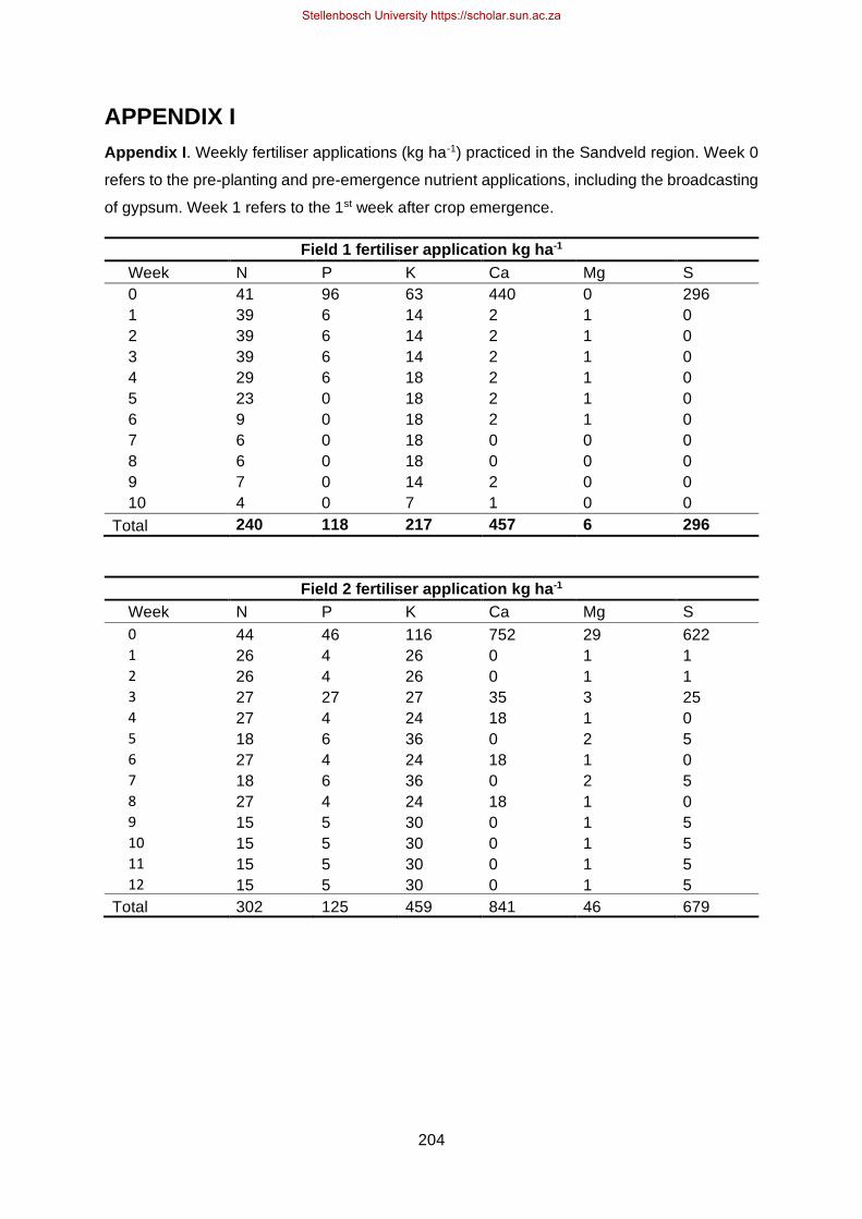
204
APPENDIX I
Appendix I. Weekly fertiliser applications (kg ha-1) practiced in the Sandveld region. Week 0
refers to the pre-planting and pre-emergence nutrient applications, including the broadcasting
of gypsum. Week 1 refers to the 1st week after crop emergence.
Field 1 fertiliser application kg ha-1
Week N P K Ca Mg S
0 41 96 63 440 0 296
1 39 6 14 2 1 0
2 39 6 14 2 1 0
3 39 6 14 2 1 0
4 29 6 18 2 1 0
5 23 0 18 2 1 0
6 9 0 18 2 1 0
7 6 0 18 0 0 0
8 6 0 18 0 0 0
9 7 0 14 2 0 0
10 4 0 7 1 0 0
Total 240 118 217 457 6 296
Field 2 fertiliser application kg ha-1
Week N P K Ca Mg S
0 44 46 116 752 29 622
1 26 4 26 0 1 1
2 26 4 26 0 1 1
3 27 27 27 35 3 25
4 27 4 24 18 1 0
5 18 6 36 0 2 5
6 27 4 24 18 1 0
7 18 6 36 0 2 5
8 27 4 24 18 1 0
9 15 5 30 0 1 5
10 15 5 30 0 1 5
11 15 5 30 0 1 5
12 15 5 30 0 1 5
Total 302 125 459 841 46 679
Stellenbosch University https://scholar.sun.ac.za

205
Field 3 fertiliser application kg ha-1
Week N P K Ca Mg S
0 56 134 138 867 25 677
1 23 5 23 0 1 0
2 23 5 23 0 1 0
3 23 5 23 0 1 0
4 28 4 24 19 1 0
5 17 6 34 0 2 0
6 28 4 24 19 1 0
7 17 6 34 0 2 0
8 28 4 24 19 1 0
9 14 5 27 0 1 0
10 14 5 27 0 1 0
11 14 5 27 0 1 0
12 14 5 27 0 1 0
Total 294 189 454 924 41 677
Field 4 fertiliser application kg ha-1
Week N P K Ca Mg S
0 56 134 138 831 25 635
1 23 5 23 0 1 0
2 23 5 23 0 1 0
3 23 5 23 0 1 0
4 28 4 24 19 1 0
5 17 6 34 0 2 0
6 28 4 24 19 1 0
7 17 6 34 0 2 0
8 28 4 24 19 1 0
9 14 5 27 0 1 0
10 14 5 27 0 1 0
11 14 5 27 0 1 0
12 14 5 27 0 1 0
Total 294 189 454 888 41 635
Stellenbosch University https://scholar.sun.ac.za
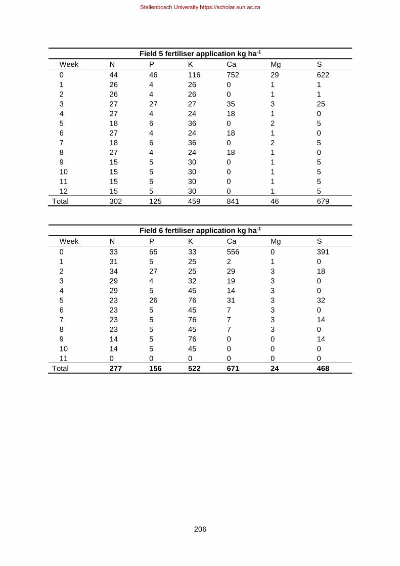
206
Field 5 fertiliser application kg ha-1
Week N P K Ca Mg S
0 44 46 116 752 29 622
1 26 4 26 0 1 1
2 26 4 26 0 1 1
3 27 27 27 35 3 25
4 27 4 24 18 1 0
5 18 6 36 0 2 5
6 27 4 24 18 1 0
7 18 6 36 0 2 5
8 27 4 24 18 1 0
9 15 5 30 0 1 5
10 15 5 30 0 1 5
11 15 5 30 0 1 5
12 15 5 30 0 1 5
Total 302 125 459 841 46 679
Field 6 fertiliser application kg ha-1
Week N P K Ca Mg S
0 33 65 33 556 0 391
1 31 5 25 2 1 0
2 34 27 25 29 3 18
3 29 4 32 19 3 0
4 29 5 45 14 3 0
5 23 26 76 31 3 32
6 23 5 45 7 3 0
7 23 5 76 7 3 14
8 23 5 45 7 3 0
9 14 5 76 0 0 14
10 14 5 45 0 0 0
11 0 0 0 0 0 0
Total 277 156 522 671 24 468
Stellenbosch University https://scholar.sun.ac.za

207
Field 7 fertiliser application kg ha-1
Week N P K Ca Mg S
0 42 116 42 566 47 415
1 22 7 37 0 0 0
2 32 7 48 9 3 5
3 22 7 37 0 0
4 32 7 48 9 3 5
5 22 7 37 0 0 0
6 32 7 48 9 3 5
7 22 7 37 0 0 0
8 23 0 49 9 3 5
9 20 0 57 0 0 0
10 20 0 57 0 0 0
Total 288 167 495 603 59 433
Field 8 fertiliser application kg ha-1
Week N P K Ca Mg S
0 56 134 138 867 25 677
1 23 5 23 0 1 0
2 23 5 23 0 1 0
3 23 5 23 0 1 0
4 28 4 24 19 1 0
5 17 6 34 0 2 0
6 28 4 24 19 1 0
7 17 6 34 0 2 0
8 28 4 24 19 1 0
9 14 5 27 0 1 0
10 14 5 27 0 1 0
11 14 5 27 0 1 0
12 14 5 27 0 1 0
Total 294 189 454 924 41 677
Stellenbosch University https://scholar.sun.ac.za

208
Field 9 fertiliser application kg ha-1
Week N P K Ca Mg S
0 35 96 63 202 0 106
1 39 6 38 2 1 0
2 39 6 38 2 1 0
3 39 6 38 2 1 0
4 39 6 38 2 1 0
5 37 0 38 2 1 0
6 16 0 38 2 1 0
7 16 0 38 2 1 0
8 16 0 38 2 1 0
9 13 0 38 0 0 0
10 13 0 38 0 0 0
Total 302 118 443 217 8 106
Stellenbosch University https://scholar.sun.ac.za

209
APPENDIX II
Appendix II. Nutrient analysis results conducted from a depth of 0 – 90 cm at 30 cm intervals. Pre-planting analysis was conducted during equipment installation and therefore, fertiliser application prior to installation dates will be reflected in the analysis. Post-harvest analysis was conducted during yield analysis at the end of crop growth. Field 1 has missing pre-planting soil analysis results.
Field 1
Sampling period Depth pH P K Ca Mg S Na Bulk density cm KCl mg kg-1 g cm-3
Post-harvest
0-30 6.4 38.3 29.3 121.8 10.5 2.7 4.0 1.54
30-60 5.8 32.5 23.0 103.0 8.0 1.2 3.8 1.46
60-90 5.1 33.8 14.3 85.8 6.5 1.4 5.0 1.48
Average 5.8 34.8 22.2 103.5 8.3 1.8 4.3 1.49
Field 2
Sampling period Depth pH P K Ca Mg S Na Bulk density cm KCl mg kg-1 g cm-3
Pre-planting
0-30 4.4 65.8 33.3 164.3 18.8 11.1 20.3 1.51
30-60 4.2 63.8 25.5 115.5 21.0 5.7 18.3 1.49
60-90 4.1 37.0 17.3 91.0 14.5 5.6 18.8 1.49
Average 4.25 55.50 25.33 123.58 18.08 7.47 19.08 1.50
Post-harvest
0-30 4.3 72.3 38.0 156.3 22.8 3.8 12.8 1.41
30-60 3.9 68.5 23.0 107.5 12.0 1.6 7.5 1.44
60-90 4.0 39.0 15.8 96.3 10.8 1.9 6.3 1.47
Average 4.07 59.92 25.58 120.00 15.17 2.42 8.83 1.44
Stellenbosch University https://scholar.sun.ac.za

210
Field 3
Sampling period Depth pH P K Ca Mg S Na Bulk density cm KCl mg kg-1 g cm-3
Pre-planting
0-30 4.8 23.5 18.0 178.3 15.5 13.0 14.0 1.56
30-60 4.4 16.5 12.0 108.8 9.0 5.7 11.8 1.59
60-90 4.8 12.0 11.5 96.0 9.3 5.2 11.0 1.60
Average 4.7 17.3 13.83 127.7 11.3 7.9 12.3 1.58
Post-harvest
0-30 5.2 19.8 27.8 135.0 11.3 7.2 11.3 1.64
30-60 5.0 15.5 22.8 128.5 10.8 5.1 11.8 1.64
60-90 4.9 13.3 19.5 115.8 9.0 4.3 11.3 1.65
Average 5.1 16.2 23.3 126.4 10.3 5.5 11.4 1.65
Field 4
Sampling period Depth pH P K Ca Mg S Na Bulk density cm KCl mg kg-1 g cm-3
Pre-planting
0-30 5.0 38.0 26.3 220.5 13.0 20.4 9.5 1.56
30-60 4.5 26.0 14.3 143.0 10.8 6.8 9.5 1.51
60-90 4.7 14.8 10.3 134.3 11.8 4.4 10.3 1.54
Average 4.7 26.3 16.9 165.9 11.8 10.5 9.8 1.54
Post-harvest
0-30 5.5 29.8 19.5 163.5 16.5 8.3 24.3 1.63
30-60 4.9 20.3 12.3 134.0 17.0 4.5 21.5 1.54
60-90 4.9 15.0 11.0 127.8 16.8 3.4 17.3 1.55
Average 5.1 21.7 14.3 141.8 16.8 5.4 21.0 1.57
Stellenbosch University https://scholar.sun.ac.za

211
Field 5
Sampling period Depth pH P K Ca Mg S Na Bulk density cm KCl mg kg-1 g cm-3
Pre-planting
0-30 4.2 84.5 31.3 147.3 18.3 7.2 15.3 1.37
30-60 3.9 84.8 19.3 109.0 12.5 5.1 13.0 1.37
60-90 3.9 66.3 16.3 86.3 11.3 3.7 11.0 1.38
Average 4.0 78.5 22.3 114.2 14.0 5.3 13.1 1.37
Post-harvest
0-30 4.4 100.0 39.5 151.0 22.5 6.3 37.5 1.42
30-60 4.0 94.0 28.8 130.8 11.0 4.6 24.5 1.40
60-90 4.0 88.8 26.5 110.3 9.3 3.6 18.3 1.44
Average 4.1 94.3 31.6 130.7 14.3 4.8 26.8 1.42
Field 6
Sampling period Depth pH P K Ca Mg S Na Bulk density cm KCl mg kg-1 g cm-3
Pre-planting
0-30 4.6 63.3 30.7 190.7 33.7 12.3 18.0 1.43
30-60 5.5 52.3 35.0 227.7 79.7 10.1 63.0 1.41
60-90 5.7 10.0 36.3 450.7 406.3 9.3 211.0 1.29
Average 5.3 41.9 34.0 289.7 173.2 10.6 97.3 1.38
Post-harvest
0-30 5.1 56.0 44.0 198.0 38.0 22.4 65.0 1.37
30-60 4.9 35.0 47.0 176.0 26.0 28.6 45.0 1.45
60-90 4.6 41.0 37.0 162.0 25.0 17.9 37.0 1.48
Average 4.8 44.0 42.7 178.7 29.7 23.0 49.0 1.43
Stellenbosch University https://scholar.sun.ac.za

212
Field 7
Sampling period Depth pH P K Ca Mg S Na Bulk density cm KCl mg kg-1 g cm-3
Pre-planting
0-30 5.1 29.8 22.3 187.5 20.3 8.0 18.3 1.46
30-60 4.6 18.0 17.8 120.0 13.0 2.8 14.3 1.49
60-90 4.6 14.8 14.8 96.8 11.5 1.7 11.3 1.48
Average 4.8 20.8 18.3 134.8 14.9 4.1 14.6 1.48
Post-harvest
0-30 5.7 20.0 50.5 171.8 19.3 5.3 43.3 1.52
30-60 4.9 16.0 25.0 120.8 13.5 5.0 24.3 1.50
60-90 4.6 15.3 21.8 106.5 12.8 4.1 19.5 1.52
Average 5.1 17.1 32.4 133.0 15.2 4.8 29.0 1.51
Field 8
Sampling period Depth pH P K Ca Mg S Na Bulk density cm KCl mg kg-1 g cm-3
Pre-planting
0-30 4.5 29.8 31.3 217.5 20.3 33.8 22.5 1.52
30-60 4.4 12.5 25.5 109.0 15.0 9.6 12.8 1.53
60-90 4.6 4.5 17.0 98.0 14.8 7.2 11.5 1.55
Average 4.5 15.6 24.6 141.5 16.7 16.8 15.6 1.53
Post-harvest
0-30 5.2 17.5 17.5 158.0 14.3 25.8 7.2 1.53
30-60 4.8 12.3 5.8 126.3 5.3 24.5 3.9 1.51
60-90 5.2 6.3 5.8 116.3 4.3 22.8 3.1 1.52
Average 5.1 12.0 9.7 133.5 7.9 24.3 4.7 1.52
Stellenbosch University https://scholar.sun.ac.za

213
Field 9
Sampling period Depth pH P K Ca Mg S Na Bulk density cm KCl mg kg-1 g cm-3
Pre-planting
0-30 4.9 18.8 12.3 198.3 36.3 17.7 36.8 1.56
30-60 4.9 15.0 11.5 174.8 32.5 14.7 34.5 1.56
60-90 4.5 13.8 11.3 112.5 21.8 11.8 29.8 1.57
Average 4.8 15.8 11.7 161.8 30.2 14.7 33.7 1.57
Post-harvest
0-30 5.0 13.5 10.5 150.5 22.8 7.1 23.3 1.54
30-60 4.9 10.3 6.5 125.8 15.5 4.7 21.5 1.54
60-90 4.7 11.8 6.3 101.5 10.0 5.0 20.8 1.55
Average 4.9 11.8 7.8 125.9 16.1 5.6 21.8 1.54
Stellenbosch University https://scholar.sun.ac.za
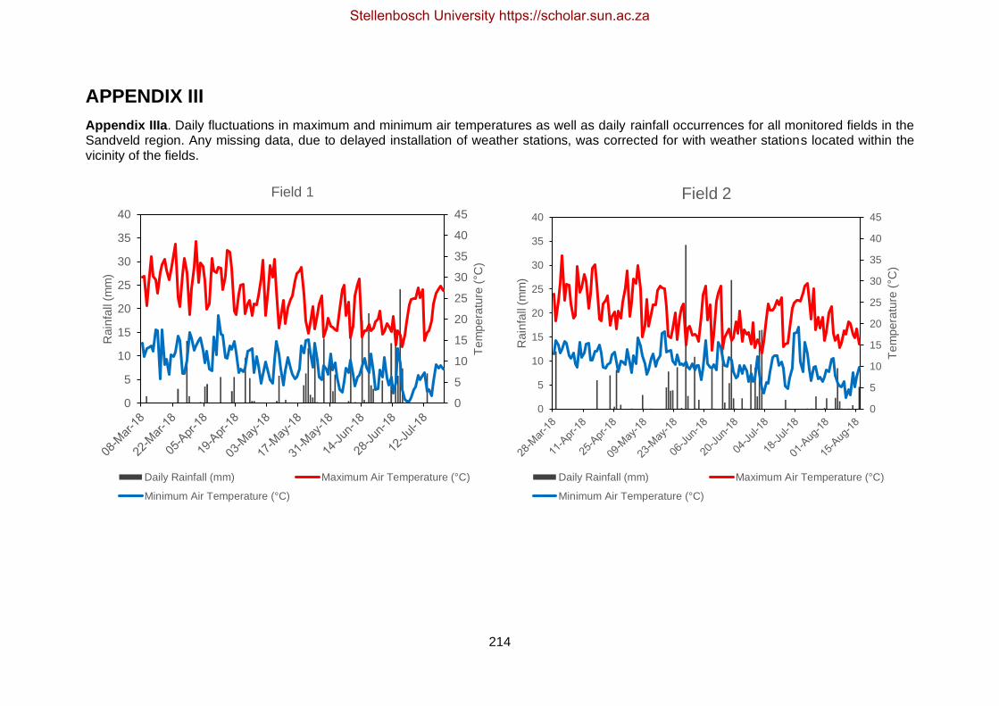
214
APPENDIX III
Appendix IIIa. Daily fluctuations in maximum and minimum air temperatures as well as daily rainfall occurrences for all monitored fields in the Sandveld region. Any missing data, due to delayed installation of weather stations, was corrected for with weather stations located within the vicinity of the fields.
0
5
10
15
20
25
30
35
40
45
0
5
10
15
20
25
30
35
40
Te
mp
era
ture
(°C
)
Rain
fall (
mm
)
Field 1
Daily Rainfall (mm) Maximum Air Temperature (°C)
Minimum Air Temperature (°C)
0
5
10
15
20
25
30
35
40
45
0
5
10
15
20
25
30
35
40
Te
mp
era
ture
(°C
)
Rain
fall (
mm
)
Field 2
Daily Rainfall (mm) Maximum Air Temperature (°C)
Minimum Air Temperature (°C)
Stellenbosch University https://scholar.sun.ac.za

215
0
5
10
15
20
25
30
35
40
45
0
5
10
15
20
25
30
35
40
Te
mp
era
ture
(°C
)
Rain
fall (
mm
)Field 3
Daily Rainfall (mm) Maximum Air Temperature (°C)
Minimum Air Temperature (°C)
0
5
10
15
20
25
30
35
40
45
0
5
10
15
20
25
30
35
40
Te
mp
era
ture
(°C
)
Rain
fall (
mm
)
Field 4
Daily Rainfall (mm) Maximum Air Temperature (°C)
Minimum Air Temperature (°C)
Stellenbosch University https://scholar.sun.ac.za

216
0
5
10
15
20
25
30
35
40
45
0
5
10
15
20
25
30
35
40
Te
mp
era
ture
(°C
)
Rain
fall (
mm
)Field 5
Daily Rainfall (mm) Maximum Air Temperature (°C)
Minimum Air Temperature (°C)
0
5
10
15
20
25
30
35
40
45
0
5
10
15
20
25
30
35
40
Te
mp
era
ture
(°C
)
Rain
fall (
mm
)
Field 6
Daily Rain (mm) Maximum Air Temperature (°C)
Minimum Air Temperature (°C)
Stellenbosch University https://scholar.sun.ac.za

217
0
5
10
15
20
25
30
35
40
45
0
5
10
15
20
25
30
35
40
Te
mp
era
ture
(°C
)
Rain
fall (
mm
)Field 7
Daily Rainfall (mm) Maximum Air Temperature (°C)
Minimum Air Temperature (°C)
0
5
10
15
20
25
30
35
40
45
0
5
10
15
20
25
30
35
40
Te
mp
era
ture
(°C
)
Rain
fall (
mm
)
Field 8
Daily Rainfall (mm) Maximum Air Temperature (°C)
Minimum Air Temperature (°C)
Stellenbosch University https://scholar.sun.ac.za

218
0
5
10
15
20
25
30
35
40
45
0
5
10
15
20
25
30
35
40
Te
mp
era
ture
(°C
)
Rain
fall (
mm
)Field 9
Daily Rainfall (mm) Maximum Air Temperature (°C)
Minimum Air Temperature (°C)
Stellenbosch University https://scholar.sun.ac.za

219
Appendix IIIb. Solar radiation interception as estimated using above canopy and below canopy ceptometer readings taken every second site visit (weather permitting). The percentage of intercepted solar radiation correlates to the crop canopy cover.
Field Row
Labels
Average of solar interception above canopy (µmol m-2 s-1)
Average of solar interception below canopy (µmol m-2 s-1)
Average percentage Intercepted solar radiation (µmol m-2 s-1)
Field 1 10-May-18 300 24 92
Field 2
10-May-18 1066 132 87
11-Jul-18 509 185 64
23-Jul-18 189 136 28
Field 3
09-Jul-18 497 102 80
23-Jul-18 998 174 83
21-Aug-18 808 204 74
11-Sep-18 1491 805 46
Field 4
21-Aug-18 802 415 46
11-Sep-18 1518 281 81
01-Oct-18 742 122 85
23-Oct-18 2028 1166 42
Field 5
22-Aug-18 1396 519 63
10-Sep-18 644 34 95
01-Oct-18 1375 85 93
30-Oct-18 1188 464 61
Field 6
21-Aug-18 1328 840 37
10-Sep-18 159 21 87
01-Oct-18 722 57 92
30-Oct-18 1790 757 57
Field 7
11-Sep-18 1524 1009 34
01-Oct-18 560 60 89
30-Oct-18 1264 526 57
Field 8
05-Dec-18 2038 288 86
07-Jan-19 1888 245 87
30-Jan-19 1032 441 57
Field 9
07-Jan-19 1007 81 92
30-Jan-19 1507 60 96
19-Feb-19 851 610 29
Stellenbosch University https://scholar.sun.ac.za
Related Documents