The Eccentricity Transform (of a Digital Shape

The Eccentricity Transform?

(of a Digital Shape)

Walter G. Kropatsch, Adrian Ion, Yll Haxhimusa, and Thomas Flanitzer

Vienna University of Technology,Pattern Recognition and Image Processing Group{krw,ion,yll,flanitzt}@prip.tuwien.ac.at

Abstract. Eccentricity measures the shortest length of the paths froma given vertex v to reach any other vertex w of a connected graph.Computed for every vertex v it transforms the connectivity structure ofthe graph into a set of values. For a connected region of a digital im-age it is defined through its neighbourhood graph and the given metric.This transform assigns to each element of a region a value that dependson it’s location inside the region and the region’s shape. The definitionand several properties are given. Presented experimental results verifyits robustness against noise, and its increased stability compared to thedistance transform. Future work will include using it for shape decom-position, representation, and matching.

1 Introduction

Recognition, manipulation and representation of visual objects can be simpli-fied significantly by “abstraction”. Abstraction extracts essential features andproperties while it neglects unnecessary details. Shape is one such form of visualabstraction, which describes distinctive features of the object’s appearance i.e.its projection on the surface of a 2D sensor (in our case the retina). If shapematching is done invariant with respect to certain deformation classes (e.g. ar-ticulated motion), shape based object recognition can be used for generic objectrecognition, a much desired ability of humans.

Different approaches that use shape for recognition exist [1–4], with manyof them using the distance transform [5] derived skeletons [6, 7] as a basis forshape description. Skeletons have proved themselves to be the basis of powerfulshape descriptors [2] with the main advantages including their ‘cue’ for a naturaldecomposition of shapes into parts (e.g. usually the parts of the skeleton of ahuman decompose its shape into body, limbs, and head) and their invariance tocertain types of movement including the very important articulated motion. Onthe other hand, one of their weak points come from their apparent locality andthe fact that they are derived from the distance transform which is known to beunstable with respect to small perturbation of the shape (e.g. spurious branchescan appear in the skeleton if a few pixels are added at the border of the region).

? Supported by the Austrian Science Fund under grants S9103-N04 and P18716-N13.

a) b) c)

d) e) f)

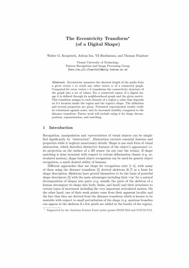
Fig. 1. Isoheight lines for distance (a-c) and eccentricity (d-f) transform of 2 images,using the euclidean (a,d), 4− (b,e), and 8− (c,f) neighbourhood. (where continuous,lighter means higher value)

The distance transform associates to each point of the shape, the minimumdistance from it to the border of the shape (see Fig. 1a: gray values are indepen-dent between the two images, and where continuously changing: lighter meanshigher value), which makes it very unstable with respect to Salt and Peppernoise and certain kind of segmentation errors. Approaches like removing regionsbelow a certain size or pruning spurious branches of the obtained skeleton havebeen used to cope with these kinds of problems, but this has been shown not tobe the optimal way and should be avoided mainly because the size of a regiondoes not tell anything about its importance [8].

Instead of minimum distance, other measures have also been used, e.g. themean time for a randomly moving particle to hit the border [9].

Inspired from graph theory, we present a new transform which associates toeach point the longest distance (geodesic) from it to the points on the borderof the shape (see Fig. 1d). We show that it is robust against the types of noisementioned above, and comment about it’s applicability to shape description andmatching.

We recall the distance transform in Sec. 2, including a formulation for thedistance transform of a graph (Sec. 2.2). The eccentricity transform is presentedin Sec. 3, beginning with a recall of the graph theory based definition for ec-centricity (Sec. 3.1). The properties of the transform are discussed in Sec. 4,

1

»»»»

1

1

11

2

2

2

2

2

3

1

1

1

¡¡

¡¡

hhhhHHHH!!!!!HHH

hhh...........................................................

TTTT

aaaa!!!!HHH!!!HHH

··

··TT

TT

@@@aaaa

%%

¡¡

¡¡©©

................................................................................

»»»»

hhhhhv

vv

v v

vv

v v

vv

v

v

v 4

4

3

3

3

2

3

3

b

c

a

4

4

e

d

¡¡

¡¡

hhhhHHHH!!!!!HHH

hhh...........................................................

TTTT

aaaa!!!!HHH!!!HHH

··

··TT

TT

@@@aaaa

%%

¡¡

¡¡

»»»»©©

................................................................................

»»»»

hhhhh

3

3

3

3

v

v

vv

v v

vv

v v

vv

v

v

a) b)

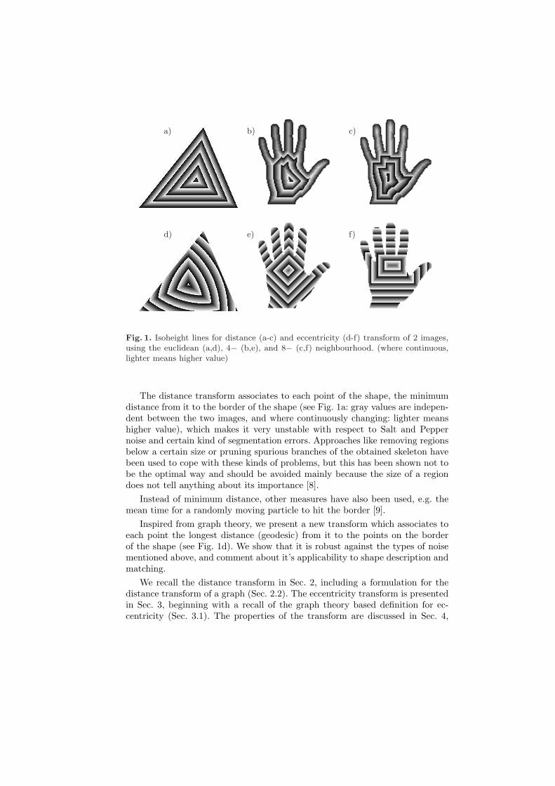
Fig. 2. Distance transform (a) and eccentricity transform (b) of a graph.

followed by computation strategies in Sec. 5. Experimental results in Sec. 6 willcomplete the presentation, summed up in Sec. 7 with conclusions and outlook.

2 Distance Transform

The distance transform assigns to each point in the binary image a value ofa distance to the closest point on its border (obstacles). Let I = B ∪ B be abinary image and let a point p ∈ B. We adapt the definition of the generaldistance function [10] for the rest of the section. A neighbourhood Ni is a pairof (Pi, di), where Pi is a finite subset of ZK and di is a function di : P → R+, fori = 0, ..., T −1 and T,K ∈ Z+. We say that pi is adjacent to pi+1 iff pi+1 = pi +rfor some r ∈ Pi. Let α be a finite sequence of neighbourhoods N0N1... NT−1,where T is called the period of the sequence. The distance transform dtα of Iassociates to every point p ∈ B the minimal distance from p to B, formally wewrite:

dtα(p) = min{λ(πα(p, q)) | q ∈ B ∧ q ∈ Nα(q), q ∈ B}, (1)

where Nα is an α-adjacency, πα(p, q) is the set of all α-paths from point p toq, and λ(πα(p, q)) is the length of one of the paths πα(p, q). The α-path is asequence of points (p0, p1, ..., pn), such that end points are p0 = p, pn = q, andpi+1 is α-adjacent to pi (0 ≤ i ≤ n− 1), then the length of this path is the sumof di(pi+1 − pi) for all i = 1, ..., n. If di(r) = 1 then the length of the path isn, the number of points. To define the chessboard distance (dt8) or the squaredistance (dt4) one takes the sequence of neighbourhood with T = 1 (α = N0) anddefines the neighbourhood P0 as in [10, page 239]. Note that there may be manyshortest paths. If there is no other shorter α-path between the same end points,then this path is called α-geodesic [11]. The border point q ∈ B is α-neighbourof a point not being in B. In the Euclidean space there is always a unique pathbetween two points, which is the straight line between the points. This straightline does not exist in digital images and thus the distance transform computedis dependent on the way the neighbourhood is defined, i.e. how the Euclideandistance is approximated. In the section below we use the definitions above asthe basis of defining the distance transform of digital images and graphs.

2.1 Distance Transform of a Digital Image

The transformation of the continuous space Rn into a discrete space Zn is doneby sampling Rn. A particular sampling scheme can be used to digitise the con-tinuous space. If there is no a priori knowledge about the local variation, theusual scheme is the square or hexagonal grid. For the sake of the presentation wewill constrain the discussion only on digital images on 2D square grids with the4−neighbourhood (city block metric), and the 8−neighbourhood (chessboardmetric). Using Eq. 1 one can define the distance transform dt4 and dt8, respec-tively. These distance transforms are easy to compute by scanning the imagetwice [12, 11], although they are not a good approximation of the Euclidean dis-tance. In Fig. 1b,c) distance transforms dt4 and dt8 of a binary image are shown.Better approximations can be found by chamfer distances [13].

2.2 Distance Transform of a Graph

If the sampling grid is not regular, one could use graph representation for thesampling points. Let G = (V,E, a, w) be the undirected weighted graph withvertices v ∈ V representing sampling points, edge set e = (v, w) ∈ E representingthe connection between vertices; and a : V → Z+ and w : E → Z+ are attributeson vertices and edges respectively. Let the weights on edges represent the cost ofgoing from one vertex to the other. In order to define the distance transform oneshould define the boundary vertices [14]. Any bounded region has a boundarythat separates it from the background. The background can be considered as thecomplement of the region with respect to the embedding space. Border faces arefaces of the dual graph that are surrounded by both vertices of G ⊂ G′ and G′.The boundary of a subgraph G = (V, E) ⊂ G′ = (V ′, E′) collects all the verticesC ⊂ V which bound border faces.

A path πG(v, w) is a sequence of vertices (v0, v1, ..., vn) in G such that theend vertices are v = v0, w = vn, all vertices are distinct and ∃e = (vi, vi+1) ∈E, i = 0, 1, ..., n− 1. The length λ(πG) of path λG is the sum of the edge weightin the sequence:

dtG(v) = min{λ(πG(v, w)), v ∈ G \ C ∧ w ∈ C}. (2)

Usually, the border vertices are set to 1. If vertices v and w are not connected,we say that the λ(πG(v, w)) is infinite. If the graph G is connected then thisdistance is a graph metric [11]. A simple example of the distance transform on agraph is given in Fig. 2a, where the edge cost is set to 1. Note that square gridcan be easily represented by graphs. In this case the weight on edges could beset to 1 (but not necessarily). Similar to the square grid, we can define the 4-,8-neighbourhood of vertices.

3 Eccentricity Transform

The eccentricity transform assigns to each point in the binary image the shortestdistance to the point farthest away from it. Analogously, to the notation pre-sented in Sec. 2 we define the eccentricity transform eccα(p) of I = B ∪B such

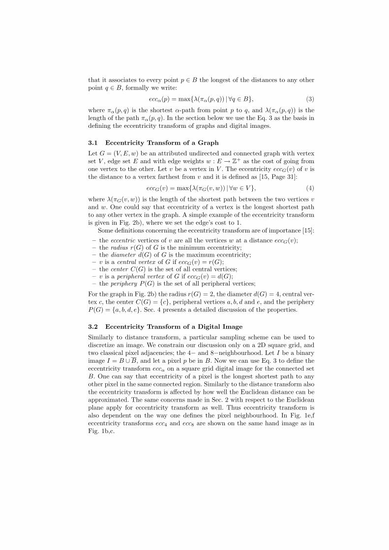
that it associates to every point p ∈ B the longest of the distances to any otherpoint q ∈ B, formally we write:

eccα(p) = max{λ(πα(p, q)) | ∀q ∈ B}, (3)

where πα(p, q) is the shortest α-path from point p to q, and λ(πα(p, q)) is thelength of the path πα(p, q). In the section below we use the Eq. 3 as the basis indefining the eccentricity transform of graphs and digital images.

3.1 Eccentricity Transform of a Graph

Let G = (V, E, w) be an attributed undirected and connected graph with vertexset V , edge set E and with edge weights w : E → Z+ as the cost of going fromone vertex to the other. Let v be a vertex in V . The eccentricity eccG(v) of v isthe distance to a vertex farthest from v and it is defined as [15, Page 31]:

eccG(v) = max{λ(πG(v, w)) | ∀w ∈ V }, (4)

where λ(πG(v, w)) is the length of the shortest path between the two vertices vand w. One could say that eccentricity of a vertex is the longest shortest pathto any other vertex in the graph. A simple example of the eccentricity transformis given in Fig. 2b), where we set the edge’s cost to 1.

Some definitions concerning the eccentricity transform are of importance [15]:– the eccentric vertices of v are all the vertices w at a distance eccG(v);– the radius r(G) of G is the minimum eccentricity;– the diameter d(G) of G is the maximum eccentricity;– v is a central vertex of G if eccG(v) = r(G);– the center C(G) is the set of all central vertices;– v is a peripheral vertex of G if eccG(v) = d(G);– the periphery P (G) is the set of all peripheral vertices;

For the graph in Fig. 2b) the radius r(G) = 2, the diameter d(G) = 4, central ver-tex c, the center C(G) = {c}, peripheral vertices a, b, d and e, and the peripheryP (G) = {a, b, d, e}. Sec. 4 presents a detailed discussion of the properties.

3.2 Eccentricity Transform of a Digital Image

Similarly to distance transform, a particular sampling scheme can be used todiscretize an image. We constrain our discussion only on a 2D square grid, andtwo classical pixel adjacencies; the 4− and 8−neighbourhood. Let I be a binaryimage I = B ∪B, and let a pixel p be in B. Now we can use Eq. 3 to define theeccentricity transform eccα on a square grid digital image for the connected setB. One can say that eccentricity of a pixel is the longest shortest path to anyother pixel in the same connected region. Similarly to the distance transform alsothe eccentricity transform is affected by how well the Euclidean distance can beapproximated. The same concerns made in Sec. 2 with respect to the Euclideanplane apply for eccentricity transform as well. Thus eccentricity transform isalso dependent on the way one defines the pixel neighbourhood. In Fig. 1e,feccentricity transforms ecc4 and ecc8 are shown on the same hand image as inFig. 1b,c.

4 Properties of the Eccentricity Transform

We shortly discuss some of the properties of the eccentricity transform, some ofthem known from graph theory and extended to the discrete domain, some areinteresting and useful in the context of describing the shape of a region.

Center: The vertices with the minimum value of the eccentricity transformare called the center of the graph. They lie in a block of the graph, i.e. thecorresponding subset of vertices containing the center is connected and does notcontain a cut vertex. We notice that the center of a discrete region is alwaysa part of the region in contrast to the center of gravity which can be locatedoutside the region in case of a concavity or a hole in the middle of the region.This may be useful in several applications, e.g. in tracking where the center ofa tracked region may be used as the start for searching the region in the nextframe of the sequence.

Robustness: The eccentricity transform is robust with respect to (salt andpepper) noise. This is due to the fact that a noise vertex on the path between twodistant points ’just goes around’ the obstacle without prolongating the length bymuch. In the case of discrete metrics (like 4− or 8−connectivity) the likelihoodof finding many paths with the same (shortest) length is very high. In such acase the eccentricity is affected only if all shortest paths between the vertex andits farthest vertex are interrupted by noise or a noisy pixel (vertex) p is addedto B such that p is at maximum distance from the vertex.

4-connectivity: In the Euclidean space two points are connected by a uniquestraight line. In the discrete space with 4-connectivity this is only the case if thetwo points are along the two coordinate axes, in all other cases there are morethan one shortest paths. In fact any permutation of the two primitive steps toconnect the two end points is also a shortest path.

This fact increases the robustness of the eccentricity transform but has alsotwo other consequences:

1. There is not a single midpoint between the two endpoints making the centerof an elongated region a diagonal line. In fact the length of this line is aslong as the smaller coordinate differences of the two end points.

2. Since the number of midpoints depends on the angle of the discrete line theresulting centers are no more rotationally invariant (which they are in theEuclidean case).

Maxima are all on the boundary if the graph has no inner pendingvertex: (See Sec. 2.2 for the boundary of a graph) If G′ is connected there arepaths between any pairs of vertices v, w ∈ V ′. Any non-border vertex has adegree greater than 1. If none of the neighbours of a vertex of degree greaterthan 1 belongs to a border face it cannot be extremal since any path leading toit can be continued.

Complementarity between distance transform and eccentricity trans-form: In the distance transform the smallest values are on the boundary andthe highest values can be found where a circle with maximum radius touches the

Algorithm 1 – Eccentricity Transform - naive implementationInput: Attributed graph G = (V, E).

1: for all v ∈ V do2: ecc(v)← 03: for all u ∈ V − {v} do4: ecc(v)← max{ecc(v), shortestPathLength(v, u)}5: end for6: end for

Output: Eccentricity ecc(v) for all vertices v ∈ V of G.

boundary in at least two opposite points. These local maxima form the skele-ton/medial axis/symmetry transform. Local maxima of the eccentricity trans-form are on the boundary while the minimum defines the center. However thereare local minima along the boundary and discontinuities inside the region whichgive rise to interesting partitionings of the region.

Invariance: The eccentricity transform computes the lengths of paths insidea given region. It is therefore invariant to any translation and invariant to rota-tion for the Euclidean metric. There is some dependency on the orientation fordiscrete metrics but not for all shapes. Furthermore in the case of thin regions, itis robust with respect to articulated motion, it may differ by the thickness of theshape at the articulation point which in many natural cases is thin in relationto the length (arms, legs, fingers).

5 Computation

Two algorithms for computing the eccentricity transform are given here. Theyare both defined for graphs, but the adaptation to digital images is straightforward. One has just to decide for a neighbourhood (α = {4, 8}) and choose thepixels that make up the connected region for which the transform will be applied.Note that Floyds [16] algorithm, that produces the minimum path length fromall vertices to all other vertices can also be used to obtain the eccentricity (foreach vertex, one has just to take the maximum of the values obtained for it).

Naive Alg. 1 iterates through all the vertices of G and for each, it calculatesthe maximum of the length of the shortest paths to all other vertices in the graph.Lines 3 - 5 can be implemented by taking the maximum of the lengths calculatedusing Dijkstra’s single-source shortest path algorithm [16]. The complexity of thenaive implementation is between O(|V |3) and O(|V ||E|+|V |2 log |V |)) dependingon the implementation of the shortest path problem.

Alg. 2 uses the fact that the set of eccentric vertices is a subset of V and thatcalculating the shortest path for each of these vertices to all the other vertices inV and combining the results (i.e. taking the maximum) is enough to obtain theeccentricity transform for the whole graph. The eccentric vertices can be foundby calculating the shortest path from the center of the graph to all the othervertices and looking at the local maximum. To find the center of a graph we findit’s diameter, which is connecting the vertices with the highest eccentricity.

Algorithm 2 – Eccentricity Transform - optimised implementationInput: Attributed graph G = (V, E).

1: ∀v ∈ V, ecc(v)← 0 /* initialise eccentricity cumulation table with 0 */2: vp← random vertex of V3: repeat4: mark vp as visited5: ∀v ∈ V, ecc(v) = max{ecc(v), shortestPathLength(v, vp)}6: vp← vertex with maximum ecc7: until (ecc not changed) or (vp allready visited) /* iterate until the endpoints of a

diameter found */8: repeat9: m← one (random) or all unvisited vertices with minimum ecc

10: for all vm ∈ m do11: ∀v ∈ V, ecc(v) = max{ecc(v), shortestPathLength(v, vm)}12: mark vm as visited13: end for14: M ← all unvisited vertices with local maximum ecc

/* M includes non monotonic maxima */15: for all vM ∈M do16: ∀v ∈ V, ecc(v) = max{ecc(v), shortestPathLength(v, vM )}17: mark vM as visited18: end for19: until ecc not changed /* repeat until converged */

Output: Eccentricity ecc(v) for all vertices v ∈ V of G.

Lines 3 - 7 start with a random point and iterate to find the vertices with thehighest eccentricity (diameter endpoints). The calculated shortest path lengthsare added to the cumulation table ecc and the vertex is marked as visited.Lines 8 - 19 iterate finding the center vertices and the local maximum until theecc cumulation table converges. On line 9 (approximate the center), two optionshave been tried, taking one or all the existing minima. On shapes without holes,both have produced the correct solution, while on shapes with holes neither ofthem did. In our experiments, the first loop (lines 3 - 7) converged after 3 cycles(random point, first diameter end, second diameter end). The second loop isbounded by the number of vertices on the border of the graph.

Alg. 2 is much faster than Alg. 1 but gives correct results only on simplyconnected shapes (no holes). On shapes with holes, complex forms of the centerappear e.g. for a disc with a circular hole in the middle, the center consists of acircle for euclidean distance, and a set of disconnected points for 4 connectivity,all concentrated around the hole. In such cases, Alg. 2 produces results close tothe correct one, but we cannot give any upper bound for the error.

6 Experiments

We have conducted experiments to test the properties of the eccentricity trans-form and find the important differences compared to the distance transform.

X

YZ

x

yz

A B

C

a

a

b

b

c cA B

C

a

a

cc

a) distance transform b) eccentricity transform

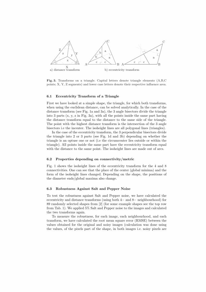
Fig. 3. Transforms on a triangle. Capital letters denote triangle elements (A,B,Cpoints; X, Y, Z segments) and lower case letters denote their respective influence area.

6.1 Eccentricity Transform of a Triangle

First we have looked at a simple shape, the triangle, for which both transforms,when using the euclidean distance, can be solved analytically. In the case of thedistance transform (see Fig. 1a and 3a), the 3 angle bisectors divide the triangleinto 3 parts (x, y, z in Fig. 3a), with all the points inside the same part havingthe distance transform equal to the distance to the same side of the triangle.The point with the highest distance transform is the intersection of the 3 anglebisectors i.e the incenter. The isoheight lines are all polygonal lines (triangles).

In the case of the eccentricity transform, the 3 perpendicular bisectors dividethe triangle into 2 or 3 parts (see Fig. 1d and 3b) depending on whether thetriangle is an optuse one or not (i.e the circumcenter lies outside or within thetriangle). All points inside the same part have the eccentricity transform equalwith the distance to the same point. The isoheight lines are made out of arcs.

6.2 Properties depending on connectivity/metric

Fig. 1 shows the isoheight lines of the eccentricity transform for the 4 and 8connectivities. One can see that the place of the center (global minima) and theform of the isoheight lines changed. Depending on the shape, the positions ofthe diameter ends/global maxima also change.

6.3 Robustness Against Salt and Pepper Noise

To test the robustness against Salt and Pepper noise, we have calculated theeccentricity and distance transforms (using both 4− and 8− neighbourhood) for89 randomly selected shapes from [2] (for some example shapes see the top rowfrom Tab. 1). We applied 5% Salt and Pepper noise to the images and calculatedthe two transforms again.

To measure the robustness, for each image, each neighbourhood, and eachtransform, we have calculated the root mean square error (RMSE) between thevalues obtained for the original and noisy images (calculation was done usingthe values, of the pixels part of the shape, in both images i.e. noisy pixels are

Histograms for the hand image

10 20 30 400

500

1000

1500

Distance

Cou

nt

75 100 1500

50

100

150

Distance

Cou

nt

a) dt4 distance transform b) ecc4 eccentricity transform

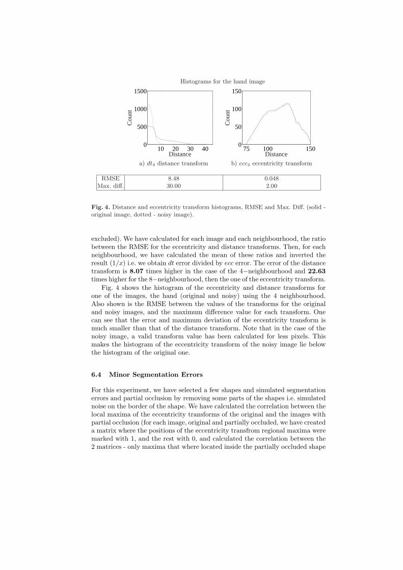
RMSE 8.48 0.048Max. diff. 30.00 2.00

Fig. 4. Distance and eccentricity transform histograms, RMSE and Max. Diff. (solid -original image, dotted - noisy image).

excluded). We have calculated for each image and each neighbourhood, the ratiobetween the RMSE for the eccentricity and distance transforms. Then, for eachneighbourhood, we have calculated the mean of these ratios and inverted theresult (1/x) i.e. we obtain dt error divided by ecc error. The error of the distancetransform is 8.07 times higher in the case of the 4−neighbourhood and 22.63times higher for the 8−neighbourhood, then the one of the eccentricity transform.

Fig. 4 shows the histogram of the eccentricity and distance transforms forone of the images, the hand (original and noisy) using the 4 neighbourhood.Also shown is the RMSE between the values of the transforms for the originaland noisy images, and the maximum difference value for each transform. Onecan see that the error and maximum deviation of the eccentricity transform ismuch smaller than that of the distance transform. Note that in the case of thenoisy image, a valid transform value has been calculated for less pixels. Thismakes the histogram of the eccentricity transform of the noisy image lie belowthe histogram of the original one.

6.4 Minor Segmentation Errors

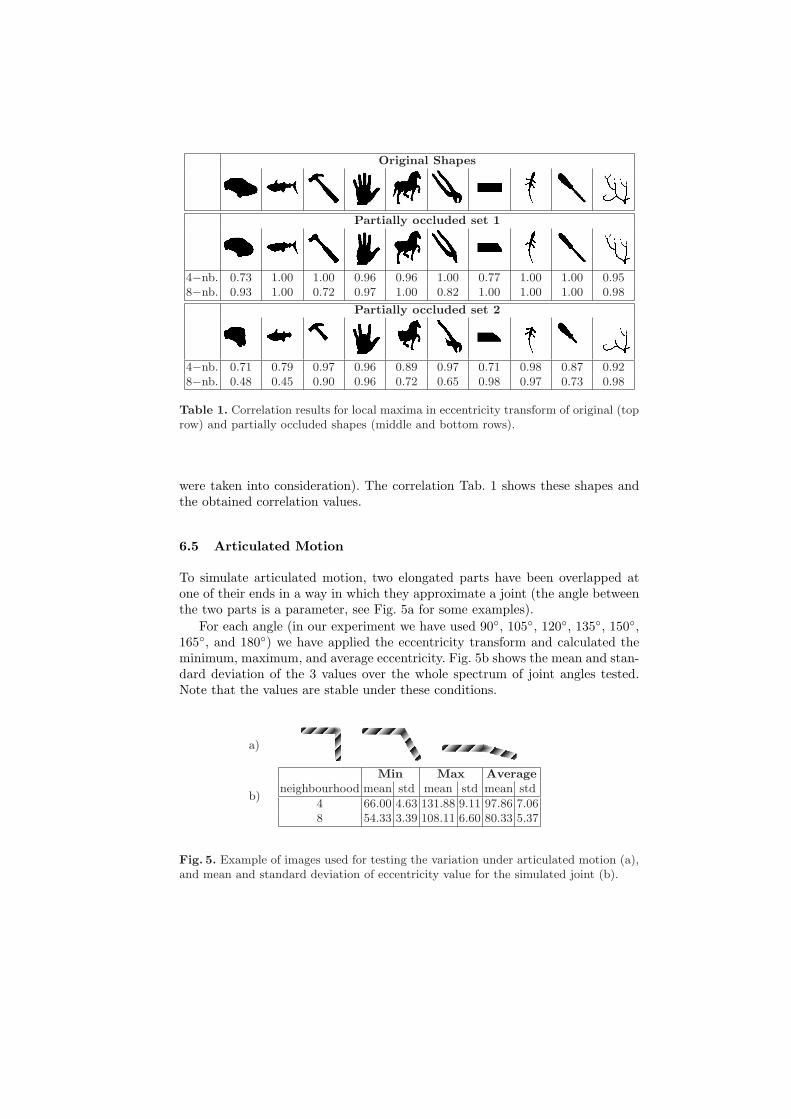
For this experiment, we have selected a few shapes and simulated segmentationerrors and partial occlusion by removing some parts of the shapes i.e. simulatednoise on the border of the shape. We have calculated the correlation between thelocal maxima of the eccentricity transforms of the original and the images withpartial occlusion (for each image, original and partially occluded, we have createda matrix where the positions of the eccentricity transfrom regional maxima weremarked with 1, and the rest with 0, and calculated the correlation between the2 matrices - only maxima that where located inside the partially occluded shape

Original Shapes

Partially occluded set 1

4−nb. 0.73 1.00 1.00 0.96 0.96 1.00 0.77 1.00 1.00 0.958−nb. 0.93 1.00 0.72 0.97 1.00 0.82 1.00 1.00 1.00 0.98

Partially occluded set 2

4−nb. 0.71 0.79 0.97 0.96 0.89 0.97 0.71 0.98 0.87 0.928−nb. 0.48 0.45 0.90 0.96 0.72 0.65 0.98 0.97 0.73 0.98

Table 1. Correlation results for local maxima in eccentricity transform of original (toprow) and partially occluded shapes (middle and bottom rows).

were taken into consideration). The correlation Tab. 1 shows these shapes andthe obtained correlation values.

6.5 Articulated Motion

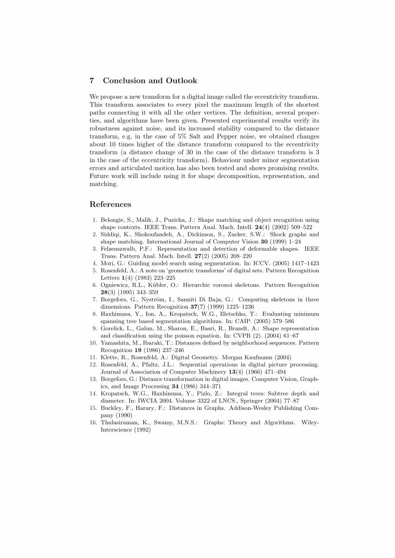
To simulate articulated motion, two elongated parts have been overlapped atone of their ends in a way in which they approximate a joint (the angle betweenthe two parts is a parameter, see Fig. 5a for some examples).

For each angle (in our experiment we have used 90◦, 105◦, 120◦, 135◦, 150◦,165◦, and 180◦) we have applied the eccentricity transform and calculated theminimum, maximum, and average eccentricity. Fig. 5b shows the mean and stan-dard deviation of the 3 values over the whole spectrum of joint angles tested.Note that the values are stable under these conditions.

a)

Min Max Averageneighbourhood mean std mean std mean std

4 66.00 4.63 131.88 9.11 97.86 7.068 54.33 3.39 108.11 6.60 80.33 5.37

b)

Fig. 5. Example of images used for testing the variation under articulated motion (a),and mean and standard deviation of eccentricity value for the simulated joint (b).

7 Conclusion and Outlook

We propose a new transform for a digital image called the eccentricity transform.This transform associates to every pixel the maximum length of the shortestpaths connecting it with all the other vertices. The definition, several proper-ties, and algorithms have been given. Presented experimental results verify itsrobustness against noise, and its increased stability compared to the distancetransform, e.g. in the case of 5% Salt and Pepper noise, we obtained changesabout 10 times higher of the distance transform compared to the eccentricitytransform (a distance change of 30 in the case of the distance transform is 3in the case of the eccentricity transform). Behaviour under minor segmentationerrors and articulated motion has also been tested and shows promising results.Future work will include using it for shape decomposition, representation, andmatching.

References

1. Belongie, S., Malik, J., Puzicha, J.: Shape matching and object recognition usingshape contexts. IEEE Trans. Pattern Anal. Mach. Intell. 24(4) (2002) 509–522

2. Siddiqi, K., Shokoufandeh, A., Dickinson, S., Zucker, S.W.: Shock graphs andshape matching. International Journal of Computer Vision 30 (1999) 1–24

3. Felzenszwalb, P.F.: Representation and detection of deformable shapes. IEEETrans. Pattern Anal. Mach. Intell. 27(2) (2005) 208–220

4. Mori, G.: Guiding model search using segmentation. In: ICCV. (2005) 1417–14235. Rosenfeld, A.: A note on ’geometric transforms’ of digital sets. Pattern Recognition

Letters 1(4) (1983) 223–2256. Ogniewicz, R.L., Kubler, O.: Hierarchic voronoi skeletons. Pattern Recognition

28(3) (1995) 343–3597. Borgefors, G., Nystrom, I., Sanniti Di Baja, G.: Computing skeletons in three

dimensions. Pattern Recognition 37(7) (1999) 1225–12368. Haxhimusa, Y., Ion, A., Kropatsch, W.G., Illetschko, T.: Evaluating minimum

spanning tree based segmentation algorithms. In: CAIP. (2005) 579–5869. Gorelick, L., Galun, M., Sharon, E., Basri, R., Brandt, A.: Shape representation

and classification using the poisson equation. In: CVPR (2). (2004) 61–6710. Yamashita, M., Ibaraki, T.: Distances defined by neighborhood sequences. Pattern

Recognition 19 (1986) 237–24611. Klette, R., Rosenfeld, A.: Digital Geometry. Morgan Kaufmann (2004)12. Rosenfeld, A., Pfaltz, J.L.: Sequential operations in digital picture processing.

Journal of Association of Computer Machinery 13(4) (1966) 471–49413. Borgefors, G.: Distance transformation in digital images. Computer Vision, Graph-

ics, and Image Processing 34 (1986) 344–37114. Kropatsch, W.G., Haxhimusa, Y., Pizlo, Z.: Integral trees: Subtree depth and

diameter. In: IWCIA 2004. Volume 3322 of LNCS., Springer (2004) 77–8715. Buckley, F., Harary, F.: Distances in Graphs. Addison-Wesley Publishing Com-

pany (1990)16. Thulasiraman, K., Swamy, M.N.S.: Graphs: Theory and Algorithms. Wiley-

Interscience (1992)