The Durham/UKST Galaxy Redshift Survey-IV. Redshift Space Distortions via the 2-Point Correlation Function

arX

iv:a

stro

-ph/

9702

228v

1 2

6 Fe

b 19

97Mon. Not. R. Astron. Soc. 000, 000–000 (0000) Printed 14 July 2011 (MN LATEX style file v1.4)

The Durham/UKST Galaxy Redshift Survey - IV.Redshift Space Distortions in the 2-Point CorrelationFunction.

A. Ratcliffe1, T. Shanks1, R. Fong1 and Q.A. Parker2

1Physics Deptartment, University of Durham, South Road, Durham, DH1 3LE.2Anglo-Australian Observatory, Coonabarabran, NSW 2357, Australia.

14 July 2011

ABSTRACTWe have investigated the redshift space distortions in the optically selectedDurham/UKST Galaxy Redshift Survey using the 2-point galaxy correlation func-tion perpendicular and parallel to the observer’s line of sight, ξ(σ, π). We presentresults for the real space 2-point correlation function, ξ(r), by inverting the optimallyestimated projected correlation function, which is obtained by integration of ξ(σ, π),and find good agreement with other real space estimates. On small, non-linear scaleswe observe an elongation of the constant ξ(σ, π) contours in the line of sight direction.This is due to the galaxy velocity dispersion and is the common “Finger of God” ef-fect seen in redshift surveys. Our result for the one-dimensional pairwise rms velocitydispersion is < w2 >1/2= 416 ± 36kms−1 which is consistent with those from recentredshift surveys and canonical values, but inconsistent with SCDM or LCDM models.On larger, linear scales we observe a compression of the ξ(σ, π) contours in the lineof sight direction. This is due to the infall of galaxies into overdense regions and theDurham/UKST data favours a value of (Ω0.6/b)∼0.5, where Ω is the mean mass den-sity of the Universe and b is the linear bias factor which relates the galaxy and massdistributions. Comparison with other optical estimates yield consistent results, withthe conclusion that the data does not favour an unbiased critical-density universe.

Key words: galaxies: clusters – galaxies: general – cosmology: observations – large-scale structure of Universe.

1 INTRODUCTION

The use of redshifts as distance estimates is commonplacein surveys which map the galaxy distribution of the Uni-verse. While redshifts are both quick and easy to acquire,they do not generally reflect the true distance to the galaxybecause of the galaxy’s own peculiar velocity with respectto the Hubble flow. Therefore, the observed clustering pat-tern will be imprinted with the galaxy peculiar velocity fieldalong the observer’s line of sight direction. While at firstthis would appear to be highly problematic for the use andunderstanding of the measured clustering statistics, theseso-called redshift space distortions can be used to estimatesome important cosmological parameters describing the dy-namics of the Universe (e.g. Peebles 1980; Kaiser 1987).

We will be investigating these redshift space distortionsusing the spatial 2-point correlation function, ξ, and denotea real space separation by r and a redshift space separa-tion by s. Non-linear and linear effects will be competingon all scales but for the most part we take the simplifying

assumption that non-linear effects dominate on small scales(< 10h−1Mpc), whereas linear effects dominate on largerscales (> 10h−1Mpc). Although this is a slightly naive ap-proach we use N-body simulations and mock catalogues toguide us in determining the accuracy of the modelling in-volved.

The initial clustering results, redshift maps, etc. of theDurham/UKST Galaxy Redshift Survey were summarizedin the first paper of this series (Ratcliffe et al. 1996a). In thispaper we present a detailed analysis of the redshift space dis-tortions in the 2-point correlation function as estimated fromthis optically selected survey. We briefly describe our surveyin Section 2. Section 3 gives a qualitative description of theeffects of the redshift space distortions on the 2-point corre-lation function. In Section 4 we describe and test methodsof obtaining the real space correlation function from red-shift space estimates. In Section 5 we describe non-lineareffects and estimate the one-dimensional rms galaxy pair-wise velocity disperison. Linear infall effects are describedin Section 6 and an estimate of Ω0.6/b is obtained. The re-

c© 0000 RAS

http://arxiv.org/abs/astro-ph/9702228v1

2 A. Ratcliffe et al.

sults of this analysis are discussed and compared with otherredshift surveys and models of structure formation in Sec-tion 7. Finally, we summarize our conclusions in Section 8.

2 THE DURHAM/UKST GALAXY REDSHIFTSURVEY

The Durham/UKST Galaxy Redshift Survey was con-structed using the FLAIR fibre optic system (Parker &Watson 1995) on the 1.2m UK Schmidt Telescope at Sid-ing Spring, Australia. This survey uses the astrometryand photometry from the Edinburgh/Durham SouthernGalaxy Catalogue (EDSGC; Collins, Heydon-Dumbleton& MacGillivray 1988; Collins, Nichol & Lumsden 1992)and was completed in 1995 after a 3-yr observing pro-gramme. The survey itself covers a ∼20 × 75 area cen-tered on the South Galactic Pole (60 UKST plates) andis sparse sampled at a rate of one in three of the galax-ies to bJ ≃ 17 mag. The resulting survey contains ∼2500redshifts, probes to a depth greater than 300h−1Mpc, witha median depth of ∼150h−1Mpc, and surveys a volume ofspace ∼4 × 106(h−1Mpc)3.

The survey is >75 per cent complete to the nominalmagnitude limit of bJ = 17.0 mag. This incompletenesswas mainly caused by poor observing conditions, intrinsi-cally low throughput fibres and other various observationaleffects. In a comparison with ∼150 published galaxy veloci-ties (Peterson et al. 1986; Fairall & Jones 1988; Metcalfe etal. 1989; da Costa et al. 1991) our measured redshifts hadnegligible offset and were accurate to ±150 kms−1. The scat-ter in the EDSGC magnitudes has been estimated at ±0.22mags (Metcalfe, Fong & Shanks 1995) for a sample of ∼100galaxies. This scatter has been confirmed by a preliminaryanalysis of a larger sample of high quality CCD photometry.All of these observational details are discussed further in aforthcoming data paper (Ratcliffe et al., in preparation).

3 REDSHIFT SPACE DISTORTIONS

We investigate the effects of redshift space distortions byestimating the spatial 2-point correlation function, ξ, as afunction of the two variables σ and π. These are the separa-tions perpendicular (σ) and parallel (π) to the line of sight.The specific definitions of σ and π we use were given in Rat-cliffe et al. (1996c), hereafter Paper III. However, we foundthat our results do not depend significantly on their exactform.

Galaxy peculiar velocities cause an otherwise isotropicreal space correlation function to become anisotropic whenobserved in redshift space. The degree of anisotropy mea-sures the low-order moments of the peculiar velocity distri-bution function (e.g. Peebles 1980). On small, non-linearscales (< 10h−1Mpc) the velocity dispersion of galaxiesin virialised regions dominates the anisotropy, causing anelongation in the contours of constant ξ along the line ofsight direction. This is the well-known “Finger of God” ef-fect seen in redshift surveys and allows one to estimate theone-dimensional pairwise rms velocity dispersion of galaxies,< w2 >1/2 (e.g. Davis & Peebles 1983). On larger, more lin-ear scales (> 10h−1Mpc) the infall of galaxies into overdense

regions dominates, causing a compression of the ξ contoursin the line of sight direction (Kaiser 1987). This effect al-lows a measurement of Ω0.6/b. While our division of thenon-linear and linear regimes is slightly naive, we will beguided by CDM mock catalogues to determine the accuracyof the modelling in the different regions.

3.1 The Redshift Space 2-Point CorrelationFunction, ξ(σ, π)

We have estimated ξ(σ, π) using the optimal methods de-termined empirically in Paper III. Briefly, this involves dis-tributing a random and homogeneous catalogue with thesame angular and radial selection functions as the originalsurvey. One then cross correlates data-data, data-randomand random-random pairs, binning them as a function ofseparation (in this case σ and π). As a result of testingMonte Carlo mock catalogues drawn from CDM N-bodysimulations we found that the estimator and weighting com-bination which most accurately traced the actual ξ and alsoproduced the minimum variance in ξ was the estimator ofHamilton (1993) and the weighting of Efstathiou (1988). Allof these techniques and the biases in them are discussed atlength in Paper III and we refer the interested reader there.

In Figs. 1 and 2 we show contour plots of constant ξ asa function of σ and π. On both of these figures we adopt thefollowing conventions: solid lines denote ξ > 1 with ∆ξ =1; short-dashed lines denote 0 < ξ < 1 with ∆ξ = 0.1;and long-dashed lines denote ξ < 0 with ∆ξ = 0.1. Forreference, the contours ξ = 1 and 0 are in thick bold and theregularly spaced thin bold lines show an isotropic correlationfunction for comparison. When the plotted scale is log-logthe binning size is 0.2dex, when it is linear-linear the binningis 1.0h−1Mpc. In both cases no formal smoothing has beenapplied.

3.2 Results from the CDM models

We have calculated the ξ(σ, π) results from two differentCDM models (Efstathiou et al. 1985; Gaztanaga & Baugh1995; Eke et al. 1996): standard CDM with Ωh = 0.5, b = 1.6(SCDM); and CDM with Ωh = 0.2, b = 1 and a cosmolog-ical constant (Λ = 0.8) to ensure a spatially flat cosmology(LCDM). In Fig. 1(a) we show the average ξ(σ, π) calculateddirectly from the 9 SCDM N-body simulations which wereavailable to us, while Fig. 1(b) shows the average from the 5available LCDM simulations. Given that these simulationsare fully volume limited with a well-defined mean densitythere are no problems with estimator/weighting schemesand we estimate ξ using the methods described in PaperIII for this case. For simplicity, we also use the distant ob-server approximation (i.e. we imagine placing the N-bodycube at a large distance from the observer) and thereforethe line of sight direction can be assumed to be one specificdirection. We choose this to be the z-direction and henceσ =

√

x2 + y2, π = z and the bins are cylindrical shells.Fig. 1(a) shows that the small scale velocity disper-

sion in the SCDM model dominates the whole plot, elon-gating the contours even on large scales (π > 10h−1Mpc).The ξ = 1 contour cuts the σ axis between 4.5-5.0h−1Mpc,which agrees well with the real space correlation length of

c© 0000 RAS, MNRAS 000, 000–000

The Durham/UKST Galaxy Redshift Survey 3

Figure 1. The results of ξ(σ, π) calculated directly from N-bodysimulations of two different CDM models. Fig. (a) shows the av-erage of the 9 available SCDM simulations, while Fig. (b) showsthe average of the 5 available LCDM simulations. The differenttypes of contours are described in detail in the text of Section 3.1.It is clear that the elongation of the contours in the line of sight(π) direction, caused by the non-linear galaxy velocity dispersion,

dominates the SCDM model. A similar effect is seen in the LCDMmodel, although at a lower level.

∼5.0h−1Mpc estimated in Paper III. While there is a strongsignal to be modelled for the non-linear results, it is verydoubtful that any useful information will be obtained forthe linear results of the SCDM model without a more so-phisticated approach than is attempted here.

Fig. 1(b) shows that the small scale velocity dispersionin the LCDM model is also the dominant feature on this

plot, albeit less pronounced than the SCDM model. Indeed,there is possible evidence of a flattening in the π directionon ∼20h−1Mpc scales. The ξ = 1 contour cuts the σ axis be-tween 6.0-6.5h−1Mpc, which again agrees well with the realspace correlation length of ∼6.0h−1Mpc estimated in PaperIII. Again, there is a strong signal for the non-linear resultsto model but this time it appears possible that a sensiblelinear result could be obtained from the LCDM model (seeSection 6).

3.3 Results from the Durham/UKST Survey

In Fig. 2 we show the results of ξ(σ, π) from theDurham/UKST survey as calculated using the optimalmethods and magnitude limits described in Ratcliffe et al.(1996b) and Paper III. As mentioned in Section 3.1 this in-cludes the estimator of Hamilton (1993) and the weightingof Efstathiou (1988). It is obvious that the noise levels forthe data are significantly higher than those of the N-bodysimulations. Given the differences in signal between the N-body simulations and the redshift survey this was to be ex-pected. As an aside, we note that the CDM mock cataloguesused later in this paper have similar noise levels to the datain plots like these. Fig. 2 shows that the non-linear veloc-ity dispersion does not dominate the whole plot (unlike theCDM models of Fig. 1) and there is no significant elongationbeyond π∼5-10h−1Mpc. Also, on larger scales than these avisible compression of the contours in the π direction in seen.Therefore, we are confident that believable non-linear andlinear results can be obtained from the Durham/UKST sur-vey using the approach attempted here.

4 THE REAL SPACE 2-POINTCORRELATION FUNCTION

We define the projected 2-point correlation function, wv(σ),by (e.g. Peebles 1980)

wv(σ) =

∫ ∞

−∞

ξ(σ, π)dπ, (1)

= 2

∫ ∞

0

ξ(√

σ2 + π2)dπ, (2)

where ξ(√σ2 + π2) is the real space correlation function. We

calculate wv(σ) using

wv(σ) = 2

∫ πcut

0

ξ(σ, π)dπ, (3)

where the noise in ξ(σ, π) at very large scales makes us trun-cate the integral at some finite limit πcut. In practice we usea πcut of 30h−1Mpc and our results are insensitive to raisingthis value.

c© 0000 RAS, MNRAS 000, 000–000


Figure 2. The results of ξ(σ, π) estimated from theDurham/UKST survey using the optimal methods involving theestimator of Hamilton (1993) and the weighting of Efstathiou(1988). Fig. (a) plots the results on a log-log scale to empha-size the large scale features, while Fig. (b) plots the results ona linear-linear scale to emphasize the small scale features. Thedifferent types of contours are described in detail in the text of

Section 3.1. One immediately sees that the noise levels in thesediagrams are significantly higher than those of the N-body sim-ulations shown in Fig. 1. These contour plots also show that thenon-linear velocity dispersion elongates the contours in the line ofsight (π) direction out to 5-10h−1Mpc. However, on larger scalesthere is evidence for a measurable flattening of the contours inthe π direction.

Figure 3. Testing the methods of estimating ξ(r) using the Abelinversion of wv(σ) from (a) the SCDM and (b) the LCDM mockcatalogues. We show a comparison of the actual ξ(r) calculateddirectly from N-body simulations (solid line) with the averageξ(r) obtained from the mock catalogues (solid symbols). Thesepoints came from taking each catalogue’s optimally estimatedξ(σ, π), performing the integral in equation 3 to give a set of

wv(σ)’s, then carrying out the summations in equation 5 to givea set of ξ(r)’s and finally averaging to obtain the results. The errorbars show the 1σ standard deviation on this mean assuming thateach mock catalogue provides an independent estimate of ξ(r).

c© 0000 RAS, MNRAS 000, 000–000


As we have discussed in Section 3, any catalogue whichuses redshifts to estimate distances suffers from the effects ofgalaxy peculiar velocities. Therefore, only the redshift space2-point correlation function, ξ(s), is directly observable froma redshift survey. However, in terms of measuring and com-paring the clustering properties of the galaxy distributionwith models of structure formation, the object of fundamen-tal interest is the real space 2-point correlation function,ξ(r). While ξ(r) is not directly observable from a redshiftsurvey we will see that it is possible to estimate it in anindirect manner. In this context we follow on from resultspresented in Paper III.

4.1 The Projected 2-Point Correlation Function

Our methods of estimating wv(σ) were tested in Paper IIIwhere the results from the Durham/UKST survey were firstpresented (using the optimal methods mentioned in Sec-tion 3.3 for calculating ξ). We then went on to model wv(σ)using a power law for ξ(r) = (r0/r)

γ and estimated thereal space correlation length, r0 = 5.1 ± 0.3, and slope,γ = 1.6 ± 0.1. In this section, rather than assume a powerlaw form, we consider a direct inversion of equation 2 to giveξ(r).

4.2 Abel Inversion

Equation 2 can be mathematically inverted using the gener-alized Abel equation to give (e.g. Lilje & Efstathiou 1988)

ξ(r) = − 1

π

∫ ∞

r

d[wv(σ)]

dσ

dσ√σ2 − r2

. (4)

Saunders, Rowan-Robinson & Lawrence (1992) consider thecase when the data is logarithmically binned and wv(σ) thentakes the form of a series of step functions, wv(σi) = wi,with logarithmic spacing centered on σi. They then linearlyinterpolate between each wv point to get around singularitiesin the integral. In this case the d[wv(σ)]/dσ factor simplifiesto a constant value for each pair of σi spacings. The rest ofthe integral can be evaluated to give ξ(r) at r = σi

ξ(σi) = − 1

π

∑

j≥i

[

wj+1 − wj

σj+1 − σj

]

ln

(

σj+1 +√

σ2j+1 − σ2

i

σj +√

σ2j − σ2

i

)

.(5)

We test this method using mock catalogues drawn fromthe SCDM and LCDM N-body simulations. These mockcatalogues have the same angular/radial selection functionsand completeness rates as the Durham/UKST survey andtheir construction was described in detail in Paper III. Weselected the mock catalogues to sample independent volumesof the simulations, giving a total of 18 and 15 to analyse fromthe SCDM and LCDM simulations, respectively. The resultsof wv(σ) from these two sets of mock catalogues were pre-sented in Paper III and Fig. 3 shows the results of applyingequation 5 to this wv(σ) data. The solid line shows the ac-tual ξ(r) calculated directly from the N-body simulationsand therefore denotes the answer we are trying to obtain.The solid symbols show the average ξ(r) obtained from themock catalogues by taking each catalogue’s optimally esti-mated ξ(σ, π), performing the integral in equation 3 to givea set of wv(σ)’s, then carrying out the summations in equa-tion 5 to give a set of ξ(r)’s and finally averaging. The error

Figure 4. Estimates of ξ(r) from the Durham/UKST survey ob-tained by Abel inversion of wv(σ). The points are calculated by

taking the optimally estimated ξ(σ, π) from Fig. 2, evaluating theintegral in equation 3 to give wv(σ) and then inverting this withequation 5 to produce ξ(r). The solid line shows the best fittingpower law to the estimated ξ(r) in the indicated range.

bars show the 1σ standard deviation on this mean assumingthat each mock catalogue provides an independent estimateof ξ(r).

The SCDM results in Fig. 3(a) show that the mockcatalogues reproduce the actual ξ(r) quite well out to∼25h−1Mpc scales (with some degree of scatter about theanswer). On scales larger than this ξ(r) is zero and there-fore there is no signal to invert, other than the noise inξ(σ, π). The LCDM results in Fig. 3(b) show that themock catalogues reproduce the actual ξ(r) very well out to∼40h−1Mpc (apart from the point at ∼7h−1Mpc which iscaused by a couple of negative ξ(r) points produced in theinversion process). Overall, we see that this method of in-version does reproduce the actual ξ(r) and its features quitewell, albeit with considerable scatter in places.

This method of estimating ξ(r) is applied to theDurham/UKST survey ξ(σ, π) data of Fig. 2. The wv(σ) re-sults were shown in Paper III and are used in equation 5 toproduce the ξ(r) shown in Fig. 4. The error bars on this plotare obtained by splitting the Durham/UKST survey into 4quadrants, applying the method to each quadrant and thenestimating a standard deviation of these results. These errorbars are of a similar size to those estimated on an individualLCDM mock catalogue. The solid line shows the minimumχ2 fit of a power law ξ(r) = (r0/r)

γ in the 0.1-20h−1Mpcregion. The best fit parameters were r0 = 4.8 ± 0.5h−1Mpcand γ = 1.6 ± 0.3, which gave a χ2 of ∼8 for 15 degrees offreedom. Note that the negative point at ∼4.5h−1Mpc wasremoved from this χ2 statistic to avoid biasing the fit. Errorson these parameters come from the appropriate ∆χ2 contourabout the minimum. However, given the correlated natureof these points we anticipate that our quoted errors are more

c© 0000 RAS, MNRAS 000, 000–000


than likely an underestimate. This should be adequate forthe simple comparison done here.

4.3 Richardson-Lucy Inversion

Richarson-Lucy inversion has recently been made popularin large-scale structure applications by Baugh & Efstathiou(1993) and here we apply it to estimate ξ(r) from wv(σ).Equation 2 can be re-written as

wv(σ) =

∫ ∞

σ

ξ(r)

(

2r√r2 − σ2

)

dr, (6)

by changing the variable of integration from π to r. If wethen define

K(σ, r) = 0 for 0 < r < σ, (7)

=2r√

r2 − σ2for σ < r <∞, (8)

our integral becomes

wv(σ) =

∫ ∞

0

ξ(r)K(σ, r)dr, (9)

which is in the form of a Fredholm integral equation of thefirst kind

φ(x) =

∫ b

a

ψ(t)P (x|t)dt, (10)

where φ(x) is the known (or observed) function, ψ(t) is theunknown function and P (x|t) is the kernel of the integralequation. Therefore, equation 6 can be numerically invertedusing the method developed independently by Richardson(1972) and Lucy (1974). Basically, one guesses an initialform for ψ(t), predicts φ(x) and uses this to update theoriginal ψ(t). This iteration continues and after n iterates

φn(x) =

∫ b

a

ψn(t)P (x|t)dt, (11)

with the next iterate of ψ(t) given by

ψn+1(t) = ψn(t)

∫ b

a

φ(x)φn(x)

P (x|t)dx∫ b

aP (x|t)dx

, (12)

where φ(x) is the actual observed function. To apply thismethod to the logarithmically binned wv(σ) data the inte-grals in equations 11 and 12 are approximated by the fol-lowing summations

wnv (σj) =

N∑

i=1

ξn(ri)K(σj , ri)ri∆ ln r, (13)

ξn+1(ri) = ξn(ri)

∑M

j=1

wv(σj)

wnv (σj)

K(σj , ri)σj∆ ln σ∑M

j=1K(σj , ri)σj∆ln σ

, (14)

where M is the number of wv(σ) bins and N = M/2 is thenumber of ξ(r) bins. Our spacing in σ is ∆ lg σ = 0.1 andhence our spacing in r is ∆ lg r = 0.2. Obviously one cannotget back more data points than are put in and N ≤ M .In general, our choice of N = M/2 should assure a fairlysmooth answer.

There are two points worth noting about Richardson-Lucy algorithms. Firstly, there is no constraint on how many

iterations are required for convergence to a stable answer.Therefore, there is no specific rule to know when to stopiterating. Too many iterations will cause convergence to thesmall scale noise features in the data, while too few impliesthat the results have not yet converged to the larger scalesignal. Experience with Richardson-Lucy techniques showsthat ∼10 iterations are generally required (e.g. Lucy 1994).Secondly, this method assumes that the function ψ(t) ≥ 0.This is not always the case for our function ξ(r). However,this is not too worrying as ξ(r) is only likely to go negative onlarge scales when it is nearly zero, this is where our inversionprocess will be least believable anyway. Also, other authors(e.g. Baugh & Efstathiou 1993; Baugh 1996) have appliedsimilar inversion techniques to the angular correlation func-tion to estimate the power spectrum (always positive) andreal space correlation function (negative tail) and find veryconsistent results.

We again test these methods using the SCDM andLCDM mock catalogues. Fig. 5 shows the results of apply-ing equations 13 and 14 to the wv(σ) data. Again, the solidline shows the actual ξ(r) calculated directly from the N-body simulations and the solid symbols show the ξ(r) ob-tained from the mock catalogues by individually invertingwv(σ) with the iteration process and averaging at the end.The circles show the results on stopping after 10 iterations,while the triangles show the results after 20 iterations. Theresults were found to be independent of the initial form ofξ(r), therefore a simple power law was used. The error barsshow the 1σ standard deviation on this mean assuming thateach mock catalogue provides an independent estimate ofξ(r).

The SCDM results in Fig. 5(a) show that the mockcatalogues reproduce the actual ξ(r) very well out to∼30h−1Mpc scales. On larger scales noise in the data dom-inates and this is the limit where we believe our inversiontechnique. It appears that the results do not change verymuch with further iteration. The LCDM results in Fig. 5(b)show a similar form to those of the SCDM mock cataloguesand reproduce the actual ξ(r) very well out to ∼40h−1Mpcscales. Again, on larger scales noise in the data dominatesand this is our believable inversion limit. Further iterationdoes not damage the stability of the inversion although theresults do become less smooth. We note that this inversiontechnique does not appear to do well at the end-points ofthe integration range, this is an artifact of the finite inte-gration range (which assumes that the signal is zero outsideof this range) and the large bins used in the summations.Therefore, our results could be improved by interpolatingbetween the wv(σ) points and then inverting this functiongiven that we could calculate it at many points. Given theuncertainties involved in ξ(σ, π) this is not attempted here.Overall, this method of inversion reproduces the actual ξ(r)and its features very well and is arguably smoother thanthe Abel inversion. However, this is offset by only having anestimate at half the number of r points.

This method of estimating ξ(r) is applied to theDurham/UKST survey ξ(σ, π) data of Fig. 2. The wv(σ) re-sults were shown in Paper III and are used in equations 13and 14 to produce the ξ(r) shown in Fig. 6. The error bars onthis plot are obtained by splitting the Durham/UKST sur-vey into 4 quadrants, applying the method to each quadrantand then estimating a standard deviation of these results.

c© 0000 RAS, MNRAS 000, 000–000


Figure 5. Testing the methods of estimating ξ(r) usingRichardson-Lucy inversion of wv(σ) from (a) the SCDM and (b)the LCDM mock catalogues. We show a comparison of the actualξ(r) calculated directly from N-body simulations (solid line) withthe average ξ(r) obtained from the mock catalogues (solid sym-bols). These points came from taking each catalogue’s optimallyestimated ξ(σ, π), performing the integral in equation 3 to give

a set of wv(σ)’s, then carrying out the iteration between equa-tions 13 and 14 to give a set of ξ(r)’s and finally averaging toobtain the results. The circles show the results on stopping after10 iterations, while the triangles show the same results after 20iterations. The error bars show the 1σ standard deviation on thismean assuming that each mock catalogue provides an indepen-dent estimate of ξ(r).

Figure 6. Estimates of ξ(r) from the Durham/UKST survey ob-tained by Richardson-Lucy inversion of wv(σ). The solid points

are calculated by taking the optimally estimated ξ(σ, π) fromFig. 2, evaluating the integral in equation 3 to give wv(σ) andthen inverting using the iteration process involving equations 13and 14 to produce ξ(r). The circles show the results on stoppingafter 10 iterations, while the triangles show the results after 20iterations. The solid line shows the best fitting power law to theestimated ξ(r) in the indicated range.

These error bars are of a similar size to those estimated on anindividual LCDM mock catalogue. It can be seen that fur-ther iteration does not improve the results, in fact it makesthem slightly less smooth. The solid line shows the minimumχ2 fit of a power law ξ(r) = (r0/r)

γ in the 0.1-20h−1Mpcregion. The best fit parameters were r0 = 4.6 ± 0.6h−1Mpcand γ = 1.6 ± 0.1, which gave a χ2 of ∼2 for 8 degrees offreedom. Note that the point at ∼4.5h−1Mpc (which wasnegative for the Abel inversion) is still low. However, it doesnot bias the fit because the larger binning in this methodhas essentially averaged over it. Errors on these parameterscome from the appropriate ∆χ2 contour about the mini-mum. We make a similar comment to before about the cor-related nature of these points implying an underestimatederror on these parameters. Again, this should be adequatefor the simple comparison done here.

4.4 Discussion

Before discussing the results in detail we make a few com-ments about the inversion methods themselves. Firstly,given that the Abel inversion is a point by point process,the noise in wv(σ) is also inverted. This is similar to what isseen if the Richardson-Lucy inversion is allow to continue it-erating, namely it converges to the small scale noise featuresin the data. Therefore, the smoothest answer is producedby the Richardson-Lucy inversion after ∼10 iterations. Sec-ondly, both of these methods do not do particularly well atthe end points of the integration range. On the large scales

c© 0000 RAS, MNRAS 000, 000–000


this was to be expected as it is here that the signal is al-most zero and the noise dominates. On small scales thisis due to a combination of the cutoff at 0.1h−1Mpc andthe approximation of the integrals in equations 13 and 14by finite summations with quite large bins. Thirdly, as aconsistency check on the Richardson-Lucy method, we haveexamined the wv(σ) produced by the iteration procedure.We find that this wv(σ) is in excellent agreement with theoriginal one obtained directly from the data. Finally, whilewe have only shown the results of testing these inversionmethods on the CDM mock catalogues, we also tested thesetechniques on other data sets. We constructed simple powerlaws in ξ(σ, π) and also more complicated power laws withbreak features, both with and without noise. The methodspassed all of these tests and therefore we are confident of ap-plying them to the Durham/UKST survey to give believableresults for ξ(r).

We now discuss the ξ(r) results obtained from theDurham/UKST survey. Figs. 4 and 6 show that the resultsfrom these two different inversion techniques agree well. TheAbel method is generally noisier then the Richardson-Lucymethod but has ξ(r) estimates at twice as many points.Comparing the power law fits gives very good agreement inboth correlation length and slope: r0 = 4.8±0.5h−1Mpc andγ = 1.6±0.3 for the Abel method, and r0 = 4.6±0.6h−1Mpcand γ = 1.6 ± 0.1 for the Richardson-Lucy method. Thesevalues are also in good agreement with those estimated bymodelling ξ(r) as a power law and fitting this model towv(σ), namely r0 = 5.1 ± 0.3 and slope γ = 1.6 ± 0.1(Paper III). We will use these estimates of ξ(r) from theDurham/UKST survey in Section 6 when comparing thereal and redshift space correlation functions to estimate avalue of Ω0.6/b.

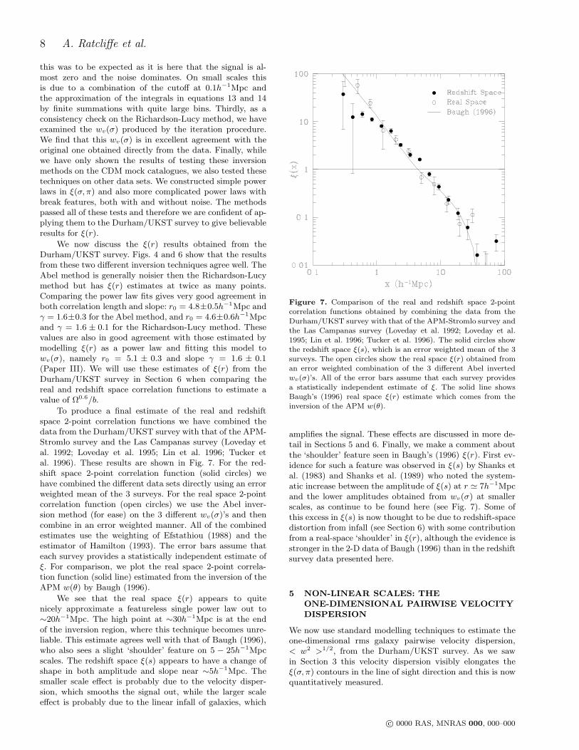
To produce a final estimate of the real and redshiftspace 2-point correlation functions we have combined thedata from the Durham/UKST survey with that of the APM-Stromlo survey and the Las Campanas survey (Loveday etal. 1992; Loveday et al. 1995; Lin et al. 1996; Tucker etal. 1996). These results are shown in Fig. 7. For the red-shift space 2-point correlation function (solid circles) wehave combined the different data sets directly using an errorweighted mean of the 3 surveys. For the real space 2-pointcorrelation function (open circles) we use the Abel inver-sion method (for ease) on the 3 different wv(σ)’s and thencombine in an error weighted manner. All of the combinedestimates use the weighting of Efstathiou (1988) and theestimator of Hamilton (1993). The error bars assume thateach survey provides a statistically independent estimate ofξ. For comparison, we plot the real space 2-point correla-tion function (solid line) estimated from the inversion of theAPM w(θ) by Baugh (1996).

We see that the real space ξ(r) appears to quitenicely approximate a featureless single power law out to∼20h−1Mpc. The high point at ∼30h−1Mpc is at the endof the inversion region, where this technique becomes unre-liable. This estimate agrees well with that of Baugh (1996),who also sees a slight ‘shoulder’ feature on 5 − 25h−1Mpcscales. The redshift space ξ(s) appears to have a change ofshape in both amplitude and slope near ∼5h−1Mpc. Thesmaller scale effect is probably due to the velocity disper-sion, which smooths the signal out, while the larger scaleeffect is probably due to the linear infall of galaxies, which

Figure 7. Comparison of the real and redshift space 2-pointcorrelation functions obtained by combining the data from the

Durham/UKST survey with that of the APM-Stromlo survey andthe Las Campanas survey (Loveday et al. 1992; Loveday et al.1995; Lin et al. 1996; Tucker et al. 1996). The solid circles showthe redshift space ξ(s), which is an error weighted mean of the 3surveys. The open circles show the real space ξ(r) obtained froman error weighted combination of the 3 different Abel invertedwv(σ)’s. All of the error bars assume that each survey providesa statistically independent estimate of ξ. The solid line showsBaugh’s (1996) real space ξ(r) estimate which comes from theinversion of the APM w(θ).

amplifies the signal. These effects are discussed in more de-tail in Sections 5 and 6. Finally, we make a comment aboutthe ‘shoulder’ feature seen in Baugh’s (1996) ξ(r). First ev-idence for such a feature was observed in ξ(s) by Shanks etal. (1983) and Shanks et al. (1989) who noted the system-atic increase between the amplitude of ξ(s) at r ≃ 7h−1Mpcand the lower amplitudes obtained from wv(σ) at smallerscales, as continue to be found here (see Fig. 7). Some ofthis excess in ξ(s) is now thought to be due to redshift-spacedistortion from infall (see Section 6) with some contributionfrom a real-space ‘shoulder’ in ξ(r), although the evidence isstronger in the 2-D data of Baugh (1996) than in the redshiftsurvey data presented here.

5 NON-LINEAR SCALES: THEONE-DIMENSIONAL PAIRWISE VELOCITYDISPERSION

We now use standard modelling techniques to estimate theone-dimensional rms galaxy pairwise velocity dispersion,< w2 >1/2, from the Durham/UKST survey. As we sawin Section 3 this velocity dispersion visibly elongates theξ(σ, π) contours in the line of sight direction and this is nowquantitatively measured.

c© 0000 RAS, MNRAS 000, 000–000


5.1 Modelling ξ(σ, π)

We follow the modelling of Peebles (1980) and define v tobe the peculiar velocity of a galaxy above the Hubble flow,therefore w = vi − vj is the peculiar velocity differenceof two galaxies separated by a vector r. Let g(r,w) be thedistribution function of w. Therefore

1 + ξ(σ, π) =

∫

[1 + ξ(r)] g(r,w)d3w, (15)

where

r2 = σ2 + r2z , rz = π − wz

H0, (16)

and wz is the component of w parallel to the line of sight,which for simplicity is called the z direction. It is commonto assume that g is a slowly varing function of r, such thatg(r,w) = g(w). Therefore, one can make the approximation∫

dwx

∫

dwy g(w) = f(wz). (17)

Equation 15 then becomes

1 + ξ(σ, π) =

∫

[1 + ξ(r)] f(wz)dwz, (18)

which further reduces to

ξ(σ, π) =

∫ ∞

−∞

ξ(r)f(wz)dwz, (19)

when the unit normalisation of f(wz) is considered. Astreaming model which describes the relative bulk motionof galaxies towards (or away from) each other can be incor-porated as follows

g(r,w) = g(w − rv(r)), (20)

where v(r) is the streaming model in question. Equation 15then becomes

1 + ξ(σ, π) =

∫

[1 + ξ(r)] f(wz − v(rz))dwz, (21)

=

∫ ∞

−∞

[

1 + ξ(

√

σ2 + r2z

)]

f [wz − v(rz)] dwz. (22)

Obviously, we require models for the real space 2-point cor-relation function, ξ(r), the distribution function, f(wz), andthe streaming motion, v(rz). The real space 2-point corre-lation function is simply modelled by a power law, ξ(r) =(r0/r)

γ , which should be accurate out to ∼20h−1Mpc. Forthe distribution function we tried both exponential andGaussian functions and found that the exponential provideda significantly better fit to the shape of the N-body simula-tion results and so is used exclusively here

f(wz) =1√

2 < w2 >1/2exp

[

−√

2|wz|

< w2 >1/2

]

, (23)

where < w2 >1/2 is the rms pairwise velocity dispersion,namely the second moment of the distribution functionf(wz)

< w2 >=

∫ ∞

−∞

f(wz)w2zdwz. (24)

A realistic streaming model might be expected to dependon the clustering, biasing and mean mass density of the

universe. The infall model of Bean et al. (1983) takes themaximal approach by assuming Ω = 1, b = 1 and uses thesecond BBGKY equation (e.g. Peebles 1980) to give

v(rz) = −H0rz

[

ξ(rz)

1 + ξ(rz)

]

. (25)

We favour this streaming model in the analysis presentedhere.

5.2 Testing the Modelling

We have tested this modelling with both the CDM simu-lations and mock catalogues. Before describing these testswe first present the answers we are trying to reproduce. Wehave calculated the values of < w2 >1/2 directly from thesimulations and find that < w2 >1/2≃ 950 and 750 kms−1

on ∼1h−1Mpc scales for the SCDM and LCDM models, re-spectively. In Paper II we estimated the real space ξ(r) cor-relation lengths to be ∼5.0h−1Mpc and ∼6.0h−1Mpc for theSCDM and LCDM models, respectively. For both of thesemodels the slope of the real space ξ(r) was ∼2.2.

In the fitting procedure there are three parameterswhich can be estimated, < w2 >1/2, r0 and γ. Given ouravailable computing constraints we only choose to fit fortwo of these and fix γ to be a constant value. The resultsobtained from this procedure are insensitive to the value ofγ chosen, provided a realistic value is used. For the CDMsimulations we use γ = 2.2. Also, when the streaming modelis used we assume that r0 = 5.0-6.0h−1Mpc in equation 25only, again the fits are relatively insensitive to the valuechosen. We fit < w2 >1/2 and r0 using an approximate χ2

statistic in the range 0-20h−1Mpc for four different valuesof σ, with the standard deviations from the simulations ormock catalogues being used accordingly in the χ2 statistic.The results of these fits using the ξ(σ, π) estimated directlyfrom the N-body simulations are shown in Figs. 8 and 9 forthe SCDM and LCDM models, respectively, with the bestfit values given in Table 1. The solid histogram denotes theaveraged ξ(σ, π) in the quoted σ range, while the solid anddotted lines show the fits with and without the streamingmodel, respectively. Similarly, Table 2 shows the results ofthe fits to the optimally estimated ξ(σ, π) from the SCDMand LCDM mock catalogues. The quoted error bars on themock catalogue results come from the 1σ standard deviationbetween the mock catalogues and therefore reflects the erroron an individual mock catalogue.

The results from the CDM simulations show thatthe streaming model only becomes important (in termsof producing consistent results for < w2 >1/2) whenσ > 1-2h−1Mpc. Of course, this assumes that < w2 >1/2

does not vary with σ. The best fit values to the CDM sim-ulation results (with streaming), had < w2 >1/2= 980 ± 22kms−1, r0 = 5.00 ± 0.24h−1Mpc for the SCDM model and< w2 >1/2= 835 ± 60 kms−1, r0 = 5.12 ± 0.69h−1Mpc forthe LCDM model. These quoted errors simply come fromthe scatter in the best fit values of Table 1. The values of< w2 >1/2 can be compared with those estimated directlyfrom the N-body simulations on ∼1h−1Mpc scales, namely950 and 750 kms−1 for the SCDM and LCDM models, re-spectively. This agreement is adequate given the slightlyad hoc assumption of an exponential distribution function.

c© 0000 RAS, MNRAS 000, 000–000


Figure 8. Histograms of ξ(σ, π) estimated from the SCDM N-body simulations as a function of π for different (constant) values of σ.The solid curve shows the minimum χ2 fit using the modelling of Section 5.1 with a streaming model, while the dotted curve shows thefit without the streaming model.

The values of r0 can be compared with the approximate realspace values estimated in Paper III, namely 5.0h−1Mpc and6.0h−1Mpc for the SCDM and LCDM models, respectively.Again, the agreement is adequate in both cases althoughslightly small for the LCDM model. However, closer inspec-tion of the LCDM ξ(r) plot on r ≤ 1h−1Mpc scales showsthat r0 is slightly lower in this region, ∼5.0h−1Mpc, whichprobably explains our measurement.

The results from the CDM mock catalogues confirm theconclusions drawn from the CDM simulation results. All ofthe < w2 >1/2 values in Table 2 agree well with their coun-terparts in Table 1 given the quoted errors (on an individual

mock catalogue). A similar statement can be made for thevalues of r0 estimated from these mock catalogues.

Overall, our tests confirm that the correct < w2 >1/2

and r0 can be reproduced by this method which modelsthe elongation in ξ(σ, π). This holds for both the ξ(σ, π)estimated directly from the N-body simulations and thatestimated using the optimal techniques for ξ from the mockcatalogues, albeit with larger scatter in this case.


We now apply the modelling of Section 5.1 to theDurham/UKST survey. We use the optimally estimated

c© 0000 RAS, MNRAS 000, 000–000


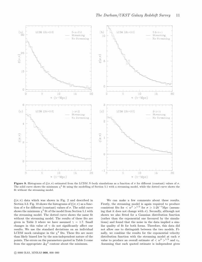
Figure 9. Histograms of ξ(σ, π) estimated from the LCDM N-body simulations as a function of π for different (constant) values of σ.The solid curve shows the minimum χ2 fit using the modelling of Section 5.1 with a streaming model, while the dotted curve shows thefit without the streaming model.

ξ(σ, π) data which was shown in Fig. 2 and described inSection 3.3. Fig. 10 shows the histograms of ξ(σ, π) as a func-tion of π for different (constant) values of σ. The solid curveshows the minimum χ2 fit of the model from Section 5.1 withthe streaming model. The dotted curve shows the same fitwithout the streaming model. The results of these fits aregiven in Table 3 where we have assumed γ = 1.7. Smallchanges in this value of γ do not significantly affect ourresults. We use the standard deviations on an individualLCDM mock catalogue in the χ2 fits. These fits are morethan likely biased low by the non-independent nature of thepoints. The errors on the parameters quoted in Table 3 comefrom the appropriate ∆χ2 contour about the minimum.

We can make a few comments about these results.Firstly, the streaming model is again required to produceconsistent fits for < w2 >1/2 for σ > 1-2h−1Mpc (assum-ing that it does not change with σ). Secondly, although notshown we also fitted for a Gaussian distribution function(rather than the exponential one favoured by the simula-tions) and found that the noise in the data implied a sim-ilar quality of fit for both forms. Therefore, this data didnot allow one to distinguish between the two models. Fi-nally, we combine the results for the exponential velocitydistribution function with the streaming model at each σvalue to produce an overall estimate of < w2 >1/2 and r0.Assuming that each quoted estimate is independent gives

c© 0000 RAS, MNRAS 000, 000–000


Table 1. Minimum χ2 fits for < w2 >1/2 and r0 from the CDMN-body simulations using the exponential distribution functionwith and without the streaming model.

σ < w2 >1/2 r0 χ2

(h−1Mpc) (kms−1) (h−1Mpc) (Nbin = 40)

SCDMStreaming Model

[0, 0.5] 990 5.1 40.0[0.5, 1] 1000 5.3 24.7[1, 2] 980 4.8 21.2[2, 4] 950 4.8 34.4

No Streaming Model[0, 0.5] 970 5.1 46.3[0.5, 1] 960 5.4 32.3[1, 2] 800 4.9 28.7[2, 4] 550 5.1 48.2

LCDMStreaming Model

[0, 0.5] 770 4.1 13.8[0.5, 1] 810 5.3 7.8[1, 2] 850 5.4 16.5[2, 4] 910 5.6 11.1

No Streaming Model[0, 0.5] 780 4.2 14.2[0.5, 1] 760 5.4 8.1[1, 2] 720 5.6 14.0[2, 4] 570 5.9 9.0

Table 2. Minimum χ2 fits for < w2 >1/2 and r0 from the CDMmock catalogues using the exponential distribution function withand without the streaming model.

σ < w2 >1/2 r0

(h−1Mpc) (kms−1) (h−1Mpc)

SCDMStreaming Model

[0, 0.5] 930 ± 190 5.0 ± 0.4[0.5, 1] 970 ± 180 5.3 ± 0.4[1, 2] 920 ± 260 4.6 ± 0.5[2, 4] 810 ± 180 4.5 ± 0.6

No Streaming Model[0, 0.5] 920 ± 190 5.0 ± 0.4[0.5, 1] 910 ± 170 5.3 ± 0.4[1, 2] 750 ± 230 4.8 ± 0.4[2, 4] 450 ± 130 5.0 ± 0.4

LCDMStreaming Model

[0, 0.5] 610 ± 180 3.8 ± 0.3[0.5, 1] 790 ± 230 5.2 ± 0.7[1, 2] 840 ± 130 5.2 ± 0.7[2, 4] 780 ± 150 5.2 ± 0.7

No Streaming Model[0, 0.5] 590 ± 170 3.9 ± 0.3[0.5, 1] 750 ± 220 5.2 ± 0.6[1, 2] 690 ± 130 5.3 ± 0.7[2, 4] 440 ± 140 5.6 ± 0.6

Table 3. Minimum χ2 fits for < w2 >1/2 and r0 from theDurham/UKST survey using the exponential distribution func-tion with and without the streaming model.

σ < w2 >1/2 r0 χ2

(h−1Mpc) (kms−1) (h−1Mpc) (Nbin = 40)

Durham/UKSTStreaming Model

[0, 0.5] 510 ± 120 5.1 ± 0.6 19.0[0.5, 1] 300 ± 50 4.7 ± 0.3 23.5[1, 2] 500 ± 65 4.5 ± 0.2 29.6[2, 4] 500 ± 65 4.7 ± 0.4 48.0

No Streaming Model[0, 0.5] 470 ± 130 5.2 ± 0.6 19.1[0.5, 1] 180 ± 70 4.8 ± 0.4 24.0[1, 2] 270 ± 90 4.8 ± 0.3 29.5[2, 4] 180 ± 80 5.5 ± 0.2 56.1

< w2 >1/2= 416 ± 36 kms−1, r0 = 4.6 ± 0.2h−1Mpc. Wemake the comment that this value of r0 agrees well withthose estimated from the Durham/UKST survey using othermethods, see Section 4.4. These results are discussed in moredetail in Section 7 where comparisons with the results fromstructure formation models and other redshift surveys aremade.

6 LINEAR SCALES: INFALL AND Ω0.6/B

We now use modelling techniques developed from the lin-ear theory result of Kaiser (1987) to estimate the quantityΩ0.6/b from the Durham/UKST survey. We saw in Section 3that on non-linear scales the velocity dispersion was mainlyresponsible for the anisotropies in ξ(σ, π). However, in Sec-tion 5 we saw that to produce consistent results it was alsonecessary to incorporate a model which imitated the stream-ing motions of galaxies. It is this infall of galaxies into over-dense regions that visibly distorts the ξ(σ, π) contours onlarger scales and this compression in the line of sight direc-tion is now quantitatively measured.

6.1 Modelling ξ(σ, π)

Kaiser (1987) used the distant observer approximation inthe linear regime of gravitational instability to show thatthe strength of an individual plane wave as measured inredshift space is amplified over that measured in real spaceby a factor

δsk = δr

k

(

1 + µ2klf(Ω)/b

)

, (26)

where δrk and δs

k are the Fourier amplitudes in real (r)and redshift (s) space, respectively, µkl is the cosine ofthe angle between the wavevector (k) and the line of sight(l), f(Ω) ≃ Ω0.6 is the logarithmic derivative of the fluc-tuation growth rate (e.g. Peebles 1980) and b is the lin-ear bias factor relating the galaxy and mass distributions,(∆ρ/ρ)g = b(∆ρ/ρ)m. The distant observer approximationrestricts use of equation 26 to opening angles in a redshiftsurvey of less than ∼50 which can cause a systematic effectat the ∼5% level in f(Ω)/b (Cole, Fisher & Weinberg 1994).

c© 0000 RAS, MNRAS 000, 000–000


Figure 10. Histograms of ξ(σ, π) estimated from the Durham/UKST survey as a function of π for different (constant) values of σ. Thesolid curve shows the minimum χ2 fit using the modelling of Section 5.1 with a streaming model, while the dotted curve shows the fitwithout the streaming model.

This (1 + µ2klf(Ω)/b) factor propagates directly through to

the power spectrum, P (k, µkl) ≡ 〈δkδ∗k〉

P s(k, µkl) = P r(k)(

1 + µ2klf(Ω)/b

)2, (27)

where the real space P r(k) is assumed to be an isotropicfunction of k only. Thus the anisotropy is a strong functionof the angle between k and l. Integrating over all µkl givesthe angle-averaged redshift space P s(k)

P s(k) =

∫ 1

−1dµklP

s(k, µkl)∫ 1

−1dµkl

, (28)

= P r(k)

[

1 +2

3

f(Ω)

b+

1

5

(

f(Ω)

b

)2]

. (29)

Fourier transforming equation 29 (which has no explicit µkl

dependence) gives the corresponding relation between theangle-averaged ξ(s) and ξ(r)

ξ(s) = ξ(r)

[

1 +2

3

f(Ω)

b+

1

5

(

f(Ω)

b

)2]

, (30)

assuming that ξ(r) is an isotropic function of r only. If thevolume integral of ξ is defined as

c© 0000 RAS, MNRAS 000, 000–000


J3(x) =

∫ x

0

ξ(y)y2dy, (31)

then

J3(s) = J3(r)

[

1 +2

3

f(Ω)

b+

1

5

(

f(Ω)

b

)2]

. (32)

We will use equations 30 and 32 as two of our methods forestimating Ω0.6/b.

Hamilton (1992) has extended Kaiser’s (1987) analysisby Fourier transforming equation 27 and noting that thecosine factor in Fourier space, µ2

kl ≡ k2l /k

2, becomes a dif-ferential operator in real space, (∂/∂|l|)2(∇2)−1. Thereforeequation 27 becomes

ξs(r, µrl) =(

1 + (f(Ω)/b)(∂/∂|l|)2(∇2)−1)2ξr(r), (33)

where µrl is the cosine of the angle between the pair separa-tion, r, and the line of sight, l. Hamilton (1992) then showsthat the solution of this equation can be written in termsof the first three even spherical harmonics of ξs(r, µrl), withthe higher moments zero (and all odd moments zero by def-inition)

ξs(r, µrl) = ξ0(r)P0(µrl) + ξ2(r)P2(µrl) + ξ4(r)P4(µrl), (34)

where Pl(µrl) are the usual Legendre polynomials and

ξl(r) =2l + 1

2

∫ 1

−1

ξs(r, µrl)Pl(µrl)dµrl. (35)

Arguably the most useful form of Hamilton’s (1992) solutionis that expressed in terms of ξ0 and ξ2 only

[

1 + 23

f(Ω)b

+ 15

(

f(Ω)b

)2]

ξ2(r) =[

43

f(Ω)b

+ 47

(

f(Ω)b

)2]

(

ξ0(r) − 3r3

∫ r

0ξ0(s)s

2ds)

,

or by defining

ξ0(r) = −ξ0(r) +3

r3

∫ r

0

ξ0(s)s2ds, (36)

ξ2(r) = −ξ2(r), (37)

it can be written as

ξ2

ξ0=

(

43β + 4

7β2)

(

1 + 23β + 1

5β2) . (38)

We will use the ratio in equation 38 as our third method forestimating Ω0.6/b.

6.2 Testing the Modelling

We have tested this modelling with the LCDM simulationsand mock catalogues. The SCDM model was not analysedbecause we felt that the one-dimensional rms galaxy pair-wise velocity dispersion too strongly dominated the ξ(σ, π)plots for a sensible answer to be obtained. As will be shownbelow this is also the case for some aspects of the LCDMmodel. Also, in Section 6.1 we noted that equation 26 andthe subsequent analysis is only strictly correct in the distantobserver approximation and that data from redshift surveyopening angles of ≤ 50 should only really be used. For red-shift surveys geometrically similar to the Durham/UKST

Figure 11. Estimates of Ω0.6/b obtained from the LCDM modelusing the method involving the ratio of real to redshift space 2-

point correlation functions (equation 30). The solid line denotesthe results obtained by averaging the ξ’s from each N-body sim-ulation and then manipulating to get an estimate of Ω0.6/b. Theshaded area denotes the 68% confidence region in Ω0.6/b obtainedfrom the scatter seen between the N-body simulation ξ results.The solid points denote the mean of the results obtained from themock catalogues. The error bars on these points are the observedstandard deviation on an individual mock catalogue.

survey this restriction has a negligible impact on the analy-sis techniques.

In Figs. 11, 12 and 13 the following conventions areadopted: the dotted line denotes the expected value off(Ω)/b ≃ Ω0.6/b = (0.2)0.6/1 ≃ 0.38; the solid line denotesthe result for Ω0.6/b obtained from the average of the LCDMsimulations (i.e. estimate an averaged ξ(σ, π) from the 5 sim-ulations and then manipulate to get one value of Ω0.6/b); theshaded area denotes the 68% confidence region in Ω0.6/b ob-tained from the scatter seen between the LCDM simulations(i.e. take the ξ(σ, π) from each of the 5 simulations, manip-ulate to get 5 values of Ω0.6/b and then average at the end);and the points with error bars are the mean and 1σ scat-ter seen in the LCDM mock catalogues (i.e. take the ξ(σ, π)from each of the 15 mock catalogues, manipulate to get 15values of Ω0.6/b and then average at the end). These errorsare the observed standard deviation between the mock cata-logues and therefore reflect the error on an individual mockcatalogue.

The results from equation 30 are shown in Fig. 11. Thismethod uses the ratio of the real to redshift space ξ’s toestimate Ω0.6/b. We estimate ξ(s) using the methods de-scribed in Paper III. We estimate ξ(r) using the Abel in-version of the projected correlation function, wv(σ), witha πcut = 30h−1Mpc, as described in Section 4. Examiningthe results obtained from the averaged ξ of the simulations(solid line), it appears that the method itself is not domi-nated by non-linear effects above ∼6h−1Mpc, although they

c© 0000 RAS, MNRAS 000, 000–000


Figure 12. The same as Fig. 11 but the Ω0.6/b results use themethod involving the ratio of real to redshift space volume inte-

grated 2-point correlation functions (equation 32).

Figure 13. The same as Fig. 11 but the Ω0.6/b results use themethod involving a ratio incorporating the second and zerothspherical harmonics of the redshift space 2-point correlation func-tion (equation 38).

could cause the ∼0.1 systematic offset in Ω0.6/b that is seenout to > 30h−1Mpc. Unfortunately, the results obtained byaveraging the 5 estimates of Ω0.6/b from each (full) simula-tion show that noise begins to dominate the inversion pro-cess between 15-20h−1Mpc. For the mock catalogues noisedominates at all scales and the results resemble a scatterplot in places. Overall, this method appears relatively in-

sensitive to non-linear effects but the large scatter (for themock catalogues) renders the method almost useless in thiscase.

The results from equation 32 are shown in Fig. 12. Thismethod uses the ratio of the real to redshift space J3’s toestimate Ω0.6/b. We estimate J3(s) by evaluating the inte-gral in equation 31 using the above ξ(s). We estimate J3(r)from the same integral but using the above ξ(r). Examiningthe results obtained from the averaged ξ of the simulations,it appears that the method itself is not dominated by non-linear effects above ∼15h−1Mpc. The results obtained byaveraging the 5 estimates of Ω0.6/b from each simulationare similarly consistent with the expected value. The resultsobtained from the mock catalogues also reproduce the cor-rect answer but with a larger scatter. Overall, this method isconsiderably more successful (in terms of more accurate re-sults) than the ξ(s)/ξ(r) one. However, one does pay a priceby having to go to larger scales before the non-linearitiesbecome negligible and the integration procedure also makesthe points highly correlated.

The results from equation 38 are shown in Fig. 13. Thismethod uses the ratio involving the second and zeroth spher-ical harmonics of ξ to estimate Ω0.6/b. The ξl’s are estimatedusing equation 35, which in practice becomes

ξl(r) = (2l + 1)∆µrl

(µirl

>0)∑

i

ξs(r, µirl)Pl(µ

irl), (39)

and we use a binning of ∆µrl = 0.2. Examining the re-sults obtained from the averaged ξ of the simulations, itappears that the method itself is severely affected by non-linearities which cause a negative value of Ω0.6/b to be mea-sured until ∼13h−1Mpc. (Such a negative value is obviouslyunphysical and simply due to the shape of the ξ(σ, π) con-tours.) Similar results are found by averaging the 5 esti-mates of Ω0.6/b from each simulation. The results obtainedfrom the mock catalogues trace the simulation results ad-equately, although not on scales < 10h−1Mpc where theyappear biased high. Overall, the impression is that the non-linearities make this method redundant. However, when con-sidering the Durham/UKST survey one must remember thatits value of the velocity dispersion is almost half that of theLCDM model. Therefore, the elongation in ξ(σ, π) whichcauses the above problems will be significantly lower.


We now apply the modelling of Section 6.1 to theDurham/UKST survey. We calculate our results using theoptimally estimated 2-point correlation function describedin Section 3.3 and Paper III. Before presenting our resultsof Ω0.6/b we show the data which produced them. Fig. 14shows the real and redshift space ξ’s, where ξ(s) is estimateddirectly from the redshift survey and ξ(r) comes from theAbel inversion of Section 4.2 shown in Fig. 4. Fig. 15 showsthe real and redshift space J3’s, where the integral in equa-tion 31 is applied to the above ξ’s. Fig. 16 shows the zerothand second spherical harmonics estimated using equation 39on the optimally estimated ξs(r, µrl). The error bars shownare those estimated from the scatter between the 4 quad-rants of the Durham/UKST survey. These errors were of a

c© 0000 RAS, MNRAS 000, 000–000


Figure 14. Comparison of the real and redshift space 2-point cor-relation functions optimally estimated from the Durham/UKST

survey. ξ(s) was estimated directly from the redshift survey (solidtriangles connected by the dotted line) and ξ(r) comes from theAbel inversion of Section 4.2 shown in Fig. 4 (solid circles con-nected by the solid line). The error bars denote the scatter seenbetween in the 4 quadrants of the Durham/UKST survey.

very similar size to those estimated on an individual LCDMmock catalogue.

We comment briefly on the results in each of thesefigures. Firstly, Fig. 14 shows that ξ(r) > ξ(s) below∼1h−1Mpc, while ξ(s) > ξ(r) on larger scales. This wasdescribed in Section 4.4. Unfortunately, the noise in theseestimates is very high and it will more than likely make anymeasurement of Ω0.6/b redundant. Secondly, Fig. 15 showsthat, once again, at small separations J3(r) > J3(s), whileat larger separations J3(s) > J3(r). There appears to bea near constant offset in the real/redshift lg J3’s on scales10-20h−1Mpc (i.e. a constant multiplicative factor in lin-ear J3). This should give a consistent estimate of Ω0.6/b onthese scales. Finally, Fig. 16 shows that ξ2 is positive until∼8h−1Mpc, which is caused by the elongation of the ξ(σ, π)contours parallel to the line of sight. On larger separationsξ2 is negative due to the compression of the ξ(σ, π) contoursparallel to the line of sight. Therefore, there appears to bea significant signal to measure in this method.

We now present the results for Ω0.6/b estimated fromthe Durham/UKST survey. Fig. 17 shows the results ofapplying equation 30 (solid squares), equation 32 (solidtriangles) and equation 38 (solid circles) to the data inFigs. 14, 15 and 16, respectively. The plotted errors de-note the standard deviation seen between the 4 quadrantsof the Durham/UKST survey. Similarly sized errors wereseen in the scatter between the individual LCDM mock cata-logues. For clarity, error bars are not shown for the ξ(s)/ξ(r)method because they are very large and only cause confu-sion.

We can make a few comments about the results from

Figure 15. Comparison of the real and redshift space J3’s es-timated from the Durham/UKST survey. These were calculated

using the integral in equation 31 with the ξ’s of Fig. 14. Again,the error bars denote the scatter seen between in the 4 quadrantsof the Durham/UKST survey.

Figure 16. The zeroth and second spherical harmonics from theDurham/UKST survey. These were calculated using equation 39on the optimally estimated ξs(r, µrl). The solid circles connectedby the solid line shows ξ0, while the solid triangles connected bythe dotted line shows −ξ2. Note that −ξ2 is plotted so that itis positive in the large scale region of interest. Again, the errorbars denote the scatter seen between in the 4 quadrants of theDurham/UKST survey.

c© 0000 RAS, MNRAS 000, 000–000


Figure 17. Estimates of Ω0.6/b obtained from the Durham/UKST survey. We use the three methods from equation 30 (solid

squares), equation 32 (solid triangles) and equation 38 (solid cir-cles) and apply them to the data in Figs. 14, 15 and 16, respec-tively. The plotted errors denote the standard deviation seen be-tween the 4 quadrants of the Durham/UKST survey. For clarity,error bars are not shown for the ξ(s)/ξ(r) method because theyare very large and only cause confusion.

these three methods. Section 6.2 showed that our region ofinterest is ∼10-30h−1Mpc because of non-linear effects onsmaller scales and noise on larger scales. For the ξ(s)/ξ(r)method, the points have no systematic trend (other than alarge random scatter) and we discount them from the fur-ther analysis. For the J3(s)/J3(r) method, we obtain quiteconsistent results although one must remember that thesepoints are not independent because of the integration prod-edure. We choose to quote the value at ∼20h−1Mpc as beingrepresentative of our results, Ω0.6/b = 0.52 ± 0.39. We be-lieve that we are being very conservative with this quotederror and, for example, the point at ∼12h−1Mpc only has anerror of ±0.19. For the ξ2/ξ0 method, we again obtain veryconsistent results and quote the value at ∼18h−1Mpc as be-ing representative, Ω0.6/b = 0.45 ± 0.38, where the quotederror is an average of the error bars in the ∼10-30h−1Mpcregion and is therefore the typical error on any individual

point in this region. Naively combining the results in a max-imum likelihood manner in the ∼10-20h−1Mpc region givesan estimate of Ω0.6/b = 0.48 ± 0.11. In this case the errorestimate is likely to be slightly underestimated given thegenerally non-independent nature of ξ points. These resultsare discussed in more detail in Section 7 where comparisonswith the results from structure formation models and otherredshift surveys are made.

7 DISCUSSION

We now discuss the results obtained from the analysis pre-sented in Sections 5 and 6. Given the observed problems withthe unweighted estimate of ξ (Paper III), we now favour theweighted estimate of ξ in all of our analysis. This explainsany slight numerical differences with respect to the quotedresults of Ratcliffe et al. (1996a). However, we state clearlythat our overall conclusions remain completely unchanged.

7.1 The One-Dimensional RMS Pairwise VelocityDispersion

The minimum χ2 fit of an exponential distribution func-tion (with a streaming model) to the optimally estimatedξ(σ, π) from the Durham/UKST survey gave a value for theone-dimensional rms pairwise velocity dispersion of 416±36kms−1. We note that this quoted error is the formal er-ror obtained from the χ2 statistic. Therefore, is it likelyto be slightly underestimated given the non-independentnature of ξ. Our observed value is of particular interestas recent estimates from new redshift surveys and the re-analysis of old redshift surveys have been measuring largervelocity dispersions than the canonical value of 340 ± 40kms−1 found by Davis & Peebles (1983) from the CfA1 sur-vey. For example, using the CfA2/SSRS2 survey, Marzke etal. (1995) find 540 ± 180 kms−1 and, using the Las Cam-panas survey, Lin et al. (1996) find 452 ± 60 kms−1. Also,Mo, Jing & Borner (1993) measured large variations (200-1000 kms−1) in the velocity dispersion for a number of sam-ples of similar size to CfA1 and they show that the esti-mated velocity dispersion is sensitive to galaxy sampling,especially dominant clusters the size of Coma. This newestimate from the Durham/UKST survey is still on theslightly low side, supporting the old Davis & Peebles (1983)value, but is not inconsistent (>3σ) with any of these othermeasured values. When considering these values it is im-portant to note that the Durham/UKST survey covers avolume ∼4 × 106h−3Mpc3, approximately twice that of theCfA2/SSRS2 survey and half that of the Las Campanas sur-vey. Also, in an unbiased (COBE-normalised) CDM model,Marzke et al. (1995) estimated that the velocity dispersionwould converge to 10% within a volume ∼5× 106h−3Mpc3.Therefore, the measurement from the Durham/UKST sur-vey is hopefully both believable and representative of theactual value in the Universe. Finally, we note that theDurham/UKST survey does not contain any extremely dom-inant clusters (of Coma-like size) and therefore will not bebiased high by this.

The best estimate of the one-dimensional rms pairwisevelocity dispersion from the SCDM and LCDM simulationswas 980 and 835 kms−1, respectively, obtained using an ex-ponential distribution function. These estimates agree wellwith the actual value of the velocity dispersion measured di-rectly from the N-body simulations. However, both of thesevalues are inconsistent with the measured value from theDurham/UKST survey at high levels of significance. In fact,taking the most negative approach possible (i.e. using the in-dividual mock catalogue velocity dispersion error bar), onestill finds a significant rejection (>3σ) of both CDM mod-els. However, it should be noted that a significant velocitybias, bv, between the matter and galaxy velocity distribu-

c© 0000 RAS, MNRAS 000, 000–000


tions (bv∼0.4), see Couchman & Carlberg (1992), wouldallow consistent results between the models and the data.Also, this rejection of the CDM models assumes that thesimple models of linear biasing used here (Bardeen et al.1986) are an adequate description of the galaxy formationprocess.

7.2 Infall and Ω0.6/b

The best estimates of Ω0.6/b from the Durham/UKST sur-vey are 0.52±0.39 for the J3(s)/J3(r) method and 0.45±0.38for the ξ2/ξ0 method, where we have (conservatively) quotedthe estimate at one separation only. Given the integrationprocedure involved in the J3 method we do not attempt tocombine these points. However, naively combining the ξ2/ξ0estimates gives Ω0.6/b = 0.48 ± 0.11. This error is likely tobe slightly underestimated given the non-independent na-ture of ξ. Our estimates can be compared with other op-

tical values of Ω0.6/b estimated using similar methods in-volving redshift space distortions. Peacock & Dodds (1994)use the real and redshift space power spectrum estimatesof various cluster, radio, optical and IRAS samples to mea-sure Ω0.6/b = 0.77 ± 0.16. Loveday et al. (1996) use theJ3 method to measure Ω0.6/b = 0.48 ± 0.12 for the APM-Stromlo survey. Lin et al. (1996) use the ξ2/ξ0 method tomeasure Ω0.6/b = 0.5 ± 0.25 for the Las Campanas survey.

As one can see, all these observed values of Ω0.6/b areconsistent with ∼0.5. Therefore, using two fiducial valuesfor b, b = 1 implies and the universe is open, Ω∼0.3, andb∼2 implies the universe has the critical-density, Ω = 1.

Finally, we state that our Ω0.6/b estimates are consis-tent with those from the two CDM models of structure for-mation considered here (SCDM and LCDM). However, giventhat these models predict (Ω0.6/b)∼0.4-0.6 we are unable todistinguish between them.

8 CONCLUSIONS

We have investigated the redshift space distortions in theDurham/UKST Galaxy Redshift Survey using the 2-pointcorrelation function perpendicular and parallel to the lineof sight, ξ(σ, π). On small, non-linear scales we observe anelongation of the ξ contours in the line of sight direction,which is due to the velocity dispersion of galaxies in virialregions. This is the common “Finger of God” effect seenin redshift surveys. On larger, linear scales we observe acompression of the ξ contours in the line of sight direction,which is due to the infall of galaxies into overdense regions.

We attempt to estimate the real space 2-point corre-lation function by direct inversion of the projected corre-lation function. We use two different inversion methods,Abel inversion and a new application of the Richardson-Lucy technique. We have tested these methods on mockcatalogues drawn from cold dark matter (CDM) N-bodysimulations and find that they reproduce the correct an-swer. We apply the methods to the Durham/UKST sur-vey and estimate ξ(r). We find that a simple power lawmodel gives best fit real space parameters of the correla-tion length, r0 = 4.8± 0.5h−1Mpc for the Abel method andr0 = 4.6±0.3h−1Mpc for the Richardson-Lucy method, andslope, γ = 1.6 ± 0.3 for the Abel method and γ = 1.6 ± 0.1

for the Richardson-Lucy method. Our estimate is consistentwith those from other redshift surveys and with the inver-sion of the APM w(θ) by Baugh (1996).

We use standard modelling techniques (e.g. Peebles1980) to estimate the one-dimensional rms pairwise veloc-ity dispersion of galaxies in the Durham/UKST survey.These methods (which were again tested on the mock cat-alogues) give an estimate of < w2 >1/2= 416 ± 36 kms−1

on ∼1h−1Mpc scales. This value agrees well with recent es-timates from new redshift surveys and re-analysis of oldredshift surveys (Markze et al. 1995; Lin et al. 1996; Moet al. 1993), although our value is still consistent with thecanonical value of Davis & Peebles (1983). We comparewith the predictions of the standard CDM model (SCDM;Ωh = 0.5 & b = 1.6) and the low density CDM model witha non-zero cosmological constant to ensure spatial flatness(LCDM; Ωh = 0.2, Λ = 0.8 & b = 1.0). We find that our re-sults are significantly (>3σ) below the estimates from thesemodels (assuming that linear biasing applies) and thereforethese models are inconsistent with the data in this con-text. This modelling also produces an estimate of the realspace correlation length from the Durham/UKST survey ofr0 = 4.6 ± 0.2h−1Mpc, which is very consistent with thepreviously quoted values.

We use the modelling techniques of Kaiser (1987)and Hamilton (1992) to estimate Ω0.6/b from theDurham/UKST survey. We test the methods with themock catalogues and find that consistent results can beobtained. The Durham/UKST survey results from theξ(s)/ξ(r) method are too noisy to obtain a useful answer.The J3(s)/J3(r) method produces an estimate of Ω0.6/b =0.52± 0.39, where we quote the estimate (and error) at onepoint only (∼20h−1Mpc) due to the non-independent na-ture of the integration procedure. The ξ2/ξ0 method givesΩ0.6/b = 0.45±0.38 at ∼18h−1Mpc, which is representativeof the results on these scales. Naively combining the pointsin the range ∼10-20h−1Mpc gives a maximum likelihood fitof 0.48± 0.11, where the error is likely to be slightly under-estimated due to the general correlated nature of ξ points.A comparison with other optical estimates of Ω0.6/b fromredshift space distortion methods gives very consistent re-sults with a value of (Ω0.6/b)≃0.5. This argues against anunbiased critical-density universe (b = 1 & Ω = 1), insteadfavouring either an unbiased low density universe (b = 1 &Ω∼0.3) or a biased critical-density universe (b∼2 & Ω = 1).Also, given that both CDM models considered here predict(Ω0.6/b)∼0.4-0.6 we cannot use our Ω0.6/b results to distin-guish between them.

Overall, combining these results with those presented inPaper III, we find that the standard CDM model underpre-dicts our 2-point correlation function results at large scalesand overpredicts the one-dimensional pairwise velocity dis-persion at small scales. Therefore, our results argue for amodel with a density perturbation spectrum more skewedtowards large scales, such as a low Ω CDM model with acosmological constant.

ACKNOWLEDGMENTS

We are grateful to the staff at the UKST and AAO for theirassistance in the gathering of the observations. S.M. Cole,

c© 0000 RAS, MNRAS 000, 000–000


C.M. Baugh and V.R. Eke are thanked for useful discussionsand supplying the CDM simulations. AR acknowledges thereceipt of a PPARC Research Studentship and PPARC arealso thanked for allocating the observing time via PATT andfor the use of the STARLINK computer facilities.

REFERENCES

Bardeen J.M., Bond J.R., Kaiser N., Szalay A.S., 1986, ApJ, 304,15

Baugh C.M., 1996, MNRAS, 280, 267Baugh C.M., Efstathiou G., 1993, MNRAS, 265, 145

Bean A.J., Efstathiou G., Ellis R.S., Peterson B.A., Shanks T.,1983, MNRAS, 205, 605

Cole S.M., Fisher K.B., Weinberg D.H., 1994, MNRAS, 267, 785

Collins C.A., Heydon-Dumbleton N.H., MacGillivray H.T., 1988,MNRAS, 236, 7p

Collins C.A., Nichol R.C., Lumsden S.L., 1992, MNRAS, 254, 295

da Costa L.N., Pellegrini P.S., Davis M., Meiksin A., SargentW.L., Tonry J.L., 1991, ApJS, 75, 935

Couchman H.M.P., Carlberg R.G., 1992, ApJ, 389, 453

Davis M., Peebles P.J.E., 1983, ApJ, 267, 465Efstathiou G., in Lawrence A., ed., 3rd IRAS, Conference, Lon-

don, Comets to Cosmology. Springer, Berlin, p. 312Efstathiou G., Davis M., Frenk C.F., White S.D.M., 1985, ApJS,

57, 241

Eke V.R., Cole S.M., Frenk C.S., Navarro J.F., 1996, MNRAS,281, 703

Fairall A.P., Jones A., 1988, Publs. Dept. Astr. Cape Town, 10

Gaztanaga E. & Baugh C.M., 1995, MNRAS, 273, 1pHamilton A.J.S., 1992, ApJ, 385, L5

Hamilton A.J.S., 1993, ApJ, 417, 19Kaiser N., 1987, MNRAS, 227, 1

Lilje P.B., Efstathiou G., 1988, MNRAS, 231, 635Lin H., Kirchner R.P., Tucker D.L., Shectman S.A., Landy S.D.,

Oemler A., Schechter P.L., 1996, submitted to ApJLoveday J., Efstathiou G., Peterson B.A., Maddox S.J., 1992,

ApJ, 400, L43Loveday J., Maddox S.J., Efstathiou G., Peterson B.A., 1995,

ApJ, 442, 457Loveday J., Efstathiou G., Maddox S.J., Peterson B.A., 1996,

ApJ, 468, 1

Lucy L.B., 1974, AJ, 79, 745Lucy L.B., 1994, AA, 289, 983

Marzke R.O., Geller M.J., da Costa L.N., Huchra J.P., 1995, AJ,110, 477

Metcalfe N., Fong R., Shanks T., Kilkenny D., 1989, MNRAS,236, 207

Metcalfe N., Fong R., Shanks T., 1995, MNRAS, 274, 769Mo H.J., Jing Y.P., Borner G., 1993, MNRAS, 264, 825

Parker Q.A., Watson F.G., 1995, in Maddox S.J., Aragon-Salamanca A., eds., 35th Herstmonceux Conf. Cambridge,Wide Field Spectroscopy and the Distant Universe. WorldScientific, Singapore, p. 33

Peacock J.A., Dodds S.J., 1994, MNRAS, 267, 1020

Peebles P.J.E., 1980, The Large-Scale Structure of the Universe,Princeton Univ. Press, Princeton, NJ

Peterson B.A., Ellis R.S., Efstathiou G.P., Shanks T., Bean A.J.,Fong R., Zen-Long Z., 1986, MNRAS, 221, 233

Ratcliffe A., Shanks T., Broadbent A., Parker Q.A., Watson F.G.,Oates A.P., Fong R., Collins C.A., 1996a, MNRAS, 281, L47

Ratcliffe A., Shanks T., Parker Q.A., Fong R., 1996b, submittedto MNRAS

Ratcliffe A., Shanks T., Fong R., Parker Q.A., 1996c, submittedto MNRAS (Paper III)

Richardson W.J., 1972, J. Opt. Soc. Am., 62, 55

Saunders W., Rowan-Robinson M., Lawrence A., 1992, MNRAS,

258, 134Shanks T., Bean A.J., Efstathiou G., Ellis R.S., Fong R., Peterson

B.A., 1983, ApJ, 274, 529Shanks T., Hale-Sutton D., Fong R., Metcalfe N., 1989, MNRAS,

237, 589Tucker D.L., Oemler A.A., Shectman S.A., Kirshner R.P., Lin H.,

Landy S.D., Schechter P.L., 1996, preprint.

c© 0000 RAS, MNRAS 000, 000–000

The Durham/UKST Galaxy Redshift Survey-IV. Redshift Space Distortions via the 2-Point Correlation Function

Documents