The DOSY Toolbox

The DOSY ToolboxA free, open source programme for processing PFG NMR diffusion data (a.k.a. DOSY data)

Current version: Version 0.6 – 13 May 2009Please direct feed-back to Mathias Nilsson, University of Manchester ([email protected]).

Dr. Mathias Nilsson School of Chemistry, University of Manchester,Oxford Road, Manchester M13 9PL, UK Telephone: +44 (0) 161 275 4668 Fax: +44 (0)161 275 [email protected]

NB This manual is basically a copy of the DOSY Toolbox wiki at the time of a new (major) release. The most up to date documentation can be found at: http://tigger.ch.man.ac.uk/dosytoolbox/doku.php

1

DOSY Toolbox manualIn addition to this manual, all the m-files (the source code) are self documented. This can be read either by opening the m-file (e.g. DOSYToolbox.m) in a text editor or type help “command” (e.g. help DOSYToolbox) at the MATLAB prompt.

Table of Contents

Quickstart

Installation

Introduction

Graphical User Interface

Menus

Processing

Diffusion Processing

2

Quick startChances are that you probably want to get started immediately and don’t want to read the whole manual. Assuming you have some experience in processing NMR data, this is for you!

1. Install the software (I am afraid that you may have to read the instructions for that).

2. Start the programme by either clicking on the icon (Windows), run the shell script (Linux and Mac), or type “DOSYToolbox “ in you MATLAB prompt (MATLAB version).

3. Import (or open) a data set using the “file” menu.

4. Pre-process you raw NMR data, using the panels, before DOSY analysis. You will probably recognise many standard features in the panels such as phasing, zero filling, referencing and baseline correction.

5. Choose one of the methods in the “Advanced Processing” panel; set your parameters and click “run” to start the processing.

6. Inspect the result in the resulting DOSY or component spectra.

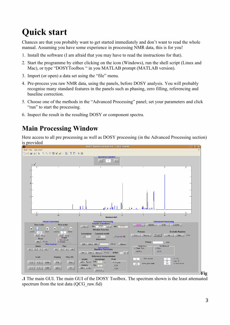
Main Processing WindowHere access to all pre processing as well as DOSY processing (in the Advanced Processing section) is provided

Fig.1 The main GUI. The main GUI of the DOSY Toolbox. The spectrum shown is the least attenuated spectrum from the test data (QCG_raw.fid)

3

Example OutputThe output from fitting the demonstration data using some of the available methods.

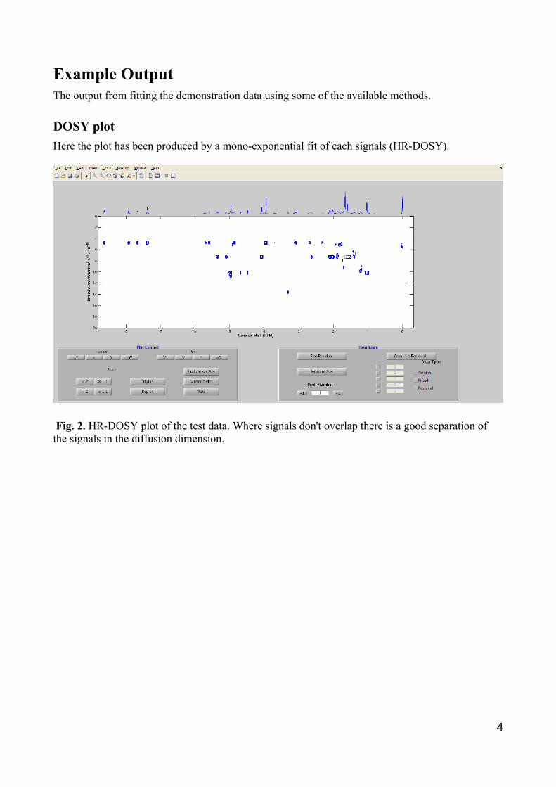
DOSY plot

Here the plot has been produced by a mono-exponential fit of each signals (HR-DOSY).

Fig. 2. HR-DOSY plot of the test data. Where signals don't overlap there is a good separation of the signals in the diffusion dimension.

4

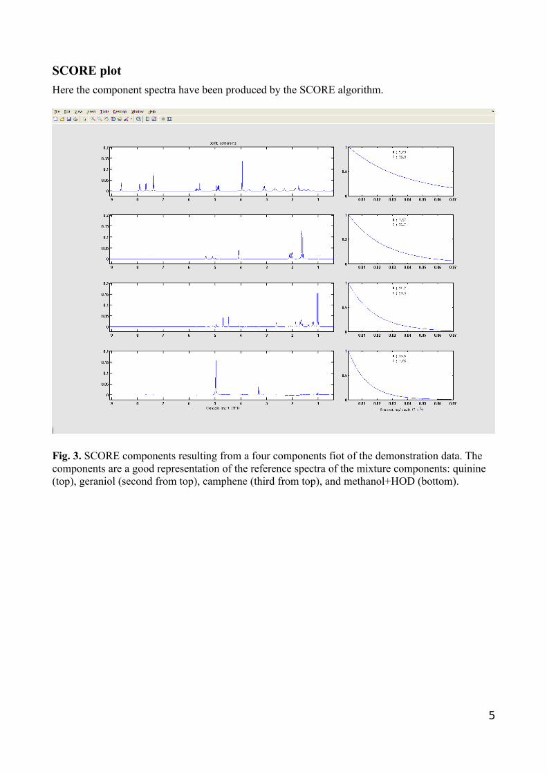
SCORE plot

Here the component spectra have been produced by the SCORE algorithm.

Fig. 3. SCORE components resulting from a four components fiot of the demonstration data. The components are a good representation of the reference spectra of the mixture components: quinine (top), geraniol (second from top), camphene (third from top), and methanol+HOD (bottom).

5

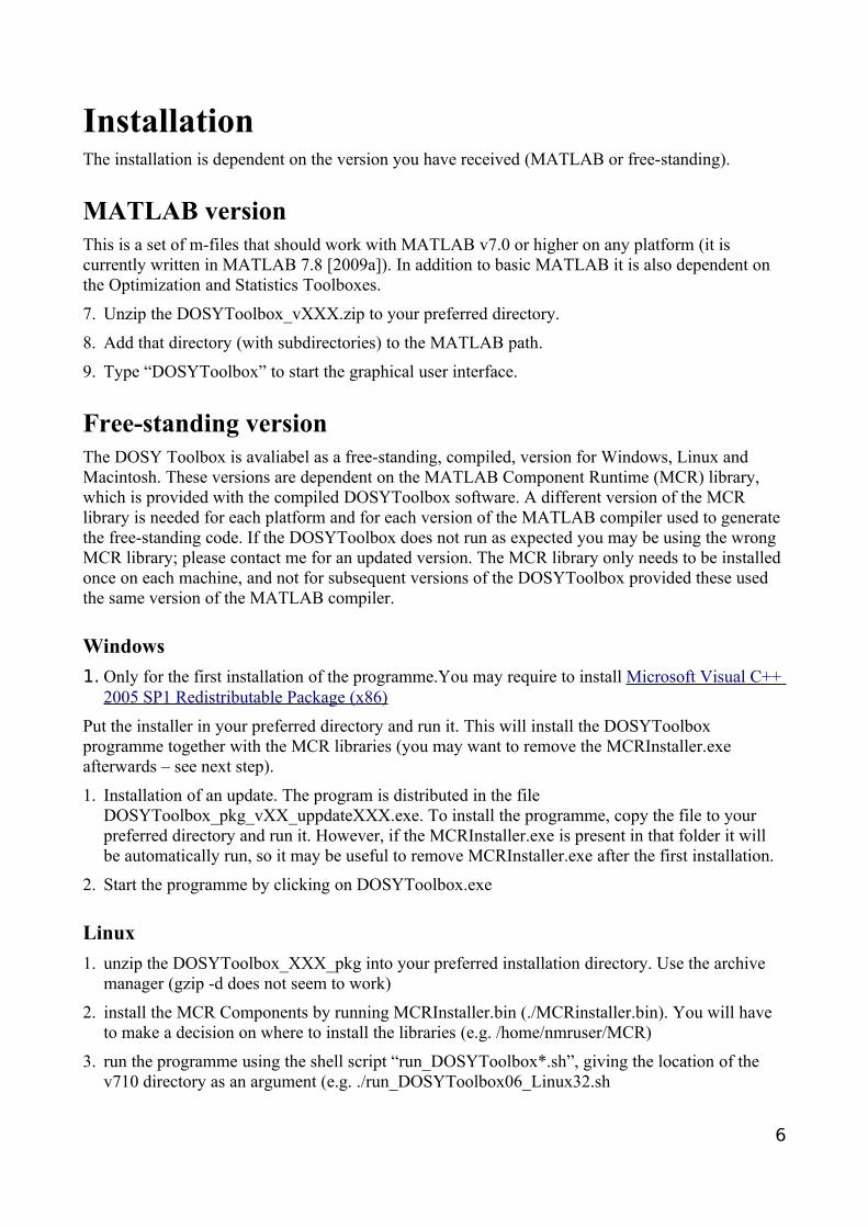
InstallationThe installation is dependent on the version you have received (MATLAB or free-standing).

MATLAB versionThis is a set of m-files that should work with MATLAB v7.0 or higher on any platform (it is currently written in MATLAB 7.8 [2009a]). In addition to basic MATLAB it is also dependent on the Optimization and Statistics Toolboxes.

7. Unzip the DOSYToolbox_vXXX.zip to your preferred directory.

8. Add that directory (with subdirectories) to the MATLAB path.

9. Type “DOSYToolbox” to start the graphical user interface.

Free-standing versionThe DOSY Toolbox is avaliabel as a free-standing, compiled, version for Windows, Linux and Macintosh. These versions are dependent on the MATLAB Component Runtime (MCR) library, which is provided with the compiled DOSYToolbox software. A different version of the MCR library is needed for each platform and for each version of the MATLAB compiler used to generate the free-standing code. If the DOSYToolbox does not run as expected you may be using the wrong MCR library; please contact me for an updated version. The MCR library only needs to be installed once on each machine, and not for subsequent versions of the DOSYToolbox provided these used the same version of the MATLAB compiler.

Windows

1. Only for the first installation of the programme.You may require to install Microsoft Visual C++ 2005 SP1 Redistributable Package (x86)

Put the installer in your preferred directory and run it. This will install the DOSYToolbox programme together with the MCR libraries (you may want to remove the MCRInstaller.exe afterwards – see next step).

1. Installation of an update. The program is distributed in the file DOSYToolbox_pkg_vXX_uppdateXXX.exe. To install the programme, copy the file to your preferred directory and run it. However, if the MCRInstaller.exe is present in that folder it will be automatically run, so it may be useful to remove MCRInstaller.exe after the first installation.

2. Start the programme by clicking on DOSYToolbox.exe

Linux

1. unzip the DOSYToolbox_XXX_pkg into your preferred installation directory. Use the archive manager (gzip -d does not seem to work)

2. install the MCR Components by running MCRInstaller.bin (./MCRinstaller.bin). You will have to make a decision on where to install the libraries (e.g. /home/nmruser/MCR)

3. run the programme using the shell script “run_DOSYToolbox*.sh”, giving the location of the v710 directory as an argument (e.g. ./run_DOSYToolbox06_Linux32.sh

6

/home/nmruser/MCR/v710)

Optional The programme can also be started by running the executable “DOSYToolbox…” (e.g. ./DOSYToolbox06_Linux32), but then you must set some environment variables (automatically set in the run_* macro). In the cshell this would be (for the example above)

setenv LD_LIBRARY_PATH /home/nmruser/MCR/v710/runtime/glnx86: /home/nmruser/MCR/v710/sys/os/glnx86: /home/nmruser/MCR/v710/sys/java/jre/glnx86/jre1.6.0/lib/i386/native_threads: /home/nmruser/MCR/v710/sys/java/jre/glnx86/jre1.6.0/lib/i386/server: /home/nmruser/MCR/v710/sys/java/jre/glnx86/jre1.6.0/lib/i386setenv XAPPLRESDIR<mcr_root> /home/nmruser/MCR/v710/X11/app-defaults

Mac

1. unzip the DOSYToolbox_XXX_pkg into your preferred installation directory. Use the archive manager (gzip -d does not seem to work)

2. install the MCR Components by running MCRInstaller.bin (./MCRinstaller.bin). You will have to make a decision on where to install the libraries (e.g. /home/nmruser/MCR)

3. run the programme using the shell script “run_DOSYToolbox*.sh”, giving the location of the v710 directory as an argument (e.g. ./run_DOSYToolbox06_Linux32.sh /home/nmruser/MCR/v710)

7

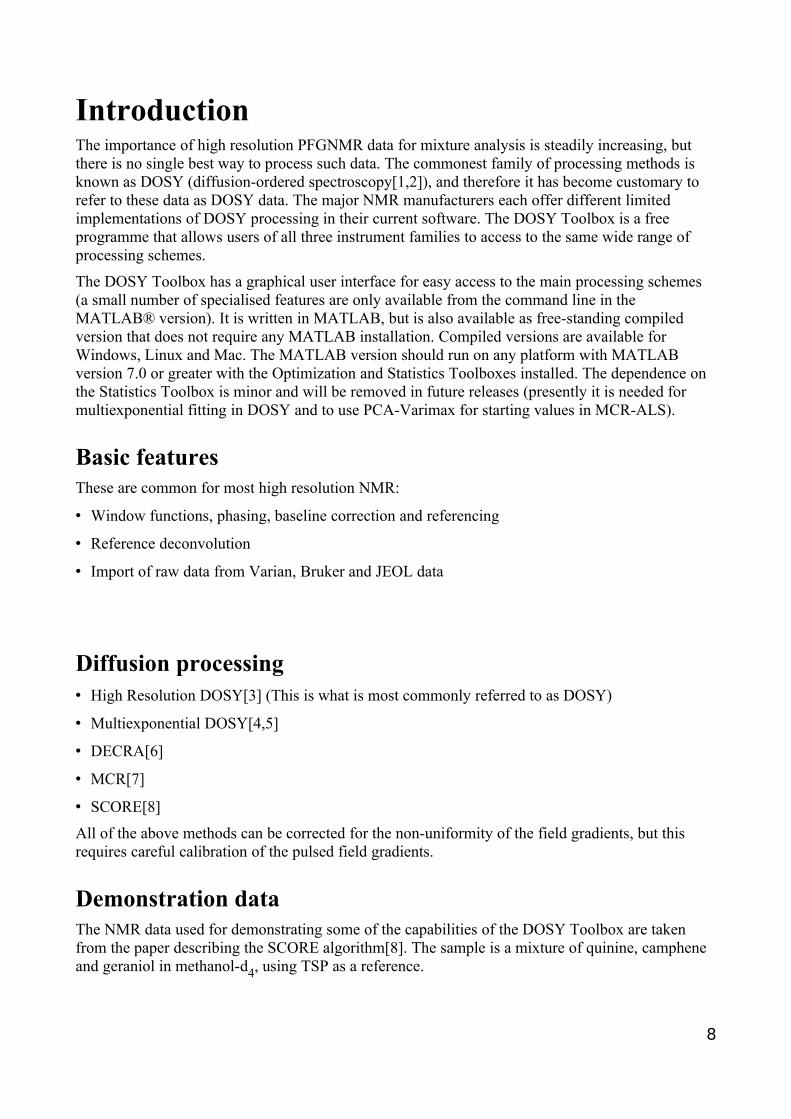
IntroductionThe importance of high resolution PFGNMR data for mixture analysis is steadily increasing, but there is no single best way to process such data. The commonest family of processing methods is known as DOSY (diffusion-ordered spectroscopy[1,2]), and therefore it has become customary to refer to these data as DOSY data. The major NMR manufacturers each offer different limited implementations of DOSY processing in their current software. The DOSY Toolbox is a free programme that allows users of all three instrument families to access to the same wide range of processing schemes.

The DOSY Toolbox has a graphical user interface for easy access to the main processing schemes (a small number of specialised features are only available from the command line in the MATLAB® version). It is written in MATLAB, but is also available as free-standing compiled version that does not require any MATLAB installation. Compiled versions are available for Windows, Linux and Mac. The MATLAB version should run on any platform with MATLAB version 7.0 or greater with the Optimization and Statistics Toolboxes installed. The dependence on the Statistics Toolbox is minor and will be removed in future releases (presently it is needed for multiexponential fitting in DOSY and to use PCA-Varimax for starting values in MCR-ALS).

Basic featuresThese are common for most high resolution NMR:

• Window functions, phasing, baseline correction and referencing

• Reference deconvolution

• Import of raw data from Varian, Bruker and JEOL data

Diffusion processing• High Resolution DOSY[3] (This is what is most commonly referred to as DOSY)

• Multiexponential DOSY[4,5]

• DECRA[6]

• MCR[7]

• SCORE[8]

All of the above methods can be corrected for the non-uniformity of the field gradients, but this requires careful calibration of the pulsed field gradients.

Demonstration dataThe NMR data used for demonstrating some of the capabilities of the DOSY Toolbox are taken from the paper describing the SCORE algorithm[8]. The sample is a mixture of quinine, camphene and geraniol in methanol-d4, using TSP as a reference.

8

References

[1] C.S. JohnsonJr., Diffusion ordered nuclear magnetic resonance spectroscopy: principles and applications, Prog. Nucl. Magn. Reson. Spectrosc. 34 (1999) 203-256. [2] G.A. Morris, Diffusion-Ordered Spectroscopy (DOSY)., in: D.M. Grant, R.K. Harris (Eds.), Encyclopedia of Nuclear Magnetic Resonance, Chichester, John Wiley & Sons Ltd, 2002: pp. 35-44. [3] H. Barjat, G.A. Morris, S. Smart, A.G. Swanson, S.C.R. Williams, High-Resolution Diffusion-Ordered 2D Spectroscopy (HR-DOSY) - A New Tool for the Analysis of Complex Mixtures, J. Magn. Reson. 108 (1995) 170-172. [4] K.F. Morris, C.S. Johnson, Diffusion-ordered two-dimensional nuclear magnetic resonance spectroscopy, J. Am. Chem. Soc. 114 (1992) 3139-3141. [5] M. Nilsson, M.A. Connell, A.L. Davis, G.A. Morris, Biexponential fitting of diffusion-ordered NMR data: Practicalities and limitations, Anal. Chem. 78 (2006) 3040-3045. [6] W. Windig, B. Antalek, Direct exponential curve resolution algorithm (DECRA): A novel application of the generalized rank annihilation method for a single spectral mixture data set with exponentially decaying contribution profiles, Chemom. Intell. Lab. Syst. 37 (1997) 241-254. [7] L.C.M. Van Gorkom, T.M. Hancewicz, Analysis of DOSY and GPC-NMR Experiments on Polymers by Multivariate Curve Resolution, J. Magn. Reson. 130 (1998) 125-130. [8] M. Nilsson, G.A. Morris, Speedy Component Resolution: An Improved Tool for Processing Diffusion-Ordered Spectroscopy Data, Anal. Chem. 80 (2008) 3777-3782.

9

The graphical user interfaceWhen you start the DOSYToolbox, the main window will open, which provides access to (almost) all processing capabilities via processing panels and menus:

Figure 4. The main GUI of the DOSY Toolbox. The spectrum shown is the least attenuated spectrum from the test data (QCG_raw.fid)

10

Menus

Files menuThe files menu provides access to importing, saving and exporting data files (the structure of the DOSYToolbox files is described in Appendix A).

Open

Opens data files saved by the DOSYToolbox (*.nmr)a.

Import

Import raw data files (FIDs) from the main NMR manufacturersb.

Available formats

• Bruker (standard format)

• Jeol (jeol generic)

• Varian (standard format)

Save

Saves the current data as *.nmr (seea).

Export

Different formats for exporting your data.

Available formats

DOSY Processing

Exports the data as *.pfg. This is the standard *.mat format and can be imported into MATLAB using “load –mat filemname.pfg” and will contain a structure required by the command line processing functions: decra_mn, dosy_mn, mcr_mn and score_mn.

Edit menu

NMR Parameters

This gives access to general NMR parameters

The parameters are:

• fpmult: multiplication factor for the first point in the FID (default 0.5)

NB! Access to coefficients for non-uniform field gradient (NUG) calibration[1] is also accessed

11

here, although they should probably be moved to DOSY parameters. The NUG specific parameters are:

• probe: the name of the probe

• gcal: the gradient calibration value (converting nominal gradient amplitude to T/m)

• c1-c4: the gradient coefficients

The parameters can be typed in or read in as a text file with one parameter per line:

ID probe 400MHz9.8100e-040.9281-0.0098-3.8342e-042.5137e-05

DOSY Parameters

This gives access to the diffusion dependent parameters. Only when known standard pulse sequences have been used for acquisition these can be correctly imported, otherwise they have to be entered by the user

The parameters are :

• Δ: diffusion time

• Δ′: corrected diffusion time

• δ: diffusin encoding time

• dosyconstant: γ2× δ2 × Δ

• γ: magnetogyric ratio of the nucleus (normally 1H)

The parameter “dosyconstant” is what is actually used in the calculations entered manually. Changing either of the other parameters will prompt you to calculate the dosyconstant using one of the options (presently only one)

12

Footnotes

aThese files are in the standard MATLAB format *.mat but renamed *.nmr. From the MATLAB command line these *.nmr files can be opened using “load –mat filename.nmr” bThe programme reads standard Varian and Bruker files, but only the JEOL Generic file format so other JEOL file types will have to be converted – consult your JEOL documentation

References

[1] M.A. Connell, P.J. Bowyer, P. Adam Bone, A.L. Davis, A.G. Swanson, M. Nilsson, et al., Improving the accuracy of pulsed field gradient NMR diffusion experiments: Correction for gradient non-uniformity, J. Magn. Reson. 198 (2009) 121-131.

13

ProcessingThese sections contain the tools to process the imported DOSY data.

Spectrum number (1)This panel is used to display the different gradient levels.

Phase correction (2)Zero and first (linear) order phase correction is applied using the slide bars. Pressing the set button enables to set the pivot point at which the first order correction is zero. Clicking the slider itself adjusts the phase in steps of 10 (degrees), the arrows on the slider in steps of 1 and the buttons below in steps of 0.1. An exact number can also be entered in the display box. The phase correction can have two different scopes. When set to global (default) the same correction is applied to all the spectra in the array, and when set to individual each array element is phased individually. The individual scopes is implemented to allow correction of gradient dependent phase shift, (not uncommonly) present in the data.

14

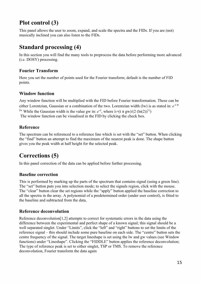
Plot control (3)This panel allows the user to zoom, expand, and scale the spectra and the FIDs. If you are (not) musically inclined you can also listen to the FIDs.

Standard processing (4)In this section you will find the many tools to preprocess the data before performing more advanced (i.e. DOSY) processing.

Fourier Transform

Here you set the number of points used for the Fourier transform; default is the number of FID points.

Window function

Any window function will be multiplied with the FID before Fourier transformation. These can be either Lorentzian, Gaussian or a combination of the two. Lorentzian width (lw) is as stated in: e-t π

lw While the Gaussian width is the value gw in: e-λ, where λ=(t π gw)/(2 (ln(2))½) The window function can be visualised in the FID by clicking the check box.

Reference

The spectrum can be referenced to a reference line which is set with the “set” button. When clicking the “find” button an attempt to find the maximum of the nearest peak is done. The shape button gives you the peak width at half height for the selected peak.

Corrections (5)In this panel correction of the data can be applied before further processing.

Baseline correction

This is performed by marking up the parts of the spectrum that contains signal (using a green line). The “set” button puts you into selection mode; to select the signals region, click with the mouse. The “clear” button clear the set regions while the “apply” button applied the baseline correction to all the spectra in the array. A polynomial of a predetermined order (under user control), is fitted to the baseline and subtracted from the data,

Reference deconvolution

Reference deconvolution[1,2] attempts to correct for systematic errors in the data using the difference between the experimental and perfect shape of a known signal; this signal should be a well separated singlet. Under “Limits”, click the “left” and “right” buttons to set the limits of the reference signal – this should include some pure baseline on each side. The “centre” button sets the centre frequency of the signal. The target lineshape is set using the lw and gw values (see Window functions) under “Lineshape”. Clicking the “FIDDLE” button applies the reference deconvolution; The type of reference peak is set to either singlet, TSP or TMS. To remove the reference deconvolution, Fourier transform the data again

15

References

[1] G.A. Morris, Reference Deconvolution., in: D.M. Grant, R.K. Harris (Eds.), Encyclopedia of Nuclear Magnetic Resonance, Chichester, John Wiley & Sons Ltd, 2002: pp. 125-131. [2] G.A. Morris, H. Barjat, T.J. Home, Reference deconvolution methods, Prog. Nucl. Magn. Reson. Spectrosc. 31 (1997) 197-257.

16

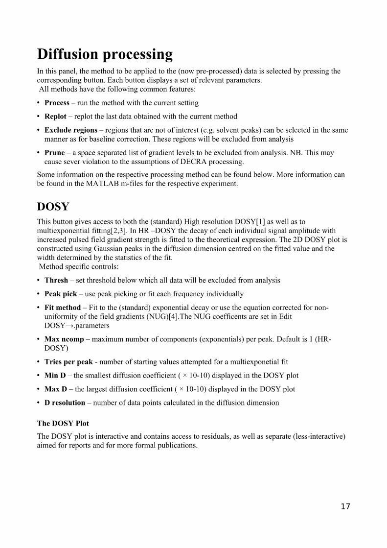
Diffusion processingIn this panel, the method to be applied to the (now pre-processed) data is selected by pressing the corresponding button. Each button displays a set of relevant parameters. All methods have the following common features:

• Process – run the method with the current setting

• Replot – replot the last data obtained with the current method

• Exclude regions – regions that are not of interest (e.g. solvent peaks) can be selected in the same manner as for baseline correction. These regions will be excluded from analysis

• Prune – a space separated list of gradient levels to be excluded from analysis. NB. This may cause sever violation to the assumptions of DECRA processing.

Some information on the respective processing method can be found below. More information can be found in the MATLAB m-files for the respective experiment.

DOSYThis button gives access to both the (standard) High resolution DOSY[1] as well as to multiexponential fitting[2,3]. In HR –DOSY the decay of each individual signal amplitude with increased pulsed field gradient strength is fitted to the theoretical expression. The 2D DOSY plot is constructed using Gaussian peaks in the diffusion dimension centred on the fitted value and the width determined by the statistics of the fit. Method specific controls:

• Thresh – set threshold below which all data will be excluded from analysis

• Peak pick – use peak picking or fit each frequency individually

• Fit method – Fit to the (standard) exponential decay or use the equation corrected for non-uniformity of the field gradients (NUG)[4].The NUG coefficents are set in Edit DOSY→.parameters

• Max ncomp – maximum number of components (exponentials) per peak. Default is 1 (HR-DOSY)

• Tries per peak - number of starting values attempted for a multiexponetial fit

• Min D – the smallest diffusion coefficient ( × 10-10) displayed in the DOSY plot

• Max D – the largest diffusion coefficient ( × 10-10) displayed in the DOSY plot

• D resolution – number of data points calculated in the diffusion dimension

The DOSY Plot

The DOSY plot is interactive and contains access to residuals, as well as separate (less-interactive) aimed for reports and for more formal publications.

17

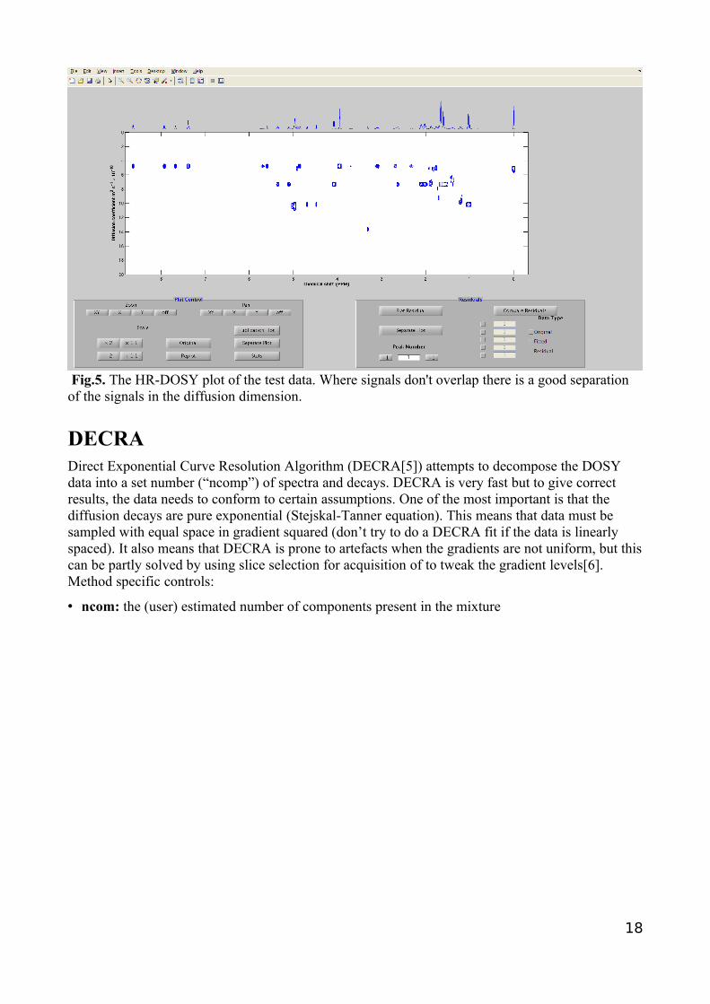
Fig.5. The HR-DOSY plot of the test data. Where signals don't overlap there is a good separation of the signals in the diffusion dimension.

DECRADirect Exponential Curve Resolution Algorithm (DECRA[5]) attempts to decompose the DOSY data into a set number (“ncomp”) of spectra and decays. DECRA is very fast but to give correct results, the data needs to conform to certain assumptions. One of the most important is that the diffusion decays are pure exponential (Stejskal-Tanner equation). This means that data must be sampled with equal space in gradient squared (don’t try to do a DECRA fit if the data is linearly spaced). It also means that DECRA is prone to artefacts when the gradients are not uniform, but this can be partly solved by using slice selection for acquisition of to tweak the gradient levels[6]. Method specific controls:

• ncom: the (user) estimated number of components present in the mixture

18

The DECRA Plot

The DECRA plot displays the fitted components.

Fig. 6. DECRA components resulting from a four components fiot of the demonstration data.

MCRMultivariate Curve Resolution is an umbrella name of a number of methods. Here a simple form of MCR-ALS (alternating least squares) is implemented[7-12]. Initial guesses can be made either as “spectra” or “decays”. Initialisation method can be either PCA-VARIMAX or DECRA (note that you need to have the gradient levels equally spaced in gradient squared). During the ALS loop certain constraints can be applied to the data. These are non-negativity for the decays and/or for the spectra. In addition, the decays can be forced to follow either the Stejskal-Tanner (pure exponential) or the NUG function (see DOSY above). Method specific controls:

• ncom: the (user) estimated number of components present in the mixture

• Init Guess: Start with initial estimates of spectra or decays

• Init Method: Method for estimating initial spectra (command line use of mcr_mn allows the usage of any user supplied spectra or decays)

• Dec constr: constraints for the decays

• Spec constr: constraints for the spectra

19

• Force decay: the decay is forced to a predetermined shape (exponential or NUG)

The MCR Plot

The MCR plot displays the fitted components.

Fig. 7. MCR components resulting from a four components fit of the demonstration data. The initialisation method was DECRA and the decays were forced to a decay shaped dtermined by the non-uniformity of the pulsed field gradients (NUG).

SCORESpeedy Component Resolution (SCORE)[13] estimates the spectra using a predetermined shape of the decay (exponential or NUG). Method specific controls:

• ncom: the (user) estimated number of components present in the mixture

• Dguess: initial estimation of the diffusion coefficients of the components in the mixture. This can either random or based on the diffusion average coefficient obtained for all the resonances in the data.

• Constraint: the component spectra can be constrained to non-negativity.

• Fitting function : Fit to the (standard) exponential decay or use the equation corrected for non-uniformity of the field gradients (NUG)[4].The NUG coefficents are set in Edit

20

DOSY→.parameters

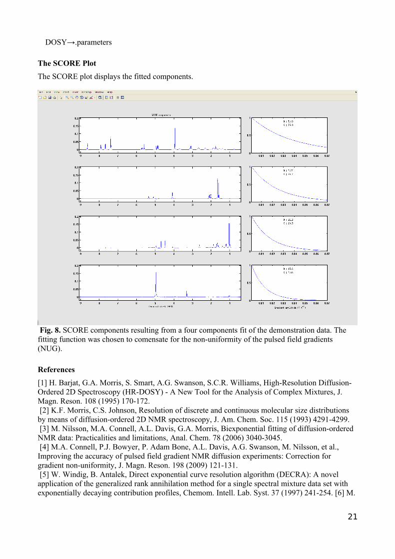
The SCORE Plot

The SCORE plot displays the fitted components.

Fig. 8. SCORE components resulting from a four components fit of the demonstration data. The fitting function was chosen to comensate for the non-uniformity of the pulsed field gradients (NUG).

References

[1] H. Barjat, G.A. Morris, S. Smart, A.G. Swanson, S.C.R. Williams, High-Resolution Diffusion-Ordered 2D Spectroscopy (HR-DOSY) - A New Tool for the Analysis of Complex Mixtures, J. Magn. Reson. 108 (1995) 170-172. [2] K.F. Morris, C.S. Johnson, Resolution of discrete and continuous molecular size distributions by means of diffusion-ordered 2D NMR spectroscopy, J. Am. Chem. Soc. 115 (1993) 4291-4299. [3] M. Nilsson, M.A. Connell, A.L. Davis, G.A. Morris, Biexponential fitting of diffusion-ordered NMR data: Practicalities and limitations, Anal. Chem. 78 (2006) 3040-3045. [4] M.A. Connell, P.J. Bowyer, P. Adam Bone, A.L. Davis, A.G. Swanson, M. Nilsson, et al., Improving the accuracy of pulsed field gradient NMR diffusion experiments: Correction for gradient non-uniformity, J. Magn. Reson. 198 (2009) 121-131. [5] W. Windig, B. Antalek, Direct exponential curve resolution algorithm (DECRA): A novel application of the generalized rank annihilation method for a single spectral mixture data set with exponentially decaying contribution profiles, Chemom. Intell. Lab. Syst. 37 (1997) 241-254. [6] M.

21

Nilsson, G.A. Morris, Improved DECRA processing of DOSY data: correcting for non-uniform field gradients, Magn. Reson. Chem. 45 (2007) 656-660. [7] L.C.M. Van Gorkom, T.M. Hancewicz, Analysis of DOSY and GPC-NMR Experiments on Polymers by Multivariate Curve Resolution, J. Magn. Reson. 130 (1998) 125-130. [8] R. Huo, R. Wehrens, J. van Duynhoven, L.M. Buydens, Assessment of techniques for DOSY NMR data processing, Analytica Chimica Acta. 490 (2003) 231-251. [9] R. Huo, R. Wehrens, L.M.C. Buydens, Improved DOSY NMR data processing by data enhancement and combination of multivariate curve resolution with non-linear least square fitting, J. Magn. Reson. 169 (2004) 257-269. [10] R. Huo, R.A. van de Molengraaf, J.A. Pikkemaat, R. Wehrens, L.M.C. Buydens, Diagnostic analysis of experimental artefacts in DOSY NMR data by covariance matrix of the residuals, Journal of Magnetic Resonance. 172 (2005) 346-358. [11] R. Huo, C. Geurts, J. Brands, R. Wehrens, L.M.C. Buydens, Real-life applications of the MULVADO software package for processing DOSY NMR data, Magn. Reson. Chem. 44 (2006) 110-117. [12] R. Huo, R. Wehrens, L. Buydens, Robust DOSY NMR data analysis, Chemometrics and Intelligent Laboratory Systems. 85 (2007) 9-19. [13] M. Nilsson, G.A. Morris, Speedy Component Resolution: An Improved Tool for Processing Diffusion-Ordered Spectroscopy Data, Anal. Chem. 80 (2008) 3777-3782.

22