The DLLA limit of BFKL in the dipole picture

arX

iv:h

ep-p

h/98

0738

9v1

15

Jul 1

998

The DLLA limit of BFKL in the DipolePicture

M. B. Gay Ducati ∗

and

V. P. Goncalves ∗∗

Instituto de Fısica, Univ. Federal do Rio Grande do Sul

Caixa Postal 15051, 91501-970 Porto Alegre, RS, BRAZIL

Abstract: In this work we obtain the DLLA limit of BFKL in thedipole picture and compare it with HERA data. We demonstrate that inleading - logarithmic - approximation, where αs is fixed, a transition betweenthe BFKL dynamics and the DLLA limit can be obtained in the region ofQ2 ≈ 150 GeV 2. We compare this result with the DLLA predictions obtainedwith αs running. In this case a transition is obtained at low Q2 (≤ 5 GeV 2).This demonstrates the importance of the next-to-leading order correctionsto the BFKL dynamics. Our conclusion is that the F2 structure function isnot the best observable for the determination of the dynamics, since there isgreat freedom in the choice of the parameters used in both BFKL and DLLApredictions.

PACS numbers: 12.38.Aw; 12.38.Bx; 13.90.+i;Key-words: Small x QCD; Perturbative calculations; BFKL pomeron.

0∗E-mail:[email protected]∗∗E-mail:[email protected]

1 Introduction

The behaviour of ep/pp scattering in high energy limit and fixed momentumtransfer is one of the outstanding open questions in the theory of the stronginteractions. In the late 1970s, Lipatov and collaborators [1] established thepapers which form the core of our knowledge of Regge limit (high energieslimit) of Quantum Chromodynamics (QCD). The physical effect that theydescribe is often referred to as the QCD pomeron, or BFKL pomeron. Thesimplest process where the BFKL pomeron applies is the very high energyscattering between two heavy quark-antiquark states, i. e. the onium-oniumscattering. For a suficiently heavy onium state, high energy scattering is aperturbative process since the onium radius gives the essential scale at whichthe running coupling is evaluated. Recently [2, 3, 4] this process was studiedin the QCD dipole picture, where the heavy quark-antiquark pair and thesoft gluons in the large Nc limit are viewed as a collection of color dipoles.In this case, the cross section can be understood as a product of the numberof dipoles in one onium state times the number of dipoles in the other oniumstate times the basic cross section for dipole-dipole scattering due to two-gluon exchange. In [2] Mueller demonstrated that the QCD dipole picturereproduces the BFKL physics. In this work we discuss the BFKL pomeronusing the QCD dipole picture.

Experimental studies of the BFKL pomeron are at present carried outmainly in HERA ep collider in deeply inelastic scattering in the region of lowvalues of the Bjorken variable x ≡ Q2

2p.q, where Q2 ≡ −q2. Here p is the four-

momentum of the proton and q is the four-momentum transfer of the eletronprobe. In this case, QCD pomeron effects are expected to give rise to apower-law growth of the structure functions as x goes to zero. However, thisstudy in deeply inelastic scattering is made difficult by the fact that the low xbehaviour is influenced by both short distance and long distance physics [5].As a result, predictions at photon virtuality Q depend on a nonperturbativeinput at a scale Q0 < Q. This makes it difficult to desantangle perturbativeBFKL predictions from nonperturbatives effects. Moreover, the program ofcalculating the next-to-leading corrections to the BFKL equation was onlyformulated recently [6]. Of course there are uncertainties due to subleadingcorrections and from the treatment of infrared region of the BFKL equationwhich will modify the predictions of this approach.

One of the most striking discoveries at HERA is the steep rise of the

1

proton structure function F2(x, Q2) with decreasing Bjorken x [7]. The be-haviour of structure function at small x is driven by the gluon through theprocess g → qq. The behaviour of the gluon distribution at small x is itselfpredicted from perturbative QCD via BFKL equation. This predicts a char-acteristic x−λ singular behaviour in the small x regime, where for fixed αs

the BFKL exponent λ = 3αs

π4ln2. It is this increase in the gluon distribu-

tion with decreasing x that produces the corresponding rise of the structurefunction. However, the determination of the valid dynamics in the small xregion is an open question, since the conventional DGLAP approach [8] cangive an excellent description of F2 at small x. The goal of this letter is todiscuss this question.

Recently Navelet et al. [9] applied the QCD dipole model to deep inelasticlepton-nucleon scattering. They assumed that the virtual photon at highQ2 can be described by an onium. For the target proton, they made anassumption that it can be approximated by a collection of onia with anaverage onium radius to be determined from the data. This model describedreasonably the F2 data in a large range of Q2(< 150 GeV 2) and x.

In this letter we obtain the double-leading-logarithmic-approximation(DLLA) limit of BFKL in the QCD dipole picture using the approach pro-posed by Navelet et al.. This limit is common to BFKL and DGLAP dy-namics. We show that using our DLLA result HERA data can be describedin the range Q2 ≥ 150 GeV 2 and all interval of x. Moreover, we compareour results with the predictions of Navelet et al. and with the predictionsobtained using DGLAP evolution equations in the small-x limit. This letteris organized as follows. In Section 2 the QCD dipole picture is presented. InSection 3 we obtain the proton structure function in this approach and itsDLLA limit. In section 4 we apply our result to F2 HERA data and presentour conclusions.

2 QCD dipole picture

In this section we describe the basic ideas of the QCD dipole picture inthe onium-onium scattering. Let A be the scattering amplitude normalizedaccording to

2

dσ

dt=

1

4π|A|2 . (1)

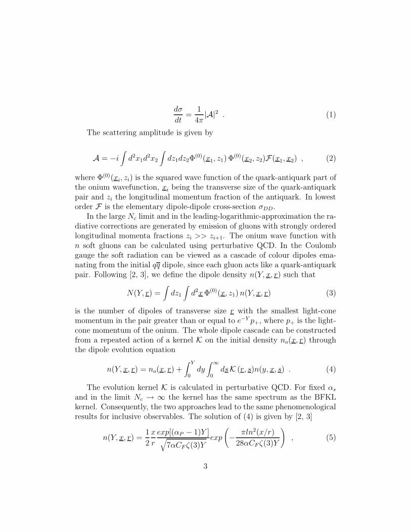
The scattering amplitude is given by

A = −i∫

d2x1d2x2

∫

dz1dz2Φ(0)(x1, z1) Φ(0)(x2, z2)F(x1, x2) , (2)

where Φ(0)(xi, zi) is the squared wave function of the quark-antiquark part ofthe onium wavefunction, xi being the transverse size of the quark-antiquarkpair and zi the longitudinal momentum fraction of the antiquark. In lowestorder F is the elementary dipole-dipole cross-section σDD.

In the large Nc limit and in the leading-logarithmic-approximation the ra-diative corrections are generated by emission of gluons with strongly orderedlongitudinal momenta fractions zi >> zi+1. The onium wave function withn soft gluons can be calculated using perturbative QCD. In the Coulombgauge the soft radiation can be viewed as a cascade of colour dipoles ema-nating from the initial qq dipole, since each gluon acts like a quark-antiquarkpair. Following [2, 3], we define the dipole density n(Y, x, r) such that

N(Y, r) =∫

dz1

∫

d2x Φ(0)(x, z1) n(Y, x, r) (3)

is the number of dipoles of transverse size r with the smallest light-conemomentum in the pair greater than or equal to e−Y p+, where p+ is the light-cone momentum of the onium. The whole dipole cascade can be constructedfrom a repeated action of a kernel K on the initial density no(x, r) throughthe dipole evolution equation

n(Y, x, r) = no(x, r) +∫ Y

0dy∫

∞

0dsK (r, s)n(y, x, s) . (4)

The evolution kernel K is calculated in perturbative QCD. For fixed αs

and in the limit Nc → ∞ the kernel has the same spectrum as the BFKLkernel. Consequently, the two approaches lead to the same phenomenologicalresults for inclusive observables. The solution of (4) is given by [2, 3]

n(Y, x, r) =1

2

x

r

exp[(αP − 1)Y ]√

7αCF ζ(3)Yexp

(

−πln2(x/r)

28αCF ζ(3)Y

)

, (5)

3

where αP − 1 = (8αCF/π)ln2.The onium-onium scattering amplitude in the leading-logarithmic approx-

imation will be written as in (2), but where F is now given by

F =∫

d2r

r

d2s

sn(Y/2, x1, r)n(Y/2, x2, s) σDD . (6)

Consequently, the cross section grows rapidly with the energy because thenumber of dipoles in the light cone wave function grows rapidly with theenergy. This result is valid in the kinematical region where Y is not verylarge. At large Y the cross section breaks down due to the diffusion to largedistances, determined by the last exponential factor in (5), and due to theunitarity constraint. Therefore new corrections should become importantand modify the BFKL behaviour [10].

The result (5) was obtained for a process with only one scale, the oniumradius. In processes where two scales are present, for example the eletron-proton deep inelastic scattering, this result is affected by non-perturbativecontributions [5]. Therefore, the application of BFKL approach at ep scat-tering must be made with caution.

3 Structure function in the QCD dipole pic-

ture

Our goal in this section is to obtain the proton structure functions

FL,T (x, Q2) =Q2

4παe.m.

σγ∗ pL,T (7)

using the QCD dipole picture. In order to do so we must make the assumptionthat the proton can be approximately described by onium configurations.Basically, we make use of the assumption

σγ∗ pL,T = σγ∗ onium

L,T ×P , (8)

where P is the probability of finding an onium in the proton. In order toobtain the σγ∗ onium

tot we will follow [9], where the kT factorization [11] wasused in the context of the QCD dipole model. We have that

σγ∗ oniumL,T =

∫

d2r dz Φ(0)(r, z) σγ∗ dipole(x, Q2, r) , (9)

4

where the γ∗ − dipole cross section reads

Q2σγ∗ dipole(x, Q2, r) =∫

d2k∫ 1

0

dz

zσγ∗ g(

x

z,k2

Q2)G(z, k, r) . (10)

In (10) σγ∗ g is the γ∗g → qq Born cross section and G is the non-integratedgluon distribution function. The relation between this function and thedipole density is expressed by

k2 G(z, k, r) =∫

s2

s

∫ 1

0

dz′

z′n(z′, r, s) σγ∗ d(

z

z′, s2k2) , (11)

where n(z′, r, s) is the density of dipoles of transverse size s with the smallestlight-cone momentum in the pair equal to z′p+ in a dipole of transverse sizer, of total momentum p+. This is given by the solution (5).

After some considerations Navelet et al. obtain

Q2σγ∗ dipole(x, Q2, r) = 4π2αe.m.

2αNc

π

∫

dγ

2πihL,T (γ)

v(γ)

γ(r2Q2)γe[ αNc

πχ(γ)ln 1

x] ,

(12)

where αNc

πχ(γ) is the BFKL spectral function (for more details see [9]).

The γ∗ onium cross section is obtained using (12) in (9). The resultdepends on the squared wave function Φ(0) of the onium state, which cannotbe computed perturbatively. Consequently, an assumption must be made.In [9] this dependence is eliminated by averaging over the wave function oftransverse size

∫

dzd2r(r2)γΦ(0)(r, z) = (M2)−γ , (13)

where M2 is a scale which is assumed to be perturbative. Therefore theproton structure functions reads

FL,T (x, Q2) =2αNc

π

∫

dγ

2πihL,T (γ)

v(γ)

γ(Q2

M2)γe[ αNc

πχ(γ)ln 1

x]P(γ, M2) , (14)

where P(γ, M2) is the Mellin-transformed probability of finding an oniumof transverse mass M2 in the proton. Using an adequate choice for thisprobability (see ref. [9]) the proton structure function can be written as

FL,T (x, Q2) =2αNc

π

∫ dγ

2πihL,T (γ)

v(γ)

γ(Q2

Q20

)γe[ αNcπ

χ(γ)ln 1

x]P(γ) . (15)

5

The expression (15) can be evaluated using the steepest descent method.The saddle point is given by

χ′(γs) = −lnQ2

Q2

0

αNc

πln 1

x

. (16)

Using in the expression (16) the expansion of the BFKL kernel near γ = 12,

we get

γs =1

2

1 −

QQ0

αNc

π7ζ(3)ln 1

x

. (17)

Consequently

F2(x, Q2) = FT (x, Q2) + FL(x, Q2)

= C a1

2

Q

Q0e[( 4αNcln2

π)ln 1

x−

a2ln2 Q

Q0]

, (18)

where

a =

(

1αNc

π7ζ(3)ln 1

x

)

. (19)

The parameters C, Q0 and α are determined by the fit. Using C = 0.077,Q0 = 0.627 GeV and α ≈ 0.11, Navelet et al. obtained that the expression(18) fits the HERA data [7] in the region Q2 ≤ 150 GeV 2.

In this letter we analize the behaviour of F2 obtained by expression (15) inthe double leading logarithmic approximation (DLLA). This limit is commonto both DGLAP and BFKL dynamics, i.e. it represents the transition regionbetween the dynamics. Therefore, before the determination of the regionwhere the BFKL dynamics (BFKL Pomeron) is valid, we must determineclearly the region where the DLLA limit is valid. In this limit χ(γ) = 1

γ.

Using this limit in (16) we get that the saddle point is at

γs =

√

√

√

√

√

αNc

πln 1

x

lnQ2

Q2

0

. (20)

6

Consequently, we get

F DLLA2 (x, Q2) =

2αNc

πC

(lnQ2

Q2

0

)1

4

(αNc

πln 1

x)

3

4

e

[

2

√

αNcπ

ln 1

xln

Q2

Q2

0

]

. (21)

The result (21) reproduces the behaviour of double leading logarithmic ap-proximation. As this result was obtained considering the dipole model, thenαs is fixed. The parameters C, α and Q0 should be taken from the fit. In thenext section we compare this result with HERA data.

4 Results and Conclusions

In this section we compare the expression (21) with the recent H1 data [7].In order to test the accuracy of the F2 parameterization obtained in formula(21), a fit of H1 data has been performed. The parameters obtained were

C = 0.0035 , Q0 = 0.45 and α = 0.19 . (22)

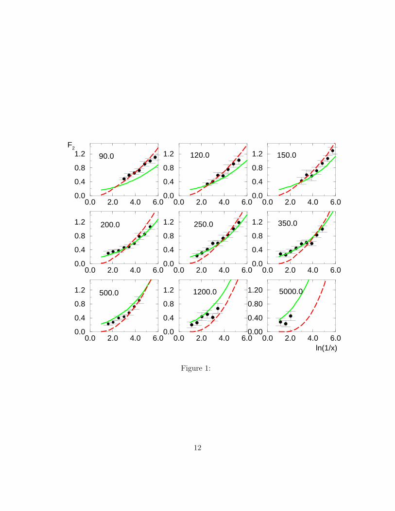
In the figures (1) and (2) we present our results at different Q2 and x.The predictions of Navelet et al. (dashed curve) are also presented. Whilethe expression (18) describes the data in region Q2 ≤ 150 GeV 2, we cansee that the expression (21) (solid curve) describes H1 data in kinematicalregion Q2 > 150 GeV 2. Therefore the HERA data are described by theDLLA expression in the high Q2 region. Moreover, we can conclude thatthere is a transition between the BFKL behaviour and the DLLA behaviourin the region Q2 ≈ 150 GeV 2. This could be the first evidence of the BFKLbehaviour in F2. However, this conclusion is not strong since that (18) and(21) were obtained in the leading-logarithmic-approximation, where αs isfixed. Moreover, the parametrizations obtained using the DGLAP evolutionequation describes the HERA data [12].

The program of calculating the next-to-leading corrections to the BFKLequation is not still concluded [10]. However, some results may be antici-pated. For instance, the NLO BFKL equation must have as limit the DLLAlimit in the region where αs log 1

xlog Q2 ≈ 1. This limit is common to

both DGLAP and BFKL dynamics. As the NLO corrections to the DGLAPevolution equations are known, the DLLA limit with αs running is well estab-lished. The DLLA limit obtained considering the DGLAP evolution equation

7

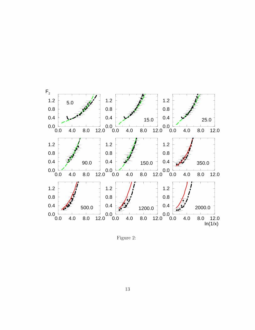
was largely discussed by Ball and Forte [13]. Consequently we can estimatethe importance of αs running in our result. In figure (2) we compare ourresults with the DLLA predictions with αs running (dot-dashed curve), ob-tained using DGLAP evolution equations in the small-x limit. In this casethe DLLA limit can describe one more large kinematical region. The regionQ2 ≤ 5 GeV 2 is not described by DLLA αs running. Consequently, the kine-matical region where the BFKL dynamics may be present is restricted to thelow Q2 region.

Our results are strongly dependent on free parameters, since there isgreat freedom in the choice of parameters used in both BFKL and DLLApredictions. This comes from theoretical uncertainties, for example, the de-termination where the pQCD is valid (i.e. the Q0 value). However, ourqualitative result agrees with the conclusion obtained by Mueller [14], thatdemonstrated that the BFKL diffusion leads to the breakdown of the OPEat small-x. Using the bounds obtained by Mueller we expect that the BFKLevolution can be visible in a limited range of x at Q2 → Q2

0. Moreover, ourresult agrees with the conclusion of Ayala et al. [15], where the shadowingcorrections to F2 structure function were considered. In this case the anoma-lous dimension is modified and the BFKL behaviour only can be visible inthe region of low Q2.

In this paper we calculate the DLLA limit of BFKL in the dipole pic-ture. The determination of this limit is very important, since it is com-mon to BFKL and DGLAP dynamics. Therefore, before the determina-tion of the region where the BFKL dynamics is valid, we must determinateclearly the region where the DLLA limit is valid. We demonstrate that inthe leading-logarithmic approximation (αs fixed) a transition region betweenthe BFKL dynamics and the DLLA limit can be obtained in the region ofQ2 ≈ 150 GeV 2. We compare this result with the DLLA predictions ob-tained with αs running. In this case a transition region is obtained at low Q2

(≤ 5 GeV 2). This demonstrates the importance of the next-to-leading ordercorrections to the BFKL dynamics. Our conclusion is that the F2 structurefunction is not the best observable in the determination of the dynamics.From the inclusive measurements of F2 it seems improbable to draw anyconclusion based on the presently available data. It is theoretically question-able whether it will be possible as long as one considers only one observable.The better observables for determination of the dynamics are the ones asso-ciated with processes where only one scale is present, since in these processes

8

it is inambigously possible to isolate the effects of the BFKL behaviour.

Acknowledgments

This work was partially financed by CNPq, BRAZIL.

References

[1] E.A. Kuraev, L.N. Lipatov and V.S. Fadin. Phys. Lett B60 (1975) 50;Sov. Phys. JETP 44 (1976) 443; Sov. Phys. JETP 45 (1977) 199; Ya.Balitsky and L.N. Lipatov. Sov. J. Nucl. Phys. 28 (1978) 822.

[2] A. H. Mueller. Nucl. Phys. B415 (1994) 373.

[3] A. H. Mueller and B. Patel. Nucl. Phys. B425 (1994) 471.

[4] Z. Chen and A. H. Mueller. Nucl. Phys. B451 (1995) 579.

[5] J. Bartels, H. Lotter and M. Vogt. Phys. Lett B373 (1996) 215.

[6] V. S. Fadin and L. N. Lipatov. Nucl. Phys. B477 (1996) 767.

[7] S. Aid et al.. Nucl. Phys. B470 (1996) 3.

[8] Yu. L. Dokshitzer. Sov. Phys. JETP 46 (1977) 641; G. Altarelli and G.Parisi. Nucl. Phys. B126 (1977) 298; V. N. Gribov and L.N. Lipatov.Sov. J. Nucl. Phys 28 (1978) 822.

[9] H. Navelet et al.. Phys. Lett B385 (1996) 357.

[10] V. S. Fadin aand L. N. Lipatov. hep-ph/9802290.

[11] S. Catani and F. Hautmann. Nucl. Phys. B427 (1994) 475.

[12] M. Gluck, E. Reya and A. Vogt. Z. Phys. C67 (1995) 433.

[13] R. Ball and S. Forte Phys. Lett B335 (1994) 77.

[14] A. H. Mueller. Phys. Lett B396 (1997) 251.

9

[15] A. L. Ayala, M. B. Gay Ducati and E. M. Levin. Nucl. Phys. B493

(1997) 305; Nucl. Phys. B511 (1998) 355.

10

Figure Captions

Fig. 1: Behavior of proton structure function predicted by BFKL (18)(dashed curve) and DLLA (21) (solid curve). Data of H1 [7]. See text.

Fig. 2: Behavior of proton structure function predicted by BFKL (18)(dashed curve), DLLA (21) (solid curve) and DLLA with running couplingconstant (dot-dashed curve). Data of H1 [7]. See text.

11

0.0 2.0 4.0 6.00.0

0.4

0.8

1.2

0.0 2.0 4.0 6.00.0

0.4

0.8

1.2

0.0 2.0 4.0 6.00.0

0.4

0.8

1.2

0.0 2.0 4.0 6.00.0

0.4

0.8

1.2

0.0 2.0 4.0 6.00.0

0.4

0.8

1.2

0.0 2.0 4.0 6.00.0

0.4

0.8

1.2

0.0 2.0 4.0 6.00.00

0.40

0.80

1.20

0.0 2.0 4.0 6.00.0

0.4

0.8

1.2

0.0 2.0 4.0 6.00.0

0.4

0.8

1.290.0 120.0 150.0

200.0 250.0 350.0

500.0

F2

5000.0

ln(1/x)

1200.0

Figure 1:

12

0.0 4.0 8.0 12.00.0

0.4

0.8

1.2

0.0 4.0 8.0 12.00.0

0.4

0.8

1.2

0.0 4.0 8.0 12.00.0

0.4

0.8

1.2

0.0 4.0 8.0 12.00.0

0.4

0.8

1.2

0.0 4.0 8.0 12.00.0

0.4

0.8

1.2

0.0 4.0 8.0 12.00.0

0.4

0.8

1.2

0.0 4.0 8.0 12.00.0

0.4

0.8

1.2

0.0 4.0 8.0 12.00.0

0.4

0.8

1.2

0.0 4.0 8.0 12.00.0

0.4

0.8

1.2

ln(1/x)

F2

5.0

15.0 25.0

90.0 150.0 350.0

500.0 1200.0 2000.0

Figure 2:

13