The distribution of wealth: Intergenerational transmission and redistributive policies Jess Benhabib Department of Economics New York University Alberto Bisin Department of Economics New York University This draft: September 2007 Abstract We study the dynamics of the distribution of wealth in an economy with inter- generational transmission of wealth and redistributive scal policy. We character- ize the transitional dynamics of the distribution of wealth as well as its stationary state. We show that the stationarywealth distribution is a Pareto distribution.We We gratefully acknowledge conversations with Marco Bassetto, Alberto Bressan, Gianluca Clementi, Isabel Correia, Mariacristina De Nardi, Raquel Fernandez, Xavier Gabaix, Leslie Greengard, Frank Hoppensteadt, Boyan Jovanovic, Nobu Kiyotaki, John Leahy, Omar Licandro, Chris Phelan, Hamid Sabourian, Tom Sargent, Pedro Teles,Viktor Tsyrennikov, Gianluca Violante, Ivan Werning, and Ed Wol/. Thanks to Nicola Scalzo and Eleonora Patacchini for help with impossibleItalian references. We also gratefully acknowledge Viktor Tsyrennikovs expert research assistance. This paper is part of the Polarization and Conict Project CIT-2-CT-2004-506084 funded by the European Commission-DG Research Sixth Framework Programme. 1

Welcome message from author
This document is posted to help you gain knowledge. Please leave a comment to let me know what you think about it! Share it to your friends and learn new things together.
Transcript

The distribution of wealth:
Intergenerational transmission
and redistributive policies�
Jess Benhabib
Department of Economics
New York University
Alberto Bisin
Department of Economics
New York University
This draft: September 2007
Abstract
We study the dynamics of the distribution of wealth in an economy with inter-
generational transmission of wealth and redistributive �scal policy. We character-
ize the transitional dynamics of the distribution of wealth as well as its stationary
state. We show that the stationary wealth distribution is a Pareto distribution.We
�We gratefully acknowledge conversations with Marco Bassetto, Alberto Bressan, Gianluca Clementi,
Isabel Correia, Mariacristina De Nardi, Raquel Fernandez, Xavier Gabaix, Leslie Greengard, Frank
Hoppensteadt, Boyan Jovanovic, Nobu Kiyotaki, John Leahy, Omar Licandro, Chris Phelan, Hamid
Sabourian, Tom Sargent, Pedro Teles,Viktor Tsyrennikov, Gianluca Violante, Ivan Werning, and Ed
Wol¤. Thanks to Nicola Scalzo and Eleonora Patacchini for help with �impossible�Italian references.
We also gratefully acknowledge Viktor Tsyrennikov�s expert research assistance. This paper is part of
the Polarization and Con�ict Project CIT-2-CT-2004-506084 funded by the European Commission-DG
Research Sixth Framework Programme.
1

study analytically the dependence of the distribution of wealth, of wealth inequal-
ity, and of utilitarian social welfare on various redistributive �scal policy instru-
ments like capital income taxes, estate taxes, and welfare subsidies.
2

1 Introduction
Rather invariably across a large cross-section of countries and time periods income and
wealth distributions are skewed to the right and display a heavy upper tail (slowly
declining top wealth shares). These observations have lead Vilfredo Pareto, in the Cours
d�Economie Politique (1897), to introduce the distributions which take his name1 and to
theorize about the possible economic and sociological factors generating wealth distrib-
utions of such form. The results of Pareto�s investigations take the form of the "Pareto�s
Law," enunciated e.g., by Samuelson (1965) as follows:
In all places and all times, the distribution of income remains the same. Nei-
ther institutional change nor egalitarian taxation can alter this fundamental
constant of social sciences.
Since Pareto, economists have lost con�dence in "fundamental constant(s) of social
sciences".2 Nonetheless distributions of income and wealth which are very concentrated
and skewed to the right have been well documented over time and across countries. For
example, Atkinson (2001), Moriguchi-Saez (2005), Piketty (2001), Piketty-Saez (2003),
and Saez-Veall (2003) document skewed distributions of income, including capital in-
come, with relatively large top shares consistently over the last century, respectively, in
the U.K., Japan, France, the U.S., and Canada. Large top wealth shares in the U.S.
1Pareto distributions are power laws. They display heavy tails, in the sense that the frequency of
events in the tails of the distribution declines more slowly than e.g., in a Normal distribution. They
represent a subset of the class of stable Levy distributions, that is, of the distributions which are obtained
from the version of the Central Limit Theorem which does not impose �nite mean and variance; see
e.g., Nolan (2005).2See Chipman (1976) for a discussion on the controversy between Pareto and Pigou regarding the
interpretation of the Law. To be fair to Pareto, his view was not necessarily that �scal policies cannot
alter the distribution of wealth, but that �scal policy is determined by the controlling elites who use it
to skew the distribution to their advantage; see Pareto (1900).
3

since the 60�s are documented e.g., by Wol¤ (1987, 2004).3 Also, heavy upper tails of
the distributions of income and wealth is a well documented empirical regularity; e.g.
Klassa, Bihama, Levy, Malcaia and Solomon (2006) for the US, Nirei-Souma (2004) for
the U.S. and Japan from 1960 to 1999, Clementi-Gallegati (2004) for Italy from 1977 to
2002, and Dagsvik-Vatne (1999) for Norway in 1998.
While Pareto was skeptical that "egalitarian taxation" could have any signi�cant
e¤ect on the distribution of income, many have later concluded that the redistributive
taxation regimes introduced after World War II did in fact signi�cantly reduce income
and wealth inequality; notably, e.g., Lampman (1962) and Kuznets (1955). Most re-
cently, Piketty (2001) has argued that redistributive taxation may have prevented large
income shares from recovering after the shocks that they experienced during World War
II in France.4
In this paper we study the dynamics of the distribution of wealth as generated
by inter-generational transmission and redistributive �scal policy. We model inter-
generational transmission of wealth is induced by parental altruism, in the form either of
pure altruism or of "joy of giving" preferences for bequests. Redistributive �scal policy
is implemented through welfare subsidies �nanced by capital income taxes and estate
taxes on bequeathed wealth.
More speci�cally, our economy is populated by a continuum of age structured over-
lapping generations of agents with a constant probability of death as in Blanchard (1985)
and Yaari (1965). The population is stationary and each agent who dies is substituted
3While income and wealth are correlated and have qualitatively similar distributions, wealth tends
to be more concentrated than income. For instance the Gini coe¢ cient of the distribution of wealth in
the U.S. in 1992 is :78, while it is only :57 for the distribution of income (Diaz Gimenez-Quadrini-Rios
Rull, 1997); see also Feenberg-Poterba (2000).4This line of argument has been extended to the U.S., Japan, and Canada, respectively, by Piketty-
Saez (2003) and Moriguchi-Saez (2005), Saez-Veall (2003).
4

by his/her child. A fraction of the agents are altruistic towards children and optimally
choose the amount of bequests they leave. Agents are born with an initial wealth which is
composed of the present discounted value of their expected future earnings, the bequests
of their parents and, if they qualify, welfare subsidies from the government. Agents face
a constant interest rate. They choose an optimal consumption-savings plan, which in-
cludes the allocation of their wealth between annuities and assets which are bequeathed
at their death. The government taxes capital income and estates to redistribute wealth
in the form of welfare subsidies. The government budget is balanced.
We show that our model generates a a stationary wealth distribution which has
the main qualitative properties which characterize wealth distributions: skewedness and
fat tails. To stress inter-generational transmission as the process of wealth dynamics
which we study, we disregard agents�earnings in most of the formal analysis.5 In other
words, we study old money rather than new money.6 In particular, we show that
inter-generational transmission and redistributive �scal policy by themselves, without
earnings�heterogeneity, are su¢ cient to induce a stationary wealth distribution which is
a power law, a Pareto distribution in particular. We are therefore able to characterize
the wealth distribution in closed form and hence to perform various comparative statics
5The importance of intergenerational transfers in accounting for wealth accumulation has emphasized
by Kotliko¤ and Summers (1981). They argue that intergenerational wealth transfers, rather than life
cycle earnings, account for up to 80% of wealth accumulation. See also Gale and Scholtz (1994) for
more moderate �ndings along the same lines.6The relative importance of old money vs new money has been studied by Elwood, Miller, Bayard,
Watson, Collins, and Hartman (1999). They classify the wealthiest individuals in the Forbes 400 in
1995 and 1996 according to whether they represent old or new money. They �nd that 43.5% of those on
the list came from old money, that is they inherited su¢ cient wealth to rank among Forbes 400, while
30.1% represented new money, consisting of individuals and families whose parents did not have great
wealth or own a business with more than a few employees. The remaining 26.4% were in intermediate
categories. See also Burris (2000), p. 364, footnote 3. Finally, see Piketty-Saez (2003) for evidence of
the relative decline of old money in accounting for top income shares in the U.S. since the 60�s.
5

exercises which enable us to analytically study the determinants of the wealth distribu-
tion and, in particolar, of wealth inequality. The two critical ingredients that drive the
Pareto wealth distribution in our model are i) the accumulation of wealth with time and,
most importantly, through inheritance, and ii) the redistribution of wealth to the young
poor through estate and capital taxes. The level of concentration and of inequality of
wealth at the stationary distribution depends on the demographic characteristics of the
economy, its structural parameters, as well as on the endogenous growth rate of the
economy. Most speci�cally, wealth is less concentrated (the Gini coe¢ cient is lower) the
higher is the density of agents receiving welfare subsidies, that is, the more wealth is
redistributed via welfare subsidies. Furthermore, wealth is less concentrated the lower is
the growth rate of individual wealth accumulation and the higher is the growth rate of
aggregate wealth. The wedge between the individual and the aggregate growth rates of
wealth depends in turn also on �scal policy: the more redistributive is �scal policy, the
smaller is the wedge, and hence the less concentrated in the wealth in the economy.
Furthermore, our explicit characterization of the stationary distribution of wealth
allows us to study analytically the dependence of wealth inequality on the di¤erent re-
distributive �scal policy instruments we study, capital income taxes and estate taxes. In
particular, wealth is less concentrated for both higher capital income taxes and estate
taxes, but the marginal e¤ect of capital income taxes is much stronger than the e¤ect of
estate taxes. When earnings are entered in the analysis we cannot solve for the whole
wealth distribution in closed form. However, we show that our results hold unchanged
for the tail of the wealth distribution. In other words, it is the intergenerational trans-
mission of wealth which in our model determines the form of the tail of the distribution.
We also perform a tentative calibration exercise to illustrate the possible contribution of
the inter-generational transmission of wealth to the determination of the observed levels
of wealth inequality. We �nd that the wealth inequality induced by intergenerational
transmission accounts for just little less than a third of the wealth inequality in the U.S.
6

in 1992. Finally, we characterize optimal redistributive taxes with respect to a utilitarian
social welfare measure. With such an "egalitarian" welfare measure, in an economy with
no labor earnings,7 maximizing social welfare is almost equivalent to minimizing the con-
centration or inequality of wealth. Nonetheless, completely minimizing wealth inequality
requires reducing the economy�s growth rate, hence at the optimal taxes inequality is
not eliminated, but in our rough benchmark calibration growth would be reduced by
1:1%. Concentrating on policies which directly a¤ect the intergenerational transmission
of wealth, we show that, robustly around our benchmark calibrated economy, social wel-
fare is maximized with zero estate taxes. Social welfare maximizing capital income taxes,
on the contrary, are positive and close to the value which minimizes wealth inequality.
Our social welfare function assigns positive weight to agents currently alive, and future
generations enter into the social welfare computations only through the bequest motive.
If we weighted future generations separately as well, we would be putting more weight on
growth, so that the optimal taxes would tolerate greater inequality and would penalize
growth by less.
1.1 Related literature
A large and diverse theoretical literature on the dynamics of individual wealth dating
back to the 1950es obtains distributions exhibiting power laws and, in particular, Pareto
distributions. Notably, Champernowne (1953), Rutherford (1955), Simon (1955), and
most of the subsequent literature study accumulation models in which an exogenous sto-
chastic process drives wealth accumulation di¤erentially for low and high wealth ranges.
Typically in these models the stochastic processes are such that there is a lower a re�ec-
tive barrier to wealth, and the higher levels of wealth thinned out by death, or by negative
expected growth.Wold-Whittle (1957) in particular study a birth and death process with
7Labor earnings would naturally limit the scope of equalization measures which reduce the agents�
incentives to supply labor or invest in human capital.
7

population growth, exogenous exponential wealth accumulation, and bequests. Most re-
cently, the analysis of stochastic processes generating power laws in the distribution of
wealth has become an important subject in Econophysics (see Mantegna-Stanley, 2000,
Gabaix-Gopikrishnan-Plerou-Stanley 2003).8
The stochastic processes which generate power laws in this whole literature are essen-
tially exogenous, that is, they are not the result of agents�optimal consumption-savings
decisions. The dynamics of wealth in these models, therefore, is not related to the deep
structural parameters of the economy nor to any policy parameter of interest. It is then
impossible in the context of these models to pursue one of the objectives of this paper,
that is, to study the dependence of the distribution of wealth on �scal policy. In fact a
speci�c �scal policy a¤ects the distribution of wealth in equilibrium not only through its
direct redistributive e¤ects, but also through its indirect e¤ect on the economy�s aggre-
gate growth rate, the rate of accumulation of private savings, and through its e¤ect on
other �scal policies required by government�s budget balance.
The recent dominant strand of the literature on wealth distribution has its emphasis
on calibrated models of dynamic equilibrium economies with heterogeneous earnings
and aptitudes.9 Notably, Castaneda-Diaz Gimenez-Rios Rull (2003) calibrate a skewed
8See Mandelbrot (1960) for the early introduction of more general power laws and stochastic processes
to obtain Pareto-Levy distributions; see also Reed-Jorgensen (2003) for Double Pareto-Lognormal dis-
tributions. Also, Nirei-Souma (2004) study multiplicative wealth accumulation models with stochastic
rates of return and a re�ective lower barrier (Kesten processes); Levy (2003) studies the implications
of di¤erential rate of return across groups; Solomon (1999) and Malcai et. al. (2002) study similar
processes in which the rate of return on wealth accumulation is interdependent across di¤erent groups
of individuals (Generalized Lotka-Volterra models); Levy (2003) shows that di¤erent rates of returns
across non-interdependent groups generate wealth distributions which are Pareto only in the tail. Also,
Das-Yargaladda (2003) and Fujihara-Ohtsuki-Yamamoto (2004) study stochastic processes in which in-
dividuals randomly interact and exchange wealth, and Souma-Fujiwara-Aoyama (2001) add network
e¤ects to such random interactions.9Pareto (1897, 1909) himself had emphasized the role of heterogeneity to explain distribution the
distribution of wealth and income. He explicitly noted that an identical stochastic process for wealth
8
strochastic distribution of skills, and hence of earnings, to quantitatively account for the
U.S. wealth distribution and Gini coe¢ cient. Other studies exploit di¤erent elements of
persistent heterogeneity in preferences in addition to a skewed distribution of earnings.10
For instance, Krusell and Smith (1998) match the skewness of the US wealth distribution
in a dynastic model by introducing persistent heterogeneity in the discount factors of
the dynasties.11 Assortative matching of attributes can also be exploited to obtain or
exacerbate the skewness of the distribution of wealth, along the lines of Mandelbrot
(1962), Becker (1973), and also Lucas (1978). Quadrini (2000), for instance, calibrates
the earning distribution to match the skewness of the US wealth distribution, and adopts
an assortative matching model to capture the role of entrepreneurship. Cagetti-De Nardi
(2000, 2003) adopt a similar approach based on di¤erences in entrepreneurial skills. De
Nardi (2004), on the other hand, exploits a non-homogeneous bequest function in an
OLG model to match the concentration of wealth in US data.12 A highly informative
across agents will not induce the skewed wealth distribution that we observe in the data (see Pareto
(1897), Note 1 to #962, p. 315-316). Pareto therefore introduced skewness into the distribution of
talents or the endowments of agents, which are then �ltered into a the wealth distribution through
a stochastic process driven by random returns (1897, Notes to #962, p. 416). He then considered
the distribution of endowments as an empirical question to be recovered by inverting the process that
maps abilities to wealth. Pareto�s methodology gave rise to an exchange with Edgeworth, who later
formalized this inverse map by the "method of translation, " and was one of the �rst to theorize that
normally distributed aptitudes would yield a log-normal distribution of incomes. For an account of this
exchange and the literature that followed, and later involved the mathematicians Cantelli and Frechet,
see Chipman (1976), section 4.5.10A mechanism which produces skewed distributions of earnings proposed by Roy (1950) is the mul-
tiplicative composition of several randomly distributed factors (e.g., talent attributes) which gives rise
to a log-normal distribution of wealth. We should also note that Mincer (1958) derives a log-normal
distribution of earnings from a simple human capital choice model.11Without additional features however calibrated in�nitely lived or dynastic agent models with skewed
endowments or heterogenous discounting in preferences have di¢ culty genering the fat left tails of wealth
distribution. See Cagetti and De Nardi (2005).12Becker and Tomes (1979, section VI) generate skewness in income distribution by introducing het-
9

survey of this literature is given by Cagetti and De Nardi (2005).
This literature provides many important insights towards understanding which com-
bination of economic factors better matches the properties of the empirical wealth dis-
tribution. In contrast to this paper however, these models are too complex to attempt
an analytical characterization of the wealth distribution and hence to isolate and study
in closed form how di¤erent economic factors contribute to the determination of the
stationary wealth distribution. Furthermore, while we focus on the inter-generational
transmission of wealth, that is on bequests rather than earnings, and show that this
factor is su¢ cient to generate a wealth distribution with a heavy upper tail, the speci�c
quantitative properties of the wealth distribution in these models are instead closely
related to the underlying assumed distribution and skewness of labor endowments and
abilities that generate skewed earnings.
In a methodological sense, therefore, this paper is more related to Wang (2006), as
both papers derive a closed form characterization of the distribution of wealth. But
the focus is di¤erent: Wang (2006) models an economy with in�nitely lived agents and
studies the distribution of wealth induced by stochastic earning processes, while we
model an overlapping generations economy and study the distribution of wealth induced
by inter-generational transmission through bequests.13
Finally, methods similar to those used to study the distribution of wealth have been
used to study other distributions with heavy upper tails. See for instance the the early
contribution of Simon-Bonini (1958) studying the statistical properties of the distribution
of �rms by size. Recently, in this context, Luttmer (2004, 2005) has obtained power laws
by the explicit modeling of the entry and exit decisions of �rms. Relatedly, Gabaix (1999)
erogeneity in the "propensity to invest in children." Huggett (1996) also calibrates an OLG model, with
involuntary bequests and an exogenous log normal distribution of labor endowments within cohorts that
matches the U.S. Gini coe¢ cient for wealth but not the fat tails of the distribution.13See also Brown-Channing-Chiang (2006a,b), who generate power law distributions of wealth via
exogenous bequest rules.
10

developed a model of the growth of cities which generates a power law distribution of
their size (a particular power law with power �1, in fact, which goes under the name of
Zipf�s Law).
2 Wealth accumulation in an OLG economy with
bequests
Consider the Overlapping Generation (OLG) economy in Yaari (1965) and Blanchard
(1985). Each agent at time t has a probability of death � (t) = pe�pt:All agents have
identical standard momentary utility from consumption. Agents also care about the
bequest they leave to their children. We assume for simplicity that agents have a single
child. At any time t an agent allocates his wealth between an asset and an annuity. The
asset pays a return r, gross of taxes. We assume r is an exogenous constant (productivity)
parameter. With perfect capital markets, by no-arbitrage, the annuity pays therefore a
return p+ r, where p is the probability of death.14
Let c(s; t) and w(s; t) denote, respectively, consumption and wealth at t of an agent
born at s. Each agent�s momentary utility function, u (c (s; t)), satis�es the standard
monotonicity and concavity assumptions. Let !(s; t) denote the amount invested in the
asset at time t by an agent born at s, with wealth w(s; t). Therefore w(s; t) � !(s; t)
denotes the amount that an agents invests in the annuity. If the agent dies at time t the
amount bequeathed is the whole amount invested in the asset, !(s; t). In other words,
the asset is in fact e¤ectively a bequest account. Letting b denote the estate tax , the
agent�s child inherits (1� b)!(s; t).
Parents have a preference for leaving bequests to their children. In particular, we
assume "joy of giving" preferences for bequests: the parent�s utility from bequests is
�� ((1� b)!(s; t)), where � denotes an increasing bequest function. Note that we have as-14In particular, life insurance can be obtained by a negative position on the annuity.
11

sumed that the argument of the parents�preferences for bequests is after-tax bequests.At
the end of this section we discuss how our analysis can be simply re-interpreted to encom-
pass the case of pure altruism on the part of the parents, that is, the case in which parents
internalize their children�s utility rather than having direct preferences for bequests.
An agent born at time s receives, at birth, initial wealth w(s; s) This initial wealth
includes bequests and government transfers. It also contains the agent�s expected present
discounted value of lifetime earnings.15 Importantly, the only stochastic component af-
fecting wealth accumulation, in this economy, is the time of death and markets are
complete.
We let � denote the capital income tax, for simplicity imposed on the holdings of both
the asset and the annuity.
The maximization problem of an agent born at time s involves choosing consumption
and bequests paths, c(s; t); !(s; t), to maximize
Z 1
t
e(�+p)(t�v) (u (c (s; v)) + p� ((1� b)! (s; v))) dv (1)
subject to:
w (s; t) = w (s; s) +
Z t
s
((r + p� �)w (s; v)� p! (s; v)� c (s; v)) dv (2)
and the transversality condition,
0 = limv!1
e�R vt r+pw (s; v) dv:
15Implicitly, we are therefore assuming that complete �nancial markets exist which allow agents to
di¤erentiate away any uncertainty about labor earnings, so that only the expected present discounted
values of earnings enters each agent�s consumption-saving problem. This is a strong assumption, as it
eliminates the e¤ects of the stochastic earning component of wealth, but it is consistent with our focus
on the study the wealth distribution induced by inter-generational transmission through bequests.
12
In the interest of closed form solutions we assume
u(c) = ln(c); � (!) = � ln!
The characterization of the optimal consumption-savings path is then straightforward.16
Proposition 1 The consumption-savings path which solves the agent�s maximization
problem (1) is characterized by:
c = �w; ! = ��w; (3)
with � = (p+�)p�+1
and
_w(s; t) = (r � � � �)w(s; t) (4)
Notably, the growth rate of an agent�s wealth, g = r � � � � ; is independent of the
preference parameter for bequests �. A relatively low preference for bequests � increases
consumption as fraction of wealth but has no e¤ect on the rate of growth of agent�s
wealth g. As a consequence, g decreases with the capital income tax � but is indepen-
dent of estate taxes b:
Pure Altruism. While we have solved for the agents�consumption-savings problem
under the assumption of "joy of giving" preferences for bequests, the same analysis can
be extended to the case of purely altruistic preferences. Consider to this e¤ect the case
of an agent who values his son�s utility � � 1.17 The altruistic agent�s maximization
problem in recursive form is:
V (w(s; t)) = maxc;!
Z 1
t
e(�+p)(t�v) (ln c (s; v) + p�V ((1� b)!(s; v))) dv
16We restrict parameters so that interior solutions obtain. We assume also that r > �p to guarantee
that the transversality condition is satis�ed.17Note that our formulation of altruism and intergenerational preferences is di¤erent from Phelps-
Pollak (1968)�s inasmuch as it induces a time-consistent preference ordering over consumption sequences
even for � < 1.
13

subject to
dw (s; t)
dt= (r + p� �)w (s; t)� p! � c (s; t)
and the transversality condition. We show in Appendix A that optimal consumption-
savings decisions of an altruistic agent correspond to those of an agent with "joy of
giving" preferences with preference for bequest � determined endogenously and equal to1
�+p(1��) . Therefore, for an altruistic agent,
c = (� + p (1� �))w; ! = �w
and
_w(s; t) = (r � � � �)w(s; t)
Note that, when � = 1 and the parent cares about his son as for himself, all of the
wealth is deposited in the bequest account, that is, ! = w, and it is fully inherited.
2.1 The aggregate economy
Regarding the demographics of the economy, we assume that the population is stationary:
for any agent who dies at any time t there is a new agent born. Since each agent in the
economy dies with probability p, at any time t; p agents die and the size of the cohort
born at s is pe�p(t�s). The total population of the economy at any time t is thereforeR t�1 pe
(s�t)pds = e(s�t)p jt�1= 1.
We also assume that, of the p agents dying at any time t, only q < p leave an
inheritance; p� q die with no estate, e.g., because they have no preferences for bequests,
� = 0.18 Recall that, in Proposition 1, we have shown that the growth of individual
18This assumption is necessary in certain speci�cations of our economy to maintain a fraction of
population with low wealth so as to keep the support of the wealth distribution su¢ ciently stationary;
see also footnote 24. Alternatively, but equivalently, we could have postulated a constant in�ow to the
population at low wealth, e.g., of migrants.
14
wealth g is independent of �. Agents who have a preference for bequest (� > 0) consume
a smaller fraction of wealth than agents who do not (� = 0), but grow at the same rate
g.
Let the aggregate economy�s growth rate of wealth be denoted g0: Aggregate wealth
is de�ned as:
W (t) =
Z t
1w(s; t)pep(s�t)ds
Let W (s; t) denote the aggregate wealth at time t of all agents born at time s. Then,
_W (t) =W (t; t)� pW (t) +Z t
�1
dw (s; t)
dtpep(s�t)ds
Since the individual growth rate of wealth is constant across all agents in our economy,19
dW (s;t)dt
= (r � � � �)W (s; t) and
_W (t) =W (t; t)� pW (t) + (r � � � �)W (t) (5)
where W (t; t) is the initial wealth of all newborn agents
The growth rate of W (t) is determined once we specify the initial wealth of all
newborn agents at each time t, W (t; t). In our economy W (t; t) is composed of i) the
�nancial wealth inherited from parents, ii) subsidies from the government, and possibly
iii) the expected present discounted value of lifetime labor earnings.
Assuming government budget balance, subsidies must equal total tax revenues minus
government expenditures. Suppose that a fraction of wealth constitutes government
expenditures which are not re-distributed to agents in the economy.20 Also, let � =w�!wdenote the constant fraction of wealth, characterized in Proposition 1, agents with
preferences for bequests (� > 0) invest in the annuity. It follows then that aggregate
inherited wealth in the economy is q (1� �) (1� b)W (t) and that tax revenues net of
expenditures is q (1� �) bW (t)+�W (t)� W (t). Suppose also that the expected present19Recall that, by Proposition 1, the growth rate g is independent of preferences for bequests, �.20Alternatively, but equivalently, we could assume that government expenditures �nance the provision
of a public good which enters additively separably into agents�preferences.
15

discounted value of lifetime labor earnings of an agent born at time t; let it be denoted
x, is a constant fraction � of wealth, x = �xW; so that it grows at the aggregate growth
rate of wealth.
Since the aggregate wealth of newborn at t,W (t; t) is comprised of aggregate inherited
wealth, of tax revenues net of expenditures, and of earnings,
W (t; t) = (q (1� �) + � � + p�x)W (t)
The dynamics of aggregate wealth then is
_W (t) = (r � � � � � p)W (t) + q (1� �)W (t) + �W (t)� W (t) + p�xW (t)
and the growth rate of aggregate wealth in the economy is
g0 = r � � � p+ q (1� �)� + p�x (6)
The growth rate of aggregate wealth g0 decreases with government expenditures as a
fraction of wealth, . Importantly, g0 decreases also with p � q, the density of agents
which at any time t die with no bequests, and with q�, the fraction of the wealth of the
agents which die at any period t which is annuatized, that is, not bequeathable. In other
words, a high fraction of agents with no preference for bequests and/or a low fraction
of bequeathable wealth (due in the model to low preferences for bequests) imply that a
higher fraction of aggregate wealth is consumed and hence a lower aggregate growth rate.
On the other hand, the growth rate of individual wealth g, as we noted, is independent
of the preference for bequests of the agent, �, and hence of �. Also, the growth rate of
aggregate wealth increases with the present value of earnings component �x, while the
growth rate of individual wealth is independent of �: The di¤erence in the growth rate
of individual and aggregate wealth is
g � g0 = p� q(1� �)� � + � p�x
In all of our subsequent analysis, the parameters of distribution of wealth and the ex-
pression for aggregate welfare will depend on g� g0; and in particular on the term � � ;
16

and not on or � separately. Therefore from here onwards, without loss of generality, we
set = 0, and interpret � as the tax rate on wealth net of the government expenditure
rate :
2.2 Welfare policy
We assume tax revenues net of expenditures are positive, that is, q (1� �) b + � > 0.
Government �scal policy includes therefore a re-distributive component, in the form of
a welfare policy. Also, note that our assumption that the expected present discounted
value of earnings of agents born at time t; x(t); is a constant fraction �x of aggregate
wealth W (t); implies that x(t) = xeg0t, for some x > 0:
The class of welfare policies we study guarantees that all agents born at any time t
with earnings but no inheritance receive a transfer of wealth to bring them to a minimum
wealth level w(t) which grows at the aggregate economy�s rate g0, that is, w(t) = weg0t.
In particular, we study means-tested subsidies:21 all agents born at any t with initial
wealth (inheritance plus earnings) less than w(t) get a transfer of wealth to bring them
to w(t).22
The total amount of subsidies paid by the government in the form of means-tested
subsidies at any time t depends on the distribution of wealth at t. In particular, the
welfare policy subsidizes the wealth of those newborn whose parents are relatively poor
21See Appendix E for a discussion on the extension to lump-sum subsidies.22Parents with "joy of giving" preferences for bequests bequeath amounts which are independent of
these welfare transfers. Purely altruistic parents, in presence of such welfare transfers, would however
choose to bequeath nothing at least until their own wealth at death is greater than w(t)�x(t)(1�b)(1��) , the
amount of wealth at death with implies a bequest equal to c(t) � x(t). With altruistic parents and
means-tested subsidies, therefore, the optimal consumption savings path derived in Proposition 1 will
be exact only for w (t) � w (t) � w (t) where w (t)! w(t) as w(t)! 0 : see the proof of Proposition 1 in
Appendix A for details. However, it would be straightforward to design a non-linear scheme of welfare
transfers with the property that the consumption savings path derived in Proposition 1 represents in
fact the optimal path also with purely altruistic parents.
17

at death, that is, have wealth between w(t) � x(t) and the amount which implies a
bequest equal to w(t) � x(t), w(t)�x(t)(1�b)(1��) .
23 Let f(w; t) denote the distribution of wealth
at time t. Total subsidies at time t are:
(p�q) (w(t)� x(t))+qZ ((1�b)(1��))�1(w(t)�x(t))
(w(t)�x(t))(w(t)� x(t)� (1� b)(1� �)w) f(w; t)dw
Our analysis is simpli�ed and results are sharper if we assume that the expected
present discounted value of earnings, x(t); is zero, that is, if we concentrate on the
intergenerational transmission of wealth. We proceed by imposing this assumption in
the next section. In this case total subsidies are:
(p� q)w(t) + qZ ((1�b)(1��))�1w(t)
w(t)
(w(t)� (1� b)(1� �)w) f(w; t)dw (7)
However, at the end of the section (see Proposition 6 )we will turn back to study the
economy with earnings to show that our results hold unchanged for the upper tail of the
wealth distribution.
3 The distribution of wealth
We study the dynamics of the distribution of wealth in economy with inheritance and
estate taxes introduced in the previous section. We solve for both the transitional dy-
namics and the stationary distribution. We study conditions under which the stationary
distribution is Pareto.
The dynamics of the distribution of wealth f(w; t)are described by a linear partial
di¤erential equation (PDE) with variable coe¢ cients, an initial condition for the initial
23Note that such subsidies can be supported by a stationary tax policy (with constant rates � ; b,
as we have assumed) only if the distribution of wealth is stationary (independent of t) or if we allow
the government to run �scal de�cits and surpluses and only require a balanced budget inter-temporally,
rather than for all t.
18

wealth distribution, and a boundary condition that re�ects the injection of wealth to
newborns under our welfare policies.
We restrict parameters so that individual wealth accumulates faster than aggregate
wealth, that is:
g � g0 = p� q(1� �)� � > 0 (8)
We will show later that this condition avoids a degenerate wealth distribution.
Let �(w) = w(1�b)(1��) denote the wealth a parent needs to have at time of death t for
his heir born at t+� to inherit wealth w.
The PDE describing the evolution of the distribution of wealth is obtained as the
Chapman-Kolmogorov equation which governs the dynamics of f(w; t) (its derivation is
detailed in Appendix A):
@f (w; t)
@t= � (p+ g) f (w; t) + q@�(w)
@wf (�(w); t))� gw f (w; t)
@w(9)
At time 0 the distribution of wealth w 2 (w;1) is exogenous. Let it be denoted
h(w). We assume for simplicity that at time t = 0 all agents have wealth greater than
minimal wealth:
h(w) = 0 for any w � w
The initial condition of the PDE is then:
f(w; 0) = h(w) (10)
The distribution of wealth at time tmust also satisfy the boundary condition (derived
in Appendix A):
f (w(t); t) =p� qg
1
w(t)+1
g
1
w(t)q
Z �(w(t))
w(t)
f(w; t)dw (11)
This boundary condition guarantees that, at each t, the population size is constant and
normalized to 1; that is,Rf(w; t)dw = 1: Note that f (w(t); t), the density of wealth at
19

w = w(t), is composed of the density of wealth corresponding to the p� q agents who do
not receive any inheritance, p�qg�g0
1w, and of the the agents whose inheritance at t is below
w(t), 1g1wqR �(w(t))w(t)
f(w; t)dw.
Formally, our problem is the following: �nd a density f(w; t) which satis�es the PDE
(9) for all w > w(t), the initial condition (10), and the boundary condition (11).The
mathematical problem is non-standard inasmuch as i) in the PDE, the unknown density
f is evaluated at di¤erent arguments, w and �(w) and ii) the boundary condition is not
independent of the unknown density f .
It will be convenient to work in variables discounted by the aggregate economy�s
growth rate g0: For this purpose de�ne discounted wealth z = we�g0t: Note that the
support of z is stationary and equal to (w;1). The PDE which we obtain after the
necessary transformations for discounted variables is:
@f (z; t)
@t= � (p+ g � g0) f (z; t) + q@�(z)
@zf (�(z); t))� (g � g0) z f (z; t)
@w(12)
with initial condition:
f(z; 0) = h(z) (13)
and boundary condition:
f(w; t) =p� qg � g0
1
w+
1
g � g01
w(t)q
Z �(w)
w
f(z; t)dz (14)
To solve (9) under (13) and (14) we apply the "method of characteristics" as detailed in
Appendix C.
Lemma 1 There exists a distribution of discounted wealth f(z; t) which satis�es (12) as
well as (13). It is characterized by:
20

f (z; t) =
8>>>>>>>>><>>>>>>>>>:
�zw
�� pg�g0�1
f (w; t� � (z; w))+
+qR zw@�(y)@yf (�(y) ; t� � (z; y)) (y)
�p
g�g0
�(g � g0)�1 (z)�
�p
g�g0+1�dy for z 2
�w;we(g�g
0)t�
e�(p+g�g0)th
�ze(g�g
0)t�
+qR zw@�(y)@yf (�(y) ; t� � (z; y)) (y)
�p
g�g0
�(g � g0)�1 (z)�
�p
g�g0+1�dy for z � we(g�g0)t
(15)
where �(z; y) = ln zln y
1g�g0
This characterization has an interesting economic interpretation. Notice that �(z; y) =ln zln y
1g�g0 represents the age of an agent who has wealth z at time t and was born with
wealth y. The age of an agent who has wealth z at time t and was born with wealth w is
then �(z; w). Consider the density of any discounted wealth level z 2�w;we(g�g
0)t�. The
�rst component of the density f(z; t) in (15) is�zw
�� pg�g0�1
f (w; t� � (z; w)). It repre-
sents the density of agents who have entered the economy with wealth w, have never
died since, and have reached wealth z at t. It is determined by the boundary condition
at time t � �(z; w). Similarly, the second component of the density f(z; t) in (15) is
qR zw@�(y)@yf (�(y) ; t � � (z; y)) (y)
�p
g�g0
�(g � g0)�1 (z)�
�p
g�g0+1�dy. It represents the den-
sity of agents who have entered the economy with some wealth y, have never died since,
and have reached wealth z at t. Consider �nally the density of discounted wealth levels
z at time t greater than we(g�g0)t. The only agents who can possess such a discounted
wealth level are: i) those agents who were born at time 0 and have never died, ii) the
children of those agents who have died at some time t0 < t and left inheritance larger
than we(g�g0)t0. The density of these agents is represented by the second line of (15).
The distribution of wealth f(z; t) must then satisfy (15) as well as (14). It is in
general impossible to �nd a closed form solution unless the boundary condition (14) has
21
the property that f(w; t) is constant in t. We will discuss two a special economies for
which this is the case in Section 3.1.
We can nonetheless study the limit distribution of the dynamics of f(z; t). First of all
we can show (see the proof of Lemma 2 in Appendix A) that the density of discounted
wealth levels z at time t which are greater than we(g�g0)t, represented by the second line
of (15), declines with time. It is in fact bounded above by e�(p�q+g�g0)th
�ze�(g�g
0)t�. It
therefore declines at a rate (greater than) p� q + g � g0 and vanishes for t!1.
Lemma 2 The distribution of wealth f(z; t) which satis�es (15) as well as (14) has a
stationary distribution, f(z), which solves the following integral equation:
f (z) =
�z
w
��� pg�g0+1
�f(w) + q
Z z
w
@�(y)
@yf (�(y)) (y)
�p
g�g0
�(g � g0)�1 (z)�
�p
g�g0+1�dy
(16)
for
f(w) =p� qg � g0
1
w+
1
g � g01
wq
Z �(w)
w
f(z)dz: (17)
3.1 Pareto distributions
The integral equation (16) can be solved for quite generally. We proceed however by
studying �rst two special simple economies which illustrate the inter-generational trans-
mission mechanism we have modeled. The two special economies we study are charac-
terized by extreme and opposite behavior in terms of bequests, full inheritance with no
estate taxes and no inheritance, but nonetheless both display a stationary distribution
of wealth which is Pareto.
Full inheritance We �rst study the an economy in which agents leave all of their
wealth as inheritance to their children. This requires a large enough � as well as no
estate taxes (b = 0).
22

Recall however that at each time t p�q agents die without leaving bequests and hence
p � q agents are born with minimal wealth w. If � = 0; x = 0; it follows immediately
that the boundary condition (14) requires:
f (w; t) =p� qg � g0
1
w;
Furthermore, from (8), g � g0 = p� q � � .
We are then ready to characterize the dynamics of the distribution of wealth in this
economy.
Proposition 2 The economy with full inheritance and no estate taxes has the following
distribution of discounted wealth at each time t:
f(z; t)
8<:p�qp�q�� w
p�qp�q�� z�(
p�qp�q��+1) for z 2
�w;we(p�q��)t
�e�(p+p��)th
�ze�(p�q��)t
�for z � we(p�q��)t
(18)
It is a truncated Pareto distribution in the range�w;we(p�q��)t
�. The ergodic distribution
of discounted wealth is
f(z) =p� q
p� q � � wp�q
p�q�� z�(p�q
p�q��+1)
which is a Pareto distribution with exponent P = p�qp�q�� and �nite mean.
24
The stationary distribution of wealth in this economy is characterized by the single
parameter P:Wealth inequality, for instance, is inversely related to the Pareto exponent
P: Let in fact G denote the Gini coe¢ cient of the stationary distribution of wealth, a
standard measure of wealth inequality. For a Pareto distribution it is well known that
G is related to P by the expression:25
G =1
2P � 124Note that the stationary distribution of wealth is not a Pareto distribution in this economy if q = p,
that is, if all agents leave full inheritance. In this case, the initial distribution of discounted wealth h(z)
remains unchanged over time.25See e.g., Chipman (1974).
23

Several properties of P = p�qp�q�� in this economy are worth noticing. First of all, P de-
pends positively on the capital tax � ; and hence the capital tax reduces wealth inequality.
(Note that � ; in fact, represents capital income taxes net of non-redistristributive gov-
ernment expenditures and hence is a measure of the re-distributional component of �scal
policy.) Furthermore when capital taxes � tends to 0, P tends to 1 (Zipf�s Law)), the
Pareto distribution looses its mean and it is maximally unequal (the Gini coe¢ cient tends
to 1). Finally, P depends positively on rate at which agents die with no inheritance,
the numerator p � q, and negatively on the di¤erence between the individual and the
aggregate growth rate of wealth, the denominator g� g0 = p� q� � . Intuitively, in fact,
a high rate at which agents die with no inheritance tends to dissipate wealth, compress
its distribution, and hence to limit inequality (the children of the agents who die with no
inheritance also receive redistributive welfare subsidies), while a high di¤erence between
the individual and the aggregate growth rate of wealth tends to spread the distribution
and hence to increase inequality. The rate at which agents die without an inheritance,
p � q, has hence both a negative e¤ect on inequality (through the numerator of P , as
observed) as well as a positive e¤ect, by increasing the di¤erence between the individual
and the aggregate growth rate of wealth in our economy (through the denominator of P ).
The positive e¤ect is a consequence of the fact that the rate at which agents die without
an inheritance a¤ects negatively aggregate consumption and a¤ects positively aggregate
savings and hence the growth rate of aggregate wealth g0. It is however straightforward
to see that, for positive capital taxes � ; the composite e¤ect of the rate at which agents
die without an inheritance on wealth inequality, p�q, is positive (that is, that the growth
e¤ect in the denominator of P dominates).
No inheritance Consider now another special economy, in fact one with opposite
behavior in terms of bequests, in which agents only invest in annuities and leave no
bequests, � = 1. This is the case, for instance, if all agents have no preferences for
24

bequests (� = 0). It would also the case if bequest declined with estate taxes26 and
estate taxes were expropriatory (b = 1).
In this economy, all p newborns at time t receive w. Consequently, the density of
wealth at the boundary w is constant over time and the boundary condition is reduced
to:
f(w; t) =p
g � g01
w; (19)
while the initial condition is the same as in (13). Furthermore, from (8), g � g0 = p� � .
It is possible then to characterize the dynamics of the distribution of wealth in this
economy.
Proposition 3 The economy without bequests has the following distribution of discounted
wealth at each time t:
f(z; t) =
8<:pp�� w
pp�� z�(
pp��+1) for z 2
�w;we(p��)t
�e�(p+p��)th
�ze�(p��)
�for z � we(p��)t
(20)
f(z; t) is a truncated Pareto distribution in the range�w;we(p��)t
�. The ergodic distrib-
ution of discounted wealth is
f(z) =p
p� � wp
p�� z�(p
p��+1)
which is a Pareto distribution with exponent P = pp�� and �nite mean.
Both the economy with no inheritance and the economy with full inheritance have
a stationary distribution of discounted wealth that is Pareto. But do both of these
economies, despite their di¤erence with respect to bequests, nonetheless have a Pareto
distribution of discounted wealth at steady state? First of all note that the economy with
full inheritance is homeomorphic to an economy without no inheritance in which agents
die with probability p�q: A sequence of generations that pass on their wealth (a dynasty)26This is not the case in our model because we assumed logarithmic preferences for bequests.
25

is in fact the natural unit of analysis in the full inheritance economy, corresponding to
what an agent is in the no inheritance economy, and such dynasties are broken (die) only
with probability p� q.
Furthermore, notice that the stochastic process generating the distribution of dis-
counted wealth in these economies has a simple character: for each agent discounted
wealth grows exponentially until a Poisson distributed stopping time hits, when dis-
counted wealth drops to a lower bound. This class of stochastic processes is studied
formally already by Cantelli (1921) and then by Fermi (1949), and it is known to aggre-
gate into a Pareto distribution at steady state.27
Also, the Pareto exponent P has a related characterization in both economies. In
summary, the Pareto distribution results as a consequence of the balancing of two op-
posite forces, wealth accumulation and redistribution. In these simple economies these
forces take the form, respectively, of i) the growth of individual wealth relative to ag-
gregate wealth, which tends to spread the distribution, and ii) death and redistributive
welfare, which tends instead to compress the distribution.
The general case We are now ready to study the case in which in which agents
leave part of their wealth as inheritance to their children and estate taxes are imposed;
that is, the case in which 0 < �; b < 1. While the analysis of the distribution of wealth in
this economy is more involved, we can nonetheless show that the stationary distribution
of discounted wealth remains Pareto and we can characterize its properties essentially in
close form.
We study directly the stationary distribution as in this case we cannot analytically
solve (15) for the transitional dynamics of f(z; t). We therefore look for a function f(z)
which satis�es the integral equation (16) and the boundary condition (17).
27Various stochastic processes for individual wealth are known to aggregate into a Pareto distribution
of wealth in the population; see Sornette (2000) for a technical review and Chipman (1976) for a careful
and outstanding account of the historical contributions of this subject; see also Levy (2003).
26

We use the transformation j = �(y) = y(1��)(1�b) and obtain, from (16):
f (z) =�zw
��� pg�g0+1
�f (w)
+q (g � g0)�1R z
(1��)(1�b)w
(1��)(1�b)f (j)
�((1� �)(1� b)j)
�p
g�g0
�z��
pg�g0+1
��dj
(21)
Recall that, from (8), g � g0 = p� q (1� �)� �We proceed by guessing a Pareto distri-
bution for f(z):
f(z) =p� aq (1� �) (1� b)p� q (1� �)� � w
p�aq(1��)(1�b)p�q(1��)�� z�(
p�aq(1��)(1�b)p�q(1��)�� +1) (22)
and then solve for the parameters a to satisfy, respectively, (21) and the boundary
condition (17).
After some algebra, we can show that the guess (22) satis�es (21) if and only if a
solves the �xed point equation:
a = ((1� �) (1� b))(p�aq(1��)(1�b)p�q(1��)�� �1) (23)
It is straightforward to show that (23) has a unique �xed point, which we denote a�, and
that 0 < a� < 1. The boundary condition (17) is also satis�ed andR1wf(z)dz = 1. We
summarize this analysis with the following result.
Proposition 4 The economy with inheritance, estate taxes, and means-tested subsidies
has a stationary distribution of discounted wealth
f(z) = p�a�q(1��)(1�b)p�q(1��)�� w
p�a�q(1��)(1�b)p�q(1��)�� z
��p�a�q(1��)(1�b)p�q(1��)�� +1
�;
for 0 < a� < 1 satisfying (23)
(24)
which is a Pareto distribution with exponent P = p�a�q(1��)(1�b)p�q(1��)�� and �nite mean. Fur-
thermore, f(z) is ergodic.
Furthermore it is straightforward to show, following the analysis of the special economies
we have studied previously, that the Gini coe¢ cient for this economy is in between that
of the full inheritance economy and that of no inheritance economy.
27

In the general economy, as in the simple economies studied above, the Pareto dis-
tribution can be usefully interpreted as resulting from the interplay of wealth accumu-
lation and redistribution. The growth rate of discounted individual wealth is g � g0 =
p � q (1� �) � � , the denominator of the exponent P . As a consequence, wealth in-
equality decreases with the aggregate growth e¤ects of the re-distributional component
of �scal policy, q (1� �)� � . It decreases also with the density of agents who receive the
welfare subsidies at birth, which can be shown to be equal to p� a�q (1� �) (1� b), the
numerator of P .
We study in detail the dependence of the Pareto exponent and of the Gini coe¢ cient
of the stationary distribution of wealth in the next section. Wealth inequality, however,
also depends on the strength of the bequest motive. An increase of the preference for
bequest, �; or of the fraction of agents with such preference, q, increases the fraction of
total wealth left as inheritance, q (1� �). As a consequence, the aggregate growth rate
of the economy increases without raising the growth rate of individual wealth, and the
Pareto coe¢ cient rises, decreasing wealth inequality.
As a corollary of Proposition 4 we may also characterize the distribution of wealth
conditional on age. Let A (z;n) characterize the stationary wealth distribution of those
agents who have reached age n: An n year old with current wealth z must have started
life with wealth ze�(g�g0)n � w. Note that at the stationary distribution of wealth f (z),
given by Proposition 4, the in�ow of the wealth distribution of newborns exactly o¤sets
the out�ow of the wealth distribution of the dying agents, so f (z) remains invariant.
Since the death rate is p the current wealth distribution of n-year old agents is given by
pf�ze�(g�g
0)n�e�pn for ze�(g�g
0)n � w :
Corollary 5 The stationary wealth distribution of agents n years old is
A (z;n) = pf�ze�(g�g
0)n�e�pn z � e(g�g0)nw
where the density f (z) is given by Proposition 4.
28
Since f (z) is a Pareto distribution on z � w, it follows that A (z;n) is also a Pareto
density on z � we(g�g0)n scaled down by the factor pe�pn. The Corollary above clearly
illustrates the role of inheritance rather than age in generating the skewness of the wealth
distribution within each age cohort in our economy.
As noted, our results in this section pertain to the distribution of wealth as generated
by intergenerational transmission and redistributive �scal policy. In other words, we have
shut o¤ an important component of wealth, earnings, by assuming x(t) = 0. How is our
analysis changed if we allow for earnings, that is to say, if
x(t) = xeg0t
for some x > 0?28
The next proposition shows that the economy of our model with no earnings provides
an approximation to the economy with earnings, in the sense that our results are un-
changed as long as we interpret them as results about the tail of the wealth distribution
rather than the whole distribution.29
Proposition 6 The economy with inheritance, estate taxes, and earnings has a sta-
tionary distribution of discounted wealth with the following properties:i) for any z, it is
bounded below by a Pareto distribution with exponent
p
p� q(1� �)� � (25)
28Our analysis can be straightforwardly extended to account for heterogeneous earnings across agents.
On the other hand, as previously noted, our analyis requires that we assume that �nancial markets allow
agents to diversify all earnings uncertainty so that only expected present discounted values of earnings
enters each agent�s consumption-saving problem. Relaxing this assumption is beyond our technical
abilities. Stochastic earning processes, however in a model with no intergenerational transmission, are
studied by Wang (2006).29The proof of the proposition below is in Appendix E.
29

and it is bounded above by a Pareto distribution with exponent
p� a�q (1� �) (1� b)p� q (1� �)� � > 1; for 0 < a� < 1 satisfying (23)
ii) for large z, it is approximated by a Pareto distribution with exponent p�a�q(1��)(1�b)
p�q(1��)�� >
1; for 0 < a� < 1 satisfying (23).
In other words, the proposition shows that in our model it is the inter-generational
bequest mechanism that determines the heavy upper tail of the wealth distribution. Of
course how far in the tail the e¤ect of earnings diminish signi�cantly is a matter for
empirical work. Piketty-Saez (2003) look at this question with time series data for top
income shares (distinguishing capital income from wages and other forms of income)
which they construct from individual �scal tax returns.
4 Redistributive Policies
In this section we study the e¤ects of changes in �scal policy, that is, changes in estate
taxes b and capital income taxes � , on the stationary distribution of discounted wealth,
as parametrized by its Pareto exponent and the minimal wealth which can be supported
by welfare. Thanks to Proposition 6 the analysis is pursued for the economy without
earnings but is directly applicable to the upper tail of the economy with earnings (the
Pareto exponent is inversely related the heaviness of the tail, as measured, e.g., by top
wealth shares). Furthermore, we characterize optimal redistributive taxes with respect
to an utilitarian social welfare measure.
4.1 Positive e¤ects of �scal policies
Fiscal policies, in the form of changes in estate taxes b and capital income taxes net of
non-redistributive government expenditures � , have a direct e¤ect on the Pareto exponent
30

of the distribution of discounted wealth. We have shown in fact in Proposition 4 that
the stationary distribution of discounted wealth is a Pareto distribution with �nite mean
whose exponent is:
P =p� a�q (1� �) (1� b)p� q (1� �)� � ; with a� = (1� �)
�p�a�q(1��)(1�b)p�q(1��)�� �1
�(26)
Fiscal policies, therefore, directly a¤ect wealth inequality as measured by the Gini
coe¢ cient of the distribution of wealth, since, as we noted G = 12P�1 . But, keeping
government expenditures constant as a fraction of wealth, changes in estate taxes and
capital income taxes are purely redistributive through welfare policy �nancing. Changes
in estate taxes b and capital income taxes net of non-redistributive government expen-
ditures � therefore also indirectly a¤ect the minimal wealth which can be supported
by welfare, w. More speci�cally, the government budget constraint at the stationary
distribution (24) can be written as (see the derivation in Appendix A):
w =(� + bq(1� �))M
p� q(1� �)(1� b)�a� + P
P�1(1� a�)� (27)
where a� solves (23) and M denotes the discounted mean wealth which is independent
of redistributive �scal policy changes.30
We can then characterize the e¤ects of changes in �scal policy b and � on the sta-
tionary distribution of discounted wealth.
Proposition 7 The Gini coe¢ cient of the economy�s stationary distribution of dis-
counted wealth is decreasing in capital income taxes net of non-redistributive government
expenditures � and is non-increasing in estate taxes b. Perfect equality (G = 0; P =1)
is attained for � = p� q (1� �), independently of b: Moreover, the minimal wealth which30It can be easily shown that equivalent formulations of the government budget constraint are:
w =P � 1P
M =1� 2G1 + 2G
(28)
31

can be supported by welfare, w, is increasing in � and non-decreasing in b: Thus as
P !1; and G! 0; perfect equality is reached when minimum wealth is equal to mean
wealth: w =M:
The e¤ects of taxes on the Pareto exponent, and therefore on inequality, operate
through several channels. To the extent that capital taxes slow the growth of individual
wealth relative to the growth of aggregate wealth (the denominator in the expression for
P ), inequality decreases.
In addition, estate and capital taxes a¤ect the numerator of the expression for P ,
p � a�q (1� �) (1� b), which has the interpretation of the fraction of the agents that
inherit wealth below w; and hence are supported by the welfare policy. Since higher
taxes increases the number of people who need be subsidized, the net e¤ect of taxes
on inequality is not immediately clear by inspection, but the Proposition above proves
that in fact capital and estate taxes reduce inequality. Note also that the e¤ect of
capital income taxes on P becomes dominant as � becomes large. As � rises towards
its upper bound, p � q (1� �), the Pareto exponent becomes large and tends towards
in�nity. Consequently the Gini coe¢ cient is reduced, and the wealth distribution be-
comes more equal. As the distribution becomes more highly peaked, the expression
a� (1� �) (1� b) = ((1� �) (1� b))P ; representing the fraction of the q agents that in-
herit wealth above w; declines. Consequently, the e¤ect of estate taxes b decline as well:
with small a� the e¤ect of b on P = p�a�q(1��)(1�b)p�q(1��)�� becomes negligible. It follows that
the higher is the value of � ; the more insigni�cant is the e¤ect of the estate taxes b on
the Pareto and Gini coe¢ cients.31
31Interestingly, Castaneda-Diaz Gimenez-Rios Rull (1993) also �nd small e¤ects of estate taxes on
the distribution of wealth in an equilibrium economy where the distribution of earnings are calibrated
to match the wealth distribution in the US.
32
4.1.1 Fiscal policy in a calibrated economy
In this section we provide a calibration of our economy with two objectives. First of
all, we aim at better illustrating the e¤ects of �scal policies on wealth inequality. Fur-
thermore, we attempt a �rst assessment of the relative importance of inter-generational
transmission of wealth, old-money, in the determination of observed wealth inequality
levels. In particular, we compute the Gini coe¢ cient of the stationary distribution of
the calibrated economy. While the Gini coe¢ cient is computed for the economy with no
earnings, it is positively related to the heaviness of the upper of the wealth distribution,
and the tail, we have shown, is invariant to the introduction of the expected present
discounted value of their earnings into the agents�initial wealth. Of course, allowing for
a stochastic process for earnings, especially one with a skewed stationary distribution
as in Castaneda-DiazGimenez-Rios Rull (2003), would add to the stationary wealth in-
equality of the economy. In this sense our calibration exercise is an attempt to estimate
the fraction of the observed wealth inequality in the U.S.that can be attributed to the
inter-generational wealth transmission mechanism.
The deep parameters of our economy consist of the probability of death p, the pro-
portion of agents who leave bequests q, the discount rate �; the preference for bequest
parameter �, and the interest rate r. We choose p = :016 for an expected produc-
tive life of p�1 = 62 years. To calibrate the stationary distribution of wealth, in fact,
we only need to set q(1 � �), rather than q and 1 � � (hence �) independently. We
then calibrate qp(1 � �) to match the proportion of non-annuitized wealth. Opera-
tionally de�ning annuitized wealth involves several conceptual complications. While the
private annuity markets are thin, we consider social security, certain employee pension
plans, and 401K retirement accounts that can be considered as annuities reserved for
retirement.32 More speci�cally, Auerbach et al. (1995) report data for the wealth
32These annuities are not necessarily voluntary but they can be undone in the market by purchasing
life insurance, which are negative annuities. Furthermore inheritances are also diluted by charitable
33
composition of U.S. males and females from 20 to 89 years of age in 1990. We com-
pute (from Tables 2a-b and 3a-b) the fraction of wealth held in non-annuitized as-
sets in 1990 as Non Human WealthNon Human Wealth + Private Pensions + Social Security and obtain 0:4 (and hence
q(1 � �) = :4p = :0064). We also choose a 4% annual discount rate � and an 8% gross
interest rate r:33
Figure 1, shows the relationship between the Gini coe¢ cient of inequality G and the
taxes b and � for our calibrated economy. It is apparent that high capital income taxes
are required to generate Gini coe¢ cients above 0:6; while estate taxes have little e¤ect
per se; see Appendix F for the tabulated values of G as a function of taxes b and � .
Figure 2, shows instead the relationship between the ratio of minimum to average
wealth, wM; and taxes b and � .
To assess the relative importance of inter-generational transmission of wealth in the
determination of observed wealth inequality levels we need a calibration of �scal policy.
Recent tax return data from the Internal Revenue Service show that in 2003 taxable
estates faced an average e¤ective tax rate of only 19% (see e.g., Friedman-Carlitz, 2005).34
Setting b = :19, the imputed �ow of bequests as a share of non-human wealth in the
calibration is therefore bq(1��) = 0:001 216, corresponding to 0:36% of GDP .35 Welfare
giving. Another complication is that bequests of married couple to children occur in steps since the
surviving spouse inherts a fraction of the estate and the full bequest accrues to the children after the
death of th surviving spouse. On the other hand bequest data does not include inter-vivos transfers.33We have also experimented with various values for r : the Gini coe¢ ent in our model is insensitive
to changes in r:34Under the 2002 tax code estates under $1 million are exempt, and tax rates are progressive up to a
top rate of 50%: In fact in 2003 taxable estates between $5 and $10 millions faced the highest e¤ective
tax rates, about 29%; the largest estates, those over $20 millions faced only a 16:5% e¤ective tax rate
because of the size of their charitable bequests.35In our calculations, the non-human wealth to GDP ratio is 3:At 8% return, in fact, non-human
wealth produces capital income that corresponds to a twelveth of itself, and a quarter of GDP, with the
rest of GDP coming from earnings and other sources.
34

35

36

transfers to the young consitute the channel through which the government redistributes
wealth in our economy. If we identify such wealth transfers with the discounted value
of public education expenditures, for the U.S. in 2003 we obtain 5:9% of GDP.36 Such
expenditures are �nanced with not only capital and estate tax proceeds but also labor,
payroll, indirect and other taxes. If all or a fraction of estate tax collections, which
are relatively insigni�cant, are allocated to �nance public expenditure revenues, there
remains a share corresponding to 5:9�5:5% of GDP to be �nanced by other taxes. If we
assume that public education expenditures are �nanced by capital taxes in proportion
to the share of capital taxes in government tax collections, about 20% (see Auerbach
et al (1995), aggregating male and female cohorts from tables 3a-b), then the share of
public education expenditures �nanced by capital and estate taxes are 1:1% to 1:2% of
GDP, or about 0:4% of non-human wealth. Accordingly, we set � = 0:004:
For this parametrization of �scal policy, with b = 0:19 and � = 0:004; at the stationary
distribution of wealth of our calibrated economy, the Pareto exponent is P = 2:6448;
implying a Gini coe¢ cient of G = 0:2321 and a ratio between minimum and average
wealth, wM= 0:6219: The US wealth Gini coe¢ cient in 1992 is around 0:78 (from Survey
of Consumer Finances data, in Castaneda et al. 2003), in which suggests that the wealth
inequality induced by intergenerational transmission can account for almost a third of
the observed wealth inequality.37
Estate tax �ows implied by thecalibration are consistent with thedata. According to OMB Watch
(2001), estate taxes in 1996 were about 0:3% of GDP; see also Gale and Slemrod (2000). Also, received
bequests, not including inter-vivos transfers, accounted for about 2% of GDP (adjusted to exclude
earning), according to Hendricks (2002) in Survey of Consumer Finance data 1989. Our calibration
yields pre-tax estates as a fraction wealth at (1� b)q(1� �); or 1:9% of GDP.36See international tables from UNICEF which report public education expenditures for 2003, at
http://stats.uis.unesco.org/TableViewer/tableView.aspx?ReportId=21937The fraction of wealth held in non-annuitized assets that we adopted in the benchmark calibration
might be imprecisely measured. To do a sensitivity analysis we compute the parameters of the wealth
distribution in the case qp (1 � �) = 0:2 and q
p (1 � �) = 0:6 obtaining, respectively, P = 1:7142; G =
37

4.2 Normative e¤ects of �scal policies
Instead of focusing on inequality, we may take social welfare to be the main target of
�scal policy. This of course requires the choice of a social welfare function.38
In the context of an additively separable (utilitarian) welfare criterion, we can inquire
into the welfare properties of the stationary distribution of wealth f(z).39 We can in fact
express the social welfare of the agents alive at an arbitrary time t as a function of the
Pareto exponent P .
Consider a representative agent who solves the maximization problem (1-2). Her op-
timal consumption-savings choice path is characterized in Section 2. Given an arbitrary
discounted wealth z at time t, her time t discounted utility along the optimal path can
be written as (see the derivation in Appendix A):
U(z) =1
� + p
�g (1 + p�)
� + p+ ln � + p� ln (��) (1� b)
�+1 + p�
� + pln z (29)
It is independent of t. Recall that a fraction p�qpof the agents have no preferences for
0:4118; wL = 0:4166 and P = 5:9208; G = 0:0922; wL = 0:8311: For the benchmark calibration ofqp (1 � �) = 0:4; but with alternative capital taxes of � = :0025; � = 0:003 and � = 0:006 the Gini
coe¢ cients in the calibration are, respectively, G = 0:4525; G = 0:4048; G = 0:1248. See also Appendix
F.38A large literature has explored the properties of social welfare functions, in particular those that
are additively separable in individual utilities and that are increasing in the mean of the distribution
of income and decreasing in a measure of its dispersion for all possible income or wealth distributions;
see Samuelson (1965) for an early contribution to the subject. Atkinson (1970) and Newbery (1970)
demonstrated that if individual utilities are strictly concave there exists no additively separable social
welfare function that satis�es these properties; and later Sheshinski (1972) demonstrated that a Rawlsian
welfare criterion would indeed satisfy them.39Chipman (1974), restricting his attention to Pareto distributions, showed that with additively sepa-
rable social welfare functions, increasing the Pareto coe¢ cient (and thus decreasing the Gini coe¢ cient)
does indeed increase social welfare if the mean (rather than the lower bound) of the distribution is kept
constant. These results however are derived in a static context and cannot be applied directly to our
model.
38

bequests, that is, they have � = 0. For these agents, given an arbitrary discounted
wealth z at time t, their time t discounted utility along the optimal path can be written
as:
U0(z) =1
� + p
�g
� + p+ ln(p+ �)
�+
1
� + pln z
The utilitarian social welfare of the agents alive at an arbitrary time, at the station-
ary wealth distribution f(z) de�ned by (24), a Pareto distribution with mean M and
exponent P , is:
(M; �; b) =q
p
Z 1
w
U(z)f(z)dz +p� qp
Z 1
w
U0(z)f(z)dz, (30)
where w =(� + bq(1� �))M
p� q(1� �)(1� b)�a� + P
P�1(1� a�)� (31)
P =p� a�q (1� �) (1� b)p� q (1� �)� � with a�solving (23) (32)
We can now consider the welfare e¤ects of di¤erent �scal policies, that is, of di¤erent
combinations of estate taxes b and capital income taxes � which satisfy government
budget balance. A policy (b; �) a¤ects on the Pareto exponent P of the stationary
distribution f(z) as P depends on � and b. Note that, in a static framework without
growth and without a bequest motive, the utilities of agents and the social welfare
function do not directly depend on b or on � except through the Pareto coe¢ cient.
Maximizing social welfare would then be equivalent to maximizing P and, given the
egalitarian social welfare function, not surprisingly, welfare would be maximized under
complete equality: P =1 and G = 0: However this is no longer the case in our dynamic
context because both � and b enter the social welfare function through g and through
the bequest motive, in addition to entering through the Pareto coe¢ cient.
The derivatives of the social welfare function with respect to � and b are reported
in the Appendix A. From Proposition 5 we know that when the Pareto exponent is
maximized at � = p� q (1� �) ; we have @P@b= 0: Consequently, for � > 0 social welfare
39

would decline in b due to the bequest motive and the optimal b would be zero. If however
� has an interior solution so that @P@b> 0; we cannot determine whether or not b will be
interior. In fact it can be shown by inspecting the derivatives in the Appendix that the
value of � that maximizes social welfare has to be less than p� q (1� �).
To better illustrate the welfare e¤ects of taxes � and b we can revert to the calibrated
economy. To compute social welfare, however, we need to distinctly set q and �: If we
set the proportion of agents who leave bequests, qpto 0:7,40 we obtain q = :0112 and
1� � = 0:58; yielding q (1� �) = 0:0065: Using 1� � = � p+�p�+1
, from Proposition 1, we
then obtain � = 12:5: Finally, we set the share of government expenditures out of wealth
to = 0:1; corresponding to about 30% of GDP.
Figure 3 shows the plot of the social welfare function as a function of b and � .
For our benchmark calibration, maximizing social welfare requires setting b = 0: The
reason is that the negative e¤ect of b on social welfare through its reduction of bequests,
given by �p� (1� b)�1 ; dominates the positive e¤ect of b on social welfare through the
Pareto exponent.41 Welfare is maximized at (� ; b) = (0:0092; 0) where the maximum
40In the Survey of Consumer Finances 1989 only 30% of subjects declare having received an inheri-
tance; see Hendricks (2001). This appears to be a severe under-estimation, however, since i) agents seem
generally to under-report gifts received (e.g., in the sample of decedents from the HRS/AHEAD survey,
studied by Hurd-Smith, 1999, 70% leave a positive estate) and since ii) it does not contain inter-vivos
transfers. See also Gale and Scholtz (1994).41In the altruistic speci�cation of preferences for bequests studied in Appendix A, this would tend
to reduce redistributive taxes at an optimum, as welfare subsidies would induce agents to reduce the
investment in assets in the early wealth accumulation stages.
Note also that our normative �scal policy analysis changes if we restrict to a formulation of "joy of
giving" preferences for bequests which depends on gross rather than net bequests. Under logarithmic
utility the share of consumption � and the portfolio allocation determined by � are independent of b;
and only the social welfare function is a¤ected. Now however the welfare maximizing b = 0:990; is still
less than the maximum of 1 but much higher than zero. When agents derive utility from gross bequests,
it becomes optimal, given the egalitarian social welfare function, to redistribute wealth with both high
capital and high estate taxes.
40

41

value of the net tax rate � is p� q (1� �) = 0:0094; so � is indeed interior.
Optimal estate taxes remain at zero, a result robust to varying , and capital taxes
are interior but close to their maximum allowed value of p � q (1� �) ; which assures
almost complete equality. At the optimum capital tax almost all the population is
concentrated just below the mean wealth of 1.42 The egalitarianism implicit in the social
welfare function is implemented through capital taxes rather than through estate taxes.
In our calibration however this comes at the expense of growth in the wealth of the
agents of 1%. This growth e¤ects is the reason why complete re-distribution (G = 0) is
not optimal in our economy.
Not surprisingly, the utilitarian social welfare criterion favors a major wealth redis-
tribution in our economy. In an economy in which e.g., hidden e¤ort or unobservable
skills and endogenous labor supply a¤ect individual earnings, as in Atkeson-Lucas (1995),
Phelan (1998), or Kocherlakota (2005), unequal wealth distributions naturally arise from
optimal tax exercises, as inequality positively a¤ects incentives. It is notable, that even
in our context, with no earnings and hence no role for labor supply incentives, optimal
taxes do not imply complete redistribution. Furthermore, our social welfare function
weighs the well-being of future generations only through the preferences of those cur-
rently alive. An alternative approach, due to Caplin and Leahy (2004), is to give weight
to future generations in addition to their implicit valuation through their current ances-
tors. Such a welfare function would put more weight on growth than a standard welfare
function and moderate the capital income taxes that impede growth in our model.
5 Discussion and Conclusions
The distribution of wealth in our economy is determined by the intergenerational trans-
mission of wealth. It is skewed, in fact it is Pareto, even without the help of a skewed
42These properties of optimal taxes are robust to the sensitivity analysis we have performed, withqp = :5; :6; and :8 and with � = 8; 10; 12; and 15; see Appendix F for details.
42

distribution of earnings. A Pareto distribution results endogenously from the interplay
and the balancing of two opposite forces, wealth accumulation and redistribution.
The economy we studied is special in several dimensions. First of all, preferences
are logarithmic to facilitate the derivation of results in closed form. More importantly,
the demographic structure of the economy is characterized by a constant probability of
death (independent of age) and an overlapping generations structure (a child is born
when a parent dies). While obviously overly restrictive and motivated by the necessity
of a stationary demographic structure to solve for consumption-savings paths in closed
form, we do not believe that these assumptions invalidate our analysis. Similar results
could be obtained in simulations provided agents save enough in old age (which can be
obtained tampering with preferences for bequests as in some of the literature surveyed
by De Nardi and Cagetti (2005). Also, we have studied a speci�c class of �scal policy,
consisting of capital income and estate taxes redistributed via means-tested subsidies.
As shown in Appendix E, most of our analysis can be extended to the case of lump-sum
subsidies, that is, to the case in which subsidies are obtained by all agents in the economy
in equal measure, an obviously much less re-distributive welfare policy. It would also
be interesting to study consumption taxes. Consumption taxes, di¤erently from capital
income taxes, have in fact no growth e¤ects, and hence would allow re-distribution with
minimal e¤ects on the growth rate of discounted wealth.
While our economy is special in several dimensions, the inter-generational wealth
transmission mechanism studied in our economy operates more generally to generate
Pareto distributions of wealth. Consider a dynastic in�nite horizon economy in which
all agents face a Poisson probability p that their wealth is wiped out unless invested in
a protected insurance account. Let !(s; t) denote the amount of wealth deposited at
time t by an agent born at time s in the protected insurance account. Let r denote the
interest rate on wealth at time t (no annuity component). Assume that the insurance
account pays a return r � �, where � � p � 0 is a measure of market imperfection.
43
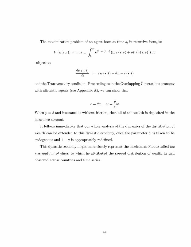
The maximization problem of an agent born at time s, in recursive form, is:
V (w(s; t)) = maxc;!
Z 1
t
e(�+p)(t�v) (ln c (s; v) + pV (!(s; v))) dv
subject to
dw (s; t)
dt= rw (s; t)� �! � c (s; t)
and the Transversality condition. Proceeding as in the Overlapping Generations economy
with altruistic agents (see Appendix A), we can show that
c = �w; ! =p
�w
When p = � and insurance is without friction, then all of the wealth is deposited in the
insurance account.
It follows immediately that our whole analysis of the dynamics of the distribution of
wealth can be extended to this dynastic economy, once the parameter � is taken to be
endogenous and 1� � is appropriately rede�ned.
This dynastic economy might more closely represent the mechanism Pareto called the
rise and fall of elites, to which he attributed the skewed distribution of wealth he had
observed across countries and time series.
44

References
H.J. Aaron and A.H. Munnell (1992): "Reassessing the Role of Wealth Transfer Taxes,"
National Tax Journal, 45, 119-43.
A. Atkeson and R.E. Lucas (1995): "E¢ ciency and Equality in a Simple Model of
Unemployment Insurance", Journal of Economic Theory, 66(1), 64-88.
A.B. Atkinson (1970): "On the Measurement of Inequality," Journal of Economic The-
ory, 2, 244-63.
A.B. Atkinson (2001): �Top Incomes in the United Kingdom over the Twentieth Cen-
tury,�mimeo, Nu¢ eld College, Oxford.
A.J. Auerbach, G. Jagadeesh Gokhale, L.J. Kotliko¤; J. Sabelhaus, and D. Weil (1995):
"The Annuitization of Americans Resources �A Cohort Analysis", NBER W.P.
5089.
G. S. Becker (1973): "A Theory of Marriage: Part I." Journal of Political Economy,
81, 4, 813-846.
G. S. Becker and N. Tomes (1979): "An Equilibrium Theory of the Distribution of
Income and Intergenerational Mobility," Journal of Political Economy, 87, 6, 1153-
1189.
K. Bjerke (1970): �Income and Wage Distributions-Part I: A Survey of the Literature,�
Review of Income and Wealth, 16(3), 235-52.
O.J. Blanchard (1985): �Debt, De�cits, and Finite Horizons,�Journal of Political Econ-
omy, 93, 223-47.
F.D. Blau and L.M. Kahn (2005): �Do Cognitive Test Scores Explain Higher U.S. Wage
Inequality?,�The Review of Economics and Statistics, 87, 1, 184-93.
45
M. Brown, C.C. Channing, and S.H. Chiang (2006a): �Limiting Densities for a Class of
Markov Processes,�mimeo, York University, Toronto.
M. Brown, C.C. Channing, and S.H. Chiang (2006b): �Wealth and Occupations in a
Natural Aristocratic Republic,�mimeo, York University, Toronto.
Burris, Val (2000): "The Myth of Old Money Liberalism: The Politics of the "Forbes"
400 Richest Americans," Social Problems, 47, 360-378.
M. Cagetti and M. De Nardi (2000): �Entrepreneurship, Bequests and the Distribution
of Wealth,�mimeo, University of Chicago.
M. Cagetti and M. De Nardi (2003): �Entrepreneurship, Frictions, and Wealth,�mimeo,
University of Chicago.
M. Cagetti and M. De Nardi (2005): �Wealth Inequality: Data and Models,�Federal
Reserve Bank of Chicago, W.P. 2005-10.
F.P. Cantelli (1921): �Sulla Deduzione delle Leggi di Frequenza da Considerazioni di
Probabilita�,�Metron, 83-91.
A. Caplin and J. Leahy (2004): "The Social Discount Rate", Journal of Political Econ-
omy,112, 2004, 1257-1268.
A. Castaneda, J. Diaz-Gimenez, and J.V. Rios-Rull (2003): �Accounting for the U.S.
Earnings and Wealth Inequality,�Journal of Political Economy, 111, 4, 818-57.
D.G. Champernowne (1953): �A Model of Income Distribution,�Economic Journal, 63,
318-51.
J.S. Chipman (1974): �The Welfare Ranking of Pareto Distributions,�Journal of Eco-
nomic Theory, 9, 275-82.
46

J.S. Chipman (1976): The Paretian Heritage, Revue europeenne des sciences sociales
et Cahiers Vilfredo Pareto, Vol. 14, No. 37, pp. 65-171,
http://www.econ.umn.edu/~jchipman/HERITAGE.pdf .
F. Clementi and M. Gallegati (2004): �Power Law Tails in the Italian Personal Income
Distribution,�forthcoming, Physica A.
J.K. Dagsvik and B.H. Vatne (1999): �Is the Distribution of Income Compatible with
a Stable Distribution?�
A. Das and S. Yarlagadda (2003): �A Distribution Function Analysis of Wealth Distri-
bution, arXiv:con-mat/0310343.
M. De Nardi (2004): �Wealth Inequality and Intergenerational Links,�Review of Eco-
nomic Studies, 71, 743-768.
A. Deaton, P.O. Gourinchas, and C. Paxson (2000): �Social Security and Inequality
over the Life Cycle,�NBER Working Paper 7570.
Elwood, Paul, S. M. Miller, Marc Bayard, Tara Watson, Charles Collins, Chris Hart-
man, (1997): Born on Third Base: The sources of wealth of the 1996 Forbes 400,
Boston: Uni�ed for a Fair Economy. For an executive summary see
http://www.faireconomy.org/press/archive/Pre_1999/forbes_400_study.html .
S.J. Farlow (1982): Partial Di¤erential Equations for Scientists and Engineers, New
York, Dover.
D. Feenberg and J. Poterba (2000): �The Income and Tax Share of Very High Income
Household: 1960-1995,�American Economic Review, 90, 264-70.
47

E. Fermi (1949): �On the Origin of Cosmic Radiation,�Physics Review, 75, 1169-74. J.
Friedman and R. Carlitz (2005): �Estate Tax Reform Could Raise Much-Needed
Revenue, Center on Budget and Policy Priorities
J. Friedman and R. Carlitz (2005): �Estate Tax Reform Could Raise Much-Needed
Revenue, Center on Budget and Policy Priorities, at Budget), available at
http://www.ombwatch.org/article/articleview/400/1/116?TopicID=1
A. Fujihara, T. Ohtsuki, and H. Yamamoto (2004): �Power-Law Tails in Nonstationary
Stochastic Processes with Asymmetrically Multiplicative Interactions,� Physical
Review E, 70, 031106.
X. Gabaix, (1999): �Zipf�s Law for Cities: An Explanation,�Quarterly Journal of Eco-
nomics, 113, 3, 739-767.
X. Gabaix, P. Gopikrishnan, V. Plerou, and H.E. Stanley (2003): �Theory of Power
Law Distributions in Financial Market Fluctuations�Nature, 423, 267-70.
W. G. Gale and J. K. Scholtz (1994): "Intergenerational Transfers and the Accumula-
tion of Wealth,�Journal of Economic Perspectives, 8, 145-160.
I.I. Gikhman and A.V. Skorokhod (1969): Introduction to the Theory of Random
Processes, Philadelphia, W.B. Saunders.
J. Diaz Gimenez, V. Quadrini, and J.V. Rios Rull (1997): �Dimensions of Inequality:
Facts on the U.S. Distributions of Earnings, Income, and Wealth,�Federal Reserve
Bank of Minneapolis Quarterly Review, 21, 2, 3-21.
J. Heckman and E. Vytlacil (2001): �Identifying the Role of Cognitive Ability in Ex-
plaining the Level of and Chance in the Return to Schooling,� The Review of
Economics and Statistics, 83, 1, 1-12.
48

L. Hendricks (2001): "Bequests and Retirement Wealth in the United States," Arizona
State University, http://www.lhendricks.org/Research/bequdata_paper.pdf
R. Herrnstein and C. Murray (1994): The Bell Curve, New York, Free Press.
A.W. Hood (2003): Partial Di¤erential Equations (10 Lectures), School of Mathemati-
cal and Computational Sciences, University of St. Andrews, mimeo, http://www-
solar.mcs.st-and.ac.uk/~alan/MT2003/PDE/PDE.html.
M. Huggett (1996): Journal of Monetary Economics, "Wealth Distribution in Life-Cycle
Economies," 38, 469-494.
M. Hurd and J.P. Smith (1999): "Savings of the Elderly and Desired Bequests," mimeo,
Rand Corporation.
M. Kalecki (1945): "On the Gibrat Distribution," Econometrica, 13, 161-170.
K. Kawamura and N. Hatano (2003): �Models of Universal Power-Law Distributions,�
arXiv:con-mat/0303331.
O. S. Klassa, O. Bihama, M. Levy, O. Malcaia and S. Solomon (2006), "The Forbes
400 and the Pareto Wealth Distribution," Economics Letters, 90(2), 290-295
N. Kocherlakota (2005): "Zero Expected Wealth Taxes: A Mirrlees Approach to Dy-
namic Optimal Taxation," Econometrica, 73, 1587-1621.
L. J. Kotliko¤ and L. H. Summers (1981) "The Role of Intergenerational Transfers in
Aggregate Capital Accumulation," Journal of Political Economy, 89, 706-732.
P. Krusell and A. A. Smith (1998): �Income and Wealth Heterogeneity in the Macro-
economy,� Journal of Political Economy, 106, 867-896.
S. Kuznets (1955): �Economic Growth and Economic Inequality,�American Economic
Review, 45, 1-28.
49

J. Laitner (2001); "Secular Change in wealth Inequality and Inheritance," Economic
Journal, 111, 691-721.
R.J. Lampman (1962): The Share of Top Wealth-Holders in National Wealth, 1922-
1956, Princeton, NJ, NBER and Princeton University Press.
M. Levy (2003): �Are Rich People Smarter?�Journal of Economic Theory, 110, 42-64.
R. E. Lucas (1978): "On the Size Distribution of Business Firms." The Bell Journal of
Economics," 9, 508-523.
E.G.J. Luttmer (2004): �The Size Distribution of Firms in an Economy with Fixed and
Entry Costs,�Federal Reserve Bank of Minneapolis W.P. 633.
E.G.J. Luttmer (2005): �Growth and the Size Distribution of Firms,� University of
Minnesota, mimeo.
O. Malcai, O. Biham, P. Richmond, and S. Solomon (2002): �Theoretical Analysis
and Simulations of the Generalized Lotka-Volterra Model,�Physical Review E, 66,
031102.
B. Mandelbrot (1960):"The Pareto-Levy Law and the Distribution of Income." Inter-
national Economic Review, 1, 79-106.
B. Mandelbrot (1962): �Paretian Distributions and Maximization,�Quarterly Journal
of Economics, 76(1), 57-85.
J. Mincer (1958): "Investment in Human Capital and Personal Income Distribution,"
Journal of Political Economy, 66, 281-302.
R.N. Mantegna and H.E. Stanley (2000): An Introduction to Econophysics, Cambridge,
U.K., Cambridge University Press.
50

C. Moriguchi and E. Saez (2005): �The Evolution of Income Concentration in Japan,
1885-2002: Evidence from Income Tax Statistics,�mimeo, University of California,
Berkeley.
C. Morisson (2000): �Historical Perspectives on Income Distribution: The Case of Eu-
rope,�in A. Atkinson and F. Bourguignon (eds.), Handbook of Income Distribution,
Amsterdam, North Holland.
D. Newbery (1970): �A Theorem on the Measurement of Inequality,�Journal of Eco-
nomic Theory, 2, 264-66.
M. Nirei and W. Souma (2004): �Two Factor Model of Income Distribution Dynamics,�
mimeo, Utah State University.
J.P. Nolan 2005): Stable Distributions; Models for Heavy Tailed Data, mimeo, Math/Stat
Department, American University, Washington, D.C.
OMB Watch, "Estate Tax and Government Revenue," 2001,
http://www.ombwatch.org/article/articleview/400/1/116?TopicID=1
V. Pareto (1897): Cours d�Economie Politique, Vol. II, F. Rouge, Lausanne.
V. Pareto (1901): "Un�Applicazione di teorie sociologiche", Rivista Italiana di So-
ciologia. 5. 402-456, translated as The Rise and Fall of Elites: An Application
of Theoretical Sociology , Transaction Publishers, New Brunswick, New Jersey,
(1991).
V. Pareto (1909): Manuel d�Economie Politique, V. Giard et E. Brière, Paris.
C. Phelan (1998): "On the Long-Run Implications of Repeated Moral Hazard," Journal
of Economic Theory, 79(2), 174-91.
51

E.S. Phelps and R.A. Pollak (1968): �On Second-best National Savings and Game-
equilibrium Growth,�Review of Economic Studies, 35, 185-99.
T. Piketty (2001): �Income Inequality in France, 1901-1998,�Journal of Political Econ-
omy.
T. Piketty and E. Saez (2003): �Income Inequality in the United States, 1913-1998,�
Quarterly Journal of Economics, CXVIII, 1, 1-39.
A.D. Polyanin and A.V. Manzhirov (1998): Handbook of Integral Equations, Boca
Raton, Florida, CRC Press.
V. Quadrini (2000): �Entrepreunership, Savings and Social Mobility,�Review of Eco-
nomic Dynamics, 3, 1-40.
W.J. Reed and M. Jorgensen (2003): �The Double Pareto-Lognormal Distribution: A
New Parametric Model for Size Distributions,�mimeo, University of Victoria.
Roy, A. D. (1950) �The Distribution of Earnings and Individual Output,�The Ecoomic
Journal,�60, 489-505.
R.S.G. Rutherford (1955): �Income Distribution: A New Model,�Econometrica, 23,
277-94.
E. Saez and M. Veall (2003): �The Evolution of Top Incomes in Canada,�NBER Work-
ing Paper 9607.
P.A. Samuelson (1965): �A Fallacy in the Interpretation of the Pareto�s Law of Alleged
Constancy of Income Distribution,�Rivista Internazionale di Scienze Economiche
e Commerciali, 12, 246-50.
N. Scafetta, S. Picozzi, and B. West (2002): �Pareto�s Law: A Model of Human Sharing
and Creativity,�arXiv:cond-mat/0209373 v1.
52

E. Sheshinski (1972): �Relation between a Social Welfare Function and the Gini Index
of Income Inequality,�Journal of Economic Theory, 4, 98-100.
H.A. Simon (1955): �On a Class of Skew Distribution Function,�Biometrika, 52, 425-40.
H.A. Simon and C.P. Bonini (1958): �The Size Distribution of Business Firms,�Amer-
ican Economic Review, 48, 607-17.
S. Solomon (1999): �Generalized Lotka-Volterra (GLV)Models,�arXiv:con-mat/9901250
v1.
G. Solon (1999): �Mobility Within and Between Generations,�mimeo
D. Sornette (2000): Critical Phenomena in Natural Sciences, Berlin, Springer Verlag.
W. Souma, Y. Fujiwara, and H. Aoyama (2001): �Small-World E¤ects in Wealth Dis-
tribution,�arXiv:con-mat/0108482.
J.C. Strikwerda (2004): Finite Di¤erence Schemes and Partial Di¤erential Equations,
Philadelphia, SIAM.
F.G. Tricomi (1957): Integral Equations, New York, Interscience (Dover edition, 1985).
M. Yaari (1965): �Uncertain Lifetime, Life Insurance, and the Theory of the Consumer,�
Review of Economic Studies, 32, No. 2, 137-150.
N. Wang (2006): �An Equilibrium Model of Wealth Distribution,�Journal of Monetary
Economics, forthcoming.
H.O.A. Wold and P. Whittle (1957), �A Model Explaining the Pareto Distribution of
Wealth,�Econometrica, 25, 4, 591-5.
E. Wol¤ (1987): �Estimates of Household Wealth Inequality in the U.S., 1962-1983,�
The Review of Income and Wealth, 33, 231-56.
53

E. Wol¤ (2004): �Changes in Household Wealth in the 1980s and 1990s in the U.S.,�
mimeo, NYU.
54

Appendix A: Proofs - for completeness
Proof of Prop. 1. The dynamic equation for wealth accumulation is
dw (s; t)
dt= (r + p� �)w (s; v)� p! (s; v)� c (s; v)
First order conditions include
! (s; t) = �c (s; t) (33)
_c (s; t) = (r � � � �) c (s; t) (34)
The aggregate dynamics for the agent can then be written as:
_w (t; s) = (r + p� �)w (t; s)� (p�+ 1) c (s; v)
Postulating c = �w; after some algebra,
dw (s; t)
dt= ((r + p� �)� � (p�+ 1))w (s; v) (35)
So that, equating (34) and (35) we verify that in fact
c = �w; with � =(p+ �)
p�+ 1(36)
Furthermore, by (33),
! = ��w;
Finally, using
_w (t; s) = (r + p� �)w (t; s)� (p�+ 1) �w (t; s)
and
� =(p+ �)
p�+ 1
55

we can solve for the growth of the agent�s wealth, which we denote g:
g = r � � � � (37)
Optimal Consumption-Savings for Altruistic Agents. The maximization prob-
lem of an agent born at time s, in recursive form, is:
V (w(s; t)) = maxc;!
Z 1
t
e(�+p)(t�v) (ln c (s; v) + p�V (!(s; v))) dv
subject to
dw (s; t)
dt= (r + p)w (s; t)� p! � c (s; t)
and the Transversality condition
We guess
V (!) = A+B ln!
Under the guess the Hamiltonian is
H = ln c+ pA� + pB� ln! + � ((r + p)w � p! � c)
and the associated First Order Conditions are
c�1 = �;_c
c= �
_�
��B
!= �
_� = � (�r � p+ p+ �) = �� (r � �)
_c = c (r � �)
with the wealth accumulation constraint.
Under the guess we can show that
56

c = �w; ! = �B�w
with
� =p+ �
p�B + 1
Also, under the guess, we can compute the value V (z) as:
V (z) = constant +1 + p�B
� + pln z
(see the "Derivation of the discounted utility along the optimal path" above). The guess
is veri�ed therefore for43
B =1 + p�B
� + p
that is
B =1
� + p(1� �)We conclude that:
� =p+ �
p� 1�+p(1��) + 1
= � + p(1� �)
and so
c = (� + p(1� �))w; ! = �w
As noted in the text (see especially footnote 22, when parents are purely altruistic,
they optimally account for welfare transfers when choosing bequests. In this case, the
consumption-savings plan obtained in Proposition 1 is not optimal.
It is straightforward to show, following the analysis just above, that this case is
homeomorphic to one in which agents have non-convex preferences for bequest of the
following kind:43Naturally we also need to require constant= A.
57

� (! (s; v)) =
8<: � lnw(v) for 0 � (1� b)! (s; v) � w(v)
� ln(1� b)! (s; v) for w(v) � (1� b)! (s; v)(38)
The optimal consumption-saving path (no capital tax for simplicity) in this case has
the following properties:
1. there exists a �nite wealth level w such that the consumption-savings path in
Proposition 1 is optimal for w > w; moreover,
w =
�w(t)
(1� b)��
�w(t) = w(0)eg
0 t =
e(r+p)tw (0)
0@1� �p+�
�e(p+�)t � 1
�1 + �
p+�
�e(p+�)t � 1
�1A
implying that
w ! w as w ! 0
and hence that the consumption-savings path in Proposition 1 is an approximation
to the optimal path for w small enough.
2. At w bequests ! jump from zero to positive, consumption c is smooth, wealth is
continuous but has a kink, as _w jumps at w.
3. The growth rate of individual wealth is not constant; let it be denoted g(w):
g(w) =
8>>><>>>:r + p� �
�(1+p�)
(p�)e(p+�)t+1
�at w = w
r + p� � at the left limit of w
r + p� � (1 + p�) at the right limit of w
and it is decreasing in wealth w.
58
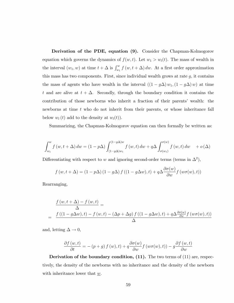
Derivation of the PDE, equation (9). Consider the Chapman-Kolmogorov
equation which governs the dynamics of f(w; t). Let w1 > wl(t). The mass of wealth in
the interval (w1; w) at time t+� isR ww1f (w; t+�) dw. At a �rst order approximation
this mass has two components. First, since individual wealth grows at rate g, it contains
the mass of agents who have wealth in the interval ((1� g�)w1; (1� g�)w) at time
t and are alive at t + �. Secondly, through the boundary condition it contains the
contribution of those newborns who inherit a fraction of their parents� wealth: the
newborns at time t who do not inherit from their parents, or whose inheritance fall
below wl (t) add to the density at wl(t)).
Summarizing, the Chapman-Kolmogorov equation can then formally be written as:
Z w
w1
f (w; t+�) dw = (1� p�)Z (1�g�)w
(1�g�)w1f (w; t) dw + q�
Z �(w)
�(w1)
f (w; t) dw + o (�)
Di¤erentiating with respect to w and ignoring second-order terms (terms in �2),
f (w; t+�) = (1� p�) (1� g�) f ((1� g�w); t) + q�@�(w)@w
f (w�(w); t))
Rearranging,
f (w; t+�)� f (w; t)�
=
=f ((1� g�w); t)� f (w; t)� (�p+�g) f ((1� g�w); t) + q�@�(w)
@wf (w�(w); t))
�
and, letting �! 0,
@f (w; t)
@t= � (p+ g) f (w); t) + q@�(w)
@wf (w�(w); t))� g@f (w; t)
@w
Derivation of the boundary condition, (11). The two terms of (11) are, respec-
tively, the density of the newborns with no inheritance and the density of the newborn
with inheritance lower that w.
59

The �rst term of (11) can be derived from the age distribution. In particular the
density of newborn agents (agents of age a = 0) with no inheritance is p� q. The wealth
w(a) of an agent of age a born with wealth w is w(a) = wega. Operating the appropriate
change of variable to obtain the distribution of wealth from the distribution of age, and
evaluating at w = w, we obtain p�qg
1w. The second term is straightforwardly derived.
Proof of Lemma 1. To solve (9) under (14) and (13) we apply the �method of
characteristics�as detailed in Appendix C. Let the characteristic space (� ; t) be de�ned
bydz
d�= (g � g0)z; dt
d�= 1:
Let z(0) = m and t(0) = 0. In the characteristic space the PDE (9) is then reduced to
the following di¤erential equation:
d (f (z(�); �))
d�= � (p+ g � g0) f (z(�); �) + q@�(z)
@zf (�(z(�)); �) (39)
It can be veri�ed that (39) has solution:
f (z (�) ; �) = e�(p+g�g0)�f (m; 0) +
Z �
0
q@�(z)
@zf (�(z(�)) ; �) e(p+g�g
0)(���)d� (40)
The characteristic space is split along the characteristic z = we(g�g0)� . In particular,
for z � we(g�g0)� the solution to the PDE is determined by the initial condition, while
for z < we(g�g0)� the solution is instead determined by the boundary condition through
the inverse transformation �(z; y) = ln zy
1(g�g0) . Then, substituting back into the original
60
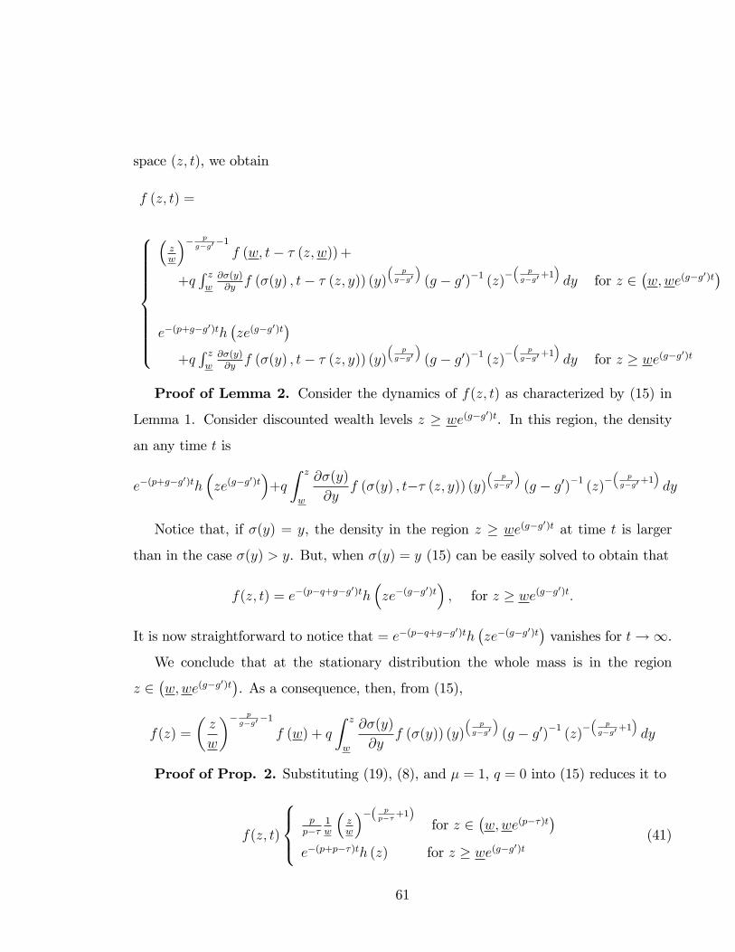
space (z; t), we obtain
f (z; t) =
8>>>>>>>>><>>>>>>>>>:
�zw
�� pg�g0�1
f (w; t� � (z; w))+
+qR zw@�(y)@yf (�(y) ; t� � (z; y)) (y)
�p
g�g0
�(g � g0)�1 (z)�
�p
g�g0+1�dy for z 2
�w;we(g�g
0)t�
e�(p+g�g0)th
�ze(g�g
0)t�
+qR zw@�(y)@yf (�(y) ; t� � (z; y)) (y)
�p
g�g0
�(g � g0)�1 (z)�
�p
g�g0+1�dy for z � we(g�g0)t
Proof of Lemma 2. Consider the dynamics of f(z; t) as characterized by (15) in
Lemma 1. Consider discounted wealth levels z � we(g�g0)t. In this region, the density
an any time t is
e�(p+g�g0)th
�ze(g�g
0)t�+q
Z z
w
@�(y)
@yf (�(y) ; t�� (z; y)) (y)
�p
g�g0
�(g � g0)�1 (z)�
�p
g�g0+1�dy
Notice that, if �(y) = y, the density in the region z � we(g�g0)t at time t is larger
than in the case �(y) > y. But, when �(y) = y (15) can be easily solved to obtain that
f(z; t) = e�(p�q+g�g0)th
�ze�(g�g
0)t�; for z � we(g�g0)t:
It is now straightforward to notice that = e�(p�q+g�g0)th
�ze�(g�g
0)t�vanishes for t!1.
We conclude that at the stationary distribution the whole mass is in the region
z 2�w;we(g�g
0)t�. As a consequence, then, from (15),
f(z) =
�z
w
�� pg�g0�1
f (w) + q
Z z
w
@�(y)
@yf (�(y)) (y)
�p
g�g0
�(g � g0)�1 (z)�
�p
g�g0+1�dy
Proof of Prop. 2. Substituting (19), (8), and � = 1, q = 0 into (15) reduces it to
f(z; t)
8><>:pp��
1w
�zw
��( pp��+1)
for z 2�w;we(p��)t
�e�(p+p��)th (z) for z � we(g�g0)t
(41)
61

Furthermore, using
f(z; t) = e�(p+p��)th�ze�(p��)t
�; for z � we(g�g0)t:
it follows that f(z; t) vanishes for t!1 and hence that f(z) is ergodic.
Finally, the mean of the stationary distribution f(z) is �nite since pp�� > 1.
Proof of Prop. 3. Consider z 2�w;we(g�g
0)t�. In this range, substituting (19),
and b = 0, in (15), it follows that f(z; t) is stationary (independent of t), and hence it
satis�es the integral equation (16), which in this case takes the form:
f (z) =
�z
w
��� pg�g0+1
�f(w) + q
Z z
w
(y)
�p
g�g0
�(g � g0)�1 (z)�
�p
g�g0+1�f (y) dy (42)
This is a Volterra integral equation of the second type, with separable kernel, for which
a closed form solution exists and is discussed in Appendix D. Applying this solution, we
obtain,
f (z) =�zw
��� pg�g0+1
�f (w)
+q (g � g0)�1R zwz��
pg�g0+1�q(g�g
0)�1�j
�p
g�g0�q(g�g0)�1
� �jw
��� pg�g0+1
�f (w) dj
(43)
Straightforward algebraic manipulations, together with (19), are now enough to produce
the closed form solution for the stationary distribution f(z).
Furthermore, as before, using
f(z; t) = e�(p+p�q��)th�ze�(p�q��)t
�; for z � we(g�g0)t:
it follows that f(z; t) vanishes for t!1 and hence that f(z) is ergodic.
Finally, the mean of the stationary distribution f(z) is �nite since p�qp�q�� > 1.
Proof of Prop. 4. The integral equation in this case, after the transformation
62

j = �(y) = y(1��)(1�b) is reduced to:
f (z) = (44)�z
w
��� pg�g0+1
�f (w) + q (g � g0)�1 �
�Z z
(1��)(1�b)
w(1��)(1�b)
f (j)
�((1� �)(1� b)j)
�p
g�g0
�z��
pg�g0+1
��dj
where g � g0 = p� q (1� �)� � . We guess:
f(z) =p� aq (1� �) (1� b)p� q (1� �)� � w
p�aq(1��)(1�b)p�q(1��)�� z�(
p�aq(1��)(1�b)p�q(1��)�� +1) (45)
and substitute into the integral equation. Let f(w) = p�aq(1��)(1�b)p�q(1��)��
1w. We obtain
z
w
�( p�aq(1��)(1�b)p�q(1��)�� +1)f(w) =
z
w
��
pg�g0+1
�f (w) + q (g � g0)�1 (z)�
�p
g�g0+1��
�Z ((1��)(1�b))�1z
((1��)(1�b))�1w
�j
w
��� pg�g0+1�aq(g�g
0)�1(1��)(1�b)�f (w) ((1� �) (1� b) j)
pg�g0 dj
and, after some algebraic manipulations,
z
w
�( p�aq(1��)(1�b)p�q(1��)�� +1)f(w) =
z
w
��
pg�g0+1
�f (w) +
+q (g � g0)�1 ((1� �) (1� b))p
g�g0 z
w
��
pg�g0+1
�w�aq(g�g
0)�1((1��)(1�b))f (w) �
�Z ((1��)(1�b))�1z
((1��)(1�b))�1wj�1+aq(g�g
0)�1(1��)(1�b)dj
and hencez
w
�( p�aq(1��)(1�b)p�q(1��)�� +1)f(w) =
63

=z
w
��
pg�g0+1
�f (w)
0@ 1 + a�1w�aq(g�g0)�1(1��)(1�b) ((1� �) (1� b))
p�aq(1��)(1�b)g�g0 �1
��zaq(g�g
0)�1(1��)(1�b) � waq(g�g0)�1(1��)(1�b)
�1A
=z
w
��
pg�g0+1
�f (w)
0B@ 1 + a�1 ((1� �) (1� b))p�aq((1��)(1�b))
g�g0 �1�zwaq(g�g0)�1(1��)(1�b) � 1
�1CA
Let a�1 ((1� �) (1� b))p�aq(1��)(1�b)
g�g0 �1
= 1; or
a = ((1� �) (1� b))p�aq(1��)(1�b)
g�g0 �1
This is �xed point equation which has a unique solution, a� < 1. In fact, it is easily
checked that ((1� �) (1� b))p�aq((1��)(1�b))
g�g0 �1
= ((1� �) (1� b))p�aq(1��)(1�b)p�q((1��))�� �1
is strictly
positive for a = 0, it has a negative derivative with respect to a, and it is less than 1 for
a = 1. Consequently,
z
w
��p�a�q((1��)(1�b))
g�g0 +1�f (w) =
=z
w
��
pg�g0+1
�f (w)
�1 +
�z
w
a�q(g�g0)�1(1��)(1�b)� 1��
=z
w
��p�a�q((1��)(1�b))
g�g0 +1�f (w)
and the guess is veri�ed.
Finally, the mean of the stationary distribution f(z) is �nite since p�a�q(1��)(1�b)
p��q(1��)�� > 1.
Since we cannot solve explicitly for the dynamics of f(z; t) in the general case under
consideration, we cannot directly show ergodicity of f(z), as in the previous special cases
studied in Propositions 2 and 3. We proceed instead by studying the stochastic process
driving a dynasty�s (that is, a succession of generations�) wealth accumulation.
To this end let �(t) denote a Poisson process with intensity p. Let then the stochastic
process governing a dynasty�s (that is, a series of successive generations�) discounted
64

wealth, denoted z(t) (with some abuse of notation), be de�ned by the following stochastic
di¤erential equation:
dz(t) = (g � g0)dt� �(z(t�))d�(t)
where �(z(t�)) =
8<: (b+ � (1� b)) z(t�) with probability p�qp�
z(t�)�wz(t�)
�z(t�) with probability q
p
and z(t�) = lims!t� z(s).
The process z(t) is a Markov jump process. Ergodicity of z(t) implies the existence
of an ergodic distribution of wealth in the population, f(z): We shall study z(t) by
the Embedded Markov Chain method; see Borovkov (1998), ch. 4, and Karlin-Taylor
(1981b), ch. 18.4. Let an embedded chain to z(t) be constructed as follows. Let z(tn)
denote the dynasty�s discounted wealth at the end of the n�th generation. The sequence
fz(t_1); z(t_2); : : :g de�nes a discrete time process, in fact a Markov chain, recursively
by:
X0 = z(0); Xn = z(tn)
where tn is the stochastic process induced by the Poisson process �(t):44
prob(tn = t) = prob(�(t) = n j �(�) < n; 8� < t)
It is now straightforward to construct the transition kernel of the Markov chain Xn,
denoted P (Xn = x j Xn�1 = z). Speci�cally,
P (Xn = x j Xn�1 = z) =
8>>><>>>:q for x = w
0 for x 2 (w; (1� �)(1� b)z)
(p� q)prob (� (�(x)) = n) for x 2 [(1� �)(1� b)z;1)
where �(x) solves x = ze(g�g0)(��tn�1(1� �)(1� b)
44A related construction of an embedded Markov chain by means of a stochastic process tn, in the
context of Queue theory, is introduced in Karlin-Taylor (1981b), p. 497.
65

Ergodicity now follows by applying Theorem 13.3.3 of Meyn-Tweedie (1993), p. 323
if we show that the Markov chain Xn is positive Harris recurrent and aperiodic (we refer
to Meyn-Tweedie (1993), ch. 5 and 10 for the precise de�nitions of these terms). In fact,
these desired properties of Xn are straightforward to verify.
Proof of Proposition 5. Since
P =p� ((1� �) (1� b))
P
q
p� q((1� �))� � (46)
The right hand side of (46) is increasing in P; for P = 1 it is larger than 1; and for P !1
it is �nite. Therefore we focus on the unique solution of P � 1: Since p�q((1� �))�� �
0; and 0 � ((1� �) (1� b))P � 1 it follows that lim�!(p�q((1��))P =1: Computing the
derivatives of P; and substituting for p� q((1� �) from 46 we get
dP
d�=
P 2
p� qn((1� �) (1� b))P (1 + P ln ((1� �) (1� b)))
o > 0 (47)
dP
db=
P 2 ((1� �) (1� b))P�1
q (1� �)p� q
n((1� �) (1� b))P (1 + P ln ((1� �) (1� b)))
o � 0 (48)
Note that dPdb= 0 would obtain only if P ! 1 and (1� �) (1� b) < 1: As shown,
this is indeed the case only if � ! (p� q((1� �)) and may also be ascertained di-
rectly by applying L�Hopital�s rule to (48). To do this �rst apply L�Hopital�s rule twice
to P 2
((1��)(1�b))�P�+1and once to P
((1��)(1�b))P by di¤erentiating with respect to � ; and show
that both expressions converge to zero as � ! (p� q((1� �)) because lim�!(p�q((1��))P =
1: Then substitute into the expression dPdbto see that lim�!p�q((1��)
dPdb= 0
p:
Derivation of the government budget constraint, (27). Consider the gov-
ernment expenditures (7), written in terms of discounted wealth and evaluated at the
stationary distribution f(z):
(p� q)w + qZ ((1�b)(1��))�1w
w
(w � (1� b)(1� �)z) f(z)dz (49)
66

Furthermore, the stationary distribution is
f(z) = f (w )z
w
��p�a�q((1��)(1�b))(p�q((1��))��) +1
�=
=p� aq ((1� �) (1� b))(p� q((1� �))� �) w
p�a�q((1��)(1�b))p�q((1��))�� z
��p�a�q((1��)(1�b))p�q((1��))�� +1
�
We proceed �rst by computingR ((1�b)(1��))�1ww
(1� b)(1� �)zf(z)dw, obtaining
(1� �) (1� b) p� aq ((1� �) (1� b))q (1� �) (1� a (1� b)) + ��
1� ((1� �) (1� b))p�aq((1��)(1�b))p�q((1��))�� �1
�w
Furthermore we computeR ((1�b)(1��))�1ww
f(z)dw, obtaining�1� ((1� �) (1� b))
p�aq((1��)(1�b))p�q((1��))��
�Substituting the computations in (49), we conclude that government expenditures are:
(p� q)w + qw
0BBB@�1� ((1� �) (1� b))
p�aq((1��)(1�b))p�q((1��))�� �1
�� (1� �) (1� b) p�aq(1��)(1�b)
q(1��)(1�a(1�b))+��1� ((1� �) (1� b))
p�aq(1��)(1�b)p�q(1��))�� �1
�1CCCA
and therefore that the government budget constraint can be written as:
w
0@ (p� q) + q�1� ((1� �) (1� b))
p�aq((1��)(1�b))p�q((1��))�� �1
��1� (1� �) (1� b) p�aq(1��)(1�b)
q(1��)(1�a(1�b))+�
�1A
= (� + bq (1� �))M
where M is average wealth.
Derivation of the discounted utility along the optimal path, (29). In our
economy, the optimal consumption-savings path of an arbitrary agent is characterized
by (3). Along this path, it is straightforward to compute
U(z) =
Z 1
t
e(�+p)(t��) (ln �w(t; �) + p� ln(1� b)��w(t; �)) d�
67

where w(t; �) = zeg(��t); or,
U(z) =
Z 1
t
e(�+p)(t��) (ln � + ln z + g(� � t) + p� ln(1� b)�� + p� ln z + p�g(� � t)) d�
We proceed to analyze separately three components of U(z):
i)R1te(�+p)(t��) (ln � + p� ln(1� b)��) d�;
ii)R1te(�+p)(t��) (1 + p�) g(� � t)d�; and �nally,
iii)R1te(�+p)(t��) (1 + p�) ln zd�.
i) Integrating,Z 1
t
e(�+p)(t��) (ln � + p� ln(1� b)��) d� = 1
� + p(ln � + p� ln(1� b)��)
ii) Integrating by parts, Z 1
t
e(�+p)(t��) (1 + p�) g(� � t)d� =
= g (1 + p�)
�� 1
� + p
�e(�+p)(t��)(� � t)
�1t+
1
� + p
Z 1
t
e(�+p)(t��)d�
�=
= g (1 + p�)
�� 1
� + p
�e(�+p)(t��)(��t)
�1t� 1
(� + p)2�e(�+p)(t��)
�1t
�=
=g (1 + p�)
(� + p)2
iii) Integrating, Z 1
t
e(�+p)(t��) (1 + p�) ln zd� =1 + p�
� + pln z
Adding up,
U(z) =1
� + p
�g (1 + p�)
� + p+ ln � + p� ln (1� b)��
�+1 + p�
� + pln z
Derivatives of utilitarian social welfare with respect to b and � .
68

@ (M; b; �)
@�= (p+ �)�2
�(1 + p�)
P�2
P � 1@P
@�� 1�
(50)
= (p+ �)�2
0@ (P � 1)�1 (1 + p�)p� q
n((1� �) (1� b))P (1 + P ln ((1� �) (1� b)))
o � 11A
@ (M; b; �)
@b(51)
= (p+ �)�1�(1 + p�)
p+ �
P�2
P � 1@P
@b� p� (1� b)�1
�
= (p+ �)�1
24 (1+p�)(P�1)(p+�)
�P�1(p+�)P (1+p�)�1(1�b)P�1
q
p�qf((1��)(1�b))P (1+P ln((1��)(1�b)))g�p (1� b)�1
35�where @P
@�and @P
@bare de�ned by (47) and (48) in the proof of Proposition 5 in Appendix
A.
69

Appendix B: On the mechanisms possibly underlying a Paretodistribution of wealth
Various stochastic processes for individual wealth are known to aggregate into a
Pareto distribution of wealth in the population; see Sornette (2000) for a technical review
and Chipman (1976) for a careful and outstanding account of the historical contributions
of this subject; see also Levy (2003).
One such process is exempli�ed here; its mathematical formulation �rst appears in
Cantelli (1921).45 Suppose a variable determining wealth (e.g., talent, age), which we
denote �, is exponentially distributed. That is the number of people with � = �0 is
N (�0) = pe�p�0
Suppose wealth increases exponentially with �:
w = aeg�; a > 0; g � 0 (52)
Therefore, we can solve for � = g�1 ln wa, operate a change of variables and express the
distribution of wealth as
N(w) = N�g�1 ln
w
a
� d�dw
that is,
N(w) =p
gapgw�(
pg+1)
This is a Pareto distribution with the exponent pg.46
45See also Fermi (1949)�s study of cosmic rays.46A notable literature appeared in Italian in the �rst decades of the twentieth century which studies
the wealth distribution resulting from di¤erent assumptions regarding the distribution of the generating
factor we called � and on the functional dependence of wealth on this factor; see Chipman (1976) for a
detailed discussion of these contributions.
70

The underlying mechanism which makes wealth Pareto distributed in our basic model
is a similar one in which the factor � is represented by age. This is clearly illustrated by
considering the simple economy with no bequests. At any time t, in this economy, the
distribution of the population by age t� s implied by the demographic structure of the
economy is in fact
N (t� s) = pe�p(t�s)
Moreover, abstracting from the complications of inheritance, each optimal consumption-
savings choices imply a wealth accumulation process results in wealth increasing expo-
nentially with age.
71

Appendix C: On the basic PDE and its solution by themethodof characteristics
We illustrate in this Appendix the "method of characteristics" for the solution of par-
tial di¤erential equation (PDE�s) by applying to a linear PDE with variable coe¢ cients,
a simple form of the PDE we solve in the paper. Consider the following PDE:
@f
@t= �af � bz @f
@z(53)
with initial condition
f(z; 0) = h(z)
Suppose �rst of all that the PDE is to be solved for z 2 <, that is, that there is no
boundary condition. The Method of Characteristics (see e.g., Farlow (1982), Ch. 27)
requires solving the PDE in the characteristic space, (� ; t), implicitly constructed as
follows:dz
d�= bz;
dt
d�= 1
that is,
z(�) = c1e�b� ; t(�) = � + c2 (54)
Let z(0) = m and t(0) = 0, so that c1 = m and c2 = 0. This construction has the
property that the chain ruledf
d�=@f
@z
@z
@�+@f
@t
@t
@�
and (53) implydf
d�= �af (55)
a simple ordinary di¤erential equation. The initial condition in characteristic space
is f(m; 0) = h(m). The di¤erential equation, together with the initial condition has
solution
f(z(�); �) = h(m)e�a�
72

Substituting back into the original space (z; t), using (54):
f(z; t) = h�ze�bt
�e�at (56)
In words: the density on z at time t is the same density that at time 0 was on ze�bt
dampened at a rate a.
Suppose now that the PDE is to be solved for z � z, and that there is a boundary
condition
f(z; t) = B;
The Method of Characteristics applies to this class of problems, boundary value prob-
lems, as follows (see e.g., Hood (2003) and Strikwerda (2004), Ch. 1.2). The charac-
teristic space is split along the characteristic z = zeb� . In particular, for z � zeb� the
solution to the PDE is determined by the initial condition, and
f(z; t) = h�ze�bt
�e�at
For z < zeb� the solution is instead determined by the boundary condition through the
inverse transformation �(z; y) = ln zy1band
f(z; t) = B1
b
�z
z
�ab
Summarizing, the solution to the boundary value problem is:
f(z; t) =
8<: B 1b
�zz
�ab
for z < zebt
h�z e�bt
�e�at for z � zebt
(57)
73

Appendix D: On Volterra-Fredholm integral equations of thesecond type
In this Appendix we report some results for the class of integral equations that we
study in the paper. We consider Volterra-Fredholm integral equations of the second type
with separable kernel:
f (z) = h (z) + �
Z �(z)
a
K(y)H(z)f(y)dy
where the real maps h; �; K; and H are continuously di¤erentiable. It is convenient to
study the following equivalent equation:
f (z) = h (z) + �
Z 1
a
~K(z; y)H(z)f(y)dy; ~K(z; y) = K(y)I[a;�(z)](z; y) (58)
where I[a;�(z)](z; y) is the indicator function of the interval [a; �(z)],
I[a;�(z)](y) =
8<: 1 for y 2 [a; �(z)]
0 otherwise. Note that ~K(z; y) is not continuous. The the-
ory of Volterra-Fredholm integral equations is, however, developed for square integrable
kernels (see Tricomi (1957)), a condition which is obviously satis�ed by ~K(z; y)H(z). For
the uniqueness of such solutions (excluding solutions that are zero almost everywhere)
see Tricomi (1957), p. 10 and Chapter II and also p.63.
A simple explicit solution is reported by Polyanin-Manzhirov (1998), Ch. 2.1-7 (equa-
tion 50), for the following integral equation:
f (z) = h (z) + �
Z z
a
y�1z�2f(y)dy; for �1 + �2 = �1
It corresponds to a special case of (58) in which:
�(z) = z; ~K(z; y) = K(y) = y�1 ; H(z) = z��1�1
74

Its solution is:
f(z) = h(z) +
Z z
a
R(z; y)h(y)dy; for R(z; y) = az�2��y�1+�
75

Appendix E: On Earnings and Lump-sum Subsidies
Consider the economy in which each agent born at time t receives an expected present
discounted value of earnings equal to x(t). We assume that the present discounted value
of earnings distributed at any time t in the economy, x(t), is a constant fraction �x of
aggregate wealth; that is, x(t) = �xW (t). As a consequence, x(t) = eg0tx for some initial
value x.
In this case, as noted in the text, the total subsidy in the economy is:
(p�q) (w(t)� x(t))+qZ ((1�b)(1��))�1(w(t)�x(t))
(w(t)�x(t))(w(t)� x(t)� (1� b)(1� �)w) f(w; t)dw
Moreover, the boundary condition is:
f (w(t); t) =p� qg
1
w(t)+1
g
1
w(t)q
Z �(w(t)�x(t))
(w(t)�x(t))f(w; t)dw
The stationary distribution satis�es the integral equation (16). For this economy we
also have
�(y) =y � x
(1� �)(1� b) ; and hence �(w) = w;@�(z)
@z=
1
(1� b)(1� �)
We operate the transformation j = �(y) = y�x(1��)(1�b) and obtain, from (16):
f (z) =�zw
��� pg�g0+1
�f (w)
+q (g � g0)�1R z�x
(1��)(1�b)w
f (j)
�((1� �)(1� b)j + x)
�p
g�g0
�(z)
��
pg�g0+1
��dj
(59)
While we do not have of a closed form solution to this integral equation, a unique solution
exists (see Appendix D). Moreover, Proposition (6) in the text states that, for large z,
the distribution of discounted wealth is approximately Pareto. We provide here the proof
of Proposition (6).
76

Proof of Prop. 6 The integral equation in this case, after the transformation
j = �(y) = y�x(1��)(1�b) is reduced to:
f (z) =�zw
��� pg�g0+1
�f (w)
+q (g � g0)�1R z�x
(1��)(1�b)w
f (j)
�((1� �)(1� b)j + x)
�p
g�g0
�(z)
��
pg�g0+1
��dj
A lower bound on f(z), l(z) is obtained by the solution to
l (z) =�zw
��� pg�g0+1
�l (w)
+q (g � g0)�1R wwf (j)
�((1� �)(1� b)j + x)
�p
g�g0
�(z)
��
pg�g0+1
��dj =
=�zw
��� pg�g0+1
�f (w)
l(z) is a power function with exponent pp�q(1��)�� ; which is a Pareto distribution inte-
grating to unity if de�ned over w � f (w)�
pp�q(1��)��
��1:
An upper bound on f(z), u(z) is obtained by the solution to
u (z) =�zw
��� pg�g0+1
�u (w)
+q (g � g0)�1R z
(1��)(1�b)w
u (j) jp
g�g0 z��
pg�g0+1
�dj
since 1 � �)(1 � b)j + x � j by construction. Adapting the proof of Prop. 5, we can
show that u(z) is a power function with exponent
p� a�q (1� �) (1� b)p� q (1� �)� � > 1; for 0 < a� < 1 satisfying (23)
which is a Pareto distribution integrating to one if de�ned forw � f (w)�p�a�q(1��)(1�b)p�q(1��)��
��1: The
distribution f(z) for z � f (w)�p�a�q(1��)(1�b)p�q(1��)��
��1lies in between u(z) and l (z) 47; both
47Alternatively the solution of f(z) may be explicitly written as the limiting solution obtained by the
successive approximation method (see Polyanin and Manhzirov, section 9.9). The it is possible to show
that the iterated kernels of f(z) lie below the iterated kernels of u(z):
77

of which converge to zero for large z and therefore it is approximated by
f (z) =�zw
��� pg�g0+1
�f (w)
+q (g � g0)�1R z
(1��)(1�b)w
f (j)
�((1� �)(1� b)j)
�p
g�g0
�(z)
��
pg�g0+1
��dj
which has the solution derived in the proof of Prop. 5: a Pareto distribution with
exponentp� a�q (1� �) (1� b)p� q (1� �)� � > 1; for 0 < a� < 1 satisfying (23)
The analysis of the economy with earnings we just developed can be also applied to
an economy without earnings but with a lump-sum subsidy rather than a means tested
welfare policy. Consider the following welfare policy: all agents born at any t with
an inheritance receive a lump-sum subsidy equal to x(t) which grows at the aggregate
economy�s rate g0: x(t) = xeg0t:48
In the case of lump-sum subsidies, the total amount of subsidies paid by the govern-
ment at any time t is independent of the distribution of wealth at t and is a constant
fraction of wealth at each time t:
(p� q)w + qx
A �scal policy (� ; b) determines the set of feasible welfare policies (w; x), which satis�es
(p� q)w(t) + qx(t) = �W (t) + qb(1� �)W (t)
We can now study the economy for which 0 < �; b < 1 where welfare policies support
a minimal discounted wealth w and provide all agents with discounted wealth greater
that or equal to w with discounted lump-sum subsidies x. Under our assumptions it
48We assume for simplicity that
(1� �)(1� b)w(t) + x(t) � w (60)
so that no inheriting agent has initial wealth smaller that the minimal wealth.
78

follows immediately that the boundary condition (19) holds, that is f (w; t) = p�qg�g0
1w. It
is straightforward to notice that Proposition 6 can be applied to this case.
79
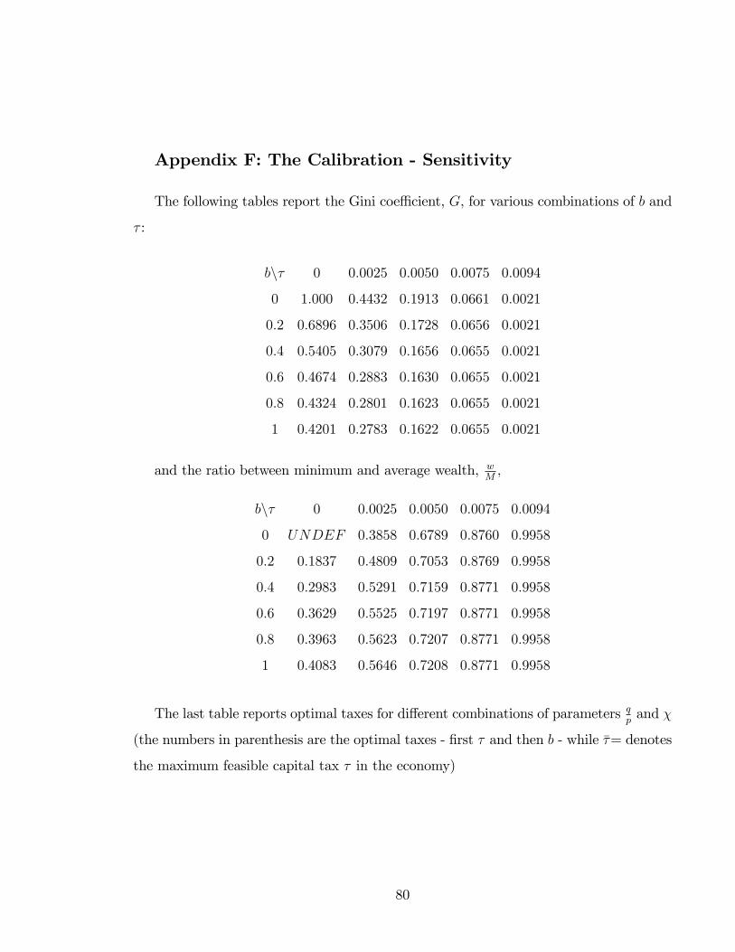
Appendix F: The Calibration - Sensitivity
The following tables report the Gini coe¢ cient, G, for various combinations of b and
� :
bn� 0 0:0025 0:0050 0:0075 0:0094
0 1:000 0:4432 0:1913 0:0661 0:0021
0:2 0:6896 0:3506 0:1728 0:0656 0:0021
0:4 0:5405 0:3079 0:1656 0:0655 0:0021
0:6 0:4674 0:2883 0:1630 0:0655 0:0021
0:8 0:4324 0:2801 0:1623 0:0655 0:0021
1 0:4201 0:2783 0:1622 0:0655 0:0021
and the ratio between minimum and average wealth, wM;
bn� 0 0:0025 0:0050 0:0075 0:0094
0 UNDEF 0:3858 0:6789 0:8760 0:9958
0:2 0:1837 0:4809 0:7053 0:8769 0:9958
0:4 0:2983 0:5291 0:7159 0:8771 0:9958
0:6 0:3629 0:5525 0:7197 0:8771 0:9958
0:8 0:3963 0:5623 0:7207 0:8771 0:9958
1 0:4083 0:5646 0:7208 0:8771 0:9958
The last table reports optimal taxes for di¤erent combinations of parameters qpand �
(the numbers in parenthesis are the optimal taxes - �rst � and then b - while ��= denotes
the maximum feasible capital tax � in the economy)
80

qpn� 8 10 12 15
:5(0:0126; 0)
�� = 0:0128
(0:0119; 0)
�� = 0:0121
(0:0112; 0)
�� = 0:0114
(0:0103; 0)
�� = 0:0105
:6(0:0119; 0)
�� = 0:0121
(0:0111; 0)
�� = 0:0113
(0:0103; 0)
�� = 0:0105
(0:0092; 0)
�� = 0:0094
:8(0:0107; 0)
�� = 0:0109
(0:0096; 0)
�� = 0:0098
(0:0085; 0)
�� = 0:0087
(0:0071; 0)
�� = 0:0073
81
Related Documents