The distribution of larval fish assemblages of Gulf St Vincent in relation to the positioning of sanctuary zones Jordan M Jones 1616020 3/11/2014 Submitted in partial fulfilment of the requirements for the degree of Bachelor of Science (Honours), School of Earth and Environmental Sciences, The University of Adelaide Supervisor: Associate Professor Ivan Nagelkerken

Welcome message from author
This document is posted to help you gain knowledge. Please leave a comment to let me know what you think about it! Share it to your friends and learn new things together.
Transcript

The distribution of larval fish
assemblages of Gulf St Vincent in
relation to the positioning of
sanctuary zones
Jordan M Jones
1616020
3/11/2014
Submitted in partial fulfilment of the requirements for the degree of
Bachelor of Science (Honours), School of Earth and Environmental Sciences,
The University of Adelaide
Supervisor: Associate Professor Ivan Nagelkerken

i
Declaration
The work presented in this thesis contains no material which has been accepted for the award
of any other degree or diploma in any university or other tertiary institution and, to the best of
my knowledge and belief, contains no material previously published or written by another
person, except where due reference is made in the text.
I give consent to this thesis being made available for photocopying and loan.
…………………..
Jordan Jones
29.10.14

ii
Table of Contents
Declaration i
Abstract 1
Introduction 2
Larval fish and population growth 2
Sanctuary zones and Gulf St Vincent 4
Methods 6
Study area 6
Aim 1: Larval distribution patterns 10
Larval sampling 10
Analysis 13
Aim 2: Sanctuary replenishment and population growth 13
Analysis 14
Aim 3: Larval communities of Gulf St Vincent and other temperate areas 14
Analysis 15
Results 15
Aim 1: Larval distribution patterns 15
Aim 2: Sanctuary replenishment and population growth 23
Aim 3: Larval communities of Gulf St Vincent and other temperate areas 25
Discussion 26
Aim 1: Patterns of larval fish assemblage 26
Aim 2: Sanctuary replenishment and population growth 32
Aim 3: Larval communities of Gulf St Vincent and other temperate areas 34
Conclusion 35
Acknowledgements 36
Literature cited 37
Appendix A 42
Appendix B 44
Appendix C 47
Appendix D 52

1
Abstract
The supply of larval fish to an area and their subsequent settlement there is an important
driver of population growth. By protecting settlement habitat and reducing mortality due to
fishing, sanctuaries within areas that are replenished by larval fish offer enhanced potential
for population growth. Little is known about the larval assemblages that occur in Gulf St
Vincent and what may drive them. This study aimed to assess the larval assemblages of Gulf
St Vincent, the potential replenishment of larvae into the Gulf’s sanctuary zones, and the
difference between assemblages in Gulf St Vincent and other temperate regions. It was found
that the larval assemblages present within Gulf St Vincent are significantly different to those
found in other temperate Australian regions in comparable seasons. Further, differences in
larval assemblages were present between different latitudinal zones of the Gulf itself. The
larval community structure differed between the Central and South, and North and South, and
average late-autumn and winter species richness and diversity where higher in the Central
zone of the Gulf than in the South, while total species richness was lowest in the North and
equal in the Central and South. Significant differences between fish the community structures
of different life stages suggest that diversity and abundance estimations of juvenile, sub-adult
and adult fish stocks may be biased by underwater visual census techniques. This study
highlights that sanctuaries within Gulf St Vincent could play a vital role for protection of
settlement habitats of unique larval communities and thus may enhance potential population
growth through larval supply and recruitment. The positioning of the sanctuaries in the North
and South works to encapsulate the different larval communities that occur in these zones.
The data obtained in this study provides baseline information which is vital for assessing the
efficacy of the sanctuary zones in the future and for understanding the processes that drive
the ecological systems in the area.

2
Introduction
Larval fish and population growth
Populations of marine species can remain stable or grow by two means. Juveniles, sub-adults
or adults may migrate into the area, or settlement stage larval fish may recruit to the area
(Booth et al. 2000; Planes et al. 2000; Wen et al. 2013). While migration may allow for
increased local populations, growth in this manner is often less significant than population
growth via recruitment (Stockhausen et al. 2000; Gerber et al. 2005). Recruitment occurs
when pelagic (open ocean living) larval fish settle into benthic (bottom living) zones and then
become part of the local population (Caley et al. 1996). Fish that recruit to an area may
originate from larvae spawned from other areas or in the area in which they eventually recruit
to (natal or self-recruitment) (Planes et al. 2000; Harrison et al. 2012). While some level of
self-recruitment may occur, for small areas a greater proportion of recruitment often comes
from larvae spawned externally to the area (Caley et al. 1996; Planes et al. 2000). Larvae of
coral trout (Plectropomus macula) and stripey snapper (Lutjanus carponotatus) on the Great
Barrier Reef, for example, have been demonstrated to have self-recruitment rates of just 7%
and 22% respectively, with the remaining larvae recruiting to other areas (Harrison et al.
2012).
Due to the openness of marine systems and populations, as well as the larval phase of many
marine species being pelagic, the process of recruitment is complex (Caley et al. 1996;
Pineda et al. 2010). Often, after being dispersed as eggs, pelagic larval fish continue to
disperse passively and actively, until they reach the settlement phase of their life-cycle
(Planes et al. 2000). Settlement is the phase at which the larvae select benthic habitats to
settle into, transferring from pelagic to the benthos (Connell 1985). After settlement,
recruitment occurs, in which the settled fish move into different habitats or join local juvenile
and adult populations (Connell 1985). The number of larvae that subsequently transition into
juveniles and adults is strongly affected by the number of larvae supplied to the area as well
as processes such as competition, predation and habitat quality (Keough and Downes 1982;
Pineda et al. 2010). These processes result in low survivorship of larvae, and movement of
settled larvae and new recruits away from the area (Keough and Downes 1982; Pineda et al.
2010). In general higher larval supply leads to potentially higher settlement and greater
potential for recruitment (for example see Stephens Jr et al. 1986). In turn, this allows for
potentially higher population growth (Booth et al. 2000). If larvae do not arrive in any given

3
area they cannot settle and subsequently recruit there, and therefore cannot contribute to the
local population growth. Where recruitment does not occur, population growth may be
minimal or non-existent, and when mortality rates are increased beyond those that are natural,
population decline is likely to eventuate (Caley et al. 1996). Due to the isolation of Saba
Marine Park, off Saba Island in the Caribbean, lack of larval supply and subsequent
recruitment has been attributed as a cause for a lack of significant population growth after
closure to fishing (Roberts 1995). The study in Saba Marine Park highlights that larval supply
and subsequent settlement often differs spatially. This is due to the dispersive pelagic phase.
Spatial variation in larval abundances and diversity has been shown to occur in terms of
depth, proximity to shore and between specific areas (Leis 1986; Doherty 1991; and others).
This variation is a function of habitat selection of settlement stage larvae, abiotic water
conditions (e.g. temperature and salinity), and factors such as currents and tides which may
aid or hinder supply to an area (Doherty 1991). Larval supply also differs temporally as
different species spawn at different times and have different lengths of dispersion time prior
to settlement (Doherty 1991; Gray and Miskiewicz 2000).
For populations of Balanus glandula (barnacles), Jasus edwardsii (spiny lobsters), Dascyllus
trimaculatus and Dascyluss flavicaudus (damselfishes), Thalassoma bifasciatum (bluehead
wrasse), Plectropomus maculatus (coral trout), and Lutjanus carponotatus (stripey snapper)
positive correlations have been found between the abundances of different life stages (Gaines
and Roughgarden 1985; Victor 1986; Schmitt and Holbrook 1996; Schmitt and Holbrook
1999; Freeman et al. 2012; Wen et al. 2013). In these studies, researchers looked specifically
at individuals observed as having recently settled into the benthos and correlated their
abundances to those of either juveniles or adults in the area. The findings of such correlations
in species of barnacles and lobsters as well as fish, suggest that, although post-settlement
processes and home ranges will differ between species, correlations between different life
stages can still be present (Grosberg and Levitan 1992). Larval recruitment could therefore
significantly facilitates population enhancement. Observations of recently settled fish rely on
knowledge of where settlement locations occur, and thus there is a significant limitation as to
the studies that can be done using these methods. An alternative method is to look at the
supply of settlement-stage larval fish rather than the abundance of newly settled fish.
Irrespective of correlation strength between larval and post-settlement stages (which may be
reduced due to a greater time lapse between the recorded life stages), this method could still
the inherent link between consecutive stages (Stephens Jr et al. 1986; Caley et al. 1996).

4
Such correlations have been undergone for the Stegastes partitus (bicolour damselfish), the
Lythrypnus dalli (blue-banded goby), the Ruscarius creaseri (formerly Artedius creaseri;
roughcheek sculpin), and Sillaginodes punctate (King George whiting) (Stephens Jr et al.
1986; Hamer and Jenkins 1997; Valles et al. 2001; Grorud-Colvert and Sponaugle 2009). In
all cases strong, positive, correlations were found between the abundances of settlement-stage
larvae and that of newly settled fish. Extrapolating this, in light of correlations being present
between abundances of newly settled fish and juvenile or adult fish, it can be expected that
abundances of settlement-stage larvae can show a certain degree of correlation to that of
juvenile or adult fish. Looking at abundances of larvae as close to settlement-stage as
possible might therefore be informative of that of younger fish (newly settled or juveniles)
(Stephens Jr et al. 1986; and others). Where a positive correlation exists between larval
supply and juvenile and adult fish this could allow assessments to be made using larval fish
abundances as to the likelihood of population growth occurring in an area.
Sanctuary zones and Gulf St Vincent
At the forefront of management for the protection of marine environments and species,
marine parks can allow for enhanced population growth (Halpern 2003). Zonation within
marine parks dictates the activities and access allowed in an area based on specific aims of
protection and thus governs the level of protection specifically defined areas receive (Marine
Parks Act 2007). By prohibiting fishing, sanctuary zones offer the highest level of protection
against overexploitation. As mortality due to fishing is eliminated, these zones have the
greatest potential for species population enhancement (Halpern and Warner 2003). Further,
by protecting habitats and maintaining habitat complexity biodiversity can be sustained
(Halpern and Warner 2003). A review of 89 studies looking at the efficacy of a total of 112
sanctuary zones found that on average biological measures, such as size, were significantly
higher within the sanctuary zones than external to them or prior to their establishment
(Halpern 2003). The occurrence and extent of such benefits are largely species specific, and
may be dependent on their life history traits (Nardi et al. 2004; Claudet et al. 2010). Marine
parks also allow increases in the abundance of adult fish within sanctuaries and proximate
fished areas (Rowley 1994; Gaines et al. 2010; Harrison et al. 2012). For long term benefits
of sanctuary zones to eventuate, populations must be able to be sustained and have the
potential for growth. Understanding the mechanisms that govern the potential for population
growth and how such mechanisms link to sanctuary zones is therefore vital.

5
Three marine parks, brought into effect in October 2014, are located in Gulf St Vincent
(DEWNR 2013). These are Encounter Marine Park, Upper Gulf St Vincent Marine Park and
Lower Yorke Peninsula Marine Park. Throughout the three marine parks, 17 sanctuary zones
have been established, 11 of which are located within Gulf St Vincent. While the sanctuary
zones were not designed specifically for the purpose of fish population enhancement, due to
the absence of mortality due to fishing, they are the areas where population enhancement has
the highest potential to occur. Due to the link between consecutive life stages, the supply of
larvae to a sanctuary zone could increase the potential for population enhancement. As larvae
move both passively and actively, the positioning of sanctuary zones is important. (Caley et
al. 1996; Freeman et al. 2012; Wen et al. 2013). Located between the Fleurieu and Yorke
Peninsula of South Australia, Gulf St Vincent is an inverse estuary covering an area of
approximately 7000 km2 (de Silva Samarasinghe and Lennon 1987). Large knowledge gaps
exist in relation to the abundance and diversity of fish in Gulf St Vincent, even less is known
about the larval supply of the area, and no data exists on the patterns of larval assemblage that
occur within the Gulf. What is known is largely species specific, focussing on species that are
commercially important or endemic to the area, and fails to look at diversity (Dimmlich et al.
2004; and others). To date, through targeted studies of commercially important species, only
a few larval species have been recorded in the area. These species are Sillaginodes punctata
(King George whiting) (Neira et al. 1998), Engraulis australis (Australian anchovy) (Neira et
al. 1998 and Dimmlich et al. 2004), Hyporhamphus melanochi (southern garfish) (Noell and
Ye 2008), Sardinops sagax (Pacific sardine) (Dimmlich et al. 2004), Spratelloides robustus
(blue sprat) (Neira et al. 1998 and Rogers et al. 2003), Pelates octolineatus (western striped
grunter) (Neira et al. 1998), Lesueurina platycephala (flathead sandfish) (Neira et al. 1998),
Pagrus auratus (Australasian snapper) (Neira et. al 1998 and Saunders 2009) and
Syngnathidae spp. (seahorses, pipefish and sea dragons) (Neira et al. 1998). While these
species are known to occur in the area, their distributive patterns are unquantified. As other
studies of larval assemblages, both in temperate Australia and other regions worldwide, show
larval assemblages to vary spatially, spatial variation of larvae can be expected to occur
within Gulf St Vincent (see for example Muhling and Beckley 2007; Keane and Neira 2008;
and others).

6
While addressing the knowledge gaps surrounding marine sanctuaries and larval supply in
general and the lack of information of larval assemblage patterns in Gulf St Vincent
specifically, this study aims to assess the following hypotheses:
1) driven by environmental attributes, larval distribution will differ spatially within Gulf
St Vincent, with distinct populations likely to occur at the head and mixed populations
likely to occur at the mouth;
2) the overlap of larval communities with sanctuary zones will highlight the potential for
enhanced population growth within the sanctuary; and
3) the larval communities of Gulf St Vincent will be similar to those of neighbouring
Spencer Gulf, but will be different to those in other temperate Australian regions.
Methods
Study area
Located between the Fleurieu and Yorke Peninsula of South Australia, Gulf St Vincent is an
inverse estuary covering an area of approximately 7000 km2 (de Silva Samarasinghe and
Lennon 1987). A maximum depth of approximately 45 m occurs at the mouth of the Gulf,
while minimum depths of around 5 m occur at the head (Petrusevics 1993; de Silva
Samarasinghe 1998). Sea surface temperatures within the Gulf are generally higher at the
head and lower at the mouth, during summer, with the pattern reversed in winter (Bye 1976).
Gulf St Vincent is an inverse estuary, with salinity increasing towards the head of the Gulf
(de Silva Samarasinghe and Lennon 1987). The patterns of salinity within Gulf St Vincent
reflect the currents that occur in the area. As seen in Figure 3 b, the area is subject to a
clockwise inflow along the western side that outflows through the central regions, and a small
anticlockwise circulation on the eastern side (Bye 1976; de Silva Samarasinghe and Lennon
1987; de Silva Samarasinghe 1998). These circulation patterns do not differ seasonally and
are present irrespective of wind direction (Bye 1976 and de Silva Samarasinghe 1998). In
contrast, the direction and magnitude of circulation at the head of the Gulf varies seasonally
dependent on wind and tides (Bye 1976). Together the abiotic factors of sea surface
temperature, salinity and currents can be expected to influence the distribution of all life-
stages of fish in the area (see for example Bruce and Short 1990). Fish distribution is further
influenced by substratum type, which too differs throughout the Gulf. Generally, mangroves

7
and seagrasses make up around 95% of the cover in the northern area where shallower and
calmer conditions occur, while as much as 40% of the area towards the mouth and extending
into Investigator Strait is rocky reef (Shepherd and Sprigg 1976; Edyvane 1999). Inherently
these different substratum types offer differing habitat complexity, with reefs more complex
than seagrasses (Shepherd and Sprigg 1976).
This study took place at 10 locations positioned along a latitudinal gradient in Gulf St
Vincent (Figure 1). While maintaining even spacing across the latitudinal gradient, where
possible the sites were positioned to correlate with sanctuary zones (as can be seen in Figure
1). By encompassing the largest latitudinal gradient as possible, this study can encapsulate
spatial variation and assess differences between the larval assemblages at the head of the
Gulf, which are likely to be isolated, and the mouth of the Gulf, which are likely to be mixed
and receive greater influx from the open ocean. Prior to commencement of this study, a
permit (number MR00014-1) was obtained to allow scientific research to be undergone
within the sanctuary zones present in Gulf St Vincent.

8
Figure 1. Map of Gulf St Vincent, showing bathymetry (depth in m), marine parks (red outline), sanctuary zones (black
outline), and sampling locations with approximate latitude (pink markers). Circle markers represent water depth of 10m,
triangle markers represent water depth of 15m and square markers represent water depth of 20m. Legend is given on the
following page. Map generated at Nature Maps SA (2014).
Location 6: 35o 3’ 30.4” S
Location 5: 34o 57’ 15.5” S
Location 4: 34o 50’ 49.9” S
Location 3: 34o 46’ 33.8” S
18
20
9
2
2
20
5
20
20
37
37
36
20
2
2
9 4
2
4
2
2
2
4
4
4
8
20 18
18 15
10
9
4
37
10
Location 1: 34o 20’ 24.4” S
Location 2: 34o 30’ 34.8” S
Location 7: 35o 9’ 47.6” S
Location 8: 35o 16’ 38.5” S
Location 9: 35o 23’ 52.68” S
Location 10: 35o 31’ 35.7” S

9
Figure 1 – continued. Map of Gulf St Vincent legend. Map generated at Nature Maps SA (2014).

10
Aim 1 – Larval distribution patterns:
Larval sampling
Larval fish were sampled during three sampling periods; April-May, June-July and August 2014.
In each sampling period all 10 locations were sampled over the fewest number of consecutive as
possible, dependent on weather. To account for changing conditions spatially and temporarily,
recordings of salinity, temperature, moon phase, and habitat type were made (see Appendix A
and Table 1). While variation in abundances may exist on a larger temporal scale (between
years) coarse relative spatial distribution patterns should remain roughly similar from year to
year (Doherty 1991). Confining the study to one year should therefore work to demonstrate
predominate relative latitudinal patterns of late-autumn and winter spawners. During the initial
sampling period, except for at the most northern which had limited variation of depth, two sites
were sampled at each location. The shallower sites, 10 m water depth at two northernmost
locations and 15 m at other 8 locations, were representative of inshore locations and the deeper,
15 m at second northernmost location and 20 m at other eight locations, of offshore. During the
second and third sampling periods, only inshore sites were sampled. Focus on inshore was due to
enabling better correlation to adult data and substrate, and allowing analysis of the largest
latitudinal gradient possible. Further, initial analysis of sampling period 1, during which all
sampling was carried out at the same depth below surface, showed no difference in the larval
assemblages of inshore and offshore locations (see Appendix B). A GPS reading was taking
during the initial sampling period to allow the same locations to be sampled in subsequent
periods.
Prior to any sampling, ethics approval was obtained to allow sampling of animals (approval
number S-2014-061), and all sampling was conducted, and reported, under Primary Industries
and Regions SA: Fisheries and Aquaculture’s S115 ministerial exemption number 9902676,
with specified allowance under Schedule 2 to sample with mesh of size 0.5mm. Larval fish were
sampled using Twin Ring nets (Sea-Gear Model 9600). Designed for collection of late- or
settlement-stage larvae, the frame consisted of two stainless steel rings; each with a mouth
diameter of 75 cm positioned alongside each other and joined in the centre by a swivel (Figure
2). By reducing net avoidance of settlement-stage, active-swimming, larvae, the large mouth
diameter worked to enhance catchability (Stehle 2007). All sampling was conducted during
daytime. Each net, fastened to the rings by net collars, had a length of 3 m. The 3 m length
encompassed a 1.5 m cylindrical top section, which worked to improve filtration efficiency, and
a 1.5 m conical section (Kelso et al. 2012). Standard mouth to length ratios used for larval

11
sampling range from 1:3 to 1:5; with a ratio of 1:4 this net fell within the recognised standard for
efficient sampling (Kelso et al. 2012). One net was of mesh size 500 µm while the other was
mesh of 1000 µm in size. Having one net of 500 µm and the other of 1000 µm allowed the most
diverse catch to be achieved, by balancing clogging of the net and extrusion of larvae, and
allowed an analysis to be done to determine the most effective and efficient net size for the area
(Smith et al. 1968). A PCV cod end was attached to end of each net for larval collection. Mesh
on one side of each cod end, to allow filtration, matched the mesh size of the net to which it was
attached.
Figure 2. Diagram of nets being towed, showing attachment of net to buoy to maintain desired sample depth, and
basic net design of Twin Ring nets (Sea-Gear Model 9600). Note figures are not to scale.
As the number of larvae sampled is directly related to the amount of water filtered through the
nets, volume filtered was calculated for each tow to allow abundances to be converted to
concentrations (i.e. number of larval per 1 m3 of water) (Muhling et al. 2008). During the initial
sampling period this was achieved by the use of a mechanical flowmeter (Sea-Gear MF315)
however, due to loss of the flowmeter, for the subsequent sampling periods calculations were
1.5 m cylindrical section 1.5 m conical section
75 cm diameter
PVC cod end
12
made based on distance towed, with recording a GPS position at the start and end of each tow.
On one occasion both methods were used and the volume filtered determined by each method
only differed by 6 m3, with the average volume sampled throughout the study being 364.16 m
3.
As greater differences in volume filtered existed between tows (see Appendix A), the change
between methods is not expected to have been an issue. During sampling, to allow the nets to
sink into the water column, weight was suspended from the centre swivel (Leis 1991). During
the first sampling period the weight consisted of a 5 kg depressor. A depth sensor attached to the
top of the swivel showed that the nets did not go deeper than an average of 2 m below the
surface. To enable sampling at greater depths, and thus allow samples to be collected closer to
the substrate and thus where settlement-stage larvae are more likely to occur (Leis 1986;
Muhling and Beckley 2007), during the two subsequent sampling periods an extra 10 kg was
added to net frame.
All sampling was conducted with the assistance of DEWNR personnel and a student volunteer
from a boat owned and operated by DEWNR. Upon arrival at a desired location and water depth,
nets were deployed from the stern of the boat. To sample 5 m above the substrate, as is common
practice for sampling settlement-stage larvae (Kelso et al. 2012; Miskiewicz pers. comm. 2014),
40 m of tow rope was released before being hitched off, a constant angle of approximately 45o
was maintained between the rope and the boat, and the boat travelled at a constant towing speed
of approximately 1 m/s (2 knots) (Johnson and Morse 1994; and others). Further, to prevent the
nets sampling deeper than the desired depth, a buoy was attached to the net’s centre swivel by a
rope of equal length to the desired sampling depth (Figure 2) (Leis 1986). The attached depth
sensor allowed an average sampling depth to be recorded, accounting for any lift of the nets that
may have occurred due to tidal activity or boat speed. The nets were towed horizontally for 15
minutes before being retrieved. On the initial sampling period retrieval utilised a single-speed
hand manual winch. This was replaced with an electric winch for the two following sampling
periods to compensate for the greater weight and to increase retrieval speed, thereby decreasing
the opportunity for larvae to escape. Once retrieved, the nets were hung vertically over the deck
of the boat and rinsed with a deck hose. During rinsing, water pressure was kept to a minimum,
balancing the need to remove larvae and organic matter caught in the net whilst not damaging
the larvae, and the cod ends were angled to avoid a heavy flow of water into them and further
reduce damage to larvae. The sample in each cod end was then emptied into its own container
containing clove oil. This immediately euthanized the larvae. To preserve the larvae, ethanol was
then added to each container until they contained a solution of at least 70% ethanol (as per Choat
et al. 1993; Johnson and Morse 1994; and others). In the Southern Seas Ecology laboratory at

13
the University of Adelaide, the samples were sorted; removing any larval fish from the sample,
and storing them in 100% ethanol. Identification was then undergone with the help of temperate
larval expert Dr Anthony Miskiewicz, the use of the larval identification guide ‘Larvae of
temperate Australian fishes: laboratory guide for larval fish identification’ (1998), and a
compiled list of fish species that have previously been recorded in the area (see Appendix C).
Analysis
Data obtained during sampling periods 1, 2 and 3, was analysed individually and as a pooled
collection. Initial analysis of sampling period 1 found no significant difference between the
larval assemblages in each mesh size (see Appendix B), and so samples from the 1000 µm mesh
were used. This reduced the number of early-stage larvae and was more time efficient in terms
of sorting. In assessing the difference between inshore and offshore and mesh size from
sampling period 1, each zone was analysed separately. Analyses were carried out in
PERMANOVA with depth (fixed) and mesh size (fixed) as factors, for the Central and South
zones, and only mesh size as a factor for the North Zone. Analysis of larval abundances in the
1000 µm mesh was then carried out using nMDS, ANOSIM, PERMANOVA, SIMPER and
BEST/BIOENV packages of Primer+ and linear regression tools of SPSS. For all tests
significance level was set at 0.05. For individual periods and the periods pooled, tests were
carried out to determine differences in the larval assemblage indices of: community structure,
total abundance, species richness and Shannon’s H’ diversity. Analysis was undergone with zone
as a fixed factor. Factor zone consisted of three levels; North, Central, and South (see Figure 3 b
and Appendix A), and the division of locations into zones was based on nMDS of the
environmental variables at each location across the three periods (Figure 3 a), as larval fish are
likely to show some correlation with environmental conditions (see for example Hart et al. 1996;
Green and Fisher 2004). For the analysis of the three periods combined, period was an additional
random factor. Factor period consisted of three levels; period 1, period 2, and period 3. For the
single factor analyses of the individual periods ANOSIM was used for significant tests between
the zones as it is more robust when dealing with small replication. For analysis with two factors,
such as the pooled periods, PERMANOVA was used. Where samples had no larvae a dummy
variable was used to ensure all data was included in statistical comparisons.
Aim 2 – Sanctuary replenishment and population growth:
The Department of Environment, Water and Natural Resources provided data on juvenile, sub-
adult and adult fish recorded by underwater visual census (UVC) during February 2012. UVC

14
was undergone along transects at depths of up to 10m. Transects located at three sites, Dodd’s
Beach, Myponga South and Myponga Point, respectively lie 0.75km, 1.78km and 3.17km from
location 9 of the larval study, and transects located at three sites, Rapid Head Windmill, Sunset
Cove South and Salt Creek/Nev’s Windmill, respectively lie 0.53km, 7.10km and 3.7km of
location 10 of the larval study. As there is an average distance of approximately 17km between
the locations of the larval studies, these transects are in relatively close proximity of the
locations. At each of the six sites four replicate transects were surveyed. The raw data from
DEWNR was sorted, grouping each species recorded into size classes representative of
‘juvenile’, ‘sub-adult’ and ‘adult’. Grouping of size classes was carried out objectively, taking
the maximum size each species can grow to and making each size class cover a range a third of
the size of the maximum. Counts where then converted to relative abundances of each size class
and each species for each replicate transect.
Analysis
Larval data from locations 9 and 10 of the three periods pooled was converted to relative
abundance of each. Community structure of the larvae at these two sites was then compared to
the community structure of juveniles, sub-adults and adults using PERMANOVA. While the
UVC fish surveys were conducted approximately two years prior to the larval study the aim is
only to test for correlations in the relative compositions of the communities. Sanctuary zone
locations are considered during the interpretation of results, with comparisons made between the
larvae found in sanctuary zones and those found outside sanctuary zones. This allowed
assessment of potential supply and recruitment to sanctuary zones, and thus the potential for
enhanced population growth.
Aim 3 – Larval communities of Gulf St Vincent and other temperate areas:
Larvae from the pooled periods were compared to larvae from two other temperate Australian
studies to assess the similarities and dissimilarities between the larval communities. Studies for
comparison are:
Spencer Gulf – ‘Survey of Planktonic Larvae Near Point Lowly’ (Miskiewicz 2010),
Sydney coastal waters – ‘Larval Fish Assemblages in South-east Australian Coastal
Waters: Seasonal and Spatial Structure’ (Gray and Miskiewicz 2000).
These studies were selected as they provided larval counts in a specified volume of water from
the same seasons, late-autumn and winter, as the current study, and were conducted at similar

15
depths using similar sampling techniques. While the Sydney coastal waters study also had data
from deeper/offshore samples, these were excluded.
Analysis
Comparisons between this study and others were done using the ANOSIM Primer+ package to
assess only the indices of community structure and total abundance. Richness and Shannon’s H’
diversity were not assessed as they would require the studies to have the same sampling effort,
due to richness inherently increasing with greater sampling effort (Gotelli and Colwell 2001).
Results
Aim 1 – Larval distribution patterns:
Post-hoc tests of the environmental variables across the periods pooled allowed separation of the
10 locations into 3 zones: North, Central and South; with the environmental variables of each
zone being significantly different to the other zones (North and Central p <0.001, North and
South p = 0.003, and Central and South p = 0.037). This is supported by clear visualisation of
the separation between the zones in the nMDS based on environmental variables (Figure 3 a).
All subsequent analyses therefore used these three zones as factor levels. Consisting of locations
1 and 2 (Figure 3 b), the North zone had an average temperature of 14.12oC, average salinity of
39, and had seagrass and unconsolidated habitat (Table 1). Sampling in the North was undergone
at an average distance of 12.32 km from shore, with samples taken at an average of 5.87 m
above the seafloor with the moon an average of 61.30% visible (Table 1). Consisting of
locations 3, 4 and 5 (Figure 3 b), the Central zone had an average temperature of 14.30oC,
average salinity of 38.61, and was dominated by seagrass habitat (Table 1). Sampling in the
Central zone was conducted at an average distance of 6.90 km from shore and 9.42 m above
seafloor with the moon an average of 73.66% visible (Table 1). Consisting of locations 6, 7, 8, 9
and 10, the South zone (Figure 3 b) had an average temperature of 14.30oC, average salinity of
37.33, and was a mix of seagrass and rocky reef habitat (Table 1). Sampling in the South zone
was conducted at an average distance of 0.83 km from shore and 9.01 m above seafloor with the
moon an average of 85.35% visible (Table 1).

16
Table 1 Environmental variables, and their standard deviations, of each zone. Temperature is degrees Celsius, moon
phase is % moon visible, salinity is ppt, distance to shore is in km, distance from seafloor is m, and for habitat type
S = seagrass, U = unconsolidated, R = reef. Detail of individual locations in Appendix A. Temperature Moon phase Salinity Distance to
shore
Distance from
seafloor
Habitat
type
North 14.1±1.6 61.3±32.4 39.0 12.3±4.2 5.9±1.5 S and U
Central 14.3±1.8 73.7±31.4 38.6±0.6 6.9±1.6 9.4±2.8 S
South 14.3±2.3 85.4±33.6 37.3±0.6 0.8±0.4 9.0±3.0 S and R
Figure 3 a) nMDS of the environmental variables across the three sampling periods pooled, showing
division of locations (number 1 – 10) into zones, where North zone is in green, Central zone is in dark
blue, and South zone is in light blue; and b) Circulatory patterns present within Gulf St Vincent and
division into zones is visualised by the circles with North in green, Central in dark blue and South in light
blue. Note: spacing of zones and locations is not to scale. Image adapted form (Bye 1976, p. 149).
1
2
4
5
6 7
8 9
3
10
a
b

17
Table 2. Statistical post-hoc results, from PERMANOVA, of the three sampling periods pooled. Significant
differences are highlighted. Interaction (zone x period) was insignificant for all assemblage indices, with p > 0.32.
No post-hoc test was done between the zones for abundance as no significant differences (p = 0.48, MS 1129.9)
were found in the initial test.
Zone (df = 2) Period (df = 2)
MS
North –
Central
Central -
South
South -
North
MS 1 - 2 2 - 3 3 - 1
Sig.
Test
stat. Sig.
Test
stat. Sig.
Test
stat.
Sig.
Test
stat. Sig.
Test
stat. Sig.
Test
stat.
Community 3445.5 0.147 1.56 0.041 1.99 0.008 2.82 6871.8 <0.001 3.41 0.002 2.14 0.037 1.71
Abundance 9637.9 <0.001 3.25 0.001 2.77 0.177 1.35
Richness 1173 0.087 2.43 0.049 2.83 0.210 1.66 2635.2 0.003 3.18 0.081 1.77 0.085 1.79
Shannon's H' 193.3 0.182 2.02 0.034 4.70 0.423 0.97 89.6 0.016 2.78 0.316 1.06 0.120 1.48
Table 3. Statistical results, from ANOSIM, of individual sampling periods. Significant differences are highlighted.
Zone
North - Central Central - South South - North
Sig. R statistic Sig. R statistic Sig. R statistic
Period 1
Community 0.600 0.00 0.125 0.32 0.619 -0.07
Abundance 0.400 0.00 0.375 0.01 0.714 -0.16
Richness 0.300 0.29 0.446 0.01 0.714 -0.14
Shannon's H' 0.400 0.08 0.571 -0.09 0.619 -0.02
Period 2
Community 0.100 0.92 0.036 0.47 0.143 0.40
Abundance 0.200 0.50 0.839 -0.19 0.143 0.31
Richness 0.400 0.04 0.482 -0.03 1.000 -0.31
Shannon's H' 1.000 -0.42 0.054 0.52 0.048 0.58
Period 3
Community 0.300 0.33 0.500 -0.01 0.667 -0.12
Abundance 0.700 -0.25 0.804 -0.20 0.905 -0.24
Richness 0.400 -0.04 0.762 -0.12 0.750 -0.09
Shannon's H' 0.300 0.17 0.750 -0.16 0.762 -0.10
Table 4. BEST results of individual periods and periods pooled, giving the environmental variable(s) with the
strongest correlation.
BEST Correlation
Period 1
Community Habitat type 0.12
Abundance Distance to shore and Salinity -0.047
Richness Distance from seafloor 0.009
Shannon's H' Habitat type 0.044
Period 2
Community Moon phase and Habitat type 0.289
Abundance Moon phase and Habitat type 0.073
Richness Temperature 0.109
Shannon's H' Salinity 0.678
Period 3
Community Distance from seafloor 0.646
Abundance Habitat type and Distance from seafloor 0.413
Richness Temperature, Habitat type and Distance from seafloor 0.457
Shannon's H' Habitat type and Distance from seafloor 0.276
Periods
1,2,3
Community Temperature 0.289
Abundance Temperature 0.116
Richness Temperature 0.188
Shannon's H' Habitat type 0.051

18
Periods 1 and 2 were significantly different for the indices of community (p < 0.001) (Figure 4
a), total abundance (p < 0.001), richness (p = 0.003), and Shannon’s H’ (p = 0.016) (Table 2);
with period 2 having greater total abundance richness and Shannon’s H’ (Figure 4 b, c, d).
Periods 2 and 3 were significantly different for the indices of community (p = 0.002) and total
abundance (p = 0.001) (Table 2 and Figure 4 a), with period 2 having greater total abundance
(Figure 4 b); and periods 1 and 3 had significantly different communities (p = 0.037) (Table 2,
Figure 4 a). These differences between periods were driven by Meuschenia spp. (leather jackets)
which had dissimilarity contributions of 48.33% for periods 1 and 2, 29.24% for periods 1 and 3,
39.01% for periods 2 and 3.
Figure 4 a) nDMS showing similarities between the larval communities of sampling periods 1, 2 and3; b) total
abundances of each sampling period with standard error and letters showing significant differences; c) richness of
each sampling periods with standard error and letters showing significant differences; and d) Shannon’s H’ of each
sampling period with standard error and letters showing significant differences. Different letters represent
significant differences.
a
a
b
a
a
a
b
c d
b
a b
b
a b

19
Community structure was significantly different (p = 0.036) between the Central and South
zones of sampling period 2 (Table 3). This difference was driven by the Gymnapistes
marmoratus (South Australian cobbler) (23.99% dissimilarity contribution). No other significant
differences for community structure were present in the individual sampling periods. Pooling the
data of the three sampling periods found significant differences in the communities of North and
South (p = 0.008) and the communities of Central and South (p = 0.041) (Table 2, Figure 5),
driven by Meuschenia spp. (30.68% dissimilarity contribution) and Tripterygiidae spp. (triple-
fin blenny) (18.53% dissimilarity contribution) respectively. Moon phase and habitat type
accounted for 28% of the variation in community structure in period 2, while temperature
explained 28% of the variation in community structure of the pooled periods (Table 4).
Figure 5. nMDS of similarity in larval communities in each location, for factor zone, with three levels of zone:
North, Central and South.
Total abundance did not differ between the zones when the periods were analysed individually
or pooled (Tables 2 and 3). However, in period 2, 53% of the variation can be explained by a
significant (p = 0.015) increasing linear regression across the latitudinal gradient, and for the
pooled periods 57% of the variation can be explained by a significant (0.007) increasing linear
regression across the latitudinal gradient (Figure 6).

20
Figure 6. Average total abundance with standard error at each location for the three sampling periods, showing an
increasing linear trend from north to south. Red line gives the trend with the outlier at location 3 excluded (R2 =
0.574, p = 0.007), and black line gives the trend with the outlier included (R2 = 0.029, p = 0.293). The outlier was
excluded as it was resultant of high number of one species being present in one trawl, and so was a random
occurrence.
Richness showed no significant differences between the zones of the individual periods (Table
3), but for the pooled periods richness was significantly higher (p = 0.049) in the Central zone
than in the South (Table 2, Figure 7).
Figure 7. Average richness of each zone for the pooled sampling periods, with error bars and letters symbolising
significant differences (where different letters represent significant differences).
b
a b
a

21
Shannon’s H’ diversity index was significantly greater in the North than the South zone of
period 2 (p = 0.048) (Table 3), with salinity explaining 67% of the variation (Table 4). When the
sampling periods were pooled, Shannon’s H’ significantly differed (p = 0.034) between the
Central and South zones, with diversity greater in the Central zone.
Figure 8. Average Shannon’s H’ of each zone for the pooled sampling periods, with error bars and letters
symbolising significant differences (where different letters represent significant differences).
While richness and Shannon’s H’ diversity are higher on average in the samples from the
Central zone than from the South, the species that contribute to the richness of each sample
means that across all samples the Central and South zones actually contain the same number of
species, thus total richness in the Central and South zones are equal (Figures 9 and 10). The
North zone has a total richness of 4, and the Central and South zones have a total richness of 12
(Figures 9 and 10).
a b a
b

22
Figure 9. Average contribution (%) of each species to the larvae found in each zone and to Gulf St Vincent as a
whole. Species that only occurred as individuals in the offshore sites or in the smaller (500 µm) mesh have been
excluded. The outlier that was excluded in total abundance analysis due to being driven by one species in one
sample has been excluded here.
Figure 10. Absolute abundance of each species to the larvae found in each zone and to Gulf St Vincent as a whole.
Species that only occurred as individuals in the offshore sites or in the smaller (500 µm) mesh have been excluded.
The outlier that was excluded in total abundance analysis due to being driven by one species in one sample has been
excluded here.
Meuschenia spp.
Gymnapistes marmoratus
Neosebastes sp.
Lepidotrigla spp.
Platycephalus sp.
Rhombosolea tapiria
Tripterygiidae spp.
Gobiesocidae spp.
Gobiidae spp.
Bathygobius krefftiii
Callionymidae spp.
Urocampus carinirostris
Stigmatopora spp.
Hippocampus sp.
Meuschenia spp.
Gymnapistes marmoratus
Neosebastes sp.
Lepidotrigla spp.
Platycephalus sp.
Rhombosolea tapiria
Tripterygiidae spp.
Gobiesocidae spp.
Gobiidae spp.
Bathygobius krefftiii
Callionymidae spp.
Urocampus carinirostris
Stigmatopora spp.
Hippocampus sp.

23
Aim 2 – Sanctuary replenishment and population growth:
Significant differences were found between the community structures of each of the life stages:
larvae, juvenile, sub-adult and adult. All p-values, for post-hoc comparrisons, between life stages
were 0.0001. Figure 11 shows separation, and thus dissimilarity, between the different life
stages, and clustering, and thus similarity, within the life stages.
Figure 11. nMDS of similarity between different life stages, showing larvae in green, juvenile in dark blue, sub-
adult in light blue, and adult in red.
One location in the North zone and four locations in the South zone are within sanctuaries
(Figure 12). A difference in the larval assemblages between these zones therefore has potentially
important implications; as, if the larvae settle in the zone, they contribute to the potential
population growth and thus efficacy of the sanctuary. In the North zone, while average species
richness is the same within and outside sanctuary zones, outside the sanctuary has higher total
richness (Figure 12). In the South zone, both average richness per sample and total richness are
higher in the sanctuary than outside the sanctuary (Figure 12). However as a greater number of
locations in the South zone are sanctuaries than non-sanctuaries there is an inherently greater
potential for higher richness to be encapsulated. In the North zone, Urocampus carinirostris
larvae were only sample outside the sanctuary, but were present in thesanctuaries of the South
(Figure 12). Callionymidae spp. and Hipppocampus sp. occur only in the Central zone where
there are no sanctuaries (Figure 12). In the South zone, all species found outside sanctuaries
were also found within sanctuaries (Figure 12).

24
Figure 12. Relative abundances of species in each zone: North, Central and South; depicting total richness inside
(blue outlie) and outside (red outline) sanctuaries. Note richness and Shannon’s H’ given in text boxes are averages
for the zone/sanctuaries within zone.
Location = 2
Zone = North
Average richness = 2.00
Shannon’s H’ = 0.23
Total richness = 3
Location = 3, 4, 5
Zone = Central
Average richness = 4.22
Shannon’s H’ = 0.42
Total richness = 12
Location = 7, 8, 9, 10
Zone = South
Average richness = 2.83
Shannon’s H’ = 0.23
Total richness = 12
Location = 1
Zone = North
Average richness = 2.00
Shannon’s H’ = 0.17
Total richness = 4
Location = 6
Zone = South
Average richness = 2.00
Shannon’s H’ = 0.19
Total richness -4
Meuschenia spp.
Gymnapisties marmoratus
Neosebastes sp.
Lepidotrigla spp.
Platycephalus sp.
Rhombosolea tapiria
Tripterygiidae spp.
Gobiesocidae spp.
Gobiidae spp.
Bathygobius krefftii
Callionymidae spp.
Urocampus carinirostris
Stigmatopora spp.
Hippocampus sp.

25
Aim 3 – Larval communities of Gulf St Vincent and other temperate areas:
The community structures of Spencer Gulf and Sydney coastal waters were significantly
different from each other and from that of the pooled sampling periods of this study (Table 5,
Figure 13 a). Total abundance was significantly different between Sydney coastal waters and
Spencer Gulf (p = 0.041), and Sydney coastal waters and Gulf St Vincent (p < 0.001). The total
abundances of Spencer Gulf and Gulf St Vincent were not significantly different (p = 0.859)
(Table 5, Figure 13 b).
Table 5. PERMANOVA results of temperate study comparison, showing in yellow results of total abundance
comparison, and in orange community structure comparison.
Sydney Spencer Gulf Gulf St Vincent
Sign. R stat. Sign. R stat. Sign. R stat.
Sydney 0.041 1.00 <0.001 0.98
Spencer Gulf 0.042 1.00 0.859 -0.20
Gulf St Vincent <0.001 1.00 <0.001 0.42
Figure 13 a) nMDS of similarity between the larval communities of different temperate Australian areas, showing
WA in green, east Australia in dark blue, Sydney in light blue, Spencer Gulf in red, and Gulf St Vincent in green
with stress 0.01; b) total abundance of larvae per 500 m3 at each temperate region, with Spencer Gulf and Gulf St
Vincent on left axis and Sydney on right axis, showing standard deviation and letters symbolising significant
differences (where different letters represent significant differences).
a
b
a
a
b

26
Discussion
Aim 1 – Larval distribution patterns:
The pooling of the sampling periods found that the late-autumn and winter larval communities
differed between the North and South zones as well as between the Central and South zones; that
average species richness and Shannon’s H’ were both highest in the Central zone; and that total
abundance increased linearly across the latitudinal gradient of the Gulf from North to South. The
hypothesis of larval distributions varying spatially within Gulf St Vincent is therefore upheld for
late-autumn and winter communities. As the patterns found for the pooled periods are unlike
those obtained by analysis of individual sampling periods, even though differences exist for at
least one assemblage index between each of the periods, it is clear that one sampling period
alone is not driving the pattern of larval assemblages. The following interpretations are therefore
based on the overall results of the pooled periods.
While remembering that they are larvae, and thus have not yet settled into the benthos, and so
may continue to move, either passively or actively, prior to settlement, the patterns observed are
indicative of the processes governing the ecological systems in the area. Differences in larval
community structure between zones may, at least partially, be governed by assemblage patterns
of adult fish. While larvae may be widely dispersed (Caley et al. 1996), the adult species present
in each zone, and their abundance within each zone, is likely to contribute to the larvae supplied
to the area. As adults, over 35% of the species sampled in this study are demersal brooders,
laying demersal eggs and caring for them (Table 6) (Patzner 2008). While pelagic spawners
release eggs into the open water, resulting in widespread dispersal, demersal spawners release
eggs closer to the substrate and have been shown to disperse less than pelagic eggs/larvae,
remaining closer to shore and dominating shallow environments (Hickford and Schiel 2003;
Patzner 2008). Dispersal, particularly passive dispersal, is restricted in demersal spawners as the
eggs have parental care until well developed larvae emerge (Hickford and Schiel 2003; Patzner
2008). The larvae of demersal spawners are often larger and stronger than those of pelagic
spawners, and so any dispersal that does occur is often more active. Larvae from demersal
spawners that are present as adults in specific areas, be it North, Central, South or a combination
of the three zones, may therefore be retained in that zone(s). While pelagic larvae may disperse
more readily, the currents present in Gulf St Vincent (Figure 3 b) may restrict or influence their
dispersal. Larvae from an adult fish that is present and spawns in the North zone may be
somewhat retained in the area due to the circular current at the head of the Gulf (Figure 3 b).
Alternatively, larvae from an adult fish present and spawning in the South may be dispersed by

27
the anti-clockwise circulation on the south-eastern coast, limiting its supply to the South zone
(Figure 3 b). While the currents could offer explanation for the recorded differences in larval
communities between North and South, and Central and South, the magnitude and direction of
the currents are suggestive of a greater difference between the North and Central zones than the
Central and South (Figure 3 b). While this is not reflected in the results, with the larval
communities of the North and Central not significantly different from each other (Table 2), this
mismatch may be due to the habitats of the North and Central zones both being dominated by
seagrass and thus more similar to each other than the South zone which is a mix of seagrass and
reef habitat. North and Central zones having similar habitat may mean that species present as
adults in the North are also as adults in the Central. Therefore, while currents may prevent a
proportion of the larvae in the North being distributed to the Central zone, and vice-versa, if the
same adult species are spawning in each zone the larval communities are likely to be similar.
The currents recognised to occur in the area coupled with the late-autumn and winter larval
communities of this study demonstrate the occurrence of a relatively distinct community
structure in the North and mixed communities in the Central and South. While BEST analysis
deemed that the environmental variable of temperature was most responsible for differences in
community structure, temperature explaining 28% of the variation, and temperature is known to
directly affect spawning time and survival of larvae (e.g. Green and Fisher 2004), there is no
temperature difference between the Central and South and the temperature in the North is only
slightly different (Table 1, Figure 14). Although a variable co-linear to temperature may better
explain the variation, not enough is known from this study.
Figure 14. Average temperature in each zone for the pooled sampling periods showing standard error.

28
Average species richness and Shannon’s H’ diversity index were both found to be highest in the
Central zone. However, across all samples, total richness was equal between the Central and
South (Figure 9 and 10). This is indicative of the larvae in the Central zone having higher
catchability, as in each sample a greater richness occurred, and may be due to the Central zone
having less habitat complexity than the South, leaving larvae more exposed with the nets able to
sample directly over or through the seagrass. Total species richness being highest in the Central
and South zones could be due to Central zone being a frontal zone within the Gulf, and the South
being a frontal zone between the Gulf and open ocean. A frontal zone is the mixing of two
different water masses and can result in a peak in diversity where the overlap occurs as species
found in each water mass overlap (Petrusevics 1993). As can be exemplified by salinity (Figure
15), the Central zone is characterised conditions between the extremes of the North and South.
By presenting mid-level conditions, the Central zone could support a greater number of species
(Bruce and Short 1990). It supports the overlap between species that are present in the North and
in the South. The South as a frontal zone between the Gulf and the open ocean supports high
species richness in the same manner. While recordings of environmental variables were not
made in this study, a change in conditions between the Gulf and open ocean has been previously
noted, with the open ocean having lower salinity and temperatures (Petrusevics 1993). The
likelihood of a frontal zone being present in the South zone of the Gulf and its presence
influencing high species richness is supported due to the occurrence of such a phenomenon in
neighbouring Spencer Gulf, which as another inverse estuary is subject to similar environmental
patterns (Bruce and Short 1990). Bruce and Short (1990) found that species richness, diversity
and abundance all peaked within the frontal zone that was found across the mouth of Spencer
Gulf. Although such frontal zones between the Gulfs and open ocean are more prominent in
summer months they are still present in autumn and winter (Bruce and Short 1990). In Gulf St
Vincent, the high total species richness in the South and Central may be heightened due to
greater influx of species from the open ocean being carried in by the currents which circulate in
from the open ocean and up through the mouth and centre of the Gulf (Figure 3 b). By
supporting greater total species richness the Central and South zones have the potential to
support greater diversity. While average diversity is highest in the Central zone (Figure 8) high
total richness of the South zone suggests total diversity would also be high in the South zone.
High diversity in the Central and South is likely to be at least somewhat due to the habitat type,
as higher habitat complexity inherently supports higher diversity (Gratwicke and Speight 2005).
While all three zones have seagrass habitats, the Central zone is closer than the North to the reef
habitats that are present in the South, and these reef habitats offer greater complexity than the
seagrass (Shepherd and Sprigg 1976). While complexity supports higher diversity, the mixed

29
seagrass and reef habitats are of greater significance as many of the species sampled live in
seagrass and reef habitats as adults, and thus larvae of these species are likely to look to settle in
seagrass and reefs (Table 6).
Figure 15. Average salinity in each zone for the pooled sampling periods showing standard error.
Table 6. Spawning method and habitat preference of species sampled. *sourced from: Patzner 2008, # sourced from
Gomon et al. 2008.
Species Egg position Habitat larvae sampled in Adult habitat
Hippocampus sp. Live young* Seagrass Seagrass beds, weed#
Stigmatopora spp. Live young* Seagrass, unconsolidated Seagrass beds, weed#
Urocampus carinirostris Live young* Seagrass, unconsolidated Seagrass beds, weed, algae#
Callionymidae spp. Pelagic eggs* Seagrass Muddy/sandy/shelly bottoms#
Bathygobius krefftii Demersal/nest
spawners*
Reef Seagrass beds#
Gobiidae spp. Demersal/nest
spawners*
Seagrass, reef Seagrass beds, mangroves, reefs,
sandy/muddy bottoms#
Gobiesocidae spp. Demersal/nest
spawners*
Reef Seagrass beds, rocky/shelly
bottoms, reefs#
Tripterygiidae spp. Demersal/nest
spawners*
Seagrass, reef Grass and algal beds, reefs,
rocky/hard bottoms, weed#
Rhombosolea tapiria Pelagic eggs* Seagrass, reef Sandy bottom#
Platycephalus sp. Pelagic eggs* Seagrass, reef Reefs, sandy/shelly/muddy
bottoms, seagrass#
Lepidotrigla spp. Pelagic eggs* Seagrass, reef Sandy/muddy bottom#
Neosebastes sp. Pelagic eggs* Seagrass, reef Reefs, hard bottoms#
Gymnapistes marmoratus Pelagic eggs* Seagrass, reef, unconsolidated Seagrass#
Meuschenia spp. Demersal eggs* Seagrass, reef, unconsolidated Reefs, weed#
While reflecting the presence of frontal zone and subsequent high total species richness in the
South zone, the linear increase in total abundance from north to south is also likely to be habitat
related. Although the Central zone may have the most seagrass habitat the South has greater

30
habitat complexity and variety. The locations sampled in the South zone are representative of
seagrass and reef habitats but are also in close proximity to sandy, muddy or shelly bottoms,
which the larvae may encounter prior to settling as they are not restricted to the location from
which they are sampled. As adults nearly 43% of the species sampled have some preference for
sandy, shelly of muddy bottoms (Table 6). While sandy bottoms are also present near the
locations in the Central and North zones these zones don’t have reef habitats, which are
recognised to support greater diversity than seagrass (Gratwicke and Speight 2005), in close
proximity. The South zone therefore has the most habitat variety. Increased habitat variety offers
the potential for a greater number of individuals to co-exist (Gratwicke and Speight 2005). Total
abundance being greater towards the south of the Gulf may be heightened by the habitat there
being of better quality. While benthic mapping is needed to quantify the quality of habitat, this is
postulated as the area is most removed from the metropolitan coastline and thus pollution and
habitat degradation is likely reduced. Further, as the southern region of the Gulf is the mouth of
the estuary, this region may receive greater larval supply from the open ocean. Such increased
larval supply could be aided by the currents along both the western and eastern costs of the Gulf
(Figure 3 b).
On a species level patterns of interest can be seen across the zones for some of the sampled
species. Meuschenia spp. (leather jackets) can be seen to dominate the late-autumn and winter
larval assemblages of each zone (Figure 9). The dominance of one or a few species is common
in studies of larval fish assemblages, and particularly in studies over late-autumn and winter,
where the number of fish that have peak spawning is reduced (Potter et al. 1993; Muhling and
Beckly 2007; Keane and Neira 2008; and others). In winter studies, adults of multiple species
may spawn and thus that species may be present as larvae but, as environmental conditions are
less favourable for many species, the number that have peak spawning is minimal, which leads
to that species, or few species, dominating. The dominance of Meuschenia spp. in this study
could be due to peak spawning in late-autumn and winter, but assessments during other seasons
is needed to determine if such a peak occurs. A peak in spawning during late-autumn and winter
would however be unlikely to be the sole explanation for such dominance, as other species, such
as Gymnapistes marmoratus (South Australian Cobbler), experience peak spawning in these
seasons (Neira 1989). The dominance of Meuschenia spp. is likely to be a combination of the
fact that they spawn in late-autumn and winter and are demersal spawners (Table 6). Larvae of
demersal spawners are on average larger than pelagic spawners and thus may be less likely to be
extruded through the nets while sampling (Hickford and Schiel 2003; Patzner 2008). Further,
demersal larvae have previously been demonstrated to remain closer to shore, dominating

31
shallow environments, than pelagic spawners which are likely to disperse further. While
Bathygobius krefftii (Krefft’s frillgoby), Gobiidae spp. (gobies), Gobiesocidae spp. (clingfishes),
and Tripterygiidae spp. are also spawned demersally, they may not have peak spawning in the
sampling seasons of this study. Although Meuschenia spp. larvae have the highest contribution
to all three zones (Figure 9), it should be noted that they occur in greatest abundance in the
South zone (Figure 10). This is likely to be due to their preference as adults, and thus selection
for as larvae, for reef habitats (Table 6). Aside from Meuschenia spp., the larvae sampled that
are spawned demersally were not found in the North zone, with Bathygobius krefftii and
Gobiesocidae spp. only found in the South (Figure 9 and 10). This absence from the North zone
and restriction of two of the taxa to one zone may demonstrate the more restricted dispersal of
demersal spawners (Hickford and Schiel 2003; Patzner 2008). Neosebastes sp. (scorpionfish),
Lepidotrigla spp. (searobins), Platycehalus sp. (flathead) and Rhombosolea tapiria (greenback
flounder) are also absent as larvae from the North zone (Figure 9 and 10), only occurring in the
Central and South. These are pelagic spawners (Table 6) and so should experience wider spread
dispersal (Hickford and Schiel 2003; Patzner 2008). Currents may be dispersing them through
the Central and South and preventing them from reaching the North, as the currents go up
through the Gulf and then circulate back down prior to reaching the North zone (Figure 3 b).
Adult data would also provide insight into the reasons for the larval distribution patterns, as, for
example, if adults are present in the North zone then the larvae may only actively disperse there
closer to settlement. Also of interest are the patterns of the Syngnathidae species; Urocampus
carinirostris (hairy pipefish), Stigmatopora spp. (pipefishes) and Hippocampus sp. (seahorse).
While Urocampus carinirostris and Stigmatopora spp. larvae are present in all three zones, their
abundances were highest in the Central zone (Figure 10) and Hippocampus sp. was only found
in the Central zone (Figures 9 and 10). This could be due to the Central zone having the most
seagrass (Figure 1) and Syngnathidae preferring seagrass habitats as adults (Table 6).
Syngnathids bear live young, resulting in reduced dispersal in many Syngnathidae species as the
young settle into the adult habitat immediately upon release (Patzner 2008). Their larval patterns
are thus likely to be highly dependent on adult patterns. While this study has highlighted some
patterns that may occur for these Syngnathidae taxa in late-autumn and winter, as they are often
cryptic species, remaining close to the substrata (Patzner 2008), sampling with plankton nets
may not be the best method for completely capturing the true patterns of these taxa. That being
said, highlighting presence of these taxa within Gulf St Vincent still works to present potential
management implications. Like Hippocampus sp. Callionymidae spp. (dragonets) were also only
found in the Central zone (Figures 9 and 10). As adults they favour muddy, sandy or shelly
bottoms so may move offshore, either in the Central zone or elsewhere, prior to settling.

32
Prior to this study only larvae of Sillaginodes punctate, Engraulis australis, Hyporhamphus
melanochi, Sardinops sagax, Spratelloides robustus, Pelates octolineatus, Lesueurina
platycephala, Pagrus auratus and Syngnathidae spp. had been recorded at similar depths in Gulf
St Vincent (Neira et al. 1998; Rogers et al. 2003; Dimmlich et al. 2004; Noell and Ye 2008;
Saunders 2009). Therefore, aside from species of the Syngnathidae family, the species sampled
in this study are different to those previously recorded as larvae in Gulf St Vincent. This study
therefore recognises the occurrence of more species as larvae in the area, providing important
baseline data. Studies of larval assemblages in other areas, both worldwide in environments
vastly different to Gulf St Vincent and in other temperate Australian areas, larval species
richness and abundances are known to be higher in spring and summer months, when
environmental conditions are more favourable, than in late-autumn and winter (Potter et al.
1993; Muhling and Beckly 2007; Keane and Neira 2008; Mifsud et al. 2010; and others). For
example, a study in neighbouring Spencer Gulf found species richness to be approximately 5
times higher in summer than in winter (Mifsud et al. 2010). The species richness and diversity of
larval fish within Gulf St Vincent is therefore likely to be higher than that encapsulated by this
study. Future studies that assess larval distribution patterns in Gulf St Vincent during seasons not
explored in this study would be insightful as to the true diversity.
Aim 2 – Sanctuary replenishment and population growth:
As the structure, richness and diversity of larval community structures can drive the assemblage
characteristics of juvenile and adult communities due to the inherent link between life stages
(Stephens Jr et al. 1986; Caley et al. 1996), the need for protection of those areas that receive
supply of unique, diverse or abundant larval assemblages, by means such as sanctuaries, can be
recognised. While all life stages in this study were significantly different from each other,
demonstrating no correlation between life stages, these differences are likely due to temporal
variations or methodological downfalls. The temporal variations occur on a scale of years, with
juvenile, sub-adult and adult data obtained two years prior to larval data, and on the scale of
season, with juvenile, sub-adult and adult data recorded in summer and larval data being
obtained in late-autumn and winter. Methodical issues include possible species bias of
underwater visual census, as species that are smaller or more cryptic may be underestimated in
counts. The likelihood of such estimation is exemplified by 79% of the larval species sampled
not being recorded in the older life stages, although inherently species that are present as larvae
should be present in older life stages, even if strong correlations in abundance do not exist. An
additional methodological error is that only the two most southern larval sampling locations had

33
data on older life stages, and thus an overall picture of correlations in the Gulf was not possible.
Because of the possibility of such confounding effects, life stage analysis of this study will be
discounted and the following discussion of management implications will be based on the
theory, as demonstrated in larger scaled studies, that correlations between life stages do exist in
nature (Gaines and Roughgarden 1985; Victor 1986; Schmitt and Holbrook 1996; Schmitt and
Holbrook 1999; Freeman et al. 2012; Wen et al. 2013; and others).
Differences in late-autumn and winter larval assemblages between the zones of Gulf St Vincent
could have management implications. By protecting natural habitats sanctuary zones offer
increased settlement opportunities (Halpern and Warner 2003). Further, if larval fish settle
within a sanctuary zone, where mortality due to fishing is eliminated, they can become part of
the local population resulting in enhanced population growth (Stockhausen et al. 2000; Gerber et
al. 2005). Currently one sanctuary is present in the North zone of Gulf St Vincent and four
sanctuaries are present in the South Zone of Gulf St Vincent. These sanctuaries could therefore
work to enhance settlement opportunities of the larval communities of the North and South,
which are distinct from each other, and higher population growth in the long term for the species
present within the sanctuaries, provided they do settle there. While larvae of one species,
Urocampus carinirostris, were sampled in a non-sanctuary area in the North zone (Figure 12),
movement of the species into the sanctuary is probable and the species occurs within the
sanctuaries in the South. All species sampled as larvae in the South were present in the
sanctuaries (Figure 12). While the Central zone has no sanctuaries and has a significantly
different larval community to the South zone, all species except for Hippocampus sp. and
Callionymidae spp. are present as larvae within a sanctuary zone (Figure 12). Further, while
present in the North and South, and thus where sanctuaries are, Stigmatopora spp., Urocampus
carinirostris, Gobiidae spp., Tripterygiidae spp., Rhombosolea tapiria and Gymnapisties
marmoratus all had highest larval abundances in the Central zone, where there are no sanctuaries
(Figures 10 and 12). If the larvae settle close to where they were sampled, i.e. with high
abundances outside of sanctuaries, the current sanctuaries may not best protect the settlement
habitats of these specific species and may not offer the highest potential for their population
growth. Future studies within Gulf St Vincent could discern changes in the larval patterns
temporally, on a scale of seasons and years, to better estimate the potential for protecting the fish
species present in the Gulf. The current study can only highlight that greatest protection of late-
autumn and winter spawners may not be achieved, but can recognise that the sanctuaries in the
North and South, where all but two of the sampled taxa occur, may provide adequate protection
of the settlement habitats of the sampled species and thus may provide potential for population

34
growth. As the South zone had highest total species richness and four sanctuaries are present in
this zone, while efficacy cannot yet be determined, the potential replenishment of larvae into
sanctuary zones is exemplified. Wen and colleagues (2013) study in the Keppel Island group of
the Great Barrier Reef found that for population of Plectropomus maculatus and Lutjanus
carponotatus the supply, and subsequent settlement, of larvae to the study sites was a stronger
driver of population growth than whether the area was open or closed to fishing. As sanctuaries,
areas that are closed to fishing, have been shown to better facilitate population growth than areas
that are open to fishing, coupling areas of larval supply and positioning of sanctuaries should
maximise the potential for population growth (Stockhausen et al. 2000; Gerber et al. 2005).
While the sanctuaries of Gulf St Vincent are too new for closure to fishing to have had an effect,
the data of this study therefore provides important baseline information that suggests larvae have
the potential to be supplied to the sanctuaries and thus could enhance future population growth.
By providing baseline data, it allows future detection of spatial and temporal changes in larval
assemblages both within and external to sanctuary zones.
Aim 3 – Larval communities of Gulf St Vincent and other temperate areas:
The importance of protecting the areas that are supplied with rich or diverse larval communities
within Gulf St Vincent is further enhanced by the uniqueness of its larval communities compared
to the larval communities found in other temperate Australian regions. While variation existed in
the larval assemblages between the zones of Gulf St Vincent, when compared to data from other
temperate Australian areas the Gulf St Vincent larval data is clustered, showing higher similarity
to each other, irrespective of zone, than to Sydney coastal waters (Figure 13 a). This works to
show that the variation within Gulf St Vincent is a true pattern in nature and strengthens the
significance of the larval assemblages in the Gulf being different to other areas. While the larval
communities of Gulf St Vincent may be expected to be different to other temperate regions, due
to the sensitivity of fish and in particular larvae, to environmental conditions, it was expected
that the larval communities of Gulf St Vincent would be similar to those of neighbouring
Spencer Gulf. However, this was not the case. As Gulf St Vincent runs along the Adelaide
metropolitan coastline it may be subject to significantly higher levels of pollutants than Spencer
Gulf. McKinley and colleagues (2011) showed that contamination, among other things, can
completely alter larval community structure, and so this could explain the differences in
community structure between Spencer Gulf and Gulf St Vincent. Investigation into the tolerance
of individual species sampled in each study to different pollutants, as well as other
environmental conditions, would allow better explanation of the differences. However, this is
35
not possible in the scope of this study as, due to inherent variation in species of the same family
or genera (for example Feminella and Matthews 1984), it would require all taxa to be identified
to species level. While the late-autumn and winter larval communities of Spencer Gulf and Gulf
St Vincent were significantly different, the two South Australian estuaries did not differ in terms
of total larval abundance. This means that different species are dominating the communities of
Spencer Gulf and Gulf St Vincent, and is what would occur if levels of pollutants, or other
environmental variables, are different between the areas (McKinley et al. 2011). While Gulf St
Vincent is dominated in late-autumn and winter by Meuschenia spp. (contributing 15.53% to the
dissimilarity between the two Gulfs), in the same months Spencer Gulf is dominated by
Gobiidae spp. and Clinidae spp. (contributing 23.05% and 19.70% respectively to the
dissimilarity between the Gulfs). Differences were found between the late-autumn and winter
larval community structure and total abundance of Gulf St Vincent, and Spencer Gulf, and
Sydney coastal waters, with Sydney coastal waters having significantly greater abundance than
both the Gulfs (Figure 13 b). This is likely due to Sydney coastal waters being open ocean
environment, i.e. not an estuary, in which more mixing between adjacent areas may occur and
resulting in increased larval supply. Further, South Australia has high species endemism and so
larval communities in the Gulfs of South Australia are likely to be dominated by different
species than in the Sydney coastal waters, resulting in significantly different community
structures (DSEWPC 2012).
Conclusion:
This study highlighted salinity, habitat type, and large-scale current patterns as potentially
important drivers of the late-autumn and winter larval assemblages of Gulf St Vincent. The
larval assemblages of Gulf St Vincent in late-autumn and winter are unique from those in other
temperate Australian areas in comparable seasons. Protection of the habitats that receive supply
of different larval communities present within the Gulf is therefore important to enhance
settlement potential and lead to long term population growth. Differences in larval assemblages
between zones of the Gulf substantiate the need for multiple sanctuaries. Although no
correlations were found between life stages in this study, larval supply to an area remains an
important process in population enhancement. Therefore, the sanctuary zones in the area,
through protecting natural settlement habitats of unique late-autumn and winter larval
assemblages, and eliminating mortality due to fishing offer enhanced population growth of these
late-autumn and winter spawners. While highlighting patterns present in late-autumn and winter,
this study provides novel baseline data; qualifying and quantifying the presence of different

36
larval species in the area, and in doing so indicating presence and diversity of adult fish species.
Such baseline data is important for understanding processes that govern the ecological systems
in the area, but also works to allow analysis of the impact of the sanctuaries in the future by
providing data obtained prior to the sanctuaries coming into effect.
Acknowledgements
I am most grateful to all the people and organisations that contributed their time, money, advice
and support to me and this research project. Sincere thanks go to my sponsors: the Department
of Environment Water and Natural Resources, the University Of Adelaide School Of Earth and
Environmental Sciences, and the Australian Research Council – without your sponsorship this
project would not have been possible.
The deepest gratitude goes to my supervisor Associate Professor Ivan Nagelkerken – who, while
providing extensive advice and guidance, always had an open door, a positive attitude, and the
faith that I could get it done. Sincere thanks also goes to the individuals at DEWNR: Shane
Holland, David Miller and Dimitri Colella, and to my volunteers: Alicia Strous, Jamie Hicks,
Christina Vicente, Jon Emmett, David Pearce, Ellie Neindorf, Tullio Rossi, Jennie Pistevos,
Silvan Goldenberg, Ben Florance and Matt McMillan – who put their brains and brawn into the
larval sampling process, and provided company and plenty of snacks on long sampling days. I
would also like to thank Dr Tony Miskiewicz for his invaluable help and advice on identifying
the larvae – without which they all would have been ‘little fishy 1’, ‘little fishy 2’…, and to my
sorting volunteers: Guy Wogon-Provo, Lucy Chapman, Alexander Kitchen, and Roberto
Binaday – who helped make it possible to get through all the samples within the honours year
and got excited with me when something different was found or a larvae looked particularly
cute.
Last, but definitely not least, I would like to thank my family and friends for their continuous
support, love and understanding – for picking me up when I was down (and from uni after long
days on the boat when my legs just didn’t want to move on solid ground), for celebrating the
wins, for having hot meals ready for me after winter sampling, for always encouraging me, for
being my sounding boards, and for so much more!
Literature cited

37
Booth DJ, Kingsford MJ, Doherty PJ, Beretta GA (2000) Recruitment of damselfishes in One Tree Island
lagoon: persistent interannual spatial patterns. Marine Ecology Progress Series 202, 219-230.
Bruce B, Short D (1990) Observations on the distribution of larval fish in relation to a frontal zone at the
mouth of Spencer Gulf, South Australia. Bur. Rural. Resour. Proc. 15, 124-137.
Bye J (1976) Chapter 11: Physical oceanography of Gulf St Vincent and Investigator Strait. In ‘Natural
history of the Adelaide region’. (Eds Twidale CR, Tyler MJ, Webb BP) pp. 143-160 (Royal Society of
South Australia: Adelaide).
Caley M, Carr M, Hixon M, Hughes T, Jones G, Menge B (1996) Recruitment and the local dynamics of
open marine populations. Annual Review of Ecology and Systematics 27, 477-500.
Choat JH, Doherty PJ, Kerrigan BA, Leis JM (1993) A comparison of towed nets, purse seine, and light
aggregation devices for sampling larvae and pelagic juveniles of coral reef fishes. Fishery Bulletin 91,
195-209.
Claudet J, Osenberg C, et al. (2010) Marine reserves: fish life history and ecological traits matter.
Ecological applications 20(3), 830-839.
Connell JH (1985) The consequences of variation in initial settlement vs. post-settlement mortality in
rocky intertidal communities. Journal of Experimental Marine Biology and Ecology 93(1-2), 11-45.
de Silva Samarasinghe J (1998) Revisiting Upper Gulf St Vincent in South Australia: the salt balance and
its implications. Estuarine, Coastal and Shelf Science 46, 51-63.
de Silva Samarasinghe J, Lennon G (1987) Hypersalinity, flushing and transient salt-wedges in a tidal
gulf—an inverse estuary. Estuarine, Coastal and Shelf Science 24(4), 483-498.
DEWNR (2013) Marine Parks. Accessed 3rd
March 2014,
<http://www.environment.sa.gov.au/marineparks/find-a-park>.
Dimmlich WF, Breed WG, Geddes M, Ward TM (2004) Relative importance of gulf and shelf waters for
spawning and recruitment of Australian anchovy, Engraulis australis, in South Australia. Fisheries
Oceanography 13(5), 310-323.
Doherty PP (1991) Spatial and temporal patterns in recruitment. Ecology of coral reef fishes-pages: 261-
293.
DSEWPC (2012) Department of Sustainability, Environment, Water, Populations and Communities.
‘Commonwealth marine Environment Report Card: Supporting the marine bioregional plan for the south-
west marine region’. Accessed 13th October 2014,
<http://www.environment.gov.au/system/files/pages/a73fb726-8572-4d64-9e33-
1d320dd6109c/files/south-west-report-card-commonwealth.pdf>.
Edyvane K (1999) Coastal and marine wetlands in Gulf St. Vincent, South Australia: understanding their
loss and degradation. Wetlands Ecology and Management 7, 83-104.
Feminella JW, Matthews WJ (1984) Intraspecific differences in thermal tolerance of Etheostoma
spectabile (Agassiz) in constant versus fluctuation environments. Journal of Fish Biology 25(4), 455-461.
Freeman DJ, Macdiarmid AB, Taylor RB, Davidson RJ, Grace RV, Haggitt TR, Kelly S, Shears NT
(2012) Trajectories of spiny lobster Jasus edwardsii recovery in New Zealand marine reserves: is
settlement a driver? Environmental Conservation 39(3), 295-304.
Gaines S, Roughgarden J (1985) Larval settlement rate: a leading determinant of structure in an
ecological community of the marine intertidal zone. Proceedings of the National Academy of Sciences
82(11), 3707-3711.

38
Gaines SD, White C, Carr MH, Palumbi SR (2010) Designing marine reserve networks for both
conservation and fisheries management. Proceedings of the National Academy of Sciences 107(43),
18286-18293.
Gerber LR, Heppell SS, Ballantyne F, Sala E (2005) The role of dispersal and demography in
determining the efficacy of marine reserves. Canadian Journal of Fisheries and Aquatic Sciences 62(4),
863-871.
Gomon MF, Bray DJ, Kuiter RH (2008) Fishes of Australia’s southern coast (Reed New Holland: NSW).
Gotelli NJ, Colwell RK (2001) Quantifying biodiversity: procedures and pitfalls in the measurement and
comparrison of species richness. Ecology letters 4(4), 379-391.
Gratwicke B, Speight MR (2005) The relationship between fish species richness, abundance and habitat
complexity in a range of shallow tropical marine habitats. Journal of fish biology 66(3), 650-667.
Gray C, Miskiewicz A (2000) Larval fish assemblages in south-east Australian coastal waters: seasonal
and spatial structure. Estuarine, Coastal and Shelf Science 50(4), 549-570.
Green BS, Fisher R (2004) Temperature influences swimming speed, growth and larval duration in coral
reef fish larvae. Journal of Experimental Marine Biology and Ecology 299, 115-132.
Grorud-Colvert K, Sponaugle S (2009) Larval supply and juvenile recruitment of coral reef fishes to
marine reserves and non-reserves of the upper Florida Keys, USA. Marine biology 156(3), 277-288.
Grosberg RK, Levitan DR (1992) For adults only? Supply-side ecology and the history of larval biology.
Trends in Ecology & Evolution 7(4), 130-133.
Halpern BS (2003) The impact of marine reserves: do reserves work and does reserve size matter?
Ecological applications 13, 117-137.
Halpern BS, Warner RR (2003) Review paper. Matching marine reserve design to reserve objectives.
Proceedings of the Royal Society of London. Series B: Biological Sciences 270(1527), 1871-1878.
Hamer PA, Jenkins GP (1997) Larval supply and short-term recruitment of a temperate zone demersal
fish, the King George whiting, Sillaginodes punctata Cuvier and Valenciennés, to an embayment in
south-eastern Australia. Journal of Experimental Marine Biology and Ecology 208(1-2), 197-214.
Harrison HB, Williamson DH, et al. (2012) Larval export from marine reserves and the recruitment
benefit for fish and fisheries. Current Biology 22(11), 1023-1028.
Hart PR, Hutchinson WG, Purser GJ (1996) Effects of photoperiod, temperature and salinity on hatchery-
reared larvae of the greenback flounder (Rhombosolea tapirina Gunther, 1862). Aquaculture 144(4), 303-
311.
Hickford MJH, Schiel DR (2003) Comparative dispersal of larvae from demersal versus pelagic
spawning fishes. Marine Ecology Progress Series 252, 255-271.
Johnson DL, Morse WW (1994) Net extrusion of larval fish: correction factors for 0.333 mm versus
0.505 mm mesh bongo nets. NAFO Sci. Counc. Stud 20, 85-92.
Keane JP, Neira FJ (2008) Larval fish assemblages along the south-east Australian shelf: linking
mesoscale non-depth-discriminate structure and water masses. Fisheries Oceanography 17(4), 263-280.
Kelso WE, Kaller MD, Rutherford DA (2012) Chapter 9: Collection, processing, and identification of
fish eggs and larvae, and zooplankton. In ‘Fisheries techniques’. (Eds Brian RM, Willis DW) pp. 363-452
(American Fisheries Society: Bethesda).

39
Keough MJ, Downes BJ (1982) Recruitment of marine invertebrates: the role of active larval choices and
early mortality. Oecologia 54(3), 348-352.
Leis JM (1986) Vertical and horizontal distribution of fish larvae near coral reefs at Lizard Island, Great
Barrier Reef. Marine Biology 90(4), 505-516.
Leis JM (1991) Vertical distribution of fish larvae in the Great Barrier Reef Lagoon, Australia. Marine
Biology 109, 157-166.
Marine Parks Act (2007) South Australia. Accessed 11th March 2014,
<http://www.legislation.sa.gov.au/LZ/C/A/MARINE%20PARKS%20ACT%202007/CURRENT/2007.6
0.UN.PDF>.
McKinley AC, Miskiewicz AG, Taylor MD, Johnston EL (2010) Strong links between metal
contamination, habitat modification and estuarine larval fish. Environmental Pollution 159(6), 1499-
1509.
Mifsud J, Neira FJ, Noll G (2010) Survey of planktonic larvae near Point Lowly. Ichthyological
Investigation. Accessed 11th March 2014,
<http://www.bhpbilliton.com/home/society/regulatory/Documents/Olympic%20Dam%20Supplementary
%20EIS/Appendices/Appendix%20H10_Entrainment%20Assessments.pdf>.
Miskiewicz AG (2014) Personal Communication.
Muhling BA, Beckley LE (2007) Seasonal variation in horizontal and vertical structure of larval fish
assemblages off south-western Australia, with implications for larval transport. Journal of Plankton
Research 29(11), 967-983.
Muhling BA, Beckley LE, Koslow JA, Pearce AF (2008) Larval fish assemblages and water mass
structure off the oligotrophic south-western Australian coast. Fisheries Oceanography 17, 16-31.
Nardi K, Jones G, Moran M, Cheng Y (2004) Contrasting effects of marine protected areas on the
abundance of two exploited reef fishes at the sub-tropical Houtman Abrolhos Islands, Western Australia.
Environmental Conservation 31(2), 160-168.
Nature Maps SA (2014) Accessed 23rd
September 2014,
<http://www.naturemaps.sa.gov.au/maps/viewer.aspx?site=NatureMaps>.
Neira FJ (1989) Larval development of the Australian Develfish, Gymnapistes marmoratus (Teleostei:
Scorpaenidae). Fishery Bulletin 87(4), 889-898.
Neira FJ, Miskiewicz AG, Trnski T (1998) ‘Larvae of temperate Australian fishes: laboratory guide for
larval fish identification.’ (Uniiversity of Western Australia Press: Perth).
Noell C, Ye, Q (2008) Chapter 31: Southern Sea Garfish. In ‘Natural History of Gulf St Vincent’. (Eds
Shepherd, SA, Bryars, S, Kirkegaard, I, Harbison, P & Jennings, JT). (Royal Society of South Australia:
Adelaide).
Patzner RA (2008) Chapter 9: Reproductive strategies of fish. In ‘Fish reproduction’. (Eds. Rocha MJ,
Arukwe A, Kapoor BG) pp. 311-351 (CRC Press: NW).
Petrusevics P (1993) SST fronts in inverse estuaries, South Australia-indicators of reduced gulf-shlef
exchange. Marine and Freshwater Research 44(2), 305-323.
Pineda J, Porri F, Starczak V, Blythe J (2010) Causes of decoupling between larval supply and settlement
and consequences for understanding recruitment and population connectivity. Journal of Experimental
Marine Biology and Ecology 392(1-2), 9-21.

40
Planes S, Galzin R, Rubies AG, Goni R, Harmelin J-G, Direach L, Lenfant P, Quetglas A (2000) Effects
of marine protected areas on recruitment processes with special reference to Mediterranean littoral
ecosystems. Environmental Conservation 27(2), 126-143.
Potter IC, Hyndes GA, Baronie FM (1993) The fish fauna of a seasonally closed Australian estuary. Is
the prevalence of estuary-spawning species high? Marine Biology 116, 19-30.
Roberts CM (1995) Rapid build-up of fish biomass in a Caribbean marine reserve. Conservation Biology
9(4), 815-826.
Rogers PJ, Geddes M, Ward TM (2003) Blue sprat Spratelloides robustus (Clupeidae: Dussumieriinae): a
temperate clupeoid with a tropical life history strategy? Marine Biology 142(4), 809-824.
Rowley RJ (1994) Marine reserves in fisheries management. Aquatic Conservation: Marine and
Freshwater Ecosystems 4(3), 233-254.
Saunders RJ (2009) The reproductive biology and recruitment dynamics of snapper, Chrysophrys
auratus. PhD thesis, University of Adelaide, Australia.
Schmitt RJ, Holbrook SJ (1996) Local-scale patterns of larval settlement in a planktivorous damselfish—
do they predict recruitment? Marine and Freshwater Research 47(2), 449-463.
Schmitt RJ, Holbrook SJ (1999) Settlement and recruitment of three damselfish species: larval delivery
and competition for shelter space. Oecologia 118, 76-86.
Shepherd S, Sprigg R (1976) Chapter 12: Substrate, sediments and subtidal ecology of Gulf St. Vincent
and Investigator Strait. In ‘Natural history of the Adelaide region’. (Eds Twidale CR, Tyler MJ, Webb
BP) pp. 161-174 (Royal Society of South Australia: Adelaide).
Smith PE, Counts RC, Clutter RI (1968) Changes in filtering efficiency of plankton-nets due to clogging
under tow. ICES Journal of Marine Science 32(2), 232-248.
Stehle M, Dos Santos A, Queiroga H (2007) Comparison of zooplankton sampling performance of
Longhurst-Hardy Plankton Recorder and Bongo nets. Journal of Plankton Research 29(2), 169-177.
Stephens Jr JS, Jordan GA, Morris P, Singer M, McGowen G (1986) Can we relate larval fish abundance
to recruitment or population stability: a preliminary analysis of recruitment to a temperate rocky reef.
CalCOFI Rep 27, 65-83.
Stockhausen WT, Lipcius RN, Hickey BM (2000) Joint effects of larval dispersal, population regulation,
marine reserve design, and exploitation on production and recruitment in the Caribbean spiny lobster.
Bulletin of marine science 66(3), 957-990.
Valles H, Sponaugle S, Oxenford H (2001) Larval supply to a marine reserve and adjacent fished area in
the Soufriere Marine Management Area, St Lucia, West Indies. Journal of Fish Biology 59, 152-177.
Victor BC (1986) Larval settlement and juvenile mortality in a recruitment-limited coral reef fish
population. Ecological Monographs 56(2), 145-160.
Wen CK, Almany GR, Williamson DH, Pratchett MS, Mannering TD, Evans RD, Leis JM, Srinivasan M,
Jones GP (2013) Recruitment hotspots boost the effectiveness of no-take marine reserves. Biological
Conservation 166, 124-131.

41
Appendix A – Recorded variables of each location sampled. For ‘zone’ N = North, C = Central and S = South.
Location
Zone Latitude
Water
depth
Temperature
(degrees C)
% moon
visible Salinity
km to
shore
Sample distance
from seafloor Habitat type
Volume
filtered (m^3)
Period 1
1 N 34 20 24.4 10m 16.10 88.3 39 12.8 8m Unconsolidated 264.48
2 N 34 30 34.8 10m 16.20 88.3 39 16.07 8m Seagrass 30% 278.39
2 N 34 30 19.1 15m 16.30 88.3 39 14.89 13m Sand 359.82
3 C 34 46 33.8 15m 16.51 88.3 38 8.39 13m Seagrass 30% 286.39
3 C 34 46 50.5 20m 16.90 88.3 38 19.9 18m Sand 244.04
4 C 34 50 49.9 15m 16.88 94.2 38 7.22 13m Seagrass 90% 285.70
4 C 34 50 28.56 20m 17.13 94.2 38 9.35 18m Sand 227.43
5 C 34 57 15.5 15m 16.59 94.2 37.5 4.66 13m Seagrass 50% 212.61
5 C 34 57 23.5 20m 16.98 94.2 37.5 8.43 18m Sand 316.61
6 S 35 3 30.4 15m 16.44 94.2 37 1.11 13m Seagrass 30% 376.29
6 S 35 2 51.9 20m 16.70 94.2 37 4.02 18m Sand 371.00
7 S 35 9 47.6 15m 16.44 99.9 37 1.1 13m Seagrass 30% 345.11
7 S 35 9 55.1 20m 16.96 99.9 37 1.88 18m Sand 359.77
8 S 35 16 38.5 15m 17.20 99.9 37 0.971 13m Reef 352.44
8 S 35 16 30.3 20m 17.15 99.9 37 1.42 18m Sand 352.44
9 S 35 23 52.68 15m 18.80 0.1 36.5 0.137 13m Reef 338.11
9 S 35 23 8.06 20m 18.67 0.1 36.5 0.83 18m Unconsolidated 458.42
10 S 35 31 35.7 15m 18.23 0.1 36.5 0.42 13m Seagrass 50% 680.12
10 S 35 29 58.83 20m 18.50 0.1 36.5 2.13 18m Unconsolidated 259.80
Period 2
1 N 34 20 24.4 10m 12.94 15.7 39 6.57 4.39m Unconsolidated 439.12
2 N 34 30 34.8 10m 14.19 15.7 39 16.13 5.06m Seagrass 30% 388.08
3 C 34 46 33.8 15m 13.75 15.7 39 8.44 6.61m Seagrass 30% 412.72
4 C 34 50 49.9 15m 13.79 15.7 39 7.25 5.61m Seagrass 90% 429.88
5 C 34 57 15.5 15m 12.36 98.1 39 4.78 9.30m Seagrass 50% 189.15

42
6 S 35 3 30.4 15m 12.69 98.1 38 1.37 8.27m Seagrass 30% 433.84
7 S 35 9 47.6 15m 12.43 100 38 1.13 5.40m Seagrass 30% 418.44
8 S 35 16 38.5 15m 13.10 100 38 1.01 6.88m Reef 381.04
9 S 35 23 52.68 15m 13.07 100 37 0.15 8.18m Reef 411.84
10 S 35 31 35.7 15m 13.53 100 37 0.56 8.80m Seagrass 50% 424.16
Period 3
1 N 34 20 24.4 10m 12.07 79.9 39 6.63 4.52m Unconsolidated 385.44
2 N 34 30 34.8 10m 13.25 79.9 39 15.69 5.27m Seagrass 30% 334.40
3 C 34 46 33.8 15m 14.15 79.9 39 8.63 7.61m Seagrass 30% 371.36
4 C 34 50 49.9 15m 12.44 88.4 39 7.93 7.08m Seagrass 90% 466.84
5 C 34 57 15.5 15m 12.18 88.4 39 4.83 9.55m Seagrass 50% 431.20
6 S 35 3 30.4 15m 12.64 88.4 38 1.36 8.20m Seagrass 30% 374.44
7 S 35 9 47.6 15m 12.62 99.9 38 1.25 5.34m Seagrass 30% 390.28
8 S 35 16 38.5 15m 12.35 99.9 38 1.18 5.43m Reef 394.68
9 S 35 23 52.68 15m 12.24 99.9 37 0.16 5.79m Reef 424.60
10 S 35 31 35.7 15m 12.77 99.9 37 0.57 7.91m Seagrass 50% 332.64
Appendix A. Recorded variables of each location sampled. For ‘zone’ N = North, C = Central and S = South. - Continued
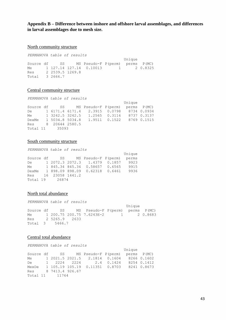
43
Appendix B – Difference between inshore and offshore larval assemblages, and differences
in larval assemblages due to mesh size.
North community structure
PERMANOVA table of results
Unique
Source df SS MS Pseudo-F P(perm) perms P(MC)
Me 1 127.14 127.14 0.10013 1 2 0.8325
Res 2 2539.5 1269.8
Total 3 2666.7
Central community structure
PERMANOVA table of results
Unique
Source df SS MS Pseudo-F P(perm) perms P(MC)
De 1 6171.4 6171.4 2.3915 0.0798 8734 0.0934
Me 1 3242.5 3242.5 1.2565 0.3116 8737 0.3137
DexMe 1 5034.8 5034.8 1.9511 0.1522 8769 0.1515
Res 8 20644 2580.5
Total 11 35093
South community structure
PERMANOVA table of results
Unique
Source df SS MS Pseudo-F P(perm) perms
De 1 2072.3 2072.3 1.4379 0.1857 9923
Me 1 845.34 845.34 0.58657 0.6565 9915
DexMe 1 898.09 898.09 0.62318 0.6461 9936
Res 16 23058 1441.2
Total 19 26874
North total abundance
PERMANOVA table of results
Unique
Source df SS MS Pseudo-F P(perm) perms P(MC)
Me 1 200.75 200.75 7.6243E-2 1 2 0.8683
Res 2 5265.9 2633
Total 3 5466.7
Central total abundance
PERMANOVA table of results
Unique
Source df SS MS Pseudo-F P(perm) perms P(MC)
Me 1 2021.5 2021.5 2.1814 0.1604 8266 0.1602
De 1 2224 2224 2.4 0.1424 8254 0.1412
MexDe 1 105.19 105.19 0.11351 0.8703 8241 0.8673
Res 8 7413.4 926.67
Total 11 11764

44
South total abundance
PERMANOVA table of results
Unique
Source df SS MS Pseudo-F P(perm) perms
De 1 405.02 405.02 0.21325 0.8062 9917
Me 1 1619.8 1619.8 0.85284 0.4236 9944
DexMe 1 569.8 569.8 0.30001 0.7313 9921
Res 16 30388 1899.3
Total 19 32983
North richness
PERMANOVA table of results
Unique
Source df SS MS Pseudo-F P(perm) perms P(MC)
Me 1 100 100 0.11077 1 2 0.8076
Res 2 1805.6 902.78
Total 3 1905.6
Central richness
PERMANOVA table of results
Unique
Source df SS MS Pseudo-F P(perm) perms P(MC)
Me 1 33.333 33.333 0.1092 0.7527 208 0.8185
De 1 1026.1 1026.1 3.3614 0.1151 207 0.0942
MexDe 1 185.87 185.87 0.60887 0.4699 209 0.4726
Res 8 2442.1 305.26
Total 11 3687.4
South richness
PERMANOVA table of results
Unique
Source df SS MS Pseudo-F P(perm) perms P(MC)
De 1 619.13 619.13 0.70558 0.4333 4993 0.4361
Me 1 114.94 114.94 0.13099 0.837 5030 0.8194
DexMe 1 619.13 619.13 0.70558 0.4466 4974 0.4323
Res 16 14040 877.48
Total 19 15393
North Shannon’s H’
PERMANOVA table of results
Unique
Source df SS MS Pseudo-F P(perm) perms P(MC)
Me 1 42.787 42.787 1 1 1 0.4254
Res 2 85.575 42.787
Total 3 128.36

45
Central Shannon’s H’
PERMANOVA table of results
Unique
Source df SS MS Pseudo-F P(perm) perms P(MC)
De 1 191.77 191.77 2.4223 0.1614 2271 0.1553
Me 1 10.236 10.236 0.12929 0.759 2270 0.7402
DexMe 1 53.934 53.934 0.68126 0.3983 2284 0.4368
Res 8 633.35 79.169
Total 11 889.29
South Shannon’s H’
PERMANOVA table of results
Unique
Source df SS MS Pseudo-F P(perm) perms P(MC)
De 1 120.73 120.73 1.456 0.2399 8282 0.2433
Me 1 5.4342 5.4342 6.5536E-2 0.7975 8205 0.8122
DexMe 1 119.76 119.76 1.4443 0.2402 8239 0.2464
Res 16 1326.7 82.919
Total 19 1572.6

46
Appendix C – Species that may be present with Gulf St Vincent
Table of fish species that have previously been recorded in Gulf St Vincent – taxa highlighted in
apricot are recognised as occurring in the Gulf in ‘Larvae of temperate Australian fishes:
laboratory guide for larval identification’ (Neira et al. 1998), taxa highlighted in purple were
recognised as occurring in the Gulf in ‘Fishes of Australia’s southern coast’ (Gomon et al.
2008); and taxa highlighted in yellow were recognised as occurring the Gulf in ‘Survey of
planktonic larvae near Point Lowly (Mifsud et al. 2010). Species with * are present in the adult
data used in this study.
Order Family Genus Species Common name
Argentiniformes Argentinidae Argentina australiae silverside
Atherinformes Atherinidae
Atherinson hepsetoides deepwater hardyhead
Atherinosoma elongata elongate hardyhead
microstoma smallmouth hardyhead
Kestratherina brevirostris shortsnout hardyhead
esox pikehead hardyhead
Leptatherina presbyteroides silver fish
Beloniformes Hemiramphidae Hyporhamphus
melanochir southern garfish
regularis river garfish
Scomberesocidae Scomberesox saurus scomberoides saury
Berycifomes
Berycidae Centroberyx gerrardi bight redfish
lineatus shalowtail
Trachichthyidae Paratrachichthys macleayi sandpaper fish
Trachichthys australis southern roughy
Clupeiformes Clupeidae
Etrumeus teres muray round herring
Hyperlophus vittatus sandy sprat
Sardinops sagax pilchard
Spratelloides robustus blue sprat
Sprattus novaehollandiae Australian sprat
Engraulidae Engraulis australis anchovy
Gadiformes Moridae
Eeyorius hutchinsi finetooth beardie
Lotella rhacina largetooth beardie
Pseudophycis
bachus red cod
barbata bearded rock cod
breviuscula bastard red cod
Gasterosteiformes
Pegasidae Pegasus lancifer sculptured seamoth
Sygnathidae
Stigmatopora
argus spotted pipefish
nigra widebody pipefish
narinosa gulf pipefish
Campichthys galei gale's pipefish
tryoni tryon's pipefish
Heraldia nocturna upside-down pipefish
Hippocampus
bleekeri potbelly seahorse
breviceps shorthead seahorse
abdominalis bigbelly seahorse
Histiogamphelus cristatus rhino pipefish
Hypselognathus horridus shaggy pipefish
rostratus knifesnout pipefish
Phycodurus eques leafy seadragon
Filicampus tigris tiger pipefish
Idiotropiscus australe pygmy pipehorse
Urocampus carinirostris hairy pipefish
Kaupus costatus deepbody pipefish
Kimblaeus bassensis trawl pipefish
Leptoichthys fistularius brushtail pipefish

47
Lissocampus caudalis smooth pipefish
runa javelin pipefish
Maroubra perserrata sawtooth pipefish
Notiocampus ruber red pipefish
Phyllopteryx taeniolatus common seadragon
Pugnaso curtirostris pugnose pipefish
Solegnathus robustus robust pipehorse
Stipecampus cristatus ringback pipefish
Vanacampus
moargaritifer hairy pipefish
phillipi port phillip pipefish
poecilolaemus longsnout pipefish
vercoi verco's pipefish
Mugiliformes Mugilidae
Aldrichetta forsteri yelloweye mullet
Liza argentea goldspot mullet
Mugil cephalus sea mullet
Perciformes
Aplodactylidae Aplodactylus arctidens * marblefish
Apogonidae
Siphamia cephalotes * wood's siphonfish
Vincentia
badia scarlet cardinalfish
conspersa * southern cardinalfish
macrocauda smooth cardinalfish
Arripidae Arripis
georgianus * Australian herring
truttaceus *
western Australian
salmon
Blenniidae Parablennius tasmanianus Tasmanian blenny
Ommobranchus anolius oyster blenny
Callionymidae
Eocallionymus papilio painted stinkfish
Foetorepus calauropomus common stinkfish
Repomucenus calcaratus spotted dragonet
Carangidae
Trachurus declivis common jack mackerel
novaezelandiae yellowtail scad
Naucrates ductor pilotfish
Pseudocaranx
dentex white trevally
wrighti skipjack trevally
georgianus silver trevally
Seriola lalandi yellowtail kingfish
hippos samsonfish
Cepolidae Cepola australis Australian bandfish
Chaetodontidae Chelmonops curiosus * western talma
Cheilodactylidae
Cheilodactylus nigripes * maggie perch
Dactylophora nigricans * dusky morwong
Nemadactylus macropterus jackass morwong
valenciennesi blue morwong
Clinidae Heteroclinus
sp. 2 whitley's weedfish
sp. 4 coleman's weedfish
sp. 5 fewray weedfish
sp. 6 milward's weedfish
adelaide Adelaide weedfish
eckloniae kelp weedfish
heptaeolus ogilby's weedfish
johnstoni johnston's weedfish
macrophthalmus large-eye weedfish
perspicillatus common weedfish
puellarum little weedfish
roseus rosy weedfish
tristis longnose weedfish
wilsoni wilson's weedfish

48
Ophiclinops pardalis spotted snake blenny
varius variegated snake blenny
Ophioclinus
antarcticus Adelaide snake blenny
brevipinnis shortfinn snake blenny
gabrieli frosted snake blenny
gracilis blackback snake blenny
ningulus variable snake blenny
Cristiceps australis
southern crested
weedfish
Peronedys anguillaris eel snake blenny
Sticharium clarkae clark's snake blenny
dorsale slender snake blenny
Dinolestidae Dinolestes lewini * longfin pike
Enoplosidae Enoplosus armatus * old wife
Gempylidae Thyrsites atun barracouta
Rexea solandri gemfish
Gerreidae Parequula melbournensis * silverbelly
Gobiesocidae
Genus C sp. 2 slender clingfish
Alabes dorsalis common shore eel
hoesei dwarf shore eel
Aspasmogaster liorhyncha smoothsnout clingfish
tasmaniensis tasmanian clingfish
Cochleoceps
bassensis broadhead clingfish
bicolor western cleaner clingfish
spatula spadenose clingfish
Creocele cardinalis broad clingfish
Parvicrepis
sp. 1 longsnout clingfish
sp. 2 obscure clingfish
parvipinnis smallfin clingfish
Posidonichthys hutchinsi posidonia clingfish
Gobiidae
Pseudogobius olorum bluespot goby
Nesogobius
sp. 1 opalescent sandgoby
sp. 2 threadfin sandgoby
sp. 4 groovedcheek goby
sp. 5 sicklefin sadgoby
greeni twinbar goby
maccullochi gridled goby
pulchellus * sailfin goby
Favonigobius lateralis southern longfin goby
Arenigobius bifrenatus bridled goby
Gobiopterus semivestita glass goby
Afurcagobius tamarensis tamar goby
Bathygobius krefftii krefft's frillgoby
Callogobius depressus flathead goby
mucosus sculptured goby
Mugilogobius platynotus flatback mangrove goby
Redigobius macrostoma largemouth goby
Tasmanogobius gloveri glover's tasmangoby
lasti scary's tasmangoby
Tridentiger trigonocephalus trident goby
Kyphosidae
Tilodon sexfasciatus * moonlighter
Scorpis aequipinnis * sea sweep
Kyphosus sydneyanus * silver drummer
Girella zebra * zebrafish
Neatypus obliquus* footballer sweep
Girella tricuspidata * luderick

49
Labridae
Achoerodus gouldii * western blue groper
Austrolabrus maculatus * blackspotted wrasse
Bodianus frenchii foxfish
Dotalabrus aurantiacus * castelnau's wrasse
Eupetrichthys angustipes snakeskin wrasse
Notolabrus
fucicola purple wrasse
parilus * brownspotted wrasse
tetricus * bluethroat wrasse
Ophthalmolepis lineolata southern maori wrasse
Pictilabrus laticlavius * senator wrasse
Pseudolabrus psittaculus rosy wrasse
Haletta semifasciata blue weed whiting
Siphonognathus beddomei * pencil weed whiting
caninis * sharpnose weed whiting
Leptoscopidae Lesueurina platycephala flathead sandfish
Crapatalus munroi pink sandfish
Mullidae Upeneichthys vlamingii * bluespotted goatfish
Odacidae Heteroscarus acroptilus * rainbow cale
Olisthops cyanomelas * herring cale
Pempherididae
Parapriacanthus elongatus * elongate bullseye
Pempheris
klunzingeri * rough bullseye
multiradiata * bigscale bullseye
ornata * orangelined bullseye
Pentacerotidae Pentaceropsis recurvirostris * longsnout boarfish
Percophidae Enigmapercis reducta broad duckbill
Pinguipedidae Parapercis ramsayi spotted grubfish
haackei wavy grubfish
Plesiopidae Paraplesiops meleagris * southern blue devil
Trachinops noarlungae * yellowhead hulafish
Pomacentridae Parma victoriae * scalyfin
Serranidae
Caesioperca lepidoptera butterfly perch
rasor * barber perch
Epinephelus sp. southern rockcod
lanceolatus queensland groper
Hypoplectrodes nigroruber * banded seaperch
maccullochi halfbanded seaperch
Lepidoperca occidentalis slender orange perch
Acanthistius serratus western wirrah
Othos dentex * harlequin fish
Sillaginidae Sillago
schomburgkii yellowfin whiting
bassensis souther school whiting
findersi eastern school whiting
Sillaginodes punctata king george whiting
Sparidae Acanthopagrus butcheri black bream
Pagrus auratus snapper
Sphyraenidae Sphyraena novaehollandiae * snook
Terapontidae Pelates octolineatus western striped grunter
Pelsartia humeralis sea trumpeter
Tripterygiidae
Brachynectes fasciatus barred threefin
Helcogramma decurrens * blackthroat threefin
Lepidoblennius marmoratus western jumping bleny
Trianectes bucephalus bighead threefin
Trinorfolkia
clarkei clark's threefin
cristata crested threefin
incisa notched threefin
Pleuronectiformes Paralichthyidae Pseudorhombus arsius largetooth flounder

50
jenynsii smalltooth flounder
Pleuronectidae Rhombosolea tapirina greenback flounder
Scorpaeniformes
Neosebastinae Neosebastes scorpaenoides common gurnard perch
Platycephalidae
Leviprora inops longhead flathead
Platycephalus
aurimaculatus toothy flathead
speculator
southern bluespotted
flathead
bassensis southern sand flathead
conatus deepwater flathead
laevigatus rock flathead
richardsoni tiger flathead
cirronasa tassel-snout flathead
Scorpaenidae Scorpaena papillosa southern red scorpionfish
Tetrarogidae
Gymnapistes marmoratus soldierfish
Centropogon latifrons western fortescue
Glyptauchen panduratus goblinfish
Triglidae
Lepidotrigla
spinosa shortfin gurnard
modesta cocky gurnard
papilio spiny gurnard
vanessa butterfy gurnard
Chelidonichthys kumu red gurnard
Pterygotrigla polyommata latchet
Tetraodontiformes
Monacanthidae
Acanthaluteres
brownii spinytail leatherjacket
spilomelanurus bridled leatherjacket
vittiger toothbrush leatherjacket
Brachaluteres jacksonianus
southern pygmy
leatherjacket
Eubalichthys
bucephalus black reef leatherjacket
cyanoura bluetail leatherjacket
gunnii gunn's leatherjacket
mosaicus mosaic leatherjacket
Meuschenia
flavolineata *
yellowstripped
leatherjacket
freycineti * sixspine leatherjacket
galii * bluelined leatherjacket
hippocrepis * horseshoe leatherjacket
scaber velvet leatherjacket
venusta
stars-and-stripes
leatherjacket
Nelusetta ayraud ocean leatherjacket
Scobinichthys granulatus rough leatherjacket
Thamnaconus degeni bluefin leatherjacket
Tetraodontidae
Contusus brevicaudus prickly toadfish
richei barred toadfish
Lagocephalus lagocephalus ocean puffer
sceleratus silver toadfish
Omegophora armilla * ringed toadfish
cyanopunctata bluespotted toadfish
Polyspina piosae orangebarred puffer
Tetractenos glaber smooth toadfish
Torquigener pleurogramma weeping toadfish

51
Appendix D – Larvae caught per 500m3 at each location
Table showing the number of fish, rounded to the nearest whole number, per 500m3 sampled at each location
Family Genus Species 0.5mm 1mm 0.5mm 1mm 0.5mm 1mm 0.5mm 1mm 0.5mm 1mm 0.5mm 1mm 0.5mm 1mm 0.5mm 1mm 0.5mm 1mm 0.5mm 1mm 0.5mm 1mm 0.5mm 1mm 0.5mm 1mm 0.5mm 1mm 0.5mm 1mm 0.5mm 1mm 0.5mm 1mm 0.5mm 1mm 0.5mm 1mm
Hyperlophus vittatus 0 0 0 0 0 0 0 0 0 0 0 0 0 0 0 0 0 0 0 0 0 0 0 0 1 0 0 0 0 0 0 0 0 0 0 0 0 0
Spratelloides robustus 0 0 0 0 0 0 0 0 0 0 0 0 0 0 0 0 0 2 0 0 0 0 1 0 0 0 0 0 0 0 0 0 0 0 0 0 0 0
Hippocampus sp. 0 0 0 0 0 0 0 0 0 0 2 2 0 0 5 0 0 0 0 0 0 0 0 0 0 0 0 0 0 0 0 0 0 0 0 0 0 2
4 4 0 0 0 0 2 2 0 0 7 2 0 0 0 0 0 0 7 3 1 0 1 0 0 3 0 0 0 0 0 0 0 0 0 0 0 0
Urocampus carinirostris 0 0 0 0 0 0 0 0 0 0 0 5 0 0 0 0 0 0 0 0 0 0 0 0 0 0 0 0 0 0 0 0 0 0 0 0 0 0
Blenniidae Ommobranchus anolius 0 0 0 0 0 0 0 0 0 0 0 0 0 0 0 0 0 0 0 0 1 0 0 0 0 0 0 0 0 0 0 0 0 0 0 0 0 0
0 0 0 0 0 1 0 0 0 0 0 0 0 0 0 0 0 0 0 0 0 0 0 0 0 0 0 0 0 0 0 0 0 1 0 0 0 0
Bathygobius krefftii 0 0 0 0 0 0 0 0 0 0 0 0 0 0 0 0 0 0 1 0 0 0 0 0 0 0 0 1 0 0 0 0 0 0 0 0 0 0
4 0 0 0 0 0 5 3 2 0 4 0 0 0 2 0 0 0 3 0 0 0 1 0 0 0 0 0 0 0 4 0 0 0 0 0 0 0
Redigobius macrostoma 0 0 0 0 0 0 0 0 0 0 0 0 0 0 0 0 0 0 1 0 0 0 0 0 0 0 0 0 0 0 0 0 0 0 0 0 0 0
Gobiesocidae 0 0 0 0 0 0 0 0 0 0 0 0 0 0 0 0 0 0 0 0 0 0 0 0 0 0 0 0 0 0 0 0 0 0 0 0 0 0
Sillaginidae Sillaginodes punctata 0 0 0 0 0 0 0 0 0 0 0 0 0 0 0 0 0 0 0 0 0 0 0 0 0 0 0 0 0 0 0 0 0 0 0 0 0 2
0 0 0 0 0 0 0 2 0 0 0 0 4 0 0 2 0 0 0 0 0 0 0 0 0 0 0 0 0 0 0 0 0 0 0 0 0 0
Pleuronectidae Rhombosolea tapiria 0 0 0 0 0 0 3 0 0 0 0 0 0 0 0 0 0 0 0 0 0 0 0 0 0 0 0 0 0 0 0 0 0 0 0 0 0 0
Platycephalus speculator 0 0 0 0 0 0 0 0 0 0 0 0 0 0 0 0 0 0 0 0 0 0 0 0 0 0 0 0 0 0 0 0 0 1 0 0 0 0
0 0 0 0 0 0 0 0 0 0 0 0 0 0 0 0 0 0 0 0 0 0 0 0 0 0 0 0 0 0 0 0 0 0 0 0 0 0
Triglidae 0 0 0 0 0 0 0 0 2 0 0 0 0 0 0 0 0 0 0 0 0 0 0 0 0 0 0 0 0 0 1 0 0 0 0 0 0 0
Neosebastinae 0 0 0 0 0 0 0 0 0 2 5 2 0 2 0 0 5 3 9 4 0 0 0 0 0 0 0 0 0 0 0 1 0 0 0 0 0 0
Tetrarogidae Gymnapistes marmoratus 0 0 0 0 0 0 0 0 0 0 0 0 0 0 0 0 0 0 0 0 0 0 0 0 0 0 0 0 0 0 0 0 0 0 0 0 0 0
Monacanthidae 0 0 0 0 1 0 0 0 0 2 4 5 0 0 7 0 13 2 3 4 0 0 1 0 36 4 4 1 11 0 1 1 0 0 0 0 0 2
Tripterygiidae spp.
Callionymidae spp.
Platycephalidae
Stigmatopora spp.
Gobiesocidae spp.
Sygnathidae
Platycephalus sp.
Gobiidae Gobiidae spp.
Lepidotrigla spp.
Sample period 1
Site 1 Site 2 Site 3 Site 4 Site 5 Site 6 Site 7 Site 8 Site 9 Site 10
15m 20m 15m 20m 15m 20m 15m 20m
Clupeidae
20m 15m 20m 15m10m 10m 15m 15m 20m 15m20m
Neosepastes sp.
Meuschenia spp.

52
Family Genus Species
Hyperlophus vittatus
Spratelloides robustus
Hippocampus sp.
Urocampus carinirostris
Blenniidae Ommobranchus anolius
Bathygobius krefftii
Redigobius macrostoma
Gobiesocidae
Sillaginidae Sillaginodes punctata
Pleuronectidae Rhombosolea tapiria
Platycephalus speculator
Triglidae
Neosebastinae
Tetrarogidae Gymnapistes marmoratus
Monacanthidae
Tripterygiidae spp.
Callionymidae spp.
Platycephalidae
Stigmatopora spp.
Gobiesocidae spp.
Sygnathidae
Platycephalus sp.
Gobiidae Gobiidae spp.
Lepidotrigla spp.
Clupeidae
Neosepastes sp.
Meuschenia spp.
Site 1 Site 3 Site 4 Site 5 Site 6 Site 7 Site 8 Site 9 Site 10 Site 1 Site 3 Site 4 Site 5 Site 6 Site 7 Site 8 Site 9 Site 10
10m 10m 15m 15m 15m 15m 15m 15m 15m 15m 15m 10m 10m 15m 15m 15m 15m 15m 15m 15m 15m 15m
1mm 1mm 1mm 1mm 1mm 1mm 1mm 1mm 1mm 1mm 1mm 1mm 1mm 1mm 1mm 1mm 1mm 1mm 1mm 1mm 1mm 1mm
0 0 0 0 0 0 0 0 0 0 0 0 0 0 0 0 0 0 0 0 0 0
0 0 0 0 0 0 0 0 0 0 0 0 0 0 0 0 0 0 0 0 0 0
0 0 0 0 0 0 0 0 0 0 0 0 0 0 0 1 0 0 0 0 0 0
1 1 0 23 8 4 0 1 0 0 2 0 1 0 1 5 0 0 0 0 0 0
1 0 0 0 0 0 0 0 0 0 0 0 0 0 0 0 0 0 0 0 0 2
0 0 0 0 0 0 0 0 0 0 0 0 0 0 0 0 0 0 0 0 0 0
0 0 0 0 0 2 0 0 0 0 0 0 0 0 0 0 0 0 0 0 0 0
0 0 0 0 0 0 0 0 0 0 0 0 0 0 0 0 0 0 0 0 0 0
0 0 0 4 8 2 0 1 3 0 0 0 0 0 0 0 0 0 0 0 0 0
0 0 0 0 0 0 0 0 0 0 0 0 0 0 0 0 0 0 0 0 0 0
0 0 0 0 0 0 0 0 7 0 0 0 0 0 0 0 0 0 0 0 0 0
0 0 0 0 0 0 0 0 0 0 0 0 0 0 0 0 0 0 0 0 0 0
0 0 0 0 3 0 0 1 0 2 0 0 0 0 0 1 2 0 1 0 0 0
0 0 0 0 0 2 0 1 0 1 0 0 0 0 0 0 0 0 0 0 0 0
0 0 0 0 0 0 0 0 0 0 0 0 0 0 0 0 0 0 0 0 0 0
0 0 0 0 0 1 1 0 0 0 0 0 0 0 0 0 0 0 0 0 1 0
0 0 0 0 0 2 0 0 0 1 0 0 0 0 1 1 0 0 0 1 2 0
0 0 0 0 0 0 0 0 0 0 1 0 0 0 0 1 1 0 3 1 0 0
1 5 5 17 13 7 0 1 0 1 0 3 6 5 0 0 1 0 0 5 4 3
5 22 10 248 22 57 20 88 37 181 158 0 7 1 0 3 5 1 0 11 4 15
Sample period 2 Sample period 3
Site 2 Site 2
Related Documents