The distance decay of similarity in climate variation and vegetation dynamics

ORIGINAL ARTICLE

The distance decay of similarity in climate variationand vegetation dynamics

Zhiqiang Zhao • Shuangcheng Li • Jianguo Liu •

Jian Peng • Yanglin Wang

Received: 3 January 2014 / Accepted: 29 September 2014 / Published online: 15 October 2014

� Springer-Verlag Berlin Heidelberg 2014

Abstract The negative relationship between similarity

and distance has been revealed in many subjects in geog-

raphy and ecology fields. This study aimed to illustrate the

strength of the distance-decay relationship in variation of

climate and vegetation, and to quantify the relationship.

Solving this problem could help to test some model spec-

ifications based on the climate and vegetation time series

on sample sites, to determine the distance function in the

spatial interpolation technique for meteorological fac-

tors and vegetation dynamics, and to use the distance-

decay perspective as a quantitative technique to adapt

strategies for future climate change and vegetation

dynamics. To achieve the study goal, we quantified varia-

tion similarity using mutual information (MI), which

measured the dependence between two variables or time

series. We carried out a distance-decay analysis of climate

and NDVI variation similarities, assessed by the MI against

the log-transformed geographical distances between mete-

orological stations. The results suggest that all station pairs

shared some similarity in the processes of climate variation

and vegetation dynamics, and the MI values showed a

gradual decrease with the increase of distance. In addition,

temperature, precipitation, and NDVI time series had

different MI value ranges and distance-decay ratios due to

various influential factors. The logarithmic distance-decay

relationships are of potential usefulness to the study of

community similarity and the neutral theory of biogeog-

raphy. Our research provides an approach for analyzing

spatial patterns in relation to dependence and synchroni-

zation that may inform future studies aiming to understand

the distribution and spatial relationship of climate and

vegetation changes.

Keywords Distance decay � Spatial pattern � Mutual

information � Climate � NDVI � China

Introduction

One of the most important fundamental concepts of

geography is distance decay, which was once called the

‘‘First Law of Geography’’: Everything is related to

everything else, but near things are more related than dis-

tant things (Tobler 1970; Sui 2004). This law indicated that

the similarity between two observations often decreases or

decays as the distance between them increases (Nekola and

White 1999). The early study of distance decay raised great

interest among researchers in spatial autocorrelation, and

led eventually to the field of geostatistics (Cressie 1993;

Nekola and White 1999). In recent years, spatial depen-

dency, which indicates the co-variation of properties within

geographic space, has become one of the most important

terms in geography (Prates-Clark et al. 2008; Chen and

Henebry 2010; Martinez et al. 2010; Viedma et al. 2012).

The negative relationship between similarity and dis-

tance covers many subjects in the fields of geography and

ecology and is related to some key theoretical issues such

as what determines diversity, distribution, and abundance

Z. Zhao (&) � S. Li � J. Peng � Y. Wang (&)

Laboratory for Earth Surface Processes, Ministry of Education,

College of Urban and Environmental Sciences, Peking

University, Beijing 100871, China

e-mail: [email protected]

Y. Wang

e-mail: [email protected]

J. Liu

Department of Fisheries and Wildlife, Center for Systems

Integration and Sustainability, Michigan State University,

East Lansing, MI 48823, USA

123

Environ Earth Sci (2015) 73:4659–4670

DOI 10.1007/s12665-014-3751-2

of species, and the way in which analyses in ecology are

performed (Bjorholm et al. 2008). In spatial biodiversity

studies, distance decay describes how the similarity in

species composition between two communities varies with

the geographic distance that separates them (Morlon et al.

2008). Generally, studies illustrated that species turnover

produces a decrease of similarity with distance along spa-

tial environmental gradients (Whittaker 1975; Cody 1975;

Baselga 2007; Soininen et al. 2007; Bjorholm et al. 2008;

Astorga et al. 2011). In island biogeography, studies

demonstrated a decrease in percent species saturation of

oceanic or habitat islands as a function of their distance

from a source pool of immigrants (Vuilleumier 1970;

Kadmon and Pulliam 1993; Nekola and White 1999).

Nevertheless, few studies have extended the distance-

decay relationships to the fields of climate variation and

vegetation dynamics. Although several regional studies

have qualitatively indicated that the similarity or correla-

tion of the normalized difference vegetation index (NDVI)

and precipitation time series decreases as distance increa-

ses (Walsh et al. 2001; Millward and Kraft 2004; Zhang

et al. 2009; Costantini et al. 2012), only a limited number

of studies have quantitatively discussed the distance-decay

function, such as Domroes and Ranatunge (1993), Bai-

gorria et al. (2007), Hofstra and New (2009), and Baigorria

and Jones (2010). Previous studies were mainly concen-

trated on climate data of meteorological stations to inter-

polate climatic data of meteorological stations and to create

gridded climate databases by investigating the distance-

decay relationships. However, to our knowledge, no pre-

vious studies have been performed to assess and compare

the distance-decay functions of vegetation dynamics and

climatic factors time series.

Due to the high cost and difficulty of gathering data,

many studies were point based but nevertheless more

interested in a wide range of large-scale regional events. For

instance, when using the tree-ring parameters to reconstruct

historical climate variance and vegetation dynamic, Chen

et al. (2012) analyzed whether the reconstruction series had

common signals for large areas. Investigating the relation-

ship between distance and the similarity of modern climate

and vegetation time series through extrapolation based on

distance-decay functions could contribute to solving the

problem of generalizing historical, modern, and future cli-

mate change from sampling points to regional climatic

variations. Also, it could help test various model specifica-

tions related to point-based databases to determine the dis-

tance function in a spatial interpolation technique for

creating gridded meteorological elements and vegetation

dynamics databases. Such an investigation could use the

distance-decay perspective to create adaptive strategies for

future global change based on the research material of a

demonstration zone.

NDVI has been commonly used as an estimator of ter-

restrial vegetation dynamics and distributions, and many

researchers have focused on the spatial and temporal cor-

relations between NDVI values and climatic factors (Li et al.

2011; Zhao et al. 2014). In this study, we first quantify

variation similarity by adopting the method of mutual

information (MI), which measures the dependence between

NDVI, temperature, and precipitation time series. Then the

preliminary results are presented, which focus on the spatial

patterns of MI and the distance-decay relationship. In

addition, using multivariate analysis, we concerned whether

there were coupled effects from climate variation similarity

and geographic distances to explain the similarity of vege-

tation dynamics between meteorological stations. Finally,

we conclude by discussing the implication of our results

concerning studies of distribution and the spatial relationship

of climate and vegetation change in geography.

Methods and materials

Methods

Mutual information

Various methods have been used to characterize the rela-

tionship between time-series data. Most commonly, the

methods were based on regression and correlation analysis

(Geerken et al. 2005; Brown et al. 2006; White et al. 2009;

Lhermitte et al. 2011), and some adopted transformation

approaches, such as principal component analysis (Gurgel and

Ferreira 2003; Lobo and Maisongrande 2008) and Fourier

transform (Lhermitte et al. 2008). Among these measurements

of independence between random variables, mutual informa-

tion (MI) is singled out by its information-theoretic back-

ground (Cover and Thomas 2006). Previous studies generally

were based on correlation analysis to describe the dependence

structure between climate and vegetation time series, and it

was incomplete. In contrast to linear correlation coefficient,

MI is sensitive also to dependencies that do not manifest

themselves in covariance (Kraskov et al. 2004).

The definition of MI between two random variables is

given by Shannon and Weaver (1949) and Cover and

Thomas (2006). For a system X with a finite set of N

possible states {x1, x2,…, xN} and system Y with a finite set

of N possible states {y1, y2,…, yN} the MI of X relative to

Y, denoted I(X; Y), is defined as

IðX; YÞ ¼X

i;jPðxi; yjÞ log

Pðxi; yjÞPðxiÞPðyjÞ

ð1Þ

where P(xi, yj) is the joint probability distribution function

of X and Y, and P(xi) and P(yj) are the marginal probability

distribution functions of X and Y, respectively.

4660 Environ Earth Sci (2015) 73:4659–4670

123

MI is useful for investigating the dependence between

two variables. High MI between two variables indicates a

large reduction in uncertainty; that is, one time series is

non-randomly associated with the other. On the other side,

low MI indicates a small reduction. MI is zero if and only if

the two time series are statistically independent. Therefore,

MI can be used as an indicator between two time series

related to their degree of independence. We assume that the

higher the MI is between two time series, the more similar

the variations will be.

Geographical distance

In this study, geographical distance between meteorologi-

cal stations was computed using formulas of spherical

trigonometry on the sphere that best approximates earth’s

surface. The geographical distance is the arc length

between any two points on the surface of the earth.

The distance between stations i and j can be given by:

Di;j ¼ R� arccos sin Ji sin Jj þ cos Wi cos Wj cos DW� �

ð2Þ

where Ji, Wi; Jj, Wj are the geographical latitude and lon-

gitude of two points, respectively, and DJ, DW their dif-

ferences; then R is the radius of the earth (R = 6,370 km).

This distance is the shortest distance along the great

circle that contains the two points. Due to the irregularity

between the sphere and earth’s surface, the possible error is

0.5 %.

Data sources

Meteorological data

Temperature and precipitation were selected to analyze the

variations of climate. The data were obtained from the

China Meteorological Administration (http://cdc.cma.gov.

cn/). Among the 752 meteorological stations, 652 stations

were selected due to the short historical records or missing

observations in some stations. To match the length of

NDVI series, the original daily temperature and precipita-

tion data from 1 April 1998 to 31 December 2008 were

aggregated into 10-day time series, which contained 387

data points each. The quality of climatic data was strictly

controlled by verifying climatic range, weather singular

value, and inner coherence.

Normalized difference vegetation index

NDVI has been widely used as an estimator of plant pro-

ductivity (Davies et al. 2007; Evans et al. 2006; Kerr and

Ostrovsky 2003) and an index for green cover monitoring

(Maselli and Chiesi 2006; Myneni et al. 1998). It is com-

puted as the ratio of two electromagnetic wavelengths (near

infrared - red)/(near infrared ? red). For this study, an

NDVI time series of satellite observations at 1-km spatial

and 10-day (dekads) temporal resolutions were used, cov-

ering the period from April 1998 to December 2008. The

time series was produced by Vlaamse Instelling voor

Technologisch Onderzoek (VITO) from the sensor VEG-

ETATION on board the SPOT-4 satellite. A registered user

can download the free SPOT-4 VEGETATION 10-day

synthesis (called ‘‘VGT-S10’’) NDVI data via the VGT

Website (http://free.vgt.vito.be/). VGT-S10 NDVI products

were synthesized from S1 (1-day resolution) NDVI pro-

ducts using a maximum value composite algorithm (Jarlan

et al. 2008).

NDVI values for each meteorological station were

extracted in raster format from each VGT-S10 image using

ArcGIS software. To reduce noise in an NDVI series, its

values for a given station were derived and averaged within

a 10-km buffer circle.

Analyses

By computing the MI value of NDVI, temperature, and

precipitation time series between each meteorological sta-

tion and the other 651 stations, three 652 9 652 matrices

are constructed, respectively. Similarly, one matrix of

distance with 652 meteorological stations was obtained.

The MI and distance coefficients are symmetric (MIi,j

= MIj,i, dij = dji). After removing the redundant values and

the main diagonal, there are 212,226 (=652 9 (652-1)/2)

MI or distance values per matrix. Each matrix is unfolded

into a vector of MI and distances, and the data were cal-

culated as the correlation between the two vectors

(Legendre and Legendre 1998; Lichstein 2007). For more

detailed descriptions about the distance matrix and method,

readers can refer to the references by Mantel (1967),

Legendre and Legendre (1998), and Lichstein (2007).

According to climatic regionalization, eastern China

shows a noticeable characteristic of latitudinal zonality,

specifically recognized as a range from tropics through

subtropics and warm temperate and temperate zones to

cool temperate zones. Thus, in eastern China, we chose 40

stations, located between 115�E and 117�E, as a longitu-

dinal sampling belt. Meanwhile, northern China shows

clear longitudinal zonality as the distribution of continents

and oceans shift from humid regions through sub-humid

and semi-arid regions to arid regions. Therefore, 50 sta-

tions (39�N–41�N) were selected, forming a latitudinal

sampling belt.

Limited by space, not all spatial patterns of MI and the

distance-decay curves of the meteorological stations are

presented in this paper. Four stations at the end of the two

Environ Earth Sci (2015) 73:4659–4670 4661

123

sampling belts (Fig. 1a; Table 1) are regarded as examples

to show the results, so the MI distance-decay curves could

cover a large range of distance (from 100 km to 4,500 km)

when doing regression analysis to reproduce distance-

decay relationships. Meanwhile, to contrast the differences

of distance-decay relationships of MI between longitude

and latitude, we chose station 54511 (Fig. 1a; Table 1)

among several stations located within both sampling belts.

In this study, the MI matrixes and distance matrix were

computed in Matlab 2010a (The MathWorks Inc., Natick,

MA, USA). MI of climate and vegetation variability

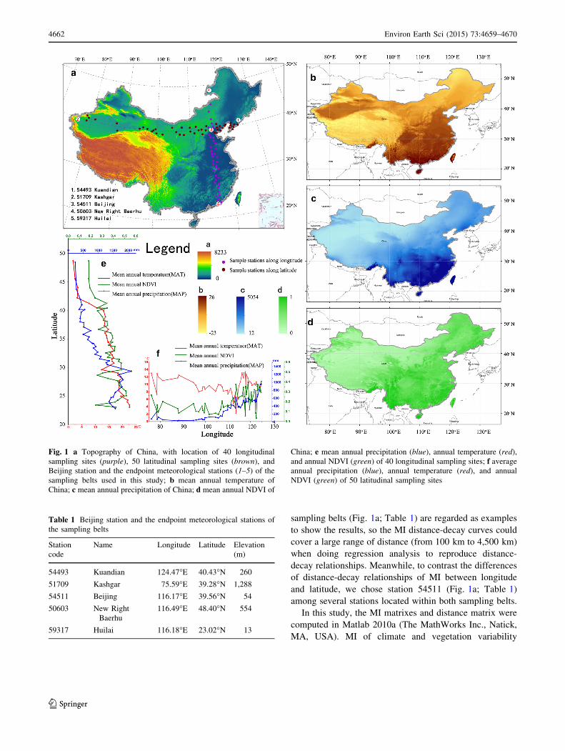
Fig. 1 a Topography of China, with location of 40 longitudinal

sampling sites (purple), 50 latitudinal sampling sites (brown), and

Beijing station and the endpoint meteorological stations (1–5) of the

sampling belts used in this study; b mean annual temperature of

China; c mean annual precipitation of China; d mean annual NDVI of

China; e mean annual precipitation (blue), annual temperature (red),

and annual NDVI (green) of 40 longitudinal sampling sites; f average

annual precipitation (blue), annual temperature (red), and annual

NDVI (green) of 50 latitudinal sampling sites

Table 1 Beijing station and the endpoint meteorological stations of

the sampling belts

Station

code

Name Longitude Latitude Elevation

(m)

54493 Kuandian 124.47�E 40.43�N 260

51709 Kashgar 75.59�E 39.28�N 1,288

54511 Beijing 116.17�E 39.56�N 54

50603 New Right

Baerhu

116.49�E 48.40�N 554

59317 Huilai 116.18�E 23.02�N 13

4662 Environ Earth Sci (2015) 73:4659–4670

123

between meteorological stations was calculated according

to formula (1).

We carried out a distance-decay analysis of climate and

NDVI variation similarities, assessed by the MI against the

log-transformed geographical distance between meteoro-

logical stations in kilometers.

MIi;j ¼ aþ b� log Di;j ð3Þ

where Di,j is the distance and MIi,j is the mutual informa-

tion of the time series from the two stations i and j, a is the

intercept, and b is the slope.

Additionally, the correlations between vegetation

dynamics similarity, climate dynamics similarity, and dis-

tance were, respectively, analyzed by Pearson Correlation

Coefficient and multiple liner regression analysis.

The fitting models and Pearson correlation coefficient

analysis were performed with the use of R, version 3.0.1

(www.r-project.org). Statistical hypothesis and significance

were verified by F test and t test.

Results

Overall mutual information of the variations

By computing the MI value of NDVI, temperature, and

precipitation time series between each meteorological sta-

tion and the other 651 stations, 212,226 MI data were

obtained, respectively. The MI values of the NDVI series

ranged from 0.017 to 2.373, and the range of MI values of

the precipitation series was 0.011*1.311, while the tem-

perature series ranged from 0.004 to 3.675 (Table 2). The

minimum and maximum MI of NDVI, precipitation, and

temperature series between the selected station and the rest

of the 651 meteorological stations are shown in Table 3.

As shown in Tables 2 and 3, the minimum MI was quite

close to zero, but not equal to zero. By the definition of MI,

the results suggested that there were no fully statistically

independent NDVI, precipitation, and temperature time

series between any two stations; that is, all station pairs

shared some similarity in the processes of climate variation

and vegetation dynamics. The results conformed to the first

statement in the ‘‘First Law of Geography’’—‘‘everything

is related to everything else,’’ which denotes explicit spa-

tial dependence (Sui 2004). This result is helpful in

understanding the synchronism in climate change and

teleconnections, the climate dynamics and anomalies being

correlated over large distances.

Spatial patterns of the mutual information

The spatial patterns of MI of the NDVI, temperature, and

precipitation series between each selected station and the

rest of the 651 meteorological stations exhibited significant

regional differentiations (Fig. 2). Overall, the highest val-

ues of MI were observed near selected stations; in contrast,

the lowest value areas were far away from the selected

stations. Compared to NDVI and precipitation, the tem-

perature series had obviously regular MI patterns. Mean-

while, MI of precipitation and NDVI series showed more

multifaceted patterns, some characteristic contour details

besides global regularity.

The figures of NDVI series suggested clear north–south

differences, and in the Tsaidam Basin, a desert region, the

MI values also showed a low value area of basin shape.

Among the MI patterns of NDVI series, the pattern of

station 59317 [Fig. 2 (1e)] displayed the largest differences

between the other four figures [Fig. 2 (1a–1d)]. Besides,

similar differences could be found in MI patterns of tem-

perature and precipitation series. MI of precipitation series

showed relatively smooth change, and the higher value

areas are in a very small range. Especially, the high value

areas are confined to small distances [Fig. 2 (3b)], which

revealed the MI pattern between station 51709, located in

Table 2 The ranges of MI values across all stations

NDVI Precipitation Temperature

Mean MI 0.413 0.157 1.251

Maximum MI 2.373 1.311 3.675

Minimum MI 0.017 0.011 0.004

Table 3 The ranges of MI values of the selected stations

NDVI Precipitation Temperature

MI_mean MI_min MI_max MI_mean MI_min MI_max MI_mean MI_min MI_max

50603 0.492 0.034 1.302 0.138 0.027 0.723 1.318 0.025 3.015

51709 0.478 0.053 1.421 0.064 0.015 0.307 1.270 0.027 2.698

54493 0.542 0.036 1.871 0.180 0.030 0.963 1.412 0.028 2.849

54511 0.469 0.037 1.271 0.179 0.032 0.664 1.409 0.026 2.820

59317 0.250 0.055 1.003 0.148 0.033 0.933 1.071 0.038 3.049

Environ Earth Sci (2015) 73:4659–4670 4663

123

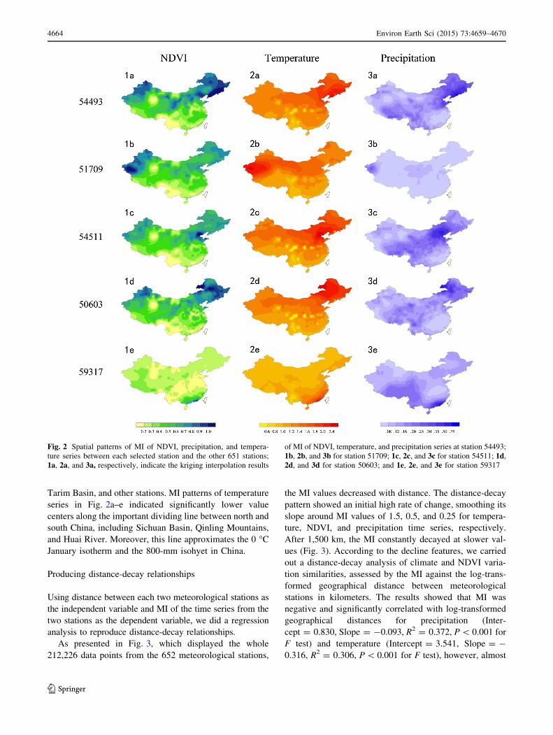
Tarim Basin, and other stations. MI patterns of temperature

series in Fig. 2a–e indicated significantly lower value

centers along the important dividing line between north and

south China, including Sichuan Basin, Qinling Mountains,

and Huai River. Moreover, this line approximates the 0 �C

January isotherm and the 800-mm isohyet in China.

Producing distance-decay relationships

Using distance between each two meteorological stations as

the independent variable and MI of the time series from the

two stations as the dependent variable, we did a regression

analysis to reproduce distance-decay relationships.

As presented in Fig. 3, which displayed the whole

212,226 data points from the 652 meteorological stations,

the MI values decreased with distance. The distance-decay

pattern showed an initial high rate of change, smoothing its

slope around MI values of 1.5, 0.5, and 0.25 for tempera-

ture, NDVI, and precipitation time series, respectively.

After 1,500 km, the MI constantly decayed at slower val-

ues (Fig. 3). According to the decline features, we carried

out a distance-decay analysis of climate and NDVI varia-

tion similarities, assessed by the MI against the log-trans-

formed geographical distance between meteorological

stations in kilometers. The results showed that MI was

negative and significantly correlated with log-transformed

geographical distances for precipitation (Inter-

cept = 0.830, Slope = -0.093, R2 = 0.372, P \ 0.001 for

F test) and temperature (Intercept = 3.541, Slope = -

0.316, R2 = 0.306, P \ 0.001 for F test), however, almost

Fig. 2 Spatial patterns of MI of NDVI, precipitation, and tempera-

ture series between each selected station and the other 651 stations;

1a, 2a, and 3a, respectively, indicate the kriging interpolation results

of MI of NDVI, temperature, and precipitation series at station 54493;

1b, 2b, and 3b for station 51709; 1c, 2c, and 3c for station 54511; 1d,

2d, and 3d for station 50603; and 1e, 2e, and 3e for station 59317

4664 Environ Earth Sci (2015) 73:4659–4670

123

no logarithmic correlation for NDVI time series (Inter-

cept = 1.105, Slope = -0.096, R2 = 0.062, P \ 0.001 for

F test).

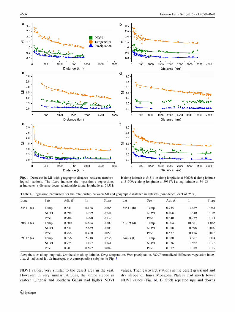
Since the study area has vast terrain and diverse climate,

with significant latitudinal and longitudinal zonality, the

distance-decay model will change along with the different

regions and sampling belts. The five selected stations of the

two sampling belts (Fig. 1a; Table 1) are regarded as

examples to show the differences between longitude and

latitude. As shown in Fig. 4 and Table 4, the MI distance-

decay curves were generally similar to each other, but had

different details. Among the three indexes, the temperature

series produced the highest initial MI and regression

slopes, the NDVI series produced lower initial MI and

regression slopes, and the precipitation series produced the

lowest initial MI and regression slopes. However, the

models of NDVI series had lower R2 values than temper-

ature and precipitation series models. The vegetation

dynamics were closely coupled with climatic fluctuations

and land use. Consequently, the spatial patterns of NDVI

time series were more complicated than those of climate

time series, especially in inhomogeneous regions. There-

fore, the distance-decay relationships of NDVI series were

not as significant as the relationships of temperature and

precipitation series.

With the 200-mm isohyet as boundaries, eastern China

has a monsoon climate while western China has a conti-

nental climate. The latitudinal sampling belt was located

within the eastern monsoon climate, where latitudinal zo-

nality was quite obvious and continuous, thus the pattern of

distance decay was relatively evident. However, the lon-

gitudinal sampling belt crossed two climate regions, and

longitudinal zonality was interrupted by undulating terrain

and other factors (Fig. 1a, e, and f), hence the pattern of

distance decay in this belt was not significant. Moreover,

because there are fewer climate stations in western China,

the sampling points in the longitudinal belt were sparse and

unevenly distributed. Therefore, the results showed that

fitness (R2) of the models along the latitude belt were much

lower than those along the longitude belt, especially for the

NDVI time series. As presented in Fig. 3 and Table 4, for

station 54511, the distance-decay curve of the NDVI time

series was more significant at the longitudinal sampling

belt (R2 = 0.694) than at the latitudinal sampling belt

(R2 = 0.408). Furthermore, for the other two latitudinal

stations in Fig. 4 and Table 4, the logarithmic regression

models of the NDVI time series had either a low correla-

tion coefficient (R2 = 0.408, 54493) or no logarithmic

correlation between MI and distance at the 95 % confi-

dence level (R2 = 0.018, 51709). Besides the difference

between the monsoon climate and continental climate, due

to the uneven terrain, the distance-decay relationship was

not clear along the latitudinal sampling belt, particularly

the model at 51709 in the NDVI series (Fig. 4d; Table 4).

Kashgar (51709), which is located at the edge of Takli-

makan Desert, featured a desert climate and had very low

Fig. 3 Distance-decay analysis of MI for temperature, NDVI, and

precipitation time series between 652 meteorological stations. The

lines represent the log-transformed geographic distance model,

a indicates a distance-decay analysis of MI for temperature time

series; b NDVI; c precipitation

Environ Earth Sci (2015) 73:4659–4670 4665

123

NDVI values, very similar to the desert area in the east.

However, in very similar latitudes, the alpine steppe in

eastern Qinghai and southern Gansu had higher NDVI

values. Then eastward, stations in the desert grassland and

dry steppe of Inner Mongolia Plateau had much lower

NDVI values (Fig. 1d, f). Such repeated ups and downs

Fig. 4 Decrease in MI with geographic distance between meteoro-

logical stations. The lines indicate the logarithmic regressions,

a indicates a distance-decay relationship along longitude at 54511;

b along latitude at 54511; c along longitude at 50603; d along latitude

at 51709; e along longitude at 59317; f along latitude at 54493

Table 4 Regression parameters for the relationship between MI and geographic distance in datasets (confidence level of 95 %)

Long Sets Adj. R2 In Slope Lat Sets Adj. R2 In Slope

54511 (a) Temp 0.841 6.168 0.685 54511 (b) Temp 0.755 3.489 0.261

NDVI 0.694 1.929 0.224 NDVI 0.408 1.340 0.105

Prec 0.904 1.090 0.139 Prec 0.840 0.939 0.111

50603 (c) Temp 0.800 6.624 0.709 51709 (d) Temp 0.904 10.661 1.065

NDVI 0.531 2.659 0.303 NDVI 0.018 0.698 0.009

Prec 0.758 0.480 0.053 Prec 0.537 0.174 0.013

59317 (e) Temp 0.856 2.718 0.236 54493 (f) Temp 0.880 3.867 0.314

NDVI 0.775 1.197 0.141 NDVI 0.336 1.622 0.125

Prec 0.807 0.692 0.082 Prec 0.872 1.019 0.119

Long the sites along longitude, Lat the sites along latitude, Temp temperature, Prec precipitation, NDVI normalized difference vegetation index,

Adj. R2 adjusted R2, In intercept, a–e corresponding subplots in Fig. 3

4666 Environ Earth Sci (2015) 73:4659–4670

123

caused a very poor degree of model fitting (R2 = 0.018)

(Table 4). This result implicitly reminds us that consider-

ation of local factors and circumstances is necessary while

doing global analyses.

Climate similarity and distance effect on vegetation

dynamics similarity

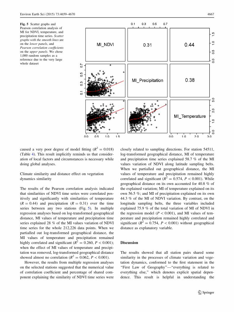
The results of the Pearson correlation analysis indicated

that similarities of NDVI time series were correlated pos-

itively and significantly with similarities of temperature

(R = 0.44) and precipitation (R = 0.31) over the time

series between any two stations (Fig. 5). In multiple

regression analyses based on log-transformed geographical

distance, MI values of temperature and precipitation time

series explained 28 % of the MI values variation of NDVI

time series for the whole 212,226 data points. When we

partialled out log-transformed geographical distance, the

MI values of temperature and precipitation remained

highly correlated and significant (R2 = 0.260, P \ 0.001);

when the effect of MI values of temperature and precipi-

tation was removed, log-transformed geographical distance

showed almost no correlation (R2 = 0.062, P \ 0.001).

However, the results from multiple regression analyses

on the selected stations suggested that the numerical value

of correlation coefficient and percentage of shared com-

ponent explaining the similarity of NDVI time series were

closely related to sampling directions. For station 54511,

log-transformed geographical distance, MI of temperature

and precipitation time series explained 58.7 % of the MI

values variation of NDVI along latitude sampling belts.

When we partialled out geographical distance, the MI

values of temperature and precipitation remained highly

correlated and significant (R2 = 0.574, P \ 0.001). While

geographical distance on its own accounted for 40.8 % of

the explained variation; MI of temperature explained on its

own 56.5 %; and MI of precipitation explained on its own

44.3 % of the MI of NDVI variation. By contrast, on the

longitude sampling belts, the three variables included

explained 75.9 % of the total variation of MI of NDVI in

the regression model (P \ 0.001), and MI values of tem-

perature and precipitation remained highly correlated and

significant (R2 = 0.754, P \ 0.001) without geographical

distance as explanatory variable.

Discussion

The results showed that all station pairs shared some

similarity in the processes of climate variation and vege-

tation dynamics, conformed to the first statement in the

‘‘First Law of Geography’’—‘‘everything is related to

everything else,’’ which denotes explicit spatial depen-

dence. This result is helpful in understanding the

Fig. 5 Scatter graphs and

Pearson correlation analysis of

MI for NDVI, temperature, and

precipitation time series. Scatter

graphs with the smooth lines are

on the lower panels, and

Pearson correlation coefficients

on the upper panels. We chose

1,000 random samples as a

reference due to the very large

whole dataset

Environ Earth Sci (2015) 73:4659–4670 4667

123

synchronism and teleconnections in climate change. As the

second statement of the ‘‘First Law of Geography’’

expresses, ‘‘near things are more related than distant

things,’’ distance played an important role in the relation-

ships between ‘‘everything’’ and ‘‘everything else’’. The

MI values between the selected stations and the other sta-

tions showed a gradual decrease with the increase of dis-

tance (Fig. 2), and the plots of MI versus distance showed a

non-linear relationship. The results also suggested that the

MI between two stations attenuates slowly down as the

distance between the two stations increases. We simulta-

neously observed that the more steep the decay of MI in

NDVI, temperature, and precipitation series from 0 to

500 km, the more gradual decline appeared in each series

between 500 and 1,500 km, and a slight decline appeared

between 1,500 km and 4,500 km. The rapid decay of MI at

short distances suggested that strong dependence of vari-

ation only occurred at the local spatial scale. The idea of

spatial similarity has been widely used in the field of

geostatistics, especially in the analysis of spatial autocor-

relation. Carrying a connotation of the results of this study,

the results promotion, scaling, and spatial interpolation

must be handled sensitively in future works.

Comparing the MI values of the three indexes in each

station, MI of the temperature series at a given distance

was at least two times higher than MI of the NDVI series

and three times higher than MI of the precipitation series.

Furthermore, as distance increased, the multiple rose

gradually. Probably because temperature is highly deter-

mined by solar radiation, the variation of temperature was

more steady and predictable. Compared to temperature,

precipitation is more of a territorial characteristic. In

addition to the impaction of land and sea distribution, local

and mesoscale landforms also play important roles in

variation of precipitation. Therefore, the precipitation ser-

ies had significantly lower MI values. Additionally, dis-

tribution patterns and process of vegetation dynamics are

mainly affected by hydrothermal conditions. Thus, MI

values of the NDVI series were numerically between MI

values of the temperature and precipitation series. Briefly

speaking, different indexes had different MI value ranges

and decay ratios due to various influential factors. The

results imply that the temperature-related results obtained

from the sampling points could represent larger regions

than precipitation-related and vegetation-related results.

Accordingly, we need to be more careful when generaliz-

ing the dry-wet variation from the sampling points to

broader regions. In this context, further study is needed

before reaching a definitive conclusion.

Several studies have revealed typically logarithmic

distance-decay relationships between plant community

similarity and distance (Tuomisto et al. 2003; Gilbert and

Lechowicz 2004; Palmer 2005; Dornelas et al. 2006;

Soininen et al. 2007), which provided support for a neutral

theory of biogeography. In a recent analysis, Astorga et al.

(2011) studied the community similarity of stream diatoms,

macroinvertebrates, and bryophytes across the same set of

sites in relation to distance and showed that the relationship

was best approximated by a logarithmic model in each

case, suggesting that patterns between macro- and micro-

organisms are not fundamentally different. In this paper,

our findings show that the distance-decay relationship

between the variation of climate elements and vegetation

cover and distance is best approximated by a logarithmic

model as well (Fig. 3; Table 4). Furthermore, natural

community distribution, species assemblages, and biodi-

versity are directly impacted by regional climatic condi-

tions. For instance, climax community, a basic concept in

ecology, is defined in relation to regional climate. Thus,

community similarity is related to climate similarity,

including the climate variation similarity. Therefore, our

results are of potential usefulness to the study of commu-

nity similarity and the neutral theory of biogeography.

Distance-decay spatial models are based on the

hypothesis that similarity between locations declines with

distance even if the environment is completely homoge-

neous (Soininen et al. 2007). However, there is no com-

pletely homogeneous region in the real world. A study by

Duque et al. (2009) showed that geographical distances

alone accounted for 12 % of variation in floristic similar-

ities, while both geographical distances and geology

explained 64 % of the total variation in multiple regression

analyses. Furthermore, the distance decay almost disap-

peared after removing environmental heterogeneity at fine

scale. In this study, the decay was not smooth or homo-

geneous at large scale. For instance, Sichuan Basin (in

Sichuan Province), Qaidam Basin (in Qinghai Province),

Qinling Mountain area, and the areas along Huai River

were low MI anomaly zones in the spatial patterns of MI

values, especially in NDVI and temperature (Fig. 2). It

signified that the variance of MI cannot be ascribed only to

distance, which should be identical in every region. Dis-

tance decay alone was insufficient. The spatial heteroge-

neity of environmental factors, such as terrain mutations

(Fig. 1), may be one reason for the non-stationary of decay.

In the future, the vertical zonality and other combined

effects of environment and geographical distances should

be taken into consideration as part of explanations on

similarity in climate variation and vegetation dynamics.

Conclusions

This study illustrates the strength of the distance-decay

relationship within variations of climate and vegetation,

and quantifies the relationship. The results suggest that

4668 Environ Earth Sci (2015) 73:4659–4670

123

variations of climate and vegetation represent spatial

dependence and obey the ‘‘First Law of Geography,’’ and

the distance-decay relationship is non-linear. Temperature,

precipitation, and NDVI time series had different MI value

ranges and distance-decay ratios due to various influential

factors. The logarithmic distance-decay relationships are of

potential usefulness to the study of community similarity

and the neutral theory of biogeography. Besides distance,

other combined effects of environment and topography

should be taken into consideration as part of explanations

on similarity in climate variation and vegetation dynamics.

Our research provides an approach for analyzing spatial

patterns in relation to dependence and synchronization that

may inform future studies aiming to understand the dis-

tribution and spatial relationship of climate and vegetation

change.

Acknowledgments This study was financially supported by grants

from the National Natural Science Foundation of China (NSFC, Nos.

41330747 and 41130534) and China Postdoctoral Science Foundation

funded project (2014M560014). The authors are grateful to the

anonymous reviewers for offering valuable suggestions to improve

the manuscript.

References

Astorga A, Oksanen J, Luoto M, Soininen J, Virtanen R, Muotka T

(2011) Distance decay of similarity in freshwater communities:

do macro-and microorganisms follow the same rules? Global

Ecol Biogeogr 21(3):365–375

Baigorria GA, Jones JW (2010) GiST: a stochastic model for

generating SPATIALLY and temporally correlated daily rainfall

data. J Clim 23(22):5990–6008. doi:10.1175/2010jcli3537.1

Baigorria GA, Jones JW, O’Brien JJ (2007) Understanding rainfall

spatial variability in southeast USA at different timescales. Int J

Climatol 27(6):749–760. doi:10.1002/Joc.1435

Baselga A (2007) Disentangling distance decay of similarity from

richness gradients: response to Soininen et al. 2007. Ecography

30:838–841

Bjorholm S, Svenning JC, Skov F, Balslev H (2008) To what extent

does Tobler’s 1st law of geography apply to macroecology? A

case study using American palms (Arecaceae). BMC Ecol

8(1):11

Brown ME, Pinzon JE, Didan K, Morisette JT, Tucker CJ (2006)

Evaluation of the consistency of long-term NDVI time series

derived from AVHRR, SPOT-vegetation, SeaWiFS, MODIS,

and Landsat ETM ? sensors. Geosci Remote Sens IEEE Trans

44(7):1787–1793. doi:10.1109/TGRS.2005.860205

Chen WR, Henebry GM (2010) Spatio-spectral heterogeneity analysis

using EO-1 Hyperion imagery. Comput Geosci UK

36(2):167–170. doi:10.1016/j.cageo.2009.05.005

Chen F, Yuan Y, Wen W, Yu S, Fan Z, Zhang R, Zhang T, Shang H

(2012) Tree-ring-based reconstruction of precipitation in the

Changling Mountains, China, since AD 1691. Int J Biometeorol

56(4):765–774

Cody ML (1975) Towards a theory of continental species diversities:

bird distributions over Mediterranean habitat gradients. Ecol

Evol Communities 214:257

Costantini ML, Zaccarelli N, Mandrone S, Rossi D, Calizza E, Rossi

L (2012) NDVI spatial pattern and the potential fragility of

mixed forested areas in volcanic lake watersheds. Forest Ecol

Manag 285:133–141. doi:10.1016/j.foreco.2012.08.029

Cover TM, Thomas JA (2006) Elements of information theory, 2nd

edn. Wiley-interscience, New York

Cressie N (1993) Statistics for spatial data. Wiley, New York

Davies RG, Orme CDL, Storch D, Olson VA, Thomas GH, Ross SG,

Ding TS, Rasmussen PC, Bennett PM, Owens IPF (2007)

Topography, energy and the global distribution of bird species

richness. Proc R Soc B Biol Sci 274(1614):1189–1197

Domroes M, Ranatunge E (1993) Analysis of inter-station daily

rainfall correlation during the southwest monsoon in the wet

zone of Sri-Lanka. Geogr Ann A 75(3):137–148

Dornelas M, Connolly SR, Hughes TP (2006) Coral reef diversity

refutes the neutral theory of biodiversity. Nature 440(7080):

80–82

Duque A, Phillips JF, von Hildebrand P et al (2009) Distance decay of

tree species similarity in protected areas on terra firme forests in

Colombian Amazonia. Biotropica 41:599–607

Evans KL, James NA, Gaston KJ (2006) Abundance, species richness

and energy availability in the North American avifauna. Global

Ecol Biogeogr 15(4):372–385

Geerken R, Zaitchik B, Evans JP (2005) Classifying rangeland

vegetation type and coverage from NDVI time series using

Fourier Filtered Cycle Similarity. Int J Remote Sens

26(24):5535–5554. doi:10.1080/01431160500300297

Gilbert B, Lechowicz MJ (2004) Neutrality, niches, and dispersal in a

temperate forest understory. Proc Natl Acad Sci USA

101(20):7651–7656. doi:10.1073/pnas.0400814101

Gurgel HC, Ferreira NJ (2003) Annual and interannual variability of

NDVI in Brazil and its connections with climate. Int J Remote

Sens 24(18):3595–3609. doi:10.1080/0143116021000053788

Hofstra N, New M (2009) Spatial variability in correlation decay

distance and influence on angular-distance weighting interpola-

tion of daily precipitation over Europe. Int J Climatol

29(12):1872–1880. doi:10.1002/Joc.1819

Jarlan L, Mangiarotti S, Mougin E, Mazzega P, Hiernaux P, Le

Dantec V (2008) Assimilation of SPOT/VEGETATION NDVI

data into a sahelian vegetation dynamics model. Remote Sens

Environ 112(4):1381–1394. doi:10.1016/j.rse.2007.02.041

Kadmon R, Pulliam HR (1993) Island biogeography: effect of

geographical isolation on species composition. Ecology 74(4):

978–981

Kerr JT, Ostrovsky M (2003) From space to species: ecological

applications for remote sensing. Trends Ecol Evol 18(6):299–305

Kraskov A, Stogbauer H, Grassberger P (2004) Estimating mutual

information. Phys Rev E 69(6):066138

Legendre P, Legendre L (1998) Numerical ecology, 2nd English edn.

Elsevier Science, Amsterdam

Lhermitte S, Verbesselt J, Jonckheere I, Nackaerts K, van Aardt JAN,

Verstraeten WW, Coppin P (2008) Hierarchical image segmen-

tation based on similarity of NDVI time series. Remote Sens

Environ 112(2):506–521. doi:10.1016/j.rse.2007.05.018

Lhermitte S, Verbesselt J, Verstraeten WW, Coppin P (2011) A

comparison of time series similarity measures for classification

and change detection of ecosystem dynamics. Remote Sens

Environ 115(12):3129–3152. doi:10.1016/j.rse.2011.06.020

Li SC, Zhao ZQ, Wang Y, Wang YL (2011) Identifying spatial

patterns of synchronization between NDVI and climatic deter-

minants using joint recurrence plots. Environ Earth Sci

64:851–859

Lichstein JW (2007) Multiple regression on distance matrices: a

multivariate spatial analysis tool. Plant Ecol 188(2):117–131

Lobo A, Maisongrande P (2008) Searching for trends of change

through exploratory data analysis of time series of remotely

sensed images of SW Europe and NW Africa. Int J Remote Sens

29(17–18):5237–5245. doi:10.1080/01431160802036441

Environ Earth Sci (2015) 73:4659–4670 4669

123

Mantel NA (1967) The detection of disease clustering and a

generalized regression approach. Cancer Res 27:209–220

Martinez B, Cassiraga E, Camacho F, Garcia-Haro J (2010)

Geostatistics for mapping leaf area index over a cropland

landscape: efficiency sampling assessment. Remote Sens Basel

2(11):2584–2606. doi:10.3390/Rs2112584

Maselli F, Chiesi M (2006) Integration of multi-source NDVI data for

the estimation of Mediterranean forest productivity. Int J Remote

Sens 27(1):55–72

Millward AA, Kraft CE (2004) Physical influences of landscape on a

large-extent ecological disturbance: the northeastern North

American ice storm of 1998. Landsc Ecol 19(1):99–111

Morlon H, Chuyong G, Condit R, Hubbell S, Kenfack D, Thomas D,

Valencia R, Green JL (2008) A general framework for the

distance-decay of similarity in ecological communities. Ecol

Lett 11(9):904–917

Myneni R, Tucker C, Asrar G, Keeling C (1998) Interannual

variations in satellite-sensed vegetation index data from 1981

to 1991. J Geophys Res 103(D6):6145–6160

Nekola JC, White PS (1999) The distance decay of similarity in

biogeography and ecology. J Biogeogr 26(4):867–878

Palmer MW (2005) Distance decay in an old-growth neotropical

forest. J Veg Sci 16:161–166

Prates-Clark CD, Saatchi SS, Agosti D (2008) Predicting geograph-

ical distribution models of high-value timber trees in the

Amazon Basin using remotely sensed data. Ecol Model

211(3–4):309–323. doi:10.1016/j.ecolmodel.2007.09.024

Shannon CE, Weaver W (1949) The mathematical theory of

communication (Urbana, IL). Univ Ill Press 19(7):1

Soininen J, McDonald R, Hillebrand H (2007) The distance decay of

similarity in ecological communities. Ecography 30(1):3–12

Sui DZ (2004) Tobler’s first law of geography: a big idea for a small

world? Ann Assoc Am Geogr 94(2):269–277

Tobler WR (1970) A computer movie simulating urban growth in the

Detroit region. Econ Geogr 46:234–240

Tuomisto H, Ruokolainen K, Yli-Halla M (2003) Dispersal, environ-

ment, and floristic variation of western Amazonian forests.

Science 299(5604):241–244. doi:10.1126/science.1078037

Viedma O, Torres I, Perez B, Moreno JM (2012) Modeling plant

species richness using reflectance and texture data derived from

QuickBird in a recently burned area of Central Spain. Remote

Sens Environ 119:208–221. doi:10.1016/j.rse.2011.12.024

Vuilleumier F (1970) Insular biogeography in continental regions.

I. The northern Andes of South America. Am Nat 104(938):

373–388

Walsh SJ, Crawford TW, Welsh WF, Crews-Meyer KA (2001) A

multiscale analysis of LULC and NDVI variation in Nang Rong

district, northeast Thailand. Agr Ecosyst Environ 85(1–3):47–64

White MA, De Beurs KM, Didan K, Inouye DW, Richardson AD,

Jensen OP, O’Keefe J, Zhang G, Nemani RR, Van Leeuwen

WJD, Brown JF, De Wit A, Schaepman M, Lin X, Dettinger M,

Bailey AS, Kimball J, Schwartz MD, Baldocchi DD, Lee JT,

Lauenroth WK (2009) Intercomparison, interpretation, and

assessment of spring phenology in North America estimated

from remote sensing for 1982–2006. Glob Change Biol

15(10):2335–2359. doi:10.1111/j.1365-2486.2009.01910.x

Whittaker RH (1975) Communities and ecosystems. MacMillan

Publishing, New York

Zhang X, Hu Y, Zhuang D, Qi Y (2009) The spatial pattern and

differentiation of NDVI in Mongolia Plateau. Geogr Res Aust

1:002

Zhao ZQ, Gao JB, Wang YL, Liu JG, Li SC (2014) Exploring

spatially variable relationships between NDVI and climatic

factors in a transition zone using geographically weighted

regression. Theoret Appl Climatol. doi:10.1007/s00704-014-

1188-x

4670 Environ Earth Sci (2015) 73:4659–4670

123