Apeiron, Vol. 11, No. 3, July 2004 58 © 2004 C. Roy Keys Inc. – http://redshift.vif.com The Dirac Electron Theory as an Approximation of Nonlinear Electrodynamics Alexander G. Kyriakos Saint-Petersburg State Institute of Technology, St. Petersburg, Russia. Present address: Athens, Greece, e-mail: [email protected] It is shown that the Dirac electron theory is an approximation of a nonlinear electromagnetic field theory. Keywords: quantum electrodynamics, non-linear field theory 1.0. Introduction In the previous paper, [1] we showed that the Dirac electron theory can be presented one-to-one as a complex form of the Maxwell theory. The question arises: why should this be so? Is this representation sheer coincidence, or is it a result of a deep relation between these theories. This question can also be formulated differently: can the vectorial Maxwell theory produce the spinor Dirac theory? To see how this question can be solved, we will consider a brief review of the development of field theory. After the discovery of the Dirac electron equation, the main task of physicists was to find the equations that describe all other particles and fields. Attempts were made, mainly, on the basis of a

Welcome message from author
This document is posted to help you gain knowledge. Please leave a comment to let me know what you think about it! Share it to your friends and learn new things together.
Transcript

Apeiron, Vol. 11, No. 3, July 2004 58
© 2004 C. Roy Keys Inc. – http://redshift.vif.com
The Dirac Electron Theory as an Approximation of
Nonlinear Electrodynamics
Alexander G. Kyriakos Saint-Petersburg State Institute of Technology, St. Petersburg, Russia. Present address: Athens, Greece, e-mail: [email protected]
It is shown that the Dirac electron theory is an approximation of a nonlinear electromagnetic field theory. Keywords: quantum electrodynamics, non-linear field theory
1.0. Introduction In the previous paper, [1] we showed that the Dirac electron theory can be presented one-to-one as a complex form of the Maxwell theory. The question arises: why should this be so? Is this representation sheer coincidence, or is it a result of a deep relation between these theories. This question can also be formulated differently: can the vectorial Maxwell theory produce the spinor Dirac theory?
To see how this question can be solved, we will consider a brief review of the development of field theory.
After the discovery of the Dirac electron equation, the main task of physicists was to find the equations that describe all other particles and fields. Attempts were made, mainly, on the basis of a

Apeiron, Vol. 11, No. 3, July 2004 59
© 2004 C. Roy Keys Inc. – http://redshift.vif.com
generalization of the already known equations: the equations of the Maxwell electromagnetic theory, the equation of the Dirac electron theory and of the Einstein equation of gravitation.
On one hand, various generalizations of the Maxwell equation (see the review in [2]) have been suggested. The most interesting of them were the nonlinear generalization suggested by G. Mie [3], and then concretized by M. Born and L. Infeld [3], the generalization on the high order derivatives of F. Bopp and B. Podolsky [5], the electromagnetic equations with a mass term of A. Proca [6], and some other.
On the basis of the Einstein equation of gravitation, attempts were made within the framework of the unified field theory to create generalizations of the electromagnetic theory on a curvilinear space (see earlier works in [7], and more recently [8, 9] and others).
On the other hand, various generalizations of the Dirac theory have been suggested (see the review in [10]). The most interesting was the nonlinear generalization of the Dirac equation postulated by Heisenberg [11] and analyzed by him and his collaborators [12]. Some promising results were obtained.
One generalization of the Dirac electron equation is the Yang-Mills equation, which is used for the description of the electroweak and the strong interactions. Also it has been shown that the classical electrodynamics equations constructed on the rotation group O(3), practically coincide with the Yang - Mills equation [13]
Nevertheless, many studies have been devoted to various mathematical representations of the Maxwell and Dirac theories, and also to the connections between these theories. The initial work here is [14] (for the Schroedinger equation). It has also been shown that the Maxwell equation can be written down in the form of the Dirac equation without a free term (see e.g. [15,16]). It was shown later that many features of the Dirac theory can be presented in an

Apeiron, Vol. 11, No. 3, July 2004 60
© 2004 C. Roy Keys Inc. – http://redshift.vif.com
electromagnetic form [17,18,19] (here see also the detailed bibliography).
Along the same lines, the following exclusion has been found: it appeared that field vectors of the Maxwell theory could not be represented in spinor form (see [20]).
In the present work it is shown that this exclusion is removed only in the case when, instead of the linear Maxwell theory, we consider a nonlinear theory of a special kind, in which the fields of an electromagnetic wave are considered as vectors of an electromagnetic field, and non-linearity arises due to the curvature of a movement trajectory of this wave. In this case, the electromagnetic field forms the objects described as spinors.
The question about what physical sense these “electromagnetic spinors” have, demands further discussion.
2.0. The electrodynamic form of the Dirac equation without mass
Let us recall the usual quantum form of the Dirac electron equation. We will begin the consideration from two typical bispinor Dirac equation forms [15,21-23]:
( )[ ] 0ˆˆˆˆˆ 2 =+⋅+ ψβαεα cmpc eorr
, (2.1)
( )[ ] 0ˆˆˆˆˆ 2 =−⋅−+ cmpc eo βαεαψrr
, (2.2)
which correspond to the classical relativistic expression of the energy of the electron:
4222 cmpc e+±=r
ε , (2.3)

Apeiron, Vol. 11, No. 3, July 2004 61
© 2004 C. Roy Keys Inc. – http://redshift.vif.com
where ∇−==rhrh ip
ti ˆ,ˆ
∂∂
ε are the operators of the energy and
momentum, pr
,ε are the electron energy and momentum, c is the
light velocity, em is the electron mass, and 1̂ˆ =oα , βαα ˆˆ,ˆ4 ≡
r are
the Dirac matrices:
,
000000000
000
ˆ,
0001001001001000
ˆ 21
−
−
=
=
ii
ii
αα
−−
=
−
−=
1000010000100001
,
001000011000
0100
ˆ 43 ααr
,
ψ is the wave function
=
4
3
2
1
ψψψψ
ψ called bispinor, +ψ is the
Hermitian-conjugate wave function. Now we will consider the derivation of the electrodynamic form
of the Dirac equations without mass term. Let us consider the plane electromagnetic wave moving on the y-axis. In the general case it has two polarizations and contains the following field vectors: zxzx HHEE ,,, , (2.4)

Apeiron, Vol. 11, No. 3, July 2004 62
© 2004 C. Roy Keys Inc. – http://redshift.vif.com
(As it is known, for all transformations the relation 0== yy HE takes place, so that there are always only four components (2.4) as in the Dirac theory).
Let us enter the electromagnetic wave fields as the Dirac bispinor matrix:
=
z
x
z
x
iHiHEE
ψ , ( )zxzx iHiHEE −−=+
ψ , (2.5)
(For all other directions of the electromagnetic waves the choice of matrices was considered in [1]).
Then the Klein-Gordon equation without mass can be written as:
( )$ $ ,ε ψ2 2 2 0− =c pr
(2.6)
Using (2.5), we can prove that (2.6) is also the equation of the electromagnetic wave, moving along the y-axis. The equation (2.6) can also be written in the following form:
( ) ( ) 0ˆˆˆˆ222 =
⋅− ψαεα pco
rr, (2.7)
In fact, taking into account that
( ) ( ) 2222 ˆˆˆ,ˆˆˆ ppo
rrr=⋅= αεεα , (2.8)
we see that the equations (2.6) and (2.7) are equivalent. Factorizing (2.7) and multiplying it from the left by the
Hermitian-conjugate function ψ + we get:
( ) ( ) 0ˆˆˆˆˆˆˆˆ =⋅+⋅−+ ψαεααεαψ pcpc oorrrr
, (2.9)
Apeiron, Vol. 11, No. 3, July 2004 63
© 2004 C. Roy Keys Inc. – http://redshift.vif.com
The equation (2.9) may be decomposed into two Dirac equations without mass:
( ) 0ˆˆˆˆ =⋅−+ pcorr
αεαψ , (2.10)
( ) 0ˆˆˆˆ =⋅+ ψαεα pcorr
, (2.11)
It is not difficult to show (using (2.5) that the equations (2.10) and (2.11) are also the Maxwell equations in the case of plane electromagnetic waves [24].
Now we will consider the question of the appearance of mass in the Dirac equation.
3.0. The appearance of the mass term The decomposition of (2.6) into (2.10) and (2.11) can be compared with the typical transformation of the massless quantum of an electromagnetic wave γ into two massive particles (electron-positron) +− ee , :
−+ +→ eeγ , (3.1)
Then the question arises: which mathematical transformation can turn the equations (2.10) and (2.11) without mass term into the equations (2.1) and (2.2) with mass term?
We will show that it can be done, at least, in two ways: either by using curvilinear metrics, or by using differential geometry.
3.1. Generalization of the Dirac equation on Riemann geometry
Generalization of the Dirac equation on Riemann geometry is connected with the parallel transport and covariant differentiation of the spinor in curvilinear space. These problems were considered for

Apeiron, Vol. 11, No. 3, July 2004 64
© 2004 C. Roy Keys Inc. – http://redshift.vif.com
the first time in the articles [25] and further in the articles [26]. We will use the most important results of this theory below.
For generalization of the Dirac equation on Riemann geometry it is necessary [25,26] to replace the usual derivative µµ ∂∂ x/≡∂
(where µx are the co-ordinates in the 4-space) with the covariant derivative: µµµ ∂ Γ+=D , (3.2)
where 3,2,1,0=µ are the summing indices and µΓ is the analogue of Christoffel’s symbols in the case of the spinor theory (called Ricci connection coefficients or the coefficient of the parallel transport of the spinor). In the theory it is shown [25] that
00ˆˆˆ pipii ααα µµ +=Γ , where ip and 0p are not the operators, but the physical values.
Thus, using (3.2) we obtain from (2.10) and (2.11):
0)( =Γ+= ψ∂αψα µµµ
µµ D ,
When a spinor moves along a straight line, all of the 0=Γµ and we have a usual derivative. But if a spinor moves along a curvilinear trajectory, then not all of the µΓ are equal to zero and a supplementary term appears. Typically, the latter is not the derivative, but it is equal to the product of the spinor itself with some coefficient
µΓ . It is not difficult to show that the supplementary term contains a mass.
Since, according to general theory [25,26], the increment in spinor µΓ has the form and the dimension of the 4-vector of the
energy-momentum, it is logical to identify µΓ with 4-vector of energy-momentum of the photon electromagnetic field:

Apeiron, Vol. 11, No. 3, July 2004 65
© 2004 C. Roy Keys Inc. – http://redshift.vif.com
{ }pp pcr
,εµ =Γ , (3.3)
where pε and pp are the electromagnetic wave energy and momentum. (Below we will prove this supposition from another point of view.) Depending on the direction of wave motion and its spin direction, µΓ can have a different form, corresponding to the equation (3.6). Thus, there are various substitutions and this allows us to obtain in the curvilinear space from (2.10) and (2.11) the following forms:
( ) ( )[ ] 0ˆˆˆˆˆˆ =⋅−−⋅−+ppoo pcpc
rrrrαεααεαψ , (3.4)
( ) ( )[ ] 0ˆˆˆˆˆˆ =⋅++⋅+ ψαεααεα ppoo pcpcrrrr
, (3.5)
The equation (3.1) in the electromagnetic representation corresponds to the transition from one photon wave to two spinning (advanced + retarded) waves. In the energetic form this corresponds to the following linear equation:
2ˆˆˆ cmpc eppo βαεα ∓rr=⋅± , (3.6)
Using (3.6), from (3.4) and (3.5) we will obtain the usual kind of Dirac equation with mass:
( )[ ] 0ˆˆˆˆˆ 2 =−⋅−+ cmpc eo βαεαψrr
, (3.7)
( )[ ] 0ˆˆˆˆˆ 2 =−⋅+ ψβαεα cmpc eorr
, (3.8)
We now find which value corresponds to the mass term in the electromagnetic form of the Dirac equation.
Apeiron, Vol. 11, No. 3, July 2004 66
© 2004 C. Roy Keys Inc. – http://redshift.vif.com
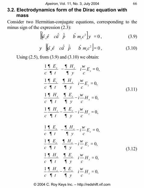
3.2. Electrodynamics form of the Dirac equation with mass
Consider two Hermitian-conjugate equations, corresponding to the minus sign of the expression (2.3):
( )[ ] 0ˆˆˆˆˆ 2 =+⋅+ ψβαεα cmpc eorr
, (3.9)
( )[ ] 0ˆˆˆˆˆ 2 =+⋅++ cmpc eo βαεαψrr
, (3.10)
Using (2.5), from (3.9) and (3.10) we obtain:
=−−
=−+
=++
=+−
,01
,01
,01
,01
zxz
xzx
zxz
xzx
Hc
iy
Et
Hc
Hc
iy
Et
Hc
Ec
iy
Ht
Ec
Ec
iy
Ht
Ec
ω∂∂
∂∂
ω∂∂
∂∂
ω∂
∂∂
∂
ω∂
∂∂
∂
(3.11)
=+−
=++
=−+
=−−
,01
,01
,01
,01
zxz
xzx
zxz
xzx
Hc
iy
Et
Hc
Hc
iy
Et
Hc
Ec
iy
Ht
Ec
Ec
iy
Ht
Ec
ω∂
∂∂
∂
ω∂
∂∂
∂
ω∂
∂∂
∂
ω∂
∂∂
∂
(3.12)
Apeiron, Vol. 11, No. 3, July 2004 67
© 2004 C. Roy Keys Inc. – http://redshift.vif.com
where h2cme=ω . The equations (3.11) and (3.12) are Maxwell
equations with imaginary currents, which differ in direction. These currents have the following form:
Eije
rrπ
ω4
= , Hijm
rrπ
ω4
= , (3.13)
and it is interesting that together with the electric current ej the magnetic current mj also exists here. The latter must be equal to zero according to the Maxwell theory [24], but its existence according to Dirac does not contradict quantum theory. (See the Dirac theory of the magnetic monopole [27].)
Thus the term that in the Dirac equation contains the electron mass, corresponds to the term that in the Maxwell equation contains the imaginary electric and the imaginary “magnetic” current.
Now we will consider the origin of the appearance of the current-mass term in the electromagnetic form by using differential geometry.
3.3. The displacement ring current We will consider the Maxwell equations without current (2.10) or (2.11), as the equations of the initial photon field. The reaction (3.1) can then be formally understood in such a way that while moving through the nucleus field, the electromagnetic wave fields may undergo a transformation and convert into the electron-positron pair.
We will show that the reason why the current-mass term appears in the equations (2.10) and (2.11) is the transition of the initial electromagnetic wave field from the linear to the curvilinear trajectory, and also that this term is the supplementary Maxwell displacement current.

Apeiron, Vol. 11, No. 3, July 2004 68
© 2004 C. Roy Keys Inc. – http://redshift.vif.com
Let the plane-polarized wave, which has the field vectors ),( zx HE , be spun with some radius pr in the plane )',','( YOX of a
fixed co-ordinate system )',',','( OZYX so that xE is parallel to the plane )',','( YOX and xH is perpendicular to it.
According to Maxwell [24] the displacement current is defined by the equation:
,41
tE
jdis ∂∂
π
rr= (3.14)
The above electrical field vector rE , which moves along the
curvilinear trajectory (let it have a direction from the centre), can be written in the form:
,nEErr
−= (3.15)
where EEr
= and rn is the normal unit-vector of the curve (having
direction to the center). The derivative of Er
with respect to t can be represented as:
t
nEn
t
E
t
E
∂
∂
∂
∂
∂
∂rr
r−−= , (3.16)
Here the first term has the same direction as rE . The existence of
the second term shows that when the wave spins the additional displacement current appears. It is not difficult to show that it has a direction tangential to the ring:
τυ
∂
∂ rr
p
p
rt
n−= , (3.17)
Apeiron, Vol. 11, No. 3, July 2004 69
© 2004 C. Roy Keys Inc. – http://redshift.vif.com
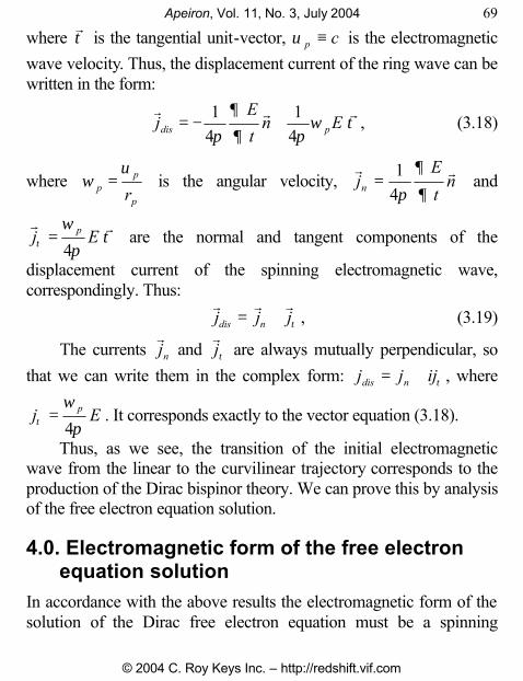
where rτ is the tangential unit-vector, cp ≡υ is the electromagnetic
wave velocity. Thus, the displacement current of the ring wave can be written in the form:
τωπ∂
∂
πrrr
Ent
Ej pdis 4
141
+−= , (3.18)
where p
pp r
υω = is the angular velocity,
r rj
E
tnn =
14π
∂
∂ and
τπ
ωτ
rrEj p
4= are the normal and tangent components of the
displacement current of the spinning electromagnetic wave, correspondingly. Thus:
r r rj j jdis n= + τ , (3.19)
The currents rjn and
rjτ are always mutually perpendicular, so
that we can write them in the complex form: τijjj ndis += , where
Ej p
π
ωτ 4
= . It corresponds exactly to the vector equation (3.18).
Thus, as we see, the transition of the initial electromagnetic wave from the linear to the curvilinear trajectory corresponds to the production of the Dirac bispinor theory. We can prove this by analysis of the free electron equation solution.
4.0. Electromagnetic form of the free electron equation solution
In accordance with the above results the electromagnetic form of the solution of the Dirac free electron equation must be a spinning

Apeiron, Vol. 11, No. 3, July 2004 70
© 2004 C. Roy Keys Inc. – http://redshift.vif.com
electromagnetic wave. Let us show that this supposition is actually correct.
From the above point of view for the y -direction photon two solutions must exist:
1) for the wave, spinning around the OZ -axis
=
=
4
1
00
00
ψ
ψ
ψ
z
x
oz
iH
E
, (4.1)
2) for the wave, spinning around the OX -axis
=
=
0
0
0
0
3
2
ψψ
ψx
zox
iHE
, (4.2)
Let us compare (4.1) and (4.2) with the Dirac theory solutions. It is known [15, 21-23] that the solution of the Dirac free
electron equation (2.1) has the form of the plane wave:
,)(exp
−−= rpt
iB jj
rrh εψ (4.3)
where 4,3,2,1=j ; B b ej ji= φ ; the amplitudes b j are the numbers
and φ is the initial wave phase. The functions (4.3) are the eigenfunctions of the energy-momentum operators, where ε and p
r
are the energy-momentum eigenvalues. Here, according to equation (2.3), for each
rp , the energy ε has either positive
4222 cmpc e++=+r
ε or negative values 4222 cmpc e+−=−r
ε .

Apeiron, Vol. 11, No. 3, July 2004 71
© 2004 C. Roy Keys Inc. – http://redshift.vif.com
Note, that generally for the particles, the equation (2.3) stands. But here we are concerned with the fields of the motionless particle in the electromagnetic representation. For the electron’s nonlinear wave fields the equation 2cme=ε stands, as it is half of the initial photon energy.
For ε + we have two linearly independent sets of four orthogonal normalizing amplitudes:
1) ( )
,0,1,, 432221 ==++
−=+
−=++
BBcm
ippcB
cmcp
Be
yx
e
z
εε (4.4)
2) ( )
,1,0,, 432221 ==+
=+−
−=++
BBcm
cpB
cmippc
Be
z
e
yx
εε (4.5)
and for ε − :
3) ( )
,,,0,1 242321 cmippc
Bcm
cpBBB
e
yx
e
z
+−+
=+−
===−− εε
(4.6)
4) ( )
,,,1,0 242321 cmcp
Bcm
ippcBBB
e
z
e
yx
+−−=
+−−
===−− εε
(4.7)
Let us analyze these solutions. 1) The existence of two linear independent solutions corresponds
with two independent orientations of the electromagnetic wave vectors, and gives a unique logical explanation for this fact.
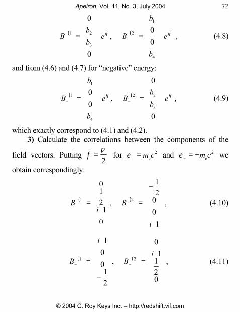
2) Since here ( )ψ ψ= y and the electron-positron fields, like the spinning waves, have momentum equal to half of the photon momentum, i.e. cme , we have cmppp eyzx === ,0 . Then for the
field vectors we obtain: from (4.4) and (4.5) for “positive” energy
Apeiron, Vol. 11, No. 3, July 2004 72
© 2004 C. Roy Keys Inc. – http://redshift.vif.com
( ) ( ) φφ ii e
b
b
Bebb
B ⋅
=⋅
= ++
4
1
2
3
21
00
,
0
0
, (4.8)
and from (4.6) and (4.7) for “negative” energy:
( ) ( ) φφ ii ebb
Be
b
b
B ⋅
=⋅
= −−
0
0
,00
3
22
4
1
1 , (4.9)
which exactly correspond to (4.1) and (4.2). 3) Calculate the correlations between the components of the
field vectors. Putting φπ
=2
for 2cme=+ε and 2cme−=−ε we
obtain correspondingly:
( ) ( )
⋅
−
=
⋅= ++
10021
,
01
210
21
i
Bi
B , (4.10)
( ) ( )B
i
Bi
− −=
⋅
−
=⋅
1 2
10012
01
120
, , (4.11)
Apeiron, Vol. 11, No. 3, July 2004 73
© 2004 C. Roy Keys Inc. – http://redshift.vif.com
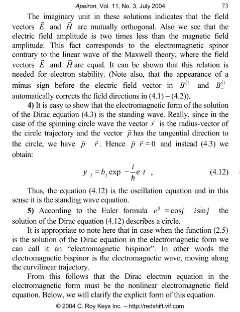
The imaginary unit in these solutions indicates that the field vectors
rE and
rH are mutually orthogonal. Also we see that the
electric field amplitude is two times less than the magnetic field amplitude. This fact corresponds to the electromagnetic spinor contrary to the linear wave of the Maxwell theory, where the field vectors
rE and
rH are equal. It can be shown that this relation is
needed for electron stability. (Note also, that the appearance of a minus sign before the electric field vector in ( )B+
1 and ( )B−1
automatically corrects the field directions in (4.1) – (4.2)). 4) It is easy to show that the electromagnetic form of the solution
of the Dirac equation (4.3) is the standing wave. Really, since in the case of the spinning circle wave the vector r
r is the radius-vector of
the circle trajectory and the vector pr
has the tangential direction to the circle, we have rp
rr⊥ . Hence 0=⋅ rp
rr and instead (4.3) we
obtain:
−= t
ib jj εψ hexp , (4.12) (3.28)
Thus, the equation (4.12) is the oscillation equation and in this sense it is the standing wave equation.
5) According to the Euler formula ϕϕϕ sincos iei += the solution of the Dirac equation (4.12) describes a circle.
It is appropriate to note here that in case when the function (2.5) is the solution of the Dirac equation in the electromagnetic form we can call it an “electromagnetic bispinor”. In other words the electromagnetic bispinor is the electromagnetic wave, moving along the curvilinear trajectory.
From this follows that the Dirac electron equation in the electromagnetic form must be the nonlinear electromagnetic field equation. Below, we will clarify the explicit form of this equation.

Apeiron, Vol. 11, No. 3, July 2004 74
© 2004 C. Roy Keys Inc. – http://redshift.vif.com
5.0. Nonlinear electrodynamic representation of the Dirac electron theory
Stability of a spinning photon is possible only by the self-action of the photon’s parts. We could introduce self-action of fields in the Dirac equation, just as external interaction is introduced in the quantum field theory equations, putting the photon mass equal to zero [15, 21-23]. But this equation may be obtained more easily using relation (3.6), for example, the expression
( )ppe pccmrr
⋅−=− αεβ ˆˆ 2 , (5.1)
By substituting (5.1) for the Dirac electron equation we obtain the nonlinear integral equation:
( ) ( )[ ] 0ˆˆˆˆ0 =−⋅+− ψαεεα pp ppcrrr
, (5.2)
where:
∫=τ
τε0
dUp , (5.3)
∫∫ ==ττ
ττ0
20
1dS
cdgpp
rrr, (5.4)
and we take that the upper limit τ is the variable. (Here SgUrr
,, are the energy density, momentum density and Poynting vector, correspondingly.)
We suppose that (5.2) is the common form of the nonlinear electron structure equation, which describes the electron in both quantum and concurrent electromagnetic forms.
In the electromagnetic form we have [24]:
Apeiron, Vol. 11, No. 3, July 2004 75
© 2004 C. Roy Keys Inc. – http://redshift.vif.com
( )
[ ]
×=
+=
HEg
HEU
rrr
rr
π
π
4181 22
, (5.5)
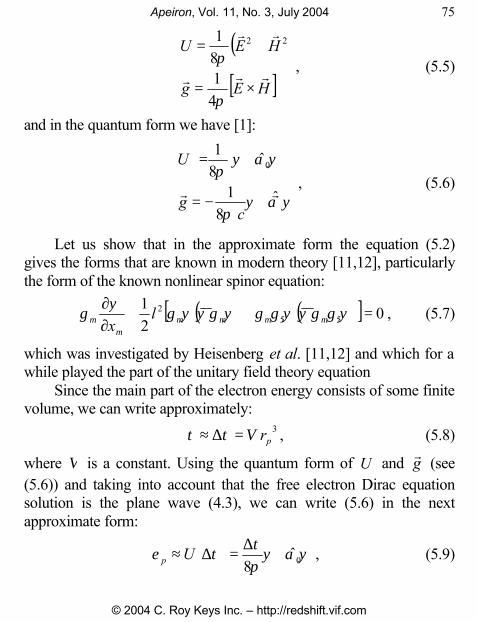
and in the quantum form we have [1]:
−=
=
+
+
ψαψπ
ψαψπ
ˆ8
1
ˆ81
0
rrc
g
U, (5.6)
Let us show that in the approximate form the equation (5.2) gives the forms that are known in modern theory [11,12], particularly the form of the known nonlinear spinor equation:
( ) ( )[ ] 021
552 =++
∂∂
ψγγψψγγψγψψγψ
γ µµµµµ
µ lx
, (5.7)
which was investigated by Heisenberg et al. [11,12] and which for a while played the part of the unitary field theory equation
Since the main part of the electron energy consists of some finite volume, we can write approximately:
3prςττ =∆≈ , (5.8)
where ς is a constant. Using the quantum form of U and gr
(see (5.6)) and taking into account that the free electron Dirac equation solution is the plane wave (4.3), we can write (5.6) in the next approximate form:
ψαψπτ
τε 0ˆ8
+∆=∆≈ Up , (5.9)
Apeiron, Vol. 11, No. 3, July 2004 76
© 2004 C. Roy Keys Inc. – http://redshift.vif.com
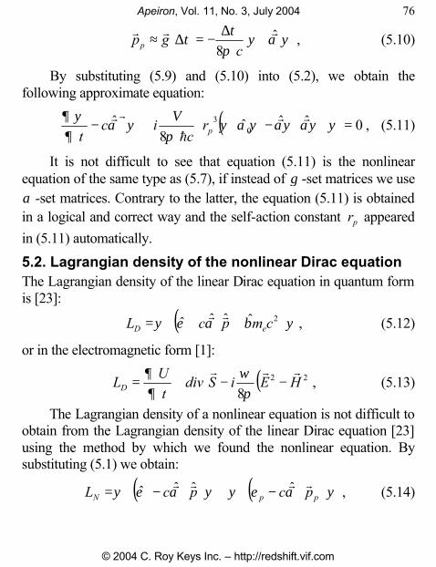
ψαψπ
ττ ˆ
8rrr +∆
−=∆≈c
gpp , (5.10)
By substituting (5.9) and (5.10) into (5.2), we obtain the following approximate equation:
( ) 0ˆˆˆ8
ˆ0
3 =−⋅+∇− ++ ψψαψαψαψπς
ψα∂
ψ∂ rrh
rrpr
cic
t, (5.11)
It is not difficult to see that equation (5.11) is the nonlinear equation of the same type as (5.7), if instead of γ -set matrices we use α -set matrices. Contrary to the latter, the equation (5.11) is obtained in a logical and correct way and the self-action constant pr appeared in (5.11) automatically.
5.2. Lagrangian density of the nonlinear Dirac equation The Lagrangian density of the linear Dirac equation in quantum form is [23]:
( ) ,ˆˆˆˆ 2 ψβαεψ cmpcL eD ++= + rr (5.12)
or in the electromagnetic form [1]:
( ),8
22 HEiSdivt
ULD
rrr−−+=
πω
∂∂
(5.13)
The Lagrangian density of a nonlinear equation is not difficult to obtain from the Lagrangian density of the linear Dirac equation [23] using the method by which we found the nonlinear equation. By substituting (5.1) we obtain:
( ) ( ) ψαεψψαεψ ppN pcpcLrrrr
⋅−+⋅−= ++ ˆˆˆˆ , (5.14)
Apeiron, Vol. 11, No. 3, July 2004 77
© 2004 C. Roy Keys Inc. – http://redshift.vif.com
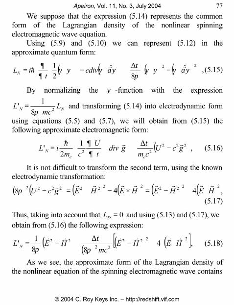
We suppose that the expression (5.14) represents the common form of the Lagrangian density of the nonlinear spinning electromagnetic wave equation.
Using (5.9) and (5.10) we can represent (5.12) in the approximate quantum form:
( ) ( ) ( ) ( )
−
∆+
−
= ++++ 22 ˆ
8ˆ
21
ψαψψψπτ
ψαψψψ∂∂ rrh cdiv
tiLN , (5.15)
By normalizing the ψ -function with the expression
NN Lmc
L 281
'π
= and transforming (5.14) into electrodynamic form
using equations (5.5) and (5.7), we will obtain from (5.15) the following approximate electromagnetic form:
( )22222
12
' gcUcm
gdivt
Ucm
iLee
Nrrh
−∆
+
+=
τ∂∂ , (5.16)
It is not difficult to transform the second term, using the known electrodynamic transformation:
( ) ( ) ( ) ( ) ( ) ( )222222222222 448 HEHEHEHEgcUrrrrrrrrr
⋅+−=×−+=−π , (5.17)
Thus, taking into account that 0=DL and using (5.13) and (5.17), we obtain from (5.16) the following expression:
( )( )
( ) ( )[ ]222222
22 488
1' HEHE
mcHEL N
rrrrrr⋅+−
∆+−=
πτ
π, (5.18)
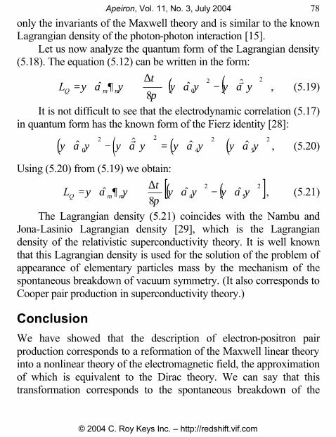
As we see, the approximate form of the Lagrangian density of the nonlinear equation of the spinning electromagnetic wave contains
Apeiron, Vol. 11, No. 3, July 2004 78
© 2004 C. Roy Keys Inc. – http://redshift.vif.com
only the invariants of the Maxwell theory and is similar to the known Lagrangian density of the photon-photon interaction [15].
Let us now analyze the quantum form of the Lagrangian density (5.18). The equation (5.12) can be written in the form:
( ) ( )
−
∆+= +++ 22
0ˆˆ
8ˆ ψαψψαψ
π
τψ∂αψ µµ
rQL , (5.19)
It is not difficult to see that the electrodynamic correlation (5.17) in quantum form has the known form of the Fierz identity [28]:
( ) ( ) ( ) ( )ψ α ψ ψ α ψ ψ α ψ ψ α ψ+ + + +− = +$ $ $ $0
2 2
4
2
5
2r, (5.20)
Using (5.20) from (5.19) we obtain:
( ) ( )[ ]2
5
2
4 ˆˆ8
ˆ ψαψψαψπτ
ψ∂αψ µµ+++ −
∆+=QL , (5.21)
The Lagrangian density (5.21) coincides with the Nambu and Jona-Lasinio Lagrangian density [29], which is the Lagrangian density of the relativistic superconductivity theory. It is well known that this Lagrangian density is used for the solution of the problem of appearance of elementary particles mass by the mechanism of the spontaneous breakdown of vacuum symmetry. (It also corresponds to Cooper pair production in superconductivity theory.)
Conclusion We have showed that the description of electron-positron pair production corresponds to a reformation of the Maxwell linear theory into a nonlinear theory of the electromagnetic field, the approximation of which is equivalent to the Dirac theory. We can say that this transformation corresponds to the spontaneous breakdown of the
Apeiron, Vol. 11, No. 3, July 2004 79
© 2004 C. Roy Keys Inc. – http://redshift.vif.com
photon, which corresponds to the creation of two massive particles, the electron and the positron.
The representation of QED in the form of a nonlinear theory of electromagnetic waves leads to an explanation of many features of modern quantum theory [30].
References [1] A.G. Kyriakos. “The electromagnetic form of the Dirac electron theory”, Apeiron, Vol. 11, No. 2, April 2004; http://arXiv.org/abs/quant-ph/0404116. [2] D. Ivanenko, A. Sokolov, The classical field theory (in Russian). Moscow- Leningrad. (1949). [3] G. Mie, Ann. D. Phys., 37, 511 (1912) ; 39, 1 (1912) ; 40, 1 (1913). [4] M Born, & L.Infeld, Proc. Roy. Soc., A 144, 425. (1934). [5] F. Bopp, Ann. D. Phys., 38, 345, (1940); B. Podolsky, Phys.Rev., 62, 68, (1941). [6] A. Proca, J. phys. et radium, ser.7, t.7, No. 8, p. 347 (1936). [7] H. F. M. Goenner, “On the History of Unified Field Theories”, Living Rev. Relativity, 7, (2004) (Online Article: http://www.livingreviews.org/lrr-2004-2 ) [8] M. Sachs, General Relativity and Matter (Reidel, 1982). [9] M. Sachs, Quantum Mechanics from General Relativity (Reidel, 1986). [10] A. Sokolov and D.Ivanenko, The quantum field theory (in Russian), Moscow-Leningrad. (1952). [11] W. Heisenberg, Introduction to the Unified Field Theory of Elementary Particles, Interscience Publishers, London, New York, Sydney, (1966). [12] Non-linear quantum field theory, (in Russian). Paper collection, edited by D.D. Ivanenko, Moscow, 1959 [13] L.H. Ryder, Quantum field theory, 2nd ed., Cambridge Univ. Press., Cambridge, UK, 1987 [14] W.J. Archibald,. Canad. Journ. Phys., 33, 565. (1955) [15] A.I. Akhiezer, and W.B. Berestetskii,. Quantum electrodynamics. Moscow, Interscience publ., New York. (1965)

Apeiron, Vol. 11, No. 3, July 2004 80
© 2004 C. Roy Keys Inc. – http://redshift.vif.com
[16] J. A. Cronin, D.F. Greenberg, V. L. Telegdi. University of Chicago graduate problems in physics. (Addison Wesley Publishing Co., 1971) Problem 6.7.
[17] R.S. Armour, Found. Phys. Vol. 34, no. 5, 815-842 (2004), http://arxiv.org/abs/hep-th/0305084 .
[18] V. Dvoeglazov, Essay on the Non-Maxwellian Theories of Electromagnetism, Hadronic Journal Supplement, 12, No. 3, pp. 241-288 (1997), arXiv: hep-th/9609144 v1.; Hadronic Journal, 16, No. 6, pp. 459-467 (1993); Il Nuovo Cimento, B112, No. 6, pp. 847-852 (1997).
[19] Recami et al, Lett. Nuovo Cim. 11, 568 (1974); E. Recami and G. Salesi, Field theory of the spinning electron: about the non-linear field eqations. Advances in Applied Clifford Algebra, vol. 5, No. 1, June 1996.
[20] A. Gsponer. Int. J. Theor. Phys. 41, 689-694. (2002). [21] F. A. Kaempfer, Concepts in quantum mechanics, Academic Press, New York
and London (1965). [22] H.A. Bethe, Intermediate Quantum Mechanics, W. A. Benjamin, Inc., New
York –Amsterdam, (1964). [23] L.T. Schiff, Quantum Mechanics, (2nd edition), McGraw-Hill Book
Company, Jnc, New York, (1955). [24] M.-A. Tonnelat, Les Principes de la Theorie Electromagnetique et de la
Relativite, Masson et C. Editeurs, Paris, (1959). [25] V. Fock, “L’Equation d’Onde de Dirac et la Geometrie de Riemann”, J. Phys.
Rad. 10 (1929) 392-405; V. Fock, “Geometrisierung der Diracschen Theorie des Electrons”, Z. Phys. 57 (1929) 261-277; V. Fock, D. Ivanenko, C.R., Phys. Zs. 30, 648 (1929).
[26] B. L. van der Waerden, „Spinoranalyse”, Gott. Nachr. (1929) 100-109; E. Schroedinger, Berliner Berich., S.105 (1932); L. Infeld und B.Van der Waerden, Berliner Berich., S.380 (1933)
[27] P. A. M. Dirac,”Quantised singularities in the electromagnetic field”, Proc. Roy. Soc., A33, 60 (1931); P. A. M. Dirac. Direction in Physics. (Edited by H. Hora and J.R. Shepanski), John Wiley and Sons, New York, (1978).
[28] T.-P. Cheng and L.-F. Li, Gauge Theory of Elementary Particle Physics Clarendon Press, Oxford, (1984); Idem: Problems and Solution, Clarendon Press, Oxford, (2000)
[29] Y. Nambu and G. Jona-Lasinio, Phys. Rev., 122, No.1, 345-358 (1961); 124, 246 (1961).

Apeiron, Vol. 11, No. 3, July 2004 81
© 2004 C. Roy Keys Inc. – http://redshift.vif.com
[30] A.G. Kyriakos, “Quantum mechanics as Electrodynamics of Curvilinear Waves”, http://arXiv.org/abs/quant-ph/0209021
Related Documents