The Development of a High-Resolution Scintillating Fiber Tracker with Silicon Photomultiplier Readout Von der Fakult¨at f¨ ur Mathematik, Informatik und Naturwissenschaften der RWTH Aachen University zur Erlangung des akademischen Grades eines Doktors der Naturwissenschaften genehmigte Dissertation vorgelegt von Diplom-Physiker Gregorio Roper Yearwood aus Aachen Berichter: Universit¨ atsprofessor Dr. Stefan Schael Universit¨ atsprofessor Dr. Tatsuya Nakada Tag der m¨ undlichen Pr¨ ufung: 06. Februar 2013 Diese Dissertation ist auf den Internetseiten der Hochschulbibliothek online verf¨ ugbar. i

Welcome message from author
This document is posted to help you gain knowledge. Please leave a comment to let me know what you think about it! Share it to your friends and learn new things together.
Transcript
The Development of a High-Resolution ScintillatingFiber Tracker with Silicon Photomultiplier Readout
Von der Fakultat fur Mathematik, Informatik und Naturwissenschaften der RWTHAachen University zur Erlangung des akademischen Grades eines Doktors der
Naturwissenschaften genehmigte Dissertation
vorgelegt von
Diplom-PhysikerGregorio Roper Yearwood
aus Aachen
Berichter:Universitatsprofessor Dr. Stefan Schael
Universitatsprofessor Dr. Tatsuya Nakada
Tag der mundlichen Prufung:06. Februar 2013
Diese Dissertation ist auf den Internetseiten der Hochschulbibliothek online verfugbar.
i

Zusammenfassung
In dieser Arbeit prasentiere ich den Aufbau und Testergebnisse eines neuartigen, modu-laren Spurdetektors aus szintillierenden Fasern, ausgelesen mit Siliziumphotomultiplier (SiPM)Arrays.
Einzelne Spurdetektormodule bestehen aus 0.25 mm dunnen, szintillierenden Fasern, diedicht gepackt in funf Lagen auf beide Seiten einer Kohlefaser/Rohacell-Struktur aufgebrachtsind. Die eigens fur diese Anwendung hergestellten SiPM Arrays haben eine Photon-Nachweis-effizienz von etwa 50 %.
Mehrere 860 mm lange und zwischen 32 mm und 64 mm breite Spurdetektormodule wur-den im November 2009 am PS-Beschleuniger am CERN in einem sekundaren 12 GeV/c Strahlgetestet. Dabei wurden Ortsauflosungen besser als 0.05 mm bei einer durchschnittlichen Lich-tausbeute von zwanzig Photonen fur minimalionisierende Teilchen gemessen.
Die vorliegende Arbeit beschreibt die Charakterisierung szintillierender Fasern und Silizi-umphotomultiplier von unterschiedlichen Typen und gibt einen Uberblick uber die Produk-tion der Detektormodule. Das Verhalten der Detektormodule im Teststrahl wird ausfuhrlichanalysiert und verschiedene Optionen fur die Ausleseelektronik werden miteinander verglichen.
Weiterhin wird die Anwendung des Spurdetektors aus szintillierenden Fasern im Rah-men des “Proton Electron Radiation Detector Aix-la-chappelle” (PERDaix) Spektrometersvorgestellt. Der PERDaix-Detektor ist ein 40 kg schweres Magnetspektrometer bestehend ausacht Spurdetektorlagen aus Fasern, einem Flugzeitdetektor aus Plastikszintillatoren mit Si-liziumphotomultiplierauslese sowie einem Ubergangsstrahlungsdetektor bestehend aus einemVliesradiator und Xe− CO2 gefullten Proportionalzahlrohrchen. Im November 2010 wurde derPERDaix Detektor von Kiruna, Schweden von einem Heliumballon im Rahmen des “Balloon-Experiments for University Students” (BEXUS) Programmes fur wenige Stunden auf eineFlughohe von 33 km getragen, wo er die kosmische Strahlung aufzeichnete. Im Mai 2011 wurdeder PERDaix-Detektor wahrend eines Strahltests am PS-Beschleuniger des CERN kalibriert.Es werden Methoden der Event-Rekonstruktion und des Detektoralignments entwickelt, die eineoptimale Analyse der Daten des PERDaix Spurdetektors erlauben. Weiterhin wird die Orts-auflosung der Spurdetektormodule, ihre Effizienz sowie die Impulsauflosung des Spektrometersbestimmt.
iii
Abstract
In this work I present the design and test results for a novel, modular tracking detectorfrom scintillating fibers which are read out by silicon photomultiplier (SiPM) arrays.
The detector modules consist of 0.25 mm thin scintillating fibers which are closely packedin five-layer ribbons. Two ribbons are fixed to both sides of a carbon-fiber composite structure.Custom made SiPM arrays with a photo-detection efficiency of about 50 % read out the fibers.
Several 860 mm long and 32 mm wide tracker modules were tested in a secondary 12 GeV/cbeam at the PS facilities, CERN in November of 2009. During this test a spatial resolutionbetter than 0.05 mm at an average light yield of about 20 photons for a minimum ionizingparticle was determined.
This work details the characterization of scintillating fibers and silicon photomultipliers ofdifferent make and model. It gives an overview of the production of scintillating fiber modules.The behavior of detector modules during the test-beam is analyzed in detail and differentoptions for the front-end electronics are compared.
Furthermore, the implementation of the proposed tracking detector from scintillating fiberswithin the scope of the PERDaix experiment is discussed. The PERDaix detector is a per-manent magnet spectrometer with a weight of 40 kg. It consists of 8 tracking detector layersfrom scintillating fibers, a time-of-flight detector from plastic scintillator bars with silicon pho-tomultiplier readout and a transition radiation detector from an irregular fleece radiator andXe/CO2 filled proportional counting tubes.
The PERDaix detector was launched with a helium balloon within the scope of the ”Balloon-Experiments for University Students” (BEXUS) program from Kiruna, Sweden in November2010. For a few hours PERDaix reached an altitude of 33 km and measured cosmic rays. InMay 2011, the PERDaix detector was characterized during a test-beam at the PS-facilities atCERN. This work introduces methods for event reconstruction and detector alignment whichallow an optimal analysis of the PERDaix tracker data. In addition, the spatial resolution andthe efficiency of detector modules as well as the momentum resolution of the spectrometer aredetermined.
iv

For my family who encouraged me to persevere.
v

Contents
Contents vi
1 Introduction 1
2 A detector for charged cosmic radiation 32.1 Cosmic rays and solar modulation . . . . . . . . . . . . . . . . . . . . . . . . . . . 3
2.1.1 Cosmic rays in the galaxy . . . . . . . . . . . . . . . . . . . . . . . . . . . . 32.1.2 The Sun and the Solar Wind . . . . . . . . . . . . . . . . . . . . . . . . . . 52.1.3 On the transport of galactic cosmic rays in the heliosphere . . . . . . . . . 6
2.2 Tracking Detectors . . . . . . . . . . . . . . . . . . . . . . . . . . . . . . . . . . . . 102.2.1 Detecting charged particles . . . . . . . . . . . . . . . . . . . . . . . . . . . 102.2.2 Observable properties of energetic charged-particles . . . . . . . . . . . . . 122.2.3 Material budget . . . . . . . . . . . . . . . . . . . . . . . . . . . . . . . . . 142.2.4 Existing concepts for tracking detectors . . . . . . . . . . . . . . . . . . . . 14
2.3 The PERDaix experiment . . . . . . . . . . . . . . . . . . . . . . . . . . . . . . . . 172.3.1 Motivation . . . . . . . . . . . . . . . . . . . . . . . . . . . . . . . . . . . . 172.3.2 Overview of the PERDaix instrument . . . . . . . . . . . . . . . . . . . . . 17
3 Scintillating Fiber Detector Modules 213.1 Scintillating Fibers . . . . . . . . . . . . . . . . . . . . . . . . . . . . . . . . . . . . 21
3.1.1 Motivation . . . . . . . . . . . . . . . . . . . . . . . . . . . . . . . . . . . . 213.1.2 Properties of plastic scintillating fibers . . . . . . . . . . . . . . . . . . . . . 213.1.3 Mechanical properties of thin scintillating fibers . . . . . . . . . . . . . . . . 223.1.4 Handling of Kuraray fibers . . . . . . . . . . . . . . . . . . . . . . . . . . . 253.1.5 Light-collection in cylindrical scintillating fibers . . . . . . . . . . . . . . . . 253.1.6 Measured far-field of Kuraray SCSF-81M fibers . . . . . . . . . . . . . . . . 273.1.7 Attenuation length of scintillating fibers . . . . . . . . . . . . . . . . . . . . 28
3.2 Manufacturing scintillating fiber modules . . . . . . . . . . . . . . . . . . . . . . . 303.2.1 The manufacturing process . . . . . . . . . . . . . . . . . . . . . . . . . . . 303.2.2 Quality control of finished scintillating fiber ribbons . . . . . . . . . . . . . 32
3.3 Overview of produced scintillating fiber modules . . . . . . . . . . . . . . . . . . . 343.3.1 Prototypes 2009 . . . . . . . . . . . . . . . . . . . . . . . . . . . . . . . . . 343.3.2 Modules for the PERDaix tracking detector . . . . . . . . . . . . . . . . . . 34
4 Silicon Photomultiplier Array Readout 394.1 Silicon Photomultipliers . . . . . . . . . . . . . . . . . . . . . . . . . . . . . . . . . 39
4.1.1 Photo-detectors for scintillating fiber trackers . . . . . . . . . . . . . . . . . 394.1.2 Photo-diodes . . . . . . . . . . . . . . . . . . . . . . . . . . . . . . . . . . . 404.1.3 Quantum Efficiency . . . . . . . . . . . . . . . . . . . . . . . . . . . . . . . 414.1.4 SiPM amplification process and gain . . . . . . . . . . . . . . . . . . . . . . 434.1.5 SiPM internal structure and geometric efficiency . . . . . . . . . . . . . . . 464.1.6 Saturation . . . . . . . . . . . . . . . . . . . . . . . . . . . . . . . . . . . . . 50
vi

4.1.7 Crosstalk . . . . . . . . . . . . . . . . . . . . . . . . . . . . . . . . . . . . . 524.1.8 After-pulsing . . . . . . . . . . . . . . . . . . . . . . . . . . . . . . . . . . . 544.1.9 Measurement of SiPM properties . . . . . . . . . . . . . . . . . . . . . . . . 55
4.2 Readout Electronics for SiPM Arrays . . . . . . . . . . . . . . . . . . . . . . . . . . 584.2.1 Carrier circuit boards for SiPM arrays . . . . . . . . . . . . . . . . . . . . . 584.2.2 Preamplifier boards . . . . . . . . . . . . . . . . . . . . . . . . . . . . . . . 604.2.3 Analog-to-digital boards . . . . . . . . . . . . . . . . . . . . . . . . . . . . . 62
4.3 SiPM calibration procedure . . . . . . . . . . . . . . . . . . . . . . . . . . . . . . . 624.4 Comparison of VA32 and SPIROC readout . . . . . . . . . . . . . . . . . . . . . . 674.5 Crosstalk between channels of the MPPC5883 . . . . . . . . . . . . . . . . . . . . . 694.6 Temperature compensation of MPPC5883v2 . . . . . . . . . . . . . . . . . . . . . . 72
5 Characterization of SciFi tracker modules 795.1 Test-beam Setup 2009 . . . . . . . . . . . . . . . . . . . . . . . . . . . . . . . . . . 79
5.1.1 T9 beam line and selected beam properties . . . . . . . . . . . . . . . . . . 795.1.2 Setup . . . . . . . . . . . . . . . . . . . . . . . . . . . . . . . . . . . . . . . 805.1.3 Trigger Setup . . . . . . . . . . . . . . . . . . . . . . . . . . . . . . . . . . . 815.1.4 Beam Telescope . . . . . . . . . . . . . . . . . . . . . . . . . . . . . . . . . . 83
5.2 Properties of SiPM during the testbeam . . . . . . . . . . . . . . . . . . . . . . . . 865.3 Performance of the scintillating fiber modules . . . . . . . . . . . . . . . . . . . . . 89
5.3.1 Analysis Procedure . . . . . . . . . . . . . . . . . . . . . . . . . . . . . . . . 895.3.2 Detector Parametrization and Alignment . . . . . . . . . . . . . . . . . . . 915.3.3 Light yield . . . . . . . . . . . . . . . . . . . . . . . . . . . . . . . . . . . . 965.3.4 Spatial Resolution . . . . . . . . . . . . . . . . . . . . . . . . . . . . . . . . 102
6 The Proton Electron Radiation Detector Aix-la-Chapelle 1136.1 The PERDaix spectrometer . . . . . . . . . . . . . . . . . . . . . . . . . . . . . . . 113
6.1.1 PERDaix scintillating fiber modules and readout . . . . . . . . . . . . . . . 1136.1.2 The PERDaix magnet . . . . . . . . . . . . . . . . . . . . . . . . . . . . . . 114
6.2 Characterization of the PERDaix spectrometer . . . . . . . . . . . . . . . . . . . . 1166.2.1 Test-beam Setup . . . . . . . . . . . . . . . . . . . . . . . . . . . . . . . . . 1166.2.2 Parametrization of detector geometry and alignment . . . . . . . . . . . . . 1166.2.3 Measured light yield . . . . . . . . . . . . . . . . . . . . . . . . . . . . . . . 1196.2.4 Spatial resolution . . . . . . . . . . . . . . . . . . . . . . . . . . . . . . . . . 1226.2.5 Momentum resolution . . . . . . . . . . . . . . . . . . . . . . . . . . . . . . 1266.2.6 Tracking efficiency . . . . . . . . . . . . . . . . . . . . . . . . . . . . . . . . 130
6.3 Flight performance of the PERDaix spectrometer . . . . . . . . . . . . . . . . . . . 134
7 Conclusion 139
A A GEANT4 simulation of the scintillating fiber tracker 141A.1 A fast simulation model for optical photon tracking in cylindrical fibers for GEANT4 141A.2 A model for a silicon photomultiplier with CR-RC shaping readout . . . . . . . . . 144
B Track detection in 3D using a Kalman Filter method 147B.1 The passage of a particle as linear dynamical model . . . . . . . . . . . . . . . . . 147B.2 Principles of the Kalman Filter . . . . . . . . . . . . . . . . . . . . . . . . . . . . . 149B.3 Fitting single particle tracks with a Kalman filter . . . . . . . . . . . . . . . . . . . 150B.4 Reconstructing particle tracks from noisy observations . . . . . . . . . . . . . . . . 152
B.4.1 Hough transform and template matching . . . . . . . . . . . . . . . . . . . 153B.4.2 Rule-based feature extraction . . . . . . . . . . . . . . . . . . . . . . . . . . 154
B.5 The Track Tree algorithm . . . . . . . . . . . . . . . . . . . . . . . . . . . . . . . . 155
vii

C Track Fit and Detector Alignment 161C.1 The linear least-squares fit and the Gauss-Markov theorem . . . . . . . . . . . . . 161C.2 Limiting step sizes and parameters with regularized least-squares . . . . . . . . . . 163C.3 Iterative reweighting to manage non-Gaussian uncertainties . . . . . . . . . . . . . 165C.4 Solving alignment matrix equations . . . . . . . . . . . . . . . . . . . . . . . . . . . 168C.5 Treatment of multiple Coulomb scattering in Track Fits . . . . . . . . . . . . . . . 170
Acknowledgements 175
Bibliography 177
List of Figures 186
List of Tables 195
viii
Chapter 1
Introduction
There are a number of theoretical problems and empirical phenomena in the world of physics whichlack a satisfactory scientific explanation. Among them are many problems which are related toCosmology (What is the nature of dark matter? ), Particle Physics (Does the Higgs exist? Is thereSupersymmetry? ) or Astrophysics (What is the origin of the observed ultra-high-energy cosmicrays? ). In search for answers to these questions, experimentalists are pushed to extremes byeither requiring the investigation of very small scales or very large scales. It so happens that forboth extremes the measurement of energetic charged-particles offers an approach to gain moreinsight into the shape of the answer. The inclination towards charged particles is of course nota coincidence. The fact is that charged-particles interact electromagnetically making them fairlyeasy to detect compared to particles that interact only via the other three fundamental forcesthat we know of, which are either too weak or too short ranged to be convenient for a detector.Since a mere inconvenience is not sufficient to deter scientists there are of course many detectorswhich successfully detect particles that interact only weakly or hadronically. Many of these, if youconsider neutrino detectors like Superkamiokande or IceCube or common neutron detectors workby using targets to produce ionizing particles that can be detected much more easily1.
A technology that dates back to the 1960s is the use of scintillating fibers to detect particles.In the early years of this millennium a new photo-detection technology, silicon photomultipliers,became available. For the past five years, we have developed a new tracking detector based onscintillating fibers and silicon photomultipliers at RWTH Aachen University. I have had the fortuneof contributing to this development from the very beginning, first as a diploma student startingin 2006 and from Summer 2007 on as a PhD student.
This work is structured as follows. Chapter two introduces the Proton Electron RadiationDetector Aix-la-chapelle (PERDaix) and motivates its application to measure cosmic rays in therigidity range from 0.5 GV/c to 5 GV/c. Chapter three gives an overview of scintillating fibers anddescribes the design and production of scintillating fiber modules for a tracking detector. Chapterfour introduces silicon photomultipliers and gives a description of the silicon photomultiplier arraysused for the scintillating fiber tracker. In chapter five the results from a test of a scintillating fibertracker prototype are given, focusing on spatial resolution and light yield. Chapter six goes intodetails of the scintillating fiber tracker built for the PERDaix experiment. It shows light yield,spatial resolution and momentum resolution of the PERDaix spectrometer measured during atestbeam at CERN in 2011. Finally, chapter six evaluates the performance of the scintillatingfiber tracker during the flight of the PERDaix detector with a high-altitude balloon in November2010.
The following list shows publications I co-authored during the writing of this thesis which arerelated to the topics of this work and in part contain further results and considerations.
• PEBS - Positron electron balloon spectrometer (2007) [1]
1One experiment that is a famous exception to that rule would be Raymond Davis Jr’s Homestake Experimentwhich used the catalysis of a nuclear transmutation to detect neutrinos.
1

1. Introduction
• A high resolution scintillating fiber tracker with SiPM readout (2007) [2]
• Silicon photomultiplier arrays - a novel photon detector for a high resolution tracker producedat FBK-irst, Italy (2008) [3]
• A high-resolution scintillating fiber tracker with SiPM array readout for cosmic-ray research(2009) [4]
• A New Instrument for Testing Charge-Sign Dependent Solar Modulation (2009) [5]
• A high-resolution scintillating fiber tracker with silicon (2010) [6]
• The Development of a high-resolution Scintillating Fiber Tracker with Silicon PhotomultiplierReadout (2011) [7]
2
Chapter 2
A detector for charged cosmicradiation
This chapter gives an overview over cosmic rays in the solar system and motivates the design of asmall spectrometer for the detection of cosmic particles in the range between 0.5 GeV and 5 GeV.It introduces basic design principles of a tracking detector and describes the PERDaix cosmic-rayspectrometer that was built around a scintillating fiber tracker.
2.1 Cosmic rays and solar modulation
2.1.1 Cosmic rays in the galaxy
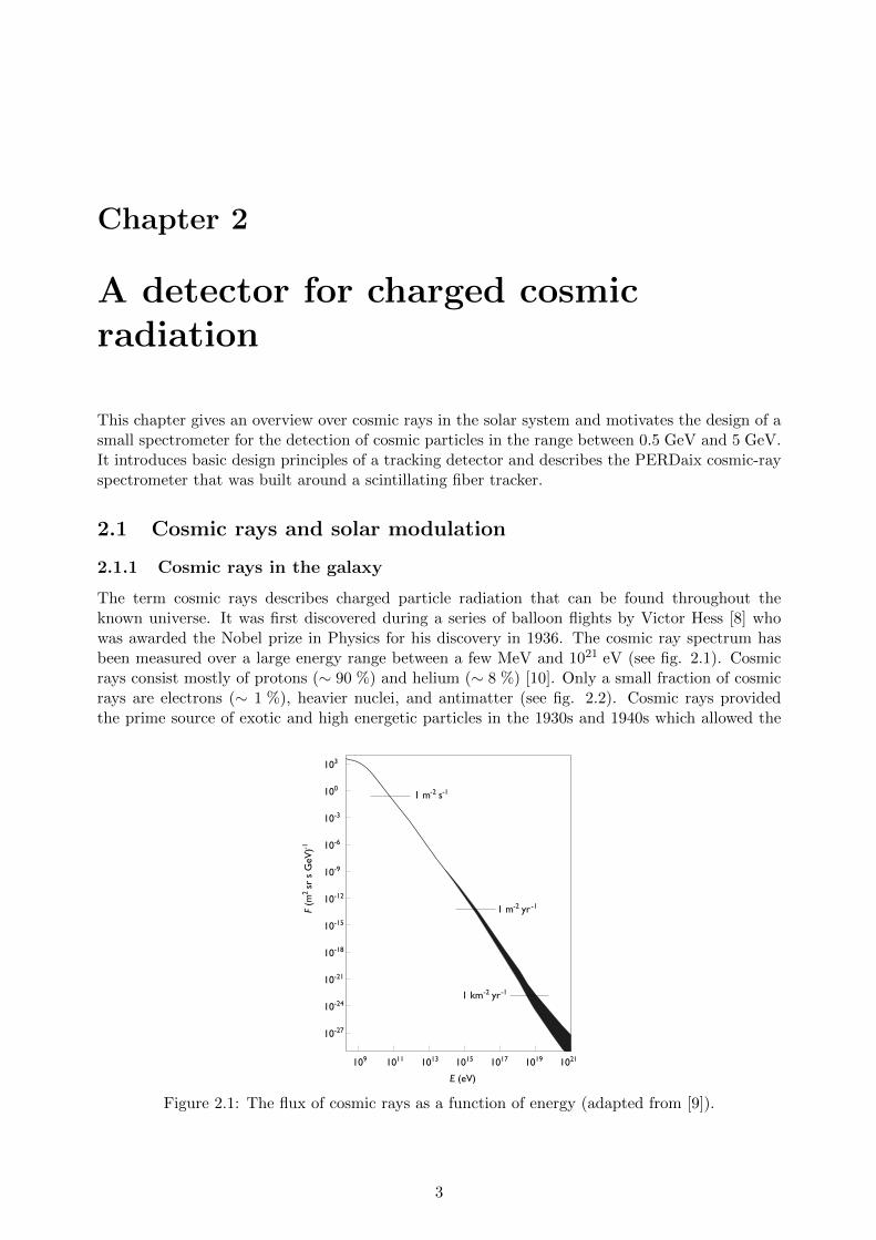
The term cosmic rays describes charged particle radiation that can be found throughout theknown universe. It was first discovered during a series of balloon flights by Victor Hess [8] whowas awarded the Nobel prize in Physics for his discovery in 1936. The cosmic ray spectrum hasbeen measured over a large energy range between a few MeV and 1021 eV (see fig. 2.1). Cosmicrays consist mostly of protons (∼ 90 %) and helium (∼ 8 %) [10]. Only a small fraction of cosmicrays are electrons (∼ 1 %), heavier nuclei, and antimatter (see fig. 2.2). Cosmic rays providedthe prime source of exotic and high energetic particles in the 1930s and 1940s which allowed the
Figure 2.1: The flux of cosmic rays as a function of energy (adapted from [9]).
3
2. A detector for charged cosmic radiation
/n) / GeVkin
(E
–110 1 10 210
Flux/(cm
2ssrGeV/n)–1
–910
–810
–710
–610
–510
–410
–310
–210
–110
1p AMS01 98
He AMS01AMS01 e-HEAT e- TOAAMS01 e+HEAT e+ TOA
BESS 98pCAPRICE 98pEGRETγ
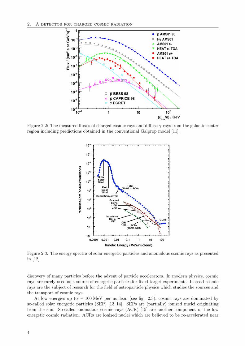
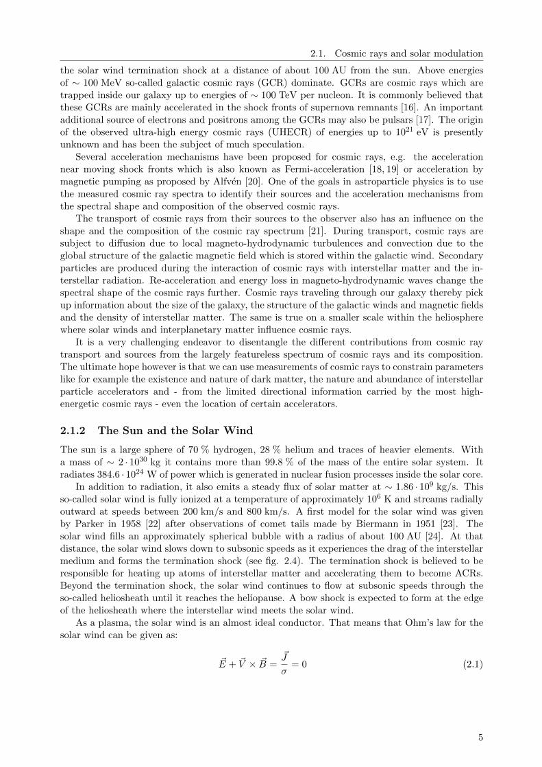
Figure 2.2: The measured fluxes of charged cosmic rays and diffuse γ-rays from the galactic centerregion including predictions obtained in the conventional Galprop model [11].
Figure 2.3: The energy spectra of solar energetic particles and anomalous cosmic rays as presentedin [12].
discovery of many particles before the advent of particle accelerators. In modern physics, cosmicrays are rarely used as a source of energetic particles for fixed-target experiments. Instead cosmicrays are the subject of research for the field of astroparticle physics which studies the sources andthe transport of cosmic rays.
At low energies up to ∼ 100 MeV per nucleon (see fig. 2.3), cosmic rays are dominated byso-called solar energetic particles (SEP) [13, 14]. SEPs are (partially) ionized nuclei originatingfrom the sun. So-called anomalous cosmic rays (ACR) [15] are another component of the lowenergetic cosmic radiation. ACRs are ionized nuclei which are believed to be re-accelerated near
4
2.1. Cosmic rays and solar modulation
the solar wind termination shock at a distance of about 100 AU from the sun. Above energiesof ∼ 100 MeV so-called galactic cosmic rays (GCR) dominate. GCRs are cosmic rays which aretrapped inside our galaxy up to energies of ∼ 100 TeV per nucleon. It is commonly believed thatthese GCRs are mainly accelerated in the shock fronts of supernova remnants [16]. An importantadditional source of electrons and positrons among the GCRs may also be pulsars [17]. The originof the observed ultra-high energy cosmic rays (UHECR) of energies up to 1021 eV is presentlyunknown and has been the subject of much speculation.
Several acceleration mechanisms have been proposed for cosmic rays, e.g. the accelerationnear moving shock fronts which is also known as Fermi-acceleration [18, 19] or acceleration bymagnetic pumping as proposed by Alfven [20]. One of the goals in astroparticle physics is to usethe measured cosmic ray spectra to identify their sources and the acceleration mechanisms fromthe spectral shape and composition of the observed cosmic rays.
The transport of cosmic rays from their sources to the observer also has an influence on theshape and the composition of the cosmic ray spectrum [21]. During transport, cosmic rays aresubject to diffusion due to local magneto-hydrodynamic turbulences and convection due to theglobal structure of the galactic magnetic field which is stored within the galactic wind. Secondaryparticles are produced during the interaction of cosmic rays with interstellar matter and the in-terstellar radiation. Re-acceleration and energy loss in magneto-hydrodynamic waves change thespectral shape of the cosmic rays further. Cosmic rays traveling through our galaxy thereby pickup information about the size of the galaxy, the structure of the galactic winds and magnetic fieldsand the density of interstellar matter. The same is true on a smaller scale within the heliospherewhere solar winds and interplanetary matter influence cosmic rays.
It is a very challenging endeavor to disentangle the different contributions from cosmic raytransport and sources from the largely featureless spectrum of cosmic rays and its composition.The ultimate hope however is that we can use measurements of cosmic rays to constrain parameterslike for example the existence and nature of dark matter, the nature and abundance of interstellarparticle accelerators and - from the limited directional information carried by the most high-energetic cosmic rays - even the location of certain accelerators.
2.1.2 The Sun and the Solar Wind
The sun is a large sphere of 70 % hydrogen, 28 % helium and traces of heavier elements. Witha mass of ∼ 2 · 1030 kg it contains more than 99.8 % of the mass of the entire solar system. Itradiates 384.6 · 1024 W of power which is generated in nuclear fusion processes inside the solar core.
In addition to radiation, it also emits a steady flux of solar matter at ∼ 1.86 · 109 kg/s. Thisso-called solar wind is fully ionized at a temperature of approximately 106 K and streams radiallyoutward at speeds between 200 km/s and 800 km/s. A first model for the solar wind was givenby Parker in 1958 [22] after observations of comet tails made by Biermann in 1951 [23]. Thesolar wind fills an approximately spherical bubble with a radius of about 100 AU [24]. At thatdistance, the solar wind slows down to subsonic speeds as it experiences the drag of the interstellarmedium and forms the termination shock (see fig. 2.4). The termination shock is believed to beresponsible for heating up atoms of interstellar matter and accelerating them to become ACRs.Beyond the termination shock, the solar wind continues to flow at subsonic speeds through theso-called heliosheath until it reaches the heliopause. A bow shock is expected to form at the edgeof the heliosheath where the interstellar wind meets the solar wind.
As a plasma, the solar wind is an almost ideal conductor. That means that Ohm’s law for thesolar wind can be given as:
~E + ~V × ~B =~J
σ= 0 (2.1)
5

2. A detector for charged cosmic radiation
Figure 2.4: An artist’s view of the heliosphere (adapted from PIA12375, NASA/JPL/JHUAPL).
where ~E is the electric field, ~B is the magnetic field, ~V is the flow speed1 of the plasma, ~J is thesolar wind current density and σ is the conductivity which approaches infinity. Using Faraday’slaw, it is found that magnetic fields in a homogeneous plasma of a constant density ρ are frozeninside the plasma:
∂ ~B
∂t= −~∇× ~E = ~∇×
(~V × ~B
)= 0 (2.2)
Along with the continuum equation
∂ρ
∂t+ ~∇× (ρ~V ) = 0 (2.3)
and the equation of motion
ρ
(∂~V
∂t+(~V · ~∇
)~V
)= ~J × ~B + ~∇p (2.4)
with the plasma pressure p, these equations form the ideal equations of magnetohydrodynamics(MHD) pioneered by H. Alfven [25] and written down concisely by Elsasser [26]. These equationsgovern the evolution of solar wind and the formation of the heliosphere around the sun.
2.1.3 On the transport of galactic cosmic rays in the heliosphere
In 1955 Parker [27] showed in his hydromagnetic dynamo model how the plasma motions withinthe sun are capable of sustaining a magnetic dipole field. The magnetic field of the sun is frozeninto the solar wind near the sun. Considering that the sun rotates at a speed of approximately
1The speed and current of the solar wind are vector fields - for conciseness they are written down here as simplevectors.
6
2.1. Cosmic rays and solar modulation
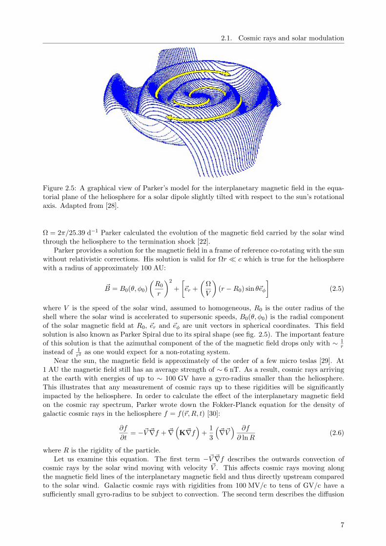
Figure 2.5: A graphical view of Parker’s model for the interplanetary magnetic field in the equa-torial plane of the heliosphere for a solar dipole slightly tilted with respect to the sun’s rotationalaxis. Adapted from [28].
Ω = 2π/25.39 d−1 Parker calculated the evolution of the magnetic field carried by the solar windthrough the heliosphere to the termination shock [22].
Parker provides a solution for the magnetic field in a frame of reference co-rotating with the sunwithout relativistic corrections. His solution is valid for Ωr c which is true for the heliospherewith a radius of approximately 100 AU:
~B = B0(θ, φ0)
(R0
r
)2
+
[~er +
(Ω
V
)(r −R0) sin θ~eφ
](2.5)
where V is the speed of the solar wind, assumed to homogeneous, R0 is the outer radius of theshell where the solar wind is accelerated to supersonic speeds, B0(θ, φ0) is the radial componentof the solar magnetic field at R0, ~er and ~eφ are unit vectors in spherical coordinates. This fieldsolution is also known as Parker Spiral due to its spiral shape (see fig. 2.5). The important featureof this solution is that the azimuthal component of the of the magnetic field drops only with ∼ 1
rinstead of 1
r2as one would expect for a non-rotating system.
Near the sun, the magnetic field is approximately of the order of a few micro teslas [29]. At1 AU the magnetic field still has an average strength of ∼ 6 nT. As a result, cosmic rays arrivingat the earth with energies of up to ∼ 100 GV have a gyro-radius smaller than the heliosphere.This illustrates that any measurement of cosmic rays up to these rigidities will be significantlyimpacted by the heliosphere. In order to calculate the effect of the interplanetary magnetic fieldon the cosmic ray spectrum, Parker wrote down the Fokker-Planck equation for the density ofgalactic cosmic rays in the heliosphere f = f(~r,R, t) [30]:
∂f
∂t= −~V ~∇f + ~∇
(K~∇f
)+
1
3
(~∇~V) ∂f
∂ lnR(2.6)
where R is the rigidity of the particle.Let us examine this equation. The first term −~V ~∇f describes the outwards convection of
cosmic rays by the solar wind moving with velocity ~V . This affects cosmic rays moving alongthe magnetic field lines of the interplanetary magnetic field and thus directly upstream comparedto the solar wind. Galactic cosmic rays with rigidities from 100 MV/c to tens of GV/c have asufficiently small gyro-radius to be subject to convection. The second term describes the diffusion
7

2. A detector for charged cosmic radiation
due to the random walk of cosmic rays between scatterings with small-scale turbulences withinthe magnetic field. The diffusion tensor K can be given in coordinates with respect to the localdirection of the interplanetary magnetic field as:
K =
κ⊥ 0 00 κ‖ κA0 −κA κ‖
(2.7)
The third term is the adiabatic energy loss. It is based on the deceleration of a particle that istrapped within an expanding magnetic cloud. One should note, however, that for large rigiditieswhere the gyro-radius of the particle becomes much larger than the size of the magnetic fieldinhomogeneities, adiabatic cooling ceases to be of significance.
In 1968 Gleeson and Axford [31] presented a solution for Parker’s transport equation in thesteady-state spherically symmetrical case assuming that the inward diffusive flux equals the out-ward convective flux κ∂f∂r = V0f . Equation 2.6 is in this case reduced to:
∂f
∂r+dR
dr
∂f
∂R= 0 (2.8)
which has the following solution for the flux J1 AU(T − Φ) at 1 AU:
J1 AU(T − Φ) = JLIS(T )(T − Φ)(T − Φ + 2M0)
T (T + 2M0)(2.9)
where JLIS(T ) is the local interstellar spectrum, T is the kinetic energy of the particle before it
enters the heliosphere, M0 is the rest mass of the particle and Φ = eZmpm Φ0 is the solar modulation
parameter which is of the order of hundreds of MeV. This model entirely neglects the fact thatboth drift and diffusion constant within the interplanetary magnetic field change over the courseof the solar cycle [32]. Comparing the force-field solution with the full one-dimensional numericalsolution [33] shows a good agreement with the force-field approximation at distances to the sunof r ≈ 1 AU. Moving to the outer heliosphere, large discrepancies between the force-field solutionand the full numerical solution become visible.
In spite of questions regarding its validity, the force-field solution continues to be relevant forexperimentalists since it offers a single observable parameter Φ0 for the effect of solar modulation onthe cosmic ray spectrum. Simple comparisons between different experiments which were performedat different times during the solar cycle are possible based on Φ0. Φ0 is used in this case tocapture the varying strength of solar modulation affecting the spectra measured at different times.Figure 2.6 shows the proton flux at 1 AU measured by the AMS-01 experiment [34] compared tothe expected proton flux inferring a local interstellar spectrum as produced by the conventionalGALPROP model [21,35] and the modulation parameter Φ0 = 474 MV [36].
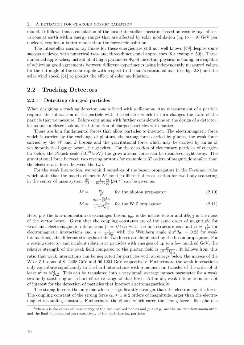
Using data from past cosmic ray experiments [34, 37–48] fig. 2.7 illustrates the correlationbetween the fitted Φ0 and the solar activity as indicated by the number of sunspots (see fig. 2.7).
The solar activity follows a cycle of 11-years or approximately 150 Carrington rotations2.After each cycle, the polarity A of the solar dipole reverses. A certain agreement exists betweenmodulation parameters Φ0 measured for one and the same particle species during the same epochof the solar cycle. The modulation parameters for different particle species measured during thesame epoch are however not compatible.
The data indicates that the determined Φ0 still depends on the mass and charge of the particle,pointing out the weakness of the force-field solution. Some of the disagreement between particlespecies may also arise from systematic uncertainties of the measurements and the used GALPROP
2One Carrington rotation is the time it takes the sun to rotate around its own axis as seen from earth (27.2753days). The first Carrington rotation was counted starting November 9, 1853.
8
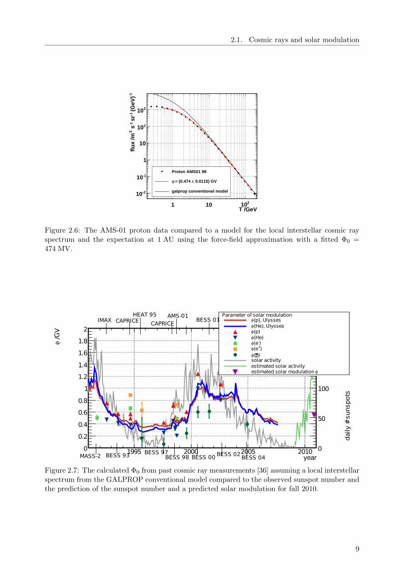
2.1. Cosmic rays and solar modulation
T /GeV1 10 210
-1 (
GeV
)-1
sr
-1 s
-2fl
ux
/m
-210
-110
1
10
210
310
Proton AMS01 98
0.0115) GV± = (0.474 φ
galprop conventionel model
Figure 2.6: The AMS-01 proton data compared to a model for the local interstellar cosmic rayspectrum and the expectation at 1 AU using the force-field approximation with a fitted Φ0 =474 MV.
year1995 2000 2005 2010
/GV
φ
0
0.2
0.4
0.6
0.8
1
1.2
1.4
1.6
1.8
2
dai
ly #
sunsp
ots
0
50
100
150
200
Parameter of solar modulation(p), Ulyssesφ(He), Ulyssesφ(p)φ(He)φ
)-(eφ)+(eφ
)p(φsolar activityestimated solar activity
φestimated solar modulation
MASS-2
IMAX
BESS 93
CAPRICEHEAT 95
CAPRICEAMS-01
BESS 97BESS 98 BESS 00
BESS 01
BESS 02BESS 04
Figure 2.7: The calculated Φ0 from past cosmic ray measurements [36] assuming a local interstellarspectrum from the GALPROP conventional model compared to the observed sunspot number andthe prediction of the sunspot number and a predicted solar modulation for fall 2010.
9
2. A detector for charged cosmic radiation
model. It follows that a calculation of the local interstellar spectrum based on cosmic rays obser-vations at earth within energy ranges that are affected by solar modulation (up to ∼ 10 GeV pernucleon) requires a better model than the force-field solution.
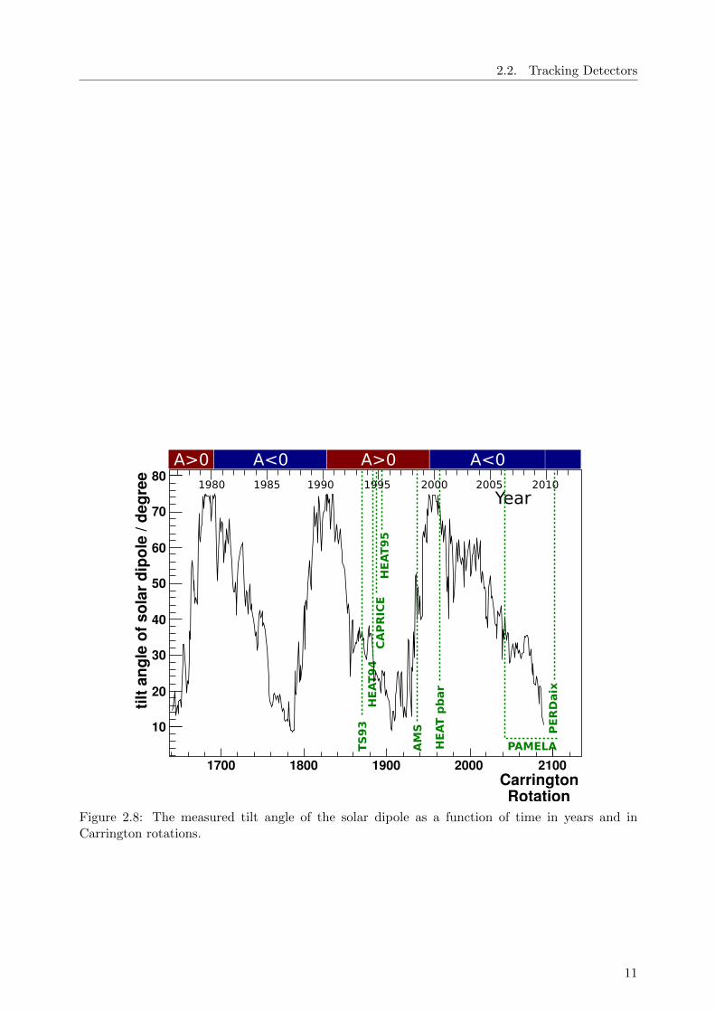
The interstellar cosmic ray fluxes for these energies are still not well known [49] despite somesuccess achieved with numerical two- and three-dimensional approaches (for example [50]). Thesenumerical approaches, instead of fitting a parameter Φ0 of uncertain physical meaning, are capableof achieving good agreements between different experiments using independently measured valuesfor the tilt angle of the solar dipole with respect to the sun’s rotational axis (see fig. 2.8) and thesolar wind speed [51] to predict the effect of solar modulation.
2.2 Tracking Detectors
2.2.1 Detecting charged particles
When designing a tracking detector, one is faced with a dilemma: Any measurement of a particlerequires the interaction of the particle with the detector which in turn changes the state of theparticle that we measure. Before continuing with further considerations on the design of a detector,let us take a closer look at the interaction of charged-particles with matter.
There are four fundamental forces that allow particles to interact. The electromagnetic forcewhich is carried by the exchange of photons, the strong force carried by gluons, the weak forcecarried by the W and Z bosons and the gravitational force which may be carried by an as ofyet hypothetical gauge boson, the graviton. For the detection of elementary particles of energiesfar below the Planck scale (1019 GeV) the gravitational force can be dismissed right away. Thegravitational force between two resting protons for example is 37 orders of magnitude smaller thanthe electrostatic force between the two.
For the weak interaction, we remind ourselves of the boson propagators in the Feynman ruleswhich state that the matrix elements M for the differential cross-section for two-body scatteringin the center of mass system dσ
dΩ = 164π2s
pfpi|M|23 can be given as:
M =gµνp2
for the photon propagator (2.10)
M =gµν−
pµpν
M2W,Z
p2−M2W,Z
for the W,Z propagator (2.11)
Here, p is the four-momentum of exchanged boson, gµν is the metric tensor and MW,Z is the massof the vector boson. Given that the coupling constants are of the same order of magnitude forweak and electromagnetic interactions (e =
√4πα with the fine structure constant α = 1
137 forelectromagnetic interactions and g = e
sin θWwith the Weinberg angle sin2 θW = 0.23 for weak
interactions), the different strengths of the two forces are dominated by the boson propagator. Fora resting detector and incident relativistic particles with energies of up to a few hundred GeV, the
relative strength of the weak field compared to the photon field is p2
p2−M2W,Z
. It follows from this
ratio that weak interactions can be neglected for particles with an energy below the masses of theW or Z bosons of 81.2468 GeV and 90.1234 GeV respectively. Furthermore the weak interactionsonly contribute significantly to the hard interactions with a momentum transfer of the order of atleast p2 ≈ M2
W,Z. This can be translated into a very small average impact parameter for a weaktwo-body scattering or a short effective range of that force. All in all, weak interactions are notof interest for the detection of particles that interact electromagnetically.
The strong force is the only one which is significantly stronger than the electromagnetic force.The coupling constant of the strong force αs ≈ 1 is 2 orders of magnitude larger than the electro-magnetic coupling constant. Furthermore the gluons which carry the strong force - like photons
3where s is the center of mass energy of the two involved bodies and pi and pf are the incident four-momentumand the final four-momentum respectively of the participating particles
10
2.2. Tracking Detectors
A<0 A<0A>0A>0
AM
S
CA
PR
ICE
HEAT p
bar
HEAT94
HEAT95
TS
93
PAMELA
1700 1800 1900 2000 2100
10
20
30
40
50
60
70
80
CarringtonRotation
tilt
an
gle
of
so
lar
dip
ole
/ d
eg
ree
1980 1985 1990 2005
Year1995 2000 2010
PER
Daix
Figure 2.8: The measured tilt angle of the solar dipole as a function of time in years and inCarrington rotations.
11

2. A detector for charged cosmic radiation
- are mass-less, so in principle the strong force should dominate interactions. However there aresome fundamental differences between gluons and photons: Gluons couple to color charge whichis only carried by only half of the twelve fermions commonly believed to be elementary particles,namely the six quarks, the constituents of the hadrons. Next, photons which couple to electriccharge, do not carry any charge themselves. Gluons which couple to color charge on the otherhand carry a color charge, meaning that there is a self-coupling of gluons to other gluons.
It follows that first of all, strong interactions do not play any role in 0th order, when trying todetect leptons. Secondly, if a hadron radiates a gluon carrying color-charge, it can be expected tobe subject to an attractive force between it and the originating hadron4. Observations suggest thatthis attractive force does not diminish with distance so the radiated gluon will necessarily remainconfined within the vicinity of the hadron. It follows that the effective range of the strong forcemust be limited. Measurements5 suggest that this effective range is approximately 1 fm. UsingHeisenberg’s Principle of Uncertainty ∆p∆x ≥ ~
2 , the momentum transfer of a strong interactionwith a nucleus has to be of the order of at least 100 MeV/c. For the passage of a relativistic protonin matter, for example, the energy loss by way of hadronic interactions may even dominate. Theindividual interaction, however, is much harder than the average electromagnetic interaction andis also often likely to result in the destruction of the measured particle. This makes relying onstrong interactions of charged hadrons unpractical for tracking detectors6 which are supposed todisturb the measured particle as little as possible.
2.2.2 Observable properties of energetic charged-particles
Position, velocity and momentum
If a single charged-particle is detected, only some of its properties are accessible for a directmeasurement. Any sufficiently high segmented detector can measure its position in time and spacegiving us the particle trajectory ~x (α) as a function of some parametrization α. By measuring thedeflection of a particle in a magnetic field, one can also determine its rigidity ~R which is definedas the product of particle momentum ~p and its charge q. The radius of curvature rκ of a particlein a locally homogeneous magnetic field can be given as
rκ =
∣∣∣~R∣∣∣∣∣∣~ep × ~B∣∣∣ (2.12)
where ~ep is the normalized direction of the particle.If one records the time along with the particle position one can determine the particle trajectory
as a function of time ~x (t) and thereby it’s velocity β = 1c
∣∣∣d~xdt ∣∣∣.Energy loss
The mean energy loss of charged particles is another quantity that is accessible to measurement.The mean energy deposit of a particle per path length in matter dE/dx depends on the particlecharge z, velocity β and its Lorentz factor γ as well as on the matter it passes through. The averagedE/dx for all charged particles except for electrons and positrons over a wide energy range (fromβγ ≈ 0.1 to βγ ≈ 1000) is described by the Bethe-Bloch formula. The Bethe-Bloch formula
4A more accurate explanation uses the fact that the strong force fits a non-abelian gauge theory. This fact canbe used to construct an asymptotic freedom for quarks in the ultra-violet limit while the coupling strength betweenquarks has an infinity at some cut-off energy [52].
5e.g. the Geiger-Marsden experiment which determined the size of a gold nucleus from the scattering of alphaparticles in 1909
6unlike for example (hadronic) calorimeters which are designed to stop the particle entirely
12

2.2. Tracking Detectors
considers the ionization (and excitation) energy loss of charged particles due to electromagneticscattering of a particle by valence electrons of the passed matter and reads:
−⟨dE
dx
⟩=
4π~2c2
mec2·α2 z
2
β2· NAρZ
A
[1
2ln
2mec2β2γ2Tmax
I2− β2 − δ (βγ)
2
](2.13)
Here, me is the electron mass, α the fine structure constant, NA Avogadro’s number, A the averageatomic mass of the material the particle passes through, ρ its density and Z is its average atomicnumber. The mean excitation potential of the bulk material I, the maximum kinetic energytransfer to a free electron Tmax and the density effect correction δ (βγ) to ionization energy losscan be looked up in literature [10]. Looking at Bethe’s formula, one finds that the quantity dE/dxallows determining the velocity of weakly relativistic particles and also the Lorentz-γ for highlyrelativistic particles of the same mass and charge. The energy loss of slow particles (γβ . 4) riseswith 1
β2 . For highly relativistic particles (γβ & 4) a logarithmic rise in dE/dx with ln γ2 is found.Just as importantly, one can determine the charge number z of the detected particle if γ is knowndue to the z2 dependence of dE/dx.
For electrons, the energy loss starting at momenta p & 100 MeV is dominated by radiativeenergy losses by Bremsstrahlung which can be described by an exponential law with the materialdependent radiation length X0 [10]:
−⟨dE
dx
⟩=
E
X0(2.14)
Radiative energy losses for heavier particles do not dominate until βγ reaches ∼ 104.
Cerenkov and transition radiation
Further measurements of particle properties are possible by way of characteristic radiation whichis emitted when a particle passes through media of certain dielectric properties.
Whenever a particle moves through a medium with refractive index n at a velocity β whichis greater than the local phase velocity of light c
n it emits so-called Cerenkov radiation under acharacteristic angle θc [10]:
cos θc =1
βn(2.15)
The number of produced Cerenkov photons per path length at a wavelength λ increases with thesquare of the particle’s charge number z [10]:
d2N
dλdx=
2παz2
λ2
(1− 1
β2n2(λ)
)(2.16)
So, Cerenkov radiation allows a measurement of the velocity β via the angle under which thephotons are radiated with respect to the particle trajectory and a measurement z via the amountof radiated photons.
Transition radiation is emitted when a particle crosses the boundary between two media of dif-ferent dielectric constants. For the transition between vacuum and a material with a characteristicplasma frequency ωp the radiated energy is given as [10]:
∆E =1
3αz2γ~ωp (2.17)
The photons are emitted under a typical angle of 1/γ in forward direction with respected to theparticle. The number radiated photons grows as (ln γ)2 so the emitted spectrum becomes harderwith increasing γ.
Like the Cerenkov radiation, transition radiation allows a measurement of z because the totalradiated energy is proportional to z2. Additionally, the energy loss via transition radiation isproportional to γ which makes it complementary to the measurement of Cerenkov radiation whichmakes β accessible but saturates at β ≈ 1.
13

2. A detector for charged cosmic radiation
2.2.3 Material budget
The precision of a tracking detector is limited by the amount of detector material disturbing theparticle trajectory. For this reason, the material budget of any such detector is one of the mostimportant considerations.
The cumulative effect of many small angle coulomb scatterings at nuclei of the detector ma-terial is commonly referred to as multiple scattering. It is particularly detrimental to the spatialmeasurement of the particle trajectory. Consider a particle of momentum p, charge z and velocityβ which is deflected by material of thickness x and radiation length X0. The central 98 % of thedistribution of deflection angles θ can be described by a Gaussian with a width σθ given as [10]:
σθ =13.6MeV
βcpz√x/X0 [1 + 0.038 ln (x/X0)] (2.18)
in the planar projection.The minimization of multiple scattering is especially important when tracking low-energy par-
ticles with γβ ∼ 1.At very high energies γβ ∼ 1000, another issue arises from radiative losses. These lead to
an exponential increase of the energy loss with the amount of material that is traversed (see sec.2.2.2) instead of an almost linear one (as can be observed for minimum ionizing particles). Highlyrelativistic particles radiate Bremsstrahlungs photons which may be energetic enough to startelectromagnetic cascades. These cascades can significantly increase the occupancy in the trackeraround the primary particle track. This may lead to ambiguities in the identification of signalsbelonging to the primary particle and thereby decrease the tracking accuracy.
2.2.4 Existing concepts for tracking detectors
In order to compare the presented detector design to existing tracking detector technologies, abrief survey of these existing technologies shall be given here.
Nuclear Emulsion Detectors
The nuclear emulsion detector dates back to the earliest observations of ionizing particle radiation.It was based on a coincidental discovery by Henri Becquerel in 1896 [53] using photographic platesand has not significantly changed since. The detectors use an emulsion of small silver halidecrystals which are no more than a few microns in size. Upon exposure to ionizing radiation asilver halide crystal changes its crystalline structure. These changes can later be used to developan image of the particle track within the nuclear emulsion by using a chemical process to turnactivated crystals into metallic silver.
Among all commonly used particle detectors, nuclear emulsion detectors still have the bestposition resolution of approximately 1 µm. Additionally they allow a dE/dx-measurement basedon the density of activated silver halide crystals. However, an obvious drawback is that the devel-opment of an image of the particle track involves a complex chemical process that severely limitsthe readout rate of a nuclear emulsion detector. On the other hand the nuclear emulsion providesa natural storage for the particle information which makes it a good candidate for integrated fluxmeasurements.
Next to integrated flux measurement of for example cosmic rays and in medical applications,nuclear emulsion detectors are primarily used for the detection of rare interactions with low back-grounds as for example in the ντ -appearance measurement by OPERA [54].
Cloud Chambers and Bubble Chambers
Charles T. R. Wilson developed the cloud chamber around the same time as the discovery ofradioactivity by Becquerel. Originally intended as a device to study the formation of clouds,
14
2.2. Tracking Detectors
it uses air supersaturated with water or alcohol vapors. In this unstable system, ionized airmolecules become cloud condensation nuclei around which small droplets may form. Chargedparticles therefore leave tracks of small droplets within the cloud chamber which can be observedoptically. The cloud chamber remained a popular detector technology up to the 1940s. Its readoutcould be triggered by Geiger-Muller counters.
In the early 1950s Donald A. Glaser [55] developed the bubble chamber which uses an unstableliquid superheated above its boiling point. In this liquid the energy deposition of a charged particleleads to the formation of bubbles which are 0.1 mm to 1 mm in size achieving spatial resolutionsdown to 10 µm.
Since the superheated liquid starts to boil very quickly a bubble chamber does not allow acontinuous readout as some forms of the cloud chamber do. Instead the super-heating has to beperformed synchronized with the particle interaction which allows a readout rate of a few tens ofHertz [10]. The bubble chamber is therefore mainly suitable for accelerators. Due to its limitations,the bubble chamber only played a marginal role in the detection of charged particles over the lasttwenty-five years.
Gaseous Tracking Detectors
The invention of gaseous detectors for measuring ionizing radiation dates back to the Geiger counterdeveloped by Hans Geiger and Ernest Rutherford in 1908 [56]. The basic principle of exploitingthe gas amplification process in high electric fields was then used for spark chambers in 1930swhich exploited the visible sparks between charged metallic plates that developed around seedions produced by a passing charged particle. In the 1960s this technology was improved towardsthe streamer chamber that prevented complete electrical breakdowns between the metallic plates bypulsing the electric field while still producing visible plasma clouds as a result of gas amplificationprocesses of primary electrons [57]. The streamer chamber allows better spatial resolutions ofup to 300 µm and is in contrast to spark chambers capable of performing dE/dx-measurements.Streamer chambers were most notably used till the 1980s, for example by the UA5 detector [58].
Georges Charpak et al. developed the multi-wire proportional chamber in 1968 [59] whichreplaced the metallic plates of the streamer chamber with planes of thin wires and moved fromthe optical readout to a purely electrical one. Wire chambers achieve resolutions of the order of0.1 mm by measuring the charge deposited on each wire as well as the drift time and also providedE/dx measurements. Many of today’s experiments at accelerators (ATLAS, CMS) [60] and alsocosmic ray experiments (BESS, AMS-02) [61,62] use wire chambers to track charged particles.
Another development in gaseous charged-particle trackers are time projection chambers [63]which were proposed in 1976 by David Nygren. Time projection chambers are gas chambers insidea strong homogeneous magnetic field. Primary electron clouds produced by charged particles driftalong the magnetic field lines in an electric field until they are amplified and detected employinga gas-electron multiplication process in very high electric fields near one end of the gas chamber.Time projection chambers are capable of measuring all three spatial coordinates by measuring thedrift time along the magnetic field inside the chamber.
One of the primary advantages of gaseous detectors is that the sensitive medium has a verylow density, so multiple scattering is much less of an issue in comparison to existing solid-statedetectors. An important issue to consider is that gaseous detectors have been known to exhibitaging which is mostly related to the degradation of the gas mixture and the polymerization ofgas molecules in the amplification zone. Furthermore the operation of a gaseous detector as atracker often requires a significant overhead in order to control the properties of the employed gas(to determine drift times and quantify gas amplification as well as to control degradation of thedetector due to aging) and to provide the required high voltages of ∼ 1 kV − 100 kV.
15
2. A detector for charged cosmic radiation
Scintillating Fiber Trackers
The use of scintillating materials which emit visible (or near-visible) light following the excitationby a charged particle can be traced back to the late 19th century as well. In particular it wasWilhelm K. Rontgen who discovered in 1895 the fluorescence of barium platinocyanide under theexposure to X-rays [64]. The process of scintillation has been used for the detection of ionizingradiation since the late 1940s [65]. In the 1950s a lot of research happened on organic scintillators[66] which were first being used for nuclear physics and later also in particle physics.
The viability of scintillating materials for the use in tracking detectors required the segmenta-tion of these scintillating materials. In 1960 R. J. Potter and R. E. Hopkins [67] proposed using astack of cylindrical fibers from organic scintillator read out via an image intensifier tube to trackcharged particles. However, these attempts were abandoned in favor of the superior bubble andspark chambers [68].
In the 1980s scintillating fibers experienced a renaissance due to the requirement for particledetectors which were able to detect events at a high frequency. While scintillating fiber trackers atthat time achieved only mediocre spatial resolutions, the low cost of scintillating fiber material andlow absorption length of several meters prompted its use to instrument large areas, most notablyby the UA2, CHORUS, DØ and OPERA experiments.
In 1987 the upgraded UA2 experiment used the first large scale scintillating fiber tracker [69]consisting of 24 layers of 2.4 m long and 1 mm thick scintillating fibers7 with a combination ofimage-intensifiers and CCDs as readout. The detector was designed as a pre-shower detector andtherefore offered only a poor spatial resolution of 0.39 mm [70]. A similar readout scheme was usedby the CHORUS scintillating fiber tracker that consisted of 1.2 million 2.3 m long and 0.5 mmthick round scintillating fibers [71]. The CHORUS fiber tracker achieved a spatial resolution of0.18 mm in ribbons of 7 staggered fiber layers. Similar in its design to the CHORUS fiber trackeris the K2K scintillating fiber tracker [72] which used 275,000 0.692 mm thick fibers arranged in3.7 m long double layers. With this setup a spatial resolution of 0.64 mm per double layer wasachieved [73].
The E835 experiment [74] and the upgraded DØ detector [75] use staggered double layers of0.835 mm thick fibers read out by visible-light photon counters (VLPCs) [76]. The used scintillatingfibers were approximately 1 m in length coupled to 4 m of clear wave-guiding fiber in case of E835and 1.6 m− 2.5 m in length coupled to 8 m− 12 m of clear fiber in case of DØ . With this setupE835 achieved a spatial resolution of the order of 0.1 mm while DØ specifies a spatial resolutionof 0.136 mm [77].
An entirely different approach was used by the OPERA target tracker [78]. This detector used26.3 mm wide and 6.86 m long scintillator bars with a 1 mm thick wavelength shifting fiber readout by a photomultiplier tube. This setup achieved a spatial resolution of the order of millimeters.
While scintillating fibers are capable of covering large areas due to the long attenuation lengthof light within the fiber, the achieved spatial resolution per unit of detector material is generallymuch worse than for silicon or gaseous detectors [10].
Silicon Trackers
Since approximately 1950 Germanium which was earlier used to sense radar waves, became popularin high energy and nuclear physics for calorimetric devices. This application uses the fact thatthe energy deposited by ionizing radiation generates minority carriers in a depleted semiconductorthat can then be detected as a current.
In the early 1980s it became possible to produce silicon wafers of sufficient size and qualityto use structured silicon as a tracking detector. Among the first experiments to use silicon stripdetectors that perform position measurements in two coordinates was the NA1 experiment [79]in 1980. Silicon detectors have the ability to perform measurements with a precision of a few
7In total 60,000 fibers were used for the UA2 experiment.
16
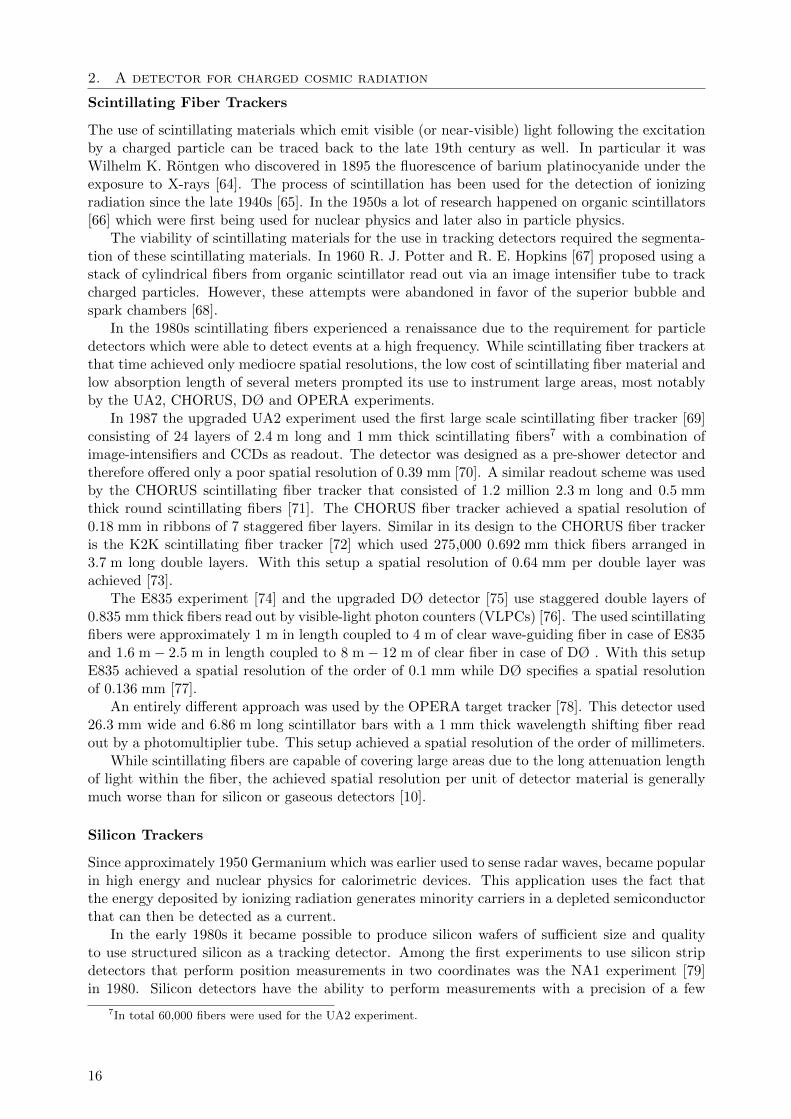
2.3. The PERDaix experiment
(a) Launch of the BEXUS-11 bal-loon.
(b) The trajectory of BEXUS-11.
Figure 2.9: PERDaix launch and flight with BEXUS-11.
microns with excellent timing properties limited only by the drift and diffusion times of minoritycarriers in the semiconductor. As a result silicon detectors are unrivaled as vertex detectors forcolliders. No other technology can perform measurements at a rate of several megahertz with acomparable single point resolution. Today, structured silicon is therefore the dominant trackingdetector technology next to gaseous detectors.
The effective strip length of today’s silicon strip sensors is limited to approximately 0.5 mgiving other technologies an edge over silicon when a large area has to be instrumented with alimited number of readout channels.
2.3 The PERDaix experiment
2.3.1 Motivation
The promotion of a better understanding of solar modulation is the scientific motivation behindthe Proton Electron Radiation Detector Aix-la-Chapelle (PERDaix). The PERDaix detector isa small detector for low-energetic cosmic rays. It contains a magnet spectrometer which has ageometrical acceptance close to 30 cm2 and a maximum detectable rigidity (MDR) of about 10 GV.The whole detector has a power consumption of 60 W and a weight of 40 kg. The experiment isdesigned for a short-duration balloon flight with a helium balloon within the scope of the BalloonEXperiments for University Students (BEXUS) [80] program. This thesis studies the feasibility ofusing spectrometers based on scintillating fibers in balloon-based experiments. The launch of thePERDaix experiment with a 100,000 m3 helium balloon from Kiruna, Sweden on November 23rd,2011 as a part of the BEXUS-11 payload concludes this study. During the flight it achieved analtitude of 33 km and traveled a distance of ∼ 450 km (see fig. 2.9) within about 4 hours.
2.3.2 Overview of the PERDaix instrument
The PERDaix cosmic ray spectrometer consists of three sub-detectors. Two double-layers ofscintillator panels with silicon photomultiplier readout are used to measure the time of flight of aparticle through the detector. In addition they produce a trigger for the readout electronics [81]. A
17
2. A detector for charged cosmic radiation
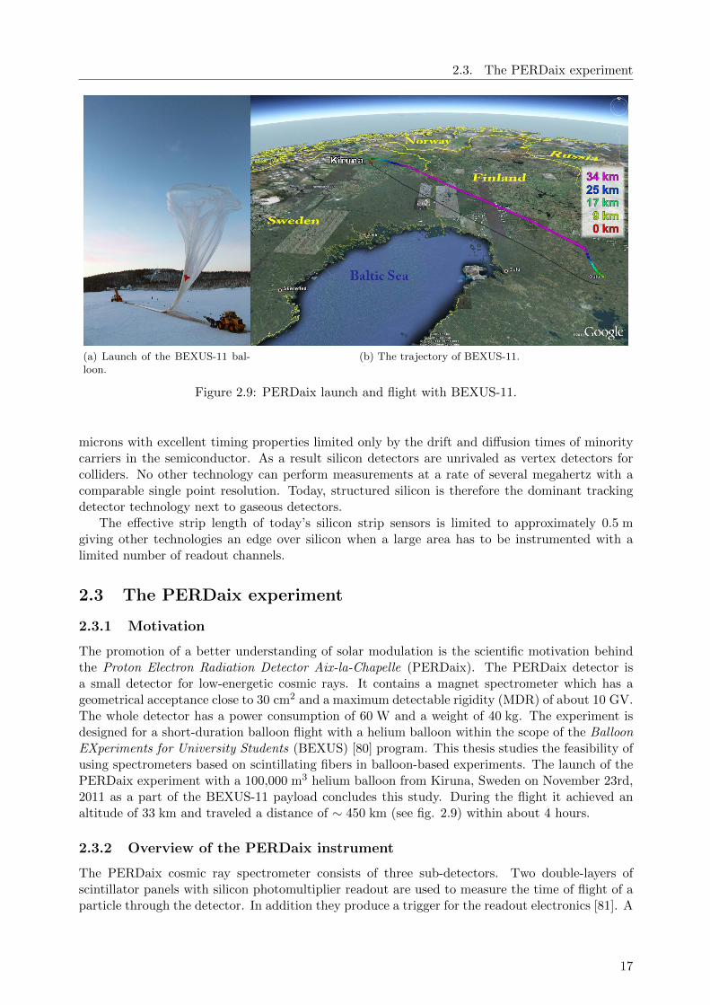
(a) A mechanical drawing of the PERDaix detector. (b) The opened PERDaix detector.
Figure 2.10: A mechanical drawing showing the structure of the PERDaix experiment without theouter carbon-fiber-composite frame.
transition radiation detector from 256 proportional straw tubes arranged in an eight layer sandwichwith an irregular polyethylene/polypropylene fleece radiator is included to separate protons fromelectrons. The design of this transition radiation detector is very similar to that of the AMS-02 TRD [62, 82]. A hollow cylindrical magnet array made up from NdFeB magnets provided analmost homogeneous magnetic field of B ≈ 0.2 T. Four layers of scintillating fiber modules withan internal stereo angle of 1 deg provide trajectory measurements. The tracker in combinationwith the magnet offers a rigidity measurement with a maximum detectable rigidity of ∼ 10 GV.
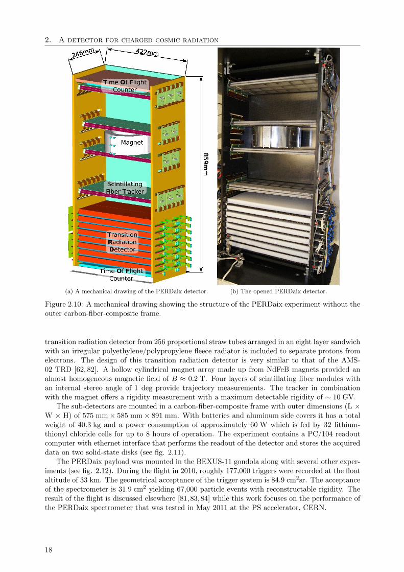
The sub-detectors are mounted in a carbon-fiber-composite frame with outer dimensions (L ×W × H) of 575 mm× 585 mm× 891 mm. With batteries and aluminum side covers it has a totalweight of 40.3 kg and a power consumption of approximately 60 W which is fed by 32 lithium-thionyl chloride cells for up to 8 hours of operation. The experiment contains a PC/104 readoutcomputer with ethernet interface that performs the readout of the detector and stores the acquireddata on two solid-state disks (see fig. 2.11).
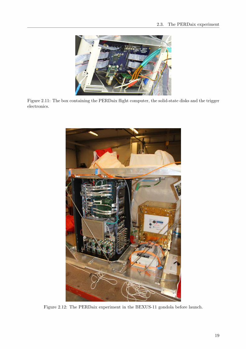
The PERDaix payload was mounted in the BEXUS-11 gondola along with several other exper-iments (see fig. 2.12). During the flight in 2010, roughly 177,000 triggers were recorded at the floataltitude of 33 km. The geometrical acceptance of the trigger system is 84.9 cm2sr. The acceptanceof the spectrometer is 31.9 cm2 yielding 67,000 particle events with reconstructable rigidity. Theresult of the flight is discussed elsewhere [81,83,84] while this work focuses on the performance ofthe PERDaix spectrometer that was tested in May 2011 at the PS accelerator, CERN.
18
2.3. The PERDaix experiment
Figure 2.11: The box containing the PERDaix flight computer, the solid-state disks and the triggerelectronics.
Figure 2.12: The PERDaix experiment in the BEXUS-11 gondola before launch.
19

Chapter 3
Scintillating Fiber Detector Modules
This chapter describes the properties of scintillating fiber modules and the production of scintil-lating fiber modules. It shows the different module designs of a prototype tested in 2009 and thePERDaix scintillating fiber tracker.
3.1 Scintillating Fibers
3.1.1 Motivation
Scintillating fibers are investigated for a balloon-borne spectrometer as was mentioned in theprevious chapter. An important limitation for balloon-borne and also space-based experiments isthe maximum weight of the total instrument which has strong implications on many other aspects,as for example the maximum permissible power consumption. Additionally, the restrictions placedupon the scientific payload by the means used to lift it to high altitudes limit the weight and thusthe strength of the magnetic field within a magnet spectrometer within air-borne or space-bornedetector. The resulting effect on the momentum resolution can be compensated by increasing thelever arm of the outer-most tracker layers. This necessitates the production of large-area trackingdetectors if the acceptance of the detector should not suffer [85].
Gaseous detectors often require a significant overhead in terms of gas systems, pressure vesselsand high voltage supply systems which discourage their use in balloon and space-based exper-iments. Furthermore, the application of high voltages to facilitate gas electron multiplicationimplies the additional risk of corona discharges in soft vacuum environments as found in thestratosphere with atmospheric pressures between 1 hPa and 10 hPa.
For silicon strip detectors, the minimum readout granularity at a given spatial resolution isimposed by the signal-over-noise ratio which decreases with the capacitance of a silicon strip (whichin turn is proportional to the length of the strip) [10]. While the maximum strip length which hasbeen realized for a silicon strip detector so far was 60 cm [86], the attenuation length of scintillatingfibers which is of the order of several meters, allows the production of long modules which lead toa lower number of readout channels and thus to a lower total power consumption for the detectorfor the same spatial resolution and instrumented area.
3.1.2 Properties of plastic scintillating fibers
At the center of a plastic scintillating fiber is a core from an organic polymer such as polystyrene(PS) which is doped with a few percent of an organic dye that allows a de-excitation of moleculesin the polymer by way of emitting scintillation light [87]. Scintillation light that is produced withinthe fiber core can partly be trapped in the fiber by surrounding the core with claddings whichhave lower refractive indices than the core.
For commercially available fibers, the core has a refractive index of 1.59 [88] to 1.60 [89] andis coated with a layer of polymethylmethacrylate (PMMA) with a refractive index of 1.49 and a
21

3. Scintillating Fiber Detector Modules
Scintillating CorePolystyrene + Dyes
n = 1.59 .. 1.60density = 1.05 g/cm3
Inner CladdingPMMA
n = 1.49density = 1.19 g/cm3
Outer CladdingFluorinated MMA
n = 1.42density = 1.43 g/cm3
ray trapped in core
ray trapped in cladding
z
x
Figure 3.1: A schematic view showing a double clad scintillating fiber. Light produced within thescintillator is partly trapped due to total internal reflection.
thickness of tens of microns. An additional cladding of fluorinated methylmethacrylate (FMMA)with a refractive index of 1.42 can be applied to the PMMA cladding in order to increase the lightcollection efficiency of the scintillating fiber (see fig. 3.1). Due to its poor adhesive properties,the FMMA cladding is commonly not used as the primary coating on the fiber core. The totaldiameter of the fiber varies between 0.25 mm and several mm for commercially available fibers.
3.1.3 Mechanical properties of thin scintillating fibers
The spatial resolution of a tracking detector made up from scintillating fibers has to be limited bythe diameter of the scintillating fibers. For the development of a high-resolution scintillating fibertracker, the thinnest commercially available fibers (see Tab. 3.1) are investigated.
Table 3.1: Nominal mechanical properties of scintillating fibers tested during the development ofthe scintillating fiber tracker presented in this work [88] [89].
inner cladding outer claddingType diameter thickness thickness
/ µm / µm / µm
Bicron BCF-20 250 7.5 2.5
Kuraray SCSF-81M 250 7.5 7.5
Kuraray SCSF-78MJ 250 7.5 7.5
22
3.1. Scintillating Fibers
fiber on spool from
manufacturer
second spool forfurther handling
of fiber
microscope
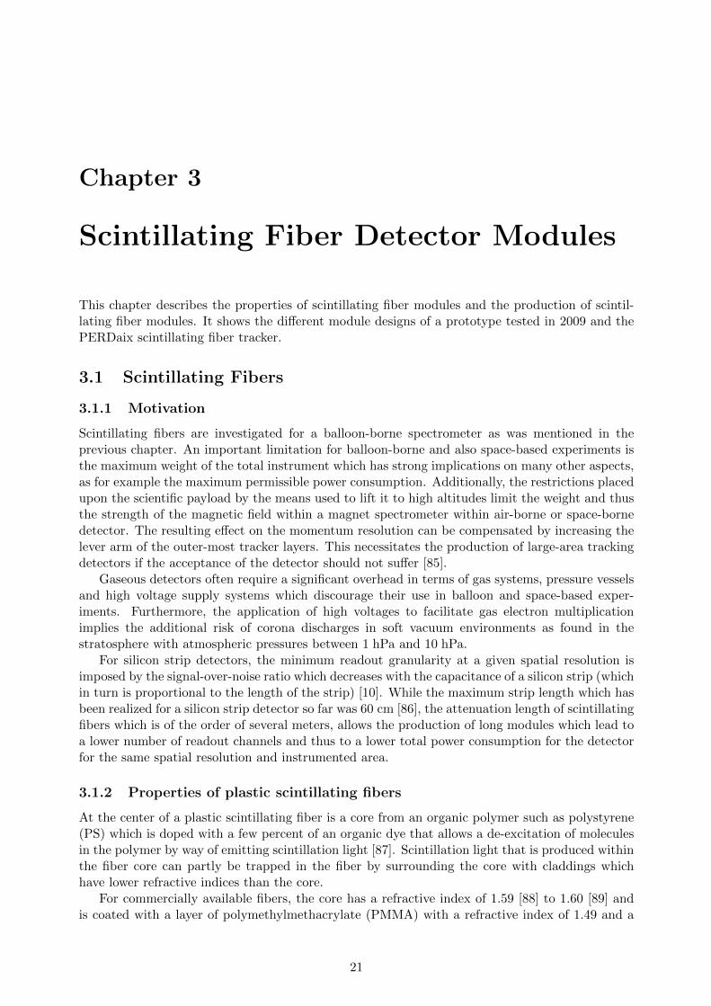
(a) A schematic of a setup to scan the fiber. (b) One frame from the microscope used to measurethe fiber diameter.
Figure 3.2: The measurement of the scintillating fiber diameter with microscope cameras.
20
40
60
80
100
120
140
160
180
00 50 100 150 200 250 300 350 400 450
position y / pixel
deriv
ativ
e of
lum
inan
ce /
arb.
uni
ts
threshold
fiber edges
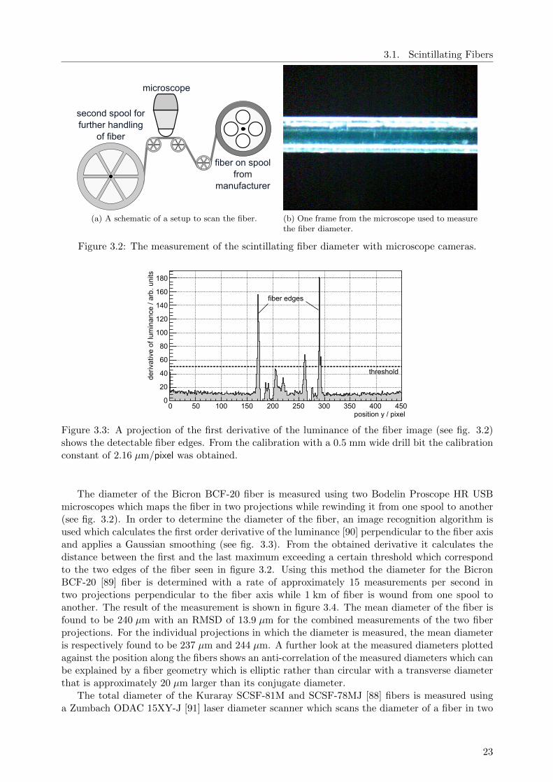
Figure 3.3: A projection of the first derivative of the luminance of the fiber image (see fig. 3.2)shows the detectable fiber edges. From the calibration with a 0.5 mm wide drill bit the calibrationconstant of 2.16 µm/pixel was obtained.
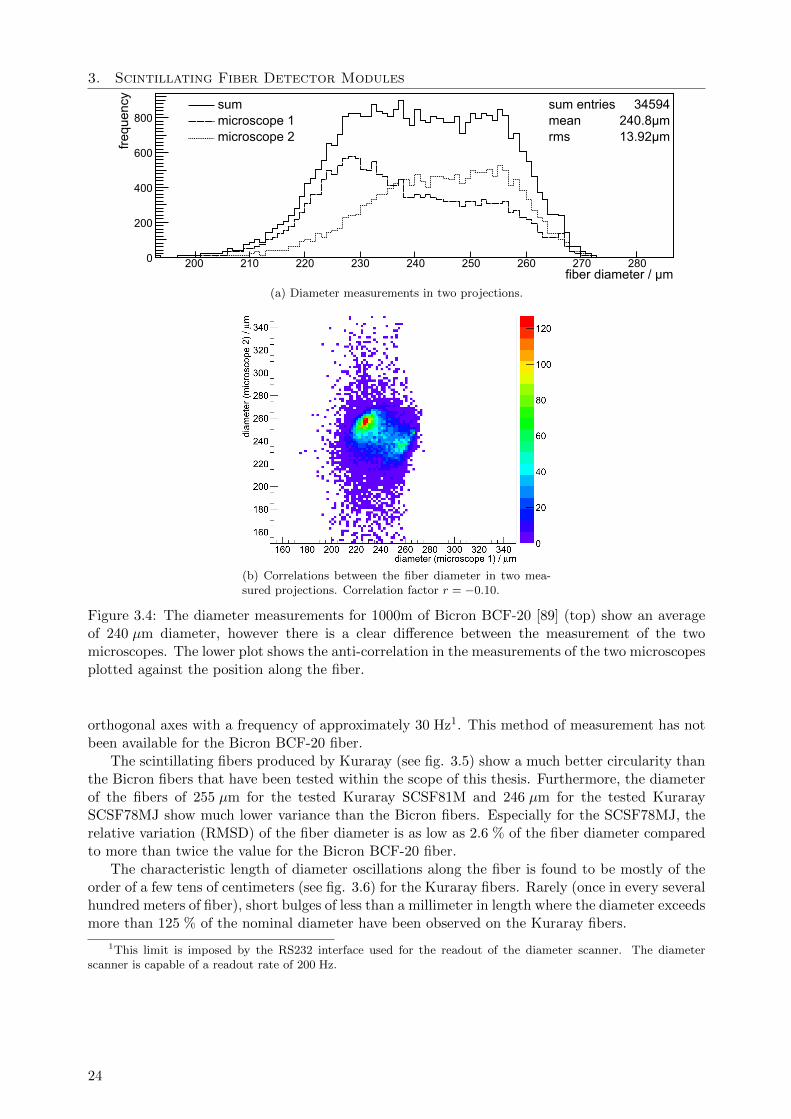
The diameter of the Bicron BCF-20 fiber is measured using two Bodelin Proscope HR USBmicroscopes which maps the fiber in two projections while rewinding it from one spool to another(see fig. 3.2). In order to determine the diameter of the fiber, an image recognition algorithm isused which calculates the first order derivative of the luminance [90] perpendicular to the fiber axisand applies a Gaussian smoothing (see fig. 3.3). From the obtained derivative it calculates thedistance between the first and the last maximum exceeding a certain threshold which correspondto the two edges of the fiber seen in figure 3.2. Using this method the diameter for the BicronBCF-20 [89] fiber is determined with a rate of approximately 15 measurements per second intwo projections perpendicular to the fiber axis while 1 km of fiber is wound from one spool toanother. The result of the measurement is shown in figure 3.4. The mean diameter of the fiber isfound to be 240 µm with an RMSD of 13.9 µm for the combined measurements of the two fiberprojections. For the individual projections in which the diameter is measured, the mean diameteris respectively found to be 237 µm and 244 µm. A further look at the measured diameters plottedagainst the position along the fibers shows an anti-correlation of the measured diameters which canbe explained by a fiber geometry which is elliptic rather than circular with a transverse diameterthat is approximately 20 µm larger than its conjugate diameter.
The total diameter of the Kuraray SCSF-81M and SCSF-78MJ [88] fibers is measured usinga Zumbach ODAC 15XY-J [91] laser diameter scanner which scans the diameter of a fiber in two
23
3. Scintillating Fiber Detector Modules
0
200
400
600
800
200 210 220 230 240 250 260 270 280fiber diameter / µm
sum entriesmeanrms
34594240.8µm13.92µm
summicroscope 1microscope 2
freq
uenc
y
(a) Diameter measurements in two projections.
(b) Correlations between the fiber diameter in two mea-sured projections. Correlation factor r = −0.10.
Figure 3.4: The diameter measurements for 1000m of Bicron BCF-20 [89] (top) show an averageof 240 µm diameter, however there is a clear difference between the measurement of the twomicroscopes. The lower plot shows the anti-correlation in the measurements of the two microscopesplotted against the position along the fiber.
orthogonal axes with a frequency of approximately 30 Hz1. This method of measurement has notbeen available for the Bicron BCF-20 fiber.
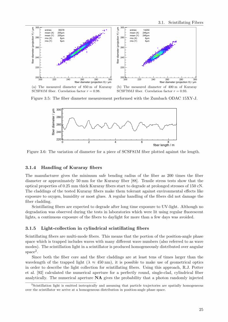
The scintillating fibers produced by Kuraray (see fig. 3.5) show a much better circularity thanthe Bicron fibers that have been tested within the scope of this thesis. Furthermore, the diameterof the fibers of 255 µm for the tested Kuraray SCSF81M and 246 µm for the tested KuraraySCSF78MJ show much lower variance than the Bicron fibers. Especially for the SCSF78MJ, therelative variation (RMSD) of the fiber diameter is as low as 2.6 % of the fiber diameter comparedto more than twice the value for the Bicron BCF-20 fiber.
The characteristic length of diameter oscillations along the fiber is found to be mostly of theorder of a few tens of centimeters (see fig. 3.6) for the Kuraray fibers. Rarely (once in every severalhundred meters of fiber), short bulges of less than a millimeter in length where the diameter exceedsmore than 125 % of the nominal diameter have been observed on the Kuraray fibers.
1This limit is imposed by the RS232 interface used for the readout of the diameter scanner. The diameterscanner is capable of a readout rate of 200 Hz.
24
3.1. Scintillating Fibers300
280
260
240
220
200200 220 240 260 280 300
fiber diameter (projection X) / µm
fiber
dia
met
er (
proj
ectio
n Y
) / µ
mentriesmean (X)mean (Y)rms (X)rms (Y)
39378255µm255µm
8µm9µm
(a) The measured diameter of 850 m of KuraraySCSF81M fiber. Correlation factor r = 0.98.
300
280
260
240
220
200200 220 240 260 280 300
fiber diameter (projection X) / µm
fiber
dia
met
er (
proj
ectio
n Y
) / µ
m
entriesmean (X)mean (Y)rms (X)rms (Y)
14250246µm246µm
6µm6µm
(b) The measured diameter of 400 m of KuraraySCSF78MJ fiber. Correlation factor r = 0.93.
Figure 3.5: The fiber diameter measurement performed with the Zumbach ODAC 15XY-J.
0 2 4 6 8220
240
260
280
300
fiber
dia
met
er /
µm
fiber length / m
Figure 3.6: The variation of diameter for a piece of SCSF81M fiber plotted against the length.
3.1.4 Handling of Kuraray fibers
The manufacturer gives the minimum safe bending radius of the fiber as 200 times the fiberdiameter or approximately 50 mm for the Kuraray fiber [88]. Tensile stress tests show that theoptical properties of 0.25 mm thick Kuraray fibers start to degrade at prolonged stresses of 150 cN.The claddings of the tested Kuraray fibers make them tolerant against environmental effects likeexposure to oxygen, humidity or most glues. A regular handling of the fibers did not damage thefiber cladding.
Scintillating fibers are expected to degrade after long time exposure to UV-light. Although nodegradation was observed during the tests in laboratories which were lit using regular fluorescentlights, a continuous exposure of the fibers to daylight for more than a few days was avoided.
3.1.5 Light-collection in cylindrical scintillating fibers
Scintillating fibers are multi-mode fibers. This means that the portion of the position-angle phasespace which is trapped includes waves with many different wave numbers (also referred to as wavemodes). The scintillation light in a scintillator is produced homogeneously distributed over angularspace2.
Since both the fiber core and the fiber claddings are at least tens of times larger than thewavelength of the trapped light (λ ≈ 450 nm), it is possible to make use of geometrical opticsin order to describe the light collection for scintillating fibers. Using this approach, R.J. Potteret al. [92] calculated the numerical aperture for a perfectly round, single-clad, cylindrical fiberanalytically. The numerical aperture NA gives the probability that a photon randomly injected
2Scintillation light is emitted isotropically and assuming that particle trajectories are spatially homogeneousover the scintillator we arrive at a homogeneous distribution in position-angle phase space.
25
3. Scintillating Fiber Detector Modules
helix modes(cladding)
2.84%
cladding modes2.42%
helix modes (core)5.89%
core modes6.29%
0 0.1 0.2 0.3 0.4 0.5 0.6 0.7 0.8 0.9 1
0.5
0.4
0.3
0.2
0.1
0
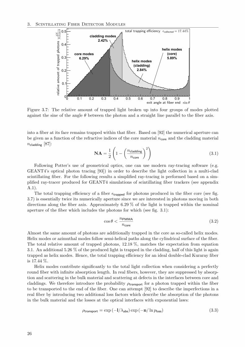
Figure 3.7: The relative amount of trapped light broken up into four groups of modes plottedagainst the sine of the angle θ between the photon and a straight line parallel to the fiber axis.
into a fiber at its face remains trapped within that fiber. Based on [92] the numerical aperture canbe given as a function of the refractive indices of the core material ncore and the cladding materialncladding [87]:
NA =1
2
(1−
(ncladdingncore
)2)
(3.1)
Following Potter’s use of geometrical optics, one can use modern ray-tracing software (e.g.GEANT4’s optical photon tracing [93]) in order to describe the light collection in a multi-cladscintillating fiber. For the following results a simplified ray-tracing is performed based on a sim-plified ray-tracer produced for GEANT4 simulations of scintillating fiber trackers (see appendixA.1).
The total trapping efficiency of a fiber εtrapped for photons produced in the fiber core (see fig.3.7) is essentially twice its numerically aperture since we are interested in photons moving in bothdirections along the fiber axis. Approximately 6.29 % of the light is trapped within the nominalaperture of the fiber which includes the photons for which (see fig. 3.1):
cos θ <nPMMA
ncore(3.2)
Almost the same amount of photons are additionally trapped in the core as so-called helix modes.Helix modes or azimuthal modes follow semi-helical paths along the cylindrical surface of the fiber.The total relative amount of trapped photons, 12.18 %, matches the expectation from equation3.1. An additional 5.26 % of the produced light is trapped in the cladding, half of this light is againtrapped as helix modes. Hence, the total trapping efficiency for an ideal double-clad Kuraray fiberis 17.44 %.
Helix modes contribute significantly to the total light collection when considering a perfectlyround fiber with infinite absorption length. In real fibers, however, they are suppressed by absorp-tion and scattering in the bulk material and scattering at defects in the interfaces between core andcladdings. We therefore introduce the probability ρtransport for a photon trapped within the fiberto be transported to the end of the fiber. One can attempt [92] to describe the imperfections in areal fiber by introducing two additional loss factors which describe the absorption of the photonsin the bulk material and the losses at the optical interfaces with exponential laws:
ρtransport = exp (−l/λabs) exp (−n/ ln ploss) (3.3)
26
3.1. Scintillating Fibers
acce
ptan
ce li
mit
of b
eam
pro
filer
10
9
8
7
6
4
5
3
2
1
00 0.1 0.2 0.3 0.4 0.5 0.6 0.7 0.8 0.9 1
perfectly round cylindrical fiberKuraray SCSF-81M (20cm)
Kuraray SCSF-81M (40cm)
Kuraray SCSF-81M (80cm)
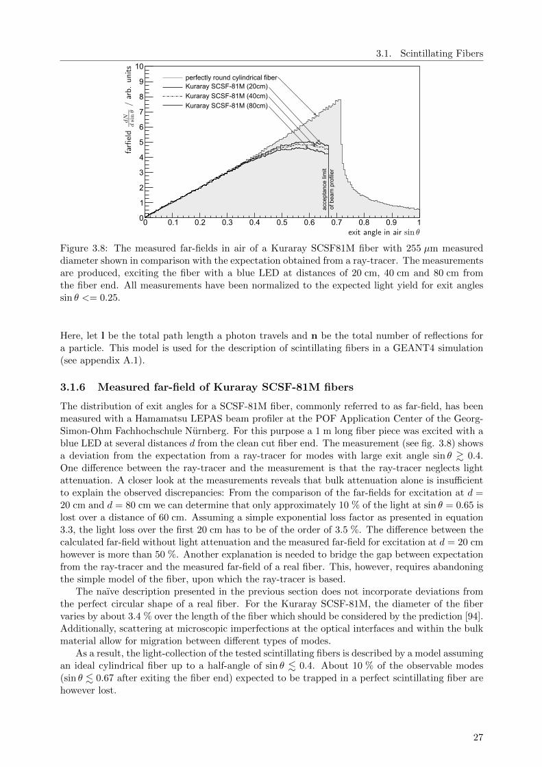
Figure 3.8: The measured far-fields in air of a Kuraray SCSF81M fiber with 255 µm measureddiameter shown in comparison with the expectation obtained from a ray-tracer. The measurementsare produced, exciting the fiber with a blue LED at distances of 20 cm, 40 cm and 80 cm fromthe fiber end. All measurements have been normalized to the expected light yield for exit anglessin θ <= 0.25.
Here, let l be the total path length a photon travels and n be the total number of reflections fora particle. This model is used for the description of scintillating fibers in a GEANT4 simulation(see appendix A.1).
3.1.6 Measured far-field of Kuraray SCSF-81M fibers
The distribution of exit angles for a SCSF-81M fiber, commonly referred to as far-field, has beenmeasured with a Hamamatsu LEPAS beam profiler at the POF Application Center of the Georg-Simon-Ohm Fachhochschule Nurnberg. For this purpose a 1 m long fiber piece was excited with ablue LED at several distances d from the clean cut fiber end. The measurement (see fig. 3.8) showsa deviation from the expectation from a ray-tracer for modes with large exit angle sin θ & 0.4.One difference between the ray-tracer and the measurement is that the ray-tracer neglects lightattenuation. A closer look at the measurements reveals that bulk attenuation alone is insufficientto explain the observed discrepancies: From the comparison of the far-fields for excitation at d =20 cm and d = 80 cm we can determine that only approximately 10 % of the light at sin θ = 0.65 islost over a distance of 60 cm. Assuming a simple exponential loss factor as presented in equation3.3, the light loss over the first 20 cm has to be of the order of 3.5 %. The difference between thecalculated far-field without light attenuation and the measured far-field for excitation at d = 20 cmhowever is more than 50 %. Another explanation is needed to bridge the gap between expectationfrom the ray-tracer and the measured far-field of a real fiber. This, however, requires abandoningthe simple model of the fiber, upon which the ray-tracer is based.
The naıve description presented in the previous section does not incorporate deviations fromthe perfect circular shape of a real fiber. For the Kuraray SCSF-81M, the diameter of the fibervaries by about 3.4 % over the length of the fiber which should be considered by the prediction [94].Additionally, scattering at microscopic imperfections at the optical interfaces and within the bulkmaterial allow for migration between different types of modes.
As a result, the light-collection of the tested scintillating fibers is described by a model assumingan ideal cylindrical fiber up to a half-angle of sin θ . 0.4. About 10 % of the observable modes(sin θ . 0.67 after exiting the fiber end) expected to be trapped in a perfect scintillating fiber arehowever lost.
27
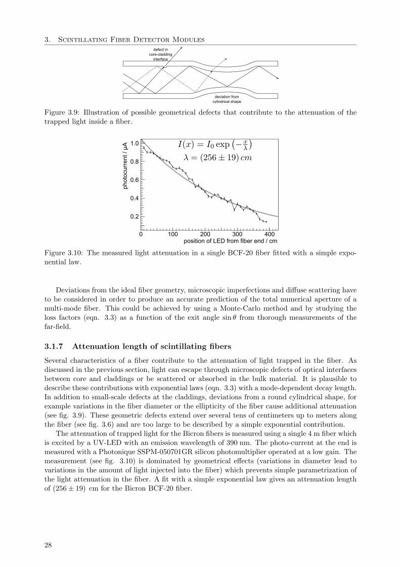
3. Scintillating Fiber Detector Modulesdefect in
core-cladding interface
deviation from cylindrical shape
Figure 3.9: Illustration of possible geometrical defects that contribute to the attenuation of thetrapped light inside a fiber.
0position of LED from fiber end / cm
0.2
0.4
0.6
phot
ocur
rent
/ µ
A
0.8
1.0
100 200 300 400
Figure 3.10: The measured light attenuation in a single BCF-20 fiber fitted with a simple expo-nential law.
Deviations from the ideal fiber geometry, microscopic imperfections and diffuse scattering haveto be considered in order to produce an accurate prediction of the total numerical aperture of amulti-mode fiber. This could be achieved by using a Monte-Carlo method and by studying theloss factors (eqn. 3.3) as a function of the exit angle sin θ from thorough measurements of thefar-field.
3.1.7 Attenuation length of scintillating fibers
Several characteristics of a fiber contribute to the attenuation of light trapped in the fiber. Asdiscussed in the previous section, light can escape through microscopic defects of optical interfacesbetween core and claddings or be scattered or absorbed in the bulk material. It is plausible todescribe these contributions with exponential laws (eqn. 3.3) with a mode-dependent decay length.In addition to small-scale defects at the claddings, deviations from a round cylindrical shape, forexample variations in the fiber diameter or the ellipticity of the fiber cause additional attenuation(see fig. 3.9). These geometric defects extend over several tens of centimeters up to meters alongthe fiber (see fig. 3.6) and are too large to be described by a simple exponential contribution.
The attenuation of trapped light for the Bicron fibers is measured using a single 4 m fiber whichis excited by a UV-LED with an emission wavelength of 390 nm. The photo-current at the end ismeasured with a Photonique SSPM-050701GR silicon photomultiplier operated at a low gain. Themeasurement (see fig. 3.10) is dominated by geometrical effects (variations in diameter lead tovariations in the amount of light injected into the fiber) which prevents simple parametrization ofthe light attenuation in the fiber. A fit with a simple exponential law gives an attenuation lengthof (256± 19) cm for the Bicron BCF-20 fiber.
28

3.1. Scintillating Fibers
HamamstsuS3590-08PIN diode
UV LED
fiber ribbon
~ 5m
~40 Vdc
RC filterKeithley Model 485Picoamperemeter
0 100 200 300 400 500position of LED from fiber end / cm
0.1
0.2
0.3
0.4
0.5
photocurrent/µA
Figure 3.11: The setup to measure the attenuation length (r) and the measured attenuation forabout 5 m long pieces of Kuraray SCSF78MJ fibers which can be described by a sum of twoexponential curves.
Table 3.2: The measured attenuation length for available Kuraray fibers averaged over multiplesamples using measurements from [95]. No significant difference between fibers of type SCSF-81Mand SCSF-78MJ are found.
Type I0/% I1/% λ0/cm λ1/cm
BCF-20 100 0 256± 19 -
SCSF-81M 52± 4 48± 3 66± 10 647± 70
SCSF-78MJ 46± 4 54± 5 74± 14 533± 57
The light attenuation for Kuraray fibers3, is measured for 5 m long fiber ribbons of aboutfive fibers. A ribbon is excited by UV LEDs while a reversely biased PIN diode attached to apico-amperemeter measures the photo-current (see fig. 3.11). The use of multiple fibers for themeasurement mitigates the effect of large-scale geometrical defects. The attenuation of the trappedlight for Kuraray fibers can be parametrized by the sum of two exponential functions4:
I(x) = I0 exp
(− x
λ0
)+ I1 exp
(− x
λ1
)(3.6)
It is assumed that the long-range component of the trapped light reflects the modes trappedwithin the fiber core while the short-range component is caused by modes trapped by the outerfiber cladding.
Both types of Kuraray fibers show similar attenuation properties. A slightly longer attenuationlength is found for the SCSF-81M fibers. Roughly half of the light exhibits a short attenuationlength of approximately 70 cm. The other half of the light shows a longer attenuation length closeto 600 cm.
3The Bicron BCF-20 fiber was no longer available to us at the time the attenuation length of Kuraray fibers wasinvestigated.
4Although the parametrization with two exponentials describes the measurement a precise description shouldintegrate over all trapped modes even if we assume a perfectly round cylindrical fiber
Ioutput =
∫d3~k
∫d3~xIscintillation
(~k, ~x
)ρtransport
(~k, ~x
)(3.4)
where ρtransport can be modeled following eqn. 3.3 making the loss probability ploss = ploss(~k, ~x
)depend on the light
mode.ρtransport = exp (−l/λabs) exp
(−n/ ln ploss
(~k, ~x
))(3.5)
29
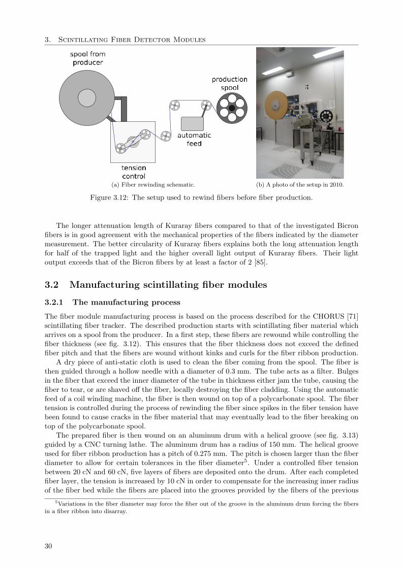
3. Scintillating Fiber Detector Modules
(a) Fiber rewinding schematic. (b) A photo of the setup in 2010.
Figure 3.12: The setup used to rewind fibers before fiber production.
The longer attenuation length of Kuraray fibers compared to that of the investigated Bicronfibers is in good agreement with the mechanical properties of the fibers indicated by the diametermeasurement. The better circularity of Kuraray fibers explains both the long attenuation lengthfor half of the trapped light and the higher overall light output of Kuraray fibers. Their lightoutput exceeds that of the Bicron fibers by at least a factor of 2 [85].
3.2 Manufacturing scintillating fiber modules
3.2.1 The manufacturing process
The fiber module manufacturing process is based on the process described for the CHORUS [71]scintillating fiber tracker. The described production starts with scintillating fiber material whicharrives on a spool from the producer. In a first step, these fibers are rewound while controlling thefiber thickness (see fig. 3.12). This ensures that the fiber thickness does not exceed the definedfiber pitch and that the fibers are wound without kinks and curls for the fiber ribbon production.
A dry piece of anti-static cloth is used to clean the fiber coming from the spool. The fiber isthen guided through a hollow needle with a diameter of 0.3 mm. The tube acts as a filter. Bulgesin the fiber that exceed the inner diameter of the tube in thickness either jam the tube, causing thefiber to tear, or are shaved off the fiber, locally destroying the fiber cladding. Using the automaticfeed of a coil winding machine, the fiber is then wound on top of a polycarbonate spool. The fibertension is controlled during the process of rewinding the fiber since spikes in the fiber tension havebeen found to cause cracks in the fiber material that may eventually lead to the fiber breaking ontop of the polycarbonate spool.
The prepared fiber is then wound on an aluminum drum with a helical groove (see fig. 3.13)guided by a CNC turning lathe. The aluminum drum has a radius of 150 mm. The helical grooveused for fiber ribbon production has a pitch of 0.275 mm. The pitch is chosen larger than the fiberdiameter to allow for certain tolerances in the fiber diameter5. Under a controlled fiber tensionbetween 20 cN and 60 cN, five layers of fibers are deposited onto the drum. After each completedfiber layer, the tension is increased by 10 cN in order to compensate for the increasing inner radiusof the fiber bed while the fibers are placed into the grooves provided by the fibers of the previous
5Variations in the fiber diameter may force the fiber out of the groove in the aluminum drum forcing the fibersin a fiber ribbon into disarray.
30
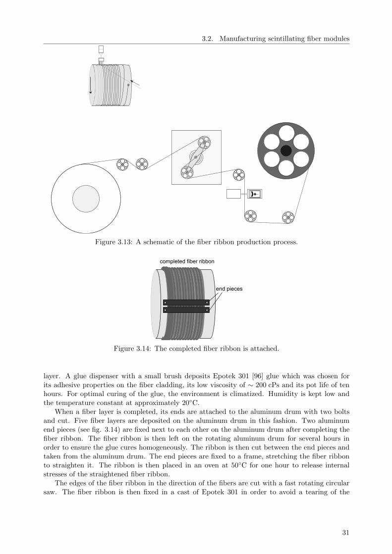
3.2. Manufacturing scintillating fiber modules
Figure 3.13: A schematic of the fiber ribbon production process.
end pieces
completed fiber ribbon
Figure 3.14: The completed fiber ribbon is attached.
layer. A glue dispenser with a small brush deposits Epotek 301 [96] glue which was chosen forits adhesive properties on the fiber cladding, its low viscosity of ∼ 200 cPs and its pot life of tenhours. For optimal curing of the glue, the environment is climatized. Humidity is kept low andthe temperature constant at approximately 20C.
When a fiber layer is completed, its ends are attached to the aluminum drum with two boltsand cut. Five fiber layers are deposited on the aluminum drum in this fashion. Two aluminumend pieces (see fig. 3.14) are fixed next to each other on the aluminum drum after completing thefiber ribbon. The fiber ribbon is then left on the rotating aluminum drum for several hours inorder to ensure the glue cures homogeneously. The ribbon is then cut between the end pieces andtaken from the aluminum drum. The end pieces are fixed to a frame, stretching the fiber ribbonto straighten it. The ribbon is then placed in an oven at 50C for one hour to release internalstresses of the straightened fiber ribbon.
The edges of the fiber ribbon in the direction of the fibers are cut with a fast rotating circularsaw. The fiber ribbon is then fixed in a cast of Epotek 301 in order to avoid a tearing of the
31
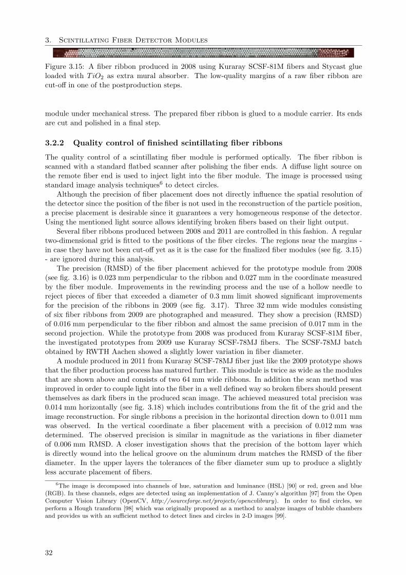
3. Scintillating Fiber Detector Modules
Figure 3.15: A fiber ribbon produced in 2008 using Kuraray SCSF-81M fibers and Stycast glueloaded with TiO2 as extra mural absorber. The low-quality margins of a raw fiber ribbon arecut-off in one of the postproduction steps.
module under mechanical stress. The prepared fiber ribbon is glued to a module carrier. Its endsare cut and polished in a final step.
3.2.2 Quality control of finished scintillating fiber ribbons
The quality control of a scintillating fiber module is performed optically. The fiber ribbon isscanned with a standard flatbed scanner after polishing the fiber ends. A diffuse light source onthe remote fiber end is used to inject light into the fiber module. The image is processed usingstandard image analysis techniques6 to detect circles.
Although the precision of fiber placement does not directly influence the spatial resolution ofthe detector since the position of the fiber is not used in the reconstruction of the particle position,a precise placement is desirable since it guarantees a very homogeneous response of the detector.Using the mentioned light source allows identifying broken fibers based on their light output.
Several fiber ribbons produced between 2008 and 2011 are controlled in this fashion. A regulartwo-dimensional grid is fitted to the positions of the fiber circles. The regions near the margins -in case they have not been cut-off yet as it is the case for the finalized fiber modules (see fig. 3.15)- are ignored during this analysis.
The precision (RMSD) of the fiber placement achieved for the prototype module from 2008(see fig. 3.16) is 0.023 mm perpendicular to the ribbon and 0.027 mm in the coordinate measuredby the fiber module. Improvements in the rewinding process and the use of a hollow needle toreject pieces of fiber that exceeded a diameter of 0.3 mm limit showed significant improvementsfor the precision of the ribbons in 2009 (see fig. 3.17). Three 32 mm wide modules consistingof six fiber ribbons from 2009 are photographed and measured. They show a precision (RMSD)of 0.016 mm perpendicular to the fiber ribbon and almost the same precision of 0.017 mm in thesecond projection. While the prototype from 2008 was produced from Kuraray SCSF-81M fiber,the investigated prototypes from 2009 use Kuraray SCSF-78MJ fibers. The SCSF-78MJ batchobtained by RWTH Aachen showed a slightly lower variation in fiber diameter.
A module produced in 2011 from Kuraray SCSF-78MJ fiber just like the 2009 prototype showsthat the fiber production process has matured further. This module is twice as wide as the modulesthat are shown above and consists of two 64 mm wide ribbons. In addition the scan method wasimproved in order to couple light into the fiber in a well defined way so broken fibers should presentthemselves as dark fibers in the produced scan image. The achieved measured total precision was0.014 mm horizontally (see fig. 3.18) which includes contributions from the fit of the grid and theimage reconstruction. For single ribbons a precision in the horizontal direction down to 0.011 mmwas observed. In the vertical coordinate a fiber placement with a precision of 0.012 mm wasdetermined. The observed precision is similar in magnitude as the variations in fiber diameterof 0.006 mm RMSD. A closer investigation shows that the precision of the bottom layer whichis directly wound into the helical groove on the aluminum drum matches the RMSD of the fiberdiameter. In the upper layers the tolerances of the fiber diameter sum up to produce a slightlyless accurate placement of fibers.
6The image is decomposed into channels of hue, saturation and luminance (HSL) [90] or red, green and blue(RGB). In these channels, edges are detected using an implementation of J. Canny’s algorithm [97] from the OpenComputer Vision Library (OpenCV, http://sourceforge.net/projects/opencvlibrary). In order to find circles, weperform a Hough transform [98] which was originally proposed as a method to analyze images of bubble chambersand provides us with an sufficient method to detect lines and circles in 2-D images [99].
32
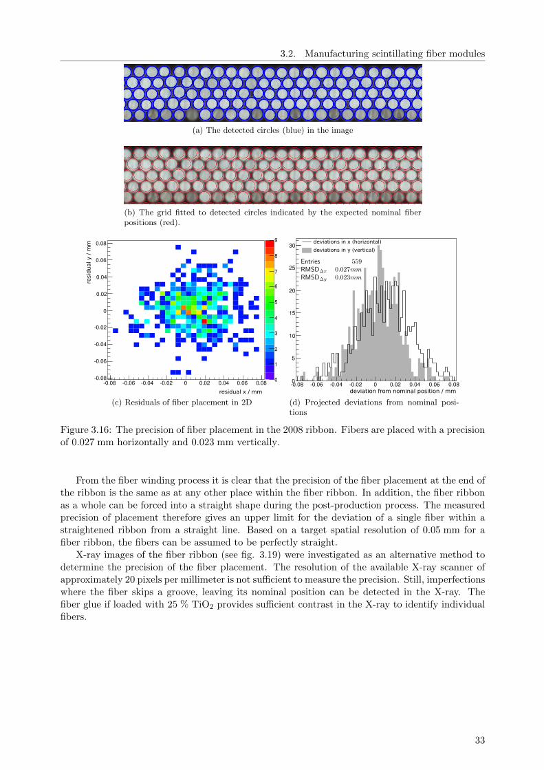
3.2. Manufacturing scintillating fiber modules
(a) The detected circles (blue) in the image
(b) The grid fitted to detected circles indicated by the expected nominal fiberpositions (red).
-0.08 -0.06 -0.04 -0.02 0 0.02 0.04 0.06 0.08-0.08
-0.06
-0.04
-0.02
0
0.02
0.04
0.06
0.08
0
1
2
3
4
5
6
7
8
9
resi
du
al y /
mm
residual x / mm
(c) Residuals of fiber placement in 2D
deviation from nominal position / mm-0.08 -0.06 -0.04 -0.02 0 0.02 0.04 0.06 0.080
5
10
15
20
25
30deviations in x (horizontal)
deviations in y (vertical)
(d) Projected deviations from nominal posi-tions
Figure 3.16: The precision of fiber placement in the 2008 ribbon. Fibers are placed with a precisionof 0.027 mm horizontally and 0.023 mm vertically.
From the fiber winding process it is clear that the precision of the fiber placement at the end ofthe ribbon is the same as at any other place within the fiber ribbon. In addition, the fiber ribbonas a whole can be forced into a straight shape during the post-production process. The measuredprecision of placement therefore gives an upper limit for the deviation of a single fiber within astraightened ribbon from a straight line. Based on a target spatial resolution of 0.05 mm for afiber ribbon, the fibers can be assumed to be perfectly straight.
X-ray images of the fiber ribbon (see fig. 3.19) were investigated as an alternative method todetermine the precision of the fiber placement. The resolution of the available X-ray scanner ofapproximately 20 pixels per millimeter is not sufficient to measure the precision. Still, imperfectionswhere the fiber skips a groove, leaving its nominal position can be detected in the X-ray. Thefiber glue if loaded with 25 % TiO2 provides sufficient contrast in the X-ray to identify individualfibers.
33
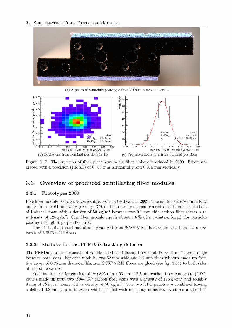
3. Scintillating Fiber Detector Modules
(a) A photo of a module prototype from 2009 that was analyzed.
-0.08 -0.06 -0.04 -0.02 0 0.02 0.04 0.06 0.08-0.08
-0.06
-0.04
-0.02
0
0.02
0.04
0.06
0.08
deviation from nominal position x / mm
devia
tion f
rom
nom
inal posi
tion y
/ m
m
(b) Deviations from nominal positions in 2D
-0.08 -0.06 -0.04 -0.02 0 0.02 0.04 0.06 0.080
100
200
300
400
500
600
700
deviation from nominal position / mm
freq
uen
cy
(c) Projected deviations from nominal positions
Figure 3.17: The precision of fiber placement in six fiber ribbons produced in 2009. Fibers areplaced with a precision (RMSD) of 0.017 mm horizontally and 0.016 mm vertically.
3.3 Overview of produced scintillating fiber modules
3.3.1 Prototypes 2009
Five fiber module prototypes were subjected to a testbeam in 2009. The modules are 860 mm longand 32 mm or 64 mm wide (see fig. 3.20). The module carriers consist of a 10 mm thick sheetof Rohacell foam with a density of 50 kg/m3 between two 0.1 mm thin carbon fiber sheets witha density of 125 g/m2. One fiber module equals about 1.6 % of a radiation length for particlespassing through it perpendicularly.
One of the five tested modules is produced from SCSF-81M fibers while all others use a newbatch of SCSF-78MJ fibers.
3.3.2 Modules for the PERDaix tracking detector
The PERDaix tracker consists of double-sided scintillating fiber modules with a 1 stereo anglebetween both sides. For each module, two 62 mm wide and 1.2 mm thick ribbons made up fromfive layers of 0.25 mm diameter Kuraray SCSF-78MJ fibers are glued (see fig. 3.24) to both sidesof a module carrier.
Each module carrier consists of two 395 mm× 63 mm× 8.2 mm carbon-fiber-composite (CFC)panels made up from two T300 EP carbon fiber skins with a density of 125 g/cm2 and roughly8 mm of Rohacell foam with a density of 50 kg/m3. The two CFC panels are combined leavinga defined 0.3 mm gap in-between which is filled with an epoxy adhesive. A stereo angle of 1
34
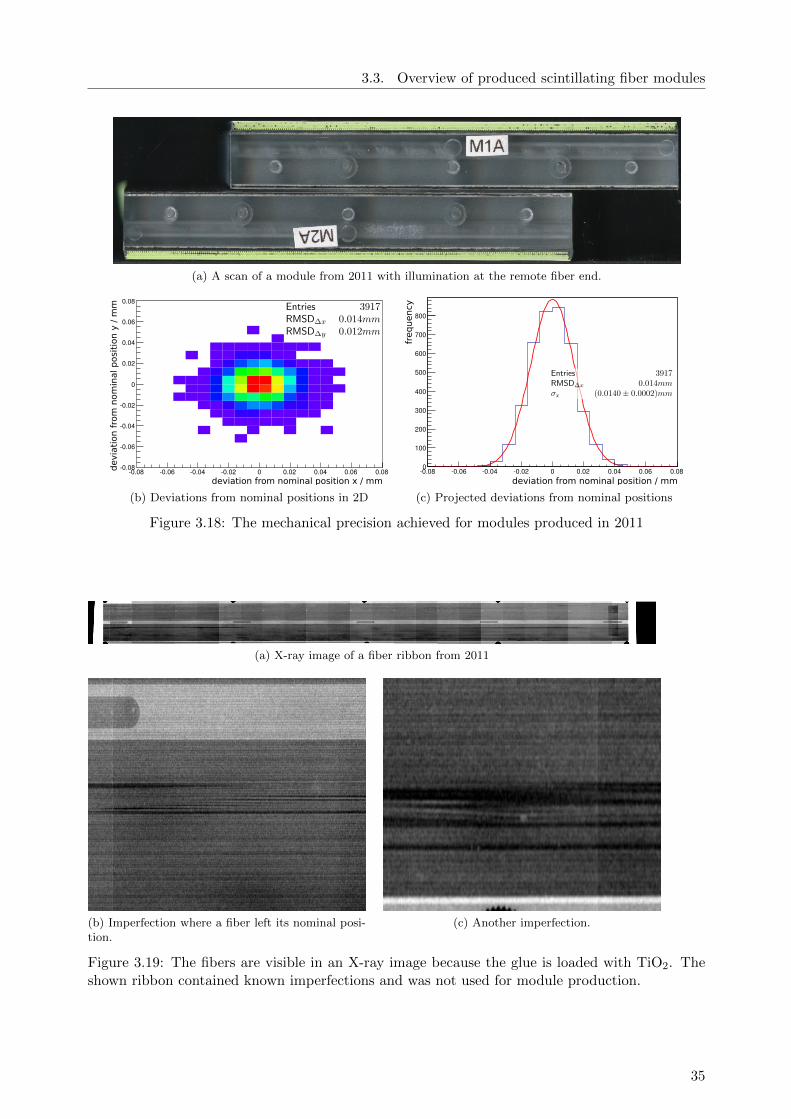
3.3. Overview of produced scintillating fiber modules
(a) A scan of a module from 2011 with illumination at the remote fiber end.
-0.08 -0.06 -0.04 -0.02 0 0.02 0.04 0.06 0.08-0.08
-0.06
-0.04
-0.02
0
0.02
0.04
0.06
0.08
deviation from nominal position x / mm
devia
tion f
rom
nom
inal p
osi
tion
y /
mm
(b) Deviations from nominal positions in 2D
-0.08 -0.06 -0.04 -0.02 0 0.02 0.04 0.06 0.080
100
200
300
400
500
600
700
800
deviation from nominal position / mm
freq
uen
cy
(c) Projected deviations from nominal positions
Figure 3.18: The mechanical precision achieved for modules produced in 2011
(a) X-ray image of a fiber ribbon from 2011
(b) Imperfection where a fiber left its nominal posi-tion.
(c) Another imperfection.
Figure 3.19: The fibers are visible in an X-ray image because the glue is loaded with TiO2. Theshown ribbon contained known imperfections and was not used for module production.
35

3. Scintillating Fiber Detector Modules
(a) Front view of fiber module.
32mm
860mm
(b) Full view of fiber module.
Figure 3.20: Pictures of the 2009 scintillating fiber module prototypes.
(a) Drawing of a single CFC panel. Precision pinsdefine the stereo angle.
(b) Drawing the combined module carrier with astereo angle of 1.
Figure 3.21: Assembly of a PERDaix fiber module carrier.
between the two panels is ensured (see fig. 3.21). Polycarbonate end pieces are glued into themodule carrier ends.
The composite module carrier has a weight of 127.8 g of which 4 · 6.8 g = 27.2 g is the contri-bution of the polycarbonate end pieces. The material budget of the entire module carrier withoutthe end pieces in radiation lengths sums up to x/X0 = 0.81 %. The adhesive which was used toproduce the carbon-fiber composite panels and to glue the two panels together makes up for afraction of 70 % of the material(see fig. 3.22). Cutouts were added to the carriers of the PERDaixmodules (see fig. 3.23). About 60 % of the carrier material was removed this way, reducing thematerial budget to x/X0 = 0.32 %.
The material budget of the complete fiber module including the fibers (ignoring the polycar-bonate end pieces) is x/X0 = 0.93 %.
36
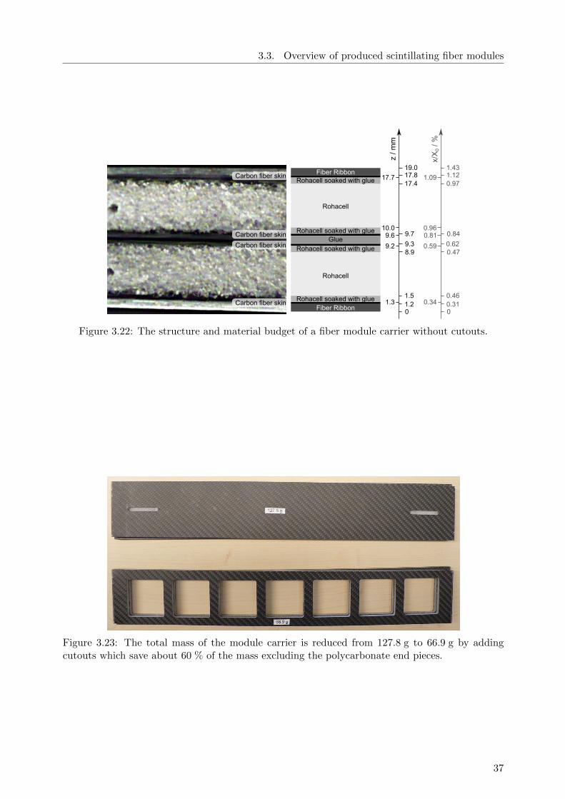
3.3. Overview of produced scintillating fiber modules
Fiber Ribbon
Fiber Ribbon
Rohacell
Rohacell
Rohacell soaked with glue
Rohacell soaked with glue
Rohacell soaked with glue
Rohacell soaked with glue
Glue
Carbon fiber skin01.21.31.5
8.99.2 9.39.6 9.7
10.0
17.417.7 17.8
19.0
z / m
m
Carbon fiber skin
Carbon fiber skin
Carbon fiber skin
00.310.340.46
0.470.59 0.620.81 0.840.96
0.971.09 1.12
1.43
x/X
0 / %
Figure 3.22: The structure and material budget of a fiber module carrier without cutouts.
Figure 3.23: The total mass of the module carrier is reduced from 127.8 g to 66.9 g by addingcutouts which save about 60 % of the mass excluding the polycarbonate end pieces.
37
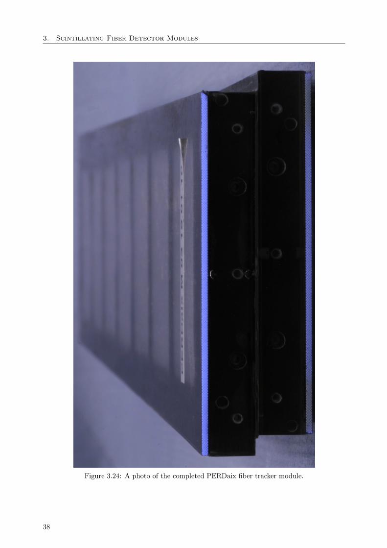
3. Scintillating Fiber Detector Modules
Figure 3.24: A photo of the completed PERDaix fiber tracker module.
38
Chapter 4
Silicon Photomultiplier ArrayReadout
This chapter introduces silicon photomultipliers. It describes the physical processes behind thistechnology and presents the characteristics of 32-channel silicon photomultiplier arrays used forthe scintillating fiber tracker.
4.1 Silicon Photomultipliers
4.1.1 Photo-detectors for scintillating fiber trackers
When a minimum-ionizing particle (m.i.p.) passes through the center of a 0.25 mm diameter fiberit crosses approximately 0.22 mm of active scintillator (in case of a multi-clad Kuraray fiber). Theexpected average energy deposit of said particle is ∆E = 45 keV1. The average light yield for acommon plastic scintillator per deposited energy is dN/dE ≈ 8 photons/keV [89]. Based on thetrapping efficiency of a perfect fiber of εtrapped = 17.44 % or 8.72 % of the total produced lightexpected at each fiber end, we arrive at an expectation for the number of photons for a single idealfiber nphotons:
nphotons =1
2∆E
dN
dEεtrapped ≈ 31 (4.1)
This calculation does not include geometrical defects in the fiber which reduce the trapping effi-ciency or the light attenuation in the bulk material. These losses are expected affect helix modesdisproportionately which make up for roughly 50 % of the trapped light. As a first estimate, alight yield of the order of ∼ 15 photons seems reasonable assuming that all helix modes are lost.
It follows that any photo-detector used for the readout of thin scintillating fibers must havea high quantum efficiency and a high gain at the same time, so few photons are registered as anelectronic pulse of sufficient amplitude. In the past, several different types of photo-detectors havebeen employed in scintillating fiber trackers. In the earliest realizations, image intensifier tubesand photographic film [67] were used. The UA-2 [69] and CHORUS [71] experiments replacedthe photographic film with more modern CCD2 cameras. Another development were positionsensitive multi-anode photomultiplier tubes like the Hamamatsu R2486 [100] or the HamamatsuR5900 [101] which have been used for scintillating fiber trackers as well. With the development ofthe visible light photon counter (VLPC) [74–76] the need for electron multiplier tubes in the formof PMTs or image intensifiers was gone. In VLPCs the amplification of primary photo-electronshappens in the depletion zone of a semiconductor. Silicon photomultipliers (SiPM) [102] are a newdevelopment in solid-state photon detectors whose application as a photo-detector for a scintillatingfiber tracker is presented in this work. A comparison of the different properties of these photo-
1Assuming a Polystyrene core for which the dE/dx of a m.i.p. equals 2.052 MeVcm
[10].2Charge-coupled devices. They have lately been replaced by so-called active pixel sensors
39
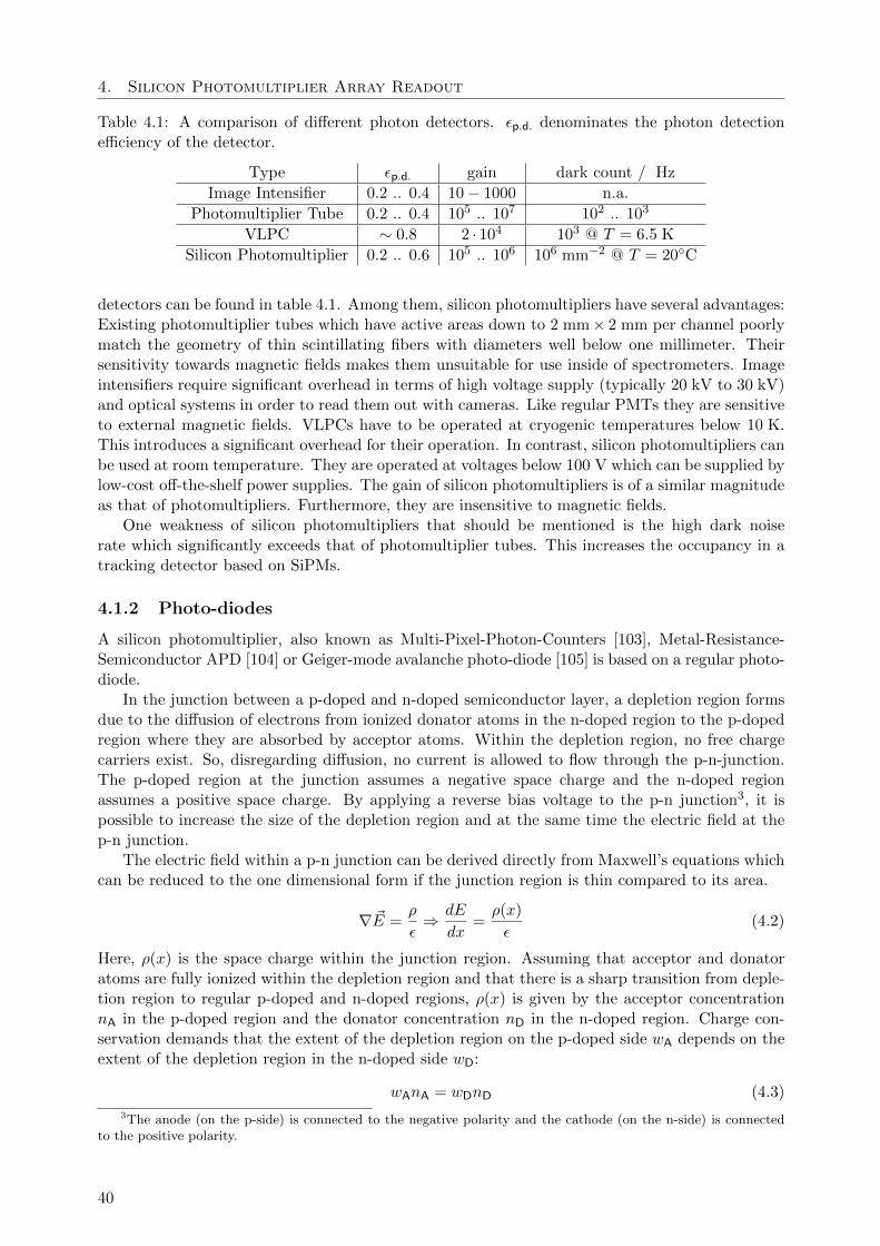
4. Silicon Photomultiplier Array Readout
Table 4.1: A comparison of different photon detectors. εp.d. denominates the photon detectionefficiency of the detector.
Type εp.d. gain dark count / Hz
Image Intensifier 0.2 .. 0.4 10− 1000 n.a.
Photomultiplier Tube 0.2 .. 0.4 105 .. 107 102 .. 103
VLPC ∼ 0.8 2 · 104 103 @ T = 6.5 K
Silicon Photomultiplier 0.2 .. 0.6 105 .. 106 106 mm−2 @ T = 20C
detectors can be found in table 4.1. Among them, silicon photomultipliers have several advantages:Existing photomultiplier tubes which have active areas down to 2 mm× 2 mm per channel poorlymatch the geometry of thin scintillating fibers with diameters well below one millimeter. Theirsensitivity towards magnetic fields makes them unsuitable for use inside of spectrometers. Imageintensifiers require significant overhead in terms of high voltage supply (typically 20 kV to 30 kV)and optical systems in order to read them out with cameras. Like regular PMTs they are sensitiveto external magnetic fields. VLPCs have to be operated at cryogenic temperatures below 10 K.This introduces a significant overhead for their operation. In contrast, silicon photomultipliers canbe used at room temperature. They are operated at voltages below 100 V which can be supplied bylow-cost off-the-shelf power supplies. The gain of silicon photomultipliers is of a similar magnitudeas that of photomultipliers. Furthermore, they are insensitive to magnetic fields.
One weakness of silicon photomultipliers that should be mentioned is the high dark noiserate which significantly exceeds that of photomultiplier tubes. This increases the occupancy in atracking detector based on SiPMs.
4.1.2 Photo-diodes
A silicon photomultiplier, also known as Multi-Pixel-Photon-Counters [103], Metal-Resistance-Semiconductor APD [104] or Geiger-mode avalanche photo-diode [105] is based on a regular photo-diode.
In the junction between a p-doped and n-doped semiconductor layer, a depletion region formsdue to the diffusion of electrons from ionized donator atoms in the n-doped region to the p-dopedregion where they are absorbed by acceptor atoms. Within the depletion region, no free chargecarriers exist. So, disregarding diffusion, no current is allowed to flow through the p-n-junction.The p-doped region at the junction assumes a negative space charge and the n-doped regionassumes a positive space charge. By applying a reverse bias voltage to the p-n junction3, it ispossible to increase the size of the depletion region and at the same time the electric field at thep-n junction.
The electric field within a p-n junction can be derived directly from Maxwell’s equations whichcan be reduced to the one dimensional form if the junction region is thin compared to its area.
∇ ~E =ρ
ε⇒ dE
dx=ρ(x)
ε(4.2)
Here, ρ(x) is the space charge within the junction region. Assuming that acceptor and donatoratoms are fully ionized within the depletion region and that there is a sharp transition from deple-tion region to regular p-doped and n-doped regions, ρ(x) is given by the acceptor concentrationnA in the p-doped region and the donator concentration nD in the n-doped region. Charge con-servation demands that the extent of the depletion region on the p-doped side wA depends on theextent of the depletion region in the n-doped side wD:
wAnA = wDnD (4.3)
3The anode (on the p-side) is connected to the negative polarity and the cathode (on the n-side) is connectedto the positive polarity.
40

4.1. Silicon Photomultipliers
pote
ntia
l
x
h
e
depletion region
e
h
e
+++++------ - ++
p-doped n-doped
photon
anode cathode
Eband gap
Ubias - UD
e
Figure 4.1: This schematic view shows the potential in a p-n-junction. A photon may createan electron-hole pair in the depletion zone which are then accelerated in opposite directions tocathode and anode.
The electric field perpendicular to the junction which is located at x = 0 (with the p-doped regionon the side x < 0) can be given as (integrating 4.2):
εE(x) =
(wA + x)nAe −wA < x < 0(wD − x)nDe 0 ≤ x < wD
0 x ≤ −wA ∨ x ≥ wD
(4.4)
Another integration gives us the dependence of the size of the depletion region on the potentialdifference between cathode and anode which is the sum of the diffusion voltage UD
4 and anexternally applied voltage Ubias: Ubias − UD =
∫dxE.
Ubias − UD =nAe
2εw2A +
nDe
2εw2D (4.5)
⇒ wA = wDnDnA
=
√2 (Ubias − UD)nDε
nA (nA + nD) e(4.6)
The electric field within the junction grows with√Ubias − UD. Electron-hole pairs which are
generated within the depletion region of a reversely biased p-n junction (e.g. due to thermalproduction of electron-hole pairs within the depletion region) are accelerated in the electric field.The electron drifts to the n-side while the hole drifts toward the p-side and can be registered ascurrent flowing through the p-n junction. A photo-diode exploits the generation of electron holepairs by photo-ionization where a photon with an energy greater than the energy band gap betweenvalence band and conduction band (> 1.1 eV for silicon) lifts an electron from the valence bandinto the conduction band, leaving a hole in the valence band (see fig. 4.1). The charge carrierscreated by photons in the depletion region may then be registered as photo-current in a reverselybiased photo-diode.
4.1.3 Quantum Efficiency
If a photon is absorbed outside of the depletion zone of a reversely biased photo-diode, it willcreate an electron and a hole which diffuse through the semiconductor until they recombine with
4UD is the voltage generated by diffusion of charge carriers between the p- and n-regions.
41
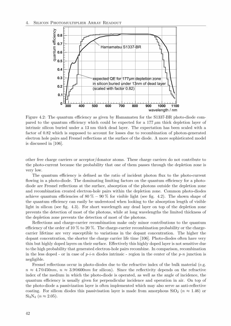
4. Silicon Photomultiplier Array Readout
300 400 500 600 700 800 900 1000 11000
0.1
0.2
0.3
0.4
0.5
0.6
0.7
0.8
Hamamatsu S1337-BR
expected QE for 177µm depletion zonein silicon buried under 13nm of dead layer(scaled with factor 0.82)
wavelength / nm
quan
tum
effi
cien
cy
Figure 4.2: The quantum efficiency as given by Hamamatsu for the S1337-BR photo-diode com-pared to the quantum efficiency which could be expected for a 177 µm thick depletion layer ofintrinsic silicon buried under a 13 nm thick dead layer. The expectation has been scaled with afactor of 0.82 which is supposed to account for losses due to recombination of photon-generatedelectron hole pairs and Fresnel reflections at the surface of the diode. A more sophisticated modelis discussed in [106].
other free charge carriers or acceptor/donator atoms. These charge carriers do not contribute tothe photo-current because the probability that one of them passes through the depletion zone isvery low.
The quantum efficiency is defined as the ratio of incident photon flux to the photo-currentflowing in a photo-diode. The dominating limiting factors on the quantum efficiency for a photo-diode are Fresnel reflections at the surface, absorption of the photons outside the depletion zoneand recombination created electron-hole pairs within the depletion zone. Common photo-diodesachieve quantum efficiencies of 80 % − 90 % for visible light (see fig. 4.2). The shown shape ofthe quantum efficiency can easily be understood when looking to the absorption length of visiblelight in silicon (see fig. 4.3). For short wavelength any dead layer on top of the depletion zoneprevents the detection of most of the photons, while at long wavelengths the limited thickness ofthe depletion zone prevents the detection of most of the photons.
Reflections and charge-carrier recombination make only minor contributions to the quantumefficiency of the order of 10 % to 20 %. The charge-carrier recombination probability or the charge-carrier lifetime are very susceptible to variations in the dopant concentration. The higher thedopant concentration, the shorter the charge carrier life time [106]. Photo-diodes often have verythin but highly doped layers on their surface. Effectively this highly doped layer is not sensitive dueto the high probability that generated electron-hole pairs recombine. In comparison, recombinationin the less doped - or in case of p-i-n diodes intrinsic - region in the center of the p-n junction isnegligible.
Fresnel reflections occur in photo-diodes due to the refractive index of the bulk material (e.g.n ≈ 4.7@450nm, n ≈ 3.9@600nm for silicon). Since the reflectivity depends on the refractiveindex of the medium in which the photo-diode is operated, as well as the angle of incidence, thequantum efficiency is usually given for perpendicular incidence and operation in air. On top ofthe photo-diode a passivization layer is often implemented which may also serve as anti-reflectivecoating. For silicon diodes this passivisation layer is made from amorphous SiO2 (n ≈ 1.46) orSi3N4 (n ≈ 2.05).
42
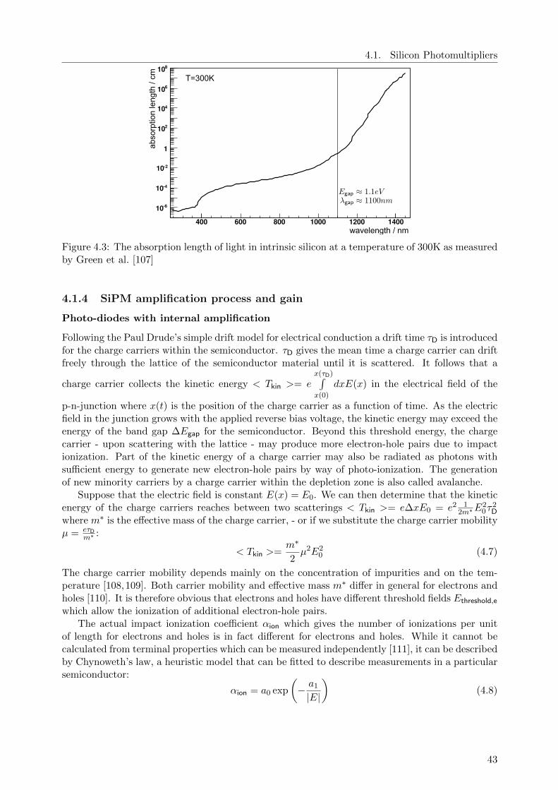
4.1. Silicon Photomultipliers
400 600 800 1000 1200 1400
-610
-410
-210
1
210
410
610
810
wavelength / nm
abso
rptio
n le
ngth
/ cm T=300K
Figure 4.3: The absorption length of light in intrinsic silicon at a temperature of 300K as measuredby Green et al. [107]
4.1.4 SiPM amplification process and gain
Photo-diodes with internal amplification
Following the Paul Drude’s simple drift model for electrical conduction a drift time τD is introducedfor the charge carriers within the semiconductor. τD gives the mean time a charge carrier can driftfreely through the lattice of the semiconductor material until it is scattered. It follows that a
charge carrier collects the kinetic energy < Tkin >= ex(τD)∫x(0)
dxE(x) in the electrical field of the
p-n-junction where x(t) is the position of the charge carrier as a function of time. As the electricfield in the junction grows with the applied reverse bias voltage, the kinetic energy may exceed theenergy of the band gap ∆Egap for the semiconductor. Beyond this threshold energy, the chargecarrier - upon scattering with the lattice - may produce more electron-hole pairs due to impactionization. Part of the kinetic energy of a charge carrier may also be radiated as photons withsufficient energy to generate new electron-hole pairs by way of photo-ionization. The generationof new minority carriers by a charge carrier within the depletion zone is also called avalanche.
Suppose that the electric field is constant E(x) = E0. We can then determine that the kineticenergy of the charge carriers reaches between two scatterings < Tkin >= e∆xE0 = e2 1
2m∗E20τ
2D
where m∗ is the effective mass of the charge carrier, - or if we substitute the charge carrier mobilityµ = eτD
m∗ :
< Tkin >=m∗
2µ2E2
0 (4.7)
The charge carrier mobility depends mainly on the concentration of impurities and on the tem-perature [108,109]. Both carrier mobility and effective mass m∗ differ in general for electrons andholes [110]. It is therefore obvious that electrons and holes have different threshold fields Ethreshold,e
which allow the ionization of additional electron-hole pairs.The actual impact ionization coefficient αion which gives the number of ionizations per unit
of length for electrons and holes is in fact different for electrons and holes. While it cannot becalculated from terminal properties which can be measured independently [111], it can be describedby Chynoweth’s law, a heuristic model that can be fitted to describe measurements in a particularsemiconductor:
αion = a0 exp
(− a1
|E|
)(4.8)
43
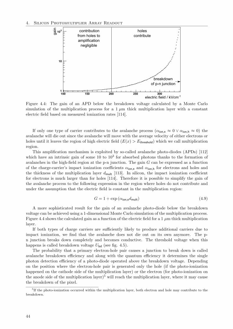
4. Silicon Photomultiplier Array Readout
100 150 200 250 3001
10
210 contribution from holes to amplification
negligible
holes contribute
breakdownof p-n junction
electric field / kVcm-1
gain
Figure 4.4: The gain of an APD below the breakdown voltage calculated by a Monte Carlosimulation of the multiplication process for a 1 µm thick multiplication layer with a constantelectric field based on measured ionization rates [114].
If only one type of carrier contributes to the avalanche process (αion,e ≈ 0 ∨ αion,h ≈ 0) theavalanche will die out since the avalanche will move with the average velocity of either electrons orholes until it leaves the region of high electric field (E(x) > Ethreshold) which we call multiplicationregion.
This amplification mechanism is exploited by so-called avalanche photo-diodes (APDs) [112]which have an intrinsic gain of some 10 to 103 for absorbed photons thanks to the formation ofavalanches in the high-field region at the p-n junction. The gain G can be expressed as a functionof the charge-carrier’s impact ionization coefficients αion,e and αion,h for electrons and holes andthe thickness of the multiplication layer dmult [113]. In silicon, the impact ionization coefficientfor electrons is much larger than for holes [114]. Therefore it is possible to simplify the gain ofthe avalanche process to the following expression in the region where holes do not contribute andunder the assumption that the electric field is constant in the multiplication region:
G = 1 + exp (αion,edmult) (4.9)
A more sophisticated result for the gain of an avalanche photo-diode below the breakdownvoltage can be achieved using a 1-dimensional Monte Carlo simulation of the multiplication process.Figure 4.4 shows the calculated gain as a function of the electric field for a 1 µm thick multiplicationlayer.
If both types of charge carriers are sufficiently likely to produce additional carriers due toimpact ionization, we find that the avalanche does not die out on its own anymore. The p-n junction breaks down completely and becomes conductive. The threshold voltage when thishappens is called breakdown voltage Ubd (see fig. 4.5).
The probability that a primary electron-hole pair causes a junction to break down is calledavalanche breakdown efficiency and along with the quantum efficiency it determines the singlephoton detection efficiency of a photo-diode operated above the breakdown voltage. Dependingon the position where the electron-hole pair is generated only the hole (if the photo-ionizationhappened on the cathode side of the multiplication layer) or the electron (for photo-ionization onthe anode side of the multiplication layer)5 will reach the multiplication layer, where it may causethe breakdown of the pixel.
5If the photo-ionization occurred within the multiplication layer, both electron and hole may contribute to thebreakdown.
44
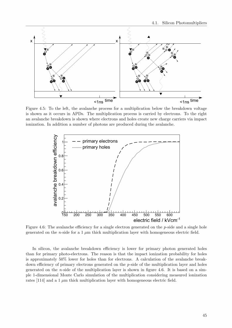
4.1. Silicon Photomultipliers
x
time
e
h
eh
e
hh
e e ee
<1ns
x
time
e
h
eh
e
hh
e e e e
<1ns
hhe
hhehhe
ee
h
Figure 4.5: To the left, the avalanche process for a multiplication below the breakdown voltageis shown as it occurs in APDs. The multiplication process is carried by electrons. To the rightan avalanche breakdown is shown where electrons and holes create new charge carriers via impactionization. In addition a number of photons are produced during the avalanche.
150 200 250 300 350 400 450 500 550 6000
0.2
0.4
0.6
0.8
1
avalanchebreakdownefficiency
electric field / kVcm-1
primary electronsprimary holes
Figure 4.6: The avalanche efficiency for a single electron generated on the p-side and a single holegenerated on the n-side for a 1 µm thick multiplication layer with homogeneous electric field.
In silicon, the avalanche breakdown efficiency is lower for primary photon generated holesthan for primary photo-electrons. The reason is that the impact ionization probability for holesis approximately 50% lower for holes than for electrons. A calculation of the avalanche break-down efficiency of primary electrons generated on the p-side of the multiplication layer and holesgenerated on the n-side of the multiplication layer is shown in figure 4.6. It is based on a sim-ple 1-dimensional Monte Carlo simulation of the multiplication considering measured ionizationrates [114] and a 1 µm thick multiplication layer with homogeneous electric field.
45
4. Silicon Photomultiplier Array Readout
Silicon Photomultipliers
A silicon photomultiplier (SiPM) is an array of photo-diodes operated in parallel above theirbreakdown voltage. Each photo-diode is a pixel of the silicon photomultiplier and is connectedin series with an integrated polysilicon quenching resistor with a resistance of about Rquench =105 Ω. When a pixel of the silicon photomultiplier breaks down, its resistance drops almost to zerocompared to the quenching resistor. The peak electric field E(0) in the junction drops due to theflowing breakdown current Ibd:
E(0) =
√2nAnDe (Ubias − UD − IbdRquench)
(nA + nD) ε(4.10)
Calculating the dynamics of quenching is a difficult task that will not be undertaken here. How-ever, we can calculate the total amount of charge that flows through the p-n junction during abreakdown. For this, we assume that Ubias − IbdRquench immediately drops below the breakdownvoltage (consequently the electric field drops below the threshold field for a breakdown). Equation4.6 shows the relation between the size of the depletion zone and the applied voltage from whichwe can calculate the total flowing charge Qbd or the gain of the silicon photomultiplier G = Qbd/e:
∆wA =
√2nDε
nA (nA + nD) e
(√Ubias − UD −
√Ubd − UD
)(4.11)
⇒ Qbd = nAApixel∆wAe (4.12)
⇒ G = Apixel
√2nDnAε
(nA + nD) e
(√Ubias − UD −
√Ubd − UD
)(4.13)
If UD/Ubd 1 and Ubd ≈ Ubias this expression simplifies to:
G = Cpixel (Ubias − Ubd) (4.14)
where
Cpixel = Apixel
√2nDnAε
(nA + nD) eUbias(4.15)
is the capacitance of a single pixel. The difference Ubias − Ubd is referred to as over-voltage.
4.1.5 SiPM internal structure and geometric efficiency
Figure 4.7 shows the cross-section of a silicon photomultiplier pixel as it is expected for the Hama-matsu MPPC [115]. It is designed around a p-n junction as previously discussed. A guard ringprevents charge carriers from outside the pixel from entering the multiplication zone. The (poly-silicon) quenching resistor and metallic contact to the pixel are implemented on top of the SiPM(see fig. 4.8). Commonly available SiPMs implement between 100 and 10,000 such pixels per mm2
which are operated in parallel, each with its own quenching resistor.Some manufacturers (as for example FBK-irst [116]) invert the structure6, placing the n-layer
on top of the p-layer inside a p-doped substrate. In doing so, they achieve a higher sensitivityfor visible light in the 500 nm to 650 nm range at the expense of a lower sensitivity for shorterwavelengths. This effect can be explained by the increased probability for primary electrons on thep-doped side of the junction to generate an avalanche leading to a breakdown of the pixel. Sincered light has a deeper reach into silicon, it is advantageous make the preferred conversion zoneas large as possible even if that requires burying it under a n-doped layer with a low avalanchebreakdown efficiency for converted electron-hole pairs.
6In fact, the first silicon photomultipliers that were produced used this inverted structure. This thesis howeverconsiders the Hamamatsu devices as baseline which use an n-type substrate with p-doped implants.
46
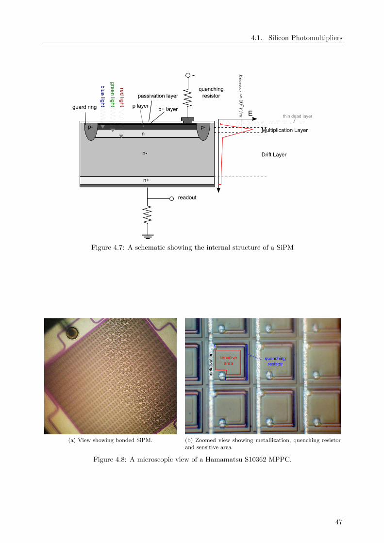
4.1. Silicon Photomultipliers
n-
n
n+
p-p-Multiplication Layer
Drift Layer
-
p+ layerguard ring
quenching resistor
readout
blue light
green light
red light
thin dead layerEp layer
passivation layer
Figure 4.7: A schematic showing the internal structure of a SiPM
(a) View showing bonded SiPM. (b) Zoomed view showing metallization, quenching resistorand sensitive area
Figure 4.8: A microscopic view of a Hamamatsu S10362 MPPC.
47
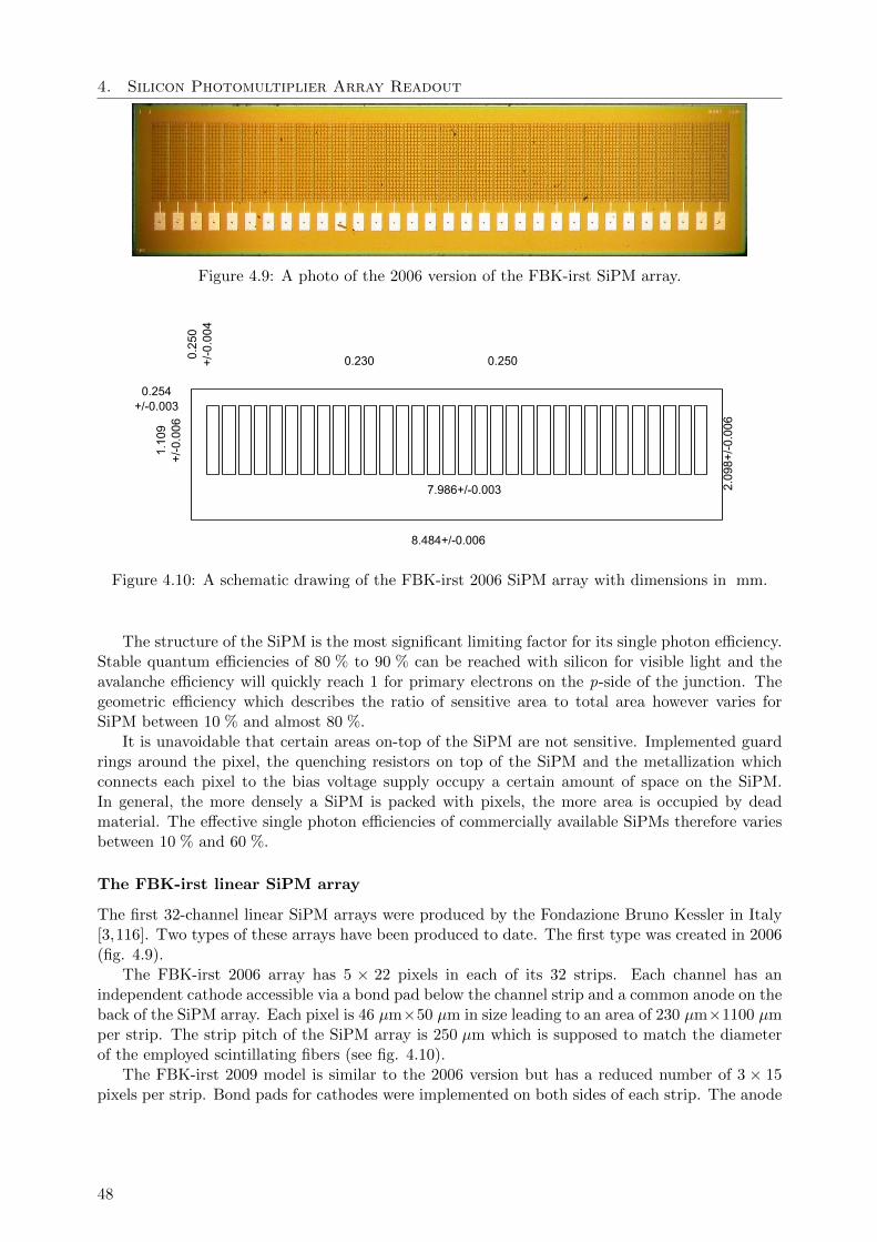
4. Silicon Photomultiplier Array Readout
Figure 4.9: A photo of the 2006 version of the FBK-irst SiPM array.
7.986+/-0.003
1.109
+/-0.006
0.254+/-0.003
2.098+/-0.006
8.484+/-0.006
0.250
+/-0.004
0.2500.230
Figure 4.10: A schematic drawing of the FBK-irst 2006 SiPM array with dimensions in mm.
The structure of the SiPM is the most significant limiting factor for its single photon efficiency.Stable quantum efficiencies of 80 % to 90 % can be reached with silicon for visible light and theavalanche efficiency will quickly reach 1 for primary electrons on the p-side of the junction. Thegeometric efficiency which describes the ratio of sensitive area to total area however varies forSiPM between 10 % and almost 80 %.
It is unavoidable that certain areas on-top of the SiPM are not sensitive. Implemented guardrings around the pixel, the quenching resistors on top of the SiPM and the metallization whichconnects each pixel to the bias voltage supply occupy a certain amount of space on the SiPM.In general, the more densely a SiPM is packed with pixels, the more area is occupied by deadmaterial. The effective single photon efficiencies of commercially available SiPMs therefore variesbetween 10 % and 60 %.
The FBK-irst linear SiPM array
The first 32-channel linear SiPM arrays were produced by the Fondazione Bruno Kessler in Italy[3,116]. Two types of these arrays have been produced to date. The first type was created in 2006(fig. 4.9).
The FBK-irst 2006 array has 5 × 22 pixels in each of its 32 strips. Each channel has anindependent cathode accessible via a bond pad below the channel strip and a common anode on theback of the SiPM array. Each pixel is 46 µm×50 µm in size leading to an area of 230 µm×1100 µmper strip. The strip pitch of the SiPM array is 250 µm which is supposed to match the diameterof the employed scintillating fibers (see fig. 4.10).
The FBK-irst 2009 model is similar to the 2006 version but has a reduced number of 3 × 15pixels per strip. Bond pads for cathodes were implemented on both sides of each strip. The anode
48
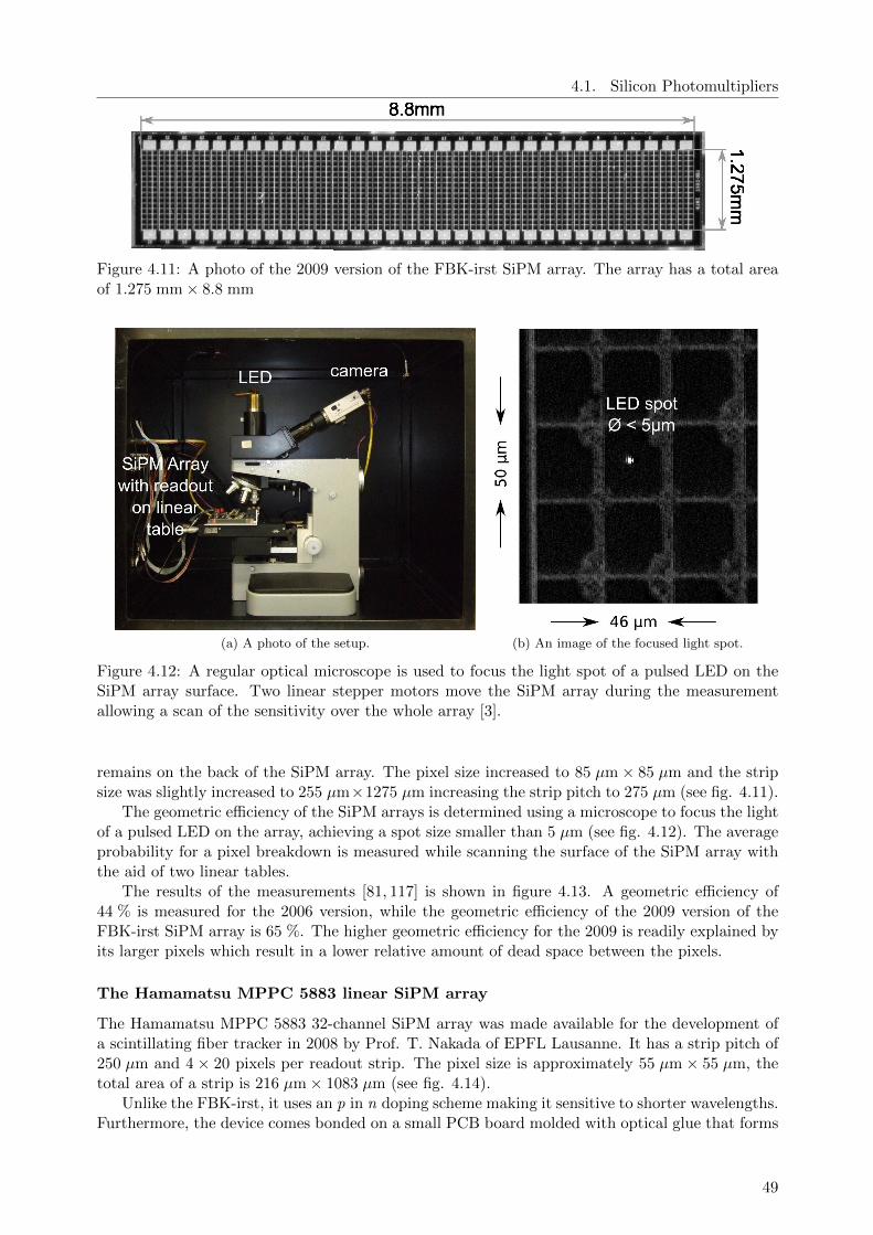
4.1. Silicon Photomultipliers
Figure 4.11: A photo of the 2009 version of the FBK-irst SiPM array. The array has a total areaof 1.275 mm× 8.8 mm
(a) A photo of the setup. (b) An image of the focused light spot.
Figure 4.12: A regular optical microscope is used to focus the light spot of a pulsed LED on theSiPM array surface. Two linear stepper motors move the SiPM array during the measurementallowing a scan of the sensitivity over the whole array [3].
remains on the back of the SiPM array. The pixel size increased to 85 µm× 85 µm and the stripsize was slightly increased to 255 µm×1275 µm increasing the strip pitch to 275 µm (see fig. 4.11).
The geometric efficiency of the SiPM arrays is determined using a microscope to focus the lightof a pulsed LED on the array, achieving a spot size smaller than 5 µm (see fig. 4.12). The averageprobability for a pixel breakdown is measured while scanning the surface of the SiPM array withthe aid of two linear tables.
The results of the measurements [81, 117] is shown in figure 4.13. A geometric efficiency of44 % is measured for the 2006 version, while the geometric efficiency of the 2009 version of theFBK-irst SiPM array is 65 %. The higher geometric efficiency for the 2009 is readily explained byits larger pixels which result in a lower relative amount of dead space between the pixels.
The Hamamatsu MPPC 5883 linear SiPM array
The Hamamatsu MPPC 5883 32-channel SiPM array was made available for the development ofa scintillating fiber tracker in 2008 by Prof. T. Nakada of EPFL Lausanne. It has a strip pitch of250 µm and 4 × 20 pixels per readout strip. The pixel size is approximately 55 µm × 55 µm, thetotal area of a strip is 216 µm× 1083 µm (see fig. 4.14).
Unlike the FBK-irst, it uses an p in n doping scheme making it sensitive to shorter wavelengths.Furthermore, the device comes bonded on a small PCB board molded with optical glue that forms
49
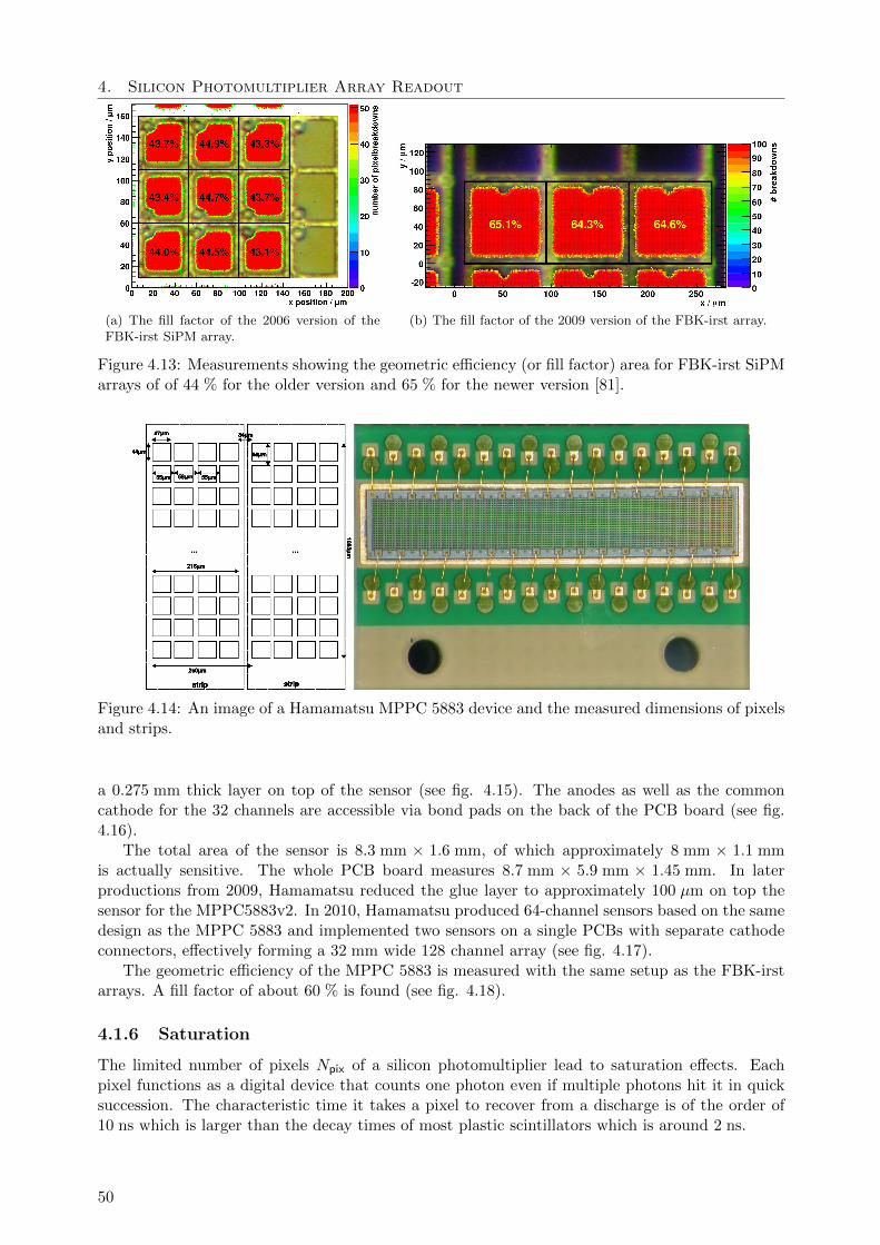
4. Silicon Photomultiplier Array Readout
(a) The fill factor of the 2006 version of theFBK-irst SiPM array.
(b) The fill factor of the 2009 version of the FBK-irst array.
Figure 4.13: Measurements showing the geometric efficiency (or fill factor) area for FBK-irst SiPMarrays of of 44 % for the older version and 65 % for the newer version [81].
Figure 4.14: An image of a Hamamatsu MPPC 5883 device and the measured dimensions of pixelsand strips.
a 0.275 mm thick layer on top of the sensor (see fig. 4.15). The anodes as well as the commoncathode for the 32 channels are accessible via bond pads on the back of the PCB board (see fig.4.16).
The total area of the sensor is 8.3 mm × 1.6 mm, of which approximately 8 mm × 1.1 mmis actually sensitive. The whole PCB board measures 8.7 mm × 5.9 mm × 1.45 mm. In laterproductions from 2009, Hamamatsu reduced the glue layer to approximately 100 µm on top thesensor for the MPPC5883v2. In 2010, Hamamatsu produced 64-channel sensors based on the samedesign as the MPPC 5883 and implemented two sensors on a single PCBs with separate cathodeconnectors, effectively forming a 32 mm wide 128 channel array (see fig. 4.17).
The geometric efficiency of the MPPC 5883 is measured with the same setup as the FBK-irstarrays. A fill factor of about 60 % is found (see fig. 4.18).
4.1.6 Saturation
The limited number of pixels Npix of a silicon photomultiplier lead to saturation effects. Eachpixel functions as a digital device that counts one photon even if multiple photons hit it in quicksuccession. The characteristic time it takes a pixel to recover from a discharge is of the order of10 ns which is larger than the decay times of most plastic scintillators which is around 2 ns.
50
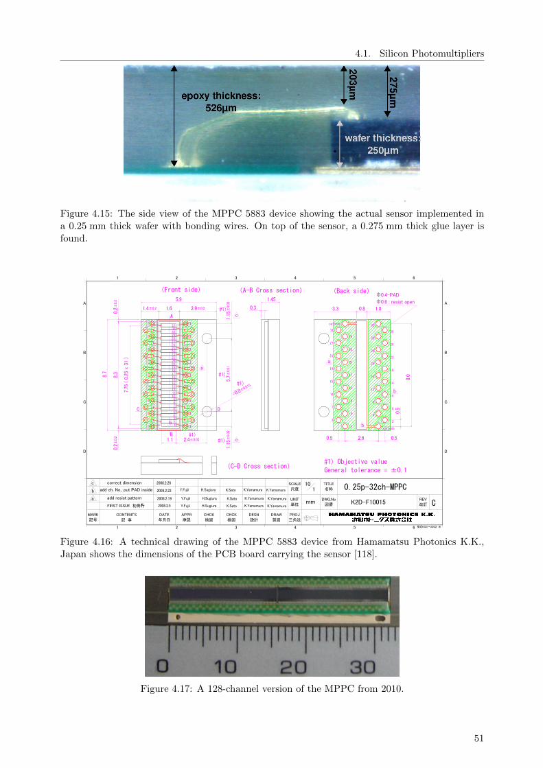
4.1. Silicon Photomultipliers
Figure 4.15: The side view of the MPPC 5883 device showing the actual sensor implemented ina 0.25 mm thick wafer with bonding wires. On top of the sensor, a 0.275 mm thick glue layer isfound.
Figure 4.16: A technical drawing of the MPPC 5883 device from Hamamatsu Photonics K.K.,Japan shows the dimensions of the PCB board carrying the sensor [118].
Figure 4.17: A 128-channel version of the MPPC from 2010.
51
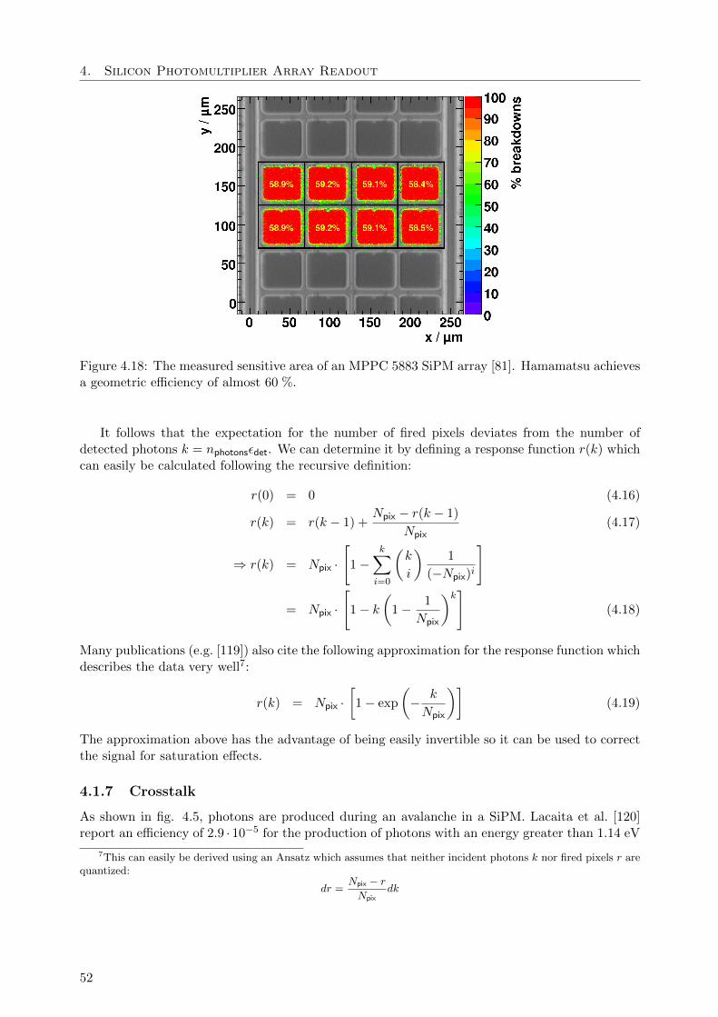
4. Silicon Photomultiplier Array Readout
Figure 4.18: The measured sensitive area of an MPPC 5883 SiPM array [81]. Hamamatsu achievesa geometric efficiency of almost 60 %.
It follows that the expectation for the number of fired pixels deviates from the number ofdetected photons k = nphotonsεdet. We can determine it by defining a response function r(k) whichcan easily be calculated following the recursive definition:
r(0) = 0 (4.16)
r(k) = r(k − 1) +Npix − r(k − 1)
Npix(4.17)
⇒ r(k) = Npix ·
[1−
k∑i=0
(k
i
)1
(−Npix)i
]
= Npix ·
[1− k
(1− 1
Npix
)k](4.18)
Many publications (e.g. [119]) also cite the following approximation for the response function whichdescribes the data very well7:
r(k) = Npix ·[1− exp
(− k
Npix
)](4.19)
The approximation above has the advantage of being easily invertible so it can be used to correctthe signal for saturation effects.
4.1.7 Crosstalk
As shown in fig. 4.5, photons are produced during an avalanche in a SiPM. Lacaita et al. [120]report an efficiency of 2.9 · 10−5 for the production of photons with an energy greater than 1.14 eV
7This can easily be derived using an Ansatz which assumes that neither incident photons k nor fired pixels r arequantized:
dr =Npix − rNpix
dk
52
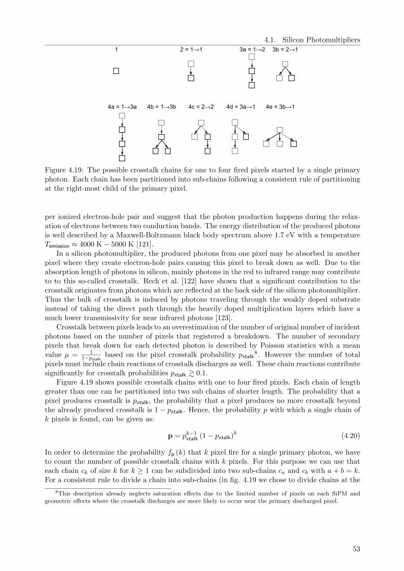
4.1. Silicon Photomultipliers
1 2 = 1→1 3a = 1→2 3b = 2→1
4a = 1→3a 4b = 1→3b 4c = 2→2 4d = 3a→1 4e = 3b→1
Figure 4.19: The possible crosstalk chains for one to four fired pixels started by a single primaryphoton. Each chain has been partitioned into sub-chains following a consistent rule of partitioningat the right-most child of the primary pixel.
per ionized electron-hole pair and suggest that the photon production happens during the relax-ation of electrons between two conduction bands. The energy distribution of the produced photonsis well described by a Maxwell-Boltzmann black body spectrum above 1.7 eV with a temperatureTemission ≈ 4000 K− 5000 K [121].
In a silicon photomultiplier, the produced photons from one pixel may be absorbed in anotherpixel where they create electron-hole pairs causing this pixel to break down as well. Due to theabsorption length of photons in silicon, mainly photons in the red to infrared range may contributeto to this so-called crosstalk. Rech et al. [122] have shown that a significant contribution to thecrosstalk originates from photons which are reflected at the back side of the silicon photomultiplier.Thus the bulk of crosstalk is induced by photons traveling through the weakly doped substrateinstead of taking the direct path through the heavily doped multiplication layers which have amuch lower transmissivity for near infrared photons [123].
Crosstalk between pixels leads to an overestimation of the number of original number of incidentphotons based on the number of pixels that registered a breakdown. The number of secondarypixels that break down for each detected photon is described by Poisson statistics with a meanvalue µ = 1
1−pxtalk based on the pixel crosstalk probability pxtalk8. However the number of total
pixels must include chain reactions of crosstalk discharges as well. These chain reactions contributesignificantly for crosstalk probabilities pxtalk & 0.1.
Figure 4.19 shows possible crosstalk chains with one to four fired pixels. Each chain of lengthgreater than one can be partitioned into two sub chains of shorter length. The probability that apixel produces crosstalk is pxtalk, the probability that a pixel produces no more crosstalk beyondthe already produced crosstalk is 1− pxtalk. Hence, the probability p with which a single chain ofk pixels is found, can be given as:
p = pk−1xtalk (1− pxtalk)k (4.20)
In order to determine the probability fp (k) that k pixel fire for a single primary photon, we haveto count the number of possible crosstalk chains with k pixels. For this purpose we can use thateach chain ck of size k for k ≥ 1 can be subdivided into two sub-chains ca and cb with a+ b = k.For a consistent rule to divide a chain into sub-chains (in fig. 4.19 we chose to divide chains at the
8This description already neglects saturation effects due to the limited number of pixels on each SiPM andgeometric effects where the crosstalk discharges are more likely to occur near the primary discharged pixel.
53

4. Silicon Photomultiplier Array Readout
right-most child of the primary pixel), we find that two chains ck1 = ca1 → cb1 and ck2 = ca2 → cb2are different if either of the two sub-chains differ:
ck1 = ck2 ⇔ [ca1 = ca2 ∧ cb1 = cb2 ] (4.21)
Therefore, the set Ck of all chains of length k fulfill Von Segner’s recurrence relation [124]. Thismeans that the set of chains of size k is equal to all chains of size k that can be created from chainswith a length smaller than k - or more specifically in terms of the number of elements in Ck:
|Ck| =k−1∑i=1
|Ci| × |Ck−i| (4.22)
with |C1| = 1.The number of crosstalk chains with k pixels Ck = |Ck| is given by the so-called Catalan
numbers:
Ck+1 = −2
(12
k + 1
)(−4)k =
(2kk
)1
k + 1(4.23)
We can therefore determine the probability that k pixels fire for one primary pixel hit by aphoton to be:
fp (k) =
(2k − 2k − 1
)pk−1xtalk (1− pxtalk)k
k(4.24)
Using Stirling’s approximation the ratio of total fired pixels to primary pixels fired by photonsr(pxtalk) can be given as:
r(pxtalk) = 1− pxtalk +∞∑k=1
4k√πk
(1− pxtalk)k+1pkxtalk (4.25)
For pxtalk . 0.32 a good approximation (better than 0.5 %) is given by the formula:
r(pxtalk) ≈ a1 · exp(a2 · pxtalk) + (1− a1) + pxtalk (4.26)
with the parameters a1 = 0.0304 and a2 = 9.6223.This result is valid as long as saturation effects due to the limited number of pixel can be
neglected. The correction term for both crosstalk and saturation of the SiPM at the same timehas to be calculated numerically.
A simplified model for crosstalk assumes that there is only generation of crosstalk (e.g. [125]).In this case the ratio of fired pixels compared to the number of detected photons is given by thegeometric series:
r(pxtalk) = (1− pxtalk)∞∑i=1
ipi−1xtalk =
1
1− pxtalk(4.27)
4.1.8 After-pulsing
Next to crosstalk so-called after-pulsing plays a role for silicon photomultipliers. Minority chargecarriers within the depletion zone of the p-n-junction may be trapped in meta-stable states duringthe discharge of a SiPM pixel [126]. These states have a decay time of tens to hundreds ofnanoseconds. The release of the trapped charge carriers may lead to another discharge of a pixelcorrelated with previous breakdown.
In the context of using a SiPM as a photon-counting device, after-pulsing behaves similar tothe simplified crosstalk model described before. The ratio of counted discharges compared to the
54

4.1. Silicon Photomultipliers
number of detected photons based on the after-pulsing probability pafter−pulsing can then be givenas9:
r(pafter−pulsing) =1
1− pafter−pulsing(4.28)
As a first order approximation (for pafter−pulsing 1 and pxtalk 1) we can therefore write thecombined response function for crosstalk an after-pulsing as:
r(pxtalk, pafter−pulsing) ≈ 1
1− pafter−pulsing· 1
1− pxtalk≈ 1
1− (pafter−pulsing + pxtalk)(4.29)
A measurement setup that is not able to distinguish between crosstalk and after-pulsing canonly measure the combined probability pafter−pulsing + pxtalk.
4.1.9 Measurement of SiPM properties
Basic properties of the available MPPC5883 [95,118], FBK-irst 2006 [127] and 2009 [81] have beenmeasured and are summarized in table 4.2. Photon detection efficiency (the probability that aphoton causes a SiPM pixel to break down) and crosstalk (as well as after-pulsing) directly influencethe performance of the scintillating fiber tracker. Therefore, these properties are discussed in alittle more detail.
Table 4.2: Basic properties of the silicon photomultiplier arrays. Noise rate and dark current aregiven per readout channel.
Hamamatsu FBK-irst FBK-irstMPPC 5883 2006 2009
number of channels 32 32 32
readout pitch / mm 0.250 0.250 0.275
pixel size / µm× µm 55× 55 46× 50 85× 85
breakdown voltage (20C) / V 69.0± 0.5 30.3± 0.3 ∼ 34
gain ∼ 106 ∼ 106 ∼ 2 · 106
peak sensitivity at wavelength / nm 450 550 550
peak photon detection efficiency / % 50 20 25
noise discharge rate (25C) / kHz ∼ 150 ∼ 600 ∼ 600
dark current (20C) / µA ∼ 0.1 n.a. n.a.
crosstalk / (1− nphotons/npixels) ∼ 0.3 ∼ 0.1 ∼ 0.1
Crosstalk and after-pulsing
The crosstalk probabilities px for the supplied SiPM arrays are measured ( [95,117]) using a pulsedLED to measure single-photon spectra of SiPM with a synchronized readout system. The measuredADC spectra are then fitted following the method described in [125]. This method assumes thesimplified crosstalk model discussed in 4.1.7.
The measured quantity px describes the cumulative effects of crosstalk and after-pulsing. Thesetup used to determine the crosstalk probability is not capable of directly distinguishing between
9Neglecting crosstalk.
55
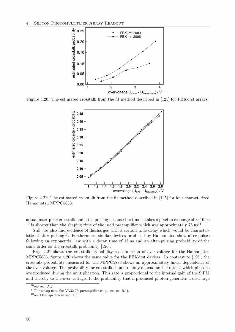
4. Silicon Photomultiplier Array Readout
1 2 3 4
0.05
0.10
0.15
0.20
0.25 FBK-irst 2009FBK-irst 2006
overvoltage (Ubias - Ubreakdown) / V
estim
ated
cro
ssta
lk p
roba
bilit
y
0.00
Figure 4.20: The estimated crosstalk from the fit method described in [125] for FBK-irst arrays.
1 1.2 1.4 1.6 1.8 2.0 2.2 2.4 2.6 2.8
0.05
0.10
0.15
0.20
0.25
0.30
0.35
0.40
0.45
overvoltage (Ubias - Ubreakdown) / V
estim
ated
cro
ssta
lk p
roba
bilit
y
Figure 4.21: The estimated crosstalk from the fit method described in [125] for four characterizedHamamatsu MPPC5883.
actual inter-pixel crosstalk and after-pulsing because the time it takes a pixel to recharge of ∼ 10 ns10 is shorter than the shaping time of the used preamplifier which was approximately 75 ns11.
Still, we also find evidence of discharges with a certain time delay which would be character-istic of after-pulsing12. Furthermore, similar devices produced by Hamamatsu show after-pulsesfollowing an exponential law with a decay time of 15 ns and an after-pulsing probability of thesame order as the crosstalk probability [126].
Fig. 4.21 shows the crosstalk probability as a function of over-voltage for the HamamatsuMPPC5883, figure 4.20 shows the same value for the FBK-irst devices. In contrast to [126], thecrosstalk probability measured for the MPPC5883 shows an approximately linear dependence ofthe over-voltage. The probability for crosstalk should mainly depend on the rate at which photonsare produced during the multiplication. This rate is proportional to the internal gain of the SiPMand thereby to the over-voltage. If the probability that a produced photon generates a discharge
10see sec. A.211The setup uses the VA32-75 preamplifier chip, see sec. 5.1).12see LED spectra in sec. 4.3
56
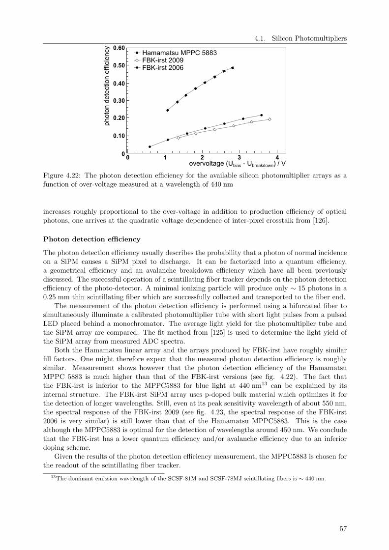
4.1. Silicon Photomultipliers
overvoltage (Ubias - Ubreakdown) / V
phot
on d
etec
tion
effic
ienc
y
0.10
0.20
0.30
0.40
0.50
0 1 2 3 4
0.60
0
FBK-irst 2009FBK-irst 2006
Hamamatsu MPPC 5883
Figure 4.22: The photon detection efficiency for the available silicon photomultiplier arrays as afunction of over-voltage measured at a wavelength of 440 nm
increases roughly proportional to the over-voltage in addition to production efficiency of opticalphotons, one arrives at the quadratic voltage dependence of inter-pixel crosstalk from [126].
Photon detection efficiency
The photon detection efficiency usually describes the probability that a photon of normal incidenceon a SiPM causes a SiPM pixel to discharge. It can be factorized into a quantum efficiency,a geometrical efficiency and an avalanche breakdown efficiency which have all been previouslydiscussed. The successful operation of a scintillating fiber tracker depends on the photon detectionefficiency of the photo-detector. A minimal ionizing particle will produce only ∼ 15 photons in a0.25 mm thin scintillating fiber which are successfully collected and transported to the fiber end.
The measurement of the photon detection efficiency is performed using a bifurcated fiber tosimultaneously illuminate a calibrated photomultiplier tube with short light pulses from a pulsedLED placed behind a monochromator. The average light yield for the photomultiplier tube andthe SiPM array are compared. The fit method from [125] is used to determine the light yield ofthe SiPM array from measured ADC spectra.
Both the Hamamatsu linear array and the arrays produced by FBK-irst have roughly similarfill factors. One might therefore expect that the measured photon detection efficiency is roughlysimilar. Measurement shows however that the photon detection efficiency of the HamamatsuMPPC 5883 is much higher than that of the FBK-irst versions (see fig. 4.22). The fact thatthe FBK-irst is inferior to the MPPC5883 for blue light at 440 nm13 can be explained by itsinternal structure. The FBK-irst SiPM array uses p-doped bulk material which optimizes it forthe detection of longer wavelengths. Still, even at its peak sensitivity wavelength of about 550 nm,the spectral response of the FBK-irst 2009 (see fig. 4.23, the spectral response of the FBK-irst2006 is very similar) is still lower than that of the Hamamatsu MPPC5883. This is the casealthough the MPPC5883 is optimal for the detection of wavelengths around 450 nm. We concludethat the FBK-irst has a lower quantum efficiency and/or avalanche efficiency due to an inferiordoping scheme.
Given the results of the photon detection efficiency measurement, the MPPC5883 is chosen forthe readout of the scintillating fiber tracker.
13The dominant emission wavelength of the SCSF-81M and SCSF-78MJ scintillating fibers is ∼ 440 nm.
57

4. Silicon Photomultiplier Array Readout
440 460 480 500 520 540 560 580
0.10
0.20
0.30
0.40
0.50
0
Hamamatsu MPPC5883FBK-irst 2009
1.5V
2.0V
2.5V
1.5V
2.5V
3.5V
wavelength / nm
phot
on d
etec
tion
effic
ienc
y
Figure 4.23: The photon detection efficiency for the Hamamatsu MPPC5883 and the FBK-irst2009 as a function of wavelength for different over-voltages.
photon energy / eV1 2 3 4 5 6 7
refle
ctiv
ity
0.2
0.3
0.4
0.5
0.6
0.7
0.8
0.9
400
500
800
700
600
300
photon wavelength / nm
Figure 4.24: Specular reflectivity of chromatized polished aluminum mirrors used for fiber moduleprototypes [128]
4.2 Readout Electronics for SiPM Arrays
4.2.1 Carrier circuit boards for SiPM arrays
Prototype 2009
The MPPC5883 SiPMs are soldered to printed circuit boards (PCB) which can be mounted ontop of the fiber modules. These PCBs are called HPO14 boards. Each HPO board has a connectorfor the front-end electronics and carries four MPPC5883 32-channel silicon photomultiplier arrays.The MPPC5883s are interleaved with four small mirrors made from polished and chromatizedaluminum pieces as mirrors. The aluminum mirrors have a reflectivity of 68 % at a wavelength of450 nm (see fig. 4.24).
An optical grease is applied to the HPO boards in order to improve the optical coupling of theMPPC5883 to the fiber ends. The employed optical compounds were NyeGel OC-459 (refractiveindex r = 1.61@450 nm) and NyeGel OCK-451 (refractive index r = 1.54@450 nm) [129].
14Hybrid Part Optical
58
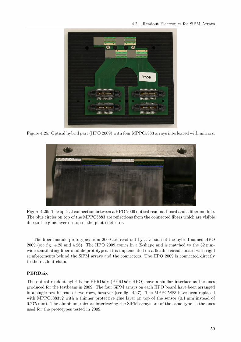
4.2. Readout Electronics for SiPM Arrays
Figure 4.25: Optical hybrid part (HPO 2009) with four MPPC5883 arrays interleaved with mirrors.
Figure 4.26: The optical connection between a HPO 2009 optical readout board and a fiber module.The blue circles on top of the MPPC5883 are reflections from the connected fibers which are visibledue to the glue layer on top of the photo-detector.
The fiber module prototypes from 2009 are read out by a version of the hybrid named HPO2009 (see fig. 4.25 and 4.26). The HPO 2009 comes in a Z-shape and is matched to the 32 mm-wide scintillating fiber module prototypes. It is implemented on a flexible circuit board with rigidreinforcements behind the SiPM arrays and the connectors. The HPO 2009 is connected directlyto the readout chain.
PERDaix
The optical readout hybrids for PERDaix (PERDaix-HPO) have a similar interface as the onesproduced for the testbeam in 2009. The four SiPM arrays on each HPO board have been arrangedin a single row instead of two rows, however (see fig. 4.27). The MPPC5883 have been replacedwith MPPC5883v2 with a thinner protective glue layer on top of the sensor (0.1 mm instead of0.275 mm). The aluminum mirrors interleaving the SiPM arrays are of the same type as the onesused for the prototypes tested in 2009.
59
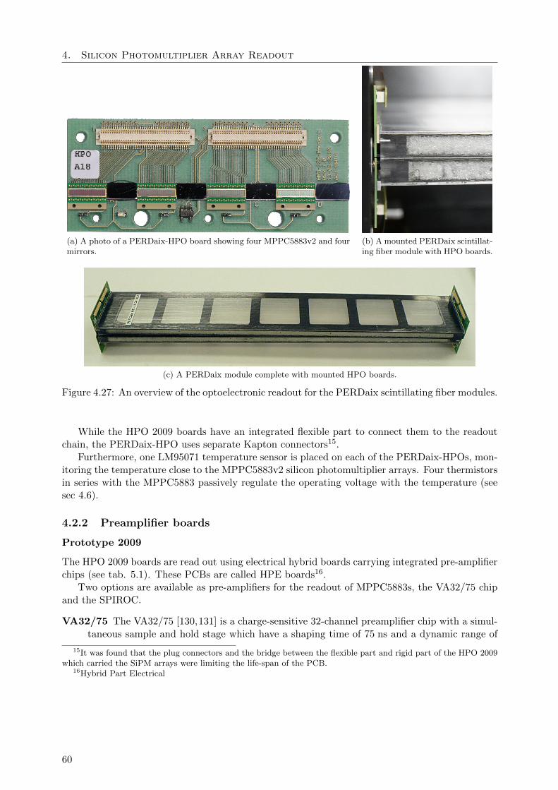
4. Silicon Photomultiplier Array Readout
(a) A photo of a PERDaix-HPO board showing four MPPC5883v2 and fourmirrors.
(b) A mounted PERDaix scintillat-ing fiber module with HPO boards.
(c) A PERDaix module complete with mounted HPO boards.
Figure 4.27: An overview of the optoelectronic readout for the PERDaix scintillating fiber modules.
While the HPO 2009 boards have an integrated flexible part to connect them to the readoutchain, the PERDaix-HPO uses separate Kapton connectors15.
Furthermore, one LM95071 temperature sensor is placed on each of the PERDaix-HPOs, mon-itoring the temperature close to the MPPC5883v2 silicon photomultiplier arrays. Four thermistorsin series with the MPPC5883 passively regulate the operating voltage with the temperature (seesec 4.6).
4.2.2 Preamplifier boards
Prototype 2009
The HPO 2009 boards are read out using electrical hybrid boards carrying integrated pre-amplifierchips (see tab. 5.1). These PCBs are called HPE boards16.
Two options are available as pre-amplifiers for the readout of MPPC5883s, the VA32/75 chipand the SPIROC.
VA32/75 The VA32/75 [130,131] is a charge-sensitive 32-channel preamplifier chip with a simul-taneous sample and hold stage which have a shaping time of 75 ns and a dynamic range of
15It was found that the plug connectors and the bridge between the flexible part and rigid part of the HPO 2009which carried the SiPM arrays were limiting the life-span of the PCB.
16Hybrid Part Electrical
60
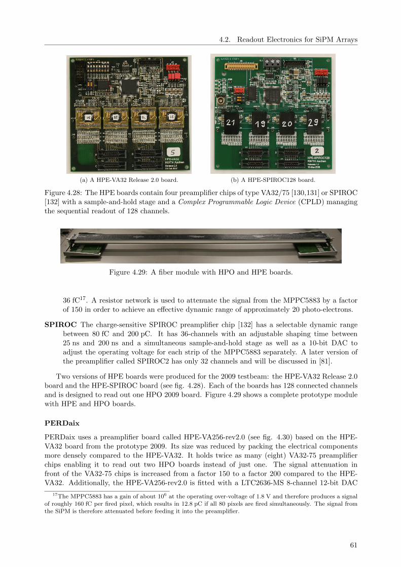
4.2. Readout Electronics for SiPM Arrays
(a) A HPE-VA32 Release 2.0 board. (b) A HPE-SPIROC128 board.
Figure 4.28: The HPE boards contain four preamplifier chips of type VA32/75 [130,131] or SPIROC[132] with a sample-and-hold stage and a Complex Programmable Logic Device (CPLD) managingthe sequential readout of 128 channels.
Figure 4.29: A fiber module with HPO and HPE boards.
36 fC17. A resistor network is used to attenuate the signal from the MPPC5883 by a factorof 150 in order to achieve an effective dynamic range of approximately 20 photo-electrons.
SPIROC The charge-sensitive SPIROC preamplifier chip [132] has a selectable dynamic rangebetween 80 fC and 200 pC. It has 36-channels with an adjustable shaping time between25 ns and 200 ns and a simultaneous sample-and-hold stage as well as a 10-bit DAC toadjust the operating voltage for each strip of the MPPC5883 separately. A later version ofthe preamplifier called SPIROC2 has only 32 channels and will be discussed in [81].
Two versions of HPE boards were produced for the 2009 testbeam: the HPE-VA32 Release 2.0board and the HPE-SPIROC board (see fig. 4.28). Each of the boards has 128 connected channelsand is designed to read out one HPO 2009 board. Figure 4.29 shows a complete prototype modulewith HPE and HPO boards.
PERDaix
PERDaix uses a preamplifier board called HPE-VA256-rev2.0 (see fig. 4.30) based on the HPE-VA32 board from the prototype 2009. Its size was reduced by packing the electrical componentsmore densely compared to the HPE-VA32. It holds twice as many (eight) VA32-75 preamplifierchips enabling it to read out two HPO boards instead of just one. The signal attenuation infront of the VA32-75 chips is increased from a factor 150 to a factor 200 compared to the HPE-VA32. Additionally, the HPE-VA256-rev2.0 is fitted with a LTC2636-MS 8-channel 12-bit DAC
17The MPPC5883 has a gain of about 106 at the operating over-voltage of 1.8 V and therefore produces a signalof roughly 160 fC per fired pixel, which results in 12.8 pC if all 80 pixels are fired simultaneously. The signal fromthe SiPM is therefore attenuated before feeding it into the preamplifier.
61
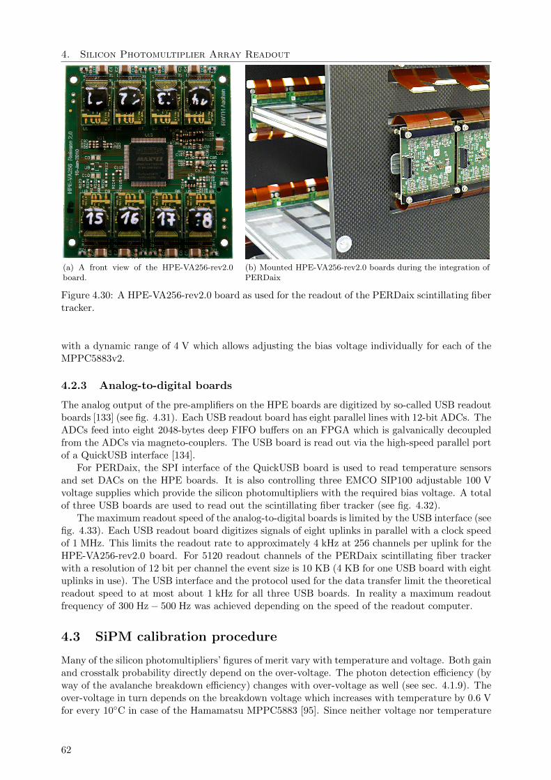
4. Silicon Photomultiplier Array Readout
(a) A front view of the HPE-VA256-rev2.0board.
(b) Mounted HPE-VA256-rev2.0 boards during the integration ofPERDaix
Figure 4.30: A HPE-VA256-rev2.0 board as used for the readout of the PERDaix scintillating fibertracker.
with a dynamic range of 4 V which allows adjusting the bias voltage individually for each of theMPPC5883v2.
4.2.3 Analog-to-digital boards
The analog output of the pre-amplifiers on the HPE boards are digitized by so-called USB readoutboards [133] (see fig. 4.31). Each USB readout board has eight parallel lines with 12-bit ADCs. TheADCs feed into eight 2048-bytes deep FIFO buffers on an FPGA which is galvanically decoupledfrom the ADCs via magneto-couplers. The USB board is read out via the high-speed parallel portof a QuickUSB interface [134].
For PERDaix, the SPI interface of the QuickUSB board is used to read temperature sensorsand set DACs on the HPE boards. It is also controlling three EMCO SIP100 adjustable 100 Vvoltage supplies which provide the silicon photomultipliers with the required bias voltage. A totalof three USB boards are used to read out the scintillating fiber tracker (see fig. 4.32).
The maximum readout speed of the analog-to-digital boards is limited by the USB interface (seefig. 4.33). Each USB readout board digitizes signals of eight uplinks in parallel with a clock speedof 1 MHz. This limits the readout rate to approximately 4 kHz at 256 channels per uplink for theHPE-VA256-rev2.0 board. For 5120 readout channels of the PERDaix scintillating fiber trackerwith a resolution of 12 bit per channel the event size is 10 KB (4 KB for one USB board with eightuplinks in use). The USB interface and the protocol used for the data transfer limit the theoreticalreadout speed to at most about 1 kHz for all three USB boards. In reality a maximum readoutfrequency of 300 Hz− 500 Hz was achieved depending on the speed of the readout computer.
4.3 SiPM calibration procedure
Many of the silicon photomultipliers’ figures of merit vary with temperature and voltage. Both gainand crosstalk probability directly depend on the over-voltage. The photon detection efficiency (byway of the avalanche breakdown efficiency) changes with over-voltage as well (see sec. 4.1.9). Theover-voltage in turn depends on the breakdown voltage which increases with temperature by 0.6 Vfor every 10C in case of the Hamamatsu MPPC5883 [95]. Since neither voltage nor temperature
62
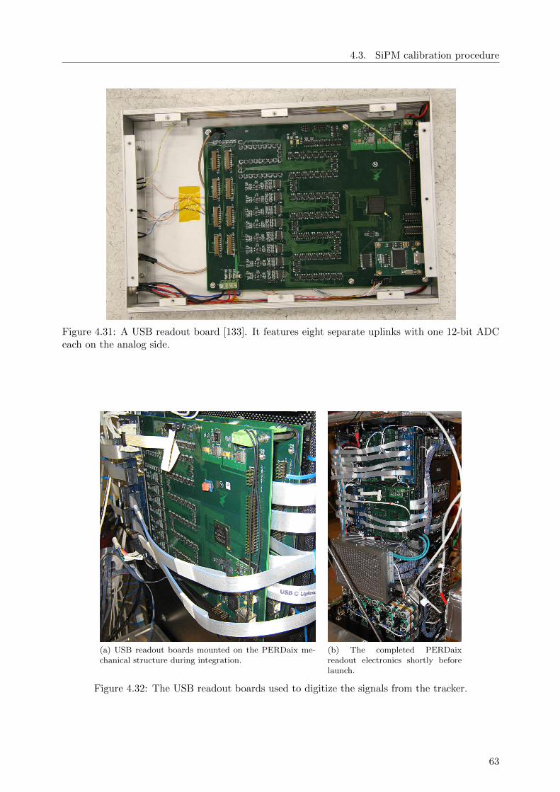
4.3. SiPM calibration procedure
Figure 4.31: A USB readout board [133]. It features eight separate uplinks with one 12-bit ADCeach on the analog side.
(a) USB readout boards mounted on the PERDaix me-chanical structure during integration.
(b) The completed PERDaixreadout electronics shortly beforelaunch.
Figure 4.32: The USB readout boards used to digitize the signals from the tracker.
63
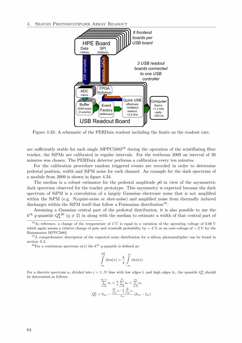
4. Silicon Photomultiplier Array Readout
HPE BoardData
<40kHzSPI
500kbit/s
256
sam
ples
sens
ors,
DA
Cs
USB Readout Board
Buffer2048 bytes(3 events)
ADC<4kHz
FPGAMultiplexer
EventFactory4KB/event
Quick USBeffectively143Mbit/sreadout: <3,5 kHz
Computertheory:
<1.2 kHzreally:
~300 Hz
8 frontendboards perUSB board
3 USB readoutboards connected
to one USB controller
Figure 4.33: A schematic of the PERDaix readout including the limits on the readout rate.
are sufficiently stable for each single MPPC588318 during the operation of the scintillating fibertracker, the SiPMs are calibrated in regular intervals. For the testbeam 2009 an interval of 30minutes was chosen. The PERDaix detector performs a calibration every ten minutes.
For the calibration procedure random triggered events are recorded in order to determinepedestal position, width and SiPM noise for each channel. An example for the dark spectrum ofa module from 2009 is shown in figure 4.34.
The median is a robust estimator for the pedestal amplitude p0 in view of the asymmetricdark spectrum observed for the tracker prototype. This asymmetry is expected because the darkspectrum of SiPM is a convolution of a largely Gaussian electronic noise that is not amplifiedwithin the SiPM (e.g. Nyquist-noise or shot-noise) and amplified noise from thermally induceddischarges within the SiPM itself that follow a Poissonian distribution19.
Assuming a Gaussian central part of the pedestal distribution, it is also possible to use thekth q-quantile Qqk
20 (q 6= 2) in along with the median to estimate a width of that central part of
18As reference, a change of the temperature of 1C is equal to a variation of the operating voltage of 0.06 Vwhich again means a relative change of gain and crosstalk probability by ∼ 3 % at an over-voltage of ∼ 2 V for theHamamatsu MPPC5883.
19A comprehensive description of the expected noise distribution for a silicon photomultiplier can be found insection A.2.
20For a continuous spectrum a(x) the kth q-quantile is defined as:
Qqk∫
−∞
dxa(x) =k
q
∞∫−∞
dxa(x)
For a discrete spectrum ai divided into i = 1..N bins with low edges li and high edges hi, the quantile Qqk shouldbe determined as follows:
m−1∑i=0
ai <kq
N∑i=0
ai <m∑i=0
ai
Qqk = hm −m∑
i=0ai− k
q
N∑i=0
ai
am(hm − lm)
64
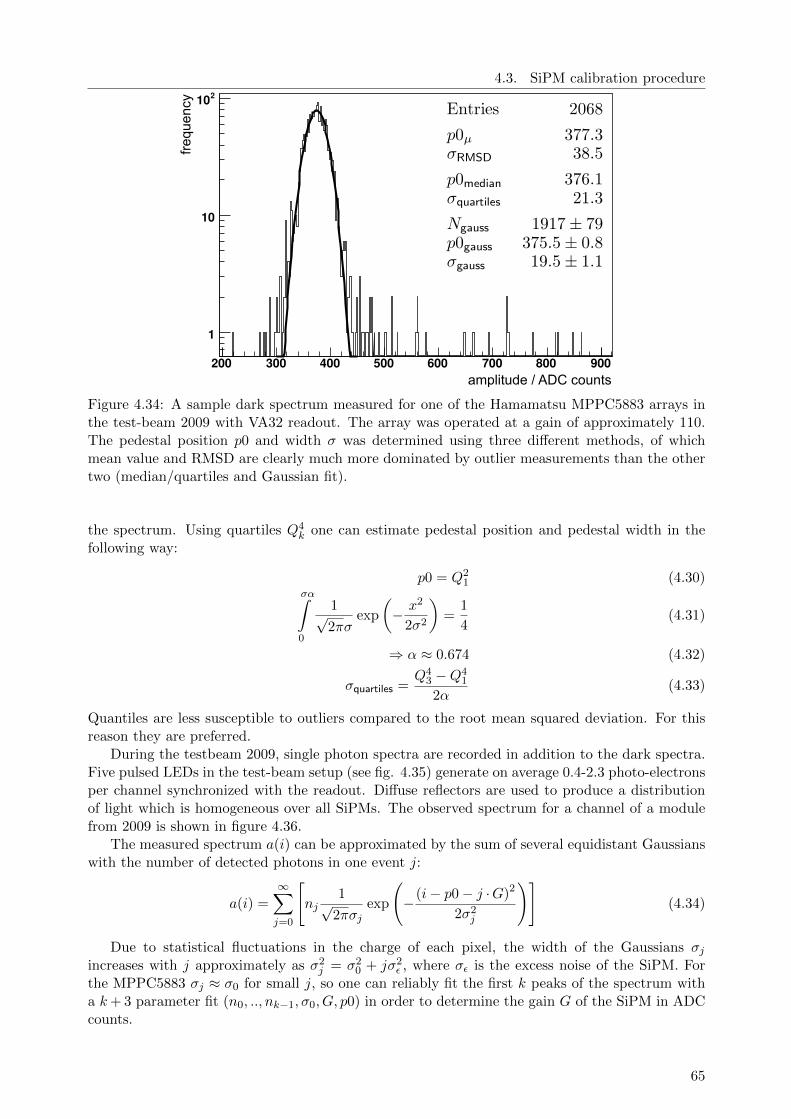
4.3. SiPM calibration procedure
200 300 400 500 600 700 800 900
1
10
210
amplitude / ADC counts
freq
uenc
y
Figure 4.34: A sample dark spectrum measured for one of the Hamamatsu MPPC5883 arrays inthe test-beam 2009 with VA32 readout. The array was operated at a gain of approximately 110.The pedestal position p0 and width σ was determined using three different methods, of whichmean value and RMSD are clearly much more dominated by outlier measurements than the othertwo (median/quartiles and Gaussian fit).
the spectrum. Using quartiles Q4k one can estimate pedestal position and pedestal width in the
following way:
p0 = Q21 (4.30)
σα∫0
1√2πσ
exp
(− x2
2σ2
)=
1
4(4.31)
⇒ α ≈ 0.674 (4.32)
σquartiles =Q4
3 −Q41
2α(4.33)
Quantiles are less susceptible to outliers compared to the root mean squared deviation. For thisreason they are preferred.
During the testbeam 2009, single photon spectra are recorded in addition to the dark spectra.Five pulsed LEDs in the test-beam setup (see fig. 4.35) generate on average 0.4-2.3 photo-electronsper channel synchronized with the readout. Diffuse reflectors are used to produce a distributionof light which is homogeneous over all SiPMs. The observed spectrum for a channel of a modulefrom 2009 is shown in figure 4.36.
The measured spectrum a(i) can be approximated by the sum of several equidistant Gaussianswith the number of detected photons in one event j:
a(i) =
∞∑j=0
[nj
1√2πσj
exp
(−(i− p0− j ·G)2
2σ2j
)](4.34)
Due to statistical fluctuations in the charge of each pixel, the width of the Gaussians σjincreases with j approximately as σ2
j = σ20 + jσ2
ε , where σε is the excess noise of the SiPM. Forthe MPPC5883 σj ≈ σ0 for small j, so one can reliably fit the first k peaks of the spectrum witha k+ 3 parameter fit (n0, .., nk−1, σ0, G, p0) in order to determine the gain G of the SiPM in ADCcounts.
65
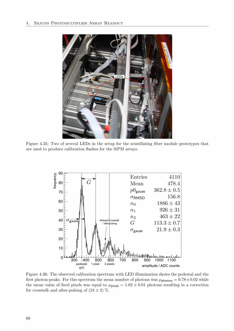
4. Silicon Photomultiplier Array Readout
Figure 4.35: Two of several LEDs in the setup for the scintillating fiber module prototypes thatare used to produce calibration flashes for the SiPM arrays.
300 400 500 600 700 800 900 1000 11000
10
20
30
40
50
60
70
80
90
delayed crosstalk/ afterpulsing
pedestal(p0)
1 pixel 2 pixels amplitude / ADC counts
frequency
Figure 4.36: The observed calibration spectrum with LED illumination shows the pedestal and thefirst photon-peaks. For this spectrum the mean number of photons was µphotons = 0.78±0.02 whilethe mean value of fired pixels was equal to µpixels = 1.02 ± 0.01 photons resulting in a correctionfor crosstalk and after-pulsing of (24± 2) %.
66
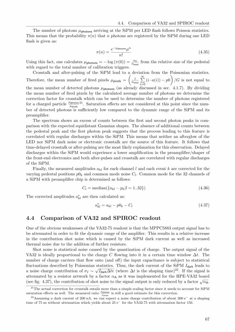
4.4. Comparison of VA32 and SPIROC readout
The number of photons µphotons arriving at the SiPM per LED flash follows Poisson statistics.This means that the probability π(n) that n photons are registered by the SiPM during one LEDflash is given as:
π(n) =e−µphotonsµn
n!(4.35)
Using this fact, one calculates µphotons = − log (π(0)) = n0ntotal
from the relative size of the pedestalwith regard to the total number of calibration triggers.
Crosstalk and after-pulsing of the SiPM lead to a deviation from the Poissonian statistics.
Therefore, the mean number of fired pixels µpixels =
(1
ntotal
∞∑i=0
(i · a(i))− p0)/G is not equal to
the mean number of detected photons µphotons (as already discussed in sec. 4.1.7). By dividingthe mean number of fired pixels by the calculated average number of photons we determine thecorrection factor for crosstalk which can be used to determine the number of photons registeredfor a charged particle
µphotonsµpixels
21. Saturation effects are not considered at this point since the num-
ber of detected photons is sufficiently low compared to the dynamic range of the SiPM and itspreamplifier.
The spectrum shows an excess of counts between the first and second photon peaks in com-parison with the expected equidistant Gaussian shapes. The absence of additional counts betweenthe pedestal peak and the first photon peak suggests that the process leading to this feature iscorrelated with regular discharges within the SiPM. This means that neither an afterglow of theLED nor SiPM dark noise or electronic crosstalk are the source of this feature. It follows thattime-delayed crosstalk or after-pulsing are the most likely explanation for this observation. Delayeddischarges within the SiPM would experience a lower amplification in the preamplifier/shaper ofthe front-end electronics and both after-pulses and crosstalk are correlated with regular dischargesof the SiPM.
Finally, the measured amplitudes akl for each channel l and each event k are corrected for thevarying pedestal positions p0k and common mode noise Cl. Common mode for the 32 channels ofa SiPM with preamplifier chip is determined as follows:
Cl = median(akl − pk|l = 1..32) (4.36)
The corrected amplitudes a∗kl are then calculated as:
a∗kl = akl − p0k − Cl (4.37)
4.4 Comparison of VA32 and SPIROC readout
One of the obvious weaknesses of the VA32-75 readout is that the MPPC5883 output signal has tobe attenuated in order to fit the dynamic range of the amplifier. This results in a relative increasein the contribution shot noise which is caused by the SiPM dark current as well as increasedthermal noise due to the addition of further resistors.
Shot noise is statistical noise caused by the quantization of charge. The output signal of theVA32 is ideally proportional to the charge C flowing into it in a certain time window ∆t. Thenumber of charge carriers that flow onto (and off) the input capacitance is subject to statisticalfluctuations described by Poissonian statistics. Thus, the dark current of the SiPM Idark leads toa noise charge contribution of σI ∼
√Idark∆te (where ∆t is the shaping time)22. If the signal is
attenuated by a resistor network by a factor αA as it was implemented for the HPE-VA32 board(see fig. 4.37), the contribution of shot noise to the signal output is only reduced by a factor
√αA.
21The actual correction for crosstalk entails more than a simple scaling factor since it needs to account for SiPMsaturation effects as well. The measured ratio
µphotons
µpixelsis still a good estimate for this correction.
22Assuming a dark current of 200 nA, we can expect a noise charge contribution of about 300 e− at a shapingtime of 75 ns without attenuation which yields about 25 e− for the VA32-75 with attenuation factor 150.
67
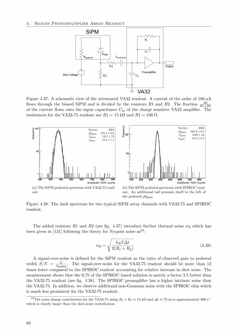
4. Silicon Photomultiplier Array Readout
Preamplifier
Cf
Rf
Output
Cin
R1
R2
Pixel
+−
Bias Voltage
Rquench
VA32
SiPM
Cprotection
Figure 4.37: A schematic view of the attenuated VA32 readout. A current of the order of 100 nAflows through the biased SiPM and is divided by the resistors R1 and R2. The fraction R2
R1+R2of the current flows onto the input capacitance Cin of the charge sensitive VA32 amplifier. Theresistances for the VA32-75 readout are R1 = 15 kΩ and R1 = 100 Ω.
200 300 400 500 600 700 800 900
1
10
210
amplitude / ADC counts
freq
uenc
y
(a) The SiPM pedestal spectrum with VA32-75 read-out.
100 200 300 400 500 600 700 800
1
10
210
freq
uenc
y
amplitude / ADC counts
(b) The SiPM pedestal spectrum with SPIROC read-out. An additional tail presents itself to the left ofthe pedestal p0gauss
Figure 4.38: The dark spectrum for two typical SiPM array channels with VA32-75 and SPIROCreadout.
The added resistors R1 and R2 (see fig. 4.37) introduce further thermal noise σR which hasbeen given in [131] following the theory for Nyquist noise as23:
σR =
√kBT∆t
2(R1 +R2)(4.38)
A signal-over-noise is defined for the SiPM readout as the ratio of observed gain to pedestalwidth S/N = G
σpedestal. The signal-over-noise for the VA32-75 readout should be more than 12
times lower compared to the SPIROC readout accounting for relative increase in shot noise. Themeasurement shows that the S/N of the SPIROC based solution is merely a factor 2.5 better thanthe VA32-75 readout (see fig. 4.38). The SPIROC preamplifier has a higher intrinsic noise thanthe VA32-75. In addition, we observe additional non-Gaussian noise with the SPIROC chip whichis much less prominent for the VA32-75 readout.
23The noise charge contribution for the VA32-75 using R1 +R2 ≈ 15 kΩ and ∆t ≈ 75 ns is approximately 600 e−
which is clearly larger than the shot-noise contribution.
68
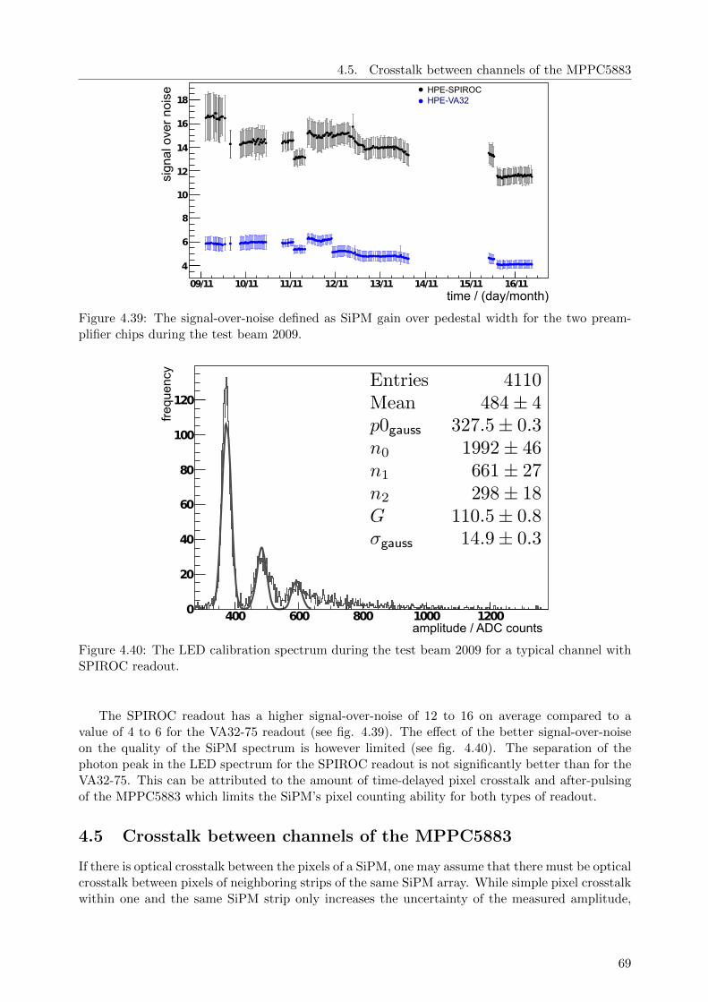
4.5. Crosstalk between channels of the MPPC5883
09/11 10/11 11/11 12/11 13/11 14/11 15/11 16/11
4
6
8
10
12
14
16
18
sign
al o
ver
nois
e
time / (day/month)
HPE-VA32HPE-SPIROC
Figure 4.39: The signal-over-noise defined as SiPM gain over pedestal width for the two pream-plifier chips during the test beam 2009.
400 600 800 1000 12000
20
40
60
80
100
120
frequency
amplitude / ADC counts
Figure 4.40: The LED calibration spectrum during the test beam 2009 for a typical channel withSPIROC readout.
The SPIROC readout has a higher signal-over-noise of 12 to 16 on average compared to avalue of 4 to 6 for the VA32-75 readout (see fig. 4.39). The effect of the better signal-over-noiseon the quality of the SiPM spectrum is however limited (see fig. 4.40). The separation of thephoton peak in the LED spectrum for the SPIROC readout is not significantly better than for theVA32-75. This can be attributed to the amount of time-delayed pixel crosstalk and after-pulsingof the MPPC5883 which limits the SiPM’s pixel counting ability for both types of readout.
4.5 Crosstalk between channels of the MPPC5883
If there is optical crosstalk between the pixels of a SiPM, one may assume that there must be opticalcrosstalk between pixels of neighboring strips of the same SiPM array. While simple pixel crosstalkwithin one and the same SiPM strip only increases the uncertainty of the measured amplitude,
69
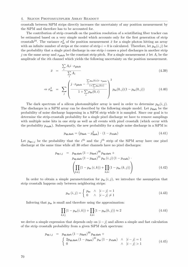
4. Silicon Photomultiplier Array Readout
crosstalk between SiPM strips directly increases the uncertainty of any position measurement bythe SiPM and therefore has to be accounted for.
The contribution of strip crosstalk on the position resolution of a scintillating fiber tracker canbe estimated based on a very simple model which accounts only for the first generation of stripcrosstalk24. The variance σ2
sx of the position measurement x for a single photon hitting an arraywith an infinite number of strips at the center of strip i = 0 is calculated. Therefore, let psx(i, j) bethe probability that a single pixel discharge in one strip i causes a pixel discharges in another stripj on the same array and xpitch be the constant strip pitch. For a single measurement x let Ai be theamplitude of the ith channel which yields the following uncertainty on the position measurement.
x =
∑iAii ·xpitch∑iAi
(4.39)
⇒ σ2sx =
∑j
j ·xpitch −
∑ipsx(0,i)i ·xpitch1+
∑ipsx(0,i)
1 +∑ipsx(0, i)
2
psx(0, j)(1− psx(0, j)) (4.40)
The dark spectrum of a silicon photomultiplier array is used in order to determine psx(i, j).The discharges in a SiPM array can be described by the following simple model. Let pdark be theprobability of noise discharge happening in a SiPM strip while it is sampled. Since our goal is todetermine the strip-crosstalk probability for a single pixel discharge we have to remove samplingswith multiple noise hits in one strip as well as all events with pixel crosstalk (which occur withthe probability pxtalk). Subsequently, the new probability for a single noise discharge in a SiPM is:
psp,dark =(pdark − p2
dark
)· (1− pxtalk) (4.41)
Let psp,i,j be the probability that the ith and the jth strip of the SiPM array have one pixeldischarge at the same time while all 30 other channels have no pixel discharges:
psp,i,j = psp,dark (1− pdark)30 psp,dark +
psp,dark (1− pdark)31 psx (i, j) (1− pxtalk) ·∏k 6=j
(1− psx (i, k)) +∏k 6=i
(1− psx (k, j))
(4.42)
In order to obtain a simple parametrization for psx (i, j), we introduce the assumption thatstrip crosstalk happens only between neighboring strips:
psx (i, j) =
psx ∧ |i− j| = 10 ∧ |i− j| 6= 1
(4.43)
Inferring that psx is small and therefore using the approximation:∏k 6=j
(1− psx(i, k)) +∏k 6=i
(1− psx(k, j)) ≈ 2 (4.44)
we derive a simple expression that depends only on |i− j| and allows a simple and fast calculationof the strip crosstalk probability from a given SiPM dark spectrum:
psp,i,j = psp,dark (1− pdark)30 psp,dark +2psp,dark (1− pdark)31 psx (1− pxtalk) ∧ |i− j| = 10 ∧ |i− j| > 1
(4.45)
70
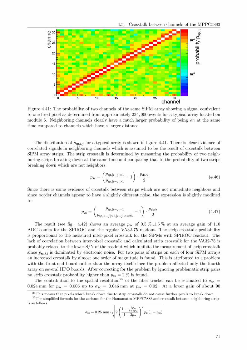
4.5. Crosstalk between channels of the MPPC5883
channel
chan
nel
prob
abili
ty p
sp,i,
j
Figure 4.41: The probability of two channels of the same SiPM array showing a signal equivalentto one fired pixel as determined from approximately 234, 000 events for a typical array located onmodule 5. Neighboring channels clearly have a much larger probability of being on at the sametime compared to channels which have a larger distance.
The distribution of psp,i,j for a typical array is shown in figure 4.41. There is clear evidence ofcorrelated signals in neighboring channels which is assumed to be the result of crosstalk betweenSiPM array strips. The strip crosstalk is determined by measuring the probability of two neigh-boring strips breaking down at the same time and comparing that to the probability of two stripsbreaking down which are not neighbors.
psx =
(psp,|i−j|=1
psp,|i−j|>1− 1
)· pdark
2(4.46)
Since there is some evidence of crosstalk between strips which are not immediate neighbors andsince border channels appear to have a slightly different noise, the expression is slightly modifiedto:
psx =
(psp,|i−j|=1
psp,|i−j|>5,|i−j|<=25− 1
)· pdark
2(4.47)
The result (see fig. 4.42) shows an average psx of 0.5 %..1.5 % at an average gain of 110ADC counts for the SPIROC and the regular VA32-75 readout. The strip crosstalk probabilityis proportional to the measured inter-pixel crosstalk for the SiPMs with SPIROC readout. Thelack of correlation between inter-pixel crosstalk and calculated strip crosstalk for the VA32-75 isprobably related to the lower S/N of the readout which inhibits the measurement of strip crosstalksince psp,i,j is dominated by electronic noise. For two pairs of strips on each of four SiPM arraysan increased crosstalk by almost one order of magnitude is found. This is attributed to a problemwith the front-end board rather than the array itself since the problem affected only the fourtharray on several HPO boards. After correcting for the problem by ignoring problematic strip pairsno strip crosstalk probability higher than psx = 2 % is found.
The contribution to the spatial resolution25 of the fiber tracker can be estimated to σsx =0.024 mm for psx = 0.005 up to σsx = 0.046 mm at psx = 0.02. At a lower gain of about 90
24This means that pixels which break down due to strip crosstalk do not cause further pixels to break down.25The simplified formula for the variance for the Hamamatsu MPPC5883 and crosstalk between neighboring strips
is as follows:
σsx = 0.25 mm ·
√√√√2
(1− 2psx
1+2psx
1 + 2psx
)2
psx(1− psx)
71
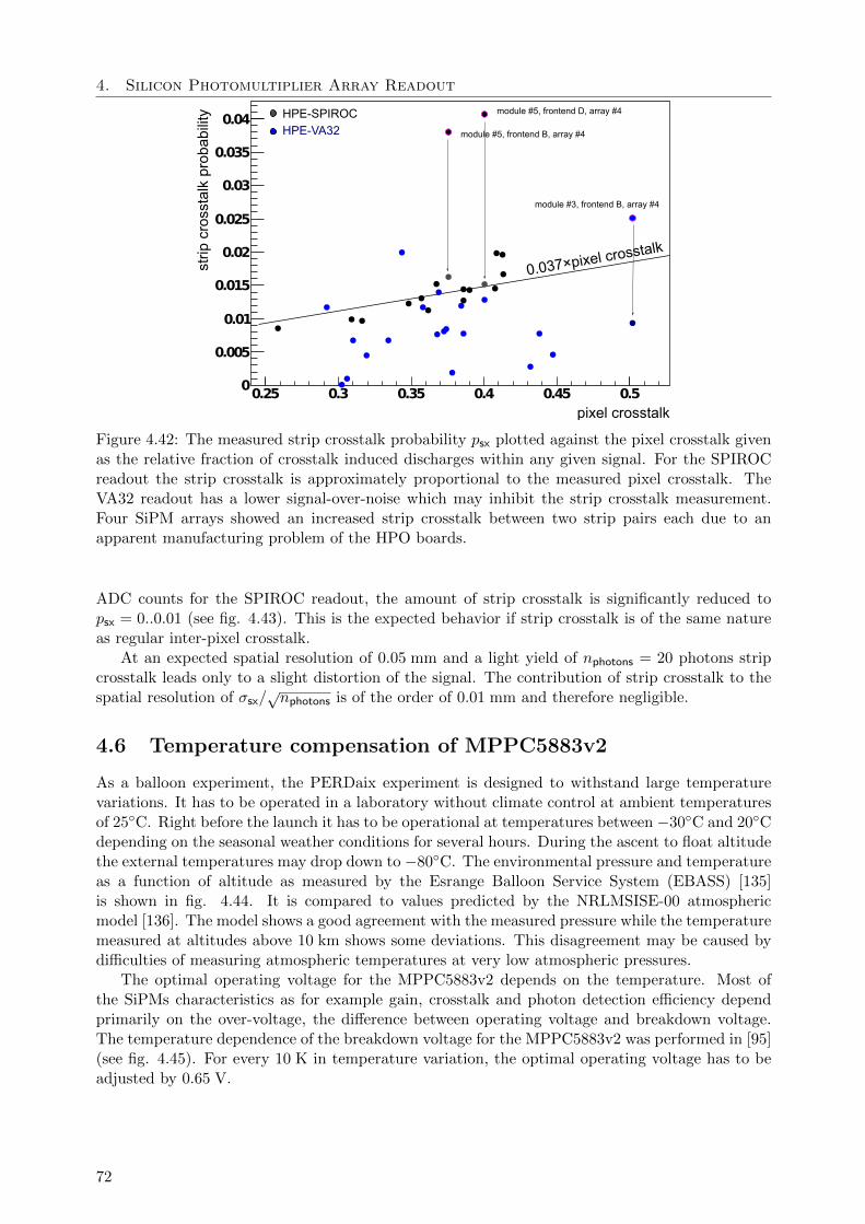
4. Silicon Photomultiplier Array Readout
HPE-VA32
HPE-SPIROC
strip
cro
ssta
lk p
roba
bilit
y
pixel crosstalk0.25 0.3 0.35 0.4 0.45 0.5
0
0.005
0.01
0.015
0.02
0.025
0.03
0.035
0.04
0.037×pixel crosstalk
module #5, frontend D, array #4
module #5, frontend B, array #4
module #3, frontend B, array #4
Figure 4.42: The measured strip crosstalk probability psx plotted against the pixel crosstalk givenas the relative fraction of crosstalk induced discharges within any given signal. For the SPIROCreadout the strip crosstalk is approximately proportional to the measured pixel crosstalk. TheVA32 readout has a lower signal-over-noise which may inhibit the strip crosstalk measurement.Four SiPM arrays showed an increased strip crosstalk between two strip pairs each due to anapparent manufacturing problem of the HPO boards.
ADC counts for the SPIROC readout, the amount of strip crosstalk is significantly reduced topsx = 0..0.01 (see fig. 4.43). This is the expected behavior if strip crosstalk is of the same natureas regular inter-pixel crosstalk.
At an expected spatial resolution of 0.05 mm and a light yield of nphotons = 20 photons stripcrosstalk leads only to a slight distortion of the signal. The contribution of strip crosstalk to thespatial resolution of σsx/
√nphotons is of the order of 0.01 mm and therefore negligible.
4.6 Temperature compensation of MPPC5883v2
As a balloon experiment, the PERDaix experiment is designed to withstand large temperaturevariations. It has to be operated in a laboratory without climate control at ambient temperaturesof 25C. Right before the launch it has to be operational at temperatures between −30C and 20Cdepending on the seasonal weather conditions for several hours. During the ascent to float altitudethe external temperatures may drop down to −80C. The environmental pressure and temperatureas a function of altitude as measured by the Esrange Balloon Service System (EBASS) [135]is shown in fig. 4.44. It is compared to values predicted by the NRLMSISE-00 atmosphericmodel [136]. The model shows a good agreement with the measured pressure while the temperaturemeasured at altitudes above 10 km shows some deviations. This disagreement may be caused bydifficulties of measuring atmospheric temperatures at very low atmospheric pressures.
The optimal operating voltage for the MPPC5883v2 depends on the temperature. Most ofthe SiPMs characteristics as for example gain, crosstalk and photon detection efficiency dependprimarily on the over-voltage, the difference between operating voltage and breakdown voltage.The temperature dependence of the breakdown voltage for the MPPC5883v2 was performed in [95](see fig. 4.45). For every 10 K in temperature variation, the optimal operating voltage has to beadjusted by 0.65 V.
72
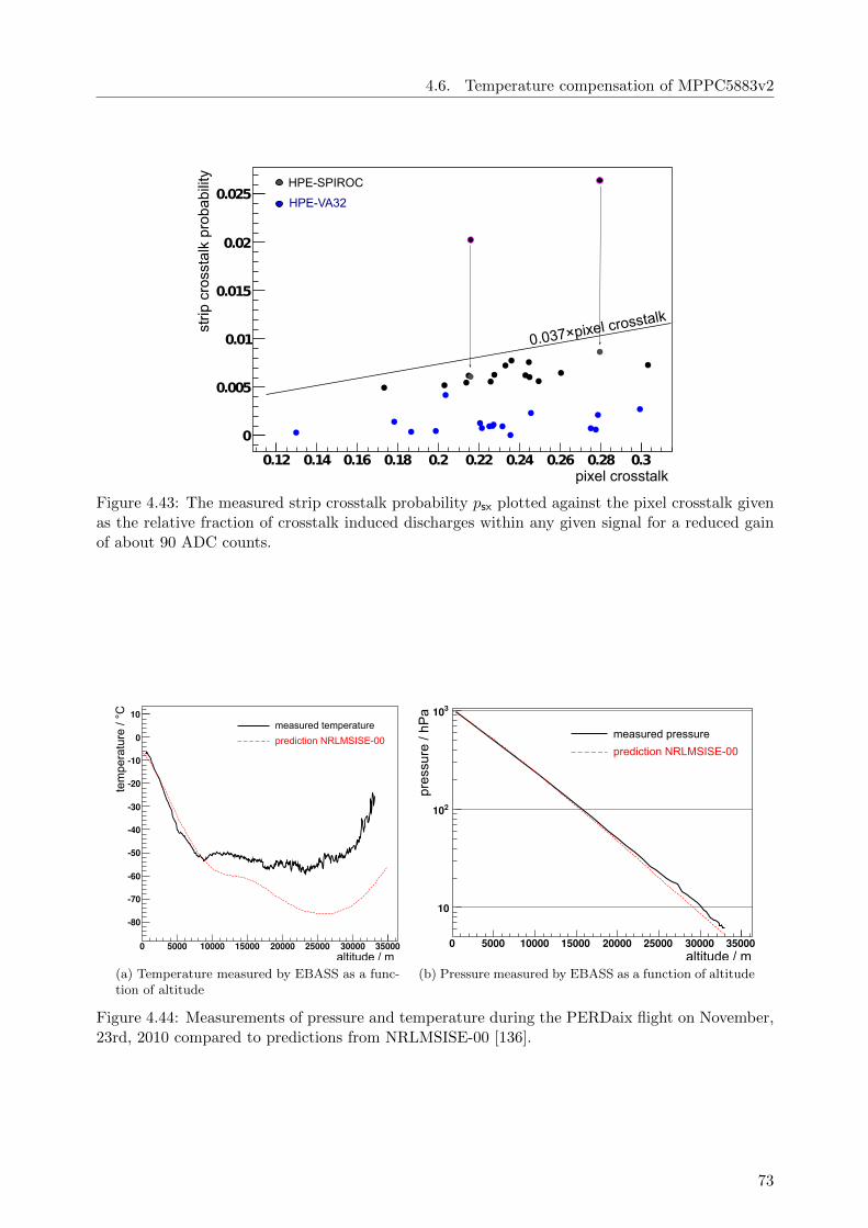
4.6. Temperature compensation of MPPC5883v2
0.12 0.14 0.16 0.18 0.2 0.22 0.24 0.26 0.28 0.3
0
0.005
0.01
0.015
0.02
0.025HPE-VA32
HPE-SPIROC
pixel crosstalk
strip
cro
ssta
lk p
roba
bilit
y
0.037×pixel crosstalk
Figure 4.43: The measured strip crosstalk probability psx plotted against the pixel crosstalk givenas the relative fraction of crosstalk induced discharges within any given signal for a reduced gainof about 90 ADC counts.
0 5000 10000 15000 20000 25000 30000 35000
-70
-60
-50
-40
-30
-20
-10
0
10
altitude / m
tem
pera
ture
/ °C
-80
measured temperature
prediction NRLMSISE-00
(a) Temperature measured by EBASS as a func-tion of altitude
0 5000 10000 15000 20000 25000 30000 35000
10
210
310
altitude / m
pres
sure
/ hP
a
measured pressure
prediction NRLMSISE-00
(b) Pressure measured by EBASS as a function of altitude
Figure 4.44: Measurements of pressure and temperature during the PERDaix flight on November,23rd, 2010 compared to predictions from NRLMSISE-00 [136].
73

4. Silicon Photomultiplier Array Readout
temperature coefficient:
Figure 4.45: The measured breakdown voltages as a function of temperature for two MPPC5883v2SiPM arrays [95].
R1
R2C1
SiP
M
Rtherm
istor
R3
Vin
signal
Figure 4.46: A schematic of the thermistor based temperature regulation used for the PERDaixtracker.
For the PERDaix scintillating fiber tracker a passive regulation based on [137] has been im-plemented. This regulation uses a thermistor (see fig. 4.46) as temperature dependent resistor infront of the SiPM to regulate the bias with changing temperature.
The resistance of a thermistor can be described as:
R(T ) = R0 exp
(B
[1
T− 1
T0
])(4.48)
with constant B and resistance R0 at temperature T0. Based on IV-curves measured for theMPPC5883v2 (see fig. 4.47) the voltage dependence of the current can be modeled as:
I(Ubias, T = const) = I0 exp
(Ubias − Ubreakdown
α
)· (Ubias − Ubreakdown) + Isaturation (4.49)
74
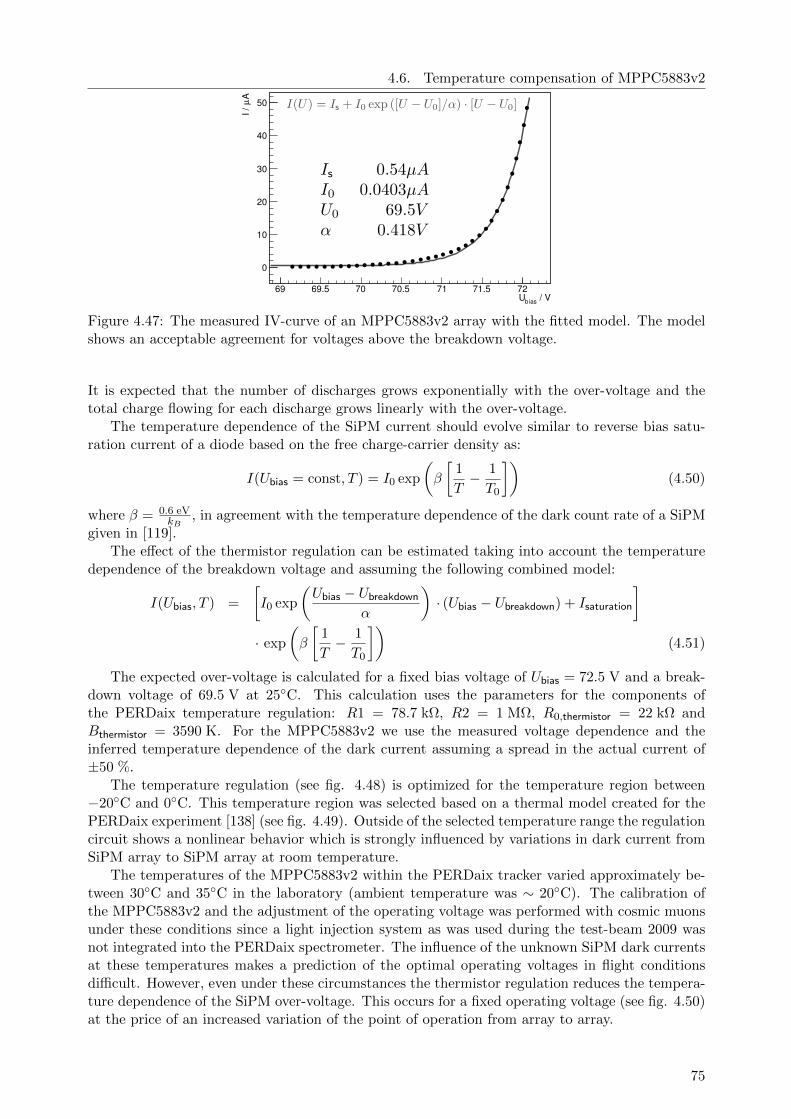
4.6. Temperature compensation of MPPC5883v2
/ VbiasU69 69.5 70 70.5 71 71.5 72
AµI/
0
10
20
30
40
50
Figure 4.47: The measured IV-curve of an MPPC5883v2 array with the fitted model. The modelshows an acceptable agreement for voltages above the breakdown voltage.
It is expected that the number of discharges grows exponentially with the over-voltage and thetotal charge flowing for each discharge grows linearly with the over-voltage.
The temperature dependence of the SiPM current should evolve similar to reverse bias satu-ration current of a diode based on the free charge-carrier density as:
I(Ubias = const, T ) = I0 exp
(β
[1
T− 1
T0
])(4.50)
where β = 0.6 eVkB
, in agreement with the temperature dependence of the dark count rate of a SiPMgiven in [119].
The effect of the thermistor regulation can be estimated taking into account the temperaturedependence of the breakdown voltage and assuming the following combined model:
I(Ubias, T ) =
[I0 exp
(Ubias − Ubreakdown
α
)· (Ubias − Ubreakdown) + Isaturation
]· exp
(β
[1
T− 1
T0
])(4.51)
The expected over-voltage is calculated for a fixed bias voltage of Ubias = 72.5 V and a break-down voltage of 69.5 V at 25C. This calculation uses the parameters for the components ofthe PERDaix temperature regulation: R1 = 78.7 kΩ, R2 = 1 MΩ, R0,thermistor = 22 kΩ andBthermistor = 3590 K. For the MPPC5883v2 we use the measured voltage dependence and theinferred temperature dependence of the dark current assuming a spread in the actual current of±50 %.
The temperature regulation (see fig. 4.48) is optimized for the temperature region between−20C and 0C. This temperature region was selected based on a thermal model created for thePERDaix experiment [138] (see fig. 4.49). Outside of the selected temperature range the regulationcircuit shows a nonlinear behavior which is strongly influenced by variations in dark current fromSiPM array to SiPM array at room temperature.
The temperatures of the MPPC5883v2 within the PERDaix tracker varied approximately be-tween 30C and 35C in the laboratory (ambient temperature was ∼ 20C). The calibration ofthe MPPC5883v2 and the adjustment of the operating voltage was performed with cosmic muonsunder these conditions since a light injection system as was used during the test-beam 2009 wasnot integrated into the PERDaix spectrometer. The influence of the unknown SiPM dark currentsat these temperatures makes a prediction of the optimal operating voltages in flight conditionsdifficult. However, even under these circumstances the thermistor regulation reduces the tempera-ture dependence of the SiPM over-voltage. This occurs for a fixed operating voltage (see fig. 4.50)at the price of an increased variation of the point of operation from array to array.
75
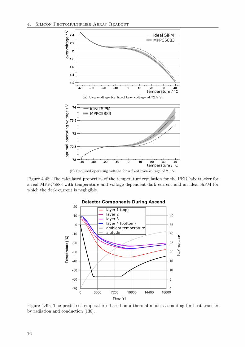
4. Silicon Photomultiplier Array Readout
temperature / °C
overv
olt
ag
e /
V
-40 -30 -20 -10 0 10 20 30 40
1.2
1.4
1.6
1.8
2
2.2
2.4 ideal SiPMMPPC5883
(a) Over-voltage for fixed bias voltage of 72.5 V.
-40 -30 -20 -10 0 10 20 30 4072
72.5
73
73.5
74 ideal SiPMMPPC5883
temperature / °C
op
tim
al op
era
tin
g v
olt
ag
e /
V
(b) Required operating voltage for a fixed over-voltage of 2.1 V.
Figure 4.48: The calculated properties of the temperature regulation for the PERDaix tracker fora real MPPC5883 with temperature and voltage dependent dark current and an ideal SiPM forwhich the dark current is negligible.
layer 1 (top)layer 2layer 3layer 4 (bottom)ambient temperaturealtitude
Figure 4.49: The predicted temperatures based on a thermal model accounting for heat transferby radiation and conduction [138].
76
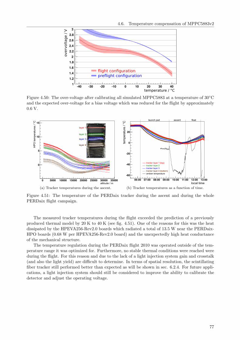
4.6. Temperature compensation of MPPC5883v2
-40 -30 -20 -10 0 10 20 30 401
1.2
1.4
1.6
1.8
2
2.2
2.4
2.6
2.8
3
temperature / °C
overv
olt
ag
e /
V
flight configurationpreflight configuration
Figure 4.50: The over-voltage after calibrating all simulated MPPC5883 at a temperature of 30Cand the expected over-voltage for a bias voltage which was reduced for the flight by approximately0.6 V.
0 5000 10000 15000 20000 25000 30000 35000
0
5
10
15
layer 1
layer 2
layer 3
layer 4
HP
O te
mpe
ratu
res
/ °C
altitude / m
(a) Tracker temperatures during the ascent.
06:00 07:00 08:00 09:00 10:00 11:00 12:00 13:00
-60
-40
-20
0
20
launch pad ascent float
local time
tem
pera
ture
/ °C
ambien temperaturetracker layer 4 (bottom)tracker layer 3tracker layer 2tracker layer 1 (top)
(b) Tracker temperatures as a function of time.
Figure 4.51: The temperature of the PERDaix tracker during the ascent and during the wholePERDaix flight campaign.
The measured tracker temperatures during the flight exceeded the prediction of a previouslyproduced thermal model by 20 K to 40 K (see fig. 4.51). One of the reasons for this was the heatdissipated by the HPEVA256-Rev2.0 boards which radiated a total of 13.5 W near the PERDaix-HPO boards (0.68 W per HPEVA256-Rev2.0 board) and the unexpectedly high heat conductanceof the mechanical structure.
The temperature regulation during the PERDaix flight 2010 was operated outside of the tem-perature range it was optimized for. Furthermore, no stable thermal conditions were reached wereduring the flight. For this reason and due to the lack of a light injection system gain and crosstalk(and also the light yield) are difficult to determine. In terms of spatial resolution, the scintillatingfiber tracker still performed better than expected as will be shown in sec. 6.2.4. For future appli-cations, a light injection system should still be considered to improve the ability to calibrate thedetector and adjust the operating voltage.
77

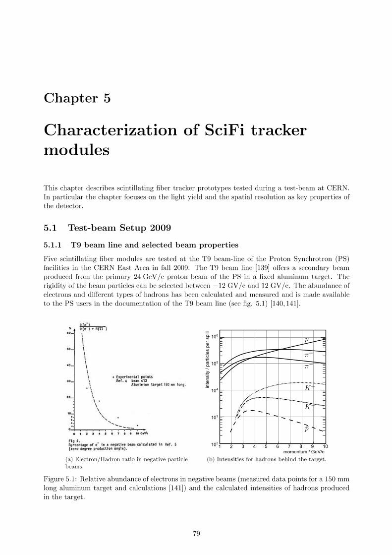
Chapter 5
Characterization of SciFi trackermodules
This chapter describes scintillating fiber tracker prototypes tested during a test-beam at CERN.In particular the chapter focuses on the light yield and the spatial resolution as key properties ofthe detector.
5.1 Test-beam Setup 2009
5.1.1 T9 beam line and selected beam properties
Five scintillating fiber modules are tested at the T9 beam-line of the Proton Synchrotron (PS)facilities in the CERN East Area in fall 2009. The T9 beam line [139] offers a secondary beamproduced from the primary 24 GeV/c proton beam of the PS in a fixed aluminum target. Therigidity of the beam particles can be selected between −12 GV/c and 12 GV/c. The abundance ofelectrons and different types of hadrons has been calculated and measured and is made availableto the PS users in the documentation of the T9 beam line (see fig. 5.1) [140,141].
(a) Electron/Hadron ratio in negative particlebeams.
1 2 3 4 5 6 7 8 9 10momentum / GeV/c
106
105
104
103
102
intensity/particlesperspill
(b) Intensities for hadrons behind the target.
Figure 5.1: Relative abundance of electrons in negative beams (measured data points for a 150 mmlong aluminum target and calculations [141]) and the calculated intensities of hadrons producedin the target.
79
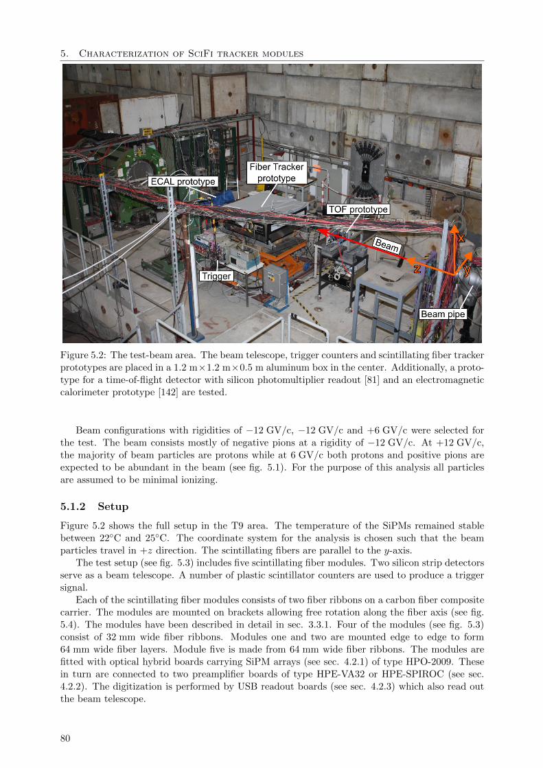
5. Characterization of SciFi tracker modules
Figure 5.2: The test-beam area. The beam telescope, trigger counters and scintillating fiber trackerprototypes are placed in a 1.2 m×1.2 m×0.5 m aluminum box in the center. Additionally, a proto-type for a time-of-flight detector with silicon photomultiplier readout [81] and an electromagneticcalorimeter prototype [142] are tested.
Beam configurations with rigidities of −12 GV/c, −12 GV/c and +6 GV/c were selected forthe test. The beam consists mostly of negative pions at a rigidity of −12 GV/c. At +12 GV/c,the majority of beam particles are protons while at 6 GV/c both protons and positive pions areexpected to be abundant in the beam (see fig. 5.1). For the purpose of this analysis all particlesare assumed to be minimal ionizing.
5.1.2 Setup
Figure 5.2 shows the full setup in the T9 area. The temperature of the SiPMs remained stablebetween 22C and 25C. The coordinate system for the analysis is chosen such that the beamparticles travel in +z direction. The scintillating fibers are parallel to the y-axis.
The test setup (see fig. 5.3) includes five scintillating fiber modules. Two silicon strip detectorsserve as a beam telescope. A number of plastic scintillator counters are used to produce a triggersignal.
Each of the scintillating fiber modules consists of two fiber ribbons on a carbon fiber compositecarrier. The modules are mounted on brackets allowing free rotation along the fiber axis (see fig.5.4). The modules have been described in detail in sec. 3.3.1. Four of the modules (see fig. 5.3)consist of 32 mm wide fiber ribbons. Modules one and two are mounted edge to edge to form64 mm wide fiber layers. Module five is made from 64 mm wide fiber ribbons. The modules arefitted with optical hybrid boards carrying SiPM arrays (see sec. 4.2.1) of type HPO-2009. Thesein turn are connected to two preamplifier boards of type HPE-VA32 or HPE-SPIROC (see sec.4.2.2). The digitization is performed by USB readout boards (see sec. 4.2.3) which also read outthe beam telescope.
80
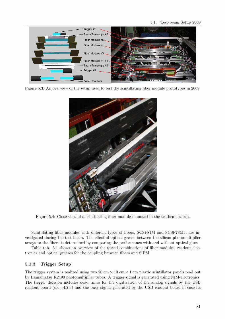
5.1. Test-beam Setup 2009
Figure 5.3: An overview of the setup used to test the scintillating fiber module prototypes in 2009.
Figure 5.4: Close view of a scintillating fiber module mounted in the testbeam setup.
Scintillating fiber modules with different types of fibers, SCSF81M and SCSF78MJ, are in-vestigated during the test beam. The effect of optical grease between the silicon photomultiplierarrays to the fibers is determined by comparing the performance with and without optical glue.
Table tab. 5.1 shows an overview of the tested combinations of fiber modules, readout elec-tronics and optical greases for the coupling between fibers and SiPM.
5.1.3 Trigger Setup
The trigger system is realized using two 20 cm× 10 cm× 1 cm plastic scintillator panels read outby Hamamatsu R2490 photomultiplier tubes. A trigger signal is generated using NIM-electronics.The trigger decision includes dead times for the digitization of the analog signals by the USBreadout board (sec. 4.2.3) and the busy signal generated by the USB readout board in case its
81
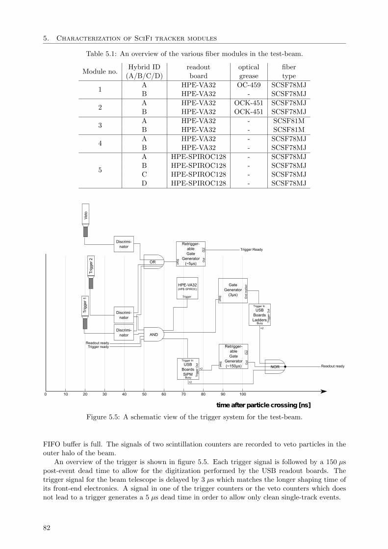
5. Characterization of SciFi tracker modules
Table 5.1: An overview of the various fiber modules in the test-beam.
Module no.Hybrid ID readout optical fiber
(A/B/C/D) board grease type
1A HPE-VA32 OC-459 SCSF78MJB HPE-VA32 - SCSF78MJ
2A HPE-VA32 OCK-451 SCSF78MJB HPE-VA32 OCK-451 SCSF78MJ
3A HPE-VA32 - SCSF81MB HPE-VA32 - SCSF81M
4A HPE-VA32 - SCSF78MJB HPE-VA32 - SCSF78MJ
5
A HPE-SPIROC128 - SCSF78MJB HPE-SPIROC128 - SCSF78MJC HPE-SPIROC128 - SCSF78MJD HPE-SPIROC128 - SCSF78MJ
10
Readout readyTrigger ready
USBBoardsSiPM
HPE-VA32(HPE-SPIROC)
Trigger
Trigger In
Trigger Ready
Retrigger-ableGate
Generator(~5µs)
Out
Out
Start
Busy Trig
gerO
ut
Retrigger-ableGate
Generator(~150µs)
Out
Out
Start
AND
Discrimi-nator
Discrimi-nator
OR
Trig
ger1
Trig
ger2
Vet
o
Discrimi-nator
Readout ready
timeafterparticlecrossing [ns]
0 20 30 40 50 60 8070 90 100
×2
×2
GateGenerator
(3µs)
End
mar
ker
Start
USBBoardsLadders
Trigger In
Busy Trig
gerO
ut
×2
NOR
Figure 5.5: A schematic view of the trigger system for the test-beam.
FIFO buffer is full. The signals of two scintillation counters are recorded to veto particles in theouter halo of the beam.
An overview of the trigger is shown in figure 5.5. Each trigger signal is followed by a 150 µspost-event dead time to allow for the digitization performed by the USB readout boards. Thetrigger signal for the beam telescope is delayed by 3 µs which matches the longer shaping time ofits front-end electronics. A signal in one of the trigger counters or the veto counters which doesnot lead to a trigger generates a 5 µs dead time in order to allow only clean single-track events.
82
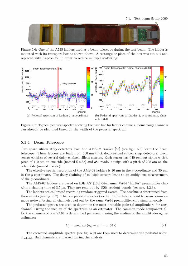
5.1. Test-beam Setup 2009
Figure 5.6: One of the AMS ladders used as a beam telescope during the test-beam. The ladder ismounted with its transport box as shown above. A rectangular piece of the box was cut out andreplaced with Kapton foil in order to reduce multiple scattering.
Beam Telescope #2: K-side
ampl
itude
/ A
DC
cou
nts
channel
noisy channels
VA#1 VA#2 VA#3 VA#4 VA#5 VA#6
(a) Pedestal spectrum of Ladder 2, y-coordinate
Beam Telescope #2: S-side, channels 0-320
ampl
itude
/ A
DC
cou
nts
channel
nois
y ch
anne
l
VA#1 VA#2 VA#3 VA#4 VA#5
(b) Pedestal spectrum of Ladder 2, x-coordinate, chan-nels 0-320
Figure 5.7: Typical pedestal spectra showing the base line for ladder channels. Some noisy channelscan already be identified based on the width of the pedestal spectrum.
5.1.4 Beam Telescope
Two spare silicon strip detectors from the AMS-02 tracker [86] (see fig. 5.6) form the beamtelescope. These ladders are built from 300 µm thick double-sided silicon strip detectors. Eachsensor consists of several daisy-chained silicon sensors. Each sensor has 640 readout strips with apitch of 110 µm on one side (named S-side) and 384 readout strips with a pitch of 208 µm on theother side (named K-side).
The effective spatial resolution of the AMS-02 ladders is 10 µm in the x-coordinate and 30 µmin the y-coordinate. The daisy-chaining of multiple sensors leads to an ambiguous measurementof the y-coordinate.
The AMS-02 ladders are based on IDE AS’ [130] 64-channel VA64 ”hdr9A” preamplifier chipwith a shaping time of 3.5 µs. They are read out by USB readout boards (see sec. 4.2.3).
The ladders are calibrated recording random triggered events. The baseline is determined fromthese events (see fig. 5.7). The raw pedestal spectra (see fig. 5.8) exhibit a non-Gaussian common-mode noise affecting all channels read out by the same VA64 preamplifier chip simultaneously.
The pedestal spectra are used to determine the most probable pedestal amplitude pi for eachchannel i using the median of the spectrum as an estimator. The common mode component Cjfor the channels of one VA64 is determined per event j using the median of the amplitudes aij asestimator:
Cj = median(aij − pi|i = 1..64) (5.1)
The corrected amplitude spectra (see fig. 5.9) are then used to determine the pedestal widthσpedestal. Bad channels are masked during the analysis.
83
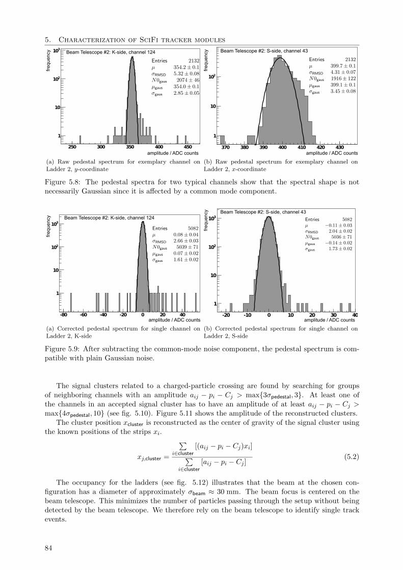
5. Characterization of SciFi tracker modules
250 300 350 400 450
1
10
210
310 Beam Telescope #2: K-side, channel 124
amplitude / ADC counts
freq
uenc
y
(a) Raw pedestal spectrum for exemplary channel onLadder 2, y-coordinate
Beam Telescope #2: S-side, channel 43
amplitude / ADC counts
freq
uenc
y
370 380 390 400 410 420 430
1
10
210
(b) Raw pedestal spectrum for exemplary channel onLadder 2, x-coordinate
Figure 5.8: The pedestal spectra for two typical channels show that the spectral shape is notnecessarily Gaussian since it is affected by a common mode component.
amplitude / ADC counts
freq
uency Beam Telescope #2: K-side, channel 124
-80 -60 -40 -20 0 20 40
1
10
210
310
(a) Corrected pedestal spectrum for single channel onLadder 2, K-side
amplitude / ADC counts
freq
uency
-20 -10 0 10 20 30 40
1
10
210
310Beam Telescope #2: S-side, channel 43
(b) Corrected pedestal spectrum for single channel onLadder 2, S-side
Figure 5.9: After subtracting the common-mode noise component, the pedestal spectrum is com-patible with plain Gaussian noise.
The signal clusters related to a charged-particle crossing are found by searching for groupsof neighboring channels with an amplitude aij − pi − Cj > max3σpedestal, 3. At least one ofthe channels in an accepted signal cluster has to have an amplitude of at least aij − pi − Cj >max4σpedestal, 10 (see fig. 5.10). Figure 5.11 shows the amplitude of the reconstructed clusters.
The cluster position xcluster is reconstructed as the center of gravity of the signal cluster usingthe known positions of the strips xi.
xj,cluster =
∑i∈cluster
[(aij − pi − Cj)xi]∑i∈cluster
[aij − pi − Cj ](5.2)
The occupancy for the ladders (see fig. 5.12) illustrates that the beam at the chosen con-figuration has a diameter of approximately σbeam ≈ 30 mm. The beam focus is centered on thebeam telescope. This minimizes the number of particles passing through the setup without beingdetected by the beam telescope. We therefore rely on the beam telescope to identify single trackevents.
84
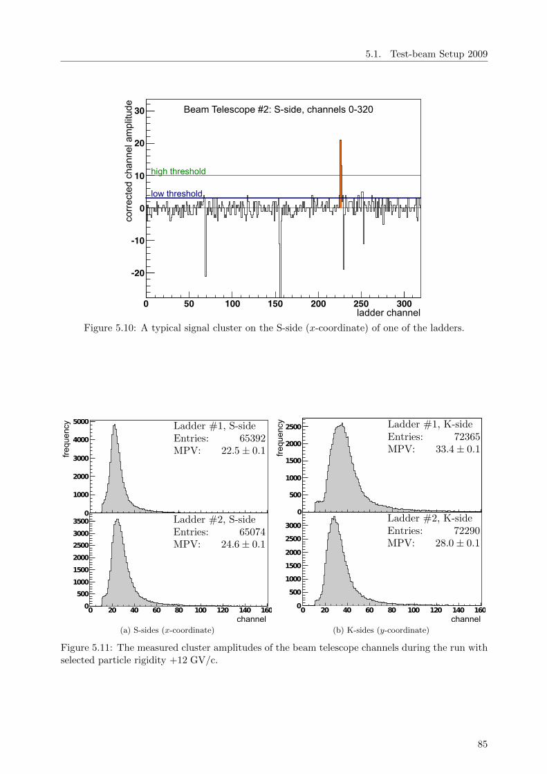
5.1. Test-beam Setup 2009
0 50 100 150 200 250 300
-20
-10
0
10
20
30 Beam Telescope #2: S-side, channels 0-320
low threshold
high threshold
ladder channel
corr
ecte
d ch
anne
l am
plit
ude
Figure 5.10: A typical signal cluster on the S-side (x-coordinate) of one of the ladders.
0
1000
2000
3000
4000
5000
0 20 40 60 80 100 120 140 1600
500
1000
1500
2000
2500
3000
3500
channel
frequency
(a) S-sides (x-coordinate)
0
500
1000
1500
2000
2500
0
500
1000
1500
2000
2500
3000
0 20 40 60 80 100 120 140 160channel
frequency
(b) K-sides (y-coordinate)
Figure 5.11: The measured cluster amplitudes of the beam telescope channels during the run withselected particle rigidity +12 GV/c.
85
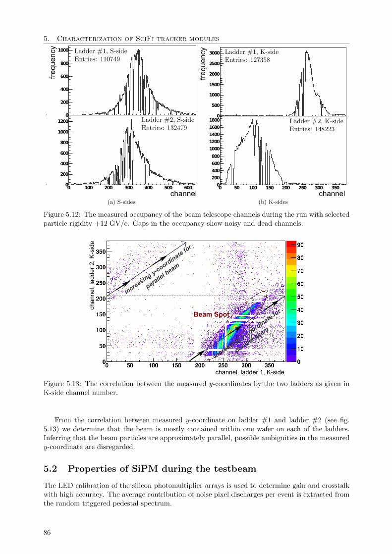
5. Characterization of SciFi tracker modules
0
0 100 200 300 400 500 6000
200
400
600
800
1000
1200
200
400
600
800
1000
channel
frequency
(a) S-sides
0 50 100 150 200 250 300 3500
200
400
600
800
1000
1200
1400
1600
1800
500
1000
1500
2000
2500
3000
0
channelfrequency
(b) K-sides
Figure 5.12: The measured occupancy of the beam telescope channels during the run with selectedparticle rigidity +12 GV/c. Gaps in the occupancy show noisy and dead channels.
channel, ladder 1, K-side
chan
nel,
ladd
er 2
, K-s
ide
Beam Spot
increasing y-coordinate fo
r
parallel b
eam
increasing y-coordinate fo
r
parallel b
eam
Figure 5.13: The correlation between the measured y-coordinates by the two ladders as given inK-side channel number.
From the correlation between measured y-coordinate on ladder #1 and ladder #2 (see fig.5.13) we determine that the beam is mostly contained within one wafer on each of the ladders.Inferring that the beam particles are approximately parallel, possible ambiguities in the measuredy-coordinate are disregarded.
5.2 Properties of SiPM during the testbeam
The LED calibration of the silicon photomultiplier arrays is used to determine gain and crosstalkwith high accuracy. The average contribution of noise pixel discharges per event is extracted fromthe random triggered pedestal spectrum.
86
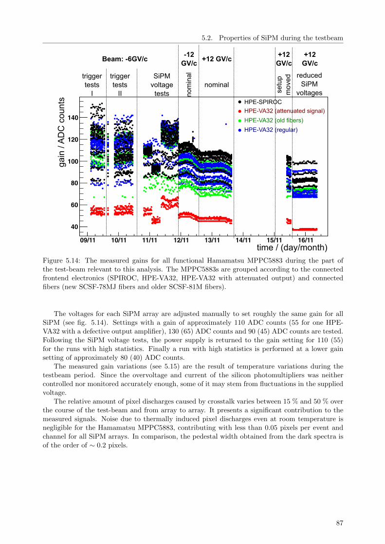
5.2. Properties of SiPM during the testbeam
09/11 10/11 11/11 12/11 13/11 14/11 15/11 16/11
40
60
80
100
120
140
gain
/ A
DC
cou
nts
time / (day/month)
triggertests
I
triggertests
II
SiPMvoltage
tests
Beam: -6GV/c
nom
inal
-12GV/c
nominal
+12 GV/c+12
GV/c
setu
pm
oved
+12GV/c
reducedSiPM
voltages
HPE-VA32 (regular)
HPE-VA32 (old fibers)
HPE-VA32 (attenuated signal)
HPE-SPIROC
Figure 5.14: The measured gains for all functional Hamamatsu MPPC5883 during the part ofthe test-beam relevant to this analysis. The MPPC5883s are grouped according to the connectedfrontend electronics (SPIROC, HPE-VA32, HPE-VA32 with attenuated output) and connectedfibers (new SCSF-78MJ fibers and older SCSF-81M fibers).
The voltages for each SiPM array are adjusted manually to set roughly the same gain for allSiPM (see fig. 5.14). Settings with a gain of approximately 110 ADC counts (55 for one HPE-VA32 with a defective output amplifier), 130 (65) ADC counts and 90 (45) ADC counts are tested.Following the SiPM voltage tests, the power supply is returned to the gain setting for 110 (55)for the runs with high statistics. Finally a run with high statistics is performed at a lower gainsetting of approximately 80 (40) ADC counts.
The measured gain variations (see 5.15) are the result of temperature variations during thetestbeam period. Since the overvoltage and current of the silicon photomultipliers was neithercontrolled nor monitored accurately enough, some of it may stem from fluctuations in the suppliedvoltage.
The relative amount of pixel discharges caused by crosstalk varies between 15 % and 50 % overthe course of the test-beam and from array to array. It presents a significant contribution to themeasured signals. Noise due to thermally induced pixel discharges even at room temperature isnegligible for the Hamamatsu MPPC5883, contributing with less than 0.05 pixels per event andchannel for all SiPM arrays. In comparison, the pedestal width obtained from the dark spectra isof the order of ∼ 0.2 pixels.
87
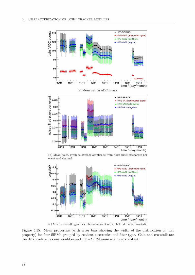
5. Characterization of SciFi tracker modules
time / (day/month)
gain
/ A
DC
cou
nts
09/11 10/11 11/11 12/11 13/11 14/11 15/11 16/11
40
60
80
100
120
140
HPE-VA32 (regular)
HPE-VA32 (old fibers)
HPE-VA32 (attenuated signal)
HPE-SPIROC
(a) Mean gain in ADC counts.
time / (day/month)
nois
e / f
ired
pixe
ls p
er e
vent
HPE-VA32 (regular)
HPE-VA32 (old fibers)
HPE-VA32 (attenuated signal)
HPE-SPIROC
09/11 10/11 11/11 12/11 13/11 14/11 15/11 16/11
0.005
0.01
0.015
0.02
0.025
0.03
0.035
(b) Mean noise, given as average amplitude from noise pixel discharges perevent and channel.
09/11 10/11 11/11 12/11 13/11 14/11 15/11 16/11
0.15
0.2
0.25
0.3
0.35
0.4
0.45
0.5
time / (day/month)
cros
stal
k
HPE-VA32 (regular)
HPE-VA32 (old fibers)
HPE-VA32 (attenuated signal)
HPE-SPIROC
(c) Mean crosstalk, given as relative amount of pixels fired due to crosstalk.
Figure 5.15: Mean properties (with error bars showing the width of the distribution of thatproperty) for four SiPMs grouped by readout electronics and fiber type. Gain and crosstalk areclearly correlated as one would expect. The SiPM noise is almost constant.
88

5.3. Performance of the scintillating fiber modules
position
correctedamplitude
Figure 5.16: A drawing showing an example for a signal cluster.
5.3 Performance of the scintillating fiber modules
5.3.1 Analysis Procedure
The following analysis procedure is used to reconstruct the recorded events and ultimately de-termine spatial resolution and light yield of the tested scintillating fiber tracker modules. Thesignal clusters for the beam telescope and scintillating fiber modules are reconstructed. The signalcluster definition for the beam telescope is described in section 5.1.4. For the scintillating fiber weuse a similar cluster definition:
A fiber cluster C consists of a number of neighboring channels of the same SiPM array C =i|i ≥ imin ∧ i ≤ imax which have amplitudes ai corrected for common mode noise and pedestalposition exceeding a certain threshold. This analysis requires all channels belonging to a cluster tohave a minimum amplitude equivalent to one pixel discharge. Furthermore, at least one channelhas to exhibit a minimum amplitude equivalent to two fired pixels:
[∀i ∈ C : ai ≥ 0.5G] ∧ [∃i ∈ C : ai ≥ 1.5G] (5.3)
Two possible estimators for the position of the passing particle are tested in this work (andcompared later in this section). The first estimator calculates the position using the center ofgravity based on the channel positions xi in the same way as it has been done for the beamtelescope clusters.
xCOG =
∑i∈C
aixi∑i∈C
ai(5.4)
A second estimator uses a median to calculate the cluster position (see fig. 5.16), where m is themedian channel of a cluster C with amplitudes ai|i ∈ C.
xmedian = xm +
∑i∈C,i>m
ai −∑
i∈C,i<mai
2am∆x (5.5)
89
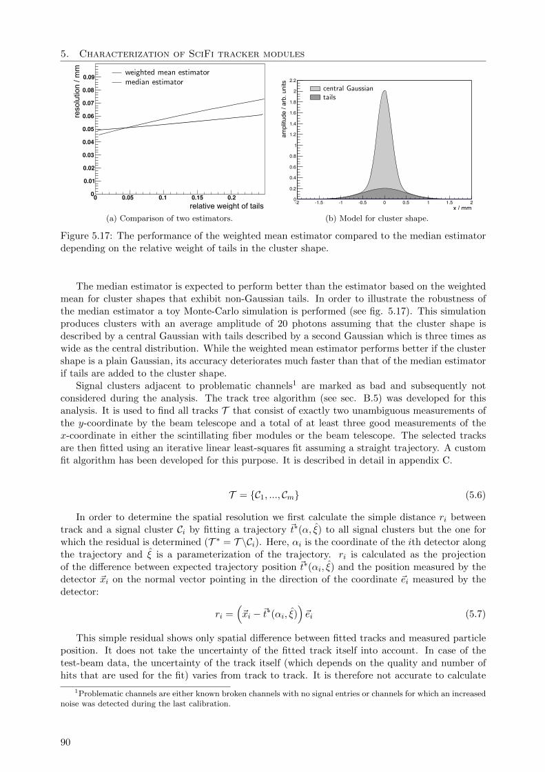
5. Characterization of SciFi tracker modules
0 0.05 0.1 0.15 0.20
0.01
0.02
0.03
0.04
0.05
0.06
0.07
0.08
0.09re
solu
tion
/ mm
relative weight of tails
(a) Comparison of two estimators.
-2 -1.5 -1 -0.5 0 0.5 1 1.5 20
0.2
0.4
0.6
0.8
1
1.2
1.4
1.6
1.8
2
2.2
x / mm
ampl
itude
/ ar
b. u
nits
(b) Model for cluster shape.
Figure 5.17: The performance of the weighted mean estimator compared to the median estimatordepending on the relative weight of tails in the cluster shape.
The median estimator is expected to perform better than the estimator based on the weightedmean for cluster shapes that exhibit non-Gaussian tails. In order to illustrate the robustness ofthe median estimator a toy Monte-Carlo simulation is performed (see fig. 5.17). This simulationproduces clusters with an average amplitude of 20 photons assuming that the cluster shape isdescribed by a central Gaussian with tails described by a second Gaussian which is three times aswide as the central distribution. While the weighted mean estimator performs better if the clustershape is a plain Gaussian, its accuracy deteriorates much faster than that of the median estimatorif tails are added to the cluster shape.
Signal clusters adjacent to problematic channels1 are marked as bad and subsequently notconsidered during the analysis. The track tree algorithm (see sec. B.5) was developed for thisanalysis. It is used to find all tracks T that consist of exactly two unambiguous measurements ofthe y-coordinate by the beam telescope and a total of at least three good measurements of thex-coordinate in either the scintillating fiber modules or the beam telescope. The selected tracksare then fitted using an iterative linear least-squares fit assuming a straight trajectory. A customfit algorithm has been developed for this purpose. It is described in detail in appendix C.
T = C1, ..., Cm (5.6)
In order to determine the spatial resolution we first calculate the simple distance ri betweentrack and a signal cluster Ci by fitting a trajectory ~t∗(α, ξ) to all signal clusters but the one forwhich the residual is determined (T ∗ = T \Ci). Here, αi is the coordinate of the ith detector alongthe trajectory and ξ is a parameterization of the trajectory. ri is calculated as the projectionof the difference between expected trajectory position ~t∗(αi, ξ) and the position measured by thedetector ~xi on the normal vector pointing in the direction of the coordinate ~ei measured by thedetector:
ri =(~xi − ~t∗(αi, ξ)
)~ei (5.7)
This simple residual shows only spatial difference between fitted tracks and measured particleposition. It does not take the uncertainty of the fitted track itself into account. In case of thetest-beam data, the uncertainty of the track itself (which depends on the quality and number ofhits that are used for the fit) varies from track to track. It is therefore not accurate to calculate
1Problematic channels are either known broken channels with no signal entries or channels for which an increasednoise was detected during the last calibration.
90

5.3. Performance of the scintillating fiber modules
merely the average uncertainty of the track fit (e.g. with a Monte Carlo method) and subtract itfrom the total uncertainty as manifested in the variance of the residuals for the considered detector.
A better estimate for the spatial resolution can be achieved in the following manner. Wecalculate the uncertainty Σi of the expected particle position ~t∗(αi, ξ). This can be achieved usingerror propagation from the covariance matrix of the track fit Σξ:
Hi =
∂[~t (x∗i , αi)
]1/∂ξ1 · · ·
[~t (x∗i , αi)
]1/∂ξn
.... . .
...
∂[~t (x∗i , αi)
]3/∂ξ1 · · ·
[~t (x∗i , αi)
]3/∂ξn
(5.8)
Σi = HiΣξHTi (5.9)
Let ~τi give the true position of the particle at the ith measurement. The residuals ri can now beexpressed as a contribution from the detector resolution rresi and a contribution from the imper-fectly determined trajectory rtracki which are distributed according to the so far unknown spatialresolution2 σ2
i and the calculated Σi.
rtracki = ~eTi(~t∗(αi)− ~τi
)(5.10)
ri = rresi + rtracki (5.11)
π(rresi ) ∼ exp
(−(rresi )2
2σ2i
)(5.12)
π(~t∗(αi)− ~τi) ∼ exp
(−(~t∗(αi)− ~τi
)TΣ−1i
(~t∗(αi)− ~τi
)2
)
⇒ π(rtracki ) ∼ exp
(−
(rtracki )2~eTi Σ−1i ~ei
2
)(5.13)
(5.14)
Since both rresi and rtracki are Gaussian distributed, the most probable value for rresi given ri canbe calculated as:
rresi = ri
√σ2i
σ2i + ~eTi Σ−1
i ~ei(5.15)
From this equation one can determine the following statement that allows an iterative solution todetermine σ2
i :
σ2i = lim
j→∞VAR [rresi (j)] (5.16)
rresi (j) = ri
√VAR [rresi (j − 1)]
VAR [rresi (j − 1)] + ~eTi Σ−1i ~ei
(5.17)
This algorithm converges3 as long as VAR [rresi (j)] & ~eTi Σ−1i ~ei. A degenerate solution exists for
VAR [rresi (j)] /~eTi Σ−1i ~ei 1.
5.3.2 Detector Parametrization and Alignment
Essentially, all used detectors perform three-dimensional measurements with reference to the localcoordinate system. The first coordinate is given by the primary measurement, the second coor-dinate is fixed by the position and orientation of the detector plane and the third coordinate is
2The spatial resolution was already used during the track fit at this point so we have to resort to an iterativesolution.
3Without proof.
91
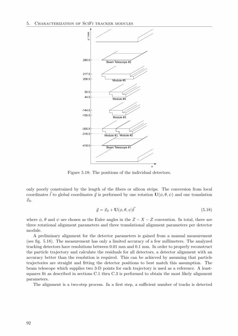
5. Characterization of SciFi tracker modules
-418.0
-316.5
-305.5
-155.5
-144.5
44.5
55.5
206.5
217.5
280.0
z / m
m
x
Beam Telescope #2
Module #5
Beam Telescope #1
Module #4
Module #3
Module #2Module #1
Figure 5.18: The positions of the individual detectors.
only poorly constrained by the length of the fibers or silicon strips. The conversion from localcoordinates ~l to global coordinates ~g is performed by one rotation U(φ, θ, ψ) and one translation~x0.
~g = ~x0 + U(φ, θ, ψ)~l (5.18)
where φ, θ and ψ are chosen as the Euler angles in the Z −X − Z convention. In total, there arethree rotational alignment parameters and three translational alignment parameters per detectormodule.
A preliminary alignment for the detector parameters is gained from a manual measurement(see fig. 5.18). The measurement has only a limited accuracy of a few millimeters. The analyzedtracking detectors have resolutions between 0.01 mm and 0.1 mm. In order to properly reconstructthe particle trajectory and calculate the residuals for all detectors, a detector alignment with anaccuracy better than the resolution is required. This can be achieved by assuming that particletrajectories are straight and fitting the detector positions to best match this assumption. Thebeam telescope which supplies two 3-D points for each trajectory is used as a reference. A least-squares fit as described in sections C.1 thru C.3 is performed to obtain the most likely alignmentparameters.
The alignment is a two-step process. In a first step, a sufficient number of tracks is detected
92

5.3. Performance of the scintillating fiber modules
and fitted with the pre-existing alignment. All trajectories ~t(ξ, α) recorded during the test-beamare assumed to be straight:
~t(ξ, α) =
ξ0
ξ1
0
+ α
ξ2
ξ3
1
(5.19)
The equation matrix X for the global least-squares fit is calculated. For this purpose we determinethe parameter αj (see also sec. B.3) which gives the position of the detector along the trajectoryfrom each 3-dimensional observation ~oj :[
UT(~t(ξi, αj)− ~x0
)](p)= o
(p)j (5.20)
This uses up the measurement o(p)j (which is always the z-coordinate in our case).
Next, the residual ~rj = UT(~t(ξi, αj)− ~x0
)−~oj is determined. The 2×3 matrix M propagates
the uncertainty of ~o(p)j to the other coordinates.
Mkl =
δkl l 6= p
∂(UT (~t(ξi,αj)−~x0))(k)
∂(UT (~t(ξi,αj)−~x0))(p) l = p
(5.21)
The contribution of the jth measurement to the equation matrix for an m-dimensional parametervector ξ is:
Xj = MjUTj
∂~t(ξi,αj)
(1)
∂ξ0· · · ∂~t(ξi,αj)
(1)
∂ξm...
. . ....
∂~t(ξi,αj)(3)
∂ξ0· · · ∂~t(ξi,αj)
(3)
∂ξm
(5.22)
The corresponding part of the covariance matrix for a three-dimensional measurement where eachof the measured coordinates is uncorrelated in local detector coordinates reads as follows:
Σ−1j =
M
σ21 0 0
0 σ22 0
0 0 σ23
MT
−1
(5.23)
The matrix equation to be solved for a track fit (in the unregularized case and without reweighting)with n observations is: X1
...Xn
T Σ−1
1 0 0
0. . . 0
0 0 Σ−1n
X1
...Xn
(ξi+1 − ξi)
=
X1...Xn
T Σ−1
1 0 0
0. . . 0
0 0 Σ−1n
M1~r1
...Mn~rn
(5.24)
After a number of iterations the equations above give a very good estimate for the trajectory basedon the current detector alignment.
93
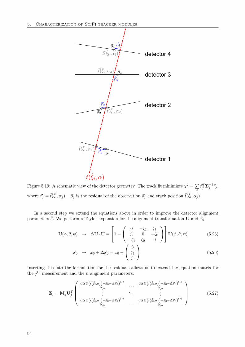
5. Characterization of SciFi tracker modules
detector 1
detector 2
detector 3
detector 4
Figure 5.19: A schematic view of the detector geometry. The track fit minimizes χ2 =∑j~rTj Σ−1
j ~rj ,
where ~rj = ~t(ξi, αj)− ~oj is the residual of the observation ~oj and track position ~t(ξi, αj).
In a second step we extend the equations above in order to improve the detector alignmentparameters ζ. We perform a Taylor expansion for the alignment transformation U and ~x0:
U(φ, θ, ψ) → ∆U ·U =
1 +
0 −ζ2 ζ1
ζ2 0 −ζ0
−ζ1 ζ0 0
U(φ, θ, ψ) (5.25)
~x0 → ~x0 + ∆~x0 = ~x0 +
ζ3
ζ4
ζ5
(5.26)
Inserting this into the formulation for the residuals allows us to extend the equation matrix forthe jth measurement and the n alignment parameters:
Zj = MjUTj
∂∆U(~t(ξi,αj)−~x0−∆~x0)
(1)
∂ζ0· · · ∂∆U(~t(ξi,αj)−~x0−∆~x0)
(1)
∂ζn...
. . ....
∂∆U(~t(ξi,αj)−~x0−∆~x0)(3)
∂ζ0· · · ∂∆U(~t(ξi,αj)−~x0−∆~x0)
(3)
∂ζn
(5.27)
94
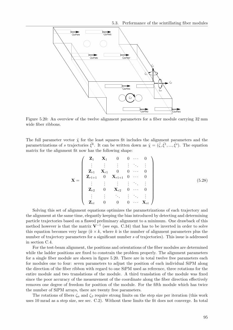
5.3. Performance of the scintillating fiber modules
Figure 5.20: An overview of the twelve alignment parameters for a fiber module carrying 32 mmwide fiber ribbons.
The full parameter vector χ for the least squares fit includes the alignment parameters and theparametrizations of s trajectories ξk. It can be written down as χ = (ζ, ξ1, ..., ξs). The equationmatrix for the alignment fit now has the following shape:
X =
Z1 X1 0 0 · · · 0...
......
.... . .
...Zr1 Xr1 0 0 · · · 0
Zr1+1 0 Xr1+1 0 · · · 0...
......
.... . .
...Zr2 0 Xr2 0 · · · 0
......
. . ....
. . ....
Zrt 0 0 0 · · · Xrt
(5.28)
Solving this set of alignment equations optimizes the parametrizations of each trajectory andthe alignment at the same time, elegantly keeping the bias introduced by detecting and determiningparticle trajectories based on a flawed preliminary alignment to a minimum. One drawback of thismethod however is that the matrix V−1 (see eqn. C.34) that has to be inverted in order to solvethis equation becomes very large (k × k, where k is the number of alignment parameters plus thenumber of trajectory parameters for a significant number s of trajectories). This issue is addressedin section C.4.
For the test-beam alignment, the positions and orientations of the fiber modules are determinedwhile the ladder positions are fixed to constrain the problem properly. The alignment parametersfor a single fiber module are shown in figure 5.20. There are in total twelve free parameters eachfor modules one to four: seven parameters to adjust the position of each individual SiPM alongthe direction of the fiber ribbon with regard to one SiPM used as reference, three rotations for theentire module and two translations of the module. A third translation of the module was fixedsince the poor accuracy of the measurement of the coordinate along the fiber direction effectivelyremoves one degree of freedom for position of the module. For the fifth module which has twicethe number of SiPM arrays, there are twenty free parameters.
The rotations of fibers ζα and ζβ require strong limits on the step size per iteration (this workuses 10 mrad as a step size, see sec. C.2). Without these limits the fit does not converge. In total
95
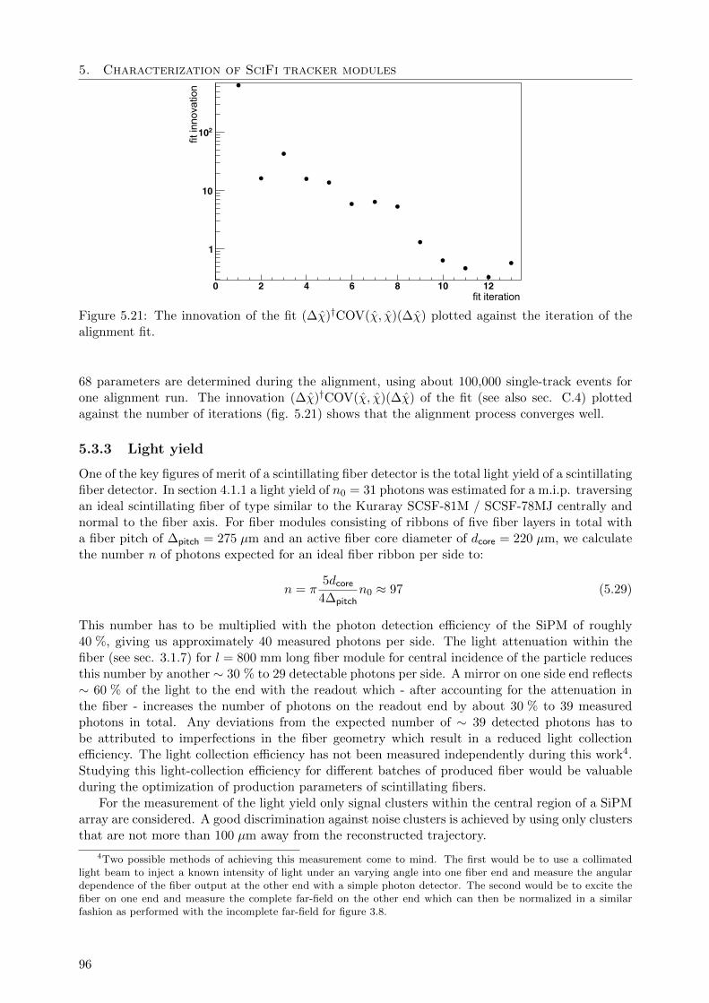
5. Characterization of SciFi tracker modules
0 2 4 6 8 10 12
1
10
210
fit iteration
fit in
nova
tion
Figure 5.21: The innovation of the fit (∆χ)†COV(χ, χ)(∆χ) plotted against the iteration of thealignment fit.
68 parameters are determined during the alignment, using about 100,000 single-track events forone alignment run. The innovation (∆χ)†COV(χ, χ)(∆χ) of the fit (see also sec. C.4) plottedagainst the number of iterations (fig. 5.21) shows that the alignment process converges well.
5.3.3 Light yield
One of the key figures of merit of a scintillating fiber detector is the total light yield of a scintillatingfiber detector. In section 4.1.1 a light yield of n0 = 31 photons was estimated for a m.i.p. traversingan ideal scintillating fiber of type similar to the Kuraray SCSF-81M / SCSF-78MJ centrally andnormal to the fiber axis. For fiber modules consisting of ribbons of five fiber layers in total witha fiber pitch of ∆pitch = 275 µm and an active fiber core diameter of dcore = 220 µm, we calculatethe number n of photons expected for an ideal fiber ribbon per side to:
n = π5dcore
4∆pitchn0 ≈ 97 (5.29)
This number has to be multiplied with the photon detection efficiency of the SiPM of roughly40 %, giving us approximately 40 measured photons per side. The light attenuation within thefiber (see sec. 3.1.7) for l = 800 mm long fiber module for central incidence of the particle reducesthis number by another ∼ 30 % to 29 detectable photons per side. A mirror on one side end reflects∼ 60 % of the light to the end with the readout which - after accounting for the attenuation inthe fiber - increases the number of photons on the readout end by about 30 % to 39 measuredphotons in total. Any deviations from the expected number of ∼ 39 detected photons has tobe attributed to imperfections in the fiber geometry which result in a reduced light collectionefficiency. The light collection efficiency has not been measured independently during this work4.Studying this light-collection efficiency for different batches of produced fiber would be valuableduring the optimization of production parameters of scintillating fibers.
For the measurement of the light yield only signal clusters within the central region of a SiPMarray are considered. A good discrimination against noise clusters is achieved by using only clustersthat are not more than 100 µm away from the reconstructed trajectory.
4Two possible methods of achieving this measurement come to mind. The first would be to use a collimatedlight beam to inject a known intensity of light under an varying angle into one fiber end and measure the angulardependence of the fiber output at the other end with a simple photon detector. The second would be to excite thefiber on one end and measure the complete far-field on the other end which can then be normalized in a similarfashion as performed with the incomplete far-field for figure 3.8.
96
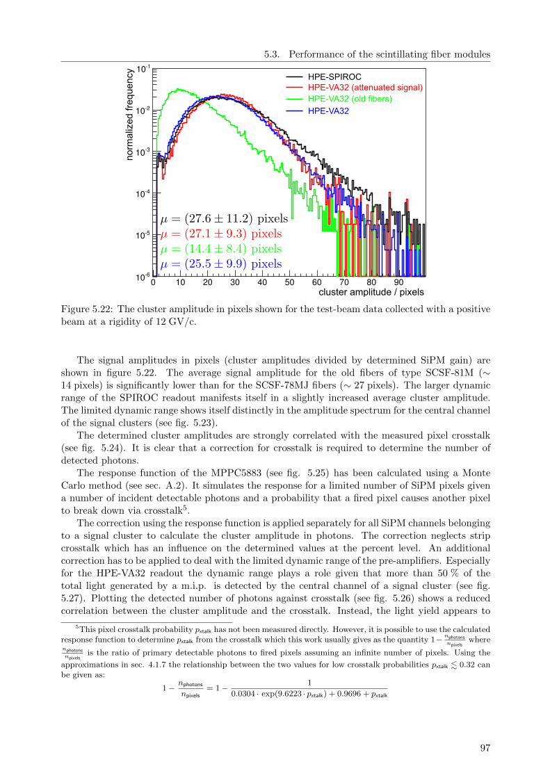
5.3. Performance of the scintillating fiber modules
0 10 20 30 40 50 60 70 80 90-610
-510
-410
-310
-210
-110
cluster amplitude / pixels
norm
alized
freq
uency
HPE-VA32 (old fibers)HPE-VA32 (attenuated signal)HPE-SPIROC
HPE-VA32
Figure 5.22: The cluster amplitude in pixels shown for the test-beam data collected with a positivebeam at a rigidity of 12 GV/c.
The signal amplitudes in pixels (cluster amplitudes divided by determined SiPM gain) areshown in figure 5.22. The average signal amplitude for the old fibers of type SCSF-81M (∼14 pixels) is significantly lower than for the SCSF-78MJ fibers (∼ 27 pixels). The larger dynamicrange of the SPIROC readout manifests itself in a slightly increased average cluster amplitude.The limited dynamic range shows itself distinctly in the amplitude spectrum for the central channelof the signal clusters (see fig. 5.23).
The determined cluster amplitudes are strongly correlated with the measured pixel crosstalk(see fig. 5.24). It is clear that a correction for crosstalk is required to determine the number ofdetected photons.
The response function of the MPPC5883 (see fig. 5.25) has been calculated using a MonteCarlo method (see sec. A.2). It simulates the response for a limited number of SiPM pixels givena number of incident detectable photons and a probability that a fired pixel causes another pixelto break down via crosstalk5.
The correction using the response function is applied separately for all SiPM channels belongingto a signal cluster to calculate the cluster amplitude in photons. The correction neglects stripcrosstalk which has an influence on the determined values at the percent level. An additionalcorrection has to be applied to deal with the limited dynamic range of the pre-amplifiers. Especiallyfor the HPE-VA32 readout the dynamic range plays a role given that more than 50 % of thetotal light generated by a m.i.p. is detected by the central channel of a signal cluster (see fig.5.27). Plotting the detected number of photons against crosstalk (see fig. 5.26) shows a reducedcorrelation between the cluster amplitude and the crosstalk. Instead, the light yield appears to
5This pixel crosstalk probability pxtalk has not been measured directly. However, it is possible to use the calculatedresponse function to determine pxtalk from the crosstalk which this work usually gives as the quantity 1− nphotons
npixelswhere
nphotons
npixelsis the ratio of primary detectable photons to fired pixels assuming an infinite number of pixels. Using the
approximations in sec. 4.1.7 the relationship between the two values for low crosstalk probabilities pxtalk . 0.32 canbe given as:
1− nphotons
npixels= 1− 1
0.0304 · exp(9.6223 · pxtalk) + 0.9696 + pxtalk
97
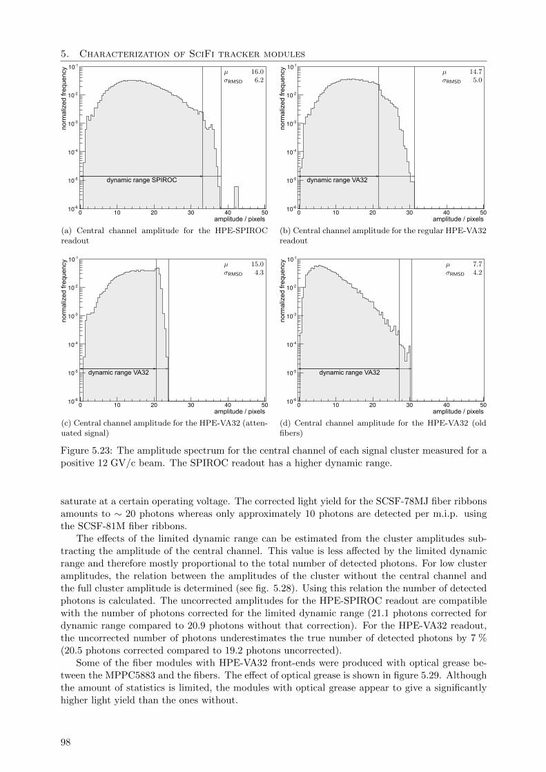
5. Characterization of SciFi tracker modules
0 10 20 30 40 50-610
-510
-410
-310
-210
-110
amplitude / pixels
norm
aliz
ed fr
eque
ncy
dynamic range SPIROC
(a) Central channel amplitude for the HPE-SPIROCreadout
0 10 20 30 40 50-610
-510
-410
-310
-210
-110
amplitude / pixels
norm
aliz
ed fr
eque
ncy
dynamic range VA32
(b) Central channel amplitude for the regular HPE-VA32readout
0 10 20 30 40 50-610
-510
-410
-310
-210
-110
amplitude / pixels
norm
aliz
ed fr
eque
ncy
dynamic range VA32
(c) Central channel amplitude for the HPE-VA32 (atten-uated signal)
0 10 20 30 40 50-610
-510
-410
-310
-210
-110
amplitude / pixels
norm
aliz
ed fr
eque
ncy
dynamic range VA32
(d) Central channel amplitude for the HPE-VA32 (oldfibers)
Figure 5.23: The amplitude spectrum for the central channel of each signal cluster measured for apositive 12 GV/c beam. The SPIROC readout has a higher dynamic range.
saturate at a certain operating voltage. The corrected light yield for the SCSF-78MJ fiber ribbonsamounts to ∼ 20 photons whereas only approximately 10 photons are detected per m.i.p. usingthe SCSF-81M fiber ribbons.
The effects of the limited dynamic range can be estimated from the cluster amplitudes sub-tracting the amplitude of the central channel. This value is less affected by the limited dynamicrange and therefore mostly proportional to the total number of detected photons. For low clusteramplitudes, the relation between the amplitudes of the cluster without the central channel andthe full cluster amplitude is determined (see fig. 5.28). Using this relation the number of detectedphotons is calculated. The uncorrected amplitudes for the HPE-SPIROC readout are compatiblewith the number of photons corrected for the limited dynamic range (21.1 photons corrected fordynamic range compared to 20.9 photons without that correction). For the HPE-VA32 readout,the uncorrected number of photons underestimates the true number of detected photons by 7 %(20.5 photons corrected compared to 19.2 photons uncorrected).
Some of the fiber modules with HPE-VA32 front-ends were produced with optical grease be-tween the MPPC5883 and the fibers. The effect of optical grease is shown in figure 5.29. Althoughthe amount of statistics is limited, the modules with optical grease appear to give a significantlyhigher light yield than the ones without.
98
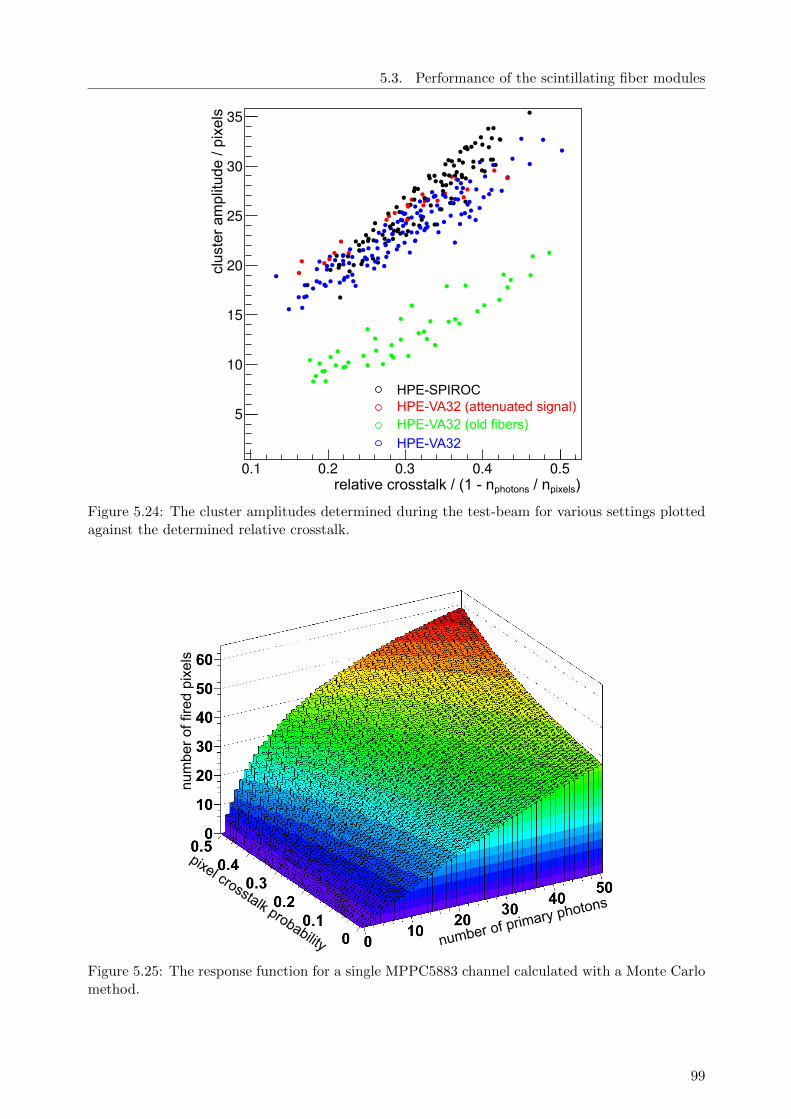
5.3. Performance of the scintillating fiber modules
0.1 0.2 0.3 0.4 0.5
5
10
15
20
25
30
35
relative crosstalk / (1 - nphotons / npixels)
clus
ter
ampl
itude
/ pi
xels
HPE-VA32 (old fibers)HPE-VA32 (attenuated signal)HPE-SPIROC
HPE-VA32
Figure 5.24: The cluster amplitudes determined during the test-beam for various settings plottedagainst the determined relative crosstalk.
number of primary photons
pixel crosstalk probability
num
ber
of fi
red
pixe
ls
Figure 5.25: The response function for a single MPPC5883 channel calculated with a Monte Carlomethod.
99
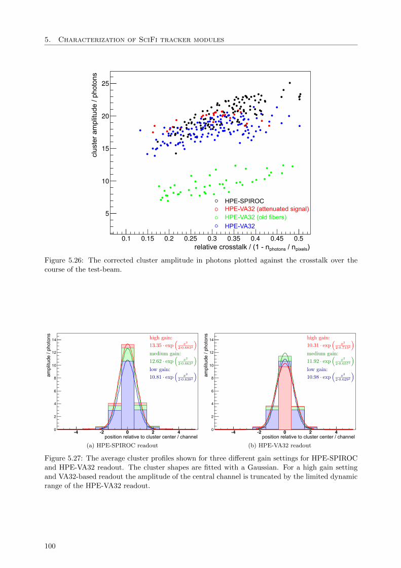
5. Characterization of SciFi tracker modules
0.1 0.15 0.2 0.25 0.3 0.35 0.4 0.45 0.5
5
10
15
20
25
HPE-VA32 (old fibers)HPE-VA32 (attenuated signal)HPE-SPIROC
HPE-VA32
relative crosstalk / (1 - nphotons / npixels)
clus
ter
ampl
itude
/ ph
oton
s
Figure 5.26: The corrected cluster amplitude in photons plotted against the crosstalk over thecourse of the test-beam.
-4 -2 0 2 40
2
4
6
8
10
12
14
position relative to cluster center / channel
ampl
itude
/ ph
oton
s
(a) HPE-SPIROC readout
-4 -2 0 2 40
2
4
6
8
10
12
14
position relative to cluster center / channel
ampl
itude
/ ph
oton
s
(b) HPE-VA32 readout
Figure 5.27: The average cluster profiles shown for three different gain settings for HPE-SPIROCand HPE-VA32 readout. The cluster shapes are fitted with a Gaussian. For a high gain settingand VA32-based readout the amplitude of the central channel is truncated by the limited dynamicrange of the HPE-VA32 readout.
100
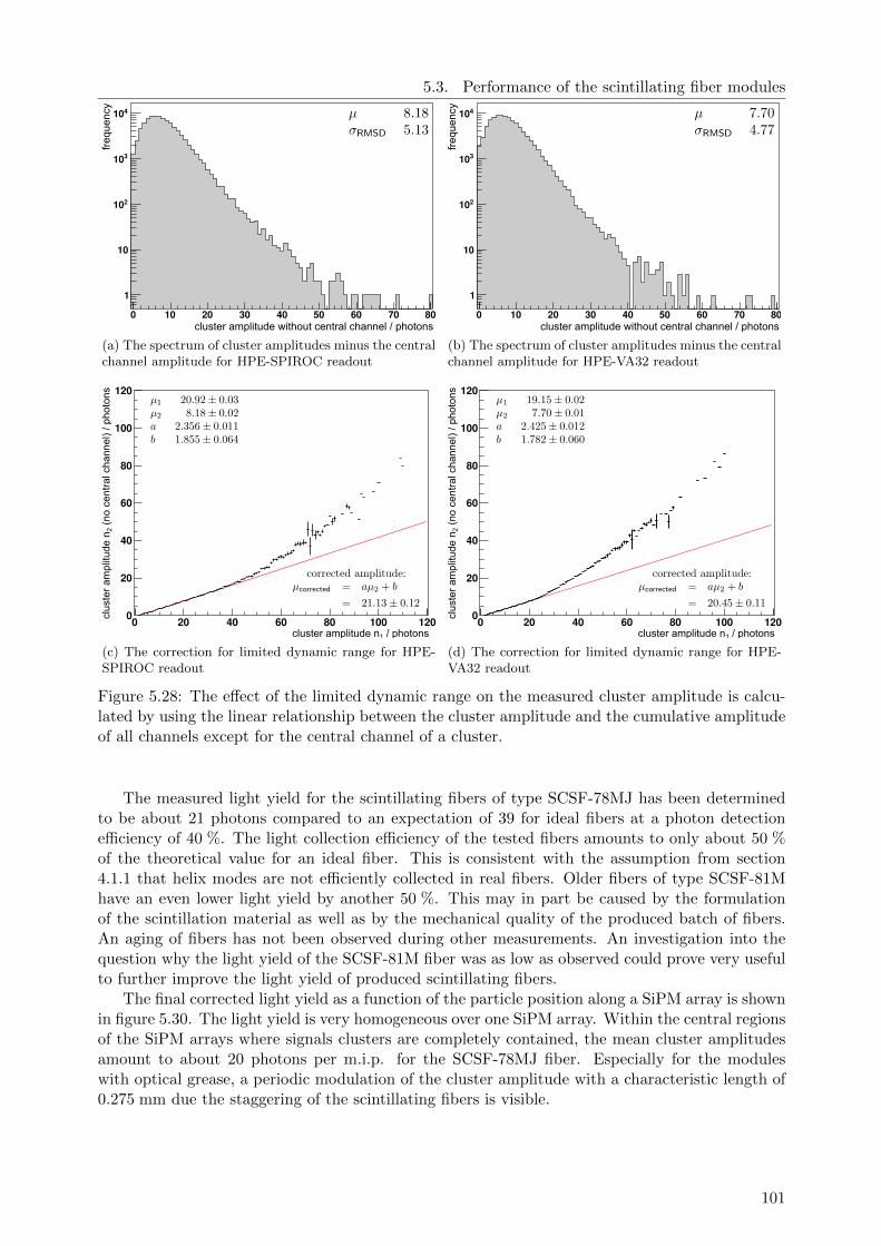
5.3. Performance of the scintillating fiber modules
0 10 20 30 40 50 60 70 80
1
10
210
310
410
cluster amplitude without central channel / photons
freq
uenc
y
(a) The spectrum of cluster amplitudes minus the centralchannel amplitude for HPE-SPIROC readout
0 10 20 30 40 50 60 70 80
1
10
210
310
410
cluster amplitude without central channel / photons
freq
uenc
y
(b) The spectrum of cluster amplitudes minus the centralchannel amplitude for HPE-VA32 readout
0 20 40 60 80 100 1200
20
40
60
80
100
120
cluster amplitude n1 / photons
clus
ter
ampl
itude
n2
(no
cent
ral c
hann
el)
/ pho
tons
(c) The correction for limited dynamic range for HPE-SPIROC readout
0 20 40 60 80 100 1200
20
40
60
80
100
120
cluster amplitude n1 / photons
clus
ter
ampl
itude
n2
(no
cent
ral c
hann
el)
/ pho
tons
(d) The correction for limited dynamic range for HPE-VA32 readout
Figure 5.28: The effect of the limited dynamic range on the measured cluster amplitude is calcu-lated by using the linear relationship between the cluster amplitude and the cumulative amplitudeof all channels except for the central channel of a cluster.
The measured light yield for the scintillating fibers of type SCSF-78MJ has been determinedto be about 21 photons compared to an expectation of 39 for ideal fibers at a photon detectionefficiency of 40 %. The light collection efficiency of the tested fibers amounts to only about 50 %of the theoretical value for an ideal fiber. This is consistent with the assumption from section4.1.1 that helix modes are not efficiently collected in real fibers. Older fibers of type SCSF-81Mhave an even lower light yield by another 50 %. This may in part be caused by the formulationof the scintillation material as well as by the mechanical quality of the produced batch of fibers.An aging of fibers has not been observed during other measurements. An investigation into thequestion why the light yield of the SCSF-81M fiber was as low as observed could prove very usefulto further improve the light yield of produced scintillating fibers.
The final corrected light yield as a function of the particle position along a SiPM array is shownin figure 5.30. The light yield is very homogeneous over one SiPM array. Within the central regionsof the SiPM arrays where signals clusters are completely contained, the mean cluster amplitudesamount to about 20 photons per m.i.p. for the SCSF-78MJ fiber. Especially for the moduleswith optical grease, a periodic modulation of the cluster amplitude with a characteristic length of0.275 mm due the staggering of the scintillating fibers is visible.
101
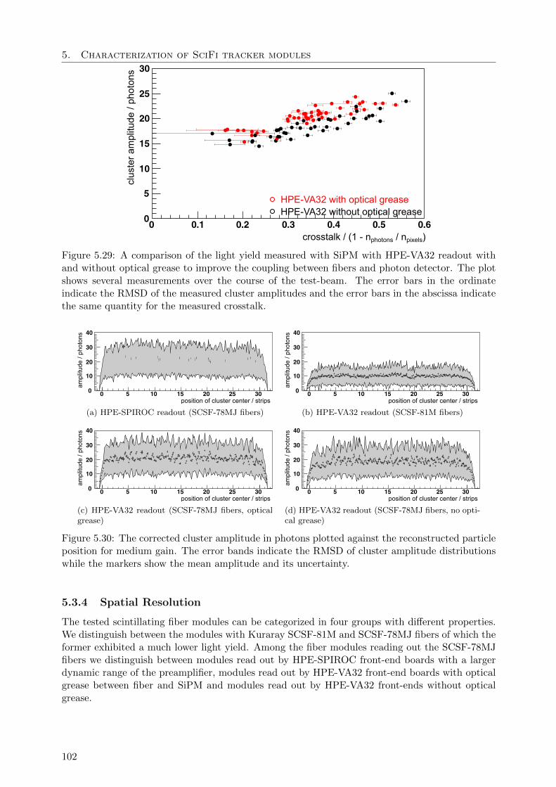
5. Characterization of SciFi tracker modules
crosstalk / (1 - nphotons / npixels)
clus
ter
ampl
itude
/ ph
oto
ns
HPE-VA32 with optical greaseHPE-VA32 without optical grease
0 0.1 0.2 0.3 0.4 0.5 0.60
5
10
15
20
25
30
Figure 5.29: A comparison of the light yield measured with SiPM with HPE-VA32 readout withand without optical grease to improve the coupling between fibers and photon detector. The plotshows several measurements over the course of the test-beam. The error bars in the ordinateindicate the RMSD of the measured cluster amplitudes and the error bars in the abscissa indicatethe same quantity for the measured crosstalk.
0 5 10 15 20 25 300
10
20
30
40
ampl
itude
/ ph
oton
s
position of cluster center / strips
(a) HPE-SPIROC readout (SCSF-78MJ fibers)
0 5 10 15 20 25 300
10
20
30
40
ampl
itude
/ ph
oton
s
position of cluster center / strips
(b) HPE-VA32 readout (SCSF-81M fibers)
0 5 10 15 20 25 300
10
20
30
40
ampl
itude
/ ph
oton
s
position of cluster center / strips
(c) HPE-VA32 readout (SCSF-78MJ fibers, opticalgrease)
0 5 10 15 20 25 300
10
20
30
40
ampl
itude
/ ph
oton
s
position of cluster center / strips
(d) HPE-VA32 readout (SCSF-78MJ fibers, no opti-cal grease)
Figure 5.30: The corrected cluster amplitude in photons plotted against the reconstructed particleposition for medium gain. The error bands indicate the RMSD of cluster amplitude distributionswhile the markers show the mean amplitude and its uncertainty.
5.3.4 Spatial Resolution
The tested scintillating fiber modules can be categorized in four groups with different properties.We distinguish between the modules with Kuraray SCSF-81M and SCSF-78MJ fibers of which theformer exhibited a much lower light yield. Among the fiber modules reading out the SCSF-78MJfibers we distinguish between modules read out by HPE-SPIROC front-end boards with a largerdynamic range of the preamplifier, modules read out by HPE-VA32 front-end boards with opticalgrease between fiber and SiPM and modules read out by HPE-VA32 front-ends without opticalgrease.
102
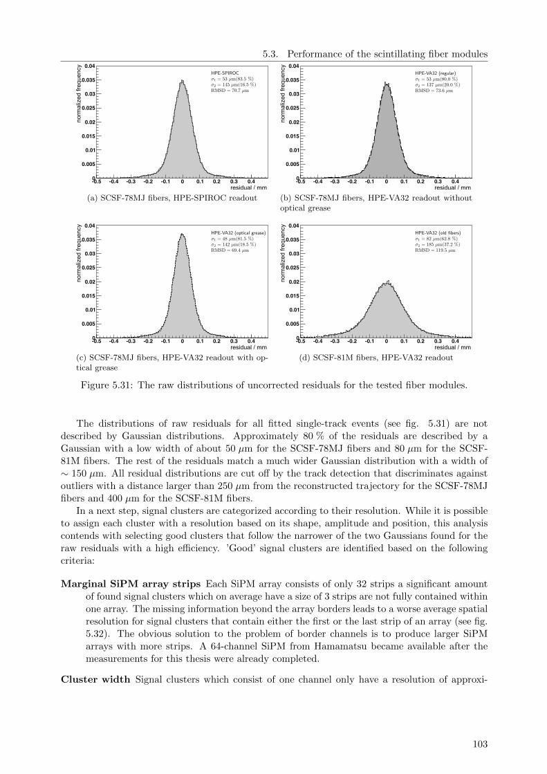
5.3. Performance of the scintillating fiber modules
-0.5 -0.4 -0.3 -0.2 -0.1 0 0.1 0.2 0.3 0.40
0.005
0.01
0.015
0.02
0.025
0.03
0.035
0.04
norm
aliz
ed fr
eque
ncy
residual / mm
(a) SCSF-78MJ fibers, HPE-SPIROC readout
-0.5 -0.4 -0.3 -0.2 -0.1 0 0.1 0.2 0.3 0.40
0.005
0.01
0.015
0.02
0.025
0.03
0.035
0.04
norm
aliz
ed fr
eque
ncy
residual / mm
(b) SCSF-78MJ fibers, HPE-VA32 readout withoutoptical grease
-0.5 -0.4 -0.3 -0.2 -0.1 0 0.1 0.2 0.3 0.40
0.005
0.01
0.015
0.02
0.025
0.03
0.035
0.04
norm
aliz
ed fr
eque
ncy
residual / mm
(c) SCSF-78MJ fibers, HPE-VA32 readout with op-tical grease
-0.5 -0.4 -0.3 -0.2 -0.1 0 0.1 0.2 0.3 0.40
0.005
0.01
0.015
0.02
0.025
0.03
0.035
0.04
norm
aliz
ed fr
eque
ncy
residual / mm
(d) SCSF-81M fibers, HPE-VA32 readout
Figure 5.31: The raw distributions of uncorrected residuals for the tested fiber modules.
The distributions of raw residuals for all fitted single-track events (see fig. 5.31) are notdescribed by Gaussian distributions. Approximately 80 % of the residuals are described by aGaussian with a low width of about 50 µm for the SCSF-78MJ fibers and 80 µm for the SCSF-81M fibers. The rest of the residuals match a much wider Gaussian distribution with a width of∼ 150 µm. All residual distributions are cut off by the track detection that discriminates againstoutliers with a distance larger than 250 µm from the reconstructed trajectory for the SCSF-78MJfibers and 400 µm for the SCSF-81M fibers.
In a next step, signal clusters are categorized according to their resolution. While it is possibleto assign each cluster with a resolution based on its shape, amplitude and position, this analysiscontends with selecting good clusters that follow the narrower of the two Gaussians found for theraw residuals with a high efficiency. ’Good’ signal clusters are identified based on the followingcriteria:
Marginal SiPM array strips Each SiPM array consists of only 32 strips a significant amountof found signal clusters which on average have a size of 3 strips are not fully contained withinone array. The missing information beyond the array borders leads to a worse average spatialresolution for signal clusters that contain either the first or the last strip of an array (see fig.5.32). The obvious solution to the problem of border channels is to produce larger SiPMarrays with more strips. A 64-channel SiPM from Hamamatsu became available after themeasurements for this thesis were already completed.
Cluster width Signal clusters which consist of one channel only have a resolution of approxi-
103

5. Characterization of SciFi tracker modules
mately 80 µm6. Very wide clusters on the other hand are equally expected to show a poorspatial resolution because the precision of the center-of-gravity estimator and the medianestimator is approximately proportional to the square root of the cluster amplitude andinversely proportional to the cluster width. In addition, wide signal clusters are likely theresult of δ-electrons and other particles being radiated by the tracked primary particle. Forthese clusters, the employed estimator for the particle position fails to produce a good esti-mate for the position of the tracked particle (see fig. 5.34). The frequency distribution ofcluster widths (see fig. 5.33) shows that the preferred width of a signal cluster is around 3with most of the clusters being in the interval between 2 and 5.
Cluster amplitude For low numbers of detected photons the accuracy of the estimator for thecluster center must suffer (see fig. 5.35). Very high amplitudes indicate a hard interaction.For one, hard interactions lead to a deterioration of the spatial information carried by thesignal cluster due to radiated secondary particles. Secondly, the limited dynamic range andsaturation effects will distort the cluster shape at high signal amplitudes and therefore reducethe precision of the used estimator for the particle position.
Cluster shape The average signal cluster is approximately Gaussian in shape with an averagewidth of 0.6 to 0.7 strips as shown in fig. 5.27 for different gain settings. We define a simpleRMSD as an estimator for the relative width w of a cluster C with amplitudes ai in channelsi:
w =
√√√√√√√∑i∈C
i2ai(∑i∈C
ai
)2 −
∑i∈C
iai∑i∈C
ai
2
As expected from the average cluster shape (see fig. 5.27) the most probable cluster RMSDw is between 0.6 and 0.7 (see fig. 5.37).
Selection Efficiency Resolution of filtered clusters
discard clusters containing marginal SiPMarray strips
84 % ∼ 100 µm
Cluster width / array channels ∈ [2, 5] 95 % ∼ 100 µm + tails
Cluster amplitude / pixels ∈ [5.5, 60] 99 % ∼ 100 µm
Cluster RMSD / array channels ≤ 1 97 % ∼ 90 µm
The described cuts have a cumulative efficiency of 75 % for the modules consisting of SCSF-78MJ fibers without optical grease7, 78 % for the modules with SCSF-78MJ fibers and opticalgrease and 60 % for the SCSF-81M fibers. The distribution of removed residuals show a widthof around 93 µm for the SCSF-78MJ fiber and 134 µm for the SCSF-81M fibers (see fig. 5.39).The resolution that can be associated with the discarded clusters is significantly reduced and theirdistribution does not match a Gaussian.
For the remaining good clusters the two different estimators for the cluster center are comparedbased on the measured distribution of residuals (see fig. 5.40). The median based estimator showsthe better performance with a 5 % narrower width of the residual distribution than the center-of-gravity estimator. This is explained by the stronger influence fluctuations in the fringes of thecluster (e.g. crosstalk between SiPM strips) have on the center-of-gravity estimator. The analysisbeyond this point therefore uses the median estimator for the cluster center.
6The actual resolution does not only depend on the SiPM array strip pitch but also on the arrangement of thefibers. It is therefore actually worse than 250 µm/
√12.
7HPE-SPIROC and HPE-VA32 show almost exactly the same performance.
104
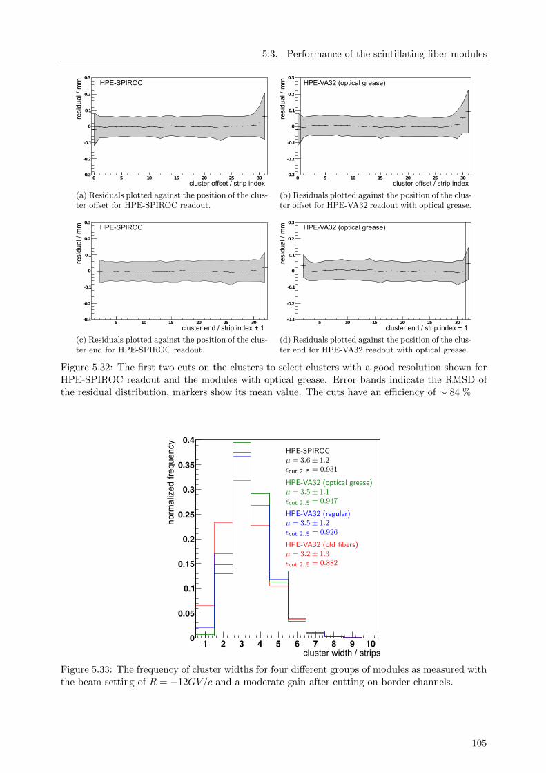
5.3. Performance of the scintillating fiber modules
HPE-SPIROC
5 10 15 20 25 30-0.3
-0.2
-0.1
0
0.1
0.2
cluster offset / strip index
residual/mm
0
0.3
(a) Residuals plotted against the position of the clus-ter offset for HPE-SPIROC readout.
HPE-VA32 (optical grease)
5 10 15 20 25 30-0.3
-0.2
-0.1
0
0.1
0.2
cluster offset / strip index
residual/mm
0
0.3
(b) Residuals plotted against the position of the clus-ter offset for HPE-VA32 readout with optical grease.
HPE-SPIROC
5 10 15 20 25 30-0.3
-0.2
-0.1
0
0.1
0.2
cluster end / strip index + 1
residual/mm
0.3
(c) Residuals plotted against the position of the clus-ter end for HPE-SPIROC readout.
HPE-VA32 (optical grease)
5 10 15 20 25 30-0.3
-0.2
-0.1
0
0.1
0.2
cluster end / strip index + 1
residual/mm
0.3
(d) Residuals plotted against the position of the clus-ter end for HPE-VA32 readout with optical grease.
Figure 5.32: The first two cuts on the clusters to select clusters with a good resolution shown forHPE-SPIROC readout and the modules with optical grease. Error bands indicate the RMSD ofthe residual distribution, markers show its mean value. The cuts have an efficiency of ∼ 84 %
1 2 3 4 5 6 7 8 9 100
0.05
0.1
0.15
0.2
0.25
0.3
0.35
0.4
cluster width / strips
norm
aliz
ed fr
eque
ncy
Figure 5.33: The frequency of cluster widths for four different groups of modules as measured withthe beam setting of R = −12GV/c and a moderate gain after cutting on border channels.
105
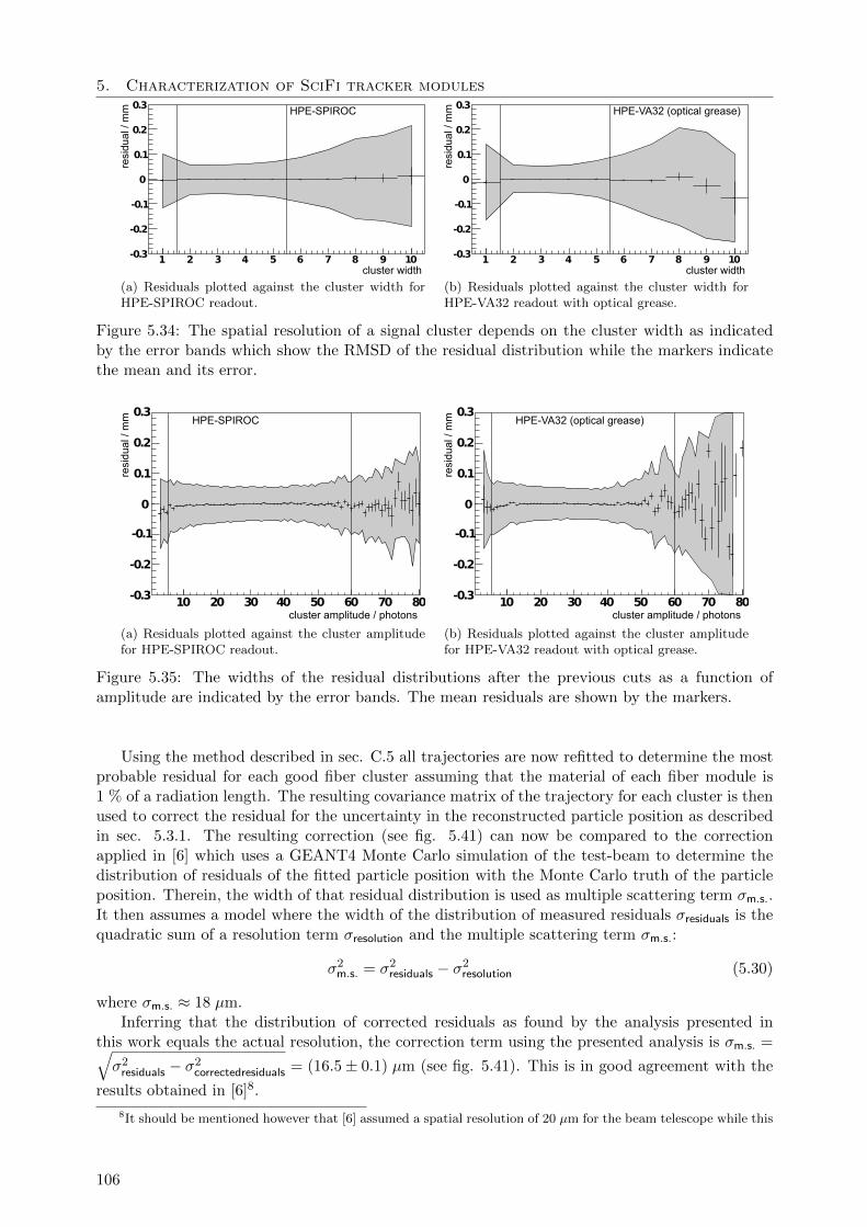
5. Characterization of SciFi tracker modules
HPE-SPIROC
cluster width
residual/mm
1 2 3 4 5 6 7 8 9 10-0.3
-0.2
-0.1
0
0.1
0.2
0.3
(a) Residuals plotted against the cluster width forHPE-SPIROC readout.
HPE-VA32 (optical grease)
cluster width
residual/mm
1 2 3 4 5 6 7 8 9 10-0.3
-0.2
-0.1
0
0.1
0.2
0.3
(b) Residuals plotted against the cluster width forHPE-VA32 readout with optical grease.
Figure 5.34: The spatial resolution of a signal cluster depends on the cluster width as indicatedby the error bands which show the RMSD of the residual distribution while the markers indicatethe mean and its error.
HPE-SPIROC
10 20 30 40 50 60 70 80-0.3
-0.2
-0.1
0
0.1
0.2
0.3
cluster amplitude / photons
residual/mm
(a) Residuals plotted against the cluster amplitudefor HPE-SPIROC readout.
HPE-VA32 (optical grease)
10 20 30 40 50 60 70 80-0.3
-0.2
-0.1
0
0.1
0.2
0.3
cluster amplitude / photons
residual/mm
(b) Residuals plotted against the cluster amplitudefor HPE-VA32 readout with optical grease.
Figure 5.35: The widths of the residual distributions after the previous cuts as a function ofamplitude are indicated by the error bands. The mean residuals are shown by the markers.
Using the method described in sec. C.5 all trajectories are now refitted to determine the mostprobable residual for each good fiber cluster assuming that the material of each fiber module is1 % of a radiation length. The resulting covariance matrix of the trajectory for each cluster is thenused to correct the residual for the uncertainty in the reconstructed particle position as describedin sec. 5.3.1. The resulting correction (see fig. 5.41) can now be compared to the correctionapplied in [6] which uses a GEANT4 Monte Carlo simulation of the test-beam to determine thedistribution of residuals of the fitted particle position with the Monte Carlo truth of the particleposition. Therein, the width of that residual distribution is used as multiple scattering term σm.s..It then assumes a model where the width of the distribution of measured residuals σresiduals is thequadratic sum of a resolution term σresolution and the multiple scattering term σm.s.:
σ2m.s. = σ2
residuals − σ2resolution (5.30)
where σm.s. ≈ 18 µm.Inferring that the distribution of corrected residuals as found by the analysis presented in
this work equals the actual resolution, the correction term using the presented analysis is σm.s. =√σ2residuals − σ2
correctedresiduals = (16.5± 0.1) µm (see fig. 5.41). This is in good agreement with the
results obtained in [6]8.
8It should be mentioned however that [6] assumed a spatial resolution of 20 µm for the beam telescope while this
106
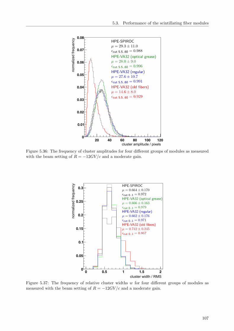
5.3. Performance of the scintillating fiber modules
20 40 60 80 100 1200
0.01
0.02
0.03
0.04
0.05
0.06
0.07
0.08
cluster amplitude / pixels
norm
aliz
ed fr
eque
ncy
Figure 5.36: The frequency of cluster amplitudes for four different groups of modules as measuredwith the beam setting of R = −12GV/c and a moderate gain.
0 0.5 1 1.5 20
0.05
0.1
0.15
0.2
0.25
0.3
cluster width / RMS
norm
aliz
ed fr
eque
ncy
Figure 5.37: The frequency of relative cluster widths w for four different groups of modules asmeasured with the beam setting of R = −12GV/c and a moderate gain.
107

5. Characterization of SciFi tracker modules
HPE-SPIROC
cluster rms / strips
residual/mm
0 0.2 0.4 0.6 0.8 1 1.2 1.4 1.6 1.8-0.3
-0.2
-0.1
0
0.1
0.2
0.3
(a) Residuals plotted against the RMSD of the clus-ter for HPE-SPIROC readout.
HPE-VA32 (optical grease)
cluster rms / strips
residual/mm
0 0.2 0.4 0.6 0.8 1 1.2 1.4 1.6 1.8-0.3
-0.2
-0.1
0
0.1
0.2
0.3
(b) Residuals plotted against the RMSD of the clus-ter for HPE-VA32 readout with optical grease.
Figure 5.38: The widths of the residual distributions after the previous cuts as a function of clusterRMSD are indicated by the error bands. The mean residuals are shown by the markers.
HPE-SPIROC
HPE-VA32 (regular)HPE-VA32 (optical grease)
norm
aliz
ed fr
eque
ncy
residual / mm-0.5 -0.4 -0.3 -0.2 -0.1 0 0.1 0.2 0.3 0.40
0.005
0.01
0.015
0.02
0.025
(a) Residuals of bad clusters for modules with SCSF-78MJ fibers.
HPE-VA32 (old fibers)
norm
aliz
ed fr
eque
ncy
residual / mm-0.5 -0.4 -0.3 -0.2 -0.1 0 0.1 0.2 0.3 0.40
0.005
0.01
0.015
0.02
0.025
(b) Residuals of bad clusters for modules with SCSF-81M fibers.
Figure 5.39: The distribution of residuals for clusters that are not considered good. The agreementwith a Gaussian is poor. A Gaussian fit is still performed to determine approximate values for theresolution amounting to 93 µm for the SCSF-78MJ fibers and 134 µm for the SCSF-81MJ fibers.
-0.2 -0.15 -0.1 -0.05 0 0.05 0.1 0.15 0.20
0.005
0.01
0.015
0.02
0.025
0.03
0.035
residual / mm
norm
aliz
ed fr
eque
ncy HPE-SPIROC
RMSD (c.o.g.): 60.5 µmRMSD (median): 58.5 µm
(a) HPE-SPIROC readout.
-0.2 -0.15 -0.1 -0.05 0 0.05 0.1 0.15 0.20
0.005
0.01
0.015
0.02
0.025
0.03
0.035
0.04
residual / mm
norm
aliz
ed fr
eque
ncy HPE-VA32 (optical grease)
RMSD (c.o.g.): 56.9 µmRMSD (median): 54.5 µm
(b) HPE-VA32 readout with optical grease.
Figure 5.40: Comparison of the residual distributions using the median and the center-of-gravityas estimators for the cluster center.
108
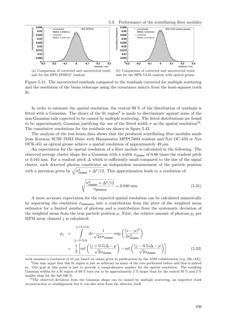
5.3. Performance of the scintillating fiber modules
RMSD: 0.0561mm
RMSD: 0.0585mmuncorrected
corrected
HPE-SPIROCno
rmal
ized
freq
uenc
y
residual / mm-0.3 -0.2 -0.1 0 0.1 0.2 0.30
0.0050.01
0.0150.020.0250.030.0350.040.045
(a) Comparison of corrected and uncorrected resid-uals for the HPE-SPIROC readout.
HPE-VA32 (optical grease)
RMSD: 0.0518mm
RMSD: 0.0544mmuncorrected
corrected
norm
aliz
ed fr
eque
ncy
residual / mm-0.3 -0.2 -0.1 0 0.1 0.2 0.30
0.0050.01
0.0150.020.0250.030.0350.040.045
(b) Comparison of corrected and uncorrected resid-uals for the HPE-VA32 readout with optical grease.
Figure 5.41: The uncorrected residuals compared to the residuals corrected for multiple scatteringand the resolution of the beam telescope using the covariance matrix from the least-squares trackfit.
In order to estimate the spatial resolution, the central 99 % of the distribution of residuals isfitted with a Gaussian. The choice of the fit region9 is made to discriminate against some of thenon-Gaussian tails expected to be caused by multiple scattering. The fitted distributions are foundto be approximately Gaussian justifying the use of the fitted width σ as the spatial resolution10.The cumulative resolutions for the residuals are shown in figure 5.42.
The analysis of the test-beam data shows that the produced scintillating fiber modules madefrom Kuraray SCSF-78MJ fibers with Hamamatsu MPPC5883 readout and Nye OC-459 or NyeOCK-451 as optical grease achieve a spatial resolution of approximately 49 µm.
An expectation for the spatial resolution of a fiber module is calculated in the following. Theobserved average cluster shape fits a Gaussian with a width σcluster of 0.66 times the readout pitchor 0.165 mm. For a readout pitch ∆ which is sufficiently small compared to the size of the signalcluster, each detected photon constitutes an independent measurement of the particle position
with a precision given by√σ2cluster + ∆2/12. This approximation leads to a resolution of:√
σ2cluster + ∆2/12
nphotons= 0.040 mm (5.31)
A more accurate expectation for the expected spatial resolution can be calculated numericallyby separating the resolution σresolution into a contribution from the jitter of the weighted meanestimator for a limited number of photons and a contribution from the systematic deviation ofthe weighted mean from the true particle position µ. First, the relative amount of photons pj perSiPM array channel j is calculated:
pj =
(j+0.5)∆∫(j−0.5)∆
dx1√
2πσclusterexp
((x− µ)2
2σ2cluster
)
=1
2
[erf
((j + 0.5)∆− µ√
2σcluster
)− erf
((j − 0.5)∆− µ√
2σcluster
)](5.32)
work assumes a resolution of 10 µm based on values given in publications by the AMS collaboration (e.g. [86,143]).9One may argue that this fit region is just as arbitrary as many of the cuts performed before and that is indeed
so. Our goal at this point is just to provide a comprehensive number for the spatial resolution. The resultingGaussian widths for a fit region of 99 % turn out to be approximately 2 % larger than for the central 95 % and 2 %smaller than for the full 100 %.
10The observed deviation from the Gaussian shape can be caused by multiple scattering, an imperfect trackreconstruction or misalignment but it can also stem from the detector itself.
109

5. Characterization of SciFi tracker modules
0
500
1000
1500
2000
2500
3000
3500
4000
-0.3 -0.2 -0.1 0 0.1 0.2 0.3residual / mm
freq
uenc
y
(a) Measured resolution for modules SCSF-81Mfibers with HPE-SPIROC readout.
-0.5 -0.4 -0.3 -0.2 -0.1 0 0.1 0.2 0.3 0.40
200
400
600
800
1000
1200
1400
1600
1800
2000
2200
0.5residual / mm
freq
uenc
y
(b) Measured resolution for modules of SCSF-81Mfibers with HPE-VA32 readout.
0
500
1000
1500
2000
2500
3000
3500
-0.3 -0.2 -0.1 0 0.1 0.2 0.3residual / mm
freq
uenc
y
(c) Measured resolution for modules of SCSF-78MJfibers with HPE-VA32 readout and optical grease.
0
500
1000
1500
2000
2500
3000
-0.3 -0.2 -0.1 0 0.1 0.2 0.3residual / mm
freq
uenc
y
(d) Measured resolution for modules SCSF-78MJfibers with HPE-VA32 readout without opticalgrease.
Figure 5.42: The residuals corrected for the resolution of the beam telescope and multiple scatteringmeasured with medium gain for positive 12 GeV/c beam particles. The inner 95 %, 99 % and 100 %of the residual distribution are fitted with a Gaussian.
With this, the uncertainty from the statistical jitter of the weighted mean estimator is:
∞∑j=−∞
(∆j − µ)2
nphotonspj (5.33)
The systematic deviation of the weighted mean estimator from the true particle position is:µ− ∞∑j=−∞
∆jpj
2
(5.34)
Averaging over the possible particle positions µ, an expression for the resolution is obtained.
σ2resolution,calc =
1
∆
∆/2∫−∆/2
d∆
∞∑j=−∞
(∆j − µ)2
nphotonspj
+
µ− ∞∑j=−∞
∆jpj
2
=σ2cluster + ∆2/12
nphotons+
1
∆
∆/2∫−∆/2
d∆
µ− ∞∑j=−∞
∆jpj
2
(5.35)
110

5.3. Performance of the scintillating fiber modules
0 0.2 0.4 0.6 0.8 10
0.02
0.04
0.06
0.08
0.1
0.12
0.14 accurate calculation (I)simple approximation (II)systematic contribution (III)
readout pitch / mm
reso
lutio
n / m
m
Figure 5.43: (I) shows the accurate calculation omitting crosstalk (eqn. 5.35). (II) shows the ex-pected spatial resolution based on the simple approximation (eqn. 5.31). (III) shows the systematiccontribution to (I) (eqn. 5.34).
Evaluating this integral for σcluster = 0.165 mm, the same expected resolution of 0.040 mm isfound (see fig. 5.43).
The expected resolution deviates from the measurement. This deviation could be explainedby an additional process that impairs the resolution and which effectively adds an additionaluncertainty of σunknown = 0.026 mm. A toy Monte-Carlo simulation is used to identify possibleexplanations. The simulation creates random clusters with 20±
√20 photons and 30% additional
pixels fired due to crosstalk. Including crosstalk and variations in the total number of photonsreduces the expected resolution slightly to 0.045 mm.
Given the uncertainties in - for example - the measurement of the cluster shape, it is possiblethat the cluster shape actually fits the sum of two Gaussians. Another Monte-Carlo simulationis conducted based on this assumption. There-in, the first Gaussian is arbitrarily assumed todescribe 98% of all photons with a width as measured of σ = σcluster. The other Gaussian isused to add tails to the central Gaussian, describing 2% of the photons exiting the fiber with awidth of σ = 3 ·σcluster. Using this parametrization a spatial resolution of 0.048 mm is simulated,showing that the measured spatial resolution is indeed compatible with the expectation based onthe presented understanding of the scintillating fiber tracker.
As expected, the spatial resolution improves with increasing average light yield (see fig. 5.44).It also varies with the crosstalk, where the crosstalk serves us merely as an estimator for the workingpoint of the silicon photomultiplier (see fig. 5.45). For high operating voltages the rising crosstalkis expected to have a negative impact on the spatial resolution while at low operating voltages thedecreasing photon efficiency impairs an accurate tracking. Between the two extremes, there is avery wide minimum. Translating the crosstalk into an over-voltage11, the optimal overvoltage forthe MPPC5883 appears to be between 2.0 V and 2.6 V.
The characterization of the prototype fiber modules showed promising results. A spatial res-olution better than 50 µm was achieved in agreement with an expectation from a Monte-Carlosimulation. Despite the dependence of the SiPM array properties of the overvoltage, no significanteffects of the overvoltage on the spatial resolution was found as long as the overvoltage was keptin a 0.6 V wide window between 2.0 V and 2.6 V.
11This is an estimate based upon measured SiPM properties (see sec. 4.1.9). Its precision is limited.
111

5. Characterization of SciFi tracker modules
5 10 15 20 25 300.04
0.05
0.06
0.07
0.08
0.09
0.1
0.11
0.12
cluster amplitude / photons
estim
ated
spa
tial r
esol
uton
/ m
m HPE-SPIROC readout (SCSF-78MJ fiber)
HPE-VA32 readout (SCSF-78MJ fiber, optical grease)HPE-VA32 readout (SCSF-81M fiber)
HPE-VA32 readout (SCSF-78MJ fiber)Monte-Carlo Prediction (30% Crosstalk)
Figure 5.44: The spatial resolution estimated using a Gaussian fit of the central 99 % of the residualdistribution as a function of amplitude plotted for single SiPM arrays during the test-beam. It iscompared to the expectation from a Monte-Carlo simulation assuming 30 % of the fired pixels tobe caused by crosstalk and a cluster width of 0.165 mm
0.1 0.15 0.2 0.25 0.3 0.35 0.4 0.45 0.5 0.55 0.60.04
0.05
0.06
0.07
0.08
0.09
0.1
0.11
0.12
crosstalk / (1 - nphotons / npixels)
estim
ated
spa
tial r
esol
uto
n / m
m
HPE-SPIROC readout (SCSF-78MJ fiber)
HPE-VA32 readout (SCSF-78MJ fiber, optical grease)HPE-VA32 readout (SCSF-81M fiber)
HPE-VA32 readout (SCSF-78MJ fiber)
1.6 1.8 2.0 2.2 2.4 2.6 2.8 3.0 3.2estimated overvoltage (Ubias - Ubreakdown) / V
Figure 5.45: The spatial resolution estimated using a Gaussian fit of the central 99 % of the residualdistribution as a function of the crosstalk plotted for single SiPM arrays during the test-beam.From the crosstalk it is possible to give a rough estimate of the over-voltage at which the SiPMare operated.
112

Chapter 6
The Proton Electron RadiationDetector Aix-la-Chapelle
The scintillating fiber tracker presented in this work was implemented as part of the PERDaixdetector. This chapter discusses the design of the detector and the performance of the magnetspectrometer during the actual flight which took place in November 2010 and its characterizationduring a test-beam at the PS accelerator facilities (CERN) in May 2011.
6.1 The PERDaix spectrometer
6.1.1 PERDaix scintillating fiber modules and readout
The spectrometer of the PERDaix detector (see sec. 2.3) consists of ten 64 mm×395 mm×18 mmscintillating fiber modules. The modules are mounted inside the CFC frame of the experiment(see fig. 6.1) with a precision of . 0.1 mm using the precision holes inside the module carrier endpieces.
The fiber modules (see sec. 3.3.2) are fitted with 40 PERDaix-HPO optical hybrid PCBs (seesec. 4.2.1). Each HPO board carries four MPPC5883v2 boards and has 128 readout channels. AllPERDaix-HPO board use Nye OC-459 as an optical grease between the scintillating fibers and thePERDaix-HPO boards.
(a) Fiber modules during integration of the experiment. (b) Readout electronics of PERDaix after finishing thecabling.
Figure 6.1: The PERDaix spectrometer during assembly.
113

6. The Proton Electron Radiation Detector Aix-la-Chapelle
Figure 6.2: The PERDaix open spectrometer with magnet.
Twenty HPE-VA256rev2.0 frontend boards (see sec. 4.2.2) with 8 × 32 preamplifier channelsread out the HPO boards. Each frontend board is connected to one of three USB analog-to-digitalboard (see sec. 4.2.3) which also distribute the operating voltage for the silicon photomultipliers.The tracker has a total of 5120 readout channels and a power consumption of 25 W includingfrontend electronics (10.75 W), USB readout boards (10.50 W) and SiPM operating voltage supply(0.25 W). It achieves a readout rate of 400 Hz limited by the readout electronics.
6.1.2 The PERDaix magnet
Next to the scintillating fiber tracker, a permanent magnet completes the PERDaix spectrometer(see fig. 6.2). The magnet is built as a hollow cylindrical magnet array based on a design byK. Halbach [144]. The magnet consists of a cylindrical aluminum matrix with an outer radius of104.6 mm, an inner radius of 75.9 mm and a height of 80 mm. The aluminum matrix holds 72VACODYM 745 TP [145] Nd-Fe-B permanent magnet cylinders. Of these, 36 had an outer radiusof 12 mm and were arranged equidistantly on a circle with a radius of 166 mm within the aluminummatrix. The remaining 36 permanent magnet cylinders with an outer radius of 16 mm formed aring with a radius of 191 mm within the aluminum housing (see fig. 6.3). The permanent magnetswere glued into the aluminum housing with a well-defined orientation. The complete magnet hasa weight of 8 kg.
The magnetic field strength at its center is 0.15 T (see fig. 6.4). The design of the magnetensures a very low external dipole moment and a mostly homogeneous field inside the magnetcylinder. In positive and negative z-direction, the field extends beyond the magnet cylinder [146].Still, the deflection of charged particles according to Monte Carlo simulations based on GEANT4can be approximated assuming a perfectly homogeneous magnetic field within the permanentmagnet cylinder [147]. The strength of that magnetic field is expected to be equivalent to B0 =0.27 T if the complete field was confined inside the cylinder. Based on this assumption, theparticle trajectories can be fitted with analytical trajectory - avoiding an iterative tracking of theparticle through the inhomogeneous magnetic field based on the measured magnetic field map anda numerical solution of the equations of motion1.
1A numerical solution to the equations of motion using a simple Runge-Kutta was attempted but abandonedsince it suffered from a much higher rate of non-converging fits than the analytical method. A solution using theclassical Runge-Kutta (RK4) was not tested.
114

6.1. The PERDaix spectrometer
(a) A 3D view of the PERDaix magnet. (b) The orientation of the permanent magnet.
Figure 6.3: A schematic of the PERDaix magnet.
x [mm]-60 -40 -20 0 20 40 60
y [m
m]
-60
-40
-20
0
20
40
60
B [
T]
0
0.05
0.1
0.15
0.2
0.25
0.3
BField_XY
(a) Measured magnetic field in the central xy-planeof the magnet.
x [mm]-60 -40 -20 0 20 40 60
z [m
m]
-80
-60
-40
-20
0
20
40
60
80
B [
T]
0
0.05
0.1
0.15
0.2
0.25
0.3
BField_XZ
(b) Measured magnetic field in the central xz-planeof the magnet.
Figure 6.4: The measured magnetic field within the PERDaix magnet [146].
115

6. The Proton Electron Radiation Detector Aix-la-Chapelle
The following description of trajectories within the magnetic field was used:
β = α− zbottomγ = max(0, β − ztop)
ρ =1
0.3B0ξ4
s = ξ2 −min(β, ztop − zbottom)
ρ
~t(ξ, α) =
ξ0
ξ1
0
+
βξ2
βξ3
α
∧ α ≤ zbottom ξ0
ξ1
0
+
ρ(√
1− s2 −√
1− ξ22) + γs
βξ3
α
∧ α > zbottom
(6.1)
This uses the state vector of the trajectory with five fit parameters ξ0, ..., ξ4. α is the freecoordinate of the particle along the trajectory. The extent of the homogeneous magnetic fieldis given by ztop = 40 mm and zbottom = −40 mm (the top and bottom position of the magnetcylinder). B0 is the strength of the magnetic field.
6.2 Characterization of the PERDaix spectrometer
6.2.1 Test-beam Setup
The PERDaix spectrometer was calibrated at the PS facilities (see sec. 5.1.1), CERN in May2011. The goal was to determine the spatial resolution of the scintillating fiber tracker (presentedhere), the momentum resolution and the particle identification power of the transition radiationdetector [83] and the time-of-flight system [81].
A secondary beam with rigidities between −10 GV/c and 10 GV/c mainly containing protons,pions and electrons was available for the test. In order to align the detector and determine thespatial resolution of the tracker, the permanent magnet of the PERDaix detector was temporarilyremoved from the detector and a rigidity of −10 GV/c was selected. With these beam settingsthree angular configurations were tested by rotating the detector. The momentum resolution wasdetermined using a negative beam with rigidities between −0.5 GV/c and −8 GV/c.
6.2.2 Parametrization of detector geometry and alignment
The detector alignment is performed using the same techniques as described in section 5.3.2,iteratively fitting both alignment parameters and the trajectory parameters in a series of globalleast squares fits. Each of the 40 HPO boards and the fibers it is reading out are consideredan independent entity for the alignment (see fig. 6.5). Every SiPM array is an alignable objectwith five alignment parameters2. The rotations of each SiPM around the local y-axis (given bythe direction of the fibers) and the local x-axis (the coordinate, measured by the SiPM) onlylead to second order effects in the reconstructed particle position. In addition, they are stronglyconstrained (to the level of a few millirads) by the mechanical precision of the detector integration,and hence fixed during the alignment. Furthermore, the rotation around the z-axis (perpendicularto the fiber plane) is the same for all four SiPM. Of the remaining parameters, the position ofthe SiPM along the z-axis is fixed since it is known from the integration with a precision of
2Out of six parameters required to constrain an object in 3D space, one parameter is lost since the length of thefibers is considered to be infinite so the position of the detector along the fiber direction is of no consequence.
116
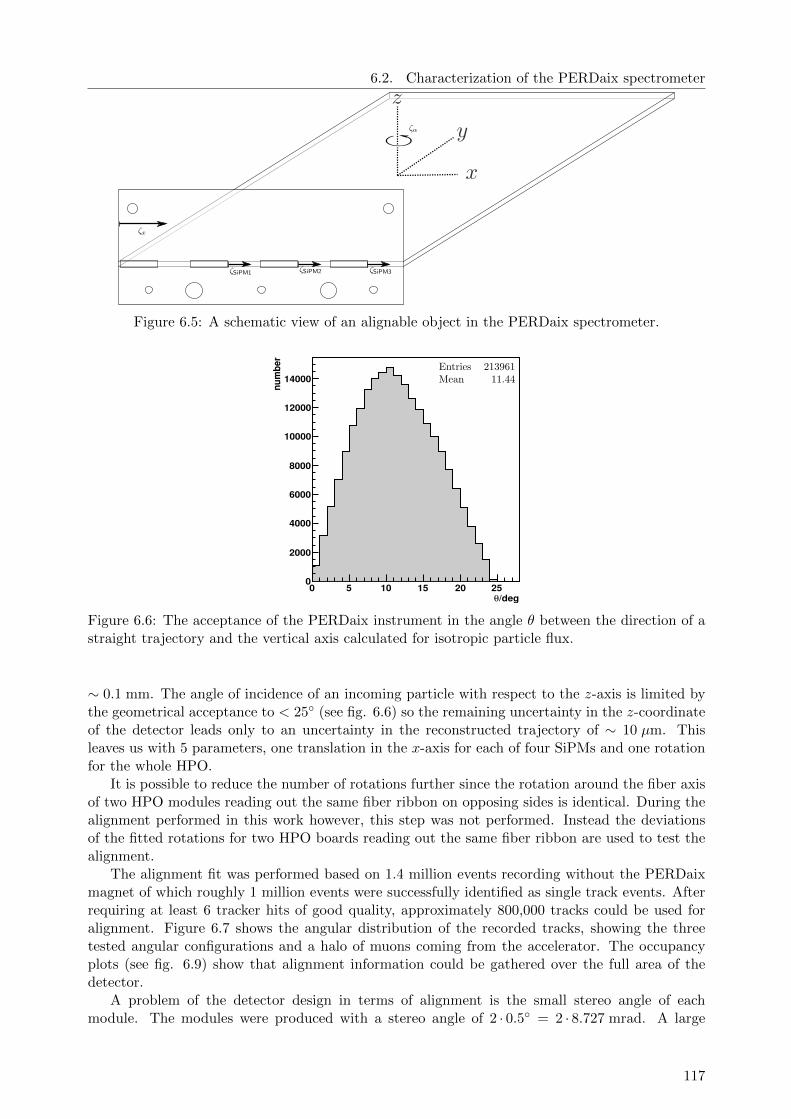
6.2. Characterization of the PERDaix spectrometer
Figure 6.5: A schematic view of an alignable object in the PERDaix spectrometer.
/degθ0 5 10 15 20 25
numbe
r
0
2000
4000
6000
8000
10000
12000
14000
Figure 6.6: The acceptance of the PERDaix instrument in the angle θ between the direction of astraight trajectory and the vertical axis calculated for isotropic particle flux.
∼ 0.1 mm. The angle of incidence of an incoming particle with respect to the z-axis is limited bythe geometrical acceptance to < 25 (see fig. 6.6) so the remaining uncertainty in the z-coordinateof the detector leads only to an uncertainty in the reconstructed trajectory of ∼ 10 µm. Thisleaves us with 5 parameters, one translation in the x-axis for each of four SiPMs and one rotationfor the whole HPO.
It is possible to reduce the number of rotations further since the rotation around the fiber axisof two HPO modules reading out the same fiber ribbon on opposing sides is identical. During thealignment performed in this work however, this step was not performed. Instead the deviationsof the fitted rotations for two HPO boards reading out the same fiber ribbon are used to test thealignment.
The alignment fit was performed based on 1.4 million events recording without the PERDaixmagnet of which roughly 1 million events were successfully identified as single track events. Afterrequiring at least 6 tracker hits of good quality, approximately 800,000 tracks could be used foralignment. Figure 6.7 shows the angular distribution of the recorded tracks, showing the threetested angular configurations and a halo of muons coming from the accelerator. The occupancyplots (see fig. 6.9) show that alignment information could be gathered over the full area of thedetector.
A problem of the detector design in terms of alignment is the small stereo angle of eachmodule. The modules were produced with a stereo angle of 2 · 0.5 = 2 · 8.727 mrad. A large
117
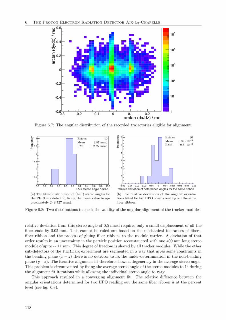
6. The Proton Electron Radiation Detector Aix-la-Chapelle
-0.3 -0.2 -0.1 0 0.1 0.2-0.6
-0.4
-0.2
0
0.2
0.4
0.6
1
10
210
310
410
510
arctan (dx/dz) / rad
arct
an (
dy/d
z) /
rad
Figure 6.7: The angular distribution of the recorded trajectories eligible for alignment.
8.00
0.5
1
1.5
2
2.5
3
0.5 × stereo angle / mrad8.2 8.4 8.6 8.8 9.0 9.2 9.4 9.6 9.8 10.0
freq
uenc
y
(a) The fitted distribution of (half) stereo angles forthe PERDaix detector, fixing the mean value to ap-proximately 2 · 8.727 mrad.
-0.05 -0.04 -0.03 -0.02 -0.01 0 0.01 0.02 0.03 0.04 0.050
1
2
3
4
5
6
relative deviation of determined angles for the same ribbon
freq
uenc
y
(b) The relative deviations of the angular orienta-tions fitted for two HPO boards reading out the samefiber ribbon.
Figure 6.8: Two distributions to check the validity of the angular alignment of the tracker modules.
relative deviation from this stereo angle of 0.5 mrad requires only a small displacement of all thefiber ends by 0.05 mm. This cannot be ruled out based on the mechanical tolerances of fibers,fiber ribbon and the process of gluing fiber ribbons to the module carrier. A deviation of thatorder results in an uncertainty in the particle position reconstructed with one 400 mm long stereomodule ofup to ∼ 11 mm. This degree of freedom is shared by all tracker modules. While the othersub-detectors of the PERDaix experiment are segmented in a way that gives some constraints inthe bending plane (x− z) there is no detector to fix the under-determination in the non-bendingplane (y−z). The iterative alignment fit therefore shows a degeneracy in the average stereo angle.This problem is circumvented by fixing the average stereo angle of the stereo modules to 1 duringthe alignment fit iterations while allowing the individual stereo angle to vary.
This approach resulted in a converging alignment fit. The relative difference between theangular orientations determined for two HPO reading out the same fiber ribbon is at the percentlevel (see fig. 6.8).
118
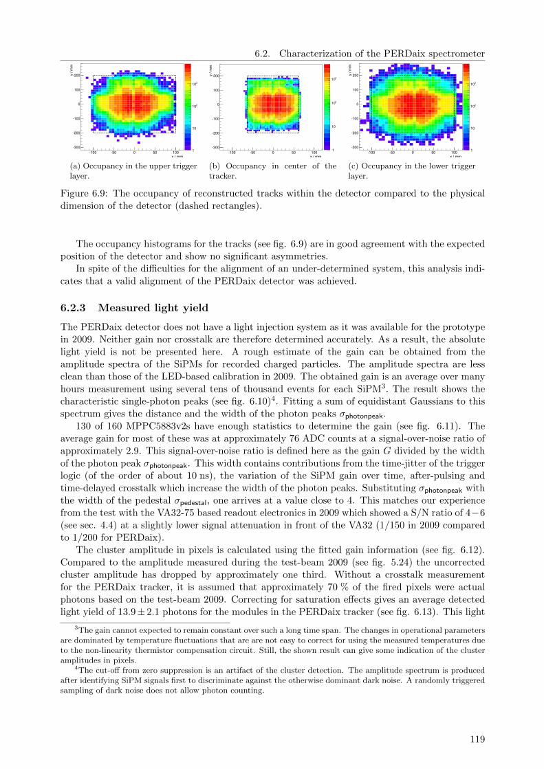
6.2. Characterization of the PERDaix spectrometer
-100 -50 0 50 100-300
-200
-100
0
100
200
1
10
210
310
x / mm
y / m
m
(a) Occupancy in the upper triggerlayer.
-100 -50 0 50 100-300
-200
-100
0
x / mm
y / m
m
100
200
1
10
210
310
(b) Occupancy in center of thetracker.
-100 -50 0 50 100-300
-200
-100
0
1
10
210
310
x / mm
y / m
m
100
200
(c) Occupancy in the lower triggerlayer.
Figure 6.9: The occupancy of reconstructed tracks within the detector compared to the physicaldimension of the detector (dashed rectangles).
The occupancy histograms for the tracks (see fig. 6.9) are in good agreement with the expectedposition of the detector and show no significant asymmetries.
In spite of the difficulties for the alignment of an under-determined system, this analysis indi-cates that a valid alignment of the PERDaix detector was achieved.
6.2.3 Measured light yield
The PERDaix detector does not have a light injection system as it was available for the prototypein 2009. Neither gain nor crosstalk are therefore determined accurately. As a result, the absolutelight yield is not be presented here. A rough estimate of the gain can be obtained from theamplitude spectra of the SiPMs for recorded charged particles. The amplitude spectra are lessclean than those of the LED-based calibration in 2009. The obtained gain is an average over manyhours measurement using several tens of thousand events for each SiPM3. The result shows thecharacteristic single-photon peaks (see fig. 6.10)4. Fitting a sum of equidistant Gaussians to thisspectrum gives the distance and the width of the photon peaks σphotonpeak.
130 of 160 MPPC5883v2s have enough statistics to determine the gain (see fig. 6.11). Theaverage gain for most of these was at approximately 76 ADC counts at a signal-over-noise ratio ofapproximately 2.9. This signal-over-noise ratio is defined here as the gain G divided by the widthof the photon peak σphotonpeak. This width contains contributions from the time-jitter of the triggerlogic (of the order of about 10 ns), the variation of the SiPM gain over time, after-pulsing andtime-delayed crosstalk which increase the width of the photon peaks. Substituting σphotonpeak withthe width of the pedestal σpedestal, one arrives at a value close to 4. This matches our experiencefrom the test with the VA32-75 based readout electronics in 2009 which showed a S/N ratio of 4−6(see sec. 4.4) at a slightly lower signal attenuation in front of the VA32 (1/150 in 2009 comparedto 1/200 for PERDaix).
The cluster amplitude in pixels is calculated using the fitted gain information (see fig. 6.12).Compared to the amplitude measured during the test-beam 2009 (see fig. 5.24) the uncorrectedcluster amplitude has dropped by approximately one third. Without a crosstalk measurementfor the PERDaix tracker, it is assumed that approximately 70 % of the fired pixels were actualphotons based on the test-beam 2009. Correcting for saturation effects gives an average detectedlight yield of 13.9± 2.1 photons for the modules in the PERDaix tracker (see fig. 6.13). This light
3The gain cannot expected to remain constant over such a long time span. The changes in operational parametersare dominated by temperature fluctuations that are are not easy to correct for using the measured temperatures dueto the non-linearity thermistor compensation circuit. Still, the shown result can give some indication of the clusteramplitudes in pixels.
4The cut-off from zero suppression is an artifact of the cluster detection. The amplitude spectrum is producedafter identifying SiPM signals first to discriminate against the otherwise dominant dark noise. A randomly triggeredsampling of dark noise does not allow photon counting.
119
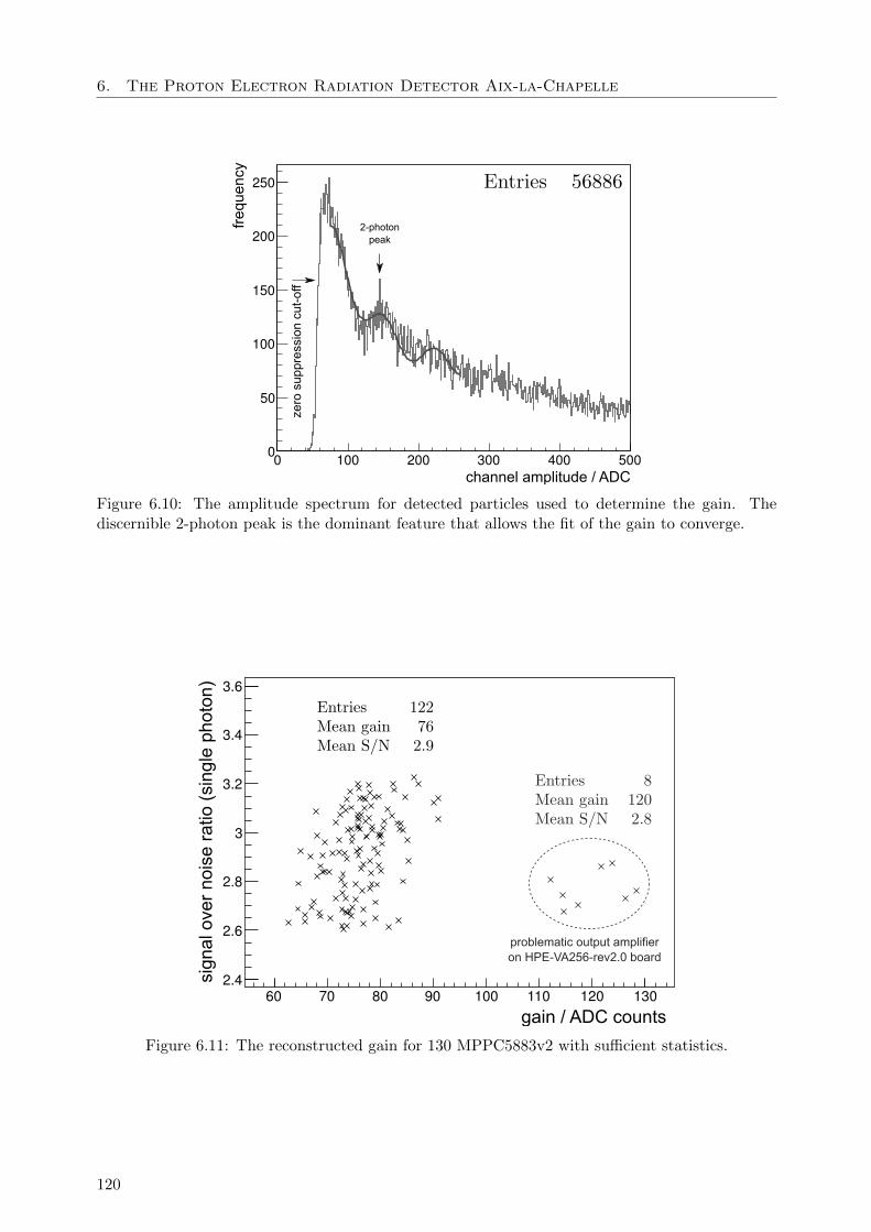
6. The Proton Electron Radiation Detector Aix-la-Chapelle
0 100 200 300 400 5000
50
100
150
200
250
zerosuppressioncut-off
2-photonpeak
channel amplitude / ADC
frequency
Figure 6.10: The amplitude spectrum for detected particles used to determine the gain. Thediscernible 2-photon peak is the dominant feature that allows the fit of the gain to converge.
60 70 80 90 100 110 120 1302.4
2.6
2.8
3
3.2
3.4
3.6
gain / ADC counts
problematic output amplifieron HPE-VA256-rev2.0 board
sign
alover
noiseratio
(singleph
oton
)
Figure 6.11: The reconstructed gain for 130 MPPC5883v2 with sufficient statistics.
120
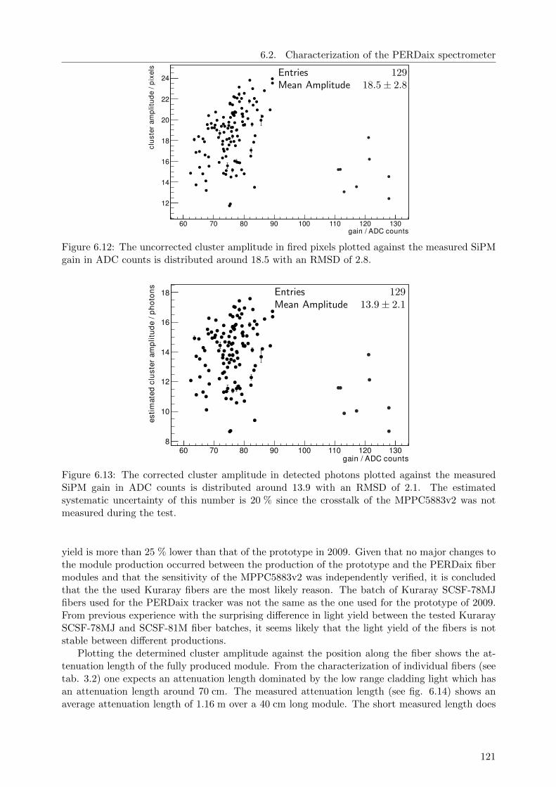
6.2. Characterization of the PERDaix spectrometer
gain / ADC counts60 70 80 90 100 110 120 130
clus
ter
ampl
itude
/pix
els
12
14
16
18
20
22
24
Figure 6.12: The uncorrected cluster amplitude in fired pixels plotted against the measured SiPMgain in ADC counts is distributed around 18.5 with an RMSD of 2.8.
gain / ADC counts60 70 80 90 100 110 120 130
estim
ated
clus
ter
ampl
itude
/pho
tons
8
10
12
14
16
18
Figure 6.13: The corrected cluster amplitude in detected photons plotted against the measuredSiPM gain in ADC counts is distributed around 13.9 with an RMSD of 2.1. The estimatedsystematic uncertainty of this number is 20 % since the crosstalk of the MPPC5883v2 was notmeasured during the test.
yield is more than 25 % lower than that of the prototype in 2009. Given that no major changes tothe module production occurred between the production of the prototype and the PERDaix fibermodules and that the sensitivity of the MPPC5883v2 was independently verified, it is concludedthat the the used Kuraray fibers are the most likely reason. The batch of Kuraray SCSF-78MJfibers used for the PERDaix tracker was not the same as the one used for the prototype of 2009.From previous experience with the surprising difference in light yield between the tested KuraraySCSF-78MJ and SCSF-81M fiber batches, it seems likely that the light yield of the fibers is notstable between different productions.
Plotting the determined cluster amplitude against the position along the fiber shows the at-tenuation length of the fully produced module. From the characterization of individual fibers (seetab. 3.2) one expects an attenuation length dominated by the low range cladding light which hasan attenuation length around 70 cm. The measured attenuation length (see fig. 6.14) shows anaverage attenuation length of 1.16 m over a 40 cm long module. The short measured length does
121
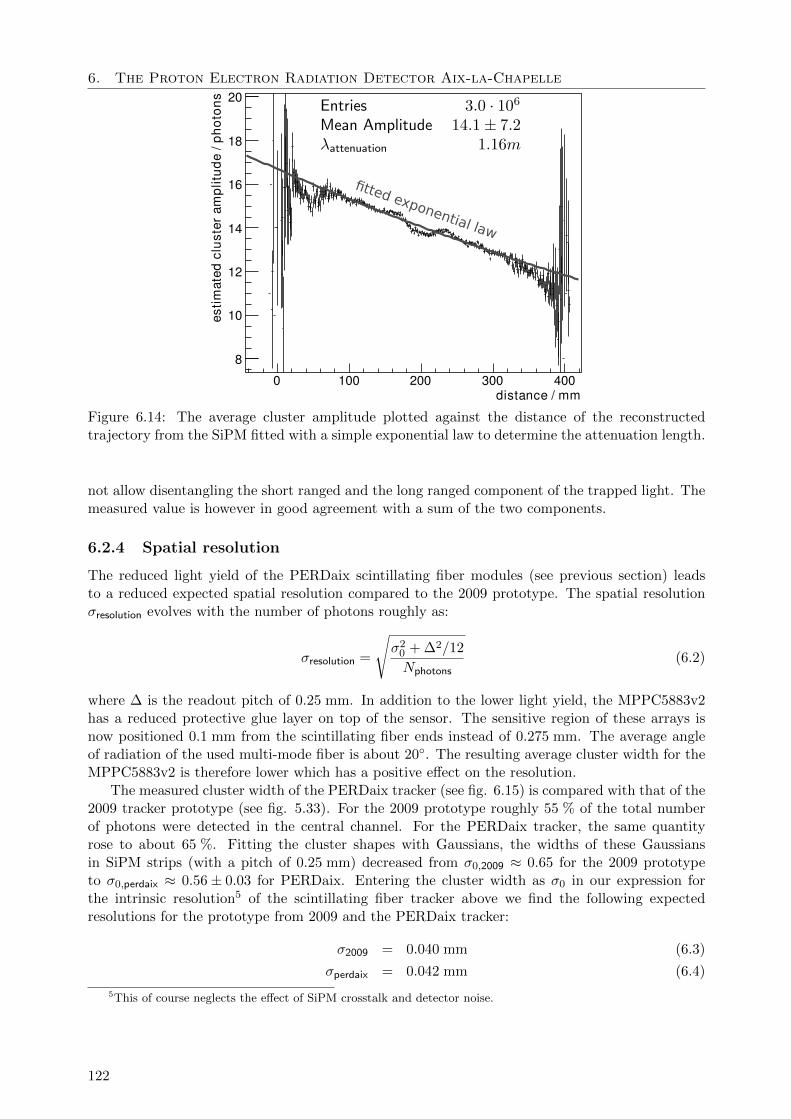
6. The Proton Electron Radiation Detector Aix-la-Chapelle
distance / mm0 100 200 300 400
estim
ated
clus
ter
ampl
itude
/pho
tons
8
10
12
14
16
18
20
fitted exponential law
Figure 6.14: The average cluster amplitude plotted against the distance of the reconstructedtrajectory from the SiPM fitted with a simple exponential law to determine the attenuation length.
not allow disentangling the short ranged and the long ranged component of the trapped light. Themeasured value is however in good agreement with a sum of the two components.
6.2.4 Spatial resolution
The reduced light yield of the PERDaix scintillating fiber modules (see previous section) leadsto a reduced expected spatial resolution compared to the 2009 prototype. The spatial resolutionσresolution evolves with the number of photons roughly as:
σresolution =
√σ2
0 + ∆2/12
Nphotons(6.2)
where ∆ is the readout pitch of 0.25 mm. In addition to the lower light yield, the MPPC5883v2has a reduced protective glue layer on top of the sensor. The sensitive region of these arrays isnow positioned 0.1 mm from the scintillating fiber ends instead of 0.275 mm. The average angleof radiation of the used multi-mode fiber is about 20. The resulting average cluster width for theMPPC5883v2 is therefore lower which has a positive effect on the resolution.
The measured cluster width of the PERDaix tracker (see fig. 6.15) is compared with that of the2009 tracker prototype (see fig. 5.33). For the 2009 prototype roughly 55 % of the total numberof photons were detected in the central channel. For the PERDaix tracker, the same quantityrose to about 65 %. Fitting the cluster shapes with Gaussians, the widths of these Gaussiansin SiPM strips (with a pitch of 0.25 mm) decreased from σ0,2009 ≈ 0.65 for the 2009 prototypeto σ0,perdaix ≈ 0.56± 0.03 for PERDaix. Entering the cluster width as σ0 in our expression forthe intrinsic resolution5 of the scintillating fiber tracker above we find the following expectedresolutions for the prototype from 2009 and the PERDaix tracker:
σ2009 = 0.040 mm (6.3)
σperdaix = 0.042 mm (6.4)
5This of course neglects the effect of SiPM crosstalk and detector noise.
122

6.2. Characterization of the PERDaix spectrometer
position relative to cluster center / SiPM strips-4 -2 0 2 4
0
2
4
6
8
10
12estim
atedclusteramplitude/photons
(a) Example for cluster shape of a single array fittedwith a Gaussian.
8 10 12 14 16 18
0.5
0.55
0.6
0.65
0.7
0.75
estimated cluster amplitude / photons
fittedclusterwidth/SiPMchannels
(b) The distribution of cluster widths for individualSiPM arrays plotted against the estimated averagelight yield per signal cluster.
Figure 6.15: The signal cluster widths for on-track clusters measured during the beam-test of thePERDaix tracker 2011.
Table 6.1: Classification of PERDaix tracker clusters.
Type Quality Frequency
Good Clusters 8 75.7 %
The cluster amplitude is lower than 6 pixels 3 7.1 %
The cluster consists of only a single channel 2 2.6 %
The amplitude of the central channel amounts to less than 40 % ofthe cluster amplitude
0 1.6 %
Cluster amplitude is smaller than 2.5 pixels −1 1.6 %
Cluster is wider than 6 channels −2 0.4 %
Cluster is next to known dead channel −3 1.1 %
Cluster includes first or last array channel −4 9.9 %
The effect of the lower light yield of the PERDaix tracker is almost compensated by thereduction of the glue layer on top of the MPPC5883v2 and the resulting narrower signal clusters.
The analysis of the PERDaix spatial resolution is performed based on the methods used in(sec. 5.3.1 and 5.3.4). The signal clusters are categorized according to their quality6. The lowestquality is assigned to signal clusters which include border channels, clusters located next to deadchannels, clusters with a large width (> 6 channels) or clusters of low amplitude (< 2.5 firedpixels). These clusters are ignored during the track fits since the distribution of residuals is highlynon-Gaussian for these types of clusters and wider than 100 µm. The remaining 87 % of clustersare further categorized as described in tab. 6.1 (see fig. 6.16).
Based on an initial estimate for the spatial resolution σestimate, the spatial resolution of trackerhits σresolution is determined. Using a material budget of 1 % of a radiation length per PERDaixfiber module (see sec. 3.3.2) allows calculating the uncertainty of the trajectory position σtrajectory
7.The spatial resolution is then measured from the residuals r given by the distance between thefitted trajectory and the particle position as measured by the detector. In order to account forσtrajectory, each residual is corrected as follows:
rcorrected = r
√σ2estimate
σ2estimate + σ2
trajectory
(6.5)
6The integer value assigned to each quality is a result of the implementation of the analysis algorithm.7For details see sec. 5.3.1, 5.3.4 and C.5
123

6. The Proton Electron Radiation Detector Aix-la-Chapelle
-4 -2 0 2 4 6 8
-210
-110
175.7%
7.1%
2.6%
1.6%1.4%
0.4%
1.1%
9.9%
quality < 0ignored duringtrack fits
normalizedfrequency
assigned integer quality
Figure 6.16: The frequency for different types (qualities) of clusters as described in tab. 6.1determined from 4 million clusters.
normalizedfrequency
-0.4 -0.3 -0.2 -0.1 0 0.1 0.2 0.3 0.40
0.01
0.02
0.03
0.04
0.05
uncorrected residual / mm
(a) The raw residuals.
normalizedfrequency
-0.2 -0.1 0 0.1 0.20
0.01
0.02
0.03
0.04
0.05
corrected residual / mm
(b) The corrected residuals.
normalizedfrequency
-0.2 -0.1 0 0.1 0.20
0.01
0.02
0.03
0.04
0.05
corrected residual (m.sc.) / mm
(c) The corrected residuals includ-ing multiple scattering corrections.
Figure 6.17: The residuals for PERDaix tracker signal clusters of the highest quality.
The central 99% of the distribution of corrected residuals is then fitted with a Gaussian. Its widthis considered to equal the spatial resolution σresolution.
Figure 6.17 shows the produced residual distributions. Including corrections for multiple scat-tering, an average spatial resolution of 0.047 mm is found for the PERDaix tracker. A majordifference between the test-beam of the tracker prototype in 2009 and the PERDaix tracker is theabsence of an accurate beam telescope to be used as a reference. The result therefore relies heavilyon the covariance matrices from the linear track fit to determine the resolution. While the spatialuncertainty for the particle position from the track fit is of the order of 0.02 mm for the 2009 data,it is of the order of 0.05 mm for the PERDaix data. This is of the same order of magnitude asthe expected spatial resolution. The resulting systematic uncertainty of the spatial resolution istherefore larger for the PERDaix detector and estimated below.
As a check for the calculated uncertainty of the fitted particle position, the residual distributionsin different tracker layers are compared. The uncorrected residuals follow a wider distribution nearthe top and bottom layer of the tracker compared to the central layers (see fig. 6.18) since thespatial constraint from the track fit becomes weaker as we move away from the tracker center. Thisis reflected by a z-dependence of the average uncertainty of the calculated trajectory σtrajectory(z).
The following calculation uses this z-dependence to estimate the systematic error on the cal-culated spatial resolution.
124

6.2. Characterization of the PERDaix spectrometer
-200 -100 0 100 200-0.15
-0.1
-0.05
0
0.05
0.1
0.15
z / mm
residuals/mm
(a) The distribution of raw residuals as a function ofz.
-200 -100 0 100 200-0.15
-0.1
-0.05
0
0.05
0.1
0.15
z / mm
correctedresiduals/mm
(b) The distribution of corrected residuals as a func-tion of z.
Figure 6.18: The blue rectangles show the RMSD of the distribution of residuals for the eightPERDaix tracker layers.
The width of the distribution of uncorrected residuals σuncorrected is the quadratic sum of themean resolution σresolution and the mean uncertainty of the trajectory position σtrajectory(z):
σuncorrected =
√(σresolution)2 + (σtrajectory(z))
2 (6.6)
For a linear trajectory in two dimensions, the uncertainty of the trajectory is given by anuncertainty in the starting point σx0 and the uncertainty of the slope σdx/dy. The two uncertaintiesare proportional to one another if they are determined by a linear fit8:
(σtrajectory(z))2 = σ2
x0 + z2σ2dx/dy = σ2
x0(1 + α2zz
2) (6.7)
where αz is a known constant depending only on the detector geometry. Based on this, overes-timating or underestimating the detector resolution σx0 would lead to inconsistent results amongthe individual detector layers. The relative systematic uncertainty of the calculated resolution istherefore estimated to be of the order of the relative variation of the calculated resolution from layerto layer. This analysis estimates a relative systematic uncertainty of the determined resolution of4 %.
An analysis of the determined resolution in several projections shall help to validate the resultfurther:
A flat distribution with almost constant resolution can be seen for the distribution of theresiduals plotted against the y-coordinate. For y . −150 mm a slight deviation (see fig. 6.19)from the expected flat distribution is observed. Due to the low occupancy in this region of thedetector, it can be neglected.
Another projection shows the residual distribution against the x-coordinate (see fig. 6.20).A systematic deviation of the mean residual from zero is found which upon zooming into the
8For a linear fit which neglects multiple scattering, we know that the state vector ξ of the trajectory (which isconveniently chosen as starting point and slopes) is given by:
ξ =(XTWX
)−1
XTWb
for an observation b, the equation matrix X and the weighting matrix W of the measurements. The covariance ofthe determined state is: (
XTWX)−1
For observations with a homogeneous uncertainty σ20 , W simplifies to 1
σ201, so the uncertainty of ξ is a linear function
of σ20 .
125

6. The Proton Electron Radiation Detector Aix-la-Chapelle
y / mm-200 -150 -100 -50 0 50 100 150 200
-0.15
-0.1
-0.05
0
0.05
0.1resi
dual
/ m
m
(a) Projection of residuals plotted against y. (b) Scatter plot of residuals plotted against y.
Figure 6.19: The residuals plotted against the position in the non-bending direction y shows asmall feature for y . −150 mm which is apparently caused by low statistics and possibly fewpoorly reconstructed tracks.
residuals in front of a single SiPM array channel can be identified as being a result of a flaweddetermination of the cluster position. The median method that has been used for the analysisof the 2009 prototype (see sec. 5.3.1) is improved by a correction which fits the shape of a sine.A corrected cluster position xcorrected based on the median position xmedian from equation 5.5 isintroduced:
xmedian = xm +A+ −A−
2a∗m∆x (6.8)
xcorrected = xmedian − 0.016 mm · sin(
6.607
0.25 mmxmedian
)(6.9)
Repeating the analysis with the new cluster definition, shows a more homogeneous residualdistribution as a function of the cluster position along the SiPM array (see fig. 6.21). Thecumulative distribution of corrected residuals now fits a Gaussian with a width of 0.045 mm.Looking at the individual SiPM arrays we find that 110 of 160 SiPM arrays have enough statisticsto determine the spatial resolution. The average resolution for each array is 0.0437 mm±0.0024 mmwith five of the arrays showing a resolution above 0.05 mm. This is in good agreement with theexpected intrinsic resolution based on cluster shape and light yield of 0.042 mm. The results forthe spatial resolution of all categories of signals is shown in table 6.2.
6.2.5 Momentum resolution
The function of the tracking detector in the PERDaix experiment is to measure the rigidity ofparticles as part of the spectrometer. The beam test allows calibrating the spectrometer withparticles of known momentum using beam rigidities between −0.5 GeV and −8.0 GeV9.
First, the homogeneous magnetic field strength B is determined which is equivalent to theinhomogeneous field PERDaix magnet. The assumption of a magnetic field with a density ofB = 0.27 T which was calculated based on the strength of individual magnets does not describe
9An analysis of the data for positive beam particles is not performed in this work since this would requiredistinguishing between protons and significantly lighter particles at low rigidities.
126
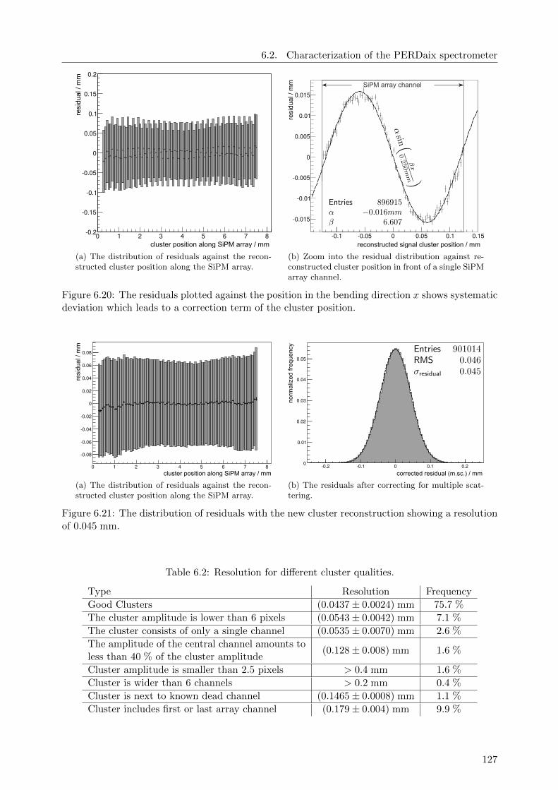
6.2. Characterization of the PERDaix spectrometer
0 1 2 3 4 5 6 7 8-0.2
-0.15
-0.1
-0.05
0
0.05
0.1
0.15
0.2
cluster position along SiPM array / mm
residual/mm
(a) The distribution of residuals against the recon-structed cluster position along the SiPM array.
-0.1 -0.05 0 0.05 0.1 0.15
-0.015
-0.01
-0.005
0
0.005
0.01
0.015
residual/mm
reconstructed signal cluster position / mm
SiPM array channel
(b) Zoom into the residual distribution against re-constructed cluster position in front of a single SiPMarray channel.
Figure 6.20: The residuals plotted against the position in the bending direction x shows systematicdeviation which leads to a correction term of the cluster position.
0 1 2 3 4 5 6 7 8
-0.08
-0.06
-0.04
-0.02
0
0.02
0.04
0.06
0.08
cluster position along SiPM array / mm
residual/mm
(a) The distribution of residuals against the recon-structed cluster position along the SiPM array.
-0.2 -0.1 0 0.1 0.20
0.01
0.02
0.03
0.04
0.05
corrected residual (m.sc.) / mm
normalizedfrequency
(b) The residuals after correcting for multiple scat-tering.
Figure 6.21: The distribution of residuals with the new cluster reconstruction showing a resolutionof 0.045 mm.
Table 6.2: Resolution for different cluster qualities.
Type Resolution Frequency
Good Clusters (0.0437± 0.0024) mm 75.7 %
The cluster amplitude is lower than 6 pixels (0.0543± 0.0042) mm 7.1 %
The cluster consists of only a single channel (0.0535± 0.0070) mm 2.6 %
The amplitude of the central channel amounts toless than 40 % of the cluster amplitude
(0.128± 0.008) mm 1.6 %
Cluster amplitude is smaller than 2.5 pixels > 0.4 mm 1.6 %
Cluster is wider than 6 channels > 0.2 mm 0.4 %
Cluster is next to known dead channel (0.1465± 0.0008) mm 1.1 %
Cluster includes first or last array channel (0.179± 0.004) mm 9.9 %
127
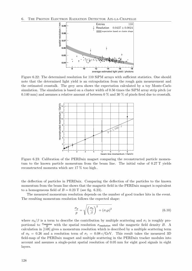
6. The Proton Electron Radiation Detector Aix-la-Chapelle
8 10 12 14 16 18
0.04
0.05
0.06
0.07
0.08
0.09
average estimated light yield / photons
spat
ial r
esol
utio
n / m
m
Figure 6.22: The determined resolution for 110 SiPM arrays with sufficient statistics. One shouldnote that the determined light yield is an extrapolation from the rough gain measurement andthe estimated crosstalk. The grey area shows the expectation calculated by a toy Monte-Carlosimulation. The simulation is based on a cluster width of 0.56 times the SiPM array strip pitch (or0.140 mm) and assumes a relative amount of between 0 % and 30 % of pixels fired due to crosstalk.
1 2 3 4 5 6 7 80
2
4
6
8
10
12
14
beam line momentum / GeV/c
reconstructedmomentum/GeV/c
Figure 6.23: Calibration of the PERDaix magnet comparing the reconstructed particle momen-tum to the known particle momentum from the beam line. The initial value of 0.27 T yieldsreconstructed momenta which are 17 % too high..
the deflection of particles in PERDaix. Comparing the deflection of the particles to the knownmomentum from the beam line shows that the magnetic field in the PERDaix magnet is equivalentto a homogeneous field of B = 0.23 T (see fig. 6.23).
The measured momentum resolution depends on the number of good tracker hits in the event.The resulting momentum resolution follows the expected shape:
σpp
=
√(σ0
β
)2
+ (σ1p)2 (6.10)
where σ0/β is a term to describe the contribution by multiple scattering and σ1 is roughly pro-portional to σresolution
B with the spatial resolution σresolution and the magnetic field density B. Acalculation in [148] gives a momentum resolution which is described by a multiple scattering termof σ0 = 0.26 and a resolution term of σ1 = 0.08 c/GeV. This result takes the measured 3Dfield-map of the PERDaix magnet and multiple scattering in the PERDaix tracker modules intoaccount and assumes a single-point spatial resolution of 0.05 mm for eight good signals in eightlayers.
128

6.2. Characterization of the PERDaix spectrometer
-0.006 -0.004 -0.002 0 0.002 0.004 0.0060
0.02
0.04
0.06
0.08
0.1
-0.5GV/c
-0.6GV/c
-0.8GV/c
-1.0GV/c
-1.5GV/c
-3.0GV/c
-4.0GV/c
-5.0GV/c
-8.0GV/c
(a) The measured inverse rigidities for each selected beam rigidity.
0 1 2 3 4 5 6 7 8 9 100
0.1
0.2
0.3
0.4
0.5
0.6
0.7
0.8
0.9
1
electrons (calculated)protons (calculated)negative beam (8 tracker hits)negative beam (7 tracker hits)negative beam (6 tracker hits)
(b) The determined momentum resolution for different numbers ofgood tracker hits associated with the particle trajectory compared tothe prediction [148].
Figure 6.24: The measured momentum resolution of the PERDaix spectrometer.
Looking at the measurement (see fig. 6.24) we find that for reconstructed tracks with exactlyone good tracker hit in each of the eight tracker layers, the resolution is slightly worse than expectedwith σ0 = 0.31 and σ1 = 0.09 c/GeV. This result does not agree with the initial expectation. Themultiple scattering term σ0 exceeds the value from [148] by 20 % and the resolution term σ1 is10 % worse than the calculation. However, one should point out that the expected momentumresolution did not include effects like misalignment, SiPM noise and the resulting ambiguities inthe track reconstruction.
The trajectory parametrization for the reconstruction of the PERDaix events used in thiswork furthermore assumed a homogeneous magnetic field inside the permanent magnet. From thecomparison of the measured deflection of charged particles of perpendicular incidence and knownmomentum to the expected deflection based on the homogeneous magnetic field assumption wecalculate a field map projected on the x − y-plane (see fig. 6.25). The relative strength of theeffective magnetic field varies between 80 % and 125 % as a function of the position of the particlein the central plane of the magnet compared to the expectation of 0.23 T. The RMSD of the
129

6. The Proton Electron Radiation Detector Aix-la-Chapelle
x / mm-100 -80 -60 -40 -20 0 20 40 60 80 100
y/m
m
-100
-80
-60
-40
-20
0
20
40
60
80
100
0.8
0.85
0.9
0.95
1
1.05
1.1
1.15
1.2
1.25
1.3 measured relative deflection
Figure 6.25: The plot shows the magnetic deflection of particles of perpendicular incidence relativeto the expected deflection for a homogeneous field of B = 0.23 T.
0 10 20 30 40 50 600
0.2
0.4
0.6
0.8
1
single fiber module
position / mm
efficiency
Figure 6.26: The measured tracking efficiency given as the probability that a reconstructed trackcontains a hit in a selected fiber layer.
variation is 8 % of the nominal field strength and therefore too low to account for the observeddiscrepancy between the expected and observed momentum resolutions.
It is possible that a better momentum resolution is achieved using a track fit using the measuredfield map of the PERDaix magnet. This possibility however is not investigated within the scopeof this thesis and the measurement above does not suggest that the expected resolution will bereached in that manner.
6.2.6 Tracking efficiency
An important quantity for any detector is the efficiency with which particles are successfullydetected. In the PERDaix detector with 5120 channels a total of 37 bad channels were identified.These are mostly caused by badly soldered MPPC5883v2 SiPM array on the PERDaix-HPOboards.
Based on photon statistics even with an average of only 9 detected photons per particle oneexpects an inefficiency far below 1 % requiring at least 2 detected photons. A detection efficiencyof at least 97.7 % (see fig. 6.26) is determined from the test beam data. This value is only alower bound for the actual efficiency since it contains contributions from the efficiency of the trackreconstruction algorithm.
It follows that the more significant source of inefficiencies for the scintillating fiber are bad signalclusters. About 13 % of all clusters have a quality which is insufficient for the track reconstruction
130

6.2. Characterization of the PERDaix spectrometer
0.2mm gaps between mirrors and sensitive
SiPM strips
mirror
mirrormirror
MPPC5883v2
MPPC5883v2
MPPC5883v2
facing SiPM strips
Figure 6.27: The design of the PERDaix HPO boards has two SiPM border channels on opposingsides of the module face each other when seen in the direction of the fibers.
(see sec. 6.2.4). The largest contribution to the inefficiency (about 9.9 % of all signals) comesfrom signal clusters that contain the first or the last channel of a SiPM array. In order to addressthis problem, the SiPM arrays are soldered to the optical hybrids with a pitch of 15.5 mm andmounted to the scintillating fiber arrays in such a way that a fiber immediately in front of a borderchannel of a SiPM array is read out by an additional SiPM array on the other end (see fig. 6.27).
In an attempt to salvage clusters which include border channels, a selection of tracks thatcontain signal clusters in two SiPM arrays reading out the same fiber ribbon is performed. Theseclusters are associated with the same particle track but read out by neighbouring strips of differentSiPM. A cluster center in the same fashion as for regular clusters cannot be calculated for thesesplit signal clusters since the response of the fibers in this region changes depending on whetherone end is covered by mirror or not. In addition, the relative position of the mirror to the sensitiveSiPM array strips is known only with a precision of about ±0.2 mm as a result of the limitedmechanical precision of the MPPC5883v2 carrier PCB (see fig. 4.16).
Let ai (i ∈ 0, 1, .., 63) be the amplitudes measured by two arrays reading out neighboringportions of a fiber ribbon. Let xi be the position along the fiber ribbon associated with eacharray channel so that xi = X0 + i · 0.25 mm for i ∈ 0, 1, .., 31 and xi = X1 + i · 0.25 mm for
i ∈ 32, 33, .., 63. The average cluster shape 〈c(Xparticle − xi)〉 ∼ exp
((Xparticle−xi)
2
2σ2cluster
)is expected
to be approximately Gaussian, so the amplitudes ai can be given as:
〈ai〉 = αi 〈c(Xparticle − xi)〉 (6.11)
Here, αi is a positive real constant which describes the response of each SiPM array channel basedon the reflective properties of one fiber end and the SiPM gain, crosstalk and photon efficiency. Itfollows that the expectation value for center of gravity 〈xcog〉 of all channels i of a split cluster Cis a monotonous function10 of the particle position Xparticle. A simulation of the average center ofgravity for split clusters assuming that the border strips on average have a 40 % lower light yieldis shown in figure 6.28.
xcog =
∑i∈C
aixi∑i∈C
ai(6.12)
∂〈xcog〉∂X
> 0 (6.13)
10Deriving∂〈xcog〉∂Xparticle
results in a lengthy expression that is always positive if αi > 0∀i.
131

6. The Proton Electron Radiation Detector Aix-la-Chapelle
-2 0 2 4 6 8 10 12 14 16 180
2
4
6
8
10
12
14
16
particle coordinate / mm
reco
nstr
ucte
d po
sitio
n / m
m
center of gravity SiPM #1
center of gravity SiPM #2
combined center of gravity
SiPM #1 SiPM #2
Figure 6.28: The expected reconstructed particle position compared to the real coordinate of aparticle traversing a fiber ribbon read out by two SiPM arrays with one channel overlap assumingthat the light yield at the border channels is only 60 % of the regular value due to the missingreflective surface on one fiber end.
The center of gravity over the entire split cluster is in conclusion a good estimator for the actualparticle position. Possible corrections to the simple center of gravity exist based on the αi param-eters and the xi which are obtained during the alignment procedure. The constants αi howeverare not known in case of the PERDaix detector so no corrections are performed.
The resolution of split clusters is estimated by looking for the residuals between expectedparticle position and the center of gravity of the split cluster. A minimum amplitude equivalent toat least three fired SiPM pixels is required for both parts of a split cluster in order to discriminateagainst noise.
Figure 6.29 shows the residuals for split clusters plotted against the particle position. The meanresidual as a function of the expected particle position does not show any significant systematicdeviation from zero. This is the expected behavior if the constants αi do not deviate stronglyfrom one another. The width of the residual distribution is approximately 0.2 mm. Compared togood signal clusters with a resolution of ∼ 0.05 mm split clusters do not contribute to the trackreconstruction in PERDaix.
There are a number of arguments that make this observation reasonable. Split clusters havea low amplitude, giving them a poorer resolution to begin with and making them very hard todistinguish from SiPM noise. Next, the properties of the used mirrors near the milled edges nextto the SiPM arrays are largely unknown and may add to a distortion of the signal cluster due toreflections. The relative amplitudes of two parts of a split cluster depend on a variety of factors,the particle position along the fiber axis being one that is not a constant and therefore directlyimpacts the spatial resolution.
The effective efficiency of the scintillating fiber tracker is ∼ 85 %. The most significant issueare low quality clusters near border channels and dead channels. It is expected that the efficiencyof future scintillating fiber trackers with SiPM arrays increases as larger SiPM arrays becomeavailable. Linear SiPM arrays with a larger number of strips show a more favorable ratio of borderstrips to non-border strips. The way SiPM arrays are interleaved with mirrors in the PERDaixtracker does not give the expected improvements. The overlap region between opposing SiPMarrays were too small to improve the quality of split signal clusters.
132

6.2. Characterization of the PERDaix spectrometer
-60 -40 -20 0 20 40 60-1.5
-1
-0.5
0
0.5
1
1.5
expected particle position / mm
dist
ance
to
reco
nstr
ucte
d cl
uste
r po
sito
n / m
m
(a) Residuals of split clusters for two neighboring fiber ribbons.
-10.5 -10 -9.5 -9 -8.5 -8 -7.5 -7-1.5
-1
-0.5
0
0.5
1.5
dist
ance
to
reco
nstr
ucte
d cl
uste
r po
sito
n / m
m
expected particle position / mm
(b) Residuals of split clusters for the overlap between two neighboringSiPM arrays.
Figure 6.29: The residuals of split clusters show a width of about 0.2 mm, rendering these clustersunusable for tracking.
133

6. The Proton Electron Radiation Detector Aix-la-Chapelle
(a) The launch vehicle carrying the gondola with the experiments before theBEXUS-11 launch
(b) BEXUS-11 carrying PERDaixinto the stratosphere
Figure 6.30: The BEXUS-11 payload including PERDaix after launch from ESRANGE, Kiruna,Sweden in November 2010
6.3 Flight performance of the PERDaix spectrometer
The scintillating fiber tracker of the PERDaix detector was tested outside the laboratory duringa balloon flight in November 2010 (see sec. 2.3). Especially the thermal conditions during theflight presented a challenge for the operation of highly temperature sensitive devices such as siliconphotomultipliers. A temperature compensation for the silicon photomultipliers was implementedas previously discussed (see sec. 4.6). The temperature compensation did not keep the over-voltageand gain constant. Additionally, neither gain nor over-voltage of the SiPM was monitored duringthe flight. The operating voltage of the SiPM was chosen based on the average signal clusteramplitude in ADC channels as the PERDaix design did not include a light injection system.
In spite of these less then optimal conditions, the PERDaix tracker shows a very stable per-formance during the flight. This illustrates once again (see sec. 5.3.4) that the actual trackingperformance is only weakly dependent on the operation point of the MPPC5883 over a wide range.
The geometrical acceptance of the of the PERDaix trigger amounts to 84 cm2. The observedtrigger rate varies between about 1 Hz on ground and 41 Hz at an altitude of 20 km. The triggerrate at float altitude remains stable11 at 36 Hz (see fig. 6.31). The calculated geometrical accep-tance of the spectrometer (tracker and magnet) is 28 cm2 or one third of the trigger acceptance.Thus, 33 % of triggers are expected to be caused by particles passing through the magnet12. Goodtracks13 passing through the magnet are successfully reconstructed for 24 % of triggered events (seefig. 6.32). Of the 177,000 triggered events at float altitude, 42,000 events could be reconstructed
11Small gaps in the shown trigger rate are the result of a recurring issue with the DAQ system that required torestart the readout system occasionally.
12This neglects noise triggers and particles that cannot be reconstructed due low momentum or interactionswithin the detector.
13A track is considered good if it was detected in at least five tracker layers and if it is from a single-track event.
134
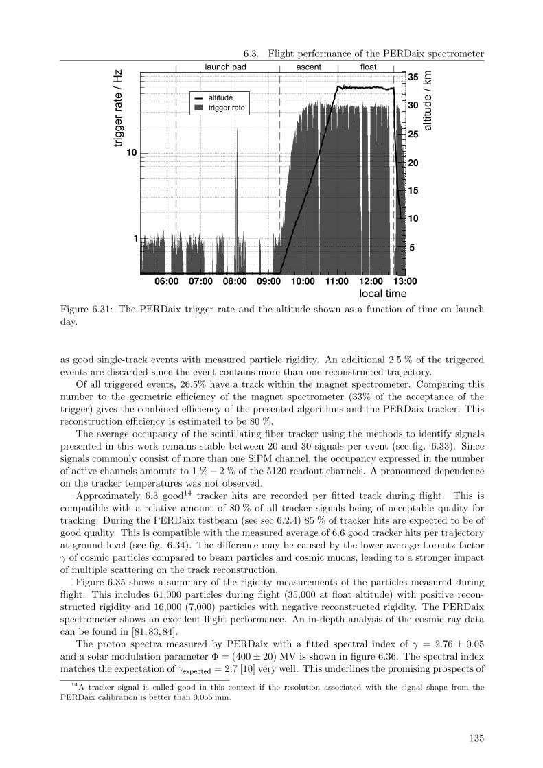
6.3. Flight performance of the PERDaix spectrometer
launch pad ascent float
10
15
10
15
20
25
30
35
06:00 07:00 08:00 09:00 10:00 11:00 12:00 13:00local time
trig
ger
rate
/ H
z
altit
ude
/ km
altitudetrigger rate
Figure 6.31: The PERDaix trigger rate and the altitude shown as a function of time on launchday.
as good single-track events with measured particle rigidity. An additional 2.5 % of the triggeredevents are discarded since the event contains more than one reconstructed trajectory.
Of all triggered events, 26.5% have a track within the magnet spectrometer. Comparing thisnumber to the geometric efficiency of the magnet spectrometer (33% of the acceptance of thetrigger) gives the combined efficiency of the presented algorithms and the PERDaix tracker. Thisreconstruction efficiency is estimated to be 80 %.
The average occupancy of the scintillating fiber tracker using the methods to identify signalspresented in this work remains stable between 20 and 30 signals per event (see fig. 6.33). Sincesignals commonly consist of more than one SiPM channel, the occupancy expressed in the numberof active channels amounts to 1 %− 2 % of the 5120 readout channels. A pronounced dependenceon the tracker temperatures was not observed.
Approximately 6.3 good14 tracker hits are recorded per fitted track during flight. This iscompatible with a relative amount of 80 % of all tracker signals being of acceptable quality fortracking. During the PERDaix testbeam (see sec 6.2.4) 85 % of tracker hits are expected to be ofgood quality. This is compatible with the measured average of 6.6 good tracker hits per trajectoryat ground level (see fig. 6.34). The difference may be caused by the lower average Lorentz factorγ of cosmic particles compared to beam particles and cosmic muons, leading to a stronger impactof multiple scattering on the track reconstruction.
Figure 6.35 shows a summary of the rigidity measurements of the particles measured duringflight. This includes 61,000 particles during flight (35,000 at float altitude) with positive recon-structed rigidity and 16,000 (7,000) particles with negative reconstructed rigidity. The PERDaixspectrometer shows an excellent flight performance. An in-depth analysis of the cosmic ray datacan be found in [81,83,84].
The proton spectra measured by PERDaix with a fitted spectral index of γ = 2.76 ± 0.05and a solar modulation parameter Φ = (400± 20) MV is shown in figure 6.36. The spectral indexmatches the expectation of γexpected = 2.7 [10] very well. This underlines the promising prospects of
14A tracker signal is called good in this context if the resolution associated with the signal shape from thePERDaix calibration is better than 0.055 mm.
135
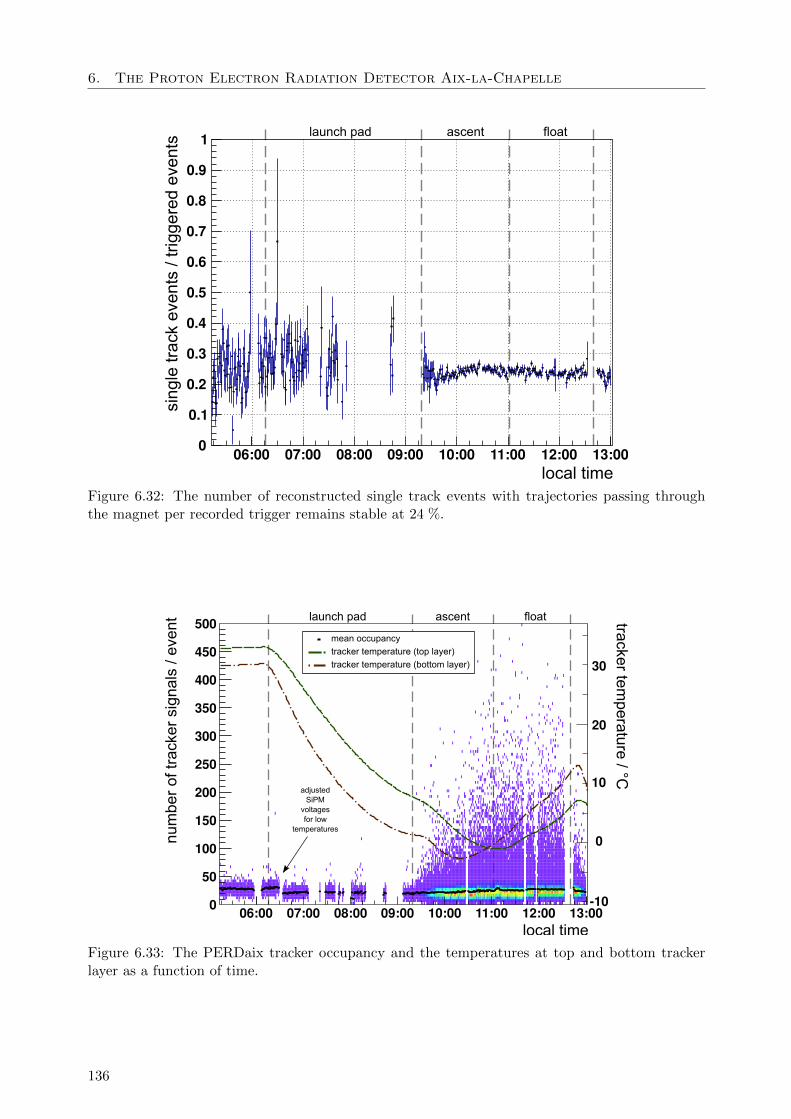
6. The Proton Electron Radiation Detector Aix-la-Chapelle
launch pad ascent float
06:00 07:00 08:00 09:00 10:00 11:00 12:00 13:00local time
sing
le tr
ack
even
ts /
trig
gere
d ev
ents 1
0.9
0.8
0.7
0.6
0.5
0.4
0.3
0.2
0.1
0
Figure 6.32: The number of reconstructed single track events with trajectories passing throughthe magnet per recorded trigger remains stable at 24 %.
launch pad ascent float500
450
400
350
300
250
200
150
100
50
0
tracker temperature / °C
-10
0
20
30
10
06:00 07:00 08:00 09:00 10:00 11:00 12:00 13:00local time
num
ber
of tr
acke
r si
gnal
s / e
vent
mean occupancy
tracker temperature (top layer)
tracker temperature (bottom layer)
adjustedSiPM
voltages for low
temperatures
Figure 6.33: The PERDaix tracker occupancy and the temperatures at top and bottom trackerlayer as a function of time.
136
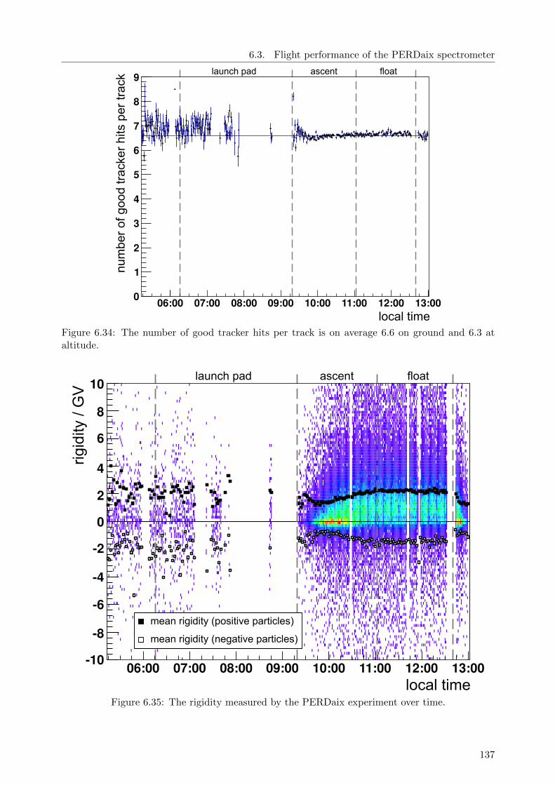
6.3. Flight performance of the PERDaix spectrometer
launch pad ascent float
06:00 07:00 08:00 09:00 10:00 11:00 12:00 13:00local time
num
ber
of g
ood
trac
ker
hits
per
trac
k
8
7
6
5
4
3
2
1
0
9
Figure 6.34: The number of good tracker hits per track is on average 6.6 on ground and 6.3 ataltitude.
launch pad ascent float
06:00 07:00 08:00 09:00 10:00 11:00 12:00 13:00local time
rigid
ity /
GV
-10
-8
-6
-4
-2
0
2
4
6
8
10
mean rigidity (negative particles)
mean rigidity (positive particles)
Figure 6.35: The rigidity measured by the PERDaix experiment over time.
137
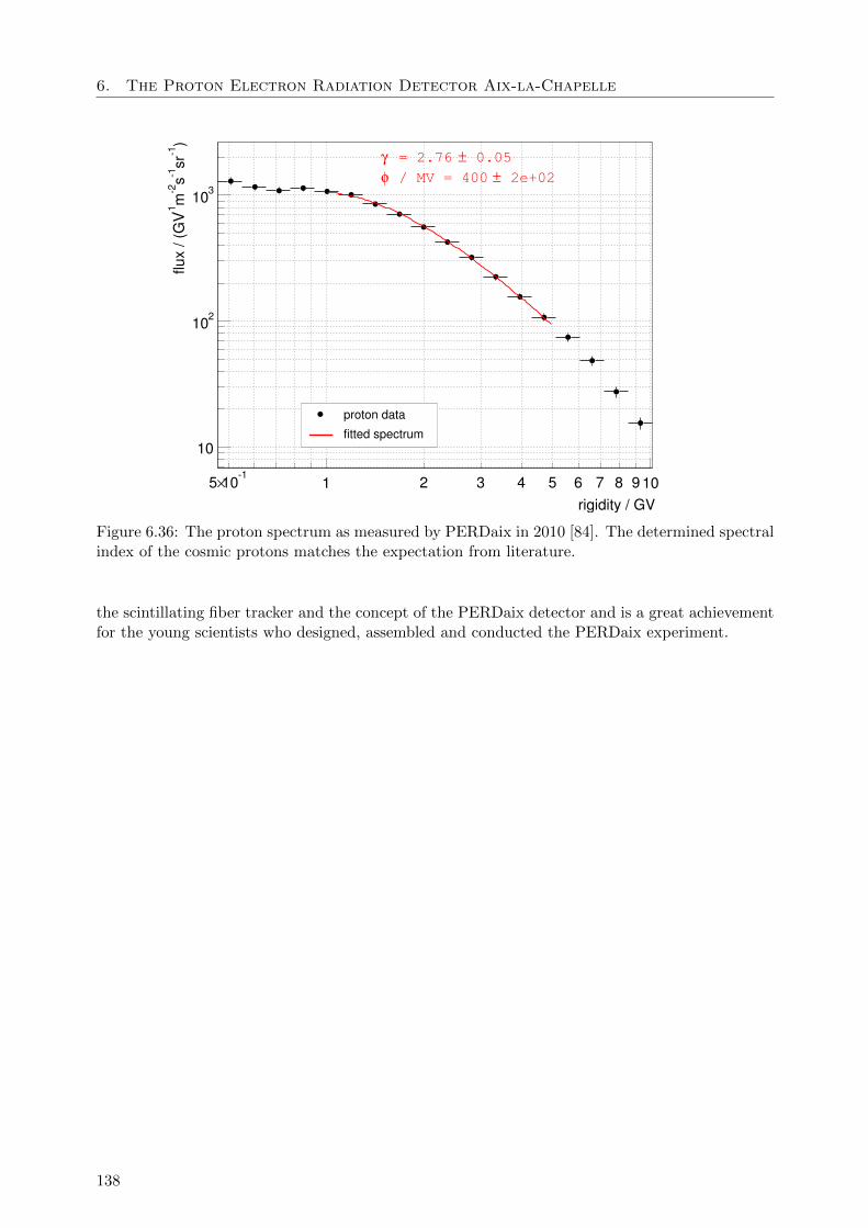
6. The Proton Electron Radiation Detector Aix-la-Chapelle
rigidity / GV
-110×5 1 2 3 4 5 6 7 8 9 10
)-1
sr-1 s
-2m
-1flu
x/(
GV
10
210
310
0.05±= 2.76γ2e+02±/ MV = 400φ
proton data
fitted spectrum
Figure 6.36: The proton spectrum as measured by PERDaix in 2010 [84]. The determined spectralindex of the cosmic protons matches the expectation from literature.
the scintillating fiber tracker and the concept of the PERDaix detector and is a great achievementfor the young scientists who designed, assembled and conducted the PERDaix experiment.
138
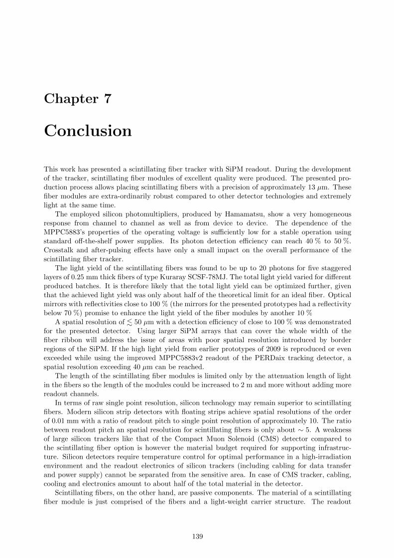
Chapter 7
Conclusion
This work has presented a scintillating fiber tracker with SiPM readout. During the developmentof the tracker, scintillating fiber modules of excellent quality were produced. The presented pro-duction process allows placing scintillating fibers with a precision of approximately 13 µm. Thesefiber modules are extra-ordinarily robust compared to other detector technologies and extremelylight at the same time.
The employed silicon photomultipliers, produced by Hamamatsu, show a very homogeneousresponse from channel to channel as well as from device to device. The dependence of theMPPC5883’s properties of the operating voltage is sufficiently low for a stable operation usingstandard off-the-shelf power supplies. Its photon detection efficiency can reach 40 % to 50 %.Crosstalk and after-pulsing effects have only a small impact on the overall performance of thescintillating fiber tracker.
The light yield of the scintillating fibers was found to be up to 20 photons for five staggeredlayers of 0.25 mm thick fibers of type Kuraray SCSF-78MJ. The total light yield varied for differentproduced batches. It is therefore likely that the total light yield can be optimized further, giventhat the achieved light yield was only about half of the theoretical limit for an ideal fiber. Opticalmirrors with reflectivities close to 100 % (the mirrors for the presented prototypes had a reflectivitybelow 70 %) promise to enhance the light yield of the fiber modules by another 10 %
A spatial resolution of . 50 µm with a detection efficiency of close to 100 % was demonstratedfor the presented detector. Using larger SiPM arrays that can cover the whole width of thefiber ribbon will address the issue of areas with poor spatial resolution introduced by borderregions of the SiPM. If the high light yield from earlier prototypes of 2009 is reproduced or evenexceeded while using the improved MPPC5883v2 readout of the PERDaix tracking detector, aspatial resolution exceeding 40 µm can be reached.
The length of the scintillating fiber modules is limited only by the attenuation length of lightin the fibers so the length of the modules could be increased to 2 m and more without adding morereadout channels.
In terms of raw single point resolution, silicon technology may remain superior to scintillatingfibers. Modern silicon strip detectors with floating strips achieve spatial resolutions of the orderof 0.01 mm with a ratio of readout pitch to single point resolution of approximately 10. The ratiobetween readout pitch an spatial resolution for scintillating fibers is only about ∼ 5. A weaknessof large silicon trackers like that of the Compact Muon Solenoid (CMS) detector compared tothe scintillating fiber option is however the material budget required for supporting infrastruc-ture. Silicon detectors require temperature control for optimal performance in a high-irradiationenvironment and the readout electronics of silicon trackers (including cabling for data transferand power supply) cannot be separated from the sensitive area. In case of CMS tracker, cabling,cooling and electronics amount to about half of the total material in the detector.
Scintillating fibers, on the other hand, are passive components. The material of a scintillatingfiber module is just comprised of the fibers and a light-weight carrier structure. The readout
139
7. Conclusion
electronics can be placed far away from the sensitive area using wave-guides. Scintillating fibertrackers thus have an advantage over larger silicon detectors in terms of total material introducedinto the detector. This is an important point since the uncertainty introduced by multiple scat-tering as well as secondary particles produced during interactions with the detector material limittotal tracker performance. In large detectors, scintillating fibers can cover more area per readoutchannel than silicon. This makes scintillating fibers also the more cost effective and less powerconsuming detector for large-scale trackers.
In comparison with gaseous detectors, scintillating fibers provide better single-point resolu-tion while gaseous detectors can achieve a far lower material budget. The timing properties ofgaseous tracking detectors which are dominated by the drift times of electrons and ions, are typ-ically worse than for plastic scintillating fibers which are effectively limited only by the speed ofthe readout electronics. Additionally, scintillating fiber trackers need less operational overhead.Gaseous tracking detectors typically require high voltages (few kV to many tens of kV), gas sys-tems and extensive monitoring to measure the drift time and to control the quality of the countinggas. The SiPM readout of a scintillating fiber tracker is operated at low voltages (< 100 V).The scintillating fiber tracker can be operated in a wide pressure and temperature range. ThePERDaix experiment demonstrated that its performance does not vary much between very coldambient temperatures (< −30C) and room temperature. Scintillating fibers also have no con-sumables and do not exhibit a severe aging as it has been observed for many gaseous detectors,giving them the edge for many applications.
Several detectors at the Large Hadron Collider (LHC) will have to upgrade within the next tenyears. Scintillating fibers tracker modules have a sufficient spatial resolution and sufficient timingproperties to be a competitive option. The PERDaix spectrometer is proof for the viability ofscintillating fibers with SiPM readout for practical charged-particle tracking detectors. The factthat scintillating fibers and SiPMs are both light and robust and require neither pressurized vesselsnor a sophisticated temperature control over a wide thermal range makes them also an excellentoption as a tracking detector for air- and space-borne spectrometers.
There are still many important details left, that this work did not address. The question ofradiation hardness of both SiPM and scintillating fibers, for example, was not discussed despitebeing of vital importance for a detector at the LHC. A light injection system for the calibration ofthe SiPM readout still has to be developed (it was one of the lessons of the PERDaix experimentthat such a system is needed). Yet, I hope that this work can prove useful for the design andconstruction of future scintillating fiber trackers and that it succeeds in conveying some of themany things that I learned during the last five years. This has been an exciting and successfuljourney for me and my colleagues and I would consider myself glad knowing that my record of itenables someone else to go just a little bit further than I did.
140
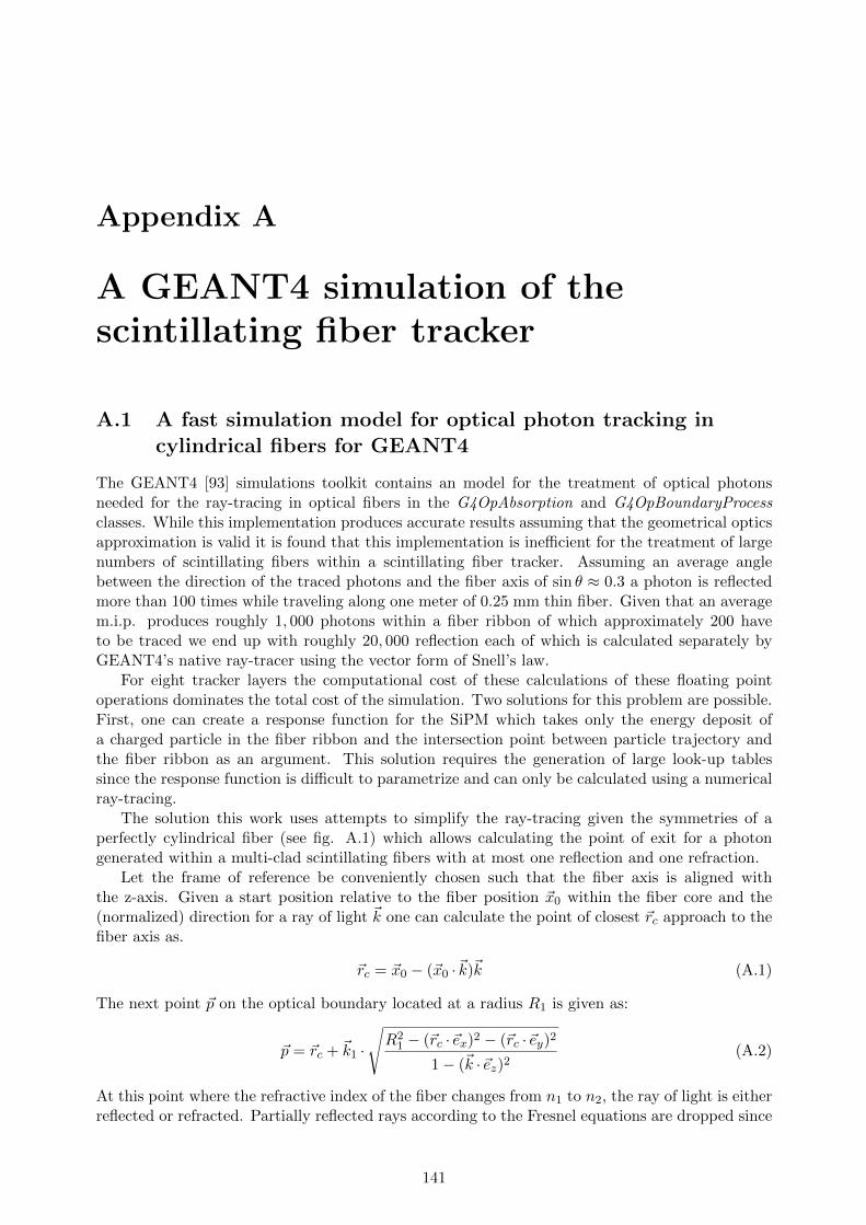
Appendix A
A GEANT4 simulation of thescintillating fiber tracker
A.1 A fast simulation model for optical photon tracking incylindrical fibers for GEANT4
The GEANT4 [93] simulations toolkit contains an model for the treatment of optical photonsneeded for the ray-tracing in optical fibers in the G4OpAbsorption and G4OpBoundaryProcessclasses. While this implementation produces accurate results assuming that the geometrical opticsapproximation is valid it is found that this implementation is inefficient for the treatment of largenumbers of scintillating fibers within a scintillating fiber tracker. Assuming an average anglebetween the direction of the traced photons and the fiber axis of sin θ ≈ 0.3 a photon is reflectedmore than 100 times while traveling along one meter of 0.25 mm thin fiber. Given that an averagem.i.p. produces roughly 1, 000 photons within a fiber ribbon of which approximately 200 haveto be traced we end up with roughly 20, 000 reflection each of which is calculated separately byGEANT4’s native ray-tracer using the vector form of Snell’s law.
For eight tracker layers the computational cost of these calculations of these floating pointoperations dominates the total cost of the simulation. Two solutions for this problem are possible.First, one can create a response function for the SiPM which takes only the energy deposit ofa charged particle in the fiber ribbon and the intersection point between particle trajectory andthe fiber ribbon as an argument. This solution requires the generation of large look-up tablessince the response function is difficult to parametrize and can only be calculated using a numericalray-tracing.
The solution this work uses attempts to simplify the ray-tracing given the symmetries of aperfectly cylindrical fiber (see fig. A.1) which allows calculating the point of exit for a photongenerated within a multi-clad scintillating fibers with at most one reflection and one refraction.
Let the frame of reference be conveniently chosen such that the fiber axis is aligned withthe z-axis. Given a start position relative to the fiber position ~x0 within the fiber core and the(normalized) direction for a ray of light ~k one can calculate the point of closest ~rc approach to thefiber axis as.
~rc = ~x0 − (~x0 ·~k)~k (A.1)
The next point ~p on the optical boundary located at a radius R1 is given as:
~p = ~rc + ~k1 ·
√R2
1 − (~rc ·~ex)2 − (~rc ·~ey)2
1− (~k ·~ez)2(A.2)
At this point where the refractive index of the fiber changes from n1 to n2, the ray of light is eitherreflected or refracted. Partially reflected rays according to the Fresnel equations are dropped since
141
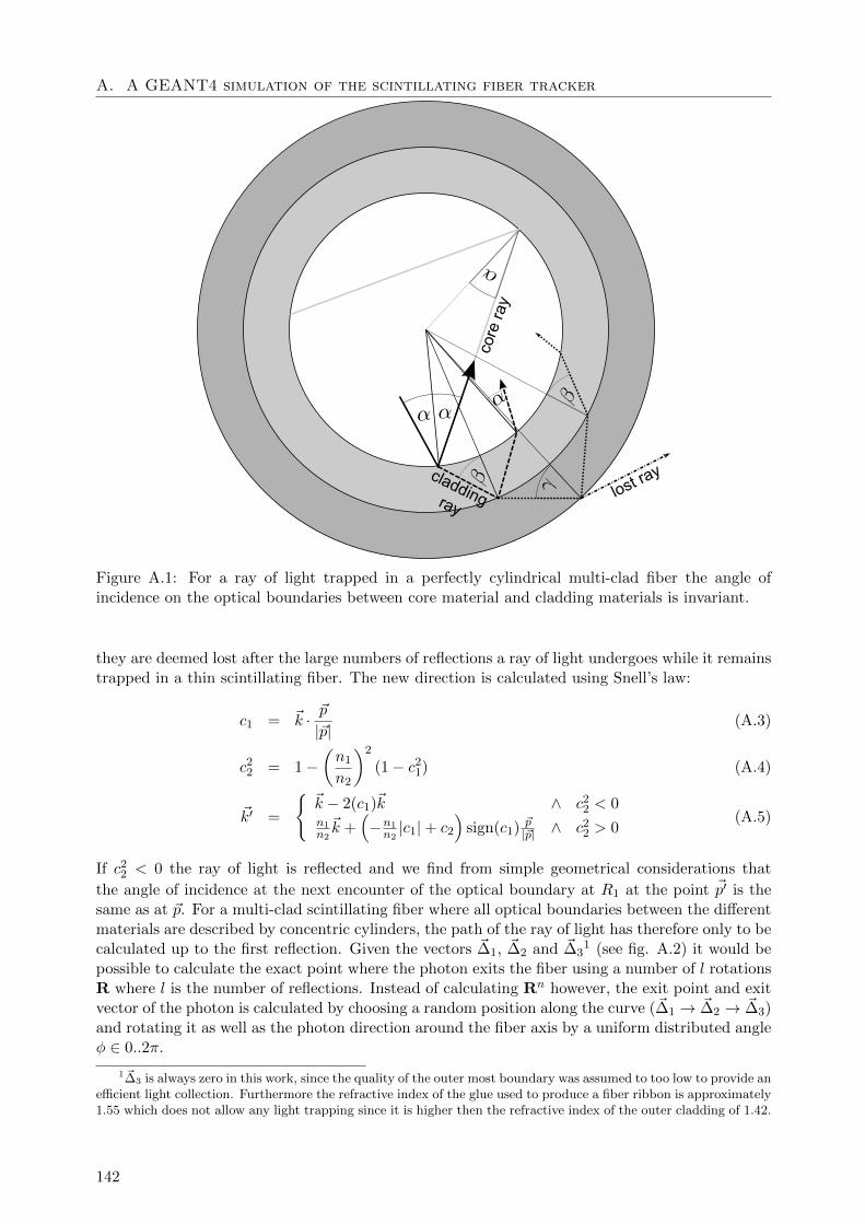
A. A GEANT4 simulation of the scintillating fiber tracker
lost ray
core
ray
claddingray
Figure A.1: For a ray of light trapped in a perfectly cylindrical multi-clad fiber the angle ofincidence on the optical boundaries between core material and cladding materials is invariant.
they are deemed lost after the large numbers of reflections a ray of light undergoes while it remainstrapped in a thin scintillating fiber. The new direction is calculated using Snell’s law:
c1 = ~k · ~p|~p|
(A.3)
c22 = 1−
(n1
n2
)2
(1− c21) (A.4)
~k′ =
~k − 2(c1)~k ∧ c2
2 < 0n1n2
~k +(−n1n2|c1|+ c2
)sign(c1) ~p
|~p| ∧ c22 > 0
(A.5)
If c22 < 0 the ray of light is reflected and we find from simple geometrical considerations that
the angle of incidence at the next encounter of the optical boundary at R1 at the point ~p′ is thesame as at ~p. For a multi-clad scintillating fiber where all optical boundaries between the differentmaterials are described by concentric cylinders, the path of the ray of light has therefore only to becalculated up to the first reflection. Given the vectors ~∆1, ~∆2 and ~∆3
1 (see fig. A.2) it would bepossible to calculate the exact point where the photon exits the fiber using a number of l rotationsR where l is the number of reflections. Instead of calculating Rn however, the exit point and exitvector of the photon is calculated by choosing a random position along the curve (~∆1 → ~∆2 → ~∆3)and rotating it as well as the photon direction around the fiber axis by a uniform distributed angleφ ∈ 0..2π.
1~∆3 is always zero in this work, since the quality of the outer most boundary was assumed to too low to provide anefficient light collection. Furthermore the refractive index of the glue used to produce a fiber ribbon is approximately1.55 which does not allow any light trapping since it is higher then the refractive index of the outer cladding of 1.42.
142
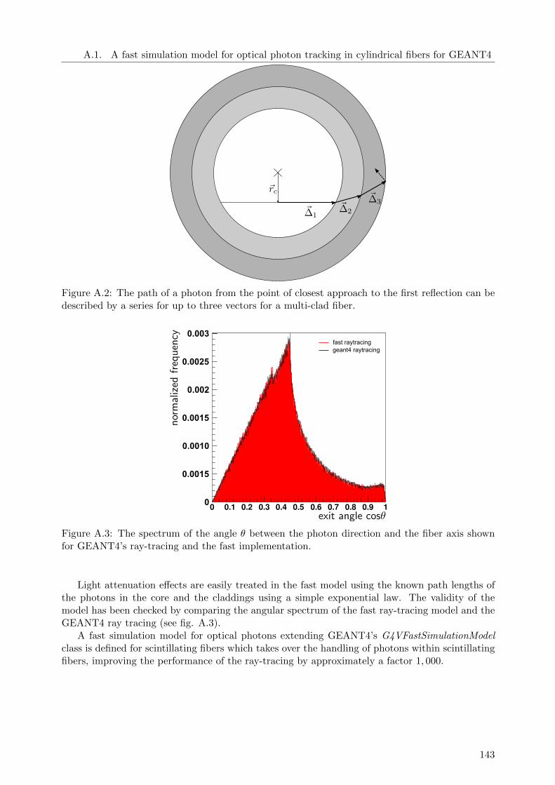
A.1. A fast simulation model for optical photon tracking in cylindrical fibers for GEANT4
Figure A.2: The path of a photon from the point of closest approach to the first reflection can bedescribed by a series for up to three vectors for a multi-clad fiber.
0 0.1 0.2 0.3 0.4 0.5 0.6 0.7 0.8 0.9 1
0.003
0.0025
0.002
0.0015
0.0010
0.0015
0
fast raytracinggeant4 raytracing
Figure A.3: The spectrum of the angle θ between the photon direction and the fiber axis shownfor GEANT4’s ray-tracing and the fast implementation.
Light attenuation effects are easily treated in the fast model using the known path lengths ofthe photons in the core and the claddings using a simple exponential law. The validity of themodel has been checked by comparing the angular spectrum of the fast ray-tracing model and theGEANT4 ray tracing (see fig. A.3).
A fast simulation model for optical photons extending GEANT4’s G4VFastSimulationModelclass is defined for scintillating fibers which takes over the handling of photons within scintillatingfibers, improving the performance of the ray-tracing by approximately a factor 1, 000.
143
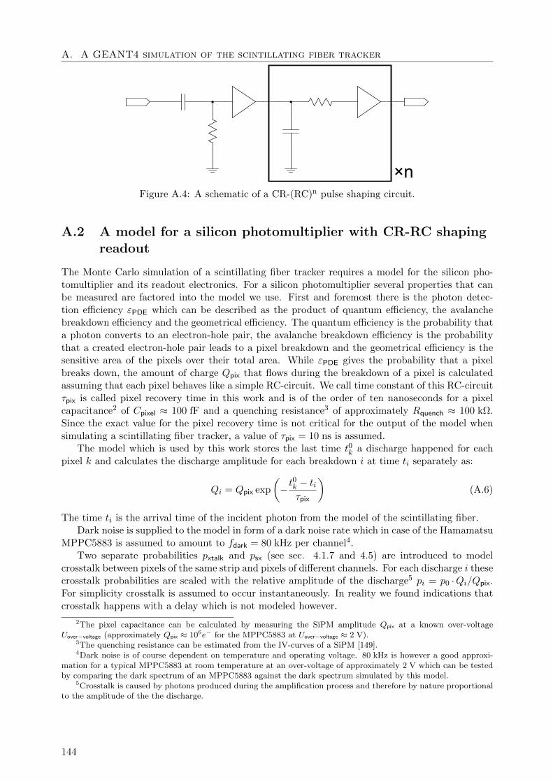
A. A GEANT4 simulation of the scintillating fiber tracker
×nFigure A.4: A schematic of a CR-(RC)n pulse shaping circuit.
A.2 A model for a silicon photomultiplier with CR-RC shapingreadout
The Monte Carlo simulation of a scintillating fiber tracker requires a model for the silicon pho-tomultiplier and its readout electronics. For a silicon photomultiplier several properties that canbe measured are factored into the model we use. First and foremost there is the photon detec-tion efficiency εPDE which can be described as the product of quantum efficiency, the avalanchebreakdown efficiency and the geometrical efficiency. The quantum efficiency is the probability thata photon converts to an electron-hole pair, the avalanche breakdown efficiency is the probabilitythat a created electron-hole pair leads to a pixel breakdown and the geometrical efficiency is thesensitive area of the pixels over their total area. While εPDE gives the probability that a pixelbreaks down, the amount of charge Qpix that flows during the breakdown of a pixel is calculatedassuming that each pixel behaves like a simple RC-circuit. We call time constant of this RC-circuitτpix is called pixel recovery time in this work and is of the order of ten nanoseconds for a pixelcapacitance2 of Cpixel ≈ 100 fF and a quenching resistance3 of approximately Rquench ≈ 100 kΩ.Since the exact value for the pixel recovery time is not critical for the output of the model whensimulating a scintillating fiber tracker, a value of τpix = 10 ns is assumed.
The model which is used by this work stores the last time t0k a discharge happened for eachpixel k and calculates the discharge amplitude for each breakdown i at time ti separately as:
Qi = Qpix exp
(−t0k − tiτpix
)(A.6)
The time ti is the arrival time of the incident photon from the model of the scintillating fiber.Dark noise is supplied to the model in form of a dark noise rate which in case of the Hamamatsu
MPPC5883 is assumed to amount to fdark = 80 kHz per channel4.Two separate probabilities pxtalk and psx (see sec. 4.1.7 and 4.5) are introduced to model
crosstalk between pixels of the same strip and pixels of different channels. For each discharge i thesecrosstalk probabilities are scaled with the relative amplitude of the discharge5 pi = p0 ·Qi/Qpix.For simplicity crosstalk is assumed to occur instantaneously. In reality we found indications thatcrosstalk happens with a delay which is not modeled however.
2The pixel capacitance can be calculated by measuring the SiPM amplitude Qpix at a known over-voltageUover−voltage (approximately Qpix ≈ 106e− for the MPPC5883 at Uover−voltage ≈ 2 V).
3The quenching resistance can be estimated from the IV-curves of a SiPM [149].4Dark noise is of course dependent on temperature and operating voltage. 80 kHz is however a good approxi-
mation for a typical MPPC5883 at room temperature at an over-voltage of approximately 2 V which can be testedby comparing the dark spectrum of an MPPC5883 against the dark spectrum simulated by this model.
5Crosstalk is caused by photons produced during the amplification process and therefore by nature proportionalto the amplitude of the the discharge.
144
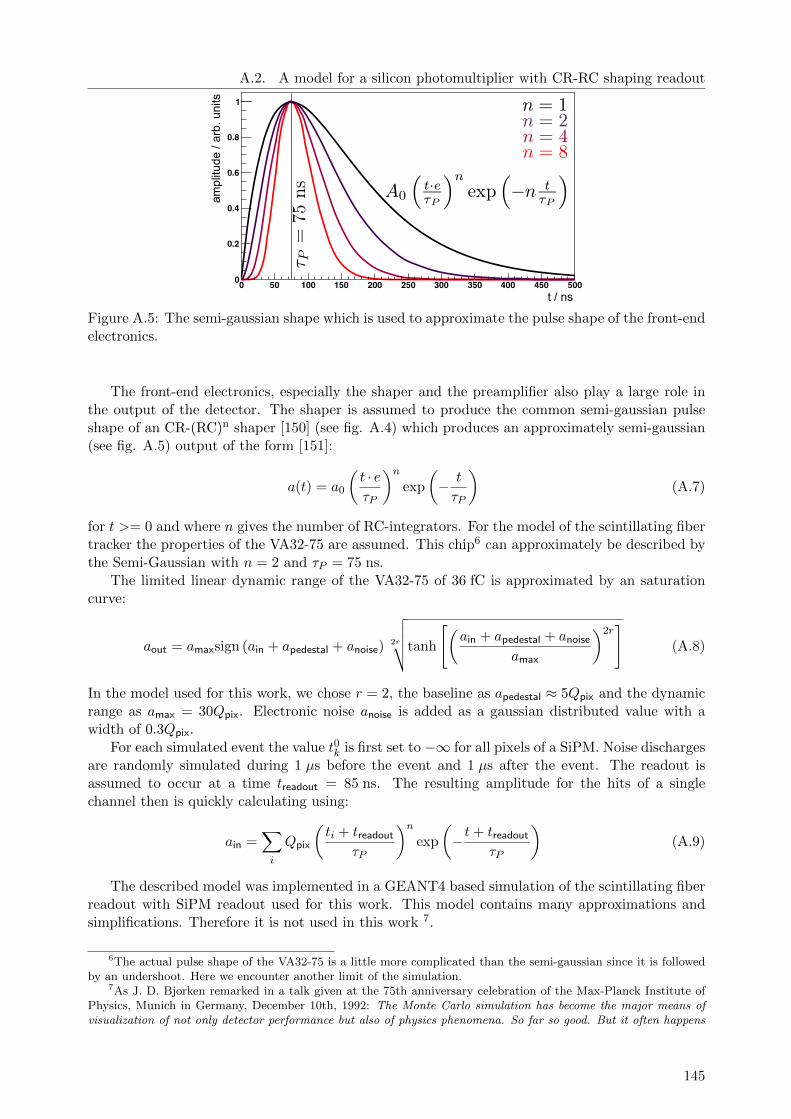
A.2. A model for a silicon photomultiplier with CR-RC shaping readout
0 50 100 150 200 250 300 350 400 450 5000
0.2
0.4
0.6
0.8
1
t / ns
ampl
itude
/ ar
b. u
nits
Figure A.5: The semi-gaussian shape which is used to approximate the pulse shape of the front-endelectronics.
The front-end electronics, especially the shaper and the preamplifier also play a large role inthe output of the detector. The shaper is assumed to produce the common semi-gaussian pulseshape of an CR-(RC)n shaper [150] (see fig. A.4) which produces an approximately semi-gaussian(see fig. A.5) output of the form [151]:
a(t) = a0
(t · eτP
)nexp
(− t
τP
)(A.7)
for t >= 0 and where n gives the number of RC-integrators. For the model of the scintillating fibertracker the properties of the VA32-75 are assumed. This chip6 can approximately be described bythe Semi-Gaussian with n = 2 and τP = 75 ns.
The limited linear dynamic range of the VA32-75 of 36 fC is approximated by an saturationcurve:
aout = amaxsign (ain + apedestal + anoise)2r
√√√√tanh
[(ain + apedestal + anoise
amax
)2r]
(A.8)
In the model used for this work, we chose r = 2, the baseline as apedestal ≈ 5Qpix and the dynamicrange as amax = 30Qpix. Electronic noise anoise is added as a gaussian distributed value with awidth of 0.3Qpix.
For each simulated event the value t0k is first set to −∞ for all pixels of a SiPM. Noise dischargesare randomly simulated during 1 µs before the event and 1 µs after the event. The readout isassumed to occur at a time treadout = 85 ns. The resulting amplitude for the hits of a singlechannel then is quickly calculating using:
ain =∑i
Qpix
(ti + treadout
τP
)nexp
(− t+ treadout
τP
)(A.9)
The described model was implemented in a GEANT4 based simulation of the scintillating fiberreadout with SiPM readout used for this work. This model contains many approximations andsimplifications. Therefore it is not used in this work 7.
6The actual pulse shape of the VA32-75 is a little more complicated than the semi-gaussian since it is followedby an undershoot. Here we encounter another limit of the simulation.
7As J. D. Bjorken remarked in a talk given at the 75th anniversary celebration of the Max-Planck Institute ofPhysics, Munich in Germany, December 10th, 1992: The Monte Carlo simulation has become the major means ofvisualization of not only detector performance but also of physics phenomena. So far so good. But it often happens
145

A. A GEANT4 simulation of the scintillating fiber tracker
that the physics simulations provided by the Monte Carlo generators carry the authority of data itself. They looklike data and feel like data, and if one is not careful they are accepted as if they were data. All Monte Carlo codescome with a GIGO (garbage in, garbage out) warning label. In that sense, I took great care to let the output of themodel look like data. However, any agreement and disagreement between Monte Carlo output and data should beregarded as equally coincidental.
146
Appendix B
Track detection in 3D using aKalman Filter method
B.1 The passage of a particle as linear dynamical model
Let us consider the passage of a particle through a very simple tracking detector which consistsof n equidistant and interchangeable detector planes at each of which a passing particle can haveone of m distinguishable states1. One can view the passage of a particle through the detector asa Markov chain [152]. This means that for each measurement i within the detector, the particlehas a certain state Si which assumes a value s ∈ Ξ where Ξ is a set of possible states. In our case,this state s = (~xi, ~pi, Ei, zi) may be comprised of a position in space ~xi which is in part definedby the i’th detector layer, a momentum ~pi, the particle energy Ei and a charge zi
2. An importantproperty of the Markov chain is that it is memoryless, meaning that the state Si+1 depends onlythe state Si or more formally:
p (Si+1 = si+1|Si = si) = p (Si+1 = si+1|Si = si, Si−1 = si−1, ..., S1 = s1) (B.1)
Thus, the process is described by the set of possible states Ξ and a transition matrix ρi→j :
si, sj ∈ Ξ (B.2)
ρi→j = p (S1 = sj |S0 = si) (B.3)
|Ξ|∑j=0
ρi→j = 1 (B.4)
Note that in general, a Markov chain does not have to be reversible. This means that wecannot necessarily deduce a probability for the state Si assuming any value sj ∈ Ξ from knowingthe state Si+1 = sk.
1For any real particle detector the measured particle can only have a finite number of distinguishable states dueto the finite precision of a any readout system.
2The particle state that we use here is only limited to properties that influence the measurement in the SciFitracker. For another detector in high energy physics, one may extend the state to reflect more particles and moreparticle properties like quantum numbers, chirality and so on. The general mechanics of the Markov chain isapplicable to a wide range of processes
147

B. Track detection in 3D using a Kalman Filter method
For our purpose we will deviate from the original formulation of the Markov chain whichassumes a finite set of discrete possible states (and was later extended for any countable statespace by Kolmogorov) and assume a continuous (and uncountable) state space S.
si, sj ∈ S (B.5)
ρ(s′, s
)= p
(Si+1 = s′|Si = s0
)(B.6)∫
S
ρ(s′, s
)ds′ = 1 (B.7)
Looking at the laws of motion governing the passage of a particle, we see that the state changeshould really be a continuous process in time t. So |∂s/∂t| should be finite. We therefore switchfrom a discrete description of the particle state Si to a continuous one S(t):
ρ(s′, s,∆ti→i+1
)= p
(S(ti+1) = s′|S(ti) = s
)(B.8)
This is known as a continuous-time Markov chain.Next, we investigate the transition from one state to another S(ti) → S(ti+1). Using the
continuity we required above, we can subdivide this transition into small time steps ε. For eachsufficiently small step, the physical laws that govern the trajectory of the particle and the mod-ification of its properties are approximately linear. We therefore introduce the transformationmatrix F(ε) which fulfills:
S(t+ ε) = s′ (B.9)
S(t) = s (B.10)
s′ = F(ε)s (B.11)
If we want to look at the state transition from S(t) to S(t+ ε) in general, there is not necessarilyjust one unique transformation matrix, instead - accounting for the number of possible valuesthat S(t+ ε) may assume according to the original Markov chain definition - there can be severalpossible transition matrices Fi. For continuous transformations, we can write Fi(ε) as Fi = 1+Giεwith generator matrix Gi ∈ G3 and the set of possible generators G. The transition matrix forS(ti)→ S(ti+1) can now be expressed as:
Fi→i+1 =
n∏k=1
(1 + Gk
∆ti→i+1
n
)(B.12)
Coming back to our detector, the full state of the particle is not directly observable. A scin-tillating fiber tracker as presented in this thesis measures only two of three spatial coordinatesand an amplitude and neither momentum, energy or charge. However the passage of the particleclearly depends on these other variables4. Instead we introduce the measurement matrix H whichtranslates from state space S to observable space O.
oi = Hisi (B.13)
We infer here that the relation between observation o and the state s is a linear one or can belinearized by a convenient choice of O and S.5
3Note that the continuous description while working very well for e.g. the laws of motion, is not trivial toimplement for seemingly discrete processes as for example the single hard scattering of a particle which results inthe creation of further particles. This fact is ignored here, since the goal is to find a description for a plain particletrajectory. In fact, we have to exclude hard scatterings as we will see later on.
4Consider for example multiple scattering (see eqn. 2.18) which depends on β = |~p|E
as well as |~p| and z.5Although this is not always the case, as for example with the AMS-02 silicon tracker [143] which due to its
readout scheme performs an ambiguous measurement in one of three coordinates, we will see later on that only alocally linear transformation H is required in order to perform a track reconstruction.
148

B.2. Principles of the Kalman Filter
The goal of the track reconstruction we are motivating here is to determine a series of most prob-able states (S(t0) = s0, ..., S(tn) = sn) based on a series of incomplete observations (o0 = Hs0, ..., on = Hsn).Returning to the Markov chain, we are now faced with a problem: Using it to assign a probability toa theory (S(t0) = s0, ..., S(tn) = sn) requires us to write down an expression for ρ (s′, s,∆ti→i+1).Without it, we cannot determine how probable or improbable the observed particle will be bein a given series of states. A simple solution for this problem involves using the central limittheorem. Under the assumption that the Markov process is homogeneous during the continuoustransition S(ti)→ S(ti+1), meaning that all possible infinitesimal transitions 1 + G occur with afixed probability π(G) during that state transition, we can write (eqn. B.12) as:
Fi→i+1 = limn→∞
(1 +
n∑k=1
Gk∆ti→i+1
n+ O
((∆ti→i+1
n
)2))
(B.14)
So for S(ti) = s and S(ti+1) = s′ follows:
s′ = Fi→i+1s = s+ limn→∞
n∑k=1
δk (B.15)
with δk = Gk∆ti→i+1
n s. If∣∣F− 1
∣∣ =∣∣G∣∣ =
∣∣∣∣∣∫G π(G)GsdG
∣∣∣∣∣ and∫Gπ(G)s†G†GsdG are finite then
δk is a random variable with well defined mean and covariance and according to the central limittheorem we can write:
ρ(s′, s,∆ti→i+1
)=
1√
2πrank(Σ)
det(Σ)exp
(−1
2
(Fs− s′
)†Σ−1
(Fs− s′
))(B.16)
Here, Σ is the covariance matrix for(Fs− s′
).
Seemingly discrete processes like hard scatterings for the passage of a particle through mattercannot be described using the central limit theorem: In order to describe them with our modelof infinitesimal transitions dF = lim
ε→01 + Gε, the generator matrix G for a discrete process must
contain infinities and therefore violates the conditions given above.In summary we have built a description for the passage of a particle through a detector based on
a Markov chain, using a hidden Markov model in which only part of the state is directly observableand the observables depend linearly on the particle state. We assume a continuous and locally(between two consecutive observations) homogeneous process which can on average be describedby the transformation exp(G∆ti→i+1) which is also known as a linear dynamical model for whicha Kalman filter provides a possibility to reconstruct a most probable series of states for a series ofobservations.
B.2 Principles of the Kalman Filter
The Kalman filter [153] named after its inventor Rudolph E. Kalman is a method to create esti-mates for the state of a linear dynamical system based on a series incomplete and noisy observa-tions. It uses a multidimensional weighted average method to combine the prediction for the stateof the system based on previous measurements or a starting value and a current observation.
Consider a series of states observed for a system (S(t0) = s0, ...S(tn) = sn). The most probabletransition ti → ti+1 is described by the transition matrix Fi. The uncertainty introduced due tothe statistical nature of the process (described in the previous section) is given by the covariancematrix Σi and is treated by the Kalman filter as process noise. A series of noisy observations(o0, ..., on) are available which linearly depend on the actual states with the measurement matrix
149

B. Track detection in 3D using a Kalman Filter method
Hi and an unknown amount of Gaussian noise oi distributed according to a known covariancematrix Ri:
oi = Hisi + oi (B.17)
The Kalman filter uses a best guess for the current state xi−1 and the uncertainty of the guessednew state given by the covariance matrix Vi−1. Based on these, a prediction x∗i for the state S(ti)is calculated using the knowledge that most likely si = Fisi−1 + si where si is a random processnoise vector which is normal distributed according to the covariance matrix Σi.
x∗i = Fixi−1 (B.18)
V∗i = FiVi−1FTi + Σi (B.19)
The new best guess for the next state xi has to be a combination of the prediction x∗i and themeasurement oi taking into account the uncertainties of each. In order to achieve that, the Kalmanfilter determines the difference between the prediction and the observation in observable space r,which has the statistical weight S−1
i (or covariance Si):
r = oi −Hix∗i (B.20)
Si = HiV∗iH
Ti + Ri (B.21)
The combination of observation and prediction is now the multidimensional case of the weightedmean which combines two values y1 and y2 with variances σ2
1 and σ22 to:
y =y1σ−21 + y2σ
−22
σ−21 + σ−2
2
= y1 + (y2 − y1)σ2
2
σ21 + σ2
2
(B.22)
σ2 =1
σ−21 + σ−2
2
= σ21 −
σ41
σ21 + σ2
2
(B.23)
In our multidimensional case we replace y1 and y2 − y1 with x∗i and r and the variances σ21 and
σ21 +σ2
2 with the covariances V∗i and Si. Since the two are defined for different spaces, V∗i is definedfor the state space S and Si is defined for observable space O one uses the projection matrix Hi
which translates between the two spaces to create a the product:
Ki = V∗iHTS−1
i (B.24)
Ki is known as the optimal Kalman gain for linear dynamical systems6. The updated best guessfor the state and the covariance matrix become:
xi = x∗i + Kir (B.25)
Vi = V∗i −KiHTV∗i (B.26)
B.3 Fitting single particle tracks with a Kalman filter
For the reconstruction of charged-particle tracks with a the scintillating fiber tracker we proposehere, a necessary first step is the choice how to describe the detector geometry. Since the detectormodules are approximately planar and rectangular, the obvious choice for a coordinate systemis Cartesian coordinates. The position and orientation of a rectangle in 3D space is given by 6parameters. In this work a rotation matrix U defined by three angles and a translation vector~x0 are used, which describe the transformation of a local position ~l with respect to the detectormodule into a global position within the global coordinate system ~g = U~l + ~x0.
6In case of a non-linear system or non-Gaussian measurement or process noise this formulation of the Kalmangain is not necessarily optimal.
150

B.3. Fitting single particle tracks with a Kalman filter
A particle trajectory is described as a parametrized function ~t (ξ1, ..., ξn, α) with parametersξ1, ..., ξn defining the shape and position of the trajectory and the variable α describing the positionalong the trajectory. Assuming that the contribution from multiple scattering is small, a slightlysimplified version of the Kalman filter described above can be used where process noise is zeroΣi = 0 and the true state of the trajectory is constant si = s (so F = 1 and x∗i = xi−1,V∗i = Vi−1). In this case the result of applying the Kalman filter does not depend on the order ofthe measurements along the trajectory.
The projection matrix Hi is - especially in case of a non-linear trajectory - a little morecomplex. First, one needs to determine the parametrization variable α, which is not part of thestate vector xi but replaces the measurement time in the original Kalman filter above. However,the position of the observation along the track α in general depends on the shape of the trajectory(ξ1, ..., ξn). We therefore need to use one coordinate the measurement oi to determine α before wecan continue. This of course means, that for any measurement oi, one coordinate cannot be usedto further constrain the shape of the trajectory7. Let oi =
(o1i , ..., o
mi
)be the observation and Hi
be chosen in such a manner that for one Ri is diagonal and secondly o1i = [oi]1 is the most accurate
measurement with variance σ2o,i,1. Let furthermore Mi be the matrix that translates a point on the
trajectory ~t (x∗i , αi) = ~t (ξ1, ..., ξn, αi)given in global spatial coordinates into the coordinate systemof the observation8. Then the following equation can be solved for αi either analytically or usinga numerical method (the work presented in this thesis uses an iterative Newton method).
o1i =
[Mi
(~t (x∗i , αi)
)]1
(B.27)
In general, the determined αi depends on the parameters ξ1, ..., ξn. Only in rare cases, forexample for parallel detector planes, a description for the trajectory can be found so that o1
i = f (αi)(where f is an invertible function) and αi does not depend on the trajectory parameters. Theimplications of this fact will become more obvious for the case of global trajectory fits in a latersection.
Knowing alpha, one can now determine the residual r′i.
r′i = oi −Mi~t (x∗i , αi) (B.28)
Since for r′i =(r′1i , ..., r
′mi
)the first element is always zero (as required by eqn. B.27), we use as
ri =(r′2i , ..., r
′mi
)as residual for the Kalman filter. The matrix Hi was not used here because at
this point we did not infer that the trajectory is linear.Instead we use a Taylor series expansion to the first order to transform the prediction of the
covariance matrix V∗i . For a trajectory defined by n parameters ξ1, ..., ξn, we introduce a matrixHi as:
Hi = QiMi
∂[~t (x∗i , αi)
]1/∂ξ1 · · ·
[~t (x∗i , αi)
]1/∂ξn
.... . .
...
∂[~t (x∗i , αi)
]3/∂ξ1 · · ·
[~t (x∗i , αi)
]3/∂ξn
(B.29)
7For this reason, all common tracking detector technologies perform measurements in at least 2-dimensions.8In simple cases where a two- or three-dimensional observation oi and the trajectory ~t (x∗i , αi) share the same
coordinate system, Mi will be a 2× 3- or 3× 3-matrix with ones on the diagonal and zero for off-diagonal entries.If the requirement that Ri is diagonal forces the coordinate system of the observation to differ from the global one,we may choose the coordinate system as follows: oi is the local position of the particle ~li plus a constant offset fromthe detector position.
oi = Mi
(U~li + ~x0
)Mi is either
(1 0 00 1 0
)UT or
1 0 00 1 00 0 1
UT depending on whether we assume a 2-d or a 3-d measurement.
Then Mi simply transforms from the global coordinate system in which the trajectory is defined into a local onewhere Ri is diagonal and σo,i,1 is minimal.
151

B. Track detection in 3D using a Kalman Filter method
with Qi defined for a 2-dimensional or 3-dimensional observation as:
Qi =
([∂~t(x∗i ,αi)/∂α]
1
[∂~t(x∗i ,αi)/∂α]0
1
)or Qi =
[∂~t(x∗i ,αi)/∂α]1
[∂~t(x∗i ,αi)/∂α]0
1 0
[∂~t(x∗i ,αi)/∂α]2
[∂~t(x∗i ,αi)/∂α]0
0 1
(B.30)
Qi reflects the usage of the observation o1i in order to determine αi which is not a part of the
state vector. In principle, it performs the propagation of the uncertainty on o1i toward the other
coordinates o2i , ..., o
mi and truncates the first coordinate of oi which cannot be used anymore in the
following. The matrix S must take into account the error propagation of determining αi as well,therefore, deviating from the original formulation of the Kalman filter, we use:
Si = HiV∗iH
Ti + QiRiQ
Ti (B.31)
From this point on, we may follow the original definitions given by the Kalman filter.
Ki = V∗iHTS−1
i (B.32)
xi = x∗i + Kir (B.33)
Vi = V∗i −KiHTV∗i (B.34)
In the way described above, it is possible to determine the parameters ξ1, ..., ξn describing thetrajectory of a particle incrementally by updating start values chosen for these parameters withmeasurements along the trajectory in an arbitrary order using the Kalman filter method. Thismethod, as used here, is not capable of treating multiple scattering9. Furthermore, the trajectory~t (ξ1, ..., ξn, α) has to be reasonably smooth, meaning that the derivations ∂~t (ξ1, ..., ξn, α) /∂ξi and∂~t (ξ1, ..., ξn, α) /∂α must be finite.
B.4 Reconstructing particle tracks from noisy observations
In a real tracking detector, especially one that uses a technology prone to exhibiting a relativelyhigh noise like silicon photomultipliers, a certain amount of noise signals which are not related tothe primary or even any particle track, needs to be expected. So we are faced with the challengeof determining which of n signals belong to the particle trajectory and at the same time of whatshape that trajectory is. This problem has been addressed many times in the field of patternrecognition and there are several established solutions for it10.
First, let us formulate the problem. We are given an unordered set of n observations O =oi1 , oi2 , ..., oin. These observations can be partitioned into subsets of observations related to acommon cause. The number of possible partitions or distinguishable theories which would explainthe set of n observations is given by Bell’s number:
Bn =n∑k=0
1
k!
k∑j=0
(−1)k−j(kj
)jn (B.35)
For a set of 10 observations the number of theories is B10 = 115975, which if one were to test
all possible partitions equals a complexity of approximately O(nn2
). In order to find the best
matching theory T = E1, ..., Em where Ei ∈ E is an explanation which corresponds to a non-empty set of observations, there are two basic approaches which are described in the following.
9The process noise Σi of the Kalman filter can be used to describe a certain amount of multiple scatteringbetween two measurements. In that case, however, the measurements cannot be added in arbitrary order anymorebut ordered as αi+1 ≥ αi or αi+1 ≤ αi.
10A good overview of techniques to detect tracks in a noisy environment was given by R. Mankel [154]
152
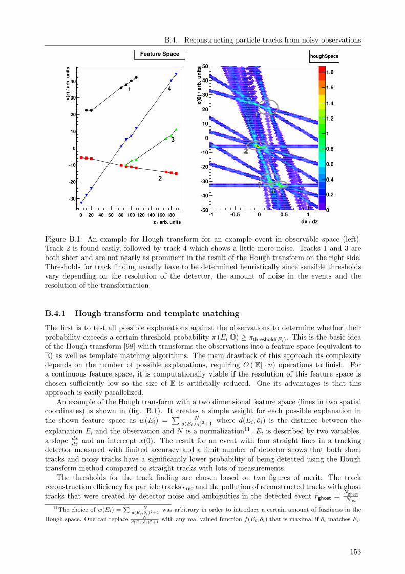
B.4. Reconstructing particle tracks from noisy observations
z / arb. units0 20 40 60 80 100 120 140 160 180
x(z)/arb.units
-30
-20
-10
0
10
20
30
40
4
3
2
1
dx / dz-1 -0.5 0 0.5 1
x(0)/arb.units
-50
-40
-30
-20
-10
0
10
20
30
40
50
houghSpacehoughSpace
0
0.2
0.4
0.6
0.8
1
1.2
1.4
1.6
1.8
Feature Space
1
2
34
Figure B.1: An example for Hough transform for an example event in observable space (left).Track 2 is found easily, followed by track 4 which shows a little more noise. Tracks 1 and 3 areboth short and are not nearly as prominent in the result of the Hough transform on the right side.Thresholds for track finding usually have to be determined heuristically since sensible thresholdsvary depending on the resolution of the detector, the amount of noise in the events and theresolution of the transformation.
B.4.1 Hough transform and template matching
The first is to test all possible explanations against the observations to determine whether theirprobability exceeds a certain threshold probability π (Ei|O) ≥ πthreshold(Ei). This is the basic ideaof the Hough transform [98] which transforms the observations into a feature space (equivalent toE) as well as template matching algorithms. The main drawback of this approach its complexitydepends on the number of possible explanations, requiring O (|E| ·n) operations to finish. Fora continuous feature space, it is computationally viable if the resolution of this feature space ischosen sufficiently low so the size of E is artificially reduced. One its advantages is that thisapproach is easily parallelized.
An example of the Hough transform with a two dimensional feature space (lines in two spatialcoordinates) is shown in (fig. B.1). It creates a simple weight for each possible explanation inthe shown feature space as w(Ei) =
∑ Nd(Ei,oi)2+1
where d(Ei, oi) is the distance between the
explanation Ei and the observation and N is a normalization11. Ei is described by two variables,a slope dx
dz and an intercept x(0). The result for an event with four straight lines in a trackingdetector measured with limited accuracy and a limit number of detector shows that both shorttracks and noisy tracks have a significantly lower probability of being detected using the Houghtransform method compared to straight tracks with lots of measurements.
The thresholds for the track finding are chosen based on two figures of merit: The trackreconstruction efficiency for particle tracks εrec and the pollution of reconstructed tracks with ghosttracks that were created by detector noise and ambiguities in the detected event rghost =
Nghost
Nrec.
11The choice of w(Ei) =∑
Nd(Ei,oi)2+1
was arbitrary in order to introduce a certain amount of fuzziness in the
Hough space. One can replace Nd(Ei,oi)2+1
with any real valued function f(Ei, oi) that is maximal if oi matches Ei.
153
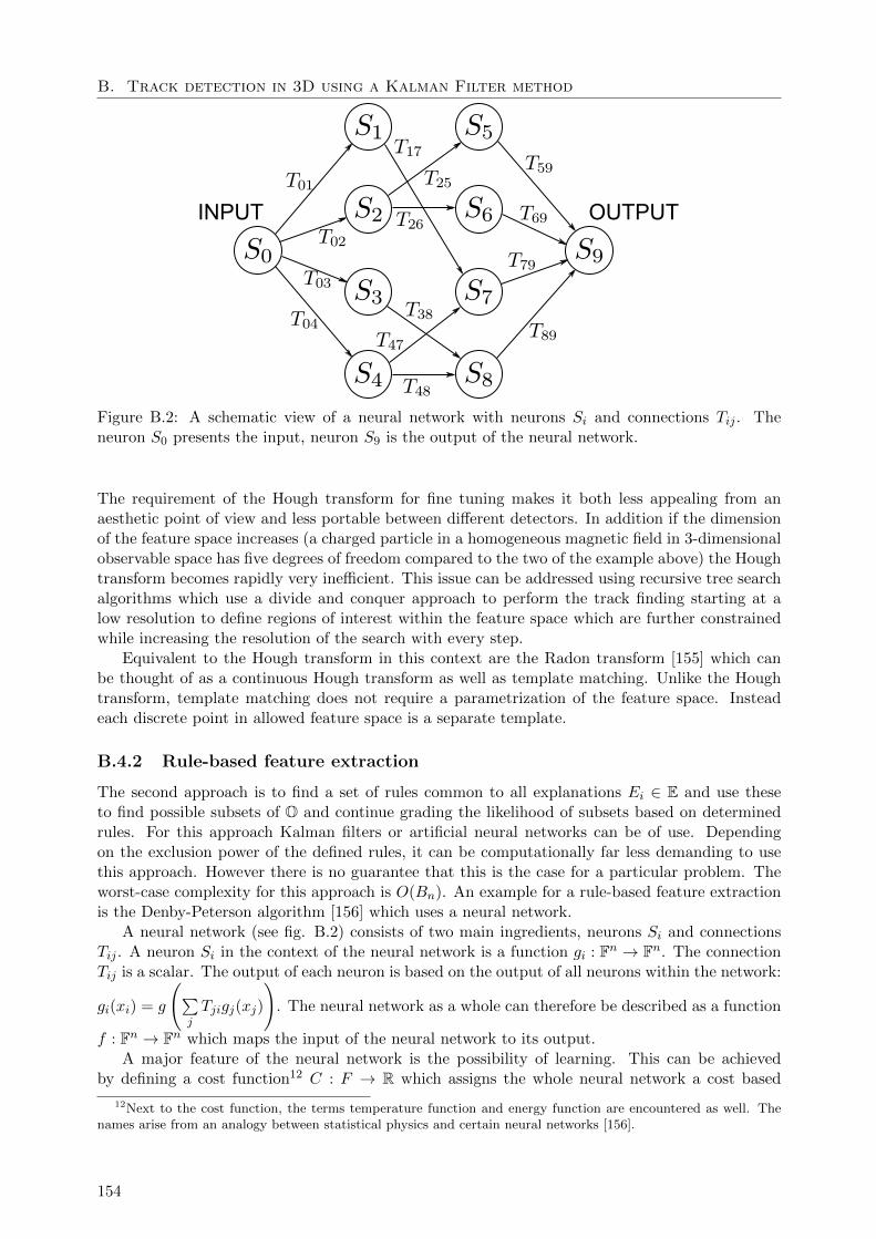
B. Track detection in 3D using a Kalman Filter method
INPUT OUTPUT
Figure B.2: A schematic view of a neural network with neurons Si and connections Tij . Theneuron S0 presents the input, neuron S9 is the output of the neural network.
The requirement of the Hough transform for fine tuning makes it both less appealing from anaesthetic point of view and less portable between different detectors. In addition if the dimensionof the feature space increases (a charged particle in a homogeneous magnetic field in 3-dimensionalobservable space has five degrees of freedom compared to the two of the example above) the Houghtransform becomes rapidly very inefficient. This issue can be addressed using recursive tree searchalgorithms which use a divide and conquer approach to perform the track finding starting at alow resolution to define regions of interest within the feature space which are further constrainedwhile increasing the resolution of the search with every step.
Equivalent to the Hough transform in this context are the Radon transform [155] which canbe thought of as a continuous Hough transform as well as template matching. Unlike the Houghtransform, template matching does not require a parametrization of the feature space. Insteadeach discrete point in allowed feature space is a separate template.
B.4.2 Rule-based feature extraction
The second approach is to find a set of rules common to all explanations Ei ∈ E and use theseto find possible subsets of O and continue grading the likelihood of subsets based on determinedrules. For this approach Kalman filters or artificial neural networks can be of use. Dependingon the exclusion power of the defined rules, it can be computationally far less demanding to usethis approach. However there is no guarantee that this is the case for a particular problem. Theworst-case complexity for this approach is O(Bn). An example for a rule-based feature extractionis the Denby-Peterson algorithm [156] which uses a neural network.
A neural network (see fig. B.2) consists of two main ingredients, neurons Si and connectionsTij . A neuron Si in the context of the neural network is a function gi : Fn → Fn. The connectionTij is a scalar. The output of each neuron is based on the output of all neurons within the network:
gi(xi) = g
(∑jTjigj(xj)
). The neural network as a whole can therefore be described as a function
f : Fn → Fn which maps the input of the neural network to its output.A major feature of the neural network is the possibility of learning. This can be achieved
by defining a cost function12 C : F → R which assigns the whole neural network a cost based
12Next to the cost function, the terms temperature function and energy function are encountered as well. Thenames arise from an analogy between statistical physics and certain neural networks [156].
154

B.5. The Track Tree algorithm
on the neural network function f . A very common form of cost function would just calculatethe mean squared residual for a training set xi, yi of inputs xi and the ideal output yi, C(f) =
1l
l∑i=1
(yi − f(xi))2. The learning can then be realized by modifying the scalars Tij using for example
the Gauss-Newton method to minimize the cost function.The Denby-Peterson algorithm uses a network, where the neurons reflect measured signals
within the detector. The possibility of the neurons to act as functions is not used at all, eachneuron Si just represents a coordinate ~xi in observable space. The connections Tij are either0 if two neurons Si and Sj are unrelated or 1 if they belong to the same particle track. Thelearning algorithm should now activate and deactivate connection based on the assumption thatall observed signals belong to particle tracks and that particle tracks are more or less straight lineswithin the detector and that recursive connections do not exist Tii = 0. These assumptions are therules according to which a set of observations is partitioned into tracks. The cost function C(f)for n neurons in this case is given as:
rij = |~xi − ~xj | (B.36)
cos θijk =(~xi − ~xj) (~xj − ~xk)
rijrjk(B.37)
C(f) = −∑i 6=j 6=k
TijTjkcosm θijkrijrjk
+ α∑j 6=k
(TijTik + TjiTki) + β
n−∑ij
Tij
2
(B.38)
m is an odd integer, α and β are positive real numbers used as Lagrange multipliers. The lastterm is minimal if there are n connections for n signals in order to avoid a local minimum of C(f)for the assumption of n unrelated signals13. The first term encourages short connections which aremostly straight by giving these types of connections a negative cost. The central term discouragesconnections by assigning all connections a cost. An example for the Denby-Peterson algorithm canbe seen in figure B.3.
One weakness of the Denby-Peterson algorithm is that it cannot be used to find a track inthree-dimensional observable space using individual observations which measure only two spatialcoordinates (for example 2-D detectors with stereo-angles). During the investigation of the al-gorithm it was also found that the local minimum where the algorithm converges (on average inO(n3)) can depend strongly on the chosen Lagrange multipliers α and β which have to be deter-mined heuristically. Since the algorithm’s parametrization does not directly include the detectoroccupancy, detector resolution or magnetic fields it is unclear how these will affect the optimalchoice for the Lagrange multipliers α and β as well as the parameter m.
It should be mentioned however that some of the short-comings of the Denby-Peterson algo-rithm have been addressed in the Elastic-Arms algorithm [157] which is also using a neural networkapproach. Unlike the Denby-Peterson algorithm, it uses a Hough transform to determine subsetsof observations that are related to common tracks. Formally speaking, it determines an approxi-mate theory T = E1, ..., Em first with a non rule-based approach and then tries to improve thematching between observation and theory by minimizing the cost function of a neural network ina similar fashion to the Denby-Peterson algorithm.
B.5 The Track Tree algorithm
The TrackTree algorithm aims to determine all possible extensions of a track seed based on aKalman filter on average in O(n2) operations14. It is based on a tree data structure where each
13Naturally, this is an approximation since the actual number of connections for the real event is nsignals − ntracks.14As for all rule-based track detection algorithms, the worst-case complexity is super-polynomial. Any event can
be converted into an undirected graph where each observation is a vertex. Now let all vertices that fit a potential
155
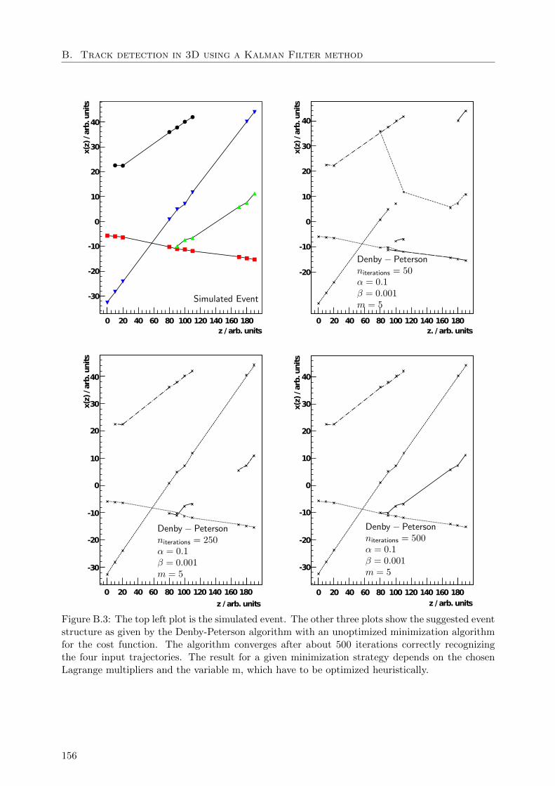
B. Track detection in 3D using a Kalman Filter method
z / arb.units0 20 40 60 80 100 120 140 160 180
x(z)/arb.units
-30
-20
-10
0
10
20
30
40
z. / arb.units0 20 40 60 80 100 120 140 160 180
x(z)/arb.units
-20
-10
0
10
20
30
40
z / arb.units
0 20 40 60 80 100 120140 160180
x(z)/arb.units
-30
-20
-10
0
10
20
30
40
z / arb.units0 20 40 60 80 100 120 140 160 180
x(z)/arb.units
-30
-20
-10
0
10
20
30
40
Figure B.3: The top left plot is the simulated event. The other three plots show the suggested eventstructure as given by the Denby-Peterson algorithm with an unoptimized minimization algorithmfor the cost function. The algorithm converges after about 500 iterations correctly recognizingthe four input trajectories. The result for a given minimization strategy depends on the chosenLagrange multipliers and the variable m, which have to be optimized heuristically.
156

B.5. The Track Tree algorithm
node contains a reference to an observation or a group of observations, a reference to its parentnode (unless it is a seed node) and a list of references to child nodes (if they exist). There is a treefor every seed node to which observations are added sequentially extending and possibly branchingthe tree (e.g. if two observations match the same parent node but are mutually exclusive). The testwhether an observation fits a parent node and the update of the underlying trajectory hypothesisof a branch are performed using a Kalman filter technique. After all observations have been addedto a tree, every leaf node (which refers to a tree node without child nodes) of the tree representsa possible trajectory hypothesis. A cleanup is performed and the remaining paths from root node(the only node within the tree with no parent) to leafs are accepted as particle tracks.
The main reason why the Kalman filter was preferred over the neural network or the Houghtransform approach was that the Kalman filter is a stable method to treat the known uncertaintiesof a realistic detector (multiple scattering - although neglected during the application in this work,resolution effects) and the expected trajectory shapes for charged particles in magnetic fields.There is little to no room for fine-tuning parameters since the known covariance matrices oftrajectory hypotheses and observations allow for an accurate estimation of the probability that acertain observation is related to a certain particle trajectory.
A step-by-step description of the algorithm is given in the following (see also fig. B.4):
1. In the first step, seed nodes are identified. This can happen using either a rule-based approachor an approach related to the Hough transform to identify groups of hits possibly or probablybelonging to the same particle track. This work uses a combinatorial approach where anycombination of two high quality hits is treated as a possible seed15.
2. All remaining observations are ordered according to a metric to produce repeatable results.This work orders observations by their quality Q which is higher if the likelihood that anobservation being related to noise is lower. The choice of the metric can have a significantimpact on the performance of the algorithm in terms of required computing time16.
3. Sequentially observations are added to the track tree. Each observation is tested againsteach leaf node of the track tree.
a) If an observation matches the trajectory hypothesis for a leaf node, it is appended tothe leaf node as a child node and a new trajectory hypothesis is calculated for the newleaf node, using the Kalman filter method to update the trajectory hypothesis of theold leaf node with the added observation.
b) If an observation does not match the trajectory hypothesis for a node, it is recursivelydeferred to the parent of the node until either a node is encountered which matches theobservation while none of the nodes children matches the observation or it is discarded.If a matching node is found, the observation is added as a new branch to the tree with
common explanation be pairwise connected. This means that we assume there is simple check to test whethertwo observation can be matched to a common explanation while testing if n observations to the same explanationrequires O(n2) operations. The task of finding all sub-graphs in which all vertices are pairwise connected withoutprior knowledge of the number of shape of the sub-graphs is known in computer science as the Clique Problem whichis a classical example of a problem believed to be NP-complete. This means that it cannot be guaranteed to besolved in polynomial time, so the actual complexity is always larger than O(nc), c ∈ R. The difference between theoriginal Clique problem and the track finding problem is that the check whether there is a common explanation forn observations can be performed in O(n). This does not change the fact that the complexity is super-polynomial,since the result of a super-polynomial divided by a polynomial (from O(n2) to O(n) means dividing the complexityby n) is still a super-polynomial.
15The reason for this less efficient approach is the low hit multiplicity in each event which allows for this some-what simpler approach which on the other hand has a very low probability of discriminating against certain eventstructures.
16It is unfortunately true as well, that the result of the Kalman filter as an expectation-maximization algorithmalso depends on the order of the added observations. This is one of the reasons, a global least-squares fit is preferredin this work to determine the final trajectory hypotheses.
157
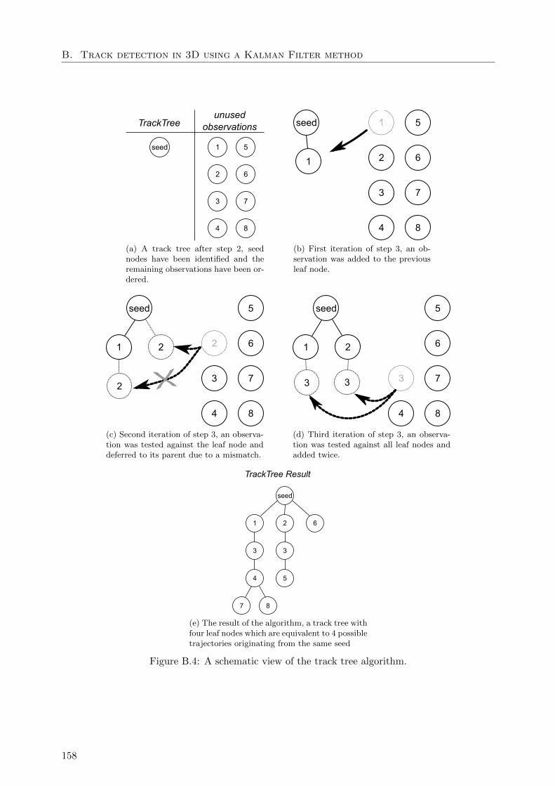
B. Track detection in 3D using a Kalman Filter method
seed 1
2
3
4
5
6
7
8
TrackTreeunused
observations
(a) A track tree after step 2, seednodes have been identified and theremaining observations have been or-dered.
seed
2
3
4
5
6
7
8
1
(b) First iteration of step 3, an ob-servation was added to the previousleaf node.
seed
3
4
5
6
7
8
1
2
2
(c) Second iteration of step 3, an observa-tion was tested against the leaf node anddeferred to its parent due to a mismatch.
seed
4
5
6
7
8
1 2
3 3
(d) Third iteration of step 3, an observa-tion was tested against all leaf nodes andadded twice.
TrackTree Result
seed
4 5
7 8
61 2
33
(e) The result of the algorithm, a track tree withfour leaf nodes which are equivalent to 4 possibletrajectories originating from the same seed
Figure B.4: A schematic view of the track tree algorithm.
158

B.5. The Track Tree algorithm
the matching node as parent and a new trajectory hypothesis is calculated for the newleaf node.
4. After all observations have been added, all leafs of the tree are tested whether the path fromroot to leaf forms an acceptable track. If the track is not acceptable, the leaf is discarded andthe test is repeated for its parent if the parent has now become a leaf node. All remainingpaths from tree root to leaf nodes form the accepted tracks.
The algorithm described above is similar to the ranger -algorithm used for the HERA-B exper-iment [158,159].
159


Appendix C
Track Fit and Detector Alignment
C.1 The linear least-squares fit and the Gauss-Markov theorem
Consider a vector of n measurements b ∈ Y ⊂ Rn with an uncertainty that follows the multi-variatenormal distribution with n×n covariance matrix Σb. Let the mapping f : X → Y be a theory that
can be parametrized by a vector ξ ∈ X ⊂ Rm (m ≤ n). The goal of the linear least-squares fit is todetermine the most-probable vector ξ given b. For this purpose we must write down an expressionfor the probability that ξ describes the truth when b was measured. This can be achieved usingBayes’ theorem.
Bayes’ theorem states that the probability of a vector ξ being true given an observation b isconnected to the probability of b given ξ in the following manner.
π(ξ|b) =π(b|ξ)π(ξ)∫
Xdξ′π(b|ξ′)π(ξ′)
(C.1)
From our precondition that the uncertainties for the measurements b are normal distributed wecan write down π(b|ξ) as:
π(b|ξ) = CN exp
(−1
2
(f(ξ)− b
)†Σ−1
b
(f(ξ)− b
))(C.2)
with normalization constant1 CN . Let us further define the convex neighborhood Nb ⊂ Y of
the measurement b so that ξ ∈ f−1(Nb) ⊂ X and∫
f−1(Nb)dξπ(b|ξ) ≈
∫Xdξπ(b|ξ). Each value for
ξ ∈ f−1(Nb) is assumed to be an approximately equally likely parameter vector.2 so π(ξ) ≈ constand Bayes theorem can in our case be simplified to:
π(ξ|b) ≈ π(b|ξ)π(ξ)∫f−1(Nb)
dξ′π(b|ξ′)π(ξ′)≈ π(b|ξ)∫
f−1(Nb)dξ′π(b|ξ′)
≈ π(b|ξ) (C.3)
1CN is chosen so that∫Xdξπ(b|ξ) = 1, in general CN 6= 1√
2πndet(Σ
b)
which would normalize the usual multi-variate
normal distribution.2In reality each value for ξ ∈ f−1(Nb) is often not equally likely although it is usually inferred since the probability
distribution π(ξ) is in most cases a priori unknown. It is important to note that the linear least-squares fit in itssimplest form is not capable of dealing with a non-flat distribution π(ξ). If it is known that some values for ξ aremore likely than others it should be taken into account as a regularization which is discussed in more detail laterin this section. Otherwise, the result of the maximization of π(ξ|b) will be distorted. A known way to address thisissue is applying a more general iterative expectation-maximization algorithm [160] which I shall no discuss in thiswork.
161
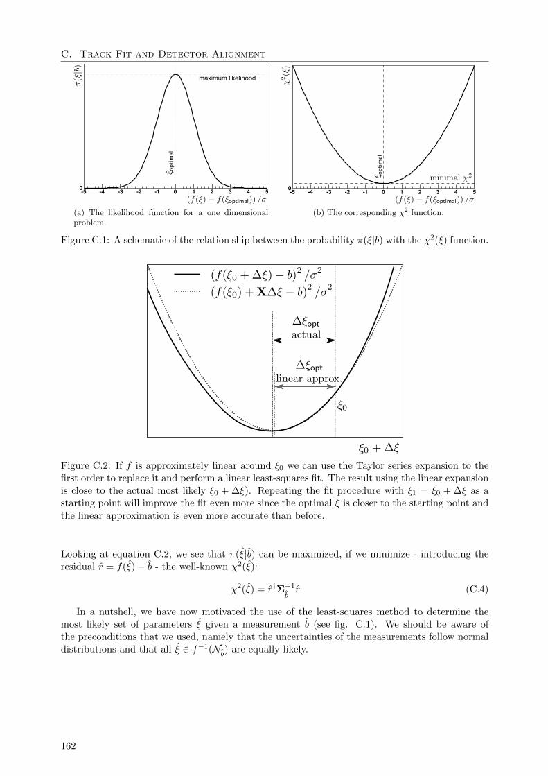
C. Track Fit and Detector Alignment
-5 -4 -3 -2 -1 0 1 2 3 4 50
maximum likelihood
(a) The likelihood function for a one dimensionalproblem.
-5 -4 -3 -2 -1 0 1 2 3 4 50
(b) The corresponding χ2 function.
Figure C.1: A schematic of the relation ship between the probability π(ξ|b) with the χ2(ξ) function.
Figure C.2: If f is approximately linear around ξ0 we can use the Taylor series expansion to thefirst order to replace it and perform a linear least-squares fit. The result using the linear expansionis close to the actual most likely ξ0 + ∆ξ). Repeating the fit procedure with ξ1 = ξ0 + ∆ξ as astarting point will improve the fit even more since the optimal ξ is closer to the starting point andthe linear approximation is even more accurate than before.
Looking at equation C.2, we see that π(ξ|b) can be maximized, if we minimize - introducing theresidual r = f(ξ)− b - the well-known χ2(ξ):
χ2(ξ) = r†Σ−1
br (C.4)
In a nutshell, we have now motivated the use of the least-squares method to determine themost likely set of parameters ξ given a measurement b (see fig. C.1). We should be aware ofthe preconditions that we used, namely that the uncertainties of the measurements follow normaldistributions and that all ξ ∈ f−1(Nb) are equally likely.
162

C.2. Limiting step sizes and parameters with regularized least-squares
In order to simplify our task, we assume that f is linear or at least can be locally linearlyapproximated within f−1(Nb) around a given start parameter vector ξ0 (see fig. C.2):
f(ξ0 + ∆ξ
)≈ f
(ξ0
)+ X∆ξ (C.5)
⇒ r = X∆ξ + f(ξ0)− b (C.6)
X =
∂f(ξ)1∂ξ1
· · · ∂f(ξ)1∂ξm
.... . .
...∂f(ξ)n∂ξ1
· · · ∂f(ξ)n∂ξm
(C.7)
where X is the n×m matrix Jacobi-matrix and |∆ξ| is small so that f(ξ0) + X∆ξ ∈ Nb. Given a
starting point ξ0 we now want to determine a ∆ξ so that ξ0 + ∆ξ minimizes χ2(ξ).
χ2(ξ0 + ∆ξ) = ∆ξ†X†Σ−1
bX∆ξ +
(f(ξ0)− b
)†Σ−1
b
(f(ξ0)− b
)+∆ξ†X†Σ−1
b
(f(ξ0)− b
)+(f(ξ0)− b
)†Σ−1
bX∆ξ (C.8)
Given that χ2(ξ0 + ∆ξ) is real, quadratic in ∆ξ, f(ξ0) and b as well as that Σ−1
bis symmet-
ric positive-definite, we know that Σ−1
bhas a single global minimum at ∇∆ξχ
2(ξ0 + ∆ξ) = 0.Expanding this equation we obtain:
0 = 2X†Σ−1
bX∆ξ + 2X†Σ−1
b
(f(ξ0)− b
)(C.9)
If X†Σ−1
bX has full rank, we can then simply determine ∆ξ as:
∆ξ =(X†Σ−1
bX)−1
X†Σ−1
b
(b− f(ξ0)
)(C.10)
This is the best linear unbiased estimator of the generalized least-squares fit as predicted by theGauss-Markov theorem in the extension by Aitken [161].
The covariance matrix for the determined ∆ξ can be determined using error propagation.
Σ∆ξ =(X†Σ−1
bX)−1
X†Σ−1
bΣbΣ
−1
bX(X†Σ−1
bX)−1
=(X†Σ−1
bX)−1
(C.11)
C.2 Limiting step sizes and parameters with regularizedleast-squares
In the previous subsection, the generalized least-squares method for fitting measurements to aparametrized theory was introduced. Let us take a closer look at the assumptions that were made.
First, we assumed that π(ξ) was flat in Nb. If this is not the case, we have to find an expression
for π(ξ) in order to revise the expression for π(ξ|b). Again, we assume that the probabilitydistribution for π(ξ) follows a multivariate normal distribution3 around a most likely parametervector ξ∗ with covariance matrix Γξ:
π(ξ) = CN exp
(−1
2
(ξ − ξ∗
)†Γ−1
ξ
(ξ − ξ∗
))(C.12)
3This is usually not the case. See next subsection for a method to deal with non-Gaussian probability distribu-tions.
163
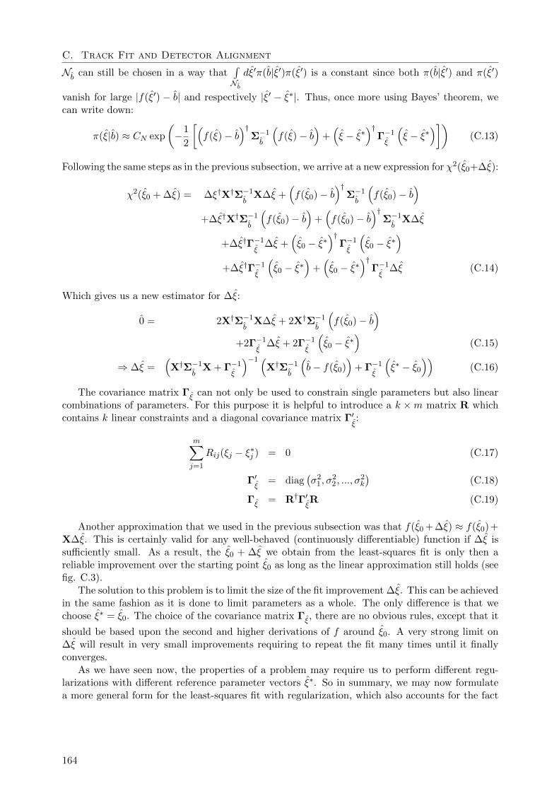
C. Track Fit and Detector Alignment
Nb can still be chosen in a way that∫Nbdξ′π(b|ξ′)π(ξ′) is a constant since both π(b|ξ′) and π(ξ′)
vanish for large |f(ξ′) − b| and respectively |ξ′ − ξ∗|. Thus, once more using Bayes’ theorem, wecan write down:
π(ξ|b) ≈ CN exp
(−1
2
[(f(ξ)− b
)†Σ−1
b
(f(ξ)− b
)+(ξ − ξ∗
)†Γ−1
ξ
(ξ − ξ∗
)])(C.13)
Following the same steps as in the previous subsection, we arrive at a new expression for χ2(ξ0+∆ξ):
χ2(ξ0 + ∆ξ) = ∆ξ†X†Σ−1
bX∆ξ +
(f(ξ0)− b
)†Σ−1
b
(f(ξ0)− b
)+∆ξ†X†Σ−1
b
(f(ξ0)− b
)+(f(ξ0)− b
)†Σ−1
bX∆ξ
+∆ξ†Γ−1
ξ∆ξ +
(ξ0 − ξ∗
)†Γ−1
ξ
(ξ0 − ξ∗
)+∆ξ†Γ−1
ξ
(ξ0 − ξ∗
)+(ξ0 − ξ∗
)†Γ−1
ξ∆ξ (C.14)
Which gives us a new estimator for ∆ξ:
0 = 2X†Σ−1
bX∆ξ + 2X†Σ−1
b
(f(ξ0)− b
)+2Γ−1
ξ∆ξ + 2Γ−1
ξ
(ξ0 − ξ∗
)(C.15)
⇒ ∆ξ =(X†Σ−1
bX + Γ−1
ξ
)−1 (X†Σ−1
b
(b− f(ξ0)
)+ Γ−1
ξ
(ξ∗ − ξ0
))(C.16)
The covariance matrix Γξ can not only be used to constrain single parameters but also linearcombinations of parameters. For this purpose it is helpful to introduce a k ×m matrix R whichcontains k linear constraints and a diagonal covariance matrix Γ′
ξ:
m∑j=1
Rij(ξj − ξ∗j ) = 0 (C.17)
Γ′ξ
= diag(σ2
1, σ22, ..., σ
2k
)(C.18)
Γξ = R†Γ′ξR (C.19)
Another approximation that we used in the previous subsection was that f(ξ0 + ∆ξ) ≈ f(ξ0) +X∆ξ. This is certainly valid for any well-behaved (continuously differentiable) function if ∆ξ issufficiently small. As a result, the ξ0 + ∆ξ we obtain from the least-squares fit is only then areliable improvement over the starting point ξ0 as long as the linear approximation still holds (seefig. C.3).
The solution to this problem is to limit the size of the fit improvement ∆ξ. This can be achievedin the same fashion as it is done to limit parameters as a whole. The only difference is that wechoose ξ∗ = ξ0. The choice of the covariance matrix Γξ, there are no obvious rules, except that it
should be based upon the second and higher derivations of f around ξ0. A very strong limit on∆ξ will result in very small improvements requiring to repeat the fit many times until it finallyconverges.
As we have seen now, the properties of a problem may require us to perform different regu-larizations with different reference parameter vectors ξ∗. So in summary, we may now formulatea more general form for the least-squares fit with regularization, which also accounts for the fact
164
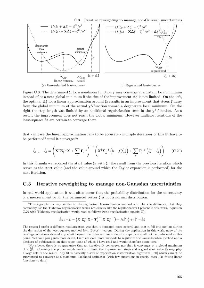
C.3. Iterative reweighting to manage non-Gaussian uncertainties
degenerate local
minimumglobal
minimum
(a) Unregularized least-squares. (b) Regularized least-squares.
Figure C.3: The determined ξi for a non-linear function f may converge at a distant local minimuminstead of at a near global minimum if the size of the improvement ∆ξ is not limited. On the left,the optimal ∆ξ for a linear approximation around ξ0 results in an improvement that steers ξ awayfrom the global minimum of the actual χ2-function toward a degenerate local minimum. On theright the step length was limited by an additional regularization term in the χ2-function. As aresult, the improvement does not reach the global minimum. However multiple iterations of theleast-squares fit are certain to converge there.
that - in case the linear approximation fails to be accurate - multiple iterations of this fit have tobe performed4 until it converges5:
ξi+1 − ξi =
(X†Σ−1
bX +
∑r
Γ−1r
)−1(X†Σ−1
b
(b− f(ξi)
)+∑r
Γ−1r
(ξ∗r − ξi
))(C.20)
In this formula we replaced the start value ξ0 with ξi, the result from the previous iteration whichserves as the start value (and the value around which the Taylor expansion is performed) for thenext iteration.
C.3 Iterative reweighting to manage non-Gaussian uncertainties
In real world application it will often occur that the probability distribution for the uncertaintyof a measurement or for the parameter vector ξ is not a normal distribution.
4This algorithm is very similar to the regularized Gauss-Newton method with the sole difference, that theycommonly use the Tikhonov regularization which not exactly like the regularization I present in this work. EquationC.20 with Tikhonov regularization would read as follows (with regularization matrix T):
ξi+1 − ξi =(X†Σ−1
bX + T
)−1
X†Σ−1
b
(b− f(ξ∗)
)+ (ξ∗ − ξi)
The reason I prefer a different regularization was that it appeared more general and that it fell into my lap duringthe derivation of the least-squares method from Bayes’ theorem. During the application in this work, none of thetwo regularizations showed any merit beyond the other and an in depth comparison shall not be performed at thispoint. Without going into more detail, there are even more methods to regularize the Gauss-Newton method and aplethora of publications on that topic, none of which I have read and would therefore quote here.
5Nota bene, there is no guarantee that an iterative fit converges, nor that it converges at a global maximumof π(ξ|b). Choosing the proper regularization to limit the improvement steps and a good start value ξ0 may playa large role in the result. Any fit is basically a sort of expectation maximization algorithm [160] which cannot beguaranteed to converge at a maximum likelihood estimator (with few exceptions in special cases like fitting linearfunctions to data).
165

C. Track Fit and Detector Alignment
Take for example a charged-particle hitting a scintillating fiber module which does not provideany positional information along a fiber except that the fiber was hit. Let bf be the measuredparticle position along the fiber6 of length λf , ξf the reconstructed particle position along thefiber and σf be the uncertainty of the measurement. In reality we have a uniform distribution forπ(ξf |bf ) which cannot be described in terms of the basic least-squares method since that has astrong requirement on normal distributed probabilities since minimizes the χ2 quantity. Still, ourfirst impulse would be to choose a σf reflect the size of the fiber:
π(ξf |bf )actual =
1λf
for |ξf − bf | ≤λf2
0 for |ξf − bf | >λf2
(C.21)
π(ξf |bf )assumed = CN exp
(−
(ξf − bf )2
2σ2f
)(C.22)
The problem is of course, that if we choose σf to small, ξf will be pulled towards the fiber centerand if we choose σf too large, we run the risk of allowing values of ξf which are actually impossiblesince they lie outside the fiber.
One solution to the problem makes use of the fact, that we perform an iterative fit which be-comes more accurate with each iteration and allows us to modify σf with each iteration. Formally,we retain the normal probability distribution but we perform a non-linear coordinate transforma-tion g on ξf − bf , so that:
π(ξf |bf )actual = CN exp
(−1
2g(ξf − bf )2
)(C.23)
For this special case, we may write down χ2 as:
χ2f = g(ξf,0 + ∆ξf − bf )2 ≈
(g(ξf,0 − bf ) + g′(ξf,0 − bf ) ·∆ξf
)2(C.24)
(C.25)
From comparison with the original form of the χ2 in the one-dimensional case we can thereforederive:
σf (ξf,0 − bf )−2 ≈g(ξf,0 − b)2 + 2g(ξf,0 − bf )g′(ξf,0 − bf )∆ξ + g′(ξf,0 − bf )2∆ξ2
(ξf,0 − bf )2 + 2(ξf,0 − bf )∆ξ + ∆ξ2(C.26)
This expression can be simplified using two further approximations. For one, we use ∆ξ2 ≈ 0 - thiswas actually already used during the Taylor expansion of g(ξ − b). And secondly we use that anyconstant term (not depending on ∆ξ) added to χ2 does not change the location of its minimumor its slope that determines the next minimization step:
σf (ξf,0, bf )−2 ≈g(ξf,0 − bf )g′(ξf,0 − bf )(ξf,0 − bf + 2∆ξ)
(ξf,0 − bf )2 + 2(ξf,0 − bf )∆ξ(C.27)
=g(ξf,0 − b)g′(ξf,0 − b)
ξf,0 − bf(C.28)
Essentially, what we have done now, is we have written down an expression for σf (ξf,0, bf ) inthe one-dimensional case that lets us simulate the behavior of the actual probability distributionπ(ξf,0 + ∆ξ|b)actual around ξf,0, so that:
π(ξf |bf )actual = CN exp
(−1
2g(ξf − bf )2
)≈ C ′N exp
((ξf,0 + ∆ξ − bf )2
2σf (ξf,0, bf )2
)(C.29)
166
C.3. Iterative reweighting to manage non-Gaussian uncertainties
-1 -0.8 -0.6 -0.4 -0.2 0 0.2 0.4 0.6 0.8 10
0.05
0.1
0.15
0.2
0.25
0.3
0.35
0.4
0.45
Figure C.4: In order to approximate the uniform uncertainty for the position along the fiber, afunction g(f(ξ)f−bf ) is introduced which approximates the uniform probability distribution. Thiswork uses α = 16.
To conclude our simple example with the position along a fiber, we may for example choose
g(f(ξ)f − bf ) =(f(ξ)f − bf )/(2λf )
)α(see fig. C.4). While in principle the higher α, the more
similar the probability distribution becomes to the uniform distribution that we aim for, we haveto keep in mind that we introduced an additional Taylor expansion deriving σf (ξf,0, bf ) that mayrequire imposing limits on ∆ξ based on the higher derivations of g at ξf,0 − bf to achieve aconvergence of the iterative fit. In a nutshell, a higher α requires a smaller step size ∆ξ and thusmore iterations to converge than a smaller α with a larger step size.
Moving on to the multi-dimensional case, the formulation above may still be a helpful approx-imation7, however the proper solution requires us to introduce a new term J in the equation thatwe wish to solve:
χ2 = g(f(ξ0) + X∆ξ − b)†Σ−1g(f(ξ0) + X∆ξ − b) (C.30)
≈ (g(f(ξ0)− b) + JX∆ξ)†Σ−1(g(f(ξ0)− b) + JX∆ξ) (C.31)
where J is the (square and symmetric positive-definite) Jacobi-matrix of g. The solution of theleast-squares problem becomes in the most general case:
ξi+1 − ξi = −
(X†J†
bΣ−1
bJbX +
∑r
J†rΓ−1r Jr
)−1
·(X†J†
bΣ−1
bgb
(f(ξi − b)
)+∑r
J†rΓ−1r gr
(ξi − ξ∗r
))(C.32)
Here, the reweighting is not only used for the measurement residual (gb, Jb), but also for theregularization (gr, Jr). Both track and alignment fits performed in this work are based on thisequation.
6bf is always the central position of the fiber for lack of further information.7In fact, for many problems where the weighting matrix Σ−1 is diagonal, choosing its diagonal entries as follows
is still an improvement over a fixed Σ−1:
σ−2i =
g(f(ξ0)i − bi)g′(f(ξ0)i − bi)f ′(ξ0)i
f(ξ0)i − bi
Nonetheless, this approximation is not optimal.
167
C. Track Fit and Detector Alignment
As criterion for the convergence of the fit the relative size of the update ξi+1 − ξi is used andcompared with a chosen ε: (
ξi+1 − ξi)
V(ξi+1 − ξi
)(C.33)
where V is the covariance matrix of the determined parameters:
V =
(X†J†
bΣ−1
bJbX +
∑r
J†rΓ−1r Jr
)−1
(C.34)
C.4 Solving alignment matrix equations
Inversions of k × k matrices as well as solving matrix equations using for example Cholesky- andQR-decomposition methods [162] have in general a computational cost of O(k3). The size of thealignment matrices for a detector depends on the number of tracks that are used for alignmentwhich is around 100,000. At 4 parameters per track for a straight trajectory this results in a400,000× 400,000 matrix to be inverted. The first difficulty that arises when handling these largematrices is memory. A dense representation of such a matrix requires 1.2 TB of memory. Sincemost of the entries are zero, it makes sense to adopt a sparse matrix format only storing non-zero entries, as for example the column-compressed storage (CCS) or Harwell-Boeing format [163]which reduces the matrix size to only a few hundred megabytes.
This work uses Timothy Davis’ SuiteSparse software package [164] to operate on large matrices.It contains efficient, in part multi-threaded methods to multiply, add and factorize sparse matrices.In particular, the QR-factorization of this package is used to solve the alignment matrix equationor invert matrices. It decomposes a matrix A into a product of matrices QR where Q is orthogonal
and R is upper triangular.∣∣∣Ax− b∣∣∣ is minimal for Rx = QT b where R =
(R′
0
)with R′ being
guaranteed to be invertible. The equation can be solved easily by back-solving using that R′ isupper triangular. Furthermore, R′ can be inverted by back-solving R′ = 1.
A further improvement for solving the alignment equations can be achieved after an examina-tion of the alignment matrix equation, following the Ansatz of the Millepede software package [165].The matrix X can be separated into s blocks Gi pertaining to the alignment parameters and blocksLi pertaining to trajectory parameters. The general shape of X can thus be written down as:
X =
G1 L1 0 0...
.... . .
...Gs 0 0 Ls
(C.35)
The shape of the covariance matrix of the measurements Σ is the one of a block-diagonal matrixand therefore its inverse is block diagonal too.
Σ−1
b=
Σ−11 0 0
0. . . 0
0 0 Σ−1s
(C.36)
⇒ X†Σ−1
bX =
∑s
G†sΣ−1s Gs G†1Σ
−11 L1 · · · G†sΣ
−11 Ls
L†1Σ−11 G1 L†1Σ
−11 L1 0 0
... 0. . . 0
L†sΣ−1s Gs 0 0 L†sΣ−1
s Ls
(C.37)
168

C.4. Solving alignment matrix equations
Finally, one may add the regularization matrix∑r
Γ−1r which should also be of block-diagonal shape
for the alignment, regularizing alignment parameters∑r
Λ−1r separately from track parameters∑
rΘ−1r,1 ...
∑r
Θ−1r,s
∑r
Γ−1r =
∑r
Λ−1r 0 0 0
0∑r
Θ−1r,1 0 0
0 0. . . 0
0 0 0∑r
Θ−1r,s
(C.38)
V−1 =
(A BB† C
)A =
(∑s
G†sΣ−1s Gs +
∑r
Λ−1r
)B =
(G†1Σ
−11 L1 · · · G†sΣ
−11 Ls
)
C =
L†1Σ
−11 L1 +
∑r
Θ−1r,1 0 0
0. . . 0
0 0 L†sΣ−1s Ls +
∑r
Θ−1r,s
The matrix V−1 can be inverted using Schur’s complement V′ =
(A−BC−1B†
)−1, which can be
calculated efficiently using that C is sparse and block-diagonal (it can be inverted in O(s) wheres is the number of tracks in the alignment fit). The matrix V′ is dense but its size is fixed by thenumber of alignment parameters.
V =
(V′ −V′BC−1
−C−1B†V′ C−1 + C−1B†V′BC−1
)(C.39)
169
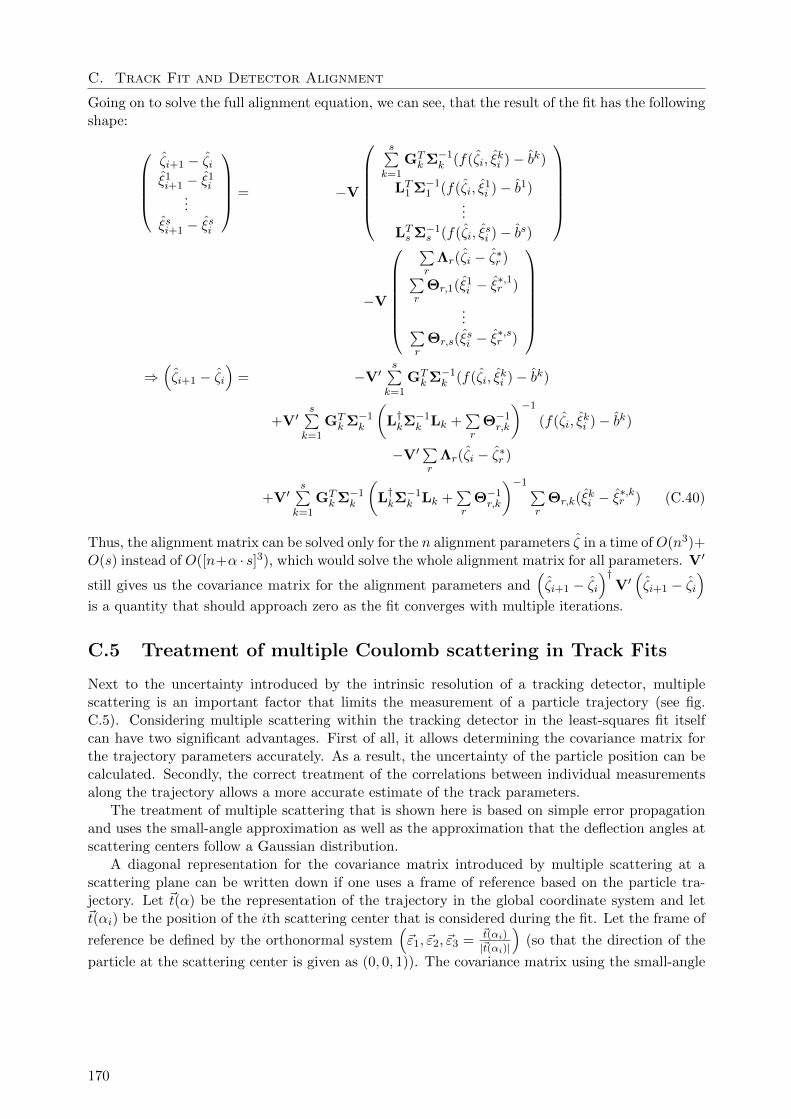
C. Track Fit and Detector Alignment
Going on to solve the full alignment equation, we can see, that the result of the fit has the followingshape:
ζi+1 − ζiξ1i+1 − ξ1
i...
ξsi+1 − ξsi
= −V
s∑
k=1
GTkΣ−1
k (f(ζi, ξki )− bk)
LT1 Σ−11 (f(ζi, ξ
1i )− b1)
...
LTs Σ−1s (f(ζi, ξ
si )− bs)
−V
∑r
Λr(ζi − ζ∗r )∑r
Θr,1(ξ1i − ξ
∗,1r )
...∑r
Θr,s(ξsi − ξ
∗,sr )
⇒(ζi+1 − ζi
)= −V′
s∑k=1
GTkΣ−1
k (f(ζi, ξki )− bk)
+V′s∑
k=1
GTkΣ−1
k
(L†kΣ
−1k Lk +
∑r
Θ−1r,k
)−1
(f(ζi, ξki )− bk)
−V′∑r
Λr(ζi − ζ∗r )
+V′s∑
k=1
GTkΣ−1
k
(L†kΣ
−1k Lk +
∑r
Θ−1r,k
)−1∑r
Θr,k(ξki − ξ
∗,kr ) (C.40)
Thus, the alignment matrix can be solved only for the n alignment parameters ζ in a time ofO(n3)+O(s) instead of O([n+α · s]3), which would solve the whole alignment matrix for all parameters. V′
still gives us the covariance matrix for the alignment parameters and(ζi+1 − ζi
)†V′(ζi+1 − ζi
)is a quantity that should approach zero as the fit converges with multiple iterations.
C.5 Treatment of multiple Coulomb scattering in Track Fits
Next to the uncertainty introduced by the intrinsic resolution of a tracking detector, multiplescattering is an important factor that limits the measurement of a particle trajectory (see fig.C.5). Considering multiple scattering within the tracking detector in the least-squares fit itselfcan have two significant advantages. First of all, it allows determining the covariance matrix forthe trajectory parameters accurately. As a result, the uncertainty of the particle position can becalculated. Secondly, the correct treatment of the correlations between individual measurementsalong the trajectory allows a more accurate estimate of the track parameters.
The treatment of multiple scattering that is shown here is based on simple error propagationand uses the small-angle approximation as well as the approximation that the deflection angles atscattering centers follow a Gaussian distribution.
A diagonal representation for the covariance matrix introduced by multiple scattering at ascattering plane can be written down if one uses a frame of reference based on the particle tra-jectory. Let ~t(α) be the representation of the trajectory in the global coordinate system and let~t(αi) be the position of the ith scattering center that is considered during the fit. Let the frame of
reference be defined by the orthonormal system(~ε1, ~ε2, ~ε3 =
~t(αi)
|~t(αi)|
)(so that the direction of the
particle at the scattering center is given as (0, 0, 1)). The covariance matrix using the small-angle
170
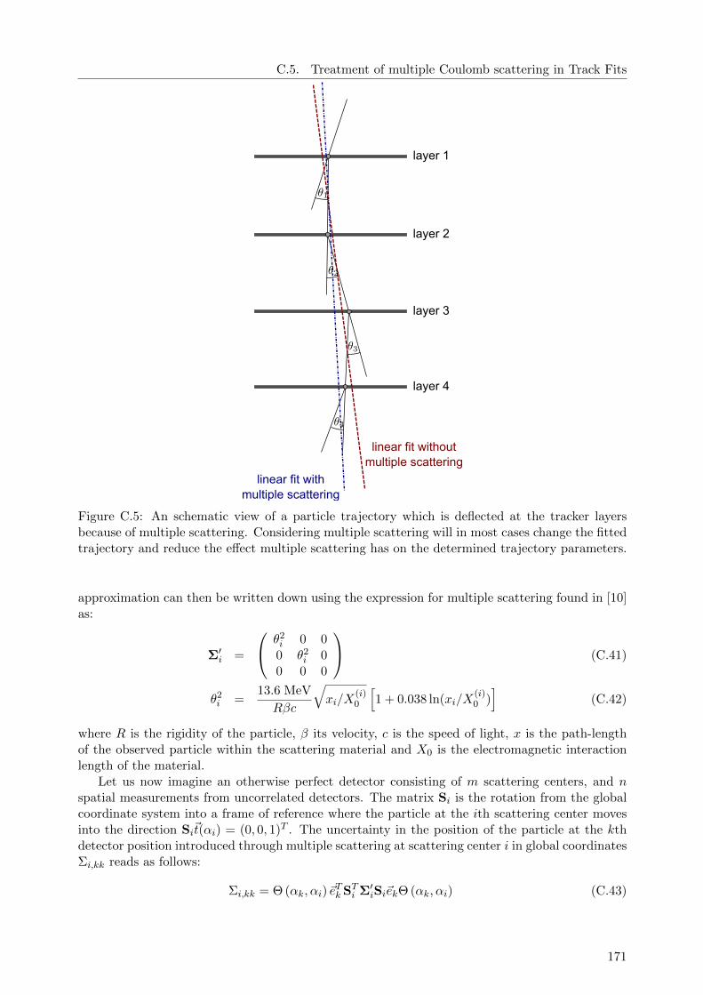
C.5. Treatment of multiple Coulomb scattering in Track Fits
layer 1
layer 2
layer 3
layer 4
linear fit withoutmultiple scattering
linear fit withmultiple scattering
Figure C.5: An schematic view of a particle trajectory which is deflected at the tracker layersbecause of multiple scattering. Considering multiple scattering will in most cases change the fittedtrajectory and reduce the effect multiple scattering has on the determined trajectory parameters.
approximation can then be written down using the expression for multiple scattering found in [10]as:
Σ′i =
θ2i 0 00 θ2
i 00 0 0
(C.41)
θ2i =
13.6 MeV
Rβc
√xi/X
(i)0
[1 + 0.038 ln(xi/X
(i)0 )]
(C.42)
where R is the rigidity of the particle, β its velocity, c is the speed of light, x is the path-lengthof the observed particle within the scattering material and X0 is the electromagnetic interactionlength of the material.
Let us now imagine an otherwise perfect detector consisting of m scattering centers, and nspatial measurements from uncorrelated detectors. The matrix Si is the rotation from the globalcoordinate system into a frame of reference where the particle at the ith scattering center movesinto the direction Si~t(αi) = (0, 0, 1)T . The uncertainty in the position of the particle at the kthdetector position introduced through multiple scattering at scattering center i in global coordinatesΣi,kk reads as follows:
Σi,kk = Θ (αk, αi)~eTk STi Σ′iSi~ekΘ (αk, αi) (C.43)
171
C. Track Fit and Detector Alignment
where ~ek is a normal vector pointing into the direction of the measured coordinate, ~t(αk) gives thepoint where the particle trajectory intersects with the kth tracker layer and Θ (αk, αi) gives thedownstream distance between scattering center and tracker layer:
Θ (αk, αi) =
0 ∧ αk ≤ αi|~t(αk)− ~t(αi)| ∧ αk > αi
(C.44)
The correlation Σi,kl between two measurements k and l which arises from multiple scatteringat the ith scattering center can furthermore be given as:
Σi,kl = Θ (αk, αi)~eTk STi Σ′iSi~elΘ (αl, αi) (C.45)
The full covariance matrix Σ can then be calculated as a simple sum over all scattering centersadding the single point resolution Σk,res for individual measurements k on the diagonal:
Σkl =∑i
Θ (αk, αi)~eTk STi Σ′iSi~elΘ (αl, αi) + δklΣk,res (C.46)
This inverse of this matrix Σ−1 is then the weighting matrix which is introduced into the fit matrixas has been discussed in the previous sections.
Upon closer examination of the resulting covariance matrix, we find that we have an additionaldegree of freedom in the interpretation of multiple scattering. This degree of freedom comes fromthe fact that the evolution of the uncertainty in the position of the trajectory depends on theactual direction of the particle. The covariance matrix of the fitted trajectory (and also - not quiteunimportantly - the fitted parameters) depends on the direction of the particle (see fig. C.6). Ingeneral we can define an arbitrary point of reference along the particle, from which we assumethe trajectory to evolve. By choosing the proper covariance matrix as input for our fit we canoptimize the fit parameters for a point of reference so that the trajectory parameters reflect themost probable state of the particle at that point of reference. All that we have to adjust in ourformulation above is the definition Θ(αi, αk) in order to choose different points of reference. Letα0 be the point along the trajectory for which to optimize, then Θ(αi, αk) can be written downas:
Θ (αk, αi) =
0 ∧ sign (αk − αi) 6= sign (α0− αi)|~t(αk)− ~t(αi)| ∧ sign (αk − αi) = sign (α0− αi)
(C.47)
Another possible optimization would be to calculate the most probable trajectory averaging overthe probabilities for upwards and downwards interpretations.
Θ (αk, αi) =|~t(αk)− ~t(αi)|√
2(C.48)
Which interpretation to prefer depends on the application. For this work the multiple scatteringtreatment is used to calculate the additional uncertainty in the position of the trajectory introducedby multiple scattering. For this purpose it is advantageous to keep the multiple correction of thespatial resolution to a minimum since both the material budget of a scattering center is onlyapproximately known and multiple scattering in general is only handled by an approximation.This is achieved by choosing α0 = αr when investigating the rth detector layer.
172
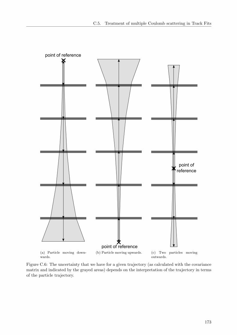
C.5. Treatment of multiple Coulomb scattering in Track Fits
point of reference
(a) Particle moving down-wards.
point of reference(b) Particle moving upwards.
point of reference
(c) Two particles movingoutwards.
Figure C.6: The uncertainty that we have for a given trajectory (as calculated with the covariancematrix and indicated by the grayed areas) depends on the interpretation of the trajectory in termsof the particle trajectory.
173

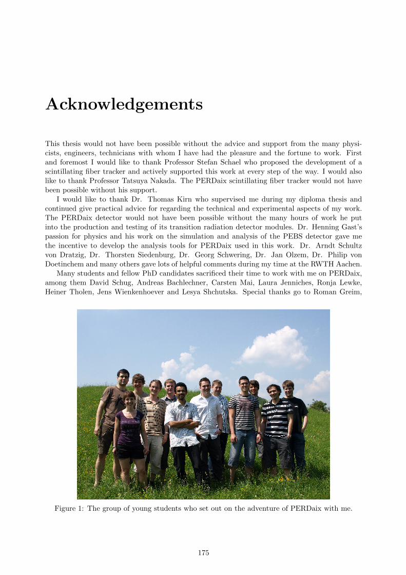
Acknowledgements
This thesis would not have been possible without the advice and support from the many physi-cists, engineers, technicians with whom I have had the pleasure and the fortune to work. Firstand foremost I would like to thank Professor Stefan Schael who proposed the development of ascintillating fiber tracker and actively supported this work at every step of the way. I would alsolike to thank Professor Tatsuya Nakada. The PERDaix scintillating fiber tracker would not havebeen possible without his support.
I would like to thank Dr. Thomas Kirn who supervised me during my diploma thesis andcontinued give practical advice for regarding the technical and experimental aspects of my work.The PERDaix detector would not have been possible without the many hours of work he putinto the production and testing of its transition radiation detector modules. Dr. Henning Gast’spassion for physics and his work on the simulation and analysis of the PEBS detector gave methe incentive to develop the analysis tools for PERDaix used in this work. Dr. Arndt Schultzvon Dratzig, Dr. Thorsten Siedenburg, Dr. Georg Schwering, Dr. Jan Olzem, Dr. Philip vonDoetinchem and many others gave lots of helpful comments during my time at the RWTH Aachen.
Many students and fellow PhD candidates sacrificed their time to work with me on PERDaix,among them David Schug, Andreas Bachlechner, Carsten Mai, Laura Jenniches, Ronja Lewke,Heiner Tholen, Jens Wienkenhoever and Lesya Shchutska. Special thanks go to Roman Greim,
Figure 1: The group of young students who set out on the adventure of PERDaix with me.
175
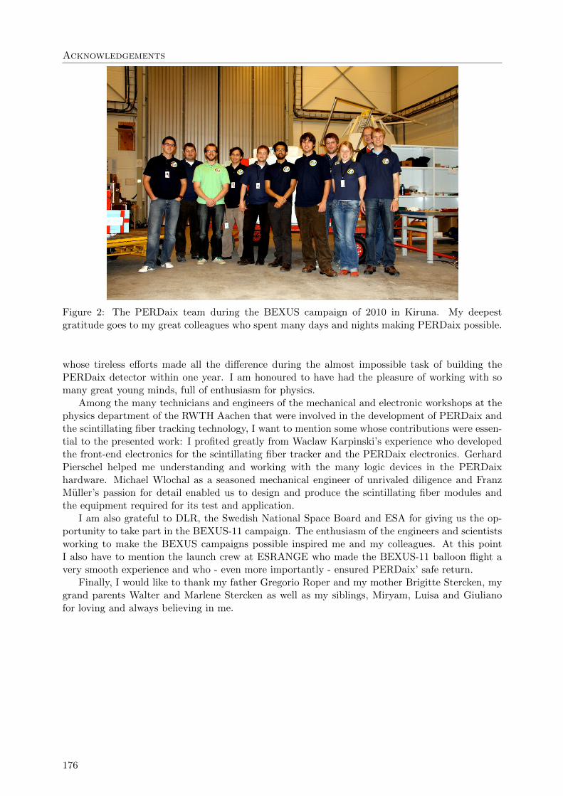
Acknowledgements
Figure 2: The PERDaix team during the BEXUS campaign of 2010 in Kiruna. My deepestgratitude goes to my great colleagues who spent many days and nights making PERDaix possible.
whose tireless efforts made all the difference during the almost impossible task of building thePERDaix detector within one year. I am honoured to have had the pleasure of working with somany great young minds, full of enthusiasm for physics.
Among the many technicians and engineers of the mechanical and electronic workshops at thephysics department of the RWTH Aachen that were involved in the development of PERDaix andthe scintillating fiber tracking technology, I want to mention some whose contributions were essen-tial to the presented work: I profited greatly from Waclaw Karpinski’s experience who developedthe front-end electronics for the scintillating fiber tracker and the PERDaix electronics. GerhardPierschel helped me understanding and working with the many logic devices in the PERDaixhardware. Michael Wlochal as a seasoned mechanical engineer of unrivaled diligence and FranzMuller’s passion for detail enabled us to design and produce the scintillating fiber modules andthe equipment required for its test and application.
I am also grateful to DLR, the Swedish National Space Board and ESA for giving us the op-portunity to take part in the BEXUS-11 campaign. The enthusiasm of the engineers and scientistsworking to make the BEXUS campaigns possible inspired me and my colleagues. At this pointI also have to mention the launch crew at ESRANGE who made the BEXUS-11 balloon flight avery smooth experience and who - even more importantly - ensured PERDaix’ safe return.
Finally, I would like to thank my father Gregorio Roper and my mother Brigitte Stercken, mygrand parents Walter and Marlene Stercken as well as my siblings, Miryam, Luisa and Giulianofor loving and always believing in me.
176

Bibliography
[1] P. von Doetinchem et al. PEBS - Positron electron balloon spectrometer. Nuclear Instru-ments and Methods in Physics Research. Section A, 581(1–2):151–155, Oct 2007.
[2] H. Gast et al. A high resolution scintillating fiber tracker with SiPM readout. NuclearInstruments and Methods in Physics Research. Section A, 581(1–2):423–426, Oct 2007.
[3] R. Greim et al. Silicon photomultiplier arrays - a novel photon detector for a high resolutiontracker produced at FBK-irst, Italy. Nuclear Physics B - Proceedings Supplements, 197(1):83–86, 2008.
[4] R. Greim et al. A high-resolution scintillating fiber tracker with SiPM array readout forcosmic-ray research. In Proceedings of the 31st ICRC, Lodz, pages 1099–1–1099–4, 2009.
[5] A. Bachlechner et al. A New Instrument for Testing Charge-Sign Dependent Solar Modula-tion. In Proceedings of the 31st ICRC, Lodz, pages 1025–1–1025–4, 2009.
[6] B. Beischer et al. A high-resolution scintillating fiber tracker with silicon photomultiplierarray readout. Nuclear Instruments and Methods in Physics Research. Section A, 622:542–554, Jul 2010.
[7] B. Beischer et al. The Development of a high-resolution Scintillating Fiber Tracker withSilicon Photomultiplier Readout. Nuclear Instruments and Methods in Physics Research.Section A, 628(1–2):403–406, 2011.
[8] V. F. Hess. Uber Beobachtungen der durchdringenden Strahlung bei sieben Freiballon-fahrten. Physikalische Zeitschrift, 13:1084–1091, 1912.
[9] S. Swordy. The energy spectra and anisotropies of cosmic rays. Space Science Reviews,99:85–94, 2001.
[10] K. Nakamura et al. (Particle Data Group). The Review of Particle Physics. Journal ofPhysics G: Nuclear and Particle Physics, 37, 2010. 075021.
[11] B. Beischer et al. Perspectives for indirect dark matter search with AMS-2 using cosmic-rayelectrons and positrons. New Journal of Physics, 11:105021, Oct 2009.
[12] R. A. Mewaldt et al. Long-term fluences of energetic particles in the heliosphere. In SOLARAND GALACTIC COMPOSITION: A Joint SOHO/ACE Workshop, pages 165–170, Nov2001.
[13] J. Ryan et al. Solar energetic particles. Space Science Reviews, 93:35–53, Jun 2000.
[14] D. V. Reames. Solar Wind: Energetic Particles. Encyclopedia of Astronomy and Astro-physics, 2002. 2312.
[15] J. R. Jokipii. Anomalous Cosmic Rays. Encyclopedia of Astronomy and Astrophysics, 2000.2320.
177

Bibliography
[16] P. Blasi. Cosmic ray acceleration in supernova remnants. In ICATPP 2010, Villa Olmo,Como 7-8, 2010. arXiv:1012.5005v1.
[17] A. K. Harding and A. G. Muslimov. Particle Acceleration Zones above Pulsar Polar Caps:Electron and Positron Pair Formation Fronts. Astrophysical Journal, 508(1):328–346, Nov1998.
[18] E. Fermi. On the Origin of Cosmic Radiation. Physical Review, 75(8):1169–1174, Apr 1949.
[19] A. R. Bell. The acceleration of cosmic rays in shock fronts - I. Royal Astronomical Society,Monthly Notices, 182:147–156, Jan 1978.
[20] H. Alfven. Momentum spectrum of cosmic radiation. Tellus, 11(1):106–115, Feb 1959.
[21] A. W. Strong et al. Cosmic-ray propagation and interactions in the Galaxy. Annual Reviewof Nuclear and Particle Science, 57:285–327, Jan 2007.
[22] E. N. Parker. Dynamics of the interplanetary gas and magnetic fields. Astrophysical Journal,128:664–676, Nov 1958.
[23] L. Biermann. Kometenschweife und solare Korpuskularstrahlung. Zeitschrift fur Astrophysik,29:274–286, May 1951.
[24] S. M. Krimigis. Imaging the Interaction of the Heliosphere with the Interstellar Mediumfrom Saturn with Cassini. Science Magazine, 326:971–973, 2009.
[25] H. Alfven. Existance of Electromagnetic-Hydrodynamic Waves. Nature, 150:405–406, 1942.
[26] W. M. Elsasser. The Hydromagnetic Equations. Physical Review, 79:183, 1950.
[27] E. N. Parker. Hydromagnetic Dynamo Models. Astrophysical Journal, 122:293–314, 1955.
[28] J. R. Jokipii and B. Thomas. Effects of drift on the transport of cosmic rays. IV - Modulationby a wavy interplanetary current sheet. Astrophysical Journal, 243(1):1115–1122, Feb 1981.
[29] E. Gavryuseva and G. Godoli. Structure and rotation of the large scale solar magneticfield observed at the Wilcox Solar Observatory. Physics and Chemistry of the Earth, PartsA/B/C, 31:68–76, Apr 2006.
[30] E. N. Parker. The passage of energetic charged particles through interplanetary space.Planetary and Space Science, 13(1):9–49, Jan 1965.
[31] L. J. Gleeson and W. I. Axford. Solar Modulation of Galactic Cosmic Rays. AstrophysicalJournal, 154:1011–1026, Dec 1968.
[32] J. R. Jokipii and E. H. Levy. Effects of particle drifts on the solar modulation of galacticcosmic rays. Astrophysical Journal, Letters to the Editor, 213:85–88, Apr 1977.
[33] R. A. Caballero-Lopez et al. Validity of the Force-Field Equation to Describe Cosmic RayModulation. In Proceedings of the 28th International Cosmic Ray Conference, pages 3867–3870, Jul 2003.
[34] J. Alcaraz et al. for the AMS Collaboration. Cosmic Protons. Physics Letters B, 490(1-2):27–35, Sep 2000.
[35] A. W. Strong and I. V. Moskalenko. Propagation of Cosmic-Ray Nucleons in the Galaxy.Astrophysical Journal, 509(1):212–228, Dec 1998.
178

Bibliography
[36] L. Jenniches. Untersuchungen zur solaren Modulation der geladenen kosmischen Hohen-strahlung. Bachelor’s thesis, RWTH Aachen University, 2009.
[37] W. Menn et al. The Absolute Flux of Protons and Helium at the Top of the AtmosphereUsing IMAX. Astrophysical Journal, 533(1):281–297, Apr 2000.
[38] R. Bellotti et al. Balloon measurements of cosmic ray muon spectra in the atmospherealong with those of primary protons and helium nuclei over midlatitude. Physical Review D,60(5):052002–1–052002–15, Jul 1999.
[39] P. Ferrando et al. Latitude variations of ∼ 7 MeV and > 300 MeV cosmic ray electronfluxes in the heliosphere: ULYSSES COSPIN/KET results and implications. Astronomyand Astrophysics, 316:528–537, Dec 1996.
[40] M. Boezio et al. The Cosmic-Ray Antiproton Flux between 3 and 49 GeV. AstrophysicalJournal, 561(2):787–799, Jul 2001.
[41] O. Adriani et al. Observation of an anomalous positron abundance in the cosmic radiation.Nature, 458:607–609, 2009. arXiv:0810.4995v1 [astro-ph].
[42] S. Orito et al. Precision Measurement of Cosmic-Ray Antiproton Spectrum. Physical ReviewLetters, 84(6):1078–1081, Feb 2000.
[43] M. Boezio et al. The Cosmic-Ray Antiproton Flux between 0.62 and 3.19 GeV MeasuredNear Solar Minimum Activity. Astrophysical Journal, 487(1), Apr 1997.
[44] R. L. Golden. Measurement of the Positron to Electron Ratio in the Cosmic Rays above5 GeV. Astrophysical Journal Letters, 457(2):L103–L106, Feb 1996.
[45] K. Abe et al. for the BESS collaboration. Measurement of the cosmic-ray low-energy antipro-ton spectrum with the first BESS-Polar Antarctic flight. Physics Letters B, 670(2):103–108,Dec 2008.
[46] K. Yamato et al. Measurements of atmospheric antiprotons. Physics Letters B, 632(4):475–479, Jan 2006.
[47] Y. Shikaze et al. Measurements of 0.2− 20 GeV/n cosmic-ray proton and helium spectrafrom 1997 through 2002 with the BESS spectrometer. Astroparticle Physics, 28(1):154–167,Sep 2007.
[48] J. M. Clem et al. Charge sign dependence of cosmic ray modulation near a rigidity of 1 GV.Journal of Geophysical Research, 105(A10):23099–23106, Oct 2000.
[49] M. S. Potgieter. Cosmic Rays in the Inner Heliosphere: Insights from Observations, Theoryand Models. Space Science Reviews, Feb 2011. DOI: 10.1007/s11214-011-9750-7.
[50] P. Bobik et al. 2D Stochastic Monte Carlo to evaluate the modulation of GCR for inner andouter solar system planets. In Proceedings of the 10th Conference on Astroparticle, Particleand Space Physics, Detectors and Medical Physics Applications, pages 881–885, Oct 2007.
[51] E. W. Cliver and A. G. Ling. 22 Year Patterns in the Relationship of Sunspot Number andTilt Angle to Cosmic-Ray Intensity. Astrophysical Journal Letters, 551(2):L189–L192, Apr2001.
[52] D. J. Gross and F. Wilczek. Ultraviolet behaviour of non-abelian gauge theories. PhysicalReview Letters, 30(26):1343–1346, Jun 1973.
179

Bibliography
[53] H. Becquerel. Sur les radiations invisibles emises par les corps phosphorescents. Comptesrendus hebdomadaires des seances de l’Academie de sciences, 122:501–503, 1896.
[54] T. Nakamura et al. The OPERA film: New nuclear emulsion for large-scale, high-precisionexperiments. Nuclear Instruments and Methods in Physics Research A, 556:80–86, 2006.
[55] D. A. Glaser. Some Effects of Ionizing Radiation on the Formation of Bubbles in Liquids.Physical Review, 87:665, 1952.
[56] E. Rutherford and H. Geiger. A Method of Counting the Number of Alpha Particles fromRadioactive Matter. Memoirs of the Manchester Literary and Philosphical Society, 52(9):1–3,1908.
[57] B. A. Dolgoshein, B. U. Rodionov, and B. I. Luchkov. Streamer Chamber. Nuclear Instru-ments and Methods, 29:270–276, 1964.
[58] J. G. Rushbrooke et al. The UA5 Streamer Chamber Experiment at the SPS p-pbar Collider.Physica Scripta, 23(4B):642–648, 1981.
[59] G. Charpak, R. Bouclier, T. Bressan, J. Favier, and C. Zupancic. The use of multiwireproportional counters to select and localize charged particles. Nuclear Instruments andMethods, 62(3):262–268, 1968.
[60] W. Riegler. High accuracy wire chambers. Nuclear Instruments and Methods in PhysicsResearch A, 494:173–178, 2002.
[61] A. Yamamoto et al. Balloon-borne experiment with a superconducting solenoidal magnetspectrometer. Advances in Space Research, 14(2):75–87, Feb 1994.
[62] Ph. von Doetinchem et al. Performance of the AMS-02 Transition Radiation Detector.Nuclear Instruments and Methods in Physics Research. Section A, 558(2):526–535, Mar 2006.
[63] H. J. Hilke. Time projection chambers. Reports on Progress in Physics, 73(116201):1–36,Oct 2010.
[64] W. K. Rontgen. On a new kind of rays. Science, 3(59):227–231, Feb 1896.
[65] J. W. Coltman et al. The Photo-Multiplier Radiation Detector. Review of Scientific Instru-ments, 19:744–770, 1948.
[66] J. B. Birks. Scintillations from Naphthalene-Anthracene Crystals. Proceedings of the PhysicalSociety. Section A, 63:1044–1046, 1950.
[67] R. J. Potter et al. The Optical Coupling of a Scintillation Chamber to an Image-IntensifyingTube. IRE Transactions on Nuclear Science, 7(2):150–158, Jun 1960.
[68] H. Leutz. Scintillating fibres. Nuclear Instruments and Methods in Physics Research. SectionA, 364:422–448, 1995.
[69] R. E. Ansorge et al. for the UA2 collaboration. The UA2 scintillating fibre detector. NuclearInstruments and Methods in Physics Research. Section A, 273(2-3):826–832, Dec 1988.
[70] A. R. Weidberg et al. for the UA2 collaboration. Performance of the UA2 Scintillating-FibreDetector. Nuclear Instruments and Methods in Physics Research. Section A, 283:646–649,189.
[71] T. Nakano et al. The CHORUS scintillating fiber tracker and opto-electronic readout system.Nuclear Instruments and Methods in Physics Research. Section A, 412(1):19–37, Jun 1998.
180
Bibliography
[72] A. Suzuki et al. for the K2K collaboration. Design, construction, and operation of SciFitracking detector for K2K experiment. Nuclear Instruments and Methods in Physics Re-search. Section A, 453(1-2):165–176, Oct 2000.
[73] B. J. Kim et al. for the K2K collaboration. Tracking performance of the scintillating fiberdetector in the K2K experiment. Nuclear Instruments and Methods in Physics Research.Section A, 497:450–466, 2003.
[74] R. Mussa et al. Development of a cylindrical scintillating fiber tracker for experiment E835at FNAL. Nuclear Instruments and Methods in Physics Research. Section A, 360:13–16,1995.
[75] V. M. Abazov et al. for the DØ Collaboration. The upgraded dø detector. NuclearInstruments and Methods in Physics Research. Section A, 565(2):463–537, Sep 2006.
[76] M. D. Petroff and M. G. Stapelbroek. Photon-counting solid-state photomultiplier. IEEETransactions on Nuclear Science, 36(1):158–162, Feb 1989.
[77] D. Adams et al. for the DØ Collaboration. Performance of a large scale scintillating fibertracker using VLPC readout. IEEE Transactions on Nuclear Science, 42(4):401–406, 1995.
[78] Y. Gornushkin et al. for the OPERA Collaboration. The target tracker detector for OPERAexperiment. IEEE Nuclear Science Symposium Conference Record, 1:126–129, Oct 2004.
[79] E. H. M. Heijne et al. A silicon surface barrier microstrip detector designed for high energyphysics. Nuclear Instruments and Methods, 178(2-3):331–343, Dec 1980.
[80] Rexus/bexus - rocket and balloon experiments for university students.http://www.rexusbexus.net.
[81] R. Greim. Work to be published as a PhD thesis. PhD thesis, RWTH Aachen University,2012.
[82] Th. Siedenburg et al. A transition radiation detector for AMS. Nuclear Physics B - Pro-ceedings Supplements, (1–3):154–158, Dec 2002.
[83] D. Schug. Measurement of the Electron Spectrum with the PERDaix experiment. Master’sthesis, RWTH Aachen University, 2011.
[84] A. Bachlechner. Measurement of the Muon Spectrum with the PERDaix Experiment. Master’sthesis, RWTH Aachen University, 2011.
[85] H. Gast. Towards a precise measurement of the cosmic-ray positron fraction. PhD thesis,RWTH Aachen University, 2009.
[86] W. J. Burger. The Alpha Magnetic Spectrometer silicon tracker. Nuclear Instruments andMethods in Physics Research. Section A, 582(3):886–891, 2007.
[87] C. P. Achenbach. Active optical fibres in modern particle physics experiments. arXiv.org,2003. arXiv:nucl-ex/0404008.
[88] Kuraray Co., Ltd. Scintillation Materials.
[89] Saint-Gobain Crystals. Scintillating Optical Fibers.
[90] G. H. Joblove and D. Greenberg. Color Spaces for Computer Graphics. In SIGGRAPH ’78Proceedings, pages 20–25, Aug 1978.
181

Bibliography
[91] Zumbach electronic AG. High Precision, Dual-Axis Measuring Heads with 3 or 16 mmMeasuring Field. ODAC.007.0005.E.
[92] R.J. Potter et al. Light-Collecting Properties of a Perfect Circular Optical Fiber. JournalOf The Optical Society Of America, 53(2):256–260, 1963.
[93] S. Agostinelli et al. GEANT4 - a simulation toolkit. Nuclear Instruments and Methods inPhysics Research. Section A, 506:250–303, 2003.
[94] A. Bachmann. Private Communication, Sep 2008.
[95] C. Mai. The Tracker of the PERDaix Experiment. Bachelor’s thesis, RWTH Aachen Uni-versity, 2009.
[96] Epoxy Technology, Inc. Epotek 301 Technical Data Sheet, 2010.
[97] J. Canny. A Computational Approach to Edge Detection. IEEE Transactions on PatternAnalysis and Machine Intelligence, PAMI-8(6):678–698, Nov 1986.
[98] P. V. C. Hough. Machine Analysis of Bubble Chamber Pictures. In International Conferenceon High Energy Accelerators and Instrumentation, 1959.
[99] R. O. Duda and P. E. Hart. Use of the hough transformation to detect lines and curvesin pictures. Communications of the Association for Computer Machinery, 15(1):11–15, Jan1972.
[100] FAROS (RD-17) Collaboration and A. M. Gorin. Fast readout of scintillating fibres usingposition-sensitive photomultipliers. Nuclear Instruments and Methods in Physics Research.Section A, 344(1):220–227, Apr 1994.
[101] M. Hoek. Design and Construction of a Scintillating Fibre Tracker for measuring HardExclusive Reactions at HERMES. PhD thesis, Justus-Liebig-Universitat Gießen, 2006.
[102] B. Dolgoshein et al. Status report on silicon photomultiplier development and its applica-tions. Nuclear Instruments and Methods in Physics Research. Section A, 536(2):368–376,Jul 2006.
[103] T. Nobuhara et al. Development of Multi-Pixel Photon Counters. In Proceedings of Inter-national Symposium on Detector Development for Particle, Astroparticle and SynchrotronRadiation Experiments (SNIC 2006), page 0126, Apr 2006. arXiv:physics/0605241.
[104] Z. Y. Sadygov et al. Avalanche Semiconductor Radiation Detectors. IEEE Transactions onNuclear Science, 43(3):1009–1013, Jun 1996.
[105] B. F. Aull et al. Geiger-Mode Avalanche Photodiodes for Three-Dimensional Imaging. Lin-coln Laboratory Journal, 13(2):335–350, 2002.
[106] S. S. Li and F. A. Lindholm. Quantum Yield of p-i-n Photodiodes. Physica Status Solidi(a), 15:237–245, 1973.
[107] M. A. Green and M. J. Keevers. Optical properties of intrinsic silicon at 300 K. Progress inPhotovoltaics: Research and Applications, 3(3):189–192, 1995.
[108] C. Jacobini et al. A review of some charge transport properties of silicon. Solid-StateElectronics, 20:77–89, 1977.
[109] T. I. Tosic et al. Mobility of majority carriers in doped noncompensated silicon. Solid-StateElectronics, 24:577–582, 1981.
182
Bibliography
[110] H. Ibach and H. Luth. Festkorperphysik. Springer Verlag, 2002.
[111] T. Lackner. Avalanche multiplication in semiconductors: A modification of Chynoweth’slaw. Solid-State Electronics, 34(1):33–42, 1991.
[112] H. Spieler. Semiconductor Detector Systems. Oxford University Press, 2005.
[113] Y. Zebda and O. Qasaimeh. Effect of impact ionization coefficient ratio on gain and frequencyresponse of an avalanche photodiode. Optics Communications, 109:422–427, Jul 1994.
[114] R. Van Overstraeten and H. De Man. Measurement of the ionization rates in diffused siliconp-n junctions. Solid-State Electronics, 13:583–608, 1970.
[115] T. Murase et al. Development of PPD: characterization and simulation. In InternationalWorkshop on New Photon Detectors PD09, page 003, 2009.
[116] C. Piemonte. A new silicon photomultiplier structure for blue light detection. NuclearInstruments and Methods in Physics Research. Section A, 568:224–232, Aug 2006.
[117] R. Greim. Lineare Silizium-Photomultiplier-Arrays. Master’s thesis, RWTH Aachen Univer-sity, 2008.
[118] Hamamatsu Photonics, K.K. FINAL INSPECTION SHEET, 0.25P-32CH-MPPC 5883.
[119] D. Renker and E. Lorenz. Advances in solid state photon detectors. Journal of Instrumen-tation, 4:P04004, Apr 2009. JINST 4 P04004.
[120] A. L. Lacaita et al. On the Bremsstrahlung Origin of Hot-Carrier-Induced Photons in SiliconDevices. IEEE Transactions on electron devices, 40(3):577–582, Mar 1993.
[121] A. N. Otte. Observation of VHE Gamma-Rays from the Vicinity of magnetized Neutron Starsand Development of new Photon-Detectors for Future Ground based Gamma-Ray Detectors.PhD thesis, Max-Planck-Institut fur Physik, 2007.
[122] I. Rech et al. A New Approach to Optical Crosstalk Modeling in Single-Photon AvalancheDiodes. IEEE Photonics Technology Letters, 20(5):330–332, Mar 2008.
[123] J. C. Sturn and C. M. Reaves. Silicon temperature measurement by infrared absorption.Fundamental processes and doping effects. IEEE Transactions on Electron Devices, 39(1):81–88, Jan 1992.
[124] J. A. von Segner. Enumeratio modorum, quibus figurae planae rectilineae per diagonalesdividuntur in triangula. Novi commentarii academiae scientiarum Petropolitanae, 7:203–209,1758/1759.
[125] V. Balagura et al. Study of scintillator strip with wavelength shifting fiber and silicon pho-tomultiplier. Nuclear Instruments and Methods in Physics Research. Section A, 564(1):590–596, Aug 2006.
[126] Y. Du and F. Retiere. After-pulsing and cross-talk in multi-pixel photon counters. NuclearInstruments and Methods in Physics Research. Section A, 596(3):396–401, Nov 2008.
[127] C. Piemonte et al. Recent developments on silicon photomultipliers produced at FBK-irst.In Nuclear Science Symposium Conference Record, 2007, pages 2089–2092, 2007.
[128] Ch. Salinga. Private Communication, Sep 2009.
[129] Nye Lubricants, Inc. Nye SmartGels & Fluids - Optical Coupling Technology.
183

Bibliography
[130] Gamma Medica, Inc., formerly Integrated Detector & Electronics AS, Norway. VA32/75Specifications.
[131] E. Nygard et al. CMOS low noise amplifier for microstrip readout Design and results. NuclearInstruments and Methods in Physics Research. Section A, 301(3):506–516, Mar 1991.
[132] M. Bouchel et al. Spiroc (sipm integrated read-out chip): Dedicated very front-end electronicsfor an ilc prototype hadronic calorimeter with sipm read-out. In Nuclear Science SymposiumConference Record, 2007, pages 1857–1860, 2007.
[133] Ecole Polytechnique Federale de Lausanne. USB readout board for SiPM and AMS2 SiliconLadders in the context of the PEBS experiment.
[134] Bitwise Systems. QuickUSB User Guide.
[135] Esrange Space Center. User’s Handbook - Sounding Rockets & Balloons, ver. 2 2011-04-11edition, 2011.
[136] J. M. Picone et al. NRLMSISE-00 empirical model of the atmosphere: Statistical com-parisons and scientific issues. Journal of Geophysical Research, 107(A12):15–1–15–16, Dec2002.
[137] H. Miyamoto et al. SiPM development and application for astroparticle physics experiments.In Proceedings of the 31st ICRC, Lodz, pages 1320–1–1320–4, 2009.
[138] G. Roper et al. Proton Electron Radiation Detector - Aix-la-Chapelle, Student ExperimentDocumentation. RWTH Aachen University, ver. 5.0 edition, 2010. http://www.perdaix.de.
[139] L. Durieu et al. The CERN PS east area in the LHC era. In Proceedings of the ParticleAccelerator Conference 1997, pages 228–230, 1997.
[140] L. Gatignon. Private Communication, May 2011.
[141] CERN. Documentation for the T9 Beamline.
[142] A. Bay et al. Tests of an electromagnetic calorimeter prototype for the PEBS experiment.Nuclear Instruments and Methods in Physics Research. Section A, Not yet published, 2012.http://lphe.epfl.ch/publications/2010/lphe-2010-004.pdf.
[143] J. Alcaraz et al. The Alpha Magnetic Spectrometer Silicon Tracker: Performance resultswith Protons and Helium nuclei. Nuclear Instruments and Methods in Physics Research.Section A, 593(3):376–398, Aug 2008.
[144] K. Halbach. Design of permanent multipole magnets with oriented rare earth cobalt material.Nuclear Instruments and Methods in Physics Research. Section A, 169(1):1–10, 1980.
[145] Vacuumschmelze GmbH & Co. KG. Selten-Erd Dauermagnete VACODYM VACOMAX.
[146] H. Tholen. The Magnet of PERDaix Bachelor’s thesis, RWTH Aachen University, 2009.
[147] B. Beischer. Private Communications, 2010.
[148] B. Beischer. Messung von Spektren primarer kosmischer Strahlung mit PERDaix, 2011. Talkat the DPG Spring Conference in Karlsruhe, Germany.
[149] H. Otono et al. Study of MPPC at liquid nitrogen temperature. In Proceedings of Interna-tional Workshop on new Photon-Detectors PD07, page PoS 007, 2007.
184

Bibliography
[150] H. Spieler. Front-End Electronics and Signal Processing. In American Institute of Physics(AIP) Conference Proceedings, pages 76–100, 2003.
[151] W. M. C. Sansen and Z. Y. Chang. Limits of low noise performance of detector readout frontends in CMOS technology. IEEE Transactions on Circuits and Systems, 37(11):1375–1382,Nov 1990.
[152] A. A. Markov. Extension of the law of large numbers to dependent quantities. IzvestiyaFiziko-matematicheskogo obschestva pri Kazanskom universitete, 2nd series, 15:135–156,1906.
[153] R. E. Kalman. A New Approach to Linear Filtering and Prediction Problems. Transactionsof the ASME–Journal of Basic Engineering, 82(Series D):35–45, 1960.
[154] R. Mankel. Pattern recognition and event reconstruction in particle physics experiments.Reports on Progress in Physics, 67:553–622, 2004.
[155] J. Radon. Uber die Bestimmung von Funktionen durch ihre Integralwerte langs gewisserMannigfaltigkeiten. Berichte uber die Verhandlungen der Koniglich-Sachsischen Gesellschaftder Wissenschaften zu Leipzig, 69(Mathematisch-Physische Klasse):262–277, 1917.
[156] C. Peterson. Track finding with neural networks. Nuclear Instruments and Methods inPhysics Research. Section A, 279(3):537–545, Jul 2010.
[157] M. Ohlsson and C. Peterson. Track Finding with Deformable Templates - The Elastic ArmsApproach. Computer Physics Communications, 71:77–98, 1992.
[158] R. Mankel. A concurrent track evolution algorithm for pattern recognition in the HERA-Bmain tracking system. Nuclear Instruments and Methods in Physics Research. Section A,395(2):169–184, Aug 1998.
[159] R. Mankel and A. Spiridonov. The Concurrent Track Evolution Algorithm: Extension forTrack Finding in the Inhomogeneous Magnetic Field of the HERA-B Spectrometer. NuclearInstruments and Methods in Physics Research. Section A, 426(2-3):268–282, May 1999.
[160] A. P. Dempster et al. Maximum likelihood from incomplete data via the EM algorithm.Journal of the Royal Statistical Society, Series B, 39(1):1–38, 1977.
[161] A. C. Aitken. On Least Squares and Linear Combinations of Observations. Proceedings ofthe Royal Society of Edinburgh, 55:42–48, 1935.
[162] W. H. Press et al. Numerical Recipes: The Art of Scientific Computing. Cambridge Univer-sity Press, 3rd edition, 2007.
[163] I. S. Duff et al. Sparse matrix test problems. ACM Transactions on Mathematical Software,15:1–14, 1989.
[164] T. A. Davis. Algorithm 9xx, SuiteSparseQR: multifrontal multithreaded rank-revealingsparse QR factorization. ACM Transactions on Mathematical Software, in submission, 2011.http://www.cise.ufl.edu/research/sparse/SuiteSparse/.
[165] V. Blobel. Millepede II - Linear Least Squares Fits with a Large Number of Parameters.Institut fur Experimentalphysik, Universitat Hamburg, 2007.
185

List of Figures
2.1 The flux of cosmic rays as a function of energy (adapted from [9]). . . . . . . . . . . . 32.2 The measured fluxes of charged cosmic rays and diffuse γ-rays from the galactic center
region including predictions obtained in the conventional Galprop model [11]. . . . . . 42.3 The energy spectra of solar energetic particles and anomalous cosmic rays as presented
in [12]. . . . . . . . . . . . . . . . . . . . . . . . . . . . . . . . . . . . . . . . . . . . . . 42.4 An artist’s view of the heliosphere (adapted from PIA12375, NASA/JPL/JHUAPL). . 62.5 A graphical view of Parker’s model for the interplanetary magnetic field in the equato-
rial plane of the heliosphere for a solar dipole slightly tilted with respect to the sun’srotational axis. Adapted from [28]. . . . . . . . . . . . . . . . . . . . . . . . . . . . . . 7
2.6 The AMS-01 proton data compared to a model for the local interstellar cosmic rayspectrum and the expectation at 1 AU using the force-field approximation with a fittedΦ0 = 474 MV. . . . . . . . . . . . . . . . . . . . . . . . . . . . . . . . . . . . . . . . . . 9
2.7 The calculated Φ0 from past cosmic ray measurements [36] assuming a local interstellarspectrum from the GALPROP conventional model compared to the observed sunspotnumber and the prediction of the sunspot number and a predicted solar modulation forfall 2010. . . . . . . . . . . . . . . . . . . . . . . . . . . . . . . . . . . . . . . . . . . . 9
2.8 The measured tilt angle of the solar dipole as a function of time in years and in Car-rington rotations. . . . . . . . . . . . . . . . . . . . . . . . . . . . . . . . . . . . . . . . 11
2.9 PERDaix launch and flight with BEXUS-11. . . . . . . . . . . . . . . . . . . . . . . . 172.10 A mechanical drawing showing the structure of the PERDaix experiment without the
outer carbon-fiber-composite frame. . . . . . . . . . . . . . . . . . . . . . . . . . . . . 182.11 The box containing the PERDaix flight computer, the solid-state disks and the trigger
electronics. . . . . . . . . . . . . . . . . . . . . . . . . . . . . . . . . . . . . . . . . . . 192.12 The PERDaix experiment in the BEXUS-11 gondola before launch. . . . . . . . . . . 19
3.1 A schematic view showing a double clad scintillating fiber. Light produced within thescintillator is partly trapped due to total internal reflection. . . . . . . . . . . . . . . . 22
3.2 The measurement of the scintillating fiber diameter with microscope cameras. . . . . . 233.3 A projection of the first derivative of the luminance of the fiber image (see fig. 3.2)
shows the detectable fiber edges. From the calibration with a 0.5 mm wide drill bit thecalibration constant of 2.16 µm/pixel was obtained. . . . . . . . . . . . . . . . . . . . . 23
3.4 The diameter measurements for 1000m of Bicron BCF-20 [89] (top) show an average of240 µm diameter, however there is a clear difference between the measurement of thetwo microscopes. The lower plot shows the anti-correlation in the measurements of thetwo microscopes plotted against the position along the fiber. . . . . . . . . . . . . . . 24
3.5 The fiber diameter measurement performed with the Zumbach ODAC 15XY-J. . . . . 253.6 The variation of diameter for a piece of SCSF81M fiber plotted against the length. . 253.7 The relative amount of trapped light broken up into four groups of modes plotted
against the sine of the angle θ between the photon and a straight line parallel to thefiber axis. . . . . . . . . . . . . . . . . . . . . . . . . . . . . . . . . . . . . . . . . . . . 26
186

List of Figures
3.8 The measured far-fields in air of a Kuraray SCSF81M fiber with 255 µm measureddiameter shown in comparison with the expectation obtained from a ray-tracer. Themeasurements are produced, exciting the fiber with a blue LED at distances of 20 cm,40 cm and 80 cm from the fiber end. All measurements have been normalized to theexpected light yield for exit angles sin θ <= 0.25. . . . . . . . . . . . . . . . . . . . . 27
3.9 Illustration of possible geometrical defects that contribute to the attenuation of thetrapped light inside a fiber. . . . . . . . . . . . . . . . . . . . . . . . . . . . . . . . . . 28
3.10 The measured light attenuation in a single BCF-20 fiber fitted with a simple exponentiallaw. . . . . . . . . . . . . . . . . . . . . . . . . . . . . . . . . . . . . . . . . . . . . . . 28
3.11 The setup to measure the attenuation length (r) and the measured attenuation forabout 5 m long pieces of Kuraray SCSF78MJ fibers which can be described by a sumof two exponential curves. . . . . . . . . . . . . . . . . . . . . . . . . . . . . . . . . . 29
3.12 The setup used to rewind fibers before fiber production. . . . . . . . . . . . . . . . . . 303.13 A schematic of the fiber ribbon production process. . . . . . . . . . . . . . . . . . . . . 313.14 The completed fiber ribbon is attached. . . . . . . . . . . . . . . . . . . . . . . . . . . 313.15 A fiber ribbon produced in 2008 using Kuraray SCSF-81M fibers and Stycast glue
loaded with TiO2 as extra mural absorber. The low-quality margins of a raw fiberribbon are cut-off in one of the postproduction steps. . . . . . . . . . . . . . . . . . . . 32
3.16 The precision of fiber placement in the 2008 ribbon. Fibers are placed with a precisionof 0.027 mm horizontally and 0.023 mm vertically. . . . . . . . . . . . . . . . . . . . . 33
3.17 The precision of fiber placement in six fiber ribbons produced in 2009. Fibers are placedwith a precision (RMSD) of 0.017 mm horizontally and 0.016 mm vertically. . . . . . . 34
3.18 The mechanical precision achieved for modules produced in 2011 . . . . . . . . . . . . 353.19 The fibers are visible in an X-ray image because the glue is loaded with TiO2. The
shown ribbon contained known imperfections and was not used for module production. 353.20 Pictures of the 2009 scintillating fiber module prototypes. . . . . . . . . . . . . . . . . 363.21 Assembly of a PERDaix fiber module carrier. . . . . . . . . . . . . . . . . . . . . . . . 363.22 The structure and material budget of a fiber module carrier without cutouts. . . . . . 373.23 The total mass of the module carrier is reduced from 127.8 g to 66.9 g by adding cutouts
which save about 60 % of the mass excluding the polycarbonate end pieces. . . . . . . 373.24 A photo of the completed PERDaix fiber tracker module. . . . . . . . . . . . . . . . . 38
4.1 This schematic view shows the potential in a p-n-junction. A photon may create anelectron-hole pair in the depletion zone which are then accelerated in opposite directionsto cathode and anode. . . . . . . . . . . . . . . . . . . . . . . . . . . . . . . . . . . . . 41
4.2 The quantum efficiency as given by Hamamatsu for the S1337-BR photo-diode com-pared to the quantum efficiency which could be expected for a 177 µm thick depletionlayer of intrinsic silicon buried under a 13 nm thick dead layer. The expectation hasbeen scaled with a factor of 0.82 which is supposed to account for losses due to recom-bination of photon-generated electron hole pairs and Fresnel reflections at the surfaceof the diode. A more sophisticated model is discussed in [106]. . . . . . . . . . . . . . 42
4.3 The absorption length of light in intrinsic silicon at a temperature of 300K as measuredby Green et al. [107] . . . . . . . . . . . . . . . . . . . . . . . . . . . . . . . . . . . . . 43
4.4 The gain of an APD below the breakdown voltage calculated by a Monte Carlo simula-tion of the multiplication process for a 1 µm thick multiplication layer with a constantelectric field based on measured ionization rates [114]. . . . . . . . . . . . . . . . . . . 44
4.5 To the left, the avalanche process for a multiplication below the breakdown voltage isshown as it occurs in APDs. The multiplication process is carried by electrons. To theright an avalanche breakdown is shown where electrons and holes create new chargecarriers via impact ionization. In addition a number of photons are produced duringthe avalanche. . . . . . . . . . . . . . . . . . . . . . . . . . . . . . . . . . . . . . . . . . 45
187

List of Figures
4.6 The avalanche efficiency for a single electron generated on the p-side and a single holegenerated on the n-side for a 1 µm thick multiplication layer with homogeneous electricfield. . . . . . . . . . . . . . . . . . . . . . . . . . . . . . . . . . . . . . . . . . . . . . 45
4.7 A schematic showing the internal structure of a SiPM . . . . . . . . . . . . . . . . . . 474.8 A microscopic view of a Hamamatsu S10362 MPPC. . . . . . . . . . . . . . . . . . . . 474.9 A photo of the 2006 version of the FBK-irst SiPM array. . . . . . . . . . . . . . . . . . 484.10 A schematic drawing of the FBK-irst 2006 SiPM array with dimensions in mm. . . . 484.11 A photo of the 2009 version of the FBK-irst SiPM array. The array has a total area of
1.275 mm× 8.8 mm . . . . . . . . . . . . . . . . . . . . . . . . . . . . . . . . . . . . . 494.12 A regular optical microscope is used to focus the light spot of a pulsed LED on the SiPM
array surface. Two linear stepper motors move the SiPM array during the measurementallowing a scan of the sensitivity over the whole array [3]. . . . . . . . . . . . . . . . . 49
4.13 Measurements showing the geometric efficiency (or fill factor) area for FBK-irst SiPMarrays of of 44 % for the older version and 65 % for the newer version [81]. . . . . . . . 50
4.14 An image of a Hamamatsu MPPC 5883 device and the measured dimensions of pixelsand strips. . . . . . . . . . . . . . . . . . . . . . . . . . . . . . . . . . . . . . . . . . . . 50
4.15 The side view of the MPPC 5883 device showing the actual sensor implemented in a0.25 mm thick wafer with bonding wires. On top of the sensor, a 0.275 mm thick gluelayer is found. . . . . . . . . . . . . . . . . . . . . . . . . . . . . . . . . . . . . . . . . . 51
4.16 A technical drawing of the MPPC 5883 device from Hamamatsu Photonics K.K., Japanshows the dimensions of the PCB board carrying the sensor [118]. . . . . . . . . . . . 51
4.17 A 128-channel version of the MPPC from 2010. . . . . . . . . . . . . . . . . . . . . . . 514.18 The measured sensitive area of an MPPC 5883 SiPM array [81]. Hamamatsu achieves
a geometric efficiency of almost 60 %. . . . . . . . . . . . . . . . . . . . . . . . . . . . 524.19 The possible crosstalk chains for one to four fired pixels started by a single primary
photon. Each chain has been partitioned into sub-chains following a consistent rule ofpartitioning at the right-most child of the primary pixel. . . . . . . . . . . . . . . . . . 53
4.20 The estimated crosstalk from the fit method described in [125] for FBK-irst arrays. . . 564.21 The estimated crosstalk from the fit method described in [125] for four characterized
Hamamatsu MPPC5883. . . . . . . . . . . . . . . . . . . . . . . . . . . . . . . . . . . . 564.22 The photon detection efficiency for the available silicon photomultiplier arrays as a
function of over-voltage measured at a wavelength of 440 nm . . . . . . . . . . . . . . 574.23 The photon detection efficiency for the Hamamatsu MPPC5883 and the FBK-irst 2009
as a function of wavelength for different over-voltages. . . . . . . . . . . . . . . . . . . 584.24 Specular reflectivity of chromatized polished aluminum mirrors used for fiber module
prototypes [128] . . . . . . . . . . . . . . . . . . . . . . . . . . . . . . . . . . . . . . . 584.25 Optical hybrid part (HPO 2009) with four MPPC5883 arrays interleaved with mirrors. 594.26 The optical connection between a HPO 2009 optical readout board and a fiber module.
The blue circles on top of the MPPC5883 are reflections from the connected fiberswhich are visible due to the glue layer on top of the photo-detector. . . . . . . . . . . 59
4.27 An overview of the optoelectronic readout for the PERDaix scintillating fiber modules. 604.28 The HPE boards contain four preamplifier chips of type VA32/75 [130,131] or SPIROC
[132] with a sample-and-hold stage and a Complex Programmable Logic Device (CPLD)managing the sequential readout of 128 channels. . . . . . . . . . . . . . . . . . . . . . 61
4.29 A fiber module with HPO and HPE boards. . . . . . . . . . . . . . . . . . . . . . . . . 614.30 A HPE-VA256-rev2.0 board as used for the readout of the PERDaix scintillating fiber
tracker. . . . . . . . . . . . . . . . . . . . . . . . . . . . . . . . . . . . . . . . . . . . . 624.31 A USB readout board [133]. It features eight separate uplinks with one 12-bit ADC
each on the analog side. . . . . . . . . . . . . . . . . . . . . . . . . . . . . . . . . . . . 634.32 The USB readout boards used to digitize the signals from the tracker. . . . . . . . . . 634.33 A schematic of the PERDaix readout including the limits on the readout rate. . . . . 64
188
List of Figures
4.34 A sample dark spectrum measured for one of the Hamamatsu MPPC5883 arrays inthe test-beam 2009 with VA32 readout. The array was operated at a gain of approxi-mately 110. The pedestal position p0 and width σ was determined using three differentmethods, of which mean value and RMSD are clearly much more dominated by outliermeasurements than the other two (median/quartiles and Gaussian fit). . . . . . . . . . 65
4.35 Two of several LEDs in the setup for the scintillating fiber module prototypes that areused to produce calibration flashes for the SiPM arrays. . . . . . . . . . . . . . . . . . 66
4.36 The observed calibration spectrum with LED illumination shows the pedestal and thefirst photon-peaks. For this spectrum the mean number of photons was µphotons =0.78 ± 0.02 while the mean value of fired pixels was equal to µpixels = 1.02 ± 0.01photons resulting in a correction for crosstalk and after-pulsing of (24± 2) %. . . . . . 66
4.37 A schematic view of the attenuated VA32 readout. A current of the order of 100 nAflows through the biased SiPM and is divided by the resistors R1 and R2. The fractionR2
R1+R2 of the current flows onto the input capacitance Cin of the charge sensitive VA32amplifier. The resistances for the VA32-75 readout are R1 = 15 kΩ and R1 = 100 Ω. . 68
4.38 The dark spectrum for two typical SiPM array channels with VA32-75 and SPIROCreadout. . . . . . . . . . . . . . . . . . . . . . . . . . . . . . . . . . . . . . . . . . . . . 68
4.39 The signal-over-noise defined as SiPM gain over pedestal width for the two preamplifierchips during the test beam 2009. . . . . . . . . . . . . . . . . . . . . . . . . . . . . . . 69
4.40 The LED calibration spectrum during the test beam 2009 for a typical channel withSPIROC readout. . . . . . . . . . . . . . . . . . . . . . . . . . . . . . . . . . . . . . . . 69
4.41 The probability of two channels of the same SiPM array showing a signal equivalentto one fired pixel as determined from approximately 234, 000 events for a typical arraylocated on module 5. Neighboring channels clearly have a much larger probability ofbeing on at the same time compared to channels which have a larger distance. . . . . 71
4.42 The measured strip crosstalk probability psx plotted against the pixel crosstalk givenas the relative fraction of crosstalk induced discharges within any given signal. Forthe SPIROC readout the strip crosstalk is approximately proportional to the measuredpixel crosstalk. The VA32 readout has a lower signal-over-noise which may inhibit thestrip crosstalk measurement. Four SiPM arrays showed an increased strip crosstalkbetween two strip pairs each due to an apparent manufacturing problem of the HPOboards. . . . . . . . . . . . . . . . . . . . . . . . . . . . . . . . . . . . . . . . . . . . . 72
4.43 The measured strip crosstalk probability psx plotted against the pixel crosstalk givenas the relative fraction of crosstalk induced discharges within any given signal for areduced gain of about 90 ADC counts. . . . . . . . . . . . . . . . . . . . . . . . . . . . 73
4.44 Measurements of pressure and temperature during the PERDaix flight on November,23rd, 2010 compared to predictions from NRLMSISE-00 [136]. . . . . . . . . . . . . . 73
4.45 The measured breakdown voltages as a function of temperature for two MPPC5883v2SiPM arrays [95]. . . . . . . . . . . . . . . . . . . . . . . . . . . . . . . . . . . . . . . . 74
4.46 A schematic of the thermistor based temperature regulation used for the PERDaixtracker. . . . . . . . . . . . . . . . . . . . . . . . . . . . . . . . . . . . . . . . . . . . . 74
4.47 The measured IV-curve of an MPPC5883v2 array with the fitted model. The modelshows an acceptable agreement for voltages above the breakdown voltage. . . . . . . . 75
4.48 The calculated properties of the temperature regulation for the PERDaix tracker fora real MPPC5883 with temperature and voltage dependent dark current and an idealSiPM for which the dark current is negligible. . . . . . . . . . . . . . . . . . . . . . . . 76
4.49 The predicted temperatures based on a thermal model accounting for heat transfer byradiation and conduction [138]. . . . . . . . . . . . . . . . . . . . . . . . . . . . . . . . 76
4.50 The over-voltage after calibrating all simulated MPPC5883 at a temperature of 30Cand the expected over-voltage for a bias voltage which was reduced for the flight byapproximately 0.6 V. . . . . . . . . . . . . . . . . . . . . . . . . . . . . . . . . . . . . . 77
189
List of Figures
4.51 The temperature of the PERDaix tracker during the ascent and during the wholePERDaix flight campaign. . . . . . . . . . . . . . . . . . . . . . . . . . . . . . . . . . . 77
5.1 Relative abundance of electrons in negative beams (measured data points for a 150 mmlong aluminum target and calculations [141]) and the calculated intensities of hadronsproduced in the target. . . . . . . . . . . . . . . . . . . . . . . . . . . . . . . . . . . . 79
5.2 The test-beam area. The beam telescope, trigger counters and scintillating fiber trackerprototypes are placed in a 1.2 m×1.2 m×0.5 m aluminum box in the center. Addition-ally, a prototype for a time-of-flight detector with silicon photomultiplier readout [81]and an electromagnetic calorimeter prototype [142] are tested. . . . . . . . . . . . . . 80
5.3 An overview of the setup used to test the scintillating fiber module prototypes in 2009. 815.4 Close view of a scintillating fiber module mounted in the testbeam setup. . . . . . . . 815.5 A schematic view of the trigger system for the test-beam. . . . . . . . . . . . . . . . . 825.6 One of the AMS ladders used as a beam telescope during the test-beam. The ladder
is mounted with its transport box as shown above. A rectangular piece of the box wascut out and replaced with Kapton foil in order to reduce multiple scattering. . . . . . 83
5.7 Typical pedestal spectra showing the base line for ladder channels. Some noisy channelscan already be identified based on the width of the pedestal spectrum. . . . . . . . . . 83
5.8 The pedestal spectra for two typical channels show that the spectral shape is notnecessarily Gaussian since it is affected by a common mode component. . . . . . . . . 84
5.9 After subtracting the common-mode noise component, the pedestal spectrum is com-patible with plain Gaussian noise. . . . . . . . . . . . . . . . . . . . . . . . . . . . . . 84
5.10 A typical signal cluster on the S-side (x-coordinate) of one of the ladders. . . . . . . . 855.11 The measured cluster amplitudes of the beam telescope channels during the run with
selected particle rigidity +12 GV/c. . . . . . . . . . . . . . . . . . . . . . . . . . . . . 855.12 The measured occupancy of the beam telescope channels during the run with selected
particle rigidity +12 GV/c. Gaps in the occupancy show noisy and dead channels. . . 865.13 The correlation between the measured y-coordinates by the two ladders as given in
K-side channel number. . . . . . . . . . . . . . . . . . . . . . . . . . . . . . . . . . . . 865.14 The measured gains for all functional Hamamatsu MPPC5883 during the part of the
test-beam relevant to this analysis. The MPPC5883s are grouped according to the con-nected frontend electronics (SPIROC, HPE-VA32, HPE-VA32 with attenuated output)and connected fibers (new SCSF-78MJ fibers and older SCSF-81M fibers). . . . . . . . 87
5.15 Mean properties (with error bars showing the width of the distribution of that property)for four SiPMs grouped by readout electronics and fiber type. Gain and crosstalk areclearly correlated as one would expect. The SiPM noise is almost constant. . . . . . . 88
5.16 A drawing showing an example for a signal cluster. . . . . . . . . . . . . . . . . . . . . 895.17 The performance of the weighted mean estimator compared to the median estimator
depending on the relative weight of tails in the cluster shape. . . . . . . . . . . . . . . 905.18 The positions of the individual detectors. . . . . . . . . . . . . . . . . . . . . . . . . . 925.19 A schematic view of the detector geometry. The track fit minimizes χ2 =
∑j~rTj Σ−1
j ~rj ,
where ~rj = ~t(ξi, αj)− ~oj is the residual of the observation ~oj and track position ~t(ξi, αj). 945.20 An overview of the twelve alignment parameters for a fiber module carrying 32 mm
wide fiber ribbons. . . . . . . . . . . . . . . . . . . . . . . . . . . . . . . . . . . . . . 955.21 The innovation of the fit (∆χ)†COV(χ, χ)(∆χ) plotted against the iteration of the
alignment fit. . . . . . . . . . . . . . . . . . . . . . . . . . . . . . . . . . . . . . . . . . 965.22 The cluster amplitude in pixels shown for the test-beam data collected with a positive
beam at a rigidity of 12 GV/c. . . . . . . . . . . . . . . . . . . . . . . . . . . . . . . . 975.23 The amplitude spectrum for the central channel of each signal cluster measured for a
positive 12 GV/c beam. The SPIROC readout has a higher dynamic range. . . . . . . 98
190
List of Figures
5.24 The cluster amplitudes determined during the test-beam for various settings plottedagainst the determined relative crosstalk. . . . . . . . . . . . . . . . . . . . . . . . . . 99
5.25 The response function for a single MPPC5883 channel calculated with a Monte Carlomethod. . . . . . . . . . . . . . . . . . . . . . . . . . . . . . . . . . . . . . . . . . . . . 99
5.26 The corrected cluster amplitude in photons plotted against the crosstalk over the courseof the test-beam. . . . . . . . . . . . . . . . . . . . . . . . . . . . . . . . . . . . . . . . 100
5.27 The average cluster profiles shown for three different gain settings for HPE-SPIROCand HPE-VA32 readout. The cluster shapes are fitted with a Gaussian. For a highgain setting and VA32-based readout the amplitude of the central channel is truncatedby the limited dynamic range of the HPE-VA32 readout. . . . . . . . . . . . . . . . . . 100
5.28 The effect of the limited dynamic range on the measured cluster amplitude is calculatedby using the linear relationship between the cluster amplitude and the cumulativeamplitude of all channels except for the central channel of a cluster. . . . . . . . . . . 101
5.29 A comparison of the light yield measured with SiPM with HPE-VA32 readout with andwithout optical grease to improve the coupling between fibers and photon detector. Theplot shows several measurements over the course of the test-beam. The error bars inthe ordinate indicate the RMSD of the measured cluster amplitudes and the error barsin the abscissa indicate the same quantity for the measured crosstalk. . . . . . . . . . 102
5.30 The corrected cluster amplitude in photons plotted against the reconstructed particleposition for medium gain. The error bands indicate the RMSD of cluster amplitudedistributions while the markers show the mean amplitude and its uncertainty. . . . . 102
5.31 The raw distributions of uncorrected residuals for the tested fiber modules. . . . . . . 1035.32 The first two cuts on the clusters to select clusters with a good resolution shown for
HPE-SPIROC readout and the modules with optical grease. Error bands indicate theRMSD of the residual distribution, markers show its mean value. The cuts have anefficiency of ∼ 84 % . . . . . . . . . . . . . . . . . . . . . . . . . . . . . . . . . . . . . 105
5.33 The frequency of cluster widths for four different groups of modules as measured withthe beam setting of R = −12GV/c and a moderate gain after cutting on border channels.105
5.34 The spatial resolution of a signal cluster depends on the cluster width as indicated bythe error bands which show the RMSD of the residual distribution while the markersindicate the mean and its error. . . . . . . . . . . . . . . . . . . . . . . . . . . . . . . . 106
5.35 The widths of the residual distributions after the previous cuts as a function of ampli-tude are indicated by the error bands. The mean residuals are shown by the markers. 106
5.36 The frequency of cluster amplitudes for four different groups of modules as measuredwith the beam setting of R = −12GV/c and a moderate gain. . . . . . . . . . . . . . . 107
5.37 The frequency of relative cluster widths w for four different groups of modules asmeasured with the beam setting of R = −12GV/c and a moderate gain. . . . . . . . . 107
5.38 The widths of the residual distributions after the previous cuts as a function of clusterRMSD are indicated by the error bands. The mean residuals are shown by the markers. 108
5.39 The distribution of residuals for clusters that are not considered good. The agreementwith a Gaussian is poor. A Gaussian fit is still performed to determine approximatevalues for the resolution amounting to 93 µm for the SCSF-78MJ fibers and 134 µm forthe SCSF-81MJ fibers. . . . . . . . . . . . . . . . . . . . . . . . . . . . . . . . . . . . . 108
5.40 Comparison of the residual distributions using the median and the center-of-gravity asestimators for the cluster center. . . . . . . . . . . . . . . . . . . . . . . . . . . . . . . 108
5.41 The uncorrected residuals compared to the residuals corrected for multiple scatteringand the resolution of the beam telescope using the covariance matrix from the least-squares track fit. . . . . . . . . . . . . . . . . . . . . . . . . . . . . . . . . . . . . . . . 109
5.42 The residuals corrected for the resolution of the beam telescope and multiple scatteringmeasured with medium gain for positive 12 GeV/c beam particles. The inner 95 %,99 % and 100 % of the residual distribution are fitted with a Gaussian. . . . . . . . . . 110
191
List of Figures
5.43 (I) shows the accurate calculation omitting crosstalk (eqn. 5.35). (II) shows the ex-pected spatial resolution based on the simple approximation (eqn. 5.31). (III) showsthe systematic contribution to (I) (eqn. 5.34). . . . . . . . . . . . . . . . . . . . . . . . 111
5.44 The spatial resolution estimated using a Gaussian fit of the central 99 % of the residualdistribution as a function of amplitude plotted for single SiPM arrays during the test-beam. It is compared to the expectation from a Monte-Carlo simulation assuming 30 %of the fired pixels to be caused by crosstalk and a cluster width of 0.165 mm . . . . . 112
5.45 The spatial resolution estimated using a Gaussian fit of the central 99 % of the residualdistribution as a function of the crosstalk plotted for single SiPM arrays during thetest-beam. From the crosstalk it is possible to give a rough estimate of the over-voltageat which the SiPM are operated. . . . . . . . . . . . . . . . . . . . . . . . . . . . . . . 112
6.1 The PERDaix spectrometer during assembly. . . . . . . . . . . . . . . . . . . . . . . . 1136.2 The PERDaix open spectrometer with magnet. . . . . . . . . . . . . . . . . . . . . . . 1146.3 A schematic of the PERDaix magnet. . . . . . . . . . . . . . . . . . . . . . . . . . . . 1156.4 The measured magnetic field within the PERDaix magnet [146]. . . . . . . . . . . . . 1156.5 A schematic view of an alignable object in the PERDaix spectrometer. . . . . . . . . . 1176.6 The acceptance of the PERDaix instrument in the angle θ between the direction of a
straight trajectory and the vertical axis calculated for isotropic particle flux. . . . . . 1176.7 The angular distribution of the recorded trajectories eligible for alignment. . . . . . . 1186.8 Two distributions to check the validity of the angular alignment of the tracker modules. 1186.9 The occupancy of reconstructed tracks within the detector compared to the physical
dimension of the detector (dashed rectangles). . . . . . . . . . . . . . . . . . . . . . . . 1196.10 The amplitude spectrum for detected particles used to determine the gain. The dis-
cernible 2-photon peak is the dominant feature that allows the fit of the gain to converge.1206.11 The reconstructed gain for 130 MPPC5883v2 with sufficient statistics. . . . . . . . . . 1206.12 The uncorrected cluster amplitude in fired pixels plotted against the measured SiPM
gain in ADC counts is distributed around 18.5 with an RMSD of 2.8. . . . . . . . . . . 1216.13 The corrected cluster amplitude in detected photons plotted against the measured SiPM
gain in ADC counts is distributed around 13.9 with an RMSD of 2.1. The estimatedsystematic uncertainty of this number is 20 % since the crosstalk of the MPPC5883v2was not measured during the test. . . . . . . . . . . . . . . . . . . . . . . . . . . . . . 121
6.14 The average cluster amplitude plotted against the distance of the reconstructed trajec-tory from the SiPM fitted with a simple exponential law to determine the attenuationlength. . . . . . . . . . . . . . . . . . . . . . . . . . . . . . . . . . . . . . . . . . . . . . 122
6.15 The signal cluster widths for on-track clusters measured during the beam-test of thePERDaix tracker 2011. . . . . . . . . . . . . . . . . . . . . . . . . . . . . . . . . . . . 123
6.16 The frequency for different types (qualities) of clusters as described in tab. 6.1 deter-mined from 4 million clusters. . . . . . . . . . . . . . . . . . . . . . . . . . . . . . . . . 124
6.17 The residuals for PERDaix tracker signal clusters of the highest quality. . . . . . . . . 1246.18 The blue rectangles show the RMSD of the distribution of residuals for the eight PER-
Daix tracker layers. . . . . . . . . . . . . . . . . . . . . . . . . . . . . . . . . . . . . . . 1256.19 The residuals plotted against the position in the non-bending direction y shows a small
feature for y . −150 mm which is apparently caused by low statistics and possibly fewpoorly reconstructed tracks. . . . . . . . . . . . . . . . . . . . . . . . . . . . . . . . . . 126
6.20 The residuals plotted against the position in the bending direction x shows systematicdeviation which leads to a correction term of the cluster position. . . . . . . . . . . . . 127
6.21 The distribution of residuals with the new cluster reconstruction showing a resolutionof 0.045 mm. . . . . . . . . . . . . . . . . . . . . . . . . . . . . . . . . . . . . . . . . . 127
192

List of Figures
6.22 The determined resolution for 110 SiPM arrays with sufficient statistics. One shouldnote that the determined light yield is an extrapolation from the rough gain measure-ment and the estimated crosstalk. The grey area shows the expectation calculated bya toy Monte-Carlo simulation. The simulation is based on a cluster width of 0.56 timesthe SiPM array strip pitch (or 0.140 mm) and assumes a relative amount of between0 % and 30 % of pixels fired due to crosstalk. . . . . . . . . . . . . . . . . . . . . . . . 128
6.23 Calibration of the PERDaix magnet comparing the reconstructed particle momentumto the known particle momentum from the beam line. The initial value of 0.27 T yieldsreconstructed momenta which are 17 % too high.. . . . . . . . . . . . . . . . . . . . . . 128
6.24 The measured momentum resolution of the PERDaix spectrometer. . . . . . . . . . . 1296.25 The plot shows the magnetic deflection of particles of perpendicular incidence relative
to the expected deflection for a homogeneous field of B = 0.23 T. . . . . . . . . . . . . 1306.26 The measured tracking efficiency given as the probability that a reconstructed track
contains a hit in a selected fiber layer. . . . . . . . . . . . . . . . . . . . . . . . . . . . 1306.27 The design of the PERDaix HPO boards has two SiPM border channels on opposing
sides of the module face each other when seen in the direction of the fibers. . . . . . . 1316.28 The expected reconstructed particle position compared to the real coordinate of a
particle traversing a fiber ribbon read out by two SiPM arrays with one channel overlapassuming that the light yield at the border channels is only 60 % of the regular valuedue to the missing reflective surface on one fiber end. . . . . . . . . . . . . . . . . . . . 132
6.29 The residuals of split clusters show a width of about 0.2 mm, rendering these clustersunusable for tracking. . . . . . . . . . . . . . . . . . . . . . . . . . . . . . . . . . . . . 133
6.30 The BEXUS-11 payload including PERDaix after launch from ESRANGE, Kiruna,Sweden in November 2010 . . . . . . . . . . . . . . . . . . . . . . . . . . . . . . . . . . 134
6.31 The PERDaix trigger rate and the altitude shown as a function of time on launch day. 1356.32 The number of reconstructed single track events with trajectories passing through the
magnet per recorded trigger remains stable at 24 %. . . . . . . . . . . . . . . . . . . . 1366.33 The PERDaix tracker occupancy and the temperatures at top and bottom tracker layer
as a function of time. . . . . . . . . . . . . . . . . . . . . . . . . . . . . . . . . . . . . . 1366.34 The number of good tracker hits per track is on average 6.6 on ground and 6.3 at altitude.1376.35 The rigidity measured by the PERDaix experiment over time. . . . . . . . . . . . . . . 1376.36 The proton spectrum as measured by PERDaix in 2010 [84]. The determined spectral
index of the cosmic protons matches the expectation from literature. . . . . . . . . . . 138
A.1 For a ray of light trapped in a perfectly cylindrical multi-clad fiber the angle of incidenceon the optical boundaries between core material and cladding materials is invariant. . 142
A.2 The path of a photon from the point of closest approach to the first reflection can bedescribed by a series for up to three vectors for a multi-clad fiber. . . . . . . . . . . . 143
A.3 The spectrum of the angle θ between the photon direction and the fiber axis shown forGEANT4’s ray-tracing and the fast implementation. . . . . . . . . . . . . . . . . . . . 143
A.4 A schematic of a CR-(RC)n pulse shaping circuit. . . . . . . . . . . . . . . . . . . . . . 144A.5 The semi-gaussian shape which is used to approximate the pulse shape of the front-end
electronics. . . . . . . . . . . . . . . . . . . . . . . . . . . . . . . . . . . . . . . . . . . 145
B.1 An example for Hough transform for an example event in observable space (left). Track2 is found easily, followed by track 4 which shows a little more noise. Tracks 1 and 3are both short and are not nearly as prominent in the result of the Hough transform onthe right side. Thresholds for track finding usually have to be determined heuristicallysince sensible thresholds vary depending on the resolution of the detector, the amountof noise in the events and the resolution of the transformation. . . . . . . . . . . . . . 153
B.2 A schematic view of a neural network with neurons Si and connections Tij . The neuronS0 presents the input, neuron S9 is the output of the neural network. . . . . . . . . . . 154
193

List of Figures
B.3 The top left plot is the simulated event. The other three plots show the suggested eventstructure as given by the Denby-Peterson algorithm with an unoptimized minimizationalgorithm for the cost function. The algorithm converges after about 500 iterationscorrectly recognizing the four input trajectories. The result for a given minimizationstrategy depends on the chosen Lagrange multipliers and the variable m, which haveto be optimized heuristically. . . . . . . . . . . . . . . . . . . . . . . . . . . . . . . . . 156
B.4 A schematic view of the track tree algorithm. . . . . . . . . . . . . . . . . . . . . . . . 158
C.1 A schematic of the relation ship between the probability π(ξ|b) with the χ2(ξ) function. 162C.2 If f is approximately linear around ξ0 we can use the Taylor series expansion to the first
order to replace it and perform a linear least-squares fit. The result using the linearexpansion is close to the actual most likely ξ0 + ∆ξ). Repeating the fit procedure withξ1 = ξ0 + ∆ξ as a starting point will improve the fit even more since the optimal ξ iscloser to the starting point and the linear approximation is even more accurate thanbefore. . . . . . . . . . . . . . . . . . . . . . . . . . . . . . . . . . . . . . . . . . . . . . 162
C.3 The determined ξi for a non-linear function f may converge at a distant local minimuminstead of at a near global minimum if the size of the improvement ∆ξ is not limited.On the left, the optimal ∆ξ for a linear approximation around ξ0 results in an improve-ment that steers ξ away from the global minimum of the actual χ2-function toward adegenerate local minimum. On the right the step length was limited by an additionalregularization term in the χ2-function. As a result, the improvement does not reachthe global minimum. However multiple iterations of the least-squares fit are certain toconverge there. . . . . . . . . . . . . . . . . . . . . . . . . . . . . . . . . . . . . . . . 165
C.4 In order to approximate the uniform uncertainty for the position along the fiber, afunction g(f(ξ)f − bf ) is introduced which approximates the uniform probability dis-tribution. This work uses α = 16. . . . . . . . . . . . . . . . . . . . . . . . . . . . . . . 167
C.5 An schematic view of a particle trajectory which is deflected at the tracker layersbecause of multiple scattering. Considering multiple scattering will in most cases changethe fitted trajectory and reduce the effect multiple scattering has on the determinedtrajectory parameters. . . . . . . . . . . . . . . . . . . . . . . . . . . . . . . . . . . . . 171
C.6 The uncertainty that we have for a given trajectory (as calculated with the covari-ance matrix and indicated by the grayed areas) depends on the interpretation of thetrajectory in terms of the particle trajectory. . . . . . . . . . . . . . . . . . . . . . . . 173
1 The group of young students who set out on the adventure of PERDaix with me. . . . 1752 The PERDaix team during the BEXUS campaign of 2010 in Kiruna. My deepest
gratitude goes to my great colleagues who spent many days and nights making PERDaixpossible. . . . . . . . . . . . . . . . . . . . . . . . . . . . . . . . . . . . . . . . . . . . . 176
194

List of Tables
3.1 Nominal mechanical properties of scintillating fibers tested during the development ofthe scintillating fiber tracker presented in this work [88] [89]. . . . . . . . . . . . . . . 22
3.2 The measured attenuation length for available Kuraray fibers averaged over multiplesamples using measurements from [95]. No significant difference between fibers of typeSCSF-81M and SCSF-78MJ are found. . . . . . . . . . . . . . . . . . . . . . . . . . . . 29
4.1 A comparison of different photon detectors. εp.d. denominates the photon detectionefficiency of the detector. . . . . . . . . . . . . . . . . . . . . . . . . . . . . . . . . . . 40
4.2 Basic properties of the silicon photomultiplier arrays. Noise rate and dark current aregiven per readout channel. . . . . . . . . . . . . . . . . . . . . . . . . . . . . . . . . . . 55
5.1 An overview of the various fiber modules in the test-beam. . . . . . . . . . . . . . . . 82
6.1 Classification of PERDaix tracker clusters. . . . . . . . . . . . . . . . . . . . . . . . . . 1236.2 Resolution for different cluster qualities. . . . . . . . . . . . . . . . . . . . . . . . . . . 127
195

LebenslaufName: Gregorio Roper Yearwood
Geburtsdatum/-ort: 26.04.1981 in Aachen
Werdegang: Seit April 2012: Projektingenieur bei EUtech Scientific Engineering
Oktober 2010 bis März 2012: wissenschaftlicher Mitarbeiter am I. Physikalischen Institut B, RWTH Aachen
Januar 2008: Praktikum am Ausbildungskernreaktor AKR-2 der TU Dresden
Oktober 2007 bis September 2010: Stipendiat des Graduiertenkollegs „Elementarteilchenphysik an der TeV-Skala “ des BmBF
seit Juli 2007: Promotion am I. Physikalischen Institut B, RWTH Aachen „The Development of a High-Resolution Scintillating Fiber Tracker with Silicon Photomultiplier Readout“
Mai 2007: Diplom in Physik mit Nebenfächern Informatik und Reaktor-technik
Januar 2006: Beginn der Diplomarbeit am I. Physikalischen Institut B, RWTH Aachen
Oktober 2001 – Mai 2007: Studium der Physik an der RWTH Aachen
Juli 2000 bis Juni 2001: Zivildienst im Seniorenzentrum Breberen
Juni 2000: Abitur am Bischöflichen Gymnasium St. Ursula, Geilenkirchen
Related Documents