THE DETERMINANTS OF STICKY COST BEHAVIOR ON POLITICAL COSTS, AGENCY COSTS, AND CORPORATE GOVERNANCE PERSPECTIVES NUCHJAREE PICHETKUN A DISSERTATION SUBMITTED IN PARTIAL FULFILLMENT OF THE REQUIREMENTS FOR THE DEGREE OF DOCTOR OF PHILOSOPHY IN BUSINESS ADMINISTRATION FACULTY OF BUSINESS ADMINISTRATION RAJAMANGALA UNIVERSITY OF TECHNOLOGY THANYABURI ACADEMIC YEAR 2012 COPYRIGHT OF RAJAMANGALA UNIVERSITY OF TECHNOLOGY THANYABURI

Welcome message from author
This document is posted to help you gain knowledge. Please leave a comment to let me know what you think about it! Share it to your friends and learn new things together.
Transcript

THE DETERMINANTS OF STICKY COST BEHAVIOR ON
POLITICAL COSTS, AGENCY COSTS, AND
CORPORATE GOVERNANCE PERSPECTIVES
NUCHJAREE PICHETKUN
A DISSERTATION SUBMITTED IN PARTIAL FULFILLMENT OF
THE REQUIREMENTS FOR THE DEGREE OF DOCTOR OF
PHILOSOPHY IN BUSINESS ADMINISTRATION
FACULTY OF BUSINESS ADMINISTRATION
RAJAMANGALA UNIVERSITY OF TECHNOLOGY THANYABURI
ACADEMIC YEAR 2012
COPYRIGHT OF RAJAMANGALA UNIVERSITY
OF TECHNOLOGY THANYABURI

THE DETERMINANTS OF STICKY COST BEHAVIOR ON
POLITICAL COSTS, AGENCY COSTS, AND
CORPORATE GOVERNANCE PERSPECTIVES
NUCHJAREE PICHETKUN
A DISSERTATION SUBMITTED IN PARTIAL FULFILLMENT OF
THE REQUIREMENTS FOR THE DEGREE OF DOCTOR OF
PHILOSOPHY IN BUSINESS ADMINISTRATION
FACULTY OF BUSINESS ADMINISTRATION
RAJAMANGALA UNIVERSITY OF TECHNOLOGY THANYABURI
ACADEMIC YEAR 2012

i
Dissertation Title The Determinants of Sticky Cost Behavior on Political Costs,
Agency Costs, and Corporate Governance Perspectives
Name - Surname Mrs. Nuchjaree Pichetkun
Program Business Administration
Dissertation Advisor Associate Professor Panarat Panmanee, Ph.D.
Dissertation Co-advisor Mrs. Nimnual Visedsun, Ph.D.
Academic Year 2012
ABSTRACT
This study aimed to investigate the determinants of sticky cost behavior of Thai
listed companies by using the structural equation modeling (SEM) approach. In order to
obtain the good-fit cost behavior model, the AMOS (Analysis of Moment Structures)
program was employed to construct the measurement models to confirm the latent variables
of the sticky cost behavior model through the confirmatory factor analysis (CFA).
The results indicate that the measurement models were good-fit models. The
exploratory factor analysis (EFA) and multiple regression analysis were utilized to specify
the determinants of cost stickiness. The results show that adjustment costs and agency
costs were positively associated with the degree of cost stickiness, whereas political costs
and corporate governance were negatively associated with the degree of cost stickiness.
These findings will contribute to management for understanding cost behavior
which is critical to managers for planning, controlling and reducing costs. In addition, the
result of this study will also contribute to investors and financial analysts for understanding
managers’ behavior, which is useful information in making the investment decisions.
However, it is not publicly disclosed.
Keywords: sticky cost behavior, asymmetrical cost behavior, adjustment costs,
political costs, agency costs, corporate governance

ii
DECLARATION
This work contains no material which has been accepted for the award of any other
degree or diploma in any university or other tertiary institution and, to the best of my
knowledge and beliefs, contains on material previously published or written by another
person, except where due reference has been made in the text.
I give consent to this copy of my dissertation, when deposited in the university
library, being available for loan and photocopying.
Nuchjaree Pichetkun

iii
ACKNOWLEDGEMENTS
This dissertation is the culmination of a long and challenging journey taken with
several wonderful people. Firstly, I would like to thank my principal advisor, Assoc. Prof.
Dr. Panarat Panmanee, whose relentless pursuit of excellence and constant thirst for
knowledge motivated and influenced my thinking about accounting. I would like to thank
my co-advisor, Dr. Nimnual Visedsun who inspired my intellectual growth.
I have greatly benefited from the suggestions and discussions with dissertation
committees, Prof. Dr. Achara Chandrachai, Asst. Prof. Dr. Wachira Boonyanet, and Asst.
Prof. Dr. Wanchai Prasertsri. I would like to thank Assoc. Prof. Dr. Kanlaya Vanichbuncha
for her helpful suggestions about research methodology. Special thanks to my accounting
faculty for their cooperation and understanding. I am forever grateful to Rajamangala
University of Technology Thanyaburi for the financial support.
Finally, I would like to thank my parents, husband and young daughters for their
supports and patience through this long research journey.
Nuchjaree Pichetkun

iv
TABLE OF CONTENTS
ABSTRACT i
DECLARATION ii
ACKNOWLEDGEMENTS iii
TABLE OF CONTENTS iv
LIST OF TABLES viii
LIST OF FIGURES x
CHAPTER ONE: INTRODUCTION 1
Background and Statement of the Problem…..…………………………..………... 1
Theoretical Perspective……………………………………………………….…… 5
Purposes of the Study……………………………………………………….……… 8
Research Questions and Hypotheses……………………….……………….……… 8
Definition of Terms……………………………………………………………….... 10
Delimitation and Limitations of the Study….……………….…………………….. 12
Significance of the Study……………………………………………………….… 13
CHAPTER TWO: LITERATURE REVIEW 15
Traditional Cost Behavior Model…….…………………………………………..... 15
Empirical Evidence of Cost Behavior………….……………………..…………… 18
Adjustment Cost Theory………….……………………..………………………….. 24
Political Process Theory …………………………………………………….…… 25
Agency Theory………….……………………..…………………………….……... 30
Corporate Governance………….……………………..……………………………. 36
Summary……………………………………………………………….................... 46

v
CHAPTER THREE: RESEARCH METHODOLOGY 50
Theoretical Framework…………………………………………………………….. 50
Research Design…………………………………………………….……………… 53
Selection of the Subjects…………..……………………………………….. 53
Instrumentation and Materials……………………………........................... 54
Variables in the Study……………………………………………………… 54
Data Collection………….….………………………………………………. 56
Data Processing and Analysis………………………………………………………. 57
The First Stage: Developing Measurement Model ………………………… 58
Confirmatory Factor Analysis (CFA)……………………………………… 58
1. Model Specification………………………………………………… 59
2. Model Identification………………………………………………… 61
3. Measure Selection and Data Collection……………………………… 62
4. Estimation and Evaluation…………………………………………… 66
5. Model Respecification……………………………………………… 69
6. Interpret Estimates…………………………………………………… 69
The Second Stage: Estimating Factor Scores……………………………….. 69
Exploratory Factor Analysis (EFA)…………………………………………. 69
The Final Stage: Constructing Structural Modeling of Sticky Cost Behavior 71
Multiple Regression Analysis……………………………………………….. 71
Robustness Test…………………………………………………………………….. 78
CHAPTER FOUR: RESERCH RESULTS 80
The Descriptive Statistic Summary……………………………………………….. 80
Measurement Models……………………………………………………………… 83
Adjustment Cost Model……………………………………………………. 83
Political Cost Model……………………………………………………….. 84

vi
Agency Cost Model……………………………………………………….. 86
Factor Scores………………………………………………………………………. 87
Structural Model of Sticky Cost Behavior …………………………………………. 88
Hypotheses Testing………………………………………………………………… 92
Robustness Tests…………………………………………………………………… 105
Summary…………………………………………………………………………… 108
CHAPTER FIVE: CONCLUSIONS AND RECOMMENDATIONS 109
Conclusion…………………………………………………………...……………... 110
Discussion of the Findings…………………………………………………………. 111
Sticky Cost Behavior of Thai Listed Companies…………………………… 111
Influence of Economic Growth……………………………………………... 113
Influence of Adjustment Costs……………………………………………… 114
Influence of Political Costs………………………………………………….. 115
Influence of Agency Costs………………………………………………….. 116
Influence of Corporate Governance………………………………………… 116
Limitations of the Study……………………………………………………………. 117
Recommendations………………………………………………………………….. 118
Recommendations for Chief Executive Officer (CEO) …………………… 118
Recommendations for Investors and financial analysts…………………… 118
Recommendations for Government or Regulators………………………… 119
Recommendations for the Stock Exchange of Thailand…………………… 119
Recommendation for Future research……………………………………… 119
LISTS OF REFERENCES………………………………………………………… 122

vii
APPENDIX
Appendix A: Total Listed Companies as of December 31, 2009
Classified by Industry Group………………………………
130
Appendix B: Samples in the Study……………………………………… 133
Appendix C: AMOS Outputs of Confirmatory Factor Analysis………. 139
Appendix D: SPSS Outputs of Exploratory Factor Analysis…………… 155
VITA 158

viii
LIST OF TABLES
Table 2.1 Summary of Variables in Cost Stickiness Research………………… 21
Table 2.2 Summary of Political Cost Variables……………………………….. 29
Table 2.3 The Characteristics of Agency Theory……………………………… 31
Table 2.4 Summary of Agency Cost Variables……………………………….. 35
Table 2.5 Definition of Corporate Governance……………………………….. 38
Table 2.6 Summary of Corporate Governance Variables…………………….. 42
Table 3.1 Selection of Data……………………………………………………. 53
Table 3.2 Variables and Measurement………………………………………… 55
Table 3.3 Model Identification………………………………………………… 62
Table 3.4 Data Preparation and Screening…………………………………….. 65
Table 3.5 Criteria for Evaluation Model……………………………………….. 68
Table 3.6 Four Conditions about Residual or Error Term……………………... 72
Table 4.1 Summary of Descriptive Statistic for Unadjusted and Adjusted Data
of Variables………………………………………………………….
81
Table 4.2 Summary of Descriptive Statistic for Transformed Data of Variables 82
Table 4.3 CFA Results of Adjustment Cost Measurement Model ……………. 84
Table 4.4 CFA Results of Political Cost Measurement Model………………… 85
Table 4.5 CFA Results of Agency Cost Measurement Model………………… 87
Table 4.6 Regression Analysis Results of Model (1)…………………………. 94
Table 4.7 Regression Analysis Results for Comparing Between Industries…... 95
Table 4.8 Regression Analysis Results of Model (2) …………………………. 97
Table 4.9 Regression Analysis Results of Model (3) …………………………. 100
Table 4.10 Regression Analysis Results of ABJ Model………………………… 102
Table 4.11 Regression Analysis Results of BLS1 Model……………………… 103
Table 4.12 Regression Analysis Results of BLS2 Model……………………… 104

ix
Table 4.13 Regression Analysis Results of ABJ Model: Random-effect and
Fixed-effect………………………………………………………….
105
Table 4.14 Regression Analysis Results of BLS1 Model: Random-effect and
Fixed-effect…………………………………………………………
106
Table 4.15 Regression Analysis Results of BLS2 Model: Random-effect and
Fixed-effect………………………………………………………….
106
Table 4.16 Regression Analysis Results of No Fixed-effect and Fixed-effect
Model………………………….…………………………………….
107
x
LIST OF FIGURES
Figure 2-1 Sticky Cost Behavior………………………………………………... 19
Figure 2-2 The Relationship between the Board of Director of a Company, Its
Management Team, and Its Shareholders……………………………
39
Figure 3-1 Theoretical Framework……………………………………………… 51
Figure 3-2 Flowchart of the Basic Step of SEM………………………………... 58
Figure 3-3 Measurement Models……………………………………………….. 60
Figure 4-1 Final Measurement Models of Adjustment Costs…………………... 83
Figure 4-2 Final Measurement Models of Political Costs……………………… 85
Figure 4-3 Final Measurement Model of Agency Costs……………………….. 86
Figure 4-4 ABJ Model…………………………………………………………... 89
Figure 4-5 BLS1 Model…………………………………………………………. 90
Figure 4-6 BLS2 Model…………………………………………………………. 91

CHAPTER 1
INTRODUCTION
This dissertation is a report of the cost behavior study of Thai listed companies and
the determinants of sticky cost behavior by using a structural equation modeling (SEM)
approach. The study is based on financial reports of one hundred and sixty companies that
were listed on the Stock Exchange of Thailand. The first chapter of the dissertation
presents the background and states the problem, introduces the theoretical perspective,
specifies the purpose of the study, and proposes research questions and hypotheses. The
chapter concludes with the definition of terms, notes the significance of the findings for
investors and managerial personnel as well as limitations of the study.
Background and Statement of the Problem
In the midst of an information-based global revolution, Thai companies are faced
with the increase of global competition because of the decline of trade barriers and the
rapid growth of economic interdependence. Those companies have been forced to produce
high-quality products and services, and provide outstanding customer services at the lowest
cost (Trairatvorakul, 2011a). To operate successfully, managers need information from
management accounting which provides timely and relevant information for planning,
controlling, decision making, and evaluating performance (Horngen, Datar, & Rajan,
2012).

2
The more the international competition increases, the more managers need cost
management information. Managers are interested in estimating past cost-behavior
patterns, since this information can help more accurate cost predictions concerning future
cost for planning, and decisions. Cost behavior is the way that costs respond to change in
activity and decision. An understanding of cost behavior is therefore critical for managers
and accountants in providing and using information to make effective decisions (Maher,
Stickney, & Weil, 2008).
From the management perspective, “…managers need to know how costs behave to
make informed decision about products, to plan, and to evaluate performance…” (Lanen,
Shannon, & Maher, 2011, p.51). The traditional model of cost behavior identifies the
separation of cost into fixed and variable components. The variable costs change
proportionately with changes in the activity volume, whereas the fixed costs remain
unchanged as the volume changes within the relevant range (Hilton, Maher, & Selto, 2008).
The recent empirical research discovered that some costs (e.g., selling, general, and
administrative costs, cost of goods sold and total operating costs) are sticky or asymmetric;
that is, costs increase more when activity rises than they decrease when activity falls by an
equivalent amount (Anderson, Banker, & Janakiraman, 2003). Therefore, costs do not
always increase or decrease proportionally with the changing of activities. In applying cost
estimation methods that are based on the traditional model of cost behavior in cost analysis
such as cost-volume-profit analysis, flexible budgeting, and cost-plus pricing, it is
necessary to consider whether costs behave mechanistically or sticky (Maher et al., 2008).

3
Otherwise, managers may lose their firm’s competitive advantage to rival companies which
have more accurate information.
From the investors’ perspective, as the published financial statements of a company
are the results of the decisions made by managers, which are based on the determinants of
cost behavior. Such information reveals the advantage of corporate governance and
management behavior which cannot be observed directly. Moreover, financial information
can affect the distribution of wealth among investors, other stakeholders, and management
(Beaver, 1989).
Previous research has shown that there is a major controversy about the
determinants of the phenomenon of cost stickiness. Anderson et al. (2003) stated that
“…sticky costs occur because managers deliberately adjust the resources committed to
activities…” (p. 47). They did not apply the agency theory for examining the reasons for
sticky costs, even though they mentioned agency costs. Chen, Lu, and Sougiannis (2009)
expanded the research of Anderson et al. (2003) and found cost asymmetry or cost
stickiness increases with managerial empire building incentive due to the conflict of
interest between managers and shareholders. However, Anderson and Lanen (2007) found
weak evidence of sticky cost. They revised the estimated models of previous research and
considered anew the foundational model of economic production. Their paper suggested
that the problem is in the “…ambiguity about what defines managerial discretion (cost
management) and how managerial discretion about redeploying verves releasing resources
interacts with recording costs in the accounting system…” (p. 29).

4
Although, Anderson and Lanen (2007) critiqued the methods of prior research, they
accepted the research questions, which have been encouraged in this field; for example,
what explains cost behavior and the role of the management in controlling costs, are
absolutely central to the field of management accounting. Furthermore, Dierynck and
Renders (2009) studied the relationship between labor cost asymmetry and earnings
management incentive and found that the degree of cost asymmetry of companies, which
have incentive to mange earnings, is declining. As managers will take measures to manage
costs and attain certain earnings targets, they may be more willing to cut labor costs when
sales decrease or less willing to increase labor costs when sales increase. In summary, the
academic research literature has not been able to provide strong evidence of the reasons of
cost stickiness.
In addition, there are only a few empirical researches that provided evidence of the
sticky cost behavior of Thai companies. To the knowledge of this researcher there are no
results in recent literature regarding how both agency costs and political costs impact on
cost stickiness. The aim of this study is to construct a model to perform a comprehensive
investigation of sticky cost behavior. It fills a gap and attempts to contribute to the
knowledge base by exploring and thereby developing a greater understanding of cost
stickiness which is useful for not only managers but also accountants, investors, financial
analysts and the other users of financial reports. These external users need information to
assist them make investment and credit decisions.
From a methodological perspective, prior research used only multiple regression
analysis to develop a sticky cost behavior model, which is a method for a single model;

5
there is one dependent variable and a number of independent variables. As there is a
limitation of multiple regression analysis, this study utilized a new method called structural
equation modeling (SEM). Smith and Langfield-Smith (2004) suggested that SEM offers
advantages over multiple regression analysis. It is the analysis of sets of relations between
observed variables and latent variables which cannot be measured directly. Therefore, this
research utilized SEM with the AMOS program (Analysis of Moment Structures) to study
the proxy of agency costs and other latent variables for searching the causes of sticky cost
behavior. According to prior research, the most accounting and finance literature examined
the agency cost measurement in addition to free cash flow such as an asset utilization ratio
(for asset management quality) and discretionary expenditure ratio (for managerial
extravagance) (Ang, Cole, & Lin, 2000; Singh & Wallance, 2003; Fleming, Heaney, &
McCosker, 2005; Truong, 2006; Chen & Yur-Austin, 2007; Florackis, 2008; Gogineni,
Linn, & Yadav, 2009; Henry, 2009). Measuring the latent variables (e.g., agency costs)
from many observed variables may result in a multicollinearity problem. Factor analysis
(that is one type of SEM) is an appropriate statistical technique for this study; it can reduce
the number of variables by summarizing information contained in a large number of
variables into a factor.
Theoretical Perspective
The theories which this study adopted are adjustment cost theory, agency theory and
political process theory, which will be discussed briefly below.
6
Firstly, adjustment cost theory is an economic theory introduced by Lucas (1967).
This theory can be used to predict the impact of economic changes on change in factors of
production. Companies change their production factors more slowly than external shocks;
they must incur adjustment costs which are inherent in adjusting the amount of the
production factors. Adjustment costs are “…costs associated with changing factor demand
that generate slow adjustment, or does stickiness arise from other aspects of a firm’s
behavior or market environment…” (Hamermesh & Pfann ,1996, p.1265). Earlier
researchers suggested that adjustment costs may be the cause of cost stickiness.
Adjustment costs have been widely studied in most previous empirical research on cost
behavior, such as Anderson et al. (2003), Subramaniam and Weidenmier (2003), Medeiros
and Costa (2004), Yang, Lee, and Park (2005), Anderson, Chen, and Young (2005), Banker
and Chen (2006b), Banker, Ciftci, and Mashruwala (2008), and Balakrishnan and Gruca
(2008). Lastly, Banker, Byzalov, and Plehn-Dujowich (2011) focused on adjustment costs
in their framework and confirmed that adjustment costs is the main factor that leads to cost
stickiness.
Secondly, agency theory was established by Jensen and Meckling (1976), and it was
used to study management incentive. The agency theory is applied to explain the
relationship and behavior between shareholders (principals) and managers (agents). They
enter a contract in which shareholders assign authority and responsibility to managers and
managers work on behalf of shareholders. The agreed contract, or incentive plan, motivates
managers to behave in the way that is aligned with shareholders’ interests. This theory
assumes that managers are self-interested, bounded rational and risk-averse, however
7
managers may not make decisions in line with the best interests of the shareholders in
mind. The agency theory focuses on the cost to shareholders caused by managers pursuing
their own interests instead of the shareholders’ interests, thus creating agency costs, which
consist of both the financial costs incurred by shareholders to control the managers’
actions, and the cost to the shareholders.
Besides the agency theory has been applied to explain the relationship and behavior
between shareholders and managers, the political process theory was able to provide
important variables in management decision regarding the discretionary expenditure items,
for example selling and administrative costs or total operating costs. The political process
is a competition among individuals for wealth transfers (Watts & Zimmerman, 1986) and
there are two points of view for consideration. Firstly, government and regulatory agencies
(external parties) have the power to transfer wealth from firms to other parties. Financial
reports are one source of information that regulators can use to choose the industry or firm
that will be singled out. Firms may attempt to affect such wealth redistribution via sticky
costs to reduce political costs. Secondly, according to Foster (1986) who stated that
“…financial statement numbers are often the basis by which wealth is distributed among
various parties, for example, in profit sharing agreements with workers...” (p.140). There
are also political costs among internal parties. The existing research has no evidence that
political costs are significant variables in management decisions (or cost management) to
maintain unutilized resources rather than adjust costs when sales revenue declines. Hence,
it is important to investigate the causes of sticky cost behavior through the application of

8
both agency and political process theories, which are able to improve the design of the
current research as well as be a remedy for the ambiguous managerial discretion.
Purposes of the Study
From the background research and theoretical perspective, this study on sticky cost
behavior of Thai listed companies has six purposes, as follows:
1. To examine sticky costs behavior of Thai listed companies
2. To investigate the determinants of cost stickiness.
3. To determine whether cost stickiness has an association with adjustment costs.
4. To verify whether cost stickiness has an association with political costs.
5. To identify whether cost stickiness has an association with agency costs.
6. To investigate whether cost stickiness has an association with corporate
governance.
Research Questions and Hypotheses
This research intends to provide empirical evidence of sticky cost behavior of Thai
listed companies. In this quantitative study, it is hypothesized that Thai listed companies
experience cost stickiness.
The empirical relations are:
Cost stickiness = f (Adjustment costs, Political costs, Agency costs, Corporate governance)
This study aims to answer research questions and test the following the hypotheses.

9
Research Question: 1. Is cost behavior of Thai listed companies sticky?
Research Hypothesis:
H1a: Cost behavior of Thai listed companies is sticky.
Research Question: 2. Is cost behavior still sticky, after controlling the economic
variables?
Research Hypothesis:
H2a: Cost behavior is still sticky, after controlling the economic variables.
Research Question: 3. Do adjustment costs affect the degree of cost stickiness?
Research Hypothesis:
H3a: Adjustment costs affect the degree of cost stickiness in a positive direction.
Research Question: 4. Do political costs affect the degree of cost stickiness?
Research Hypothesis:
H4a: Political costs affect the degree of cost stickiness in a positive direction.
Research Question: 5. Do agency costs affect the degree of cost stickiness?
Research Hypothesis:
H5a: Agency costs affect the degree of cost stickiness in a positive direction.

10
Research Question: 6. Does corporate governance affect the degree of cost stickiness?
Research Hypothesis:
H6a: Corporate governance affects the degree of cost stickiness in a negative
direction.
Definition of Terms
The definition of specific terms and phrases for purpose of this current research are
as follows.
Adjustment Costs. Costs associated with making any changes. For example, one
must consider adjustment costs for hiring a new employee, or the costs of lost production in
the event of layoffs. All companies have adjustment costs, especially when they seek to
achieve greater efficiency (Farlex Financial Dictionary).
Administrative Costs. Costs incurred for the firm as a whole, in contrast with
specific functions such as manufacturing or selling; includes items such as salaries of top
executives, general office rent, legal fees, and auditing free (Maher et al., 2008, p. 512).
Agency Costs. Costs that arise from the inefficiency of a relationship between an
agent and a principal. In a publicly-traded company, agency costs may arise because the
company's executives (the agents) may act in their own interest in a way that is detrimental
to shareholders (the principals). For example, they may raise their own salaries to an
unrealistic level. Agency costs are best reduced by providing appropriate incentives to
align the interests of both agents and principals (Farlex Financial Dictionary).

11
Cost behavior. The functional relation between changes in activity and changes in
cost ; for example : fixed versus variable cost (Maher et al., 2008, p. 528).
Cost driver. A variable, such as the level of activity or volume, which causally
affects costs over a given time span (Horngren et al., 2012, p. 32).
Fixed costs. Costs remain unchanged in total as the volume of activity changes
(Hilton et al., 2008, p. 54).
Political costs. Costs associated with the government expropriating wealth from
companies and redistributing it to other parties in society (Foster, 1986, p. 37).
Sticky cost. Costs are sticky when the magnitude of the increase in costs associated
with an increase in activity is greater than the magnitude of the decrease in costs associated
with an equivalent decrease in activity (Anderson et al., 2003, p. 48).
Selling and administrative costs (SG&A costs). Costs not specifically identifiable
with, or assigned to, production (Maher et al., 2008, p.588). SG&A costs consist of the
combined payroll costs (salaries, commissions, and travel expenses of executives, sales
people and employees), and advertising expenses.
Relevant range. The band of normal activity level or volume in which there is a
specific relationship between the level of activity or volume and the cost in question
(Horngren et al., 2012, p. 33).
Variable costs. Costs change in total in proportion to a change in the activity
volume (Hilton et al., 2008, p. 54).

12
The geometric symbols for structural equation models (Byrne, 2010, p. 9)
A circle (or ellipse) represents unobserved latent factors.
A square (or rectangle) represents observed variables.
A single-headed arrow represents the impact of one variable on
another.
A double-headed arrow represents covariances or correlations
between pairs of variables.
ε ε represents measurement error for an observed variable.
Delimitation and Limitation of the Study
This research used the secondary data obtained from the financial reports of Thai
listed companies during 2001-2009 that are available in the database of setsmart.com (see
Appendix A). Other data was obtained from the website for the Stock Exchange of
Thailand, or the company’s own website. This study investigated only the behavior of
selling and administrative costs (SG&A), cost of goods sold (COS) and total operating
costs (TOP).

13
The samples of one hundred and sixty companies listed on the Stock Exchange of
Thailand (see Appendix B) were selected. The study confined itself to purposive selection,
and this procedure may decrease the generalization of the results.
Significance of the Study
A study of sticky cost behavior of Thai listed companies is important for several
reasons.
1. The results of this research provided empirical evidence of sticky cost behavior
of Thai listed companies. Understanding the causes of sticky cost behavior in turn assists
managers and accountants to realistically estimate costs. With improved cost prediction
Thai managers can make well-informed planning and control decision. If cost is predicted
without considering sticky cost behavior, there will be either an underestimation or
overestimation of costs in response to a change in activity.
2. The results of this research are used to support a positive accounting theory for
explaining and predicting the behavior of managers by linking sticky cost behavior to the
economic wealth transfer between managers and shareholders within the political process
of the firm, along with the political process theory. This is pioneering research that used
political costs as an important variable influencing the decisions of management through the
phenomenon of cost stickiness.
3. This study contributed empirically to the Securities and Exchange Commission
(SEC) and the Stock Exchange of Thailand (SET) for concerning the regulation for
corporate governance standards. There are a few studies that applied corporate governance

14
variables to be explanatory variables for cost stickiness research. These earlier results
presented little evidence that corporate governance is able to reduce cost stickiness, this
study supported this conclusion. Furthermore, most of the earlier studies applied each
corporate governance variable individually (such as Ang et al., 2000; Singh & Wallance,
2003; Truong, 2006; Dittmar & Mahrt-Smith, 2007; Florackis, 2008; Jelinek & Stuerke,
2009; Chen & Chuang, 2009). In the econometric studies of corporate governance, the
interrelationships between corporate governance variables were investigated. Endogeneity
problems in corporate governance research are serious. To remedy these problems, this
study used corporate governance indexes (CGI) as a proxy for corporate governance, which
was developed by the National Corporate Governance of Thailand.
4. This study utilized new multivariable techniques (SEM) to examine the patterns
of interrelationships between several constructs due to the fact that these latent variables
cannot be measured or observed directly such as adjustment costs, political costs, and
agency costs. This is a new method to investigate sticky cost behavior.

15
CHAPTER 2
LITERATURE REVIEW
The main purpose of this chapter is to provide a review of the literature that
considers the key theoretical issues related to the research study proposal of sticky cost
behavior and its determinants. This chapter starts with the background of the traditional
cost behavior model and introduces the procedure to separate variable cost component.
Then, discussing the theoretical concepts that guided this study is necessary to understand
management’s incentive. The first theoretical underpinning came out of the theory of
adjustment costs, which argues that managers are hesitant about changing production
factors when they are faced with shocks because of adjustment costs. The second
theoretical reference was derived from agency theory, from an organizational perspective;
agency theory postulates that managers make decisions with regard to their own interests
instead of shareholders’ interests. The third theoretical reference came from the political
process theory, which argues that the behaviors of members of an organization are
influenced by the political process. The literature of corporate governance is presented in
next section.
Traditional Cost Behavior Model
In the traditional cost behavior model, management accountants create assumptions
on cost behavior that the variation in the level of a single activity (the cost driver) is able to
explain the variation in total costs and cost behavior is approximate by linear cost function

16
within the relevant range. That is variable costs vary in direct proportion to a change in
activity, and that fixed costs remain constant throughout the relevant range. Hence, Costs
are classified as variable and fixed with respect to a specific activity and for a given time
period. It is consistent with economic cost theory which proposes that cost function is
linear in the short run (the relevant range) and total cost can be described as two distinct
components (Demski, 2008). They are variable cost that varies with revenues and fixed
cost that does not varies with revenues. In addition, Horngren et al. (2012) stated that
“…Surveys of practice repeatedly show that identifying a cost as variable or fixed provides
valuable information for making many management decisions and is an important input
when evaluating performance…” (p.30).
In the short-run, managers can only adjust some of resources, these resources are
variable cost components whereas the resources that managers cannot adjust are fixed cost
components. The accountants usually approximate short-run cost curve with a linear cost
function as follows.
TC = F + V
TC = F + S (1)
From (1); F = TC - S (2)
Where:
TC = Total costs
F = Fixed costs
V = Variable costs

17
S = Sales (or Activity or Cost driver)
= Variable costs as a percentage of sales, that is, V= S
White, Sondhi and Fried (2003) introduced the following procedure to estimate
operating leverage when cost structure function is applied to real data.
1) Estimate Individual Components
The investigation of the total costs components provides an understanding of
which costs are fixed and which are variable; then segregates the fixed cost component.
This step simplifies the complex estimation procedure for the other cost components.
2) Use Regression Analysis to Estimate
The estimation of the variable costs components uses regression analysis with
the following equation.
Cost = a + b (Sales) + e (3)
Where:
a = estimator of fixed cost components
b = estimator of variable cost components ( )
e = the error term
This step runs the regression by using changes in cost rather than changes in
sales to alleviate the autocorrelation problem. The intercept (a) would include changes in
(fixed) costs due to factors rather than sales volume.
This procedure assumes that the cost structure function does not change over the
time period examined. For checking this assumption, there is the estimate of a sequence of

18
’s for the regression period. The ’s should exhibit no trend and should be consistent
with the regression results. If the results do not display according to the assumption, the
best estimation of will be the estimate obtained from using the previous two years’ data
using the following equation (differential equation).
= )1()2(
)1()2(
yearSyearS
yearTCyearTC
(4)
Since cost function always changes during the time period examined, the equation
(4) is the best estimator of variable costs components. This study separated fixed
components from total costs by applying the equation (4) and integrating it with the model
of Balakrishnan, Labro, and Soderstrom (2010).
Empirical Evidence of Cost Behavior
Empirical research has found overhead costs are not proportional to overhead
activities by using cross-sectional data from one hundred hospitals in Washington State at
department level since 1989 and 1990 (Noreen & Soderstrom, 1994) and using panel data
from one hundred and eight hospitals in Washington State during 1977-1992 (Noreen &
Soderstrom, 1997). Consequently, Noreen and Soderstrom (1997) confirmed that costing
systems which assume costs are proportional to activity will overstate relevant overhead
costs for decision-making and performance evaluation purposes.
Anderson et al. (2003) introduced the concept of a sticky cost behavior.
Figure 2-1 shows sticky cost behavior. They examined cost behavior by using selling,
general, and administrative (SG&A) costs and sales revenue of 7,629 firms over a twenty

19
year period (during 1979-1998). They found that SG&A costs are sticky; SG&A costs
increased 0.55% per 1% increase in sales revenue but decreased only 0.35% per 1%
decrease in sales revenue.
Tol
al C
ost
Activity Volume
Cost behavior a
s activ
ity in
creasess
Cost behavior as
activity decreases
Source: Maher, Stickney, and Weil, 2008: 160
Figure 2-1 Sticky Cost Behavior
Several research investigated cross-countries differences in sticky cost behavior.
Medeiros and Costa (2004) studied the properties of sticky costs and the stickiness of
SG&A costs in Brazilian companies and confirmed cost stickiness existed for Brazilian
companies. Calleja, Steliaros, and Thomas (2006) used data for a sample of US, UK,
French and German companies. Their results found costs are stickier for French and
German companies than for US and UK companies due to differences in the corporate
governance regimes across these four countries. Banker and Chen (2006a) analyzed a
sample of nineteen OECD countries and recommended that labor market characteristics are
significant factors for across-country variations in the degree of cost stickiness.

20
In Asian countries, Yang et al. (2005) inspected cost behavior of Korean general
hospitals, and found that total costs, labor cost and administrative costs are sticky. The
results provided strong support that the more hospitals have assets intensity or employees
intensity, the more costs are sticky. Kuo (2007) found that SG&A costs of the Taiwanese
computer electronic industry are sticky; costs increased 0.47% per 1% increase in sales
revenue but decreased only 0.32% per 1% decrease in sales revenue. The cost stickiness
was higher when the companies belong to related product diversification or their capacity
utilization reaches more limits in computer electronic industry. Recent study on cost
behavior of Japanese companies revealed that SG& A costs and cost of goods sold (COS)
are sticky. SG&A costs and COS increase 0.60% and 0.96% per 1% increase in sales
revenue respectively. However, SG&A costs and COS decrease only 0.42% and 0.90% per
1% decrease in sales revenue respectively (Yasukata & Kajiwara, 2008).
Previous research has attempted to identify the causes of cost stickiness (see Table
2.1), and has been centered on economic factors which make managers hesitate to reduce
cost. In assessing the factors that lead to a reduction in the market demand, management
considers measures of economic activity. A decline in demand is more likely to endure in
periods of recession than in periods of economic growth. Anderson et al. (2003) used the
percentage growth in real gross national product (GNP) as a measure of economic growth
and found that the degree of cost stickiness is greater during a period of increased growth.
The same results were found in previous research, Banker and Chen (2006a) included
variable measuring the rate of macroeconomic growth (GDP) to study cost stickiness of
nineteen OECD countries during 1996-2005.

21
Table 2.1 Summary of Variables in Cost Stickiness Research
Independent Variables or
Control Variable
Authors
Employee intensity Anderson, Banker, and Janakiraman(2003)
Subramaniam and Weidenmier (2003)
Medeiros and Costa (2004)
Yang, Lee, and Park (2005)
Anderson, Chen, and Young (2005)
Banker and Chen (2006b)
Banker, Ciftci, and Mashruwaly (2008)
Balakrishnan and Gruca (2008)
Banker, Byzalov, and Plehn-Dujowich (2011)
Asset intensity
Anderson, Banker, and Janakiraman (2003)
Medeiros and Costa (2004)
Yang, Lee, and Park (2005)
Banker and Chen (2006b)
Anderson and Lanen (2007)
Banker, Ciftci, and Mashruwaly (2008)
Banker, Byzalov, and Plehn-Dujowich (2011)
Economic growth
Anderson, Banker, and Janakiraman (2003)
Banker and Chen (2006b)
Anderson and Lanen (2007)
Banker, Ciftci, and Mashruwaly (2008)
Chen, Lu, and Sougiannis (2008)
Banker, Byzalov, and Plehn-Dujowich (2011)
Corporate governance
Calleja, Steliaros, and Thomas (2006)
Banker and Chen (2006b)
Chen, Lu, and Sougiannis (2008)
Industry characteristics
Calleja, Steliaros, and Thomas (2006)
Anderson and Lanen (2007)
Magnitude of the change in activity
Subramaniam and Weidenmier (2003)
Balakrishnan, Petersen, and Soderstrom (2004)
Calleja, Steliaros, and Thomas (2006)
Current capacity utilization*
Balakrishnan, Petersen, and Soderstrom (2004)
Anderson, Chen and Young (2005)

22
Table 2.1 Summary of Variables in Cost Stickiness Research (Cont.)
Independent Variables or
Control Variable
Authors
Fixed assets intensity Subramaniam and Weidenmier (2003)
Inventory intensity
Subramaniam and Weidenmier (2003)
Interest ratio
Subramaniam and Weidenmier (2003)
Magnitude of the change in activity*
Balakrishnan, Petersen, and Soderstrom (2004)
Labour market characteristics
Banker and Chen (2006b)
Climatic conditions*
Bosch and Blandon (2007)
Market fluctuations* Bosch and Blandon (2007)
Core service* Balakrishnan and Gruca (2008)
Ownership types*
Hospital’s mission*
Nature of resources*
Balakrishnan and Soderstrom (2008)
Perceived uncertainty Order backlog*
Banker, Ciftci, and Mashruwaly (2008)
* Variables which used in organizational level
Most empirical research presented the evidence of stickiness for costs in large
samples of companies from multiple industries such as Anderson et al. (2003), Subramaniam
and Weidenmier (2003), Medeiros and Costa (2004), Calleja et al. (2006), Banker and Chen
(2006b) and Chen et al. (2008). On the other hand, research examining small samples of
companies from single industry presented mixed results. Anderson et al. (2005) found that
only operating costs are sticky and supported that cost stickiness is the result of rational

23
decisions by managers. Bosch and Blandon (2007) suggested fixed and variable costs are
sticky for farms and cost stickiness is reduced with better managerial decision practices.
The study of operating costs of a hospital, Balakrishnan and Gruca (2008) found
operating costs are sticky, and core service costs are stickier than other services costs. The
results suggested that the variation in stickiness is due to variation in ownership.
Nonetheless, Balakrishnan and Soderstrom (2008) provided limited evidence of cross-
sectional variation in stickiness and failed to find evidence of differences in stickiness
between patient care and service department costs for hospitals.
Subramaniam and Weidenmier (2003) explored how different industry may
differentially affect the sticky cost behavior and found that manufacturing is the “stickiest”
industry, while merchandising is the “least sticky” industry.
In summary, prior research has found that: 1) cost behavior is sticky in different
countries; 2) economic growth is the determinant of cost stickiness. Based on the
discussion of the traditional cost behavior model and empirical evidence of cost behavior,
the following questions may be raised:
Q1: Is cost behavior of Thai listed companies sticky? and
Q2: Is cost behavior still sticky, after controlling the economic variables?
It is proposed that cost behavior of Thai listed companies is also sticky and cost
behavior is still sticky, after controlling the economic variables. In accordance with these
research questions, the study introduced the following hypotheses.
H1a: Cost behavior of Thai listed companies is sticky.
H2a: Cost behavior is still sticky, after controlling the economic variables.

24
Adjustment Cost Theory
The cost of adjustment theory was introduced by Lucas (1967). When a shock
happens, a company cannot immediately change its factors of production without the cost
of adjustment, that is changing the level of the production factors used is financially costly.
Many researchers have adapted this concept to change circumstances such as changes of
investment or capital (Mortensen, 1973; Epstien & Denny, 1986; Cooper & Haltiwanger,
2006; Groth & Khan, 2010), change of employment (Leitao, 2011; Nakamura, 1993) and
changes of the level of inventories (Danziger, 2008).
Adjustment costs “…are implicit, in that they result in lost output and are thus not
measured and reported on income and expenditure statement generated by firm’s
accounts…” (Hamermesh & Pfann, 1996, p. 1267). Labor adjustment costs are a result of
changing the number of employees in the company, or costs related to the flow of
employees for example search costs, cost of training, severance pay and overhead cost of
maintaining. Capital adjustment costs are costs of changing the level of capital services
such as in case of equipment capacity, adjustment costs are delivery and installing costs
associated with purchasing new equipment, and disposal costs associated with its
retirement. If managers need to increase or decrease committed resources, adjustment costs
will be incurred, therefore managers may be hesitant about cutting resources when sales
decline.
Previous research on cost stickiness used intensity of total assets and intensity of
employees as proxies for adjustment costs. In addition, when operating activities rely more
on assets and employee, adjustment costs are costly in case of demand decreasing. To

25
support this, all prior research indicated that cost stickiness is impacted by both intensity of
assets and intensity of employees. (Anderson et al., 2003; Subramaniam & Weidenmier,
2003; Medeiros & Costa, 2004; Yang et al., 2005; Anderson et al., 2005)
Although, adjustment costs are not explicit monetary costs presented in financial
reports, prior research utilized only the intensity of total assets and the number of
employees as proxies of adjustment costs. This current study, however utilises three
variables to measure adjustment costs -i.e. stock intensity, equity intensity, and capital
intensity. They are measured from the book value of common stock, equity (or net assets)
and fixed assets that are reported in the statement of financial position of the company.
In summary, prior research has found that adjustment costs influenced the degree of
cost stickiness. Based on the discussion for adjustment costs, the following question is
raised:
Q3: Do adjustment costs affect the degree of cost stickiness?
It is proposed that adjustment costs will moderate the extent of resources decreases
for decreases in sales, so adjustment costs will influence the degree of cost stickiness. In
accordance with this research question, the study introduced the following hypothesis.
H3a. Adjustment costs affect the degree of cost stickiness in a positive direction.
Political Process Theory
Political costs were added into the model as variables in order to account for their
influence on sticky cost behavior. This study introduced the political process theory to
expand the knowledge base about sticky cost behavior because “…society, politics and

26
economics are inseparable, and economic issues cannot meaningfully be investigated in the
absence of considerations about the political, social and institutional framework in which
the economic activity take place…”(Deegan & Unerman, 2011,p. 322).
Political process theory adopts the self-interest assumption that a politician
endeavor to maximize their utility. Therefore, the political process is a competition for
wealth transfer through governance service. Political costs are associated with the
government expropriating wealth from companies and redistributing it to other parties in
society (Foster, 1986). The corporations must incur the costs of coalescing into a lobbying
group and becoming informed about how prospective government actions will affect them
(Watts & Zimmerman, 1986). Political process theory proposes postulations about the use
of accounting numbers in the political process; for example, politicians may use large
reported earnings as evidence of monopoly. Consequently, the management of large
companies may prefer to manage earning to optimal level by maintaining unutilized
resources rather than adjust costs when sales revenue declines.
On the other hand, a profit-sharing agreement with employees always uses financial
statement numbers as a basis for the profit-sharing plan (Foster, 1986). Management has
the potential to affect their compensation by adjusting costs when sales revenue declines.
Empirical research suggested that political costs are important variables in the
disclosure and accounting method decisions. Management will attempt to reduce political
costs. Wong (1988) found that companies, with a higher effective tax rate, larger market
concentration ratio and more capital intensive, volunteered to disclose current cost financial
statements. This result supported that political costs influenced management’s decision to

27
voluntary disclose. Further, political costs influenced managers’ decision to disclose
segment reports (Birt, Bilson, Smith, & Whaley, 2006) and corporate social responsibility
(CSR) disclosures (Belkaoui & Karpik, 1989; Gamerschlag, Moller, & Verbeeten, 2010).
In conclusion, companies disclosed this information to decrease or avoid political costs.
Additionally, political costs also influence the manager’s choices of accounting
policies. The political process theory explains that managers utilize accounting choices to
decrease wealth transfers resulting from the regulatory process (Watts & Zimmerman,
1986; Grace & Leverty, 2010). Inoue and Thomas (1996) concluded that an effective tax
rate significantly affects the managers’ choices of accounting methods.
This study applied the political process theory to search for and identify the
determinants of sticky cost behavior and utilized political costs as an independent variable.
There are five variables that are used as a proxy for political costs (see Table 2.2).
1) Size
The investigators have used company size as a proxy for the company’s political
sensitivity and as an incentive for management to mange earnings. The larger a company is
the more likely is the occurrence of wealth transfer, when compared to small company
(Watts & Zimmerman, 1986; Kern & Morris, 1991; Lamm-Tennant & Rollins, 1994; Seay,
Pitts, & Kamery, 2004). Hence, this study hypothesized that larger company experiences a
higher degree of cost stickiness than a small company.
2) Risk
The political costs vary with the company’s risk. The high-risk company is more
likely to maintain costs when sales revenue declines. Beta of company’s stock is a measure

28
of risk. (Peltzman, 1976; Zmijewski & Hagerman,1981; Watts & Zimmerman, 1986; Seay
et al., 2004).
3) Capital intensity
The capital intensive company is subject to relatively more political costs and
more cost stickiness. Wong (1988) and Belkaoui and Karpik (1989) measured political
costs by capital intensity in their research.
4) Concentration
Concentration ratio is a measure of the degree of competition in an industry
(Watts & Zimmerman, 1986; Wong ,1988; Godfrey & Jones,1999). The higher
competition degree, the more likely the management is to stick costs to reduce political
costs.
5) Tax ratio
Effective tax rate is a component of the political costs (Kern & Morris, 1991).
Inoue and Thomas (1996) confirmed that taxation has significant an impact on managers’
choice because the Japanese tax system is related to the financial reporting system.

29
Table 2.2 Summary of Political Cost Variables
Political Cost Variables Authors
Size Watts and Zimmerman (1986)
Kern and Morris (1991)
Lamm-Tennant and Rollins (1994)
Seay, Pitts, and Kamery (2004)
Risk Peltzman (1976)
Zmijewski and Hagerman (1981)
Watts and Zimmerman (1986)
Seay, Pitts, and Kamery (2004)
Capital intensity
Wong (1988)
Belkaoui and Karpik (1989)
Concentration Watts and Zimmerman (1986)
Wong (1988)
Godfrey and Jones (1999)
Tax Kern and Morris (1991)
Inoue and Thomas (1996)
In sum, prior research has found that political costs are a major influence on
managers, and their decision on disclosing information and choice of accounting methods.
This study introduced political costs to investigate cost behavior; the following questions
may be raised:
Q4: Do political costs affect the degree of cost stickiness?
It is proposed that political costs influence the degree of cost stickiness because
management may maintain the company’s earnings at an optimal level in order to reduce
wealth transfers. In accordance with this research question, the study introduced the
following hypothesis.
H4a: Political costs affect the degree of cost stickiness in a positive direction.

30
Agency Theory
Agency theory was developed by Jensen and Meckling (1976), and it was used to
study the incentives of management. The characteristics of agency theory are summarized
in Table 2.3. Agency theory is applied to explain the relationship and behavior between
shareholders (principals) and managers (agents). They enter a contract in which the
shareholders assign authority and responsibility to managers and managers work on behalf
of the shareholders. The incentive plan, or contract, motivates the managers to behave in
the way that is aligned with the shareholders’ interests.
Agency theory assumes that managers are self-interested, bounded rational and risk-
averse. Managers may not make decisions with the best interests of the shareholders in
mind. Agency theory focuses on the agency costs to shareholders that arise from managers
pursuing their own interests instead of the shareholders’ interests or interests of the firm.
These agency costs consist of both of the costs incurred by shareholders to control
managers’ actions and the costs to the shareholders if managers pursue their own interests
that are not in the interests of shareholders. Methods of controlling the manager’s action
include auditing, monitoring measures, rewards and penalties to motivate managers to act
in the best interests of the shareholders. When managers fail to make decisions with the
best interests of the firm and company in mind this is considered as divergent behavior,
such as empire building or shirking. Agency theory predicts that divergent behavior will
occur if not constrained by corporate governance.

31
Table 2.3 The Characteristics of Agency Theory
Characteristics Details of Characteristics
Key idea Principal-agent relationships should reflect efficient
organization of information and risk-bearing costs
Unit of analysis Contract between principal and agent
Human assumptions Self-interest
Bounded rationality
Risk aversion
Organizational assumptions Partial goal conflict among participants
Efficiency as the effectiveness criterion
Information asymmetry between principal and agent
Information assumption Information as a purchasable commodity
Contracting problems Agency (moral hazard and adverse selection)
Risk sharing
Problem domain Relationships in which the principal and agent have partly
differing goals and risk preferences
Source: Eisenhardt, 1989: 59
Although Anderson et al. (2003) explained the impact of managers’ decisions on
cost behavior; few studies have explored the underlying theory affecting management
decisions. Chen et al. (2008) and Banker et al. (2011) draw on agency theory, and used
free cash flow to measure the degree of managers’ empire-building incentives. The results
found cost stickiness is greater in firm-years with higher free cash flows. Their results
suggested that corporate governance can reduces cost stickiness. Furthermore, Banker et

32
al. (2008) examined the role of managers’ optimism in managerial decisions regarding the
capacity of activity resources that led to costs. Accordingly, exploring management
decision processes and additional factors which affect cost behavior in each industry is
important to better understand cost stickiness.
The majority of results implied that sticky costs occur when decisions by a manager
arise with the adjustment of committed resources in response to a change in activities.
Nevertheless, previous research on the cost stickiness phenomenon found only indirect
evidence on the proposition that sticky cost behavior is the result of decisions made by
management.
This study applied the agency theory because cost stickiness may stem from empire
building incentives. Thus, this study used agency costs as an independent variable to
explain sticky cost behavior and postulated that the company with higher agency costs has
the higher degree of cost stickiness. The existing research has applied financial statement-
based agency cost measures as follows.
1) Asset utilization ratio
This ratio acts as a proxy for management’s efficiency in the use of assets which
is measured by sales divided by total assets. This provides a measure of the effectiveness
of company investment decisions and the ability of the company’s management to direct
assets to their most productive use. A company with lower asset utilization ratio is making
non-optimal investment decisions, or using funds to purchase unproductive assets, thereby
creating agency costs for shareholders. This is a variable used by Ang et al. (2000), Singh

33
and Wallance (2003) and McKnight and Weir (2009). A lower asset utilization ratio is a
signal of agency misalignment and the existence of agency costs.
2) Discretionary expenditure ratio
This is a proxy for management’s efficiency in perquisite consumption which is
measured as selling and administrative expense divided by sales. This is variable was used
by Ang et al. (2000), Singh and Wallance (2003), Truong (2006), Florackis (2008), Henry
(2009) and Jelinek and Stuerke (2009). A higher discretionary expenditure ratio is an
indicator of agency misalignment and the existence of agency costs.
3) Free cash flow (FCF)
FCF is involved in underinvestment which is measured as cash flow from
operating activity minus dividend, divided by sales. A company with agency problems will
have a high free cash flow. This variable was employed by Chen et al. (2008), Florackis
(2008), Chae, Kim and Lee (2009), and Banker et al. (2011).
4) Tobin’s Q
This factor is employed as a representation of managerial performance. The
premise is that poorly-performing managers are more likely to make decisions that increase
agency costs. The lower Tobin’s Q ratio result indicates poor managerial performance and
the existence of agency costs. This is similar to variables used by Lang, Stulz,and
Walkling (1991), Dey (2008) and Heney (2009).
5) Size
Larger companies have a greater scale of operations, which provides greater
opportunity and incentive for managers to shirk (Demsetz & Lehn, 1985). Hence, larger

34
companies will have higher agency conflicts. Similar to Dey (2008) and Birt, Bilson,
Smith, and Whaley (2006), this variable was used to measure agency costs.
6) Leverage
It is probable that companies with greater leverage will have higher agency costs
related to debt. The companies with a higher leverage ratio have a greater incentive to
manage earnings so that they are protected against the adverse effects on their debt rating
(Dey, 2008). This means that when leverage increases, agency costs of debt also increase
(Jensen, 1986).
7) ROA (Return on Assets)
Earlier research utilized ROA as a proxy for firm performance, similar to Tobin’s
Q (Dey, 2008; Jelinek & Stuerke, 2009). The lower ROA indicates poor performance and
agency problems.
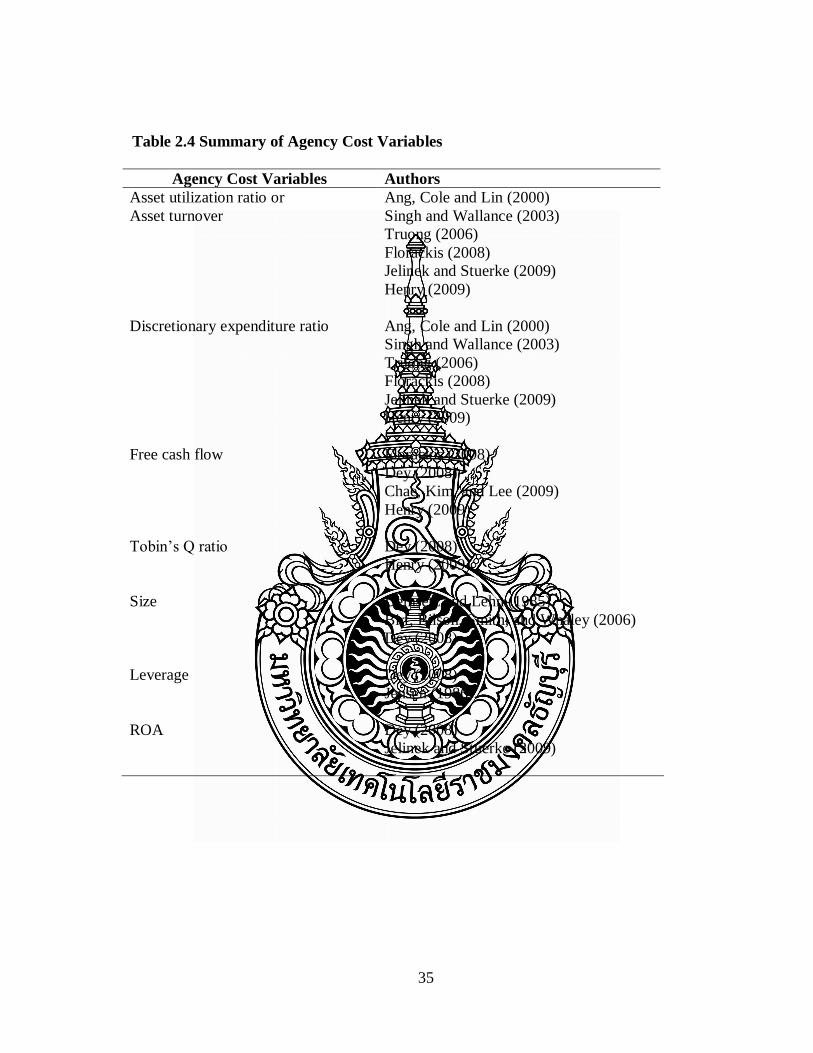
According to existing studies, this research gathered these variables together in
order to develop measurement model of agency costs (see Table 2.4). Based on the
discussion of the degree of cost stickiness in context of the agency theory, the following
question may be raised:
Q5: Do agency costs affect the degree of cost stickiness?
It is proposed that agency costs positively relate to the degree of cost stickiness. In
accordance with this research question, the study introduced the following hypothesis.
H5a: Agency costs affect the degree of cost stickiness in a positive direction.
35
Table 2.4 Summary of Agency Cost Variables
Agency Cost Variables Authors
Asset utilization ratio or
Asset turnover
Ang, Cole and Lin (2000)
Singh and Wallance (2003)
Truong (2006)
Florackis (2008)
Jelinek and Stuerke (2009)
Henry (2009)
Discretionary expenditure ratio Ang, Cole and Lin (2000)
Singh and Wallance (2003)
Truong (2006)
Florackis (2008)
Jelinek and Stuerke (2009)
Henry (2009)
Free cash flow Florackis (2008)
Dey (2008)
Chae, Kim, and Lee (2009)
Henry (2009)
Tobin’s Q ratio Dey (2008)
Henry (2009)
Size Demsetz and Lehn (1985)
Birt, Bilson, Smith, and Whaley (2006)
Dey (2008)
Leverage Dey (2008)
Jensen (1986).
ROA Dey (2008)
Jelinek and Stuerke (2009)

36
Corporate Governance
Corporate governance is one of the most commonly used phrases when a financial
crisis occurred. Beginning with the East Asian financial crises during 1997-1998, the
collapse of America’s largest companies, such as Enron in 2001 and WorldCom in 2002, and
the current American sub-prime crisis, weak corporate governance is mentioned as one of the
possible causes of these crises.
Chavalit Thanachanan, chairman of Stock Exchange of Thailand said that “…In
Thailand, recognition of the value of corporate governance was brought into sharp focus as
a result of the 1997 economic crisis…
…good governance practices are what provide the moral and ethical framework
that should underpin any business model to ensure its sustainability and to increase investor
confidence…”
Definition of Corporate Governance
The term “corporate governance” has no single formal definition (Turner, 2009,
p.5), and there are many definitions of corporate governance from the narrowest which is
restricted to the relationship between a firm and its owner (shareholders). This is the
“agency theory” (the traditional finance paradigm). Whereas the broadest definition
describes the relationship between a firm and other “stakeholders”, it is the “stakeholder
theory”. The definitions of corporate governance are different and are subject to the
viewpoint of the individual researcher, practitioner or policy maker. Table 2.5 shows
definitions of corporate governance in many perspectives.

37
For Thailand, the National Corporate Governance Committee of Thailand defines
“Corporate governance as
- Relationship between the board of director of a company, its management team, its
shareholders and other stakeholders in leading the company’s direction and monitoring its
operations.
- A structure and internal process ensuring that the board of directors evaluates the
performance of management team transparently and effectively.
- A System having structure and process of leadership and corporate control to
establish the transparent working environment, and to enhance the company’s
competitiveness to preserve capital and to increase shareholders’ long-term value by taking
into consideration; business ethics, the interests of other stakeholders and society.”
Figure 2-2 displays the relationship between the board of director of a company, its
management team, and its shareholders.
In conclusion, there is no established academic definition of corporate governance,
since it is difficult to find the words and phrases that capture the entire aspect of modern
corporate life.

38
Table 2.5 Definition of Corporate Governance
Corporate governance is… Authors
. . . the process of supervision and control intended to ensure that
the company’s management acts in accordance with the interests
of shareholders.
Parkinson
(1994)
. . . the governance role is not concerned with the running of the
business of the company per se, but with giving overall direction
to the enterprise, with overseeing and controlling the executive
actions of management and with satisfying legitimate expectations
of accountability and regulation by interests beyond the corporate
boundaries.
Tricker (1984)
. . . the governance of an enterprise is the sum of those activities
that make up the internal regulation of the business in compliance
with the obligations placed on the firm by legislation, ownership and
control. It incorporates the trusteeship of assets, their management
and their deployment.
Cannon (1994)
. . . the relationship between shareholders and their companies and
the way in which shareholders act to encourage best practice (e.g.,
by voting at AGMs and by regular meetings with companies’ senior
management). Increasingly, this includes shareholder ‘activism’
which involves a campaign by a shareholder or a group of
shareholders to achieve change in companies.
The Corporate
Governance
Handbook
(1996)
. . . the structures, process, cultures and systems that engender the successful operation of the organization.
Keasey and
Wright
(1993)
. . . the system by which companies are directed and controlled. The Cadbury
Report (1992)
. . . the system of checks and balances, both internal and external to
companies, which ensures that companies discharge their
accountability to all their stakeholders and act in a socially
responsible way in all areas of their business activity.
Solomon and
Solomon (2004)
Source: Adapt from Solomon & Solomon, 2004

39
Shareholders
-Appoint the directors to be their representatives.
-Regularly monitor the performance of the
appointed directors.
Directors
-Possess a strong leadership, control, and plan.
-Honestly and prudently perform their duties.
-Appoint a qualified management team to be
their representative for business management.
Management Team
-Perform according to the board of directors’ policy.
-Ensure good cooperation among the team.
-Honestly and prudently perform their duties.
-Maximize returns.
-Be responsible for assigned
duties to shareholders.
Be responsible for board of
directors.
Source: www.cgthailand.org
Figure 2-2 The Relationship between the Board of Director of a Company,
Its Management Team, and Its Shareholders.
Benefit of Corporate Governance
The National Corporate Governance Committee of Thailand defines “Benefit of
corporate governance as
-Increasing operational efficiency and effectiveness
Corporate governance is a tool to evaluate and monitor internal operations of a
company. It helps creating, therefore, useful guidelines for improving its operation workflow.

40
-Enhancing competitiveness
An organization with good corporate governance is widely accept comparable to
international standard and processes comparative advantage in term of strategic
management.
-Enhancing stakeholders’ confidence toward an organization
Corporate governance ensures the transparency of business management and
avoids an opportunity of executives and management taking advantages for their own
benefit. In other words, stakeholders would not take any risks to an organization without
good corporate governance.
-Maximizing shareholders’ value
Good corporate governance boosts shareholders’ confidence to invest leading to
increasing value of the company’s shares in their portfolio.”
Corporate governance is a major benefit to the company, especially to maximize
company value. Therefore, many researchers have examined corporate governance’s
effects and have proven its benefit.
Corporate Governance Variables
Corporate governance issues arise from two situations, the first is the agency
problems, or conflict of interest that is caused by the separation of ownership and control in
modern organizations. The second is when there are incomplete contracts between
management and shareholders (Hart, 1995). From an agency theory, Jensen and Meckling
(1976) suggested that the zero agency–cost base case is the firm owned solely by a single

41
owner-manager. When a manager owns less than 100 percent of firm’s equity, there is the
potential of conflicts of interest between managers and shareholders. Moreover, there are
agency costs from using an agent (e.g., when a manager will use the firm’s resources for his
personal benefit) and agency costs from mitigating the conflicts. Thus, the majority of
corporate governance research examined whether corporate governance mechanisms can
minimize the gap between managers’ and shareholders’ interests and the impact of
corporate governance mechanisms on corporate performance. If corporate governance
mechanisms can align managers’ and shareholders’ interests, then they should have a
positive impact on the company’s performance.
Jensen (1993) presented that there are four basic categories of corporate
governance; legal and regulatory mechanisms, internal control mechanisms, internal control
mechanisms, and product market competition. Internal control mechanisms consists of the
firm’s ownership structure, the board of directors, the executive compensation, and the
firm’s debt structure. These are the variables most frequently used academic research and
in documents for public interest (see Table 2.6); For example Ang et al. (2000), Singh and
Wallance (2003), Truong (2006), Florackis (2008), Jelinek and Stuerke (2009), and Chen
and Chuang (2009). There are interactions between these variables, which contribute to
serious endogeneity problems in corporate governance research (Bhagat & Jefferis, 2002).
42
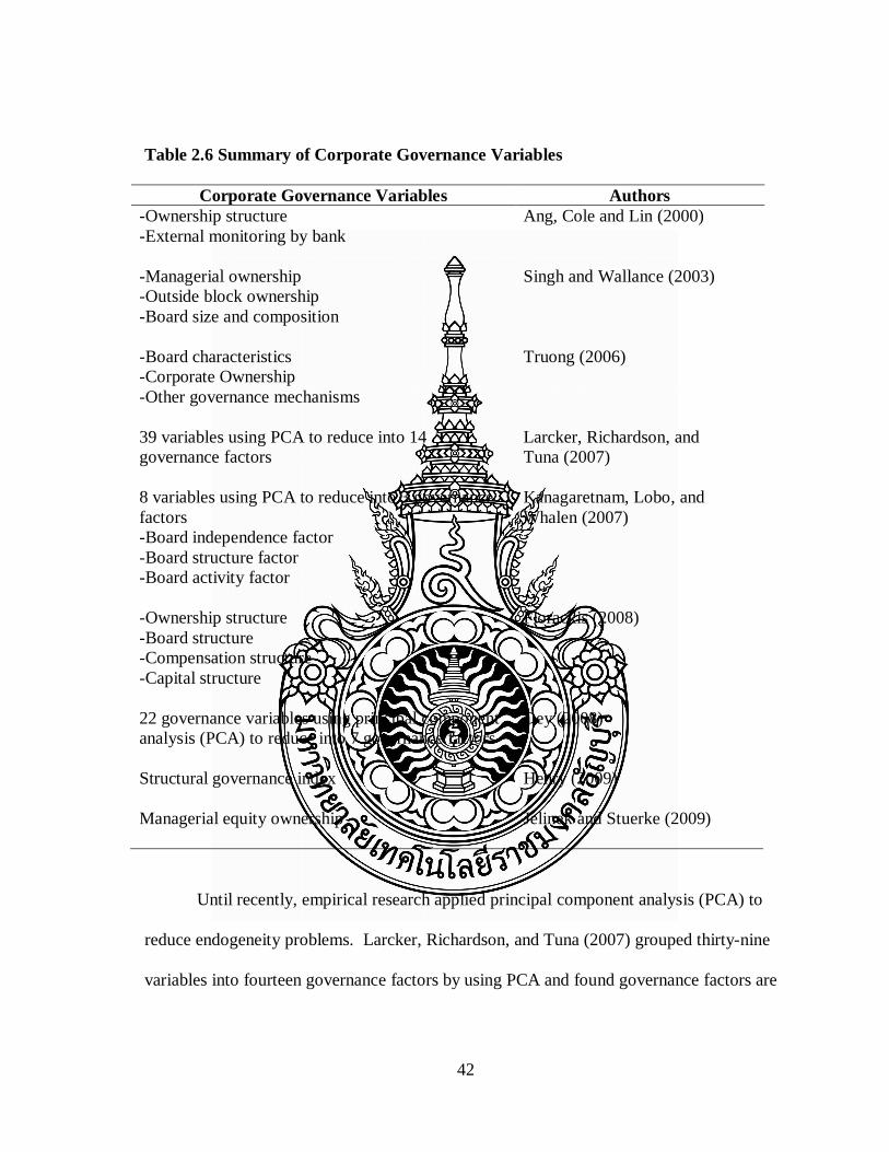
Table 2.6 Summary of Corporate Governance Variables
Corporate Governance Variables Authors
-Ownership structure
-External monitoring by bank
Ang, Cole and Lin (2000)
-Managerial ownership
-Outside block ownership
-Board size and composition
Singh and Wallance (2003)
-Board characteristics
-Corporate Ownership
-Other governance mechanisms
Truong (2006)
39 variables using PCA to reduce into 14
governance factors
Larcker, Richardson, and
Tuna (2007)
8 variables using PCA to reduce into 3 governance
factors
-Board independence factor
-Board structure factor
-Board activity factor
Kanagaretnam, Lobo, and
Whalen (2007)
-Ownership structure
-Board structure
-Compensation structure
-Capital structure
Florackis (2008)
22 governance variables using principal component
analysis (PCA) to reduce into 7 governance factors
Dey (2008)
Structural governance index Henry (2009)
Managerial equity ownership Jelinek and Stuerke (2009)
Until recently, empirical research applied principal component analysis (PCA) to
reduce endogeneity problems. Larcker, Richardson, and Tuna (2007) grouped thirty-nine
variables into fourteen governance factors by using PCA and found governance factors are

43
related to future operating performance and excess stock returns. Kanagaretnam, Lobo, and
Whalen (2007) used PCA to reduce eight variables into three governance factors and
showed that good corporate governance can reduce information asymmetry around
quarterly earnings announcements. Dey (2008) examined seven governance factors form
twenty-two governance variables, and suggested the composition and functioning of the
board, the independence of the auditor, and the equity-based compensation of directors are
significantly associated with performance. However, these associates were found primarily
only for companies with high agency conflicts.
The majority of previous research supported the finding that corporate governance
lead to higher corporate performance. Ang et al. (2000) presented agency costs are higher
when there is an external, rather than an internal firm manager and an increase in the
number of non-manager shareholders. Agency costs are inversely related to the manager’s
ownership share and lower with greater monitoring by banks and other financial
institutions. Singh and Wallance (2003) and Truong (2006) found that managerial
ownership is positively related to asset utilization, but it is not related to discretionary
expenses. However, Florackis (2008) pointed out that managerial ownership, managerial
compensation and ownership concentration are strongly associated with agency costs, both
asset utilization ratio and expenditure ratio.
Jelinek and Stuerke (2009) proposed that the relationship between agency costs and
managerial equity ownership is nonlinear. The research reveals managerial equity
ownership is positively associated with the return on assets and asset utilization, but
negatively associated with the expense ratio.

44
In Thailand, the Thai Institute of Directors Association (IOD) has conducted the
corporate governance report, which presented the results of the evaluation of corporate
governance practices of Thai listed companies since 2001. The Securities and Exchange
Commission (SEC) and the Stock Exchange of Thailand (SET) recognize the important of
this study and have supported this project in the hope that corporate governance standards
will be raised and benefit both the investors and companies. The current evaluation criteria
are corporate governance indexes (CGI) or ratings, that are based on the components of the
code of practice. Thai listed companies are evaluated according to one hundred and thirty-
two criteria in the following five categories derived from the Organization for Economic
Cooperation and Development (OECD) principles of corporate governance:
1. Rights of Shareholders
2. Equitable Treatment of Shareholders
3. Role of Stakeholders
4. Disclosure and Transparency
5. Board Responsibilities
Listed companies in Thailand are then categorized into the following six groups
according to their corporate governance performance:
1. Excellent CGI = 5
2. Very Good CGI = 4
3. Good CGI = 3
4. Satisfactory CGI = 2
5. Pass CGI = 1

45
6. N/A
This study used CGI as a proxy for the corporate governance variable in order to
correct the problem of endogeneity between corporate governance variables and provide
empirical evidence for regulating corporate governance standards.
Empirical research of cost behavior which considered corporate governance, started
with research by Calleja et al. (2006) and Banker and Chen (2006a). They found that the
corporate governance system influences the degree of cost stickiness. Costs of companies
that are subject to the code-law system of corporate governance are stickier than costs of
companies which are subject to the common-law system of corporate governance. They did
not add corporate governance as a variable into the cost behavior model. Lastly, Chen et al.
(2008) and Banker et al. (2011) found cost asymmetry, or cost stickiness, increases with
managerial empire building incentives due to the conflict of interest between managers and
shareholders. Chen et al. (2008) suggested that good corporate governance can reduce cost
stickiness by preventing managers’ over-spending on selling, general and administrative
costs (SG&A costs).
In summary, earlier research has found that corporate governance factors impact on
cost stickiness. Based on the discussion of causes and consequences of the sticky cost
behavior and empirical evidence of cost behavior, the following questions may be raised:
Q6: Does corporate governance affect the degree of cost stickiness?
It is proposed that there is a negative association between the strength of corporate
governance and the degree of cost stickiness. In accordance with this research question, the
study introduced the following hypothesis.

46
H6a: Corporate governance affects the degree of cost stickiness in a negative
direction.
Summary
The research of Anderson et al. (2003) encouraged academic research in the area of
cost behavior, especially in cost stickiness. The previous research indicated that many
countries experience sticky cost behavior. Anderson and Lanen (2007) suggested that
future research should include the theories of management decision making and cost
management that are most consistent with observed cost behavior. Based on the review of
the relevant literature, cost stickiness research is still academically, an unexplored area. In
order to analyze sticky cost behavior of Thai companies, this research linked the variables
that impact on the degree of cost stickiness such as economic growth and adjustment costs.
In addition, Chen et al. (2008) concluded in their research that SG&A cost asymmetry
arises from management’s deliberate action, which explained by agency theory, and
corporate governance has an impact on managers’ decisions about discretionary costs.
Furthermore, Watts and Zimmerman (1986) suggested in a positive accounting theory that
internal political processes have an effect on the incentive of managers to choose
accounting procedures. Managers may promote earnings to the optimal target for their own
and shareholders’ interests.
This study applied the previous findings to examine sticky cost behavior of Thai
listed companies. As mentioned above, adjustment costs, political costs, agency costs, and
corporate governance have influence on management incentives. Therefore, this study
investigated the impacts of these variables on cost stickiness.

47
The main interest here is to determine whether cost behavior of Thai companies is
sticky or asymmetric in the same manner as observed in the other countries. This study
postulated that cost behavior is sticky because costs are the results of management
decisions. It is also possible that the adjustment cost theory, political process theory, and
agency theory are able to explain and predict the behavior of Thai managers.
In this review there was no investigation and study of the latent constructs for
adjustment costs, political costs, and agency costs measured by multiple indicators. To
address this issue, latent constructs for adjustment costs, political costs, and agency costs
were developed and examined in this study using confirmatory factor analysis (CFA).
In addition, three models were applied for investigating sticky cost behavior.
1. ABJ model. Anderson, Banker, and Janakiraman (2003) developed a log model
to investigate cost stickiness.
ABJ Model :
ln ][1,
,
ti
ti
TC
TC = β0 + β1 ln ][
1,
,
ti
ti
S
S + β2 Dec_Di,t* ln ][
1,
,
ti
ti
S
S+εi,t
or
ln ][1,
,
ti
ti
TC
TC = β0 + β1 Sale Change + β2 Dec_Di,t* Sale Change +εi,t
Where, for sample companies i, at year t
TC = Total operating costs
S = Total sales
Dec_Di,t = 1 when sales have decreased from year t-1 to t, and 0 otherwise

48
ln ][1,
,
ti
ti
S
S
= Sale Change
Cost is sticky, when β1 more than β1 + β2 or β2 < 0
2. BLS 1 model. Balakrishnan, Labro, and Soderstrom (2010) used a simulated
dataset and showed that ABJ model captures “mechanical” sticky cost behavior associated
with committed fixed cost. In addition, Nasev (2009) identified that one of three major
factors arising from the cost stickiness is the fixing of cost. Costs are fixed in the sense that
they are occurred, although committed resources are not fully utilized when the level of
activity declines (Banker & Hughes, 1994). Balakrishnan et al. (2010) proposed a model
which removed committed fixed cost by using a percentage change in costs and sales.
BLS1 Model:
][1,
1,,
ti
titi
TC
TCTC= β0 + β1 ][
,
1,,
ti
titi
S
SS + β2 Dec_Di,t* ][
,
1,,
ti
titi
S
SS +εi,t
or
][1,
1,,
ti
titi
TC
TCTC= β0 + β1 Sale Change + β2 Dec_Di,t* Sale Change +εi,t
Where, for sample companies i, at year t
TC = Total operating costs
S = Total sales
Dec_Di,t = 1 when sales have decreased from year t-1 to t, and 0 otherwise
][,
1,,
ti
titi
S
SS = Sale Change
Cost is sticky, when β1 more than β1 + β2 or β2 < 0
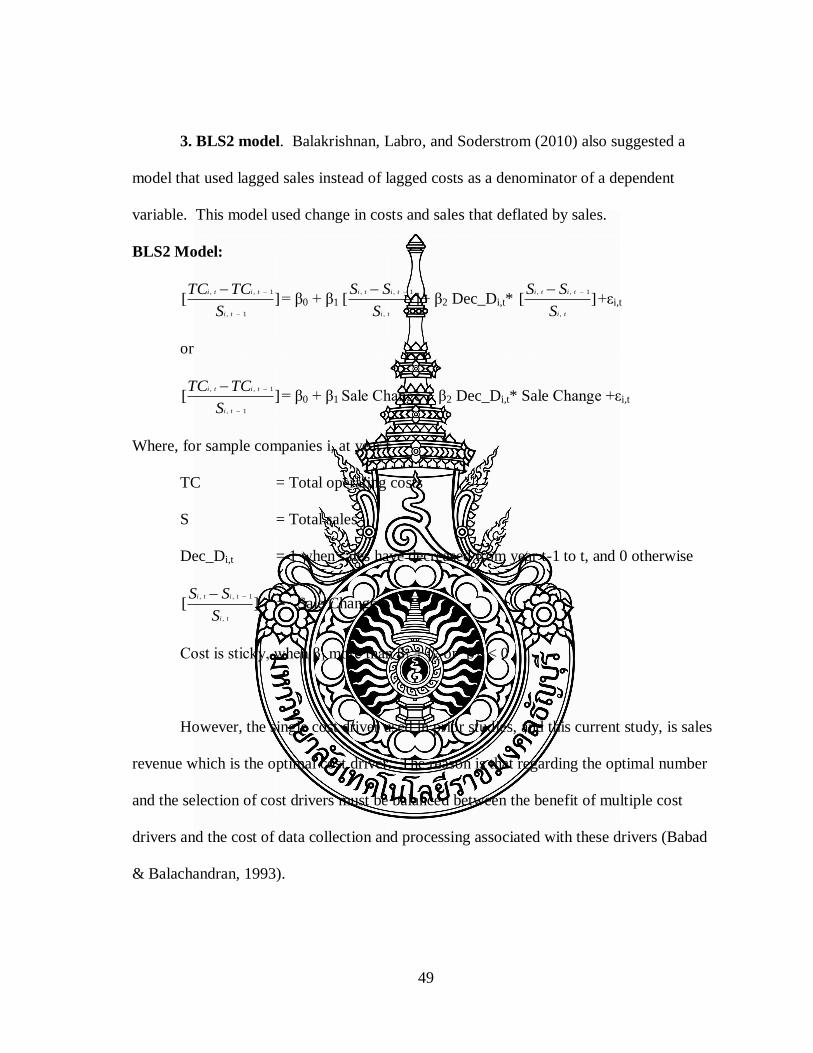
49
3. BLS2 model. Balakrishnan, Labro, and Soderstrom (2010) also suggested a
model that used lagged sales instead of lagged costs as a denominator of a dependent
variable. This model used change in costs and sales that deflated by sales.
BLS2 Model:
][1,
1,,
ti
titi
S
TCTC= β0 + β1 ][
,
1,,
ti
titi
S
SS + β2 Dec_Di,t* ][
,
1,,
ti
titi
S
SS +εi,t
or
][1,
1,,
ti
titi
S
TCTC= β0 + β1 Sale Change + β2 Dec_Di,t* Sale Change +εi,t
Where, for sample companies i, at year t
TC = Total operating costs
S = Total sales
Dec_Di,t = 1 when sales have decreased from year t-1 to t, and 0 otherwise
][,
1,,
ti
titi
S
SS = Sale Change
Cost is sticky, when β1 more than β1 + β2 or β2 < 0
However, the single cost driver used in prior studies, and this current study, is sales
revenue which is the optimal cost driver. The reason is that regarding the optimal number
and the selection of cost drivers must be balanced between the benefit of multiple cost
drivers and the cost of data collection and processing associated with these drivers (Babad
& Balachandran, 1993).

50
CHAPTER 3
RESEARCH METHODOLOGY
The purposes of this investigative and quantitative study were to identify the factors
that affect cost behavior and contribute factors that impact on sticky cost behavior of Thai
listed companies. The independent variables were derived from the adjustment cost theory,
political process theory, and agency theory. The dependent variable was cost stickiness.
This chapter presents the theoretical framework and describes the design of the research, as
well as data processing and analysis.
Theoretical Framework
To better understand the determinants of sticky cost behavior or asymmetrical cost
behavior, the theoretical framework was developed. There are both measurement model
and structural models in this overall framework. The measurement model was proposed to
investigate theoretical constructs, or latent variables, that cannot be observed directly. The
relationships of observed and latent variables of adjustment costs, political costs and
agency costs, were specified a priori, and described as implied conceptual models (see
Figures 3-1). They are measurement models as analyzed in confirmatory factor analysis
(CFA), which is Semi-SEM. Kline (2011) explained that “…The multiple-indicator
approach to measurement of CFA represents literally half the basic rational of analyzing
covariance structures in SEM - the analysis of structure model is the other half- so CFA is
crucial technique…”.

51
EMPLOY_I
STOCK_I
EQUITY_I
CAPITAL_I
ADJUSTMENT
COSTS
FCF
ASSET_UT
DIS_EX
ROA
AGENCY
COSTS
BETA
COMPETE
TAX
POLITICAL
COSTS
COST STICKINESS
H1
SALES
COSTS
TQ
LEV_R
SIZE
H3
H5
H4
Measurement Model Structural Model
ASSET_I
H6
CORPORATE GOVERNANCE
CONTROL VARIABLES
• GDP_GROWTH
• SALE_GROWTH
H2
Figure 3-1 Theoretical Framework

52
Figure 3-1 shows theoretical framework of this research.
Where
ASSET_I = assets intensity
EMPLOY_I = employee intensity
STOCK_I = stock intensity
EQUITY_I = equity intensity
CAPITAL_I = capital intensity
BETA = risk
COMPETE = concentration ratio
TAX = tax ratio
SIZE = size
FCF = free cash flow
ASSET_UT = asset utilization ratio
DIS_EX = discretionary expense ratio
ROA = return on assets
TQ = Tobin’s Q
LEV_R = leverage ratio
GDP_GROWTH = GDP growth
SALE_GROWTH = sale growth

53
Research Design
Selection of the Subjects
The target companies for this study were those listed on the Stock Exchange of
Thailand. As of December 31, 2009 there were a total of four hundred and seventy-one
companies, classified into eight categories by the Stock Exchange of Thailand (see
Appendix A). This study used the purposive selection procedure to investigate the cost
behavior of companies in seven industries, with the exception of the financials industry and
property fund sector in property and construction industry, because of the unavailability of
standardized financial reports. The analysis spanned nine years between 2001-2009. After
eliminating companies with missing values of variables and with sales decreasing less than
three years, the final sample comprised of one hundred and sixty companies (see Appendix
B), with one thousand, two hundred and eighty company-year observations (from only
eight years due to time lag). Table 3.1 shows the sample selection under consideration.
Table 3.1 Selection of Data
Total listed companies as of December 31, 2009 471 companies
Special industries
-Financial industry 61
-Property Fund 26 (87)
384
Missing data and not calendar year (71)
313
Listed after 2001 (52)
261
Sales decreasing < 3 years (during 2001-2009) (101)
160 companies
Number of observations 1,280 observations

54
The number of observations, or subjects, used in this study was appropriate for
multivariate analysis. There are twenty-one variables so the resulting subjects-to-variables
ratio is more than twenty. The level of statistical significance (α) is 95%
Instrumentation and Materials
This study adapted the model of Anderson et al. (2003) which used selling, general,
and administrative (SG&A) costs as a proxy for costs and sales revenue as a proxy for
activity due to the paucity of cost and activity driver data. They used data on SG&A costs
and sales revenue, since sale volume drives many of the components of SG&A costs
(Cooper & Kaplan, as cited in Anderson et al., 2003). SG&A costs are significant costs for
performing business which the manager should pay attention to control those (Chen et al.,
2008). Furthermore, SG&A costs are often highly discretionary in nature which is a ripe
target for cost reduction (White & Dieckman, 2005). However, this study used total
operating costs (TOP) as the proxy for costs because of the different classifying items in
financial reports. Banker et al. (2011) and Balakrishnan et al. (2010) also used total
operating costs (TOP) as the proxy for costs. In additional, this study adapted two models
of Balakrishnan et al. (2010), which removed committed fixed cost (BLS1 Model and
BLS2 Model).
Variables in the Study
Literature reviews show that cost stickiness is influenced by factors other than
activity change. For the investigation into the reasons for sticky cost behavior, this study

55
examined three latent variables (adjustment costs, political costs, and agency costs) by
controlling the economic factors (Table 3.2).
Table 3.2 Variables and Measurement
Variables Symbol Measurement
Independent Variables
-Adjustment Costs
Asset Intensity ASSET_I Total assets/Total sales
Employee Intensity EMPLOYEE_I Number of employees/Total sales
Stock Intensity STOCK_I Book value of common stocks/Total sales
Equity Intensity EQUITY_I Equity/Total sales
Capital Intensity CAPITAL_I Fixed assets/Total sales
- Political Costs
Capital Intensity CAPITAL_I Fixed assets/Total sales
Risk BETA Beta of company ’s stock
Concentration Ratio COMPETE % of total industry sales made by 8 largest
companies in the industry
Tax Ratio TAX Tax expense/Earnings before Tax
Size SIZE Natural log of total assets
- Agency Costs
Size SIZE Natural log of total assets
Free Cash Flow FCF (Cash flow from operating activity –Dividend)
/Total assets
Asset Utilization Ratio ASSET_UT Total sales/Total assets

56
Table 3.2 Variables and Measurement (cont.) Variables Symbol Measurement
Discretionary expense ratio DIS_EX SG&A costs/Total Sales
Return on assets ROA EBIT/Total assets
Tobin’s Q TQ (Market capital + Long term debts)/Total assets
Leverage ratio LEV_R Total debts/Total assets
-Corporate Governance
Corporate Governance
Index
CGI The Thai IOD’s rating (1-5)
Control Variables
GDP Growth GDP_GROWTH Gross Domestic Product growth in year t
Sales Growth SALE_GROWTH Sales growth of the industry of company i in year t
Dependent Variable
- Cost Stickiness STICKY Difference between the change in costs for a 1-
percent increase in sales and the change in costs for
a 1-percent decrease in sales
Data Collection
A quantitative research method, based on secondary data, was applied in this
analysis. The data on costs, sales revenue, assets, liabilities and equity was available in
financial reports of Thai listed companies, which were available in the database of SEC. In
addition, other data can be derived from SET and the companies’ own websites.
Fortunately, the companies’ financial reports can also be accessed from SETSMART (SET
Market Analysis and Reporting Tool), the web-based application from the SET.

57
Data Processing and Analysis
There were three stages of analysis in this study. The first stage is confirmatory
factor analysis (CFA), to evaluate and optimize the priori measurement models for
adequate model fit and validity. CFA is a type of structural equation modeling (SEM)
which deals with measurement models. The measurement models represent the
relationship between observed measures and latent variables. The measurement models for
adjustment costs, political costs, and agency costs were evaluated and optimized separately.
The second stage is exploratory factor analysis (EFA), to obtain a more parsimonious set of
composite scores (i.e., factor scores) that are then used in subsequent analyses (e.g.,
regression) instead of the measured variable scores. The last stage is multiple regression
analysis, to analyze the data for the purpose of answering the research questions.
Data was prepared and screened before being analyzed, because the majority of
estimated methods in SEM make a specific distributional assumption about the data. Data-
related problems can make the result biased and SEM computer programs failed to yield a
logical solution (Kline, 2011). AMOS version 18 software was used to analyze the data for
measurement models. In contrast, the structural model defines relations among latent
variables. The software application used to organize and analyze the data for structural
model was SPSS version 17.

58
The First Stage: Developing Measurement Models
Confirmatory Factor Analysis (CFA)
CFA specifies the "measurement models" delineating how measured variables
reflect certain latent variables. Once these measurement models are deemed satisfactory,
then the researcher can explore path models (called structural models) that link the latent
variables. This section shall present and explain the six basic steps in the structural
equation modeling (SEM) that were utilized in this study. A flowchart of these steps is
displayed in figure 3-2.
1. Model
specification
2. Model
identified?
3.Select measures,
collect, prepare,
and screen data
4. Model fit
adequate?
5. Model
respecification
6. Interpret estimates
no
yes
no
yes
Source: adapted from Kline, 2011: 92
Figure 3-2 Flowchart of the Basic Steps of SEM

59
1. Model Specification
SEM is a priori methodology. The hypothetical model based on extant theory
and research was specified in advance. The analysis cannot take place until the proposed
conceptual models of the relationships between the variables were defined (Kline, 2011).
Figure 3-3 shows the measurement models based on prior research and theories of
adjustment costs, political costs, and agency costs.
Model specification is the specification and formulating statements regarding a
set of parameters, which are described as either free or fixed. Free parameters are
estimated from the data, but fixed parameters are not estimated from the data and their
value is fixed at zero. In a path diagram, free parameters are represented by an arrow from
one variable to another, but fixed parameters are represented by the absence of an arrow.
The index of model adequacy is indicated by the degree to which the pattern of free and
fixed parameters are defined in a model, which is consistent with the pattern of variances
and covariances from observed data (Hoyle, 1995).

60
EMPLOY_I
STOCK_I
EQUITY_I
CAPITAL_I
ADJUSTMENT
COSTS
FCF
ASSET_UT
DIS_EX
ROA
AGENCY
COSTS
BETA
COMPETE
TAX
POLITICAL
COSTS
TQ
LEV_R
SIZE
ASSET_I
Figure 3-3 Measurement Models

61
2. Model Identification
Model identification is the considering of whether a unique set of model
parameter estimates can be derived from the observed data. If a unique value of the model
parameters can be found, the model is determined to be identified. Consequently, the
parameters are decided to be estimable and so the model can be evaluated empirically. One
of the requirements for identifying is that the model degree of freedom (df) must be more
than zero.
Degree of freedom = number of variances and covariances – number of free
parameters.
The number of variances and covariances =
Where p = number of observed variables in the model
If a value for one or more parameters can be acquired in multiple ways from
observed data, the model is overidentified (i.e., df > 0). The model that has a positive
degree of freedom allows for the rejection of the model thus rendering it of scientific use.
The objective of SEM is to specify model and make it meet the criterion of
overidentification.
If (for each parameter) a value can be obtained through only one manipulation
of observed data, the model is just identified (i.e.,df = 0). The model that shows a zero
degree of freedom is not scientifically interesting because it can never be rejected. Finally,
the underidentified model (i.e., df < 0) cannot be estimated since a unique value cannot be
obtained from the observed data (Hoyle, 1995; Byrne, 2010).

62
Considering the CFA model in Figure 3-3, Table 3.3 shows the identification of
three measurement models which were overidentified.
Table 3.3 Model Identification
Model p No. of variances and
covariances
(A)
No. of free
parameters
(B)
df
(A)-(B)
Identification
Adjustment costs 5 5(5+1)/2 = 15 10 5 Over
Political costs 5 5(5+1)/2 = 15 10 5 Over
Agency costs 7 7(7+1)/2 = 28 14 14 Over
3. Measure Selection and Data Collection
The preparation and screening of the collected data is of utmost importance
because the used estimation methods make specific data distribution and data-related
problems can cause illogical results from SEM computer programs (Kline, 2011).
3.1 Assessment of Outliers
There were a number of observations in this study that were assessed as
outliers, which are the observations whose scores were different from all the others in a
given set of data. Univariate outliners can be detected easily by examining frequency
distribution (Kline, 2011). Therefore, the extreme observations were eliminated from the
estimation by discarding an observation if it was either the highest or lowest 0.5% of its
distribution, resulting in one hundred and forty-three observations being eliminated,
thereby reducing the original one thousand, two hundred and eighty observations to a total
of one thousand, one hundred and thirty-seven. Furthermore, multivariate outliers were

63
assessed; those that had extreme scores on two or more variables. An approach to the
detection of multivariate outliers is considering the squared Mahalanobis distance (D2) for
each observation. This statistic indicates the distance in standard deviation units between a
set of scores for one case and the sample means for all variables. An outlying observation
will have a D2 value that is distinct from all the other D
2value (Byrne, 2010). Appendix C
exhibits minimal evidence for serious multivariate outliers in this study for transformed
variables.
3.2 Assessment of Collinearity and Normality
The original data file should be screened for collinearity and normality. The
collinearity can occur when separate variables measure the same thing. Tolerance and
variance inflation factor (VIF) are statistics that can detect collinearity among three or more
variables or multivariate collinearity. Kline (2011) recommended that a tolerance value
less than 0.10 or VIF greater than 10.0 may indicate extreme multivariate collinearity.
Table 3.4 reveals no item to be substantially multivariate collinearity (VIF = 1.0320 to
4.3860).
Multivariate normality is the most important assumption in SEM analysis
and especially in use of AMOS (Arbuckle, 2007). Estimation in SEM with maximum
likelihood assumes multivariate normality; this means that all univariate distributions are
normal and each variable is normally distributed for each value of every other variable and
all bivariate scatterplots are linear, and finally the distribution of residuals is homoscedastic
(Kline, 2011). It is very difficult to assess all these aspects of multivariate normality.
Fortunately, many cases of multivariate normality are detectable through the inspection of

64
univariate normality. Non-normal distribution is caused by skewness and kurtosis. Kline
(2011) suggested that when the absolute value of skew index is greater than 3.0 it indicates
extremely skewness, and when the absolute value of the kurtosis index is greater than 10.0
suggests that there is a problem; and when this value is greater than 20.0 it signifies that
there is a serious problem. Table 3.4 reveals no item to be extremely skewness or kurtosis
after data transformation (Skewness = -.693 to 2.204 and Kurtosis = .072 to 6.535).
However, the maximum likelihood estimation, which is the estimation technique in AMOS,
is robust against moderate violation of multivariate normality (Anderson & Garbing, 1988;
Bentler & Chou, 1987).

65
Table 3.4 Data Preparation and Screening
Tolerance Variance inflation factor
(VIF)
Skewness Kurtosis
ADJUSTMENT COSTS
ASSET_I .228 4.386 .768 .569
EMPLOY_I .831 1.203 -.610 .072
CAPITAL_I .631 1.585 .000 .581
EQUITY_I .330 3.030 -.085 1.276
STOCK_I .517 1.934 .160 .424
POLITICAL COSTS
CAPITAL_I .963 1.038 .000 .581
BETA .770 1.299 .943 .293
COMPET .945 1.058 1.033 2.875
TAX .969 1.032 1.153 2.106
SIZE .806 1.241 .603 .072
AGENCY COSTS
SIZE .811 1.233 .603 .072
FCF .922 1.085 .118 2.253
ASSET_UT .776 1.289 .983 1.293
DIS_EX .774 1.292 1.516 2.603
ROA .717 1.395 -.693 3.241
TQ .806 1.241 2.204 6.535
LEV_R .811 1.233 .603 1.594

66
4. Estimation and Evaluation
Model estimation is concerned with utilizing an SEM computer tool (i.e.,
AMOS) to calculate the estimates of free parameters from a set of observed data. The
method used in AMOS is maximum likelihood estimation. It is an iterative method that
involves a series of attempts to derive estimates of the free parameters that imply a
covariance matrix like the observed covariance matrix (Hoyle, 1995). During the
estimation process, iteration continues until the differences between corresponding values
in the implied and observed matrices (a residual matrix) are minimal. Therefore, a main
purpose of estimation is obtaining the closest-fitting statistical solution that can be
determined; that is goodness of model fit.
After estimation process had been done, the models were evaluated, which
comprises of the assessment of the model fit, path coefficients, and standard errors. Kline
(2011) recommended four approximate fit indexes that are the most widely presented in the
SEM literature. They are Root Mean Square Error of Approximation (RMSEA), Goodness
of Fit Index (GFI), Comparative Fit Index (CFI) and Standardized Root Mean Square
Residual (SRMR).
In addition, the quality of the latent construct should be evaluated. This index
indicates the internal consistency in a given set of observed variables. It is referred to as
maximal reliability in the context of scale construction and as the measure of construct
reliability (Hancock & Mueller, 2006).
Construct reliability =

67
Where
is standardized regression weight
is summation
Construct reliability measures convergent validity that is proportion of covariance
in set of observed variables.
Table 3.5 summaries the criteria for evaluation model.

68
Table 3.5 Criteria for Evaluation Model
Four types assessment indicators Index
Referred
to as
Fit standards and applicability
Assessment of Chi-square test 2 test P > 0.05
the overall 2/df <2 or <3
model fit Absolute Fit Index GFI >0.95 AGFI >0.90 or >0.80
RMSEA 0.05 “good fit”, 0.05-0.08 “not bad fit”, 0.08-0.10 “moderate model” > 0.10 “bad fit”
RMR <0.05, the smaller it is, the better the fitness will be. ECVI A good indicator for diagnosis of cross-validity of model,
the smaller its value, the smaller the degree of volatility of model goodness-of-fit and the better the hypothetical model will be.
Comparative Fit index CFI >0.90, indicating the degree of improvement of model
compared with nothingness, suitable for small samples .
NFI >0.90, indicating the degree of improvement of model compared with nothingness.
RFI >0.90, when the data fully fit model, the value is 1. Parsimony Fit Measures NCP As close to 0 as possible, indicating the model has perfect
goodness-of-fit, suitable for comparison between models. AIC AIC value of hypothesized model should be smaller than
that of saturated model and independent model.
Hoelter’s Critical N CN > 200 , sample size is adequate. Measurement Model Assessment
The size of path coefficient is the basis of the assessment. All the standard path coefficients greater than 0.7 indicate the good measurement system.
Structural
Equation Modeling Assessment
The ratio for each endogenous variable to be explained of
variance by other variable (referred to as explanatory power)R2 . The bigger each R2 is ,the better. In general R2 more than 0.03 indicate good explanatory power.
Reliability Construct Reliability >0.50
Source: Adapt from Hsu, Su,Kao, Shu,Lin, & Tseng, 2012: 4

69
5. Model Respecification
When the initial model is poor, a respecified model must be identified. Model
respecification should be introduced to good fit by theoretical consideration rather than a
statistical one (Kline, 2011). The results of this second model were evaluated after the
initial model was respcified. This iterating processes continue until the model exhibits
adequate fit.
6. Interpret Estimates
The final step is accurate and complete reporting on the parameter estimates.
The result reports have a comment on the magnitudes and signs of the parameter estimates.
The Second Stage: Estimating Factor Scores
Exploratory Factor Analysis (EFA)
This study utilized factor analysis to summarize relationships between the variables
in the form of a more parsimonious set of factor scores so that these factor scores can then
be used in multiple regression analyses instead of the measured variable scores.
Exploratory factor analysis (EFA) is the statistical method that can be used for exploring
the relationships among measured variables and trying to determine whether these
relationships can be summarized in a smaller number of latent constructs (Thompson,
2004). The software application used to analyze in this stage was SPSS version 17.0.

70
There are five steps for EFA, as follows (Vanichbuncha, 2010).
1. Use KMO (Kaiser-Meyer-Olkin) to check appropriation of data for EFA.
KMO Recommendation
0.9 Marvelous
0.8 Meritorious
0.7 Middling
0.6 Mediocre
0.5 Miserable
0.5 Unacceptable
2. Select factor extraction method. This study used principal component analysis.
3. Consider number of factor. Using eigenvalues determine the appropriate number
of factor.
4. Identify original variables for each factor. Factor loading is considered to select
variables for each factor.
5. Rotate axis of factor. The most popular method is varimax used in this study.
In summary, the EFA extraction method used for this study is the principal
component analysis. It was used to compute factor pattern coefficients. Factor rotation
was performed by the varimax rotation method. Then the regression method was used to
obtain factor scores. If there are multiple factors in one latent construct, factor scores will
be weighted average with a percentage of variance.

71
The Final Stage: Constructing Structural Model of Cost Behavior
Multiple regression analysis
Multiple regression analysis was used to analyze the relationship among variables,
especially causal relationship, such as when there is one dependent and two or more
independent variables in multiple regression analysis. This study examined the conditions
when the data was analyzed. There are four conditions about residual or error term (e), as
follows (Vanichbuncha, 2010).
1. e is normal.
2. V(e) (= 2)
is constant. If V(e) is not constant, Heteroscedastic problem will
occur.
3. et and et+1 are independent. As the data in this study is panel data, there are
mixed between cross-sectional and time-series data, this condition is necessary.
If et and et+1 are not independent, an autocorrelation problem will occur. The
Durbin-Watson formula was used to examine the problem, the resulting Durbin-
Watson value, which is between 1 to 3, is practically implied that et and et+1 are
independent.
4. X1,…….,Xk is independent. If X1,…….,Xk is not independent, A
multicollinearity problem will occur (X is independent variable). Tolerance and
VIF (variance inflation factor) were used to detect multicollinearity. If the
tolerance value closes to 1, then multicollinearity may be a serious problem. If

72
however the VIF value is more than 10, then multicollinearity may be
influencing the least square estimate of regression coefficients.
Three models were used to investigate the conditions. Table 3.6 illustrates that
residual terms of both the ABJ model and BLS1 model are normal while the residual term
of BLS2 model is approximately normal. Residual terms of all models are constant, so they
are homoscedasticity. All models have no autocorrelation and multicollinearity problems
(Durbin-Watson < 3 and VIF < 10).
Table 3.6 Four Conditions about Residual or Error Term
Model Normality Homoscedasticity Autocorrelation Multicollinearity
Skewness V(e) Durbin-Watson VIF
ABJ Model -.102 constant 2.330 1.184-2.846 BLS1 Model 1.131 constant 2.406 1.184-2.058
BLS2 Model 2.899 constant 2.457 1.184-2.058
After examining these conditions, the models of Anderson et al. (2003) and
Balakrishnan et al. (2010) were employed to investigate cost stickiness.

73
Model (1) : The basic model was analyzed to answer research question 1 and to test
hypothesis 1.
Q1 : Is cost behavior of Thai listed companies sticky?
H10: Cost behavior of Thai listed companies is not sticky.
H1a: Cost behavior of Thai listed companies is sticky.
ABJ Model :
ln ][1,
,
ti
ti
TC
TC = β0 + β1 Sale Change + β2 Dec_Di,t* Sale Change +εi,t
BLS1 Model:
][1,
1,,
ti
titi
TC
TCTC= β0 + β1 Sale Change + β2 Dec_Di,t* Sale Change +εi,t
BLS2 Model:
][1,
1,,
ti
titi
S
TCTC= β0 + β1 Sale Change + β2 Dec_Di,t* Sale Change +εi,t
Where, for sample companies i, at year t
TC = Total operating costs
S = Total sales
Dec_Di,t = 1 when sales have decreased from year t-1 to t, and 0 otherwise
Sale Change
= ln ][1,
,
ti
ti
S
S for ABJ Model
Sale Change = ][,
1,,
ti
titi
S
SS for BLS1 and BLS2 Model
Cost is sticky, when β1 more than β1 + β2 .

74
Hence, H10 : β1 = β2 = 0
H1a : β1 > β1 + β2 or β2 < 0
Model (2) : The basic model with the economic variables was analyzed to answer research
question 2 and to test hypothesis 2.
Q2 : Is cost behavior sticky, after controlling the economic variables?
H 20: Cost behavior is not sticky, after controlling the economic variables.
H 2a: Cost behavior is still sticky, after controlling the economic variables.
ABJ Model :
ln ][1,
,
ti
ti
TC
TC = β0 + β1 Sale Change + β2 Dec_Di,t* Sale Change
+ β3 GDP_GROWTH + β4 SALE_GROWTH+εi,t
BLS1 Model:
][1,
1,,
ti
titi
TC
TCTC= β0 + β1 Sale Change + β2 Dec_Di,t* Sale Change
+β3 GDP_GROWTH + β4 SALE_GROWTH +εi,t
BLS2 Model:
][1,
1,,
ti
titi
S
TCTC= β0 + β1 Sale Change + β2 Dec_Di,t* Sale Change
+β3 GDP_GROWTH + β4 SALE_GROWTH +εi
Where, for sample companies i, at year t
TC = Total operating costs
S = Total sales
Dec_Di,t = 1 when sales have decreased from year t-1 to t, and 0 otherwise

75
Sale Change
= ln ][1,
,
ti
ti
S
S for ABJ Model
Sale Change = ][,
1,,
ti
titi
S
SS for BLS1 and BLS2 Model
Cost is sticky, when β1 more than β1 + β2 + . β3 + β4
Hence,
H20 : βi = 0 i = 1,2,…….,4
H2a : β1 > β1 + β2 + β3 + β4
or β2 < 0 or β3 < 0 or β4< 0
Model (3) : The full model with all variables was analyzed to answer research question 3,
4,5 and to test hypothesis 3,4,5.
Q3: Do adjustment costs affect the degree of cost stickiness?
Q4: Do political costs affect the degree of cost stickiness?
Q5: Do agency costs affect the degree of cost stickiness?
H30: Adjustment costs do not affect the degree of cost stickiness in a positive
direction.
H3a: Adjustment costs affect the degree of cost stickiness in a positive direction.
H40: Political costs do not affect the degree of cost stickiness in a positive
direction.
H4a: Political costs affect the degree of cost stickiness in a positive direction.
H50: Agency costs do not affect the degree of cost stickiness in a positive direction.
H5a: Agency costs affect the degree of cost stickiness in a positive direction.

76
ABJ Model :
ln ][1,
,
ti
ti
TC
TC = β0 + β1 Sale Change
+ β2 Dec_Di,t* Sale Change
+ β3 GDP_GROWTH + β4 SALE_GROWTH + β5 ADJUSTMENT COSTS
+ β6 POLITICAL COSTS + β7 AGENCY COSTS + εi,t
BLS1 Model:
][1,
1,,
ti
titi
TC
TCTC= β0 + β1 Sale Change
+ β2 Dec_Di,t* Sale Change
+ β3 GDP_GROWTH + β4 SALE_GROWTH + β5 ADJUSTMENT COSTS
+ β6 POLITICAL COSTS + β7 AGENCY COSTS + εi,t
BLS2 Model:
][1,
1,,
ti
titi
S
TCTC= β0 + β1 Sale Change
+ β2 Dec_Di,t* Sale Change
+ β3 GDP_GROWTH + β4 SALE_GROWTH + β5 ADJUSTMENT COSTS
+ β6 POLITICAL COSTS + β7 AGENCY COSTS + εi,t
Where, for sample companies i, at year t
TC = Total operating costs
S = Total sales
Dec_Di,t = 1 when sales have decreased from year t-1 to t, and 0 otherwise
Sale Change
= ln ][1,
,
ti
ti
S
S for ABJ Model
Sale Change = ][,
1,,
ti
titi
S
SS for BLS1 and BLS2 Model

77
Adjustment costs affect the degree of cost stickiness in a positive direction,
when β5 less than 0
Hence,
H30 : β5 = 0
H3a : β5 < 0
The higher the political costs, the more likely the manager is to influence earnings.
Political costs affect the degree of cost stickiness in a positive direction, when β6 less than
0.
Hence,
H40 : β6 = 0
H4a : β6 < 0
The higher the agency costs, the more likely the manager is to retain costs; that is
the “stickier” cost behavior. Agency costs affect the degree of cost stickiness in a positive
direction, when β7 less than 0
Hence,
H50 : β7 = 0
H5a : β7 < 0

78
ABJ Model, BlS1 Model and BLS2 Model: The observations were separated into weak
corporate governance or good corporate governance. Then model (3) of three models were
analyzed to answer research question 6 and to test hypothesis 6.
Q6: Does corporate governance affect the degree of cost stickiness?
H60: Corporate governance does not affect the degree of cost stickiness in a
negative direction.
H6a: Corporate governance affects the degree of cost stickiness in a negative
direction.
The stronger the corporate governance, the more likely the manager is to utilize
resources efficiently; that is the “less sticky” cost behavior.
β21 = degree of cost stickiness of weak corporate governance
β22 = degree of cost stickiness of strong corporate governance
Hence,
H60 : β21 = 0 or β22 = 0
H6a : β21 < 0 and β21 < β22
Robustness Test
The data in this study was panel data that repeated measurements at different points
in time within the same company. Regression can capture both variations over the
companies and variation over time, so panel-data methods are more sophisticated than
cross-section-data method (Cameron & Trivedi, 2009). Since each additional time period
of data is dependent on the previous period, the standard error of panel-data estimators

79
must be adjusted. The basic linear models for panel data are fixed-effects and random-
effects models. The fixed-effects model removes the effect of time-invariant characteristics
from independent variables therefore the net effects of them can be assessed while the
random-effects model assumes that the variation across companies is random and
uncorrelated with the independent variables included in the model. The Hausman test is
required to decide between fixed or random effects (Green, 2008).
Although the results of multiple regression analysis did not find autocorrelation in
this study, it utilized the linear model for panel data to confirm the hypotheses testing. The
software application used to analyze the panel data was STATA version 11.

80
CHAPTER 4
RESEARCH RESULTS
This chapter describes the descriptive statistics of the research sample and the
results from the confirmatory factor analysis (CFA) of the measurement models that is the
first step of the structural equation model (SEM) analysis. This research can use only one
step of SEM (or Semi-SEM) because the cost stickiness cannot be measured directly, which
is represented by the coefficient (β2) in the regression model. Hence, multiple regression
analysis was used to analyze the structural model instead of the second step of SEM.
The first step of this analysis used CFA to confirm the measurement models of three
latent (unobserved) variables within the AMOS program. The three latent variables are
adjustment costs, political costs, and agency costs. The measurement models were verified
to ensure that they fit to the data. The second step of this analysis used EFA, using
principle components analysis (PCA) with varimax rotation. The final step of this analysis
created the structure model by multiple regression analysis with SPSS program.
The Descriptive Statistic Summary
Table 4.1 provides the descriptive statistics for the variables extracted from both
the financial reports and the reports of SET. As mentioned in chapter 3, this study
eliminated the extreme observations and the number of observations, with the result that the
initial one thousand, two hundred and eighty observations were reduced to one thousand,
one hundred and thirty-seven. The mean and median of the most variables did not display

81
much difference between before and after adjustment. The variable that was dramatically
changed, after dropping some outliners was STOCK_I. The mean of STOCK_I variable
before adjustment was 0.8381 become 0.4161 with less standard deviation (from 9.26537 to
0.80393).
Table 4.1 Summary of Descriptive Statistic for Unadjusted and Adjusted Data of
Variables
Unadjusted data(1280 observations) Adjusted data (1137 observations)
Variables Mean Median Standard
Deviation
Mean Median Standard
Deviation
PANEL A. Sale and Total Operating Costs
ABJ MODEL
TOPC 0.0408 0.0454 0.25986 0.0374 0.0431 0.21578
SALE_INC (Sale Change) 0.0392 0.0444 0.30005 0.0362 0.0378 0.22296
SALE_DEC (Dec_D*Sale Change) -0.0589 0.0000 0.22836 -0.0565 0.0000 0.13927
BLS1 MODEL
TOPC 0.0763 0.0465 0.30874 0.0623 0.0440 0.23789
SALE_INC (Sale Change) 0.0831 0.0454 0.36820 0.0624 0.0394 0.24205
SALE_DEC (Dec_D*Sale Change) -0.0382 0.0000 0.23590 -0.0470 0.0000 0.10944
BLS2 MODEL
TOPC 0.0638 0.0433 0.33335 0.0523 0.0382 0.24254
SALE_INC (Sale Change) 0.0831 0.0454 0.36820 0.0624 0.0394 0.24205
SALE_DEC (Dec_D*Sale Change) -0.0382 0.0000 0.21359 -0.0470 0.0000 0.10944
PANEL B. Adjustment Costs
ASSET_I 1.7077 1.1174 1.98640 1.5429 1.0977 1.38891
EMPLOY_I 0.0007 0.0005 0.00074 0.0007 0.0005 0.00066
STOCK_I 0.8381 0.2127 9.26537 0.4161 0.2071 0.80393
EQUITY_I 1.0523 0.6532 1.72773 0.9711 0.6597 1.14529
CAPITAL_I 0.7044 0.3635 1.46301 0.6085 0.3614 0.90310
PANEL C. Political Costs
CAPITAL_I 0.7044 0.3635 1.46301 0.6085 0.3614 0.90310
BETA 0.5187 0.3800 0.52775 0.4784 0.3500 0.46029
COMPET 0.6799 0.6867 0.08592 0.6761 0.6867 0.08440
TAX 0.1353 0.0891 0.15220 0.1400 0.1053 0.14724
SIZE 14.8471 14.6617 1.34329 14.8153 14.6405 1.28000
PANEL D. Agency Costs
SIZE 14.8471 14.6617 1.34329 14.8153 14.6405 1.28000
FCF 0.0483 0.0512 0.10982 0.0511 0.0525 0.09024
DIS_EX 0.1679 0.1285 0.22177 0.1574 0.1261 0.11246
ROA 0.0689 0.0732 0.09813 0.0724 0.0744 0.07989
TQ 0.8120 0.6298 0.89880 0.7655 0.6295 0.56333
LEV_R 0.4245 0.4039 0.25248 0.4022 0.3872 0.22439
PANEL E. Corporate Governance
CGI 3.1250 4.0000 1.52846 3.1214 4.0000 1.51613
PANEL F. Control Variables
GDP_GROWTH 0.0422 0.0509 0.02782 0.0426 0.0504 0.02756
SALE_GROWTH 0.1197 0.0961 0.21254 0.1190 0.0961 0.21486

82
Panel B, C, and D of Table 4.2 display the descriptive statistics of variables which
are the proxy for adjustment costs, political costs, and agency costs after the transformation
of the data. All of variable distributions were close to normal because the absolute value of
skew index was less than 3.0, while the absolute value of kurtosis index was less than 10.0.
As soon as the data had been prepared and screened, multivariate statistic analysis can be
used in this study.
Table 4.2 Summary of Descriptive Statistic for Transformed Data of Variables
Transformed data(1137 observations)
Variables Mean Median Standard
Deviation
Skewness kurtosis
PANEL B. Adjustment Costs
ASSET_I 0.2001 0.0982 0.65596 0.768 0.569 EMPLOY_I -7.8378 -7.6255 1.15290 -0.610 0.072
STOCK_I -1.5694 -1.5672 1.17510 0.160 0.424
EQUITY_I -0.4220 -0.4187 0.87750 -0.085 1.276 CAPITAL_I -1.0429 -1.0167 1.02711 0.000 0.581
PANEL C. Political Costs CAPITAL_I -1.0429 -1.0167 1.02711 0.000 0.581
BETA 0.4938 0.3600 0.46833 0.943 0.293
COMPET 0.6764 0.6867 0.08118 1.033 2.875
TAX .14000 0.1053 0.14724 1.153 2.106 SIZE 14.8350 14.6573 1.28590 0.603 0.072
PANEL D. Agency Costs SIZE 14.8350 14.6573 1.28590 0.603 0.072
FCF 0.0521 0.0527 0.09263 0.118 2.253
DIS_EX 0.1592 0.1284 0.11220 1.516 2.603
ROA 0.0722 0.0740 0.07962 -0.693 3.241 TQ 0.7677 0.6267 0.57012 2.204 6.535
LEV_R 0.4128 0.3975 0.23382 0.603 1.594

83
Measurement Models
This is the first stage of analysis to establish the knowledge foundation about the
implied measurement models for adjustment costs, political costs, and agency costs. The
measurement models were tested by using confirmatory factor analysis (CFA).
Adjustment Cost Model
The final measurement model of adjustment costs was indicated by four
observed variables (asset intensity, stock intensity, equity intensity, and capital intensity).
Employee intensity was deleted from the model (p = .712, squared multiple
correlation=.00). The AMOS output is in Appendix C. Figure 4-1 illustrates the final
measurement model with standardized coefficients and squared multiple correlations.
Figure 4-1 Final Measurement Model of Adjustment Costs

84
Measurement Model Fit: Measurement Model of adjustment costs is good fit.
Table 4.3 shows the comparison of the adjustment cost model fit results with recommended
values.
Quality of the Latent Construct: The variance of latent variable can be
explained by observed variables 96%.
Table 4.3 CFA Results of Adjustment Cost Measurement Model
Model 2/ dƒ p-value GFI CFI RMSEA CN
Construct
Reliability
Adjustment Cost 1.477 .224 .999 1.000 .020 2955 .96
Recommended values < 3 > .05 > .95 > .90 .05 > 200 > .50
In summary, the result confirmed that adjustment costs can be measured by asset
intensity, stock intensity, equity intensity, and capital intensity. These observed variables
are presented in financial reports.
Political Cost Model
The final measurement model of political costs was indicated by five observed
variables (capital intensity, risk, concentration ratio, tax ratio, and size). The AMOS output
is in Appendix C. Figure 4-2 illustrates the final measurement model with standardized
coefficients and squared multiple correlations.

85
Figure 4-2 Final Measurement Model of Political Costs
Measurement Model Fit: Measurement Model of political costs is good fit
because 2/ dƒ statistic did not exceeded 3.0. Table 4.4 displays the comparison of the
political cost model fit results with recommended values.
Quality of the Latent Construct: The variance of latent variable can be
explained by observed variables 63%.
Table 4.4 CFA Results of Political Cost Measurement Model
Model 2/ dƒ p-value GFI CFI RMSEA CN
Construct
Reliability
Political Cost 1.600 .202 .999 .997 .003 2128 .63
Recommended values < 3 > .05 > .95 > .90 .05 > 200 > .50
In summary, the result confirmed that political costs can be measured by capital
intensity, risk, concentration ratio, tax ratio, and size. These observed variables are
presented in financial reports and reports of SET.

86
Agency Cost Model
The final measurement model of agency costs was indicated by six observed
variables (size, free cash flow, discretionary expense ratio, ROA, Tobin’s Q, and leverage
ratio). The asset utilization ratio was deleted from the model in the initial step. The AMOS
output is in Appendix C. Figure 4-3 illustrates the final measurement model with
standardized coefficients and squared multiple correlations.
Figure 4-3 Final Measurement Model of Agency Costs
Measurement Model Fit: Measurement Model of agency costs is good fit.
Table 4.5 exhibits the comparison of the agency cost model fit results with recommended
values.

87
Quality of the Latent Construct: The variance of latent variable can be
explained by observed variables 65%.
Table 4.5 CFA Results of Agency Cost Measurement Model
Model 2/ dƒ p-value GFI CFI RMSEA CN
Construct
Reliability
Agency Cost 2.171 .089 .998 .994 .032 1364 .65
Recommended values < 3 > .05 > .95 > .90 .05 > 200 > .50
In summary, the result confirmed that agency costs can be measured by size, free
cash flow, discretionary expense ratio, ROA, Tobin’s Q, and leverage ratio. These
observed variables are presented in financial reports and reports of SET.
Factor Scores
This is the second stage of analysis to estimate factor scores. An exploratory factor
analysis was performed on three constructs; adjustment costs, political costs, and agency
costs.
Adjustment costs
The measurement model from CFA found that asset intensity, stock intensity, equity
intensity, and capital intensity can be used to measure adjustment costs. The next step was
the estimation of the factor scores.
Data is appropriate for EFA (KMO = .739). This analysis resulted in one factor with
eigenvalues greater than one, explaining 67.98% of variance. (see Appendix D.)

88
Political costs
The measurement model from CFA found that capital intensity, risk, concentration
ratio, tax ratio, and size can be used to measure political costs. The next step was the
estimation of the factor scores.
Data is appropriate for EFA (KMO = .515). This analysis resulted in three factors
with eigenvalues greater than .999, explaining 73.58% of variance (see Appendix D.). In
this case, factor scores were weighted average with a percentage of variance.
Agency costs
The measurement model from CFA found that size, free cash flow, discretionary
expense ratio, ROA, Tobin’s Q, and leverage ratio can be used to measure agency costs.
The next step was the estimation of the factor scores.
Data is appropriate for EFA (KMO = .545). This analysis resulted in two factors with
eigenvalues greater than .997, explaining 67.84% of variance (see Appendix D.). In this
case, factor scores were weighted average with a percentage of variance.
Structural Model of Sticky Cost Behavior
This is final stage of analysis to develop the cost sticky behavior model. The four
conditions about residual or error term were investigated. Then the multiple regression
analysis was used to formulate model according to Figure 4-4, Figure 4-5 and Figure 4-6.

89
ABJ MODEL
ln ][1,
,
ti
ti
TC
TC = -.019 + .954 Sale Change - .097 Dec_Di,t* Sale Change
+ .053 GDP_GROWTH + .068 POLITICAL COSTS
- .059 AGENCY COSTS + εi,t
STOCK_I
EQUITY_I
CAPITAL_I
ADJUSTMENT
COSTS
FCF
DIS_EX
ROA
AGENCY
COSTS
COMPET
TAX
POLITICAL
COSTS
COST STICKINESS
H1
SALES
COSTS
TQ
LEV_R
SIZE
H3
H5
H4
Measurement Model Structural Model
.97
.84
.58
-.25
.23
-.65
.23
.36
-.27
.69
.58
-.34
-.087
-.059
.068
ASSET_I
.66
.20
CONTROL VARIABLES
• GDP_GROWTH
• SALE_GROWTH
H2
BETA -.66
-.092
Figure 4-4 ABJ Model

90
BLS1 MODEL
][1,
1,,
ti
titi
TC
TCTC= -.020 + .941 Sale Change
- .085 Dec_Di,t* Sale Change
+ .050 GDP_GROWTH + .075 POLITICAL COSTS
- .073 AGENCY COSTS + εi,t
STOCK_I
EQUITY_I
CAPITAL_I
ADJUSTMENT
COSTS
FCF
DIS_EX
ROA
AGENCY
COSTS
COMPET
TAX
POLITICAL
COSTS
COST STICKINESS
H1
SALES
COSTS
TQ
LEV_R
SIZE
H3
H5
H4
Measurement Model Structural Model
.97
.84
.58
-.25
.23
-.65
.23
.36
-.27
.69
.58
-.34
-.073
-.073
.075
ASSET_I
.66
.20
CONTROL VARIABLES
• GDP_GROWTH
• SALE_GROWTH
H2
BETA -.66
-.083
Figure 4-5 BLS1 Model

91
BLS2 MODEL
][1,
1,,
ti
titi
S
TCTC= -.026 + .882 Sale Change
- .074 Dec_Di,t* Sale Change
+ .048 GDP_GROWTH - .045 ADJUSTMENT COSTS
+ .084 POLITICAL COSTS - .088 AGENCY COSTS + εi,t
STOCK_I
EQUITY_I
CAPITAL_I
ADJUSTMENT
COSTS
FCF
DIS_EX
ROA
AGENCY
COSTS
COMPET
TAX
POLITICAL
COSTS
COST STICKINESS
H1
SALES
COSTS
TQ
LEV_R
SIZE
H3
H5
H4
Measurement Model Structural Model
.97
.84
.58
-.25
.23
-.65
.23
.36
-.27
.69
.58
-.34
-.060
-.088
.084
ASSET_I
.66
.20
CONTROL VARIABLES
• GDP_GROWTH
• SALE_GROWTH
H2
BETA -.66
-.045
-.070
Figure 4-6 BLS2 Model

92
Hypotheses Testing
Research Question: 1. Is cost behavior of Thai listed companies sticky?
The purpose of question 1 was to explore cost behavior of Thai listed companies.
Costs were separated into three categories; cost of goods sold, selling, general and
administrative costs and total operating costs. The multiple regression analysis was applied
to three models; ABJ model, BLS1 model, and BLS2 model. The results revealed that cost
of goods sold behavior and selling, general and administrative costs behavior are not sticky,
whereas total operating costs behavior is sticky. Total operating costs increased 0.88-
0.96% per 1% increase in sales revenue but decreased only 0.82-.087% per 1% decrease in
sales revenue. Evidence for this is in Table 4.6 that displays the regression analysis results
of Model (1).
Research Hypothesis:
H1a. Cost behavior of Thai listed companies is sticky.
Hypothesis 1a predicted that cost behavior of Thai listed companies is sticky. To
test this hypothesis, change in cost was regressed on change in sale. A detail description of
the finding is presented separately by type of cost as follows.
Cost of goods sold
The overall of three regression models were statistically significant (F = 958.466,
p<.001; F = 195.223, p<.001; F = 1891.029, p<.001). As shown in Table 4.6, cost of goods
sold behavior is not sticky for ABJ model and BLS1 model (β2 = -.024, p = .411;

93
β2 = -.033, p = .332). However, cost of goods sold is sticky for BLS2 model (β2 = -.046,
p < .05). Therefore, hypothesis 1a was not fully supported by the behavior of cost of goods
sold.
Selling, general and administrative costs
Overall the three regression models were statistically significant (F = 133.776,
p<.001; F = 83.969, p<.001; F = 83.919, p<.001). As shown in Table 4.6, selling, general
and administrative costs are not sticky for all models (β2 = -.023, p = .598; β2 = .005,
p = .887; β2 = .013, p = .720). Hence hypothesis 1a was not supported by the behavior of
selling, general and administrative costs.
Total operating costs
All three regression models were statistically significant (F = 2222.402, p<.001;
F = 2302.846, p<.001; F = 1406.103, p<.001). As shown in Table 4.6, total operating costs
are sticky for all models (β2= -.087, p<.001; β2=-.073, p<.001; β2=-.060, p<.01). Thereby,
hypothesis 1a was supported by the behavior of total operating costs.

94
Table 4.6 Regression Analysis Results of Model (1)
ABJ Model : ln ][1,
,
ti
ti
TC
TC = β0 + β1 Sale Change
+ β2 Dec_Di,t* Sale Change
+εi,t
BLS1 Model: ][1,
1,,
ti
titi
TC
TCTC= β0 + β1 Sale Change
+ β2 Dec_Di,t* Sale Change
+εi,t
BLS2 Model: ][1,
1,,
ti
titi
S
TCTC= β0 + β1 Sale Change
+ β2 Dec_Di,t* Sale Change
+εi,t
Cost of Goods sold ABJ Model BLS 1 Model BLS 2 Model
Coefficient t-stat Sig Coefficient t-stat Sig Coefficient t-stat Sig
Intercept .005 0.737 .016 1.025 -.003 -0.733 Sale Change .812 27.429 *** .527 15.544 *** .906 48.011 *** Dec_D* Sale Change -.024 -0.823 -.033 -0.970 -.046 -2.427 * Adjusted R-Squared 62.80% 25.50% 76.90% Durbin-Watson 3.193 2.335 2.462
Selling, general and
administrative costs ABJ Model BLS 1 Model BLS 2 Model
Coefficient t-stat Sig Coefficient t-stat Sig Coefficient t-stat Sig
Intercept -.001 -0.168 .020 1.984 ** -.002 -1.388 Sale Change .455 10.418 *** .356 9.696 *** .350 9.548 *** Dec_D* Sale Change -.023 -0.528 .005 0.142 .013 0.359
Adjusted R-Squared 18.90% 12.70% 12.70% Durbin-Watson 2.081 2.044 2.028
Total Operating Cost ABJ Model BLS 1 Model BLS 2 Model
Coefficient t-stat Sig Coefficient t-stat Sig Coefficient t-stat Sig
Intercept .000 -0.202 .000 -0.220 -.006 -1.240
Sale Change .960 43.851 *** .942 53.912 *** .883 41.881 *** Dec_D* Sale Change -.087 -3.971 *** -.073 -4.186 *** -.060 -2.868 ** Adjusted R-Squared 79.60% 80.20% 71.20% Durbin-Watson 2.341 2.416 2.464
Note: *, **, *** represent significance levels of .05, .01 and .001 , respectively.
Since only total operating costs are sticky, this study emphasized the behavior of
total operating costs to find out the determinants of cost stickiness. In addition, to expand
the knowledge about sticky cost behavior of Thai listed companies, this study divided the
observations into seven industries and analyzed each individually. From Table 4.7 it can be
seen that services industry is the “stickiest” industry.

95
Table 4.7 Regression Analysis Results for Comparing Between Industries 1. Argo & Food Industry ABJ Model BLS1 Model BLS 2 Model
Coefficient t-stat Sig Coefficient t-stat Sig Coefficient t-stat Sig
Intercept .000 -0.041 .005 0.627 .002 0.251
Sale Change .990 22.475 *** .946 25.431 *** .961 27.266 ***
Dec_D* Sale Change -.088 -2.005 * -.029 -0.774 -.041 -1.157
Adjusted R-Squared 85.10% 85.70% 87.10%
Durbin-Watson 2.560 2.591 2.546
Number of Observations 193 193 193
2. Consumer Products
Industry
ABJ Model BLS1 Model BLS 2 Model
Coefficient t-stat Sig Coefficient t-stat Sig Coefficient t-stat Sig
Intercept .001 0.233 .003 0.623 .001 0.209
Sale Change .925 15.346 *** .908 17.407 *** .864 15.081 ***
Dec_D* Sale Change .009 0.153 .028 0.532 .062 1.079
Adjusted R-Squared 87.00% 86.80% 84.10%
Durbin-Watson 2.568 2.633 2.500
Number of Observations 185 185 185
3. Industrials Industry ABJ Model BLS1 Model BLS 2 Model
Coefficient t-stat Sig Coefficient t-stat Sig Coefficient t-stat Sig
Intercept .006 0.640 .008 0.772 .010 0.964
Sale Change 1.018 14.893 *** .974 17.359 *** .903 14.642 ***
Dec_D* Sale Change -.132 -1.934 -.101 -1.796 -.039 -0.626
Adjusted R-Squared 81.40% 79.90% 75.80%
Durbin-Watson 2.052 2.081 2.143
Number of Observations 180 180 180
4. Property & Construction
Industry
ABJ Model BLS1 Model BLS 2 Model
Coefficient t-stat Sig Coefficient t-stat Sig Coefficient t-stat Sig
Intercept .001 0.133 -.001 -0.095 .000 0.046
Sale Change .930 22.381 *** .949 28.516 *** .925 25.848 ***
Dec_D* Sale Change -.015 -0.358 -.046 -1.374 -.024 -0.659
Adjusted R-Squared 84.30% 85.20% 82.90%
Durbin-Watson 2.435 2.291 2.300
Number of Observations 202 202 202
5. Resources Industry ABJ Model BLS1 Model BLS 2 Model
Coefficient t-stat Sig Coefficient t-stat Sig Coefficient t-stat Sig
Intercept .017 1.020 .000 -.004 -.048 -1.763
Sale Change .966 16.671 *** .983 18.446 *** 1.032 17.176 ***
Dec_D* Sale Change .005 0.092 -.034 -0.635 -.151 -2.509 *
Adjusted R-Squared 93.70% 92.70% 90.70%
Durbin-Watson 2.290 2.549 2.382
Number of Observations 39 39 39
6. Services Industry ABJ Model BLS1 Model BLS 2 Model
Coefficient t-stat Sig Coefficient t-stat Sig Coefficient t-stat Sig
Intercept -.005 -0.442 -.011 -0.941 -.034 -2.024
Sale Change .917 11.702 *** .885 14.014 *** .780 10.658 ***
Dec_D* Sale Change -.173 -2.210 * -.196 -3.104 ** -.201 -2.753 **
Adjusted R-Squared 59.70% 56.20% 41.20%
Durbin-Watson 2.298 2.541 2.499
Number of Observations 241 241 241
7. Technology Industry ABJ Model BLS1 Model BLS 2 Model
Coefficient t-stat Sig Coefficient t-stat Sig Coefficient t-stat Sig
Intercept .008 0.602 .010 0.766 .007 0.488
Sale Change .871 12.826 *** .892 16.160 *** .869 14.128 ***
Dec_D* Sale Change .021 0.315 .020 0.369 .019 0.310
Adjusted R-Squared 78.00% 81.50% 77.00%
Durbin-Watson 1.829 1.951 1.862
Number of Observations 97 97 97
Note: *, **, *** represent significance levels of .05, .01 and .001 , respectively.

96
Research Question: 2. Is cost behavior still sticky, after controlling the economic
variables?
The purpose of question 2 was to confirm the behavior of total operating costs, after
controlling the economic variables. Economic variables are GDP growth and sale growth.
Overall the three regression models were statistically significant (F = 1130.090, p<.001;
F = 1168.763, p<.001; F = 711.547, p<.001). As can see in Table 4.8, total operating costs
are still sticky. This table displays the regression analysis results of Model (2).
Research Hypothesis:
H2a. Cost behavior is still sticky, after controlling the economic variables.
Hypothesis 2a predicted that Cost behavior is still sticky, after controlling the
economic variables. Hypothesis 2a was supported for all models (β2= -.092, p<.001;
β2= -.083, p<.001; β2=-.070, p<.001), as detailed in Table 4.8.

97
Table 4.8 Regression Analysis Results of Model (2)
ABJ Model : ln ][1,
,
ti
ti
TC
TC = β0 + β1 Sale Change
+ β2 Dec_Di,t* Sale Change
+β3 GDP_GROWTH + β4 SALE_GROWTH +εi
BLS1 Model: ][1,
1,,
ti
titi
TC
TCTC= β0 + β1 Sale Change
+ β2 Dec_Di,t* Sale Change
+β3 GDP_GROWTH+ β4 SALE_GROWTH +εi
BLS2 Model: ][1,
1,,
ti
titi
S
TCTC= β0 + β1 Sale Change
+ β2 Dec_Di,t* Sale Change
+β3 GDP_GROWTH+ β4 SALE_GROWTH +εi
Total Operating Costs ABJ Model BLS 1 Model BLS 2 Model
Coefficient t-stat Coefficient t-stat Coefficient t-stat
Intercept -.019 -3.256 -.020 -3.179 -.026 -3.319 Sale Change .945 42.839 *** .932 52.957 *** .872 41.004 *** Dec_D* Sale Change -.092 -4.214 *** -.083 -4.706 *** -.070 -3.293 ***
(Dec_D* Sale Change *Variable) GDP_GROWTH 1 .053 3.548 *** .050 3.389 *** .049 2.761 ** SALE_GROWTH1 .012 0.823 .011 0.757 .015 0.897
Adjusted R-Squared 79.90% 80.40% 71.40% Durbin-Watson 2.352 2.426 2.471
Note: *, **, *** represent significance levels of .05, .01 and .001 , respectively.
Research Question: 3. Do adjustment costs affect the degree of cost stickiness?
The purpose of question 3 was to identify the determinants of sticky costs behavior
of Thai listed companies. The multiple regression analysis was applied to three models;
ABJ model, BLS1 model, and BLS2 model. All three regression models were statistically
significant (F = 654.256, p<.001; F = 680.449, p<.001; F = 414.529, p<.001). The results
indicated that adjustment costs affect the degree of cost stickiness.

98
Research Hypothesis:
H3a. Adjustment costs affect the degree of cost stickiness in a positive direction.
Hypothesis 3a proposed that as adjustment costs were occurred there was a higher
degree of cost stickiness. According to Table 4.9, hypothesis 3a was supported with
statistical significance for BLS2 model (β3 = -.045, p = .013). Hypothesis 3a was not
supported for ABJ model (β3 = -.020, p = .183) and BLS1 model (β3 = -.020, p = .172).
Research Question: 4. Do political costs affect the degree of cost stickiness?
The purpose of question 4 was to examine the determinants of sticky costs behavior
of Thai listed companies. The multiple regression analysis was applied to three models;
ABJ model, BLS1 model, and BLS2 model, and all three regression models were
statistically significant. The results shown in Table 4.9 demonstrate that political costs
affect the degree of cost stickiness.
Research Hypothesis:
H4a: Political costs affect the degree of cost stickiness in a positive direction.
Hypothesis 4a proposed that political costs will affect the degree of cost stickiness
in a positive direction. Hypothesis 4a demonstrated that there was a strong effect that was
statistically significant (β4 = .068, p = .000; β4 =.075, p = .000; β4 =.084, p = .000), but
indicated that political costs influence the degree of cost stickiness in a negative direction.

99
Research Question: 5. Do agency costs affect the degree of cost stickiness?
The purpose of question 5 was to investigate the determinants of sticky costs
behavior of Thai listed companies. The multiple regression analysis was applied to three
models; ABJ model, BLS1 model, and BLS2 model, and all three regression models were
statistically significant. The results displayed in Table 4.9 indicated that agency costs
affect the degree of cost stickiness.
Research Hypothesis:
H5: Agency costs affect the degree of cost stickiness in a positive direction.
Hypothesis 5a proposed that agency costs will affect the degree of cost stickiness.
Hypothesis 5a was supported with statistically significant (β5 = -.059, p = .002; β5 =-.073,
p = .000; β5 = -.088, p=.000) and indicated that agency costs influence the degree of cost
stickiness in a positive direction.

100
Table 4.9 Regression Analysis Results of Model (3)
ABJ Model : ln ][1,
,
ti
ti
TC
TC = β0 + β1 Sale Change
+ β2 Dec_Di,t* Sale Change
+ β3 GDP_GROWTH + β4 SALE_GROWTH + β5 ADJUSTMENT COSTS
+ β6 POLITICAL COSTS + β7 AGENCY COSTS + εi,t
BLS1 Model: ][1,
1,,
ti
titi
TC
TCTC= β0 + β1 Sale Change
+ β2 Dec_Di,t* Sale Change
+ β3 GDP_GROWTH + β4 SALE_GROWTH + β5 ADJUSTMENT COSTS
+ β6 POLITICAL COSTS + β7 AGENCY COSTS + εi,t
BLS2 Model: ][1,
1,,
ti
titi
S
TCTC= β0 + β1 Sale Change
+ β2 Dec_Di,t* Sale Change
+ β3 GDP_GROWTH + β4 SALE_GROWTH + β5 ADJUSTMENT COSTS
+ β6 POLITICAL COSTS + β7 AGENCY COSTS + εi,t
ABJ Model BLS1 Model BLS 2 Model
Coefficient t Sig Coefficient t Sig Coefficient t Sig
Intercept -.019 -3.314 -.020 -3.239 -.026 -3.391
Sale Change .954 42.711 *** .941 53.093 *** .882 41.146 ***
Dec_D* Sale Change -.097 -4.457 *** -.085 -4.859 *** -.074 -3.502 **
GDP_GROWTH .053 3.612 *** .050 3.456 *** -.045 -2.782 **
SALE_GROWTH .006 .423 .005 .349 .010 .611
ADJUSTMENT COSTS -.020 -1.331 -.020 -1.366 -.045 -2.496 *
POLITICAL COSTS .068 3.644 *** .075 4.061 *** .084 3.759 ***
AGENCY COSTS -.059 -3.107 *** -.073 -3.894 *** -.088 -3.914 ***
Adjusted R-Squared 80.10% 80.70% 71.80%
Durbin-Watson 2.330 2.406 2.457
Number of Observations 1137 1137 1137 Skewness -.102 1.131 2.899
Note: *, **, *** represent significance levels of .05, .01 and .001 , respectively.

101
Research Question: 6. Does corporate governance affect the degree of cost stickiness?
The purpose of question 6 was to explore the effect of corporate governance. The
samples were divided into two groups; weak corporate governance and strong corporate
governance based on corporate governance indexes (CGI). The multiple regression
analysis was applied to three models; ABJ model, BLS1 model, and BLS2 model, and all
three regression models were statistically significant. The results displayed in Table 4.10,
Table 4.11, and Table 4.12 indicated that corporate governance affects the degree of cost
stickiness.
Research Hypotheses:
H6a: The higher corporate governance affects the degree of cost stickiness in a
negative direction.
Hypothesis 6a predicted that corporate governance will affect the degree of cost
stickiness. Hypothesis 6a was supported with statistically significant and indicated that
corporate governance influences the degree of cost stickiness in a negative direction.
The data analysis was considered as follows.
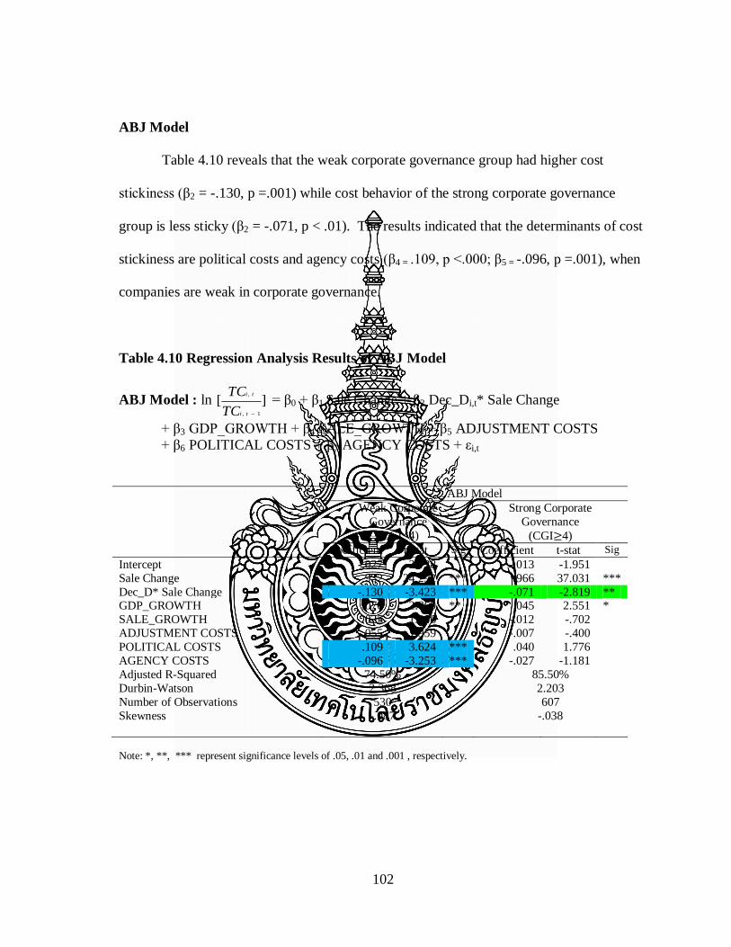
102
ABJ Model
Table 4.10 reveals that the weak corporate governance group had higher cost
stickiness (β2 = -.130, p =.001) while cost behavior of the strong corporate governance
group is less sticky (β2 = -.071, p < .01). The results indicated that the determinants of cost
stickiness are political costs and agency costs (β4 = .109, p <.000; β5 = -.096, p =.001), when
companies are weak in corporate governance.
Table 4.10 Regression Analysis Results of ABJ Model
ABJ Model : ln ][1,
,
ti
ti
TC
TC = β0 + β1 Sale Change
+ β2 Dec_Di,t* Sale Change
+ β3 GDP_GROWTH + β4 SALE_GROWTH + β5 ADJUSTMENT COSTS
+ β6 POLITICAL COSTS + β7 AGENCY COSTS + εi,t
ABJ Model
Weak Corporate
Governance
(CGI<4)
Strong Corporate
Governance
(CGI 4)
Coefficient t-stat Sig Coefficient t-stat Sig
Intercept -.027 -2.738 -.013 -1.951
Sale Change .932 24.292 *** .966 37.031 ***
Dec_D* Sale Change -.130 -3.423 *** -.071 -2.819 ** GDP_GROWTH .070 2.869 ** .045 2.551 *
SALE_GROWTH .025 1.046 -.012 -.702
ADJUSTMENT COSTS -.055 -1.959 -.007 -.400
POLITICAL COSTS .109 3.624 *** .040 1.776
AGENCY COSTS -.096 -3.253 *** -.027 -1.181
Adjusted R-Squared 74.50% 85.50%
Durbin-Watson 2.368 2.203
Number of Observations 530 607
Skewness -.087 -.038
Note: *, **, *** represent significance levels of .05, .01 and .001 , respectively.

103
BLS1 Model
Table 4.11 demonstrates that the weak corporate governance group had higher cost
stickiness (β2 = -.129, p < .001) while cost behavior of the strong corporate governance
group is less sticky (β3 = -.052, p<.01). The results indicated that the determinant of cost
stickiness are political costs and agency costs (β4 = .110, p <.001; β5 = -.120, p <.001), when
companies are weak in corporate governance.
Table 4.11 Regression Analysis Results of BLS1 Model
BLS1 Model: ][1,
1,,
ti
titi
TC
TCTC= β0 + β1 Sale Change
+ β2 Dec_Di,t* Sale Change
+ β3 GDP_GROWTH + β4 SALE_GROWTH + β5 ADJUSTMENT COSTS
+ β6 POLITICAL COSTS + β7 AGENCY COSTS + εi,t
BLS1 Model
Weak Corporate
Governance
(CGI<4)
Strong Corporate
Governance
(CGI 4)
Coefficient t-stat Sig Coefficient t-stat Sig
Intercept -.032 -2.906 -.014 -1.879
Sale Change .928 30.194 *** .949 46.791 ***
Dec_D* Sale Change -.129 -4.168 *** -.052 -2.616 **
GDP_GROWTH .062 2.540 ** .048 2.778 **
SALE_GROWTH .025 1.089 -.016 -.965 ADJUSTMENT COSTS -.047 -1.707 -.012 -.707
POLITICAL COSTS .110 3.696 *** .041 1.896
AGENCY COSTS -.120 -4.144 *** -.024 -1.089
Adjusted R-Squared 75.00% 86.00%
Durbin-Watson 2.479 2.195
Number of Observations 530 607
Skewness 1.375 .088
Note: *, **, *** represent significance levels of .05, .01 and .001 , respectively.

104
BLS2 Model
Table 4.12 demonstrates that the weak corporate governance group had high cost
stickiness (β2 = -.144, p < .001) while cost behavior of the strong corporate governance
group is not sticky. The results indicated that the determinant of cost stickiness is
adjustment costs, political costs, and agency costs (β3 = -.066, p <.05; β4 = .115, p =.001;
β5 = -.141, p <.001), when companies are weak in corporate governance. However,
adjustment costs still influence cost behavior of the strong corporate governance group.
Table 4.12 Regression Analysis Results of BLS2 Model
BLS2 Model: ][1,
1,,
ti
titi
S
TCTC= β0 + β1 Sale Change
+ β2 Dec_Di,t* Sale Change
+ β3 GDP_GROWTH + β4 SALE_GROWTH + β5 ADJUSTMENT COSTS
+ β6 POLITICAL COSTS + β7 AGENCY COSTS + εi,t
BLS2 Model
Weak Corporate
Governance
(CGI<4)
Strong Corporate
Governance
(CGI 4)
Coefficient t-stat Sig Coefficient t-stat Sig
Intercept -.046 -3.126 -.016 -2.215
Sale Change .881 24.276 *** .903 39.961 ***
Dec_D* Sale Change -.144 -3.937 *** -.023 -1.047
GDP_GROWTH .051 1.782 .059 3.102 **
SALE_GROWTH .029 1.071 -.016 -.873
ADJUSTMENT COSTS -.066 -2.019 * -.037 -2.006 *
POLITICAL COSTS .115 3.277 *** .032 1.334
AGENCY COSTS -.141 -4.104 *** -.008 -.322
Adjusted R-Squared 65.10% 82.60% Durbin-Watson 2.685 1.911
Number of Observations 530 607
Skewness 2.680 -1.878
Note: *, **, *** represent significance levels of .05, .01 and .001 , respectively.

105
Robustness Tests
This study performed a robustness check in an attempt to confirm that cost behavior
of Thai listed companies is sticky and to validate the determinants of cost stickiness. The
STATA version 11 software was used to analyze this panel data.
ABJ model, BLS1model, and BLS2 model were replicated by using linear models
for panel data that is fixed-effects and random-effects model (see Table 4.13, Table 4.14
and Table 4.15). As soon as these models have been carried out, the Hausman test was
executed in order to test whether random-effects model is appropriate instead of fixed-
effects model (Green, 2008). The results of the Hausman test indicated that fixed-effects
models are appropriate for all of three models.
Table 4.13 Regression Analysis Results of ABJ Model: Random-effect and Fixed-effect
ABJ Model Random-effects
ABJ Model Fixed-effects
Coefficient t Sig Coefficient t Sig
Intercept -.019 -3.31 -.027 -4.46
Sale Change .896 42.71 *** .939 38.43 *** Dec_D* Sale Change -.148 -4.46 *** -.198 -5.07 ***
GDP_GROWTH .400 3.61 *** .482 4.20 ***
SALE_GROWTH .006 0.42 .009 0.53
ADJUSTMENT COSTS -.004 -1.33 -.011 -1.13
POLITICAL COSTS .024 3.64 ** .035 3.17 **
AGENCY COSTS -.021 -3.11 ** -.112 -7.97 ***
Adjusted R-Squared 80.22% 75.01%
Note: *, **, *** represent significance levels of .05, .01 and .001 , respectively.

106
Table 4.14 Regression Analysis Results of BLS1 Model: Random-effects and Fixed-effects
BlS1 Model
Random-effects BLS1 Model Fixed-effects
Coefficient t Sig Coefficient t Sig
Intercept -.020 -3.24 -.028 -4.20
Sale Change .908 53.09 *** .939 47.02 ***
Dec_D* Sale Change -.180 -4.86 *** -.207 -4.71 ***
GDP_GROWTH .417 3.46 *** .517 4.12 ***
SALE_GROWTH .006 0.35 -.007 -0.40
ADJUSTMENT COSTS -.005 -1.37 -.010 -0.99
POLITICAL COSTS .029 4.06 *** .037 3.05 **
AGENCY COSTS -.028 -3.89 *** -.127 -8.28 *** Adjusted R-Squared 80.99% 75.58%
Note: *, **, *** represent significance levels of .05, .01 and .001 , respectively.
Table 4.15 Regression Analysis Results of BLS2 Model: Random-effects and Fixed-effects
BlS2 Model
Random-effects BLS2 Model Fixed-effects
Coefficient t Sig Coefficient t Sig
Intercept -.026 -3.39 -.035 -4.21
Sale Change .864 41.15 *** .888 36.14 ***
Dec_D* Sale Change -.159 -3.50 *** -.198 -3.67 ***
GDP_GROWTH .445 2.78 ** .530 3.43 ***
SALE_GROWTH .012 0.61 .012 0.56
ADJUSTMENT COSTS -.010 -2.50 * -.019 -1.53
POLITICAL COSTS .033 3.76 *** .051 3.41 ***
AGENCY COSTS -.035 -3.91 *** -.139 -7.32 ***
Adjusted R-Squared 71.99% 68.59% Note: *, **, *** represent significance levels of .05, .01 and .001 , respectively.
Panel A of Table 4.16 shows the results that did not consider the fixed effects as
panel B displays the results that were considered the fixed effects. It is evident that β2
coefficient is negative and statistical significant for all models. Therefore, these results
have further strengthened the conviction that the cost behavior of Thai listed companies is
sticky and the determinants of cost stickiness are adjustment costs, political costs, and
agency costs.

107
Table 4.16 Regression Analysis Results of No Fixed-effects and Fixed-effects models
Model: Cost change = β0 + β1 Sale change+ β2 Dec_Di,t* Sale change
+ β3 GDP_GROWTH + β4 SALE_GROWTH + β5 ADJUSTMENT COSTS
+ β6 POLITICAL COSTS + β7 AGENCY COSTS + εi,t
Panel A ABJ Model BLS1 Model BLS 2 Model
Coefficient t Coefficient t Coefficient t
Intercept -.019 -3.314 -.020 -3.239 -.026 -3.391
Sale Change .954 42.711 *** .941 53.093 *** .882 41.146 ***
Dec_D* Sale Change -.097 -4.457 *** -.085 -4.859 *** -.074 -3.502 ***
GDP_GROWTH .053 3.612 *** .050 3.456 *** .049 2.782 **
SALE_GROWTH .006 0.432 .005 0.349 .010 0.611
ADJUSTMENT COSTS -.020 -1.331 -.020 -1.366 -.045 -2.496 *
POLITICAL COSTS .068 3.644 *** .075 4.061 *** .084 3.759 *** AGENCY COSTS -.059 -3.107 ** -.073 -3.894 *** -.088 -3.914 ***
Adjusted R-Squared 80.10% 80.70% 71.80%
Panel B ABJ Model Fixed-effect
BLS1 Model Fixed-effect
BLS 2 Model Fixed-effect
Coefficient t Coefficient t Coefficient t
Intercept -.027 -4.46 -.028 -4.20 -.035 -4.21
Sale Change .939 38.43 *** .939 47.02 *** .888 36.14 ***
Dec_D* Sale Change -.198 -5.07 *** -.207 -4.71 *** -.198 -3.67 *** GDP_GROWTH .485 4.20 *** .517 4.12 *** .530 3.53 ***
SALE_GROWTH .009 0.53 .007 0.40 .012 0.56
ADJUSTMENT COSTS -.011 -1.13 -.010 -0.99 -.019 -1.53
POLITICAL COSTS .035 3.17 ** .037 3.05 ** .051 3.41 ***
AGENCY COSTS -.112 -7.97 *** -.128 -8.28 *** -.139 -7.32 ***
Adjusted R-Squared 75.01% 75.58% 66.98%
Panel C ABJ Model Random-effect
BLS1 Model Random-effect
BLS 2 Model Random-effect
Coefficient t Coefficient t Coefficient t
Intercept -.019 -3.31 -.020 -3.24 -.026 -3.39
Sale Change .896 42.71 *** .908 53.09 *** .864 41.15 ***
Dec_D* Sale Change -.148 -4.46 *** -.180 -4.86 *** -.159 -3.50 ***
GDP_GROWTH .400 3.61 *** .417 3.46 *** .412 2.78 **
SALE_GROWTH .006 0.42 .006 0.35 .012 0.61
ADJUSTMENT COSTS -.004 -1.13 -.005 -1.37 -.010 -2.50 *
POLITICAL COSTS .024 3.64 *** .029 4.06 *** .033 3.76 ***
AGENCY COSTS -.021 -3.11 ** -.028 -3.89 *** -.035 -3.91 ***
Adjusted R-Squared 80.22% 80.84% 71.99%
Note: *, **, *** represent significance levels of .05, .01 and .001 , respectively.

108
Summary
The analysis was comprised of three stages. The first stage consisted of a series of
confirmatory factor analyses to assure that the measurement models had adequate fit to the
data (e.g., adjustment cost model, political cost model, and agency cost model). All of
measurement models demonstrated good fit and were supported for construct reliability.
The second stage consisted of a series of exploratory factor analyses to acquire factor
scores for the next stage. The factor scores of adjustment costs, political costs, and agency
costs were able to capture information and explain 67.98% , 73.58%, and 67.84% of
variance. The final stage consisted of constructing three structural models of cost behavior
by multiple regression analysis. The overall models were supported with statistical
significance .001 level.
Testing of the hypotheses revealed that all of six hypotheses were supported with
statistical significance ranging from the .001 level to the .05 level. There was significant
support for the stickiness of cost behavior in Thai listed companies, especially total
operating costs. Agency costs, political costs, and corporate governance demonstrated a
strong influence on cost stickiness. Adjustment costs exerted a mediate influence on cost
stickiness. The details of these finding will be discussed further in chapter 5.

109
CHAPTER 5
CONCLUSIONS AND RECOMMENDATIONS
This final chapter of the dissertation restates the research questions and reviews the
methods used in the study. The major sections of this chapter are conclusions and
discussions of the findings, limitations of the study, and recommendations.
The current study is concerned with the following research questions:
1. Is the cost behavior of Thai listed companies sticky?
2. Is the cost behavior still sticky, after controlling the economic variables?
3. Do adjustment costs affect the degree of cost stickiness?
4. Do political costs affect the degree of cost stickiness?
5. Do agency costs affect the degree of cost stickiness?
6. Does corporate governance affect the degree of cost stickiness?
The research questions for the current study were utilized to develop the following
six hypotheses:
H1a: The cost behavior of Thai listed companies is sticky.
H2a: The cost behavior is still sticky, after controlling the economic variables.
H3a: Adjustment costs affect the degree of cost stickiness in a positive direction.
H4a: Political costs affect the degree of cost stickiness in a positive direction.
H5a: Agency costs affect the degree of cost stickiness in a positive direction.
H6a: Corporate governance affects the degree of cost stickiness in a negative
direction.

110
The hypotheses were tested using the structural models of sticky cost behavior from
a set of quantitative statistical analysis. As explained in chapter 1, this study is based on
financial reports of Thai listed companies to investigate sticky cost behavior and the
determinants of sticky cost behavior. The study examined sticky cost behavior using a
structural equation modeling (SEM) approach, a relatively new approach for sticky cost
behavior research. The analysis utilized three sticky cost behavior models- i.e. ABJ model,
BLS1 model, and BLS2 model. ABJ model is a log linear model which was developed by
Anderson, Banker, and Janakiraman (2003). BLS1 model and BLS2 model were proposed
by Balakrisman, Labro, and Soderstrom (2010). They are models which removed
committed fixed costs, because BLS1 model used percentage change in costs and sales,
while BLS2 model used change in costs and sales that deflated by sales.
In the first stage of analysis the measurement models of adjustment costs, political
costs, and agency costs were developed and tested by confirmatory factor analysis (CFA).
The second stage of analysis the more parsimonious set factor scores were estimated by
exploratory factor analysis (EFA) and used in multiple regression analysis. The final stage
of analysis the structural models of sticky cost behavior were constructed. In addition,
fixed-effects models (linear models for panel data) were conducted and compared to the no
fixed-effects models.
Conclusions
This study found that behavior of total operating costs was sticky for all models
(ABJ model, BLS1 model, and BLS2 model). Total operating costs increased by around
111
0.93% per 1% increased in sale revenue, but decreased only 0.86% per 1% decreased in
sale revenue. The results provided support for Hypothesis 1. However, the behavior of
cost of goods sold and selling, general and administrative costs were not sticky.
Behavior of total operating costs was still sticky after controlling economic growth
for all models. The results provided support for Hypothesis 2. Even though GDP growth
had a significant influence on cost stickiness in a negative direction, cost behavior was still
sticky and stickier than before controlling economic growth.
The only BLS2 model demonstrated the effect of adjustment costs on the degree of
cost stickiness in a positive direction, while agency costs affected the degree of cost
stickiness in a positive direction for all models. However, political costs and corporate
governance affected the degree of cost stickiness in a negative direction. The findings
provide support for Hypothesis 3, Hypothesis 5 and Hypothesis 6, but do not provide
support for Hypothesis 4.
Discussions of the Finding
Sticky Cost Behavior of Thai Listed Companies
The results of the hypotheses testing for sticky cost behavior partially supported the
existing literature. Behavior of cost of goods sold and selling, general and administrative
costs were not sticky. These findings differed from the previous research by Anderson et
al. (2003), Subramaniam and Weidenmier (2003), Medeiros and Costa (2004), Banker et al.
(2008), Balakrishnan and Gruca (2008) and Banker et al. (2011). On the contrary, behavior
of total operating costs was sticky. This finding provided support to prior research

112
(Anderson et al., 2003; Subramaniam & Weidenmier, 2003; Medeiros and Costa, 2004;
Banker et al., 2008; Balakrishnan & Gruca, 2008). The difference in findings might be
explained by variation in classification and reclassification of the items in financial reports.
For example, doubtful debt accounts are selling, general and administrative costs, but are
separated as significant items in some years or in some companies. This means that it did
not have a consistent classification. Another possible explanation for this was that in
emerging markets firms could not forecast accurate sales while costs were committed.
These unfavorable variances from this expectation were pushed into cost of goods sold.
However, some firms immediately recorded sales revenues when they received purchases
orders and cash deposit. Thus, the degree of cost stickiness might depend on the firms’
bargaining power over buyers or suppliers.
Additionally, this study investigated sticky cost behavior by categorizing samples
into industries, and found that cost behavior of services industry was the “stickiest”. This
finding differed from previous research by Subramaniam and Weidenmier (2003), who
reported that manufacturing is the “stickiest” due to its high levels of fixed assets and
inventory. It was capital intensive sector. The difference might be explained by variance
in the geographic region, type, and quality of services. Thai services industry consists of
commerce, health care services, media and publishing, tourism and leisure, and
transportation and logistics sectors. There was a number of skill labors in these sectors, as
well as being labor intensive sectors.
In-depth interviews showed that a company’s image is important. The companies
cannot reduce a number of employees although sales decrease. They must maintain quality
113
of their services; for example, in the case of a premium airline. The front officers and
skilled employees such as aviators, aircraft mechanics and crews were retained while sales
decrease.
It was also consistent with the previous evidence that the firing costs for labor are
higher than the hiring cost (Jaramillo, Schiantarelli, & Sembenelli, 1993; Pfann & Plam,
1993; Goux, Maurin, & Pauchet, 2001). This was supported by the Labour Protection Act
B.E. 2541 (1998) which required that “Severance pay must be paid to an employee who
his/her employment is terminated”. An employee who has worked for an uninterrupted
period of 10 years or more must receive payment of not less than his/her last rate of wages
for 300 days. Furthermore, the Thai economic conditions reports of the Bank of Thailand
(2001-2009) showed that the service sector has been affected by political uncertainty (such
as the closure of airports in 2008), the unrest in the three southernmost provinces (during
2004-2009), the outbreak of avian flu in poultry (2004) and the natural disaster in six
provinces (Phuket, Krabi, Ranong, Phangnga, Trang, and Satun) along the Andaman coast
(Tsunami in 2004). Despite these unfavorable events, the value of exports of services,
particularly tourism revenue, could rebound in a short time. Hence, managers might
maintain labor when sales decreased.
Influence of Economic Growth
The time period of this study was 2001-2009. There were many critical events such
as the uncertainties regarding the US-Iraq War, the outbreak of Severe Acute Respiratory
Syndrome (SARS), high world oil prices, the US subprime, global economic downturn, and

114
global financial crisis. Thai companies were most severely affected by these global
economic crises. The Thai economy had grown at the beginning of the study period, and
then it slowed down from 2004. “In 2009, the overall economy contracted by 2.3 percent
year-on-year, the first time in a decade, due to the global financial crisis which significant
affected Thailand’s major trading partner countries” (Bank of Thailand, 2009). Therefore,
this study used economic growth as controlled variables in order to investigate only the
effect of sale changes on the degree of cost stickiness.
Costs behavior was still sticky after controlling economic growth. The results
reveal that they were not only economic variables but also other factors which affect the
degree of cost stickiness. Several research studies supported the effects of economic
growth on sticky cost behavior (Anderson et al., 2003; Banker & Chen, 2006b; Anderson &
Lanen, 2007; Banker et al., 2008; Chen et al.,2008; Banker et al., 2011). The findings
implied that the degree of cost stickiness was subjected to the deliberate resource
adjustment decision made by managers.
Influence of Adjustment Costs
The results show the effects of adjustment costs on the degree of cost stickiness
partially supported the findings in the existing literature (Anderson et al., 2003;
Subramaniam & Weidenmier , 2003; Medeiros & Costa, 2004; Banker et al., 2008;
Balakrishnan & Gruca, 2008; Chen et al., 2008). Only BLS2 model demonstrates that
adjustment costs affected the degree of cost stickiness. The premise of adjustment cost
theory, which managers will be hesitant about making the decision to decrease resources

115
when sales decrease, was confirmed by these findings. Additionally, the current findings
also supported research by Banker et al. (2011) who studied with the Global Compustat
data which included seventeen countries and found that, for most countries higher
adjustment costs were associated with a significantly higher degree of cost stickiness.
Influence of Political Costs
The accounting research recognized the effects of financial reports on the
distribution wealth and power in society (Deegan & Unerman, 2011). The political process
theory proposed that management utilizes accounting choices to decrease wealth transfers
resulting from the regulatory process (Watts & Zimmerman, 1986; Grace & Leverty, 2010).
Empirical research suggested that political costs were important variables in disclosure
decision and accounting method decision.
This study added political costs into the sticky cost behavior models as variables in
order to account for their impacts on sticky cost behavior. It was assumed that political
costs affected the degree of cost stickiness in a positive direction, whereas the result was
found that political costs affected the degree of cost stickiness in a negative direction. The
possible explanations for this finding might be that most of the previous studies were done
in the US, where there are many choices for financial accounting standards, that are
difference from the Thai financial accounting standards, which have only a few accounting
choices. Political costs might affect in an adverse direction in the case of Thai companies.
Even though the results differed from the prior hypothesis, they demonstrate that
political costs were related to the degree of cost stickiness. This provided further evidence

116
to support the accounting research which found that high political cost companies have a
greater incentive to adjust accounting numbers and financial ratios to obtain the desired
target (Seay et al., 2004).
Influence of Agency Costs
Agency costs showed significant effects on sticky cost behavior, and therefore
provided support for the existing literature (Anderson et al., 2003; Banker et al., 2008;
Chen et al., 2008; Banker et al., 2011). This result confirms the agency theory which
proposed that managers might not behave in the way that aligned with shareholders’
interests. Then, sticky costs might occur from the role of manager, in adjusting committed
resources in response to a change in activities. The evidence from this study reveals that
higher agency costs were associated with a significantly higher degree of cost stickiness.
Influence of Corporate Governance
As mentioned in the results, the samples were separated into two groups based on
current corporate governance indexes (CGI). This study utilized CGI as a proxy of
corporate governance. Even though CGI could not be a variable in the model, the findings
were consistent with earlier studies (Chen et al., 2008). It proved that corporate governance
could reduce agency costs and the degree of cost stickiness. Corporate governance made
managers act that aligned with shareholders’ interests rather than their own interests. In
addition, the study confirmed that CGI, which are the current evaluation criteria of Thai

117
Institute of Directors Association, are practical indicators and able to be used as a corporate
governance standard for Thai companies.
Limitations of the Study
It is important to understand the limitations of this research so that circumspection
can be exercised when interpreting and referring to the results. To begin with new
methodology was introduced in this study was only Semi-SEM, so indirect effects of the
variables could not be examined. The measurement models of adjustment costs, political
costs, and agency costs were constructed with confirmatory factor analysis (CFA). The all
models were good fit, while construct reliability of political cost model was not high. It is
recommended that in future studies, which utilize political costs as variables, should
continue to develop an appropriate and reliable measurement model of political costs.
It is also important to recognize that the data set in this study was from an archived
source. Data was collected from financial reports and documents of the Stock Exchange of
Thailand and Thai Institute of Directors Association. Specifically, items in financial
statements, their classification were not consistent among companies and across year to
year. Collecting the data must be done with cautious consideration and judgment.
Although the data used in this study was collected by accountants, there was the risk that
some confounding effects might have been introduced into the models. Caution should be
taken into deliberation when interpreting the results.

118
Recommendations
Recommendations for Chief Executive Officer (CEO)
To increase the potential for competition, Thai companies should have accounting
systems that are consistent with international standards, transparent and verifiable
(Trairatvorakul, 2011b). Information is therefore important. Management accounting is
a part of the information system. The chief executive officers, or managers, need economic
information in order to make decisions efficiently concerning the allocation of scarce
economic resources (Atrill & McLaney, 2009). An understanding of cost behavior is
critical to managers so that they can predict accurate future costs. The evidence from this
study suggests that the total operating cost behavior is sticky. Knowing that cost behavior
is sticky assists managers and accountants realize and to be careful when they apply the
cost estimation method that is based on the traditional model of cost behavior in cost
analysis.
Recommendations for Investors and financial analysts
Another factor that must be considered for understanding managers’ behavior, the
determinants of sticky cost behavior may reveal the behavior of managers which is not
disclosed in published financial reports. This is material information for investors and
financial analysts when they analyze financial statements. They can then make an informed
decision so that they will receive high returns from their investment.

119
Recommendations for Government or Regulators
In this study, the political costs were shown to be associated with the degree of cost
stickiness. The result implies that the government policies have an influence on cost
behavior of companies. Hence, the government should consider policies and regulations in
both macroeconomic and microeconomic perspectives. For example, the Thai Government
expects to raise the daily minimum wage for employees nationwide to Bt300, or US$10
early next year (“Minimum Wage Ball in Govt Court,” 2012). This study has highlighted
that cost behavior of the service industry is “stickiest”, thus by increasing the daily
minimum wage will most likely have a strong impact on the survival of the service industry
which has a number of skilled employees.
Recommendations for the Stock Exchange of Thailand
This study proved that good corporate governance can reduce agency costs. The
Thai Institute of Directors Association (IOD) should encourage and invite companies to
engage in the IOD’s project which has reported the results of the evaluation of corporate
governance practices of Thai listed companies since 2001. When a company has good
corporate governance it also implies that corporate value will be increased.
Recommendations for Future Research
While this study served to answer some of questions for sticky cost behavior in
regarding the context of adjustment costs, political costs, and agency costs, there are other
questions that were not covered in this study. It is recommended that in future research

120
other variables that affect management decision such as life cycle of company, company’s
culture, company’s strategy, leadership style, and environmental changes should also be
considered.
A further important recommendation is the research model. Political process theory
was incorporated into the model via political costs and was a major addition that has not
been adequately addressed in the existing literature in regard to the effects it had on cost
stickiness. In addition, the new method and alternative models were utilized to develop
cost behavior models. Although the results of the models relations were mixed, there were
a sufficient number of paths which had statistically significant interaction between
constructs to support the complex relationships.
Additionally, the measurement model of latent variables should be strongly
considered and improved for future research. This study is the first step for developing a
measurement model in the study of cost behavior study; while the measurement model of
political costs has a construct reliability of only 63% although it is a good fit statistically.
Because political costs cannot observed directly, the design and development of a
measurement model of political costs will be a challenge. Further research should examine
new variables for the latent variable. For instance, employee intensity is measured from the
number of employees, this may not be appropriate for the current economic condition, in
which companies outsource work. The majority of employees come from outsourced
companies.
This study utilized secondary data, collected from financial statements which is
information provided for external users. The cost behavior models from this study are

121
original models which can be used for continuous research. If organizational, or inside
data, can be collected, other interesting variables can be investigated such as research
conducted by Balakrishnan et al. (2004), Anderson et al. (2005), Bosch and Blandon
(2007), Balakrishnan and Gruca (2008), Balakrishnan and Soderstrom (2008) and Banker et
al. (2008). The cost behavior models will be optimal, powerful and useful.
This study utilized merely Semi-SEM to construct sticky cost behavior model since
cost stickiness cannot be measured directly. The current research by Weiss (2010)
introduced the measurement method of cost stickiness by quarterly time frames. Future
research should investigate and enhance the measurement of cost stickiness annual
calculations. SEM will be powerful tool for studying sticky cost behavior because it is able
to examine both direct and indirect effects.
Lastly, it is recommended that a confirmation of the findings of this study should
also be conducted with non-listed companies, as additional research results that utilize
different samples would validate that the results found here could then, possibly, be
generalized and applied to all Thai companies.

122
LIST OF REFERENCES
Anderson, J. C., & Gerbing, D. W. (1988). Structural Equation Modeling in Practice: A
Review and Recommended Two-step Approach. Psychological Bulletin, 103(3),
411-423.
Anderson, M. C., Banker, R. D., & Janakiraman, S. N. (2003). Are Selling, General, and
Administrative Costs "Sticky"? Journal of Accounting Research, 41(1), 47-63.
Anderson, S. W., & .Lanen, W. N. (2007). Understanding Cost Management: What Can
We Learn from the Evidence on 'Sticky Costs? Working Paper. Rice University.
Anderson, W. S., Chen, C. X., & Young, S. M. (2005). Sticky Costs as Competitive
Response : Evidence on Strategic Cost Management at Southwest Airlines.
Working Paper. Rive University.
Ang, J. S., Cole, R. A., & Lin, J. W. (2000). Agency Costs and Ownership Structure.
Journal of Finance, 55(1), 81-106.
Arbuckle,J.L. (2007). AmosTM
16 user’s guide. Chicago : SPSS.
Atrill, P.,& McLaney, E. (2009) Management Accounting for Decision Makers (6th ed.).
Harlow: Prentice-Hall, Inc.
Babad, Y. M., & Balachandran, B. V. (1993). Cost driver optimization in activity-based
costing. The Accounting Review, 68(3), 563.
Balakrishnan, R., & Gruca, T. S. (2008). Cost Stickiness and Core Competency: A Note.
Contemporary Accounting Research, 25(1), 993-1006.
Balakrishnan, R., Labro, E., & Soderstrom, N. (2010). Cost Structure and Sticky Costs.
Working Paper .University of Iowa.
Balakrishnan, R., Petersen, M. J., & Soderstrom, N. S. (2004). Does Capacity Utilization
Affect the "Stickiness" of Cost? Journal of Accounting, Auditing & Finance,
283-299.
Balakrishnan, R., & Soderstrom, N. S. (2008). Cross-Sectional Variation in Cost
Stickiness Reaction (Research Paper Series). Boulder: University of Colorado.
Banker, R. D., Byzalov, D., & Plehn-Dujowich, J.M. (2011). Sticky Cost Behavior:
Theory and Evidence. Working Paper. Temple University.
Banker, R. D., & Chen, L. (2006a). Labor Market Characteristics and Cross-Country
Differences in Cost Stickiness. Working Paper. Temple University.

123
Banker, R. D., & Chen, L. (2006b). Predicting Earnings Using a Model Based on Cost
Variability and Cost Stickiness. The Accounting Review, 81(2), 285-307.
Banker, R. D., Ciftci, M., & Mashruwala, R. (2008). Managerial Optimism, Prior Period
Sales Changes, and Sticky Cost Behavior. Working Paper. Temple University.
Banker, R. D., & Hughes, J. S. (1994). Product Costing and Pricing. The Accounting
Review, 69(3), 479-494.
Beaver, William H. (1989). Financial Reporting: An Accounting Revolution (2nd
Ed.).
New Jersey: Prentice-Hall, Inc.
Belkaoui, A., & Karpik, P. G. (1989). Determinants of the Corporate Decision to
Disclose Social Information. Accounting, Auditing and Accountability Journal
2(1), 36-51.
Bentler, P. M. & Chou, C. P. (1987). Practice Issue in Structural Equation Modeling.
Sociological Methods and Research, 16(1), 78-117.
Bhagat, S., & Jefferis., R. H. (2002). The Econometrics of Corporate Governance
Studies. London: The MIT Press.
Birt, J. l., Bilson, C. M., Smith, T., & Whaley, R. E. (2006). Ownership, Competition,
and Financial Disclosure. Australian Journal of Management, 31(2), 235-263.
Bosch, J. M. A., & Blandon, J. G. (2007). Cost Stickiness Revisited : Empirical
Aplication for Farms. Working Paper. University de Barcelona.
Byrne, B. M. (2010). Structural Equation Modeling with AMOS (2nd
ed.). New York:
Routledge.
Calleja, K., Steliaros, M. E., & Thomas, D. C. (2006). A Note on Cost Stickiness: Some
International Comparisons. Management Accounting Research, 17, 127-140.
Cameron, A. Colin, & Trivedi, pravin K. (2009). Microecomometrics Using Stata. Texas
:Stata Press.
Chae, J., Kim, S., & Lee, E. J. (2009). How Corporate Governance Affects Payout Policy
under Agency Problems and External Financing Constraints. Journal of Banking
& Finance, In Press, Corrected Proof.
Chen, C. X., Lu, H., & Sougiannis, T. (2008). Managerial Empire Building, Corporate
Governance, and the Asymmetrical Behavior of Selling, General, and
Administrative Costs. Paper presented at the 2009 Management Accounting
Section Research and Case Conference, Florida.

124
Chen, X., & Yur-Austin, J. (2007). Re-measuring Agency Costs: The Effectiveness of
Blockholders. Quarterly Review of Economics and Finance, 47(5), 588-601.
Chen, Y.-R., & Chuang, W.-T. (2009). Alignment or entrenchment? Corporate
governance and cash holdings in growing firms. Journal of Business Research,
62(11), 1200-1206.
Cooper, R.W., & Haltiwanger, C.J. (2006). On the Nature of Capital Adjustment Costs.
Review of Economic Study, 73, 611-633.
Danizger, L.(2008). Adjustment Costs, Inventories and Output. The Scandinavian
Journal of Economic, 110(3), 519-542.
Deegan, C.,& Unerman, J. (2011). Financial Accounting Theory (2nd
ed.). London:
McGraw-Hill Companies,Inc.
Demsetz, H.,& Lehn, K.(1985). The Structure of Corporate Ownership: Causes and
Consequences. Journal of Political Economy, 93, 1155-1177.
Demski, J. S. (2008). Managerial Uses of Accounting Information (2nd
ed.). New York:
Springer Science and Business Media,LLC.
Dey, A. (2008). Corporate Governance and Agency Conflicts. Journal of Accounting
Research, 46(5), 1143-1181.
Dierynck, B., & Renders, A. (2009). Earnings Management Incentives and the
Asymmetric Behavior of Labor Costs. Paper presented at the 2009 GMARS
Conference.
Dittmar, A., & Mahrt-Smith, J. (2007). Corporate Governance and the Value of Cash
Holdings. Journal of Financial Economics, 83(3), 599-634.
Eisenhardt, K. M. (1989). Agency Theory : An Assessment and Review. The Academy of
Management Review, 14(1), 57-74.
Epstein, L. G., & Denny, M.G.S. (1986). The Multivariate Flexible Accelerator Model:
Its Empirical Restrictions and an Application to U.S. Manufacturing.
Econometrica, 51(3), 647-674.
Fleming, G., Heancy, R., & McCosker, R. (2005). Agency Costs and Ownership
Structure in Australia. Pacific-Basin Finance Journal, 13, 29-52.
Florackis, C. (2008). Agency Costs and Corporate Governance Mechanisms: Evidence
for UK firms. International Journal of Managerial Finance, 4(1), 37-59.
Foster, G. (1986). Financial Statement Analysis (2 ed.). New Jersey: Prentice-Hall,Inc.

125
Gamerschlag, R., Moller, K., & Verbeeten, F. (2010). Determinants of Voluntary CSR
Disclosure: Empirical Evidence from Germany. Review Management Science,
1-30.
Godfrey, J. M., & Jones, K. L. (1999). Political cost influence on income smoothing via
extraordinary item classification. Accounting & Finance, 39, 229-254.
Gogineni, S., Linn, S. C., & Yadav, P. K. (2009). Empirical Evidence on Ownership
Structure, Manangement Control and Agency Costs. Working Paper. University
of Oklahoma.
Goux, D., Maurin, E., & Pauchet, M. (2001). Fixed-term Contracts and the dynamics of
Labour Demand. Review of Economic Studies, 45, 533-552.
Grace, M. F., & Leverty, J. T. (2010). Political Cost Incentives for Managing the
Property-Liability Insurer Loss Reserve. Journal of Accounting Research, 48,
21-49.
Green, H.W. (2008). Econometric Analysis (7 ed.). New York: Pearson Education, Inc.
Groth, C.,& Khan, H. (2010). Investment Adjustment Costs : An Empirical Assessment.
Journal of Money, Credit and Banking, 42(8), 1469-1494.
Hamermesh, D. S.,& Pfann, G. A. (1996). Adjustment Costs in Factor Demand. Journal
of Economic literature, 34(3), 1264-1292.
Hancock, G. R., & Mueller, R, O. (2006). Structural Equation Modeling: A Second
Course. Connecticut : Information Age Publishing, Inc.
Hart, O. (1995). Corporate Governance : Some Theory and Implications. The Economic
Journal, 105(430), 678-689.
Henry, D. (2009). Agency Costs, Ownership Structure and Corporate Governance
Compliance: A Private Contracting Perspective. Pacific-Basin Finance Journal,
In Press, Corrected Proof.
Hsu, I.-Y., Su, T.-S., Kao, C.-S., Shu, Y.-L., Lin, P.-R., & Tseng, J.-M. (2012). Analysis
of Business Safety Performance by Structural Equation Models. Safety Science,
50, 1-11.
Hilton, R. W., Maher, M. W., & Selto, F. H. (2008). Cost Management : Strategies for
Business Decisions (4th ed.). New York: McGraw-Hill ,Inc.
Homburg, C., & Julia, N. (2008). How Timely are Earnings When Costs are Sticky?
Implications for the Link Between Conditional Conservatism and Cost Stickiness.
Paper presented at the European Accounting Association Conference.

126
Horngren, C. T., Datar, S. M., &Rajan, M.V. (2012). Cost Accounting : A Managerial
Emphasis (14th ed.). New Jersey: Pearson Education, Inc.
Hoyle, Rick H. (1995). Structural Equation Modeling.(2nd
ed.). London: SAGE
Publications,Inc.
Inoue, T., & Thomas, W. B. (1996). The Choice of Accounting Policy in Japan. Journal
of International Financial Management and Accounting, 7(1), 1-23.
Jaramillo, F., Schiantarelli, F., & Sembenelli, A. (1993). Are Adjustment Costs for labor
Asymmetric? An Econometric Test on Panel Data for Italy. Review of Economic
and Statistic, 74, 640-648.
Jelinek, K., & Stuerke, P. S. (2009). The Nonlinear Relation Between Agency Costs and
Managerial Equity Ownership. International Journal of Managerial Finance,
5(2), 156-178.
Jensen, M. C. (1986). Agency Costs of Free Cash Flow, Corporate Finance, and
Takeovers. American Economic Review, 76(2), 323-329.
Jensen, M. C. (1993). The Modern Industrial Revolution, Exit, and The Failure of
Internal Control Systems. Journal of Finance, 48, 831-880.
Jensen, M. C., & Meckling, W. H. (1976). Theory of the Firm : Managerial Behavior,
Agency Costs and Ownership Structure. Journal of Financial Economics, 3(4),
305-360.
Kanagaretnam, K., Lobo, G. J., & Whalen, D. J. (2007). Does Good Corporate
Governance Reduce Information Asymmetry Around Quarterly Earnings
Announcements? Journal of Accounting and Public Policy, 26(4), 497-522.
Kern, B. B., & Morris, M. H. (1991). Taxes and Firm Size: The Effect of Tax Legislation
during the 1980s. The Journal of the American Taxation Association, 80-96.
Kline, R. B.(2011). Principles and Practice of Structural Equation Modeling (3rd
ed.).
New York: Guilford Press.
Kuo, K. (2007). The Impact of Product Diversification and Capacity Utilization on Cost
Behavior : A test of Cost Stickiness. Working Paper. Taiwan University.
Lamm-Tennant, J., & Rollins, T. (1994). Incentives for Discretionary Accounting
Practices: Ownership Structure, Earning, Size, and Taxation. The Journal of Risk
and Insurance, 61(3), 476-491.

127
Lanen, W. N.,Shannon W. S.,& Maher, M, W.(2011). Fundamental of Cost Accounting
(3rd
ed.). New York: McGraw-Hill.
Lang, L. H.P., Stulz, R. M., & Walkling, R. A. (1991). A Test of the Free Cash Flow
Hypothesis. Journal of Financial Economics.29, 315.335.
Larcker, D. F., Richardson, S. A., & Tuna, I. (2007). Corporate Governance, Accounting
Outcomes, and Organizational Performance. The Accounting Review, 82(4), 963-
1008.
Leitao, N. C. (2011). Intra-industry Trade, Knowledge and Adjustment Costs. Journal of
Applied Sciences,11(14), 2652- 2656.
Lucas, R. E. (1967). Adjustment Costs and the Theory of Supply. The Journal of Political
Economy, 75(4), 321- 334.
Maher, M. W., Stickney, C. P., & Weil, R. L. (2008). Manangerial Accounting : An
Introduction to Concepts, Methods and Uses (10 ed.). Manson: Thomson Higher
Education.
McKnight, P. J., & Weir, C. (2009). Agency Costs, Corporate Governance Mechanisms
and Ownership Structure in Large UK Publicly Quoted Companies: A Panel Data
Analysis. The Quarterly Review of Economics and Finance, 49(2), 139-158.
Medeiros, O. R., & Costa, P. S. (2004). Cost Stickiness in Brazilian Firms. Paper
presented at the 4th USP Congress of Managerial Control and Accounting.
Minimum Wage Ball in Govt Court (2012, September 6). The Nation, pp. A1, A2.
Mortensen, D. T.(1973). Generalized Costs of Adjustment and Dynamic factor Demand
Theory. Econometrica,41(4), 657- 665.
Nakamura, S. (1993). An Adjustment Cost model of Long-term Employment in Japan.
Journal of Applied Econometrics, 8 (2), 175-194.
Nasev, J. (2009). Conditional and Unconditional Conservatism : Implications for
Accounting Based Valuation and Risky Projects. Berlin: Gabler.
Noreen, E., & Soderstrom, N. (1994). Are Overhead Costs Strictly Proportional to
Activity? : Evidence From Hospital Departments. Journal of Accounting and
Economics, 17(1-2), 255-278.
Noreen, E., & Soderstrom, N. (1997). The Accuracy of Proportional Cost Models:
Evidence from Hospital Service Departments. Review of Accounting Studies, 2(1),
89-114.

128
Peltzman, S. (1976). Toward a More General Theory of Regulation. Journal of law and
Economics, 19(8), 211-240.
Pfann, G. A., & Plam, F. C. (1993). Asymmetric Adjustment Costs in Non-linear Labour
Demand Model for the Netherlands and U.K. Manufacturing Sectors. Review of
Economic Studies, 60, 379-412.
Seay, S. S., Pitts, S. T., & Kamery, R. H. (2004). The Contribution of Firm-specific
Factors: Theory Development of the Ratio Adjustment Process. Paper presented at
the Alli Academies international Conference, New Orleans.
Singh, M., & Wallace, N. D. (2003). Agency Costs, Ownership Structure and Corporate
Governance Mechanisms. Journal of Banking & Finance, 27(5), 793-816.
Solomon, J., & Solomon, A. (2004). Corporate Governance and Accountability. West
Sussex: John Wiley & Sons, Ltd.
Smith, D.& Langfield-Smith, K. (2004). Structural Equation Modeling on Management
Accounting Research : Critical Analysis and Opportunities. Journal of Accounting
Literature,23,49-86.
Subramaniam, C., & Weidenmier, M. L. (2003). Additional Evidence on the Sticky
Behavior of Costs. Working Paper. Texas Christian University.
Thompson, B. (2004). Exploratory and Confirmatory Factor Analysis: Understanding
Concepts and Applications. Washington DC: American Psychological
Association.
Trairatvorakul, P. (2011a). ASEAN Economic Community 2015: Opportunities or
Threats? Retrieved May 2, 2012 from http://www.bot.or.th/English/PressAnd
Speeches/Speeches/ Gov/SpeechGov_15Sep2011.pdf)
Trairatvorakul, P. (2011b). Changing and Adapting in Financial Business Sector for
Preparing into Trade Liberalization. Retrieved May 2, 2012 from http://www.bot.or.th/Thai/Press AndSpeeches/ Speeches/Gov/
SpeechGov_07oct2011.pdf - 126k
Truong, T. (2006). Corporate Boards, Ownership and Agency Costs: Evidence from
Australia. The Business Review, Cambridge, 5(2), 163.
Turner, C. (2009). Corporate Governance : A practical Guide for Accountants. Oxford:
Elsevier Ltd.
Vanichbuncha, K.(2010). Multivariate Statistical Methods.Bangkok.

129
Watts, R. L., & Zimmerman, J. L. (1986). Positive Accounting Theory. New Jersey:
Prentice-Hall, Inc.
White, G. I., Sondhi, A. C., & Fried, D. (2003). The Analysis and Use of Financial
Statements (3 ed.). New York: John Wiley & Sons Inc.
White, T., & Dieckman, E. (2005). Seizing Control of SGA. Financial Manangement,
20-23.
Wong, J. (1988). Economic Incentives for the Voluntary disclosure of Current Cost
Financial Statements. Journal of Accounting and Economics, 10, 151-167.
Weiss, D. (2010). Cost Behavior and Analysts' Earnings Forecasts. Accounting Review,
85, 1441-1471.
Yang, D. H., Lee, Y. T., & Park, K. H. (2005). Sticky Cost Behavior Analysis of General
Hospitals in Korea. Korean Journal of Health Policy and Administration, 15(1),
78-96.
Yasukata, K., & Kajiwara, T. (2008). Are 'Sticky Costs' the Result of Deliberate Decision
of Managers? Paper presented at the 2008 Annual Conference of the Japan
Accounting Association, Japan.
Zmijewski, M., & Hagerman, R. (1981). An Income Strategy Approach to the Positive
Theory of Accounting Standard Setting Choice . Journal of Accounting and
Economics, 8, 129-149.

130
Appendix A
Total Listed Companies as of December 31, 2009 Classified by Industry Group

131
Total Listed Companies as of December 31, 2009 Classified by Industry Group
Industry
Number
Sector
Number
Industry/Sector Symbol Total
Listed
1 Agro & food Industry ARGO 39
1 Agribusiness ARGI 17
12 Food & Beverage FOOD 22
2 Consumer products CONSUMP 40
27 Fashion FASHION 6
15 Home & Office Product HOME 24
22 Personal Products &Pharmaceuticals PERSON 10
3 Financials FINCIAL 61
2 Banking BANK 17
11 Finance & securities FIN 12
16 Insurance INSUR 32
4 Industrials INDUS 69
29 Automotive AUTO 19
32 Industrial Materials &Machinery IMM 23
26 Paper & Printing Materials PAPER 2
4 Petrochemicals & Chemicals PETRO 12
21 Packaging PKG 13
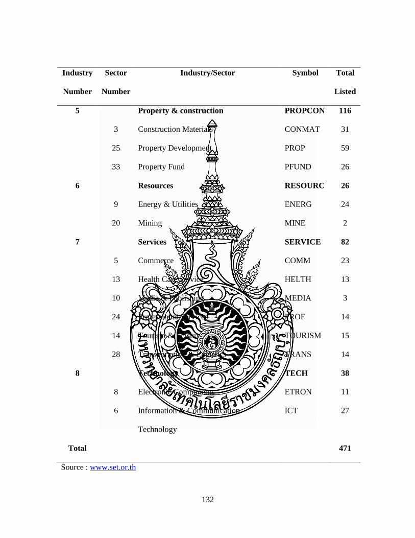
132
Industry
Number
Sector
Number
Industry/Sector Symbol Total
Listed
5 Property & construction PROPCON 116
3 Construction Materials CONMAT 31
25 Property Development PROP 59
33 Property Fund PFUND 26
6 Resources RESOURC 26
9 Energy & Utilities ENERG 24
20 Mining MINE 2
7 Services SERVICE 82
5 Commerce COMM 23
13 Health Care Service HELTH 13
10 Media & Publishing MEDIA 3
24 Professional Services PROF 14
14 Tourism & Leisure TOURISM 15
28 Transportation & Logistics TRANS 14
8 Technology TECH 38
8 Electronic Components ETRON 11
6 Information & Communication
Technology
ICT 27
Total 471
Source : www.set.or.th

133
Appendix B
Samples in the Study

134
Samples in the Study
Argo & Food Industry
Agribusiness
No. Security
Name Company Name URL
1 ASIAN ASIAN SEAFOODS COLDSTORAGE PUBLIC COMPANY LIMITED www.asianseafoods.net
2 CFRESH SEAFRESH INDUSTRY PUBLIC COMPANY LIMITED www.seafresh.com
3 CHOTI KIANG HUAT SEA GULL TRADING FROZEN FOOD PUBLIC CO., LTD. www.kst-hatyai.com
4 CM CHIANGMAI FROZEN FOODS PUBLIC COMPANY LIMITED www.cmfrozen.com
5 CPI CHUMPORN PALM OIL INDUSTRY PUBLIC COMPANY LIMITED www.cpi-th.com
6 EE ETERNAL ENERGY PUBLIC COMPANY LIMITED www.eternalenergy.co.th
7 GFPT GFPT PUBLIC COMPANY LIMITED www.gfpt.co.th
8 LEE LEE FEED MILL PUBLIC COMPANY LIMITED www.leepattana.com
9 PPC PAKFOOD PUBLIC COMPANY LIMITED -
10 SSF SURAPON FOODS PUBLIC COMPANY LIMITED www.surapon.com
11 STA SRI TRANG AGRO-INDUSTRY PUBLIC COMPANY LIMITED www.sritranggroup.com
12 TLUXE THAILUXE ENTERPRISES PUBLIC COMPANY LIMITED www.thailuxe.com
13 TRS TRANG SEAFOOD PRODUCTS PUBLIC COMPANY LIMITED www.trstrang.com
14 TRUBB THAI RUBBER LATEX CORPORATION (THAILAND) PUBLIC CO.,LTD. www.thaitex.com
15 UPOIC UNITED PALM OIL INDUSTRY PUBLIC COMPANY LIMITED www.upoic.co.th
Food & Beverages
16 F&D FOOD AND DRINKS PUBLIC COMPANY LIMITED www.foodanddrinks.co.th
17 LST LAM SOON (THAILAND) PUBLIC COMPANY LIMITED www.lamsoon.co.th
18 MALEE MALEE SAMPRAN PUBLIC COMPANY LIMITED www.malee.co.th
19 PR PRESIDENT RICE PRODUCTS PUBLIC COMPANY LIMITED www.mama-ricenoodles.com
20 SFP SIAM FOOD PRODUCTS PUBLIC COMPANY LIMITED www.siamfood.co.th
21 SORKON S.KHONKAEN FOOD INDUSTRY PUBLIC COMPANY LIMITED www.sorkon.co.th
22 SSC SERM SUK PUBLIC COMPANY LIMITED www.sermsukplc.com
23 TC TROPICAL CANNING (THAILAND) PUBLIC COMPANY LIMITED www.tropical.co.th
24 TUF THAI UNION FROZEN PRODUCTS PUBLIC COMPANY LIMITED www.thaiuniongroup.com
25 TVO THAI VEGETABLE OIL PUBLIC COMPANY LIMITED www.tvothai.com
26 UFM UNITED FLOUR MILL PUBLIC COMPANY LIMITED www.ufm.co.th
Consumer Products Industry
Fashion
27 BATA BATA SHOE OF THAILAND PUBLIC COMPANY LIMITED www.bata.co.th
28 BNC THE BANGKOK NYLON PUBLIC COMPANY LIMITED www.bncsocks.com
29 BTNC BOUTIQUE NEWCITY PUBLIC COMPANY LIMITED www.btnc.co.th
30 CPH CASTLE PEAK HOLDINGS PUBLIC COMPANY LIMITED www.castlepeak.thailand.com
31 CPL C.P.L. GROUP PUBLIC COMPANY LIMITED www.cpl.co.th
32 ICC I.C.C. INTERNATIONAL PUBLIC COMPANY LIMITED www.icc.co.th
33 NC NEWCITY (BANGKOK) PUBLIC COMPANY LIMITED www.newcity.co.th
34 PAF PAN ASIA FOOTWEAR PUBLIC COMPANY LIMITED www.pan-ptr.com/paf
35 PG PEOPLE'S GARMENT PUBLIC COMPANY LIMITED www.pg.co.th
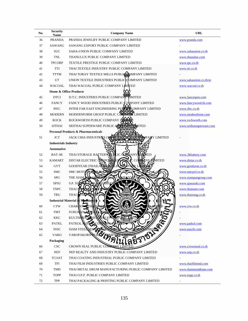
135
No. Security
Name Company Name URL
36 PRANDA PRANDA JEWELRY PUBLIC COMPANY LIMITED www.pranda.com
37 SAWANG SAWANG EXPORT PUBLIC COMPANY LIMITED -
38 SUC SAHA-UNION PUBLIC COMPANY LIMITED www.sahaunion.co.th
39 TNL THANULUX PUBLIC COMPANY LIMITED www.thanulux.com
40 TPCORP TEXTILE PRESTIGE PUBLIC COMPANY LIMITED www.tpc.co.th
41 TTI THAI TEXTILE INDUSTRY PUBLIC COMPANY LIMITED www.tti.co.th
42 TTTM THAI TORAY TEXTILE MILLS PUBLIC COMPANY LIMITED -
43 UT UNION TEXTILE INDUSTRIES PUBLIC COMPANY LIMITED www.sahaunion.co.th/ut
44 WACOAL THAI WACOAL PUBLIC COMPANY LIMITED www.wacoal.co.th
Home & Office Products
45 DTCI D.T.C. INDUSTRIES PUBLIC COMPANY LIMITED www.lancerpen.com
46 FANCY FANCY WOOD INDUSTRIES PUBLIC COMPANY LIMITED www.fancywood.th.com
47 IFEC INTER FAR EAST ENGINEERING PUBLIC COMPANY LIMITED www.ifec.co.th
48 MODERN MODERNFORM GROUP PUBLIC COMPANY LIMITED www.modernform.com
49 ROCK ROCKWORTH PUBLIC COMPANY LIMITED www.rockworth.com
50 SITHAI SRITHAI SUPERWARE PUBLIC COMPANY LIMITED www.srithaisuperware.com
Personal Products & Pharmaceuticals
51 JCT JACK CHIA INDUSTRIES (THAILAND) PUBLIC COMPANY LIMITED -
Industrials Industry
Automative
52 BAT-3K THAI STORAGE BATTERY PUBLIC COMPANY LIMITED www.3kbattery.com
53 KAMART DISTAR ELECTRIC CORPORATION PUBLIC COMPANY LIMITED www.distar.co.th
54 GYT GOODYEAR (THAILAND) PUBLIC COMPANY LIMITED www.goodyear.co.th
55 SMC SMC MOTORS PUBLIC COMPANY LIMITED www.smcpcl.co.th
56 SPG THE SIAM PAN GROUP PUBLIC COMPANY LIMITED www.siampangroup.com
57 SPSU S.P. SUZUKI PUBLIC COMPANY LIMITED www.spsuzuki.com
58 TNPC THAI NAM PLASTIC PUBLIC COMPANY LIMITED www.thainam.com
59 TRU THAI RUNG UNION CAR PUBLIC COMPANY LIMITED www.thairung.co.th
Industrial Material & Machinery
60 CTW CHAROONG THAI WIRE & CABLE PUBLIC COMPANY LIMITED www.ctw.co.th
61 FMT FURUKAWA METAL (THAILAND) PUBLIC COMPANY LIMITED -
62 KKC KULTHORN KIRBY PUBLIC COMPANY LIMITED -
63 PATKL PATKOL PUBLIC COMPANY LIMITED www.patkol.com
64 SSSC SIAM STEEL SERVICE CENTER PUBLIC COMPANY LIMITED www.ssscth.com
65 VARO VAROPAKORN PUBLIC COMPANY LIMITED -
Packaging
66 CSC CROWN SEAL PUBLIC COMPANY LIMITED www.crownseal.co.th
67 NEP NEP REALTY AND INDUSTRY PUBLIC COMPANY LIMITED www.nep.co.th
68 TCOAT THAI COATING INDUSTRIAL PUBLIC COMPANY LIMITED -
69 TFI THAI FILM INDUSTRIES PUBLIC COMPANY LIMITED www.thaifilmind.com
70 TMD THAI METAL DRUM MANUFACTURING PUBLIC COMPANY LIMITED www.thaimetaldrum.com
71 TOPP THAI O.P.P. PUBLIC COMPANY LIMITED www.topp.co.th
72 TPP THAI PACKAGING & PRINTING PUBLIC COMPANY LIMITED -
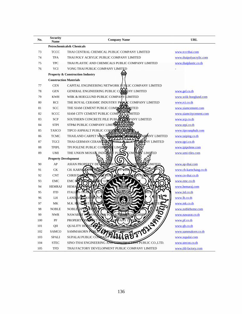
136
No.
Security
Name Company Name URL
Petrochemicals& Chenicals
73 TCCC THAI CENTRAL CHEMICAL PUBLIC COMPANY LIMITED www.tcccthai.com
74 TPA THAI POLY ACRYLIC PUBLIC COMPANY LIMITED www.thaipolyacrylic.com
75 TPC THAI PLASTIC AND CHEMICALS PUBLIC COMPANY LIMITED www.thaiplastic.co.th
76 YCI YONG THAI PUBLIC COMPANY LIMITED -
Property & Construction Industry
Construction Materials
77 CEN CAPITAL ENGINEERING NETWORK PUBLIC COMPANY LIMITED
78 GEN GENERAL ENGINEERING PUBLIC COMPANY LIMITED www.gel.co.th
79 KWH WIIK & HOEGLUND PUBLIC COMPANY LIMITED www.wiik-hoeglund.com
80 RCI THE ROYAL CERAMIC INDUSTRY PUBLIC COMPANY LIMITED www.rci.co.th
81 SCC THE SIAM CEMENT PUBLIC COMPANY LIMITED www.siamcement.com 82 SCCC SIAM CITY CEMENT PUBLIC COMPANY LIMITED www.siamcitycement.com
83 SCP SOUTHERN CONCRETE PILE PUBLIC COMPANY LIMITED www.scp.co.th
84 STPI STP&I PUBLIC COMPANY LIMITED www.stpi.co.th
85 TASCO TIPCO ASPHALT PUBLIC COMPANY LIMITED www.tipcoasphalt.com 86 TCMC THAILAND CARPET MANUFACTURING PUBLIC COMPANY LIMITED www.taiping.co.th
87 TGCI THAI-GERMAN CERAMIC INDUSTRY PUBLIC COMPANY LIMITED www.tgci.co.th
88 TPIPL TPI POLENE PUBLIC COMPANY LIMITED www.tpipolene.com
89 UMI THE UNION MOSAIC INDUSTRY PUBLIC COMPANY LIMITED www.umi-tiles.com
Property Development
90 AP ASIAN PROPERTY DEVELOPMENT PUBLIC COMPANY LIMITED www.ap-thai.com 91 CK CH. KARNCHANG PUBLIC COMPANY LIMITED www.ch-karnchang.co.th
92 CNT CHRISTIANI & NIELSEN (THAI) PUBLIC COMPANY LIMITED www.cn-thai.co.th
93 EMC EMC PUBLIC COMPANY LIMITED www.emc.co.th
94 HEMRAJ HEMARAJ LAND AND DEVELOPMENT PUBLIC COMPANY LIMITED www.hemaraj.com
95 ITD ITALIAN-THAI DEVELOPMENT PUBLIC COMPANY LIMITED www.itd.co.th
96 LH LAND AND HOUSES PUBLIC COMPANY LIMITED www.lh.co.th
97 MK M.K. REAL ESTATE DEVELOPMENT PUBLIC COMPANY LIMITED www.mk.co.th
98 NOBLE NOBLE DEVELOPMENT PUBLIC COMPANY LIMITED www.noblehome.com
99 NWR NAWARAT PATANAKARN PUBLIC COMPANY LIMITED www.nawarat.co.th
100 PF PROPERTY PERFECT PUBLIC COMPANY LIMITED www.pf.co.th
101 QH QUALITY HOUSES PUBLIC COMPANY LIMITED www.qh.co.th
102 SAMCO SAMMAKORN PUBLIC COMPANY LIMITED www.sammakorn.co.th
103 SPALI SUPALAI PUBLIC COMPANY LIMITED www.supalai.com
104 STEC SINO-THAI ENGINEERING AND CONSTRUCTION PUBLIC CO.,LTD. www.stecon.co.th
105 TFD THAI FACTORY DEVELOPMENT PUBLIC COMPANY LIMITED www.tfd-factory.com

137
Resources Industry
Energy & Utilities
No. Security
Name Company Name URL
106 BAFS BANGKOK AVIATION FUEL SERVICES PCL. www.bafsthai.com
107 BCP THE BANGCHAK PETROLEUM PUBLIC COMPANY LIMITED www.bangchak.co.th
108 EGCO ELECTRICITY GENERATING PUBLIC COMPANY LIMITED www.egco.com
109 LANNA THE LANNA RESOURCES PUBLIC COMPANY LIMITED www.lannar.com
110 SUSCO SIAM UNITED SERVICES PUBLIC COMPANY LIMITED www.susco.co.th
111 TCC THAI CAPITAL CORPORATION PUBLIC COMPANY LIMITED www.thaiheat.com
Mining
112 PDI PADAENG INDUSTRY PUBLIC COMPANY LIMITED www.padaeng.com
Services Industry
Commerce
113 LOXLEY LOXLEY PUBLIC COMPANY LIMITED www.loxley.co.th
114 SINGER SINGER THAILAND PUBLIC COMPANY LIMITED www.singerthai.co.th
115 SPI SAHA PATHANA INTER-HOLDING PUBLIC COMPANY LIMITED www.spi.co.th
Health Care Services
116 AHC AIKCHOL HOSPITAL PUBLIC COMPANY LIMITED www.aikchol.com
117 CMR CHIANG MAI RAM MEDICAL BUSINESS PUBLIC COMPANY LIMITED
118 KDH KRUNGDHON HOSPITAL PUBLIC COMPANY LIMITED www.kdh.co.th
119 NEW WATTANA KARNPAET PUBLIC COMPANY LIMITED www.wattanahospital.com
120 SVH SAMITIVEJ PUBLIC COMPANY LIMITED www.samitivej.co.th
121 VIBHA VIBHAVADI MEDICAL CENTER PUBLIC COMPANY LIMITED www.vibhavadi.com
Media & Publishing
122 APRINT AMARIN PRINTING AND PUBLISHING PUBLIC COMPANY LIMITED www.amarin.co.th
123 FE FAR EAST DDB PUBLIC COMPANY LIMITED www.fareastddb.com
124 LIVE LIVE INCORPORATION PUBLIC COMPANY LIMITED www.live.co.th
125 MATI MATICHON PUBLIC COMPANY LIMITED www.matichon.co.th
126 NMG NATION MULTIMEDIA GROUP PUBLIC COMPANY LIMITED www.nationgroup.com
127 P-FCB PRAKIT HOLDINGS PUBLIC COMPANY LIMITED -
128 POST THE POST PUBLISHING PUBLIC COMPANY LIMITED www.bangkokpost.com
129 SPORT SIAM SPORT SYNDICATE PUBLIC COMPANY LIMITED www.siamsport.co.th/
130 TBSP THAI BRITISH SECURITY PRINTING PUBLIC COMPANY LIMITED www.tbsp.co.th
131 TONHUA TONG HUA COMMUNICATIONS PUBLIC COMPANY LIMITED -
132 WAVE WAVE ENTERTAINMENT PUBLIC COMPANY LIMITED
Tourism & Leisure
133 ASIA ASIA HOTEL PUBLIC COMPANY LIMITED www.asiahotel.co.th
134 CSR CITY SPORTS AND RECREATION PUBLIC COMPANY LIMITED
135 DTC DUSIT THANI PUBLIC COMPANY LIMITED www.dusit.com
136 ERW THE ERAWAN GROUP PUBLIC COMPANY LIMITED www.TheErawan.com
137 LRH LAGUNA RESORTS & HOTELS PUBLIC COMPANY LIMITED www.lagunaresorts.com
138 MANRIN THE MANDARIN HOTEL PUBLIC COMPANY LIMITED www.mandarin-bkk.com
139 OHTL OHTL PUBLIC COMPANY LIMITED www.mandarin-oriental.com

138
No. Security
Name Company Name
URL
140 ROH ROYAL ORCHID HOTEL (THAILAND) PUBLIC COMPANY LIMITED
141 SHANG SHANGRI-LA HOTEL PUBLIC COMPANY LIMITED www.shangri-la.com
Transportation & Logistics
142 ASIMAR ASIAN MARINE SERVICES PUBLIC COMPANY LIMITED www.asimar.com
143 RCL REGIONAL CONTAINER LINES PUBLIC COMPANY LIMITED www.rclgroup.com
144 SST SUB SRI THAI WAREHOUSE PUBLIC COMPANY LIMITED www.subsrithai.co.th
145 TSTE THAI SUGAR TERMINAL PUBLIC COMPANY LIMITED www.TSTEGROUP.com
146 WIN WYNCOAST INDUSTRIAL PARK PUBLIC COMPANY LIMITED www.wyncoast.com
Technology Industry
Electronic Components
147 DELTA DELTA ELECTRONICS (THAILAND) PUBLIC COMPANY LIMITED www.deltathailand.com
148 DRACO DRACO PCB PUBLIC COMPANY LIMITED www.dracopcb.com
149 HANA HANA MICROELECTRONICS PUBLIC COMPANY LIMITED www.hanagroup.com
150 KCE KCE ELECTRONICS PUBLIC COMPANY LIMITED www.kcethai.in.th
151 SVI SVI PUBLIC COMPANY LIMITED www.svi.co.th
152 TEAM TEAM PRECISION PUBLIC COMPANY LIMITED www.teampcba.com
Information & Communication Technology
153 ADVANC ADVANCED INFO SERVICE PUBLIC COMPANY LIMITED www.ais.co.th
154 JAS JASMINE INTERNATIONAL PUBLIC COMPANY LIMITED www.jasmine.com
155 MSC METRO SYSTEMS CORPORATION PUBLIC COMPANY LIMITED www.metrosystems.co.th
156 SAMART SAMART CORPORATION PUBLIC COMPANY LIMITED www.samartcorp.com
157 SAMTEL SAMART TELCOMS PUBLIC COMPANY LIMITED www.samtel.com
158 INTUCH SHIN CORPORATION PUBLIC COMPANY LIMITED www.shincorp.com
159 SVOA SVOA PUBLIC COMPANY LIMITED www.svoa.co.th
160 TT&T TT&T PUBLIC COMPANY LIMITED www.ttt.co.th

139
Appendix C
AMOS Outputs of Confirmatory Factor Analysis

140
AMOS Outputs of Confirmatory Factor Analysis
Adjustment Cost Model
Maximum Likelihood Estimates
Regression Weights:
Estimate S.E. C.R. P Label
ASSET_I <--- ADJUST_COST 1.000
EQUITY_I <--- ADJUST_COST 1.151 .031 37.307 *** par_1
STOCK_I <--- ADJUST_COST 1.220 .047 26.002 *** par_2
EMPLOY_I <--- ADJUST_COST .020 .055 .369 .712 par_3
CAPITAL_I <--- ADJUST_COST .931 .043 21.645 *** par_4
Standardized Regression Weights:
Estimate
ASSET_I <--- ADJUST_COST .973
EQUITY_I <--- ADJUST_COST .837
STOCK_I <--- ADJUST_COST .663
EMPLOY_I <--- ADJUST_COST .011
CAPITAL_I <--- ADJUST_COST .579
Covariances:
Estimate S.E. C.R. P Label
e2 <--> e5 .228 .030 7.706 *** par_5
e2 <--> e3 .318 .032 9.927 *** par_6
e2 <--> e4 .082 .018 4.689 *** par_7
e3 <--> e5 -.081 .023 -3.454 *** par_8
Correlations:
Estimate
e2 <--> e5 .237
e2 <--> e3 .313
e2 <--> e4 .149
e3 <--> e5 -.110

141
Variances:
Estimate S.E. C.R. P Label
ADJUST_COST
.407 .019 20.972 *** par_9
e1
.023 .007 3.137 .002 par_10
e2
1.328 .056 23.833 *** par_11
e3
.773 .035 22.268 *** par_12
e4
.230 .014 16.909 *** par_13
e5
.701 .031 22.955 *** par_14
Squared Multiple Correlations:
Estimate
CAPITAL_I
.335
EQUITY_I
.701
STOCK_I
.439
EMPLOY_I
.000
ASSET_I
.947
Implied Covariances
CAPITAL_I EQUITY_I STOCK_I EMPLOY_I ASSET_I
CAPITAL_I 1.054
EQUITY_I .436 .769
STOCK_I .381 .572 1.380
EMPLOY_I .236 .092 .328 1.328
ASSET_I .379 .469 .497 .008 .430
Implied Correlations
CAPITAL_I EQUITY_I STOCK_I EMPLOY_I ASSET_I
CAPITAL_I 1.000
EQUITY_I .485 1.000
STOCK_I .316 .555 1.000
EMPLOY_I .199 .091 .242 1.000
ASSET_I .563 .815 .645 .011 1.000

142
Residual Covariances
CAPITAL_I EQUITY_I STOCK_I EMPLOY_I ASSET_I
CAPITAL_I .000
EQUITY_I -.011 .000
STOCK_I .000 .010 .000
EMPLOY_I -.004 .000 .003 .000
ASSET_I .001 .000 -.001 .000 .000
Standardized Residual Covariances
CAPITAL_I EQUITY_I STOCK_I EMPLOY_I ASSET_I
CAPITAL_I .000
EQUITY_I -.370 .000
STOCK_I .000 .276 .000
EMPLOY_I -.110 .007 .084 .003
ASSET_I .055 .000 -.041 -.001 .000
Model Fit Summary
CMIN
Model NPAR CMIN DF P CMIN/DF
Default model 14 1.477 1 .224 1.477
Saturated model 15 .000 0
Independence model 5 2514.770 10 .000 251.477
RMR, GFI
Model RMR GFI AGFI PGFI
Default model .004 .999 .992 .067
Saturated model .000 1.000
Independence model .311 .538 .307 .359
Baseline Comparisons
Model NFI
Delta1
RFI
rho1
IFI
Delta2
TLI
rho2 CFI
Default model .999 .994 1.000 .998 1.000
Saturated model 1.000
1.000
1.000
Independence model .000 .000 .000 .000 .000

143
Parsimony-Adjusted Measures
Model PRATIO PNFI PCFI
Default model .100 .100 .100
Saturated model .000 .000 .000
Independence model 1.000 .000 .000
NCP
Model NCP LO 90 HI 90
Default model .477 .000 8.180
Saturated model .000 .000 .000
Independence model 2504.770 2343.570 2673.293
FMIN
Model FMIN F0 LO 90 HI 90
Default model .001 .000 .000 .007
Saturated model .000 .000 .000 .000
Independence model 2.214 2.205 2.063 2.353
RMSEA
Model RMSEA LO 90 HI 90 PCLOSE
Default model .020 .000 .085 .683
Independence model .470 .454 .485 .000
AIC
Model AIC BCC BIC CAIC
Default model 29.477 29.626 99.983 113.983
Saturated model 30.000 30.159 105.542 120.542
Independence model 2524.770 2524.823 2549.951 2554.951
ECVI
Model ECVI LO 90 HI 90 MECVI
Default model .026 .026 .033 .026
Saturated model .026 .026 .026 .027
Independence model 2.223 2.081 2.371 2.223

144
HOELTER
Model HOELTER
.05
HOELTER
.01
Default model 2955 5103
Independence model 9 11
Assessment of normality
Variable min max skew c.r. kurtosis c.r.
CAPITAL_I -4.404 2.489 .000 -.002 .573 3.943
EQUITY_I -4.348 2.568 -.085 -1.169 1.265 8.706
STOCK_I -5.371 2.771 .160 2.196 .417 2.873
EMPLOY_I -11.717 -5.416 -.609 -8.383 .066 .457
ASSET_I -1.306 2.618 .767 10.555 .561 3.862
Multivariate
10.821 21.806
Observations farthest from the centroid (Mahalanobis distance)
Observation number Mahalanobis d-squared p1 p2
461 43.093 .000 .000
127 41.290 .000 .000
131 37.800 .000 .000
647 33.782 .000 .000
754 33.135 .000 .000
475 30.186 .000 .000
670 25.546 .000 .000
512 23.852 .000 .000
648 21.560 .001 .000
755 21.530 .001 .000
130 21.125 .001 .000
772 20.740 .001 .000
129 20.710 .001 .000
883 20.683 .001 .000
572 20.615 .001 .000
694 20.523 .001 .000
128 20.231 .001 .000
710 19.451 .002 .000
138 19.303 .002 .000
756 19.142 .002 .000
693 18.622 .002 .000
656 18.531 .002 .000
709 18.459 .002 .000

145
Political Cost Model
Maximum Likelihood Estimates
Regression Weights:
Estimate S.E. C.R. P Label
CAPITAL_I <--- POLITICAL_COST 1.000
SIZE <--- POLITICAL_COST -4.115 .949 -4.337 *** par_1
BETA <--- POLITICAL_COST -1.523 .435 -3.504 *** par_2
COMPET <--- POLITICAL_COST -.101 .030 -3.398 *** par_3
TAX <--- POLITICAL_COST .168 .049 3.453 *** par_6
Standardized Regression Weights:
Estimate
CAPITAL_I <--- POLITICAL_COST .198
SIZE <--- POLITICAL_COST -.649
BETA <--- POLITICAL_COST -.660
COMPET <--- POLITICAL_COST -.253
TAX <--- POLITICAL_COST .231
Covariances:
Estimate S.E. C.R. P Label
e5 <--> e1 .149 .053 2.807 .005 par_4
e3 <--> e1 .014 .003 5.328 *** par_5
e5 <--> e4 .029 .007 4.090 *** par_7
Correlations:
Estimate
e5 <--> e1 .151
e3 <--> e1 .174
e5 <--> e4 .209
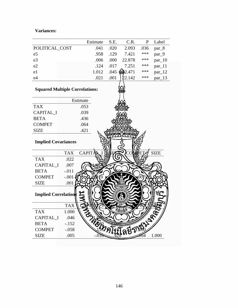
146
Variances:
Estimate S.E. C.R. P Label
POLITICAL_COST
.041 .020 2.093 .036 par_8
e5
.958 .129 7.421 *** par_9
e3
.006 .000 22.878 *** par_10
e2
.124 .017 7.251 *** par_11
e1
1.012 .045 22.471 *** par_12
e4
.021 .001 22.142 *** par_13
Squared Multiple Correlations:
Estimate
TAX
.053
CAPITAL_I
.039
BETA
.436
COMPET
.064
SIZE
.421
Implied Covariances
TAX CAPITAL_I BETA COMPET SIZE
TAX .022
CAPITAL_I .007 1.054
BETA -.011 -.063 .219
COMPET -.001 .010 .006 .007
SIZE .001 -.020 .258 .017 1.655
Implied Correlations
TAX CAPITAL_I BETA COMPET SIZE
TAX 1.000
CAPITAL_I .046 1.000
BETA -.152 -.130 1.000
COMPET -.058 .115 .167 1.000
SIZE .005 -.016 .428 .164 1.000

147
Residual Covariances
TAX CAPITAL_I BETA COMPET SIZE
TAX .000
CAPITAL_I -.007 .001
BETA -.001 -.005 .000
COMPET .000 .000 .000 .000
SIZE -.001 -.008 -.002 .001 -.003
Standardized Residual Covariances
TAX CAPITAL_I BETA COMPET SIZE
TAX .000
CAPITAL_I -1.529 .012
BETA -.265 -.369 .000
COMPET -.267 .046 -.293 .000
SIZE -.179 -.211 -.123 .181 -.042
Model Fit Summary
CMIN
Model NPAR CMIN DF P CMIN/DF
Default model 13 3.200 2 .202 1.600
Saturated model 15 .000 0
Independence model 5 356.357 10 .000 35.636
RMR, GFI
Model RMR GFI AGFI PGFI
Default model .003 .999 .992 .133
Saturated model .000 1.000
Independence model .069 .893 .840 .596
Baseline Comparisons
Model NFI
Delta1
RFI
rho1
IFI
Delta2
TLI
rho2 CFI
Default model .991 .955 .997 .983 .997
Saturated model 1.000
1.000
1.000
Independence model .000 .000 .000 .000 .000
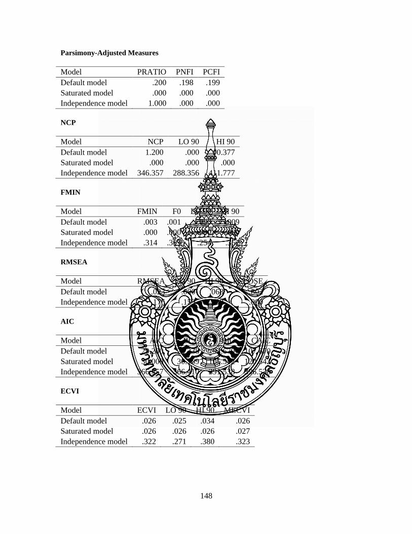
148
Parsimony-Adjusted Measures
Model PRATIO PNFI PCFI
Default model .200 .198 .199
Saturated model .000 .000 .000
Independence model 1.000 .000 .000
NCP
Model NCP LO 90 HI 90
Default model 1.200 .000 10.377
Saturated model .000 .000 .000
Independence model 346.357 288.356 411.777
FMIN
Model FMIN F0 LO 90 HI 90
Default model .003 .001 .000 .009
Saturated model .000 .000 .000 .000
Independence model .314 .305 .254 .362
RMSEA
Model RMSEA LO 90 HI 90 PCLOSE
Default model .023 .000 .068 .802
Independence model .175 .159 .190 .000
AIC
Model AIC BCC BIC CAIC
Default model 29.200 29.338 94.670 107.670
Saturated model 30.000 30.159 105.542 120.542
Independence model 366.357 366.410 391.538 396.538
ECVI
Model ECVI LO 90 HI 90 MECVI
Default model .026 .025 .034 .026
Saturated model .026 .026 .026 .027
Independence model .322 .271 .380 .323

149
HOELTER
Model HOELTER
.05
HOELTER
.01
Default model 2128 3270
Independence model 59 74
Assessment of normality
Variable min max skew c.r. kurtosis c.r.
TAX .000 .919 1.152 15.852 2.092 14.396
CAPITAL_I -4.404 2.489 .000 -.002 .573 3.943
BETA -.470 2.310 .942 12.969 .287 1.973
COMPET .546 .995 1.031 14.198 2.857 19.666
SIZE 11.944 19.278 .603 8.295 .066 .456
Multivariate
7.020 14.147
Observations farthest from the centroid (Mahalanobis distance)
Observation number Mahalanobis d-squared p1 p2
791 40.775 .000 .000
309 30.142 .000 .000
604 26.951 .000 .000
798 25.636 .000 .000
72 22.633 .000 .000
307 22.100 .001 .000
477 21.390 .001 .000
781 20.209 .001 .000
656 20.122 .001 .000
769 19.714 .001 .000
777 19.631 .001 .000
773 19.551 .002 .000
778 18.800 .002 .000
765 18.449 .002 .000
273 18.231 .003 .000
775 18.206 .003 .000
770 18.071 .003 .000
776 18.007 .003 .000
1040 17.865 .003 .000
774 17.499 .004 .000

150
Agency Cost Model
Maximum Likelihood Estimates
Regression Weights:
Estimate S.E. C.R. P Label
SIZE <--- AGENCY_COST 9.031 1.800 5.018 *** par_1
FCF <--- AGENCY_COST 1.000
DIS_EX <--- AGENCY_COST -.918 .169 -5.444 *** par_2
ROA <--- AGENCY_COST 1.654 .227 7.288 *** par_3
TQ <--- AGENCY_COST 9.908 1.252 7.916 *** par_4
LEV_R <--- AGENCY_COST -2.355 .365 -6.446 *** par_5
Standardized Regression Weights:
Estimate
SIZE <--- AGENCY_COST .235
FCF <--- AGENCY_COST .360
DIS_EX <--- AGENCY_COST -.273
ROA <--- AGENCY_COST .693
TQ <--- AGENCY_COST .579
LEV_R <--- AGENCY_COST -.336
Covariances:
Estimate S.E. C.R. P Label
e1 <--> e3 -.020 .004 -4.416 *** par_6
e1 <--> e2 -.013 .003 -3.761 *** par_7
e2 <--> e5 -.007 .002 -3.953 *** par_8
e1 <--> e6 .093 .009 10.346 *** par_9
e3 <--> e5 .012 .002 5.963 *** par_10
e3 <--> e6 -.004 .001 -4.811 *** par_11
Correlations:
Estimate
e1 <--> e3 -.147
e1 <--> e2 -.122
e2 <--> e5 -.174
e1 <--> e6 .339
e3 <--> e5 .243
e3 <--> e6 -.161

151
Variances:
Estimate S.E. C.R. P Label
AGENCY_COST
.001 .000 4.418 *** par_12
e1
1.553 .068 22.870 *** par_13
e2
.007 .000 20.740 *** par_14
e3
.012 .001 21.967 *** par_15
e4
.003 .000 10.541 *** par_16
e5
.216 .014 14.945 *** par_17
e6
.048 .002 22.113 *** par_18
Squared Multiple Correlations:
Estimate
LEV_R
.113
TQ
.335
ROA
.480
DIS_EX
.074
FCF
.130
SIZE
.055
Implied Covariances
LEV_R TQ ROA DIS_EX FCF SIZE
LEV_R .055
TQ -.026 .326
ROA -.004 .018 .006
DIS_EX -.001 .002 -.002 .013
FCF -.003 .004 .002 -.001 .009
SIZE .069 .099 .017 -.029 -.003 1.644
Implied Correlations
LEV_R TQ ROA DIS_EX FCF SIZE
LEV_R 1.000
TQ -.194 1.000
ROA -.233 .401 1.000
DIS_EX -.054 .033 -.189 1.000
FCF -.121 .076 .250 -.098 1.000
SIZE .232 .136 .163 -.202 -.026 1.000

152
Residual Covariances
LEV_R TQ ROA DIS_EX FCF SIZE
LEV_R .000
TQ .003 -.001
ROA .000 .000 .000
DIS_EX .000 -.001 .000 .000
FCF -.001 .000 .000 .000 .000
SIZE .002 .013 .000 .000 -.003 .008
Standardized Residual Covariances
LEV_R TQ ROA DIS_EX FCF SIZE
LEV_R .000
TQ .747 -.057
ROA .126 -.021 .000
DIS_EX .152 -.349 -.365 -.049
FCF -1.621 .219 -.073 1.498 .012
SIZE .189 .578 -.121 -.040 -.757 .118
Model Fit Summary
CMIN
Model NPAR CMIN DF P CMIN/DF
Default model 18 6.512 3 .089 2.171
Saturated model 21 .000 0
Independence model 6 611.794 15 .000 40.786
RMR, GFI
Model RMR GFI AGFI PGFI
Default model .003 .998 .987 .143
Saturated model .000 1.000
Independence model .031 .849 .789 .606

153
Baseline Comparisons
Model NFI
Delta1
RFI
rho1
IFI
Delta2
TLI
rho2 CFI
Default model .989 .947 .994 .971 .994
Saturated model 1.000
1.000
1.000
Independence model .000 .000 .000 .000 .000
Parsimony-Adjusted Measures
Model PRATIO PNFI PCFI
Default model .200 .198 .199
Saturated model .000 .000 .000
Independence model 1.000 .000 .000
NCP
Model NCP LO 90 HI 90
Default model 3.512 .000 15.015
Saturated model .000 .000 .000
Independence model 596.794 519.588 681.407
FMIN
Model FMIN F0 LO 90 HI 90
Default model .006 .003 .000 .013
Saturated model .000 .000 .000 .000
Independence model .539 .525 .457 .600
RMSEA
Model RMSEA LO 90 HI 90 PCLOSE
Default model .032 .000 .066 .771
Independence model .187 .175 .200 .000
AIC
Model AIC BCC BIC CAIC
Default model 42.512 42.735 133.163 151.163
Saturated model 42.000 42.260 147.759 168.759
Independence model 623.794 623.869 654.011 660.011

154
ECVI
Model ECVI LO 90 HI 90 MECVI
Default model .037 .034 .048 .038
Saturated model .037 .037 .037 .037
Independence model .549 .481 .624 .549
HOELTER
Model HOELTER
.05
HOELTER
.01
Default model 1364 1980
Independence model 47 57
Assessment of normality
Variable min max skew c.r. kurtosis c.r.
LEV_R .005 2.057 .602 8.293 1.582 10.886
TQ .063 4.219 2.201 30.303 6.501 44.745
ROA -.336 .312 -.692 -9.532 3.222 22.174
DIS_EX .021 .712 1.514 20.846 2.586 17.803
FCF -.281 .524 .118 1.621 2.237 15.400
SIZE 11.944 19.278 .603 8.295 .066 .456
Multivariate
35.897 61.770
Observations farthest from the centroid (Mahalanobis distance)
Observation number Mahalanobis d-squared p1 p2
461 43.093 .000 .000
127 41.290 .000 .000
131 37.800 .000 .000
647 33.782 .000 .000
754 33.135 .000 .000
475 30.186 .000 .000
670 25.546 .000 .000
512 23.852 .000 .000
648 21.560 .001 .000
755 21.530 .001 .000
130 21.125 .001 .000
772 20.740 .001 .000
129 20.710 .001 .000
883 20.683 .001 .000

155
Appendix D
SPSS Outputs of Exploratory Factor Analysis

156
SPSS Outputs of Exploratory Factor Analysis
Adjustment Cost
KMO and Bartlett's Test
Kaiser-Meyer-Olkin Measure of Sampling Adequacy. .739
Bartlett's Test of Sphericity Approx. Chi-Square 2295.613
df 6
Sig. .000
Total Variance Explained
Component
Initial Eigenvalues Extraction Sums of Squared Loadings
Total
% of
Variance Cumulative % Total
% of
Variance Cumulative %
1 2.719 67.975 67.975 2.719 67.975 67.975
2 .693 17.316 85.291
3 .422 10.559 95.850
4 .166 4.150 100.000
Extraction Method: Principal Component Analysis.
Political Cost
KMO and Bartlett's Test
Kaiser-Meyer-Olkin Measure of Sampling
Adequacy.
.515
Bartlett's Test of
Sphericity
Approx. Chi-Square 355.573
df 10
Sig. .000

157
Total Variance Explained
Component
Initial Eigenvalues Extraction Sums of Squared Loadings Rotation Sums of Squared Loadings
Total
% of
Variance Cumulative % Total
% of
Variance Cumulative % Total
% of
Variance Cumulative %
1 1.565 31.291 31.291 1.565 31.291 31.291 1.521 30.418 30.418
2 1.115 22.301 53.593 1.115 22.301 53.593 1.121 22.412 52.830
3 .999 19.990 73.582 .999 19.990 73.582 1.038 20.752 73.582
4 .791 15.825 89.407
5 .530 10.593 100.000
Extraction Method: Principal Component Analysis.
Agency Cost
KMO and Bartlett's Test
Kaiser-Meyer-Olkin Measure of Sampling Adequacy. .545
Bartlett's Test of Sphericity Approx. Chi-Square 610.269
df 15
Sig. .000
Total Variance Explained
Component
Initial Eigenvalues Extraction Sums of Squared Loadings Rotation Sums of Squared Loadings
Total
% of
Variance Cumulative % Total
% of
Variance Cumulative % Total
% of
Variance Cumulative %
1 1.708 28.459 28.459 1.708 28.459 28.459 1.521 25.345 25.345
2 1.366 22.764 51.223 1.366 22.764 51.223 1.358 22.633 47.978
3 .997 16.618 67.841 .997 16.618 67.841 1.192 19.863 67.841
4 .819 13.656 81.497
5 .598 9.967 91.464
6 .512 8.536 100.000
Extraction Method: Principal Component Analysis.

158
VITA
Nuchjaree Pichetkun was born in Saraburi, Thailand on August 9, 1960. She
received her Bachelor of Business Administration in Accounting (Second-Class Honors)
in October 1982 from Thammasat University. She joined Capet King Co.,Ltd. as an
accountant in 1982 and Electricity Generation Authority of Thailand as a foreign voucher
officer in 1984. In January 1986, she completed her Master of Accountancy from
Chulalongkorn University. She has been a lecturer of accounting department in Faculty of
Business Administration, Rajamangala University of Technology Thanyaburi since 1986.
Related Documents