The Determinants of European Returns, Spillovers …...The Determinants of European Returns,Spillovers and Contagion Lara Cathcarta, Lina El-Jahelb, Ravel Jabboura, aImperial College

The Determinants of European Returns, Spillovers and Contagion

Lara Cathcarta, Lina El-Jahelb, Ravel Jabboura,∗

aImperial College London, South Kensington Campus, London SW7 2AZ, tel: +44 (0)20 7589 5111bThe Business School, University of Auckland, Private Bag 92019, Auckland 1142, New Zealand

Abstract

Nowadays, returns are affected not only by country fundamentals but also by worldwide eventssuch as financial crises. One characteristic these shocks have in common is their widespread na-ture as they can propagate from one country to the other. Using a panel of European countriescovering the period 2003-2012, this research explores the factors that jointly determine returnsand the transmission of external and internal shocks. This information should allow regulators todecide on adequate macro-preventive measures to protect countries from the harmful consequencesof these shocks. Beyond trade and financial linkages which are the principal channels investigatedby previous research, we find that bank-specific factors at the heart of the new Basel III regulationalso play a role in the channeling of global shocks. While this finding is not new in itself, our maincontribution is in showing that both returns and shock transmission are governed by different com-binations of the same factors across various samples of the banking sector. This study will thereforeconstitute a forward-looking assessment of enhancements brought by the new regulation thus com-plementing the recent capital monitoring exercise by the European System of Financial Supervision.

JEL classification: F49 G21 G29

Keywords: Capital Ratio, Spillover, Contagion

1. Introduction

Finance and economic researchers base their understanding of the interaction between countrieson a scientific concept from the field of communications. In that respect, a financial shock actingas a signal is assumed to cross international borders using as its “media” the “linkages” betweencountries while being “amplified/reduced” by country-specific factors at the “sending/receiving”end. Under this scheme, since the receiving country has almost no control over the initial shock,it can only regulate the strength of the transmission and the tuning at the receiving end.

The importance of understanding the forces that govern this interaction can be seen in thefollowing two examples. When the United States (US) was hit by the subprime crisis in 2007, theEuro-Area (EA) suffered the aftermath. Similarly, the EA sovereign crisis that followed in late20091 delayed the US recovery. In fact, the turmoil in the EA brought back into question the

∗Corresponding authorEmail addresses: [email protected] (Lara Cathcart), [email protected] (Lina El-Jahel),

[email protected] (Ravel Jabbour)1According to Tong and Zuccardi (2011), the euro crisis began on October 16, 2009, with the words of Greek

prime minister “We have large hidden debts and spending”.

Preprint submitted to the International Conference on Credit Risk Evaluation 2013 August 14, 2013

purpose of a unified Europe2 as it revealed the downside of having safer countries put at risk fromtheir riskier neighbors.

As these examples illustrate, the study of how one economy is affected by another is more thana matter of exchange rate fluctuations; especially in the case of the EA where the issue does notpresent itself. Krugman (2008) first developed the concept of an “international finance multiplier”to help understand interconnections (linkages) between financial markets. Combined with financialvulnerabilities, this concept was later formalized in general equilibrium by Devereux and Yetman(2010). Many empirical works have lent themselves in one way or another to the same concept.Nonetheless, the empirical testing of similar frameworks began much earlier in order to evaluatethe cross-border impact on returns as well as the transmission mechanism by which returns areaffected. This was based on acquired knowledge from pre-established models such as the CAPMsupplemented with a variety of explanatory variables which include bilateral and country-specificfactors (Dungey et al. (2004), Bekaert et al. (2005) and Poirson and Schmittman (2012) to namea few). As per Calvo et al. (1993), the latter are also known as push and pull factors, respectively.

In this research we contribute to the existing literature by looking at the differential role playedby these factors in jointly determining bank returns and shock transmission using a 2003-2012dataset of eight EA countries and the UK. To our knowledge, this is the first paper to attemptsuch a combinatorial approach as Bekaert et al. (2009) conceded that different approaches couldlead to different conclusions. This allows us to compare some of the contrasting results found in theliterature under a unified framework. Our paper is closest to the work of Baele (2005) who focusedon stock market volatility instead of bank returns and Fratzscher (2012) who have an internationalrather than Euro-oriented.

Whereas there is a restricted set of bilateral push factors to choose from that includes lending,investment and trade, there is an extensive list available for the set of country-specific pull factorswhich encompass various risk indicators. We select capitalization as our main country-risk variableand proxy for credit risk in order to reflect on the impact of the Basel II capital regulation onEurope. Implemented as part of the Capital Adequacy Directive (CAD (2006)), this regulationwas enforced by all EU member countries including the UK (FSA (2006)) by 2007. Based on Shin(2012), the reason the EU signed the agreement faster than other advanced countries, notably theU.S., was because legislators recognized that European banks became experienced at gaming theinitial Basel I Accord (CAD (2000)). Hence, one purpose for our work will be in assessing theBasel II regulation thereby determining the need for the new Basel III regulation.

Over the last two decades, capital has received mixed reviews in terms of how it can affectstock performance (see Cathcart et al. (2013b)). While not referring to equity returns in par-ticular, Berger and Bouwman (2013) examined the effects of capital on a different measure ofprofitability, ROA, for US banks between 1984 and 2009. Their view is that capital has a posi-tive effect depending on the type of crisis and the size of the banks. Note that their study doesnot account for “Too-Big-To-Fail” banks (TBTF), otherwise known as Systematically ImportantFinancial Institutions (SIFIs). Indeed, Chan-Lau et al. (2012a) admitted that their results couldbe biased towards banks with strong capital bases which were normally the TBTF institutions.Another contribution of our work will be to factor those banks into the analysis.

Note that the effect of capital ratios can be dented by other factors which, until Basel III,were not part of the international regulation. One such factor is leverage, which is set by national

2The birth of the Euro in 1999 was based on a series of economic treaties that brought the member countrieswithin closer dependency of each other (single currency, free movement of population, removal of trade barriers).

2

regulators, and was found to be strongly associated with balance-sheet risk (Adrian and Shin(2010))). Looking jointly at both ratios, Chan-Lau et al. (2012a) find that banks’ equity returns areboosted by high equity-to-asset (leverage3) ratios. This finding agrees with Devereux and Yetman(2010) and is based on the inability of Basel’s risk-based capital ratio to reflect risks adequately.Notably, a zero risk-weight was attributed to some EA countries’ domestic government debt duringthe crisis despite the fact that their sovereign’s creditworthiness had deteriorated.

With regards to international shock transmission, the study of cross-country effects of capitalratios goes back as early as Peek and Rosengren (1997) who examine the effects of these ratios forJapanese parent banks and how they influence the lending behavior of their branches in the US.The study showed how capital can act as a channel propagating a shock from parent to subsidiary.More importantly, the purpose behind the Basel regulation was to increase banks’ resilience againstsuch shocks, in other words, decrease the banks’ sensitivity resulting from international exposure.A small exercise by the ECB (2011) showed that this is indeed the case. While this result is re-asserted in Poirson and Schmittman (2012), the authors are surprised to find occurrences of theopposite effect. This could either be due to their particular setup or their use of leverage insteadof risk-based capital requirements as a proxy for the banks’ capital level. We revisit this finding inour results.

Another contribution of our work is to test our results across a spectrum of samples goingfrom the largest banks (SIFIs/TBTF) to the whole countries’ banking sector. Also, in line withthe suggestion by Berger and Bouwman (2013) of assessing any differential role of capital betweencrisis and normal times, we divide our sample into pre and post 2007 in the spirit of Ehrmannet al. (2004) in order to investigate the extent to which the fact that EU (and US) banks were well-capitalized prior to the crash (Chami and Cosimano (2010) and Persaud (2013)) fared well for themduring the crisis. Note that Poirson and Schmittman (2012) devised a similar procedure but didnot account for the possibility that their results could be biased by the synchronous introductionof the new Basel rules with the unfolding of the crisis.

Whereas similar variations in sample and time have lead previous authors to remain inconclusiveregarding their results (Poirson and Weber (2011)), we filter out a set of persistent findings from ourstudy. Namely, that although Basel capital requirements reflect negatively on EU country returns,they help prevent shock transmission. Note that while most of the literature focuses on individualbanks, in our model, we use aggregate country measures in order to evaluate the broader macroimplications of our findings, in agreement with the emphasis on macroprudential policy advocatedby Basel III.

The paper is hence structured as follows. In section 2 we present an overview of the literatureon shock transmission. In section 3, we introduce our methodology. This is followed by a discussionof our results and robustness tests in sections 4 and 5. We conclude with our contributions, policyrecommendations and possible extensions.

2. Shock Transmission: Spillovers or Contagion?

During the EA crisis, country risk indicators, known as Credit Default Swaps (CDS), andbond returns for (peripheral) European countries displayed historically high spread co-movement

3Leverage is not to be confused with the traditional corporate finance definition of Debt/Equity. In fact both“capital” measures differ mainly in their denominator: the leverage ratio uses Unweighted assets (UWA) whereasthe capital ratio uses risk-weighted-assets (RWA) in relation to capital (numerator).

3

compared to normal times (IMF (2011)). This suggests that, in times of economic turmoil, countryindicators tend to behave similarly, meaning that the potential “spillover” between the countriesis high which might lead to further failures (Cheung et al. (2010)).

Essentially, spillovers are transmissions that occur due to the interconnectedness between coun-tries (Dungey et al. (2004)). The transmissions usually relate to returns but can equally apply tovolatility (Baele (2005)), growth (Poirson and Weber (2011)) and even fiscal aspects (Ivanova andWeber (2011)). Methods to capture them vary from using a standard VAR model as in Dieboldand Yilmaz (2009) or more complex SVAR models as in Ehrmann et al. (2004)4. While thesemodels are able to integrate many components, they remain overly dependent on the sometimesunverifiable assumptions underlying the identification matrix. As a result, GARCH methods havealso been used; yet, the problem of selecting the model parameters arises and is subject to thechoice of sample and information criteria (Dungey and Martin (2007)). Other methods have alsobeen proposed which use the Conditional Probability of Distress (CoPoD) as in Sergoviano (2006).

A more tractable method of studying spillovers involves a two-stage regression, the first stagebeing a return model that includes at least a global factor (common to all stocks) and country-specific5 factors belonging to the region, sector and industry. Before running the model, thestandard regression constraint on the coefficients being constant is relaxed. This can be donethrough repeatedly estimating the model at various time periods (rolling window) or throughusing more elaborate time-varying coefficient models. The coefficients then become the dependentvariable of a second-stage model where the explanatory variables are arbitrarily chosen.

For instance, Brooks and DelNegro (2006) use a latent factor model for emerging marketsbetween 1985 and 2002. Their second stage factors include international sales and income ratios.Nonetheless, the more common practice evolves around bilateral linkages, specifically trade andfinance, as these are well-known for varying across time and markets (Blanchard et al. (2010)).The first factor relates to how countries channel their excess demand (supply) through imported(exported) goods and are thus potentially affected, ceteris paribus, by changes to these economicforces (Kose and Yi (2006)). As a result, banks are also impacted by lower trade as they deal withmost of the guarantees such as letters of credit (Tong and Zuccardi (2011)). The second factorarises because of international capital flows such as lending (Foreign Claims-FC) and investment(Foreign Direct Investment-FDI). Similarly, if one country becomes reluctant to lend, its partnerwill experience tighter credit conditions resulting in a squeeze on banks and the economy.

With the creation of the Euro, these bilateral linkages were intensified thus creating “by farthe biggest export market [and] largest single banking sector exposure” in the world according toPoirson and Weber (2011). Together, these factors are a close representation of the Forbes andChinn (2004) model which we extend in this research bearing in mind the lack of consensus asto which linkage is more relevant. Clearly, this depends on other variables mainly: the prevailingcircumstances, time period, sample and model specifications which greatly differ between authorsthus leading them to different conclusions. For instance, Forbes and Chinn (2004) find that between1986-1995, bilateral linkages are insignificant but from 1996-2000 they do play a role. Moreover,despite growth in international capital flows, trade linkages are the most important channel indetermining spillovers from the world’s largest economies to the rest of the globe. In contrast,while using the same methodology as their predecessors but looking at a period between 1997 and

4For a full list of applied VAR methods refer to Poirson and Weber (2011)5The important difference with the country-specific factors mentioned earlier is that these are systematic whereas

the previous ones were idiosyncratic.

4

2009, Balakrishnan et al. (2009) find the opposite result. The latter finding agrees with Blanchardet al. (2010) who investigate the post-subprime period.

While it is common in the literature to mix the spillover effect with contagion6, the latter isrecently attracting a lot of interest from the research community. Since we differentiate betweenboth transmission methods in this paper, it is important to choose which definition of contagionwe are referring to. In fact, a survey of almost a dozen definitions of contagion is listed in Forbes(2012)7. The most popular are “excess co-movement” (Kaminsky et al. (2003)) above what wouldbe expected from economic fundamentals (Bekaert et al. (2005) and Fratzscher (2012)). Despiteseveral approaches devoted to quantifying contagion, namely the Dynamic Conditional Correlation(DCC) used by Savva et al. (2009) and Yiu et al. (2010)8, in this study, we measure it as being theresidual transmission (Masson (1999)) after accounting for other sources of transmission (Dungeyand Martin (2007)). More succinctly, it refers to the co-movement after accounting for spillovereffects.

Theoretical explanations for contagion have evolved around Kaminsky et al. (2003)’s “unholytrinity”. Their theory relies on abrupt reversals in capital inflows and surprise announcementsalongside the existence of a “leveraged common lender”. The latter effect arises when countries aresupported by the same (creditor) country or international financial institution(s) (VanRijckeghemand Weder (2003)) which help contagion spread from country to country. Similarly, at the debtor’send, leverage is significantly related to contagion even if institutions themselves are not directly hitby a shock (Kiyotaki and Moore (2002)). Indeed, Forbes (2012) finds a clear association betweenleverage and contagion although the author’s definition of leverage is somewhat different than ours9.Moreover, since Devereux and Yetman (2010) corroborate the fact that country interdependenceand capital constraints play a role in contagion, this justifies our usage of capital and leverage ratiosas explanatory variables in our model. Finally, Bae et al. (2003) find that exchange rate changes,interest rate levels, and return volatility are good predictors of contagion. Since the variablesinvestigated by these authors are already factored into bilateral factors such as trade, investmentand lending (albeit with a certain lag), this justifies our use of the latter variables in explainingcontagion.

3. Methodology

3.1. Data

Our dataset contains nine EU member countries10: Austria, Belgium, Germany, France, Greece,Italy, Portugal, Spain and the United Kingdom. In 2012, these countries accounted for around 75%

6Dungey and Martin (2007) see the difference between spillovers and contagion in the timing of the initial impactof the shock. “Spillovers are the transmission at time t or later, of shocks which occurred at time t - 1 [...]. Contagion,however, is the contemporaneous or later transmission of unexpected shocks”.

7Some definitions of contagion such as that in Forbes and Rigobon (2002) which relies on unconditional correlationcoefficients has lead the authors to reject the existence of contagion in many crises episodes (1987, 1994, 1997). Werestrict ourselves to definitions that found some evidence of contagion.

8Refer to Dungey et al. (2004) for an exhaustive list of methods.9Leverage is defined as “the ratio of private credit by deposit money banks and other financial institutions to

bank deposits, including demand, time and saving deposits in nonbanks”.10Ireland had to be removed as its country index became obsolete at one point in time according to MSCI. Likewise,

the Netherlands data series was discontinued in 2007 and Finland had no Banks Industry Group. Aside from thesethree countries, the rest cover all countries in the IMF (2011) report and EU-countries in Chan-Lau et al. (2012a).

5

of EU GDP. On the other hand, the world’s two largest economic areas, the US and EU (aggregate),each stood at 19% of World GDP. We label them as partners.

As in Ammer and Mei (1996) and Chan-Lau et al. (2012b), we use each country’s MorganStanley Capital International daily price bank index (BKMSCI) between 2003 and 2012 to computethe simple return level using logarithmic price difference. All prices are taken in local currencyto abstract from currency movements as suggested in Savva et al. (2009). Note that in such aperiod where interest rates reached historical lows, whether we use excess or simple returns doesnot change the validity of our results.

We also keep with the MSCI series when choosing the world and regional stock index for theUS and EU series, denoted respectively as MSCI US and MSCI EU. This makes the data morehomogeneous unlike the use of specific country indices (such as S&P) as in Baele (2005) and Dungeyand Martin (2007). Note that an alternative would have been to run a principal-component analysison the World stock index. However, the reason we opt for these two indices instead of picking thelatter is because we want to compute the bilateral linkages between each individual country andits partners. Choosing the World as a “partner” would not only make the task more difficult andprone to measurement error, but it also prevents us from directly identifying any causal factorrelated to a specific partner as was the case in Poirson and Schmittman (2012). For these reasons,we selected the US as an identifier of global shocks because of its size (Dungey and Martin (2007)and Devereux and Yetman (2010)) and the EU aggregate as an identifier of regional shocks. Inthis case, linkages between the countries and the US/EU are readily available for each country.

According to Poirson and Schmittman (2012), the fact that our global and regional indices arethe most highly correlated with the World index would suggest that it would be difficult to isolatethe individual effect of each partner. This problem was stressed by Forbes and Chinn (2004) andadmittedly biased the results in Brooks and DelNegro (2006). Given that we restrict our studyto country level we isolate the problem from spreading to other smaller categories, for instancesectoral and industry, as in the case of these authors. Nonetheless, to remedy the problem weorthogonalize the EU index on the US index in similar fashion to Fratzscher (2012). The residualsbecome the new EU index for our study11. As can be seen in Table I the correlation between thetwo indices is almost zero.

Furthermore, in order to measure the influence of bilateral push factors we obtain foreign directinvestment (FDI) data from the OECD, (yearly aggregated) bank foreign claims (FC) from the BISconsolidated banking statistics and imports (IMP) from the IMF DOTS database. Consistentlywith Forbes and Chinn (2004) all flows are measured from partner to country to estimate the effectof a reduction of either factor on the recipient country12. All variables are weighted relative tothe country’s GDP to eliminate stationarity concerns. Finally, capital (leverage) ratios TCERWA(TCETA), defined as Total Common Equity divided by Total Risk-Weighted Assets (TangibleAssets) are obtained from Bankscope. Correlation between all variables is provided in Table II.Our positive correlation estimates between bilateral linkages are in line with those of Balakrishnanet al. (2009) and Fratzscher (2012). It is also important to point out that bilateral linkages andcapital ratios are uncorrelated.

11We do not perform the reverse procedure because based on Ehrmann et al. (2004)’s result, between 1999 and2004, the US accounted for 26% of the variance in three different EA assets while the EA only accounted for 8%.This makes the spillover effect much stronger from the US to the EU.

12Depending on the direction of trade, other authors choose exports instead; however, in our setting, exports froma given country are the imports of the partner which constitute the risk factor.

6

At this point, since we assume that the effect on the banking sector is captured by the countrybank index, the choice of what sample of banks to include becomes crucial. As such, Bruno andShin (2013) compute a global index based on the summation of a specified variable across the Top10banks ranked according to asset size. However, this unweighted method along with averaging

Table I:Correlation matrix for MSCI bank indices (2003-2012)

The data below shows the correlation between the Morgan Stanley Capital International(MSCI) daily price indices of various countries in our sample.

US EU AUS BEL DEU FRA GRE ITA POR SPA UK

US 1.00EU 0.07 1.00

AUS 0.40 0.56 1.00BEL 0.43 0.55 0.62 1.00DEU 0.47 0.54 0.60 0.63 1.00FRA 0.47 0.67 0.65 0.71 0.69 1.00GRE 0.23 0.40 0.45 0.40 0.38 0.43 1.00ITA 0.49 0.62 0.62 0.67 0.69 0.81 0.41 1.00POR 0.28 0.42 0.45 0.52 0.44 0.55 0.39 0.54 1.00SPA 0.52 0.69 0.64 0.67 0.66 0.81 0.44 0.80 0.56 1.00UK 0.50 0.65 0.63 0.65 0.65 0.77 0.39 0.68 0.47 0.73 1.00

Table II:Correlation Matrix for Explanatory Variables (2003-2012)

The data below show the correlation between the different explanatory variables in our model.Bilateral Variables are shown with respect to the US and EU partner countries. Capital and leverageratios are computed for the FullSample (see Table III) but results do not differ dramatically forother bank samples.

FC USA FDI USA I USA FC EUR FDI EUR I EUR TCR TCETA

FC USA 1.00FDI USA 0.52 1.00

I USA 0.48 0.40 1.00FC EUR 0.46 0.41 0.36 1.00FDI EUR 0.19 0.26 0.43 0.37 1.00

I EUR 0.10 0.15 0.62 0.32 0.65 1.00TCERWA 0.08 0.07 0.05 -0.07 0.01 0.03 1.00TCETA 0.06 0.07 -0.07 -0.13 -0.03 -0.04 0.53 1.00

Table III:Bank Numbers based on Sample Size

The data shows the number of banks that form each of our samples.

SIFI IMF Top200 Top10 Top30 FullRank FullSample

AUS 0 3 2 10 30 261 402BEL 0 2 2 10 30 48 174DEU 1 7 13 10 30 1587 2796SPA 2 5 9 10 30 128 316FRA 4 5 16 10 30 249 779UK 4 6 17 10 30 269 714

GRE 0 1 1 10 18 18 42ITA 1 5 8 10 30 576 1055POR 0 3 2 10 30 33 78

Total 12 37 70 90 258 3169 6356

7

across a given sample, is subject to a bank size bias. In order to circumvent this problem inthe same manner used by the World Bank to calculate international debt statistics, we computecountry aggregate measures for the abovementioned ratios based on the median values of a specificsample. Note that in order to remove any sample bias we do so for seven sub-categories of banks(Table III). In principal, each sub-category encompasses the previous and so on. The first, SIFIs,is based on a set of criteria in addition to size, defined in BCBS (2011)13. The second is a list ofthe most important banks per country as established by the IMF. For the next samples, instead ofimposing heuristic thresholds as in Berger and Bouwman (2013), we rely on country rankings byBankscope based on asset size. This creates a more reflective sample of each country’s top banks,albeit making the initial sample sizes more heterogeneous. Hence, the third sample includes banksthat figure amongst the world top 200. The fourth and fifth are top 10 and top 30 banks percountry. The sixth sample includes all banks that were ranked by Bankscope for a given country.The seventh category includes all banks in the database.

Note that, based on the fact that more open economies are more exposed to larger trade shocks(VanRijckeghem and Weder (2003), Blanchard et al. (2010) and Tong and Zuccardi (2011)) othermeasures could have been used instead of imports such as trade openness (Exports plus Importsdivided by GDP) and financial or capital account openness (Foreign Assets plus Liabilities dividedby GDP). While these variables appear to be influential, Balakrishnan et al. (2009) show that thisis not the case which supports their exclusion from our model. As an alternative, the Chinn-Itomeasure for capital account restrictions could have been used as in Fratzscher (2012)14; however, forthe countries we selected, there is no difference between countries owing to the obsoleteness of thismeasure due to the removal of trade barriers between EU countries. Other variables have similarlybeen excluded mainly for reasons of collinearity and inconsistency between various authors. For afull list of variable exclusions see Appendix15.

3.2. Model

3.2.1. Returns

The return model is setup using an adapted version of the CAPM16. In other words, country i ’smarket index BKMSCI now becomes the LHS variable which is explained by the contemporaneousglobal and regional indices MSCI US and MSCI EU, where j ∈ [US, EU]. We also add the matricesof Bilateral Variables (BV = [FC, FDI, IMP]) and Capital Variables (CV = [TCERWA, TCETA])which are lagged to eliminate endogeneity concerns.

BKMSCIit,j = αj + β0,jMSCIj,t + β1,jBVit−1 + β2,jCVit−1 + εit,j (1)

All models are estimated using fixed-effects and Newey-White robust estimators. Note that, inthis context, robust estimation is done based on the country dimension (i), which, in other words,leads to the same results as clustering by country. Indeed, Poirson and Schmittman (2012) detected

13The full list is given in FSB (2012).14Note that these authors found no significance in this factor both during and after the crisis.15Note that size is already factored into the definition of our samples as per Table III.16There have also been models who use Fama-French like factors instead as in Bekaert et al. (2009)

8

the presence of country clusters for individual banks while Tong and Zuccardi (2011) found similarbehavior for stocks clustered by SIC. However, as this study takes place at a more macro level(country banking industry), we can only cluster by country.

3.2.2. Spillover

The standard single-factor spillover model of Frankel and Rose (1998) has been extended in theliterature, leading to multi-factor models as in Forbes and Chinn (2004). As mentioned earlier, thetime-varying nature of this model is due to a relaxation of the constant constraint on MSCI US andMSCI EU coefficient in equation (1). We use a window period of 6 months (180 days) as in ECB(2011) to concentrate on short-term fluctuations as opposed to longer windows such as Aharonyand Swary (1983) and Bunda et al. (2009). The first stage model becomes:

BKMSCIit,j = αj + β0,j,tMSCIj,t + εit,j (2)

The “beta” coefficients now measure the time-varying sensitivity of the bank indices to shockscoming from the US or EU. Yearly aggregated betas then constitute the dependent variable for thenext stage regression which incorporates BVs and CVs as the main set of explanatory variables.

β0,j,t = θj + β1,j,tBVit−1 + β2,j,tCVit−1 + µit,j (3)

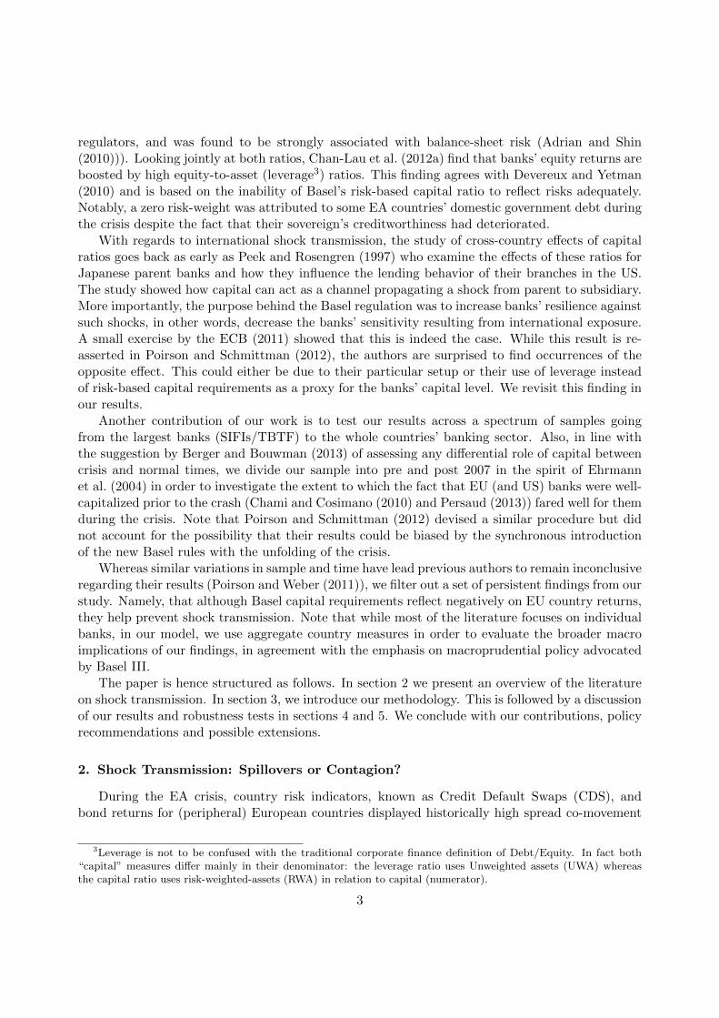
In Figure 1, we plot the individual country betas based on equation (3) . These graphs are in thesame spirit as that in Brooks and DelNegro (2004) which describes an aggregate developed marketstock index during the period 1986-2001. Note that increases in beta are normally a reflection ofgreater economic and financial integration across countries or an increased sensitivity due to crises.

Bearing in mind the six month window used, in most of the graphs, one can see two peaksoccurring respectively around the dates of the subprime and Euro crises which are preceded bya period of relative calm. This suggests that a more interesting approach would be to divide thesample period into a tranquil (2003-2007) versus a crisis period (2007-2011)17. This can also beinterpreted as a pre/post-Basel setting which would account for any differential role played by theexogenous implementation of the capital regulation in the second period.

3.2.3. Contagion

Contagion is the portion of interdependence which is not accounted for by the spillover effectin accordance with Masson (1999).

ε̂it,j = BKMSCIit −∑

j=US,EU

β̂0,j,tMSCIit,j (4)

Residuals ε̂it,j are derived by re-arranging the terms in equation (2) using the estimated spillovereffect obtained from equation (3) as shown in the formula below. Figure 2 displays the residualsstemming from (4) and thus reflects the contagion effect. As expected this effect is arbitrary forevery country and hence we cannot capture any similarities at this stage as we did in the case ofthe spillover effect.

17Note the effect of the lag on the end date.

9

Figure 1: Country Betas

10

Figure 2: Country Residuals (Horizontal line denotes the 0 intercept)

11

4. Results

4.1. Background Analysis

In this following, we evaluate the assumption made in section 3.2 that any EU country is likelyto be predominantly affected by its partnerships with the US and countries within the EU; thelatter being the strongest of both as reported by Bekaert et al. (2005). We compute the betas forthe whole period by regressing each individual country’s BKMSCI index on that of MSCI US andMSCI EU18 The difference in beta between both partners is shown in Figure3. Clearly, countrybetas with respect to the EU are all higher than those of the US by around 0.6, with France havingalmost double that of Portugal. Next, we plot the individual country betas in Figure 4. We observea linear beta trend between EU countries with regard to both the EU and US. We notice that theslopes of the linear fittings are almost the same with the R2s being equal up to three significantfigures. This is due to the orthogonalization we performed earlier on the MSCI indices.

Moreover, Figure 4 shows a clear separation between countries according to the magnitudeof their respective betas. In fact, the ranking of countries seems to be the same with respect tothe EU and US especially for countries with the lowest rankings. Aside from the UK whose betacould be affected by the fact that it is a non-EA member, the nations on the left-hand side arethe peripheral countries which were subject to rescue programs during the euro crisis. Hence,these countries are referred to hereafter as “program” countries. In contrast, with the exceptionof Italy19, the “non-program” countries at the right-hand side are the strongest powers within theEU. Also, the fact that France and Germany have the highest beta for the EU and US respectivelyreinforces the opinion of the IMF (2011) that spillovers within the EA will be mainly channeledby these two countries.

In addition, lending to EA countries played a prominent role during the euro crisis. In thespirit of Waysand et al. (2010) and Shin (2012), we present some figures describing the overallsituation of these countries. In Figure 5, we plot the amount of lending of US banks to their EUcounterparties based on BIS estimates. We observe that the negative impact on lending from theUS to EU countries was short-lived during the subprime crisis but increased considerably afterwardscompared to pre-crisis levels. Note however, that with the exception of the UK, the bulk of lendingwent to the core countries (N-PRGM) as they were perceived as safe borrowers. In turn, this leftthe task of lending to peripheral countries (PRGM) to the core countries, specifically France andGermany, in addition to the UK. This is showcased in Figure 6 which illustrates the amount oflending from core countries to the periphery. It is worthwhile pointing out that France did notparticipate in funding Portugal and Spain. Nonetheless, it still held the greatest debt proportionof the largest indebted country, Italy (130% of GDP according to IMF estimates), which raisedspillover concerns from and to this country during the EA-crisis. This is in contrast to Germanywho drastically cut down lending to the Iberic peninsula and was therefore less at risk from anegative spillover emanating from Europe’s periphery. Finally, note that the UK, which took partin lending to the periphery, is also the heaviest borrower from the US (almost equal to the total ofEA countries). This points to the particular role held by this country, and numerous attempts torenegotiate its position, within the EU.

18All results are highly significant (p-value ≈ 0).19Besides being a program country, Italy’s position in the ranking is clearly a reflection of the size of its GDP:

third (EA), fourth(EU).

12

Figure 3: Difference Between EU and US Betas (2003-2012)

Figure 4: Beta Coefficients against US and EU (2003-2012)

13

Figure 5: Foreign Claims (in Trillions) of US banks on EU counterparties (Source:BIS consolidated banking statistics)

Figure 6: Lending by Core to Peripheral EA Countries

14

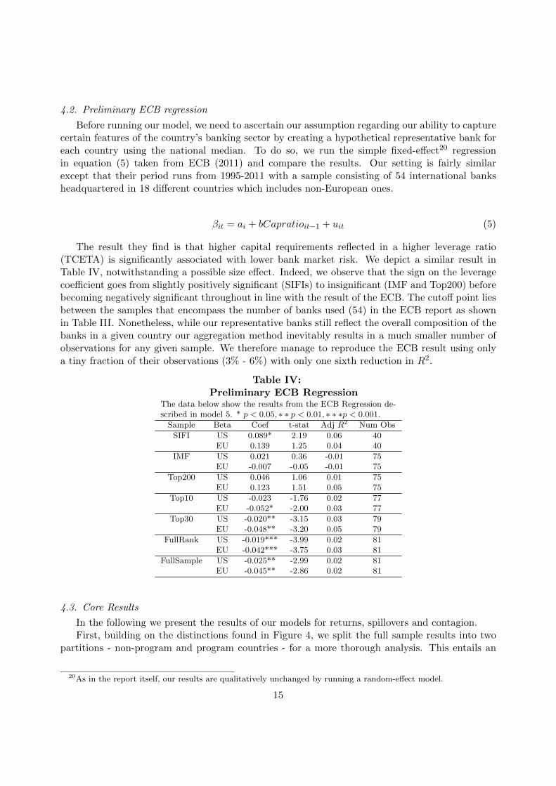
4.2. Preliminary ECB regression

Before running our model, we need to ascertain our assumption regarding our ability to capturecertain features of the country’s banking sector by creating a hypothetical representative bank foreach country using the national median. To do so, we run the simple fixed-effect20 regressionin equation (5) taken from ECB (2011) and compare the results. Our setting is fairly similarexcept that their period runs from 1995-2011 with a sample consisting of 54 international banksheadquartered in 18 different countries which includes non-European ones.

βit = ai + bCapratioit−1 + uit (5)

The result they find is that higher capital requirements reflected in a higher leverage ratio(TCETA) is significantly associated with lower bank market risk. We depict a similar result inTable IV, notwithstanding a possible size effect. Indeed, we observe that the sign on the leveragecoefficient goes from slightly positively significant (SIFIs) to insignificant (IMF and Top200) beforebecoming negatively significant throughout in line with the result of the ECB. The cutoff point liesbetween the samples that encompass the number of banks used (54) in the ECB report as shownin Table III. Nonetheless, while our representative banks still reflect the overall composition of thebanks in a given country our aggregation method inevitably results in a much smaller number ofobservations for any given sample. We therefore manage to reproduce the ECB result using onlya tiny fraction of their observations (3% - 6%) with only one sixth reduction in R2.

Table IV:Preliminary ECB Regression

The data below show the results from the ECB Regression de-scribed in model 5. * p < 0.05, ∗ ∗ p < 0.01, ∗ ∗ ∗p < 0.001.

Sample Beta Coef t-stat Adj R2 Num Obs

SIFI US 0.089* 2.19 0.06 40EU 0.139 1.25 0.04 40

IMF US 0.021 0.36 -0.01 75EU -0.007 -0.05 -0.01 75

Top200 US 0.046 1.06 0.01 75EU 0.123 1.51 0.05 75

Top10 US -0.023 -1.76 0.02 77EU -0.052* -2.00 0.03 77

Top30 US -0.020** -3.15 0.03 79EU -0.048** -3.20 0.05 79

FullRank US -0.019*** -3.99 0.02 81EU -0.042*** -3.75 0.03 81

FullSample US -0.025** -2.99 0.02 81EU -0.045** -2.86 0.02 81

4.3. Core Results

In the following we present the results of our models for returns, spillovers and contagion.First, building on the distinctions found in Figure 4, we split the full sample results into two

partitions - non-program and program countries - for a more thorough analysis. This entails an

20As in the report itself, our results are qualitatively unchanged by running a random-effect model.

15

unavoidable decrease in the number of observations, which, in the case of the program samplewas too small to avoid excessive multi-collinearity and hence had to be discarded. We infer thebehavior of banks in this sample from the full and non-program samples whose sizes are in linewith the existing literature (Poirson and Schmittman (2012)).

Second, for each of these samples, we highlight only the results which are found to be con-sistently significant across all banking samples using the order prescribed in Table III. We wereforced to drop the SIFI sample due to an insufficient number of observations as Austria, Belgium,Greece and Portugal are not on the list (see Table III); nevertheless, these banks are included inthe IMF sample.

Third, we run the analysis for the pre and post crisis sub-periods, with emphasis on the latteras it is usually more deserving of policy attention. Note that we choose to emphasize the crisisrather than the regulatory effect as there seems to be no consistently significant regulatory changebetween pre and post 2007 aside.

In this setup, we encountered another issue with multi-collinearity. This is highlighted in TableV where the Variance Inflation Factors (VIFs) for the TCERWA and TCETA are larger then 10and the Conditioning Index (CI) is above 3021. We attribute this to the property of the capitalratio of tending towards the leverage ratio when the proportion of highly risk-weighted assetsincreases. As shown in Cathcart et al. (2013a), this allows for the correlation between the tworatios to change. Hence, the 53% correlation between the two ratios in Table II is reasonable in aperiod that combines variations from a tranquil (pre-2007) and crisis (post-2007) periods.

Nonetheless, as can be seen by comparing the Full Sample and pre/post-2007 partitions, thisproblem is not due to high correlations between variables in our sample (as shown in Table II);but to the smaller number of observations obtained by splitting the sample population across timesub-samples. To remediate the problem we use the ratio of risk-weighted assets to total assets(RWATA) instead of the capital and leverage ratios as shown in our Updated model in Table V.Indeed, this modification removes the multi-collinearity problem as shown by the low CIs 22. Notethat as mentioned in Cathcart et al. (2013a), the RWATA ratio is reflective of the credit riskundertaken by a bank and is actually equal to the ratio of the leverage and capital ratios. Hence ifthis interaction between both ratios gives a significant result, we relate our findings to the capital(leverage) ratio on the basis that it is inversely correlated with risk-weighted assets (total assets).

A nice feature of our model is that it allows us to determine the significant variables for eachscenario of returns, spillovers and contagion in a consistent manner. In fact, our small numberof variables provide an easier tool for policy-makers to handle than huge multi-variate models.However, the fact that we are unable to go beyond the stated number of regressors to keep clearof multi-collinearity creates another problem, namely omitted variable bias. We resolve it byusing fixed effects estimations in order to capture missing bank-specific effects as in Cetorelli andGoldberg (2011) who suffer from similar small sample problems.

21The VIF relates to an R2 greater than 90% in the auxiliary regressions while the CI is the threshold for multi-collinearity as established by Belsley et al. (1980).

22Effectively, this brings down our t-stats to the same magnitude as those in Poirson and Schmittman (2012).Also, to ensure that the problem does not arise again we display the CI in all upcoming regressions noting that allfactors have a VIF less then 10.

16

Table V:Multicolinearity Tests

The results in this table show the Variance Inflation Factors (VIFs) for our model variables and Condi-tioning Index (CI) of the overall regression. Results relate to the IMF Sample for the Return model on theUS. VIF is defined as 1

1−R2 where R2 is the explanatory power of the auxiliary regression defined as eachvariable regressed on the remainig ones. Typically a V IF > 10 or CI > 30 signals that multi-colinearityis present.

Original Full Sample Post-2007 Pre-2007 Updated Full Sample Post-2007 Pre-2007

MSCI 1.19 1.36 3.60 MSCI 1.12 1.30 3.21FC 3.80 5.59 9.36 FC 3.17 3.45 8.24FDI 2.11 3.08 1.75 FDI 2.09 2.44 1.82IMP 5.65 10.07 9.07 IMP 4.05 4.01 8.62

TCERWA 21.31 38.70 22.69 RWATA 2.58 2.62 3.78TCETA 10.47 13.16 13.02 - - - -

CI 29.41 37.73 42.48 CI 15.84 18.37 17.87

4.3.1. Returns

The predominance of the MSCI indices is clearly showcased across our Full and NonProgram23

country samples (Tables VI-VII). Whereas the EU-index is mostly significant as each countrymirrored the overall regional context, the US-index is only relevant during the crisis period as EUcountries suffered the effects of the subprime crisis. As such, the EU coefficients is understandablytwice as high as the US coefficient during crisis periods. In fact, the MSCI component is soimportant at macro level that compared to the Spillover and Contagion models which do notdirectly account for this factor as a direct explanatory variable, the Return model exhibits thehighest explanatory power. Indeed, running the model with either of the MSCI indices as a regressorcan explain at least 30% of the changes in country returns. Clearly, this is a characteristic of ourcountry-level CAPM model where idiosyncratic elements do not play as important a role as in theconventional bank-level model (in comparison to the 18% achieved by Chan-Lau et al. (2012a)).A similar finding was previously reported by Balakrishnan et al. (2009) who obtain an R2 of 40%by regressing an emerging market index on an advanced market index.

Second, the persistent push factor affecting returns in both samples during the pre-crisis periodsand with respect to both US and EU partners is IMP. This result can be better interpreted byinspecting the NonProgram sample which shows FDI as being positively significant, albeit onlywith respect to the EU. Noting that countries with FDI assets absorb losses from those with FDIliabilities (The Committee on International Economic Policy and Reform (2012)), this means thatEU countries which attracted capital flows from their partners were considered as solid investmentstrategies which were likely to yield ex-post higher returns. In contrast, IMP is understood to havethe reverse effect of FDI since any depreciation of the Euro domestic exchange rate results in asubsequent increase in exports (current account) to US and EU partners; this is simultaneouslyaccompanied by a deterioration in investment (capital account). The opposite result holds in thecase of an appreciation. This does not imply however that the two factors are perfectly inverselycorrelated. While the correlation between the two factors is highest in the context of the EU (0.65as shown in Table II) and positive (as expected according to Balakrishnan et al. (2009), this is not

23F-stats could not be calculated for this particular because the number of regressors is greater than or equal tothe number of clusters. This issue can be resolved by running the model using OLS without altering significantlyour results.

17

Table VI:Full Sample - Returns

The results below are from running equation (1) for the six samples of banks using all EU countries in our dataset. L. denotes lagged values. Highlighted cells are factorsmostly consistent across bank samples. t-stats are given between brackets below the coefficients. * p < 0.05, ∗ ∗ p < 0.01, ∗ ∗ ∗p < 0.001.

SAMPLE IMF Top200 Top10

PARTNER US EU US EU US EU

PERIOD Post-2007 Pre-2007 Post-2007 Pre-2007 Post-2007 Pre-2007 Post-2007 Pre-2007 Post-2007 Pre-2007 Post-2007 Pre-2007

MSCI 2.277*** 0.690 4.579*** 1.423* 2.459*** 0.769 4.633*** 1.772** 2.609*** 0.742 5.020*** 1.763**(7.23) (1.25) (7.22) (1.98) (5.25) (1.40) (7.15) (3.33) (5.40) (1.28) (5.47) (3.19)

L.FC -0.000 0.000 0.000 -0.000 0.000 0.000 0.000 -0.000 0.000 0.000 0.000 -0.000(-1.41) (0.31) (1.41) (-0.46) (0.31) (0.08) (0.69) (-1.04) (0.18) (0.26) (0.53) (-1.01)

L.FDI 0.001 0.000 0.000 0.000 0.001 -0.000 0.000 0.000 0.000 -0.000 0.000 0.000(1.01) (0.04) (1.27) (0.80) (1.00) (-0.25) (1.18) (1.16) (0.25) (-0.37) (1.36) (1.14)

L.IMP -0.000 -0.001*** -0.000 -0.000* 0.000 -0.001*** -0.000 -0.000* 0.001 -0.001*** -0.000 -0.000(-0.25) (-3.49) (-1.01) (-1.89) (0.00) (-5.35) (-0.92) (-2.01) (0.55) (-6.68) (-1.10) (-1.73)

L.RWATA 0.000 -0.000 -0.000 -0.000 0.000* -0.000 0.000 0.000 0.000* -0.000 0.000* -0.000(1.28) (-1.70) (-1.07) (-0.93) (2.17) (-0.44) (0.48) (0.01) (2.17) (-0.97) (1.88) (-0.38)

CONS -0.004 0.008** 0.007 0.007 -0.016* 0.005 0.003 0.003 -0.019** 0.006** -0.003 0.004(-1.02) (3.05) (0.90) (1.81) (-2.08) (1.70) (0.31) (1.23) (-2.34) (2.62) (-0.86) (1.55)

R2 0.32 0.54 0.43 0.52 0.35 0.46 0.43 0.48 0.37 0.49 0.45 0.49Num Obs 36 38 36 38 36 38 36 38 36 38 36 38

F-stat 33.39 38.47 45.75 4.37 26.09 61.55 67.24 3.60 58.84 77.75 26.31 3.42CI 18.38 17.88 12.78 17.00 15.96 23.29 10.50 15.60 19.91 23.31 11.98 14.57

SAMPLE Top30 FullRank FullSample



MSCI 2.704*** 0.887 5.079*** 1.843*** 2.329*** 0.887 4.509*** 1.761*** 2.514*** 0.887 4.507*** 2.037***(4.83) (1.49) (5.39) (3.56) (8.91) (1.51) (8.25) (3.44) (8.33) (1.57) (8.75) (4.69)

L.FC -0.000 -0.000 0.000 -0.000 -0.000 -0.000 0.000 -0.000 -0.000 -0.000 0.000 -0.000(-0.45) (-0.30) (0.43) (-1.34) (-1.31) (-0.30) (1.17) (-1.09) (-0.93) (-0.33) (1.03) (-1.37)

L.FDI 0.000 -0.000 0.000 0.000 0.000 -0.000 0.000 0.000 0.001 -0.000 0.001 0.000**(0.19) (-0.22) (1.04) (1.12) (0.31) (-0.24) (1.17) (1.11) (1.33) (-0.22) (1.10) (2.44)

L.IMP -0.001 -0.001*** -0.000 -0.000** -0.000 -0.001*** -0.000 -0.000** -0.000 -0.001*** -0.000 -0.000***(-0.26) (-5.66) (-1.04) (-2.47) (-0.26) (-5.88) (-0.98) (-2.39) (-0.13) (-6.43) (-0.94) (-3.73)

L.RWATA 0.000** -0.000 0.000* 0.000 0.000 -0.000 -0.000 0.000 0.000** 0.000 -0.000 0.000**(2.57) (-0.02) (1.89) (1.36) (1.38) (-0.01) (-0.45) (0.43) (2.90) (0.19) (-0.39) (3.11)

CONS -0.020*** 0.004** -0.004 0.002 -0.008 0.004*** 0.006 0.003 -0.011 0.003*** 0.007 0.000(-3.74) (3.09) (-0.82) (1.15) (-1.04) (4.33) (0.62) (1.03) (-1.67) (3.46) (0.55) (0.02)

R2 0.39 0.45 0.44 0.51 0.33 0.45 0.43 0.48 0.34 0.45 0.43 0.57Num Obs 36 38 36 38 36 38 36 38 36 38 36 38

F-stat 77.76 60.69 76.70 5.24 56.26 80.16 43.27 3.92 81.63 104.69 40.12 7.15CI 20.11 20.51 12.78 15.94 23.06 20.30 14.79 16.45 25.25 22.03 15.96 16.92

18

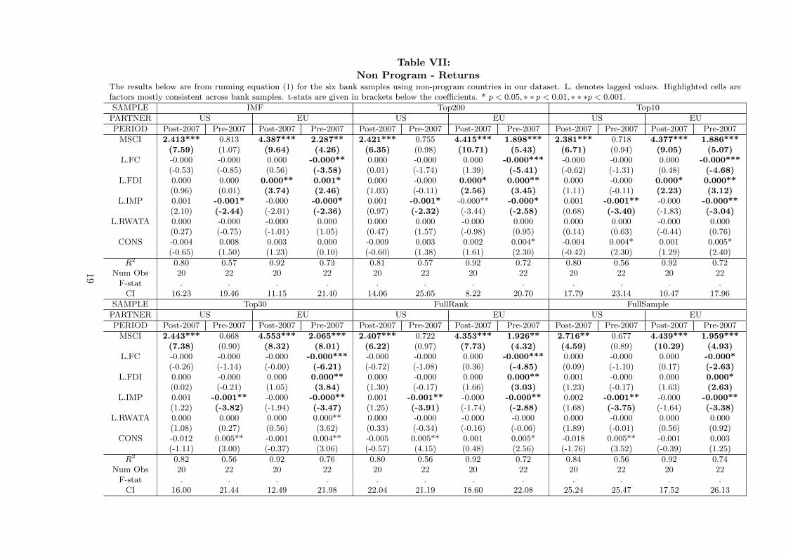
Table VII:Non Program - Returns

The results below are from running equation (1) for the six bank samples using non-program countries in our dataset. L. denotes lagged values. Highlighted cells arefactors mostly consistent across bank samples. t-stats are given in brackets below the coefficients. * p < 0.05, ∗ ∗ p < 0.01, ∗ ∗ ∗p < 0.001.




MSCI 2.413*** 0.813 4.387*** 2.287** 2.421*** 0.755 4.415*** 1.898*** 2.381*** 0.718 4.377*** 1.886***(7.59) (1.07) (9.64) (4.26) (6.35) (0.98) (10.71) (5.43) (6.71) (0.94) (9.05) (5.07)

L.FC -0.000 -0.000 0.000 -0.000** 0.000 -0.000 0.000 -0.000*** -0.000 -0.000 0.000 -0.000***(-0.53) (-0.85) (0.56) (-3.58) (0.01) (-1.74) (1.39) (-5.41) (-0.62) (-1.31) (0.48) (-4.68)

L.FDI 0.000 0.000 0.000** 0.001* 0.000 -0.000 0.000* 0.000** 0.000 -0.000 0.000* 0.000**(0.96) (0.01) (3.74) (2.46) (1.03) (-0.11) (2.56) (3.45) (1.11) (-0.11) (2.23) (3.12)

L.IMP 0.001 -0.001* -0.000 -0.000* 0.001 -0.001* -0.000** -0.000* 0.001 -0.001** -0.000 -0.000**(2.10) (-2.44) (-2.01) (-2.36) (0.97) (-2.32) (-3.44) (-2.58) (0.68) (-3.40) (-1.83) (-3.04)

L.RWATA 0.000 -0.000 -0.000 0.000 0.000 0.000 -0.000 0.000 0.000 0.000 -0.000 0.000(0.27) (-0.75) (-1.01) (1.05) (0.47) (1.57) (-0.98) (0.95) (0.14) (0.63) (-0.44) (0.76)

CONS -0.004 0.008 0.003 0.000 -0.009 0.003 0.002 0.004* -0.004 0.004* 0.001 0.005*(-0.65) (1.50) (1.23) (0.10) (-0.60) (1.38) (1.61) (2.30) (-0.42) (2.30) (1.29) (2.40)

R2 0.80 0.57 0.92 0.73 0.81 0.57 0.92 0.72 0.80 0.56 0.92 0.72Num Obs 20 22 20 22 20 22 20 22 20 22 20 22

F-stat . . . . . . . . . . . .CI 16.23 19.46 11.15 21.40 14.06 25.65 8.22 20.70 17.79 23.14 10.47 17.96




MSCI 2.443*** 0.668 4.553*** 2.065*** 2.407*** 0.722 4.353*** 1.926** 2.716** 0.677 4.439*** 1.959***(7.38) (0.90) (8.32) (8.01) (6.22) (0.97) (7.73) (4.32) (4.59) (0.89) (10.29) (4.93)

L.FC -0.000 -0.000 -0.000 -0.000*** -0.000 -0.000 0.000 -0.000*** 0.000 -0.000 0.000 -0.000*(-0.26) (-1.14) (-0.00) (-6.21) (-0.72) (-1.08) (0.36) (-4.85) (0.09) (-1.10) (0.17) (-2.63)

L.FDI 0.000 -0.000 0.000 0.000** 0.000 -0.000 0.000 0.000** 0.001 -0.000 0.000 0.000*(0.02) (-0.21) (1.05) (3.84) (1.30) (-0.17) (1.66) (3.03) (1.23) (-0.17) (1.63) (2.63)

L.IMP 0.001 -0.001** -0.000 -0.000** 0.001 -0.001** -0.000 -0.000** 0.002 -0.001** -0.000 -0.000**(1.22) (-3.82) (-1.94) (-3.47) (1.25) (-3.91) (-1.74) (-2.88) (1.68) (-3.75) (-1.64) (-3.38)

L.RWATA 0.000 0.000 0.000 0.000** 0.000 -0.000 -0.000 -0.000 0.000 -0.000 0.000 0.000(1.08) (0.27) (0.56) (3.62) (0.33) (-0.34) (-0.16) (-0.06) (1.89) (-0.01) (0.56) (0.92)

CONS -0.012 0.005** -0.001 0.004** -0.005 0.005** 0.001 0.005* -0.018 0.005** -0.001 0.003(-1.11) (3.00) (-0.37) (3.06) (-0.57) (4.15) (0.48) (2.56) (-1.76) (3.52) (-0.39) (1.25)

R2 0.82 0.56 0.92 0.76 0.80 0.56 0.92 0.72 0.84 0.56 0.92 0.74Num Obs 20 22 20 22 20 22 20 22 20 22 20 22

F-stat . . . . . . . . . . . .CI 16.00 21.44 12.49 21.98 22.04 21.19 18.60 22.08 25.24 25.47 17.52 26.13

19

sufficient to cause any multi-collinearity concerns judging by the conditioning index (CI) of theseregressions. Our explanation is supported by the work of Forbes and Chinn (2004) who do not findany such problem by incorporating both factors together. We believe the reasons for this imperfectcorrelation are the lags between both factors and their different multipliers.

Thirdly, RWATA provides a significant pull mechanism for returns. Its positive sign suggeststhat banks with lower risk-weighted assets (higher capital ratios) were effectively obtaining lowerreturns especially during the crisis24. Hence, on a macro level, this result contradicts that in Bergerand Bouwman (2013). At first, the latter could be justified on the grounds of moral hazard withregard to large banks which were excluded from these authors’ sample. However, we notice thatthis behavior also extends to the entire banking sector (FullSample) which includes the smallerbanks as well. A more general explanation could be the fact that setting aside money for highercapital cushions constrains the bank from using it in more profitable investments. To compensatefor this, banks are forced to invest in riskier projects where the downside is triggered during crisistimes. Another explanation is that the amount of capital set aside did not reflect the risk inherentin sovereign debt whose yields widened during the crisis thus lowering returns. Notice that thementioned effect is not reflected in the NonProgram sample suggesting that this effect was mosthighly experienced by Program countries.

4.3.2. Spillover

At the full sample level (Table VIII), aside from the FC effect during pre-crisis for the US, nofactor appears to have played a role in explaining spillovers in the EU. Taking into considerationthe lag in this variable, this means that any increase in lending to these countries would result inan ex-post increase in their sensitivity to crises in the US. Indeed, according to Figure 5 overalllending to the EU’s “safe” countries (mainly Germany and France) increased towards the end of thesubprime crisis which explains why the effect is replicated identically in the sample of non-programcountries (Table IX). We can also speculate that this effect was also present for the Programcountries, since accounting as well for the six month (window) delay, the increase in sensitivityin all countries occurred mostly around the same time, as can be seen in Figure 1. In essence,this confirms the statement by the IMF (2011) which described these countries as “exhibiting thegreatest potential for spillover effects in times of stress”.

Moreover, we observe a persistent IMP component with regard to the EU crisis period affectingnon-program countries. This implies that if the US increased its imports from these countries,this would make them more reliant on the overall economic status of the US, as documented inKalemli-Ozcan et al. (2012) thus increasing the safe countries’ sensitivity to shocks affecting theentire region. We would normally expect the same significance for the EU partner. However,despite the strongest IMP effect being observed in this case of the largest sample (IMF), the effectdoes not trickle down to the rest of the banking sector. In other words, it was only the largestbanks which were sensitive to trade shocks arising in the EU which would seem counter-intuitive.Nevertheless, the signs are identical across all samples.

Finally, for the NonProgram countries we find that higher RWATA lead to a higher potentialfor spillover effects. This result is in agreement with those found previously in ECB (2011) andPoirson and Schmittman (2012) for TCETA. In other words, countries with a higher capitalizedbanking sector are better able to cope with these risky assets and are hence more likely to avoidspillovers. In fact, this effect is only noticeable before the introduction of Basel II. While the

24A statement made also by the Economist (2013).

20

Table VIII:Full Sample - Spillover

The results below are from running equations (2) and (3) for the six bank samples using all EU countries in our dataset. L. denotes lagged values. Highlightedcells are factors mostly consistent across bank samples. t-stats are given in brackets below the coefficients. * p < 0.05, ∗ ∗ p < 0.01, ∗ ∗ ∗p < 0.001.




L.FC -0.008 0.067*** 0.007 0.011 -0.004 0.058** 0.008 0.010 -0.005 0.056** 0.008 0.010(-0.67) (3.58) (1.00) (1.22) (-0.26) (2.42) (1.22) (1.06) (-0.44) (3.11) (1.26) (1.15)

L.FDI -0.011 0.002 -0.020 0.052 0.004 0.006 -0.021 0.052* 0.006 0.013 -0.018 0.050(-0.34) (0.06) (-1.09) (1.77) (0.15) (0.21) (-1.04) (2.02) (0.17) (0.62) (-0.90) (1.83)

L.IMP 0.085 -0.003 -0.011 -0.008 0.081 0.031 -0.010 -0.007 0.077 0.016 -0.006 -0.009(1.10) (-0.01) (-0.61) (-0.53) (0.95) (0.20) (-0.62) (-0.50) (0.88) (0.12) (-0.35) (-0.62)

L.RWATA -0.006 0.002 -0.011 -0.006 -0.000 0.007 -0.011 0.008 -0.001 0.011** -0.019 0.005(-0.91) (0.20) (-0.75) (-1.53) (-0.00) (0.86) (-0.90) (1.43) (-0.24) (2.44) (-1.58) (0.77)

CONS 0.918* 0.309 2.041** 0.978** 0.593 -0.011 1.974** 0.353 0.661 -0.182 2.309*** 0.501(1.92) (0.62) (2.35) (3.22) (0.83) (-0.02) (2.75) (1.28) (1.50) (-0.65) (5.00) (1.81)

R2 0.10 0.09 0.08 0.29 0.07 0.11 0.07 0.30 0.07 0.16 0.13 0.29Num Obs 36 38 36 38 36 38 36 38 36 38 36 38

F-stat 0.89 13.17 0.82 1.77 0.56 12.87 0.89 1.61 0.56 17.15 1.63 1.45CI 18.07 16.69 12.68 15.10 15.55 20.92 10.30 14.21 19.49 21.22 11.80 13.36




L.FC -0.005 0.063** 0.009* 0.011 -0.004 0.067*** 0.007 0.010 -0.006 0.065*** 0.007 0.010(-0.47) (3.31) (2.03) (1.43) (-0.48) (3.63) (1.25) (1.17) (-0.59) (3.74) (1.48) (1.16)

L.FDI 0.008 -0.020 -0.003 0.059* -0.005 0.001 -0.009 0.055* 0.002 0.018 -0.004 0.053(0.20) (-0.64) (-0.14) (1.91) (-0.15) (0.05) (-0.47) (1.86) (0.07) (0.75) (-0.22) (1.84)

L.IMP 0.084 -0.019 -0.003 -0.007 0.077 -0.015 -0.003 -0.007 0.082 -0.017 -0.017 -0.007(1.21) (-0.10) (-0.17) (-0.48) (0.92) (-0.08) (-0.17) (-0.45) (1.16) (-0.08) (-0.97) (-0.36)

L.RWATA -0.003 0.008 -0.035** -0.006 0.005 0.006 -0.027 -0.002 -0.006 0.009 -0.028** -0.001(-0.26) (1.20) (-2.55) (-1.52) (0.59) (0.55) (-1.27) (-0.30) (-0.81) (0.87) (-2.49) (-0.09)

CONS 0.721 0.051 2.996*** 0.980*** 0.341 0.088 2.721** 0.806*** 0.907* -0.046 3.048*** 0.751*(1.13) (0.17) (4.03) (4.46) (0.56) (0.39) (2.70) (3.38) (1.87) (-0.14) (3.54) (2.25)

R2 0.07 0.13 0.20 0.30 0.08 0.12 0.13 0.28 0.09 0.13 0.17 0.28Num Obs 36 38 36 38 36 38 36 38 36 38 36 38

F-stat 0.70 26.02 4.24 1.80 1.67 22.09 1.74 1.24 0.88 8.40 4.79 1.23CI 19.77 19.10 12.65 14.39 22.68 18.72 14.63 15.22 24.73 20.32 15.72 15.49

21

Table IX:Non Program - Spillover

The results below are from running equations (2) and (3) for the six bank samples using non-program countries in our dataset. L. denotes lagged values. Highlightedcells are factors mostly consistent across bank samples. t-stats are given in brackets below the coefficients. * p < 0.05, ∗ ∗ p < 0.01, ∗ ∗ ∗p < 0.001.




L.FC 0.008 0.059** 0.001 0.008 0.033 0.039* -0.001 0.009 0.017 0.052* 0.007 0.011(0.51) (3.30) (0.23) (0.76) (1.85) (2.19) (-0.18) (0.68) (1.08) (2.32) (0.98) (0.90)

L.FDI 0.008 -0.024 -0.051** 0.066 0.015 0.009 -0.036* 0.043 -0.039 0.016 -0.025 0.045(0.18) (-0.81) (-2.96) (1.12) (0.85) (0.32) (-2.26) (1.13) (-0.98) (0.78) (-0.72) (0.93)

L.IMP 0.198** -0.131 0.030*** -0.011 0.243*** 0.056 0.017 -0.001 0.272*** 0.005 0.019 -0.011(3.54) (-0.45) (5.68) (-0.44) (6.09) (0.36) (0.97) (-0.04) (4.88) (0.03) (1.10) (-0.48)

L.RWATA 0.008 0.051** 0.025 0.009 0.025 0.023* 0.016 0.022* 0.016 0.018** -0.027 0.013(0.95) (3.49) (1.50) (0.34) (1.53) (2.70) (1.45) (2.23) (1.16) (4.10) (-1.43) (2.07)

CONS -0.174 -1.062* 0.110 0.576 -1.210 -0.537 0.809 -0.076 -0.769 -0.234 2.074* 0.352(-0.29) (-2.42) (0.18) (0.44) (-1.46) (-0.76) (1.88) (-0.13) (-1.09) (-0.54) (2.69) (0.95)

R2 0.22 0.12 0.15 0.24 0.31 0.17 0.07 0.36 0.25 0.18 0.16 0.29Num Obs 20 22 20 22 20 22 20 22 20 22 20 22

F-stat 99.68 102.11 116.69 10.67 19.43 32.05 1.74 96.03 61.29 82.73 2.46 35.25CI 15.81 18.67 11.13 18.79 13.65 23.91 8.09 19.18 17.41 21.30 10.37 16.62




L.FC 0.014 0.059** 0.006 0.010 0.006 0.068** 0.004 0.009 0.004 0.067** 0.005 0.011(1.49) (3.32) (0.76) (0.77) (0.88) (3.56) (0.45) (0.77) (0.33) (4.60) (0.68) (0.93)

L.FDI -0.073 -0.055 -0.019 0.067 -0.057 -0.007 -0.024 0.062 -0.008 0.031 -0.011 0.054(-1.78) (-1.69) (-0.70) (1.07) (-2.02) (-0.29) (-0.92) (1.09) (-0.32) (1.05) (-0.38) (1.22)

L.IMP 0.238*** -0.073 0.021 -0.009 0.230** -0.061 0.014 -0.010 0.192** -0.079 0.001 -0.014(4.92) (-0.37) (1.48) (-0.35) (4.05) (-0.27) (0.89) (-0.35) (4.35) (-0.33) (0.04) (-0.39)

L.RWATA 0.031* 0.016* -0.028 -0.004 0.022* 0.009 -0.009 0.000 0.003 0.020* -0.023 0.006(2.14) (2.30) (-0.67) (-0.44) (2.27) (0.63) (-0.28) (0.02) (0.27) (2.37) (-0.86) (0.31)

CONS -1.275 0.058 2.168 0.972** -0.877 0.211 1.663 0.863** 0.074 -0.175 2.505 0.646(-2.01) (0.13) (1.42) (3.30) (-1.72) (1.38) (1.26) (3.93) (0.20) (-0.36) (1.44) (1.38)

R2 0.33 0.18 0.10 0.24 0.33 0.15 0.05 0.24 0.20 0.22 0.09 0.24Num Obs 20 22 20 22 20 22 20 22 20 22 20 22

F-stat 88.84 11.23 1.31 9.26 12.06 59.66 0.66 1.85 79.92 40.12 16.07 0.67CI 15.56 20.27 12.48 19.26 21.65 19.85 18.40 20.48 24.75 24.23 17.50 23.87

22

effect itself is weaker in the post-crisis despite no regulatory changes affecting the capital ratiothresholds, we speculate that the reason could be because of an offsetting effect introduced by thelowering of the leverage factor (TCETA), during this period. Indeed, Poirson and Schmittman(2012) were surprised that leverage can in some cases be insignificant, or even have a positive effecton spillovers. The authors assumed this peculiarity was due to a reversal between bank size andvulnerability. In contrast, we show here that such a result can occur irrespective of size (comparingIMF to FullSample in Tables VIII and IX). In any case, this supports the introduction by Basel IIIof the leverage ratio as a backstop measure in order to maintain the beneficial aspect of risk-basedcapital ratios.

Note that the explanatory power of our model coincides to a large extent with the 22-28% rangeof R2 in Poirson and Schmittman (2012) which, as the authors highlight, were almost double thatof Brooks and DelNegro (2006). Nonetheless, the advantage of our model is in achieving the samepower with a much smaller set of factors.

4.3.3. Contagion

Despite the possibility of model misspecification in the case of contagion as highlighted inBekaert et al. (2005), looking at the full sample (Table X), it would appear at first that the onlyfactor increasing the potential for contagion from the US is FDI. With the notable absence of anycapital related effects, this means that a shock emanating from the US could affect EU countriesindirectly via alternative channels such as other countries or factors.

While the FDI effect is to a certain extent reproduced in our NonProgram sample, we note thenegative effect of FC during the pre-crisis period. This means that lending from the US could beinterpreted as a signal that a given country was solid economically-speaking which would counteractthe effects of contagion that could a priori emanate from these alternative channels.

In sum, while our findings point out that countries might have the incentive to reduce theircapital ratios in order to achieve higher returns, nonetheless having a substantial amount of capitalcan shield them from the effects of spillover. Hence, it is important to maintain these capitalratios at sensible levels as they can act as a counterweight to the sometimes aggravating effects ofbilateral linkages. As a matter of fact, this finding applies to all bank samples irrespective of size.

5. Robustness

In order to strengthen the validity of our results we run a series of robustness tests covering allthree models presented above. All tests are on the Full Sample in order to avoid any unintendedmulti-collinearity.

First, we would like to assert if the results we are obtaining are linked to EA countries only orare driven somewhat by the UK. Therefore, we remove the UK from our EU sample and check ifthe Returns results in Table VI change. In Table I, we see that this is not the case except for aweakening of the trade relationship with the EU. This was expected given that the UK is one ofthe largest trading partners with the EU.

Second, in Table II, we introduce the credit-to-gdp gap (CRGDP), a cyclical macro-economicvariable which the Basel committee on Basel III views as the determinant of the new counter-cyclicalcapital cushions. We choose this variable for both its macroeconomic (control) and regulatory (newcapital buffers) content. As described in BCBS (2010), we construct this variable by taking

23

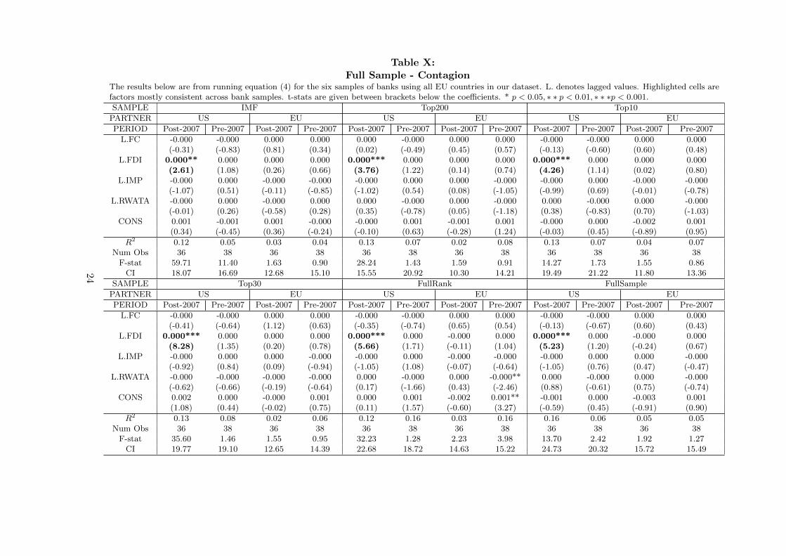
Table X:Full Sample - Contagion

The results below are from running equation (4) for the six samples of banks using all EU countries in our dataset. L. denotes lagged values. Highlighted cells arefactors mostly consistent across bank samples. t-stats are given between brackets below the coefficients. * p < 0.05, ∗ ∗ p < 0.01, ∗ ∗ ∗p < 0.001.




L.FC -0.000 -0.000 0.000 0.000 0.000 -0.000 0.000 0.000 -0.000 -0.000 0.000 0.000(-0.31) (-0.83) (0.81) (0.34) (0.02) (-0.49) (0.45) (0.57) (-0.13) (-0.60) (0.60) (0.48)

L.FDI 0.000** 0.000 0.000 0.000 0.000*** 0.000 0.000 0.000 0.000*** 0.000 0.000 0.000(2.61) (1.08) (0.26) (0.66) (3.76) (1.22) (0.14) (0.74) (4.26) (1.14) (0.02) (0.80)

L.IMP -0.000 0.000 -0.000 -0.000 -0.000 0.000 0.000 -0.000 -0.000 0.000 -0.000 -0.000(-1.07) (0.51) (-0.11) (-0.85) (-1.02) (0.54) (0.08) (-1.05) (-0.99) (0.69) (-0.01) (-0.78)

L.RWATA -0.000 0.000 -0.000 0.000 0.000 -0.000 0.000 -0.000 0.000 -0.000 0.000 -0.000(-0.01) (0.26) (-0.58) (0.28) (0.35) (-0.78) (0.05) (-1.18) (0.38) (-0.83) (0.70) (-1.03)

CONS 0.001 -0.001 0.001 -0.000 -0.000 0.001 -0.001 0.001 -0.000 0.000 -0.002 0.001(0.34) (-0.45) (0.36) (-0.24) (-0.10) (0.63) (-0.28) (1.24) (-0.03) (0.45) (-0.89) (0.95)

R2 0.12 0.05 0.03 0.04 0.13 0.07 0.02 0.08 0.13 0.07 0.04 0.07Num Obs 36 38 36 38 36 38 36 38 36 38 36 38

F-stat 59.71 11.40 1.63 0.90 28.24 1.43 1.59 0.91 14.27 1.73 1.55 0.86CI 18.07 16.69 12.68 15.10 15.55 20.92 10.30 14.21 19.49 21.22 11.80 13.36




L.FC -0.000 -0.000 0.000 0.000 -0.000 -0.000 0.000 0.000 -0.000 -0.000 0.000 0.000(-0.41) (-0.64) (1.12) (0.63) (-0.35) (-0.74) (0.65) (0.54) (-0.13) (-0.67) (0.60) (0.43)

L.FDI 0.000*** 0.000 0.000 0.000 0.000*** 0.000 -0.000 0.000 0.000*** 0.000 -0.000 0.000(8.28) (1.35) (0.20) (0.78) (5.66) (1.71) (-0.11) (1.04) (5.23) (1.20) (-0.24) (0.67)

L.IMP -0.000 0.000 0.000 -0.000 -0.000 0.000 -0.000 -0.000 -0.000 0.000 0.000 -0.000(-0.92) (0.84) (0.09) (-0.94) (-1.05) (1.08) (-0.07) (-0.64) (-1.05) (0.76) (0.47) (-0.47)

L.RWATA -0.000 -0.000 -0.000 -0.000 0.000 -0.000 0.000 -0.000** 0.000 -0.000 0.000 -0.000(-0.62) (-0.66) (-0.19) (-0.64) (0.17) (-1.66) (0.43) (-2.46) (0.88) (-0.61) (0.75) (-0.74)

CONS 0.002 0.000 -0.000 0.001 0.000 0.001 -0.002 0.001** -0.001 0.000 -0.003 0.001(1.08) (0.44) (-0.02) (0.75) (0.11) (1.57) (-0.60) (3.27) (-0.59) (0.45) (-0.91) (0.90)

R2 0.13 0.08 0.02 0.06 0.12 0.16 0.03 0.16 0.16 0.06 0.05 0.05Num Obs 36 38 36 38 36 38 36 38 36 38 36 38

F-stat 35.60 1.46 1.55 0.95 32.23 1.28 2.23 3.98 13.70 2.42 1.92 1.27CI 19.77 19.10 12.65 14.39 22.68 18.72 14.63 15.22 24.73 20.32 15.72 15.49

24

Table XI:Non Program - Contagion

The results below are from running equation (4) for the six bank samples using non-program countries in our dataset. L. denotes lagged values. Highlighted cells arefactors mostly consistent across bank samples. t-stats are given in brackets below the coefficients. * p < 0.05, ∗ ∗ p < 0.01, ∗ ∗ ∗p < 0.001.




L.FC 0.000 -0.000*** 0.000 -0.000 0.000 -0.000** 0.000 -0.000 0.000 -0.000* 0.000 -0.000(0.51) (-4.68) (1.54) (-0.96) (0.96) (-2.53) (0.67) (-0.83) (1.53) (-2.21) (0.95) (-1.26)

L.FDI 0.001* 0.000 0.000 0.000 0.001** 0.000 -0.000 0.000 0.000 0.000 -0.000 0.000(2.21) (0.35) (0.08) (1.06) (3.34) (1.08) (-0.13) (1.36) (1.01) (0.96) (-0.12) (1.38)

L.IMP -0.000 -0.000 -0.000 -0.000 -0.000 -0.000 -0.000 -0.000 0.000 -0.000 -0.000 -0.000(-0.44) (-1.10) (-0.46) (-1.28) (-0.08) (-1.18) (-0.24) (-1.52) (0.81) (-1.11) (-0.54) (-0.93)

L.RWATA 0.000 0.000 -0.000 0.000 0.000 -0.000 0.000 -0.000* 0.000 -0.000 0.000 -0.000(0.39) (1.15) (-0.16) (0.96) (1.02) (-1.40) (0.13) (-2.30) (1.67) (-1.22) (1.27) (-1.95)

CONS -0.001 -0.003 0.000 -0.002 -0.006 0.001 -0.001 0.002 -0.007 0.001 -0.003 0.002(-0.25) (-1.02) (0.03) (-0.83) (-0.92) (1.80) (-0.25) (2.07) (-1.60) (1.95) (-1.29) (1.87)

R2 0.23 0.25 0.07 0.16 0.33 0.20 0.07 0.18 0.36 0.19 0.25 0.18Num Obs 20 22 20 22 20 22 20 22 20 22 20 22

F-stat 51.67 23.95 2.28 106.05 83.09 46.75 2.71 1.83 4.09 10.84 6.78 2.05CI 15.81 18.67 11.13 18.79 13.65 23.91 8.09 19.18 17.41 21.30 10.37 16.62




L.FC 0.000 -0.000* 0.000 -0.000 0.000 -0.000** 0.000 -0.000 0.000 -0.000** 0.000 -0.000(1.11) (-2.56) (0.10) (-0.68) (0.67) (-2.98) (0.98) (-1.02) (1.85) (-3.03) (0.44) (-1.04)

L.FDI 0.000 0.000 -0.000 0.000 0.000 0.000 -0.000 0.000 0.000* 0.000 -0.000 0.000(1.68) (1.83) (-0.78) (1.57) (1.86) (1.68) (-0.85) (1.66) (2.41) (1.24) (-1.32) (1.09)

L.IMP -0.000 0.000 -0.000 -0.000* -0.000 0.000 -0.000 -0.000 0.000 -0.000 0.000 -0.000(-0.30) (0.03) (-0.96) (-2.20) (-0.44) (0.66) (-0.68) (-0.95) (1.21) (-0.31) (1.33) (-0.25)

L.RWATA 0.000 -0.000 0.000* -0.000 0.000 -0.000 0.000 -0.000** 0.000** 0.000 0.000* -0.000(1.49) (-1.22) (2.25) (-0.62) (0.82) (-1.61) (1.25) (-2.94) (4.25) (0.04) (2.61) (-0.55)

CONS -0.005 0.001* -0.006** 0.001* -0.003 0.001** -0.005 0.001*** -0.011*** 0.000 -0.010** 0.001(-1.52) (2.65) (-2.98) (2.33) (-0.74) (2.78) (-1.68) (5.27) (-5.08) (0.75) (-2.87) (0.94)

R2 0.30 0.16 0.35 0.07 0.28 0.27 0.31 0.22 0.58 0.15 0.41 0.08Num Obs 20 22 20 22 20 22 20 22 20 22 20 22

F-stat 94.23 13.43 4.20 14.17 98.84 22.93 4.58 53.50 91.49 80.09 81.16 75.60CI 15.56 20.27 12.48 19.26 21.65 19.85 18.40 20.48 24.75 24.23 17.50 23.87

25

the CRGDP deviation from the long-term trend using a Hodrick-Prescott filter25. The variableintroduces no additional explanatory power with regards to contagion26 while maintaining thesignificance of the FDI factor as in Table X. In other words, contagion is as likely to occur in anystate of the economy after accounting for other lending sources such as FC.

Third, wholesale funding emerged in Poirson and Schmittman (2012) as a leading pull factorin spillovers. However, the authors acknowledge that the opposite result was found in Tressel(2011)’s work. We use the same indicator, loans-to-deposits, to gauge the effect of wholesalefunding. We find that this ratio only starts to appear significant as the number of banks increasesto encompass the whole of the banking sector. This brings together both findings regarding theimpact of wholesale funding and confirms the necessity of our contribution in avoiding any sampleeffects. Moreover, this opens an interesting research question to explain why smaller banks aremore sensitive to spillovers via wholesale funding. This could be due to the fact that smaller banksare less capable of replacing sources of wholesale funding by other resources in the same way thatlarger banks are able to.

Finally, despite having excluded liquidity from our study on the basis of multi-collinearity con-cerns, we include it only for illustrative purposes27. We find that liquidity is the only factor whichis able to minimize the impacts of spillovers (Table IV) and contagion (Table IV) simultaneously,noticeably in larger sample banks that do not suffer as much from multi-collinearity. This meansthat liquidity seems to be the best protection against transmission shocks especially when sol-vency constraints play no meaningful role. The latter agrees with the importance attributed byFratzscher (2012) to country-specific fundamentals (albeit not not to bank-specific factors such asleverage and liquidity per se); thus reinforcing the introduction of liquidity standards in Basel III.Therefore, applying a similar model to a larger sample would be a good venue to corroborate ourresults.

6. Conclusion

Boosting a country’s economy through higher returns while safeguarding it from externalitieshave always been main targets of policy-makers. With the creation of the EU, this objective becameeven more central as the targets shifted to a regional scale with the added concern of protectingthe EU, not only from the rest of the world, but from itself. Indeed, the recent Euro crisis broughtto light the internal vulnerabilities of Europe which threatened to break up the union just over adecade after its creation.

Whereas the economic target was achieved after 1999 through relaxing constraints on bilaterallinkages between countries (mainly trade and investment), Europe’s leaders witnessed during thecrisis that more was needed with regards to the safety target. The latter has been handed overto the EU’s regulatory bodies whose role is being questioned for not achieving enough oversight.As a result, the EU Commission has favored extending the supervisory powers of the CentralBank (ECB) while promoting a full banking union. In turn, this creates a sizable problem forany regulator: that of choosing uniform safety targets for the EU’s banking sector in order toensure its financial stability. In that regard, the problem facing regulators is the diversity of

25Using a smoothness parameter of 400,000 as suggested by the BCBS.26Except in the last regression for each sample where multi-collinearity occurs. We discard the results from these

regressions.27Liquidity is defined as total liquid assets to total deposits and short term funding.

26

country-specific vulnerabilities that so far have been outside the jurisdiction of EU authorities.One European regulation which escaped such criticism due to its homogeneous enforcement acrossmember countries was the Basel II/CRD regulation. As one lever of the safety mechanism, theregulation still got its share of scrutiny for not doing enough to safeguard the sanctity of thebanking sector. This has propelled efforts towards increased capital measures and a backstopleverage requirement under Basel III.

Note that even if regulators mainly focus on the whole macroeconomic banking sector, somebanks, particularly, the SIFIs have attracted a lot of criticism in both the US and EU crises. Whilewe do not uncover any aspect particularly related to this sample of banks, one of our contributionshas been in establishing the key factors for each mentioned scenario using a diversity of samplesranging from the largest banks (including the SIFIs) to the whole of the banking sector. Despitedata limitations similar to those encountered in the literature, this makes our results more robustthan those of authors who focus only on one particular sample. Moreover, whereas Poirson andSchmittman (2012) have attempted a similar exercise which included European countries, the meritof our approach is in the use of country-to-country linkages rather than overall country exposures.More generally, such authors have focused on explaining individual bank behavior whereas ourmethod addresses the overall banking sector. This should prove more useful for regulators as itpoints the axis towards macroprudential policy which has become one of the central pillars of theBasel III regulation.

Furthermore our main purpose in this research was to shed light on where the vulnerabilitiesof the EU lie with respect to the safety targets mentioned earlier in order to help policy-makers inaddressing them. Indeed, by building a model that encompasses both the linkages between countriesand country-specific components we detect which factors are more prevalent in increasing returnsand containing spillovers and contagion. Due to data limitations, we do so only for our full sampleof countries and a partition of non-program countries. Nonetheless, we subject these results to abattery of robustness tests to ascertain their validity.

For instance, we find that FDI played an important role in keeping returns afloat particularlyfor non-program countries. However, we find that high capital ratios (low risk-weighted assets)curtail returns for all countries. This has become a subject of concern for the banking industryas it shows a tradeoff between profitability and safety; the reason being that banks exceeding thetarget thresholds can afford to take more risk since they can cover their losses. Hence, while ourresults show that the enforcement of Basel II was unable to reverse that trend, the guidelines inBasel III with respect to increasing the threshold requirements will make it more difficult for banksto partake in similar wrongdoing (moral hazard).

Nonetheless, in conjunction with the lending and import factors’ effect on spillovers, capitalratios emerge as the primary safety mechanism for non-program countries. This accentuates theimportance attributed to higher capital buffers in the banking industry despite the cautioningagainst a possible credit crunch arising from the newly-established capital increments under BaselIII. Similarly, the introduction of a leverage threshold also seems to be well-founded in order topreserve the safety benefits of capital ratios.

Still, our results indicate that capital ratios cannot prevent contagion from occuring. Thisraises the question as to which other factors might be missing from our model. While we make anattempt at addressing that question through the use of the credit-to-gdp ratio as advocated by theBCBS for its counter-cyclical capital buffers, this matter requires further analysis. In fact, sincewe find that solvency is not a solution, we believe liquidity would be a good starting point.

27

The EU crisis spurred the debate with regard to the direction that macroprudential policyshould take in either enforcing capital controls to maintain the linkage channel between countriesor improve country’s resilience to shocks via idiosyncratic measures. One characteristic of the EUcrisis is that trade and financial linkages were shown to be intrinsically two sides of the same coin(twin deficits). However, they are not the only important factors. Attention should be given aswell to the regulatory side. Whereas capital and leverage ratios might have detrimental effects forprofitability, they deserve a lot of credit in arguably more important situations such as safeguardingcountries from the spread of crises. Our conclusion from this work is therefore to support therecommendation of Cheung et al. (2010) for the need of policy-makers to balance between thevarious tradeoffs that can affect the dynamics of global interdependence. In other words, whereasFDI can be benefitial especially for Non-Program country returns, it can also increase the riskof contagion; hence the need for a proper balance when considering the enforcement of capitalcontrols.

Appendix A.

28

Table I:Full Sample - Returns - noUK

The results below are from running equation (1) for the six samples of banks using all EU countries in our dataset. L. denotes lagged values. Highlighted cells are factorsmostly consistent across bank samples. t-stats are given between brackets below the coefficients. * p < 0.05, ∗ ∗ p < 0.01, ∗ ∗ ∗p < 0.001.




MSCI 2.303*** 0.363 4.595*** 1.389 2.539*** 0.579 4.632*** 1.767** 2.838*** 0.509 5.182*** 1.766**(6.66) (0.64) (7.85) (1.84) (5.52) (1.13) (8.75) (3.01) (4.44) (0.87) (5.77) (2.84)

L.FC -0.000 0.001 0.000 -0.000 -0.000 0.000 0.000 -0.000 0.000 0.000 0.000 -0.000(-0.32) (1.59) (0.98) (-0.51) (-0.06) (0.75) (0.77) (-0.88) (0.24) (0.93) (0.31) (-0.85)

L.FDI 0.000 -0.001 0.001 0.000 0.001 -0.000 0.001 0.000 -0.000 -0.001 0.000 0.000(0.55) (-1.13) (1.30) (0.56) (0.57) (-0.76) (1.13) (0.96) (-0.17) (-1.00) (1.33) (0.90)

L.IMP -0.000 -0.002*** -0.000 -0.000 0.000 -0.002*** -0.000 -0.000 0.001 -0.002*** -0.000 -0.000(-0.20) (-5.90) (-1.04) (-1.22) (0.06) (-6.45) (-0.97) (-1.56) (0.94) (-5.15) (-1.03) (-1.25)

L.RWATA 0.000 -0.000 -0.000 -0.000 0.000*** -0.000 0.000 0.000 0.000* -0.000 0.000 -0.000(1.11) (1.21) (-0.84) (-1.01) (3.68) (-0.46) (0.06) (0.12) (2.01) (-1.15) (1.79) (-0.31)

CONS -0.004 0.010*** 0.008 0.007* -0.017** 0.005 0.005 0.003 -0.024* 0.007** -0.002 0.004(-1.29) (4.44) (0.84) (1.93) (-2.86) (1.60) (0.37) (1.03) (-1.92) (2.78) (-0.39) (1.43)

R2 0.31 0.62 0.45 0.53 0.34 0.49 0.45 0.48 0.38 0.54 0.46 0.49Num Obs 32 34 32 34 32 34 32 34 32 34 32 34

F-stat 67.62 70.93 34.48 3.89 45.87 108.99 37.42 3.22 39.78 102.37 27.21 2.88CI 23.19 25.75 21.86 23.46 19.06 26.53 16.41 22.05 25.05 24.63 16.67 20.89




MSCI 2.738*** 0.717 5.076*** 1.836** 2.359*** 0.756 4.406*** 1.759** 2.530*** 0.681 4.437*** 2.122***(4.42) (1.04) (5.21) (3.23) (7.84) (1.09) (8.34) (3.03) (6.89) (1.11) (8.35) (3.89)

L.FC -0.000 0.000 0.000 -0.000 -0.000 0.000 0.000 -0.000 -0.000 0.000 0.000 -0.000(-0.03) (0.70) (0.28) (-0.83) (-0.35) (0.66) (0.97) (-0.80) (-0.15) (0.72) (0.80) (-0.74)

L.FDI 0.000 -0.000 0.000 0.000 0.000 -0.000 0.001 0.000 0.001 -0.001 0.001 0.000*(0.08) (-0.77) (1.16) (1.15) (0.08) (-0.72) (1.27) (0.97) (0.76) (-0.77) (1.22) (2.06)

L.IMP -0.000 -0.002*** -0.000 -0.000 -0.000 -0.002*** -0.000 -0.000 -0.000 -0.002*** -0.001 -0.000**(-0.20) (-4.87) (-1.05) (-1.86) (-0.20) (-5.01) (-1.04) (-1.67) (-0.08) (-5.62) (-1.02) (-3.22)

L.RWATA 0.000* -0.000 0.000 0.000 0.000 -0.000 -0.000 0.000 0.000** -0.000 -0.000 0.000**(2.31) (-0.60) (1.51) (0.75) (1.26) (-0.47) (-0.83) (0.28) (2.54) (-0.57) (-0.54) (2.87)

CONS -0.022** 0.005*** -0.001 0.002 -0.009 0.004*** 0.010 0.003 -0.012 0.004*** 0.011 0.000(-2.43) (3.95) (-0.23) (0.83) (-1.06) (4.50) (0.81) (1.03) (-1.78) (5.91) (0.69) (0.05)

R2 0.39 0.49 0.45 0.50 0.32 0.48 0.45 0.49 0.33 0.48 0.45 0.58Num Obs 32 34 32 34 32 34 32 34 32 34 32 34

F-stat 56.23 90.86 49.75 4.33 87.61 104.42 29.73 3.25 58.06 84.05 23.57 6.12CI 22.34 24.93 17.81 19.23 24.87 25.79 17.72 18.13 28.41 28.44 19.58 19.98

29

Table II:Full Sample - Contagion - CRGDP





L.FC 0.000 0.000 0.000 0.000 0.000 0.000 0.000 0.000* 0.000 0.000 0.000 0.000*(0.05) (0.28) (0.78) (1.80) (0.20) (0.39) (0.44) (2.09) (0.11) (0.33) (0.54) (2.03)

L.FDI 0.000** 0.000 0.000 0.000** 0.000** 0.000 0.000 0.000** 0.000*** 0.000 0.000 0.000**(2.82) (1.47) (0.26) (2.41) (3.02) (1.56) (0.14) (2.39) (3.38) (1.42) (0.02) (2.55)

L.IMP -0.000 0.000 -0.000 -0.000** -0.000 0.000 0.000 -0.000** -0.000 0.000 -0.000 -0.000**(-1.02) (0.47) (-0.16) (-2.78) (-0.97) (0.60) (0.05) (-3.13) (-0.94) (0.69) (-0.04) (-3.08)

L.RWATA 0.000 0.000 -0.000 0.000 0.000 -0.000 0.000 -0.000 0.000 -0.000 0.000 -0.000(0.09) (0.35) (-0.58) (0.61) (0.35) (-0.49) (0.07) (-0.36) (0.34) (-0.39) (0.70) (-0.47)

L.CRGDP 0.000 -0.000 -0.000 -0.000** 0.000 -0.000 -0.000 -0.000** 0.000 -0.000 -0.000 -0.000**(0.55) (-1.43) (-0.43) (-2.90) (0.93) (-1.39) (-0.23) (-2.91) (1.00) (-1.31) (-0.34) (-3.17)

CONS 0.000 -0.001 0.001 -0.001 -0.000 0.000 -0.001 -0.000 -0.000 -0.000 -0.002 -0.000(0.10) (-0.85) (0.38) (-0.89) (-0.15) (0.03) (-0.31) (-0.10) (-0.08) (-0.29) (-0.90) (-0.06)

R2 0.13 0.13 0.03 0.27 0.13 0.13 0.02 0.26 0.13 0.12 0.04 0.26Num Obs 36 38 36 38 36 38 36 38 36 38 36 38

F-stat 73.58 33.45 1.73 9.99 26.89 7.63 1.32 10.96 9.47 21.60 1.31 14.68CI 19.44 17.29 16.31 36.34 17.00 21.71 11.93 35.53 21.63 22.11 13.39 34.30




L.FC -0.000 0.000 0.000 0.000* 0.000 0.000 0.000 0.000* 0.000 0.000 0.000 0.000*(-0.09) (0.28) (1.06) (2.13) (0.03) (0.03) (0.47) (2.06) (0.30) (0.30) (0.42) (2.08)

L.FDI 0.000*** 0.000 0.000 0.000** 0.000*** 0.000 -0.000 0.000** 0.000*** 0.000 -0.000 0.000**(5.05) (1.56) (0.21) (2.69) (4.91) (1.81) (-0.11) (2.32) (3.45) (1.57) (-0.23) (2.53)

L.IMP -0.000 0.000 0.000 -0.000** -0.000 0.000 -0.000 -0.000* -0.000 0.000 0.000 -0.000**(-0.90) (0.62) (0.06) (-3.33) (-1.02) (0.94) (-0.06) (-2.26) (-1.00) (0.68) (0.42) (-2.72)

L.RWATA -0.000 -0.000 -0.000 0.000 0.000 -0.000 0.000 -0.000 0.000 -0.000 0.000 -0.000(-0.45) (-0.11) (-0.24) (1.36) (0.20) (-1.29) (0.39) (-1.14) (0.88) (-0.35) (0.72) (-0.12)

L.CRGDP 0.000 -0.000 -0.000 -0.000*** 0.000 -0.000 0.000 -0.000** 0.000 -0.000 0.000 -0.000**(0.58) (-1.13) (-0.34) (-3.78) (0.78) (-1.11) (0.07) (-2.62) (1.06) (-1.42) (0.10) (-3.12)

CONS 0.001 -0.000 0.000 -0.001 -0.000 0.000 -0.002 0.000 -0.002 -0.000 -0.003 -0.000(0.66) (-0.39) (0.06) (-1.80) (-0.02) (0.73) (-0.54) (0.63) (-0.65) (-0.39) (-0.85) (-0.44)

R2 0.13 0.12 0.02 0.28 0.13 0.18 0.03 0.29 0.17 0.12 0.05 0.26Num Obs 36 38 36 38 36 38 36 38 36 38 36 38

F-stat 34.54 41.46 1.14 11.58 35.89 15.02 1.88 26.40 8.40 61.97 1.48 10.09CI 21.27 19.60 15.12 35.34 25.16 19.28 16.00 35.80 28.41 21.14 17.19 36.00

30

Table III:Full Sample - Spillover - LTD

The results below are from running equations (2) and (3) for the six bank samples using all EU countries in our dataset. L. denotes lagged values. Highlightedcells are factors mostly consistent across bank samples. t-stats are given in brackets below the coefficients. * p < 0.05, ∗ ∗ p < 0.01, ∗ ∗ ∗p < 0.001.




L.FC -0.007 0.067*** 0.008 0.011 0.001 0.056* 0.008 0.010 -0.003 0.046** 0.008 0.009(-0.56) (3.59) (1.85) (1.18) (0.03) (2.05) (1.10) (1.03) (-0.29) (2.47) (1.42) (0.99)

L.FDI 0.011 0.001 -0.042 0.050 0.008 0.002 -0.026 0.052* 0.011 0.021 -0.022 0.047(0.22) (0.03) (-1.79) (1.72) (0.34) (0.11) (-1.50) (2.00) (0.36) (1.32) (-1.22) (1.82)

L.IMP 0.074 -0.004 0.001 -0.009 0.107 0.043 -0.008 -0.007 0.086 -0.044 -0.005 -0.011(0.92) (-0.02) (0.06) (-0.56) (1.31) (0.25) (-0.49) (-0.49) (1.14) (-0.25) (-0.32) (-0.87)

L.RWATA -0.006 0.002 -0.013 -0.006 -0.002 0.002 -0.013 0.007 -0.006 0.006* -0.024* 0.003(-1.11) (0.24) (-1.33) (-1.24) (-0.17) (0.16) (-0.92) (1.25) (-1.05) (1.94) (-2.00) (0.61)

L.LTD 0.002 -0.000 0.006 -0.001 0.005 0.006 0.004 0.000 0.005* 0.008 0.006 0.003(1.24) (-0.21) (1.48) (-0.49) (1.83) (1.00) (0.81) (0.03) (2.15) (1.48) (1.10) (1.46)

CONS 0.660 0.338 1.009 1.025** -0.111 -0.549 1.429* 0.348 0.147 -0.781 1.755** 0.219(1.58) (0.63) (0.91) (3.15) (-0.14) (-0.64) (1.89) (1.26) (0.31) (-1.50) (2.77) (0.57)

R2 0.13 0.09 0.17 0.29 0.16 0.18 0.09 0.30 0.16 0.28 0.17 0.31Num Obs 36 38 36 38 36 38 36 38 36 38 36 38

F-stat 0.83 10.68 2.49 1.30 1.50 6.41 1.13 1.38 2.88 4.67 2.88 2.39CI 20.89 18.64 18.10 17.33 21.30 23.31 19.79 17.45 23.99 25.54 21.75 19.76




L.FC 0.005 0.070** 0.007 0.010 -0.003 0.065*** 0.006 0.010 -0.005 0.060*** 0.007 0.009(0.42) (3.18) (1.22) (1.66) (-0.38) (3.76) (1.19) (1.14) (-0.59) (3.72) (1.55) (1.08)

L.FDI 0.025 -0.027 -0.003 0.063* -0.009 -0.002 -0.009 0.054 -0.012 0.010 0.002 0.052(0.76) (-1.00) (-0.15) (2.04) (-0.31) (-0.12) (-0.48) (1.77) (-0.43) (0.40) (0.11) (1.56)

L.IMP 0.096 -0.057 -0.003 -0.010 0.093 -0.029 -0.002 -0.007 0.103 -0.047 -0.020 -0.007(1.81) (-0.31) (-0.19) (-0.75) (1.26) (-0.15) (-0.12) (-0.45) (1.68) (-0.22) (-1.03) (-0.36)

L.RWATA -0.004 0.011 -0.034** -0.004 0.008 0.007 -0.020 -0.002 -0.009 0.009 -0.034*** -0.001(-0.45) (1.55) (-2.84) (-0.97) (1.17) (0.60) (-1.02) (-0.26) (-1.84) (1.00) (-3.65) (-0.05)

L.LTD 0.005* 0.002 0.006 0.001 0.007** 0.001 0.012 0.000 0.008*** 0.003 0.015 0.001(2.23) (1.29) (1.53) (1.21) (2.51) (0.86) (1.36) (0.07) (2.53) (1.81) (1.59) (0.17)

CONS 0.063 -0.336 2.211** 0.745*** -0.601 -0.058 1.116 0.795** 0.205 -0.305 1.874* 0.697(0.10) (-0.85) (2.57) (4.17) (-0.84) (-0.16) (0.68) (2.60) (0.33) (-0.94) (1.92) (1.44)

R2 0.14 0.24 0.24 0.34 0.14 0.14 0.19 0.28 0.17 0.18 0.29 0.28Num Obs 36 38 36 38 36 38 36 38 36 38 36 38

F-stat 6.37 5.92 36.10 1.79 49.97 33.15 7.35 1.57 4.60 10.59 15.66 1.72CI 20.48 21.84 27.68 19.18 27.75 21.96 17.18 17.46 28.58 23.50 18.16 19.11

31

Table IV:Full Sample - Spillover - LIQR





L.FC -0.008 0.069** 0.010 0.011 -0.001 0.041** 0.011* 0.017* -0.002 0.043** 0.010* 0.017*(-0.78) (3.35) (1.70) (1.13) (-0.07) (2.66) (2.16) (1.94) (-0.25) (3.06) (2.04) (1.98)

L.FDI 0.009 -0.009 -0.012 0.052 0.052 -0.025 -0.013 0.073** 0.008 -0.009 -0.009 0.074**(0.23) (-0.22) (-0.74) (1.72) (1.41) (-0.62) (-0.69) (2.98) (0.25) (-0.28) (-0.44) (2.48)

L.IMP 0.096 -0.036 -0.015 -0.008 0.083 0.026 -0.011 -0.020* 0.098 0.002 -0.018 -0.020*(1.39) (-0.17) (-0.92) (-0.52) (1.08) (0.18) (-0.79) (-2.27) (1.14) (0.01) (-0.87) (-1.97)

L.RWATA -0.006 0.004 -0.014 -0.006 0.003 0.007 -0.012 0.008 0.005 0.010* -0.011 0.007(-0.85) (0.47) (-1.07) (-1.52) (0.37) (0.97) (-1.10) (1.35) (0.92) (2.27) (-0.78) (1.16)

L.LIQR -0.008 0.011 -0.020*** 0.000 -0.015** 0.007 -0.026*** -0.013* -0.015* 0.005 -0.025* -0.013*(-1.40) (1.02) (-4.71) (0.02) (-2.37) (0.98) (-3.70) (-1.99) (-2.01) (0.76) (-2.10) (-2.30)

CONS 1.017* 0.002 2.457** 0.972** 0.674 -0.119 2.383*** 0.582* 0.591 -0.138 2.496*** 0.568*(2.29) (0.00) (3.21) (3.25) (1.05) (-0.28) (3.80) (2.07) (1.39) (-0.43) (5.50) (2.12)

R2 0.15 0.13 0.19 0.29 0.20 0.14 0.23 0.38 0.16 0.17 0.21 0.38Num Obs 36 38 36 38 36 38 36 38 36 38 36 38

F-stat 1.78 8.66 7.47 1.67 2.41 7.85 7.13 3.65 4.81 12.83 5.92 2.47CI 33.99 30.07 22.13 44.54 26.23 40.64 24.69 24.52 25.25 36.37 24.34 27.33




L.FC -0.002 0.082*** 0.009* 0.012** 0.000 0.066*** 0.007 0.011 -0.002 0.064*** 0.006 0.011(-0.18) (3.68) (2.10) (2.34) (0.04) (3.70) (1.19) (1.10) (-0.14) (3.63) (0.93) (1.19)

L.FDI 0.005 -0.018 -0.004 0.058 -0.015 0.002 -0.011 0.055 0.012 0.015 -0.011 0.054(0.13) (-0.65) (-0.20) (1.65) (-0.45) (0.09) (-0.51) (1.84) (0.29) (0.64) (-0.56) (1.83)

L.IMP 0.089 -0.074 -0.004 -0.009 0.103 -0.032 -0.002 -0.008 0.096 -0.023 -0.005 -0.009(1.20) (-0.43) (-0.22) (-0.76) (1.17) (-0.16) (-0.15) (-0.46) (1.26) (-0.12) (-0.21) (-0.42)

L.RWATA 0.002 0.008 -0.032* -0.006 0.009 0.007 -0.025 -0.002 -0.005 0.009 -0.024** -0.000(0.17) (1.43) (-2.14) (-1.12) (1.22) (0.59) (-1.02) (-0.32) (-0.79) (0.85) (-2.56) (-0.04)

L.LIQR -0.012 -0.010** -0.007 -0.008 -0.018* -0.003 -0.005 0.001 -0.013 -0.003 -0.024* 0.005(-0.92) (-2.48) (-0.50) (-1.36) (-2.04) (-1.42) (-0.24) (0.76) (-1.69) (-1.64) (-2.03) (1.60)

CONS 0.652 0.308 2.968*** 1.110** 0.343 0.177 2.721** 0.773** 0.993* 0.043 3.095*** 0.630(0.97) (0.94) (4.03) (3.12) (0.64) (0.85) (2.68) (2.87) (2.21) (0.12) (3.71) (1.65)

R2 0.10 0.21 0.21 0.36 0.13 0.14 0.13 0.28 0.12 0.13 0.21 0.29Num Obs 36 38 36 38 36 38 36 38 36 38 36 38

F-stat 1.54 20.26 3.33 1.85 48.34 87.76 1.84 1.66 2.14 7.40 9.10 1.23CI 26.91 30.47 20.81 22.71 28.55 21.66 33.94 18.24 29.13 24.24 30.10 19.31

32

Table V:Full Sample - Contagion - LIQR





L.FC -0.000 -0.000 0.000 0.000 0.000 0.000 0.000 0.000 -0.000 -0.000 0.000 0.000(-0.30) (-0.88) (0.73) (0.42) (0.10) (0.15) (0.46) (1.69) (-0.12) (-0.27) (0.65) (1.00)

L.FDI 0.000** 0.000 0.000 0.000 0.000** 0.000 0.000 0.000 0.000*** 0.000 0.000 0.000(3.00) (1.07) (0.24) (0.64) (3.15) (1.66) (0.12) (1.84) (4.01) (1.26) (0.05) (1.44)

L.IMP -0.000 0.000 -0.000 -0.000 -0.000 0.000 0.000 -0.000** -0.000 0.000 -0.000 -0.000(-0.89) (0.73) (-0.10) (-0.79) (-0.90) (0.64) (0.09) (-2.55) (-0.84) (0.88) (-0.08) (-1.41)

L.RWATA 0.000 0.000 -0.000 0.000 0.000 -0.000 0.000 -0.000 0.000 -0.000 0.000 -0.000(0.01) (0.16) (-0.53) (0.18) (0.50) (-0.70) (0.06) (-1.32) (0.45) (-0.56) (0.75) (-0.84)

L.LIQR -0.000 -0.000 0.000 -0.000 -0.000 -0.000 0.000 -0.000** -0.000 -0.000 -0.000 -0.000**(-0.37) (-0.83) (0.04) (-0.68) (-1.02) (-1.27) (0.06) (-2.80) (-0.11) (-0.81) (-0.14) (-2.47)

CONS 0.001 -0.000 0.000 0.000 -0.000 0.001 -0.001 0.001** -0.000 0.000 -0.002 0.001(0.38) (-0.07) (0.27) (0.07) (-0.04) (1.02) (-0.29) (2.34) (-0.04) (0.34) (-0.82) (1.04)

R2 0.13 0.08 0.03 0.05 0.15 0.14 0.02 0.21 0.13 0.08 0.04 0.11Num Obs 36 38 36 38 36 38 36 38 36 38 36 38

F-stat 57.71 4.23 2.43 0.60 30.10 1.25 2.05 7.76 11.18 1.15 1.47 4.23CI 33.99 30.07 32.13 44.54 26.23 40.64 24.69 24.52 25.25 36.37 24.34 27.33




L.FC -0.000 -0.000 0.000 0.000 0.000 -0.000 0.000 0.000 0.000 -0.000 0.000 0.000(-0.18) (-0.06) (0.97) (1.70) (0.11) (-0.88) (0.20) (0.06) (0.06) (-0.70) (0.26) (0.25)

L.FDI 0.000*** 0.000 0.000 0.000 0.000*** 0.000 -0.000 0.000 0.000*** 0.000 -0.000 0.000(6.40) (1.79) (0.06) (1.06) (3.58) (1.82) (-0.62) (1.10) (5.27) (1.13) (-0.36) (0.63)

L.IMP -0.000 0.000 -0.000 -0.000** -0.000 0.000 0.000 -0.000 -0.000 0.000 0.000 -0.000(-0.78) (0.24) (-0.13) (-2.61) (-0.58) (0.97) (0.07) (-0.46) (-0.89) (0.68) (0.62) (-0.31)

L.RWATA -0.000 -0.000 0.000 -0.000 0.000 -0.000* 0.000 -0.000** 0.000 -0.000 0.000 -0.000(-0.04) (-1.17) (0.24) (-1.22) (0.55) (-1.90) (0.91) (-2.77) (0.89) (-0.66) (0.83) (-0.80)

L.LIQR -0.000 -0.000** -0.000 -0.000*** -0.000 -0.000*** -0.000 -0.000** -0.000 -0.000** -0.000 -0.000**(-0.56) (-3.06) (-0.78) (-6.37) (-1.51) (-6.12) (-1.57) (-2.87) (-1.39) (-3.26) (-0.40) (-2.82)

CONS 0.001 0.001* -0.000 0.001*** 0.000 0.001** -0.002 0.001*** -0.001 0.001 -0.002 0.001(0.80) (1.92) (-0.11) (3.49) (0.11) (2.54) (-0.67) (4.88) (-0.47) (0.87) (-0.83) (1.21)

R2 0.14 0.19 0.04 0.20 0.18 0.25 0.13 0.23 0.17 0.08 0.05 0.07Num Obs 36 38 36 38 36 38 36 38 36 38 36 38

F-stat 23.20 34.19 1.80 48.10 25.12 12.70 3.43 13.60 14.21 4.57 2.36 4.20CI 26.91 27.47 20.81 22.71 28.55 21.66 33.94 18.24 29.13 24.24 30.10 19.31

33

Appendix B.

Table I: List of Excluded variablesVariable Source Reason

VIX Chan-Lau et al. (2012a) Marginal contributionEuribor-OIS Chan-Lau et al. (2012a) Insignificant (High Collinearity)

BtM Brooks and DelNegro (2006) No substantial additionSize Berger and Bouwman (2013) Capital has a positive effect irrespective of size

IP/LIBOR Balakrishnan et al. (2009) Not significantCommodity Price Growth Balakrishnan et al. (2009) & Forbes (2012) Opposite results

Interest Rates/TED Forbes (2012) Significant depending on the chosen sampleCurrent account/fiscal deficits Balakrishnan et al. (2009) Already reflected in bilateral linkages

34

References

, 2000. Directive 2000/12/ec of the european parliament and of the council. http://eur-lex.europa.eu/LexUriServ/LexUriServ.do?uri=OJ:L:2000:126:0001:0059:EN:PDF.

, 2006. Capital requirements directive. http://www.fsa.gov.uk/pages/about/what/international/pdf/crd\

%20(pl).pdf., 2006. Directive 2006/49/ec of the european parliament and of the council. http://eur-lex.europa.eu/LexUriServ/

LexUriServ.do?uri=CONSLEG:2006L0048:20100330:EN:PDF.Adrian, T., Shin, H., 2010. Liquidity and leverage. Journal of Financial Intermediation 19 (3), 418–437.Aharony, J., Swary, I., 1983. Contagion effects of bank failures: Evidence from capital markets. The Journal of

Business 56 (3), 305–322.Ammer, J., Mei, J., 1996. Measuring international economic linkages with stock market data. The Journal of Finance

51 (5), 1743–1763.Bae, K.-H., Karolyi, A., Stulz, R., 2003. A new approach to measuring financial contagion. The Review of Financial

Studies 16 (3), 717–763.Baele, L., 2005. Volatility spillover effects in european equity markets. The Journal of Financial and Quantitative

Analysis 40 (2), 373–401.Balakrishnan, R., Danninger, S., Elekdag, S., Tytell, I., 2009. The transmission of financial stress from advanced to

emerging economies, IMF Working Paper.BCBS, 2010. Countercyclical capital buffer proposal. Bank for International Settlements, 1–42.BCBS, 2011. Global systemically important banks: Assessment methodology and the additional loss absorbency

requirement. Bank for International Settlements, 1–32.Bekaert, G., Harvey, C., Ng, A., 2005. Market integration and contagion. The Journal of Business 78 (1), 39–69.Bekaert, G., Hodrick, R., Zhang, X., 2009. International stock return comovements. The Journal of Finance LXIV (6),

1–36.Belsley, D., Kuh, E., Welsch, R., 1980. Regression diagnostics: Identifying influential data and sources of collinearity.

New York: John Wiley and Sons.Berger, A., Bouwman, C., 2013. How does capital affect bank performance during financial crises? Journal of

Financial Economics, 1–31, In Press.Blanchard, O., Faruqee, H., Das, M., 2010. The initial impact of the crisis on emerging market countries. Brookings

Papers on Economic Activity, 263–323.Brooks, R., DelNegro, M., 2004. The rise in comovement across national stock markets: market integration or it

bubble? Journal of Empirical Finance 11, 659–680.Brooks, R., DelNegro, M., 2006. Firm-level evidence on international stock market comovement. Review of Finance

10, 69–98.Bruno, V., Shin, H., 2013. Capital flows, cross-border banking and global liquidity. NBER, 1–51Working Paper No.

19038.Bunda, I., Hamann, J., Lall, S., 2009. Correlations in emerging market bonds: The role of local and global factors.

Emerging Markets Review 10 (2), 67–96.Calvo, G., Leiderman, L., Reinhart, C., 1993. Capital inflows and real exchange rate appreciation in latin america:

The role of external factors. IMF Staff Papers 40, 108–150.Cathcart, L., El-Jahel, L., Jabbour, R., 2013a. The basel capital requirement puzzle: A study of changing intercon-

nections between leverage and risk-based capital ratios. Imperial College London, 1–24, Working paper.Cathcart, L., El-Jahel, L., Jabbour, R., 2013b. The risk-based capital credit crunch hypothesis, a dual perspective.

Imperial College London, 1–40, Working paper.Cetorelli, N., Goldberg, L., 2011. Global banks and international shock transmission: Evidence from the crisis. IMF

Economic Review 59 (1), 41–76.Chami, R., Cosimano, T., 2010. Monetary policy with a touch of basel. Journal of Economics and Business 62,

161–175.Chan-Lau, J., Liu, E., Schmittmann, J., 2012a. Equity returns in the banking sector in the wake of the great recession

and the european sovereign debt crisis, IMF Working Paper.Chan-Lau, J., Mitra, S., Ong, L., 2012b. Identifying contagion risk in the international banking system: An extreme

value theory approach. International Journal of Finance and Economics 17 (4), 390–406.Cheung, W., Fung, S., Tsai, S.-C., 2010. Global capital market interdependence and spillover effect of credit risk:

Evidence from the 2007-2009 global financial crisis. Applied Financial Economics 20, 85–103.Committee on International Economic Policy and Reform, 2012. Banks and cross-border capital flows: Policy chal-

lenges and regulatory responses. Brookings Report, 1–60.

35

Devereux, M., Yetman, J., 2010. Leverage constraints and the international transmission of shocks. Journal of Money,Credit and Banking 42 (6), 1–36, , Supplement.

Diebold, F., Yilmaz, K., 2009. Measuring financial asset return and volatility spillovers, with application to globalequity markets. The Economic Journal 119, 158–171.

Dungey, M., Fry, R., Gonzlez-Hermosillo, B., Martin, V., 2004. Empirical modeling of contagion: A review ofmethodologies, IMF Working Paper.

Dungey, M., Martin, V., 2007. Unravelling financial market linkages during crises. Journal of Applied Economics 22,89–119.

ECB, 2011. Financial stability review, 128–130, December.Economist, Feb 23 2013. Cap and flayed. http://www.economist.com/news/finance-and-economics/

21572220-europe-looks-set-limit-bank-bonuses-cap-and-flayed.Ehrmann, M., Fratzscher, M., Rigobon, R., 2004. An international financial transmission model, IMF Working Paper.Forbes, K., 2012. The ‘big c’:identifying and mitigating contagion, Federal Reserve Bank 2012 Jackson Hole Sympo-

sium.Forbes, K., Chinn, M., 2004. A decomposition of global linkages in financial markets over time. The Review of

Economics and Statistics 86 (3), 705–722.Forbes, K., Rigobon, R., 2002. No contagion, only interdependence: Measuring stock market comovements. The

Journal of Finance 57 (5), 2223–2261.Frankel, J., Rose, A., 1998. The endogeneity of the optimum currency area criteria. Economic Journal 108, 1009–1025.Fratzscher, M., 2012. Capital flows, push versus pull factors and the global financial crisis. Journal of International

Economics 88, 341356.FSB, Nov 2012. Update of group of global systemically important banks. http://www.financialstabilityboard.

org/publications/r_121031ac.pdf.IMF, 2011. Euro area policies: Spillover report for the 2011 article iv consultation and selected issues. IMF Country

Report 11/185, 1–58.Ivanova, A., Weber, S., 2011. Do fiscal spillovers matter?, IMF Working Paper.Kalemli-Ozcan, S., Papaioannou, E., Perri, F., 2012. Global banks and crisis transmission. Journal of International

Economics 89 (2), 495510.Kaminsky, G., Reinhart, C., Vegh, C., 2003. The unholy trinity of financial contagion. The Journal of Economic

Perspectives 17 (4), 51–74.Kiyotaki, N., Moore, J., 2002. Balance-sheet contagion. The American Economic Review, 46–50May.Kose, A., Yi, K.-M., 2006. Can the standard international business cycle model explain the relation between trade

and comovement? Journal of International Economics 68, 267–295.Krugman, P., 2008. The international finance multiplier. http://www.princeton.edu/\~pkrugman/finmult.pdf.Masson, P., 1999. Multiple equilibria, contagion, and the emerging market crises, IMF Working Paper.Peek, J., Rosengren, E., 1997. The international transmission of financial shocks: The case of japan. American

Economic Review 87, 495–505.Persaud, A., Jan 26 2013. Vive la difference. http://www.economist.com/news/finance-and-economics/

21570657-guest-article-avinash-persaud-emeritus-professor-gresham-college.Poirson, H., Schmittman, J., 2012. Risk exposures and financial spillovers in tranquil and crisis times: Bank level

evidence, IMF working paper.Poirson, H., Weber, S., 2011. Growth spillover dynamics from crisis to recovery, IMF Working Paper.Savva, C., Osborn, D., Gill, L., 2009. Spillovers and correlations between us and major european stock markets: The

role of the euro. Applied Financial Economics 19, 1595–1604.Sergoviano, M., 2006. Consistent information multivariate density optimizing methodology. Financial Markets Group,

London School of Economics, Discussion Paper 557.Shin, H., 2012. Global banking glut and loan risk premium. IMF Economic Review 60 (2), 1–38.Tong, S. C. H., Zuccardi, I., 2011. Did the euro crisis affect non-financial firm stock prices through a financial or

trade channel?, IMF Working Paper.Tressel, T., 2011. What is driving banking sector stress? fundamentals or a loss of confidence?IMF mimeo.VanRijckeghem, C., Weder, B., 2003. Spillovers through banking centers: A panel data analysis. Journal of Interna-

tional Money and Finance 22 (4), 483–509.Waysand, C., Ross, K., DeGuzman, J., 2010. European financial linkages: A new look at imbalances, IMF Working

Paper.Yiu, M., Hoa, W.-Y., Cho, D., 2010. Dynamic correlation analysis of financial contagion in asian markets in global

financial turmoil. Applied Financial Economics 20, 345–354.

36

The Determinants of European Returns, Spillovers …...The Determinants of European Returns,Spillovers and Contagion Lara Cathcarta, Lina El-Jahelb, Ravel Jabboura, aImperial College

Documents