The Detection of Stress Corrosion Cracking in Natural Gas ...

University of Tennessee, Knoxville University of Tennessee, Knoxville

TRACE: Tennessee Research and Creative TRACE: Tennessee Research and Creative

Exchange Exchange

Masters Theses Graduate School

12-2007

The Detection of Stress Corrosion Cracking in Natural Gas The Detection of Stress Corrosion Cracking in Natural Gas

Pipelines Using Electromagnetic Acoustic Transducers Pipelines Using Electromagnetic Acoustic Transducers

Austin P. Albright University of Tennessee - Knoxville

Follow this and additional works at: https://trace.tennessee.edu/utk_gradthes

Part of the Electrical and Computer Engineering Commons

Recommended Citation Recommended Citation Albright, Austin P., "The Detection of Stress Corrosion Cracking in Natural Gas Pipelines Using Electromagnetic Acoustic Transducers. " Master's Thesis, University of Tennessee, 2007. https://trace.tennessee.edu/utk_gradthes/99

This Thesis is brought to you for free and open access by the Graduate School at TRACE: Tennessee Research and Creative Exchange. It has been accepted for inclusion in Masters Theses by an authorized administrator of TRACE: Tennessee Research and Creative Exchange. For more information, please contact [email protected].

https://trace.tennessee.edu/

https://trace.tennessee.edu/

https://trace.tennessee.edu/utk_gradthes

https://trace.tennessee.edu/utk-grad

https://trace.tennessee.edu/utk_gradthes?utm_source=trace.tennessee.edu%2Futk_gradthes%2F99&utm_medium=PDF&utm_campaign=PDFCoverPages

http://network.bepress.com/hgg/discipline/266?utm_source=trace.tennessee.edu%2Futk_gradthes%2F99&utm_medium=PDF&utm_campaign=PDFCoverPages

mailto:[email protected]

To the Graduate Council:

I am submitting herewith a thesis written by Austin P. Albright entitled "The Detection of Stress

Corrosion Cracking in Natural Gas Pipelines Using Electromagnetic Acoustic Transducers." I

have examined the final electronic copy of this thesis for form and content and recommend that

it be accepted in partial fulfillment of the requirements for the degree of Master of Science, with

a major in Electrical Engineering.

Hairong Qi, Major Professor

We have read this thesis and recommend its acceptance:

Donald W. Bouldin, Michael J. Roberts

Accepted for the Council:

Carolyn R. Hodges

Vice Provost and Dean of the Graduate School

(Original signatures are on file with official student records.)

To the Graduate Council:I am submitting herewith a thesis written by Austin P. Albright entitled “The De-tection of Stress Corrosion Cracking in Natural Gas Pipelines using ElectromagneticAcoustic Transducers.” I have examined the final electronic copy of this thesis forform and content and recommend that it be accepted in partial fulfillment of therequirements for the degree of Master of Science, with a major in Electrical Engineer-ing.

Hairong Qi

Hairong Qi, Major Professor

We have read this dissertationand recommend its acceptance:

Donald W. Bouldin

Donald W. Bouldin

Michael J. Roberts

Michael J. Roberts

Accepted for the Council:

Carolyn R. Hodges

Carolyn R. Hodges, Vice Provostand Dean of the Graduate School

(Original signatures are on file with official student records.)

The Detection of Stress CorrosionCracking in Natural Gas Pipelinesusing Electromagnetic Acoustic

Transducers

A ThesisPresented for the

Master of Science DegreeThe University of Tennessee, Knoxville

Austin Peter AlbrightDecember 2007

Copyright c© 2007 by Austin Peter Albright.All rights reserved.

ii

Dedication

To the glory of my Lord and Savior, Jesus Christand to my beautiful, patient wife Melissa.

iii

Acknowledgments

First and most importantly, I am deeply indebted to my wife Melissa and to my fam-ily (The Albrights - Steve, Peggy, Seth, Cindy, Kevin, and Manju) (The Dyers - Ron,Cindy, Kaye, Christy, and Ashley) for there encouragement and support, especiallywhen I would get stressed and frustrated about every little thing and flip-out. WhereI am today is in no small part due to their love and support... especially Melissa’s.

Secondly, I would like to acknowledge and thank Dr. Venugopal “Venu” K. Varmaand Mr. Raymond W. Tucker, Jr. for everything they have done for me. Their workis the foundation of all the work I have done, which is covered in this thesis. Dr.Varma and I spent hours and hours collecting data from different pipes, and eventu-ally the machined pipe. Mr. Tucker and Dr. Varma allowed me to develop my skillsas a researcher within a supportive team environment. Additionally, I would like tothank Mr. Tucker for being my “engineering dad.” His willingness to support mywork, his guidance throughout my studies on selecting classes, prioritizing my life,encouraging me to apply for fellowships, and to pursue graduate school as the meansto a career in research and development.

I also want to thank Dr. Hairong Qi for her unbelievable patience with me throughout the excruciatingly slow process of writing this thesis. The two and half years ofresearch seemed to fly by compared to the year and a half it has taken me to writethis. Dr. Qi has treated me like a real person, but still managing to keep me movingforward, all while coming to realize and handle the fact that I am perpetually wrongabout how long I think it will take me to do something and when it “surely” will bedone by. I want to thank all of the AICIP crew for their friendship and companyduring this process. For sitting through my thesis defense presentation every time Ireally thought I was going to be defending it that month.

I want to acknowledge Mr. Conard Murray at my undergraduate alma mater,Tennessee Technological University, as well. Mr. Murray taught me more hands onelectronics design, construction, and debugging then any course I ever taken. Hehelped me keep my hands dirty and the soldering iron hot. Not to mention the art ofscrounging and salvaging I learned by following him around has saved me hundreds ofdollars in parts and repairs and has definitely benefited the mobile sensor platforms

iv

in the AICIP lab at the University of Tennessee - Knoxville.

Also important to my sanity during the writing process were Tom Karnowski andPhilip Bingham out at Oak Ridge National Lab. They are my “work buddies.” Tak-ing the time talk when I was needed a break to regain prospective on whatever detailI was obsessing about at that point in the writing process.

I would like to thank the members of my committee: Dr. Donald W. Bouldin andDr. Michael J. Roberts. I greatly appreciate their time and patience as I perpetuallytold them I would have this thesis to them by a specific day and then missed it everysingle time.

Finally, I acknowledge that there is not anything funny in this thesis. Usually,I try and add something humorous just to show that engineers do have a sense ofhumor. Unfortunately, I could not think of any good puns involving stress corrosioncracks that would crack anybody up.

v

Abstract

This thesis describes the refinement of a non-destructive, in-line inspection system

sensor for the detection of stress corrosion cracks (SCCs) in natural gas pipelines.

The sensors are prototype electromagnetic acoustic transducers (EMATs) for non-

contact ultrasonic inspection. The focus areas discussed involve the statistically

validated performance improvements achieved through the addition of 12 more fea-

tures, the addition of Principal Component Analysis plus Linear Discriminant Anal-

ysis (PCA+LDA) to the classification algorithm, and most significantly the creating

of a training set. The training set allowed PCA+LDA to be included in the classifi-

cation algorithm, as well as allowing one set of no-flaw signature features, one PCA

projection matrix, and one LDA projection matrix to be used on multiple pipes and

on multiple scanned paths from a pipe. A discrete wavelet decomposition is used to

separate the frequency content of each EMAT sample (signature) into five distinct

bands. From these decomposed signatures, features are extracted for classification.

The classification begins with the projection of the features using the PCA projec-

tion matrix derived from the training set, immediately followed by the projection

of the PCA projected features using the LDA projection matrix that was also de-

rived from the training set. Finally, the PCA+LDA projected features are classified

based on their Mahalanobis distances from the PCA+LDA projected no-flaw training

set features. Using the improved feature set and this classification procedure, SCC

identification improved 14% and there was an 80% reduction in the number of false

positives. In addition, there was a 30% improvement in the detection of the most

critical SCCs. SCCs whose average through wall depths were between 35% and 54%.

vi

Contents

1 Introduction 1

1.1 Motivation . . . . . . . . . . . . . . . . . . . . . . . . . . . . . . . . . 2

1.2 Stress Corrosion Cracks . . . . . . . . . . . . . . . . . . . . . . . . . 3

1.2.1 Source and Characteristics of SCCs . . . . . . . . . . . . . . . 3

1.2.2 Visual SCC Identification . . . . . . . . . . . . . . . . . . . . 5

1.3 Current In-Line Inspection Methods . . . . . . . . . . . . . . . . . . . 9

1.3.1 Ultrasonic Methods . . . . . . . . . . . . . . . . . . . . . . . . 9

1.3.2 Magnetic Flux Leakage (MFL) . . . . . . . . . . . . . . . . . . 10

1.4 Electromagnetic Acoustic Transducers . . . . . . . . . . . . . . . . . 13

1.4.1 Basic EMAT Properties . . . . . . . . . . . . . . . . . . . . . 13

1.4.2 Basic Operation of an EMAT . . . . . . . . . . . . . . . . . . 14

1.5 ORNL Sensor System . . . . . . . . . . . . . . . . . . . . . . . . . . . 18

1.5.1 Hardware . . . . . . . . . . . . . . . . . . . . . . . . . . . . . 19

1.5.2 Software . . . . . . . . . . . . . . . . . . . . . . . . . . . . . . 21

1.6 Contributions . . . . . . . . . . . . . . . . . . . . . . . . . . . . . . . 21

1.7 Document Organization . . . . . . . . . . . . . . . . . . . . . . . . . 23

2 Preprocessing and Feature Extraction 24

2.1 EMAT Signals . . . . . . . . . . . . . . . . . . . . . . . . . . . . . . . 24

2.2 Preprocessing Procedures . . . . . . . . . . . . . . . . . . . . . . . . . 28

2.2.1 Convert Position from Resolver “Units” to Inches . . . . . . . 28

2.2.2 EMAT Signature Corruption . . . . . . . . . . . . . . . . . . . 31

2.2.3 Signature Quality Check . . . . . . . . . . . . . . . . . . . . . 36

2.3 Feature Extraction . . . . . . . . . . . . . . . . . . . . . . . . . . . . 40

2.3.1 Discrete Wavelet Transform . . . . . . . . . . . . . . . . . . . 40

2.3.2 The Features and Their Calculations . . . . . . . . . . . . . . 42

vii

3 Pattern Recognition and Classification 52

3.1 Dimensionality Reduction . . . . . . . . . . . . . . . . . . . . . . . . 52

3.1.1 Principal Component Analysis (PCA) . . . . . . . . . . . . . . 52

3.1.2 Linear Discriminant Analysis (LDA) . . . . . . . . . . . . . . 54

3.1.3 PCA+LDA . . . . . . . . . . . . . . . . . . . . . . . . . . . . 60

3.2 Classifier – Mahalanobis Distance . . . . . . . . . . . . . . . . . . . . 63

3.3 Complete Classification Algorithm . . . . . . . . . . . . . . . . . . . . 64

4 Experiments and Results 69

4.1 The Training Set . . . . . . . . . . . . . . . . . . . . . . . . . . . . . 69

4.2 Interpreting the Mahalanobis Distance . . . . . . . . . . . . . . . . . 76

4.3 Experiments . . . . . . . . . . . . . . . . . . . . . . . . . . . . . . . . 80

4.3.1 Both Feature Sets using the Original Classification Algorithm 82

4.3.2 Both Feature Sets using the Final Classification Algorithm . . 84

4.3.3 Results Summary . . . . . . . . . . . . . . . . . . . . . . . . . 89

4.4 Blind Scan of a Decommissioned Pipe Containing Real SCCs . . . . . 96

5 Conclusions 110

5.1 Future Work . . . . . . . . . . . . . . . . . . . . . . . . . . . . . . . . 111

Bibliography 113

Vita 119

viii

List of Tables

2.1 Chronological Feature Set Progression . . . . . . . . . . . . . . . . . 45

3.1 Eigenvalues of 25-Feature Training Set . . . . . . . . . . . . . . . . . 66

4.1 Parabolic Cuts Machining Specifications . . . . . . . . . . . . . . . . 77

4.2 Synthetic SCC Defect Dimensions . . . . . . . . . . . . . . . . . . . . 78

4.3 Conservative Estimate of Length Requiring Replacement . . . . . . . 85

4.4 Defects Identified using the Original Feature Set and the Original Clas-

sifier . . . . . . . . . . . . . . . . . . . . . . . . . . . . . . . . . . . . 86

4.5 Defects Identified using the Final Feature Set and the Original Classifier 87

4.6 Defects Identified using the Original Feature Set and the Final Classifier 90

4.7 Defects Identified using the Final Feature Set and the Final Classifier 91

ix

List of Figures

1.1 Stress Corrosion Cracks . . . . . . . . . . . . . . . . . . . . . . . . . 4

1.2 Fluorescent MPI image of an SCC colony . . . . . . . . . . . . . . . . 7

1.3 Color contrast MPI image of an SCC colony . . . . . . . . . . . . . . 7

1.4 MPI yoke . . . . . . . . . . . . . . . . . . . . . . . . . . . . . . . . . 8

1.5 Ultrasonic Tool using a Liquid Couplant Slug . . . . . . . . . . . . . 10

1.6 The ROSEN 56” Corrosion Detection Pig . . . . . . . . . . . . . . . . 11

1.7 Interaction between a Defect’s and Magnetic Field’s Orientation . . . 11

1.8 MFL Scans of Man-Made Defects . . . . . . . . . . . . . . . . . . . . 12

1.9 EMAT Head . . . . . . . . . . . . . . . . . . . . . . . . . . . . . . . . 15

1.10 Ultrasonic Transducer Configuration Methods . . . . . . . . . . . . . 17

1.11 The ORNL sensor platform i.e PIG . . . . . . . . . . . . . . . . . . . 20

1.12 Timing Diagram . . . . . . . . . . . . . . . . . . . . . . . . . . . . . 22

2.1 Idealistic Wave Propagation . . . . . . . . . . . . . . . . . . . . . . . 25

2.2 Idealistic Received (A-scan) Signal . . . . . . . . . . . . . . . . . . . 26

2.3 EMAT Signature Collected while Moving . . . . . . . . . . . . . . . . 27

2.4 A-scan to Edge to B-scan . . . . . . . . . . . . . . . . . . . . . . . . 29

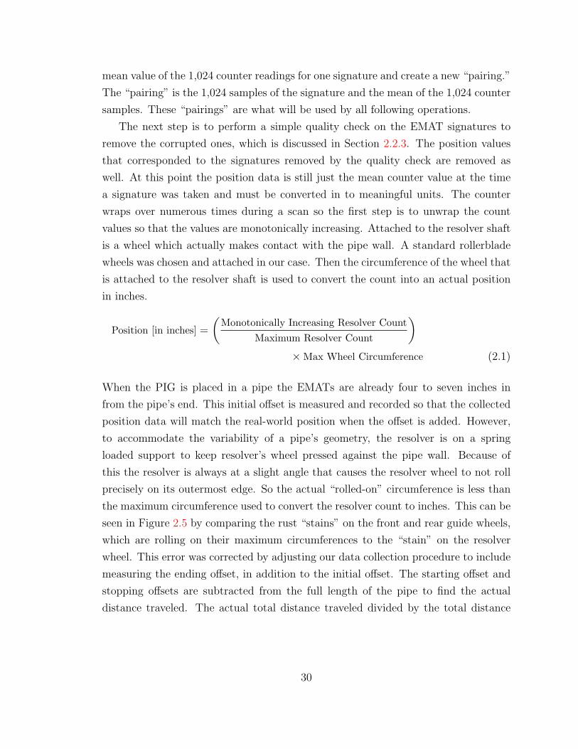
2.5 Resolver, Resolver Wheel, and a Guide Wheel . . . . . . . . . . . . . 32

2.6 Condition of Inside Pipe Wall . . . . . . . . . . . . . . . . . . . . . . 34

2.7 Debris Removal from EMAT under motion . . . . . . . . . . . . . . . 34

2.8 B-scan showing a loss in synchronization . . . . . . . . . . . . . . . . 35

2.9 Examples of Corrupted Signatures . . . . . . . . . . . . . . . . . . . . 37

2.10 Sections of an EMAT Signature used . . . . . . . . . . . . . . . . . . 39

2.11 Signature Section Extracted for DWT . . . . . . . . . . . . . . . . . . 41

2.12 Wavelet Decomposition Levels . . . . . . . . . . . . . . . . . . . . . . 43

2.13 Comparison of the Feature Set with and without the FFT-bin Features 51

x

3.1 PCA Dimensionality Reduction Example . . . . . . . . . . . . . . . . 55

3.2 LDA Dimensionality Reduction Example . . . . . . . . . . . . . . . . 58

3.3 1-D LDA projection versus 1-D PCA projection . . . . . . . . . . . . 59

3.4 LDA+PCA Dimensionality Reduction Example . . . . . . . . . . . . 61

3.5 1-D LDA, PCA, and PCA+LDA Projection Comparison . . . . . . . 62

3.6 Flowchart of the Complete Classification Algorithm . . . . . . . . . . 68

4.1 Layout of Scanlines in Machined Pipe . . . . . . . . . . . . . . . . . . 73

4.2 Synthetic SCC Colonies . . . . . . . . . . . . . . . . . . . . . . . . . 74

4.3 Depth Profiles . . . . . . . . . . . . . . . . . . . . . . . . . . . . . . . 75

4.4 Effect of EMAT width on Flaw width . . . . . . . . . . . . . . . . . . 81

4.5 Difference between Stationary and Moving No-Flaw Signatures . . . . 83

4.6 True Positives, False Positives, and False Negatives for the Original

Features Set with the Original Classifier . . . . . . . . . . . . . . . . 88

4.7 True Positives, False Positives, and False Negatives for the Final Fea-

tures Set with the Original Classifier . . . . . . . . . . . . . . . . . . 88

4.8 True Positives, False Positives, and False Negatives for the Original

Features Set with the Final Classifier . . . . . . . . . . . . . . . . . . 92

4.9 True Positives, False Positives, and False Negatives for the Final Fea-

tures Set with the Final Classifier . . . . . . . . . . . . . . . . . . . . 92

4.10 Comparison of All True Positives, False Positives, and False Negatives 93

4.11 Percentage of Detected Defects by Average Depth . . . . . . . . . . . 94

4.12 Percentage of All Detected Defects by Average Depth Range . . . . . 95

4.13 Mahalanobis Distance Results from Scan of a Decommissioned Pipe . 98

4.14 Corrosion Patches at Arrow 1 . . . . . . . . . . . . . . . . . . . . . . 99


4.16 SCC Colonies at Defect #6 . . . . . . . . . . . . . . . . . . . . . . . 101

4.17 SCCs, Corrosion, and Pitting at Arrow 3 . . . . . . . . . . . . . . . . 102

4.18 SCCs and Corrosion at Arrow 4 . . . . . . . . . . . . . . . . . . . . . 103

4.19 SCC Embedded in a Corrosion Patch at Arrow 5 . . . . . . . . . . . 104

4.20 SCCs at Defect #7 . . . . . . . . . . . . . . . . . . . . . . . . . . . . 105

4.21 First Half of the Corrosion Patches at Arrow 6 . . . . . . . . . . . . . 106

4.22 Last Half of the Corrosion Patches at Arrow 6 . . . . . . . . . . . . . 107

4.23 Corrosion Patch at Arrow 7 . . . . . . . . . . . . . . . . . . . . . . . 107

4.24 SCCs and Pitting at Defect #9 . . . . . . . . . . . . . . . . . . . . . 108

xi


xii

Chapter 1

Introduction

According to the Energy Information Administration’s 2006 Annual Energy Review,

the United States consumed 22.2 trillion cubic feet of natural gas in 2005 and are

projected to have consumed 21.8 trillion cubic feet during 2006 [1]. Natural gas is the

second most common source of energy production in the United States; accounting

for 33.76% of the energy generated in 2005 and is estimated to have fueled the same

amount of generation in 2006. This translate into 18.6 quadrillion Btu of energy in

2005, 19 quadrillion Btu in 2006 [1].

All of this supply at some point must travel through a portion of the interstate

natural gas distribution system. The Office of Pipeline Safety (OPS) 2005 statistics

for natural gas transmission pipelines reports that there is currently 45,998 miles of

steel transmission pipe with diameters over 20 inches but less than 28 inches and

69,332 miles of pipe with diameters over 28 inches, for a total large diameter pipeline

mileage of 115,330 [2]. This is 40.4% of all natural gas transmission pipeline in the U.S.

If you consider the fact that pipes as small as four inches in diameter can be classified

as transmission pipelines it is clear that the majority of all natural gas is distributed

via these large diameter steel pipelines. The 2005 OPS statistics for transmissions

pipelines also show that of the 285,782.3 miles of natural gas transmission pipeline in

the U.S. 72.9% of it is at least 25 years old, 62.4% is at least 35 years old, and 37.2%

is 45 years old or more. A mere 14.7% of all transmission pipeline was constructed

in the last 15 years [2]. Because of the significant role of natural gas in every aspect

of our society, as well as the danger inherent to a combustible gas, it is critical that

the natural gas transmission system be inspected and maintained.

1

The regular inspection and maintenance of pipelines is needed in order to pro-

vide reliable service, protect the public, and lower cost. While there are numerous

challenges to pipeline inspection the most prominent and long running challenge is

access to the pipes. Almost all natural gas pipelines are buried and since rust, cor-

rosion, pitting, and cracking, to name a few defects that are inspected for, can occur

anywhere on the pipe excavation for inspection is not a reasonable option. Which is

why the present advanced pipe inspection tools inspect pipes for internal and external

defects and damage without requiring their excavation. This process of inspecting

the pipe from the inside is known as in-line inspection (ILI). ILI tools are loaded in-

side the pipeline to be inspected and perform non-destructive inspection (NDI) (also

known as non-destructive testing (NDT)). The ILI tools travel inside the pipes and

are generally propelled by the pressurized contents of the pipeline. These ILI tools

are referred to as pipe inspection gauges (PIGs).

While there are several methods which have been and continue to be used for

in-line NDI they all suffer from either the out right inability to detect stress corrosion

cracks (SCCs), or require the use of a coupling liquid that means natural gas distri-

bution must be halted. Because of these issues natural gas pipelines are seldom, if

ever, fully inspected for SCCs.

1.1 Motivation

Only in the last few decades has the desire of the industry to locate stress corrosion

cracks (SCC) developed in to an actual demand and need for SCC detection. This

is due to the shear age of the pipelines along with increased governmental regulation

and oversight plus. Though there are methods for inspecting pipelines for defects and

damage these techniques all suffer from a variety of disadvantages, such as:

• Inability to detect SCC.

• Require a liquid coupling.

• Require cutting or degrading service to the end-user.

• Cannot be performed as an in-line inspection technique.

Of these items obviously the inability to detect SCCs is the biggest problem.

Followed by the need for liquid coupling, which itself causes the operation of the

2

pipeline to be stopped or at the best limited. The current federally congressionally

mandated regulations for the inspection of gas pipelines, 49 CFR 192, which exten-

sively references the American Society of Mechanical Engineers and American Na-

tional Standards Institute standard on “Gas Transmission and Distribution Pipping

Systems” (ASME\ANSI B31.8) and “Managing System Integrity of Gas Pipelines”

(ASME\ANSI B31.8S), list only one method for determining the presence of SCCs,

direct assessment. Direct assessment means excavating a section of pipeline in a lo-

cation favorable to the formation of SCCs, removing any protective coating, cleaning

the exposed pipe, and then visually inspecting the area using magnetic particle in-

spection.∗ So while locations with conditions conducive to the formation of SCCs are

logical places to check for SCCs, inspecting a few feet of a multi-mile pipeline still

leaves many opportunities for disaster. Entire pipelines need to be inspected every

few years to find and mitigate any SCC damage and to monitor for SCC formation.

This has led to research into the use of Electromagnetic Acoustic Transducers

(EMATs) as a means of performing ultrasonic inspection of ferromagnetic materials

(e.g., steel pipes, steel plate, steel beams, etc.) without the need for a liquid couplant.

The focus of the research covered by this thesis is to detect SCCs using EMATs in large

diameter natural gas pipelines, specifically 26-inch and 30-inch diameter pipelines.

1.2 Stress Corrosion Cracks

Stress corrosion cracks are a growing concern due to the age of the nation’s infras-

tructure. The gradual process that leads to the formation of SCCs has meant that

until the last few years SCCs were not a high priority (compared to mechanical dam-

age.) The characteristics of SCCs and their formation contributes to the difficulties

in detecting them. These traits and the method for visually identifying SCCs are

discussed in the following sections.

1.2.1 Source and Characteristics of SCCs

The majority of SCCs result from the same basic process, though as with any natural

phenomena there are exceptions to the “rule”. SCCs are considered to be an envi-

ronmental failure source [3]. The general series of events that lead to the formation

∗This process is also known as a Bell Hole Examination

3

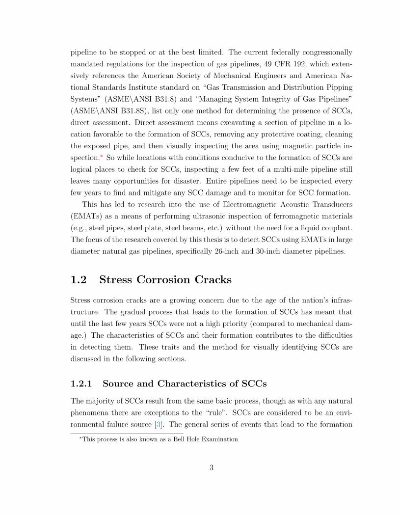
(a) Single SCC (b) SCC Colony

Figure 1.1: Typical SCCs formations. (a) A single SCC. (b) A colony of SCCs. Noticethe “zig-zag” nature of the cracks. This is the primary trait for distinguishing a realSCC from a scratch in the pipe identified using magnetic particle inspection.

of an SCC starts with the penetration of the protective coating (e.g., tar, PVC, etc)

on the pipe. These breaches usually are due to either damage to the coating during

installation, a pressure point from a rock or such cutting through the coating, coating

break down, or a combination of these. Once moisture is under the coating, corro-

sion forms on the pipe wall. A crack (or cracks) form in the corrosion due to cyclic

loading of the pipe. This cyclic loading primarily comes from changes and/or fluctu-

ations in the operating pressure of the pipeline. Extreme temperature variations of

the pipe’s environment can also contribute. The stresses of expansion and contrac-

tion due to temperature changes are far less significant than variations in internal

operating pressure.

SCCs form along the axial direction of pipes almost exclusively. SCCs can occur as

single cracks, Figure 1.1(a), or in colonies, Figure 1.1(b). SCCs can be distinguished

from other line-like marks and/or defects by the piecewise nature that an SCC “line”

exhibits compared to the smooth, continuous “line” of other line-like defects, such a

scratch. This piecewise trait is due to the fact that virtually every SCC of significant

length, i.e. greater than a third of an inch, is composed of SCCs that have grown

together as seen in Figure 1.1, 1.2, and 1.3. There are two types of SCCs, high pH

SCC and near-neutral pH SCC, where pH refers to the pH of the actual pipe surface

environment at the crack location [4].

SCCs occur in all types of metal. The aerospace industry has been particularly

interested in SCC for much longer than the pipeline industry. So while there is much

4

more information and research data available on SCCs in aluminum and other metals

used by the aerospace industry there is a very limited amount of information on SCCs

in pipelines. Due to the rarity of SCC samples available for study the profile of SCCs

with respect to how they penetrate through a pipe wall is not well known. It is known

that SCCs are an inter-granular crack. That is an SCC will usually crack between

the actual grains that form the steel of the pipe.

1.2.2 Visual SCC Identification

There is a technique available that can make SCCs visually detectable, magnetic

particle inspection. Magnetic particle inspection (MPI) uses fine magnetic particles

that are applied to the area to be inspected. There are two types of particles, color

contrast particles visible under normal lighting and fluorescent particles that are only

visible under a black light. Either type of particle can be applied in either a liquid

suspension (wet) or as a dry powder. The mean particle size for the Magnaflux R©†

fluorescent particle is six microns (6µm) and the black color contrast particles are

less than 20 microns (20µm) [6, 7]. Once the area has been “painted” with the

suspension a magnetic field is applied across the site. The magnetic field is created

so that potential defects will be perpendicular or close to perpendicular to the flux

lines. Any “breaks” in the surface of the magnetized object being inspected allow

leakage which draws the magnetic particles in to the “break” [8]. This is more clearly

explained in the following quote from the NDT Resource Center

“A strong magnetic field is established in the pipe wall using either mag-

nets or by injecting electrical current into the steel. Damaged areas of

the pipe can not support as much magnetic flux as undamaged areas so

magnetic flux leaks out of the pipe wall at the damaged areas” [9].

The closer to perpendicular a defect is to the flux lines the stronger the flux leakage

will be and ideally more particles that will be drawn into the defect. The size of a

defect is directly related to the amount of potential flux leakage that could occur due

to the defect. A small crack, even perfectly oriented with the magnetic field, will not

attract as many particles as a larger crack several degrees off of perpendicular with

† These particle sizes are for Magnaflux R© 7HF black color contrast product and Magnaglo R© 14AAqua-Glo fluorescent particles. Magnaflux R© is a company founded by the discoverer of “magneticparticle crack-finding method” [5] and is still a leading producer and distributor of MPI equipmentand supplies today.

5

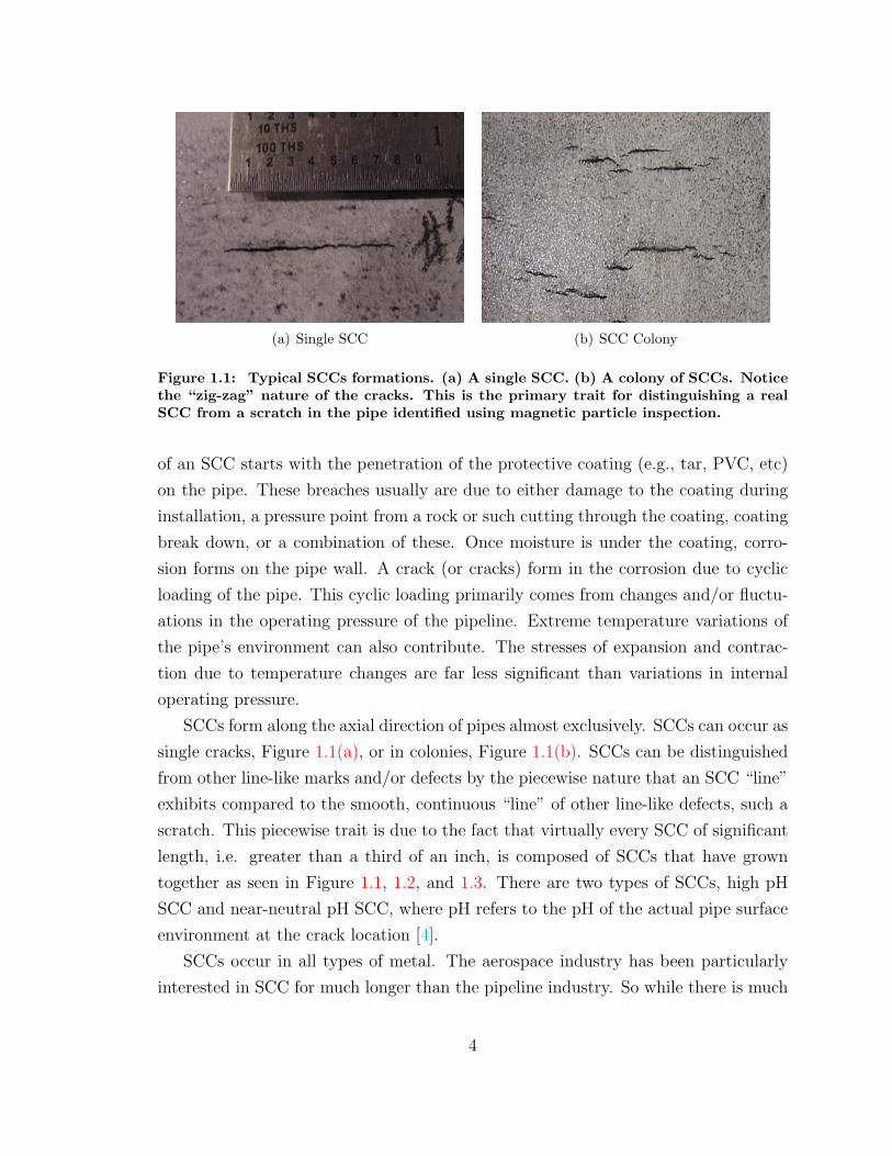
the magnetic field will. If fluorescent magnetic particles are used a black light would

be used at this point in the MPI process to check for any defects in the area coated

with the particle suspension. Figure 1.2 shows an SCC colony identified using liquid

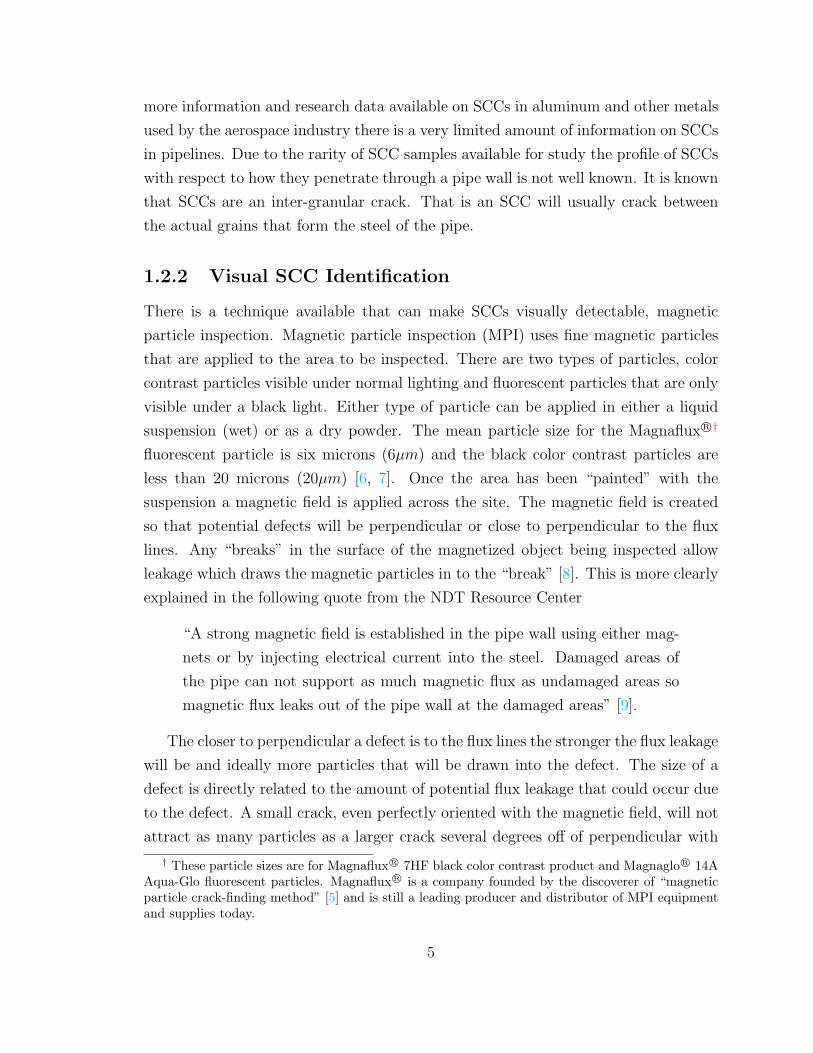
fluorescent MPI. If color contrast particles are used the metal must either be a light

color or a contrasting background applied, such as white paint. Figure 1.3 shows an

SCC colony identified using liquid color contrast MPI. If any defects are located,

measurements are taken from one end of the pipe segment to the beginning of the

defect, from the longitudinal weld to the defect, and the length of the defect. Color

photographs are also taken of the defect. When the inspection of the selected area

is complete the magnetic field is removed and if desired/required the area is rinsed

with water to remove the particles, suspending liquid, and contrast paint if used.

Regardless, of whether the area is rinsed or not the particles do not remain magnetized

and cannot be used to identify defects without re-applying both the magnetic field

and a fresh coat of the liquid suspension.

There are also some major caveats that come with the use of MPI. First, as

is probably apparent at this point, the pipe section must be removed from service,

excavated, and any protective coating stripped from the pipe. Second, scratches,

manufacturing defects, manufacturing handling marks, etc. are also made visible.

This makes it very difficult to identify SCCs that might be “mixed” in with any other

crack-like markings e.g., scratches, manufacturing process marks. Finally, and most

significantly, is that no depth information can be obtained using MPI. While these

problems mean that superficial marks can be misinterpreted as SCCs, the character-

istics of SCCs do help to distinguish SCCs from manufacturing marks and scratches.

The decommissioned pipe sections containing SCCs that were used in the blind

test of our sensor system where all inspected using liquid fluorescent magnetic particle

inspection when the sections were first obtained by the Battelle Pipeline Simulation

Facility (PSF).Since naturally occurring SCC samples are of such rarity, the SCC

sample pipes have been shared with organizations all across the nation. Sometime the

borrowing organization alters the pipe such as by cutting off a section andbackslashor

welding a section on to the SCC pipe. This was the situation with pipe sample

inspected during the most recent blind test of the system. The length of the pipe

was changed while on loan. The length of the pipe is what the defects found during

the original MPI inspection was referenced to. With the particles from that MPI

assessment no longer present, the defect locations could not be confirmed without

6

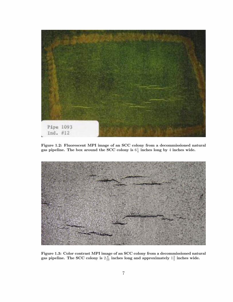
Figure 1.2: Fluorescent MPI image of an SCC colony from a decommissioned naturalgas pipeline. The box around the SCC colony is 6 1

4 inches long by 4 inches wide.

Figure 1.3: Color contrast MPI image of an SCC colony from a decommissioned naturalgas pipeline. The SCC colony is 2 8

10 inches long and approximately 1 25 inches wide.

7

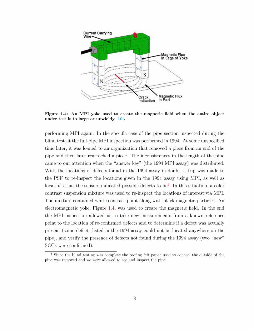
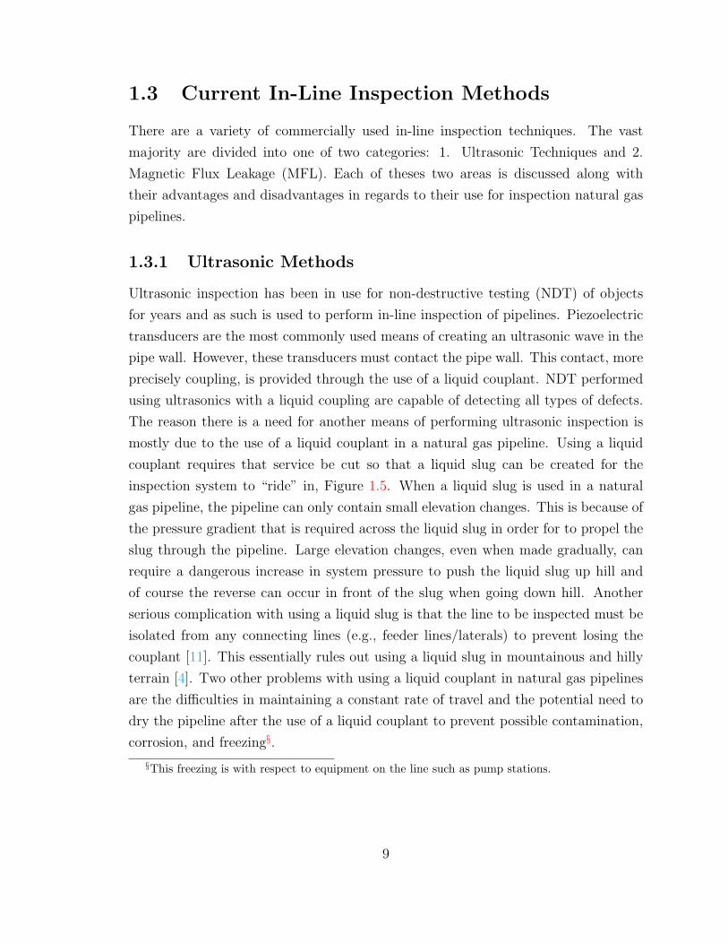
Figure 1.4: An MPI yoke used to create the magnetic field when the entire objectunder test is to large or unwieldy [10].

performing MPI again. In the specific case of the pipe section inspected during the

blind test, it the full-pipe MPI inspection was performed in 1994. At some unspecified

time later, it was loaned to an organization that removed a piece from an end of the

pipe and then later reattached a piece. The inconsistences in the length of the pipe

came to our attention when the “answer key” (the 1994 MPI assay) was distributed.

With the locations of defects found in the 1994 assay in doubt, a trip was made to

the PSF to re-inspect the locations given in the 1994 assay using MPI, as well as

locations that the sensors indicated possible defects to be‡. In this situation, a color

contrast suspension mixture was used to re-inspect the locations of interest via MPI.

The mixture contained white contrast paint along with black magnetic particles. An

electromagnetic yoke, Figure 1.4, was used to create the magnetic field. In the end

the MPI inspection allowed us to take new measurements from a known reference

point to the location of re-confirmed defects and to determine if a defect was actually

present (some defects listed in the 1994 assay could not be located anywhere on the

pipe), and verify the presence of defects not found during the 1994 assay (two “new”

SCCs were confirmed).

‡ Since the blind testing was complete the roofing felt paper used to conceal the outside of thepipe was removed and we were allowed to see and inspect the pipe.

8

1.3 Current In-Line Inspection Methods

There are a variety of commercially used in-line inspection techniques. The vast

majority are divided into one of two categories: 1. Ultrasonic Techniques and 2.

Magnetic Flux Leakage (MFL). Each of theses two areas is discussed along with

their advantages and disadvantages in regards to their use for inspection natural gas

pipelines.

1.3.1 Ultrasonic Methods

Ultrasonic inspection has been in use for non-destructive testing (NDT) of objects

for years and as such is used to perform in-line inspection of pipelines. Piezoelectric

transducers are the most commonly used means of creating an ultrasonic wave in the

pipe wall. However, these transducers must contact the pipe wall. This contact, more

precisely coupling, is provided through the use of a liquid couplant. NDT performed

using ultrasonics with a liquid coupling are capable of detecting all types of defects.

The reason there is a need for another means of performing ultrasonic inspection is

mostly due to the use of a liquid couplant in a natural gas pipeline. Using a liquid

couplant requires that service be cut so that a liquid slug can be created for the

inspection system to “ride” in, Figure 1.5. When a liquid slug is used in a natural

gas pipeline, the pipeline can only contain small elevation changes. This is because of

the pressure gradient that is required across the liquid slug in order for to propel the

slug through the pipeline. Large elevation changes, even when made gradually, can

require a dangerous increase in system pressure to push the liquid slug up hill and

of course the reverse can occur in front of the slug when going down hill. Another

serious complication with using a liquid slug is that the line to be inspected must be

isolated from any connecting lines (e.g., feeder lines/laterals) to prevent losing the

couplant [11]. This essentially rules out using a liquid slug in mountainous and hilly

terrain [4]. Two other problems with using a liquid couplant in natural gas pipelines

are the difficulties in maintaining a constant rate of travel and the potential need to

dry the pipeline after the use of a liquid couplant to prevent possible contamination,

corrosion, and freezing§.

§This freezing is with respect to equipment on the line such as pump stations.

9

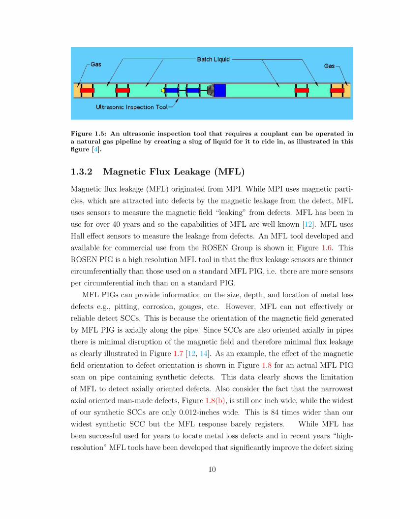
Figure 1.5: An ultrasonic inspection tool that requires a couplant can be operated ina natural gas pipeline by creating a slug of liquid for it to ride in, as illustrated in thisfigure [4].

1.3.2 Magnetic Flux Leakage (MFL)

Magnetic flux leakage (MFL) originated from MPI. While MPI uses magnetic parti-

cles, which are attracted into defects by the magnetic leakage from the defect, MFL

uses sensors to measure the magnetic field “leaking” from defects. MFL has been in

use for over 40 years and so the capabilities of MFL are well known [12]. MFL uses

Hall effect sensors to measure the leakage from defects. An MFL tool developed and

available for commercial use from the ROSEN Group is shown in Figure 1.6. This

ROSEN PIG is a high resolution MFL tool in that the flux leakage sensors are thinner

circumferentially than those used on a standard MFL PIG, i.e. there are more sensors

per circumferential inch than on a standard PIG.

MFL PIGs can provide information on the size, depth, and location of metal loss

defects e.g., pitting, corrosion, gouges, etc. However, MFL can not effectively or

reliable detect SCCs. This is because the orientation of the magnetic field generated

by MFL PIG is axially along the pipe. Since SCCs are also oriented axially in pipes

there is minimal disruption of the magnetic field and therefore minimal flux leakage

as clearly illustrated in Figure 1.7 [12, 14]. As an example, the effect of the magnetic

field orientation to defect orientation is shown in Figure 1.8 for an actual MFL PIG

scan on pipe containing synthetic defects. This data clearly shows the limitation

of MFL to detect axially oriented defects. Also consider the fact that the narrowest

axial oriented man-made defects, Figure 1.8(b), is still one inch wide, while the widest

of our synthetic SCCs are only 0.012-inches wide. This is 84 times wider than our

widest synthetic SCC but the MFL response barely registers. While MFL has

been successful used for years to locate metal loss defects and in recent years “high-

resolution” MFL tools have been developed that significantly improve the defect sizing

10

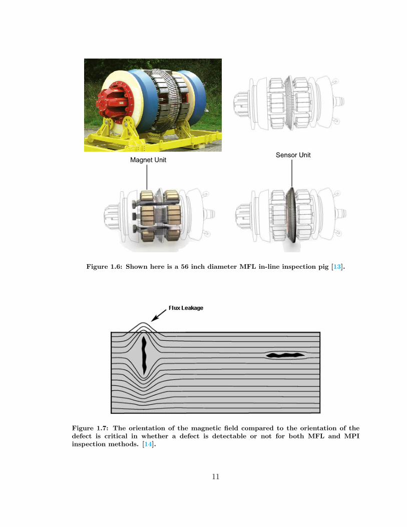
Figure 1.6: Shown here is a 56 inch diameter MFL in-line inspection pig [13].

Figure 1.7: The orientation of the magnetic field compared to the orientation of thedefect is critical in whether a defect is detectable or not for both MFL and MPIinspection methods. [14].

11

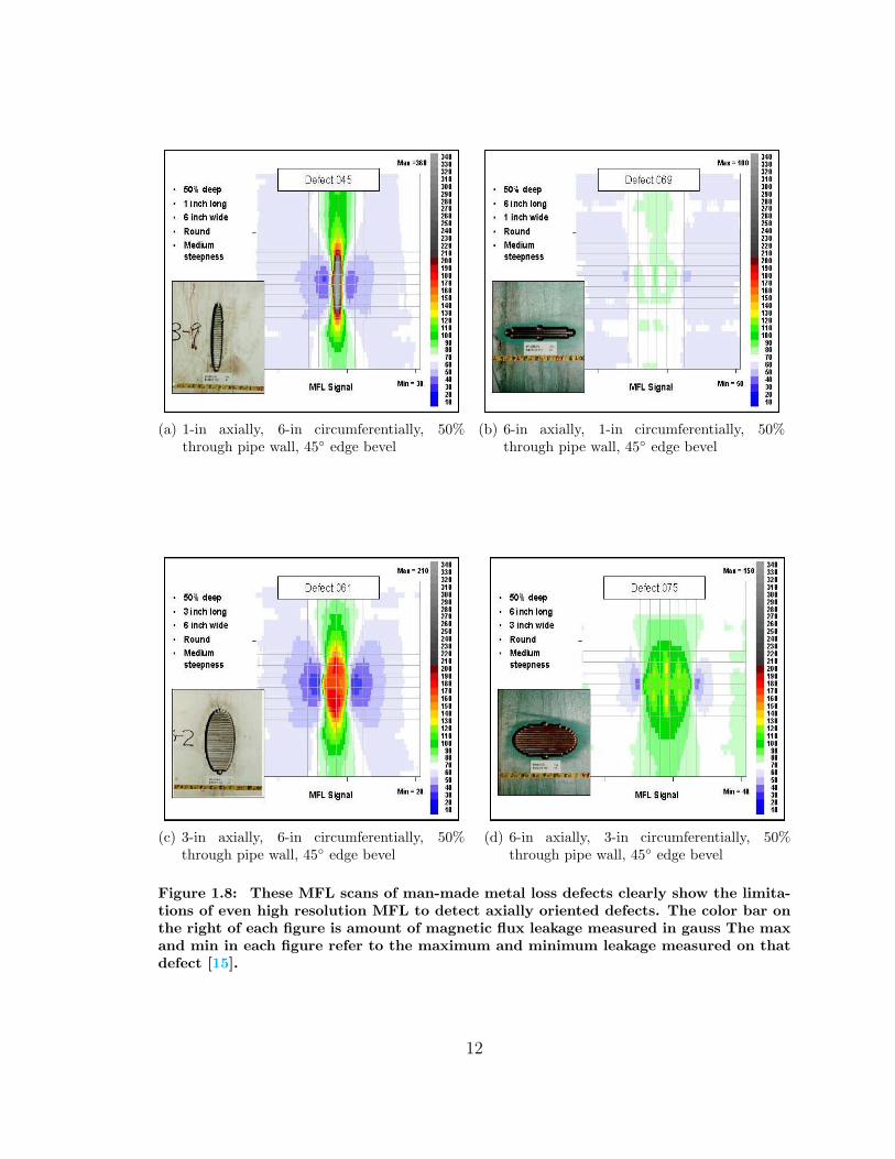
(a) 1-in axially, 6-in circumferentially, 50%through pipe wall, 45◦ edge bevel

(b) 6-in axially, 1-in circumferentially, 50%through pipe wall, 45◦ edge bevel

(c) 3-in axially, 6-in circumferentially, 50%through pipe wall, 45◦ edge bevel

(d) 6-in axially, 3-in circumferentially, 50%through pipe wall, 45◦ edge bevel

Figure 1.8: These MFL scans of man-made metal loss defects clearly show the limita-tions of even high resolution MFL to detect axially oriented defects. The color bar onthe right of each figure is amount of magnetic flux leakage measured in gauss The maxand min in each figure refer to the maximum and minimum leakage measured on thatdefect [15].

12

and location accuracy. Still, even these “high-resolution” MFL systems are still unable

to detect all but the largest and most sever axial defects of any type. There has and

continues to be research toward producing an MFL unit that creates a circumferential

magnetic field. For more information and a detailed discussion of MFL’s capabilities

see [12, 15].

1.4 Electromagnetic Acoustic Transducers

1.4.1 Basic EMAT Properties

Electromagnetic acoustic transducers (EMATs) are used to create an ultrasonic guided

wave without the need of a liquid coupling. This capability is what makes EMATs

stand out as a solution for providing non-contact (couplant-free) ultrasonic inspection

of natural gas pipelines, and can be designed to fit almost any pipe diameter. EMATs

affect the atomic lattice of the material to produce a guided wave. There are a num-

ber of wave types that can be produced with an EMAT depending on the coil and

magnet configuration. Several of the more common types used for material inspection

are the Shear Vertical (SV), Shear Horizontal (SH), Lamba wave, and longitudinal

wave [16, 17, 18]. The ORNL EMATs designed by Dr. Venugopal K. Varma¶ are

specifically tailored to create an SH-wave which propagates circumferentially in the

pipe wall. The ultrasonic wave an EMAT creates in the pipe wall is produced by

the interactions of a static magnetic field from the strong permanent magnets in the

EMAT and the oscillatory electromagnetic field produced when a coil of wire, also

inside the EMAT, is energized. The coil inside the EMAT overlays the permanent

magnets and is excited by a widowed frequency burst. When the coil is excited it

produces eddy currents in the pipe wall, which in the presence of the static mag-

netic field results in the production of an electromagnetic force given by the Lorentz

equation, Eqn. (1.1),

f = J ×Bo (1.1)

where,

¶Dr. Venugopal K. Varma has been the primary investigator of the EMAT natural gas pipelineinspection sensor project at Oak Ridge National Laboratory since its inception in late 2001.

13

f body force per unit volume,

J the induced dynamic current density,

B static magnetic induction.

If the material being inspected is ferromagnetic then there is also a magnetostric-

tive contribution to the body force, f [19]. The ORNL EMATs have been designed so

that the face (the side that goes toward the inner pipe wall) fits the inside curvature

of 30-inch diameter pipes‖ and can also operate in 26-inch diameter pipes. One of

the ORNL EMATs is shown in Figure 1.9 without the protective mylar film used

to cover the epoxy-potted coil and permanent magnets. The mylar film serves as a

replaceable wear surface to protect the EMAT. While the theory and detail opera-

tion and properties of EMATs can be shown and explained with the combination of

calculations and principals used with electromagnetic fields and thinking of the pipe

wall as a waveguide (which it is) with its reflection coefficients and transmission line

properties, these details are beyond the scope of this research, but are available with

in-depth explanations of calculations and principles in [19].

There is one more noteworthy issue specific to the collection of data from pipe

sections regarding the reflection of the guided wave. The issue is that in the sections

of pipe used for testing when the EMATs are with in 12 to 16 inches of the end of the

pipe the ultrasonic waves are reflect off the end. The ends of the pipe are equivalent

to a “wall” placed across the end of the wave guide that is the inner and outer faces

of the pipe wall. This is because the ends of the pipe are junctions between two

transmission mediums with extremely different propagation velocity constants. The

closer the EMATs get to the end the strong the reflected wave strength and the more

acutely corrupted the sampled signals. This means that the data collected close to

the ends of the pipes is unreliable. Fortunately, the end-effect issue is only a concern

in the test pipes, since operational pipelines are continuous welded pipe.

1.4.2 Basic Operation of an EMAT

EMATs can be configured and driven in several ways. There are three “standard”

methods/modes for configuring ultrasonic transducers, which are Pulse-Echo, Pitch-

Catch, and Through-Transmission [20].

‖Pipe diameters are given for the outside diameter, inside diameters vary based on the wallthickness. This variation is not enough to prevent a 30-inch diameter tool from working in any30-inch diameter pipe. I mention this because pipes are listed, classed, and discussed referring tothe outside diameter (ODS) and wall thickness.

14

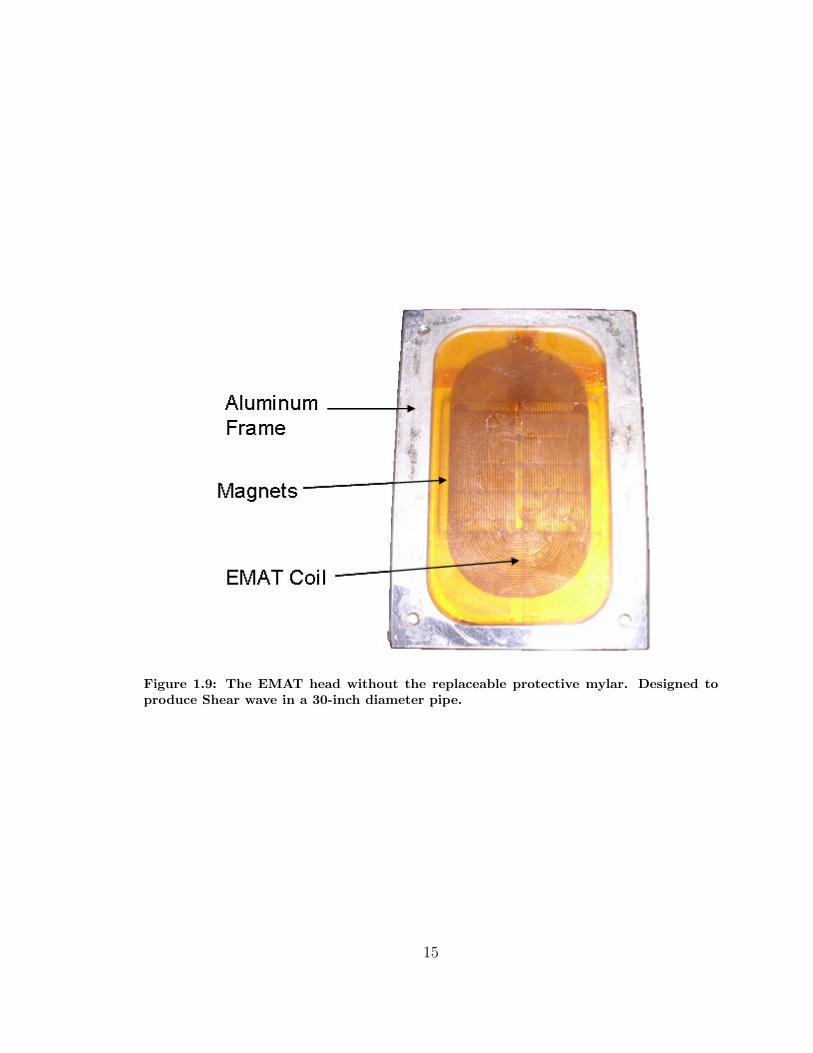
Figure 1.9: The EMAT head without the replaceable protective mylar. Designed toproduce Shear wave in a 30-inch diameter pipe.

15

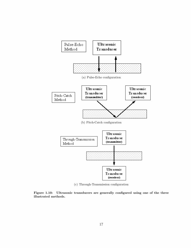
• Pulse-Echo mode uses one transducer to both transmit and receive the signal,

Figure 1.10(a). Pulse-echo is commonly used to inspect planar objects such as

steel plates, semi-conductor wafers, etc. Pulse-echo is problematic for pipeline

inspection because the transducer is moving while the echo is returning from

the outer pipe wall.

• Pitch-Catch mode can be done using one or two transducers. When two trans-

ducers are used one transducer pitches (transmits) the signal and the other

transducer catches (receives) the signal. The transducers do not change func-

tionality i.e. the transmitter is always the transmitter, the receiver is always

the receiver. The pipe’s inner and outer walls function as a wave guide for

the transmitted ultrasonic wave “carrying” it to the receiver, Figure 1.10(b).

The spacing between the two transducers is variable depending on the hardware

used and other user selected traits. It is possible to operate in pitch-catch mode

using a single transducer if the object to be inspected forms a closed path i.e. a

circle. The single transducer transmits the signal, then its functionality swaps

to receiver as the signal circumvents the pipe. However, care must be taken

so that the transducer does not move out of range of the returning wave(s)

(reflected and/or round-trip).

• Through-Transmission mode uses two transducer, one on each side of the object

being inspected, Figure 1.10(c). Through-transmission is not applicable to in-

line pipe inspection since the outside of the pipe is not accessible.

The ORNL EMATs are configured in the pitch-catch mode with an arc length of

approximately 12-inch between the outside edges of the receiver and transmitter

EMATS∗∗. The input signal to the transmitter EMAT is a windowed frequency burst

from the tone-burst card. This frequency burst, or driving frequency, controls which

mode the SH-wave is generated at [16, 19]. The driving frequency is tuned to excite

SH mode 1 (SH1). The frequency to achieve SH1 differs from pipe to pipe and is

dependent upon the wavelength and material velocity. Frequency, wavelength, and

velocity are all related via Eqn. (1.2),

f =v

λ(1.2)

∗∗The arc length is given as an approximate because the EMATS are on spring loaded struts soas to keep the EMATs pressed against the inside pipe wall and therefore vary.

16

(a) Pulse-Echo configuration

(b) Pitch-Catch configuration

(c) Through-Transmission configuration

Figure 1.10: Ultrasonic transducers are generally configured using one of the threeillustrated methods.

17

where,

f frequency,

v velocity of sound in the material,

λ wavelength.

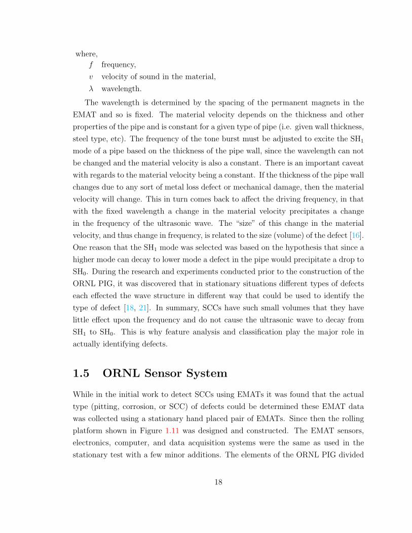
The wavelength is determined by the spacing of the permanent magnets in the

EMAT and so is fixed. The material velocity depends on the thickness and other

properties of the pipe and is constant for a given type of pipe (i.e. given wall thickness,

steel type, etc). The frequency of the tone burst must be adjusted to excite the SH1

mode of a pipe based on the thickness of the pipe wall, since the wavelength can not

be changed and the material velocity is also a constant. There is an important caveat

with regards to the material velocity being a constant. If the thickness of the pipe wall

changes due to any sort of metal loss defect or mechanical damage, then the material

velocity will change. This in turn comes back to affect the driving frequency, in that

with the fixed wavelength a change in the material velocity precipitates a change

in the frequency of the ultrasonic wave. The “size” of this change in the material

velocity, and thus change in frequency, is related to the size (volume) of the defect [16].

One reason that the SH1 mode was selected was based on the hypothesis that since a

higher mode can decay to lower mode a defect in the pipe would precipitate a drop to

SH0. During the research and experiments conducted prior to the construction of the

ORNL PIG, it was discovered that in stationary situations different types of defects

each effected the wave structure in different way that could be used to identify the

type of defect [18, 21]. In summary, SCCs have such small volumes that they have

little effect upon the frequency and do not cause the ultrasonic wave to decay from

SH1 to SH0. This is why feature analysis and classification play the major role in

actually identifying defects.

1.5 ORNL Sensor System

While in the initial work to detect SCCs using EMATs it was found that the actual

type (pitting, corrosion, or SCC) of defects could be determined these EMAT data

was collected using a stationary hand placed pair of EMATs. Since then the rolling

platform shown in Figure 1.11 was designed and constructed. The EMAT sensors,

electronics, computer, and data acquisition systems were the same as used in the

stationary test with a few minor additions. The elements of the ORNL PIG divided

18

into either hardware or software components and are described in the following two

sections.

1.5.1 Hardware

The PIG is a rolling frame designed to fit into 30-inch diameter pipes. It also can be

converted to fit into 26-inch diameter pipes. The frame holds an industrial computer,

an electronics box, a position resolver, and the spring loaded support assembles for

the EMATs. The industrial computer contains dual Intel Xeon processors, a Datel

PCI-417F data acquisition card, and a Matec TB-1000 gated amplifier tone-burst

card. Both the Datel and Matec cards plug in to the PCI bus of the computer. The

Datel card is capable of a sampling at 10 MHz per channel with 14-bit resolution

on each of its four channels [22]. Only two of these channels are used in the system

and so the two channels are sampled using a 5 MHz sampling rate. One samples the

position resolver and the other samples the received signal from the receiver EMAT.

The Matec tone-burst card creates the excitation signal at the driving frequency that

is sent to the transmitting EMAT. The tone-burst card is designed specifically for use

in non-destructive ultrasonic testing. It is capable of producing a gated sinusoid in the

frequency range of 50kHz to 20MHz with a peak output power of 450 Watts at 5 MHz

[23]. The majority of the time we use a driving frequency in the range of 200 KHz to

300 KHz. One of the tone-burst card features is a dedicated “initialization” output.

This output is a scaled down version of the signal sent to the transmitter EMAT.

The “initialization” signal and excitation signal are sent simultaneously allowing the

data acquisition to record during the entire transmit-receive process of the EMATs.

The Matec card also contains a built-in amplifier which the received signal is passed

through after going through the pre-amplifier.

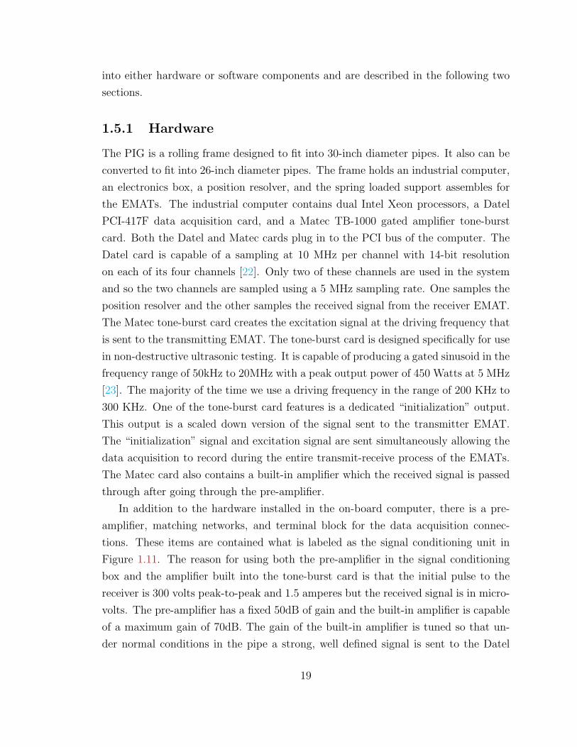
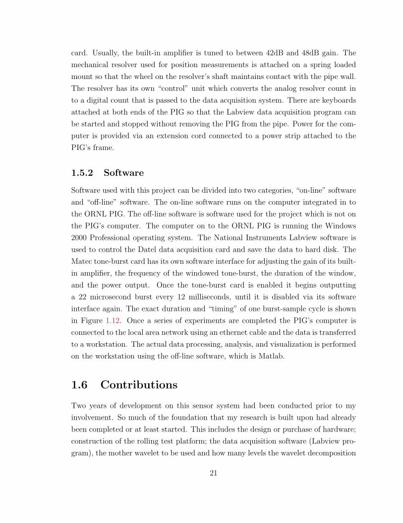
In addition to the hardware installed in the on-board computer, there is a pre-

amplifier, matching networks, and terminal block for the data acquisition connec-

tions. These items are contained what is labeled as the signal conditioning unit in

Figure 1.11. The reason for using both the pre-amplifier in the signal conditioning

box and the amplifier built into the tone-burst card is that the initial pulse to the

receiver is 300 volts peak-to-peak and 1.5 amperes but the received signal is in micro-

volts. The pre-amplifier has a fixed 50dB of gain and the built-in amplifier is capable

of a maximum gain of 70dB. The gain of the built-in amplifier is tuned so that un-

der normal conditions in the pipe a strong, well defined signal is sent to the Datel

19

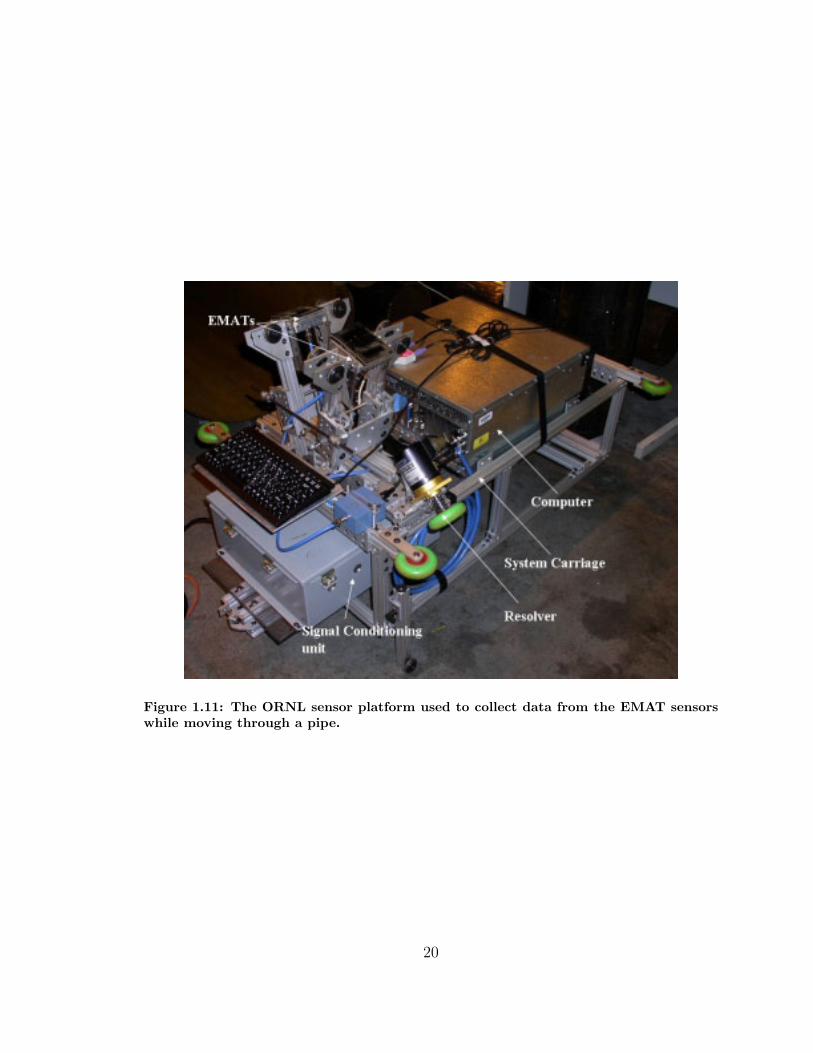
Figure 1.11: The ORNL sensor platform used to collect data from the EMAT sensorswhile moving through a pipe.

20

card. Usually, the built-in amplifier is tuned to between 42dB and 48dB gain. The

mechanical resolver used for position measurements is attached on a spring loaded

mount so that the wheel on the resolver’s shaft maintains contact with the pipe wall.

The resolver has its own “control” unit which converts the analog resolver count in

to a digital count that is passed to the data acquisition system. There are keyboards

attached at both ends of the PIG so that the Labview data acquisition program can

be started and stopped without removing the PIG from the pipe. Power for the com-

puter is provided via an extension cord connected to a power strip attached to the

PIG’s frame.

1.5.2 Software

Software used with this project can be divided into two categories, “on-line” software

and “off-line” software. The on-line software runs on the computer integrated in to

the ORNL PIG. The off-line software is software used for the project which is not on

the PIG’s computer. The computer on to the ORNL PIG is running the Windows

2000 Professional operating system. The National Instruments Labview software is

used to control the Datel data acquisition card and save the data to hard disk. The

Matec tone-burst card has its own software interface for adjusting the gain of its built-

in amplifier, the frequency of the windowed tone-burst, the duration of the window,

and the power output. Once the tone-burst card is enabled it begins outputting

a 22 microsecond burst every 12 milliseconds, until it is disabled via its software

interface again. The exact duration and “timing” of one burst-sample cycle is shown

in Figure 1.12. Once a series of experiments are completed the PIG’s computer is

connected to the local area network using an ethernet cable and the data is transferred

to a workstation. The actual data processing, analysis, and visualization is performed

on the workstation using the off-line software, which is Matlab.

1.6 Contributions

Two years of development on this sensor system had been conducted prior to my

involvement. So much of the foundation that my research is built upon had already

been completed or at least started. This includes the design or purchase of hardware;

construction of the rolling test platform; the data acquisition software (Labview pro-

gram), the mother wavelet to be used and how many levels the wavelet decomposition

21

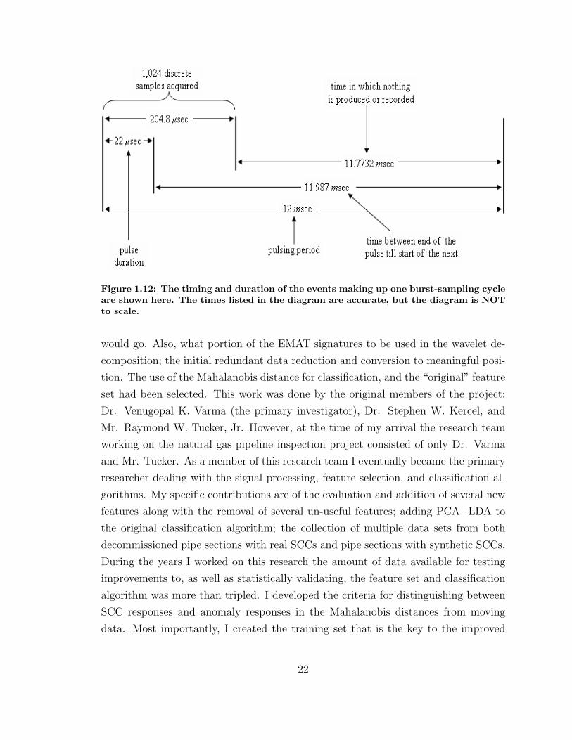
Figure 1.12: The timing and duration of the events making up one burst-sampling cycleare shown here. The times listed in the diagram are accurate, but the diagram is NOTto scale.

would go. Also, what portion of the EMAT signatures to be used in the wavelet de-

composition; the initial redundant data reduction and conversion to meaningful posi-

tion. The use of the Mahalanobis distance for classification, and the “original” feature

set had been selected. This work was done by the original members of the project:

Dr. Venugopal K. Varma (the primary investigator), Dr. Stephen W. Kercel, and

Mr. Raymond W. Tucker, Jr. However, at the time of my arrival the research team

working on the natural gas pipeline inspection project consisted of only Dr. Varma

and Mr. Tucker. As a member of this research team I eventually became the primary

researcher dealing with the signal processing, feature selection, and classification al-

gorithms. My specific contributions are of the evaluation and addition of several new

features along with the removal of several un-useful features; adding PCA+LDA to

the original classification algorithm; the collection of multiple data sets from both

decommissioned pipe sections with real SCCs and pipe sections with synthetic SCCs.

During the years I worked on this research the amount of data available for testing

improvements to, as well as statistically validating, the feature set and classification

algorithm was more than tripled. I developed the criteria for distinguishing between

SCC responses and anomaly responses in the Mahalanobis distances from moving

data. Most importantly, I created the training set that is the key to the improved

22

classification accuracy. The training set contains a group of no-flaw features that are

used to perform the final step of the classification algorithm. This group of no-flaw

features is the first and only group that has successfully worked on multiple scanlines,

on multiple pipes.

1.7 Document Organization

The remainder of this thesis, documents the details of the methods, algorithms, and

validation of the research discussed in this thesis. Chapter 2 presents the prepro-

cessing steps, the feature extraction, the original feature set, and the final feature

set. This is followed by an explanation of the discriminant analysis techniques and

classifier used in either the original classification algorithm, the final classification

algorithm, or both, in Chapter 3. Experimental results from this research are pro-

vided in Chapter 4. These experimental results present the significant improvements

achieved as a result of this research by comparing the results from multiple trials of

multiple test in which the original and final feature sets were used in conjunction with

both the original and final classification algorithms. Finally, we conclude in Chapter 5

with a summary of the achievements as well as the recommendations for future work.

23

Chapter 2

Preprocessing and Feature

Extraction

The data collected from the EMATs and the resolver must undergo several prepro-

cessing steps before it is suitable for use. This is necessary so that the EMAT and

resolver data are uniformly formatted and to eliminate the large amount of duplicate

data collected from the resolver. The resolver data collected is straight forward, how-

ever the EMAT signals are more difficult to understand and so will be explained in

the next section to provide a common baseline for the material on feature extraction

in Section 2.3.

2.1 EMAT Signals

In ultrasonic NDT, the collected data/signals can be represented using a number of

formats specific to the ultrasonic NDT field. There are three defacto standard formats

known as A-scan, B-scan, and C-scan. These formats provide representations that

correlate/orient the signal(s), time, and the position on the scanned object.

An A-scan is the actual received signal. This is commonly described as the RF

signal and is either displayed as received, Figure 2.3, or as a rectified version of the

received signal. The A-scan signals are what are referred to as signatures through out

this thesis. We do not rectify our A-scans, i.e. EMAT signatures, since this would

decrease the information of the signatures and thus the information in the features.

An A-scan connects time (x-axis) to signal amplitude (y-axis). When an ultrasonic

inspection is performed the sound wave travels through the material and is reflected

24

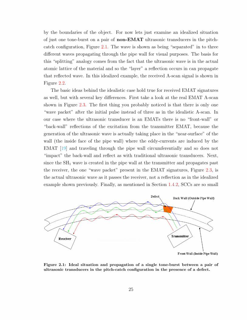
by the boundaries of the object. For now lets just examine an idealized situation

of just one tone-burst on a pair of non-EMAT ultrasonic transducers in the pitch-

catch configuration, Figure 2.1. The wave is shown as being “separated” in to three

different waves propagating through the pipe wall for visual purposes. The basis for

this “splitting” analogy comes from the fact that the ultrasonic wave is in the actual

atomic lattice of the material and so the “layer” a reflection occurs in can propagate

that reflected wave. In this idealized example, the received A-scan signal is shown in

Figure 2.2.

The basic ideas behind the idealistic case hold true for received EMAT signatures

as well, but with several key differences. First take a look at the real EMAT A-scan

shown in Figure 2.3. The first thing you probably noticed is that there is only one

“wave packet” after the initial pulse instead of three as in the idealistic A-scan. In

our case where the ultrasonic transducer is an EMATs there is no “front-wall” or

“back-wall” reflections of the excitation from the transmitter EMAT, because the

generation of the ultrasonic wave is actually taking place in the “near-surface” of the

wall (the inside face of the pipe wall) where the eddy-currents are induced by the

EMAT [19] and traveling through the pipe wall circumferentially and so does not

“impact” the back-wall and reflect as with traditional ultrasonic transducers. Next,

since the SH1 wave is created in the pipe wall at the transmitter and propagates past

the receiver, the one “wave packet” present in the EMAT signatures, Figure 2.3, is

the actual ultrasonic wave as it passes the receiver, not a reflection as in the idealized

example shown previously. Finally, as mentioned in Section 1.4.2, SCCs are so small

Figure 2.1: Ideal situation and propagation of a single tone-burst between a pair ofultrasonic transducers in the pitch-catch configuration in the presence of a defect.

25

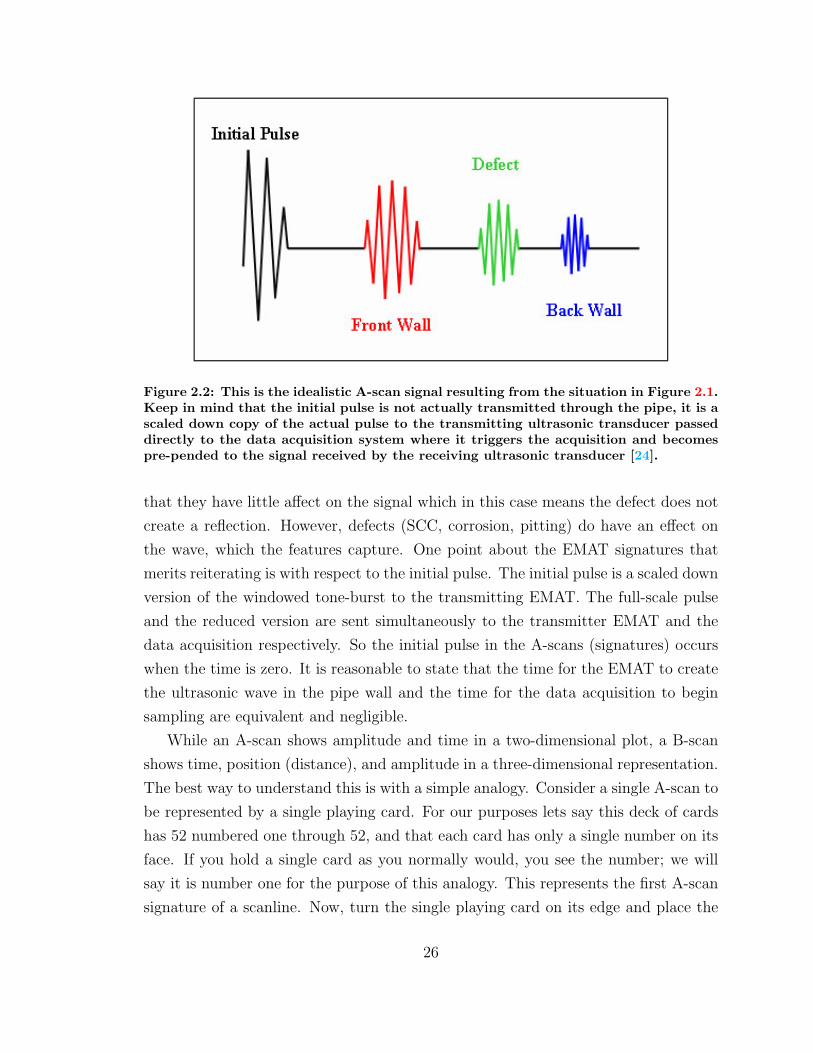
Figure 2.2: This is the idealistic A-scan signal resulting from the situation in Figure 2.1.Keep in mind that the initial pulse is not actually transmitted through the pipe, it is ascaled down copy of the actual pulse to the transmitting ultrasonic transducer passeddirectly to the data acquisition system where it triggers the acquisition and becomespre-pended to the signal received by the receiving ultrasonic transducer [24].

that they have little affect on the signal which in this case means the defect does not

create a reflection. However, defects (SCC, corrosion, pitting) do have an effect on

the wave, which the features capture. One point about the EMAT signatures that

merits reiterating is with respect to the initial pulse. The initial pulse is a scaled down

version of the windowed tone-burst to the transmitting EMAT. The full-scale pulse

and the reduced version are sent simultaneously to the transmitter EMAT and the

data acquisition respectively. So the initial pulse in the A-scans (signatures) occurs

when the time is zero. It is reasonable to state that the time for the EMAT to create

the ultrasonic wave in the pipe wall and the time for the data acquisition to begin

sampling are equivalent and negligible.

While an A-scan shows amplitude and time in a two-dimensional plot, a B-scan

shows time, position (distance), and amplitude in a three-dimensional representation.

The best way to understand this is with a simple analogy. Consider a single A-scan to

be represented by a single playing card. For our purposes lets say this deck of cards

has 52 numbered one through 52, and that each card has only a single number on its

face. If you hold a single card as you normally would, you see the number; we will

say it is number one for the purpose of this analogy. This represents the first A-scan

signature of a scanline. Now, turn the single playing card on its edge and place the

26

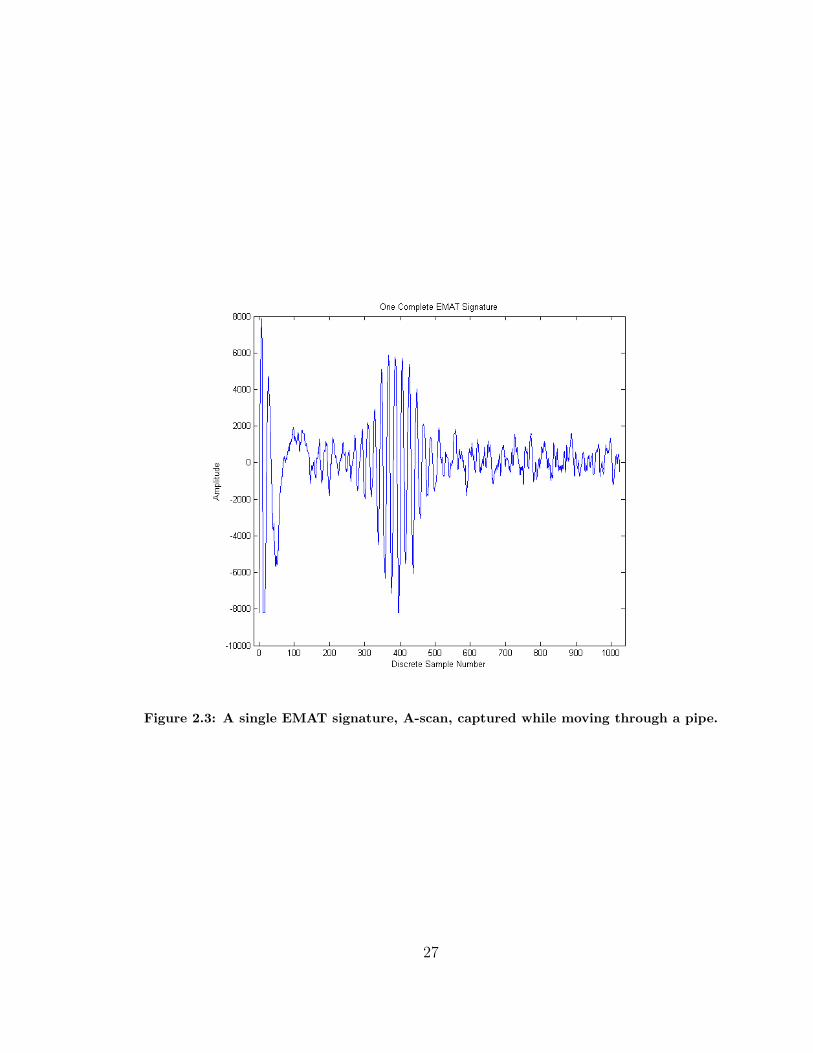
Figure 2.3: A single EMAT signature, A-scan, captured while moving through a pipe.

27

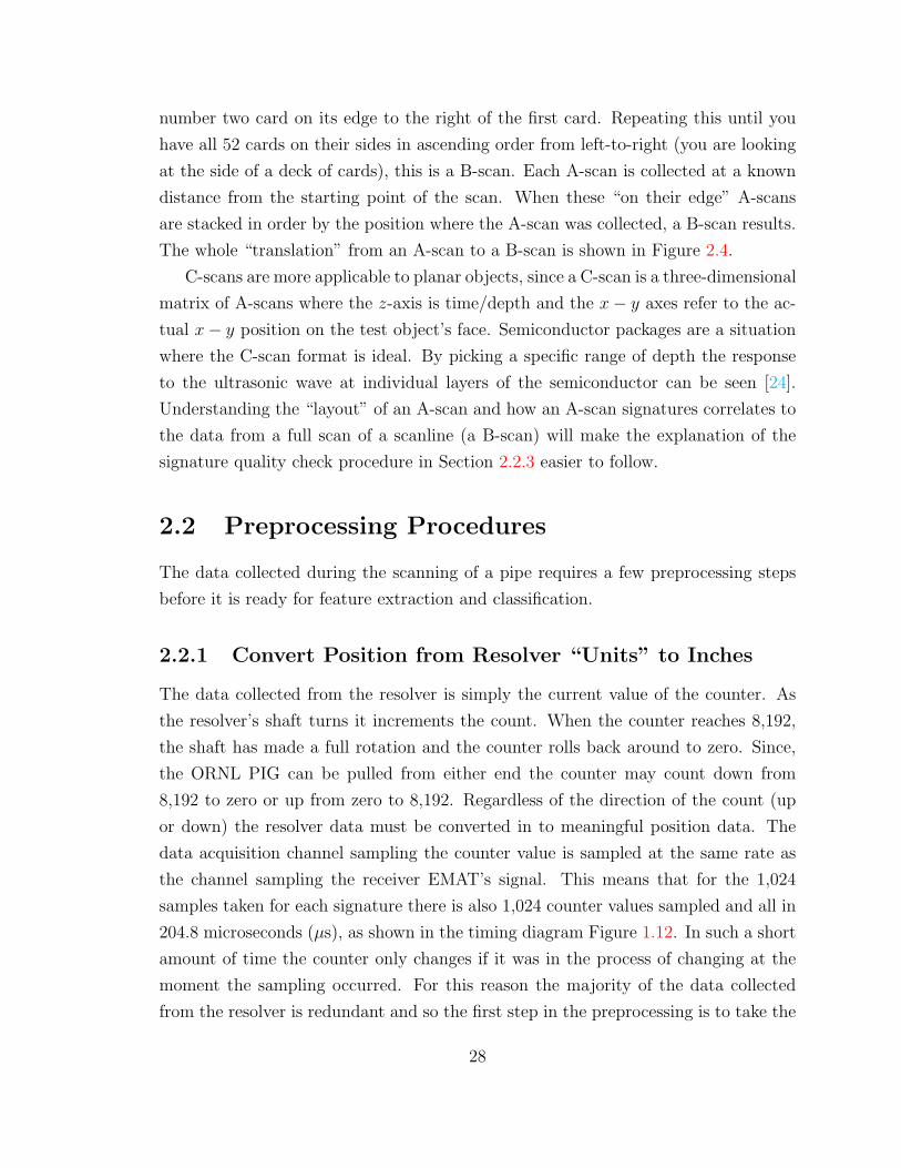
number two card on its edge to the right of the first card. Repeating this until you

have all 52 cards on their sides in ascending order from left-to-right (you are looking

at the side of a deck of cards), this is a B-scan. Each A-scan is collected at a known

distance from the starting point of the scan. When these “on their edge” A-scans

are stacked in order by the position where the A-scan was collected, a B-scan results.

The whole “translation” from an A-scan to a B-scan is shown in Figure 2.4.

C-scans are more applicable to planar objects, since a C-scan is a three-dimensional

matrix of A-scans where the z-axis is time/depth and the x− y axes refer to the ac-

tual x− y position on the test object’s face. Semiconductor packages are a situation

where the C-scan format is ideal. By picking a specific range of depth the response

to the ultrasonic wave at individual layers of the semiconductor can be seen [24].

Understanding the “layout” of an A-scan and how an A-scan signatures correlates to

the data from a full scan of a scanline (a B-scan) will make the explanation of the

signature quality check procedure in Section 2.2.3 easier to follow.

2.2 Preprocessing Procedures

The data collected during the scanning of a pipe requires a few preprocessing steps

before it is ready for feature extraction and classification.

2.2.1 Convert Position from Resolver “Units” to Inches

The data collected from the resolver is simply the current value of the counter. As

the resolver’s shaft turns it increments the count. When the counter reaches 8,192,

the shaft has made a full rotation and the counter rolls back around to zero. Since,

the ORNL PIG can be pulled from either end the counter may count down from

8,192 to zero or up from zero to 8,192. Regardless of the direction of the count (up

or down) the resolver data must be converted in to meaningful position data. The

data acquisition channel sampling the counter value is sampled at the same rate as

the channel sampling the receiver EMAT’s signal. This means that for the 1,024

samples taken for each signature there is also 1,024 counter values sampled and all in

204.8 microseconds (µs), as shown in the timing diagram Figure 1.12. In such a short

amount of time the counter only changes if it was in the process of changing at the

moment the sampling occurred. For this reason the majority of the data collected

from the resolver is redundant and so the first step in the preprocessing is to take the

28

Fig

ure

2.4:

On

the

left

ofth

efigu

reis

asi

ngl

eA

-sca

n,to

the

righ

tof

whic

his

the

sam

eA

-sca

nin

its

B-s

can

form

follow

edby

the

B-s

can

for

the

entire

scan

line

from

whic

hth

eA

-sca

nor

igin

ated

.

29

mean value of the 1,024 counter readings for one signature and create a new “pairing.”

The “pairing” is the 1,024 samples of the signature and the mean of the 1,024 counter

samples. These “pairings” are what will be used by all following operations.

The next step is to perform a simple quality check on the EMAT signatures to

remove the corrupted ones, which is discussed in Section 2.2.3. The position values

that corresponded to the signatures removed by the quality check are removed as

well. At this point the position data is still just the mean counter value at the time

a signature was taken and must be converted in to meaningful units. The counter

wraps over numerous times during a scan so the first step is to unwrap the count

values so that the values are monotonically increasing. Attached to the resolver shaft

is a wheel which actually makes contact with the pipe wall. A standard rollerblade

wheels was chosen and attached in our case. Then the circumference of the wheel that

is attached to the resolver shaft is used to convert the count into an actual position

in inches.

Position [in inches] =

(Monotonically Increasing Resolver Count

Maximum Resolver Count

)×Max Wheel Circumference (2.1)

When the PIG is placed in a pipe the EMATs are already four to seven inches in

from the pipe’s end. This initial offset is measured and recorded so that the collected

position data will match the real-world position when the offset is added. However,

to accommodate the variability of a pipe’s geometry, the resolver is on a spring

loaded support to keep resolver’s wheel pressed against the pipe wall. Because of

this the resolver is always at a slight angle that causes the resolver wheel to not roll

precisely on its outermost edge. So the actual “rolled-on” circumference is less than

the maximum circumference used to convert the resolver count to inches. This can be

seen in Figure 2.5 by comparing the rust “stains” on the front and rear guide wheels,

which are rolling on their maximum circumferences to the “stain” on the resolver

wheel. This error was corrected by adjusting our data collection procedure to include

measuring the ending offset, in addition to the initial offset. The starting offset and

stopping offsets are subtracted from the full length of the pipe to find the actual

distance traveled. The actual total distance traveled divided by the total distance

30

traveled according to the resolver gives a position correction factor, Eqn. (2.2).

Position Correction Factor =Actual Distance Traveled

Resolver’s Distance Traveled(2.2)

The position data is then multiplied by the position correction factor to correct for

the resolver’s wheel rolling on a smaller circumference. Finally, the true position at

which each signature was acquired is found by taking the position data in inches,

multiplied by the position correction factor, plus the starting offset, plus half the

width of the EMAT head, Eqn. (2.3). The reason half the width of the EMAT head

is added is that the center of the resolver shaft and the center of the EMAT heads are

all aligned with one another. So the resolver yields the position of the center of the

EMATs but the starting offset is measured to the outside edge of the EMAT head

not the center.

Corrected Position = Position Data [ininches] × Position Correction Factor

+ Starting Offset + Half the Width of the EMAT Head(2.3)

2.2.2 EMAT Signature Corruption

There are a variety of things that affect the quality of the collected signatures, such as

debris build up between the EMAT head and pipe wall, an out of round pipe, loss of

synchronization in the data acquisition, and so on. All of these things are sources of

signature quality issues and can be placed into one of two categories: coupling issues

or electronics issues. Coupling issues refers to the electromagnetic coupling between

the EMATs and the pipe wall. Put in the simplest terms possible, coupling issues

boil down to “what is going on between the face of the EMAT and the face of the

inner pipe wall.” What follows is a brief explanation of the issues that cause the mass

majority of the corrupted signatures.

Coupling Related:

• When the roundness of a pipe section has become more oval than circular the

gap between the EMAT heads and the pipe wall is no longer uniform. The

active face of the EMAT heads were designed as arcs to fit the curvature of a

30-inch diameter circle. We have seen this cause the gap, which is nominally a

31

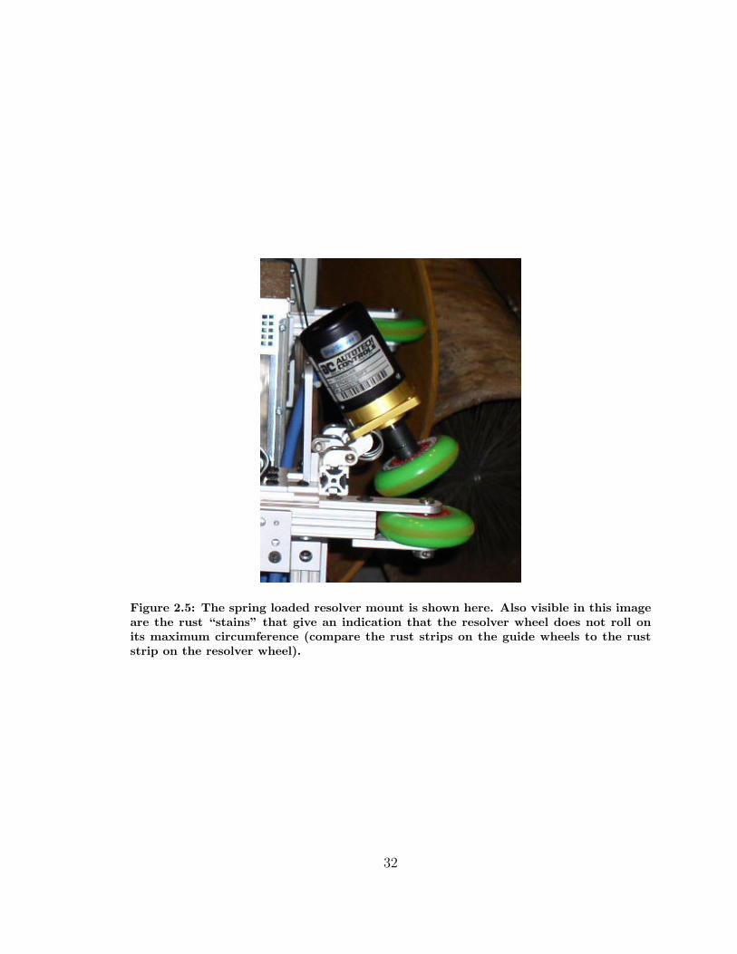
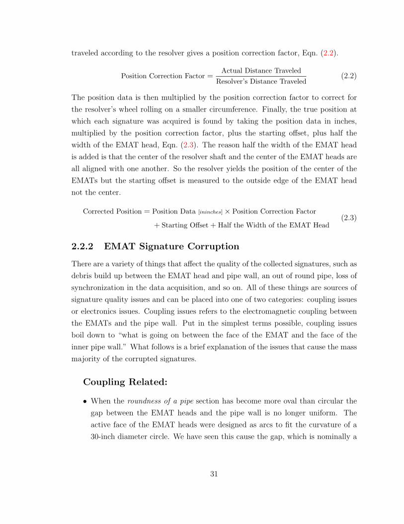
Figure 2.5: The spring loaded resolver mount is shown here. Also visible in this imageare the rust “stains” that give an indication that the resolver wheel does not roll onits maximum circumference (compare the rust strips on the guide wheels to the ruststrip on the resolver wheel).

32

uniform one to three millimeter gap, shrink till the center of the EMAT head is

touching the pipe wall while the outer edges have quarter inch gaps.

• Certain situations and types of debris on the inside pipe wall can cause the

spacing rollers to travel over the debris instead of on the pipe wall. This in-

creases the gap between the EMAT head and the pipe wall which degrades the

coupling and attenuates signal transmission. One example of an attenuating

type of debris are delaminations (flakes) that are not knocked loose from the

wall as the EMATs begin to pass by and so cause a second “air gap.”Figure 2.6

shows a fairly typical inner pipe wall and the rust, scale/flakes, and such that

forms. A situation we encountered where debris effected the spacing rollers was

a large area of caked on dirt left behind by muddy water running through the

test pipe and slowly drying, leaving a continuous patch of dirt firmly adhered.

The spacing rollers were actually rolling on the caked on debris, which absorbed

the signal from the transmitting EMAT as well as increased the gap to the pipe

wall.

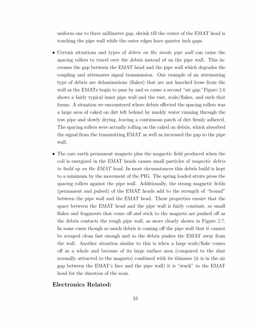
• The rare earth permanent magnets plus the magnetic field produced when the

coil is energized in the EMAT heads causes small particles of magnetic debris

to build up on the EMAT head. In most circumstances this debris build is kept

to a minimum by the movement of the PIG. The spring loaded struts press the

spacing rollers against the pipe wall. Additionally, the strong magnetic fields

(permanent and pulsed) of the EMAT heads add to the strength of “bound”

between the pipe wall and the EMAT head. These properties ensure that the

space between the EMAT head and the pipe wall is fairly constant, so small

flakes and fragments that come off and stick to the magnets are pushed off as

the debris contacts the rough pipe wall, as more clearly shown in Figure 2.7.

In some cases though so much debris is coming off the pipe wall that it cannot

be scraped clean fast enough and so the debris pushes the EMAT away from

the wall. Another situation similar to this is when a large scale/flake comes

off as a whole and because of its large surface area (compared to the dust

normally attracted to the magnets) combined with its thinness (it is in the air

gap between the EMAT’s face and the pipe wall) it is “stuck” to the EMAT

head for the duration of the scan.

Electronics Related:

33

Figure 2.6: This was taken from inside a 30-inch diameter test pipe containingreal SCCs. The image is of an approximately two feet wide three feet tall area ofinside pipe wall.

Figure 2.7: This diagram shows the natural “self-cleaning” action resulting asthe EMAT travels across the rough pipe wall.

34

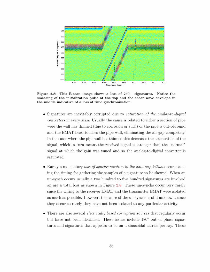
Figure 2.8: This B-scan image shows a loss of 250+ signatures. Notice thesmearing of the initialization pulse at the top and the shear wave envelope inthe middle indicative of a loss of time synchronization.

• Signatures are inevitably corrupted due to saturation of the analog-to-digital

converters in every scan. Usually the cause is related to either a section of pipe

were the wall has thinned (due to corrosion or such) or the pipe is out-of-round

and the EMAT head touches the pipe wall, eliminating the air gap completely.

In the cases where the pipe wall has thinned this decreases the attenuation of the

signal, which in turn means the received signal is stronger than the “normal”

signal at which the gain was tuned and so the analog-to-digital converter is

saturated.

• Rarely a momentary loss of synchronization in the data acquisition occurs caus-

ing the timing for gathering the samples of a signature to be skewed. When an

un-synch occurs usually a two hundred to five hundred signatures are involved

an are a total loss as shown in Figure 2.8. These un-synchs occur very rarely

since the wiring to the receiver EMAT and the transmitter EMAT were isolated

as much as possible. However, the cause of the un-synchs is still unknown, since

they occur so rarely they have not been isolated to any particular activity.

• There are also several electrically based corruption sources that regularly occur

but have not been identified. These issues include 180◦ out of phase signa-

tures and signatures that appears to be on a sinusoidal carrier per say. These

35

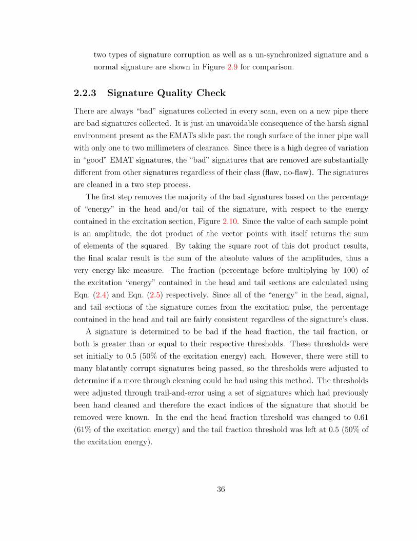
two types of signature corruption as well as a un-synchronized signature and a

normal signature are shown in Figure 2.9 for comparison.

2.2.3 Signature Quality Check

There are always “bad” signatures collected in every scan, even on a new pipe there

are bad signatures collected. It is just an unavoidable consequence of the harsh signal

environment present as the EMATs slide past the rough surface of the inner pipe wall

with only one to two millimeters of clearance. Since there is a high degree of variation

in “good” EMAT signatures, the “bad” signatures that are removed are substantially

different from other signatures regardless of their class (flaw, no-flaw). The signatures

are cleaned in a two step process.

The first step removes the majority of the bad signatures based on the percentage

of “energy” in the head and/or tail of the signature, with respect to the energy

contained in the excitation section, Figure 2.10. Since the value of each sample point

is an amplitude, the dot product of the vector points with itself returns the sum

of elements of the squared. By taking the square root of this dot product results,

the final scalar result is the sum of the absolute values of the amplitudes, thus a

very energy-like measure. The fraction (percentage before multiplying by 100) of

the excitation “energy” contained in the head and tail sections are calculated using

Eqn. (2.4) and Eqn. (2.5) respectively. Since all of the “energy” in the head, signal,

and tail sections of the signature comes from the excitation pulse, the percentage

contained in the head and tail are fairly consistent regardless of the signature’s class.

A signature is determined to be bad if the head fraction, the tail fraction, or

both is greater than or equal to their respective thresholds. These thresholds were

set initially to 0.5 (50% of the excitation energy) each. However, there were still to

many blatantly corrupt signatures being passed, so the thresholds were adjusted to

determine if a more through cleaning could be had using this method. The thresholds

were adjusted through trail-and-error using a set of signatures which had previously

been hand cleaned and therefore the exact indices of the signature that should be

removed were known. In the end the head fraction threshold was changed to 0.61

(61% of the excitation energy) and the tail fraction threshold was left at 0.5 (50% of

the excitation energy).

36

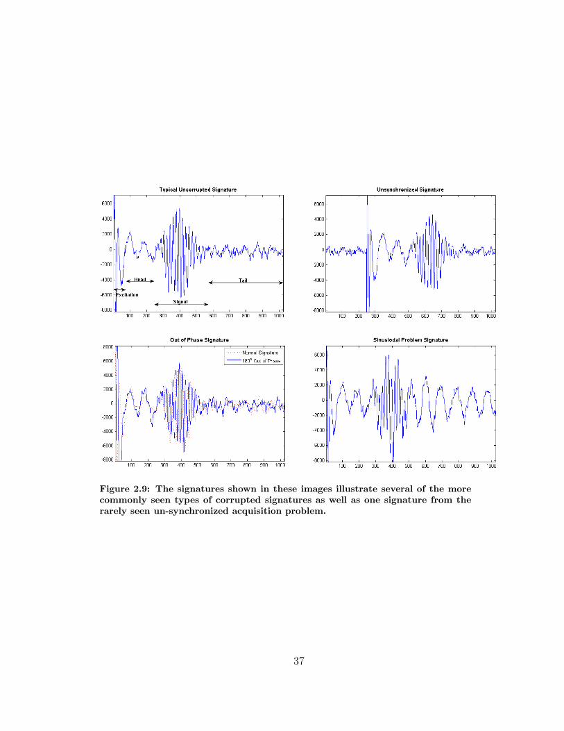
Figure 2.9: The signatures shown in these images illustrate several of the morecommonly seen types of corrupted signatures as well as one signature from therarely seen un-synchronized acquisition problem.

37

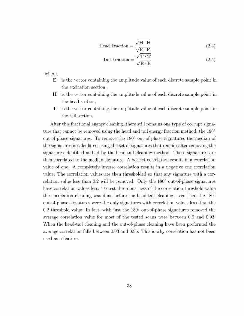
Head Fraction =

√H ·H√E · E

(2.4)

Tail Fraction =

√T ·T√E · E

(2.5)

where,

E is the vector containing the amplitude value of each discrete sample point in

the excitation section,

H is the vector containing the amplitude value of each discrete sample point in

the head section,

T is the vector containing the amplitude value of each discrete sample point in

the tail section.

After this fractional energy cleaning, there still remains one type of corrupt signa-

ture that cannot be removed using the head and tail energy fraction method, the 180◦

out-of-phase signatures. To remove the 180◦ out-of-phase signatures the median of

the signatures is calculated using the set of signatures that remain after removing the

signatures identified as bad by the head-tail cleaning method. These signatures are

then correlated to the median signature. A perfect correlation results in a correlation

value of one. A completely inverse correlation results in a negative one correlation

value. The correlation values are then thresholded so that any signature with a cor-

relation value less than 0.2 will be removed. Only the 180◦ out-of-phase signatures

have correlation values less. To test the robustness of the correlation threshold value

the correlation cleaning was done before the head-tail cleaning, even then the 180◦

out-of-phase signatures were the only signatures with correlation values less than the

0.2 threshold value. In fact, with just the 180◦ out-of-phase signatures removed the

average correlation value for most of the tested scans were between 0.9 and 0.93.

When the head-tail cleaning and the out-of-phase cleaning have been preformed the

average correlation falls between 0.93 and 0.95. This is why correlation has not been

used as a feature.

38

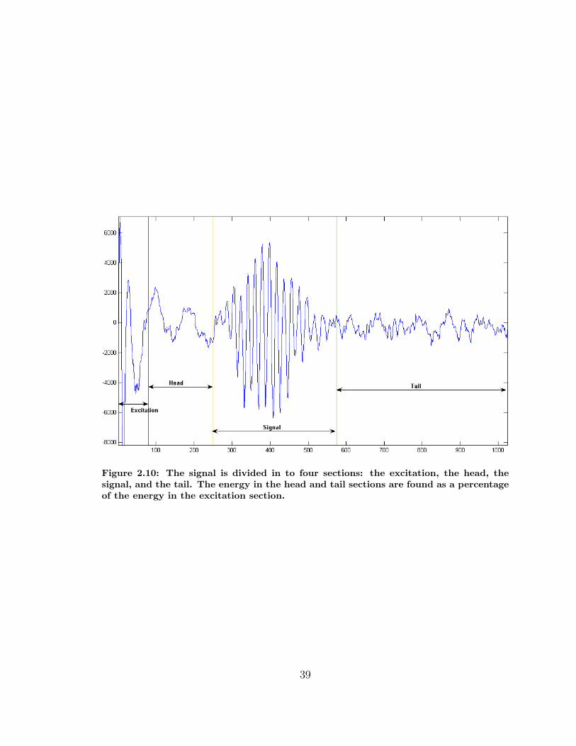
Figure 2.10: The signal is divided in to four sections: the excitation, the head, thesignal, and the tail. The energy in the head and tail sections are found as a percentageof the energy in the excitation section.

39

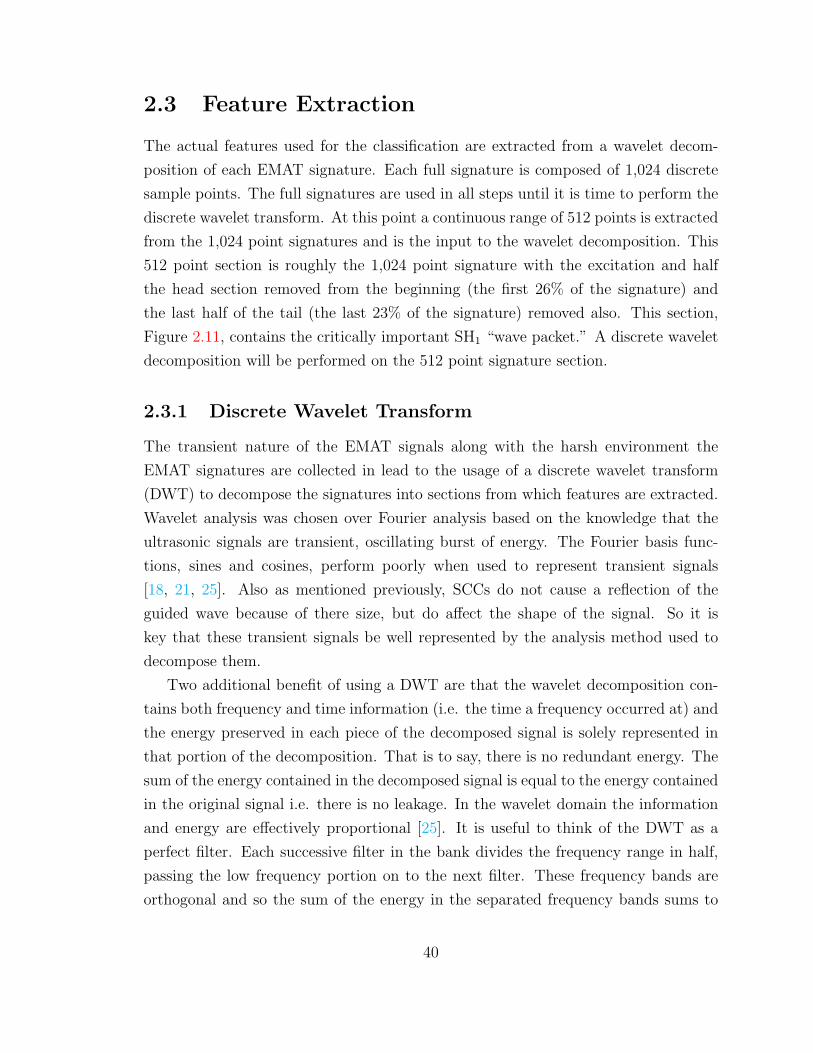
2.3 Feature Extraction

The actual features used for the classification are extracted from a wavelet decom-

position of each EMAT signature. Each full signature is composed of 1,024 discrete

sample points. The full signatures are used in all steps until it is time to perform the

discrete wavelet transform. At this point a continuous range of 512 points is extracted

from the 1,024 point signatures and is the input to the wavelet decomposition. This

512 point section is roughly the 1,024 point signature with the excitation and half

the head section removed from the beginning (the first 26% of the signature) and

the last half of the tail (the last 23% of the signature) removed also. This section,

Figure 2.11, contains the critically important SH1 “wave packet.” A discrete wavelet

decomposition will be performed on the 512 point signature section.

2.3.1 Discrete Wavelet Transform

The transient nature of the EMAT signals along with the harsh environment the

EMAT signatures are collected in lead to the usage of a discrete wavelet transform

(DWT) to decompose the signatures into sections from which features are extracted.

Wavelet analysis was chosen over Fourier analysis based on the knowledge that the

ultrasonic signals are transient, oscillating burst of energy. The Fourier basis func-

tions, sines and cosines, perform poorly when used to represent transient signals

[18, 21, 25]. Also as mentioned previously, SCCs do not cause a reflection of the

guided wave because of there size, but do affect the shape of the signal. So it is

key that these transient signals be well represented by the analysis method used to

decompose them.

Two additional benefit of using a DWT are that the wavelet decomposition con-

tains both frequency and time information (i.e. the time a frequency occurred at) and

the energy preserved in each piece of the decomposed signal is solely represented in

that portion of the decomposition. That is to say, there is no redundant energy. The

sum of the energy contained in the decomposed signal is equal to the energy contained

in the original signal i.e. there is no leakage. In the wavelet domain the information

and energy are effectively proportional [25]. It is useful to think of the DWT as a

perfect filter. Each successive filter in the bank divides the frequency range in half,

passing the low frequency portion on to the next filter. These frequency bands are

orthogonal and so the sum of the energy in the separated frequency bands sums to

40

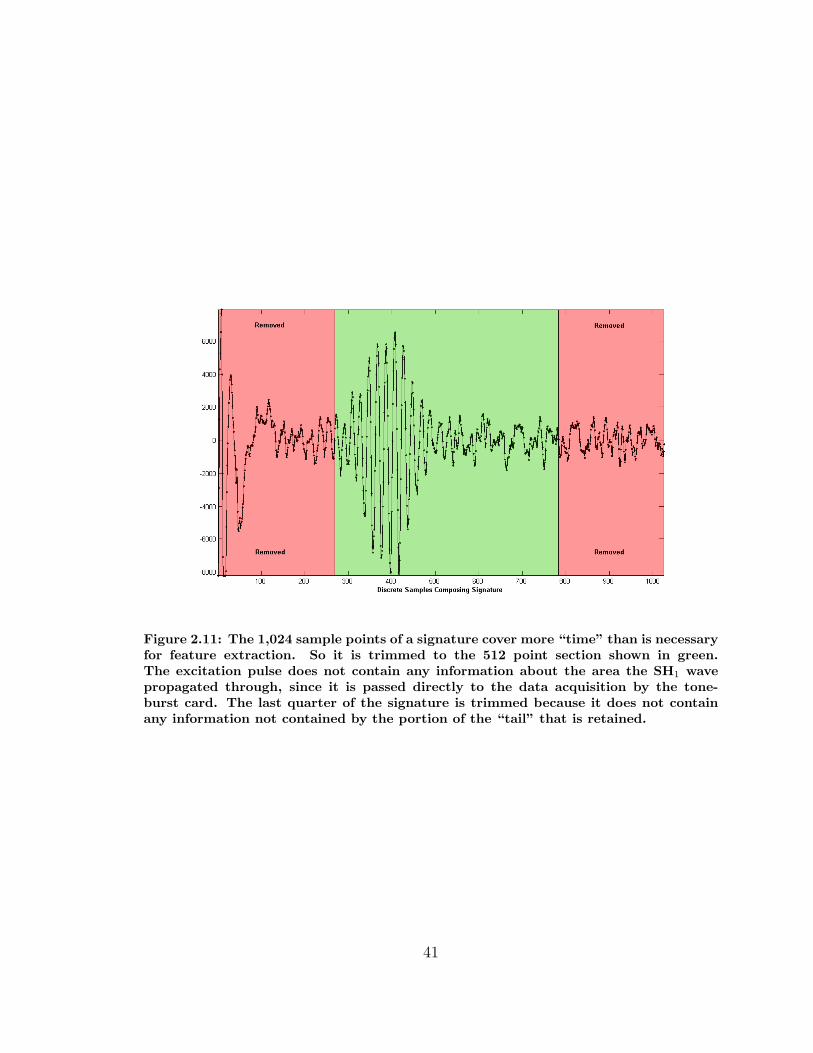
Figure 2.11: The 1,024 sample points of a signature cover more “time” than is necessaryfor feature extraction. So it is trimmed to the 512 point section shown in green.The excitation pulse does not contain any information about the area the SH1 wavepropagated through, since it is passed directly to the data acquisition by the tone-burst card. The last quarter of the signature is trimmed because it does not containany information not contained by the portion of the “tail” that is retained.

41

the total energy contained in the full signal. There is no leakage as long as the basis

function (mother wavelet) is an orthogonal function and the results of the decompo-

sition accurately separates the signal in to sub-signals representing specific frequency

bands [18, 25, 26]. The mother wavelet used for our DWT is a 58 coefficient Symlet

wavelet. Using this mother wavelet each signature is decomposed to a “depth” of four

layers.

The mother wavelet is scaled by a factor of two and time shifted until the “closest”

fit to the signal being transformed is found. When this weighted sum representation

is reached it has effectively divided the input signal’s frequency content in half, as if

it were passed through a perfect lowpass filter. The portion of the signal passed by

this lowpass filter is called the approximation. The portion “rejected” by the lowpass

filter (the high frequency content) is called the detail [18, 26]. An approximation

component plus its matching detail component form one wavelet decomposition level.

The approximate component can then be passed through the same procedure to

from another set of components, as illustrated in Figure 2.12. Each level in the

decomposition divides frequency content of the input signal, the original full signal

or the level above’s approximation component, in half. The mother wavelet is scaled

and shifted progressively, separating out bands of frequency content each time a “fit”

is found. In the end, signal under test can be fully represented by the weighted

sum of these bands [18, 25]. For the remainder of this thesis the “parts” of the DWT

decomposed signal are identified as Approx-4, Detail-4, Detail-3, Detail-2, and Detail-

1, which also corresponds to the wavelet decomposition tree in Figure 2.12. Once the

wavelet decomposition of the data set is completed we are ready to calculate the

features of each decomposed signature.

2.3.2 The Features and Their Calculations

The features are the numerical representation of signature traits that are expected

to allow a classification to be made as to whether the signature was collected over a

defect in the pipe. The selection of features is the most difficult aspect of developing

a classification algorithm. Ideally, potential features are chosen based on either the

recommendations of experts in the application field, the previous research in the field,

or both [27, 28, 29]. When the target application involves prototype sensors, in an

experimental system, in what is essentially an entirely new field of application the

42

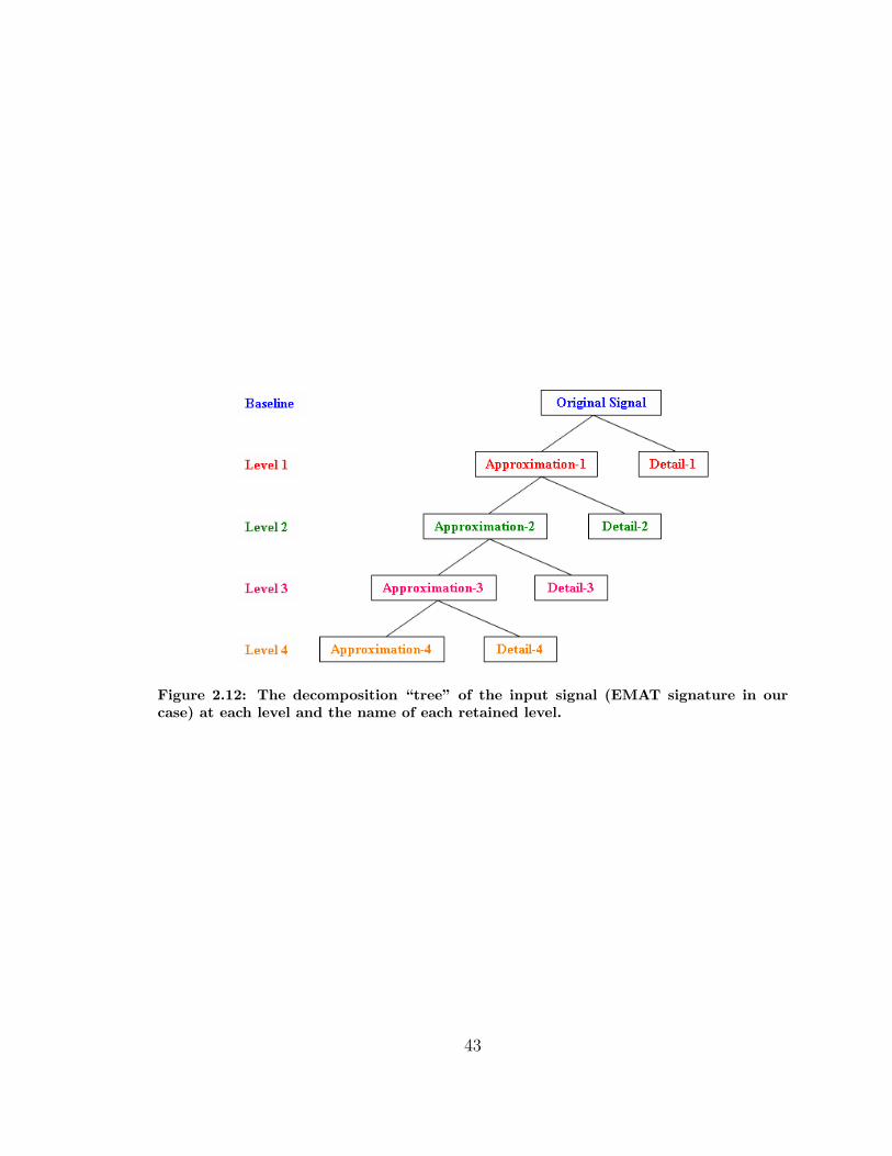
Figure 2.12: The decomposition “tree” of the input signal (EMAT signature in ourcase) at each level and the name of each retained level.

43

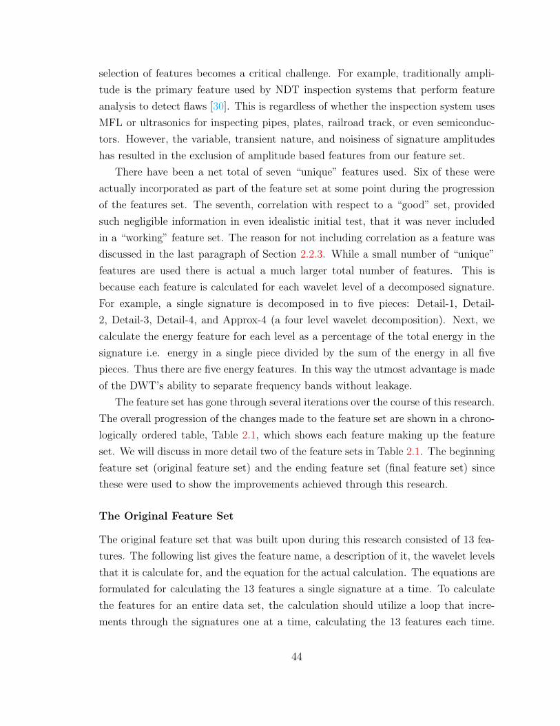
selection of features becomes a critical challenge. For example, traditionally ampli-

tude is the primary feature used by NDT inspection systems that perform feature

analysis to detect flaws [30]. This is regardless of whether the inspection system uses

MFL or ultrasonics for inspecting pipes, plates, railroad track, or even semiconduc-

tors. However, the variable, transient nature, and noisiness of signature amplitudes

has resulted in the exclusion of amplitude based features from our feature set.

There have been a net total of seven “unique” features used. Six of these were

actually incorporated as part of the feature set at some point during the progression

of the features set. The seventh, correlation with respect to a “good” set, provided

such negligible information in even idealistic initial test, that it was never included

in a “working” feature set. The reason for not including correlation as a feature was

discussed in the last paragraph of Section 2.2.3. While a small number of “unique”

features are used there is actual a much larger total number of features. This is

because each feature is calculated for each wavelet level of a decomposed signature.

For example, a single signature is decomposed in to five pieces: Detail-1, Detail-

2, Detail-3, Detail-4, and Approx-4 (a four level wavelet decomposition). Next, we

calculate the energy feature for each level as a percentage of the total energy in the

signature i.e. energy in a single piece divided by the sum of the energy in all five

pieces. Thus there are five energy features. In this way the utmost advantage is made

of the DWT’s ability to separate frequency bands without leakage.

The feature set has gone through several iterations over the course of this research.

The overall progression of the changes made to the feature set are shown in a chrono-

logically ordered table, Table 2.1, which shows each feature making up the feature

set. We will discuss in more detail two of the feature sets in Table 2.1. The beginning

feature set (original feature set) and the ending feature set (final feature set) since

these were used to show the improvements achieved through this research.

The Original Feature Set

The original feature set that was built upon during this research consisted of 13 fea-

tures. The following list gives the feature name, a description of it, the wavelet levels

that it is calculate for, and the equation for the actual calculation. The equations are

formulated for calculating the 13 features a single signature at a time. To calculate

the features for an entire data set, the calculation should utilize a loop that incre-

ments through the signatures one at a time, calculating the 13 features each time.

44

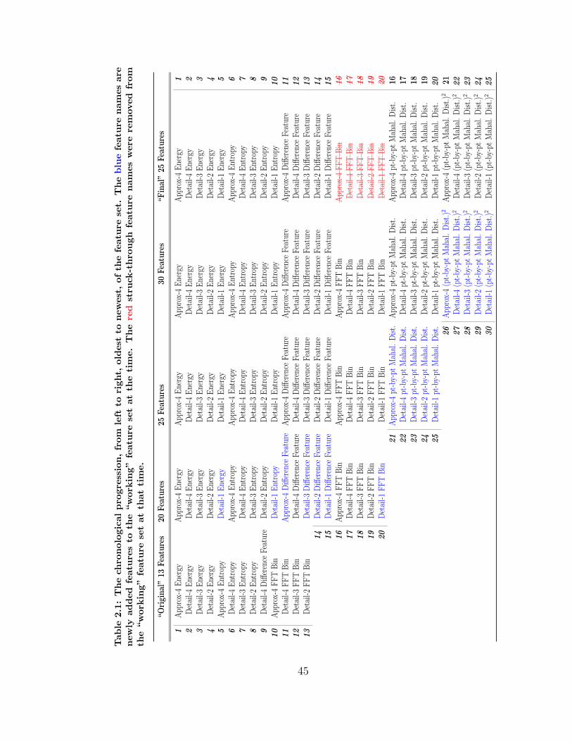
Tab

le2.

1:T

he

chro

nol

ogic

alpro

gres

sion

,fr

omle

ftto

righ

t,ol

des

tto

new

est,

ofth

efe

ature

set.

The

blu

efe

ature

nam

esar

enew

lyad

ded

feat

ure

sto

the

“w

orkin

g”fe

ature

set

atth

etim

e.T

he

red

stru

ck-t

hro

ugh

feat

ure

nam

esw

ere

rem

oved

from

the

“w

orkin

g”fe

ature

set

atth

atti

me.

“Ori

ginal

”13

Fea

ture

s20

Fea

ture

s25

Fea

ture

s30

Fea

ture

s“F

inal

”25

Fea

ture

s

1A

ppro

x-4

Ene

rgy

App

rox-

4E

nerg

yA

ppro

x-4

Ene

rgy

App

rox-

4E

nerg

yA

ppro

x-4

Ene

rgy

12

Det

ail-4

Ene

rgy

Det

ail-4

Ene

rgy

Det

ail-4

Ene

rgy

Det

ail-4

Ene

rgy

Det

ail-4

Ene

rgy

23

Det

ail-3

Ene

rgy

Det

ail-3

Ene

rgy

Det

ail-3

Ene

rgy

Det

ail-3

Ene

rgy

Det

ail-3

Ene

rgy

34

Det

ail-2

Ene

rgy

Det

ail-2

Ene

rgy

Det

ail-2

Ene

rgy

Det

ail-2

Ene

rgy

Det

ail-2

Ene

rgy

45

App

rox-

4E

ntro

pyD

etai

l-1E

nerg

yD

etai

l-1E

nerg

yD

etai

l-1E

nerg

yD

etai

l-1E

nerg

y5

6D

etai

l-4E

ntro

pyA

ppro

x-4

Ent

ropy

App

rox-

4E

ntro

pyA

ppro

x-4

Ent

ropy

App

rox-

4E

ntro

py6

7D

etai

l-3E

ntro

pyD

etai

l-4E

ntro

pyD

etai

l-4E

ntro

pyD

etai

l-4E

ntro

pyD

etai

l-4E

ntro

py7

8D

etai

l-2E

ntro

pyD

etai

l-3E

ntro

pyD

etai

l-3E

ntro

pyD

etai

l-3E

ntro

pyD

etai

l-3E

ntro

py8

9D

etai

l-4D

iffer

ence

Feat

ure

Det

ail-2

Ent

ropy

Det

ail-2

Ent

ropy

Det

ail-2

Ent

ropy

Det

ail-2

Ent

ropy

910

App

rox-

4FFT

Bin

Det

ail-1

Ent

ropy

Det

ail-1

Ent

ropy

Det

ail-1

Ent

ropy

Det

ail-1

Ent

ropy

1011

Det

ail-4

FFT

Bin

App

rox-

4D

iffer

ence

Feat

ure

App

rox-

4D

iffer

ence

Feat

ure

App

rox-

4D

iffer

ence

Feat

ure

App

rox-

4D

iffer

ence

Feat

ure

1112

Det

ail-3

FFT

Bin

Det

ail-4

Diff

eren

ceFe

atur

eD

etai

l-4D

iffer

ence

Feat

ure

Det

ail-4

Diff

eren

ceFe

atur

eD

etai

l-4D

iffer

ence

Feat

ure

1213

Det

ail-2

FFT

Bin

Det

ail-3

Diff

eren

ceFe

atur

eD

etai

l-3D

iffer

ence

Feat

ure

Det

ail-3

Diff

eren

ceFe

atur

eD

etai

l-3D

iffer

ence

Feat

ure

1314

Det

ail-2

Diff

eren

ceFe

atur

eD

etai

l-2D

iffer

ence

Feat

ure

Det

ail-2

Diff

eren

ceFe

atur

eD

etai

l-2D

iffer

ence

Feat

ure

1415

Det

ail-1

Diff

eren

ceFe

atur

eD

etai

l-1D

iffer

ence

Feat

ure

Det

ail-1

Diff

eren

ceFe

atur

eD

etai

l-1D

iffer

ence

Feat

ure

1516

App

rox-

4FFT

Bin

App

rox-

4FFT

Bin

App

rox-

4FFT

Bin

App

rox-

4FFT

Bin

1617

Det

ail-4

FFT

Bin

Det

ail-4

FFT

Bin

Det

ail-4

FFT

Bin

Det

ail-4

FFT

Bin

1718

Det

ail-3

FFT

Bin

Det

ail-3

FFT

Bin

Det

ail-3

FFT

Bin

Det

ail-3

FFT

Bin

1819

Det

ail-2

FFT

Bin

Det

ail-2

FFT

Bin

Det

ail-2

FFT

Bin

Det

ail-2

FFT

Bin

1920

Det

ail-1

FFT

Bin

Det

ail-1

FFT

Bin

Det

ail-1

FFT

Bin

Det

ail-1

FFT

Bin

2021

App

rox-

4pt

-by-

ptM

ahal

.D

ist.

App

rox-

4pt

-by-

ptM

ahal

.D

ist.

App

rox-

4pt

-by-

ptM

ahal

.D

ist.

1 622

Det

a il-4

pt-b

y-pt

Mah

al.

Dis

t.D

etai

l-4pt

-by-

ptM

ahal

.D

ist.

Det

ail-4

pt-b

y-pt

Mah

al.

Dis

t.1 7

23D

eta i

l-3pt

-by-

ptM

ahal

.D

ist.

Det

ail-3

pt-b

y-pt

Mah

al.

Dis

t.D

etai

l-3pt

-by-

ptM

ahal

.D

ist.

1 824

Det

a il-2

pt-b

y-pt

Mah

al.

Dis

t.D

etai

l-2pt

-by-

ptM

ahal

.D

ist.

Det

ail-2

pt-b

y-pt

Mah

al.

Dis

t.1 9

25D

eta i

l-1pt

-by-

ptM

ahal

.D

ist.

Det

ail-1

pt-b

y-pt

Mah

al.

Dis

t.D

etai

l-1pt

-by-

ptM

ahal

.D

ist.

2026

App

rox-

4(p

t-by

-pt

Mah

al.

Dis

t.)2

App

rox-

4(p

t-by

-pt

Mah

al.

Dis

t.)2

2 127

Det

a il-4

(pt-

by-p

tM

ahal

.D

ist.

)2D

etai

l-4(p

t-by

-pt

Mah

al.

Dis

t.)2

2228

Det

a il-3

(pt-

by-p

tM

ahal

.D

ist.

)2D

etai

l-3(p

t-by

-pt

Mah

al.

Dis

t.)2

2329

Det

a il-2

(pt-

by-p

tM

ahal

.D

ist.

)2D

etai

l-2(p

t-by

-pt

Mah

al.

Dis

t.)2

2430

Det

a il-1

(pt-

by-p

tM

ahal

.D

ist.

)2D

etai

l-1(p

t-by

-pt

Mah

al.

Dis

t.)2

25

45

The variables and notation used in the equations are described the first time they are

used in an equation.

Energy – The fraction of the full signal’s energy contained in the Approx-4, Detail-4,

Detail-3, and Detail-2 wavelet levels.

Fi =

∑nk=1 S2

j(k)∑Np=1 S2(p)

(2.6)

where,

Fi vector holding the 13 features of the ith signature (F is the feature matrix),

S vector holding the wavelet decomposition of a signature,

Sj portion of the wavelet decomposition that make up the jth wavelet level,

j is the wavelet level, where Detail-1 = 1, Detail-2 = 2, ..., Approx-4 = 5,

k is an index to the elements of wavelet level j,

n number of discrete points in the jth wavelet level (e.g., for Detail-1 n = 256,

Detail-4 n = 32),

p is an index to the elements of the entire decomposed signature,

N is the total number discrete points in the decomposed signature.

Entropy – The fraction of the total Shannon’s entropy of the signal that is contained

in the Approx-4, Detail-4, Detail-3, and Detail-2 wavelet levels.

Fi = −n∑

k=1

Sj(k) ln (Sj(k)) (2.7)

Difference Measure – the mean Detail-4 of a set of “no-flaw” signatures (the ex-

pected Detail-4 signal) which is subtracted from the Detail-4 of the signature

under test. This produces a vector containing the difference between each data

point. The dot product is taken of the difference vector with itself and this

scalar value is the difference measure.

Fi =(Sj − µj

)T (Sj − µj

)(2.8)

where,

µj is the mean of the wavelet level j portion of the no-flaw signatures.

FFT Bin Number – A fast Fourier transform (FFT) is performed on Approx-4,

Detail-4, Detail-3, and Detail-2 using a step size that equals the number of

46

data points used to represent the level under test, e.g., the FFT step size for

Approx-4 and Detail-4 would be 32. Each of the points in the step is a bin;

the bin with the maximum value from the FFT is the scalar that becomes the

feature. For example, say the seventh discrete point of an FFT results had the

largest value for the Detail-4 of some signature X, then signature X ’s Detail-4

FFT Bin feature value would be seven.

Y(h) =N∑

g=1

Sj(k) exp

(−2πi

N(k − 1)(h− 1)

)Fi = h, when max {Y(h) } (2.9)

where,

Y the fast Fourier transform of S,

h index to the elements of Y.

For the calculating features of the original feature set the no-flaw signatures were

signatures taken while the pig was stationary in the pipe. An area in the pipe that

was free of flaws (SCCs, pitting, corrosion, etc) based on the SCC assay, which was

done upon receipt of the pipe by the Battelle PSF, and a visual inspection at the time

of our inspection. While we have found these initial assays to be a good indication of

were SCCs maybe on the decommissioned pipes, the assay was often done a decade

or more before we inspected the pipe. In several cases, SCCs were found that were

not on the original assay and in one case the pipe was cut and re-welded causing the

point from which the measurements of the axial distances to all the SCCs listed in

the assay to be “lost.”∗ Usually these “pauses” were either at the beginning of the

scan after the data acquisition was started but prior to the wench being engaged or at

the end of the scan once the wench was stopped but before the data acquisition was

halted. There were occasionally intentional pauses in the midst of a scan as well in

order to collect a stationary set of signatures. A copy of the signatures making up a

stationary section would be made and processed using the same procedures as used on

the entire scan, as described previously in Section 2.2 and 2.3. The Detail-4s of all the

“no-flaw” set (stationary signature set) were averaged to form an expected Detail-4

∗The cutting and re-welding were done to the sample pipe while it was on loan from PSF toanother facility and the “changes” were not documented beyond stating a section was removed andreattached. When we were inspecting this pipe as part of a blind test we measured the pipe andfound it was a foot shorter than the documentation said it was.

47

signal. The issue with this original technique for forming the “no-flaw” set was that

there was no real assurance that the signatures in the stationary ranges were flaw free.

It was later found that the assumption that the locations were the no-flaw signatures

were collected were truly defect free was erroneous. Additionally, the fact that the

“good” set was composed of stationary signatures while the signatures under test

were collected while moving seriously skewed the classification results toward almost

all signatures producing defect responses. However, these problems are addressed by

the features and a more method for calculating the feature that is more representative

of the data being classified.

The Final Feature Set

The features belong to the final feature set are listed along with the feature name, a

description of the feature, the wavelet levels that it is calculate for, and the equation

for the actual calculation. The equations are formulated for calculating the 13 features

a single signature at a time. To calculate the features for an entire data set, the

calculation should utilize a loop that increments through the signatures one at a

time, calculating the 13 features each time. The variables and notation used in the

equations are described the first time they are used in an equation.

Energy – The fraction of the full signal’s energy contained in the Approx-4, Detail-4,

Detail-3, Detail-2, and Detail-1 wavelet levels.

Fi =

∑nk=1 S2

j(k)∑Np=1 S2(p)

(2.10)

where,

Fi vector holding the 13 features of the ith signature (F is the feature matrix),

S vector holding the wavelet decomposition of a signature,

Sj portion of the wavelet decomposition that make up the jth wavelet level,

j is the wavelet level, where Detail-1 = 1, Detail-2 = 2, ..., Approx-4 = 5,

k is an index to the elements of wavelet level j,

n number of discrete points in the jth wavelet level (e.g., for Detail-1 n = 256,

Detail-4 n = 32),

p is an index to the elements of the entire decomposed signature,

N is the total number discrete points in the decomposed signature.

48

Entropy – The entropy (Shannon’s entropy) that is contained in the Approx-4,

Detail-4, Detail-3, Detail-2, and Detail-1 wavelet levels.

Fi = −n∑

k=1

Sj(k) ln (Sj(k)) (2.11)

Difference Measure – An average Approx-4, Detail-4, Detail-3, Detail-2, and Detail-

1 is calculated from the no-flaw signatures of the training set. These “expected”

signals are subtracted from their matching wavelet level in the signature under

test. This produces a vector containing the difference between each data point,

one per wavelet level. The dot product is taken of each difference vector with

itself and this scalar value is the difference measure for that particular wavelet

level.

Fi =(Sj − µj

)T (Sj − µj

)(2.12)

where,

µj is the mean of the wavelet level j portion of the no-flaw signatures.

Point-by-Point MD – Each discrete point of a wavelet level is treated as if it were

an actual feature unto itself, hence point-by-point. The Mahalanobis distance

is calculated using the corresponding wavelet level of the no-flaw signatures as

the source of the covariance matrix and the mean vector. The point-by-point

Mahalanobis distance results in a scalar that represents how closely the wavelet

level under test matches the known no-flaw signatures, while still allowing the

inherent variance in each wavelet level of the known no-flaw signatures. This is

calculated for the Approx-4, Detail-4, Detail-3, Detail-2, and Detail-1 levels.

Fi = (Sj − µj)T Σ−1

j (Sj − µj) (2.13)

This equations show the point-by-point Mahalanobis distance expanded so that the

point-by-point calculation is shown.

Fi =[(

Sj(1)− µj(1)),(Sj(2)− µj(2)

), · · ·

(Sj(n)− µj(n)

)]·

Σ−1j ·

(Sj(1)− µj(1)

)(Sj(2)− µj(2)

)...(

Sj(n)− µj(n))

(2.14)

49

where,

Σj is the covariance matrix of the training set’s wavelet level j no-flaw signatures.

(Point-by-Point MD)2 the value from calculating the point-by-point Mahalanobis

distance feature for Approx-4, Detail-4, Detail-3, Detail-2, and Detail-1 is squared.

The FFT-bin features were removed because they provided little to no classifica-

tion benefits. In fact the only difference between the original feature set with and

without the FFT-bin features was a small DC offset. The Mahalanobis distances

shown in Figure 2.13, show the Mahalanobis distance resulting from classifying the

same data set, using the same classification technique, and the same “good” set. The

only difference is that the FFT-bin features were removed from the feature set before

classification in first case, Figure 2.13(top), and with them still included in the fea-

ture set for the second case, Figure 2.13(middle). Finally, the results from the two

cases are overlaid to show the negligible DC offset that is the only contribution of the

FFT-bin features, Figure 2.13(bottom).

The point-by-point Mahalanobis distance features were added so that if a defect

causes a discernible change only in a particular frequency band or two this useful

information will be represented in the feature set. By using the no-flaw signatures

from the training set along with the Mahalanobis distance the variations due to sliding

through the pipe. Along this same line of thinking, all of the wavelet levels that

were not calculated for a feature were added (e.g., Detail-1 energy, Detail-1 entropy,

etc.). This way since it is unclear yet how different types of defects (i.e. single SCC,

corrosion, pitting, an SCC colony) affect the ultrasonic signal.

50

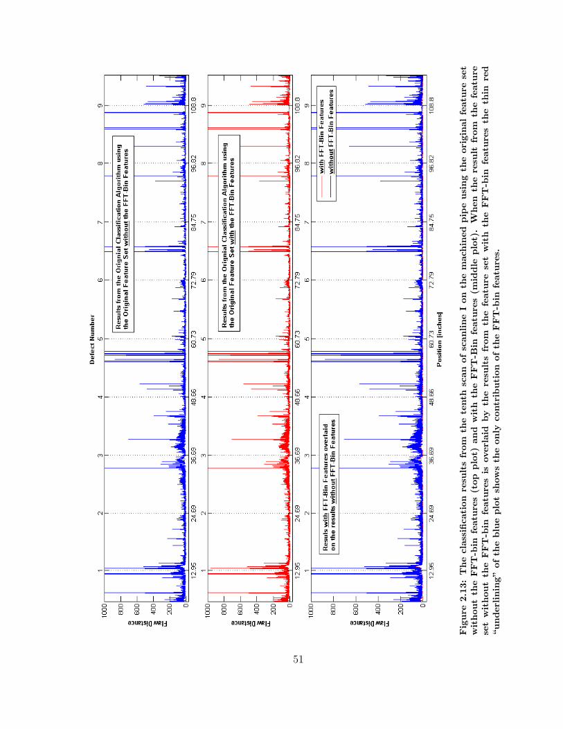
Fig

ure

2.13

:T

he

clas

sifica

tion

resu

lts

from

the

tenth

scan

ofsc

anline

Ion

the

mac

hin

edpip

eusi

ng

the

orig

inal

feat

ure

set

withou

tth

eFFT

-bin

feat

ure

s(t

opplo

t)an

dw

ith

the

FFT

-Bin

feat

ure

s(m

iddle

plo

t).

When

the

resu

ltfr

omth

efe

ature

set

wit

hou

tth

eFFT

-bin

feat

ure

sis

over

laid

by

the

resu

lts

from

the

feat

ure

set

with

the

FFT

-bin

feat

ure

sth

eth

inre

d“under

linin

g”of

the

blu

eplo

tsh

ows

the

only

contr

ibuti

onof

the

FFT

-bin

feat

ure

s.

51

Chapter 3

Pattern Recognition and

Classification

Now, that signatures have been pre-processed, the blatantly corrupt signatures re-

moved, the 512 point range extracted and decomposed via the DWT, and the features

extracted from the decomposition; things are ready for the classification algorithm.

To avoid confusion this chapter begins with brief explanations of the individual algo-

rithms used to develop what will be referred to as the final classification algorithm

from here on. This is followed by a description of the final classification algorithm as

a whole.

3.1 Dimensionality Reduction

The features on there own are unable to clearly identify known SCCs (synthetic or

natural) without causing a large number of false defect identifications (i.e. false

positives). Dimensionality reduction plays a critical roll in our ability to identify

SCCs in pipes. Dimensionality reduction techniques are separated into two groups:

supervised techniques such as linear discriminant analysis (LDA), and unsupervised

techniques like principal component analysis (PCA).

3.1.1 Principal Component Analysis (PCA)

Principal component analysis (PCA) is a beneficial discriminant analysis technique

that, in simplest of terms, seeks to project a set of features into the most efficient

52

space possible while preserving the variance of the data set [27]. This is regardless of

the effect upon the discernibility between classes. PCA provides the ability to reduce

the redundancy of the data by identifying dimensions containing little variance. The

components that contribute little to the total variance of the data set are essentially

stochastic noise, so PCA is useful for removing stochastic noise from the data. PCA is

capable of projecting a n-dimensional feature space to a d -dimensional feature space,

where d < n. Overall, PCA seeks a projection that optimize the feature space such

that the maximum amount of variance is retained, were the variance is regarded as

the information content, while minimizing the mean-square error [27, 31, 32].

To derive a projection using PCA it is important to recognize that a vector of

weights is sought that will minimize the mean-square error, while at the same time

maximizing the in-feature variance. The mean of each feature needs to be zero so for

a n×x data set, where n is the number of dimensions (features) and x is the number

of samples, a mean vector is formed with the mean of each dimension. The mean

vector is then subtracted from each n-dimension sample i.e. the mean feature value is

subtracted from the “matching” dimension’s elements. With the mean removed the

covariance matrix is calculated for the data set. The covariance matrix’s eigenvalues

and eigenvectors are calculated. Each eigenvalue has an associated eigenvector. The

eigenvectors are sorted so that their associated eigenvalues are largest to smallest. The

largest eigenvalue corresponds to the eigenvector that is the principal component i.e.

contains the greatest variance/information. The dimensionality is reduced by keeping

only the features necessary to retain 90 to 98 percent of the total variance contained in

the complete feature set. The percentage of information is calculated using Eq. (3.1)

in which the eigenvalues are summed beginning with the largest value and continuing

in descending order until the desired amount of information is retained. Whether

the percentage of retained variance is between 90% and 98% or something different

entirely is up to the system designer.

Percent Information Retained =λ1 + λ2 + · · ·+ λn∑n

i=1 λi

(3.1)

where,

λi is the ith largest eigenvalue.

The eigenvalues that are not needed to reach the desired percentage are discarded

along with their associated eigenvectors. In a two-dimensional data set the smallest,

53

non-trivial, mean-square error is obtained when the data is projected on to a line

that passes through the mean of the entire data set [27, 31]. The direction of this

line is in the direction of the eigenvector that minimizes the mean-square error. The

eigenvector(s) that will provide these traits are the largest eigenvalues of the data set’s

covariance matrix. The eigenvalues provide a scalar representation of the variance in

a single feature/dimension. Using just the set of eigenvectors corresponding to the

eigenvalues retained, a projection matrix is formed. Since the features are the rows

and the samples are the columns in the data matrix the projection matrix must be

transposed before it is multiplied by the data matrix, as shown in Eq. (3.2).

Y = E T

set ·X (3.2)

where,

Y the projected data set matrix

Eset the matrix formed by the set of eigenvectors retained

X the original mean-removed data set matrix

As a simplistic example a data sets containing two classes represented by two

features is shown in Figure 3.1(a), after the full data set was normalized so that each

feature has a mean of zero and unit standard deviation. This is done so that mere

scaling does not allow a feature to become dominant during the analysis. While the

two classes are obviously easily separated by a line with only a marginal number of

points being miss-classified it is the effect of reducing the dimensionality from two

dimensions to one using PCA that is important here. In Figure 3.1(b), the first and

second principal components (PCs) are plotted indicating the line the data would

be projected to when either the first or second PC is used. Figure 3.1(c) show a

histogram of the number of samples located in the same spots when all the samples

were projected to one dimension using the primary PC. Figure 3.1(d) is the histogram

when all the samples are projected onto the secondary PC.

3.1.2 Linear Discriminant Analysis (LDA)

Linear Discriminant Analysis (LDA), also known as the Fischer Linear Discriminant

technique is another method for projecting data to a lower dimensionality. When

LDA is used to project data with more than two classes it is also occasionally re-

ferred to as Multiple Discriminant Analysis (MDA) [27]. PCA and LDA both seek

54

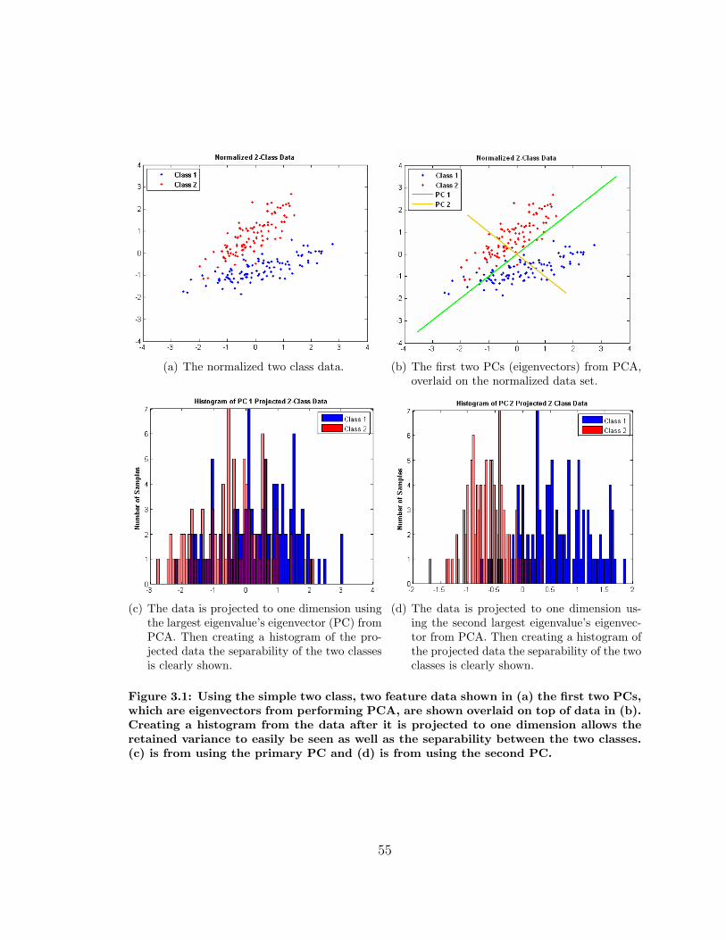
(a) The normalized two class data. (b) The first two PCs (eigenvectors) from PCA,overlaid on the normalized data set.

(c) The data is projected to one dimension usingthe largest eigenvalue’s eigenvector (PC) fromPCA. Then creating a histogram of the pro-jected data the separability of the two classesis clearly shown.

(d) The data is projected to one dimension us-ing the second largest eigenvalue’s eigenvec-tor from PCA. Then creating a histogram ofthe projected data the separability of the twoclasses is clearly shown.

Figure 3.1: Using the simple two class, two feature data shown in (a) the first two PCs,which are eigenvectors from performing PCA, are shown overlaid on top of data in (b).Creating a histogram from the data after it is projected to one dimension allows theretained variance to easily be seen as well as the separability between the two classes.(c) is from using the primary PC and (d) is from using the second PC.

55

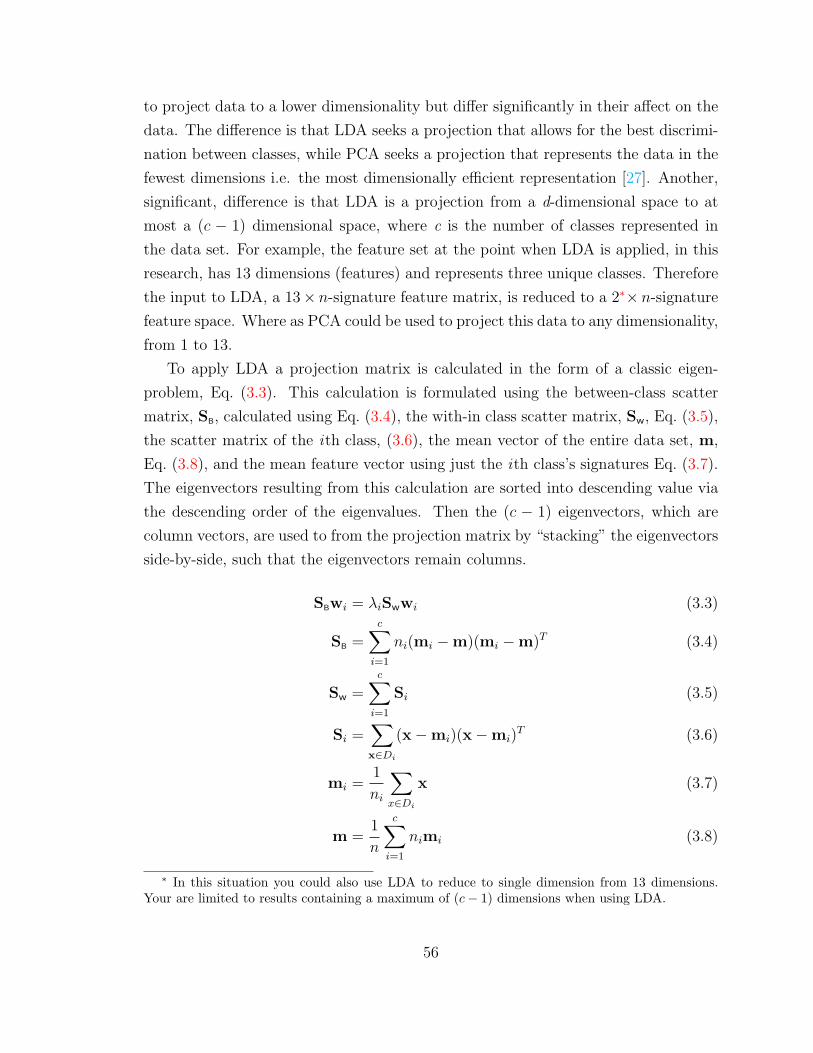
to project data to a lower dimensionality but differ significantly in their affect on the

data. The difference is that LDA seeks a projection that allows for the best discrimi-

nation between classes, while PCA seeks a projection that represents the data in the

fewest dimensions i.e. the most dimensionally efficient representation [27]. Another,

significant, difference is that LDA is a projection from a d-dimensional space to at

most a (c − 1) dimensional space, where c is the number of classes represented in

the data set. For example, the feature set at the point when LDA is applied, in this

research, has 13 dimensions (features) and represents three unique classes. Therefore

the input to LDA, a 13× n-signature feature matrix, is reduced to a 2∗× n-signature

feature space. Where as PCA could be used to project this data to any dimensionality,

from 1 to 13.

To apply LDA a projection matrix is calculated in the form of a classic eigen-

problem, Eq. (3.3). This calculation is formulated using the between-class scatter

matrix, SB, calculated using Eq. (3.4), the with-in class scatter matrix, Sw, Eq. (3.5),

the scatter matrix of the ith class, (3.6), the mean vector of the entire data set, m,

Eq. (3.8), and the mean feature vector using just the ith class’s signatures Eq. (3.7).

The eigenvectors resulting from this calculation are sorted into descending value via

the descending order of the eigenvalues. Then the (c − 1) eigenvectors, which are

column vectors, are used to from the projection matrix by “stacking” the eigenvectors

side-by-side, such that the eigenvectors remain columns.

SBwi = λiSwwi (3.3)

SB =c∑

i=1

ni(mi −m)(mi −m)T (3.4)

Sw =c∑

i=1

Si (3.5)

Si =∑x∈Di

(x−mi)(x−mi)T (3.6)

mi =1

ni

∑x∈Di

x (3.7)

m =1

n

c∑i=1

nimi (3.8)

∗ In this situation you could also use LDA to reduce to single dimension from 13 dimensions.Your are limited to results containing a maximum of (c− 1) dimensions when using LDA.

56

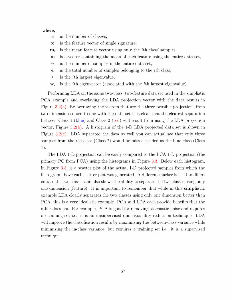
where,

c is the number of classes,

x is the feature vector of single signature,

mi is the mean feature vector using only the ith class’ samples,

m is a vector containing the mean of each feature using the entire data set,

n is the number of samples in the entire data set,

ni is the total number of samples belonging to the ith class,

λi is the ith largest eigenvalue,

wi is the ith eigenvector (associated with the ith largest eigenvalue).

Performing LDA on the same two-class, two-feature data set used in the simplistic

PCA example and overlaying the LDA projection vector with the data results in

Figure 3.2(a). By overlaying the vectors that are the three possible projections from

two dimensions down to one with the data set it is clear that the clearest separation

between Class 1 (blue) and Class 2 (red) will result from using the LDA projection

vector, Figure 3.2(b). A histogram of the 1-D LDA projected data set is shown in

Figure 3.2(c). LDA separated the data so well you can actual see that only three

samples from the red class (Class 2) would be miss-classified as the blue class (Class

1).

The LDA 1-D projection can be easily compared to the PCA 1-D projection (the

primary PC from PCA) using the histograms in Figure 3.3. Below each histogram,

in Figure 3.3, is a scatter plot of the actual 1-D projected samples from which the

histogram above each scatter plot was generated. A different marker is used to differ-

entiate the two classes and also shows the ability to separate the two classes using only

one dimension (feature). It is important to remember that while in this simplistic

example LDA clearly separates the two classes using only one dimension better than

PCA; this is a very idealistic example. PCA and LDA each provide benefits that the

other does not. For example, PCA is good for removing stochastic noise and requires

no training set i.e. it is an unsupervised dimensionality reduction technique. LDA

will improve the classification results by maximizing the between-class variance while

minimizing the in-class variance, but requires a training set i.e. it is a supervised

technique.

57

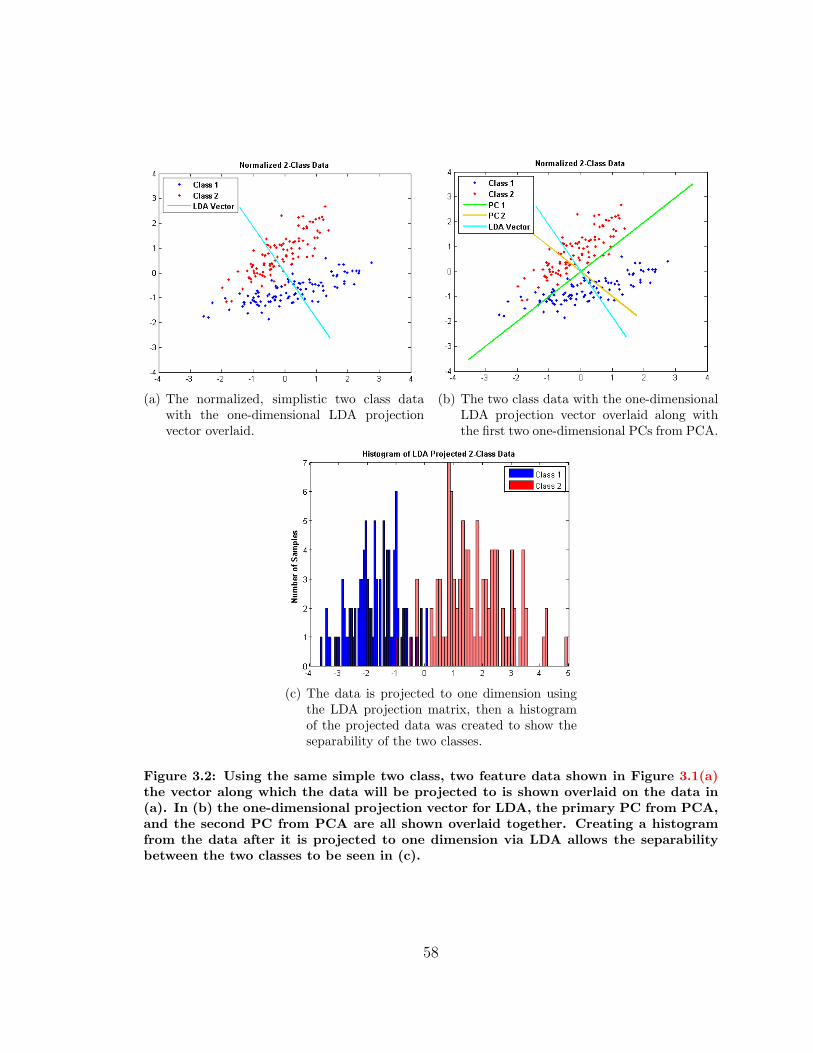
(a) The normalized, simplistic two class datawith the one-dimensional LDA projectionvector overlaid.

(b) The two class data with the one-dimensionalLDA projection vector overlaid along withthe first two one-dimensional PCs from PCA.

(c) The data is projected to one dimension usingthe LDA projection matrix, then a histogramof the projected data was created to show theseparability of the two classes.

Figure 3.2: Using the same simple two class, two feature data shown in Figure 3.1(a)the vector along which the data will be projected to is shown overlaid on the data in(a). In (b) the one-dimensional projection vector for LDA, the primary PC from PCA,and the second PC from PCA are all shown overlaid together. Creating a histogramfrom the data after it is projected to one dimension via LDA allows the separabilitybetween the two classes to be seen in (c).

58

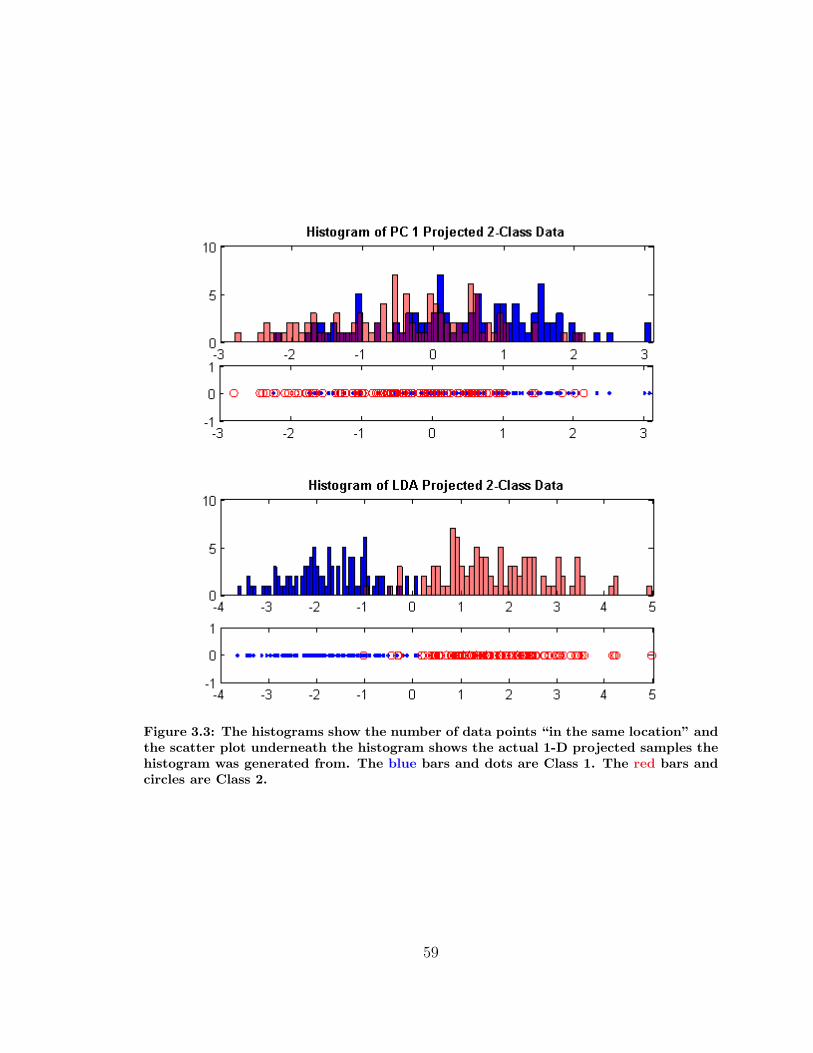
Figure 3.3: The histograms show the number of data points “in the same location” andthe scatter plot underneath the histogram shows the actual 1-D projected samples thehistogram was generated from. The blue bars and dots are Class 1. The red bars andcircles are Class 2.

59

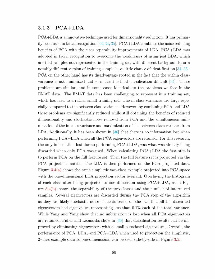
3.1.3 PCA+LDA

PCA+LDA is a innovative technique used for dimensionality reduction. It has primar-

ily been used in facial recognition [33, 34, 35]. PCA+LDA combines the noise reducing

benefits of PCA with the class separability improvements of LDA. PCA+LDA was

adopted in facial recognition to overcome the weaknesses of using just LDA, which

are that samples not represented in the training set, with different backgrounds, or a

notably different version of training sample have little chance of identification [34, 35].

PCA on the other hand has its disadvantage rooted in the fact that the within class-

variance is not minimized and so makes the final classification difficult [34]. These

problems are similar, and in some cases identical, to the problems we face in the

EMAT data. The EMAT data has been challenging to represent in a training set,

which has lead to a rather small training set. The in-class variances are large espe-

cially compared to the between class variance. However, by combining PCA and LDA

these problems are significantly reduced while still obtaining the benefits of reduced

dimensionality and stochastic noise removal from PCA and the simultaneous mini-

mization of the in-class variance and maximization of the between-class variance from

LDA. Additionally, it has been shown in [36] that there is no information lost when

performing PCA+LDA when all the PCA eigenvectors are retained. For this research,

the only information lost due to performing PCA+LDA, was what was already being

discarded when only PCA was used. When calculating PCA+LDA the first step is

to perform PCA on the full feature set. Then the full feature set is projected via the

PCA projection matrix. The LDA is then performed on the PCA projected data.

Figure 3.4(a) shows the same simplistic two-class example projected into PCA-space

with the one-dimensional LDA projection vector overlaid. Overlaying the histogram

of each class after being projected to one dimension using PCA+LDA, as in Fig-

ure 3.4(b), shows the separability of the two classes and the number of intermixed

samples. Several eigenvectors are discarded during the PCA step of the algorithm

as they are likely stochastic noise elements based on the fact that all the discarded

eigenvectors had eigenvalues representing less than 0.1% each of the total variance.

While Yang and Yang show that no information is lost when all PCA eigenvectors

are retained, Fidler and Leonardis show in [35] that classification results can be im-

proved by eliminating eigenvectors with a small associated eigenvalues. Overall, the

performance of PCA, LDA, and PCA+LDA when used to projection the simplistic,

2-class example data to one-dimensional can be seen side-by-side in Figure 3.5.

60

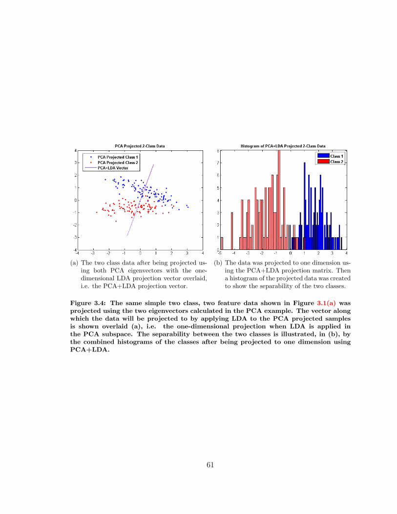
(a) The two class data after being projected us-ing both PCA eigenvectors with the one-dimensional LDA projection vector overlaid,i.e. the PCA+LDA projection vector.

(b) The data was projected to one dimension us-ing the PCA+LDA projection matrix. Thena histogram of the projected data was createdto show the separability of the two classes.

Figure 3.4: The same simple two class, two feature data shown in Figure 3.1(a) wasprojected using the two eigenvectors calculated in the PCA example. The vector alongwhich the data will be projected to by applying LDA to the PCA projected samplesis shown overlaid (a), i.e. the one-dimensional projection when LDA is applied inthe PCA subspace. The separability between the two classes is illustrated, in (b), bythe combined histograms of the classes after being projected to one dimension usingPCA+LDA.

61

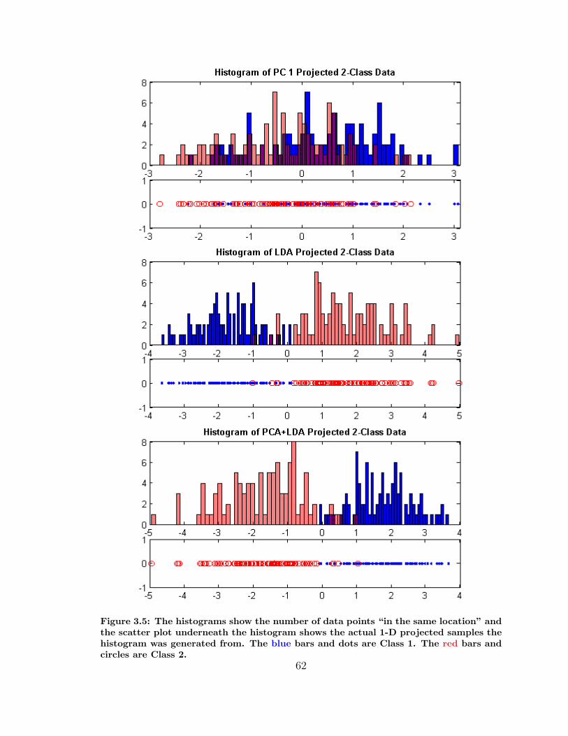
Figure 3.5: The histograms show the number of data points “in the same location” andthe scatter plot underneath the histogram shows the actual 1-D projected samples thehistogram was generated from. The blue bars and dots are Class 1. The red bars andcircles are Class 2.

62

3.2 Classifier – Mahalanobis Distance

There is still quite a bit of variability in just the features from known no-flaw sig-

natures even after performing PCA+LDA upon them. Combined with the fact that

there is such a small number of known SCC signatures in existence limits the number

of applicable classification algorithms. Because of the inability to quantify the sever-

ity of real SCCs (defects identified using MPI could be mere scratches or completely

through the pipe wall) the ability of signatures taken over real SCCs have no guaran-

tee of being even slightly representative of the “standard” SCC signature. However,

no-flaw signatures can be selected with acceptable confidence. These factors lead

to the selection of Mahalanobis distance for a classifier. The Mahalanobis distance

accommodates both the fact that statistically only the no-flaw signatures are well

represented and that there is an non-negligible amount of variation even in just the

no-flaw class’s signatures. The calculation of the Mahalanobis distance, Eqn. (3.9),

returns a scalar value indicating a signatures distance from the “target” clusters cen-

troid. We refer to the Mahalanobis distance value as the “flaw distance,” since the

larger the distance the more “flaw-like” the signature under test is.

Mahalanobis Distance = (x− µ)T Σ−1(x− µ) (3.9)

Mahalanobis distance differs from Euclidean distance in that Mahalanobis distance

calculates a distance from the centroid of a multi-dimensional cloud of data while

Euclidean distance is calculated from a single data point to another single point.

The Mahalanobis distance calculates the distance from a single data point to the

“target” set. The covariance matrix of “target” set is used in the calculation of the

Mahalanobis distance and is how the shape of the hyper-ellipsoid “cloud” formed by

the “target” set [27, 32].

The covariance matrix used in the calculation allows the shape of the cluster to

be a factor in the distance [27]. This is regardless of the unknown multi-dimensional

shape a cluster forms. For example, if a sample is close to a protruding lobe but not

necessarily the centroid of the cluster it will not receive an “unfairly” long Maha-

lanobis distance.

63

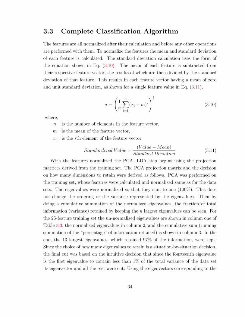
3.3 Complete Classification Algorithm

The features are all normalized after their calculation and before any other operations

are performed with them. To normalize the features the mean and standard deviation

of each feature is calculated. The standard deviation calculation uses the form of

the equation shown in Eq. (3.10). The mean of each feature is subtracted from

their respective feature vector, the results of which are then divided by the standard

deviation of that feature. This results in each feature vector having a mean of zero

and unit standard deviation, as shown for a single feature value in Eq. (3.11),

σ =

(1

n

n∑i=1

(xi −m)2

) 12

(3.10)

where,

n is the number of elements in the feature vector,

m is the mean of the feature vector,

xi is the ith element of the feature vector.

Standardized V alue =(V alue−Mean)

Standard Deviation(3.11)

With the features normalized the PCA+LDA step begins using the projection

matrices derived from the training set. The PCA projection matrix and the decision

on how many dimensions to retain were derived as follows. PCA was performed on

the training set, whose features were calculated and normalized same as for the data

sets. The eigenvalues were normalized so that they sum to one (100%). This does

not change the ordering or the variance represented by the eigenvalues. Then by

doing a cumulative summation of the normalized eigenvalues, the fraction of total

information (variance) retained by keeping the n largest eigenvalues can be seen. For

the 25-feature training set the un-normalized eigenvalues are shown in column one of

Table 3.3, the normalized eigenvalues in column 2, and the cumulative sum (running

summation of the “percentage” of information retained) is shown in column 3. In the

end, the 13 largest eigenvalues, which retained 97% of the information, were kept.

Since the choice of how many eigenvalues to retain is a situation-by-situation decision,

the final cut was based on the intuitive decision that since the fourteenth eigenvalue

is the first eigenvalue to contain less than 1% of the total variance of the data set

its eigenvector and all the rest were cut. Using the eigenvectors corresponding to the

64

thirteen largest eigenvalues the 25-features of each signature are projected into 13

features in the PCA subspace.

The LDA step of PCA+LDA brings up an important detail that contributed

to the improvements resulting from the final classification algorithm. Since LDA

projects to a maximum of (number of classes − 1) dimensions if the only classes

were flaw and no-flaw then the results would be a one-dimensional vector. However,

by creating a third class in the training set of signatures corresponding to anomalies

in the Mahalanobis distance at locations on the training pipe known to be free of any

type of defect LDA results in a two-dimensional projection and Mahalanobis distance

can still be used as the classifier. This resulted in a significant change to the responses

from anomalies in the Mahalanobis distance.

These changes made the anomaly responses distinguishable from defect responses

and so the characteristics that a response must have in order to be a defect were

developed. So projecting the PCA features using the three class LDA projection

matrix derived from the PCA projected training set data produces the final features

used in the classification of each signature. Using the Mahalanobis distance calculated

with the PCA+LDA projected no-flaw portion of the training set as the “target,” a

Mahalanobis distance value for each signature in the data set under-test is found. This

Mahalanobis distance is then examined and responses (spikes in the flaw distance)

that meet the criteria to be a defect are visually identified along with their axial

position in the scanned pipe.

One common question that arises about the Mahalanobis distance is, “if the Ma-

halanobis distance is calculated with the flaw signatures from the training set as the

“target” set and likewise for the anomaly signatures in the training set.” The answer

is we do not. The reason is that the flaw signatures in the training set are from

synthetic SCCs and so could result in real SCCs being mis-classified. The reason the

anomaly signatures are not used either is that there is no benefit in this identification.

Anomalies’ are present in every single pipe that has ever been scanned in the course

of the project’s life. Pipes that were in service for decades and pipes that have never

been used or even buried all show anomaly responses. As no anomaly response has

ever corresponded to a defect (real or synthetic) it is our opinion that they are in-

trinsic, metallurgic differences in the pipe’s composition that affect the ferromagnetic

properties at the specific locations the anomaly response appears. Additionally, the

concern is to identify a signature as being a flaw or no-flaw not as an anomalies.

65

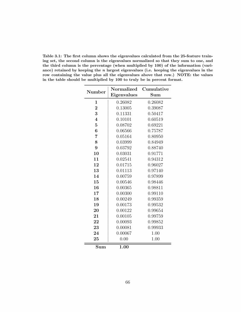
Table 3.1: The first column shows the eigenvalues calculated from the 25-feature train-ing set, the second column is the eigenvalues normalized so that they sum to one, andthe third column is the percentage (when multiplied by 100) of the information (vari-ance) retained by keeping the n largest eigenvalues (i.e. keeping the eigenvalues in therow containing the value plus all the eigenvalues above that row.) NOTE: the valuesin the table should be multiplied by 100 to truly be in percent format.

NumberNormalized CumulativeEigenvalues Sum

1 0.26082 0.260822 0.13005 0.390873 0.11331 0.504174 0.10101 0.605195 0.08702 0.692216 0.06566 0.757877 0.05164 0.809508 0.03999 0.849499 0.03792 0.8874010 0.03031 0.9177111 0.02541 0.9431212 0.01715 0.9602713 0.01113 0.9714014 0.00759 0.9789915 0.00546 0.9844616 0.00365 0.9881117 0.00300 0.9911018 0.00249 0.9935919 0.00173 0.9953220 0.00122 0.9965421 0.00105 0.9975922 0.00093 0.9985223 0.00081 0.9993324 0.00067 1.0025 0.00 1.00

Sum 1.00

66

So in summary, the no-flaw signatures in the training set do represent the no-flaw

signatures found in both the machined pipe and the decommissioned pipes that have

been inspected. Because of this the training set no-flaw signatures can be used with

confidence as the “target” for calculating Mahalanobis distance.

67

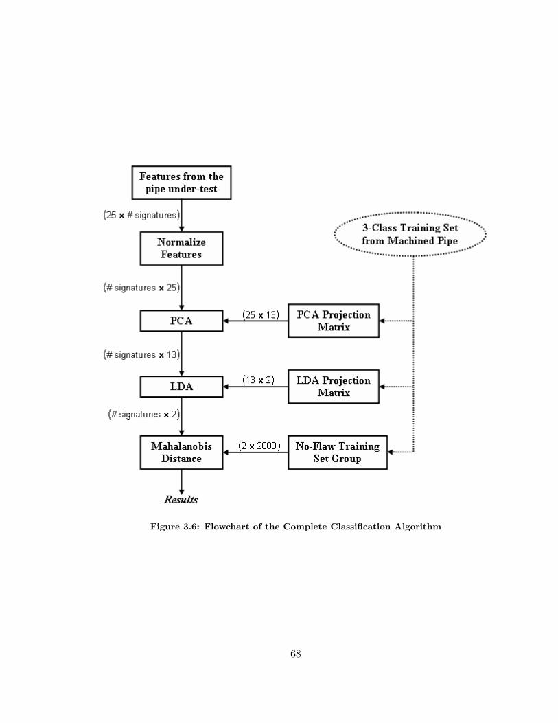
Figure 3.6: Flowchart of the Complete Classification Algorithm

68

Chapter 4

Experiments and Results

Once features have been extracted from the wavelet decomposition of the EMAT

signals they are ready for use in identifying the presence or lack of SCCs in the

scanned section of pipe. This classification is performed as described in Section 3.3.

All of the following results and statistics make use of the data collected from multiple

scans of the machined pipe in order to have an objective, quantified ground truth to

compare the original and final classification algorithms’ results when both the original

and final feature sets are used. Only scanline I and II made up of parabolic cuts are

used, since the parabolic cuts are the most realistic synthetic SCCs. The scanlines

and synthetic SCCs (parabolic cuts) and their creation will now be explained.

4.1 The Training Set

In the beginning of working on the ability to detect SCCs while moving, a training

set was simply the selection of a range (or ranges) of signatures after the signature

quality check (Section 2.2.3) that appeared to be “normal” when displayed as a B-

scan.∗ Signatures that were abnormal when compared to the 100 signatures or so

before and after it were removed. At the end of this process a set of signatures which

still contained the variation seen between known good signatures but contained no

signatures that would be an outlier from the rest of the set. This process took

days to perform and in the end the set was really just for use as the “no-flaw” set

∗At the time when training sets (i.e. good sets) were constructed by hand in this manner thesignature quality check did not yet include the 180◦ out-of-phase check or the use the improvedthresholds.

69

(“good” set) when calculating the expected signal needed for calculating the difference

features (Section 2.3.2) and to calculate the centroid and covariance matrix used in

the Mahalanobis distance. The most disappointing things of all were that a) the set

generally only produced results semi-close to what was anticipated for the scanline

the set was derived from; b) no set created this way ever worked on a different pipe,

even if the pipes were the same diameter and had the same wall thickness; and c) the

range(s) of signatures selected based on their appearance in the B-scan could contain

signatures taken over a defect.

In one particularly unfortunate incident involving a blind test on a pipe contain-

ing natural SCCs, the ranges of “no-flaw” signatures were selected based on there

appearance from the B-scan and carefully examined and cleaned by hand turned out

to be almost entirely flaw signatures. So in this incident it turned out that the smaller

the Mahalanobis distance was the likelier is was actual defect, but of course this was

not know until the results were released. While this was the worst-case scenario it

is representative of the risk of creating a no-flaw set in this manner. Even when the

ranges selected from known good areas were used to generate a no-flaw set it was not

useful for evaluating the ability of the classification algorithm to identify SCCs, since

the flaw indications could actually be a metallurgic anomaly or such. In the end, the

creation of a fully quantized training set was one of the most important and difficult

outcomes of this work.

This truly supervised training set data has allowed a classification algorithm to be

developed that is “transportable” between different pipes of the same diameter and

wall thickness as the pipe used to create the training set, between 30-inch diameter

with a different wall thickness, and even 26-inch diameter pipes. The difficulty in

developing a classification algorithm to detect SCCs is primarily due to the rarity of

pipes containing SCCs available for testing. Because of this we do not have enough

real SCC signatures to adequately characterize a signature as an SCC signature.In

order to detect SCCs we needed a known set of defects in a known environment. By

“known set of defects” what is meant is that the SCCs depths, lengths, and widths are

known. The problem with needing SCCs with known dimensions is that to determine

the depth along the entire length of an SCCs requires the defect area be removed

from the pipe and either thinly sliced or x-rayed. It is possible to determine a max-

imum depth, without destroying the pipe, using a specialized ultrasonic inspection

technique, applicable only from the exterior of the pipe specimen.

70

This specialized inspection is costly and must be done by a highly skilled technician

with access to calibration blocks. A technician was hired to do this inspection in hopes

of determining depth and thus the severity of the SCCs contained in a pipe that was

inspected during a blind test and demonstration at the Battelle PSF. The data from

this did provided insight in to the severity and thus the sensitivity of our EMAT

sensor system to depth. However, it was not possible to determine the “amount” of

an SCC that was at or close to its measured maximum depth. In addition, when this

technique is used on a SCC colony, it only provides the maximum depth of the entire

colony, but again how much of the colony is at or near that depth is unknown. Based

on these results, it was possible to determine if an SCC that was not detected during

the blind trial was due to it being too shallow.† However, a confident determination

as to what the limitations of the sensor system are based solely on these specialized

measurements cannot be made, since there are still too many unknowns with regards

to the actual SCCs.

As for a known environment, this is referring to the pipe containing the defects.

What the pipe has been subjected to during its “life.” So to develop reliable statistics

as to the sensor systems capabilities and to improve the quality of our features (e.g.,

add new features, remove redundant or noisy features, etc) a pipe was purchased and

precision synthetic SCCs machined in to it.

A 10-foot long section of brand new 30-inch diameter, 0.375-inch thick pipe was

purchased. By using a new, never-been-used section of pipe we eliminated the pos-

sibility of there being any defects (corrosion, pitting, SCCs), that the pipe is out-of-

round, and that any unknown, undocumented alteration, testing, or abuse occurred

to the pipe. To create synthetic SCCs that closely mimicked the characteristics of

natural SCCs a set of size and spacing specifications for machining synthetic SCC

defects in to the pipe [37] were determined that would mimic real SCCs. In the end

a machining facility with an electrical discharge machining (EDM) system capable of

accommodating the pipe segment was contracted to perform the machining. EDM

machining can be used on hardened steel and is capable of making precise angles,

cuts, curves, even cavities, all with tolerances at or near 0.0001-inches [38]. This pipe

is referred to as the machined pipe through out the remainder of this thesis.

†If an SCC had a maximum depth that was shallow compared to the wall thickness it is safe toassume that is why it was not detected.

71

Four lines of synthetic defects were created, each line contains nine defects sepa-

rated by 12-inches from center-to-center, and each scanline separated by 60◦ circum-

ferentially, Figure 4.1. These defects, from left to right, are numbered one through

nine. This one through nine from left to right numbering will be constant through

out the remainder of this thesis, unless otherwise stated. The defect classification

results from the machined pipe are also displayed with defect-1 on the left edge and

defect-9 on the right edge. Defect-1 on each scanline consist of either two or three

staggered cuts to simulate an SCC colony and serves a second purpose of being a

physical indication of which end of the pipe defect-1 is actually on. The layout of

the two staggered cuts and three staggered cuts are shown in Figure 4.2(a) and Fig-

ure 4.2(b) respectively. All the cuts for defect-1 are made to exactly the same width,

depth, and when applicable length specifications.

The width and length of typical SCCs have been measured and thus can be “trans-

lated” in to dimensions for the creation of synthetic SCCs in the new pipe. What

the depth profile should be was a far more difficult decision. In the end two of the

four scanlines were made using the EDM process, scanline III and IV. All the defects

in scanline III and IV have uniform depth for the entire defect’s length. This also

means that there are straight, 90◦ vertical transition “in to” and “out of” the cuts.

Figure 4.3(a) shows the generic profile of the EDM cuts. The depth, width, and

length of each rectangular cut was specified in [37]. The other two scanlines, scanline

I and II, were made using a circular cutting wheel with a one inch diameter to the

specifications also in [37]. These defects are what we have come to refer to as the

parabolic cuts (defects).

The parabolic defects are spaced 12-inch a part center-to-center. Since the parabolic

cuts were made using a cutting wheel, the depth and width were specified, but not

the length. The specified depth is the maximum depth into the pipe and is essentially

a point depth. So the parabolic cuts only have the length that was necessary for the

wheel to penetrate the pipe wall to the specified depth. Figure 4.3(b) shows a generic

depth profile for a parabolic cut. The specific dimensions for the defects on scanline I

and II, including the length of each defect as measured after the specified depth was

reached, are shown in Table 4.1. Since the specified depth of each parabolic cut is a

point depth, the average depth is also included as part of the data in Table 4.2. The

fact that the parabolic cuts do not have a uniform depth and transition gradually “in

to” and “out of” the pipe is far more SCC-like than the rectangular cuts.

72

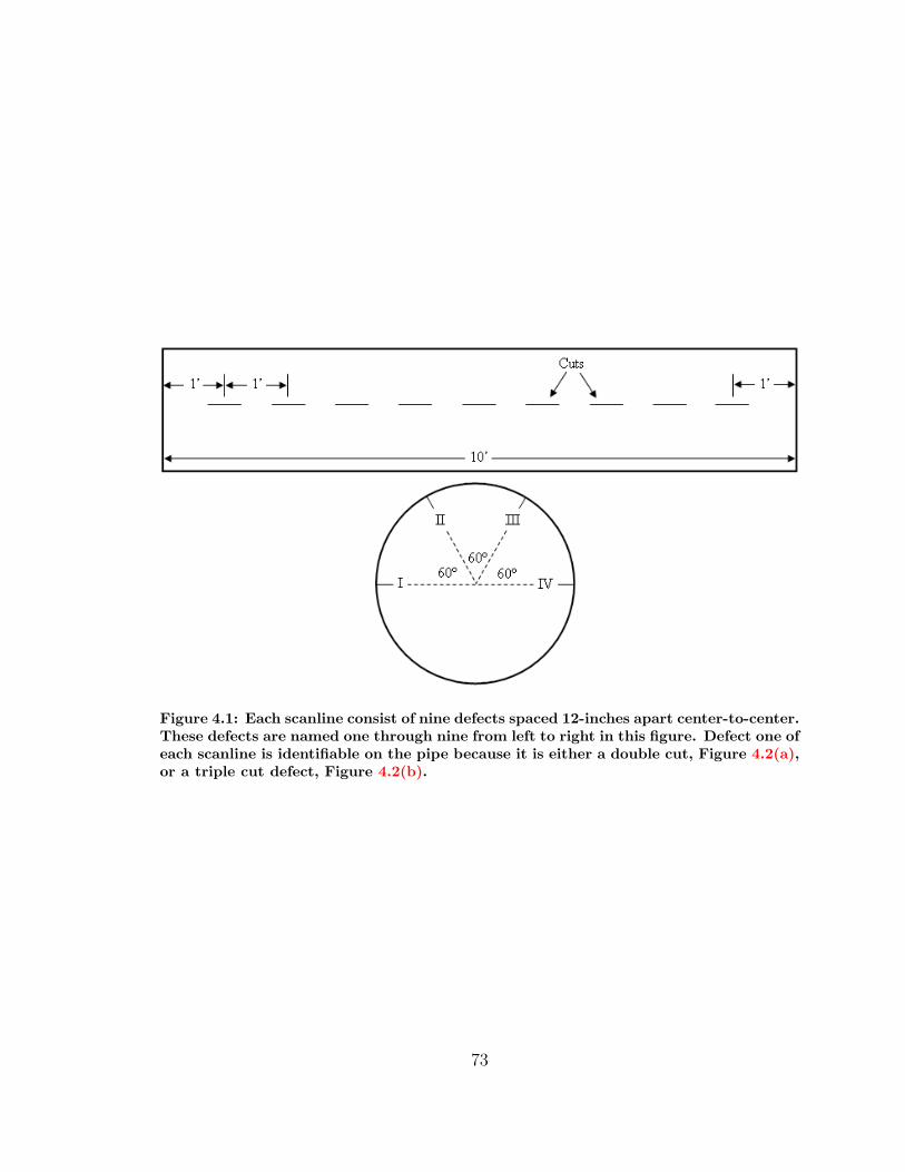
Figure 4.1: Each scanline consist of nine defects spaced 12-inches apart center-to-center.These defects are named one through nine from left to right in this figure. Defect one ofeach scanline is identifiable on the pipe because it is either a double cut, Figure 4.2(a),or a triple cut defect, Figure 4.2(b).

73

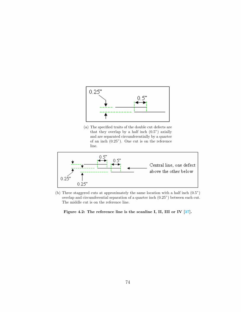
(a) The specified traits of the double cut defects arethat they overlap by a half inch (0.5”) axiallyand are separated circumferentially by a quarterof an inch (0.25”). One cut is on the referenceline.

(b) Three staggered cuts at approximately the same location with a half inch (0.5”)overlap and circumferential separation of a quarter inch (0.25”) between each cut.The middle cut is on the reference line.

Figure 4.2: The reference line is the scanline I, II, III or IV [37].

74

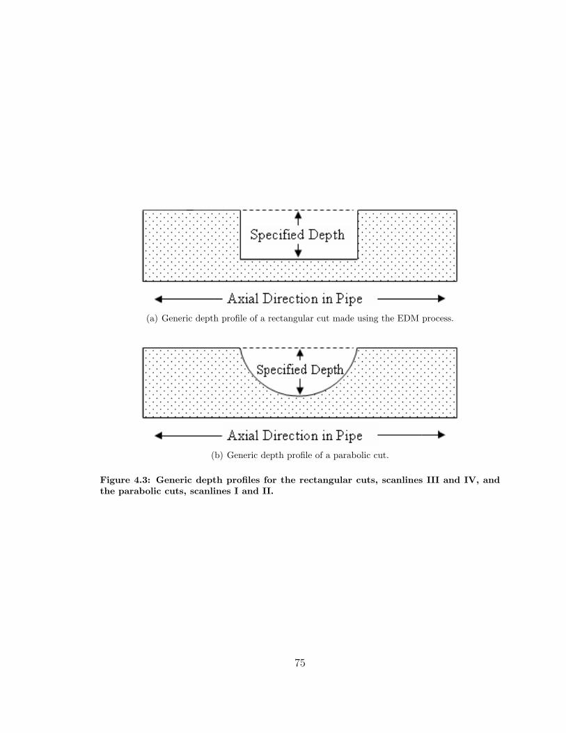
(a) Generic depth profile of a rectangular cut made using the EDM process.

(b) Generic depth profile of a parabolic cut.

Figure 4.3: Generic depth profiles for the rectangular cuts, scanlines III and IV, andthe parabolic cuts, scanlines I and II.

75

Because the length, width, and exact maximum depth of each SCC-like parabolic

cut were known, the exact signatures taken over each of the parabolic cuts on scanline

I and II, with one exception, were used to construct a “flaw” set. The exception is

that after segmenting out the signatures taken across each defect in scanline I and

II, the signatures from the 0.035-inch deep defects (the 10% max depth defects, 6.3%

average depth). This is in order to eliminate the possibility that these very shallow,

single “crack” defects would have the effect of including no-flaw signatures in with

flaw signatures, effectively biasing flaw signature group in the training set. The same

defects on an operational pipeline would not merit repair, let alone attention. Since

the pipe was known to be brand new and every defect was placed according to the

design specifications, the signatures from the anomaly locations where extracted and

used to create an addition class called the anomaly class. These anomalies produce

dome shaped response in the Mahalanobis distance, similar in shape to an upside-

down soup bowl, and have been seen in every pipe we have scanned. Finally, no-flaw

signatures were collected as well. The final training set consist of 961 flaw signatures,

1157 anomaly signatures, and 2000 no-flaw signatures.

4.2 Interpreting the Mahalanobis Distance

Once the Mahalanobis distance is calculated, it is the spikes that are of interest. The

larger the distances from zero, the greater the difference between the features of the

signature under test and the features derived from the no-flaw signature set. By call-

ing the distance the flaw distance, the plots of the Mahalanobis distance classification

can be interpreted more intuitively, i.e. the larger the distance the more flaw like the

signature.

Using the original classification technique there was no hope of designing a pattern

recognition algorithm that could take the classification results (Mahalanobis distance)

and mark the flaw indications which were SCCs. This was because there was no

consistency between classifications. Each pipe and sometimes each scanline on each

pipe needed its own custom no-flaw set. Also there were frequently false positive flaw

indications with large flaw distance values in locations where no known flaws of any

type were located. As a result of this different feature sets and classification algorithms

were experimented with. During these in-depth studies of numerous Mahalanobis

distances, SCC responses were visually identified. This allowed a set of criteria that

76

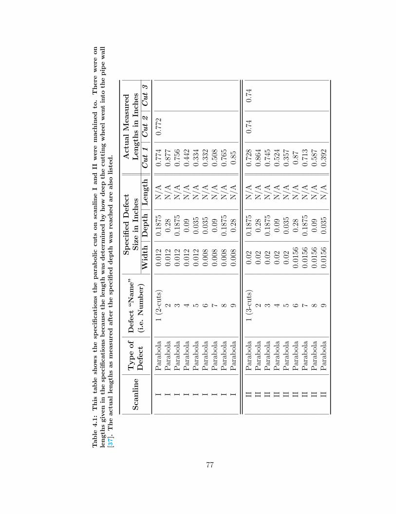
Tab

le4.

1:T

his

table

show

sth

esp

ecifi

cati

ons

the

par

abol

iccu

tson

scan

line

Ian

dII

wer

em

achin

edto

.T

her

ew

ere

onle

ngt

hs

give

nin

the

spec

ifica

tion

sbec

ause

the

lengt

hw

asdet

erm

ined

by

how

dee

pth

ecu

ttin

gw

hee

lw

ent

into

the

pip

ew

all

[37]

.T

he

actu

alle

ngt

hs

asm

easu

red

afte

rth

esp

ecifi

eddep

thw

asre

ached

are

also

list

ed.

Sca

nline

Type

of

Defe

ctD

efec

t“N

ame”

(i.e

.N

um

ber

)

Speci

fied

Defe

ctA

ctualM

easu

red

Siz

ein

Inch

es

Length

sin

Inch

es

Wid

thD

epth

Length

Cut1

Cut2

Cut3

IPar

abol

a1

(2-c

uts

)0.

012

0.18

75N

/A0.

774

0.77

2I

Par

abol

a2

0.01

20.

28N

/A0.

877

IPar

abol

a3

0.01

20.

1875

N/A

0.75

6I

Par

abol

a4

0.01

20.

09N

/A0.

442

IPar

abol

a5

0.01

20.

035

N/A

0.33

4I

Par

abol

a6

0.00

80.

035

N/A

0.33

2I

Par

abol

a7

0.00

80.

09N

/A0.

508

IPar

abol

a8

0.00

80.

1875

N/A

0.76

5I

Par

abol

a9

0.00

80.

28N

/A0.

85

IIPar

abol

a1

(3-c

uts

)0.

020.

1875

N/A

0.72

80.

740.

74II

Par

abol

a2

0.02

0.28

N/A

0.86

4II

Par

abol

a3

0.02

0.18

75N

/A0.

745

IIPar

abol

a4

0.02

0.09

N/A

0.52

4II

Par

abol

a5

0.02

0.03

5N

/A0.

357

IIPar

abol

a6

0.01

560.

28N

/A0.

87II

Par

abol

a7

0.01

560.

1875

N/A

0.71

3II

Par

abol

a8

0.01

560.

09N

/A0.

587

IIPar

abol

a9

0.01

560.

035

N/A

0.39

2

77

Table 4.2: There are two scanlines containing parabolic cuts on the machined pipe.This table list the depth of each defect, what percentage of the pipe wall thickness themaximum depth is, the average depth of the cut (since the maximum depth listed is apoint depth), and the percentage of the pipe wall thickness the average depth reaches[37].

Parabolic Flaw Set I

NumberMaximum % of Average Average

Depth Wall Depth of Cut % Wall

1 0.1875 50.00% 0.131 34.82%2 0.28 74.67% 0.200 53.46%3 0.1875 50.00% 0.131 34.82%4 0.09 24.00% 0.061 16.31%5 0.035 9.33% 0.024 6.27%6 0.035 9.33% 0.024 6.27%7 0.09 24.00% 0.061 16.31%8 0.1875 50.00% 0.131 34.82%9 0.28 74.67% 0.200 53.46%

Parabolic Flaw Set II

NumberMaximum % of Average Average

Depth Wall Depth of Cut % Wall

1 0.1875 50.00% 0.131 34.82%2 0.28 74.67% 0.200 53.46%3 0.1875 50.00% 0.131 34.82%4 0.09 24.00% 0.061 16.31%5 0.035 9.33% 0.024 6.27%6 0.28 74.67% 0.200 53.46%7 0.1875 50.00% 0.131 34.82%8 0.09 24.00% 0.061 16.31%9 0.035 9.33% 0.024 6.27%

78

a response in the Mahalanobis distance must poses in order to be a defect (SCC)

indication.

1. The response must roughly be triangular without a bottom in shape.

2. A “white-cone” must be visible under the response.

3. The sides of the triangular “spike” should be “thin”.

Since only the most blatantly bad signatures are removed during the quality check step

of the preprocessing there can still be corrupted signatures present. These “missed”

corrupt signatures show up in the Mahalanobis distance as single points with flaw

distances hundreds to thousands of times the largest flaw distance of a non-solitary-

point spike. Because of this the Mahalanobis distance results are usually filtered

using two different filters/smoothing operations to allow the shape, magnitude, and

presence of a “white-cone” to be determined.

The most frequently used filter is simply a running averaging operation where the

Mahalanobis distance of every five signatures is replaced by the average and the five

associated position measurements are replaced by the average of the position values. A

new Mahalanobis distance vector and position vector are assembled with the average

flaw distance and position representing the five signatures and their positions. This

is safely done without affecting the characteristics used to identify defect indications

as an SCC since the axial resolution of the EMAT system is so high. On average

there are 91 signatures per inch before cleaning, 78 signatures per inch after cleaning,

and 16 signatures per inch after the running average operation. The EMAT head

itself is 2.75-inches wide and the coil (the active sensing area) is 1.5-inches wide. So,

with 16 signatures per inch there is still substantially high resolution, given that each

signature senses at least a 1.5-inch wide, axial “window.”

It is also relevant at this point to mention that the length of a defect can be

determined by measuring the width of the defect’s response starting were the response

rises above the mean level of the flaw distances leading up to the defect response and

ending where the response returns to the mean flaw distance values following the

response. This is illustrated in Figure 4.4 where the actual flaw has a length of 0.865-

inches and the defect response measures 2.54-inches, subtracting 1.5-inches for the

width of the active portion of the EMAT returns a width of 1.04-inches. This is quite

an acceptable measure of the flaw’s actual length considering the subjectiveness of

selecting the location where the response rises above and returns to the local average

79

flaw distance and that the focus of this research has been on the more important goal

of reliable, repeatable SCC detection. After all you cannot size what you cannot find.

Finally, the other filter commonly applied to the Mahalanobis distances removes

spikes formed by single points. This “spike filter” takes nine data points at a time

and calculates the mean and standard deviation of their flaw distance values. Then

the mean plus two and a half times the standard deviation is used as a threshold.

Any single point with a flaw distance greater than the threshold is replaced by the

mean flaw distance value of the nine points.

4.3 Experiments

This section describes and shows the outcomes from using the final 25-feature set and

the original 13-feature set with both the final classification algorithm and the original

classification algorithm. The data classified is from the two scanlines with parabolic

cuts, scanline I and II. Ten scans of each scanline are classified and the number of

correctly identified defects (true positives), incorrectly identified defects (false posi-

tives), undetected defects (false negatives), and the repeatability of a detection are

calculated (i.e. number of times a defect was identified correctly (true positive) in

the ten scans of a scanline). The validation of the final feature set, training set, and

final classification algorithm is shown by these experiments as well. The two scanlines

and the ten scans of each are two unique tests with ten trials of each test conducted,

allowing for confidence in the results.

In the following sections the two key comparisons are made by calculating the

difference between classification results 1. when the original and final feature sets are

classified using just the original classification algorithm, 2. when the original and final

feature sets are classified using only the final classification algorithm. This way the

effects of the different feature sets and the effects of the two classification techniques

can be isolated and compared as two separate events. By being able to evaluate these

two changes separately improvements solely due to the feature set, solely due to the

classification algorithm, and then due to the combination of these will be shown.

80

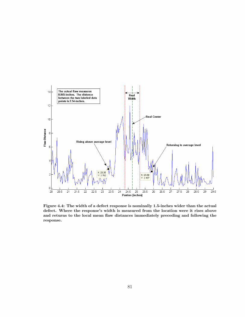
Figure 4.4: The width of a defect response is nominally 1.5-inches wider than the actualdefect. Where the response’s width is measured from the location were it rises aboveand returns to the local mean flaw distances immediately preceding and following theresponse.

81

4.3.1 Both Feature Sets using the Original Classification Al-

gorithm

In this section the classification results using the original feature set with the origi-

nal classification technique is compared with the classification results when the final

feature set is also used in conjunction with the original classification technique. This

provides a baseline for comparing the two feature sets based on the effectiveness of

the original classification technique.

The original classification algorithm used to detect SCCs at the beginning of this

research used the thirteen original features and the Mahalanobis distance from a

“good” set as the classifier. At the time the 13-feature set was in use, the “good” set

was formed by taking stationary data from a location that was marked as defect-free

in the pipe under test. This data was acquired from scans taken of a decommissioned

pipe containing natural SCCs at the Battelle PSF. The defect-free area was based

on the information in the pipe’s original assay report. Early on it became apparent

that the stationary no-flaw signatures did not adequately reflect the variation that is

present in no-flaw signatures taken while moving, as can be seen in Figure 4.5.

Because the stationary signatures were not providing an acceptable “good” set

pauses during scans to collect stationary “good” sets were eliminated. Instead the

“good” sets were created from signatures gathered while moving, but still from a

range in the pipe under test listed as defect free. Since the original classification

algorithm used a “good” set from an actual decommissioned pipe, a problem prone

attribute in itself, in order to calculate the original feature set and use the original

classification algorithm on the machined pipe the no-flaw signatures in the training

set are used as the “good” set. All other steps and calculations for the original

features and the original classification algorithm remain as they were. The use of

the no-flaw signatures from the training set constructed from the machined pipe data

actually improves the original feature set and classifier’s calculations since there is

100% certainty that the no-flaw signatures are flaw and anomaly free. Something

that could never be claimed about a “good” set derived from a decommissioned pipe

section.

Before continuing it is important to take note of what the highest priorities as far

as defect detection goes. There is no standard that address calculating the remaining

strength of a pipe section containing a crack. There is a standard for making such

a calculation for external corrosion on a pipe. This calculation is conservative even

82

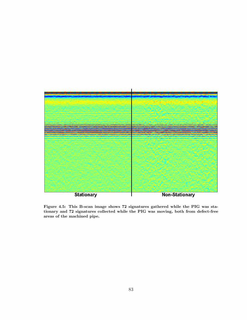
Figure 4.5: This B-scan image shows 72 signatures gathered while the PIG was sta-tionary and 72 signatures collected while the PIG was moving, both from defect-freeareas of the machined pipe.

83

for corrosion and so if used for other types of defects provides at least the same

conservative estimate of remaining strength. The remaining strength of a pipe section

is based on how long and deep the defect is. The calculation results in a length that

a defect with same maximum through wall depth would be when either the pressure

in the pipeline would need to be lowered or the section repaired to continue operating

at the current pressure [39]. For the defects on the machined pipe the length that

each defect must equal or exceed is shown in Table 4.3. The results when using the

original features set with the original classifier are shown in Table 4.4.

The results for the final feature set using the original classifier are shown in Ta-

ble 4.5. There is a sub-table for each scanline. The numbers listed on the left-hand

side identifies one of the 10 scans. The row shows which defects were detected during

that scan. The maximum through wall depth percentage and the average through

wall depth percentage of each defect on the scan line are listed below their respec-

tive defect number. Each column is a single synthetic SCC defect and the scans in

which it was detected. The percentage at the bottom of each column represents the

percentage of times that defect was detected. A detection is indicated by a ‘X’.

With this in mind, notice in Tables 4.4 and 4.5 that the deepest defects are

repeatedly detected, while the shallower defects are detected at a much lower rate, if

at all. This directly impacts the number of false negatives since each row of the table

that has a column without an ‘X’ is automatically a false negative. The number of

true positives, false positives, and false negatives for the original feature set, original

classification algorithm combination is shown in Figure 4.6 and for the final feature

set, original classification algorithm combination in Figure 4.7. The number of false

positive is still of importance since in the eventual commercial usage of this technology

to inspect natural gas pipelines locations with true positives, and therefore false

positives, would likely be excavated for repair. As this is not an easy, cheap, or

inexpensive proposition it is just as important that there be as close to 100% true

positive detection of significant defects while keeping the false positives to a minimum.

4.3.2 Both Feature Sets using the Final Classification Algo-

rithm

The section contains the results when using the original features set with the final

classification algorithm, Table 4.6 and for when the final feature set is used with the

84

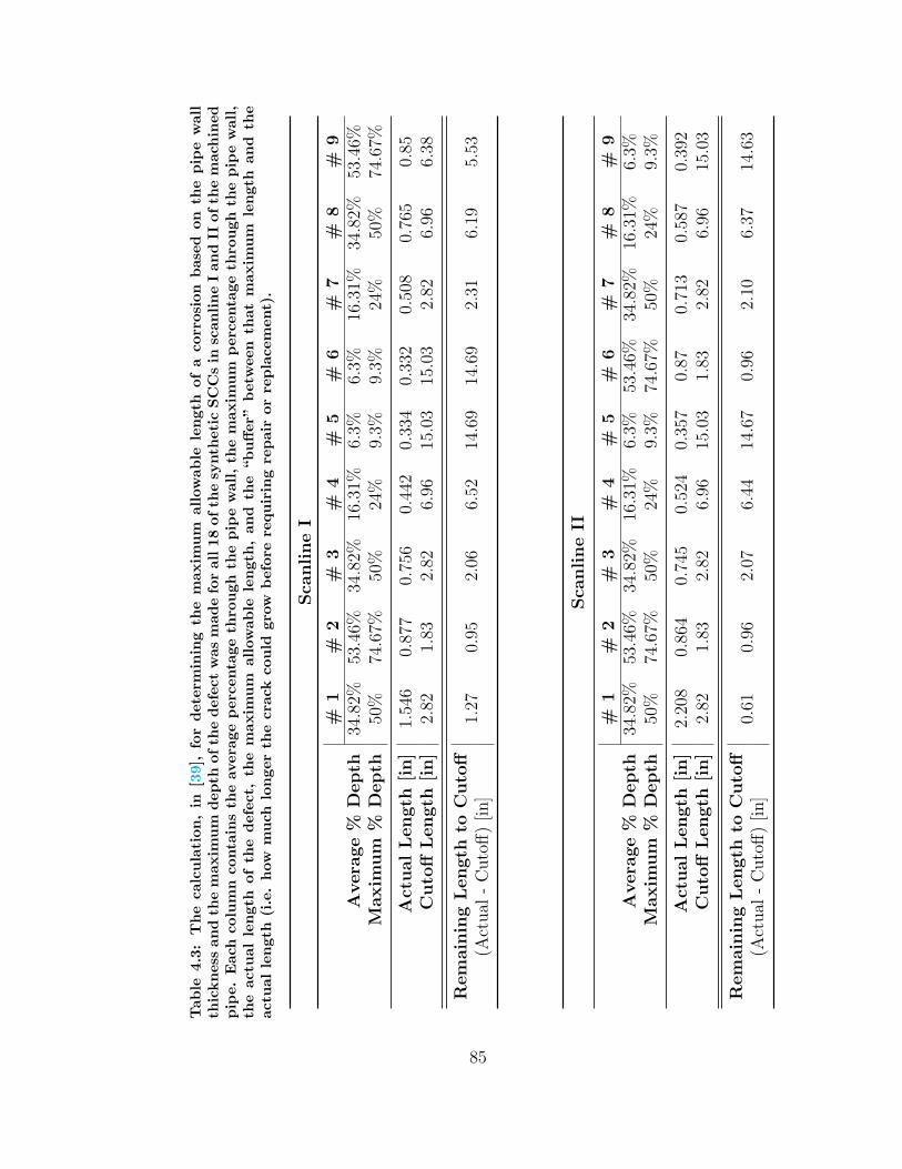
Tab

le4.

3:T

he

calc

ula

tion

,in

[39]

,fo

rdet

erm

inin

gth

em

axim

um

allo

wab

lele

ngt

hof

aco

rros

ion

bas

edon

the

pip

ew

all

thic

knes

san

dth

em

axim

um

dep

thof

the

def

ectw

asm

ade

for

all18

ofth

esy

nth

etic

SC

Csin

scan

line

Ian

dII

ofth

em

achin

edpip

e.Eac

hco

lum

nco

nta

ins

the

aver

age

per

centa

geth

rough

the

pip

ew

all,

the

max

imum

per

centa

geth

rough

the

pip

ew

all,

the

actu

alle

ngt

hof

the

def

ect,

the

max

imum

allo

wab

lele

ngt

h,

and

the

“buffer

”bet

wee

nth

atm

axim

um

lengt

han

dth

eac

tual

lengt

h(i.e

.how

much

longe

rth

ecr

ack

could

grow

bef

ore

requir

ing

repai

ror

repla

cem

ent)

.

Sca

nline

I

#1

#2

#3

#4

#5

#6

#7

#8

#9

Avera

ge

%D

epth

34.8

2%53

.46%

34.8

2%16

.31%

6.3%

6.3%

16.3

1%34

.82%

53.4

6%M

axim

um

%D

epth

50%

74.6

7%50

%24

%9.

3%9.

3%24

%50

%74

.67%

Act

ualLength

[in]

1.54

60.

877

0.75

60.

442

0.33

40.

332

0.50

80.

765

0.85

Cuto

ffLength

[in]

2.82

1.83

2.82

6.96

15.0

315

.03

2.82

6.96

6.38

Rem

ain

ing

Length

toC

uto

ff1.

270.

952.

066.

5214

.69

14.6

92.

316.

195.

53(A

ctual

-C

uto

ff)

[in]

Sca

nline

II

#1

#2

#3

#4

#5

#6

#7

#8

#9

Avera

ge

%D

epth

34.8

2%53

.46%

34.8

2%16

.31%

6.3%

53.4

6%34

.82%

16.3

1%6.

3%M

axim

um

%D

epth

50%

74.6

7%50

%24

%9.

3%74

.67%

50%

24%

9.3%

Act

ualLength

[in]

2.20

80.

864

0.74

50.

524

0.35

70.

870.

713

0.58

70.

392

Cuto

ffLength

[in]

2.82

1.83

2.82

6.96

15.0

31.

832.

826.

9615

.03

Rem

ain

ing

Length

toC

uto

ff0.

610.

962.

076.

4414

.67

0.96

2.10

6.37

14.6

3(A

ctual

-C

uto

ff)

[in]

85

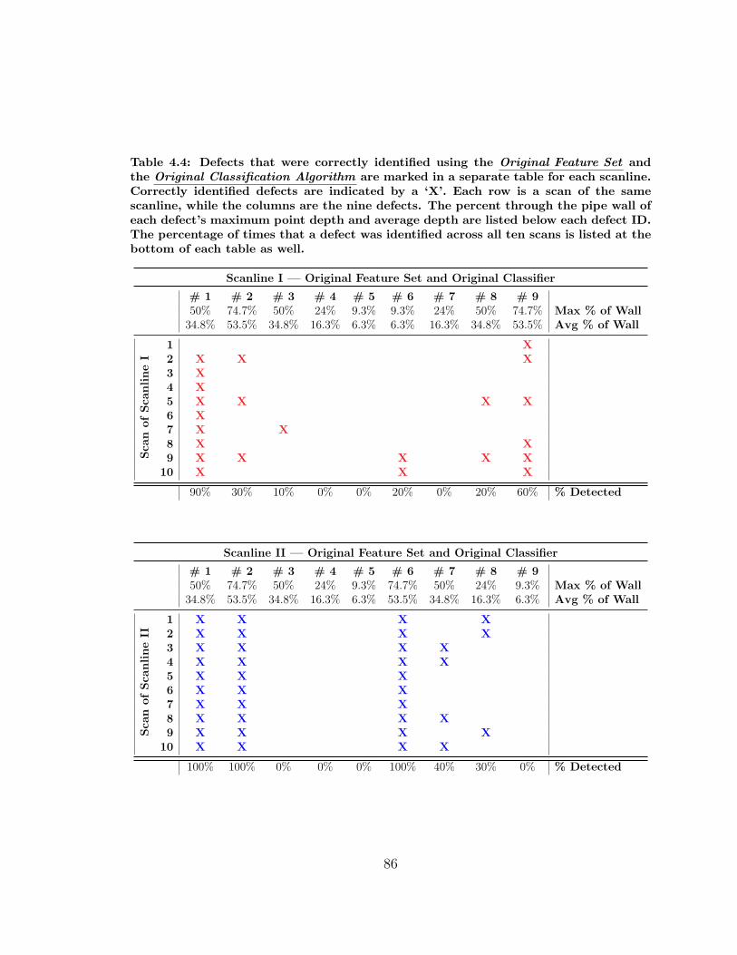
Table 4.4: Defects that were correctly identified using the Original Feature Set andthe Original Classification Algorithm are marked in a separate table for each scanline.Correctly identified defects are indicated by a ‘X’. Each row is a scan of the samescanline, while the columns are the nine defects. The percent through the pipe wall ofeach defect’s maximum point depth and average depth are listed below each defect ID.The percentage of times that a defect was identified across all ten scans is listed at thebottom of each table as well.

Scanline I — Original Feature Set and Original Classifier

# 1 # 2 # 3 # 4 # 5 # 6 # 7 # 8 # 950% 74.7% 50% 24% 9.3% 9.3% 24% 50% 74.7% Max % of Wall

34.8% 53.5% 34.8% 16.3% 6.3% 6.3% 16.3% 34.8% 53.5% Avg % of Wall

Sca

nofSca

nline

I

1 X2 X X X3 X4 X5 X X X X6 X7 X X8 X X9 X X X X X

10 X X X

90% 30% 10% 0% 0% 20% 0% 20% 60% % Detected

Scanline II — Original Feature Set and Original Classifier

# 1 # 2 # 3 # 4 # 5 # 6 # 7 # 8 # 950% 74.7% 50% 24% 9.3% 74.7% 50% 24% 9.3% Max % of Wall

34.8% 53.5% 34.8% 16.3% 6.3% 53.5% 34.8% 16.3% 6.3% Avg % of Wall

Sca

nofSca

nline

II

1 X X X X2 X X X X3 X X X X4 X X X X5 X X X6 X X X7 X X X8 X X X X9 X X X X

10 X X X X

100% 100% 0% 0% 0% 100% 40% 30% 0% % Detected

86

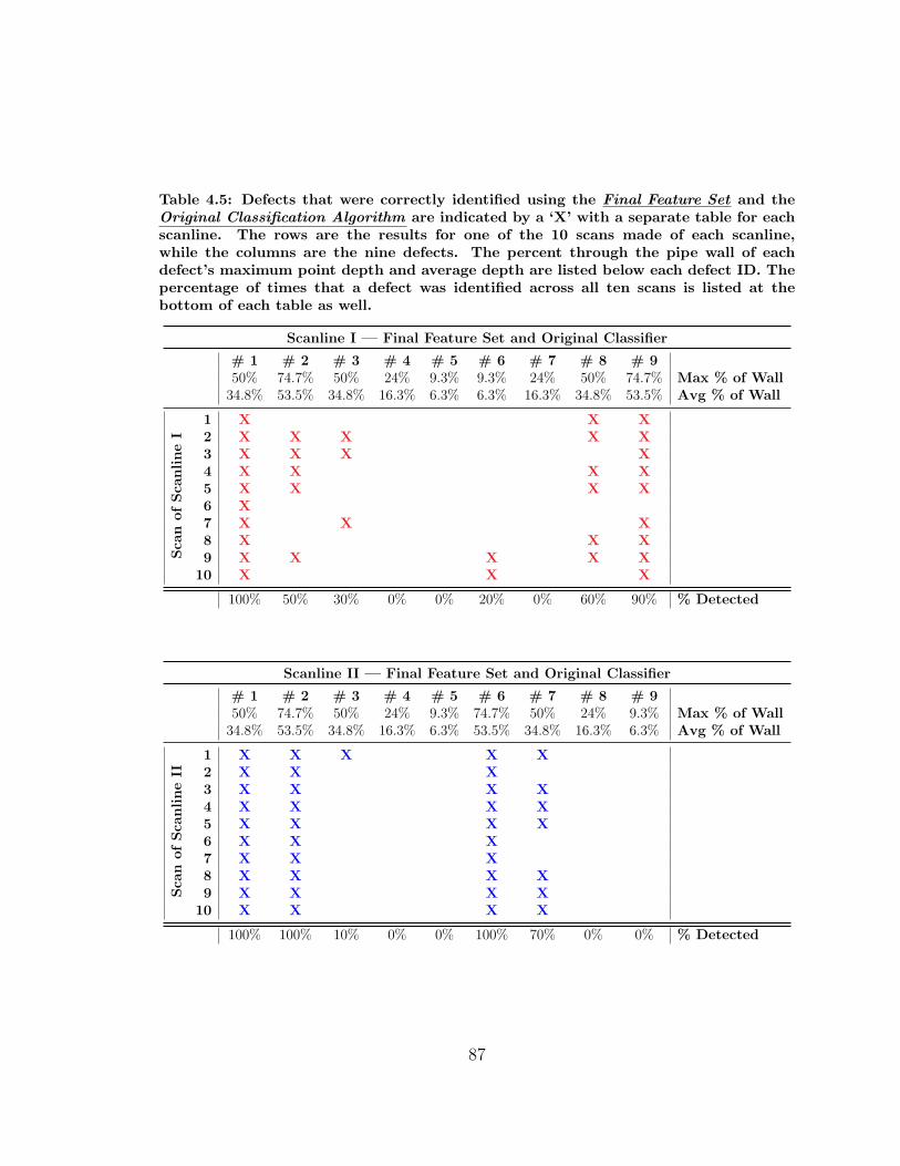
Table 4.5: Defects that were correctly identified using the Final Feature Set and theOriginal Classification Algorithm are indicated by a ‘X’ with a separate table for eachscanline. The rows are the results for one of the 10 scans made of each scanline,while the columns are the nine defects. The percent through the pipe wall of eachdefect’s maximum point depth and average depth are listed below each defect ID. Thepercentage of times that a defect was identified across all ten scans is listed at thebottom of each table as well.

Scanline I — Final Feature Set and Original Classifier

# 1 # 2 # 3 # 4 # 5 # 6 # 7 # 8 # 950% 74.7% 50% 24% 9.3% 9.3% 24% 50% 74.7% Max % of Wall

34.8% 53.5% 34.8% 16.3% 6.3% 6.3% 16.3% 34.8% 53.5% Avg % of Wall

Sca

nofSca

nline

I

1 X X X2 X X X X X3 X X X X4 X X X X5 X X X X6 X7 X X X8 X X X9 X X X X X

10 X X X

100% 50% 30% 0% 0% 20% 0% 60% 90% % Detected

Scanline II — Final Feature Set and Original Classifier

# 1 # 2 # 3 # 4 # 5 # 6 # 7 # 8 # 950% 74.7% 50% 24% 9.3% 74.7% 50% 24% 9.3% Max % of Wall

34.8% 53.5% 34.8% 16.3% 6.3% 53.5% 34.8% 16.3% 6.3% Avg % of Wall

Sca

nofSca

nline

II

1 X X X X X2 X X X3 X X X X4 X X X X5 X X X X6 X X X7 X X X8 X X X X9 X X X X

10 X X X X

100% 100% 10% 0% 0% 100% 70% 0% 0% % Detected

87

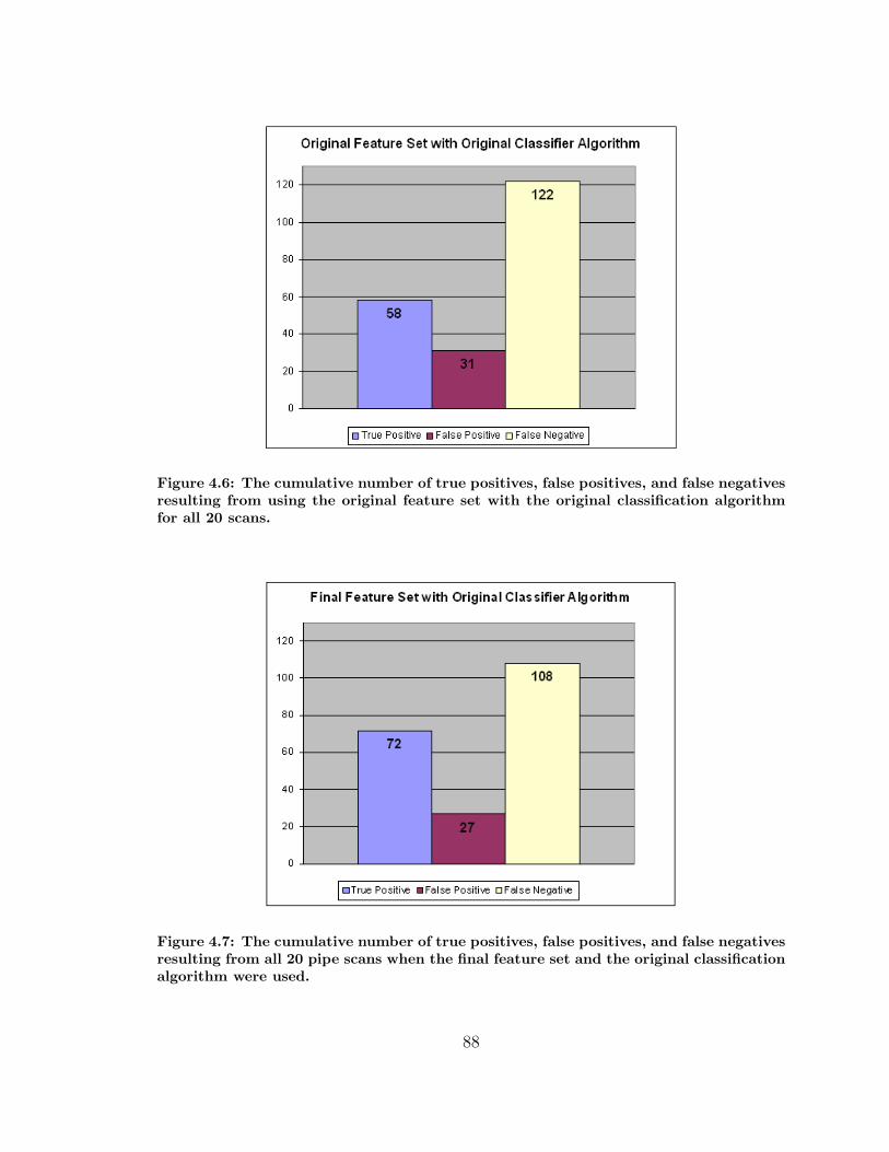
Figure 4.6: The cumulative number of true positives, false positives, and false negativesresulting from using the original feature set with the original classification algorithmfor all 20 scans.

Figure 4.7: The cumulative number of true positives, false positives, and false negativesresulting from all 20 pipe scans when the final feature set and the original classificationalgorithm were used.

88

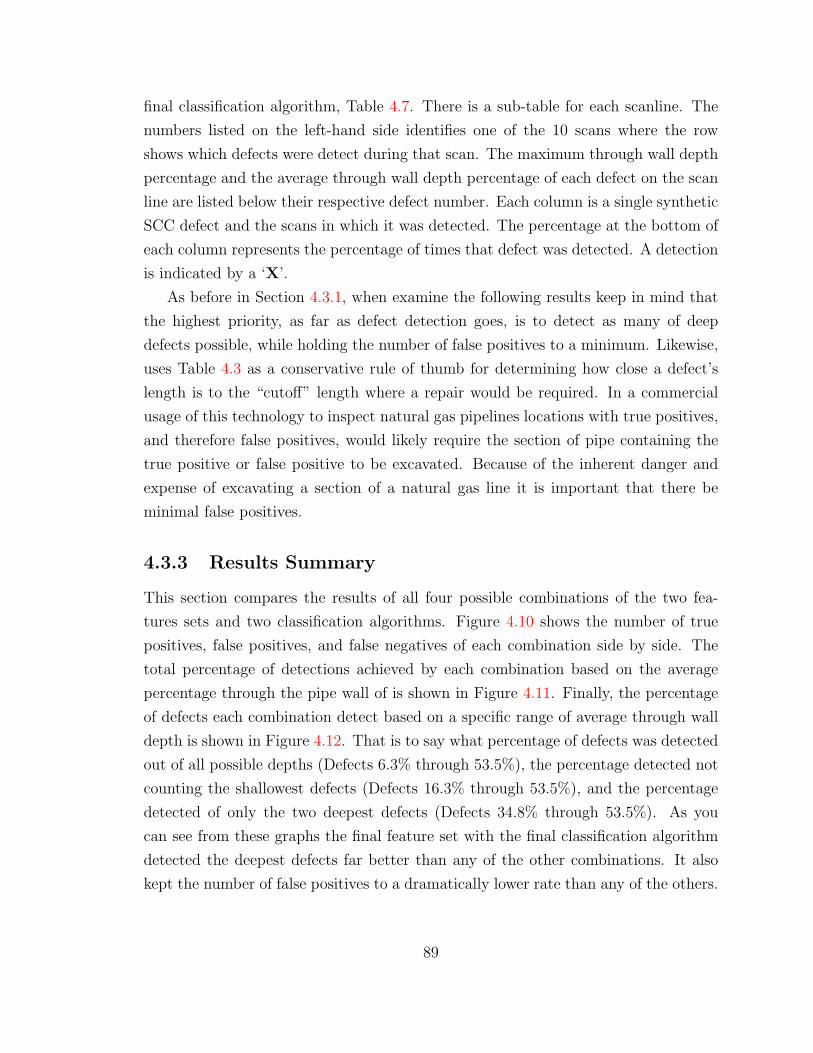
final classification algorithm, Table 4.7. There is a sub-table for each scanline. The

numbers listed on the left-hand side identifies one of the 10 scans where the row

shows which defects were detect during that scan. The maximum through wall depth

percentage and the average through wall depth percentage of each defect on the scan

line are listed below their respective defect number. Each column is a single synthetic

SCC defect and the scans in which it was detected. The percentage at the bottom of

each column represents the percentage of times that defect was detected. A detection

is indicated by a ‘X’.

As before in Section 4.3.1, when examine the following results keep in mind that

the highest priority, as far as defect detection goes, is to detect as many of deep

defects possible, while holding the number of false positives to a minimum. Likewise,

uses Table 4.3 as a conservative rule of thumb for determining how close a defect’s

length is to the “cutoff” length where a repair would be required. In a commercial

usage of this technology to inspect natural gas pipelines locations with true positives,

and therefore false positives, would likely require the section of pipe containing the

true positive or false positive to be excavated. Because of the inherent danger and

expense of excavating a section of a natural gas line it is important that there be

minimal false positives.

4.3.3 Results Summary

This section compares the results of all four possible combinations of the two fea-

tures sets and two classification algorithms. Figure 4.10 shows the number of true

positives, false positives, and false negatives of each combination side by side. The

total percentage of detections achieved by each combination based on the average

percentage through the pipe wall of is shown in Figure 4.11. Finally, the percentage

of defects each combination detect based on a specific range of average through wall

depth is shown in Figure 4.12. That is to say what percentage of defects was detected

out of all possible depths (Defects 6.3% through 53.5%), the percentage detected not

counting the shallowest defects (Defects 16.3% through 53.5%), and the percentage

detected of only the two deepest defects (Defects 34.8% through 53.5%). As you

can see from these graphs the final feature set with the final classification algorithm

detected the deepest defects far better than any of the other combinations. It also

kept the number of false positives to a dramatically lower rate than any of the others.

89

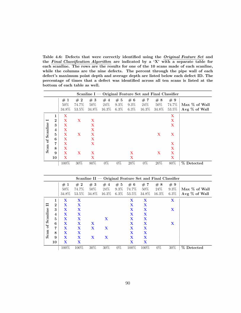
Table 4.6: Defects that were correctly identified using the Original Feature Set andthe Final Classification Algorithm are indicated by a ‘X’ with a separate table foreach scanline. The rows are the results for one of the 10 scans made of each scanline,while the columns are the nine defects. The percent through the pipe wall of eachdefect’s maximum point depth and average depth are listed below each defect ID. Thepercentage of times that a defect was identified across all ten scans is listed at thebottom of each table as well.

Scanline I — Original Feature Set and Final Classifier

# 1 # 2 # 3 # 4 # 5 # 6 # 7 # 8 # 950% 74.7% 50% 24% 9.3% 9.3% 24% 50% 74.7% Max % of Wall

34.8% 53.5% 34.8% 16.3% 6.3% 6.3% 16.3% 34.8% 53.5% Avg % of Wall

Sca

nofSca

nline

I

1 X X2 X X X X3 X X X4 X X5 X X X X X6 X X7 X X X8 X X9 X X X X X X

10 X X X X

100% 30% 80% 0% 0% 20% 0% 20% 80% % Detected

Scanline II — Original Feature Set and Final Classifier

# 1 # 2 # 3 # 4 # 5 # 6 # 7 # 8 # 950% 74.7% 50% 24% 9.3% 74.7% 50% 24% 9.3% Max % of Wall

34.8% 53.5% 34.8% 16.3% 6.3% 53.5% 34.8% 16.3% 6.3% Avg % of Wall

Sca

nofSca

nline

II

1 X X X X X2 X X X X3 X X X X X4 X X X X5 X X X X X6 X X X X X X7 X X X X X X8 X X X X9 X X X X X X

10 X X X X

100% 100% 30% 30% 0% 100% 100% 0% 30% % Detected

90

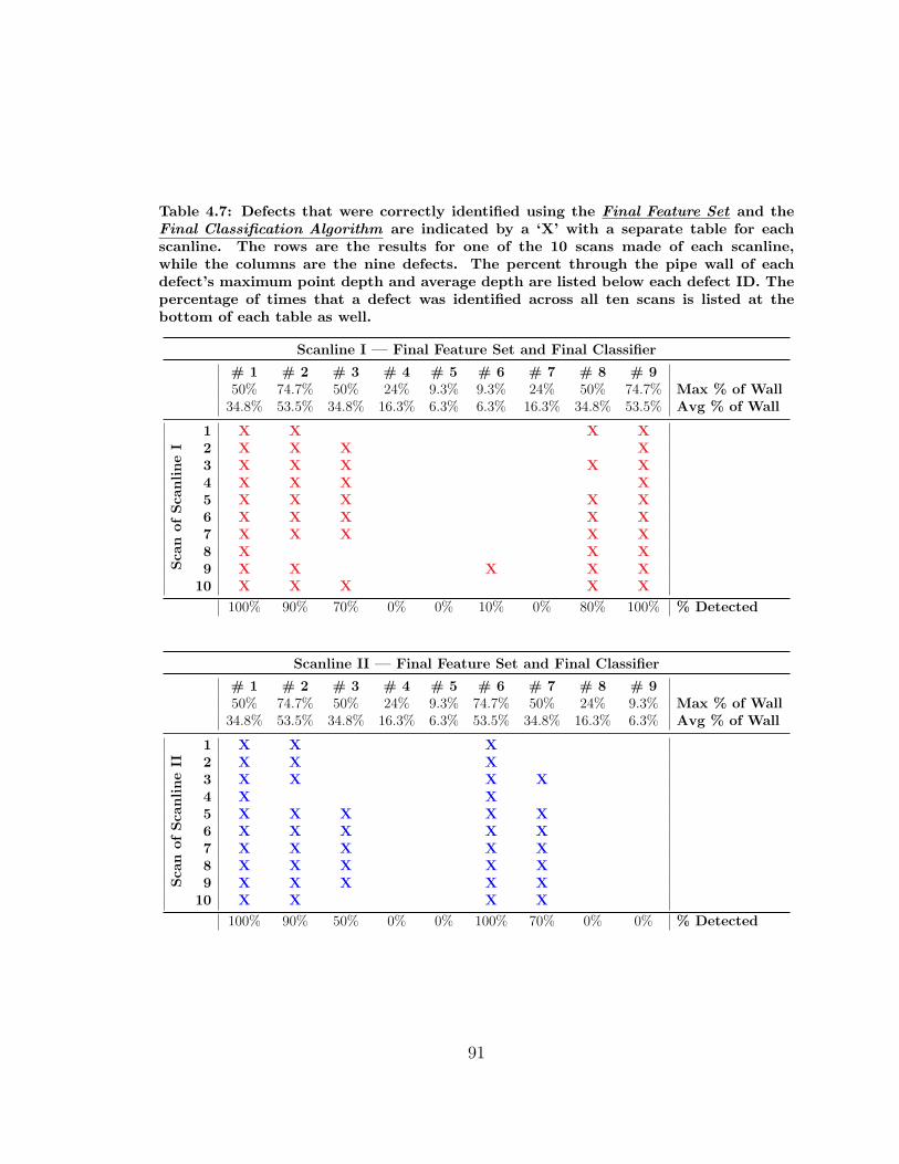
Table 4.7: Defects that were correctly identified using the Final Feature Set and theFinal Classification Algorithm are indicated by a ‘X’ with a separate table for eachscanline. The rows are the results for one of the 10 scans made of each scanline,while the columns are the nine defects. The percent through the pipe wall of eachdefect’s maximum point depth and average depth are listed below each defect ID. Thepercentage of times that a defect was identified across all ten scans is listed at thebottom of each table as well.

Scanline I — Final Feature Set and Final Classifier

# 1 # 2 # 3 # 4 # 5 # 6 # 7 # 8 # 950% 74.7% 50% 24% 9.3% 9.3% 24% 50% 74.7% Max % of Wall

34.8% 53.5% 34.8% 16.3% 6.3% 6.3% 16.3% 34.8% 53.5% Avg % of Wall

Sca

nofSca

nline

I

1 X X X X2 X X X X3 X X X X X4 X X X X5 X X X X X6 X X X X X7 X X X X X8 X X X9 X X X X X

10 X X X X X

100% 90% 70% 0% 0% 10% 0% 80% 100% % Detected

Scanline II — Final Feature Set and Final Classifier

# 1 # 2 # 3 # 4 # 5 # 6 # 7 # 8 # 950% 74.7% 50% 24% 9.3% 74.7% 50% 24% 9.3% Max % of Wall

34.8% 53.5% 34.8% 16.3% 6.3% 53.5% 34.8% 16.3% 6.3% Avg % of Wall

Sca

nofSca

nline

II

1 X X X2 X X X3 X X X X4 X X5 X X X X X6 X X X X X7 X X X X X8 X X X X X9 X X X X X

10 X X X X

100% 90% 50% 0% 0% 100% 70% 0% 0% % Detected

91

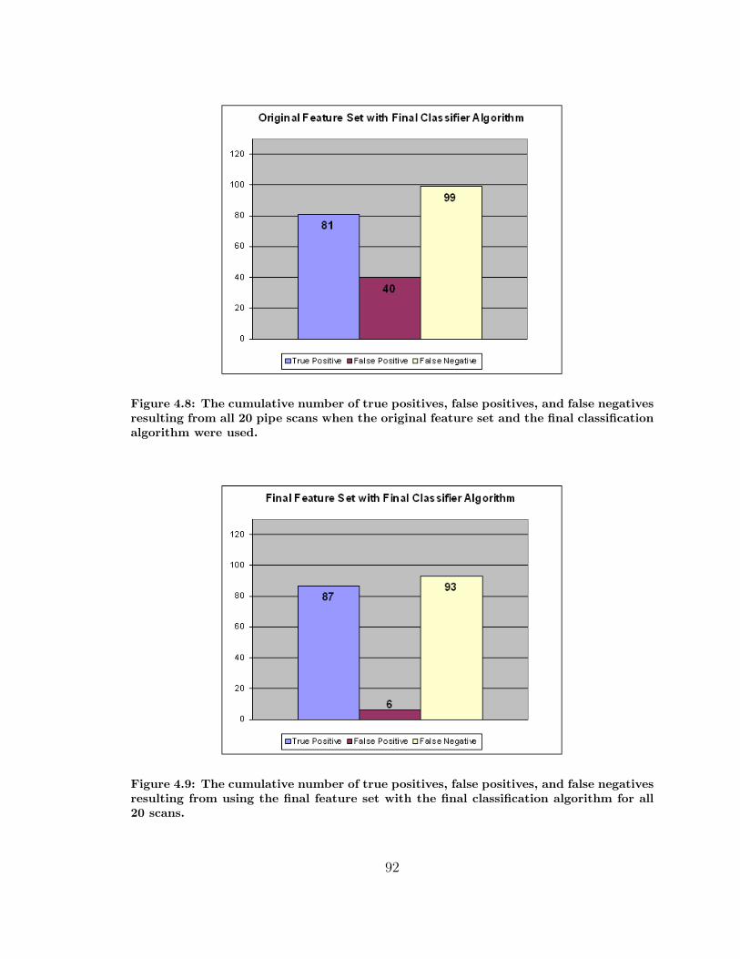
Figure 4.8: The cumulative number of true positives, false positives, and false negativesresulting from all 20 pipe scans when the original feature set and the final classificationalgorithm were used.

Figure 4.9: The cumulative number of true positives, false positives, and false negativesresulting from using the final feature set with the final classification algorithm for all20 scans.

92

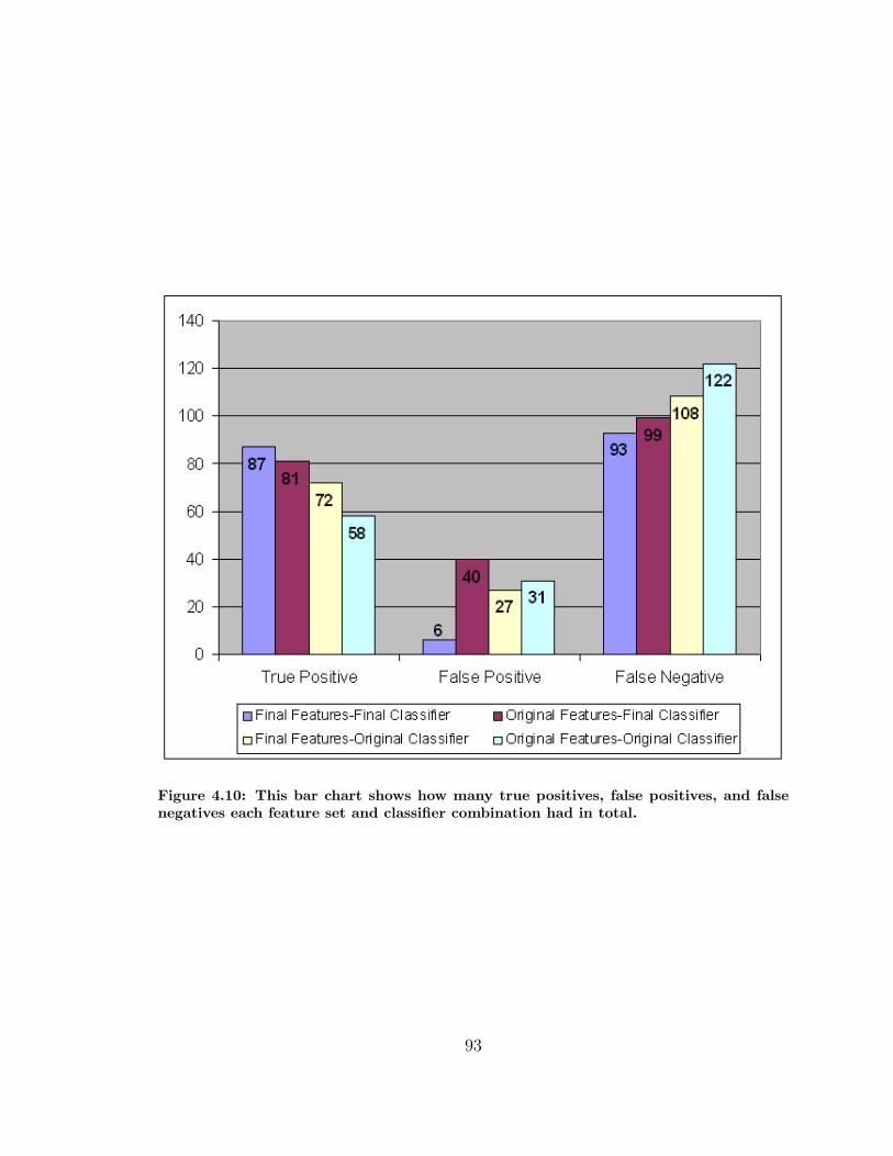
Figure 4.10: This bar chart shows how many true positives, false positives, and falsenegatives each feature set and classifier combination had in total.

93

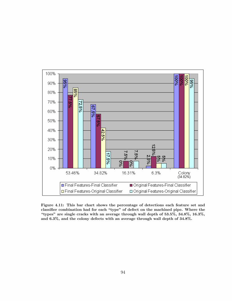
Figure 4.11: This bar chart shows the percentage of detections each feature set andclassifier combination had for each “type” of defect on the machined pipe. Where the“types” are single cracks with an average through wall depth of 53.5%, 34.8%, 16.3%,and 6.3%, and the colony defects with an average through wall depth of 34.8%.

94

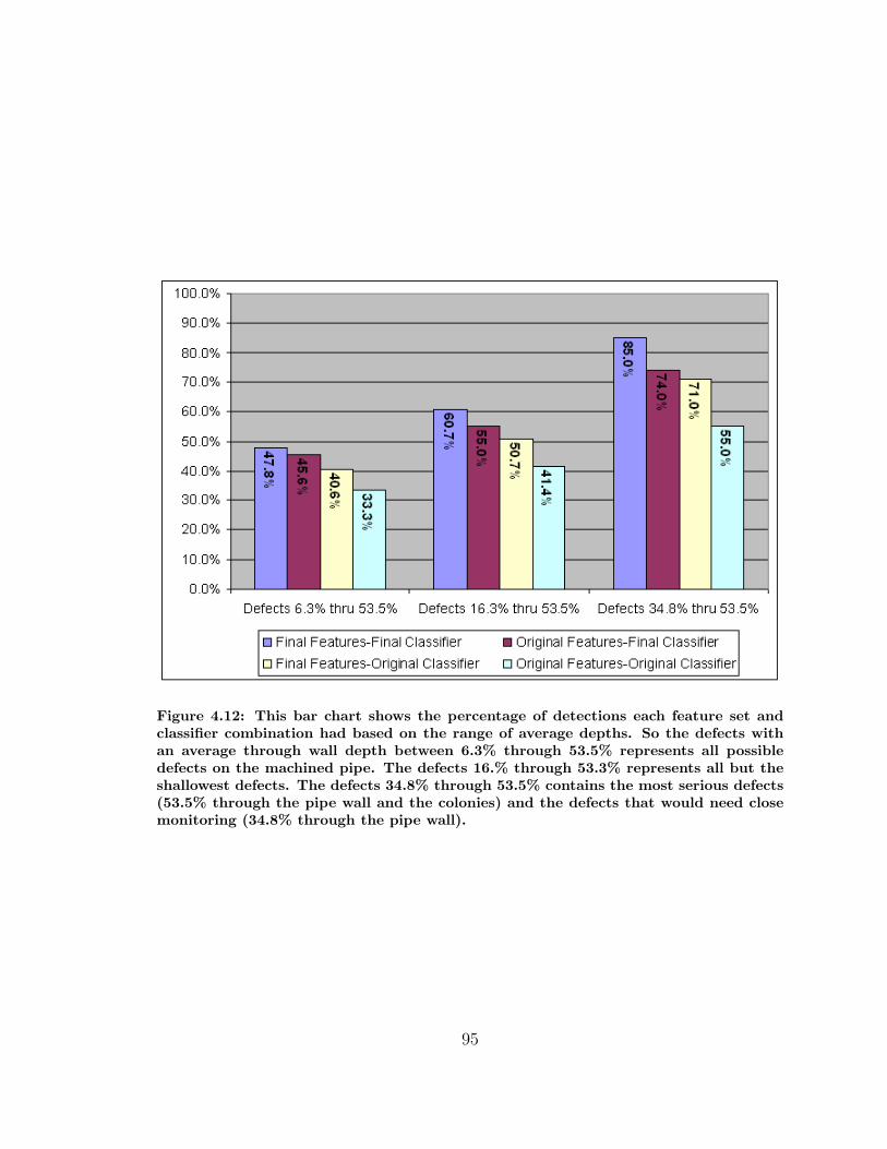
Figure 4.12: This bar chart shows the percentage of detections each feature set andclassifier combination had based on the range of average depths. So the defects withan average through wall depth between 6.3% through 53.5% represents all possibledefects on the machined pipe. The defects 16.% through 53.3% represents all but theshallowest defects. The defects 34.8% through 53.5% contains the most serious defects(53.5% through the pipe wall and the colonies) and the defects that would need closemonitoring (34.8% through the pipe wall).

95

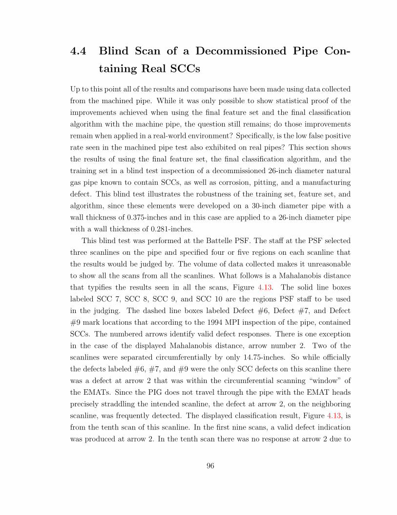
4.4 Blind Scan of a Decommissioned Pipe Con-

taining Real SCCs

Up to this point all of the results and comparisons have been made using data collected

from the machined pipe. While it was only possible to show statistical proof of the

improvements achieved when using the final feature set and the final classification

algorithm with the machine pipe, the question still remains; do those improvements

remain when applied in a real-world environment? Specifically, is the low false positive

rate seen in the machined pipe test also exhibited on real pipes? This section shows

the results of using the final feature set, the final classification algorithm, and the

training set in a blind test inspection of a decommissioned 26-inch diameter natural

gas pipe known to contain SCCs, as well as corrosion, pitting, and a manufacturing

defect. This blind test illustrates the robustness of the training set, feature set, and

algorithm, since these elements were developed on a 30-inch diameter pipe with a

wall thickness of 0.375-inches and in this case are applied to a 26-inch diameter pipe

with a wall thickness of 0.281-inches.

This blind test was performed at the Battelle PSF. The staff at the PSF selected

three scanlines on the pipe and specified four or five regions on each scanline that

the results would be judged by. The volume of data collected makes it unreasonable

to show all the scans from all the scanlines. What follows is a Mahalanobis distance

that typifies the results seen in all the scans, Figure 4.13. The solid line boxes

labeled SCC 7, SCC 8, SCC 9, and SCC 10 are the regions PSF staff to be used

in the judging. The dashed line boxes labeled Defect #6, Defect #7, and Defect

#9 mark locations that according to the 1994 MPI inspection of the pipe, contained

SCCs. The numbered arrows identify valid defect responses. There is one exception

in the case of the displayed Mahalanobis distance, arrow number 2. Two of the

scanlines were separated circumferentially by only 14.75-inches. So while officially

the defects labeled #6, #7, and #9 were the only SCC defects on this scanline there

was a defect at arrow 2 that was within the circumferential scanning “window” of

the EMATs. Since the PIG does not travel through the pipe with the EMAT heads

precisely straddling the intended scanline, the defect at arrow 2, on the neighboring

scanline, was frequently detected. The displayed classification result, Figure 4.13, is

from the tenth scan of this scanline. In the first nine scans, a valid defect indication

was produced at arrow 2. In the tenth scan there was no response at arrow 2 due to

96

the orientation of the EMATs with respect to the scanline being slightly different. All

other responses in the displayed scan are typical of the nine other scans. After the

results of the blind inspection were released a follow-up trip to the Battelle PSF was

made specifically to visually re-inspecting and document the size, type, and location

of defects on the pipe. Additionally, all the locations that corresponded to a defect

response in the Mahalanobis distance were inspected. This was done to allow us to

determine a possible source for what at the time was thought to be an unacceptably

high number of false positives. It turned out that there was not a false positive

problem, instead the systems ability to detect multiple types of flaws was proven‡.

Figures 4.14 through Figure 4.25 are the pictures taken corresponding to each arrow

and defect in Figure 4.13. The caption of each image list the defect or arrow label

of the corresponding defect response in the Mahalanobis distance and the type of

defect(s) present, along with any significant additional information regarding that

defect(s).

‡Until this blind test, all of the decommissioned pipe sections that had been scanned had containedonly SCCs and some very minor corrosion. This decommissioned pipe section was the first to containSCCs and significant corrosion and pitting.

97

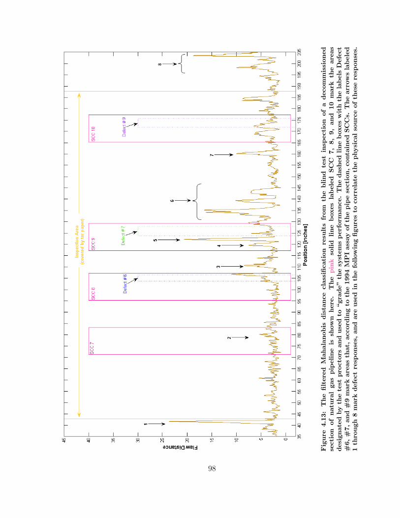
Fig

ur e

4.13

:T

he

filt

ered

Mah

alan

obis

dis

tance

clas

sifica

tion

resu

lts

from

the

blind

test

insp

ecti

onof

adec

omm

issi

oned

sect

ion

ofnat

ura

lga

spip

elin

eis

show

nher

e.T

he

pin

kso

lid

line

box

esla

bel

edSC

C7,

8,9,

and

10m

ark

the

area

sdes

ignat

edby

the

test

pro

ctor

san

duse

dto

“gr

ade”

the

syst

ems

per

form

ance

.T

he

das

hed

line

box

esw

ith

the

label

sD

efec

t#

6,#

7,an

d#

9m

ark

area

sth

at,ac

cord

ing

toth

e19

94M

PI

assa

yof

the

pip

ese

ctio

n,co

nta

ined

SC

Cs.

The

arro

ws

label

ed1

thro

ugh

8m

ark

def

ect

resp

onse

s,an

dar

euse

din

the

follow

ing

figu

res

toco

rrel

ate

the

physi

calso

urc

eof

thes

ere

spon

ses.

98

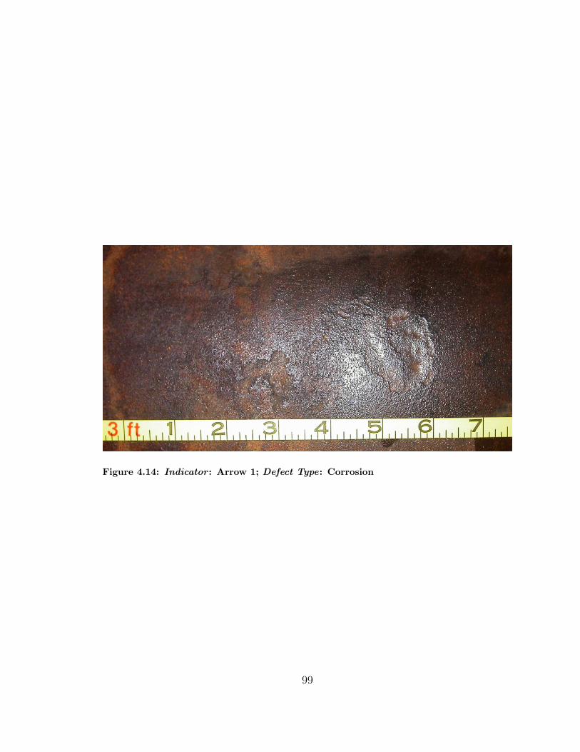
Figure 4.14: Indicator : Arrow 1; Defect Type: Corrosion

99

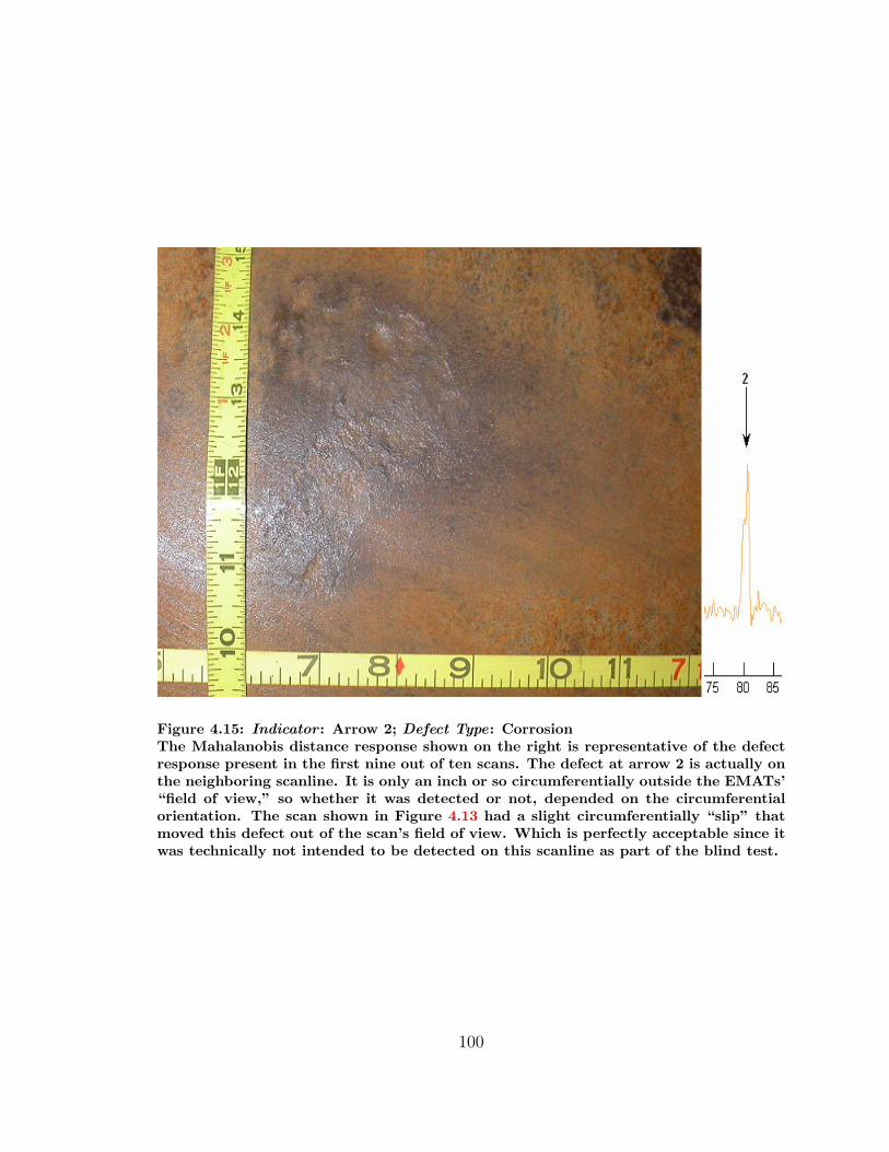
Figure 4.15: Indicator : Arrow 2; Defect Type: CorrosionThe Mahalanobis distance response shown on the right is representative of the defectresponse present in the first nine out of ten scans. The defect at arrow 2 is actually onthe neighboring scanline. It is only an inch or so circumferentially outside the EMATs’“field of view,” so whether it was detected or not, depended on the circumferentialorientation. The scan shown in Figure 4.13 had a slight circumferentially “slip” thatmoved this defect out of the scan’s field of view. Which is perfectly acceptable since itwas technically not intended to be detected on this scanline as part of the blind test.

100

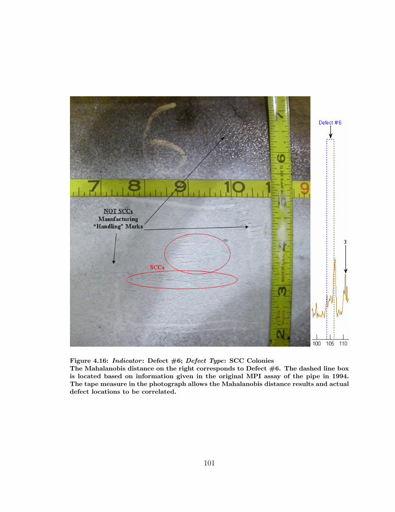
Figure 4.16: Indicator : Defect #6; Defect Type: SCC ColoniesThe Mahalanobis distance on the right corresponds to Defect #6. The dashed line boxis located based on information given in the original MPI assay of the pipe in 1994.The tape measure in the photograph allows the Mahalanobis distance results and actualdefect locations to be correlated.

101

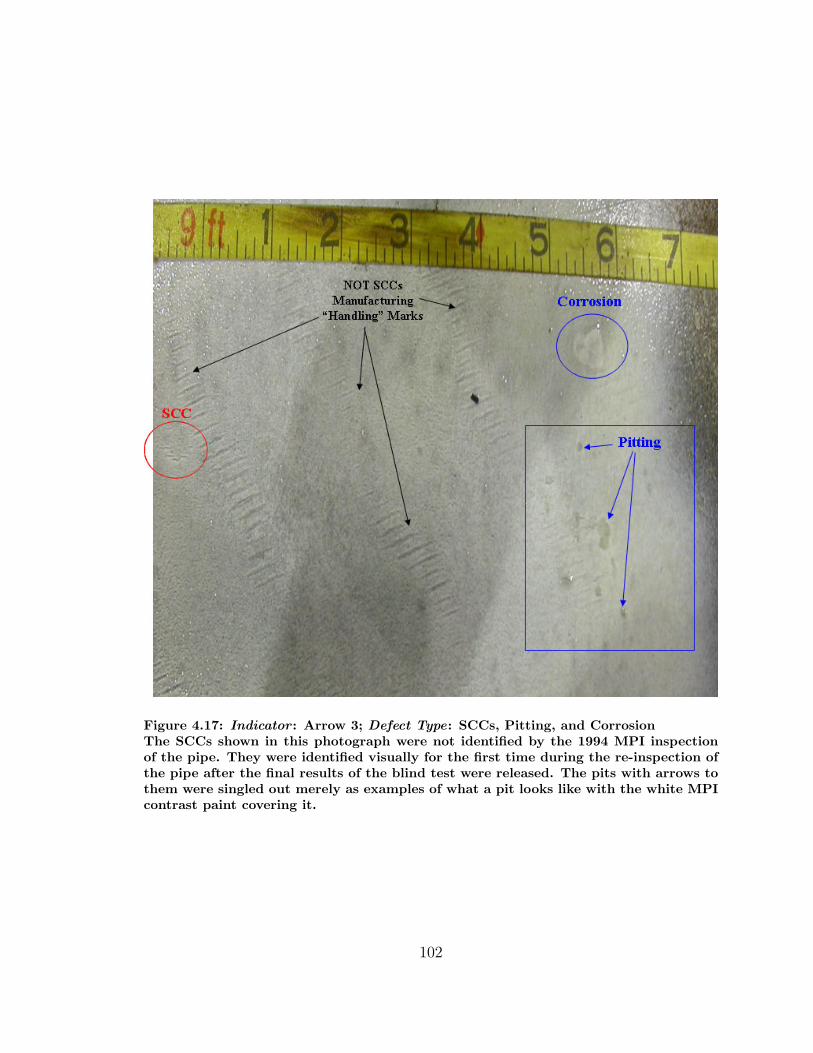
Figure 4.17: Indicator : Arrow 3; Defect Type: SCCs, Pitting, and CorrosionThe SCCs shown in this photograph were not identified by the 1994 MPI inspectionof the pipe. They were identified visually for the first time during the re-inspection ofthe pipe after the final results of the blind test were released. The pits with arrows tothem were singled out merely as examples of what a pit looks like with the white MPIcontrast paint covering it.

102

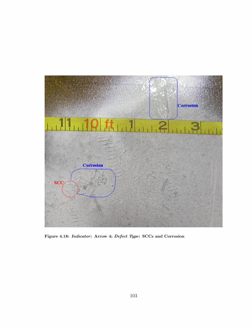
Figure 4.18: Indicator : Arrow 4; Defect Type: SCCs and Corrosion

103

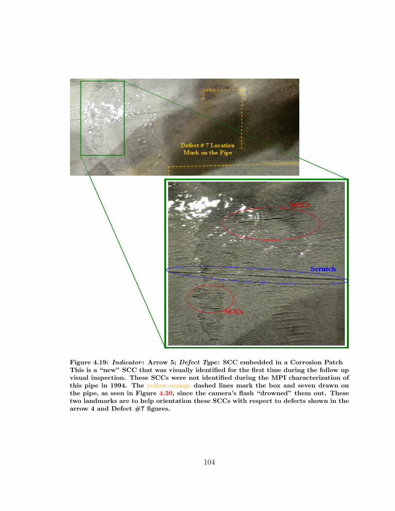
Figure 4.19: Indicator : Arrow 5; Defect Type: SCC embedded in a Corrosion PatchThis is a “new” SCC that was visually identified for the first time during the follow upvisual inspection. These SCCs were not identified during the MPI characterization ofthis pipe in 1994. The yellow-orange dashed lines mark the box and seven drawn onthe pipe, as seen in Figure 4.20, since the camera’s flash “drowned” them out. Thesetwo landmarks are to help orientation these SCCs with respect to defects shown in thearrow 4 and Defect #7 figures.

104

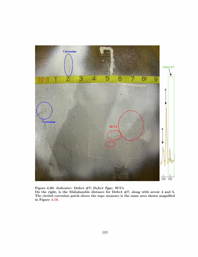
Figure 4.20: Indicator : Defect #7; Defect Type: SCCsOn the right, is the Mahalanobis distance for Defect #7, along with arrow 4 and 5.The circled corrosion patch above the tape measure is the same area shown magnifiedin Figure 4.19.

105

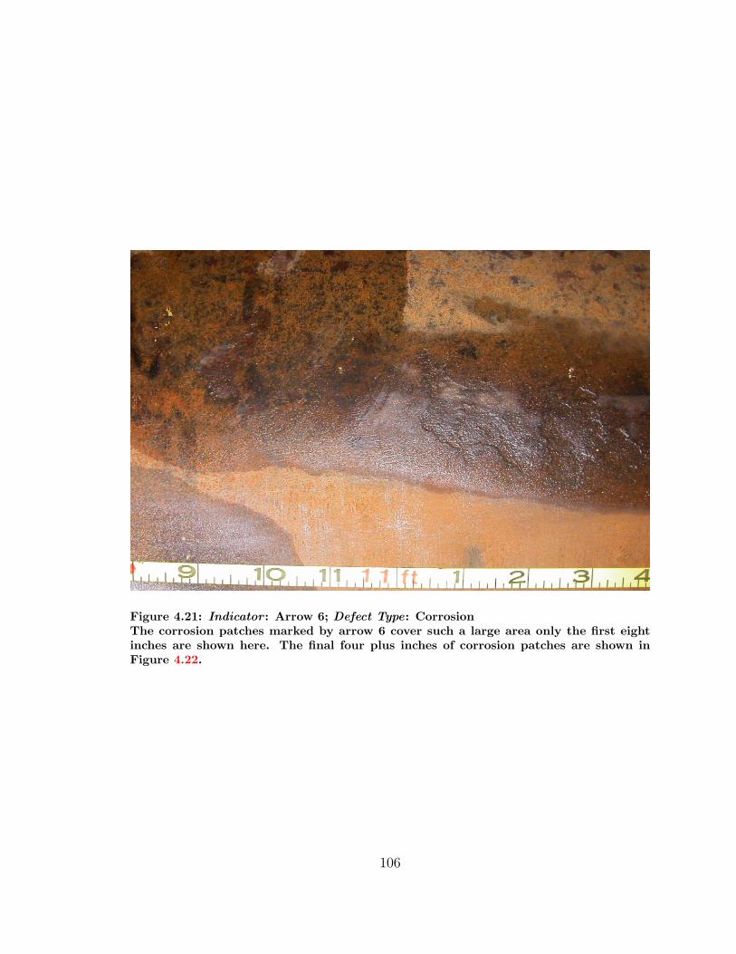
Figure 4.21: Indicator : Arrow 6; Defect Type: CorrosionThe corrosion patches marked by arrow 6 cover such a large area only the first eightinches are shown here. The final four plus inches of corrosion patches are shown inFigure 4.22.

106

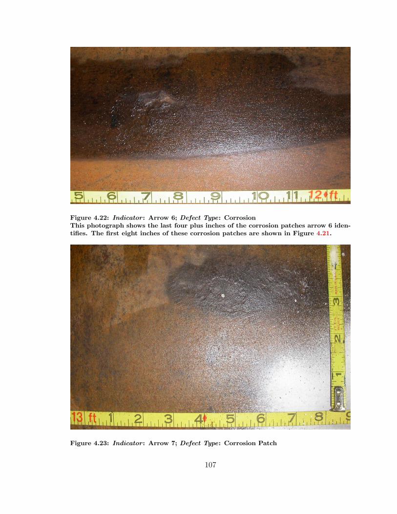
Figure 4.22: Indicator : Arrow 6; Defect Type: CorrosionThis photograph shows the last four plus inches of the corrosion patches arrow 6 iden-tifies. The first eight inches of these corrosion patches are shown in Figure 4.21.

Figure 4.23: Indicator : Arrow 7; Defect Type: Corrosion Patch

107

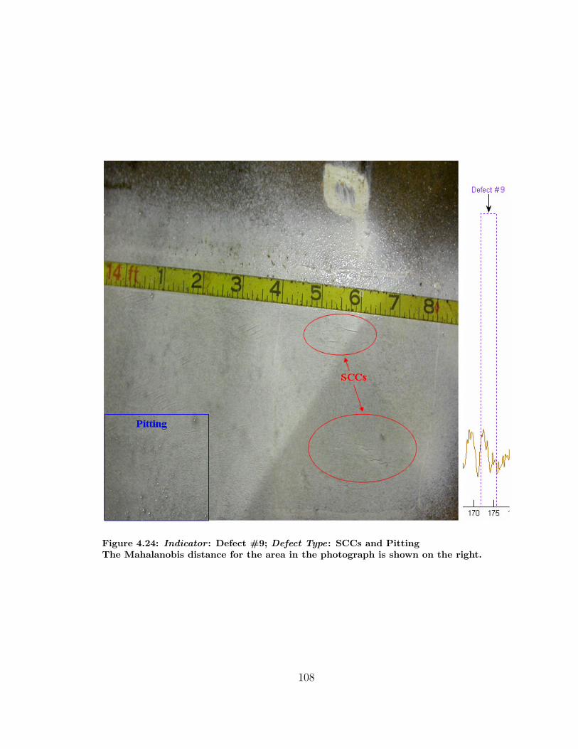
Figure 4.24: Indicator : Defect #9; Defect Type: SCCs and PittingThe Mahalanobis distance for the area in the photograph is shown on the right.

108

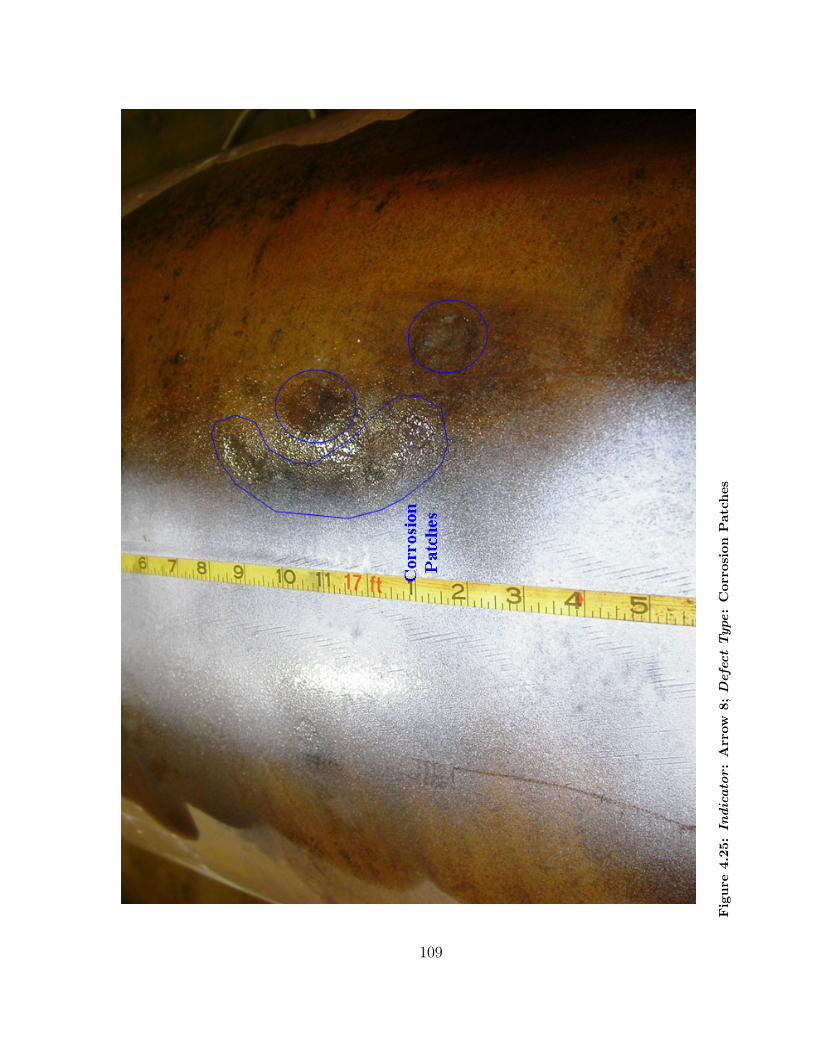
Fig

ure

4.25

:In

dic

ato

r:

Arr

ow8;

Defe

ctType:

Cor

rosi

onPat

ches

109

Chapter 5

Conclusions

While there has been a notable increase in research to develop a means for detecting

SCCs in natural gas pipelines there are still significant challenges facing this research,

such as overcoming the attenuation the protective coating on buried pipes causes.

However, through the research presented in this thesis a method which overcomes the

foremost challenge of simply detecting SCCs using non-contact, ultrasonic inspection

while moving was presented. There is still plenty of room for further improvement, but

a foundation is firmly in place. While most of the results shown in this thesis focus on

synthetic SCCs in a clean, unused pipe, the majority of this research was performed

using data collected from decommissioned pipe containing real SCCs. The results

from the experiments involving real SCC samples are far more difficult to objectively

quantify due to the uncertainty associated with these decommissioned pipe sections.

This same uncertainty prevented a training set from being formed using natural SCCs.

Before the training set created from the parabolic cuts on machined pipe, there was

not a single “good” set that produced repeatable, believable∗ results on a pipe other

than the one it was created from. However, the training set constructed from the

machined pipe has been successfully used on 30-inch diameter pipes with different

wall thickness from the machined pipe as well as on 26-inch diameter pipes with wall

thicknesses different from that of the machined pipe. Formerly, having a “good” set

that performed the same for all the scanlines on the same piece of pipe the set was

created from was a rare event. Also, using PCA+LDA has significantly improved the

discernibility of both synthetic and real SCC. Primarily by suppressing the responses

∗Sometimes there would not be a single defect response in an entire Mahalanobis distance resultor everything would produce a defect response; so the results were not believable.

110

generated by metallurgic variations and small changes in gap between the EMAT

and the pipe wall. The system has detected 100% of the synthetic colony SCCs with

an average volume of missing material equaling only 0.0039 cubic inches, 95% of the

synthetic single crack SCCs with an average volume of missing material equaling a

mere 0.0024 cubic inches, and 67.5% of the synthetic SCCs with an average volume

of missing material equal to just 0.0014 cubic inches!

5.1 Future Work

As with any experimental system with the goal of making a classification, the clas-

sification is only as good as the feature set and therefore by association in this case

the training set. The final feature set does not take advantage of any phase or fre-

quency information. While some investigations into at least simple frequency base

features was done and in the end were found to be detrimental to the classification,

there is likely beneficial information in the frequency domain. In particular, a feature

utilizing phase in some way or another may hold potential. Of the existing features,

the quality/benefit of the point-by-point Mahalanobis distance squared feature is

still something of a question. In a quick test using the final classification algorithm

the final feature set was used with and without the point-by-point Mahalanobis dis-

tance squared features. The classification results were better when the point-by-point

Mahalanobis distance squared features were included. At the time these test were

enough to continue using the point-by-point Mahalanobis distance squared features,

but a more thorough investigation would be beneficial.

Since nearly all SCCs which would require repair or heightened monitoring can be

detected this research is ready for the next big step. The next significant goal is two

equally important items; the ability to distinguish between types of defects and the

ability to objectively determine at least crack length and ideally crack depth (max-

imum depth, average depth, or both). The ability to distinguish types of defects is

important and necessary advancement for the system. When the final feature set and

final classification algorithm were used to perform a blind inspection of a decommis-

sioned section of 26-inch diameter natural gas pipeline, as shown in Section 4.4,defect

responses were produced that corresponded in every instance to an actual defect on

the pipe. The caveat however is that the sources of the defect responses are not lim-

ited to just SCCs, but include corrosion and pitting. The ability to detect all types of

111

defects is a desired outcome, since only the ability to use just one inspection tool to

inspect for all major pipe integrity issues is highly desired by the pipeline industry.

But without the ability to separate the major types of defects and some measure of

either the volume of missing material or the maximum depth and length of a defect,

the remaining life of the pipe and priority for repair cannot be determined.

The classification results from using the original feature set and the original classi-

fier were so inconsistent that there was no possibility of automating the identification

of defect responses. However, with the improvements yielded by the combination of

the final feature set and the final classification algorithm, the results have consistent

behavior that could be used to automate the identification of defects responses and

include the ability to disregard anomaly responses. This would be very beneficial,

ideally eliminating the need for a highly experienced person to visually identify de-

fect responses from anomaly response. This would also greatly reduce the amount of

time needed for this task.

112

Bibliography

113

Bibliography

[1] Energy Information Administration. Annual Energy Review 2006. Tech.

Rep. DOE/EIA-0384(2006), Energy Information Administration (EIA), June

2007. URL: http://tonto.eia.doe.gov/FTPROOT/multifuel/038406.pdf; Re-

leased: June 27, 2007; Next Update: June 2008.

[2] Office of Pipeline Safety. 2005 Transmission Annuals Data. Electronic Data

Files, June 2006. URL: http://ops.dot.gov/stats/DT98.htm.

[3] Eiber, R. J. and Kiefner, J. F. Failure Analysis and Prevention. ASM Handbook,

vol. 11, 2002.

[4] Michael Baker Jr., I. Stress Corrosion Cracking Study. Tech. Rep. Integrity

Management Program, Report TTO Number 8, Delivery Order DTRS56-02-D-

70036, Department of Transportation, Office of Pipeline Safety, January 2005.

[5] Magnaflux. Innovations: A Timeline. Website. URL: http://www.magnaflux.

com/overview/timeline.stm, accessed Jan 11, 2007.

[6] Magnaflux. 7HF Black/9CM Red Visible Magnetic Particle Wet

Method Prepared Bath. Product Data Sheet, April 2003. URL:

http://www.magnaflux.com/files/library/pds/material product data sheets/

Magnaflux∼reg 7HF∼9CM Wet Method Visible Prepared Bath.pdf, accessed

Jan 11, 2007.

[7] Magnaflux. 14AM, 14A Aqua-Glo, 14A Redi-Bath, 20B Fluorescent Mag-

netic Particle Prepared Bath. Product Data Sheet, July 2004. URL:

http://www.magnaflux.com/files/library/pds/material product data sheets/

Magnaglo∼reg 14AM 14A Aqua-Glo 14A Redi-Bath 20B.pdf, accessed Jan 11,

2007.

114

http://tonto.eia.doe.gov/FTPROOT/multifuel/038406.pdf

http://ops.dot.gov/stats/DT98.htm

http://www.magnaflux.com/overview/timeline.stm

http://www.magnaflux.com/overview/timeline.stm

http://www.magnaflux.com/files/library/pds/material_product_data_sheets/Magnaflux~reg_7HF~9CM_Wet_Method_Visible_Prepared_Bath.pdf

http://www.magnaflux.com/files/library/pds/material_product_data_sheets/Magnaflux~reg_7HF~9CM_Wet_Method_Visible_Prepared_Bath.pdf

http://www.magnaflux.com/files/library/pds/material_product_data_sheets/Magnaglo~reg_14AM_14A_Aqua-Glo_14A_Redi-Bath_20B.pdf

http://www.magnaflux.com/files/library/pds/material_product_data_sheets/Magnaglo~reg_14AM_14A_Aqua-Glo_14A_Redi-Bath_20B.pdf

[8] Jiles, D. C. Review of magnetic methods for nondestructive evaluation (Part 2).

NDT International, vol. 23, no. 2, pp. 83–92, April 1990. Formerly known as

Non-Destructive Testing; Continued as NDT & E International.

[9] Iowa State University. Pipeline Inspection. Website, May 2003. URL:

http://www.ndt-ed.org/AboutNDT/SelectedApplications/PipelineInspection/

PipelineInspection.htm, accessed Feb 21, 2007.

[10] Iowa State University. Portable Magnetizing Equipment for Magnetic

Particle Inspection. Website, April 2003. URL: http://www.ndt-ed.

org/EducationResources/CommunityCollege/MagParticle/Equipment/

EquipmentPortable.htm, accessed Jan 11, 2007.

[11] Clark, T. and Nestleroth, B. Gas Pipeline Pigability. Topical Report. OSTI ID:

826134, Battelle for the Department of Energy, Columbus, OH, April 2004.

[12] Nestleroth, J. B. and Bubenik, T. A. Magnetic Flux Leakage (MFL) Technol-

ogy For Natural Gas Pipeline Inspection. Tech. Rep., February 1999. URL:

http://www.battelle.org/pipetechnology/MFL/MFL98Main.html; for The Gas

Research Institute (GRI).

[13] ROSEN. Corrosion Detection Pig (CDP). Website. URL: http:

//www.roseninspection.net/RosenInternet/InspectionServices/ILInspection/

MagneticFlux/CDP/, accessed Mar 3, 2007.

[14] Iowa State University. Magnetic Field Orientation and Flaw Detectability.

Website, September 2006. URL: http://www.ndt-ed.org/EducationResources/

CommunityCollege/MagParticle/Physics/FieldOrientation.htm, accessed Feb

23, 2007.

[15] Nestleroth, J. B. and Bubenik, T. A. MFL Tutorial. Tech. Rep., Octo-

ber 2000. URL: http://www.battelle.org/pipetechnology/MFL/Links/tutorial1.

html?; Created as aid for the Magnetic Flux Leakage (MFL) Technology For

Natural Gas Pipeline Inspection report.

[16] Hirao, M. and Ogi, H. SH-wave EMAT technique for gas pipeline inspection.

NDT & E International, vol. 32, no. 3, pp. 127–132, Apr 1999.

115

http://www.ndt-ed.org/AboutNDT/SelectedApplications/PipelineInspection/PipelineInspection.htm

http://www.ndt-ed.org/AboutNDT/SelectedApplications/PipelineInspection/PipelineInspection.htm

http://www.ndt-ed.org/EducationResources/CommunityCollege/MagParticle/Equipment/EquipmentPortable.htm



http://www.battelle.org/pipetechnology/MFL/MFL98Main.html

http://www.roseninspection.net/RosenInternet/InspectionServices/ILInspection/MagneticFlux/CDP/



http://www.ndt-ed.org/EducationResources/CommunityCollege/MagParticle/Physics/FieldOrientation.htm

http://www.ndt-ed.org/EducationResources/CommunityCollege/MagParticle/Physics/FieldOrientation.htm

http://www.battelle.org/pipetechnology/MFL/Links/tutorial1.html?

http://www.battelle.org/pipetechnology/MFL/Links/tutorial1.html?

[17] Luo, W. and Rose, J. Guided wave thickness measurement with EMATs. Insight:

Non-Destructive Testing and Condition Monitoring, vol. 45, no. 11, pp. 735–739,

November 2003.

[18] Tucker Jr., R. W., Kercel, S. W., and Varma, V. K. Characterization of Gas

Pipeline Flaws using Wavelet Analysis. In: Proceedings of SPIE, vol. 5132, pp.

485–493. Gatlinburg, TN, United States, 2003.

[19] Thurston, R. N. and Pierce, A. D. (editors). Ultrasonic Measurement Methods,

Physical Acoustics, vol. 19. New York: Academic Press, 1990.

[20] Harkins, W. Ultrasonic Testing of Aerospace Materials. Tech. Rep., Mar-

shall Space Flight Center, February 1999. URL: http://www.nasa.gov/offices/

oce/llis/0765.html; NASA Engineering Network, Public Lessons Learned Entry:

0765.

[21] Kercel, S. W., Tucker Jr., R. W., and Varma, V. K. Pipeline Flaw Detection

with Wavelet Packets and GAs. In: Proceedings of SPIE - The International

Society for Optical Engineering, vol. 5103, pp. 217–226. Orlando, FL, United

States, 2003.

[22] Datel, Inc. PCI-417 Series Advanced Performance Analog Boards for Desktop

PCI Bus Computers. Manual., 2003. Note: All Datel data acquisition products

discontinued as of Sep. 30, 2004.

[23] Instruments, M. TB-1000 Gated Amplifier/Receiver Plug-In Card. Tech. Rep.,

2002. URL: http://www.matec.com/mindt/products/pc cards/tb-1000/; Ac-

cessed Jan 11, 2007.

[24] Sigmund, J. A,B,C’s of Ultrasonics. PowerPoint Presentation, 2001. URL:

http://www.sonix.com/learning/ultrasonics.php3, accessed February 10, 2007.

[25] Kercel, S. W., Klein, M. B., and Pouet, B. In-Process Detection of Weld De-

fects using Laser-Based Ultrasonic Lamb Waves. Technical Report. ORNL/TM-

2000/346, Oak Ridge National Laboratory, Oak Ridge, TN, November 2000.

[26] Akansu, A. N. and Haddad, R. A. Multiresolution Signal Decomposition: Trans-

forms, Subbands, Wavelets. 1st edn. Academic Press, 1992.

116

http://www.nasa.gov/offices/oce/llis/0765.html

http://www.nasa.gov/offices/oce/llis/0765.html

http://www.matec.com/mindt/products/pc_cards/tb-1000/

http://www.sonix.com/learning/ultrasonics.php3

[27] Duda, R. O., Hart, P. E., and Stork, D. G. Pattern Classification. 2nd edn. New

York: John Wiley & Sons, Inc., 2001.

[28] Zhao, J., Wang, G.-Y., Wu, Z.-F., et al. The Study on Technologies for Feature

Selection. In: Proceedings of 2002 International Conference on Machine Learning

and Cybernetics, vol. 2, pp. 689–693. Beijing, China, 2002.

[29] Guyon, I. and Elisseeff, A. An Introduction to Variable and Feature Selection.

Journal of Machine Learning Research, vol. 3, pp. 1157–1182, 2003.

[30] Bubenik, T., Nestleroth, J., Davis, R., et al. In-Line Inspection Technologies

for Mechanical Damage and SCC in Pipelines - Final Report. Report. DTRS56-

96-C-0010, U.S. Department of Transportation, Office of Pipeline Safety, June

2000.

[31] Hubert, C. J. Applied Discriminant Analysis. New York: John Wiley & Sons,

Inc., 1994.

[32] Jain, A. K., Duin, R. P. W., and Mao, J. Statistical pattern recognition: a review.

IEEE Transactions on Pattern Analysis and Machine Intelligence, vol. 22, no. 1,

pp. 4–37, 2000.

[33] Price, J. and Gee, T. Face recognition using direct, weighted linear discriminant

analysis and modular subspaces. Pattern Recognition, vol. 38, no. 2, pp. 209–219,

Feb 2005.

[34] Zhao, W., Chellappa, R., and Krishnaswamy, A. Discriminant analysis of prin-

cipal components for face recognition. In: Proceedings Third IEEE International

Conference on Automatic Face and Gesture Recognition, pp. 336–341. IEEE,

Nara, Japan: IEEE Computer Society, 1998.

[35] Fidler, S. and Leonardis, A. Robust LDA Classification by Subsampling. In:

Conference on Computer Vision and Pattern Recognition Workshop, vol. 8, p. 97.

Los Alamitos, CA, USA: IEEE Computer Society, 2003.

[36] Yang, J. and Yang, J.-Y. Why can LDA be performed in PCA transformed space?

Pattern Recognition, vol. 36, no. 2, pp. 563–566, February 2003.

117

[37] Varma, V. K. Dimensions and Layout for the Machined SCC, January 2005.

Internal project documentation of specifications supplied to the machine shop

contracted to produce the synthetic SCCs in the machined pipe.

[38] Kreith, F. and Goswami, D. Y. The CRC Handbook of Mechanical Engineering.

The Mechanical Engineering Handbook Series, 2nd edn. Boca Raton: CRC Press,

2005. Mechanical Engineering Handbook.

[39] ASME. Manual for Determining the Remaining Strength of Corroded Pipelines.

Manual. ASME B31G-1991, ASME International, 1991.

118

Vita

Austin Peter Albright, the son of Steve and Peggy Albright, was born in Knoxville,

TN, on July 31, 1980. He graduated from Central High School in Knoxville in 1999.

In May of 2004 he graduated from Tennessee Technological University (TTU) in

Cookeville, Tennessee with a Bachelor of Science in Electrical Engineering. While

an undergraduate at TTU he was a teaching assistant for Introduction to Electrical

Engineering and an assistant to the research and development engineer. His senior

year at TTU, Austin was part of the student hardware team that built the winning

robot at the IEEE Southeast Conference (SeCon) student hardware competition in

2004. After graduating in 2004, he began working at Oak Ridge National Labora-

tory through the Higher Education Research Experience Program. In 2005, Austin

began working on a Master of Science in Electrical Engineering at the University

of Tennessee - Knoxville (UTK). During his graduate studies Austin was awarded

the Department of Homeland Security Fellowship, becoming the only Department of

Homeland Security Fellow in the entire state of Tennessee. At UTK, Austin worked

with the Advanced Imaging and Collaborative Information Processing lab led by Dr.

Hairong Qi. He has been working on the course work for a PhD in Electrical Engi-

neering at UTK for the last year and a half, while simultaneously writing the thesis

for his Master’s degree. He graduated with a Master of Science Degree in Electrical

Engineering in December 2007, and has continued to pursue a doctorate in Electrical

Engineering. Austin currently lives in Knoxville, TN with his wife Melissa.

119

The Detection of Stress Corrosion Cracking in Natural Gas ...

Documents