THE DETECTION AND HABITABILITY OF EXTRASOLAR MOONS

THE DETECTION AND HABITABILITYOF EXTRASOLAR MOONS

LUNAN SUN

Department of AstronomyDepartment of Physics

University of Illinois at Urbana-ChampaignUrbana, IL, 61801

1

Abstract

Extrasolar moons, or exomoons, are natural satellites orbiting exomoons. Thehabitability of this type of objects are becoming increasingly interesting andpopular. In this paper, I present the discussion about basic properties of moonsincluding formation and habitability in our solar system and beyond and findthat the satellites around gas giants are mainly formed via accretion mecha-nism. Next, the discussion of current techniques of detecting exomoons suchas direct imaging, gravitational microlensing and transit time variation(TTV)and transit duration variation(TDV) is demonstrated. It is possible to directlyimage exomoons with active tidal heating activities, and the result of a planet-moon system using microlensing and the detailed explanation of TTV and TDVare shown. Then, some hypothetical simulations within which constraints suchas magnetic field shielding, runaway greenhouse effect and orbital dynamics areapplied. Researchers reach the conclusion that exomoons need to be embed-ded in the host planet’s magnetosphere and generate its own magnetic field toprotect radiation from both the star and the planet. In the simulation aboutrunaway greenhouse effect, people found that it is possible for an moon to beinhabitable even if the planet does not spend its entire time in the habitablezone(HZ). Finally suggestions on future observations and simulations have beenmade along with a brief introduction of future extra solar objects detection mis-sions. All facts indicate that the study of the exomoons is of great attractionand promising result in the near future.

Subject heading: extrasolar moons; exomoons; detection; habitability; sim-ulation

1. Introduction

Investigating the existence and evolution of life outside Earth is always one of the main mo-

tivation and guidance of astronomical observation. Following the development of detecting

instruments and refinement of observing methods, scientists started to looking for extrater-

2

restrial life from the terrestrial planets in the Solar system, their moons, the moons around

the Jovian planets in the solar system, and finally to the planets outside the solar system. At

around 20 years ago, people made first definitive detections of exoplanet (Mayor & Queloz,

1995), and until now more than 1700 such planets have been confirmed and dedicated pro-

grams of looking for Earth-like planets orbiting within the habitable zone of Sun-like star

have been made by NASAs Kepler project(Petigura et al., 2013). However, no interesting

and promising discoveries have been made until today. Almost all the candidates within the

irradiation habitable zones around Sun-size stars are much greater than Earth in both sizes

and masses(Borucki et al., 2011, Batalha et al.,2012).

Since the size of exoplanets found inside habitable zones is significantly larger and more

massive, it is natural to think about the possibility of their satellites to be Earth-size. Com-

pared to the periodical motions of planets around the star, which have determining effects on

the temperature, magnetic field, atmosphere and many other key elements of the habitabil-

ity, the motions of exomoons are more complicated. For example, the eclipse of the star due

to its host planet will be frequent and could have importance on radiation receiving(Dole,

1964). Furthermore, since the size of the planet is no longer ignorable, the consideration

of the stellar light reflected from the planet to the moon and planets own thermal emission

should be taken. The interaction of the moons with host planets such as tidal heating due

planets themselves and the combination of that with the star are also energy sources which

would maintain the temperature of exomoons for a certain period of time.(Reynolds et al.,

1987; Scharf, 2006; Henning et al., 2009; Heller & Barnes, 2012).

Besides consideration on the heat and energy source from radiation and geological mecha-

nism, analysis of exomoon orbits is another effective way of understanding the habitability of

the extrasolar satellites. First, the moons should be gravitationally bound to the host planet.

If we combine this gravitational effect with the influence of the star, the moon should orbit

inside the Hill radius to maintain a stable orbiting motion rather than be gravitationally

attracted by host star. Another effect is tidal forces. It has been predicted that in most cases

3

the tide from the planet is very strong that the moons will be tidally locked to the planet,

similar to the Earth-Moon system(Dole, 1964; Henning et al.,2009; Kipping et al.,2010; Heller

& Barnes., 2012). In such system, one side of the moon is facing towards the planet forever,

or the rotation period of the moon is equal to its orbital period. Porter and Grundy(2001)

also showed that for a tidally locked moon, its orbit is in the planet’s equatorial plane, and

its rotation axis will be perpendicular to the plane. A simple deduction from this fact is that

the obliquity of the moons vanishes, thus absence of the seasons on those moons. Detailed

studies and simulations on exomoons at the Hill radius and tidal locking radius have been

conducted(Hinkel & Kane, 2013) and many intriguing results are claimed such as exomoons

can stay habitable even its host planet does not spend its entire orbit within the habitable

zone. Also, for extrasolar stellar system, some other effects such as planet-planet scatter-

ing(PPS) may have destructive impact on the survival of natural satellites around them.

(Gong, et al., 2013)

To examine the correctness and precision of the theory, real observational data are nec-

essary. The most fundamental question is among the thousands of exoplanets discovered,

how many and what type of them may contain moons. In general, the moons of planets are

formed by three mechanisms, first is that both the moon and its host were formed together

from a single accretion disk; second, the moons may be large asteroid or comet got caught

by the gravity of host; and third is due to a significant impact and the moon was the por-

tion of the planets being knocked off(Voisey, 2011). The typical size of moons generated by

different mechanisms varies. Captured bodies are more likely to be small in size considering

the meteorites and comets in the solar system, therefore they are hardest be detect. Whereas

accretion disks usually create most massive moons so they hold the priority of observing

survey. In theory, the captured satellites are usually in an orbit with relatively large eccen-

tricity and large angle between the orbiting plane and equatorial plane of the planet(irregular

satellites)(Gong, et al., 2013). And It offers another explanation that they are unlikely to be

habitable.

4

Based on methods used for exoplanets, several strategies of locating extra-solar moons are

proposed. Direct imaging, even highly challenging for detecting exoplanets, is not applicable

of looking for moons. Doppler spectroscopy of host planet is a process of analyzing the com-

position of the target object, in theory if the spectra have major sudden changes with time, it

is likely that another object is in the line of sight and the chemical composition of that object

can also be obtained. However, although the spectra of some exoplanets have been retrieved,

the noise of the spectra due to that of the host star affects the quality of planets spectra,

overwhelming any possible changes engendered by a moon. Gravitational microlensing is an-

other useful tool of detecting exoplanets. According to the theory of general relativity, mass

will cause space time curvature. For a sufficiently massive object, its effect of warping space

will bend the light passing its vicinity. When the light behind the massive object travels near

it on the way to the detector, a circle called an Einstein ring will form around the object

and such features provides locations and mass of the objects. Theoretical works showed that

although the moons will create changes in patterns in microlensing magnification, the signals

will be seriously smeared out in lensing light curves(Han & Han, 2002). Nevertheless, recent

report of discovering moon-like object orbiting a rogue planet using microlensing rekindles

the validity of this method(Bennett et al., 2013), albeit the possibility that this system,

MOA-2011-BLG-262, is a star-planet system. Pulsar timing, a way of tracking motion of

pulsars by detecting the slight anomalies in the timing of radio pulses, is capable of detecting

planets much smaller than other methods can. Theoretical work has been done to show the

feasibility of method in detecting natural satellite orbiting a pulsar planet(Lewis, Sackett,

Mardling, 2008).

Currently the most well-studied and widely-adopted technique of targeting exoplanets and

possibility exomoons is the transit method. As the exoplanet pass in the middle between

its host star and Earth along the line of sight, it will block off part of host stars light

can cause a dip in the light received from the star, calling a transit of the planet. By

observing variation in the duration of each transit(transit-duration variation, TDV), or in the

periodicity of a transit(transit-timing variation, TTV), number and size of candidate planets

5

can be determined. Nowadays the most fully-developed project of searching exomoons, the

Hunt for Exomoons with Kepler (HEK), mainly apply TTV and TDV methods to trace

the potential candidates using the data collected by Kepler space telescope(Kipping et al.,

2012; Kipping et al., 2013; Kipping et al., 2014). In their project, the planets are selected

with various criteria and they develop a standard of confirming a moon signal: 1, Improved

evidence of the planet-with-moon fits at > 4 sigma confidence. 2, Planet-with-moon evidences

indicate a preference for a) a non-zero radius moon b) a non-zero mass moon. 3, Parameter

posterior are physical, in particular the density of the host planet. 4, a) Mass and b) radius of

the moon converge away from zero. (Kipping et al., 2014) Although no compelling evidence of

discovery has been announced, the project is promising and credible due to their sophisticated

and careful theory predictions and observing approach.

The structure of the paper is as follows. In §2, we will talk about the basic concepts and

properties related to the natural satellites and extra solar objects. It includes the fundamental

parameters such as size, number, temperature and motions. §3 presents the comparison

and examination of various observing techniques. A detailed analysis of HEK, about the

procedure of host planets selection, TTV and TDV results and progress to-date would be

given with the current data provided by the team. Moreover, a discussion about the conflict

between in the invalidity of microlensing method in theory and recently attainable observation

of planet-moon system will be given. In §4, we discuss further about those properties based on

both current literature with theoretical modulations and further analysis on the habitability

of exomoons. For example, how does the moons on Hills radius or tidal locking orbit remain

stable and habitable if its hist planet is fully or partially inside the habitable zone. Other

researches on green house effect and magnetic field will also be discussed briefly. In the last

chapter, we will make a short summary about the exomoons and their potential habitability

and offer some models that might contain favorable targets that can be traced and studied

in the future detection surveys.

6

2. Theory

2.1 The moons in solar system

Extrasolar moons, or exomoons, are natural satellites orbiting extrasolar planets or other

objects with similar masses outside the solar system. From current observations of satellite

systems in the solar system, it is logical to think about the abundance of this type of object in

planetary systems outside ours. Nevertheless, based on the current detection of exoplanets,

in most extrasolar planetary systems, the type of planets are very different from the solar

system. New types of planets such as hot Jupiters or gas giants orbiting inside the habitable

zone may expand the range of the appearance and properties of the moon orbiting around

them, but at the same time theory suggests that for planets close to the host star, the

synchronous orbit would be outside the Hill radius, causing any moon to spiral inwards to

the planet and be destroyed.(Lewis, 2011) As a result, numerous models and simulations

have been undertaken before any real detection of this type of object

To study the hypothetical moons outside the solar system, it is natural to start with

making a summary of the properties of moons in the solar system. First, for each of the four

gas giants in the solar system there are at least one large moon along with several smaller

moons. Satellites of Jupiter, Saturn and Uranus share more common features, they all have

moons with size and mass comparable with the Moon. However, since the host planet is

much larger than the Earth, they carry smaller moon to planet mass ratio, from 0.011% to

0.025%. Moreover, the orbits of these moons are nearly circular and on the planets equatorial

plane.The moon-planet distance is fairly short compared with host planets’ physical size.

The last gas giant, Neptune, has some notable differences from the other three. Its sole large

moon, Triton, has a significant inclination and orbits in a retrograde direction on its orbit.

Such properties have suggested that Triton was captured by Neptune rather than accreting

from a planetary disk(Agnor & Hamilton, 2006), which is one of the major methods of moons

7

formation. Nevertheless, Triton is also relatively close to its host planet and moon plus tiny

planet mass ratio. Since gas giants constitute most of the current inventory of exoplanet,

properties mentioned above provide a suggestion of potential patterns of satellites orbiting

around an extrasolar gas giant, even those with extremely small orbital radius.

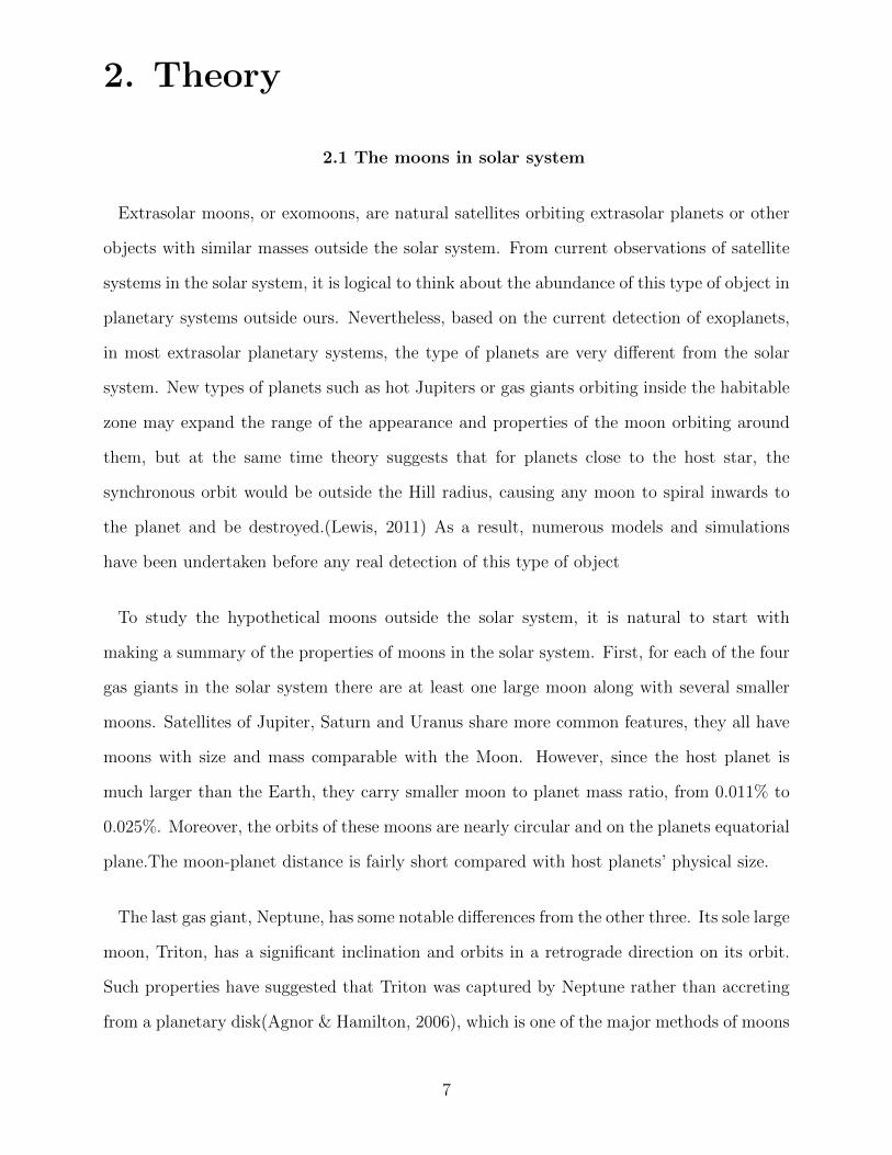
Now we discuss the moons of smaller terrestrial planets. Among the four terrestrial planets

in solar system, only the Earth carries a relatively large moon. Although Earth is smaller

in size and mass than gas giants by multiple times, its moon is comparable to those around

gas giant and that gives a moon to planet mass ratio of about one per cent for Earth-moon

system. In addition, the orbit of the Moon is nearly circular and slightly inclined, which

shares the trait of moons around gas giants. It has been predicted that Earths moon was

formed by impact, another possible way of forming natural satellite around planet.

Figure 1: Moons of solar system. The photo shows major large moons at their relative sizes to each other and to Earth.Pictured are Earth’s Moon; Jupiter’s Callisto, Ganymede, Io and Europa; Saturn’s Iapetus, Enceladus, Titan, Rhea, Mimas,Dione and Tethys; Neptune’s Triton; Uranus’ Miranda, Titania and Oberon and Pluto’s Charon. Image from NASA, http://solarsystem.nasa.gov/multimedia/display.cfm?IM_ID=6163

8

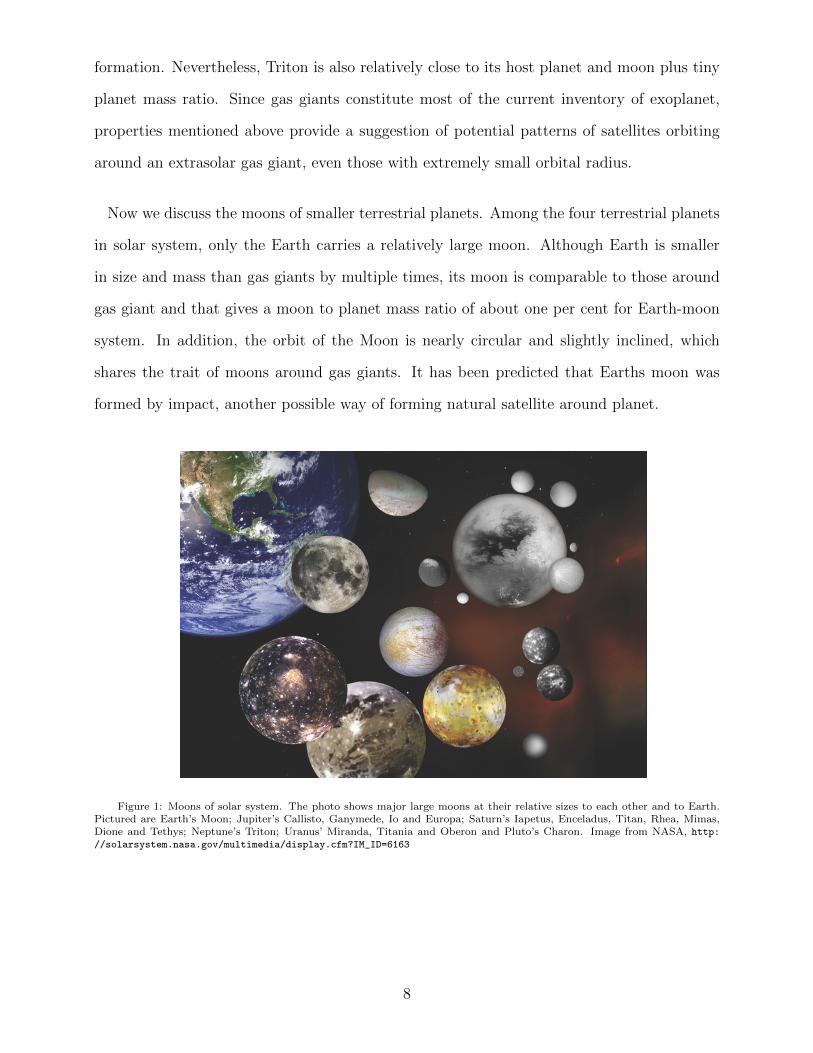
Table 1: The length of orbital semimajor axis and diameter of major moons of gas giants in solar system. The data aregiven in standard units and in units of host planet radii. Image from [Kane, Hinkel & Raymond, 2013]

2.2 Mechanisms of forming satellites

As mentioned in the introduction, there are three major ways contributing to moons

formation. Disk accretion, impact generation, and captured satellites.

Disk accretion plays a key role in forming moons around gas giants. Regular satellites of

four gas giants in the solar system are believed to be formed within their circumplanetary

disks. Such a model explains the circular shapes and low inclination of moons orbits since

the planetary disk is in general circular and aligned with planets equatorial plane. It has

been suggested that the mass of regular satellites in the disk is determined by the balance

between the accretion rate of material onto the protomoons and orbital decay of these proto-

moons within the accretion disk onto the growing gas giant.(Canup & Ward, 2006) Another

9

theoretical suggestion is that given a two component disk model with a dense inner sub-disk

extending out to the centrifugal radius and a less dense shell. (Mosqueria &Estrada 2003a,b)

These predictions give plausible results such that there are about 4 large moons within 60

planetary radii of the planet and they yield a total mass about 0.01% of host planets mass.

The second model also suggests that the migration timescale of the moons is much longer

than the formation timescale.

For terrestrial planets, the most plausible way of forming a moon is through giant impacts

between planetary embryos. Numerical simulation shows that this process is frequent, with

average of two impacts for one moon’s formation(Agnor, Canup & Levison, 1999). Impact

between two terrestrial mass protoplanets can generate a circular orbiting disk of debris and a

moon can form within this disk by gravitational attraction at a distance of several planetary

radii. (Wada, Kokubo & Makino 2006). Another simulation by Canup & Levison, 2006, is

closer to the Earth-Moon system. If the planetary embryos are around the mass of Earth,

the impact disk of debris could finally result in a single moon with mass up to 4% of the

planets mass. The impact theory cannot explain the inclination in that it depends on the

nature of the original impact. More dynamical processes such as re-impact, a moon on a

close, inclined orbit or a moon on a distant coplanar orbit can be formed due to different

inclination. (Atobe & Ida 2007).

A planet can also host a moon by capturing wandering object in space when the objects

trajectory is close enough to the planet. During this process, the object must lose energy

by some mechanisms. One is the thee-body interaction among the host planet, the existing

moon and captured protomoon(Agnor & Hamilton 2006). And the other is tidal dissipation

to fit a bound orbit of the planet(Podsiadlowski et al. 2010). According to the dynamics of

capturing process, the moons orbit is likely to have a very high eccentricity and the moon is

probably in retrograde motion(Lewis 2011). With time passing by, the elliptical shape will

smear out to be circular by tidal decay.

10

2.3 Natural satellite outside solar system

From table 1 we can see that the largest moon in the Solar System, in both mass and

radius, Ganymede, has a radius of about 0.413 radius of Earth and mass of about 0.025

Earth mass. So question as to whether more massive moons could have formed around

exoplanets is brought up. Calculation indicates that the upper bound of mass for moons

formed by disk accretion of giant planets is one ten thousandth of the mass of the host

planet(Canup & Ward 2006), which is also called mass-constrained in situ formation(Heller

& Barnes 2013). Therefore, to create a moon with Earth mass, the host planet need to be

at least ten thousand times the mass of the Earth, which is about 31 times more massive

than Jupiter. However, based on NASA Exoplanet Archive, the most massive exoplanet

discovered so far is approximately 28.5 times Jupiter mass and it may be ruled out of being a

planet but a brown dwarf due to its mass(Sahlmann et al., 2013). So it is almost impossible

for an Earth-mass moon accreted from a planetary disk. On the flip side, another study

of formation of Jupiter and Saturn satellite system suggests that moons of size similar to

Ganymede or Titan is common in most gas giants, and it also provides the possibility of

Mars-mass or even Earth-mass moons(Sasaki, et al. 2010)

Here we can conduct a simple calculation to verify the conclusion of mass-constrained in

situ formation given by Canup and Ward. We sum all the moons of the two largest gas

giants in the Solar System and compare it with the host planet mass. All the moons data

are taken from database of Solar System Exploration by NASA. Here the total satellite mass

is given by adding all the satellite with mass greater than 1017 kilograms. For Jupiter, its

mass is 1.8983 × 1027 kg(Williams 2006) and the total moon mass is 3.9311 × 1023 kg. For

Saturn, its mass is 5.6846× 1026 kg (Williams 2006) and the total moon mass is 1.405× 1023

kg. So the moon to planet mass ratio is 2.07 × 10−4 for Jupiter and 2.472 × 10−4, which is

very close to the theoretical prediction. And we can make a conclusion that if the gas giant

can maintain its disk during formation(not disturbed by host star, for example), the greatest

possible moon mass should be around ten thousandths of its mass.

11

2.4 Habitability of Exomoons

When people first proposed the viability of habitable exomoons, only very few exoplanet

were discovered and all of them were giant planet (Williams et al. 1997). As a result,

simple and straightforward idea for rocky satellites orbiting around those gas planets possibly

providing a life-supporting environment was claimed. Jovian planet candidate orbiting on

the outer edge of parent stars habitable zone(HZ) are mentioned such as 47 Urase Majoris.

Several arguments that question the habitability are the stability of moons orbital motion,

the effect of high energy particles from the magnetic field of host planet, the persistent heat

source from the star and planet, the durability of exomoons atmosphere, which can be divided

into two parts, the exterior sources like illumination, and interior sources, like greenhouse

effect.

Owing to the limitation of observing apparatus and techniques, even today most of exo-

planet candidates found in the stellar HZ are gas giants or super Earths instead of Earth-like

planets. Therefore, the habitability of extrasolar moons of this observed planets is under

active study. Now people have made great effort discussing from all the aspects that may

affect the habitability of exomoons. In next sections discussions of several mainly discussed

points will be given.

12

3. Detection

3.1 Overview

During the middle of 1990s, people made first confirmed detections of exoplanet (Mayor

& Queloz, 1995). With the improvement of observing devices and variation of detection

methods, more than 1700 such planets have been confirmed (Petigura et al., 2013). The

smallest exoplanet discovered so far is moon-sized (Barclay et al. 2013), indicating the

resolution and other capabilities for todays observing equipments are capable of looking for

extrasolar objects that are as small as regular natural satellites in our Solar System.

Another motivation of searching exomoon originates from the somewhat distressing results

of exoplanet observation. Although thousands of candidates are confirmed, most of them are

gas giants. On those gigantic planets, lack of complex molecules and severe environmental

conditions highly constrain the habitability, not to mention the scorching temperatures on

gas giants very close to the star (hot Jupiters). Among those terrestrial exoplanets, few of

them are suitable for life supporting merely by considering their distance from the host star.

Based on data given by Habitable Exoplanet Catalog (HEC), before April 2014, there are

only 20 potentially habitable targets out of 1793 confirmed exoplanets and all of them are

superterran1. If one thinks about other facts such as hazardous radiation shielding or runaway

greenhouse effect, this number should keep shrinking. For instance, as mentioned in section 3,

M dwarf stars have strong magnetic burst and emission of high energy radiations(Gurzadian

1970; Silverstri et al. 2005). A planet orbiting an M dwarf would probably lose its atmosphere

because of the intense bombardment of high energy particles from the host star. Therefore,

taking the Sun as reference, it is logical to looking for habitable planets around K-type stars.

However, from Borucki et al. (2011) and Batalha et al. (2012), almost all the candidates

within the irradiation habitable zones around Sun-size stars are much greater than Earth in

both sizes and masses. According to this fact, people started to aim the telescopes to those

1http://phl.upr.edu/projects/habitable-exoplanets-catalog

13

in-zone gas giants and try to unearth the traces of satellites around them.

The number of exomoons should be abundant. If we consider Solar system, each gas giant

carries one or more moons with size comparable to that of the Moon, not to mention the total

number of 166 satellites orbiting the 8 planets (Hinkel & Kane 2013). As stated in HEC,

among the nine potentially habitable planets, there may be 30 habitable exomoons around

them(Torres 2012) 2. Others studies on the formation scenario and frequency forecast also

indicate the number of moons (Morishima et al. 2010; Elser et al. 2011). With a substantial

sample collection, it is nevertheless challenging to detect exomoons in that their sizes and

luminosity are negligible compared to the host planet and stars. Several possible ways of

detection and results are mentioned in detail below.

3.2 Direct Imaging

At first glance, the direct imaging method is implausible for observing exomoons. Nowa-

days, even for exoplanets, direct imaging it is a very demanding job because of high contrast

ratio between the stars and planet and tiny star-planet separation(figure 6). To observe the

object directly, it requires the object to have a relatively large angular size and temperature.

The least massive exoplanet discovered via direct imaging, Foualhaut b, is twice as massive

as Jupiter, and the coolest one, 59 Virginis b, has a mean temperature of 510 K. Both the

size and temperature are greatly exceed the scale for a exomoon, especially a potentially

habitable one.

However, some efforts of direct imaging exomoons have been made by Peters & Turner(2013).

They argued that for a tidally heated exomoons, it is possible for the existing and planned

telescopes to directly observe them. They believed that tidally heated exomoons can be far

more bright than their host planets as much as 0.1% as luminous as the host star if it is a low

mass stellar primary. Furthermore, tidally heated configurations can last as long as billions

of years, meaning that they may keep bright when host stars pass their main sequence phase.

2The data is taken as of 3 January 2013.

14

They may consist of a larger sample size of directly imaging candidates than gas giants since

they need to be young and at a large projected separation to be directly imaged.

They first consider the tidal heating representative in the Solar System, Io, and applied

the luminosity equation given by Reynolds et al. (1987) and Segatz et al. (1988):

Ltidal =42πG5/2

19(R7

Sρ2M

5/2P

µQ)(

e2

a15/2)

where G is the gravitational constant, µ is the moon’s elastic rigidity, Q is the moon’s

dissipation function(or quality factor), e is the eccentricity of the moon’s orbit, a is the semi-

major axis of the moon’s orbit, ρ is the density of the moon, Rs is the radius of the moon, and

Mp is the mass of the planet of the host planet. Later they also discussed the expression for

effective temperature by Stefan-Boltzmann Law. And they claimed that the exomoons can

be detected if the contrast of the star and the planet with the moon(Lstar/Lsat andLp/Lsat) is

small so the light of the moons can stand out to be perceived by telescope. Later they believe

the limiting temperature of tidal heating moons can surpass 1000K, which can provide fairly

strong luminosity.

In order to maintain the tidal heating, or preserve effective tidal force, the satellite should

keep along highly eccentric orbits. One mechanism of sustaining eccentricity is through

resonance with other moons, such as the 1:2:4 resonance of Io, Europa and Ganymede. Io is

being heated by tidal forces 4.5 Gyr after the formation of the solar system, which suggests

tidal heating can occur in old planetary systems. (Turner & Peter, 2013) Moreover, Majita

(2007) demonstrated the possibility of maintain orbital eccentricity via perturbation from

other planets and Georgakarakos (2002 & 2003) offered models of stellar perturbation to

sustain an eccentric lunar orbit.

The most sensitive high-contrast imaging instruments currently on the sky, VLTs NACO

and Subarus HiCIAO, can in theory detect an exomoon with twice the Earths radius for a

5-sigma. However, two-Earth-radius exomoon, as mentioned in Chapter 2, violated the in

15

situ satellite formation by Canup & Ward (2006). The authors argued that such exomoon

can be formed via other processes such as impact. Several future detectors like JWSTs Mid-

Infrared Instrument(MIRI) (figure 3) and SPICA would offer more promising results due to

their higher contrast(≈ 10−6, from Peters & Turner (2013) ).

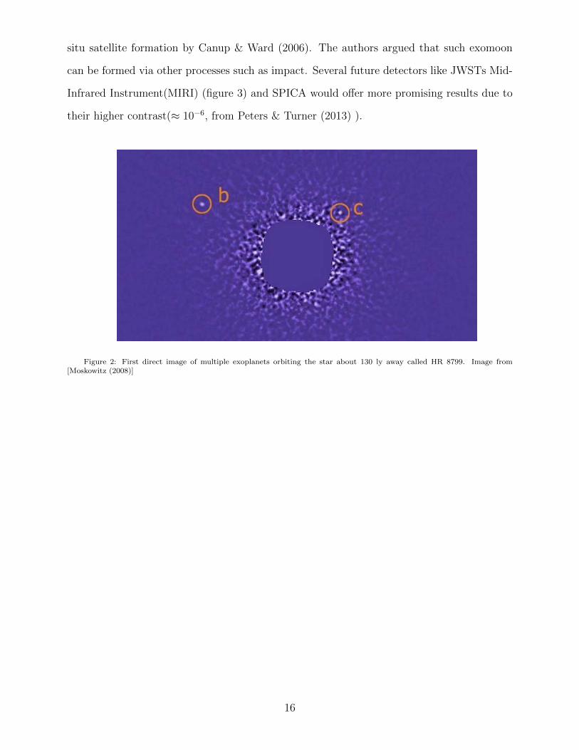
Figure 2: First direct image of multiple exoplanets orbiting the star about 130 ly away called HR 8799. Image from[Moskowitz (2008)]

16

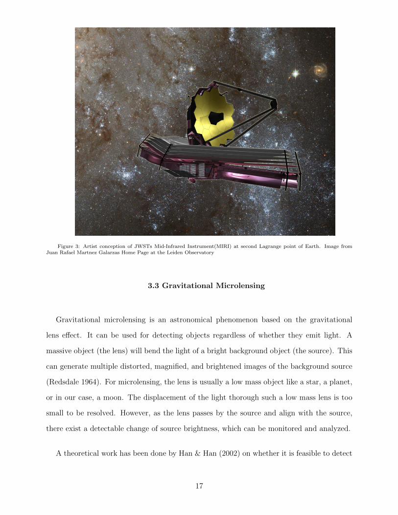
Figure 3: Artist conception of JWSTs Mid-Infrared Instrument(MIRI) at second Lagrange point of Earth. Image fromJuan Rafael Martnez Galarzas Home Page at the Leiden Observatory

3.3 Gravitational Microlensing

Gravitational microlensing is an astronomical phenomenon based on the gravitational

lens effect. It can be used for detecting objects regardless of whether they emit light. A

massive object (the lens) will bend the light of a bright background object (the source). This

can generate multiple distorted, magnified, and brightened images of the background source

(Redsdale 1964). For microlensing, the lens is usually a low mass object like a star, a planet,

or in our case, a moon. The displacement of the light thorough such a low mass lens is too

small to be resolved. However, as the lens passes by the source and align with the source,

there exist a detectable change of source brightness, which can be monitored and analyzed.

A theoretical work has been done by Han & Han (2002) on whether it is feasible to detect

17

satellites around exoplanets. From their research, they believed that detecting satellite signals

in lensing light curves would be very hard in that satellites signals are severely smeared out

by the finite source effect even for events where background star has small angular radius.

During the investigation, they carried out a simulation of Galactic microlensing events of

a stellar system containing a 0.3 solar mass star, an Earth-mass planet and a Moon-mass

satellite.

However, Han & Han′s work does not mark a dead end of microlensing detection of

extrasolar satellite. In contrast, the first possible planet-moon system outside the Solar

System was detected using this type of method, although this system is free-floating, which

means it does not undergo a circular motion around a star or stellar object (Bennett, D.P.

et al. 2013).Their observing target, MOA-2011-BLG-262, was fit well by a lens model with

main lens of roughly 4 Jupiter mass and a sub-Earth mass moon. However, an alternative

best-fit model was also proposed, in which a Neptune-size planet is orbiting around a faint

dwarf star. Bennets research team called it a unlucky accident since the two models fit almost

equally well so that they can even be represented using the same line on the light curve (see

the black curve in figure 4).

Now the lensing event MOA-2011-BLG-262 has moved out of alignment with the source

star so scientists have no chance to observe and confirm the result again(Moskowitz 2013).

This is one of the major disadvantages of the microlensing method. David Kipping, the leader

of Hunt for exomoons with Kepler (HEK), commented on this discovery that microlensing has

only one snapshot whereas through transiting we can see events over and over again.(Witze,

2013) In the next section his works will be presented systematically.

18

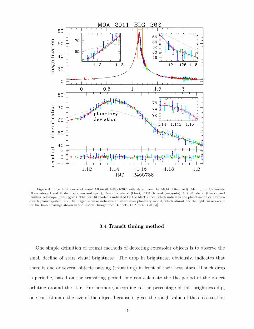
Figure 4: The light curve of event MOA-2011-BLG-262 with data from the MOA 1.8m (red), Mt. John UniversityObservatory I and V -bands (green and cyan), Canopus I-band (blue), CTIO I-band (magenta), OGLE I-band (black), andFaulkes Telescope South (gold). The best fit model is indicated by the black curve, which indicates one planet-moon or a browndwarf- planet system, and the magenta curve indicates an alternative planetary model, which almost fits the light curve exceptfor the limb crossings shown in the inserts. Image from[Bennett, D.P. et al. (2013)]

3.4 Transit timing method

One simple definition of transit methods of detecting extrasolar objects is to observe the

small decline of stars visual brightness. The drop in brightness, obviously, indicates that

there is one or several objects passing (transiting) in front of their host stars. If such drop

is periodic, based on the transiting period, one can calculate the the period of the object

orbiting around the star. Furthermore, according to the percentage of this brightness dip,

one can estimate the size of the object because it gives the rough value of the cross section

19

area of the object compared to the star. And the absolute size of the object can be obtained

if the absolute size of the star is known from its spectral type, mass-to-light ratio, density and

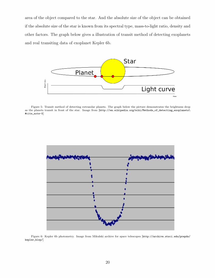
other factors. The graph below gives a illustration of transit method of detecting exoplanets

and real transiting data of exoplanet Kepler 6b.

Figure 5: Transit method of detecting extrasolar planets. The graph below the picture demonstrates the brightness dropas the planets transit in front of the star. Image from [http://en.wikipedia.org/wiki/Methods_of_detecting_exoplanets\#cite_note-5]

Figure 6: Kepler 6b photometry. Image from Mikulski archive for space telescopes [http://archive.stsci.edu/prepds/kepler_hlsp/]

20

Nevertheless, until recently the smallest planet detected using transit method is still

Neptune-sized(Kipping 2009). Due to the limit of instruments, Earth-sized and sub Earth-

sized objects such as exomoons cannot be detected using this method. However, two methods

derived from transit method can bring the sensitivity down to sub Earth-mass level. The first

one is called transit-timing variation (TTV). The basic idea of TTV is that once a transit

object is discovered, one can analyze the variations in the timing of a transit. If there is a

small objects, like a smaller exoplanet or a satellite, then the period of the transit of the

major planet would be perturbed by the gravitational effect of these smaller orbiting objects.

Since this is a detection of perturabtion, the sensitivity can be much higher than normal

transit technique. Both theory and observation have prove that TTV is able to detect an

Earth-mass exoplanet (Miralda-Escude 2001; Holman & Murray 2004) and TTV is also a

useful tool of locating other members in a stellar system with one transit planet detected

(Ballard et al. 2011).

Another method is called transit-duration variation (TDV). Instead of studying the slight

change of period between transits, TDV focus on the variation of how much time one transit

takes. The reason for this variation can be the apsidal precession for eccentric planets (Hol-

man & Murray 2004), general relativity (Pal & Kocsis 2008), or the existence of exomoon.

I what is so far the only official detection project of exomoon, as part of the Kepler mission,

the Hunt for Exomoons with Kepler (HEK) project applied TTV and TDV techniques to

search possible exomoon candidates around exoplanets discovered via Kepler telescope. The

idea of TTV detection of exomoon is demonstrated in the figure below:

21

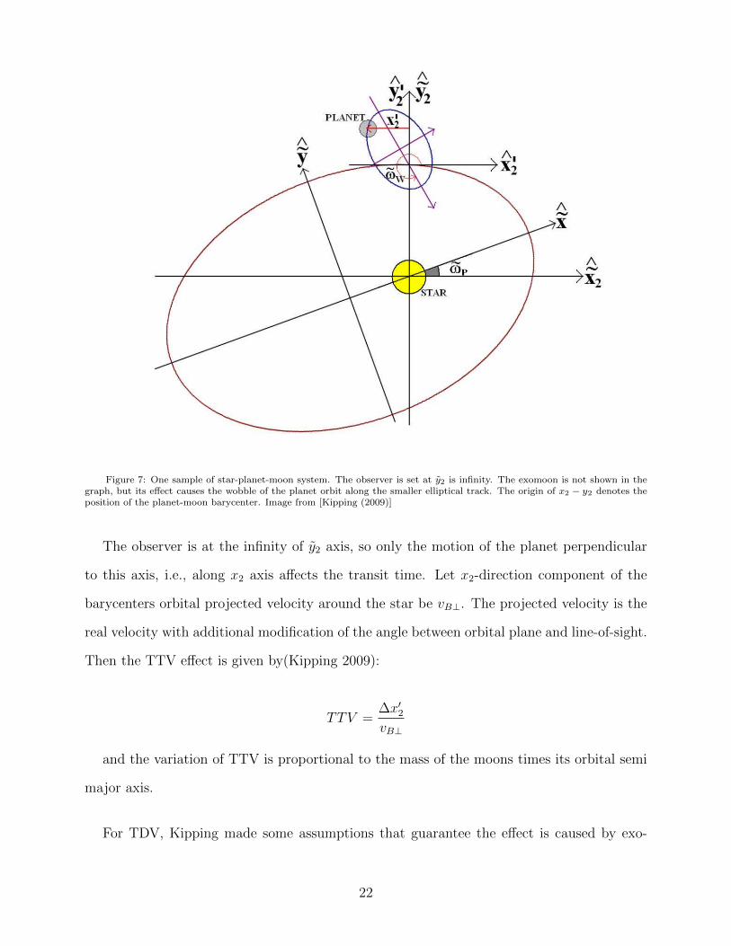
Figure 7: One sample of star-planet-moon system. The observer is set at y2 is infinity. The exomoon is not shown in thegraph, but its effect causes the wobble of the planet orbit along the smaller elliptical track. The origin of x2 − y2 denotes theposition of the planet-moon barycenter. Image from [Kipping (2009)]

The observer is at the infinity of y2 axis, so only the motion of the planet perpendicular

to this axis, i.e., along x2 axis affects the transit time. Let x2-direction component of the

barycenters orbital projected velocity around the star be vB⊥. The projected velocity is the

real velocity with additional modification of the angle between orbital plane and line-of-sight.

Then the TTV effect is given by(Kipping 2009):

TTV =∆x′2vB⊥

and the variation of TTV is proportional to the mass of the moons times its orbital semi

major axis.

For TDV, Kipping made some assumptions that guarantee the effect is caused by exo-

22

moons. In the system there is no additional perturbation, and the orbital inclinations of

planets and moons do not vary from orbit to orbit. The projected velocity of planet-moon

barycenter relative to the star and the projected velocity of the planet relative to the barycen-

ter do not vary significantly. Then he found the variation of TDV is proportional to the mass

of the moon times its orbital semi major axis to the -1/2 power.

Several conclusions have been made on two methods. First, from the relationship between

the mass, radius and timing variation, the ratio of TDV to TTV allows for determining

mass and radius of exomoon separately. Next, the TTV and TDV have a similar order of

magnitude in signal strength. And TDV lags TTV by 90 degrees in phase, so TDV can be a

great complementary technique of TTV.

Unfortunately, although with sophisticated and well-developed theory governing observa-

tion, the real application for HEK has not yield fruitful results. The HEK project distills

more than two thousands known transiting planet candidates found by Kepler down to the

most promising candidates for hosting a moon via methods of visual identification (TSV),

automatic filtering (TSA) and targets-of-opportunity (TSO) with a final stage of target pri-

oritization (TSP) (Kipping et al. 2012). With 4 published papers, 32 stellar systems have

been examined (KIC-11623629, KIC-11622600, KIC-10810838, KIC-5966322, KIC-9965439,

KIC-7761545, KIC- 11297236; KOI-365, KOI-1876, KOI-174, KOI-303, KOI-722, KOI-1472,

KOI-1857 in (Kipping, et al 2013)3; Kepler-22, KOI-87, KIC 10593626 in (Kipping, et

al 2013)4; KIC-8845205, KIC-7603200, KIC-12066335, KIC-6497146, KIC- 6425957, KIC-

10027323, KIC-3966801, KIC-11187837; KOI-463, KOI-314, KOI- 784, KOI-3284, KOI-663,

KOI-1596, KOI-494, KOI-252 in (Kipping et al 2014)), but no convincing signal of exomoon

has been reported.

3arXiv:1301.1853v2 [astro-ph.EP] 6 Mar 20134arXiv:1306.1530v2 [astro-ph.EP] 9 Sep 2013

23

4. Habitability

This chapter presents studies on discussing the habitability of exomoons from different

parameters that may contribute significant constrains. Since so far no exomoons inside

a stellar system has been detected, all analysis is given via computer simulations. The

results shown by these experiments not only provide theoretical support of habitable extra

solar moons, but also offers suggestions on targeting fields of detection in future observation

missions.

4.1 Runaway greenhouse effect

Runaway green house effect is a process in which a net positive feedback, in which the

effects of a small disturbance on a system include an increase in the magnitude of the pertur-

bation (Zeckerman & Jefferson 1996), between surface temperature and atmospheric opacity

increases the strength of the greenhouse effect on a planet until its oceans boil away (Rasool

& De Bergh 1970). One of the most famous example is such effect on Venus in its early

history. By its definition, run away greenhouse effect is lethal to life since it will dry out the

ocean of an object, which is considered to be the origin of lifeforms. Hence, it is of great

importance to understand the condition whether an exomoon would experience greenhouse

effect when people are selecting inhabitable candidates.

As a giant planet converts gravitational energy into heat, it may irradiate a Earth-like

moon to an extent that triggers the runaway greenhouse effect (Baraffe et al. 2003; Leconte

& Chabrier 2013; Heller & Barnes 2013). Barnes et al. 2013 have shown that a Earth-size

moon can become totally dehydrated on the surface by runaway greenhouse effect within 100

Myr. And this duration can change considerably depending on planets surface gravitation,

initial water quantity, stellar X-ray and ultraviolet (XUV) radiation (Heller & Barnes 2013).

The simulation was performed by Heller and Barnes (2013) by considering a range of

hypothetical planet-moon binaries orbiting a Sun-like star during different epochs of the

24

systems lifetime. For the hypothetical planet, they simply follow the rule of mass-constrained

in situ formation of extrasolar moons which claims that the more massive the host planet,

the more massive the moons. So they adopt a Jovian planet of approximately 13 Jupiter

masses. They made the assumption that this object can be described by Baraffe et al. (2003)

evolution model of a giant planet instead of a brown dwarf.

The illumination of the planet is given by flux equation:

F∗ =σSBT

4∗√

1− e2∗p

(R∗a∗p

)2

Where σSB is the Stefan-Boltzmann constant, T∗ is the stellar effective temperature, R∗

is the stellar radius, e∗p is the orbital eccentricity of the star-planet system, and a∗p is the

planets orbital semi-major axis. The equation can be applied to both the host star and

planet, from which we can reach the total illumination absorbed by the moon. Heller and

Barnes applied dual pass band of optical and infrared for computation:

Fi =L∗(t)(1− As,opt)

16πa2∗p

+Lp(t)(1− As,IR

16πa2ps

for Earth-like planet, the bolometric albedo can vary substantially depending on orbital

radius, from 0.18 at inner edge of HZ to 0.45 at out edge (Kopparapu et al. 2013). Here

they took the average of 0.3 for optical albedo for stars’ luminosity, which have effective

temperature from 3000K to 6000K. And for infrared albedo, they considered the model in

which an Earth-like planet orbiting a cool star with effective temperature of 2500K, and it

yields the albedo to be 0.05(Kasting et al. 1993; Selsis et al. 2007; Kopparapu et al. 2013)

The way of assessing wether run away greenhouse effect would dehydrate the moon is to

compare the total illumination flux plus the tidal heat flux with the critical flux for a runaway

greenhouse. The critical flux is given by Pierrehumbert (2010, Eq. 4.94). In their simulation,

the first case with rocky Earth-mass, Earth-size moon, yields a critical flux of 295 W/m2.

And in the second one, with a moon a quarter of Earths mass and a ice to mass ratio of 25%

25

(they called it ”super Ganymede”), they obtained a critical flux of 266 W/m2.

After running the simulation and data analysis, they found that thermal irradiation from

a 13 Jupiter mass planet on an Earth size moon at a distance of 10 Jupiter radius can

trigger a runaway greenhouse effect for about 200 million years. As for the icy planet (super

Ganymede), it would be subject to a runway greenhouse effect if either orbital period or

orbital distance is larger than the first case. In both cases, great amount of hydrogen and thus

water would be lost, which makes the planet temporarily or possibly for always uninhabitable.

Tidal heating, as another heat source, would exacerbate the situation of the moons. At last,

they proposed another scenario in which moons can escape from the early runaway greenhouse

effect. By means of gravitational capture, moon mergers from objects like Trojans and others,

the moon can form or in its satellite position after the planets cooling process. Furthermore,

a desiccated moon in the HZ has a chance of resuscitation by bombardment of comets or

meteorites later.

4.2 Magnetic Shielding

One of the challenges to a moons habitability is the flux of high energy particle stripping

off atmosphere and preventing formation of complex molecule on the surface of the moon.

Thus a habitable moon requires a strong magnetosphere similar to that of Earths. However,

section 2.3 mentions that a standard disk accretion model of exomoon forming suggests a

near impossibly of a Earth-mass moon. Therefore, the moon can only be safe from high

energy radiation under the shield of magnetosphere of its host planet(Heller & Zuluaga

2013). However, the planetary radiation belt could also be harmful to the moon. So the only

possible way for the moon to be life supporting in shielding detrimental radiation is to let

the host planet screen off the stellar and outer space radiation while to let its self-generating

magnetic field block the radiation from the host planet. The mere example in the Solar

System is Ganymede with an approximately 750nT magnetic field (Kivelson et al. 1996).

26

Heller & Zuluaga (2013) constructed a simulation model for the evolution of magnetic

environment gas giant planets with thresholds from the runaway greenhouse effect to assess

the habitability of exomoons. First they chose Sun-like star as the host star since M dwarf

stars have strong magnetic burst and emission of high energy radiations(Gurzadian 1970;

Silverstri et al. 2005). As for planet construction, they explored two extreme scenarios

between which most giant planet planets are expected. Lastly, they suspected moons of

roughly the mass and size of Mars by examining both its existence and detection.

Moreover, they analyze the habitability problem with an additional constraint of runaway

greenhouse effect (see section 3.2)and tidal heating. Two thresholds are set as boundary

between inhabitable and non-habitable state: (1) The moons tidal heating reaches a surface

flux comparable to Jupiters moon Io, or 2 W m−2, which is called Io Limits. At this limit, the

non-habitability is triggered by violent tectonic activities. (2) The moons global energy flux

exceeds the critical flux and thus causes the run away greenhouse effect. Further approxima-

tion were made regarding planetary dynamos, such as convection on a spherical conduction

shell governing a scaling law for the magnetic field strength, the ratio between inertial forces

to Coriolis forces, the polytropic density model of core density, thermal diffusivity, and the

electrical conductivity.

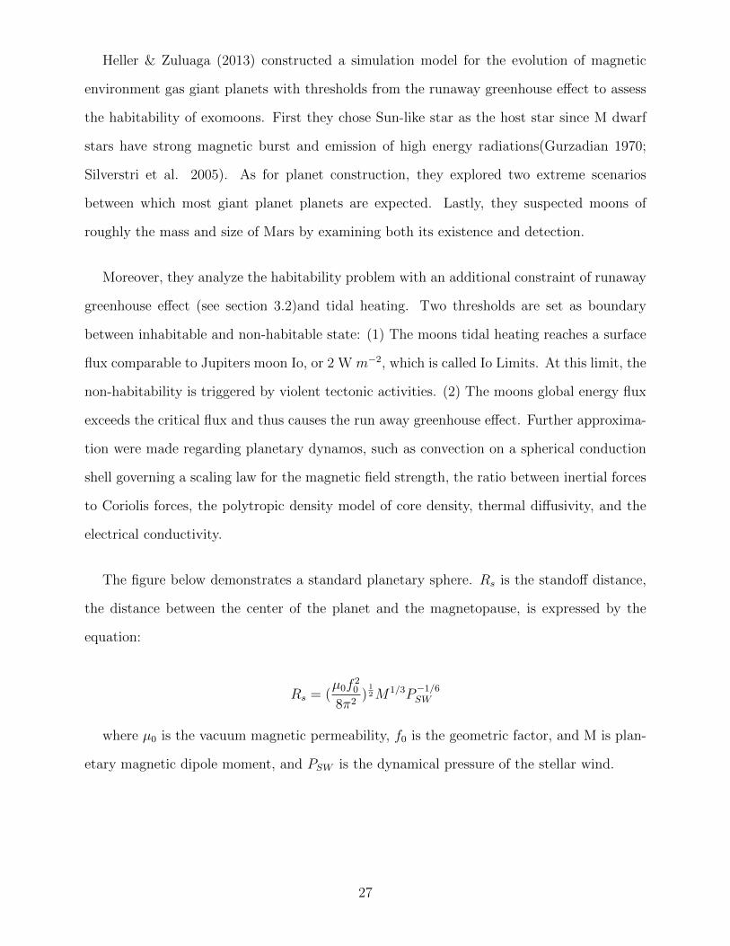
The figure below demonstrates a standard planetary sphere. Rs is the standoff distance,

the distance between the center of the planet and the magnetopause, is expressed by the

equation:

Rs = (µ0f

20

8π2)12M1/3P

−1/6SW

where µ0 is the vacuum magnetic permeability, f0 is the geometric factor, and M is plan-

etary magnetic dipole moment, and PSW is the dynamical pressure of the stellar wind.

27

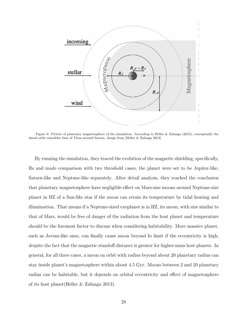
Figure 8: Picture of planetary magnetosphere of the simulation. According to Heller & Zuluaga (2013), conceptually thedazed orbit resembles that of Titan around Saturn. Image from [Heller & Zuluaga 2013]

By running the simulation, they traced the evolution of the magnetic shielding, specifically,

Rs and made comparison with two threshold cases, the planet were set to be Jupiter-like,

Saturn-like and Neptune-like separately. After detail analysis, they reached the conclusion

that planetary magnetosphere have negligible effect on Mars-size moons around Neptune-size

planet in HZ of a Sun-like star if the moon can retain its temperature by tidal heating and

illumination. That means if a Neptune-sized exoplanet is in HZ, its moon, with size similar to

that of Mars, would be free of danger of the radiation from the host planet and temperature

should be the foremost factor to discuss when considering habitability. More massive planet,

such as Jovian-like ones, can finally cause moon beyond Io limit if the eccentricity is high,

despite the fact that the magnetic standoff distance is greater for higher-mass host planets. In

general, for all three cases, a moon on orbit with radius beyond about 20 planetary radius can

stay inside planet’s magnetosphere within about 4.5 Gyr. Moons between 2 and 20 planetary

radius can be habitable, but it depends on orbital eccentricity and effect of magnetosphere

of its host planet(Heller & Zuluaga 2013).

28

4.3 Orbital Dynamics

The most critical factor that guides the temperature, climate, tectonic activity, and many

other parameters that control the habitability of an exomoon is its motion on the lunar

orbit. With the additional orbital motion around the host planet, a exomoon has a much

more complex moving trace with respect to the host star than a planet. As a result, we

expect a more complex mechanism of absorbing illumination from the star due to frequent

eclipses. Figure 8 gives a simple demonstration of radiation receiving of an exomoon when

it is orbiting inside a stellar system.

Figure 9: Geometry of the triple system of a star, a planet, and a moon with illuminations indicated by different shadings(pole view). For ease of visualization, the moons orbit is coplanar with the planets orbit about the star and the planets orbitalposition with respect to the star is fixed. Combined stellar and planetary irradiation on the moon is shown for four orbitalphases. Projection effects as a function of longitude and latitude are ignored, and we neglect effects of a penumbra. Radiiand distances are not to scale, and starlight is assumed to be plane-parallel. In the right panel, the surface normal on thesubplanetary point is indicated by an arrow. For a tidally locked moon this spot is a fixed point on the moons surface. For ps= 0 four longitudes are indicated. Image from [Heller & Barnes 2013]

Things are even more complicated in the extrasolar stellar systems. So far many discovered

giant exoplanets share a prominent feature of significant eccentricities (Gong et al. 2013),

and it is likely explained by planet-planet scattering (PPS) between giant planets (Rasio

& Ford 1996; Weidenschilling & Marzari 1996; Lin & Ida 1997; Raymond et al. 2013,

etc.). Simulation given by Gong et al. (2013) has shown that PPS is a destructive process

to the planet-moon systems, and it is almost impossible for moons to survive around hot

Jupiters formed by PPS. This theoretical experiment defines a significant number of stellar

29

system unfavorable of discovering exomoons and narrows down the targets by a great extent.

Nevertheless, many simulations running on the Solar System-like stellar systems, in which

orbits have a comparatively small eccentricity, provide insightful ideas for both theory and

detections. Below the simulating model given by Hinkel & Kane (2013) is discussed in detail.

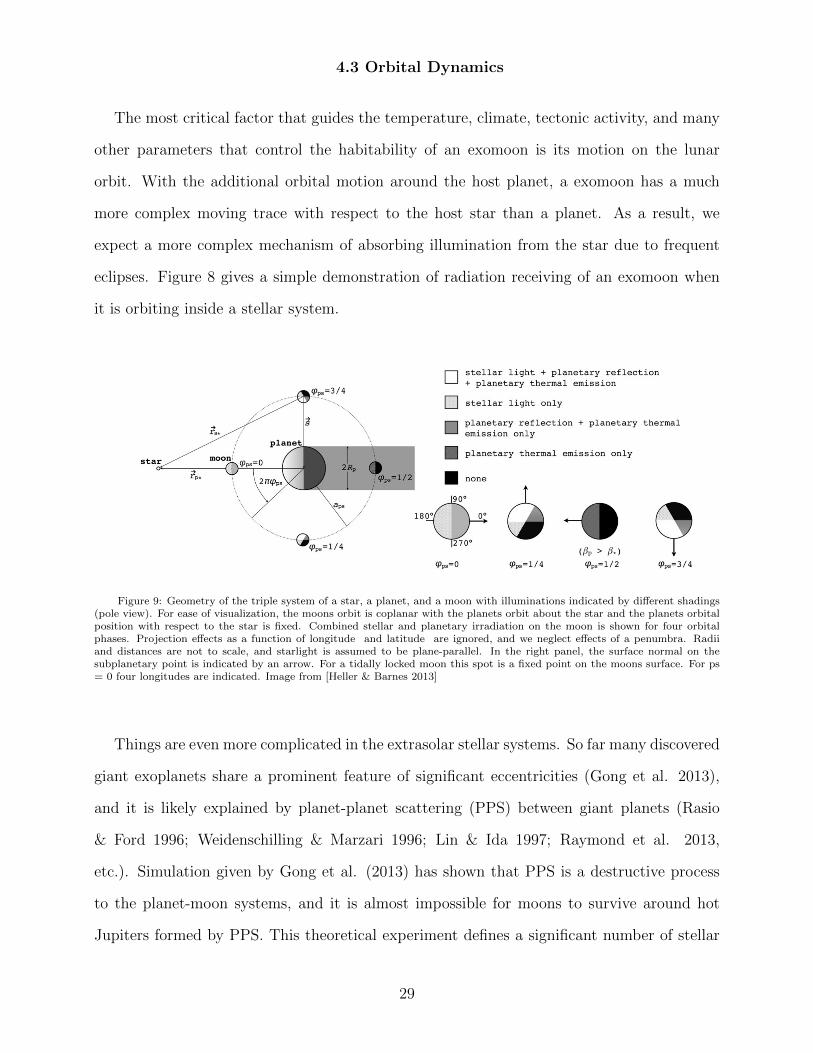
In Hinkel and Kanes experiment, they wanted to examine the effect of a large planet-

satellite distance on the flux on the moons surface and study the habitability of the moon

even if the host planet is not fully inside the HZ. They adopted the codes from Heller and

Barnes (2013) discussed in section 3.2 to calculate the total illuminating flux received by the

moons. To improve Hellers result, they modified the methodology and compute the mean

flux absorbed on the moon;s surface over a whole planet revolution. they made a flux phase

profile for an Earth-sized moon orbiting a Jupiter-sized planet at 1 AU from a Sun-sized star

for one year (See figure 10).

Figure 10: Flux phase profile for an Earth-sized moon orbiting a Jupiter-sized planet at 1 AU from a Sun-sized star for oneyear. The upper panel is the stellar flux over total and the lower one is comparison between reflective and thermal flux. Theorbit is circular with radius 0.01 AU and zero inclination. Image from [Hinkel & Kane 2013]

To fit the real case more closely, one should take eccentricity of the planet’s orbit into

30

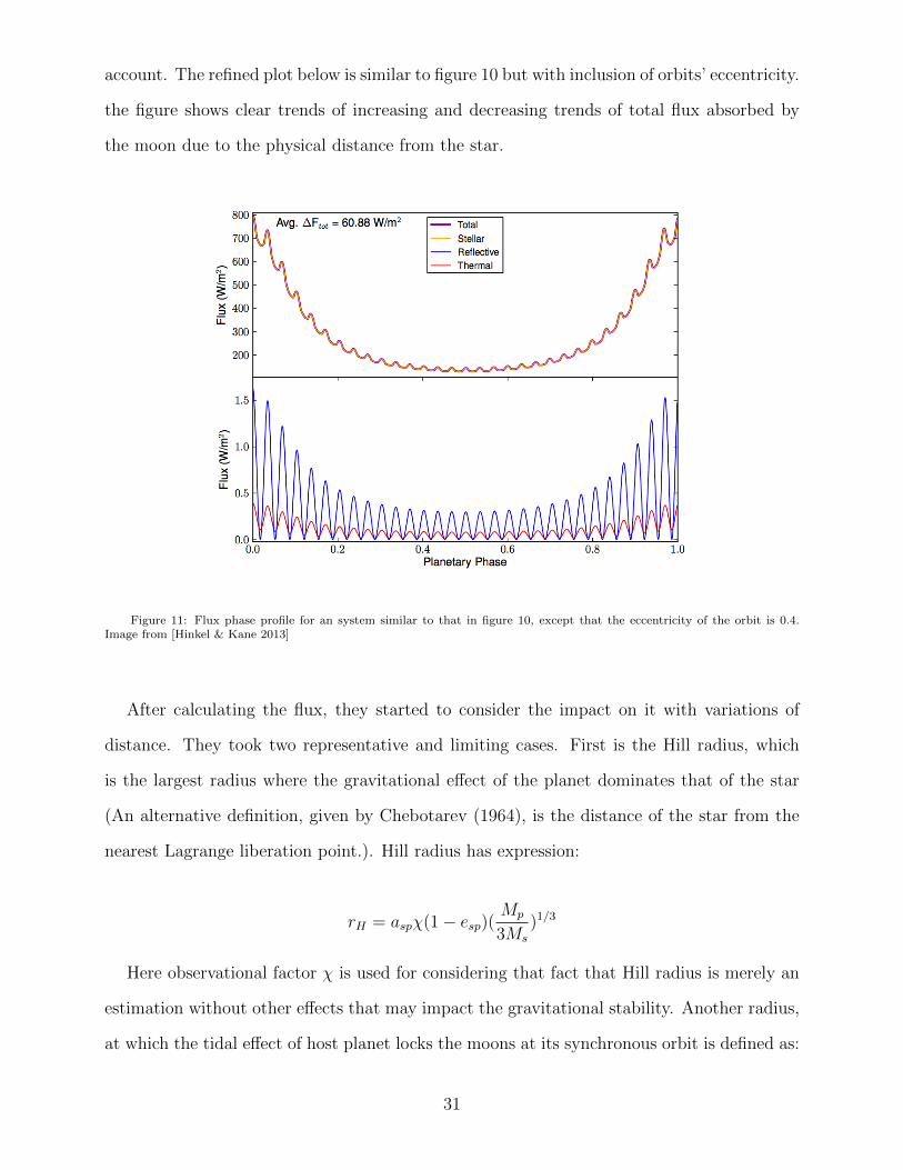
account. The refined plot below is similar to figure 10 but with inclusion of orbits’ eccentricity.

the figure shows clear trends of increasing and decreasing trends of total flux absorbed by

the moon due to the physical distance from the star.

Figure 11: Flux phase profile for an system similar to that in figure 10, except that the eccentricity of the orbit is 0.4.Image from [Hinkel & Kane 2013]

After calculating the flux, they started to consider the impact on it with variations of

distance. They took two representative and limiting cases. First is the Hill radius, which

is the largest radius where the gravitational effect of the planet dominates that of the star

(An alternative definition, given by Chebotarev (1964), is the distance of the star from the

nearest Lagrange liberation point.). Hill radius has expression:

rH = aspχ(1− esp)(Mp

3Ms

)1/3

Here observational factor χ is used for considering that fact that Hill radius is merely an

estimation without other effects that may impact the gravitational stability. Another radius,

at which the tidal effect of host planet locks the moons at its synchronous orbit is defined as:

31

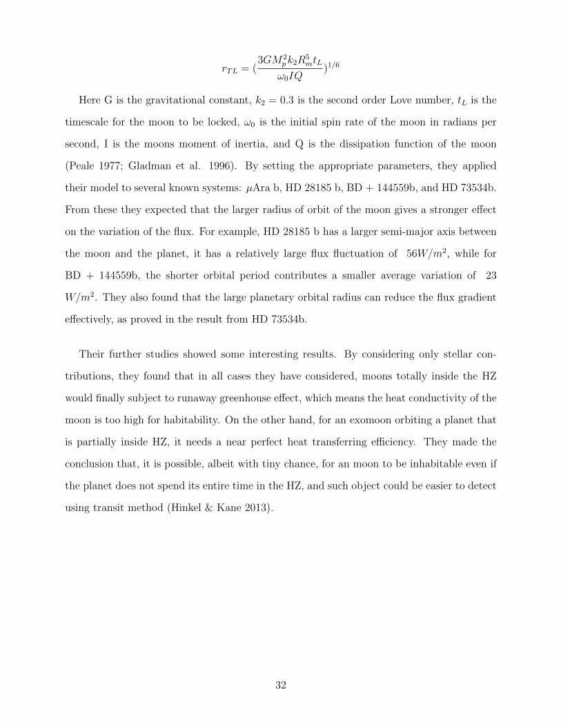
rTL = (3GM2

pk2R5mtL

ω0IQ)1/6

Here G is the gravitational constant, k2 = 0.3 is the second order Love number, tL is the

timescale for the moon to be locked, ω0 is the initial spin rate of the moon in radians per

second, I is the moons moment of inertia, and Q is the dissipation function of the moon

(Peale 1977; Gladman et al. 1996). By setting the appropriate parameters, they applied

their model to several known systems: µAra b, HD 28185 b, BD + 144559b, and HD 73534b.

From these they expected that the larger radius of orbit of the moon gives a stronger effect

on the variation of the flux. For example, HD 28185 b has a larger semi-major axis between

the moon and the planet, it has a relatively large flux fluctuation of 56W/m2, while for

BD + 144559b, the shorter orbital period contributes a smaller average variation of 23

W/m2. They also found that the large planetary orbital radius can reduce the flux gradient

effectively, as proved in the result from HD 73534b.

Their further studies showed some interesting results. By considering only stellar con-

tributions, they found that in all cases they have considered, moons totally inside the HZ

would finally subject to runaway greenhouse effect, which means the heat conductivity of the

moon is too high for habitability. On the other hand, for an exomoon orbiting a planet that

is partially inside HZ, it needs a near perfect heat transferring efficiency. They made the

conclusion that, it is possible, albeit with tiny chance, for an moon to be inhabitable even if

the planet does not spend its entire time in the HZ, and such object could be easier to detect

using transit method (Hinkel & Kane 2013).

32

5. Conclusion

As a young and active topic in astronomy observation and research, extrasolar objects are

becoming one of the major fields and job securities in future astronomy. From theoretical

point of view, numerous factors and parameters that control the density of extrasolar objects

manifest the complexity of simulation. And the blossom of innovative ideas will further

escalate the difficulties since as a new realm of study, there exist so many unknown elements.

From the observational side, many new missions of detecting exoplanets are coming out,

such as James Webb Space Telescope(JWST) (figure 3 in chapter 2), Transiting Exoplanet

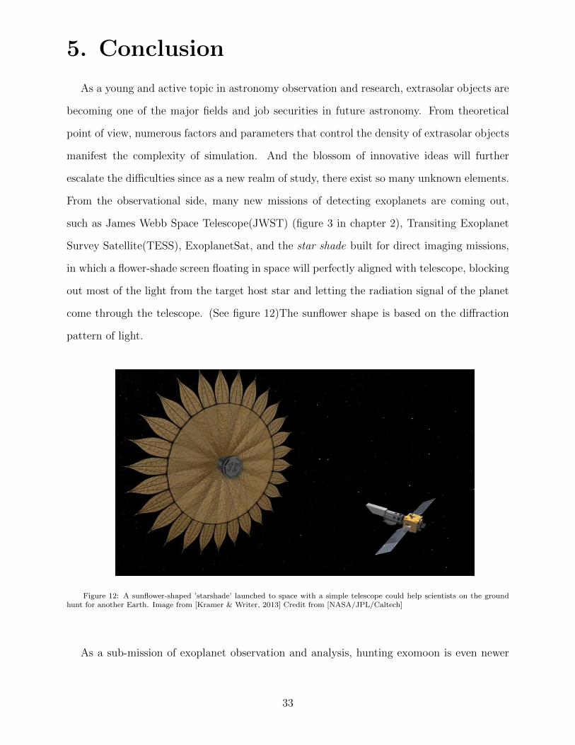
Survey Satellite(TESS), ExoplanetSat, and the star shade built for direct imaging missions,

in which a flower-shade screen floating in space will perfectly aligned with telescope, blocking

out most of the light from the target host star and letting the radiation signal of the planet

come through the telescope. (See figure 12)The sunflower shape is based on the diffraction

pattern of light.

Figure 12: A sunflower-shaped ’starshade’ launched to space with a simple telescope could help scientists on the groundhunt for another Earth. Image from [Kramer & Writer, 2013] Credit from [NASA/JPL/Caltech]

As a sub-mission of exoplanet observation and analysis, hunting exomoon is even newer

33

than its upper-level expedition. They formed via other mechanisms from the planets depen-

dent on type of host planet. They orbit on more variable tracks because the gravitational

effect of both host star as well as the host planet. They possess some common and inter-

esting features that are atypical for plants like tidal locking and tidal heating. Their mass

are also highly limited according to host planet’s mass. Things become more complicated

when discussing habitability. From chapter 4, one can see that for exomoons to keep away

from hazardous radiation, they require a very well-designed and delicate magnetosphere. If

one added more constrains by considering more factors such as avoiding runway greenhouse

effect for time scale of hundreds of millions of year, stable orbits free of violent planet-planet

scattering, suitable and lasting heating process from either radiation outside or tectonic dy-

namics inside, the lists of requirements for creating a ideal model for habitable model of

exomoon is quite demanding. So far all the literature published can only be able to run their

simulations with certain few constrains. However, despite the tremendous complexity, a real

habitable model needs appropriate forms and orders from every aspects, just like the Earth.

There is still a long way to go for searching a perfect candidate theoretically.

On the other hand, the observational techniques for exomoons is similar to those of hunt-

ing exoplanets but with different bias. So far what’s intriguing is that methods that were

once announced impossible for targeting exomoons’s signals are now either gained supports

in theory, as in direct imaging, or obtained real detection data, as in gravitational microlens-

ing. From the result derived by Peter & Tuner(2013), it is surprising that tidally-heated

exommons can reach temperature as high as 1000K so that their radiations become stronger

than many exoplanets at the same distance. Similarly surprising for the detection of MOA-

2011-BLG-262, a free floating planet-moon system. It not only a remarkable event of lensing

observation but at same time provides tentative evidence of the possible abundance of a

new type of celestial body system. The mere systematic exomoon detection project, the

Hunt for Exomoon with Kepler (HEK), applies transit timing variation(TTV) and transit

duration variation(TDV) methods on selected Kepler exoplanets. Unfortunately, until the

current period no confirmed result has been announced. But with mature theories and careful

34

conduction, it is of great hopes for the project to obtain promising outcomes in the future.

Searching home similar to us is for long a vast motivation of astronomy. Since the discovery

of first exoplanet 20 years ago, this field becomes the most fruitful aim of study in that

more than 2000 targets have been confirmed and many among them are potentially contain

liquid water. The speed of updating results for exoplanets is so high that just within the

same month of composition of the article, another habitable candidate, Kepler-186f, has been

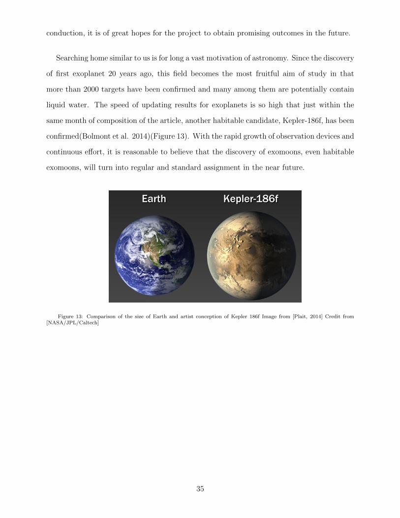
confirmed(Bolmont et al. 2014)(Figure 13). With the rapid growth of observation devices and

continuous effort, it is reasonable to believe that the discovery of exomoons, even habitable

exomoons, will turn into regular and standard assignment in the near future.

Figure 13: Comparison of the size of Earth and artist conception of Kepler 186f Image from [Plait, 2014] Credit from[NASA/JPL/Caltech]

35

List of Figures

1: Moons of solar system. The photo shows major large moons at their relative sizes toeach other and to Earth. Pictured are Earth’s Moon; Jupiter’s Callisto, Ganymede, Io andEuropa; Saturn’s Iapetus, Enceladus, Titan, Rhea, Mimas, Dione and Tethys; Neptune’sTriton; Uranus’ Miranda, Titania and Oberon and Pluto’s Charon. Image from NASA,http://solarsystem.nasa.gov/multimedia/display.cfm?IM_ID=6163

2: First direct image of multiple exoplanets orbiting the star about 130 ly away calledHR 8799. Image from [Moskowitz (2008)]

3: Artist conception of JWSTs Mid-Infrared Instrument(MIRI) at second Lagrange pointof Earth. Image from Juan Rafael Martnez Galarzas Home Page at the Leiden Observatory

4: The light curve of event MOA-2011-BLG-262 with data from the MOA 1.8m (red),Mt. John University Observatory I and V -bands (green and cyan), Canopus I-band (blue),CTIO I-band (magenta), OGLE I-band (black), and Faulkes Telescope South (gold). Thebest fit model is indicated by the black curve, and the magenta curve indicates an alternativeplanetary model, which almost fits the light curve except for the limb crossings shown in theinserts. Image from[Bennett, D.P. et al. (2013)]

5: Transit method of detecting extrasolar planets. The graph below the picture demon-strates the brightness drop as the planets transit in front of the star. Image from [http://en.wikipedia.org/wiki/Methods_of_detecting_exoplanets\#cite_note-5]

6: Kepler 6b photometry. Image from Mikulski archive for space telescopes [http://archive.stsci.edu/prepds/kepler_hlsp/]

7: One sample of star-planet-moon system. The observer is set at y2 is infinity. Theexomoon is not shown in the graph, but its effect causes the wobble of the planet orbit alongthe smaller elliptical track. The origin of x2 − y2 denotes the position of the planet-moonbarycenter. Image from [Kipping (2009)]

8: Picture of planetary magnetosphere of the simulation. According to Heller & Zuluaga(2013), conceptually the dazed orbit resembles that of Titan around Saturn. Image from[Heller & Zuluaga 2013]

9: Geometry of the triple system of a star, a planet, and a moon with illuminations

36

indicated by different shadings (pole view). For ease of visualization, the moons orbit iscoplanar with the planets orbit about the star and the planets orbital position with respectto the star is fixed. Combined stellar and planetary irradiation on the moon is shown forfour orbital phases. Projection effects as a function of longitude and latitude are ignored,and we neglect effects of a penumbra. Radii and distances are not to scale, and starlightis assumed to be plane-parallel. In the right panel, the surface normal on the subplanetarypoint is indicated by an arrow. For a tidally locked moon this spot is a fixed point on themoons surface. For ps = 0 four longitudes are indicated. Image from [Heller & Barnes 2013]

10: Flux phase profile for an Earth-sized moon orbiting a Jupiter-sized planet at 1 AUfrom a Sun-sized star for one year. The upper panel is the stellar flux over total and thelower one is comparison between reflective and thermal flux. The orbit is circular with radius0.01 AU and zero inclination. Image from [Hinkel & Kane 2013]

11: Flux phase profile for an system similar to that in figure 10, except that the eccentricityof the orbit is 0.4. Image from [Hinkel & Kane 2013]

12: A sunflower-shaped ’starshade’ launched to space with a simple telescope could helpscientists on the ground hunt for another Earth. Image from [Kramer & Writer, 2013] Creditfrom [NASA/JPL/Caltech]

13: Comparison of the size of Earth and artist conception of Kepler 186f Image from[Plait, 2014] Credit from [NASA/JPL/Caltech]

Table 1: The length of orbital semimajor axis and diameter of major moons of gas giantsin solar system. The data are given in standard units and in units of host planet radii. Imagefrom [Kane, Hinkel & Raymond, 2013]

37

Reference

Agnor., C. B, Hamilton, D. P., 2010, Icarus, 208, 824-836.Agnor, C. B., Canup, R. M., & Levison, H. F. 1999, Icarus, 142, 219Ballard, S., et al. 2011 ApJ, 743,200BBaraffe, I., Chabrier G., Barman, T., Allard F., Hauschildt P.H., 2003, A&A, 402, 701Barclay, T., et al. 2013, ApJ, 768, 101Basri, G., et al. 2011, ApJ, 736, 19Batalha, M., et al. 2013, ApJS, 204, 24Bennett., D., et al. 2014, ApJ, 785, 155.Bolmont, E., et al. 2014, submitted (arXiv: 1404.4368v1)Borucki, W. J., et al. 2011, ApJ, 736, 19Canup, R. M., & Ward, W. R., 2006, Nature 441, 834-839Chebotarev, G.A., 1964, Astr. Zu. 41, 983Dole, S. H. 1964, Habitable planets for man, New York, Blaisdell Pub. Co. [1st ed.]Elser, S., Moore, B., Stadel, J., Morishima, R., 2011, submitted (arxiv:1105.4616)Georgakarakos, N. 2002, Mon. Not. R. Astron. Soc., 337, 559 - 2003, Mon. Not. R. Astron.Soc., 345, 340Gong et al. 2013 ApJ 769 L14Gladman, B., Dane Quinn, D., Nicholson, P., & Rand, R. 1996, Icarus, 122, 166Gurzadian, G.A., 1970 Bol.Obs.Tonontzintla Tacubaya, 5, 255Han, C., Han, W., 2002, Apj, 580:490493Heller, R., Barnes, R., Astrobiology. January 2013, 13(1): 18-46Henning, W. G., OConnell, R. J., Sasselov, D. D. 2009, ApJ, 707, 1000Kane, S. R., & Hinkel, N. R. 2013, ApJ, 762, 7,. 1211.2812.Kasting, J. F., Whitmire, D. P., & Reynolds, R. T. 1993, Icarus, 101, 108Kipping, D. M. 2010, MNRAS, 409, L119Kipping, D. M., Bakos, G. A., Buchhave, L. A., Nesvorny, D. & Schmitt, A. 2012, ApJ,750, 115Kipping, D. M., 2013a, MNRAS, 435, 2152Kipping, D. M., 2013b, MNRAS, submitted (arXiv:1311.1170)Kipping, D. M., Hartman, J., Buchhave, L. A., Schmitt, A., Nesvorny, D. & Bakos, G. A.,2013a, ApJ, 770, 101Kipping, D. M., Forgan, D., Hartman, J., Nesvorny, D., Bakos, G. A., Schmitt, A. R. &Buchhave, L. A., 2013b, ApJ, 777, 134Kipping, D. M., Spiegel, D. S. & Sasselov, D., 2013, MNRAS, 434, 1883Kipping, D. M., Forgan, D., Hartman, J., Nesvorny, D., Bakos, G. A., Schmitt, A. R., 2014,MINRAS, submitted(arXiv:1401.1210)Kivelson, M. G., et al. 1996, Science, 273, 337340

38

Kopparapu, R. K., Ramirez, R., Kasting, J. F., et al. 2013, ApJ, 765, 131Leconte, J. & Chabrier, G. 2013, Nature Geoscience, 6, 347Lewis K. M., Sackett P. D., Mardling R. A., 2008, ApJ, 685, L153Lewis K. M., 2011, EPJ Web of Conferences, epj-conferences.orgLin, D. N. C., & Ida, S. 1997, ApJ, 477, 781Mayor, M., Queloz, D., 1995, Nature 378, 355-359Holman & Murray, 2004, Science :- ,2005 307 (1291)Heller, R. & Zuluaga, J. I., 2013, ApJL 776, 33. arxiv:1309.0811Matija, C. 2007, Science, 318, 244Miralda-Escude, 2001, Apj, 564, (2): 1019Morishima, R., Stadel, J., Moore, B., 2010. Icarus. 207, 517-535Moskowitz, C., 2013, Scientific Americanhttp://www.scientificamerican.com/article/exomoon-alien-planet/

Mosqueira, I., Estrada, P. R. 2003a. Icarus 163, 198-231Mosqueira, I., Estrada, P. R. 2003b. Icarus 163, 232-255.Pal, A.,& Kocsis, B. 2008, ArXiv e-prints, 806, arXiv:0806.0629Peale, S. J. 1977, in IAU Colloq. 28: Planetary Satellites, ed. J. A. Burns, 87111Petigura, E., Howard, Howard, A., Marcy, G., 2013, PNAS 110 no.48Pierrehumbert, R. T. 2010, Principles of Planetary ClimatePodsiadlowski, U., Ph., et al. 2010b, A&A, 519, A25Porter, S. B., Grundy, W. M. 2011, ApJ, 736, L14Rasio, F. A., & Ford, E. B. 1996, Science, 274, 954Rasool, S.I., and C. De Bergh, 1970 Nature, 226, 1037-1039Reynolds, R. T., McKay, C. P., Kasting, J. F. 1987, Advances in Space Research, 7, 125Sahlmann, J., et al., 2013, A&A, 551, 52Sasaki, T., Stewart, G. R., and Ida, S. 2010. ApJ., 714, 10521064.Segatz, M., Spohn, T., Ross, M. N., Schubert, G., 1988. Icarus 75, 187206Selsis, F., Kasting, J. F., Levrard, B., et al. 2007, A&A, 476, 1373Scharf, C. A. 2006, ApJ, 648, 1196Silvestri, N.M., Hawley, S.L., & Oswalt, T.D. 2005a, AJTurner, E. L., Peters, M. A., 2013, ApJ, 798, 98Torres, A. M., 2012, Planetary Habitability Laboratory,http://phl.upr.edu/press-releases/anewonlinedatabaseofhabitableworlds

Viosey, J. 2011, universetoday, http://www.universetoday.com/90745/Wada, K., Kobuko, E., & Makino., J., 2006, ApJ, 638:1180-1186,Weidenschilling, S. J., & Marzari, F. 1996, Nature, 384, 619Williams, D. R., 2006, http://www.webcitation.org/616VxHVlQWilliams, D. R., 2006,http://nssdc.gsfc.nasa.gov/planetary/factsheet/jupiterfact.html

Williams, D. M., Kasting, J. F., Wade, R. A., 1997, Nature, 385: 234-236Witze, A., 2013, Nature, http://www.nature.com/news/first-possible-exomoon-spotted-1.14430?WT.ec_id=NEWS-20131224

Zuckerman, B. & Jefferson, D., 1996, Jones & Bartlett Learning, 42, ISBN 9780867209662.

39