The Detection and Attribution of Climate Change Using an Ensemble of Opportunity

The Detection and Attribution of Climate Change Using an Ensemble of OpportunityDÁITHÍ A. STONE

Department of Physics, and Department of Zoology, University of Oxford, Oxford, United Kingdom

MYLES R. ALLEN

Department of Physics, University of Oxford, Oxford, United Kingdom

FRANK SELTEN AND MICHAEL KLIPHUIS

Royal Netherlands Meteorological Institute (KNMI), De Bilt, Netherlands

PETER A. STOTT

Hadley Centre for Climate Prediction and Research, Reading, United Kingdom

(Manuscript received 13 June 2005, in final form 24 April 2006)

ABSTRACT

The detection and attribution of climate change in the observed record play a central role in synthesizingknowledge of the climate system. Unfortunately, the traditional method for detecting and attributingchanges due to multiple forcings requires large numbers of general circulation model (GCM) simulationsincorporating different initial conditions and forcing scenarios, and these have only been performed with asmall number of GCMs. This paper presents an extension to the fingerprinting technique that permits theinclusion of GCMs in the multisignal analysis of surface temperature even when the required families ofensembles have not been generated. This is achieved by fitting a series of energy balance models (EBMs)to the GCM output in order to estimate the temporal response patterns to the various forcings.

This methodology is applied to the very large Challenge ensemble of 62 simulations of historical climateconducted with the NCAR Community Climate System Model version 1.4 (CCSM1.4) GCM, as well assome simulations from other GCMs. Considerable uncertainty exists in the estimates of the parameters infitted EBMs. Nevertheless, temporal response patterns from these EBMs are more reliable and the com-bined EBM time series closely mimics the GCM in the context of transient forcing. In particular, detectionand attribution results from this technique appear self-consistent and consistent with results from othermethods provided that all major forcings are included in the analysis.

Using this technique on the Challenge ensemble, the estimated responses to changes in greenhouse gases,tropospheric sulfate aerosols, and stratospheric volcanic aerosols are all detected in the observed record,and the responses to the greenhouse gases and tropospheric sulfate aerosols are both consistent with theobserved record without a scaling of the amplitude being required. The result is that the temperaturedifference of the 1996–2005 decade relative to the 1940–49 decade can be attributed to greenhouse gasemissions, with a partially offsetting cooling from sulfate emissions and little contribution from naturalsources.

The results support the viability of the new methodology as an extension to current analysis tools for thedetection and attribution of climate change, which will allow the inclusion of many more GCMs. Short-comings remain, however, and so it should not be considered a replacement to traditional techniques.

1. Introduction

The detection and attribution of observed climatechange play a central role in climate change research,

both because of its role in connecting the many otherresearch branches in the field (Houghton et al. 2001;International Ad Hoc Detection and AttributionGroup 2005) and because of its ultimate implicationsfor individual stakeholders (Allen 2003; Allen and Lord2004). This field came into its own with the first experi-ment with a fully coupled general circulation model(GCM) to include ensembles of simulations represent-ing the transient response to separate forcing sources

Corresponding author address: Dáithí A. Stone, AOPP, Depart-ment of Physics, University of Oxford, Clarendon Laboratory,Parks Road, Oxford OX1 3PU, United Kingdom.E-mail: [email protected]

504 J O U R N A L O F C L I M A T E VOLUME 20

© 2007 American Meteorological Society

JCLI3966

(Tett et al. 1999; Stott et al. 2000). Such ensemblespermit spatiotemporal comparisons with observed cli-mate change that simultaneously serve to strengthenand constrain our confidence in our observations, ourunderstanding of sources of past forcing, and our un-derstanding of climate processes encapsulated in thedynamical models. Furthermore, they also provide atest of the cause–effect relationship required by stake-holders in the climate change issue.

This methodology for detection and attribution de-pends on the generation of ensembles of climate modelsimulations following multiple forcing scenarios. Theensembles are necessary in order to accurately extractthe underlying climate response to particular externalforcings from the natural internal variability of the cli-mate system. However, such families of ensembles re-quire large computational resources and it may be dif-ficult or even unfeasible to run so many simulations ofa given GCM. Currently, the necessary set of ensembleshas been performed with only a few GCMs (Stott et al.2006). However, the generation of the single ensembleof simulations including a relatively comprehensive setof external forcings is more feasible and common. Herewe develop a procedure that allows application of thestandard detection and attribution methodology whenonly such an ensemble forced with a single large set offorcings is available. The development of this proce-dure will allow the eventual inclusion of many moreGCMs into the detection and attribution frameworkand thus a more robust characterization of the impor-tance of the various external forcings on past and futureclimate change.

2. Model and data

We use output from the Challenge Project conductedin the summer of 2003 by the Dutch MeteorologicalInstitute (KNMI) using machines at the AcademicComputing Centre in Amsterdam (SARA; Selten et al.2003). This project consists of a 62-member initial con-dition ensemble of simulations of the National Centerfor Atmospheric Research (NCAR) Community Cli-mate System Model version 1.4 (CCSM1.4) coveringthe 1940–2080 period. The CCSM1.4 is a fully coupledGCM of the atmosphere, ocean, sea ice, and land sur-face (Boville et al. 2001), making this the largest initialcondition ensemble of transient climate simulationswith a coupled GCM at present. Each simulation wasinitialized by a small random perturbation in the tem-perature field of the atmosphere in an initial state ob-tained from an earlier transient simulation. This en-semble is designed to provide a large dataset onchanges in extreme events and so all members are

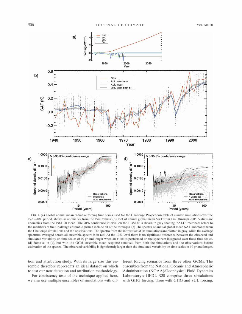
forced with the identical historical scenario of pre-scribed forcings through to 2000 following C. M. Am-mann et al. (2006, personal communication). Thesecomprise changes in the mass mixing ratios of tropo-spheric greenhouse gases (GHGs), changes in sulfateemissions [resulting in tropospheric sulfate aerosols(SUL) through an interactive sulfate simulation (Raschet al. 2000)], changes in the optical depth from strato-spheric volcanic aerosols (VOL), and changes in solarradiation (SOL) according to Hoyt and Schatten(1993). For this study we estimate the global GHG forc-ing (Fig. 1a) from the mass mixing ratios of the variousgases inputted to the GCM simulations (Dai et al. 2001)according to the formulas in Table 6.2 of Ramaswamyet al. (2001), while the SUL forcing is taken as theglobal column-integrated burden simulated in theGCM’s interactive sulfate model scaled to the 1940 and1990 combined direct and indirect forcing estimates ofBoucher and Pham (2002). Because the CCSM1.4 onlyincludes the direct effect of sulfate aerosols in its cal-culations, we may expect to find that the GCM under-estimates the SUL response. The optical depth of thestratospheric aerosols of C. M. Ammann et al. (2006,personal communication) is multiplied by �20 to rep-resent the VOL forcing (Wigley et al. 2005), while thesolar forcing of Hoyt and Schatten (1993) is multipliedby 0.175 to account for the planetary albedo and thegeometrical nature of the SOL forcing.

Deseasonalized monthly surface air temperature(SAT) anomalies from the GCM simulations are inter-polated onto the HadCRUT2v dataset of 5° � 5° grid-ded monthly mean observed SAT anomalies of Jonesand Moberg (2003) and Rayner et al. (2003) accordingto the availability of observations. Annual global meansare calculated for both datasets and used in the subse-quent analysis. These time series are plotted in Fig. 1b.Considering the availability of observations through tothe end of 2005 we include these extra years in theanalysis. The GHG forcing after 2000 in these simula-tions follows a business-as-usual scenario similar to theIntergovernmental Panel on Climate Change (IPCC)Special Report on Emissions Scenarios (SRES) A1 sce-nario (Dai et al. 2001) and close to what has actuallyoccurred. On the other hand the SUL, VOL, and SOLforcings are held constant at year 2000 values. This isreasonably appropriate for the currently fairly stableSUL emissions and for VOL due to the lack of anylarge volcanic eruptions since 2000, but it does misssome of the latest solar cycle and so may lead to a slightunderestimate of the SOL detection.

The lack of ensembles forced with subsets of theseexternal forcings means that this large set of simula-tions cannot be used in a traditional multisignal detec-

1 FEBRUARY 2007 S T O N E E T A L . 505

tion and attribution study. With its large size this en-semble therefore represents an ideal dataset on whichto test our new detection and attribution methodology.

For consistency tests of the technique applied here,we also use multiple ensembles of simulations with dif-

ferent forcing scenarios from three other GCMs. Theensembles from the National Oceanic and AtmosphericAdministration (NOAA)/Geophysical Fluid DynamicsLaboratory’s GFDL-R30 comprise three simulationswith GHG forcing, three with GHG and SUL forcing,

FIG. 1. (a) Global annual mean radiative forcing time series used for the Challenge Project ensemble of climate simulations over the1920–2080 period, shown as anomalies from the 1940 values. (b) Plot of annual global mean SAT from 1940 through 2005. Values areanomalies from the 1961–90 mean. The 90% confidence interval on the EBM fit is shown in gray shading. “ALL” members refers tothe members of the Challenge ensemble (which include all of the forcings). (c) The spectra of annual global mean SAT anomalies fromthe Challenge simulations and the observations. The spectra from the individual GCM simulations are plotted in gray, while the averagespectrum averaged across all ensemble spectra is in red. At the 10% level there is no significant difference between the observed andsimulated variability on time scales of 10 yr and longer when an F test is performed on the spectrum integrated over these time scales.(d) Same as in (c), but with the GCM ensemble mean response removed from both the simulations and the observations beforeestimation of the spectra. The observed variability is significantly larger than the simulated variability on time scales of 10 yr and longer.


Fig 1 live 4/C

three with GHG, SUL, and SOL forcing, and three withall four forcings (Broccoli et al. 2003). The ensemblesfrom the NCAR Parallel Climate Model (PCM) com-prise 5 simulations with GHG forcing, 4 with SUL forc-ing, 12 with GHG and SUL forcing (some also includechanging stratospheric ozone forcing), 5 with SOL forc-ing, 4 with VOL forcing, 4 with SOL and VOL forcing,and 4 with all of these forcings (Meehl et al. 2003). Theensembles from the Met Office’s (UKMO) ThirdHadley Centre Coupled Ocean–Atmosphere GCM(HadCM3) comprise four simulations with GHG forc-ing, four with GHG and SUL forcing (and also chang-ing stratospheric ozone), four with VOL and SOL forc-ing, and four with both these anthropogenic and naturalforcings (Stott et al. 2000; Tett et al. 2002). With thesemultiple ensembles we can compare the results of thisnew methodology applied here with results from tradi-tional detection and attribution studies.

3. Method

For traditional multisignal detection and attributionmethods using GCM simulations we need informationabout the response of the climate system to each of theforcings individually. This is clearly not available froma set of simulations that only includes the combinedforcing scenario. However, the global mean SAT re-sponse of GCMs tends to closely follow that of a simpletuned energy balance model (EBM) (McAvaney et al.2001). Thus, in an ensemble forced with a number ofexternal forcings it may be possible to deduce the GCMresponse to individual forcings by fitting a series ofEBMs to the total GCM response, with each EBM rep-resenting the response to a different forcing. EachEBM has a different set of parameters because there isno a priori reason to expect, for instance, that the oceanheat uptake corresponding to the SUL forcing, which isconcentrated over Northern Hemisphere land, shouldbe identical to that for the more global GHG forcing.

We start with an EBM for forcing i:

ci

�Ti�t, z�

�t� Fi�t� � �iTi�t, z� � ki

�2Ti�t, z�

�z2 . �1�

Here Ti(t, z) is the time series, as a function of depth inthe mixed layer, of the global annual mean temperatureresponse to the evolving forcing Fi shown in Fig. 1a. Noboundary conditions are imposed for the bottom of themixed layer. Here ci, (1/�i), and ki are the heat capacityof the ocean mixed layer, the climate sensitivity, andthe parameter for vertical diffusion in the ocean mixed

layer for forcing i and are tuned to reproduce the meanresponse of the GCM.

Supposing that the temperature responses to indi-vidual forcings add linearly to give the response to thesum of the forcings, we can add the results of the EBMsto get the total temperature response

T�t, z� � �i�1

m

Ti�t, z�. �2�

This assumption of linear additivity, implicit in the stan-dard detection methodology, appears to hold in GCMoutput (Gillett et al. 2004). Our aim in fitting the pa-rameters for the EBM is to minimize the squared dif-ference between the total annual mean EBM SAT timeseries, which we denote as the vector T � T(t, 0), andthe mean response TGCM from the ensemble of GCMsimulations over the 1940–2005 period. The EBMs arespun up with 20 yr of varying forcings before the start ofthe comparison in 1940. To tune the parameters in thisstudy we use a downhill simplex method, an iterativegeometric method for finding the minimum in a multi-dimensional function (Nelder and Mead 1965). Uncer-tainty in this fit arises from the finite GCM ensemblesize and the accuracy of the parameter-fitting algo-rithm. While the downhill simplex method is fairly ro-bust, we are trying to locate the global minimum in a12-dimensional space using 66 temporal data points, sothe parameter fits may end up being somewhat uncer-tain. The arising distribution of plausible EBM param-eter sets and EBM output is estimated using a boot-strap resampling procedure in which 62 simulations arerandomly selected with replacement from the full set of62 GCM simulations. This is performed 100 times, withthe mean response of the selected simulations used asinput to the analysis to estimate another plausible set ofEBM parameters.

Now that we have estimated the responses of theGCM to individual forcings, we can proceed with thestandard detection and attribution methodology (Allenand Tett 1999). Under this, we express the observedtemperature response pattern Tobs as a linear sum ofthe simulated responses determined for each forcing(Ti) plus a residual (�0):

Tobs � �i�1

m

Ti�i � �0. �3�

Here i is the scaling factor corresponding to the re-sponse to forcing i that is to be estimated in the regres-sion. This relational model depends on the GCM toproperly reproduce the temporal pattern of the re-


sponse and for the EBM to properly reproduce theGCM response, but it explicitly corrects for errors inthe amplitude of this response pattern. The regressionis performed on the full global annual time series. Thisis a limitation of this study because spatial informationcan be important for detecting climate response signals(S. A. Crooks et al. 2006, unpublished manuscript,hereafter referred to as CR06; Stott et al. 2006). Incor-porating spatial information will be a future develop-ment of this methodology, but for now we want to keepthe EBM approximation as simple and appropriate aspossible. No optimization or data reduction is used asthis is of limited applicability to the temporal data ana-lyzed here.

A control simulation is needed both to estimate thecovariance of the residual term, �0, and to estimate theuncertainty of the i scaling parameters. The internalvariability is estimated from the 62 ensemble simula-tions with the transient ensemble mean response re-moved. The resulting anomaly time series are multi-plied by (62/61) to account for bias in the removal ofthe mean response. We use these pseudocontrol simu-lations because they provide more data (4092 yr) thanexists in any available control simulation. Half (31) ofthese pseudocontrol simulations are used for estimatingthe covariance of the noise term while the other half areused to obtain an independent estimate of the i distri-butions.

The regression formulation used here, referred to asordinary least squares (OLS), does not include any er-ror in the estimate of the simulated responses; this erroris taken into account through the bootstrap resampling.In summary, the attribution results presented here ac-count for sampling uncertainty from both the observa-tions (during the regression step) and the simulations(through the Monte Carlo sampling). The inclusion ofthe latter source of uncertainty depends implicitly uponthe ability of the EBM to represent it. While deficien-cies in the EBM fits may partly represent uncertaintyarising from structural differences between the GCMand the real world, this uncertainty should not be con-sidered to be included in this analysis. This study alsodoes not account for uncertainty in the source of theforcings nor in how those sources (e.g., emissions) areconverted into radiative forcings.

4. Results

a. Comparison of variability

Figure 1c shows the power density spectra of annualglobal mean SAT anomalies over the 1940 though 2005period. All spectra have been estimated using a Han-

ning filter of width 65 yr. The lower power at the 130-yrtime scale in the GCM simulations than in the obser-vations reflects the smaller long-term trend visible inFig. 1b. The significance tests on the spectra take ac-count of the filtering, but they assume a stationary pro-cess. It should be noted that this assumption is almostdefinitely invalid due both to the spatiotemporal natureof the observational masking and the changing externalforcings. Considering that these two factors tend to op-erate on longer time scales, we would expect this as-sumption to be weakest at longer time scales; the dis-crepancy between the estimated confidence range inthe observed spectrum and the spread of the simulatedspectra at longer time scales is indicative of this. Attime scales of 10 yr and longer, that is, those relevantfor long-term climate change, there is no significantdifference, at the 10% level, between the spectra ofobserved SAT and the ensemble mean spectrum fromthe GCM simulations. These time scales are of interestas they are the most relevant to anthropogenicallyforced climate change. Of course this test is of onlylimited use because it does not distinguish between theinternally generated and externally driven componentsof the variability. The issue is that the GCM may beproducing similar variability for the wrong reason, forexample, by overestimating the externally forced re-sponse and underestimating the internally generatedvariability.

A first step in improving this comparison is to re-move the GCM’s estimate of the total externally forcedresponse. If we assume the GCM is producing the sameresponses as the real world is, then we can remove theensemble mean response of the GCM simulations fromall of the time series. The resulting spectra are plottedin Fig. 1d. The spectra of the GCM simulations havebeen scaled by a factor of (62/61) to account for thereduction in variance due to the removal of the meanresponse. Because a large part of the externally forcedvariability has been removed, there is now a muchcloser agreement between the estimate of the confi-dence range of the observed spectrum and the spread ofthe simulated spectra at long time scales. We now findthat the decadal variability in the observations is sig-nificantly larger than in the GCM simulations. This sug-gests that the GCM overly damps long-term variability.However, it could equally reflect an underestimate oroverestimate in the GCM’s response to external forcingand thus that we have not properly removed the totalforced response from the observed time series. Toelaborate on this comparison we need to produce amore confident estimate of the forced response, whichwill require us to first determine the GCM responses to


each of the forcings and then to compare the responsepatterns with the observed SAT time series.

b. Fitting the EBMs

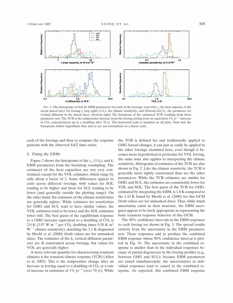
Figure 2 shows the histograms of the ci, (1/�i), and ki

EBM parameters from the bootstrap resampling. Theestimates of the heat capacities are not very con-strained, except for the VOL estimates, which range byonly about a factor of 2. Some differences appear toexist across different forcings, with values for SOLtending to be higher and those for SUL tending to belower (and generally outside the plotting range). Onthe other hand, the estimates of the climate sensitivitiesare generally tighter. While estimates for sensitivitiesfor GHG and SUL tend to have similar values, theVOL estimates tend to be lower and the SOL estimateslower still. The best guess of the equilibrium responseto a GHG increase equivalent to a doubling of CO2 is2.0 K (3.97 W m�2 per CO2 doubling times 0.50 K m2

W�1 climate sensitivity), matching the 2.1 K diagnosedby Meehl et al. (2000) (both values are for unmaskeddata). The estimates of the ki vertical diffusion param-eter are ill constrained across forcings, but values forVOL are generally higher.

A more relevant quantity for characterizing transientclimates is the transient climate response (TCR) (Allenet al. 2005). This is the temperature change after anincrease in forcing equal to a doubling of CO2 at a rateof increase in emissions of 1% yr�1 (over 70 yr). While

the TCR is defined for and traditionally applied toGHG forced changes, it can just as easily be applied tothe other forcings examined here; even though it be-comes more hypothetical in particular for VOL forcing,the same issue also applies to interpreting the climatesensitivity. Histograms of estimates of the TCR are alsoshown in Fig. 2. Like the climate sensitivity, the TCR isgenerally more tightly constrained than are the otherparameters. While the TCR estimates are similar forGHG and SUL, the estimates are consistently lower forVOL and SOL. The best guess of the TCR for GHG,estimated by integrating the EBM, is 1.8 K compared tothe 1.43 K found by Meehl et al. (2000) for this GCM(both values are for unmasked data). Thus, while muchuncertainty exists in their structure, the EBM surro-gates appear to be fairly appropriate in representing thebasic transient response behavior of this GCM.

The 90% confidence intervals in the EBM responsesto each forcing are shown in Fig. 3. The spread resultsentirely from the uncertainty in the EBM parametersets. These responses add to produce the combinedEBM response whose 90% confidence interval is plot-ted in Fig. 1b. The uncertainty in the combined re-sponse is smaller than in the individual responses be-cause of partial degeneracy in the forcing profiles (e.g.,between GHG and SUL); because EBM parametersare tuned simultaneously, the uncertainties in indi-vidual responses tend to cancel in the combined re-sponse. As expected, this combined EBM response

FIG. 2. The histograms of best-fit EBM parameters for each of the forcings: (top left) ci, the heat capacity of theocean mixed layer for forcing i; (top right) (1/�i), the climate sensitivity; and (bottom left) ki, the parameter forvertical diffusion in the mixed layer. (bottom right) The histogram of the estimated TCR resulting from theseparameter sets. The TCR is the temperature increase from the forcing arising from an equivalent 1% yr�1 increasein CO2 concentrations up to a doubling after 70 yr. The horizontal scale is identical on all plots. Note that thehistograms follow logarithmic bins and so are not normalized on a linear scale.


Fig 2 live 4/C

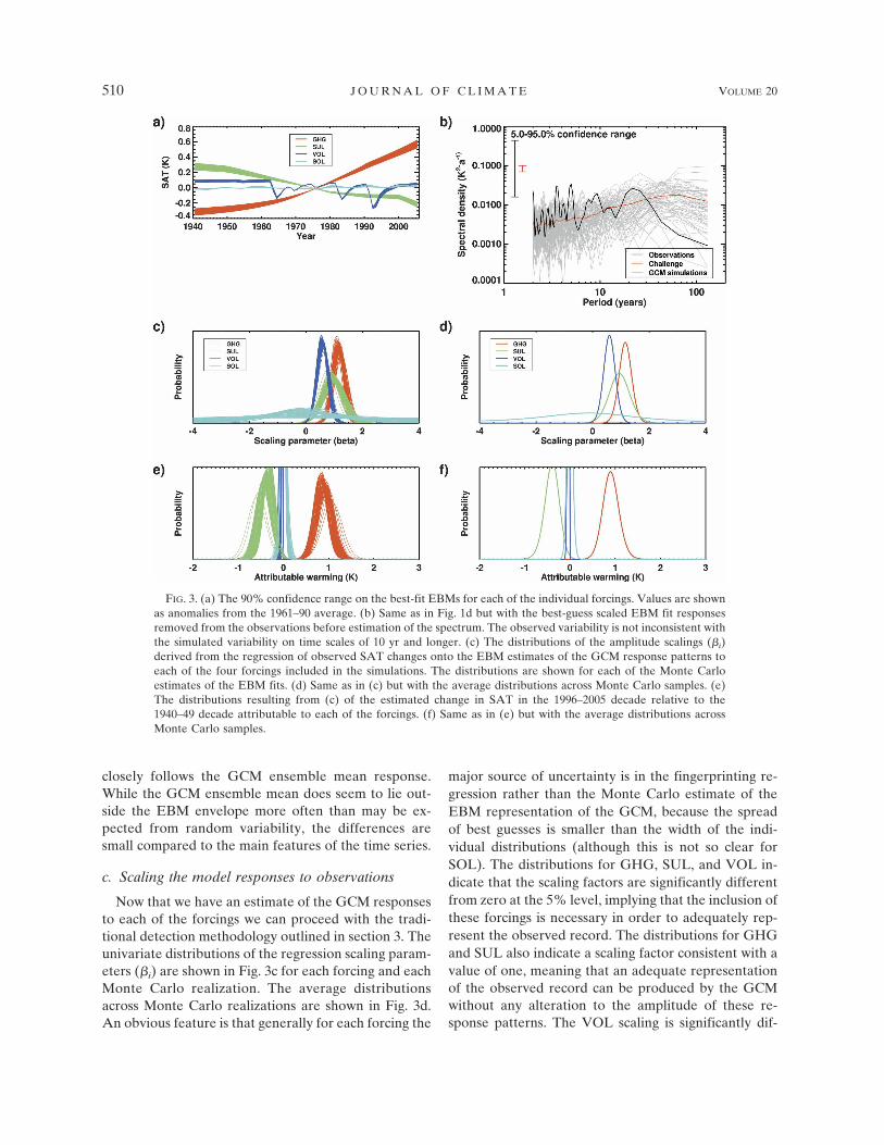
closely follows the GCM ensemble mean response.While the GCM ensemble mean does seem to lie out-side the EBM envelope more often than may be ex-pected from random variability, the differences aresmall compared to the main features of the time series.

c. Scaling the model responses to observations

Now that we have an estimate of the GCM responsesto each of the forcings we can proceed with the tradi-tional detection methodology outlined in section 3. Theunivariate distributions of the regression scaling param-eters (i) are shown in Fig. 3c for each forcing and eachMonte Carlo realization. The average distributionsacross Monte Carlo realizations are shown in Fig. 3d.An obvious feature is that generally for each forcing the

major source of uncertainty is in the fingerprinting re-gression rather than the Monte Carlo estimate of theEBM representation of the GCM, because the spreadof best guesses is smaller than the width of the indi-vidual distributions (although this is not so clear forSOL). The distributions for GHG, SUL, and VOL in-dicate that the scaling factors are significantly differentfrom zero at the 5% level, implying that the inclusion ofthese forcings is necessary in order to adequately rep-resent the observed record. The distributions for GHGand SUL also indicate a scaling factor consistent with avalue of one, meaning that an adequate representationof the observed record can be produced by the GCMwithout any alteration to the amplitude of these re-sponse patterns. The VOL scaling is significantly dif-

FIG. 3. (a) The 90% confidence range on the best-fit EBMs for each of the individual forcings. Values are shownas anomalies from the 1961–90 average. (b) Same as in Fig. 1d but with the best-guess scaled EBM fit responsesremoved from the observations before estimation of the spectrum. The observed variability is not inconsistent withthe simulated variability on time scales of 10 yr and longer. (c) The distributions of the amplitude scalings (i)derived from the regression of observed SAT changes onto the EBM estimates of the GCM response patterns toeach of the four forcings included in the simulations. The distributions are shown for each of the Monte Carloestimates of the EBM fits. (d) Same as in (c) but with the average distributions across Monte Carlo samples. (e)The distributions resulting from (c) of the estimated change in SAT in the 1996–2005 decade relative to the1940–49 decade attributable to each of the forcings. (f) Same as in (e) but with the average distributions acrossMonte Carlo samples.


Fig 3 live 4/C

ferent from one though, indicating that the GCM has atendency to overestimate the VOL response amplitude,as may be guessed from visual inspection of Fig. 1b. Onthe other hand, the SOL scaling is poorly constrainedand the observations are consistent both with its ab-sence and presence. Considering that the historical evo-lution of SOL forcing is poorly known, this result mayjust as easily be indicative of a problem with the forcingscenario used here as of a problem with the GCM ormethodology.

d. Comparison of internally generated variability

The residual variability after removal of the scaledresponse patterns from the observations is significantlyhigher (based on an F test) than the variability in thefirst subset of 31 pseudocontrol simulations, producedby subtracting the ensemble mean change from the first31 transient simulations. We can also examine this re-sidual in the context of the spectra we were examiningearlier. The spectra of the residuals, estimated by sub-tracting the best-guess EBM fit adjusted by the appro-priate scalings from the observations, are plotted in Fig.3b. The variability at interdecadal time scales in theobservations does not differ significantly from thepseudocontrol simulations. Inspection of the spectrasuggests the main discrepancy is at time scales of 3–6 yr,which are less important for the slowly varying anthro-pogenic forcings than for the more rapidly varyingnatural forcings.

e. Attributable warming to present

With estimates of the scaling factors, we can nowestimate the amount of SAT change between 2005 and1940 attributable to the various forcings (Figs. 3e,f). Forconsistency with other studies and because of the non-linear nature of the response patterns, we estimate theattributable warming as the difference between the1996–2005 mean SAT and the 1940–49 mean SAT inthe scaled EBM response. GHG forcing dominatesover this interval, contributing a significant warming ofaround 0.6–1.2 K. This is partly countered by a signifi-cant cooling from SUL forcing of around a quarter to athird that magnitude. The SOL and VOL forcings con-tribute little because their values are almost identical inthe two decades compared.

f. Projections of global mean climate

If we suppose that the EBM approximation holdsbeyond the historical climate and into future climates,and that the linear additivity of the forcings also holds,

then we can also extend our estimates of attributablewarming into the future if we suppose a certain scenarioof forcing for the future (Allen et al. 2000; Stott andKettleborough 2002). The GCM has only been used todetermine the temporal response pattern of the climatesystem to the various forcings, but not the amplitudes ofthose patterns. Thus, if the basic assumptions of thefingerprinting methodology hold, such scaled estimatesof future warming are in fact constrained by the ob-served climate record, and not by the GCM itself.

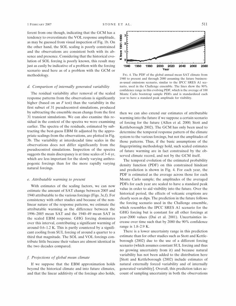
The temporal evolution of the estimated probabilitydensity function (PDF) on this constrained hindcastand prediction is shown in Fig. 4. For each year, thePDF is estimated as the average across those for eachMonte Carlo sample; the amplitudes of the averagedPDFs for each year are scaled to have a standard peakvalue in order to aid visibility into the future. Over thehistorical period, the effects of volcanic eruptions areclearly seen as dips. The prediction in the future followsthe forcing scenario used in the Challenge ensemble,which resembles the IPCC SRES A1 scenario for theGHG forcing but is constant for all other forcings atyear-2000 values (Dai et al. 2001). Uncertainties in-crease over time such that by 2080 the 90% confidencerange is 1.8–2.9 K.

There is a lower uncertainty range in this predictionestimate than for other studies such as Stott and Kettle-borough (2002) due to the use of a different forcingscenario (which assumes constant SUL forcing and thusno growing uncertainty from it) and because naturalvariability has not been added to the distribution here[Stott and Kettleborough (2002) include estimates ofnatural externally forced variability and of internallygenerated variability]. Overall, this prediction takes ac-count of sampling uncertainty in both the observations

FIG. 4. The PDF of the global annual mean SAT climate from1940 to present and through 2080 assuming the future business-as-usual emissions scenario, similar to the IPCC SRES A1 sce-nario, used in the Challenge ensemble. The lines show the 90%confidence range in this evolving PDF, which is the average of 100Monte Carlo bootstrap sample PDFs and is standardized eachyear to have a standard peak amplitude for visibility.


and the GCM simulations. It does not, of course, ac-count for uncertainty in past or future emissions andforcings. While deficiencies in the EBM fitting to theGCM output could represent some uncertainty arisingfrom the structural differences between the GCM andthe real world, this prediction should not be consideredto comprehensively account for that uncertainty.

5. Sensitivity of results

The technique developed in this paper involves add-ing another fitting step into the detection and attribu-tion framework, which adds more potential uncertaintyand possibly decreases the robustness of the results. Inthis section we test the robustness of the results to somechanges in the input and methodology.

a. Substituting observations with GCM simulations

A first question is whether the method is estimatingthe correct values for the detection results. This can betested using a perfect model setup, whereby the obser-vations are replaced by a single random simulation foreach of the 100 Monte Carlo samples. Because theGCM is implicitly reproducing the correct responsepattern and amplitude in this setup, the scaling param-eters should be centered on a value of one. The result-ing average probability distribution of scaling values isshown in Fig. 5a. As expected, the scaling parameterdistributions are all centered on a value of about one(except possibly for the very broad SOL). As with theobservations, the GHG and VOL responses are themost tightly constrained, but in general the width of the

distributions is wider than when the comparison isagainst the observations. This probably arises becausewe have used multiple simulations in place of the ob-servations throughout the different Monte Carlosamples, rather than repetitively using the same simu-lation. The inability to constrain the SOL scaling in thisperfect model exercise suggests that the SOL responsesimply has too small a signal-to-noise ratio to be de-tected. Notably, the residual variability in about 30% ofthe Monte Carlo samples is inconsistent at the 10%level with the residual variability; this usually involves asmaller residual, highlighting a bias in the methodology.

b. Number of transient simulations

Most applications of this methodology will be withGCM ensembles with far fewer than 62 simulations.With such smaller ensembles, the EBM fits might notbe expected to be as accurate due to the larger samplinguncertainty. Furthermore, if the ensembles are quitesmall (e.g., one member) then the Monte Carlo ap-proach used here to quantify this uncertainty cannot beapplied, so it would be useful to use the large ensemblehere to characterize this component of the uncertainty.The estimated confidence ranges on the scaling param-eters for different ensemble sizes ranging from 1 to 15members are shown in Figs. 5c and 5d. In this analysis,the given number of simulations was randomly selectedfrom all of the 62 members of the Challenge ensemblewith replacement; otherwise the analysis is identical tobefore. As in the full 62-member ensemble analysis,GHG, SUL, and VOL responses are detected for allensemble sizes. Beyond ensembles of three, the scaling

FIG. 5. (a), (b) Same as in Figs. 3d,f but replacing the observations with random GCM simulations. Also shownare the 90% confidence intervals on the (c) i scaling parameters and the (d) 1996–2005 vs 1940–49 attributablewarming as a function of the number of historical GCM simulations used.


Fig 5 live 4/C

parameter values are only marginally more uncertainwhen fewer simulations are used. Attributable warmingvalues show no noticeable changes. This indicates thatthe main source of uncertainty is not sampling of theGCM but sampling of the observations and/or limita-tions in the applicability of the one-dimensional EBMsurrogate to the GCM. In particular there may be asmall limit to the amount of information contained inthe globally averaged data used here, and this limit isreached with ensembles of about three members. Thisis a limitation of the temporal methodology used hereversus the standard attribution method, in that tighterconstraints than those found here can be obtained usingspatiotemporal data from multiple simulations (Stott etal. 2006).

c. Consistency with the standard attribution method

Multiple ensembles of simulations with differentforcing scenario combinations exist from the GFDL-R30, PCM1, and UKMO-HadCM3 GCMs. These simu-lations can therefore be used both as an internal con-sistency test of the methodology applied here and as anexternal consistency test with the results from the stan-dard fingerprinting method applied to temporal dataonly. In the analysis of these GCMs, we use the periodstarting in 1901 and ending in 1995–2002, depending

upon the length of available of simulations. The forcingscenarios used are provided by PCMDI [see Stone et al.(2007) for more information].

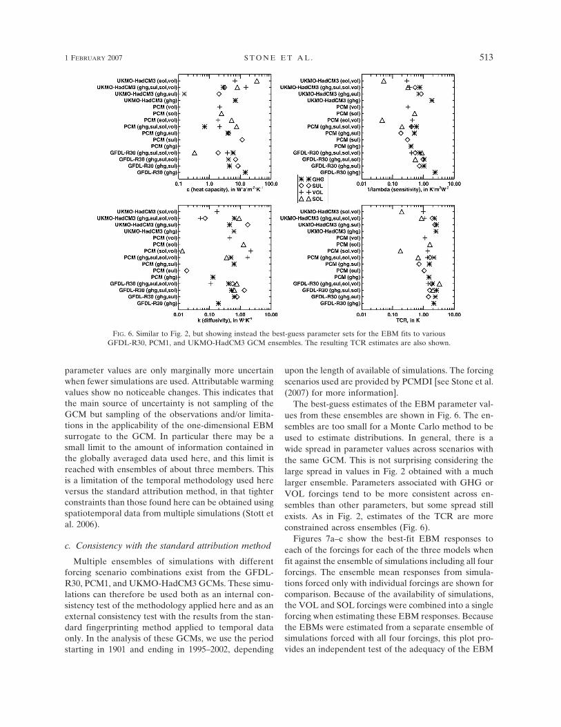
The best-guess estimates of the EBM parameter val-ues from these ensembles are shown in Fig. 6. The en-sembles are too small for a Monte Carlo method to beused to estimate distributions. In general, there is awide spread in parameter values across scenarios withthe same GCM. This is not surprising considering thelarge spread in values in Fig. 2 obtained with a muchlarger ensemble. Parameters associated with GHG orVOL forcings tend to be more consistent across en-sembles than other parameters, but some spread stillexists. As in Fig. 2, estimates of the TCR are moreconstrained across ensembles (Fig. 6).

Figures 7a–c show the best-fit EBM responses toeach of the forcings for each of the three models whenfit against the ensemble of simulations including all fourforcings. The ensemble mean responses from simula-tions forced only with individual forcings are shown forcomparison. Because of the availability of simulations,the VOL and SOL forcings were combined into a singleforcing when estimating these EBM responses. Becausethe EBMs were estimated from a separate ensemble ofsimulations forced with all four forcings, this plot pro-vides an independent test of the adequacy of the EBM

FIG. 6. Similar to Fig. 2, but showing instead the best-guess parameter sets for the EBM fits to variousGFDL-R30, PCM1, and UKMO-HadCM3 GCM ensembles. The resulting TCR estimates are also shown.


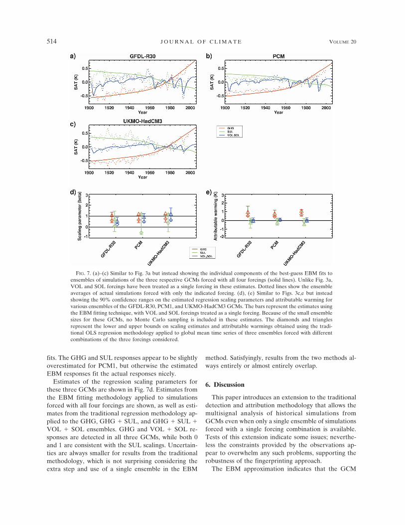
fits. The GHG and SUL responses appear to be slightlyoverestimated for PCM1, but otherwise the estimatedEBM responses fit the actual responses nicely.

Estimates of the regression scaling parameters forthese three GCMs are shown in Fig. 7d. Estimates fromthe EBM fitting methodology applied to simulationsforced with all four forcings are shown, as well as esti-mates from the traditional regression methodology ap-plied to the GHG, GHG � SUL, and GHG � SUL �VOL � SOL ensembles. GHG and VOL � SOL re-sponses are detected in all three GCMs, while both 0and 1 are consistent with the SUL scalings. Uncertain-ties are always smaller for results from the traditionalmethodology, which is not surprising considering theextra step and use of a single ensemble in the EBM

method. Satisfyingly, results from the two methods al-ways entirely or almost entirely overlap.

6. Discussion

This paper introduces an extension to the traditionaldetection and attribution methodology that allows themultisignal analysis of historical simulations fromGCMs even when only a single ensemble of simulationsforced with a single forcing combination is available.Tests of this extension indicate some issues; neverthe-less the constraints provided by the observations ap-pear to overwhelm any such problems, supporting therobustness of the fingerprinting approach.

The EBM approximation indicates that the GCM

FIG. 7. (a)–(c) Similar to Fig. 3a but instead showing the individual components of the best-guess EBM fits toensembles of simulations of the three respective GCMs forced with all four forcings (solid lines). Unlike Fig. 3a,VOL and SOL forcings have been treated as a single forcing in these estimates. Dotted lines show the ensembleaverages of actual simulations forced with only the indicated forcing. (d), (e) Similar to Figs. 3c,e but insteadshowing the 90% confidence ranges on the estimated regression scaling parameters and attributable warming forvarious ensembles of the GFDL-R30, PCM1, and UKMO-HadCM3 GCMs. The bars represent the estimates usingthe EBM fitting technique, with VOL and SOL forcings treated as a single forcing. Because of the small ensemblesizes for these GCMs, no Monte Carlo sampling is included in these estimates. The diamonds and trianglesrepresent the lower and upper bounds on scaling estimates and attributable warmings obtained using the tradi-tional OLS regression methodology applied to global mean time series of three ensembles forced with differentcombinations of the three forcings considered.


Fig 7 live 4/C

used in the Challenge ensemble responds differently tomost forcings. While the estimated GCM responses toGHG, SUL, and VOL forcing are detected in the ob-served record, the response to SOL forcing is not. Theobservational constraints on the responses indicate thatrecent climate change has been driven by GHG forcing,with a partial counteracting effect from SUL forcing,and thus provides constraints on future warming.

CR06 also develop a technique for extracting multi-signal attribution results from ensembles of a singleforcing scenario. Their technique applies a space–timeseparable approach to extract spatial response patterns,rather than the temporal patterns used here. When ap-plied to identical GCM simulations both methods pro-duce broadly similar results, although CR06 seem morelikely to detect SUL and SOL responses but not VOLresponses, while the EBM fitting method tends to findthe opposite. The difference in the VOL detection ap-pears at least partly due to the use of forcing time se-ries, rather than response time series, to estimate thespatial response pattern in the method of CR06. Weplan in future work to incorporate the EBM fits devel-oped here into the method of CR06 in order to developa more comprehensive attribution methodology.

The methodology used here requires EBMs to befitted to GCM output and one would like the tunedparameters in the EBMs to be robustly constrained.Unfortunately that does not appear to be the case here.However, the parameter sets tend to lead to EBMs withrelatively more robust behavior, such as that character-ized by the TCR and by the response pattern. The latteris judged by the ability of the regression to consistentlydetect and scale the response pattern appropriately.Consequently, detection and attributable warming re-sults appear fairly robust.

The extended methodology developed here shouldnot be considered a replacement for the traditionalmultisignal detection and attribution procedure. Nev-ertheless, the tests indicate that the new step is fulfillingits purpose in providing an adequate surrogate for theGCM response behavior. Thus application of this tech-nique will allow the inclusion of many more GCMs intothe detection and attribution framework and permit amore robust quantification of the contribution of exter-nal forcings to past and future climate change.

Acknowledgments. The authors wish to thank CasparAmmann, Simon Crooks, Mark Hawkins, and HugoLambert for their help with the analysis. We also thankFrancis Zwiers and two anonymous reviewers for manyhelpful comments on earlier versions of the manuscript.We acknowledge the HadCRUT2v dataset provided bythe Climate Research Unit (UEA), the GFDL-R30

simulation output provided by the Geophysical FluidDynamics Laboratory (NOAA), and the PCM1 simu-lation output provided by the Climate and Global Dy-namics Division (UCAR). D. A. S. and P. A. S. weresupported by the U.K. Department for Environment,Food, and Rural Affairs, and D. A. S. was also partiallysupported by a Wellcome Trust Showcase Award.M. R. A. received partial support from the U.S.NOAA/DoE International Detection and AttributionGroup.

REFERENCES

Allen, M., 2003: Liability for climate change. Nature, 421, 891–892.——, and S. F. B. Tett, 1999: Checking for model consistency in

optimal fingerprinting. Climate Dyn., 15, 419–434.——, and R. Lord, 2004: The blame game. Nature, 432, 551–552.——, P. A. Stott, J. F. B. Mitchell, R. Schnur, and T. L. Delworth,

2000: Uncertainty in forecasts of anthropogenic climatechange. Nature, 407, 617–620.

——, and Coauthors, 2005: Observational constraints on climatesensitivity. Avoiding Dangerous Climate Change, J. S.Schellnhuber et al., Eds., Cambridge University Press, 281–289.

Boucher, O., and M. Pham, 2002: History of sulfate aerosol ra-diative forcings. Geophys. Res. Lett., 29, 1308, doi:10.1029/2001GL014048.

Boville, B. A., J. T. Kiehl, P. J. Rasch, and F. O. Bryan, 2001:Improvements to the NCAR CSM-1 for transient climatesimulations. J. Climate, 14, 164–179.

Broccoli, A. J., K. W. Dixon, T. D. Delworth, T. R. Knutson, R. J.Stouffer, and F. Zeng, 2003: Twentieth-century temperatureand precipitation trends in ensemble climate simulations in-cluding natural and anthropogenic forcing. J. Geophys. Res.,108, 4798, doi:10.1029/2003JD003812.

Dai, A., T. M. L. Wigley, B. A. Boville, J. T. Kiehl, and L. E. Buja,2001: Climate of the twentieth and twenty-first centuriessimulated by the NCAR Climate System Model. J. Climate,14, 485–519.

Gillett, N. P., M. F. Wehner, S. F. B. Tett, and A. J. Weaver, 2004:Testing the linearity of the reponse to combined greenhousegas and sulfate aerosol forcing. Geophys. Res. Lett., 31,L14201, doi:10.1029/2004GL020111.

Houghton, J. T., Y. Ding, D. J. Griggs, M. Noguer, P. J. van derLinden, X. Dai, K. Maskell, and C. A. Johnson, Eds., 2001:Climate Change 2001: The Scientific Basis. Cambridge Uni-versity Press, 881 pp.

Hoyt, D. V., and K. H. Schatten, 1993: A discussion of plausiblesolar irradiance variations, 1700–1992. J. Geophys. Res., 98,18 895–18 906.

International Ad Hoc Detection and Attribution Group, 2005:Detecting and attributing external influences on the climatesystem: A review of recent advances. J. Climate, 18, 1291–1314.

Jones, P. D., and A. Moberg, 2003: Hemispheric and large-scalesurface air temperature variations: An extensive revision andan update to 2001. J. Climate, 16, 206–223.

McAvaney, B. J., and Coauthors, 2001: Model evaluation. ClimateChange 2001: The Scientific Basis, J. T. Houghton et al., Eds.,Cambridge University Press, 471–524.


Meehl, G. A., W. D. Collins, B. A. Boville, J. T. Kiehl, T. M. L.Wigley, and J. M. Arblaster, 2000: Response of the NCARClimate System Model to increased CO2 and the role ofphysical processes. J. Climate, 13, 1879–1898.

——, W. M. Washington, T. M. L. Wigley, J. M. Arblaster, and A.Dai, 2003: Solar and greenhouse gas forcing and climate re-sponse in the twentieth century. J. Climate, 16, 426–444.

Nelder, J. A., and R. Mead, 1965: A simplex method for functionminimization. Comput. J., 7, 308–313.

Ramaswamy, V., and Coauthors, 2001: Radiative forcing of cli-mate change. Climate Change 2001: The Scientific Basis, J. T.Houghton et al., Eds., Cambridge University Press, 349–416.

Rasch, P. J., M. C. Barth, J. T. Kiehl, S. E. Schwartz, and C. M.Benkovitz, 2000: A description of the global sulfur cycle andits controlling processes in the National Center for Atmo-spheric Research Community Climate Model, Version 3. J.Geophys. Res., 105, 1367–1385.

Rayner, N. A., D. E. Parker, E. B. Horton, C. K. Folland, L. V.Alexander, D. P. Rowell, E. C. Kent, and A. Kaplan, 2003:Global analyses of sea surface temperature, sea ice and nightmarine air temperature since the late nineteenth century. J.Geophys. Res., 108, 4407, doi:10.1029/2002JD002670.

Selten, F., M. Kliphuis, and H. Dijkstra, 2003: Transient coupledensemble climate simulations to study changes in the prob-ability of extreme events. CLIVAR Exchanges, Vol. 8, No. 4,

International CLIVAR Project Office, Southampton, UnitedKingdom, 11–13.

Stone, D. A., M. R. Allen, and P. A. Stott, 2007: A multimodelupdate on the detection and attribution of global surfacewarming. J. Climate, 20, 517–530.

Stott, P. A., and J. A. Kettleborough, 2002: Origins and estimatesof uncertainty in predictions of twenty-first century tempera-ture rise. Nature, 416, 723–726.

——, S. F. B. Tett, G. S. Jones, M. R. Allen, J. F. B. Mitchell, andG. J. Jenkins, 2000: External control of 20th century tempera-ture by natural and anthropogenic forcings. Science, 290,2133–2137.

——, J. F. B. Mitchell, J. M. Gregory, B. D. Santer, G. A. Meehl,T. L. Delworth, and M. R. Allen, 2006: Observational con-straints on past attributable warming and predictions of fu-ture global warming. J. Climate, 19, 3055–3069.

Tett, S. F. B., P. A. Stott, M. R. Allen, W. J. Ingram, and J. F. B.Mitchell, 1999: Causes of twentieth-century temperaturechange near the Earth’s surface. Nature, 399, 569–572.

——, and Coauthors, 2002: Estimation of natural and anthropo-genic contributions to twentieth century temperature change.J. Geophys. Res., 107, 4306, doi:10.1029/2000JD000028.

Wigley, T. M. L., C. Ammann, B. D. Santer, and S. C. B. Raper,2005: Effect of climate sensitivity on the response to volcanicforcing. J. Geophys. Res., 110, D09107, doi:10.1029/2004JD005557.


The Detection and Attribution of Climate Change Using an Ensemble of Opportunity

Documents