THE DESIGN AND TESTING OF SOIL PRESSURE

THE DESIGN AND TESTING OF SOIL PRESSURE

SENSORS FOR IN-FIELD AGRICULTURAL AND

FORESTRY TRAFFIC

JONATHAN LINDSAY EWEG

DISSERTATION

Submitted in partial fulfilment of the

requirements for the degree of MScEng

School of Bioresources Engineering and Environmental Hydrology

University of KwaZulu-Natal

Pietermaritzburg

2005

ACKNOWLEDGEMENTS

The author wishes to express his sincere appreciation for the assistance given by the

following:

• Professor PW Lyne, South African Sugarcane Research Institute, for supervision

and assistance throughout the project.

• Dr CN Bezuidenhout, School of Bioresources Engineering and Environmental

Hydrology, University of KwaZulu-Natal, for supervision and assistance

throughout the project.

• The School of Bioresources Engineering and Environmental Hydrology, for

assistance and funding.

• The University of KwaZulu-Natal, for funding in the form of the post graduate

scholarship.

• Dr R van Antwerpen and the South African Sugarcane Research Institute, for

funding and assistance with field trials.

• Dr C Smith and the Institute for Commercial Forestry Research, for funding and

assistance with field trials.

• Mr A Hill and Mr R van Zyl, School of Bioresources Engineering and

Environmental Hydrology, University of KwaZulu-Natal, for their invaluable

assistance in developing and constructing various equipment.

• Mr Peter Odell for supplying the vehicle used in the Richmond field trial.

• Mr B Marx Mr E Black and Mr C Lusso for their assistance with field trials.

• Last but not least, my family, particularly my wife Ingrid, for the love and

support.

11

ABSTRACT

Soil compaction has been shown to have a negative effect on both the environment and

on economic profitability of agriculture. Soil compaction management strategies to

ensure the sustainability of an agricultural activity need to be developed, tested and

implemented. These strategies must be based on a sound understanding of the soil

compaction process. This is best achieved by measuring the propagation of stress in the

form of pressure, caused by surface contact pressure, through the soil profile. Pressure

in the soil can be measured by a direct strain gauge pressure transducer, or a fluid-filled

bulb connected to a pressure transducer. Specific objectives of this study included the

design, construction, insertion technique and evaluation of direct strain gauge and

fluid-filled bulb soil pressure sensors for the measurement of soil pressure caused by

in-field agricultural and forestry traffic. The evaluation of the sensors indicated that the

fluid-filled pressure bulbs provided an inexpensive and effective method of measuring

the pressure in soils caused by in-field traffic. Numerous sensors were placed in the soil

during a field trial, which furthered the understanding of the pressure propagation

through the soil and ultimately the soil compaction process. The sensors and their

usefulness could however be further improved by a standardized calibration method and

apparatus. The verification of the model developed in this dissertation may greatly

improve the understanding of pressure propagation through an agricultural soil due to

in-field traffic.

ID

TABLE OF CONTENTS

Page

LIST OF TABLES VI

LIST OF FIGURES vu

1 INTRODUCTION 1

2 MEASURING THE EFFECTS OF SOIL COMPACTION ON RELEVANT SOIL

PROPERTIES 4

2.1 Measuring Changes in Bulk Density 4

2.1.1 Measuring Strain in Soils 6

2.2 Measuring Changes in Penetration Resistance 8

2.2.1 Static cone penetrometers 9

2.2.2 Dynamic cone penetrometers 12

2.2.3 Drop cone penetrometers 12

2.2.4 Continuous soil strength measurements 12

2.2.5 The use of acoustics to measure the effects of soil compaction 14

2.3 Measuring Changes in Fluid Conductivity 15

3 MEASURING PRESSURE IN SOILS 18

3.1 Direct Strain Gauge Soil Pressure Sensors 19

3.1.1 Specifications of direct strain gauge soil pressure sensors 20

3.1.2 Insertion techniques 21

3.1.3 Positioning of sensors 22

3.1.4 Calibration techniques 23

3.2 Fluid-filled Soil Pressure Sensors 24

3.3 Discussion and Conclusions 28

4 DESIGN AND INITIAL EVALUATION OF DIFFERENT SOIL PRESSURE

SENSORS 30

4.1 Direct Strain Gauge Soil Pressure Sensors 31

4.1.1 Design 31

4.1.2 Calibration 35

4.1.3 Testing 38

4.2 Fluid-filled Soil Pressure Sensor 40

4.2.1 Design 40

IV

4.2.2 Effect of bulb deformation on accuracy

4.2.3 Testing

4.3 Sensor Attribute Weightings and Discussion

5 FIELD TESTING OF FLUID-FILLED BULB SENSORS

5.1 Methods

5.2 Results

5.3 Discussion

6 DISCUSSION, CONCLUSIONS AND RECOMMENDATIONS

6.1 Discussion and Conclusions

6.2 Recommendations for Further Research

7 REFERENCES

APPENDIX A

v

44

47

50

54

54

57

63

65

65

67

69

75

LIST OF TABLES

Page

Table 2.1 The effects of contact pressure and number of passes on penetration

resistance (after Hattingh, 1989) 11

Table 2.2 The effects of various in-field traffic on air permeability and bulk

density of various soils (after Schafer-Landefeld et a/., 2004) 16

Table 4.1 Decision analysis to aid with the selection of a direct strain gauge

soil pressure sensor. 32

Table 4.2 Variables used to calculate the expected deflection of the cantilever

beam (mm) 33

Table 4.3 Decision analysis to aid the choice of material for the design and

development of a fluid-filled bulb soil pressure sensor 41

Table 4.4 Sensor names and positions for a test conducted at Ukulinga,

Pietermarizburg, South Africa 49

Table 4.5 Summery of how effectively the sensors met the ideal design

properties 53

Table 5.1 Soil texture properties of samples taken from a soil compaction trial

site, near Richmond, South Africa 54

Table 5.2 Geotechnical properties of samples taken from a soil compaction

trial site, near Richmond, South Africa 54

Table 5.3 Sensor names and positions. x values are the perpendicular distance

from the centre of the tyre, y values are distance in the direction of

travel and z values are depth from the soil surface 57

Table A.l Showing the constants of the polynomial equations, obtained by

plotting /ca, kb, kc, sa, sb & se against their respective y-positions 78

VI

LIST OF FIGURES

Page

Figure 2.1 Nuclear density meter used to measure the bulk density and moisture

content of the soil 5

Figure 2.2 Grid of plastic tracer pins showing the effects of strain in the soil

after pressure was applied to the soil surface in the form of a wheeled

vehicle (van den Akker, 2004) 6

Figure 2.3 A telescopic rod, with anchor plates for measuring the displacement

(strain) in soils (Freitag, 1971) 7

Figure 2.4 Sensor for measuring soil displacement using electromagnetic fields

and an adjustable micrometer to balance the electromagnetic fields

(Freitag,1971) 8

Figure 2.5 (a) A digital manual static cone penetrometer, (b) an analogue

manual static cone penetrometer (Forestry, 2004) 9

Figure 2.6 (a) A tractor mounted mechanical static cone penetrometer (Raper et

at., 1999), (b) a wheel mounted mechanical static cone penetrometer 10

Figure 2.7 Maximum penetration resistance of a soil after a number of passes of

two vehicle types, which applied different surface contact pressure

(after Hattingh, 1989) 11

Figure 2.8 The smooth blade with strain gauges mounted on it (Adamchuk et

at.,2001b) 13

Figure 2.9 Blade with individual sensing tips (Chung et at., 2003) 13

Figure 2.1 0 Penetration resistance (smooth line) and acoustic amplitude vs time

for a constantly varying depth showing the effect of a hardpan layer

by the increase in both the penetration resistance and the acoustic

amplitude between 10 and 20 seconds (after Tekeste et aI., 2002) 15

Figure 2.11 (a) The shank "tip" design and (b) the sensor being used to

continuously measure air permeability across a field (Koostra and

Stombaugh, 2003) 17

Figure 3.1 The WAZAU pressure transducer on the right hand side of the photo

can be seen mounted in housings to form stress state transducers

(centre) and vertical soil pressure sensors (left) (Wazau, 2004) 20

vu

36

Figure 3.2 Schematic top view of a Stress State Transducer (pearman et al.,

1996) 21

Figure 3.3 Pressures recorded by a SST, shown in Figure 3.2 (pearman et a!.,

1996) 21

Figure 3.4 Two methods used to place soil pressure sensors in a soil (van den

Akker, 1989) a depicts fill, b lose topsoil and c firm subsoil 22

Figure 3.5 The cylinder used to check the pressure transducers which had been

calibrated using water pressure (van den Akker, 1989) 23

Figure 3.6 The AgTech ground pressure sensor (after Turner and Raper, 2001) 24

Figure 3.7 The drilling of a hole for the placement of the AgTech SPS (Turner,

2001) 25

Figure 3.8 Pressure induced by a rubber tyre, as recorded by an AgTech SPS

100 mm below the soil surface (Turner and Raper, 2001) 25

Figure 3.9 Pressure induced by a rubber tracked skidder, as recorded by an

AgTech SPS 100 mm below the soil surface (Turner and Raper,

2001) 26

Figure 4.1 An open direct strain gauge soil pressure sensor 33

Figure 4.2 (a) Close-up of the direct strain gauge soil pressure senor insertion

device, (b) insertion of a soil pressure sensor, note the labour and

large weight required 35

Figure 4.3 Calibration of a direct strain gauge soil pressure sensor usmg a

cantilevered beam to apply a force to the sensitive face of the sensor

and a scale to measure the weight being applied, which was then

converted to pressure

Figure 4.4 Calibration of a direct strain gauge soil pressure sensor using a

cantilever beam to apply the load 36

Figure 4.5 Tyre used to calibrate the direct strain gauge soil pressure sensors,

note that the sensitive face of the sensor faced the inner tube 37

Figure 4.6 Two independent calibrations on a direct strain gauge soil pressure

sensor using an inner tube to apply the pressure 37

Figure 4.7 The response of a direct strain gauge soil pressure sensor, at

approximately 200 mm depth, to an agricultural tractor passing over

the soil surface at Ukulinga, Pietermarizburg, South Africa 39

Vlll

46

49

Figure 4.8 Results from direct strain gauge SPS tested at the South African

Sugarcane Research Institutes experimental site, Komatipoort, South

Africa 39

Figure 4.9 Schematic showing how dirt in a direct strain gauge sensor could

have resulted in the sudden decreases in pressure noted during the

compaction event 40

Figure 4.10 The bulb of the fluid-filled bulb soil pressure sensor, made from the

fmgertip of a latex surgical glove. The bulb is approximately 20 mm

wide 42

Figure 4.11 (a) The MPX 5700DP pressure transducer, (b) the T-piece and (c)

the tap, were used in conjunction with the fluid-filled bulb sensors 42

Figure 4.12 Calibration of a MPX 5700DP pressure transducer 43

Figure 4.13 Schematic showing a fluid-filled bulb's response to an applied

pressure. Note the soils horizontal reaction must apply a pressure

equal to the applied pressure before a state of equilibrium can be

reached 44

Figure 4.14 A fluid-filled bulb sensor with a 20 mm diameter ring to prevent it

from flattening 46

Figure 4.15 Histogram of the average pressure measured by two standard fluid­

filled bulb soil pressure sensors and two modified ring bulb soil

pressure sensors, in a pressure pot at incremental loads. P-values

were obtained using a simple analysis ofvariance

Figure 4.16 A single vehicle pass over two fluid-filled bulb soil pressure sensors,

buried at a depth of approximately 150 mm at Ukulinga,

Pietermarizburg, South Africa. A difference in soil pressure before

and after the event (residual) is indicated by a 48

Figure 4.17 Inserting fluid-filled bulb soil pressure sensors, using an auger, for a

test at Ukulinga, Pietermaritzburg, South Africa 48

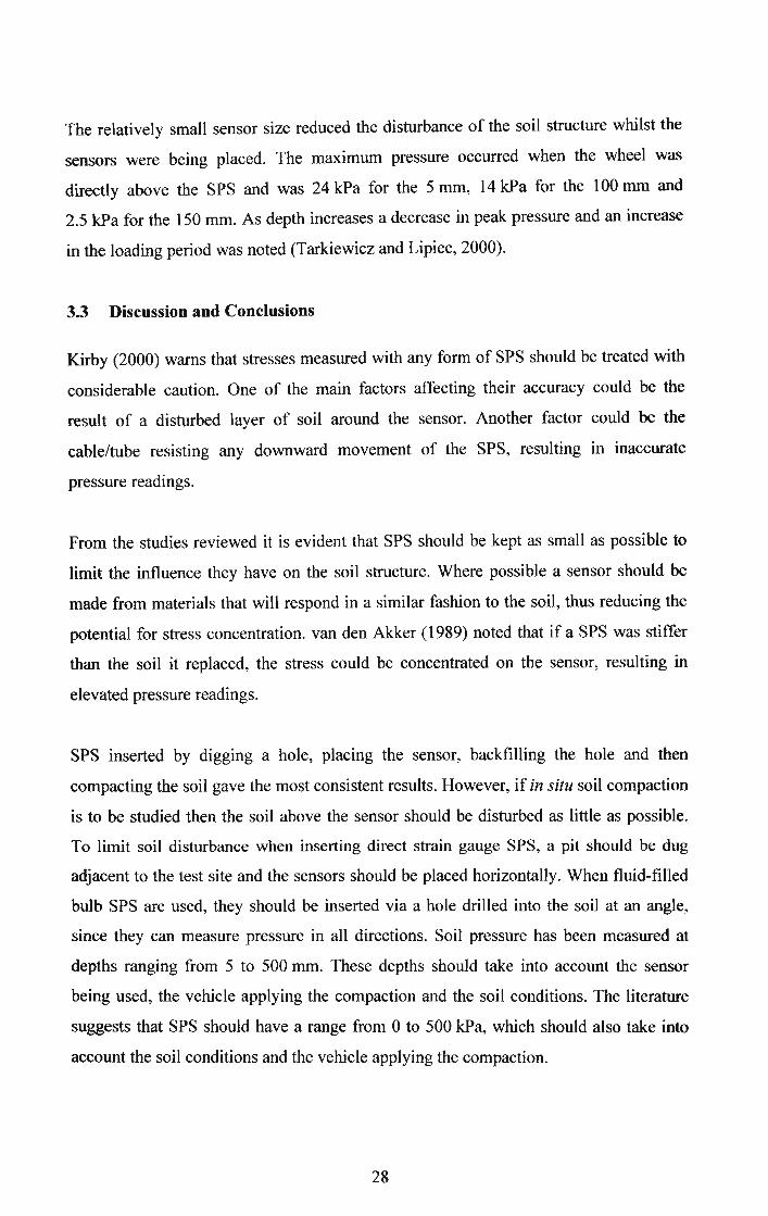
Figure 4.18 A schematic showing the axis system used to describe the sensor

positions

Figure 4.19 Results obtained from fluid-filled bulb soil pressure sensors used in a

test at Ukulinga, Pietermarizburg, South Africa. A small agricultural

tractor was driven forwards over the sensors, which were inserted to

different depths and x-positions 50

IX

Figure 5.1 Self-loading trailer used ID a soil compaction field trial near

Richmond, South Africa 55

Figure 5.2 Illustration of the nest layout and the tyre path for the soil

compaction trial near Richmond, South Africa 56

Figure 5.3 The pressure measured by all sensors during the soil compaction

event plotted against time 58

Figure 5.4 A frame extracted from the video of the soil compaction event,

Richmond, South Africa, used to calculate the position of the wheel

relative to each sensor. (a) Indicates a reference distance and (b)

indicates the position of the centre of the wheel 58

Figure 5.5 Pressure measured by all sensors plotted against relative wheel

position from a field trial, Richmond, South Africa. Negative wheel

position values depict pressure detected before the centre of the

wheel has passed over the sensors 59

Figure 5.6 Pressure measured by all sensors at a given depth plotted against

relative wheel position, Richmond, South Africa 60

Figure 5.7 Pressure measured by Sensor A plotted against (a) time and (b)

relative wheel position, Richmond, South Africa. Figure 5.9 contains

a zoomed plot of the encircled area in (b) above 61

Figure 5.8 Pressure measured by Sensor J plotted against (a) time and (b)

relative wheel position, Richmond, South Africa 61

Figure 5.9 Close-up of the pressure measured by Sensor A when the wheel

travelled 20 mm backwards, between 170 mm and 200 mm relative

to Sensor A, Richmond, South Africa 62

Figure 5.10 Peak pressure (kPa), measured by each sensor (x) during a field trial,

Richmond South Africa, plotted against x-position and z-position

(depth). Isobars were calculated by using the DWLS smoother with a

tension of 0.2 in SYSTAT 63

Figure A.I Examples of the Gaussian functions, taken at y = 0, that were used to

represent pressure distribution (along the x-axis) in the soil 76

Figure A.2 Plot of k against z-position (depth) for y-position equal to zero 77

Figure A.3 ka plotted against three y-positions 78

x

Figure AA Modelled pressure (in kPa) profile, perpendicular to the travel

direction (x-position), below (z-position) the centre of the wheel (y =

oplane) 79

Figure A.5 Surface or contact pressure (in kPa) profile showing the predicted

pressure between the soil surface (x&y-positions) and the tyre/soil

interface (z = 0 plane) 79

Figure A.6 Graph showing how the modelled pressure (in kPa) propagates

through the soil profile (z-position) along the length of the tyre

(y-position), below the centre of the tyre (x = 0 plane) 80

Figure A.7 An illustration for the possible cause of the maximum pressure

occurring in front of the wheel 80

Xl

1 INTRODUCTION

Soil compaction occurs frequently in nature, commonly caused by raindrops, animals,

wetting and drying of the soil and even the weight of the soil itself (Cohron, 1971).

Mankind however, is responsible for causing the bulk of severe and deep soil

compaction (Cohron, 1971). The magnitude and consequence of these soil compaction

events differ significantly, depending on the soil texture and moisture content and the

vehicle load and tyre type/pressure.

In agriculture, soil compaction is a concern as it influences plant growth and ultimately

yield (Trouse, 1971). Conversely, civil engineers are concerned with a soil's state of

compaction because it will have an effect on how much load the soil can support. The

military are also concerned with soil compaction as it may affect the mobility of

vehicles (Richmond et aI., 1995). Ruts formed by the vehicles may also have a unique

thennal signature, which could be used to identify the type of military vehicles present

in an area (Eastes et aI., 2004). This dissertation will only consider the compaction of

soils in agricultural fields by vehicles.

Smith (1999) and Williams et al. (2004) noted that soil compaction has led to increased

soil strength, resulting in reduced root growth and decreases in oxygen levels,

infiltration rates, water retention and nutrient uptake. Smittle and Threadgill (1977) was

cited by Coates (2001) as having concluded that root growth generally followed a

similar pattern to soil strength, often confining roots to a potentially dryer topsoil layer.

These factors have been found to have numerous negative effects, resulting in reduced

agricultural yields and ultimately reduced sustainability of agriculture.

Pagliai and lones (2002) found that flooding may be exacerbated by increased runoff

resulting from subsoil compaction. Runoff may be increased as a result of a lower

infiltration rate resulting from changes in the soil structure, namely reduced pore spaces

and reduced plant growth, resulting in reduced interception of precipitation. During

precipitation a compacted soil will reach saturation before a less compacted soil,

resulting in increased runoff and possibly causing flooding. In addition soil erosion may

be aggravated by increased runoff.

1

The basic soil compaction process can be defmed as a change in volume for a given

mass of soil (McKibben, 1971). Harris (1971) attributes the change in volume that

occurs when a soil is compacted to one of the following four processes;

• the solid particles are compressed,

• the air within the pore spaces are compressed,

• there is a change in the liquid or gas contents in the pore spaces, and

• the soil particles are rearranged to fit more closely.

For granular soils that are not saturated, the major factor contributing to a volume

change, is the extent to which the soil particles can change position by rolling or sliding

to fit more closely (Harris, 1971).

Compaction of agricultural soils may give rise to reduced yields, which poses a threat to

the long-term sustainability of agriculture (Voorhees, 2000). According to De Wrachien

(2002): "There is an increasingly urgent need to match land types and land uses in the

most functional way, so as to maximize sustainable production and to satisfy the

manifold needs of society, while at the same time, preserving the environment. Land

use projects are caught between two seemingly contradictory requirements: ecological

conservation and economical viability. Both are interchangeably related to

sustainability." Soil compaction in agriculture is a clear example of these requirements,

with ecological conservation requiring less soil compaction, while for economic

feasibility, larger and heavier equipment is needed.

Soil compaction requires management if the sustainability of agriculture is to be

realized. Management techniques can only be considered sustainable if they can be

practiced indefinitely without undesirable consequences to the environment and the

economic viability of agriculture (Pagliai and lones, 2002). Since compaction in the

topsoil can be alleviated by cultivation, it is not perceived to be a serious problem in the

medium to long-term. However, once subsoil compaction occurs, it can be extremely

difficult and expensive to alleviate (lones, 2002). The mitigation of soil compaction,

particularly subsoil compaction, may be considered unsustainable and thus management

techniques should rather focus on minimizing the occurrence of soil compaction. Soil

compaction can only be managed if it can be measured and predicted; therefore careful

2

measurements and the development of tools to predict the effects of soil compaction are

required under different agricultural scenarios.

The compaction of agricultural soils is however a complex phenomenon, involving

numerous soil properties and significant interrelationships between the physical,

biological and chemical properties of soils. Agri-environmental factors, such as

weather, climate, tillage and agronomic treatments may also have a significant influence

on the compaction of agricultural soils (McKibben, 1971). As with any agricultural

process, it is important to manage soil compaction by managing the agri-environmental

factors.

The focus of this dissertation is to establish methods of measuring compaction within

agricultural soils. A review of relevant literature on methods of measuring soil

compaction was conducted. Soil compaction can be quantified by measuring either the

resultant effects on various soil properties or the forces in the soil, causing the soil

particles to realign and become compacted (Hattingh, 1989). A concise review of

methods of measuring soil compaction is given by Freitag (1971). Significant work on

the use of a variety of direct strain gauge Soil Pressure Sensors (SPS) has been

undertaken by van den Akker (1989) and van den Akker and Stuiver (1989). Turner

(2001) and Turner and Raper (2001) are leaders in the development of an indirect form

of strain gauge SPS, in the form ofa fluid-filled bulb.

Based on the literature reviewed, the development and testing of an instrument for

measuring soil compaction was undertaken. The instrument was evaluated, conclusions

drawn and finally recommendations are offered for future research into the development

of SPS and techniques related to their use.

3

2 MEASURING THE EFFECTS OF SOIL COMPACTION ON

RELEVANT SOIL PROPERTIES

Soil compaction can be quantified in several different ways and there is no single

standard measurement. This is probably due to the complex character and high

variability of soils and the variety of forces imposed on them (McKibben, 1971). If the

effects of soil compaction are to be measured then the soil properties both before and

after the compaction event need to be measured (Turner and Raper, 2001). Hattingh

(1989) found that the effects of soil compaction could be measured in terms of changes

in dry bulk density, penetration resistance and water infiltration or porosity. Fazekas

and Horn (2004) noted that bulk density is often used, while interactions between

hydraulic and mechanical processes are seldom considered when quantifying soil

compaction. Penetration resistance was found by Smittle and Threadgill (1977), cited by

Coates (2001), to be closely related to root growth, making it a useful parameter for

measuring soil compaction in agriculture.

Various methods used to measure the effects of soil compaction are reviewed in this

chapter. These include measuring changes in bulk densities, soil strengths and a soils

ability to conduct fluids.

2.1 Measuring Changes in Bulk Density

Bulk Density can either refer to the in situ density of soil or the dry density of soil. The

in situ density of soil is the total mass of a soil sample (including moisture) divided by

the volume it occupies. The dry density of a soil is the mass of soil solids exclusively,

divided by the volume of the sample. Dry density or dry bulk density therefore does not

include the current soil moisture content and has been regarded as more useful in

determining a soil's state of compactness (Das, 1998).

Vehicles exert pressure on the soil surface and this pressure results in a physical process

which reduces the volume of the soil. Since soil and water particles can be considered

relatively incompressible, any residual change in volume can be attributed to a change

in pore spaces caused by a reorientation of the soil particles. The realignment of soil

4

particles is the result of an increase in the pressure in the soil and ultimately the bulk

density of the soil is increased (Lu et al., 2004).

The two parameters that are needed to determine bulk density are the mass and volume

of a soil sample. If dry bulk density is required then the mass should be determined after

the sample has been oven dried to evaporate all moisture. If a clod of soil is sealed to

prevent the ingress of water, then its volume may be measured by immersing it in water

and calculating the volume of water displaced. This can be achieved by coating soil

clods with resin (Malinda et aI., 2000). Freitag (1971) reports on devices that use sand,

oil or water balloons to measure the volume of an irregularly shaped hole. These

methods are labour intensive, time consuming and disturb the original soil structure.

Nuclear density meters are often used to determine the dry density and moisture content

of soils (Das, 1998). Gamma rays interact primarily with electrons in the soil. The

energy drop of a beam of gamma rays which have passed through a soil is closely

related to the density of the soil. Neutrons on the other hand react primarily with

hydrogen atoms. Since most hydrogen found in the soil is in the form of water, the

energy drop of a beam of neutrons passing through a soil provides an indication of soil

moisture content (Freitag, 1971). Nuclear density meters are a quick and easy method of

taking field measurements, but they are expensive, difficult to calibrate and require

special handling and storage facilities due to the radioactive material (Anon, 2004).

Figure 2.1 shows an example of a nuclear density meter.

Figure 2.1 Nuclear density meter used to measure the bulk density and moisture

content of the soil

5

2.1.1 Measuring Strain in Soils

Strain is defIned as a change in length divided by the original length of a material. Since

soil that is compacted by a surface force tends to displace in the vertical plane, it is

possible to calculate volume change from vertical soil strain. Once the volume change is

known it is possible to calculate the change in bulk density.

Stereo photography was used by van den Akker and Stuiver (1989) and van den Akker

(1999) to measure the strain in the soil due to vehicle traffIc. The studies were

conducted by digging a pit and placing plastic tracer pins in a rectangular grid pattern

on the face perpendicular to the direction of travel. The pit was photographed and then

refilled and the compaction applied. After the soil compaction event the pit was

carefully uncovered and the grid was photographed. Figure 2.2 shows the grid after the

soil compaction event. Stereo-analytical photogrammetric procedures were used to

calculate any change in the x, y and z coordinates of each grid point. Similarly, Freitag

(1971) reports that lead shot has been used to construct a rectangular grid. The positions

of the lead shot were measured before and after the soil compaction event, using X-rays.

Figure 2.2 Grid of plastic tracer pins showing the effects of strain in the soil after

pressure was applied to the soil surface in the form of a wheeled vehicle

(van den Akker, 2004)

6

Strain gauges attached to a telescopic rod with plates or anchors at each end can be used

to measure strain in the soil. The plates move with the soil and thus the displacement of

the telescopic rod is equivalent to the strain in the soil (Freitag, 1971). Figure 2.3 shows

a telescopic sensor used to measure strain.

Figure 2.3 A telescopic rod, with anchor plates for measuring the displacement (strain)

in soils (Freitag, 1971)

Another type of sensor, based on electromagnetic fields, may be used to measure strain.

Two identical coils are placed in the soil, while another set of coils is attached to a

micrometer above the soil surface. A voltage is then applied to one of the coils above

the ground and one of the coils below the ground. When the two coils above the soil are

separated by the same distance as the two coils below the surface, the electromagnetic

fields will balance. Strain in the soil can be read directly off the micrometer (Freitag,

1971). Figure 2.4 shows a diagram of an adjustable micrometer and the coils which

produced the electromagnetic fields. These methods are time consuming and disturb the

soil profile, making them unsuitable for extensive field experiments.

Arvidsson et al. (2002) made use of displacement probes filled with silicon oil to

measure strain. These sensors consisted of a cylinder, filled with silicon oil and sealed

at the top with a movable piston. The base of the cylinder was connected via a tube to

the atmosphere and a pressure transducer. As the piston moved it displaces a

proportional quantity of silicon oil into the tube, applying a pressure on the transducer.

Silicon oil was selected because it is relatively inert. The probes were rectangular in

7

shape, 70 mm long, 35 mm wide and 36 mm high. A pressure transducer connected to

the base of the probe was used to measure any changes in the pressure in the silicon oil.

These changes in pressure were related to a change in the volume of fluid resulting from

vertical strain. The probes were inserted in a hole drilled laterally into the side of a pit.

The pressure was recorded by a data logger, located in the pit. The probes were installed

at 0.3,0.5 and 0.7 m depths. A load cell with a diameter of 17 mm was mounted on top

ofthe probes to measure vertical soil pressure which will be discussed in Chapter 4.

Figure 2.4 Sensor for measuring soil displacement using electromagnetic fields and an

adjustable micrometer to balance the electromagnetic fields (Freitag, 1971)

2.2 Measuring Changes in Penetration Resistance

Penetration resistance of the soil is defined as its ability to resist penetration by a plate,

cone or footing of some sort. Although there is much supporting evidence that

penetration resistance is closely related to strength parameters commonly used to define

soil properties, the mechanics are not well understood, and penetration resistance should

only be considered empirical and used for comparative purposes (Freitag, 1971). Miller

et of. (2001), however, noted that soil penetration resistance can be related to bulk

density. He explained that measuring soil resistance using a cone penetrometer was

generally quicker and easier than measuring soil density and thus is the most common

measure of the effects of soil compaction. The next section will review static cone

penetrometers, dynamic cone penetrometers, drop cone penetrometers and continuous

"on the fly" soil penetration resistance measurements. In addition, a relatively new

8

technique which makes use of acoustics to determine a soil's resistance to the

penetration of a cone will be reviewed.

2.2.1 Static cone penetrometers

The following discussion of static cone penetrometers is summarised from Jones and

Kunze (2004). Static cone penetrometers consist of a metal rod, with a cone shaped

leading edge. The penetrometer should be pushed into the soil at a constant rate. This

can be done by hand but mechanical penetrometers are more accurate due to their ability

to achieve a constant insertion rate. The force required to insert the penetrometer is

typically measured by a strain gauge type of load cell and can be linked to a digital data

acquisition system. Figure 2.5 shows a manual static cone penetrometer with a digital

data acquisition system and with an analogue gauge. Figure 2.6 shows a picture of a

tractor mounted and wheel mounted mechanical static cone penetrometer, both

equipped with digital data acquisition systems.

Figure 2.5 (a) A digital manual static cone penetrometer, (b) an analogue manual static

cone penetrometer (Forestry, 2004)

9

Figure 2.6 (a) A tractor mounted mechanical static cone penetrometer (from Raper et

aI., 1999), (b) a wheel mounted mechanical static cone penetrometer

In a study of soil compaction, under various forestry harvesting techniques, Hattingh

(1989) chose to use cone penetration resistance to determine the soil compaction caused

by various field operations. The static cone penetrometer was chosen due to ease of use

and the strong relationship between penetration resistance and root development, crop

growth and yield. Hattingh (1989) does, however, note that soil type, penetration speed,

cone characteristics and soil water content may influence the readings. The American

Society of Agricultural and Biological Engineers (ASABE) provide standards for cone

penetrometers (ASAE S313 .3, 2000).

The results of penetration tests for a depth range of 0 to 850 mm conducted by Hattingh

(1989) are presented in Table 2.1 and are illustrated in graphic form in Figure 2.7. It can

be seen that an increase in the strength of the soil is proportional to both the surface

contact pressure and the number of vehicle passes. The data also indicated that higher

contact pressure resulted in a greater volume of soil being negatively affected (strength

exceeding 2000 kPa). Soil with a soil strength of greater than 2000 kPa can be

considered to greatly retard root growth (Coates, 2001).

10

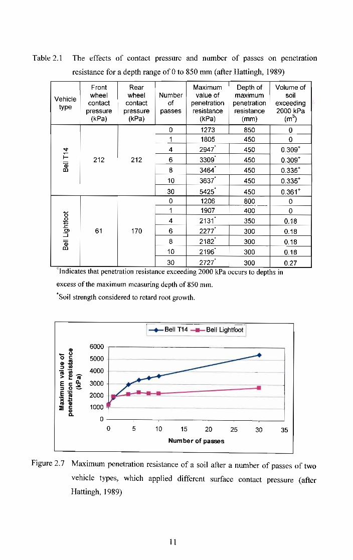
Table 2.1 The effects of contact pressure and number of passes on penetration

resistance for a depth range of 0 to 850 mm (after Hattingh, 1989)

Front Rear Maximum Depth of Volume of

Vehiclewheel wheel Number value of maximum soil

contact contact of penetration penetration exceedingtype

pressure pressure passes resistance resistance 2000 kPa(kPa) (kPa) (kPa) (mm) (m3

)

0 1273 850 0

1 1805 450 0

4 2947· 450 0.309+.;r...... ·..... 212 212 6 3309 450 0.309+Q.j

8 3464· 450 0.335+m10 3637· 450 0.335+

30 5425· 450 0.361+

0 1206 800 0

..... 1 1907 400 00 ·.E 4 2131 350 0.18......c ·Cl 61 170 6 2277 300 0.18:.:::i ·Q.j 8 2182 300 0.18cc 10 2196· 300 0.18

30 2727· 300 0.27"lndicates that penetration resIstance exceedmg 2000 kPa occurs to depths in

excess of the maximum measuring depth of 850 mm.

'Soil strength considered to retard root growth.

I-+-Bell T14 _Bell Lightfoot I

3530252015105

6000 ,---------------------,

5000 +--~----------__:::::;;;o..._==----_____J

4000 +-----------::::;~.--:'-------------I

3000 +---Y''-----------------=-------I

2000 ~c.~:::t!I::~:::::::::========~___J1000 "'f-------------------_____J

O-t-------;---.,----,---r----,--------l

o

CD_ uo c:CDS::s fI)ii"ji _> .. IIIEc:D.::SO~E;l.- I!='5:E i

Q.

Number of passes

Figure 2.7 Maximum penetration resistance of a soil after a number of passes of two

vehicle types, which applied different surface contact pressure (after

Hattingh, 1989)

II

2.2.2 Dynamic cone penetrometers

Dynamic cone penetrometers (DCP) use a slide hammer to impart a known amount of

kinetic energy on the cone. Either the number of blows for a fixed distance or the

distance per blow is recorded, giving a comparative measure of soil strength. The slide

length, drop weight and the cone angle can be varied for different soil strengths (lones

and Kunze, 2004). Herrick and lones (2002) noted that DCP are more consistent and

repeatable than manual static cone penetrometers. He continues that they are, however,

prone to becoming stuck in some soils. DCP give an empirical measure of soil

compaction and can be used to compare the soil compaction caused by different field

operations, rather than the degree of compaction present in different soil types.

2.2.3 Drop cone penetrometers

This apparatus consists of a 1 m long guide tube and a 2 kg cone with a lifting rod. The

cone has an angle of 30° and a collar to ensure it falls perpendicular to the ground. Once

the cone has been dropped, the depth of penetration is measured. lones and Kunze

(2004) found that this is a quick, inexpensive and repeatable method of measuring

surface soil strength. A limitation of this method is that it only measures the amount of

compaction present in the topsoil.

2.2.4 Continuous soil strength measurements

When subsoil compaction is deemed to affect the economic viability of a cultivated

field, deep tillage will be required to alleviate the soil compaction. Deep tillage is

expensive and should only be practiced were necessary. Precision deep tillage can be

used to vary the depth of tillage across a field depending on the severity and depth of

soil compaction (Wells et al., 2001). Due to a relatively low density of measurements

achievable, even with automated cone penetrometers, soil strength data is limited to a

few points in a field. This resulted in maps of soil strength, based on this data, having a

limited representation of actual conditions (Adamchuk et al., 2001 a).

Adamchuk et al. (2001a) developed a smooth blade with strain gauges mounted on it,

which was capable of dynamically measuring soil strength across a field, at three

different depths. Figure 2.8 shows the smooth blade and the tractor configuration.

12

Adamchuk et al. (2001b) later made improvements to the model, which converted the

strain gauge signals into soil strength, making it possible to estimate the soil strength

across a constantly varying depth. Both systems were connected to a Differential Global

Positioning System (DGPS) allowing for a three dimensional map of soil strength to be

produced. Mouazen et al. (2003) used a smooth blade to measure the draught required

to overcome the soil strength. Dry bulk density was then predicted by using a model,

which included draught, depth and moisture content as input variables. A system was

developed by Chung et al. (2003) which made use of individual sensing tips, connected

to load cells, to measure the soil strength at various depths. Figure 2.9 shows a

schematic of the blade with individual sensing tips being used to acquire soil strength

data. Note the GPS receiver and the depth sensing wheel.

Laptop Computerand DAQ Equipment

Figure 2.8 The smooth blade with strain gauges mounted on it (Adamchuk et al.,

200lb)

GPS receiver -+ location od speed

Strength

Figure 2.9 Blade with individual sensing tips (Chung et al., 2003)

13

2.2.5 The use of acoustics to measure the effects of soil compaction

Lu et al. (2004) reported that acoustic techniques could be used to investigate changes

in the mechanical and structural properties of soils. Such changes could be the result of

soil compaction, which could be induced by the use of agricultural machinery. Acoustic

measurements are essentially empirical measures of the effects of soil compaction

(Tekeste et al., 2002). Changes in the amplitude of sound waves in a frequency range

can be related to a change in the degree of soil strength.

Acoustic techniques for measunng soil compaction consist of either SeISmIC or

acoustic-to-seismic coupling. Seismic waves are caused by the shearing of the soil,

caused by the measuring device, which can then be related to soil strength. Tekeste et

al. (2002) developed a metal spike which was bolted onto a blade and pulled through

the soil. A microphone mounted on rubbers and placed in a cavity in the spike. This

made it possible to take continuous measurements between two points as opposed to

point measurements. Experiments were performed in the soil bins at the National Soil

Dynamics Laboratory (NSDL) located in Auburn, United States of America.

A hardpan layer can be defined as a hard layer of soil, which is often located between

the topsoil and the subsoil. It is often caused by the plough smearing the layer of soil

below the set plough depth and is sometimes referred to as a plough pan. During

experiments conducted by Tekeste et al. (2002) a hardpan layer was created in the soil

bins using one or two passes of a solid wheel. The degree of soil compaction was then

measured at constantly varying depth, using the cone index and acoustic methods

described above. Tekeste et al. (2002) did not provide the units of measurement for

amplitude in the report; however since amplitude measurements are considered

empirical the magnitude of the variations in amplitude may be compared with cone

index. Figure 2.10 shows a close correlation between the two methods and both

methods show the presence of the hardpan layer.

14

4.--------,,....------r------.--------r------r-----"l

.g 3.5

.€Q.E 3<t:()

.~ 25:3o()

<t: 2"'0§

~~ 1

"'0.sQ)

s::oU

5 10 15

Time (s)20 25 30

Figure 2.10 Penetration resistance (smooth line) and acoustic amplitude vs time for a

constantly varying depth showing the effect of a hardpan layer by the

increase in both the penetration resistance and the acoustic amplitude

between 10 and 20 seconds (after Tekeste et al., 2002)

Tekeste et al. (2002) found that due to the sensor's small size, it was possible to mount

the acoustic metal spike onto an existing blade. This could save energy and time by

making use of the acoustic detector to automatically control the depth of a tillage

operation to remove a hardpan layer.

Lu et al. (2004) noted that comparing acoustic methods with conventional techniques of

measuring the effects of soil compaction, showed that acoustic methods were quick to

perform and non-destructive. This made acoustic measurements suitable for extensive

in situ measurements of variations in soil physical properties due to soil compaction.

2.3 Measuring Changes in Fluid Conductivity

Freitag (1971) argues that fluid conductivity can be used as an indication of soil

compaction, since sufficient evidence exists, indicating that a restricted flow of air or

water, reduces plant growth. Li et al. (2001) found that the infiltration rate of simulated

rainfall for soil's which had been trafficked was 25% compared to 70% for

15

non-trafficked soil's. Freitag (1971) did, however, warn that fluid conductivity should

onl be considered as a relative indication of soil compaction since the conductivity of a

soil is a function of both the soil's physical properties and its structure. Two soils with

similar porosities may have different water conductivities due to different soil

structures. The relative conductivity of air through various soils may not be as

divergent. This may be attributed to the lower cohesive bonds between soil and air,

resulting in the soil structure having less effect on conductivity (Freitag, 1971).

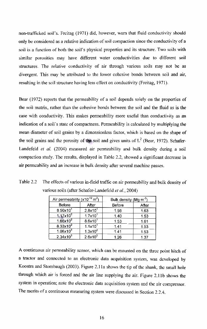
Bear (1972) reports that the permeability of a soil depends solely on the properties of

the soil matrix, rather than the cohesive bonds between the soil and the fluid as is the

case with conductivity. This makes permeability more useful than conductivity as an

indication of a soil's state of compactness. Permeability is calculated by multiplying the

mean diameter of soil grains by a dimensionless factor, which is based on the shape of

the soil grains and the porosity of t . soil and gives units of L2 (Bear, 1972). Schafer­

Landefeld et al. (2004) measured air permeability and bulk density during a soil

compaction study. The results, displayed in Table 2.2, showed a significant decrease in

air permeability and an increase in bulk density after several machine passes.

Table 2.2 The effects of various in-field traffic on air permeability and bulk density of

various soils (after Schafer-Landefeld et aI., 2004)

Air permeabilil'J (x1 0-12 m2) Bulk density Ma m-3

)

Before After Before After8.50x101 2.8x101 1.56 1.631~ 17x102 1.7x101 1.40 1.531.66x102 8.6x101 1.53 1.618.33x102 1.1x101 1.41 1.531.06x103 1.3x102 1.41 1.532.34x103 2.6x102 1.26 1.37

A continuous air permeability sensor, which can be mounted on the three point hitch of

a tractor and connected to an electronic data acquisition system, was developed by

Koostra and Stombaugh (2003). Figure 2.11a shows the tip of the shank, the small hole

through which air is forced and the air line supplying the air. Figure 2.11 b shows the

system in operation; note the electronic data acquisition system and the air compressor.

The merits of a continuous measuring system were discussed in Section 2.2.4.

16

Figure 2.11 (a) The shank "tip" design and (b) the sensor being used to continuously

measure air permeability across a field (from Koostra and Stombaugh,

2003)

Smith (1999) found instances where soil compaction improved yields. This was found

to occur in some sandy soils where compaction increased the available water content of

the soil by reducing pore sizes. In these instances, an increase in bulk density would

relate to a decrease in porosity and a decrease in fluid conductivity, but there was an

increase in crop yield.

Most of the methods of measuring the effects of soil compaction are time-consuming,

costly and often only express the results in relative terms. There is a need to be able to

predict the effects of soil compaction and ultimately crop yields of various vehicles on a

given soil type, at a specific moisture content, bulk density and surface contact pressure.

This is possible only if the propagation of soil stress through a soil is thoroughly

understood and ultimately modelled. Chapter 3 will assess methods of measuring stress

in soils.

17

3 MEASURING PRESSURE IN SOILS

Various methods of measuring the resulting effects of a compaction event on soil

properties are reviewed in Chapter 2. If, however, the soil compaction process is to be

understood, then Hattingh (1989) recommended that the forces in the soil causing the

compaction be measured. He suggested this could be achieved by monitoring the

pressure in a soil during a compaction event. This concurred with recommendations

made by Turner and Raper (2001). Soil stress or pressure is defmed as the force applied

to the soil divided by the area over which it is applied. Pressure measurements are

important for gaining a greater understanding of the mechanics of the soil compaction

process (Freitag, 1971). Soil pressure varies spatially and a matrix of sensors is required

to gain an understanding of the soil compaction process. Measuring the pressure in the

soil makes it possible to measure the event and not just the result of the event. Hattingh

(1989), however, noted that methods of measuring the pressure in a soil during a

compaction event tended to be time-consuming, expensive and complex.

The main requirements of a pressure-sensing element are accuracy and a freedom from

influence by any forces other than those normal to the measuring face (Freitag, 1971).

The accuracy of Soil Pressure Sensors (SPS) has improved significantly with the

increased accuracy of commercially available pressure transducers. The construction of

a sensor may, however, introduce some inaccuracies and thus all SPS should be

calibrated before use. Selig (1964) and Selig and Vey (1964), cited by Freitag (1971),

noted two main influences on SPS. First, the sensor may not respond to the forces

exerted on it in exactly the same manner as the soil it has replaced. Secondly, placing

the sensor in the soil may cause discontinuities in the soil, resulting in the soil around

the sensor responding differently from the rest of the soil mass.

Theoretically, soil pressure as a result of a wheel or track should be symmetrical about

an axis parallel to the direction of travel and passing through the centre of the wheel or

track (van den Akker, 1999). In previous experiments, van den Akker (1989), had found

this to be largely true. It may therefore be possible to use symmetry to reduce the

number of readings required during an experiment.

18

Freitag (1971) presented the following general methods of measuring soil pressure;

• strain gauges on a deflecting diaphragm, simple beam or cantilever beam, or

• pressure in a fluid that is resisting a change in volume.

These methods are all based on some form of pressure transducer. A pressure transdqeer

was described by Helfrick and Cooper (1990) as a device that takes a non electrical,

commonly mechanical, input and converts it into an electrical signal.

The two main pressure readings taken in relation to soil compaction are peak pressure

and residual pressure. Turner and Raper (2001) described peak pressure as the

difference between the pressure before the vehicle passes over the SPS and the

maximum pressure resulting from the traffic. Residual pressure can be described as the

pressure remaining in the soil some time after the compaction event. The two main

methods of measuring soil pressure, as given by Freitag (1971), are investigated in the

following sub-sections. A summary of various sensor properties, insertion techniques,

positioning and calibration of soil pressure sensors used by other authors will be given.

3.1 Direct Strain Gauge Soil Pressure Sensors

A strain gauge is a type of transducer, which converts strain into a change of electric

resistance. The device consists of a thin wire or foil, which is bonded to the material

undergoing strain. The change in electric resistance of the wire or foil of the strain

gauge is proportional to the displacement of the parent material. The change in

resistance is measured with a specially adapted Wheatstone Bridge (Helfrick and

Cooper, 1990). The strain of a diaphragm of known dimensions and material properties

may be converted into stress or pressure. Nichols et al. (1987) noted that the most

common type of SPS made use of a deforming diaphragm and a strain gauge, and either

measure pressure in one plane or in a number of planes. These are frequently referred to

as vertical SPS and stress state transducers (SST). Figure 3.1 shows an example of a

commercially available pressure transducer (left hand side of photo), a SPS for

measuring vertical soil pressure (right hand side of photo) and a SST (centre).

19

Figure 3.1 (a) The WAZAU pressure transducer can be mounted in housings to fonn

(b) a stress state transducer and (c) a vertical soil pressure sensor (Wazau,

2004)

3.1.1 Specifications of direct strain gauge soil pressure sensors

Size and pressure range were two commonly reported specifications of SPS, they will

therefore be reviewed in this section. van den Akker (1989) conducted an experiment,

which involved using four vertical SPS at various depths. The SPS had a height of

80 mm and diameter of 20 mm. In another experiment van den Akker (1999) used five

SPS to measure the vertical pressure between soft topsoil and firm subsoil. The sensors

had a diameter of 76 mm and a height of 17 mm. Alakukku et al. (2002) conducted an

experiment using vertical SPS, which had a diameter of 30 mm and a height of 6 mm.

During these experiments a range of pressures from 0 to 490 kPa were measured.

A SST was defined by Nichols et al. (1987) as a SPS which could measure soil pressure

in six different planes. Figure 3.2 illustrates a schematic of a SST with details of

orientation. Note the diaphragm ofpz is horizontal and thus measures vertical pressure.

The larger overall diameter and height of the SST, compared to the vertical pressure

sensor, can be seen. Nichols et al. (1987), Bailey et al. (1988), Pearman et al. (1996),

Johnson and Bailey (2002) and Abu-Hamdeh and Reeder (2003) all report using SST to

measure soil compaction. Figure 3.3 summarises results from Pearman et al. (1996),

where pressures of between 0 and 500 kPa were recorded, note pz records the highest

pressures. Kirby (2000) found that vertical SPS yielded estimates of vertical soil

pressure closer to the expected value than SST. This may have been due to the SST

20

larger dimensions, causing the soil around the sensor to respond in a different manner to

the applied pressure.

Tire direction!of travel

Pt

Figure 3.2 Schematic top view of a Stress State Transducer (Pearman et aI., 1996)

o

·1.0 -0.5 0.0 0.5 1.0Longitudinal distance from axle, m

Figure 3.3 Pressures recorded by a Stress State Transducer, shown m Figure 3.2

(Pearman et aI., 1996)

3.1.2 Insertion techniques

Vertical SPS and SST are commonly placed by digging a pit to the required depth,

placing the sensor, backfilling the hole and then re-compacting the soil in an attempt to

achieve the initial soil condition. Another approached used by van den Akker (1989), in

an attempt to minimise soil disturbance, was to dig a pit offset parallel to the travel

21

direction and create a small horizontal tunnel in which to place the sensors. The

horizontal holes had widths and heights similar to that of the sensor in an attempt to

minimize soil disturbance and insure a good contact between the soil and the SPS. The

holes were then carefully refilled to reduce the effect they may have had on the structure

of the soil. Figure 3.4 shows the two different placement methods. Method A is the

common method while Method B is the pit dug adjacent to the vehicle's path. Method

A provided more repeatable results, possibly due to the soil used to fill the hole being

more homogeneous than the undisturbed soil found above the sensors placed using

Method B. van den Akker (1989) recommended that Method A be used in comparative

experiments, while Method B should be used in experiments where in-field undisturbed

soils are being studied.

~...... a· .... ...... . . . .. ,.~ ,­..... , ...-, ­..,,:.. .'.:.:,:;~:~b ::~

:"·l'::':':"'~",., ••. e'

Method A Method 8

Figure 3.4 Two methods used to place soil pressure sensors in a soil (van den Akker,

1989). a depicts fill, b loose topsoil and c firm subsoil

3.1.3 Positioning of sensors

van den Akker (1989) and van den Akker (1999) placed SPS at a depth of 300~

between the soft topsoil and the firm subsoil. During the latter experiment, however,

sensors were not only placed directly below the predicted centre of the wheel path but at

distances of 125,250, 375 and 500 mm from the first sensor perpendicular to the travel

direction. Alakukku et al. (2002) placed SPS at a depth of 200 and 300 mm below the

predicted centre of the wheel track and a second set of sensors at the same depths but

100 - 150 mm away from the first set.

SST have been placed at a range of depths and distances from the centre of the

predicted wheel track. Gysi (2000), Alakukku et al. (2002) and Arvidsson et al. (2002)

found that the measured peak pressure at depths of 150,200 and 300 mm, respectfully,

22

were greater than the predicted surface contact pressure. This was most likely due to the

pressure under the tyre not having a uniform distribution. This could be especially true

for agricultural tyres with large lugs, which could reduce the contact area on firmer

surfaces.

3.1.4 Calibration techniques

Water pressure was used by van den Akker (1989) to calibrate the SPS used in an

experiment he conducted. This was then checked using a soil filled cylinder with a

diameter of 0.40 m and height of 0.35 m. A hard layer of soil, 0.1 m deep, was placed at

the bottom of the cylinder. The sensors were placed with their top surface level with the

top of the hard layer of soil, see Figure 3.5. The cylinder was then filled with loose soil.

The sides of the cylinder were covered with grease and a thin sheet of plastic was

placed between this and the soil to reduce the friction between the soil and the cylinder.

A load was applied by means of a piston to the entire soil surface. The measured

vertical pressure was found to be 1 - 3 % higher than the pressure applied by the plate

to the soil surface. This was thought to have been due to the stresses concentrating

around the pressure sensor owing to it being firmer than the soil around it.

I·0,. 40

l Applied load

rsssSSSS$Bs~Piston I

25

10

• • 0 ...........................................:::::::::::::::::::::::::::::::::::::::::::::::::::::::::::::::::::::::::::::::::::..:-:.:..:..:.: ..:.:-: ..:..>: ..:-: ..:<.:..:..:..::::::::::::::::::::::::::::::;::::::::::::::::::::::::::::'~ii:::::::::::::::::

Loose topsoil

Hard subsoil

Figure 3.5 The cylinder used to check the pressure transducers which had been

calibrated using water pressure (van den Akker, 1989)

23

3.2 Fluid-filled Soil Pressure Sensors

Fluid-filled SPS consist of either a small bulb made from a flexible membrane or a rigid

container with one face being made up of a flexible membrane. The flexible membrane

could consist of rubber, latex or silicon. This sensitive head is connected by a hose or

tube to a pressure transducer, which frequently uses a strain gauge to measure the

deflection of a diaphragm, which is then related to pressure. The system is filled with a

fluid and sealed. Commonly used fluids include water, silicon oil and hydraulic oil. It is

important to ensure that the fluid used is compatible with the material used for the bulb,

as some fluids may perish or dissolve rubber, latex or silicon.

Turner and Raper (2001) used an AgTech SPS to measure soil pressure. The sensor

consisted of a 25 mm fluid-filled rubber bulb, as shown in Figure 3.6. It was placed in a

predrilled hole, which was made using an adjustable drill fixture to ensure exact

positioning. Figure 3.7 shows the adjustable drill fixture; note the electric drill which is

powered by the vehicle battery. From the results shown in Figure 3.8 and Figure 3.9 the

maximum peak pressure recorded was approximately 120 kPa. The data logger recorded

20 readings per soil compaction event.

Figure 3.6 The AgTech ground pressure sensor (after Turner and Raper, 2001)

24

Figure 3.7 The drilling of a hole for the placement of the AgTech SPS (Turner, 2001)

1e .•~ =----------- ~

18.8

.­.....:5

Pressure (lIS i )ae .8 r-n-......,..TTT,.,...,.,..,-rTTT-rrr-rn..,.,,'Tr1rTT"1n-r1n-r,.,.,..n...rn-rn-TTT......,.-n-T....,.,..,...,...,.TI~......n-nr-n-.

1288

Figure 3.8 Pressure induced by a rubber tyre, as recorded by an AgTech SPS 100 mm

below the soil surface (Turner and Raper, 2001)

25

Caterpi lIar - centered transducer 19 at deep

:::~14.e~

~12.e~

..J.e.e~

~ ~

~ a.et6.e~

···l2 ••

...Pressure (psi)ae .e -rrrrrrrr-rr-rrrrr,.,.,..,..,.....,..".,rT'I1....,.,.......,...-rn-rn..".,.T'TT.",.".,..yn-TT"f'rI'Trrr1'T'r~-"~

j

e.eE------------------------~

E-2 <:..LLJ..L..L.LLL.J..L..LU-.LL..LLL..LLL.L.UL.L.UL.L-LJ-L.L-I....L.LJ....L.LJ............-'-'-'..L-W...L-W.-L.L.L~~"'_'_'_~~'_'_'_........

TiN: eHistoru

Figure 3.9 Pressure induced by a rubber tracked tractor, as recorded by an AgTech

SPS 100 mm below the soil surface (Turner and Raper, 2001)

The AgTech sensors were found to be sensitive to temperature changes and placement

induced stresses (Turner, 2001). Once the bulb has been placed in the soil it is

pressurised to ensure it makes positive contact with the soil. This made it necessary to

convert the readings into a relative pressure. This is commonly achieved by using the

pressure before the soil compaction event as an effective zero. The AgTech sensors

were thus more suited to comparative experiments. The effect of a rubber tyre passing

over a sensor at a 100 mm depth can be seen in Figure 3.8. Figure 3.9 shows the effect

of a rubber track passing over a sensor at the same depth. Note that the tyre caused

approximately 25% greater peak pressure, but the track applied a lower pressure for a

longer period of time resulting in a similar absolute residual pressure.

Turner and Raper (2001) compared the results of the AgTech SPS with results obtained

from a SST. They noted that it took two people 1-2 hours to place three SST sensors,

while two people were able to place, drive over and log 40 readings in an hour using the

AgTech SPS. In their comparison with the SST, Turner and Raper (2001) placed the

AgTech SPS at 50, 100 and 150 mm depths. Two AgTech sensors were placed at

26

1.5 times the lug spacing to maximise the probability of a lug passing over one of the

sensors. The peak and residual values were extracted from a plot of the pressure history

of each event. Turner and Raper (2001) found the 50 mm data to be more scattered than

the rest. This could have been due to the soil fracturing and releasing some residual

stress after the event, especially if the lug had passed directly over the sensor. The soil

above the 50 mm AgTech SPS was found to be between 12 and 25 mm deep after the

event. Turner and Raper (2001) found the peak and residual pressure to be

approximately 1.5 times higher when the lug passed directly over the sensor at the

100 mm depth. Significantly more scatter was noted when measuring residual pressure

with the SST than with the AgTechs. This is thought to be due to the higher rigidity of

the SST not allowing them to deform slightly and respond in a similar fashion to the soil

(Turner and Raper, 2001).

Tarkiewicz and Lipiec (2000) used fluid-filled SPS, with a dimension of 20xlOx5 mm

to measure the pressure in a soil bin. The soil bin had dimensions of

350x350x4500 mm. The measuring head of the fluid-filled SPS consisted of a small

container which was covered with a rubber membrane 0.5 mm thick and 8 mm in

diameter. This was connected by a metal tube with a diameter of 0.5 mm to a pressure

transducer. Silicon oil was used to transfer the pressure from the rubber membrane to

the pressure transducer since it is incompressible and relatively inactive. Soil strain was

simultaneously measured during their experiments. Sensors were placed at 5, 100 and

150 mm below the soil surface. The stress was simulated with a weighted wheel. The

tyre was 350x120 mm and had a weight of20 kg.

Tarkiewicz and Lipiec (2000) selected the transducers such that the transducer

connected to the shallowest sensor had a maximum range of 600 kPa, the middle

transducer 250 kPa and the deepest transducer had a maximum range of 40 kPa.

Linearity of the transducers was found to be within 0.15%, temperature induced errors

for 35° C did not exceed 2% and hysteresis effects were less than 0.05% of the full scale

output. An AT-MIO-64E-3 card was installed for acquiring data from the pressure

transducers. The logger was capable of recording 32 sensors at a rate of 500 000

measurements per second.

27

The relatively small sensor size reduced the disturbance of the soil structure whilst the

sensors were being placed. The maximum pressure occurred when the wheel was

directly above the SPS and was 24 kPa for the 5 mm, 14 kPa for the 100 mm and

2.5 kPa for the 150 mm. As depth increases a decrease in peak pressure and an increase

in the loading period was noted (Tarkiewicz and Lipiec, 2000).

3.3 Discussion and Conclusions

Kirby (2000) warns that stresses measured with any form of SPS should be treated with

considerable caution. One of the main factors affecting their accuracy could be the

result of a disturbed layer of soil around the sensor. Another factor could be the

cable/tube resisting any downward movement of the SPS, resulting in inaccurate

pressure readings.

From the studies reviewed it is evident that SPS should be kept as small as possible to

limit the influence they have on the soil structure. Where possible a sensor should be

made from materials that will respond in a similar fashion to the soil, thus reducing the

potential for stress concentration. van den Akker (1989) noted that if a SPS was stiffer

than the soil it replaced, the stress could be concentrated on the sensor, resulting in

elevated pressure readings.

SPS inserted by digging a hole, placing the sensor, backfilling the hole and then

compacting the soil gave the most consistent results. However, if in situ soil compaction

is to be studied then the soil above the sensor should be disturbed as little as possible.

To limit soil disturbance when inserting direct strain gauge SPS, a pit should be dug

adjacent to the test site and the sensors should be placed horizontally. When fluid-filled

bulb SPS are used, they should be inserted via a hole drilled into the soil at an angle,

since they can measure pressure in all directions. Soil pressure has been measured at

depths ranging from 5 to 500 mm. These depths should take into account the sensor

being used, the vehicle applying the compaction and the soil conditions. The literature

suggests that SPS should have a range from 0 to 500 kPa, which should also take into

account the soil conditions and the vehicle applying the compaction.

28

Direct strain gauge SPS are robust and reliable, however, there are some questions as to

their accuracy, owing to their rigid body, which is thought to result in poor contact with

the soil. Insertion techniques for in situ soil pressure measurements with direct strain

gauge sensors pose some challenges. The materials required to construct direct strain

gauge SPS are relatively inexpensive and easily available (approximately RJOO per

sensor), however, commercially available sensors are prohibitively expensive if a large

number of sensors are required (approximately R6000 per sensor).

Fluid-filled bulb SPS can measure pressure ornni-directionally and make use of fluid

pressure transducers, which are relatively inexpensive, easily available and have built in

software to allow them to interface with most personal computers. Fluid-filled bulbs

may also give a better contact with the soil compared to other rigid sensors.

The literature was inconclusive as to whether direct strain gauge or fluid-filled SPS

perform better. Direct strain gauge SPS have been the preferred method of measuring

soil pressure for many years, however, the relatively new technique of using fluid-filled

bulbs to measure pressure in soils deserves further investigation. For this reason it was

decided to research the design, construction and use of direct strain gauge and

fluid-filled bulb SPS for measuring the pressure in soils during compaction trials during

in-field agricultural and forestry traffic.

29

4 DESIGN AND INITIAL EVALUATION OF DIFFERENT SOIL

PRESSURE SENSORS

From the literature reviewed in the previous chapter it is evident that both direct strain

gauge and fluid-filled bulb pressure sensors have the potential to be cost effective and

accurate for measuring pressure in soils. It was therefore decided to investigate the use

of these two technologies for measuring pressure in situ. This would include the design

and an initial testing of the two sensor types, resulting in a decision as to which type

performed better and should be used in a field trial. The preliminary tests were merely

to assess the performance of the sensors themselves and were not a soil compaction

trial. Details of the soil and vehicle were therefore not reported for these initial tests.

The following list of ideal design properties were considered;

a. high measurement accuracy,

b. positive contact between the sensor and the soil,

c. the sensor should have a similar plastic, elastic and structural response to the

soil which it has replaced,

d. the size of the sensor should be kept to a minimum to limit soil disturbance,

e. obtaining the raw materials and manufacturing of the sensors should be time

and cost efficient,

f. data acquisition should be simple and cost effective,

g. calibration should be easy and accurate,

h. minimal disturbance to the soil's structural profile should occur during

insertion, and

i. insertion should be time and energy efficient.

An evaluation of two separate designs, namely a direct strain gauge and a fluid-filled

SPS, was conducted to establish how well they met the above mentioned design

properties. The two sensors were given ratings from one to five based on how well they

achieved these ideal design properties. A five was given if the sensor was thought to

have fully met the criteria and a one if it failed to meet a certain criteria. Each design

property was then assigned a weighting based on how important it was in achieving the

objective of gaining a better understanding of the soil compaction process. A weighting

of three indicates, that a particular design property was thought to have been essential in

30

gaining a better understanding of the soil compaction process. A weighting of one

indicates that the particular design property was thought to have little influence on the

understanding of the soil compaction process but for practical reasons should still be

considered.

4.1 Direct Strain Gauge Soil Pressure Sensors

Direct strain gauge SPS are commercially available, but their cost is prohibitive if a

large number of sensors are required for field measurements. Another major challenge

is the ability to insert the soil pressure sensors without disturbing the soil above the

sensor. For these reasons it was decided to design and develop a new direct strain gauge

SPS, including an insertion technique, which would result in less aisturbance to the~

soil's structure.

4.1.1 Design

Three possible direct strain gauge SPS designs where considered, namely: diaphragm,

simple beam and cantilever beam. Some preliminary investigations were conducted to

establish how effectively each design met the ideal design properties listed above. A

decision analysis was developed during which a rating of three was given if it was felt

that the sensor type would meet a particular design property exceptionally well. A rating

of one was given if it was anticipated that a sensor type could have difficulty in meeting

a design property, and lastly a two was given to any sensor type that may meet a design

property adequately. If the sensor types were expected to perform similarly they were

left out. Table 4.1 contains the results of the analysis of how each sensor type

performed. From the decision analysis the cantilever beam strain gauge was expected to

meet the ideal design properties the most effectively and was therefore selected as the

type of direct strain gauge SPS to be designed and tested.

The literature reviewed in Chapter 3 indicated the importance of the achieving the

minimum size possible when designing SPS, however, there are some physical

constraints. The high cost and scarcity of exceptionally small strain gauges resulted in

the selection of a strain gauge that required an area 14 mm by 5 mm. A direct strain

gauge SPS requires a sensor perpendicular to the strain to negate any temperature

31

effects. This necessitated that the cantilever beam be both wide and long enough to

accommodate the two strain gauges, resulting in a cantilever beam 33 mm long and

14.5 mm wide. Stainless steel was chosen because of its durability and 0.75 mm thick

stainless steel plate was used as it was the thinnest readily available plate.

Table 4.1 Decision analysis to aid with the selection of a direct strain gauge soil

pressure sensor.

Ideal design property DiaphragmSimple Cantileverbeam beam

High measurement accuracy 3 2 2

Cost effectiveness 1 2 3

Readily available materials 1 2 3

Easy to construct 1 2 3

Easy & accurate to calibrate 3 2 1

Easy to insert 1 3 3Total 10 13 15

The cavity in the sensor body must allow for enough space for the solder terminals and

the deflection of the cantilever beam when pressure is applied. This required a

calculation to check what size cavity was required and hence the thickness of the body.

Although literature suggested that SPS should be capable of measuring pressures as

high as 500 kPa, a decision was taken to design the sensors to measure a maximum

pressure of 250 kPa. This was based on the fact that the sensors would not be placed at

less than 100 mm depths as it was not practical to place sensors at depths of less than

100 mm without causing major soil disturbance. Equation 4.1 was used to calculate the

expected deflection of the cantilever beam at a pressure of 250 kPa (Gere and

Timoshenko, 1997). The deflection at 250 kPa is given in Table 4.2.

q·L4

8 =-----"--­B 8.£.1

x

(4.2)

where 58

q

L

E

=

=

deflection at end of cantilever beam with uniform load (m),

magnitude of uniform load (N/m),

length of cantilever beam (m),

modulus of elasticity of material (Pa), and

moment of inertia about the x axis (m4)

32

Table 4.2 Variables used to calculate the expected deflection of the cantilever beam

(mm)

Deflection Pressure q L b h E I (m4)

(mm) (kPa) (N/m) (mm) (mm) (mm) (GPa)

1.37 250 3625 33 14.5 0.75 193 2.0E-12

It was decided that the solder terminals of the strain gauges and the connecting wires

would require a further 2.5 mm of space in the cavity. Finally, there must be sufficient

area to connect the cantilever beam to the body of the sensor. Based on the above

information the sensor body was made from 6 mm stainless steel and was 40 mm long

and 20 mm wide. A 4 mm deep, 14.5 mm wide and 33 mm long cavity was machined

out of the body. The cantilever beam was attached to the body of the sensor with a

stainless steel screw.

Cables with a thickness of 0.5 mm and Teflon insulation were selected based on the

design of the insertion device and were attached to the body of the sensor to avoid

influences on the readings, due to tension applied to them. Figure 4.1 shows an open

sensor. The two strain gauges on the thin cantilever beam, the cavity in the body and the

wires glued to the body are all visible. A CRI OX Campbell Scientific logger was used

to record the data.

Figure 4.1 An open direct strain gauge soil pressure sensor

33

The importance of causing minimal soil structure disturbance during insertion of SPS

was outlined in Chapter 3. van den Akker (1989) recorded inserting SPS horizontally

from a pit dug adjacent to the wheel's projected travel path, however, to avoid

disturbing the soil structure the pit must be dug some distance from the final sensor

position. The pit would need to be wider than the distance through the soil the SPS must

travel to make insertion possible. A pit this size would be labour intensive to dig and if

the soil compaction trial also includes yield analysis, disturbing the trial site may not be

possible.

This led to the design and development of an insertion device which allowed the sensors

to be placed along an arc, ensuring the sensors were parallel with the soil surface, see

Figure 4.2 (b). This ensured that the soil directly above the sensor had not been

disturbed. The insertion device consisted of a base, an arm and a spanner. The base had

four long legs and a vertical section with various height options. The arm consisted of

two 3 mm steel plates which had a 4 mm spacer between them. At the one end of the

arm there was a disc with a number of round bars connecting it to the arm. This allowed

the spanner to be easily attached and repositioned (similar in operation to a ratchet) see

Figure 4.2 (a). A hole through this end allowed a pin to be inserted and the arm would

rotate about this point. At the other end there was a receptor, which housed the sensor

during insertion. The sensor would be ejected by a sliding 3 mm steel plate in the centre

of the arm once it was in the correct position, ensuring the sensor was penetrating

undisturbed soil.

The leading edge of the insertion device was 0.5 mm wider than the rest of the arm.

This reduced the contact between the soil and the arm, reducing the amount of force

required to overcome friction. Figure 4.2 (b) shows the insertion device in operation, a

large mass was required to prevent the frame from moving and this method was

therefore labour intensive and time consuming. In some cases it was not possible to

place sensors below 250 mm as a result of hard and rocky soils.

34

Figure 4.2 (a) Close-up of the direct strain gauge soil pressure sensor insertion device,

(b) insertion of a soil pressure sensor, note the labour and large weight

required

4.1.2 Calibration

Since the sensors were open to atmosphere it was not possible to calibrate them in a

pressure pot. Initially, two calibration techniques were investigated. In the fIrst meth~

the sensors were placed on an accurate scale and incremental unifonn weights were

applied to a cantilever beam resting on the sensors. Weight was converted to pressure

by dividing by the contact area. Results, however, were not repeatable owing to small

deviations in the uniformity of the pressure applied. Figure 4.3 illustrates this

calibration setup. The potential difference (mV) readings from the SPS were plotted

against weight readings from the scale. Figure 4.4 shows weight plotted against

potential difference of two independent calibrations of the same sensor. It is evident that

large differences between the two calibrations exist. These inconsistencies detected

during calibration imply that this design may be sensitive to pressure uniformity. This

could be a problem in a structured soil as micro inconsistencies may occur. Second

order polynomial trend lines were fItted to each data series and R2 values ranged from

0.49 to 0.99.

35

Sla.otC " I' ...

~-~'...; ,,~~

~.

_,J . . _.-_.

to

Figure 4.3 Calibration of a direct strain gauge soil pressure sensor using a

cantilevered beam to apply a force to the sensitive face of the sensor and a

scale to measure the weight of the force being applied, which was then

converted to pressure

-50

>' -100.§.CDuf -150

~:e -200'ii..c.!I~ -250

caIW-~~

~

•16

• •• .•..- •

-300

o 0.5 1.5

Mass (kg)

2 2.5

Figure 4.4 Calibration of a direct strain gauge soil pressure sensor using a cantilever

beam to apply the load

During a second calibration attempt it was decided that a known pressure could be

applied to the sensor using an inner tube of a tyre, A window was cut into a tyre and the

36

sensor inserted with the sensitive face (cantilever beam) facing the inner tube (Figure

4.5). The tyre was incrementally inflated and pressure and potential difference (mV)

readings were recorded. Figure 4.6 shows a graph of pressure vs. potential difference.

Second order polynomial trend lines were fitted to each calibration data series and R2

values were consistently above 0.98. This implies that the inner tube applied a more

uniform pressure to the SPS, compared to the scale technique.

Approximate SPS

position, inserted

between tyre and

Figure 4.5 Tyre used to calibrate the direct strain gauge soil pressure sensors, note that

the sensitive face of the sensor faced the inner tube

-30

40

~• -souc!~ -60'g

i -70cS0

Q,

-80

-90

0 20 40 60 80 100

Pressure (kPa)

Figure 4.6 Two independent calibrations on a direct strain gauge soil pressure sensor

using an inner tube to apply the pressure

37

4.1.3 Testing

The sensors were initially tested at the University of KwaZulu-Natal's research farm,

Ukulinga, Pietermaritzburg, South Africa (29°40' S, 30°24' E and 786 m above sea

level). A sensor was buried at a depth of approximately 200 mm. An agricultural tractor

was driven forwards over the sensor and then reversed. Figure 4.7 shows the response

of a sensor to a two wheel drive agricultural tractor with single rear tyres. The first and

last smaller responses were due to the front wheel and the larger centre responses were

due to the vehicle's rear wheel. The soil was visibly dry and granular (like marbles)

resulting in no residual pressure.

A second set of tests were conducted at the South African Sugarcane Research

Institute's (SASRI) experimental site in Komatipoort, South Africa (25°34' S, 31 °57' E

and 166 m above sea level). Two sensors were inserted to a depth of 160 mm and

220 mm, respectively, using the technique described in Section 4.1.1. A rigid truck with

three axles was driven over the sensors. The potential difference measured by the direct

strain gauges was converted into a pressure value using the inner tube based calibration

curves. Figure 4.8 shows the results of the test. Note that the sensor at 160 mm

registered a sudden decrease in pressure during the soil compaction event (marked by A

in Figure 4.8). This could have been caused by dirt in the sensor, which would cause the

cantilever beam to respond like a simply supported beam (see Figure 4.9) and hence

bend in the opposite direction, registering a decrease in pressure although the applied

pressure was increasing.

38

15

..:> 10.sQlCJcl!!Ql 5!E't:I

III..CQl...

00a.

-5 --+""rrTTTl""T"TTTI--rTrTTT,TT1'--rTTTTTlrTTTTi,,iTTTniTTTnTln,iTT,TTT,""TII,n,--'

1 51 101 151 201Data points

251 301II

Figure 4.7 The response of a direct strain gauge soil pressure sensor, at approximately

200 mm depth, to an agricultural tractor passing over the soil surface at

Ukulinga, Pietermarizburg, South Africa

1_160 mm ~220 mm I30

25

20-cva.~ 15-~~!/) 10!/)

~a.

5

0

-5

lt

~ Jl r-....

:k..

~ r/,,-". 1/

.- A'I' '" '" '" '" '" '" '" '"

10 19 28 37 46 55 64 73 82 91 100 109 118

Data points

Figure 4.8 Results from direct strain gauge SPS tested at the South African Sugarcane

Research Institute's experimental site, Komatipoort, South Africa

39

----- ---- --- ---Initial position:

cantilever beam

Final position:

cantilever beam

Final position: simply

supported beam

Initial position:

cantilever beam

Dirt, restricting

range of motion

Figure 4.9 Schematic showing how dirt in a direct strain gauge sensor could have

resulted in the sudden decreases in pressure noted during the compaction

event

4.2 Fluid-filled Soil Pressure Sensor

Although fluid-filled sensors have been used for some time to measure soil pressure, the

use of fluid-filled bulbs is to the author's knowledge a relatively new development and

although this method shows potential, it needs to be more conclusively researched. An

advantage of fluid-filled bulb SPS over direct strain gauge SPS, it that they can be

inflated once they have been inserted, ensuring they make positive contact with the

surrounding soil. However, some questions have been raised as to whether fluid-filled

bulb SPS measure the maximum applied pressure or the horizontal strength of the soil.

This will be considered during the design and development of a fluid-filled SPS.

4.2.1 Design

A "brain storming" exercise was conducted to explore materials that could be used to

make a fluid-filled bulb SPS. It was concluded that a piece of silicon tube could be

placed around a cotton wheel shaped core, latex condoms, balloons used to make shapes

and finally the fingertips of latex medical gloves all showed potential. A decision

analysis following the same method as the one described in Section 4.1.1, was

conducted. The results are shown in Table 4.3.

40

Table 4.3 Decision analysis to aid the choice of material for the design and

development of a fluid-filled bulb soil pressure sensor

Ideal design propertySilicon Latex

BalloonsMedical glove

tube condom fingertips

High measurement accuracy 1 3 2 3

Positive contact with soil 1 3 2 3

Small size 2 1 3 2

Cost effectiveness 2 3 3 3

Readily available materials 2 3 3 3

Easy to construct 1 3 3 3Easy to insert 3 2 2 2

Total 12 18 18 19

The condoms, balloons and glove fingertips were found to perform very similarly in the

decision analysis. However, two other factors must be considered. Firstly the condoms

were much larger than the other three sensor types and secondly the balloons perished

over time, causing them to leak. This resulted in the decision to use glove fmgertips in

the design and development of a fluid-filled bulb SPS (Figure 4.10).

The glove fingertips resulted in a bulb of comparatively small size (approximately

20 mm diameter and 25 mm length). The bulb was secured onto the end of a 6 mm

pneumatic hose using cotton. A layer of Teflon tape was placed between the latex and

the cotton to protect the latex and to prohibit any chemical reactions between the latex

and the cotton. The other end of the pneumatic hose consisted of aT-piece, with a tap

on the one side and a commercially available pressure transducer on the other (see

Figure 4.11). The pneumatic hose, T-piece and the tap were supplied by FESTO South

Africa. Pressure transducers, available from Freescale, were cost-effective and readily

available. The MPX 5700DP transducer, which is capable of measuring pressures up to

700 kPa was selected. The pressure transducers were calibrated with air pressure and

found to be linear. A number of sensors were checked and found to have similar

relationships relating their output (mV) to pressure (kPa). Figure 4.12 shows an

example of a calibration.

4]

Figure 4.10 The bulb of the fluid-filled bulb soil pressure sensor, made from the

fingertip of a latex surgical glove. The bulb is approximately 20 mm wide

Figure 4.11 (a) The MPX 5700DP pressure transducer, (b) the T-piece and (c) the tap,

were used in conjunction with the fluid-filled bulb sensors

42

2250

>' 2000e 1750-~ 1500CJ=~

1250a.

~.- 1000~-= 750.--=~ 500....0~ 250

~./

~/'

/ y= 3.1703x+ 390.06

/ R2 = 0.9998~

oo 100 200 300 400 500 600

Pressure (kPa)

Figure 4.12 Calibration graph of a MPX 5700DP pressure transducer

Water was used to fill the bulbs as it is not corrosive to latex and can be considered

reasonably incompressible in the pressure range that was expected. Similar sensors used

in water filled tensiometers have been used extensively by Lorentz (2004), without any

known negative effects. The tap seen in Figure 4.11 was used to bleed any air bubbles

out of the system and pressurise the system.

The fluid-filled bulbs were inserted into a hole, drilled by an auger at a 45° angle to the

soil surface and perpendicular to the travel direction. The auger consisted of two parts,

namely an outside sleeve and a modified wood auger. The outside sleeve was

constructed from stainless steel pipe with an outside diameter of 19.05 mm and a wall

thickness of 1.5 mm. It had two cutting faces which were designed to feed the soil into

the pipe as the pipe cut the soil. The wood auger was extended and was used to

regularly remove loose dirt from the centre of the first auger before it became

compacted, thus minimising disturbances.

Once the hole had been drilled to the correct depth, the sensor was placed down the

centre of the outside sleeve. Once in position, the outside sleeve was removed and the

bulb was filled with 5 ml of water. The pneumatic hose was allowed to move during the

filling of the bulb to ensure that the latex did not fold around the hose and pop. The hole

was then back-filled with fine sand which was poured down a piece of copper pipe to

43

ensure no cavities were left near the sensor. The sensor was then inflated to

approximately 20 kPa to ensure good contact had been made with the soil. This method

of insertion was found to be time consuming and rocky soils posed some problems with

drilling of the holes, but it was perceived to cause minimal disturbance to the soil

structure and provided good contact with the soil.

4.2.2 Effect of bulb deformation on accuracy

The pressure in the bulb can be assumed to be equal and acting in all directions,

however, when a load is applied vertically on the soil surface the vertical stress in the

soil will always be greater than the horizontal stress (Das, 1998). In the context of

fluid-filled bulb SPS, this implies that a higher vertical pressure applied to the

fluid-filled bulb will induce a pressure, equal to the vertical pressure, acting in all

directions. Since the soil is likely to have a lower horizontal strength, the fluid-filled

bulb pressure may supersede the horizontal soil strength. This may result in the soil

compacting horizontally until a state of equilibrium is reached. This will result in the

flattening of the fluid-filled bulb as indicated by the dotted oval in Figure 4.13. The

phenomenon was noticed during initial experimental work and posed the question as to

whether there will be some attenuation of the maximum applied pressure.

1Applied

I

Pressure

New Lower Pressure Equal--'--~

to the Soil's Reaction?

•-------------,,,

---------.~, ,

Soil

Reaction

Fluid-filled Bulb

--- ---~-

, ,\..---------,,

Figure 4.13 Schematic showing a fluid-fuled bulb's response to an applied pressure.

Note the soils horizontal reaction must apply a pressure equal to the

applied pressure before a state of equilibrium can be reached

44

The above theory can be summarised as; a fluid-filled bulb will exert a pressure, equal

to the maximum applied pressure, in all directions. Since the horizontal soil stress is

generally lower than the vertical soil stress the fluid-filled bulb will flatten. This may

result in the bulb measuring a lower pressure than the maximum pressure that would

have occurred if there had been no SPS. It can also be expressed in mathematical form,

see Equation 4.1.

PA =Ps + PR

where PA

Ps

PR

true pressure in soil at the depth of the sensor (kPa),

pressure measured by fluid-filled bulb SPS (kPa), and

pressure reduction due to bulb deformation (kPa).

(4.1)

To test the above theory a pressure pot similar to the one used by van den Akker (1989),

described in Section 3.1.4 (pg 23) and illustrated in Figure 3.5, was constructed. A

special sensor, which had a rigid ring around the bulb to prevent any horizontal

movement, was developed, see Figure 4.14. Two of these ring soil pressure sensors and

two standard fluid-filled bulb SPS were placed at the same depth and an equal distance

from the centre of the pressure pot. The soil in the pressure pot was then incrementally

loaded by a hydraulic press. The average pressure readings for the ring and standard

sensors, at seven different load increments were plotted in Figure 4.15.

A null hypothesis was used to check whether the ring sensors may measure higher

pressures than the standard fluid-filled bulb SPS. The null hypothesis is given as

follows:

Ho indicates both sensor types recorded the same pressure readings, and

HI indicates the ring sensors measured higher pressure than the standard ones.

Statistical significances (p-values) were calculated for each test (load increment). Small

p-values (p < 0.05) indicate that Ho is unlikely to be true and therefore HI cannot be

ruled out (Easton and McCol1, 2005). The p-values obtained from a simple analysis of

variance are shown in Figure 4.15. The high p-values do not necessarily mean that Ho is

true, but rather that there is not sufficient evidence to reject Ho in favour of HI. It will

therefore be assumed that fluid-fil1ed bulb SPS measured the same pressure as the ring

45

soil pressure sensor, which can be assumed to be the maximum pressure that would be

present in a soil if there were no external objects present.

Figure 4.14 A fluid-filled bulb sensor with a 20 mm diameter ring to prevent it from

flattening

I Bulb sensor - Ring sensor!

225 -,--------------------------,p=O.125

Ci 200 +---------------------------1Do~ 175 +------------------------::-=--:-:--

~ 150 +---------------------­

i 125 +-----------------'----­CD~ 100 +---------------­!; 75+----------------e 50 -j------------Do 25 -\-''"---=='--------­

o +-~-L....,---Ilo:ro

1 2 3 4 5

Test Number

6 7

Figure 4.15 Histogram of the average pressure measured by two standard fluid-filled

bulb soil pressure sensors and two modified ring bulb soil pressure sensors,

in a pressure pot at incremental loads (p-values were obtained using a

simple analysis of variance)

46

4.2.3 Testing

Initial performance evaluation of the fluid-filled bulb SPS (Figure 4.10) was conducted

at the University of KwaZulu-Natals research farm, Ukulinga, Pietermaritzburg, South

Africa. Two sensors were buried at a depth of approximately 150 mm. The tractor, used

in the experiment reported in Section 4.1.3 (pg 37), was set up in the same manner and

then driven forwards over the sensors. The results of the initial test are presented in

Figure 4.16. Note the residual pressure difference (indicated by u) due to a higher soil

moisture content than during the previous experiment (Figure 4.7). The small difference

in readings obtained from Bulb A and B may have been due to the position of the tyre,

or the difference caused by the lugs of the tyre.

Further to the results above it was decided to conduct a second test at the same site

during which a "nest" of sensors were placed at various depths and positions. Five

fluid-filled bulb SPS were placed in the field at Ukulinga using the insertion technique

described in Section 4.2.1. Figure 4.17 shows a hole being drilled before inserting a

sensor. Note the frame which was constructed to hold the auger at a 45° angle, had

adjustable feet which allowed it to be set parallel to the ground. A coordinate system,

shown in Figure 4.18, was s~tup. The x-axis was perpendicular to the travel direction,

the y-axis parallel to the travel direction and the z-axis perpendicular to the soil surface

(depth). The frame allowed the auger to be moved in the x and y plane, it could then

clamped once in the correct position. This allowed for the accurate positioning of each

sensor. The sensors were named alphabetically. Their names and positions are shown in

Table 4.4. The bulb of Sensor E burst while it was being pressurised. This was thought

to have been the result of not allowing the pneumatic hose to move back a little in the

hole as the bulb filled, resulting in the latex stretching past the hose and tearing.

47

I-BUlbA-B~1500 ,---------------...------------,

:>g 1200 +---------Ioi1f---­CD()Ce!E 900 +-~~~~~~----.----t~~~~~~---t_____1l__~~~~~~_l

'tJ

ca..S 600 +--------ir-----'-iiiiiiiiii ;;;;;;;;;;iiiiil--~-~++--....,

o a~ t

300 -1------.--,------.--,-------,---,------,---,------,----'

1 101 201 301 401 501 601 701 801 901

Sequential data points

Figure 4.16 A single vehicle pass over two fluid-filled bulb soil pressure sensors, buried

at a depth of approximately 150 mm at Ukulinga, Pietermarizburg, South

Africa. A difference in soil pressure before and after the event (residual) is

indicated by a

Figure 4.17 Inserting fluid-filled bulb soil pressure sensors, using an auger, for a test at

Ukulinga, Pietermaritzburg, South Africa

48

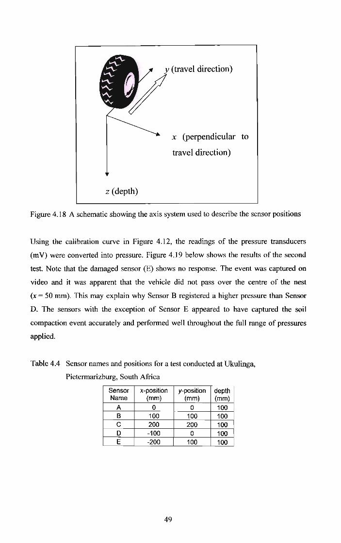
y (travel direction)

x (perpendicular to

travel direction)

z (depth)

Figure 4.18 A schematic showing the axis system used to describe the sensor positions

Using the calibration curve in Figure 4.12, the readings of the pressure transducers

(mV) were converted into pressure. Figure 4.19 below shows the results of the second

test. Note that the damaged sensor (E) shows no response. The event was captured on

video and it was apparent that the vehicle did not pass over the centre of the nest

(x = 50 mm). This may explain why Sensor B registered a higher pressure than Sensor

D. The sensors with the exception of Sensor E appeared to have captured the soil

compaction event accurately and performed well throughout the full range of pressures

applied.

Table 4.4 Sensor names and positions for a test conducted at Ukulinga,

Pietermarizburg, South Africa

Sensor x-position y-position depthName (mm) (mm) (mm)

A 0 0 100B 100 100 100C 200 200 100D -100 0 100E -200 100 100

49

I-A-B C-D-E!

60

50 -

- 40caD.~-Cl) 30I-::;,fI)fI)Cl) 20l-

D.

10

01 101 201 301 401 501 601 701 801 901

Sequential data points

Figure 4.19 Results obtained from fluid-filled bulb soil pressure sensors used in a test at

Ukulinga, Pietermarizburg, South Africa. A small agricultural tractor was

driven forwards over the sensors, which were inserted to different depths

and lateral positions

4.3 Sensor Attribute Weightings and Discussion

Based on the test described at the beginning of Chapter 4 the two sensor types were

evaluated according to how well they met the ideal design criteria, summarised in

Table 4.5. In order to design an accurate sensor, a high level of instrument accuracy is

required. High measurement accuracy was therefore assigned a weighting of three in

Table 4.5. The strain gauges used for the direct strain gauge SPS and the pressure

transducer used for the fluid-filled bulb SPS were found to be accurate and consistent if

they had consistent inputs and were both assigned a rating of four.

It is of utmost importance that there is good contact between the sensors and the soil.

For this reason, having a positive contact with the soil was assigned a weighting of

three. It was deemed that the fluid-filled bulb sensors made exceptional contact with the

soil since they could be pressurised once in the soil, allowing the latex to stretch and fill

all cavities. The fluid-filled bulb was given a rating of five, while the direct strain gauge

SPS, even with the insertion technique used, were only allocated a rating of three as

50

there remains some doubt as to whether positive contact between the sensors and the

soil is achieved.

It is also imperative that the sensor responds in a similar fashion to the soil it has

replaced. If the SPS is rigid compared to the soil it has replaced there may be a stress

concentration on it (van den Akker, 1989). Alternatively if the SPS is softer than the soil

it may deform too easily allowing the soil above it to arch, resulting in a lower stress

being exerted on the SPS. "Similar response to soil" was therefore assigned a weighting

of three. The direct strain gauge SPS were made from stainless steel and had a very

small range of motion and a solid perimeter and were therefore only given a rating of

two. The fluid-filled bulb SPS on the other hand were made from latex whose strength

can be assumed to be negligible, however the water they are filled with can be

considered incompressible. The pressure at any point in a fluid will be equal in all

directions. The bulb will exert a force, equal to the force applied to the ''top'' surface of

the bulb, on the soil at the "sides" of the bulb. This will allow the bulb to deform until

the pressure applied is equal to the pressure resisting deformation Figure 4.13 illustrates

this point. For this reason the fluid-filled bulb SPS was allocated a rating of four.

In an experiment conducted by Tarkiewicz and Lipiec (Tarkiewicz and Lipiec, 2000), it

was found that a small sensor size resulted in less disturbance of the soils structure

whilst placing the sensors. For this reason size was allocated a weighting of two. Both

the direct strain gauge and the fluid-filled bulb SPS were comparatively small and

therefore given a rating of four.

The cost effectiveness, availability of materials, ease of construction and a simple and

cost effective data acquisition system should not play a pivotal roll in the design of any

scientific measuring equipment. However, it must be remembered that the number of

sensors is affected by the above design properties and the use of a large number of

sensors in a field trial will greatly improve the understanding of the soil compaction

process. It was therefore concluded that the aforementioned design properties should all

be considered, but a weighting of only one should be assigned to these. The fluid-filled

bulb SPS were found to perform better on all accounts and were given higher ratings

than the direct strain gauge SPS.

51

Calibration of any sensor is vital, it was therefore assigned a weighting of three. The

calibration of SPS is however a difficult and complex matter. If the sensor is a sealed

unit (air tight) then it could be calibrated in a pressure vessel. This however does not

indicate how accurately a sensor will measure the pressure in the soil. A cylinder, as

described in Section 3.1.4 (pg 23), with a greased plastic lining, filled with soil and a

piston applying a known force to the surface is of some help. There are however, still

unaccounted for pressure losses into the sidewalls of the cylinder. The calibration of the

direct strain gauge SPS proved to be a major stumbling block and their calibrations

were only assigned a rating of one. The transducers used for fluid-filled bulb SPS were

calibrated and found to be very accurate. Calibration of the bulb-soil interface proved to

be more challenging. A cylinder and piston as described above was constructed and

used. It was found to give very repeatable results however the pressure measured was

lower than the pressure applied to the soil surface by the piston. For this reason they

were only given a rating of three and future work into the calibration technique should

be considered.

The minimal disturbance of the structure of a soil is of vital importance if an

understanding of the pressure propagation through a structured soil is to be gained. It

was therefore allocated a weighting of three. It was felt that the insertion technique of

both the direct strain-gauge and the fluid-filled bulb SPS caused minimal disturbance

and were both assigned a rating of four.

Finally it was decided that some practical consideration should be given to how

physically demanding and time consuming the insertion of the sensors was. Although

this would not influence their accuracy, it may constrain how many sensors can be used

in anyone trial thus indirectly limiting understanding gained from that trial. For this

reason "easy to insert" was given a weighting of two. The insertion of both the direct

strain gauge and the fluid-filled bulb SPS was found to be time consuming, inserting the

direct strain gauge SPS was however more physically demanding and was therefore

only allocated a rating of two. The fluid-filled bulb sensors were allocated a rating of

three.

From Table 4.5 below it can be seen that both sensors managed to achieve most of the

ideal design properties effectively with the direct strain gauge sensors scoring 65 and

52

the fluid-filled bulb sensors 91. Table 4.5 supported the decision that the fluid-filled

bulb SPS perfonned the best and would therefore be further evaluated in a large scale

field trial, described in Chapter 5.

Table 4.5 Summary of how effectively the sensors met the ideal design properties

Direct strain Fluid-f'"illedIdeal Design Properties Weighting 2:aU2:e bulb

Rating WxR Rating WxR

High measurement accuracy 3 4 12 4 12

Positive contact with soil 3 3 9 5 15

Similar response to soil 3 2 6 4 12

Small size 2 4 8 4 8Cost effectiveness 1 3 3 5 5

Readily available materials 1 3 3 4 4

Easy to construct 1 2 2 4 4

Simple & cost effective data acquisition 1 3 3 4 4

Easy & accurate to calibrate 3 I 3 3 9

Minimal soil structure disturbance 3 4 12 4 12

Easy to insert 2 2 4 3 6Sum of products 65 91

53

5 FIELD TESTING OF FLUID-FILLED BULB SENSOJlS

From the evaluation of the direct strain gauge and fluid-filled bulb sensors in the

previous chapter it was apparent that the fluid-filled bulb sensors were better suited to

use in field trials where a large number of sensors are to be used. The objective of this

chapter was to ascertain whether the use of fluid-filled bulb SPS, in a field trial, would

lead to a better understanding of how pressure propagates through a soil during a

compaction event, ultimately resulting in improved management strategies.

5.1 Methods

The fluid-filled bulbs were tested at a site near Richmond in KwaZulu-Natal, South

Africa (29°52' S, 30°12' E and 1075 m above sea level). The trial site was undulating,

(see Figure 5.1) and had harvested, Eucalyptus Smithii on it.

Soil samples were taken from the trial site and analysed to determine various texture

and geotechnical properties. Soil texture properties are presented in Table 5.1 and

geotechnical properties in Table 5.2.

Table 5.1 Soil texture properties of samples taken from a soil compaction trial site,

near Richmond, South Africa

Clay (%) Silt (%) Sand (%) Organic Matter (%) Texture

19 14 67 6.42 Sandy Loam

Table 5.2 Geotechnical properties of samples taken from a soil compaction trial site,

near Richmond, South Africa

Internal Angle of Cohesion Structural Strength Dry Bulk Water

Friction (pre-consolidated) Density Content

21° 10 kPa 150 kPa 796 kg·m-J 44.1%

The area had recently been harvested by hand. The timber was placed in bundles of

approximately 4 tons and loaded onto a self-loading trailer. The trailer was hitched to an

agricultural tractor, which transported the bundles to a nearby loading zone. Figure 5.1

shows the tractor and trailer combination, note the smooth tyre on the trailer, which was

54

used in this trial. A smooth tyre was selected to reduce any possible effects that lugged

tyres may have on the pressure uniformity. The tyre was a Firestone 10.5-16 ZS, 14 ply

radial tyre with a diameter of approximately 1 rn, a contact width of approximately

280 mm and was inflated to 424 kPa. The weight exerted by the tyre on the ground was

measured to be 2148 kg with the axle at an 11 % slope, to replicate the slope of the

trailer on the trial site. The trailer was reversed, perpendicular to the slope, over the nest

of sensors to ensure that the readings were not affected by previous soil compaction

events (the tractors wheels). Maintaining a constant speed, while ensuring the wheel

followed a particular path, posed a challenge for the driver while driving in a rearward

direction.

Figure 5.1 Self-loading trailer used in a soil compaction field trial near Richmond,

South Africa

Using the insertion technique described in Section 4.2.1 (pg 42) and the frame described

in Section 4.2.3 (pg 46), 16 sensors were placed, in a "nest" at a range of depths and

positions. Figure 5.2 is a schematic of the nest layout. The coordinate system was setup

using the same approach as the one described in Section 4.2.3 (see Figure 4.18 for more

details). The coordinate system has its origin on the soil surface directly above Sensor

A. Note that there were two sensors inserted every 100 mm in the y-direction; one was

55

inserted from the negative x-direction and the other from the positive x-direction. Five

sensors were placed at the 100 mm depth, five at 200 mm, three at 300 mm and three at

400 mm. The dark blue sensors, in Figure 5.2 are at a depth of 100 mm, the green

sensors are 200 mm deep, the orange sensors are 300 mm deep and the purple sensors

are 400 mm deep. The zigzag red lines indicate the edges of the tyre while the dashed

line indicates the centre line of the tyre.

Due to the variation in the y-positions of the sensors, it was anticipated that they would

begin registering pressure at different times. Similarly they were expected to experience

maximum pressure at different times. To allow the sensors to be compared with each

other it was necessary to compare the pressure data when the wheel was an equal

distance (y-position) from each sensor. A 100 mm square grid was marked out on the

surface to allow the position of the wheel to be accurately recorded by video. The tyre

did not pass over the centre of the nest and the x-positions of the sensors were therefore

adjusted by subtracting 40 mm from their initial position. Table 5.3 summarises the nest

layout, note the adjusted x positions.

DEPTH

• 100 r""lr""l

# 200 MM

# 400 MM

Figure 5.2 Illustration of the nest layout and the tyre path for the soil compaction trial

near Richmond, South Africa

56

Table 5.3 Sensor names and positions. x values are the perpendicular distance from

the centre of the tyre, y values are distance in the direction of travel and z

values are depth from the soil surface

Sensor x-pos Adjusted y-pos z-posName (mm) x-pas (mm) (mm) (mm)

A 0 -40 0 100B 100 60 0 100C -100 -140 100 1000 200 160 100 100E -200 -240 200 100F 200 160 200 200G -200 -240 300 200H 100 60 300 200I -100 -140 400 200J 0 -40 400 200K -150 -190 500 300L 0 -40 500 300M -150 -190 600 400N 150 110 600 3000 0 -40 700 400P 150 110 700 400

5.2 Results

Figure 5.3 illustrates the bulb pressure recorded during the soil compaction event

plotted against time. The sensors started to register pressure at different times, which

was as a result of their different y-positions (Table 5.3). It was also noted that some

sensors registered pressure for a longer period of time, which was caused by the vehicle

not travelling at a constant speed.

The above mentioned problems were addressed by relating each data point to its

distance from the centre of the tyre, as opposed to relating it to time. The video of the

event was broken into frames and every fifth frame was digitally analysed. This equated

to one frame every 0.2 seconds. The tyre position was determined by drawing a vertical

line from the lowest point of the rim to determine the centre of the wheel (Figure 5.4).

57

co 0 N C"> Il) <0Il) C? C? 0 C? C?<0 r-- r-- r-- r-- r--~ C"> C"> C"> C"> C">

..... .... .... .... .... ........ .... .....

140

120

100-caD. 80oX-CD 60I-:sfI)fI) 40CDl-D.

20

0

-20N ~ Il) r--Il) ~

Il) Il)

<0 <0 <0 <0~ C"> C"> C">.... .... .... ......... .... ..... ....

Figure 5.3 The pressure measured by all sensors during the soil compaction event

plotted against time

Figure 5.4 A frame extracted from the video of the soil compaction event, Richmond,

South Africa, used to calculate the position of the wheel relative to each

sensor. (a) Indicates a reference distance and (b) indicates the position of

the centre of the wheel

Once the position of the wheel relative to the sensors was calculated, the pressure

recorded by each sensor was plotted against the relative wheel position. Figure 5.5 show

the sensors once they had been synchronised.

58

-A

-B

C

-D

-E

-F

-G

-H

-I

J

:- K-L

-M

-N

500 -0

p

-250 0 250

Relative wheel position (mm)

~

I v\I

,~

J ,- 1\/ f

,-- \

~ 1 /"V ~ '\.. \,~~

~lE

,~~~ 1'=-- ~ ,=-c-- ~,

~: - .(-~ .. 'I i~' I'= . . -

-20

-500

140

120

100

li 80D.~-l! 60~fI)fI) 40l!D.

20

0

Figure 5.5 Pressure measured by all sensors plotted against relative wheel position

from a field trial, Richmond, South Africa. Negative wheel position values

depict pressure detected before the centre of the wheel has passed over the

sensors

The sensors were divided into groups that were at the same depth. These groups are

plotted against wheel position in Figure 5.6. Note that the pressure decreases with depth

as would be expected. Figure 5.7 and 5.8 show the pressure measured by Sensor A and J

plotted against time and against wheel position, respectively. Arrows connect the same

points in the time and the wheel position plots. This illustrates the inconsistency of the

travel speed of the vehicle applying the compaction.

In some instances the wheel changed direction, as the driver stopped the vehicle was

allowed to run back, this can be seen in Figure 5.9. Note that when the direction

changes the first time there is an increase in pressure, possibly due to the momentum of

the load transferring additional weight to the rear of the trailer as it slowed down. When

the direction changes for the second time (back to the original direction) there is a

decrease in the pressure measured by the sensor. This may have been due to some load

transferring back onto the tractor's hitch during the second direction change. The

fluid-filled bulb SPS was capable of measuring a change in pressure of approximately

15 kPa during a change in wheel position of 10 mm.

59

100 mm depth I-A-B C-D-EI

140 -_ 120/ ~ "'\. x=-40

:. 100 /~ 80 '\.CD... 60 / x=60 "-:::JCIl 40 / 'at.CIl .-- r--.....CD 20...

f - --Q.0-

t.ia~ x =1110 x =-240-20

JI200 mm depth I--F--G--H--I

80I '"!~

60 p..r:.- .~..Q.

~ 40!~r-J x = -14U

~!:::J 20

l~=-• ~~ ~

Q. 0x=160 x =·240 x=60

-20

300 mm depth I K L-NI

20

ii 15 - ...n.

Q.

~-..-~~

;- 10

~ ~ '-~5CIl - ... -CIl

CD '~.- i... 0 ~ --Q. --

-5 -

400nmdepth I-M-O pix =-40

6

I .1.. 4

'c,J,r~:~~;1~-

Q.

~"" r.n j

! 2 :;~ -±---- r-- ,"V - f ·v -X'!:::J• ~ ""I~ 0 ~··~'X'r r ~--·tQ.

-2-400 -300 -200 -100 0 100 200 300 400 500

Relative wheel position (mm)

Figure 5.6 Pressure measured by all sensors at a given depth plotted against relative

wheel position, Richmond, South Africa

60

a) Sensor A

6

_ 140 ,--------_------------'-----------,1

:. 120t======~lt~~~~~p,~============~1~100 # ,f 80 +-------II---t----t---.,\..--------------jl:::J 60 -I-------#---+------j----'~ -----------II

: 40 t====~J~t====t===t==~~;;;;~~~;;;;:====~If 20 I "Q. 0 ...I~-___,,.--+-----r_+-----r'tt------,--__;f_r.-..........-::::!!!!IIII..._-~

o 1 2 3 +010 (secl4

\ 5 /

40035050 100 150 200 250 300o-200 -150 -100 -50

b) 140 .----- +----+-__--\\__+-/ ---,:. 120 +---------;o~-!III!!!~~--~---\\_--I/'----------l~ 100 .f-------~,"----....-=----_·--"""~--i\---r__/------_tlD 80 +------~~,---------"',~-_t\-__JI'--------_i~ 60 +----------..~f--------~.....~_;------f-.::.y_-------_i: 40 +----------::Jl.,.J~----------""_~....-II''_f\+''--'-'''~in·..-"-!i,,,-~-__------j

f 20 .f------.M-"~------------.\"l""w.~l'_.r-------_tQ. 0 _ .......J'~..,._-__,_-__._--,--.....,_-.....,_-__,_-=::::::::~~.....,...__~_~..I

-250

Relative wheel position (mm)

Figure 5.7 Pressure measured by Sensor A plotted against (a) time and (b) relative

wheel position, Richmond, South Africa. Figure 5.9 contains a zoomed plot

of the encircled area in (b) above

a) SensorJ

_ 70

:'60~50

T1 11

f 40I / '"I / "-~30 I \ / "• 20f 10 .J \ / '"Q. \ / -0

7 \

3 4 5 6 8 9) 11 12 13 14

Time (sec)

b) \ /_ 70

:'60\ -I

~ ~~50.JI" '"f 40 .,

""-:::J 30

i 20....., "'-

It 10 ~ ~

0-250 -200 -150 -100 -50 0 50 100 150 200 250 300 350 400

Relative wheel position (mm)

Figure 5.8 Pressure measured by Sensor J plotted against (a) time and (b) relative

wheel position, Richmond, South Africa

61

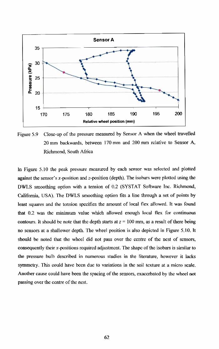
Sensor A35 -,----------------------------,

- 30 ~..---------~-------;---------jtaD..:Jtt.-f 25 +----------=~~\a.;:;;;:=_:;;:------~------~::JCl)

fD. 20 -1----------------~_._---~c--_j

200195190185180175

15 -1----,------,-----,------,-----,-------1

170

Relative wheel position (mm)

Figure 5.9 Close-up of the pressure measured by Sensor A when the wheel travelled

20 mm backwards, between 170 mm and 200 mm relative to Sensor A,

Richmond, South Africa

In Figure 5.10 the peak pressure measured by each sensor was selected and plotted

against the sensor's x-position and z-position (depth). The isobars were plotted using the

OWLS smoothing option with a tension of 0.2 (SYSTAT Software Inc. Richmond,

California, USA). The OWLS smoothing option fits a line through a set of points by

least squares and the tension specifies the amount of local flex allowed. It was found

that 0.2 was the minimum value which allowed enough local flex for continuous

contours. It should be note that the depth starts at z = 100 mm, as a result of there being

no sensors at a shallower depth. The wheel position is also depicted in Figure 5.10. It

should be noted that the wheel did not pass over the centre of the nest of sensors,

consequently their x-positions required adjustment. The shape of the isobars is similar to

the pressure bulb described in numerous studies in the literature, however it lacks

symmetry. This could have been due to variations in the soil texture at a micro scale.

Another cause could have been the spacing of the sensors, exacerbated by the wheel not

passing over the centre of the nest.

62

o~-----

No Data

....-..EE.........N

100

200",

X\ ....\ ' .

:./":::..;".: ..../

x

300 x x x

'. ~ --_.--

400 x x x

200100-100 0X (mm)

-200500 1.--_-.1..__--'--__-'---_--1.__---'

-300

Figure 5.10 Peak pressure (kPa), measured by each sensor (x) during a field trial,

Richmond South Africa, plotted against x-position and z-position (depth).

Isobars were calculated by using the DWLS smoother with a tension of 0.2

inSYSTAT

5.3 Discussion

In general the trial was a success with a large amount of valuable data being generated.

The soil at the trial site was easy to handle and although the placement of the sensors

was time consuming, no major problems or difficulties were encountered. The use of a

smooth, non-lugged tyre was expected to apply a more uniform pressure to the soil

surface in comparison to a lugged tyre. However, some improvements could be made,

such as an improved method of determining the y-position of the wheel or alternatively

maintaining a consistent speed of the vehicle. A consistent speed may also result in

fewer dynamic effects, and may therefore produce data points that are more consistent,

and easier to analyse. The effects of the inconsistent speed on pressure were shown in

Figure 5.9. The lack of symmetry in Figure 5.10 may also be a result of the inconsistent

63

speed and resultant dynamic loading. The literature reviewed in Chapter 3 indicated that

pressure propagation through a soil should be symmetrical if a symmetrical load is

applied to a homogeneous soil surface. More research to determine if there are any

correlations between a sensor's position and when it first starts to register pressure or

when it reaches its peak value may be significant if a deeper understandi,ng of soil

compaction is to be gained. The influence of dynamic loading must be minimized if this

is to be achieved.

This trial demonstrated the effectiveness of the fluid-filled bulb SPS in measuring the

pressure in the soil at various depths and numerous positions perpendicular to the

wheel's travel direction. The trial established that the fluid-filled bulb SPS were cost

effective and relatively easy to construct and insert. They performed well at a range of

pressures, particularly the higher pressures which generally result in higher levels of

compaction and are therefore of greater significance.

The lack ofdata between the soil surface and the sensors at the 100 mm depth, as shown

in Figure 5.10, makes the understanding of the soil compaction process difficult. It is,

however, impractical to place sensors at depths of less than 100 mm as there will be

significant soil disturbance. A possible solution would be the development of a model to

interpolate and extrapolate measured soil pressure readings.

Theoretically, once matrices of data, relating pressure to x-position, y-position and

z-position (depth) have been obtained, these values could be interpolated and even

extrapolated. This would require the development of a model which would allow a

pressure at any given point in the soil to be estimated. While the value of such an

equation would add to the understanding of the soil compaction process, it should be

acknowledged that in many cases extrapolating measured results may generate

misleading information. Also, a reasonably high resolution of measurements is required

to confirm the use of a function of this nature. Appendix A aims to demonstrate this

concept, although it is acknowledged that the dataset, discussed in this chapter, will

probably not fulfil the statistical requirements to allow this function to be used with

confidence. However, demonstrating the future potential of such a model could aid in

the planning of the layout of future trials, to validate this model.

64

6 DISCUSSION, CONCLUSIONS AND RECOMMENDATIONS

6.1 Discussion and Conclusions

Soil compaction has numerous consequences; of particular concern for agriculture is the

reduction in yields, ultimately influencing the sustainability of agricultural production.

Mitigation against soil compaction can only occur if a thorough understanding of the

soil compaction process, supported by scientific measurements, exists. Measuring the

effects of soil compaction is commonly achieved by measuring changes in;

• the bulk density of a soil,

• the penetration resistance ofa soil, and

• changes in a soils ability to conduct a fluid.

Although some of these measurements are useful in quantifying the severity of soil

compaction resulting from a particular event, they do not explain the processes that

cause these changes.

Examining the pressure propagation through the soil during a compaction event has led

to a greater understanding of the underlying soil compaction processes. Three methods

have been used to measure the pressure in soil's, namely;

• direct strain gauge soil pressure sensors,

• fluid-filled bulb soil pressure sensors, and

• piezoelectric based soil pressure sensors.

The following significant aspects need to be considered when selecting and designing

soil pressure sensors (SPS);

• the presence of a disturbed layer around the sensor, often caused by the

insertion technique,

• the sensors could respond differently than the soil it has replaced,

• the effect wireslhoses may have, by preventing movement of a sensor,

• the cost, availability of materials and the ease of manufacture need to be

considered if numerous sensors are to be used in multiple sensor nests, and

• the cost, accuracy, sample rate and ease of the data acquisition.

During this study it was decided to develop and test two types of soil pressure

measuring devices; namely the direct strain gauge SPS and the fluid-filled bulb SPS.

65

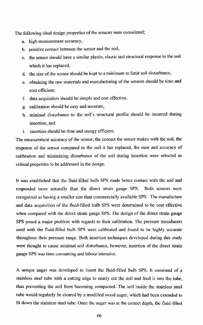
The following ideal design properties of the sensors were considered;

a high measurement accuracy,

b. positive contact between the sensor and the soil,

c. the sensor should have a similar plastic, elastic and structural response to the soil

which it has replaced,

d. the size of the sensor should be kept to a minimum to limit soil disturbance,

e. obtaining the raw materials and manufacturing of the sensors should be time and

cost efficient,

f. data acquisition should be simple and cost effective,

g. calibration should be easy and accurate,

h. minimal disturbance to the soil's structural profile should be incurred during

insertion, and

1. insertion should be time and energy efficient.

The measurement accuracy of the sensor, the contact the sensor makes with the soil, the

response of the sensor compared to the soil it has replaced, the ease and accuracy of

calibration and minimizing disturbance of the soil during insertion were selected as

critical properties to be addressed in the design.

It was established that the fluid-filled bulb SPS made better contact with the soil and

responded more naturally than the direct strain gauge SPS. Both sensors were

recognized as having a smaller size than commercially available SPS. The manufacture

and data acquisition of the fluid-filled bulb SPS were determined to be cost effective

when compared with the direct strain gauge SPS. The design of the direct strain gauge

SPS posed a major problem with regards to their calibration. The pressure transducers

used with the fluid-filled bulb SPS were calibrated and found to be higWy accurate

throughout their pressure range. Both insertion techniques developed during this study

were thought to cause minimal soil disturbance, however, insertion of the direct strain

gauge SPS was time consuming and labour intensive.

A unique auger was developed to insert the fluid-filled bulb SPS. It consisted of a

stainless steel tube with a cutting edge to neatly cut the soil and feed it into the tube,

thus preventing the soil from becoming compacted. The soil inside the stainless steel

tube would regularly be cleared by a modified wood auger, which had been extended to

fit down the stainless steel tube. Once the auger was at the correct depth, the fluid-filled

66

bulb SPS was be placed down the centre of the stainless steel tube, ensuring that it was

in the correct position and preventing the hole from collapsing. Previously fluid-fllled

bulb SPS have been inserted into augured holes, however, the insertion technique

described above is thought to be more effective in minimising soil disturbance than

those used in the past.

It was concluded that the fluid-filled bulb SPS could be used in field trials where a large

nest of sensors is to be inserted. Fluid-filled bulb SPS were evaluated successfully in

such a trial. To the author's knowledge this was the largest number of sensors used to

record a single event and there are plans to utilise the sensors in future soil compaction

trials, indicating the successfulness of these sensors. Some improvements could,

however, be made to the trial design and layout, with the specific aim of making the

analysis of the data easier and increasing the significance of the results.

6.2 Recommendations for Further Research

• The calibration of SPS poses a major challenge as there are a number of external

influences. A standardised calibration technique and apparatus may be of value.

The apparatus could consist of a pressure pot, with strain gauges around the

cylinder to measure the magnitude of force, perpendicular to the applied force, in

the walls of the cylinder. Force may also be transferred into the side walls of the

cylinder by the friction between the walls of the cylinder and the soil. This force

could be measured by using a cylinder with a piston at the top and the bottom

and calculating the difference in force between the two pistons. The weight of

the soil would need to be accounted for.

• The experimental procedure could be refined in order to reduce the amount of

effort required during data analysis. The greatest improvement may be gained by

ensuring that the wheel passes over the sensors at a constant speed. This could

limit any dynamic effects.

• An insertion technique allowing the direct strain gauge SPS to be placed along

an arc was developed. This minimized the disturbance of the soil directly above

the sensors. To the author's knowledge this technique had never been used

67

before. It was however not possible to place sensors below 250 mm and the

technique was labour intensive and time consuming. Further research and

development of this technique may be worthwhile.

• The interaction of direct strain gauge SPS with the soil is unknown due to their

rigid construction. However, if they are to be used, they should use a diaphragm

and not a beam or cantilever beam.

• If measuring the residual soil pressure is considered important the durability of

the SPS would need to be considered. Another consideration will be the

interaction between the sensor and the soil as the pressure is removed from the

surface. Sensors may have either significantly greater or lower restoring forces

than the soil they replace.

• Appendix A serves as an illustration of a model which could be developed,

using the data obtained using the fluid-filled bulb SPS to be interpolated and

extrapolated. An alternative sensor layout may be required during future trials to

statistically verify the use of the model.

68

7 REFERENCES

Abu-Hamdeh, N.H, and Reeder, RC 2003. Measuring and predicting stress distribution

under tractive devices in undisturbed soils. Biosystems Engineering 85 (4): 493­

502.

Adamchuk, VJ, Morgan, M.T, and Sumali, H 2001a. Applications of a strain gauge

array to estimate soil mechanical impedance on-the-go. Transactions of the

ASAE 44 (6): 1377-1383.

Adamchuk, VJ, Morgan, M.T, and Sumali, H. 2001b. Mapping ofspatial and vertical

variation of soil mechanical resistance using a linear pressure model. ASAE

Meeting Paper No. 01-1019. St. Joseph, Michigan, USA.

Alakukku, L, Ahokas, J, and Ristolainen, A. 2002. Response of Clay Soil

Macroporosity to Stress Caused by Tracked Tractors. In ed. M. Pagliai and R

Jones Sustainable Land Management - Environmental Protection: A Soil

Physical Approach ch. 4, 319-330 CATENA VERLAG GMBH. Reiskirchen,

Germany.

Agricultural Engineers Yearbook ofStandards. 2000. S313.3. Soil Cone Penetrometer.

ASAE, St. Joseph, Michigan, USA.

Anon. 2004. Concrete Catalog, Soil Compaction Handbook. [Internet]. Available from:

<http://www.concrete-catalog.com/soil_compaction.htm1>. [Accessed 02

September 2004]

Arvidsson, J, Trautner, A, and Keller, T. 2002. Influence of tyre inflation pressure on

stress and displacement in the subsoil. In ed. M. Pagliai and R Jones

Sustainable Land Management - Environmental Protection: A Soil Physical

Approach ch. 4, 331-338 CATENA VERLAG GMBH. Reiskirchen, Germany.

Bailey, A.C, Nichols, T.A, and Johnson, C.E 1988. Soil stress state determination under

wheel loads. Transactions ofthe ASAE 31 (5): 1309-1314.

Bear, J. 1972. Dynamics of Fluids in Porous Media. Dover Publications, Inc. New

York, USA.

Chung, S, Sudduth, K.A, and Hummel, J.W. 2003. On-the-go soil strength profile

sensor using a load cell array. ASAE Meeting Paper No. 031071. St. Joseph,

Michigan, USA.

Coates, W.E 2001. Reduced tillage systems for irrigated cotton: Is soil compaction a

concern. Applied Engineering in Agriculture, ASAE 17 (3): 273-279.

69

Cohron, G.T. 1971. Forces Causing Soil Compaction. In ed. K. K. Barnes, W. M.

Carleton, H. M. Taylor, R. 1. Throckmorton, and G. E. Vanden Berg

Compaction ofAgricultural Soils 471 ASAE. St. Joseph, Michigan, USA.

Das, B.M. 1998. Principles of Geotechnical Engineering. PWS Publishing Company.

Boston, USA.

De Wrachien, D. 2002. Sustainable land use: The role of agricultural engineering. In ed.

M. Pagliai and R. Jones Sustainable Land Management - Environmental

Protection: A Soil Physical Approach ch. 1, 19-32 CATENA VERLAG GMBH.

Reiskirchen, Germany.

Eastes, J.W., Mason, G.L., and Kusinger, A.E. 2004. Thermal Signiture Characteristics

ofVehiclefferrain Interaction Disturbances: Implications for Battlefield Vehicle

Classification. Applied Spectroscopy 58 (5): 510-515.

Easton, V.J., and McColl, J.H. 2005. Statistics Glossary. [Internet]. Available from:

http://www.cas.lancs.ac.uk/glossary_vl.1/hyptest.html#pvalue. [Accessed 28

October 2005]

Fazekas, 0., and Horn, R. 2004. Interaction between soil stability and pore water

pressure as a function of the loading time during compaction test. [Internet].

Proc. 2nd Eurosoil Congress in Freiburg/Germany. Available from:

<http://kuk.uni-freiburg.de/hosted/eurosoiI2004/fullyapers/id270_Fazekas_full.

pdf>. [Accessed 13 August 2004]

Forestry, Suppliers Inc. 2004. Manual cone pentrometers. [Internet]. Available from:

<http://www.forestry-suppliers.com/search.asp?stext=soil%20compaction>.

[Accessed 27 August 2004]

Freitag, D.R. 1971. Methods of measuring soil compaction. In ed. K. K. Bames, W. M.

Carleton, H. M. Taylor, R. I. Throckmorton, and G. E. Vanden Berg

Compaction ofAgricultural Soils 471 ASAE. St. Joseph, Michigan, USA.

Gere, J.M., and Timoshenko, S.P. 1997. Mechanics of Materials. PWS Publishing

Company. Boston, USA.

Gysi, M. 2000. Soil compaction due to heavy agricultural wheel traffic. Unpublished

Phd Dissertation, School of Natural Sciences, Swiss Federal Institute of

Technology Zurich, Zurich, Switzerland.

Harris, W.L. 1971. The soil compaction process. In ed. K. K. Bames, W. M. Carleton,

H. M. Taylor, R. 1. Throckmorton, and G. E. Vanden Berg Compaction of

Agricultural Soils 471 St. Joseph, Michigan, USA.

70

Hattingh, J.M. 1989. Soil Compaction Under Different Forest Harvesting Techniques.

Report No. 640. PU for CHE, Potchefstroom, RSA.

Helfrick, A.D., and Cooper, W.D. 1990. Modern Electrical Instrumentation and

Measurement Techniques. Prentice-Hall International, Inc. New Jersey, USA.

Herrick, J.E, and Jones, T.L 2002. A dynamic cone penetrometer for measuring soil

penetration resistance. Soil Science Society ofAmerican Journal 66 (4): 1320­

1324.

Johnson, C.E, and Bailey, A.C. 2002. Soil Compaction. In ed. Advances in Soil

Dynamics Volume 2 ch. 3, 155-178 ASAE. S1. Joseph, Michigan, USA.

Jones, D, and Kunze, M. 2004. Guide to Sampling Soil Compaction using Hand-held

Soil Penetrometers. Report No. CEMML TPS 04-1. Centre for Environmental

Management of Military Lands, Fort Collins, Colorado, USA.

Jones, R. 2002. Assessing the vulnerability of soils to degradation. In ed. M. Pagliai and

R. Jones Sustainable Land Management - Environmental Protection: A Soil

Physical Approach ch. 1, 33-44 CATENA VERLAG GMBH. Reiskirchen,

Germany.

Kirby, J.M. 2000. Analysis and use of earth pressure cells. In: eds. 4th International

Conference on Soil Dynamics, ICSD-IV organising committee, Adelaide,

Australia.

Koolen, AJ and Kuipers, H. 1983. Agricultural Soil Mechanics. Springer - Verlag,

Berlin, Germany.

Koostra, B.K, and Stombaugh, T.S. 2003. Development and evaluation ofa sensor to

continuously measure air permeability of soil. ASAE Meeting Paper No.

031072. S1. Joseph, Michigan, USA.

Li, Y, Tullberg, J.N, and Freebaim, D.M 2001. Traffic and residue cover effects on

infiltration. Australian Journal ofSoil Research 39: 239-247.

Lorentz, S.A., 2004. Personal Communication, Univesity of KwaZulu-Natal,

Pietermaritzburg, South Africa, 6 September 2004.

L~ Z., Hickey, C.J., and Sabatier, J.M. 2004. Effects of compaction on the acoustic

velocity in soils. Soil Science Society ofAmerican Journal 68 (1): 7-16.

Malinda, D., Schultz, J., and Darling, R. 2000. Advances to overcome root zone

constraints to crop productivity. In: eds. lh International Conference on Soil

Dynamics, Adelaide, Australia.

71

McKibben, E.G. 1971. Introduction. In ed. K. K. Barnes, W. M. Carleton, H. M. Taylor,

R I. Throckmorton, and G. E. Vanden Berg Compaction ofAgricultural Soils

471 ASAE. St. Joseph, Michigan, USA.

Miller, RE, Hazard, J, and Howes, J. 2001. Precision, Accuracy and Efficiency ofFour

Tools for Measuring Soil Bulk Density or Strength. Report No. PNW-RP-532.

United States Department of Agriculture, Washington D.e., USA.

Mouazen, A.M., Dumont, K., Maertens, K., and Ramon, H. 2003. Two-dimentional

prediction of spatial variation in topsoil compaction of a sandy loam field-based

on measured horizontal force of compaction sensor, cutting depth and moisture

content. Soil & Tillage Reasearch 74: 91-102.

Nichols, T.A, Bailey, A.C, Johnson, C.E, and Grisso, D.R 1987. A stress state

transducer for soil. Transactions ofthe ASAE 30 (5): 1237-1241.

Pagliai, M , and Jones, R. 2002. Sustainable Land Management - Environmental

Protection: A Soil Physical Approach. CTENA VERLAG GMBH. Reiskirchen,

Germany.

Pearman, RK, Way, T.R, Johnson, C.E, Boo, E.C, Bailey, A.C, and Raper, R.L 1996.

Soil stresses and rut depths from tires of a mechanical front wheel drive tractor.

Transactions ofthe ASAE 39 (4): 1249-1257.

Raper, RL, Washington, RH, and Jarrell, J.D 1999. A tractor-mounted multiple-probe

soil cone penetrometer. Applied Engineering in Agriculture, ASAE 15 (4): 287­

290.

Richmond, P.W., Shoop, S.A., and Blaisdell, G.L. 1995. Cold Regions Mobility Models.

Report No. CRREL Report 95-1. Cold Regions Research & Engineering

Laboratory, US Army Corps of Engineers, USA.

Schafer-Landefeld, L, Brandhuber, R, Fermer, S, Koch, H, and Stockfisch, N 2004.

Effects of agricultural machinery with high axle load on soil properties of

normally managed fields. Soil & Tillage Research 75: 75-86.

Selig, E.T. 1964. A review of stress and strain measurments III soil. In: eds. -.

Symposium on Soil-Structure Interaction Proc:, 172-186.

Selig, E.T., and Vey, E. 1964. Piezoelectric gages for dynamic soil stress

measurements. In Measurements and Relations ofSoil Stress and Strength. 48,

HRB-NAS-NRC Pub. 1170: 34-48. Highway Res. Rec.,

Smith, e.W 1999. Impacts of harvesting operations and suggested management

stratergies. In. Site damage and long-term site productivity offorest plantations

72

in South Africa. ICFR Hand Book Series No. 1/99: ICFR, Pietermartizburg,

RSA.

Smittle, D.A, and Threadgill, E.D 1977. Response of southernpea (Vigna unguiculata

(L.) Walp.) to tillage methods. HortScience 12 (6): 556-558.

Sohne, W 1958. Fundamentals of pressure distribution and soil compaction under

tractor tyres. Agricultural Engineering 39: 276-281.

SYSTAT, 10-2-01. SYSTAT Software Inc. Richmond, California, USA.

Tarkiewicz, S., and Lipiec, J. 2000. Methods for simultaneous recourding of stress and

displacments in soil under wheels of agricultural machinery. In ed. R Horn, J. J.

H. van den Akker, and J. Arvidsson Subsoil Compaction - Distribution,

Processes and Consequences ch. 5, 435-441 CATENA VERLAG GMBH.

Reiskirchen, Germany.

Tekeste, M.Z., Grift, T.E., and Raper, RL. 2002. Acoustic compaction layer detection.

Presented at the 2002 ASAE Annual International Meeting / CIGR XVth World

Congress, Hyatt Regency, Chicago, Illinois, USA, 28-31 July 2002.

Trouse, A.C. 1971. Soil Conditions as They Affect Plant Establishment, Root

Development, and Yield. In ed. K. K. Barnes, W. M. Carleton, H. M. Taylor, R.

I. Throckmorton, and G. E. Vanden Berg Compaction ofAgricultural Soils 471

ASAE. St. Joseph, Michigan, USA.

Turner, R 2001. Device speeds compaction measuring process. [Internet]. 2001.

Available from: http://www.asae.org/imis/StaticContent/3/decO1/device.html.

[Accessed 06 January 2004]

Turner, R, and Raper, RL. 2001. Soil stress residual as indicators ofsoil compaction.

Presented at the 2001 ASAE Annual Internation Meeting, Paper No. 011063.

ASAE, St Joseph, Michigan, USA.

van den Akker, J.J.H. 1989. Reliability of pressure cells to measure traffic-induced

stress in the topsoil subsoil interface. In: eds. 4th European ISTVS Conference,

Wageningen, The Netherlands, 21-23 March 1989.

van den Akker, J.J.H. 1999. Development, verification and use of the subsoil

compaction model SOCOMO. In: eds. J. J. H. van den Akker, J. Arvidsson, and

R Horn. Experiences with the Impact and Prevention ofSubsoil Compaction in

the European Community., 321-336. DLO Winand Staring Centre, Wageningen,

The Netherlands, 28-30 May 1998.

73

van den Akker, J.J.H. 2004. Photographed point grid for measunng soil strain.

[Internet]. Alterra. Available from: <http://www.alterra-research.nl/servlet/page

?-pageid=335&_dad=portal30&_schema=PORTAL30>. [Accessed 02

September 2004]

van den Akker, J.J.H, and Stuiver, H.J 1989. A sensitive method to measure and

visualise deformation and compaction of the subsoil with a photographed point

grid. Soil & Tillage Reasearch 14: 209-214.

Voorhees, W.B. 2000. Interaction of axle load, soil water regime, and soil texture on

long-term subsoil compaction and crop yields in North America. In: eds. 4th

International Conference on Soil Dynamics, Adelaide, Australia.

Wazau. 2004. Pressure sensors. [Internet]. Available from:

<http://www.wazau.com/en/sensors/druckaufuehmer.html>. [Accessed 03

September 2004]

Wells, L.G, Stombaugh, T.S, and Shearer, S.A. 2001. Application and assessment of

precision deep tillage. ASAE Meeting Paper No. 01-1032. St. Joseph, Michigan,

USA.

Williams, J, Bordas, V, and Gascoigne, H. 2004. Conserving land and water for society:

Global challenges and perspectives. In: eds. ISCO 2004-13th International Soil

Conservation Organisation Conference, ISCO, Brisbane, Australia.

74

APPENDIX A

AN INTRODUCTION TO NUMERICAL INTERPOLATION AND

EXTRAPOLATION OF OBSERVED PRESSURE DATA

Introduction

To gain a better understanding of the soil compaction process, the pressure in the soil, at

any position relative to the wheel, should be known. It may be possible to calculate the

pressure at any point in the soil by developing an equation that could interpolate and to

some extent, extrapolate measured pressure readings to the area below the tyre where it

is difficult to place sensors. This exercise may need to be combined with existing

knowledge of soil compaction, such as;

• soil pressure follows a quadratic decline with respect to depth (Sohne, 1958),

• in many cases the mean soil contact pressure equals 1.2 times the tyre inflation

pressure (Koolen, 1983), and

• soil pressure at a specific depth follows a symmetrical distribution (van den

Akker, 1989; van den Akker, 1999).

The aim of this Appendix is to demonstrate the potential to interpolate and extrapolate

measured pressure in a three-dimensional soil medium. This would enable isobars of

pressure to be inferred from a nest of sensors below a wheel. It should be noted that the

trial described in Chapter 5, was not designed for the purpose of model building and

relationships and statistical coefficients should not be regarded as significant. All

objectives for this study were achieved in Chapters 2 to 5 and Appendix A serves

merely as an indicator of a possible application of the technology already developed in

this study. A significant amount of further research will be required in order to develop

a scientifically sound model. Results from Chapter 5 do, however, create the

opportunity to theoretically introduce and demonstrate this approach.

Model Description

The same system of axes described in Section 4.2.3 and illustrated in Figure 4.18 (pg

44) were used. van den Akker, (1999) strongly supported the concept of a symmetrical

75

pressure distribution in the soil below a tyre, assummg the tyre is applying a

symmetrical load. In addition a simple statistical hypothesis test on the data described in

Chapter 5, could not exclude this assumption. It was therefore decided to fit a

symmetrical function, with a turning point at x equal to zero, to allow interpolation

between sensors at the same z-positions (depths). This was done at the 100 mm,

200 mm and 300 mm z-positions (depths). This was then repeated for three different

y-positions (-75 mm, 0 mm & 75 mm). A Gaussian function was preferred due to its

symmetry and provided the best-fit for the data. An example from y-position equal to

zero can be seen in Figure A.I below and the equation of the Gaussian function is

shown in Equation A.I.

(A.I)

where P

x

k

s

pressure (kPa),

x-position (mm),

constant related to the amplitude, and

constant related to the spread.

1-100 mm -200 mm -300 mm I400 ,--------------,---- --,

200ox-position (mm)

50 t- U-_-+-_~----.:k~=---.:3=-::1=29~.7~__15 =63.383

ot----====~===t=::~~=~-200

350 -t----------H-+---------l

300 -t--------I--t-+--..=....:.------l

k =11882100 t------=-==-==:=---f--f-----1----.J\--+---------l

5 =28.372

"'i 250 t--------t-t-\,----------1~

~ 200 t---------+-----1f----+----------l

i 150CL t-------+------1---\----------l

Figure A.I Examples of the Gaussian functions. for three depths, taken at y = 0, that

were used to represent pressure distribution (along the x-axis) in the soil

76

Model Calibration and Illustration

Once the k & S values were determined for the three z-positions (depths) and at the three

different y-positions, they were plotted against z-position (depth), to allow the

interpolation and extrapolation of the pressure at various z-positions (depths). Figure

A.2 shows examples of k vs. depth for the three y-positions. A second order polynomial

trend line was fitted to the k values giving Equation A.2. An exponential trend line was

fitted to the S values giving Equation A.3.

25000 ,-----;---------------,

20000 -t-----~___¥<_-------------i

15000 -t-------~~-----------i

.lC10000 +---------~~-----------i

400300200

Depth (mm)

100

O-t-------,------,---------,-----

o

5000 +-----------------"'~...,_----

Figure A.2 Plot of k against z-position (depth) for various y-positions and x-position

equal to zero

(A.2)

where k

z

constant from Equation A.I

depth (mm), and

constants.

S = Sa + e(Sb(Z-SJ)

where S constant from Equation A.I(A.3)

z depth (mm), and

constants.

Lastly ka, kb, kc, Sa, Sb & Se were plotted against their y-positions, to allow for

interpolation of pressure along the y-axis. An example of ka can be seen in Figure A.3.

Second order polynomial trend lines were fitted to all figures giving the constants

shown in Table A.I, and example of equation of ka is shown in Equation AA.

77

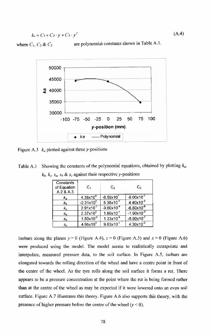
ka =C1 + C2 . Y + C3 . y2 (AA)

where Cl, C2 & C3 are polynomial constants shown in Table AI.

..-~~

•30000

-100 -75 -50 -25 0 25 50 75 100

y-position (mm)

50000

35000

.= 40000

45000

• ka -Polynomial

Figure A3 ka plotted against three y-positions

Table Al Showing the constants of the polynomial equations, obtained by plotting k{b

kb, kc, S{b Sb & Se against their respective y-positions

Constantsof Equation C1 C2 C3

A2 &A.3

ka 4.38x104 -6.59x101 -8.00x10-1

kb -2.21x102 5.38x10-1 4.40x10--3

ke 2.91x10·1 -9.60x10-4 -6.80x10~

Sa 2.37x101 1.90x1O-1 -1.90x10-3

Sb 1.50x10·2 1.33x10-4 -8.90x10·7

Se 4.95x101 9.83x10-1 4.30x1O-3

Isobars along the planes y = 0 (Figure AA), Z = 0 (Figure A.5) and x = 0 (Figure A.6)

were produced using the model. The model seems to realistically extrapolate and

interpolate, measured pressure data, to the soil surface. In Figure A5, isobars are

elongated towards the rolling direction of the wheel and have a centre point in front of

the centre of the wheel. As the tyre rolls along the soil surface it forms a rut. There

appears to be a pressure concentration at the point where the rut is being formed rather

than at the centre of the wheel as may be expected if it were lowered onto an even soil

surface. Figure A 7 illustrates this theory. Figure A6 also supports this theory, with the

presence ofhigher pressure before the centre of the wheel (y < 0).

78

o

100EE..........N

200

150ox (mm)

300 '--- ------L ---'

-150

Figure AA Front view showing modelled pressure (in kPa), perpendicular to the travel

direction (x-position) and below (z-position) the centre of the wheels axis

(y = 0 plane)

Travel Direction

-75 I

.. - .

~~:"ii~~:i:::::::::::::::i:::·:::·::::i::ii::ii::::i::::::::::::::::::::/:::;::::i:\::i::::i::::::::::::::i;::::::::::::::::::::::::::::

EE..........><

0-#&:::.::.::::.:.:.:.:,::.:::::::.:.:.:.:.:.:.:.:.:.:.:.:.:::.~ :...:.~.~.:.~.:.:.~.~~.:.:.:.~:.. ~..:.:..: :..:..:.: :.:.~:.::::::::::-. ":-. :::.:.::": :"::.:::. . - "

75 I

75 0 -75y(mm)

Figure A.5 Top view showing surface or contact pressure (in kPa) predicted by the

model between the soil surface (x&y-positions) and the tyre/soil interface

(z = 0 plane)

79

Travel Direction~

.·:··600- ..: ....:::::::::::.:.....o.......-:-~,,-------.;;:----:-":"~~==.::::....::::....::::..::::..::::.=..=!

500 ..

_ 100EE-N 200

200'\00

-75oy(mm)

300 L----"c:.:.:.:...- --L-. ---'

75

Figure A.6 Side view showing how the modelled pressure (in kPa) propagates through

the soil profile (z-position) along the length of the tyre (y-position), below

the middle of the tyre (x = 0 plane)

I Travel direCtiOn>

IRut formed by wheel

Position of the maximum

pressure reading

INatural Ground level

Figure A.7 An illustration for the possible cause of the maximum pressure occurring

forward of the wheel's axis of rotation

Summary and Discussion

Although the results of the model discussed in this chapter are meant for illustrative

purposes only, the numerical interpolation and extrapolation of data obtained by soil

pressure sensors can potentially be of substantial benefit. It is, however, important to

design future trials with a high enough density and symmetrical distribution of sensors,

to enable the validation of this model.

80