The Design and Integration of an Airborne Imager and Flight ...

University of Tennessee, Knoxville University of Tennessee, Knoxville

TRACE: Tennessee Research and Creative TRACE: Tennessee Research and Creative

Exchange Exchange

Masters Theses Graduate School

5-2007

The Design and Integration of an Airborne Imager and Flight The Design and Integration of an Airborne Imager and Flight

Campaign to Study the Time Evolution and Vertical Structures of Campaign to Study the Time Evolution and Vertical Structures of

Polar Mesospheric Clouds Polar Mesospheric Clouds

Jason David Reimuller University of Tennessee - Knoxville

Follow this and additional works at: https://trace.tennessee.edu/utk_gradthes

Part of the Navigation, Guidance, Control and Dynamics Commons

Recommended Citation Recommended Citation Reimuller, Jason David, "The Design and Integration of an Airborne Imager and Flight Campaign to Study the Time Evolution and Vertical Structures of Polar Mesospheric Clouds. " Master's Thesis, University of Tennessee, 2007. https://trace.tennessee.edu/utk_gradthes/318

This Thesis is brought to you for free and open access by the Graduate School at TRACE: Tennessee Research and Creative Exchange. It has been accepted for inclusion in Masters Theses by an authorized administrator of TRACE: Tennessee Research and Creative Exchange. For more information, please contact [email protected].

To the Graduate Council:

I am submitting herewith a thesis written by Jason David Reimuller entitled "The Design and

Integration of an Airborne Imager and Flight Campaign to Study the Time Evolution and Vertical

Structures of Polar Mesospheric Clouds." I have examined the final electronic copy of this thesis

for form and content and recommend that it be accepted in partial fulfillment of the

requirements for the degree of Master of Science, with a major in Aviation Systems.

Stephen Corda, Major Professor

We have read this thesis and recommend its acceptance:

U. Peter Solies, Richard Ranaudo

Accepted for the Council:

Carolyn R. Hodges

Vice Provost and Dean of the Graduate School

(Original signatures are on file with official student records.)

To the Graduate Council: I am submitting herewith a thesis written by Jason David Reimuller entitled “The Design and Integration of an Airborne Imager and Flight Campaign to Study the Time Evolution and Vertical Structures of Polar Mesospheric Clouds.” I have examined the final electronic copy of this thesis for form and content and recommend that it be accepted in partial fulfillment of the requirements for the degree of Master of Science, with a major in Aviation Systems. Stephen Corda ___________________________

Major Professor We have read this dissertation and recommend its acceptance: U. Peter Solies

Richard Ranaudo

Accepted for the Council: Linda Painter

Interim Dean of Graduate Studies

(Original signatures are on file with official student records.)

The Design and Integration of an Airborne Imager and Flight Campaign to Study the Time Evolution and Vertical

Structures of Polar Mesospheric Clouds

A Thesis

Presented for the

Master of Science

Degree

The University of Tennessee, Knoxville

Jason David Reimuller

May 2007

ii

Copyright © 2007 by Jason David Reimuller

all rights reserved

iii

Dedication

To my grandfather, B/Gen. Willis Fred Chapman

iv

Acknowledgements

I would like to acknowledge the support of the fine professors of the University of

Tennessee Space Institute. I would especially like to recognize the support of Dr. U.

Peter Solies, Dr. Stephen Corda, and Dr. Ralph Kimberlin.

I would also like to acknowledge the support of the fine professors of the University of

Colorado, especially to Dr. Jeffrey Thayer for his continued patient work with an

unorthodox candidate. I would also like to thank Dr. David Rusch and Dr. William

McClintock of the Laboratory for Atmospheric and Space Physics for the opportunities to

be involved with the AIM mission that they have provided to me.

Finally, I would like to acknowledge my kinfolk whose continued support is invaluable.

In particular, to my parents Patricia Chapman and David Reimuller, to Jason Gatten and

Aaron Joslin for helping me to keep focus on the bigger picture, and to Chris Lundeen for

always reminding me to keep a healthy play ethic.

v

Abstract

The Design and Integration of an Airborne Imager and Flight Campaign to Study the Time Evolution and Vertical

Structures of Polar Mesospheric Clouds

Jason David Reimuller, M.S. Aviation Systems, Physics

The University of Tennessee Space Institute, 2007

Supervisor: Stephen Corda

The scientific objective of this study is to design an aircraft flight experiment that will provide airborne imaging data, augmenting satellite data, to advance the fundamental understanding of polar mesospheric clouds (PMCs). By capturing simultaneous top and bottom views of the PMCs, these airborne images will both provide insight into the time evolution of PMCs, and into the micro-features of these clouds, from which gravity waves and other details of the clouds vertical structures may be obtained. These data may help us better understand the driving mechanisms of these clouds and ultimately those elements of global climatic change, which are believed to cause their expanding presence. The proposed imager will use a similar charged-coupled device and interface as that of the Aeronomy of Ice in the Mesosphere’s (AIM’s) Cloud Imager and Particle Size (CIPS) imager and will observe the clouds in both the visible spectra and in a near-ultraviolet spectrum closer to the sensitivity of the CIPS imager. The sensor is to be integrated aboard UTSIs Piper Navajo. Algorithms for satellite intercept trajectories and airborne imager positioning are developed for flight campaigns, scheduled for the 2007 Boreal Summer along a series of airstrips in both Northern Quebec and Alaska.

vi

TABLE OF CONTENTS 1. Introduction …………………………………………….………………….…….... 1 1.1 Polar Mesospheric Clouds (PMCs) ……………………………………………….. 1 1.2 The Aeronomy of Ice in the Mesosphere (AIM) Spacecraft Mission ………...…… 3 1.3 Scientific Objectives ………...…………………………………………………….. 4 2. System Concepts and Design …………………………………………………….. 5 2.1 Requirements ………………………………………………………………………. 5 2.2 Calculating and Projecting the True Anomalies from the Mean Anomalies ……… 6 2.3 GPS Locations of Common Volumes ……………………………………………... 7 2.4 Aircraft Data Inputs ……………………………………………………….……..... 11 2.5 Adjust Targeting Vector for Aircraft Attitude Values …………………………….. 12 2.6 Imaging and Data Collection ……………………………………………………… 14 2.7 After the Overpass ………………………………………………………………… 14 3. Imager Design …………………………………………………………………… 15 3.1 Signal Definition ………………………………………………………………….. 15 3.2 Defining the Noise ………………………………………………………………... 16 3.3 Photon Count per Pixel Relationship Derivation …………………………………. 17 3.4 Wavelength Integrated Solar Irradiance ………………………………………….. 17 3.5 Bandpass for the Filtered Lens …………………………………………………… 18 3.6 CCD Design Choices ……………………………………………………………... 19 3.7 Field of View (FOV) Determination ……………………………………………… 21 3.8 Time Delayed Integration (TDI) ………………………………………………….. 22 3.9 Lens Selection ……………………………………………………………….…….. 24 3.10 System Integration ………………………………………………………….……. 24

4. Instrument Integration onto an Airborne Platform …………………….…..…. 29

4.1 System Components ……………………………………………………………… 29 4.2 Flight Computer Inputs …………………………………………………………... 29 4.3 Flight Computer Algorithm and Outputs ……………………………….…………29 4.4 Electrical Interface Overview …………………………….…………….………… 33 4.5 Mechanical Interface Overview ………………………………….…………….…. 33

vii

5. Flight Testing ……………………………………………………………………... 35 5.1 Aircraft Description ……………………………………………………………......35 5.2 Scope of Tests …………………………………………………………………….. 36 5.3 Drag Force Calculations ………………………………………………………….. 36 5.4 Performance Flight Testing ………………………………………………………. 38 5.5 Stability and Control Flight Testing ……………………………………………… 44 5.6 Control Surface Blanking ………………………………………………………… 47

6. Flight Research Campaign ………………………………………………………. 48

6.1 Defining the Geometry ……………………………………………………………. 48 6.2 Flight Campaign …………………………………………………………………... 51 6.3 Computing Intercept Trajectories …………………………………………………. 53

7. Summary and Conclusions ……………………………………………………… 56

List of References ……………………………………………………………………. 58 APPENDIX A: Airglow Spectra …………………………………………………….. 61 APPENDIX B: NORAD Two Line Element Sets ………………………………...…. 64 APPENDIX C: ECEF to SEZ Conversion ………………………………...………… 66 APPENDIX D: Code …………………………………………………………..….…. 68 Vita …………………………………………………………………………………… 77

viii

LIST OF TABLES

Table 2.1: Calculating GPS Locations of CIPS Images …………………………....10 Table 3.1: Newport Optics Model 10XM35-360 ……………………………….....20 Table 3.2: TDI Dwell Time and Number of Runs ………………………………... 25 Table 3.3: Lens Parameter Comparison …………………………………………... 25 Table 3.4: Change in FOV due to Market Availability of Lenses ………………... 26 Table 4.1: Flight Computer Inputs ………………………………………………... 31 Table 4.2: Flight Computer Output to the Sensor from the Algorithm - Ranges … 32 Table 4.3: Flight Computer Output to the Sensor from the Algorithm - Units ….... 32 Table 4.4: Flight Computer Input from the Sensor ……………………………….. 32 Table 5.1: Drag Area Components for the Sensor ………………………………... 36 Table 5.2: Drag Forces Obtained through CFD Analysis ………………………… 37 Table 6.1: Airport Data for Observation Campaigns ……………………………... 53 Table 6.2: Optimal Midnight Latitudes as a Function of Campaign Day ………… 54

ix

LIST OF FIGURES Figure 1.1: Polar Mesospheric Clouds ………………………………………….…… 1 Figure 1.2: Polar Mesospheric Cloud Illumination …………………………….…..... 2 Figure 2.1: Calipso Orbital Data as Provided by NORAD.……………………..….. 10 Figure 2.2: Nominal Imager Coverage for Flight Along-Track AIM Overpass ……. 12 Figure 2.3: Aircraft, Common Volume, and Satellite Geometry and Variables ……. 13 Figure 3.1: The Solar Spectrum ………………………………………………….….. 20 Figure 3.2: Lens Field of View ……………………………………………………… 23 Figure 3.3: Three Lens Choices a) 15.56o FOV, b) 58.00o FOV, c) Full Sky FOV ... 25 Figure 3.4: Lens and Filter Integration – Top View ………………..……………….. 26 Figure 3.5: Lens and Filter Integration – Side View ………………..……………….. 28 Figure 3.6: Lens and Filter Integration – Front View…..……………………….…… 28 Figure 4.1: System Overview ………………………………………………………... 30 Figure 4.2: Sensor Installation on Navajo Aircraft (isometric view) and Truss ..…… 34 Figure 4.3: Sensor Installation on Navajo Aircraft (Front View) ………………..….. 34 Figure 5.1: Piper Navajo …………………………………………………………….. 35 Figure 6.1: Defining the Optimal Angle below the Terminator ……………………... 49 Figure 6.2: AIM Satellite / PMC / Aircraft Geometry ………………………………. 50 Figure 6.3: Solar Motion Angles …………………………………………………….. 52 Figure A.1: Airglow Spectrum Flux versus Wavelength ……………………………. 61 Figure A.2: Airglow Spectrum from 330nm to 346nm ………..…………………….. 61 Figure A.3: Airglow Spectrum from 346nm to 800nm ………..…………………….. 62 Figure A.4: Airglow Spectrum from 362nm to 376nm ……….……………….…….. 62 Figure B.1: NORAD Two Line Element Sets ……………………………………….. 64 Figure C.1: ECEF Representation of Aircraft and Satellite …………………………. 67

x

NOMENCLATURE

AHRS Altitude Heading Reference System AIM Aeronomy of Ice in the Mesosphere AMSL Above Mean Sea Level AOA Angle of Attack ARPS Advanced Radar Processing System CCD Charged-Coupled Device CFD Computational Fluid Dynamics CIPS Cloud Imager and Particle Size CU University of Colorado ECEF Earth Centered, Earth Fixed ECI Earth Centered Intertial FIC Flight Computer FOV Field Of View GHA Greenwich Hour Angle GPS Global Positioning System IDL Interactive Data Language IRU Inertial Reference Unit LASP Laboratory for Atmospheric and Space Physics LIDAR Light Detection and Ranging NORAD North American Air Defense Command OAT Outside Air Temperature PMC Polar Mesospheric Cloud PQW Perifocal Coordinate System ROC Rate of Climb SEZ Elevation – Azimuth SMEX Small Explorer SNOE Student Nitric Oxide Explorer SNR Signal to Noise Ratio TDI Time Delayed Integration TLE Two Line Element UTC Universal Coordinated Time UTSI University of Tennessee Space Institute

xi

LIST OF SYMBOLS

a Albedo Atel Area of the Telescope Adet Area of the Detector Apixel Pixel Area Az Azimuth D Lens Diameter E Eccentric Anomaly e Eccentricity El Elevation Fdet Focal Length of Detector Fdet Irradiance at the Detector Fsun Solar Irradiance Ftgt Focal Length of the Target FL Focal Length F# F-Number i Inclination M Mean Anomaly N Noise at the CCD Nr Read Noise Nt Thermionic Noise Nair Airglow Noise Nrnd Random Noise P Orbital Period Ptotal Total Photon Rate Ptotal(det) Total Photon Rate Reaching the Detector p Semiparameter Q Conversion Efficiency of the Detector r Position

)(λT Transmissivity as a Function of Wavelength T0 Image ‘time hack’ from LASP timage CIPS Image Interval Time tint Integration Time tn CIPS Image Times ttrans transmissivity tlens lens transmissivity tfilter filter transmissivity Vac Aircraft Velocity v Velocity Xcn Cloud Longitude Ycn Cloud Latitude

xii

LIST OF SYMBOLS (Cont.)

σ Standard Deviation λc Central Wavelength θ Field Of View μ Gravitational Parameter of Earth ν True Anomaly λ Co-Latitude Ω Right Ascension of Ascending Node ω Argument of Perigee λ Longitude ϕ Latitude ρ Radius in Earth Centric Coordinate System χ Optimal Angle below the Terminator β Angular Range of Overpass ϕ Angle Below Terminator δ Solar Declination

1

1. Introduction

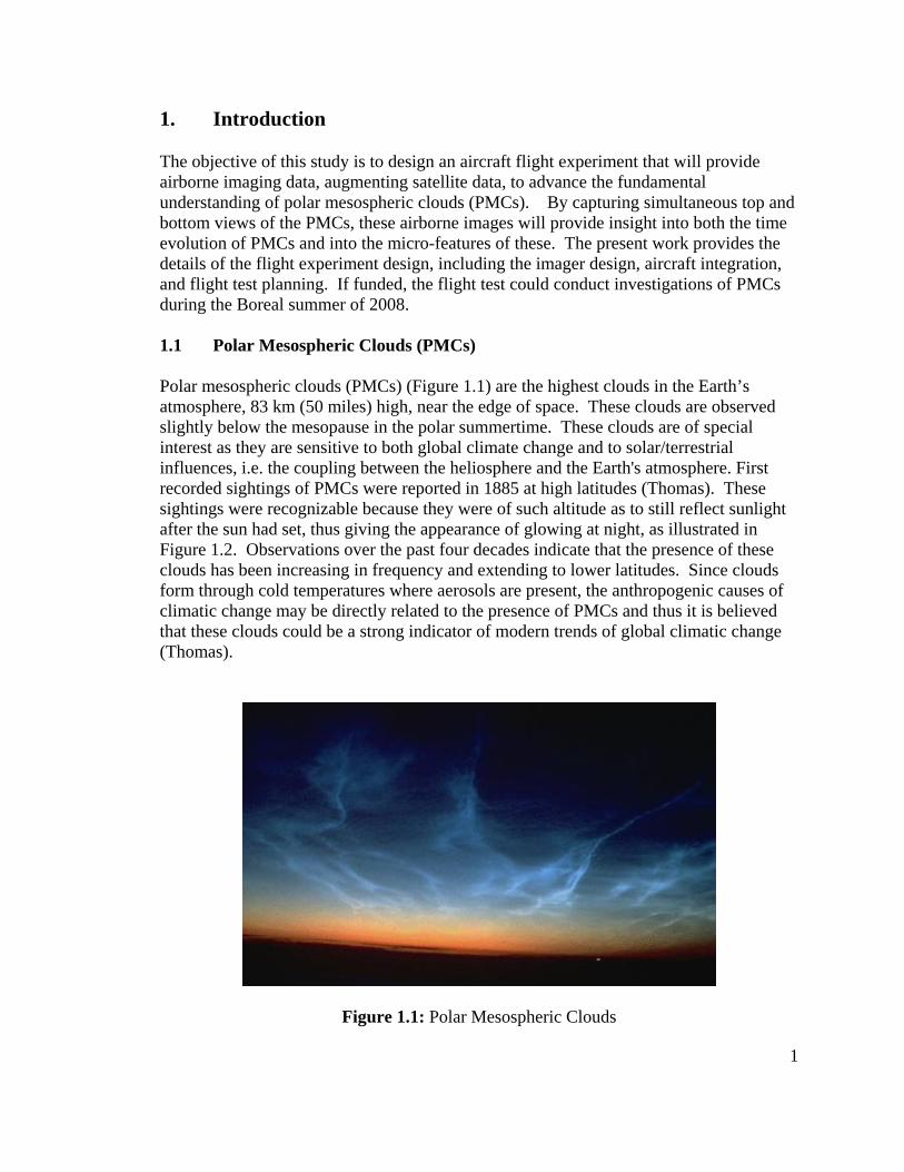
The objective of this study is to design an aircraft flight experiment that will provide airborne imaging data, augmenting satellite data, to advance the fundamental understanding of polar mesospheric clouds (PMCs). By capturing simultaneous top and bottom views of the PMCs, these airborne images will provide insight into both the time evolution of PMCs and into the micro-features of these. The present work provides the details of the flight experiment design, including the imager design, aircraft integration, and flight test planning. If funded, the flight test could conduct investigations of PMCs during the Boreal summer of 2008. 1.1 Polar Mesospheric Clouds (PMCs) Polar mesospheric clouds (PMCs) (Figure 1.1) are the highest clouds in the Earth’s atmosphere, 83 km (50 miles) high, near the edge of space. These clouds are observed slightly below the mesopause in the polar summertime. These clouds are of special interest as they are sensitive to both global climate change and to solar/terrestrial influences, i.e. the coupling between the heliosphere and the Earth's atmosphere. First recorded sightings of PMCs were reported in 1885 at high latitudes (Thomas). These sightings were recognizable because they were of such altitude as to still reflect sunlight after the sun had set, thus giving the appearance of glowing at night, as illustrated in Figure 1.2. Observations over the past four decades indicate that the presence of these clouds has been increasing in frequency and extending to lower latitudes. Since clouds form through cold temperatures where aerosols are present, the anthropogenic causes of climatic change may be directly related to the presence of PMCs and thus it is believed that these clouds could be a strong indicator of modern trends of global climatic change (Thomas).

Figure 1.1: Polar Mesospheric Clouds

2

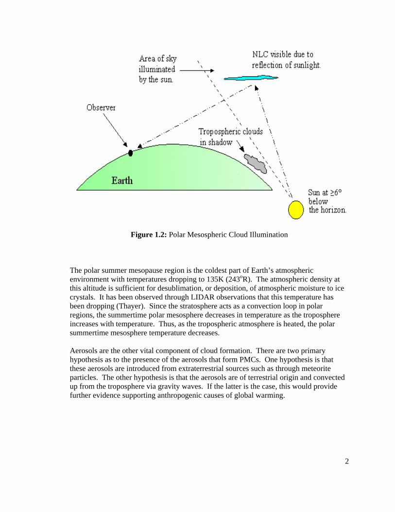
Figure 1.2: Polar Mesospheric Cloud Illumination

The polar summer mesopause region is the coldest part of Earth’s atmospheric environment with temperatures dropping to 135K (243oR). The atmospheric density at this altitude is sufficient for desublimation, or deposition, of atmospheric moisture to ice crystals. It has been observed through LIDAR observations that this temperature has been dropping (Thayer). Since the stratosphere acts as a convection loop in polar regions, the summertime polar mesosphere decreases in temperature as the troposphere increases with temperature. Thus, as the tropospheric atmosphere is heated, the polar summertime mesosphere temperature decreases. Aerosols are the other vital component of cloud formation. There are two primary hypothesis as to the presence of the aerosols that form PMCs. One hypothesis is that these aerosols are introduced from extraterrestrial sources such as through meteorite particles. The other hypothesis is that the aerosols are of terrestrial origin and convected up from the troposphere via gravity waves. If the latter is the case, this would provide further evidence supporting anthropogenic causes of global warming.

3

1.2 The Aeronomy of Ice in the Mesosphere (AIM) Spacecraft Mission

AIM is an approved minisatellite mission within NASA's SMEX (Small Explorer) program designed to provide frequent, low-cost access to space for a variety of missions The AIM mission was approved in May 2004 and is scheduled to launch in March 2007. The objective of AIM is to observe and study PMCs. The results from this mission will provide the basis for study of long-term variability in the mesospheric climate.

The goal of the AIM mission is to study PMCs and to test various hypotheses as to their formation. There are six fundamental questions that the AIM mission seeks to answer.

1. PMC Microphysics: AIM will observe the global morphology of PMC particle size, occurrence frequency and dependence upon H2O and temperature. 2. Gravity Wave Effects: AIM will observe gravity waves to see if they enhance PMC formation by perturbing the required temperature for condensation and nucleation. 3. Temperature Variability: AIM will explore weather dynamical variability controls the length of the cold summer mesopause season, its latitudinal extent and its possible inter-hemispheric asymmetry. 4. Hydrogen Chemistry: AIM will investigate the relative roles of gas phase chemistry, surface chemistry, condensation/sublimation and dynamics in determining the variability of water vapor in the polar mesosphere. 5. PMC Nucleation Environment: AIM will hope to determine weather PMC formations are controlled solely by changes in the frost point or are they driven also by extraterrestrial forcings such as cosmic dust influx or ionization. 6. Long-Term Mesospheric Change: AIM will determine what is needed to establish a physical basis for the study of mesospheric climate change and its relationship to global change.

To attempt to answer the above questions, the AIM spacecraft is to be equipped with three payloads: 1) the Solar Occultation For Ice Experiment (SOFIE), 2) the Cloud Imaging and Particle Size (CIPS) experiment, and 3) the Cosmic Dust Experiment (CDE). SOFIE will analyze the mesosphere at the limb of the Earth. Later, CIPS will analyze this area as the AIM spacecraft flies over this common volume. During this time, the CDE experiment will be sensing for meteorite particulate to see if this flux is contributing to PMC nucleation.

4

1.3 Scientific Objectives

There are two primary scientific objectives to augment the AIM spacecraft research with data taken from an airborne platform:

1. Investigation of the Vertical Structure and Seeding Mechanisms of PMCs Common volume measurements can be obtained by an upward looking imager by using Rayleigh scattering off of the diatomic oxygen and nitrogen molecules in the near ionosphere as a background. By comparing any Mie scattering from these images with Mie scattering of the downward looking Cloud Imaging and Particle Size (CIPS) imager, both upward and downward irradiance profiles may be obtained as well as better understanding of gravity waves. 2. Determination of the Time Evolution of PMCs and their Microstructures An aircraft can track a prominent cloud that is detected by the AIM spacecraft. By focusing a LIDAR instrument on the cloud, a temperature profile may be made throughout the lifespan of the cloud.

5

2. System Concepts and Design 2.1 Requirements An overview of the complete flight imager system is provided in this section. As discussed earlier, there are two objectives of each flight: 1) loiter and image the time evolution of a PMC, and 2) infer vertical structures of PMCs by taking synchronous images with the AIM satellite. The first objective will be met by simply flying a loiter pattern in the vicinity of a PMC and recording images. The direction of the imager will be determined by an approximation of the latitude and longitude of the clouds as provided by the flight researcher. An airborne imager provides the means to meet the aforementioned scientific objectives in ways space borne imagers and ground-based imagers cannot. Due to the nature of their orbits, space based imagers cannot loiter effectively at polar latitudes to study PMC time evolution. Furthermore, an airborne imager would have two distinct advantages over ground-based imagers: 1) They be flown above the majority of the absorbing atmosphere and tropospheric clouds, and 2) an aircraft may position itself at an ideal location for a satellite overpass once for every day of the campaign season. The second objective is a bit more complicated and will be described in detail here. The AIM satellite provides no telemetry describing its orbital elements or position. Tracking of the satellite is reliant upon NORAD Two-Line Element sets (TLEs) (www.sat.dundee.ac.uk ) that are provided in near real-time for every artificial satellite in Earth orbit. For the present flight test, the TLE data will be read into the on-board computer algorithm before each flight. The TLE data includes inclination (degrees), right ascension of ascending node (degrees), eccentricity, argument of perigee (degrees), mean anomaly (degrees), mean motion (revs per day), and the revolution number. From these data, Earth Centered, Earth Fixed (ECEF) data is derived in terms of latitude and longitude. In addition, times are needed when the CIPS camera is projected to take an image. The CIPS camera takes an image every 43 seconds. We know that the period of the satellite will be approximately 96.7 minutes, as derived in Equation 2.1, and this allows for up to three common volume images to be taken.

(2.1) The radius of the AIM orbit is 6978.137km, or a circumference of 43845km. For up to three common volume measurements to be taken, the aircraft imager must be able to achieve a zenith angle of at least 77o. The GPS locations of the common volumes are calculated as follows:

sskm

kmaP 580144.398600

)600137.6378(22 23

33

=+

== πμ

π

6

1) Receive the most recent TLEs from NORAD before flight. 2) Receive a current time of image from AIM mission control at the Laboratory for Atmospheric and Space Physics (LASP), Boulder, CO before flight. Record times of each common volume image to be taken (t1, t2, and t3). The image period of 43 seconds is equivalent to 4.976852 x 10-4 day. 3) Compute the mean anomaly of the AIM satellite at the projected location of the closest common volume image to the aircraft loiter location. Project the mean anomalies of the preceding and the following CIPS images. This process is detailed in Section 2.2. 4) Having three values for mean anomaly of each of three projected images, the GPS locations of the common volumes may be calculated (Xc1, Yc1, Xc2, Yc2, Xc3, Yc3). This process is detailed in Section 2.3.

2.2 Calculating and Projecting the True Anomalies from the Mean Anomalies We are given the following from NORAD TLE sets: argument of perigee, eccentricity, inclination, right ascension, the mean motion (revolutions per day), and the mean anomaly. The semi-major axis is readily derived and from the mean motion and the mean anomalies at other times may be derived. The TLE data provides the instantaneous UTC time and the mean anomaly. From this time, predicted image times will be extrapolated by

sec)43(0 nttt imagen ++= (2.2)

Tn is the predicted image time. T0 is the time listed on the TLE. Timage is the time between T0 and the first image. This value will be received from LASP. Local time will be calculated by adjusting for Local Hour Angle. An Alaska campaign as described in Section Seven will be at UTC+10. A Northern Quebec/Nunavut Campaign will be conducted at UTC+5. Since all orbital parameters except the mean anomaly remain constant for future times, the mean anomaly for each predict is incremented as follows:

( )ta

M Δ=Δ 3

μ (2.3)

where the semimajor axis (a) may be expressed as 2

pa rra

+= . For a 43 second image

period in a circular (e=0) orbit, the change in mean anomaly is:

7

( ) =+

=Δ skmkmskmM 43

)600137.6378(44.398600

3

23

0.046573245 rad = 2.6683988 deg.

True anomalies (ν ) are calculated through the eccentric anomalies (E). First, E2 is calculated from M2.

)sin(* 222 EeEM −= (2.4) Next, the true anomaly is calculated from the eccentric anomaly:

⎟⎠⎞

⎜⎝⎛

+−

=⎟⎠⎞

⎜⎝⎛

2tan

11

2tan ν

eeE (2.5)

2.3 GPS Locations of Common Volumes For the AIM orbit, roughly 135 images will be taken in the time it takes the satellite to make one orbit. The longitude and latitude of each of these image positions are then derived by the true anomalies calculated through the algorithm in the previous section. We are given all six Keplerian orbital elements for all image times between time t0 and time t0+n(43sec) as well as their true anomalies. The following algorithm will convert these orbital elements to Earth Centered, Earth Fixed (ECEF) Longitude and Latitude coordinates for each image: 1) Convert Orbit Elements to ECI: From the orbital elements supplied by the TLE sets, the semiparameter (p) is calculated from the semi-major axis: )1( 2eap −= (2.5) The position and velocity vectors of the satellite in a Perifocal Coordinate System (PQW) are then calculated. A PQW system is oriented where the P-axis points towards perigee and the Q-axis is 90 degrees from the P axis in the direction of satellite motion. The W-axis is normal to the orbit.

⎥⎥⎥⎥⎥⎥

⎦

⎤

⎢⎢⎢⎢⎢⎢

⎣

⎡

+

+

=

0)cos(1

)sin()cos(1

)cos(

υυ

υυ

epe

p

rPQWv ( )

⎥⎥⎥⎥⎥⎥⎥

⎦

⎤

⎢⎢⎢⎢⎢⎢⎢

⎣

⎡

+

−

=

0

)cos(

)sin(

υμ

υμ

ep

p

vPQWv (2.6)

8

A series of coordinate rotations may then be used to transform the satellites position in the PQW coordinate system to its position in a generalized IJK coordinate system. The IJK system expresses the satellite position independent of the satellites perigee and is oriented where the I axis is aligned with the ‘first point of Aires’, a celestial fix. The K axis is aligned with the Earths axis of rotation.

[ ][ ][ ] PQWPQWIJK rPQWIJKrROTiROTROTr vvv

⎥⎦

⎤⎢⎣

⎡=−−Ω−= )(3)(1)(3 ω (2.7a)

[ ][ ][ ] PQWPQWIJK vPQWIJKvROTiROTROTv vvv

⎥⎦

⎤⎢⎣

⎡=−−Ω−= )(3)(1)(3 ω (2.7b)

Expressing the above in terms of the orbital elements, we may write:

⎥⎥⎥

⎦

⎤

⎢⎢⎢

⎣

⎡Ω−Ω+Ω−Ω+Ω

ΩΩ−Ω−Ω−Ω=⎥

⎦

⎤⎢⎣

⎡

)cos()sin()cos()sin()sin()sin()cos()cos()cos()cos()sin()sin()cos()sin()cos()cos()sin(

)sin()sin()cos()cos()sin()sin()cos()cos()sin()sin()cos()cos(

iiiiii

iii

PQWIJK

ωωωωωωωωωω

(2.8)

2) Advance the Time: The Greenwich Sidereal Time (GST) is calculated by recognizing the rotation rate of the earth to be 52921158553.7 −= EEω . Then, )(0 tGSTGST E Δ+= ω (2.9) GST0 is the set angle that exists between the First Point of Aires and the line of zero longitude (Greenwich) 3) Convert ECI to ECEF: Converting from ECI to ECEF simply involves a rotation about the Earths polar axis so that the x-axis is now in alignment with Greenwich rather than Aires:

⎥⎥⎥

⎦

⎤

⎢⎢⎢

⎣

⎡−=⎥⎦

⎤⎢⎣⎡

1000)cos()sin(0)sin()cos(

GSTGST

GSTGST

ECIECEF θθ

θθ (2.10)

Where GSTθ is the Greenwich Sidereal Time (GST). 4) Compute the Latitude and Longitude for this ECEF: The longitude, λ , is calculated by the x and y-components of the ECEF vector defined in step three.

⎟⎟⎠

⎞⎜⎜⎝

⎛= −

x

y

rr1tanλ (2.11)

9

The total distance of the ECEF vector is required to calculate the latitude. By using 222

zyx rrrr ++= , we may solve for the latitude:

⎟⎠⎞

⎜⎝⎛= −

rrz1sinφ (2.12)

5) Increment Time, Compute new True Anomaly: The time is incremented by the CIPS image time of 43s. As per section 2.2, the next mean anomaly is calculated and the true anomaly is derived from this. A predicts table is provided in Table 2.1 and is seeded with orbital data for the Calipso satellite as provided by the NORAD TLE in Figure 2.1 below. Calipso data is only provided as an analogy. To generate the predicts for each day of the campaign, the Mean Anomaly is first advanced to the ascending node (M=0) and the corresponding change in time is added to the satellite time. For each CIPS image

s

daysecendingNodTimePastAssPeriodMt nn 864001*)()(*

360(deg)

⎥⎦⎤

⎢⎣⎡ +=Δ (2.13)

where the period is calculated by taking the inverse of the revs/day (1/14.57123301, or 0.06862837 days, or 5929.5 seconds for Claipso). From this, the semi-major axis is calculated (7080.62km for Calipso).

μ

π3

2 aP = , or 32

2

4πμPa = (2.14)

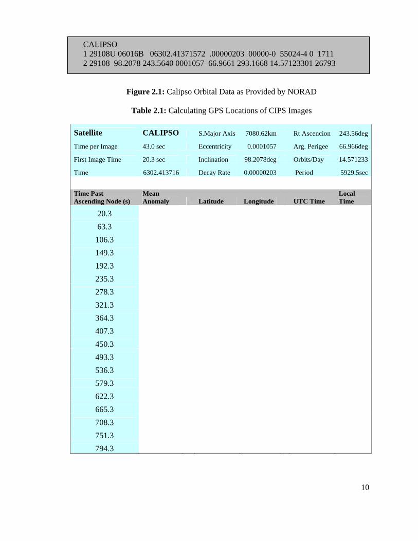
Next, the day fraction is then converted to Universal Coordinated Time (UTC) HH:MM:SS format. Local Time is then adjusted for the Alaskan (UTC+9hrs) or the Eastern Time Zone (UTC+5hrs). Finally, given the Mean Anomalies for each projected image and the five constant orbital elements, the predicted latitude and longitude for each overpass are calculated using the Orbital Elements to ECI and the ECI to ECEF algorithms as presented in Appendix D. From this list of predicts, three filters are applied: 1) the longitude of the common volumes must be within 12 degrees of the airstrip, 2) the latitude must be between 50oN and 70oN, and 3) the time must be within one hour of local midnight. The first filter is to select the closest overpass. The second filter discriminates against any overpasses of latitude where PMCs can not be observed, and the third filter assures that the solar declination may be placed at six degrees below the terminator at a latitude within the limits defined in filter two. Local midnight is calculated by knowing the longitude of the campaign airstrip.

10

Figure 2.1: Calipso Orbital Data as Provided by NORAD

Table 2.1: Calculating GPS Locations of CIPS Images

Satellite CALIPSO S.Major Axis 7080.62km Rt Ascencion 243.56deg

Time per Image 43.0 sec Eccentricity 0.0001057 Arg. Perigee 66.966deg

First Image Time 20.3 sec Inclination 98.2078deg Orbits/Day 14.571233

Time 6302.413716 Decay Rate 0.00000203 Period 5929.5sec

Time Past Ascending Node (s)

Mean Anomaly Latitude Longitude UTC Time

Local Time

20.3

63.3

106.3

149.3

192.3

235.3

278.3

321.3

364.3

407.3

450.3

493.3

536.3

579.3

622.3

665.3

708.3

751.3

794.3

CALIPSO 1 29108U 06016B 06302.41371572 .00000203 00000-0 55024-4 0 1711 2 29108 98.2078 243.5640 0001057 66.9661 293.1668 14.57123301 26793

11

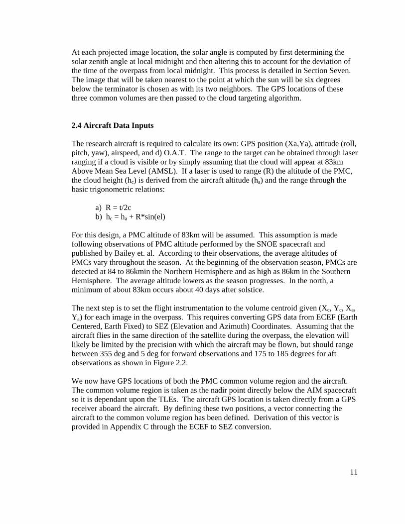
At each projected image location, the solar angle is computed by first determining the solar zenith angle at local midnight and then altering this to account for the deviation of the time of the overpass from local midnight. This process is detailed in Section Seven. The image that will be taken nearest to the point at which the sun will be six degrees below the terminator is chosen as with its two neighbors. The GPS locations of these three common volumes are then passed to the cloud targeting algorithm. 2.4 Aircraft Data Inputs The research aircraft is required to calculate its own: GPS position (Xa,Ya), attitude (roll, pitch, yaw), airspeed, and d) O.A.T. The range to the target can be obtained through laser ranging if a cloud is visible or by simply assuming that the cloud will appear at 83km Above Mean Sea Level (AMSL). If a laser is used to range (R) the altitude of the PMC, the cloud height (hc) is derived from the aircraft altitude (ha) and the range through the basic trigonometric relations: a) R = t/2c b) hc = ha + R*sin(el) For this design, a PMC altitude of 83km will be assumed. This assumption is made following observations of PMC altitude performed by the SNOE spacecraft and published by Bailey et. al. According to their observations, the average altitudes of PMCs vary throughout the season. At the beginning of the observation season, PMCs are detected at 84 to 86kmin the Northern Hemisphere and as high as 86km in the Southern Hemisphere. The average altitude lowers as the season progresses. In the north, a minimum of about 83km occurs about 40 days after solstice. The next step is to set the flight instrumentation to the volume centroid given (Xc, Yc, Xa, Ya) for each image in the overpass. This requires converting GPS data from ECEF (Earth Centered, Earth Fixed) to SEZ (Elevation and Azimuth) Coordinates. Assuming that the aircraft flies in the same direction of the satellite during the overpass, the elevation will likely be limited by the precision with which the aircraft may be flown, but should range between 355 deg and 5 deg for forward observations and 175 to 185 degrees for aft observations as shown in Figure 2.2. We now have GPS locations of both the PMC common volume region and the aircraft. The common volume region is taken as the nadir point directly below the AIM spacecraft so it is dependant upon the TLEs. The aircraft GPS location is taken directly from a GPS receiver aboard the aircraft. By defining these two positions, a vector connecting the aircraft to the common volume region has been defined. Derivation of this vector is provided in Appendix C through the ECEF to SEZ conversion.

12

Figure 2.2: Nominal Imager Coverage for Flight Along-Track AIM Overpass

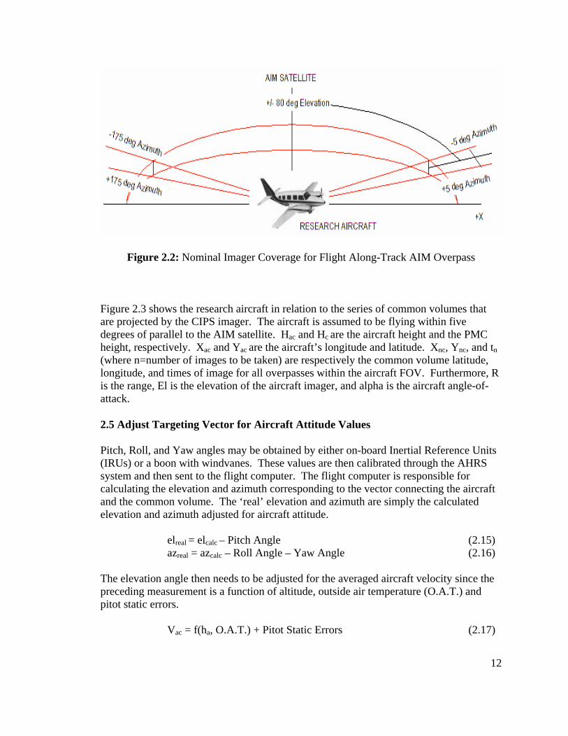
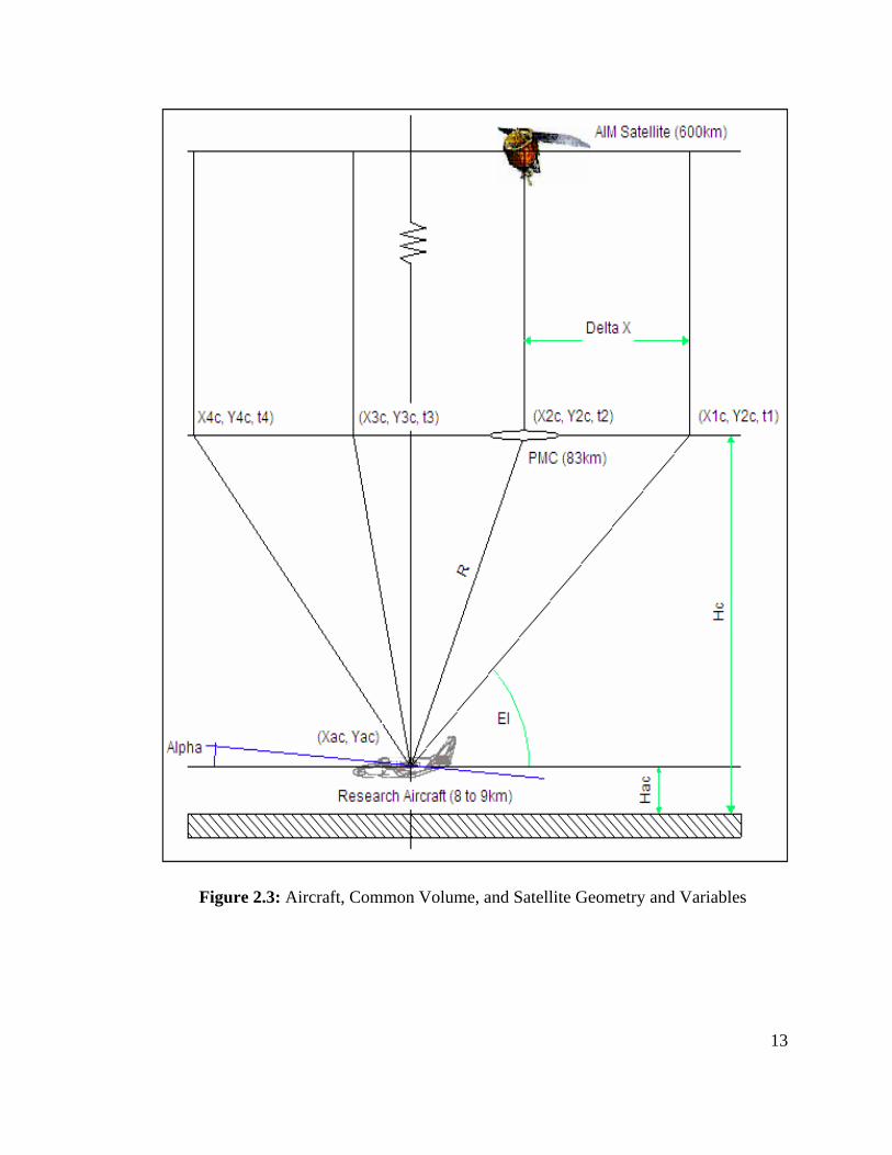
Figure 2.3 shows the research aircraft in relation to the series of common volumes that are projected by the CIPS imager. The aircraft is assumed to be flying within five degrees of parallel to the AIM satellite. Hac and Hc are the aircraft height and the PMC height, respectively. Xac and Yac are the aircraft’s longitude and latitude. Xnc, Ync, and tn (where n=number of images to be taken) are respectively the common volume latitude, longitude, and times of image for all overpasses within the aircraft FOV. Furthermore, R is the range, El is the elevation of the aircraft imager, and alpha is the aircraft angle-of-attack.

2.5 Adjust Targeting Vector for Aircraft Attitude Values

Pitch, Roll, and Yaw angles may be obtained by either on-board Inertial Reference Units (IRUs) or a boon with windvanes. These values are then calibrated through the AHRS system and then sent to the flight computer. The flight computer is responsible for calculating the elevation and azimuth corresponding to the vector connecting the aircraft and the common volume. The ‘real’ elevation and azimuth are simply the calculated elevation and azimuth adjusted for aircraft attitude.

elreal = elcalc – Pitch Angle (2.15) azreal = azcalc – Roll Angle – Yaw Angle (2.16)

The elevation angle then needs to be adjusted for the averaged aircraft velocity since the preceding measurement is a function of altitude, outside air temperature (O.A.T.) and pitot static errors.

Vac = f(ha, O.A.T.) + Pitot Static Errors (2.17)

13

Figure 2.3: Aircraft, Common Volume, and Satellite Geometry and Variables

14

2.6 Imaging and Data Collection Imaging: Since the maximum solar zenith angle is projected not to exceed 77o, the Chapman Function will not be used and solar irradiance upon each CCD pixel may be approximated by the simpler )cos(1 θ relation. Thus, the intensity of each CCD pixel is multiplied first by )cos(1 θ where θ is the sensor elevation angle and again by

)cos(1 β where β is the sensor azimuth angle. This method scales for intensity each image so that images may be compared independent of the angle through which the image is taken, permitting better comparison with CIPS images. The received signal must also account for the asymmetry parameter (g) which is a function of the Mie scattering profile of the particle sizes and will vary between -1 and 1, with a value of -1 corresponding to 100% backscatter, 0 corresponding to isotropic backscatter, and 1 corresponding to full forward scatter. For ice expected at PMC altitudes, we can initially assume this parameter to be 0.8, but results from the AIM satellite will help to refine this assumption. Data Collection: A 400Gb external hard disk will be used to store images through the flight computer. Data to be analyzed after flight operations are complete. The following data will be stored during each mission include all payload images, lens setting number, time stamp, and cloud centroids (to verify CIPS data). 2.7 After the Overpass The research aircraft is not capable of the flight speeds required to intercept the AIM satellite on the next overpass at PMC observation latitudes. Thus, after the overpass the aircraft will either remain to image the time evolution of the PMC, if one is observed, or return to the airstrip if one has not been observed. After returning to the airstrip, data is downloaded and stored while overpass times and common volume predictions are generated for the next overpass to occur near local midnight the following day. Calibration factors for the altitude height and O.A.T. are computed as well.

15

3. Imager Design The imager is designed to be a self-contained instrument interfacing with the aircraft’s flight computer and power supply and contains a Charge Coupled Device (CCD), an adjustable lens/filter wheel containing four lens/filter combinations, and a servo-controlled active platform that will regulate the elevation and the roll of the active lens. The system is attached to an aluminum truss mounted on the rear cargo door of the aircraft. When extended, the imager is designed to track a specific area of cloud and produce digital images through one of four lens/filter combinations. The imager will 1) produce images at full-sky, wide-view, and narrow-view field-of-view (FOV), 2) produce a filtered image symmetric about a central wavelength of 350nm, and 3) track a common volume through a range of +/- 80 degrees of elevation and +/- 5 degrees of roll. For common volume measurements, it is advantageous to use the same type of CCD as is aboard the AIM spacecraft. The airborne imager to be used will be derived from the CCD that was used on the CIPS engineering model and is based around an Atmel Full Field CCD (TH7899M) with a resolution of 2048 x 2048 pixels. The pixel area intrinsic to this CCD is 0.0014cm2 (0.00022in2). In front of the CCD, four filters are mounted in a wheel, each attached to its respective lens. These selections will permit both focused and wide-field observations as well as observations within different wavelength bandpasses. The lens/filter wheel is controlled by a stepper motor so that the optical configuration may be changed between integration times during flight. 3.1 Signal Definition

The irradiance at the detector may be calculated from knowledge of the radiance, Ftgt, focal length, FL, the area of the detector, Adet, and the telescope area, Atel. Radiance may be considered a product of the wavelength integrated solar radiance multiplied by the albedo, )(aAlbedoFF suntgt ⋅= .

2det

detL

teltgt

F

AAFF = (3.1)

If we substitute the preceding expression for Ftgt and express Fsun as an integral over the wavelength, we get an equation for the total photon rate, Ptotal, at the detector.

∫Δ

⋅⋅⋅

=λ

λλ dTFF

AAaP sun

L

teltotal )(2

det (3.2)

Since most commercial optical lens systems are classified by an ‘f-number’ (F#), which is a ratio of the lens diameter over the focal length, we may write:

⎟⎠⎞

⎜⎝⎛== 22

2

2 #1

44 FFD

FA

LL

tel ππ (3.3)

16

In a CCD, each pixel may be modeled as an independent detector, so detAApixel = . Combining this and equation 3.3 into equation 3.2, we get:

∫Δ

⋅==λ

λλπ

dTFF

aAPF sun

pixeltotal )(

)#(4 2(det)det (3.4)

where the integral is the weighted response of the system. The interference filter determines this bypass. We open up the bandpass until we get a nominal signal. Since photon arrival may be considered a random process, we may use a Poisson statistical process. This is possible for any event where the probability is small and proportional to time. Thus, the rate of occurrence is Poisson distributed, though this distribution approaches a Gaussian shape when the event number exceeds 100. Thus, the number of photon events seen by the detector is a product of the arrival rate of photons at the detector, Pdet, the conversion efficiency of the detector in converting the photons to electrons, Qe, and the integration time, tint, and we may express the signal as intdet tQPS e= 3.2 Defining the Noise The noise seen by the CCD comes from several sources: 1) the random noise, Nrnd, associated with the signal, 2) the thermionic noise, Nt, 3) the read noise, Nr, and 4) the airglow, Nair. We sum these to get an expression for the total noise:

airrtrnd NNNNN +++= (3.5)

where intdet tQPN er = , since the standard deviation of a randomly occurring event is

expressed as ∑=

=n

i

i

Nd

1

22σ . (3.6)

The read noise is taken initially as the value of 35 that was obtained through testing of the CIPS CCD (McClintock). By cooling the CCD in a manner similar to the CIPS CCD, the thermionic noise may be effectively neglected. Furthermore, by analyzing the airglow spectra shown in Appendix A, we will neglect airglow noise for all observations between 300 and 700nm, though at several isolated wavelengths, this noise source must be considered. Broadfoot & Kendall (www.eso.org) give the spectrum of the airglow from 300 nm to 1 μm based on photoelectric observations at Kitt Peak near zenith within 30o of the galactic pole. The spectral resolution is 50nm and the scan step four times smaller.

These data were obtained from the Space Shuttle at an altitude of 358 km on December 5, 1990. Two spectra are shown, of which the upper one was taken closer to the dusk terminator. It therefore also shows OII 834 and HeI 584 (in second order), which are features belonging to the dayglow.

17

3.3 Photon Count per Pixel Relationship Derivation We choose a silicon CCD because our wavelength range spans parts of the visible and UV spectrum. Assume Qe = 0.3, wavelength dependant. At micron1⟩λ , silicon becomes transparent. At nm300⟨λ , photons get absorbed too soon. For a first approximation, we will choose to design the sensor to give a signal-to-noise ration (SNR) of 50. Combining the signal noise and the read noise in quadrature, we may write:

50)( int

2det

intdet =+

==tRQP

tQPnoisesignalSNR

reade

e (3.7)

2

intdetintdet 50 readee RtQPtQP +=

We set the integration time, tint = 1sec and Qe = 0.3.

readRPP 250075009.0 det2

det +=

Thus, solving in quadrature for a read noise of 35, Pdet = 11335 photon events. 3.4 Wavelength Integrated Solar Irradiance Typical market CCDs have pixel areas on the order of 7-25 microns2. For CIPS,

2)0036.0( cmApix = with an image intensifier and 2)0014.0( cmApix = without an image intensifier. CIPS operates at 265nm central wavelength with a bandpass of approximately nm10± .

⎟⎟⎠

⎞⎜⎜⎝

⎛ ⋅⋅⋅

=photons

strscmrayleighsstrcm

photonsP )(104

sec11335

2

62detπ

= 142.44mR

From this result, we now may go ‘back up the chain’ to see how big ∫Δ

⋅λ

λλ dTFsun )(

needs to be. The signal, S, is then equal to the number of photon events, N:

11335 photon events= intdet tQP e ⋅⋅ = ∫Δ

⋅⋅⋅⋅⋅λ

λλπ

dTFtaQFA

sunepix )(

)#(4 int2 (3.8)

where the transmission coefficient is a function of wavelength and is approximated as the summation of the lens transmissivity and the filter transmissivity:

18

filterlenstrans ttt += (3.9)

We approximate F#=4.0 and nmc 350=λ . We assume initially that the filter sensitivity models a square function and has a transmittance of 30%. The albedo may be modeled by assuming that the function drops off as the Raleigh function with wavelength. Higher albedos are recorded at shorter wavelengths because of the larger radiative absorption cross-section. Thus, at 350nm, an observed cloud will only be 0.329 times as bright as a cloud at 265nm.

The CIPS camera was built to observe at 265nm wavelengths. At these wavelengths, a really bright PMC will have an albedo of about 10-4, but most PMCs are much fainter, having an albedo as low as 10-5. Thus, if it is known that the CIPS CCD may observe albedos of 10-5 at 265nm wavelengths, then this result may be extrapolated through the

Rayleigh relationship to 350nm observations by substituting a= 45 )350265)(10(

nmnm− into

Equation 3.8, yielding

11335= ∫Δ

−

λ

λπ dFnmnmcm

sun)3.0()350265)(10)(3.0(

)0.4(4)0014.0( 45

2

Solving for the wavelength-integrated solar irradiance gives us

∫Δλ

λdFsun = 5.5766 x 1014 (3.10)

A cloud is thus only about 1/3 as bright at 350nm wavelengths as it is at 265nm, justifying the choice of selecting blue-shifted filters in the visible range. They act as a compromise between using a silicon CCD and maintaining a good albedo. Higher albedo exists at a shorter wavelength because there is a larger relative absorption cross section. 3.5 Bandpass for the Filtered Lens

The fourth imager will be filtered about 350nm. The bandpass must, however, be wide enough so that the chosen SNR is obtained. We compute the bandpass from the derivation of the previous section:

∫Δλ

λdFsun = 5.5766 x 1014 ph/cm2*s*nm .

The bandpass may be computed numerically. From a central wavelength, the solar irradiance is calculated. The bandpass is then expanded to both higher and lower wavelengths by 1nm intervals and integrated until the nominal value is reached. An Interactive Data Language (IDL) code is provided in Appendix D. We will assume a filter to exist that models this bandpass perfectly as a square wave.

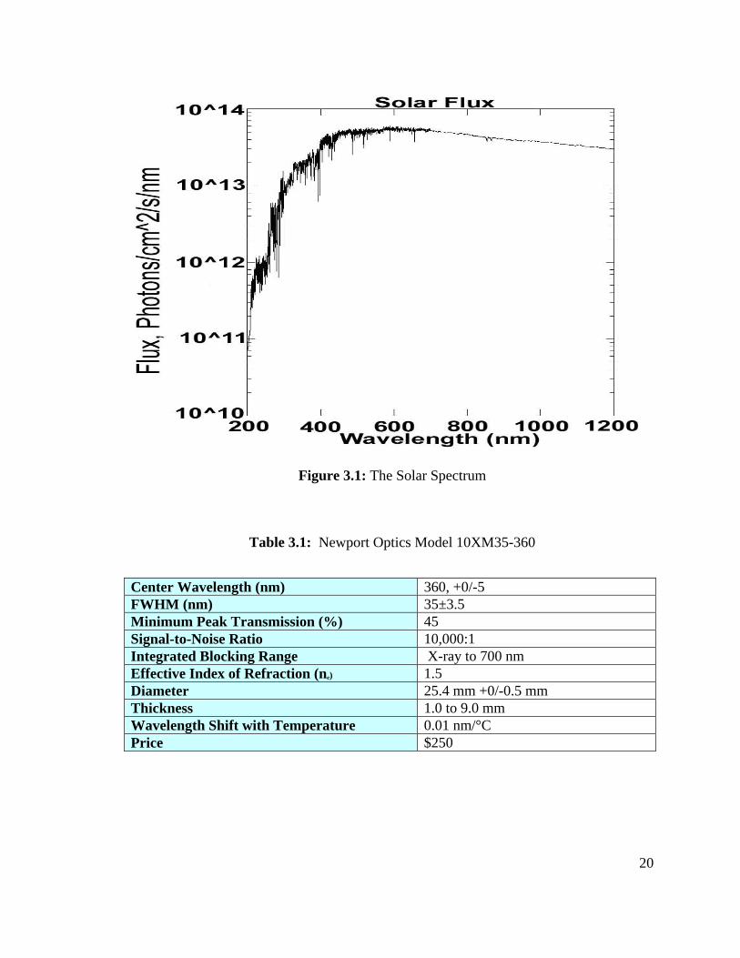
19

Filters let us image the cloud at different wavelengths, thus telling us more about their composition. Filters may prove beneficial to the SNR as well, since albedo value diminishes rapidly as higher wavelength values are reached, assuming this value is governed by the Rayleigh function. Figure 3.1 was plotted from a database using an IDL routine. It shows the solar irradiance received at the earth’s atmosphere as a function of wavelength and approximates a blackbody spectrum with notable absorption lines. For the conceptual design, an approximation of the solar flux was made for the region of the computed bandpass distributed symmetrically around a 350nm central wavelength. Flux values between 300nm and 400nm are estimated to be 2.0 x 1013 photons/(cm*s*nm). The Newport Optics Model 10XM35-360 filter fits these requirements well (Table 3.1). 3.6 CCD Design Choices Choosing the Integration Time: The integration time is determined by the desired resolution of the image. For full resolution (2048 x 2048) of the filtered lens, the integration time is about 3.2 seconds. The integration time to achieve a SNR of 50 may be found by revisiting the relationship originally used while assuming an integration time of one second and where Pdet = 11335 photon events:

intintdetintdet 5050 tRtQPtQP readee += In solving for tint we obtain an integration time of 3.12 seconds. This time may be increased to achieve a better SNR. For PMC observations, this integration time will be considered sufficient. The CCD will perform the following actions for each image taken:

1) Close the shutter 2) Read three times to clear CCD of any latent image. 3) Enable the shutter for a specified integration time 4) Close the shutter 5) Read out the CCD

These additional actions add about 20% more time to the CCD integration time, so we may estimate that each image would require 4 seconds to integrate and read out.

20

Figure 3.1: The Solar Spectrum

Table 3.1: Newport Optics Model 10XM35-360

Center Wavelength (nm) 360, +0/-5 FWHM (nm) 35±3.5 Minimum Peak Transmission (%) 45 Signal-to-Noise Ratio 10,000:1 Integrated Blocking Range X-ray to 700 nm Effective Index of Refraction (ne) 1.5 Diameter 25.4 mm +0/-0.5 mm Thickness 1.0 to 9.0 mm Wavelength Shift with Temperature 0.01 nm/°C Price $250

21

Choosing the Resolution: Signal may be increased by each of four different techniques: 1) increase the integration time, 2) increase the binning of pixels, 3) use a wider spectrum, and 4) increase detector cooling. Since space is not a driving requirement as it is on a spacecraft, we can assume that the CCD may be cooled so that thermionic detector noise is negligible. Furthermore, by using a binning technique, resolution may be substituted for integration time. The CIPS camera is not a high spatial resolution device. The resolution of the CIPS CCD passed to the ground is only 360 x 180 pixels. One advantage of simultaneous airborne imaging is that fine detail of PMCs may be recorded by using a higher resolution imager. Care must be taken that the resolution is not so fine as to make it difficult to geolocate the fine airborne images with the wider and coarser spacecraft images. To deal with this issue, two lenses are chosen. The first will be a wide angle lens and the second lens will produce higher resolution. The specific resolutions will be derived in Section 3.7. Choosing the Central Wavelengths: Four lens / filter combinations will be used. The first will be an unfiltered wide angle lens which is analogous to the CIPS camera. The second will be an unfiltered high-resolution lens. The third will be a fisheye ‘acquisition’ lens and forth will be filtered wide angle lenses centered about 350nm. This wavelength was chosen to fill in the lower wavelength end of the visible spectrum where the albedo of the clouds will still be strong. The fields of view of each of these lenses will be derived in Section 3.7. 3.7 Field of View (FOV) Determination

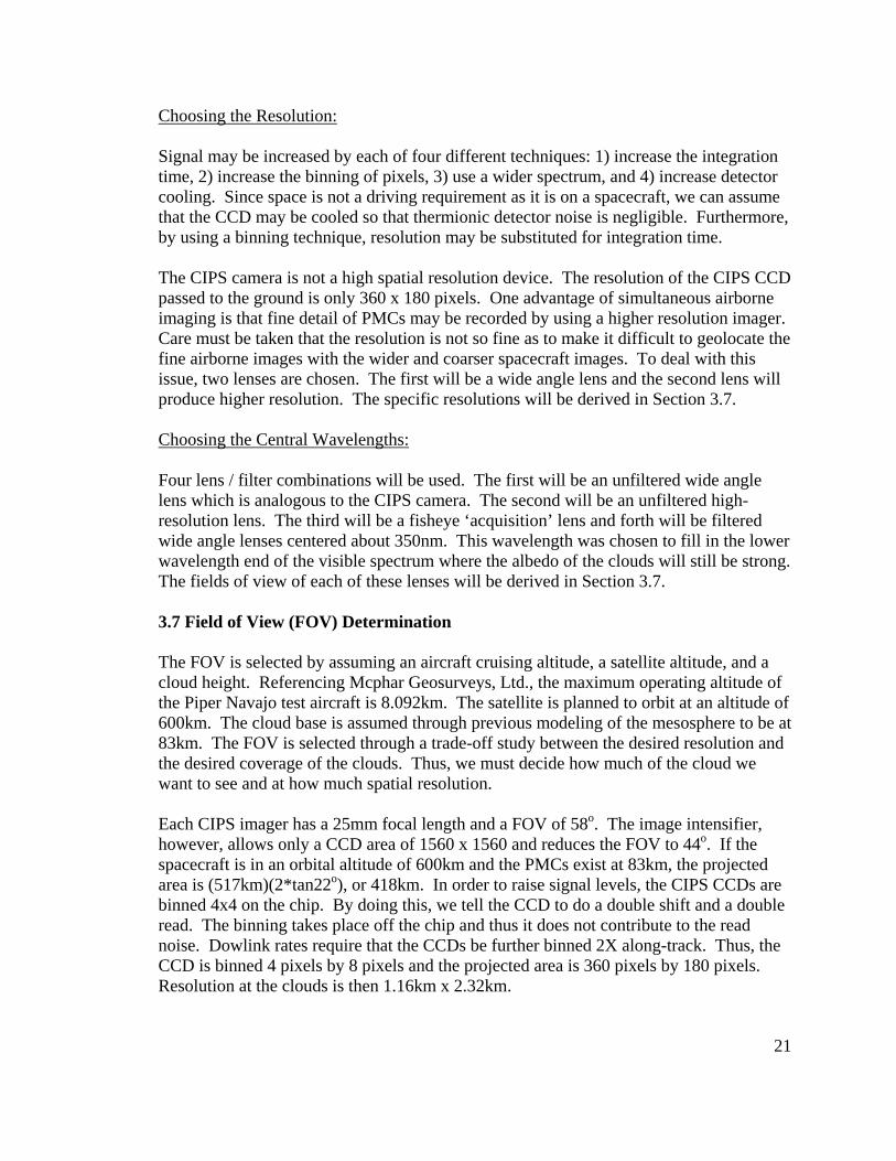
The FOV is selected by assuming an aircraft cruising altitude, a satellite altitude, and a cloud height. Referencing Mcphar Geosurveys, Ltd., the maximum operating altitude of the Piper Navajo test aircraft is 8.092km. The satellite is planned to orbit at an altitude of 600km. The cloud base is assumed through previous modeling of the mesosphere to be at 83km. The FOV is selected through a trade-off study between the desired resolution and the desired coverage of the clouds. Thus, we must decide how much of the cloud we want to see and at how much spatial resolution. Each CIPS imager has a 25mm focal length and a FOV of 58o. The image intensifier, however, allows only a CCD area of 1560 x 1560 and reduces the FOV to 44o. If the spacecraft is in an orbital altitude of 600km and the PMCs exist at 83km, the projected area is (517km)(2*tan22o), or 418km. In order to raise signal levels, the CIPS CCDs are binned 4x4 on the chip. By doing this, we tell the CCD to do a double shift and a double read. The binning takes place off the chip and thus it does not contribute to the read noise. Dowlink rates require that the CCDs be further binned 2X along-track. Thus, the CCD is binned 4 pixels by 8 pixels and the projected area is 360 pixels by 180 pixels. Resolution at the clouds is then 1.16km x 2.32km.

22

Two lenses will be chosen here. The first will be a fisheye lens similar to the one used on CIPS. The optical system on CIPS unrestricted by the image intensifier is 58o. If the aircraft is to fly at 8km altitude, the difference between the aircraft altitude and the cloud altitude is 75km. The projected area is (75km)(2*tan29o) square, or 83km square. This yields a resolution of 40 x 40 meters. The second lens choice would be to produce a high resolution. 10m x 10m will be considered high. Thus,

kmkm

75*201.0*2048tan2 1−=θ =15.54o for High Resolution (10mx10m) Imaging,

and

=θ 58o for Wide Angle (40m x 40m) Imaging. The CCD area will be set at 0.02867m x 0.02867m, which is a standard size in the industry and the one chosen for ATMELs TH7899M CCD. To achieve a 58 degree FOV, a short focal length is desirable. The CIPS optical system employs a ‘telecentric lens’ and makes a good analogy, so we may set the focal length at 0.025m. The FOV geometry is presented in Figure 3.2. We see here that the FOV of the aircraft can, at best, image only a small percentage of the image obtained by the CIPS imager. 3.8 Time Delayed Integration (TDI) Time Delayed Integration (TDI) is a method of scanning in which a frame transfer device produces a continuous video image of a moving object by means of a stack of linear arrays aligned with and synchronized to the movement of the object to be imaged in such a way that, as the image moves from one line to the next, the stored charge moves along with it, providing higher resolution at lower light levels than is possible with a line-scan camera. TDI is a somewhat similar means of acquiring a continuous two dimensional image using an area array CCD sensor. If the row by row transfer of charge in the photosites proceeds at a rate equal to and in the same direction as the apparent motion of the subject being imaged, accumulation of charge integrates during the entire time required for the row of charge to move from the top of the sensor to the serial register (or to the storage area of the device, in the case of a frame transfer CCD). This integration time provides an increase in sensitivity over the line array CCD sensor proportional to the number of rows of photosites of the area array sensor. Like the two dimensional image acquired using a line array sensor, the TDI image has a maximum width in pixels equal to the number of photosites in a row of the sensor and a length limited only by the maximum storage capacity of the system collecting the data.

23

Figure 3.2: Lens Field of View

24

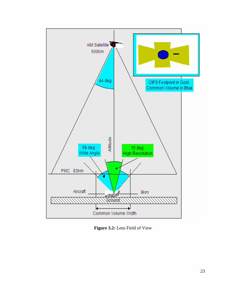
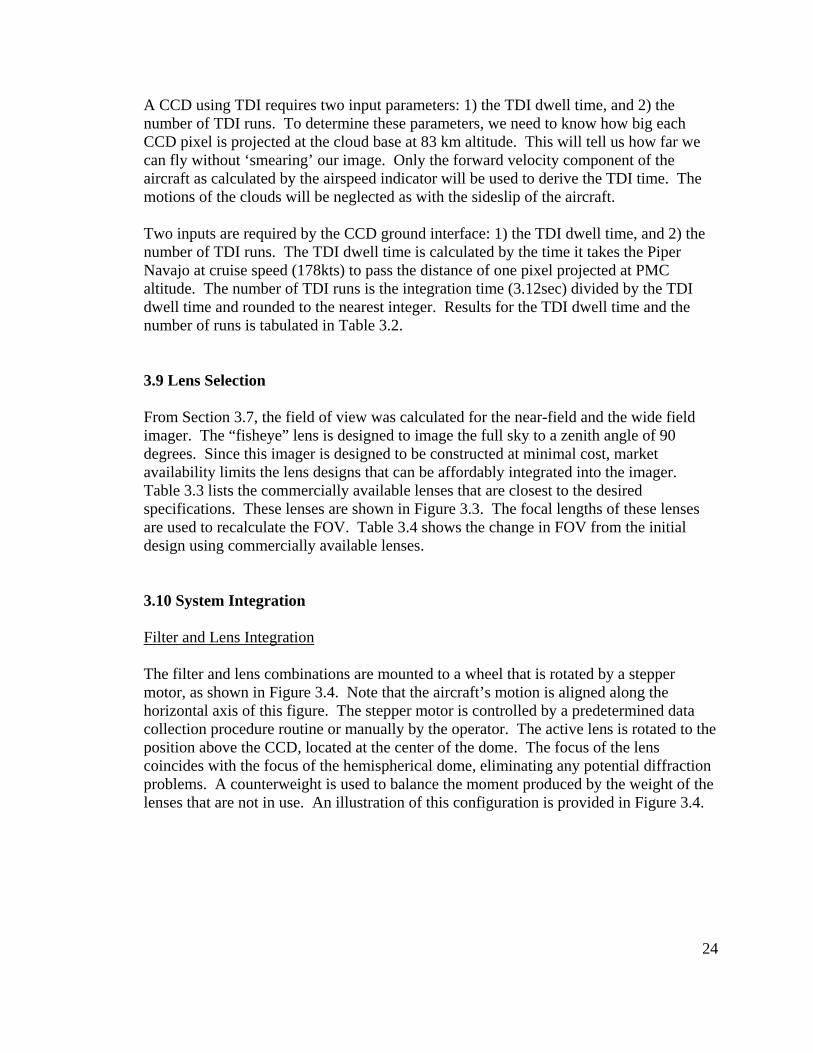
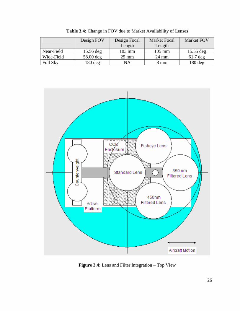
A CCD using TDI requires two input parameters: 1) the TDI dwell time, and 2) the number of TDI runs. To determine these parameters, we need to know how big each CCD pixel is projected at the cloud base at 83 km altitude. This will tell us how far we can fly without ‘smearing’ our image. Only the forward velocity component of the aircraft as calculated by the airspeed indicator will be used to derive the TDI time. The motions of the clouds will be neglected as with the sideslip of the aircraft. Two inputs are required by the CCD ground interface: 1) the TDI dwell time, and 2) the number of TDI runs. The TDI dwell time is calculated by the time it takes the Piper Navajo at cruise speed (178kts) to pass the distance of one pixel projected at PMC altitude. The number of TDI runs is the integration time (3.12sec) divided by the TDI dwell time and rounded to the nearest integer. Results for the TDI dwell time and the number of runs is tabulated in Table 3.2. 3.9 Lens Selection From Section 3.7, the field of view was calculated for the near-field and the wide field imager. The “fisheye” lens is designed to image the full sky to a zenith angle of 90 degrees. Since this imager is designed to be constructed at minimal cost, market availability limits the lens designs that can be affordably integrated into the imager. Table 3.3 lists the commercially available lenses that are closest to the desired specifications. These lenses are shown in Figure 3.3. The focal lengths of these lenses are used to recalculate the FOV. Table 3.4 shows the change in FOV from the initial design using commercially available lenses. 3.10 System Integration Filter and Lens Integration The filter and lens combinations are mounted to a wheel that is rotated by a stepper motor, as shown in Figure 3.4. Note that the aircraft’s motion is aligned along the horizontal axis of this figure. The stepper motor is controlled by a predetermined data collection procedure routine or manually by the operator. The active lens is rotated to the position above the CCD, located at the center of the dome. The focus of the lens coincides with the focus of the hemispherical dome, eliminating any potential diffraction problems. A counterweight is used to balance the moment produced by the weight of the lenses that are not in use. An illustration of this configuration is provided in Figure 3.4.

25

Table 3.2: TDI Dwell Time and Number of Runs Aircraft: Lens FOV Resolution TDI Dwell Time Number of TDI Runs

15.54 degrees 10 meters 0.1091sec 29 58 degrees 40 meters 0.4364sec 7 AIM Satellite: Lens FOV Resolution TDI Dwell Time Number of TDI Runs

44 degrees 1200 meters 0.4063 sec 32

Table 3.3: Lens Parameter Comparison

Field of View 15.56 degree 58.00 degree Full Sky

Product Name Sigma Sigma EX Macro Sigma EX DG Mount Minolta Minolta Nikon AF-D

Focal Length 24 mm 105mm 8mm Focus Type Autofocus Autofocus Autofocus

Camera Format Digital SLR Digital SLR Digital SLR Max Aperture f/2.8 f/2.8 f/4

Filter Size 52 mm 58 mm N/A Diameter 2.6 in 2.9 in 2.9 in Length 1.8 in 3.8 in 2.5 in

a) b) c)

Figure 3.3: Three Lens Choices a) 15.56o FOV, b) 58.00o FOV, c) Full Sky FOV

26

Table 3.4: Change in FOV due to Market Availability of Lenses

Figure 3.4: Lens and Filter Integration – Top View

Design FOV Design Focal Length

Market Focal Length

Market FOV

Near-Field 15.56 deg 103 mm 105 mm 15.55 deg Wide-Field 58.00 deg 25 mm 24 mm 61.7 deg Full Sky 180 deg NA 8 mm 180 deg

27

Active Platform

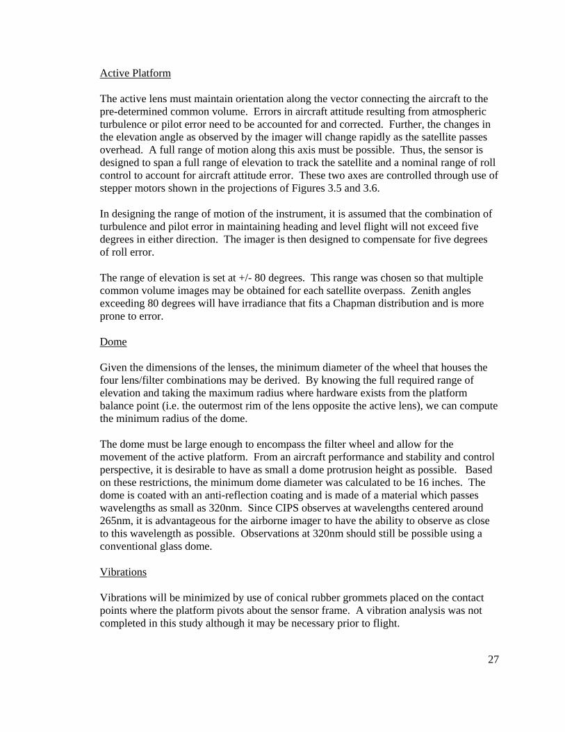
The active lens must maintain orientation along the vector connecting the aircraft to the pre-determined common volume. Errors in aircraft attitude resulting from atmospheric turbulence or pilot error need to be accounted for and corrected. Further, the changes in the elevation angle as observed by the imager will change rapidly as the satellite passes overhead. A full range of motion along this axis must be possible. Thus, the sensor is designed to span a full range of elevation to track the satellite and a nominal range of roll control to account for aircraft attitude error. These two axes are controlled through use of stepper motors shown in the projections of Figures 3.5 and 3.6.

In designing the range of motion of the instrument, it is assumed that the combination of turbulence and pilot error in maintaining heading and level flight will not exceed five degrees in either direction. The imager is then designed to compensate for five degrees of roll error.

The range of elevation is set at +/- 80 degrees. This range was chosen so that multiple common volume images may be obtained for each satellite overpass. Zenith angles exceeding 80 degrees will have irradiance that fits a Chapman distribution and is more prone to error.

Dome

Given the dimensions of the lenses, the minimum diameter of the wheel that houses the four lens/filter combinations may be derived. By knowing the full required range of elevation and taking the maximum radius where hardware exists from the platform balance point (i.e. the outermost rim of the lens opposite the active lens), we can compute the minimum radius of the dome.

The dome must be large enough to encompass the filter wheel and allow for the movement of the active platform. From an aircraft performance and stability and control perspective, it is desirable to have as small a dome protrusion height as possible. Based on these restrictions, the minimum dome diameter was calculated to be 16 inches. The dome is coated with an anti-reflection coating and is made of a material which passes wavelengths as small as 320nm. Since CIPS observes at wavelengths centered around 265nm, it is advantageous for the airborne imager to have the ability to observe as close to this wavelength as possible. Observations at 320nm should still be possible using a conventional glass dome.

Vibrations

Vibrations will be minimized by use of conical rubber grommets placed on the contact points where the platform pivots about the sensor frame. A vibration analysis was not completed in this study although it may be necessary prior to flight.

28

Figure 3.5: Lens and Filter Integration – Side View

Figure 3.6: Lens and Filter Integration – Front View

29

4. Instrument Integration onto an Airborne Platform

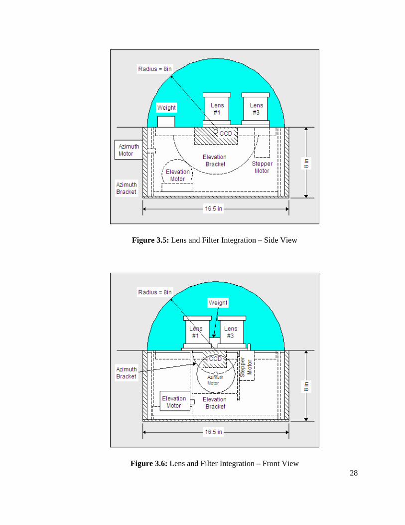
4.1 System Components The aircraft integration system overview is shown in Figure 4.1. The major systems components include the flight computer, flight instrumentation computer (FIC). The Advanced Radar Processing System (ARPS) system provides pitot-static information such as airspeed and altitude while the Altitude Heading Reference System (AHRS) system provides information from the inertial reference unit such as roll, pitch, and yaw angles. This real-time data is combined with inputs from the flight engineer as well as the real-time geospatial position provided by a GPS receiver. The flight computer receives real-time flight data from the AHRS and ARPS that is processed by the FIC.

The flight computer processes the input data using the algorithm that is presented in Section Two. The flight computer output data is sent to the CCD ground interface, the stepper motor, and the elevation and azimuth motors within the instrument platform. Data received by the CCD imager is then sent back to the flight computer to be processed and stored along with the GPS position, the image time, and the lens and filter tags.

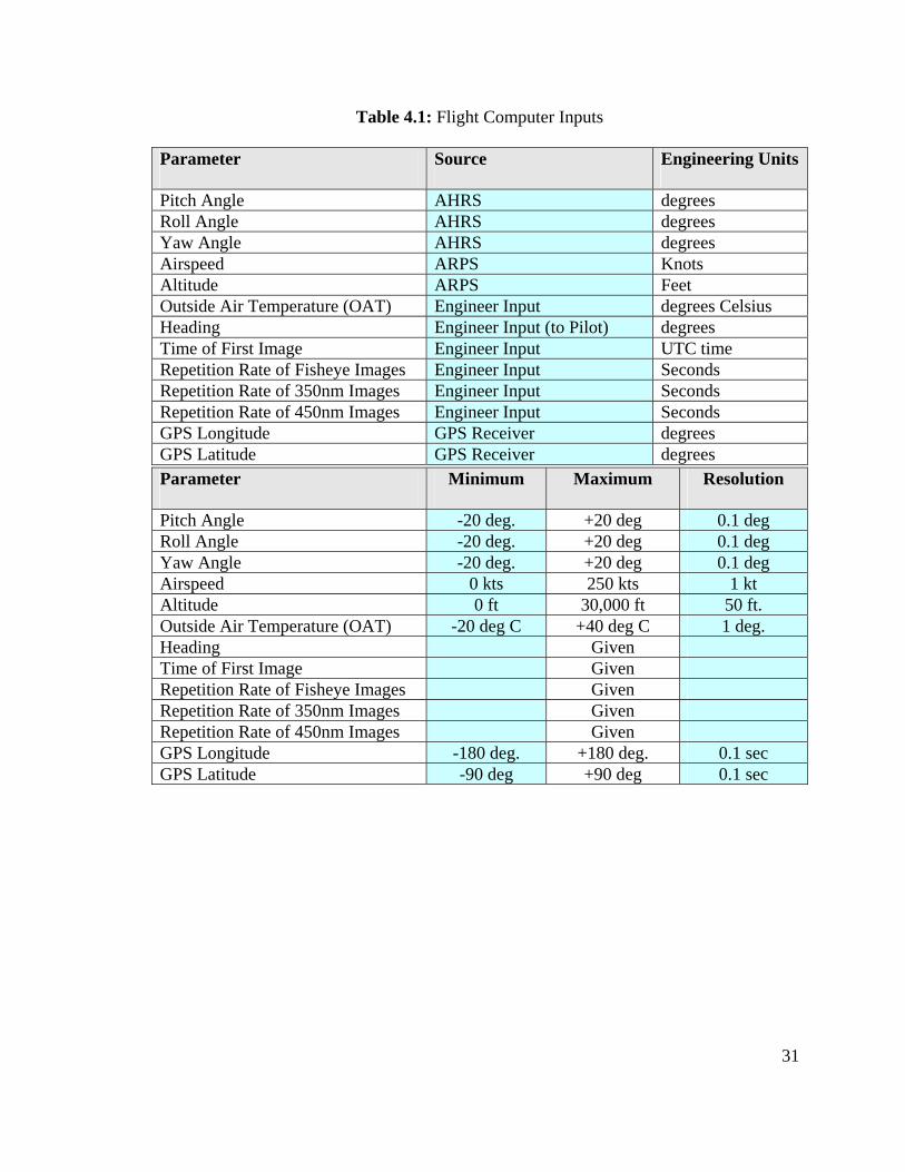
4.2 Flight Computer Inputs

Table 4.1 lists the inputs received by the flight computer from both automated and manual sources. The parameter limits are set by the aircraft’s performance limits. The parameter resolution is set by the nominal precision desired.

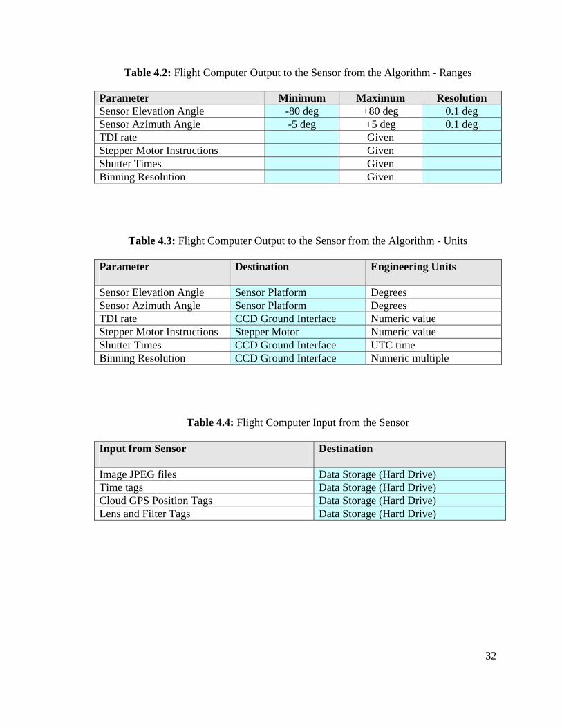
4.3 Flight Computer Algorithm and Outputs

Table 4.2 lists the outputs produced by the flight computer and sent to the imager components. The sensor elevation angle range is set by the imager distortion limits. The sensor azimuth angle range is set by the anticipated accuracy of the pilot to maintain the designated heading with no roll. As before, the parameter resolution is set by the nominal precision desired. The final data inputs to the flight computer received from the sensor are given in Table 4.3 and the flight computer input from the sensor is given in Table 4.4. The data is archived on a 400 GB external hard drive.

30

Figure 4.1: System Overview

31

Table 4.1: Flight Computer Inputs

Parameter Source Engineering Units

Pitch Angle AHRS degrees Roll Angle AHRS degrees Yaw Angle AHRS degrees Airspeed ARPS Knots Altitude ARPS Feet Outside Air Temperature (OAT) Engineer Input degrees Celsius Heading Engineer Input (to Pilot) degrees Time of First Image Engineer Input UTC time Repetition Rate of Fisheye Images Engineer Input Seconds Repetition Rate of 350nm Images Engineer Input Seconds Repetition Rate of 450nm Images Engineer Input Seconds GPS Longitude GPS Receiver degrees GPS Latitude GPS Receiver degrees

Parameter Minimum Maximum Resolution

Pitch Angle -20 deg. +20 deg 0.1 deg Roll Angle -20 deg. +20 deg 0.1 deg Yaw Angle -20 deg. +20 deg 0.1 deg Airspeed 0 kts 250 kts 1 kt Altitude 0 ft 30,000 ft 50 ft. Outside Air Temperature (OAT) -20 deg C +40 deg C 1 deg. Heading Given Time of First Image Given Repetition Rate of Fisheye Images Given Repetition Rate of 350nm Images Given Repetition Rate of 450nm Images Given GPS Longitude -180 deg. +180 deg. 0.1 sec GPS Latitude -90 deg +90 deg 0.1 sec

32

Table 4.2: Flight Computer Output to the Sensor from the Algorithm - Ranges

Table 4.3: Flight Computer Output to the Sensor from the Algorithm - Units Parameter Destination Engineering Units

Sensor Elevation Angle Sensor Platform Degrees Sensor Azimuth Angle Sensor Platform Degrees TDI rate CCD Ground Interface Numeric value Stepper Motor Instructions Stepper Motor Numeric value Shutter Times CCD Ground Interface UTC time Binning Resolution CCD Ground Interface Numeric multiple

Table 4.4: Flight Computer Input from the Sensor

Input from Sensor Destination

Image JPEG files Data Storage (Hard Drive) Time tags Data Storage (Hard Drive) Cloud GPS Position Tags Data Storage (Hard Drive) Lens and Filter Tags Data Storage (Hard Drive)

Parameter Minimum Maximum Resolution Sensor Elevation Angle -80 deg +80 deg 0.1 deg Sensor Azimuth Angle -5 deg +5 deg 0.1 deg TDI rate Given Stepper Motor Instructions Given Shutter Times Given Binning Resolution Given

33

4.4 Electrical Interface Overview

The flight computer, GPS receiver, the ground control equipment, and the instrument drive motors all require power. The aircraft supplies 28V DC power which will be transformed to 115V AC power using a commercial AC adapter. Power supplied through this adapter will drive the flight computer, a GPS receiver, and ground control equipment.

Flight Computer: The flight computer is a Toshiba Laptop computer with a Windows XP operating system, an external 400GB hard drive for image storage. The flight computer requires 15V power at 4A and will receive power through an AC adapter from the aircraft power system. The research aircraft uses a 28V DC electrical system so this power will be transformed first to 115V AC power through a transformer. The flight computer will plug directly into the transformer. GPS Receiver: A Garmin GPSMAP 60C GPS receiver is used because it has a USB inter-face. Power to the GPS receiver may be provided by batteries or by an AC adapter.

Ground Control Equipment (GCE): The GCE supplies power to and commands the CCD. It requires 115V AC power.

Instrument Mechanical Interfaces: The instrument requires additional power to drive the elevation and azimuth servo motors as well as the stepper motor. Power to these motors will be provided directly from the 28V aircraft electrical system.

4.5 Mechanical Interface Overview

Figures 4.2 and 4.3 show the sensor attached to the twin-engine Navajo aircraft. The sensor is attached to the rear, upper entrance door of the aircraft. The door location was selected so that the sensor could protrude outside of the fuselage without necessitating cutting into the aircraft structure. The sensor is mounted on a retractable platform so that it can be retracted when not in use, optimizing flight performance and reducing stability and control issues during most phases of flight, notably during takeoff and landing. Solid model mechanical design drawings were created by the UTSI Aviation Systems Computational Fluid Dynamics (CFD) group. Figure 4.2a also illustrates the support to which the sensor is mounted. The aluminum truss is bolted to the cargo door and the sensor is free to be extended outside of the aircraft via an opening in the door or retracted within the aircraft when data is no longer being collected.

The decision to mount the sensor to the cargo door was made largely out of necessity to not compromise the structure of the aircraft. By integrating the sensor mount to the cargo door, a separate cargo door may be procured so that the research team need only change the cargo door in order to conduct research campaigns. As the sensor is mounted on the cargo door, it will impart onto the aircraft both drag and a yawing moment, requiring flight testing to ensure that the aircraft remains in safe operating conditions in flight.

34

Figure 4.2: Sensor Installation on Navajo Aircraft (isometric view) and Truss

Figure 4.3: Sensor Installation on Navajo Aircraft (Front View)

35

5. Flight Testing

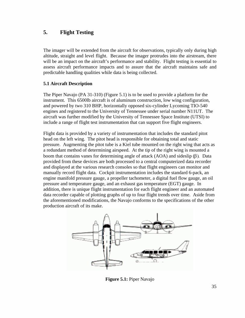
The imager will be extended from the aircraft for observations, typically only during high altitude, straight and level flight. Because the imager protrudes into the airstream, there will be an impact on the aircraft’s performance and stability. Flight testing is essential to assess aircraft performance impacts and to assure that the aircraft maintains safe and predictable handling qualities while data is being collected. 5.1 Aircraft Description The Piper Navajo (PA 31-310) (Figure 5.1) is to be used to provide a platform for the instrument. This 6500lb aircraft is of aluminum construction, low wing configuration, and powered by two 310 BHP, horizontally opposed six-cylinder Lycoming TIO-540 engines and registered to the University of Tennessee under serial number N11UT. The aircraft was further modified by the University of Tennessee Space Institute (UTSI) to include a range of flight test instrumentation that can support five flight engineers. Flight data is provided by a variety of instrumentation that includes the standard pitot head on the left wing. The pitot head is responsible for obtaining total and static pressure. Augmenting the pitot tube is a Kiel tube mounted on the right wing that acts as a redundant method of determining airspeed. At the tip of the right wing is mounted a boom that contains vanes for determining angle of attack (AOA) and sideslip (β). Data provided from these devices are both processed to a central computerized data recorder and displayed at the various research consoles so that flight engineers can monitor and manually record flight data. Cockpit instrumentation includes the standard 6-pack, an engine manifold pressure gauge, a propeller tachometer, a digital fuel flow gauge, an oil pressure and temperature gauge, and an exhaust gas temperature (EGT) gauge. In addition, there is unique flight instrumentation for each flight engineer and an automated data recorder capable of plotting graphs of up to four flight trends over time. Aside from the aforementioned modifications, the Navajo conforms to the specifications of the other production aircraft of its make.

Figure 5.1: Piper Navajo

36

5.2 Scope of Tests All tests are conducted within the prescribed limits of the Pilot’s Operating Handbook (POH). Flight tests are generally done both with the center of gravity (CG) set near the forward limit and with the CG set near the aft limit. Performance testing is conducted in both configurations of climb (flaps retracted and power set at 75% maximum) and powered approach (flaps down and power set to achieve a trim airspeed of 1.5 Vso). 5.3 Drag Force Calculations The sensor will impart a drag force on the aircraft. This force will have an effect upon the aircraft’s performance as well as its stability and control characteristics. The reference area of the aircraft will be the wing surface area (S). The surface area of the main wing is 229 ft2. The flow will be analyzed as a combination of turbulent and laminar flow. The first thing to be calculated is the Reynolds number at the cruise velocity of 200 knots and the cruise altitude of 12,000 ft.

624 1097.7

/10120.2)5)(/689.1*200(Re x

sftxftsftcV

=== −ν

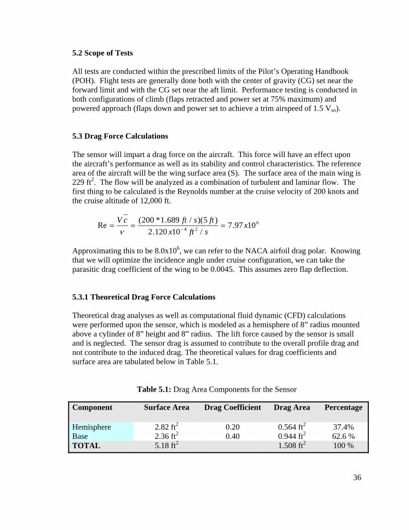
Approximating this to be 8.0x106, we can refer to the NACA airfoil drag polar. Knowing that we will optimize the incidence angle under cruise configuration, we can take the parasitic drag coefficient of the wing to be 0.0045. This assumes zero flap deflection. 5.3.1 Theoretical Drag Force Calculations Theoretical drag analyses as well as computational fluid dynamic (CFD) calculations were performed upon the sensor, which is modeled as a hemisphere of 8” radius mounted above a cylinder of 8” height and 8” radius. The lift force caused by the sensor is small and is neglected. The sensor drag is assumed to contribute to the overall profile drag and not contribute to the induced drag. The theoretical values for drag coefficients and surface area are tabulated below in Table 5.1.

Table 5.1: Drag Area Components for the Sensor Component Surface Area Drag Coefficient Drag Area Percentage

Hemisphere 2.82 ft2 0.20 0.564 ft2 37.4% Base 2.36 ft2 0.40 0.944 ft2 62.6 % TOTAL 5.18 ft2 1.508 ft2 100 %

37

The total parasitic drag coefficient can then be calculated by summing up the drag areas and dividing by the reference area.

2911.018.5

508.12

2

0 ==Σ

=ftft

SSCC D

D

The force produced by the sensor in the airflow at 200 knots is then

( ) lbfktsftslftvACF DD 2042

689.1*200)/002377.0)(18.5)(2911.0(2

232

2

=== ρ

The sensor does not affect non-aerodynamic sources of parasitic drag such as engine drag, gear drag, or scrubbing drag. Interference drag is assumed to be negligible as fillets will be designed into the interface of the sensor with the fuselage. The values derived through CFD analysis and provided by the UTSI Design Group are tabulated in Table 5.2 The drag force of the sensor in a 200knot airstream gathered by the CFD analysis match within 83% of the result produced through theoretical analysis. The results from the CFD analysis will be used in the subsequent predictions of flight test results. 5.3.2 Relative Increase in Drag The two dimensional cross sectional area of the sensor will be used as a reference area. For the front projection, this area is 1.410 ft2. As previously determined, the drag coefficient of the sensor is approximated as 0.2911. The percent increase in drag force is calculated below

( ) ( )( )

( ) ( )( )2

22

229*018.0140.1*2911.0229*018.0

%ft

ftftSC

SCSCIncrease

ACD

SENSORDACD +=

+= = 10.0%

Table 5.2: Drag Forces Obtained through CFD Analysis

Drag (lbf)

Lift (lbf)

100 kts 150 kts 200 kts 100 kts 150 kts 200 kts

0 AOA 39.6 93 171 0 AOA 4.5 1.28 3.5

10 AOA 34.6 81 147 10 AOA 5.5 17 27

38

5.4 Performance Flight Testing The addition of the instrument will affect the performance characteristics of the aircraft. Three flight tests are recommended to assure that the aircraft stays within safe operating conditions when the instrument is extended in flight. First, the characteristics of the aircraft under a stall will be observed. Second, the level flight performance will be tested. Finally, the climb performance will be tested. 5.4.1 Stalling Speed Determination The purpose of the stalling speed determination flight test is to 1) determine the stalling characteristics of the Piper Navajo with the payload attached, 2) define the maximum lift coefficient with the payload extended, and 3) verify that these characteristics comply with FAR Part 23. The stalling speed determination flight test is conducted through a test flight conducted in smooth air under Visual Meteorological Conditions (VMC) outside of the Tullahoma Regional Airport in Tullahoma, Tennessee. 5.4.1.1 Test Procedure

The FAA defines a stall as: (1) An uncontrollable downward pitching motion of the airplane; (2) A downward pitching motion of the airplane that results from the activation of a stall avoidance device (for example, stick pusher); or (3) The control reaching the stop. The Navajo is tested under the first of the previous definitions as it has neither a stick-pusher or a design that allows for the control to reach the stop before a downward pitching motion. Vso is defined to be the stalling speed in approach configuration and Vs1 is defined to be the stalling speed in cruise configuration. Testing is done with the engine idling, the throttle(s) closed or at not more than the power necessary for zero thrust at a speed not more than 110 percent of the stalling speed.

Testing is done in accordance with FAR 23.49 and FAR 23.201. From steady flight in cruise configuration at 1.5 Vs1 , airspeed is decreased at the rate of one knot per second until the stall occurs. The airspeeds corresponding to the sounding of the stall warning, the physical buffeting of the flow separation, and the actual uncontrolled pitch-down is recorded. Power-on and power-off stall data is obtained for the aircraft in cruise configuration (gear and flaps up) since this will be the configuration the aircraft will be in when the sensor is extended. 5.4.1.2 Projected Results The stalling speed can be derived directly from the definition of the coefficient of lift, CL, assumed to be 1.42 for the Navajo. In level, unaccelerated flight, the lifting force equals the weight and we may write:

39

SVCWL L2

2ρ

== (5.1)

By solving for the velocity, we get:

max

12

Lstall CS

WVρ

=42.11

002377.02

2296500

32 ftslftlbf

= = 129.7 ft/s.

This translates to 76.9 KIAS, which complies with Piper’s published performance results of 77 knots. The assumption is made that the instrument will not effect the overall lift coefficient and it will further make a negligible contribution to the overall vehicle mass, so the stalling speed is expected to be unaffected by the configuration of the sensor.

5.4.1.2 FAR Compliance

FAR Regulation Part 23.49 defines the stalling period of the aircraft. VSO and VS1 are determined by flight tests, using the procedure and meeting the flight characteristics specified in FAR Part 23.201. FAR regulations require that VSO at maximum weight must not exceed 61 knots for all single-engine airplanes.

FAR Part 23.201 governs wings-level stalls. This regulation states that it must be possible to produce and to correct roll by unreversed use of the rolling control and to produce and to correct yaw by unreversed use of the directional control, up to the time the airplane stalls. FAR Part 23.203 covers turning flight and accelerated turning stalls.

FAR Part 23.207 involves the aircraft’s stall warning. By incorporating a clear and distinctive buzzer that can not be confused with any routine engine noises, the Navajo complies with this regulation. Furthermore, this section mandates that the stall warning must begin at a speed exceeding the stalling speed by a margin of not less than 5 knots and must continue until the stall occurs.

5.4.2 Level Flight Performance

The purpose of this flight test is to determine the level flight performance characteristics of the Piper Navajo wit the sensor extended by using the BHPiw versus Viw method. From these performance results, we determined 1) the maximum calibrated air speed at 75% power, 2) the maximum range speed, and 3) the maximum endurance speed. The stalling speed determination flight test is conducted through a test flight conducted in smooth air under Visual Meteorological Conditions (VMC) outside of the Tullahoma Regional Airport in Tullahoma, Tennessee.

40

5.4.2.1 Test Procedure Data is recorded at a span of airspeeds ranging from maximum level flight speed to stall speed. The first airspeed datum lies near the aircraft’s full power setting and the last datum lies near the stalling speed. Data at both low altitude and high altitude is recorded. The values for manifold pressure are also recorded at three different altitudes that lie between the two test altitudes. Each data point is generated with the aircraft in a gear up, flaps up configuration. The first data point was recorded with the aircraft in level flight at maximum airspeed (maximum RPM and full propeller setting). The aircraft is given at least three minutes to accelerate at each power and propeller setting so that only stabilized data is obtained. After stabilization, the following data is recorded: indicated airspeed, pressure altitude, free air temperature, engine RPM, manifold pressure, and integrated fuel consumption. After recording, power is reduced by reducing the manifold pressure and the above procedure is repeated. This process was repeated until the minimum level flight speed (at stall) is reached. 5.4.2.2 Projected Results Results are obtained for the maximum calibrated air speed (CAS), the maximum range speed, and the maximum endurance speed. To solve for the maximum level flight speed, we recognize that this is the point where the thrust force is equal to the drag force (T=D). We first multiply both sides by the freestream velocity as such:

V BpP v η== DTreq (5.2) The total drag force is a summation of the parasitic drag and the lift-induced drag, io DDD += . At the maximum velocity, the parasitic drag will be dominant and we can neglect the term for the induced drag. Thus,

SVCDD Do2

0 2==

ρ (5.3)

Combining gives us

SVCD3

0BpP2

=ρη (5.4)

An initial assumption of 0.85 is made for the value of the propulsive efficiency. Further iterations may fine-tune this parameter. Total power is the sum of the two engines, each producing 310 BHP. Using the assumption that 04 dd CC = , we take CD =0.018. If we rewrite the drag force and solve for v, we get:

41

3Bp

)max(

P2ρ

ηSC

VD

level = = 332 )002377.0)(229(0180.0

)550)(310*2)(85.0(2ftslft

shplbffthp ⋅⋅

Solving gives sftV level /66.389)max( = , or more commonly knotslevelV 87.230)max( = . This estimate is higher than the performance specifications published by Piper, but we seek only a relative percentage change in maximum level flight speed. The drag coefficient term is increased by 10.0%, as derived previously. With the instrument extended, CD=0.0198 and other parameters remain constant

3Bp

/)max(

P2ρ

ηSC

VD

sensorwlevel = = 332 )002377.0)(229(0198.0

)550)(310*2)(85.0(2ftslft

shplbffthp ⋅⋅

Solving gives sftV level /48.377)max( = , or more commonly knotslevelV 65.223)max( = . The ratio of these two velocities is 0.9687. Thus, there is a projected 3.126% decrease in the maximum level flight speed as a result of the extension of the sensor in flight. The maximum indicated level flight speed is published by Piper to be 188 knots, so the maximum level flight speed with the sensor extended is projected to be 182.1 knots. 5.4.2.3 FAR Compliance There are no FAR regulations regulating level flight performance. 5.4.3 Climb Performance The purpose of this flight test is to determine the climb performance of the Piper Navajo with the sensor extended at its maximum rate of climb speed using the Piw versus Ciw method. Climb performance includes 1) the maximum rate of climb at sea level, 2) the service ceiling, and 3) the maximum ceiling. Results will be compared to the requirements of FAR part 23.67. The climb performance flight test is conducted through a test flight conducted in smooth air in the absence of temperature inversions under Visual Meteorological Conditions (VMC) outside of the Tullahoma Regional Airport in Tullahoma, Tennessee. 5.4.3.1 Test Procedure Climb performance tests are performed at range of altitudes. Climbs are performed in pairs at headings that are normal to any wind velocity and opposed to each other in direction by 180 degrees so that the effects of wind may be averaged out. Testing is conducted with gear and flaps retracted and at maximum continuous power. Data is recorded at 30-second intervals throughout the duration of three minutes. At each 30-second interval, the following data were recorded: airspeed, pressure altitude, free air temperature, engine RPM, manifold pressure, integrated fuel consumption. From these data, climb performance parameters may be extrapolated.

42

5.4.3.2 Projected Results The rate of climb performance is shown to vary linearly with altitude. Service ceiling has been defined to be the highest altitude at which the aircraft can still maintain a 100 ft/min climb rate. Absolute ceiling is defined as the maximum attainable altitude the aircraft can achieve in standard conditions. The best rate of climb speed occurs at the minimum power required velocity. Piper publishes this speed to be 75 knots at sea level. Given this velocity, we may determine the vertical velocity through the relation:

WDV

WBHP

VV pv −==

ηγ

550sin (5.5)

At this speed with the sensor retracted,

SVCD D2

2ρ

= =0.0218(0.002377/2sl/ft3)(75.0kts*1.689)2(229ft2)

So, D=190.4 lbf. With the sensor extended, we multiply this force by 1.10, yielding D=209.4 lbf. For 75 knot airspeeds, the propeller efficiency (np) will be assumed to be 0.70. For the aircraft with the sensor retracted, the rate of climb (ROC) speed is

fpmsftlbs

sftlbslbs

hpVv 1981/01.336500

)/689.1*75)(4.190(6500

)70.0)(620(550==−=

With the sensor extended, the drag force becomes 209.4lbf and the ROC is 32.64 ft/s, or 1959 ft/m. The ratio of these vertical velocities is 0.9887, so the extension of the sensor causes a 1.13% reduction in the ROC. Piper publishes the maximum rate of climb to be 1115 ft/min, so by extending the sensor, this will be expected to be 1102 ft/min. Through trigonometry, we can calculate the maximum angle of climb for the Navajo with the sensor extended:

Angle of Maximum Climb = 45.14689.1*75

64.32tantan 11 == −−

VVv degrees (5.6)

5.4.3.2 FAR Compliance

FAR Part 23.63 requires all normal, utility, and acrobatic category reciprocating engine-powered airplanes of 6,000 pounds or less maximum weight to comply with FAR Part 23.65(a), Part 23.67(a), where appropriate, and Part 23.77(a) at maximum takeoff or landing weight, as appropriate, in a standard atmosphere and out of ground effect. FAR Part 23.65(a) mandates that these aircraft have a steady climb gradient at sea level of at least 11.5Vs1 ft/min where Vs1 is in knots. FAR Part 23.77(a) regulates aircraft

43

performance with regards to a balked landing, requiring aircraft of 6,000 pounds or less maximum weight to maintain a steady gradient of climb at sea level of at least 3.3 percent with full takeoff power, extended landing gear and a climb speed equal to VREF. It is required to demonstrate compliance with FAR Part 23.67 since the Navajo is a twin-engine aircraft. Compliance with FAR Part 23.77 may be shown through the relation

60*688.1*)(

min)/.(..3.3tanktsV

ftCOR

s

= (5.7)

5.4.4 Maximum Range and Endurance

Loiter speed is important parameter since much of the aircraft’s observation campaign will be performed at loiter. The minimum power required speed is the speed at which the aircraft’s endurance is maximized, which may be taken from the engine performance graphs. To compute the speed for minimum power required in level flight conditions, we first observe that Preq = Dv. We set the first derivative of this product to zero and solve for the minimum value. At this specific point, the coefficient of lift, assuming a parabolic drag polar, is:

e3 Α=′ πDoL CC (5.8)

By substituting this value into the lift equation and solving for the velocity at this specific point, we may write:

e312

(min)PrΑ

=πρ Do

eq CSWV (5.9)

We also note that e is the Span Efficiency Factor, which is a measure of the geometric ellipticity of the wing planform. It has been estimated here to be 0.85. Substituting these values, we get:

)85.0)(0.6()018.0(31

002377.02

2296500

32(min)Pr πftslftlbfV eq =

Solving, we get sftV eq 24.160(min)Pr = , or 94.94 knots. If we alter the drag coefficient by 10.0% so that CD=0.0198, then sftV eq 46.156(min)Pr = , or 92.70 knots. The difference in the maximum endurance speed is 2.36%, so it is recommended that loiter operations with the sensor extended be performed at a speed that is 2.36% less than the speed recommended for the aircraft without the sensor.

44

5.5 Stability and Control Flight Testing The addition of the sensor will also affect the stability and control characteristics of the aircraft. Two additional flight tests are recommended to assure that the aircraft stays within safe operating conditions when the instrument is extended in flight. First, the characteristics of the aircraft’s lateral-directional static stability is tested and next the aircraft’s engine-out minimum control speed is determined. 5.5.1 Lateral-Directional Static Stability The purpose of this flight test is to determine the lateral-directional static stability characteristics of the Piper Navajo by placing the aircraft into steady sideslips and comparing the results to the requirements specified in FAR Part 23.177. Since the sensor is offset from the aircraft’s CG, it is expected to produce a moments about the three axes. Of these moments, the yawing moment is assumed to be significant. The lateral-directional static stability test is conducted through a test flight conducted in smooth air under Visual Meteorological Conditions (VMC) outside of the Tullahoma Regional Airport in Tullahoma, Tennessee. 5.5.1.1 Test Procedure Steady sideslips are performed through a range of sideslip angles up to a maximum sideslip. A minimum of three recordings are performed for both left and right sideslips. Data is taken for both clean, level flight as well as a 3 degree powered approach for each of two airspeeds: 1.2Vs1 and 1.8Vs1. At each trim condition, the following parameters are recorded: indicated airspeed, pressure altitude, RPM, manifold pressure, bank angle, rudder position and force, aileron position and force, and sideslip angle. At each steady sideslip, the following parameters are recorded: bank angle, sideslip angle, rudder position and force, and aileron position and force. Relations between sideslip angle and the above parameters for steady sideslip are then plotted against each other. 5.5.1.2 Projected Results The drag coefficient and the drag force, Dd of the sensor is known from prior analysis. We may determine the yawing moment due to the sensor from the equation ddd lDN =Δ (5.10) where dNΔ is the yawing moment due to the sensor, Dd is the drag due to the device, and ld is the lateral distance of the device from the CG of the aircraft, assumed to be 30cm for

45

the Navajo. The wingspan (b) is 40.67ft. Static stability will be least in slower flight so we will use the CFD results for sensor drag at a cruising speed of 100knots at zero AoA (39.6lbf). Using b=40.67ft. If a zero sideslip angle is maintained when the sensor is extended, this condition may be expressed as 0=Δ+Δ rrNNd CC δδ (5.11) where bqSNC wdNd Δ=Δ Plugging in the values from above, )67.40)(229)(2007.0()5.2)(6.39( 2 ftftftlbfCNd =Δ = 0.0530. The maximum rudder deflection of the Navajo was measured to be 30 degrees, or 0.5236 radians. Lateral directional static stability is defined below from the derivative, rNC δ . Stability is implied by a large, negative value of this derivative.

r

NrN

CCδ

δδ Δ

Δ−= = -0.0530/0.5236 = -0.1012 (5.12)

We see that the aircraft should be stable at 100knots and at all airspeeds higher. This should be verified by flight test, where it can be shown that the Navajo has positive directional static stability in airspeeds ranging from 1.2Vs1 to the maximum airspeed with the sensor extended. This may be demonstrated by the recovery of the aircraft from skids without use of rudder. Furthermore, we are to show that the Navajo has positive lateral static stability at the airspeed of 1.2Vs1. This may be demonstrated by the raising of the low wing during sideslip in all flap and power configurations. Compliance with CAR 3.118 may be demonstrated if in straight, steady sideslips, the rudder and aileron control displacements and forces increase steadily as sideslip angle increases. Compliance with FAR Part 23.177 may be demonstrated if the rudder deflections and forces are proportional to the sideslip angle. 5.5.1.3 FAR Requirements FAR Part 23.177 covers directional and lateral stability. It follows CAR 3.118 and mandates that an aircraft exhibit static directional stability for all configurations of landing gear and flap positions for all airspeeds from 1.2Vs1 to the maximum airspeed. This stability shall be demonstrated by recovery from a skid with the rudder free. In addition, it shall be shown that positive static directional stability exists by demonstrating that the ability to raise the low wing during a sideslip at the same airspeed. CAR 3.118 also requires that the rudder and aileron displacements and forces shall increase steadily as the straight, steady sideslip angle is increased. FAR Part 23.177 specifies further that these deflections and forces be proportional to sideslip angle.

46

5.5.2 Engine-Out Minimum Control Speed Determination The purpose of this test flight is to determine the minimum control speed of the Piper Navajo with one engine out. Since there will be an asymmetric force produced by the drag force acting upon the sensor, controllability along the yaw axis becomes even a greater concern following the loss of an engine. The test will assume that directional control is solely a function of the rudder. Results will be compared to the requirements specified in FAR Part 23.147 and FAR Part 23.149. The engine-out minimum control speeds of the Piper Navajo for both forward and aft CG loadings are determined from flight testing conducted in Visual Meteorological Conditions (VMC) outside of the Tullahoma Regional Airport in Tullahoma, Tennessee. 5.5.2.1 Test Procedure The rudder effectiveness coefficient is determined by measuring the control positions in straight, steady sideslips in the aft CG position. In this test, rudder side-force are ignored. Tests are performed at three altitudes: 3000, 5000, and 7000 ft AMSL. At each altitude, the aircraft is stabilized at 2650 RPM and full throttle at 140 knots indicated airspeed. The left engine is then reduced to idle while heading, airspeed, and a five degree right bank is maintained. Due to safety concerns, the left engine was not completely shut off and some error is then induced by using an engine idle versus an engine-off condition. The airspeed is then reduced in 15 knot increments and data was recorded at each increment between 140 and 95 KIAS. At each stabilized airspeed after engine shut-down, the following parameters were recorded: indicated airspeed (Vi), pressure altitude (Hpi), engine RPM, manifold pressure (MP), rudder deflection (δri), aileron deflection (δai), bank angle (φ), and sideslip (β). Plots were generated to show the relationships between corrected airspeed and each of three parameters: δri, δai, and β. The engine-out minimum control speed was then determined by extrapolating the plots of rudder deflection versus airspeed for each tested altitude. To determine if engine-out minimum control speed at sea level is less than 1.2Vs1, a plot is generated illustrating the relationship between Vmc and pressure altitude, which is then extrapolated to sea level. By fitting a second order equation to the data points generated from the three altitudes through rudder deflection angles spanning a range from 0 to 20 degree, compliance with FAR Part 23.149 and FAR Part 23.147 is demonstrated. 5.5.2.2 Projected Results For propeller-driven twin engine aircraft, the yaw coefficient is created as the thrust vector becomes offset from the longitudinal axis as a result of having an inoperative engine. This moment is defined as

47

WbVYCBHPC TPLpNTprop )(550η= (5.13) By summing the yawing moments, 0=++ rrNNNTprop CCC δβ δβ (5.14) Adding the moment caused by the sensor, bqSNC wdNd Δ=Δ , we get 0=Δ+++ wdrrNNNTprop qSNCCC δβ δβ (5.15) The critical engine is the left-mounted engine. In the event of an engine-out scenario, the left yawing moment will be compounded by the drag force on the sensor. The stability derivatives are to be obtained experimentally through flight testing. 5.5.2.3 FAR Compliance Testing of a twin engine aircraft under engine-out conditions must still meet the FAR requirements as specified for the static lateral directional stability flight tests. As stated in section 5.4.1.3, FAR Part 23.177 covers directional and lateral stability and mandates that an aircraft exhibit static directional stability for all configurations of landing gear and flap positions for all airspeeds from 1.2Vs1 to the maximum airspeed. CAR 3.118 also requires that the rudder and aileron displacements and forces shall increase steadily as the straight, steady sideslip angle is increased. FAR Part 23.177 specifies further that these deflections and forces be proportional to sideslip angle. 5.6 Control Surface Blanking The sensor must be positioned so that its wake does not interfere with elevator control and the empennage of the aircraft does not interfere with the sensors FOV. Assuming that the angle of attack (AoA) of the aircraft will fluctuate between 0 and 15 degrees, the sensor should be placed high enough so that the wake from a 0 degree AoA would not interfere with the elevator. This is done simply by mounting the base of the sensor at a greater height on the cargo door than the horizontal stabilizer. The FOV of the sensor would not be obstructed in this case.

48

6. Flight Research Campaign

The purpose of the flight research campaign is to take simultaneous images from the aircraft of a common volume of 83km altitude where the SNR received from Mie scattered sunlight off of PMC particulates is at a maximum.

6.1 Defining the Geometry

The signal to noise may be computed numerically by first calculating the free-space solar irradiance from the solar function at the imager sensitive. The irradiance at the PMC may be obtained through some basic approximations. If we assume that 1) the atmospheric density may be modeled exponentially by using the Standard Atmosphere (1976) (www.pdas.com), and 2) multiple scatterings are negligible, we may numerically integrate the attenuation of the solar irradiance and produce a function of solar irradiance at the PMC versus the minimum altitude through which the ray passes. We then adjust this value by multiplying it by the Mie phase function, PM( χ ), where the angle χ is the angle between the perpendicular bisector of the incoming solar ray (the terminator) and the line which passes through the PMC normal to the surface of the earth, as shown in Figure 6.1.

Noise received at the imager is computed in the same manner as described in Section 2. From these data, the optimal angle below the terminator may be found for PMC observations at the specified altitude. Calculations performed by Rusch, et. al. (Rusch) has calculated this value to be approximately six degrees and this value will be assumed for the present calculations. Having obtained the optimal angle below the terminator at which to observe PMCs, the next step is to account for the apparent solar motion as a result of the tilt of the earth and the eccentricity of Earth’s orbit about the Sun. This apparent motion traces a well-referenced analemma. We may combine these effects to yield the solar declination,δ . The terminator is defined to be orthogonal to this angle if the widely accepted assumption that the incoming solar rays are parallel is used. From the terminator, the previously derived optimal angle below the terminator, χ , is added. Ideally, the sensors on the aircraft and the AIM spacecraft should be positioned along the radial defined by the angle where the common volume exists. The positioning geometry is illustrated in Figure 6.2. The angle β is the maximum angle at which the common volume altitude is visible from the aircraft. Realistically, both multiple scattering and Chapman function approximations restrict this angle significantly from the geometrical maximum. As previously selected, β spans 77o to either side of normal. The angle defined by the summation of the solar declination and the optimal angle below the terminator (6o) defines the optimal angle at which to image PMC activity at local midnight. The time of local midnight is derived from the longitude of the AIM overpass at this latitude, or the Greenwich Hour Angle (GHA). If the overpass was to happen exactly at local midnight, no other calculations would be necessary.

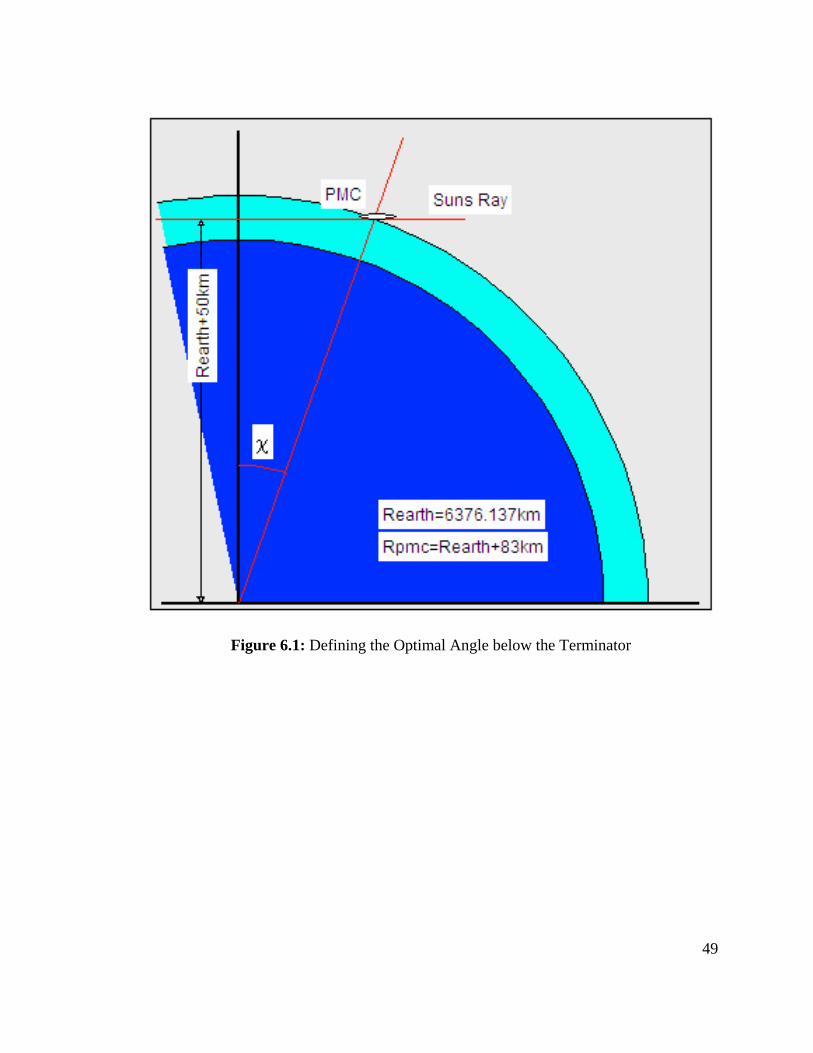
49

Figure 6.1: Defining the Optimal Angle below the Terminator

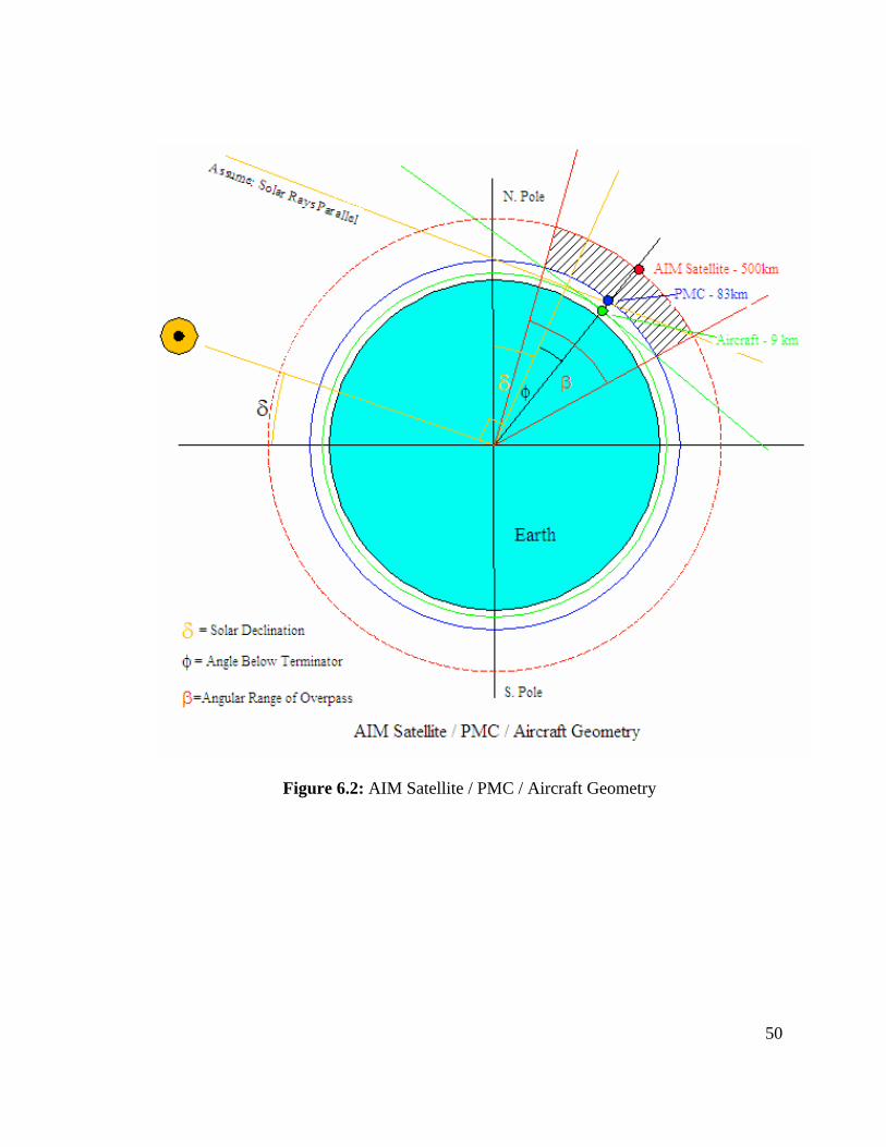
50

Figure 6.2: AIM Satellite / PMC / Aircraft Geometry

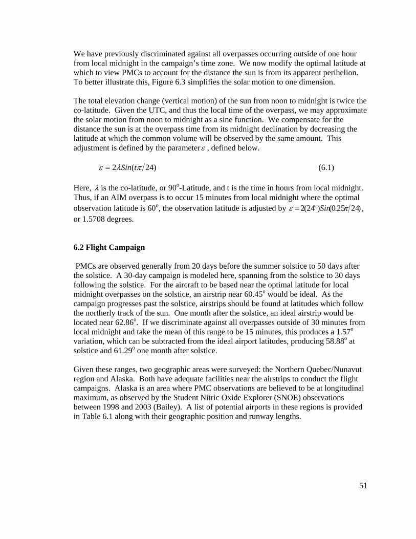
51

We have previously discriminated against all overpasses occurring outside of one hour from local midnight in the campaign’s time zone. We now modify the optimal latitude at which to view PMCs to account for the distance the sun is from its apparent perihelion. To better illustrate this, Figure 6.3 simplifies the solar motion to one dimension. The total elevation change (vertical motion) of the sun from noon to midnight is twice the co-latitude. Given the UTC, and thus the local time of the overpass, we may approximate the solar motion from noon to midnight as a sine function. We compensate for the distance the sun is at the overpass time from its midnight declination by decreasing the latitude at which the common volume will be observed by the same amount. This adjustment is defined by the parameterε , defined below.

)24(2 πλε tSin= (6.1) Here, λ is the co-latitude, or 90o-Latitude, and t is the time in hours from local midnight. Thus, if an AIM overpass is to occur 15 minutes from local midnight where the optimal observation latitude is 60o, the observation latitude is adjusted by )2425.0()24(2 πε Sino= , or 1.5708 degrees. 6.2 Flight Campaign PMCs are observed generally from 20 days before the summer solstice to 50 days after the solstice. A 30-day campaign is modeled here, spanning from the solstice to 30 days following the solstice. For the aircraft to be based near the optimal latitude for local midnight overpasses on the solstice, an airstrip near 60.45o would be ideal. As the campaign progresses past the solstice, airstrips should be found at latitudes which follow the northerly track of the sun. One month after the solstice, an ideal airstrip would be located near 62.86o. If we discriminate against all overpasses outside of 30 minutes from local midnight and take the mean of this range to be 15 minutes, this produces a 1.57o variation, which can be subtracted from the ideal airport latitudes, producing 58.88o at solstice and 61.29o one month after solstice. Given these ranges, two geographic areas were surveyed: the Northern Quebec/Nunavut region and Alaska. Both have adequate facilities near the airstrips to conduct the flight campaigns. Alaska is an area where PMC observations are believed to be at longitudinal maximum, as observed by the Student Nitric Oxide Explorer (SNOE) observations between 1998 and 2003 (Bailey). A list of potential airports in these regions is provided in Table 6.1 along with their geographic position and runway lengths.

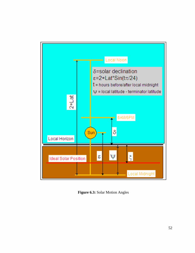
52

Figure 6.3: Solar Motion Angles

53

Table 6.1: Airport Data for Observation Campaigns

6.3 Computing Intercept Trajectories We know the latitude and longitude at which the aircraft is stationed. For the predicted observation, we have the longitude, latitude, and UTC time of the AIM overpass. From these data, we derive the local time of the overpass which producesε . Subtractingε from the optimal observation latitude at local midnight, we get the common volume latitude, through which the common volume longitude is extrapolated. Thus, the distance and heading the aircraft is to fly is calculated through equations 6.2 and 6.3.

Distance = 22 )()( cvairstripcvairstrip LonLonLatLat −+− (6.2)

Heading = tan-1 ⎟⎟⎠

⎞⎜⎜⎝

⎛

−

−

cvairstrip

cvairstrip

LonLonLatLat

(6.3)

Transit time is calculated by first dividing the distance (eq. 6.2) by the cruising speed of the aircraft. The aircraft loiter is then computed by subtracting twice the transit time and the flight reserve from the aircraft endurance, as shown in equation 6.4. Results of these calculations are tabulated in Table 6.2.

Loiter Time = Endurance - 2(Transit Time) – Flight Reserves (6.4)

Airport Latitude Longitude Runway Length

Code Airport Location (degrees) (degrees) (feet) NORTHERN QUEBEC / NUNAVUT CAMPAIGN

YVP Kuujjuaq Airport Kuujjuaq, Quebec 58.07 -68.25 6000 Paved

YZG Salluit Airport Salluit, Quebec 62.18 -75.67 3500 Paved

YWB Kangiqsujuaq Airport Kangiqsujuaq, Quebec 61.05 -71.55 3500 Unpaved

YFB Iqaluit Airport Iqaluit, Nunavut 63.75 -68.55 8200 Paved ALASKA CAMPAIGN

TKJ Tok Airport Tok, Alaska 63.295 -143.006 1670 Paved

PAMR Merrill Field Airport Anchorage, Alaska 61.214 -149.844 4000 Paved

PAFA Fairbanks International Airport Fairbanks, Alaska 64.815 -147.856 11800 Paved

PAHN Haines Airport Haines, Alaska 59.244 -135.524 4000 Paved

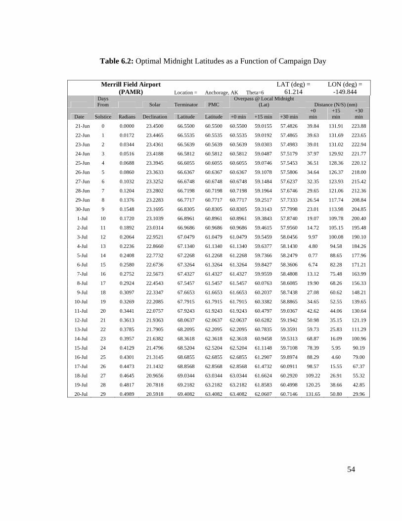
54

Table 6.2: Optimal Midnight Latitudes as a Function of Campaign Day

Merrill Field Airport

(PAMR) Location = Anchorage, AK Theta=6 LAT (deg) =

61.214 LON (deg) =

-149.844

Days From Solar Terminator PMC

Overpass @ Local Midnight (Lat) Distance (N/S) (nm)

Date Solstice Radians Declination Latitude Latitude +0 min +15 min +30 min +0 min

+15 min

+30 min

21-Jun 0 0.0000 23.4500 66.5500 60.5500 60.5500 59.0155 57.4826 39.84 131.91 223.88

22-Jun 1 0.0172 23.4465 66.5535 60.5535 60.5535 59.0192 57.4865 39.63 131.69 223.65

23-Jun 2 0.0344 23.4361 66.5639 60.5639 60.5639 59.0303 57.4983 39.01 131.02 222.94

24-Jun 3 0.0516 23.4188 66.5812 60.5812 60.5812 59.0487 57.5179 37.97 129.92 221.77

25-Jun 4 0.0688 23.3945 66.6055 60.6055 60.6055 59.0746 57.5453 36.51 128.36 220.12

26-Jun 5 0.0860 23.3633 66.6367 60.6367 60.6367 59.1078 57.5806 34.64 126.37 218.00

27-Jun 6 0.1032 23.3252 66.6748 60.6748 60.6748 59.1484 57.6237 32.35 123.93 215.42

28-Jun 7 0.1204 23.2802 66.7198 60.7198 60.7198 59.1964 57.6746 29.65 121.06 212.36

29-Jun 8 0.1376 23.2283 66.7717 60.7717 60.7717 59.2517 57.7333 26.54 117.74 208.84

30-Jun 9 0.1548 23.1695 66.8305 60.8305 60.8305 59.3143 57.7998 23.01 113.98 204.85

1-Jul 10 0.1720 23.1039 66.8961 60.8961 60.8961 59.3843 57.8740 19.07 109.78 200.40

2-Jul 11 0.1892 23.0314 66.9686 60.9686 60.9686 59.4615 57.9560 14.72 105.15 195.48

3-Jul 12 0.2064 22.9521 67.0479 61.0479 61.0479 59.5459 58.0456 9.97 100.08 190.10

4-Jul 13 0.2236 22.8660 67.1340 61.1340 61.1340 59.6377 58.1430 4.80 94.58 184.26

5-Jul 14 0.2408 22.7732 67.2268 61.2268 61.2268 59.7366 58.2479 0.77 88.65 177.96

6-Jul 15 0.2580 22.6736 67.3264 61.3264 61.3264 59.8427 58.3606 6.74 82.28 171.21

7-Jul 16 0.2752 22.5673 67.4327 61.4327 61.4327 59.9559 58.4808 13.12 75.48 163.99

8-Jul 17 0.2924 22.4543 67.5457 61.5457 61.5457 60.0763 58.6085 19.90 68.26 156.33

9-Jul 18 0.3097 22.3347 67.6653 61.6653 61.6653 60.2037 58.7438 27.08 60.62 148.21

10-Jul 19 0.3269 22.2085 67.7915 61.7915 61.7915 60.3382 58.8865 34.65 52.55 139.65

11-Jul 20 0.3441 22.0757 67.9243 61.9243 61.9243 60.4797 59.0367 42.62 44.06 130.64

12-Jul 21 0.3613 21.9363 68.0637 62.0637 62.0637 60.6282 59.1942 50.98 35.15 121.19

13-Jul 22 0.3785 21.7905 68.2095 62.2095 62.2095 60.7835 59.3591 59.73 25.83 111.29

14-Jul 23 0.3957 21.6382 68.3618 62.3618 62.3618 60.9458 59.5313 68.87 16.09 100.96

15-Jul 24 0.4129 21.4796 68.5204 62.5204 62.5204 61.1148 59.7108 78.39 5.95 90.19

16-Jul 25 0.4301 21.3145 68.6855 62.6855 62.6855 61.2907 59.8974 88.29 4.60 79.00

17-Jul 26 0.4473 21.1432 68.8568 62.8568 62.8568 61.4732 60.0911 98.57 15.55 67.37

18-Jul 27 0.4645 20.9656 69.0344 63.0344 63.0344 61.6624 60.2920 109.22 26.91 55.32

19-Jul 28 0.4817 20.7818 69.2182 63.2182 63.2182 61.8583 60.4998 120.25 38.66 42.85

20-Jul 29 0.4989 20.5918 69.4082 63.4082 63.4082 62.0607 60.7146 131.65 50.80 29.96

55

If we assume that we want the overpass to occur at a time after one-half of the loiter time has been used to image potential PMC evolution, then we may backtrack to determine the optimal take-off time.

Take-Off Time = Overpass Time – (Endurance - Flight Reserves - 0.5(Loiter Time) – Transit Time) (6.5)

The East-West distance is a function of the latitude as well as the difference in longitude between the airstrip and the common volume.

Distance (E/W) = ⎟⎠⎞

⎜⎝⎛ −

−90

90 LatLonLon cvairstrip (6.6)

We may now solve for distance and heading, given northerly and easterly distances in nautical miles:

Distance = 22 ))/(())/(( WEDistSNDist + (6.7)

Heading = tan-1 ⎟⎟⎠

⎞⎜⎜⎝

⎛)/()/(

WEDistSNDist

(6.8)

56

7. Summary and Conclusions

The following conclusions may be made following this analysis and design: 1) Insight into the vertical structure and time evolution of PMCs may be obtained by synchronous imaging using a satellite and an airborne imager. 2) Two or three common volume images may be taken during each overpass of the AIM satellite. One overpass during observation conditions will occur each day. 3) Turbulence and pilot error in maintaining heading and level flight attitude may be compensated for by integrating an active platform with the imager. The active platform will be capable of scanning an elevation range of +/- 80 degrees from zenith and a roll range of +/- 5 degrees. 4) The imager will be modeled off of the CIPS engineering model CCD and will be able to obtain images through one of four lens/filter combinations. Filtered images are based around a 350nm central frequency, which is a compromise between the desire to image near the CIPS imagers sensitivity and the desire to use inexpensive, off-the-shelf instrumentation. 5) Wide angle imaging is performed using a 105mm focal length lens with a FOV of 58 degrees, yielding a resolution of 40m x 40m at PMC altitudes. Narrow imaging is performed using a 24mm focal length lens with a FOV of 15.54 degrees, yielding a resolution of 10m x 10m at the same altitudes. TDI dwell time is 0.1091s for 29 TDI runs for the narrow FOV lens and 0.4364s for 7 TDI runs for the wide angle FOV lens. 6) The imager will be mounted to the rear cargo door and be extended in flight. To assure the maintenance of safe flight characteristics, a flight test program will be conducted. Prior analysis shows that these flight tests are both feasible and safe to perform. Performance flight tests include level flight performance and climbing performance. Stability and Control flight tests include static lateral/directional stability and engine-out minimum speed flight tests. Stalling speed determination and control surface blanking are also qualitatively analyzed. 7) A flight campaign may be built around an observation period starting at the summer solstice and extending for 30 days. There are sufficient facilities to conduct operations on either Northern Quebec and Nunavut or Alaska. Aircraft endurance is sufficient to obtain at least one hour of images before the overpass and one hour of images after the overpass.

57

Recommendations for Future Work

Collaboration between CU and UTSI would be recommended to continue with future development work. As of November 18, 2006, means to simplify the instrument are being looked into, as well as with alternative methods to mount the sensor to the aircraft. For the initial flight campaign, scheduled for the Boreal Summer of 2007, an instrument using only one lens and filter combination is being considered. This instrument may then be mounted in the nose of the aircraft and positioned so that it may image PMCs that are observable to the north. Though this method would greatly simplify the mechanics of integrating an active platform, a very precise flight plan must be conducted. Vibration testing must be performed at the component level as well as the system level. UTSI may perform a vibration analysis for all vibrational modes up to 10MHz. In addition, consideration must be given to condensation on the instrument by using optical glass and a ventilated and heated nose compartment. Flight testing must also be performed so that conditions that are to be expected during the actual flight campaign are reproduced as actual as possible before deploying the aircraft to the campaign environment. The minimal acceptable flight altitude must also be determined.

58

LIST OF REFERENCES

59

LIST OF REFERENCES

Aeronomy of Ice in the Mesosphere Small Explorer Concept Study Report, December

2001. Anderson, J.D. 1989. Introduction to Flight, 3rd ed, McGrxaw-Hill, Inc. Bailey, S.M. et al., 2005, Observations of Polar Mesospheric Clouds by the Student

Nitric Oxide Explorer, Journal of Geophysical Research, Vol. 110, American Geophysical Union.

Conversation with William McClintock, Laboratory for Atmospheric and Space Physics,

Boulder, CO, May 2006. Conversation with Dave Rusch, Laboratory for Atmospheric and Space Physics, Boulder,

CO, May 2006. Hansen, Flemming, 2002 ‘DTU Satellite Systems and Design Course, Orbital

Mechanics’, Danish Space Research Institute. Hecht E. 2002, Optics, 4th ed, San Francisco, Addison-Wesley. Howell, S. P. 2003. Practical Celestial Navigation, Revised Edition, Mystic Seasport. Kimberlin, R.D. 2003. Flight Testing of Fixed Wing Aircraft. American Institute for

Aeronautics and Astronautics. Nerem, Steve, 2006. Class Notes – Astrodynamics, University of Colorado, Boulder, CO. Raymer, D.P., 1989, Aircraft Design: A Conceptual Approach, Washington D.C., AIAA

Education Series, AIAA. Reimuller, Jason D. 2004, ’Stability and Control Flight Testing of the Piper Navajo’,

University of Tennessee Space Institute, Tullahoma, TN. Reimuller, Jason D. 2005, Performance Flight Testing of the Piper Navajo’, University of

Tennessee Space Institute, Tullahoma, TN. Salby, M. L. 1996. Fundamentals of Atmospheric Physics, San Diego, CA: Academic

Press. Solies, U. Peter, 2005 Lecture Notes, University of Tennessee Space Institute,

Tullahoma, TN.

60

LIST OF REFERENCES Stinton, D., 1983, The Design of the Aeroplane, Cambridge, Grenada Publishing, Inc,

University Press.

Thomas, G.E. 2003. Are Noctilucent Clouds Harbringers of Global Change in the Middle Atmosphere? Laboratory for Atmospheric and Space Physics, Elsevier, Ltd.

UTSI Fixed Wing Performance Flight Testing – Course Notes, September 2004.

University of Tennessee Space Institute, Tullahoma, TN. UTSI Fixed Wing Stability and Control Flight Testing – Course Notes, September 2004.

University of Tennessee Space Institute, Tullahoma, TN. Vallado, D.A. 2001. Fundamentals of Astrodynamics, El Segundo, CA: Microcosm

Press. Websites: http://www.newport.com http://www.madsci.org/posts/archives/dec2000/978194854.Eg.r.html http://www.electrim.com/tdipaper.html http://aanda.u-strasbg.fr:2002/articles/aas/full/1998/01/ds1449/node6.html http://www.sat.dundee.ac.uk/tle.html http://www.eso.org/observing/dfo/quality/UVES/pipeline/sky_spectrum.html http://www.pdas.com/atmos.htm

61

APPENDIX A

Airglow Spectra

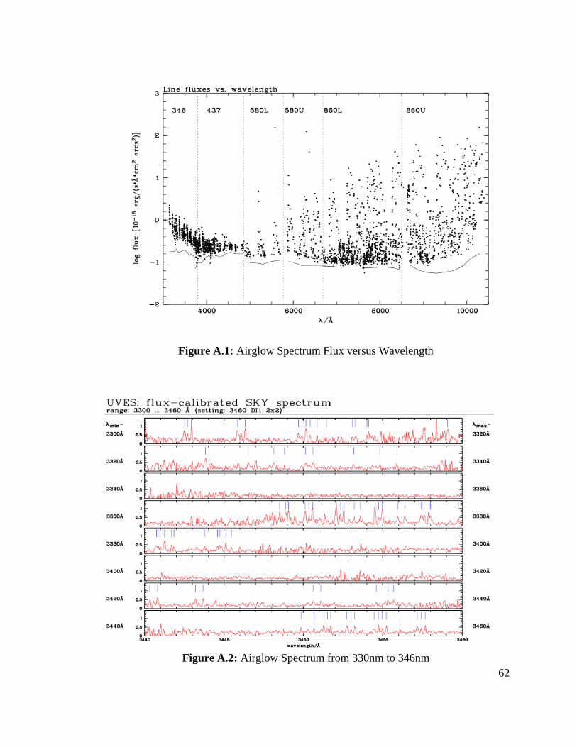
62

Figure A.1: Airglow Spectrum Flux versus Wavelength

Figure A.2: Airglow Spectrum from 330nm to 346nm

63

Figure A.3: Airglow Spectrum from 346nm to 362nm

Figure A.4: Airglow Spectrum from 362nm to 376nm

64

APPENDIX B

NORAD Two Line Element Sets

65

NORAD TLE sets are presented in the format described in Figure B1. The first line lists most of the identifying information about the spacecraft. The classical orbit elements are listed on the second line. These are the data that will be retrieved for the orbital predicts in this algorithm.

Figure B.1: NORAD Two Line Element Sets

66

APPENDIX C

ECEF to SEZ Conversion

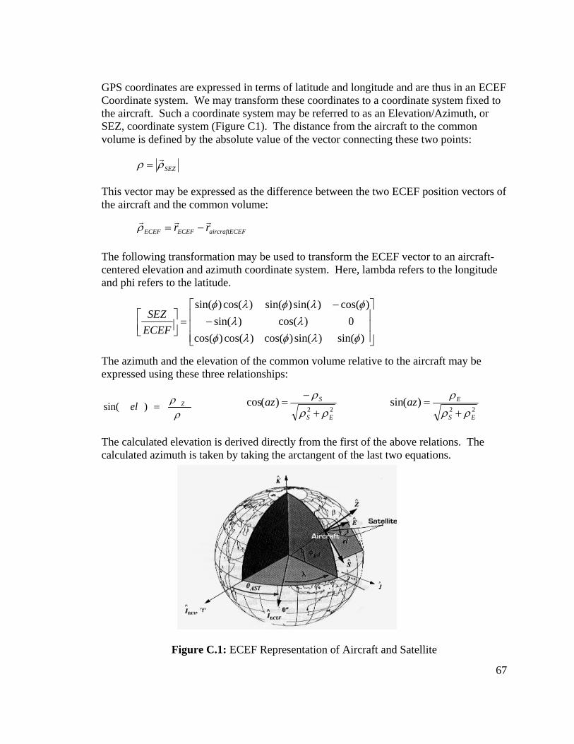
67

GPS coordinates are expressed in terms of latitude and longitude and are thus in an ECEF Coordinate system. We may transform these coordinates to a coordinate system fixed to the aircraft. Such a coordinate system may be referred to as an Elevation/Azimuth, or SEZ, coordinate system (Figure C1). The distance from the aircraft to the common volume is defined by the absolute value of the vector connecting these two points:

This vector may be expressed as the difference between the two ECEF position vectors of the aircraft and the common volume:

The following transformation may be used to transform the ECEF vector to an aircraft-centered elevation and azimuth coordinate system. Here, lambda refers to the longitude and phi refers to the latitude.

The azimuth and the elevation of the common volume relative to the aircraft may be expressed using these three relationships:

The calculated elevation is derived directly from the first of the above relations. The calculated azimuth is taken by taking the arctangent of the last two equations.

Figure C.1: ECEF Representation of Aircraft and Satellite

ρρ Zel =)sin(

⎥⎥⎥

⎦

⎤

⎢⎢⎢

⎣

⎡−

−=⎥⎦

⎤⎢⎣⎡

)sin()sin()cos()cos()cos(0)cos()sin(

)cos()sin()sin()cos()sin(

φλφλφλλ

φλφλφ

ECEFSEZ

EFaircraftECECEFECEF rr rrr−=ρ

SEZρρr

=

22)(sin

ES

Eazρρ

ρ+

=22

)(cosES

Sazρρ

ρ+

−=

68

APPENDIX D

Code

69

D1 : Solar Bandwidth Code (IDL) ; ; Solar Flux Plot Program ; !path = !path + ';C:\Documents and Settings\reimuller\Desktop\Thesis' !path = !path + 'd:/idllib' cd, 'C:\Documents and Settings\reimuller\Desktop\Thesis' ; ; This script supports 2 output formats: ; X windows (out='x') and Postscript ('ps') ; psfile='plotsf.ps' out='ps' if (out eq 'ps') then begin ; For Postscript use device fonts (pick Helvetica) set_plot, 'ps' device, filename=psfile, /color, /portrait, /helvetica, $ xsize=18, ysize=24, xoffset=1.5, yoffset=2.0 !p.font=0 endif if (out eq 'win') then begin ; For X windows use the Hershey stroked fonts set_plot, 'win' window, xsize=525, ysize=700, title='Solar Flux' !p.font=-1 endif ; ;plot solar flux ; @d:/idllib/prpwl.pro restore,'arvesen_final.sav' !x.range=[200,1200] !x.tickv=[200,400,600,800,1000,1200] !x.ticks=5 !y.title='Flux, ph/cm2/s/nm' !x.title='Wavelength, nm' plot_io,wlfinal/10,fluxfinal, title='Solar Flux' ; ; Integrate over wavelength ; pi=!pi i=1 & sign=1.0 signalstrength=400 wavelength=350.0 ; Defines Center Wavelength (nm) wl=(wavelength-200)*25 signal=fluxfinal(wavelength) while (signal lt signalstrength) do begin wlindex=0.04*i wplus=wl+wlindex wminus=wl-wlindex signal=signal+fluxfinal(wplus)+fluxfinal(wminus) i=i+1 endwhile dlambda=2.0*(0.04*i) print, 'Central Wavelength= ',wavelength, ' nm' print, 'Range of Wavelength= ',dlambda, ' nm' ; ; Close Program ; if (out ne 'x') then device, /close end

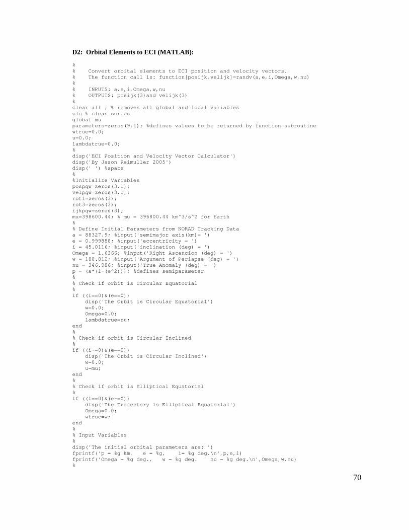
70

D2: Orbital Elements to ECI (MATLAB): % % Convert orbital elements to ECI position and velocity vectors. % The function call is: function[posijk,velijk]=randv(a,e,i,Omega,w,nu) % % INPUTS: a,e,i,Omega,w,nu % OUTPUTS: posijk(3)and velijk(3) % clear all ; % removes all global and local variables clc % clear screen global mu parameters=zeros(9,1); %defines values to be returned by function subroutine wtrue=0.0; u=0.0; lambdatrue=0.0; % disp('ECI Position and Velocity Vector Calculator') disp('By Jason Reimuller 2005') disp(' ') %space % %Initialize Variables pospqw=zeros(3,1); velpqw=zeros(3,1); rot1=zeros(3); rot3=zeros(3); ijkpqw=zeros(3); mu=398600.44; % mu = 396800.44 km^3/s^2 for Earth % % Define Initial Parameters from NORAD Tracking Data a = 88327.9; %input('semimajor axis(km)= ') e = 0.999888; %input('eccentricity = ') i = 45.0116; %input('inclination (deg) = ') Omega = 1.6366; %input('Right Ascencion (deg) = ') w = 188.812; %input('Argument of Periapse (deg) = ') nu = 346.986; %input('True Anomaly (deg) = ') p = (a*(1-(e^2))); %defines semiparameter % % Check if orbit is Circular Equatorial % if ((i==0)&(e==0)) disp('The Orbit is Circular Equatorial') w=0.0; Omega=0.0; lambdatrue=nu; end % % Check if orbit is Circular Inclined % if ((i~=0)&(e==0)) disp('The Orbit is Circular Inclined') w=0.0; u=mu; end % % Check if orbit is Elliptical Equatorial % if ((i==0)&(e~=0)) disp('The Trajectory is Elliptical Equatorial') Omega=0.0; wtrue=w; end % % Input Variables % disp('The initial orbital parameters are: ') fprintf('p = %g km, e = %g, i= %g deg.\n',p,e,i) fprintf('Omega = %g deg., w = %g deg. nu = %g deg.\n',Omega,w,nu) %

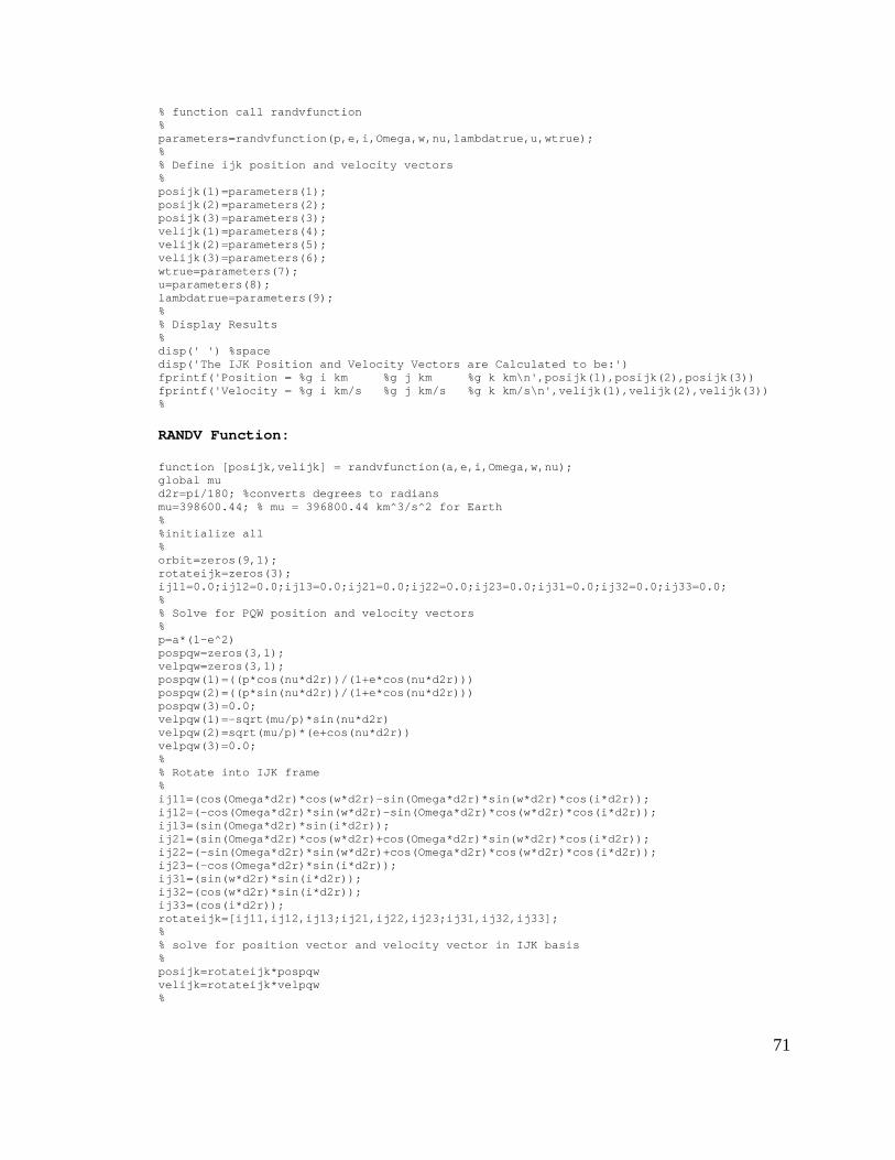
71

% function call randvfunction % parameters=randvfunction(p,e,i,Omega,w,nu,lambdatrue,u,wtrue); % % Define ijk position and velocity vectors % posijk(1)=parameters(1); posijk(2)=parameters(2); posijk(3)=parameters(3); velijk(1)=parameters(4); velijk(2)=parameters(5); velijk(3)=parameters(6); wtrue=parameters(7); u=parameters(8); lambdatrue=parameters(9); % % Display Results % disp(' ') %space disp('The IJK Position and Velocity Vectors are Calculated to be:') fprintf('Position = %g i km %g j km %g k km\n',posijk(1),posijk(2),posijk(3)) fprintf('Velocity = %g i km/s %g j km/s %g k km/s\n',velijk(1),velijk(2),velijk(3)) % RANDV Function: function [posijk,velijk] = randvfunction(a,e,i,Omega,w,nu); global mu d2r=pi/180; %converts degrees to radians mu=398600.44; % mu = 396800.44 km^3/s^2 for Earth % %initialize all % orbit=zeros(9,1); rotateijk=zeros(3); ij11=0.0;ij12=0.0;ij13=0.0;ij21=0.0;ij22=0.0;ij23=0.0;ij31=0.0;ij32=0.0;ij33=0.0; % % Solve for PQW position and velocity vectors % p=a*(1-e^2) pospqw=zeros(3,1); velpqw=zeros(3,1); pospqw(1)=((p*cos(nu*d2r))/(1+e*cos(nu*d2r))) pospqw(2)=((p*sin(nu*d2r))/(1+e*cos(nu*d2r))) pospqw(3)=0.0; velpqw(1)=-sqrt(mu/p)*sin(nu*d2r) velpqw(2)=sqrt(mu/p)*(e+cos(nu*d2r)) velpqw(3)=0.0; % % Rotate into IJK frame % ij11=(cos(Omega*d2r)*cos(w*d2r)-sin(Omega*d2r)*sin(w*d2r)*cos(i*d2r)); ij12=(-cos(Omega*d2r)*sin(w*d2r)-sin(Omega*d2r)*cos(w*d2r)*cos(i*d2r)); ij13=(sin(Omega*d2r)*sin(i*d2r)); ij21=(sin(Omega*d2r)*cos(w*d2r)+cos(Omega*d2r)*sin(w*d2r)*cos(i*d2r)); ij22=(-sin(Omega*d2r)*sin(w*d2r)+cos(Omega*d2r)*cos(w*d2r)*cos(i*d2r)); ij23=(-cos(Omega*d2r)*sin(i*d2r)); ij31=(sin(w*d2r)*sin(i*d2r)); ij32=(cos(w*d2r)*sin(i*d2r)); ij33=(cos(i*d2r)); rotateijk=[ij11,ij12,ij13;ij21,ij22,ij23;ij31,ij32,ij33]; % % solve for position vector and velocity vector in IJK basis % posijk=rotateijk*pospqw velijk=rotateijk*velpqw %

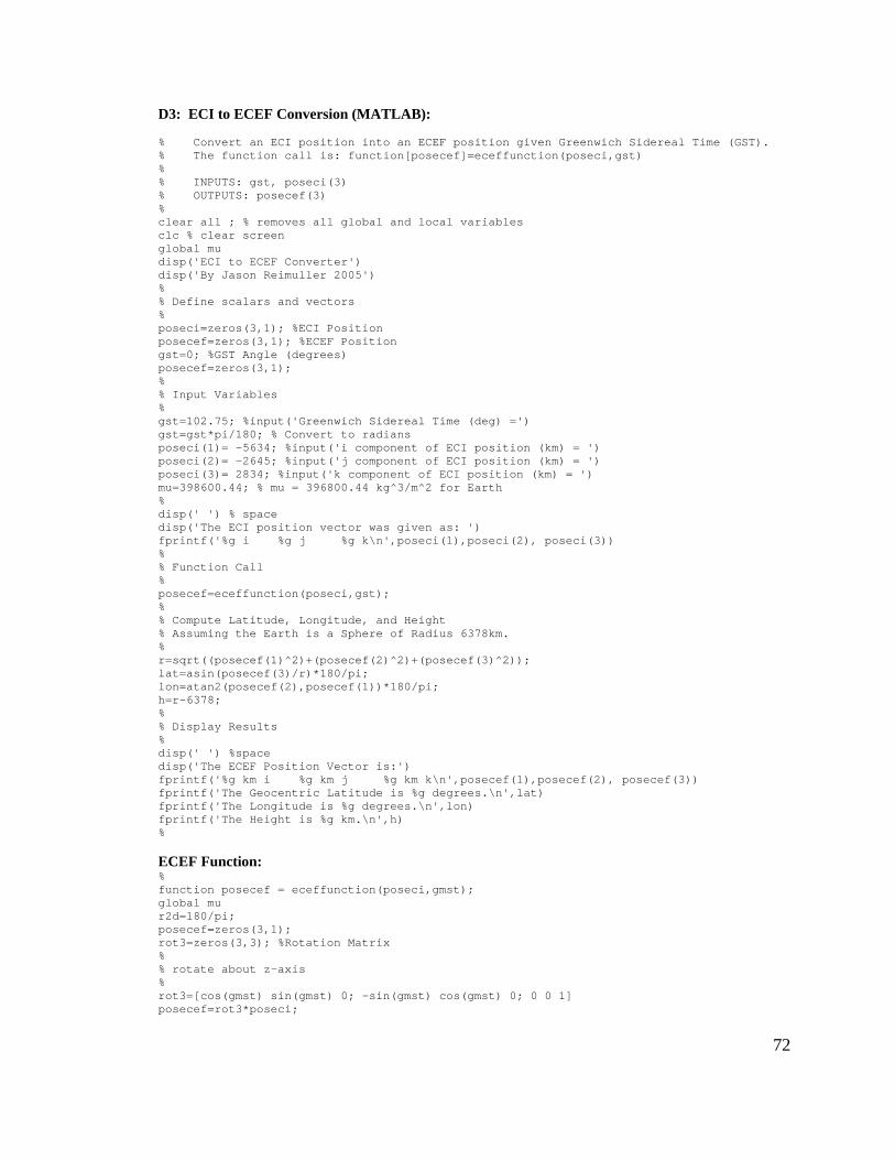
72

D3: ECI to ECEF Conversion (MATLAB): % Convert an ECI position into an ECEF position given Greenwich Sidereal Time (GST). % The function call is: function[posecef]=eceffunction(poseci,gst) % % INPUTS: gst, poseci(3) % OUTPUTS: posecef(3) % clear all ; % removes all global and local variables clc % clear screen global mu disp('ECI to ECEF Converter') disp('By Jason Reimuller 2005') % % Define scalars and vectors % poseci=zeros(3,1); %ECI Position posecef=zeros(3,1); %ECEF Position gst=0; %GST Angle (degrees) posecef=zeros(3,1); % % Input Variables % gst=102.75; %input('Greenwich Sidereal Time (deg) =') gst=gst*pi/180; % Convert to radians poseci(1)= -5634; %input('i component of ECI position (km) = ') poseci(2)= -2645; %input('j component of ECI position (km) = ') poseci(3)= 2834; %input('k component of ECI position (km) = ') mu=398600.44; % mu = 396800.44 kg^3/m^2 for Earth % disp(' ') % space disp('The ECI position vector was given as: ') fprintf('%g i %g j %g k\n',poseci(1),poseci(2), poseci(3)) % % Function Call % posecef=eceffunction(poseci,gst); % % Compute Latitude, Longitude, and Height % Assuming the Earth is a Sphere of Radius 6378km. % r=sqrt((posecef(1)^2)+(posecef(2)^2)+(posecef(3)^2)); lat=asin(posecef(3)/r)*180/pi; lon=atan2(posecef(2),posecef(1))*180/pi; h=r-6378; % % Display Results % disp(' ') %space disp('The ECEF Position Vector is:') fprintf('%g km i %g km j %g km k\n',posecef(1),posecef(2), posecef(3)) fprintf('The Geocentric Latitude is %g degrees.\n',lat) fprintf('The Longitude is %g degrees.\n',lon) fprintf('The Height is %g km.\n',h) % ECEF Function: % function posecef = eceffunction(poseci,gmst); global mu r2d=180/pi; posecef=zeros(3,1); rot3=zeros(3,3); %Rotation Matrix % % rotate about z-axis % rot3=[cos(gmst) sin(gmst) 0; -sin(gmst) cos(gmst) 0; 0 0 1] posecef=rot3*poseci;

73

D4: Range, Azimuth, and Elevation (MATLAB): % Compute the range, elevation, and azimuth of a satellite given an ECEF position and % the latitude, longitude, and height of the tracking station. % The function call is: function[postopo]=topofunction(posecef,lat,lon,h) % % INPUTS: lat, lon, h, posecef(3) % OUTPUTS: range, el, az % clear all ; % removes all global and local variables clc % clear screen global mu d2r=pi/180; %Conversion r2d=180/pi; %Conversion disp('Satellite Range and Az/El Calculator') disp('By Jason Reimuller 2005') recef=[-1000 -8000 5000] % % Function Call % azel=ecef2sezfunction(recef); % % Display Results % el=azel(1)*r2d; az=azel(2)*r2d; range=azel(3); disp(' ') % space disp('From the Perspective of the Ground Station') fprintf('The Elevation is %g degrees.\n',el) fprintf('The Azimuth is %g degrees.\n',az) fprintf('The Range is %g kilometers.\n',range) % TOPO Function: % function azel = topofunction(posecef,possite,lat,lon,h); global mu r2d=180/pi; d2r=pi/180; postopo=zeros(3,1); azel=zeros(3,1); rhoecef=zeros(3,1); rho=0.0; % % Define Rotations % lat=(90-lat)*d2r; lon=lon*d2r; rhoecef=posecef-possite; rot2=zeros(3,3); rot3=zeros(3,3); %Rotation Matrix rot2=[cos(lat) 0 -sin(lat); 0 1 0; sin(lat) 0 cos(lat)]; rot3=[cos(lon) sin(lon) 0; -sin(lon) cos(lon) 0; 0 0 1]; postopo=rot2*rot3*rhoecef; % Solve for Rho (SEZ) % % Solve for Azimuth and Elevation Data % rho=sqrt((postopo(1)^2)+(postopo(2)^2)+(postopo(3)^2)); % azel(1)=asin(postopo(3)/rho); %Elevation in Radians azel(2)=asin(postopo(2)/(sqrt((postopo(1)^2)+(postopo(2)^2)))); % Azimuth in Radians azel(3)=rho; %

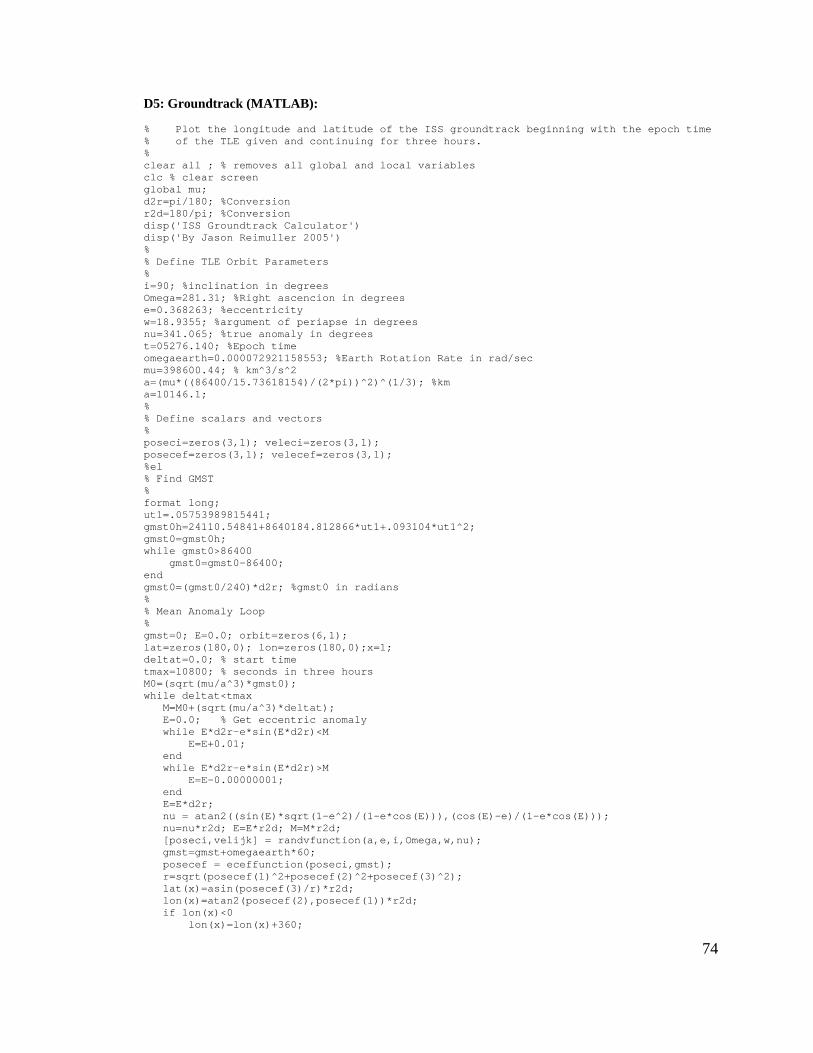
74

D5: Groundtrack (MATLAB): % Plot the longitude and latitude of the ISS groundtrack beginning with the epoch time % of the TLE given and continuing for three hours. % clear all ; % removes all global and local variables clc % clear screen global mu; d2r=pi/180; %Conversion r2d=180/pi; %Conversion disp('ISS Groundtrack Calculator') disp('By Jason Reimuller 2005') % % Define TLE Orbit Parameters % i=90; %inclination in degrees Omega=281.31; %Right ascencion in degrees e=0.368263; %eccentricity w=18.9355; %argument of periapse in degrees nu=341.065; %true anomaly in degrees t=05276.140; %Epoch time omegaearth=0.000072921158553; %Earth Rotation Rate in rad/sec mu=398600.44; % km^3/s^2 a=(mu*((86400/15.73618154)/(2*pi))^2)^(1/3); %km a=10146.1; % % Define scalars and vectors % poseci=zeros(3,1); veleci=zeros(3,1); posecef=zeros(3,1); velecef=zeros(3,1); %el % Find GMST % format long; ut1=.05753989815441; gmst0h=24110.54841+8640184.812866*ut1+.093104*ut1^2; gmst0=gmst0h; while gmst0>86400 gmst0=gmst0-86400; end gmst0=(gmst0/240)*d2r; %gmst0 in radians % % Mean Anomaly Loop % gmst=0; E=0.0; orbit=zeros(6,1); lat=zeros(180,0); lon=zeros(180,0);x=1; deltat=0.0; % start time tmax=10800; % seconds in three hours M0=(sqrt(mu/a^3)*gmst0); while deltat<tmax M=M0+(sqrt(mu/a^3)*deltat); E=0.0; % Get eccentric anomaly while E*d2r-e*sin(E*d2r)<M E=E+0.01; end while E*d2r-e*sin(E*d2r)>M E=E-0.00000001; end E=E*d2r; nu = atan2((sin(E)*sqrt(1-e^2)/(1-e*cos(E))),(cos(E)-e)/(1-e*cos(E))); nu=nu*r2d; E=E*r2d; M=M*r2d; [poseci,velijk] = randvfunction(a,e,i,Omega,w,nu); gmst=gmst+omegaearth*60; posecef = eceffunction(poseci,gmst); r=sqrt(posecef(1)^2+posecef(2)^2+posecef(3)^2); lat(x)=asin(posecef(3)/r)*r2d; lon(x)=atan2(posecef(2),posecef(1))*r2d; if lon(x)<0 lon(x)=lon(x)+360;

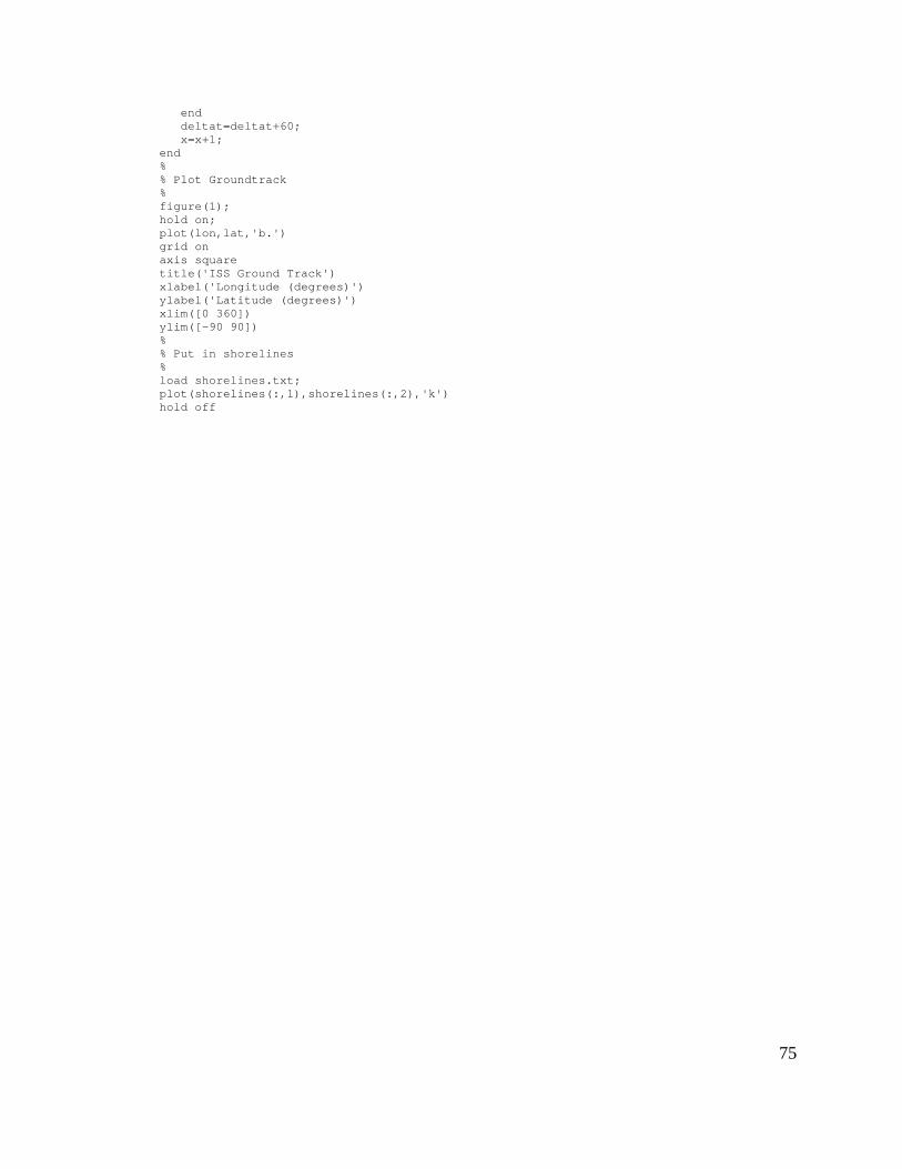
75

end deltat=deltat+60; x=x+1; end % % Plot Groundtrack % figure(1); hold on; plot(lon,lat,'b.') grid on axis square title('ISS Ground Track') xlabel('Longitude (degrees)') ylabel('Latitude (degrees)') xlim([0 360]) ylim([-90 90]) % % Put in shorelines % load shorelines.txt; plot(shorelines(:,1),shorelines(:,2),'k') hold off

76

ECEF to SEZ Function: % function azel = ecef2sezfunction(recef); global mu r2d=180/pi; d2r=pi/180; rhosez=zeros(3,1); rhoecef=zeros(3,1); azel=zeros(3,1); % % rboulder=6379.77 lonboulder=-105.270*d2r latboulder=40.015*d2r recef=[-1000 -8000 5000] rsite=[rboulder*cos(latboulder)*cos(lonboulder) rboulder*cos(latboulder)*sin(lonboulder) rboulder*sin(latboulder)] rhoecef=recef-rsite % % Define Rotations % lat=40.015*d2r; lon=-105.270*d2r; rot=zeros(3,3); %Rotation Matrix rot=[sin(lat)*cos(lon) sin(lat)*sin(lon) -cos(lat); -sin(lon) cos(lon) 0; cos(lat)*cos(lon) cos(lat)*sin(lon) sin(lat)] rhosez=rot*rhoecef' % % Solve for Azimuth and Elevation Data % rho=sqrt((rhosez(1)^2)+(rhosez(2)^2)+(rhosez(3)^2)) azel(1)=asin(rhosez(3)/rho) %Elevation in Radians az1=asin(rhosez(2)/(sqrt((rhosez(1)^2)+(rhosez(2)^2)))) az2=acos(-rhosez(1)/(sqrt((rhosez(1)^2)+(rhosez(2)^2)))) azel(2)=atan2(az1,az2) azel(3)=rho %

77

Vita

Jason David Reimuller was born in Vienna, Austria on 29 May 1972 to Patricia

Helmer Chapman and David Paul Reimuller. He has received a Bachelor of Science in

Aerospace Engineering from the Florida Institute of Technology, a Master of Science in

Physics from San Francisco State University, a Master of Science in Aviation Systems

from the University of Tennessee, and is currently pursuing a doctoral degree in

Aerospace Engineering Sciences from the University of Colorado, Boulder. He has

industry experience in satellite operations, propulsion engineering, atmospheric remote

sensing, and the cost analysis and acquisition of spacecraft systems. He has served as an

officer in the US Air Force.