Mon. Not. R. Astron. Soc. 347, 508–540 (2004) The depolarization properties of powerful radio sources: breaking the radio power versus redshift degeneracy J. A. Goodlet, 1 C. R. Kaiser, 1 P. N. Best 2 and J. Dennett-Thorpe 3 1 Department of Physics and Astronomy, University of Southampton, Southampton SO17 1BJ 2 Institute for Astronomy, Royal Observatory Edinburgh, Blackford Hill, Edinburgh EH9 3HJ 3 Astron, PO Box 2, 7990 AA Dwingeloo, the Netherlands Accepted 2003 September 17. Received 2003 September 17; in original form 2002 November 28 ABSTRACT We define three samples of extragalactic radio sources of Fanaroff–Riley type II, containing 26 objects in total. The control sample consists of 6C and 7C sources with radio powers of around 10 27 W Hz −1 at 151 MHz and redshifts of z ∼ 1. The other samples contain 3CRR sources either with comparable redshifts but radio powers about a decade larger or with comparable radio powers but redshifts around z ∼ 0.4. We use these samples to investigate the possible evolution of their depolarization and rotation measure properties with redshift and radio power independently. We used VLA data for all sources at ∼4800 MHz and two frequencies within the 1400-MHz band, either from our own observations or from the archive. We present maps of the total intensity flux, polarized flux, depolarization, spectral index, rotation measure and magnetic field direction where not previously published. Radio cores were detected in 12 of the 26 radio sources. Of the sources, 14 show a strong Laing–Garrington effect, but almost all of the sources show some depolarization asymmetry. All sources show evidence for an external Faraday screen being responsible for the observed depolarization. We find that sources at higher redshift are more strongly depolarized. Rotation measure shows no trend with either redshift or radio power. However, variations in the rotation measure across individual sources increase with the redshift of the sources but do not depend on their radio power. Key words: magnetic fields – polarization – galaxies: active – galaxies: jets. 1 INTRODUCTION Observations of the polarization properties of extragalactic radio sources can provide information on the relationships between the radio source properties and their environments as well as the evo- lution of both with redshift. Many previous studies of variations in polarization properties have suffered from a degeneracy between radio power and redshift due to Malmquist bias, present in all flux- limited samples. A good example of this effect is the depolarization correlations found independently by Kronberg, Conway & Gilbert (1972) and Morris & Tabara (1973). Kronberg et al. (1972) found that depolarization of the radio lobes generally increased with redshift whereas Morris & Tabara (1973) found depolarization to increase with radio luminosity. Because of the flux-limited samples (PKS and 3C) used by both authors, it is difficult to distinguish which is the fundamental correlation, or whether some combination of the two occurs. Both suggestions have ready explanations: (i) If radio sources are confined by a dense medium, then synchrotron losses due to adiabatic expansion are re- duced, the internal magnetic field is stronger and a more luminous E-mail: [email protected] radio source results; if this confining medium also acts as a Faraday medium, more luminous sources will tend to be more depolarized. (ii) Sources at different cosmological epochs may reside in differ- ent environments and/or their intrinsic properties may change with redshift. Hill & Lilly (1991) observed that galaxy densities around Fanaroff–Riley type II (FRII) radio sources increased with red- shift out to z ≈ 0.5 and beyond, but Wold et al. (2001) did not find this trend in a recent study. Welter, Perry & Kronberg (1984) argued that the increase in rotation measure with redshift is primarily attributable to an increasing contribution of interven- ing matter. However, depolarization asymmetries within a source, e.g the Laing–Garrington effect, increase with redshift, which im- plies an origin local to the host galaxy (Garrington & Conway 1991). To break this apparent degeneracy effect, we defined three sub- samples of sources chosen from the 3CRR and 6C/7C catalogues: The control sample consists of 6C and 7C sources at redshift ≈1 with radio powers of around 10 27 W Hz −1 at 151 MHz. Another sample at the same redshift consists of 3CRR sources with radio powers around a magnitude higher at 151 MHz. The final sample consists of 3CRR sources at redshift z ≈ 0.4, again with radio pow- ers of around 10 27 W Hz −1 at 151 MHz (Fig. 1). The observations C 2004 RAS

Welcome message from author
This document is posted to help you gain knowledge. Please leave a comment to let me know what you think about it! Share it to your friends and learn new things together.
Transcript
Mon. Not. R. Astron. Soc. 347, 508–540 (2004)
The depolarization properties of powerful radio sources: breakingthe radio power versus redshift degeneracy
J. A. Goodlet,1� C. R. Kaiser,1 P. N. Best2 and J. Dennett-Thorpe3
1Department of Physics and Astronomy, University of Southampton, Southampton SO17 1BJ2Institute for Astronomy, Royal Observatory Edinburgh, Blackford Hill, Edinburgh EH9 3HJ3Astron, PO Box 2, 7990 AA Dwingeloo, the Netherlands
Accepted 2003 September 17. Received 2003 September 17; in original form 2002 November 28
ABSTRACTWe define three samples of extragalactic radio sources of Fanaroff–Riley type II, containing 26objects in total. The control sample consists of 6C and 7C sources with radio powers of around1027 W Hz−1 at 151 MHz and redshifts of z ∼ 1. The other samples contain 3CRR sourceseither with comparable redshifts but radio powers about a decade larger or with comparableradio powers but redshifts around z ∼ 0.4. We use these samples to investigate the possibleevolution of their depolarization and rotation measure properties with redshift and radio powerindependently. We used VLA data for all sources at ∼4800 MHz and two frequencies withinthe 1400-MHz band, either from our own observations or from the archive. We present mapsof the total intensity flux, polarized flux, depolarization, spectral index, rotation measure andmagnetic field direction where not previously published. Radio cores were detected in 12 ofthe 26 radio sources. Of the sources, 14 show a strong Laing–Garrington effect, but almost allof the sources show some depolarization asymmetry. All sources show evidence for an externalFaraday screen being responsible for the observed depolarization. We find that sources at higherredshift are more strongly depolarized. Rotation measure shows no trend with either redshiftor radio power. However, variations in the rotation measure across individual sources increasewith the redshift of the sources but do not depend on their radio power.
Key words: magnetic fields – polarization – galaxies: active – galaxies: jets.
1 I N T RO D U C T I O N
Observations of the polarization properties of extragalactic radiosources can provide information on the relationships between theradio source properties and their environments as well as the evo-lution of both with redshift. Many previous studies of variations inpolarization properties have suffered from a degeneracy betweenradio power and redshift due to Malmquist bias, present in all flux-limited samples. A good example of this effect is the depolarizationcorrelations found independently by Kronberg, Conway & Gilbert(1972) and Morris & Tabara (1973).
Kronberg et al. (1972) found that depolarization of the radio lobesgenerally increased with redshift whereas Morris & Tabara (1973)found depolarization to increase with radio luminosity. Because ofthe flux-limited samples (PKS and 3C) used by both authors, itis difficult to distinguish which is the fundamental correlation, orwhether some combination of the two occurs. Both suggestionshave ready explanations: (i) If radio sources are confined by a densemedium, then synchrotron losses due to adiabatic expansion are re-duced, the internal magnetic field is stronger and a more luminous
�E-mail: [email protected]
radio source results; if this confining medium also acts as a Faradaymedium, more luminous sources will tend to be more depolarized.(ii) Sources at different cosmological epochs may reside in differ-ent environments and/or their intrinsic properties may change withredshift.
Hill & Lilly (1991) observed that galaxy densities aroundFanaroff–Riley type II (FRII) radio sources increased with red-shift out to z ≈ 0.5 and beyond, but Wold et al. (2001) didnot find this trend in a recent study. Welter, Perry & Kronberg(1984) argued that the increase in rotation measure with redshiftis primarily attributable to an increasing contribution of interven-ing matter. However, depolarization asymmetries within a source,e.g the Laing–Garrington effect, increase with redshift, which im-plies an origin local to the host galaxy (Garrington & Conway1991).
To break this apparent degeneracy effect, we defined three sub-samples of sources chosen from the 3CRR and 6C/7C catalogues:The control sample consists of 6C and 7C sources at redshift ≈1with radio powers of around 1027 W Hz−1 at 151 MHz. Anothersample at the same redshift consists of 3CRR sources with radiopowers around a magnitude higher at 151 MHz. The final sampleconsists of 3CRR sources at redshift z ≈ 0.4, again with radio pow-ers of around 1027 W Hz−1 at 151 MHz (Fig. 1). The observations
C© 2004 RAS

Depolarization properties of powerful radio sources 509
Figure 1. A radio power–redshift plot showing the three subsamples usedin the observations. Sample A is represented by ‘×’, sample B by ‘◦’ andsample C by ‘∗’. The lines mark the flux limits for the 3CRR and 6C samples.A spectral index of 0.75 was used to shift the 3CRR data to 151 MHz.
of sample sources can then be used to study the source propertiesand the medium around the source, thus discovering which corre-late with redshift and which correlate with radio power. This shouldenable us to answer the following questions:
(i) Does a relationship exist between radio power and the envi-ronment in which a given radio source lives?
(ii) Do the environments evolve with redshift?
The structure of this paper is as follows. Section 2 describes indetail the sample selection and the VLA observations. Section 3contains the results, including the maps of the 26 sources from thethree samples. Section 4 discusses the observed trends across thesamples, detailing any correlations between observables. Section 5summarizes the conclusions of the paper. All values are calculatedassuming H0 = 50 km s−1 Mpc−1 and �m = 0.5 (� = 0).
2 T H E V L A O B S E RVAT I O N SA N D DATA R E D U C T I O N
2.1 Sample selection
Sample A was defined as a subsample chosen from the 6CE (Ealeset al. 1997) subregion of the 6C survey (Hales et al. 1990), andthe 7C III subsample (Lacy et al. 1999) drawn from the 7C and 8Csurveys (Pooley, Waldram & Riley 1998). The selected sources haveredshifts 0.8 < z < 1.3, and radio powers at 151 MHz between 6.5 ×1026 W Hz−1 < P151 MHz < 1.35 × 1027 W Hz−1. Sample B wasdefined as a subsample from the revised 3CRR survey by Laing,Riley & Longair (1983) containing sources within the same redshiftrange but with powers in the range 6.5 × 1027 W Hz−1 < P151 MHz <
1.35 × 1028 W Hz−1. Sample C is also from the 3CRR catalogue; ithas the same radio power distribution as the control sample, sampleA, but with 0.3 < z < 0.5. We only include sources that were moreluminous than the flux limits of the original samples at 151 MHz(Fig. 1). In all samples only sources with angular sizes θ � 10 arcsec(corresponding to≈90 kpc at z=1) were included (see Table 1). Thisangular size limit is imposed by the depolarization measurements, asthey require a minimum of 10 independent telescope beams (1 arcsecper beam) over the entire source. The distributions of linear sizesof the radio lobes are reasonably matched across all the samples
Table 1. Details of the sources in samples A, B and C. Sources in italicsare quasars. σ ν gives the noise level in the final total flux maps at frequency ν.
Source z P151 MHz Angular size σ 4.8 σ 1.4
(W Hz−1) (arcsec) (πJy) (πJy)
6C 0943+39 1.04 1.0 × 1027 10 20 556C 1011+36 1.04 1.1 × 1027 49 15 656C 1018+37 0.81 8.8 × 1026 64 24 506C 1129+37 1.06 1.1 × 1027 15 21 606C 1256+36 1.07 1.3 × 1027 14 18 706C 1257+36 1.00 1.1 × 1027 38 33 1007C 1745+642 1.23 9.5 × 1026 16 30 607C 1801+690 1.27 1.0 × 1027 21 24 757C 1813+684 1.03 7.1 × 1026 52 23 47
3C 65 1.18 1.0 × 1028 17 22 613C 68.1 1.24 1.1 × 1028 52 41 1003C 252 1.11 7.2 × 1027 60 23 1003C 265 0.81 6.5 × 1027 78 32 703C 268.1 0.97 1.0 × 1028 46 32 683C 267 1.14 1.0 × 1028 38 25 613C 280 1.00 1.2 × 1028 15 33 753C 324 1.21 1.3 × 1028 10 26 70
4C 16.49 1.29 9.9 × 1027 16 25 813C 16 0.41 7.4 × 1026 63 36 803C 42 0.40 7.5 × 1026 28 29 703C 46 0.44 7.9 × 1027 168 20 533C 299 0.37 6.9 × 1026 11 39 773C 341 0.45 8.8 × 1026 70 26 883C 351 0.37 7.6 × 1026 65 31 1003C 457 0.43 9.6 × 1027 190 18 804C 14.27 0.39 8.8 × 1026 30 30 90
(Fig. 2). Each sample initially contained nine sources; the source3C 109 was subsequently excluded from sample C as the VLA datawere of much poorer quality than the rest of the sample. Each ofthe resulting subsamples contains one to three quasars. The sourcesin the three subsamples are representative of sources with similarredshifts, radio powers and sizes. However, the samples are notstatistically complete because of observing time limitations. Wepicked sources that were fairly well observed at 4.8 GHz at B-array(and C-array if needed) in the archives, ensuring that a minimum ofnew observations was needed. Full details of the samples are givenin Table 1.
The ratio of angular to physical size varies only by a factor of1.3 between z = 0.4 and z = 1.4. This ensured that all the sourceswere observed at similar physical resolutions. All redshift valuesfor 6C sources were taken from Eales et al. (1997) except for 6C1018+37, which was taken from Rawlings, Eales & Lacy (2001).The 7C sources were taken from Lacy et al. (1999). The 3CRRsources were taken from Spinrad et al. (1985), 4C 16.49 was takenfrom Barkhouse & Hall (2001), 4C 14.27 was taken from Herbig &Readhead (1992) and 3C 457 was taken from Hewitt & Burbridge(1991).
2.2 Very large array observations
Observations of all 26 radio galaxies were made close to 1.4 GHzusing the A-array configuration and a 25-MHz bandwidth. Thisbandwidth was used instead of 50 MHz to reduce the effect ofbandwidth depolarization. The maximum angular size that can besuccessfully imaged using A-array at 1.4 GHz is 38 arcsec. Some 12sources were larger than this and were observed additionally withB-array. Observations were also made at 4.8 GHz using a 50-MHz
C© 2004 RAS, MNRAS 347, 508–540

510 J. A. Goodlet et al.
(a) (b)
Figure 2. Linear size–redshift plots of the three subsamples used in the observations. Symbols as in Fig. 1. Part (a) assumes H0 = 50 km s−1 Mpc−1 and �m =0.5, �� = 0. Part (b) assumes H0 = 50 km s−1 Mpc−1, and �m = 0.35, �� = 0.65.
Table 2. Details of the VLA observations for sample A with the integration times included. SeeTables 3 and 4 for samples B and C, respectively.
Source Array Frequency Bandwidth Observing prog. Int.config. (MHz) (MHz) (dd/mm/yy) (min)
6C 0943+39 A 1465, 1665 25 31/07/99 (AD429) 16B 4885, 4535 50 20/05/01 (AD444) 31
6C 1011+36 A 1465, 1665 25 31/07/99 (AD429) 16B 1452, 1652 25 20/05/01 (AD444) 17B 4885, 4535 50 25/02/97 (AL397) 21
4885, 4535 50 20/05/01 (AD444) 30C 4885, 4535 50 12/06/00 (AD429) 20
6C 1018+37 A 1465, 1665 25 31/07/99 (AD429) 16B 1452, 1652 25 20/05/01 (AD444) 17B 4885, 4535 50 20/05/01 (AD444) 31C 4885, 4535 50 12/06/00 (AD429) 20
6C 1129+37 A 1465, 1665 25 31/07/99 (AD429) 16B 4885, 4535 50 20/05/01 (AD444) 17
4885, 4535 50 25/02/97 (AL397) 21
6C 1256+36 A 1465, 1665 25 31/07/99 (AD429) 16B 4885, 4535 50 27/02/93 (AR287) 15
6C 1257+36 A 1465, 1665 25 31/07/99 (AD429) 16B 4885, 4535 50 20/05/01 (AD444) 16
4885, 4535 50 25/02/97 (AL397) 22
7C 1745+642 A 1465, 1665 25 31/07/99 (AD429) 16B 4885, 4535 50 20/05/01 (AD444) 11
4885, 4535 50 23/11/97 (AL401) 31
7C 1801+690 A 1465, 1665 25 31/07/99 (AD429) 16B 4885, 4535 50 26/03/96 (AB978) 29
4885, 4535 50 23/11/97 (AL401) 17
7C 1813+684 A 1465, 1665 25 31/07/99 (AD429) 16B 1452, 1652 25 20/05/01 (AD444) 16B 4885, 4535 50 20/05/01 (AD444) 39
4885, 4535 50 23/11/97 (AL401) 19C 4885, 4535 50 12/06/00 (AD429) 20
bandwidth. The maximum observable angular size in B-array at4.8 GHz is 36 arcsec. The same 12 sources as before were thenobserved at 4.8 GHz with C-array. This ensured that both 1.4 and5 GHz observations were equally matched in sensitivity and reso-lution. Details of the observations are given in Tables 2–4.
Sources in the 6C and 7C samples have a typical bridge surfacebrightness of ≈70 µJy beam−1 in 5-GHz A-array observations (Bestet al. 1999). In order to detect 10 per cent polarization at 3σ inB-array observations, we required an rms noise level of 20 µJybeam−1, corresponding to 70 min of integration time. At 1.4 GHz,
C© 2004 RAS, MNRAS 347, 508–540

Depolarization properties of powerful radio sources 511
Table 3. Details of the VLA observations for sample B.
Source Array Frequency Bandwidth Observing prog. Int.config. (MHz) (MHz) (dd/mm/yy) (min)
3C 65 A 1465, 1665 25 31/07/99 (AD429) 16B 4885, 4535 50 20/05/01 (AD444) 20
3C 68.1 A 1417, 1652 25 31/07/99 (AD429) 16B 1417, 1652 25 13/07/86 (AL113) 20B 4885, 4535 50 19/07/86 (AB369) 300C 4885, 4535 50 12/06/00 (AD429) 20
3C 252 A 1465, 1665 25 31/07/99 (AD429) 16B 1465, 1665 25 20/05/01 (AD444) 27B 4885, 4535 50 19/07/86 (AB369) 97C 4885, 4535 50 12/06/00 (AD429) 20
3C 265 A 1417, 1652 25 31/07/99 (AD429) 16B 1417, 1652 25 13/07/86 (AL113) 30B 4873, 4823 50 17/12/83 (AM224) 238C 4873, 4823 50 12/06/00 (AD429) 20
3C 267 A 1465, 1665 25 31/07/99 (AD429) 16B 4873, 4823 50 17/12/83 (AM224) 56
3C 268.1 A 1417, 1652 25 31/07/99 (AD429) 16B 1417, 1652 25 13/07/86 (AL113) 30B 4885, 4835 50 15/08/88 (AR166) 20
4885, 4835 50 01/06/85 (AR123) 21C 4885, 4835 50 06/11/86 (AL124) 102
3C 280 A 1465, 1665 25 31/07/99 (AD429) 16B 4873, 4823 50 17/12/83 (AM224) 46
3C 324 A 1465, 1665 25 31/07/99 (AD429) 16B 4873, 4823 50 17/12/83 (AM224) 51
4C 16.49 A 1465, 1652 25 31/07/99 (AD429) 16B 4885, 4535 50 04/03/97 (AB796) 30
assuming α = −1.3, bridges will be a factor of 4 more luminous. Atthis frequency, the exposure time is set by the requirement to havean adequate amount of uv coverage to map the bridge structures.The 20-min observations were split into 4 × 5 min intervals. Thisobservation splitting to improve uv coverage was also done for the4.8-GHz data.
At 1.4 GHz the integration time on all the sources is above theminimum required for good signal-to-noise ratio. As Table 2 demon-strates, for many of our sources the integration times at 5 GHz areconsiderably less than the 70 min requirement, as a result of tele-scope time constraints. Many of the observed properties that dependon polarization observations (e.g. depolarization and rotation mea-sure) are therefore poorly measured in the fainter components at5 GHz. The values obtained are then only representative of the smallregion detected and not the entire component. Spectral index is in-dependent of the polarization measurements and so it is relativelyunaffected by the short integration times.
The 3CRR sources are more luminous, but much of this is due tothe increase in the luminosity of their hotspots; their bridge struc-tures are only a few times brighter than those of the 6C/7C IIIsources. To reach a 3σ detection of 7 per cent polarization on thebridge structures, a total integration time of 30 min was requiredat 5 GHz and 20 min at 1.4 GHz, split into 3–4 min intervals toimprove uv coverage. The vast majority of the sources in samplesB and C had at least this minimum amount of time on source (seeTables 3 and 4).
Most observations at 1.4 GHz using A-array were obtained on1999 July 31 (AD429). The data from this day are strongly affectedby a thunderstorm at the telescope site during most of the observa-
Table 4. Details of the VLA observations for sample C.
Source Array Frequency Bandwidth Observing prog. Int.config. (MHz) (MHz) (dd/mm/yy) (min)
3C 16 A 1452, 1502 25 14/09/87 (AL146) 59B 1452, 1502 25 25/11/87 (AL146) 39B 4885, 4535 50 20/05/01 (AD444) 20
4885, 4535 50 17/11/87 (AH271) 10C 4885, 4535 50 12/06/00 (AD429) 20
3C 42 A 1452, 1502 25 14/09/87 (AL146) 40B 4885, 4535 50 23/12/91 (AF213) 67
3C 46 A 1452, 1502 25 31/07/99 (AD429) 16B 1452, 1502 25 25/11/87 (AL146) 35B 4885, 4535 50 20/05/01 (AD444) 20C 4885, 4535 50 12/06/00 (AD429) 20
3C 299 A 1452, 1502 25 31/07/99 (AD429) 16B 4835, 4535 50 20/05/01 (AD444) 15
4885, 4835 50 28/01/98 (AP331) 15
3C 341 A 1452, 1502 25 14/09/87 (AL146) 38B 1452, 1502 25 25/11/87 (AL146) 47B 4885, 4535 50 20/05/01 (AD444) 11
4935, 4535 50 26/10/92 (AA133) 25C 4885, 4535 50 12/06/00 (AD429) 20
3C 351 A 1452, 1502 25 31/07/99 (AD429) 16B 1452, 1502 25 25/11/87 (AL146) 56B 4885, 4835 50 19/07/86 (AB369) 12
4885, 4535 50 20/05/01 (AD444) 16C 4885, 4835 50 09/10/87 (AA64) 22
3C 457 A 1452, 1502 25 31/07/99 (AD429) 16B 1452, 1502 25 25/11/87 (AL146) 30B 4885, 4535 50 20/05/01 (AD444) 50C 4885, 4535 50 12/06/00 (AD429) 20
4C 14.27 A 1452, 1502 25 14/09/87 (AL146) 28B 4885, 4535 50 20/05/01 (AD444) 17
tions. Even after removal of bad baselines and antennas, the noiselevel in these data remained at least twice that of the theoreticalvalue. However, careful calibration and CLEANing reduced this ef-fect to a minimum. Sample A was most affected by the thunderstormand the lack of observing time at all frequencies. However, we findthat the results obtained by Best et al. (1999) for some of the sourcesin sample A are in good agreement with our results. We are thereforeconfident that our data are reliable for fluxes above the 3σ noise level.We checked the polarization calibration of 1999 July 31 (AD429)by comparing with the B-array data at 1.4 GHz (for the 12 sourcesthat had B-array data) to confirm that the position angle (PA) ofboth data sets agreed to within 15 degrees in all sources. This ad-ditional check allowed us to ensure that the 1.4-GHz polarizationangle calibration was accurate.
The data were reduced using the AIPS software package producedby the National Radio Astronomy Observatory. At 1.4 GHz the twointermediate frequencies (IFs) were reduced separately, producingindependent observations at 1665 and 1465 MHz. The reason forthe separation is due to the significant rotation of the polarizationangle between the two frequencies. If the two frequencies were notseparated, then there would be some degree of artificial depolariza-tion at 1.4 GHz; this was not a problem at 4.8 GHz. Each sourcewas then CLEANed using IMAGR, an AIPS task, and then improvedby two cycles of phase self-calibration followed by amplitude–phase self-calibration. For sources larger than 12 arcsec, the uv datafrom the low-resolution array configurations were self-calibratedusing source models resulting from the high-resolution arrays to
C© 2004 RAS, MNRAS 347, 508–540
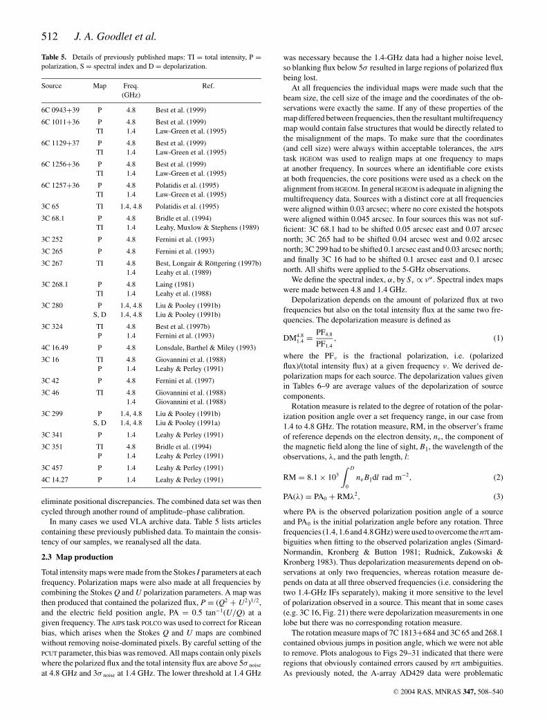
512 J. A. Goodlet et al.
Table 5. Details of previously published maps: TI = total intensity, P =polarization, S = spectral index and D = depolarization.
Source Map Freq. Ref.(GHz)
6C 0943+39 P 4.8 Best et al. (1999)
6C 1011+36 P 4.8 Best et al. (1999)TI 1.4 Law-Green et al. (1995)
6C 1129+37 P 4.8 Best et al. (1999)TI 1.4 Law-Green et al. (1995)
6C 1256+36 P 4.8 Best et al. (1999)TI 1.4 Law-Green et al. (1995)
6C 1257+36 P 4.8 Polatidis et al. (1995)TI 1.4 Law-Green et al. (1995)
3C 65 TI 1.4, 4.8 Polatidis et al. (1995)
3C 68.1 P 4.8 Bridle et al. (1994)TI 1.4 Leahy, Muxlow & Stephens (1989)
3C 252 P 4.8 Fernini et al. (1993)
3C 265 P 4.8 Fernini et al. (1993)
3C 267 TI 4.8 Best, Longair & Rottgering (1997b)1.4 Leahy et al. (1989)
3C 268.1 P 4.8 Laing (1981)TI 1.4 Leahy et al. (1988)
3C 280 P 1.4, 4.8 Liu & Pooley (1991b)S, D 1.4, 4.8 Liu & Pooley (1991b)
3C 324 TI 4.8 Best et al. (1997b)P 1.4 Fernini et al. (1993)
4C 16.49 P 4.8 Lonsdale, Barthel & Miley (1993)
3C 16 TI 4.8 Giovannini et al. (1988)P 1.4 Leahy & Perley (1991)
3C 42 P 4.8 Fernini et al. (1997)
3C 46 TI 4.8 Giovannini et al. (1988)1.4 Giovannini et al. (1988)
3C 299 P 1.4, 4.8 Liu & Pooley (1991b)S, D 1.4, 4.8 Liu & Pooley (1991a)
3C 341 P 1.4 Leahy & Perley (1991)
3C 351 TI 4.8 Bridle et al. (1994)P 1.4 Leahy & Perley (1991)
3C 457 P 1.4 Leahy & Perley (1991)
4C 14.27 P 1.4 Leahy & Perley (1991)
eliminate positional discrepancies. The combined data set was thencycled through another round of amplitude–phase calibration.
In many cases we used VLA archive data. Table 5 lists articlescontaining these previously published data. To maintain the consis-tency of our samples, we reanalysed all the data.
2.3 Map production
Total intensity maps were made from the Stokes I parameters at eachfrequency. Polarization maps were also made at all frequencies bycombining the Stokes Q and U polarization parameters. A map wasthen produced that contained the polarized flux, P = (Q2 + U2)1/2,and the electric field position angle, PA = 0.5 tan−1(U/Q) at agiven frequency. The AIPS task POLCO was used to correct for Riceanbias, which arises when the Stokes Q and U maps are combinedwithout removing noise-dominated pixels. By careful setting of thePCUT parameter, this bias was removed. All maps contain only pixelswhere the polarized flux and the total intensity flux are above 5σ noise
at 4.8 GHz and 3σ noise at 1.4 GHz. The lower threshold at 1.4 GHz
was necessary because the 1.4-GHz data had a higher noise level,so blanking flux below 5σ resulted in large regions of polarized fluxbeing lost.
At all frequencies the individual maps were made such that thebeam size, the cell size of the image and the coordinates of the ob-servations were exactly the same. If any of these properties of themap differed between frequencies, then the resultant multifrequencymap would contain false structures that would be directly related tothe misalignment of the maps. To make sure that the coordinates(and cell size) were always within acceptable tolerances, the AIPS
task HGEOM was used to realign maps at one frequency to mapsat another frequency. In sources where an identifiable core existsat both frequencies, the core positions were used as a check on thealignment from HGEOM. In general HGEOM is adequate in aligning themultifrequency data. Sources with a distinct core at all frequencieswere aligned within 0.03 arcsec; where no core existed the hotspotswere aligned within 0.045 arcsec. In four sources this was not suf-ficient: 3C 68.1 had to be shifted 0.05 arcsec east and 0.07 arcsecnorth; 3C 265 had to be shifted 0.04 arcsec west and 0.02 arcsecnorth; 3C 299 had to be shifted 0.1 arcsec east and 0.03 arcsec north;and finally 3C 16 had to be shifted 0.1 arcsec east and 0.1 arcsecnorth. All shifts were applied to the 5-GHz observations.
We define the spectral index, α, by Sν ∝ να . Spectral index mapswere made between 4.8 and 1.4 GHz.
Depolarization depends on the amount of polarized flux at twofrequencies but also on the total intensity flux at the same two fre-quencies. The depolarization measure is defined as
DM4.81.4 = PF4.8
PF1.4, (1)
where the PFν is the fractional polarization, i.e. (polarizedflux)/(total intensity flux) at a given frequency ν. We derived de-polarization maps for each source. The depolarization values givenin Tables 6–9 are average values of the depolarization of sourcecomponents.
Rotation measure is related to the degree of rotation of the polar-ization position angle over a set frequency range, in our case from1.4 to 4.8 GHz. The rotation measure, RM, in the observer’s frameof reference depends on the electron density, ne, the component ofthe magnetic field along the line of sight, B‖, the wavelength of theobservations, λ, and the path length, l:
RM = 8.1 × 10³
∫ D
0
ne B‖dl rad m−2, (2)
PA(λ) = PA0 + RMλ2, (3)
where PA is the observed polarization position angle of a sourceand PA0 is the initial polarization angle before any rotation. Threefrequencies (1.4, 1.6 and 4.8 GHz) were used to overcome the nπ am-biguities when fitting to the observed polarization angles (Simard-Normandin, Kronberg & Button 1981; Rudnick, Zukowski &Kronberg 1983). Thus depolarization measurements depend on ob-servations at only two frequencies, whereas rotation measure de-pends on data at all three observed frequencies (i.e. considering thetwo 1.4-GHz IFs separately), making it more sensitive to the levelof polarization observed in a source. This meant that in some cases(e.g. 3C 16, Fig. 21) there were depolarization measurements in onelobe but there was no corresponding rotation measure.
The rotation measure maps of 7C 1813+684 and 3C 65 and 268.1contained obvious jumps in position angle, which we were not ableto remove. Plots analogous to Figs 29–31 indicated that there wereregions that obviously contained errors caused by nπ ambiguities.As previously noted, the A-array AD429 data were problematic
C© 2004 RAS, MNRAS 347, 508–540

Depolarization properties of powerful radio sources 513
Table 6. Properties of the sample A radio source components. Errors are 5 per cent or less, unless stated otherwise. The spectral indices α are the mean valuesfor each component, calculated between approximately 4800 and 1465 MHz. The depolarization measures DM are the mean values of the ratio of the fractionalpolarization between approximately 4800 and 1465 MHz for each component. The rotation measures RM are the mean values between approximately 4710,1665 and 1465 MHz and are quoted in the observer’s frame of reference. The Faraday dispersion � is given in equation (5). σ RM is the rms in the rotationmeasure. All mean values take into account pixels above 5σ rms at 4.7 GHz and above 3σ rms at 1.4 GHz.
4710 MHz 1465 MHzSource Comp. Total Polar- Total Polar- RM α DM4.8
1.4 Ave. σ RM
flux ization flux ization �
(mJy) (per cent) (mJy) (per cent) (rad m−2) (rad m−2) (rad m−2)
6C 0943+39 W 31.0 11.8 71.7 5.4 1.6 ± 2 −0.72 2.19 15.01 16.1E 42.0 2.7 136.4 0.7 −19.1 ± 6 −1.01 3.86 19.7 101.4
6C 1011+36 N 44.3 7.8 119.6 5.1 30.8 ± 5 −0.88 1.53 11.1 12.8S 18.7 12.2 50.9 11.5 12.6 ± 4 −0.89 1.06 4.1 10.1
Core 3.22 – 0.7 ± 0.5 – – 1.35 – – –
6C 1018+37 NE 46.4 10.0 125.8 8.1 0.85 ± 3 −0.85 1.23 7.71 6.1SW 28.7 7.0 76.3 2.9 11.2 ± 2 −0.84 2.41 15.9 2.9Core 0.63 ± 0.2 – – – – – – – –
6C 1129+37 NW 46.5 7.3 129.1 2.9 −19.3 ± 4 −0.85 2.51 16.3 54.0SE 73.2 16.3 215.0 3.2 0.08 ± 3 −0.90 5.09 21.61 22.0
6C 1256+36 NE 57.8 10.4 148.9 7.7 5.9 ± 3 −0.79 1.35 9.3 21.8SW 101.4 8.9 288.5 8.8 15.4 ± 3 −0.87 1.01 1.7 14.0
6C 1257+36 NW 43.5 17.0 102.2 13.4 −115.3 ± 9 −0.71 1.27 8.3 10.0SE 20.5 9.8 73.0 5.2 −115.6 ± 10 −1.06 1.88 13.5 16.0
Core 0.29 ± 0.08 – – – – – – – –
7C 1745+642 N 23.5 9.6 64.5 5.2 – −0.86 1.85 13.3 –Core 84.1 4.9 69.4 2.9 65.4 ± 4 0.16 ± 0.1 1.69 12.3 20.9
S 33.8 8.6 98.5 9.5 12.8 ± 3 −0.91 0.91 − 3.1
7C 1801+690 N 8.8 ± 3 3.0 28.2 2.7 44.8 ± 3 −0.97 1.11 5.5 16.0Core 79.1 1.8 78.4 4.0 30.3 ± 3 0.007 0.45 – 1.80
S 28.7 10.0 75.8 7.2 20.8 ± 2 −0.81 1.39 9.7 10.0
7C 1813+684 NE 15.0 7.7 44.8 9.5 13.9 ± 3 −0.92 0.81 − 85.0SW 30.2 8.4 78.1 7.4 −68.4± 7 −0.79 1.14 6.1 41.7Core 3.32 – 2.65 – – 0.19 ± 0.1 – – –
and were found to be the cause of the jumps. To overcome thisproblem, we shifted the position angles at 1.4 GHz data down by10–15 degrees when the PA maps were produced. This resolved anyambiguities.
Table 4 shows that all sources in sample C were observed with IFsseparated by only 50 MHz or less at around 1.4 GHz. This means thatthey were not well enough separated at 1.4 GHz to overcome the nπ
ambiguities. To compensate for this lack of separation, the 4.8-GHzobservations were split into their two component frequencies, 4885and 4535 MHz. We then used four frequencies for the fit instead ofthree, but we are still only marginally sensitive to nπ jumps. Theresulting rotation measure maps cover the same frequency range assamples A and B but use different frequencies for the fit. This wasnot possible in the case of 3C 351 and 299, resulting in larger uncer-tainties in the rotation measurements for these sources. In the case ofsample C, for any source that has a large range of rotation measures(>80 rad m−2), the AIPS task RM will force the rotation measure intoa range ±40 rad m−2 around the mean rotation measure. This isdue to the lack of frequency separation at 1.4 GHz and it can causejumps. In the case of 3C 457 these jumps were severe and we wereunable to resolve them. The rotation measure and magnetic fieldmaps for this source were not included in the analysis. The rota-tion measure varies smoothly over all other sources in this sample.The error affects the absolute value of the rotation measure for eachsource and therefore it does not affect the difference in the rotationmeasure, dRM, and the rms variation in the rotation measure, σ RM.
All rotation measure maps contain only pixels where polarizedflux was observed at levels above 3σ noise at all three frequencies.We chose the lower noise threshold to allow for a larger coverageof RM measurements over the lobes. However, even with this lowerthreshold there were still a few sources where there was very littleto no rotation measure observed.
All depolarization, spectral index, rotation measure and magneticfield direction maps were overlaid with contours of total intensityat 4.8 GHz.
Tables 6–9 give the total flux, percentage polarized flux at both1.4 and 4.8 GHz, the depolarization, rotation measure and spectralindex between 1.4 and 4.8 GHz. All properties are averaged oversource components like the source core or individual lobes, andgiven in the observer’s frame of reference. This averaging reducesthe effect of the noise features seen in the maps. The total flux,polarized flux and rotation measure values are the averaged valuesdetermined from the maps with the AIPS task TVSTAT. Percentagepolarization, depolarization and spectral index are then calculatedfrom these average values. All integrated quantities in Tables 6–9are calculated excluding pixels below the 3σ noise threshold.
3 T H E R E S U LT S
In Figs 3–28, maps of the radio properties discussed above are pre-sented for all the sources from the three samples. Each figure showsthe depolarization map (where the polarization was detected at allfrequencies), the spectral index map, the rotation measure map and
C© 2004 RAS, MNRAS 347, 508–540

514 J. A. Goodlet et al.
Table 7. As Table 6 but for sample B.
4790 MHz 1465 MHzSource Comp. Total Polar- Total Polar- RM α DM4.8
1.4 Ave. σ RM
flux ization flux ization �
(mJy) (per cent) (mJy) (per cent) (rad m−2) (rad m−2) (rad m−2)
3C 65 W 524.0 19.3 1683.1 5.4 −82.6 ± 7 −1.0 3.57 19.1 21.4E 240.9 9.2 800.4 7.2 −86.1 ± 6 −1.03 1.28 8.4 9.7
3C 252 NW 178.7 6.4 592.2 5.9 15.7 ± 6 −1.0 1.08 4.7 20.2SE 80.0 14.1 300.5 6.8 58.5 ± 6 −1.1 2.07 14.5 45.4
Core 1.98 – 1.33 – – 0.33 – – –
3C 267 E 184.0 8.9 745.7 6.8 −9.6 ± 3 −1.17 1.31 8.8 24.4Core 1.87 ± 1 – 1.05 ± 2 – – 0.48 – – –
W 479.2 3.5 1294.6 3.3 −21.5 ± 3 −0.83 1.06 4.1 23.4
3C 280 E 326.0 8.0 1219.2 4.4 −37.7 ± 8 −1.01 1.82 13.1 20.1W 1289.2 10.0 3191.6 6.5 −7.5 ± 4 −0.76 1.54 11.1 1.5
3C 324 NE 432.6 9.3 1525.2 5.6 22.1 ± 4 −1.05 1.66 12.1 23.0SW 166.0 7.8 651.8 4.0 43.0 ± 5 −1.14 1.95 13.9 16.8
4C 16.49 N 107.2 8.3 307.2 13.0 −4.3 ± 5 −0.88 0.64 − 56.4Jet 8.5 ± 4 14.5 45.9 7.2 30.1 ± 4 −1.41 2.01 14.2 57.2
Core 9.64 ± 2 2.7 58.2 3.5 – −1.50 0.77 – –S 142.3 7.0 695.3 6.4 0.9 ± 3 −1.32 1.09 5.0 56.4
3C 68.1 N 667.2 8.6 1767.4 7.0 −26.6 ± 5 −0.82 1.23 7.7 27.7S 36.8 11.4 134.6 6.6 57.9 ± 2 −1.08 1.73 12.5 59.8
3C 265 NW 224.0 10.0 478.7 5.8 42.2 ± 6 −0.62 1.72 12.5 21.9SE 318.9 6.2 835.0 4.2 32.8 ± 3 −0.78 1.48 10.6 22.8
3C 268.1 E 262.3 5.0 816.4 3.4 21.7 ± 5 −0.92 1.47 10.5 10.8W 2296.6 4.7 4699.0 2.7 26.8 ± 6 −0.58 1.74 12.6 13.3
Table 8. Reduced χ2 values for the rotation measure fits for Figs 29–31.
Source Lobe n = −1 n = 0 n = 1 Symbol
6C 1256+36 S 382 51 1.91 ×981.6 1.23 976.5 ◦
4C 16.49 N 1.6 669 2917 ◦2772 90.1 1.7 ×
4C 16.49 S 151.9 0.9 62 ◦45.4 0.4 34.8 ×
the magnetic field direction map (when a rotation measure is de-tected), if no previously published maps exist. For the three 7Csources, 6C 1018+37, and 3C 65, 267 and 46, polarization mapshave also been included for both 1.4 and 4.8 GHz, as there are nopublished polarization maps of these sources. Table 5 contains alisting of published maps for all sources. In all cases only regionsfrom the top end of the grey-scales saturate, as we have alwayskept the lowest values well inside the grey-scales, to ensure that noinformation has been lost.
In order to check the quality of our maps we also used the maxi-mum entropy method implemented in the AIPS task VTESS instead ofthe CLEAN algorithm. The resulting maps are not significantly dif-ferent from those produced by the CLEAN algorithm. In fact, VTESS
is not necessarily superior to CLEAN in producing accurate maps ofextended low surface brightness regions (Rupen 1997).
Depolarization shadows (regions where the depolarization is ap-preciably greater than in the surrounding area) are seen in a fewsources, e.g. Fig. 19, and may be real features. These were firstfound by Fomalont et al. (1989) in a study of Fornax A. Depolariza-tion shadows can be caused by the parent galaxy, as in the case of 3C324, or by an external galaxy in the foreground of the source, causinga depolarizing silhouette (Best, Longair & Rottgering 1997a).
Polarization angle measurements are ambiguous by ±nπ and thiscan introduce ambiguities in the rotation measure. A change of π
between 1.4 and 5 GHz introduced by the fitting algorithm willcause a change of ≈80 rad m−2 in rotation measure. To determine ifany strong rotation measure feature is real, a plot of the polarizationangle against λ2, including nπ ambiguities, can be produced. Thebest fit from AIPS is then overlaid. Any true feature will not showany errors in nπ. This has been done for two sources: 4C 16.49and 6C 1256+36. The resulting fits are presented in Figs 29–31and will be discussed in the relevant notes on these sources. Thecorresponding χ2 values for the fits are tabulated in Table 8. Anothertest that a feature is real is that a true jump in rotation measure causesdepolarization near the jump but the magnetic field map shows nocorresponding jump in the region.
3.1 Notes on the individual sources
3.1.1 Sample A
3.1.1.1 Source 6C 0943+39 (Fig. 3) No core is detected in theobservations; Best et al. (1999) detected a core at 8.2 GHz andminimally at 4.8 GHz. Our non-detection is probably due to thedifferent resolution of the data. The value of the rotation measurein the eastern lobe must be considered with caution as it is based ononly a few pixels.
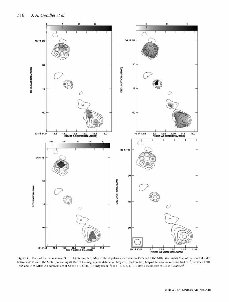
3.1.1.2 Source 6C 1011+36 (Fig. 4) This is a classic double-lobedstructure, showing a strong core at both 4.7 and 1.4 GHz with aninverted spectrum.
3.1.1.3 Source 6C 1018+37 (Fig. 5) The maps were made withthe smaller arrays only at each frequency. In the 1.4-GHz A-arraydata set the lower lobe was partially resolved out but this wascompounded by the high noise, so no feasible combination of the
C© 2004 RAS, MNRAS 347, 508–540

Depolarization properties of powerful radio sources 515
Table 9. As Table 6 but for sample C. Rotation measure is between 4800, 4500, 1502 and 1450 MHz.
4710 MHz 1452 MHzSource Comp. Total Polar- Total Polar- RM α DM4.8
1.4 Ave. σ RM
flux ization flux ization �
(mJy) (per cent) (mJy) (per cent) (rad m−2) (rad m−2) (rad m−2)
3C 42 NW 353.9 12.5 999.7 12.3 −2.4 ± 5 −0.87 1.02 2.4 14.1SE 450.6 7.5 1266.3 7.4 5.0 ± 5 −0.86 1.01 1.7 14.2
4C 14.27 NW 107.0 12.4 368.2 8.8 −13.0 ± 4 −1.06 1.41 9.9 5.4SE 124.8 9.6 489.3 9.3 −17.3 ± 5 −1.17 1.03 2.9 4.8
3C 46 NE 162.7 16.2 488.0 12.8 −4.8 ± 5 −0.94 1.27 16.9 3.9SW 173.7 13.7 506.4 12.0 −2.9 ± 1 −0.91 1.14 12.5 4.2Core 2.54 – 7.94 – – −0.97 – – –
3C 457 NE 208.6 15.8 692.0 15.7 – −1.02 1.01 – –SW 290.5 11.9 898.9 10.0 – −0.94 1.19 − –Core 3.03 – 2.63 – – 0.12 – – –
3C 351 NE 971.7 6.8 2327.9 8.1 1.00 ± 5 −0.73 0.84 – 13.0Diffuse 122.2 26.4 421.3 13.7 −8.7 ± 1 −1.03 1.93 13.7 12.0
Core 18.3 18.6 46.2 8.2 −0.53 ± 2 −0.77 2.27 15.3 5.0SW 77.1 22.8 235.7 8.9 4.4 ± 3 −0.93 2.56 16.4 10.8
3C 341 NE 123.8 28.0 336.4 19.6 20.3 ± 5 −0.85 1.43 10.1 10.0SW 265.9 26.4 862.6 17.2 18.2 ± 5 −1.0 1.53 11.1 12.0
3C 299 NE 876.5 0.79 ± 0.5 2592.4 0.43 ± 0.3 −126.3 ± 8 −0.93 1.84 13.2 75.9SW 53.7 3.1 122.6 2.6 16.0 ± 5 −0.71 1.19 7.10 6.9
3C 16 NE 22.1 ± 3 10.8 60.9 4.9 – −0.87 2.2 15.0 –SW 484.9 14.7 1510.9 8.2 −4.3 ± 3 −0.97 1.79 12.9 17.4
Figure 3. Maps of the radio source 6C 0943+39. (top left) Map of the depolarization between 4710 and 1465 MHz. (top right) Map of the spectral indexbetween 4710 and 1465 MHz. (bottom left) Map of the rotation measure (rad m−2) between 4710, 1665 and 1465 MHz. (bottom right) Map of the magneticfield direction (degrees). All contours are at 5σ at 4710 MHz, (0.5 mJy beam−1) × (−1, 1, 2, 4, . . . , 1024). Beam size of 2.5 × 1.4 arcsec2.
C© 2004 RAS, MNRAS 347, 508–540
516 J. A. Goodlet et al.
Figure 4. Maps of the radio source 6C 1011+36. (top left) Map of the depolarization between 4535 and 1465 MHz. (top right) Map of the spectral indexbetween 4535 and 1465 MHz. (bottom right) Map of the magnetic field direction (degrees). (bottom left) Map of the rotation measure (rad m−2) between 4710,1665 and 1465 MHz. All contours are at 5σ at 4710 MHz, (0.4 mJy beam−1) × (−1, 1, 2, 4, . . . , 1024). Beam size of 3.5 × 3.2 arcsec2.
C© 2004 RAS, MNRAS 347, 508–540

Depolarization properties of powerful radio sources 517
Figure 5. Maps of the radio source 6C 1018+37. (top left) The 4710-MHz total intensity map with vectors of polarization overlaid. The contour levels are at5σ , (100 µJy beam −1) × (−1, 1, 2, 4, . . . , 1024). One arcsecond corresponds to 1.7 × 10⁻³Jy beam −1. (top right) The 1465-MHz total intensity map withvectors of polarization overlaid. The contour levels are at 3σ , (0.5 mJy beam−1) × (−1, 1, 2, 4, . . . , 1024). One arcsecond corresponds to 1.7 × 10⁻³ Jybeam −1. (middle left) Map of the depolarization between 4710 and 1465 MHz. (middle right) Map of the spectral index between 4710 and 1465 MHz. (bottomright) Map of the magnetic field direction (degrees). (bottom left) Map of the rotation measure (rad m−2) between 4710, 1665 and 1465 MHz. All contours(c–f) are at 5σ at 4885 MHz, (100 µJy beam −1) × (−1, 1, 2, 4, . . . , 1024). Beam size of 4 × 4 arcsec2.
C© 2004 RAS, MNRAS 347, 508–540

518 J. A. Goodlet et al.
Figure 6. Maps of the radio source 6C 1129+37. (top left) Map of the depolarization between 4710 and 1465 MHz. (top right) Map of the spectral indexbetween 4710 and 1465 MHz. (bottom right) Map of the magnetic field direction (degrees). (bottom left) Map of the rotation measure (rad m−2) between 4710,1665 and 1465 MHz. All contours are at 5σ at 4710 MHz, (0.3 mJy beam−1) × (−1, 1, 2, 4, . . . , 1024). Beam size of 2.5 × 1.4 arcsec2.
A- and B-arrays was possible. To maintain consistency, the B-array4.7-GHz data were also excluded.
3.1.1.4 Source 6C 1129+37 (Fig. 6) The SE lobe contains twodistinct hotspots. Best et al. (1999) found three hotspots. Our non-detection is probably due to the different resolutions of the twoobservations. The source shows distinct regions of very strong de-polarizations; however, these regions are slightly smaller than thebeam size.
3.1.1.5 Source 6C 1256+36 (Fig. 7) The rotation measure mapshows distinct changes in the values of the rotation measure. Fig. 31shows that, although the jump in RM does not correspond to a jumpin depolarization, it is not due to any error in the fitting program.
3.1.1.6 Source 6C 1257+37 (Fig. 8) A core was detected at4.7 GHz but was absent from the 1.4-GHz data. The high noiselevel and short observation time meant that the southern lobe hadvery little polarized flux above the noise level, resulting in a reli-able value for the rotation measure being found in only a few pixelsaround the hotspots.
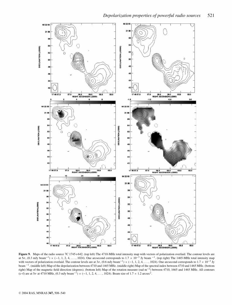
3.1.1.7 Source 7C 1745+642 (Fig. 9) This is a highly core domi-nated source, with the northern lobe appearing faintly. There is anindication of a jet-like structure leading down from the core intothe southern, highly extended, off-axis, lobe. The source is a weakcore-dominated quasar (Barkhouse & Hall 2001).
3.1.1.8 Source 7C 1801+690 (Fig. 10) This is an asymmetric core-dominated quasar (Barkhouse & Hall 2001). The northern lobe is
C© 2004 RAS, MNRAS 347, 508–540

Depolarization properties of powerful radio sources 519
Figure 7. Maps of the radio source 6C 1256+36. (top left) Map of the depolarization between 4710 and 1465 MHz. (top right) Map of the spectral indexbetween 4710 and 1465 MHz. (bottom right) Map of the magnetic field direction (degrees). (bottom left) Map of the rotation measure (rad m−2) between 4710,1665 and 1465 MHz. All contours are at 5σ at 4710 MHz, (0.25 mJy beam−1) × (−1, 1, 2, 4, . . . , 1024). Beam size of 2.5 × 1.4 arcsec2.
very faint and appears to be much closer to the core componentthan the more extended southern lobe. It shows very little polariza-tion compared to the relatively strong polarization of the core andsouthern components.
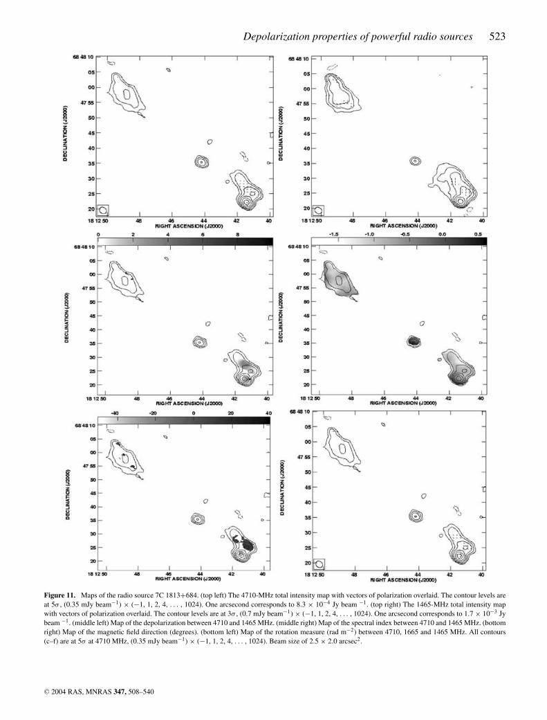
3.1.1.9 Source 7C 1813+684 (Fig. 11) This is the faintest of thesources in sample A and is also a quasar (Barkhouse & Hall 2001).The source shows a compact core that is present at all observingfrequencies, but it is too faint to detect any reliable polarizationproperties.
3.1.2 Sample B
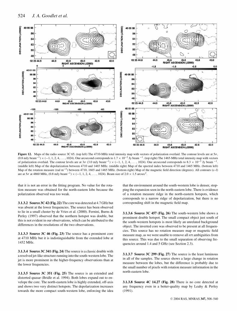
3.1.2.1 Source 3C 65 (Fig. 12) The western lobe shows a strongdepolarization shadow that is smaller than the beam size. Best (2000)found the source to lie in a cluster, which might account for thepresence of the depolarization shadow and the large depolarizationoverall.
3.1.2.2 Source 3C 68.1 (Fig. 13) The source is a quasar (Bridleet al. 1994). A core has been detected by Bridle et al. (1994) indeeper observations.
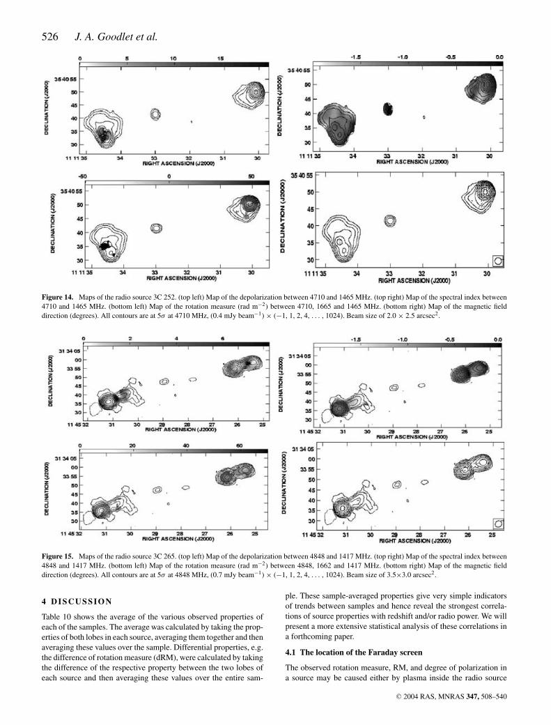
3.1.2.3 Source 3C 252 (Fig. 14) The south-eastern lobe showsa sharp drop in the polarization between the 4.7 and 1.4 GHzobservations.
3.1.2.4 Source 3C 265 (Fig. 15) The north-western lobe showsevidence of a compact, bright region with a highly ordered magneticfield, which Fernini et al. (1993) show is the primary hotspot athigher resolutions.
3.1.2.5 Source 3C 267 (Fig. 16) The eastern lobe is highly ex-tended, reaching to the core position, which can be seen in the1.4-GHz image. The large depolarization region in the western lobecoincides with a region of no observed rotation measure. The coreis strongly inverted, with α = 0.48.
C© 2004 RAS, MNRAS 347, 508–540

520 J. A. Goodlet et al.
Figure 8. Maps of the radio source 6C 1257+37. (top left) Map of the depolarization between 4710 and 1465 MHz. (top right) Map of the spectral indexbetween 4860 and 1465 MHz. (bottom right) Map of the magnetic field direction (degrees). (bottom left) Map of the rotation measure (rad m−2) between 4710,1665 and 1465 MHz. All contours are at 5σ at 4710 MHz, (0.25 mJy beam−1) × (−1, 1, 2, 4, . . . , 1024). Beam size of 2.0 × 1.4 arcsec2.
3.1.2.6 Source 3C 268.1 (Fig. 17) The average spectral index overthe entire source is α =−0.66, which is rather flat, but taking the 4.8-GHz data from Gregory & Condon (1991) and 1.4-GHz data fromLaing & Peacock (1980) the value is very similar, α = −0.68.
3.1.2.7 Source 3C 280 (Fig. 18) The value of the rotation measureand the magnetic field direction in the eastern lobe must be treatedwith caution as they are based on only a small region of the entirelobe. The sharp changes in the rotation measure map are not seen inthe magnetic field map, and the depolarization map shows a similarstructure, suggesting that it is not due to a fitting error.
3.1.2.8 Source 3C 324 (Fig. 19) The north-eastern lobe shows ev-idence of a depolarization shadow. Best (2000) found the source tolie in a cluster, which may explain the faint shadow.
3.1.2.9 Source 4C 16.49 (Fig. 20) The source is a quasar(Barkhouse & Hall 2001) that shows a strong radio core, jet structureand possibly a small counter-jet. The source is highly asymmetric,with the lower lobe almost appearing to connect to the core. It hasa very steep spectral index, α < −1.0, making it an atypical source.Figs 29 and 30 demonstrate that the sharp changes in the rotationmeasure map are not due to any fitting errors.
3.1.3 Sample C
3.1.3.1 Source 3C 16 (Fig. 21) The source shows a strong south-western lobe, with a relaxed north-eastern lobe. The south-westernlobe shows a strong depolarization feature that is narrower than thebeam size. The strong rotation measure feature is evident in thedepolarization map but not in the magnetic field map, indicating
C© 2004 RAS, MNRAS 347, 508–540
Depolarization properties of powerful radio sources 521
Figure 9. Maps of the radio source 7C 1745+642. (top left) The 4710-MHz total intensity map with vectors of polarization overlaid. The contour levels areat 5σ , (0.3 mJy beam−1) × (−1, 1, 2, 4, . . . , 1024). One arcsecond corresponds to 1.7 × 10⁻³ Jy beam −1. (top right) The 1465-MHz total intensity mapwith vectors of polarization overlaid. The contour levels are at 3σ , (0.6 mJy beam−1) × (−1, 1, 2, 4, . . . , 1024). One arcsecond corresponds to 1.7 × 10⁻³ Jybeam −1. (middle left) Map of the depolarization between 4710 and 1465 MHz. (middle right) Map of the spectral index between 4710 and 1465 MHz. (bottomright) Map of the magnetic field direction (degrees). (bottom left) Map of the rotation measure (rad m−2) between 4710, 1665 and 1465 MHz. All contours(c–f) are at 5σ at 4710 MHz, (0.3 mJy beam−1) × (−1, 1, 2, 4, . . . , 1024). Beam size of 1.7 × 1.2 arcsec2.
C© 2004 RAS, MNRAS 347, 508–540

522 J. A. Goodlet et al.
Figure 10. Maps of the radio source 7C 1801+690. (top left) The 4710-MHz total intensity map with vectors of polarization overlaid. The contour levelsare at 5σ , (0.3 mJy beam−1) × (−1, 1, 2, 4, . . . , 1024). One arcsecond corresponds to 1.7 × 10⁻³ Jy beam −1. (top right) The 1465 MHz total intensity mapwith vectors of polarization overlaid. The contour levels are at 3σ , (0.6 mJy beam−1) × (−1, 1, 2, 4, . . . , 1024). One arcsecond corresponds to 1.7 × 10⁻³ Jybeam −1. (middle left) Map of the depolarization between 4710 and 1465 MHz. (middle right) Map of the spectral index between 4710 and 1465 MHz. (bottomright) Map of the magnetic field direction (degrees). (bottom left) Map of the rotation measure (rad m−2) between 4710, 1665 and 1465 MHz. All contours(c–f) are at 5σ at 4710 MHz, (0.30 mJy beam−1) × (−1, 1, 2, 4, . . . , 1024). Beam size of 2.2 × 1.5 arcsec2.
C© 2004 RAS, MNRAS 347, 508–540
Depolarization properties of powerful radio sources 523
Figure 11. Maps of the radio source 7C 1813+684. (top left) The 4710-MHz total intensity map with vectors of polarization overlaid. The contour levels areat 5σ , (0.35 mJy beam−1) × (−1, 1, 2, 4, . . . , 1024). One arcsecond corresponds to 8.3 × 10⁻⁴ Jy beam −1. (top right) The 1465-MHz total intensity mapwith vectors of polarization overlaid. The contour levels are at 3σ , (0.7 mJy beam−1) × (−1, 1, 2, 4, . . . , 1024). One arcsecond corresponds to 1.7 × 10⁻³ Jybeam −1. (middle left) Map of the depolarization between 4710 and 1465 MHz. (middle right) Map of the spectral index between 4710 and 1465 MHz. (bottomright) Map of the magnetic field direction (degrees). (bottom left) Map of the rotation measure (rad m−2) between 4710, 1665 and 1465 MHz. All contours(c–f) are at 5σ at 4710 MHz, (0.35 mJy beam−1) × (−1, 1, 2, 4, . . . , 1024). Beam size of 2.5 × 2.0 arcsec2.
C© 2004 RAS, MNRAS 347, 508–540
524 J. A. Goodlet et al.
Figure 12. Maps of the radio source 3C 65. (top left) The 4710-MHz total intensity map with vectors of polarization overlaid. The contour levels are at 5σ ,(0.8 mJy beam−1) × (−1, 1, 2, 4, . . . , 1024). One arcsecond corresponds to 1.7 × 10⁻² Jy beam −1. (top right) The 1465-MHz total intensity map with vectorsof polarization overlaid. The contour levels are at 3σ (3.0 mJy beam−1) × (−1, 1, 2, 4, . . . , 1024). One arcsecond corresponds to 8.3 × 10⁻³ Jy beam −1.(middle left) Map of the depolarization between 4710 and 1465 MHz. (middle right) Map of the spectral index between 4710 and 1465 MHz. (bottom left)Map of the rotation measure (rad m−2) between 4710, 1665 and 1465 MHz. (bottom right) Map of the magnetic field direction (degrees). All contours (c–f)are at 5σ at 4860 MHz, (0.8 mJy beam−1) × (−1, 1, 2, 4, . . . , 1024). Beam size of 2.0 × 1.5 arcsec2.
that it is not an error in the fitting program. No value for the rota-tion measure was obtained for the north-eastern lobe because thepolarization observed was too weak.
3.1.3.2 Source 3C 42 (Fig. 22) The core was detected at 4.7 GHz butwas absent at the lower frequencies. The source has been observedto lie in a small cluster by de Vries et al. (2000). Fernini, Burns &Perley (1997) observed that the northern hotspot was double, butthis is not evident in our observations, which can be attributed to thedifferences in the resolutions of the two observations.
3.1.3.3 Source 3C 46 (Fig. 23) The source has a prominent coreat 4710 MHz but it is indistinguishable from the extended lobe at1452 MHz.
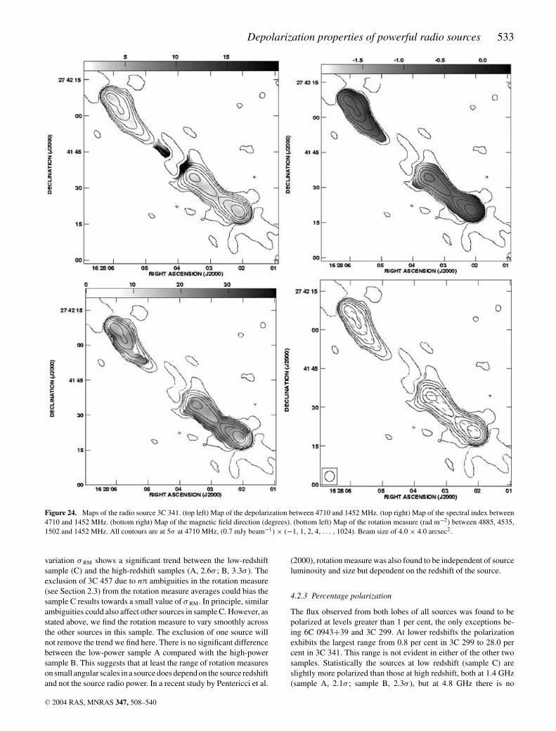
3.1.3.4 Source 3C 341 (Fig. 24) The source is a classic double witha resolved jet-like structure running into the south-western lobe. Thejet is more prominent in the higher-frequency observations than atthe lower frequencies.
3.1.3.5 Source 3C 351 (Fig. 25) The source is an extended anddistorted quasar (Bridle et al. 1994). Both lobes expand out to en-velope the core. The north-eastern lobe is highly extended, off-axisand shows two very distinct hotspots. The depolarization increasestowards the more compact south-western lobe, enforcing the idea
that the environment around the south-western lobe is denser, stop-ping the expansion seen in the north-eastern lobe. There is evidenceof a rotation measure ridge in the north-eastern hotspots, whichcorresponds to a narrow ridge of depolarization, but there is nocorresponding shift in the magnetic field map.
3.1.3.6 Source 3C 457 (Fig. 26) The south-western lobe shows aprominent double hotspot. The small compact object just south ofthe south-western hotspots is most likely an unrelated backgroundobject. The inverted core was observed to be present at all frequen-cies. This source has no rotation measure map or magnetic fieldmeasure map, as we were unable to remove all nπ ambiguities fromthis source. This was due to the small separation of observing fre-quencies around 1.4 and 5 GHz (see Section 2.3).
3.1.3.7 Source 3C 299 (Fig. 27) The source is the least luminousin all of the samples. The source shows a large change in rotationmeasure between the lobes, but the difference is probably due tothe small number of pixels with rotation measure information in thenorth-eastern lobe.
3.1.3.8 Source 4C 14.27 (Fig. 28) There is no core detected atany frequency even in a better-quality map by Leahy & Perley(1991).
C© 2004 RAS, MNRAS 347, 508–540

Depolarization properties of powerful radio sources 525
Figure 13. Maps of the radio source 3C 68.1. (top left) Map of the depolarization between 4710 and 1417 MHz. (top right) Map of the spectral index between4710 and 1417 MHz. (bottom right) Map of the magnetic field direction (degrees). (bottom left) Map of the rotation measure (rad m−2) between 4710, 1662and 1417 MHz. All contours are at 5σ at 4710 MHz, (2.0 mJy beam−1) × (−1, 1, 2, 4, . . . , 1024). Beam size of 3.5 × 3.5 arcsec2.
C© 2004 RAS, MNRAS 347, 508–540
526 J. A. Goodlet et al.
Figure 14. Maps of the radio source 3C 252. (top left) Map of the depolarization between 4710 and 1465 MHz. (top right) Map of the spectral index between4710 and 1465 MHz. (bottom left) Map of the rotation measure (rad m−2) between 4710, 1665 and 1465 MHz. (bottom right) Map of the magnetic fielddirection (degrees). All contours are at 5σ at 4710 MHz, (0.4 mJy beam−1) × (−1, 1, 2, 4, . . . , 1024). Beam size of 2.0 × 2.5 arcsec2.
Figure 15. Maps of the radio source 3C 265. (top left) Map of the depolarization between 4848 and 1417 MHz. (top right) Map of the spectral index between4848 and 1417 MHz. (bottom left) Map of the rotation measure (rad m−2) between 4848, 1662 and 1417 MHz. (bottom right) Map of the magnetic fielddirection (degrees). All contours are at 5σ at 4848 MHz, (0.7 mJy beam−1) × (−1, 1, 2, 4, . . . , 1024). Beam size of 3.5×3.0 arcsec2.
4 D I S C U S S I O N
Table 10 shows the average of the various observed properties ofeach of the samples. The average was calculated by taking the prop-erties of both lobes in each source, averaging them together and thenaveraging these values over the sample. Differential properties, e.g.the difference of rotation measure (dRM), were calculated by takingthe difference of the respective property between the two lobes ofeach source and then averaging these values over the entire sam-
ple. These sample-averaged properties give very simple indicatorsof trends between samples and hence reveal the strongest correla-tions of source properties with redshift and/or radio power. We willpresent a more extensive statistical analysis of these correlations ina forthcoming paper.
4.1 The location of the Faraday screen
The observed rotation measure, RM, and degree of polarization ina source may be caused either by plasma inside the radio source
C© 2004 RAS, MNRAS 347, 508–540

Depolarization properties of powerful radio sources 527
Figure 16. Maps of the radio source 3C 267. (top left) The 4848-MHz total intensity map with vectors of polarization overlaid. The contour levels are at 5σ
(0.8 mJy beam−1) × (−1, 1, 2, 4, . . . , 1024). One arcsecond corresponds to 8.3 × 10⁻³ Jy beam −1. (top right) The 1465-MHz total intensity map with vectorsof polarization overlaid. The contour levels are at 3σ , (1.3 mJy beam−1) × (−1, 1, 2, 4, . . . , 1024). One arcsecond corresponds to 8.3 × 10⁻³ Jy beam −1.(middle left) Map of the depolarization between 4848 and 1465 MHz. (middle right) Map of the spectral index between 4848 and 1465 MHz. (bottom left)Map of the rotation measure (rad m−2) between 4848, 1665 and 1465 MHz. (bottom right) Map of the magnetic field direction (degrees). All contours (c–f)are at 5σ at 4848 MHz, (0.8 mJy beam−1) × (−1, 1, 2, 4, . . . , 1024). Beam size of 2.2 × 2.0 arcsec2.
Figure 17. Maps of the radio source 3C 268.1. (top left) Map of the depolarization between 4848 and 1417 MHz. (top right) Map of the spectral indexbetween 4848 and 1417 MHz. (bottom left) Map of the rotation measure (rad m−2) between 4848, 1662 and 1417 MHz. (bottom right) Map of the magneticfield direction (degrees). All contours are at 5σ , (5.2 mJy beam−1) × (−1, 1, 2, 4, . . . , 1024). Beam size of 4.0 × 3.5 arcsec2 .
itself (internal depolarization) or by a Faraday screen in betweenthe source and the observer (external depolarization). In the lattercase the screen may be local to the radio source or within our ownGalaxy, or both. Only in the case of an external Faraday screen local
to the radio source do our measurements contain information on thesource environment.
The average RM we observe in our sources is consistent witha Galactic origin (Leahy 1987). This is also consistent with the
C© 2004 RAS, MNRAS 347, 508–540

528 J. A. Goodlet et al.
Figure 18. Maps of the radio source 3C 280. (top left) Map of the depolarization between 4848 and 1465 MHz. (top right) Map of the spectral index between4848 and 1465 MHz. (bottom left) Map of the rotation measure (rad m−2) between 4848, 1665 and 1465 MHz. (bottom right) Map of the magnetic fielddirection (degrees). All contours are at 5σ at 4848 MHz (0.8 mJy beam−1) × (−1, 1, 2, 4, . . . , 1024). Beam size of 1.6 × 1.6 arcsec2.
Figure 19. Maps of the radio source 3C 324. (top left) Map of the depolarization between 4848 and 1465 MHz. (top right) Map of the spectral index between4848 and 1465 MHz. (bottom left) Map of the rotation measure (rad m−2) between 4848, 1665 and 1465 MHz. (bottom right) Map of the magnetic fielddirection (degrees). All contours are at 5σ at 4848 MHz, (1.5 mJy beam−1) × (−1, 1, 2, 4, . . . , 1024). Beam size of 2.2 × 1.6 arcsec2.
absence of any significant differences of RM between our sam-ples (see Table 10). However, we observe large variations of RMwithin individual lobes on small angular scales. These are proba-bly caused by a Faraday screen local to the source (Leahy 1987)
and therefore must be corrected for the source redshift by multi-plying dRM and σ RM by a factor (1 + z)2 to allow a valid com-parison between sources. The variation of RM on large angularscales (tens of arcseconds), i.e. between the two lobes of a source,
C© 2004 RAS, MNRAS 347, 508–540

Depolarization properties of powerful radio sources 529
Figure 20. Maps of the radio source 4C 16.49. (top left) Map of the depolarization between 4710 and 1465 MHz. (top right) Map of the spectral index between4710 and 1465 MHz. (bottom right) Map of the magnetic field direction (degrees). (bottom left) Map of the rotation measure (rad m−2) between 4710, 1665and 1465 MHz. All contours are at 5σ at 4710 MHz, (0.8 mJy beam−1) × (−1, 1, 2, 4, . . . , 1024). Beam size of 2.2 × 1.8 arcsec2.
C© 2004 RAS, MNRAS 347, 508–540

530 J. A. Goodlet et al.
Figure 21. Maps of the radio source 3C 16. (top left) Map of the depolarization between 4710 and 1452 MHz. (top right) Map of the spectral index between4710 and 1452 MHz. (bottom right) Map of the magnetic field direction (degrees). (bottom left) Map of the rotation measure (rad m−2) between 4885, 4535,1502 and 1452 MHz. All contours are at 5σ at 4710 MHz, (0.40 mJy beam−1) × (−1, 1, 2, 4, . . . , 1024). Beam size of 3.5 × 3.5 arcsec2.
C© 2004 RAS, MNRAS 347, 508–540

Depolarization properties of powerful radio sources 531
Figure 22. Maps of the radio source 3C 42. (top left) Map of the depolarization between 4710 and 1452 MHz. (top right) Map of the spectral index between4710 and 1465 MHz. (bottom right) Map of the magnetic field direction (degrees). (bottom left) Map of the rotation measure (rad m−2) between 4885, 4535,1502 and 1452 MHz. All contours are at 5σ at 4710 MHz, (1.0 mJy beam−1) × (−1, 1, 2, 4, . . . , 1024). Beam size of 2.5 × 1.8 arcsec2.
dRM, may still be somewhat influenced by the Galactic Faradayscreen. Nevertheless, the large variations of RM found on arc-second scales measured by σ RM suggest an origin local to thesource.
The observed degree of depolarization in a source depends on thedistribution of the Faraday depths covered by the projected area ofthe telescope beam, i.e. the variation of RM on the smallest angularscales. We therefore assume that the depolarization in our sourcesis caused by plasma local to the sources. If the depolarization iscaused by a local but external Faraday screen, and the distributionof Faraday depths in this screen is Gaussian with standard deviation�, then (e.g. Burn 1966)
mλ = m0 exp{−2�2[λ/(1 + z)]4}, (4)
where mλ is the percentage polarization at observed wavelength λ
and m0 is the initial percentage polarization before any depolariza-tion. Since we measure mλ at two observing frequencies (1.4 and4.8 GHz), we can solve equation (4) for � as a function of the
depolarization measure,
� =√
(1 + z)4 ln DM4.81.4
2(λ4
1.4 − λ44.8
) rad m−2. (5)
We can now, for each source, compare the value of � as de-rived from the measured depolarization with the observed rmsof the rotation measure. If the Faraday dispersion is less thanthe rms of the rotation measure, then our observations are con-sistent with an external Faraday screen (Garrington & Conway1991).
Fig. 32 displays the Faraday dispersion, �, for each lobe of thesources against the rms of the rotation measures observed. It is evi-dent from the plot that the value of σ RM > � for most components.There are a few sources where this is not the case. However, thesecomponents belong to sources where the depolarization or rotationmeasure is only determined reliably for a few pixels, so an accu-rate value is not obtainable for σ RM or �. There is little correlationbetween � and σ RM. This is a strong indicator that the Faraday
C© 2004 RAS, MNRAS 347, 508–540

532 J. A. Goodlet et al.
Figure 23. Maps of the radio source 3C 46. (top left) The 4710-MHz total intensity map with vectors of polarization overlaid. The contour levels are at 5σ ,(0.25 mJy beam−1) × (−1, 1, 2, 4, . . . , 1024). One arcsecond corresponds to 1.7 × 10⁻³ Jy beam −1. (top right) The 1452-MHz total intensity map with vectorsof polarization overlaid. The contour levels are at 3σ (1.0 mJy beam−1) × (−1, 1, 2, 4, . . . , 1024). One arcsecond corresponds to 5.5 × 10⁻⁴ Jy beam −1.(middle right) Map of the depolarization between 4710 and 1452 MHz. (middle left) Map of the spectral index between 4710 and 1452 MHz. (bottom right)Map of the rotation measure (rad m−2) between 4885, 4535, 1502 and 1452 MHz. (bottom left) Map of the magnetic field direction (degrees). All contours(c–f) are at 5σ at 4710 MHz, (0.25 mJy beam−1) × (−1, 1, 2, 4, . . . , 1024). Beam size of 4.5 × 3.0 arcsec2.
medium responsible for variations of RM on small angular scales,and thus for the polarization properties of our sources, is consistentwith being external but local to the sources.
4.2 Trends with redshift and radio power
4.2.1 Spectral index
We found no significant correlation between spectral index and red-shift or radio power as suggested by others (Veron & Veron 1972;Onuora 1989; Athreya & Kapahi 1999), which used much largersamples. This suggests that the trend may be present but becauseof the fact that our sample is small we do not find any significanttrend. However, there are trends found with the difference in spec-tral index between the two lobes. Sample B shows a larger averagedifference in the spectral indices between the two lobes of a givensource than the other samples (sample A, 2.5σ ; sample C, 3.3σ ).Sample B contains the sources with the highest radio power, and so
we find that in our samples the difference in spectral index increaseswith radio power rather than with redshift. The trend of the differ-ence in the spectral index between the two lobes may be related tothe extra luminosity of the 3CRR hotspots compared to the 6C/7Chotspots (see Section 2.2). On average we find that the hotspots ofour sources have shallower spectral indices. The average spectralindex integrated over the entire sources will therefore depend on thefraction of emission from the hotspots compared to the extendedlobe, thus creating the observed trend.
4.2.2 Rotation measure
As mentioned above, we find no significant difference in the av-erage RM between our samples. Similarly, there is no statisticallysignificant trend of the difference of RM between the two lobes ofeach source with redshift or radio power. This is consistent with aGalactic origin of the RM properties of the sources on large scales.On small angular scales, the variation of RM as measured by its rms
C© 2004 RAS, MNRAS 347, 508–540
Depolarization properties of powerful radio sources 533
Figure 24. Maps of the radio source 3C 341. (top left) Map of the depolarization between 4710 and 1452 MHz. (top right) Map of the spectral index between4710 and 1452 MHz. (bottom right) Map of the magnetic field direction (degrees). (bottom left) Map of the rotation measure (rad m−2) between 4885, 4535,1502 and 1452 MHz. All contours are at 5σ at 4710 MHz, (0.7 mJy beam−1) × (−1, 1, 2, 4, . . . , 1024). Beam size of 4.0 × 4.0 arcsec2.
variation σ RM shows a significant trend between the low-redshiftsample (C) and the high-redshift samples (A, 2.6σ ; B, 3.3σ ). Theexclusion of 3C 457 due to nπ ambiguities in the rotation measure(see Section 2.3) from the rotation measure averages could bias thesample C results towards a small value of σ RM. In principle, similarambiguities could also affect other sources in sample C. However, asstated above, we find the rotation measure to vary smoothly acrossthe other sources in this sample. The exclusion of one source willnot remove the trend we find here. There is no significant differencebetween the low-power sample A compared with the high-powersample B. This suggests that at least the range of rotation measureson small angular scales in a source does depend on the source redshiftand not the source radio power. In a recent study by Pentericci et al.
(2000), rotation measure was also found to be independent of sourceluminosity and size but dependent on the redshift of the source.
4.2.3 Percentage polarization
The flux observed from both lobes of all sources was found to bepolarized at levels greater than 1 per cent, the only exceptions be-ing 6C 0943+39 and 3C 299. At lower redshifts the polarizationexhibits the largest range from 0.8 per cent in 3C 299 to 28.0 percent in 3C 341. This range is not evident in either of the other twosamples. Statistically the sources at low redshift (sample C) areslightly more polarized than those at high redshift, both at 1.4 GHz(sample A, 2.1σ ; sample B, 2.3σ ), but at 4.8 GHz there is no
C© 2004 RAS, MNRAS 347, 508–540

534 J. A. Goodlet et al.
Figure 25. Maps of the radio source 3C 351. (top left) Map of the depolarization between 4810 and 1452 MHz. (top right) Map of the spectral index between4810 and 1452 MHz. (bottom right) Map of the magnetic field direction (degrees). (bottom left) Map of the rotation measure (rad m−2) between 4810, 1502and 1452 MHz. All contours are at 5σ at 4810 MHz, (1.0 mJy beam−1) × (−1, 1, 2, 4, . . . , 1024). Beam size of 4.5 × 4.0 arcsec2.
C© 2004 RAS, MNRAS 347, 508–540

Depolarization properties of powerful radio sources 535
Figure 26. Maps of the radio source 3C 457. (left) Map of the depolarization between 4710 and 1452 MHz. (right) Map of the spectral index between 4710and 1452 MHz. All contours are at 5σ at 4710 MHz, (0.3 mJy beam−1) × (−1, 1, 2, 4, . . . , 1024). Beam size of 5.0 × 3.0 arcsec2.
Figure 27. Maps of the radio source 3C 299. (left) Map of the rotation measure (rad m−2) between 4770, 1502 and 1452 MHz. (right) Map of the magneticfield direction (degrees). All contours are at 5σ at 4770 MHz, (0.7 mJy beam−1) × (−1, 1, 2, 4, . . . , 1024). Beam size of 2.5 × 2.0 arcsec2.
significant difference. There is no trend observed comparing thelow radio power sources (sample A) with the high-power objects(sample B). This suggests that percentage polarization decreasesfor increasing redshift but is less dependent on radio power.
So far we have considered percentage polarizations measuredin the observing frame. We argue in Section 4.1 that variations ofthe rotation measure on small angular scales which determine thedegree of polarization are caused in Faraday screens local tothe sources. The trend with redshift may therefore simply reflectthe different shifts of the observing frequency in the source restframe for sources at low and high redshift. Using Burn’s law in theform of equations (4) and (5), we can determine for each source thepercentage polarization expected to be observable at a frequencycorresponding to a wavelength of 5 cm in its rest frame. The results
for individual sources are presented in Table 11 and the sample av-erages are summarized in Table 12. Again, sources at low redshift(sample C) are slightly more polarized than sources at high red-shift, but only sample B (2.1σ ) shows a result that is marginallysignificant. As before, there is no trend with radio power, indicatingthat the trend with redshift, although weak, is dominant. This is notcaused by pure Doppler shifts of the observing frequencies.
4.2.4 Depolarization
Comparing the average depolarization of individual samples witheach other, we find only very weak trends with redshift or radiopower. When the samples are averaged together, we find a trendin depolarization with redshift but none with radio power. Samples
C© 2004 RAS, MNRAS 347, 508–540

536 J. A. Goodlet et al.
Figure 28. Maps of the radio source 4C 14.27. (top left) Map of the depolarization between 4710 and 1452 MHz. (top right) Map of the spectral index between4710 and 1452 MHz. (bottom left) Map of the rotation measure (rad m−2) between 4885, 4535, 1502 and 1452 MHz. (bottom right) Map of the magnetic fielddirection (degrees). All contours are at 5σ at 4710 MHz, (0.4 mJy beam−1) × (−1, 1, 2, 4, . . . , 1024). Beam size of 2.5 × 2.0 arcsec2.
Figure 29. A plot of the polarization angle against λ2, allowing for nπ, forthe northern lobe of 4C 16.49, with the dashed lines showing the best-fittingmodels. All nπ solutions for the 5-GHz data are considered and plotted.Data for two small regions, one on each side of the jump, are plotted with ◦indicating one side of the jump and × the other. Table 8 shows the χ2 valuesfor each fit. The jump plotted lies south-west of the central intensity contour.
A + C (low radio power) are statistically identical to sample B(high radio power), suggesting that there is no trend with radiopower in our sources. By considering the averaged depolarizationof samples A + B (high redshift) compared with that of sample C(low redshift), there is a weak trend with redshift, which is echoed inthe dDM values. However, both results are not significant. This mayconfirm the results of Kronberg et al. (1972): redshift is the dominantfactor compared to radio power in determining the depolarizationproperties of a source.
Analogous to the discussion above on percentage polarization, thecosmological Doppler shifts of the observing frequencies influencethe trend of DM with redshift, and in fact the true trend is stronger
Figure 30. As Fig. 30 but for 4C 16.49 southern lobe. Data for two smallregions, one on each side of the jump, are plotted. These regions lie eitherside of the jump south of the peak intensity contour.
than that naively observed. To demonstrate this, we use equation (5)to derive the standard deviation of Faraday depths, �, for eachsource. By setting z = 1 we then rescale all the depolarizations DM4.8
1.4
to the same redshift. This allows all three samples to be comparedwithout any bias due to pure redshift effects (see Tables 11 and 12). Ifthere was no intrinsic difference between the high-redshift and low-redshift samples, then we would expect these values to be consistentwith each other. This is evidently not the case. The high-redshiftsamples are, on average, significantly more depolarized (sample A,2.2σ ; sample B, 3.2σ ) than their low-redshift counterparts (sampleC). Comparing sample A with sample B, we find no trend with radiopower. However, a note of caution must be issued as the correctionsapplied use Burn’s law may actually be too large. Considering theprecorrected and the corrected values together, it is obvious thatthere is a connection between redshift and depolarization but there
C© 2004 RAS, MNRAS 347, 508–540

Depolarization properties of powerful radio sources 537
Figure 31. As Fig. 30 but for 6C 1256+36 southern lobe. Data for twosmall regions, one on each side of the jump, are plotted.
is no significant trend of depolarization with radio power. Thereis also a connection between the difference in the depolarization,dDM, and the redshift of the source, but no significant trend of thedifference in the depolarization with the radio power of the source.As noted in Section 2.3, regions with signal-to-noise ratio S/N < 3σ
were blanked in the map production. In individual sources, blankingof low S/N regions in the polarization maps will cause the measureddepolarization to be underestimated. Sources in sample A are moreaffected by this problem than objects in the other samples. Thereforewe probably underestimate the average depolarization in sample A,implying that the trend with redshift could be even stronger than ourfindings suggest.
The trends of percentage polarization and of depolarization withredshift are probably related in the sense that a lower degree of de-polarization at low redshift also leads to a higher observed degree ofpolarization. Clearly a variation of the initial polarization, m0, withredshift would lead to variations of the observed mλ independent ofthe properties of any external Faraday screen. Therefore both trendscould also be caused by a significantly higher level of m0 of thesources at low redshift (sample C). Using equation (4) we find m0 =9.3 ± 1.1 for sample A, m0 = 9.1 ± 1.0 for sample B and m0 =13.5 ± 2.5 for sample C. The uncertainties associated with the useof Burn’s law in extrapolating from our observations to λ = 0 arelarge. There is no difference between average initial polarization of
Table 10. Mean properties of the sources averaged over each sample, with the associated error. Differential properties (dDM, dα, dRM) arederived by taking the difference of the respective property between the two lobes of each source and then averaging this difference over eachsample; dRM is in the source frame. σ RM is the rms of the RM over the source, in the source reference frame. Properties in italics (the last tworows) are in the source frame of reference.
Property Sample Sample Sample Sample SampleA B C A + B A + C
Average z 1.06 ± 0.04 1.11 ± 0.05 0.41 ± 0.01 1.08 ± 0.03 0.75 ± 0.08Average P151 (1.02 ± 0.06) × 1027 (1.01 ± 0.07) × 1028 (8.02 ± 0.40) × 1026 (5.57 ± 1.16) × 1027 (8.97 ± 0.47) × 1026
Average D 220.34 ± 46.40 262.69 ± 55.41 399.57 ± 122.50 241.51 ± 35.43 304.69 ± 64.50Average DM 1.82 ± 0.32 1.61 ± 0.13 1.42 ± 0.12 1.71 ± 0.17 1.63 ± 0.18dDM 0.93 ± 0.26 0.61 ± 0.22 0.43 ± 0.18 0.77 ± 0.17 0.69 ± 0.17Average α −0.87 ± 0.01 −0.92 ± 0.06 −0.94 ± 0.03 −0.90 ± 0.03 −0.90 ± 0.02dα 0.13 ± 0.04 0.23 ± 0.04 0.10 ± 0.03 0.18 ± 0.03 0.12 ± 0.02Average PF1.4 6.29 ± 0.86 5.88 ± 0.64 9.89 ± 1.75 6.08 ± 0.52 7.98 ± 1.01Average PF4.8 8.91 ± 1.03 8.76 ± 0.89 13.31 ± 2.48 8.83 ± 0.66 10.98 ± 1.36Average RM 29.03 ± 12.81 26.41 ± 7.74 16.24 ± 8.33 27.64 ± 7.05 23.55 ± 8.07dRM 97.85 ± 36.41 115.96 ± 42.81 50.77 ± 43.29 107.44 ± 27.62 77.68 ± 27.54σ RM 115.62 ± 33.43 122.94 ± 28.48 29.45 ± 9.98 119.49 ± 21.11 78.69 ± 22.36
sources in samples A and B. The difference found for m0 at lowredshift (sample C) compared to high redshift (samples A and B)is small compared to the difference found for the depolarizationcomparing the same samples. This suggests that the differences inpercentage polarization and depolarization are due to variation withredshift of the Faraday screens local to the sources rather than todifferences in the initial degree of polarization. However, note thatthe variation of m0 is not significantly smaller than the trend ofpercentage polarization with redshift.
Burn’s law predicts a steep decrease of percentage polarizationwith increasing observing frequency. Although the decrease maywell be ‘softened’ by geometrical and other effects in more real-istic source models (Laing 1984), the value of DM may be smallfor sources in which our observing frequencies are lower than thefrequency at which strong depolarization occurs. For such sourceswe expect to measure a low value of DM associated with a lowpercentage polarization. Akujor & Garrington (1995) show that oneof our sources, 3C 299 (sample C), is strongly depolarized between1.6 and 8.4 GHz, with almost all of the depolarization taking placebetween 4.8 and 8.4 GHz. We measure only a very low percentagepolarization for this source, and the average value of DM4.8
1.4 = 1.5is also lower than DM8.4
1.6 ∼ 4 as measured by Akujor & Garrington(1995). If many of our sources at low redshift were affected bystrong depolarization at frequencies higher than 4.8 GHz, then thismay cause the trend of DM with redshift noted above. The absenceof any other sources with very low degrees of polarization combinedwith a low value for DM, at least in the low-redshift sample C, ar-gues against this bias. In fact, Tabara & Inoue (1980) show that oursources 3C 42, 46, 68.1, 265, 267, 324 and 341 depolarize stronglyonly at frequencies lower than our observing frequencies. 3C 16, 65,252, 268.1 and 280 do depolarize strongly between 1.4 and 4.8 GHz.In all the sources mentioned in Tabara & Inoue (1980), none havestrong depolarization at frequencies higher than 4.8 GHz. There isno information for 4C 14.27 and 16.49, and 3C 351, 299 and 457.Those sources which do depolarize strongly between our observingfrequencies, 1.4 and 4.8 GHz, could in principle have inaccuratevalues of the rotation measure because of this. However, the pix-els containing most depolarized regions of the source are likely tohave been blanked because of insufficient signal-to-noise ratio intheir polarization at 1.4 GHz; the rotation measure is determinedfrom the unblanked (less-depolarized) regions of the source, andwill therefore be reliable.
C© 2004 RAS, MNRAS 347, 508–540

538 J. A. Goodlet et al.
Figure 32. Plot of the Faraday dispersion, �, against the rms of the rotationmeasures for each source.
Table 11. Recalculated average depolarization and dDM for each source ifit was located at z = 1 and average percentage polarization of all sources ifit was emitted at 5 cm in the rest frame.
Source z �z DMz=1 dDMz=1 Polarizationλrest = 5 cm
6C 0943+39 1.04 74.12 3.31 1.98 3.16C 1018+37 0.81 42.95 1.49 0.52 8.326C 1011+36 1.04 36.11 1.33 0.66 5.636C 1129+37 1.06 83.07 4.49 3.43 3.096C 1256+36 1.07 29.53 1.21 0.40 8.266C 1257+36 1.00 45.51 1.58 0.61 9.397C 1801+690 1.27 41.24 1.45 0.54 3.337C 1813+684 1.03 6.96 1.01 0.25 8.477C 1745+642 1.23 47.81 1.65 1.36 7.32
3C 65 1.18 75.33 3.50 4.61 6.263C 252 1.11 50.66 1.76 1.36 6.363C 267 1.14 32.34 1.26 0.35 5.043C 280 1.00 48.79 1.68 0.28 5.483C 324 1.21 54.34 2.42 0.58 4.743C 265 0.81 35.56 1.37 0.14 5.053C 268.1 0.97 42.13 1.57 0.25 3.073C 68.1 1.24 45.11 1.85 0.98 10.2 h4C 16.49 1.29 31.04 1.23 0.47 6.76
3C 42 0.40 4.59 1.00 0.01 9.854C 14.27 0.39 14.34 1.05 0.08 9.083C 46 0.44 15.06 1.05 0.03 12.453C 457 0.43 10.50 1.03 0.04 12.883C 351 0.37 23.82 1.14 0.15 8.593C 341 0.45 21.91 1.11 0.02 18.573C 16 0.41 27.54 1.19 0.06 6.643C 299 0.37 20.20 1.10 0.1 1.52
Strom (1973), Strom & Jagers (1988), Pedelty et al. (1989) andIshwara-Chandra et al. (1998) find an anticorrelation of depolariza-tion with linear size. Thus our findings could be the result of oursample C containing larger sources than samples A and B. Fig. 33shows that there is a weak anticorrelation between physical sourcesize and depolarization. A Spearman rank test gives a confidencelevel of around 90 per cent for this anticorrelation. However, thistrend is due to the two largest sources in sample C, 3C 46 and 457.Removing these sources yields an average depolarization measureof 1.50 ± 0.15 for sample C, which is not significantly different
from the average with these two sources included. Thus we can ruleout the possibility that the larger depolarization at high redshift iscaused by selecting preferentially small sources at low redshift.
Liu & Pooley (1991b) observed depolarization to correlate withspectral index but there are no obvious correlations in any of oursamples when we examined the sources individually or as a com-bined sample.
Eight sources show dDM � 1 over the source and a further sixshow 0.5 � dDM < 1. This implies that 14 out of 24 sources,for which a depolarization measurement exists in both lobes, showa significant asymmetry in the depolarization of their lobes. Wewould expect a proportion of the sources to be observed at anglesconsiderably smaller than 90◦ to our line of sight. Therefore it is notsurprising that so many sources are found to be candidates for theLaing–Garrington effect.
Several sources show signs of depolarization shadows in at leastone of the lobes. Of these, 6C 1256+36 was observed to lie in acluster by Roche, Eales & Hippelein (1998), as were 3C 65 and324 (Best 2000). Best et al. (1998b) observed 3C 324 in the submil-limetre (850 µm) and found a large dust mass centred around 3C324. The host galaxy was shown to be the cause of the very strongdepolarization (Best et al. 1998a).
4.2.5 Summary
From the trends listed above, we can conclude that the variationsof RM on small angular scales and the associated depolarization ofthe radio emission are probably caused by a Faraday screen that isexternal but local to the source. This implies that any trends with ra-dio power and/or redshift reflect changes of the source environmentdepending on these quantities. We find that percentage polarizationdecreases with redshift while depolarization increases with redshift.According to Burn’s law (Burn 1966), this implies an increase in thesource environments of either the plasma density or the magneticfield strength or both with redshift. Such an interpretation is alsosupported by the increased depolarization asymmetry of sources athigh redshift compared with their low-redshift counterparts. Note,however, that the trends reported here are based on averaging theobserved properties of sources within three samples and that someof them are not highly significant. A more detailed statistical analy-sis of our observations in a forthcoming paper will help to test thesecrude trends.
5 C O N C L U S I O N S
In this paper we present the complete data set of our three samplesof radio galaxies and radio-loud quasars. The three samples weredefined such that two of them overlap in redshift and two have similarradio powers. Thus we are able to study the effects of redshift andradio power on various source properties.
Even without a formal analysis of the correlation between sourceproperties, some general trends are already discernible. There islittle correlation between � and σ RM, suggesting that the Faradaymedium responsible for variations of RM on small angular scalesis consistent with being external but local to the sources. Thereis also little correlation between rotation measure and redshift orradio power, which is consistent with a Galactic origin of the RMproperties of the sources on large scales. However, we find that therms fluctuations of the rotation measure correlate with redshift butnot radio power to a confidence level of >99.9 per cent, determinedin the sources’ frame of reference.
C© 2004 RAS, MNRAS 347, 508–540

Depolarization properties of powerful radio sources 539
Table 12. Average DM and dDM now shifted so that all the measurements are taken at z = 1. Average polarization of all thesources, shifted to a common rest-frame wavelength of 5 cm using equation (5).
Property Sample Sample Sample Sample SampleA B C A + B A + C
Average DMz=1 1.95 ± 0.39 1.85 ± 0.24 1.08 ± 0.02 1.90 ± 0.22 1.54 ± 0.23dDMz=1 1.08 ± 0.34 1.00 ± 0.47 0.06 ± 0.02 1.04 ± 0.28 0.60 ± 0.22PFλrest=5cm 6.32 ± 0.86 5.88 ± 0.65 9.82 ± 1.85 6.10 ± 0.53 7.97 ± 1.04
Figure 33. Average depolarization against projected linear size (kpc) for all three samples. Symbols as in Fig. 1. Part (a) assumes H0 = 50 km s−1 Mpc−1,and �m = 0.5, �� = 0. Part (b) assumes H0 = 50 km s−1 Mpc−1, and �m = 0.35, �� = 0.65.
We find that the polarization of a source anticorrelates with itsredshift but is independent of its radio power, resulting in the low-redshift sample having much higher degrees of polarization, in gen-eral. We also detect higher degrees of depolarization in the high-redshift samples (A and B) compared to sources at lower redshift(sample C). This suggests that depolarization is correlated with red-shift. These two results are probably related in that lower depolariza-tion at low redshift leads to both lower depolarization measurementsand also higher degrees of observed polarization.
Our findings on the rotation measurements and polarization prop-erties of our sources are indicative of an increase of the densityand/or the strength of the magnetic field in the source environmentswith increasing redshift.
We find a number of possible depolarization shadows, mostly insources known to be located in cluster environments.
We find no correlation between the spectral index and redshiftor radio power. However, we do find that the difference in thespectral index, across individual sources, increases for increasingradio power of the source and also with increasing redshift of asource.
A more detailed investigation into these findings will be presentedin a forthcoming paper.
AC K N OW L E D G M E N T S
We would like to thank Mark Lacy for his radio data of the 7Csources and helpful advice. We are grateful to VLA archives forproviding us with the archival data. We also thank our referee, J. P.Leahy, for many helpful comments. JAG would like to thank PPARCfor financial support in the form of a studentship. PNB would like
to thank the Royal Society for generous financial support throughits University Research Fellowship scheme.
R E F E R E N C E S
Akujor C. E., Garrington S. T., 1995, A&AS, 112, 235Athreya R. M., Kapahi V. K., 1999, in Rottgering H. J. A., Best P. N.,
Lehnert H. D., eds, Proc. Conf. The Most Distant Radio Galaxies. RoyalNetherlands Acad. Arts, the Netherlands, p. 453
Barkhouse W. A., Hall P. B., 2001, ApJ, 121, 2843Best P. N., 2000, MNRAS, 317, 720Best P. N., Longair M. S., Rottgering H. J. A., 1997a, MNRAS, 287, 785Best P. N., Longair M. S., Rottgering H. J. A., 1997b, MNRAS, 292, 578Best P. N., Carilli C. L., Garrington S. T., Longair M. S., Rottgering
H. J. A., 1998a, MNRAS, 299, 357Best P. N. et al., 1998b, MNRAS, 301, L15Best P. N., Eales S. A., Longair M. S., Rawlings S., Rottgering H. J. A.,
1999, MNRAS, 303, 616Bridle A. H., Hough D. H., Lonsdale C. J., Burns J. O., Laing R. A., 1994,
AJ, 108, 766Burn B. J., 1966, MNRAS, 133, 67de Vries W. H., van Breugel W. J. M., Quirrenbach A., Roberts J., Fidkowski
K., 2000, A&AS, 197, 2003Eales S., Rawlings S., Law-Green D., Cotter G., Lacy M., 1997, MNRAS,
291, 593Fernini I., Burns J. O., Bridle A. H., Perley R. A., 1993, AJ, 105, 1690Fernini I., Burns J. O., Perley R. A., 1997, AJ, 114, 2922Fomalont E. B., Ebneter K. A., van Breugel W. J. M., Ekers R. D., 1989,
ApJ, 346, L17Garrington S. T., Conway R. G., 1991, MNRAS, 250, 198Giovannini G., Feretti L., Gregorini L., Parma P., 1988, A&A, 199, 73Gregorini L., Padrielli L., Parma P., Gilmore G., 1988, A&AS, 74, 107Gregory P. C., Condon J. J., 1991, ApJS, 75, 1011
C© 2004 RAS, MNRAS 347, 508–540

540 J. A. Goodlet et al.
Hales S. E. G., Masson C. R., Warner P. J., Baldwin J. E., 1990, MNRAS,246, 256
Herbig T., Readhead A. C. S., 1992, ApJS, 81, 93Hewitt A., Burbridge G., 1991, ApJ, 75, 297Hill G. J., Lilly S. J., 1991, ApJ, 367, 1Ishwara-Chandra C. H., Saikia D. J., Kapahi V. K., McCarthy P. J., 1998,
MNRAS, 300, 269Kronberg P. P., Conway R. G., Gilbert. J. A., 1972, MNRAS, 156, 275Lacy M., Rawlings S., Hill G. J., Bunker A. J., Ridgway S., Stern D., 1999,
MNRAS, 308, 1096Laing R. A., 1981, MNRAS, 195, 261Laing R. A., 1984, Physics of Energy Transport in Extragalactic Radio
Sources. NRAO, Greenbank, p. 90Laing R. A., Peacock J. A., 1980, MNRAS, 190, 903Laing R. A., Riley J. M., Longair M. S., 1983, MNRAS, 204, 151Law-Green J. D. B., Leahy J. P., Alexander P., Allington-Smith J. R., van
Breugel W. J. M., Eales S. A., Rawlings S. G., Spinrad M., 1995,MNRAS, 274, 939
Leahy J. P., 1987, MNRAS, 226, 433Leahy J. P., Perley R. A., 1991, AJ, 102, 537Leahy J. P., Muxlow T. W. B., Stephens P. W., 1989, MNRAS, 239, 401Liu R., Pooley G., 1991a, MNRAS, 249, 343Liu R., Pooley G., 1991b, MNRAS, 253, 669Lonsdale C. J., Barthel P. D., Miley G. K., 1993, ApJS, 87, 63Morris D., Tabara H., 1973, PASJ, 25, 295
Onuora L. I., 1989, Ap&SS, 162, 349Pedelty J. A., Rudnick L., McCarthy P. J., Spinrad H., 1989, AJ, 97, 647Pentericci L., Reeven W. V., Carilli C. L., Rottgering H. J. A., Miley G. K.,
2000, A&AS, 145, 121Polatidis A. G., Wilkinson P. N., Xu W., Readhead A. C. S., Pearson T. J.,
Taylor G. B., Vermeulen R. C., 1995, ApJS, 98, 1Pooley D. M., Waldram E. M., Riley J. M., 1998, MNRAS, 298,
637Rawlings S., Eales S., Lacy M., 2001, MNRAS, 322, 523Roche N., Eales S., Hippelein H., 1998, MNRAS, 295, 946Rudnick I., Zukowski E., Kronberg P. P., 1983, A&AS, 52, 317Rupen M. P., 1997, VLA Scientific Memorandum No. 172. Available at
http://www.vla.nrao.edu/memos/sciSimard-Normandin M., Kronberg P. P., Button S., 1981, ApJS, 45, 97Spinrad H., Djorgovski S., Marr J., Agiular L., 1985, PASP, 97, 932Strom R. G., 1973, A&A, 25, 303Strom R. G., Jagers W. J., 1988, A&A, 194, 79Tabara H., Inoue M., 1980, A&AS, 39, 379Veron M. P., Veron P., 1972, A&A, 18, 82Welter G. L., Perry J. J., Kronberg P. P., 1984, ApJ, 279, 19Wold M., Lacy M., Lilje P. B., Serjeant S., 2001, MNRAS, 323, 231
This paper has been typeset from a TEX/LATEX file prepared by the author.
C© 2004 RAS, MNRAS 347, 508–540
Related Documents