The deep-water motion through the Lifamatola Passage and its contribution to the Indonesian throughflow

ARTICLE IN PRESS

Contents lists available at ScienceDirect

Deep-Sea Research I

Deep-Sea Research I 56 (2009) 1203–1216

0967-06

doi:10.1

� Cor

E-m

irsansb@

journal homepage: www.elsevier.com/locate/dsri

The deep-water motion through the Lifamatola Passage and itscontribution to the Indonesian throughflow

Hendrik M. van Aken a,�, Irsan S. Brodjonegoro b, Indra Jaya c

a NIOZ Royal Netherlands Institute for Sea Research, Texel, The Netherlandsb ITB Institute of Technology Bandung, Bandung, Indonesiac IPB Bogor Agricultural University, Indonesia

a r t i c l e i n f o

Article history:

Received 28 August 2008

Received in revised form

26 January 2009

Accepted 1 February 2009Available online 7 February 2009

Keywords:

Indonesian throughflow

INSTANT

Lifamatola Passage

Current measurements

37/$ - see front matter & 2009 Elsevier Ltd. A

016/j.dsr.2009.02.001

responding author.

ail addresses: [email protected] (H.M. van Aken),

ocean.itb.ac.id (I.S. Brodjonegoro), indrajaya

a b s t r a c t

In order to estimate the contribution of cold Pacific deep water to the Indonesian

throughflow (ITF) and the flushing of the deep Banda Sea, a current meter mooring

has been deployed for nearly 3 years on the sill in the Lifamatola Passage as part of

the International Nusantara Stratification and Transport (INSTANT) programme. The

velocity, temperature, and salinity data, obtained from the mooring, reflect vigorous

horizontal and vertical motion in the lowest 500 m over the �2000 m deep sill, with

speeds regularly surpassing 100 cm/s. The strong residual flow over the sill in the

passage and internal, mainly diurnal, tides contribute to this bottom intensified motion.

The average volume transport of the deep throughflow from the Maluku Sea to the

Seram Sea below 1250 m is 2.5 Sv (1 Sv ¼ 106 m3/s), with a transport-weighted mean

temperature of 3.2 1C. This result considerably increases existing estimates of the inflow

of the ITF into the Indonesian seas by about 25% and lowers the total mean inflow

temperature of the ITF to below 13 1C. At shallower levels, between 1250 m and the

sea surface, the flow is directed towards the Maluku Sea, north of the passage. The

typical residual velocities in this layer are low (�3 cm/s), contributing to an estimated

northward flow of 0.9–1.3 Sv. When more results from the INSTANT programme for the

other Indonesian passages become available, a strongly improved estimate of the mass

and heat budget of the ITF becomes feasible.

& 2009 Elsevier Ltd. All rights reserved.

1. Introduction

In his description of the warm return flow of thethermohaline overturning circulation, Gordon (1986)stressed that interocean exchange of thermocline watersis an essential process to maintain this density-drivenglobal circulation system. One of the important exchangeprocesses is the Indonesian throughflow (ITF), whichtransports water from the low latitude Pacific Oceanthrough the Indonesian seas to the eastern Indian Ocean.

ll rights reserved.

@ipb.ac.id (I. Jaya).

Gordon (1986) assumed that in the ITF about 8.5 Sv(1 Sv ¼ 106 m3/s) flows in the upper 1000 m throughseveral branches in the Indonesian seas, while diapycnalmixing in the ITF maintains a local downward air–sea heatexchange of about 100 W/m2. Simulations with oceangeneral circulation models as well as with coupled globalclimate models have shown that the existence of the ITFhas far-reaching consequences for the global oceancirculation and climate (e.g. Schneider, 1998; Wajsowiczand Schneider, 2001; Pandey et al., 2007).

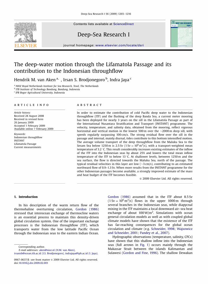
Hydrographic observations (temperature, salinity, CFCs)have shown that this shallow inflow into the Indonesianseas (full arrows in Fig. 1) occurs mainly through theMakassar Strait between the islands Kalimantan andSulawesi (Gordon and Fine, 1996). The shallow Dewakan

www.sciencedirect.com/science/journal/dsri

www.elsevier.com/locate/dsri

dx.doi.org/10.1016/j.dsr.2009.02.001

mailto:[email protected]



ARTICLE IN PRESS

110-15

-10

-5

0

5

10

Kalimantan

Sulawesi

Java

Australia

Irian

Pacific Ocean

Indian Ocean

Sulawesi

Sea

Banda SeaD

L

O

T

115 120 125 130 135

Fig. 1. Map of the Indonesian throughflow. The full arrows depict the main shallow throughflow route via Makassar Strait. The dashed arrows show the

deep throughflow from the Pacific Ocean via the Banda Sea to the Indian Ocean. The full line shows the 2000-m isobath, while the shaded area is

shallower than 500 m. The area in the rectangle encompasses the Lifamatola Passage and is enlarged in Fig. 2. The capitals D, L, O, and T indicate the

approximate locations of, respectively, the Dewakan sill, Lombok Strait, Ombai Strait, and Timor Passage.

H.M. van Aken et al. / Deep-Sea Research I 56 (2009) 1203–12161204

sill at the southern end of Makassar Strait (D in Fig. 1) hasa sill depth of about 680 m (Gordon et al., 2003b). Currentmeasurements in Makassar Strait have shown that thethroughflow through Makassar Strait is about 10 Sv, witha maximum contribution from the layer between 150and 200 m (Gordon et al., 1999, 2003a). The mean tempe-rature of the throughflow in Makassar Strait is nearly 15 1C(Vranes et al., 2002; Gordon et al., 2003a). The main exitsof the ITF towards the Indian Ocean are the passagesbetween the lesser Sunda Islands (Nusantara), in parti-cular Lombok Strait, Ombai Strait, and Timor Passage (L, O,and T in Fig. 1, respectively).

Because of the limited depth of the Dewakan sill inMakassar Strait, ventilation of the deep basins in theBanda Sea, with depths in the Weber Deep surpass-ing 7000 m, requires another pathway. Van Riel (1956)derived, from the changing temperature stratificationmeasured during the Snellius Expedition in 1929–1930,that the flushing of the deep Banda Sea follows a pathwayfrom the Pacific Ocean, via the Lifamatola Passage eastof Sulawesi (box in Fig. 1, and Fig. 2). The sill in thispassage has a depth between 1900 and 2000 m (van Riel,1956; Broecker et al., 1986), allowing a deep throughflowwith temperatures well below that of the throughflow inMakassar Strait. Van Aken et al. (1988) and Gordon et al.(2003b) have shown, from tracer distributions, that the

hydrographic stratification in the deep Banda Sea agreeswith a ventilation by deep overflow from the Pacific Oceanvia the Lifamatola Passage. Thereby the cold through-flow water descends from the Lifamatola sill along thetopography in an approximately 500 m thick layer, firstinto the 5000 m deep Seram Sea, and second from theSeram Sea over a 3500 m deep sill into the Banda Sea (VanAken et al., 1988). Along this path some heating of thebottom water is observed, mainly attributed to mixingwith warmer overlying water near the sills (Van Akenet al., 1988). Consequent deep upwelling and mixing in theBanda Sea then brings the deep throughflow water from adepth of 5000 to about 1000 m (Van Aken et al., 1991;Gordon et al., 2003b). Above the latter level the waterfrom the deep throughflow leaves the Banda Sea towardsthe Indian Ocean through the southern exits, joining theshallow throughflow water from Makassar Strait over the680 m deep Dewakan sill.

Direct measurements of the flow across the sill in theLifamatola Passage and subsequent transport estimatesare scarce. Over 70 years ago Lek (1938) carried outobservations with an Ekman current meter at an anchorstation of the RV Snellius which lasted less than 35 h.At 1500 m he found a mean southeastward flow of about5 cm/s. He also observed strong internal semidiurnal anddiurnal tides, with amplitudes reaching over, respectively,

ARTICLE IN PRESS

128127126125Longitue (E)

3

2

1

Latit

ude

(S)

Obimayor

MangoleLifamatola

Seram Sea

Maluku Sea

Banda Sea

0Distance (km)

2000

1800

1600

1400

1200

1000

Dep

th (m

)

5 10 15 20 25 30 35

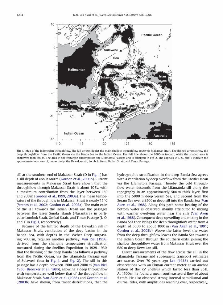
Fig. 2. Plot of the topography near the Lifamatola Passage, between the small Lifamatola Island and the larger island Obimayor, with isobaths every

1000 m (a), based on the Smith and Sandwell (1997) 20 �20 resolution ETOPO-2 topographic data set. The cross indicates the position of the current meter

mooring near the sill of the passage, while the arrow in the direction 1291 shows the observed mean current direction in the lowest 500 m. The line,

perpendicular to the vector, ending in dots, is the cross-section for which transports have been calculated. The bottom profile along this line is shown in

(b). The mooring was located at x ¼ 14.7 km.

H.M. van Aken et al. / Deep-Sea Research I 56 (2009) 1203–1216 1205

30 and 15 cm/s at several depths. Broecker et al. (1986)reported observations with two self-recording currentmeters over the sill, each about 10 m above the bottom,which lasted 28 days. They found a typical steadysoutheastward residual velocity of about 25 cm/s, inagreement with a deep flow of Pacific water towards theBanda Sea. This flow was modified by weaker (�10 cm/s)diurnal and semidiurnal tides. Van Aken et al. (1988)reported 3.5 months of current measurements with acurrent meter mooring over the sill. At 60 m above thebottom the mean velocity was 61 cm/s, directed to thesoutheast, while at 200 m above the sill the mean velocitywas 40 cm/s, in the same direction. Superimposed onthe mean residual flow were tidal motions of a mixedsemidiurnal and diurnal character, leading to totalvelocities in the bottom layer that regularly surpassed1 m/s. From these current measurements the deep inflowbelow 1500 m was estimated to be 1.5 Sv. Luick andCresswell (2001) carried out observations with a singlecurrent meter mooring, located at 11410N, nearly 400 km

north of the Lifamatola Passage, in a 230 km wide passageof the Maluku Sea east of Sulawesi. Assuming a horizon-tally homogenous flow, they reported a southwardtransport between 740 and 1500 m of 7 Sv. However, onecan question whether a single observational point can berepresentative for the ocean circulation in that 230 kmwide passage, especially since the hydrographic observa-tions (T, S, O2) indicate the presence of a cycloniccirculation in the Maluku Sea below 1800 m (Luick andCresswell, 2001).

Several research programmes have aimed at the directmeasurement of the other branches of the ITF, both inMakassar Strait (Gordon et al., 1999, 2003a) and in thesouthern exit channels (Murray and Arief, 1988; Molcardet al., 1994, 1996, 2001). However, the observations fromthose experiments do not supply a contemporaneous dataset of the ITF, since the experiments were carried outin different years. Therefore, the average structureand magnitude of the total transport of mass, heat, andfreshwater by the ITF are not well known. This lack of

ARTICLE IN PRESS


information hampers the validation of ocean generalcirculation models and global climate models. In responseto this lack of knowledge the International NusantaraStratification and Transport (INSTANT) programme wasestablished to directly and simultaneously measure theITF, both in the northern inflow passages and in thesouthern outflow passages (Sprintall et al., 2004). In thisinternational research programme, scientists from Indo-nesia, the USA, Australia, France, and the Netherlandscooperated to determine the strength of the ITF enteringand leaving the Indonesian seas during three consecutiveyears. Variations in the ITF will be related to changes inthe meteorological and oceanographic forcing (sea level,monsoons, El Nino, Indian Ocean Dipole, etc.). This paperdeals with the observations with a current meter mooringover the sill in Lifamatola Passage, carried out during theINSTANT programme. It mainly focuses on the through-flow of the Lifamatola Passage and its variability, but alsodescribes the higher-frequency (tidal) current oscillationsin the passage.

2. The data

The sill depth in Lifamatola Passage is about 2000 m(Fig. 2). Slightly downstream of the sill a mooring wasdeployed twice for a period of about 1.5 years, leading to atotal mooring period of over 34 months (Table 1). Thedeployment cruise in January 2004, the service cruise in

Table 1Description of the INSTANT moorings in the Lifamatola Passage.

Mooring name Latitude Longitude

LOCO-10-1 1149.10N 126157.80E

Height above bottom (m) Instrument type Serial number

1535 RDI ADCP 3553

1534 SBE 37 Microcat 2672

1232 Aanderaa RCM 11 243






608 RDI ADCP 3714


Mooring name Latitude Longitude

LOCO-10-2 1149.10N 126157.80E

Height above bottom (m) Instrument type Serial number

1233 RDI ADCP 3553






608 RDI ADCP 3714


July 2005, and the recovery cruise in January 2006 wereall carried out with the Indonesian RV Baruna Jaya I.During these cruises, series of CTD casts were alsorecorded, with during each cruise at least one CTD castclose to the mooring position, reaching from the seasurface to the bottom. For the first period the mooring wasfitted with two RDI 75 kHz ADCPs (Long Ranger), coveringthe upper and lower parts of the water column, upwardlooking near the surface, and downward looking in thebottom layer. At intermediate levels, three Aanderaa RCM11 acoustic current meters were mounted. All RDIand Aanderaa instruments were fitted with a tilt sensorfor the correction of the velocity, measured from a tiltedmooring. Each of these instruments contained a tempera-ture sensor, while the ADCPs were also fitted with apressure sensor. Additionally five Sea Bird ElectronicsMicrocats (SBE37SM) were mounted to record pressure,temperature, and salinity (Table 1). The mooring positionappeared to be about 30 m shallower than the deepestpart of the nearby deep channel over the sill, at a distanceof about 1 km further northeast. After recovery of thismooring it appeared that because of a faulty but un-documented setting of these instruments, only 7 of the 80data bins of 8 m length were recorded, strongly diminish-ing the information on the ITF, which is assumed to beconcentrated in the near-surface and near-bottom layers.Moreover, it appeared that because of very strong tidesthe 15-min average velocity at mid-levels regularlysurpassed 140 cm/s. This caused a serious blow-down of

Deployment date Recovery date Corrected depth (m)

26-01-2004 17-07-2005 2019

Sampling interval (min)

30

5

15

5

15

5

15

5

30

No data

Deployment date Recovery date Corrected depth (m)

17-07-2005 04-12-2006 2017

Sampling interval (min)

30

5

15

5

15

5

5

30

ARTICLE IN PRESS


the mooring with an average range of 435 m, adding to theinformation loss. In the second deployment period themooring was shortened by 300 m to reduce blow-down,which decreased to an average range of 252 m. However,thereby the possibility to measure velocity in the upper300 m was lost. The faulty ADCP setting was also repaired,so that effectively in the second period our information onthe current structure covered a larger part of the watercolumn, although data reached only to 300 m below thesea surface. The bias in the horizontal velocity, induced bythe horizontal motion of the sensors due to the blow-down, was estimated to be about 2 cm/s or less, with aperiodic character. Since the focus of this paper is on thethroughflow, and since the dominant tides have anamplitude of at least an order of magnitude larger, thisbias has been ignored.

After recovery of the moorings, the recorded directionswere corrected for the magnetic variation, and, by acombination of low-pass filtering (filter width E1/h) andsub-sampling every whole hour, a synchronous hourlydata set for all sensors and ADCP bins was produced,including sensor or bin depth. A shift of the time baseof each instrument was applied in this process to correctfor the effects of different recording intervals and thedifferent meanings of the time stamps in the differentinstruments (beginning, centre, or end of the recordinginterval). From these synchronized and depth-dependentdata, time series of hourly data were calculated at fixeddepth levels by means of vertical linear interpolation,every 100 m in the upper 1600 m and every 50 m from1600 to 2000 m. Continuous hourly data records areavailable for the interpolation depth interval from 1000to 1500 m in the first deployment period, and for the1000–2000 m depth interval in the second deploymentperiod. In order to recover information on the low-frequency flow in the parts of the water column wheredata were available only for part of the tidal periodbecause of the mooring blow-down, the monthly mean

-100

-50

0

50

100

Eas

t com

pone

nt(c

m/s

)

01/01

/04

01/04

/04

01/07

/04

01/10

/04

01/01

/05

01/04

/05

01

-100

-50

0

50

100

Nor

th c

ompo

nent

(cm

/s)

Fig. 3. Time series of the hourly current components at a de

residual current was estimated from a harmonic analysiswith the dominant tidal frequencies (see below). For thefirst deployment period this supplied us with monthlymean residual current data from 500 to 1800 m, and forthe second period from 300 to 2000 m.

From the average current components between 1500and 2000 m, measured during the second deploymentperiod, the mean deep current direction was determinedto be 1291 (arrow in Fig. 2). This direction appears tobe well aligned with the deep channel over the sill. In thefollowing discussion we have rotated our geographicreference frame, naming the direction 1291 along-channel,and the direction perpendicular to the channel, 2191,cross-channel.

3. The character of the currents and their variability

Current data at 1500 m are available for the wholedeployment period (Fig. 3). At this level the mean velocityis 14.7 cm/s to the southeast (1191). The magnitudes of thetemporal variation of the current components, expressedas standard deviation, are 20.7 and 17.5 cm/s for, respec-tively, the east and north components. The plot of bothvelocity components (Fig. 3) shows a considerable con-tribution from the tides, with an envelope that showsmore or less regular fortnightly variability, indicative ofthe spring tide–neap tide phenomenon, as well as longer-term changes of the residual flow. At 1500 m the tidescause a regular reversal of the current direction. This tidalreversal of the current direction is observed even duringspring tide at 2000 m, about 20 m above the bottom.However, during neap tide the residual current at 2000 mis larger than the tidal contribution, maintaining a per-manent southeastward bottom flow. During 0.16% ofthe 1-h data records the current speed at 1500 m exceeds1 m/s. This fraction increases to 12.6% at 2000 m. Variabilityat lower frequencies can be observed in the background,

/07/05

01/10

/05

01/01

/06

01/04

/06

01/07

/06

01/10

/06

01/01

/07

Date

pth of 1500 m for both deployment periods combined.

ARTICLE IN PRESS


leading, for example, to a reversal of the low-passflow direction at 1500 m during the weeks around 1 April2006.

The rotary spectrum (not shown) has characteristictidal bands centred around about N cpd (cycle per day),N being an integer number between 1 and 12. Analysis

of the anisotropy of these tidal bands of rotary spectra atthe interpolation depths has shown that apart from thesemidiurnal tidal bands at 1500 m the variable currentsat tidal frequencies are mainly linearly polarized. Thecharacteristic amplitudes of the anti-clockwise (ACW) andclockwise (CW) components for those tidal bands were allof the same order of magnitude with ratios ACW/CWvarying between 0.7 and 1.4, on average 1.0 (70.1 stdev).As a single exception more extreme values of the ACW/CWratios were found only in the semidiurnal band at 1500 m,where the ACW/CW ratio was 2.7, indicative of thedominance of ACW motion at this depth in this frequencyband. This suggests a large influence of the topography onother frequencies and at deeper levels in the channel overthe sill. The tidal currents below 1500 m were all alignedin the along-channel direction.

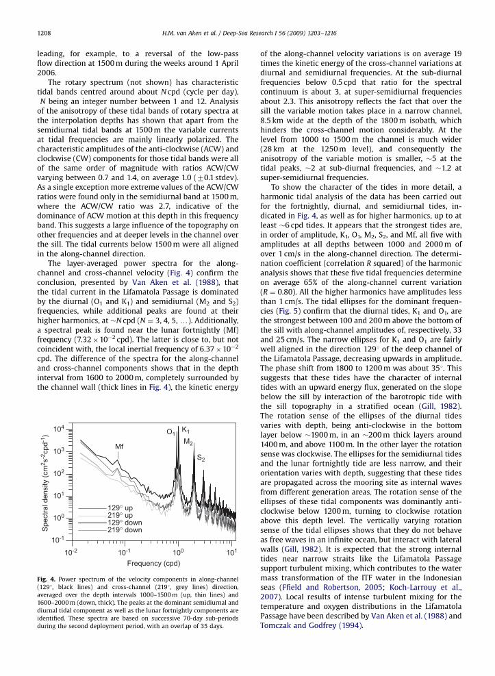
The layer-averaged power spectra for the along-channel and cross-channel velocity (Fig. 4) confirm theconclusion, presented by Van Aken et al. (1988), thatthe tidal current in the Lifamatola Passage is dominatedby the diurnal (O1 and K1) and semidiurnal (M2 and S2)frequencies, while additional peaks are found at theirhigher harmonics, at �N cpd (N ¼ 3, 4, 5, y). Additionally,a spectral peak is found near the lunar fortnightly (Mf)frequency (7.32�10�2 cpd). The latter is close to, but notcoincident with, the local inertial frequency of 6.37�10�2

cpd. The difference of the spectra for the along-channeland cross-channel components shows that in the depthinterval from 1600 to 2000 m, completely surrounded bythe channel wall (thick lines in Fig. 4), the kinetic energy

10-2 10-1 100 101

Frequency (cpd)

10-1

100

101

102

103

104

Spe

ctra

l den

sity

(cm

2 s-2

cpd-1

)

129° up219° up129° down219° down

Mf

O1K1

M2

S2

Fig. 4. Power spectrum of the velocity components in along-channel

(1291, black lines) and cross-channel (2191, grey lines) direction,

averaged over the depth intervals 1000–1500 m (up, thin lines) and

1600–2000 m (down, thick). The peaks at the dominant semidiurnal and

diurnal tidal component as well as the lunar fortnightly components are

identified. These spectra are based on successive 70-day sub-periods

during the second deployment period, with an overlap of 35 days.

of the along-channel velocity variations is on average 19times the kinetic energy of the cross-channel variations atdiurnal and semidiurnal frequencies. At the sub-diurnalfrequencies below 0.5 cpd that ratio for the spectralcontinuum is about 3, at super-semidiurnal frequenciesabout 2.3. This anisotropy reflects the fact that over thesill the variable motion takes place in a narrow channel,8.5 km wide at the depth of the 1800 m isobath, whichhinders the cross-channel motion considerably. At thelevel from 1000 to 1500 m the channel is much wider(28 km at the 1250 m level), and consequently theanisotropy of the variable motion is smaller, �5 at thetidal peaks, �2 at sub-diurnal frequencies, and �1.2 atsuper-semidiurnal frequencies.

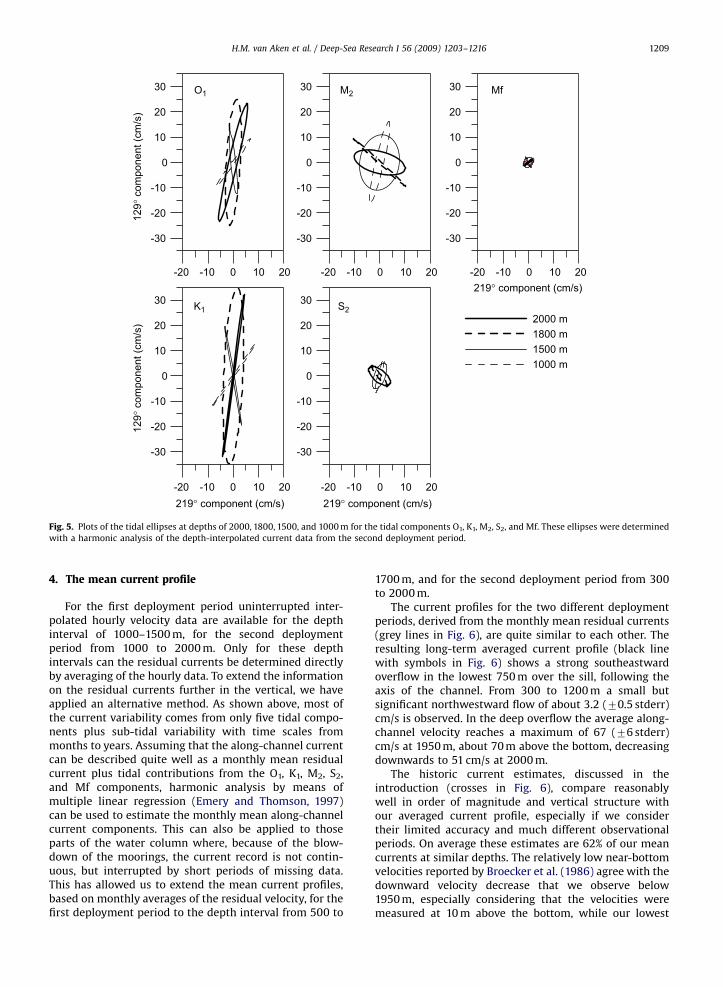
To show the character of the tides in more detail, aharmonic tidal analysis of the data has been carried outfor the fortnightly, diurnal, and semidiurnal tides, in-dicated in Fig. 4, as well as for higher harmonics, up to atleast �6 cpd tides. It appears that the strongest tides are,in order of amplitude, K1, O1, M2, S2, and Mf, all five withamplitudes at all depths between 1000 and 2000 m ofover 1 cm/s in the along-channel direction. The determi-nation coefficient (correlation R squared) of the harmonicanalysis shows that these five tidal frequencies determineon average 65% of the along-channel current variation(R ¼ 0.80). All the higher harmonics have amplitudes lessthan 1 cm/s. The tidal ellipses for the dominant frequen-cies (Fig. 5) confirm that the diurnal tides, K1 and O1, arethe strongest between 100 and 200 m above the bottom ofthe sill with along-channel amplitudes of, respectively, 33and 25 cm/s. The narrow ellipses for K1 and O1 are fairlywell aligned in the direction 1291 of the deep channel ofthe Lifamatola Passage, decreasing upwards in amplitude.The phase shift from 1800 to 1200 m was about 351. Thissuggests that these tides have the character of internaltides with an upward energy flux, generated on the slopebelow the sill by interaction of the barotropic tide withthe sill topography in a stratified ocean (Gill, 1982).The rotation sense of the ellipses of the diurnal tidesvaries with depth, being anti-clockwise in the bottomlayer below �1900 m, in an �200 m thick layers around1400 m, and above 1100 m. In the other layer the rotationsense was clockwise. The ellipses for the semidiurnal tidesand the lunar fortnightly tide are less narrow, and theirorientation varies with depth, suggesting that these tidesare propagated across the mooring site as internal wavesfrom different generation areas. The rotation sense of theellipses of these tidal components was dominantly anti-clockwise below 1200 m, turning to clockwise rotationabove this depth level. The vertically varying rotationsense of the tidal ellipses shows that they do not behaveas free waves in an infinite ocean, but interact with lateralwalls (Gill, 1982). It is expected that the strong internaltides near narrow straits like the Lifamatola Passagesupport turbulent mixing, which contributes to the watermass transformation of the ITF water in the Indonesianseas (Ffield and Robertson, 2005; Koch-Larrouy et al.,2007). Local results of intense turbulent mixing for thetemperature and oxygen distributions in the LifamatolaPassage have been described by Van Aken et al. (1988) andTomczak and Godfrey (1994).

ARTICLE IN PRESS

-30

-20

-10

0

10

20

30

-30

-20

-10

0

10

20

30

2000 m1800 m1500 m1000 m

-30

-20

-10

0

10

20

30

-20

-30

-20

-10

0

10

20

30

129°

com

pone

nt (c

m/s

)12

9° c

ompo

nent

(cm

/s)

-30

-20

-10

0

10

20

30

O1

K1

M2

S2

Mf

-10 0 10 20 -20 -10 0 10 20

-20 -10 0 10 20 -20 -10 0 10 20

-20 -10 0 10 20219° component (cm/s)

219° component (cm/s) 219° component (cm/s)

Fig. 5. Plots of the tidal ellipses at depths of 2000, 1800, 1500, and 1000 m for the tidal components O1, K1, M2, S2, and Mf. These ellipses were determined

with a harmonic analysis of the depth-interpolated current data from the second deployment period.


4. The mean current profile

For the first deployment period uninterrupted inter-polated hourly velocity data are available for the depthinterval of 1000–1500 m, for the second deploymentperiod from 1000 to 2000 m. Only for these depthintervals can the residual currents be determined directlyby averaging of the hourly data. To extend the informationon the residual currents further in the vertical, we haveapplied an alternative method. As shown above, most ofthe current variability comes from only five tidal compo-nents plus sub-tidal variability with time scales frommonths to years. Assuming that the along-channel currentcan be described quite well as a monthly mean residualcurrent plus tidal contributions from the O1, K1, M2, S2,and Mf components, harmonic analysis by means ofmultiple linear regression (Emery and Thomson, 1997)can be used to estimate the monthly mean along-channelcurrent components. This can also be applied to thoseparts of the water column where, because of the blow-down of the moorings, the current record is not contin-uous, but interrupted by short periods of missing data.This has allowed us to extend the mean current profiles,based on monthly averages of the residual velocity, for thefirst deployment period to the depth interval from 500 to

1700 m, and for the second deployment period from 300to 2000 m.

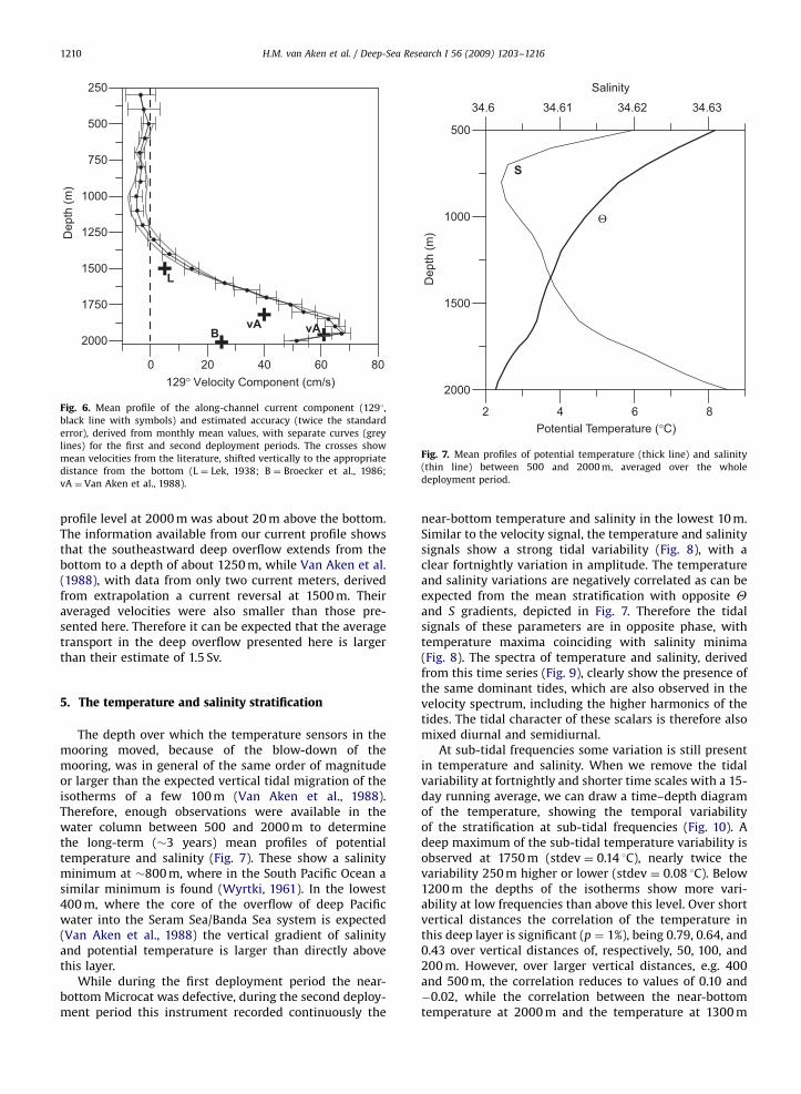
The current profiles for the two different deploymentperiods, derived from the monthly mean residual currents(grey lines in Fig. 6), are quite similar to each other. Theresulting long-term averaged current profile (black linewith symbols in Fig. 6) shows a strong southeastwardoverflow in the lowest 750 m over the sill, following theaxis of the channel. From 300 to 1200 m a small butsignificant northwestward flow of about 3.2 (70.5 stderr)cm/s is observed. In the deep overflow the average along-channel velocity reaches a maximum of 67 (76 stderr)cm/s at 1950 m, about 70 m above the bottom, decreasingdownwards to 51 cm/s at 2000 m.

The historic current estimates, discussed in theintroduction (crosses in Fig. 6), compare reasonablywell in order of magnitude and vertical structure withour averaged current profile, especially if we considertheir limited accuracy and much different observationalperiods. On average these estimates are 62% of our meancurrents at similar depths. The relatively low near-bottomvelocities reported by Broecker et al. (1986) agree with thedownward velocity decrease that we observe below1950 m, especially considering that the velocities weremeasured at 10 m above the bottom, while our lowest

ARTICLE IN PRESS

0

2000

1750

1500

1250

1000

750

500

250

L

BvA vA

Dep

th (m

)

129° Velocity Component (cm/s)20 40 60 80

Fig. 6. Mean profile of the along-channel current component (1291,

black line with symbols) and estimated accuracy (twice the standard

error), derived from monthly mean values, with separate curves (grey

lines) for the first and second deployment periods. The crosses show

mean velocities from the literature, shifted vertically to the appropriate

distance from the bottom (L ¼ Lek, 1938; B ¼ Broecker et al., 1986;

vA ¼ Van Aken et al., 1988).

2

2000

1500

1000

500

Dep

th (m

)

34.6

Salinity

S

Θ

34.61 34.62 34.63

4 6 8Potential Temperature (°C)

Fig. 7. Mean profiles of potential temperature (thick line) and salinity

(thin line) between 500 and 2000 m, averaged over the whole

deployment period.


profile level at 2000 m was about 20 m above the bottom.The information available from our current profile showsthat the southeastward deep overflow extends from thebottom to a depth of about 1250 m, while Van Aken et al.(1988), with data from only two current meters, derivedfrom extrapolation a current reversal at 1500 m. Theiraveraged velocities were also smaller than those pre-sented here. Therefore it can be expected that the averagetransport in the deep overflow presented here is largerthan their estimate of 1.5 Sv.

5. The temperature and salinity stratification

The depth over which the temperature sensors in themooring moved, because of the blow-down of themooring, was in general of the same order of magnitudeor larger than the expected vertical tidal migration of theisotherms of a few 100 m (Van Aken et al., 1988).Therefore, enough observations were available in thewater column between 500 and 2000 m to determinethe long-term (�3 years) mean profiles of potentialtemperature and salinity (Fig. 7). These show a salinityminimum at �800 m, where in the South Pacific Ocean asimilar minimum is found (Wyrtki, 1961). In the lowest400 m, where the core of the overflow of deep Pacificwater into the Seram Sea/Banda Sea system is expected(Van Aken et al., 1988) the vertical gradient of salinityand potential temperature is larger than directly abovethis layer.

While during the first deployment period the near-bottom Microcat was defective, during the second deploy-ment period this instrument recorded continuously the

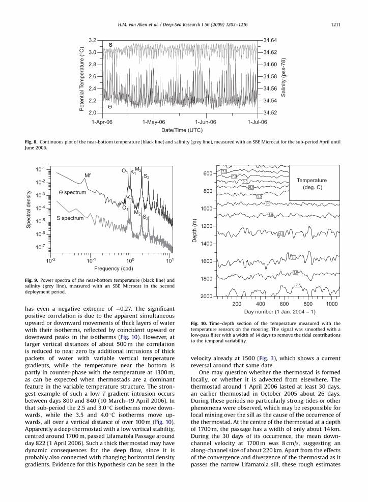
near-bottom temperature and salinity in the lowest 10 m.Similar to the velocity signal, the temperature and salinitysignals show a strong tidal variability (Fig. 8), with aclear fortnightly variation in amplitude. The temperatureand salinity variations are negatively correlated as can beexpected from the mean stratification with opposite Yand S gradients, depicted in Fig. 7. Therefore the tidalsignals of these parameters are in opposite phase, withtemperature maxima coinciding with salinity minima(Fig. 8). The spectra of temperature and salinity, derivedfrom this time series (Fig. 9), clearly show the presence ofthe same dominant tides, which are also observed in thevelocity spectrum, including the higher harmonics of thetides. The tidal character of these scalars is therefore alsomixed diurnal and semidiurnal.

At sub-tidal frequencies some variation is still presentin temperature and salinity. When we remove the tidalvariability at fortnightly and shorter time scales with a 15-day running average, we can draw a time–depth diagramof the temperature, showing the temporal variabilityof the stratification at sub-tidal frequencies (Fig. 10). Adeep maximum of the sub-tidal temperature variability isobserved at 1750 m (stdev ¼ 0.14 1C), nearly twice thevariability 250 m higher or lower (stdev ¼ 0.08 1C). Below1200 m the depths of the isotherms show more vari-ability at low frequencies than above this level. Over shortvertical distances the correlation of the temperature inthis deep layer is significant (p ¼ 1%), being 0.79, 0.64, and0.43 over vertical distances of, respectively, 50, 100, and200 m. However, over larger vertical distances, e.g. 400and 500 m, the correlation reduces to values of 0.10 and�0.02, while the correlation between the near-bottomtemperature at 2000 m and the temperature at 1300 m

ARTICLE IN PRESS

1-Apr-06Date/Time (UTC)

2.0

2.2

2.4

2.6

2.8

3.0

3.2

Pot

entia

l Tem

pera

ture

(°C

)

34.52

34.54

34.56

34.58

34.60

34.62

34.64S

Θ

Sal

inity

(pss

-78)

1-May-06 1-Jun-06 1-Jul-06

Fig. 8. Continuous plot of the near-bottom temperature (black line) and salinity (grey line), measured with an SBE Microcat for the sub-period April until

June 2006.

10-2 10-1 100 101

Frequency (cpd)

10-7

10-6

10-5

10-4

10-3

10-2

10-1

Spe

ctra

l den

sity Θ spectrum

S spectrum

MfO1

O1

K1

K1

M2

M2

S2

S2

Fig. 9. Power spectra of the near-bottom temperature (black line) and

salinity (grey line), measured with an SBE Microcat in the second

deployment period.

200Day number (1 Jan. 2004 = 1)

2000

1800

1600

1400

1200

1000

800

600

Dep

th (m

)

Temperature(deg. C)

7.57.0

6.5

6.0

5.5

5.0

4.5

4.0

3.5

3.0

2.5

400 600 800 1000

Fig. 10. Time–depth section of the temperature measured with the

temperature sensors on the mooring. The signal was smoothed with a

low-pass filter with a width of 14 days to remove the tidal contributions

to the temporal variability.


has even a negative extreme of �0.27. The significantpositive correlation is due to the apparent simultaneousupward or downward movements of thick layers of waterwith their isotherms, reflected by coincident upward ordownward peaks in the isotherms (Fig. 10). However, atlarger vertical distances of about 500 m the correlationis reduced to near zero by additional intrusions of thickpackets of water with variable vertical temperaturegradients, while the temperature near the bottom ispartly in counter-phase with the temperature at 1300 m,as can be expected when thermostads are a dominantfeature in the variable temperature structure. The stron-gest example of such a low T gradient intrusion occursbetween days 800 and 840 (10 March–19 April 2006). Inthat sub-period the 2.5 and 3.0 1C isotherms move down-wards, while the 3.5 and 4.0 1C isotherms move up-wards, all over a vertical distance of over 100 m (Fig. 10).Apparently a deep thermostad with a low vertical stability,centred around 1700 m, passed Lifamatola Passage aroundday 822 (1 April 2006). Such a thick thermostad may havedynamic consequences for the deep flow, since it isprobably also connected with changing horizontal densitygradients. Evidence for this hypothesis can be seen in the

velocity already at 1500 (Fig. 3), which shows a currentreversal around that same date.

One may question whether the thermostad is formedlocally, or whether it is advected from elsewhere. Thethermostad around 1 April 2006 lasted at least 30 days,an earlier thermostad in October 2005 about 26 days.During these periods no particularly strong tides or otherphenomena were observed, which may be responsible forlocal mixing over the sill as the cause of the occurrence ofthe thermostad. At the centre of the thermostad at a depthof 1700 m, the passage has a width of only about 14 km.During the 30 days of its occurrence, the mean down-channel velocity at 1700 m was 8 cm/s, suggesting analong-channel size of about 220 km. Apart from the effectsof the convergence and divergence of the thermostad as itpasses the narrow Lifamatola sill, these rough estimates

ARTICLE IN PRESS


show that the thermostad was much longer than thewidth of the channel. This suggests that the thermostadwas advected from the Maluku Sea to the Lifamatola sill.The cause of the formation of such deep thermostadsupstream of the passage remains uncertain yet. Therelatively large size of the thermostad in the along-flowdirection ensures that the change of the pressure gradientdue to the presence of a thermostad probably extendsover the whole Lifamatola sill, and thereby influences thewhole deep overflow.

6. Transports through Lifamatola Passage

With the velocity data, obtained from the moorings,we can calculate the volume transport across a sectionthat runs perpendicular to the mean along-channel deepflow in the direction of 2191. The endpoints of that sectionare given in Table 2. The section runs from a ridge,extending northwestwards from Obimayor (depth1090 m) across the deep channel in the Lifamatola Passage(maximum depth �2050 m) to a ‘‘shallow’’ platformeast–southeast of Lifamatola (depth 1645 m). The widthof this section is 36.2 km, while at 1750 m it is only10.5 km wide, intersected by the bottom topography(Fig. 2b). For the calculation of the transport we assumethat the measured velocity profile (Fig. 6) is representativefor the vertical velocity structure across the whole section.For the levels below the deepest interpolated velocitylevel, 2000 m, we apply the 2000-m velocity. Given thenarrow width of the deep channel at these levels, theeffect of this, or any other extrapolation, is very small.

The along-channel volume transport Tr over the sillbetween the depth levels z0 and z1 has been computed

Table 2Endpoints of the transport section, through which the transports are

calculated.

Latitude Longitude

1139.900S 127105.140E

1155.070S 126152.810E

01/01/04

Date/Tim

-2

0

2

4

6

8

Volu

me

trans

port

129°

(Sv)

01/07/04 01/01/05 01/07/05

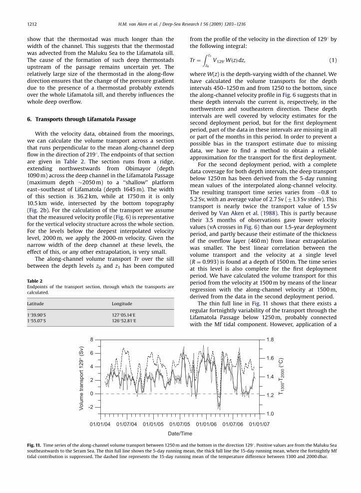
Fig. 11. Time series of the along-channel volume transport between 1250 m and

southeastwards to the Seram Sea. The thin full line shows the 5-day running me

tidal contribution is suppressed. The dashed line represents the 15-day runnin

from the profile of the velocity in the direction of 1291 bythe following integral:

Tr ¼

Z z1

z0

V129�WðzÞdz, (1)

where W(z) is the depth-varying width of the channel. Wehave calculated the volume transports for the depthintervals 450–1250 m and from 1250 to the bottom, sincethe along-channel velocity profile in Fig. 6 suggests that inthese depth intervals the current is, respectively, in thenorthwestern and southeastern direction. These depthintervals are well covered by velocity estimates for thesecond deployment period, but for the first deploymentperiod, part of the data in these intervals are missing in allor part of the months in this period. In order to prevent apossible bias in the transport estimate due to missingdata, we have to find a method to obtain a reliableapproximation for the transport for the first deployment.

For the second deployment period, with a completedata coverage for both depth intervals, the deep transportbelow 1250 m has been derived from the 5-day runningmean values of the interpolated along-channel velocity.The resulting transport time series varies from �0.8 to5.2 Sv, with an average value of 2.7 Sv (71.3 Sv stdev). Thistransport is nearly twice the transport value of 1.5 Svderived by Van Aken et al. (1988). This is partly becausetheir 3.5 months of observations gave lower velocityvalues (vA crosses in Fig. 6) than our 1.5-year deploymentperiod, and partly because their estimate of the thicknessof the overflow layer (460 m) from linear extrapolationwas smaller. The best linear correlation between thevolume transport and the velocity at a single level(R ¼ 0.993) is found at a depth of 1500 m. The time seriesat this level is also complete for the first deploymentperiod. We have calculated the volume transport for thisperiod from the velocity at 1500 m by means of the linearregression with the along-channel velocity at 1500 m,derived from the data in the second deployment period.

The thin full line in Fig. 11 shows that there exists aregular fortnightly variability of the transport through theLifamatola Passage below 1250 m, probably connectedwith the Mf tidal component. However, application of a

e

1.0

1.2

1.4

1.6

1.8

01/01/06 01/07/06 01/01/07

T 130

0-T 2

000

(°C

)

the bottom in the direction 1291. Positive values are from the Maluku Sea

an, the thick full line the 15-day running mean, where the fortnightly Mf

g mean of the temperature difference between 1300 and 2000 dbar.

ARTICLE IN PRESS


15-day running mean (thick full line in Fig. 11) effectivelysuppresses this tidal contribution. A peculiar phenomen-on in the transport time series is the 22-day period around1 April 2006, where the along-channel volume transportbelow 1250 m is negative. It appears that this is caused bythe lowering of the zero-velocity interface, on average at�1250 m, to a level of nearly 1700 m, the deepest currentreversal level observed in our records. This loweringcoincides with the presence of the thermostad in thepassage, centred around the same depth of 1700 m, asdescribed above. A similar phenomenon, although lessextreme, occurred around 20 October 2005. Apparentlythe vertical temperature gradient is related to the strengthof the deep throughflow. The temperature differencebetween 1300 and 2000 m, assumed to be representativefor the vertical temperature gradient in the deep through-flow and the presence of thermostads (Fig. 11, dashedline), shows a regular coincidence of high- or low-transport events with high or low temperature gradients.

The along-channel transport, derived from the 15-dayrunning mean time series in Fig. 11, averaged over thewhole near-3-year deployment period, amounts to 2.4(71.5 stdev) Sv, while the transport derived from theaveraged profiles in Fig. 6 amounts to 2.5 Sv. Apparentlythe averaged velocity profile is not very sensitive to thebias caused by levels with incomplete data from the firstdeployment period.

In order to determine the average temperature of thedeep throughflow below 1250 m, we have to determinethe transport-weighted mean temperature. The transport-weighted temperature TTW is defined as

TTW ¼

R z1

z0V129�TðzÞWðzÞdz

Tr, (2)

where T(z) is the depth-dependent temperature, observedwith the temperatures sensors in the mooring and Tr isdefined in (1). When we calculate the long-term meanvalue of this TTW with the 5-day-averaged time seriesof the along-channel velocity and temperature for thesecond deployment period, we obtain a mean transport-weighted temperature of 3.21 1C, while the use of meanvertical profiles of temperature and velocity for thisperiod results in a mean temperature of 3.25 1C. Appar-ently the effects of any Reynolds terms in the total heat(temperature) transport are negative, but small, and canbe ignored. For the total 34-month deployment period themean temperature of the deep throughflow, derived fromthe long-term mean profiles of temperature and along-channel velocity, is 3.22 1C. The mean salinity of the deepthroughflow, determined similarly, is 34.617, agreeingwith the (near-homogeneous) salinity in the deep BandaSea below 2000 m (34.615–34.620; Van Aken et al., 1988,1991).

In the layer from 250 to 1250 m a significant meanvelocity from the Maluku Sea to the Seram Sea is observed(Fig. 6). Given the increasing width of the LifamatolaPassage from 1250 to the sea surface, the assumption thatthe transport at these levels can be estimated fromvelocity measurements at a single mooring becomesquestionable. But if we do this, the total volume transportin the 1000 m thick layer between 250 and 1250 m

amounts to �1.0 (71.1 stdev) Sv, which means a stronglyvarying, but on average northwestward, transport towardsthe Maluku Sea. An annual cycle of the northwestwardvelocity can be discerned only at 300 and 400 m depth, incounter-phase with the near-surface Ekman Transport at71S in the Banda Sea (Sprintall and Liu, 2005). If weassume that the residual velocity at 300 m extends to thesea surface, we arrive at a small residual northwestwardtransport in the upper 1250 m of 1.3 Sv. However,estimates of the current structure in Makassar Strait haveshown that the vertical current structure in the upper300 m of the Indonesian seas may show a considerableseasonal variability (Gordon et al., 2003a). These esti-mates of the transport above 1250 m, given above, areprobably not very accurate, and should be interpretedwith care.

7. Discussion

The data obtained with the INSTANT mooring in theLifamatola Passage show that vigorous motion occurs inthe deep channel across the sill. That motion consists ofthe residual flow, contributing to the deep ITF of coldwater from the Pacific Ocean towards the Banda Sea andof vertically varying internal tides. Since the southernexits of the Banda Sea are all shallower than the sill in theLifamatola Passage, this sill controls the deep throughflowfrom the Pacific to the Indian Ocean (Gordon et al.,2003b).

In the tidal motion the diurnal tides K1 and O1 aredominant, although Wyrtki (1961) has reported that inthe sea areas around Sulawesi, also in the LifamatolaPassage, the surface tide is mixed, but prevailing semi-diurnal. Apparently the mooring was not intersecteddirectly by a semidiurnal internal tidal wave beam.Generation of (lower-frequency) diurnal internal tides byinteraction of the barotropic tide and topography in astratified sea requires a smaller critical bottom slope thanthe generation of the (higher-frequency) semidiurnalinternal tides, while a propagating diurnal internal wavebeam will also follow a less-steep path than thesemidiurnal tide (Gill, 1982). The steeper critical bottomslope is probably found deeper on the sill, at a largerdistance from the mooring near the top of the sill, than thesmaller slope, where diurnal internal tides are generated.The shorter distance to the critical slope combined withthe less-steep wave beams will favour the diurnal tide toreach the mooring. These frequency-dependent differ-ences in generation areas and wave propagation mayexplain the observed local dominance of the diurnalinternal tides over the sill.

We can assume that the strong tidal variation of thenear-bottom temperature and salinity, measured duringthe second deployment period (Fig. 8), is caused mainly byvertical tidal motion of the isotherms and isohalines. Fromthe temperature signal and the mean vertical gradientof the potential temperature we then derive the standarddeviation of the vertical excursion to be 156 m. Thestandard deviation of the vertical excursion, derived fromthe variations of the salinity, is 144 m, within 10% a similar

ARTICLE IN PRESS


value. This value agrees with the large vertical motionof the isotherms presented for periods of 4 days byVan Aken et al. (1988), who show depth variations ofisothermals (peak–trough) of about 400 m (their Fig. 8).This result also indicates that it is hard to derive the near-bottom vertical stratification from only a few CTD casts.More detailed modelling studies on the generationof internal tides, in combination with resulting generationof turbulent mixing in a general circulation model,like those carried out by Koch-Larrouy et al. (2007),may shed light on the question where and how internaltides contribute to the enhanced turbulent mixing inthe deep Indonesian seas, derived by Van Aken et al.(1988, 1991).

The main transport in the Lifamatola Passage, respon-sible for the cold part of the ITF and the ventilation of thedeep Banda Sea, appears to be concentrated in the lowerlayer of the water column below 1250 m (Fig. 6), with avelocity maximum of over 65 cm/s at �70 m above thebottom. The observed downward decrease of the velocitybelow that level is probably related to friction effects inthe near-bottom layers. The long-term mean volumetransport in this cold ITF, estimated in different ways,amounts to 2.4–2.5 Sv for the total 34-month deploymentperiod. This is nearly 60% higher than the volumetransport of 1.5 Sv, derived from a much shorter deploy-ment period of only 3.5 months, reported by Van Aken etal. (1988). This difference is not necessarily connectedwith long-term changes. From our 34-month transportrecord (Fig. 11) one can derive that on average 15% of the3-month-average transports have a magnitude of 1.5 Sv orless. It can be concluded that the relatively low transport,reported by Van Aken et al. (1988), is not really a rareevent.

The time series of the cold transport, shown in Fig. 11,shows an occasionally strong variation with a time scale ofabout 1 month. It has been shown that the negative-transport event around 1 April 2006 coincided with thepresence of a deep hydrographic feature centred at1700 m, characterized by a strongly reduced verticaltemperature gradient, a thermostad. Below 1700 m theresidual flow was then still directed towards the SeramSea, with near-bottom velocities at 1950 m of well over40 cm/s. The negative correlation between the tempera-ture at 1950 and 1300 m suggests that variations in thevertical temperature gradient, as they occur in a thermo-stad, are a dominant feature below 1250 m. To analyzewhether the relation between the presence of a thermo-stad in the lowest 750 m and the reduction of the deepoverflow can be generalized, we have determined thecorrelation between the 15-day running mean of thevolume transport below 1250 m and the temperaturedifference between 1300 and 2000 m. The resultingcorrelation is 0.62. Apparently, deep thermostads areencountered regularly in the Lifamatola Passage, and theycause a decrease in the volume transport. The source anddynamics of these deep features are unknown yet, but thecoincidence of the strong thermostad at 1700 m with thelow-transport event, as well as the significant correlationbetween transport and vertical temperature gradient,suggests that both are related.

The long-term averaged deep transport derived fromour data, 2.5 Sv, is considerably smaller than the south-ward transport between 740 and 1500 m of �7 Sv, derivedby Luick and Cresswell (2001) for a section in the MalukuSea between Sulawesi and Halmahera. The transport overa similar depth interval derived from our mooring data, is�0.3 Sv, directed to the northwest. This large contrastclearly indicates, as was already suggested by Luick andCresswell (2001), that the assumption that the averagedcurrent data from a mooring at the extreme western sideof a 230 km wide section are representative for the entirewidth of this passage is indeed doubtful. Representativedeep current observations are more likely obtained for oursection of only 36 km wide, although even in this casethe lateral homogeneity is still an assumption, not yet aproven fact. At shallower levels of, e.g., 500 m the cross-channel distance between the isobaths in the LifamatolaPassage is about one third of the section used by Luickand Cresswell (2001), but even over such a distance itis doubtful that the use of a single current meter moor-ing will produce an accurate estimate of the shallowtransport.

The inflow of cold water through the LifamatolaPassage, in addition to the main ITF branch through theMakassar Strait, influences not only the volume budget ofthe ITF but also the heat transport. The existing transportestimate of the strength of the warm Makassar Straitbranch based on the Arlindo Experiment (Gordon et al.,1999) is 9.3 Sv. The deep inflow through LifamatolaPassage, presented here, adds over 25% of cold water tothis estimate. Vranes et al. (2002) derived the transport-weighted temperature in Makassar Strait by four differentmethods and found a mean value of 14.6 (71.8 stdev) 1C. Ifwe combine these (non-contemporary!) results with themean transport and transport-weighted temperature fromthe deep transport in Lifamatola Passage (2.5 Sv and3.2 1C), we arrive at a total northern inflow of the ITF intothe Indonesian seas of 11.8 Sv, with a transport-weightedmean temperature of about 12.2 1C. This temperature isconsiderably lower than the temperature estimates fromthe past of well over 20 1C (Gordon et al., 2003). Whenconsidering these results, one has to be aware that theseresults are obtained by putting together data collectedfrom different experiments, carried out over differentyears. But new data from all the different contemporaryexperiments of the INSTANT programme may lead to athorough revision of the heat budget of the ITF.

The 2.5 Sv cold deep water entering the Banda Seasystem with a mean temperature of 3.2 1C rises there toshallower levels before it can leave for the Indian Oceanthrough the passages between the lesser Sunda Islands oraround Timor. According to Gordon et al. (2003b) thisdeep water leaves the Banda Sea after upwelling to depthsbetween 1300 and 680 m or shallower, before it leaves forthe Indian Ocean. The deeper part of this throughflowoccurs through the Timor Passage and Ombai Strait(T and O in Fig. 1). This agrees quite well with theavailable ETOPO-2 20 �20 resolution topographic data set(Smith and Sandwell, 1997). Preliminary direct transportestimates of the throughflow entering the Indian Ocean,derived from other parts of the INSTANT experiment,

ARTICLE IN PRESS


suggest a deep maximum in this throughflow at �1000 mdepth (Sprintall et al., 2009). At that level the Banda Seahas a mean temperature of �5.0 1C (Van Aken et al., 1988).The heat transported by 2.5 Sv at 5 1C is larger that by thesame volume transport in the Lifamatola Passage at 3.2 1C.This implies that the heat flux of the deep throughflow inthe Band Sea is divergent, and extra heat has to besupplied to warm the upwelling cold water (Munk, 1966;Van Aken et al., 1991). This heat source is supplied byturbulent mixing with the overlying water. Given that thesurface of the Banda Sea is �6.7�1011 m2, and the specificheat of sea water is about 4000 J/kg/1C, the downwardturbulent heat flux in the Banda Sea at a level of 1000 mshould supply 28 W/km2 to support the divergent advec-tive heat flux. If the cold throughflow rises up to theshallower level of 500 m, where the mean temperature is8 1C (Van Aken et al., 1988), a downward turbulent heatflux of 74 W/m2 is required. Upwelling of the cold ITF toeven shallower and warmer levels needs even larger heatinputs. This heat is supplied by the cooling of theoverlying water, and ultimately by cooling of the atmo-sphere in Indonesia. Apparently, maintenance of the deepthroughflow through the Lifamatola Passage may have aconsiderable influence on the local climate, of the sameorder of magnitude as the heat flux sustained by thethroughflow of thermocline water (�100 W/m2) proposedby Gordon (1986).

The downward turbulent heat flux in the water columnis balanced by the upward advective heat flux. Using thevertical advection–diffusion model, proposed by Munk(1966), and using a deep transport estimate of 1 Sv,Van Aken et al. (1988, 1991) were able the estimate theturbulent diffusion coefficient in the Banda Sea to be9�10–4 m2/s. Given a known temperature stratification inthe Banda Sea, the turbulent diffusion coefficient derivedfrom Munk’s model is proportional to the verticalupwelling velocity, which is in its turn proportional tothe deep inflow of cold water. With our new estimateof an inflow of 2.5 Sv, this leads to an estimate of about2.2�10–3 m2/s, more than a factor of 20 higher thanthe generally accepted canonical value of 10–4 m2/s forthe world ocean (Gargett, 1984). Apparently, the stronginternal tides in the Banda Sea contribute strongly to theturbulent energy budget responsible for the maintenanceof the downward turbulent heat flux and the considerablemixing in the Banda Sea (Van Aken et al., 1988; Koch-Larrouy et al., 2007).

When more results from the INSTANT programmebecome available, it is likely that a more reliable budgetfor the ITF of mass, heat, and freshwater than currentlyavailable can be produced. These will form a benchmarkfor model simulations of the interocean exchange be-tween the Pacific and Indian Oceans and are expectedto boost our understanding of these processes for theoceanic climate.

Acknowledgements

We thank the captains and crew of the Baruna Jaya I ofthe Indonesian Agency for Research and Application of

Technology (BPPT) and the technicians and scientists fromthe Agency for Marine and Fisheries Research (BRKP) fortheir support during the research cruises. Many Indone-sian students also participated in the three cruises. TheoHillebrand and Sven Ober prepared and serviced theinstruments, while Marcel Bakker, Jack Schilling, and LeonWuijs were responsible for the construction and handlingof the mooring, and Kees Veth replaced HMvA during thelast cruise. Funding for the mooring equipment wasreceived from the Netherlands Foundation for ScientificResearch (NWO) via the LOCO investment programme,and via the IMAU of Utrecht University from the COAChInternational Research School. Ship time of the RV BarunaJaya I was made available by the BRKP.

References

Broecker, W.S., Patzert, W.C., Toggweiler, J.R., Stuiver, M., 1986. Hydro-graphy, chemistry, and radioisotopes in the southeast Asian waters.Journal of Geophysical Research 91, 14,345–14,354.

Emery, W.J., Thomson, R.E., 1997. Data Analysis Methods in PhysicalOceanography. Pergamon, Oxford, p. 634.

Ffield, A., Robertson, R., 2005. Indonesian seas finestructure variability.Oceanography 18, 108–111.

Gargett, A.E., 1984. Vertical eddy diffusivity in the ocean interior.Dynamics of Atmospheres and Oceans 42, 359–393.

Gill, A.E., 1982. Atmosphere–Ocean Dynamics. Academic Press, London,p. 662.

Gordon, A.L., 1986. Interocean exchange of thermocline water. Journal ofGeophysical Research 91, 5037–5046.

Gordon, A.L., Fine, R.A., 1996. Pathways of water between the Pacific andIndian oceans in the Indonesian sea. Nature 379, 146–149.

Gordon, A.L., Susanto, R.D., Ffield, A., 1999. Throughflow within MakassarStrait. Geophysical Research Letters 26, 3325–3328.

Gordon, A.L., Susanto, R.D., Vranes, K., 2003a. Cool Indonesian through-flow as a consequence of restricted surface layer flow. Nature 425,824–828.

Gordon, A.L., Giulivi, C.F., Ilahude, A.G., 2003b. Deep topographic barrierswithin the Indonesian Seas. Deep-Sea Research II 50, 2205–2228.

Koch-Larrouy, A., Madec, G., Bouruet-Aubertot, P., Gerkema, T., Bessieres,L., Molcard, R., 2007. On the transformation of Pacific water intoIndonesian throughflow water by internal tidal mixing. GeophysicalResearch Letters 34, L04604.

Lek, L., 1938. The Snellius Expedition in the eastern part of the EastIndian Archipelago 1929–1930. Vol. II: Oceanographic results. Part 3:Die Ergebnisse der Strom- und Seriemessungen (in German).

Luick, J.L., Cresswell, G.R., 2001. Current measurements in the MalukuSea. Journal of Geophysical Research 106, 13953–13958.

Molcard, R., Fieux, M., Swallow, J.C., Ilahude, A.G., Banjarnahor, J.,1994. Low frequency variability of the currents in Indonesianchannels (Savu-Roti and Roti-Ashmore Reef). Deep-Sea Research I41, 1643–1661.

Molcard, R., Fieux, M., Ilahude, A.G., 1996. The Indo-Pacific throughflowin the Timor Passage. Journal of Geophysical Research 101,12,411–12,420.

Molcard, R., Fieux, M., Syamsudin, F., 2001. The throughflow withinOmbai Strait. Deep-Sea Research I 48, 1237–1253.

Munk, W.H., 1966. Abyssal recipes. Deep-Sea Research 13, 707–730.Murray, S.P., Arief, D., 1988. Throughflow into the Indian Ocean through

the Lombok Strait, January 1985–January 1986. Nature 333, 444–447.Pandey, V.K., Bhatt, V., Pandey, A.C., Das, I.M.L., 2007. Impact of

Indonesian throughflow blockage on the Southern Indian Ocean.Current Science 93, 399–406.

Schneider, N., 1998. The Indonesian throughflow and the global climatesystem. Journal of Climate 11, 676–689.

Smith, W.H.F., Sandwell, D.T., 1997. Global sea floor topographyfrom satellite altimetry and ship depth soundings. Science 277,1956–1962.

Sprintall, J., Wijffels, S., Gordon, A.L., Ffield, A., Molcard, R., Susanto, R.D.,Soesilo, I., Spaheluwakan, J., Surachman, Y., van Aken, H.M., 2004.INSTANT, a new international array to measure the Indonesianthroughflow. EOS, Transactions, American Geophysical Union 85(39), 369–376.

ARTICLE IN PRESS


Sprintall, J., Wijffels, S.E., Molcard, R., Jaya, I., 2009. Direct estimates ofthe Indonesian Throughflow entering the Indian Ocean: 2004–2006.Journal of Geophysical Research, in press.

Sprintall, J., Liu, W.T., 2005. Ekman mass and heat transport in theIndonesian seas. Oceanography 18 (4), 88–97.

Tomczak, M., Godfrey, J.S., 1994. Regional Oceanography, and Introduc-tion. Pergamon, Oxford, p. 422.

Van Aken, H.M., Punjanan, J., Saimima, S., 1988. Physical aspects of theflushing of the East Indonesian basins. Netherlands Journal of SeaResearch 22, 315–339.

Van Aken, H.M., van Bennekom, A.J., Mook, W., Postma, H., 1991.Application of Munk’s abyssal recipes to tracer distributions in thedeep waters of the South Banda Sea. Oceanologica Acta 14, 151–162.

Van Riel, P.M., 1956. The Snellius Expedition in the eastern part of theEast Indian Archipelago 1929–1930. Vol. II: Oceanographic results.Part 5: The bottom water. Ch. II: Temperature.

Vranes, K., Gordon, A.L., Ffield, A., 2002. The heat transport of theIndonesian Throughflow and implications for the Indian Ocean heatbudget. Deep-Sea Research II 49, 1391–1410.

Wajsowicz, R.C., Schneider, E.K., 2001. The Indonesian throughflow’seffect on global climate determined from the COLA coupled climatemodel. Journal of Climate 14, 3029–3042.

Wyrtki, K., 1961. NAGA Report. Vol. 2: Scientific results ofmarine investigations of the South China Sea and the Gulf ofThailand 1959–1961. Scripps Institution of Oceanography, La Jolla,p. 195.

The deep-water motion through the Lifamatola Passage and its contribution to the Indonesian throughflow

Documents