The deep ocean density structure at the Last Glacial Maximum: What was it and why? Thesis by Madeline Diane Miller In Partial Fulfillment of the Requirements for the Degree of Doctor of Philosophy California Institute of Technology Pasadena, California 2014 (Defended September 27, 2013)

The deep ocean density structure at the last glacial maximum what was it and why
Jul 18, 2015
Welcome message from author
This document is posted to help you gain knowledge. Please leave a comment to let me know what you think about it! Share it to your friends and learn new things together.
Transcript
The deep ocean density structure at the Last Glacial
Maximum: What was it and why?
Thesis by
Madeline Diane Miller
In Partial Fulfillment of the Requirements
for the Degree of
Doctor of Philosophy
California Institute of Technology
Pasadena, California
2014
(Defended September 27, 2013)

ii
c© 2014
Madeline Diane Miller
All Rights Reserved

iii
into the sea all the rivers go, and yet the sea is never filled, and still to their goal the
rivers go
–Ecclesiastes, The Jerusalem Bible Translation

iv
Acknowledgements
The work described in this thesis would not have been possible without my advisor, Jess
Adkins. He provided the impetus, and the structural and intellectual support for my
projects. Further, Jess has encouraged me to explore bold research paths and, when
setbacks inevitably arose, he helped me learn from them, in the process nudging me
towards becoming an independent researcher. Jess models and teaches a broad, problem-
based approach to research. While many oceanographers incorporate data or concepts
outside their traditional focus (i.e. biological, physical, or chemical) to their work, Jess
does not cross disciplinary boundaries, he simply does not see them. He teaches us both
by telling us directly and, even more impressively, by his example that we should always
use the best tool to answer our questions, whether the tool is something we already know
or is well outside our “tool box”. I look forward to continuing to learn from Jess in the
future.
I am indebted to Nadia Lapusta for her support as the Mechanical Engineering option
representative in smoothing the way for me to pursue an unconventional thesis topic. My
thesis committee – John Brady, Chris Charles, Richard Murray, and Mark Simons – have
been equally open-minded in assisting with work outside their primary areas of interest
and very generous with their time.
Thanks go to Dimitris Menemenlis for his open-ended support, encouragement and ad-
vising in ocean and ice modeling, supercomputing, and all things related to MITgcm.
Dimitris welcomed me into his research group at JPL, vastly increasing the number of
oceanographers with whom I’ve been able to interact over the course of my PhD. My work
has particularly benefited from input from Daria Halkides, Jessica Hausman, An Nguyen,
Michael Schodlok and Gunnar Spreen.
v
Over the last two years, Mark Simons has been slowly and stealthily saddled with the
role of being my unofficial second advisor. Mark’s expertise and guidance were essential
to the work in this thesis that relies on inverse methods, and he has shared liberally his
time, ideas, code, server, and scientific contacts. I continue to be impressed by Mark’s
tireless enthusiasm for science and his ability to see the construction hidden behind every
research roadblock, best encapsulated by his own words: “...but look how much you’ve
learned !”
Sarah Minson has not only generously allowed me to use her code, CATMIP, but has also
provided significant technical support in applying CATMIP to my research problems,
despite the fact they do not overlap with hers. Sarah has additionally shared with me a
great deal of her time and expertise on Bayesian MCMC parameter estimation.
Through Mark’s and Sarah’s introductions, my work has been improved from conversa-
tions with Francisco Ortega, Bryan Riel, Michael Aivazis and Jim Beck.
I have been lucky to share many hours in the last few years with the vibrant people in my
research group: Anna Beck, Andrea Burke, Stacy Carolin, Alex Gagnon, Sophie Hines,
Paige Logan, Nele Meckler, Guillaume Paris, Ted Present, James Rae, Morgan Raven,
Alex Rider, Harald Sodemann, Adam Subhas, and Nithya Thiagarajan. I have learned
many things from all of you, not the least of which is how to keep the fun in good science.
The pore fluid sampling intercomparison was made possible in large part by the Integrated
Ocean Drilling Program (IODP), the Consortium for Ocean Leadership, and collabora-
tion with David Hodell. The success of our ship-based work was certainly due to David’s
extensive previous experience on IODP expeditions and his geochemical expertise. The
technicians in the chemistry lab on IODP Expedition 339, Chris Bennight and Erik Moort-
gat, were unendingly patient and extremely meticulous in helping us complete our work.
My organic geochemist counterpart Alexandrina Tzanova was an excellent teammate and
the source of much comic relief on our shift. Chief scientists Javier Hernandez Molina and
Dorrik Stow generously granted David’s and my extensive sample request. Much of my
post-cruise work was supported by a Consortium for Ocean Leadership Post Expedition
Award.

vi
The NASA Advanced Supercomputer (NAS) support and Caltech’s GPS IT and High Per-
formance Computing (HPC) support, particularly Mike Black and Naveed Near-Ansari,
have been extremely responsive and patient in assisting me debug issues on Pleiades,
Salacia and Fram over the course of my research. I am particularly grateful that experts
in the NAS Control Room are available 24x7.
At various stages in building experiments at Caltech, some of which are not discussed in
this thesis, I have benefited greatly from the help of all of the machinists in the Physics
shop, as well as Caltech’s scientific glassblower Rick Gerhart.
Finally, I would like to thank my family and friends for their love, support, and on-demand
cheering. In particular, Chuck Booten, John Eaton, Milt Edgerton, Pat Edgerton, Zach
Lebo, Christina Liebner, Diane Miller, Ethan Miller, Sara Davis Miller, Steph Miller,
Zach Miller, Luigi Perotti, and Phyllis Wolf have cheered extra-loudly for me throughout
my time here at Caltech. E al sior tenente, con cui ho condiviso questa marcia, vorrei
dire che ghe sem.

vii
Abstract
The search for reliable proxies of past deep ocean temperature and salinity has proved
difficult, thereby limiting our ability to understand the coupling of ocean circulation and
climate over glacial-interglacial timescales. Previous inferences of deep ocean temperature
and salinity from sediment pore fluid oxygen isotopes and chlorinity indicate that the deep
ocean density structure at the Last Glacial Maximum (LGM, ∼20,000 years BP) was set
by salinity, and that the density contrast between northern and southern sourced deep
waters was markedly greater than in the modern ocean. High density stratification could
help explain the marked contrast in carbon isotope distribution recorded in the LGM
ocean relative to that we observe today, but what made the ocean’s density structure
so different at the LGM? How did it evolve from one state to another? Further, given
the sparsity of the LGM temperature and salinity data set, what else can we learn by
increasing the spatial density of proxy records?
We investigate the cause and feasibility of a highly and salinity stratified deep ocean at
the LGM and we work to increase the amount of information we can glean about the past
ocean from pore fluid profiles of oxygen isotopes and chloride. Using a coupled ocean–
sea ice–ice shelf cavity model we test whether the deep ocean density structure at the
LGM can be explained by ice–ocean interactions over the Antarctic continental shelves,
and show that a large contribution of the LGM salinity stratification can be explained
through lower ocean temperature. In order to extract the maximum information from
pore fluid profiles of oxygen isotopes and chloride we evaluate several inverse methods
for ill-posed problems and their ability to recover bottom water histories from sediment
pore fluid profiles. We demonstrate that Bayesian Markov Chain Monte Carlo parameter
estimation techniques enable us to robustly recover the full solution space of bottom
viii
water histories, not only at the LGM, but through the most recent deglaciation and the
Holocene up to the present. Finally, we evaluate a non-destructive pore fluid sampling
technique, Rhizon samplers, in comparison to traditional squeezing methods and show
that despite their promise, Rhizons are unlikely to be a good sampling tool for pore fluid
measurements of oxygen isotopes and chloride.
ix
Contents
Acknowledgements iv
Abstract vii
Contents ix
List of Figures xiii
List of Tables xxvii
1 Introduction 1
2 Reconstructing δ18O and salinity histories from pore fluid profiles: What
can we learn from regularized least squares? 12
2.1 Introduction . . . . . . . . . . . . . . . . . . . . . . . . . . . . . . . . . . . 12
2.2 Methods . . . . . . . . . . . . . . . . . . . . . . . . . . . . . . . . . . . . . 17
2.2.1 The forward problem . . . . . . . . . . . . . . . . . . . . . . . . . . 17
2.2.1.1 Simplifying assumptions . . . . . . . . . . . . . . . . . . . 17
2.2.1.2 Finite difference solution technique . . . . . . . . . . . . . 20
2.2.1.3 Green’s function approach . . . . . . . . . . . . . . . . . . 20
2.2.2 The inverse problem . . . . . . . . . . . . . . . . . . . . . . . . . . 21
2.2.2.1 Ill-posed nature of inverse problem . . . . . . . . . . . . . 21
2.2.2.2 Truncated SVD solution . . . . . . . . . . . . . . . . . . . 23
2.2.2.3 Zeroth-order Tikhonov regularization . . . . . . . . . . . . 24
2.2.2.4 Second-order Tikhonov regularization . . . . . . . . . . . . 26
2.2.2.5 Parameter choice . . . . . . . . . . . . . . . . . . . . . . . 27
x
2.3 Results . . . . . . . . . . . . . . . . . . . . . . . . . . . . . . . . . . . . . . 29
2.3.1 Recovering a stretched sea level boundary condition . . . . . . . . . 29
2.3.1.1 Properties of G . . . . . . . . . . . . . . . . . . . . . . . . 30
2.3.1.2 TSVD least squares inverse solution . . . . . . . . . . . . 30
2.3.1.3 Zeroth order Tikhonov regularization . . . . . . . . . . . . 33
2.3.1.4 Zeroth order Tikhonov regularization with noise . . . . . . 34
2.3.1.5 Resolution of the inverse solution . . . . . . . . . . . . . . 42
2.3.1.6 Second order Tikhonov regularization . . . . . . . . . . . . 46
2.3.1.7 Variable damping . . . . . . . . . . . . . . . . . . . . . . . 53
2.3.2 The effect of the diffusion parameter . . . . . . . . . . . . . . . . . 56
2.4 Discussion . . . . . . . . . . . . . . . . . . . . . . . . . . . . . . . . . . . . 61
2.5 Conclusions . . . . . . . . . . . . . . . . . . . . . . . . . . . . . . . . . . . 63
3 What is the information content of pore fluid δ18O and [Cl−]? 64
3.1 Introduction . . . . . . . . . . . . . . . . . . . . . . . . . . . . . . . . . . . 64
3.2 Methods . . . . . . . . . . . . . . . . . . . . . . . . . . . . . . . . . . . . . 68
3.2.1 Forward model . . . . . . . . . . . . . . . . . . . . . . . . . . . . . 68
3.2.2 The inverse problem . . . . . . . . . . . . . . . . . . . . . . . . . . 70
3.2.2.1 Bayesian Markov Chain Monte Carlo sampling . . . . . . 70
3.2.2.2 Model parameterization . . . . . . . . . . . . . . . . . . . 71
3.2.2.3 Cost function . . . . . . . . . . . . . . . . . . . . . . . . . 72
3.2.3 Choice of priors . . . . . . . . . . . . . . . . . . . . . . . . . . . . . 72
3.2.3.1 Prior information from sea level records . . . . . . . . . . 73
3.2.3.2 Prior information from modern ocean property spreads . . 74
3.2.3.3 Accounting for different-than-modern past ocean property
spreads . . . . . . . . . . . . . . . . . . . . . . . . . . . . 77
3.2.3.4 Diffusion coefficient prior . . . . . . . . . . . . . . . . . . 78
3.3 Results . . . . . . . . . . . . . . . . . . . . . . . . . . . . . . . . . . . . . . 79
3.3.1 Synthetic problem . . . . . . . . . . . . . . . . . . . . . . . . . . . 79
3.3.1.1 Linear problem – uninformative prior . . . . . . . . . . . . 80
3.3.1.2 Linear problem – sea level prior with varying variance and
covariance . . . . . . . . . . . . . . . . . . . . . . . . . . . 89
xi
3.3.1.3 Linear Problem – recovery of models with known variance
and covariance . . . . . . . . . . . . . . . . . . . . . . . . 99
3.3.1.4 Nonlinear problem – recovery of models with known vari-
ance and covariance, allowing D0 and initial condition to
vary . . . . . . . . . . . . . . . . . . . . . . . . . . . . . . 114
3.3.2 Real data . . . . . . . . . . . . . . . . . . . . . . . . . . . . . . . . 119
3.4 Discussion and ongoing investigations . . . . . . . . . . . . . . . . . . . . . 121
3.5 Conclusions . . . . . . . . . . . . . . . . . . . . . . . . . . . . . . . . . . . 134
4 New techniques for sediment interstitial water sampling 147
4.1 Motivation and background . . . . . . . . . . . . . . . . . . . . . . . . . . 147
4.2 Methods . . . . . . . . . . . . . . . . . . . . . . . . . . . . . . . . . . . . . 150
4.2.1 Shipboard sampling . . . . . . . . . . . . . . . . . . . . . . . . . . . 150
4.2.1.1 Squeeze samples . . . . . . . . . . . . . . . . . . . . . . . 150
4.2.1.2 Rhizon samples . . . . . . . . . . . . . . . . . . . . . . . . 151
4.2.2 δ18O and δD measurements . . . . . . . . . . . . . . . . . . . . . . 153
4.2.3 [Cl−] measurements . . . . . . . . . . . . . . . . . . . . . . . . . . . 154
4.3 Results . . . . . . . . . . . . . . . . . . . . . . . . . . . . . . . . . . . . . . 156
4.3.1 Stable isotopes . . . . . . . . . . . . . . . . . . . . . . . . . . . . . 157
4.3.2 Chloride . . . . . . . . . . . . . . . . . . . . . . . . . . . . . . . . . 158
4.4 Discussion . . . . . . . . . . . . . . . . . . . . . . . . . . . . . . . . . . . . 160
4.5 Conclusions . . . . . . . . . . . . . . . . . . . . . . . . . . . . . . . . . . . 166
5 The role of ocean cooling in setting glacial southern source bottom water
salinity 167
Abstract 168
5.1 Introduction . . . . . . . . . . . . . . . . . . . . . . . . . . . . . . . . . . . 169
5.2 Methods . . . . . . . . . . . . . . . . . . . . . . . . . . . . . . . . . . . . . 173
5.2.1 Model Setup . . . . . . . . . . . . . . . . . . . . . . . . . . . . . . . 173
5.2.2 Salinity Tracers . . . . . . . . . . . . . . . . . . . . . . . . . . . . . 176
5.2.3 Boundary Conditions . . . . . . . . . . . . . . . . . . . . . . . . . . 177
5.2.4 Control Integration Comparison with Data . . . . . . . . . . . . . . 178
xii
5.2.5 Experiments . . . . . . . . . . . . . . . . . . . . . . . . . . . . . . . 181
5.3 Results and Discussion . . . . . . . . . . . . . . . . . . . . . . . . . . . . . 182
5.3.1 Diagnosis of Water Mass Changes – Net Salinity Fluxes and Changes184
5.3.2 Diagnosis of Water Mass Changes – Regional Variations and Salin-
ity Flux Tracers . . . . . . . . . . . . . . . . . . . . . . . . . . . . . 188
5.3.3 Diagnosis of Water Mass Changes – Regional Differences in Ice Shelves195
5.3.4 Relevance to Glacial Oceans . . . . . . . . . . . . . . . . . . . . . . 197
5.3.5 The Effect of Unmodelled Processes . . . . . . . . . . . . . . . . . . 198
5.4 Conclusions . . . . . . . . . . . . . . . . . . . . . . . . . . . . . . . . . . . 199
6 Concluding remarks 202
A Titration methods for [Cl−] measurement 206
A.1 Theory . . . . . . . . . . . . . . . . . . . . . . . . . . . . . . . . . . . . . . 206
A.2 Equipment . . . . . . . . . . . . . . . . . . . . . . . . . . . . . . . . . . . . 207
A.3 Standards . . . . . . . . . . . . . . . . . . . . . . . . . . . . . . . . . . . . 208
Bibliography 209
xiii
List of Figures
2.1 Illustration of the method previously used to reconstruct the LGM salinity
and δ18O. Changes in salinity scaled to the sea level curve, up to a scaling
constant. Low sea level corresponds to high salinity and vice versa. (a)
shows boundary conditions produced using three different scaling factors,
and (b) shows the model output using those boundary conditions overlaid on
measured data in sediment pore fluids (black circles). Each color corresponds
to a different LGM – modern scaling factor. . . . . . . . . . . . . . . . . . 15
2.2 Picard plot for G size 251 x 251. . . . . . . . . . . . . . . . . . . . . . . . . 31
2.3 (a) shows the synthetic model (red) used to generate synthetic data and the
model recovered using the TSVD method (blue). (b) is the synthetic data
(red) generated by the synthetic model and used to find the inverse solution
plotted against the data generated by the recovered model using TSVD (blue). 32
2.4 L-curve for G size 251 x 251, 0th order Tikhonov regularization . . . . . . . 33
2.5 0th order Tikhonov regularization, no noise . . . . . . . . . . . . . . . . . . 36
2.6 0th order Tikhonov regularization, no noise . . . . . . . . . . . . . . . . . . 37
2.7 0th order Tikhonov regularization, no noise . . . . . . . . . . . . . . . . . . 38
2.8 0th order Tikhonov regularization with noise, G 251 x251 . . . . . . . . . . 39
2.9 0th order Tikhonov regularization with noise, G 301 x 626 . . . . . . . . . . 40
2.10 0th order Tikhonov regularization with noise, G 301 x 1251 . . . . . . . . . 41
2.11 Resolution diagonals and LGM spike tests, 0th order regularization . . . . . 45
2.12 2nd order regularization, no noise, using L-curve criterion for α . . . . . . . 47
2.13 2nd order regularization, no noise, using L-curve criterion for α . . . . . . . 48
2.14 2nd order regularization, no noise, using L-curve criterion for α . . . . . . . 49
xiv
2.15 2nd order regularization with noise, α chosen with discrepancy principle, G
251 x 251 . . . . . . . . . . . . . . . . . . . . . . . . . . . . . . . . . . . . . 50
2.16 2nd order regularization with noise, α chosen with discrepancy principle, G
301 x 626 . . . . . . . . . . . . . . . . . . . . . . . . . . . . . . . . . . . . . 51
2.17 2nd order regularization with noise, α chosen with discrepancy principle, G
301 x 1251 . . . . . . . . . . . . . . . . . . . . . . . . . . . . . . . . . . . . 52
2.18 2nd order resolution matrix diagonals and LGM spike test, G 251 x 251 . . 53
2.19 Spike tests comparing the skill of constant vs. variable damping through the
sensitivity matrix technique. The first row, (a) - (c) use a constant damping
parameter α = 1 and the standard second-order Tikhonov regularization.
The second row, (d) - (f) use α=1 and the variable sensitivity matrix S in
place of the uniform L. . . . . . . . . . . . . . . . . . . . . . . . . . . . . . . 55
2.21 D0 = 2.9× 10⁻⁵ cm2 s−1, 2nd order regularization with noise, G 251 x 251 . 58
2.22 0th order reg, D0 = 2.9 × 10⁻⁷ cm2 s−1 (a) 0.05% noise G 251x251 and
discrep criterion (c) 0.1% noise (e) 0.5% noise (g) 1% noise. . . . . . . . . . 59
2.23 2nd order reg, D0 = 2.9 × 10⁻⁷ cm2 s−1 (a) 0.05% noise G 251x251 and
discrep criterion (c) 0.1% noise (e) 0.5% noise (g) 1% noise. . . . . . . . . . 60
3.1 Measured profiles of (a) δ18O and (b) salinity (converted from the measured
[Cl−] values). Note that the x-axis for ODP Site 1239 in (a) has a wider range
than the others. The values in all of the measured data profiles increase
towards a local maximum several tens of meters below the sea floor. . . . . . 65
3.2 Information in the measured δ18O and [Cl−] (shown converted to equivalent
salinity). Circles represent the modern sediment-water interface value, while
triangles are the maximum value measured in the pore fluids between 0 and
100 mbsf. . . . . . . . . . . . . . . . . . . . . . . . . . . . . . . . . . . . . . 66
3.3 Locations of the ODP sites where we have pore fluid profile measurements
of δ18O and [Cl−] overlain on the modern ocean bottom water salinity. Note
that the range of modern ocean bottom water salinity is quite narrow. . . . 67
3.4 Reconstructions of past sea level relative to present (black circles) and the
points we use for sea level in computing the prior mean salinity and δ18O
(blue triangles) . . . . . . . . . . . . . . . . . . . . . . . . . . . . . . . . . . 75

xv
3.5 (a) Modern S below 2000m, GISS database accessed 9/12/2012, excluding
the Mediterranean Sea. Blue curve is Gaussian distribution with standard
deviation used for priors (b) modern δ18O below 2000m . . . . . . . . . . . . 76
3.6 Prior probability for D0 is log-normal centered on 50×10−6 cm2 s−1, with
standard deviation of the logarithm equal to 1.5. . . . . . . . . . . . . . . . 79
3.7 Synthetic example with 0.05% noise added to the data. Units for salinity on
the y-axis are g kg−1. Red dashed line is the synthetic (true) model used to
generate the data. The black dots represent mean positions of prior salinity
nodes. The blue triangles are the posterior mean salinity nodes. (a) has 0
covariance in the prior, (b) has T= 1000 years covariance timescale prior, (c)
T=2000 years, (d) T = 3000 years, (e) T= 4000 years, (f) T = 5000 years,
(g) T = 6000 years. . . . . . . . . . . . . . . . . . . . . . . . . . . . . . . . 83
3.8 Histograms of synthetic solution assuming 100 g kg−1 variance. Blue is the
histogram of the prior samples, red is the histogram of the posterior samples.
(a) has a prior with no covariance while (b) has a prior covariance timescale
of 6000 years . . . . . . . . . . . . . . . . . . . . . . . . . . . . . . . . . . . 85
3.9 Ratio of posterior variance to prior variance for the linear synthetic case with
100 = σ2I and µI set by scaling to sea level curve. Each colored line depicts
a different value for the prior covariance timescale T, from 0 to 6000 years . 86
3.10 Posterior correlation maps for examples inverting the stretched sea level
curve using a wide (σ = 10 g kg−1) Gaussian prior with varying values of
T. The axes’ values are the age in ka BP of each node. Each colored block
is the posterior correlation between the nodes represented by the values
on the x and y axis. For this reason the maps are symmetric about the
diagonal. The scale is from -1 to 1 in unitless Pearson correlation coefficient
rx,y = E[(X−µx)(Y−µy)]
σxσy. Values between -0.2 and 0.2 have been masked with
white. (a) has 0 covariance in the prior, (b) has T= 1000 years covariance
timescale prior, (c) T=2000 years, (d) T = 3000 years, (e) T= 4000 years,
(f) T = 5000 years, (g) T = 6000 years. . . . . . . . . . . . . . . . . . . . . 87

xvi
3.11 Shift in the mean solution from prior to posterior as a function of covariance
timescale T. Each line represents a different value of T in years, from 0 years
to 6000 years. As T increases, the temporal dependence of the mean shift is
flattened or damped. . . . . . . . . . . . . . . . . . . . . . . . . . . . . . . . 88
3.12 Lomb-Scargle periodogram of the posterior mean for the stretched sea level
example using a wide Gaussian prior. The black line is the periodogram
of the prior mean for comparision. Each color is the periodogram of the
posterior mean with a different prior covariance timescale T in years, from 0
to 6000 years. The vertical lines overlain show the peak frequencies for the
prior and those of the posterior for the example T = 6000 years. . . . . . . . 89
3.13 Synthetic example with 0.05% noise added to the data. The prior nodes
are independent (no covariance) Gaussians centered around a salinity curve
scaled to sea level with varying variance. (a) 0.02 g kg−1 (b) 0.5 g kg−1. (c)
1 g kg−1. Red dashed line is the synthetic (true) model used to generate the
data. The black dots represent mean positions of prior salinity nodes and
the black lines are the 10 highest probability samples from the prior. The
blue triangles are the posterior mean salinity nodes and the blue lines are
the 10 highest probability samples from the posterior. . . . . . . . . . . . . 93
3.14 Posterior correlation matrices for models shown in Fig. 3.13 where the prior
T=0. The axes’ values are the age in ka BP of each node. Each colored block
is the posterior correlation between the nodes represented by the values
on the x and y axis. For this reason the maps are symmetric about the
diagonal. The scale is from -1 to 1 in unitless Pearson correlation coefficient
rx,y = E[(X−µx)(Y−µy)]
σxσy. Values between -0.2 and 0.2 have been masked with
white. (a) 0.02 g kg−1 variance, (b) 0.5 g kg−1 variance, (c) 1 g kg−1 variance 93

xvii
3.15 Synthetic example with 0.05% noise added to the data. The prior nodes
have Gaussian covariance with time scale T = 1000 years centered around
a salinity curve scaled to sea level with varying variance. (a) 0.02 g kg−1
(b) 0.5 g kg−1. (c) 1 g kg−1. Red dashed line is the synthetic (true) model
used to generate the data. The black dots represent mean positions of prior
salinity nodes and the black lines are the 10 highest probability samples from
the prior. The blue triangles are the posterior mean salinity nodes and the
blue lines are the 10 highest probability samples from the posterior. . . . . 94
3.16 Posterior correlation matrices for models shown in Fig. 3.15, where T =
1000 years. The axes’ values are the age in ka BP of each node. Each
colored block is the posterior correlation between the nodes represented by
the values on the x and y axis. For this reason the maps are symmetric
about the diagonal. The scale is from -1 to 1 in unitless Pearson correlation
coefficient rx,y = E[(X−µx)(Y−µy)]
σxσy. Values between -0.2 and 0.2 have been
masked with white. (a) 0.02 g kg−1 variance, (b) 0.5 g kg−1 variance, (c) 1
g kg−1 variance . . . . . . . . . . . . . . . . . . . . . . . . . . . . . . . . . . 94
3.17 Synthetic example with 0.05% noise added to the data. The prior nodes
have Gaussian covariance with time scale T = 3000 years centered around
a salinity curve scaled to sea level with varying variance. (a) 0.02 g kg−1
(b) 0.5 g kg−1. (c) 1 g kg−1. Red dashed line is the synthetic (true) model
used to generate the data. The black dots represent mean positions of prior
salinity nodes and the black lines are the 10 highest probability samples from
the prior. The blue triangles are the posterior mean salinity nodes and the
blue lines are the 10 highest probability samples from the posterior. . . . . 95
3.18 Posterior correlation matrices for models shown in Fig. 3.17 where T = 3000
years. The axes’ values are the age in ka BP of each node. Each colored
block is the posterior correlation between the nodes represented by the values
on the x and y axis. For this reason the maps are symmetric about the
diagonal. The scale is from -1 to 1 in unitless Pearson correlation coefficient
rx,y = E[(X−µx)(Y−µy)]
σxσy. Values between -0.2 and 0.2 have been masked with
white. (a) 0.02 g kg−1 variance, (b) 0.5 g kg−1 variance, (c) 1 g kg−1 variance 95
xviii
3.19 Synthetic example with 0.05% noise added to the data. The prior nodes
have Gaussian covariance with time scale T = 5000 years centered around
a salinity curve scaled to sea level with varying variance. (a) 0.02 g kg−1
(b) 0.5 g kg−1. (c) 1 g kg−1. Red dashed line is the synthetic (true) model
used to generate the data. The black dots represent mean positions of prior
salinity nodes and the black lines are the 10 highest probability samples from
the prior. The blue triangles are the posterior mean salinity nodes and the
blue lines are the 10 highest probability samples from the posterior. . . . . 96
3.20 Posterior correlation matrices for models shown in Fig. 3.19, where T=5000
years. The axes’ values are the age in ka BP of each node. Each colored
block is the posterior correlation between the nodes represented by the values
on the x and y axis. For this reason the maps are symmetric about the
diagonal. The scale is from -1 to 1 in unitless Pearson correlation coefficient
rx,y = E[(X−µx)(Y−µy)]
σxσy. Values between -0.2 and 0.2 have been masked with
white. (a) 0.02 g kg−1 variance, (b) 0.5 g kg−1 variance, (c) 1 g kg−1 variance 96
3.21 Histograms of synthetic solution assuming 0.02 g kg−1 variance. Blue is
the histogram of the prior samples, red is the histogram of the posterior
samples. (a) has a prior with no covariance while (b) has a prior covariance
timescale of 5000 years. Each box is one node of the time series we are
estimating. From left to right and top to bottom the nodes move forward in
time, starting at 125 ka BP and ending at the present, 0 ka BP. . . . . . . . 100
3.22 Histograms of synthetic solution assuming 1 g kg−1 variance. Blue is the
histogram of the prior samples, red is the histogram of the posterior sam-
ples. (a) has a prior with 0 covariance while (b) has a prior with 5000 year
timescale covariance. Each box is one node of the time series we are esti-
mating. From left to right and top to bottom the nodes move forward in
time, starting at 125 ka BP and ending at the present, 0 ka BP. . . . . . . . 101

xix
3.23 The ratio of posterior variance (σ2F ) to prior variance (σ2
I ) for a range of
different input priors and data from the stretched sea level curve example.
Each color corresponds to a different value of T, the covariance timescale
in years, while each symbol is a different input variance. The symbols help
delineate the different lines, but the variance shrinkage is primarily a function
of T . . . . . . . . . . . . . . . . . . . . . . . . . . . . . . . . . . . . . . . . 102
3.24 Shift in the mean of the posterior population (µF ) with respect to the mean of
the prior distribution (µI), normalized to the mean of the prior distribution.
Each color corresponds to a different value of T, the covariance timescale in
years, while each symbol is a different input variance. . . . . . . . . . . . . . 102
3.25 Difference between the posterior mean and the true synthetic model (g kg−1)
as a function of prior variance and covariance. Each color corresponds to
a different value of T, the covariance timescale in years. Each symbol is a
different input variance, from 0.02 to 1 g kg−1 . . . . . . . . . . . . . . . . . 103
3.26 Same as Figure 3.25, except also including the examples with wide Gaussian
prior σ2I = 100 g kg−1 . . . . . . . . . . . . . . . . . . . . . . . . . . . . . . 103
3.27 Ten random models drawn from the scaled sea level curve with variance 0.02
g kg−1 and covariance T = 4000 years. Red is the target or true model from
which the data was generated. Black circles are the mean of the posterior
samples. Black stars and dashed line are the mean priors . . . . . . . . . . . 105
3.28 Top: difference between the mean of the posterior and the true model (g
kg−1) used to generate the data for the 10 random sample synthetic models
shown in Figure 3.27, that were drawn from a distribution with 0.02 g kg−1
variance and 4000 year covariance timescale T. Bottom: difference between
the mean of the prior and the true model for the same set. . . . . . . . . . . 106
3.29 Ten random models drawn from the scaled sea level curve with variance 0.02
g kg−1 and covariance T = 0 years. Red is the target or true model from
which the data was generated. Black circles are the mean of the posterior
samples. Black stars and dashed line are the mean priors . . . . . . . . . . . 107

xx
3.30 Top: difference between the mean of the posterior and the true model (g
kg−1) used to generate the data for the 10 random sample synthetic models
shown in Figure 3.29, that were drawn from a distribution with 0.02 g kg−1
variance and 0 year covariance timescale T. Bottom: difference between the
mean of the prior and the true model for the same set. . . . . . . . . . . . . 108
3.31 Ten random models drawn from the scaled sea level curve with variance 0.5
g kg−1 and covariance T = 4000 years. Red is the target or true model from
which the data was generated. Black circles are the mean of the posterior
samples. Black stars and dashed line are the mean priors . . . . . . . . . . . 109
3.32 Top: difference between the mean of the posterior and the true model (g
kg−1) used to generate the data for the 10 random sample synthetic models
shown in Figure 3.31, that were drawn from a distribution with 0.5 g kg−1
variance and 4000 year covariance timescale T. Bottom: difference between
the mean of the prior and the true model for the same set. . . . . . . . . . . 110
3.33 Ten random models drawn from the scaled sea level curve with variance 0.5
g kg−1 and covariance T = 0 years. Red is the target or true model from
which the data was generated. Black circles are the mean of the posterior
samples. Black stars and dashed line are the mean priors . . . . . . . . . . . 111
3.34 Top: difference between the mean of the posterior and the true model (g
kg−1) used to generate the data for the 10 random sample synthetic models
shown in Figure 3.33, that were drawn from a distribution with 0.5 g kg−1
variance and 0 year covariance timescale T. Bottom: difference between the
mean of the prior and the true model for the same set. . . . . . . . . . . . . 112
3.35 Reduction in variance from (σ2I ) to posterior (σ2
F ) for random samples with
different variance and covariance drawn from known priors. Blue lines have
prior variance 0.02 g kg−1 while red lines have prior variance 0.5 g kg−1. The
reduction of variance from the prior to the posterior is a strong function of
covariance timescale T . . . . . . . . . . . . . . . . . . . . . . . . . . . . . . 112
3.36 Reduction in variance from prior (σ2I ) to posterior (σ2
F ) for random sample
models generated from a distribution with 0.02 g kg−1 = σ2 and 4000 years
= T when CATMIP is fed the wrong prior (0.5 g kg−1 = σ2I , 4000 years = T)113

xxi
3.37 Reduction in variance from prior (σ2I ) to posterior (σ2
F ) for random sample
models generated from a distribution with 0.02 g kg−1 = σ2 and 4000 years
= T when CATMIP is fed the wrong prior (0.5 g kg−1 = σ2I , 0 years = T) . 113
3.38 Reduction in variance from prior (σ2I ) to posterior (σ2
F ) for random sample
models generated from a distribution with 0.02 g kg−1 = σ2 and 4000 years
= T when CATMIP is fed the wrong prior (0.02 g kg−1 = σ2I , 0 years = T) 114
3.39 Top – difference between the true time series solution and the mean posterior,
compared to bottom – the difference between the prior and the true time
series solution for random synthetic model samples in the nonlinear problem
with 1=σ2, 0 years = T . . . . . . . . . . . . . . . . . . . . . . . . . . . . . 115
3.40 Top – difference between the true time series solution and the mean posterior,
compared to bottom – the difference between the prior and the true time
series solution for random synthetic model samples in the nonlinear problem
with 1=σ2, 6000 years = T . . . . . . . . . . . . . . . . . . . . . . . . . . . 116
3.41 Comparison of prior and posterior distributions of D0 for the nonlinear ran-
dom synthetic cases. (a) is a random example from the distribution 0.05 g
kg−1 = σ2, 0 years = T, (b) is a random example from the distribution 0.05 g
kg−1 = σ2, 6000 years = T, (c) is a random example from the distribution 1
g kg−1 = σ2, 0 years = T, and (d) is a random example from the distribution
1 g kg−1 = σ2, 6000 years = T. . . . . . . . . . . . . . . . . . . . . . . . . . 117
3.42 Variance reduction in the posterior (σ2F ) relative to the prior (σ2
I ) for random
synthetic cases drawn from the distribution 1 g kg−1=σ2, and both 0 and
6000 years = T . . . . . . . . . . . . . . . . . . . . . . . . . . . . . . . . . 118
3.43 Comparison of prior (blue) and posterior (red) marginals for a random syn-
thetic drawn from the distribution 1=σ2, and both 0 years = T . . . . . . . 119
3.44 Mean of 1000 posterior δ18O time series models recovered from data at sites
ODP 981, 1063, 1093, 1123 and 1239, with varying prior assumptions (see
inset legends). . . . . . . . . . . . . . . . . . . . . . . . . . . . . . . . . . . . 122
3.45 Mean of 1000 posterior δ18O initial conditions recovered from data at sites
ODP 981, 1063, 1093, 1123 and 1239, compared to data (black stars), with
varying prior assumptions (see inset legends). . . . . . . . . . . . . . . . . . 123
xxii
3.46 Mean of 1000 posterior D0 for δ18O recovered from data at sites ODP 981,
1063, 1093, 1123 and 1239, with varying prior assumptions (see inset legends).124
3.47 Mean of 1000 posterior salinity time series models recovered from data at
sites ODP 981, 1063, 1093, 1123 and 1239, with varying prior assumptions
(see inset legends). . . . . . . . . . . . . . . . . . . . . . . . . . . . . . . . . 125
3.48 Mean of 1000 posterior salinity initial conditions recovered from data at sites
ODP 981, 1063, 1093, 1123 and 1239, compared to data (black stars), with
varying prior assumptions (see inset legends). . . . . . . . . . . . . . . . . . 126
3.49 Mean of 1000 posterior D0 for salinity recovered from data at sites ODP 981,
1063, 1093, 1123 and 1239, with varying prior assumptions (see inset legends).127
3.50 Marginal posterior distribution for D0 of δ18O at Site 981 with the prior
assumptions of σ2I = 1 h and T = 2000 years. . . . . . . . . . . . . . . . . . 127
3.51 LGM value of (a) S and (b) δ18O . . . . . . . . . . . . . . . . . . . . . . . . 129
3.52 T/S plots with LGM reconstructions using σ2 = 1 for both δ18O and S (red)
compared to Adkins et al. (2002) (blue) and modern (orange). Here we take
the LGM as the time with maximum in S. (a) uses a prior with T = 0 years
while (b) uses a prior with T = 6000 years . . . . . . . . . . . . . . . . . . . 130
3.53 T/S plots with LGM reconstructions using σ2 = 0.05 for S and =0.1 for δ18O
(red) compared to Adkins et al. (2002) (blue) and modern (orange). Here
we take the LGM as the time with maximum in S. (a) uses a prior with T
= 0 years while (b) uses a prior with T = 6000 years . . . . . . . . . . . . . 130
3.54 Modern mean annual salinity at ODP Sites 1123 and 1239 . . . . . . . . . . 135
4.1 Intercomparison of measurements from Rhizon (black triangles) and squeeze
(open circles) samples as reported in Schrum et al. (2012). Note that the
reported error bars are smaller than the plot symbols. . . . . . . . . . . . . 149
4.2 Schematic of high-resolution sampling using syringes. Each numbered sec-
tion represents 1.5 m of core. CC denotes core catcher. The core barrel is
9.5 m long, but individual sediment cores vary in length. . . . . . . . . . . . 151
4.3 Rhizon samplers in cores . . . . . . . . . . . . . . . . . . . . . . . . . . . . . 152
4.4 HR consistency standard . . . . . . . . . . . . . . . . . . . . . . . . . . . . . 156
4.5 Standard and sample replicate precision . . . . . . . . . . . . . . . . . . . . 156

xxiii
4.6 Depth profiles of δ18O and δD measured in both squeeze and Rhizon samples
at site U1385 . . . . . . . . . . . . . . . . . . . . . . . . . . . . . . . . . . . 158
4.7 Histograms of offset between Rhizon measurements and squeeze sample mea-
surements interpolated to the Rhizon positions. (a) δ18O, (b) δD . . . . . . 159
4.8 Offset between Rhizon sample measurements and squeeze sample measure-
ments as a function of depth (mbsf). (a) δ18O, (b) δD . . . . . . . . . . . . 159
4.9 Depth profiles of [Cl−] measured in both squeeze and Rhizon samples at site
U1385 . . . . . . . . . . . . . . . . . . . . . . . . . . . . . . . . . . . . . . . 160
4.10 Histograms of the [Cl−] (g kg−1) offset between Rhizon sample measurements
and squeeze sample measurements interpolated to the depths of the Rhizon
samples . . . . . . . . . . . . . . . . . . . . . . . . . . . . . . . . . . . . . . 161
4.11 [Cl−] (g kg−1) offset between Rhizon sample measurements and squeeze sam-
ple measurements as a function of depth . . . . . . . . . . . . . . . . . . . . 161
4.12 Offset between Rhizon and squeeze sample [Cl−] as a function of the age of
the IAPSO standard (days) used to measure the Rhizon sample . . . . . . . 161
4.13 Hydrogen isotope ratios vs. oxygen isotope ratios . . . . . . . . . . . . . . . 164
4.14 Chloride fractionation vs. isotope ratios (a) shows chloride vs. δ18O, (b)
shows chloride vs. δD . . . . . . . . . . . . . . . . . . . . . . . . . . . . . . 165
4.15 Fractionation vs. depth . . . . . . . . . . . . . . . . . . . . . . . . . . . . . 165
5.1 Histogram of modern Weddell Sea continental shelf properties (figure after
Nicholls et al. (2009)). See Table 1 for water mass abbreviations. Continen-
tal shelf in this figure is defined after Nicholls et al. (2009) as south of 70◦S
and west of 0◦. Curved lines are surface isopycnals separated by 0.1 kg m−3.
Gray scale shows the base 10 logarithm of the frequency of each value. Bin
sizes are 0.005 in both S and Θ0 . . . . . . . . . . . . . . . . . . . . . . . . . 171
xxiv
5.2 Computational domain and bathymetry. White area indicates floating ice
shelves and black area is land/grounded ice comprising the Antarctic conti-
nent. LIS: Larsen Ice Shelf, RIS: Ronne Ice Shelf, FIS: Filchner Ice Shelf.
We do not include ice shelves east of the Antarctic Peninsula. Model do-
main bathymetry in meters is represented by the gray scale. In the following
analyses we use the space between the ice shelf front and the 1000-m con-
tour as the continental shelf in order to include water in the Filchner and
Ronne depressions in our analysis. Note that water under the ice shelves is
not included, but the water found equatorward of the eastern Weddell ice
shelves is included. . . . . . . . . . . . . . . . . . . . . . . . . . . . . . . . . 174
5.3 Histogram of control integration continental shelf properties. Weddell Sea
continental shelf is defined after Nicholls et al. (2009) to be south of 70◦S
and west of 0◦. Gray scale shows the base 10 logarithm of the frequency of
each value. Bin sizes are 0.001 in both S and Θ0. . . . . . . . . . . . . . . . 179
5.4 Θ0/S properties of water in two layers along domain bottom down to 1700
m from the control and from two sensitivity experiments at their annual
salinity maxima. Together these two layers represent, on average, ∼150 m of
vertical thickness. The open ocean and the shelf region west of the Antarctic
Peninsula are excluded. All potential temperatures are referenced to the
surface. Curved lines are isopycnals. The distance between the isopycnal
lines is 0.1 kg m−3 . . . . . . . . . . . . . . . . . . . . . . . . . . . . . . . . 183
5.5 Sensitivity of volume-averaged domain salinity to volume-averaged domain
potential temperature. All values are 10-year averages. Each experiment is
represented by one point. The control experiment is at Θ0 = 0.5 . . . . . . . 185
xxv
5.6 Magnitude of salinity fluxes integrated over the entire domain. E–P–R =
evaporation − precipitation − runoff. For reference, 1010 g s−1 = 6.5 m
yr−1 of sea ice exported (assuming a spatial cover of the total domain ocean
area), so the variation between the sea ice export between the control and
the coldest sensitivity experiment is ∼ 0.82–1.03 m yr−1. Precipitation and
runoff are prescribed in our experiments, so the change in E–P–R is due to
a change in evaporation only. The magnitude of the sea ice and evaporation
contributions to domain salinity are 0.5 – 1 order larger than the magnitude
of the ice shelf contribution in all experiments. However, the sea ice is much
less sensitive to ocean temperature change than the ice shelves. . . . . . . . 186
5.7 Change in salinity fluxes integrated over the entire domain. Each experiment
is represented by the domain steady state volume-averaged potential tem-
perature. All values are 10-year averages. For reference, 109 g s−1 = 0.65 m
yr−1 of sea ice exported (assuming a spatial cover of the total domain ocean
area). Sea ice and evaporation are of approximately equal magnitude but
opposite sign; their combination is an order of magnitude smaller than all
other fluxes, that is, they essentially cancel each other’s contribution. . . . 187
5.8 Change in surface salinity fluxes over the continental shelf, computed as
sensitivity minus control experiment. Each experiment is represented on the
x-axis by the domain steady state volume average potential temperature.
All values are 10-year averages. The boundaries of the continental shelf are
taken as the 1000-meter depth contour, excluding land to the north and/or
west of the Antarctic Peninsula. For reference, 10−7 g s−1 is equivalent
to the export of 0.11 m yr−1 from the entire continental shelf. E–P–R =
evaporation − precipitation − runoff. The only change in E–P–R across
the experiments is due to evaporation. Salinity flux changes due to sea ice
dominate the change in surface fluxes over the continental shelf. . . . . . . . 189

xxvi
5.9 (a) Minimum sea ice area for three experiments, from left to right: η = 0,
η = 0.4, η = 0.8. (b) Maximum sea ice area for three experiments, from
left to right: η = 0, η = 0.4, η = 0.8. The color scale indicates grid cell
concentration and is unitless. All values represent a 10-year average and
a weekly average during the week in which the total sea ice volume is at
its yearly maximum. The 1000-m depth contour is overlain to indicate the
continental shelf break. Grounded ice is indicated by hash marks and floating
ice shelves are adjoined to the grounded ice and colored white. . . . . . . . . 190
5.10 Depth integrated salt tracer fields for the sensitivity experiment in which
the boundaries are cooled 40% towards the freezing point from the control
experiment (η = 0.4). Color values are in m g kg−1 and represent the
difference between the sensitivity and control experiments. All are 10-year
averages. Black shaded area is land, white shaded area is ice shelves and
the black contour line represents the location of the 1000-m bottom depth
contour. . . . . . . . . . . . . . . . . . . . . . . . . . . . . . . . . . . . . . 193
5.11 Ice shelf and sea ice salinity tracer values integrated over the bottom water-
filled layer on the continental shelf. All values represent the 10-year-averaged
difference between sensitivity and control. The boundaries of the continental
shelf are taken as the area between the ice shelf front and the 1000-m depth
contour, shown in Fig. 5.2, excluding land to the north and/or west of the
Antarctic Peninsula. . . . . . . . . . . . . . . . . . . . . . . . . . . . . . . . 194
5.12 Comparison of time-averaged and spatially-integrated volume melt rate of
ice shelves in western and eastern sectors of domain. The western sector
corresponds to the Filchner-Ronne Ice Shelf and all ice shelves in the West-
ern Weddell Sea. The eastern sector is all ice shelves to the east of the
Filchner-Ronne Ice Shelf. All values represent the 10-year-average of a spa-
tial integration. . . . . . . . . . . . . . . . . . . . . . . . . . . . . . . . . . . 196

xxvii
List of Tables
2.1 Summary of G properties . . . . . . . . . . . . . . . . . . . . . . . . . . . . 30
3.1 Sea level compilation . . . . . . . . . . . . . . . . . . . . . . . . . . . . . . . 137
5.1 Abbreviations used in text . . . . . . . . . . . . . . . . . . . . . . . . . . . . 201

1
Chapter 1
Introduction
Over the last ∼0.8 Ma (Ma = one million years), the Earth has experienced glacial
cycles with a dominant ∼100 ka (ka = one thousand years) period (Ruddiman et al.,
1989, Lisiecki and Raymo, 2007). At the glacial maxima, ice sheets blanketed extensive
swaths of the northern hemisphere continents (CLIMAP Project Members, 1976), and the
mean annual atmospheric temperature dropped globally relative to temperatures during
interglacials (glacial minima), with values of -2◦C over the tropics to -30◦C over the
Northern Hemisphere continental ice sheets (Braconnot et al., 2007). While solar energy
received by the Earth due to changes in the Earth’s orbit around the sun has major
variability on periods of 23 ka, 41 ka and 100 ka, spectral analysis of temperature records
in ocean sediments and ice cores over the last 0.8 million years shows that the magnitude
of the 100 ka year climate variability is disproportionate to the changes in solar input
on the same timescale. As compared to the solar forcing and climate response at 23 ka
and 41 ka periods, the 100 ka climate cycle appears to be nonlinear with respect to solar
variability. Thus, it is commonly believed that one or more process internal to the Earth’s
climate system must explain the recent dominance of the 100 ka glacial cycle (Hays et al.,
1976, Imbrie et al., 1992, 1993).
The CO2 concentration in the atmosphere, as recorded over the past 0.8 Ma in ice core
bubbles, has mirrored atmospheric temperature changes. From glacial maxima to glacial
minima, CO2 increased by 80-100 ppmv (Petit et al., 1999). As a greenhouse gas CO2
can amplify temperature changes, which may contribute to the nonlinearity of the 100

2
ka atmospheric temperature cycle (Jouzel et al., 2007). While we are interested in longer
timescales, we have a relative richness of data spanning the most recent deglaciation, a pe-
riod of warming and ice sheet collapse following the Last Glacial Maximum (LGM, roughly
26-19 ka BP). The ∆14C of atmospheric CO2, a measure of the amount of radiocarbon
(14C) in the atmosphere, steadily declined over the last deglaciation as the atmospheric
concentration of CO2 increased. Somehow, the CO2 simultaneously increased in concen-
tration and became older. Further, during a period known as the “Mystery Interval”,
there was a sharp jump in CO2 concomitant with a drop in ∆14C from 17.5 ka to 14.5
ka (Beck et al., 2001, Hughen et al., 2000, 2004, Fairbanks et al., 2005, Broecker and
Barker, 2007). While part of the decrease in ∆14C may have been due to a decline in
the rate of atmospheric production of 14C over the last 40,000 years (Laj et al., 2002,
Frank et al., 1997), other evidence shows that the production of 14C remained steady
over the deglaciation (Muscheler et al., 2004). Whether or not atmospheric radiocar-
bon production changed over the last 40 ka, the declines implied are not large enough
to explain the full atmospheric signal in atmospheric ∆14C relative to atmospheric CO2
(Broecker and Barker, 2007). Instead, it seems increasingly likely that a long-isolated,
and thus radiocarbon-depleted, reservoir of CO2 was released to the atmosphere during
the deglaciation through steady degassing punctuated by one or two (Marchitto et al.,
2007) burps. The most likely candidate for the source of the depleted radiocarbon is
the ocean, given its large capacity for storing carbon (∼39,000 Pg vs. 2,700 Pg in the
atmosphere and terrestrial reservoirs combined (Sigman and Boyle, 2000)) and sluggish
circulation (Broecker and Denton, 1989). Moderate changes in the oceanic ∆14C and
CO2 budget can lead to large changes in the atmosphere’s ∆14C, due to the relative
size difference between the ocean and atmosphere carbon reservoirs(Burke and Robinson,
2012). As the atmospheric CO2 and temperature records are synced, it seems likely that
whatever altered carbon exchange between the ocean and atmosphere also affected the
ocean–atmosphere heat exchange.
There are a variety of hypotheses for how the ocean is able to modulate atmospheric CO2
and temperature. The leading ideas suggest that past glacial cycles were caused by a
combination of changes in biological productivity or efficiency and physical reorganiza-
tion of oceanic circulation (Knox and McElroy, 1984, Sarmiento and Toggweiler, 1984,
3
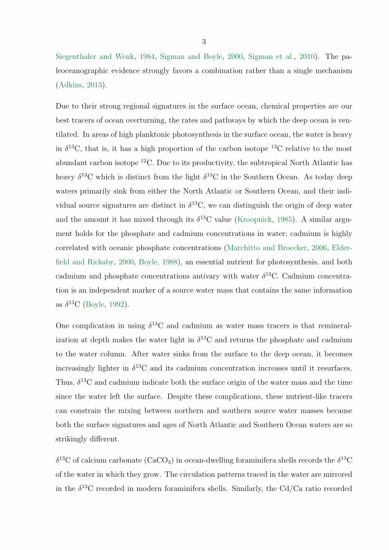
Siegenthaler and Wenk, 1984, Sigman and Boyle, 2000, Sigman et al., 2010). The pa-
leoceanographic evidence strongly favors a combination rather than a single mechanism
(Adkins, 2013).
Due to their strong regional signatures in the surface ocean, chemical properties are our
best tracers of ocean overturning, the rates and pathways by which the deep ocean is ven-
tilated. In areas of high planktonic photosynthesis in the surface ocean, the water is heavy
in δ13C, that is, it has a high proportion of the carbon isotope 13C relative to the most
abundant carbon isotope 12C. Due to its productivity, the subtropical North Atlantic has
heavy δ13C which is distinct from the light δ13C in the Southern Ocean. As today deep
waters primarily sink from either the North Atlantic or Southern Ocean, and their indi-
vidual source signatures are distinct in δ13C, we can distinguish the origin of deep water
and the amount it has mixed through its δ13C value (Kroopnick, 1985). A similar argu-
ment holds for the phosphate and cadmium concentrations in water; cadmium is highly
correlated with oceanic phosphate concentrations (Marchitto and Broecker, 2006, Elder-
field and Rickaby, 2000, Boyle, 1988), an essential nutrient for photosynthesis, and both
cadmium and phosphate concentrations antivary with water δ13C. Cadmium concentra-
tion is an independent marker of a source water mass that contains the same information
as δ13C (Boyle, 1992).
One complication in using δ13C and cadmium as water mass tracers is that remineral-
ization at depth makes the water light in δ13C and returns the phosphate and cadmium
to the water column. After water sinks from the surface to the deep ocean, it becomes
increasingly lighter in δ13C and its cadmium concentration increases until it resurfaces.
Thus, δ13C and cadmium indicate both the surface origin of the water mass and the time
since the water left the surface. Despite these complications, these nutrient-like tracers
can constrain the mixing between northern and southern source water masses because
both the surface signatures and ages of North Atlantic and Southern Ocean waters are so
strikingly different.
δ13C of calcium carbonate (CaCO3) in ocean-dwelling foraminifera shells records the δ13C
of the water in which they grow. The circulation patterns traced in the water are mirrored
in the δ13C recorded in modern foraminifera shells. Similarly, the Cd/Ca ratio recorded
4
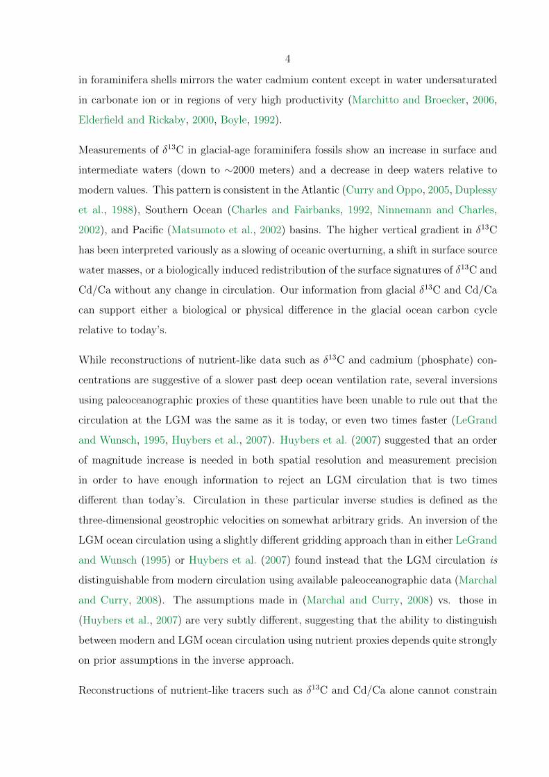
in foraminifera shells mirrors the water cadmium content except in water undersaturated
in carbonate ion or in regions of very high productivity (Marchitto and Broecker, 2006,
Elderfield and Rickaby, 2000, Boyle, 1992).
Measurements of δ13C in glacial-age foraminifera fossils show an increase in surface and
intermediate waters (down to ∼2000 meters) and a decrease in deep waters relative to
modern values. This pattern is consistent in the Atlantic (Curry and Oppo, 2005, Duplessy
et al., 1988), Southern Ocean (Charles and Fairbanks, 1992, Ninnemann and Charles,
2002), and Pacific (Matsumoto et al., 2002) basins. The higher vertical gradient in δ13C
has been interpreted variously as a slowing of oceanic overturning, a shift in surface source
water masses, or a biologically induced redistribution of the surface signatures of δ13C and
Cd/Ca without any change in circulation. Our information from glacial δ13C and Cd/Ca
can support either a biological or physical difference in the glacial ocean carbon cycle
relative to today’s.
While reconstructions of nutrient-like data such as δ13C and cadmium (phosphate) con-
centrations are suggestive of a slower past deep ocean ventilation rate, several inversions
using paleoceanographic proxies of these quantities have been unable to rule out that the
circulation at the LGM was the same as it is today, or even two times faster (LeGrand
and Wunsch, 1995, Huybers et al., 2007). Huybers et al. (2007) suggested that an order
of magnitude increase is needed in both spatial resolution and measurement precision
in order to have enough information to reject an LGM circulation that is two times
different than today’s. Circulation in these particular inverse studies is defined as the
three-dimensional geostrophic velocities on somewhat arbitrary grids. An inversion of the
LGM ocean circulation using a slightly different gridding approach than in either LeGrand
and Wunsch (1995) or Huybers et al. (2007) found instead that the LGM circulation is
distinguishable from modern circulation using available paleoceanographic data (Marchal
and Curry, 2008). The assumptions made in (Marchal and Curry, 2008) vs. those in
(Huybers et al., 2007) are very subtly different, suggesting that the ability to distinguish
between modern and LGM ocean circulation using nutrient proxies depends quite strongly
on prior assumptions in the inverse approach.
Reconstructions of nutrient-like tracers such as δ13C and Cd/Ca alone cannot constrain
5
ocean circulation (without other assumptions), as their values are also a function of biolog-
ical productivity, biological efficiency, time, ocean redox state and carbonate saturation,
which are themselves functions of each other. While radioisotope data is promising as
an independent “clock” or measurement of rates, we still have many uncertainties about
radioisotope initial values at any point in time or space, limiting their utility.
In modern oceanography, water mass sources and pathways can be tracked in large part
through temperature and salinity, which are almost perfectly conservative tracers in the
ocean interior. Additionally, large-scale ocean circulation is balanced by horizontal density
gradients (assuming geostrophic and hydrostatic balance). The density of ocean water is
set by temperature and salinity, thus temperature and salinity give us both conservative
tracers of pathways and estimates of velocities.
It is clear that knowledge of the past ocean’s temperature and salinity fields would vastly
improve our ability to distinguish between hypothetical past circulations. Short of that, a
proxy for water density could be used to estimate large-scale flows, although the picture
of circulation we can draw from temperature and salinity is more complete than that from
density alone.
Paleodensity proxies
δ18O (a normalized ratio of 18O relative to 16O) of foraminifera shells records the tem-
perature and δ18O of the water in which the foraminifera grew. Today there is a strong
correlation between δ18O of water and the salinity of water, as the same processes that
change the δ18O likewise change the salinity (evaporation, precipitation, ice-ocean inter-
actions). Locally there is often a simple (linear) relationship between water density and
the δ18O of the foraminifera growing in that water. Thus, if one assumes that the δ18O–
salinity relationship is constant in time one can locally reconstruct the geostrophic flow
(Lynch-Stieglitz et al., 1999a,b, Lynch-Stieglitz, 2001, Hirschi and Lynch-Stieglitz, 2006,
Lynch-Stieglitz et al., 2006). The main drawback to this technique is that the density–
δ18O relationship varies quite strongly spatially in the ocean and there is no guarantee that
this relationship is constant in time under changing circulation and ice melting conditions
(Lynch-Stieglitz et al., 2008).
6
In lieu of a paleodensity proxy, we need to combine both paleotemperature (paleother-
mometer) and paleosalinity proxies to reconstruct the past ocean density structure.
Paleotemperature proxies
Several reliable proxies for past surface ocean temperature exist, including alkenone satu-
ration ratios, and planktonic foraminifera species assemblages (see for example de Vernal
et al. (2006)). These proxies record the temperature of the upper few meters of the ocean,
but an understanding of how the ocean density gradients changed in the past will require
proxies for intermediate and deep ocean temperature. A variety of paleothermometers
have been proposed, but we still lack a robust technique to reconstruct past sub-surface
ocean temperature.
The δ18O recorded in the calcium carbonate shells of foraminifera, δ18Oc is a function
of temperature, but also of the δ18O of water, δ18Ow, which can vary due to changes in
ice–ocean interactions, evaporation, precipitation and mixing. δ18Ow varies substantially
in space, making δ18Oc a poor proxy for deep ocean temperature.
The elemental ratio Mg/Ca in foraminiferal shells is sensitive to temperature. However,
the relationship between Mg/Ca uptake and temperature is itself sensitive to carbonate ion
([CO2−3 ]) saturation state and temperature. In carbonate undersaturated water and/or
cold water (below ∼ 3◦C), that is, deep ocean conditions, Mg/Ca is not reliable as a
temperature proxy without knowledge of the carbonate saturation state (Elderfield et al.,
2006, Rosenthal et al., 2006, Yu and Elderfield, 2008). The proper use of Mg/Ca to
reconstruct past deep ocean temperature requires another proxy for carbonate saturation
state, which has not yet been developed. Even when the [CO2−3 ] is or is assumed well-
known, the reported error for temperature in best case scenarios is ±0.5−1.0◦C Elderfield
et al. (2012, see e.g.), which is quite large relative to the typical range of deep ocean
temperatures of ∼ 5◦C.
The extent of clumping of the heavy isotopes of carbon and oxygen (13C and 18O) in
carbonate shells records the temperature of formation of the shell, which in an oceanic
setting, is the temperature of the water in which the animal grew (Ghosh et al., 2006,
Eiler, 2011). Measurement of isotope clumping in ocean dwelling carbonate shell building
7
animals is a robust paleothermometer, in that it records only temperature. One major
limitation of clumped isotope paleothermometry is that inter-laboratory calibrations as
yet have not achieved any better than ±2◦C offsets in their measurements of the same
standard, restricting the accuracy of any absolute temperature measurement. Clumped
isotope measurements also require large quantities of samples to achieve high precision
results (Eiler, 2011). For this reason they have been most successfully used for ocean
temperature reconstructions on deep sea corals (Thiagarajan et al., 2011), massive rel-
ative to foraminifera. Unfortunately deep sea corals are not ubiquitous either spatially
or in time, due to their sensitivity to environmental parameters such as aragonite satu-
ration state and oxygen saturation of the water. Deep sea corals appear quite sparse or
entirely absent below 2600m (Thiagarajan et al., 2013). Foraminifera measurements have
been made successfully on sets of hundreds of foraminifera, but it can often be difficult
to find this many foraminifera in a sediment sample and impractical to use them all for
a single temperature reconstruction. New advances in techniques may allow us to make
measurements on smaller samples, such as 10-20 individuals, but for now clumped iso-
tope thermometry can only identify large temperature signals (Grauel et al., 2013). In
the deep ocean the temperature change over glaciations and deglaciations probably was
less than 4◦C, making the clumped isotope thermometry technique difficult to apply to
understanding our recent climate history.
With an independent estimate of the water δ18O in the past, we could reconstruct tem-
perature from δ18Oc in foraminifera. By combining measurements of sediment pore fluid
δ18O with a numerical model of advection and diffusion in sediments, McDuff (1985),
Schrag and DePaolo (1993), Schrag et al. (1996), Paul et al. (2001), Adkins et al. (2002),
Schrag et al. (2002) and Malone et al. (2004) found δ18Ow histories that, input to their
model, produced output that fit the measured data, allowing them to estimate the LGM
δ18Ow and temperatures at those sites. The advantages of this technique are that it is
not sensitive to ocean chemistry or pressure and though the time resolution is limited,
the absolute error may be smaller than that of other paleotemperature proxies. However,
this technique’s major limitation is that finding the history of bottom water δ18O from
present-day pore fluid measurements is an inverse problem with a non-unique solution.
As yet, a robust approach to this modeling has not been established. Due to the ability of
8
isotopes to diffuse in the sediments, the time resolution of the technique is guaranteed to
be lower than that of clumped isotope or paired Mg/Ca and δ18Oc measurements, which
are sealed upon shell formation. So far only one time point in the past has been estimated,
the LGM. As part of this thesis, we search for a robust approach to extracting deep ocean
δ18Ow histories using pore fluid measurements.
Paleosalinity proxies
Past deep ocean salinity is notoriously difficult to reconstruct, in part because the modern
range of deep ocean salinities is quite narrow. The wide range of surface ocean salinities
and temperatures allow us to examine the sensitivity of surface-dwelling foraminifera,
coccolithophores, dinoflagellate cysts and diatoms to their environments and use our un-
derstanding of this environmental sensitivity to read the sedimentary records. In contrast,
over the very narrow range of deep ocean salinities and temperatures it is difficult to iden-
tify the sensitivity of benthic foraminiferal species to their environments, and the deep
ocean salinity range is particularly small. Surface salinity can be reasonably well recon-
structed through dinoflagellate cyst species assemblages (de Vernal et al., 2005), but there
is no generally applicable salinity paleo proxy for depths below 5-10m.
To date, the only measurement that claims to definitively identify past ocean salinity is
reconstructions from present-day sediment pore fluid profiles. In a method analogous to
that for the δ18Ow problem, McDuff (1985) and Adkins et al. (2002) reconstructed the
LGM salinity using pore fluid measurements of [Cl−] as a conservative measure of salinity.
Published results from pore fluid reconstructions of LGM temperature and salinity suggest
that at the Last Glacial Maximum (LGM), the salinity contrast between northern source
deep water and southern source bottom water was reversed with respect to the contrast
today. Further, the density gradient between deep waters was larger than that of the
modern (Adkins et al., 2002), the only true mechanistic support for the hypothesis that
the deep ocean’s reservoir of carbon was physically isolated in the past. In addition to
temperature, salinity, density and circulation pathways, pore fluid reconstructions have
the potential to yield information about spatial variability in mass wasting of glaciers
through the changing values of δ18Ow in time and space.

9
Despite their promise, and the lack of other reliable techniques, sediment pore fluid recon-
structions of past ocean δ18Ow and salinity have not caught on in the paleoceanographic
community. This is in part because the information-to-sample ratio so far has been quite
low. The recommended amount of sediment to do one LGM reconstruction is at minimum
one hundred 5-cm samples, that is, 5 m of sediment core. In contrast, a single time point
reconstruction of any other climate variable can require as little as 1-3 mm of core, and
usually multiple measurements can be performed on the same section. Squeezing pore
fluids from a sample destroys the sample for other purposes (F. Sierro, personal commu-
nication), and thus LGM pore fluid reconstructions are a very inefficient use of precious
sediment.
The other likely reason that more researchers have not enthusiastically adopted the pore
fluid proxy technique is that the reconstruction of the LGM values is ad hoc; there is no
consistent and robustly demonstrated method to invert for bottom water histories from
pore fluid profiles. Instead, each publication has relied on similar but different approaches,
requiring the need to every time re-demonstrate the insensitivity of their results to changes
in their parameters. The lack of a consistent and proven method makes the entry cost to
working with pore fluids as a proxy for deep ocean salinity and δ18O quite high.
Are pore fluids a reliable proxy for past ocean δ18O, temperature, and salinity? If so, can
we use them to reconstruct the deglacial evolution of the ocean rather than just the LGM
values, making more efficient use of the sediment? Alternatively, or additionally, is there
a way to dramatically increase the number of measurements we make with pore fluids
without sacrificing other climate records? Finally, given our knowledge of the modern
ocean, is there a way to explain how the ocean density stratification was dominated by
salinity at the LGM?
This thesis attempts to remove the barriers to the use of pore fluid proxy for δ18O,
temperature and salinity. Our main goal is to robustly determine the information content
of pore fluid profiles, that is, what they can tell us about the past ocean and what they
can not. As part of this work, we examined the oceanic feasibility of the temperature and
salinity distribution from Adkins et al. (2002)’s pore fluid LGM temperature and salinity
reconstruction. Simultaneously we sought to advance the feasibility and reliability of
10
collecting and measuring sediment pore fluid δ18O and [Cl−] in order to encourage wider
participation and global dataset size.
In Chapter 2 we examine the ability of traditional regularized least squares inverse meth-
ods to recover information about past ocean δ18O and salinity from sediment pore fluid
profiles. With synthetic examples, we show that regularization destroys the resolution of
the inverse solution. Further, we demonstrate that the underlying approach in regularized
inversions places constraints on the inverse problem’s solution that do not mesh with our
a priori information. This work was done in collaboration with Jess Adkins and Mark
Simons.
Chapter 3 places the pore fluid inverse problem in a fully nonlinear Bayesian framework.
We apply a Bayesian Markov Chain Monte Carlo parameter estimation technique to
estimate the robustness of present-day pore fluid profiles as a proxy for LGM δ18O and
salinity and consider whether these profiles can be used to reconstruct the full deglacial
evolution of δ18O, temperature and salinity. We show that, in general, δ18O and salinity
in the Holocene can be reliably reconstructed using pore fluid data, but that information
about the LGM is more uncertain. This work was done in collaboration with Jess Adkins,
Mark Simons, and Sarah Minson.
Chapter 4 addresses the reliability of a new technique for ocean sediment pore fluid
sampling. The use of pore fluid δ18O and [Cl−] as paleoceanographic proxies has in
part been limited by the difficulty of obtaining samples, as their procurement destroys
other ocean sediment climate records. We evaluate Rhizon samplers in comparison to the
traditional squeezing technique, and show that Rhizon samplers contaminate [Cl−] and
δ18O in ocean sediment pore fluid samples. This work was done in collaboration with Jess
Adkins, David Hodell, and the science party and technical staff on IODP Expedition 339,
with major assistance from Christopher Bennight and Erik Moortgat.
Finally, in Chapter 5 we examine the role of ice–ocean processes in a cold ocean on
setting the temperature and salinity distribution at the LGM. In this work we ask whether
our current knowledge of oceanic processes can explain a higher-than-modern salinity
stratification of deep ocean water masses at the LGM. We test whether reduced ice shelf

11
basal melting due to interaction with a cold ocean could switch the direction of salt
stratification between the deep North and South Atlantic. Chapter 5 has previously
appeared in the journal Paleoceanography and was completed in collaboration with Jess
Adkins, Dimitris Menemenlis, and Michael Schodlok.

12
Chapter 2
Reconstructing δ18O and salinityhistories from pore fluid profiles:What can we learn from regularizedleast squares?
2.1 Introduction
Using constraints from sediment pore fluid profiles of δ18O and chlorinity, Adkins et al.
(2002) inferred that there were larger density differences between deep water masses at
the Last Glacial Maximum (LGM), due primarily to their salinities. Of the sites consid-
ered, they concluded that Glacial Southern Source Bottom Water (GSSBW), deep water
originating from the southern hemisphere, was the densest due to its salinity. These re-
sults contrast strikingly with the distribution of today’s deep ocean water masses whose
density differences are set primarily by temperature; modern southern source deep water,
Antarctic Bottom Water (AABW), is the densest deep ocean water mass because it is
cold, while remaining less saline than overlying water masses.
The greater inferred stratification in deep water density supports the hypothesis that
there was a physically isolated reservoir of CO2 in the deep ocean at the LGM (Broecker
and Barker, 2007). In fact, these reconstructed LGM salinities and temperatures from
pore fluids are the only paleoceanographic evidence for an isolated reservoir that solely
record physical, rather than biological or chemical, changes in the ocean. While the

13
LGM distribution of δ13C, Cd/Ca and δ18O indicate the possibility of a slower than
modern ocean overturning circulation, inverse analyses (Gebbie, 2012, Huybers et al.,
2007, LeGrand and Wunsch, 1995) have shown the LGM ocean distributions are also
consistent with a modern circulation and differences in surface properties. Knowledge of
the past ocean’s bottom temperature and salinity field would be a significant contribution
to the picture of past ocean circulation, enabling us to untangle physical changes from
chemical and biological signals and better explain why tracer fields in the past ocean
varied so strikingly from those of today’s ocean.
To date, the only data set that claims to unequivocally identify past ocean density gra-
dients is the pore fluid reconstruction of LGM values. However, the data set in Adkins
et al. (2002) consists of four spatial points at one time. In order to fully understand the
changing ocean circulation over the most recent deglaciation, we need more points in both
time and space. We address a method to increase the spatial resolution of LGM density
reconstructions in Chapter 4, while here we investigate whether we can increase the past
temporal information we can recover from pore fluid profiles.
Previous efforts to reconstruct bottom water δ18O and S from modern pore fluid profiles
focused on recovering only one point in the time series, the value at the LGM. The focus
on the LGM was because in most paleoceanographic records the LGM can be identified
as a large, persistent signal and because modern pore fluid profiles record only a diffusive
history of the bottom water time series. In the appropriate sedimentary environment,
variability at the sediment-water interface is a strong control on the pore fluid concen-
trations, but the effects of small magnitude or high frequency forcing on the pore fluid
profile are heavily damped.
The method previously used to reconstruct LGM δ18O and chlorinity in Adkins et al.
(2002), Paul et al. (2001), Schrag et al. (1996), Schrag and DePaolo (1993) and Mc-
Duff (1985) relied on a number of restrictive assumptions that made it impossible to
recover the deglacial histories of δ18O and [Cl−]. Their essential approaches relied on
the supposition that δ18O and [Cl−] are both conservative tracers in ocean sediments
and determined by one-dimensional advection and diffusion. While there is significant
two- or three-dimensional advective fluid flow in many places on the ocean floor associ-
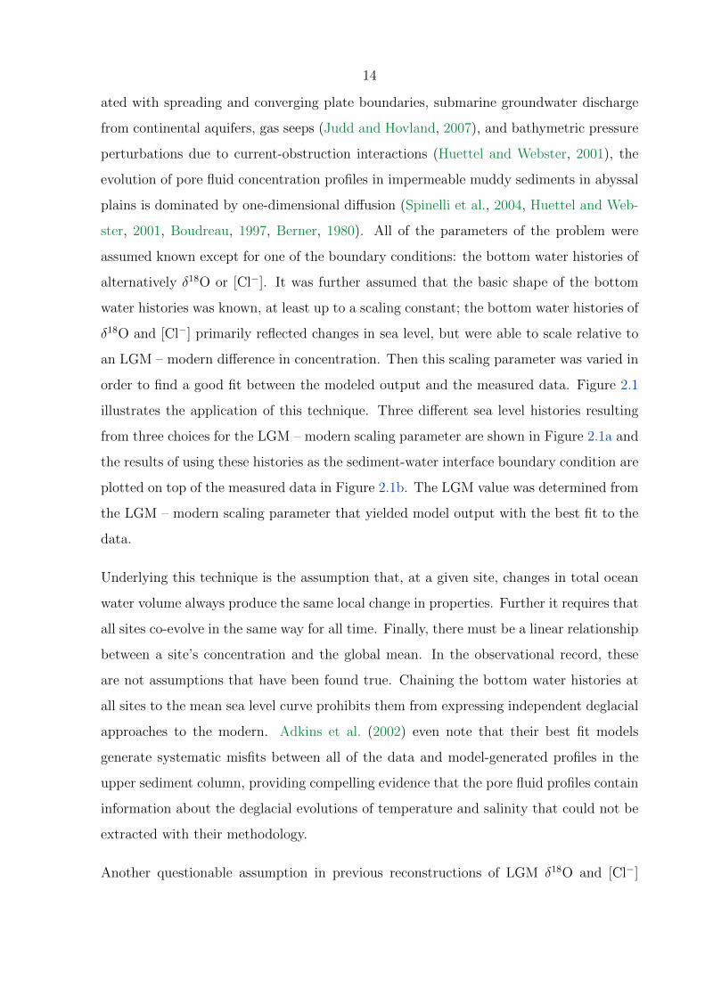
14
ated with spreading and converging plate boundaries, submarine groundwater discharge
from continental aquifers, gas seeps (Judd and Hovland, 2007), and bathymetric pressure
perturbations due to current-obstruction interactions (Huettel and Webster, 2001), the
evolution of pore fluid concentration profiles in impermeable muddy sediments in abyssal
plains is dominated by one-dimensional diffusion (Spinelli et al., 2004, Huettel and Web-
ster, 2001, Boudreau, 1997, Berner, 1980). All of the parameters of the problem were
assumed known except for one of the boundary conditions: the bottom water histories of
alternatively δ18O or [Cl−]. It was further assumed that the basic shape of the bottom
water histories was known, at least up to a scaling constant; the bottom water histories of
δ18O and [Cl−] primarily reflected changes in sea level, but were able to scale relative to
an LGM – modern difference in concentration. Then this scaling parameter was varied in
order to find a good fit between the modeled output and the measured data. Figure 2.1
illustrates the application of this technique. Three different sea level histories resulting
from three choices for the LGM – modern scaling parameter are shown in Figure 2.1a and
the results of using these histories as the sediment-water interface boundary condition are
plotted on top of the measured data in Figure 2.1b. The LGM value was determined from
the LGM – modern scaling parameter that yielded model output with the best fit to the
data.
Underlying this technique is the assumption that, at a given site, changes in total ocean
water volume always produce the same local change in properties. Further it requires that
all sites co-evolve in the same way for all time. Finally, there must be a linear relationship
between a site’s concentration and the global mean. In the observational record, these
are not assumptions that have been found true. Chaining the bottom water histories at
all sites to the mean sea level curve prohibits them from expressing independent deglacial
approaches to the modern. Adkins et al. (2002) even note that their best fit models
generate systematic misfits between all of the data and model-generated profiles in the
upper sediment column, providing compelling evidence that the pore fluid profiles contain
information about the deglacial evolutions of temperature and salinity that could not be
extracted with their methodology.
Another questionable assumption in previous reconstructions of LGM δ18O and [Cl−]

15
0 20 40 60 80 100 12034.5
35
35.5
36
36.5
37
kya
Sa
lin
ity
(g
kg
−1)
(a)
35 35.5 360
50
100
150
Salinity (g kg−1
)
De
pth
(m
bs
f)
(b)
Figure 2.1: Illustration of the method previously used to reconstruct the LGM salinity andδ18O. Changes in salinity scaled to the sea level curve, up to a scaling constant. Low sealevel corresponds to high salinity and vice versa. (a) shows boundary conditions producedusing three different scaling factors, and (b) shows the model output using those boundaryconditions overlaid on measured data in sediment pore fluids (black circles). Each colorcorresponds to a different LGM – modern scaling factor.
was that the dominant diffusion coefficient at a site could be computed using a scaling
approach with the knowledge that the LGM was uniformly at 20 ka BP. The controlling
diffusion coefficient, D0, was calculated as D0 = L2
T, where T = 20,000 years and L was
the depth of the maximum value of δ18O or [Cl−] in the sediments. Recent studies have
shown that the LGM occurred at different times for different glaciers (Clark et al., 2009),
which calls into question the idea of a synchronous LGM in the ocean, particularly with
the knowledge that the ocean equilibration timescales are long (Wunsch and Heimbach,
2008). Intuition also suggests that the bottom water histories and the diffusion coefficient
at each site covary; a higher diffusion coefficient would leave behind a more damped trace
of the LGM δ18O and [Cl−] maximum in the modern measured profiles.
We seek a robust method to reconstruct past ocean bottom temperature and salinity from
sediment core interstitial water profiles of δ18O and [Cl−] in combination with δ18O of
benthic foraminifera that will allow us to release the restrictions listed above, particularly
the requirement that local bottom water histories can only vary from the global mean by
a single, time-invariant, scaling constant. Our main aim is to identify whether we can

16
recover the deglacial histories of δ18O and [Cl−] from modern pore fluid profiles, while
at the same time re-evaluate the information about the LGM yielded by the pore fluid
profiles.
We have revisited the problem with a variety of inverse methods that allow us to release
the previous assumption that bottom water histories scaled to the sea level curve, allowing
us to 1) test the robustness of previous reconstructions and 2) examine whether we can
extract more information than the LGM value from present-day interstitial water profiles.
The solution to an inverse diffusion problem is not unique, and thus without some as-
sumptions the problem is intractable. In this chapter we frame our problem as a linear
inverse problem by assuming we do in fact know the dominant diffusion coefficient at a
site and focus primarily on reconstructing the ocean bottom water histories of δ18O and
[Cl−]. In Chapter 3 we release the requirement that the diffusion coefficient is known, and
examine how doing so affects our uncertainty in past ocean time series of δ18O and [Cl−].
In what follows we evaluate the skill of several regularization methods for linear inversions
in recovering bottom water histories from pore fluid profiles. We rely on synthetic exam-
ples, in which we choose hypothetical synthetic models of bottom water histories, generate
synthetic data by running these through a forward model of advection and diffusion in
ocean sediments, and then invert the synthetic data and compare the inverse solution
with the known solution. These synthetic examples allow us to explore the nature of our
inverse problem as well as the limitations of regularized inversions both in their practical
use and in error estimation. Our work in Chapter 2 motivates the more complex inverse
approach described in Chapter 3.

17
2.2 Methods
2.2.1 The forward problem
2.2.1.1 Simplifying assumptions
The movement of chemical species in porous sediments is a well-studied topic. In-depth
treatment and analysis of the processes involved and the breadth of modeling assumptions
can be found in Berner (1980) and Boudreau (1997). The following outlines the approach
we use, which relies primarily on these two works.
We assume that the processes that modify tracer concentrations in interstitial water are
one-dimensional, that is, all changes are in the vertical direction and there are no net
velocity, concentration or pressure gradients in the (local) horizontal directions. The one-
dimensional approximation is expected to be appropriate for locations in the ocean lacking
bedforms, with spatially uniform sedimentary deposition and oceanic concentrations and
consolidated clays, which, in spite of their physical anisotropy, have isotropic permeability
(Spinelli et al., 2004). In practice, the assumption of one-dimensional sediment concen-
tration evolution is rarely tested. We further assume that our concentrations of interest
are conservative, that is, they are not modified by in situ chemical reactions.
The basic equation describing interstitial concentration (c) as a function of depth (z,
positive downwards) and time (t) can then be written:
∂ (φc)
∂t= D0
∂
∂z
(φ
θ2
∂c
∂z
)− ∂ (uφc)
∂z. (2.1)
φ is known as the sediment porosity, defined as:
φ =interconnected volume
total sediment + liquid volume. (2.2)
θ is the sediment tortuosity, which is the resistance of the sediment to interstitial flow due
to grain alignment. D0 is a constant diffusion coefficient, which includes the diffusivity in

18
water of the chemical species of interest. Diffusion due to biological mixing is lumped into
the unknown parameter D0. In reality chemical diffusivity varies with sediment depth,
as it is a function of temperature and ionic strength, but for simplicity in the following
examples it is held constant. u is the vertical velocity of the water with respect to the
sediment, predominantly due to sediment compaction.
Expanding out Equation 2.1 leads to
c∂φ
∂t+ φ
∂c
∂t= D0
∂
∂z
(φ
θ2
)∂c
∂z+D0φ
θ2
∂2c
∂z2− ∂ (φuc)
∂z. (2.3)
Assuming steady state compaction, ∂φ∂t
= 0. Steady state compaction requires a constant
sedimentation rate, which is generally not true on glacial–interglacial timescales (e.g.,
Raymo, 1997, McManus et al., 1998). Here we ignore time evolution of sedimentation rate
and compaction, as their effects on the temporal evolution of pore fluid tracer profiles are
negligible as compared to other factors (Adkins and Schrag, 2003)
The last term on the right hand side of Equation 2.3 expands out to
∂ (φuc)
∂z= φ∂(uc)
∂z+ uc∂φ
∂z
= φc∂u∂z
+ φu ∂c∂z
+ uc∂φ∂z. (2.4)
In a steady, incompressible, flow mass conservation (where the mass flux per unit area at
z is ρfφu) allows the first and third terms of Equation 2.4 to cancel, yielding:
∂ (φuc)
∂z= φu
∂c
∂z. (2.5)
Given these two conditions, Equation 2.3 becomes:
φ∂c
∂t= D0
∂
∂z
(φ
θ2
)∂c
∂z+D0φ
θ2
∂2c
∂z2− φu∂c
∂z
=∂D∗
∂z
∂c
∂z+D∗
∂2c
∂z2− φu∂c
∂z
=
(∂D∗
∂z− φu
)∂c
∂z+D∗
∂2c
∂z2, (2.6)

19
where D∗ = D0φθ2
. A common model for θ2 is θ2 = φf where f is the non-dimensional
formation factor:
f =bulk sediment specific electrical resistivity
porewater resistivity, (2.7)
which means ∂D∗
∂z= D0
∂∂z
(1f
). θ and f are both unknown, but laboratory measurements
suggest that a good approximation for f is φ−n, where n averages 1.8 over various sedi-
ments (Berner, 1980). More complicated models for tortuosity have been proposed, (e.g.
Boudreau and Meysman, 2006), but the differences in their fits to empirical data are very
subtle. With this, ∂D∗
∂z= n φn−1 D0
∂φ∂z
= 1.8 φ0.8 D0∂φ∂z
.
Our final equation describing concentration evolution with time and space is
∂c
∂t=
(1.8 φ0.8D0
∂φ
∂z− u)∂c
∂z+ φ1.8D0
∂2c
∂z2. (2.8)
φ and ∂φ∂z
are measured quantities. In the simple examples that follow, we use a constant
φ = 0.8. D0 is an unknown parameter, but laboratory measurements suggest that its order
should be 10−6−10−5 cm2 s−1 for [Cl−] (Li and Gregory, 1974). In the following examples
we examine the sensitivity of our solutions to D0 by solving the linear regularization
problems using three different orders of magnitude of D0 (from 2.9 x 10⁻⁷ to 2.9 x 10⁻⁵.
To determine u as a function of z, we assume that compaction ceases at some depth (this
is commonly seen in the profiles of φ). At this depth of no compaction, the fluid and solid
burial velocities are the same, i.e. uz = wz. Then φu = φzwz, or u = φzwz
φ. wz can be
determined from an appropriate dating scheme of the sediment core sections.
The solution to Equation 2.8 requires two boundary conditions and an initial condition.
We specify a Dirichlet (first-type) boundary condition at the sediment–water interface as
the concentration as a function of time. At the bottom boundary we choose a Neumann
(derivative) boundary condition to be a fixed first derivative of concentration. The bottom
boundary choice represents an interaction with deeper sediments or crust that does not
change over our timescales of interest.

20
2.2.1.2 Finite difference solution technique
We solve (integrate) the forward problem (Equation 2.8) with a quadrature rule method,
that is, we approximate the derivatives and the integral locally. As the effect of diffusion
greatly outweighs that of advection in our problem (Peclet numbers < 10−3), we use an
Implicit-Explicit (IMEX) method for a computationally efficient and stable integration.
IMEX methods combine an implicit method to integrate the stiff terms of the equation,
in our case the diffusion term, with an explicit method to integrate the non-stiff terms
(advection). IMEX methods avoid the excessively small time steps necessary to stably
explicitly integrate the diffusion term, while also avoiding iteratively inverting the matrix
associated with the implicit advective term. The IMEX method we use is a second
order Semi-implicit Backward Differentiation Formula (SBDF) as described in Ascher
et al. (1995). For the implicit solver, we use the tridiagonal matrix algorithm (TDMA),
which is a simplified form of Gaussian elimination appropriate for tridiagonal systems of
equations.
By examining the convergence behavior of the forward solution, we choose a time step
of ∆t = 10 years and discretize depth with ∆ z = 50 cm. Over the integration time of
125,000 years and 150 m of sediment these choices lead to a 2-norm error in the solution
of O(10−4).
2.2.1.3 Green’s function approach
If we fix all the parameters in Equation 2.8 in time except for c(z), our problem is a
system of linear partial differential equations. Linearity allows us to use a discrete Green’s
function approach in examining the solution to a variety of forcing conditions. We can
write any discretized linear system of equations generally as Gm = d, where G is a matrix
of discrete Green’s functions, m is the discretized “model” (in our case the boundary
forcing conditions and the initial condition) and d represents a vector of measured data,
the present-day measured concentration profile.
In the following examples we fix the intial and bottom boundary conditions and solve
21
only for the top boundary condition, the evolution of δ18O or [Cl−] at the sediment-water
interface on the ocean floor. Thus m is simply a concentration time series. We construct
G by computing finite difference impulse responses to the set of orthonormal boundary
conditions. These impulse responses form the columns of the matrix G. The ith row of
G, scaled by the boundary condition model m, generates the ith measured data point
in d. Then multiplication of G by any boundary condition vector (which is a linear
combination of unit vectors) yields the present day concentration profile that arises in
response to that boundary condition time series.
The dimensions of G are arbitrary, depending on the choice of discretization. In order
to eliminate convergence problems, we compute roughly discretized G matrices from a
converged finite difference solution. The finite difference computation of the columns of
G always uses 10 year time step and 50 cm space step, regardless of the temporal and
spatial discretization of G.
Once the forward problem is framed using discrete Green’s functions, it is numerically
much more efficient to solve; instead of inverting matrices we can use direct matrix multi-
plication. Additionally, the discrete Green’s function approach provides a natural frame-
work for addressing the inverse problem.
2.2.2 The inverse problem
For completeness we summarize the necessary theoretical background to solving discrete
ill-posed problems. Unless otherwise noted, the information in sections 2.2.2.1– 2.2.2.5 is
from Aster et al. (2005) and Hansen (1998).
2.2.2.1 Ill-posed nature of inverse problem
In practice, we measure the modern concentration profile c(z)|t=mod. From this set of
observations we wish to infer the past time evolution of water properties at the sediment
– water interface, c0(t). The evolution of the bottom boundary condition cL(z) is also
unknown, as is the initial condition c(z)|t=past. Once we have framed the problem using
22
discrete Green’s functions, as described above, the solution to the discretized problem
may be written as
m = G−1d (2.9)
where m in our case is the bottom water boundary condition.
Due to the particular nature of our problem, the inversion of G is not straightforward.
The continuous problem can be written generally as:
∫ b
a
G(z, t)m(t)dt = d(z), a ≤ z ≤ b , (2.10)
where the kernel G is a Green’s function that represents the advection-diffusion operation
on m(t). d(z) is what we observe or measure, in our case the concentration as a function
of depth in the sediment, and G is theoretically known. This equation is a Fredholm
integral equation of the first kind with a square integrable kernel. The solution for m(t)
in this equation is a classical example of a linear ill-posed problem; that is, the solution
for m(t) is not unique and a small perturbation to the measured data can lead to an
arbitrarily large, or unconstrained, change in the solution. (Hansen, 1998).
In real measurement cases, d(z) is always discrete, and so we are considering the dis-
cretized version of the integral equation, which is just the discrete Green’s function. A
discrete ill-posed problem always results from the discretization of a continuous ill-posed
problem. Discrete ill-posed problems are almost always indeterminate so it is impossible
to directly invert G. Instead, all solutions must be some variant of a least-squares solution.
Even in the rare case that a discrete ill-posed problem is full rank, the solution will be
unstable to small perturbations or noise. Instability of discrete ill-posed problems is fur-
ther compounded by the fact that a mathematically full-rank G can become numerically
rank-deficient due to limitations in machine precision.
The SVD of G in an ill-posed problem has singular values and right and left singular
vectors with particular properties that make the computation of a least-squares solution
unstable. The shape and size of G are determined by the number of data points in d and
the level of discretization of the problem. No matter how finely or roughly we discretize
the problem, the singular values of the matrix G decay uniformly to 0 (or the machine
23
precision limit). The uniform decay of singular values to 0 means that our problem is “ill-
posed” rather than simply being “rank-deficient”. While the modes of G that correspond
to very small singular values clearly do not contribute much to the solution, in practice it
is difficult to truncate G and apply a truncated least-squares method to the problem, as
there is no clear divide between large and small singular values. The left and right singular
vectors associated with small singular values are highly oscillatory, with the number of
zero crossings increasing monotonically with i (i representing the index of the singular
value). In the forward problem, these oscillations are damped by being multiplied by
small singular values. However, in the inverse problem, division by singular values leads
to amplification of these oscillations, which are magnified in the presence of measurement
noise.
The solution of linear ill-posed inverse problems requires some form of regularization or
stabilization of the solution. A common and relatively simple technique is that found by
solving a damped least squares problem, also known as Tikhonov regularization. In the
following examples we primarily focus on various approaches to finding the inverse solution
to Equation 2.8 using Tikhonov regularization. However, while the inverse solution to
Equation 2.8 is an ill-posed problem, due to the limitations of machine precision, it is also
numerically rank-deficient. As rank-deficient inverse problems can be solved efficiently
using a truncated SVD of G, we include a discussion of the inverse solutions we recover
using a truncated least-squares method and compare it to the solutions we recover using
regularization in place of truncation.
2.2.2.2 Truncated SVD solution
When G is not an invertible matrix, the least squares or generalized inverse solution m†
to the inverse problem for m that satisfies
Gm = d (2.11)
is written as
m† = G†d , (2.12)
24
where G† is
G† =(GTG
)−1GT , (2.13)
which can be written in terms of the singular value decomposition of G as
m† = VS−1UTd . (2.14)
In a rank-deficient or ill-posed least squares inverse problem, the solution to Equation 2.14
will be unstable due to division by very small singular values when taking the inverse
of S. A rank-deficient problem is one in which G is not full rank and there is a clear
divide between non-zero and zero singular values in S. In the truncated SVD (TSVD)
least squares inverse method, one simply truncates the small singular values and their
corresponding left and right singular vectors in V and U, and computes the generalized
inverse m† using the TSVD. In a true rank-deficient inverse problem, the information
associated with the missing rank modes can never be recovered; it is irreversibly lost by
the rank-deficiency of the forward problem. Rank-deficient problems are thus distinct
from discrete ill-posed problems, in which there is a very small but non-zero amount of
information retained by the data about the modes associated with the small singular
values.
2.2.2.3 Zeroth-order Tikhonov regularization
In a zeroth-order Tikhonov regularization, we look for the solution m with the smallest
norm, that is
min ||m||2 (2.15)
that also satisfies
||Gm− d||2 ≤ δ , (2.16)
where δ represents the maximum tolerated error in the regularized solution. Constraining
the norm of m has the effect of preferring small magnitude solutions, or, as we discuss
later, represents the prior assumption that m is equal to 0. By using the method of
Lagrange multipliers, we can reframe this optimization problem as the damped least

25
squares problem
min ||Gm− d||22 + α2||m||22 , (2.17)
where α is the regularization or damping parameter. This is equivalent to an ordinary
least squares problem:
min
∣∣∣∣∣∣∣∣∣∣∣∣G
αI
m−
d
0
∣∣∣∣∣∣∣∣∣∣∣∣2
2
, (2.18)
which can be solved by the method of normal equations:
[GT αI
]G
αI
m =[GT αI
]d
0
(2.19)
or (GTG + α2I
)m = GTd. (2.20)
Using the Singular Value Decomposition (SVD):
G = USVT (2.21)
the solution to the Tikhonov regularization as a function of α is given by:
mα =k∑i=1
s2i
s2i + α2
(U.,i)T d
siV.,i , (2.22)
where U.,i is the ith column of U, V.,i is the ith column of V, and si is the ith singular
value, that is, the ith diagonal component of S.
Thus the norm of the regularized inverse solution using this technique will always be
smaller than (if not equal to) that of the true solution, since α2 is always greater than 0.
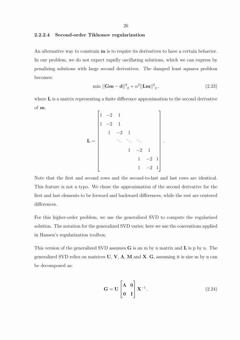
26
2.2.2.4 Second-order Tikhonov regularization
An alternative way to constrain m is to require its derivatives to have a certain behavior.
In our problem, we do not expect rapidly oscillating solutions, which we can express by
penalizing solutions with large second derivatives. The damped least squares problem
becomes:
min ||Gm− d||22 + α2||Lm||22 , (2.23)
where L is a matrix representing a finite difference approximation to the second derivative
of m,
L =
1 −2 1
1 −2 1
1 −2 1. . . . . . . . .
1 −2 1
1 −2 1
1 −2 1
.
Note that the first and second rows and the second-to-last and last rows are identical.
This feature is not a typo. We chose the approximation of the second derivative for the
first and last elements to be forward and backward differences, while the rest are centered
differences.
For this higher-order problem, we use the generalized SVD to compute the regularized
solution. The notation for the generalized SVD varies; here we use the conventions applied
in Hansen’s regularization toolbox.
This version of the generalized SVD assumes G is an m by n matrix and L is p by n. The
generalized SVD relies on matrices U, V, Λ, M and X. G, assuming it is size m by n can
be decomposed as:
G = U
Λ 0
0 I
X−1 . (2.24)
27
U is m by n with orthonormal columns, X is n by n and nonsingular, and Λ is p by p
and diagonal, with diagonal elements
0 ≤ λ1 ≤ λ2 ≤ · · · ≤ λp ≤ 1 . (2.25)
The matrix L can be decomposed as:
L = V[M 0
]X−1 , (2.26)
V is p by p and orthogonal and M is a p by p diagonal matrix with
1 ≥ µ1 ≥ µ2 ≥ · · · ≥ µp > 0 , (2.27)
λi and µi are related by the relationship
λ2i + µ2
i = 1, i = 1, 2, . . . , p , (2.28)
and the generalized singular values are
γi =λiµi. (2.29)
Using these conventions, the regularized solution for a higher-order Tikhonov regulariza-
tion where L is different from the identity matrix is:
mα,L =
p∑i=1
γ2i
γ2i + α2
(U.,i)T d
λiX.,i +
n∑i=p+1
(UT.,id)X.,i (2.30)
2.2.2.5 Parameter choice
In theory we would like to choose a value for the damping parameter α that enables us
to recover as much information as possible about the true value of m. In practice, when
we are inverting real data to find an input model, we can never determine whether we
have obtained the true model. So, when we recover a single model from a regularized

28
inversion, there is no technique that guarantees the best choice of α. In recognition that
the choice of α is always somewhat arbitrary, we consider some simple empirical methods
to illustrate how varying α affects our example solutions.
In the zeroth-order Tikhonov regularization, any value of α comes with a trade-off between
its effect on the solution error-norm ||Gm − d||2 and the model norm ||m||2. In many
problems, ||Gm−d||2 increases monotonically with α and ||m||2 decreases monotonically
with α. Due to these properties, the curve of ||m||2 plotted against ||Gm − d||2 often
has a characteristic L shape in log space, the corner of which would represent the best
trade-off between damping and model size. The L-curve criterion of choosing α is the
choice of α that gives the corner of the L-curve. One common way to find the damping
parameter that corresponds to this corner is to fit a spline to the function and compute
the point of maximum negative curvature (Hansen and O’Leary, 1993). To find the point
of maximum negative curvature, one plots ||Gm− d||2 as the abscissa and ||m||2 as the
ordinate as a function of varying α. Another method that is essentially equivalent is to
compute the minimum in the function P (t) = ||m||||Gm− d|| (Johnston and Gulrajani,
2000, Lian et al., 1998). In the following examples, the L-curve is not very well-behaved;
there is either no well-defined corner or two corners and thus both of these methods fail.
For this reason, in the no-noise cases we show a few different magnitude values of α that
return a close fit to the original synthetic model.
In the presence of noise, a sensible choice of α is one that satisfies the discrepancy principle.
The discrepancy principle is to take the value of α for which the misfit ||Gm − d||2 is
equal to the 2-norm error (noise) in the data. The underlying goal of the discrepancy
principle is to ensure that the inverse solution does not overfit the noise in the data.
29
2.3 Results
2.3.1 Recovering a stretched sea level boundary condition
In this example we generate a synthetic data set that looks like an ideal “LGM-like”
concentration profile. That is, it has a maximum chloride concentration several 10s of
meters below the sediment–water interface that is the result of increased water salinity at
the Last Glacial Maximum, due primarily to glacier expansion.
To generate the synthetic data set, at the sediment–water interface we use the same
forcing function as that in Adkins et al. (2002), which is a scaled version of the sea-level
curve extending back to 125 ka before present. We take the LGM salinity to be 38 g kg−1
and the modern salinity as 35 g kg−1 and use the difference between these two to scale
the sea level curve to salinity assuming that the ocean is a rectangular basin that is today
3800 m deep. At the bottom boundary, we set ∂c∂z
= 0. φ is a constant 0.8, u is a constant
0.01 cm yr−1 and D0 is 2.9 × 10⁻⁶ cm2 s−1. The initial condition is a uniform profile,
c(z) = 35 g kg−1.
Once we have a synthetic data set, we apply various inverse methods to the synthetic
data to recover the original forcing function or model, m. We then can evaluate the skill
of the inverse methods by comparing the inverse solution in each case to the synthetic
model we used to generate the data. The data used for the inverse problem is the actual
data minus the initial condition response. In this way we avoid inverting for the initial
condition. The model that we invert for is the top (sediment–water interface) boundary
condition.
In the following cases we compare several different levels of discretization of the problem.
Table 2.1 summarizes the characteristics of the Gs. The coarsest resolution G was chosen
to be square and to have a spatial resolution similar to the typical measurement spatial
resolution.

30
Table 2.1: Summary of G properties
Dimensions ∆ z ∆ t Time domain Space domainof G (cm) (yrs) (yrs) (m)
251 x 251 50 500 125,000 125301 x 626 50 200 125,000 150301 x 1251 50 100 125,000 150
2.3.1.1 Properties of G
Figure 2.2 illustrates the general behavior of the G matrix. (a) is the full Picard plot,
while (b) is zoomed in on the singular values above the noise floor. σi are the singular
values of G, |uTi d/σi| are the magnitudes of the modes contributing to the generalized
inverse solution, and the coefficients |uTi d| are known as the Fourier coefficients. This type
of figure is called a “Picard Plot” as it illustrates whether the Picard condition is satisfied
for the generalized inverse problem m† = G†d. In order for the generalized inverse solution
to be stable, the Picard condition requires that at some point the Fourier coefficients must
decay faster than their corresponding σi values. We can see that the Picard condition is
not satisfied, as the Fourier coefficients oscillate around the singular values, which means
that determination of a stable generalized inverse will require regularization. The decay
of the singular values is smooth until the singular values reach a noise floor around the
33rd value. Without the machine precision limit, we expect these values to continue to
decay smoothly towards 0. The inversion of G to find m is an ill-posed problem; there
is no clear cut-off between large magnitude and small magnitude parts of the solution.
The very small singular values will amplify any noise in the data vector when we compute
generalized inverse solutions.
2.3.1.2 TSVD least squares inverse solution
Although the inverse problem is ill-posed, the numerical rank deficiency of G hints that
we may be able to at least partially stabilize our generalized inverse solution by truncating
the SVD at the noise floor. In Figure 2.3 we show the results of truncation beyond the
33rd singular value, using the restriction that singular values must be greater than 10*eps,
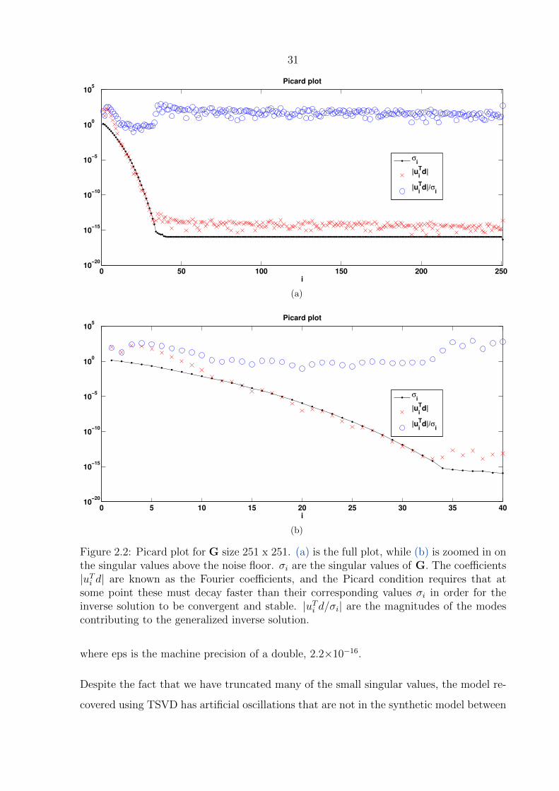
31
0 50 100 150 200 25010
−20
10−15
10−10
10−5
100
105
i
Picard plot
σi
|ui
Td|
|ui
Td|/σ
i
(a)
0 5 10 15 20 25 30 35 4010
−20
10−15
10−10
10−5
100
105
i
Picard plot
σi
|ui
Td|
|ui
Td|/σ
i
(b)
Figure 2.2: Picard plot for G size 251 x 251. (a) is the full plot, while (b) is zoomed in onthe singular values above the noise floor. σi are the singular values of G. The coefficients|uTi d| are known as the Fourier coefficients, and the Picard condition requires that atsome point these must decay faster than their corresponding values σi in order for theinverse solution to be convergent and stable. |uTi d/σi| are the magnitudes of the modescontributing to the generalized inverse solution.
where eps is the machine precision of a double, 2.2×10⁻¹⁶.
Despite the fact that we have truncated many of the small singular values, the model re-
covered using TSVD has artificial oscillations that are not in the synthetic model between

32
0 10 20 30 40 50 60 70 80 90 100 110 12033
34
35
36
37
38
39
ka BP
Sa
lin
ity
TSVD least squares inverse solution
TSVD
Actual Model
(a)
35 35.5 36
0
2000
4000
6000
8000
10000
12000
Salinity (g/kg)
Sed
imen
t D
ep
th (
cm
)
TSVD
Synthetic
(b)
Figure 2.3: (a) shows the synthetic model (red) used to generate synthetic data andthe model recovered using the TSVD method (blue). (b) is the synthetic data (red)generated by the synthetic model and used to find the inverse solution plotted against thedata generated by the recovered model using TSVD (blue).
5 ka BP and 30 ka BP, and is artificially smooth relative to the true synthetic model
between 30 ka BP and 125 ka BP. The artificial smoothness we can understand as infor-
mation lost through the truncation of some of the modes of the solution. The artificial
oscillations, however, are evidence of instability in the generalized inverse solution. The
instability in the generalized inverse is due to the fact that the Picard condition is not
satisfied even when we truncate the singular values below the noise floor. Referring back
to Figure 2.2b, we see that the Fourier coefficients and singular values decay at roughly
the same rate between i=10 and i=33.
From i=3 to i=10, the Fourier coefficients do decay faster than the singular values, so we
might consider an even more severe truncation at i=10. However, the condition number of
GT , the truncated version of G, is 86 when we truncate at i=10. The condition number
represents approximately the ratio of the error in the generalized inverse solution to the
error in the data vector d; a matrix with condition number 86 is therefore quite unstable
to noise in the data. In addition, truncation at i=10 forces us to lose the ability to recover
the vast majority of modes in the original synthetic model.
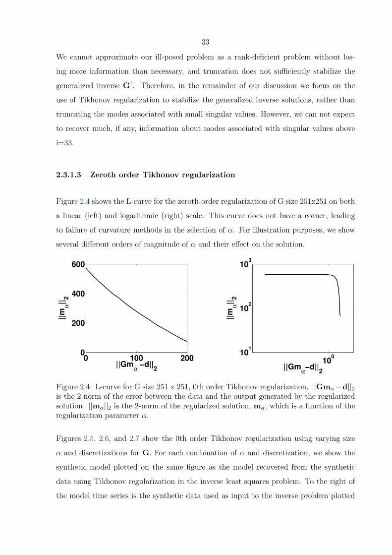
33
We cannot approximate our ill-posed problem as a rank-deficient problem without los-
ing more information than necessary, and truncation does not sufficiently stabilize the
generalized inverse G†. Therefore, in the remainder of our discussion we focus on the
use of Tikhonov regularization to stabilize the generalized inverse solutions, rather than
truncating the modes associated with small singular values. However, we can not expect
to recover much, if any, information about modes associated with singular values above
i=33.
2.3.1.3 Zeroth order Tikhonov regularization
Figure 2.4 shows the L-curve for the zeroth-order regularization of G size 251x251 on both
a linear (left) and logarithmic (right) scale. This curve does not have a corner, leading
to failure of curvature methods in the selection of α. For illustration purposes, we show
several different orders of magnitude of α and their effect on the solution.
0 100 2000
200
400
600
||Gmα −d||
2
||m
α||
2
100
101
102
103
||Gmα−d||
2
||m
α||
2
Figure 2.4: L-curve for G size 251 x 251, 0th order Tikhonov regularization. ||Gmα−d||2is the 2-norm of the error between the data and the output generated by the regularizedsolution. ||mα||2 is the 2-norm of the regularized solution, mα, which is a function of theregularization parameter α.
Figures 2.5, 2.6, and 2.7 show the 0th order Tikhonov regularization using varying size
α and discretizations for G. For each combination of α and discretization, we show the
synthetic model plotted on the same figure as the model recovered from the synthetic
data using Tikhonov regularization in the inverse least squares problem. To the right of
the model time series is the synthetic data used as input to the inverse problem plotted

34
alongside the data generated using the regularized inverse solution as forcing to the for-
ward model. In all of these cases without noise, the regularized least squares solution,
used as a boundary condition to the forward model, generates data indistinguishable from
the synthetic data.
Even when α is close to 0, as shown in Figure 2.5 where α = 10−14, the oscillations
in the synthetic model between 30 ka and 125 ka BP are not recovered in the inverse
solution. This is not a function of resolution, as demonstrated by the fact that when G
has 100 year temporal resolution (size 301x1251) there are even higher frequency artificial
oscillations between 0 and 10 ka BP in the recovered time series. The recovered time
series between 30 ka and 125 ka BP is strikingly similar to the values recovered over the
same time period by the TSVD method. We therefore conclude that the information lost
is that of the modes associated with the singular values below the noise floor. We do not
lose this information due to damping, but because they are unrecoverable because of the
limitations of machine precision.
Increased discretization in time in general does not enable us to recover any more informa-
tion from the signal. The one exception is perhaps shown in Figure 2.6 where the increase
in resolution from G size 251x251 to size 301x626 enables more of the pattern from 30 to
125 ka BP to appear in the regularized inverse solution. High frequency variability is not
recovered from the data by the regularization; however, the very large maximum around
20ky before present seems well recovered, as are the mean slope of approach and retreat
from this maximum. Instead of increasing information recovery, the near-present oscil-
lations in Figure 2.5e demonstrate that increased discretization, without an equivalent
increase in damping, enhances the instability of the inverse solution.
2.3.1.4 Zeroth order Tikhonov regularization with noise
In the previous example we used perfect data as input to the regularizations. In reality,
there will always be noise in the data due to measurement error. To simulate measurement
error, we add white noise to the synthetic data profile. We then choose a regularization
parameter using the discrepancy principle to ensure that we do not overfit the noise.
35
Figures 2.8, 2.9, and 2.10 show the results of regularized inversions with increasingly larger
magnitudes of simulated measurement noise and increasing resolution of G. Accounting
for noise requires the use of a larger damping parameter, which increases the bias of the
solution and decreases the value of the reconstructed LGM salinity. Further, the noisier
the data, the more oscillatory the regularized solution becomes in the approach to the
present. This problem worsens with increased resolution of G. These oscillations are not
present in the original synthetic model; they are entirely a product of the instability of
the regularized inverse.
The near-present oscillations are the result of unstable oscillatory modes associated with
small singular values being smeared into the near-present solution. In order to damp these
oscillations, we can increase the damping parameter, but this would increase the damping
everywhere in the solution. With increasingly resolved G, the oscillatory nature of the
solutions becomes worse. The increasingly resolved G is increasingly underdetermined
and has more modes associated with very small singular values. The number of well-
resolved singular values remains essentially constant with resolution of G (O(10)), but the
number of minute singular values and associated unstable modes increases with increasing
discretization.
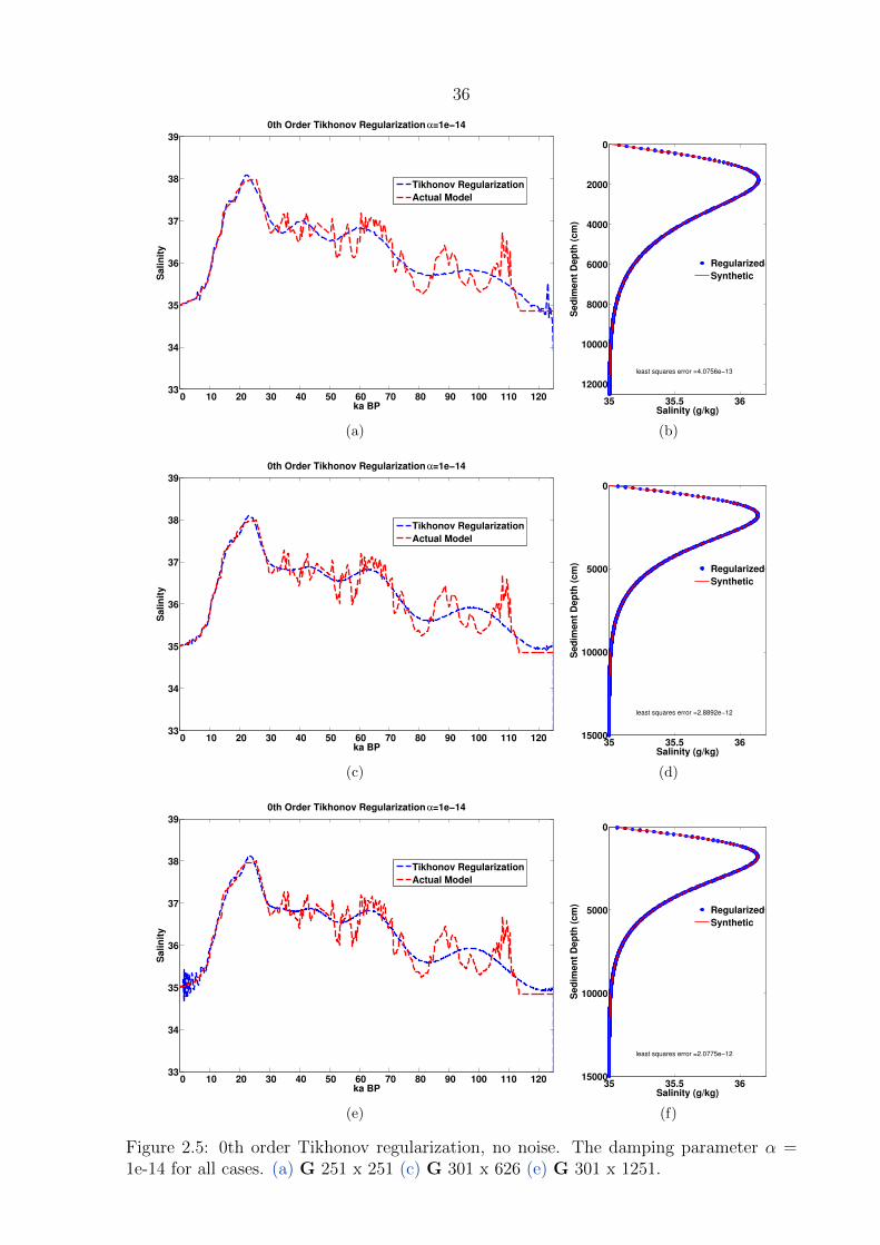
36
0 10 20 30 40 50 60 70 80 90 100 110 12033
34
35
36
37
38
39
ka BP
Sa
lin
ity
0th Order Tikhonov Regularization α=1e−14
Tikhonov Regularization
Actual Model
(a)
35 35.5 36
0
2000
4000
6000
8000
10000
12000
Salinity (g/kg)
Sed
imen
t D
ep
th (
cm
)
Regularized
Synthetic
least squares error =4.0756e−13
(b)
0 10 20 30 40 50 60 70 80 90 100 110 12033
34
35
36
37
38
39
ka BP
Sali
nit
y
0th Order Tikhonov Regularization α=1e−14
Tikhonov Regularization
Actual Model
(c)
35 35.5 36
0
5000
10000
15000
Salinity (g/kg)
Sed
imen
t D
ep
th (
cm
)
Regularized
Synthetic
least squares error =2.8892e−12
(d)
0 10 20 30 40 50 60 70 80 90 100 110 12033
34
35
36
37
38
39
ka BP
Sa
lin
ity
0th Order Tikhonov Regularization α=1e−14
Tikhonov Regularization
Actual Model
(e)
35 35.5 36
0
5000
10000
15000
Salinity (g/kg)
Sed
imen
t D
ep
th (
cm
)
Regularized
Synthetic
least squares error =2.0775e−12
(f)
Figure 2.5: 0th order Tikhonov regularization, no noise. The damping parameter α =1e-14 for all cases. (a) G 251 x 251 (c) G 301 x 626 (e) G 301 x 1251.
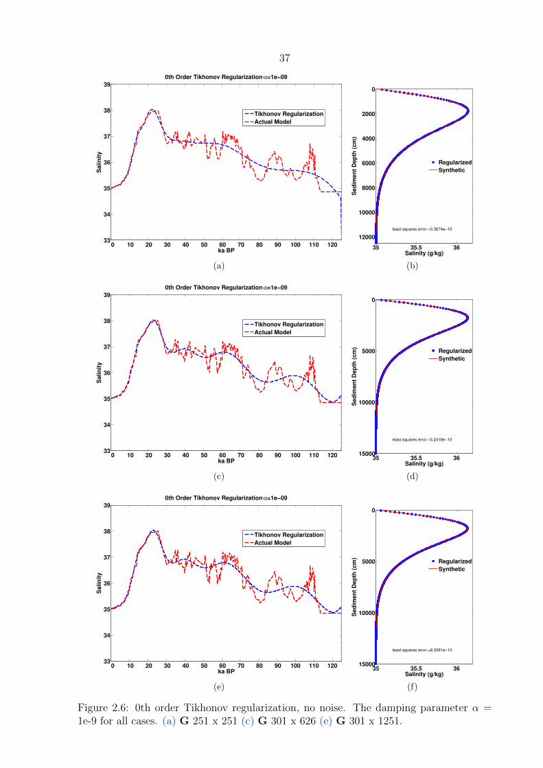
37
0 10 20 30 40 50 60 70 80 90 100 110 12033
34
35
36
37
38
39
ka BP
Sa
lin
ity
0th Order Tikhonov Regularization α=1e−09
Tikhonov Regularization
Actual Model
(a)
35 35.5 36
0
2000
4000
6000
8000
10000
12000
Salinity (g/kg)
Sed
imen
t D
ep
th (
cm
)
Regularized
Synthetic
least squares error =3.3674e−10
(b)
0 10 20 30 40 50 60 70 80 90 100 110 12033
34
35
36
37
38
39
ka BP
Sali
nit
y
0th Order Tikhonov Regularization α=1e−09
Tikhonov Regularization
Actual Model
(c)
35 35.5 36
0
5000
10000
15000
Salinity (g/kg)
Sed
imen
t D
ep
th (
cm
)
Regularized
Synthetic
least squares error =5.2418e−10
(d)
0 10 20 30 40 50 60 70 80 90 100 110 12033
34
35
36
37
38
39
ka BP
Sa
lin
ity
0th Order Tikhonov Regularization α=1e−09
Tikhonov Regularization
Actual Model
(e)
35 35.5 36
0
5000
10000
15000
Salinity (g/kg)
Sed
imen
t D
ep
th (
cm
)
Regularized
Synthetic
least squares error =9.3391e−10
(f)
Figure 2.6: 0th order Tikhonov regularization, no noise. The damping parameter α =1e-9 for all cases. (a) G 251 x 251 (c) G 301 x 626 (e) G 301 x 1251.
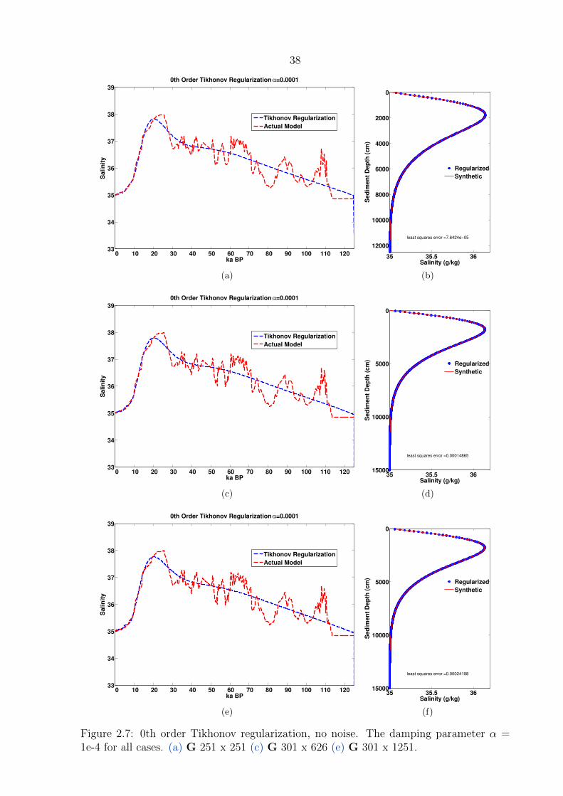
38
0 10 20 30 40 50 60 70 80 90 100 110 12033
34
35
36
37
38
39
ka BP
Sa
lin
ity
0th Order Tikhonov Regularization α=0.0001
Tikhonov Regularization
Actual Model
(a)
35 35.5 36
0
2000
4000
6000
8000
10000
12000
Salinity (g/kg)
Sed
imen
t D
ep
th (
cm
)
Regularized
Synthetic
least squares error =7.6424e−05
(b)
0 10 20 30 40 50 60 70 80 90 100 110 12033
34
35
36
37
38
39
ka BP
Sali
nit
y
0th Order Tikhonov Regularization α=0.0001
Tikhonov Regularization
Actual Model
(c)
35 35.5 36
0
5000
10000
15000
Salinity (g/kg)
Sed
imen
t D
ep
th (
cm
)
Regularized
Synthetic
least squares error =0.00014865
(d)
0 10 20 30 40 50 60 70 80 90 100 110 12033
34
35
36
37
38
39
ka BP
Sa
lin
ity
0th Order Tikhonov Regularization α=0.0001
Tikhonov Regularization
Actual Model
(e)
35 35.5 36
0
5000
10000
15000
Salinity (g/kg)
Sed
imen
t D
ep
th (
cm
)
Regularized
Synthetic
least squares error =0.00024198
(f)
Figure 2.7: 0th order Tikhonov regularization, no noise. The damping parameter α =1e-4 for all cases. (a) G 251 x 251 (c) G 301 x 626 (e) G 301 x 1251.
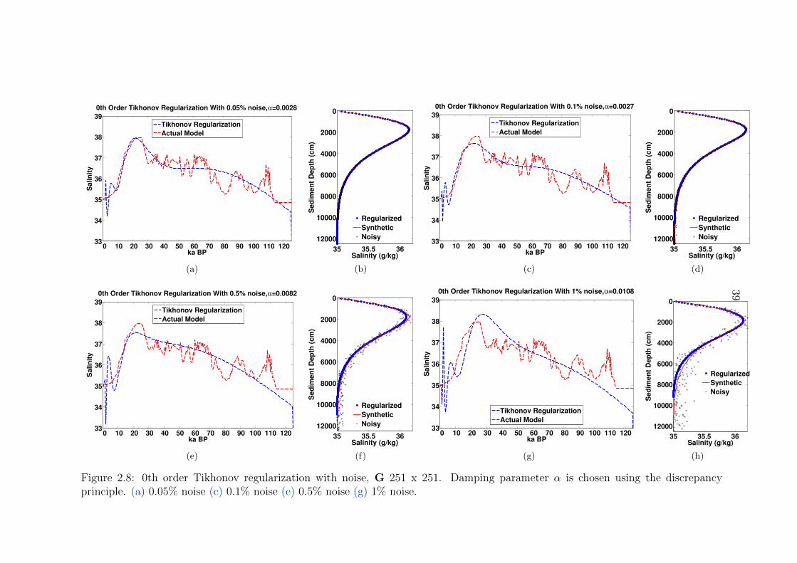
39
0 10 20 30 40 50 60 70 80 90 100 110 12033
34
35
36
37
38
39
ka BP
Sa
lin
ity
0th Order Tikhonov Regularization With 0.05% noise, α=0.0028
Tikhonov Regularization
Actual Model
(a)
35 35.5 36
0
2000
4000
6000
8000
10000
12000
Salinity (g/kg)
Se
dim
en
t D
ep
th (
cm
)
Regularized
Synthetic
Noisy
(b)
0 10 20 30 40 50 60 70 80 90 100 110 12033
34
35
36
37
38
39
ka BP
Salin
ity
0th Order Tikhonov Regularization With 0.1% noise, α=0.0027
Tikhonov Regularization
Actual Model
(c)
35 35.5 36
0
2000
4000
6000
8000
10000
12000
Salinity (g/kg)
Se
dim
en
t D
ep
th (
cm
)
Regularized
Synthetic
Noisy
(d)
0 10 20 30 40 50 60 70 80 90 100 110 12033
34
35
36
37
38
39
ka BP
Salin
ity
0th Order Tikhonov Regularization With 0.5% noise, α=0.0082
Tikhonov Regularization
Actual Model
(e)
35 35.5 36
0
2000
4000
6000
8000
10000
12000
Salinity (g/kg)
Se
dim
en
t D
ep
th (
cm
)
Regularized
Synthetic
Noisy
(f)
0 10 20 30 40 50 60 70 80 90 100 110 12033
34
35
36
37
38
39
ka BP
Sa
lin
ity
0th Order Tikhonov Regularization With 1% noise, α=0.0108
Tikhonov Regularization
Actual Model
(g)
35 35.5 36
0
2000
4000
6000
8000
10000
12000
Salinity (g/kg)
Se
dim
en
t D
ep
th (
cm
)
Regularized
Synthetic
Noisy
(h)
Figure 2.8: 0th order Tikhonov regularization with noise, G 251 x 251. Damping parameter α is chosen using the discrepancyprinciple. (a) 0.05% noise (c) 0.1% noise (e) 0.5% noise (g) 1% noise.
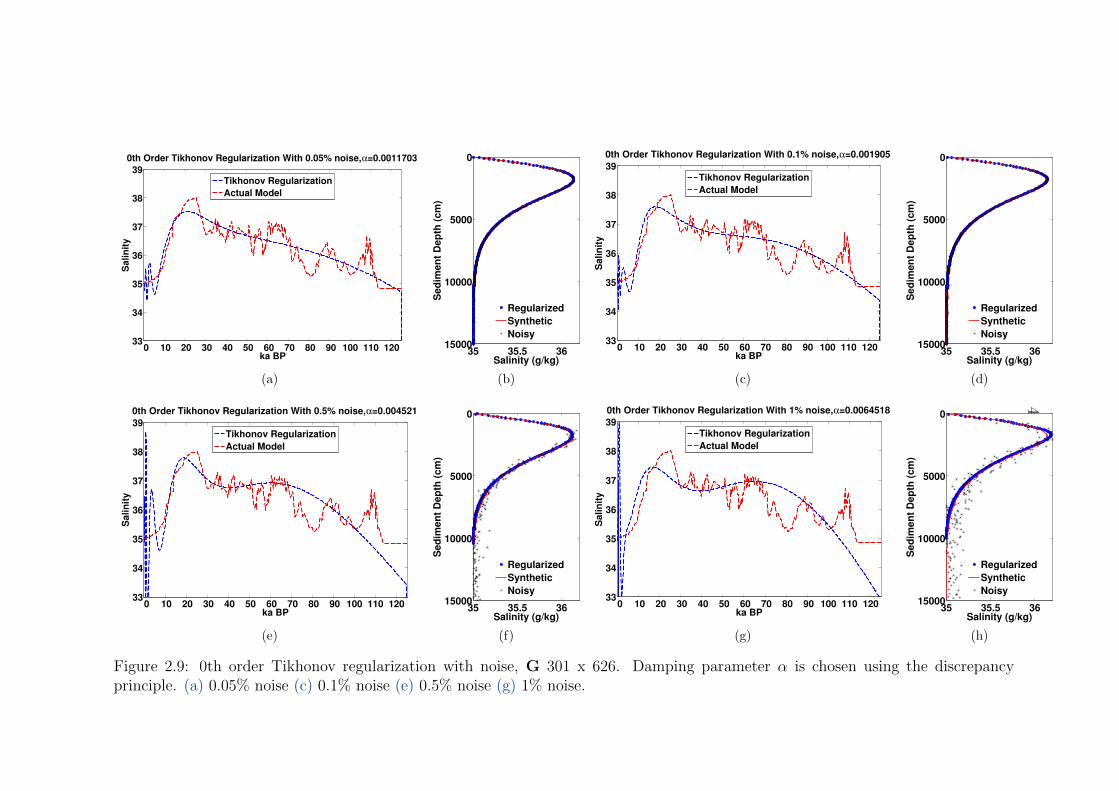
40
0 10 20 30 40 50 60 70 80 90 100 110 12033
34
35
36
37
38
39
ka BP
Sa
lin
ity
0th Order Tikhonov Regularization With 0.05% noise, α=0.0011703
Tikhonov Regularization
Actual Model
(a)
35 35.5 36
0
5000
10000
15000
Salinity (g/kg)
Se
dim
en
t D
ep
th (
cm
)
Regularized
Synthetic
Noisy
(b)
0 10 20 30 40 50 60 70 80 90 100 110 12033
34
35
36
37
38
39
ka BP
Salin
ity
0th Order Tikhonov Regularization With 0.1% noise, α=0.001905
Tikhonov Regularization
Actual Model
(c)
35 35.5 36
0
5000
10000
15000
Salinity (g/kg)
Se
dim
en
t D
ep
th (
cm
)
Regularized
Synthetic
Noisy
(d)
0 10 20 30 40 50 60 70 80 90 100 110 12033
34
35
36
37
38
39
ka BP
Salin
ity
0th Order Tikhonov Regularization With 0.5% noise, α=0.004521
Tikhonov Regularization
Actual Model
(e)
35 35.5 36
0
5000
10000
15000
Salinity (g/kg)
Se
dim
en
t D
ep
th (
cm
)
Regularized
Synthetic
Noisy
(f)
0 10 20 30 40 50 60 70 80 90 100 110 12033
34
35
36
37
38
39
ka BP
Sa
lin
ity
0th Order Tikhonov Regularization With 1% noise, α=0.0064518
Tikhonov Regularization
Actual Model
(g)
35 35.5 36
0
5000
10000
15000
Salinity (g/kg)
Se
dim
en
t D
ep
th (
cm
)
Regularized
Synthetic
Noisy
(h)
Figure 2.9: 0th order Tikhonov regularization with noise, G 301 x 626. Damping parameter α is chosen using the discrepancyprinciple. (a) 0.05% noise (c) 0.1% noise (e) 0.5% noise (g) 1% noise.

41
0 10 20 30 40 50 60 70 80 90 100 110 12033
34
35
36
37
38
39
ka BP
Sa
lin
ity
0th Order Tikhonov Regularization With 0.05% noise, α=0.0011
Tikhonov Regularization
Actual Model
(a)
35 35.5 36
0
5000
10000
15000
Salinity (g/kg)
Se
dim
en
t D
ep
th (
cm
)
Regularized
Synthetic
Noisy
(b)
0 10 20 30 40 50 60 70 80 90 100 110 12033
34
35
36
37
38
39
ka BP
Salin
ity
0th Order Tikhonov Regularization With 0.1% noise, α=0.0018
Tikhonov Regularization
Actual Model
(c)
35 35.5 36
0
5000
10000
15000
Salinity (g/kg)
Se
dim
en
t D
ep
th (
cm
)
Regularized
Synthetic
Noisy
(d)
0 10 20 30 40 50 60 70 80 90 100 110 12033
34
35
36
37
38
39
ka BP
Salin
ity
0th Order Tikhonov Regularization With 0.5% noise, α=0.0027
Tikhonov Regularization
Actual Model
(e)
35 35.5 36
0
5000
10000
15000
Salinity (g/kg)
Se
dim
en
t D
ep
th (
cm
)
Regularized
Synthetic
Noisy
(f)
0 10 20 30 40 50 60 70 80 90 100 110 12033
34
35
36
37
38
39
ka BP
Sa
lin
ity
0th Order Tikhonov Regularization With 1% noise, α=0.0045
Tikhonov Regularization
Actual Model
(g)
35 35.5 36
0
5000
10000
15000
Salinity (g/kg)
Se
dim
en
t D
ep
th (
cm
)
Regularized
Synthetic
Noisy
(h)
Figure 2.10: 0th order Tikhonov regularization with noise, G 301 x 1251. Damping parameter α is chosen using the discrepancyprinciple.(a) 0.05% noise. (c) 0.1% noise (e) 0.5% noise (g) 1% noise.
42
2.3.1.5 Resolution of the inverse solution
The oscillations of near-present solution components is confusing, as our intuition tells us
that the information closer to the present should be better constrained than the informa-
tion in the past. This is true, but in a regularized inversion the behavior of poorly resolved
modes is spread or smeared among parameters. One way to see this effect more clearly
is by examining the resolution matrix. The resolution matrix describes the averaging
behavior of the regularization. Recall that
Gmtrue = d (2.31)
and the generalized inverse solution m† is related to the true solution in this way:
m† = G†d = G†Gmtrue = Rmmtrue . (2.32)
A perfect resolution solution would have Rm equal to the identity matrix. Otherwise, Rm
is a symmetric matrix that describes how much the generalized inverse solution smears
the original model m into the recovered model m†.
In the 0th order Tikhonov regularizations, the recovered model is
mα =(GTG + α2I
)−1GTd = G#d , (2.33)
so
Rm,α = G#G = VFVT , (2.34)
where V takes its traditional meaning from the SVD of G and F is a diagonal matrix
with diagonal elements equal to the filter factors:
fi =s2i
s2i + α2
. (2.35)
All of the elements of Rm,α take values between 0 and 1. 1 implies perfect resolution while
43
0 means none of the information about the parameter is recovered in the right place. By
examining the diagonal of Rm,α, we can see how well each model parameter is resolved
by G. Figures 2.11a, 2.11c, 2.11e are plots of the diagonal of Rm,α for various values of
α. The x-axis corresponds to the past time associated with each model element and the
y-axis is the associated diagonal value of the resolution matrix. In all cases, the resolution
of the model elements recovered by the regularized inverse are better closer to the present.
As the damping parameter α increases, the drop-off in resolution with time in the past
becomes steeper, as evidenced by the fact that the curves are stacked vertically with the
smallest damping parameter curves at the top (closest to 1) and the largest damping
parameter curves have resolution diagonals less than 0.1.
In the best case scenarios shown, with α = 10−8(α2 = 10−16), seven times are perfectly
resolved in the regularized inverse. When α2 increases to 10, all of the model elements
are poorly resolved in the regularized inverse, with maximum diagonal of the resolution
matrix equal to 0.1. The number of parameters resolved by the regularization does not
vary much with differing discretization, but the positions of the well-resolved parameters
shift forward in time as the discretization increases relative to their positions in the more
roughly discretized problem. Figures 2.11a, 2.11c, 2.11e have the same x-axis limits, but
the maximum age with a resolution diagonal equal to one in these plots is 3000 years BP
for G size 251x151, while only 700 years BP for G size 301x1251.
The columns of the resolution matrix show how information of each parameter is smeared
into other parameters. A visually informative technique is to look at the behavior of a
spike model (unit step change) in response to the resolution matrix. Since we are especially
interested in reconstructing the LGM, we show the results of a spike test positioned at
the LGM, roughly 20,000 years BP. For consistency between different Gs the spike test
is 1000 years long. We use α = 10−4 in the spike test because use of the discrepancy
principle in the regularized inversions with noise consistently required α ≥ 10−4.
Figures 2.11b, 2.11d, and 2.11f demonstrate that the information at the LGM is poorly
resolved by the inverse solution. The diagonal element in all discretizations of G is < 0.2
and the bulk of the signal has been spread tens of thousands of years both forwards
and backwards in time. Apparently, the regularization’s seeming recovery of the LGM’s

44
magnitude in Figures 2.8, 2.9, and 2.10 was actually an artifact of the smoothness of our
synthetic model; information has been smeared from other times into the LGM.
The spike test also demonstrates that the smeared contribution of past information to
the near-present solution is quite oscillatory. Thus the oscillatory behavior we see in the
modern solution under noise is in part a result of smearing forward of poorly resolved
older components amplified by the magnitude of the noise.
As a general principle, the left and right singular vectors associated with smaller singular
values have more zero crossings (number of zero crossings increases with i). While these
oscillations are damped in the forward problem when multiplied by small singular values,
the recovery of inverse solutions with the singular value in the denominator amplifies high
frequency variations. In this case, noise appears as a high frequency variation.
With increased damping parameter, the smearing of oscillations is increased. The near-
present values are not smeared as much as the older values, but they preferentially receive
smeared information from the older values. When summed with the well-resolved near-
present information, this smearing leads to the initially counterintuitive high magnitude
oscillations.

45
0 1000 2000 3000 4000 50000
0.1
0.2
0.3
0.4
0.5
0.6
0.7
0.8
0.9
1
Years BP
Rm
,α(i
,i)
1e−8
1e−5
1e−4
1e−2
1e−1
0.316
1
3.16
(a)
0 5 10 15 20 25 30 35 40 45 50 55 60−0.2
0
0.2
0.4
0.6
0.8
1
ka BP
mtrue
mα
(b)
0 1000 2000 3000 4000 50000
0.1
0.2
0.3
0.4
0.5
0.6
0.7
0.8
0.9
1
Years BP
Rm
,α(i
,i)
1e−8
1e−5
1e−4
1e−2
1e−1
0.316
1
3.16
(c)
0 5 10 15 20 25 30 35 40 45 50 55 60−0.2
0
0.2
0.4
0.6
0.8
1
1.2
kya
mtrue
mα
(d)
0 1000 2000 3000 4000 50000
0.1
0.2
0.3
0.4
0.5
0.6
0.7
0.8
0.9
1
Years BP
Rm
,α(i
,i)
1e−8
1e−5
1e−4
1e−2
1e−1
0.316
1
3.16
(e)
0 5 10 15 20 25 30 35 40 45 50 55 60−0.2
0
0.2
0.4
0.6
0.8
1
1.2
kya
mtrue
mα
(f)
Figure 2.11: (a) G 251x251 resolution matrix diagonals as a function of α (b) G 251 x 251resolution matrix LGM spike test (c) G 301 x 626 resolution matrix diagonals as a functionof α (d) G 301 x 626 resolution matrix LGM spike test (e) G 301 x 1251 resolution matrixdiagonals as a function of α (f) G 301 x 1251 resolution matrix LGM spike test using α= 1e-04.

46
2.3.1.6 Second order Tikhonov regularization
In order to reduce the oscillatory behavior of the solution we can perform a second order
Tikhonov regularization. The second order Tikhonov regularization penalizes the norm
of the second derivative of the solution, and thus prefers solutions with fewer minima
and maxima, which will reduce the solution’s oscillatory behavior. Note that using this
method, the minimum magnitude of α for a smooth solution is smaller than that for the
zeroth-order regularization, as demonstrated in Figures 2.12–2.14. The magnitudes are
not directly comparable because they have different units; in the zeroth-order case we
damp the amplitude of the solution while in the second-order regularization we damp the
second derivative. In the noisy cases, Figures 2.15–2.17, the boundary condition recovered
using the regularization is much smoother than the synthetic boundary condition, and has
a wider and lower magnitude LGM. Also, the concentration profile produced by using the
regularized model as the forcing condition has a much larger error. Because the penalty
on the second derivative is applied uniformly to the solution, it flattens the maximum
corresponding to the LGM as well as reducing the unwanted oscillations.
The second order regularization is much more stable than the zeroth order regularization,
but it still does not resolve individual model parameters very well, as shown in Figure 2.18
which is the resolution matrix for different values of α. In this case, more information is
smeared backward in time rather than forward, explaining the long-period oscillation in
the old time nodes.
The example we are inverting for is quite smooth, and a case with higher frequency vari-
ability would not be recovered well by the second-order Tikhonov regularized inversion.
This method does penalize more rapidly oscillating solutions over slowly oscillating solu-
tions, however there is no specific frequency dependence to the penalty. Ideally we want
a penalty on solutions that oscillate more rapidly than physically sensible, while allow-
ing physically reasonable oscillations. One way to do this is to use a variable damping
parameter α. Next we consider one particular choice of variable α and its effect on our
ability to recover our synthetic time series.

47
0 10 20 30 40 50 60 70 80 90 100 110 12033
34
35
36
37
38
39
ka BP
Sa
lin
ity
2nd order Tikhonov Regularization, α = 1e−14
Tikhonov Regularization
Actual Model
(a)
35 35.5 36
0
2000
4000
6000
8000
10000
12000
Salinity (g/kg)
Sed
imen
t D
ep
th (
cm
)
2nd order Tikhonov Regularization, α = 1e−14
Regularized
Synthetic
least squares error =7.0609e−13
(b)
0 10 20 30 40 50 60 70 80 90 100 110 12033
34
35
36
37
38
39
ka BP
Sali
nit
y
2nd order Tikhonov Regularization, α = 1e−14
Tikhonov Regularization
Actual Model
(c)
35 35.5 36
0
5000
10000
15000
Salinity (g/kg)
Sed
imen
t D
ep
th (
cm
)
2nd order Tikhonov Regularization, α = 1e−14
Regularized
Synthetic
least squares error =9.3056e−12
(d)
0 10 20 30 40 50 60 70 80 90 100 110 12033
34
35
36
37
38
39
ka BP
Sa
lin
ity
2nd order Tikhonov Regularization, α = 1e−14
Tikhonov Regularization
Actual Model
(e)
35 35.5 36
0
5000
10000
15000
Salinity (g/kg)
Sed
imen
t D
ep
th (
cm
)
2nd order Tikhonov Regularization, α = 1e−14
Regularized
Synthetic
least squares error =2.1827e−11
(f)
Figure 2.12: 2nd order regularization, no noise, using α =1e-14 (a) G 251 x 251 (c) G301 x 626 (e) G 301 x 1251.
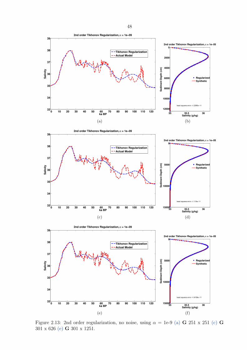
48
0 10 20 30 40 50 60 70 80 90 100 110 12033
34
35
36
37
38
39
ka BP
Sa
lin
ity
2nd order Tikhonov Regularization, α = 1e−09
Tikhonov Regularization
Actual Model
(a)
35 35.5 36
0
2000
4000
6000
8000
10000
12000
Salinity (g/kg)
Sed
imen
t D
ep
th (
cm
)
2nd order Tikhonov Regularization, α = 1e−09
Regularized
Synthetic
least squares error =1.2395e−11
(b)
0 10 20 30 40 50 60 70 80 90 100 110 12033
34
35
36
37
38
39
ka BP
Sali
nit
y
2nd order Tikhonov Regularization, α = 1e−09
Tikhonov Regularization
Actual Model
(c)
35 35.5 36
0
5000
10000
15000
Salinity (g/kg)
Sed
imen
t D
ep
th (
cm
)
2nd order Tikhonov Regularization, α = 1e−09
Regularized
Synthetic
least squares error =1.115e−11
(d)
0 10 20 30 40 50 60 70 80 90 100 110 12033
34
35
36
37
38
39
ka BP
Sa
lin
ity
2nd order Tikhonov Regularization, α = 1e−09
Tikhonov Regularization
Actual Model
(e)
35 35.5 36
0
5000
10000
15000
Salinity (g/kg)
Sed
imen
t D
ep
th (
cm
)
2nd order Tikhonov Regularization, α = 1e−09
Regularized
Synthetic
least squares error =1.6159e−11
(f)
Figure 2.13: 2nd order regularization, no noise, using α = 1e-9 (a) G 251 x 251 (c) G301 x 626 (e) G 301 x 1251.
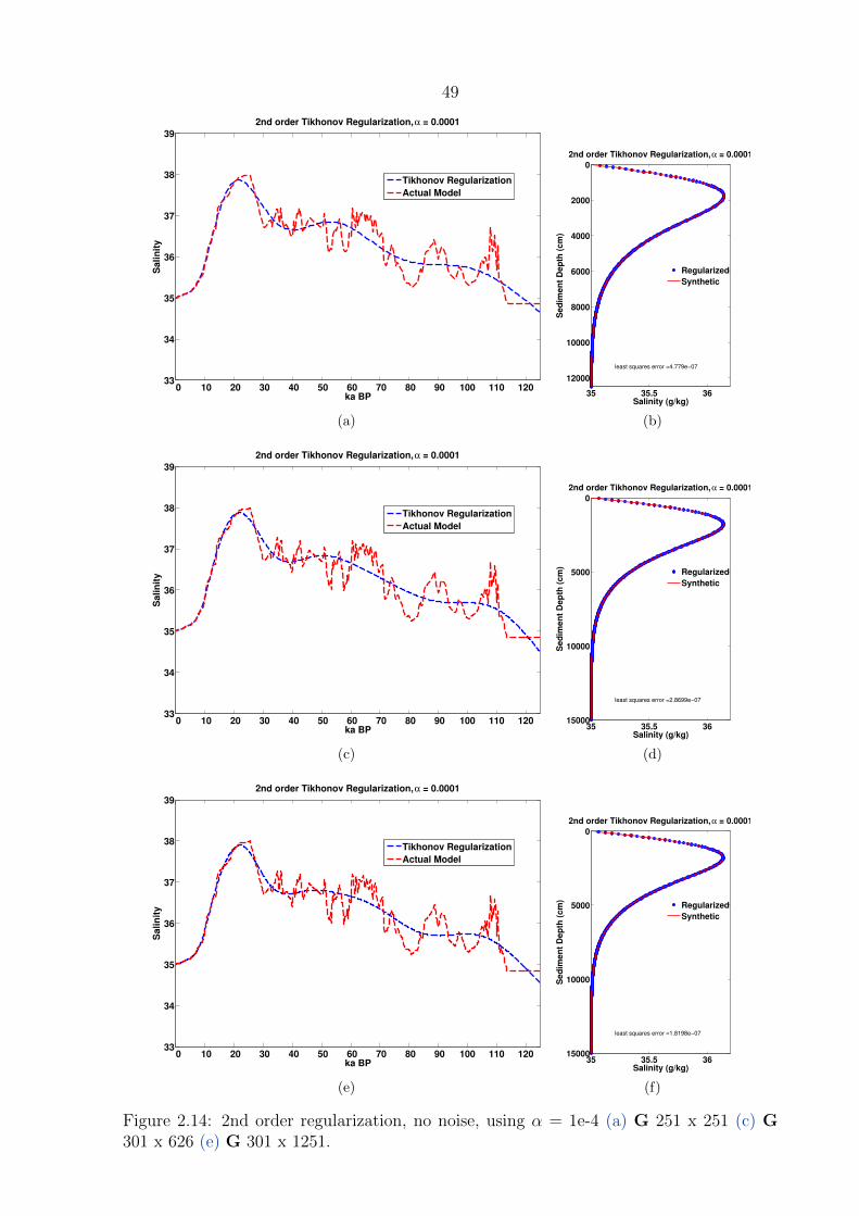
49
0 10 20 30 40 50 60 70 80 90 100 110 12033
34
35
36
37
38
39
ka BP
Sa
lin
ity
2nd order Tikhonov Regularization, α = 0.0001
Tikhonov Regularization
Actual Model
(a)
35 35.5 36
0
2000
4000
6000
8000
10000
12000
Salinity (g/kg)
Sed
imen
t D
ep
th (
cm
)
2nd order Tikhonov Regularization, α = 0.0001
Regularized
Synthetic
least squares error =4.779e−07
(b)
0 10 20 30 40 50 60 70 80 90 100 110 12033
34
35
36
37
38
39
ka BP
Sali
nit
y
2nd order Tikhonov Regularization, α = 0.0001
Tikhonov Regularization
Actual Model
(c)
35 35.5 36
0
5000
10000
15000
Salinity (g/kg)
Sed
imen
t D
ep
th (
cm
)
2nd order Tikhonov Regularization, α = 0.0001
Regularized
Synthetic
least squares error =2.8699e−07
(d)
0 10 20 30 40 50 60 70 80 90 100 110 12033
34
35
36
37
38
39
ka BP
Sa
lin
ity
2nd order Tikhonov Regularization, α = 0.0001
Tikhonov Regularization
Actual Model
(e)
35 35.5 36
0
5000
10000
15000
Salinity (g/kg)
Sed
imen
t D
ep
th (
cm
)
2nd order Tikhonov Regularization, α = 0.0001
Regularized
Synthetic
least squares error =1.8198e−07
(f)
Figure 2.14: 2nd order regularization, no noise, using α = 1e-4 (a) G 251 x 251 (c) G301 x 626 (e) G 301 x 1251.

50
0 10 20 30 40 50 60 70 80 90 100 110 12033
34
35
36
37
38
39
ka BP
Sa
lin
ity
2nd Order Tikhonov Regularization With 0.05% noise, α=1.2432
Tikhonov Regularization
Actual Model
(a)
35 35.5 36
0
2000
4000
6000
8000
10000
12000
Salinity (g/kg)
Se
dim
en
t D
ep
th (
cm
)
Regularized
Synthetic
Noisy
(b)
0 10 20 30 40 50 60 70 80 90 100 110 12033
34
35
36
37
38
39
ka BP
Salin
ity
2nd Order Tikhonov Regularization With 0.1% noise, α=1.6835
Tikhonov Regularization
Actual Model
(c)
35 35.5 36
0
2000
4000
6000
8000
10000
12000
Salinity (g/kg)
Se
dim
en
t D
ep
th (
cm
)
Regularized
Synthetic
Noisy
(d)
0 10 20 30 40 50 60 70 80 90 100 110 12033
34
35
36
37
38
39
ka BP
Sa
lin
ity
2nd Order Tikhonov Regularization With 0.5% noise, α=11.0165
Tikhonov Regularization
Actual Model
(e)
35 35.5 36
0
2000
4000
6000
8000
10000
12000
Salinity (g/kg)
Se
dim
en
t D
ep
th (
cm
)
Regularized
Synthetic
Noisy
(f)
0 10 20 30 40 50 60 70 80 90 100 110 12033
34
35
36
37
38
39
ka BP
Sa
lin
ity
2nd Order Tikhonov Regularization With 1% noise, α=9.1441
Tikhonov Regularization
Actual Model
(g)
35 35.5 36
0
2000
4000
6000
8000
10000
12000
Salinity (g/kg)
Se
dim
en
t D
ep
th (
cm
)
Regularized
Synthetic
Noisy
(h)
Figure 2.15: 2nd order regularization with noise, α chosen with discrepancy principle, G 251 x 251. (a) 0.05% noise (c) 0.1% noise(e) 0.5% noise (g) 1% noise.
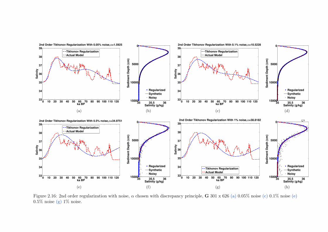
51
0 10 20 30 40 50 60 70 80 90 100 110 12033
34
35
36
37
38
39
ka BP
Sa
lin
ity
2nd Order Tikhonov Regularization With 0.05% noise, α=1.5925
Tikhonov Regularization
Actual Model
(a)
35 35.5 36
0
5000
10000
15000
Salinity (g/kg)
Se
dim
en
t D
ep
th (
cm
)
Regularized
Synthetic
Noisy
(b)
0 10 20 30 40 50 60 70 80 90 100 110 12033
34
35
36
37
38
39
ka BP
Sa
lin
ity
2nd Order Tikhonov Regularization With 0.1% noise, α=10.5228
Tikhonov Regularization
Actual Model
(c)
35 35.5 36
0
5000
10000
15000
Salinity (g/kg)
Se
dim
en
t D
ep
th (
cm
)
Regularized
Synthetic
Noisy
(d)
0 10 20 30 40 50 60 70 80 90 100 110 12033
34
35
36
37
38
39
ka BP
Sa
lin
ity
2nd Order Tikhonov Regularization With 0.5% noise, α=34.9751
Tikhonov Regularization
Actual Model
(e)
35 35.5 36
0
5000
10000
15000
Salinity (g/kg)
Se
dim
en
t D
ep
th (
cm
)
Regularized
Synthetic
Noisy
(f)
0 10 20 30 40 50 60 70 80 90 100 110 12033
34
35
36
37
38
39
ka BP
Salin
ity
2nd Order Tikhonov Regularization With 1% noise, α=38.8182
Tikhonov Regularization
Actual Model
(g)
35 35.5 36
0
5000
10000
15000
Salinity (g/kg)
Se
dim
en
t D
ep
th (
cm
)
Regularized
Synthetic
Noisy
(h)
Figure 2.16: 2nd order regularization with noise, α chosen with discrepancy principle, G 301 x 626 (a) 0.05% noise (c) 0.1% noise (e)0.5% noise (g) 1% noise.
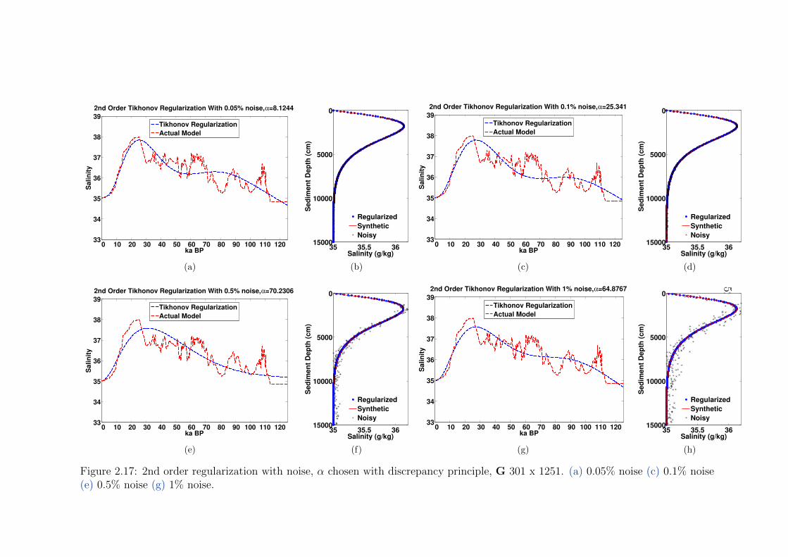
52
0 10 20 30 40 50 60 70 80 90 100 110 12033
34
35
36
37
38
39
ka BP
Sa
lin
ity
2nd Order Tikhonov Regularization With 0.05% noise, α=8.1244
Tikhonov Regularization
Actual Model
(a)
35 35.5 36
0
5000
10000
15000
Salinity (g/kg)
Se
dim
en
t D
ep
th (
cm
)
Regularized
Synthetic
Noisy
(b)
0 10 20 30 40 50 60 70 80 90 100 110 12033
34
35
36
37
38
39
ka BP
Salin
ity
2nd Order Tikhonov Regularization With 0.1% noise, α=25.341
Tikhonov Regularization
Actual Model
(c)
35 35.5 36
0
5000
10000
15000
Salinity (g/kg)
Se
dim
en
t D
ep
th (
cm
)
Regularized
Synthetic
Noisy
(d)
0 10 20 30 40 50 60 70 80 90 100 110 12033
34
35
36
37
38
39
ka BP
Sa
lin
ity
2nd Order Tikhonov Regularization With 0.5% noise, α=70.2306
Tikhonov Regularization
Actual Model
(e)
35 35.5 36
0
5000
10000
15000
Salinity (g/kg)
Se
dim
en
t D
ep
th (
cm
)
Regularized
Synthetic
Noisy
(f)
0 10 20 30 40 50 60 70 80 90 100 110 12033
34
35
36
37
38
39
ka BP
Salin
ity
2nd Order Tikhonov Regularization With 1% noise, α=64.8767
Tikhonov Regularization
Actual Model
(g)
35 35.5 36
0
5000
10000
15000
Salinity (g/kg)
Se
dim
en
t D
ep
th (
cm
)
Regularized
Synthetic
Noisy
(h)
Figure 2.17: 2nd order regularization with noise, α chosen with discrepancy principle, G 301 x 1251. (a) 0.05% noise (c) 0.1% noise(e) 0.5% noise (g) 1% noise.

53
0 1000 2000 3000 4000 50000
0.1
0.2
0.3
0.4
0.5
0.6
0.7
0.8
0.9
1
Years BP
Rm
,α(i
,i)
1e−8
1e−5
1e−4
1e−2
1e−1
0.316
1
3.16
(a)
0 5 10 15 20 25 30 35 40 45 50 55 60−0.2
0
0.2
0.4
0.6
0.8
1
1.2
kya
mtrue
mα
(b)
Figure 2.18: 2nd order resolution matrix diagonals and LGM spike test, G 251 x 251.(a) resolution matrix diagonals as function of α (b) 2nd order regularization spike test, G251 x 251, α=1e-9.
2.3.1.7 Variable damping
We are most interested in recovering information about ocean bottom water histories be-
tween the LGM and today, and we are willing to sacrifice our ability to recover the older
parts of the time series. The spike tests illustrated that some of the poorly recovered
information in the past is showing up as artificial oscillations in the present. To eliminate
these oscillations with a uniform damping parameter, we must sacrifice resolution every-
where in the solution, and higher values of damping parameters cause more information
to be smeared among modes.
Instead, we can vary α such that the poorly resolved modes in the inverse solution are
damped more than the well resolved nodes. Following Culaciati (2013), we distinguish be-
tween well and poorly resolved nodes through the matrix GTG. The relative magnitudes
of each model vector element’s contribution to the measured data profile is proportional
to its corresponding diagonal element in GTG. Similarly to Culaciati (2013) (the only
difference is that we do not consider data covariance weights as all of our data covariances
are equal), we construct a sensitivity damping matrix S by multiplying the inverse square
root of the ith diagonal value of GTG, normalized by the largest diagonal value, by the
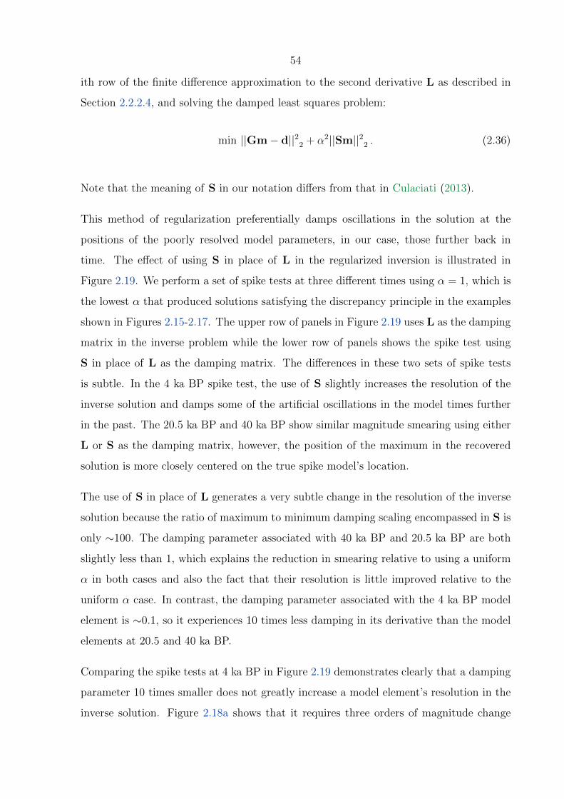
54
ith row of the finite difference approximation to the second derivative L as described in
Section 2.2.2.4, and solving the damped least squares problem:
min ||Gm− d||22 + α2||Sm||22 . (2.36)
Note that the meaning of S in our notation differs from that in Culaciati (2013).
This method of regularization preferentially damps oscillations in the solution at the
positions of the poorly resolved model parameters, in our case, those further back in
time. The effect of using S in place of L in the regularized inversion is illustrated in
Figure 2.19. We perform a set of spike tests at three different times using α = 1, which is
the lowest α that produced solutions satisfying the discrepancy principle in the examples
shown in Figures 2.15-2.17. The upper row of panels in Figure 2.19 uses L as the damping
matrix in the inverse problem while the lower row of panels shows the spike test using
S in place of L as the damping matrix. The differences in these two sets of spike tests
is subtle. In the 4 ka BP spike test, the use of S slightly increases the resolution of the
inverse solution and damps some of the artificial oscillations in the model times further
in the past. The 20.5 ka BP and 40 ka BP show similar magnitude smearing using either
L or S as the damping matrix, however, the position of the maximum in the recovered
solution is more closely centered on the true spike model’s location.
The use of S in place of L generates a very subtle change in the resolution of the inverse
solution because the ratio of maximum to minimum damping scaling encompassed in S is
only ∼100. The damping parameter associated with 40 ka BP and 20.5 ka BP are both
slightly less than 1, which explains the reduction in smearing relative to using a uniform
α in both cases and also the fact that their resolution is little improved relative to the
uniform α case. In contrast, the damping parameter associated with the 4 ka BP model
element is ∼0.1, so it experiences 10 times less damping in its derivative than the model
elements at 20.5 and 40 ka BP.
Comparing the spike tests at 4 ka BP in Figure 2.19 demonstrates clearly that a damping
parameter 10 times smaller does not greatly increase a model element’s resolution in the
inverse solution. Figure 2.18a shows that it requires three orders of magnitude change

55
0 5 10 15 20 25 30 35 40 45 50 55 60−0.2
0
0.2
0.4
0.6
0.8
1
ka BP
mtrue
mα
(a)
0 5 10 15 20 25 30 35 40 45 50 55 60−0.2
0
0.2
0.4
0.6
0.8
1
ka BP
mtrue
mα
(b)
0 5 10 15 20 25 30 35 40 45 50 55 60−0.2
0
0.2
0.4
0.6
0.8
1
ka BP
mtrue
mα
(c)
0 5 10 15 20 25 30 35 40 45 50 55 60−0.2
0
0.2
0.4
0.6
0.8
1
ka BP
mtrue
mα
(d)
0 5 10 15 20 25 30 35 40 45 50 55 60−0.2
0
0.2
0.4
0.6
0.8
1
ka BP
mtrue
mα
(e)
0 5 10 15 20 25 30 35 40 45 50 55 60−0.2
0
0.2
0.4
0.6
0.8
1
ka BP
mtrue
mα
(f)
Figure 2.19: Spike tests comparing the skill of constant vs. variable damping through thesensitivity matrix technique. The first row, (a) - (c) use a constant damping parameterα = 1 and the standard second-order Tikhonov regularization. The second row, (d) - (f)use α=1 and the variable sensitivity matrix S in place of the uniform L.
in α to increase the resolution of the model element at year 2500 from 0.6 to 1. In the
generalized inverse solution to the damped least squares problem, the values of S or L
modify the generalized singular values and modes of the solution in a complex manner.
The generalized singular values and generalized inverse represented by Equation 2.30 are
derived from the generalized SVD of the extended matrix
G
L
, or alternatively
G
S
.
We are in the process of deriving an analytical relationship between the resolution matrix
of the inverse solution that uses the damping matrix S and the resolution matrix of the
inverse solution using damping matrix L, but this is complicated by the fact that there
is no clear connection between the diagonal of GTG and the SVD of G.
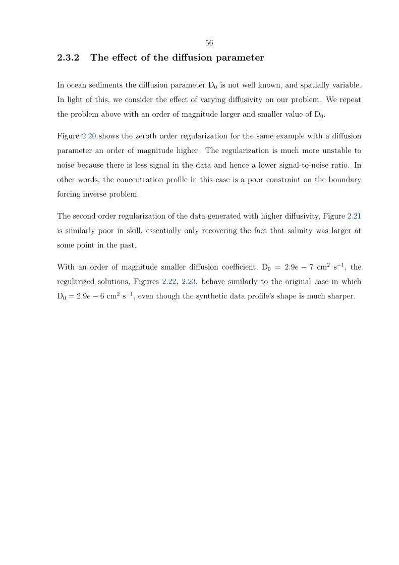
56
2.3.2 The effect of the diffusion parameter
In ocean sediments the diffusion parameter D0 is not well known, and spatially variable.
In light of this, we consider the effect of varying diffusivity on our problem. We repeat
the problem above with an order of magnitude larger and smaller value of D0.
Figure 2.20 shows the zeroth order regularization for the same example with a diffusion
parameter an order of magnitude higher. The regularization is much more unstable to
noise because there is less signal in the data and hence a lower signal-to-noise ratio. In
other words, the concentration profile in this case is a poor constraint on the boundary
forcing inverse problem.
The second order regularization of the data generated with higher diffusivity, Figure 2.21
is similarly poor in skill, essentially only recovering the fact that salinity was larger at
some point in the past.
With an order of magnitude smaller diffusion coefficient, D0 = 2.9e − 7 cm2 s−1, the
regularized solutions, Figures 2.22, 2.23, behave similarly to the original case in which
D0 = 2.9e− 6 cm2 s−1, even though the synthetic data profile’s shape is much sharper.
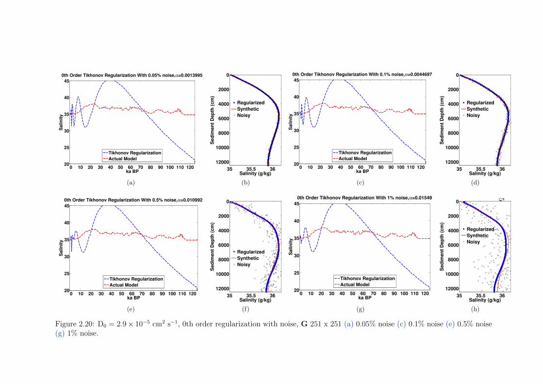
57
0 10 20 30 40 50 60 70 80 90 100 110 12020
25
30
35
40
45
ka BP
Sa
lin
ity
0th Order Tikhonov Regularization With 0.05% noise, α=0.0013995
Tikhonov Regularization
Actual Model
(a)
35 35.5 36
0
2000
4000
6000
8000
10000
12000
Salinity (g/kg)
Se
dim
en
t D
ep
th (
cm
)
Regularized
Synthetic
Noisy
(b)
0 10 20 30 40 50 60 70 80 90 100 110 12020
25
30
35
40
45
ka BP
Sa
lin
ity
0th Order Tikhonov Regularization With 0.1% noise, α=0.0044697
Tikhonov Regularization
Actual Model
(c)
35 35.5 36
0
2000
4000
6000
8000
10000
12000
Salinity (g/kg)
Se
dim
en
t D
ep
th (
cm
)
Regularized
Synthetic
Noisy
(d)
0 10 20 30 40 50 60 70 80 90 100 110 12020
25
30
35
40
45
ka BP
Salin
ity
0th Order Tikhonov Regularization With 0.5% noise, α=0.010992
Tikhonov Regularization
Actual Model
(e)
35 35.5 36
0
2000
4000
6000
8000
10000
12000
Salinity (g/kg)
Se
dim
en
t D
ep
th (
cm
)
Regularized
Synthetic
Noisy
(f)
0 10 20 30 40 50 60 70 80 90 100 110 12020
25
30
35
40
45
ka BP
Salin
ity
0th Order Tikhonov Regularization With 1% noise, α=0.01549
Tikhonov Regularization
Actual Model
(g)
35 35.5 36
0
2000
4000
6000
8000
10000
12000
Salinity (g/kg)
Se
dim
en
t D
ep
th (
cm
)
Regularized
Synthetic
Noisy
(h)
Figure 2.20: D0 = 2.9× 10⁻⁵ cm2 s−1, 0th order regularization with noise, G 251 x 251 (a) 0.05% noise (c) 0.1% noise (e) 0.5% noise(g) 1% noise.
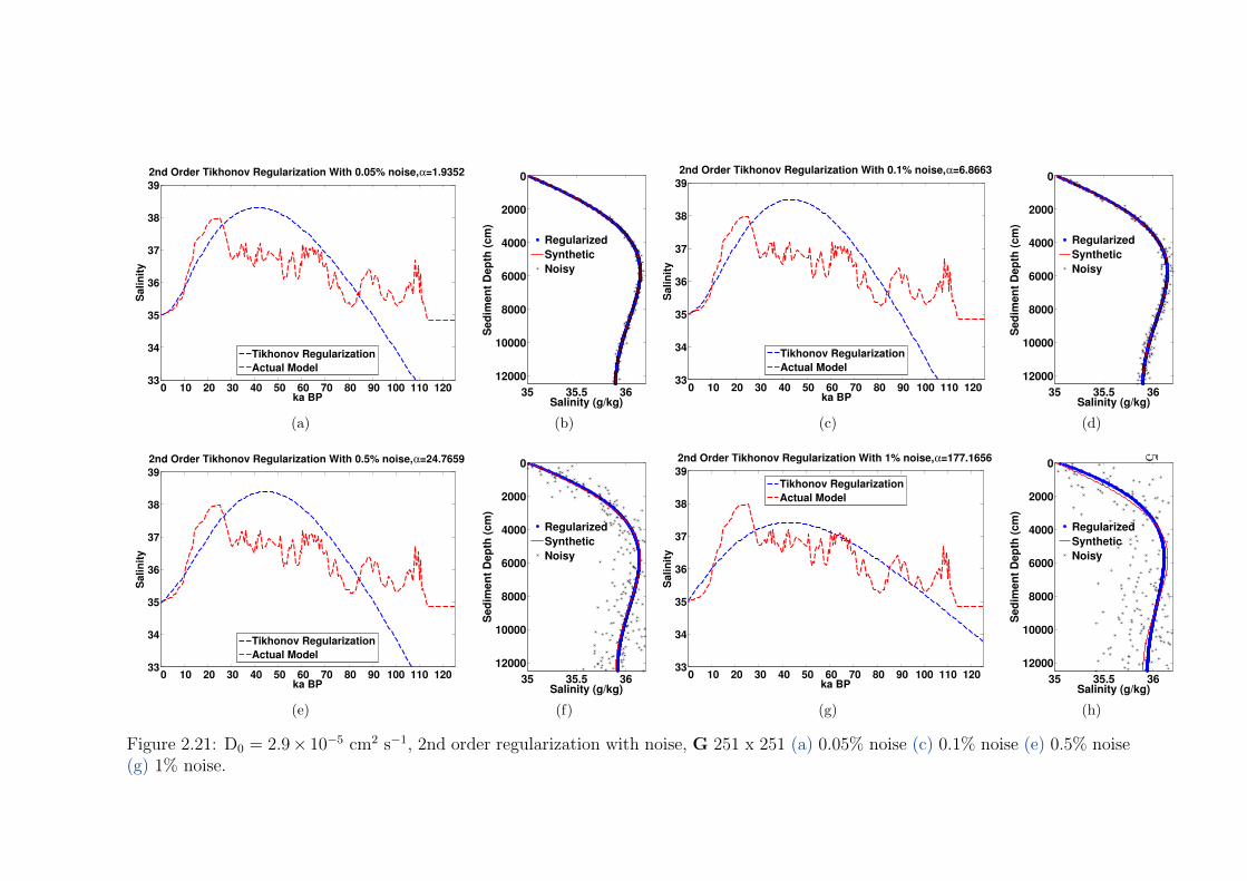
58
0 10 20 30 40 50 60 70 80 90 100 110 12033
34
35
36
37
38
39
ka BP
Sa
lin
ity
2nd Order Tikhonov Regularization With 0.05% noise, α=1.9352
Tikhonov Regularization
Actual Model
(a)
35 35.5 36
0
2000
4000
6000
8000
10000
12000
Salinity (g/kg)
Se
dim
en
t D
ep
th (
cm
)
Regularized
Synthetic
Noisy
(b)
0 10 20 30 40 50 60 70 80 90 100 110 12033
34
35
36
37
38
39
ka BP
Salin
ity
2nd Order Tikhonov Regularization With 0.1% noise, α=6.8663
Tikhonov Regularization
Actual Model
(c)
35 35.5 36
0
2000
4000
6000
8000
10000
12000
Salinity (g/kg)
Se
dim
en
t D
ep
th (
cm
)
Regularized
Synthetic
Noisy
(d)
0 10 20 30 40 50 60 70 80 90 100 110 12033
34
35
36
37
38
39
ka BP
Sa
lin
ity
2nd Order Tikhonov Regularization With 0.5% noise, α=24.7659
Tikhonov Regularization
Actual Model
(e)
35 35.5 36
0
2000
4000
6000
8000
10000
12000
Salinity (g/kg)
Se
dim
en
t D
ep
th (
cm
)
Regularized
Synthetic
Noisy
(f)
0 10 20 30 40 50 60 70 80 90 100 110 12033
34
35
36
37
38
39
ka BP
Sa
lin
ity
2nd Order Tikhonov Regularization With 1% noise, α=177.1656
Tikhonov Regularization
Actual Model
(g)
35 35.5 36
0
2000
4000
6000
8000
10000
12000
Salinity (g/kg)
Se
dim
en
t D
ep
th (
cm
)
Regularized
Synthetic
Noisy
(h)
Figure 2.21: D0 = 2.9× 10⁻⁵ cm2 s−1, 2nd order regularization with noise, G 251 x 251 (a) 0.05% noise (c) 0.1% noise (e) 0.5% noise(g) 1% noise.

59
0 10 20 30 40 50 60 70 80 90 100 110 12033
34
35
36
37
38
39
ka BP
Sa
lin
ity
0th Order Tikhonov Regularization With 0.05% noise, α=0.0018589
Tikhonov Regularization
Actual Model
(a)
35 35.5 36 36.5
0
2000
4000
6000
8000
10000
12000
Salinity (g/kg)
Sed
imen
t D
ep
th (
cm
)
Regularized
Synthetic
Noisy
(b)
0 10 20 30 40 50 60 70 80 90 100 110 12033
34
35
36
37
38
39
ka BP
Sa
lin
ity
0th Order Tikhonov Regularization With 0.1% noise, α=0.0022834
Tikhonov Regularization
Actual Model
(c)
35 35.5 36 36.5
0
2000
4000
6000
8000
10000
12000
Salinity (g/kg)
Sed
imen
t D
ep
th (
cm
)
Regularized
Synthetic
Noisy
(d)
0 10 20 30 40 50 60 70 80 90 100 110 12033
34
35
36
37
38
39
ka BP
Sa
lin
ity
0th Order Tikhonov Regularization With 0.5% noise, α=0.0059868
Tikhonov Regularization
Actual Model
(e)
35 35.5 36 36.5
0
2000
4000
6000
8000
10000
12000
Salinity (g/kg)
Sed
imen
t D
ep
th (
cm
)
Regularized
Synthetic
Noisy
(f)
0 10 20 30 40 50 60 70 80 90 100 110 12033
34
35
36
37
38
39
ka BP
Sa
lin
ity
0th Order Tikhonov Regularization With 1% noise, α=0.0063708
Tikhonov Regularization
Actual Model
(g)
35 35.5 36 36.5
0
2000
4000
6000
8000
10000
12000
Salinity (g/kg)
Sed
imen
t D
ep
th (
cm
)
Regularized
Synthetic
Noisy
(h)
Figure 2.22: 0th order reg, D0 = 2.9 × 10⁻⁷ cm2 s−1 (a) 0.05% noise G 251x251 and discrep criterion (c) 0.1% noise (e) 0.5% noise(g) 1% noise.

60
0 10 20 30 40 50 60 70 80 90 100 110 12033
34
35
36
37
38
39
ka BP
Salin
ity
2nd Order Tikhonov Regularization With 0.05% noise, α=0.34483
Tikhonov Regularization
Actual Model
(a)
35 35.5 36 36.5
0
2000
4000
6000
8000
10000
12000
Salinity (g/kg)
Sed
imen
t D
ep
th (
cm
)
Regularized
Synthetic
Noisy
(b)
0 10 20 30 40 50 60 70 80 90 100 110 12033
34
35
36
37
38
39
ka BP
Salin
ity
2nd Order Tikhonov Regularization With 0.1% noise, α=1.4339
Tikhonov Regularization
Actual Model
(c)
35 35.5 36 36.5
0
2000
4000
6000
8000
10000
12000
Salinity (g/kg)
Sed
imen
t D
ep
th (
cm
)
Regularized
Synthetic
Noisy
(d)
0 10 20 30 40 50 60 70 80 90 100 110 12033
34
35
36
37
38
39
ka BP
Salin
ity
2nd Order Tikhonov Regularization With 0.5% noise, α=3.0588
Tikhonov Regularization
Actual Model
(e)
35 35.5 36 36.5
0
2000
4000
6000
8000
10000
12000
Salinity (g/kg)
Sed
imen
t D
ep
th (
cm
)
Regularized
Synthetic
Noisy
(f)
0 10 20 30 40 50 60 70 80 90 100 110 12033
34
35
36
37
38
39
ka BP
Salin
ity
2nd Order Tikhonov Regularization With 1% noise, α=13.6651
Tikhonov Regularization
Actual Model
(g)
35 35.5 36 36.5
0
2000
4000
6000
8000
10000
12000
Salinity (g/kg)
Sed
imen
t D
ep
th (
cm
)
Regularized
Synthetic
Noisy
(h)
Figure 2.23: 2nd order reg, D0 = 2.9 × 10⁻⁷ cm2 s−1 (a) 0.05% noise G 251x251 and discrep criterion (c) 0.1% noise (e) 0.5% noise(g) 1% noise.

61
2.4 Discussion
The advantages of solving an ill-posed inverse problem via linear regularized least squares
are the speed of solution and relative simplicity of the implementation. While we have
considered a simplified version of our problem here, it illustrates clearly many of the
general issues in extracting information from discrete ill-posed problems. By applying
standard regularized least squares inverse techniques to recovering a synthetic model of
bottom water salinity from a synthetic pore fluid profile, we are able to identify how ill-
posed the problem is and evaluate the information we can gain from least squares tools.
For our specific problem, we find that we can not recover much information about the
past using a regularization technique.
Evaluation of G, even without consideration of the generalized inverse, shows that there
are very few well-resolved independent modes contained in the data, perhaps order O(10).
Thus, regardless of the method we use to invert the data, there is a huge amount of infor-
mation loss about the sediment-water interface boundary forcing history due to diffusion.
We will not be able to recover information about high frequency variability in the bottom
water history from the measured data.
In the presence of noise, none of the regularized least squares methods we have shown
are capable of returning a satisfactory solution, that is, a solution close to the synthetic
model we used. Satisfactory for us would be a reliable estimate of the LGM value and
a time series between the LGM and the modern time that is close to the true solution.
The zeroth order Tikhonov regularization suffers from introducing artificial oscillations
into the near present solution, while the second order Tikhonov regularization generally
oversmooths the solution such that neither the LGM magnitude nor position is recovered.
The diffusion coefficient D0 is likely to be closer to 1×10⁻⁵ than 1×10⁻⁶ cm2 s−1, but
we see that values of D0 near 1×10⁻⁵ cm2 s−1 significantly reduce the skill of regularized
least squares methods at recovering our synthetic model.
One major disadvantage of regularized least squares inverse methods is that it is difficult
to quantify the error in the solution, which is why we did not compute the quantitative
error between the true (synthetic) model and the inverse solutions. The various different
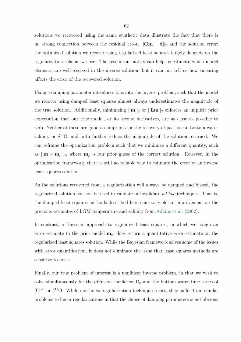
62
solutions we recovered using the same synthetic data illustrate the fact that there is
no strong connection between the residual error, ||Gm − d||2 and the solution error;
the optimized solution we recover using regularized least squares largely depends on the
regularization scheme we use. The resolution matrix can help us estimate which model
elements are well-resolved in the inverse solution, but it can not tell us how smearing
affects the error of the recovered solution.
Using a damping parameter introduces bias into the inverse problem, such that the model
we recover using damped least squares almost always underestimates the magnitude of
the true solution. Additionally, minimizing ||m||2 or ||Lm||2 enforces an implicit prior
expectation that our true model, or its second derivatives, are as close as possible to
zero. Neither of these are good assumptions for the recovery of past ocean bottom water
salinity or δ18O, and both further reduce the magnitude of the solution returned. We
can reframe the optimization problem such that we minimize a different quantity, such
as ||m − mp||2, where mp is our prior guess of the correct solution. However, in the
optimization framework, there is still no reliable way to estimate the error of an inverse
least squares solution.
As the solutions recovered from a regularization will always be damped and biased, the
regularized solution can not be used to validate or invalidate ad hoc techniques. That is,
the damped least squares methods described here can not yield an improvement on the
previous estimates of LGM temperature and salinity from Adkins et al. (2002).
In contrast, a Bayesian approach to regularized least squares, in which we assign an
error estimate to the prior model mp, does return a quantitative error estimate on the
regularized least squares solution. While the Bayesian framework solves some of the issues
with error quantification, it does not eliminate the issue that least squares methods are
sensitive to noise.
Finally, our true problem of interest is a nonlinear inverse problem, in that we wish to
solve simultaneously for the diffusion coefficient D0 and the bottom water time series of
[Cl−] or δ18O. While non-linear regularization techniques exist, they suffer from similar
problems to linear regularizations in that the choice of damping parameters is not obvious
63
and they are sensitive to noise in the data.
2.5 Conclusions
Using synthetic examples, we have explored the ability of linear regularized least squares
methods to estimate past deep ocean salinity and δ18O from sediment pore fluid profiles
of [Cl−] and δ18O. We show that regularized least squares methods are highly sensitive
to noise in the data and to the diffusion coefficient in our problem. Of the regularization
techniques we have explored, we have not discovered any that satisfactorily recover bottom
water histories from data that resemble our measurements.
There are three major limitations to regularized least squares inverse methods. The main
limitation is that damped least squares optimization techniques provide a single solution
to a non-unique problem. In order to recover a solution, these techniques must minimize
some constraint, which limits our view of the possible solutions that could have generated
the data. Since we know that the solution is non-unique, we are interested in determining
a range of solutions, rather than just one that minimizes a somewhat arbitrary constraint.
The second major limitation is that these methods are very sensitive to noise in the data.
Finally, the choice of damping parameter is quite arbitrary. Together these limitations
make it practically impossible to assign an error bound on an inverse solution.
With these considerations in mind, we conclude that regularized least squares techniques
are not the ideal way estimate past ocean bottom water time series from pore fluid profiles.
As an alternative we turn to a Bayesian Markov Chain Monte Carlo (MCMC) parameter
estimation method in Chapter 3.
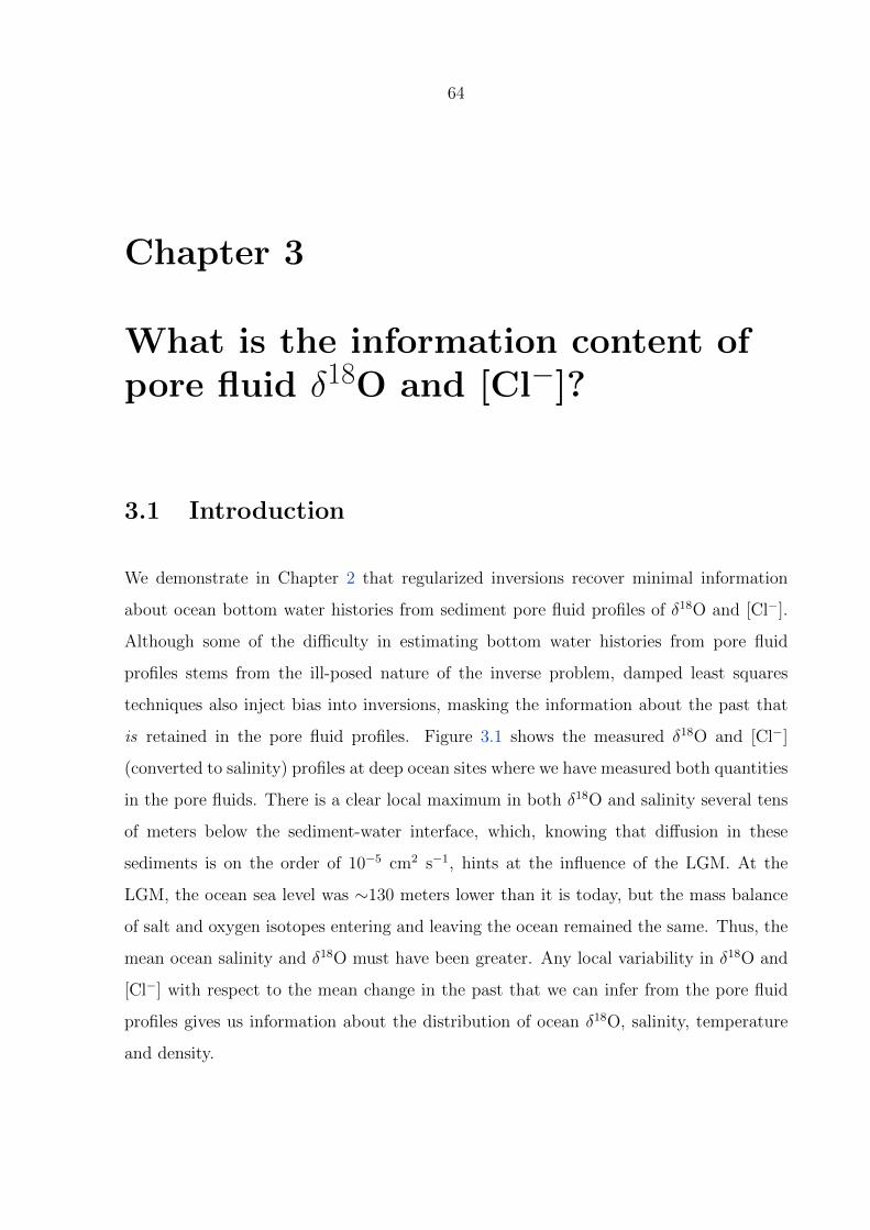
64
Chapter 3
What is the information content ofpore fluid δ18O and [Cl−]?
3.1 Introduction
We demonstrate in Chapter 2 that regularized inversions recover minimal information
about ocean bottom water histories from sediment pore fluid profiles of δ18O and [Cl−].
Although some of the difficulty in estimating bottom water histories from pore fluid
profiles stems from the ill-posed nature of the inverse problem, damped least squares
techniques also inject bias into inversions, masking the information about the past that
is retained in the pore fluid profiles. Figure 3.1 shows the measured δ18O and [Cl−]
(converted to salinity) profiles at deep ocean sites where we have measured both quantities
in the pore fluids. There is a clear local maximum in both δ18O and salinity several tens
of meters below the sediment-water interface, which, knowing that diffusion in these
sediments is on the order of 10−5 cm2 s−1, hints at the influence of the LGM. At the
LGM, the ocean sea level was ∼130 meters lower than it is today, but the mass balance
of salt and oxygen isotopes entering and leaving the ocean remained the same. Thus, the
mean ocean salinity and δ18O must have been greater. Any local variability in δ18O and
[Cl−] with respect to the mean change in the past that we can infer from the pore fluid
profiles gives us information about the distribution of ocean δ18O, salinity, temperature
and density.

65
−1 0 1
0
50
100
150
200
250
300
350
ODP Site 981
δ18
O
Dep
th (
mb
sf)
−1 0 1
0
50
100
150
200
250
300
350
ODP Site 1063
δ18
O
Dep
th (
mb
sf)
−1 0 1
0
50
100
150
200
250
300
350
ODP Site 1093
δ18
O
Dep
th (
mb
sf)
−1 0 1
0
50
100
150
200
250
300
350
ODP Site 1123
δ18
O
Dep
th (
mb
sf)
−2 0 2
0
50
100
150
200
250
300
350
ODP Site 1239
δ18
O
Dep
th (
mb
sf)
(a)
34.5 35 35.5 36
0
50
100
150
200
250
300
350
ODP Site 981
S
Dep
th (
mb
sf)
34.5 35 35.5 36
0
50
100
150
200
250
300
350
ODP Site 1063
S
Dep
th (
mb
sf)
34.5 35 35.5 36
0
50
100
150
200
250
300
350
ODP Site 1093
S
Dep
th (
mb
sf)
34.5 35 35.5 36
0
50
100
150
200
250
300
350
ODP Site 1123
S
Dep
th (
mb
sf)
34.5 35 35.5 36
0
50
100
150
200
250
300
350
ODP Site 1239
S
Dep
th (
mb
sf)
(b)
Figure 3.1: Measured profiles of (a) δ18O and (b) salinity (converted from the measured[Cl−] values). Note that the x-axis for ODP Site 1239 in (a) has a wider range than theothers. The values in all of the measured data profiles increase towards a local maximumseveral tens of meters below the sea floor.
As an illustration of the potential for pore fluid δ18O and [Cl−] profiles to tell us about
strikingly different past bottom water conditions, we plot the maximum change in δ18O vs
maximum change in [Cl−] in the upper 100 meters below sea floor at sites where we have
sediment depth profiles of both in Figure 3.2. For reference, the geographical locations of
these sites are overlaid on their modern bottom water salinity in Figure 3.3. We see that
the maximum measured values cluster around a different mean than the modern sediment-
water interface values, and that the ordering of the maximum values is spatially distinct
from that of the modern values. For example, 1093 and 1239 are the lowest salinity points
in the modern, but their maximum salinity values in the pore fluids are higher than those
at the other sites. The difference between the modern and maximum pore fluid δ18O on
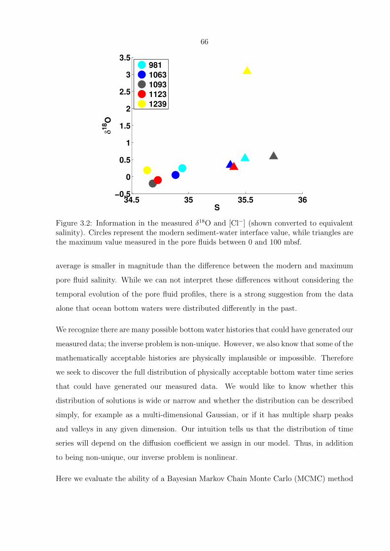
66
34.5 35 35.5 36−0.5
0
0.5
1
1.5
2
2.5
3
3.5
S
δ1
8O
981
1063
1093
1123
1239
Figure 3.2: Information in the measured δ18O and [Cl−] (shown converted to equivalentsalinity). Circles represent the modern sediment-water interface value, while triangles arethe maximum value measured in the pore fluids between 0 and 100 mbsf.
average is smaller in magnitude than the difference between the modern and maximum
pore fluid salinity. While we can not interpret these differences without considering the
temporal evolution of the pore fluid profiles, there is a strong suggestion from the data
alone that ocean bottom waters were distributed differently in the past.
We recognize there are many possible bottom water histories that could have generated our
measured data; the inverse problem is non-unique. However, we also know that some of the
mathematically acceptable histories are physically implausible or impossible. Therefore
we seek to discover the full distribution of physically acceptable bottom water time series
that could have generated our measured data. We would like to know whether this
distribution of solutions is wide or narrow and whether the distribution can be described
simply, for example as a multi-dimensional Gaussian, or if it has multiple sharp peaks
and valleys in any given dimension. Our intuition tells us that the distribution of time
series will depend on the diffusion coefficient we assign in our model. Thus, in addition
to being non-unique, our inverse problem is nonlinear.
Here we evaluate the ability of a Bayesian Markov Chain Monte Carlo (MCMC) method
67
!!"#
!"#$
!%$#
!%&#
$'!
Figure 3.3: Locations of the ODP sites where we have pore fluid profile measurements ofδ18O and [Cl−] overlain on the modern ocean bottom water salinity. Note that the rangeof modern ocean bottom water salinity is quite narrow.
to reconstruct bottom water histories from pore fluid profiles of δ18O and [Cl−]. We
simultaneously recover initial conditions and the diffusion coefficient D0. A Bayesian
approach allows us to explicitly include our prior information and uncertainty in the
inverse problem and recover a distribution of models with varying probability. Markov
Chain Monte Carlo methods allow us to consider the fully nonlinear problem and are
robust to local minima and maxima. Our work relies on the use of an algorithm named
Cascading Adaptive Tempering Metropolis in Parallel (CATMIP, Minson et al. (2013)).
We first describe the general methodological approach to the forward problem which has
many overlaps with the synthetic example in Chapter 2 and explain how we encapsulate
our knowledge about the deep ocean as probability distributions that can be supplied to
a numerical Bayesian MCMC sampler. We then illustrate the similarities and differences
between regularized inverse methods and the Bayesian MCMC approach with synthetic
examples. Finally we apply the technique to δ18O and [Cl−] data from sediment pore
fluids at five Ocean Drilling Program (ODP) sites, 981, 1063, 1093, 1123 and 1239, and

68
identify the robust and non-robust quantities that can be recovered from this data set.
For clarity in the text we often refer to [Cl−] as salinity or S, using the conversion factor
S = 19.35435
[Cl−] g kg−1, however all of the data measurements are derived from pore fluid
[Cl−]. In our synthetic examples we consider the evolution of salinity, but as δ18O and S
are both conservative tracers away from the surface of the ocean and in the sediments,
our conclusions apply equally to the reconstruction of both δ18O and S, as well as other
conservative tracers.
3.2 Methods
3.2.1 Forward model
We assume that [Cl−] and δ18O are chemically inert and that there are no horizontal
gradients in the sediment and ocean properties. This allows us to represent the time
evolution of each individual tracer, c, with a one-dimensional advection-diffusion equation:
∂ (φc)
∂t= D0
∂
∂z
(φ
θ2
∂c
∂z
)− ∂ (uφc)
∂z. (3.1)
φ is the sediment porosity, θ is the sediment tortuosity, and D0 is the diffusivity in water
of the chemical species of interest. D0 is a function of temperature and ionic strength,
but we take it as an unknown constant in order the reduce the dimensionality of our
inverse problem. If we make a conservative estimate that the temperature gradient in
the sediments is 100◦C/km, the bottom of our cores will have felt temperatures up to
35◦C. Li and Gregory (1974) estimate that there is roughly a factor of two ratio between
the diffusion coefficient for [Cl−] at 35◦C and that at 0◦C. Since we do not include the
temperature gradient dependence of the diffusion coefficient, we will underestimate the
effect of the bottom boundary condition and lower part of the sediment pore fluid values
on controlling the inverse solution. In general we find that including the temperature
gradient does not qualitatively affect the fit of an inverse model’s output to the data. u is
the vertical velocity of the water with respect to the sediment, which is predominantly due

69
to sediment compaction. z is the depth in the sediment, defined increasing downwards.
Assuming bulk steady-state compaction simplifies this equation to
φ∂c
∂t=
(∂D∗
∂z− φu
)∂c
∂z+D∗
∂2c
∂z2, (3.2)
where D∗ = D0φθ2
. A typical model for θ2 is θ2 = φf where f is the non-dimensional
formation factor:
f =bulk sediment specific electrical resistivity
porewater resistivity. (3.3)
Laboratory measurements suggest that a good approximation for f is φ−n, where n aver-
ages 1.8 over various sediments Berner (1980). Our final equation describing concentration
evolution with time and space is
∂c
∂t=
(1.8 φ0.8D0
∂φ
∂z− u)∂c
∂z+ φ1.8D0
∂2c
∂z2. (3.4)
φ in our model is a smoothed version of the measured porosity in each core. With the
steady-state compaction assumption, u is derived from the sedimentation rate and porosity
data as described in Chapter 2. The concentration profiles at any given time result from
Equation 3.4, an initial condition and two boundary conditions. The top (ocean–sediment
interface) boundary condition is the tracer time evolution in the water overlying the core
site that we seek to constrain. At the bottom boundary we assign a gradient boundary
condition. Equation 3.4 is a stiff partial differential equation, so we solve it with a second
order Implicit-Explicit (IMEX) method for its solution. The advection terms are solved
explicitly while the diffusion terms are solved implicitly (Ascher et al., 1995). The time
step in the solver is 10 years and the spatial resolution is 50 cm. The total integration
time is 125,000 years.
70
3.2.2 The inverse problem
With typical values of D0, φ and u, the solution to Equation 3.4 is heavily diffusion
dominated (Peclet O(1e−3) ), and a classic example of an ill-posed problem. The same
concentration profile at a given time can be produced by an infinite number of forcing
conditions. It is not possible to directly invert the measured concentration profile and
recover a unique concentration forcing history. However, many of these infinite mathe-
matically feasible solutions are non-physical. For example, a species concentration can not
be negative. Using a Bayesian approach, we can restrict the solution space by applying
our prior knowledge of the problem. Bayes’ theorem states that:
P (Θ|D) ∝ P (D|Θ)P (Θ) , (3.5)
where Θ is a vector of model parameters and D is the measured data. In words, the
probability that a given model/set of model parameters produced the measured data is
proportional to the product of the prior probability of those parameters and the likeli-
hood of the data produced using those model parameters. P (Θ) is known as the prior
probability, and encompasses our knowledge of the model parameters independent of the
data measurements D. P (D|Θ) is the likelihood, computed using the error between the
measured data and data produced by the forward model using a given set of model pa-
rameters Φ. P (Θ|D) is the posterior probability distribution, or posterior. Bayesian
Markov Chain Monte Carlo (Bayesian MCMC) sampling provides us with a probabil-
ity distribution proportional to the posterior probability distribution of possible model
parameters.
3.2.2.1 Bayesian Markov Chain Monte Carlo sampling
The brute force way to solve this problem is to choose a large range of possible values of
model parameters and perform an integral over all of them to find the probability of any
given parameter. In high-dimensional problems, computing this integral is intractable.
We take a Markov Chain Monte Carlo approach to the integral that instead samples
the Bayesian posterior. A variety of approaches have been proposed for this. We use
71
an algorithm called Cascading Adaptive Tempering Metropolis In Parallel (CATMIP)
(Minson et al., 2013), which has been demonstrated to behave very efficiently for high-
dimensional problems. CATMIP is initialized with the prior probability distribution and
evolves from the prior to the posterior in a series of tempering or cooling steps. At
each cooling step a new probability distribution is proposed and the change between
distributions from step to step is monitored to track the evolution. For a given set of
proposed parameters, the likelihood is computed by integrating the forward model with
those parameters and computing a misfit cost function between the model output and
the measured data. Unless otherwise specified, all of the cases described here use a chain
length of 1000 steps and 1000 chains.
3.2.2.2 Model parameterization
Our problem has many unknowns: the top and bottom boundary condition time series,
the initial condition, and the diffusion coefficient D0. We are primarily interested in
recovering the top boundary condition, the time series of [Cl−] or δ18O in the water,
but its solution is not independent of that of the other unknowns. This dependence
requires that we must solve for all of the unknowns simultaneously, which results in a
very high-dimensional problem. Also, since one of our unknowns is D0, the inversion
is non-linear. To make the solution tractable we make simplifying assumptions. These
assumptions can be thought of as part of our prior or choice of model, although we do
not formally evaluate the probability distribution associated with the model choice. We
expect that the bottom boundary condition is not changing rapidly with time, and we
assign a constant in time bottom boundary gradient to each site. The solution is very
sensitive to D0, so we seek to recover the time series of bottom water concentrations that
is our top boundary condition simultaneously to the coefficient D0. The time series is
parameterized as a set of concentrations at fixed time points spaced 2000 years apart near
the present-day with increasing resolution further back in time. Our choice of time points
reflects our understanding that, at low sedimentation rate sites such as those we consider,
the resolution of any paleorecord will not be greater than a few thousand years due to
bioturbation at the sediment–water interface. The diffusion-dominated information in the
72
pore fluids will be lower resolution than the information recorded in the solid state. In
order to not degrade the accuracy of the finite difference solution, we linearly interpolate
between the fixed time point parameters to create the input to the forward model.
3.2.2.3 Cost function
We assume our error is exponentially distributed to compute the likelihood function
P (D|Θ) ∝ e−1/2(dm−dobs)TC−1D (dm−dobs) (3.6)
The data covariance matrix CD is diagonal, under the assumption that the errors of
individual measurements are independent. dm is the data produced by the forward model,
given the model parameters Θ, while dobs is the observed (measured) data.
We use an exponential error assumption rather than a Gaussian error assumption in
order to reduce the effect of extreme data outliers on our solutions. Pore fluids are flame-
sealed into glass vials on retrieval, and if extreme care is not taken in this process, a
sample can partially evaporate, changing its δ18O and [Cl−] concentration. Alternatively,
a vial may appear to be sealed but is not, such that it partially evaporates during the
time in transport from the sampling site to the laboratory. Errors in handling that
lead to evaporation can go unnoticed but later appear as scatter far outside our typical
measurement error. We generally can not quantify the error associated with these seeming
outliers. The exponential error assumption allows us to assign our typical measurement
standard deviation to the data covariance matrix diagonal while still being robust to
handling error which can not be quantified.
3.2.3 Choice of priors
The posterior solution to our problem is highly sensitive to our choice of prior. This
sensitivity implies that if we could improve our prior confidence we could improve our
confidence in the solutions. We have high confidence in some of our prior assumptions,
73
such as our estimate of the mean sea level in the past. Other prior information necessary
to the problem is more difficult to choose. We show the results with different, reasonable
priors and discuss the implications of each one to water mass histories, as well as the
biases induced by the given prior.
We choose Gaussian distributions for our prior probabilities of the salinity or δ18O at any
point in time. Recall that we have parameterized the boundary condition in our problem
as a set of nodes; each node represents the value of salinity or δ18O at a given time.
We assign a prior mean and standard deviation to each node. The standard deviation
represents the expected spread of ocean salinities or δ18O values around the mean at
that time. In order to enforce smoothness of our solutions, we further impose covariance
between the node values. For the boundary condition forcing, the prior probability is a
multidimensional Gaussian that can be written as a covariance matrix.
3.2.3.1 Prior information from sea level records
There is little information about past deep ocean salinity from paleo proxies. However,
we do have confidence in sea level reconstructions. Assuming the major ion quantities
are conservative over our time period of interest, the mean ocean salinity is determined
by the amount of water in the oceans, that is, the sea level. We treat the ocean as a
rectangular basin that is 3800 m deep today so that the concentrations scale directly to
changes in sea level:
St = Smod +ht − hmod
hLGM − hmod(SLGM − Smod) . (3.7)
Here t denotes the time (in the past), mod indicates the modern mean ocean value, and
h is the absolute mean sea level height. We take the modern mean ocean salinity to be
34.68 and the LGM mean ocean salinity as SLGM = hmodSmod/hLGM = 35.9.
There have been many attempts to estimate the past contribution of δ18O|w to the δ18O|cof benthic foraminifera at the LGM (e.g. Emiliani, 1966, Shackleton, 1967, Dansgaard and
Tauber, 1969, Chappell and Shackleton, 1986, Fairbanks, 1989, Mix, 1987, Schrag et al.,
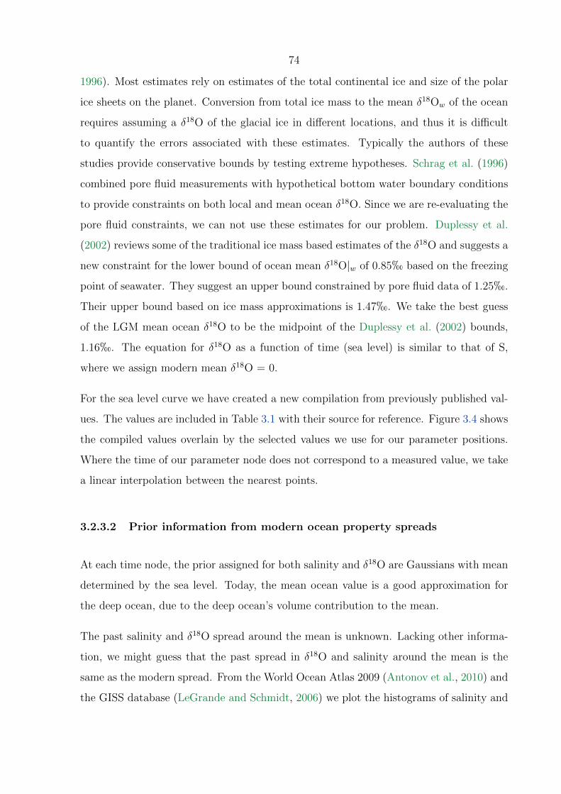
74
1996). Most estimates rely on estimates of the total continental ice and size of the polar
ice sheets on the planet. Conversion from total ice mass to the mean δ18Ow of the ocean
requires assuming a δ18O of the glacial ice in different locations, and thus it is difficult
to quantify the errors associated with these estimates. Typically the authors of these
studies provide conservative bounds by testing extreme hypotheses. Schrag et al. (1996)
combined pore fluid measurements with hypothetical bottom water boundary conditions
to provide constraints on both local and mean ocean δ18O. Since we are re-evaluating the
pore fluid constraints, we can not use these estimates for our problem. Duplessy et al.
(2002) reviews some of the traditional ice mass based estimates of the δ18O and suggests a
new constraint for the lower bound of ocean mean δ18O|w of 0.85h based on the freezing
point of seawater. They suggest an upper bound constrained by pore fluid data of 1.25h.
Their upper bound based on ice mass approximations is 1.47h. We take the best guess
of the LGM mean ocean δ18O to be the midpoint of the Duplessy et al. (2002) bounds,
1.16h. The equation for δ18O as a function of time (sea level) is similar to that of S,
where we assign modern mean δ18O = 0.
For the sea level curve we have created a new compilation from previously published val-
ues. The values are included in Table 3.1 with their source for reference. Figure 3.4 shows
the compiled values overlain by the selected values we use for our parameter positions.
Where the time of our parameter node does not correspond to a measured value, we take
a linear interpolation between the nearest points.
3.2.3.2 Prior information from modern ocean property spreads
At each time node, the prior assigned for both salinity and δ18O are Gaussians with mean
determined by the sea level. Today, the mean ocean value is a good approximation for
the deep ocean, due to the deep ocean’s volume contribution to the mean.
The past salinity and δ18O spread around the mean is unknown. Lacking other informa-
tion, we might guess that the past spread in δ18O and salinity around the mean is the
same as the modern spread. From the World Ocean Atlas 2009 (Antonov et al., 2010) and
the GISS database (LeGrande and Schmidt, 2006) we plot the histograms of salinity and

75
0 20 40 60 80 100 120 140−150
−100
−50
0
50
ka BP
Sea L
evel (m
)
Data CompilationNode Positions
Figure 3.4: Reconstructions of past sea level relative to present (black circles) and thepoints we use for sea level in computing the prior mean salinity and δ18O (blue triangles)
δ18O for all points deeper than 2000 m in Figure 3.5. Note that today these are not simple
Gaussians; at best they could be described as a mixture of Gaussians. In particular the
Atlantic and Pacific can be identified in the salinity histogram as unique water masses.
We fit a Gaussian pdf envelope around each histogram, as shown in the blue curves in
Figure 3.5, to estimate the modern mean and spread around the mean. Applying this
method gives a modern deep ocean σS = 0.12 g kg−1 and σδ18O = 0.25h. In addition to
the possible spread of deep ocean property values, the prior variances must also account
for error in the sea level curve. We choose an error of 10 m at the LGM. Propagation
of 10 m error through the scaling for sea level gives an error of 0.098 g kg−1 in salinity.
The LGM δ18O error is not directly related to the sea level, but Duplessy et al. (2002)
suggest an error on their estimate for mean δ18Ow should be 0.2h. Summing together
the modern spread and the error yields σS = 0.218 or a variance σ2S = 0.05. σδ18O=0.45
and σ2
δ18O=0.20h.
Today the covariance between δ18O and S varies by water mass/basin. Our choice of defi-
nition of the prior means induces an implicit prior covariance between the mean δ18O and
S that is constant in time and space, although we expect that it varies with time and loca-
tion in the ocean. The solution for δ18O and salinity at a given site are, however, entirely
separate, allowing any combination of the two to arise in the posterior distributions.

76
To represent the fact that neighboring points in a time series at a given location are not
independent, since the evolution of δ18O and salinity at deep ocean sites is dominated by
eddy diffusion, we assign covariances to the points in the time series. The covariances are
chosen to have the form:
σij = σ2iie−
(ti−tj)2
2T2 , (3.8)
where T is a timescale of covariance. When ti − tj = T , the correlation between the time
series values at those times is ∼0.6, while if ti − tj = 2T , the correlation between the
values is ∼0.1. T is roughly half of an ocean site’s memory of its previous value, which is
a somewhat ambiguous concept physically.
T is set by ocean mixing, which is spatially variable and depends at least in part on
the global distribution of temperature and salinity through its dependence on the slope
of isopycnals. Much of the information in T is encapsulated in the ever-elusive eddy
diffusivity parameter, κ. T and κ are related in a scaling argument sense through a
length-scale L, that is,
2T =L2
κ, (3.9)
where we have written 2T to represent the amount of time it would take for an ocean
site to completely forget its previous value. κ is a spatially variable tensor quantity, with
34.4 34.6 34.8 35 35.20
1
2
3
4
5
S
(a)
−1 −0.5 0 0.5 10
0.5
1
1.5
2
2.5
3
δ18
O
(b)
Figure 3.5: (a) Modern S below 2000m, GISS database accessed 9/12/2012, excluding theMediterranean Sea. Blue curve is Gaussian distribution with standard deviation used forpriors (b) modern δ18O below 2000m
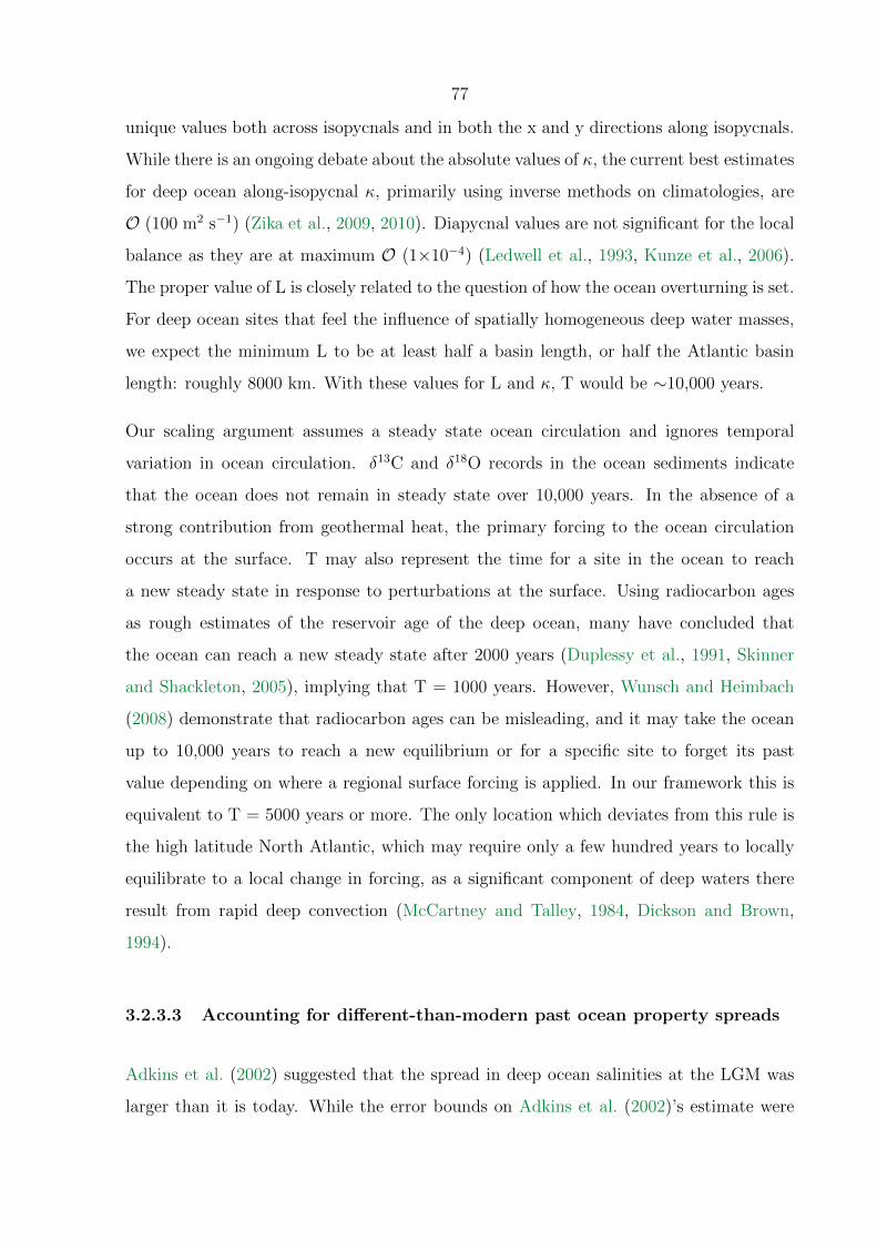
77
unique values both across isopycnals and in both the x and y directions along isopycnals.
While there is an ongoing debate about the absolute values of κ, the current best estimates
for deep ocean along-isopycnal κ, primarily using inverse methods on climatologies, are
O (100 m2 s−1) (Zika et al., 2009, 2010). Diapycnal values are not significant for the local
balance as they are at maximum O (1×10⁻⁴) (Ledwell et al., 1993, Kunze et al., 2006).
The proper value of L is closely related to the question of how the ocean overturning is set.
For deep ocean sites that feel the influence of spatially homogeneous deep water masses,
we expect the minimum L to be at least half a basin length, or half the Atlantic basin
length: roughly 8000 km. With these values for L and κ, T would be ∼10,000 years.
Our scaling argument assumes a steady state ocean circulation and ignores temporal
variation in ocean circulation. δ13C and δ18O records in the ocean sediments indicate
that the ocean does not remain in steady state over 10,000 years. In the absence of a
strong contribution from geothermal heat, the primary forcing to the ocean circulation
occurs at the surface. T may also represent the time for a site in the ocean to reach
a new steady state in response to perturbations at the surface. Using radiocarbon ages
as rough estimates of the reservoir age of the deep ocean, many have concluded that
the ocean can reach a new steady state after 2000 years (Duplessy et al., 1991, Skinner
and Shackleton, 2005), implying that T = 1000 years. However, Wunsch and Heimbach
(2008) demonstrate that radiocarbon ages can be misleading, and it may take the ocean
up to 10,000 years to reach a new equilibrium or for a specific site to forget its past
value depending on where a regional surface forcing is applied. In our framework this is
equivalent to T = 5000 years or more. The only location which deviates from this rule is
the high latitude North Atlantic, which may require only a few hundred years to locally
equilibrate to a local change in forcing, as a significant component of deep waters there
result from rapid deep convection (McCartney and Talley, 1984, Dickson and Brown,
1994).
3.2.3.3 Accounting for different-than-modern past ocean property spreads
Adkins et al. (2002) suggested that the spread in deep ocean salinities at the LGM was
larger than it is today. While the error bounds on Adkins et al. (2002)’s estimate were

78
not well-defined, their solutions did provide acceptable fits to the pore fluid concentration
data profiles. Thus, whether or not Adkins et al. (2002)’s estimates are the most likely,
we want them to be allowable. In this way we can better compare the differences in our
solutions and methodologies. It is possible that the ocean had a wider salinity spread
in the past, but we do not have any a priori information on what the magnitude of the
spread was.
In general, Bayesian MCMC methods allow us to shrink but not expand the prior. That
is, the posterior on a given parameter may be more narrow than the prior, but it can
never be wider. For a Gaussian prior we are unlikely to recover solutions more than
two standard deviations from the mean of the prior. So, to allow for the possibility of
the LGM salinities estimated by Adkins et al. (2002), we consider the sensitivity of our
solution to wider-than-modern prior variances, up to two orders of magnitude larger than
the modern spread.
3.2.3.4 Diffusion coefficient prior
The prior we assign to the diffusion coefficient, D0, is log-normal. We choose this prior
because D0 is what is known as a Jeffreys parameter (Tarantola, 2005). Jeffreys parame-
ters are positive but invariant under scale transformations: physical parameters that are
greater than zero but could vary by orders of magnitude. In the case of diffusion, labora-
tory studies find diffusion coefficients for chloride between 1-20 ×10−6 cm2 s−1, varying as
a function of temperature, pressure, and ionic content (constraints imposed by electroneu-
trality) (Li and Gregory, 1974). The diffusivity of δ18O represents the relative diffusion
of water oxygen isotopes, which will mirror the diffusion of H182 O in water, O(1 × 10⁻⁵)
cm2 s−1, also a function of temperature (Wang et al., 1953). As shown in Figure 3.6, we
choose a mean diffusion coefficient of 50.5 ×10⁻⁶ cm2 s−1 and the standard deviation of
the ln(D0) equal to 1.5. While these choices do allow for greater than expected diffusion
and account somewhat for potential bioturbation, the main motivation for these numbers
is to determine whether the coefficient is resolved by the information in the measured
data. We expect that the true solution is close to 1×10⁻⁵ cm2 s−1, for both δ18O and
chloride.
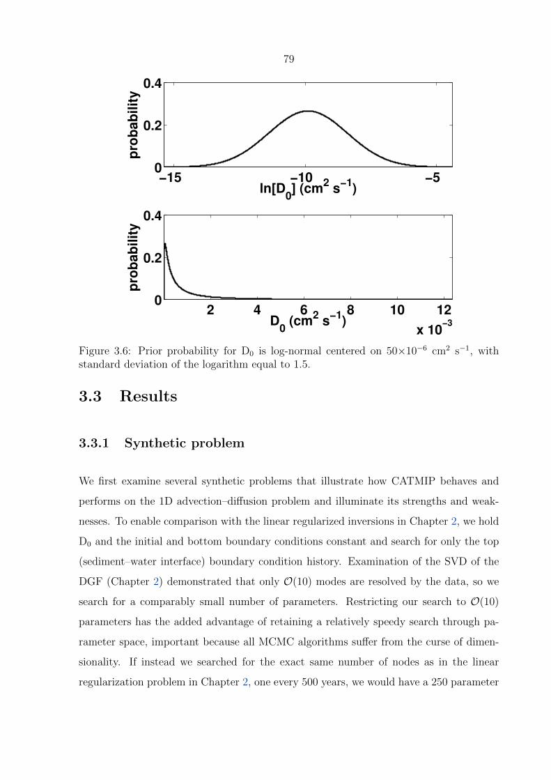
79
−15 −10 −50
0.2
0.4
ln[D0] (cm
2 s
−1)
pro
bab
ilit
y
2 4 6 8 10 12
x 10−3
0
0.2
0.4
D0 (cm
2 s
−1)
pro
bab
ilit
y
Figure 3.6: Prior probability for D0 is log-normal centered on 50×10−6 cm2 s−1, withstandard deviation of the logarithm equal to 1.5.
3.3 Results
3.3.1 Synthetic problem
We first examine several synthetic problems that illustrate how CATMIP behaves and
performs on the 1D advection–diffusion problem and illuminate its strengths and weak-
nesses. To enable comparison with the linear regularized inversions in Chapter 2, we hold
D0 and the initial and bottom boundary conditions constant and search for only the top
(sediment–water interface) boundary condition history. Examination of the SVD of the
DGF (Chapter 2) demonstrated that only O(10) modes are resolved by the data, so we
search for a comparably small number of parameters. Restricting our search to O(10)
parameters has the added advantage of retaining a relatively speedy search through pa-
rameter space, important because all MCMC algorithms suffer from the curse of dimen-
sionality. If instead we searched for the exact same number of nodes as in the linear
regularization problem in Chapter 2, one every 500 years, we would have a 250 parameter

80
problem. The problem is parameterized by 22 salinity nodes, with higher resolution closer
to the present. The minimum ∆t is 2000 years.
The synthetic model in the following cases is identical to the stretched sea level example
described in Chapter 2. Past salinity is scaled to sea level changes through a constant
factor, determined by assuming that the LGM salinity was 37.1 and the LGM sea level
was 131 meters lower than it is today. D0 = 2.5 × 10⁻⁵ cm2 s−1 and the porosity is a
constant 0.8 with depth. The advective velocity at the depth of no compaction is 0.01 cm
year−1. The length of the domain is 150 meters. Initial salinity is a constant-with-depth
35.8 g kg−1. The bottom boundary condition is ∂C∂z|L = 0. As before, the forward model is
run with these parameters and a synthetic pore water profile data set is generated. This
data is then fed to CATMIP to return an inverse solution, and the results generated by
CATMIP are compared to the original known forcing used to generate the data.
In all of the following cases we use the same synthetic data set which is generated by
running the synthetic model forward in time 125,000 years. Synthetic noise is added to the
synthetic data at the 0.05% level. 0.05% noise represents essentially perfect measurement
precision, no random outliers, and no sample collection problems. Our motivation is to
consider the best possible measurement scenario in order to test the limitations of the
inverse method.
3.3.1.1 Linear problem – uninformative prior
We seek to provide CATMIP with a completely uninformative prior in order to identify
what information is contained in the data alone. In this example we do not constrain
the salinity to follow the sea level curve; instead we assign the same Gaussian prior in
salinity to every node. Intuitively we expect the most uninformative prior in salinity to be
a uniform prior between 0 and 60 g kg−1 where 60 represents an evaporative environment
and 0 is freshwater. In the deep ocean more reasonable bounds might be 20–45 g kg−1.
However, tests with both of these choices of prior show that the CATMIP algorithm is
ill-suited for use with hard bounds. As random walk steps are drawn from a distribution
centered around zero, if the current model is located near a hard bound, many models
81
proposed will fall outside the hard bound. This leads to a high rejection rate and the
posterior distribution having an artificial peak near the bound. The artificial peak results
from two things that happen when models outside the bound are rejected. First, instead
of taking a step, the model remains in place. Second, at the next cooling step, the step
size is smaller, keeping the models from moving to a different region of the solution space.
These two behaviors have the effect of focusing the models near a hard bound, leading to
an artificially high posterior probability there.
CATMIP’s difficulty with hard bounds stems ironically from a design feature intended
for flexibility. That is, the information passed to CATMIP from our physical model is
the numerical values of parameters, their prior probabilities, and their likelihoods from
comparing the forward model runs to data. In the present framework there is no way
to distinguish between a low probability due to an infinite PDF tail-off or due to a hard
bound. However, ideally, the adaptive step-scaling in CATMIP should treat these two
cases differently.
While there are algorithmic solutions to CATMIP’s difficulty with hard bounds, they are
not essential to the present work. We work around the limitation on hard bounds by
using a very wide Gaussian spread around the sea level curve as an uninformative prior.
To represent the idea that the sea level curve is a poor constraint on deep ocean salinity,
we assign a prior standard deviation of 10, or variance of 100, g kg−1 to all salinity nodes
around the mean sea level curve, such that values outside the range 25–45 have vanishingly
small probabilities. The mean salinity scaled to sea level has a minimum value of 34.7 g
kg−1 and a maximum value of 35.9 g kg−1, so the choice of mean scaled to the sea level
is almost identical to choosing a uniform mean of 35 g kg−1.
Applying this wide Gaussian prior to every past salinity nodes we find that the data
alone is a poor constraint on the absolute values of the salinity parameters. As shown in
Figure 3.7, the recovered mean is oscillatory and does not resemble the synthetic input
model. A movie of the highest posterior probability models demonstrates that the mean
solution does not represent many models with similar values, but tradeoffs between pa-
rameters. However, as the covariance timescale increases, the highest probability models
in the posterior become more representative of the mean in the nodes closest to 0 kya.

82
The highest probability models also do not resemble the synthetic model. When we con-
strain the smoothness of the solutions by increasing the prior covariance between model
parameters, the node solution magnitudes are damped near the present. With increasing
covariance, the damping extends further back in time. This uni-directional backwards-
directed bleeding results from the fact that the three most modern nodes, from 6 kya to
present, are well-constrained by the data. Increasing the prior covariance expands the
influence that the most recent 6000 years has on the earlier part of the recovered time
series.
The variance of the posterior distributions is a strong function of the prior covariances.
Figure 3.8 compares the marginal distributions of the wide Gaussian prior example with 0
covariance and 6000 year covariance timescale. Visual inspection reveals higher covariance
forces an increase in the number of posteriors that are slimmer than their priors. While
in the 0 covariance timecale case the posteriors that are shrunk only go back to ∼6 kya,
when a 6000 year covariance timescale is imposed through the prior, the salinity node
posteriors back to at least 24 kya are shrunk significantly relative to their priors.
In order to quantify this phenomenon, we compute the ratio of variances between pos-
terior and prior as a function of salinity node position in time, for a range of covariance
timescales. Figure 3.9 demonstrates that as the covariance timescale increases, the shrink-
ing of the variance from prior to posterior extends further into the past. Posterior variance
is determined by prior covariance and this relationship is proportional to information age
in the diffusion problem. In other words, when less information about the salinity at a
given time can be determined directly from the data, the inverse solution at that time is
more sensitive to information we impose through the prior covariance.
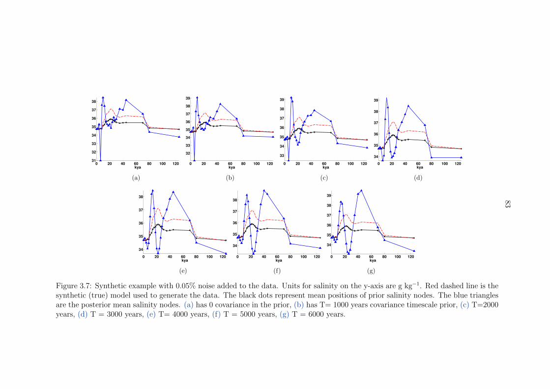
83
0 20 40 60 80 100 12031
32
33
34
35
36
37
38
kya
(a)
0 20 40 60 80 100 120
32
33
34
35
36
37
38
39
kya
(b)
0 20 40 60 80 100 120
33
34
35
36
37
38
39
kya
(c)
0 20 40 60 80 100 120
34
35
36
37
38
39
kya
(d)
0 20 40 60 80 100 120
34
35
36
37
38
kya
(e)
0 20 40 60 80 100 120
34
35
36
37
38
kya
(f)
0 20 40 60 80 100 120
34
35
36
37
38
39
kya
(g)
Figure 3.7: Synthetic example with 0.05% noise added to the data. Units for salinity on the y-axis are g kg−1. Red dashed line is thesynthetic (true) model used to generate the data. The black dots represent mean positions of prior salinity nodes. The blue trianglesare the posterior mean salinity nodes. (a) has 0 covariance in the prior, (b) has T= 1000 years covariance timescale prior, (c) T=2000years, (d) T = 3000 years, (e) T= 4000 years, (f) T = 5000 years, (g) T = 6000 years.
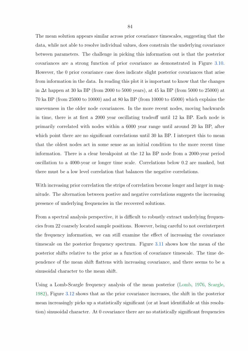
84
The mean solution appears similar across prior covariance timescales, suggesting that the
data, while not able to resolve individual values, does constrain the underlying covariance
between parameters. The challenge in picking this information out is that the posterior
covariances are a strong function of prior covariance as demonstrated in Figure 3.10.
However, the 0 prior covariance case does indicate slight posterior covariances that arise
from information in the data. In reading this plot it is important to know that the changes
in ∆t happen at 30 ka BP (from 2000 to 5000 years), at 45 ka BP (from 5000 to 25000) at
70 ka BP (from 25000 to 10000) and at 80 ka BP (from 10000 to 45000) which explains the
unevenness in the older node covariances. In the more recent nodes, moving backwards
in time, there is at first a 2000 year oscillating tradeoff until 12 ka BP. Each node is
primarily correlated with nodes within a 6000 year range until around 20 ka BP, after
which point there are no significant correlations until 30 ka BP. I interpret this to mean
that the oldest nodes act in some sense as an initial condition to the more recent time
information. There is a clear breakpoint at the 12 ka BP node from a 2000-year period
oscillation to a 4000-year or longer time scale. Correlations below 0.2 are masked, but
there must be a low level correlation that balances the negative correlations.
With increasing prior correlation the strips of correlation become longer and larger in mag-
nitude. The alternation between postive and negative correlations suggests the increasing
presence of underlying frequencies in the recovered solutions.
From a spectral analysis perspective, it is difficult to robustly extract underlying frequen-
cies from 22 coarsely located sample positions. However, being careful to not overinterpret
the frequency information, we can still examine the effect of increasing the covariance
timescale on the posterior frequency spectrum. Figure 3.11 shows how the mean of the
posterior shifts relative to the prior as a function of covariance timescale. The time de-
pendence of the mean shift flattens with increasing covariance, and there seems to be a
sinusoidal character to the mean shift.
Using a Lomb-Scargle frequency analysis of the mean posterior (Lomb, 1976, Scargle,
1982), Figure 3.12 shows that as the prior covariance increases, the shift in the posterior
mean increasingly picks up a statistically significant (or at least identifiable at this resolu-
tion) sinusoidal character. At 0 covariance there are no statistically significant frequencies

85
0 20 40 600
10
20
30
40
50
60Salinity Node 125 ka BP
0 20 40 600
20
40
60
80Salinity Node 80 ka BP
0 20 40 600
10
20
30
40
50
60Salinity Node 70 ka BP
0 20 40 600
20
40
60
80Salinity Node 45 ka BP
0 20 40 600
10
20
30
40
50
60Salinity Node 40 ka BP
0 20 40 600
20
40
60
80Salinity Node 35 ka BP
0 20 40 600
20
40
60
80Salinity Node 30 ka BP
0 20 40 600
20
40
60
80Salinity Node 28 ka BP
0 20 40 600
20
40
60
80Salinity Node 26 ka BP
0 20 40 600
10
20
30
40
50
60Salinity Node 24 ka BP
0 20 40 600
20
40
60
80Salinity Node 22 ka BP
0 20 40 600
20
40
60
80Salinity Node 20 ka BP
0 20 40 600
20
40
60
80Salinity Node 18 ka BP
0 20 40 600
10
20
30
40
50
60Salinity Node 16 ka BP
0 20 40 600
10
20
30
40
50
60Salinity Node 14 ka BP
0 20 40 600
10
20
30
40
50
60Salinity Node 12 ka BP
0 20 40 600
20
40
60
80Salinity Node 10 ka BP
0 20 40 600
20
40
60
80Salinity Node 8 ka BP
0 20 40 600
20
40
60
80Salinity Node 6 ka BP
0 20 40 600
20
40
60
80Salinity Node 4 ka BP
0 20 40 600
20
40
60
80Salinity Node 2 ka BP
0 20 40 600
20
40
60
80Salinity Node 0 ka BP
(a)
20 40 600
20
40
60
80Salinity Node 125 ka BP
20 40 600
20
40
60
80Salinity Node 80 ka BP
20 40 600
10
20
30
40
50
60Salinity Node 70 ka BP
20 40 600
10
20
30
40
50
60Salinity Node 45 ka BP
20 40 600
20
40
60
80Salinity Node 40 ka BP
20 40 600
20
40
60
80Salinity Node 35 ka BP
20 40 600
10
20
30
40
50
60Salinity Node 30 ka BP
20 40 600
10
20
30
40
50
60Salinity Node 28 ka BP
20 40 600
10
20
30
40
50
60Salinity Node 26 ka BP
20 40 600
10
20
30
40
50
60Salinity Node 24 ka BP
20 40 600
20
40
60
80Salinity Node 22 ka BP
20 40 600
10
20
30
40
50
60Salinity Node 20 ka BP
20 40 600
20
40
60
80Salinity Node 18 ka BP
20 40 600
20
40
60
80Salinity Node 16 ka BP
20 40 600
10
20
30
40
50
60Salinity Node 14 ka BP
20 40 600
20
40
60
80Salinity Node 12 ka BP
20 40 600
20
40
60
80Salinity Node 10 ka BP
20 40 600
20
40
60
80Salinity Node 8 ka BP
20 40 600
20
40
60
80Salinity Node 6 ka BP
20 40 600
10
20
30
40
50
60Salinity Node 4 ka BP
20 40 600
10
20
30
40
50
60Salinity Node 2 ka BP
20 40 600
10
20
30
40
50
60Salinity Node 0 ka BP
(b)
Figure 3.8: Histograms of synthetic solution assuming 100 g kg−1 variance. Blue is thehistogram of the prior samples, red is the histogram of the posterior samples. (a) has aprior with no covariance while (b) has a prior covariance timescale of 6000 years

86
0 10 20 30 40 50 60 70 80 90 100 110 1200
0.1
0.2
0.3
0.4
0.5
0.6
0.7
0.8
0.9
1
ka BP
σ2 F/σ
2 I
0
1000
2000
3000
4000
5000
6000
Figure 3.9: Ratio of posterior variance to prior variance for the linear synthetic case with100 = σ2
I and µI set by scaling to sea level curve. Each colored line depicts a differentvalue for the prior covariance timescale T, from 0 to 6000 years
in the data that can be recovered. The power spectrum of the 0-year prior covariance
example’s posterior mean is essentially flat, and all of the p-values of the frequencies are
∼ 1. As the prior covariance timescale increases the frequencies of peak power in the
posterior shift to lower values (longer periods) and become more significant. Note that
while p-values close to 1 are not statistically significant, and increasingly small p-values
are more likely to be statistically significant, there is no clear cutoff in p-value between
statistically significant and insignificant values.
We can separate out the behavior of the posterior mean and prior mean to identify their
individual contributions to this frequency spectrum. The posterior mean, Figure 3.12,
shifts to lower frequencies with greater prior covariance. The number of frequencies re-
covered in the posterior also declines as the prior covariance increases.
Interestingly, the recovered frequencies in the posterior mean are higher than those in the
prior mean. The prior mean also has a larger number of statistically significant frequencies
than the posterior. The data filters out low frequencies; no matter the prior covariance,
all of the posterior frequencies fall in a certain band. We can also convince ourselves that
increasing the prior covariance timescale T has the effect of picking up harmonics of the
prior sea level curve, although we do not know yet whether this is significant.
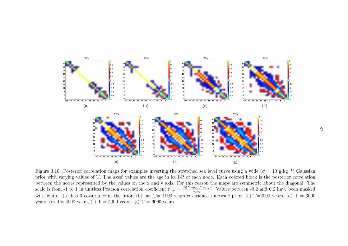
87
CorrF
125 70 40 30 26 22 18 14 10 6 2
0
4
8
12
16
20
24
28
35
45
80
−1
−0.8
−0.6
−0.4
−0.2
0
0.2
0.4
0.6
0.8
1
(a)
CorrF
125 70 40 30 26 22 18 14 10 6 2
0
4
8
12
16
20
24
28
35
45
80
−1
−0.8
−0.6
−0.4
−0.2
0
0.2
0.4
0.6
0.8
1
(b)
CorrF
125 70 40 30 26 22 18 14 10 6 2
0
4
8
12
16
20
24
28
35
45
80
−1
−0.8
−0.6
−0.4
−0.2
0
0.2
0.4
0.6
0.8
1
(c)
CorrF
125 70 40 30 26 22 18 14 10 6 2
0
4
8
12
16
20
24
28
35
45
80
−1
−0.8
−0.6
−0.4
−0.2
0
0.2
0.4
0.6
0.8
1
(d)
CorrF
125 70 40 30 26 22 18 14 10 6 2
0
4
8
12
16
20
24
28
35
45
80
−1
−0.8
−0.6
−0.4
−0.2
0
0.2
0.4
0.6
0.8
1
(e)
CorrF
125 70 40 30 26 22 18 14 10 6 2
0
4
8
12
16
20
24
28
35
45
80
−1
−0.8
−0.6
−0.4
−0.2
0
0.2
0.4
0.6
0.8
1
(f)
CorrF
125 70 40 30 26 22 18 14 10 6 2
0
4
8
12
16
20
24
28
35
45
80
−1
−0.8
−0.6
−0.4
−0.2
0
0.2
0.4
0.6
0.8
1
(g)
Figure 3.10: Posterior correlation maps for examples inverting the stretched sea level curve using a wide (σ = 10 g kg−1) Gaussianprior with varying values of T. The axes’ values are the age in ka BP of each node. Each colored block is the posterior correlationbetween the nodes represented by the values on the x and y axis. For this reason the maps are symmetric about the diagonal. Thescale is from -1 to 1 in unitless Pearson correlation coefficient rx,y = E[(X−µx)(Y−µy)]
σxσy. Values between -0.2 and 0.2 have been masked
with white. (a) has 0 covariance in the prior, (b) has T= 1000 years covariance timescale prior, (c) T=2000 years, (d) T = 3000years, (e) T= 4000 years, (f) T = 5000 years, (g) T = 6000 years.

88
0 10 20 30 40 50 60 70 80 90 100 110 120−0.2
−0.15
−0.1
−0.05
0
0.05
0.1
0.15
ka BP
(µF−
µI)/
µI
0
1000
2000
3000
4000
5000
6000
Figure 3.11: Shift in the mean solution from prior to posterior as a function of covariancetimescale T. Each line represents a different value of T in years, from 0 years to 6000years. As T increases, the temporal dependence of the mean shift is flattened or damped.
89
0 0.1 0.2 0.3 0.4 0.5 0.6 0.7 0.8 0.9 1x 10⁻⁴
0
2
4
6
8
frequency (years−1)
spec
tral
pow
er
0100020003000400050006000
0100020003000400050006000
Posterior Means
0 0.1 0.2 0.3 0.4 0.5 0.6 0.7 0.8 0.9 1x 10⁻⁴
0
0.5
1
frequency (years−1)
p−value
1/125,000 yrs 1/62,500 yrs 1/42,000 yrs 1/31,250 yrs 1/25,000 yrs
Figure 3.12: Lomb-Scargle periodogram of the posterior mean for the stretched sea levelexample using a wide Gaussian prior. The black line is the periodogram of the prior meanfor comparision. Each color is the periodogram of the posterior mean with a different priorcovariance timescale T in years, from 0 to 6000 years. The vertical lines overlain show thepeak frequencies for the prior and those of the posterior for the example T = 6000 years.
3.3.1.2 Linear problem – sea level prior with varying variance and covariance
The uninformative prior example demonstrated that there is very little information about
past concentration histories in the data alone. The data alone constrain at most 6000
years of the bottom water boundary condition, assuming that the initial condition, D0
and the other boundary condition are known. However, the uninformative prior example
was a very stringent test, as the deep ocean salinity is unlikely to be able to stray so
far from the mean. In the next example we consider how constraining the past ocean
salinity more tightly to the mean sea level records contributes to recovering past deep
ocean properties from present-day pore fluid profiles.
Deep ocean salinities should be near the mean ocean value, although their exact proximity
is what we want to determine from the pore fluid data. The way we have framed the
problem requires assigning a prior variance in addition to a prior mean on each salinity
node. We do not have any prior information on the standard deviation of salinity at the
LGM. Solutions that are more than two standard deviations from the prior mean are

90
unlikely to be recovered, even if their data likelihood is high, due to the multiplication
factor of 0 from the prior. To recover an LGM value of 37.1, the LGM salinity of site
1093 estimated by Adkins et al. (2002), when our prior information tells us that the mean
ocean salinity at the LGM was 35.9, the prior standard deviation should be at least 0.6,
even without accounting for error in the sea level curve. On the other hand, recall that
the maximum standard deviation we could apply to the modern deep ocean salinity is 0.1
g kg−1. Already these two standard deviations generate an order of magnitude difference
in prior variance.
While we expect that the salinity values will covary in time, we do not want to restrict
their covariance with the prior, instead looking at what arises in the posterior. One tricky
point about this is that if there is covariance in parameters, assigning 0 covariance in the
prior will penalize solutions with covariance. Stated in another way, no matter what level
of covariance is assigned in the prior, solutions with both more than and less than this
level of covariance are penalized in the search.
A second tricky point to remember is that the variance and covariance are part of the
prior, and can not be sampled on as parameters in the problem. If we were to sample
on these parameters, we would be regenerating the prior probability distributions at each
cooling step, violating the continuity of the cooling. Looked at from another perspective,
this would be a nested prior. That is if we stated the prior was “actually” just on the
variance and covariance parameters, these do not uniquely determine the salinity at each
time, and we still need an interior random generation.
With these points in mind, we consider varying levels of variance and covariance in the
prior, and their effect on solution space recovery. We show solutions with variance of 0.02,
0.5 and 1 to show the sensitivity of the solution to this parameter.
Figure 3.13 shows an example with 0 prior covariance and varying levels of prior vari-
ance around a mean prior scaled to the sea level curve. At the 0.02 level of variance,
the mean of the solution space does not recover the synthetic model. The solutions do
generally increase backwards in time, showing that data contains information that the
past salinity was higher. With increased prior variance, the individual solutions can take

91
on more extreme values, but there is not a significant change in the mean recovered time
series. Examining the correlations between parameters in Figure 3.14 helps explain this
phenomenon. The maps are essentially identical for all three covariance cases. Having
the same covariance between parameters is what makes the mean constant throughout
the cases. The fact that the mean doesn’t change between covariance levels means that
the mean and some covariance is recovered by the data, but the variance is not. There
is also some checkerboarding in the most modern parameters, the switching between red
and blue colors in the covariance plots as we read along the horizontal rows, suggesting
that the mean value of these nodes is resolved by the data but the absolute values are
not.
As we increase the covariance from 0 to 5000 years, the mean of the recovered time
series solutions improves in its match to the last 40k years. The improved match of the
recovered mean time series to the synthetic input at 5000 years prior covariance shows
that the stretched curve that we chose as a synthetic has an underlying covariance time
scale of 5000 years at least in the more modern section of the time series. The 5000 year
covariance timescale does not affect points in the past as much as those in the present,
as seen in the correlation plot, because they are separated by more than 5000 years.
Their correlations or covariances with other parameters are hence very small and do not
constrain the problem very much. As the covariance increases, the jaggedness of the
solutions clearly drops, as seen by the top ten selected time series plotted in Figures 3.13–
3.19. When T=5000, CATMIP does an excellent job of recovering our synthetic time
series from the LGM to present. In all variance cases the error between the recovered
mean LGM value and the true synthetic value is < 0.1 and for other points the error
is < 0.05. Also while the individual models have some oscillations, the mean estimated
time series does not suffer from instability to noise as did the regularized least squares
solutions in Chapter 2.
The literature contains many examples of sea level-type signals, such as ice core δ18O
records that show high spectral power in the time series at longer frequencies (10–100kyr)
and possibly bulges around the 4000 year frequency (Wunsch, 2003). As the synthetic has
a linear relationship with sea level we expect that its spectral characteristics are similar
92
to that of a sea level signal.
For any given covariance timescale, the posterior correlation maps are essentially the same.
The posterior correlations, and hence the posterior covariances, are primarily determined
by the prior covariances. This result reinforces the point that we can not recover much
covariance information from the data that is separate from the prior covariance. It is
true that the assigned prior covariances are all positive, while we are recovering negative
covariances. By essentially forcing certain covariances to be positive, the rest of the pa-
rameters must compensate in response, generating the negative covariances. The negative
covariances in the posterior are a response to the prior positive covariances.
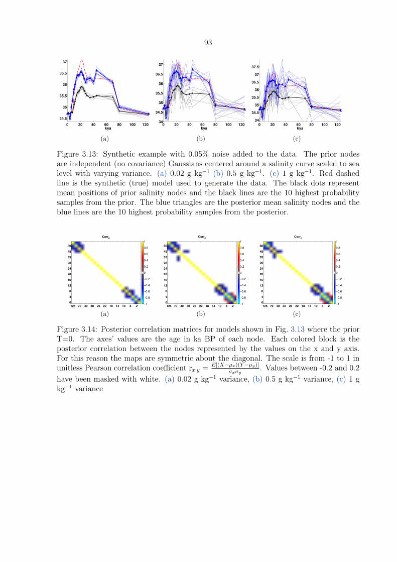
93
0 20 40 60 80 100 120
34.5
35
35.5
36
36.5
37
kya
(a)
0 20 40 60 80 100 12034
34.5
35
35.5
36
36.5
37
kya
(b)
0 20 40 60 80 100 12034
34.5
35
35.5
36
36.5
37
37.5
kya
(c)
Figure 3.13: Synthetic example with 0.05% noise added to the data. The prior nodesare independent (no covariance) Gaussians centered around a salinity curve scaled to sealevel with varying variance. (a) 0.02 g kg−1 (b) 0.5 g kg−1. (c) 1 g kg−1. Red dashedline is the synthetic (true) model used to generate the data. The black dots representmean positions of prior salinity nodes and the black lines are the 10 highest probabilitysamples from the prior. The blue triangles are the posterior mean salinity nodes and theblue lines are the 10 highest probability samples from the posterior.
CorrF
125 70 40 30 26 22 18 14 10 6 2
0
4
8
12
16
20
24
28
35
45
80
−1
−0.8
−0.6
−0.4
−0.2
0
0.2
0.4
0.6
0.8
1
(a)
CorrF
125 70 40 30 26 22 18 14 10 6 2
0
4
8
12
16
20
24
28
35
45
80
−1
−0.8
−0.6
−0.4
−0.2
0
0.2
0.4
0.6
0.8
1
(b)
CorrF
125 70 40 30 26 22 18 14 10 6 2
0
4
8
12
16
20
24
28
35
45
80
−1
−0.8
−0.6
−0.4
−0.2
0
0.2
0.4
0.6
0.8
1
(c)
Figure 3.14: Posterior correlation matrices for models shown in Fig. 3.13 where the priorT=0. The axes’ values are the age in ka BP of each node. Each colored block is theposterior correlation between the nodes represented by the values on the x and y axis.For this reason the maps are symmetric about the diagonal. The scale is from -1 to 1 inunitless Pearson correlation coefficient rx,y = E[(X−µx)(Y−µy)]
σxσy. Values between -0.2 and 0.2
have been masked with white. (a) 0.02 g kg−1 variance, (b) 0.5 g kg−1 variance, (c) 1 gkg−1 variance

94
0 20 40 60 80 100 120
34.5
35
35.5
36
36.5
37
kya
(a)
0 20 40 60 80 100 120
34
34.5
35
35.5
36
36.5
37
kya
(b)
0 20 40 60 80 100 120
34.5
35
35.5
36
36.5
37
37.5
38
kya
(c)
Figure 3.15: Synthetic example with 0.05% noise added to the data. The prior nodeshave Gaussian covariance with time scale T = 1000 years centered around a salinity curvescaled to sea level with varying variance. (a) 0.02 g kg−1 (b) 0.5 g kg−1. (c) 1 g kg−1.Red dashed line is the synthetic (true) model used to generate the data. The black dotsrepresent mean positions of prior salinity nodes and the black lines are the 10 highestprobability samples from the prior. The blue triangles are the posterior mean salinitynodes and the blue lines are the 10 highest probability samples from the posterior.
CorrF
125 70 40 30 26 22 18 14 10 6 2
0
4
8
12
16
20
24
28
35
45
80
−1
−0.8
−0.6
−0.4
−0.2
0
0.2
0.4
0.6
0.8
1
(a)
CorrF
125 70 40 30 26 22 18 14 10 6 2
0
4
8
12
16
20
24
28
35
45
80
−1
−0.8
−0.6
−0.4
−0.2
0
0.2
0.4
0.6
0.8
1
(b)
CorrF
125 70 40 30 26 22 18 14 10 6 2
0
4
8
12
16
20
24
28
35
45
80
−1
−0.8
−0.6
−0.4
−0.2
0
0.2
0.4
0.6
0.8
1
(c)
Figure 3.16: Posterior correlation matrices for models shown in Fig. 3.15, where T =1000 years. The axes’ values are the age in ka BP of each node. Each colored block is theposterior correlation between the nodes represented by the values on the x and y axis.For this reason the maps are symmetric about the diagonal. The scale is from -1 to 1 inunitless Pearson correlation coefficient rx,y = E[(X−µx)(Y−µy)]
σxσy. Values between -0.2 and 0.2
have been masked with white. (a) 0.02 g kg−1 variance, (b) 0.5 g kg−1 variance, (c) 1 gkg−1 variance

95
0 20 40 60 80 100 120
35
35.5
36
36.5
37
kya
(a)
0 20 40 60 80 100 120
34.5
35
35.5
36
36.5
37
kya
(b)
0 20 40 60 80 100 120
34.5
35
35.5
36
36.5
37
37.5
38
kya
(c)
Figure 3.17: Synthetic example with 0.05% noise added to the data. The prior nodeshave Gaussian covariance with time scale T = 3000 years centered around a salinity curvescaled to sea level with varying variance. (a) 0.02 g kg−1 (b) 0.5 g kg−1. (c) 1 g kg−1.Red dashed line is the synthetic (true) model used to generate the data. The black dotsrepresent mean positions of prior salinity nodes and the black lines are the 10 highestprobability samples from the prior. The blue triangles are the posterior mean salinitynodes and the blue lines are the 10 highest probability samples from the posterior.
CorrF
125 70 40 30 26 22 18 14 10 6 2
0
4
8
12
16
20
24
28
35
45
80
−1
−0.8
−0.6
−0.4
−0.2
0
0.2
0.4
0.6
0.8
1
(a)
CorrF
125 70 40 30 26 22 18 14 10 6 2
0
4
8
12
16
20
24
28
35
45
80
−1
−0.8
−0.6
−0.4
−0.2
0
0.2
0.4
0.6
0.8
1
(b)
CorrF
125 70 40 30 26 22 18 14 10 6 2
0
4
8
12
16
20
24
28
35
45
80
−1
−0.8
−0.6
−0.4
−0.2
0
0.2
0.4
0.6
0.8
1
(c)
Figure 3.18: Posterior correlation matrices for models shown in Fig. 3.17 where T = 3000years. The axes’ values are the age in ka BP of each node. Each colored block is theposterior correlation between the nodes represented by the values on the x and y axis.For this reason the maps are symmetric about the diagonal. The scale is from -1 to 1 inunitless Pearson correlation coefficient rx,y = E[(X−µx)(Y−µy)]
σxσy. Values between -0.2 and 0.2
have been masked with white. (a) 0.02 g kg−1 variance, (b) 0.5 g kg−1 variance, (c) 1 gkg−1 variance
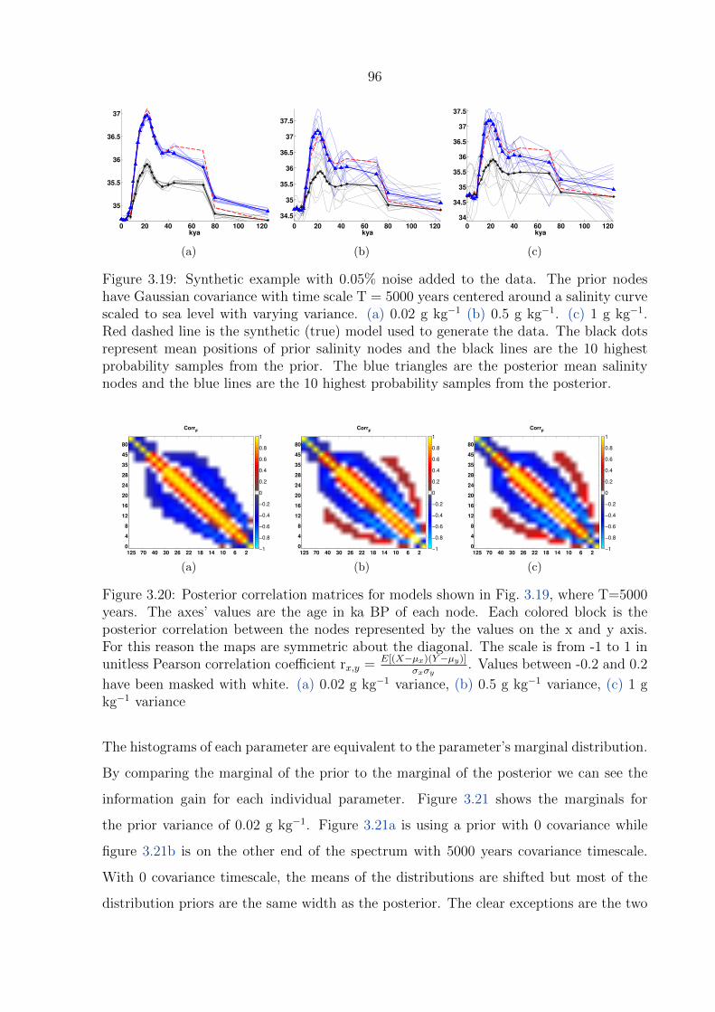
96
0 20 40 60 80 100 120
35
35.5
36
36.5
37
kya
(a)
0 20 40 60 80 100 120
34.5
35
35.5
36
36.5
37
37.5
kya
(b)
0 20 40 60 80 100 120
34
34.5
35
35.5
36
36.5
37
37.5
kya
(c)
Figure 3.19: Synthetic example with 0.05% noise added to the data. The prior nodeshave Gaussian covariance with time scale T = 5000 years centered around a salinity curvescaled to sea level with varying variance. (a) 0.02 g kg−1 (b) 0.5 g kg−1. (c) 1 g kg−1.Red dashed line is the synthetic (true) model used to generate the data. The black dotsrepresent mean positions of prior salinity nodes and the black lines are the 10 highestprobability samples from the prior. The blue triangles are the posterior mean salinitynodes and the blue lines are the 10 highest probability samples from the posterior.
CorrF
125 70 40 30 26 22 18 14 10 6 2
0
4
8
12
16
20
24
28
35
45
80
−1
−0.8
−0.6
−0.4
−0.2
0
0.2
0.4
0.6
0.8
1
(a)
CorrF
125 70 40 30 26 22 18 14 10 6 2
0
4
8
12
16
20
24
28
35
45
80
−1
−0.8
−0.6
−0.4
−0.2
0
0.2
0.4
0.6
0.8
1
(b)
CorrF
125 70 40 30 26 22 18 14 10 6 2
0
4
8
12
16
20
24
28
35
45
80
−1
−0.8
−0.6
−0.4
−0.2
0
0.2
0.4
0.6
0.8
1
(c)
Figure 3.20: Posterior correlation matrices for models shown in Fig. 3.19, where T=5000years. The axes’ values are the age in ka BP of each node. Each colored block is theposterior correlation between the nodes represented by the values on the x and y axis.For this reason the maps are symmetric about the diagonal. The scale is from -1 to 1 inunitless Pearson correlation coefficient rx,y = E[(X−µx)(Y−µy)]
σxσy. Values between -0.2 and 0.2
have been masked with white. (a) 0.02 g kg−1 variance, (b) 0.5 g kg−1 variance, (c) 1 gkg−1 variance
The histograms of each parameter are equivalent to the parameter’s marginal distribution.
By comparing the marginal of the prior to the marginal of the posterior we can see the
information gain for each individual parameter. Figure 3.21 shows the marginals for
the prior variance of 0.02 g kg−1. Figure 3.21a is using a prior with 0 covariance while
figure 3.21b is on the other end of the spectrum with 5000 years covariance timescale.
With 0 covariance timescale, the means of the distributions are shifted but most of the
distribution priors are the same width as the posterior. The clear exceptions are the two
97
most modern nodes parameters, 0 and 2ka BP. In contrast, when the prior covariance
increases to 5000 years, many more nodes have shrunk in variance. Their means are also
in a different position than in the case with 0 covariance priors. It is not easy to see how
far back the change extends, but in Figure 3.22 which is the same but with variance 1
instead of 0.02, we can much more clearly see that the variance of parameter distributions
shrinks backward in time to at least the salinity node at 24 ka BP.
We show how the variance of the posterior shrinks with respect to that of the prior
for a range of variances and covariances together in Figure 3.23. The lines are color-
coded by covariance timescale which serves to illustrate that the results almost collapse
with covariance timescale, or at least are primarily a function of covariance timescale.
A variance shrinkage of more than 0.5 is probably not significant. Otherwise, this plot
very much resembles the resolution plots from Chapter 2. That is, nodes representing
information further back in time are less well resolved than modern nodes. This resolution
is different in that we are not comparing the true solution to the recovered solution. Rather
we are demonstrating the impact of the information from the data on evolving the prior
to become the posterior. With greater covariance, the nodes are increasingly well resolved
in variance and the resolution of the nodes extends further back in time. The main point
of this plot is that the variance in the posterior, or resolution of the method, is a strong
function of the covariance in the prior. The prior covariance sets the posterior variance.
The relationship between parameter mean and prior covariance and variance is shown in
Figure 3.24. Again, much of the information collapses on the covariance timescale. Next
we see that as the covariance time scale increases, the temporal pattern of the mean shift
is squashed, or flattened. This illustrates the point that the shift in the mean of each
individual parameter is a function of the covariance. It reinforces the point brought up
by the plots comparing the mean with different levels of variance; increasing the variance
in the prior does not change the mean of the recovered solution sets, but increasing the
covariance does.
Comparing priors and posteriors is one way to see the information change of the method,
but it does not tell us how well the solution is recovered. Figures 3.13-3.17 demonstrate
that the posterior may not include the true solution if the prior is not an accurate rep-
98
resentation of the solution space. We can be tricked by a strong change in the posterior
probability distribution relative to the prior. In Figures 3.25 and 3.26 we plot the differ-
ence between the mean of the posterior distribution and the true synthetic model used to
generate the data, for a variety of input covariance timescales and variances.
The error between the posterior mean and the true model is a function of covariance
timescale, which we interpret again to mean that the underlying covariance timescale of
the synthetic model was closer to 5000 than to 0. However, there also seems to be a
fundamental frequency in the error that is constant between different prior variance and
covariance assumptions. We believe this fundamental frequency is due to the relationship
between the prior and the true synthetic model. Recall that the synthetic is a stretched
version of the prior, such that when CATMIP searches for models that improve on the
prior in their fit to the data, it will find good fits along the directions of stretching. It then
will realign its search in this direction of covariance, tending to populate the posterior
with more values that lie along a particular direction. The relationship between the prior
mean and the true model is fixed throughout these different examples, explaining why a
fundamental frequency arises in the difference between posterior means and true model.
99
3.3.1.3 Linear Problem – recovery of models with known variance and co-
variance
In the stretched sea level example above, the variance and covariance of the posteriors are
different than those of the priors, and the relationships between nodes in the time series
oscillate between correlation and anti-correlation. In generating this synthetic example,
we did not specify the underlying variance and covariance of the synthetic model. Our
results suggest that the underlying covariance of the synthetic model is 5000 years or
more. The obvious question at this point is: If the covariance and variance are known,
does this information in addition to the measured data profile allow us to recover the true
model?
To answer this question we generate random sample models from a Gaussian prior with
mean determined by the sea level curve to drive the forward model and produce data
that we invert with CATMIP. We show how well CATMIP, using this synthetic data,
recovers the inputs drawn from a very tight prior, 0.02 g kg−1 variance and 4000 year
covariance, and a less informative prior, with 0.5 g kg−1 variance and both 0 and 4000
year covariances.
Then, we consider what happens when the wrong prior is assigned to CATMIP. Since in
reality we do not know the variance and covariance of the time series that generated the
data, we consider the bias in our solution if our prior information about these parameters
is wrong.
Figure 3.27 shows ten random sample models drawn from a very tight prior with 0.02 g
kg−1 variance and 4000 year covariance, in addition to the mean of the recovered solutions
and the prior mean. Although we may have expected that the recovered mean of the
solutions was the same as the prior mean, this is not the case. Instead, the recovered
posterior mean more closely resembles the synthetic model, at least in the most recent 20
ka before present. Looking backwards in time, the posterior mean decreasingly resembles
the synthetic model, more so the more the synthetic model deviates from the prior mean.
A more accurate representation of the error in the recovered solution is shown in Fig-
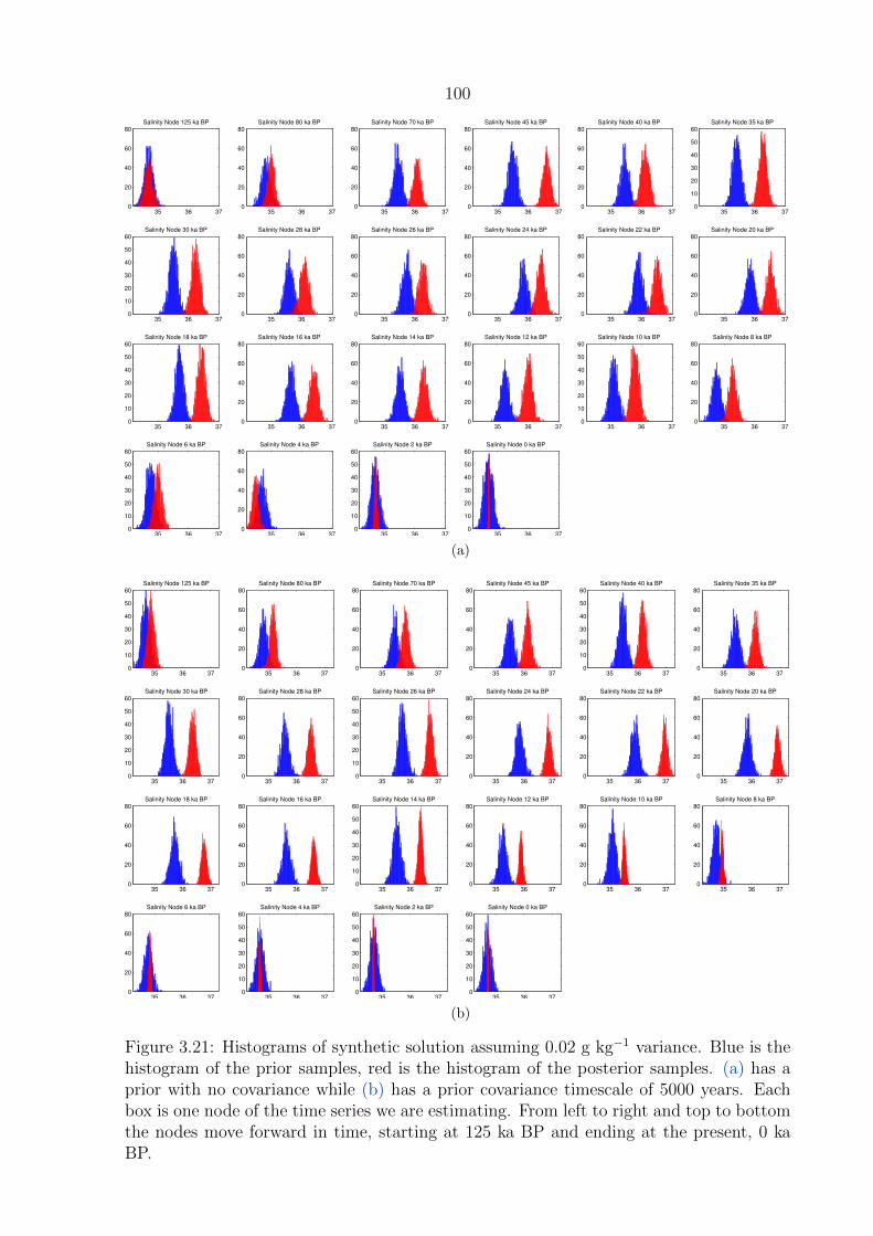
100
35 36 370
20
40
60
80Salinity Node 125 ka BP
35 36 370
20
40
60
80Salinity Node 80 ka BP
35 36 370
20
40
60
80Salinity Node 70 ka BP
35 36 370
20
40
60
80Salinity Node 45 ka BP
35 36 370
20
40
60
80Salinity Node 40 ka BP
35 36 370
10
20
30
40
50
60Salinity Node 35 ka BP
35 36 370
10
20
30
40
50
60Salinity Node 30 ka BP
35 36 370
20
40
60
80Salinity Node 28 ka BP
35 36 370
20
40
60
80Salinity Node 26 ka BP
35 36 370
20
40
60
80Salinity Node 24 ka BP
35 36 370
20
40
60
80Salinity Node 22 ka BP
35 36 370
20
40
60
80Salinity Node 20 ka BP
35 36 370
10
20
30
40
50
60Salinity Node 18 ka BP
35 36 370
20
40
60
80Salinity Node 16 ka BP
35 36 370
20
40
60
80Salinity Node 14 ka BP
35 36 370
20
40
60
80Salinity Node 12 ka BP
35 36 370
10
20
30
40
50
60Salinity Node 10 ka BP
35 36 370
20
40
60
80Salinity Node 8 ka BP
35 36 370
10
20
30
40
50
60Salinity Node 6 ka BP
35 36 370
20
40
60
80Salinity Node 4 ka BP
35 36 370
10
20
30
40
50
60Salinity Node 2 ka BP
35 36 370
10
20
30
40
50
60Salinity Node 0 ka BP
(a)
35 36 370
10
20
30
40
50
60Salinity Node 125 ka BP
35 36 370
20
40
60
80Salinity Node 80 ka BP
35 36 370
20
40
60
80Salinity Node 70 ka BP
35 36 370
20
40
60
80Salinity Node 45 ka BP
35 36 370
10
20
30
40
50
60Salinity Node 40 ka BP
35 36 370
20
40
60
80Salinity Node 35 ka BP
35 36 370
10
20
30
40
50
60Salinity Node 30 ka BP
35 36 370
20
40
60
80Salinity Node 28 ka BP
35 36 370
10
20
30
40
50
60Salinity Node 26 ka BP
35 36 370
20
40
60
80Salinity Node 24 ka BP
35 36 370
20
40
60
80Salinity Node 22 ka BP
35 36 370
20
40
60
80Salinity Node 20 ka BP
35 36 370
20
40
60
80Salinity Node 18 ka BP
35 36 370
20
40
60
80Salinity Node 16 ka BP
35 36 370
10
20
30
40
50
60Salinity Node 14 ka BP
35 36 370
20
40
60
80Salinity Node 12 ka BP
35 36 370
20
40
60
80Salinity Node 10 ka BP
35 36 370
20
40
60
80Salinity Node 8 ka BP
35 36 370
20
40
60
80Salinity Node 6 ka BP
35 36 370
10
20
30
40
50
60Salinity Node 4 ka BP
35 36 370
10
20
30
40
50
60Salinity Node 2 ka BP
35 36 370
10
20
30
40
50
60Salinity Node 0 ka BP
(b)
Figure 3.21: Histograms of synthetic solution assuming 0.02 g kg−1 variance. Blue is thehistogram of the prior samples, red is the histogram of the posterior samples. (a) has aprior with no covariance while (b) has a prior covariance timescale of 5000 years. Eachbox is one node of the time series we are estimating. From left to right and top to bottomthe nodes move forward in time, starting at 125 ka BP and ending at the present, 0 kaBP.

101
32 34 36 38 400
20
40
60
80Salinity Node 125 ka BP
32 34 36 38 400
20
40
60
80Salinity Node 80 ka BP
32 34 36 38 400
10
20
30
40
50
60Salinity Node 70 ka BP
32 34 36 38 400
20
40
60
80Salinity Node 45 ka BP
32 34 36 38 400
20
40
60
80Salinity Node 40 ka BP
32 34 36 38 400
20
40
60
80Salinity Node 35 ka BP
32 34 36 38 400
20
40
60
80Salinity Node 30 ka BP
32 34 36 38 400
20
40
60
80Salinity Node 28 ka BP
32 34 36 38 400
20
40
60
80Salinity Node 26 ka BP
32 34 36 38 400
20
40
60
80Salinity Node 24 ka BP
32 34 36 38 400
20
40
60
80Salinity Node 22 ka BP
32 34 36 38 400
20
40
60
80Salinity Node 20 ka BP
32 34 36 38 400
10
20
30
40
50
60Salinity Node 18 ka BP
32 34 36 38 400
20
40
60
80Salinity Node 16 ka BP
32 34 36 38 400
10
20
30
40
50
60Salinity Node 14 ka BP
32 34 36 38 400
20
40
60
80Salinity Node 12 ka BP
32 34 36 38 400
20
40
60
80Salinity Node 10 ka BP
32 34 36 38 400
10
20
30
40
50
60Salinity Node 8 ka BP
32 34 36 38 400
10
20
30
40
50
60Salinity Node 6 ka BP
32 34 36 38 400
20
40
60
80Salinity Node 4 ka BP
32 34 36 38 400
20
40
60
80Salinity Node 2 ka BP
32 34 36 38 400
10
20
30
40
50
60Salinity Node 0 ka BP
(a)
32 34 36 380
10
20
30
40
50
60Salinity Node 125 ka BP
32 34 36 380
20
40
60
80Salinity Node 80 ka BP
32 34 36 380
20
40
60
80Salinity Node 70 ka BP
32 34 36 380
20
40
60
80Salinity Node 45 ka BP
32 34 36 380
20
40
60
80Salinity Node 40 ka BP
32 34 36 380
20
40
60
80Salinity Node 35 ka BP
32 34 36 380
20
40
60
80Salinity Node 30 ka BP
32 34 36 380
20
40
60
80Salinity Node 28 ka BP
32 34 36 380
10
20
30
40
50
60Salinity Node 26 ka BP
32 34 36 380
20
40
60
80Salinity Node 24 ka BP
32 34 36 380
20
40
60
80Salinity Node 22 ka BP
32 34 36 380
20
40
60
80Salinity Node 20 ka BP
32 34 36 380
20
40
60
80Salinity Node 18 ka BP
32 34 36 380
20
40
60
80Salinity Node 16 ka BP
32 34 36 380
20
40
60
80Salinity Node 14 ka BP
32 34 36 380
20
40
60
80Salinity Node 12 ka BP
32 34 36 380
10
20
30
40
50
60Salinity Node 10 ka BP
32 34 36 380
10
20
30
40
50
60Salinity Node 8 ka BP
32 34 36 380
10
20
30
40
50
60Salinity Node 6 ka BP
32 34 36 380
20
40
60
80Salinity Node 4 ka BP
32 34 36 380
20
40
60
80Salinity Node 2 ka BP
32 34 36 380
20
40
60
80Salinity Node 0 ka BP
(b)
Figure 3.22: Histograms of synthetic solution assuming 1 g kg−1 variance. Blue is thehistogram of the prior samples, red is the histogram of the posterior samples. (a) has aprior with 0 covariance while (b) has a prior with 5000 year timescale covariance. Eachbox is one node of the time series we are estimating. From left to right and top to bottomthe nodes move forward in time, starting at 125 ka BP and ending at the present, 0 kaBP.

102
0 10 20 30 40 50 60 70 80 90 100 110 1200
0.2
0.4
0.6
0.8
1
1.2
1.4
ka BP
σ2 F/σ
2 I
0
1000
2000
3000
4000
5000
Figure 3.23: The ratio of posterior variance (σ2F ) to prior variance (σ2
I ) for a range ofdifferent input priors and data from the stretched sea level curve example. Each colorcorresponds to a different value of T, the covariance timescale in years, while each symbolis a different input variance. The symbols help delineate the different lines, but thevariance shrinkage is primarily a function of T
0 10 20 30 40 50 60 70 80 90 100 110 120−0.02
−0.01
0
0.01
0.02
0.03
0.04
0.05
ka BP
(µF−
µI)/
µI
0
1000
2000
3000
4000
5000
Figure 3.24: Shift in the mean of the posterior population (µF ) with respect to the meanof the prior distribution (µI), normalized to the mean of the prior distribution. Eachcolor corresponds to a different value of T, the covariance timescale in years, while eachsymbol is a different input variance.

103
0 10 20 30 40 50 60 70 80 90 100 110 120−0.8
−0.6
−0.4
−0.2
0
0.2
0.4
0.6
ka BP
mtr
ue−
mm
ean
0
1000
2000
3000
4000
5000
Figure 3.25: Difference between the posterior mean and the true synthetic model (g kg−1)as a function of prior variance and covariance. Each color corresponds to a different valueof T, the covariance timescale in years. Each symbol is a different input variance, from0.02 to 1 g kg−1
0 10 20 30 40 50 60 70 80 90 100 110 120−4
−3
−2
−1
0
1
2
3
4
ka BP
mtr
ue−
mm
ea
n
0
1000
2000
3000
4000
5000
Figure 3.26: Same as Figure 3.25, except also including the examples with wide Gaussianprior σ2
I = 100 g kg−1
104
ure 3.28. Plotted are the error in the posterior from the true solution and the difference
in the prior from the true solution. The reduction in error from the prior to the posterior
indicates the amount of information the data is retaining above and beyond the prior
variance and covaraince. The error envelope between the posterior mean and the true
solution is much flatter from 0 to ∼ 20 ka BP. Further back in time the flattening, if any,
is much more subtle.
Since we know from the previous examples that long timescales of covariance help restrict
the posterior solution space more, the obvious question is what about the case with 0 year
timescale covariance? Figure 3.29 shows the recovery of ten random samples with these
parameters. The synthetic models are more jagged and the posterior does not follow
the synthetic model even in the most recent time nodes. The posterior seems to be a
smoother version of the solution, particularly noticeable in Figure 3.29d and 3.29h. The
posterior nodes in the most recent 10 ka are sitting at the average of their two neighboring
true nodes. Indeed, Figure 3.30, which compares the error in the posterior relative to the
difference in the synthetic from the prior, shows that shrinking the error envelope from
prior to posterior happens over a much shorter time period, ∼10ka BP rather than the
∼20ka BP seen in the case with 4000 year timescale covariance. Thus, even when the
model is drawn from a known prior, longer covariance timescale models can be more
reliably recovered.

105
0 2 4 6 8 10 12
x 104
34.2
34.4
34.6
34.8
35
35.2
35.4
35.6
35.8
36
36.2
Years B.P.
(a)
0 2 4 6 8 10 12
x 104
34.2
34.4
34.6
34.8
35
35.2
35.4
35.6
35.8
36
Years B.P.
(b)
0 2 4 6 8 10 12
x 104
34.4
34.6
34.8
35
35.2
35.4
35.6
35.8
36
36.2
Years B.P.
(c)
0 2 4 6 8 10 12
x 104
34.4
34.6
34.8
35
35.2
35.4
35.6
35.8
36
36.2
Years B.P.
(d)
0 2 4 6 8 10 12
x 104
34.2
34.4
34.6
34.8
35
35.2
35.4
35.6
35.8
36
Years B.P.
(e)
0 2 4 6 8 10 12
x 104
34.2
34.4
34.6
34.8
35
35.2
35.4
35.6
35.8
36
36.2
Years B.P.
(f)
0 2 4 6 8 10 12
x 104
34.2
34.4
34.6
34.8
35
35.2
35.4
35.6
35.8
36
36.2
Years B.P.
(g)
0 2 4 6 8 10 12
x 104
34.2
34.4
34.6
34.8
35
35.2
35.4
35.6
35.8
36
36.2
Years B.P.
(h)
0 2 4 6 8 10 12
x 104
34.4
34.6
34.8
35
35.2
35.4
35.6
35.8
36
36.2
Years B.P.
(i)
0 2 4 6 8 10 12
x 104
34.2
34.4
34.6
34.8
35
35.2
35.4
35.6
35.8
36
Years B.P.
(j)
Figure 3.27: Ten random models drawn from the scaled sea level curve with variance 0.02g kg−1 and covariance T = 4000 years. Red is the target or true model from which thedata was generated. Black circles are the mean of the posterior samples. Black stars anddashed line are the mean priors
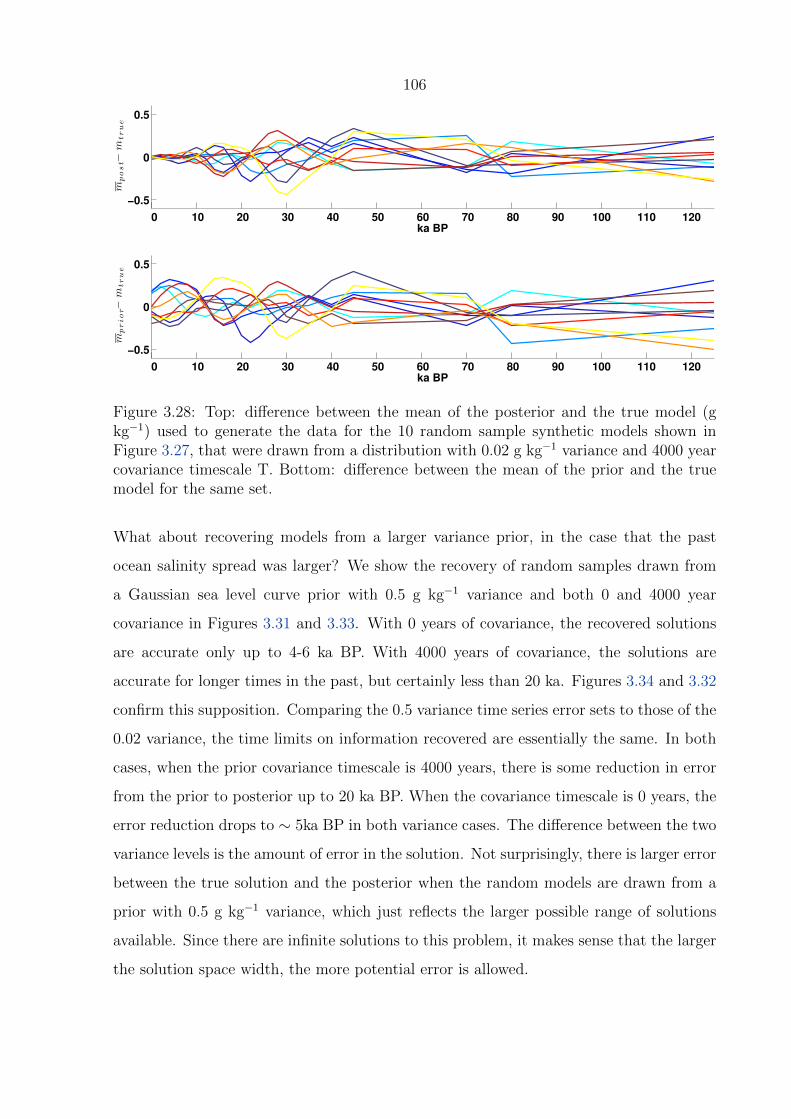
106
0 10 20 30 40 50 60 70 80 90 100 110 120
−0.5
0
0.5m
post−
mtrue
ka BP
0 10 20 30 40 50 60 70 80 90 100 110 120
−0.5
0
0.5
mprior−
mtrue
ka BP
Figure 3.28: Top: difference between the mean of the posterior and the true model (gkg−1) used to generate the data for the 10 random sample synthetic models shown inFigure 3.27, that were drawn from a distribution with 0.02 g kg−1 variance and 4000 yearcovariance timescale T. Bottom: difference between the mean of the prior and the truemodel for the same set.
What about recovering models from a larger variance prior, in the case that the past
ocean salinity spread was larger? We show the recovery of random samples drawn from
a Gaussian sea level curve prior with 0.5 g kg−1 variance and both 0 and 4000 year
covariance in Figures 3.31 and 3.33. With 0 years of covariance, the recovered solutions
are accurate only up to 4-6 ka BP. With 4000 years of covariance, the solutions are
accurate for longer times in the past, but certainly less than 20 ka. Figures 3.34 and 3.32
confirm this supposition. Comparing the 0.5 variance time series error sets to those of the
0.02 variance, the time limits on information recovered are essentially the same. In both
cases, when the prior covariance timescale is 4000 years, there is some reduction in error
from the prior to posterior up to 20 ka BP. When the covariance timescale is 0 years, the
error reduction drops to ∼ 5ka BP in both variance cases. The difference between the two
variance levels is the amount of error in the solution. Not surprisingly, there is larger error
between the true solution and the posterior when the random models are drawn from a
prior with 0.5 g kg−1 variance, which just reflects the larger possible range of solutions
available. Since there are infinite solutions to this problem, it makes sense that the larger
the solution space width, the more potential error is allowed.

107
0 2 4 6 8 10 12
x 104
34.2
34.4
34.6
34.8
35
35.2
35.4
35.6
35.8
36
36.2
Years B.P.
(a)
0 2 4 6 8 10 12
x 104
34.2
34.4
34.6
34.8
35
35.2
35.4
35.6
35.8
36
36.2
Years B.P.
(b)
0 2 4 6 8 10 12
x 104
34.4
34.6
34.8
35
35.2
35.4
35.6
35.8
36
36.2
Years B.P.
(c)
0 2 4 6 8 10 12
x 104
34.4
34.6
34.8
35
35.2
35.4
35.6
35.8
36
36.2
Years B.P.
(d)
0 2 4 6 8 10 12
x 104
34.4
34.6
34.8
35
35.2
35.4
35.6
35.8
36
36.2
Years B.P.
(e)
0 2 4 6 8 10 12
x 104
34.5
35
35.5
36
Years B.P.
(f)
0 2 4 6 8 10 12
x 104
34.4
34.6
34.8
35
35.2
35.4
35.6
35.8
36
36.2
Years B.P.
(g)
0 2 4 6 8 10 12
x 104
34.4
34.6
34.8
35
35.2
35.4
35.6
35.8
36
36.2
Years B.P.
(h)
0 2 4 6 8 10 12
x 104
34.4
34.6
34.8
35
35.2
35.4
35.6
35.8
36
36.2
Years B.P.
(i)
0 2 4 6 8 10 12
x 104
34.2
34.4
34.6
34.8
35
35.2
35.4
35.6
35.8
36
36.2
Years B.P.
(j)
Figure 3.29: Ten random models drawn from the scaled sea level curve with variance0.02 g kg−1 and covariance T = 0 years. Red is the target or true model from which thedata was generated. Black circles are the mean of the posterior samples. Black stars anddashed line are the mean priors
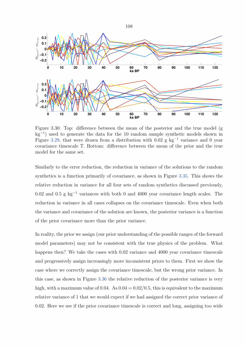
108
0 10 20 30 40 50 60 70 80 90 100 110 120
−0.2
−0.1
0
0.1
0.2m
post−
mtrue
ka BP
0 10 20 30 40 50 60 70 80 90 100 110 120
−0.2
−0.1
0
0.1
0.2
mprior−
mtrue
ka BP
Figure 3.30: Top: difference between the mean of the posterior and the true model (gkg−1) used to generate the data for the 10 random sample synthetic models shown inFigure 3.29, that were drawn from a distribution with 0.02 g kg−1 variance and 0 yearcovariance timescale T. Bottom: difference between the mean of the prior and the truemodel for the same set.
Similarly to the error reduction, the reduction in variance of the solutions to the random
synthetics is a function primarily of covariance, as shown in Figure 3.35. This shows the
relative reduction in variance for all four sets of random synthetics discussed previously,
0.02 and 0.5 g kg−1 variances with both 0 and 4000 year covariance length scales. The
reduction in variance in all cases collapses on the covariance timescale. Even when both
the variance and covariance of the solution are known, the posterior variance is a function
of the prior covariance more than the prior variance.
In reality, the prior we assign (our prior understanding of the possible ranges of the forward
model parameters) may not be consistent with the true physics of the problem. What
happens then? We take the cases with 0.02 variance and 4000 year covariance timescale
and progressively assign increasingly more inconsistent priors to them. First we show the
case where we correctly assign the covariance timescale, but the wrong prior variance. In
this case, as shown in Figure 3.36 the relative reduction of the posterior variance is very
high, with a maximum value of 0.04. As 0.04 = 0.02/0.5, this is equivalent to the maximum
relative variance of 1 that we would expect if we had assigned the correct prior variance of
0.02. Here we see if the prior covariance timescale is correct and long, assigning too wide
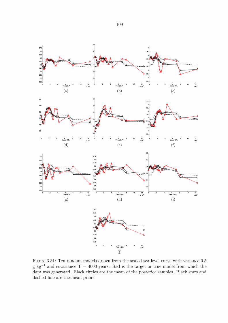
109
0 2 4 6 8 10 12
x 104
32.5
33
33.5
34
34.5
35
35.5
36
36.5
37
37.5
Years B.P.
(a)
0 2 4 6 8 10 12
x 104
33
34
35
36
37
38
Years B.P.
(b)
0 2 4 6 8 10 12
x 104
32.5
33
33.5
34
34.5
35
35.5
36
36.5
37
Years B.P.
(c)
0 2 4 6 8 10 12
x 104
33
34
35
36
37
38
Years B.P.
(d)
0 2 4 6 8 10 12
x 104
33
34
35
36
37
38
Years B.P.
(e)
0 2 4 6 8 10 12
x 104
32.5
33
33.5
34
34.5
35
35.5
36
36.5
37
37.5
Years B.P.
(f)
0 2 4 6 8 10 12
x 104
32.5
33
33.5
34
34.5
35
35.5
36
36.5
37
Years B.P.
(g)
0 2 4 6 8 10 12
x 104
32.5
33
33.5
34
34.5
35
35.5
36
36.5
37
37.5
Years B.P.
(h)
0 2 4 6 8 10 12
x 104
33
34
35
36
37
38
Years B.P.
(i)
0 2 4 6 8 10 12
x 104
32.5
33
33.5
34
34.5
35
35.5
36
36.5
37
Years B.P.
(j)
Figure 3.31: Ten random models drawn from the scaled sea level curve with variance 0.5g kg−1 and covariance T = 4000 years. Red is the target or true model from which thedata was generated. Black circles are the mean of the posterior samples. Black stars anddashed line are the mean priors
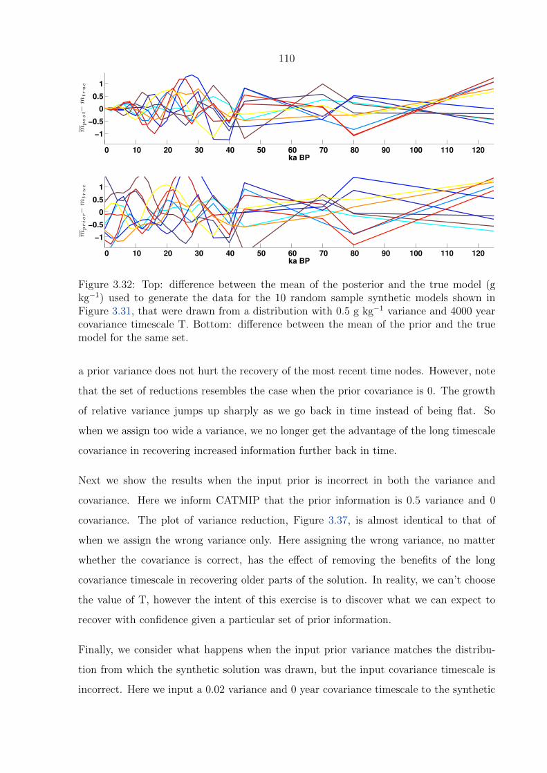
110
0 10 20 30 40 50 60 70 80 90 100 110 120
−1
−0.5
0
0.5
1m
post−
mtrue
ka BP
0 10 20 30 40 50 60 70 80 90 100 110 120
−1
−0.5
0
0.5
1
mprior−
mtrue
ka BP
Figure 3.32: Top: difference between the mean of the posterior and the true model (gkg−1) used to generate the data for the 10 random sample synthetic models shown inFigure 3.31, that were drawn from a distribution with 0.5 g kg−1 variance and 4000 yearcovariance timescale T. Bottom: difference between the mean of the prior and the truemodel for the same set.
a prior variance does not hurt the recovery of the most recent time nodes. However, note
that the set of reductions resembles the case when the prior covariance is 0. The growth
of relative variance jumps up sharply as we go back in time instead of being flat. So
when we assign too wide a variance, we no longer get the advantage of the long timescale
covariance in recovering increased information further back in time.
Next we show the results when the input prior is incorrect in both the variance and
covariance. Here we inform CATMIP that the prior information is 0.5 variance and 0
covariance. The plot of variance reduction, Figure 3.37, is almost identical to that of
when we assign the wrong variance only. Here assigning the wrong variance, no matter
whether the covariance is correct, has the effect of removing the benefits of the long
covariance timescale in recovering older parts of the solution. In reality, we can’t choose
the value of T, however the intent of this exercise is to discover what we can expect to
recover with confidence given a particular set of prior information.
Finally, we consider what happens when the input prior variance matches the distribu-
tion from which the synthetic solution was drawn, but the input covariance timescale is
incorrect. Here we input a 0.02 variance and 0 year covariance timescale to the synthetic

111
0 2 4 6 8 10 12
x 104
32
33
34
35
36
37
Years B.P.
(a)
0 2 4 6 8 10 12
x 104
33
34
35
36
37
38
Years B.P.
(b)
0 2 4 6 8 10 12
x 104
32
33
34
35
36
37
38
Years B.P.
(c)
0 2 4 6 8 10 12
x 104
33
33.5
34
34.5
35
35.5
36
36.5
37
37.5
38
Years B.P.
(d)
0 2 4 6 8 10 12
x 104
33
34
35
36
37
38
Years B.P.
(e)
0 2 4 6 8 10 12
x 104
33
34
35
36
37
38
Years B.P.
(f)
0 2 4 6 8 10 12
x 104
33
34
35
36
37
38
Years B.P.
(g)
0 2 4 6 8 10 12
x 104
33
34
35
36
37
38
Years B.P.
(h)
0 2 4 6 8 10 12
x 104
33
34
35
36
37
38
Years B.P.
(i)
0 2 4 6 8 10 12
x 104
33
34
35
36
37
38
Years B.P.
(j)
Figure 3.33: Ten random models drawn from the scaled sea level curve with variance0.5 g kg−1 and covariance T = 0 years. Red is the target or true model from which thedata was generated. Black circles are the mean of the posterior samples. Black stars anddashed line are the mean priors
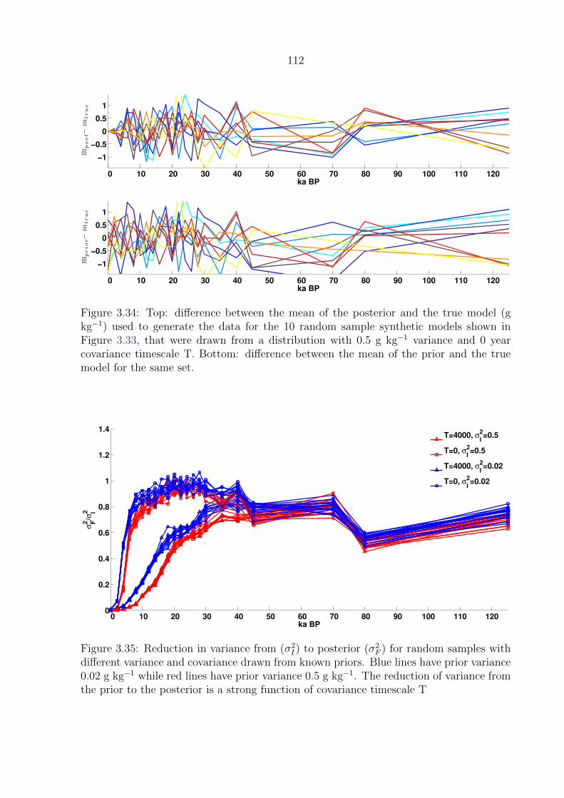
112
0 10 20 30 40 50 60 70 80 90 100 110 120
−1
−0.5
0
0.5
1
mpost−
mtrue
ka BP
0 10 20 30 40 50 60 70 80 90 100 110 120
−1
−0.5
0
0.5
1
mprior−
mtrue
ka BP
Figure 3.34: Top: difference between the mean of the posterior and the true model (gkg−1) used to generate the data for the 10 random sample synthetic models shown inFigure 3.33, that were drawn from a distribution with 0.5 g kg−1 variance and 0 yearcovariance timescale T. Bottom: difference between the mean of the prior and the truemodel for the same set.
0 10 20 30 40 50 60 70 80 90 100 110 1200
0.2
0.4
0.6
0.8
1
1.2
1.4
ka BP
σ2 F/σ
2 I
T=4000, σ2
I=0.5
T=0, σ2
I=0.5
T=4000, σ2
I=0.02
T=0, σ2
I=0.02
Figure 3.35: Reduction in variance from (σ2I ) to posterior (σ2
F ) for random samples withdifferent variance and covariance drawn from known priors. Blue lines have prior variance0.02 g kg−1 while red lines have prior variance 0.5 g kg−1. The reduction of variance fromthe prior to the posterior is a strong function of covariance timescale T

113
0 10 20 30 40 50 60 70 80 90 100 110 1200
0.005
0.01
0.015
0.02
0.025
0.03
0.035
0.04
0.045
ka BP
σ2 F/σ
2 I
4000
Figure 3.36: Reduction in variance from prior (σ2I ) to posterior (σ2
F ) for random samplemodels generated from a distribution with 0.02 g kg−1 = σ2 and 4000 years = T whenCATMIP is fed the wrong prior (0.5 g kg−1 = σ2
I , 4000 years = T)
0 10 20 30 40 50 60 70 80 90 100 110 1200
0.005
0.01
0.015
0.02
0.025
0.03
0.035
0.04
0.045
ka BP
σ2 F/σ
2 I
4000
Figure 3.37: Reduction in variance from prior (σ2I ) to posterior (σ2
F ) for random samplemodels generated from a distribution with 0.02 g kg−1 = σ2 and 4000 years = T whenCATMIP is fed the wrong prior (0.5 g kg−1 = σ2
I , 0 years = T)

114
0 10 20 30 40 50 60 70 80 90 100 110 1200
0.2
0.4
0.6
0.8
1
1.2
1.4
ka BP
σ2 F/σ
2 I
4000
Figure 3.38: Reduction in variance from prior (σ2I ) to posterior (σ2
F ) for random samplemodels generated from a distribution with 0.02 g kg−1 = σ2 and 4000 years = T whenCATMIP is fed the wrong prior (0.02 g kg−1 = σ2
I , 0 years = T)
models drawn from the distribution with 0.02 variance and 4000 year covariance. The
variance reduction looks like a scaled version of the previous two cases with 0.5 variance.
In all of these cases we apply a less restrictive prior to the synthetic examples than the
true prior. So if the prior is wrong, in that it admits more solutions than it should, we
recover significantly less information than if our prior is a good description of the solution
space.
3.3.1.4 Nonlinear problem – recovery of models with known variance and
covariance, allowing D0 and initial condition to vary
When we recover the bottom water time series from real data, the coefficient D0 and
the initial conditions in the sediment are unknown. We now show a synthetic problem
in which we sample on these parameters in addition to nodes that represent the bottom
water time series. Here we consider a sediment domain of 350 meters and the initial
condition nodes are placed evenly spaced from top to bottom of the sediment column.
We consider four nodes and allow the prior for each of these nodes to be an independent
Gaussian centered at 34.6 g kg−1 with a standard deviation of 1 g kg−1.

115
0 10 20 30 40 50 60 70 80 90 100 110 120−2
−1
0
1
2m
post−
mtrue
ka BP
0 10 20 30 40 50 60 70 80 90 100 110 120−2
−1
0
1
2
mprior−
mtrue
ka BP
Figure 3.39: Top – difference between the true time series solution and the mean posterior,compared to bottom – the difference between the prior and the true time series solutionfor random synthetic model samples in the nonlinear problem with 1=σ2, 0 years = T
The boundary condition time series for this problem has slightly increased resolution
further back in time than the linear problems considered above, and thus there are 30
nodes representing the time series for salinity. In total the problem has 35 parameters.
We run a set of random synthetic cases drawn from Gaussians with both 0 and 6000
year covariance timescales in order to consider the extreme values of interest for the real
ocean. We also consider a variance of both 0.05 and 1. 0.05 represents a similar-to-modern
variance in deep ocean salinity while 1 is an extreme case that allows for vastly different
scenarios in the deep ocean.
Similarly to the linear case, the error in the reconstructed solutions are primarily a function
of the covariance timescale T. By comparing Figures 3.39 and 3.40 we see that the error
envelope expands moving backwards in time, and the amount it expands is inversely
propotional to the covariance timescale T.
In general the diffusion coefficient is well-resolved by the data. The posterior variance of
D0 is much smaller than the prior variance in all of the cases we considered. Figure 3.41
shows characteristic comparisons of prior, posterior and true values of D0 from the random
synthetic solutions. The mean of the posterior aligns closely with the true solution and

116
0 10 20 30 40 50 60 70 80 90 100 110 120−2
−1
0
1
2m
post−
mtrue
ka BP
0 10 20 30 40 50 60 70 80 90 100 110 120−2
−1
0
1
2
mprior−
mtrue
ka BP
Figure 3.40: Top – difference between the true time series solution and the mean posterior,compared to bottom – the difference between the prior and the true time series solutionfor random synthetic model samples in the nonlinear problem with 1=σ2, 6000 years = T
is not a strong function of the timeseries prior covariances. However, the posteriors are
wider in the cases with wider prior variance in the salinity nodes. A greater spread in
salinities allows a greater spread in diffusion coefficient (or vice versa), demonstrating the
fundamental covariance between the diffusion coefficient and the time series of salinities
that produce the same measured data.
One consequence of allowing D0 and the initial conditions to vary is that the posteriors in
some cases can be wider than the priors. Figure 3.42 shows that the variance reduction in
the cases when T = 6000 and σ2 =1 can be larger than 1, which means that the posterior
has widened relative to the prior. Additionally the reduction in variance shrinks much
less with a large covariance timescale T than it did in the linear cases. This is because
the additional freedom in the added free parameters allows those to change rather than
the time series, letting a wider variety of time series remain in the distribution.
In some cases, the posteriors of our parameters have significantly non-Gaussian distribu-
tions. Figure 3.43 is a comparision of the prior and posterior marginals from a random
synthetic example drawn from the distribution σ2 = 1 g kg−1 and 0 years = T. The
posterior for the log of D0 has two peaks. Similarly the posterior for the boundary con-
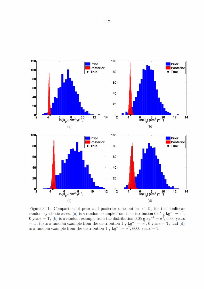
117
2 4 6 8 10 12 140
20
40
60
80
100
120
ln(D0) (cm
2 yr
−1)
Prior
Posterior
True
(a)
2 4 6 8 10 12 140
20
40
60
80
100
ln(D0) (cm
2 yr
−1)
Prior
Posterior
True
(b)
2 4 6 8 10 120
20
40
60
80
100
ln(D0) (cm
2 yr
−1)
Prior
Posterior
True
(c)
2 4 6 8 10 12 140
20
40
60
80
100
ln(D0) (cm
2 yr
−1)
Prior
Posterior
True
(d)
Figure 3.41: Comparison of prior and posterior distributions of D0 for the nonlinearrandom synthetic cases. (a) is a random example from the distribution 0.05 g kg−1 = σ2,0 years = T, (b) is a random example from the distribution 0.05 g kg−1 = σ2, 6000 years= T, (c) is a random example from the distribution 1 g kg−1 = σ2, 0 years = T, and (d)is a random example from the distribution 1 g kg−1 = σ2, 6000 years = T.

118
0 10 20 30 40 50 60 70 80 90 100 110 1200
0.5
1
1.5
ka BP
σ2 F/σ
2 I
6000
0
Figure 3.42: Variance reduction in the posterior (σ2F ) relative to the prior (σ2
I ) for randomsynthetic cases drawn from the distribution 1 g kg−1=σ2, and both 0 and 6000 years = T
dition salinity node at 4K BP has two peaks. There is a strong cross correlation between
the values of these two parameters (not shown). In cases such as these the mean of
the distributions is not a good descriptor of the best estimate for these two parameters.
These double peaked distributions arise because the data is not a strong constraint on
the solution without knowledge of the diffusion coefficient as well.
Figure 3.43 illustrates a promising point about the initial condition parameters, which is
that the top three initial condition nodes are strongly resolved by the synthetic data. The
fourth (bottom) initial condition posterior, however, is almost identical to its prior. The
histograms for the intial conditions in this case are very similar to those in the cases that
have well-resolved diffusion coefficients. We do not particularly care about recovering
the initial conditions, but at the same time we want to avoid arbitrarily choosing an
initial condition that has a strong influence on the boundary condition time series that
is recovered. For this reason it is a promising sign that the initial condition is recovered
fairly well in these examples. In these synthetic examples, the true initial condition is a
vertical line. The measured data after 125,000 years of boundary forcing retain much of
this vertical line. Thus, the data has many points that constrain the initial condition.
Because there are many points that define the straight line in the data, these synthetic
cases may be especially skilled at retaining information about the initial condition.
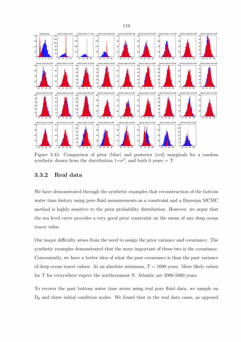
119
4 6 8 10 120
20
40
60
80log(Diffusivity)
32 34 36 380
50
100
150
200
250
300Salinity Node 0 mbsf
32 34 36 380
100
200
300
400Salinity Node 117 mbsf
32 34 36 380
50
100
150
200Salinity Node 233 mbsf
32 34 36 380
20
40
60
80Salinity Node 350 mbsf
32 34 36 380
20
40
60
80Salinity Node 125 ka BP
32 34 36 380
20
40
60
80Salinity Node 110 ka BP
32 34 36 380
20
40
60
80Salinity Node 95 ka BP
32 34 36 380
10
20
30
40
50
60Salinity Node 85 ka BP
32 34 36 380
20
40
60
80Salinity Node 80 ka BP
32 34 36 380
20
40
60
80Salinity Node 75 ka BP
32 34 36 380
10
20
30
40
50
60Salinity Node 70 ka BP
32 34 36 380
10
20
30
40
50
60Salinity Node 65 ka BP
32 34 36 380
20
40
60
80Salinity Node 60 ka BP
32 34 36 380
10
20
30
40
50
60Salinity Node 55 ka BP
32 34 36 380
10
20
30
40
50
60Salinity Node 50 ka BP
32 34 36 380
20
40
60
80Salinity Node 45 ka BP
32 34 36 380
10
20
30
40
50
60Salinity Node 40 ka BP
32 34 36 380
10
20
30
40
50
60Salinity Node 35 ka BP
32 34 36 380
10
20
30
40
50
60Salinity Node 30 ka BP
32 34 36 380
10
20
30
40
50
60Salinity Node 28 ka BP
32 34 36 380
20
40
60
80Salinity Node 26 ka BP
32 34 36 380
20
40
60
80Salinity Node 24 ka BP
32 34 36 380
20
40
60
80Salinity Node 22 ka BP
32 34 36 380
10
20
30
40
50
60Salinity Node 20 ka BP
32 34 36 380
20
40
60
80Salinity Node 18 ka BP
32 34 36 380
20
40
60
80Salinity Node 16 ka BP
32 34 36 380
20
40
60
80Salinity Node 14 ka BP
32 34 36 380
20
40
60
80Salinity Node 12 ka BP
32 34 36 380
10
20
30
40
50
60Salinity Node 10 ka BP
32 34 36 380
20
40
60
80Salinity Node 8 ka BP
32 34 36 380
20
40
60
80Salinity Node 6 ka BP
32 34 36 380
20
40
60
80Salinity Node 4 ka BP
32 34 36 380
20
40
60
80Salinity Node 2 ka BP
32 34 36 380
20
40
60
80
100
120Salinity Node 0 ka BP
Figure 3.43: Comparison of prior (blue) and posterior (red) marginals for a randomsynthetic drawn from the distribution 1=σ2, and both 0 years = T
3.3.2 Real data
We have demonstrated through the synthetic examples that reconstruction of the bottom
water time history using pore fluid measurements as a constraint and a Bayesian MCMC
method is highly sensitive to the prior probability distribution. However, we argue that
the sea level curve provides a very good prior constraint on the mean of any deep ocean
tracer value.
Our major difficulty arises from the need to assign the prior variance and covariance. The
synthetic examples demonstrated that the more important of these two is the covariance.
Conveniently, we have a better idea of what the past covariance is than the past variance
of deep ocean tracer values. At an absolute minimum, T = 1000 years. More likely values
for T for everywhere expect the northernmost N. Atlantic are 2000-5000 years.
To recover the past bottom water time series using real pore fluid data, we sample on
D0 and three initial condition nodes. We found that in the real data cases, as opposed

120
to the synthetic examples, we needed to explicitly fix the top (sediment-water interface)
boundary condition to be equal to the oldest boundary condition, as otherwise it was able
to take on unrealistic values. At z=L, the bottom of the spatial integration domain, we
assign a gradient boundary. The boundary condition at z=L is chosen by computing the
slope of the bottom measured values. When there is data below 150 meters, we compute
this gradient using those points below 150 meters. Otherwise we take the bottommost
five points and compute their slope with depth. The length of the spatial domain in all
of the following cases is 350 meters. In some cases, as will be demonstrated, there are no
data constraints below 150 meters, particularly in δ18O measurements.
Figure 3.44 is a compilation of the mean posterior δ18O recovered at our sites using
extreme values in the prior of σ2 and T. σ2 = 0.2h and σ2 = 0.05 g kg−1 represent
modern-like ocean spread in δ18O and S respectively, while σ2 = 1 is one to two orders
of magnitude larger in order to allow very different solutions into our set. The general
shape of the histories is closely constrained by the prior assumption of the sea level curve,
however each time node has some independence, best exemplified by the results at ODP
1063 and ODP 981.
The δ18O histories at site 1093 are very similar from the LGM to present. The same
can be said for site 1239 with the exception of the case with prior σ2=1 and T = 2000
years. Generally for all of the sites, larger prior variance allows solutions that are very
different in shape than the sea level curve. In fact, the larger variance of the δ18O is not
the reason that the mean changes. Instead, when the prior variance on the time series
nodes is higher, the mean diffusion coefficient recovered is also higher and has a wider
posterior marginal. Allowing more choices of δ18O or S allows more choices of D0, and
vice versa. Indeed, as shown in Figure 3.46, even with widely varying priors the recovered
D0 is very similar at sites 1093, 1123, and 1239. In contrast the recovered D0 at site 1063
varies by a factor of two and at site 981 varies by an order of magnitude.
The initial conditions in δ18O that are recovered, shown in Figure 3.45, are not very
different between different prior assumptions at 1093, 1123 and 1239, but have more
variability at site 981. Because of the covariance of the parameters, the same explanation
applies to the initial conditions as to the diffusion coefficients. A wider range of priors in
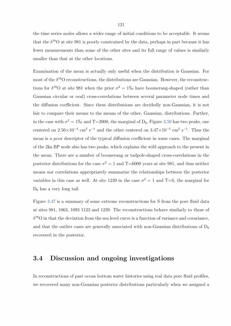
121
the time series nodes allows a wider range of initial conditions to be acceptable. It seems
that the δ18O at site 981 is poorly constrained by the data, perhaps in part because it has
fewer measurements than some of the other sites and its full range of values is similarly
smaller than that at the other locations.
Examination of the mean is actually only useful when the distribution is Gaussian. For
most of the δ18O reconstructions, the distributions are Gaussian. However, the reconstruc-
tions for δ18O at site 981 when the prior σ2 = 1h have boomerang-shaped (rather than
Gaussian circular or oval) cross-correlations between several parameter node times and
the diffusion coefficient. Since these distributions are decidedly non-Gaussian, it is not
fair to compare their means to the means of the other, Gaussian, distributions. Further,
in the case with σ2 = 1h and T=2000, the marginal of D0, Figure 3.50 has two peaks, one
centered on 2.56×10⁻⁴ cm2 s−1 and the other centered on 3.47×10⁻⁵ cm2 s−1. Thus the
mean is a poor descriptor of the typical diffusion coefficient in some cases. The marginal
of the 2ka BP node also has two peaks, which explains the wild approach to the present in
the mean. There are a number of boomerang or tadpole-shaped cross-correlations in the
posterior distributions for the case σ2 = 1 and T=6000 years at site 981, and thus neither
means nor correlations appropriately summarize the relationships between the posterior
variables in this case as well. At site 1239 in the case σ2 = 1 and T=0, the marginal for
D0 has a very long tail.
Figure 3.47 is a summary of some extreme reconstructions for S from the pore fluid data
at sites 981, 1063, 1093 1123 and 1239. The reconstructions behave similarly to those of
δ18O in that the deviation from the sea level curve is a function of variance and covariance,
and that the outlier cases are generally associated with non-Gaussian distributions of D0
recovered in the posterior.
3.4 Discussion and ongoing investigations
In reconstructions of past ocean bottom water histories using real data pore fluid profiles,
we recovered many non-Gaussian posterior distributions particularly when we assigned a
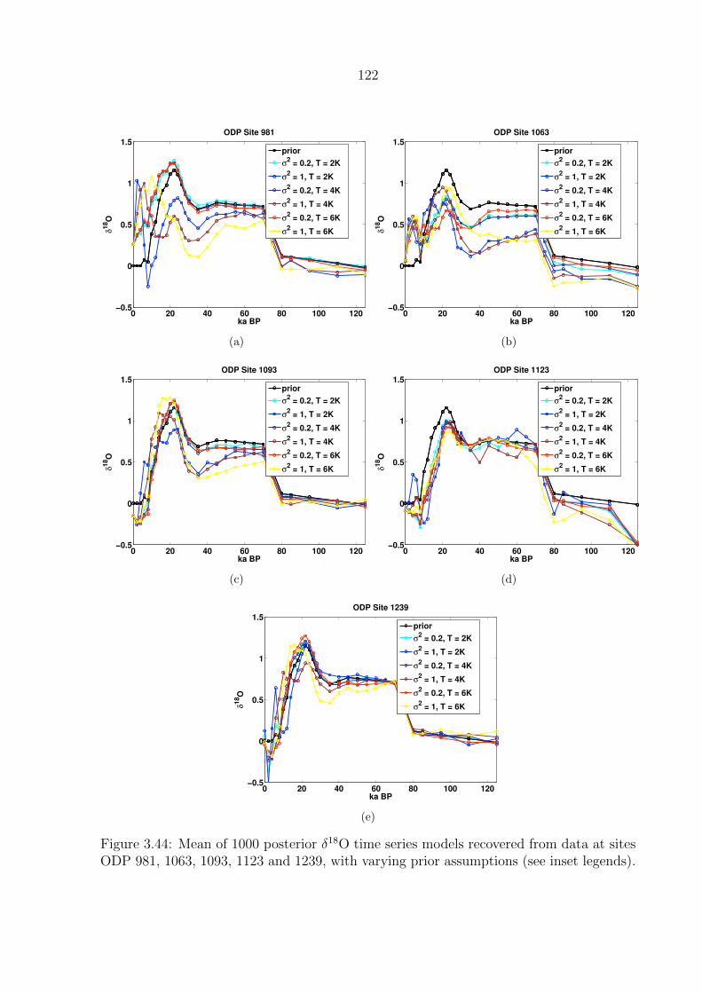
122
0 20 40 60 80 100 120−0.5
0
0.5
1
1.5
ka BP
ODP Site 981
δ18O
prior
σ2 = 0.2, T = 2K
σ2 = 1, T = 2K
σ2 = 0.2, T = 4K
σ2 = 1, T = 4K
σ2 = 0.2, T = 6K
σ2 = 1, T = 6K
(a)
0 20 40 60 80 100 120−0.5
0
0.5
1
1.5
ka BP
ODP Site 1063
δ18O
prior
σ2 = 0.2, T = 2K
σ2 = 1, T = 2K
σ2 = 0.2, T = 4K
σ2 = 1, T = 4K
σ2 = 0.2, T = 6K
σ2 = 1, T = 6K
(b)
0 20 40 60 80 100 120−0.5
0
0.5
1
1.5
ka BP
ODP Site 1093
δ18O
prior
σ2 = 0.2, T = 2K
σ2 = 1, T = 2K
σ2 = 0.2, T = 4K
σ2 = 1, T = 4K
σ2 = 0.2, T = 6K
σ2 = 1, T = 6K
(c)
0 20 40 60 80 100 120−0.5
0
0.5
1
1.5
ka BP
ODP Site 1123δ
18O
prior
σ2 = 0.2, T = 2K
σ2 = 1, T = 2K
σ2 = 0.2, T = 4K
σ2 = 1, T = 4K
σ2 = 0.2, T = 6K
σ2 = 1, T = 6K
(d)
0 20 40 60 80 100 120−0.5
0
0.5
1
1.5
ka BP
ODP Site 1239
δ18O
prior
σ2 = 0.2, T = 2K
σ2 = 1, T = 2K
σ2 = 0.2, T = 4K
σ2 = 1, T = 4K
σ2 = 0.2, T = 6K
σ2 = 1, T = 6K
(e)
Figure 3.44: Mean of 1000 posterior δ18O time series models recovered from data at sitesODP 981, 1063, 1093, 1123 and 1239, with varying prior assumptions (see inset legends).

123
−0.4 −0.2 0 0.2 0.4 0.6
0
50
100
150
200
250
300
350
De
pth
(m
bs
f)
ODP Site981
δ18
O
prior
σ2 = 0.2, T = 2K
σ2 = 1, T = 2K
σ2 = 0.2, T = 4K
σ2 = 1, T = 4K
σ2 = 0.2, T = 6K
σ2 = 1, T = 6K
data
(a)
−2 −1.5 −1 −0.5 0 0.5
0
50
100
150
200
250
300
350
De
pth
(m
bs
f)
ODP Site1063
δ18
O
prior
σ2 = 0.2, T = 2K
σ2 = 1, T = 2K
σ2 = 0.2, T = 4K
σ2 = 1, T = 4K
σ2 = 0.2, T = 6K
σ2 = 1, T = 6K
data
(b)
−0.2 0 0.2 0.4 0.6 0.8
0
50
100
150
200
250
300
350
De
pth
(m
bs
f)
ODP Site1093
δ18
O
prior
σ2 = 0.2, T = 2K
σ2 = 1, T = 2K
σ2 = 0.2, T = 4K
σ2 = 1, T = 4K
σ2 = 0.2, T = 6K
σ2 = 1, T = 6K
data
(c)
−2 −1.5 −1 −0.5 0 0.5
0
50
100
150
200
250
300
350
De
pth
(m
bs
f)
ODP Site1123
δ18
O
prior
σ2 = 0.2, T = 2K
σ2 = 1, T = 2K
σ2 = 0.2, T = 4K
σ2 = 1, T = 4K
σ2 = 0.2, T = 6K
σ2 = 1, T = 6K
data
(d)
−2 −1 0 1 2 3 4
0
50
100
150
200
250
300
350
De
pth
(m
bs
f)
ODP Site1239
δ18
O
prior
σ2 = 0.2, T = 2K
σ2 = 1, T = 2K
σ2 = 0.2, T = 4K
σ2 = 1, T = 4K
σ2 = 0.2, T = 6K
σ2 = 1, T = 6K
data
(e)
Figure 3.45: Mean of 1000 posterior δ18O initial conditions recovered from data at sitesODP 981, 1063, 1093, 1123 and 1239, compared to data (black stars), with varying priorassumptions (see inset legends).
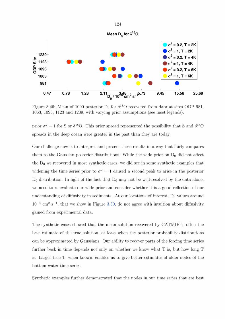
124
0.47 0.78 1.28 2.11 3.48 5.73 9.45 15.58 25.69
981
1063
1093
1123
1239
D0 / 10
−5 cm
2 s
−1
OD
P S
ite
Mean D0 for δ
18O
σ2 = 0.2, T = 2K
σ2 = 1, T = 2K
σ2 = 0.2, T = 4K
σ2 = 1, T = 4K
σ2 = 0.2, T = 6K
σ2 = 1, T = 6K
Figure 3.46: Mean of 1000 posterior D0 for δ18O recovered from data at sites ODP 981,1063, 1093, 1123 and 1239, with varying prior assumptions (see inset legends).
prior σ2 = 1 for S or δ18O. This prior spread represented the possibility that S and δ18O
spreads in the deep ocean were greater in the past than they are today.
Our challenge now is to interpret and present these results in a way that fairly compares
them to the Gaussian posterior distributions. While the wide prior on D0 did not affect
the D0 we recovered in most synthetic cases, we did see in some synthetic examples that
widening the time series prior to σ2 = 1 caused a second peak to arise in the posterior
D0 distribution. In light of the fact that D0 may not be well-resolved by the data alone,
we need to re-evaluate our wide prior and consider whether it is a good reflection of our
understanding of diffusivity in sediments. At our locations of interest, D0 values around
10−4 cm2 s−1, that we show in Figure 3.50, do not agree with intuition about diffusivity
gained from experimental data.
The synthetic cases showed that the mean solution recovered by CATMIP is often the
best estimate of the true solution, at least when the posterior probability distributions
can be approximated by Gaussians. Our ability to recover parts of the forcing time series
further back in time depends not only on whether we know what T is, but how long T
is. Larger true T, when known, enables us to give better estimates of older nodes of the
bottom water time series.
Synthetic examples further demonstrated that the nodes in our time series that are best
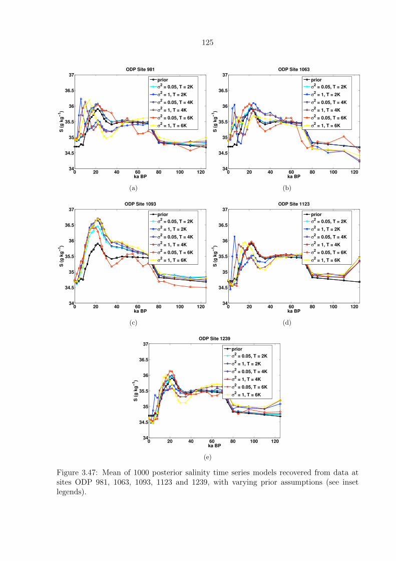
125
0 20 40 60 80 100 12034
34.5
35
35.5
36
36.5
37
ka BP
ODP Site 981
S (
g k
g−
1)
prior
σ2 = 0.05, T = 2K
σ2 = 1, T = 2K
σ2 = 0.05, T = 4K
σ2 = 1, T = 4K
σ2 = 0.05, T = 6K
σ2 = 1, T = 6K
(a)
0 20 40 60 80 100 12034
34.5
35
35.5
36
36.5
37
ka BP
ODP Site 1063
S (
g k
g−
1)
prior
σ2 = 0.05, T = 2K
σ2 = 1, T = 2K
σ2 = 0.05, T = 4K
σ2 = 1, T = 4K
σ2 = 0.05, T = 6K
σ2 = 1, T = 6K
(b)
0 20 40 60 80 100 12034
34.5
35
35.5
36
36.5
37
ka BP
ODP Site 1093
S (
g k
g−
1)
prior
σ2 = 0.05, T = 2K
σ2 = 1, T = 2K
σ2 = 0.05, T = 4K
σ2 = 1, T = 4K
σ2 = 0.05, T = 6K
σ2 = 1, T = 6K
(c)
0 20 40 60 80 100 12034
34.5
35
35.5
36
36.5
37
ka BP
ODP Site 1123
S (
g k
g−
1)
prior
σ2 = 0.05, T = 2K
σ2 = 1, T = 2K
σ2 = 0.05, T = 4K
σ2 = 1, T = 4K
σ2 = 0.05, T = 6K
σ2 = 1, T = 6K
(d)
0 20 40 60 80 100 12034
34.5
35
35.5
36
36.5
37
ka BP
ODP Site 1239
S (
g k
g−
1)
prior
σ2 = 0.05, T = 2K
σ2 = 1, T = 2K
σ2 = 0.05, T = 4K
σ2 = 1, T = 4K
σ2 = 0.05, T = 6K
σ2 = 1, T = 6K
(e)
Figure 3.47: Mean of 1000 posterior salinity time series models recovered from data atsites ODP 981, 1063, 1093, 1123 and 1239, with varying prior assumptions (see insetlegends).
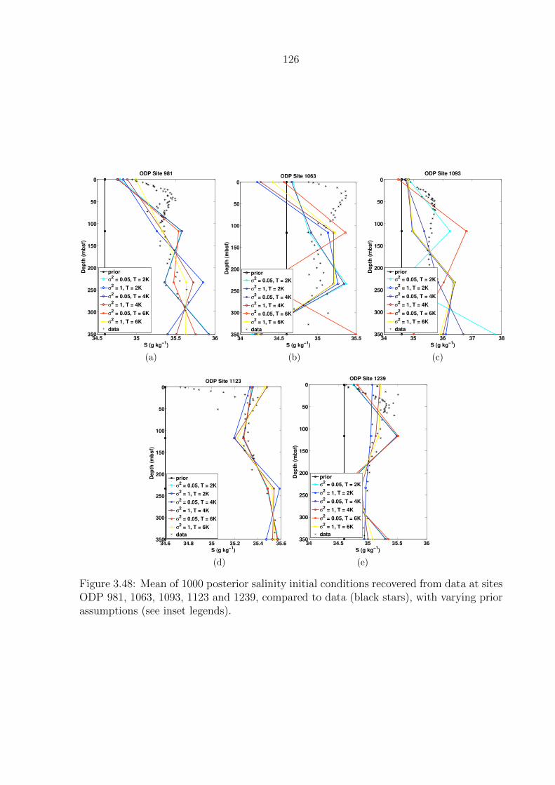
126
34.5 35 35.5 36
0
50
100
150
200
250
300
350
De
pth
(m
bs
f)
ODP Site 981
S (g kg−1
)
prior
σ2 = 0.05, T = 2K
σ2 = 1, T = 2K
σ2 = 0.05, T = 4K
σ2 = 1, T = 4K
σ2 = 0.05, T = 6K
σ2 = 1, T = 6K
data
(a)
34 34.5 35 35.5
0
50
100
150
200
250
300
350
De
pth
(m
bs
f)
ODP Site 1063
S (g kg−1
)
prior
σ2 = 0.05, T = 2K
σ2 = 1, T = 2K
σ2 = 0.05, T = 4K
σ2 = 1, T = 4K
σ2 = 0.05, T = 6K
σ2 = 1, T = 6K
data
(b)
34 35 36 37 38
0
50
100
150
200
250
300
350
De
pth
(m
bs
f)
ODP Site 1093
S (g kg−1
)
prior
σ2 = 0.05, T = 2K
σ2 = 1, T = 2K
σ2 = 0.05, T = 4K
σ2 = 1, T = 4K
σ2 = 0.05, T = 6K
σ2 = 1, T = 6K
data
(c)
34.6 34.8 35 35.2 35.4 35.6
0
50
100
150
200
250
300
350
De
pth
(m
bs
f)
ODP Site 1123
S (g kg−1
)
prior
σ2 = 0.05, T = 2K
σ2 = 1, T = 2K
σ2 = 0.05, T = 4K
σ2 = 1, T = 4K
σ2 = 0.05, T = 6K
σ2 = 1, T = 6K
data
(d)
34 34.5 35 35.5 36
0
50
100
150
200
250
300
350
De
pth
(m
bs
f)
ODP Site 1239
S (g kg−1
)
prior
σ2 = 0.05, T = 2K
σ2 = 1, T = 2K
σ2 = 0.05, T = 4K
σ2 = 1, T = 4K
σ2 = 0.05, T = 6K
σ2 = 1, T = 6K
data
(e)
Figure 3.48: Mean of 1000 posterior salinity initial conditions recovered from data at sitesODP 981, 1063, 1093, 1123 and 1239, compared to data (black stars), with varying priorassumptions (see inset legends).
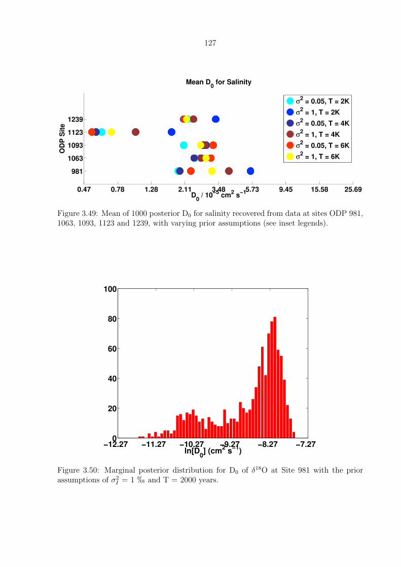
127
0.47 0.78 1.28 2.11 3.48 5.73 9.45 15.58 25.69
981
1063
1093
1123
1239
D0 / 10
−5 cm
2 s
−1
OD
P S
ite
Mean D0 for Salinity
σ2 = 0.05, T = 2K
σ2 = 1, T = 2K
σ2 = 0.05, T = 4K
σ2 = 1, T = 4K
σ2 = 0.05, T = 6K
σ2 = 1, T = 6K
Figure 3.49: Mean of 1000 posterior D0 for salinity recovered from data at sites ODP 981,1063, 1093, 1123 and 1239, with varying prior assumptions (see inset legends).
−12.27 −11.27 −10.27 −9.27 −8.27 −7.270
20
40
60
80
100
ln[D0] (cm
2 s
−1)
Figure 3.50: Marginal posterior distribution for D0 of δ18O at Site 981 with the priorassumptions of σ2
I = 1 h and T = 2000 years.

128
resolved by the data fall roughly within the most recent 10,000 years before present.
We are certain that there is very little additional information (beyond the information
encapsulated in the prior) that can be recovered earlier than 20,000 years ago. Depending
on the prior information we provide, the same data can be consistent with an LGM
salinity/δ18O either short in duration and high in magnitude or one that lasted longer
and was lower magnitude.
When the prior variance is large, the time series we recover increasingly resembles a
smoothed version of the true forcing history the further we look back in time. The
smoothing will tend to underestimate maxima and overestimate minima, as well as alias
information into different times. However, the LGM values for high prior variance prob-
ably underestimate the true LGM values.
Figure 3.51 shows the LGM values of S and δ18O for various prior assumptions. At the
LGM, the salinity at site 1093 is always greater than that at the other sites. While it
could be greater, the value at 1093 was mean ∼ 36.6. This is 0.5 lower than the mean
estimate of Adkins et al. (2002). Other robust features of the LGM, irrespective of prior
assumptions, are that the salinity at site 981 is greater than that at 1063, and 1239 has
higher salinity than 1123.
Our results differ from the estimates of Adkins et al. (2002) most strikingly in the LGM
salinity at ODP site 1093. The diffusion coefficients we recover are quite similar to their
estimate of 2×10⁻⁵ cm2 s−1, such that we can not explain the difference solely through
a different diffusion coefficient. We will need to investigate the details of the cause of
this large change in solution more carefully, but we hypothesize that the ability of our
boundary forcing to vary from a stretched sea level curve can account for much of the
difference. Recall the synthetic stretched sea level example shown in Figures 3.13-3.19
produced the same output with a low, wide high salinity in the past as a highly peaked
LGM salinity signal. In general, stretching the sea level by a single scaling constant has
the effect of narrowing the shape of the LGM relative to its sea level signal. Our solutions
with a longer period of moderately high salinity can produce a similar residual signal in
the modern sediment concentration profile as would a sharp and rapid peak in salinity.
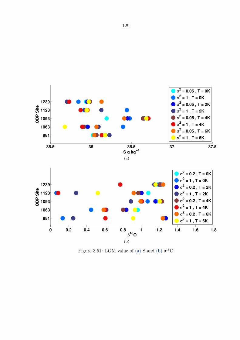
129
35.5 36 36.5 37 37.5
981
1063
1093
1123
1239
S g kg−1
OD
P S
ite
σ2 = 0.05 , T = 0K
σ2 = 1 , T = 0K
σ2 = 0.05 , T = 2K
σ2 = 1 , T = 2K
σ2 = 0.05 , T = 4K
σ2 = 1 , T = 4K
σ2 = 0.05 , T = 6K
σ2 = 1 , T = 6K
(a)
0 0.2 0.4 0.6 0.8 1 1.2 1.4 1.6 1.8
981
1063
1093
1123
1239
δ18
O
OD
P S
ite
σ2 = 0.2 , T = 0K
σ2 = 1 , T = 0K
σ2 = 0.2 , T = 2K
σ2 = 1 , T = 2K
σ2 = 0.2 , T = 4K
σ2 = 1 , T = 4K
σ2 = 0.2 , T = 6K
σ2 = 1 , T = 6K
(b)
Figure 3.51: LGM value of (a) S and (b) δ18O

130
Salinity
Θ0
34.5 35 35.5 36 36.5 37 37.5
−4
−3
−2
−1
0
1
2
3
(a)
Salinity
Θ0
34.5 35 35.5 36 36.5 37 37.5
−2
−1
0
1
2
3
(b)
Figure 3.52: T/S plots with LGM reconstructions using σ2 = 1 for both δ18O and S (red)compared to Adkins et al. (2002) (blue) and modern (orange). Here we take the LGMas the time with maximum in S. (a) uses a prior with T = 0 years while (b) uses a priorwith T = 6000 years
Salinity
Θ0
34.5 35 35.5 36 36.5 37 37.5
−2
−1
0
1
2
3
(a)
Salinity
Θ0
34.5 35 35.5 36 36.5 37 37.5
−3
−2
−1
0
1
2
3
(b)
Figure 3.53: T/S plots with LGM reconstructions using σ2 = 0.05 for S and =0.1 for δ18O(red) compared to Adkins et al. (2002) (blue) and modern (orange). Here we take theLGM as the time with maximum in S. (a) uses a prior with T = 0 years while (b) uses aprior with T = 6000 years
131
Considering the reconstruction of temperature and salinity at the LGM, shown for dif-
ferent prior assumptions in Figures 3.53 and 3.52, we see that the spatial distribution
of density is a stronger function of variance than covariance. With large prior variance,
Figure 3.52, assigning a longer covariance does not significantly change the distribution
of LGM temperature and salinity. In contrast, when our prior variance is quite narrow,
Figure 3.53, the posterior spread of temperature and salinity is similarly narrow, whether
or not we assign a long covariance timescale in the prior.
There is a great deal of variability in the δ18O reconstructed using this method, both
at each site and spatially. The spatial differences in δ18O would suggest that there is a
strong local component of δ18O that could tell us about variations in glacier mass wasting
through the deglaciation.
The δ18O and S histories at a given site are not constrained to follow the same shape
curve, and thus their reconstructions have different shapes. If we knew T, we could use
this information to look at the evolution of water mass histories, using a combination of
δ18O and S. The reconstructed time history’s evolution from the LGM to the present is a
strong function of T.
Both the salinity and δ18O histories at site 1123 and site 1239 show a reversal in direction
in the last 6000 years that is independent of the prior T, and σ2 and seems to reflect
an inflection in slope in the upper parts of the sediment pore fluid profile measurements.
While these sites are both in the Pacific, they are not in the same water mass today, as
demonstrated by the salinity contour plots in Figure 3.54. Site 1123 lies in what is mostly
Antarctic Bottom Water (AABW) while Site 1239 is in Pacific Deep Water (PDW). The
salinity of PDW today is set primarily by upward diffusion of AABW. The average vertical
diffusivity in the Pacific implied by optimization calculations is quite high relative to the
rest of the abyssal ocean (Talley, 2013).
The concomitant reversal in direction of δ18O and S suggests either a glaciological source or
precipitation for their changes. A change in glacial meltwater fraction and precipitation
fraction in these water masses would have similar signals. Sea ice is not light in δ18O
relative to ocean water, however a large snow accumulation on the sea ice could also have

132
a precipitation-like signal in δ18O.
Glacier regrowth in the Holocene could in theory cause a reversal in the salinity and δ18O
trend in the ocean. While most reconstructions of the sea level curve over the most recent
deglaciation show a monotonic approach to present, the error bars on individually dated
sea level estimates are large enough to allow for the possibility of a reversal in direction.
The approach to present sea level from the LGM is best constrained by dating fossil
Acropora palmata coral reefs, which live between -5 and -1 meters relative to the sea level
(msl). In some cases A. palmata can survive until -17 msl (Bruckner, 2002), but this is
considered rare enough that error bars on depths determined by dating A. palmata are
typically +5 m. Sea level rise from the last deglaciation either halted or slowed around
4 ka BP (Milne and Mitrovica, 2008, Toscano et al., 2011), where coral estimates reach
less than -5 msl. As early as 3657 ±120 BP there are A. palmata samples from St. Croix
measuring -3.08 msl (Toscano et al., 2011). The +5 m error on these records allow for
the possibility that sea level has dropped as much as 1.2 m between 4 ka BP and present
due to glacier regrowth. The St. Croix records agree with records in Tahiti of a ∼-2 msl
A. robusta sample dated to 5040 ± 40 BP (Bard et al., 1996).
In the mean ocean δ18O, 1-5 m of missing sea level represented by error bars on A.
palmata sea level reconstructions are almost imperceptible. Using the rectangular box
ocean scaling with a modern mean depth of 3800 m and assuming that the melted glacier
has -40h δ18O, a melting of an ice volume equivalent to 5 m of sea level is equivalent to
-0.05h when distributed over the ocean. Then 1 m would yield a mean ocean change of
-0.01h. Despite the fact that ODP Sites 1123 and 1239 show a robust reversal in the
mean, -0.01h is smaller than the error bar on any value of δ18O, such that the other sites
could be feeling the mean change as well. In contrast, the reversal in δ18O at ODP 1123
and 1239 is as much as -0.25h with respect to present values. One explanation for this
large signal in δ18O is that the changes were isolated to the Pacific. A second explanation
is that there is some aliasing in the reconstruction such that the minimum excursion is
an underestimate of the true value.
The modern distribution of δ18O, however, clearly demonstrates a local component, and
we can expect the local histories to be independent of the global mean, particularly during

133
adjustment. Adjustments to the global mean sea level are felt immediately at the surface
of the ocean, where the water is added, while the deep ocean may not sense a mean change
for thousands of years. Surface adjustments in the N. Atlantic are felt quite quickly in the
deep N. Atlantic. If the reversal we see is due to a glacier regrowth, the signal is unlikely
to originate from the N. Atlantic as the effect on deep water δ18O would be first felt there
before propagating to the Pacfic. Instead we propose that we see something that is either
limited to the Pacific or that originates in the Pacific. The signal we see in the Pacific
could be still propagating to the Atlantic today with a few thousand year lag.
The timing of the salinity and δ18O trend reversal in the Pacific cores may not correspond
to the timing of their forcing. We could be seeing the adjustment of the Pacific after
Meltwater pulse 1-A or 1-B. As the Pacific is thought to have the most inertia of all the
ocean basins, the meltwater pulses would take the longest time both to reach and to leave
the Pacific sites.
Glacier regrowth would remove water from the ocean and increase the mean ocean salinity
and δ18O. However, our reconstructions of bottom water salinity and δ18O in the Atlantic
do not show concrete evidence of either of these scenarios, which indicates the process
is concentrated in the Pacific or that the effects are felt most strongly in SAMW and
AAIW formation in the Pacific. Thus, we expect that this process, either the final surge
of glacial melt or the glacier regrowth happened in the Antarctic Ice Sheet.
Recent studies of the formation of Subantarctic Mode Water (SAMW) and Antarctic
Intermediate Water (AAIW) suggest that the formation of these two water masses is
zonally asymmetric, and happens predominantly in the Pacific sector of the Southern
Ocean (Sallee et al., 2010, Hartin et al., 2011). SAMW formation is driven by wintertime
deep convection, and the densest classes of SAMW contribute to the properties of AAIW.
The salinity of SAMW and AAIW are between 34 and 34.5 (Sloyan and Rintoul, 2001).
A greater contribution of SAMW and/or AAIW to the compositions of Pacific bottom
waters relative to today could easily explain the late Holocene salinity and δ18O signal in
Site 1123 and 1239, even without any change in their salinities.
We may be seeing a shift of a front in the Pacific sector of the Southern Ocean. The

134
exact position of iceberg melt is poorly constrained (Tournadre et al., 2012), but icebergs
are seldom found north of 60◦S in the South Pacific. This contrasts with the S. Atlantic
in which icebergs are found as far north as 45◦S. The Polar and Subantarctic fronts in
the S. Pacific are southward of their positions in the Indian and Atlantic Ocean. A
poleward contraction of the ACC fronts could shift the position of the fresh meltwater
input southward. Water subducted as Subantarctic Mode Water would thus become
saltier. The transport of Subantarctic Mode Water today goes through the Pacific before
returning to the Atlantic. Before returning to the Atlantic, the signal may mix out
throughout the Pacific basin, which is a very large volume of water. Alternatively, if
the lag between Pacific and Atlantic is several thousand years long, the salinification of
SAMW due to glacial regrowth may be just being felt now in the Atlantic deep water. If
the signal we see in the Pacific sites is a shift in circumpolar fronts, that could explain
differences between 1093 and 1123 because 1123 is farther north than 1093.
3.5 Conclusions
The distributions of the bottom water time series solutions that we recover from the
pore fluid profiles are highly sensitive to our prior assumptions, reflecting the ill-posed
nature of an inverse diffusion problem. Bayesian MCMC methods allow us to explicitly
describe our prior biases and uncertainties in physical terms and are additionally much
less sensitive to noisy data than are regularized least squares methods. Given our modern
understanding of the ocean and its history, the spread in salinities at the LGM did not
need to be as high as reported in Adkins et al. (2002) to produce the measured pore
fluid profiles. We show that the diffusion coefficient at each site is generally well-resolved,
but our wide prior on the diffusion coefficient allows some posterior distributions that
are implausible, requiring a re-evaluation of our technique. Our technique allows us to
reconstruct time series over the most recent deglaciation with high confidence, and we
find that the evolution of salinity and δ18O during the Holocene contrasts between the
Atlantic and the Pacific. Our method allows us to extract time variable local information
from each site over and above the information we have from sea level records. Local
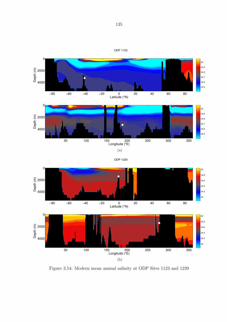
135
Latitude (°N)
Depth
(m
)
−80 −60 −40 −20 0 20 40 60 80
0
2000
4000
34.5
34.6
34.7
34.8
34.9
35
34.5
34.6
34.7
34.8
34.9
35
ODP 1123
Longitude (°E)
De
pth
(m
)
50 100 150 200 250 300 350
0
2000
4000
(a)
Latitude (°N)
De
pth
(m
)
−80 −60 −40 −20 0 20 40 60 80
0
2000
4000
34
34.2
34.4
34.6
34.8
35
34
34.2
34.4
34.6
34.8
35
ODP 1239
Longitude (°E)
De
pth
(m
)
50 100 150 200 250 300 350
0
2000
4000
(b)
Figure 3.54: Modern mean annual salinity at ODP Sites 1123 and 1239

136
differences can be extracted from the data that differ between the Atlantic and Pacific,
supporting a variety of interesting hypotheses about the progression of sea level rise or
evolution of Southern Ocean dynamics between the LGM and today.
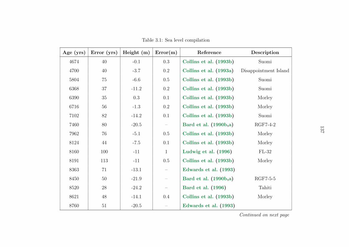
137
Table 3.1: Sea level compilation
Age (yrs) Error (yrs) Height (m) Error(m) Reference Description
4674 40 -0.1 0.3 Collins et al. (1993b) Suomi
4700 40 -3.7 0.2 Collins et al. (1993a) Disappointment Island
5804 75 -6.6 0.5 Collins et al. (1993b) Suomi
6368 37 -11.2 0.2 Collins et al. (1993b) Suomi
6390 35 0.3 0.1 Collins et al. (1993b) Morley
6716 56 -1.3 0.2 Collins et al. (1993b) Morley
7102 82 -14.2 0.1 Collins et al. (1993b) Suomi
7460 80 -20.5 – Bard et al. (1990b,a) RGF7-4-2
7962 76 -5.1 0.5 Collins et al. (1993b) Morley
8124 44 -7.5 0.1 Collins et al. (1993b) Morley
8160 100 -11 1 Ludwig et al. (1996) FL-32
8191 113 -11 0.5 Collins et al. (1993b) Morley
8363 71 -13.1 – Edwards et al. (1993)
8450 50 -21.9 – Bard et al. (1990b,a) RGF7-5-5
8520 28 -24.2 – Bard et al. (1996) Tahiti
8621 48 -14.1 0.4 Collins et al. (1993b) Morley
8760 51 -20.5 – Edwards et al. (1993)
Continued on next page
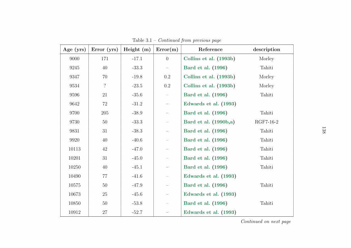
138
Table 3.1 – Continued from previous page
Age (yrs) Error (yrs) Height (m) Error(m) Reference description
9000 171 -17.1 0 Collins et al. (1993b) Morley
9245 40 -33.3 – Bard et al. (1996) Tahiti
9347 70 -19.8 0.2 Collins et al. (1993b) Morley
9534 ? -23.5 0.2 Collins et al. (1993b) Morley
9596 21 -35.6 – Bard et al. (1996) Tahiti
9642 72 -31.2 – Edwards et al. (1993)
9700 205 -38.9 – Bard et al. (1996) Tahiti
9730 50 -33.3 – Bard et al. (1990b,a) RGF7-16-2
9831 31 -38.3 – Bard et al. (1996) Tahiti
9920 40 -40.6 – Bard et al. (1996) Tahiti
10113 42 -47.0 – Bard et al. (1996) Tahiti
10201 31 -45.0 – Bard et al. (1996) Tahiti
10250 40 -45.1 – Bard et al. (1996) Tahiti
10490 77 -41.6 – Edwards et al. (1993)
10575 50 -47.9 – Bard et al. (1996) Tahiti
10673 25 -45.6 – Edwards et al. (1993)
10850 50 -53.8 – Bard et al. (1996) Tahiti
10912 27 -52.7 – Edwards et al. (1993)
Continued on next page
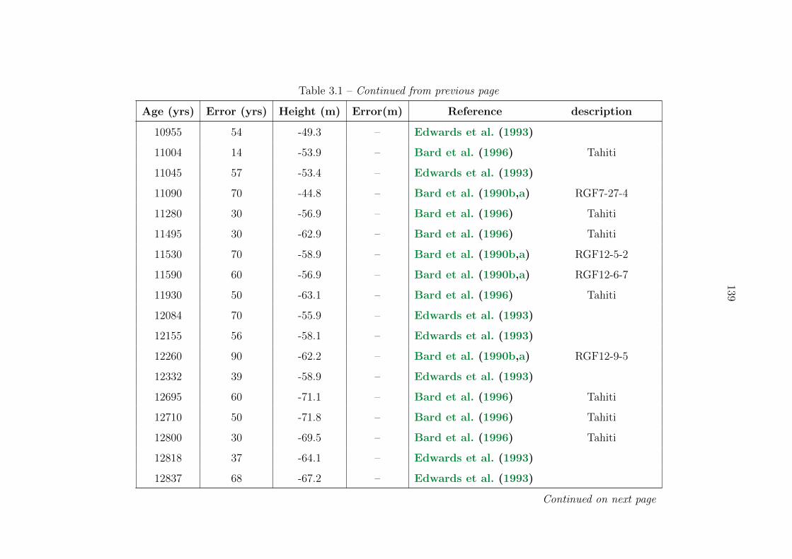
139
Table 3.1 – Continued from previous page
Age (yrs) Error (yrs) Height (m) Error(m) Reference description
10955 54 -49.3 – Edwards et al. (1993)
11004 14 -53.9 – Bard et al. (1996) Tahiti
11045 57 -53.4 – Edwards et al. (1993)
11090 70 -44.8 – Bard et al. (1990b,a) RGF7-27-4
11280 30 -56.9 – Bard et al. (1996) Tahiti
11495 30 -62.9 – Bard et al. (1996) Tahiti
11530 70 -58.9 – Bard et al. (1990b,a) RGF12-5-2
11590 60 -56.9 – Bard et al. (1990b,a) RGF12-6-7
11930 50 -63.1 – Bard et al. (1996) Tahiti
12084 70 -55.9 – Edwards et al. (1993)
12155 56 -58.1 – Edwards et al. (1993)
12260 90 -62.2 – Bard et al. (1990b,a) RGF12-9-5
12332 39 -58.9 – Edwards et al. (1993)
12695 60 -71.1 – Bard et al. (1996) Tahiti
12710 50 -71.8 – Bard et al. (1996) Tahiti
12800 30 -69.5 – Bard et al. (1996) Tahiti
12818 37 -64.1 – Edwards et al. (1993)
12837 68 -67.2 – Edwards et al. (1993)
Continued on next page
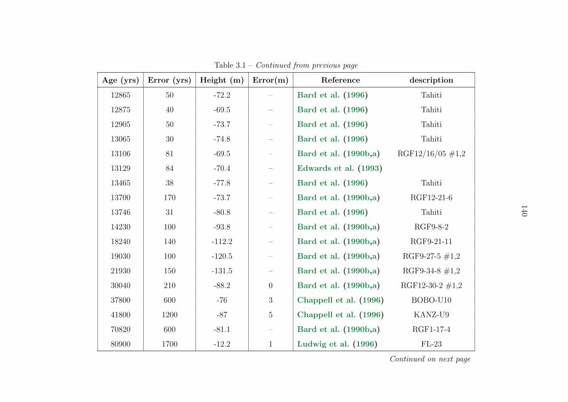
140
Table 3.1 – Continued from previous page
Age (yrs) Error (yrs) Height (m) Error(m) Reference description
12865 50 -72.2 – Bard et al. (1996) Tahiti
12875 40 -69.5 – Bard et al. (1996) Tahiti
12905 50 -73.7 – Bard et al. (1996) Tahiti
13065 30 -74.8 – Bard et al. (1996) Tahiti
13106 81 -69.5 – Bard et al. (1990b,a) RGF12/16/05 #1,2
13129 84 -70.4 – Edwards et al. (1993)
13465 38 -77.8 – Bard et al. (1996) Tahiti
13700 170 -73.7 – Bard et al. (1990b,a) RGF12-21-6
13746 31 -80.8 – Bard et al. (1996) Tahiti
14230 100 -93.8 – Bard et al. (1990b,a) RGF9-8-2
18240 140 -112.2 – Bard et al. (1990b,a) RGF9-21-11
19030 100 -120.5 – Bard et al. (1990b,a) RGF9-27-5 #1,2
21930 150 -131.5 – Bard et al. (1990b,a) RGF9-34-8 #1,2
30040 210 -88.2 0 Bard et al. (1990b,a) RGF12-30-2 #1,2
37800 600 -76 3 Chappell et al. (1996) BOBO-U10
41800 1200 -87 5 Chappell et al. (1996) KANZ-U9
70820 600 -81.1 – Bard et al. (1990b,a) RGF1-17-4
80900 1700 -12.2 1 Ludwig et al. (1996) FL-23
Continued on next page
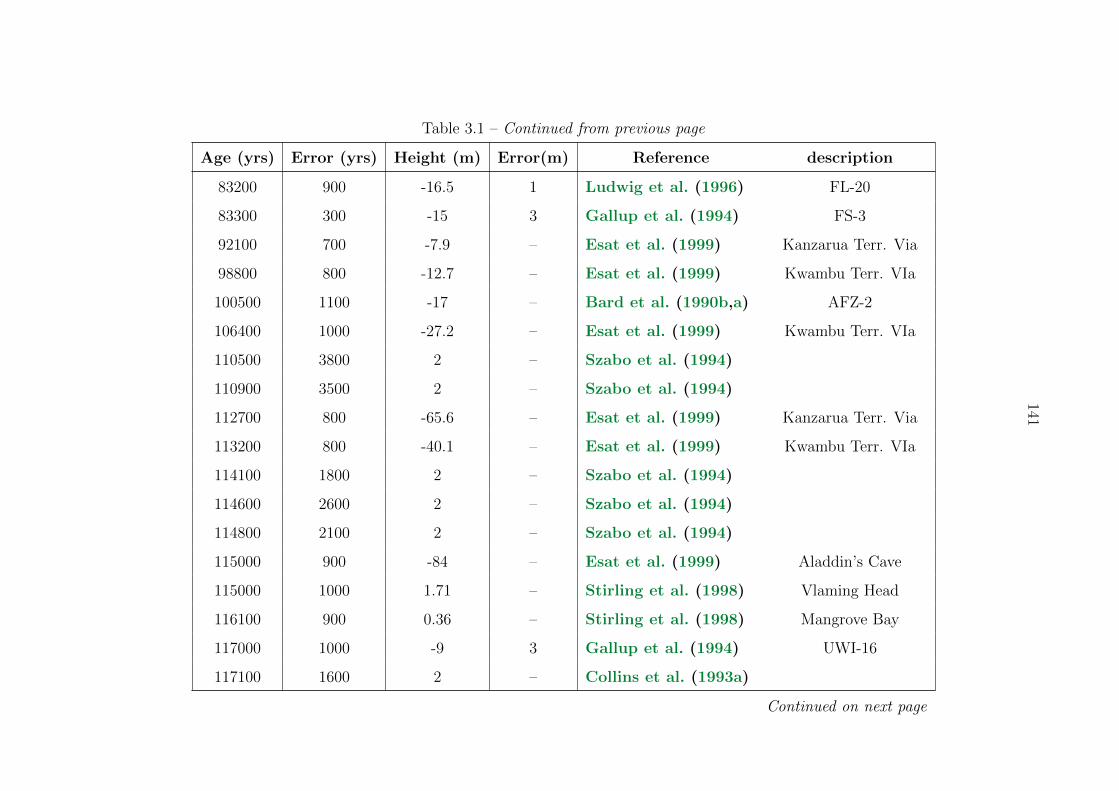
141
Table 3.1 – Continued from previous page
Age (yrs) Error (yrs) Height (m) Error(m) Reference description
83200 900 -16.5 1 Ludwig et al. (1996) FL-20
83300 300 -15 3 Gallup et al. (1994) FS-3
92100 700 -7.9 – Esat et al. (1999) Kanzarua Terr. Via
98800 800 -12.7 – Esat et al. (1999) Kwambu Terr. VIa
100500 1100 -17 – Bard et al. (1990b,a) AFZ-2
106400 1000 -27.2 – Esat et al. (1999) Kwambu Terr. VIa
110500 3800 2 – Szabo et al. (1994)
110900 3500 2 – Szabo et al. (1994)
112700 800 -65.6 – Esat et al. (1999) Kanzarua Terr. Via
113200 800 -40.1 – Esat et al. (1999) Kwambu Terr. VIa
114100 1800 2 – Szabo et al. (1994)
114600 2600 2 – Szabo et al. (1994)
114800 2100 2 – Szabo et al. (1994)
115000 900 -84 – Esat et al. (1999) Aladdin’s Cave
115000 1000 1.71 – Stirling et al. (1998) Vlaming Head
116100 900 0.36 – Stirling et al. (1998) Mangrove Bay
117000 1000 -9 3 Gallup et al. (1994) UWI-16
117100 1600 2 – Collins et al. (1993a)
Continued on next page
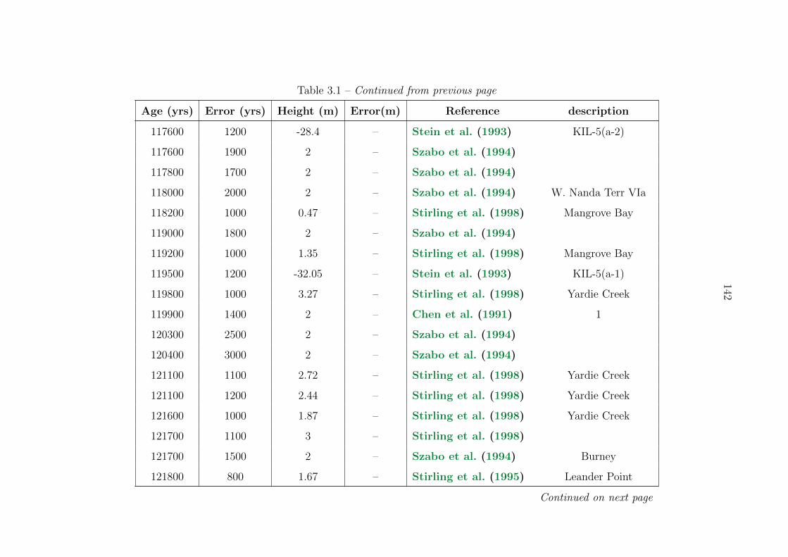
142
Table 3.1 – Continued from previous page
Age (yrs) Error (yrs) Height (m) Error(m) Reference description
117600 1200 -28.4 – Stein et al. (1993) KIL-5(a-2)
117600 1900 2 – Szabo et al. (1994)
117800 1700 2 – Szabo et al. (1994)
118000 2000 2 – Szabo et al. (1994) W. Nanda Terr VIa
118200 1000 0.47 – Stirling et al. (1998) Mangrove Bay
119000 1800 2 – Szabo et al. (1994)
119200 1000 1.35 – Stirling et al. (1998) Mangrove Bay
119500 1200 -32.05 – Stein et al. (1993) KIL-5(a-1)
119800 1000 3.27 – Stirling et al. (1998) Yardie Creek
119900 1400 2 – Chen et al. (1991) 1
120300 2500 2 – Szabo et al. (1994)
120400 3000 2 – Szabo et al. (1994)
121100 1100 2.72 – Stirling et al. (1998) Yardie Creek
121100 1200 2.44 – Stirling et al. (1998) Yardie Creek
121600 1000 1.87 – Stirling et al. (1998) Yardie Creek
121700 1100 3 – Stirling et al. (1998)
121700 1500 2 – Szabo et al. (1994) Burney
121800 800 1.67 – Stirling et al. (1995) Leander Point
Continued on next page
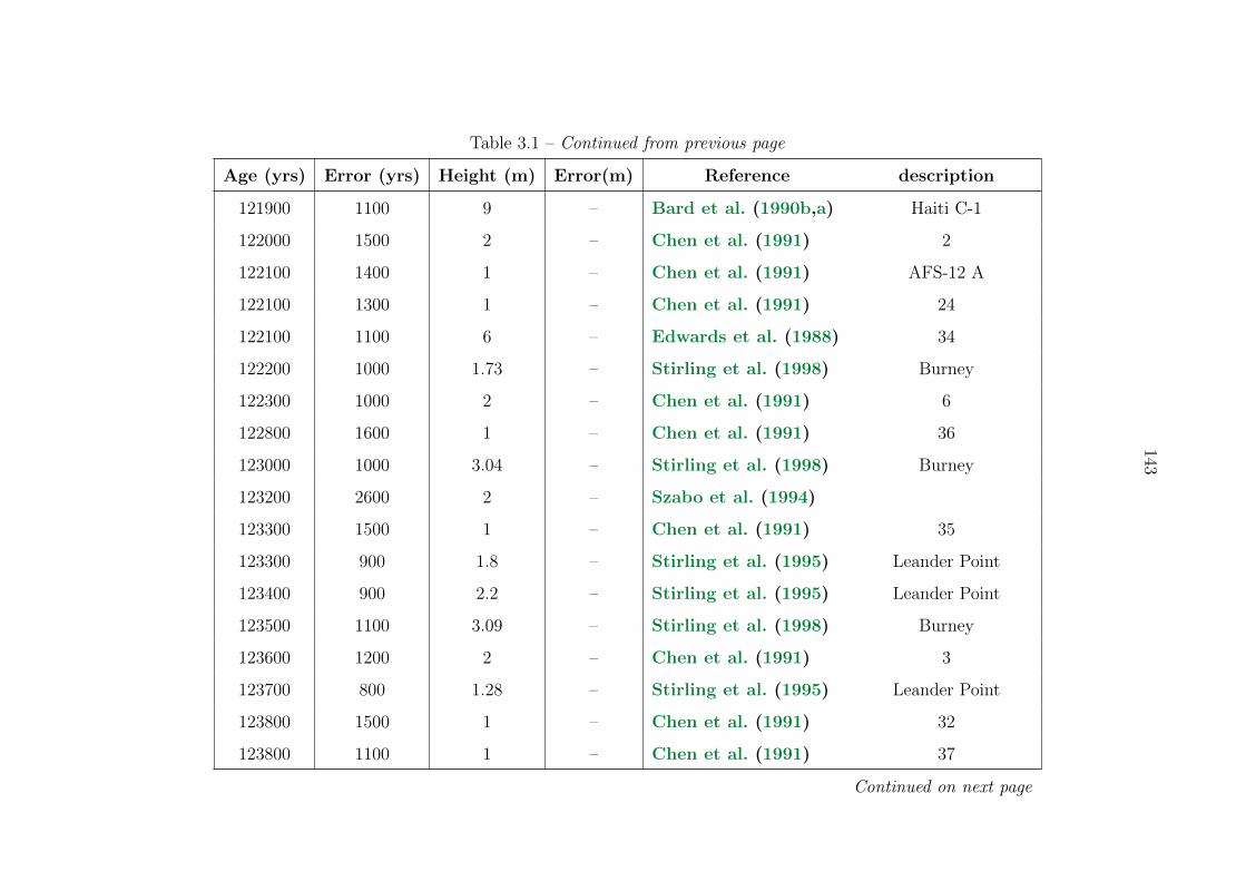
143
Table 3.1 – Continued from previous page
Age (yrs) Error (yrs) Height (m) Error(m) Reference description
121900 1100 9 – Bard et al. (1990b,a) Haiti C-1
122000 1500 2 – Chen et al. (1991) 2
122100 1400 1 – Chen et al. (1991) AFS-12 A
122100 1300 1 – Chen et al. (1991) 24
122100 1100 6 – Edwards et al. (1988) 34
122200 1000 1.73 – Stirling et al. (1998) Burney
122300 1000 2 – Chen et al. (1991) 6
122800 1600 1 – Chen et al. (1991) 36
123000 1000 3.04 – Stirling et al. (1998) Burney
123200 2600 2 – Szabo et al. (1994)
123300 1500 1 – Chen et al. (1991) 35
123300 900 1.8 – Stirling et al. (1995) Leander Point
123400 900 2.2 – Stirling et al. (1995) Leander Point
123500 1100 3.09 – Stirling et al. (1998) Burney
123600 1200 2 – Chen et al. (1991) 3
123700 800 1.28 – Stirling et al. (1995) Leander Point
123800 1500 1 – Chen et al. (1991) 32
123800 1100 1 – Chen et al. (1991) 37
Continued on next page

144
Table 3.1 – Continued from previous page
Age (yrs) Error (yrs) Height (m) Error(m) Reference description
123800 900 0.7 – Stirling et al. (1995) Leander Point
124000 2000 1.8 0.1 Collins et al. (1993a)
124000 1200 2 – Szabo et al. (1994)
124100 1500 2.16 – Stirling et al. (1995) Leander Point
124200 900 0.68 – Stirling et al. (1995) Leander Point
124300 1000 1.2 – Stirling et al. (1998) Tantabiddi Bay
124500 1300 6 – Edwards et al. (1988) C
124700 1000 2.3 – Stirling et al. (1998) Yardie Creek
124800 1100 0.92 – Stirling et al. (1998) Vlaming Head
124900 1300 8 – Bard et al. (1990b,a) Haiti C-4 #1,2
124900 2100 0 – Chen et al. (1991) 29
125000 3800 2 – Szabo et al. (1994)
125100 1000 8 – Bard et al. (1990b,a) AFM3 #1,2
125100 1300 2 – Szabo et al. (1994)
125400 900 1.83 – Stirling et al. (1995) Rottnest Is.
125400 1100 0.92 – Stirling et al. (1998) Vlaming Head
125400 1100 1.79 – Stirling et al. (1998) Mangrove Bay
125500 800 0.45 – Stirling et al. (1995) Rottnest Is.
Continued on next page
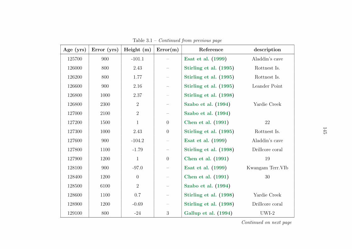
145
Table 3.1 – Continued from previous page
Age (yrs) Error (yrs) Height (m) Error(m) Reference description
125700 900 -101.1 – Esat et al. (1999) Aladdin’s cave
126000 800 2.43 – Stirling et al. (1995) Rottnest Is.
126200 800 1.77 – Stirling et al. (1995) Rottnest Is.
126600 900 2.16 – Stirling et al. (1995) Leander Point
126800 1000 2.37 – Stirling et al. (1998)
126800 2300 2 – Szabo et al. (1994) Yardie Creek
127000 2100 2 – Szabo et al. (1994)
127200 1500 1 0 Chen et al. (1991) 22
127300 1000 2.43 0 Stirling et al. (1995) Rottnest Is.
127600 900 -104.2 – Esat et al. (1999) Aladdin’s cave
127800 1100 -1.79 – Stirling et al. (1998) Drillcore coral
127900 1200 1 0 Chen et al. (1991) 19
128100 900 -97.0 – Esat et al. (1999) Kwangam Terr.VIb
128400 1200 0 – Chen et al. (1991) 30
128500 6100 2 – Szabo et al. (1994)
128600 1100 0.7 – Stirling et al. (1998) Yardie Creek
128900 1200 -0.69 – Stirling et al. (1998) Drillcore coral
129100 800 -24 3 Gallup et al. (1994) UWI-2
Continued on next page
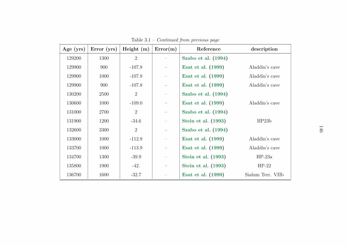
146
Table 3.1 – Continued from previous page
Age (yrs) Error (yrs) Height (m) Error(m) Reference description
129200 1300 2 – Szabo et al. (1994)
129900 900 -107.8 – Esat et al. (1999) Aladdin’s cave
129900 1000 -107.8 – Esat et al. (1999) Aladdin’s cave
129900 900 -107.8 – Esat et al. (1999) Aladdin’s cave
130200 2500 2 – Szabo et al. (1994)
130600 1000 -109.0 – Esat et al. (1999) Aladdin’s cave
131000 2700 2 – Szabo et al. (1994)
131900 1200 -34.6 – Stein et al. (1993) HP23b
132600 3300 2 – Szabo et al. (1994)
133000 1000 -112.8 – Esat et al. (1999) Aladdin’s cave
133700 1000 -113.9 – Esat et al. (1999) Aladdin’s cave
134700 1300 -39.9 – Stein et al. (1993) HP-23a
135800 1900 -42. – Stein et al. (1993) HP-22
136700 1600 -32.7 – Esat et al. (1999) Sialum Terr. VIIb
147
Chapter 4
New techniques for sedimentinterstitial water sampling
4.1 Motivation and background
Chloride and oxygen isotopes in ocean sediment interstitial water, commonly known as
pore waters, can be used to reconstruct past ocean salinity and δ18O, and in combination
with the δ18Oc of benthic foraminifera, past temperature as well. As noted in Chapter 1,
there are no other methods by which we can reliably reconstruct past bottom water
salinity or δ18O. However, obtaining high depth resolution pore fluid samples for chloride
and oxygen isotope measurement is limited by the current interstitial water recovery
method, which destroys large sections of ocean sediment cores, disrupting the chronology
of other records. In order to reconstruct the bottom water concentration history at a
given location, we need a high-resolution depth profile of samples: at least one sample
every 1.5 meters of core depth down to at least 150 meters below seafloor (mbsf). The
traditional way to obtain these samples is to slice off a complete 5-10 cm piece of the
sediment core, known as a “whole round”, and squeeze the water out of the sediment
using a hydraulic press. The pressure in the squeezer can reach as much as 300 MPa,
which is well above the typical pressures reached at the seafloor or in the ocean sediments
(6000 m of seawater is ∼60 MPa), and the pressure is applied uniaxially. Squeezing the
sediment crushes foraminiferal tests, causing them to become unrecognizable; therefore
the removal of a whole round interrupts the chronology of the sediment core. At typical
148
sedimentation rates of 1-10 cm/ka, this interruption can mean the loss of thousands of
years of climate history.
For many years the only scientific platform capable of recovering long sediment cores
from the deep ocean has been the Integrated Ocean Drilling Program (IODP; formerly the
Ocean Drilling Program and the Deep Sea Drilling Program), an international consortium
that operates two ocean drilling vessels. IODP expeditions are costly and logistically
complicated, and can take over 10 years to progress from initial proposal to expedition.
There have been no IODP expeditions specifically aimed at recovering high-resolution
pore fluid profiles, meaning that the profiles that have been recovered have necessitated
that the pore fluid sampling does not interfere with or significantly compromise other
expedition goals.
One way to advance the number of high-resolution pore fluid profiles is to propose an
IODP expedition focused on their recovery. While a single expedition could target a
specific set of locations, long-term high spatial resolution sampling of the ocean floor can
not be accomplished this way. Another route to higher volume recovery of pore fluid
profiles is through the use of new remotely operated sea floor drill rigs such as MARUM’s
MeBo. Even better, we could find a new, non-destructive method to sample pore fluids
on IODP expeditions.
In order to resolve this pore fluid sampling issue, I participated in a research expedition
through the Integrated Ocean Drilling Program (Expedition 339) to collect samples and
test a non-destructive water sampling method. I collaborated on this project with David
Hodell, who took samples with me at sea and then measured the stable (oxygen and hydro-
gen) water isotopes while I measured the chloride concentration in our home laboratories.
We tested whether Rhizon samplers (Rhizosphere Research Products, Seeberg-Elverfeldt
et al. (2005)), a tool developed for terrestrial soil sampling, can recover water from deep
ocean sediments at high depth resolution.
Rhizons have been used on several deep ocean drilling expeditions, but there is little doc-
umentation on how these samplers behave with respect to traditional squeezing methods.
In particular, it is unknown whether Rhizon sampling significantly affects the concentra-
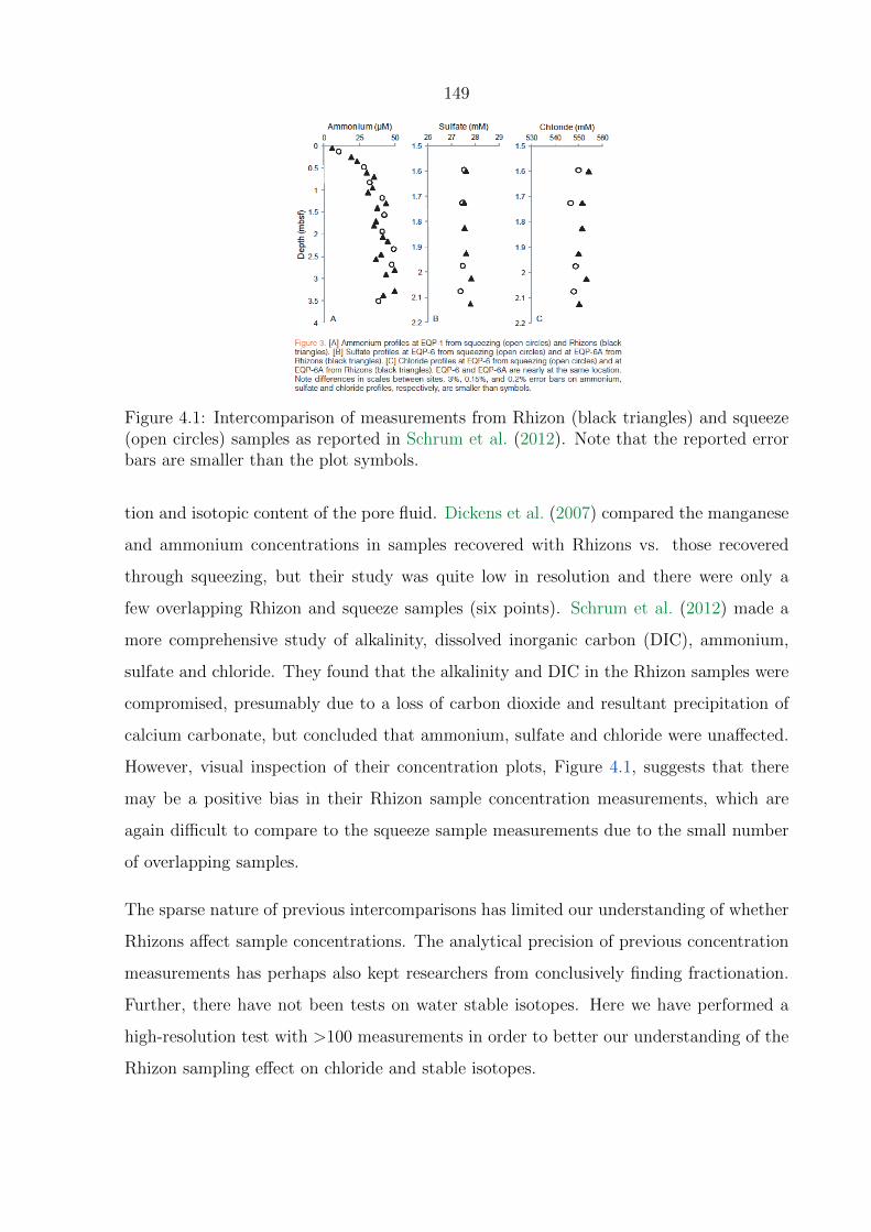
149
Figure 4.1: Intercomparison of measurements from Rhizon (black triangles) and squeeze(open circles) samples as reported in Schrum et al. (2012). Note that the reported errorbars are smaller than the plot symbols.
tion and isotopic content of the pore fluid. Dickens et al. (2007) compared the manganese
and ammonium concentrations in samples recovered with Rhizons vs. those recovered
through squeezing, but their study was quite low in resolution and there were only a
few overlapping Rhizon and squeeze samples (six points). Schrum et al. (2012) made a
more comprehensive study of alkalinity, dissolved inorganic carbon (DIC), ammonium,
sulfate and chloride. They found that the alkalinity and DIC in the Rhizon samples were
compromised, presumably due to a loss of carbon dioxide and resultant precipitation of
calcium carbonate, but concluded that ammonium, sulfate and chloride were unaffected.
However, visual inspection of their concentration plots, Figure 4.1, suggests that there
may be a positive bias in their Rhizon sample concentration measurements, which are
again difficult to compare to the squeeze sample measurements due to the small number
of overlapping samples.
The sparse nature of previous intercomparisons has limited our understanding of whether
Rhizons affect sample concentrations. The analytical precision of previous concentration
measurements has perhaps also kept researchers from conclusively finding fractionation.
Further, there have not been tests on water stable isotopes. Here we have performed a
high-resolution test with >100 measurements in order to better our understanding of the
Rhizon sampling effect on chloride and stable isotopes.
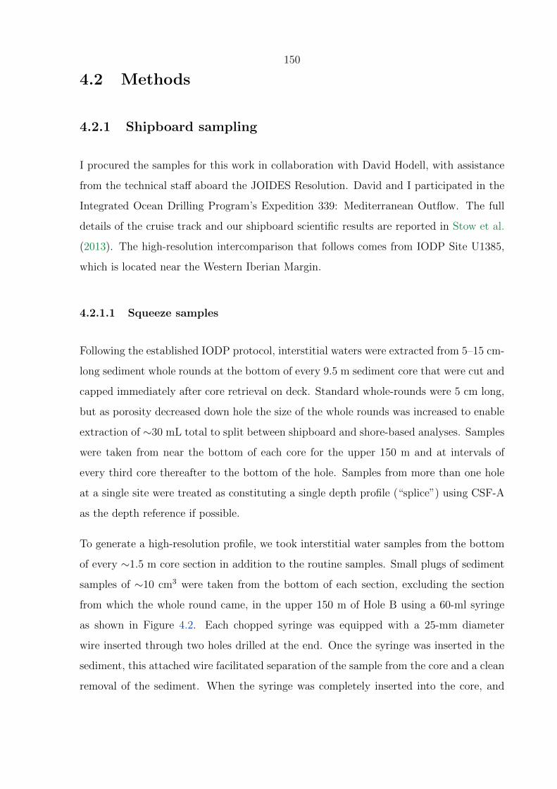
150
4.2 Methods
4.2.1 Shipboard sampling
I procured the samples for this work in collaboration with David Hodell, with assistance
from the technical staff aboard the JOIDES Resolution. David and I participated in the
Integrated Ocean Drilling Program’s Expedition 339: Mediterranean Outflow. The full
details of the cruise track and our shipboard scientific results are reported in Stow et al.
(2013). The high-resolution intercomparison that follows comes from IODP Site U1385,
which is located near the Western Iberian Margin.
4.2.1.1 Squeeze samples
Following the established IODP protocol, interstitial waters were extracted from 5–15 cm-
long sediment whole rounds at the bottom of every 9.5 m sediment core that were cut and
capped immediately after core retrieval on deck. Standard whole-rounds were 5 cm long,
but as porosity decreased down hole the size of the whole rounds was increased to enable
extraction of ∼30 mL total to split between shipboard and shore-based analyses. Samples
were taken from near the bottom of each core for the upper 150 m and at intervals of
every third core thereafter to the bottom of the hole. Samples from more than one hole
at a single site were treated as constituting a single depth profile (“splice”) using CSF-A
as the depth reference if possible.
To generate a high-resolution profile, we took interstitial water samples from the bottom
of every ∼1.5 m core section in addition to the routine samples. Small plugs of sediment
samples of ∼10 cm3 were taken from the bottom of each section, excluding the section
from which the whole round came, in the upper 150 m of Hole B using a 60-ml syringe
as shown in Figure 4.2. Each chopped syringe was equipped with a 25-mm diameter
wire inserted through two holes drilled at the end. Once the syringe was inserted in the
sediment, this attached wire facilitated separation of the sample from the core and a clean
removal of the sediment. When the syringe was completely inserted into the core, and
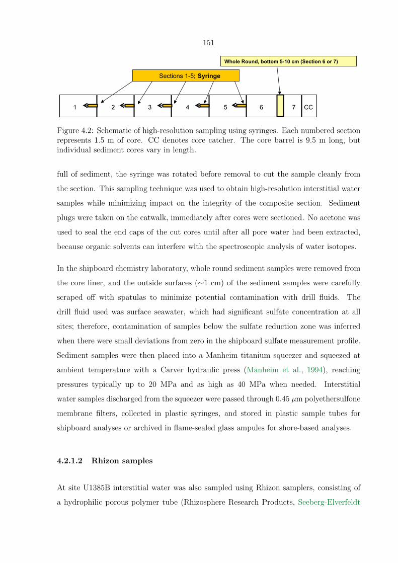
151
EXPEDITION 339 PORE WATER SAMPLING
IWSy entry: Sample Type = CYL Sample Tool = SYRINGE Test = IW Name = IWSy(interval) Volume=25 or 50cc
All Cores •Upper 50 m: IWSy (1/2 of 50 cc Syringe), length=5cm Bottom Sec. 1-4 or 5; •50 to 150m: IWSy (50cc Syringe), Length=10cm Bottom Sec 1-4 or 5; •0 to 200m: IW (5cm WR) Bottom of Sec. 5 or 6.
1 2 3 4 5 6 7 CC
Sections 1-5; Syringe
Whole Round, bottom 5-10 cm (Section 6 or 7)
IW (Whole Round) entry: Sample Type = WRND Sample Tool = SPATULA Test = IW Name = IW(interval) Volume=176cc
Figure 339-Methods–H–F1
Figure 4.2: Schematic of high-resolution sampling using syringes. Each numbered sectionrepresents 1.5 m of core. CC denotes core catcher. The core barrel is 9.5 m long, butindividual sediment cores vary in length.
full of sediment, the syringe was rotated before removal to cut the sample cleanly from
the section. This sampling technique was used to obtain high-resolution interstitial water
samples while minimizing impact on the integrity of the composite section. Sediment
plugs were taken on the catwalk, immediately after cores were sectioned. No acetone was
used to seal the end caps of the cut cores until after all pore water had been extracted,
because organic solvents can interfere with the spectroscopic analysis of water isotopes.
In the shipboard chemistry laboratory, whole round sediment samples were removed from
the core liner, and the outside surfaces (∼1 cm) of the sediment samples were carefully
scraped off with spatulas to minimize potential contamination with drill fluids. The
drill fluid used was surface seawater, which had significant sulfate concentration at all
sites; therefore, contamination of samples below the sulfate reduction zone was inferred
when there were small deviations from zero in the shipboard sulfate measurement profile.
Sediment samples were then placed into a Manheim titanium squeezer and squeezed at
ambient temperature with a Carver hydraulic press (Manheim et al., 1994), reaching
pressures typically up to 20 MPa and as high as 40 MPa when needed. Interstitial
water samples discharged from the squeezer were passed through 0.45 µm polyethersulfone
membrane filters, collected in plastic syringes, and stored in plastic sample tubes for
shipboard analyses or archived in flame-sealed glass ampules for shore-based analyses.
4.2.1.2 Rhizon samples
At site U1385B interstitial water was also sampled using Rhizon samplers, consisting of
a hydrophilic porous polymer tube (Rhizosphere Research Products, Seeberg-Elverfeldt
152
Figure 4.3: Rhizon samplers in cores
et al. (2005)). Rhizon samplers were carefully inserted through holes drilled in the core
liner. Syringes were attached to each Rhizon sampler with a luer-lock, pulled to generate
vacuum, and held open with wooden spacers. Samplers were left in place during the
core temperature equilibration (∼3 hours). The Rhizon samplers were used in sets of
three, spaced 3 cm apart, with the center Rhizon inserted at the center of each section
(i.e., 75 cm from the section top). The typical arrangement of the samplers is shown in
Figure 4.3. Water from all three samplers was combined into one sample in a centrifuge
tube and shaken to mix before analysis and splitting.
In contrast to the methods on previous cruises, the Rhizon samplers were used dry in order
to avoid sample contamination from pre-soaking. In qualitative tests we found that flow
rate through the Rhizons did not depend on pre-soaking. Further, stable water isotope
measurements were sensitive to the isotopic values of the solution in which the Rhizons

153
were pre-soaked even when the first few milliliters were discarded from the syringe during
sampling. That is, the syringe was removed from the core, a few milliliters of water was
discarded, then the syringe was re-attached and a fresh sample was taken. This fresh
sample’s isotopic measurement was different than those of the sample taken with a dry
Rhizon. Because of the low total water volume recovery, the pre-soaking fluid can not be
flushed completely from the Rhizon in order to recover an un-contaminated measurement.
In the same manner as for the squeeze samples, Rhizon samples were archived in flame-
sealed glass ampules for shore-based analyses.
4.2.2 δ18O and δD measurements
Oxygen and hydrogen isotopes measurements of interstitial waters were made by cavity
ringdown laser spectroscopy (CRDS). CRDS is a time-based measurement system that
uses a laser to quantify spectral absorption lines unique to H162 O, H18
2 O, and 2H16O in
an optical cavity (Gupta et al., 2009). The equipment consisted of an L1102-i Picarro
water isotope analyzer manufactured in July 2009 (Serial Number: 202-HBDS033; 200-
CPVU-HBQ33), an A0211 high-precision vaporizer manufactured in August 2011 (SN:
VAP 292), and a CTC HTC-Pal liquid autosampler (SN: 142552). The Picarro L1102-I
measures δ18O, δD, and total H2O concentration simultaneously. Guaranteed precision
for liquid water using the L1102-I with autosampler injection is ≤ 0.1h for δ18O and
≤ 0.5h for δD. Guaranteed drift is ≤ ±0.3h for δ18O and ≤ ±0.9h for δD. Precision
and drift are defined based on the standard deviation and range (max-min) of the average
values for 12 injections of the same water sample (tap water) measured 12 times, which
is equivalent to 144 injections averaged in blocks of 12.
For the present work, approximately 500 µl of filtered interstitial water was loaded in
a 2-mL septa top glass vial and placed in the autosampler. Each water sample was
injected nine times into the vaporizer. Memory effects from previous samples were avoided
by rejecting the first three results and averaging the final six injections. An internal
seawater standard (SPIT) was analyzed between each unknown sample to correct for
drift. Each value measured on an unknown sample was normalized to the mean of the

154
two adjacent standards. Analysis of each sample, consisting of nine injections, took 90
minutes. Three hours per sample is required if one includes the time needed to measure
bracketing standards. The vaporizer septa were changed regularly after no more than
300 injections. Considerable salt buildup occurred in the vaporizer, which necessitated
its periodic cleaning.
The instrument was calibrated using three working standards from the University of
Cambridge with known values: Delta (δ18O = -27.6h, δD = -213.5h), Botty (δ18O
= -7.65h, δD = -52.6h), and either SMOW or SPIT (δ18O = 0h, δD = 0h). The
δ18O and δD of SPIT are indistinguishable analytically from SMOW. Because the Picarro
analyzer is extremely linear, it is only necessary to use three calibration standards. The
calibration line was determined by subtracting the measured values of SPIT from each
of the standards and deriving a regression equation forced through the origin. The slope
of the δ18O regression varied between 1.051 and 1.083 (average = 1.067), whereas the δD
slope varied from 1.129 to 1.160 (average = 1.147). Measured δ18O and δD were corrected
to VSMOW in parts per thousand (h) by multiplying the SPIT-normalized value by the
slope of the calibration line.
Because organic compounds can cause spectroscopic interference in CRDS and affect
isotopic results, we processed the data using Picarro’s ChemCorrect software that iden-
tifies irregularities caused by hydrocarbons. Despite significant amounts of methane in
headspace samples, pore water samples were not flagged as being contaminated by the
ChemCorrect software suggesting that methane gas is lost during the interstitial water
sampling and squeezing process.
4.2.3 [Cl−] measurements
The [Cl−] of each sample is measured by potentiometric titration against silver nitrate
to form the precipitate silver chloride. Our titration apparatus is custom-built, and we
describe the technical details in Appendix A. In brief, the chloride concentration of the
sample is determined by the equivalence-point of the reaction: when an equivalent amount
of silver nitrate reagent to the amount of chloride in solution has been added. The
155
equivalence point is determined potentiometrically by identifying the maximum ∆E∆V
, where
E is the potential difference between the reagent and solution and V is the volume of
reagent that has been added to the sample. The addition of reagent to the solution is
controlled by a stepper motor coupled to a precision micrometer buret. The stepper
motor and the voltage acquisition are driven through a LabVIEW program. After filling
the buret with reagent and placing the tip of the buret in the sample beaker, the entire
reaction is automated.
For the following work the sample sizes were ∼600 µL. The true size of the samples
was determined through weighing on a precision balance. The silver nitrate reagent had
a concentration of ∼0.23 M, which resulted in equivalence points at around 1.5 mL of
reagent added.
To determine the chloride concentration of an unknown sample, we weigh out a sample
and then titrate to the equivalence point. The concentration of an unknown sample is
calculated from the sample’s weight, the volumetric equivalence point and the concentra-
tion of the silver nitrate reagent. The approximate concentration of the silver nitrate is
determined during its preparation, but to have a more accurate and precise knowledge
of its concentration we calibrate the concentration by titrating against a known standard
3-5 times at the beginning of each measurement day. Our standard is the IAPSO P-Series
Normal Standard Seawater (S=35). Because there is high evaporation in Southern Cali-
fornia, once we break the factory seal on a standard, we store it with parafilm around the
top and inside a glass jar that is ∼1/3 full of water. We use a standard for a maximum
of two weeks. To check the continuing validity of this storage method, when we open a
new standard we compare the old values to the new ones. We also measure a consistency
standard in triplicate every measurement day to ensure that there is no significant evap-
oration of the standard. Our consistency standard is low salinity, ∼ 33 g kg−1, surface
seawater from the North Pacific, in the vicinity of Hydrate Ridge. Figure 4.4 shows the
temporal stability of this procedure.
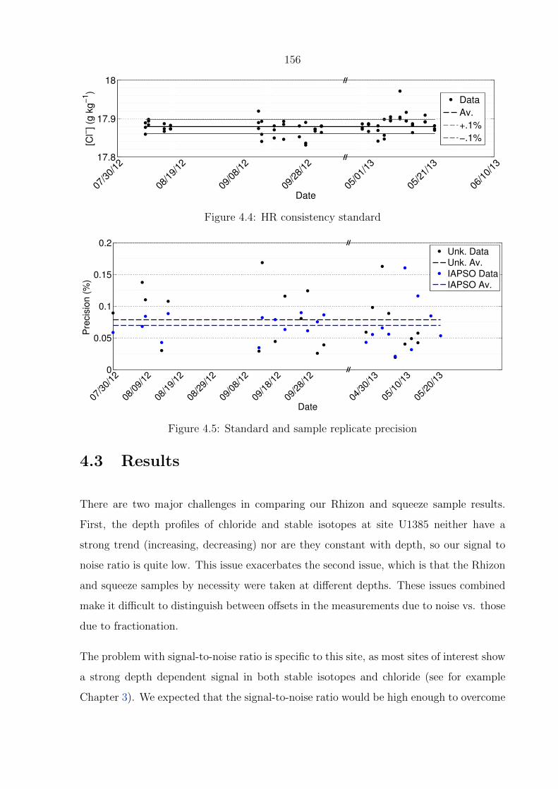
156
17.8
17.9
18
//
//
07/3
0/12
08/1
9/12
09/0
8/12
09/2
8/12
05/0
1/13
05/2
1/13
06/1
0/13
Date
[Cl−
] (g
kg
−1)
//
//
//
//
//
//
Data
Av.
+.1%
−.1%
Figure 4.4: HR consistency standard
0
0.05
0.1
0.15
0.2
//
//
07/3
0/12
08/0
9/12
08/1
9/12
08/2
9/12
09/0
8/12
09/1
8/12
09/2
8/12
04/3
0/13
05/1
0/13
05/2
0/13
Date
Pre
cis
ion
(%
)
//
//
//
//
//
//
Unk. Data
Unk. Av.
IAPSO Data
IAPSO Av.
Figure 4.5: Standard and sample replicate precision
4.3 Results
There are two major challenges in comparing our Rhizon and squeeze sample results.
First, the depth profiles of chloride and stable isotopes at site U1385 neither have a
strong trend (increasing, decreasing) nor are they constant with depth, so our signal to
noise ratio is quite low. This issue exacerbates the second issue, which is that the Rhizon
and squeeze samples by necessity were taken at different depths. These issues combined
make it difficult to distinguish between offsets in the measurements due to noise vs. those
due to fractionation.
The problem with signal-to-noise ratio is specific to this site, as most sites of interest show
a strong depth dependent signal in both stable isotopes and chloride (see for example
Chapter 3). We expected that the signal-to-noise ratio would be high enough to overcome
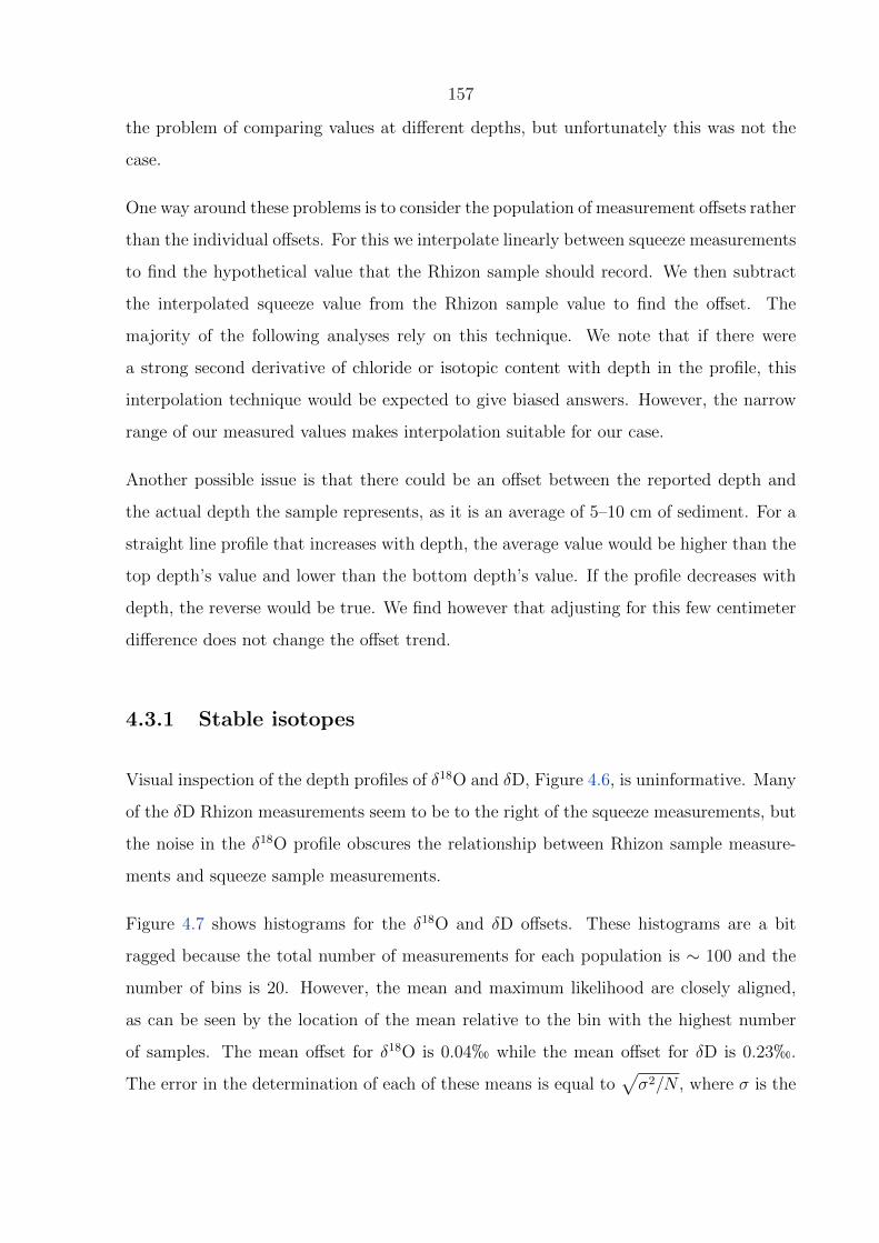
157
the problem of comparing values at different depths, but unfortunately this was not the
case.
One way around these problems is to consider the population of measurement offsets rather
than the individual offsets. For this we interpolate linearly between squeeze measurements
to find the hypothetical value that the Rhizon sample should record. We then subtract
the interpolated squeeze value from the Rhizon sample value to find the offset. The
majority of the following analyses rely on this technique. We note that if there were
a strong second derivative of chloride or isotopic content with depth in the profile, this
interpolation technique would be expected to give biased answers. However, the narrow
range of our measured values makes interpolation suitable for our case.
Another possible issue is that there could be an offset between the reported depth and
the actual depth the sample represents, as it is an average of 5–10 cm of sediment. For a
straight line profile that increases with depth, the average value would be higher than the
top depth’s value and lower than the bottom depth’s value. If the profile decreases with
depth, the reverse would be true. We find however that adjusting for this few centimeter
difference does not change the offset trend.
4.3.1 Stable isotopes
Visual inspection of the depth profiles of δ18O and δD, Figure 4.6, is uninformative. Many
of the δD Rhizon measurements seem to be to the right of the squeeze measurements, but
the noise in the δ18O profile obscures the relationship between Rhizon sample measure-
ments and squeeze sample measurements.
Figure 4.7 shows histograms for the δ18O and δD offsets. These histograms are a bit
ragged because the total number of measurements for each population is ∼ 100 and the
number of bins is 20. However, the mean and maximum likelihood are closely aligned,
as can be seen by the location of the mean relative to the bin with the highest number
of samples. The mean offset for δ18O is 0.04h while the mean offset for δD is 0.23h.
The error in the determination of each of these means is equal to√σ2/N , where σ is the

158
precision of an individual measurement, assuming that the precision for each measurement
is the same. With a reported precision of 0.1h in δ18O and 0.5h in δD and 87 samples,
the error in the mean offset for δ18O is 0.01h while the error for the mean offset of δD is
0.05h. As compared to the reported measurement precision, these mean offsets are both
statistically significant.
Neither the offsets in δ18O nor those in δD show a clear trend with depth, as demon-
strated in Figure 4.8a and 4.8b. Instead this view of the data confirms that of the
histograms, which is that most of the Rhizon measurement values are greater than the
squeeze measurement values.
−0.5 0 0.50
50
100
150
de
pth
(C
SF
−A
, to
p)
δ18
O
U1385B Squeeze vs. Rhizon
Squeeze
Rhizon
(a)
−2 −1 0 1 2 3 40
50
100
150
dep
th (
CS
F−
A, to
p)
δD
U1385B Squeeze vs. Rhizon
Squeeze
Rhizon
(b)
Figure 4.6: Depth profiles of δ18O and δD measured in both squeeze and Rhizon samplesat site U1385
4.3.2 Chloride
In contrast, in the [Cl−] depth profile, Figure 4.9, the Rhizon measurements lie clearly to
the right of the squeeze measurements in the upper ∼80 m, although below that point
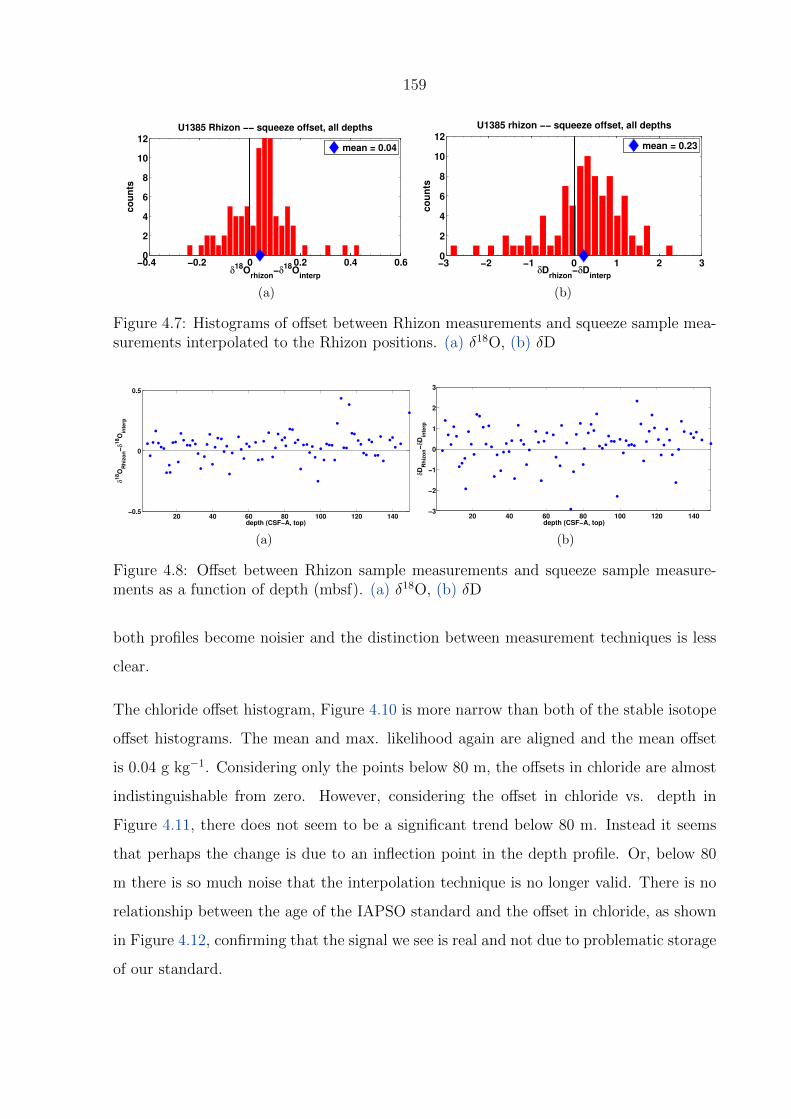
159
−0.4 −0.2 0 0.2 0.4 0.60
2
4
6
8
10
12
δ18
Orhizon
−δ18
Ointerp
co
un
tsU1385 Rhizon −− squeeze offset, all depths
mean = 0.04
(a)
−3 −2 −1 0 1 2 30
2
4
6
8
10
12
δDrhizon
−δDinterp
co
un
ts
U1385 rhizon −− squeeze offset, all depths
mean = 0.23
(b)
Figure 4.7: Histograms of offset between Rhizon measurements and squeeze sample mea-surements interpolated to the Rhizon positions. (a) δ18O, (b) δD
20 40 60 80 100 120 140−0.5
0
0.5
depth (CSF−A, top)
δ1
8O
Rh
izo
n−
δ1
8O
inte
rp
(a)
20 40 60 80 100 120 140−3
−2
−1
0
1
2
3
depth (CSF−A, top)
δD
Rh
izo
n−
δD
inte
rp
(b)
Figure 4.8: Offset between Rhizon sample measurements and squeeze sample measure-ments as a function of depth (mbsf). (a) δ18O, (b) δD
both profiles become noisier and the distinction between measurement techniques is less
clear.
The chloride offset histogram, Figure 4.10 is more narrow than both of the stable isotope
offset histograms. The mean and max. likelihood again are aligned and the mean offset
is 0.04 g kg−1. Considering only the points below 80 m, the offsets in chloride are almost
indistinguishable from zero. However, considering the offset in chloride vs. depth in
Figure 4.11, there does not seem to be a significant trend below 80 m. Instead it seems
that perhaps the change is due to an inflection point in the depth profile. Or, below 80
m there is so much noise that the interpolation technique is no longer valid. There is no
relationship between the age of the IAPSO standard and the offset in chloride, as shown
in Figure 4.12, confirming that the signal we see is real and not due to problematic storage
of our standard.
160
19 19.2 19.4 19.6 19.8 200
50
100
150
de
pth
(C
SF
−A
, to
p)
[Cl−]
U1385B Squeeze Interpolation
interp. − squeeze
meas. − squeeze
meas. − rhizon
Figure 4.9: Depth profiles of [Cl−] measured in both squeeze and Rhizon samples at siteU1385
4.4 Discussion
There is a significant offset between measurements on Rhizon samples and squeezed sam-
ples in both stable isotopes and chloride. There are several possible reasons for this
observed difference.
Rhizon samples were taken over an ∼3 hour period during which water evaporation may
have changed the isotopes and chloride concentration. We were unable to carefully control
for this time, which may be one contributor to the noisiness in the data.
In a similar way, the hydrophilic membrane of the sampler may have absorbed some of the
water, creating higher measured chloride concentrations, or caused diffusional fraction-
ation of the stable isotopes, which we expect would preferentially affect the δD relative
to δ18O as the relative mass difference, and thus the difference in diffusivity, between
hydrogen isotopes is greater than that between the oxygen isotopes.
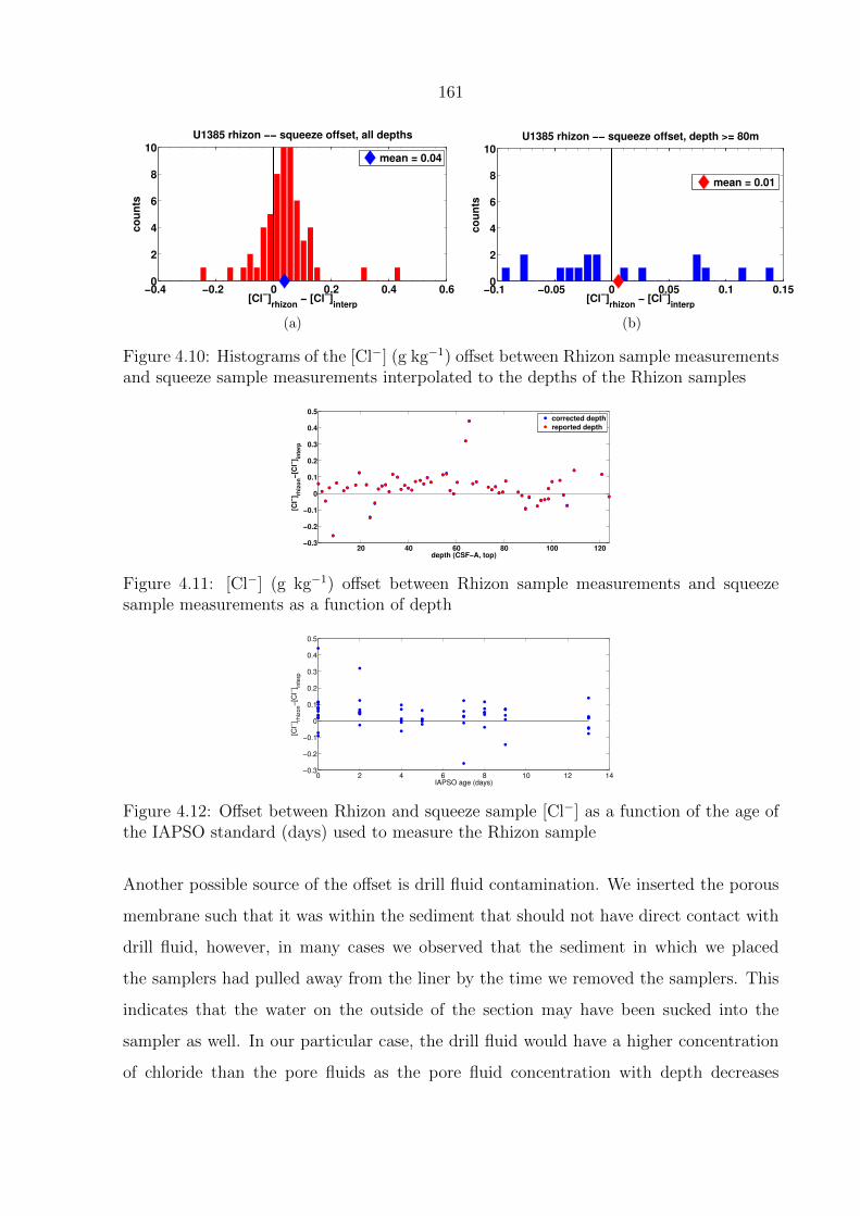
161
−0.4 −0.2 0 0.2 0.4 0.60
2
4
6
8
10
[Cl−]rhizon
− [Cl−]interp
co
un
tsU1385 rhizon −− squeeze offset, all depths
mean = 0.04
(a)
−0.1 −0.05 0 0.05 0.1 0.150
2
4
6
8
10
[Cl−]rhizon
− [Cl−]interp
co
un
ts
U1385 rhizon −− squeeze offset, depth >= 80m
mean = 0.01
(b)
Figure 4.10: Histograms of the [Cl−] (g kg−1) offset between Rhizon sample measurementsand squeeze sample measurements interpolated to the depths of the Rhizon samples
20 40 60 80 100 120−0.3
−0.2
−0.1
0
0.1
0.2
0.3
0.4
0.5
depth (CSF−A, top)
[Cl−
] rhiz
on−
[Cl−
] inte
rp
corrected depth
reported depth
Figure 4.11: [Cl−] (g kg−1) offset between Rhizon sample measurements and squeezesample measurements as a function of depth
0 2 4 6 8 10 12 14−0.3
−0.2
−0.1
0
0.1
0.2
0.3
0.4
0.5
IAPSO age (days)
[Cl−
] rhiz
on−
[Cl−
] inte
rp
Figure 4.12: Offset between Rhizon and squeeze sample [Cl−] as a function of the age ofthe IAPSO standard (days) used to measure the Rhizon sample
Another possible source of the offset is drill fluid contamination. We inserted the porous
membrane such that it was within the sediment that should not have direct contact with
drill fluid, however, in many cases we observed that the sediment in which we placed
the samplers had pulled away from the liner by the time we removed the samplers. This
indicates that the water on the outside of the section may have been sucked into the
sampler as well. In our particular case, the drill fluid would have a higher concentration
of chloride than the pore fluids as the pore fluid concentration with depth decreases

162
slightly at least in the upper ∼ 50 m of the depth profile. This could explain part of the
trend we see with depth in the chloride, specifically that the deeper chloride values are
saltier and thus a slight contamination with a saltier source has a smaller relative effect
on the measurement offset.
Evaporative fractionation has been intensively studied, and there are good theoretical
predictions for the relationship between δ18O and δD undergoing evaporation. We can
therefore compare the relationships between the stable isotopes and chloride to see if the
offset is consistent with evaporative fractionation.
Our case can be described best by open-system Rayleigh fractionation. The ratio of
heavy to light isotope, R, (i.e.18O16O
for oxygen or DH
for hydrogen ) in a pool of water with
essentially infinite molecules and fixed conditions can be described by:
R = R0
(N
N0
)(α−1)
. (4.1)
R0 is the initial isotope ratio, N is the total number of molecules remaining, N0 is the
original number of molecules and α is the fractionation factor. At 20◦C the evaporative
fractionation factor for 18O relative to 16O is 1.0098 and for deuterium relative to protium
is 1.084 (Gat, 1996).
Under evaporation the fraction of material left, NN0
, is also known as f. f will be equal
for both pairs of isotopes, such that there is a linear relationship between the logs of the
element ratios, i.e.:αH − 1
αO − 1lnRO
RO0
= lnRH
RH0
. (4.2)
While the spectroscopic technique used in CRDS does not yield isotope ratios, the ratios
can be computed simply from the δ values as follows;
δ18O
1000+ 1 =
R
Rstd
, (4.3)

163
such that the relationship between δ18O and δD under evaporation is:
αH − 1
αO − 1ln
δ18Ofinal
1000+ 1
δ18Oinitial
1000+ 1
= ln
δDfinal
1000+ 1
δDinitial
1000+ 1
. (4.4)
Substituting in the α values, this is:
8.5714 ln
δ18Ofinal
1000+ 1
δ18Oinitial
1000+ 1
= ln
δDfinal
1000+ 1
δDinitial
1000+ 1
. (4.5)
For our purpose, we assume the initial isotope ratio is that of the interpolated squeeze
measurement. The final isotope ratio is that measured in the Rhizon sample. The hy-
pothesis we test with these choices is that the Rhizon values are fractionated relative to
the squeeze values because they are left open to the atmosphere longer. It is important
to note that in some cases the squeeze samples do sit for ∼1 hour in the squeezers; thus,
we never have a perfect control on no evaporation.
The red line labeled evaporative fractionation in Figure 4.13 shows the assumed rela-
tionship between the oxygen and hydrogen isotope ratios. The 2-norm error of the data
relative to the prediction, assuming all the error is in the hydrogen measurements, is
0.0083 while the 1-norm error is 0.0574. The blue line is a linear fit to the logarithmic
data. The slope of the line is 4.557. The 2-norm error is 0.0071 and the 1-norm error
of this fit is 0.0502. If I propagate the precision of the hydrogen isotope measurements
through the Rayleigh equation, the theoretical 2-norm error must be greater than 0.0066
and the 1-norm error should be greater than 0.0622. Therefore the difference between the
evaporative fractionation and the empirically calculated relationship between hydrogen
and oxygen isotopes is indistinguishable.
The evolution of concentrations with evaporations can be described analogously to Rayleigh
fractionation, where f =Vfinal
Vinitial= [Cl−]initial
[Cl−]final. Then the relationship between chloride con-

164
10−0.0001 100 100.0001
10−0.001
100
100.001
R/R0|oxygen
R/R
0| hydr
ogen
dataevaporative fractionationlog−linear fit
Figure 4.13: Hydrogen isotope ratios vs. oxygen isotope ratios
centrations and δ18O can be written:
1
α− 1ln
δ18Ofinal
1000+ 1
δ18Oinitial
1000+ 1
= ln
([Cl−]initial[Cl−]final
). (4.6)
However, as shown in Figures 4.14 and 4.15, there is not a strong relationship between
the fractionation factor calculated from the chloride concentrations and that calculated
from the isotope ratios, nor does the fractionation of the isotopes and [Cl−] have a trend
with depth.
Since the fractionation signal in the [Cl−] is clearer than that in the stable isotopes, we
can consider whether the amount of fractionation, assuming it is evaporative, could be
expected to be detectable by the Picarro. The most fractionated chloride measurement
yields an f of 0.98. This would yield a ratio RR0|O of 0.9998. For a typical measured
δ18Ofinal equal to 0.4h, the measured δ18Oinitial would be equal to 0.6h which is greater
than the precision of the Picarro and therefore detectable. However, most of the [Cl−]
determined f values are greater than 0.99, which would yield a measured difference in δ18O
of less than 0.1h, indistinguishable from 0 given the measurement precision of the Picarro.
Because the relationship between isotope fractionation and chloride concentration due to
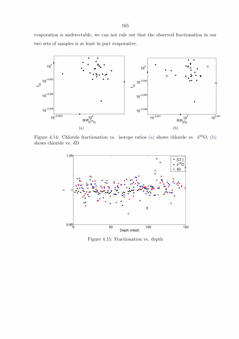
165
evaporation is undetectable, we can not rule out that the observed fractionation in our
two sets of samples is at least in part evaporative.
10−0.0001
100
10−0.009
10−0.006
10−0.003
100
R/R0|18
O
f Cl
(a)
10−0.001
100
100.001
10−0.009
10−0.006
10−0.003
100
R/R0|D
f Cl
(b)
Figure 4.14: Chloride fractionation vs. isotope ratios (a) shows chloride vs. δ18O, (b)shows chloride vs. δD
0 50 100 1500.95
1
1.05
Depth (mbsf)
f
[Cl−]
δ18
O
δD
Figure 4.15: Fractionation vs. depth
166
4.5 Conclusions
We found that Rhizons were unable to be used in the very deepest, highly compacted
ocean sediments. Near the Advanced Piston Core (APC) refusal depth, our attempts
to insert Rhizons into the sediments without pre-drilling the sediment were typically
unsuccessful. Even when pre-drilling the sediment, the sediment would quickly fill in,
crushing the Rhizon and leading to sub-optimal water extraction.
In less compacted sediments, the Rhizons caused contamination of the chloride concentra-
tion and oxygen isotope values. Our analysis indicates that this contamination is caused
either by evaporative or diffusive fractionation, rather than a blank in the Rhizon or
mixing with drill fluid.
In the future we need to find a way to markedly increase the number of high quality
measurements of sediment pore fluid chloride and oxygen isotopes, as we still lack suitable
alternative ways to reconstruct ocean temperature and salinity. Emerging technologies in
ocean sediment drilling, such as the MeBo, may afford an increase in spatial density of
pore fluid measurements.
167
Chapter 5
The role of ocean cooling in settingglacial southern source bottom watersalinity

168
Abstract
At the Last Glacial Maximum (LGM), the salinity contrast between northern source deep
water and southern source bottom water was reversed with respect to the contrast to-
day. Additionally, Glacial Southern Source Bottom Water (GSSBW) was saltier than
Antarctic Bottom Water (AABW), over and above the difference implied by the mean
sea level. This study examines to what extent cold temperatures, through their effect
on ice formation and melting, could have caused these differences. Computational sensi-
tivity experiments using a coupled ice shelf cavity - sea ice - ocean model are performed
in a Weddell Sea domain, as a representative case study for bottom water formation
originating from Antarctic continental shelves. Ocean temperatures at the domain open
boundaries are systematically lowered to determine the sensitivity of Weddell Sea water
mass properties to a range of cool ocean temperatures. The steady state salinities differ
between experiments due to temperature-induced responses of ice shelf and sea ice melt-
ing and freezing, evaporation and open boundary fluxes. The results of the experiments
indicate that reduced ocean temperature can explain up to 30% of the salinity difference
between GSSBW and AABW, primarily due to decreased ice shelf melting. The smallest
and most exposed ice shelves, which abut narrow continental shelves, have the greatest
sensitivity to the ocean temperature changes, suggesting that at the LGM there could
have been a shift in geographical site dominance in bottom water formation. More sea ice
is formed and exported in the cold ocean experiments, but the effect of this on salinity is
negated by an equal magnitude reduction in evaporation.
169
5.1 Introduction
Paleo reconstructions of deep ocean salinity and temperature at the Last Glacial Max-
imum (LGM; see Table 1 for abbreviations) indicate that ocean density gradients were
primarly set by salinity. Recent modeling studies (Bouttes et al., 2009, 2010) suggest that
this stratification could have had a significant impact on the rate of the mean overturning
circulation and the carbon cycle, but it is unknown whether or by what mechanism the
salinity/density gradient could have been created and maintained. We investigate to what
extent sea ice - ice sheet - ocean interactions over the Antarctic continental shelves could
explain this change in salinity structure.
At the LGM the sea level was around 125 m lower than it is today due to the expansion
of continental ice sheets, corresponding to an average ocean salinity increase of roughly
1.2 g kg−1. The salinity of Atlantic Glacial Southern Source Bottom Water (GSSBW) at
the LGM was 2.3 g kg−1 higher than that of modern Antarctic Bottom Water (AABW),
leaving 1.1 g kg −1 unexplained by a contraction of the oceans (Adkins et al., 2002).
Water at sites occupied by northern source intermediate/deep water was saltier as well,
but the salinity increase there roughly matched the average, or was slightly lower. Thus at
the LGM the Atlantic Ocean deep water masses were more stratified in salinity. As δ18O
measurements show that deep ocean temperatures were all similar and close to the freezing
point (Adkins et al., 2002, Malone et al., 2004, Schrag et al., 2002), density gradients
would have been primarily set by salinity. The observed glacial salinity stratification,
when compared to the modern temperature stratification, corresponds to a higher than
modern density stratification between northern and southern deep water. In addition,
the LGM version of NADW, Glacial North Atlantic Intermediate Water (GNAIW), was
fresher than GSSBW in the Atlantic, which is opposite in sign to the salinity difference
between NADW and AABW today.
In the modern, NADW is a precursor to AABW. AABW has a lower salinity than NADW
due to modifications that occur in the Southern Ocean. The properties of NADW help
determine these Southern Ocean processes and how they contribute to the final charac-
teristics of AABW. The salinity maximum that distinguishes NADW from other water
170
masses identifies it as the main contributor to Circumpolar Deep Water (CDW) (Reid and
Lynn, 1971). CDW interacts with water masses formed and modified over the Antarctic
continental shelves to eventually transform into AABW. In the Southern Ocean there is an
excess of precipitation over evaporation, and over the Antarctic continental shelves there
is an additional freshwater input from basal melting of marine-based ice sheets inside ice
shelf cavities. Brine rejection from sea ice combined with sea ice export compensates
for these freshwater fluxes over continental shelves, such that the salinity of continen-
tal shelf waters can be as high or higher than that of CDW. Antarctic continental shelf
water properties, in particular those in the Weddell and Ross Seas and on the Adelie
Coast, determine the properties of AABW. The details of how continental shelf waters
are transformed to AABW and the properties of AABW vary with location, but share
many general similarities. There is also evidence that water exported from the Weddell
Sea makes up more than half of AABW (Orsi et al., 1999). Therefore we consider the
modern Weddell Sea as a representative source of AABW formation in our study.
A detailed review of the modern processes responsible for water masses in the Weddell
Sea and how they contribute to bottom water formation can be found in Nicholls et al.
(2009) and references therein. Figure 5.1 shows the Θ0/S properties of water masses on
the modern Weddell Sea continental shelf. A subset of these water masses can be used to
illustrate the main processes that contribute to AABW properties. Brine rejection and
sea ice export in the Weddell Sea form High Salinity Shelf Water (HSSW: S > 34.5),
the highest density water formed on the continental shelf. Ice Shelf Water (ISW: Θ0 <
−1.9◦C), the second highest density continental shelf water mass, is formed in large part
from ice shelf meltwater. Overflows of ISW and HSSW entrain other water along their
paths to the abyssal Weddell Sea, primarily diluted CDW in the form of Warm Deep Water
and Modified Warm Deep Water (MWDW). The original properties of ISW, HSSW and
modified CDW are evident in Weddell Sea Bottom Water (WSBW) and Weddell Sea Deep
Water (WSDW), the deepest Weddell Sea water masses. The export of WSDW at the
northwest boundary of the Weddell Sea is the Weddell Sea’s main contribution to AABW
(Fahrbach et al., 1995, Foldvik et al., 2004, Gordon et al., 2010). Sea ice and ice shelves,
by determining the properties of ISW and HSSW, heavily influence the final properties
of AABW.
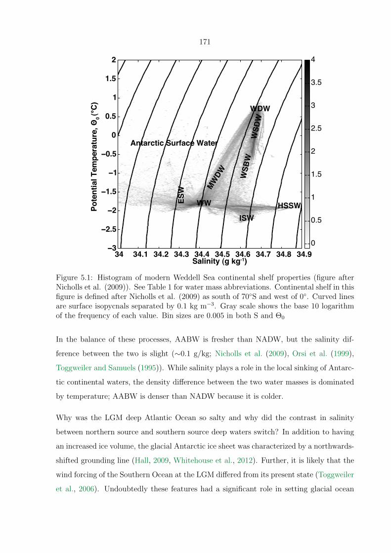
171
Salinity (g kg-1)
Pote
ntia
l Tem
pera
ture
, Θ0 (°
C)
ESW
WWMW
DW
WDW
WSD
W
WSB
W
HSSWISW
34 34.1 34.2 34.3 34.4 34.5 34.6 34.7 34.8 34.9−3
−2.5
−2
−1.5
−1
−0.5
0
0.5
1
1.5
2
0
0.5
1
1.5
2
2.5
3
3.5
4
Antarctic Surface Water
Figure 5.1: Histogram of modern Weddell Sea continental shelf properties (figure afterNicholls et al. (2009)). See Table 1 for water mass abbreviations. Continental shelf in thisfigure is defined after Nicholls et al. (2009) as south of 70◦S and west of 0◦. Curved linesare surface isopycnals separated by 0.1 kg m−3. Gray scale shows the base 10 logarithmof the frequency of each value. Bin sizes are 0.005 in both S and Θ0
In the balance of these processes, AABW is fresher than NADW, but the salinity dif-
ference between the two is slight (∼0.1 g/kg; Nicholls et al. (2009), Orsi et al. (1999),
Toggweiler and Samuels (1995)). While salinity plays a role in the local sinking of Antarc-
tic continental waters, the density difference between the two water masses is dominated
by temperature; AABW is denser than NADW because it is colder.
Why was the LGM deep Atlantic Ocean so salty and why did the contrast in salinity
between northern source and southern source deep waters switch? In addition to having
an increased ice volume, the glacial Antarctic ice sheet was characterized by a northwards-
shifted grounding line (Hall, 2009, Whitehouse et al., 2012). Further, it is likely that the
wind forcing of the Southern Ocean at the LGM differed from its present state (Toggweiler
et al., 2006). Undoubtedly these features had a significant role in setting glacial ocean
172
circulation. However, long before the ice sheets expanded to their most recent maximum
extent, the mean deep ocean temperature had already cooled ∼ 1.5 − 2◦C below its
temperature during the last interglacial and during the modern periods (Chappell and
Shackleton, 1986, Cutler et al., 2003). The approach to the LGM ocean and ice sheet
states may have been initiated by this advance cooling and its resultant feedbacks.
In this study, we hypothesize that the cool ocean temperatures prior to and during the
LGM can account for a significant portion of the increased southern source bottom water
salinity observed at the LGM, due to a reduction in freshwater from ice shelf basal melting
and an increase in salinity from sea ice processes on the Antarctic continental shelves. To
test this hypothesis, we perform a set of numerical ocean cooling sensitivity experiments in
a regional Weddell Sea domain. We examine how ocean properties on the continental shelf
change in response to lower ocean temperatures and changes in ice - ocean interactions
in the Weddell Sea. We additionally consider the relative influence of ice shelves versus
sea ice in setting continental shelf water properties, and how the balance between the two
changes in response to increasingly cool temperatures.
As modern bottom water formation depends on the complex interaction between sea ice,
ice shelves and the ocean, our experiments use an ocean general circulation model (ocean
GCM) coupled to dynamic/thermodynamic sea ice and thermodynamic ice shelf cavity
models. While the ice sheet’s total contribution to the freshwater and thermodynamic
budgets plays a key role in setting modern deep water formation, the distributed locations
of meltwater injection and their interactions with ocean and sea ice dynamics cannot be
neglected (Hellmer, 2004). Further, due to the complex interactions of different compo-
nents of the ice-ocean-atmosphere system, it is difficult to predict how the system will
respond to a temperature change. For example, observed Antarctic sea ice area has not
decreased in response to warming ocean temperatures (Zwally et al., 2002).

173
5.2 Methods
5.2.1 Model Setup
We use the Massachusetts Institute of Technology general circulation model (MITgcm;
Marshall et al., 1997a,b) in a regional domain configuration to investigate the effect of
ocean cooling on ice shelf and sea ice processes. The integration domain (Fig. 5.2) is
derived from a global cube sphere grid configuration with horizontal grid spacing of ∼18
km (Menemenlis et al., 2008); it encompasses the Weddell Sea and the ocean border-
ing Queen Maud Land, and it extends slightly into the Antarctic Circumpolar Current
(identified in the model by surface velocities greater than 0.5 m/s); it also covers a small
section of the Bellinghausen Sea west of the Antarctic Peninsula. Ocean bathymetry is
from the so-called S2004 blend (Marks and Smith, 2006). Ice shelf cavity bathymetry
for the Filchner-Ronne Ice Shelf (FRIS) and for the Larsen Ice Shelf in the Weddell Sea
as well as for the Eastern Ice Shelves are derived from BEDMAP (Lythe et al., 2001),
and ice shelf thicknesses are taken from DiMarzio et al. (2008) using firn corrections from
van den Broeke et al. (2008).
The MITgcm is a three-dimensional general circulation model, which solves the primitive
equations for fluid on a rotating sphere. Our MITgcm configuration uses the hydrostatic
and Boussinesq approximations. The effect of turbulent eddy transport and mixing are
parameterized by a combination of several schemes. There is a diffusive flux of properties
along isoneutral surfaces proportional to the local gradient of the properties as described
in Redi (1979). The advective component of turbulence is approximated using the Griffies
(1998) skew flux formulation of the Gent and McWilliams (1990) eddy transport velocity.
To account for vertical mixing due to boundary layer dynamics and to unresolved processes
such as shear instabilities, internal wave activity, and convection, we include the K-Profile
Parameterization (KPP) scheme (Large et al., 1994). Using the Gent-McWilliams/Redi
parameterization in combination with the KPP requires an additional flux/slope taper-
ing scheme to remove spurious interactions between the parameterizations (Large et al.,
1997). The physical equations are integrated using a finite volume discretization in locally
orthogonal curvilinear coordinates, with the vertical dimension described by level coordi-

174
0 500 1000 2000 3000 4000 5000 6000
−80
−80
−40
−40 0
0
−70
−70−70
−60
−60 −60
−50
Weddell Sea
RIS
FISLIS
AntarcticPeninsula Antarctica
Figure 5.2: Computational domain and bathymetry. White area indicates floating iceshelves and black area is land/grounded ice comprising the Antarctic continent. LIS:Larsen Ice Shelf, RIS: Ronne Ice Shelf, FIS: Filchner Ice Shelf. We do not include iceshelves east of the Antarctic Peninsula. Model domain bathymetry in meters is repre-sented by the gray scale. In the following analyses we use the space between the ice shelffront and the 1000-m contour as the continental shelf in order to include water in theFilchner and Ronne depressions in our analysis. Note that water under the ice shelvesis not included, but the water found equatorward of the eastern Weddell ice shelves isincluded.
nates. There are 50 vertical levels with thicknesses that increase monotonically from 10
m near the surface to 456 m at the deepest level. The bathymetry is represented using
the partial cell formulation of Adcroft et al. (1997) with a minimum fraction equal to 0.3.
175
The ocean model is coupled to the dynamic and thermodynamic sea ice model described
in Losch et al. (2010). Our configuration assumes that the sea ice has no heat capacity, a
setup commonly described as a “zero-layer model” of the thermodynamics. Sea ice model
parameters are adjusted using a Green’s function approach (Menemenlis et al., 2005).
Data constraints include sea ice thickness from Upward Looking Sonar (ULS; Harms
et al., 2001) and ice motion from satellite passive microwave data (Kwok et al., 1998).
Optimized parameters include ocean albedo (0.15), dry ice albedo (0.88), wet ice albedo
(0.79), dry snow albedo (0.95), wet snow albedo (0.82), air/ocean drag (1.02), air/ice drag
(0.0012), ocean/ice drag (0.0055), ice strength P ∗ (12500 N m−2), and lead closing Ho
(1.0). See Nguyen et al. (2011) for a detailed description of the above parameters and of
the optimization methodology.
The thermodynamic ice shelf cavity model is that described in Losch (2008). The shape
and thickness of the ice shelves do not change as a result of melting or freezing at the
interface, but there is a time-dependent flux of heat and freshwater between the ice shelf
and the ocean. The fundamental melt-freeze process is defined by “three-equation ther-
modynamics” (Hellmer and Olbers, 1989, Jenkins et al., 2001).
Exchange of heat and freshwater between the base of the ice sheet and the ocean is param-
eterized as a diffusive turbulent tracer flux of temperature or salinity. Following Holland
and Jenkins (1999), turbulent diffusivities of temperature and salinity are, respectively,
γT = 10−4 and γS = 5.05× 10⁻⁷. Freshwater flux in kg is
q =ρ cp γTL
(Tb − T ) +ρI cp,I κ
Lh(Tb − Ts),
where positive q values indicate melting, ρ is the density of seawater determined by the
nonlinear equation of state of Jackett et al. (2006), ρI is the density of ice (917 kg m−3),
cp is the specific heat of seawater (3974 J kg−1 K−1), cp,I is that of ice (2000 J kg−1 K−1),
L is the latent heat of fusion (334 kJ kg−1), κ is the conductivity of heat through the ice
(1.54×10⁻⁶ m2 s−1), and h is the local thickness of the ice shelf, which varies in space but
is constant in time. T is in-situ ocean temperature in ◦C, computed as a volume-weighted
average of the two levels of ocean below the ice shelf grid cells, Tb is the temperature
at the ice interface, which is assumed to be at the in-situ freezing point, and Ts denotes
176
the surface temperature of the ice shelf, here a constant −20◦C. While the water freezing
point in the ocean model is calculated from the non-linear equation of state of Jackett
et al. (2006),the in-situ freezing point in the ice shelf equations is determined from the
linearized equation of state:
Tb = 0.0901− 0.0575Sb − 7.61× 10⁻⁴ pb,
where Sb is the salinity and pb is the in-situ pressure in dBar of the water at the ice
interface. Pressure is computed using the hydrostatic approximation. The salt flux at the
interface is a virtual salinity flux calculated from:
q (Sb − SI) = ρ γs (Sb − S),
where S is ocean salinity computed in the same water volume as T . SI is the ice salinity,
which we take to be 0. The above three equations are solved for Sb, Tb, and q. The
contribution to the ocean is then given by an advective tracer flux to the ocean:
ρK∂X
∂z= (ρ γX − q)(Xb −X),
where X is the tracer, either T or S, and K is the vertical eddy diffusivity of the mixing
scheme (M. Losch, pers. com. 2010).
5.2.2 Salinity Tracers
In order to distinguish salinity changes originating from ice shelf basal melt or freeze
from those occurring at the surface ocean interface with sea ice and the atmosphere, we
augment our copy of the MITgcm code with two new three-dimensional tracers. One
tracer tracks changes in grid cell salinity from the ice shelf, while the other accumulates
salinity changes resulting from surface processes. In our model configuration, the ice shelf
and sea ice freshwater fluxes, in addition to salt rejected from sea ice, are applied to the
surface level of the salinity field as virtual salinity fluxes, that is, the freshwater flux is
converted to an equivalent salinity flux and does not change the volume of the grid cell
177
to which it is added. Each tracer adds the values of its respective virtual salinity fluxes
to the top layer of a three-dimensional passive tracer field at each time step, which then
evolve in time and space in the same manner as the salt field. We do not separate surface
salt fluxes due to precipitation, evaporation, and runoff from those due to freezing and
melting of ice in our surface salt tracer for reasons discussed later in the text.
5.2.3 Boundary Conditions
The same year (1994) of lateral and surface boundary conditions is repeated for every
year of the 50-year control and sensitivity integrations in order to force the model to a
quasi-steady state, which is reached after about 30 model years. We consider steady state
to be the period in the integration after which the variations in yearly-mean change of
the domain-averaged salinity and temperature values are, respectively, less than 10−4%
and 10−2%, which corresponds to approximately 2 ×10⁻⁵ g kg−1 and 10−3 ◦C. Values we
report as steady state are averages over the final 10 years of each integration.
Lateral and surface boundary conditions for the control experiment are taken from year
1994 of an Estimating the Circulation and Climate of the Ocean, Phase 2 (ECCO2)
solution known as “cube78”. The cube78 solution was obtained using model Green’s
functions to adjust a global, eddying ocean and sea ice configuration of the MITgcm
(Menemenlis et al., 2008). The prescribed lateral boundary conditions are temperature,
salinity, velocity of water and sea ice, sea ice area, and sea ice thickness. Oceanic boundary
conditions are prescribed as monthly-mean values, which are interpolated in time to each
model time step (1200 s) in order to avoid temporal discontinuities. Sea ice boundary
conditions are interpolated to the model time step from daily-mean values.
Surface boundary conditions (six-hourly downwelling short wave and long wave radia-
tion, 10-meter wind velocity, 2-meter atmospheric temperature and humidity, and pre-
cipitation) used for the cube78 solution are primarily based on the European Centre for
Medium-Range Weather Forecasts (ECMWF) 40-year reanalysis (ERA-40; Uppala et al.,
2005) except for precipitation, which is primarily based on the Global Precipitation Cli-
matology Project (GPCP; Adler et al., 2003). Surface atmospheric conditions remain the

178
same throughout all the experiments; they are all forced with the cube78 surface atmo-
spheric conditions. However, because heat and water fluxes at the surface are diagnosed,
they are able to vary with changing surface ocean temperature. Specifically, surface heat
flux and evaporation are calculated using the Large and Pond (1982) bulk formulae and
surface wind stress is calculated using the drag coefficient parameterization of Large and
Yeager (2004).
All control and sensitivity experiments are initialized from rest and from temperature
and salinity values from the January World Ocean Atlas 2009 (WOA09; Locarnini et al.,
2010, Antonov et al., 2010) interpolated onto our model grid. Data used to construct
WOA09 are sparse in this region, particularly inside the ice shelf cavities, as ocean and
ice conditions limit observations.
5.2.4 Control Integration Comparison with Data
Our control integration generally resembles modern data in the Weddell Sea, despite some
significant deficiencies. We note that the modern data shown here are distinct from those
used as our initial condition; to our knowledge these were not incorporated in the WOA09
compilation. Also they were not available to optimize the global ECCO2 solution we use
for lateral boundary conditions. Figures 5.1 and 5.3 are logarithmic (base 10) histograms
of modern data and control experiment properties over the continental shelf. They are
plotted as histograms in order to highlight the water masses that are most typical, but
the scales are not comparable between figures.
Modern data sampling occurs during Southern Hemisphere summer; therefore the plot
of our control experiment shows points from October - June. Seasonal transitions in our
control may not correspond exactly to seasonal transitions in the modern, so our control
experiment might have more winter type water properties than the modern data. Taking
measurements near or under ice shelves is difficult, which is another source of differences
between the model results and the data. In our computational setup we can easily sample
at every point below the ice shelves. This is why our control ISW potential temperatures
have values as low as -3◦C, which corresponds to the in-situ freezing point at the deepest
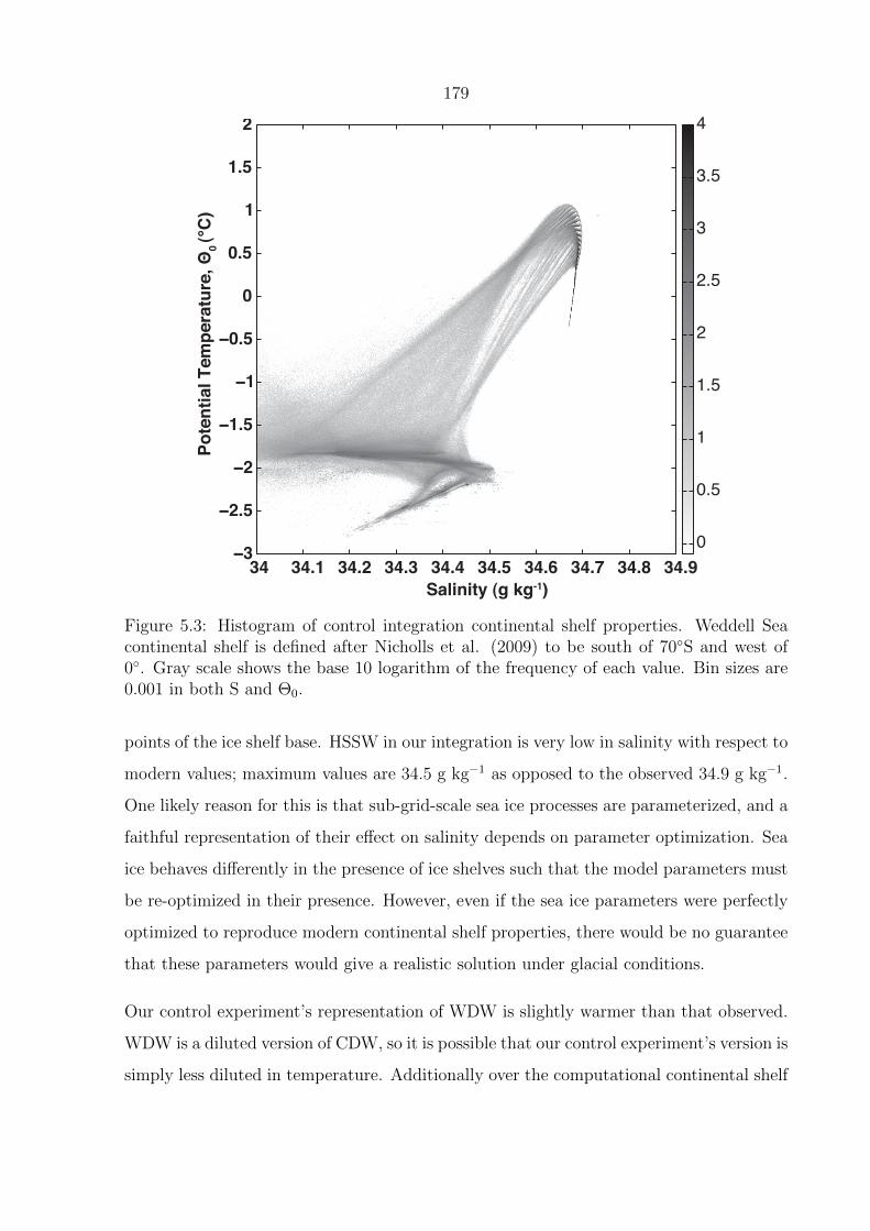
179
Salinity (g kg-1)
Pote
ntia
l Tem
pera
ture
, Θ0 (°
C)
34 34.1 34.2 34.3 34.4 34.5 34.6 34.7 34.8 34.9−3
−2.5
−2
−1.5
−1
−0.5
0
0.5
1
1.5
2
0
0.5
1
1.5
2
2.5
3
3.5
4
Figure 5.3: Histogram of control integration continental shelf properties. Weddell Seacontinental shelf is defined after Nicholls et al. (2009) to be south of 70◦S and west of0◦. Gray scale shows the base 10 logarithm of the frequency of each value. Bin sizes are0.001 in both S and Θ0.
points of the ice shelf base. HSSW in our integration is very low in salinity with respect to
modern values; maximum values are 34.5 g kg−1 as opposed to the observed 34.9 g kg−1.
One likely reason for this is that sub-grid-scale sea ice processes are parameterized, and a
faithful representation of their effect on salinity depends on parameter optimization. Sea
ice behaves differently in the presence of ice shelves such that the model parameters must
be re-optimized in their presence. However, even if the sea ice parameters were perfectly
optimized to reproduce modern continental shelf properties, there would be no guarantee
that these parameters would give a realistic solution under glacial conditions.
Our control experiment’s representation of WDW is slightly warmer than that observed.
WDW is a diluted version of CDW, so it is possible that our control experiment’s version is
simply less diluted in temperature. Additionally over the computational continental shelf

180
we find more points with properties of modern Antarctic Surface Water than apparent in
the data, which typically is characteristic of the open ocean away from the continental
shelf. This could be because the Weddell Gyre intrudes further onto the shelf in the model
than observed, probably as a result of the grid discretization.
The control integration’s representation of WSDW and WSBW is very narrow in property
space and essentially determined by the boundary conditions. The absence of HSSW
explains in part the absence of typical WSDW and WSBW, as HSSW mixes with WDW
to form these two. Still, it is not necessary that HSSW take on its most extreme value in
salinity to form deep water; in fact both WDW and WSDW are higher in salinity than
WSBW but have lower densities than WSBW due to their warmer temperatures.
Although the control experiment produces low salinity HSSW, there is another reason
why we observe a gap in property space between the control HSSW and WDW. The
rapid increase of vertical grid size close to the depth of the shelf break, in combination
with the coarse horizontal resolution, cause shelf properties to mix away rapidly. As a
result, there is negligible transport from the shelf to the deep ocean in our experiments.
Resolution of dense overflows in the modern Weddell Sea requires ∆ z and ∆ h < 100
m (Legg et al., 2006, Winton et al., 1998), a grid several orders of magnitude finer than
ours. However, the grid that we use is already an order of magnitude finer than typical
coupled climate models. This is not merely an artifact of our regional computational
setup; a recent study diagnosing bottom water formation in ocean general circulation
models finds that MITgcm, even in the ECCO global configuration, forms its deepest
waters primarily through transformation of intermediate waters (Downes et al., 2011).
Other models have similar and sometimes worse problems. Improved representation of
bottom water formation, and its role in ocean ventilation changes under future and past
climate scenarios, will require very high resolution or development and implementation of
a sub-grid-scale parameterization.
The melt rate magnitude and patterns of the Filchner-Ronne and western Weddell Sea ice
shelves in our control experiment compare well with estimates from modern satellite data.
Recent estimates from interferometric synthetic-aperture radar (InSAR) data and flux-
gate modelling give a net melt rate of the combined western ice shelves in our numerical

181
domain of 109 ± 24.8 km3 yr−1 (Joughin and Padman, 2003, Rignot et al., 2008). In our
control experiment the combined 10-year-averaged freshwater flux of these ice shelves is
111.6 km3 yr−1. In contrast the melt rates of the eastern ice shelves in our control experi-
ment are about an order of magnitude higher than recent data estimates; we compute an
average of 1071 km3 yr−1 compared to an estimate of 73 ± km3 yr−1 from available data
(Rignot et al., 2008). Although the control melt rates of the eastern ice shelves are likely
too high, this does not have a significant direct effect on the continental shelf properties
and property changes in our experiments, as discussed later. Most of this meltwater is
exported as buoyant surface water. However, the anomalously high meltwater flux to the
surface ocean could have a damping effect on the sea ice response in our experiments. In
the control, the overproduction of ice shelf meltwater could insulate the sea ice from the
underlying ocean conditions. The ocean cooling in our experiments causes and thus coin-
cides with the removal of this anomalous ice shelf freshwater, such that the sensitivity of
the sea ice model in this region to changes in ocean conditions might be underestimated.
5.2.5 Experiments
Eight numerical cooling experiments are done by changing the ocean open boundary
temperatures only. The experimental boundary conditions in potential temperature, Θe,
are defined as
Θe = Θc − η(Θc −Θfr)
where Θc is the boundary potential temperature of the control integration, Θfr is the
salinity and pressure-dependent freezing point, and η ranges from 0.1 to 0.8. Thus η = 0.1
corresponds to the least cooling, while η = 0.8 represents the experiment with the most
cooling. Note that each boundary grid cell can take on a different value; the boundary
conditions are not homogeneous.
Modification of the boundary temperatures alters the density of the boundary points with
respect to those of the control. To ensure that our experiments are examining the effect
of thermodynamic rather than dynamic changes, we also perform a separate set of eight
“density-compensated” integrations. In addition to the temperature changes described
182
above, in the density-compensated integrations we change the salinity of the boundary
conditions; to retain the control densities with colder temperatures requires decreasing
the salinity of each point. We use a local linear approximation of ∂ρ∂S
at each point to
compute the change in salinity necessary to restore the density of the point to that of the
control. The density compensated integrations result in ice melt patterns and magnitudes
virtually indistinguishable from those of the non-compensated experiments, however they
display a very large freshening flux from the boundaries that confuses the interpretation
of our results. For this reason we discuss only the non-compensated experiments.
5.3 Results and Discussion
We find large changes in the properties of water masses formed over the continental shelf
in response to our cooling experiments. Modern water masses such as ISW, HSSW, and
WDW/CDW are identified by their potential temperature and salinity. These identifying
properties are exactly the properties that change with each cooling experiment. For
this reason, instead of using Θ0/S cutoff values to define water masses, we examine how
properties change in fixed locations of interest. The locations which would tell us the most
about modification of AABW properties would be the bottom of the Weddell Sea and the
deep levels of the ocean near the northwestern edge of the Weddell Sea. However, the lack
of a properly resolved or parameterized bottom boundary layer in the model restricts us
to examining experimental results on and near the continental shelf.
With these considerations in mind, our essential result is illustrated in Fig. 5.4, which
shows the Θ0/S properties of water for the control and for two representative cooling
sensitivity experiments at their annual salinity maxima, the time at which we expect
the largest quantity of HSSW. In order to highlight changes in water masses over the
continental shelf that can lead to significant changes in bottom water formation, we
plot water properties of the two bottom-most layers of the domain down to the 1700-
m depth cutoff and water properties inside the ice shelf cavities. Together these two
layers represent, on average, ∼150 m of vertical thickness. Below ∼1700 m the water
properties of the control experiment are dominated by the boundary conditions. The

183
Salinity (g kg-1)
Θ0
(°C
)
34 34.1 34.2 34.3 34.4 34.5 34.6 34.7 34.8 34.9 35−3
−2.5
−2
−1.5
−1
−0.5
0
0.5
1
1.5
2
η=0.8η=0.4Control
Figure 5.4: Θ0/S properties of water in two layers along domain bottom down to 1700 mfrom the control and from two sensitivity experiments at their annual salinity maxima.Together these two layers represent, on average, ∼150 m of vertical thickness. The openocean and the shelf region west of the Antarctic Peninsula are excluded. All potentialtemperatures are referenced to the surface. Curved lines are isopycnals. The distancebetween the isopycnal lines is 0.1 kg m−3
signal of continental shelf processes, a combination of Θ0 and S, deepens by almost 1000
m in our sensitivity experiments as the domain produces denser water able to descend
futher down the continental slope; however, comparison across experiments requires a
fixed-depth cutoff. The potential temperature of water in the ice shelf cavities (ISW) is
already closely constrained by the in-situ freezing point in the control experiment and
does not change noticeably in the experiments. Water masses that correspond to modern
ISW and HSSW increase significantly in salinity, up to a maximum of about 0.3 units
in response to the maximum cooling experiment. At the surface freezing point, which is
the temperature of HSSW, this change in salinity corresponds to an increase in surface
density of 0.24 kg/m3. This increase in surface density is equal to the modern surface
184
density contrast between HSSW and WDW.
Plotting down to the 1700-m depth encompasses the water that lies along the base of
continental shelf and somewhat below the shelf break. This enables us to examine the
density contrast of shelf water with the water it entrains as it descends the slope and how
the contrast changes with cooler temperature experiments. There is a slight increase in
salinity in the warmer, deeper water masses, but the increase is small relative to that of
shelf waters. For this reason, the increase in density on the shelf in our experiments is
almost identical to a change in surface density contrast between HSSW and WDW. As
the continental shelf water overflows the shelf, its density contrast with the surroundings
would tend to increase due to the thermobaric effect (Killworth, 1977). Even without
thermobaric considerations, a surface density increase of 0.24 kg/m3 is more than double
the modern density difference between NADW and AABW of about 0.1 kg/m3.
However, the density contrast between the overflow and the overlying water would also
tend to decrease due to entrainment. In the modern Weddell Sea, the effect of entrainment
on density contrast is small due to the weak density stratification of the water column.
An increase in water column stratification, particularly if there is a large density gradient
at the shelf break, can counteract the increase in overflow source density and reduce the
ability of a high salinity signal to migrate from the continental shelf to the abyssal ocean
(Price and O’Neil-Baringer, 1994). Even if the density (and salinity) at the shelf break is
increased, it does not guarantee an increase in bottom water density.
5.3.1 Diagnosis of Water Mass Changes – Net Salinity Fluxes
and Changes
Figure 5.5 demonstrates that the relationship between domain-averaged S and domain-
averaged Θ0 is linear, with a slope of - 0.006 g kg−1/◦C and a maximum decrease of 0.016
g kg−1. This maximum is an order of magnitude smaller than the changes in HSSW
implied by Fig. 5.4. This is because Figure 5.4 does not include properties of the deep or
surface ocean, nor does it account for the volume associated with each water property
pair. Salinity changes in our experiments are concentrated in particular regions of the

185
−3 −2.5 −2 −1.5 −1 −0.5 0 0.534.64
34.642
34.644
34.646
34.648
34.65
34.652
34.654
34.656
34.658
34.66
Domain Mean Potential Temperature, Θ0 (°C)
Dom
ain
Mea
n Sa
linity
(g k
g-1)
Figure 5.5: Sensitivity of volume-averaged domain salinity to volume-averaged domainpotential temperature. All values are 10-year averages. Each experiment is representedby one point. The control experiment is at Θ0 = 0.5
domain.
To identify the mechanisms that contribute the most to our experimental results, we
consider salinity fluxes to the domain from distinct sources. While in the real ocean many
of these salinity fluxes are freshwater fluxes (evaporation, precipitation, and melting), we
use a volume conserving configuration of MITgcm. In this light, it is more sensible to
discuss salinity fluxes, keeping in mind that they have the opposite sign to freshwater
fluxes.
For reference, Figure 5.6 shows the absolute values of the salinity fluxes that contribute
to the salinity of the whole domain. The bulk of our discussion will demonstrate the
importance of changes in ice shelf fluxes over that of changes in sea ice fluxes across the
experiments. However, it is important to keep in mind that the average salinity of water
in each experiment is determined primarily by the salinity of water entering and exiting
the domain and by the sea ice and surface fluxes. In the modern Weddell Sea, for example,
water masses such as HSSW are higher in salinity than NADW/CDW because of sea ice
formation and export. The control experiment ice shelf contribution is about an order of
magnitude smaller than the sum of the other terms (Fig. 5.6). In contrast, changes in
the ice shelf salinity flux are an order of magnitude larger than changes in the large salt
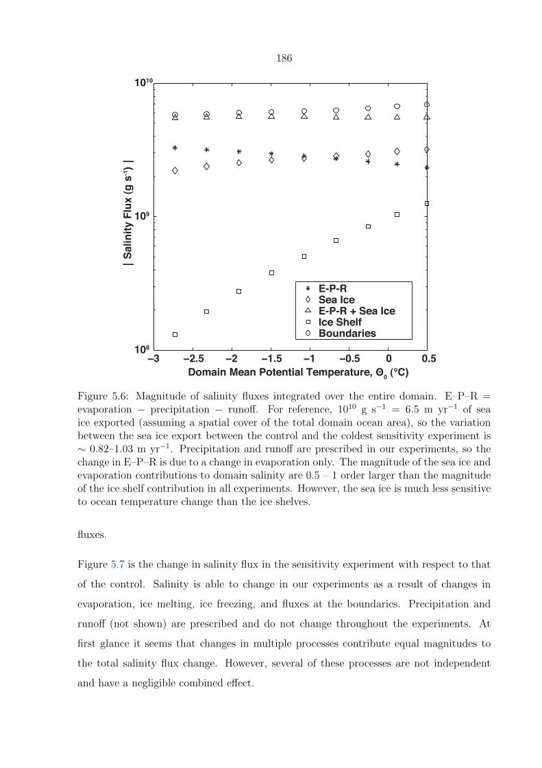
186
−3 −2.5 −2 −1.5 −1 −0.5 0 0.5108
109
1010
Domain Mean Potential Temperature, Θ0 (°C)
┃Sa
linity
Flu
x (g
s-1)┃
E-P-RSea IceE-P-R + Sea IceIce ShelfBoundaries
Figure 5.6: Magnitude of salinity fluxes integrated over the entire domain. E–P–R =evaporation − precipitation − runoff. For reference, 1010 g s−1 = 6.5 m yr−1 of seaice exported (assuming a spatial cover of the total domain ocean area), so the variationbetween the sea ice export between the control and the coldest sensitivity experiment is∼ 0.82–1.03 m yr−1. Precipitation and runoff are prescribed in our experiments, so thechange in E–P–R is due to a change in evaporation only. The magnitude of the sea ice andevaporation contributions to domain salinity are 0.5 – 1 order larger than the magnitudeof the ice shelf contribution in all experiments. However, the sea ice is much less sensitiveto ocean temperature change than the ice shelves.
fluxes.
Figure 5.7 is the change in salinity flux in the sensitivity experiment with respect to that
of the control. Salinity is able to change in our experiments as a result of changes in
evaporation, ice melting, ice freezing, and fluxes at the boundaries. Precipitation and
runoff (not shown) are prescribed and do not change throughout the experiments. At
first glance it seems that changes in multiple processes contribute equal magnitudes to
the total salinity flux change. However, several of these processes are not independent
and have a negligible combined effect.
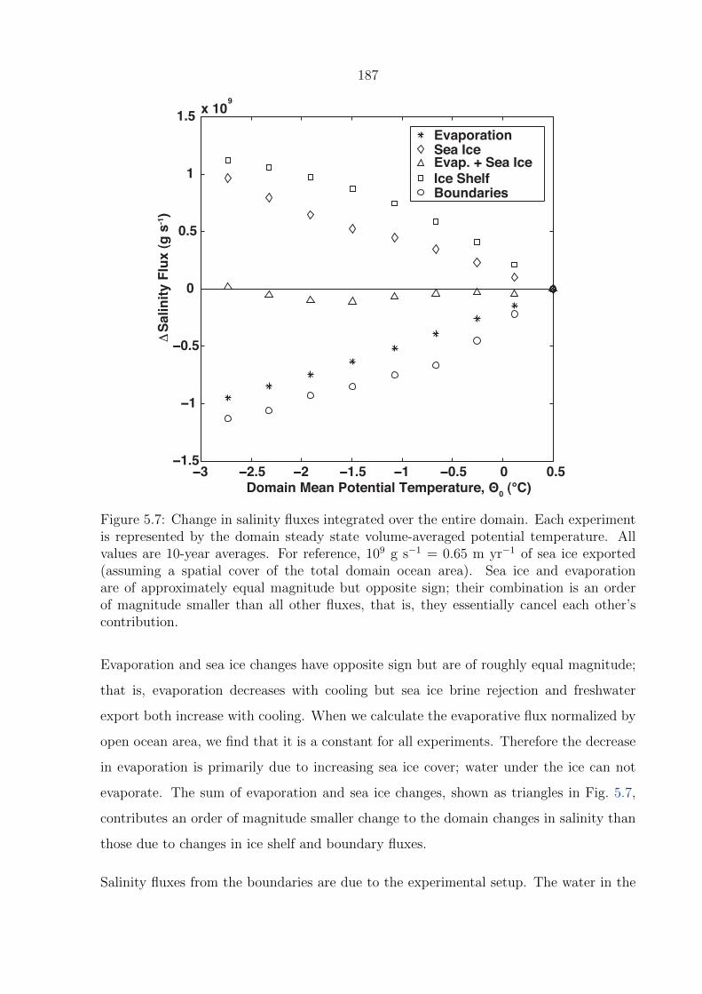
187
−3 −2.5 −2 −1.5 −1 −0.5 0 0.5−1.5
−1
−0.5
0
0.5
1
1.5 x 10
Domain Mean Potential Temperature, Θ0 (°C)
Δ Sal
inity
Flu
x (g
s-1)
EvaporationSea IceEvap. + Sea IceIce ShelfBoundaries
9
Figure 5.7: Change in salinity fluxes integrated over the entire domain. Each experimentis represented by the domain steady state volume-averaged potential temperature. Allvalues are 10-year averages. For reference, 109 g s−1 = 0.65 m yr−1 of sea ice exported(assuming a spatial cover of the total domain ocean area). Sea ice and evaporationare of approximately equal magnitude but opposite sign; their combination is an orderof magnitude smaller than all other fluxes, that is, they essentially cancel each other’scontribution.
Evaporation and sea ice changes have opposite sign but are of roughly equal magnitude;
that is, evaporation decreases with cooling but sea ice brine rejection and freshwater
export both increase with cooling. When we calculate the evaporative flux normalized by
open ocean area, we find that it is a constant for all experiments. Therefore the decrease
in evaporation is primarily due to increasing sea ice cover; water under the ice can not
evaporate. The sum of evaporation and sea ice changes, shown as triangles in Fig. 5.7,
contributes an order of magnitude smaller change to the domain changes in salinity than
those due to changes in ice shelf and boundary fluxes.
Salinity fluxes from the boundaries are due to the experimental setup. The water in the

188
experimental domain becomes increasingly saltier with each experiment, but the velocities
at the boundaries are prescribed. This leads to an increased flux of salt out of the domain
of the same order of magnitude as the increase in salt flux to the domain from reduced
net melting of the ice shelves, the primary source of experimental salinity flux changes.
In the global ocean the exported salt would either recirculate into the Weddell Sea or be
deposited at another location. The salinity stratification of both the Weddell Sea and the
global ocean depends on the destination of this salt. However, because our integrations
are done in a regional domain and our domain boundaries are non-interactive, the effect
of this large quantity of salt is completely unknown and appears to us as a loss of salt.
The ice shelf changes in melting and freezing, which have a salinifying effect on the domain
as it is cooled, are an order of magnitude larger than the combined changes in surface
processes, which are co-dependent. The increased boundary flux of salinity depends on
the increase in domain salinity, so it is a result of the ice-shelf-induced salinity increase
rather than a competing process.
5.3.2 Diagnosis of Water Mass Changes – Regional Variations
and Salinity Flux Tracers
There is significant spatial variation in the salinity fluxes that contribute to the domain
means. Salinity fluxes due to ice shelf melting and freeze-on occur only where there are
ice shelves. Perhaps less obvious is the non-uniformity in sea ice and evaporative fluxes.
While in the domain average the temperature-induced increase in sea ice is balanced by
a decrease in evaporation, this is not true everywhere. Figure 5.8 shows that in our
sensitivity experiments, changes due to sea ice dominate the changes in surface salinity
flux over the continental shelf. This is because in all of our experiments, and in the modern
ocean, the continental shelf is almost completely covered with sea ice year-round. In our
experiments there is a small increase in sea ice cover over the continental shelf, as shown
in Figures 5.9a and 5.9b, which leads to a small decrease in evaporation with increasingly
cool ocean temperatures. However, the increase in area and thickness of sea ice formed
over the continental shelf contributes a more significant quantity of salt. In total, the

189
−3 −2.5 −2 −1.5 −1 −0.5 0 0.5−1
0
1
2
3
4
5 x 10⁷
Domain Mean Potential Temperature, Θ0 (°C)
Δ Sa
linity
Flu
x (g
s-1)
EvaporationSea IceE-P-R + Sea IceE-P-R
Figure 5.8: Change in surface salinity fluxes over the continental shelf, computed assensitivity minus control experiment. Each experiment is represented on the x-axis bythe domain steady state volume average potential temperature. All values are 10-yearaverages. The boundaries of the continental shelf are taken as the 1000-meter depthcontour, excluding land to the north and/or west of the Antarctic Peninsula. For reference,10−7 g s−1 is equivalent to the export of 0.11 m yr−1 from the entire continental shelf.E–P–R = evaporation − precipitation − runoff. The only change in E–P–R across theexperiments is due to evaporation. Salinity flux changes due to sea ice dominate thechange in surface fluxes over the continental shelf.
change in sea ice over the continental shelf is quite small relative to the domain change,
as can be seen by comparing the y-axes of Fig. 5.8 and Fig. 5.7. We have not investigated
the cause of the constant sea ice flux in the warmest three experiments, but one possibility
is that it results from slight differences in the lateral path of the deep Weddell Gyre, which
we observe in the experiments. It might also be related to the meltwater overproduction
of the eastern ice shelves in the control experiment discussed previously. While the change
in sea ice is important relative to other surface salinity fluxes over the continental shelf,

190
0.1
0.2
0.3
0.4
0.5
0.6
0.7
0.8
0.9
1
(a)
0.1
0.2
0.3
0.4
0.5
0.6
0.7
0.8
0.9
1
(b)
Figure 5.9: (a) Minimum sea ice area for three experiments, from left to right: η = 0,η = 0.4, η = 0.8. (b) Maximum sea ice area for three experiments, from left to right:η = 0, η = 0.4, η = 0.8. The color scale indicates grid cell concentration and is unitless.All values represent a 10-year average and a weekly average during the week in which thetotal sea ice volume is at its yearly maximum. The 1000-m depth contour is overlain toindicate the continental shelf break. Grounded ice is indicated by hash marks and floatingice shelves are adjoined to the grounded ice and colored white.
it is small when compared to the ice shelf flux changes. Also, a change in salinity flux
over the continental shelf is not equivalent to a change in continental shelf salinity.
Regional variations in salinity fluxes and their distribution result in a pattern of salinity
change quite different than that implied by the domain mean. With the salinity tracers
described in the Methods section, we are able to determine how different processes con-
tribute to changes in properties across experiments and where changes are concentrated
geographically. To review, we have one salinity tracer that tracks salinity fluxes from the
ice shelves and a second tracer that tracks the salinity fluxes from the surface. The latter
is a combination of atmospheric fluxes and sea ice fluxes. However, since we showed in
the previous section (3.1) that the changes in atmospheric fluxes are due to the sea ice,

191
it is appropriate to think of our surface tracer as equivalent to a sea ice tracer. For these
analyses we define the continental shelf as the region between the ice shelf front and the
1000-m depth contour. We use 1000 m rather than 500 m in order to include water inside
the Filchner and Ronne depressions on the continental shelf.
We find that the majority of the salinity change on the continental shelf is due to a
reduction in ice shelf melting, as shown in Figures 5.10 and 5.11. The total salt flux over
the continental shelf in our experiments is dominated by the sea ice, as observed today,
but the change in salt flux across experiments is dominated by changes in ice sheet basal
melting. Figure 5.10 shows the change in distribution of the surface and ice shelf tracers
as vertical integrals for a representative (40% cooling) experiment. Overall, the maximum
change is largest in the ice shelf salinity tracer.
The effect of the ice shelf melt changes are not only larger but also concentrated on the
continental shelf. Figure 5.10 demonstrates that most of the change in ice shelf tracer
in our experiments occurs over the continental shelf and near the shelf break, with a
particularly high concentration of change inside and in the outflow from the Filchner
Depression.
If we consider water lying along the bottom of the continental shelf instead of the vertical
integral, we find that the salinity change of bottom water precursors is predominantly due
to a net reduction in ice shelf melting. Figure 5.11 is the evolution of salinity tracers on the
bottom of the continental shelf as temperature decreases in the numerical experiments.
The bottom is the partially or fully water-filled grid cell above a completely land-filled
cell. The computation of salinity changes in Fig. 5.11 accounts for grid-cell volume,
unlike the salinity change implied by Fig. 5.4. We do not consider water inside ice shelf
cavities, as typically this water is significantly modified by the time it reaches the shelf
break. After applying these filters, the water we consider is a layer on average 67 m
thick. For reference, typical observed overflow plume thicknesses in Antarctica can be
anywhere from 30 to 200 m (Muench et al., 2009). In Θ0/S space, this continental shelf
water roughly corresponds to the high salinity water lying along the surface freezing line
shown in Fig. 5.4 — analogous to modern ISW and HSSW. The 0.3 g kg−1 change in
salinity as suggested by Fig. 5.4 might not have represented a large volume of water, but
192
when volume is accounted for, the bottom water increase in salinity is still 0.3 g kg−1.
Together Figs. 5.10 and 5.11 demonstrate that, in our experiments, cooling continental
shelf source waters increases the salinity of bottom water precursors, and this is primarily
due to reduced net ice shelf basal melting.
In contrast, the majority of the changes in the sea ice tracer occur away from the con-
tinental shelf and are due to an increase in average sea ice area and thickness in this
region. Sea ice changes dominate the changes in salinity north of the shelf break. This
increased sea ice cover north of the continental shelf break salinifies the water that would
be entrained into the continental shelf overflow on its path to the bottom of the sea,
although model issues prevent us from seeing how this evolves. This would reduce the
density contrast between continental shelf water masses and open ocean water, and would
mitigate the freshening effect of entrainment. That is, an increase in salinity off the shelf
would help retain the high salinity signature of the shelf water masses throughout the
shelf overflow’s transformation to bottom water. In the control integration (and modern
ocean) the continental shelf is perennially covered in sea ice, so the surface ocean is al-
ready at the freezing point. Under these conditions, decreasing the ocean temperature
further does not have a large effect on sea ice thickness.
Over the continental shelf, significant changes in sea ice, and the resultant salinity mod-
ifications, would require a large decrease in atmospheric temperature or an increase in
export velocity. Lower atmospheric temperature and higher wind stress would increase
the bulk heat flux between ocean and atmosphere, enabling an increase in the thickness
or formation rate of sea ice. Alternatively the higher wind stress could remove thicker
sea ice with the same area, or could enable faster removal of sea ice from the continental
shelves, either of which would increase the net freshwater export rate. Both scenarios are
certainly possible at the LGM. Atmospheric temperature and export velocities of sea ice
are the same for all experiments, so the primary way for ice export to increase in our
experiments is through an increase in ice thickness.

193
Ice Shelf Salt Tracer
Sea Ice Salt Tracer
−50 0 50 100 150 200
Figure 5.10: Depth integrated salt tracer fields for the sensitivity experiment in whichthe boundaries are cooled 40% towards the freezing point from the control experiment(η = 0.4). Color values are in m g kg−1 and represent the difference between the sensitivityand control experiments. All are 10-year averages. Black shaded area is land, white shadedarea is ice shelves and the black contour line represents the location of the 1000-m bottomdepth contour.

194
−3.5 −3 −2.5 −2 −1.5 −1 −0.5 0−0.05
0
0.05
0.1
0.15
0.2
0.25
0.3
0.35
Δ Θ Domain Mean
Mea
n Δ
S (g
kg-1
) Sen
sitiv
ity−C
ontr
ol
TotalIce ShelfSea IceBoundary Flux
0
Figure 5.11: Ice shelf and sea ice salinity tracer values integrated over the bottom water-filled layer on the continental shelf. All values represent the 10-year-averaged differencebetween sensitivity and control. The boundaries of the continental shelf are taken asthe area between the ice shelf front and the 1000-m depth contour, shown in Fig. 5.2,excluding land to the north and/or west of the Antarctic Peninsula.
195
5.3.3 Diagnosis of Water Mass Changes – Regional Differences
in Ice Shelves
Although the shapes and sizes of the ice shelves are fixed in our experiments, they
vary across the numerical domain. The smaller, shallower, ice shelves to the east of
the Filchner-Ronne Ice Shelf are more sensitive to changes in the boundary temperature
forcing. Comparing the total melt rate of the large ice shelves with that of the smaller ice
shelves in the east of our numerical domain (Fig. 5.12), we find that there is a greater
cumulative flux of meltwater from the small eastern shelves than from the large shelves,
except in the coldest experiment. This does not mean that all of this water makes it into
the Weddell Sea proper; the majority is so buoyant that it rises to the surface and is
exported from the domain.
The large change in freshwater flux from the eastern shelves is not the determining factor
in our results. With our current tools we can not distinguish the geographical source of
the ice shelf salinity forcing in our salt tracers. However, we can compute the reduction in
freshwater flux from different regions required to cause the changes in salt tracers on the
continental shelf. The volume of water we consider to define the continental shelf (up to
the 1000-m contour) is 3.77 ×10¹³ m3. Assuming a typical density of salt water of 1027.5
kg m−3 and that of glacial meltwater of 999.8 kg m−3, a maximum change in salinity of
0.3 g kg−1, and using the model salt-to-freshwater conversion factor of 33.4 g kg−1, we
find that a net 3.48 ×10¹¹ m3 of meltwater is required to explain the maximum difference
in salinity between the control and the coldest experiment. If the residence time of these
waters on the shelf is one year, that corresponds to a difference in freshwater input of 3.48
×1011 m3 yr−1. If instead the continental shelf water is completely renewed only every
10 years, the difference in freshwater flux required to maintain this salinity difference
between the two experiments is an order of magnitude smaller. The maximum difference
in freshwater flux magnitude from the western ice shelves is only 2.83×10¹⁰ m3 yr−1, which
means that unless the residence time of water on the shelf is more than 10 years, some
change in freshwater flux from the eastern ice shelves is necessary to explain the observed
changes in our experiments. This is expected, because our definition of the continental
shelf includes the shelf directly in front of the eastern ice shelves. The combined shelf
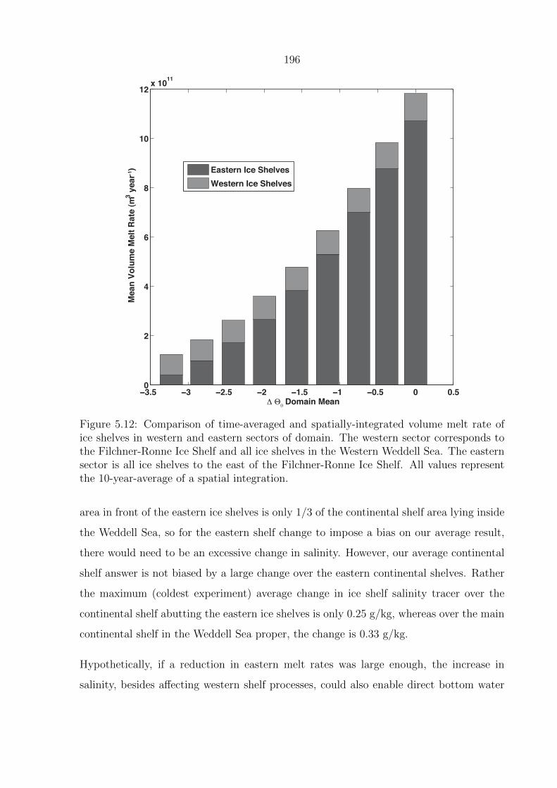
196
−3.5 −3 −2.5 −2 −1.5 −1 −0.5 0 0.50
2
4
6
8
10
12x 1011
Δ Θ0 Domain Mean
Mea
n Vo
lum
e M
elt R
ate
(m3 y
ear-1
)
Eastern Ice ShelvesWestern Ice Shelves
Figure 5.12: Comparison of time-averaged and spatially-integrated volume melt rate ofice shelves in western and eastern sectors of domain. The western sector corresponds tothe Filchner-Ronne Ice Shelf and all ice shelves in the Western Weddell Sea. The easternsector is all ice shelves to the east of the Filchner-Ronne Ice Shelf. All values representthe 10-year-average of a spatial integration.
area in front of the eastern ice shelves is only 1/3 of the continental shelf area lying inside
the Weddell Sea, so for the eastern shelf change to impose a bias on our average result,
there would need to be an excessive change in salinity. However, our average continental
shelf answer is not biased by a large change over the eastern continental shelves. Rather
the maximum (coldest experiment) average change in ice shelf salinity tracer over the
continental shelf abutting the eastern ice shelves is only 0.25 g/kg, whereas over the main
continental shelf in the Weddell Sea proper, the change is 0.33 g/kg.
Hypothetically, if a reduction in eastern melt rates was large enough, the increase in
salinity, besides affecting western shelf processes, could also enable direct bottom water
197
formation from the eastern continental shelves. Today, water formed through interactions
with the eastern ice shelves does find its way onto the continental shelves in the Weddell
Sea. By preconditioning the water properties that enter the Weddell Sea, the eastern shelf
interactions indirectly affect the bottom water formation processes to the west, although
the relative magnitude of the eastern shelf contribution is still uncertain (Nicholls et al.,
2009). However, the extremely low salinity in front of the eastern ice shelves suppresses
direct bottom water formation (Fahrbach et al., 1994).
5.3.4 Relevance to Glacial Oceans
We do not simulate the LGM. As such, it is difficult to compare our sensitivity exper-
iments to data, because we have purposely not modified a large number of important
variables. However, we believe that the sensitivity experiment that is most appropriate to
compare to LGM data is our most extreme temperature scenario. First, the temperature
changes of interest to the LGM ocean are not as large as the domain-averaged temper-
ature suggests. The temperature change on the shelf is much smaller than the average
temperature change of the whole domain, which is significant because a large volume of
deep water in our domain does not interact with the continental shelf. Using the same
definition of continental shelf as for the salinity tracers, we find that the average poten-
tial temperature on the continental shelf in our most extreme experiment is -2.00◦C. In
comparison, the average potential temperature on the continental shelf in our control is
-1.65◦C. The sensitivity of continental shelf salinity to continental shelf temperature is
thus much higher than the sensitivity of the whole domain salinity to whole domain tem-
perature: 0.875 g kg−1/◦C as opposed to 0.006 g kg−1/◦C. Given these considerations, a
0.3 g kg−1 change in salinity due to a continental shelf potential temperature decrease of
0.13◦C is reasonable. It does not require unphysically cold temperatures. With a sim-
ple change in temperature we can account for 30% of the difference in salinity contrast
observed between GNAIW and GSSBW.
We do not address how the temperature at the boundaries of our computational Weddell
Sea domain could be depressed to such low levels. There are two possibilities: (i) either
198
the temperature of WDW/CDW was lower or (ii) relatively warm CDW did not intrude
onto the continental shelves. Our setup does not favor one or the other of these hypotheses
— we simply make the water colder. So, even if northern source deep water was not a
precursor to GSSBW at the LGM, the fact that the ocean was cooler still explains a
significant fraction of the high measured bottom water salinity.
5.3.5 The Effect of Unmodelled Processes
In order to focus on the sensitivity of bottom water formation to ocean temperature,
we do not simulate the LGM. As previously discussed, a change in wind stress and/or
atmospheric temperature could have an important role in changing the bottom water prop-
erties. In addition, there is evidence that both atmospheric temperature over Antarctica
(Petit et al., 1999) and sea surface temperature in the Southern Ocean (Gersonde et al.,
2005) were lower at the LGM than they are today. All of these factors could contribute
to increasing the sea ice export. Increased sea ice export from LGM deep water formation
sites probably played a larger role in increasing the salinity of LGM bottom water than
it does in our experiments, but we specifically did not simulate that.
Another factor that we do not consider is a change in bathymetry of the land or ice shelf
cavities. However, in our experiments the smaller ice shelves showed the greatest change
in melt rate in the experiments. Isolated ice shelf cavity process studies also indicate
that ice shelf basal melting depends strongly on ice sheet morphology (Little et al., 2009).
This is significant to inferred ice shelf conditions at the LGM. Reconstructions of the
LGM Antarctic ice sheet extent suggest that the grounding line was located further north
(Anderson et al., 2002) , which could mean that the ice shelves at the LGM were configured
similarly to the small ice shelves located to the east of the Weddell Sea in our experiments:
either shallow and abutted by a narrow continental shelf or overhanging the continental
shelf break. The fact that melt rates of these smaller ice shelves are more sensitive
to temperature could mean that temperature played a greater relative role in setting
shelf water salinity than it does with the modern shelf configuration that we used in our
experiments. In short, given the correct ice sheet and ice shelf shapes at the LGM, small
199
perturbations in temperature might generate a larger ice shelf salinity response.
It is important to remember that the ice sheet morphology dynamically responds to
changes in ocean conditions, a factor we have neglected by using fixed-shape ice shelf
cavities. The inclusion of tides, which are influenced by ice shelf cavity and continental
shelf shapes, could change the total Filchner-Ronne ice shelf melt rate by an order of
magnitude (Makinson et al., 2011). It is also possible that the outward migration of
the ice sheet grounding line meant that there was no Antarctic continental shelf or ice
shelves, in which case the bottom water formation process at the LGM would have been
fundamentally different (Paillard and Parrenin, 2004).
Besides water properties, bottom water formation depends heavily on the rate of produc-
tion and movement off the shelf. The modern production rate suggests that the residence
time of high density water on the continental shelf is between 5 and 7 years (Gill, 1973,
Gordon et al., 2010). While water does leave our domain, the open boundary configuration
fixes its export rate.
5.4 Conclusions
Cooling the ocean has a significant effect on the salinity of the water lying on the con-
tinental shelf of the Weddell Sea, water that in the modern is a precursor to Antarctic
Bottom Water. Pore fluid measurements find that the salinity gradient between GSSBW
and GNAIW was 1.1 units greater than the gradient between AABW and NADW. With
ocean cooling alone, we can explain as much as 30% of this change in salinity stratifica-
tion. Almost all of this change is due to a reduction of basal melting from marine-based
ice sheets over and in the vicinity of the Weddell Sea continental shelf, but a small portion
can also be attributed to the export of thicker sea ice. Similar changes in ice shelf basal
melting could have occurred over the other Antarctic continental shelves at the LGM,
which in addition to transport and recirculation of circumpolar water masses, might have
increased the contribution of this particular effect. The effect we observe in our experi-
ments is due primarily to thermodynamics and not to a dynamic (i.e., buoyancy-driven)

200
response to temperature changes; while ocean temperature can not account for all of
the measured salinity difference between GSSBW and AABW, it is of the same order of
magnitude and must be considered as one of several important salinity drivers.
While this is a significant number, it can not explain all of the change in salinity. Among
the candidates for explaining the remaining 70%, ice shelf shape and wind-driven changes
in sea ice processes are likely to have significant roles. Bathymetric changes at the LGM,
including the shape and exposure of the continental shelf and ice shelves, as well as their
effect on tidal mixing, may have been important in setting the salinity of GSSBW. In our
experiments, small ice shelves, such as those that may have existed at the LGM, were
more sensitive to changes in ocean temperature than the larger ones, perhaps due to their
greater exposure to open ocean conditions. In the modern ocean, this sensitivity and
exposure to warm ocean conditions contribute to blocking direct bottom water formation
in front of the small ice shelves, such that processes over smaller continental shelves, in
front of smaller ice shelves, have only an indirect role in bottom water formation. In a
reduced open ocean temperature environment this constraint might have been lifted, such
that significant bottom water formation could have occurred in front of small ice shelves.
With a narrow and more spatially homogeneous continental shelf ringing the Antarctic
continent, bottom water formation may have been more geographically distributed than it
is today. Decreased atmospheric temperature and increased wind stress near the Antarctic
continent also may have contributed to an increased salinity flux from sea ice formation
and export. Our experiments show that a decrease in ocean temperature alone does
not significantly increase the ocean salinification due to sea ice export, in part because
greater sea ice cover reduces ocean evaporation. Due to the limitations of a regional model
in representing water export rates, future studies on this subject should investigate the
feedback between changes in property (Θ0, S) and density stratification in a circumpolar
or global configuration.
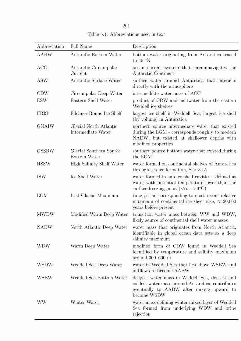
201
Table 5.1: Abbreviations used in text
Abbreviation Full Name Description
AABW Antarctic Bottom Water bottom water originating from Antarctica tracedto 40 ◦N
ACC Antarctic CircumpolarCurrent
ocean current system that circumnavigates theAntarctic Continent
ASW Antarctic Surface Water surface water around Antarctica that interactsdirectly with the atmosphere
CDW Circumpolar Deep Water intermediate water mass of ACC
ESW Eastern Shelf Water product of CDW and meltwater from the easternWeddell ice shelves
FRIS Filchner-Ronne Ice Shelf largest ice shelf in Weddell Sea, largest ice shelf(by volume) in Antarctica
GNAIW Glacial North AtlanticIntermediate Water
northern source intermediate water that existedduring the LGM - corresponds roughly to modernNADW, but existed at shallower depths withmodified properties
GSSBW Glacial Southern SourceBottom Water
southern source bottom water that existed duringthe LGM
HSSW High Salinity Shelf Water water formed on continental shelves of Antarcticathrough sea ice formation, S > 34.5
ISW Ice Shelf Water water formed in sub-ice shelf cavities - defined aswater with potential temperature lower than thesurface freezing point (<≈ −1.9◦C)
LGM Last Glacial Maximum time period corresponding to most recent relativemaximum of continental ice sheet size, ≈ 20,000years before present
MWDW Modified Warm Deep Water transition water mass between WW and WDW,likely source of continental shelf water masses
NADW North Atlantic Deep Water water mass that originates from North Atlantic,identifiable in global ocean data sets as a deepsalinity maximum
WDW Warm Deep Water modified form of CDW found in Weddell Seaidentified by temperature and salinity maximumaround 300–600 m
WSDW Weddell Sea Deep Water water in Weddell Sea that lies above WSBW andoutflows to become AABW
WSBW Weddell Sea Bottom Water deepest water mass in Weddell Sea, densest andcoldest water mass around Antarctica, contributeseventually to AABW after mixing upward tobecome WSDW
WW Winter Water water mass defining winter mixed layer of WeddellSea formed from underlying WDW and brinerejection

202
Chapter 6
Concluding remarks
In this thesis, we used a combination of idealized ocean modeling, geological records, and
both traditional regularized least squares optimization and Bayesian MCMC parameter
estimation inverse methods to shed light on an outstanding puzzle about past ocean
density stratification.
With inferences from sediment pore fluid profiles of [Cl−] and δ18O, Adkins et al. (2002)
inferred that the LGM ocean had a wider range of densities than the modern ocean, and
that the ocean density stratification was set by salinity. In contrast, the modern ocean
stratification is controlled by temperature. This result was a major scientific advance, as it
provided the first evidence that the ocean was more physically stratified in the past. Such
strong physical stratification could explain other records showing major spatial contrasts
in ocean chemistry at the LGM.
While Adkins et al. (2002)’s results were revolutionary, they left many questions unanswered.
How did the deep ocean’s density, which today is controlled by temperature, become a
function of salinity? What did this imply about the ocean circulation? How did the ocean
density stratification evolve from the LGM to the present? By answering these questions
we could make significant progress towards understanding how the ocean interacts with
the climate system over long timescales. We have sought to answer these questions in this
thesis.
How could density variations in the ocean be primarily determined by salinity, and
203
are LGM temperatures and salinities linked? Using a state-of-the-art ocean model, we
investigated whether ocean temperature, through its effect on ice–ocean interactions,
could induce the inferred LGM salinity stratification. Using the Weddell Sea as a case
study, we explored the impact of lower ocean temperatures on Antarctic ice–ocean interactions.
We found that changes in ice-shelf–ocean interactions due to temperature alone lead to
a significant increase in the salinity of water that feeds the deepest ocean. Our results
show that the maximum possible salinity due to temperature change could only account
for part of the inferred deep ocean salinity stratification in Adkins et al. (2002), which
means one of several possibilities. Another process, such as increased export of sea ice
due to a change in wind patterns, may have contributed to the inferred high salinity
bottom water. While it is very likely that the sea ice export was greater at the LGM due
to changes in the wind, wind patterns are even more difficult to reconstruct than deep
ocean temperature. Alternatively, the model may not properly represent the cold ocean
state. Finally, the inferred salinity at the LGM may have been overestimated. That said,
our work demonstrates that ocean temperature, through its interaction with ice shelves,
can have a significant role in changing the salinity and density stratification of the deep
ocean. This insight is new; previously the interaction between ice shelves and the ocean
had been largely ignored as an important player in past ocean stratification changes.
The evidence for glacial salinity stratification presented in Adkins et al. (2002) is a
sparse data set. To determine whether this small set of points is representative of
the entire ocean, we have worked to increase the number of and our ability to make
measurements. Obtaining high depth resolution sediment pore fluid samples for [Cl−]
and δ18O measurement and inversion is limited by the current interstitial water recovery
method, which destroys large sections of ocean sediment cores, disrupting the chronology
of other records. We tested whether Rhizon samplers, a non-destructive tool developed
for terrestrial soil sampling, can recover water from deep ocean sediments at high depth
resolution. Rhizons were unable to be used in the very deepest, highly compacted ocean
sediments. In less compacted sediments, the Rhizons caused contamination of the chloride
concentration and oxygen isotope values, making them unsuitable for our purposes.
Oxygen isotopes and chloride concentration in ocean sediment interstitial fluid record the

204
integrated history of the water properties at the water–sediment interface, not only those
at the LGM, and the effects of diffusion and advection in the sediments. Thus, recovery of
LGM bottom water properties requires inverting the profiles. Previous inversion methods
applied to this problem led to a systematic offset between data and model, indicating
possible errors in the reported solutions. Further, these previous approaches only allowed
for the solution of the salinity or δ18O at the LGM, despite the fact that the profile is
set by the temporal evolution of bottom water and not solely the value at the LGM. We
aimed to find a robust inverse method that would allow us to extract the full information
content of the pore fluid profiles, including the evolution of [Cl−] and δ18O from the LGM
to present.
We showed that traditional regularized least squares inverse methods are unsuitable for
this task as they recover only one solution to a non-unique problem, are very sensitive
to noise in the data, and it is impossible to robustly quantify the error associated with
the solution they recover. We instead turned to Bayesian Markov Chain Monte Carlo
parameter estimation methods to reconstruct the histories of δ18O and [Cl−] from modern
pore fluid profiles. Relying on a highly parallelized sampler, CATMIP, we can solve
simultaneously for unknown sediment properties, such as diffusivity, in addition to the
history of δ18O and salinity. Our new Bayesian approach is a major improvement over
the previous method, because it weaves our uncertainty about past physical parameters
into the fabric of the problem, and is much less sensitive to noise than regularized least
squares inversions.
Our preliminary results suggest that that the deep ocean was indeed more salinity stratified
at the LGM, however the LGM salinity stratification may have been smaller than previously
reported. Encouragingly, [Cl−] and δ18O between the LGM and present day can be
reconstructed with even higher confidence than their values at the LGM. Our current
evidence hints at a striking dichotomy between the Pacific and Atlantic in their deep
ocean water mass evolution during the deglaciation and Holocene. Measurements at more
ocean sediment core sites will improve our ability to constrain the global water mass and
deep ocean density evolution between the LGM and today.
We need to find a way to markedly increase the number of high quality measurements of

205
sediment pore fluid chloride and oxygen isotopes, as we still lack suitable alternative ways
to reconstruct ocean temperature and salinity. We expect that increased use of emerging
remotely operated ocean drilling technologies, such as the MeBo, will afford a marked
increase in the global spatial density of pore fluid profiles.

206
Appendix A
Titration methods for [Cl−]measurement
A.1 Theory
The [Cl−] of each sample is measured by titration against silver nitrate. I measure the
progression of this reaction potentiometrically. The basic reaction is:
[Cl−] + [Ag+] [AgCl](s) . (A.1)
The chloride concentration of the sample is determined by the equivalence-point of the
reaction: when an equivalent amount of silver nitrate reagent to the amount of chloride
in solution has been added. There is an electrode in the titrant and the sample solution,
and I measure the voltage difference across these two. To close the circuit, the tip of
the titrant buret is placed in the sample beaker, which also protects against issues with
surface tension. That is, as the micrometer is advanced, a drop of solution does not have
to separate from the tip of the buret to enter the sample. At any given time, the voltage
drop measured across the two solutions is equal to the difference in potential on each
electrode, defined by the Nernst equation
E = −RTnF
lnQ , (A.2)
207
where R is the gas constant, T the absolute temperature, n is the number of electrons
reacting at the electrode, F is the Faraday constant (charge on one gram equivalent of an
ion) and Q is proportional to the activity of the ion to which the electrode is sensitive.
The electrodes used are almost pure silver, which are sensitive to the silver ion activity
through the surface reaction
Ag(s) Ag+ + e− . (A.3)
As the titration reaction proceeds in the beaker, the silver ion activity goes from ∼ 0 to
a larger number, controlled by equilibrium with the silver chloride that precipitates out.
The result of this increase in silver ion activity in my sample mean that the voltage drop
across the electrodes is decreasing throughout each measurement. In my methodology,
the practical difference between activity and concentration is negligible.
A.2 Equipment
The voltage drop progression is measured using a National Instruments USB-6210 Multifunction
DAQ. I sample the measurements using LabVIEW. Because there is a significant amount
of background noise in our lab, I filter by averaging 80 samples taken at a frequency of
800 Hz. This is not a unique choice, but it should bypass the typical building power
frequency noise at 50 or 60 Hz.
The micrometer is attached to an Applied Motion stepper motor. The motor is also driven
through LabVIEW, allowing me to automate the titration procedure except for loading
the sample and titrant.
During the titration, the solution is stirred using a mini stir bar and plate.
208
A.3 Standards
To determine the chloride concentration of an unknown sample, I weigh out a sample and
then titrate to the equivalence point. Once I know the volume of silver nitrate added to
the sample and the weight of the sample, determining the concentration simply requires
knowing the precise concentration of silver nitrate.
I know the rough concentration of the silver nitrate from preparation, but to have a more
precise knowledge of its concentration I calibrate my silver nitrate by titrating a known
standard.
My standard is the IAPSO P-Series Normal Standard Seawater (S=35). Because there is
high evaporation in Southern California, once I open a standard I store it with parafilm
around the top and inside a glass jar that is ∼ one third full of water. I use a standard
for a maximum of 2 weeks. When I open a new standard I compare the old values to
the new ones. I also measure a consistency standard in triplicate every day that I am
making measurements to ensure that there is no significant evaporation of my standard.
My consistency standard is low salinity ∼ 33 g kg−1 surface seawater from the N. Pacific,
in the vicinity of Hydrate Ridge.

209
Bibliography
A. Adcroft, C. Hill, and J. Marshall. The representation of topography by shaved cells in
a height coordinate model. Monthly Weather Review, 125(9):2293–2315, 1997. 174
J. F. Adkins. The role of deep ocean circulation in setting glacial climates.
Paleoceanography, August 2013. doi: 10.1002/palo.20046. 3
J. F. Adkins, K. McIntyre, and D. P. Schrag. The salinity, temperature and δ18O of the
glacial deep ocean. Science, 298(5599):1769–1773, 2002. xxii, 7, 8, 9, 12, 13, 14, 29, 62,
77, 78, 90, 128, 130, 134, 169, 202, 203
J.F. Adkins and Daniel P Schrag. Reconstructing Last Glacial Maximum bottom water
salinities from deep-sea sediment pore fluid profiles. Earth and Planetary Research
Letters, 216:109–123, 2003. doi: 10.1016/S0012-821X(03)00502-8. 18
R. F. Adler, G. J. Huffman, A. Chang, R. Ferraro, P. Xie, J. Janowiak, B. Rudolf,
U. Schneider, S. Curtis, D. Bolvin, A. Gruber, J. Susskind, P. Arkin, and E. Nelkin.
The version-2 global precipitation climatology project (gpcp) monthly precipitation
analysis (1979-present). Journal of Hydrometeorology, 4:1147–1167, 2003. 177
J. B. Anderson, S. S. Shipp, A. L. Lowe, J. S. Wellner, and A. B. Mosola. The Antarctic Ice
Sheet during the Last Glacial Maximum and its subsequent retreat history: a review.
Quaternary Science Reviews, 21:49–70, 2002. 198
Antonov et al. World Ocean Atlas 209, Volume 2: Salinity. U.S. Government Printing
Office, Washington, D.C., 2010. 74, 178
U. M. Ascher, S. J. Ruuth, and B. T. R. Wetton. Implicit-Explicit Methods for Time-
210
Dependent Partial Differential Equations. SIAM Journal on Numerical Analysis, 32
(3):797–823, 1995. 20, 69
R. C. Aster, B. Borchers, and C. H. Thurber. Parameter Estimation and Inverse Problems.
Elsevier Academic Press, 2005. 21
E. Bard, B. Hamelin, and R. G. Fairbanks. U-Th ages obtained by mass spectrometry
in corals from Barbados: sea level during the past 130,000 years. Nature, 346:456–458,
1990a. 137, 138, 139, 140, 141, 143, 144
E. Bard, B. Hamelin, R. G. Fairbanks, and A. Zindler. Calibration of the 14C timescale
over the past 30,000 years using mass spectrometric U-Th ages from Barbados corals.
Nature, 345:405–410, 1990b. 137, 138, 139, 140, 141, 143, 144
E. Bard, B. Hamelin, M. Arnold, L. Montaggioni, G. Cabioch, G. Faure, and F. Rougerie.
Deglacial sea-level record from Tahiti corals and the timing of global meltwater
discharge. Nature, 382:241–244, 1996. 132, 137, 138, 139, 140
J. W. Beck, D. A. Richards, R. L. Edwards, B. W. Silverman, P. L. Smart, D. J. Donahue,
S. Hererra-Osterheld, G. S. Burr, L. Calsoyas, A. J. Jull, and D. Biddulph. Extremely
large variations of atmospheric 14C concentration during the last glacial period. Science,
292:2453–8, 2001. doi: 10.1126/science.1056649. 2
R. A. Berner. Early Diagenesis: A Theoretical Approach. Princeton University Press,
1980. 14, 17, 19, 69
B. P. Boudreau. Diagenetic Models and Their Implementation: Modelling Transport and
Reaction in Aquatic Sediments. Springer-Verlag, 1997. 14, 17
B. P. Boudreau and F. J. R. Meysman. Predicted tortuosity of muds. Geology, 34(8):693,
2006. doi: 10.1130/G22771.1. 19
N. Bouttes, D.M. Roche, and D. Paillard. Impact of strong deep ocean stratification on
the glacial carbon cycle. Paleoceanography, 24(3):1–11, 2009. 169
N. Bouttes, D. Paillard, and D.M. Roche. Impact of brine-induced stratification on the
glacial carbon cycle. Climate of the Past, 6(5):575–589, 2010. 169

211
E. A. Boyle. Cadmium: chemical tracer of deepwater paleoceanography. Paleoceanography,
3(4):471–489, 1988. 3
E. A. Boyle. Cadmium and δ13C paleochemical ocean distributions during the Stage 2
Glacial Maximum. Annual Review of Earth and Planetary Sciences, 20:245–287, 1992.
3, 4
P. Braconnot, B. Otto-Bliesner, S. Harrison, S. Joussaume, J.-Y. Peterchmitt, A. Abe-
Ouchi, M. Crucifix, E. Driesschaert, Th. Fichefet, C. D. Hewitt, M. Kageyama,
A. Kitoh, A. Laıne, M.-F. Loutre, O. Marti, U. Merkel, G. Ramstein, P. Valdes, S. L.
Weber, Y. Yu, and Y. Zhao. Results of PMIP2 coupled simulations of the Mid-Holocene
and Last Glacial Maximum Part 1: experiments and large-scale features. Climate of
the Past, 3(2):261–277, June 2007. ISSN 1814-9332. doi: 10.5194/cp-3-261-2007. URL
http://www.clim-past.net/3/261/2007/. 1
W. Broecker and S. Barker. A 190 h drop in atmosphere’s ∆14C during the “Mystery
Interval”(17.5 to 14.5 kyr). Earth and Planetary Science Letters, 256(1-2):90–99, 2007.
doi: 10.1016/j.epsl.2007.01.015. 2, 12
W. S. Broecker and G. H. Denton. The role of ocean-atmosphere reorganizations in
glacial cycles. Geochimica et Cosmochimica Acta, 53(10):2465–2501, 1989. doi: 10.
1016/0016-7037(89)90123-3. 2
A. W. Bruckner. Proceedings of the Caribbean Acropora Workshop: Potential Application
of the U.S. Endangered Species Act as a Conservation Strategy. In NMFS-OPR-24,
NOAA Technical Memorandum, pages 1–199, Silver Spring, MD, 2002. 132
A. Burke and L. F. Robinson. The Southern Ocean’s role in carbon exchange during the
last deglaciation. Science, 335(6068):557–61, 2012. doi: 10.1126/science.1208163. 2
J. Chappell and N. J. Shackleton. Oxygen isotopes and sea level. Nature, 324(13):137–140,
1986. 73, 172
J. Chappell, A. Omura, T. Esat, M. McCulloch, J. Pandolfi, Y. Ota, and B. Pillans.
Reconciliation of late Quaternary sea levels derived from coral terraces at Huon

212
Peninsula with deep sea oxygen isotope records. Earth and Planetary Science Letters,
141:227–236, 1996. 140
C. D. Charles and R. G. Fairbanks. Evidence from Southern Ocean sediments for the
effect of North Atlantic deep-water flux on climate. Nature, 355:416–419, 1992. 4
J. H. Chen, H. A. Curran, B. White, and G. J. Wasserburg. Precise chronology of the last
interglacial period: U- 230Th data from fossil coral reefs in the Bahamas. Geological
Society of America Bulletin, 103:82–97, 1991. 142, 143, 144, 145
P. U. Clark, A. S. Dyke, J. D. Shakun, A. E. Carlson, J. Clark, B. Wohlfarth, J. X.
Mitrovica, S. W. Hostetler, and A. M. McCabe. The Last Glacial Maximum. Science,
325(5941):710–4, 2009. doi: 10.1126/science.1172873. 15
CLIMAP Project Members. The surface of the ice-age earth. Science, 191(4232):1131–
1137, 1976. URL http://www.jstor.org/stable/1741505. 1
L. B. Collins, Z. R. Zhu, K.-H. Wyrwoll, B. G. Hatcher, P. E. Playford, J. H. Chen,
A. Eisenhauer, and G. J. Wasserburg. Late Quaternary evolution of coral reefs on a
cool-water carbonate margin: the Abrolhos Carbonate Platforms, southwest Australia.
Marine Geology, 110:203–212, 1993a. 137, 141, 144
L. B. Collins, Z. R. Zhu, K.-H. Wyrwoll, B. G. Hatcher, P. E. Playford, A. Eisenhauer, J. H
Chen, G. J Wasserburg, and G. Bonani. Holocene growth history of a reef complex on a
cool-water carbonate margin: Easter Group of the Houtman Abrolhos, Eastern Indian
Ocean. Marine Geology, 115(1-2):29–46, 1993b. doi: 10.1016/0025-3227(93)90073-5.
137, 138
F. H. Ortega Culaciati. Aseismic Deformation in Subduction Megathrusts: Central Andes
and North-East Japan. PhD Dissertation, California Institute of Technology, 2013. 53,
54
W. B. Curry and D. W. Oppo. Glacial water mass geometry and the distribution of δ13C
of∑
CO2 in the western Atlantic Ocean. Paleoceanography, 20(1), 2005. 4
K. B. Cutler et al. Rapid sea-level fall and deep-ocean temperature change since the last
interglacial period. Earth and Planetary Research Letters, 206:253–271, 2003. 172
213
W. Dansgaard and H. Tauber. Glacier Oxygen-18 Content and Pleistocene Ocean
Temperatures. Science, 166(3904):499–502, 1969. 73
A. de Vernal, F. Eynaud, M. Henry, C. Hillaire-Marcel, L. Londeix, S. Mangin,
J. Matthiessen, F. Marret, T. Radi, A. Rochon, S. Solignac, and J.-L. Turon.
Reconstruction of sea-surface conditions at middle to high latitudes of the Northern
Hemisphere during the Last Glacial Maximum (LGM) based on dinoflagellate cyst
assemblages. Quaternary Science Reviews, 24(7-9):897–924, 2005. doi: 10.1016/j.
quascirev.2004.06.014. 8
A. de Vernal, A. Rosell-Mele, M. Kucera, C. Hillaire-Marcel, F. Eynaud, M. Weinelt,
T. Dokken, and M. Kageyama. Comparing proxies for the reconstruction of LGM sea-
surface conditions in the northern North Atlantic. Quaternary Science Reviews, 25
(21-22):2820–2834, 2006. doi: 10.1016/j.quascirev.2006.06.006. 6
G. R. Dickens, M. Koelling, D. C. Smith, and L. Schnieders. Rhizon Sampling of Pore
Waters on Scientific Drilling Expeditions: An Example from the IODP Expedition 302,
Arctic Coring Expedition (ACEX). Scientific Drilling, 4, 2007. doi: 10.2204/iodp.sd.
4.08.2007. 149
R. R. Dickson and J. Brown. The production of North Atlantic Deep Water: Sources,
rates and pathways. Journal of Geophysical Research, 99(C6):12319–12341, 1994. 77
J. DiMarzio, A. C. Brenner, R. Schutz, C. A. Shuman, and H. J. Zwally. GLAS/ICESat
500 m laser altimetry digital elevation model of Antarctica, 2008. 173
S. M. Downes, A. Gnanadesikan, S. M. Griffies, and J. L. Sarmiento. Water mass exchange
in the Southern Ocean in coupled climate models. Journal of Physical Oceanography,
2011. doi: 10.1175/2011JPO4586.1. 180
J. Duplessy, L. Labeyrie, and C. Waelbroeck. Constraints on the ocean oxygen isotopic
enrichment between the Last Glacial Maximum and the Holocene: Paleoceanographic
implications. Quaternary Science Reviews, 21(1-3):315–330, 2002. doi: 10.1016/
S0277-3791(01)00107-X. 74, 75
214
J. C. Duplessy, N. J. Shackleton, R. G. Fairbanks, L. Labeyrie, D. Oppo, and N. Kallel.
Deepwater source variations during the last climatic cycle and their impact on the
global deepwater circulation. Paleoceanography, 3(3):343–360, 1988. 4
J. C. Duplessy, E. Bard, M. Arnold, N. J. Shackleton, J. Duprat, and L. Labeyrie. How
fast did the ocean-atmosphere system run during the last deglaciation? Earth and
Planetary Research Letters, 103:27–40, 1991. 77
R. L. Edwards, F. W. Taylor, and G. J. Wasserburg. Dating earthquakes with high-
precision Thorium-230 ages of very young corals. Earth and Planetary Research Letters,
90(4):371–381, 1988. doi: 10.1016/0012-821X(88)90136-7. 143, 144
R. L. Edwards, J. W. Beck, G. S. Burr, D. J. Donahue, J. M. Chappell, A. L. Bloom,
E. R. Druffel, and F. W. Taylor. A Large Drop in Atmospheric 14C/12C and Reduced
Melting in the Younger Dryas, Documented with 230Th Ages of Corals. Science, 260:
962–8, 1993. doi: 10.1126/science.260.5110.962. 137, 138, 139, 140
J. M. Eiler. Paleoclimate reconstruction using carbonate clumped isotope thermometry.
Quaternary Science Reviews, 30(25-26):3575–3588, 2011. doi: 10.1016/j.quascirev.2011.
09.001. 6, 7
H. Elderfield and R. Rickaby. Oceanic Cd/P ratio and nutrient utilization in the glacial
Southern Ocean. Nature, 405(6784):305–10, 2000. doi: 10.1038/35012507. 3, 4
H. Elderfield, J. Yu, P. Anand, T. Kiefer, and B. Nyland. Calibrations for benthic
foraminiferal Mg/Ca paleothermometry and the carbonate ion hypothesis. Earth and
Planetary Research Letters, 250(3-4):633–649, 2006. doi: 10.1016/j.epsl.2006.07.041. 6
H. Elderfield, P. Ferretti, M. Greaves, S. Crowhurst, I. N. McCave, D. Hodell, and A. M.
Piotrowski. Evolution of ocean temperature and ice volume through the mid-Pleistocene
climate transition. Science, 337(6095):704–9, 2012. doi: 10.1126/science.1221294. 6
C. Emiliani. Paleotemperature analysis of Caribbean cores P6304-8 and P6304-9 and a
generalized temperature curve for the past 425,000 years. The Journal of Geology, 74
(2):109–126, 1966. 73
215
T. M. Esat, M. T. McCulloch, J. Chappell, B. Pillans, and A. Omura. Rapid Fluctuations
in Sea Level Recorded at Huon Peninsula During the Penultimate Deglaciation. Science,
283:197–201, 1999. doi: 10.1126/science.283.5399.197. 141, 145, 146
E. Fahrbach, R.G. Peterson, G. Rohardt, P. Schlosser, and R. Bayer. Bottom water
formation in the southeastern Weddell Sea. Deep Sea Research Part I, 41(2):389–411,
1994. 197
E. Fahrbach, G. Rohardt, N. Scheele, M. Schroder, V. Strass, and A. Wisotzki. Formation
and discharge of deep and bottom water in the northwestern Weddell Sea. Journal of
Marine Research, 53(4):515–538, 1995. 170
R. G. Fairbanks. A 17,000-year glacio-eustatic sea level record: influence of glacial melting
rates on the Younger Dryas event and deep-ocean circulation. Nature, 342:637–642,
1989. 73
R. G. Fairbanks, R. A. Mortlock, T.-C. Chiu, L. Cao, A. Kaplan, T. P. Guilderson, T. W.
Fairbanks, A. L. Bloom, P. M. Grootes, and M.-J. Nadeau. Radiocarbon calibration
curve spanning 0 to 50,000 years BP based on paired 230Th/234U/238U and 14C dates
on pristine corals. Quaternary Science Reviews, 24(16-17):1781–1796, 2005. doi: 10.
1016/j.quascirev.2005.04.007. 2
A. Foldvik, T. Gammelsrød, S. Østerhus, E. Fahrbach, G. Rohardt, M. Schroder, K. W.
Nicholls, L. Padman, and R. A. Woodgate. Ice shelf water overflow and bottom water
formation in the southern Weddell Sea. Journal of Geophysical Research, 109(C2):1–15,
2004. 170
M. Frank, B. Schwarz, S. Baumann, P. W. Kubik, M. Suter, and A. Mangini. A 200 kyr
record of cosmogenic radionuclide production rate and geomagnetic field intensity from
Be-10 in globally stacked deep-sea sediments. Earth and Planetary Research Letters,
149:121–129, 1997. 2
C. D. Gallup, R. L. Edwards, and R. G. Johnson. The timing of high sea levels over the
past 200,000 years. Science, 263(5148):796–800, 1994. doi: 10.1126/science.263.5148.
796. 141, 145

216
J. R. Gat. Oxygen and Hydrogen Isotopes in the Hydrologic Cycle. Annual Review of
Earth and Planetary Sciences, 24(1):225–262, 1996. doi: 10.1146/annurev.earth.24.1.
225. 162
G. Gebbie. Tracer transport timescales and the observed Atlantic-Pacific lag in the timing
of the Last Termination. Paleoceanography, 27(3), 2012. doi: 10.1029/2011PA002273.
13
P. R. Gent and J. C. McWilliams. Isopycnal mixing in ocean circulation models. Journal
of Physical Oceanography, 20:150–155, 1990. 173
R. Gersonde, X. Crosta, A. Abelmann, and L. Armand. Sea-surface temperature and
sea ice distribution of the Southern Ocean at the EPILOG Last Glacial Maximum—
a circum-Antarctic view based on siliceous microfossil records. Quaternary Science
Reviews, 24:869–896, 2005. 198
P. Ghosh, J. Adkins, H. Affek, B. Balta, W. Guo, E. A. Schauble, D. Schrag, and
J. M. Eiler. 13C–18O bonds in carbonate minerals: A new kind of paleothermometer.
Geochimica et Cosmochimica Acta, 70(6):1439–1456, 2006. doi: 10.1016/j.gca.2005.11.
014. 6
A.E. Gill. Circulation and bottom water production in the Weddell Sea. Deep-Sea
Research, 20(2):111–140, 1973. 199
A.L. Gordon, B. Huber, D. McKee, and M. Visbeck. A seasonal cycle in the export of
bottom water from the Weddell Sea. Nature Geoscience, 3(8):551–556, 2010. 170, 199
A.-L. Grauel, T. W. Schmid, B. Hu, C. Bergami, L. Capotondi, L. Zhou, and S. M.
Bernasconi. Calibration and application of the clumped isotope thermometer to
foraminifera for high-resolution climate reconstructions. Geochimica et Cosmochimica
Acta, 108:125–140, 2013. doi: 10.1016/j.gca.2012.12.049. 7
S.M. Griffies. The Gent-McWilliams skew flux. Journal of Physical Oceanography, 28(5):
831–841, 1998. 173
P. Gupta, D. Noone, J. Galewsky, C. Sweeny, and B. H. Vaughn. Demonstration of
high-precision continuous measurements of water vapor isotopologues in laboratory
217
and remote field deployments using wavelength-scanned cavity ring-down spectroscopy
( WS-CRDS ) technology. Rapid Communications in Mass Spectrometry, 23:2534–2542,
2009. doi: 10.1002/rcm. 153
B. L. Hall. Holocene glacial history of Antarctica and the sub-Antarctic islands.
Quaternary Science Reviews, 28:2213–2230, 2009. 171
P. C. Hansen. Rank-Deficient and Discrete Ill-Posed Problems. Society for Industrial and
Applied Mathematics, 1998. 21, 22
P. C. Hansen and D. P. O’Leary. The Use of the L-Curve in the Regularization of Discrete
Ill-Posed Problems. SIAM Journal on Scientific Computing, 14(6):1487–1503, 1993. doi:
10.1137/0914086. 28
S. Harms, E. Fahrbach, and V.H. Strass. Sea ice transports in the Weddell Sea. Journal
of Geophysical Research, 106(C5):9057–9073, 2001. 175
C. A. Hartin, R. A. Fine, B. M. Sloyan, L. D. Talley, T. K. Chereskin, and J. Happell.
Formation rates of Subantarctic mode water and Antarctic intermediate water within
the South Pacific. Deep Sea Research Part I: Oceanographic Research Papers, 58(5):
524–534, 2011. doi: 10.1016/j.dsr.2011.02.010. 133
J. D. Hays, J. Imbrie, and N. J. Shackleton. Variations in the Earth’s Orbit: Pacemaker
of the Ice Ages. Science, 194(4270):1121–1132, 1976. 1
H. H. Hellmer. Impact of Antarctic ice shelf basal melting on sea ice and deep ocean
properties. Geophysical Research Letters, 31(10):1–4, 2004. 172
H. H. Hellmer and D. J. Olbers. A two-dimensional model of the thermohaline circulation
under an ice shelf. Antarctic Science, 1(4):325–336, 1989. 175
J. J.-M. Hirschi and J. Lynch-Stieglitz. Ocean margin densities and paleoestimates of the
Atlantic meridional overturning circulation: A model study. Geochemistry, Geophysics,
Geosystems, 7(10), 2006. doi: 10.1029/2006GC001301. 5
D. M. Holland and A. Jenkins. Modelling thermodynamic ice-ocean interactions at the
base of an ice shelf. Journal of Physical Oceanography, 29(8):1787–1800, 1999. 175
218
M. Huettel and I. T. Webster. Porewater flow in permeable sediments. In Boudreau, B.
P. and Jørgensen, B. B., editor, The Benthic Boundary Layer: Transport processes and
biogeochemistry, chapter 7. Oxford University Press, 2001. 14
K. Hughen, S. Lehman, J. Southon, J. Overpeck, O. Marchal, C. Herring, and J. Turnbull.
14C activity and global carbon cycle changes over the past 50,000 years. Science, 303
(5655):202–7, 2004. doi: 10.1126/science.1090300. 2
K. A. Hughen, J. R. Southon, S. J. Lehman, and J. T. Overpeck. Synchronous
Radiocarbon and Climate Shifts During the Last Deglaciation. Science, 290:1951–1954,
2000. doi: 10.1126/science.290.5498.1951. 2
P. Huybers, G. Gebbie, and O. Marchal. Can Paleoceanographic Tracers Constrain
Meridional Circulation Rates? Journal of Physical Oceanography, 37(2):394–407, 2007.
doi: 10.1175/JPO3018.1. 4, 13
J. Imbrie, E. A. Boyle, S. C. Clemens, A. Duffy, W. R. Howard, G. Kukla, J. Kutzbach,
D. G. Martinson, A. Mcintyre, A. Mix, B. Molfino, J. J. Morley, L. C. Peterson, N. G.
Pisias, W. L. Prell, M. E. Raymo, N. J. Shackleton, and J. R. Toggweiler. On the
structure and origin of major glaciation cycles: 1. Linear Responses to Milankovitch
forcing. Paleoceanography, 7(6):701–738, 1992. 1
J. Imbrie, A. Berger, E. A. Boyle, S. C. Clemens, A. Duffy, W. R. Howard, G. Kukla,
J. Kutzbach, D. G. Martinson, A. Mcintyre, A. C. Mix, B. Molfino, J. J. Morley,
L. C. Peterson, N. G. Pisias, W. L. Prell, M. E. Raymo, N. J. Shackleton, and J. R.
Toggweiler. On the structure and origin of major glaciation cycles 2. The 100,000-year
cycle. Paleoceanography, 8(6):699–735, 1993. 1
D. R. Jackett, T. J. McDougall, R. Feistel, D. G. Wright, and S. M. Griffies. Algorithms for
density, potential temperature, conservative temperature, and the freezing temperature
of seawater. Journal of Atmospheric and Oceanic Technology, 23(12):1709–1728, 2006.
175, 176
A. Jenkins, H. H. Hellmer, and D. M. Holland. The role of meltwater advection in the
formulation of conservative boundary conditions at an ice-ocean interface. Journal of
Physical Oceanography, 31(1):285–296, 2001. 175
219
P. R. Johnston and R. M. Gulrajani. Selecting the corner in the L-curve approach to
Tikhonov regularization. IEEE Transactions on Biomedical Engineering, 47(9):1293–
1296, 2000. 28
I. Joughin and L. Padman. Melting and freezing beneath Filchner-Ronne Ice Shelf,
Antarctica. Geophysical Research Letters, 30(9):1477–1481, 2003. 181
J. Jouzel, V. Masson-Delmotte, O. Cattani, G. Dreyfus, S. Falourd, G. Hoffmann,
B. Minster, J. Nouet, J. M. Barnola, J. Chappellaz, H. Fischer, J. C. Gallet, S. Johnsen,
M. Leuenberger, L. Loulergue, D. Luethi, H. Oerter, F. Parrenin, G. Raisbeck,
D. Raynaud, A. Schilt, J. Schwander, E. Selmo, R. Souchez, R. Spahni, B. Stauffer, J. P.
Steffensen, B. Stenni, T. F. Stocker, J. L. Tison, M. Werner, and E. W. Wolff. Orbital
and millennial Antarctic climate variability over the past 800,000 years. Science, 317
(5839):793–6, August 2007. doi: 10.1126/science.1141038. 2
A. Judd and M. Hovland. Seabed Fluid Flow. Cambridge University Press, 2007. 14
P. D. Killworth. Mixing on the Weddell Sea continental slope. Deep-Sea Research, 24:
427–448, 1977. 184
F. Knox and M. B. McElroy. Changes in Atmospheric CO2: Influence of the Marine Biota
at High Latitude. Journal of Geophysical Research, 89(D3):4629–4637, 1984. 2
P. M. Kroopnick. The distribution of 13C of σCO2 in the world oceans. Deep-Sea Research,
32(1):57–84, 1985. 3
E. Kunze, E. Firing, J. M. Hummon, T. K. Chereskin, and A. M. Thurnherr. Global
abyssal mixing inferred from lowered ADCP shear and CTD strain profiles. Journal of
Physical Oceanography, 36:1553–1576, 2006. 77
R. Kwok, A. Schweiger, D.A. Rothrock, S. Pang, and C. Kottmeier. Sea ice motion from
satellite passive microwave data assessed with ERS SAR and buoy data. Journal of
Geophysical Research, 103(C4):8191–8214, 1998. 175
C. Laj, C. Kissel, A. Mazaud, E. Michel, R. Muscheler, and J. Beer. Geomagnetic field
intensity, North Atlantic Deep Water circulation and atmospheric ∆14C during the last
50 kyr. Earth and Planetary Research Letters, 200:177–190, 2002. 2
220
W. G. Large and S. G. Yeager. Diurnal to decadal global forcing for ocean and sea-
ice models: The data sets and flux climatologies. Tech. Note TN-460+STR, NCAR,
Boulder, CO, 2004. 178
W. G. Large, J. C. McWilliams, and S. C. Doney. Oceanic vertical mixing: A review and
a model with a nonlocal boundary layer parameterization. Reviews of Geophysics, 32
(4):363–403, 1994. 173
W.G. Large and S. Pond. Sensible and latent heat flux measurements over the ocean.
Journal of Physical Oceanography, 12:464–482, 1982. 178
W.G. Large, G. Danabasoglu, S. C. Doney, and J. C. McWilliams. Sensitivity to surface
forcing and boundary layer mixing in a global ocean model: Annual-mean climatology.
Journal of Physical Oceanography, 27:2418–2447, 1997. 173
J. R. Ledwell, A. J. Watson, and C. S. Law. Evidence for slow mixing across the
pycnocline. Nature, 364:701–703, 1993. 77
S. Legg, R. W. Hallberg, and J.B. Girton. Comparison of entrainment in overflows
simulated by z-coordinate, isopycnal and non-hydrostatic models. Ocean Modelling,
11(1–2):69–97, 2006. 180
P. LeGrand and C. Wunsch. Constraints from paleotracer data on the North Atlantic
circulation during the Last Glacial Maximum. Paleoceanography, 10(6):1011–1045,
1995. doi: 10.1029/95PA01455. 4, 13
A. N. LeGrande and G. A. Schmidt. Global gridded data set of the oxygen isotopic
composition in seawater. Geophysical Research Letters, 33(12):1–5, 2006. doi: 10.1029/
2006GL026011. 74
Y.-H. Li and S. Gregory. Diffusion of ions in sea water and in deep-sea sediments.
Geochimica et Cosmochimica Acta, 38:703–714, 1974. 19, 68, 78
J. Lian, D. Yao, and B. He. A New Method for Implementation of Regularization in
Cortical Potential Imaging. In Proceedings of the 20th Annual International Conference
of the IEEE Engineering in Medicine and Biology Society, Vol. 20, No 4, volume 20,
pages 2155–2158, 1998. 28
221
L. E. Lisiecki and M. E. Raymo. Plio-Pleistocene climate evolution: trends and transitions
in glacial cycle dynamics. Quaternary Science Reviews, 26(1-2):56–69, 2007. doi: 10.
1016/j.quascirev.2006.09.005. 1
C.M. Little, A. Gnanadesikan, and M. Oppenheimer. How ice shelf morphology controls
basal melting. Journal of Geophysical Research, 114(C12):1–14, 2009. 198
R.A. Locarnini et al. World Ocean Atlas 2009, Volume 1: Temperature. U.S. Government
Printing Office, Washington, D.C., 2010. 178
N. R. Lomb. Least-Squares Frequency Analysis of Unequally Spaced Data. Astrophysics
and Space Science, 39:447–462, 1976. 84
M. Losch. Modeling ice shelf cavities in a z coordinate ocean general circulation model.
Journal of Geophysical Research, 113(C3):1–15, 2008. 175
M. Losch, D. Menemenlis, J.-M. Campin, P. Heimbach, and C. Hill. On the
formulation of sea-ice models. Part 1: Effects of different solver implementations and
parameterizations. Ocean Modelling, 33(1–2):129–144, 2010. 175
K. R. Ludwig, D. R. Muhs, K. R. Simmons, R. B. Halley, and E. A. Shinn. Sea-level
records at ∼80 ka from tectonically stable platforms: Florida and Bermuda. Geology,
24(3):211–214, 1996. 137, 140, 141
J. Lynch-Stieglitz. Using ocean margin density to constrain ocean circulation and surface
wind strength in the past. Geochemistry, Geophysics, Geosystems, 2(12), 2001. doi:
10.1029/2001GC000208. URL http://doi.wiley.com/10.1029/2001GC000208. 5
J. Lynch-Stieglitz, W. B. Curry, and N. Slowey. Weaker Gulf Stream in the Florida Straits
during the Last Glacial Maximum. Nature, 402:644–648, 1999a. 5
J. Lynch-Stieglitz, W. B. Curry, and Niall Slowey. A geostrophic transport estimate
for the Florida Current from the oxygen isotope composition of benthic foraminifera.
Paleoceanography, 14(3):360–373, 1999b. 5
J. Lynch-Stieglitz, W. B. Curry, D. W. Oppo, U. S. Ninneman, C. D. Charles, and
J. Munson. Meridional overturning circulation in the South Atlantic at the last
222
glacial maximum. Geochemistry Geophysics Geosystems, 7(10), 2006. doi: 10.1029/
2005GC001226. 5
J. Lynch-Stieglitz, J. Hirschi, O. Marchal, and U. Ninnemann. Prospects for
reconstructing the Atlantic meridional overturning from cross-basin density estimates.
PAGES, 16(1):28–29, 2008. doi: 10.1029/2006GC001383.Hirschi. 5
M. B. Lythe, D. G. Vaughan, and the BEDMAP Consortium. BEDMAP: A new ice
thickness and subglacial topographic model of Antarctica. Journal of Geophysical
Research, 106(B6):11335–11351, 2001. 173
K. Makinson, P. R. Holland, A. Jenkins, K. W. Nicholls, and D.M. Holland. Influence of
tides on melting and freezing beneath Filchner-Ronne Ice Shelf, Antarctica. Geophysical
Research Letters, 38(6):6–11, 2011. 199
M. J. Malone, J. B. Martin, J. Schonfeld, U. S. Ninnemann, D. Nurnberg, and T. S.
White. The oxygen isotopic composition and temperature of Southern Ocean bottom
waters during the Last Glacial Maximum. Earth and Planetary Research Letters, 222
(1):275–283, 2004. 7, 169
F. T. Manheim, E. G. Brooks, and W. J. Winters. Description of a Hydraulic Sediment
Squeezer. Technical report, Department of the Interior, U.S. Geological Survey, Woods
Hole, MA, 1994. 151
O. Marchal and W. B. Curry. On the Abyssal Circulation in the Glacial Atlantic. Journal
of Physical Oceanography, 38(9):2014–2037, 2008. doi: 10.1175/2008JPO3895.1. 4
T. M. Marchitto and W. S. Broecker. Deep water mass geometry in the glacial Atlantic
Ocean: A review of constraints from the paleonutrient proxy Cd/Ca. Geochemistry,
Geophysics, Geosystems, 7(12), 2006. doi: 10.1029/2006GC001323. 3, 4
T. M. Marchitto, S. J. Lehman, J. D. Ortiz, J. Fluckiger, and A. van Geen. Marine
radiocarbon evidence for the mechanism of deglacial atmospheric CO2 rise. Science,
316:1456–9, 2007. doi: 10.1126/science.1138679. 2
K. M. Marks and W. H. F. Smith. An evaluation of publicly available global bathymetry
grids. Mar. Geophys. Res., 27:19–34, 2006. 173

223
J. Marshall, A. Adcroft, C. Hill, L. Perelman, and C. Heisey. A finite-volume,
incompressible Navier-Stokes model for studies of the ocean on parallel computers.
Journal of Geophysical Research, 102(C3):5753–5766, 1997a. 173
J. Marshall, C. Hill, L. Perelman, and A. Adcroft. Hydrostatic, quasi-hydrostatic and
non-hydrostatic ocean modeling. Journal of Geophysical Research, 102(C3):5733–5752,
1997b. 173
K. Matsumoto, T. Oba, J. Lynch-Stieglitz, and H. Yamamoto. Interior hydrography
and circulation of the glacial Pacific Ocean. Quaternary Science Reviews, 21(14-15):
1693–1704, 2002. doi: 10.1016/S0277-3791(01)00142-1. 4
M. S. McCartney and L. D. Talley. Warm-to-Cold Water Conversion in the Northern
North Atlantic Ocean. Journal of Physical Oceanography, 14:922–935, 1984. 77
R. E. McDuff. The chemistry of interstitial waters, Deep Sea Drilling Project Leg 86. In
G. R. Heath, L. H. Burckle, A.E. D’Agostino, U. Bleil, K.-I. Horai, R.D. Jacobi, T.R.
Janecek, I. Koizumi, L.A. Krissek, S. Monechi, N. Lenotre, J.J. Morley, P. Schultheiss,
and A.A. Wright, editors, Initial Reports of the Deep Sea Drilling Project, volume 86,
chapter 31, pages 675–687. U.S. Government Printing Office, Washington, D.C., 1985.
doi: doi:10.2973/dsdp.proc.86.131.1985. 7, 8, 13
J. F. McManus, R. F. Anderson, W. S. Broecker, M. Q. Fleisher, and S. M. Higgins.
Radiometrically determined sedimentary fluxes in the sub-polar North Atlantic during
the last 140,000 years. Earth and Planetary Science Letters, 155:29–43, 1998. 18
D. Menemenlis, I. Fukumori, and T. Lee. Using Green’s functions to calibrate an ocean
general circulation model. Monthly Weather Review, 133(5):1224–1240, 2005. 175
D. Menemenlis et al. ECCO2: High resolution global ocean and sea ice data synthesis.
Mercator Ocean Quarterly Newsletter, 31:13–21, 2008. 173, 177
G. Milne and J. Mitrovica. Searching for eustasy in deglacial sea-level histories.
Quaternary Science Reviews, 27(25-26):2292–2302, 2008. doi: 10.1016/j.quascirev.2008.
08.018. 132

224
S. E. Minson, M. Simons, and J. L. Beck. Bayesian inversion for finite fault earthquake
source models I: theory and algorithm. Geophysical Journal International, 2013. doi:
10.1093/gji/ggt180. 67, 71
A. C. Mix. The oxygen-isotope record of glaciation. In North America and Adjacent
Oceans During The Last Deglaciation, chapter 6, pages 111–135. Geological Society of
America, 1987. 73
R. D. Muench, A. K. Wahlin, T. M. Ozgokmen, R. Hallberg, and L. Padman. Impacts of
bottom corrugations on a dense Antarctic outflow: NW Ross Sea. Geophysical Research
Letters, 36(23):L23607, 2009. 191
R. Muscheler, J. Beer, G. Wagner, C. Laj, C. Kissel, G. M. Raisbeck, F. Yiou, and P. W.
Kubik. Changes in the carbon cycle during the last deglaciation as indicated by the
comparison of 10Be and 14C records. Earth and Planetary Research Letters, 219(3-4):
325–340, 2004. doi: 10.1016/S0012-821X(03)00722-2. 2
A. T. Nguyen, D. Menemenlis, and R. Kwok. Arctic ice-ocean simulation with optimized
model parameters: approach and assessment. Journal of Geophysical Research, 116:
C04025, 2011. 175
K.W. Nicholls, S. Østerhus, K. Makinson, T. Gammelsrod, and E. Fahrbach. Ice-ocean
processes over the continental shelf of the southern Weddell Sea. Reviews of Geophysics,
47(3):1–23, 2009. 170, 171, 197
U. S. Ninnemann and C. D. Charles. Changes in the mode of Southern Ocean circulation
over the last glacial cycle revealed by foraminiferal stable isotopic variability. Earth
and Planetary Research Letters, 201, 2002. 4
A. H. Orsi, G. C. Johnson, and J. L. Bullister. Circulation, mixing and production of
Antarctic Bottom Water. Progress in Oceanography, 43(1):55–109, 1999. 170, 171
D. Paillard and F. Parrenin. The Antarctic ice sheet and the triggering of deglaciations.
Earth and Planetary Research Letters, 227(3-4):263–271, 2004. doi: 10.1016/j.epsl.
2004.08.023. 199
225
H. A. Paul, S. M. Bernasconi, D. W. Schmid, and J. A. Mckenzie. Oxygen isotopic
composition of the Mediterranean Sea since the Last Glacial Maximum: constraints
from pore water analyses. Earth and Planetary Research Letters, 192, 2001. 7, 13
J.R. Petit et al. Climate and atmospheric history of the past 420,000 years from the
Vostok ice core, Antarctica. Nature, 399(6735):429–436, 1999. 1, 198
J. F. Price and M. O’Neil-Baringer. Outflow and deep water production by marginal seas.
Progress in Oceanography, 33(3):161–200, 1994. 184
M. E. Raymo. The timing of major climate terminations. Paleoceanography, 12(4):577–
585, 1997. 18
M. H. Redi. Oceanic isopycnal mixing by coordinate rotation. Journal of Physical
Oceanography, 12:1154–1158, 1979. 173
J. Reid and R. J. Lynn. On the influence of the Norwegian-Greenland and Weddell
seas upon the bottom waters of the Indian and Pacific oceans. Deep-Sea Research, 18:
1063–1088, 1971. 170
E. Rignot, J. L. Bamber, M. R. Van Den Broeke, C. Davis, Y. Li, W. J. Van De Berg,
and E. van Meijgaard. Recent Antarctic ice mass loss from radar interferometry and
regional climate modelling. Nature Geoscience, 1:106–110, 2008. 181
Y. Rosenthal, C. H. Lear, D. W. Oppo, and B. K. Linsley. Temperature and carbonate
ion effects on Mg/Ca and Sr/Ca ratios in benthic foraminifera: Aragonitic species
Hoeglundina elegans. Paleoceanography, 21(1), 2006. doi: 10.1029/2005PA001158. 6
W. F. Ruddiman, M. E. Raymo, D. G. Martinson, B. M. Clement, and J. Backman.
Pleistocene evolution: Northern Hemisphere ice sheets and North Atlantic ocean.
Paleoceanography, 4(4):353–412, 1989. 1
J.-B. Sallee, K. Speer, S. Rintoul, and S. Wijffels. Southern Ocean Thermocline
Ventilation. Journal of Physical Oceanography, 40(3):509–529, 2010. doi: 10.1175/
2009JPO4291.1. 133
226
J. L. Sarmiento and J. R. Toggweiler. A new model for the role of the oceans in determining
atmospheric pCO2. Nature, 308:621–624, 1984. 2
J. D. Scargle. Studies in Astronomical Time Series Analysis. II. Statistical Aspects of
Spectral Analysis of Unevenly Spaced Data. The Astrophysical Journal, 263:835–853,
1982. 84
D. P. Schrag and D. J. DePaolo. Determination of δ18O of Seawater in the Deep Ocean
during the Last Glacial Maximum. Paleoceanography, 8(1):1, 1993. doi: 10.1029/
92PA02796. 7, 13
D.P. Schrag, G. Hampt, and D.W. Murray. Pore Fluid Constraints on the Temperature
and Oxygen Isotopic Composition of the Glacial Ocean. Science, 272(5270), 1996. 7,
13, 73, 74
D.P. Schrag, J.F. Adkins, K. McIntyre, J.L. Alexander, D.A. Hodell, C.D. Charles, and
J.F. McManus. The oxygen isotopic composition of seawater during the Last Glacial
Maximum. Quaternary Science Reviews, 21:331–342, 2002. 7, 169
H. N. Schrum, R. W. Murray, and B. Gribsholt. Comparison of Rhizon Sampling and
Whole Round Squeezing for Marine Sediment Porewater. Scientific Drilling, 13:47–50,
2012. doi: 10.2204/iodp.sd.13.08.2011. xxii, 149
J. Seeberg-Elverfeldt, M. Schluter, T. Feseker, and M. Kolling. Rhizon sampling of
porewaters near the sediment-water interface of aquatic systems. Limnology and
Oceanography: Methods, 3:361–371, 2005. 148, 151
N. J. Shackleton. Oxygen isotope analyses and Pleistocene temperatures re-assessed.
Nature, 215(5096):15–17, 1967. 73
U. Siegenthaler and T. Wenk. Rapid atmospheric CO2 variations and ocean circulation.
Nature, 308:624–626, 1984. 3
D. M. Sigman and E. A. Boyle. Glacial/interglacial variations in atmospheric carbon
dioxide. Nature, 407:859–869, 2000. 2, 3
227
D. M. Sigman, M. P. Hain, and G. H. Haug. The polar ocean and glacial cycles
in atmospheric CO2 concentration. Nature, 466(7302):47–55, 2010. doi: 10.1038/
nature09149. 3
L. Skinner and N. Shackleton. An Atlantic lead over Pacific deep-water change across
Termination I: implications for the application of the marine isotope stage stratigraphy.
Quaternary Science Reviews, 24(5-6):571–580, March 2005. doi: 10.1016/j.quascirev.
2004.11.008. 77
B. M. Sloyan and S. R. Rintoul. Circulation, Renewal, and Modification of Antarctic
Mode and Intermediate Water. Journal of Physical Oceanography, 31(4):1005–1030,
April 2001. doi: 10.1175/1520-0485(2001)031〈1005:CRAMOA〉2.0.CO;2. 133
G. A. Spinelli, E. R. Giambalvo, and A. T. Fisher. Hydrologic properties and distribution
of sediments. In EE Davis and H Elderfield, editors, Hydrogeology of the Oceanic
Lithosphere, chapter 6, pages 151–188. Cambridge University Press, 2004. 14, 17
M. Stein, G. J. Wasserburg, P. Aharon, J. H. Chen, Z. R. Zhu, A. Bloom, and J. Chappell.
TIMS U-series dating and stable isotopes of the last interglacial event in Papua New
Guinea. Geochimica et Cosmochimica Acta, 57:2541–2554, 1993. 142, 146
C. H. Stirling, T. M. Esat, M. T. McCulloch, and K. Lambeck. High-precision U-series
dating of corals from Western Australia and implications for the timing and duration
of the Last Interglacial. Earth and Planetary Science Letters, 135:115–130, 1995. 142,
143, 144, 145
C. H Stirling, T. M Esat, K. Lambeck, and M. T. McCulloch. Timing and duration of
the Last Interglacial: evidence for a restricted interval of widespread coral reef growth.
Earth and Planetary Science Letters, 160:745–762, 1998. doi: 10.1016/S0012-821X(98)
00125-3. 141, 142, 143, 144, 145
D.A.V. Stow, F.J. Hernandez-Molina, C. Alvarez Zarikian, and the Expedition
339 Scientists. Proceedings of the IODP. 339, 2013. doi: 10.2204/iodp.proc.339.2013.
150
228
B. J. Szabo, K. R. Ludwig, D. R. Muhs, and K. R. Simmons. Thorium-230 ages of corals
and duration of the last interglacial sea-level high stand on Oahu, Hawai’i. Science,
266(5182):93–6, 1994. doi: 10.1126/science.266.5182.93. 141, 142, 143, 144, 145, 146
L. D. Talley. Closure of the global overturning circulation through the Indian, Pacific and
Southern Oceans: Schematics and transports. Oceanography, 26(1):80–97, 2013. 131
A. Tarantola. Inverse Problem Theory and Methods for Model Parameter Estimation.
Society for Industrial and Applied Mathematics, 2005. 78
N. Thiagarajan, J. Adkins, and J. Eiler. Carbonate clumped isotope thermometry of
deep-sea corals and implications for vital effects. Geochimica et Cosmochimica Acta,
75(16):4416–4425, 2011. doi: 10.1016/j.gca.2011.05.004. 7
N. Thiagarajan, D. Gerlach, M. L. Roberts, A. Burke, A. McNichol, W. J. Jenkins, A. V.
Subhas, R. E. Thresher, and J. F. Adkins. Movement of deep-sea coral populations on
climatic timescales. Paleoceanography, 28(2):227–236, June 2013. doi: 10.1002/palo.
20023. 7
J. R. Toggweiler and B. Samuels. The effect of sea ice on the salinity of Antarctic bottom
waters. Journal of Physical Oceanography, 25:1980–1997, 1995. 171
J. R. Toggweiler, J. L. Russell, and S. R. Carson. Midlatitude westerlies, atmospheric
CO2, and climate change during the ice ages. Paleoceanography, 21, 2006. 171
M. A. Toscano, W. R. Peltier, and R. Drummond. ICE-5G and ICE-6G models
of postglacial relative sea-level history applied to the Holocene coral reef record of
northeastern St Croix, U.S.V.I.: investigating the influence of rotational feedback on
GIA processes at tropical latitudes. Quaternary Science Reviews, 30(21-22):3032–3042,
October 2011. doi: 10.1016/j.quascirev.2011.07.018. 132
J. Tournadre, F. Girard-Ardhuin, and B. Legresy. Antarctic icebergs distributions,
20022010. Journal of Geophysical Research, 117(C5):2002–2010, May 2012. doi:
10.1029/2011JC007441. 134
S. M. Uppala, P. W. Kallberg, A. J. Simmons, U. Andrae, V. da Costa Bechtold,
M. Fiorino, J. K. Gibson, J. Haseler, A. Hernandez, G. A. Kelly, X. Li, K. Onogi,
229
S. Saarinen, N. Sokka, R.P. Allan, E. Andersson, K. Arpe, M.A. Balmaseda, A.C.M.
Beljaars, L. van de Berg, J. Bidlot, N. Bormann, S. Caires, F. Chevallier, A. Dethof,
M. Dragosavac, M. Fisher, M. Fuentes, S. Hagemann, E. Holm, B.J. Hoskins, L. Isaksen,
P.A.E.M. Janssen, R. Jenne, A.P. McNally, J.-F. Mahfouf, J.-J. Morcrette, N.A.
Rayner, R.W. Saunders, P. Simon, A. Sterl, K.E. Trenberth, A. Untch, D. Vasiljevic,
P. Viterbo, and J. Woollen. The ERA-40 re-analysis. Quarterly Journal of the Royal
Meteorological Society, 131:2961–3012, 2005. 177
M. van den Broeke, W. J. van de Berg, and E. van Meijgaard. Firn depth correction along
the Antarctic grounding line. Antarctic Science, 20:513–517, 2008. 173
J. H. Wang, C. V. Robinson, and I. S. Edelman. Self-diffusion and Structure of Liquid
Water. III. Measurement of the Self-diffusion of Liquid Water with H2, H3 and O18 as
Tracers. Journal of the American Chemical Society, 75(2):466–470, 1953. doi: 10.1021/
ja01098a061. 78
P. L. Whitehouse, M. J. Bentley, and A. M. Le Brocq. A deglacial model for Antarctica:
geological constraints and glaciological modelling as a basis for a new model of Antarctic
glacial isostatic adjustment. Quaternary Science Reviews, 32:1–24, 2012. 171
M. Winton, R. Hallberg, and A. Gnanadesikan. Simulation of density-driven frictional
downslope flow in z-coordinate ocean models. Journal of Physical Oceanography, 28:
2163–2174, 1998. 180
C. Wunsch. The spectral description of climate change including the 100 ky energy.
Climate Dynamics, 20:353–363, 2003. doi: 10.1007/s00382-002-0279-z. 91
C. Wunsch and P. Heimbach. How long to oceanic tracer and proxy equilibrium?
Quaternary Science Reviews, 27(7-8):637–651, 2008. doi: 10.1016/j.quascirev.2008.01.
006. 15, 77
J. Yu and H. Elderfield. Mg/Ca in the benthic foraminifera Cibicidoides wuellerstorfi
and Cibicidoides mundulus: Temperature versus carbonate ion saturation. Earth and
Planetary Research Letters, 276(1-2):129–139, 2008. doi: 10.1016/j.epsl.2008.09.015. 6
230
J. D. Zika, B. M. Sloyan, and T. J. McDougall. Diagnosing the Southern Ocean
Overturning from Tracer Fields. Journal of Physical Oceanography, 39(11):2926–2940,
2009. doi: 10.1175/2009JPO4052.1. 77
J. D. Zika, T. J. McDougall, and B. M. Sloyan. Weak Mixing in the Eastern North
Atlantic: An Application of the Tracer-Contour Inverse Method. Journal of Physical
Oceanography, 40(8):1881–1893, August 2010. doi: 10.1175/2010JPO4360.1. 77
H.J. Zwally, J.C. Comiso, C.L. Parkinson, D.J. Cavalieri, and P. Gloersen. Variability of
Antarctic sea ice 1979-1998. Journal of Geophysical Research, 107(C5):3041, 2002. 172
Related Documents